INTERNATIONAL JOURNAL FOR NUMERICAL METHODS IN FLUIDSInt. J. Numer. Meth. Fluids 2001; 34: 561–584

Transient effects of orthogonal pipe oscillations onlaminar developing incompressible flow

B. Benhamou, N. Galanis*,1 and A. Laneville

THERMAUS Research Group, Departement de Genie Mecanique, Uni6ersite de Sherbrooke, Sherbrooke,Quebec, Canada J1K 2R1

SUMMARY

This paper presents a numerical study of the transient developing laminar flow of a Newtonianincompressible fluid in a straight horizontal pipe oscillating around the vertical diameter at its entrance.The flow field is influenced by the tangential and Coriolis forces, which depend on the through-flowReynolds number, the oscillation Reynolds number and the angular amplitude of the pipe oscillation.The impulsive start of the latter generates a transient pulsating flow, whose duration increases with axialdistance. In any cross-section, this flow consists of a pair of symmetrical counter-rotating vortices, whichare alternatively clockwise and anti-clockwise. The circumferentially averaged friction factor and the axialpressure gradient fluctuate with time and are always larger than the corresponding values for a stationarypipe. On the other hand, local axial velocities and local wall shear stress can be smaller than thecorresponding stationary pipe values during some part of the pipe oscillation. The fluctuation amplitudeof these local variables increases with axial distance and can be as high as 50% of the correspondingstationary pipe value, even at short distances from the pipe entrance. Eventually, the flow field reachesa periodic regime that depends only on the axial position. The results show that the transient flow fielddepends on the pipe oscillation pattern (initial position and/or direction of initial movement). Copyright© 2000 John Wiley & Sons, Ltd.

KEY WORDS: fluid flow; laminar flow; oscillating pipe; transient flow

1. INTRODUCTION

The problem of fluid flow in a moving duct is encountered in many engineering applications,such as turbomachines and oscillating pipes in a ship. Movements such as uniform rotationabout an axis either parallel or perpendicular to the main flow direction [1–3], oscillatorytranslation [4,5] or axial oscillations [6] have been studied numerically, analytically andexperimentally. Most theoretical investigations deal with the fully developed laminar flow caseand consider steady or fully established periodic conditions.

* Correspondence to: THERMAUS Research Group, Departement de Genie Mecanique, Universite de Sherbrooke,Sherbrooke, Quebec, Canada J1K 2R1.1 E-mail: nicolas.galanis@gme.usherb.ca

Copyright © 2000 John Wiley & Sons, Ltd.Recei6ed June 1999

Re6ised October 1999

B. BENHAMOU, N. GALANIS AND A. LANEVILLE562

Our literature survey revealed that problems involving large amplitude, low frequency, radialduct oscillations about an axis perpendicular to the main flow direction have not been studied.This problem is of considerable theoretical interest and can have practical importance forinternal flows in moving systems (road vehicles, ships, etc.). The pipe oscillations will inducea time-dependent transverse motion of the fluid. As established in other similar problems [3],this secondary motion can modify the axial velocity profile and increase pressure losses [7]. Theresulting complex flow field is of considerable practical interest in heat/mass transfer devices,as it is expected to enhance the rate of both these phenomena.

The present study aims to establish the characteristics of the time-dependent, axiallydeveloping, laminar flow of an incompressible Newtonian fluid within a horizontal pipe,initially at rest, which is subjected to sinusoidal oscillations about a vertical axis for t %\0(with primed letters indicating dimensional variables). The pipe movement introduces thetangential and Coriolis forces in the momentum equations that describe the relative motion ofthe fluid with respect to the pipe. These forces, which depend on the direction of the oscillatorypipe movement and on the position of the fluid particles, result in a complex flow fieldstructure. This structure depends on the values of three non-dimensional parameters: thethrough-flow Reynolds number, the oscillation Reynolds number and the amplitude of thepipe oscillations. The coupled non-linear, three-dimensional transient equations that describethis flow field have been solved numerically for different combinations of these threenon-dimensional parameters [8,9].

In this paper we focus on the transient behaviour of the flow field following the impulsiveinitiation of the pipe oscillations. The motivation is to show and explain the effects of the pipeoscillations on some flow properties. In order to achieve this, a single combination of theproblem parameters has been analysed for three different oscillation patterns. In all cases, theangular frequency of the oscillations is equal to the ratio of the mean axial velocity to the pipediameter.

2. PROBLEM FORMULATION

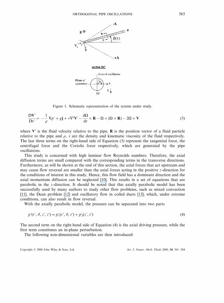
Figure 1 shows a schematic representation of the system under study. An incompressibleNewtonian fluid enters a straight circular pipe of constant diameter, which is initiallystationary, with a uniform velocity V0. At t %=0, the pipe starts oscillating around its verticaldiameter at z %=0, with an angular velocity

V=b: y=Av cos(vt %)y (1)

where the angular position of the pipe axis is

b=A sin(vt %) (2)

v and A are the angular frequency and the amplitude of the pipe oscillations respectively.Therefore, the problem under consideration is a transient developing flow, which we assume tobe laminar. A non-inertial frame of reference moving with the pipe is used and the momentumconservation equation is expressed as follows:

Copyright © 2000 John Wiley & Sons, Ltd. Int. J. Numer. Meth. Fluids 2000; 34: 561–584

ORTHOGONAL PIPE OSCILLATIONS 563

Figure 1. Schematic representation of the system under study.

DV%Dt %

= −1r

9p %+g j+n92V%−dVdt

×R−V× (V×R)−2V×V (3)

where V% is the fluid velocity relative to the pipe, R is the position vector of a fluid particlerelative to the pipe and r, n are the density and kinematic viscosity of the fluid respectively.The last three terms on the right-hand side of Equation (3) represent the tangential force, thecentrifugal force and the Coriolis force respectively, which are generated by the pipeoscillations.

This study is concerned with high laminar flow Reynolds numbers. Therefore, the axialdiffusion terms are small compared with the corresponding terms in the transverse directions.Furthermore, as will be shown at the end of this section, the axial forces that act upstream andmay cause flow reversal are smaller than the axial forces acting in the positive z-direction forthe conditions of interest in this study. Hence, this flow field has a dominant direction and theaxial momentum diffusion can be neglected [10]. This results in a set of equations that areparabolic in the z-direction. It should be noted that this axially parabolic model has beensuccessfully used by many authors to study other flow problems, such as mixed convection[11], the Dean problem [12] and oscillatory flow in coiled ducts [13], which, under extremeconditions, can also result in flow reversal.

With the axially parabolic model, the pressure can be separated into two parts

p %(r %, u, z %, t %)=p %1(r %, u, t %)+p %2(z %, t %) (4)

The second term on the right-hand side of Equation (4) is the axial driving pressure, while thefirst term constitutes an in-plane perturbation.

The following non-dimensional variables are then introduced:

Copyright © 2000 John Wiley & Sons, Ltd. Int. J. Numer. Meth. Fluids 2000; 34: 561–584

B. BENHAMOU, N. GALANIS AND A. LANEVILLE564

Vr=V %r

n/D, Vu=

V %un/D

, Vz=V %zV0

(5a)

r=r %D

, z=z %

DRe, t=

t %D2/n

(5b)

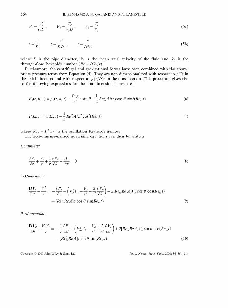
where D is the pipe diameter, V0 is the mean axial velocity of the fluid and Re is thethrough-flow Reynolds number (Re=DV0/n).

Furthermore, the centrifugal and gravitational forces have been combined with the appro-priate pressure terms from Equation (4). They are non-dimensionalized with respect to rV0

2 inthe axial direction and with respect to r(n/D)2 in the cross-section. This procedure gives riseto the following expressions for the non-dimensional pressures:

P1(r, u, t)=p1(r, u, t)−D3gn2 r sin u−

12

Rev2 A2r2 cos2 u cos2(Revt) (6)

P2(z, t)=p2(z, t)−12

Rev2 A2z2 cos2(Revt) (7)

where Rev=D2v/n is the oscillation Reynolds number.The non-dimensionalized governing equations can then be written

Continuity:

(Vr

(r+

Vr

r+

1r(Vu

(u+(Vz

(z=0 (8)

r-Momentum:

DVr

Dt−

Vu2

r= −

(P1

(r+�9m

2 Vr−Vr

r2 −2r2

(Vu

(u

�−2[RevRe A ]Vz cos u cos(Revt)

+ [Rev2 ReA ]z cos u sin(Revt) (9)

u-Momentum:

DVu

Dt+

VrVu

r= −

1r(P1

(u+�9m

2 Vu−Vu

r2 +2r2

(Vr

(u

�+2[RevReA ]Vz sin u cos(Revt)

− [Rev2 ReA ]z sin u sin(Revt) (10)

Copyright © 2000 John Wiley & Sons, Ltd. Int. J. Numer. Meth. Fluids 2000; 34: 561–584

ORTHOGONAL PIPE OSCILLATIONS 565

z-Momentum:

DVz

Dt= −

dP2

dz+9m

2 Vz+2�Rev

ReAn

(Vr cos u−Vu sin u) cos(Revt)

−�Rev

2

ReAn

r cos u sin(Revt) (11)

where

9m2 =(2

(r2+1r(

(r+

1r2

(2

(u2

In the momentum equations (9)–(11) the parameters RevRe and ReRev2 indicate respec-

tively the effect of the Coriolis force and the tangential force in the r–u plane. The ratiosRev/Re and Rev

2 /Re represent respectively the effect of the Coriolis force and the tangentialforce in the z-direction.

The boundary conditions for the problem under consideration are

Vr=Vu=0, Vz=1 at z=0 (12a)

Vr=Vu =Vz=0 at r=0.5 (12b)

We also consider that the flow field is symmetrical with respect to the horizontal plane passingthrough the pipe centreline. Therefore

Vu=0,(Vr

(u=0,

(Vz

(u=0 at u=0 and u=p (13)

Finally, the initial velocity field is obtained as the steady state solution of Equations (8)–(11)with boundary conditions (12) and (13) and A=0.

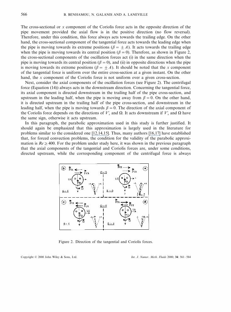
At this point a discussion of the direction of the oscillation forces in Equations (9)–(11) isin order, as they greatly influence the flow field. As indicated in Figure 1, the pipe oscillatesbetween two extreme positions at b= −A and b= +A. When the pipe is moving fromb= −A towards b= +A, the angular velocity (V=b: ) is positive and the leading edge is atu=0. When it is moving from b= +A towards b= −A, the angular velocity is negative andthe leading edge is at u=p. The centrifugal, tangential and Coriolis forces can be expressed,in Cartesian co-ordinates respectively as

F= −V× (V×R)= +V2r cos ux+V2z %z (14)

Ft= −dVdt

×R= +v2bz %x−v2bx %z (15)

Fc= −2V×V %= −2VV %zx+2VV %xz (16)

Copyright © 2000 John Wiley & Sons, Ltd. Int. J. Numer. Meth. Fluids 2000; 34: 561–584

B. BENHAMOU, N. GALANIS AND A. LANEVILLE566

The cross-sectional or x component of the Coriolis force acts in the opposite direction of thepipe movement provided the axial flow is in the positive direction (no flow reversal).Therefore, under this condition, this force always acts towards the trailing edge. On the otherhand, the cross-sectional component of the tangential force acts towards the leading edge whenthe pipe is moving towards its extreme positions (b=9A). It acts towards the trailing edgewhen the pipe is moving towards its central position (b=0). Therefore, as shown in Figure 2,the cross-sectional components of the oscillation forces act (i) in the same direction when thepipe is moving towards its central position (b=0), and (ii) in opposite directions when the pipeis moving towards its extreme positions (b=9A). It should be noted that the x componentof the tangential force is uniform over the entire cross-section at a given instant. On the otherhand, the x component of the Coriolis force is not uniform over a given cross-section.

Next, consider the axial components of the oscillation forces (see Figure 2). The centrifugalforce (Equation (14)) always acts in the downstream direction. Concerning the tangential force,its axial component is directed downstream in the trailing half of the pipe cross-section, andupstream in the leading half, when the pipe is moving away from b=0. On the other hand,it is directed upstream in the trailing half of the pipe cross-section, and downstream in theleading half, when the pipe is moving towards b=0. The direction of the axial component ofthe Coriolis force depends on the directions of V %x and V. It acts downstream if V %x and V havethe same sign, otherwise it acts upstream.

In this paragraph, the parabolic approximation used in this study is further justified. Itshould again be emphasized that this approximation is largely used in the literature forproblems similar to the considered one [12,14,15]. Thus, many authors [16,17] have establishedthat, for forced convection problems, the condition for the validity of the parabolic approxi-mation is Re]400. For the problem under study here, it was shown in the previous paragraphthat the axial components of the tangential and Coriolis forces are, under some conditions,directed upstream, while the corresponding component of the centrifugal force is always

Figure 2. Direction of the tangential and Coriolis forces.

Copyright © 2000 John Wiley & Sons, Ltd. Int. J. Numer. Meth. Fluids 2000; 34: 561–584

ORTHOGONAL PIPE OSCILLATIONS 567

directed downstream. These forces are respectively proportional to A ·Rev/Re, A ·Rev2 /Re

(Equation (11)) and A2 ·Rev2 (Equation (7)). For this study, both Reynolds numbers are of the

same large magnitude. Therefore, the axial components of the Coriolis force (�A) andtangential force (�A ·Rev) are negligible compared with the corresponding component of thecentrifugal force (�A2 ·Rev

2 ). Hence, the possibility of flow reversal is excluded and theparabolic approximation is valid.

3. NUMERICAL METHOD

The governing equations (8)–(11) are solved numerically using a control volume method [18].According to this method, a fully implicit numerical scheme is used to transform theseequations to finite difference ones. The unsteady term is approximated by a backwarddifference, the axial advective term by an upwind difference and the diffusive and transverseconvective terms by the power law scheme. The computer program is based on Patankar’sprocedure adapted for transient three-dimensional parabolic flows [10]. Major modifications ofthis procedure include (i) the implantation of the SIMPLE-C algorithm for handling thein-plane pressure–velocity coupling [19], (ii) the use of the method proposed by Raithby andSchneider [20] for the calculation of the streamwise pressure gradient dP2/dz and (iii) theadaptation necessary to handle the time-dependent terms.

As the flow field is assumed symmetrical with respect to the horizontal diameter (u=0,u=p), the computation is performed only over one half of the circular cross-section.

Several different discretization grids have been tested. Table I shows the effects of thenumber of nodes in the u- and r-directions on the peripherally averaged friction factor

fRe=2p

& p

0

�(Vz

(r�

r=0.5

du (17)

Similar results for the axial pressure gradient are not presented but will be referred to. Anincrease of the number of nodes from 832 (26×32 in the circumferential and radial directionsrespectively) to 1440 (36×40 in the u- and r-directions respectively) results in a change of lessthan 1 per cent for the predicted values of the friction factor and of less than 2 per cent forthose of the pressure gradient. In view of these and other similar results, the 26×32 grid has

Table I. Effect of cross-sectional grid on the calculated average friction factorfor Re=500, Rev=1000 and A=10°.

36×4036×3240×3226×32z %/D

0.10 62.40462.84862.84862.84828.660 28.664 28.6641.00 28.620

5.20 19.9020 19.9088 19.9076 19.881418.2492 18.259410.25 18.2576 18.2354

17.426617.448217.450217.436421.05

Copyright © 2000 John Wiley & Sons, Ltd. Int. J. Numer. Meth. Fluids 2000; 34: 561–584

B. BENHAMOU, N. GALANIS AND A. LANEVILLE568

Table II. Effect of axial grid on the calculated average friction factor forRe=500, Rev=1000 and A=10°.

1.02 3.02z %/D 5.02 12.02 20.50

28.5626 21.8583 20.0180D1 18.2992 17.495128.1751 21.4837 19.5900 17.8053D2 17.0310

been retained for subsequent calculations. It should be noted that in all these cases, the gridspacing is uniform along the circumferential direction. On the other hand, in the radialdirection grid points are more closely packed near the pipe wall. Similarly, Table II shows theeffects of the axial discretization on the peripherally averaged friction factor. Grid D1 consistsof a non-uniform mesh with 110 cross-sections. The axial step size varies from 10−6 near thepipe entrance to 5·10−4 near its exit. Grid D2 is obtained by halving the step size of D1. Theresults differ by less than 3 per cent for both the friction factor and the axial pressure gradient.For the calculations presented here grid D2 was retained. For these calculations, the CPU timeis typically about 11 min per time step on an IBM RISC6000 model 375.

Several time steps have been tested to ensure that the results are accurate and independentof the time step (see Table III). A time step of Dt=T/65 has finally been chosen. T is the pipeoscillation period (T=2p/Rev). The maximum resulting uncertainty is approximately Db/A=0.1 for the angular position of the pipe. The calculated results for the peripherally averagedfriction factor are within 0.3 per cent of those obtained with Dt=T/451.

All grid independence tests were conducted for the case of a high oscillation Reynoldsnumber (Rev=1000), which causes sharp velocity gradients. For the tests presented in TablesI, II and III, the through-flow Reynolds number is fixed at Re=500 and the oscillationamplitude is A=10°. Analogous grid independence tests for Re=1000 gave similar results.

In each time step, the computation is marched in the z-direction. At each marching step, asufficient number of iterations have been performed to ensure a converged solution. Twoconvergence criteria must be satisfied

– the local values of velocities at some sample points have to be converged within at leastfour significant digits;

– the mass balance over each control volume must be satisfied to within 10−4.

Table III. Effect of time step (Dt) on the average friction factor at z %/D=20.5for Re=500, A=10° and Rev=139.

Dt2=T/150Dt1=T/451 Dt3=T/65b (°) (VB0)

16.66120.0 16.6170 16.63235.0 17.2453 17.2327 17.2111

17.210017.234917.24849.210.0 17.1679 17.1482 17.1130

Copyright © 2000 John Wiley & Sons, Ltd. Int. J. Numer. Meth. Fluids 2000; 34: 561–584

ORTHOGONAL PIPE OSCILLATIONS 569

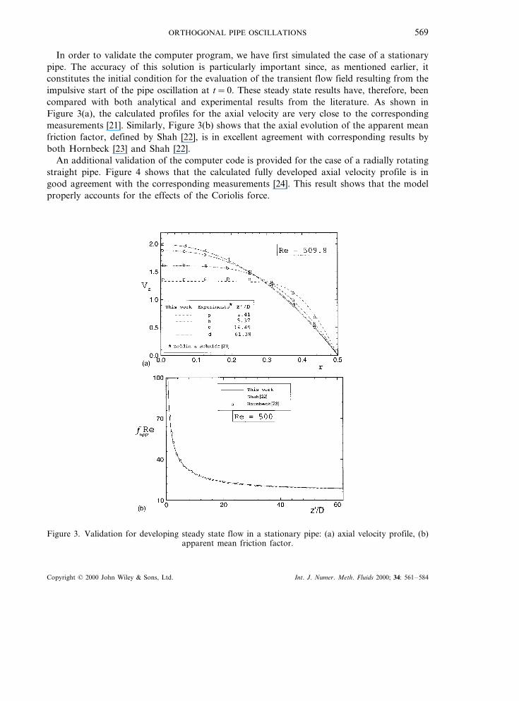
In order to validate the computer program, we have first simulated the case of a stationarypipe. The accuracy of this solution is particularly important since, as mentioned earlier, itconstitutes the initial condition for the evaluation of the transient flow field resulting from theimpulsive start of the pipe oscillation at t=0. These steady state results have, therefore, beencompared with both analytical and experimental results from the literature. As shown inFigure 3(a), the calculated profiles for the axial velocity are very close to the correspondingmeasurements [21]. Similarly, Figure 3(b) shows that the axial evolution of the apparent meanfriction factor, defined by Shah [22], is in excellent agreement with corresponding results byboth Hornbeck [23] and Shah [22].

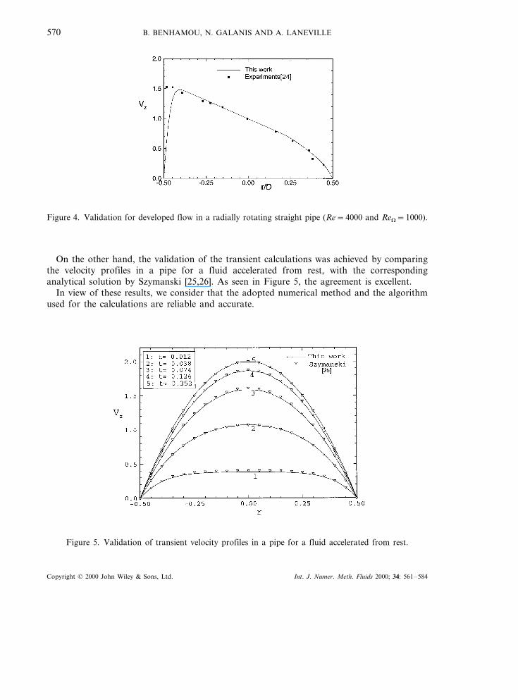
An additional validation of the computer code is provided for the case of a radially rotatingstraight pipe. Figure 4 shows that the calculated fully developed axial velocity profile is ingood agreement with the corresponding measurements [24]. This result shows that the modelproperly accounts for the effects of the Coriolis force.

Figure 3. Validation for developing steady state flow in a stationary pipe: (a) axial velocity profile, (b)apparent mean friction factor.

Copyright © 2000 John Wiley & Sons, Ltd. Int. J. Numer. Meth. Fluids 2000; 34: 561–584

B. BENHAMOU, N. GALANIS AND A. LANEVILLE570

Figure 4. Validation for developed flow in a radially rotating straight pipe (Re=4000 and ReV=1000).

On the other hand, the validation of the transient calculations was achieved by comparingthe velocity profiles in a pipe for a fluid accelerated from rest, with the correspondinganalytical solution by Szymanski [25,26]. As seen in Figure 5, the agreement is excellent.

In view of these results, we consider that the adopted numerical method and the algorithmused for the calculations are reliable and accurate.

Figure 5. Validation of transient velocity profiles in a pipe for a fluid accelerated from rest.

Copyright © 2000 John Wiley & Sons, Ltd. Int. J. Numer. Meth. Fluids 2000; 34: 561–584

ORTHOGONAL PIPE OSCILLATIONS 571

4. RESULTS

Many simulations have been performed but, in the interest of brevity, only some selectedresults are presented here to describe the structure of the transient flow field during the firstfew cycles after the initiation of the pipe oscillations. The results presented here were calculatedwith Re=1000, Rev=1000 and A=18°, while the pipe length to diameter ratio was 40.46.For these values, we have established, by means of an experimental visualization, that the flowis laminar. Numerical results include the time evolutions of the different velocity componentsas well as those of the in-plane perturbation pressure and of the local friction coefficient fl atselected points in the flow field. The latter variable is calculated from the relation

flRe=�(Vz

(r�

r=0.5

(18)

The results also include the time evolutions of the axial driving pressure gradient and thecircumferentially averaged friction factor (Equation (17)).

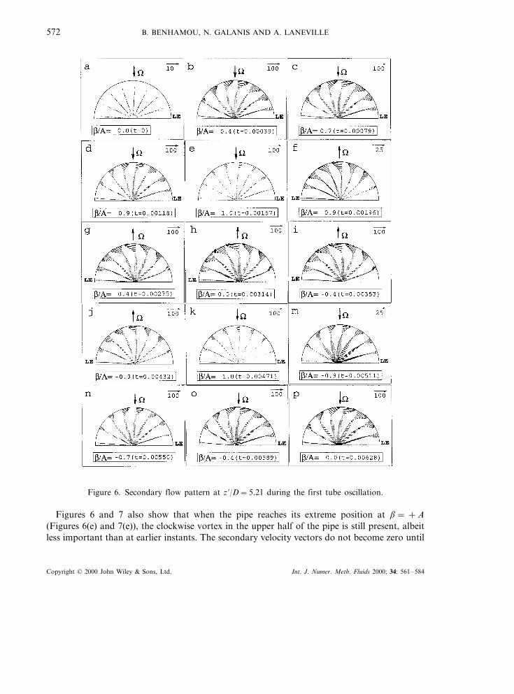
4.1. Initiation of the secondary flow

Figures 6 and 7 show the time evolutions of the in-plane velocity vectors at z %/D=5.21 andz %/D=40.46 respectively, corresponding to the secondary fluid motion during the first pipeoscillation. The vectors on the upper-right-hand of each part of these figures indicate the scalefor velocity vectors. At t=0 (see Figures 6(a) and 7(a)) the secondary motion is purely radialand decreases with axial distance reflecting the axial development of the axisymmetricboundary layer. The modification of this initial flow field immediately after the impulsiveinitiation of the pipe oscillations can be understood by examining the direction and relativemagnitude of the oscillation forces, which were discussed earlier.

During the first quarter of the initial oscillation when the pipe moves towards b= +A, thex components of the Coriolis force is negative everywhere within the flow field (see Figure2(d)). However, since this component of the Coriolis force is, according to Equation (16),proportional to Vz, its value near the pipe wall is negligible. Therefore, the fluid in the coreregion experiences a force in the negative x-direction and moves towards the pipe wall at thetrailing edge. It then pushes the fluid in this region to the leading edge along the pipe wall, asseen in Figures 6(b)–(d) and 7(b)–(d). Therefore, the initial secondary flow pattern in the tophalf of the pipe consists of a clockwise vortex. As mentioned above, the transversal componentof the tangential force is uniform over a given cross-section of the pipe at a given instant.Hence, this force can not initiate a transverse fluid movement.

It should be noted that, near the pipe entrance, the secondary flow pattern is similar to theone generated by the centrifugal force in a curved pipe [12] (Dean’s problem). The essentialdifference between these two flow fields is due to the fact that, in the present case, the intensityof the vortices is time-dependent. Further downstream, however, the present case secondaryflow is much more complex. Thus, the velocity profile along a given radius exhibits localminima and an additional weak vortex appears near the trailing edge (see Figure 7(f) and (m)).

Copyright © 2000 John Wiley & Sons, Ltd. Int. J. Numer. Meth. Fluids 2000; 34: 561–584

B. BENHAMOU, N. GALANIS AND A. LANEVILLE572

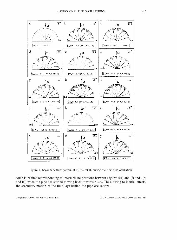
Figure 6. Secondary flow pattern at z %/D=5.21 during the first tube oscillation.

Figures 6 and 7 also show that when the pipe reaches its extreme position at b= +A(Figures 6(e) and 7(e)), the clockwise vortex in the upper half of the pipe is still present, albeitless important than at earlier instants. The secondary velocity vectors do not become zero until

Copyright © 2000 John Wiley & Sons, Ltd. Int. J. Numer. Meth. Fluids 2000; 34: 561–584

ORTHOGONAL PIPE OSCILLATIONS 573

Figure 7. Secondary flow pattern at z %/D=40.46 during the first tube oscillation.

some later time (corresponding to intermediate positions between Figures 6(e) and (f) and 7(e)and (f)) when the pipe has started moving back towards b=0. Thus, owing to inertial effects,the secondary motion of the fluid lags behind the pipe oscillations.

Copyright © 2000 John Wiley & Sons, Ltd. Int. J. Numer. Meth. Fluids 2000; 34: 561–584

B. BENHAMOU, N. GALANIS AND A. LANEVILLE574

A final point of interest arising from Figures 6 and 7 is the apparent symmetry of thesecondary flow patterns for instants differing by half a pipe oscillation period (see, forexample, Figures 6(d) and (j) or 7(f) and 7(m)). This point is addressed in detail later.

4.2. Transient e6olution of the axial 6elocity

Figure 8 shows the time evolution of the axial velocity at point M (u=0, r=0.25) for threedifferent axial positions during the first four pipe oscillations. The initial values of VzM at t=0(i.e. when the pipe is at rest at b=0) correspond to the steady state solution discussed earlier(see Figure 3). An analysis of the axial components of the tangential and Coriolis forcesexplains the initial variation of the axial velocity shown in this figure. Thus, at t=0, the pipeis at b=0; therefore, according to Equation (15), the axial component of the tangential forceis zero. At that instant, V is positive and maximum, while for the point M (u=0, r=0.25)under consideration, the velocity in the x-direction is negative, as it is due to the boundarylayer growth and is, therefore, directed towards the centre of the pipe. Thus, according toEquation (16), the axial component of the Coriolis force at t=0 is negative. This explains thefact that the axial velocity at M decreases immediately after the pipe oscillation is initiated att=0. Later, as the pipe moves towards b= +A and then back towards b=0, the sum of theaxial components of the tangential and Coriolis forces is continuously negative. Therefore, theacceleration of Vz observed in Figure 8 as the pipe approaches b=0 cannot be explained onthis basis. It is rather a result of the complex interaction between these axial forces, the axialpressure gradient and the coupling between the axial and in-plane motions.

It should be noted that VzM at z %/D=5.21 reaches its extreme values when the pipe is atb:0. Further downstream, however, for z %/D=11.21 and z %/D=40.46, for example, theextreme values of the axial velocity at M occur earlier than the central angular position of thepipe. As indicated by these results, the time lag between the occurrence of the extreme valuesof VzM and b decreases with increasing distance from the pipe entrance.

Figure 8. Time evolution of the axial velocity at point M (u=0, r=0.25).

Copyright © 2000 John Wiley & Sons, Ltd. Int. J. Numer. Meth. Fluids 2000; 34: 561–584

ORTHOGONAL PIPE OSCILLATIONS 575

Figure 8 also shows that during the first pipe oscillation, the extreme values of the axialvelocity differ from the corresponding values for subsequent oscillations. Furthermore, thecorresponding amplitude is greatest at z %/D=40.46 and smallest at z %/D=11.21, while theaverage value increases monotonically with axial distance. On the other hand, during thefourth pipe oscillation, the amplitude of VzM increases monotonically with z, while its averagevalue is greatest at z %/D=11.21. This complicated behaviour is attributed to the fact that pointM is situated in the central core region at z %/D=5.21 and in the boundary layer atz %/D=40.46.

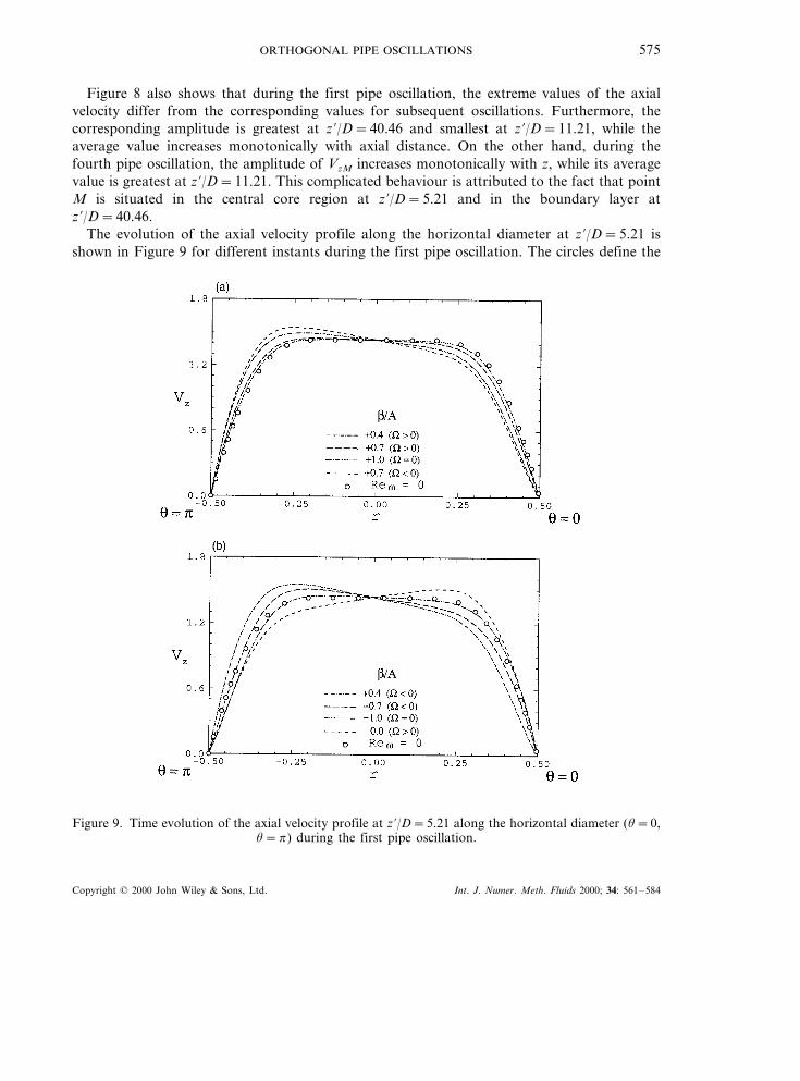
The evolution of the axial velocity profile along the horizontal diameter at z %/D=5.21 isshown in Figure 9 for different instants during the first pipe oscillation. The circles define the

Figure 9. Time evolution of the axial velocity profile at z %/D=5.21 along the horizontal diameter (u=0,u=p) during the first pipe oscillation.

Copyright © 2000 John Wiley & Sons, Ltd. Int. J. Numer. Meth. Fluids 2000; 34: 561–584

B. BENHAMOU, N. GALANIS AND A. LANEVILLE576

corresponding velocity profile for a stationary pipe (cf. Figure 3), which is also the initialvelocity profile at t=0 for the transient problem under study. As the pipe moves from b=0towards b= +A, the axial velocity near the leading edge (u=0) decreases while it increasesnear the trailing edge (u=p) in order to satisfy the mass conservation equation. Thisbehaviour is obviously due to the fluid inertia, which prevents it from following the impulsiveinitiation of the pipe movement at t=0. It is important to note that this tendency continueseven after the pipe has started moving back towards b=0. Thus, the maximum distortion ofthis velocity profile during the first pipe oscillation occurs when b/A= +0.4 and the pipe ismoving towards b=0 (VB0). Then, as the pipe movement continues beyond b=0 towardsb= −A, the lack of symmetry diminishes and for b= −A, the velocity profile is almostidentical to that for a stationary pipe. Finally, when the pipe reaches once again the positionb=0, the axial fluid velocity near the leading edge (u=0) is higher than that near the trailingedge. The distortion of the velocity profile during this first pipe oscillation can be quantifiedby the ratio of its maximum value to the velocity on the axis of a stationary pipe. In the caseof Figure 9, this ratio is equal to 1.07.

The corresponding evolutions of the axial velocity profile at z %/D=11.21 and z %/D=40.46are qualitatively similar to those of Figure 9. However, the ratio quantifying the distortion ofthe profile decreases with axial distance: its value is 1.04 at z %/D=11.21 and 1.01 atz %/D=40.46. The latter value indicates that, far from the entrance, where the velocity profilefor a stationary pipe is quasi-parabolic, the maximum velocity during the pipe oscillation doesnot change much, although its position oscillates around the longitudinal axis of the pipe.

4.3. E6olution of some local 6ariables

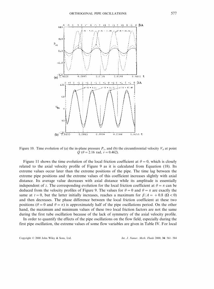
Figure 10 shows the time evolution of the in-plane pressure P1 (see Equation (6)) and of thecircumferential velocity Vu at a particular point Q (u=2.16 rad, r=0.462) for three differentaxial positions. This pressure is closely related to the secondary motion depicted in Figures 6and 7. For the particular point Q, which is in the upper left quadrant of the cross-section, thispressure decreases when the pipe is moving from b= −A towards b= +A and increaseswhen the pipe is moving in the opposite direction. For z %/D=40.46, the extreme values of thisvariable occur when b:9A. As z %/D decreases, these extreme values occur later. Therefore,as is the case for VzM, the time lag between the occurrence of the extreme values of P1Q

decreases with increasing axial distance. The extreme values of P1Q are essentially the same forall cycles, including the first. This is not the case for VuQ for which the extreme values duringthe first pipe oscillation are quite different from the corresponding values for subsequentoscillations. Contrary to the case of VzM (see Figure 8), the extreme values of VuQ occur whenthe tube is very close to b=0 and the influence of axial distance on the phase differencebetween the oscillations of VuQ and b is negligible.

The influence of axial distance on the amplitudes of P1 and VuQ during the fourth pipeoscillation is qualitatively and quantitatively different. Both these amplitudes increase withaxial distance. However, on the basis of the results of Figure 10, the amplitude of P1 increaseslinearly with the axial distance, while that of VuQ increases very rapidly near the pipe entranceand then tends towards an asymptotic value that is independent of the axial distance.

Copyright © 2000 John Wiley & Sons, Ltd. Int. J. Numer. Meth. Fluids 2000; 34: 561–584

ORTHOGONAL PIPE OSCILLATIONS 577

Figure 10. Time evolution of (a) the in-plane pressure P1, and (b) the circumferential velocity Vu at pointQ (u=2.16 rad, r=0.462).

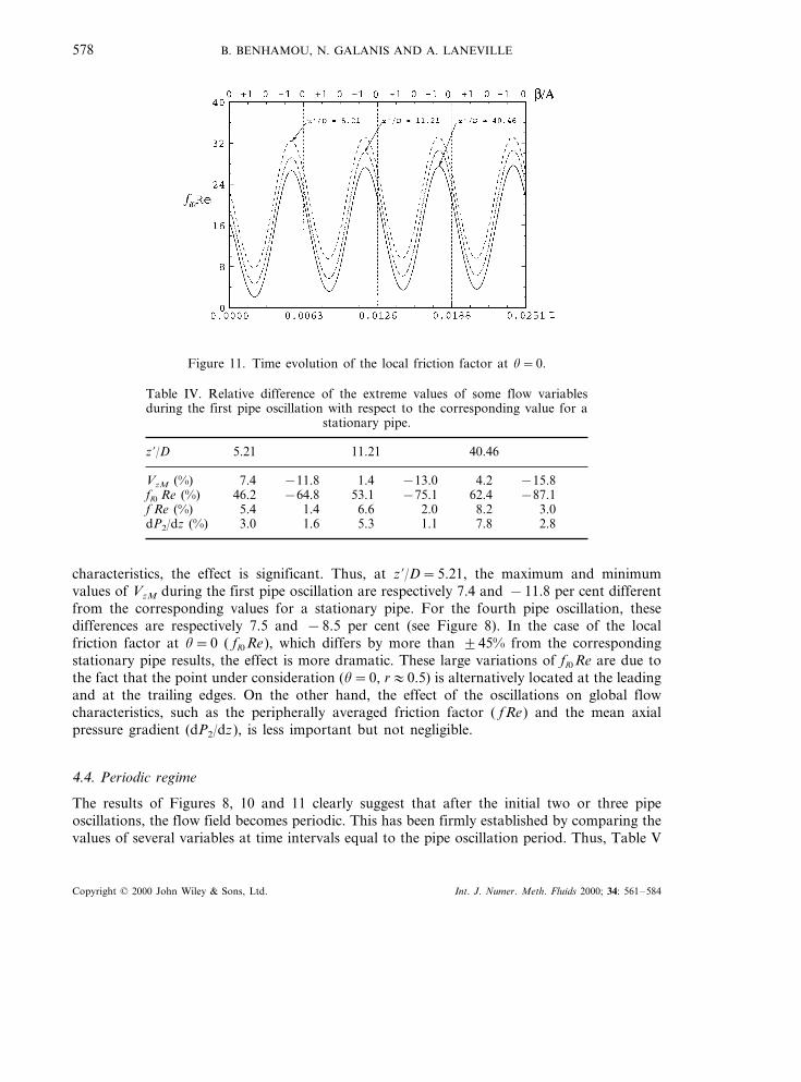
Figure 11 shows the time evolution of the local friction coefficient at u=0, which is closelyrelated to the axial velocity profile of Figure 9 as it is calculated from Equation (18). Itsextreme values occur later than the extreme positions of the pipe. The time lag between theextreme pipe positions and the extreme values of this coefficient increases slightly with axialdistance. Its average value decreases with axial distance while its amplitude is essentiallyindependent of z. The corresponding evolution for the local friction coefficient at u=p can bededuced from the velocity profiles of Figure 9. The values for u=0 and u=p are exactly thesame at t=0, but the latter initially increases, reaches a maximum for b/A= +0.8 (VB0)and then decreases. The phase difference between the local friction coefficient at these twopositions (u=0 and u=p) is approximately half of the pipe oscillations period. On the otherhand, the maximum and minimum values of these two local friction factors are not the sameduring the first tube oscillation because of the lack of symmetry of the axial velocity profile.

In order to quantify the effects of the pipe oscillations on the flow field, especially during thefirst pipe oscillation, the extreme values of some flow variables are given in Table IV. For local

Copyright © 2000 John Wiley & Sons, Ltd. Int. J. Numer. Meth. Fluids 2000; 34: 561–584

B. BENHAMOU, N. GALANIS AND A. LANEVILLE578

Figure 11. Time evolution of the local friction factor at u=0.

Table IV. Relative difference of the extreme values of some flow variablesduring the first pipe oscillation with respect to the corresponding value for a

stationary pipe.

z %/D 5.21 11.21 40.46

7.4 −11.8 1.4 −13.0VzM (%) 4.2 −15.846.2 −64.8 53.1 −75.1 62.4 −87.1fl0 Re (%)5.4 1.4 6.6f Re (%) 2.0 8.2 3.03.0dP2/dz (%) 1.6 5.3 1.1 7.8 2.8

characteristics, the effect is significant. Thus, at z %/D=5.21, the maximum and minimumvalues of VzM during the first pipe oscillation are respectively 7.4 and −11.8 per cent differentfrom the corresponding values for a stationary pipe. For the fourth pipe oscillation, thesedifferences are respectively 7.5 and −8.5 per cent (see Figure 8). In the case of the localfriction factor at u=0 ( fl0Re), which differs by more than 945% from the correspondingstationary pipe results, the effect is more dramatic. These large variations of fl0Re are due tothe fact that the point under consideration (u=0, r:0.5) is alternatively located at the leadingand at the trailing edges. On the other hand, the effect of the oscillations on global flowcharacteristics, such as the peripherally averaged friction factor ( fRe) and the mean axialpressure gradient (dP2/dz), is less important but not negligible.

4.4. Periodic regime

The results of Figures 8, 10 and 11 clearly suggest that after the initial two or three pipeoscillations, the flow field becomes periodic. This has been firmly established by comparing thevalues of several variables at time intervals equal to the pipe oscillation period. Thus, Table V

Copyright © 2000 John Wiley & Sons, Ltd. Int. J. Numer. Meth. Fluids 2000; 34: 561–584

ORTHOGONAL PIPE OSCILLATIONS 579

shows that at z %/D=11.21 there is no variation whatsoever of any of the six variables after thefourth pipe oscillation; in fact, the difference between corresponding values at t=3T andt=4T is in all cases less than 0.1 per cent of the former values. The same levels of confidencefor the existence of periodicity are obtained earlier at z %/D=5.21. Thus there is no variationwhatsoever of any of the six variables after the third pipe oscillation, while the differencebetween corresponding values at t=2T and t=3T is in all cases less than 0.1 per cent. On theother hand, at z %/D=40.46, the convergence towards the periodic flow regime takes muchlonger: the values for P1 (u=0.06, r=0.256) differ by 3 per cent between t=5T and t=6T.However, all the other variables differ by less than 1 per cent between these two instants andthe tendency towards the existence of an established periodic flow regime is clear even at thisdistance from the entrance.

4.5. Flow resistance

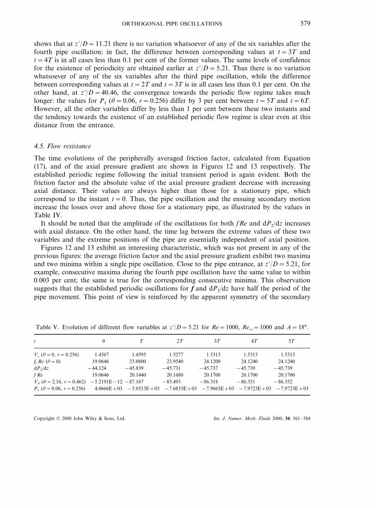
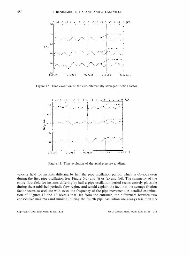
The time evolutions of the peripherally averaged friction factor, calculated from Equation(17), and of the axial pressure gradient are shown in Figures 12 and 13 respectively. Theestablished periodic regime following the initial transient period is again evident. Both thefriction factor and the absolute value of the axial pressure gradient decrease with increasingaxial distance. Their values are always higher than those for a stationary pipe, whichcorrespond to the instant t=0. Thus, the pipe oscillation and the ensuing secondary motionincrease the losses over and above those for a stationary pipe, as illustrated by the values inTable IV.

It should be noted that the amplitude of the oscillations for both fRe and dP2/dz increaseswith axial distance. On the other hand, the time lag between the extreme values of these twovariables and the extreme positions of the pipe are essentially independent of axial position.

Figures 12 and 13 exhibit an interesting characteristic, which was not present in any of theprevious figures: the average friction factor and the axial pressure gradient exhibit two maximaand two minima within a single pipe oscillation. Close to the pipe entrance, at z %/D=5.21, forexample, consecutive maxima during the fourth pipe oscillation have the same value to within0.003 per cent; the same is true for the corresponding consecutive minima. This observationsuggests that the established periodic oscillations for f and dP2/dz have half the period of thepipe movement. This point of view is reinforced by the apparent symmetry of the secondary

Table V. Evolution of different flow variables at z %/D=5.21 for Re=1000, Rev=1000 and A=18°.

4T3T2TT 5T0t

1.53131.53131.5277 1.53131.45951.4567Vz (u=0, r=0.256)24.1200fl Re (u=0) 24.1240 24.124019.0646 23.0800 23.9540

−45.731 −45.737 −45.739 −45.739dP2/dz −44.124 −45.83920.1700 20.1700f Re 19.0646 20.1440 20.1680 20.1700

Vu (u=2.16, r=0.462) −86.352−86.351−86.318−85.493−87.167−5.2191E−12−7.9723E+03−7.9723E+03−7.9663E+03−7.6835E+03−5.0513E+034.0666E+03P1 (u=0.06, r=0.256)

Copyright © 2000 John Wiley & Sons, Ltd. Int. J. Numer. Meth. Fluids 2000; 34: 561–584

B. BENHAMOU, N. GALANIS AND A. LANEVILLE580

Figure 12. Time evolution of the circumferentially averaged friction factor.

Figure 13. Time evolution of the axial pressure gradient.

velocity field for instants differing by half the pipe oscillation period, which is obvious evenduring the first pipe oscillation (see Figure 6(d) and (j) or (g) and (o)). The symmetry of theentire flow field for instants differing by half a pipe oscillation period seems entirely plausibleduring the established periodic flow regime and would explain the fact that the average frictionfactor seems to oscillate with twice the frequency of the pipe movement. A detailed examina-tion of Figures 12 and 13 reveals that, far from the entrance, the differences between twoconsecutive maxima (and minima) during the fourth pipe oscillation are always less than 0.5

Copyright © 2000 John Wiley & Sons, Ltd. Int. J. Numer. Meth. Fluids 2000; 34: 561–584

ORTHOGONAL PIPE OSCILLATIONS 581

per cent. At this point, therefore, we ascertain that the frequency of the two variables shownin Figures 12 and 13 is indeed twice that of the pipe oscillations.

4.6. Effects of the pipe oscillation pattern

The results presented in the previous sections were obtained for the pipe oscillation patterndefined by Equations (1) and (2) (case 1). However, results have also been calculated for twoother oscillation patterns described by the following relations:

Case 2

b= −A sin(vt %) and V= −Av cos(vt %)y (19)

Case 3

b=A cos(vt %) and V= −Av sin(vt %)y (20)

For both cases 1 and 2, the pipe starts its oscillations at b=0. It is initially moving towardsb= +A in case 1 (V\0) and towards b= −A in case 2 (VB0). In case 3, the pipe starts itsoscillations at b= +A. In all three cases, the values of the flow parameters are the same:A=18° and Re=Rev=1000.

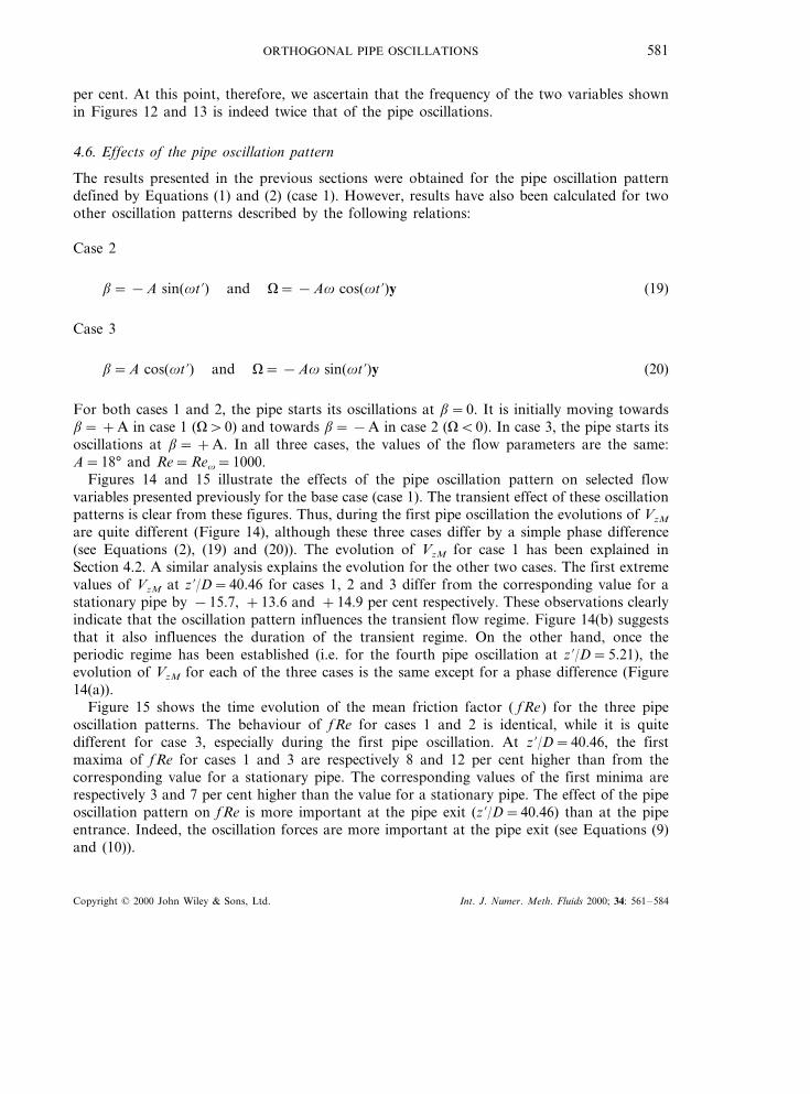
Figures 14 and 15 illustrate the effects of the pipe oscillation pattern on selected flowvariables presented previously for the base case (case 1). The transient effect of these oscillationpatterns is clear from these figures. Thus, during the first pipe oscillation the evolutions of VzM

are quite different (Figure 14), although these three cases differ by a simple phase difference(see Equations (2), (19) and (20)). The evolution of VzM for case 1 has been explained inSection 4.2. A similar analysis explains the evolution for the other two cases. The first extremevalues of VzM at z %/D=40.46 for cases 1, 2 and 3 differ from the corresponding value for astationary pipe by −15.7, +13.6 and +14.9 per cent respectively. These observations clearlyindicate that the oscillation pattern influences the transient flow regime. Figure 14(b) suggeststhat it also influences the duration of the transient regime. On the other hand, once theperiodic regime has been established (i.e. for the fourth pipe oscillation at z %/D=5.21), theevolution of VzM for each of the three cases is the same except for a phase difference (Figure14(a)).

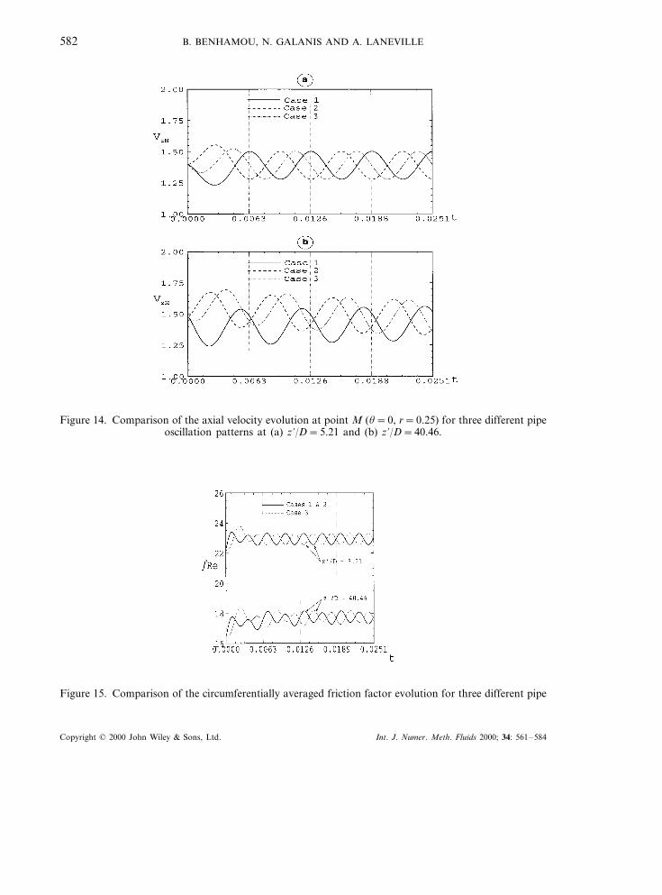
Figure 15 shows the time evolution of the mean friction factor ( fRe) for the three pipeoscillation patterns. The behaviour of fRe for cases 1 and 2 is identical, while it is quitedifferent for case 3, especially during the first pipe oscillation. At z %/D=40.46, the firstmaxima of fRe for cases 1 and 3 are respectively 8 and 12 per cent higher than from thecorresponding value for a stationary pipe. The corresponding values of the first minima arerespectively 3 and 7 per cent higher than the value for a stationary pipe. The effect of the pipeoscillation pattern on fRe is more important at the pipe exit (z %/D=40.46) than at the pipeentrance. Indeed, the oscillation forces are more important at the pipe exit (see Equations (9)and (10)).

Copyright © 2000 John Wiley & Sons, Ltd. Int. J. Numer. Meth. Fluids 2000; 34: 561–584

B. BENHAMOU, N. GALANIS AND A. LANEVILLE582

Figure 14. Comparison of the axial velocity evolution at point M (u=0, r=0.25) for three different pipeoscillation patterns at (a) z %/D=5.21 and (b) z %/D=40.46.

Figure 15. Comparison of the circumferentially averaged friction factor evolution for three different pipe

Copyright © 2000 John Wiley & Sons, Ltd. Int. J. Numer. Meth. Fluids 2000; 34: 561–584

ORTHOGONAL PIPE OSCILLATIONS 583

5. CONCLUSION

The interaction between the developing laminar flow in a straight horizontal pipe and theimpulsively initiated oscillations of the latter around the vertical diameter at its entrance hasbeen studied numerically. It is believed that the computations presented here are the first oftheir kind. The inertial forces acting on the fluid generate a pulsating flow, which ischaracterized by a pair of counter-rotating vortices symmetrical about the horizontal planethrough the longitudinal axis of the pipe. These vortices are alternatively clockwise andanti-clockwise. Their intensity varies with both time and axial distance. This secondary flowinfluences the axial velocity profile, which is no longer axisymmetric. Thus, the position of theaxial velocity maximum oscillates along the horizontal diameter of the pipe. Its value near thetube entrance is higher than that for a stationary pipe while far downstream, these two maximaare essentially the same. All local flow variables (velocity components, pressure and local wallshear stress) oscillate with the same frequency as the pipe. After an initial transient regime allthese oscillations became periodic. The duration of this transient regime increases with axialdistance. This duration also depends on the pipe oscillation pattern. On the other hand,average variables (such as the axial pressure gradient and the peripherally averaged frictionfactor) exhibit two maxima and two minima during a single pipe oscillation. After the transientregime, these variables oscillate with twice the frequency of the pipe oscillations.

ACKNOWLEDGMENTS

The authors wish to thank the Natural Sciences and Engineering Research Council of Canada for itsfinancial support.

REFERENCES

1. Morris WD. Heat Transfer and Fluid Flow in Rotating Coolant Channels. Research Studies Press, Wiley: NewYork, 1981.

2. Soong CY, Lin ST, Hwang GJ. An experimental study of convective heat transfer in radially rotating rectangularducts. ASME Journal of Heat Transfer 1991; 113: 604.

3. Fann S, Yang W-J. Hydrodynamically and thermally developing laminar flow through rotating channels havingisothermal walls. Numerical Heat Transfer Part A 1992; 22: 257.

4. Kurwzeg UH, Chen J. Heat transfer along an oscillating flat plate. ASME Journal of Heat Transfer 1988; 110:789.

5. Kazakia JY, Rivlin RS. The influence of vibration on Poiseuille flow of a non-Newtonian fluid. Rheologica Acta1978; 17: 210.

6. Maloy KJ, Goldburg W. Measurements on transition to turbulence in a Taylor–Couette cell with oscillatory innercylinder. Physics of Fluids A 1993; 5: 1438.

7. Berman J, Mockros LF. Flow in a rotating non-aligned straight pipe. Journal of Fluid Mechanics 1984; 144: 297.8. Benhamou B, Galanis N, Laneville A. Laminar flow in a tube subject to sinusoidal oscillations. In ECCOMAS’98,

Athens, Greece, vol. 1, Papailiou K (ed.). Wiley: New York, 1998; 1302.9. Benhamou B, Galanis N, Laneville A. Numerical study of laminar incompressible flow in an oscillating tube. In

CSME’98 Forum, Toronto, Canada 19–22 May, vol. 1, Rosen MA, Naylor D, Kawall JG (eds). RyersonPolytechnic University: Toronto, 1998; 169.

10. Patankar SV, Spalding DB. A calculation procedure for heat, mass and momentum transfer in three-dimensionalparabolic flows. International Journal for Heat and Mass Transfer 1972; 15: 1787.

11. Ouzzane M, Galanis N. Developing mixed convection flow in an inclined tube under circumferentially non-uni-form heating at outer surface. Numerical Heat Transfer Part A 1999; 35: 609.

Copyright © 2000 John Wiley & Sons, Ltd. Int. J. Numer. Meth. Fluids 2000; 34: 561–584

B. BENHAMOU, N. GALANIS AND A. LANEVILLE584

12. Bara B, Nandakumar K, Masliyah JH. An experimental and numerical study of the Dean problem: flowdevelopment towards two-dimensional multiple solutions. Journal of Fluid Mechanics 1992; 244: 339.

13. Ravi Sankar S, Nandakumar K, Masliyah JH. Oscillatory flows in coiled square ducts. Physics of Fluids 1988; 31:1348.

14. Pollard A. The numerical calculation of partially elliptic flows. Numerical Heat Transfer 1979; 2: 267.15. Cheng CH, Weng CJ, Aung W. Buoyancy effect on the flow reversal of three-dimensional developing flow in a

vertical rectangular duct. A parabolic model solution. ASME Journal of Heat Transfer 1995; 117: 238.16. Shah RK, London AL. Laminar Flow Forced Con6ection in Ducts. Academic Press: New York, 1978.17. Pagliarini G. Steady laminar heat transfer in the entry region of circular tubes with axial diffusion of heat and

momentum. International Journal for Heat Mass Transfer 1989; 32: 1037.18. Patankar S. Numerical Heat Transfer and Fluid Flow. McGraw-Hill: New York, 1980.19. Van Doormaal JP, Raithby GD. Enhancements of the SIMPLE method for predicting incompressible fluid flows.

Numerical Heat Transfer 1984; 7: 147.20. Raithby GD, Schneider GE. Numerical solution of problems in incompressible fluid flow: treatment of the

velocity–pressure coupling. Numerical Heat Transfer 1979; 3: 417.21. Zeldin B, Schmidt FW. Developing flow with combined forced-free convection in an isothermal vertical tube.

ASME Journal of Heat Transfer 1972; 94: 211.22. Shah RK. A correlation for laminar hydrodynamic entry length solutions for circular and non-circular ducts.

ASME Journal of Fluids Engineering 1978; 100: 177.23. Hornbeck RW. Laminar flow in the entrance region of a pipe. Applied Science Research Section A 1964; 13: 224.24. Ito H, Nanbu K. Flow in rotating straight pipes of circular cross section. ASME Journal of Basic Engineering

1971; 93: 383.25. Szymanski P. Quelques solutions exactes des equations de l’hydrodynamique du fluide visqueux dans le cas d’un

tube cylindrique. Journal de mathematiques pures et appliquees Serie 9 1932; 11: 67.26. Schlichting H. Boundary Layer Theory. McGraw Hill: New York, 1979.

.

Copyright © 2000 John Wiley & Sons, Ltd. Int. J. Numer. Meth. Fluids 2000; 34: 561–584