transient and secular radioactive equilibrium revisited
TRANSCRIPT

1
Transient and secular radioactive equilibrium revisited
Qinghui Zhang, Ph.D.,
Radiation Oncology Department, University of Nebraska Medical Center, Omaha 68198
Departments of Medical Physics, Memorial Sloan-Kettering Cancer Center,
New York, NY 10065
Chandra Burman, Ph.D.,
Departments of Medical Physics, Memorial Sloan-Kettering Cancer Center,
New York, NY 10065
Howard Amols, Ph.D.
Department of Radiation Oncology, Columbia University Medical Center,
New York, Ny 10032
Departments of Medical Physics, Memorial Sloan-Kettering Cancer Center,
New York, NY 10065
Abstract: The two definitions of radioactive equilibrium are revisited in this paper. The
terms “activity equilibrium” and “effective life equilibrium” are proposed to take the
place of currently used terms “transient equilibrium” and “secular equilibrium”. The
proposed new definitions have the advantage of providing a clearer physics meaning.
Besides the well known instant activity equilibrium, another class of exact effective life-
time equilibrium is also discussed in this letter.

2
Radioactive decay is one of the most important phenomena in the atomic and nuclear
physics [1]. Since the paper [7] of Amols and Bardash[7], several publications have
discussed the confusions of the definitions of transient and secular radioactive
equilibrium [1-11]. It has also been pointed out [6, 9, 10] that an exact equilibrium only
exists for an instant in time; however, some kind of approximate equilibrium may exist
(called pseudo-radioactive equilibrium in [9]). The purposes of this letter are (1) to clarify
the confusions of the definitions of transient and secular radioactive equilibrium (2) to
give physics explanations for these definitions. To do this, in this letter, we examine the
definitions of radioactive equilibrium and propose new definitions that have a clearer
physics meaning. We also show that there is another class of exact equilibrium besides
the well known instant equilibrium.
For a decay process cba , the numbers of parent )(tNa and daughter
)(tNb nuclei change according to the following equations:
)()(
tNdt
tdNaa
a , (1)
and
)()()(
tNtNdt
tdNbbaa
b . (2)

3
Here a and b are the decay constants of the parent and daughter respectively. The
solutions of Eqs (1, 2) are
t
aaaeNtN
)0()( (3)
and
ba
t
a
t
b
b
etNeN
ba
tbe
tae
aN
ab
at
beb
NtN
)0()0(
))(0()0()( . (4)
Because ba seldom occurs in the natural world, we will ignore this situation in this
letter. Eq. (1) and (2) can be rewritten as
aa
dt
tNd
)(ln , (5)
b
b
aa
b
tN
tN
dt
tNd
)(
)()(ln . (6)
The right hand sides (RHS) of Eq. (1) and Eq. (2) always approximate to zero when time
goes to infinity; however, this is not always the case for the RHS of Eq. (5) and Eq. (6).
We point out that Eq. (5) and Eq. (6) remain valid if we change the numbers of parent
and daughter nuclei to activity, given by )()( tNtA aaa and )()( tNtA bbb respectively.
Then we have
aa
dt
tAd
)(ln , (7)
b
b
aa
b
tN
tN
dt
tAd
)(
)()(ln . (8)
In radioactive decay, there are two different definitions of equilibrium [1-5]:

4
(1) Assuming the RHS of Eq. (2) is zero, i.e., the number of daughter nuclei or
daughter activity is a constant [2, 3], one obtains )()( ebbeaa tNtN .It is found
that at time
))0()0()((
)0(ln
1 2
aabbab
aa
ba
eNN
Nt
(9a)
or (when 0)0( bN )
ba
b
a
et
)ln(
(9b)
the parent and daughter have the same activity, called transient equilibrium for its
short duration and exists only when ba as observed from Eq. (9). If
0a and ba , then )()( tNtN bbaa for very large t; that is daughter
activity is slightly bigger than its parent’s. This is called secular equilibrium
because of its long duration (This is a pseudo-radioactive equilibrium according
to [9]).
(2) When the ratio of the activities of daughter to parent is constant with time,
daughter and parent are said to be in equilibrium [1, 4, 5]. Defining
)1()0(
)0(
)(
)(
)(
)( )()( t
ab
bt
aa
bb
aa
bb
a
b baba eeN
N
tN
tN
tA
tAy
, (10)
one obtains t
bba
aa
bb baeN
N
dt
dy )()(
)0(
)0(
by using Eqs (3) and (4). It is
clear that for ab
t
1
and ba , 0dt
dyand
ab
by
; thus an
approximate equilibrium is obtained. The case where b
a
is very small (i.e., parent
5
lifetime is long relative to daughter) and y approaches unity is called secular
equilibrium. The case where b
a
is large and y is not unity is called transient
equilibrium because of the relatively short lifetime of the parent to daughter.
In the following, we refer to the above two definitions as Definition I (i.e.,daughter
activity is constant) and Definition II (i.e., ratio of daughter activity to parent activity is
constant). Because the physics meaning of Definition II is not clear, in the following, we
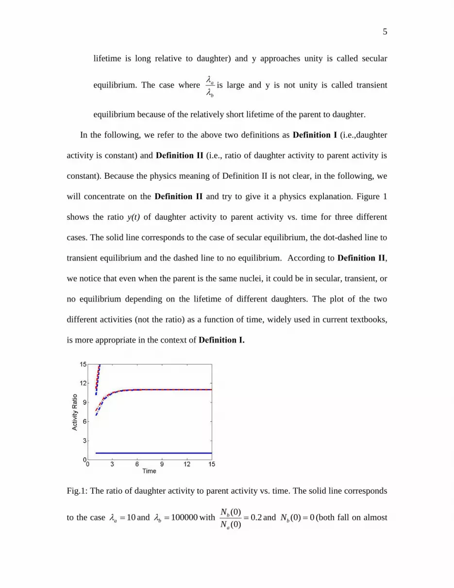
will concentrate on the Definition II and try to give it a physics explanation. Figure 1
shows the ratio y(t) of daughter activity to parent activity vs. time for three different
cases. The solid line corresponds to the case of secular equilibrium, the dot-dashed line to
transient equilibrium and the dashed line to no equilibrium. According to Definition II,
we notice that even when the parent is the same nuclei, it could be in secular, transient, or
no equilibrium depending on the lifetime of different daughters. The plot of the two
different activities (not the ratio) as a function of time, widely used in current textbooks,
is more appropriate in the context of Definition I.
Fig.1: The ratio of daughter activity to parent activity vs. time. The solid line corresponds
to the case 10a and 100000b with 2.0)0(
)0(
a
b
N
Nand 0)0( bN (both fall on almost

6
the same line in the figure), the dot-dashed line to 10a and 11b with 2.0)0(
)0(
a
b
N
N
(red) and 0)0( bN (blue), and the dashed line to 10a and 999999.9b with
2.0)0(
)0(
a
b
N
N (red) and 0)0( bN (blue). Here the time unit is arbitrary.
Current textbooks describe two types of equilibrium (Definitions I and II given above),
where each type of equilibrium is further separated into transient and secular equilibrium
according to its duration. This leads to confusion if one simply uses transient and secular
equilibrium without mentioning which type of equilibrium [6-11]. Transient and secular
equilibrium have been used for a long time without confusion until the emergence of
Definition I. In physics, an equilibrium definition normally is named by its unchanged
observation and not by its duration of time. Because of the confusion of transient
equilibrium and secular equilibrium, we propose to give a name to each type of
equilibrium. For Definition I, since the activities of daughter is constant (i.e, activities of
the parent and daughter are the same from Eq. (2)), we refer to it as “activity
equilibrium”. The physics meaning of Definition II will become apparent below.
Define a new variable ab AAtytz lnln)(ln)( and substituting Eqs. (7, 8), we
obtain .)(
)(lnln)(ab
b
aa
ab
tN
tN
dt
Ad
dt
Ad
dt
tdz Notice that the RHS of Eq. (7) tells
us the lifetime of the parent (because mean lifetime is a
1). We define
dt
activityd )ln(as
the effective life time, (from Eq. (7)) which is exactly equal to the mean lifetime for the
parent and (from Eq. (8)) is only approximately true for the daughter nuclei. However as

7
shown below, the effective lifetime equals the daughter after a long time. Thus 0)(
dt
tdz
reflects the equivalence between the effective lifetimes of the parent and daughter.
Therefore, definition two can be called the effective lifetime equilibrium. The effective
decay parameter (which is a constant) of the parent is a and the effective decay
parameter (which is not a constant) of the daughter is (whenab
a
a
b
N
N
)0(
)0()
tif
tif
eN
NtN
tN
baa
bab
b
ab
at
ab
a
a
b
ab
b
aaeffb
ba
)(
,
)0(
)0(
1
)(
)(
(11a)
or (when 0)0( bN )
tif
tif
etN
tN
baa
bab
bt
abb
b
aaeffb
ba
)(,1)(
)( (11b)
We define effaeffb
tD,,
11)(
or
effa
effbtR
,
,)(
to reflect the differences between the
effective life time of the daughter and parent. In Fig.2, D vs. time is shown. One observes
that when ba and t goes to infinity, D approaches zero because the daughter has an
effective life time similar to the parent (solid line and dot dashed line). It is interesting
thing to notice that although the activity ratio is quite different (solid and dot dashed lines
in Fig.1), their effective life time at large times is the same. When ba and time goes
to infinity, D is the difference between the daughter and parent (dashed line). In Fig.1,
when ab , we obtain a different ratio of parent activity to daughter activity for
different b when time goes to infinity. On the other hand, the difference in parent and

8
daughter effective lifetimes remains the same for different b in Fig.2. Therefore, Fig.2
clearly tells us that the effective lifetime is an appropriate name for the definition II.
Fig.2: The difference between effective lifetime of daughter and parent, aeffb
D
11
,
,
vs. time. The solid line corresponds to cases 10a and 100000b with
2.0)0(
)0(
a
b
N
Nand 0)0( bN (both fall on almost the same line in the figure), the dot-
dashed line to 10a and 11b with 2.0)0(
)0(
a
b
N
N(red) and 0)0( bN (blue) and the
dashed line to 10a and 8.9b with 2.0)0(
)0(
a
b
N
N (red) and 0)0( bN (blue). Here
the time unit is arbitrary.
From Eq. (11a), we notice an interesting phenomenon. If
ab
a
a
b
N
N
)0(
)0( , (12)
Then
9
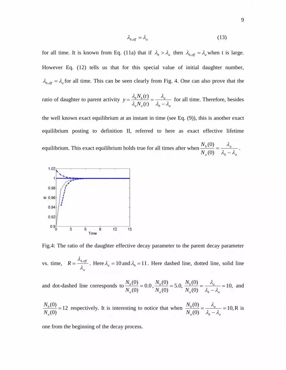
aeffb , (13)
for all time. It is known from Eq. (11a) that if ab then aeffb , when t is large.
However Eq. (12) tells us that for this special value of initial daughter number,
aeffb , for all time. This can be seen clearly from Fig. 4. One can also prove that the
ratio of daughter to parent activity ab
a
aa
bb
tN
tNy
)(
)( for all time. Therefore, besides
the well known exact equilibrium at an instant in time (see Eq. (9)), this is another exact
equilibrium posting to definition II, referred to here as exact effective lifetime
equilibrium. This exact equilibrium holds true for all times after whenab
a
a
b
N
N
)0(
)0(.
Fig.4: The ratio of the daughter effective decay parameter to the parent decay parameter
vs. time, a
effbR
, . Here 10a and 11b . Here dashed line, dotted line, solid line
and dot-dashed line corresponds to 0.0)0(
)0(
a
b
N
N, ,0.5
)0(
)0(
a
b
N
N,10
)0(
)0(
ab
a
a
b
N
N
and
12)0(
)0(
a
b
N
N respectively. It is interesting to notice that when ,10
)0(
)0(
ab
a
a
b
N
N
R is
one from the beginning of the decay process.

10
Given these definitions, we can classify the two different types of transient equilibrium
and secular equilibrium. By coincidence, secular equilibrium of Definition I (activity
equilibrium) and secular equilibrium of Definition II (effective lifetime equilibrium) is
similar. This can be understood by noting that if the daughter activity is the same as the
parent activity, then the daughter decay behavior is similar to its parent, and the
daughter’s effective life time must be the same as that of the parent. We make the
following observations:
(1): As stated clearly in Ref. [6], this letter is only of academic interest. Because the
number of decay processes is limited, we can simply define transient and secular
equilibrium for each process. On the other hand, physics is also a logical science. The
definition of physical concepts should be very strict. Therefore, we think the new
definition given here would be more appropriate in textbook descriptions.
(2): Even with these new definitions, we do not suggest dividing each equilibrium into
two classes, namely, transient and secular; since this classification can lead to confusion
[7]. Instead we propose referring to first class of them as activity equilibrium and
effective life-time equilibrium, respectively. For secular equilibrium of both cases, we
can call them “activity equilibrium and effective lifetime equilibrium” because activity
equilibrium and effective lifetime equilibrium occur at the same time.
(3): We emphasize that the equilibrium here is an approximate one. There is only exact
equilibrium at one time instant in present textbook. In this letter, we have noted another
class of exact equilibrium.
11
In conclusion: Two definitions of radioactive equilibrium are proposed in this letter,
which we refer to as activity equilibrium and effective life-time equilibrium, respectively.
Given these proposed definitions, we believe that the confusion related to transient and
secular equilibrium no long exist. We further observe that in addition to the well known
activity equilibrium at one time instant, there is also another exact effective life-time
equilibrium.
Acknowledgement: The authors like to thank Dr. W. R. Hendee and Dr. D. R. Bednarek
for helpful communications. The authors also like to thank Dr. G. S. Mageras for his
helpful discussions and help in writing.
1R.D. Evans, The atomic nucleus (McGraw-Hill, New York, 1955).
2W. R. Hendee, G. S. Ibbott, E. G. Hendee, Radiation Therapy Physics, 3
rd ed. (Wiley,
New York, 2004).
3H. E. Johns, and J. R. Cunningham, The physics of radiology, 4
th (Thomas, Illinois,
1983).
4F. M. Khan, The physics of radiation therapy, 3
rd ed. (Lippincott Williams & Wilkins
2003).
5 F. H. Attix, Introduction to radiological physics and radiation dosimetry, (Wiley, New
York,1986).

12
6 W. R. Hendee, D. R. Bednarek, “ The concepts of transient and secular equilibrium are
incorrectly described in most textbooks and incorrectly taught to most physics students
and residents,” Med. Phys. 31(6), 1313-1315 (2004).
7 H. I. Amols and M. Bardash,“ The definition of transient and secular radioactive
equilibrium,” Med. Phys. 20(6), 1751-1752 (1993).
8 F. M. Khan,“ comments on the definition of transient and secular radioactive
equilibrium,” Med. Phys. 20(6) 1755-1756 (1993).
9 H. W. Andrews, M. Ivanovic, and D. A. Weber, “Pseudoradioactive equilibrium,”,
Med. Phys. 20(6) 1757(1993).
10 W. R. Hendee, “Comment on the definition of transient and secular radioactive
equilibrium,” Med. Phys. 20(6) 1753(1993).
11H. I. Amols and M. Bardash, “Response to the response to the definition of transient
and secular radioactive equilibrium,” Med. Phys. 20(6) 1759 (1993).