traditional and bulk methods for biofilms
TRANSCRIPT


Biofouling Methods

Biofouling Methods
Edited by
Sergey DobretsovDepartment of Marine Science and Fisheries,College of Agricultural and Marine Sciences, Sultan Qaboos University, Al Khoud, Muscat, Oman
Jeremy C. ThomasonEcoteknica SCP, Administración Siglo XXI, Yucatán, México
David N. WilliamsM&PC Technology Centre, International Paint Ltd, Gateshead, Tyne & Wear, UK

This edition first published 2014 © 2014 by John Wiley & Sons, Ltd.
Registered Office
John Wiley & Sons, Ltd., The Atrium, Southern Gate, Chichester, West Sussex, PO19 8SQ, UK
Editorial Offices
9600 Garsington Road, Oxford, OX4 2DQ, UK
The Atrium, Southern Gate, Chichester, West Sussex, PO19 8SQ, UK
111 River Street, Hoboken, NJ 07030-5774, USA
For details of our global editorial offices, for customer services and for information about
how to apply for permission to reuse the copyright material in this book please see our website
at www.wiley.com/wiley-blackwell.
The right of the author to be identified as the author of this work has been asserted in accordance
with the UK Copyright, Designs and Patents Act 1988.
All rights reserved. No part of this publication may be reproduced, stored in a retrieval system,
or transmitted, in any form or by any means, electronic, mechanical, photocopying, recording or otherwise,
except as permitted by the UK Copyright, Designs and Patents Act 1988, without the prior permission
of the publisher.
Designations used by companies to distinguish their products are often claimed as trademarks. All brand
names and product names used in this book are trade names, service marks, trademarks or registered trademarks
of their respective owners. The publisher is not associated with any product or vendor mentioned in this book.
Limit of Liability/Disclaimer of Warranty: While the publisher and author(s) have used their best efforts in
preparing this book, they make no representations or warranties with respect to the accuracy or completeness
of the contents of this book and specifically disclaim any implied warranties of merchantability or fitness for
a particular purpose. It is sold on the understanding that the publisher is not engaged in rendering professional
services and neither the publisher nor the author shall be liable for damages arising herefrom. If professional
advice or other expert assistance is required, the services of a competent professional should be sought.
Library of Congress Cataloging-in-Publication Data
Biofouling methods / edited by Sergey Dobretsov, Jeremy C. Thomason, David N. Williams. – First edition.
pages cm
Includes index.
ISBN 978-0-470-65985-4 (cloth)
1. Fouling. 2. Fouling organisms. I. Dobretsov, Sergey. II. Thomason, Jeremy.
III. Williams, David N. (David Neil), 1966–
TD427.F68B564 2014
628.9′6–dc23
2014018424
A catalogue record for this book is available from the British Library.
Wiley also publishes its books in a variety of electronic formats. Some content that appears in print may not be
available in electronic books.
Cover images:
Main image: Carmen Kamlah, with assistance of Mauricio Cifuentes.
Insets:
Left: Sergey Dobretsov, 2006.
Middle: Dr Matthew Strom, Industry/University Center for Biosurfaces, State University of
New York at Buffalo.
Right: Sergey Dobretsov, 2013.
Set in 10/12pt Times by SPi Publisher Services, Pondicherry, India
1 2014

List of Contributors xii
Introduction xvi
Guide to Methods xviii
Part I Methods for Microfouling 1Part Editor: Sergey Dobretsov
1 Microscopy of biofilms 3Section 1 Traditional light and epifluorescent microscopy 4
Sergey Dobretsov and Raeid M.M. Abed 1.1 Introduction 4
1.2 Determination of bacterial abundance 8
1.3 Catalyzed reporter deposition fluorescent in situ
hybridization (CARD-FISH) 9
1.4 Suggestions, with examples, for data analysis and presentation 12
Acknowledgements 13
References 13
Section 2 Confocal laser scanning microscopy 15
Koty Sharp 1.5 Introduction 15
1.6 Materials, equipment, and method 18
1.7 Image acquisition 21
1.8 Presentation 21
1.9 Troubleshooting hints and tips 21
1.10 Notes 23
References 23
Section 3 Electron microscopy 26
Omar Skalli, Lou G. Boykins, and Lewis Coons 1.11 Introduction 26
1.12 Transmission electron microscopy (TEM) 27
1.13 Scanning electron microscopy (SEM) 35
References 40
2 Traditional and bulk methods for biofilms 44Section 1 Traditional microbiological methods 45
Hans-Uwe Dahms 2.1 Introduction 45
2.2 Enrichment culture, isolation of microbes 45
2.3 Counting methods 48
2.4 Troubleshooting hints and tips 49
References 50
Contents

vi Contents
Section 2 Bulk methods 52
Sergey Dobretsov 2.5 Introduction 52
2.6 Measurement of biofilm thickness 53
2.7 Biofilm dry weight determination 54
2.8 Biofilm ATP content 55
2.9 Troubleshooting hints and tips 56
Acknowledgements 57
References 57
3 Biocide testing against microbes 58Section 1 Testing biocides in solution: flow cytometry
for planktonic stages 59
Tristan Biggs, Tom Vance, and Glen Tarran 3.1 Introduction 59
3.2 Method introductions 60
3.3 Pros and cons 66
3.4 Materials and equipment 67
3.5 Methods 68
3.6 Troubleshooting hints and tips 70
3.7 Suggestions 71
References 72
Section 2 Biocide testing using single and multispecies biofilms 76
Torben Lund Skovhus 3.8 Introduction 76
3.9 Questions to answer when applying biocides 76
3.10 Laboratory methods for testing biocide effect 78
3.11 Field methods for testing biocide effect 81
3.12 Troubleshooting hints and tips 83
Acknowledgements 84
References 84
4 Molecular methods for biofilms 87Section 1 Isolation of nucleic acids 88
Isabel Ferrera and Vanessa Balagué 4.1 Introduction 88
4.2 Materials 89
4.3 Isolation of DNA from a biofilm 90
4.4 Troubleshooting hints and tips 91
References 91
Section 2 PCR and DNA sequencing 93
Christian R. Voolstra, Manuel Aranda, and Till Bayer 4.5 PCR and DNA sequencing: General introduction 93
4.6 PCR 93
4.7 Microbial marker genes – 16S 94
4.8 DNA sequencing 95
4.9 454 16S amplicon pyrotag sequencing 95
4.10 Protocol 1: DNA extraction using the Qiagen DNeasy
Plant Mini Kit 96

Contents vii
4.11 Protocol 2: Full-length 16S PCR using the Qiagen
Multiplex Kit 98
4.12 Protocol 3: Analysis of full-length 16S genes 100
4.13 Protocol 4: 16S amplicon PCR for 454 sequencing using
the Qiagen Multiplex Kit 102
4.14 Protocol 5: Trimming and filtering of 454 16S pyrotag
sequencing 106
4.15 Protocol 6: Taxon-based analyses 108
4.16 Protocol 7: Phylogeny-based analyses 109
References 111
Section 3 Community comparison by genetic fingerprinting techniques 114
Raeid M.M. Abed and Sergey Dobretsov 4.17 Introduction 114
4.18 History and principles of the methods 115
4.19 Advantages and limitations of fingerprinting techniques 116
4.20 Materials and equipment 116
4.21 Suggestions for data analysis and presentation 121
4.22 Troubleshooting hints and tips 121
Acknowledgements 122
References 122
Section 4 Metagenomics 125
Sarah M. Owens, Jared Wilkening, Jennifer L. Fessler, and Jack A. Gilbert 4.23 Introduction and brief summary of methods 125
4.24 Overview of metagenomics methods 125
4.25 Method introduction 126
4.26 Overview of DNA handling for BAC library construction 127
4.27 BAC and Fosmid library construction 127
4.28 Library handling, archiving, and databasing 128
4.29 Facilitating library screening 128
4.30 Time frame considerations 129
4.31 Materials and equipment 129
4.32 Detailed methods: DNA handling and BAC library
construction 130
4.33 Troubleshooting tips 131
4.34 Suggestions for data analysis 132
4.35 Suggestions for presentation of data 134
Acknowledgements 135
References 135
5 Methods for biofilm constituents and turnover 138Section 1 Destructive and nondestructive methods 139
Arnaud Bridier, Florence Dubois-Brissonnet, and Romain Briandet 5.1 Introduction 139
5.2 Pros and cons of destructive and nondestructive
M-LSM methods for biofilm analysis 140
5.3 Materials and equipment required for M-LSM 140

viii Contents
5.4 Example of questions than can be answered with the method 140
5.5 Suggestions for data analysis and presentation 148
References 149
Section 2 Biofilm formation and quorum sensing bioassays 153
Clayton E. Cox, William J. Zaragoza, Cory J. Krediet, and Max Teplitski 5.6 Introduction 153
5.7 Materials and equipment 157
5.8 Methods 157
Acknowledgements 165
References 165
6 Sampling and experiments with biofilms in the environment 168Section 1 Field trials with biofilms 169
Jeremy C. Thomason 6.1 Introduction 169
6.2 Materials and equipment 170
6.3 Method 170
6.4 Troubleshooting hints and tips 171
6.5 Suggestions for data analysis and presentation 172
References 173
Section 2 Sampling from large structures such as ballast tanks 175
Robert L. Forsberg, Anne E. Meyer, and Robert E. Baier 6.6 Introduction 175
6.7 Materials and equipment 178
6.8 Troubleshooting hints and tips 180
6.9 Analytical methods 180
6.10 Suggestions for data analysis and presentation 182
References 182
Section 3 Sampling from living organisms 184
Christina A. Kellogg 6.11 Introduction 184
6.12 Historical background 185
6.13 Advantages and limitations of collection techniques 185
6.14 Protocols 186
6.15 Suggestions for data analysis 187
6.16 Troubleshooting hints and tips 187
Acknowledgment 188
References 188
Section 4 Optical methods in the field 190
Richard J. Murphy 6.17 Introduction 190
6.18 Examples of the use of optical methods 191
6.19 Spectral characteristics of biofilms 192
6.20 The use of chlorophyll-a as an index of biomass of biofilm 193
6.21 Multi-versus hyperspectral measurements
(CIR imagery versus field spectrometry) 194
6.22 Calibration of data to reflectance 195

Contents ix
6.23 Suggestions for data analysis and presentation 195
6.24 Methods 197
6.25 Troubleshooting hints and tips 201
References 202
7 Laboratory experiments and cultures 204Section 1 Static, constant depth and/or flow cells 205
Robert L. Forsberg, Anne E. Meyer, and Robert E. Baier 7.1 Introduction 205
7.2 Portable Biofouling Unit 207
7.3 Pros and cons of the method 207
7.4 Materials and equipment 208
7.5 Suggestions for data analysis 209
7.6 “Benchmark” bacteria and biofilm characterization 210
7.7 Troubleshooting hints and tips 212
References 212
Section 2 Mixed population fermentor 214
Jennifer Longyear 7.8 Introduction 214
7.9 Pros and cons 215
7.10 Fermentor 215
7.11 Mixed species microfouling culture 215
7.12 Utilizing the fermentor test section 218
7.13 Troubleshooting, hints and tips 218
References 219
Part II Methods for Macrofouling, Coatings and Biocides 221Part Editors: Jeremy C. Thomason, David N. Williams.
8 Measuring larval availability, supply and behavior 223Section 1 Larval availability and supply 224
Sarah Dudas and Joe Tyburczy 8.1 Introduction to measuring larval availability and supply 224
8.2 Measuring settlement and recruitment 235
References 238
Section 2 Larval behavior 241
Jeremy C. Thomason 8.3 Introduction 241
8.4 Method for tracking larvae 242
8.5 Troubleshooting hints and tips 245
8.6 Suggestions for data analysis and presentation 246
References 249
9 Assessing macrofouling 251Section 1: Assessing fouling assemblages 252
João Canning-Clode and Heather Sugden 9.1 Introduction 252
9.2 A note on taxonomy 253
9.3 Field methods 253

x Contents
9.4 Digital methods 258
9.5 Functional groups 261
9.6 Predicting total richness: from the known to the unknown 264
References 267
Section 2 Assessment of in-service vessels for biosecurity risk 271
Francisco Sylvester and Oliver Floerl 9.7 Introduction 271
9.8 Surveys of vessel hulls 272
9.9 Sample and data analysis 277
Acknowledgements 279
References 279
Section 3 Experiments on a global scale 281
Mark Lenz 9.10 Experiments in ecology: the need for scaling up 281
9.11 GAME – a program for modular experimental research
in marine ecology 281
9.12 Marine macrofouling communities as model systems 282
9.13 Chronology of a GAME project 283
Acknowledgements 289
References 289
10 Efficacy testing of nonbiocidal and fouling-release coatings 291 Maureen E. Callow, James A. Callow, Sheelagh Conlan,
Anthony S. Clare, and Shane Stafslien 10.1 Introduction 291
10.2 Test organisms 293
10.3 Test samples 294
10.4 “Antifouling” settlement assays 295
10.5 Fouling-release assays 299
10.6 Adhesion assays for high-throughput screening 304
10.7 Apparatus 310
Acknowledgements 313
References 314
11 Contact angle measurements 317Section 1 Surface characterization by contact angle measurements 318
Doris M. Fopp-Spori 11.1 Introduction 318
11.2 Liquids in contact with solids 318
11.3 Reproducible contact angle measurements 320
11.4 Surface energy calculations 323
References 324
Section 2 Underwater contact angle measurement by the captive
bubble method 326
Pierre Martin-Tanchereau 11.5 Introduction 326
11.6 Materials and requirements 327
11.7 Method 329

Contents xi
11.8 Surface energy 330
Acknowledgements 330
References 331
12 Efficacy testing of biocides and biocidal coatings 332 Christine Bressy, Jean-François Briand, Chantal Compère, and Karine Réhel 12.1 Introduction 332
12.2 Laboratory assays for biocides 333
12.3 Field test methodology for biocidal coatings 337
References 343
13 Commercialization 346Section 1 Processing a new marine biocide from innovation through
regulatory approvals towards commercialization 347
Lena Lindblat 13.1 Introduction 347
13.2 Basics about the regulatory landscape from the
academic perspective 349
13.3 Risk, risk assessment and risk management 349
13.4 Future directions 353
13.5 Conclusions 355
References 356
Section 2 From laboratory to ship: pragmatic development of fouling
control coatings in industry 358
Richie Ramsden and Jennifer Longyear 13.6 Introduction 358
13.7 Laboratory coating development 358
13.8 Laboratory bioassay screening 359
13.9 Fitness for purpose (FFP) testing 360
13.10 Field antifouling performance testing 361
13.11 Test patch and vessel trials 363
13.12 Performance monitoring 364
13.13 Summary 365
References 365
Index 366

List of contributors
Raeid M.M. AbedBiology Department,
College of Science,
Sultan Qaboos University,
Al Khoud, Muscat, Oman
Manuel ArandaRed Sea Research Center,
King Abdullah University of Science
and Technology (KAUST),
Thuwal, Saudi Arabia
Robert E. BaierState University of New York
at Buffalo,
Buffalo, NY, USA
Vanessa BalaguéDepartment of Marine Biology
and Oceanography,
ICM (Institute of Marine Sciences),
CSIC (The Spanish National
Research Council),
Barcelona, Spain
Till BayerRed Sea Research Center,
King Abdullah University of Science
and Technology (KAUST),
Thuwal, Saudi Arabia
Tristan BiggsPML Applications Ltd, Plymouth,
UK Currently: NIOZ – Royal Netherlands
Institute for Sea Research,
’t Horntje (Texel), The Netherlands
Lou G. BoykinsIntegrated Microscopy Center and
Department of Biological Sciences,
The University of Memphis,
Memphis, TN, USA
Christine BressyLaboratoire MAPIEM,
Université de Toulon, France
Jean-François BriandLaboratoire MAPIEM,
Université de Toulon,
France
Romain BriandetThe Micalis Institute,
INRA/AgroParisTech,
Massy, France
Arnaud BridierThe Micalis Institute,
INRA/AgroParisTech,
Massy, France
James A. CallowSchool of Biosciences,
University of Birmingham,
Birmingham, UK
Maureen E. CallowSchool of Biosciences,
University of Birmingham,
Birmingham, UK
João Canning-ClodeCentre of IMAR of the University
of the Azores,
Department of Oceanography
and Fisheries/UAz & LARSyS
Associated Laboratory,
Horta, Azores, Portugal
Center of Oceanography,
Faculty of Sciences,
University of Lisbon, Lisbon,
Portugal Smithsonian Environmental
Research Center,
Edgewater, MD, USA
List of contributors xiii
Anthony S. ClareSchool of Marine Science
and Technology,
Newcastle University,
Newcastle upon Tyne, UK
Chantal CompèreRecherches et Développements
Technologiques,
IFREMER/Centre de Bretagne,
Plouzané, France
Sheelagh ConlanNatural Sciences and Psychology,
Liverpool John Moores University,
Liverpool, UK
Lewis CoonsIntegrated Microscopy Center
and Department of Biological
Sciences,
The University of Memphis,
Memphis, TN, USA
Clayton E. CoxSchool of Natural Resources
and Environment,
University of Florida – IFAS,
Microbiology Graduate Program,
University of Florida,
Gainesville, FL, USA
Hans-Uwe DahmsDepartment of Biomedical
Science and Environmental
Biology,
Kaohsiung Medical University,
Kaohsiung, Taiwan
Sergey DobretsovDepartment of Marine Science
and Fisheries,
College of Agricultural
and Marine Sciences,
Sultan Qaboos University,
Al Khoud, Muscat, Oman
Florence Dubois-BrissonnetThe Micalis Institute,
INRA/AgroParisTech,
Massy, France
Sarah DudasDepartment of Zoology,
Oregon State University,
Corvallis, OR,
USA Currently: Centre for
Shellfish Research,
Vancouver Island University,
Nanaimo, BC, Canada
Isabel FerreraDepartment of Marine Biology
and Oceanography,
ICM (Institute of Marine Sciences),
CSIC (The Spanish National
Research Council),
Barcelona, Spain
Jennifer L. FesslerArgonne National Laboratory,
Argonne, IL, USA
Oliver FloerlNational Institute of Water and
Atmospheric Research (NIWA),
Christchurch,
New Zealand Currently:
Cawthron Institute,
Nelson, New Zealand
Doris M. Fopp-SporiETH Zürich, Zurich,
Switzerland Currently:
Metrology Department,
Oerlikon Balzers Coating AG,
Balzers, Liechtenstein
Robert L. ForsbergState University of New York at Buffalo,
Buffalo, NY, USA
Jack A. GilbertArgonne National Laboratory,
Argonne,
IL. Department of Ecology
and Evolution,
University of Chicago,
Chicago, IL, USA
Christina A. KelloggU.S. Geological Survey,
St. Petersburg, FL, USA

xiv List of contributors
Cory J. KredietSchool of Natural Resources
and Environment,
University of Florida – IFAS,
Gainesville, FL,
USA Stanford University
School of Medicine,
Stanford, CA, USA
Mark LenzGEOMAR Helmholtz Centre
for Ocean Research, Kiel, Germany
Lena LindblatI-Tech AB,
Gothenburg, Sweden
Jennifer LongyearM&PC Technology Centre,
International Paint Ltd,
Gateshead, Tyne & Wear, UK
Pierre Martin-TanchereauM&PC Technology Centre,
International Paint Ltd,
Gateshead, Tyne & Wear, UK
Anne E. MeyerState University of New York at Buffalo,
Buffalo, NY, USA
Richard J. MurphyAustralian Centre for Field Robotics,
Department of Aerospace,
Mechanical & Mechatronic Engineering,
The University of Sydney,
Sydney, NSW, Australia
Sarah M. OwensArgonne National Laboratory,
Argonne, IL,
USA Computation Institute,
University of Chicago,
Chicago, IL, USA
Richie RamsdenM&PC Technology Centre,
International Paint Ltd,
Gateshead,
Tyne & Wear, UK
Karine RéhelLaboratoire de Biotechnologie
et Chimie Marine,
Lorient, France
Koty SharpDepartments of Marine Science
and Biology
Eckerd College,
St. Petersburg,
FL, USA
Omar SkalliIntegrated Microscopy Center and
Department of Biological Sciences,
The University of Memphis,
Memphis, TN, USA
Torben Lund SkovhusDNV GL, Corrosion Management
and Technical Advisory,
Bergen, Norway
Shane StafslienCenter for Nanoscale Science
and Engineering,
North Dakota State University,
Fargo, ND, USA
Heather SugdenThe Dove Marine Laboratory,
School of Marine Science
and Technology,
Newcastle University,
North Shields,
Tyne & Wear,
UK Ecoteknica UK Ltd,
Newcastle upon Tyne, UK
Francisco SylvesterDepartment of Ecology,
Genetics and Evolution,
Faculty of Exact and Natural Sciences,
University of Buenos Aires,
Buenos Aires,
Argentina Currently: Faculty
of Natural Sciences,
National University of Salta,
Salta, Argentina

List of contributors xv
Glen TarranPML Applications Ltd, Plymouth, UK
Max TeplitskiSchool of Natural Resources
and Environment,
University of Florida – IFAS
Soil and Water Science Department,
University of Florida,
Gainesville, FL, USA
Jeremy C. ThomasonEcoteknica SCP,
Administración Siglo XXI,
Mérida, Yucatán, México
Joe TyburczyDepartment of Zoology,
Oregon State University,
Corvallis, OR,
USA Currently: University of California
Sea Grant Extension Program,
Eureka, CA, USA
Jared WilkeningArgonne National Laboratory,
Argonne, IL, USA
David N. WilliamsM&PC Technology Centre,
International Paint Ltd,
Gateshead,
Tyne & Wear, UK
Tom VancePML Applications Ltd,
Plymouth, UK
Christian R. VoolstraRed Sea Research Center,
King Abdullah University of Science
and Technology (KAUST),
Thuwal, Saudi Arabia
William J. ZaragozaMicrobiology Graduate Program,
University of Florida – IFAS,
Gainesville, FL,
USA Produce Safety & Microbiology
Research Unit,
Western Regional Research Center,
Agricultural & Research Service,
U.S. Department of Agriculture,
Albany, CA, USA

Introduction
Biofouling is the accumulation of unwanted biological material at an interface and we nor-
mally associate it with the growth of organisms on surfaces in aquatic environments, be they
hard or soft, living or non-living, surfaces. The organisms making up the unwanted biologi-
cal assemblage may range in size from nanoscale viruses to large macroscopic algae several
meters long, and the methods required to study these assemblages are accordingly diverse.
Although the study of biofouling has taken off in recent decades, with the term first
appearing in the literature in the mid-1970s, the issue has been noted for millennia, and the
term antifouling has a much more antiquated usage associated with the use of tars, paints,
and copper sheathing to control the growth of biofouling on ships in days gone by. This
reflects the huge impact that biofouling has on vessels, causing both drag and corrosion.
Indeed, much of the current driving force behind research into biofouling is the need of the
global merchant marine fleet and also navies to reduce the cost of propulsion. This economic
driver has the benefit of also reducing the global fleet’s carbon footprint, that is, the same
performance but with less fuel. More recently, with the advent of large off-shore engineering
projects, such as oil and gas installations, and coastal projects, such as power stations and
desalination plants, the awareness of the impact of biofouling on both hydraulics and corro-
sion has increased considerably outside of the sphere of shipping. This concern is further
driving the need for more research into both fundamental processes and novel antifouling
technologies.
Biofouling and antifouling research is now a substantial academic field with its own journal
and a biennial conference. It was also the focus of a recent Wiley-Blackwell textbook, Durr
and Thomason’s (2010) Biofouling, which brought the literature in the field up to date. That
book was a key review of the current boundaries but contained only a summary of research
methods. Conversely, the aim of this book, Biofouling Methods, is to be an essential com-
panion to the former work by providing a “cook book” of practical recipes for those who are
currently working in, or just entering, the biofouling field. We have strived to ensure that the
book includes methods are that tried and tested as well as those at the cutting edge, thus
encompassing the full diversity of the field. We expect this book to become the essential
methodological reference for all those working on biofouling and antifouling in academia,
namely aquatic biologists, ecologists, environmental scientists, and also for research and
development technologists in the antifouling industry. It will also be relevant to anyone who
has to monitor biofouling, such as aquaculture producers, managers of off-shore and coastal
installation in the oil, gas and desalination sectors, amongst others. This book will also be
useful for some specialized practical courses and for graduate and postgraduate students
undertaking their own research.
The book is organized in two parts:
1. Methods for Microfouling (Part Editor: Sergey Dobretsov)2. Methods for Macrofouling, Coatings and Biocides (Part Editors: Jeremy C. Thomason,
David N. Williams)

Introduction xvii
Each chapter aims to cover a brief history of the method(s) to ensure suitable acknowledgement
of the original inventors, includes some examples of the successful use of the method, and
examples of the questions that can be answered with the method. Each chapter may cover
several methods in a clearly defined subarea. The materials and equipment and methods
are described in sufficient detail that the method can be readily implemented and
troubleshooting hints and tips are given to permit rapid problem solving along with
suggestions with examples for data analysis and presentation. Some chapters vary from
this theme, particularly where there is little experimental methodology to describe and we
were not overly prescriptive to the authors.
We hope that this book serves its purpose and that you find the methods described here to
be useful for your research.
Sergey Dobretsov
(Muscat, Oman)
Jeremy C. Thomason
(Mérida, México)
David N. Williams
(Felling, UK)

Guide to methods

What do you want to do?
Study micro-fouling Study macro-fouling Study coatings
Chapter 1, Chapter 4 & 5
Chapter 4, Chapter 7, Chapter 10 & 13
Chapter 9, Chapter 12, Chapter 13
Chapter 8, Chapter 10 & 13
Chapter 4, Chapter 6
Chapter 10 Chapter 12 & 13
Chapter 7, Chapter 10 & 11
Chapter 6, Chapter 8, Chapter 12 & 13
Chapter 3, Chapter 12
Chapter 11, Chapter 13
Chapter 8, Chapter 9
Chapter 8, Chapter 9, Chapter 10, Chapter 12 & 13
Chapter 2, Chapter 5
Chapter 4, Chapter 5 & 6
Chapter 3, Chapter 12
Chapter 4, Chapter 5 & 6
Chapter 7, Chapter 10, Chapter 12
Chapter 8, Chapter 9
Chapter 9, Chapter 12
Visualise microbes in biofilms
Grow biofilm microbes
Measure biofilm properties
Test biocides
Study biofilm community dynamics
Sample and measure biofilms in
the field
Test coating efficacy
Test biocides
Test coatings in the field
Test coatings in the laboratory
Bring your coating to market
Measure surface properties
Measure fouling pressure
Quantify the fouling community
Fouling on ships
Do experiments with fouling
Study coating efficacy
Study coating efficacy against biofilms
Study biofilm communities

Part IMethods for MicrofoulingPart Editor: Sergey Dobretsov

Biofouling Methods, First Edition. Edited by Sergey Dobretsov, Jeremy C. Thomason and David N. Williams. © 2014 John Wiley & Sons, Ltd. Published 2014 by John Wiley & Sons, Ltd.
1 Microscopy of biofilms
Abstract
Identification, visualization and investigation of biofouling microbes are not possible with-out light, epifluorescence and electron microscopy. The first section of this chapter presents methods of quantification of microbes in biofilms and Catalyzed Reporter Deposition Fluorescent in situ hybridization (CARD-FISH). The second section provides an overview of Laser Scanning Confocal Microscopy (LSCM) imaging, which focuses mainly on the Fluorescent in situ Hybridization Technique (FISH) technique. This technique is very useful for visualization and quantification of different groups of microorganisms. The third section describes the principles of transmission (TEM) and scanning (SEM) electron microscopy.

Biofouling Methods, First Edition. Edited by Sergey Dobretsov, Jeremy C. Thomason and David N. Williams. © 2014 John Wiley & Sons, Ltd. Published 2014 by John Wiley & Sons, Ltd.
Section 1 Traditional light and epifluorescent microscopy
Sergey Dobretsov1 and Raeid M.M. Abed2
1 Department of Marine Science and Fisheries, College of Agricultural and Marine Sciences, Sultan Qaboos University, Al Khoud, Muscat, Oman2 Biology Department, College of Science, Sultan Qaboos University, Al Khoud, Muscat, Oman
1.1 Introduction
Light microscopy is among the oldest methods used to investigate microorganisms [1, 2]. Early microscopic observations are usually associated with the name of Antony van Leeuwenhoek, who was able to magnify microorganisms 200 times using his designed microscope [1]. A modern light microscope has a magnification of about 1000× and is able to resolve objects separated by 0.275 μm. This resolving power is limited by the wave-length of the used light for the illumination of the specimens. Several light microscopy techniques, such as bright field, dark field and phase contrast, enhance contrast between microorganisms and background [1]. Fluorescent microscopy takes advantage of the abil-ity of some materials or organisms to emit visible light when irradiated with ultraviolet radiation at a specific wavelength. Phototrophic organisms have a natural fluorescence due to the presence of chlorophyll in their cells [3]. Other organisms require additional dyes in order to become fluorescent.
Light microscopy is a simple and cheap method [2]. It is commonly used for observation of relatively large (>0.5 μm) cells of microorganisms (Figure 1.1). In comparison, epifluo-rescent microscopy provides higher resolution and is generally used for observation of bacteria or cell organelles. The pros and cons of these methods are presented in Table 1.1.
Epifluorescent stains allow quick and automatic counting of bacteria using flow cytometry (discussed later in this chapter). Epifluorescent microscopy is preferable over scanning electron microscopy (SEM) (Chapter 1, section 3) for bacterial size and abundance studies [4]. While direct light microscopy measurements can be highly sensitive to low cell num-bers, electron microscopy methods are not. Light and epifluorescent microscopy has the advantage over electron microscopy that a larger surface area can be assessed for a given amount of time [5]. Two fluorescent stains are widely used to stain microbial cells, namely 4’,6-diamidino-2-phenylindole (DAPI), which binds to DNA [6] (Figure 1.2), and acrydine orange, which binds to DNA and RNA as well as to detritus particles [7]. Therefore, the estimated number of bacteria stained with DAPI is on average 70% of bacterial counts made with acrydine orange [8]. The use of DAPI stain allows a longer period between slide

Microscopy of biofilms 5
preparation and counting, since DAPI fluorescence fades less rapidly than acrydine orange. DAPI staining does not allow accurate measurement of the size of the bacterial cells, since it could only stain the specific part of the cell containing DNA [8]. Visualization of bacteria in dense biofilms is highly difficult. This problem can be overcome to a certain extent by using confocal scanning laser microscopy (CSLM) (Chapter 1, part 2). DAPI staining has been intensively used for determination of bacterial abundance in water samples [9] as well as in biofilms [10]. This can be useful for the determination of the efficiency of biocides (Chapter 2).
Length = 100.75 µm
Figure 1.1 Microfouling community dominated by different cyanobacteria, diatoms and bacteria under a light microscope. Magnification 100×. Picture by Julie Piraino. For color detail, please see color plate section.
Table 1.1 Pros and cons of light and epifluorescent microscopy.
Method Pros Cons
Light microscopy
• Relatively inexpensive method (<$500) and does not require specialized equipment
• Simple sample preparation. In order to increase contrast, object can be stained
• Visualization of small microorganisms (>0.5 mm) is difficult
• Only large cell organelles (such as nucleus) can be visualized
• Counting of bacteria is difficultEpifluorescent microscopy
• Small microorganisms, such as bacteria, can be visualized and easily counted
• Photosynthetic organisms, such as diatoms and cyanobacteria, do not require staining
• Specialized selective probes allow staining of different cell organelles or different groups of microorganisms
• Require specialized equipment, relatively expensive (>$10 000) equipment (epifluorescent microscope with UV lamp)
• Usually requires staining with fluorescent probes

6 Biofouling Methods
Fluorescent in situ hybridization (FISH) allows quick phylogenetic identification (phylogenic staining) of microorganisms in environmental samples without the need to cultivate them or to amplify their genes using the polymerase chain reaction (PCR) [11] (Table 1.2, Figure 1.3). This method is based on the identification of microorganisms using short (15–20 nucleotides) rRNA-complementary fluorescently labeled oligonucleo-tide probes (species, genes or group specific) that penetrate microbial cells, bind to RNA and emit visible light when illuminated with UV light [12]. Common fluorescent dyes include Cy3, Cy5 and Alexa®. In comparison with other molecular methods (Chapter 3), FISH provides quantitative data about abundance of bacterial groups without PCR bias [13]. The FISH-based protocol is presented later in this chapter (Chapter 1, section 2); here the modified protocol of catalyzed reporter deposition fluorescent in situ hybridiza-tion (CARD-FISH) is described. CARD-FISH is based on the deposition of a large number of labeled tyramine molecules by peroxidase activity (Figure 1.3), which enhances visualization of a small, slow growing or starving bacteria that have a small amount of rRNA and, thus, give a weak FISH signal [14]. Additionally, CARD-FISH can be used for the visualization and assessment of the densities of microorganisms in the samples that have high background fluorescence, such as algal surfaces, fluorescent paints, phototro-phic biofilms and sediments [14–16]. In this procedure, FISH probes are conjugated with the enzyme (horseradish peroxidase) and after hybridization the subsequent deposition of fluorescently labeled tyramides results in substantially higher signal intensities on target cells [16]. The critical step of CARD-FISH is to ensure probe microbial cell permeability with cellular integrity, especially in diverse, multispecies microbial communities [17]. Recent improvements in CARD-FISH samples preparation, permeabilization and staining techniques have resulted in a significant improvement in detection rates of benthic and planktonic marine bacteria [14, 15].
0.01 mm
Figure 1.2 Bacterial cells stained with DAPI visualized under an epifluorescent microscope. Magnification 1000 ×. For color detail, please see color plate section.

Table
1.2
C
omm
on p
robe
s us
ed in
FIS
H a
nd C
ARD
-FIS
H a
nd th
eir s
peci
fic c
ondi
tions
. Det
aile
d in
form
atio
n ab
out r
RNA
-targ
eted
olig
onuc
leot
ide
prob
es
can
be fo
und
in th
e pu
blic
dat
abas
e Pr
obeB
ase
(http
://w
ww
.mic
robi
al-e
colo
gy.n
et/d
efau
lt.as
p) [1
9, 2
0].
Pro
be
Sequen
ce (
5’-
3’)
of
the
pro
be
Targ
et g
roup
Form
am
ide
(%)
Ref
eren
ce
Univ
ersa
lEU
B338
GC
T G
CC
TC
C C
GT
AG
G A
GT
Mos
t of b
acte
ria20
–35
[21]
Eury
806
CA
C A
GC
GTT
TA
C A
CC
TA
GEu
ryar
chae
a20
[22]
NO
NEU
BA
CT
CC
T A
CG
GG
A G
GC
AG
CN
on-sp
ecifi
c to
bac
teria
(con
trol f
or E
UB3
38)
20[2
3]
Gro
up s
pec
ific
ALF
968
GG
T A
AG
GTT
CTG
CG
C G
TTA
lpha
prot
eoba
cter
ia e
xcep
t Ric
ketts
iale
s20
[24]
GA
M42
a*G
CC
TTC
CC
A C
AT C
GT
TTM
ost G
amm
apro
teob
acte
ria35
[25]
CF3
19a
TGG
TC
C G
TG T
CT
CA
G T
AC
Bact
eroi
dete
s (m
ost F
lavo
bact
eria
, som
e Ba
cter
oide
tes,
so
me
Sphi
ngob
acte
ria)
35[2
6]
BET4
2a**
GC
C T
TC C
CA
CTT
CG
T TT
Beta
prot
eoba
cter
ia35
[25]
LGC
354C
CC
G A
AG
ATT
CC
C T
AC
TG
CFi
rmic
utes
(Gra
m-p
ositi
ve b
acte
ria w
ith lo
w G
+ C
con
tent
)35
[27]
HG
C69
ATA
T A
GT
TAC
CA
C C
GC
CG
TA
ctin
obac
teria
(hig
h G
+ C
Gra
m-p
ositi
ve b
acte
ria)
25[2
8]
Gen
es s
pec
ific
GV
AG
G C
CA
CA
A C
CT
CC
A A
GT
AG
Vibr
io s
pp.
30[2
9]
Spec
ies
spec
ific
Psea
erA
TCT
CG
G C
CT
TGA
AA
C C
CC
Pseu
dom
onas
aer
ugin
osa
30[3
0]
*GA
M42
a re
quire
s co
mpe
titor
GC
C T
TC C
CA
CTT
CG
T TT
that
incr
ease
s ch
ance
s of
spe
cific
bin
ding
.**
BET4
2a re
quire
s co
mpe
titor
GC
C T
TC C
CA
CAT
CG
T TT
that
incr
ease
s ch
ance
s of
spe
cific
bin
ding
.

8 Biofouling Methods
1.2 Determination of bacterial abundance
1.2.1 Material and equipment
The materials and equipment necessary for counting bacteria in biofilms using DAPI stain-ing are listed in Table 1.3.
1.2.2 Method
1. Add a few drops of DAPI solution in order to fully cover the biofilm.2. Stain for 15 minutes in the dark. Stained samples should be processed within 2–3 days in
order to avoid loss of bacterial numbers [18].3. Place a cover slip.4. Remove excess water using filter paper.5. Place immersion oil on the top of the cover slip.6. Using 100× objective count bacteria in 20 fields of view selected randomly. In the case
of digital camera coupled with an epifluorescent microscope, an automatic counting of
Epifluorescent microscopy
Environmental sample
Fixation
Hybridization with probes
Washing
DAPI staining
Fish Card-fish
Fixation andembedding
Permeabilization andinactivation of peroxidases
Tyramide signalamplification
Figure 1.3 Outline of fluorescent in situ hybridization (FISH) and catalyzed reporter deposition fluorescent in situ hybridization (CARD-FISH).

Microscopy of biofilms 9
microorganisms is possible using free image processing software ImageJ (http://rsbweb.nih.gov/ij/).
7. Calculate the number of bacteria.8. Slides can be storied frozen at –20 °C in the dark for up to one year.
1.2.3 Troubleshooting hints and tips
Special attention should be paid in the random selection of fields of view for microbial counting. This can be done using MS Excel or other software that allow a table of random X and Y stage coordinates to be generated.
A stock solution of DAPI (1 mg ml–1 in distilled water) can be prepared and stored in a dark cold (+4 °C) place for several months. This stock solution can be diluted with distilled water prior to staining in order to make working solution.
1.3 Catalyzed reporter deposition fluorescent in situ hybridization (CARD-FISH)
1.3.1 Material and equipment
The materials and equipment necessary for CARD-FISH are listed in Table 1.4.
1.3.2 Sample preparation
Microbial samples should be fixed with paraformadehyde (final concentration 2–3%) for 12 h at 4 °C. Short (1–12 h) fixation by 3% formaldehyde is possible. Fixed samples should be washed with PBS buffer for 30–60 minutes and then stored in a 2:3 PBS:ethanol mixture at –20 °C for further use without loss in signal. In the case of cell suspensions, the suspen-sion should be filtered through non-fluorescent black 0.2 μm filters prior to staining.
1.3.3 Method
Embedding
1. Mark slides or filters using pencil or permanent marker that resists alcohol.2. Dip filters in 0.1–0.2% low melting agarose and air dry them at 35 °C.
Table 1.3 Materials and equipment needed for the DAPI-based determination of bacterial abundance in biofilms.
Materials Equipment
Biofilm samples developed on glass slides and fixed with 3% formaldehyde or glutaraldehyde
Epifluorescent microscope with total magnification at least 1000×
Glass slides A blue filter set (excitation 365 nm, splitter 395 nm, barrier filter 420 nm) for DAPI stain
Cover slips An eye piece of known areaImmersion oil4,6-Diamidino-2-phenylindole (DAPI) working solution 50 µg ml–1
Blotting paper

10 Biofouling Methods
3. Dehydrate slides or filters in 96% ethanol for one minute at room temperature.4. Air dry slides or filters at room temperature. Samples may be stored at –20 °C for several
weeks without loss in signal.
Permeabilization and inactivation of peroxidases
1. Incubate in lysozyme at 37 °C for >60 minutes.2. Incubate in achromopeptidase at 37 °C for >30 minutes.3. Wash twice with MQ water (1 minute at room temperature).4. Incubate in 0.01 M HCl for 10 minutes at room temperature in order to bleach endoge-
nous peroxidise.5. Wash twice with MQ water (1 minute at room temperature).6. Wash with 96% ethanol (1 minute at room temperature). Air dry samples at room temperature.
The samples may be stored at –20 °C for several weeks without loss in signal.
Hybridization and washing
1. Place filters or slides in the centrifuge tubes. Use 1.5 ml and 50 ml centrifuge tubes for filters and microscopic slides, respectively. Place a blotting paper in the large centrifuge tube.
2. Prepare hybridization solution containing appropriate amount of formamide (Table 1.5). Mix 400 μl of hybridization solution and 4 μl of probe solution (concentration = 50 ng μl–1) and add to filters or slides. Cover the microscopic slide with a cover slip. Wet the blot-ting paper in the large centrifuge tube with hybridization solution. It should not be dripping wet.
Table 1.4 Materials and equipment needed for CARD-FISH.
Materials Equipment
Fixed biofilm samples on glass slides or non- fluorescent (e.g., black 0.2 µm Millipore®, GTBP02500) filters (see sample preparation)
Epifluorescent microscope with a total magnification of at least 1000×
Glass slides A blue filter set (excitation 365 nm, splitter 395 nm, barrier filter 420 nm) for DAPI stain and specific filter for the labeled probe
Cover slips An eye piece of a known areaImmersion oil Water bath4,6-Diamidino-2-phenylindole (DAPI) working solution (concentration = 50 µg ml–1)
Thermostatic incubator
50 ml or 1.5 ml centrifuge tubesHorseradish-labeled oligonucleotide probe (Table1.2)Reagents: 96% ethanol, 0.2% low-gelling agarose, lysozyme, 0.01 M HCl, achromopeptidase, MilliQ water, phosphate buffer saline (PBS) buffer (NaCl – 8.01 g, KCl – 0.2 g, Na2HPO4 2H2O – 1.78 g, KH2PO4 – 0.27 g, add 1 l of distilled water, adjust to pH = 7.6), 2% paraformaldehyde solution in distilled water, 0.0015% H2O2 solution, hybridization solution prepared according to Table 1.5, washing solution prepared according to Table 1.6.Blotting paper

Microscopy of biofilms 11
3. Incubate filters or slides in the centrifuge tubes at 35 °C for at least two hours. Longer incubation gives better results usually.
4. Prepare appropriate washing solution (Table 1.6). Wash filters or slides in a pre-warmed washing buffer (10 minutes at 37 °C) (Table 1.7). Do not air dry after washing.
Tyramide signal amplification
1. Remove excess of water using blotting paper. Do not let the filters or slides run dry. Incubate them in 1× PBS buffer for 15 minutes with mild agitation.
Table 1.5 Hybridization solutions for horseradish labeled probes. Amount of compounds is enough for one probe hybridization. These solutions are stable for 2 months at –20 °C. Pre-warm the mixtures in water bath (60 °C) until dextran sulfate dissolves.
Compound
Formamide concentration
20% 25% 30% 35%
5 M NaCl (µl) 360 360 360 3601 M Tris-HCl (µl) 40 40 40 40Dextran sulfate (g) 0.2 0.2 0.2 0.2Formamide (µl) 400 500 600 700MilliQ water (µl) 1000 900 800 70010% (w/v) Blocking reagent (Roche #1096176) dissolved in maleic acid buffer (µl)
200 200 200 200
10% Sodium dodecyl sulfate (SDS) (µl) 2 2 2 2
Table 1.6 Washing buffer solutions for horseradish labeled probes. Amount of compounds is enough to prepare 50 ml of washing solution. Pre-warm washing buffer at 37 °C in order to dissolve compounds.
Compound
Formamide concentration
20% 25% 30% 35%
1 M Tris-HCl (µl) 1000 1000 1000 10005 M NaCl (µl) 1350 950 640 4200.5 M EDTA (µl) 500 500 500 50010% SDS (µl) 50 50 50 50MilliQ water (µl) 47 100 47 500 47 810 48 030
Table 1.7 Amplification buffer solution. Can be used for any formamide concentration. p-iodophenylboronic acid (IPBA; 20 mg IPBA per 1 mg tyramide) enhances the CARD-FISH signal of tyramides labeled with Alexa488 and Alexa546 but does not work for tyramides labeled with Alexa350 and Cy3.
Compound Amount
20× PBS buffer 2 ml10% (w/v) Blocking reagent (Roche #1096176) in maleic acid buffer, pH = 7.5. Can be autoclaved and storied at –20 °C
0.4 ml
5 M NaCl solution in MilliQ water 16 mlSterile MilliQ water To a final volume 40 mlDextrane sulfate. Buffer can be heated to 60 °C in order to dissolve it. 4 g

12 Biofouling Methods
2. Incubate samples in a substrate mix (1 part fluorescently labeled tyramide, 10–500 parts of amplification buffer and 0.0015% H
2O
2) for 20 minutes in the dark at 46 °C.
3. Remove excess of buffer using blotting paper. Do not let the filters or slides run dry.4. Wash filters or slides in 1× PBS buffer for 5–10 minutes at room temperature.5. Wash twice in 50 ml of MilliQ water at room temperature in the dark.6. Wash in 50 ml of 96% ethanol at room temperature in the dark.7. Air dry samples. These samples can be stored at –20 °C for several weeks without loss
in signal.8. Overlay each slide or filter with 10 μl DAPI solution and incubate for five minutes in the
dark (see determination of bacterial abundance using DAPI stain).9. Mount slide or filter under a cover glass. Rapid loss of fluorescence can be prevented
by using anti-fading reagents.10. Observe sample under an epifluorescent microscope. Count bacterial cells stained with
DAPI (total count) and amount of bacteria stained with probe. It is recommended to count about 600–800 bacterial cells [15].
1.3.4 Troubleshooting hints and tips
One of the common problems of CARD-FISH is the high background fluorescence, which might be due to (i) the use of high tyramide concentration, (ii) high probe concentration and (iii) short washing. Possible solutions may include decreasing tyramide concentrations or increasing the blocking reagent concentrations, decreasing the probe concentrations and extended washing in deionized water.
Low signal intensity might be observed and could be due to several reasons:
● Low ribosome content of target cells. In this case it is recommended to increase the tyra-mide concentration or the temperature during the tyramide signal amplification. A pro-longed hybridization time (>4 hours) may also help.
● Too low tyramide concentration. Check the concentration and increase it 1.5–2 times. ● The probes has too low or no activity. In this case, check the probe. Make sure that the probe is thawed only once and is not be stored in the fridge for more than six months. Check the pH of the PBS buffer (should be around 7.6) and H
2O
2 concentration and its age. If neces-
sary, prepare new PBS buffer and H2O
2 solution. Check the reactivity of the tyramide.
● The horseradish peroxidase is not coupled with the probe. In this case, use new horserad-ish peroxidase probe.
● The horseradish peroxidase probe cannot penetrate the cell wall. In this case, try different permeabilization protocols.
1.4 Suggestions, with examples, for data analysis and presentation
The number of bacteria per an eye piece of a known area obtained using DAPI counting can be transformed to a number of bacteria per mm2 [10]. In the case of normally distributed data, densities of bacteria can be compared using a t-test (for the comparison of 2 means) or ANOVA followed by a suitable post hoc (for multiple comparisons). Usually, normality of the data can be improved by taking the natural log.

Microscopy of biofilms 13
Usually, FISH or CARD-FISH data are expressed as percentages of total bacterial num-bers obtained using particular oligonucleotide probe versus total DAPI counts for the same sample. This can be calculated using the following formula:
% DAPI count = n/N × 100
where n = number of bacteria stained with the probe and N = number of bacteria stained with DAPI.
Acknowledgements
The work of SD was supported by a Sultan Qaboos University (SQU) internal grant IG/AGR/FISH/12/01 and by a HM Sultan Qaboos Research Trust Fund SR/AGR/FISH/10/01.
References
1. Madigan, M.T., Martinko, J.M., Dulap, P.V. and Clark, D.P. 2009. Brock Biology of Microorganisms. Pearson Benjamin Cummings, San Francisco, CA.
2. Bradbury, S. and Bracegirdle, B. 1998. Introduction to Light Microscopy. BIOS Scientific Publishers, New York.
3. Lichtman, J.W. and Conchello, J-A. 2005. Fluorescent microscopy. Nature Methods 2: 910–919.4. Fuhrman, J. A. 1981. Influence of method on the apparent size distribution of bacterio-plankton cells:
Epifluorescence microscopy compared to scanning electron microscopy. Marine Ecology Progress Series 5: 103–106.
5. Wigglesworth-Cooksey, B. and Cooksey, K.E. 2005. Use of fluorophore-conjugated lectins to study cell-cell interactions in model marine biofilms. Applied Environmental Microbiology 71: 428–435.
6. Porter, K. G., and Feig, Y. S. 1980. The use of DAPI for identifying and counting aquatic microflora. Limnology and Oceanography 25: 943–948.
7. Zimmerman, R., and Meyer-Reil, L.-A. 1974. A new method for fluorescence staining of bacterial populations on membrane filters. Kiel Meeresforschung 30: 24–27.
8. Suzuki, M.T., Sherr, E.B. and Sherr, B.F. 1993. DAPI direct counting underestimates bacterial abundances and average cell size compare to AO direct counting. Limnology and Oceanography 38: 1556–1570.
9. Kirchman, D.L., Sigda, J., Kapuscinski, R. and Mitchell, R. 1982. Statistical analysis of the direct count method for enumerating bacteria. Applied Environmental Microbiology 44: 376–382.
10. Dobretsov, S. and Thomason, J. 2011. The development of marine biofilms on two commercial non-biocidal coatings: a comparison between silicone and fluoropolymer technologies. Biofouling 27: 869–880.
11. De Long, E.E., Wickham, G.S. and Pace, N.R. 1989. Phylogenetic stains: ribosomal RNA-based probes for the identification of single cells. Science 243: 1360–1363.
12. Volkhard, A., Kempf, J., Trebesius, K. and Autenrienth, I.B. 2000. Fluorescent in situ hybridization allows rapid identification of microorganisms in blood cultures. Journal Clinical Microbiology 38: 830–838.
13. Amman, R.I., Ludwig, W. and Schleifer, K.-H. 1995. Phylogenetic identification and in situ detection of individual microbial cells without cultivation. Microbiology Review 59: 143–169.
14. Shiraishi, F., Zippel, B., Neu, T.R. and Arp, G. 2008. In situ detection of bacteria in calcified biofilms using FISH and CARD-FISH. Journal of Microbiological Methods 75: 103–108.
15. Pernthaler, A., Pernthaler, J. and Amann, R. 2002 Fluorescent in situ hybridization and catalyzed reporter deposition for the identification of marine bacteria. Applied Environmental Microbiology 68: 3094–3101.
16. Sekar, R., Pernthaler, A., Pernthaler, J. et al. 2003. An improved protocol for quantification of freshwater Actinobacteria by fluorescence in situ hybridization. Applied and Environmental Microbiology 69: 2928–2935.
17. Schönhuber, W., Fuchs, B., Juretschko, S. and Amman, R. 1997. Improved sensitivity of whole-cell hybridization by the combination of horseradish peroxidase-labeled oligonucleotides and tyramide signal amplification. Applied and Environmental Microbiology 63: 3268–3273.

14 Biofouling Methods
18. Turley, C.M. and Hughes, D.J. 1992. Effects of storage on direct estimates of bacterial numbers in preserved seawater samples. Deep-sea Research 39: 375–394.
19. Loy, A., Horn, M. and Wagner, M. 2003. ProbeBase: an online resource for rRNA-targeted oligonucleotide probes. Nucleic Acids Research 31: 514–516.
20. Loy, A., Maixner, F., Wagner, M. and Horn, M. 2007. probeBase – an online resource for rRNA-targeted oligonucleotide probes: new features 2007. Nucleic Acids Research 35: 800–804.
21. Amann, R.I., Binder, B.J., Olson, R.J. et al. 1990. Combination of 16S rRNA-targeted oligonucleotide probes with flow cytometry for analyzing mixed microbial populations. Applied Environmental Microbiology 56: 1919–1925.
22. Teira, E., Reinthaler, T., Pernthaler, A. et al. 2004. Combining catalyzed reporter deposition-fluorescence in situ hybridization and microautoradiography to detect substrate utilization by Bacteria and Archaea in the deep ocean. Applied Environmental Microbiology 70: 4411–4414.
23. Wallner, G., Amann, R. and Beisker, W. 1993. Optimizing fluorescent in situ hybridization with rRNA-targeted oligonucleotide probes for flow cytometric identification of microorganisms. Cytometry 14: 136–143.
24. Neef, A. 1997. Anwendung der in situ Einzelzell-Identifizierung von Bakterien zur Populationsanalyse in komplexen mikrobiellen Biozönosen. Doctoral thesis, Technische Universität München, Munich, Germany.
25. Manz, W., Amann, R., Ludwig, W. et al. 1992. Phylogenetic oligodeoxynucleotide probes for the major subclasses of Proteobacteria: problems and solutions. Systematic and Applied Microbiology 15: 593–600.
26. Manz, W., Amann, R., Ludwig, W. et al. 1996. Application of a suite of 16S rRNA-specific oligonucleotide probes designed to investigate bacteria of the phylum cytophaga-flavobacter-bacteroides in the natural environment. Microbiology 142: 1097–1106.
27. Meier H., Amann, R., Ludwig, W. and Schleifer, K.-H. 1999. Specific oligonucleotide probes for in situ detection of a major group of gram-positive bacteria with low DNA G + C content. Systematic and Applied Microbiology 22: 186–196.
28. Roller, C.,Wagner, M., Amann, R. et al. 1994. In situ probing of Gram-positive bacteria with high DNA G + C content using 23S rRNA- targeted oligonucleotides. Microbiology 140: 2849–2858.
29. Eilers, H., Pernthaler, J., Glöckner, F. and Amann, R. 2000. Culturability and in situ abundance of pelagic bacteria from the North Sea. Applied Environmental Microbiology 66: 3044–3051.
30. Hogardt, M., Trebesius, K., Geiger, A.M. et al. 2000. Specific and rapid detection by fluorescent in situ hybridization of bacteria in clinical samples obtained from cystic fibrosis patients. Journal Clinical Microbiology 38: 818–825.

Biofouling Methods, First Edition. Edited by Sergey Dobretsov, Jeremy C. Thomason and David N. Williams. © 2014 John Wiley & Sons, Ltd. Published 2014 by John Wiley & Sons, Ltd.
1.5 Introduction
Laser scanning confocal microscopy (LSCM) imaging offers many advantages over conven-tional light and fluorescence microscopy, including the elimination of out-of-focus signal and the capability to collect images from serial sections of thick specimens. First invented and developed by Marvin Minsky in the 1950s, the confocal microscope was not widely used by researchers until lasers became used in conjunction with confocal microscopes in the 1980s. The result was LSCM, which, in contrast to conventional fluorescence microscopy, illumi-nates and scans specimens with a beam of light from a laser source. This excitation results in the system’s ability to focus exclusively on planes within thick, opaque objects and eliminate signal from out-of-focus planes, producing “optical sections” of a specimen. Optical sections of a sample can, therefore, be obtained without the disturbance from physical sectioning, making confocal microscopy a popular tool for in situ imaging of microbial biofilms and other samples thicker than a few micrometers. Confocal image processing software offers the ability to acquire a series of optical sections that have matching register (to “build a z-stack”) and render those into three-dimensional images. The laser source also provides the user with the ability to expose the sample to a specific or narrow range of excitation wavelengths, resulting in a reduction of autofluorescence and an increase in specific detection of the target. Most confocal image acquisition software has the ability to link multiparameter quantitative data sets of fluorescence intensity to each image, which can translate into measurements including, but not limited to, cell counts, cell size, cell species identification, biofilm thick-ness, and quantitative gene expression within biofilmed surfaces.
The development of LSCM has its origins in the biomedical sciences, where it was used to image cells in vivo, but with the advancement of molecular techniques for the study of microbial communities in the 1980s and 1990s, it quickly became a tool widely used by microbial ecologists. In the past 20+ years, researchers have used confocal microscopy to study in situ physical structure, polysaccharide excretion, and metabolite production in natural and cultured biofilms [1–10] [reviewed in 11, 12]. LSCM has been used exten-sively with fluorescence in situ hybridization (FISH) techniques to assess the taxonomic
Section 2 Confocal laser scanning microscopy
Koty SharpDepartments of Marine Science and Biology, Eckerd College, St. Petersburg, FL, USA

16 Biofouling Methods
composition Sequence of environmental biofilms. In situ hybridization was first designed as a technique to target 16S rRNA molecules in fixed bacterial cells and visualize and identify individual bacterial cells among natural samples using radiography and fluorescence-based detection methods [13–15]. The small subunit (16S) rRNA molecule has been well-established as a phylogenetic marker for bacterial phylogeny, and oligodeoxynucleotide probes targeting 16S rRNA molecules in bacterial ribosomes have become so widely used as primers and probes by microbial ecologists (Chapter 1.1) that oligonucleotides with custom sequences are commercially available at extremely low costs, and these oligonu-cleotides can be ordered with fluorophore labels either conjugated to one of the ends of the probe fragment or with a label incorporated throughout the probe.
The general bacterial oligonucleotide EUB338 was developed first as a probe that would hit a majority of known bacteria [14, 15,]. As molecular techniques allowed identification of more and more previously uncharacterized bacterial groups, new probes (EUB338II and EUB338III) were developed to be used in combination with the original probe, now named EUB338I, to ensure coverage of diverse bacterial taxa, including the strains from the orders Planctomycetales and Verrucomicrobiales [18]. Over the past decade, important advances have been made on the design and development of sequence-specific 16S oligonucleotide probes, targeting specific bacterial taxa or groups. Sequence-specific probes have been designed targeting hypervariable regions of 16S rRNA from most of the known bacterial taxonomic groups [16, 17]. Another important development in the science of oligonucleotide probe design was the determination of steric accessibility of regions across the 16S rRNA molecule. Studies show that variation in primary sequence across different bacterial taxonomic groups results in differential secondary structure and accessibility of particular regions of the 16S molecule. Patterns of accessibility of particular regions of the 16S molecule have been well characterized and appear to vary across phylogenetic affiliation [16, 17]. Methods have been developed to increase probe binding to less accessible regions of the 16S molecule [17], to amplify the signal from end-labeled oligonu-cleotide probes [19], and to construct probes with higher intensity signal [20]. In situ hybridi-zation with end-labeled oligonucleotide probes (FISH) and amplification of signal from those end-labeled probes (CARD-FISH) are detailed in this chapter (Figure 1.3), but any type of hybridization can be imaged on a confocal microscope with the following imaging protocol.
The data that result from FISH approaches are no longer limited to taxonomic identifica-tion and localization of bacteria. In order to determine which genes are being expressed by bacteria or what proteins and other bioactive molecules are being synthesized, LSCM is now used with variations on FISH, combined with microanalytical and chemical methods, such as immunohistochemistry and Raman spectroscopy, to detect gene expression, protein synthesis, and certain metabolites of interest to single bacterial cells [32–34, 53–58].
Fully equipped LSCM setups across a wide range of costs are available from a variety of major microscopy companies. A typical LSCM package includes a microscope, laser line(s), a laser scan head attached to the microscope via fiber optic cables, and a computer with enough processing speed and memory specifications for image acquisition and processing. A schematic diagram of a typical LSCM setup is shown in Figure 1.4. The epifluorescence microscope is often outfitted with filter sets customized to the user’s needs and a charge-coupled device (CCD) camera to allow the researcher to image single plane images from the epifluorescence scope before switching to confocality. Attached to the epifluorescence scope is a scan head, which contains a series of mirrors and beam splitters that focus the laser beam emission onto the sample and then collect and detect specific wavelengths of light via photomultiplier tubes (PMTs). The light is detected through a series of pinholes, apertures of adjustable diameter that are confocal with each other, which allow exclusive detection of

Microscopy of biofilms 17
specific two-dimensional planes on the Z-axis without noise from other out-of-focus planes. Detection of emitted light, or signal, from the sample is collected point-by-point or line-by-line on a two-dimensional plot. User-defined scan speed results in variation in resolution (typically ranging from 512 × 512 to 1028 × 1028 pixels). Though slow scan speed yields a high image resolution, there is a trade-off in target photobleaching that must be considered by the user and, as a result, optimal image acquisition speed is often determined by the user based on empirical testing of image resolution and target fluorophore bleaching rates.
Several laser lines can be employed in conventional LSCM systems. Multiple lasers, including krypton–argon and helium–neon, can be attached to the epifluorescence scope via a single laser scan head. The lasers, in addition to specialized filter sets, can be controlled by acquisi-tion software for detection of specific wavelength ranges to target fluorophores of interest. This combination offers confocal systems the ability to excite a specimen with light from a narrow range of wavelengths and detect specific wavelengths of emission from the specimen. High performance confocal systems, such as the Zeiss LSM 710 system, have spectral imag-ing, or the capability to detect emission at a 5 nm range and produce a spectral profile of each pixel of an image, yielding increased target signal acquisition specificity and sensitivity.
There is now a wide range of fluorescent molecular probes and labels that have been developed for biological imaging. Among the most commonly used for confocal microscopy applications are fluorophores for labeling oligonucleotide probes. The fluorophores can be
Photomultiplier (PMT)
Pinhole
Beam splitter
Objective lens
xy
z
Z Control
Scanner
Laser
Figure 1.4 General schematic diagram of a typical LSCM setup. Sample (green) is exposed to the laser. source. (Image used with permission of Carl Zeiss MicroImaging).

18 Biofouling Methods
detected in the near-UV, visible, and near-infrared wavelengths, including blue (DAPI, Alexa Fluor® 405), green (FITC and fluoroscein derivatives; Alexa Fluor® 488), red (Cy 3; TRITC, rhodamine, and rhodamine derivatives; Alexa Fluor® 568) and far-red (Cy 5 and Alexa Fluor® 635) wavelengths. Alexa Fluor® dyes (Invitrogen Life Technologies), have a higher cost than the Cy or the FITC dyes, but they are also more robust to photobleaching, which is critical when the user is trying to image a faint signal that requires prolonged exci-tation by the laser. Imaging with two or three wavelength ranges (i.e., DAPI, FITC, and Cy 3) is sufficient for the desired goal in many applications. One of the most promising recent developments in FISH imaging of microbial ecology is the use of increased numbers of probes. Combinatorial labeling and spectral imaging FISH (CLASI-FISH) is a recently developed protocol [29] in which the authors used spectral imaging and performed FISH with factorial combinations of fluorophores to detect an unprecedented high number of fluo-rescent probes in a single specimen. In Figure 1.5, images from this study show that the spectral imaging capacity of the Zeiss LSM 710 system and construction of combinatorial probes allowed simultaneous imaging and localization of 15 distinct probes, identifying bacterial taxa important to the initial developmental stages of dental biofilms [29].
LSCM is an effective, nondestructive tool for quantifying, characterizing diversity of, visual-izing the structural characteristics, and determining the activity of organisms in microbial bio-films. LSCM systems are becoming increasingly common in multiuser equipment facilities in research institutions; the methods and sample preparation described here are a summary of basic methods used in for determining the phylogenetic makeup of cells in fixed or live biofilms.
1.6 Materials, equipment, and method
1.6.1 Materials and stock solutions
● Fixed biofilm sample on glass slide or other substrate (see Notes 1, 2) ● Cover slips
Raw spectral image merge Taxon-assigned segmented image
Figure 1.5 Confocal images of CLASI-FISH-labeled human oral biofilm. Color in spectral images (left) represents the merge of six different fluorophore channels. Color in the segmented image (right) represents resulting false coloration of cells from each of the 15 taxa. Scale bar: 10 μm. Source: From Valm et al. [29] and reproduced with the permission of Proceedings of the National Academy of Sciences. For color detail, please see color plate section.

Microscopy of biofilms 19
● Immersion oil ● 50 ml tubes ● Stock solutions (Table 1.8) ● Oligonucleotide probe (Chapter 1.1, Table 1.2).
1.6.2 Equipment
● Microscope ● Laser line(s) ● Laser scan head attached to the microscope via fiber optic cables ● Computer.
1.6.3 Methods
Localizing specific phylogenetic groups of bacteria in a sample (FISH)
1. Submerge sample in fixative of choice (see Notes 1, 2, 6–8).2. Remove fixative from sample.3. Perform a dehydration series (50, 80, 96% ethanol) on sample, three minutes per ethanol
concentration.4. Remove ethanol and air dry the biofilm sample.5. The sample is ready for FISH or microscopy or can be stored at room temperature for
months [30]. Cells can be imaged and enumerated in fixed or live cells via nucleic acid stains 4′,6-diamidino-2-phenylindole (DAPI) and/or acridine orange (see Chapter 1.1 for method). DAPI, which emits fluorescence in the blue wavelengths, is an ideal counterstain to fluorophores commonly used for FISH, such as those in the yellow, green, orange, red, and far red wavelengths.
6. Prepare 2 ml of hybridization buffer (Table 1.9), containing appropriate concentration of formamide per specimen (see Note 9).
7. Add probe(s) of interest to a final concentration of 5 ng/ul each probe (see Note 10).8. Overlay specimen with 10–200 ul probe/hybridization buffer.9. Place clean tissue or filter paper along the side of a 50 ml tube and wet the paper with
remaining hybridization buffer (this is a hybridization chamber).
Table 1.8 Solutions for fixing and fluorescence in situ hybridization of biofilm samples for LSCM (see Notes 3–5).
Reagent/Solution
Fixation 2.5 % glutaraldehyde*Note4 % paraformaldehyde*Note
Hybridization 5 M NaCland Washing 1 M Tris-HCl, pH 7.4
0.5 M EDTAMilliQ water10% Sodium dodecyl sulfate (SDS)Molecular grade formamide*Note
Mounting VectaShield or Citifluor*Note

20 Biofouling Methods
10. Place the slide, keeping it flat, into the 50 ml tube, cap it tightly, and incubate it, lying sideways, at 46 °C in dark for at least two hours.
11. Remove hybridization solution from specimen by tipping specimen, decanting solu-tion, or rinsing in wash buffer (Table 1.10).
12. Incubate specimen in wash buffer at 48 °C for a time according to hybridization incuba-tion time (see Notes 11, 12).
13. Remove wash buffer.14. Air dry the specimen at room temperature.15. Mount in VectaShield or Citifluor for imaging.
Table 1.9 Hybridization buffer and wash buffer recipes for hybridization buffer containing 35% formamide.
Hybridization Buffer
Stock Volume Final Concentration
5 M NaCl 360 µl 900 mM1 M Tris-HCl pH 7.4 40 µl 20 mMFormamide (molecular grade) 700 µl 35%dH2O 1.9 ml —10% SDS 2 µl 0.01%
Wash Buffer
Stock Volume Final Concentration
5 M NaCl 800 µl 80 mM1 M Tris-HCl pH 7.4 1 ml 20 mM500 mM EDTA 500 µl 5 mMdH2O add to 50 ml —10% SDS 50 µl 0.01% SDS
Table 1.10 Concentrations of NaCl in washing buffer (48°C) at different concentrations of formamide in hybridization buffer (46°C).
% Formamide in hybridization buffer mM NaCl in washing buffer
0 9005 636
10 45015 31820 22525 15930 11235 8040 5645 4050 2855 2060 1465 1070 775 580 3.5

Microscopy of biofilms 21
1.7 Image acquisition
There is a general sequence of steps for obtaining a confocal image of a specimen. Each brand’s software program will differ slightly but the following broad guidelines should guide a beginning user through any LSCM acquisition and analysis.
1. Turn on the mercury (HBO) lamp.2. Turn on the computer and run the LSCM software.3. View the specimen on the microscope (without the confocal scan head on).4. Using the microscope in epifluorescence mode, view specimen under the filter cube of
choice and adjust the specimen/magnification so that the region of interest is centered in the field of view.
5. Select a configuration of lasers, filters, and mirrors, according to which fluorophore is being detected.
6. Select the option on the LSCM software to scan the specimen with the laser scan head, and scan the image using a short-duration scan to “find” the specimen or optimize speci-men orientation.
7. Once a low-resolution image of the sample is visible, adjust the software settings to take a longer scan with increased resolution.
The above steps detail a sequence for taking a single-plane image; for generation of z-stacks, series of images in the x-y plane, see your software user manual. In general, taking a z-stack includes defining the upper and lower limit of the z-position within the specimen, choosing an interval or “thickness” of each section slice, optimizing the resolution and image acquisition settings, and running the acquisition software so that it collects an image across each section within the “stack.”
1.8 Presentation
For publication-quality images, it is best to use the LSCM software for acquisition of 12-bit images with a pixel depth of 1024 × 1024 pixels. However, while exploring the sam-ple or scanning for an appropriate portion specimen, it is best practice to minimize scan speed and use low-resolution imaging until generation of an image for presentation. In software from most of the leading brands of microscope software, the resulting image file is a proprietary file format. The files, which average around 0.5 MB to 5 MB in size depending on resolution, are organized via a small (<1 MB) database file. There is an option to export the files into compatible file formats from image acquisition software, including jpg or tiff, which can then be annotated and saved in a separate location from the raw image files.
1.9 Troubleshooting hints and tips
When beginning confocal imaging efforts on samples, it is useful to image unhybridized samples in the different detection channels available on the system. This is important for two reasons: (i) it will help the researcher determine in which wavelengths the specimens emit the least autofluorescence, so that the detection channels and, subsequently, fluorophores that will produce the highest signal:noise ratio can be selected; (ii) inherent autofluorescence

22 Biofouling Methods
(such as photosynthetic pigments, bioactive compounds) has often been used to characterize general structural arrangement or other parameters of the specimen. Note that fixation of a sample will alter the fluorescent characteristics of a specimen. It is, therefore, necessary to assess the baseline fluorescence of a specimen after fixation if the hybridization or staining is being done on fixed samples. Once the baseline fluorescence of a sample is assessed, the user can select the fluorophore label or stain to be used for the application.
If samples are on slides or an apparatus that allows movement of the slide, submerge the slides in a 50 ml plastic tube full of wash buffer, with a maximum of two slides per tube, back to back so the samples do not touch.
One of the most significant challenges in imaging natural biofilms is the shape of the surface. Use of LSCM to image biofilms cultivated on flat surfaces, such as Robbins devices or other flow-through reactors, is more straightforward than microscopy on wild surfaces, such as pieces of rocks, algae, wood, or plastic. Irregular substrates can be placed in sterile seawater in small petri dishes or depression slides with a water immersion lens on an upright microscope. Substrate opacity also is most easily overcome by imaging on an upright system.
Whenever possible, perform hybridizations in a hybridization oven with accurate digitally measured temperature control. A single degree difference in temperature may affect probe hybridization stringency.
Formamide concentration in the hybridization buffer destabilizes DNA–DNA hybrids, therefore controlling stringency of probe-target binding [31]. When formamide concentration is increased in the hybridization buffer, the level of monovalent cations (NaCl in this case) is decreased in order to maintain the low stability of DNA–DNA binding. When testing new probes and new hybridization buffers, the NaCl concentration in the wash buffer should be adjusted to accommodate the altered formamide concentration. Table 1.10 shows the concen-tration adjustments at hybridization temperature of 46 °C and wash temperature of 48 °C.
Unprobed specimens often exhibit autofluorescence from photosynthetic pigments and polysaccharide fluorescence properties, and this noise is a significant problem that often requires additional protocol adjustment and testing. Techniques developed to overcome high sample autofluorescence, such as CARD-FISH for signal enhancement [19] and DOPE-FISH [20], which constructs brighter probes with more signal molecules, are two methods that help to increase the ratio of probe-conferred fluorescence to autofluorescence in probed specimens. Some researchers find it useful to photobleach the pigments in samples with the laser line or UV lamps before hybridization, but those protocols are at the expense of run-ning the laser source and can potentially do damage to the cellular structure in specimens.
Optimal stringency conditions promoting probe specificity are adjusted most easily by changing formamide concentration in the hybridization buffer. Hybridization conditions for optimal stringency of previously tested probes are available in probeBase (http://www.microbial-ecology.net/probebase/), a searchable catalog-like database of published rRNA-targeted oligonucleotide probes for FISH and microarray technology [21] maintained by the University of Vienna Department of Microbial Ecology. A list of some of the most com-monly used probe sequences are listed in Table 1.2. probeCheck is another useful online tool that links to ribosomal 16S rRNA sequence databases, such as SILVA, RDP-II, and Greengenes, for checking probe or primer coverage and specificity [22]. In testing a novel FISH probe, it is best to test the stringency across a range of formamide concentrations empirically.
When scanning images, it is best practice taking images of the specimen at low magnifi-cation and then move to higher magnification. Depending on the fluorophore used and

Microscopy of biofilms 23
the laser intensity setting, the scan may leave a faded square where the scan head bleached the specimen. This is unfortunately impossible to reverse once it is done, and it can scar an otherwise informative image.
1.10 Notes
Note 1: Though glutaraldehyde strongly cross-links nucleic acids and preserves cells extremely well, it exhibits more autofluorescence than paraformaldehyde. As a result, paraformaldehyde is often chosen for fluorescence and confocal imaging.
Note 2: Fixation can be done in a well-buffered, 2–5% paraformaldehyde solution that has similar osmolarity to the specimen itself. In biomedical applications, phosphate-buffered saline and 3-(N-morpholino)propanesulfonic acid (MOPS) paraformaldehyde solutions are common. In marine research, especially in field research, liquid paraform-aldehyde stocks are particularly useful, because hazardous paraformaldehyde in its powder form can be avoided. These stocks can be diluted directly in sterile filtered (0.22 μm) seawater.
Note 3: It is helpful to sterile filter all solutions that go into the hybridization buffer to exclude any autofluorescent particles from the hybridization.
Note 4: These reagents can be stored at room temperature.Note 5: In addition to the user-made solutions, commercially available molecular grade
deionized formamide, VectaShield (Vector Labs, Burlingame, CA) and Citifluor (Citifluor, Ltd, London, UK), are used in this protocol. These reagents should be stored at 4 °C.
Note 6: Prolonged exposure to fixatives should be avoided because it decreases cell perme-ability to probes, and for bacterial biofilms and samples should not be fixed for more than about four hours.
Note 7: Biofilms should be fixed in a small volume; often this can be done by submerging the biofilmed surface in a small petri dish or vessel with an area enclosed by inert aquar-ium silicone adhesive.
Note 8: In order to study the fully hydrated, intact biofilm for in situ visualization, skip the fixation step altogether and add stains or perform hybridizations on unfixed samples if possible.
Note 9: Hybridization solution volume will vary based on the sample/vessel used, but a volume of 10–200 μl is typical. For example, if the specimen is a biofilm on a glass microscopy slide, use enough hybridization solution to cover the specimen to ensure that the entire specimen is exposed to the solution and that none of the specimen dries during hybridization.
Note 10: for use of multiple probes (such as EUB338I, EUB338II, and EUB338III), add probes in equimolar concentration at 5 ng/μl final concentration each.
Note 11: 20 min wash after a two hour hybridization, 30 min after a three hour hybridization, an so on.
References
1. Parsek, M.R. and Greenberg, E.P. 1999. Quorum sensing signals in development of Pseudomonas aeruginosa biofilms. Biofilms, 310: 43–55.
2. Schmidt, M., Cavaco, A., Gierlinger, N., et al. 2009. In situ imaging of barnacle (Balanus amphitrite) cyprid cement using confocal Raman microscopy. Journal of Adhesion, 85(2–3): 139–151.

24 Biofouling Methods
3. Bjorkoy, A. and Fiksdal, L. 2009. Characterization of biofouling on hollow fiber membranes using confocal laser scanning microcscopy and image analysis. Desalination, 245(1–3): 474–484.
4. Bester, E., Kroukamp, O., Wolfaardt, G.M., et al. 2010. Metabolic differentiation in biofilms as indicated by carbon dioxide production rates. Applied and Environmental Microbiology, 76(4): 1189–1197.
5. Chen, M.Y., Lee, D.J. and Tay, J.H. 2006. Extracellular polymeric substances in fouling layer. Separation Science and Technology, 41(7): 1467–1474.
6. Chen, M.-Y., Lee, D.-J., Yang, Z., et al. 2006. Fluorecent staining for study of extracellular polymeric substances in membrane biofouling layers. Environmental Science and Technology, 40(21): 6642–6646.
7. Norton, T.A., Thompson, R.C., Pope, J., et al. 1998. Using confocal laser scanning microscopy, scanning electron microscopy and phase contrast light microscopy to examine marine biofilms. Aquatic Microbial Ecology, 16(2): 199–204.
8. White, D.C., Arrage, A.A., Nivens, D.E., et al. 1996. Biofilm ecology: On-line methods bring new insights into MIC and microbial biofouling. Biofouling, 10(1–3): 3–16.
9. Decho, A.W. and Kawaguchi, T. 1999. Confocal imaging of in situ natural microbial communities and their extracellular polymeric secretions using Nanoplast (R) resin. Biotechniques, 27(6): 1246–1252.
10. Pope, R., Little, B., and Ray, R. 2000. Microscopies, spectroscopies and spectrometries applied to marine corrosion of copper. Biofouling, 16(2–4): 83.
11. Lawrence, J.R. and Neu, T.R. 1999. Confocal laser scanning microscopy for analysis of microbial biofilms. Biofilms, 310: 131–144.
12. Neu, T.R., Manz, B., Volke, F., et al. 2010. Advanced imaging techniques for assessment of structure, composition and function in biofilm systems. FEMS Microbiology Ecology, 72(1): 1–21.
13. Delong, E.F., Wickham, G.S., and Pace, N.R. 1989. Phylogenetic stains – ribosomal RNA-based probes for the identification of single cells. Science, 243(4896): 1360–1363.
14. Giovannoni, S.J., DeLong, E.F., Olsen, G.J., and Pace, N.R. 1988. Phylogenetic group-specific oligodeoxynucleotide probes for identification of single microbial cells. Journal of Bacteriology, 170(2): 720–726.
15. Amann, R.I., Krumholz, L., and Stahl, D.A. 1990. Fluorescent oligonucleotide probing of whole cells for determinative, phylogenetic, and environmental studies in microbiology. Journal of Bacteriology, 172(2): 762–770.
16. Behrens, S., Rühland, C., Inácio, J., et al. 2003. In situ accessibility domains of small-subunit rRNA of members of the domains Bacteria, Archaea, and Eucarya to Cy3-labeled oligonucleotide probes. Applied and Environmental Microbiology, 69(3): 1748–1753.
17. Fuchs, B.M., Wallner, G., Beisker, W., et al. 1998. Flow cytometric analysis of the in situ accessibility of Escherichia 16S rRNA for fluorescently labeled oligonucleotide probes. Applied and Environmental Microbiology, 64: 4973–4982.
18. Daims, H., Brühl, A., Amann, R., et al. 1999. The domain-specific probe EUB338 is insufficient for the detection of all Bacteria: development and evaluation of a more comprehensive probe set. Systematic and Applied Microbiology, 22(3): 434–444.
19. Pernthaler, A., Pernthaler, J., and Amann, R., 2002. Fluorescence in situ hybridization and catalyzed reporter deposition for the identification of marine bacteria. Applied and Environmental Microbiology, 68(6): 3094–3101.
20. Stoecker, K., Dorninger, C., Daims, H., and Wagner, M. 2010. Double labeling of oligonucleotide probes for fluorescence in situ hybridization (DOPE-FISH) improves signal intensity and increases rRNA accessibility. Applied and Environmental Microbiology, 76(3): 922–926.
21. Loy, A., Maixner, F., Wagner, M., and Horn, M. 2007. probeBase – an online resource for rRNA-targeted oligonucleotide probes: new features 2007. Nucleic Acids Research, 35: D800–D804.
22. Loy, A., Arnold, R., Tischler, P., et al. 2008. probeCheck – a central resource for evaluating oligonucleotide probe coverage and specificity. Environmental Microbiology, 10(10): 2894–2898.
23. Moraru, C., Lam, P., Fuchs, B.M., et al. 2010. GeneFISH - an in situ technique for linking gene presence and cell identity in environmental microorganisms. Environmental Microbiology, 12(11): 3057–3073.
24. Huang, W.E., Stoecker, K., Griffiths, R., et al. 2007. Raman-FISH: combining stable-isotope Raman spectroscopy and fluorescence in situ hybridization for the single cell analysis of identity and function. Environmental Microbiology, 9(8): 1878–1889.
25. Lechene, C.P., Luyten, Y., McMahon, G., and Distel, D.L., 2007. Quantitative imaging of nitrogen fixation by individual bacteria within animal cells. Science, 317(5844): 1563–1566.
26. Neu, T.R. and Lawrence, J.R. 1997. Development and structure of microbial biofilms in river water studied by confocal laser scanning microscopy. FEMS Microbiology Ecology, 24(1): 11–25.

Microscopy of biofilms 25
27. Neu, T.R., Swerhone, G.D.W., Böckelmann, U., and Lawrence, J.R. 2005. Effect of CNP on composition and structure of lotic biofilms as detected with lectin-specific glycoconjugates. Aquatic Microbial Ecology, 38(3): 283–294.
28. Neu, T.R., Woelfl, S., and Lawrence, J.R. 2004. Three-dimensional differentiation of photo-autotrophic biofilm constituents by multi-channel laser scanning microscopy (single-photon and two-photon excitation). Journal of Microbiological Methods, 56(2): 161–172.
29. Valm, A.M., Mark Welch, J.L., Riekena, C.W., et al. 2011. Systems-level analysis of microbial community organization through combinatorial labeling and spectral imaging. Proceedings of the National Academy of Sciences of the United States of America, 108(10): 4152–4157.
30. Manz, W. 1999. In situ analysis of microbial biofilms by rRNA-targeted oligonucleotide probing. Biofilms, 310: p. 79–91.
31. Schwarzacher, T. and Heslop-Harrison, J. 2000. Practical In Situ Hybridization. , BIOS, Oxford, UK.

Biofouling Methods, First Edition. Edited by Sergey Dobretsov, Jeremy C. Thomason and David N. Williams. © 2014 John Wiley & Sons, Ltd. Published 2014 by John Wiley & Sons, Ltd.
Section 3 Electron microscopy
Omar Skalli, Lou G. Boykins, and Lewis CoonsIntegrated Microscopy Center and Department of Biological Sciences, The University of Memphis, Memphis, TN, USA
1.11 Introduction
Shortly after the invention of the transmission and scanning electron microscopes, in the 1930s, biologists realized the potential that these instruments had to revolutionize their field by enabling scrutinizing biological structures beyond the 200 nanometers resolution of compound light microscopes [1–4]. To explore this new resolution landscape, ingenious methods and tools were rapidly devised to fix, stain and process cells and tissues for obser-vation with high-energy electron beams [1–4]. The investigations carried out by electron microscopy pioneers revealed novel organelles and provided morphological and functional information about biomolecules such as nucleic acids and proteins [5, 6]. These studies also revealed that bacteria, which at the time were thought of as “bags of enzymes”, had a cellular architecture and internal organelles [7]. Ernst Ruska, one of the electron microscope’s fathers, also used his invention to investigate viruses, which had so far eluded morphological characterization as their size was smaller than the light microscopes resolu-tion limit [8, 9]. By the 1970s, electron microscopy had produced a “bountiful harvest of new structural information that had culminated in the unified new field of science called cell biology” [10] and electron microscopes had become a staple of most research- oriented biology departments.
It is thus perhaps surprising that, to the best of our knowledge, one had to wait for the late 1960s for investigators to add electron microscopy to the arsenal of light microscopy and microbiological approaches used to study biofilms. Jones and colleagues, in 1969, developed transmission electron microscopy (TEM) methods which, they predicted “will prove useful in studying the ecology of naturally occurring microbial films in aquatic systems”, and employed these methods to characterize slime layers growing in polluted streams [11]. Their observations provided a structural characterization of the extracel-lular slime matrix and established its relationship with the microorganisms in the slime. A few years later, the structure and nitrification capacity of bacteria in the slime of aqua-culture systems was further examined by TEM [12]. From that time on, TEM became often used to obtain information on the types of microorganisms present in biofilms and

Microscopy of biofilms 27
on the nature, abundance, and organization of the extracellular matrix [13–15]. Scanning electron microscopy (SEM) was introduced in biofilm investigations in the 1980s and first served to characterize the growth of sessile Sphaerotilus natans in a continuous flow recycle system [16] and bacterial adherence to catheter lumen [17–19]. Since then, SEM has remained a widely used method for investigating biofilms of medical and environ-mental interest [15, 20–23].
TEM generates two-dimensional structural information with a resolution 10–100 times better than that of light microscopes [24]. Sample preparation for TEM involves sectioning samples into thin (~40–70 nm) sections and staining them with uranyl acetate and lead citrate. When sections are illuminated by the electron beam of a TEM, an image is formed by the electrons passing through the sample unabsorbed by the stain. With SEM, the electron beam scans the surface of a three-dimensional sample and an image of the surface is created by collecting the secondary and/or backscattered electrons bounc-ing off the sample surface. SEMs enable magnification ranging from 20× to 30 000× and spatial resolution up to 50 nm [24–26]. SEMs can also be equipped with an attachment to perform energy dispersive X-ray spectroscopy (EDS or EDX). EDS is an important tool for biofilm analysis because it enables mapping the elemental composition of spe-cific regions on a sample [24–26].
Nowadays, morphological assessment of biofilms frequently combines TEM and/or SEM with confocal laser scanning microscopy (Chapter 1, part 2). In the following, the principal methods for biofilm preparation for TEM or SEM observations are described. Instructions on how to operate TEM and SEM are beyond the scope of this chapter and are best left to the manufacturers of these instruments.
1.12 Transmission electron microscopy (TEM)
1.12.1 Purpose of TEM
TEM affords morphological observations at a resolution of up to 0.2 nm, but a resolution of 2–20 nm is usually sufficient for most biofilm studies [24]. TEM allows identification of the types of microorganisms present in biofilms because its high resolution enables the visualization of organelles specific to various types of microorganisms. For example, nuclei and mitochondria are present in algae and protozoa, but not in bacteria. Algae can be further distinguished from protozoa by chloroplasts. It may also be possible to dif-ferentiate between different types of bacteria based on shape and/or features of the cell wall and the presence of specific organelles such as pili, flagella and cytoplasmic inclusions.
TEM observations of a fish tank biofilm revealed different types of prokaryotes, some of which appeared as individual cells while others formed clusters. The cytoplasm of these prokariotes contained highly electron-dense inclusions similar to those found in nitrifying bacteria (Figure 1.6). TEM studies also demonstrated the complex organismal complexity of waste water biofilms [27] and of intracellular infection in otitis media biofilms [28]. However, in recent years, molecular methods such as fluorescence in situ hybridization (FISH) and polymerase chain reaction (PCR) have proven more effective than TEM in ana-lyzing the taxonomic complexity of biofilms [29, 30].
TEM, however, remains unrivaled for characterizing the fine structure of the extracel-lular matrix of biofilms and evaluating its relationship with the microorganisms in the

28 Biofouling Methods
2 µm
Figure 1.6 Transmission electron micrograph of biofilm from a catfish tank. This low-magnification image demonstrates that the biofilm consists of prokaryotes with different morphologies. Two types of microorganisms, however, appear to be predominant, one forming clusters (arrowheads) whereas the other one (arrows) appears as individual cells surrounded by an electron-dense material, which may be a thick cell wall or secreted material. Both prokaryotes contain highly electron-dense inclusions (V-shaped arrowheads). These microorganisms are surrounded by a loose fibrillar extracellular material (asterisks). Note that ruthenium red was added to the glutaraldehyde and osmium tetroxide fixatives to enhance preservation and contrast of extracellular glycoproteins.
100 µm
Figure 1.7 Transmission electron micrograph (30 000×) demonstrating the fibrillar nature of the extracellular matrix (asterisk) in biofilms from catfish tanks. Some of the fibrils appear to associate with a denser, homogenous matrix (arrows) apparently binding the prokaryotes (arrowheads) together. Note that ruthenium red was added to the glutaraldehyde and osmium tetroxide fixatives to enhance preservation and contrast of extracellular glycoproteins.

Microscopy of biofilms 29
biofilm [31–33], as illustrated in Figure 1.7 for a biofilm from a catfish tank. It is thus very likely that TEM will remain a relevant tool to understand the biology of biofilms because the extracellular biofilm matrix is the key component that binds various organ-isms into a film and that binds this film to a substratum [32].
1.12.2 Material and equipment for TEM
Sample preparation for TEM is time consuming and requires highly skilled technicians or investigators experienced in thin sectioning. TEM also necessitates expensive and maintenance-demanding instrumentation, the centerpiece of which is, of course, the TEM apparatus itself. For these reasons, many academic institutions have created core facilities staffed with personnel specialized in processing samples for TEM and in main-taining and operating the TEM equipment. These facilities also house material and equip-ment necessary for sample processing for TEM, as listed in Table 1.11
Investigators using core TEM facilities, however, are usually responsible for fixation of the sample. These investigators should also have an understanding of the processing steps following fixation, should troubleshooting become necessary.
1.12.3 Sample preparation for TEM
Fixation
1. Mince sample into 1 mm3 pieces in the fixation solution consisting of 2% glutaraldehyde plus 2% paraformaldehyde in 0.1 M sodium cacodylate buffer (pH 7.3). Allow fixation to proceed for at least two hours at 4 ºC, with agitation.
All reagents should be electron microscopy grade. Ready to use fixative solutions can be purchased from specialized vendors of electron microscopy products and this is highly recommended for consistent results. Keeping the size of the sample pieces small is critical as glutaraldehyde cross-links proteins and cross-linked proteins eventually act as barrier slowing down the penetration of glutaraldehyde. Paraformaldehyde infiltrates into tissue faster than glutaraldehyde but tissue preservation is not as good as with gluta-raldehyde. Therefore, the combination of these two chemicals is an optimal primary fixative.
Some protocols also call for adding 1% (final) ruthenium red to the fixative described above to enhance the contrast of the bacterial cell wall glycocalyx [34–36]; it is normal for ruthenium red to turn the fixative bright red. Figures 1.6 and 1.7 were obtained with samples fixed with ruthenium red added to glutaraldehyde/formaldehyde and to the osmium tetroxide in the post fixation step described below.
2. Rinse 3 × 10 minutes with 4 ºC sodium cacodylate buffer (0.1 M, pH 7.3) (SCB).3. Post-fix sample at 4 ºC in 2% osmium tetroxide in SCB for two hours. This step is
important for membrane preservation. If 1% ruthenium red was added in the glutaral-dehyde fixation step above, it should also be added to the osmium tetroxide solution, which will then turn bright red.
Alternatively, post-fixation may be performed with 3% potassium ferricyanide and 0.8% OsO
4 in SCB at 4 ºC for two hours; this solution is considered to be optimal for
membrane preservation and may improve the membrane contrast as well.4. Rinse 3 × 10 minutes in cold SCB at 4 ºC.

30 Biofouling Methods
Table 1.11 Material and equipment needed for the different steps of specimen preparation for TEM and SEM.
TEM SEM
Fixation Standard laboratory equipment to prepare solutions including: precision balances, pH meter, magnetic stirrer, hot plates, graduated cylinders, beakers, and MilliQ water system.Chemical fume hood to handle noxious fixatives and embedding chemicals.Degreased, clean razor blades, No. 10 scalpel blades, and pink dental wax for mincing samples prior to fixation.Dissecting microscope to identify sample parts of interest.Fine point tweezers to handle minced tissue pieces.Urine cups as vessels for sample fixation.4 ºC refrigerator to store solutions and samples in fixative.
Same as for TEM
Tissue embedding
Borosilicate glass or polyethylene vials with caps.Baskets for carrying tissue pieces from vial to vial.Pre-embedding tissue processing can be either manual or with an automatic, dedicated tissue processor for TEM.Embedding molds or BEEM capsules. Oven (up to 80 ºC) for curing.
Not applicable
Tissue sectioning
Ultramicrotome placed on an anti-vibration table.Diamond knives.Glass knife breaker.Standard light microscopy equipment to stain and observe semi-thin sections. Dissecting microscope and blades to trim the blocks.Copper grids to hold thin sections; grids may be either uncoated or formvar coated.
Not applicable
Staining Standard laboratory equipment for preparing solutions.Fine point tweezers to handle grids during staining.Filter paper.Grid storage boxes.
Standard laboratory equipment for preparing solutions.
Critical point drying
Not applicable. Critical point dryer apparatus for SEM and liquid CO2
Sputter coating
Not applicable. Sputter coater instrument for SEM.Sputtering targets such as gold or gold/palladium (60:40).SEM stubs.Tape or paste to attach samples to stub.SEM stubs storage box.
Observation Transmission electron microscope capable of generating at least 60 kV.
Scanning electron microscope (1–30 kV) or Environmental SEM (ESEMs are capable of functioning in both ESEM and regular SEM modes). Attachment module for EDS if necessary.

Microscopy of biofilms 31
5. Rinse 3 × 10 minutes with distilled water at room temperature.6. En bloc stain samples with 2% (w/v) aqueous uranyl acetate for one hour at room
temperature.7. Rinse samples 3 × 10 minutes with distilled water at room temperature.8. Dehydrate at room temperature in graded ethanol series 10%, 20%, 40%, 50%, 60%,
70%, 80%, 90%, absolute ethanol, 3 × 10 minutes for each ethanol dilution.
Embedding
Embedding of biological material for TEM is routinely performed in Eponate, which is a viscous epoxy resin. Note that low viscosity, hydrophilic media are also available for TEM embedding. These media include Spurr, LR White and LR Gold. They are useful for immu-nogold labeling of proteins because they preserve antigenicity better than Eponate and because immuno-labeling reagents penetrate these hydrophilic media more easily than Eponate [37]. Spurr is also sometimes used for samples that are difficult to infiltrate such as chitinous material and bone [38].
Unless stated otherwise, embedding in Eponate is performed at room temperature and with constant agitation, which is best achieved with a rotary shaker. The following steps are involved:
1. Rinse sample 3 × 10 minutes in propylene oxide.2. Infiltrate sample with 1:1 propylene oxide:eponate mixture for 30 minutes.3. Infiltrate sample with Eponate (2 × 1 hour). Thirty minutes prior to transferring sample to
an embedding mold, place sample in Eponate under vacuum to degas Eponate and to improve infiltration of viscous Eponate into the sample.
4. Place a small drop of Eponate in the area of the flat embedding mold or the BEEM cap-sule where the sample will be transferred. Remove air bubbles from the drop of Eponate with dissecting needles. With applicator sticks or toothpicks, transfer the sample into the drop of Eponate and orient sample such that it will be close to the surface of the final block, which is toward the small end of the flat embedding mold or toward the extremity of the Beem capsule. Finish filling the mold or Beem capsule with Eponate.
5. Cure the Eponate in an oven at 70 ºC for 18–48 hours. Cured Eponate should be hard.6. Remove the hard Eponate block containing the sample from the mold.
Semi-thin section preparation and staining
Prior to carrying out thin sectioning, semi-thin (0.5 μm thick) sections are obtained from the Eponate blocks containing the samples. These sections are examined by light microscopy to determine whether the sample in the block will be useful for TEM observation [39]. This step is necessary because the pieces minced off the initial sample are small and thus may represent a portion of the sample containing our interest. For instance, some of the 1 mm3 pieces minced off of a biofilm may contain debris material without interest for the study, while other pieces actually contain the microorganisms and their matrix. Only blocks containing such sample pieces should be selected for further processing. In addition, light microscopic observation of semi-thin sec-tions enables the investigator to select areas of interest for further ultra-thin sectioning [39].
Semi thin sections are prepared and stained as follows:
1. Excessive epoxy resin is shaved off the tissue block with a clean razor blade.2. Semi-thin sections are obtained with an ultramicrotome fitted with either glass knives or
diamond knives. Operating the ultramicrotome is delicate and should be taught or per-formed by a skilled operator.

32 Biofouling Methods
3. Transfer the semi-thin sections onto a glass slide for light microscopy and let them dry and adhere to the slide.
4. Stain the semi-thin sections with filtered aqueous 0.5% toluidine blue plus 1% borax, for five minutes on a hot plate at 100 ºC.
5. Rinse excess stain with running tap water, and remove excess stain with 95% ethanol containing a drop of acetic acid per 50 ml ethanol. The slides are then further rinsed with tap water, air dried, and mounted with a glass cover slip for light microscopy observation.
Preparation of thin sections
Blocks selected for thin sectioning may require additional trimming around the sample to minimize the area being sectioned. Part of the sample than may not be useful for observation may also be trimmed off. The smaller the area sectioned, the higher the chance to obtain quality thin sections.
An ultramicrotome fitted with a diamond blade is used to thin section selected blocks. Sections should be 50–70 nm thick for unsupported grid or ~30 nm for forvar-coated grids, as the forvar film contributes to the overall thickness and will reduce the brightness and contrast of the image during TEM observation. Thin sectioning with the ultramicrotome and picking up thin sections onto copper grids are skills requiring patience and experience and should be taught by an experienced operator.
The grids with the sections are then air dried in a clean dish covered by a lid.Focused ion beam (FIB) microscopes have recently emerged as an alternative to thin
sectioning with ultamicrotomes [40, 41]. However, FIBs are much more costly than ultramicrotomes.
Staining thin-sections with uranyl acetate and lead citrate
Staining should be performed at room temperature using only dry sections. The staining steps can be carried out by depositing a drop of staining solution on a clean surface (e.g. the bottom of tissue culture Petri dish) and by placing the face of the grid supporting the section in contact with the drop.
1. Stain dry thin sections with 4% (w/v) aqueous uranyl acetate for 30 minutes, protected from light. This will enhance contrast of the sections.
2. Rinse with distilled water several times.3. Freshly prepare Reynolds lead citrate. For 50 ml of Reynolds lead citrate add 1.33 g of
lead nitrate and 1.76 g of sodium citrate to 30 ml of distilled water; dissolve with constant stirring (may take up to 1 h). To the milky white suspension add 8 ml of freshly prepared 1 M (1 N) sodium hydroxide until mixture clears. Add distilled water up to 50 ml. The solution may be filtered or passed through a Millipore filter to remove any undissolved material.
4. Stain for two minutes with Reynolds lead citrate, protected from light. Also protect from ambient carbon dioxide by placing dry sodium hydroxide pellets in the staining container (carbon dioxide may dissolve in the staining solution and form insoluble lead carbonate).
5. Rinse with distilled water several times.

Microscopy of biofilms 33
6. Air dry the grids under the lid of a clean petri dish to protect the sections from dust.7. Store the grids at room temperature in a TEM grids storage box kept in a dry and dust-
free environment. Under these conditions, stained sections on grids can be stored indefinitely.
1.12.4 Troubleshooting hints and tips
Inadequate fixation
Poorly fixed organisms display mitochondria with swollen or blown out cristae, breaks in the plasma membrane or cell wall, disruption of the general cellular architecture, and cellular lysis. Poor fixation cannot be remedied and new samples need to be collected. The key factors in effective fixation include: using electron microscopy grade fixative and chemicals, mincing the tissue in primary fixative into pieces no bigger than 1–2 mm3 to ensure rapid penetration of the fixative, using a volume of fixative about 20 times that of the tissue pieces. In addition, it is imperative to fix the tissue immediately after sampling to avoid autolysis. Samples frozen either before or after fixation should never be used because the ice crystals forming during freezing will mangle biological structures.
Poor plastic embedding
This problem may result in air bubbles or excessive softness of the plastic block or tissue and eventually hinder sectioning. In addition, incomplete plastic infiltration will cause the tissue to pull off the plastic block during sectioning and/or in the formation of holes in the sections. Poor plastic embedding may occur when samples have not been thoroughly dehydrated after fixation or when sample agitation during the embedding steps was insuf-ficient. The use of an 1:1 epoxy:propylene oxide mixture is important in helping the vis-cous epoxy resin infiltrate the sample. Ideally, epoxy infiltration should be carried out under vacuum with constant rotation or agitation. Processing time with propylene oxide during infiltration of viscous epoxy resin should be minimized to prevent lipid removal from membranes.
Improper embedding with epoxy resins cannot be remedied. The only alternative is to repeat the embedding and pre-embedding steps with spare sample pieces; it is therefore strongly advised that a sample of interest should be minced into many small pieces that can be used as backup should problem arise during the embedding.
Poor quality thin sections
Major problems encountered with thin sections include excessive thickness, shatter, holes, streaks, and folding of sections onto themselves. Assuming proper sample fixation and plas-tic embedding, the quality of thin sections is highly dependent on the skills of the technician performing the ultramicrotome sectioning. In addition, care should be taken to section with ultramicrotomes that are regularly serviced by the vendor and to avoid diamond knifes that are at the end of their lifetime.
Sections that are too thick or folded onto themselves will appear opaque during TEM observation. Chatter manifests itself as a periodic variation in electron density of thin

34 Biofouling Methods
sections, akin to a compression wave. Chatter is usually the result of improper clearance angle vibrations occurring during sectioning and because of thinness of the sections even the slightest vibration may cause chatter. Chatter can be minimized by placing the ultrami-crotome on an anti-vibration table and away from air drafts. Holes and streaks in sections may be caused by diamond knives that are at the end of their lifetime.
Low contrast
Poor contrast in thin sections observed by TEM may be due to insufficient fixation or staining. Insufficient fixation results in tissue autolysis and degradation of biomolecules capable to binding uranium and/or lead; this cannot be remedied. Poor contrast due to insufficient staining with uranyl acetate may be remedied by re-staining the sections with a fresh solution of uranyl acetate; in addition, make sure to include an en block staining step with uranyl acetate prior to dehydration. Reduced structural detail and contrast of glycogen, ribosomes, and membrane lipoprotein may also be caused by excessive lead citrate staining time (over two minutes).
Precipitation artifacts
Osmium tetroxide may cause black peppery precipitation throughout the sample. The color of osmium tetroxide is normally straw yellow but it will turn black when con-taminated with incompatible substances. This could be due to improper washing between the glutaldehyde and osmium steps, dirty dissecting instruments or processing containers, or insufficient washing in 0.1 M sodium cacodylate buffer after the osmium tetroxide fixation step.
Fine needle crystals precipitation may occur when phosphate buffer saline is present dur-ing en bloc uranyl acetate staining [42]. Precipitation may also occur when using uranyl acetate solutions that are milky or cloudy rather than clear and crisp yellow in color. To avoid precipitation, always keep uranyl acetate solutions protected from direct light by stor-ing them in amber colored or aliminum foil wrapped bottles.
Improperly prepared Reynold lead acetate can be responsible for precipitate on grids. With time, Reynold lead acetate solution will form precipitate due to reaction with ambient carbon dioxide.
Finally, precipitation may be caused by impurities in the copper grids reacting with heavy metal stains. This problem may be avoided by cleaning the grids by sonication in ethanol.
Dirt and dust contamination
During TEM observations, dirt and dust will appear as filamentous or aggregated material above the section focal plane and will obscure part of the section while the remaining sec-tion is in focus. Dirt and dust may look very similar to staining precipitates (see above) but precipitates tend to be widely spread over sections whereas dirt and dust are more ran-domly distributed. Dirt and dust can be avoided by keeping sections covered at all times when staining, washing and drying, and by using only filtrated solutions and very clean staining and wash containers. In addition, staining and washing thin sections should not be performed in dusty areas or in areas with air drafts. Dirt and dust contamination can be further avoided by avoiding storing TEM sample grids in the open air and by keeping them

Microscopy of biofilms 35
in storage boxes dedicated for TEM grids. Evidently, these boxes should be very clean and if necessary new TEM grids box may be washed with a mild detergent and rinsed with tap and distilled water before being thoroughly dried.
1.12.5 Data analysis and presentation
TEM images are recorded digitally and should be saved as grayscale TIF files. If neces-sary, contrast and gamma point adjustments can be performed with specialized software such as ImageJ or Photoshop. Digital manipulations should be applied to the whole image and not to selected image parts to avoid generating misleading information with respect to contrast in different parts of the image. Scale bars should be added digitally when taking the image and should be used to calculate the dimensions of structures of interest in the image.
Morphometric and stereological quantitative analysis of TEM images can be performed [43, 44] and may be useful in estimating the fraction of the biofilm volume occupied by microorganisms and extracellular matrix components. These methods, however, are very involved and sometime require serial thin sectioning the sample.
1.13 Scanning electron microscopy (SEM)
1.13.1 Purpose of SEM
SEM and TEM are complementary in biofilm high-resolution characterization because TEM provides a two-dimensional image of intracellular organelles while SEM yields a three-dimensional rendering of the surface of the biofilm, thereby revealing the overall shape of the organisms composing the biofilm as well as their organization relative to each other and to the extracellular matrix. For example, SEM examination of fish tank biofilms revealed rod-shaped bacteria densely packed at the surface of a granular extracellular matrix (Figure 1.8A–C). High-magnification SEM observations further demonstrated the presence of two types of bacteria differing by their size (Figure 1.8C), which was in agreement with TEM observations of the same biofilm (Figures 1.6 and 1.7).
SEM necessitates thorough sample dehydration prior to sputter coating with a con-ductive metal. The dehydration steps inevitably lead to some shrinkage, which may alter the size and shape of the organisms present in the biofilm and is also detrimental to the structure of the extracellular matrix [45, 46]. Environmental SEM (ESEM) is a modality of SEM than can be used to minimize sample shrinkage as it does not involve dehydration (Figure 1.8D). However, due to their high moisture content, samples for ESEM cannot be coated with metals. Due to the lack of metal coating of the sample, ESEM images are less contrasted than their SEM counter parts (compare Figures 1.8C and 1.8D).
SEM may also be fitted with optional equipment for energy-dispersive X-ray spectroscopy (EDS or EDX). EDS is a method that can provide highly informative characterization of the elemental composition of biofilms either by determining rela-tive percentage of specific elements or by mapping specific elements to particular fea-tures of the sample [47]. EDS, for example, was instrumental in showing that bacterial biofilms collected in arctic waters were sulfur-rich [48] and in determining the response of bacterial biofilms to silver [49]. EDS also suggested that some dinosaurian soft tis-sues recovered in fossils were actually iron-laden bacterial biofilms [50] and was

36 Biofouling Methods
instrumental in revealing the role of biofilms in the deposition of gold nanoparticles in natural gold deposits [51].
Two fairly recent SEM modalities, field emission gun (FEG) and focused ion beam (FIB) SEM bring the resolution of SEM close to that of TEM [52] and also enable intracellular features to be visualized by varying the energy of the incident electron beam and using the secondary electrons emitted by the specimen to form an image [53, 54]. In addition, the backscattered electron detector of FEG SEM can serve to identify gold particles conjugated to antibodies against specific proteins [55].
While the fixation and staining steps for SEM are similar to those of TEM, SEM sample preparation does not require plastic embedding and thin sectioning. SEM sample preparation is thus less labor intensive and less technically challenging than TEM. This makes SEM advantageous for routine, rapid analysis of biofilms. It has been suggested, however, that TEM may be more suited than SEM to characterize the extra-cellular matrix of biofilms, as the matrix structure may be optimally preserved after embedding in plastic resin [47].
1 µm
1 µm2 µm
(C) (D)
10 µm
(A) (B)
Figure 1.8 Scanning electron micrographs of a catfish tank biofilm. (A) Low magnification demonstrates that the biofilm consists of aggregated grains covered by filamentous-structures, which at higher magnification appear to be rod-shaped bacteria (B). (C) In addition, high magnification observations reveal heterogeneity in the size of the microorganisms present in the biofilm, with some of these organisms (arrows) larger than others (arrowheads). (D) Sample processed for ESEM display features similar to those of samples processed for SEM (A–C) but the contrast of ESEM images is lower than that of SEM images due to the absence of metal coating during sample preparation for ESEM. Note that ruthenium red was added to the glutaraldehyde and osmium tetroxide fixatives to enhance preservation and contrast of extracellular glycoproteins.

Microscopy of biofilms 37
1.13.2 Material and equipment for SEM
The equipment listed in Table 1.11 should enable individual investigators to prepare samples for SEM or ESEM in their laboratory. Sample preparation for EDS is carried out as for SEM or ESEM. Similar to TEMs, SEMs are capital pieces of equipment and, therefore, often belong to institutional research core facilities rather than to individual laboratories.
1.13.3 Sample preparation for SEM
1. Carefully wipe off razor or scalpel blades with alcohol to remove any greasy substance that the manufacturer might have used to prevent rusting. With a clean blade, mince the sample submerged in primary fixative into 1–2 mm3 pieces; clean, pink dental wax is a common support to mince the sample.
Immediately place pieces into vials that can be capped to avoid evaporation and minimize changes in pH of the fixative, which contain about 20 times the sample volume of 2% (v/v) glutaldehyde and 2% (v/v) paraformaldehyde in 0.1 M sodium cacodylate buffer (SCB) (pH = 7.3). Several pieces of a given sample may be placed into the same vial provided that there is ample space between them. Fix at 4 ºC for a minimum of two hours. Samples may be kept under these conditions until ready for further steps. It is normal for the sample to appear darker in color after fixation.
As described above for TEM, 1% (final) ruthenium red may be added to the glutaraldehyde/paraformaldehyde fixative to enhance the contrast of the bacterial cell wall glycocalyx [56–58]. Figure 1.8 was obtained with samples fixed this way.
2. Rinse 3 × 10 minutes in 4 ºC SCB.3. Post-fix the sample with 2% osmium tetroxide in SCB for two hours at 4 ºC. Note:
osmium tetroxide will form a black precipitate if phosphate-containing buffers are used (hence the utility of SBC). Osmium tetroxide is critical for optimal preservation of lipid-containing structures.
If 1% ruthenium red was added in the glutaraldehyde/paraformaldehyde fixation step above, it should also be added to the osmium tetroxide solution, which will then turn bright red.
4. Rinse 3 × 10 minutes with SCB at 4 ºC.5. Rinse 3 × 10 minutes with distilled water at 25 ºC.6. Stain samples with 2% (w/v distilled water) uranyl acetate for one hour (this is some-
times referred to as “en bloc” staining as opposed to staining of sections). This step increases the contrast of the sample during SEM observation.
7. Rinse samples 3 × 10 minutes with distilled water at 25 ºC.8. Dehydrate sample in graded series of ethanol including 20%, 40%, 50%, 60%, 70%,
80%, 90% and absolute ethanol. Perform each step 3 × 5 minutes at 25 ºC.9. Thoroughly dry the samples either by critical point drying (CPD) or with hexamethyl-
disialzane (HMDS).For critical point drying, the sample is placed in the chamber of the CPD apparatus
and is covered with absolute ethanol. The CPD chamber is closed securely and cooled down to 0 ºC or lower with liquid carbon dioxide (CO
2) as per the manufacturer’s
instructions. Next, cold, liquid carbon dioxide is introduced into the chamber and allowed to mix with the absolute ethanol. The chamber is then purged and refilled with liquid CO
2 several times until all of the ethanol is replaced with CO
2. Complete
removal of alcohol is achieved when a tissue paper placed at the purge vent does not get

38 Biofouling Methods
wet. The CPD chamber is then filled with cold liquid carbon dioxide. The CPD fill switch and purge switch are turned off sequentially and the CPD heat switch is then turned on. When the CPD chamber temperature and pressure rise to 32 ºC and 1250 psi, respectively, the carbon dioxide becomes gaseous and transparent. Samples should then be equilibrated at this critical point for several minutes. The gas in the chamber should then be bled off very slowly until the pressure becomes less than 150 psi, at which point the chamber can be vented and the sample removed.
HMDS drying is an inexpensive and rapid alternative to CPD. After the last absolute ethanol bath, samples are incubated for five minutes each in the following: 1:1 ethanol:HMDS, 1:2 ethanol:HMDS, and, finally, pure HMDS. Samples are then air dried in a clean area at room temperature or in a desiccators under low vacuum. Caution: HMDS is very toxic; use with caution under a fume hood following MSDS guidelines.
10. Mount CPD or HMDS dried sample onto SEM stubs. The simplest method is to attach the sample on the SEM stub with regular double-sided adhesive tabs. Other adhesives that can be used include: double-sided adhesive tabs containing carbon, silver or copper to improve conductivity and various gluing pastes, including colloidal silver paste, isopropanol-based colloidal graphite paste, or water-basde colloidal graphite paste. These adhesive pastes and tapes can be purchased from electron microscopy products suppliers.
11. Sputter coat samples with metal or carbon. The purpose of this step is to make non-conductive biofilm samples conductive by applying a thin metallic layer with a sputter coater apparatus dedicated to SEM (Table 1.11). Gold, gold–palladium (60:40), palladium, or platinum can be used to coat samples with low vacuum sputter coater. Gold–palladium was used by us to prepare fish tank biofilm for SEM (Figure 1.8). Note that newer sputter coaters are equipped with turbo pumps that can achieve high vacu-ums permissive to coating with additional targets, including carbon, chromium, silver, and tungsten, which could be useful for some applications.
The thickness of the metal layer should be determined by trial and error, but usually for biological samples and with a gold–palladium target, 60 nm thickness is a good start. It is preferable to err on the thin layer side, because adding additional metal coat-ing can be easily done but a thick metal coating layer cannot be made thinner.
The sputter coater apparatus should be used as directed by the manufacturer. Generally, this requires installing the target of interest and selecting the desired thick-ness of the metal coating. Afterwards, the mounted specimen is transferred onto the sputter coater table, the lid of the chamber is closed and the chamber is then pumped to required vacuum. Next, argon is allowed into the chamber, and coating and sample rotation can start. When the process is over, the chamber is vented and the sample can be removed with tweezers.
12. The stubs with mounted samples can then be stored in a dedicated box, which should be kept in a dessicator until ready for SEM observations.
1.13.4 Sample preparation for ESEM
For ESEM, steps 1–7 are the same as above for SEM. It is important to thoroughly rinse with distilled water in step 7, such that no buffer salt remains on the samples. After the water washes, the samples are mounted on SEM stubs as described in step 10

Microscopy of biofilms 39
above and are then ready for ESEM observation. Sputter coating is not to be performed on samples for ESEM.
1.13.5 Troubleshooting hints and tips
Fixation artifacts
These are evidenced by membrane blebbing or disruption. It cannot be stressed enough that samples need to be fixed quickly and that the volume of fixative needs to be at least 20 times that of the sample. In addition, the fixative needs to be of the proper concentra-tion, buffer molar concentration and pH. Freezing the sample should never be performed prior to or after fixation. If necessary, samples can be stored for several weeks in primary fixative at 4 ºC.
Gross sample damageSmall and fragile samples might have been damaged during handling, resulting in cracks, cuts, and holes. Using applicator sticks (or tooth picks) and careful sample handling may remedy the problem.
Gross precipitationGross precipitation may be caused by: (i) insuffisient rinsing between glutaraldehyde fixation and uranyl acetate en bloc staining; (ii) the presence of phosphate ions during osmium tetroxide fixation and/or uranyl acetate staining; (iii) poor water purity – when-ever possible use 800 mOhms MilliQ water; (iv) improperly prepared solutions – osmium tetroxide should be straw yellow, a black color means gross contamination; uranyl acetate solution should be crisp, clear yellow in color and should not appear milky or cloudy. Uranyl acetate precipitation appears as a white surface precipitate on the sample.
Visible moisture in the CPD chamber after ventingThis will result in improper sample drying, which will lead to inadequate metal coating, as a moisture layer will form between the sample and the metal coating. To prevent condensa-tion of ambient room air rushing into the CPD chamber, vent the chamber slowly after the sample has been dried at the critical point temperature.
Crystal forming on the sample during ESEMThis is caused by residual salt left on the sample due to insufficient washing with distilled water.
Excessive sample shrinkingThis may occur when some of the lower alcohol concentration steps are skipped during the dehydration procedure. Excessive shrinking may also occur when tissue is dehydrated with HMDS rather than by CPD. In addition, HMDS may cause cracking artifacts. Therefore, if possible, CPD is preferred to HMDS. Excessive CPD may also create shrinking artifacts; consequently, samples should not be held at the critical point and temperature longer than necessary.

40 Biofouling Methods
CrackingSamples may crack if subjected to an electron beam of too high a voltage, or if drying is insufficient (which may occur if the sample is too large) or has been performed with HMDS, or if metal coating is poor. The only alternative is to start over with an unprocessed piece of fixed sample and to optimize the conditions.
Poor surface detailsToo much sputter metal coating may mask fine detail; excessive coating cannot be removed without damaging the sample. Too little metal coating decreases image detail and causes charge artifacts that result in instability of the electron beam during SEM observation. In the case of insufficient coating, the sample can be recoated.
Improper sample orientationIf the samples are not oriented properly for observation, they can be remounted in the desired orientation on another SEM stub. A magnifying binocular may be used to ensure that sam-ples are mounted in the desired orientation. Samples might need to be recoated after remounting for reorientation.
1.13.6 Data analysis and presentation
SEM data consist of digital pictures of representative sample fields. Image files should be in TIF format rather than in formats involving compression algorithms, such as jpeg, because this may result in pixilation. In addition, images should be grayscale rather than indexed color or bitmap. Scale bars should be included during picture collection and should be used to calculate the dimensions of structures of interest and/or to obtain quantitative information on number of organisms present per unit surface and/or percentage of biofilm occupied by microorganisms.
Stereoscopic views can be acquired by taking two pictures, one that is not tilted and the other one that is titled at the eucentric working distance of the SEM. The two images should then be merged with image processing software and the resulting image can be evaluated with stereoscopic glasses if needed.
EDS analysis can be documented as percentage of relative elemental abundance, which can be represented visually with spectrum where the different elements of interest are rep-resented by peaks which height is proportional to the elemental relative abundance. Depending on the study, normalization to specific element(s) may be desirable.
References
1. Rasmussen, N. 1999. Picture Control: the Electron Microscope and the Transformation of Biology in America, 1940–1960. Stanford University Press, Redwood City, CA.
2. Haguenau, F., Hawkes, P.W., Hutchison, J.L., et al. 2003. Key events in the history of electron microscopy. Microscopy and Microanalysis, 9: 96–138.
3. Afzelius, B.A. and Maunsbach, A.B. 2004. Biological structure research; the first 50 years. Tissue Cell, 36: 83-94.
4. Ruska, E. 1987. Nobel lecture: the development of the electron microscope and of electron microscopy. Bioscience Reports, 7: 607–629.
5. Satir, P. 1997. Keith R. Porter and the first electron micrograph of a cell. Endeavour, 21: 169-171.

Microscopy of biofilms 41
6. Sabatini, D.D. 2005. In awe of subcellular complexity: 50 years of trespassing boundaries within the cell. Annual Review of Cell and Developmental Biology, 21: 1–33
7. Weibull, C. 1958. Bacterial protoplasts. Annual Review of Microbiology, 12: 1–26.8. Ruska, H. 1943. Versuch zu einer ordnung der virusarten. Archiv für die gesamte Virusforsch, 2:
480–498.9. Roingeard, P. 2008. Viral detection by electron microscopy: past, present and future. Biology of the Cell,
100: 491–50110. Fawcett, D.W. 1981. The Cell. W.B. Saunders Co.11. Jones, H.C., Roth, I.L., and Sanders, W.M. III. 1969. Electron microscopic study of a slime layer.
Journal of Bacteriology, 99: 316–325.12. Johnson, P.W. and Sieburth, J.M. 1976. In situ morphology of nitrifying-like bacteria in aquaculture
systems. Applied and Environmental Microbiology, 31: 423–432.13. Ridgway, H.F., Kelly, A., Justice, C., and Olson, B.H. 1983. Microbial fouling of reverse osmosis
membranes used in advanced wastewater treatment technology: chemical, bacteriological, and structural analysis. Applied and Environmental Microbiology, 45: 1066–1084.
14. Masurat, P., Fru, E.C., and Pedersen, K. 2005. Identification of Meiothermus as the dominant genus in a storage system for spent nuclear fuel. Journal of Applied Microbiology, 98: 727–740.
15. Marrie, T.J., Nelligan, J., and Costerton, J.W. 1982. A scanning and transmission electron microscopic study of an infected endocardial pacemaker lead. Circulation, 66: 1339–1341.
16. McCoy, W.F. and Costerson, J.W. 1982. Growth of sessile Sphaerotilus natans in a tubular recycle system. Applied and Environmental Microbiology, 43: 1490–1494.
17. Locci, R., Peters, G., and Pulverer, G. 1981. Microbial colonization of prosthetic devices. I. Microtopographical characteristics of intravenous catheters as detected by scanning electron microscopy. Zentralbl. Bacteriol. Parasitenkd. Infectionskr. Hyg. Abt. 1 Orig. Reihe B, 173: 285–292.
18. Peters, G., Locci, R., and Pulverer, G.. 1981. Microbial colonization of prosthetic devices. II. Scanning electron microscopy of naturally infected intravenous catheters. Zentralbl. Bakteriol. Parisitenkd. Infektionskr. Hyg. Abt. 1 Orig. Reihe B, 173: 293–299.
19. Franson, T.R., Sheth, N.K., Rose, H. D., and Sohnle, P.G. 1984. Scanning electron microscopy of bacteria adherent to intravascular catheters. Journal of Clinical Microbiology, 20: 500–505.
20. Collins, S.P., Pope, R. K., Scheetz, R.W., et al. 1993. Advantages of environmental scanning electron microscopy in studies of microorganisms. Microscopy Research and Technique, 25: 398–405.
21. Wallace, P., Arey, B., and Mahaffee, W. 2011. Subsurface examination of a foliar biofilm using scanning electron- and focused-ion-beam microscopy. Micron 42: 579–585.
22. Miura, Y., Watanabe, Y., and Okabe, S. 2007. Membrane biofouling in pilot-scale membrane bioreactors (MBRs) treating municipal wastewater: impact of biofilm formation. Environmental Science & Technology, 41: 632–638.
23. Delatolla, R., Tufenkji, N., Comeau, Y., et al. 2009. In situ characterization of nitrifying biofilm: minimizing biomass loss and preserving perspective. Water Research, 43: 1775–1787.
24. Egerton, R.F. 2005. Physical Principles of Electron Microscopy: an Introduction to TEM, SEM, and AFM. Springer.
25. Cazaux, J. 2005. Recent developments and new strategies in scanning electron microscopy. Journal of Microscopy, 217(Pt 1): 16–35.
26. Stokes, D.J. 2003. Recent advances in electron imaging, image interpretation and applications: environmental scanning electron microscopy. Philosophical Transactions. Series A, Mathematical, Physical, and Engineering Sciences, 361: 2771–2787.
27. Eighmy, T.T., Maratea, D., and Bishop, P.L. 1983. Electron microscopic examination of wastewater biofilm formation and structural components. Applied and Environmental Microbiology, 45: 1921–1931.
28. Ruth, B., Thornton, P.J., Rigby, E., et al. 2011. Multi-species bacterial biofilm and intracellular infection in otitis media. BMC Pediatrics, 11: 94.
29. Amann, R. and Fuchs, B.M. 2008. Single-cell identification in microbial communities by improved fluorescence in situ hybridization techniques. Nature Reviews. Microbiology, 6: 339–348.
30. Bottari, B., Ercolini, D., Gatti, M., and Neviani, E. 2006. Application of FISH technology for microbiological analysis: current state and prospects. Applied Microbiology and Biotechnology, 73: 485–494.
31. Reese, S. and Guggenheim, B. 2007. A novel TEM contrasting technique for extracellular polysaccharides in in vitro biofilms. Microscopy Research and Technique, 70: 816–822.

42 Biofouling Methods
32. Steven, S., Branda1, A., Vik, S., et al. 2005. Biofilms: the matrix revisited. Trends in Microbiology, 13: 20–26.
33. Williams, D.L. and Bloebaum, R.D. 2010. Observing the biofilm matrix of Staphylococcus epidermidis ATCC 35984 grown using the CDC biofilm reactor. Microscopy and Microanalysis, 16: 143–152.
34. Costerton, J.W. and Irvin, R.T. 1981. The bacterial glycocalyx in nature and disease. Annual Review of Microbiology, 35: 299–324.
35. Cagle, G.D., Pfister, R.M., and Vela, G.R. 1972. Improved staining of extracellular polymer for electron microscopy: examination of Azotobacter, Zoogloea, Leuconostoc, and Bacillus. Applied Microbiology, 24: 477–487.
36. Fulcher, T.P., Dart, J.K., McLaughlin-Borlace, L., et al. 2001. Demonstration of biofilm in infectious crystalline keratopathy using ruthenium red and electron microscopy. Ophthalmology, 108: 1088–1092.
37. Mayhew, T.M., Mühlfeld, C., Vanhecke, D., and Ochs, M. 2009. A review of recent methods for efficiently quantifying immunogold and other nanoparticles using TEM sections through cells, tissues and organs. Annals of Anatomy, 191: 153–170.
38. Wallis, M.A. and Griffin, R.L. 1973. A routine method for embedding animal tissues in Spurr resin for electron microscopy. Journal of Clinical Pathology, 26: 77–78.
39. Chormanee, N., Sukmee, J., Lekmak, D., et al. 2009. Usefulness of semi-thin section in ultrastructural pathology. Journal of the Microscopy Society of Thailand, 23: 66–69.
40. Giannuzzi, L.A., Phifer, D., Giannuzzi, N.J., and Capuano, M.J. 2007. Two-dimensional and 3-dimensional analysis of bone/dental implant interfaces with the use of focused ion beam and electron microscopy. Journal of Oral and Maxillofacial Surgery, 65: 737–747.
41. Drobne, D., Milani, M., Ballerini, M., et al. 2004. Focused ion beam for microscopy and in situ sample preparation: application on a crustacean digestive system. Journal of Biomedical Optics, 9: 1238–1243.
42. Louw, J., Williams, K., Harper, I.S., and Walfe-Coote, S.A. 1990. Electron dense artefactual deposits in tissue sections: the role of ethanol, uranyl acetate and phosphate buffer. Stain Technology, 65: 243–250.
43. Mouton, P.R. 2002. Principles and Practices of Unbiased Stereology: an Introduction for Bioscientists. The John Hopkins University Press.
44. Weibel, E.R. 1980. Stereological Methods for Biological Morphometry. Academic Press.45. Little, B., Wagner, P., Ray, R., ET AL. 1991. Biofilms: an ESEM evaluation of artifacts introduced
during SEM preparation.Journal of Industrial Microbiology, 8: 213–221.46. Kachlany, S.C., Levery, S.B., Kim, J.S., et al. 2001. Structure and carbohydrate analysis of the
exosaccharide capsule of Pseudomonas pudita. Environmental Microbiology, 3: 774–784.47. Walker, J.T., Verran, J., Boyd, R.D., and Percival, S. 2001. Microscopy methods to investigate structure
of potable water biofilms. Methods in Enzymology, 337: 243–255.48. Clarke, S., Mielke, R.E., Neal, A., et al. 2010. Bacterial and mineral elements in an artic biofilm:
a correlative study using fluorescence and electron microscopy. Microscopy and Microanalysis, 16: 153–165.
49. Kostenko, V., Lyczak, J., Turner, K., and Martinuzzi, R.J. 2010. Impact of silver-containing wound dressings on bacterial biofilm viability and susceptibility to antibiotics during prolonged treatment. Antimicrobial Agents and Chemotherapy, 54: 5120–5131.
50. Kaye, T.G., Gaugler, G., and Sawlowicz, Z. 2008. Dinosaurian soft tissues interpreted as bacterial biofilms. PLoS ONE, 3: e2808.
51. Reith, F., Fairbrother, L., Nolze, G., et al. 2010. Nanoparticle factories: Biofilms hold the key to gold dispersion and nugget formation. Geology, 38: 843–846.
52. Pawley, J. 1997. The development of field-emission scanning electron microscopy for imaging biological surfaces. Scanning, 1997 19: 324–336
53. Sant’Anna, C., Campanati, L., Gadelha, C., et al. 2005. Improvement on the visualization of cytoskeletal structures of protozoan parasites using high-resolution field emission scanning electron microscopy (FESEM). Histochemistry and Cell Biology, 124: 87–95.
54. Allen, T.D., Rutherford, S.A., Murray, S., et al. 2007. Visualization of the nucleus and nuclear envelope in situ by SEM in tissue culture cells. Nature Protocols, 2: 1180–1184.
55. Stick, R. and Goldberg, M.W. 2010. Oocytes as an experimental system to analyze the structure of endogenous and ectopically expressed nuclear envelope components by field-emission scanning electron microscopy. Methods, 51: 170–176.

Microscopy of biofilms 43
56. Priester, J.H., Horst, A.M., Van de Werfhorst, L.C., et al. 2007. Enhanced visualization of microbial biofilms by staining and environmental scanning electron microscopy. Journal of Microbiological Methods, 68: 577–587.
57. Dustin, L., Williams J., and Bloebaum R.D. 2010. Observing the biofilm matrix of Staphylococcus epidermidis ATCC 35984 grown using the CDC biofilm reactor. Microscopy and Microanalysis, 16: 143–152.
58. Erlandsen, S.L., Kristich, C.J., Dunny, G.M., and Wells, C.L. 2004. High-resolution visualization of the microbial glycocalyx with low-voltage scanning electron microscopy: dependence on cationic dyes. The Journal of Histochemistry and Cytochemistry, 52: 1427–1435.

Biofouling Methods, First Edition. Edited by Sergey Dobretsov, Jeremy C. Thomason and David N. Williams. © 2014 John Wiley & Sons, Ltd. Published 2014 by John Wiley & Sons, Ltd.
2 Traditional and bulk methods for biofilms
Abstract
Traditional microbiological methods are needed for all scientists working with biofilms and microbes, and for those testing antimicrobial biocides. The first part of the chapter focuses on traditional microbiological isolation and enrichment methods that are needed to provide viable cells from in situ for in vivo approaches in genomics, transcriptomics, proteomics, metabolomics and various biodiversity investigations in fundamental and applied research. The second part of the chapter describes methods for the determination of weight, thickness and the activity of biofilms.

Biofouling Methods, First Edition. Edited by Sergey Dobretsov, Jeremy C. Thomason and David N. Williams. © 2014 John Wiley & Sons, Ltd. Published 2014 by John Wiley & Sons, Ltd.
Section 1 Traditional microbiological methods
Hans-Uwe DahmsDepartment of Biomedical Science and Environmental Biology, Kaohsiung Medical University, Kaohsiung, Taiwan
2.1 Introduction
Traditional microbiological isolation and enrichment methods are needed to provide viable cells from in situ for in vivo approaches in genomics, transcriptomics, proteomics, metabo-lomics and various biodiversity investigations in fundamental and applied research [1]. Koch is best known for his contributions to the germ theory of disease, proving that spe-cific diseases were caused by specific pathogenic microorganisms. He developed a series of criteria that have become known as the Koch’s postulates. Koch was one of the first scientists to focus on the isolation of bacteria in pure culture, resulting in his description of several novel bacteria including Mycobacterium tuberculosis, the causative agent of tuberculosis [1].
2.2 Enrichment culture, isolation of microbes
The most common method of microbiological culture uses Petri dishes with a layer of agar-based growth medium to grow microbial cultures [1]. This is generally done inside an incu-bator. Another method is liquid culture, where the bacteria are grown suspended in a liquid nutrient medium [1]. Bottles of liquid culture are often placed in shakers in order to intro-duce oxygen into the liquid and to maintain the uniformity of the culture. A microbiological culture, or microbial culture, is a method of multiplying microbial organisms by letting them reproduce in predetermined culture media under controlled laboratory conditions. Microbial cultures are used to determine the type of organism, its abundance in the sample being tested, or both. It is one of the primary diagnostic methods of microbiology and is also used as an analytical tool by letting the agent affect microbial growth in a predetermined medium. The term culture is more generally used informally to refer to “selectively grow-ing” a specific kind of microorganism in the laboratory. Microbial cultures provide the base of any subsequent diagnostic method used extensively as a research tool in molecular

46 Biofouling Methods
biology. It is often essential to isolate a pure culture of microorganisms. A pure (or axenic) culture is a population of cells or multicellular organisms growing in the absence of other species or types. A pure culture may originate from a single cell or single organism, in which case the cells are genetic clones of one another. As a medium of a microbial plate culture commonly agarose gel (agar) is used. Agar is a gelatinous substance derived from seaweed. A cheap substitute for agar is guar gum, which can be used for the isolation and maintenance particularly of thermophiles at elevated temperatures.
2.2.1 Enrichment culture
An enrichment culture is a medium with specific and known qualities that favors the growth of a particular microorganism. The enrichment culture’s environment will support the growth of a selected microorganism, while inhibiting the growth of others (Table 2.1). Examples include high temperatures that will select for thermophiles and high salt concen-trations that will select for halophiles.
Table 2.1 Growth media commonly used for plate or broth cultures.
Differential media Lactose fermenting gram-negative (MacConkey agar/Sorbitol- MacConkey agar, Eosin methylene blue). Hektoen enteric agar. sulfur (Bismuth sulfite agar)
Fungal media Dermatophyte test medium. Potato dextrose agar. Sabouraud agar
Selective media Gram-positive Actinobacteria Mycobacterium tuberculosis (Lowenstein–Jensen medium, Middlebrook 7H9 Broth, Middlebrook 7H10 Agar, Middlebrook 7H11 Agar). Mycoplasma pneumonia (Eaton’s agar)
Firmicutes Corynebacterium diphtheriae (Hoyle’ agar). Enterococcus (Bileesculin agar). Lactobacillus (MRS agar). Staphylococcus (Mannitol salt agar)
Gram-negative Alphaproteobacteria Brucella abortus (Brucella agar)
Betaproteobacteria Neisseria (Thayer–Martin agar)
Gammaproteobacteria Bordetella (Bordet–Gengou agar). Enterobacteriaceae (VRBD agar). Haemophilus influenzae/Legionella pneumophila (Buffered charcoal yeast extract agar). Pseudomonas aeruginosa (Cetrimide agar). Salmonella (XLT agar). DCA agar. Salmonella/Shigella (XLD agar)
Non-selective media Chocolate agar. Nutrient agar. Plate count agar
Other media Cysteine lacotose electrolyte deficient agar. Cystine tryptic agar. Endo agar. Muller–Hinton agar/PNP agar. R2a agar. Simmons’ citrate agar. Trypticase soy agar. TSI agar

Traditional and bulk methods for biofilms 47
Preparing the enrichment culture:
1. Prepare a selective medium in Petri dishes by adding a thin layer of agar-based growth medium.
2. Inoculate the medium in the Petri dish with the desired microorganisms.3. Incubate the plates at an optimal temperature for the growing of the selected bacteria
(=typically at environmental temperature).
2.2.2 Isolation of microbes
Pure cultures of single-celled organisms are commonly isolated and grown under aseptic conditions, requiring sterilized instruments and filtered and still air [2]. Isolated colonies of microorganisms are usually obtained by growing them on the surface of a Petri dish. Developing pure culture techniques is crucial to the observation of the specimens in ques-tion. The most common method to isolate individual cells and produce a pure culture is to prepare a streak plate. The streak plate method is a way to physically separate the microbial population and is achieved by spreading the inoculate back and forth with an inoculating loop over the solid agar plate. Upon incubation, colonies will arise and single cells can be isolated from the biomass.
In liquid culture the desired bacteria are suspended in liquid broth, a nutrient medium [2]. These are ideal for the preparation of an antimicrobial assay. The liquid broth will be inocu-lated with bacteria and let grow overnight (they may use a shaker for uniform growth). Then aliquots of the sample would be taken to test for the antimicrobial activity of a specific drug or protein (antimicrobial peptides). Alternatively, static liquid cultures can be used that are not shaken and provide the microbes with an oxygen gradient [3]. For single-celled eukary-otes, such as yeast, the isolation of pure cultures uses the same techniques as for bacterial cultures. Pure cultures of multicellular organisms are often more easily isolated by simply picking out a single individual to initiate a culture. This is a useful technique for pure cultures of fungi, multicellular algae, and small metazoa, for example.
A more common cultivation method is the Petri dish (or plate) method. The dish contains an appropriate growth medium for the microorganism of interest, usually gelled with agar. To isolate a pure culture, the initial sample (inoculum) is manipulated using an inoculation loop or needle to spread and dilute the cells on the surface of the plate. The objective is to eventually have some areas of the Petri dish with isolated single cells. The culture is incubated under appropriate environmental conditions until the cells are grown and visible colonies appear. Well-isolated colonies have a high probability of being grown from single cells and, therefore, of being pure cultures. Pure cultures can also be prepared by high dilution from a liquid culture into a liquid medium. At sufficient dilution only a fraction of the inoculated culture tubes grow and the probability is high that those cultures originated from a single cell. Microbiological cultures can be grown in Petri dishes of differing sizes that have a thin layer of agar-based growth medium. Once the growth medium in the Petri dish is inoculated with the desired bacteria, the plates are incubated at the best temperature for the growth of the selected microbes.
Preparing the plate culture:
1. Dilute an environmental sample in sterilized environmental waters.2. Spread 200 μl of the inoculum evenly on the agar surface with a sterile bent glass rod by
rotating the plate.

48 Biofouling Methods
3. Incubate the inoculated plate in an inverted position at 37 °C for 48–72 hours.4. Observe the plate for the appearance of colonies and record the results.5. Pick selected colonies with a sterile inoculating loop and streak onto a second plate.6. Incubate the inoculated plates in an inverted position at optimal temperature for 24–72
hours.7. If purification cannot be assured, repeat steps 5 and 6.
2.3 Counting methods
2.3.1 Direct counting of cells, spores, viable plate counts
There are several methods that can be used for counting the cells and spores of bacteria and other microbes. These include direct counts, plate counts, and most probable number (MPN) determinations.
Direct count
The density of cells, spores, and so on of microorganisms can be enumerated by counting their number in a unit volume. The simplest technique is to use a special counting chamber of a type that is used in a hemocytometer for counting blood cells. The counting chamber is simply a ruled slide with a supported glass cover that holds a definite volume of fluid (Chapter 1).
Viable plate count
This is one of the most common methods for the enumeration of microorganisms [4]. Serial dilutions of suspensions of bacteria are plated onto a suitable solid medium. The method of serial dilution of a given sample has already been described earlier, where there could be 10–1–10–8 or more dilutions of the sample. Dilution procedures influence the overall counting process. One disadvantage of the viable plate count is the assumption that each colony arises from one cell. In microbes where cells grow in patches together, the true population size would be underestimated. Another limitation of the viable plate count method is its selectivity. The nature of the growth medium and the incubation conditions determine which bacteria can grow and should thus be counted. Viable counting considers only those cells that are capable of growth on a given medium under the set of condition used for incubation. Sometimes cells are viable but cannot be cultured. Plate count agar (PCA) is a microbiological growth medium commonly used to assess or to monitor “total” or viable bacterial growth of a sample. PCA is not a selective medium. The composition of plate count agar may vary, but typically it contains (w/v): 0.5% peptone/ 0.25% yeast extract/ 0.1% glucose/ 1.5% agar/ pH adjusted to neutral at 25 °C [5].
1. Spread suspensions over the growth medium or mix with the agar prior to its solidifica-tion and then pour into the dish.
2. Incubate the plates so that colonies are formed.3. Count total number of colonies that are visible to the unaided eye where counting plates
should provide 30–300 colonies as a minimum (it is assumed that each CFU [colony forming unit] arises from a viable cell).
4. Multiply CFU number with the dilution factor to find out the number of viable microbial cells in the original environmental sample.

Traditional and bulk methods for biofilms 49
Petrifilm count
Petrifilm counts are much used in many microbiology-related industries and fields to culture various microorganisms and are meant to be a more efficient method for detec-tion and enumeration compared to conventional plating techniques [5]. A majority of its use is for the testing of food. Petrifilm plates are designed to be as accurate as conven-tional plating methods. Ingredients usually vary from plate to plate depending on what microorganism is being cultured but, generally, a Petrifilm comprises a cold-water-sol-uble gelling agent, nutrients, and indicators for activity and enumeration. A typical Petrifilm plate has a 10 cm (H) × 7.5 cm (W) bottom film that contains a foam barrier accommodating the plating surface (a circular area of about 20 cm2) and a top film, which encloses the sample within the Petrifilm. A 1 × 1 cm yellow grid is printed on the back of the plate to assist enumeration. A plastic “spreader” is also used to spread the inoculum evenly. Petrifilm plates have become widely used because of their cost-effec-tiveness, simplicity, convenience, and ease of use [6]. For example, conventional plating would require preparing agar for pour plating, or using agar plates and vial inoculum loops for streak plating; but for Petrifilm plates, the agar is completely housed in a sin-gle unit so that only the sample has to be added, which saves time. For incubation, Petrifilm plates can be safely stacked and incubated just like Petri dishes. Since they are paper thin, more plates can be stacked together than Petri dishes. For enumeration, Petrifilm plates can be used on any colony counter for enumeration just like a Petri dish. Various enumeration experiments have shown very little or no variance between counts obtained through Petrifilm and standard agar counts [7]. In some cases, Petrifilms were more sensitive in detection than standard microbiology methods, other than the case that a higher sensitivity could possibly lead to an increased risk of false positive results [8]. Enumeration becomes more difficult if a sample is too dark in color, since the stained colonies are less visible.
1. Prepare a sample through standard weighing and serial dilution.2. Adjust for pH if necessary.3. Inoculate with the diluted sample by lifting the top layer to expose the plating surface
with a 1 ml pipette.4. Slowly roll down the top film by using a “spreader” for even distribution – while it takes
a minute for gelling to occur.5. After incubation colonies appear either as splotches, spots which are surrounded by bub-
bles, or a combination of both in a strain-specific manner.6. Enumerate with a standard colony counter.7. Pick out individual colonies for interpretation while lifting the top film effortlessly to
expose the gel.
2.4 Troubleshooting hints and tips
Qualitative and quantitative analyses of microbial communities are hindered by the inability to cultivate most of the bacterial taxa within a sample. The counts of colony forming units (CFUs) can be orders of magnitude lower than epifluorescence direct counts [9] or those obtained by flow cytometry [10] or molecular identification [11].

50 Biofouling Methods
Photooxidation, resulting in the formation of oxygen radicals was identified as one of the reasons for noncultiviable effects. It inhibits the growth of aerobic or facultatively aerobic organisms [12]. Accordingly, in most treatments during the present study, the presence of sodium pyruvate increases the number of CFUs. The exogenous addition of any oxygen radical scavenger into the culture medium may prevent the accumulation of hydrogen peroxide during metabolism and will permit growth and replication of the bacteria. Most successful supplements proven to prevent superoxides in the medium include catalase, sodium pyruvate, and superoxide dismutase according to Olson and colleagues [12]. These agents destroy free radicals and peroxide in the media, thereby allowing the organisms to grow at higher oxygen tensions. These authors explain their finding by the fact that the uncoupling agent carbonyl cyanide-p-(trifluoromethoxy)phenylhydrazone substantially reduces the level of peroxide production. Other explana-tions of enhanced aerotolerance of several microaerophils include their ability to scav-enge and immobilize toxic forms of oxygen [13]. The latter authors also suggested that a sudden transfer of cells to nutrient-rich agar at temperatures optimal for enzyme activity initiates an imbalance in metabolism, thereby producing superoxide and free radicals. Gonzalez-Flecha and Demple [14] showed that Escherichia coli generates superoxide when being provided with substrate under non-growth conditions. Others have concluded that improved recovery of marine bacteria associated with Haliclona (G.) cymaeformis can be achieved by using a wide variety of low to high nutrient media, together with medium amendments, such as sodium pyruvate that increase the resist-ance to harmful oxygen radicals, and dark incubation.
References
1. Madigan, M. (2009). Brock Biology of Microorganisms. Pearson/Benjamin Cummings, San Francisco.
2. Old, D.C. and Duguid, J.P. (1970). Selective Outgrowth of fimbriate bacteria in static liquid medium. Journal of Bacteriology, 103(2): 447–456.
3. Isenberg, H.D. (ed.). (1992). Clinical Microbiology Procedures Handbook. American Society for Microbiology, Washington, DC.
4. Kiernan, J.A. (2008) Histological and Histochemical Methods. Theory and Practice. Scion, Bloxham, UK. ISBN 9781904842422.
5. Atlas, R.M. (2004). Handbook of Microbiological Media. CRC Press, London, p. 1390.6. Nero, L.A., Beloti, V., Barros, M.D.F., et al. (2006). Comparison of Petrifilm aerobic count plates and
De Man-Rogosa-Sharpe agar for enumeration of lactic acid bacteria. Journal of Rapid Methods & Automation in Microbiology, 14: 249–257.
7. Watterworth, L.A. and Schraft, H. (2005). Enumeration of heterotrophs, fecal coliforms, and Escherichia coli in water: comparison of 3 M Petrifilm plates with standard plating procedures [electronic version]. Journal of Microbiological Methods, 60: 335-342.
8. Silva, B.O., Caraviello, D.Z., Rodrigues, A.C. & Ruegg, P.L. (2005). Evaluation of Petrifilm for the Isolation of Staphylococcus aureus from Milk Samples [electronic version]. Journal of Dairy Science, 88: 3000–3006.
9. Hobbie, J.E., Daley, R.J., and Jasper, S. (1977). Use of Nucleopore filters for counting bacteria by fluorescence microscopy. Applied Environmental Microbiology, 33: 1225–1229.
10. Givan, A.L. (2001). Flow Cytometry: First Principles. 2nd edn. Wiley-Liss, John Wiley & Sons Ltd, Chichester.
11. Amann, R.I., Ludwig, W., and Schleifer, K.-H. (1995). Phylogenetic identification and in situ detection of individual microbial cells without cultivation. Microbiological Reviews, 59: 143-169.

Traditional and bulk methods for biofilms 51
12. Olson, J.B., Lord, C.C., and McCarthy, P.J. (2000). Improved recoverability of microbial colonies from marine sponge samples. Microbiology and Ecology, 40: 139–147.
13. Krieg, N.R. and Hoffman, P.S. (1986). Microaerophily and oxygen toxicity. Annual Review of Microbiology, Wiley-Liss, 107–130.
14. Gonzalez-Flecha, B. and Demple, B. (1995). Metabolic sources of hydrogen peroxide in aerobically growing Escherichia coli. Journal of Biological Chemistry, 270: 13681–13687.

Biofouling Methods, First Edition. Edited by Sergey Dobretsov, Jeremy C. Thomason and David N. Williams. © 2014 John Wiley & Sons, Ltd. Published 2014 by John Wiley & Sons, Ltd.
Section 2 Bulk methods
Sergey DobretsovDepartment of Marine Science and Fisheries, College of Agricultural and Marine Sciences, Sultan Qaboos University, Al Khoud, Muscat, Oman
2.5 Introduction
Determination of a biofilm weight, thickness, and biomass is important for better engi-neering and reduction of operational costs [1]. These biofilm parameters are dependent on environmental conditions (temperature, water flow, presence of biocides, etc.) as well as the species present in the film. Biofilm thickness is an important parameter and deter-mines the rate at which nutrients and antibiotics or biocides can penetrate biofilms [2]. Very thick biofilms increase drag and, thus, can affect performance of ships, pipes and heat exchangers. For example, a 1 mm thick biofilm developed on a 23 m ship caused an 80% increase in friction drag and caused a 15% loss in ship speed [1]. Biofilm thickness on a coupon or a slide can be determined in situ using light and scanning confocal laser microscopes (SCLM) (Chapter 1), laser triangulation sensor, and two-photon excitation microscopy [3]. In this part of the chapter a nondestructive technique for biofilm thick-ness measurement using a light microscope is described [4]. This method was developed by Bakke and Olsson [4] and has been used in anti-fouling studies [5]. The advantage of this method is that it does not require any special equipment, is relatively inexpensive and can be applied to thick biofilms. The disadvantage of the method is associated with accuracy measurement, especially with thick and dense biofilms with a low water con-tent (Table 2.2).
The biomass of a biofilm on coupons or slides can be determined directly by weighing, or indirectly by measurements of total carbon (TC) and total organic carbon (TOC). Each method has its own advantages and disadvantages, as presented in the Table 2.2. In this Chapter determination of biofilm dry weight is discussed [6]. Biomass of photosynthetic biofilms can be determined by the amount of chlorophyll (Chapter 5).
Biological activity of a biofilm can be determined by the amount of adenosine-5′-triphosphate (ATP) present [12]. This method indirectly estimates biomass of live microorganisms in the biofilm, since all living cells contain ATP as their main energy

Traditional and bulk methods for biofilms 53
source [13]. The method of standard determination of microorganisms by ATP (D4012) was developed in 1981 by ATSM international [14]. It allows rapid quantification of living microbial biomass in cultures, fresh water, food and medicine (Table 2.2) [9–11]. This method is based on the reaction of ATP with a luciferin-luciferase complex during which a photon of light that can be detected by a luminometer is produced. The amount of light generated is proportional to the ATP concentration, which is correlated with the amount of bacterial cells and total biomass of a biofilm. Large numbers of companies that produce ATP-measuring kits (i.e., Hygiena, UK or Promega, USA) provide a unique opportunity to use this method for biofilm measurements. The disadvantage of this method is that dis-solved salts in seawater, biocides and some other chemicals can affect results of this assay [15]. For example, Dobretsov and Thomason [5] could not find any correlation between the amount of microorganisms present on antifouling coatings immersed in seawater and ATP measurements. Transportation and storage of the samples also can influence the physiological activity of the cells and level of ATP [16]. The extensive calibration for qualitative analysis of microbial ATP is required. In this chapter, determination of living microorganisms in terrestrial and freshwater biofilms using a Hygiena (UK) ATP-measuring kit is described.
2.6 Measurement of biofilm thickness
2.6.1 Material and equipment
The materials and equipment necessary for biofilm thickness measurements are presented in Table 2.3.
Table 2.2 Advantages and disadvantages of the methods used for biofilm quantification.
Method Advantages Disadvantages Reference
Biofilm thickness
Does not require any special equipment, cheap, can be applied to thick biofilms
Accuracy of measurements are low, especially with thick and dense biofilms and low water content
[4]
Dry weight Simple and inexpensive method and does not require any specialized equipment
Requires development of biofilms on pre-weighed artificial substrata. It provides inaccurate measurements for thin and loose biofilms
[6]
Total carbon (TC) and total organic carbon (TOC)
Highly sensitive Requires specialized equipment (TOC analyzer) and frequent checks and controls
[7, 8]
Amount of ATP present
Simple, rapid, relatively inexpensive and can be standardized
Uses indirect biomass quantification, which depends on amount of ATP present in the cell. Salts and other chemicals and biofilm storage conditions can affect result of this method. The extensive calibration is required
[9] [10] [11]

54 Biofouling Methods
2.6.2 Method
1. Calibrate the microscope’s fine adjustment knob using a standard, cover slip or other transparent object with known thickness. Put marks at the top and the bottom for easier focusing. Determine the advance of each division of the fine adjustment knob. Usually, one complete turn of the fine adjustment knob (200 divisions) advances the lens about 200 µm, thus each division represents an advance of 1 µm.
2. Place a cover slip onto the slide.3. Mount the slide on the stage of the microscope. Use immersion oil if necessary.4. Focus on the surface of the biofilm and record the number of the fine adjustment knob
divisions.5. Focus on the base of the biofilm and record the number of divisions.6. Subtract numbers and calculate the number of fine adjustment knob divisions that pass.7. Using step 1 calculate optical thickness.8. Optical thickness is different from the actual physical thickness because of differences
between refractive indexes of air (oil) and of biofilms, which mostly consists of water (Figure 2.1). The actual thickness of the biofilm will be greater than the measured optical thickness. Since the refractive index of air is equal to 1.0 and that of water is 1.33, the actual thickness of the biofilm equals optical thickness multiplied by the constant 1.33.
9. Select another field of view and repeat steps 4–8. At least three randomly selected fields of views should be measured [17].
2.7 Biofilm dry weight determination
2.7.1 Material and equipment
The materials and equipment necessary for biofilm dry weight determination are presented in Table 2.4.
2.7.2 Method
1. Weigh slides or cover slips individually. Record their weight and mark them with a permanent marker.
2. Expose slides or cover slips (samples) to biofouling.3. Collect your samples and dry them at 700 C in an oven for 2–3 days.4. Weigh samples individually. Record their weight.5. Difference between the final weight and the initial weight gives you the dry weight of the
biofilm.6. Put your samples in china beakers and mark them individually.
Table 2.3 Materials and equipment necessary for biofilm thickness measurements.
Material Equipment
Biofilm samples developed on glass slides
Microscope with graduated fine adjustment knob and 100× objective lens
Cover slipsImmersion oilA standard with known thickness

Traditional and bulk methods for biofilms 55
7. Burn the samples using a muffle furnace at 4500 C for 4 hours.8. Cool your samples.9. Weigh the samples individually. If you cannot measure the weight of the samples imme-
diately store them in a desiccator.10. Subtract the weight of the sample from the weight recorded after burning. This gives
you the ash weight of the sample.11. Difference between the dry weight and the ash weight gives you the organic weight of
the biofilm.
2.8 Biofilm ATP content
2.8.1 Material and equipment
The materials and equipment necessary for the determination of biofilm ATP content are presented in Table 2.5.
Objective lens
Biofilm
Air
Optical depth
Physical depth
Glass slide
Phy
sica
lth
ickn
ess
Opt
ical
thic
knes
s
Figure 2.1 Light paths through the biofilms and air to the objective lends (modified from [4]).
Table 2.4 Materials and equipment necessary for biofilm dry weight determination.
Material Equipment
Cover slips or microscope slides Oven with temperature 70 °CHeat resistant china beakers Analytical balance (accuracy ± 1 µg)Heat resistant permanent marker Muffle furnace with temperature 450 °C

56 Biofouling Methods
2.8.2 Method
1. Remove the cap from the Hygiena swab.2. Make three random horizontal swabs. Sampled area should be about 1500 mm2. Place the
cap back.3. Snap and squeeze several times the Snap valve®. Make sure that all liquid reagents from
the vial are released.4. Insert Hygiena swab in a luminometer and record ATP as relative light units (RLU) for
60 s. Longer time intervals will result in degradation of ATP and will give unreliable readings. All ATP measurements should be made in the shade.
5. Discard the swab.6. Repeat steps 1–5 with a new Hygiena swab. It is recommended to use at least three rep-
licated measurements for each biofilm. As a negative control use a clean swab and as a positive control use the Positive control kit® from Hygiena.
7. In order to translate RLU readings into ATP, prepare the ATP calibration curve. For this insert an Hygiena swab in a known concentration of ATP solution. A separate ATP solu-tion must be prepared for each dilution. The resulting RLU can be plotted against the added ATP concentration to generate the calibration curve.
2.9 Troubleshooting hints and tips
When water immersion objective is used for biofilm thickness measurements in water, the correction should not be applied. Since the biofilm refractive index is not equal to that of water, the accuracy of biofilm thickness measurements is decreased when thick and dense biofilms with low water contents are examined [3].
Care should be taken over the interference of sea salt with ATP measurements and meas-uring ATP in seawater biofilms should be avoided [5]. The problem can be solved partially by filtration of samples through a 0.2 μm filter membrane and washing them with distilled water [18].
Usually the ATP concentration of aquatic bacteria remains stable. In the case of specific accuracy an ATP-per-cell concentration can be determined experimentally. To obtain this, the total ATP concentration of the bacterial sample and the total concentrations of microbial cells in the sample should be determined. The microbial cell densities can be measured using DNA binding fluorescent dyes followed flow cytometry or, alternatively, epifluores-cent microscopy (Chapter 1).
Table 2.5 Materials and equipment for biofilm ATP content determination.
Material Equipment
Alive freshwater or terrestrial biofilm on a substratum (microscope slides, panels, coupons, filters, etc.)
Luminometer SystemSURE II®
Ultrasnap® Hygiena swaps (Hygiena, UK)Positive control kit® from Hygiena and ATP standard solution

Traditional and bulk methods for biofilms 57
Acknowledgements
This work was supported by a Sultan Qaboos University (SQU) internal grant IG/AGR/FISH/12/01 and by a HM Sultan Qaboos Research Trust Fund SR/AGR/FISH/10/01.
References
1. Lewthwaite, J.C., A.F. Molland, and K.W. Thomas 1985. An investigation into the variation of ship skin frictional resistance with fouling. Trans Roy Inst Naval Architects 127: pp. 269–284
2. Yebra, D.M., S. Kiil, C.E. Weinell, and K. Dam-Johansen 2006. Effects of marine microbial biofilms on the biocide release rate from antifouling paints — A model-based analysis. Progress in organic coatings 57: pp. 56–66
3. Paramonova, E., Ed D. de Jong, B.P. Krom, H.C. van der Mei, H.J. Busscher, and P.K. Sharma 2007. Low-load compression testing: a novel way of measuring biofilm thickness. Applied and Environmental Microbiology 73: pp. 7023–7028
4. Bakke, R., and P.Q. Olsson 1986. Biofilm thickness measurements by light microscopy. Journal of Microbiological Methods 5: pp. 93–98
5. Dobretsov, S., and J.C. Thomason 2011. The development of marine biofilms on two commercial non-biocidal coatings: a comparison between silicone and fluoropolymer technologies. Biofouling 27: 869–880
6. Pederson, K. 1982. Method for studying microbial biofilms in flowing-water systems. Applied and Environmental Microbiology 43: pp. 6–13
7. Trulear, M.G. 1983 Cellular reproduction and extracellular polymer formation in the development of biofilms. Montana State University, 141p.
8. Bakke, R., M.G. Trulear, J.A. Robinson, and W.G. Characklis 1984. Activity of Pseudomonas aeruginosa in biofilms: steady state. Biotech Bioeng 26: pp. 1418-1424
9. Siragusa, G.R., C.N. Cutter, W.J. Dorsa, and M. Koohmaraie 1995. Use of a rapid microbial ATP bioluminescence assay to detect contamination on beef and pork carcasses. J Food Protection 58: pp. 770–775
10. Delahayle, E., B. Welte, Y. Levi, G. Leblon, and A. Montiel 2003. An ATP-based method for monitoring the microbiological drinking water quality in a distribution network. Water Research 37: pp. 3689–3696
11. Frundzhyan, V., and N. Ugarova 2007. Bioluminescent assay of total bacterial contamination of drinking water. Luminescence 22: pp. 241–244
12. Geesey, G.G., and D.C. White 1990. Determination of bacterial growth and activity at solid-liquid interfaces. Annu Rev Microbiol 44: pp. 579–602.
13. Russel, J.B., and G.M. Cook 1995. Energetics of bacterial growth: balance of anabolic and catabolic reactions. Microbiol Mol Biol Rev 59: pp. 48–62
14. http://www.astm.org/Standards/D4012.htm Accessed 1/07/201215. Webster, J.J., G. J. Hampton, J.T. Wilson, W.C. Ghiorse, and F.R. Leach 1985. Determination of
Microbial Cell Numbers in Subsurface Samples. Ground Water 23: pp. 17–2516. Griebe, T. G. Schaule, S. Wuertz 1997. Determination of microbial respiratory and redox activity in
activated sludge. J Ind Microb Biotech 19: pp. 118–12217. O’Toole, G. A., and R. Kolter 1998 Initiation of biofilm formation in Pseudomonas fluorescens WCS365
proceeds via multiple, convergent signaling pathways: a genetic analysis. Molecular Microbiology 28: pp.449–461.
18. Veza, J.M., M. Ortiz, J.J. Sadhwani, J.E. Gonzalez and F.J. Santana 2008. Measurement of biofouling in seawater: some practical tests. Desalination 220: 326–334

Biofouling Methods, First Edition. Edited by Sergey Dobretsov, Jeremy C. Thomason and David N. Williams. © 2014 John Wiley & Sons, Ltd. Published 2014 by John Wiley & Sons, Ltd.
3 Biocide testing against microbes
Abstract
This chapter describes methods for testing biocides against microbes. The first part describes a method using flow cytometry to test biocides against multispecies communities of plank-tonic microbial assemblage and Part 2 describes methods to test biocides against both single and multispecies biofilms.

Biofouling Methods, First Edition. Edited by Sergey Dobretsov, Jeremy C. Thomason and David N. Williams. © 2014 John Wiley & Sons, Ltd. Published 2014 by John Wiley & Sons, Ltd.
Section 1 Testing biocides in solution: flow cytometry for planktonic stages
Tristan Biggs1,2, Tom Vance1, and Glen Tarran1
1 PML Applications Ltd, Plymouth, UK2 Currently: NIOZ – Royal Netherlands Institute for Sea Research, ’t Horntje (Texel), The Netherlands
3.1 Introduction
Flow cytometry (FCM) came to life during World War II, driven by the need to detect bacterial spores in warfare [1–3]. Throughout the 1970s, FCM was mainly developed for use in biomedical research [4, 5] to aid in the counting of different blood cell types and for the detection of disorders such as leukaemia and cancers. It was not until the late 1970s that FCM started to be used in the field of microbiology [6, 7].
FCM is an ideal tool to test the efficacy of single and mixtures of potential and known biocides on single celled plankton, as flow cytometers are able to identify individual cell types, sizes and abundance throughout the planktonic component of the marine environment from which the fouling process is initiated. FCM provides a rapid method to quantitatively measure large numbers of cells and samples, identifying subpopulations based on light scat-tering and fluorescence optical properties. Endogenous optical signals may arise naturally, as seen in phytoplankton, reflecting cell size, structure, and pigmentation, whereas other cellular properties, such as membrane integrity, can be made detectable by the use of fluo-rescent stains [8]. Some cytometers also have cell sorting capabilities, enabling single cells or particular groups to be isolated from the community for more in-depth mode-of-action studies on the damaged populations.
Chlorophyll is the principal way of distinguishing phytoplankton from other particles [9–12]. Trask et al. (1982) [13] was one of the first published studies using FCM to differentiate between unialgal cultures based on the difference in chlorophyll fluorescence intensity. More recently, biological oceanographers have used endogenous characteristics such as this to divide the phytoplankton community smaller than 20 μm into: picocyanobacteria (Synechococcus spp. and Prochlorococcus spp., [14, 15]), picoeukaryotic phytoplankton (0.2–2 μm), and nanoeukaryotic (2–20 μm) phytoplankton [16]. This has enabled them to study the distributions and dynamics of each of these groups [17–21].
When assessing biocide efficacy, it is not only important to enumerate the population in question, but also to assess individual cell viability. The most frequently used techniques to assess viability are based on the assessment of a cell’s membrane integrity [22]. Membrane

60 Biofouling Methods
integrity provides protection and control over intracellular contents and allows the generation of electrochemical gradients that endow the ability to live, but does not guarantee cell repli-cation [23]. Cells that have lost their membrane integrity are essentially dead as they are unable to maintain electrochemical gradients necessary for viability, are exposed to the environment and will eventually decompose. Membrane integrity measurements do not require any cell activity, so are suitable for starved, dormant or injured cells that may require reactivation to recover more complex functions [23].
By adding dyes to samples that target specific cell components, such as DNA, nonpig-mented populations can be discriminated from other particles. To differentiate between target cells, background noise and abiotic particles, and to test membrane integrity, nucleic acid stains can be used in combination with FCM. Stains such as SYTO 9 [24, 25] and Hoechst 33342 [26] penetrate both intact and permeabilized cells, whereas stains such as SYTOX Blue, SYTOX Green, and propidium iodide (PI) [27–30] are considered to be unable to penetrate intact cells, but strongly stain permeabilized cells. However, there are exceptions [31].
The LIVE/DEAD® BacLightTM bacterial viability kit, developed by Molecular Probes (Eugene, OR, USA) utilizes a combination of SYTO 9 and PI to provide live (green) and compromised (red) cell estimations and, in the case of double staining of a cell, energy transfer from the green nucleic acid probes to the red PI fluorescence enables the discrimi-nation of live cells and those with compromised membranes [32].
SYTOX Green is a high-affinity nucleic acid stain that easily penetrates cells with com-promised plasma membranes but does not cross the membranes of living eukaryotic and prokaryotic cells [28, 33, 34]. Upon binding to DNA the dye exhibits >100-fold increase in green fluorescence, enabling live and dead cells to be discriminated. Sytox Green was first used by Veldhuis et al. in 2001 [35] to assess marine phytoplankton viability, both in cultures and samples from the North Atlantic Ocean.
Indicators of metabolic activity, such as nonfluorescent enzyme probes that are reduced into fluorescent compounds by enzyme activity in the cell, or charged dyes, which selectively accumulate inside the cell based on the membrane potential and can, therefore, label cells under low levels of activity [36–41], could also be used for live/dead determinations. However, these methods generally have limited applicability to natural communities due to the broad spectrum of responses observed between cells (inter and intraspecies variation), making it difficult to distinguish specific size group-ings based on fluorescence [36, 40].
The methods presented in this section focus on the use of natural aquatic communities, generally smaller than 20 μm, to assess biocide efficacy. The ability to use natural communi-ties in this way is a major advantage because biological systems are based on heterogeneity [42], which highlights the importance of analyzing whole community structure [31], and testing biocide efficacy on cultured organisms, either singly or in combinations, does not guarantee that the product under test will actually be successful in the aquatic environment.
3.2 Method introductions
3.2.1 Method I: Phytoplankton growth rate assay
Based on the optical properties of cells, chlorophyll a fluorescence (>650 nm), phycoeryth-rin fluorescence (585 ± 21 nm) and side scatter (SSC) can be used to discriminate the phytoplankton assemblage (Figure 3.1). In phytoplankton, mortality is expressed by the

Biocide testing against microbes 61
compromisation of the cell membrane followed by degradation of the photopigments and then fragmentation of the genomic DNA, resulting in disintegration into unrecognizable debris (apart from phytoplankton with more solid cell walls, e.g., diatoms). Biocide efficacy based on growth inhibition of phytoplankton (e.g., efficacy of photosystem II inhibitors) can be tested by utilizing their endogenous pigmentation to obtain cell counts at various biocide concentrations over a time course of a few days. This method can be used to follow the rela-tively short (24–72 h) and long term effects of a biocide on phytoplankton numbers and community structure.
3.2.2 Method II: Nanoeukaryotic plankton viability assessed via SYTOX Green staining
SYTOX Green is an asymmetrical cyanine dye, with three positive charges enabling live and dead cells to be distinguished, as nucleic acids of compromised cells will fluoresce bright green whereas in live cells the whole cell gains only moderately in green fluorescence [34]. The most common dye used to address cell viability, PI, is not suitable for use with phytoplankton, since the emission spectrum overlaps with that of chlorophyll [35]; however, SYTOX Green has similar characteristics to PI with its exclusion by numerous live phytoplankton species, as confirmed by Veldhuis et al. [34].
This method is based on the enumeration of live cells to represent biocide efficacy. If cellular DNA is degraded, nonviable cells (debris) will not test positive after SYTOX staining due to the lack of a binding target. A compromised membrane, however, typically enhances green fluorescence by two orders of magnitude, allowing clear separation of viable and compromised cells. This assay allows the detection of compromised cells
Figure 3.1 FCM data plots of seawater from the L4 time series station (50o15’N, 04o13’W) in the Western English Channel: (a) common cyanobacteria, Synechococcus spp, on a scatter plot of SSC versus orange fluorescence (cyanobacteria distinguished from other phytoplankton by high orange fluorescence due to phycoerythrin); (b) pico and nanophytoplankton on a plot of SSC versus red fluorescence (chlorophyll a) with Synechococcus spp. gated out.
100
101
102
103
104
Side scatter
Ora
nge
fluor
esce
nce
100 101 102 103 104
Synechococcus spp
(a)
100
101
102
103
104
Red
fluo
resc
ence
(b)
100 101
Side scatter
102 103 104
Nanophytoplankton
Picophytoplankton

62 Biofouling Methods
in mixed communities that still possess their photopigment and can be applicable in field assays [35].
3.2.3 Method III: Bacterial viability assay
Nonphotosynthetic prokaryotes generally have no autofluorescence, do not share the permeability or uptake kinetics of eukaryotic cell envelopes, and are usually less permeable to fluorochromes [31]. A common characteristic of all bacteria is that they contain DNA, which makes DNA an excellent staining target for enumeration. However, the presence or absence of DNA alone can be misleading, as stains can also bind to biological debris and dead cells [23]. Combined DNA staining, which also tests for a compromised cell mem-brane (viability based on membrane integrity), is a more reliable method [23]. The LIVE/DEAD® BacLightTM Bacterial Viability and Counting Kit (L/D) utilizes a mixture of two nucleic acid stains: green fluorescent SYTO® 9 and red fluorescent PI. SYTO 9 is highly cell permeant and will stain all bacteria, dead and alive, causing them to fluoresce bright green, whereas PI will only enter bacteria with damaged membranes; therefore, these com-promised cells will exhibit significantly less green fluorescence due to energy transfer to PI and often fluoresce red. The cell type and gram character, which is highly variable within a natural community, influences the amount of red fluorescent staining exhibited by dead bacteria [43], so biocide efficacy should be based on numbers of “live” cells compared with controls.
3.2.4 Examples of successful use
Method I
Devilla et al. [44] investigated the toxicological responses of single microalgal species and natural marine phytoplankton communities after exposure to four antifouling booster biocides over 72 h. Primary production and quantum yield were impaired by exposure to all biocides tested. Readman et al. [45] used natural pigmentation and HPLC pigment analysis to investigate the toxicity of Irgarol 1051 on natural phytoplankton communities showing a reduction in eukaryotic abundance over a 72 h exposure period. Zamora-Ley et al. [46] revealed phytoplankton community changes across a natural Irgarol concentra-tion gradient in a canal system and Dahl and Blanck [47] studied the effects of Irgarol contamination close to a marina in Sweden. The authors [47] found that the photosyn-thetic activity of periphyton was significantly decreased only a few hours after exposure, and long term (3 week) exposure caused a decrease in biomass and a significant change in community structure [47].
Method II
There are few published studies that assess the viability of natural populations using SYTOX Green and none that assess the effects of biocides. Veldhuis et al. [35] used SYTOX Green to test the viability of a large selection of cultured marine phytoplankton and a natural phytoplankton assemblage (consisting of Synechococcus spp, a picoeu-karyote and a nanoeukaryote). They concluded that there is great inter and intraspecific variation in cell viability both in cultures and in the oceanic environment and that the

Biocide testing against microbes 63
assay allowed detection of changes in the viability of phytoplankton just prior to full cell degradation.
Buma et al. [48] investigated the impact of environmental concentrations of Irgarol on growth, viability, and quantum yield of cultured phytoplankton species. For each species, four regions were distinguished based on chlorophyll and SYTOX fluorescence: living, dying, dead, and deteriorated, with increasing green fluorescence. Van de Poll et al. [49] assessed the effects of excessive photosynthetically active radiation (PAR) and ultraviolet (UV) radiation on the viability of cultures of Emiliania huxleyi and Thalassiosira weiss-flogii. The authors showed viability loss was more pronounced in UV treatments combined with lincomycin and that E. huxleyi was more sensitive to excessive irradiance than T. weissflogii.
Recently, the efficacy of various biocides has been tested at the Plymouth Marine Laboratory (unpublished) on natural phytoplankton communities from the L4 time series station (50o15’N, 04o13’W) in the Western English Channel. Seawater samples were treated with various biocides alongside untreated and heat killed controls in experiments that were run for 72 hours. Subsamples were taken at T
4, T
12, T
24 and T
72 h to test the efficacy
of the biocides over short (4 h) to longer (72 h) time periods. At these time periods, the samples were stained with SYTOX Green and analyzed by FCM to quantify Synechococcus spp. cyanobacteria, picoeukaryote phytoplankton and nanoeukaryote phytoplankton. Synechococcus spp. were found to be unreliably stained with SYTOX Green. Heat killed picoeukaryotes showed higher SYTOX Green fluorescence than live controls but there was still significant overlap between live and dead cells (Figures 3.2c and Fig 3.3c). In the case of nanoeukaryotes, however, SYTOX Green staining of live and heat killed treatments was completely different, with clear separation between live (Figure 3.2c, R2) and dead nanoeu-karyotes (Figure 3.3c, R3). This was also repeated for samples treated with biocides (Figure 3.3d). The same results were also obtained using samples of water from the River Yealm estuary, six miles to the southeast of Plymouth, UK. It seems likely then, that natu-rally occurring nanoeukaryotes in seawater stained with SYTOX Green can provide a useful assay for testing the efficacy of biocides.
Method III
The L/D stain can reliably separate live and dead bacterial cells [36, 50]; however, this is when analyzing pure cultures in simple matrices [51]. There are few data available describing membrane integrity studies assessed via FCM within environmental commu-nities, with most looking at wastewater treatment plants [52]. Others have assessed viability using the L/D stain either by epifluorescence microscopy or spectrophotometry [51, 53–57].
Torres et al. [58] used SYTO 13 and PI to successfully show decreases in the numbers of “live”’ slime forming enterobacteria in cultures isolated from paper mills during treatment with six kinds of antimicrobials. However, no untreated control counts were shown.
The application of the L/D stain to assess the efficacy of biocides using natural bacte-rial communities has been carried out at the Plymouth Marine Laboratory using seawater from the L4 time series station (50o15’N, 04o13’W) in the Western English Channel (unpublished). Experiments were set up and run as for phytoplankton in Method II. Staining of untreated samples enabled discrimination between high nucleic acid containing

64 Biofouling Methods
(HNA) and low nucleic acid containing (LNA) bacteria. The “dead” stain component (PI) proved to be unable to separate live and dead bacteria. Other studies using clinical bacterial isolates have also failed to recognize more than one population based on the dead component [36, 59]. The combination of PI and SYTO 9 or SYTO 16, however, was found to reliably stain all bacteria (Figure 3.4a, R1 and R2). In heat killed and biocide treated samples the fluorescence of all bacteria decreased by more than an order of mag-nitude (Figures 3.4b and 3.4c, R3), indicating that both HNA and LNA bacteria had been effectively rendered nonviable.
Figure 3.2 Flow cytometry data file of negative live control phytoplankton sample analyzed in WinMDI 2.9 software (Joseph Trotter, http://facs.scripps.edu); (a) orange versus red fluorescence properties of the phytoplankton, with region R1 (Synechococcus, cryptophyte, algae and debris); (b) SSC versus red fluorescence properties of the phytoplankton, with R1 gated out; (c) SSC versus green fluorescence properties of the phytoplankton stained with SYTOX Green, with R1 gated out and R2 representing nanoeukaryotes.
Orange fluorescence
(a)
R1
Red
fluo
resc
ence
100
101
102
103
104
100 101 102 103 104
Side scatter
(b)
Red
fluo
resc
ence
100
101
102
103
104
100 101 102 103 104
Side scatter
(c)
Gre
en fl
uore
scen
ce
R2
100
101
102
103
104
100 101 102 103 104

Biocide testing against microbes 65
Although live groupings for HNA and LNA bacteria were observed, it is recommended to use counts based on LNA bacteria with caution, as compromised but possibly viable HNA bacteria may fall within the LNA bacterial grouping and be counted as live, as seen in Figure 3.4b, R2. Based on these results, it is recommended to focus on the HNA bacteria to assess biocide efficacy. However, repeating the assay (e.g., over 24–72 h +) to assess whether or not the abundance of these groups change, will also provide more reliable live LNA bacterial counts.
Figure 3.3 Flow cytometry data file of positive heat killed control and biocide-treated phytoplankton sample. Data analysed in WinMDI 2.8 software (Joseph Trotter, http://facs.scripps.edu): (a) orange versus red fluorescence properties of the phytoplankton, with region R1 (Synechococcus, cryptophyte algae and debris); (b) SSC versus red fluorescence properties of the phytoplankton, with R1 gated out; (c) SSC versus green fluorescence properties of the phytoplankton stained with SYTOX Green, with R1 gated out and R2 and R3 representing live and dead nanoeukaryotes respectively; (d) a biocide-treated sample, also with R1 gated out (NOTE: biocide treatment has altered SSC values and R3 has been positioned to account for this).
(a)
100 101
Orange fluorescence
102 103 104
R1
100
101
102
103
104R
ed fl
uore
scen
ce(b)
Side scatter
100 101 102 103 104100
101
102
103
104
Red
fluo
resc
ence
(c)
100 101
Side scatter
102 103 104100
101
102
103
104
R3
R2
Gre
en fl
uore
scen
ce
(d)
100 101
Side scatter
102 103 104100
101
102
103
104
Gre
en fl
uore
scen
ce
R3
R2

66 Biofouling Methods
3.3 Pros and cons
3.3.1 Method I
This method allows the enumeration of phytoplankton communities following standardized techniques without the use of staining or sample preparation. Samples can be analyxed immediately or fixed (e.g., glutaraldehyde) and stored at –80 °C for analysis at a later date because this method is not based on membrane integrity (fixation permeabilizes the cell membrane). Unfortunately, only plankton with natural pigmentation can be analyzed with-out staining and this method follows changes in phytoplankton communities over a few days rather than providing an instantaneous measurement of live and dead cells. This is due to chlorophyll measurements misrepresenting numbers of live cells over short time periods
Figure 3.4 Flow cytometry data file analyzed in WinMDI 2.9 software (Joseph Trotter, http://facs.scripps.edu) showing SSC versus green fluorescence properties of the stained bacteria; (a) negative live control; (b) positive heat killed control; (c) biocide exposed sample. (Note: The majority of particles falling on the diagonal line in (c) are due to interaction of the biocide with the stains and/or seawater.) For color detail, please see color plate section.
100
101
102
103
104
Gre
en fl
uore
scen
ce
R1
R2
Side scatter
100 101 102 103 104
(a)
100
101
102
103
104
Gre
en fl
oure
scen
ce
R1
R2
R3
100 101 102 103 104
Side scatter
(b)
100
101
102
103
104
Gre
en fl
uore
scen
ce
R1
R2
R3
100 101 102 103 104
Side scatter
(c)

Biocide testing against microbes 67
(<1 day) as, even though counts based on chlorophyll may show a single cluster of cells with equal fluorescence, a proportion of these cells may be nonviable upon staining with SYTOX Green and subsequently disappear from the sample over time [35].
3.3.2 Method II
The use of SYTOX Green for biocide efficacy testing provides a fast, easy-to-use method that can be used in solutions with high salinity (i.e., seawater) [34], and unlike enzymatic methods (based on esterase activity) the response (fluorescence) does not decline with reducing viability [60].
3.3.3 Method III
This assay has several advantages: it is a reliable, sensitive, rapid and easy-to-use method with reduced background fluorescence, obtaining results within the hour. The assay can reli-ably enumerate intact and compromised bacterial cells to assess biocide efficacy based on abundance. A decrease in L/D staining efficiency may occur, however, if high levels of phosphate compounds are present [43].
A single viability assay alone cannot assign a true dead or alive status. Although mem-brane integrity may provide the most reliable single indicator, some bacteria with compro-mised membranes may be able to recover and reproduce, even though scored “dead” by the assay. Combining various measures of viability would provide a more robust measure [43], for example, enzyme activity or direct plate counts. However, when applied to natural com-munities these are of little use due to the reasons discussed previously. Repeating the assay over a specified time period (e.g., 24–72 h +) is recommended to assess the recovery, if any, of compromised cells.
SYBR® Green I nucleic acid stain (1:10 000 final dilution) is a much more cost effective stain (per sample) than SYTO 9, and when combined with PI (same final concentration as in L/D stain) and potassium citrate (300 mM for enhanced uptake of SYBR® Green I by live cells), bacterial viability estimations can also be made. However, the time required for full staining is greater (30 min to 1 h) and the discrimination between HNA and LNA bacterial groups is less visible.
3.4 Materials and equipment
3.4.1 Method I: Phytoplankton growth rate assay
● Flow cytometer with a laser emitting blue light at 488nm. ● Flow cytometry analysis tubes. ● Flow rate calibration beads. ● Aquatic test sample and biocides. ● Water bath. ● Timer. ● 100 μm nylon mesh
3.4.2 Method II: Nanoeukaryote viability assay
● Flow cytometer with a laser emitting blue light at 488nm. ● Flow cytometry analysis tubes.

68 Biofouling Methods
● Flow rate calibration beads. ● Aquatic test sample and biocides. ● Water bath. ● Timer. ● SYTOX® Green nucleic acid stain. ● Milli-Q water. ● 100 μm nylon mesh.
3.4.3 Method III: Bacterial viability assay
● Flow cytometer with a laser emitting blue light at 488nm. ● Flow cytometry analysis tubes. ● Flow rate calibration beads. ● Aquatic test sample and biocides. ● Water bath. ● Timer. ● SYTO® 9 green fluorescent nucleic acid stain (kept in a freezer). ● OR SYTO® 16 green fluorescent nucleic acid stain (kept in a freezer). ● Propidium Iodide (working solution kept in the fridge). ● OR BacLight Kit (kept in fridge). ● Milli-Q water. ● 100 μm nylon mesh.
3.5 Methods
3.5.1 Method I: Phytoplankton growth rate assay
1. Spike aquatic samples (e.g. 2 l × 5 replicates) with biocide working solutions alongside live (negative) and heat killed (positive) (1 ml aliquots for five minutes at 80 °C) controls to follow degradation of cells.
2. Incubate for 72 hours (or desired study length) under natural light cycle, temperature and irradiance.
3. Sample twice daily (2 ml: at the beginning of the experiment (T0) for initial counts, four
hours after exposure (T4) for immediate effects, then as required (e.g., every 12 hours) and
analyze immediately after sampling, or fix cells in 0.5% final concentration glutaraldehyde for 30 minutes at 4 °C, then snap freeze in liquid nitrogen and store at –80 °C until analysis.
4. For analysis on a Becton Dickinson FACSort flow cytometer, see Table 3.1 for instru-ment settings. Note: the voltages are for guidance only. Some flow cytometers do not
Table 3.1 FACScan instrument settings for phytoplankton analysis. Threshold: FL3–35 (adjust as/if necessary).
Detector Voltage Mode
FSCSSCFL1 (Green)FL2 (Orange)FL3 (Red)
E00300344475450
LOGLOGLOGLOGLOG

Biocide testing against microbes 69
require the operator to alter detector voltages. Analyze for at least five minutes on a high flow rate or until at least 1000 events of the desired phytoplankton group are recorded. Use scatter plots of SSC on the X axis and either red or orange fluorescence on the Y axis to enumerate phytoplankton groupings (Figure 3.1).
3.5.2 Method II: Nanoeukaryote viability assay
1. Test for biocide/stain incompatibility and background fluorescence in distilled water and a 0.1 μm filtered sample following the protocol described below, before sample analysis.
2. As step 1 of Method I.3. Collect 2 ml samples to be analyzed in flow cytometry tubes.4. Analyze immediately after collection. For each milliliter of sample to be analyzed, add
10 μl SYTOX Green working solution (1:50 dilution of 5 mM commercial stock in Milli-Q water).
5. Allow all samples to stain in the dark at room temperature for 15 minutes prior to analysis on a high flow rate for a minimum of five minutes or until at least 1000 events of the desired phytoplankton group are recorded. Use instrument settings shown in Table 3.1; however, adjust FL1 voltage to 490 and FL2 voltage to 450 (or as required).
3.5.3 Method III: Bacterial viability assay
1. As steps 1–3 of Method II, collecting only 1 ml samples for staining.2. Analyze immediately after collection. For each milliliter of sample to be analyzed add
either:
● BacLight Kit: 1.5 μl of PI + 1.5 μl SYTO 9 from vials provided. ● SYTO 9 and PI bought separately: 1 μl PI working solution* + 1 μl SYTO 9 commercial stock (5 mM in DMSO) OR
● SYTO 16 and PI bought separately: 1 μl PI working solution* + 2 μl SYTO 16 commercial stock (1 mM in DMSO).
● PI working solution: 2 mg PI powder in 100 μl DMSO at room temperature.
3. Allow all samples to stain in the dark at room temperature for 15 minutes.4. Analyze on flow cytometer for two minutes on a low flow rate using instrument settings
in Table 3.2 as a guide.
Table 3.2 FACScan instrument settings for bacterial analysis. Threshold: FL1–200 (adjust as required).
Detector Voltage Mode
FSCSSCFL1 (Green)FL2 (Orange)FL3 (Red)
EØ1490650625650
LOGLOGLOGLOGLOG

70 Biofouling Methods
3.6 Troubleshooting hints and tips
● FCM does not directly measure cell viability, it is more of a proxy for it. A true measure of viability is whether the cells in question persist in the sample or not and in what abun-dance. FCM represents an ideal tool for assessing this quantitative aspect of cell viability. If performed correctly, FCM can provide reliable counts in real time (<1 h) of not only total abundance (live plus dead) but also compromised and intact cells that, if repeated over a specified time period, will determine how useful a biocide is, i.e. has it decreased the abundance of a particular group or has it inhibited their growth.
● In coastal or inland waters high levels of autofluorescence and nonspecific dye binding (e.g., from phototrophic pigments, organic compounds and certain fluorochrome physico-chemical properties or lipophilic tendancies) may cause problems and the use of FCM can be limited in aquatic systems with high particulate and solid phase content [23].
● Although PI might be the most stringent indicator of membrane integrity [61, 62], this can be temporarily affected during periods of fast cell growth [63–65] and temporary permea-bilization effects. The presence of solvents may also interfere with dye uptake/exclusion [62], particularly in the marine environment, where secretion of antimicrobial peptides/pore formers is widespread [66–69].
● In many cases a compromised cell grouping is observed in which case cell sorting to reveal their culturability is recommended. The extent to which populations recover from a (partial) loss of viability remains unclear but is most likely species dependent [35], and varying permeability to SYTOX Green during different growth cycles [35] may result in viable cells counted as dead.
● The mode of action of a biocide should be taken into account when testing biocide efficacy, for example, DNA binding and membrane disrupting biocides may affect the staining efficiency with DNA and membrane associated stains. When testing biocide efficacy with a fluorescence assay, the biocide should not interact with the fluorescent probe itself because the probes fluorescent response may be affected. This should always be tested before starting any fluorescent stain-based assay by measuring the fluorescence of filtered samples containing only the test biocide and the fluorescent stain.
● All samples should be pre-screened through a 100 μm nylon mesh to prevent clogging of the flow cell.
● Insufficient PI concentration can give rise to double-positive populations (43). In highly productive waters the optimization of SYTO 9/PI concentration is recommended.
● Fluorescence yield of SYTOX Green has been shown to reduce with high salinity [34]. In highly saline/productive waters, optimization of SYTOX Green concentration is recom-mended. Veldhuis et al. [34] recommended a 20 μM concentration of SYTOX Green in seawater when staining an algal culture.
● An optimal staining period of 15–30 minutes is recommended as, after this time, the fluorescence yield will start to decrease.
● For biocide efficacy testing based on membrane integrity, the fixation of samples (e.g., glutaraldehyde) should not be carried out prior to analysis as this permeabilizes the cell membrane allowing entry of DNA stains, rendering a live/dead determination unreliable.
● A (cross-linking) fixative should not be used as a positive (kill) control as fixation creates covalent bonds between proteins which may alter the fluorochrome target binding.
● To maximize counting efficiency with a flow cytometer with analog to digital data con-verters (ADCs), event rates should be kept below 1000 events per second, so that the flow cytometer does not fail to detect events during the electronic “deadtime” [8], and to

Biocide testing against microbes 71
minimize coincidence [70]. To reduce event rates, the threshold can be increased to prevent the processing of events below the region of interest, or samples can be diluted in 0.1 μm filtered seawater.
● Efficacy comparisons should only be made between biocides tested on the same sample collected at the same time, as, at other times of the year, community shifts may affect overall efficacy (interspecies variation), so results would not be comparable.
● Due to the heterogeneity of natural samples and the fact that some organisms may aggre-gate under stress or become filamentous at low temperatures, viable organisms may fluo-resce at variable intensities (e.g., high green fluorescent values) or have high side scatter values which may not fall within the live grouping [23].
● As with most (or even all) viability measurements, none of these techniques are devoid of bias as only a single characteristic is tested. It is recommended that flow cytometry and single cell sorting are used alongside other techniques, for example, epifluorescent microscopy with fluorescent indicators of metabolic activity, to provide a more robust assignment of a live or dead status to an individual cell.
● The sorting of cells with compromised membranes should ideally be performed to assess their culturability. However, the vast majority (>99%) of microbes present in the environ-ment have so far proven unculturable in the laboratory [71–73], so it is recommended to follow the persistence (total and viable numbers) of the target group in the sample over a specified time period (e.g., 24–72 h or longer) post-exposure.
● In many cases, a dead cell count is possible but should not be used in a live/dead ratio, as inevitably dead cells will break up into unrecognizable debris (possibly influenced more so by the biocide mode of action) and so misrepresent efficacy. It is recommended that biocide efficacy be based on a percentage comparison of live cells in treated samples with controls.
3.7 Suggestions
3.7.1 Data analysis
Method I
1. Open a live untreated sample (negative control) data file as a dot plot (or density plot) with side scatter on the X axis and orange fluorescence on the Y axis (Figure 3.1a).
2. For cyanobacterial counts, draw a region around cyanobacterial grouping (discriminated by high orange fluorescence, Figure 3.1a). For pico/nanophytoplankton counts, open the same data file again but with SSC on the X axis and red fluorescence on the Y axis and with the cyanobacterial grouping (Figure 3.1a) gated out (Figure 3.1b).
3. Copy the regions to the positive controls and biocide-treated samples making note of the number of events in each region. Convert event number to cells per milliliter for comparisons.
Method II
1. Open a live untreated sample (negative control) data file as a dot plot with orange fluo-rescence on the X axis and red fluorescence on the Y axis. Draw a region (R1) as shown in Figure 3.2a.
2. Open a second plot with SSC on the X axis and red fluorescence on the Y axis to see “normal” phytoplankton. Make sure the plot has been gated to exclude the events in R1 on the orange vs red fluorescence plot (Figure 3.2b).

72 Biofouling Methods
3. Open a third plot with SSC on the X axis and green fluorescence on the Y axis, also gated to exclude events in R1 (Figure 3.2c).
4. Draw a region around the nanoeukaryotes (Figure 3.2c, R2).5. Repeat the process of opening three plots for the positive control and copy R1–R3 to
check efficiency of heat treatment (Figures 3.3a, 3.3b and 3.3c). The dead nanoeukary-otes should be visible just above R2 (Figure 3.3c).
6. Create a new region (R3) on the positive control plot around where the nanoeukaryotes have moved to. Note: there are still events in R2. Treat these as a blank and subtract from experimental samples.
Method III
1. Open a live untreated sample data file as a density plot with SSC on the X axis and green fluorescence on the Y axis (Figure 3.4a).
2. Repeat for a heat treated sample (Figure 3.4b).3. Draw a region around the HNA and LNA bacteria on the negative control (Figure 3.4a,
R1 + R2 respectively).4. Copy the regions to the positive control plot to check efficiency of heat treatment in killing
HNA and LNA bacteria (Figure 3.4b).5. Create a new region (R3) on the positive control plot where the HNA/LNA bacteria have
moved to, just for reference (Figure 3.4b).6. Open a new density plot of SSC versus green fluorescence for an experimental sample.
Copy regions R1-R3 to this third plot and observe where the HNA and LNA bacteria appear (Figure 3.4c).NOTE: In experimental samples it may not be a clear case of live or dead. There are likely to be a lot of bacteria that fall between R2 and R3. These bacteria are compro-mised/not healthy HNA bacteria that have been affected by the experimental treatment.
7. Open a stats region and record the events remaining in R1 and R2.
NOTE: Use R2 events with caution as described in methods section “Method III: Bacterial viability assay”.
3.7.2 Presentation
When presenting flow cytometry data, which compares biocide efficacy based on counts, bar charts are suggested for presentation of results with error bars representing +/–1 standard deviation of the mean and a live/dead ratio (based on differences in live counts) shown above each bar. An example of a FCM scatter plot with a brief explanation of the gated areas should be included in the report, so that the reviewer has some idea of background interference and the robustness of counts from gated areas.
References
1. Ferry, R.M., Farr, L.E., and Hartman, M.G. 1949. The preparation and measurement of the concentration of dilute bacterial aerosols. Chemical Reviews, 44(2): 389–417.
2. Gucker, F.T., O’Konski, C., Pickard, H.B., and Pitts, J.N. 1947. A photoelectric counter for colloidal particles. Journal of the American Chemical Society, 69: 2422–2431.
3. Gucker, F.T. and O’Konski, C. 1949. Electronic methods of counting aerosol particles. Chemical Reviews, 44(2): 373–388.

Biocide testing against microbes 73
4. Barlogie, B., Spitzer, G., Hart, J.S. 1976. DNA histogram analysis of human hemopoietic cells. Blood, 48: 245–258.
5. Crissman, H.A., Stevenson, A.P., Orlicky, D.J., et al. 1978. Detailed studies on the application of three fluorescent antibiotics for DNA staining in flow cytometry. Stain Technology, 53: 321–330.
6. Paau, A.S., Cowles, J.R., and Oro, J. 1977. Flow-microfluorometric analysis of Escherichia coli, Rhizobium meliloti, and Rhizobium japonicum at different stages of the growth cycle. Canadian Journal of Microbiology, 23(9): 1165–1169.
7. Hutter, K.J. and Eipel, H.E. 1978. Flow cytometric determination of cellular substances in algae, bacteria, moulds and yeasts. Antonie van Leeuwenhoek, 44: 269–282.
8. Collier, J.L. 2000. Flow cytometry and the single cell in phycology. Journal of Phycology, 36: 628–644.9. Veldhuis, M.J.W. and Kraay, G.W. 2000. Application of flow cytometry in marine phytoplankton
research, current applications and future perspectives. Scientia Marina, 62(2): 121–134.10. Burkill, P.H. 1987. Analytical flow cytometry and its application to marine microbial ecology. In:
Microbes in the Sea (ed. M.A. Sleigh). John Wiley & Sons, Inc., New York, pp. 139–166.11. Yentsch, C.M. and Horan, P.K. 1989. Cytometry in the aquatic sciences. Cytometry, 10: 497–499.12. Carr, M.R., Tarran, G.A., and Burkill, P.H. 1996. Discrimination of marine phytoplankton species
through the statistical analysis of their flow cytometric signatures. Journal of Plankton Research, 18(7): 1225–1238.
13. Trask, B.J., van den Engh, G.J., and Elgershuizen, J.H.B.W. 1982. Analysis of phytoplankton by flow cytometry. Cytometry, 2(4): 258–264.
14. Olson, R.J., Chisholm, S.W., Zettler, E.R., and Armburst, E.V. 1990. Pigments, size, and distribution of Synechococcus in the North Atlantic and Pacific Oceans. Limnology and Oceanography, 35: 45–58.
15. Campbell, L., Nolla, H.A., and Vaulot, D. 1994. The importance of Prochlorococcus to community structure in the central North Pacific Ocean. Limnology and Oceanography, 39: 954–961.
16. Ackleson, S.G. and Spinrad, R.W. 1988. Size and refractive index of individual marine particulates: a flow cytometric approach. Applied Optics, 27: 1270–1277.
17. Olson, R.J., Chisholm, S.W., Zettler, E.R., et al. 1990. Spatial and temporal distributions of prochlorophyte picoplankton in the North Atlantic Ocean. Deep Sea Research, 37: 1033–1051.
18. Campbell, L. and Vaulot, D. 1993. Photosynthetic picoplankton community structure in the subtropical North Pacific Ocean near Hawaii (station ALOHA). Deep Sea Research, 40: 2043–2060.
19. DuRand, M.D. and Olson, R.J. 1996. Contributions of phytoplankton light scattering and cell concentration changes to diel variations in beam attenuation in the equatorial Pacific from flow cytometric measurements of pico-, ultra- and nanoplankton. Deep Sea Research II, 43: 891–906.
20. Partensky, F., Blanchot, J., Lantoine, F., et al. 1996. Vertical structure of picophytoplankton at different trophic sites of the tropical northeastern Atlantic Ocean. Deep Sea Research I, 43: 1191–1213.
21. Cavender-Bares, K.K., Mann, E.L., Chishom, S.W., et al. 1999. Differential response of equatorial Pacific phytoplankton to iron fertilization. Limnology and Oceanography, 44: 237–246.
22. Lloyd, D. and Hayes, A.J. 1995. Vigor, vitality and viability of microorganisms. FEMS Microbiology Letters, 133: 1–7.
23. Vives-Rego, J., Lebaron, P., and Nebe-von-Caron, G. 2000. Current and future applications of flow cytometry in aquatic microbiology. FEMS Microbiology Reviews, 24: 429–448.
24. Lebaron, P., Parthuisot, N., and Catala, P. 1998. Comparison of blue nucleic acid dyes for flow cytometric enumeration of bacteria in aquatic systems. Applied and Environmental Mircobiology, 64: 1725–1730.
25. Lebaron, P., Catala, P., and Parthuisot, N. 1998. Effectiveness of SYTOX green stain for bacterial viability assessment. Environmental Microbiology, 64: 2697–2700.
26. Achilles, J., Stahl, F., Harms, H., and Müller, S. 2007. Isolation of intact RNA from cytometrically sorted Saccharomyces cerevisiae for the analysis of intrapopulation diversity of gene expression. Nature Protocols, 2: 2203–2211.
27. Gant, V.A., Warnes, G., Phillips, I., and Savidge, G.F. 1993. The application of flow cytometry to the study of bacterial responses to antibiotics. Journal of Medical Microbiology, 39: 147–154.
28. Roth, B.L., Poot, M., Yue, S.T., and Millard, P.J. 1997. Bacterial viability and antibiotic susceptibility testing with SYTOX green nucleic acid stain. Applied and Environmental Mircobiology, 63: 2421–2431.
29. Comas, J. and Vives-Rego, J. 1998. Enumeration, viability and heterogeneity in Staphylococus aureus cultures by flow cytometry. Journal of Microbiological Methods, 32: 45–53.
30. Williams, S.C., Hong, Y., Danavall, D.C.A., et al. 1998. Distinguishing between living and nonliving bacteria: evaluation of the vital stain propidium iodide and its combined use with molecular probes in aquatic samples. Journal of Microbiological Methods, 32: 225–236.

74 Biofouling Methods
31. Müller, S. and Nebe-von-Caron, G. 2010. Functional single-cell analyses: flow cytometry and cell sorting of microbial populations and communities. FEMS Microbiology Reviews, 33: 554–587.
32. Haugland, R.P. 1999. Molecular Probes handbook of fluorescent probes and research chemicals, Molecular Probes Inc., Eugene, OR, USA.
33. Molecular Probes, SYTOX Green Nucleic Acid Stain. 2006. Product Information Sheet, Molecular Probes Inc., Eugene, OR, USA.
34. Veldhuis, M.J.W., Cucci, T.L., and Sieracki, M.E. 1997. Cellular DNA content of marine phytoplankton using two new fluorochromes: Taxonomic and ecological implications. Journal of Phycology, 33: 527–541.
35. Veldhuis, M.J.W., Kraay, G.W., and Timmermans, K.R. 2001. Cell death in phytoplankton: correlation between changes in membrane permeability, photosynthetic activity, pigmentation and growth. European Journal of Phycology, 36: 167–177.
36. Suller, M.T.E. and Lloyd, D. 1999. Fluorescence monitoring of antibiotic-induced bacterial damage using flow cytometry. Cytometry, 35: 235–241.
37. Kaprelyants, A.S. and Kell, D.B. 1992. Rapid assessment of bacterial viability and vitality by rhodamine 123 and flow cytometry. Journal of Applied Bacteriology, 72: 410–422.
38. Comas, J. and Vives-Rego, J. 1997. Assessment of the effects of gramicidin, formaldehyde, and surfactants on Escherichia coli by flow cytometry using nucleic acid and membrane potential dyes. Cytometry, 29: 58–64.
39. Want, A., Thomas, O.R.T., Kara, B., et al. 2009. Studies related to antibody fragment (Fab) production in Escherichia coli W3110 fed-batch fermentation processes using multiparameter flow cytometry. Cytometry Part A, 75A: 148–154.
40. Catala, P., Pathuisot, N., Bernard, L., et al. 1999. Effectiveness of CSE to counterstain particles and dead bacterial cells with permeabilised membranes: application to viability assessment in waters. FEMS Microbiology Letters, 178: 219–226.
41. Cools, I., D’Haese, E., Uyttendaele, M., et al. 2005. Solid phase cytometry as a tool to detect viable but non-culturable cells of Campylobacter jejuni. Journal of Microbiological Methods, 63: 107–114.
42. Gefen, O. and Balaban, N.Q. 2008. The importance of being persistent: heterogeneity of bacterial populations under antibiotic stress. FEMS Microbioly Reviews, 33: 704–717.
43. Molecular Probes Inc. 2004. LIVE/ DEAD BacLight Bacterial Viability Kit. Product Information Sheets, Molecular Probes Inc., Eugene, OR USA.
44. Devilla, R.A., Brown, M.T., Donkin, M., et al. 2005. Impact of antifouling booster biocides on single microalgal species and on a natural marine phytoplankton community. Marine Ecology Progress Series, 286: 1–12.
45. Readman, J.W., Devilla, R.A., Tarran, G., et al. 2004. Flow cytometry and pigment analyses as tools to investigate the toxicity of herbicides to natural phytoplankton communities. Marine Environmental Research, 58: 353–358.
46. Zamora-Ley, I.M., Gardinali, P.R., and Jochem, F.J. 2006. Assessing the effects of Irgarol 1051 on marine phytoplankton populations in Key Largo Harbor, Florida. Marine Pollution Bulletin, 52: 935–941.
47. Dahl, B. and Blanck, H. 1996. Toxic effects of the antifouling agent irgarol 1051 on periphyton communities in coastal water microcosms. Marine Pollution Bulletin, 32(4): 342–350.
48. Buma, A.G.J., Sjollema, S.B., van de Poll, W.H., et al. 2009. Impact of the antifouling agent Irgarol 1051 on marine phytoplankton species. Journal of Sea Research, 61: 133–139.
49. van de Poll, W.H., Visser, R.J.W., and Buma, A.G.J. 2007. Acclimation to a dynamic irradiance regime changes excessive irradiance sensitivity of Emiliania huxleyi and Thalassiosira weissflogii. Limnology and Oceanography, 52(4): 1430–1438.
50. Haugland, R. 1996. Assays for cell viability, proliferation and function. In: Molecular Probes Handbook of Fluorescent Probes and Research Chemicals (ed. M. Spence). Molecular Probes Inc.: Eugene, OR, USA, pp. 366–398.
51. Queric, N.V., Soltwedel, T., and Arntz, W.E. 2004. Application of a rapid direct viable count method to deep-sea sediment bacteria. Journal of Microbiological Methods, 57: 351–367.
52. Hoefel, D., Monis, P.T., Grooby, W.L., et al. 2005. Profiling bacterial survival through a water treatment process and subsequent distribution system. Journal of Applied Microbiology, 99: 175–186.
53. Decamp, O. and Rajendran, N. 1998. Bacterial loss and degradation of bacterial membrane in preserved seawater samples. Marine Pollution Bulletin, 36: 856–859.
54. Decamp, O. and Rajendran, N. 1998. Assessment of bacterioplankton viability by membrane integrity. Marine Pollution Bulletin, 36(9): 739–741.

Biocide testing against microbes 75
55. Naganuma, T. 1996. Differential enumeration of intact and damaged marine planktonic bacteria based on cell membrane integrity. Journal of Aquatic Ecosystem Health, 5: 217–222.
56. Tam, L., Kevan, P.G., and Trevors, J.T. 2003. Viable bacterial biomass and functional diversity in fresh and marine waters in the Canadian Arctic. Journal of Microbiological Methods, 57: 351–367.
57. Schumann, R., Schiewer, U., Karsten, U., and Rieling, T. 2003. Viability of bacteria from different aquatic habitats. II. Cellular fluorescent markers for membrane integrity and metabolic activity. Aquatic Microbial Ecology, 32: 137–150.
58. Torres, E.C., Gibello, A., Nande, M., et al. 2008. Fluorescent in situ hybribization and flow cytometry as tools to evaluate the treatments for the control of slime-forming enterobacteria in paper mills. Applied Microbiology and Biotechnology, 78: 889–897.
59. Lopez-Amoroz, R., Mason, D.J., and Lloyd, D. 1995. Flow cytometric assessment of Escherichia coli and Salmonella typhimurium starvation-survival in sea water using rhodamine 123, propidium iodide and oxonol. Applied and Environmental Mircobiology, 61: 2521–2526.
60. Jochem, F.J. 1999. Dark survival strategies in marine phytoplankton assessed by cytometric measurement of metabolic activity with fluorescein diacetate. Marine Biology, 135: 721–728.
61. Pore, R.S. 1994. Antibiotic susceptibility testing by flow-cytometry. Journal of Antimicrobial Chemotherapy, 34: 613–627.
62. Nebe-von-Caron, G., Stephens, P., and Badley, R.A. 1998. Assessment of bacterial viability status by flow cytometry and single cell sorting. Journal of Applied Microbiology, 84: 988–998.
63. Mailaender, C., Reiling, N., Engelhardt, H., et al. 2004. The MspA porin promotes growth and increases antibiotic susceptibility of both Mycobacterium bovis BCG and Mycobacterium tuberculosis. Microbiology, 150: 853–864.
64. Cabeen, M.T. and Jacobs-Wagner, C. 2005. Bacterial cell shape. Nature Reviews Microbiology, 3: 601–610.
65. Shi, L., Günther, S., Hübschmann, T., et al. 2007. Limits of propidium iodide as a cell viability indicator for environmental bacteria. Cytometry Part A, 71A: 592–598.
66. Sperstad, S.V., Haug, T., Blencke, H.M., et al. 2011. Antimicrobial peptides from marine invertebrates: Challenges and perspectives in marine antimicrobial peptide discovery. Biotechnology Advances, 29(5): 519–530.
67. Nguyen, L.T., Haney, E.F., and Vogel, H.J. 2011. The expanding scope of antimicrobial peptide structures and their modes of action. Trends in Biotechnology, 29(9): 464–472.
68. Patrzykat, A., Friedrich, C.L., Zhang, L., et al. 2002. Sublethal concentrations of Pleurocidin-derived antimicrobial peptides inhibit macromolecular synthesis in Escherichia coli. Antimicrobial Agents and Chemotherapy, 46(3): 605–614.
69. Krupovic, M., Daugelavicius, R., and Bamford, D.H. 2007. Polymyxin B induces lysis of marine Pseudoalteromonads. Antimicrobial Agents and Chemotherapy, 51(11): 3908–3914.
70. Marie, D., Brussaard, C.P.D., Thyrhaug, R., et al. 1999. Enumeration of marine viruses in culture and natural samples by flow cytometry. Applied and Environmental Mircobiology, 65(1): 45–52.
71. Joint, I., Muhling, M., and Querellou, J. 2010. Culturing marine bacteria – an essential prerequisite for biodiscovery. Microbial Biotechnology, 3(5): 564–575.
72. Eguchi, M. 1999. The nonculturable state of marine bacteria. Iin Proceedings of the 8th International Symposium on Microbial Ecology. . Atlantic Canada Society for Microbial Ecology, Halifax, Canada.
73. Singh, B.K. 2010. Exploring microbial diversity for biotechnology: the way forward. Trends in Biotechnology, 28(3): 111–116.
74. Barbesti, S., Citterio, S., Labra, M.S., et al., 2000. Two and three-color fluorescence flow cytometry analysis of immunoidentified viable bacteria. Cytometry, 40: 214–218.

Biofouling Methods, First Edition. Edited by Sergey Dobretsov, Jeremy C. Thomason and David N. Williams. © 2014 John Wiley & Sons, Ltd. Published 2014 by John Wiley & Sons, Ltd.
Section 2 Biocide testing using single and multispecies biofilms
Torben Lund SkovhusDNV GL, Corrosion Management and Technical Advisory, Bergen, Norway
3.8 Introduction
This part of the chapter discusses concepts of evaluating the effect of biocide application in industrial systems with examples from the oil industry [1–6]. The oil industry is of interest from a water handling and biofouling perspective because in mature oil fields the industry often handles more water than oil [7]. With examples and experience from the oil industry the focus is on how biocides in general can be tested in laboratory and field experiments to combat growth of microorganisms. These are general methods and can be applicable for all water handling industries. Input and suggestions are given on how the effect of a biocide application can be tested in industrial systems [5, 8]. The focus is on state-of-the-art knowledge of currently applied testing procedures and recommendations are given for test-ing biocides in the most optimal way – both in the liquid phase and in biofilms found in industrial process systems. Also discussed is the importance of testing biocide efficiency in both the laboratory and in field testing scenarios to obtain the most cost-efficient biocide treatment strategy. Description of a laboratory test protocol is provided.
3.9 Questions to answer when applying biocides
Significant reasons for testing the performance of biocides are (i) to avoid overdosing, (ii) to avoid a product that has a low performance in the system, and (iii) to obtain good control of growth of microorganisms while the system is still clean and relatively free of sessile microorganisms.
When the aim is testing the effect of a biocide in a particular industry system, the use of the Biocide Testing Approach (BTA) outlined in Figure 3.5 is considered best available practice.
Not all questions in Figure 3.5 can be answered with one single test. And getting around all elements of the BTA will require several test protocols and a strategic approach towards test of biocide performance.

Biocide testing against microbes 77
The current practice in the oil industry for testing biocides is the NACE standard docu-ment “Selection, Application, and Evaluation of Biocides in the Oil and Gas Industry” [4]. This document, written in 2003 and published a few years later, mainly describes that the effect of biocides should be tested in both laboratory and field scenarios with culturing methods such as most-probable-number (MPN) with serial dilutions [9]. However, with the introduction of Molecular Microbiological Methods (MMM) to the oil industry [10–19] this approach has started to change and alternative test protocols are now giving faster and more accurate answers when testing biocide efficacy in both laboratory experiments and field tests [8, 20, 21].
When introducing a new biocide in a system several tests are needed to obey local envi-ronmental regulations and legislation. Along with the actual inhibitory effect towards micro-organisms, investigations should also be carried out on the compatibility of different fluids in the system (e.g., oil and water) and the metallurgy of pipes, vessels, pumps, and other internal structures the biocide will get in contact with. However, determining the measurable biocide effect on the microbiological growth is very important when choosing a biocide treatment regime. Such microbiological tests are not trivial and are often carried out in many different ways, ranging from pure laboratory tests to full-scale field tests. Figure 3.6 outlines the kind of knowledge the operator will obtain from the various kinds of biocide tests based on different analytical methods and test procedures (field or laboratory based protocols).
The simplest tests are traditional kill tests, in which selected laboratory strains are dosed with different concentrations of the biocide. From these tests, kill curves (survival as a func-tion of concentration or contact time) are generated using the MPN technique with serial dilu-tions. Traditional kill tests should be seen as preliminary tests in the development of a new biocide formulation and such tests do not reflect the real environment the biocide should
Any HSEaspects?
Type ofbiocide?
Field orlab test?
Whichtest
strains?
Biofilmeffect?
Biocidetesting
Dosing?[CT, DCand DF]
Mode ofaction?
Effect onactivity?
Figure 3.5 Biocide Testing Approach (BTA): Answers to each element in the figure are essential to establish an optimal biocide efficiency test protocol. Reproducibility and statistical confidence are both important factors in the Biocide Testing Approach. (HSE = Health, Safety & Environment. CT = contact time, DC = dosage concentration and DF = dosage frequency.)

78 Biofouling Methods
perform in [21]. The concept of bioassays [5, 21] and field evaluations [8] of biocides are, on the contrary, used to rank the performance of different biocides against each other and to define dosing procedures for field use such as contact time (CT) × dosage concentration (DC) × dosage frequency (DF). The pros and cons of the three different testing approaches are discussed in the following two sections. Additionally, a protocol of laboratory based bioassays will be provided.
3.10 Laboratory methods for testing biocide effect
An overview and evaluation of often used laboratory biocide tests are given in Table 3.3. There might be different variations to each of the methods but the principal of each concept is generic between different systems and industries. For each testing concept a few refer-ences with more detailed protocols are given for further reading. Some of the tests are offered as commercial services and test protocols are, therefore, modified slightly and not always available to the public.
As seen from Table 3.3 several concepts are available for testing biocide performance in the laboratory. From a cost–benefit point of view it is important to keep in mind what kind of answers are needed to solve a particular problem the most optimal way (Figure 3.6).
If the job is to develop a new biocide formulation from scratch, detailed and controlled high throughput kill tests are the preferred approach. However, if the job is to select two biocides from a list of ten potential products for later field trials, then the bioassay approach is preferred. The bioassay concept is a strong tool for ranking different products or concen-trations of the same product in controlled laboratory experiments. Bioassays use actual water and biofilm (e.g., pigging debris) from the field where the product will be applied. Often a threefold approach is used to determine the biocide effect [5, 21]. With the bioassay,
Knowledge from analytical methods and system information
Kno
wle
dge
from
sys
tem
ana
lyze
d
Field tests
Apply biofilm andwater from thefield site
Selected microbesfrom culturecollection
Serial dilutions(often MPN)
FISH, DAPI, qPCR,metabolites
FISH, DAPI, qPCR,metabolites andrisk evaluation
Bioassays used torank products inthe laboratory
Field evaluationof biocide effect atprocess plant
Traditional killtests performed inthe laboratory
Figure 3.6 Overview of ways to test the effect of biocides towards microorganisms and the gained knowledge obtained at each level of the investigation. Traditional kill tests are often performed by the biocide manufacture in the development stage of the product while bioassays and field evaluations are often carried out as a third party test for the operator [8].

Table
3.3
C
once
pts
of te
sting
bio
cide
per
form
ance
in th
e la
bora
tory
.
Test
and r
efer
ence
sO
utc
om
ePro
s (+
)Cons
(–)
Bio
cide
kill
tes
ts[2
1]Ki
ll cu
rves
bas
ed o
n gr
owin
g pu
re c
ultu
res
at
vario
us b
ioci
de c
once
ntra
tions
.Re
sults
ofte
n of
lim
ited
rele
vanc
e to
fiel
d sc
enar
ios.
Usu
ally
app
lied
in th
e in
itial
pha
se fo
r de
term
inin
g m
ode
of a
ctio
n of
a n
ew b
ioci
de
form
ulat
ion.
Giv
e in
dica
tion
of m
inim
um in
hibi
tory
co
ncen
tratio
n an
d ex
posu
re ti
me.
Low
cos
t and
eas
y to
per
form
with
sel
ecte
d la
bora
tory
stra
ins.
Hig
h th
roug
hput
can
be
obt
aine
d w
ith ro
bots.
Hig
hly
cont
rolle
d ex
perim
ents
in th
e la
bora
tory
ofte
n w
ith h
igh
accu
racy
and
low
var
iatio
n.
Low
rele
vanc
e of
exp
erim
ents
if co
nclu
sion
s sh
ould
refle
ct c
ompl
ex b
iofil
m c
onso
rtia
foun
d in
the
field
. Sev
eral
impo
rtant
stra
ins
of h
igh
rele
vanc
e in
the
full-
scal
e sy
stem
ar
e no
t eas
ily c
ultiv
ated
.In
cuba
tion
tem
pera
ture
and
med
ia
com
posi
tion
need
to b
e op
timiz
ed fo
r gr
owth
of e
ach
strai
n te
sted.
Bio
ass
ays
[5]
Inoc
ulum
from
the
field
(wat
er o
r deb
ris).
Info
rmat
ion
on g
row
th/i
nhib
ition
(DA
PI/
qPC
R), a
ctiv
ity o
f sel
ecte
d gr
oups
(FIS
H/q
PCR/
RT-q
PCR)
and
met
abol
ic a
ctiv
ity. S
ever
al o
f th
e m
olec
ular
mic
robi
olog
ical
met
hods
are
de
scrib
ed in
this
boo
k (e
.g.,
Cha
pter
s 1
and
4).
Thre
efol
d ap
proa
ch to
cov
er g
row
th/i
nhib
ition
, ac
tivity
and
mic
robi
al m
etab
olis
m w
ith d
iffer
ent
met
hods
.Si
mul
atin
g w
orst
case
sce
nario
obt
aine
d w
ith
flask
s co
ntai
ning
gro
wth
med
ium
toge
ther
with
fie
ld in
ocul
um.
Poss
ibili
ty to
hav
e go
od c
ontro
ls in
labo
rato
ry
setu
p.Se
vera
l bio
cide
pro
duct
s ca
n be
ana
lyze
d in
pa
ralle
l.
Requ
ires
sam
ples
of w
ater
/bio
film
/pig
ging
de
bris
from
the
field
site
whi
ch c
an ta
ke
som
e tim
e to
org
aniz
e.
Flow
loops
[20,
22]
A ra
nge
of b
ioci
des
at d
iffer
ent c
once
ntra
tions
ca
n be
teste
d on
the
syste
m w
ater
/bio
film
und
er
dyna
mic
(tra
nsie
nt) c
ondi
tions
. Alte
rnat
ivel
y stu
ds c
an b
e re
mov
ed a
nd s
uspe
nded
in
bioc
ide
solu
tions
. Hen
ce, i
t can
be
dete
rmin
ed
if a
bioc
ide
is ju
st re
mov
ing
sess
ile b
acte
ria d
ue
to s
urfa
ctan
t act
ivity
and
/or i
f the
bio
cide
is
killi
ng th
e ba
cter
ia.
Giv
es th
e be
st in
dica
tion
of if
bio
cide
s w
ill w
ork
in th
e fie
ld a
nd if
ther
e ar
e an
y in
tera
ctio
ns w
ith
othe
r pro
duct
ion
chem
ical
s.Th
ese
tests
are
mos
t rel
evan
t to
field
sce
nario
s si
nce
the
syste
m w
ater
and
mic
robe
s ar
e us
ed in
th
e te
sting
with
out p
re-c
ultu
ring.
Can
take
a lo
ng ti
me
for
mic
robe
s to
form
a
biof
ilm in
the
flow
tube
s. V
ery
inte
nsiv
e w
ork
requ
ired
for
the
dyna
mic
testi
ng,
gene
ratin
g m
any
sam
ples
for
anal
ysis
. The
bi
ocid
e te
sting
take
s ap
prox
imat
ely
6
wee
ks p
lus
the
time
take
n fo
r th
e bi
ofilm
to
form
.
CM
U (
Corr
osi
on
Monitori
ng U
nit)
[23]
Labo
rato
ry g
ener
ated
info
rmat
ion
on g
ener
al
corr
osio
n ra
tes,
sur
face
che
mis
try c
ompo
sitio
n,
pitti
ng c
orro
sion
and
MIC
obt
aine
d fro
m o
ne
sam
ple.
Sim
ulat
ing
full-s
cale
sys
tem
with
flow
/tur
bule
nce
and
inoc
ulum
from
the
field
. Lar
ge s
urfa
ce
area
of e
ach
met
al s
lide
give
s go
od e
stim
ate
of T
otal
Wei
ght L
oss
(TW
L). M
etal
slid
es c
an b
e pr
oduc
ed o
f var
ious
allo
ys a
nd ty
pes
of w
eldi
ng.
Will
nee
d in
ocul
um fr
om th
e fie
ld s
ite a
nd
need
tim
e in
the
labo
rato
ry b
efor
e bi
ofilm
ha
s be
en e
stabl
ishe
d.

80 Biofouling Methods
concept information is obtained on (i) growth/inhibition (DAPI), (ii) activity of selected groups of microbes (FISH/qPCR), and (iii) metabolic activity of selected groups of microbes (production of various metabolites). Solids such as pigging debris contain biofilm from the system and are, therefore, a much more realistic matrix to test compared to planktonic water samples.
If biofilm penetration effect, contact time (CT), dosage concentration (DC), and dosage frequency (DF) of a few selected biocide products need to be evaluated on field specific inoculum (water/biofilm material) prior to field testing, one should aim for testing the products in a flow-loop setup or via a Corrosion Monitoring Unit (CMU). For all the testing concepts that include a sample from the field for inoculum, good planning and fast transport of the sample to the laboratory is essential for a successful result. The bioassay test is described in detail here. This method has been chosen because of its simplicity and avail-ability for the general public.
3.10.1 The bioassay method
The biocides tested with this method [5, 21] are ranked relative to each other and a control with one biocide added. This approach is often the first step towards selection of a well performing biocide in a water treatment system.
The antimicrobial efficacies of the biocides are tested at three levels: (i) the effect on growth and/or inhibition of microorganism based on enumeration of cells, (ii) numbers and activity of specific microbial groups, and (iii) metabolic activity based on concentrations of metabolites. Subsamples of the liquid and gas (headspace) phases were sterile withdrawn from the bioassays when they were initiated (Day 0), and at one week (Day 7) and three weeks (Day 21) after the start of incubation.
In Figure 3.7 an overview is given of when subsamples were withdrawn for the analyses.
3.10.2 Protocol for Bioassay
● Liquid and biofilm are sampled at the field site and transferred to the laboratory. ● All incubations are initiated at Day 0 and samples are withdrawn as outlined in Figure 3.7 (multiple incubation temperatures can be applied).
Growth/inhibition
Microbe identity
Metabolism
+ nutrients amended
Analysis Day 0
+
+
+
+
+ + +
+ +
+
+
++
–
–
Day 7 Day 21
DAPI
FISH
qPCR
SO4/H2S
CO2/CH4
Figure 3.7 Scheme showing when samples are withdrawn for analyses. Parallel incubations are performed, where microbial growth is stimulated in one set of incubations (growth medium added) to simulate the worst case scenario.

Biocide testing against microbes 81
● Microbial growth is monitored over time by staining total cells with 4′,6-diamidino-2-phenylindole (DAPI) and subsequently counting cell numbers in an epifluorescence microscope.
● Specific microbial groups are enumerated by qPCR analyses, which targets DNA spe-cific of Bacteria, Archaea, or the sulfate-reducing bacteria (SRB) and methanogenic Archaea.
● The fraction of active bacteria out of total microorganisms (DAPI) is examined by FISH analysis using a EUB probe mix specific for bacteria.
● Metabolic activity is assayed by measuring concentrations of sulfate, sulfide, methane, and total inorganic carbon during incubations.
● Sulfate concentrations in the liquid are measured by ion chromatography (IC). ● Sulfide, methane, and inorganic carbon concentrations are measured in the liquid and the gas phase by gas chromatography (GC).
● The applied biocides (typically 2–8 different types) are ranked from the best to the worst performing biocide.
● The two best performing biocides qualify for field tests.
Table 3.4 outlines the equipment and materials required for running the laboratory based bioassay.
3.11 Field methods for testing biocide effect
When the number of biocide products is reduced via laboratory tests to a few remaining products, a number of different tests are recommended for evaluating the performance effect in the field. In such tests a good reference sample that is unaffected by the biocide is impor-tant. What is needed as an optimal reference sample is a native bacterial population that can be compared to one that has seen the biocide. This can be a sample taken upstream of the biocide dosing point or a microbiological data set obtained before injection of the new biocide is initiated (i.e., historic data can serve as the reference or baseline). The strength of field evaluations is that the biocide product is tested directly in the actual process system on a complex microbiological community.
An overview and evaluation of frequently used field tests for biocide performance are pre-sented in Table 3.5. Some of the tests are specific for industries and systems where corrosion is a problem, such as the oil industry. However, the concept of obtaining biofilm samples from the system for analysis is generic towards all water handling industries. For each testing con-cept in Table 3.5 a few references are given for further reading. However, as these tests are often offered as a commercial service public protocols are not always available.
Table 3.4 Materials and equipment for bioassays.
Materials Equipment
FISH, DAPI and qPCR protocolsSeveral 1 L glass incubation bottles Incubator (heating cabinet)Bacterial growth medium qPCR machine (96 plate format)DNA extraction kit Epifluorescence microscopeBiocides for testing purpose + MSDS IC and GC

Table
3.5
C
once
pts
of te
sting
bio
cide
per
form
ance
in th
e fie
ld.
Sam
ple
types
and
refe
rence
sO
utc
om
ePro
s (+
)Cons
(–)
Wate
r sa
mple
s[8
, 10,
13,
17]
Mic
robi
olog
y nu
mbe
rs (c
ells/
ml)
are
give
n as
ei
ther
abu
ndan
ce (q
PCR)
or a
ctiv
ity (F
ISH
).Tr
end
lines
ove
r tim
e ar
e ne
eded
with
a
real
istic
sam
plin
g fre
quen
cy to
giv
e in
dica
tion
of th
e pe
rform
ance
of t
he b
ioci
de.
Wat
er s
ampl
es a
re e
asy
to s
ampl
e an
d to
ana
lyze
with
bot
h M
PN a
nd m
olec
ular
m
icro
biol
ogic
al m
etho
ds (M
MM
). Lo
w c
ost
invo
lved
with
sam
plin
g an
d pr
oces
sing
sa
mpl
es.
Wat
er s
ampl
es o
nly
refle
ct w
hat t
akes
pla
ce
in th
e bi
ofilm
to a
lim
ited
degr
ee.
Cau
tion
shou
ld b
e ta
ken
whe
n in
terp
retin
g M
PN re
sults
– a
s on
ly a
min
or p
erce
ntag
e of
th
e m
icro
bes
in th
e fie
ld c
an b
e cu
lture
d.Pig
gin
g d
ebri
s sa
mple
s*[1
0]
Mic
robi
al a
bund
ance
is m
easu
red
with
qPC
R (c
ells/
g). A
ctiv
ity o
f mic
robe
s in
deb
ris s
ampl
es
can
be m
easu
red
with
the
RT-q
PCR
met
hod.
The
mic
robi
olog
y nu
mbe
rs c
an b
e re
late
d di
rect
ly to
tota
l sus
pend
ed s
olid
s (T
SS) a
nd
biom
ass
in th
e sy
stem
dur
ing
a pi
ggin
g op
erat
ion.
Deb
ris/b
iofil
m c
onta
ins
the
surfa
ce li
ving
m
icro
bes
in th
e sy
stem
.
Ofte
n sa
mpl
ing
can
be d
iffic
ult a
s sta
ff w
ill n
eed
to w
ait a
t the
pig
rece
iver
unt
il th
e pi
g ar
rives
to c
atch
the
“clo
ud”
that
ar
rives
bef
ore
the
pig
itsel
f. Se
lect
ion
of a
re
pres
enta
tive
debr
is s
ampl
e is
ofte
n di
fficu
lt fro
m >
1 m
3 of d
ebris
.Si
des
trea
m U
nit,
bio
pro
bes
and
corr
osi
on c
oupons*
[24,
25,
26]
The
sam
plin
g de
vice
s ar
e pa
rt of
the
proc
ess
syste
m in
stalla
tion
and
biof
ilm is
reco
vere
d fro
m m
etal
sur
face
s at
a re
gula
r int
erva
l of 1
–3
mon
ths.
Mic
robi
olog
y nu
mbe
rs a
re g
iven
as
abun
danc
e (q
PCR)
or a
ctiv
ity (F
ISH
) in
ce
lls/c
m2 .
Cor
rosi
on c
oupo
ns a
re m
ainl
y us
ed to
obt
ain
gene
ral c
orro
sion
rate
s by
Tot
al W
eigh
t Los
s.
How
ever
, sur
face
che
mis
try, p
ittin
g co
rros
ion,
m
icro
bial
abu
ndan
ce a
nd M
IC c
an a
lso b
e m
easu
red.
This
is a
n ea
sy w
ay to
get
bio
film
sam
ples
fro
m th
e sy
stem
. Sev
eral
uni
ts/pr
obes
/co
upon
s ca
n be
ope
rate
d at
the
sam
e tim
e on
di
ffere
nt w
ater
type
s.Ea
sy to
sam
ple
and
proc
ess
for o
n-si
te s
taff.
The
biof
ilm c
onta
ins
the
surfa
ce li
ving
m
icro
bes
in th
e sy
stem
. Stro
ng e
vide
nce
of th
e ac
tual
cor
rosi
on ra
te is
obt
aine
d. If
in
clud
ed a
s pa
rt of
a b
ioci
de m
onito
ring
prog
ram
the
bioc
ide
effe
ct a
nd c
orro
sion
ra
tes
can
be c
orre
late
d.
Uni
ts ea
sily
plu
g an
d, th
eref
ore,
nee
d to
be
flush
ed re
gula
rly. T
his
will
rem
ove
exis
ting
biof
ilm. T
he s
ize
of th
e su
rface
are
a is
sm
all ~
0.5
cm2 .
Cor
rosi
on a
naly
sis
by T
otal
W
eigh
t Los
s (T
WL)
is n
ot a
n op
tion.
Cor
rosi
on c
oupo
ns n
eed
spec
ial t
rain
ed
pers
onne
l for
pul
ling
the
coup
ons
from
hig
h pr
essu
re s
yste
ms.
CM
U (
Corr
osi
on
Monitori
ng U
nit)*
[23]
Fiel
d ge
nera
ted
info
rmat
ion
on g
ener
al
corr
osio
n ra
tes,
sur
face
che
mis
try c
ompo
sitio
n,
pitti
ng c
orro
sion
, mic
robi
al a
bund
ance
and
M
IC o
btai
ned
from
one
sam
ple.
Larg
e su
rface
are
a of
eac
h m
etal
slid
e gi
ves
good
esti
mat
e of
Tot
al W
eigh
t Los
s (T
WL)
. M
etal
slid
es c
an b
e pr
oduc
ed o
f var
ious
al
loys
and
type
s of
wel
ding
.
Tran
spor
tatio
n of
cou
pons
from
the
field
ca
n ta
ke s
ome
time.
Spe
cial
con
tain
ers
with
an
iner
t atm
osph
ere
are
need
ed d
urin
g tra
nspo
rtatio
n to
the
labo
rato
ry.
*Fie
ld m
etho
ds w
here
cor
rosi
on/b
ioco
rros
ion
are
the
mai
n pr
oble
ms,
suc
h as
in th
e oi
l ind
ustry
[27,
28]
.

Biocide testing against microbes 83
Testing the effect of biocides in full-scale field tests can be conducted based on various samples retrieved from the system before and after biocide treatment. Here water samples are of the lowest value, as they are transient to the system to be tested. Biofilm samples are the preferred samples to include in monitoring programs, as they contain historic information of how the biocide has affected the inner surface of the system and the sessile microorganisms. Biofilm samples are to be obtained from the production system, where they will give most optimal answers to the operator. Often this will be near a biocide injection point, downstream a vessel or at the end of a pipeline where biofilm monitoring is important.
As seen from Table 3.5 several approaches are available for testing biocide perfor-mance in the field. Detailed protocols of analysis of microbial communities using FISH and flow cytometry are discussed in Chapters 1 & 3 of this book. Traditional plate count-ing methods are discussed in Chapter 2 and PCR-based methods are presented in the Chapter 4. It is highly recommended to have in place a comprehensive monitoring pro-gram with water samples, pigging debris and removable surfaces before changing con-tact time (CT), dosage concentration (DC), and dosage frequency (DF) when a new biocide formulation needs to be tested. If more intensified testing is needed, a SideStream Unit or a Corrosion Monitoring Unit (CMU) should be a part of the test program. The CMU is a side-stream unit connected to the main pipeline that can mimic the system flow and turbulence via its rotating cylinder. During biocide tests the CMU will contain one kind of metal that reflects the system, but it can also contain different kinds of metals/coatings if the program is expanded to also evaluate the metal/coating persistence towards production fluids and microbial attacks.
3.12 Troubleshooting hints and tips
Several concepts for testing biocide efficacy (Tables 3.3 and 3.5) and the new understanding of specific microorganisms involved in MIC and biofouling from MMM need to be combined for better biocide testing tools for the industry. One single method will not cover all the ques-tions in Figure 3.5, but basic knowledge of what questions to ask and what answers each method can give is essential. With the new possibilities of MMM it has also become highly relevant to test the effect of specific biocides against known strains of troublesome microor-ganisms from industrial systems that are not easily cultured by the traditional culturing meth-ods. Microbiological information from dynamic test systems will provide valuable insight into the effect of the biocides against specific groups and strains of troublesome microorganisms and, finally, lead to a more cost efficient and environmental friendly biocide approach.
For all field methods logging operational parameters, such as production stop, addition of chemicals, and inconsistent biocide dosage, to keep track of them during the experimental period of a field trial is also important, as this can create noise in the data obtained [8].
Based on the most recent literature and several years of experience working hands-on with biocide testing both in the laboratory and in the field, the following recom-mendations are given:
● Before starting out to test a biocide make a strategy on how to get answers to each of the elements in Figure 3.5. Define what methods to be applied and at what cost before starting out. Start with laboratory experiments (e.g., kill tests and bioassays) and follow-up with full-scale field tests.

84 Biofouling Methods
● In the monitoring program aim for water samples for trends over time and biofilm samples for defining the likelihood of biofouling and MIC. Also, aim for selected molecular microbiological methods for abundance and activity and phase out cultur-ing methods over time. Have strong monitoring programs (water, pigging debris and removable biofilm samples) in place to measure how the system will respond to a new biocide approach.
● Optimize the biocide strategy by having a risk-based approach to the biocide application. Have a third party evaluation body in place to verify the suggested effect provided by the chemical vendor. Challenge the biocide manufacturers to provide even better and more environmental friendly products based on new knowledge obtained with a combination of MMM and the latest test procedures.
● If possible, combine an optimized biocide approach with an effective cleaning protocol (steam/soak/mechanical). Keep the system clean from day one and apply an effective biocide in optimized amounts.
● When implementing a biocide strategy, it is important to build strong data sets of both biocide dosage and abundances of microbes in water and biofilm when monitoring the effect of the strategy. Combine process information with microbiology data to draft trends over time and adjust for noise introduced by operational parameters.
● When including microorganisms related to MIC, such as sulfate-reducing prokaryotes (SRP) and methanogens, in the monitoring program for water samples and biofilm, opera-tors can then transform microbiology numbers and corrosion monitoring results to actual MIC threat using a MMM toolbox. Operators can, thereby, quantify and adjust current and future biocide treatment strategies for the benefit of the environment and safer operation.
Acknowledgements
Thanks to my former colleagues at the Danish Technological Institute (DTI) for giving valu-able input to this manuscript. Also thanks to Jan Larsen, Ian Vance, Edward Burger and Richard Eckert for their input, comments and detailed review of this manuscript.
References
1. Talbot, R.E., Larsen, J., and Sanders, P. 2000. Experience with the use of tetrakishydroxymethyl-phosphonium sulfate (THPS) for the control of downhole hydrogen sulfide. NACE Paper 00123, NACE International, Houston, TX. (www.OnePetro.org; last accessed 5 March 2014)
2. Fink, J.K. 2003. Oil Field Chemicals. Gulf Professional Publishing, Burlington.3. Greene, E.A., Brunelle, V., Jenneman, G.E., and Voordouw, G. 2006. Synergistic inhibition of microbial
sulfide production by combinations of the metabolic inhibitor nitrite and biocides. Applied and Environmental Microbiology, 72(12): 7897–7901.
4. NACE International. 2006. Selection, Application, and Evaluation of Biocides in the Oil and Gas Industry. Publication 31205, NACE International, Houston, TX. (www.nace.org; last accessed 5 March 2014)
5. Hansen, L.H., Larsen, J., Jensen, M., et al. 2009. The application of bioassays for evaluating in-situ biocide efficiency in offshore oil production in the North Sea. SPE International Symposium on Oilfield Chemistry, 20–22 April 2009, The Woodlands, TX, SPE Paper 121656, Society of Petroleum Engineers. (www.OnePetro.org; last accessed 5 March 2014)
6. Kelland, M.A. 2009. Production Chemicals for the Oil and Gas Industry. CRC Press, Boca Raton, FL.

Biocide testing against microbes 85
7. Voordouw, G., Grigoryan, A.A., Lambo, A., et al. 2009. Sulfide remediation by pulsed injection of nitrate into a low temperature Canadian heavy oil reservoir. Environmental Science & Technology, 43(24): 9512–9518.
8. Skovhus, T.L., Thomsen, U.S., Gydesen, B., and Hansen, L.H. 2011. Concept for evaluating the effect of biocides in offshore field tests: a case study, TEKNA Oilfield Chemistry Symposium 2011, Geilo, Norway. Petroleum Abstracts (University of Tulsa, USA).
9. NACE International. 2004. Field Monitoring of Bacterial Growth in Oil and Gas Systems. Publication TM0194, NACE International, Houston, TX. (www.nace.org; last accessed 5 March 2014)
10. Larsen, J., Zwolle, S., Kjellerup, B.V., et al. 2005. Identification of bacteria causing souring and biocorrosion in the Halfdan Field by application of new molecular techniques. NACE Paper 05629, NACE International, Houston, TX. (www.OnePetro.org; last accessed 5 March 2014)
11. Larsen, J., Skovhus, T.L., Agerbæk, M., et al. 2006. Bacterial diversity study applying novel molecular methods on Halfdan produced waters. NACE Paper 06668, NACE International, Houston, TX. (www.OnePetro.org; last accessed 5 March 2014)
12. Larsen, J., Skovhus, T.L., Saunders, A.M., et al. 2008. Molecular identification of MIC bacteria from scale and produced water: similarities and differences. NACE Paper 08652, NACE International, Houston, TX. (www.OnePetro.org; last accessed 5 March 2014)
13. Larsen, J., Sørensen, K., Højris, B., and Skovhus, T.L. 2009. Significance of troublesome sulfate-reducing prokaryotes (SRP) in oil field systems. NACE Paper 09389, NACE International, Houston, TX. (www.OnePetro.org; last accessed 5 March 2014)
14. Larsen, J., Rasmussen, K., Pedersen, H., et al. 2010. Consortia of MIC bacteria and archaea causing pitting corrosion in top side oil production facilities. NACE Paper 10252, NACE International, Houston, TX. (www.OnePetro.org; last accessed 5 March 2014)
15. Larsen, J., Sørensen, K., Holmkvist, L., and Skovhus, T.L. 2011. Identification and quantification of microorganisms involved in downhole MIC in a Dan oil producing well. NACE Paper 11223, NACE International, Houston, TX. (www.OnePetro.org; last accessed 5 March 2014).
16. Gittel, A., Sørensen, K., Skovhus, T. L., et al. 2009. Prokaryotic community structure and sulfate reducer activity in water from high-temperature oil reservoirs with and without nitrate treatment. Applied and Environmental Microbiology, 75(22): 7086–7096.
17. Skovhus, T.L., Højris, B., Saunders, A.M., et al. 2009. Practical Use of New Microbiology Tools in Oil Production. SPE Paper 109104, Society of Petroleum Engineers. (www.OnePetro.org; last accessed 5 March 2014).
18. Skovhus, T.L., Sørensen, K., Larsen, J., et al. 2010. Rapid determination of MIC in oil production facilities with a DNA-based diagnostic kit. SPE International Conference on Oilfield Corrosion, 24–25 May 2010, Aberdeen, UK, SPE Paper 130744, Society of Petroleum Engineers. (www.OnePetro.org; last accessed 5 March 2014)
19. Whitby, C. and Skovhus, T.L. 2011. Applied Microbiology and Molecular Biology in Oilfield Systems. Springer, New York.
20. Keasler, V., Bennett, B., Diaz, R., Lindemuth, P., et al. 2009. Identification and analysis of biocides effective against sessile organisms. SPE International Symposium on Oilfield Chemistry, 20–22 April 2009, The Woodlands, TX, SPE Paper 121082, Society of Petroleum Engineers. (www.OnePetro.org; last accessed 5 March 2014)
21. Holmkvist, L., Thomsen, U.S., Larsen, J., et al. 2011. Problems caused by microbes and treatment strategies: monitoring microbial responses to biocides; bioassays – a concept to test the effect of biocides on both Archaea and bacteria in oilfield systems. In: Applied Microbiology and Molecular Biology in Oilfield Systems (Eds. C. Whitby, C. and T.L. Skovhus). Springer, New York, pp. 117–124.
22. Keasler, V., Bennett, B., Bromage, B., et al. 2010. Bacterial characterization and biocide qualification for full wellstream crude oil pipelines. NACE Paper 10250, NACE International, Houston, TX. (www.OnePetro.org; last accessed 5 March 2014)
23. Jensen M., Blidegn, L., Juhler, S., et al. 2012. Improved dynamic biocide testing using methanogenic and sulfate-reducing biofilms under pipeline conditions. NACE Paper C2012-0001279, NACE International, Houston, TX. (www.OnePetro.org; last accessed 5 March 2014)
24. Sanders, P.F., 1988. Control of biocorrosion using laboratory and field assessments. International Biodeterioration, 24: 239–246.

86 Biofouling Methods
25. Maxwell, S. 2005. Implications of re-injection of produced water on microbially influenced corrosion (MIC) in offshore water injection systems. NACE Paper 05549, NACE International, Houston, TX. (www.OnePetro.org; last accessed 5 March 2014)
26. Harris, J.B., Webb, R., and Jenneman, G. 2010. Evaluating corrosion inhibitors as a means to control MIC in produced water. NACE Paper 10256, NACE International, Houston, TX. (www.OnePetro.org; last accessed 5 March 2014)
27. Heidersbach, R. 2011. Metallurgy and Corrosion Control in Oil and Gas Production, John Wiley & Sons, Inc, Hoboken, NJ.
28. Markoff, C. and Larsen, E. 2010. Managing MIC at Valhall, TEKNA Oilfield Chemistry Symposium 2010, Geilo, Norway. Petroleum Abstracts (University of Tulsa, USA).

Biofouling Methods, First Edition. Edited by Sergey Dobretsov, Jeremy C. Thomason and David N. Williams. © 2014 John Wiley & Sons, Ltd. Published 2014 by John Wiley & Sons, Ltd.
4 Molecular methods for biofilms
Abstract
This chapter deals with both classical and modern molecular methods that can be useful for the identification of microorganisms, elucidation and comparison of microbial communi-ties, and investigation of their diversity and functions. The most important and critical steps necessary for all molecular methods is DNA isolation from microbial communities and environmental samples; these are discussed in the first part. The second part provides an overview over DNA polymerase chain reaction (PCR) amplification and DNA sequencing methods. Protocols and analysis software as well as potential pitfalls associated with application of these methods are discussed. Community fingerprinting analyses that can be used to compare multiple microbial communities are discussed in the third part. This part focuses on Denaturing Gradient Gel Electrophoresis (DGGE), Terminal Restriction Fragment Length Polymorphism (T-RFLP) and Automated rRNA Intergenic Spacer Analysis (ARISA) methods. In addition, classical and next-generation metagenomics methods are presented. These are limited to bacterial artificial chromosome and Fosmid libraries and Sanger and next-generation 454 sequencing, as these methods are currently the most frequently used in research.

Biofouling Methods, First Edition. Edited by Sergey Dobretsov, Jeremy C. Thomason and David N. Williams. © 2014 John Wiley & Sons, Ltd. Published 2014 by John Wiley & Sons, Ltd.
Section 1 Isolation of nucleic acids
Isabel Ferrera and Vanessa BalaguéDepartment of Marine Biology and Oceanography, ICM (Institute of Marine Sciences), CSIC (The Spanish National Research Council), Barcelona, Spain
4.1 Introduction
Biofilms occur naturally in different terrestrial and aquatic environments where they play an important role in the functioning of the ecosystem by being involved in the cycling of nutri-ents and in self-purification processes [1, 2]. In addition, biofilms have several applications in biotechnological and industrial processes, such as wastewater treatment and removal of heavy metals and other contaminants [3–8]. The efficiency and reliability of such biofilms depend greatly on their complexity and species richness, which determine, to a large extent, the success of their biotechnological applications [9]. Understanding the structure and dynamics of the microbial populations present in biofilms is, therefore, critical. Traditionally, studies of microbial diversity were based on microscope identification and isolation of microorganisms in pure cultures (Chapters 1 and 2). However, due to the high degree of selectivity inherent to culturing and the limited morphological traits of microorganisms, these methods allow only the identification of a very small fraction of all organisms present. Nowadays, molecular ecology techniques allow a detailed characterization of biofilm com-munity composition circumventing cultivation [10]. However, except for some hybridiza-tion methods (i.e., Chapter 1), most molecular techniques require a first step of DNA extraction. Although many different nucleic acid extraction procedures have been devel-oped, the physicochemical and biological properties of the sample may greatly bias the DNA extraction process. Therefore, choosing the most suitable extraction method is critical for the subsequent reliability on the results.
Nucleic acid isolation methods generally include three steps: cell lysis, removal of unwanted substances, and a final step of DNA purification and recovery. The first criti-cal step is the cell lysis, which can be achieved by enzymatic (lysozyme, proteinase K) or mechanical procedures (freeze–thawing, sonication, bead-beating). Removal of pro-teins, polysaccharides and other unwanted substances is likewise important to avoid their interference in subsequent analyses. Phenol–chloroform–isoamyl alcohol is com-monly used to recover DNA, since it separates nucleic acids into an aqueous phase and precipitates proteins and other cell components into the organic phase. The last step is

Molecular methods for biofilms 89
the purification of nucleic acids, which may dramatically reduce the efficiency of the recovery. However, obtaining high quality extracted DNA is as important as recovering large quantities, since most DNA procedures co-extract substances than can interfere with PCR amplification [11, 12]. The method used should, therefore, result in a com-promise between yield and purity.
Described here is a protocol for the extraction of nucleic acids from biofilms that com-bines physical and enzymatic cell lysis followed by phenol–chloroform extraction and a combined step of DNA concentration and purification. The protocol described was opti-mized to extract nucleic acids from high-diversity biofilms and allows high DNA yields of high purity to be obtained for subsequent PCR-based diversity analyses [13]. The method has been successfully applied to characterize the diversity of complex sulfide-oxidizing biofilms [14, 15]. The procedures detailed are based on small sample size extractions but the amount of biofilm needed will be largely dependent upon the amount of heterogeneity found in the sample.
4.2 Materials
The complete list of materials and equipment is shown in Table 4.1. Some details are:
● NaCl (0.9%). Add 0.9 g of NaCl to 100 ml of milliQ water. Filter through a sterile 0.2 μm filter.
● Lysis buffer. 1 ml of 1M Tris-HCl (pH 8.3), 1.6 ml of 0.5M EDTA (pH 8.0), 5.3 g of sucrose and 17.4 ml of milliQ water. Filter through a sterile 0.2 μm filter. Use fresh or store at –20 ºC.
● Lysozyme. Add 1 mg of lysozyme (S6876 SIGMA) to 25 μl of lysis buffer. Prepare fresh or store at –20 ºC.
● Proteinase K. Add 0.2 mg of proteinase K (P2308 SIGMA) to 25 μl of lysis buffer. Prepare fresh or store at –20 ºC.
● SDS 10% (sodium dodecyl sulfate). Add 10 g of SDS (71729, Fluka) to 100ml of milliQ sterile water. Store at room temperature.
Caution: wear a protective mask when handling SDS.
Table 4.1 List of materials and equipment.
Materials Equipment
NaCl (0.9%) Mini-BEADBEATER (BioSpec Products)Lysis buffer Ice bathLysozyme Centrifuge 5417R (Eppendorf) for 2 ml tubesProteinase K Centrifuge 5430 (Eppendorf) for Amicon tubesSDS 10% (sodium dodecyl sulfate) Hybridization oven (Hybrigene, Techne)Phenol–chloroform–isoamyl alcohol (25:24:1) NanoDrop ND-1000 (Thermo Fisher Scientific)Chloroform–isoamyl alcohol (24:1)Tris (10 mM)Sterile scalpelsSterile Microtubes, safe-lock (2 ml )Sterile glass beads (150 µm of diameter)Amicon Ultra 100 kDa

90 Biofouling Methods
● Phenol–chloroform–isoamyl alcohol, 25:24:1, saturated with 10 mM Tris, pH 8.0, 1 mM EDTA. (P3803 SIGMA). Store at 4 ºC.
● Chloroform–isoamyl alcohol, 24:1. Mix 24 ml of chloroform (372978 SIGMA) with 1 ml of isoamyl alcohol (3-methylbutanol, I9392 SIGMA). Store at 4 ºC.
Caution: phenol–chloroform–isoamyl alcohol and chloroform are carcinogens and very hazardous in case of skin contact (irritant), of eye contact (irritant), of ingestion, and of inhalation. Work under a fume hood and use protective gloves, clothing and goggles.
● Tris (10 mM). Add 0.12 g of Tris (T6791, SIGMA) to 100 ml of water, adjust to pH 8.3. Autoclave and store at 4 ºC.
● Sterile scalpels. ● Sterile Microtubes, safe-lock 2 ml (0030 120.094, Eppendorf). ● Sterile glass beads (150 μm of diameter, BioSpec Products). ● Amicon Ultra 100kDa (UFC810096, Millipore).
4.3 Isolation of DNA from a biofilm
1. Recover approximately 10 mg of biofilm material by using a sterile scalpel and add it to a tube containing 1 ml of saline solution (0.9% NaCl).
2. Centrifuge biomass for five minutes at 12 000 rpm (Eppendorf 5417R), discard supernatant and resuspend the pellet with 1 ml of lysis buffer (40 mM EDTA, 50 mM Tris-HCl, 0.75 M sucrose).
3. Add 0.1 g of sterile glass beads (150 μm diameter) and bead-beat for three cycles of 80 s keeping the tube in an ice bath for 30 s after each cycle.
4. Collect the lysate by centrifuging for one minute at 12 000 rpm (Eppendorf 5417R) and transfer the supernatant to a new tube.
5. Add 25 μl of lysozyme (final concentration: 1 mg ml–1) and incubate sample at 37 °C for 45 min with slight movement.
6. Add 25 μl of proteinase K (final concentration: 0.2 mg ml–1) and 100 μl of 10% SDS (final concentration: 1%). Incubate at 55 °C for one hour with slight movement.
7. Extract twice with phenol–chloroform–isoamyl alcohol (25:24:1, vol:vol:vol). Add 750 μl of phenol mixture to the lysate, carefully mix and centrifuge for 10 min at 12 000 rpm (Eppendorf 5417R). Recover the aqueous phase (upper phase) carefully, trans-fer to a new tube and repeat step 7.
8. Add 750 μl of chloroform–isoamyl alcohol (24:1), vortex slightly and spin for 10 min at 12 000 rpm (Eppendorf 5417R). Recover the aqueous phase very carefully and transfer to a 100 kDa Amicon filter unit (UFC810096, Millipore).
9. Concentrate and purify the extracted nucleic acids with the Amicon tube. Add 1 ml of sterile Tris 10 mM (or milliQ water) and spin down at 3000 rpm (Eppendorf 5430) to 100–200 μl. This step can take 2–10 minutes depending on the sample.
10. Repeat this step at least three times. In the last wash, collect 100–200 μl of purified nucleic acids by pipetting.
11. Quantify DNA and determine its purity (A260
/A280
ratio) using a NanoDrop (Thermo Fisher Scientific).
12. Keep the extract at –80 °C for subsequent analyses.

Molecular methods for biofilms 91
4.4 Troubleshooting hints and tips
● Biofims are highly structured systems and obtaining a representative sample is challenging due to heterogeneity. Different sample sizes and replicates should be tested for each type of biofilm.
● This protocol has been optimized for the extraction of small samples. For larger extractions, volumes and concentrations of reagents should be scaled and optimized.
● The efficiency of the protocol should be tested in terms of quantity, purity and diversity recovered for each type of sample.
● Several commercial kits are available but they tend to provide lower yields. ● If samples cannot be extracted immediately, preserving them in lysis buffer (pH 8.3) may help in reducing DNA degradation, in particular in samples coming from acidic environments (acidic pH degrades DNA).
● To improve cell lysis in very complex samples, the incubation time for proteinase K can be lengthen to three hours. DNA yields may be also improved by increasing the amount of proteinase K in the reaction.
● When recovering the aqueous phase from the chloroform phase be very careful to avoid the interface. If necessary, longer centrifuge times can be applied.
● Safe-lock or screw-cap tubes, which provide better sealing and evaporation protection, should be used at least when using phenol–chloroform–isoamyl alcohol and chloroform due to their toxicity.
● One A260
unit equals 50 μg/ml of DNA. Pure DNA has a A260
/A280
ratio of 1.8–2.00. A ratio >1.8 suggests little protein contamination in the DNA extract.
References
1. Sabater, S., Guasch, H., Romaní, A., and Muñoz, I. 2002. The effect of biological factors on the efficiency of river biofilms in improving water quality. Hydrobiologia, 469: 149–156.
2. Battin, T.J., Kaplan, L.A., Newbold, D., and Hansen, C.M.E. 2003. Contributions of microbial biofilms to ecosystem processes in stream mesocosms. Nature, 426: 439–442.
3. Schumacher, G. and Sekoulov, I. 2002. Polishing of secondary effluent by an algal biofilm process. Water Sci Technol, 46: 83–90.
4. Syed, M.A. and Henshaw, P.F. 2003. Effect of tube size on performance of a fixed-film tubular bioreactor for conversion of hydrogen sulfide to elemental sulfur. Water Res, 37: 1932–1938.
5. Ferrera, I., Sánchez, O., and Mas, J. 2004. A new non-aerated illuminated packed-column reactor for the development of sulfide-oxidizing biofilms. Appl Microbiol Biotechnol, 64: 659–664.
6. Hurse, T.J. and Keller, J. 2004. Reconsidering the use of photosynthetic bacteria for removal of sulfide from wastewater. Biotechnol Bioeng, 85: 47–55.
7. Mehta, S.K. and Gaur, J.P. 2005. Use of algae for removing heavy metal ions from wastewater: progress and prospects. Crit Rev Biotechnol, 25: 113–152.
8. Guzzon, A., Bohn, A., Diociaiuti, M., and Albertano, P. 2008. Cultured phototrophic biofilms for phosphorus removal in wastewater treatment. Water Res, 42: 4357–4367.
9. Von Canstein, H., Kelly, S., Li, Y., and Wagner-Döbler, I. 2002. Species diversity improves the efficiency of mercury-reducing biofilms under changing environmental conditions. Appl Environ Microbiol, 68: 2829–2837.
10. Pace, N.R. 1997. A molecular view of microbial diversity and the biosphere. Science, 276: 734–740.
11. Tsai, Y.L. and Olson, B.H. 1991. Rapid method for direct extraction of DNA from soil and sediments. Appl Environ Microbiol, 57: 1070–1074.

92 Biofouling Methods
12. Rochelle, P.A., Fry, J.C., Parkes, R.J., and Weightman, A.J. 1992. DNA extraction for 16S rRNA gene analysis to determine genetic diversity in deep sediment communities. FEMS Microbiol Lett, 100: 59–66.
13. Ferrera, I., Massana, R., Balagué, V., et al. 2010. Evaluation of DNA extraction methods from complex phototrophic biofilms. Biofouling, 26: 349–357.
14. Ferrera, I., Massana. R., Casamayor. E.O., et al. 2004. High-diversity biofilm for the oxidation of sulfide-containing effluents. Appl Microbiol Biotechnol, 64: 726–734.
15. Ferrera, I., Sánchez, O., and Mas, J. 2007. Characterization of a sulfide-oxidizing biofilm developed in a packed-column reactor. Int Microbiol, 10: 29–37.

Biofouling Methods, First Edition. Edited by Sergey Dobretsov, Jeremy C. Thomason and David N. Williams. © 2014 John Wiley & Sons, Ltd. Published 2014 by John Wiley & Sons, Ltd.
4.5 PCR and DNA sequencing: General introduction
The molecular biology toolbox to analyze microbial diversity is unequivocally linked to two methodologies: (i) the polymerase chain reaction (PCR) and (ii) DNA sequencing. While PCR is a molecular technique to amplify virtually unlimited amounts of a particular DNA sequence from only a few DNA copies of input material, DNA sequencing refers to the actual determination of the sequence of nucleotides of a strand of DNA (or RNA). Application of both approaches in order to amplify and determine the DNA of microbial marker genes, allows the understanding of microbial diversity with an ever-increasing resolution and accuracy. Especially nowadays, with the emergence of next generation sequencing (NGS) technologies, we have a tool in hand that pays tribute to the sheer endless variety of micro-organisms. In the following, an overview of PCR amplification and DNA sequencing methods that are used in microbial diversity analyses is provided. Furthermore, protocols and analysis software are introduced and the potential pitfalls or shortcomings associated with the appli-cation of these methods and protocols are discussed.
4.6 PCR
In its principle, the method relies on amplification of a defined DNA region or fragment by using primers (short DNA fragments, also called oligonucleotides) that bind to complemen-tary stretches of DNA and serve as starting points for a thermostable DNA polymerase. Through thermal cycling steps of repeated heating and cooling, (i) template DNA is melted, so that (ii) complementary primers can bind, and (iii) DNA polymerase will synthesize DNA starting from the primers bound to specific complementary target regions. Amplification works in that the DNA generated also serves as a template for replication in subsequent PCR cycles, thereby yielding an exponential increase in DNA. There is a wide array of different PCR techniques available but the general principle is always the same.
Section 2 PCR and DNA sequencing
Christian R. Voolstra, Manuel Aranda, and Till BayerRed Sea Research Center, King Abdullah University of Science and Technology (KAUST), Thuwal, Saudi Arabia

94 Biofouling Methods
4.7 Microbial marker genes – 16S
The characterization of bacterial diversity and composition is intimately associated with the use of the 16S rRNA gene, which codes for the small ribosomal subunit in all bacteria and archaea. Its properties make it an ideal genetic marker [1]: (i) ubiquity, (ii) extreme sequence conservation mixed with very variable parts, (iii) domain structure with variable evolution-ary rates. While the majority of all studies nowadays use the 16S rRNA gene for bacterial community analyses, there are other markers that have been suggested and used, for exam-ple, the 5S rRNA gene [2]. Furthermore, Marsh et al. [3] introduced several bacterial house-keeping genes that have the potential to be used as phylogenetic markers (e.g., heat shock proteins, topoisomerases, etc.). Specific metabolic genes can be used to further characterize a “known” community, for example, genes associated with nitrogen metabolism have been widely used for soil community analysis [4–6].
PCR-amplify eachsample with 16S (18S)
tagged universalprimers
Mix samples andsequence on high-
throughput sequencer
Pre-processing
Use barcode to assignsequence to the
sample it came from
Taxon-basedanalysis
ClusterNearest/average/furthest neighbor
OTU set(3% cutoff)
Network-basedmeta-analyses ofsamples and taxa
Alpha diversity andrarefaction
(e.g. Chao1)
Aligned sequences
Assign taxonomyRDP/SILVA/greengenes
Distribution amongphyla/taxa
Beta diversity andunique OTUs in
samples(e.g. SONS,
BrayCurtis, Jaccard,IndicSpecies)
Phylogeny-basedanalysis
Phylogenetic tree
Plot main differences inPCoA, correlate axes withmetadata (UniFrac, biplots)
Beta diversity,relation of samples
(UniFrac, tree,heatmap)
- Discard low-quality reads- Trim barcodes- Remove primers- Align
Figure 4.1 Analysis of 16S amplicon data sets. After the researcher has decided on a set of specific barcoded 16S primers, the samples are amplified, mixed, and sequenced on a 454 pyrosequencer. Subsequent assignment to samples based on barcodes, trimming of barcodes, and primer and low-quality read removal give rise to a set of unique sequences that will be used in all downstream analyses. Here, two possible analysis paths are shown. The first is taxon based, and all sequences are clustered into operational taxonomic units (OTUs) with a specific cutoff (here: 3%). These data can be used to calculate metrics for the alpha and beta diversity. The phylogenetic identity of the OTUs can be determined by searching a representative sequence in a 16S database. The second analysis is phylogeny-based. Here, the first step is the calculation of a phylogenetic tree from all sequences. This tree is the basis for estimation of beta diversity measures. Alpha diversity is estimated in combination with the taxonomic assignment of the single reads.

Molecular methods for biofilms 95
Current diversity estimates of bacterial species richness give a minimum number of 35,498 bacterial species on earth [7] that span over 59 phyla [8]; most are, unsurprisingly, dominated by uncultured organisms (ARB database version 108 (September 2012): 618 442 high quality sequences of 1200 bp and larger). Our knowledge about the vast diversity of microorganisms is largely based on sequencing of the 16S rRNA gene. It is fair to say that this gene has not only changed our naive view on microbiology but, even more importantly, it has changed our way of how to study them.
4.8 DNA sequencing
DNA sequencing includes several methods and technologies. In its very essence it is the determination of the sequence of nucleotides of a strand of DNA (or RNA) and has become an indispensable tool in molecular research, as exemplified by the exponential growth of nucleo-tide databases. Until recently, the chain-termination method developed by Sanger and coworkers in 1977 was the method of choice due to its relative ease and accuracy [9]. The key principle of the Sanger method is the use of dideoxynucleotide triphosphates (ddNTPs) that cannot form covalent bonds to adjacent nucleotides due to the missing hydroxyl-group on the 3′ sugar carbon atom [9, 10]. The method was improved over the years to finally give rise to dye-terminator sequencing that utilizes differential fluorescent labeling of the chain terminator ddNTPs, which permits sequencing of all four nucleotides in a single reaction. The human and mouse genomes were sequenced with this technology [11, 12] and the method is nowadays still in use for regular low-capacity sequencing. However, sequencing has recently experienced a multitude of different approaches that are collectively summarized as “next-generation sequencing (NGS)” or “high-throughput sequencing”; even “third-generation sequencing” is already being developed. The names pay tribute to the significant increase in nucleotides sequenced and the decrease in cost per base by parallelizing the sequencing process, producing thousands or millions of sequences at the same time [13]. There are tens of different technologies but the most popular current methods are 454 pyrosequencing by RocheDiagnostics, Illumina (Solexa) sequencing, and Applied Biosystems’ SOLiD sequencing (see [14] for review). All methods use slightly dif-ferent technologies and provide different read lengths and throughput. In general, it is either hundreds of millions of (very) short reads (e.g., SOLID, >108 reads at 75 bp length) or millions of reads of moderate length (e.g. 454, ~106 reads at 450 bp length). For the remainder of this chapter reference is made only to classical Sanger and next-generation 454 sequencing, as these two methods are most popular and in use in current research elucidating microbial structure, community, and function. Most typical approaches include 16S surveys by either traditional PCR-based clone-and-sequence approaches of full-length 16S genes or by high-throughput amplicon sequencing of partial 16S genes. While only a couple of 16S sequences might have been used in studies a decade ago, today’s approach encompass thousands of Sanger and millions of 454 sequences that typically cover multiple samples, conditions, and habitats in order to accurately assess species abundance and diversity [15–18]. Protocols and the use and analysis of full-length 16S Sanger and 454 16S amplicon sequencing are discussed in the following sections.
4.9 454 16S amplicon pyrotag sequencing
In comparison to the “classical” clone-and-sequence approach, high-throughput 454 16S tag sequencing bypasses the need for costly and tedious cloning of 16S genes. 454 pyrosequencing technology is about three orders of magnitude less expensive than Sanger sequencing in terms

96 Biofouling Methods
of cost per base, and sequences nine orders of magnitude more bases per run. Sogin et al. [19] were the first to adapt pyrosequencing technology for 16S analysis. In short, they PCR-amplified the short V6 variable region of the bacterial 16S rRNA gene from different marine environ-ments by using universal primers and ran them separately within a single 454 run. This run generated more than 100 000 amplicons or “16S pyrotags” of 100 bp in length, and still super-sedes any Sanger-based study to date. As of 2011, current 454 sequencing technology (GS FLX Titanium chemistry) has average read lengths of >400 bp and produces 500 Mb per run. Hence, the length difference between Sanger-based 16S full length sequencing and high-throughput 16S tag sequencing becomes smaller, and the resolution of pyrosequencing approaches become better by providing higher resolution of phylogenetic data for every single tag sequenced.
The introduction of new and more powerful sequencing methods to assess microbial diversity by 16S rRNA sequencing are revolutionizing the field, yet this approach has revealed and introduced questions and computational demands that were not fully anticipated by Sanger-based sequencing studies. Unidimensional diversity indices (i.e., the relative abundance of each species) and total operational taxonomic unit (OTU) estimates (i.e., alpha diversity or the biodiversity/species richness within a particular community or ecosystem) are accurate tools to analyze single-community studies. However, high-throughput sequenc-ing has made multisample/ecosystem/time course studies possible; these demand tools that can directly assess overall phylogenetic similarities between samples (i.e., beta diversity or how lineages are shared among samples) and community structure (i.e., abundance informa-tion). A typical flow of analysis, once the 16S amplicons have been sequenced, are trimming (i.e., removal of barcode tags and primer sequences) and filtering to yield a set of unique sequences of high quality. With these data in hand, a choice has to be made of whether the analysis is phylogeny-based (i.e., making use of a phylogenetic tree to relate the sequences) or taxon-based (i.e., treating all taxa at a given rank as phylogenetically equivalent) (Figure 4.1). Some of the software and the basic steps of such an analysis are introduced in the following sections. Note that in the majority of cases the library preparation and sequenc-ing is performed by a company or sequencing center and is not covered here.
4.10 Protocol 1: DNA extraction using the Qiagen DNeasy Plant Mini Kit
4.10.1 Materials and equipment
Materials EquipmentMicropipette tips Water bath or thermo mixer at 65°CQiagen DNeasy Plant Mini Kit Microcentrifuge1.5 ml microcentrifuge tubes MicropipettesLiquid nitrogen Mortar and pestle
4.10.2 Protocol
Things to do/note before starting:
● Buffer AP1 may form precipitates upon storage. If necessary, warm to 65˚C to redissolve. ● Preheat a water bath to 65˚C. ● All centrifugation steps are carried out at room temperature (15–25˚C) in a microcentrifuge.

Molecular methods for biofilms 97
Procedure
1. Pre-chill mortar and pestles by adding liquid nitrogen.2. Add sample and grind it until a fine powder. Keep adding liquid nitrogen to assure the
sample does not warm up. If more than a 100 mg of sample is processed at a time transfer the excess powder to a microcentrifuge tube and store at –80˚C for additional extractions.
3. Transfer approximately 50–100 mg of powdered sample to a fresh microcentrifuge tube and add 400 μl Buffer AP1.
4. Add 4 μl RNAse A (100 mg/ml), mix and incubate the mixture for 10 min at 65 °C. Mix two or three times during incubation by inverting tube.This step lyses the cells.
5. Add 130 μl Buffer AP2, mix and incubate for 5 min on ice.This step precipitates detergent, proteins, and polysaccharides.
6. Centrifuge for 5 min at 20 000 × g (14 000 rpm).7. Pipet the lysate (~300–400 μl) into the QIAshredder Mini spin column (lilac) placed in
a 2 ml collection tube.8. Centrifuge for 2 min at 20 000 × g.9. Transfer the flow-through fraction from step 8 into a new reaction vial (not supplied in
kit) without disturbing the cell-debris pellet.About 300 μl is recovered. Note how much lysate is recovered and determine the vol-
ume for the next step.10. Add 1.5 volumes of Buffer AP3/E directly to the cleared lysate and immediately mix by
pipetting.For example, if 300 μl is recovered, add 1.5 volumes, or 450 μl of Buffer AP3/E.
A precipitate may form after the addition of Buffer AP3/E, but it will not affect the DNeasy procedure.Note: Ensure that ethanol has been added to Buffer AP3/E prior to using.Note: It is important to pipet Buffer AP3/E directly onto the cleared lysate and to mix immediately.
11. Pipet 650 μl of the mixture from step 10, including any precipitate that may have formed into DNAeasy Mini spin column placed in a 2 ml collection tube (supplied with kit).
12. Centrifuge for 1 min at 7000 × g. Discard flow-through. Reuse collection tube in step 13.13. Repeat steps 11 and 12 with remaining sample. Discard flow-through and collection tube.14. Place DNAeasy Mini spin column into a new 2 ml collection tube (supplied in kit), add
500 μl Buffer AW. Centrifuge for 1 min at 7000 × g. Discard flow-through. Reuse collec-tion tube in step 15.Note: Ensure that ethanol has been added to Buffer AW prior to using.
15. Add 500 μl Buffer AW to the DNAeasy Mini spin column. Centrifuge DNAeasy Mini spin column with collection tube for 2 min at 20 000 × g to dry the membrane. Discard collection tube.
If after washing with Buffer AW, the membrane is significantly colored, reduce the amount of starting material in future preps and perform an additional washing with 500 μl of ethanol (96–100 %). Centrifuge for 2 min at 20,000 × g to dry.
It is important to dry the membrane of the spin column, since residual ethanol may interfere with subsequent reactions.Note: After centrifugation, remove the spin column from the collection tube carefully so the column does not come into contact with the flow-through, as this will result in the carryover of ethanol.

98 Biofouling Methods
16. Transfer the DNAeasy Mini spin column to a 1.5 ml microcentrifuge tube (not sup-plied). Open the spin column and let it sit for 3 min to dry.
17. Pipet 50 μl Buffer AE directly onto the DNAeasy membrane. Incubate for 3 min at room temperature. Then, centrifuge for 1 min at 7000 × g to elute.
18. Repeat step 16, using a fresh microcentrifuge tube. After measuring the yield and quality of the eluates, the corresponding elutions of the same samples may be merged if desired.
19. Measure concentration of your DNA with NanoDrop. Determine the amount you need for PCR reaction and dilute accordingly if necessary.
4.10.3 Troubleshooting
Bacterial community analyses based on PCRs have a number of steps that may introduce biases, starting with DNA extraction. Bacterial cell walls, for example, have different chemical compo-sitions and some might be more amenable to disruption than others. Another confounding factor is that PCR reactions might be inhibited by environmental compounds from the samples themselves (reviewed by [20]). Methods for sample collection and DNA extraction must, there-fore, take into account factors such as coextraction of inhibiting substances from, for example, soil and/or differential lysis of structurally different cells. For this reason, a number of compa-nies (e.g., Qiagen, MoBio, Invitrogen, etc.) now provide specialized DNA Isolation Kits that take into account the peculiarities of the different environments where the samples are coming from (e.g., microbial, soil, biofilm, food, water, fecal, plant DNA isolation). In our hands, we have good experience with the Qiagen DNeasy Plant Mini Kit as it works on a broad class of samples and provides clean DNA that is free from contaminants and enzyme inhibitors.
4.11 Protocol 2: Full-length 16S PCR using the Qiagen Multiplex Kit
The protocol provided here describes the amplification of full-length 16S rDNA with the 27 F/1492R primer combination. There are other primers, and different primers have been shown to display different biases. Table 4.2 provides an overview of the different primers that are currently in use.
Table 4.2 Primers for full-length PCR amplification of 16S genes in microorganism diversity studies. Note that the 27F and 1492R primers are the most commonly used. However, there are some publications that show a failure to amplify some bacterial taxa [24]. In addition, 27F and 1492R primers may cross-amplify other genes from marine eukaryotes; in this case 63F and 1542R are suggested as alternatives [25].
Primer name Sequence Reference Notes
8F AGAGTTTGATCCTGGCTCAG [28] Same binding region as the improved 27F.27F AGAGTTTGATCMTGGCTCAG [29] The “gold standard” with 1492R for full
length sequencing.63F CAGGCCTAACACATGCAAGTC [30] With 1542R alternative to 27F/1492R when
problems with cross amplification occur [25].1492R GGTTACCTTGTTACGACTT [22] The “gold standard” with 27F for full length
sequencing.1542R AAGGAGGTGATCCAGCCGCA [31] With 63F alternative to 27F/1492R when
problems with cross amplification occur [25].

Molecular methods for biofilms 99
4.11.1 Materials and equipment
Materials EquipmentMicropipette tips MicrocentrifugeQiagen Multiplex PCR Kit MicropipettesPrimers (10 μM) Thermocycler1.5 ml microcentrifuge tubes0.2 ml PCR tubes (sterile)Water (molecular biology grade)
4.11.2 Protocol
Usually several reactions are performed using the same primer pairs. In this case, it is more efficient to prepare a master mix that contains all reagents except for the template.
1. Calculate the total amount of PCR reactions per primer pair including two controls (positive and negative control reaction).
2. Based on 25 μl per PCR reaction, calculate the total volume of all reactions per primer pair and add one reaction volume in excess, for example, 10 reactions which makes 10 × 25 μl = 250 μl, + 1 in excess = 275 μl final volume.
3. Dilute template DNAs to a concentration of 30 ng/μl. If some samples have less than 30 ng/μl try to dilute all samples to the same concentration so that the same volume is used for each PCR.
4. Calculate the master mix as follows:
● Half the final volume 2× Qiagen Multiplex Mix. ● 0.5 μl Primer mix per reaction (containing both primers at 10 mM). ● Half the final volume minus the amount of primers and samples in μl of H
2O.
5. Pipette 1 μl of sample into the PCR tubes.6. Add 24 μl of master mix to each tube to make the total reaction volume 25 μl.7. Place the PCR tubes in the thermocycler and start the appropriate program.
PCR program for thermocycler
Primer pair 27F-1492R1. 95 °C 15 min. Taq activation2. 94 °C 30s } DNA denaturation3. 54 °C 30 s } × 27 step 2–4 Primer annealing4. 72 °C 60 s } DNA synthesis5. 72 °C 30 min. final extension, addition of A-overhangs
In order to determine if the PCR yielded sufficient amplification of a product in the anticipated size range, an aliquot of each PCR reaction is run on an electrophoresis gel: approximately 5 μl of 25 μl PCR on a 1% agarose gel. Alternatively, more sophisticated methods, such as the use of a Bioanalyzer, suit the same purpose.
Once it has been verified that the PCR yielded a single product with the correct size, the PCR fragments are ready for purification, ligation, cloning, and sequencing. There are a number of commercial vendors that offer PCR clean up and cloning kits. Depending on the type of cloning kit used, for example, TA based, it should be verified that the polymerase

100 Biofouling Methods
used for the PCR produces fragments with an A-overhang. Polymerases usually add that by default; however, some enzymes, such as many proof reading polymerases, do not or require an additional extension step at the end of the PCR cycle. In the case that TA cloning kits are used it is advisable to directly proceed with the cloning reaction, since A-overhangs are subject to degradation and sensitive to freezing.
4.11.3 Troubleshooting
The analysis of 16S rRNA sequences found in an environment as a proxy for the organisms represented in that environment has revolutionized our understanding of microbial communi-ties [21]. Despite the costs associated with Sanger sequencing, a clone-and-sequence approach still remains the “gold standard” for identifying novel taxa or lineages. This is mainly due to the fact that only full-length (or near full-length) sequences are sufficient for accurate phylogenetic tree building. The method uses conserved primers to amplify full-length 16S sequences from environmental or other samples. Those will be subsequently cloned into bacterial vectors and sequenced via Sanger sequencing technology. One of the most popular primer pairs is 27F/1492R (Table 4.2), the numbers denoting the nucleotide position accord-ing to the Escherichia coli 16S rRNA gene [22]. Much of the 16S data available in public sequence repositories are based on this and a few other primer pairs that broadly target bacteria and archaea. However, even phylogenetically “broad” primers have been shown to miss phylogenetic diversity due to primer mismatches, or amplify unwanted species such as host eukaryotes [23–25]. Thus, all sequence-based studies that rely on faithful amplification of the 16S rRNA genes from the original DNA sample are biased or partially error-prone. Furthermore, it has been shown that sample treatment (e.g., freezing or non-freezing of samples, DNA extraction method) influence 16S diversity in the final analysis [26, 27].
cDNA-based sequencing prepared from environmental RNAs may be an alternative, as the need for PCR-based amplification is completely bypassed. However, this might be a more useful methodology for high-throughput sequencing (as discussed in the next section). For comparative purposes, (biased) 16S amplification remains a valid tool, as inherent biases will be present equally in all samples analyzed. Studies that target full-length 16S sequences continue to expand the known “tree of life” at a steady pace and provide a valuable reference base for the high-throughput technologies.
4.12 Protocol 3: Analysis of full-length 16S genes
4.12.1 Materials and equipment
● Laptop/computer ● Sequence files ● Sequence software
4.12.2 Protocol
Clipping and exporting sequences
As the sequencing takes place on a Sanger sequencer, so-called trace files are obtained from the sequencing laboratory (ending in .ab1 or .abi). These contain the chromatograms of the sequence reads, depicted in Figure 4.2.

Molecular methods for biofilms 101
To view and edit the trace files, a sequence editing and assembly program is needed. Good choices are CodonCode Aligner or Sequencher, both available for OSX and Windows (http://www.codoncode.com, http://www.genecodes.com/).
Usually, not the whole sequence read is usable. Some quality editing is required to remove parts that are not good enough to reliably call the correct nucleotide. The sequence editor of choice will offer an option to clip low quality sequence at both ends. Additionally, the part of the sequence that comes from the cloning vector needs to be removed, which again is done automatically in programs such as CodonCode Aligner or Sequencher, after choosing the vector used. Refer to the program manual.
Once all reads are quality and vector trimmed, the forward and reverse reads are assem-bled to yield one sequence. Note that this contig sequence may be in the reverse orientation for some of the clones sequenced. For further processing it is sufficient to work only with the contig sequences; these can be exported from the sequence-editing program in the text-based FASTA format. Renaming the contig sequences may be required to resemble the sample names. This is the last step of sequence editing.
Identification of sequences
Identification of the sequences can be achieved using two types of database. Firstly, the NCBI GenBank database is a general collection of all nucleotide sequences (http://www.ncbi.nlm.nih.gov/genbank/). Searching in GenBank has the advantage that the most closely related sequence will be the top hit (even if the sequence is an unexpected non-16S contami-nant, which is thus easily found). However, for the analysis of 16S genes, GenBank has the disadvantage that analyzing a large number of sequences has to be done manually. For 16S sequences the nucleotide-based BLASTN from the online BLAST service (http://blast.ncbi.nlm.nih.gov/) is the method of choice.
A more specific database is the Ribosomal Database Project (RDP) (http://rdp.cme.msu.edu) [32], which contains only bacterial and archaeal 16S sequences. A sequence search in the RDP database is not only much faster than a BLAST search in GenBank but the results are automatically sorted by species and phylogeny, and can be exported in a text-based table.
Phylogenetic analysis
While the RDP classifier shows a rough phylogenetic assignment of the sequences, it may be necessary to refine this analysis and include the obtained 16S sequences in a phylogenetic tree. The most widely used software to analyze bacterial phylogenies is ARB [8]. ARB builds on the SILVA alignment [33] of all known 16S sequences and a
62
T T T T T T T T T T T T T T T T T� � � � � � � � � � � � � � � � �� � � � � � � � � � � � � � � � ��� � � � � � � � � � � � ��
64 66 68 70 72 74 76 78 80 82 84 86 88 90 92 94 96 98 100 102 104 106 108 110 112 114 116 118 120 122 124 126
Figure 4.2 Example chromatogram. Each peak represents a base position and each “color” (depicted as gray levels) represents a base. The height of the peaks shows the light intensity as the florescent marked fragment passes the detector.

102 Biofouling Methods
phylogenetic tree of all these sequences. New sequences can be added to this tree, and new trees can be calculated based on a subset of sequences with different algorithms. This, for example, enables the user to calculate trees of just their microbes of interest with closely related sequences and export those for publishing. In addition, ARB offers tools for calculating oligonucleotides that match only a subset of 16S sequences, to generate taxon-specific primers or probes.
A full description of the ARB software is out of the scope of this book. Briefly, to add a new sequence to an ARB database it needs to be aligned to the SILVA database alignment. This can be done on the SILVA web implementation of the SINA aligner (http://www.arb-silva.de/aligner/). After alignment in FASTA format, the sequence file can be imported into ARB and added to the main tree. If a tree is to be calculated with a subset of the available sequences, the alignment can be edited using the editor function and, if necessary, truncated or modified using a filter. ARB then offers several integrated programs to calculate a tree, such as PHYLIP (http://www.phylip.com/) or PHYML [34]. In addition, taxon-specific probes can be calculated for further experiments, such as fluo-rescent in situ hybridization (FISH).
4.12.3 Troubleshooting
Especially in complex samples, care has to be taken to check for cross-amplification of the PCR primers with other templates that are similar to the 16S sequence, such as 23S or 12S of eukaryotes, or 16S of chloroplasts. The second will be classified as such with the RDP classifier, but 23S sequences will be misclassified and have to be searched via BLAST in GenBank to be identified as a cross-amplified unwanted PCR product/contamination.
4.13 Protocol 4: 16S amplicon PCR for 454 sequencing using the Qiagen Multiplex Kit
16S amplicon sequencing is in principle the same as full length 16S cloning and sequencing, except that the cloning is replaced by the emulsion PCR of the sequencing library genera-tion, and that the sequencing chemistry is different. Also, the sequencing length is around 400 bp on the 454 sequencer, but this is bound to change. As opposed to cloning and Sanger sequencing, millions of 16S molecules can be sequenced with these methods at one time and with less manual work.
4.13.1 Materials and equipment
Materials EquipmentMicropipette tips MicrocentrifugeQiagen Multiplex PCR Kit MicropipettesPrimers (10 μM) Thermocycler1.5 ml microcentrifuge tubes0.2 ml PCR tubes (sterile)Water (Molecular Biology Grade)

Molecular methods for biofilms 103
4.13.2 Protocol
1. Calculate the total amount of PCR reactions (three replicates per biological sample) including two controls (positive and negative control reaction).
2. Based on 25 μl per PCR reaction, calculate the total volume of all reactions and add 1–2 reaction volumes in excess, for example, 10 samples makes 10 × 3 × 25 μl = 750 μl, + 1 in excess, +2 controls = 825 μl final volume.
3. Dilute the sample DNA extracted previously to a concentration of 30 ng/μl. If some samples have less than 30 ng/μl try to dilute all samples to the same concentration so that the same volume is use for each PCR.
4. Calculate the master mix as follows:
● Half the final volume 2× Qiagen Multiplex Mix. ● 0.5 μl non-barcode primer per reaction (10 μM). ● Half the final volume minus the amount of primers and samples in μl of H
2O.
5. Prepare one PCR tube per sample and replicate.6. Pipette 1 μl of sample into the tubes (use more if the concentration was below 30 ng/μl)
To keep track always pipette sample 1 in the first tube, sample 2 in the second, etc.).7. Add 0.5 μl of the sample specific primer (barcode primer).8. Add 23.5 μl of master mix to each tube and add water to make the total reaction volume
in each tube 25 μl. (e.g., if 2 μl of sample has been added, 22.5 μl of master mix is needed to make up the 25 μl).
9. Mix the reaction carefully and spin down briefly.10. Place the PCR tubes in the thermocycler and start the appropriate program.
PCR program for thermocycler
Primer pair 784F–061R1. 95 °C 15 min.2. 94 °C 30 s }3. 54 °C 30 s } x27 steps 2–44. 72 °C 60 s }5. 72 °C 10 min.
4.13.3 Troubleshooting
Primer dimers
PCR reactions tend to produce a certain amount of primer dimers. These manifest as short fragments that stem from self- or cross-annealed primers. Such short fragments are not sufficiently removed using regular PCR purification methods. Since these short products also contain the sequencing adaptor sequences it is important to remove them before send-ing samples for sequencing. Omitting this step might lead to short fragments quenching the sequencing reaction and to a decrease of the amount of valuable sequences recovered. In order to remove these fragments, the PCR products are separated on an agarose gel and the band of the amplicon size is cut out for subsequent recovery of the DNA. In the case that several samples are going to be multiplexed for sequencing it is advisable to pool the samples first and to run the pooled sample mix on an agarose gel to remove any primer dimers present. There are numerous kits from different vendors available for the recovery

104 Biofouling Methods
of DNA from agarose gels. We have good experience using the Qiagen QIAquick and MinElute Gel Extraction Kits as well as the Zymoclean Gel DNA Recovery Kit from Zymo Research.
Amplicon primer design and multiplexing
Roughly one million 16S genes are sequenced by each 454 run. It is important to keep in mind that if the goal is to estimate the major bacterial phyla, relatively few sequences per sample are needed (in the order of 100 sequences/sample). For example, 100 sequences were sufficient to explain microbial community differences in the guts of mammals [35]. As with all statistical analyses, broad patterns require only shallow sampling. For 16S rDNA high-throughput sequencing, a 1000 sequences/sample approach allows inferring the frequency of species at 1% abundance [36]. Given that current 454 amplicon sequencing yields about one million reads per sequencing run, this allows for ample sample numbers and replication (however, extensive sequencing is needed if the wish is to characterize all microbial members of a community, especially if many species are rare). This is accom-plished by generating PCR amplicons that are amplified with differently tagged primers and are subsequently pooled for sequencing on the 454 platform (without the need for physical separation of reactions on a 454 sequencing plate). These so-called 454 amplicon tag primers harbor, besides a 454-specific sequencing primer and key, a unique sequence tag in their sequence that in the best case does not influence DNA amplification. Primers are usually around 50 nt long and follow the here depicted order: 5′ – 454 specific sequencing primer – key – MID/tag – primer 3′.
A multitude of different primer tags is available that employ different approaches and even allow for error-correcting wrongly called bases within the tag [37–40]. Additionally, some researchers have added nonspecific dinucleotides 5′ of the actual primer and 3′ before the tag in order to further control biased amplification. Roche provides 132 different MIDs (multiplex identifiers).
PCR and 16S primers
The protocol provided here describes the amplification of partial 16S genes. 16S amplicons are usually run in triplicates to balance for initial, uneven amplification of 16S genes in the sample. Furthermore, it is common to use 27 PCR cycles in order to avoid the problem of heavy exponential amplification (and hence overrepresentation) of some of the 16S genes in the final stages of the PCR.
A number of primers exist that target different regions of the 16S genes (Table 4.3). As a proxy, the amplicon generated should not be longer than the maximum sequencing length of the sequencing technology used (450 nt with Roche 454 FLX technology; 700 nt with GS FLX Titanium XL+). Furthermore, the primers should be selected based on the premise that they do not yield “side” products. This has been identified as a severe problem in some cases as almost all primers listed in Table 4.3 generate (eukaryotic) side products depending on the DNA source. Before going big, it is definitely advisable to test the PCR products generated by the primer pair of choice (i) by checking the number of bands on a gel or by Bioanalyzer and (ii) by sequencing some clones via traditional Sanger sequencing. In general, if data from different samples are to be compared, the same DNA isolation method, PCR conditions, and primer pair should be used.

Table
4.3
Pr
imer
s fo
r PC
R am
plifi
catio
n of
16S
ampl
icon
s to
ass
ess
mic
roor
gani
sm d
iver
sity
by
454
sequ
enci
ng.
Reg
ion
am
plif
ied
Pri
mer
fw
dPri
mer
rev
Pri
mer
fw
d s
equen
cePri
mer
rev
seq
uen
ceRef
eren
ceCove
rage*
V1–V
227
F33
8RA
GA
GTT
TGAT
CC
TGG
CTC
AG
TGC
TGC
CTC
CC
GTA
GG
AG
T[2
8]31
.9V3
338F
533R
AC
TCC
TAC
GG
GA
GG
CA
GC
AG
TTA
CC
GC
GG
CTG
CTG
GC
AC
[41]
94.5
V6U
789F
U10
68R
TAG
ATA
CC
CSS
GTA
GTC
CC
TGA
CG
RCRG
CC
ATG
C[4
2]92
.0V5
–V6
784F
1061
RA
GG
ATTA
GAT
AC
CC
TGG
TAC
RRC
AC
GA
GC
TGA
CG
AC
[43]
87.3
V1-V
28F
(27F
)35
7RA
GA
GTT
TGAT
CC
TGG
CTC
AG
CTG
CTG
CC
TYC
CG
TA[4
4]32
.6V3
–V4
347F
803R
GG
AG
GC
AG
CA
GTR
RGG
AAT
CTA
CC
RGG
GTA
TCTA
ATC
C[4
5]92
.2V1
–V2–
V327
F-B
519R
AG
RGTT
YGAT
YMTG
GC
TCA
GG
WAT
TAC
CG
CG
GC
KGC
TG[4
6]34
.4V5
–V6
799F
1115
RA
AC
MG
GAT
TAG
ATA
CC
CKG
AG
GG
TTG
CG
CTC
GTT
G[4
7]78
.6V6
–V8
926F
1392
RA
AA
CTY
AA
AKG
AAT
TGA
CG
GA
CG
GG
CG
GTG
TGTR
C[4
8]73
.8
*Cov
erag
e w
as d
eter
min
ed b
y m
atch
ing
both
prim
ers
with
no
mis
mat
ches
aga
inst
the
16S
SILV
A d
atab
ase
(ver
sion
108
, 387
334
sequ
ence
s, b
acte
ria o
nly)
.

106 Biofouling Methods
Amplicon PCR pooling
From our personal observation (and others), even small differences in the amount of pooled DNA coming from the different biological samples makes up for a huge difference in number of sequenced amplicons. The underlying premise is that if all samples are equally represented in the pooled DNA for sequencing, then an equal number of them should be sequenced sub-sequently. In order to accomplish this, it is strongly advised to use methods that only measure dsDNA concentration (e.g., Qubit by Invitrogen) for accurate pooling, rather than methods that rely on measuring nucleotide abundance at 260 nm (e.g., NanoDrop and others).
4.14 Protocol 5: Trimming and filtering of 454 16S pyrotag sequencing
Several software programs are available for the analysis of 16S tags, such as QUIIME or mothur [49, 50] (http://www.qiime.org/, http://www.mothur.org). Both packages provide mostly the same functions but differ in details and implementation. Mothur is a single (C++) executable, QIIME is based on Python scripts.
4.14.1 Materials and equipment
Materials EquipmentSequence data, 454 sff files ComputerSoftware: mothur or QIIME
4.14.2 Protocol
There is a logical flow to prepare 454 amplicon data for high-level analysis. The order of commands executed are presented in the following with reference to mothur and QIIME.
1. Error reduction
It has become customary to use software designed to reduce the errors in 454 sequencing data. Such software is Amplicon Noise [66]. If using mothur an implementation of these algorithms is available as a command (shhh.flows), QIIME provides a script to run Amplicon Noise.
2. Quality trimming of sequences and barcode splitting
Even after error correction the sequence, quality will degrade towards the end of the read. Quality trimming is thus necessary, and can happen at different thresholds. Both mothur and QIIME provide facilities to do this, trim.seqs and split_libraries.py, respec-tively. In both cases, the commands will also split the reads into different sets according to the barcodes provided in a separate mapping file.
3. Chimera detection
PCR has the side effect that it can generate chimeric sequences in reactions with multiple templates. To remove these, analysis software packages offer chimera detection algorithms.

Molecular methods for biofilms 107
Both mothur and QIIME offer different options by implementing third party programs such as UCHIME [52] or ChimeraSlayer [53].
4. Alignment
To calculate trees of all sequences that are necessary for some analysis tools, an alignment of the reads is necessary. Usually alignment tools that are designed specifically for rRNA align-ments are used to align the reads to an existing aligned sequence database, mostly either SILVA or greengenes [33, 54]. mothur provides the align.seqs command, which offers different algorithms for searching the closest database sequence and for the alignment. QIIME includes the align_seqs.p script that is equivalent to the mothur command. The finished alignment can be trimmed, to ensure all sequences have the same length, and optionally a lane mask can be applied to exclude overly variable positions from further analysis [22].
5. OTU clustering
The determination of operational taxonomic units (OTUs) does not rely on an alignment, but rather on a distance matrix of reads that is used as a measure for clustering similar sequences. mothur performs both steps separately in two commands, dist.seqs and cluster, QIIME offers the script pick_otus_through_otu_table.py to perform all steps starting from the sequence file. Usually, a cutoff of 3% differences is chosen for OTU clus-tering but other values are possible.
6. Taxonomic assignment
Once the sequences are grouped to OTUs, we would like to know what species the OTUs may represent. For this task a single read from each OTU is used as a representative sequence, and matched against a database. In QIIME, this step is performed with the same script as step 5, mothur has the classify.otu command. Both can use fast naive Bayesian methods, such as the RDP classifier [32].
4.14.3 Troubleshooting
The decision of which software to use, for example mothur or QIIME, is up to the user. Both perform similar tasks. mothur is just one executable file that has a command line interface, QIIME consists of a collection of Python scripts.
The steps outlined here can be performed in a multitude of ways, using different algorithms and settings for all commands. As generally with computational analyses, the user should take care to note all commands and options as they were used. This type of analysis produces many data files as the analysis proceeds and it is easy to lose track. It is worthwhile to keep a text file with all commands used so the analysis can be re-run with small changes without having to manually issue all commands again. mothur provides the option to run an analysis from a text file of commands, and QIIME can be run from a script. In addition the final files generated in these steps should be saved in a new directory to continue the analysis.
Mothur as well as QIIME are actively developed, and provide support via internet forums that are a good resource for problem solving (http://www.mothur.org/forum/, https://groups.google.com/group/qiime-forum).

108 Biofouling Methods
4.15 Protocol 6: Taxon-based analyses
4.15.1 Materials and equipment
Materials EquipmentEdited sequence files ComputerSoftware: mothur or QIIME
4.15.2 Protocols
Alpha diversity
To estimate alpha diversity measures, such as species richness and diversity, several methods can be used in addition to raw OTU counts, such as the Chao1 index [55] or the ACE index [56]. These measures of richness can be used to plot collectors curves, which display the richness in relation to the number of samples taken. Furthermore, it allows an assessment of whether a sufficient number of samples have been taken by displaying a curve that flattens out. Similarly, rarefaction curves plot the number of species expected at a certain sampling depth, that is, the number of species that would be found if sampling effort was reduced to a specified level. This then allows comparisons amongst communities where sampling effort is unequal.
In mothur, the command collect.single will calculate collectors curves using various metrics, such as Chao1 or ACE. The QIIME script alpha_rarefaction.py performs steps to calculate alpha diversity measures, as well as rarefaction curves. To calcu-late the latter, mothur provides the rarefaction.single command.
Beta diversity
As for alpha diversity, many different methods exist for calculating beta diversity, the distance between two microbial communities. One class of these methods is based on absence or presence, such as the Jaccard similarity coefficient or Sorenson similarity coef-ficient [57], while others also take abundance of the taxa into account, for example the Bray–Curtis similarity coefficient [58] or the Yue & Clayton theta similarity coefficient [59]. A diverse array of such calculators is implemented in, for example, the mothur software and is accessible via the summary.shared command. The script beta_diversity.py is the equivalent in the QIIME package.
However, most of the time the researcher is not only interested in how similar or dissimi-lar different communities are but also what the actual OTUs or taxa are that make the differ-ence. Indicspecies [60] is a package for the statistical software R [61] that identifies OTUs significantly overrepresented in a given sample set in comparison to other sample sets, such as from two environments, and allows the identification of taxa that contribute to beta diver-sity measures.
Indicspecies is a script for the statistical language R. As input it requires a table of OTU counts with samples in rows and OTUs in columns, in addition to a variable that provides information on sample groups. An example R script is:
library(indicspecies)dat < –read.table("inpu_OTU_data.txt",header = T,row.names = 1)clu < –c(1,1,1,2,2,2)names(clu) < -row.names(dat)

Molecular methods for biofilms 109
datr1M = multipatt(dat, clu,func = "r")datIndVal1M = multipatt(dat, clu,func = "IndVal",nperm = 10000)sink("indicspecies_result.txt")summary(datr1M)summary(datIndVal1M)
The first line loads the Indicspecies library, which must be installed (see the R documen-tation). The second line reads the input data and the third creates a vector variable that defines the groups. In this example the first three samples are assigned to group 1, the second three to group 2. The following two lines run the group/OTU association calculations. Two different algorithms are used; refer to the Indicspecies documentation and publication for details. The sink command redirects output to a file, and the two summary commands print the results of both calculations.
Last, taxon-based analyses can be used for building networks that relate species and samples to one another giving rise to true meta-analyses that not only explain microbial community dif-ferences from sequence(d) differences but from differences in the underlying biology/ecology of the samples [35]. Generating networks can be done with the make_otu_network.py script contained in QIIME. It creates files that contain the network data, which in turn can be visualized with the Cytoscape program (http://www.cytoscape.org/).
4.15.3 Troubleshooting
Usually in multiplexed sample sequencing not all samples will have the same number of reads. However, unequal numbers of reads can affect the result for some analyses, for example beta diversity measures. There are two options to deal with this problem, either subsampling all sample sets so all contain the same number of reads [62] or normalizing. To normalize the data the counts of reads per OTU is divided by the total number of reads in the whole sample. This method has the disadvantage that it is often harder to do statistics on fractions.
4.16 Protocol 7: Phylogeny-based analyses
4.16.1 Materials and equipment
Materials EquipmentSequence files ComputerSoftware: mothur or QIIME
4.16.2 Protocols
Assignment of sequences to bacterial species
In phylogeny-based analyses, taxa are operationally defined by relatedness to another sequence in a phylogenetic tree. Similarly to representative OTU sequences, all sequenced 16S fragments can be assigned to a species or taxon in a database. For instance, sequences can be matched by BLAST (http://blast.ncbi.nlm.nih.gov/Blast.cgi), pairwise alignment, or by the count of oligonucleotide frequencies [36, 63]. The most commonly used databases are SILVA [33], greengenes [54], and RDP [64]. However, with the “flood” of uncharacter-ized data in public databases, trying to classify new sequences by BLAST is likely to hit sequences with unclear annotations such as “uncultured soil bacterium”. For this reason,

110 Biofouling Methods
tools that are based on curated full-length databases such as SILVA [33] become ever more important. Once all sequences are associated with a taxon in such a database, abundances can be counted on different taxonomic levels and, for example, displayed in a stack plot.
As in step 6 of Protocol 5, a taxonomic classification has been assigned to the OTUs, the same can be done to all reads independently of OTUs. mothur’s classify.seqs command performs this function, given a taxonomy database and the sequences. Based on its output, the phylotype command groups sequences that are assigned to the same taxa. The output is thus a list of reads for every taxon at different levels (phylum, class, order, etc.).
UniFrac-based partitioning of data
In addition to the identification of sequences, phylogenetic methods can also be used to describe the relatedness of different communities similar to the OTU-based beta diversity metrics described above. UniFrac is a popular choice for this analysis [65]. The program determines the fraction of unique branch lengths (hence the name) between trees of the samples to calculate a distance measure. The method has been shown to be especially powerful when samples are heterogeneous or when the number of sequences per sample is low [36]. This is because, unlike taxon-based measures, information on similarities and differences among species can be used, and thus differences at the species or genus level receive less weight than those at the phylum level (although still considered in the overall analysis). The original UniFrac, however, suffered from two shortcomings: (i) building and analyzing trees with millions of sequences is computationally very demanding and (ii) the program only took unique sequences into account and was insensitive to abundance changes. This is why FastUniFrac [66], which uses a guide tree to speed up calculation, and weighted UniFrac [67], which takes abundances into account, were developed. Interestingly, though, qualitative and quantitative methods of diversity measures are not complementary but, rather, lead to different insights into possible factors that structure the microbial communities under analysis [67].
Lastly, similar to the taxon-based network approach that relates species to samples, princi-pal coordinate analysis (PCoA) based on UniFrac phylogenetic distance measures can be used to identify specific environmental variables that drive community differences. This has been exemplified in an analysis of 16S rRNA data from 111 diverse environments, where the major environmental determinant was found to be salinity rather than temperature, pH, or any other physical factor represented in the environments where the samples came from [68].
The UniFrac metric can be calculated from within mothur in the weighted and unweighted varieties, using the unifrac.weighted and unifrac.unweighted commands, respectively. QIIME’s beta_diversity_metrics.py script can be supplied with dist_weighted_unifrac and dist_unweighted_unifrac as part of the – metrics option. Additionally, dist_weighted_normalized_unifrac is availa-ble if the number of reads between samples has not been normalized or subsampled previously.
4.16.3 Troubleshooting
With all these methods, algorithms, and approaches at hand, the challenge really becomes to understand and use all of the available software and tools (Figure 4.1 provides an overview over the methods covered here). There are now a variety of packages available that provide a “one-stop shop” for microbial community analysis [49, 50, 69, 70]. Examples have been provided here to use within the two softwares mothur and QIIME, both of which are free,

Molecular methods for biofilms 111
regularly updated, and with a good user support. In the end, the researcher is advised to compare available methods in order to get a deep(er) understanding of the data and to decide which one describes the differences and similarities best.
References
1. Woese, C.R. Jun, 1987. Bacterial evolution. Microbiological Reviews, 51, 221.2. Hofle, M.G., Haas, H., and Dominik, K. Jul, 1999. Seasonal dynamics of bacterioplankton community
structure in a eutrophic lake as determined by 5S rRNA analysis. Applied and Environmental Microbiology, 65, 3164.
3. Marsh, T.L. Jun, 1999. Terminal restriction fragment length polymorphism (T-RFLP): an emerging method for characterizing diversity among homologous populations of amplification products. Current Opinion in Microbiology, 2, 323.
4. Mergel, A., Schmitz, O., Mallmann, T., and Bothe, H. Jun, 2001. Relative abundance of denitrifying and dinitrogen-fixing bacteria in layers of a forest soil. FEMS Microbiology Ecology, 36, 33.
5. Scala, D.J. and Kerkhof, L.J. Apr, 1999. Diversity of nitrous oxide reductase (nosZ) genes in continental shelf sediments. Applied and Environmental Microbiology, 65, 1681.
6. Braker, G., Zhou, J., Wu, L., et al. May, 2000. Nitrite reductase genes (nirK and nirS) as functional markers to investigate diversity of denitrifying bacteria in pacific northwest marine sediment communities. Applied and Environmental Microbiology, 66, 2096.
7. Schloss, P.D. and Handelsman, J. Dec, 2004. Status of the microbial census. Microbiology and Molecular Biology Reviews. 68, 686.
8. Ludwig, W., Strunk, O., Westram, R., et al. 2004. ARB: a software environment for sequence data. Nucleic Acids Research, 32, 1363.
9. Sanger, F., Nicklen, S., Coulson, A.R. Dec, 1977. DNA sequencing with chain-terminating inhibitors. Proceedings of the National Academy of Sciences of the United States of America, 74, 5463.
10. Sanger, F. Dec 11, 1981. Determination of nucleotide sequences in DNA. Science, 214, 1205.11. Lander, E.S. and Conso, I.H.G.S. Feb 15, 2001. Initial sequencing and analysis of the human genome.
Nature, 409, 860.12. Venter, J.C., Adams, M.D., Myers, E.W., et al. Feb 16, 2001. The sequence of the human genome.
Science, 291, 1304.13. Zhou, X., Ren, L., Meng, Q., et al. Jun, 2010. The next-generation sequencing technology and
application. Protein & Cell, 1, 520.14. Metzker, M.L. Jan, 2010. Sequencing technologies – the next generation. Nature Reviews. Genetics, 11, 31.15. Ley, R.E., Turnbaugh, P.J. and Klein, S., Gordon, J.I. Dec 21, 2006. Microbial ecology: human gut
microbes associated with obesity. Nature, 444, 1022.16. Ley, R.E., Bäckhed, F., Turnbaugh, P. et al. Aug 2, 2005. Obesity alters gut microbial ecology.
Proceedings of the National Academy of Sciences of the United States of America, 102, 11070.17. Dunn, A.K. and Stabb, E.V. Dec, 2005. Culture-independent characterization of the microbiota of the
ant lion Myrmeleon mobilis (Neuroptera: Myrmeleontidae). Applied and Environmental Microbiology, 71, 8784.
18. Schauer, M. and Hahn, M.W. Apr, 2005. Diversity and phylogenetic affiliations of morphologically conspicuous large filamentous bacteria occurring in the pelagic zones of a broad spectrum of freshwater habitats. Applied and Environmental Microbiology, 71, 1931.
19. Sogin, M.L., Morrison, H.G., Huber, J.A., et al. Aug 8, 2006. Microbial diversity in the deep sea and the underexplored “rare biosphere”. Proceedings of the National Academy of Sciences of the United States of America, 103, 12115.
20. Wilson, M.J., Weightman, A.J., and Wade, W.G. 1997. Applications of molecular ecology in the characterization of uncultured microorganisms associated with human disease. Reviews in Medical Microbiology, 8, 91.
21. Lane, D.J., Pace, B., Olsen, G.J., et al. Oct, 1985. Rapid determination of 16S ribosomal RNA sequences for phylogenetic analyses. Proceedings of the National Academy of Sciences of the United States of America, 82, 6955.
22. Lane, D.J. 1991. 16S/23S rRNA sequencing. In: Nucleic Acid Techniques in Bacterial Systematics (eds E. Stackebrandt and M. Goodfellow). John Wiley & Sons Ltd, Chichester, UK, pp. 115–175.

112 Biofouling Methods
23. Baker, G.C., Smith, J.J., and Cowan, D.A. Dec, 2003. Review and re-analysis of domain-specific 16S primers. Journal of Microbiological Methods, 55, 541.
24. Frank, J.A., Reich, C.I., Sharma, S., et al. Apr, 2008. Critical evaluation of two primers commonly used for amplification of bacterial 16S rRNA genes. Applied and Environmental Microbiology, 74, 2461.
25. Galkiewicz, J.P. and Kellogg, C.A. Dec, 2008. Cross-kingdom amplification using bacteria-specific primers: complications for studies of coral microbial ecology. Applied and Environmental Microbiology, 74, 7828.
26. Sekar, R., Kaczmarsky, L.T., and Richardson, L.L. Apr, 2009. Effect of freezing on PCR amplification of 16S rRNA genes from microbes associated with black band disease of corals. Applied and Environmental Microbiology, 75, 2581.
27. Hong, S., Bunge, J., Leslin, C., et al. Dec, 2009. Polymerase chain reaction primers miss half of rRNA microbial diversity. The ISME Journal, 3, 1365.
28. Edwards, U., Rogall, T., Blocker, H., et al. Oct 11, 1989. Isolation and direct complete nucleotide determination of entire genes. Characterization of a gene coding for 16S ribosomal RNA. Nucleic Acids Research, 17, 7843.
29. Weisburg, W.G., Barns, S.M., Pelletier, D.A., and Lane, D.J. Jan, 1991. 16S ribosomal DNA amplification for phylogenetic study. Journal of Bacteriology, 173, 697.
30. Marchesi, J.R., Sato, T., Weightman, A.J., et al. Feb, 1998. Design and evaluation of useful bacterium-specific PCR primers that amplify genes coding for bacterial 16S rRNA. Applied and Environmental Microbiology, 64, 795.
31. Joulian, C., Ollivier, B., Patel, B.K.C., and Roger, P.A. 1998. Phenotypic and phylogenetic characterization of dominant culturable methanogens isolated from ricefield soils. FEMS Microbiology Ecology, 25, 135.
32. Wang, Q., Garrity, G.M., Tiedje, J.M., and Cole, J.R. Aug, 2007. Naive Bayesian classifier for rapid assignment of rRNA sequences into the new bacterial taxonomy. Applied and Environmental Microbiology, 73, 5261.
33. Pruesse, E., Quast, C., Knittel, K., et al. 2007. SILVA: a comprehensive online resource for quality checked and aligned ribosomal RNA sequence data compatible with ARB. Nucleic Acids Research, 35, 7188.
34. Guindon, S., Dufayard, J.F., Lefort, V., et al. May, 2010. New algorithms and methods to estimate maximum-likelihood phylogenies: assessing the performance of PhyML 3.0. Systematic Biology, 59, 307.
35. Ley, R.E., Hamady, M., Lozupone, C., et al. Jun 20, 2008. Evolution of mammals and their gut microbes. Science, 320, 1647.
36. Hamady, M. and Knight, R. Jul, 2009. Microbial community profiling for human microbiome projects: Tools, techniques, and challenges. Genome Research, 19, 1141.
37. Hamady, M., Walker, J.J., Harris, J.K., et al. 2008. Error-correcting barcoded primers for pyrosequencing hundreds of samples in multiplex. Nature Methods, 5, 235.
38. Parameswaran, P., Jalili, R., Tao, L., et al. 2007. A pyrosequencing-tailored nucleotide barcode design unveils opportunities for large-scale sample multiplexing. Nucleic Acids Research, 35, e130.
39. Binladen, J., Gilbert, M.T.P., Bollback, J.P., et al. 2007. The Use of Coded PCR Primers Enables High-Throughput Sequencing of Multiple Homolog Amplification Products by 454 Parallel Sequencing. PloS ONE, 2, e197.
40. Hoffmann, C., Minkah, N., Leipzig, J., et al. 2007. DNA bar coding and pyrosequencing to identify rare HIV drug resistance mutations. Nucleic Acids Research, 35, e91.
41. Huse, S.M., Dethlefsen, L., Huber, J.A., et al. Nov, 2008. Exploring microbial diversity and taxonomy using SSU rRNA hypervariable tag sequencing. PLoS Genetics, 4, e1000255.
42. Wang, Y. and Qian, P.Y. 2009. Conservative fragments in bacterial 16S rRNA genes and primer design for 16S ribosomal DNA amplicons in metagenomic studies. PloS ONE, 4, e7401.
43. Andersson, A.F., Lindberg, M., Jakobsson, H., et al. 2008. Comparative analysis of human gut microbiota by barcoded pyrosequencing. PloS ONE, 3, e2836.
44. McKenna, P., Hoffmann, C., Minkah, N., et al. Feb 8, 2008. The macaque gut microbiome in health, lentiviral infection, and chronic enterocolitis. PLoS Pathogens. 4, e20.
45. Nossa, C.W., Oberdorf, W.E., Yang, L., et al. Sep 7, 2010. Design of 16S rRNA gene primers for 454 pyrosequencing of the human foregut microbiome. World Journal of Gastroenterology, 16, 4135.
46. Apprill, A., Marlow, H.Q., Martindale, M.Q., and Rappe, M.S. Jun, 2009. The onset of microbial associations in the coral Pocillopora meandrina. The ISME Journal, 3, 685.

Molecular methods for biofilms 113
47. Chelius, M.K., and Triplett, E.W. Apr, 2001. The Diversity of Archaea and Bacteria in Association with the Roots of Zea mays L. Microbial Ecology, 41, 252.
48. Engelbrektson, A., Kunin, V., Wrighton, K.C., et al. May, 2010. Experimental factors affecting PCR-based estimates of microbial species richness and evenness. The ISME Journal, 4, 642.
49. Schloss, P.D., Westcott, S.L., Ryabin, T., et al. 2009. Introducing mothur: Open-source, platform-independent, community-supported software for describing and comparing microbial communities. Applied and Environmental Microbiology, 75, 7537.
50. Caporaso, J.G., Kuczynski, J., Stombaugh, J., et al. May, 2010. QIIME allows analysis of high-throughput community sequencing data. Nature Methods, 7, 335.
51. Quince, C., Lanzen, A., Davenport, R., and Turnbaugh, P. 2011. Removing noise from pyrosequenced amplicons. BMC Bioinformatics, 12, 38.
52. Edgar, R.C., Haas, B.J., Clemente, J.C., et al. Aug 15, 2011. UCHIME improves sensitivity and speed of chimera detection. Bioinformatics, 27, 2194.
53. Haas, B.J., Gevers, D., Earl, A.M., et al. Mar, 2011. Chimeric 16S rRNA sequence formation and detection in Sanger and 454-pyrosequenced PCR amplicons. Genome Research, 21, 494.
54. DeSantis, T.Z., Hugenholtz, P., Larsen N., et al. Jul, 2006. Greengenes, a chimera-checked 16S rRNA gene database and workbench compatible with ARB. Applied and Environmental Microbiology, 72, 5069.
55. Chao, A. 1984. Nonparametric Estimation of the Number of Classes in a Population. Scandinavian Journal of Statistics, 11, 265.
56. Chao, A., Hwang, W.H., Chen, Y.C., and Kuo, C.Y. 2000. Estimating the number of shared species in two communities. Statistica Sinica, 10, 227.
57. Chao, A., Chazdon, R.L., Colwell, R.K., and Shen, T.J. 2005. A new statistical approach for assessing similarity of species composition with incidence and abundance data. Ecology Letters, 8, 148.
58. Magurran, A.E. 2003. Measuring Biological Diversity. Blackwell Science Ltd, Oxford, UK.59. Yue, J. and Clayton, M. 2005. A similarity measure based on species proportions. Communications in
Statistics: Theory and Methods, 34, 2123.60. De Caceres, M. and Legendre, P. Dec, 2009. Associations between species and groups of sites: indices
and statistical inference. Ecology, 90, 3566.61. R Development Core Team, 2011. R: A Language and Environment for Statistical Computing.
R Foundation for Statistical Computing, Vienna, Austria.62. Carcer, D.A., Denman, S.E., McSweeney, C., and Morrison, M. Dec, 2011. Evaluation of subsampling-
based normalization strategies for tagged high-throughput sequencing data sets from gut microbiomes. Applied and Environmental Microbiology, 77, 8795.
63. Schloss, P. D. 2010. The effects of alignment quality, distance calculation method, sequence filtering, and region on the analysis of 16S rRNA gene-based studies. PLoS Computational Biology, 6, e1000844.
64. Cole, J.R., Chai, B., Farris, R.J., et al. Jan, 2007. The ribosomal database project (RDP-II): introducing myRDP space and quality controlled public data. Nucleic Acids Research, 35, D169.
65. Lozupone, C. and Knight, R. Dec, 2005. UniFrac: a new phylogenetic method for comparing microbial communities. Applied and Environmental Microbiology, 71, 8228.
66. Hamady, M., Lozupone, C., and Knight, R. 2009. Fast UniFrac: facilitating high-throughput phylogenetic analyses of microbial communities including analysis of pyrosequencing and PhyloChip data. The ISME Journal, 4, 17.
67. Lozupone, C.A., Hamady, M., Kelley, S.T., and Knight, R. Mar, 2007. Quantitative and qualitative beta diversity measures lead to different insights into factors that structure microbial communities. Applied and Environmental Microbiology, 73, 1576.
68. Lozupone, C.A. and Knight, R. Jul 3, 2007. Global patterns in bacterial diversity. Proceedings of the National Academy of Sciences of the United States of America, 104, 11436.
69. Giongo, A., Crabb, D.B., Davis-Richardson, A.G. et al. Jul, 2010. PANGEA: pipeline for analysis of next generation amplicons. The ISME Journal, 4, 852.
70. Mori, H., Maruyama, F., and Kurokawa, K. 2010. VITCOMIC: visualization tool for taxonomic compositions of microbial communities based on 16S rRNA gene sequences. BMC Bioinformatics, 11, 332.

Biofouling Methods, First Edition. Edited by Sergey Dobretsov, Jeremy C. Thomason and David N. Williams. © 2014 John Wiley & Sons, Ltd. Published 2014 by John Wiley & Sons, Ltd.
4.17 Introduction
Genetic fingerprinting techniques allows entire microbial assemblages in their natural hab-itats to be detected in single assays [1–4]. Although the diversity of microbial communities can be best studied by sequencing cloned polymerase chain reaction (PCR) products obtained directly from environmental DNA or by 454 pyrosequencing (Chapter 4.13), fin-gerprinting tools are rapid, easy to perform and have the major advantage of allowing direct comparison of bacterial communities in a large number of samples [5–10]. Fingerprinting techniques can be ideally employed to study the spatial distribution of bac-terial communities, follow their dial and seasonal changes, and monitor population dynam-ics in response to changes in environmental conditions. Most fingerprinting techniques are PCR-dependent and involve the amplification of specific DNA fragments. The techniques provide a pattern or a profile of the community diversity based on the separation of unique DNA species. The DNA coding for the ribosomal RNA gene (rDNA) is now routinely used as a molecular marker, because it is present in all organisms, long enough to allow reliable phylogenetic analysis, and contains both conserved and variable sequences, enabling proper alignment of sequences and easy design of specific primers [11]. A large number of 16S rRNA sequences is now available in public databases. Currently, three fingerprinting methods are mainly used for analyses of mixed microbial communities: denaturing gradi-ent gel electrophoresis (DGGE), terminal-restriction fragment length polymorphism (T-RFLP), and automated ribosomal intergenic spacer analysis (ARISA). The practical details of these techniques are provided here. These techniques have been used to study bacterial composition in fouling communities [12–15] and to follow temporal and spatial changes in biofilm community composition [16, 17]. In theory, these techniques can facili-tate following the succession in bacterial communities during biofilm development, changes that might occur after certain treatments such as the application of biocides or antifouling paints, and comparing the composition of different biofilms developed at dif-ferent depths and at different locations.
Section 3 Community comparison by genetic fingerprinting techniques
Raeid M.M. Abed1 and Sergey Dobretsov2
1 Biology Department, College of Science, Sultan Qaboos University, Al Khoud, Muscat, Oman2 Department of Marine Science and Fisheries, College of Agricultural and Marine Sciences, Sultan Qaboos University, Al Khoud, Muscat, Oman

Molecular methods for biofilms 115
4.18 History and principles of the methods
Denaturing gradient gel electrophoresis (DGGE) has been introduced into microbial ecol-ogy by Gerard Muyzer in 1993 [7]. It is an electrophoresis method that separates DNA frag-ments after PCR amplification along a denaturing gradient (Figure 4.3). The interaction between hydrogen bonds weakens upon increasing the concentration of formamide and urea, which are used as denaturants in polyacrylamide gels, consequently resulting in the separation of the two strands of DNA. DGGE discriminates DNA fragments having differ-ent sequences and different AT/GC content. To improve the sensitivity of electrophoretic separation, a complete strand separation is prevented by the addition of a GC-rich stretch with a very high melting domain (GC clamp) at one end of the molecule during PCR.
Terminal restriction fragment length polymorphism (T-RFLP) was first described by Liu and colleagues in 1997 [1]. It involves the extraction of DNA from environmental samples
DNA extraction
PCR
T-RFLPDGGE ARISA
ITS16S16S
Separation based on size of ITS
Fluorescent label
Restriction digestion
Separation based on size of T-RFs
0 170 340 510 680 850
5400
3600
1800
0
Separation based on sequence
GC clampFluorescent label
Figure 4.3 An overview of the different steps involved in microbial community analysis by DGGE, T-RFLP and ARISA techniques. Nucleic acids from an environmental sample are extracted, PCR amplified and the obtained bands are then analyzed. Note that the used primers amplify 16S rRNA in the case of DGGE and T-RFLP but its region in the case of ARISA. For color detail, please see color plate section.

116 Biofouling Methods
followed by PCR-amplification using specific primers (Figure 4.3). One of the primers should be fluorescently labeled, which subsequently leads to the generation of PCR prod-ucts carrying the fluorescence label at one terminal. The PCR products are digested with selected restriction endonucleases producing fluorescently-labeled terminal fragments with different sizes. These fragments are separated on high-resolution sequencing gels or by automated sequencers, which are capable to automatic detection of at least two different fluorescent dyes. The separation of fragments is based on the different size of labeled PCR products. The sizes of fragments are represented by peaks. Each peak corresponds to a spe-cific bacterial species and each microbial community is characterized by a unique peak profile, while similar bacterial species have similar endonuclease restriction sites and produce similar TRF fragments.
The ARISA technique uses the highly variable internal transcribed (ITS) regions of rDNA (Figure 4.3) and was used in 1999 by Fisher and Triplett to analyze freshwater bacterial com-munities [18]. After PCR amplification, different ITS regions will have different lengths, which could be discriminated according to their migration distance. These fragments are separated on a sequencer where every fragment is represented by a peak profile. Similar to T-RFLP, each microbial community will be represented by a unique peak profile.
4.19 Advantages and limitations of fingerprinting techniques
All fingerprinting techniques have the advantage of being able to process many samples at the same time and to compare bacterial communities among different samples or in a single sample after certain treatments. Unlike T-RFLP and ARISA, DGGE provides the possibility of sequencing DGGE bands and performing phylogenetic analysis. The major advantage of using T-RFLP and ARISA, on the other hand, is the use of an automated sequencer, which gives highly reproducible results. The outputs of an automated sequencer are in numerical format that allows an easy storage and handling of the data.
All fingerprinting techniques, like other methods, have limitations. Biases can be intro-duced by sample handling, uneven cell lysis during DNA extraction as well as preferential amplification of certain sequences in the PCR step [2, 19]. These techniques underestimate the bacterial diversity in samples and fail to recover all bacteria in a community. The tech-niques are not quantitative, although some researches use the band intensity or the peak area as a good measure of abundance. The obtained sequences from DGGE are short and quite difficult to get. On DGGE gels, heteroduplex molecules are sometimes detected on gels [2]. Different sequences may co-migrate on DGGE gels or form a single peak on T-RFLP and ARISA and will be indistinguishable.
4.20 Materials and equipment
DGGE, T-RFLP and ARISA share similar steps but require different materials and equip-ments (Table 4.4). The three methods involve (i) sampling of the biofilms, (ii) DNA extrac-tion and quantification, and (iii) PCR using specific primers. These procedures are presented earlier in this book. Here, the focus is on specific procedures. Different PCR primers should be used for the amplification of DNA (Table 4.5). While the forward primer for DGGE carried a GC clamp, it must be fluorescently labeled (FAM or ROX) in case of T-RFLP and ARISA. A hot-start program is usually used with the respective annealing

Molecular methods for biofilms 117
temperature, except in the case of DGGE using the bacterial primers where a touchdown program is used [20].
4.20.1 Denaturing gradient gel electrophoresis (DGGE)
Casting the DGGE gel
1. Clean the two glass plates and the two 1 mm thick spacers with soap and dH2O, dry and then wipe with 70% ethanol using dust-free Kimwipes. After drying, apply a grease film on each side of the spacers.
Table 4.4 Materials, equipments and chemicals required for the DGGE, T-RFLP and ARISA fingerprinting techniques.
DGGE T-RFLP ARISA
DNA DNA DNAPCR thermocycler + primers Fluorescently labeled primers Fluorescently labeled primersIce bath PCR thermocycler PCR thermocyclerVrotex Benchtop centrifuges 96 well platesCentrifuges Micropipettes Eppendorf tubesPower supply for electrophoresis unit
Eppendorf tubes Micropipettes
DGGE system: e.g. Dcode system Water bath/incubater Agarose gel electrophoresis(Bio-Rad170-9080) including gradient
Agarose gel electrophoresis Nanodrop
former PCR purification kit (Qiagen) PCR purification kit (Qiagen) or sephadox
Peristaltic pump (Bio-Rad 731-8142)
Restriction enzymes Formamide
UV transilluminator Automated sequencer ROX standard, Map MarkerGel documentation system Statistical analysis software (Bioventures-2500 GeneScan)
50X TAE buffer Tris base 242 gAcetic acid, glacial 57.1 m l0.5 M EDTA, pH 8.0 100 mldH2O to 1000 ml
Mix. Autoclave for 20–30 minutes. Store at room temperature.10% ammonium persulfate Ammonium persulfate 0.1 g
dH2O 1.0 mlStore at –20 °C for about a week.
10X Gel loading buffer Bromophenol blue 0.025 gXylene cyanol 0.025 ml100% Glycerol (v/v) 5.0 ml
Mix and aliquots, store at room temperaturedH2O to 10 ml
0% urea/formamide DGGE solution
40% Acrylamide/Bis (37.5:1) 22.5 ml50X TAE buffer 3 mldH2O to 150 ml
80% urea/formamide DGGE solution
40% Acrylamide/Bis (37.5:1) 22.5 ml50X TAE buffer 3 mlFormamide (deionized freshly) 48 mlUrea 50.4 gdH2O to 150 ml

Table
4.5
Pr
imer
s us
ed in
DG
GE,
ARI
SA a
nd T
-RFL
P. F
orw
ard
(F) a
nd re
vers
e (R
) prim
ers
havi
ng th
e sa
me
supe
rcrip
ted
num
ber c
an b
e co
mbi
ned
in P
CR.
Pri
mer
sSe
quen
ce (
′-3
′)Ta
rget
gro
up/m
ole
cule
Tech
niq
ue
Annea
ling
Tem
p.
(°C)
Ref
eren
ce
GM
5F1
CC
TAC
GG
GA
GG
CA
GC
AG
Bact
eria
/16S
rRN
AD
GG
E58
[7]
907R
C1
CC
GTC
AAT
TCC
TTTG
AG
TTT
Bact
eria
/16S
rRN
AD
GG
E56
[2]
907R
M1
CC
GTC
AAT
TCM
TTTG
AG
TTT
Bact
eria
/16S
rRN
AD
GG
E56
[2]
CYA
359F
2G
GG
GA
ATYT
TCC
GC
AAT
GG
GC
yano
bact
eria
/16S
rRN
AD
GG
E60
[24]
CYA
781R
2G
AC
TAC
WG
GG
GTA
TCG
AAT
CC
CW
TTC
yano
bact
eria
/16S
rRN
AD
GG
E60
[24]
ARC
344F
3A
CG
GG
GYG
CA
GC
AG
GC
GC
GA
Arc
haea
/16S
rRN
AD
GG
E54
[25]
ARC
915R
3G
TGC
TCC
CC
CG
CC
AAT
TCC
TA
rcha
ea/1
6S rR
NA
DG
GE
56[2
5]27
F4A
GA
GTT
TGAT
CC
TGG
CTC
AG
Bact
eria
/16S
rRN
AT-R
FLP
48[2
6]51
9R4
GW
ATTA
CC
GC
GC
GG
CKG
CKG
CTG
Bact
eria
/16S
rRN
AT-R
FLP
54[2
6]13
92R4
AC
GG
GC
GG
TGTG
TRC
Bact
eria
/16S
rRN
AT-R
FLP
48[2
7]8
F5G
GC
TAC
CTT
GC
CTT
GC
CA
CG
AC
TTC
Bact
eria
/16S
rRN
AT-R
FLP
55[2
1]14
92R5
GG
CTA
CC
TTG
CC
AC
GA
CTT
CBa
cter
ia/1
6S rR
NA
T-RFL
P55
[21]
ITSF
6G
TCG
TAA
CA
AG
GTA
GC
CG
TABa
cter
ia/
ITS
ARI
SA58
[28]
ITSR
eub6
GC
CA
AG
GC
ATC
CA
CC
Bact
eria
/ IT
SA
RISA
58[2
8]C
Y-A
RISA
-F7
GYC
AYRC
CC
GA
AG
TCRT
TAC
Cya
noba
cter
ia/
ITS
ARI
SA50
[29]
CY-
23S3
0R7
CH
TCG
CC
TCTG
TGTG
CC
WA
GG
TC
yano
bact
eria
/ IT
SA
RISA
50[2
9]

Molecular methods for biofilms 119
2. Place the spacers on the large glass plate with the greased margin facing the outside of the plate. Carefully place the short glass plate on the top, make sure that the bottom of the plate and the spacers are flush with the bottom of the long plate.
3. Place a clamp at each side of the gel sandwich, hold it firmly and tighten the screws enough to hold the plates in place. Make sure again that the plates and the spaces are flush against the clamps, tighten the clamp screws until it is finger tight.
4. Put the whole unit in the casting stand with the short glass plate facing, fix in casting slot by turning the screws. Check the gel sandwich for any leakage by adding buffer
5. A peristaltic pump (Model EP-1, Bio-Rad 731-8142) and gradient former (Model 385, Bio-Rad 165-2000) are used to cast the gel. Clean the gradient former with dH2O before use and check the tubes for any gel remains that might block the flow. Connect the outflow of the gradient former to the peristaltic pump and, from the other side of the peristaltic pump, connect a needle. Place the needed between the two glass plates.
6. Prepare the denaturing solutions in clean plastic tubes. A 20–60% gradient is used in the case of cyanobacteria and 20–80% is used for bacteria. To prepare the 20% denaturant solution, mix 8.25 and 2.75 ml of the 0% and 80% denaturant solution, respectively (Table 4.4) but for the 60% denaturant solution mix 2.75 and 8.28 ml of the 0% and 80% denaturant solution, respectively.
7. To the above two solutions, add 53 μl ammonium persulfate and 9 μl of TEMED and mix thoroughly. Now, the work has to proceed quickly to avoid gel polymerization before casting is finished.
8. Close the connection valve between the two gradient chambers. Pour the high dena-turant solution into the outflow chamber and the low denaturant solution in the other. Place a small magnet in the outflow chamber and turn on the magnetic stirrer at 250 rpm.
9. Start the peristaltic pump at a rate of about 4 ml min–1, allowing the high denaturant solution to flow. Open the connection between the two gradient chambers by turning the valve. Make sure that the two denaturant solution start mixing.
10. After finishing, place the comb between the two glass plates after pushing the needle to the side. Pour 5 ml of the 0% denaturant solution after the addition of 25 μl ammonium persulfate and 5 μl TEMED into the outflow chamber to overlay the gradient. Reduce the speed of the peristaltic pump to avoid disturbance of the gradient.
11. Remove the needle and clean the gradient chamber and the pump tubes by passing water through them. This will remove any gel remains.
12. Leave the gel to polymerize for 3–5 hours. Polymerized gel can also be stored overnight. To avoid drying out, add water to the wells and cover the gel with alu-minum foil.
Running and loading the DGGE gel
1. Prepare 1X TAE buffer from the 50X stock solution (Table 4.4). Fill the electrophoresis unit with 1X TAE buffer (about 7 l for DCode system- Bio-Rad). Avoid reusing the run-ning buffer as it might affect the migration and resolution of the bands.
2. After the gel has polymerized, remove the gel sandwich from the casting stand and attach it to the electrophoresis unit core. Attach a similar set of large and small glass plates on the other side of the core as a buffer dam.

120 Biofouling Methods
3. Place the core into the tank and carefully remove the comb. Place the lid of the electrophoresis unit on the tank. Make sure that the lid is stable and the stirrer bar is in place.
4. Switch on the electrophoresis unit and adjust the temperature to 60 ºC. Preheating the buffer to 60 ºC may take 1–1.5 h; this time can be reduced if the buffer is heated in a microwave.
5. Prepare the samples for loading. Quantify the PCR products and use 30–60 μl based on the estimated concentration. It is recommended to load about 500 ng of the DNA onto the DGGE gel. Mix with 10X gel loading buffer in a 4:1 ratio.
6. When the buffer reaches 60 ºC, switch off the electrophoresis unit and remove the lid and place it on the lid stand.
7. Use a syringe to pull up the buffer from the electrophoresis unit and rinse traces of non-polymerized acrylamide from the wells.
8. Load the samples slowly into the wells using a 50 μl Hamilton syringe. Rinse the syringe several times before loading the next sample to avoid mixing samples together. If the size of some samples is too large to fit into the well size, then load half the amount and after running the gel for 10 min load the second half.
9. After loading is finished. Place the lid on carefully and turn on the electrophoresis unit. The gel might be run for 10 min at 10 V until the temperature goes back to 60 ºC.
10. Run the gel at 200 V for 3.5 h. Keep an eye on the gel during running.11. When the running time is over, turn off the power and slowly remove the lid. Take the
core out and detach the gel sandwich. Remove carefully one of the glass plates and the spaces.
12. Incubate the gel on the glass plate 30 minutes in aqueous ethidium bromide solution (0.5 μg/l).
13. After staining, remove the gel from ethidium bromide solution and place it carefully on a UV-transilluminator. Photograph the gel using a Polaroid camera or a gel documenta-tion system.
4.20.2 Terminal restriction fragment length polymorphism (T-RFLP)
1. After PCR, check the amplification products on 1.5% agarose in 1X TAE buffer. If the PCR products look good, purify using PCR purification kits and quantify the PCR products.
2. Digestion of PCR products: The following enzymes can be used for the PCR product digestion: AluI, HaeI, HaeIII, HhaI, MspI, MnlISau3AI and TaqI (see Troubleshooting). Each enzyme is having its own optimal conditions for digestion (temperature, time, buffer, etc.) and readers are advised to follow up enzyme-specific protocols.
3. Purify digested PCR products using ethanol or PCR kits.4. Prepare a mixture of digested amplicons, deionized formamide, loading buffer and inter-
nal GeneScan size standard (ROX). Denature mixture at 94 °C for five minutes and immediately chill on ice.
5. Load on gels and use it for gel electrophoresis.6. Electrophorize the mixture in the GeneScan mode using ABI sequencers according to the
manufacturer’s protocol.7. Assignment of TRFs: GeneScan software calculates size of the fragments according to
GeneScan ROX standard. The error in assignment is usually >1 bp (see Troubleshooting).

Molecular methods for biofilms 121
4.20.3 Automated rRNA intergenic spacer analysis (ARISA)
1. After PCR, check the amplification products on 1.5% agarose in 1X TAE buffer.2. If the PCR products look good, then purify them on sephadox, quantify the PCR products
after purification using Nanodrop.3. Calculate the amount of the ARISA-PCR needed for the capillary electrophoresis.
Normally between 100–150 ng of PCR product is needed per run.4. Remove the deionized HiDi-formamide from the freezer.5. Prepare a mix by pipetting for each reaction the following reagents:
● ROX standard (Map Marker, Bioventures- 2500 GeneScan) (µl) 0.5 ● Tracking dye (µl) 0.5 ● Deionized HiDi formamide (µl) 14 ● PCR product (100–150 ng) (µl) x
6. Mix the appropriate amount of formamide and the MapMarker for the number of samples being run. Aliquot 15 μl of the mixture into plate/strip tubes.
7. Add the PCR product.8. Mix gently and spin down to collect the mixture at the bottom of the tube.9. Denature at 95 ºC for three minutes then keep on ice for at least five minutes.
10. Analyze using an automated sequencer, specify that a long run to 2000 bp is needed
4.21 Suggestions for data analysis and presentation
DGGE gels provide useful information by comparing the banding pattern among different samples or different treatments in terms of the number (species richness), position and intensity of bands (species eveness). Bands can be cut from DGGE gel, DNA eluted in TE buffer and then sequenced. The partial sequences of DGGE bands (about 400 bp) are good enough for phylogenetic analysis. DGGE patterns can also be statistically analyzed when the same amount of DNA is loaded on the wells. A binary matrix is first generated represent-ing the presence and absence of bands in different samples; this matrix can then be used to create a multidimensional scaling (MDS) or an unweighted pairwise grouping with mathe-matical averages (UPGMA). The T-RFLP data can be interpreted by comparing patterns for the absence and presence of certain peaks. The peaks can be identified if a parallel clone library is constructed and an in silico analysis of the sequences is performed. Multivariate analysis (MDS) and cluster analysis can be also used to interpret T-RFLP data. ARISA data can be interpreted in a similar way to T-RFLP. Data could be analyzed using software such as Gene Mapper, PRIMER, vegan R package and correspondence analysis using CANOCO.
4.22 Troubleshooting hints and tips
● The acrylamide percentage may vary according to the primer set in DGGE. Most environ-mental samples show good result with 6% acrylamide.
● Assemble the gel sandwich properly to avoid gel solution leaks. Do not apply excessive force on the plates otherwise they crack.
● If smeared and fuzzy bands appear on the DGGE gel, this might be due to several reasons, including PCR problems, old reagents and buffers, improper gradients or changes in the temperature.

122 Biofouling Methods
● Change the buffer in the DGGE tank after 2–3 runs, although it is recommended to use fresh buffer every run if possible.
● Selection of enzymes is a critical factor for T-RFLP analysis and can affect the whole comparison. According to our experimental data, MspI and HaeIII give better resolution for T-RFLP of marine biofilms (for enzyme comparison see [21]). It is recommended to test several enzymes on the samples and selecting the one that produces the larger number of TRF fragments.
● It is not possible to correlate individual phylotype TRFs with particular microbial species. Several on-line research tools, such as TAP-TRFLP [22] (http://rdp.cme.msu.edu), torast (http://www.torast.de), and MiCA (http://mica.ibest.uidaho.edu/), are available for virtual hydrolysis of 16S RNA sequences. These programs can perform a virtual digestion of known sequences of bacteria from the database and provide the size of the TRF frag-ments. However, some of the common bacteria can have similar lengths of TRFs, which makes their identification difficult. As a consequence, investigators usually combine T-RFLP analysis with generation of clone libraries. In this case, individual clones can be sequenced and their TRFs size determined.
● Peaks <35 bp in size should be discarded to avoid detection of primers. Additionally, peaks with intensity less then certain threshold level (for example >100 fluorescent units in height) should be excluded from the analysis [23]. It has been observed that multiple peaks are often generated in T-RFLP analysis from individual strains. Generation of pseudo-TRFs can lead to an overestimation of microbial diversity in environmental samples.
● It is recommended to optimize the DNA extraction protocol before performing ARISA as the data may depend on this step. Use the same protocol for all samples to allow com-parison. The PCR step should be in triplicate and peak patterns should be checked for reproducibility. Merge the data of triplicate samples by considering the peak as real if it appears at least in two of the replicates.
Acknowledgements
We are greatly thankful to the Hanse Institute for Advanced Studies, Delmenhorst, Germany, for hosting RA and providing all the resources for writing this chapter.
References
1. Liu, W.T., Marsh, T.L., Cheng, H., and Forney, L.J. 1997. Characterization of microbial diversity by determining terminal restriction fragment length polymorphisms of genes encoding 16S rRNA. Applied and Environmental Microbiology, 63: 4516–4522.
2. Muyzer, G. and Smalla, K. 1998. Application of denaturing gradient gel electrophoresis (DGGE) and temperature gradient gel electrophoresis (TGGE) in microbial ecology. Antonie Van Leeuwenhoek, 73: 127–141.
3. Ramette, A. 2009. Quantitative community fingerprinting methods for estimating the abundance of operational taxonomic units in natural microbial communities. Applied and Environmental Microbiology, 75: 2495–2505.
4. Hewson, I. and Fuhrman, J.A. 2006. Improved strategy for comparing microbial assemblage fingerprints. Microbial Ecology, 51: 147–153.
5. Ferris, M.J., Muyzer, G., and Ward, D.M. 1996. Denaturing gradient gel electrophoresis profiles of 16S rRNA-defined populations inhabiting a hot spring microbial mat community. Applied and Environmental Microbiology, 62: 340–346.

Molecular methods for biofilms 123
6. Moeseneder, M.M., Arrieta, J.M., Muyzer, G., et al. 1999. Optimization of terminal-restriction fragment length polymorphism analysis for complex marine bacterioplankton communities and comparison with denaturing gradient gel electrophoresis. Applied and Environmental Microbiology, 65: 3518–3525.
7. Muyzer, G., Dewaal, E.C., and Uitterlinden, A.G. 1993. Profiling of complex microbial-populations by denaturing gradient gel electrophoresis analysis of polymerase chain reaction amplified genes coding for 16S ribosomal RNA. Applied and Environmental Microbiology, 59: 695–700.
8. Santegoeds, C.M., Nold, S.C., and Ward, D.M. 1996. Denaturing gradient gel electrophoresis used to monitor the enrichment culture of aerobic chemoorganotrophic bacteria from a hot spring cyanobacterial mat. Applied and Environmental Microbiology, 62: 3922–3928.
9. Okubo, A. and Sugiyama, S.-I. 2009. Comparison of molecular fingerprinting methods for analysis of soil microbial community structure. Ecological Research, 24: 1399–1405.
10. Danovaro, R., Luna, G.M., Dell’Anno, A., and Pietrangeli, B. 2006. Comparison of two fingerprinting techniques, terminal fragment length polymorphism and automated ribosomal intergenic spacer analysis, for determination of bacterial diversity in aquatic environments. Applied and Environmental Microbiology, 72: 5982–5989.
11. Abed, R.M.M. 2009. Nucleic acid-based techniques for studying diversity and activity of bacterial communities in oil-contaminated sediments. In: Contaminated Sediments, Vol. 5 (T.A. Kassim and D. Barceló). Springer Verlag, Berlin/Heidelberg, pp. 97–160.
12. Granhall, U., Welsh, A., Throback, I.N., et al. 2010. Bacterial community in paper mills processing recycled paper. Journal of Industrial Microbiology and Biotechnology, 37: 1061–1069.
13. Bohus, V., Toth, E.M., Szekely, A.J., et al. 2010. Microbiological investigation of an industrial ultra pure supply water plant using cultivation-based and cultivation-independent methods. Water Research, 44: 6124–6132.
14. Lin, H.J., Gao, W.J., Leung, K.T., and Liao, B.Q. 2011. Characterization of different fractions of microbial flocs and their role in membrane fouling. Water Science and Technology, 63: 262–269.
15. Gao, D.W., An, R., Tao, Y., et al. 2011. Simultaneous methane production and wastewater reuse by a membrane-based process: evaluation with raw domestic watewater. Journal of Hazaradous Materials, 186: 383–389.
16. Wu, B., Yi, S., and Fane, A.G. 2011. Microbial behaviors involved in cake fouling in membrane bioreactors under different solids retention times. Bioresource Technology, 102: 2511–2516.
17. Wietz, M., Hall, M.R., and Hoj, L. 2009. Effects of seawater ozonation on biofilm development in aquaculture tanks. Systematic and Applied Microbiology, 32: 266–277.
18. Fisher, M.M. and Triplett, E.W. 1999. Automated approach for ribosomal intergenic spacer analysis of microbial diversity and its application to freshwater bacterial communities. Applied and Environmental Microbiology, 65: 4630–4636.
19. Von Wintzingerode, F., Göbel, U.B., and Stackebrandt, E. 1997. Determination of microbial diversity in environmental samples: pitfalls of PCR-based rRNA analysis. FEMS Microbiology Reviews, 21: 213–229.
20. Santegoeds, C.M., Ferdelman, T.G., Muyzer, G., and de Beer, D. 1998. Structural and functional dynamics of sulfate reducing populations in bacterial biofilms. Applied and Environmental Microbiology, 64: 3731–3739.
21. Zhang, R., Thiyagarajan, V., and Qian, P.-Y. 2008. Evaluation of terminal-restriction fragment length polymorphism analysis in contrasting marine environments. FEMS Microbiology Ecology, 65: 169–178.
22. Marsh, T.L., Saxman, P.R., Cole, J.R., and Tiedje, J.M. 2000. Terminal restriction fragment length polymorphism analysis program, a web-based research tool for microbial community analysis. Applied and Environmental Microbiology, 66: 3616–3620.
23. Dunbar, J., Ticknor, L.O., and Kuske, C.R. 2000. Assessment of microbial diversity in four southwestern United States soils by 16S rRNA gene terminal restriction fragment analysis. Applied and Environmental Microbiology, 66: 2943–2950.
24. Nübel, U., Garcia-Pichel, F., and Muyzer, G. 1996. PCR primers to amplify 16S rRNA genes from cyanobacteria. Applied and Environmental Microbiology, 63: 3327–3332.
25. Raskin, L., Poulsen, L.K., Noguera, D.R., et al. 1994. Quantification of methanogenic groups in anaerobic biological reactors by oligonucleotide probe hybridization. Applied and Environmental Microbiology, 60: 1241–1248.
26. Sessitsch, A., Weilharter, A., Gerzabek, M.H., et al. 2001. Microbial population structures in soil particle size fractions of a long-term fertilizer field experiment. Applied and Environmental Microbiology, 67: 4215–4224.

124 Biofouling Methods
27. Lukow, T., Dunfield, P.F., and Liesack, W. 2000. Use of the T-RFLP technique to assess spatial and temporal changes in the bacterial community structure within an agricultural soil planted with transgenic and non-transgenic potato plants. FEMS Microbiology Ecology, 32: 241–247.
28. Cardinale, M.L., Brusetti Quatrini, P., Borin, S., et al. 2004. Comparison of different primer sets for use in automated intergenic spacer analysis of complex bacterial communities. Applied and Environmental Microbiology, 70: 6147–6156.
29. Wood, S.A., Rueckert, A., Cowan, D.A., and Cary, S.C. 2008. Sources of edaphic cyanobacterial diversity in the Dray Valleys of Eastern Antarctica. The ISME Journal, 2: 308–320.

Biofouling Methods, First Edition. Edited by Sergey Dobretsov, Jeremy C. Thomason and David N. Williams. © 2014 John Wiley & Sons, Ltd. Published 2014 by John Wiley & Sons, Ltd.
4.23 Introduction and brief summary of methods
Handelsman et al. first used the term “metagenomics” [1] in referring to a community genome that is accessible only by molecular amplification and manipulation via cloning, hybridization, and sequencing techniques. The scientific community has been pushed to develop new methodologies and to adopt technologies from other scientific fields to better characterize these biological systems, since the vast majority of a microbial community can-not be cultured using traditional cultivation techniques. Our resulting ability to sequence directly from environmental samples has broadened our field of view. However, as we expand our investigations, we are discovering that we have just begun in our search to understand who is out there, and what they are doing in terms of function, interaction, and occupation of ecological niche space. Detailed studies of different environments have shown that greater than 90% of metagenomes have not yet been described [2, 3].
4.24 Overview of metagenomics methods
Relationship of the methods to each other and of this chapter to related chaptersThe various methods used in metagenomics span (i) assessing microbial diversity, (ii) sur-veying genes, (iii) gathering environmental genomes, and (iv) determining community metabolism. All of these efforts are enabled by the collection and analysis of sequence data; however, the specific methods and technology employed will vary with research purpose.
This portion of the chapter is limited to the special handling of DNA needed to construct BAC (bacterial artificial chromosome) and Fosmid libraries from marine water samples. Other methods for metagenomics are discussed in Chapter 4 Section 2. This part of the chapter also briefly addresses the related topics of library archiving, databasing, and screening. Extraction methods outside of this scope are addressed in a separate section (Chapter 4 Section 1).
A BAC is used for transforming and cloning in bacteria, most typically E. coli. It is based on a functional fertility plasmid. A notable benefit of using BACs is that they
Section 4 Metagenomics
Sarah M. Owens1,2, Jared Wilkening1, Jennifer L. Fessler1, and Jack A. Gilbert1,3
1 Argonne National Laboratory, Argonne, IL, USA2 Computation Institute, University of Chicago, Chicago, IL, USA3 Department of Ecology and Evolution, University of Chicago, Chicago, IL, USA

126 Biofouling Methods
permit larger sized inserts than Fosmids, making them useful for assessing large genomic fragments, which is especially relevant for sequencing genomes with high repetitive regions, or for expressing, screening and characterizing functional characteristics associ-ated with whole operons. Fosmids, also used almost exclusively in E. coli, consist of about 40 kb of random genomic DNA. Fosmid systems are useful for constructing stable libraries from complex genomes. Both are F-plasmid vectors, which are useful in devel-oping libraries, as they contain genes that aid in the even distribution of plasmids after cell division.
4.25 Method introduction
Large-insert plasmids are useful for capturing microbial metagenomes. This procedure was first performed using the BAC vector on the hyper-diverse soil environment [4, 5]. The BAC vector is able to maintain large inserts (>600 kb) within the host [6]. A single BAC insert may contain an entire genetic operon, giving its host a functional pathway through expres-sion of an F-factor based origin of replication (oriV) in E. coli. Expression-based functional screens on antibacterial, lipase, amylase, nuclease, and hemolytic activity were conducted by Rondon et al. [4]. Nearly concomitantly, another study also used the BAC vector to screen a marine metagenome [7], leading to the identification of the potentially important bacterial proteorhodopsin pathway.
Although BAC libraries are a beneficial tool, there are significant difficulties to overcome with their construction. Firstly, supplying enough DNA of the preferred size range can be difficult. Large volumes of sample (e.g., >500 l of seawater) may need to be processed to obtain the necessary amount of DNA [8]. Secondly, the desired insert sizes may be difficult to produce, as the conditions needed for larger size selection of DNA (e.g., enzymatic diges-tion) are particularly difficult to optimize. This can result in suboptimal insert sizes of 5–20 kb, decreasing the benefit of using the BAC vector.
Alternatively, Fosmid vectors, despite their smaller insert size, have become the preferred option (based on publication frequency) for the majority of researchers. With their more uniform insert sizes and stability, Fosmids are more amenable to high-efficiency cloning. Further, smaller environmental sample sizes are required to provide sufficient DNA for cloning, for example, 15–40 l of seawater [9, 10]. Like BAC vectors, Fosmids also contain oriV, but with a 40 kb insert. Coincidentally, 40 kb is the average size of DNA fragment produced by shearing during gentle DNA extraction techniques. Gentle extraction, however, may not be effective at accessing DNA from all members of a community [11]. The develop-ment of commercial kits for both BAC and Fosmid library construction (e.g., Epicentre) has led to many published studies using large-insert libraries to capture the metagenomes of different communities.
There are four general use categories for constructing BAC and Fosmid library screens. The first is gene expression studies, such as those mentioned earlier [4, 8]. These rely on E. coli having the appropriate gene expression and translation mechanisms for the particular gene and its genomic context in a cloned insert. The second is screening inserts via PCR for particular genes [10, 12, 13]; this method, however, is prone to bias from the varying efficiency of PCR amplifications. The third, accessing vast quantities of genetic information, has come about through massive random end-sequencing efforts of metagen-omic Fosmid clones [9]. Finally, the recent development of high-throughput sequencing technologies has led to the massively-parallel sequencing of Fosmid clone insert

Molecular methods for biofilms 127
sequences and subsequent assembly [11]. A game-changing example has been the devel-opment of 454-pyrosequening. This technology represents a valuable resource even in comparison with new technologies such as high-throughput sequencing, because of the multiple ways in which a large-insert library can be analyzed.
4.26 Overview of DNA handling for BAC library construction
This section provides a high-level overview of the special handling methods required to prepare DNA for BAC library construction. No special handling is needed for Fosmid library construction. Step-by-step procedural instructions appear in Section 4.36.
It is important to note at the outset that mechanical shearing must be avoided completely in order to obtain sufficient quantities of DNA for use in large-size BACs. A large volume (between 300 and 1000 l) of seawater is required for processing, which occurs at ambient temperature. Seawater samples can be prefiltered; this functions to size-fractionate the sam-ple and to remove larger eukaryotic organisms. Samples are then concentrated down to a final volume of 1–5 l. In doing so, optimization of the pump speed is necessary to prevent clogging of the filter. After the samples are concentrated, cells are harvested by centrifugation and the cell pellet is re-suspended. Cells from the pellet are mixed with low-melt agarose to form an agarose plug. The cells contained in the plug are then subjected to the DNA extraction steps of lysis and protein denaturing, then the plug/DNA is washed and re-suspended in Tris. DNA, still embedded in the agarose plug, is finally digested with Hind III restriction endonuclease for use in BAC cloning using the CopyControl BAC library construction kit (Epicentre). The agarose plug containing restricted DNA is then placed into a pulse-field gel electrophoresis (PFGE) run as described later and the DNA is pulled by the current from the plug to be size fractionated in the gel.
4.27 BAC and Fosmid library construction
The following tips are designed to augment the manufacturer’s instructions for the pCC-1Fos, pCC2Fos, and pCC1BAC vector kits (Epicentre). The choice between pCC1Fos and pCC2Fos is dependent on the sequencing methodology being used. The pCC2FOS vector has only three base pairs between the primer annealing sites and the start of the insert, and hence is useful for high-throughput, short-read sequencing technologies, as it limits the sequencing of uninformative vector sequence. For Fosmid library construction:
● DNA is size-selected using a 1% (w/v) low melting point agarose gel (in 1x TAE buffer) on a CHEF-II pulsed-field gel electrophoresis system (Bio-Rad), using 1x TAE at 14 °C, 6 V cm–1 for 15 h, with a switch time of 0.5–10 s.
● For BAC cloning, DNA is size fractionated using the same system but for 22 h with switch times of 20–40 s.
● In Fosmid libraries, 6 ul of size-selected DNA is used in a 10 μl vector ligation reaction held at 4 ºC overnight. Ligations are packaged using the manufacturer’s methodology but over two four-hour periods.
● BAC vectors with inserts are transformed directly into cells with no phage packaging.

128 Biofouling Methods
4.28 Library handling, archiving, and databasing
Library picking, plating, and archiving can all be performed manually or on an appropriate robotic platform. Clones should first be arrayed in 96-well plates, which can be replicated and archived into 384-well plates (with 10% glycerol media for –80 °C storage) using a 96-well pin replicator (e.g., Boekel Scientific). It is particularly important to have a struc-tured archiving system with large libraries, and for this it is recommended to barcode the plates using the HandleBar program [14].
4.29 Facilitating library screening
Screening metagenomic libraries using expression analysis can be done by standard culturing or specific colorimetric detection screens. Culturing on solid media would be use-ful for (as an example) screening for antibiotic resistance, in which antibiotics in the medium will inhibit growth of any cells that do not harbor an active antibiotic resistance gene on the Fosmid or BAC vector. Colormetric screens can be used in high-throughput 96-well or 384-well microtiter plate format, in combination with a photometric spectrophotometer to detect color development. This approach is especially useful for detecting ligand binding for pro-teins generated by genes encoded on BAC or Fosmid vectors in the host cell. One of the
Collect environmental
sample
Extract DNA
Generate libraries
Requires > 500 l of seawater
Requires only 15–40 l of seawater
Special handling of DNA. Must avoid mechanical shearing.
Requires large of amounts of DNA of appropriate fragment size – 600 kb.
Optimization of BAC protocol necessary for success.
More difficult to produce than Fosmidlibraries.
No special handling of DNA. Can use mechanical shearing.
Typical gentle extraction techniques shear DNA to appropriate insert size – 40 kb.
Workflow for library construction FosmidBAC
Use Epicentre® pCC2Fos kits to generate libraries.pCC2Fos kits generate clones appropriate for high-throughput sequencing.
Determine clone type based on
research objective
Exploring genomes with highly repetitive regions
Exploring whole operons
Expression studies not requiring the entire operon
Making libraries quickly and easily
Figure 4.4 Workflow indicating differences between BAC and Fosmid Clone libraries. This figure helps determine what type of clone should be used, as well as special instructions for construction.

Molecular methods for biofilms 129
most significant problems is expression yield for targets of screens. Therefore, both BAC and Fosmid library kits (Epicentre) are now provided in copy-control format. During the exponential growth phase of culturing, the number of copies of the vector per cell is tempo-rarily increased to between 10 and 20. This is highly recommended for expression studies, as it can greatly increase the yield of any expressed product, and the normal single copy number is usually not enough to trigger a positive result.
4.30 Time frame considerations
For Fosmid library construction and arraying, a full two weeks should be allowed if per-forming manual arraying and archiving, depending on the size of the library desired. For BAC library construction, an additional week should be timetabled to allow for concentra-tion of the sample and preparation of the DNA.
4.31 Materials and equipment
Most materials are standard molecular biology equipment and reagents. These are detailed in Table 4.6 and the following sections.
4.31.1 Materials for DNA handling
● Hollow fiber filter cartridge with a residual volume of 1–5 l (Pall). ● Quatroflow valve pump at 12 l min–1 (Pall). ● Hind III restriction enzyme with buffer (New England Biolabs, 50 000 units). ● 96-well pin replicator (Boekel Scientific).
4.31.2 Materials for BAC library preparation
● CopyControl™ BAC library construction kit, pCC1BAC (Epicentre). ● 10 mM Tris/HCl pH 8.0, prewarmed to 45 °C.
Table 4.6 General materials and equipment required.
Materials Equipment
Hind III restriction enzyme with buffer CHEF-II pulsed-field gel electrophoresis systemCopyControl™ BAC library construction kit, pCC1BAC
Hollow fiber filter cartridge, 1–5 l Residual volume
10 mM Tris/HCl, pH 8.0 Quatroflow valve pump1% (w/v) low melting point agarose gel in 1x TAE Buffer
96-well pin replicator1 ml syringe
Lysis buffer Incubator/ShakerProtein denaturing buffer Ice bucket4 mM spermidine0.5 M EDTA10% glycerol mediaCopyControl™ Fosmid library production kit, pCC1Fos or pCC2Fos

130 Biofouling Methods
● 1% (w/v) low melting point agarose gel in 1x TAE Buffer (Sigma). ● 1 ml syringe, stored at 4 °C. ● Lysis buffer, containing: 10 mM Tris (pH8.0), 50 mM NaCl, 0.1 mM EDTA, 1% sarkosyl, 0.2% sodium deoxycholate, and 1 mg ml–1 lyzozyme (Sigma).
● Incubator that shakes. ● Protein denaturing buffer, containing: 1% sarkosyl, 1 mg ml–1 proteinase K and 0.5 M EDTA (Sigma).
● 10 mM Tris/HCl (pH 8.0). ● 1x Hind III buffer (New England Biolabs) 20 μg Bovine Serum Albumin (Sigma), and 4 mM spermidine (Sigma).
● 0.5 M EDTA (pH 8.0) Sigma. ● Ice bucket and ice. ● CHEF-II pulsed-field gel electrophoresis system (Bio-Rad). ● 10% glycero l media for –80 °C storage.
4.31.3 Materials for Fosmid library preparation
● CopyControl™ Fosmid Library Production Kit , pCC1Fos, or CopyControl™ HTP Fosmid Library Production Kit (pCC2Fos) (Epicentre).
● 1% (w/v) low melting point agarose gel (in 1x TAE buffer). ● CHEF-II pulsed-field gel electrophoresis system (Bio-Rad). ● 10% glycerol media for –80 °C storage. ● 96-well pin replicator (e.g., Boekel Scientific).
4.32 Detailed methods: DNA handling and BAC library construction
The following describes the appropriate methodology for DNA preparation from a marine sample. Important additional information that can affect the outcome of this procedure is noted in the previous sections Overview of DNA Handling, and BAC and Fosmid Library Construction.
4.32.1 Methods for preparation from a DNA sample
1. Collect 300–1000 l of seawater for processing at ambient temperature.2. Perform size-fractionation of the sample.3. Concentrate aquatic samples using tangential flow filtration with a hollow-fiber filter
cartridge (e.g., Pall).4. When a residual volume of approximately 1–5 l is reached, use a Quatroflow valve pump
(Pall) at 12 l min–1.5. After sample concentration, harvest cells by centrifugation at 8000 × g for five minutes.6. Resuspend the pellet in 500 ml of 10 mM Tris/HCl pH 8.0, prewarmed to 45 °C.7. Mix immediately with 500 ml of 45 °C 1% low melting point agarose (Sigma) in 1x TAE
buffer.8. Draw mixture into a 1 ml syringe that has been stored at 4 °C. This will form an
agarose plug.

Molecular methods for biofilms 131
9. Equilibrate the agarose plug in 10 volumes of lysis buffer, consisting of 10 mM Tris (pH8.0), 50 mM NaCl, 0.1 mM EDTA, 1% sarkosyl, 0.2% sodium deoxycholate, and 1 mg ml–1 lyzozyme (reagents from Sigma).
10. Incubate the equilibrated agarose plug at 37 °C for 30 min with gentle shaking.11. Transfer the plug into 40 ml of protein denaturing buffer (1% sarkosyl, 1 mg ml–1 pro-
teinase K (Sigma) and 0.5 M EDTA).12. Incubate with gentle shaking at 55 °C for 48 h.13. Wash the agarose plug to remove EDTA by adding 50 ml of 10 mM Tris/HCl (pH 8.0)
and placing it on ice for 30 minutes.14. Transfer the plug to 200 μl 1x Hind III buffer (New England Biolabs), 20 μg Bovine
Serum Albumin (Sigma), and 4 mM spermidine (Sigma).15. Equilibrate on ice for 20 minutes.16. Begin the process of partially digesting the DNA by adding 5 U of Hind III per 1 μg
of DNA.17. Equilibrate the digestion mix on ice for 20 min, then incubate at 37 °C for 20 minutes.18. Inactivate the digestion by adding 0.1 volumes of 0.5 M EDTA (pH 8.0).19. DNA should be quantified by running on a standard agarose gel electrophoresis
run, or using a spectrophotometer and estimating concentration using a OD230
measurement.
20. The DNA is now ready for BAC cloning using the CopyControl BAC Library Construction Kit (Epicentre).
21. Construct the BAC library using the appropriate vector kit. Refer to the section titled Library Construction for tips to augment those provided in the kit.
22. After construction of the library, continue on with archiving, databasing, and screening.
4.32.2 Fosmid library construction
1. Size-select DNA using a 1% (w/v) low melting point agarose gel (in 0.5 TBE) on a CHEF-II pulsed-field gel electrophoresis system (Bio-Rad), using 0.5 TBE at 14 °C, 6 V cm–1 for 15 h, with a switch time of 0.5–10 s.
2. 6 μl of this size-selected DNA is used in a 10 μl vector ligation reaction held at 4 ºC overnight. Ligations are packaged using the manufacturer’s methodology but over two four-hour periods
3. Complete the instructions outlined in the manufacturer’s protocol, using the appropriate vector kit.
4. After construction of the library, continue on with archiving, databasing, and screening.
4.33 Troubleshooting tips
Fundamentally, BAC libraries are much harder to generate than Fosmid libraries purely because DNA quality is much harder to optimize for BAC library generation. Further (and unfortunately), there are very few aspects that can be generalized across different sample types. The common focus areas, however, for optimizing and improvement are DNA extraction and restriction enzyme digestion. Both can be checked using gel elec-trophoresis, and it is suggested that a start is made with samples for which there is plenty of starting material, as it is likely that it will be necessary to use a large amount

132 Biofouling Methods
of this material to optimize these steps. The kit manuals provide an excellent resource for exploring troubleshooting and should be consulted. It is absolutely essential that mechanical shearing be avoided completely in order to obtain sufficient quantities of DNA for use in large-size BACs.
Optimization of Pulse Field Gel Electrophoresis (PFGE) is also an area for extensive test-ing, and as such the recommended parameters should be taken as a beginning point or as a suggestion only.
Screening metagenomic libraries using PCR analysis can be greatly facilitated by pooling 96 clones to a single culture. This enables screening of 9216 clones in a single 96-well PCR reaction. If a rare gene is to be screened in the library, this can greatly reduce the number of PCRs required to isolate the specific Fosmid clone of interest. Once a pool is identified, the original 96-well plate can be pooled by row to produce an 8 PCR reaction analysis and then each clone in the positive row can be screened individually.
Library storage is another hotspot for problems. Libraries should always be stored follow-ing transformation of cells. Cells should be stored in a 10% glycerol stock at –80 °C, although other strategies may also be adequate. Always remember to aliquot the samples appropriately at whatever cell density is required for the particular screening strategy. Whether cells are stored in a random library or as arrayed single clones in a 96-well format will also depend on the downstream screening. In a 96-well format it is possible to go back and re-culture a single clone, once identified.
4.34 Suggestions for data analysis
Currently the two most commonly available sequencing platforms are 454 GS FLX and Illumina/Solexa. Both types of instruments produce sequence files with per base quality information. The standard file formats are SFF in the case of 454 and FASTQ for Illumina. Many sequencing facilities will filter the lowest quality sequences, although this may or may not be sufficient depending on the desired analysis.
Functional annotation and taxonomic classification is the most commonly desired analysis of pyrosequencing data and can be performed using a variety of different meth-ods and reference data sets. Typically, they involve comparing reads against a database of sequences with known annotations, scoring them on the basis of similarity to database sequences. Detailed descriptions of such tools can be found in almost every bioinformat-ics study published in recent years; here a brief overview is provided. The volume of data produced by current sequencing technology requires access to specialized computational facilities. These facilities provide necessary resources and expertise to a broad community of users. Fortunately, online community resources exist to process pyrosequencing data. For metagenomic and 16S rRNA reads, MG-RAST (http://metagenomics.anl.gov) has been operational since 2007 and services users internationally. Additionally, VAMPS (http://vamps.mbl.edu), RDPII (http://rdp.cme.msu.edu) and QIIME (http://qiime.org) process 16S rRNA reads. These tools allow users to upload their data, process, analyze, and visualize them with facility computing resources. Use of these community resources provides significant cost savings and requires little to no in-house expertise on the part of the user.
Regardless of the method of annotation, it is highly recommended that sequence data be treated to remove sequencing technology biases. This is especially true in the case

Molecular methods for biofilms 133
of studies that utilize 454 technology to produce amplicon-based 16s rRNA sequence data. Data produced with the technology should be filtered for artificially replicated sequences [15] and long homopolymer-derived base-calling errors with tools like PyroNoise [16] or Denoiser [17]. Most of the previously mentioned community resources offer these services as part of their standard pipelines. Research continues to identify a standardized set of “best practices” to preprocess raw high-throughput sequencing data.
When dealing with large-scale data, analyses of the taxonomic or functional content of genomic and metagenomic samples frequently rely on comparisons of abundance profiles (tabular counts of the OTUs or functions found among groups of samples) and a few key principles should be kept in mind. A common mistake is to conduct an experiment with a design that does not properly account for statistical considerations, leading to data sets that are too sparse to achieve statistically robust conclusions. This issue can be remedied by the inclusion of additional, publically available data; however, the inclusion of such data intro-duces new statistical artifacts (laboratory bias/error) that must be accounted for to ensure that observed trends are “real” and not the product of sample-dependent bias or error. Before application of any given statistical test, it is necessary to determine the distribution of the data sets in question. Data that are normally distributed should be processed with parametric tests. Data that exhibit nonnormal or unknown distributions must be considered with non-parametric procedures. Alternatively, nonnormal data can often be treated with a simple transformation to approximate a normal distribution, making application of parametric tests possible. In most cases, the choice of tests and data processing/normalization proce-dures is arbitrary; researchers with limited expertise may find it appropriate to consult with statisticians or bioinformaticists who are well-versed with processing of large scale bio-logical data.
It is essential to use metagenomic pyrosequencing in an appropriate manner to enable testing of specific hypotheses. To be able to test a hypothesis, it is necessary to use statistical analyses. If uncertain whether an interpretation is valid, researchers are encouraged to consult a statistician or investigator with experience in statistically rele-vant experimental design. Outlined here is a recent experiment we have performed to determine the relative impact of three environmental variables on bacterial community function using a mesocosm experiment and pyrosequencing metagenomics. Note, this experiment was performed using shotgun metagenomics, not BAC and Fosmid libraries. Direct sequencing strategies can be found in other sections in this chapter. This experi-ment is an excellent example of the power of statistical design in facilitating downstream processing of data.
We wanted to determine the relative impact of temperature, salinity and phosphate con-centration on the microbial metagenome in a surface water sample. Firstly, 800 l of surface water was isolated and divided into forty 20 l acid-washed carboys that were sealed with a gas permeable membrane. A three-way cross-replicated analysis was then applied. Each carboy was exposed to two levels for each variable, producing eight treatments that were replicated five times each (Table 4.7).
To determine the original community metagenomic profile, five replicate one-liter samples of the original water were filtered onto 0.22 μm Sterivex filters and stored at –80 °C. The experiment was run for four weeks, at the end of which one liter of water was collected in triplicate from each carboy and processed in the same way. DNA was extracted using the methodology of Gilbert et al. [18] and then pyrosequenced as described elsewhere in this chapter. MG-RAST database was used to annotate the resulting FASTA

134 Biofouling Methods
file and the relative abundance of specific functions in each sample was determined. Nonparametric multivariate statistical techniques for community composition and uni-variate analysis of variance tests for diversity measures were performed. We were able to determine whether a particular combination of the factors (an interaction) caused an even greater shift in the diversity of the community due to the beneficial design of our three-way crossed analysis. Univariate tests of diversity indices use a higher-way ANOVA but are carried out with distribution free, permutation-based (PERMANOVA) routines [19]. Functional characterization of the communities was performed and produced an abun-dance matrix of operational taxonomic units compared against experimental condition. Community similarity between samples was represented by calculating a Bray–Curtis similarity matrix. Nonmetric multidimensional scaling was used to visualize the relation-ship between the experimental factors and these were formally tested using a combination of permutation-based PERMANOVA and fully nonparametric ANOSIM tests [20]. Essentially, the experiment was designed as a simple three-way, fixed-factor, fully-crossed design. The PERMANOVA tests determine whether main effect differences exist between the levels of a particular factor (e.g., high/low temperature) and whether there is evidence of these interacting with other factors in the design (e.g., effects only seen for high temperature with high phosphate concentration, not with low phosphate concentra-tion, etc.). PERMANOVA is important for the multivariate compositional data, where it is applied to test for main effects and interactions. The robustness of these results for particular main effects (not interactions) can be assessed by the fully nonparametric ANOSIM tests.
4.35 Suggestions for presentation of data
Data presentation is a major component of any project, and when not done appropriately it is not possible to adequately convey the results and findings in publications and presenta-tions. Strategies for visualization of data, such as the nonmetric multidimensional scaling described above, can affect the way the researcher interprets the data. One of the most powerful methodologies for exploring gene distribution across different ecosystems is still comparative metagenomics [21, 22]. Researchers wishing to compare functional com-munity dynamics across different metagenomic data sets will find numerous tools and technologies to aid them [23, 24]. One primary concern researchers should be aware of
Table 4.7 Representation of the eight treatment conditions for statistical experimental design.
High temperature High salinity High phosphate concentrationLow phosphate concentration
Low salinity High phosphate concentrationLow phosphate concentration
Low temperature High salinity High phosphate concentrationLow phosphate concentration
Low salinity High phosphate concentrationLow phosphate concentration

Molecular methods for biofilms 135
pertains to the ability to contextualize “omic” sequencing data with environmental data from the ecosystem of isolation [25, 26]. A lack of contextualization will likely limit the impact power of future studies. However, appropriately contextualized data sets that have environ-mental metadata describing the niche space in which the community was structured will interface well with new techniques that are being developed. This forward-thinking approach can give us the ability to broaden our impact, resolve our findings, and direct our next big questions [27].
One of the main concerns since the advent of high-throughput sequencing has been how to appropriately analyze this data (for a comprehensive overview see [28] and [23]). The primary problems stem from the difficulties in assembling and annotating data generated as short read lengths by the sequencing platforms. Assembly is critical for reconstructing genes and operons, for assigning function, for improving the annota-tion of taxonomy [29–31], and for re-assembling whole genomes from metagenomic DNA [32]. Annotation of function is a significant hurdle, with or without assembly, and the problem is compounded by the sheer quantity of sequence data being generated. Navigating such volumes of data is most easily accomplished by automated approaches but these have become standard with little or no capability for manual assessment of accuracy [33, 34]. In order to define the accuracy of assembly and annotation of metagenomic data, in silico simulated data from fragmented genomes can be used [35]. Even more appropriate would be the assessment of accuracy by using actual fragmented genomic DNA from known organisms [36].
Acknowledgements
This work was supported by the U.S. Department of Energy under Contract DE-AC02-06CH11357.
References
1. Handelsman, J., Rondon, M.R., Brady, S.F., et al. 1998. Molecular biological access to the chemistry of unknown soil microbes: a new frontier for natural products. Chem Biol, 5: R245.
2. Rusch, D.B., Halpern, A.L., Sutton, G., et al. 2007. The Sorcerer II global ocean sampling expedition: northwest Atlantic through eastern tropical Pacific. PLoS Biol, 5: e77.
3. Gilbert, J.A., Field, D., Huang, Y., et al. 2008. Detection of large numbers of novel sequences in the metatranscriptomes of complex marine microbial communities. PLoS ONE, 3: e3042.
4. Rondon, M.R., August, P.R., Bettermann, A.D., et al. 2000. Cloning the soil metagenome: a strategy for accessing the genetic and functional diversity of uncultured microorganisms. Appl Environ Microbiol, 66: 2541.
5. Shizuya, H., Birren, B., Kim, U.-J., et al. 1992. Cloning and stable maintenance of 300-kilobase-pair fragments of human DNA in Escherichia coli using an F-factor-based vector. Proc Natl Acad Sci USA, 89: 8794.
6. Zimmer, R. and Gibbins, A.M.V. 1997. Construction and characterization of a large-fragment chicken bacterial artificial chromosome library. Genomics, 42: 217.
7. Beja, O., Aravind, L., Koonin, E.V., et al. 2000. Bacterial rhodopsin: Evidence for a new type of phototrophy in the sea. Science, 289: 1902.
8. Beja, O., Suzuki, M.T., Koonin, E.V., et al. 2000. Construction and analysis of bacterial artificial chromosome libraries from a marine microbial assemblage. Environmental Microbiology, 2: 516.

136 Biofouling Methods
9. DeLong, E.F., Preston, C.M., Mincer, T., et al. 2006. Community genomics among stratified microbial assemblages in the ocean’s interior. Science, 311: 496.
10. Gilbert, J.A., Muhling, M., and Joint, I. 2008. A rare SAR11 fosmid clone confirming genetic variability in the ‘Candidatus Pelagibacter ubique’ genome. ISME J, 2: 790.
11. Temperton, B., Field, D., Oliver, A., et al. 2009. Bias in assessments of marine microbial biodiversity in fosmid libraries as evaluated by pyrosequencing. ISME J, 3: 792.
12. Suzuki, M.T., Beja, O., Taylor, L.T., and Delong, E.F. 2001. Phylogenetic analysis of ribosomal RNA operons from uncultivated coastal marine bacterioplankton. Environ Microbiol, 3: 323.
13. Gilbert, J.A., Thomas, S., Cooley, N.A., et al. 2009. Potential for phosphonoacetate utilization by marine bacteria in temperate coastal waters. Environ Microbiol, 11: 111.
14. Booth, T., Gilbert, J., Neufeld, J.D., et al. 2007. Handlebar: a flexible, web-based inventory manager for handling barcoded samples. Biotechniques, 42: 300.
15. Schmidt, T.M., Gomez-Alvarez, V., and Teal, T.K. 2009. Systematic artifacts in metagenomes from complex microbial communities. ISME J, 3: 1314.
16. Quince, C., Lanzén, A., Curtis, T.P., et al. 2009. Accurate determination of microbial diversity from 454 pyrosequencing data. Nat Methods, 6: 639.
17. Reeder, J. and Knight, R. 2010. Rapidly denoising pyrosequencing amplicon reads by exploiting rank-abundance distributions. Nat Methods, 7: 668.
18. Gilbert, J.A., Field, D., Swift, P., et al. 2010. The taxonomic and functional diversity of microbes at a temperate coastal site: a ‘multi-omic’ study of seasonal and diel temporal variation. PLoS ONE, 5, e15545.
19. Anderson, M.J. 2001. A new method for non-parametric multivariate analysis of variance. Asutral Ecology, 26, 32.
20. Clarke, K.R. 1993. Non-parameteric multivariate analyses of changes in community structure. Austral Ecology, 18: 117.
21. Swanson, K.S., Dowd, S.E., Suchodolski, J.S., et al. 2011. Phylogenetic and gene-centric metagenomics of the canine intestinal microbiome reveals similarities with humans and mice. ISME J, 5: 639.
22. Biddle, J.F., White, J.R., Teske, A.P., and House, C.H. 2011. Metagenomics of the subsurface Brazos-Trinity Basin (IODP site 1320): comparison with other sediment and pyrosequenced metagenomes. ISME J, 5: 1038.
23. Delmont, T.O., Robe, P., Cecillon, S., et al. 2011. Accessing the soil metagenome for studies of microbial diversity. Appl Environ Microbiol, 77: 1315.
24. Mitra, S., Gilbert, J.A., Field, D., and Huson, D.H. 2010. Comparison of multiple metagenomes using phylogenetic networks based on ecological indices. ISME J, 4: 1236.
25. Yilmaz, P., Kottmann, R., Field, D., et al. 2011. Minimum information about a marker gene sequence (MIMARKS) and minimum information about any (x) sequence (MIxS) specifications. Nat Biotech, 29: 415.
26. Field, D., Amaral-Zettler, L., Cochrane, G., et al. 2011. The Genomic Standards Consortium. PloS Biology, 9: e1001088.
27. Weber, M., Teeling, H., Huang, S., et al. 2011. Practical application of self-organizing maps to interrelate biodiversity and functional data in NGS-based metagenomics. ISME J, 5: 918.
28. Wooley, J.C., Godzik, A., and Friedberg, I. 2010. A primer on metagenomics. PloS Comput Biol, 6: e1000667.
29. Zhu, W.H., Lomsadze, A., and Borodovsky, M. 2010. Ab initio gene identification in metagenomic sequences. Nucleic Acids Res, 38: e132.
30. Narasingarao, P., Podell, S., Ugalde, J.A., et al. 2011. De novo metagenomic assembly reveals abundant novel major lineage of Archaea in hypersaline microbial communities. ISME J: 81–93.
31. Warren, R.L. and Holt, R. 2011. Targeted assembly of short sequence reads. PLoS ONE, 6: e19816.32. Hess, M., Sczyrba, A., Egan, R., et al. 2011. Metagenomic discovery of biomass-degrading genes and
genomes from cow rumen. Science, 331: 463.33. Temperton, B., Gilbert, J.A., Quinn, J.P., and McGrath, J.W. 2011. Novel analysis of oceanic surface
water metagenomes suggests importance of polyphosphate metabolism in oligotrophic environments. PLoS ONE 6, e16499.
34. Schmieder, R. and Edwards, R. Mar 9, 2011. Fast identification and removal of sequence contamination from genomic and metagenomic datasets. PLoS ONE 6, e17288.

Molecular methods for biofilms 137
35. Pignatelli, M. and Moya, A. May 23, 2011. Evaluating the fidelity of de novo short read metagenomic assembly using simulated data. PLoS ONE 6, e19984.
36. Morgan, J.L., Darling, A.E., and Eisen, J.A. 2010. Metagenomic sequencing of an in vitro-simulated microbial community. PLoS ONE, 5, e10209.
The submitted manuscript has been created by UChicago Argonne, LLC, Operator of Argonne National Laboratory ("Argonne"). Argonne, a U.S. Department of Energy Office of Science laboratory, is operated under Contract No. DE-AC02-06CH11357. The U.S. Government retains for itself, and others acting on its behalf, a paid-up nonexclusive, irrevocable worldwide license in said article to reproduce, prepare derivative works, distribute copies to the public, and perform publicly and display publicly, by or on behalf of the Government.

Biofouling Methods, First Edition. Edited by Sergey Dobretsov, Jeremy C. Thomason and David N. Williams. © 2014 John Wiley & Sons, Ltd. Published 2014 by John Wiley & Sons, Ltd.
5 Methods for biofilm constituents and turnover
Abstract
Sensitive, rapid and specific methods for monitoring development and turnover are extremely important for a comprehensive understanding of biofilms. The first part of this chapter describes methods of Multimodal Laser Scanning Microscopy (ML-SM) for in situ identifi-cation of biofilm components and monitoring of biofilm development, pattern of gene expression, and visualization of dynamic molecular processes in biofilms. The second part gives an overview of designing and characterizing luminescent reporter systems for high-throughput screening of bioactive molecules. This part specifically addresses the GacS/GacA two-component regulatory system, which is central to biofilm formation in all γ-proteobacteria, and any well understood regulatory cascade can be targeted with a similar approach by targeting important promoters in the pathway. Methods described in this chap-ter are useful in screening compounds and their libraries for antibacterial, quorum sensing and biofilm inhibitory compounds.
Biofouling Methods, First Edition. Edited by Sergey Dobretsov, Jeremy C. Thomason and David N. Williams. © 2014 John Wiley & Sons, Ltd. Published 2014 by John Wiley & Sons, Ltd.
Section 1 Destructive and nondestructive methods
Arnaud Bridier, Florence Dubois-Brissonnet and Romain BriandetThe Micalis Institute, INRA/AgroParisTech, Massy, France
5.1 Introduction
It is now generally assumed that a biofilm constitutes a heterogeneous and dynamic com-munity within which cells are found in different physiological states and express specific biological activities in response to their direct and changing micro-environment [1]. Experimentally, biofilms were first studied by using the same methodologies and equipment as those traditionally used in laboratories for planktonic cultures. Although these traditional approaches enable a global view of the biofilm composition and physiology to be obtained, they demonstrate some limitations, as they are generally destructive and do not take into account the heterogeneity of the cell phenotypes nor the local composition/structure of the biological edifice. Therefore, using these approaches, it is not possible to have access to the local dynamic molecular processes or cell physiology in the structures, which are of prime importance in the understanding of structure/function relationships within microbial com-munities. In recent years, the development of innovative microscopy techniques such as laser scanning microscopy (LSM) in combination with fluorescent labeling has greatly transformed imaging in biofilm research, leading to the explosion of novel information on microbial communities (Chapter 1 describes basic LSM techniques). The continuous improvements of spatial, spectral and temporal resolution of this imaging tool have allowed the emergence of advanced Multimodal Laser Scanning Microscopy (M-LSM) techniques in biofilm analysis [2, 3]. These approaches now give the possibility to deeply characterize the native and dynamic structure of biofilms.
Consistent development in fluorescent markers able to target different biofilm compo-nents (cells with distinct physiological states, different extracellular matrix components, etc.) provides crucial information on biofilm spatial composition. The advances in the field of genetics and, especially, in the construction of cells self-expressing fluorescent proteins [4, 5] (constitutively or in association with specific genes) have opened vast potential for biofilm research, giving the possibility to follow noninvasively in real time the different steps of biofilm structure development together with the expression of tar-geted genes during this dynamic process [6, 7]. In addition, advanced techniques have

140 Biofouling Methods
been developed to study in real time the dynamic molecular processes in biofilms, enabling the reactivity of cells in biofilms to antimicrobial agents, for example, to be deciphered more completely [8–10]. Other advanced multimodal fluorescence-based approaches have also been implemented for in situ cellular and molecular diffusion-reaction pro-cesses within native biofilms. These time-resolved approaches include FRAP (Fluorescence Recovery After Photobleaching), FLIM (Fluorescence Lifetime IMaging) and FCS (Fluorescence Correlation Spectroscopy) [2]. While FRAP can be implemented on stand-ard commercial confocal laser scanning microscope (CLSM) [11], FLIM and FCS neces-sitate specific adaptations [12]. In addition to model fluorophores, these techniques can be used to decipher the diffusion-reaction processes not only in the biofilm of antimicrobial molecules such as antibiotics [13], but also of biological particles such as viruses or phages [14].
In this part of the chapter, the M-LSM approach is presented using three examples of applications that it is felt are the most useful for microbial biofilm turnover analysis and also the most representative of the different potentialities of the method: (i) multispectral in situ identification of biofilm components; (ii) 4D monitoring of biofilm development and pattern of gene expression; (iii) visualization of molecular dynamics processes in biofilm with special reference to local antimicrobial activity.
5.2 Pros and cons of destructive and nondestructive M-LSM methods for biofilm analysis
The pros and cons of destructive and nondestructive M-LSM methods are compared in the Table 5.1 with respect to the three example applications detailed here.
5.3 Materials and equipment required for M-LSM
Specific materials and equipment required for M-LSM approaches are summarized in Table 5.2.
5.4 Example of questions than can be answered with the method
5.4.1 Multispectral in situ identification of biofilm components
The use of multispectral (space xyz, wavelength λ) laser scanning microscopy has become very popular in recent years along with the development of new dyes and fluorescent pro-teins. The ability to discriminate between emission/excitation spectra of different fluores-cent markers made it possible to identify and localize simultaneously various components directly in native hydrated biofilms. It therefore enables the simultaneous and noninvasive visualization of the global spatial organization of biofilm and the local identification of the cells, cellular states or matrix components such as polysaccharides, proteins or nucleic acids, for example. Thomas R. Neu and John R. Lawrence, for example, successfully used fluorescent lectins to identify in situ the spatial organization of polysaccharides in biofilm or to demonstrate the existence of exoplymeric substances (EPS) microdomains in which

Table
5.1
Pr
os a
nd c
ons
of d
estru
ctiv
e an
d no
ndes
truct
ive
M-LS
M m
etho
ds.
Aim
of
analy
sis
Met
hods
Pro
sCons
Ref
eren
ces
Bio
film
co
mposi
tion
Des
truct
ive
Det
achm
ent o
f the
bio
film
from
the
supp
ort b
y so
nica
tion,
vor
tex
and/
or s
crat
chin
g of
the
surfa
ce a
nd
cent
rifug
atio
n. Q
uant
ifica
tion
of
cells
in th
e pe
llet a
fter d
ilutio
n an
d pl
atin
g on
Pet
ri pl
ates
.Ex
tract
ion
and
quan
tific
atio
n of
mat
rix c
onsti
tuen
ts (p
rote
ins,
ca
rboh
ydra
tes
or n
ucle
ic a
cids
) in
the
supe
rnat
ent b
y bi
oche
mic
al
colo
rimet
ric a
ssay
. Qua
ntifi
catio
n/id
entif
icat
ion
of th
e ex
tract
ed
mat
rix c
ompo
nent
s by
liqu
id o
r ga
s ch
rom
atog
raph
y, s
pect
rosc
opy
tech
niqu
es.
Glo
bal q
uant
ifica
tion
of c
ells
and
iden
tific
atio
n of
mat
rix
cons
titue
nts.
No
info
rmat
ion
on b
iofil
m
hete
roge
neity
. Bia
s ca
used
by
non
hom
ogen
eous
de
tach
men
t and
ext
ract
ion
steps
. Lim
its o
f pla
te c
ount
ing
(via
ble
nonc
ultiv
able
cel
ls,
phys
iolo
gy o
f cel
ls). L
imits
of
the
accu
racy
of b
ioch
emic
al
colo
rimet
ric m
etho
ds.
15–1
9
Non
destr
uctiv
e M
-LSM
Use
of f
luor
esce
nt m
arke
rs w
ith
com
patib
le e
xcita
tion/
emis
sion
sp
ectra
to id
entif
y in
situ
and
si
mul
tane
ously
spe
cific
mat
rix
cons
titue
nts
and
cell
phys
iolo
gy b
y LS
M.
Spat
ial i
nfor
mat
ion
is
pres
erve
d an
d it
is p
ossi
ble
to v
isua
lize
the
loca
l bi
ofilm
het
erog
enei
ty, t
he
orga
niza
tion
of c
ells
and
mat
rix c
onsti
tuen
ts at
the
cell
scal
e.
No
spec
ifici
ty o
f flu
ores
cent
m
arke
rs to
the
cons
titue
nt o
r ce
llula
r sta
tes
targ
eted
(Fal
se
stain
ing
of li
ve c
ells
as d
ead
for e
xam
ple)
. Flu
ores
cent
m
arke
rs c
anno
t ful
ly p
enet
rate
w
ithin
the
biof
ilm re
sulti
ng in
a
low
leve
l of f
luor
esce
nt in
in
ner l
ayer
s of
cel
ls.
20–2
3
(Con
tinue
d)

Aim
of
analy
sis
Met
hods
Pro
sCons
Ref
eren
ces
Bio
film
dev
elopm
ent
Des
truct
ive
Qua
ntifi
catio
n of
cel
ls an
d id
entif
icat
ion/
quan
tific
atio
n of
m
atrix
con
stitu
ents
afte
r det
achm
ent
at d
iffer
ent t
ime
durin
g bi
ofilm
de
velo
pmen
t.
Glo
bal q
uant
ifica
tion
of c
ells
and
mat
rix c
onsti
tuen
ts at
the
diffe
rent
tim
e po
ints.
Do
not p
rovi
de d
ata
on th
e th
ree-
dim
ensi
onal
stru
ctur
e an
d th
e he
tero
gene
ity o
f the
bi
ofilm
. Onl
y al
low
s en
d-po
int a
naly
ses
and
not t
he
cont
inuo
us m
onito
ring
of a
gi
ven
sam
ple
over
tim
e.
24, 2
5
Non
destr
uctiv
e M
-LSM
4D (x
yzt)
visu
aliz
atio
n of
bio
film
de
velo
pmen
t by
LSM
usi
ng s
train
s ex
pres
sing
fluo
resc
ent p
rote
ins
(con
stitu
tivel
y or
und
er th
e ex
pres
sion
of s
peci
fic g
enes
of
inte
rest)
.
Dire
ct n
onin
vasi
ve a
nd th
us
dyna
mic
obs
erva
tion
of th
e di
ffere
nt s
teps
of b
iofil
ms
3D
struc
ture
gro
wth
. Mon
itorin
g of
spa
tiote
mpo
ral e
xpre
ssio
n of
targ
eted
gen
e in
the
biof
ilm.
Requ
ired
gene
tical
ly
engi
neer
ed s
train
s.
Expr
essi
on o
f flu
ores
cent
pr
otei
ns m
ight
be
limite
d in
bio
film
due
to o
xyge
n lim
itatio
ns fo
r exa
mpl
e.
26, 2
7
Bio
film
re
act
ivity t
o
antim
icro
bia
l agen
ts
Des
truct
ive
Met
hods
der
ived
from
sta
ndar
dize
d pr
otoc
ol u
sed
for p
lank
toni
c or
dep
osite
d an
d dr
ied
cells
: im
mer
sion
of b
iofil
ms
in
antim
icro
bial
age
nt s
olut
ion
and
trans
fer i
n ne
utra
lizin
g ag
ents
to
stop
bioc
idal
act
ivity
. Det
achm
ent
of b
iofil
m b
efor
e se
rial d
ilutio
n an
d pl
atin
g of
the
deta
ched
sus
pens
ion
to e
num
erat
e su
rviv
ors
and
dete
rmin
e Lo
g re
duct
ion
of c
ells.
Glo
bal e
valu
atio
n of
th
e bi
ofilm
resi
stanc
e to
an
timic
robi
al tr
eatm
ent.
Do
not p
rovi
de s
patia
l in
form
atio
n on
the
hete
roge
neity
of r
esis
tanc
e of
cel
ls in
the
biof
ilm. E
nd-
poin
t tec
hniq
ue w
hich
is
not c
ompa
tible
to d
ynam
ic
obse
rvat
ion
of a
giv
en
sam
ple
over
tim
e.
28, 2
9
Non
destr
uctiv
e M
-LSM
Tim
e-la
pse
4D v
isua
lizat
ion
of
bioc
ide
activ
ity in
bio
film
by
LSM
.Sp
atio
tem
pora
l inf
orm
atio
n of
bio
cide
dyn
amic
act
ivity
in
the
biof
ilm 3
D s
truct
ure.
In
form
atio
n on
the
loca
l he
tero
gene
ity o
f res
ista
nce.
Loca
l obs
erva
tion.
Can
not
quan
tify
a br
oad
rang
e of
re
duct
ion
due
to th
e si
ze o
f th
e m
icro
scop
ic fi
le o
bser
ved.
8–10
Table
5.1
(c
ontin
ued)

Table
5.2
M
ater
ials
and
equi
pmen
t use
d in
M-LS
M.
Equip
men
tM
ate
rial
Spec
ific
ity
Ref
eren
ces
Lase
r sc
annin
g
mic
rosc
ope
An
inve
rted
mic
rosc
ope
is p
refe
rred
to in
situ
obs
erva
tions
. Obj
ectiv
es w
ith n
umer
ical
ape
rture
bet
wee
n 0.
8 an
d 1.
4 fo
r ade
quat
e re
solu
tion
of s
ingl
e ce
ll sc
ale
obse
rvat
ions
. Diff
eren
t las
ers
for s
imul
tane
ous
mul
tispe
ctra
l exc
itatio
n (U
V la
ser,4
05 n
m),
mul
tilin
e ar
gon
lase
r (45
8, 4
76, 4
88, 4
96, a
nd 5
14 n
m),
heliu
m–n
eon
lase
rs (5
43 o
r 633
nm
).
30
Bio
film
dev
ices
co
mpatible
w
ith L
SM
Mic
rosc
ope
slide
, LSM
ded
icat
ed m
icro
titer
pla
te (s
tatic
gro
wth
) or f
low
cel
l (dy
nam
ic g
row
th)
31, 3
2
Fluore
scen
t m
ark
ers
Nuc
leic
aci
d m
arke
rsSy
to® n
ucle
ic a
cid
stain
s,
DA
PI, A
crid
ine
oran
geN
ucle
ic a
cids
. Tot
al c
ell d
ying
, vis
ualiz
atio
n of
bio
film
ar
chite
ctur
e.31
, 33
Prop
idiu
m io
dide
, Syt
ox®
dead
cel
l sta
ins
Nuc
leic
aci
ds. O
nly
pene
trate
in c
ells
with
com
prom
ised
m
embr
anes
. Mem
bran
e in
tegr
ity in
dica
tors
.34
, 35
Lipop
hilic
mar
kers
FM® li
poph
ilic
styry
l dye
sC
ytop
lasm
ic m
embr
ane
and
vesi
cula
tion
dyin
g.36
, 37
Enzy
mat
ic m
arke
rsC
TC, X
TTC
leav
ed in
fluo
resc
ent r
esid
ue b
y ce
llula
r de
hydr
ogen
ases
. Dyi
ng o
f res
pira
tory
act
ive
cells
.38
CFD
A, C
alce
in-A
M,
Che
mch
rom
e V6
®C
leav
ed in
fluo
resc
ent r
esid
ue b
y ce
llula
r este
rase
s.
Dyi
ng o
f este
rasi
c ac
tive
cells
.8,
9
Am
ine
mar
kers
Am
ine-
, thi
ol-re
activ
e pr
obes
Am
ine
or th
iol r
esid
ues.
Iden
tific
atio
n of
ext
race
llula
r or
exte
rnal
mem
bran
e as
soci
ated
pro
tein
s.36
Am
yloi
d pr
otei
n m
arke
rsTh
iofla
vine
SId
entif
icat
ion
of a
myl
oid
prot
ein
fiber
s.39
Lect
ins
Con
A, W
GA
, PN
AId
entif
icat
ion
of c
arbo
hydr
ates
of t
he e
xtra
cellu
lar m
atrix
.40
, 41
Fluo
resc
ent p
rote
ins
Gre
en F
luor
esce
nt P
rote
in
(GFP
) and
its
deriv
ativ
es
(RFP
, CFP
, YFP
), m
Che
rry
Con
stitu
tive
expr
essi
on b
y ce
lls o
r ass
ocia
ted
with
the
expr
essi
on o
f spe
cific
gen
es (r
epor
ter f
usio
n). E
nabl
e th
e no
ndes
truct
ive
4D m
onito
ring
of b
iofil
m d
evel
opm
ent o
r vi
sual
izat
ion
of s
peci
fic g
enes
exp
ress
ion
in th
e th
ree-
dim
ensi
onal
stru
ctur
e ov
er ti
me.
7, 4
2, 4
3
Fluo
resc
ently
labe
lled
antib
odie
sId
entif
icat
ion
of s
peci
es o
r spe
cific
com
pone
nts.
44Fl
uore
scen
tly la
belle
d ol
igon
ucle
otid
e pr
obes
Reco
mbi
natio
n w
ith s
peci
fic ta
rget
ed g
ene
sequ
ence
. Id
entif
icat
ion
of s
peci
es.
45, 4
6
Data
pro
cess
ing
soft
ware
3D re
cons
truct
ion
softw
are:
IMA
RIS®
(Bitp
lane
), A
MIR
A® (V
isag
e Im
agin
g), I
mag
eJ31
, 47–
49Q
uant
ifica
tion
of b
iofil
m s
truct
ure:
CO
MST
AT, P
HLIP
, ISA
3D, D
AIM
E50
–53
DA
PI: 4
′,6-d
iam
idin
o-2-
phen
ylin
dole
; CTC
: 5-c
yano
-2,3
-dito
lyl t
etra
zoliu
m; X
TT: 2
,3-b
is(2
-met
hylo
xy-4
-nitr
o-5-
sulfo
phen
yl)-2
H-te
trazo
lium
-5 c
arbo
xani
lide;
C
FDA
: car
boxy
fluor
esce
in d
iace
tate
; Con
A: C
onca
nava
lin A
; WG
A: w
heat
ger
m a
gglu
tinin
; PN
A: p
eanu
t agg
lutin
in

144 Biofouling Methods
the extracellular polymers are considered to be an efficient matrix for the localisation of a variety of factors [21–23].
Table 5.2 summarizes some of the most commonly used fluorescent markers of biofilm components and their application. For instance, fluorescent lectins are markers that bind specific oligosaccharide subunits and are used to identify extracellular polysaccharides [22].
Figure 5.1B illustrates the use of the combination of a nucleic acid marker (Syto 9) and two lectins (ConA and WGA) in a biofilm of the pathogen Staphylococcus aureus. Some other examples of biofilm fluorescent dying are shown in Figure 5.1 also.
Figure 5.1 Example of biofilm staining using different fluorescent markers. (A) Staphylococcus aureus ATCC 27217 biofilm stained with Syto9 and propidium iodide (Invitrogen). Green correspond to total cells and red/yellow correspond to membrane altered cells and also extracellular nucleic acids. (B) Staphylococcus aureus biofilm stained using Syto9 (total cells in green) and two lectins: ConA (red) and WGA (blue) (Invitrogen). (C) Amyloid fiber TasA stained with Thioflavine in Bacillus subtilis biofilms. (D) Bacillus subtilis 24-h biofilm of strain 168 carrying a GFP-hag transcriptional fusion and stained using the lipohilic marker FM4-64, which dye the cytoplasmic membrane in red (Invitrogen). For color detail, please see color plate section.
(A) (B)
(C) (D)

Methods for biofilm constituents and turnover 145
Protocol
1. After development in the desired conditions (nature of substratum, growth medium, tem-perature, etc.), the biofilm is rinsed using fresh medium or physiological buffer. Note that biofilms can also be sampled directly from natural or industrial ecosystems and trans-ferred on an LSM compatible device for the observation. It is also possible to work on biofilms directly on their natural substratum if it can be sampled and transferred under the microscope (small fragment of pipes or industrial equipment for examples).
2. The biofilm is then immerged in fresh medium containing a given concentration (accord-ing to the manufacturer’s instructions) of one or more fluorescent marker(s).
3. Next, the biofilm is kept in dark to enable the dying of cells and/or others components (typically for 15 min).
4. The labelled biofilm is then transferred under the LSM and laser excitation and fluores-cence signal recuperation are adjusted according to fluorescent spectra of the markers before multispectral scanning of biofilms. Single images (xy) or 3D z-stack (xyz) were then performed to described biofilms structure.
5. Images series obtained can then be processed using various software (Table 5.2) enabling the quantification and the 3D reconstruction of biofilms components.
5.4.2 4D monitoring of biofilm development and pattern of gene expression
Secondly, we are interested by the use of M-LSM in the analysis of biofilm development. Biofilm formation is a dynamic process that can be schematically divided in five fundamental steps: the initial reversible attachment of cells to surface; irreversible attachment, possibly due to EPS production; early development of biofilm architecture; maturation of the three-dimensional structure; and dispersion of cells [54]. The recent advances in the field of genet-ics and, especially, in the construction of cells self-expressing fluorescent proteins [4, 5] (constitutively or in association with specific genes) have opened vast potential for biofilm research [6, 7]. Indeed, the use of 4D LSM imaging (xyzt) combined with the use of cells expressing fluorescent reporter proteins (blue CFP, green GFP, yellow YFP, red mCherry, etc.) has allowed the nondestructive and, thus, continuous monitoring of the sequence of events leading to biofilm construction [27, 42]. It is also possible, as elegantly proposed by Tim Tolker-Nielsen and coworkers [26, 27], to mix two strains genetically tagged by different fluorescent proteins (wild-type with specific mutants or two different species for example) and to trace in time the spatialization of both strains using multispectral 4D LSM. It can be noted that decreasing the time scale of time-lapse acquisitions from hours to seconds allows tracking of bacterial movements within the matrix and has already provided the identification of local dynamic events, such as a superficial bacterial migration or the existence of voids in microcolonies containing swimming cells within P. aeruginosa biofilms [55]. These spatio-temporal approaches highly contributed to the global understanding of the Pseudomonas aeruginosa mushroom structure largely reviewed elsewhere [56]. Moreover, the association of LSM time-lapse microscopy with fluorescent reporter fusions can be used to trace the spatio-temporal expression of specific gene at a single cell level within the overall biofilm structure, rather than general metabolic activity [7, 43, 57, 58].
When studying single cell gene expression in biofilms, it should be remembered that: (i) oxygen limitation within thick biofilms may impede the fluorescent protein maturation

146 Biofouling Methods
necessary for fluorescence, which could be misinterpreted as a loss of gene expression; (ii) the low level of metabolic activity that can locally occur within biofilms can limit cell fluo-rescence intensity; (iii) the precise chronology of events needs specific handling as most of the GFP reporters are very stable in the cell. The relationship between fluorescence accumulation in the cell and gene expression dynamics could require mathematical processing [59] or the use of short-life instable GFP reporters [60].
Protocol
Dynamics systems such as flow cells appear to be the most appropriate systems for 4D bio-film formation monitoring, as they enable the renewal of the nutrients promoting biofilm development along with the elimination of planktonic cells that can hinder adhered cells visualization. Therefore, protocol steps are presented below with respect to these dynamic “in-flow” systems. However, it should be noted that the use of static system (LSM compat-ible microtiter plate, for example [31]) can also be used.
1. The first step consists of the sterilization and assembly of the flow cell system with all components (flow cell, silicone tubing, bubble trap, peristaltic pump, media and waste bottles) according to the procedure described by Weiss Nielsen et al. [61].
2. Flush the system completely with fresh medium by starting the peristaltic pump.3. Stop the peristaltic pump and fill the flow cell with a suspension of fluorescent protein
tagged bacteria adjusted to the desired optical density (DO600nm
= 0.01 on average) using a sterile syringe with needle. Careful attention should be paid not to introduce bubbles into the chamber.
4. Remove the needle before immediately sealing the injection hole on tube with sili-cone glue.
5. Let the system without flow for one hour to enable the adhesion of bacteria on the substratum.
6. The flow cell is then transferred under the LSM, which is set to take z-stack of horizontal plane images (xyz) at fixed time intervals during biofilm development (each 30 min for 24 h, for example). Fluorescence signal is recorded according to the fluorescent protein strain used (within the range 500–600 nm for GFP green fluorescence or 580–700 nm for mCherry red fluorescence, for example).
7. The peristaltic pump is then restarted (typically at 1–2 ml/h) and the acquisition launched.8. After the experiment, 4D images series (xyzt) recorded can be processed using various
software (Table 5.2), enabling the quantification and the 3D reconstruction of biofilms at different development time point. A film of the development of the biofilm can thus be made.
5.4.3 Visualization of molecular dynamics processes in biofilm with special reference to local antimicrobial activity
As a last example of applications, we will focus on the study of antimicrobial action on biofilms. Indeed, the resistance of biofilms to antimicrobial agents is one of the most important features of these communities due to the considerable economic and health impact that it generates [62–65]. It is generally assumed that this resistance is heterogeneous

Methods for biofilm constituents and turnover 147
in the biofilm. The development of methods to determine this local heterogeneity in order to improve our understanding of the mechanisms of biofilm resistance to antimi-crobial is, therefore, of great importance to improve biofilm control strategies. In 1995, Huang et al. [66] proposed a method that incorporated the use of fluorogenic stains associate with a cryotomy step before biofilm visualization under a fluorescence micro-scope. Briefly, after the disinfection step, the biocide was neutralized and the biofilm was stained using CTC (respiratory active cells) and 4,6-diamidino-2-phenylindole (DAPI) (total cells). The biofilms were then cryo-embedded using a commercial tissue embedding medium and frozen sections were cut with a cryostat. Finally, the 5 µm thick sections were examined under an epifluorescence microscope, where both live and dead cells could be discriminated in the structure. Using this method, the authors were able to demonstrate the nonuniform loss of respiratory activity in biofilms treated with monochloramine, thus illustrating the spatial heterogeneity of biocide action in the structure.
During the past ten years, the emergence of multimodal LSM and improvements to fluorescent labelling have provided an opportunity for the direct investigation of biocide reactivity within the native structure of biofilms [67]. LSM was first used to explore the 3D structure of biofilms at fixed-in-time points after disinfection and staining with fluo-rescent markers, such as the widely used BacLight Live/Dead viability kit (Invitrogen), made up of DNA-intercalating dyes that enable the measurement of bacterial membrane integrity [68–70]. More recently, a direct time-lapse xyzt LSM technique, initially devel-oped by P.S. Stewart and coworkers, was used to enable the real-time visualization of biocide activity within the biofilm [8–10]. These time-lapse CLSM methods can thus provide information on the dynamics of biocide action in the biofilm and the spatial het-erogeneity of bacteria-related susceptibilities that are crucial to a clearer understanding of biofilm resistance mechanisms.
Experimentally, the cells in the biofilms are first of all stained with fluorescent esterasic markers to enable the real-time monitoring of cell inactivation. This tagging mechanism implies that noncharged and nonfluorescent substrate penetrates the cell. After being modi-fied by intracellular esterases it becomes a negatively charged impermeant fluorophore and is trapped in the cells. The three-dimensional structure of the biofilm is then scanned nonin-vasively by LSM at regular time intervals during exposure to the biocide. Spatial and tem-poral patterns of biocide action can be visualized in the structure by monitoring the fluorescence loss that corresponds to the leak of a fluorophore outside the cells due to the membrane permeabilization by biocides.
Protocol
1. After development in the desired conditions or its sampling from natural or industrial environments, the biofilm is rinsed in 150 mM NaCl.
2. Biofilm is then immerged in 100 µl of a solution containing an esterasic marker such as Chemchrome V6 (1:100 of commercial solution diluted in Chemsol B16 buffer (AES Chemunex, Ivry-sur-Seine, France)).
3. Biofilm is then incubated in the dark at 20 °C for one hour in order to reach fluorescence equilibrium.
4. Biofilm is then rinsed to eliminate any excess of Chemchrome V6 and then refilled with 100 µl of Chemsol B16 buffer.

148 Biofouling Methods
5. Next, biofilm on its support is transferred onto the stage of the confocal laser scanning microscope. The CLSM control software should be set to take xyz images series at fixed time intervals during biocide treatment.
6. After the launch of the acquisition, 100 µl of biocide are gently added in biofilm medium just after the completion of the first scan. The biofilm structure is then scanned at regular time intervals during biocide treatment and emitted fluorescence recorded within a range of 500 to 600 nm in order to capture Chemchome V6 green fluorescence loss.
7. Images series recorded can be processed using various software (Table 5.2), enabling the quantification and the 3D reconstruction of the fluorescence in the biofilm at different development time point during biofilm treatment.
As an example, the time and spatial inactivation of Staphylococcus aureus biofilms (ATCC 6538) by benzalkonium chloride (0.5% w/v) was measured (Figure 5.2). Figure 5.2a shows the decrease of fluorescence intensity (alteration of membrane integrity) at five different depths (Z-step of 5 µm) of Staphylococcus aureus ATCC 6538 biofilm during treatment with the biocide. The 4D (xyzt) reconstruction of biofilm survivors during inactivation by benza-lkonium chloride was reconstructed from confocal images series and is presented in Figure 5.2b. These results showed a gradual inactivation rate of cells depending on the depth within the biofilm. Indeed, while a loss of fluorescence was observed from the beginning of the biocide treatment in upper layers (in yellow and blue), the layers close to the surface (in black and red) began to be inactivated after one minute of treatment, illustrating the delayed penetration of the biocide in biofilm likely due to diffusion/reaction limitations.
5.5 Suggestions for data analysis and presentation
LSM image series collected throughout observations can be processed using different softwares. Free image quantification software programs (Table 5.2) have been developed to enable the extraction of architectural biofilm metrics from confocal images series, including biovolume, mean thickness, roughness, area coverage, porosity, area-to-volume ratio, spatial spreading, and fractal dimension. The calculation of these different numeri-cal parameters enables statistical analyses to be performed. In addition, various software programs allow the reconstruction of the 3D structure directly from LSM image series (Table 5.2). Examples of different presentation modes of the IMARIS® software (Bitplane) are presented in Figures 5.1 and 5.2. Figure 5.1 shows the “easy 3D” projection mode with the virtual shadow projection on the right (which materializes the section of the bio-film) whereas “Iso-surface” projection mode was used for the 3D reconstructions dis-played in Figure 5.2.
Fluorescence intensity can also be quantified easily using microscope dedicated software. This can be useful to obtain the curve of fluorescence intensity decrease over time during a disinfection treatment, for example. Kinetic parameters can be extracted from these experi-mental curves by the fitting of bacterial destruction models using tools such as GinaFIT, a freeware add-in for Microscoft Excel® [71]. These numerical values describe the dynamic of cell inactivation (illustrated by the fluorescence loss as described earlier) and allow com-parison statistically of the reactivity of biofilm formed by different strain as has been recently proposed [8].

Methods for biofilm constituents and turnover 149
References
1. Stewart, P.S. and Franklin, M.J. 2008. Physiological heterogeneity in biofilms. Nature Rev Microbiol, 6: 199–210.
2. Bridier, A., Tischenko, E., Dubois-Brissonnet, F., et al. 2011. Deciphering biofilm structure and reactivity by multiscale time-resolved fluorescence analysis. Adv Exp Med Biol, 715: 333–349.
3. Neu, T.R., Manz, B., Volke, F., et al. 2010. Advanced imaging techniques for assessment of structure, composition and function in biofilm systems. FEMS Microbiol Ecol, 72: 1–21.
4. Lagendijk, E.L., Validov, S., Lamers, G.E., et al. 2010. Genetic tools for tagging Gram-negative bacteria with mCherry for visualization in vitro and in natural habitats, biofilm and pathogenicity studies. FEMS Microbiol Lett, 305: 81–90.
t0
t30sec
t1min 30sec
t1 min
t2 min
(b)
Nor
mal
ized
fluo
resc
ence
inte
nsity
1Z
S.aureus ATCC 6538 biofilm section20 µm
Surface5 µm
10 µm15 µm
0.5
00 60 120 180 240
Time (s)
(a)
Figure 5.2 (a) Quantification of Chemchrome V6 fluorescence intensity loss (membrane permeabilization) during benzalkonium chloride C14 treatment (0.5% w/v) at five different depths in a S. aureus ATCC 6538 biofilm. (b) Representation of fluorescence loss in the biofilm during the biocide treatment after 0, 30 s, 1 min, 1 min 30 s, and 2 min of application. Each image corresponds to the 3D reconstruction of fluorescence in biofilm using the IMARIS software (Bitplane®). For color detail, please see color plate section.

150 Biofouling Methods
5. Veening, J.W., Smits, W.K., Hamoen, L.W., et al. 2004. Visualization of differential gene expression by improved cyan fluorescent protein and yellow fluorescent protein production in Bacillus subtilis. Appl Environ Microbiol, 70: 6809–6815.
6. Folkesson, A., Haagensen, J.A., Zampaloni, C., et al. 2008. Biofilm induced tolerance towards antimicrobial peptides. PLoS ONE, 3: e1891.
7. Vlamakis, H., Aguilar, C., Losick, R., and Kolter, R. 2008. Control of cell fate by the formation of an architecturally complex bacterial community. Genes Dev, 22: 945–953.
8. Bridier, A., Dubois-Brissonnet, F., Greub, G., et al. 2011. Dynamics of the action of biocides in Pseudomonas aeruginosa biofilms. Antimicrob Agents Chemother, 55: 2648–2654.
9. Davison, W.M., Pitts, B., and Stewart, P.S. 2010. Spatial and temporal patterns of biocide action against Staphylococcus epidermidis biofilms. Antimicrob Agents Chemother, 54: 2920–2927.
10. Takenaka, S., Trivedi, H.M., Corbin, A., et al. 2008. Direct visualization of spatial and temporal patterns of antimicrobial action within model oral biofilms. Appl Environ Microbiol, 74: 1869–1875.
11. Waharte, F., Steenkeste, K., Briandet, R., and Fontaine-Aupart, M.P. 2010. Diffusion measurements inside biofilms by image-based fluorescence recovery after photobleaching (FRAP) analysis with a commercial confocal laser scanning microscope. Appl Environ Microbiol, 76: 5860–5869.
12. Guiot, E., Georges, P., Brun, A., et al. 2002. Heterogeneity of diffusion inside microbial biofilms determined by fluorescence correlation spectroscopy under two-photon excitation. Photochem Photobiol, 75: 570–578.
13. Daddi Oubekka, S., Briandet, R., Waharte, F., Fontaine-Aupart, M.-P., and Steenkeste, K. 2011. Image-based Fluorescence Recovery After Photobleaching (FRAP) to dissect vancomycin diffusion-reaction processes in Staphylococcus aureus biofilms. Proceedings of SPIE, Vol. 8087(1). doi: 10.1117/12.889461.
14. Briandet, R., Lacroix-Gueu, P., Renault, M., et al. 2008. Fluorescence correlation spectroscopy to study diffusion and reaction of bacteriophages inside biofilms. Appl Environ Microbiol, 74: 2135–2143.
15. Coulon, C., Vinogradov, E., Filloux, A., and Sadovskaya, I. 2010. Chemical analysis of cellular and extracellular carbohydrates of a biofilm-forming strain Pseudomonas aeruginosa PA14. PLoS ONE, 5(12): e14220.
16. Denkhaus, E., Meisen, S., Telgheder, U., and Wingender, J. 2007. Chemical and physical methods for characterisation of biofilms. Microchimica Acta, 158: 1–27.
17. Dogsa, I., Kriechbaum, M., Stopar, D., and Laggner, P. 2005. Structure of bacterial extracellular polymeric substances at different pH values as determined by SAXS. Biophys J, 89: 2711–2720.
18. Merritt, J.H., Kadouri, D.E., and O’Toole, G.A. 2005. Growing and analyzing static biofilms. Curr Protoc Microbiol, Chapter 1. Unit 1B.1.
19. Oliveira, R., Marques, F., and Azeredo, J. 1999. Purification of polysaccharides from a biofilm matrix by selective precipitation of proteins. Biotechnol Tech, 13: 391–393.
20. Baum, M.M., Kainovic, A., O’Keeffe, T., et al. 2009. Characterization of structures in biofilms formed by a Pseudomonas fluorescence isolated from soil. BMC Microbiol, 9: 103.
21. Lawrence, J.R., Swerhone, G.D., Kuhlicke, U., and Neu, T.R. 2007. In situ evidence for microdomains in the polymer matrix of bacterial microcolonies. Can J Microbiol, 53: 450–458.
22. Neu, T., Swerhone, G.D., and Lawrence, J.R. 2001. Assessment of lectin-binding analysis for in situ detection of glycoconjugates in biofilm systems. Microbiology, 147: 299–313.
23. Neu, T.R. and Lawrence, J.R. 1999. Lectin-binding analysis in biofilm systems. Methods Enzymol, 310: 145–152.
24. Gilmore, K.S., Srinivas, P., Akins, D.R., et al. 2003. Growth, development, and gene expression in a persistent Streptococcus gordonii biofilm. Infect Immun, 71: 4759–4766.
25. Jain, A., and Bhosle, N.B. 2008. Role of beta 1-4 linked polymers in the biofilm structure of marine Pseudomonas sp CE-2 on 304 stainless steel coupons. Biofouling 24: 283–290.
26. Klausen, M., Aaes-Jørgensen, A., Molin, S., and Tolker-Nielsen, T. 2003. Involvement of bacterial migration in the development of complex multicellular structures in Pseudomonas aeruginosa biofilm. Mol Microbiol, 50: 61–68.
27. Tolker-Nielsen, T., Brinch, U.C., Ragas, P.C., et al. 2000. Development and dynamics of Pseudomonas sp. biofilms. J Bacteriol, 182: 6482–6489.
28. Campanac, C., Pineau, L., Payard, A., et al. 2002. Interactions between biocide cationic agents and bacterial biofilms. Antimicrob Agents Chemother, 46: 1469–1474.
29. Stewart, P.S., Rayner, J., Roe, F., and Rees, W.M. 2001. Biofilm penetration and disinfection efficacy of alkaline hypochlorite and chlorosulfamates. J Appl Microbiol, 91: 525–532.

Methods for biofilm constituents and turnover 151
30. Lawrence, J.R. and Neu, T.R. 1999. Confocal laser scanning microscopy for analysis of microbial biofilms. Methods Enzymol, 310: 131–142.
31. Bridier, A., Dubois-Brissonnet, F., Boubetra, A., et al. 2010. The biofilm architecture of sixty opportunistic pathogens deciphered using a high throughput CLSM method. J Microbiol Methods, 82: 64–70.
32. Sternberg, C., and Tolker-Nielsen, T. 2006. Growing and analyzing biofilms in flow-cells. Curr Protoc Microbiol, Chapter 1. Unit 1B. 2.
33. Habimana, O., Heir, E., Langsrud, S., et al. 2010. Enhanced surface colonization by Escherichia coli O157:H7 in Biofilms Formed by an Acinetobacter calcoaceticus isolate from meat-processing environments. Appl Environ Microbiol, 76: 4557–4559.
34. Dheilly, A., Soum-Soutera, E., Klein, G.L., et al. 2010. Antibiofilm activity of the marine bacterium Pseudoalteromonas sp. strain 3 J6. Appl Environ Microbiol, 76: 3452–3461.
35. Hope, C.K. and Wilson, M. 2004. Analysis of the effects of chlorhexidine on oral biofilm vitality and structure based on viability profiling and an indicator of membrane integrity. Antimicrob Agents Chemother, 48: 1461–1468.
36. Blair, K.M., Turner, L., Winkelman, J.T., et al. 2008. A molecular clutch disables flagella in the Bacillus subtilis biofilm. Science, 320: 1636–1638.
37. Ma, L., Conover, M., Lu, H., et al. 2009. Assembly and development of the Pseudomonas aeruginosa biofilm matrix. PLoS Pathog, 5: e1000354.
38. Franks, A.E., Nevin, K.P., Glaven, R.H., and Lovley, D.R. 2009. Microtiming coupled to microarray analysis to evaluate the spatial metabolic status of Geobacter sulfurreducens biofilms. ISME J, 4: 509–519.
39. Garcia, M.C., Lee, J.T., Ramsook, C.B., et al. 2011. A role for amyloid in cell aggregation and biofilm formation. PLoS ONE 6: e17632.
40. Johnsen, A.R., Hausner, M., Schnell, A., and Wuertz, S. 2000. Evaluation of fluorescently labeled lectins for noninvasive localization of extracellular polymeric substances in Sphingomonas biofilms. Appl Environ Microbiol, 66: 3487–3491.
41. Strathmann, M., Wingender, J., and Flemming, H.C. 2002. Application of fluorescently labelled lectins for the visualization and biochemical characterization of polysaccharides in biofilms of Pseudomonas aeruginosa. J Microbiol Methods, 50: 237–248.
42. Klausen, M., Gjermansen, M., Kreft, J.U., and Tolker-Nielsen, T. 2006. Dynamics of development and dispersal in sessile microbial communities: examples from Pseudomonas aeruginosa and Pseudomonas putida model biofilms. FEMS Microbiol Lett, 261: 1–11.
43. Rieu, A., Briandet, R., Habimana, O., et al. 2008. Listeria monocytogenes EGD-e biofilms: no mushrooms but a network of knitted chains. Appl Environ Microbiol, 74: 4491–4497.
44. Gu, F., Lux, R., Du-Thumm, L., et al. 2005. In situ and non-invasive detection of specific bacterial species in oral biofilms using fluorescently labeled monoclonal antibodies. J Microbiol Methods, 62: 145–160.
45. Al-Ahmad, A., Wunder, A., Auschill, T.M., et al. 2007. The in vivo dynamics of Streptococcus spp., Actinomyces naeslundii, Fusobacterium nucleatum and Veillonella spp. in dental plaque biofilm as analysed by five-colour multiplex fluorescence in situ hybridization. J Med Microbiol, 56: 681–687.
46. Diaz, P.I., Chalmers, N.I., Rickard, A.H., et al. 2006. Molecular characterization of subject-specific oral microflora during initial colonization of enamel. Appl Environ Microbiol, 72: 2837–2848.
47. Bridier, A., Le Coq, D., Dubois-Brissonnet, F., et al. 2011. The spatial architecture of Bacillus subtilis biofilms deciphered using a surface-associated model and in situ imaging. PLoS ONE, 6(1): e16177.
48. Villena, G.K., Fujikawa, T., Tsuyumu, S., and Gutierrez-Correa, M. 2010. Structural analysis of biofilms and pellets of Aspergillus niger by confocal laser scanning microscopy and cryo scanning electron microscopy. Bioresour Technol, 101: 1920–1926.
49. Xi, C. W., and Wu, J.F. 2010. dATP/ATP, a multifunctional nucleotide, stimulates bacterial cell lysis, extracellular DNA release and biofilm development. PLoS ONE, 5(10), e13415.
50. Heydorn, A., Nielsen, A.T., Hentzer, M., et al. 2000. Quantification of biofilm structures by the novel computer program COMSTAT. Microbiology, 146(10): 2395–2407.
51. Xavier, J.B., White, D.C., and Almeida, J.S. 2003. Automated biofilm morphology quantification from confocal laser scanning microscopy imaging. Water Sci Technol, 47: 31–37.
52. Beyenal, H., Donovan, C., Lewandowski, Z., and Harkin, G. 2004. Three-dimensional biofilm structure quantification. J Microbiol Methods, 59: 395–413.
53. Daims, H., Lucker, S., and Wagner, M. 2006. daime, a novel image analysis program for microbial ecology and biofilm research. Environ Microbiol, 8: 200–213.

152 Biofouling Methods
54. Kjelleberg, S., Marshall, K.C., and Givskov, M. 2007. The biofilm mode of life. In: The Biofilm Mode of Life, Mechanisms and Adaptations (eds S. Kjelleberg and M. Givskov). Horizon Bioscience, Wymondham, UK, pp.5–21.
55. Webb, J.S., Thompson, L.S., James, S., et al. 2003. Cell death in Pseudomonas aeruginosa biofilm development. J Bacteriol, 185: 4585–4592.
56. Parsek, M.R., and Tolker-Nielsen, T. 2008. Pattern formation in Pseudomonas aeruginosa biofilms. Curr Opin Microbiol, 11: 560–566.
57. Lequette, Y. and Greenberg, E.P. 2005. Timing and localization of rhamnolipid synthesis gene expression in Pseudomonas aeruginosa biofilms. J Bacteriol, 187: 37–44.
58. McLoon, A.L., Kolodkin-Gal, I., Rubinstein, S.M., et al. 2011. Spatial regulation of histidine kinases governing biofilm formation in Bacillus subtilis. J Bacteriol, 193: 679–685.
59. Botella, E., Fogg, M., Jules, M., et al. 2010. pBaSysBioII: an integrative plasmid generating gfp transcriptional fusions for high-throughput analysis of gene expression in Bacillus subtilis. Microbiology, 156: 1600–1608.
60. Andersen, J.B., Sternberg, C., Poulsen, L.K., et al. 1998. New unstable variants of green fluorescent protein for studies of transient gene expression in bacteria. Appl Environ Microbiol, 64: 2240–2246.
61. Weiss Nielsen, M., Sternberg, C., Molin, S., and Regenberg, B. 2011. Pseudomonas aeruginosa and Saccharomyces cerevisiae biofilm in flow cells. J Vis Exp, 47: pii.
62. Beech, I.B., Sunner, J.A., and Hiraoka, K. 2005. Microbe-surface interactions in biofouling and biocorrosion processes. Int Microbiol, 8: 157–168.
63. Burmolle, M., Thomsen, T.R., Fazli, M., et al. 2010. Biofilms in chronic infections – a matter of opportunity – monospecies biofilms in multispecies infections. FEMS Immunol Med Microbiol, 59: 324–336.
64. Coenye, T., Honraet, K., Rossel, B., and Nelis, H.J. 2008. Biofilms in skin infections: Propionibacterium acnes and acne vulgaris. Infect Disord Drug Targets, 8: 156–159.
65. Costerton, J.W., Stewart, P.S., and Greenberg, E.P. 1999. Bacterial biofilms: a common cause of persistent infections. Science, 284: 1318–1322.
66. Huang, C.T., Yu, F.P., Mcfeters, G.A., and Stewart, P.S. 1995. Nonuniform spatial patterns of respiratory activity within biofilms during disinfection. Appl Environ Microbiol, 61: 2252–2256.
67. Bridier, A., Briandet, R., Thomas, V., and Dubois-Brissonnet, F. 2011. Resistance of bacterial biofilms to disinfectants: a review. Biofouling, 27: 1017–1032.
68. Kim, J., Pitts, B., Stewart, P. S., et al. 2008. Comparison of the antimicrobial effects of chlorine, silver ion, and tobramycin on biofilm. Antimicrob Agents Chemother, 52: 1446–1453.
69. Tachikawa, M., Tezuka, M., Morita, M., et al. 2005. Evaluation of some halogen biocides using a microbial biofilm system. Water Res, 39: 4126–4132.
70. Thomas, V., Bouchez, T., Nicolas, V., et al. 2004. Amoebae in domestic water systems: resistance to disinfection treatments and implication in Legionella persistence. J Appl Microbiol, 97: 950–963.
71. Geeraerd, A.H., Valdramidis, V., and Van Impe, J.F. 2005. GInaFiT, a freeware tool to assess non-log-linear microbial survivor curves. Int J Food Microbiol, 102: 95–105.

Biofouling Methods, First Edition. Edited by Sergey Dobretsov, Jeremy C. Thomason and David N. Williams. © 2014 John Wiley & Sons, Ltd. Published 2014 by John Wiley & Sons, Ltd.
Section 2 Biofilm formation and quorum sensing bioassays
Clayton E. Cox1,2, William J. Zaragoza2,3, Cory J. Krediet1,4, and Max Teplitski1,5
1 School of Natural Resources and Environment, University of Florida – IFAS, Gainesville, FL, USA2 Microbiology Graduate Program, University of Florida – IFAS, Gainesville, FL, USA3 Produce Safety & Microbiology Research Unit, Western Regional Research Center, Agricultural & Research Service, U.S. Department of Agriculture, Albany, CA, USA4 Stanford University School of Medicine, Stanford, CA, USA5 Soil and Water Science Department, University of Florida, Gainesville, FL, USA
5.6 Introduction
5.6.1 Regulatory cascades controlling biofilm formation in Gram-negative bacteria
The recognition of the role of biofilms as recalcitrant reservoirs of pathogens [1–5] resulted in the explosion of the biofilm research. Over the past decade, environmental cues (e.g., nutrient availability, host metabolites, physical and chemical properties of the colonized surfaces, temperature, oxygen tension, salt concentration and osmolarity) and self-produced signals (e.g., indole, cyclic-diguanylate, acetyl-phosphate, N-acylhomoserine lactones) playing a role in the establishment, maturation and dispersion of biofilms formed by Gram-negative bacteria have been identified [6]. Formation of a biofilm was defined as a complex, multistep process that involves 1–10% of bacterial genes [7–10]. Even though both Gram-negative and Gram-positive bacteria form biofilms of industrial and medical importance [11, 12], this part of the chapter focuses on the methods for identifying signal(s) and their antagonists that may affect the global regulatory system GacS/GacA, which is known to be central to biofilm formation in all γ-proteobacteria [13, 14].
Manipulation of bacterial signaling and regulatory pathways is one of the experimental approaches for controlling biofilms [15–18]. Bacterial cell-to-cell signaling (known as “Quorum Sensing”, QS) has been the target of many recent investigations. “QS” generally refers to any signal exchange effected in a population in a density-dependent manner. QS sets off gene regulatory pathways involved in controlling certain steps in biofilm for-mation and maturation [19]. The best characterized examples of QS are based on the perception of N-acyl homoserine lactones (AHL) by the homologues of the LuxR AHL receptors. Robust bioassays have been developed for the identification of quorum sensing inhibitors, these protocols have been recently published [20–23], and therefore will not be further revisited here.
In all γ-proteobacteria studied to date, QS itself is controlled by the orthologs of the GacS/GacA/Csr system. As the search for biofilm inhibitors continues, it is important to

154 Biofouling Methods
delineate all the regulatory cascades that lead to biofilm formation as well as the compounds that can disrupt them. Therefore, this chapter focuses on the protocols for identifying com-pounds that disrupt bacterial GacS/GacA two-component gene regulatory cascade and, thus, affect biofilm formation. A protocol for identifying bacterial mutants that are deficient in biofilm formation is then described.
5.6.2 GacS/GacA regulatory cascade and its role in biofilm formation by γ-proteobacteria
The effect of the GacS/GacA orthologs on biofilm formation is mediated by the post-tran-scriptional regulatory Csr (Rsm) system. Upon perception of a signal, the ortholog of the sensor kinase GacS phosphorylate the ortholog of GacA (a FixJ-type response regulator) in most γ-proteobacteria [24, 25]. However, a more complicated phosphorylation cascade involving sensor kinases RetS and LadS occurs in pseudomonads [26, 27]). Phosphorylated GacA protein binds within promoter regions of the genes encoding small regulatory RNAs (known as csr or rsm regulatory RNAs) and effect their transcription [28, 29]. Therefore, the GacS/GacA two-component system promotes biofilm formation by upregulating transcrip-tion of the csr (rsm) regulatory srRNAs, which in turn antagonizes activity of the CsrA (RsmA) RNA-binding protein and this promotes synthesis of polymers required for biofilm formation (Figure 5.3) [3, 10, 25].
Even though there are some notable differences in the biochemical mechanisms of phosphorylation of GacA orthologs [13, 26, 27], interactions of GacA with the target promoters of the csr srRNA appear to be evolutionarily conserved. As shown in Figure 5.4, gacA from Serratia marcescens effected regulation of the csrB-luxCDABE reporter in the E. coli gacA (uvrY) mutant. Similar cross-complementation of gacA mutants has been reported [31, 32]. These observations establish that GacA orthologs from closely-related bacteria target and bind to the same conserved sequences within promoters of regulated genes. The ability of the S. marcescens plasmid-borne gacA to effect the expression of the E. coli–based csrB-luxCDABE reporter further demonstrates the utility of the reporter that is described below.
The signal perceived by GacS has been elusive. Recently, formate and acetate were shown to be involved in the activation of the E. coli GacS/GacA system although they act through different mechanisms [33] and neither appear to be the specific signal. It is not yet clear whether the signal that ultimately triggers the function of GacA is the same in all bacteria. The reporters described below are suitable for searching for such signals, their “mimics” and antagonists which could be produced by other organisms.
5.6.3 Luminescent reporters for characterizing GacS/ GacA-mediated signaling
Traditionally, luminescent reporters have been used as versatile tools for documenting bac-terial gene regulation in real time. While these reporters are convenient, it is important to include appropriate controls to account for any potential indirect inhibition of luminescence. For example, any compound that affects the synthesis of the substrate for luciferase would be detected using this bioassay. To address this possibility, a reporter (pTIM2442) was developed in which a luxCDABE cassette is driven by a strongly expressed promoter from phage λ [3]. The pTIM2442 reporter has been used as a control construct in screens of natural compounds to eliminate those that inhibit luminescence [15, 20] (e.g., by affecting

Methods for biofilm constituents and turnover 155
growth, metabolism, synthesis of the substrate for luciferase or its function). pTIM2442 car-ries resistance to ampicillin.
To directly search for compounds that inhibit bacterial GacS/GacA/Csr regulatory pathways, luminescent promoter probe reporters were engineered, which carry predicted promoters of csrB orthologs cloned upstream of the promoterless luxCDABE reporter on a multicopy plasmid. Reporters based on the csrB of Salmonella enterica sv. Typhimurium and Vibrio vulnificus have already been described [25, 34]. The P
csrB-luxCDABE reporter
pMT41 used in the experiments described in this chapter was constructed as follows. Firstly, a genomic fragment spanning the predicted csrB promoter of E. coli K-12 was amplified with Pfu polymerase using primers AGAAGCCTTTCCCTGAAACACCATC and CCTCAAATCTTGCGGAATTCCTTAA. The resulting ~380 bp PCR fragment was gel purified and cloned into pTOPO Zero Blunt PCR cloning vector, from which it was excised with EcoRI and subcloned into pSB401 [35], which was completely digested with EcoRI and treated with CIAP. The resulting construct was confirmed by sequencing. pMT41 carries resistance to tetracycline. Its functionality was validated in a bioassay (Figure 5.4).
The advantage of this approach is that only small amounts of the sample are needed to effect detectable changes in the reporter activity, which makes these assays conducive to the
Catabolite control, others?
uvrCyecF
Ac-P?
csrB
CsrA
csrC
rpoS
Oxidative stressresponse
Virulence
BiofilmMotilityOther
flhDC
ADP
ATP
Acetate
GacS-P
GacS
GacA
GacA-P
pgsAgacA
Figure 5.3 Pathways leading to GacS/GacA-mediated gene expression. In all γ-proteobacteria GacS/GacA orthologs control “housekeeping” genes and horizontally acquired virulence genes regulating behaviors such as stress responses, attachment, motility, biofilm formation, virulence, and quorum sensing behaviors through the csr post-transcriptional regulatory system. GacS, a transmembrane sensor kinase, perceives an environmental signal (likely acetate [30]) and autophosphorylates. Phosphorylated GacS then transphosphorylates a response regulator GacA, which binds to the promoter region upstream of the csrB sRNA gene to regulate its expression. The csrB regulatory RNA can sequester up to 18 CsrA molecules. Free CsrA protein binds to mRNA of target genes to either stabilize or de-stabilize messages. Stabilized messages are translated (flhDC) and de-stabilized messages are targeted for degradation (rpoS).

156 Biofouling Methods
high throughput 96-, 384- or even 1536-well formats. The assay described in this chapter can be adapted to search a wide range of activities. The range is limited only by the ability to design a proper reporter system. While we focus on the csrB-luxCDABE reporter, any promoter region that can be cloned could be placed in front of the promoterless luxCDABE cassette [35] and used exactly as described in this chapter. Unlike the traditional luxAB reporter, the luxCDABE cassette carries genes for the production of the substrate for lucif-erase, thus avoiding the use of exogenous substrates, such as aldehydes (which are also toxic to the cells), making real-time assays possible. Relying on the luxCDABE cassette as the reporter can be a disadvantage because the activity of luciferase can be energetically taxing. Any compound that nonspecifically disrupts metabolism, blocks the function of luciferase
1000000
100000
10000
Lum
ines
cenc
e (c
ount
s pe
r se
cond
)
1000
100
10
11 2 3 4 5
Time (hours)
6 7 8 9 10
E. coli MG1655, wild type (uvrY+)
E. coli RG133 (uvrY-)
E. coli RG133 pBAD18-gacA,+ arabinose
E. coli RG133 pBAD18-gacA,+ glucose
E. coli RG133 pBAD18,+ arabinose
Figure 5.4 Expression of E. coli pMT41 (csrB-luxCDABE) promoter reporter. To reconstruct the UvrY-csrB pathway of E. coli, the promoter of E. coli K-12 csrB sRNA was cloned upstream of a promoterless luxCDABE cassette (pMT41). Regulation of the reporter was tested in E. coli MG1655 uvrY33::Tn5 mutant (gacA orthologous mutant) in the presence of gacA from Serratia marcescens PDL100 expressed from an arabinose-inducible promoter on pBAD18-gacA. The gacA plasmid was constructed as follows. Firstly, genomic gacA from S. marcescens PDL100 was amplified with Taq polymerase using primers ACATCTCAGGCTATAACAGAGGCTG and TCGTCACGCAAAAGAACATTATATC. The resulting ~1000 bp PCR fragment was gel purified and cloned into pCR2.1-TOPO PCR cloning vector, from which it was excised with EcoRI and subcloned into pBAD18, which was completely digested with EcoRI and treated with CIAP. The resulting construct was confirmed by sequencing. pBAD18-gacA carries resistance to ampicillin. Strains contained the promoter reporter in the wild type E. coli MG1655 ( ), or gacA (uvrY) mutant RG133 ( ), with pBAD18-gacA in the presence of 50 mM arabinose ( ) or with the pBAD18 vector control in the presence of arabinose ( ). The substitution of glucose for arabinose eliminated complementation by gacA borne on pBAD18-gacA ( ).

Methods for biofilm constituents and turnover 157
or interferes with the production of the luciferase substrate will be scored as a potentially interesting compound. Using the pTIM2442 λ-luxCDABE reporter as a control accounts for this uncertainty. As interesting compounds are identified, it is advisable to follow up on the bioassays using quantitative RT-PCR assays (with, for example, csrB as a target) or physi-ological (biofilm) assays to establish that the function of the interesting compound is sepa-rate from its potential effects on the luxCDABE cassette.
5.7 Materials and equipment
The materials and equipment required are shown in Tables 5.3 and 5.4.
5.8 Methods
5.8.1 Assays of compounds that affect GacS/ GacA-mediated signaling
Sample preparation
1. If samples are dissolved in water they can be assayed directly. For samples dissolved in volatile organic solvents such as methanol, ethanol or acetonitrile, solvents will need to be evaporated on a sterile flow bench for 1–5 hours. Samples dissolved in chloroform or ethyl acetate need to be evaporated first, then re-constituted in another solvent prior to aliquoting them into the wells of a microtiter plate (this is to avoid corrosion of plastic plates by these solvents).
2. Add aliquots of sample to the wells of multiwell flat-bottom black polystyrene plates. To monitor both luminescence and growth, we use black microtiter plates with clear bottoms.
Table 5.3 General laboratory supplies.
Lux Assays Biofilm Assays
Glass culture tubes ✓ ✓Sterile glass vials and plastic tubes for storing chemical solutions
✓ ✓
1.5 ml microcentrifuge tubes ✓ ✓Disposable pipette tips ✓ ✓50 ml Falcon tubes (BD Biosciences) ✓ ✓Black flat-bottomed polystyrene plates, 96-well (Costar 3916) or 384-well (Nunc 142761)
✓
Clear 96-well flat-bottomed polystyrene plates (Fisher 12-565-501 or similar)
✓
1% crystal violet solution (1 g of crystal violet powder in 100 ml of 95% ethanol)
✓
33% acetic acid (aqueous solution) ✓Luria Bertani (LB) broth (Miller, Fisher Scientific) ✓ ✓Colonization Factor Antigen (CFA) Broth [36] ✓Target compounds to be tested against constructs ✓ ✓Multimode microtiter plate reader Victor-3 (Perkin Elmer, Fremont, CA), equipped with Wallac1420 Manager Work-station software or similar
✓ ✓

158 Biofouling Methods
We avoid using white plates or black plates with white inserts. Even though luminescence counts in white plates are higher, so are the background and light “leakage” from nearby wells [11]. Volatile compounds should be assayed on separated plates.
Reporter preparation
1. Cultures of the reporter strains are always started from glycerol stock maintained at –80°C. Incubate the cultures over night at 37 °C with shaking (approximately 200 rpm) in 5 ml LB tubes with appropriate antibiotics.
2. It is advisable to conduct bioassays of the compounds of interest in two rounds. During the first round, all compounds are tested using the MG1655 pMT41 and MG1655 pTIM2442 reporters. This allows elimination of false-positive compounds that inhibit luminescence in both the csrB-luxCDABE reporter and in the constitutively luminescent reporter pTIM2442. An example of data obtained using these reporters and a subset of the compounds from the LOPAC library is shown in Figure 5.5.
3. To ensure a population of active cells, overnight cultures are diluted 1/100 in fresh LB broth with appropriate antibiotics and incubated at 37 °C with shaking (approximately 200 rpm). Cultures should reach an optical density at 600 nm (O.D.) of 0.3. This may take from 1.5 to 3 hours.
4. Measure the optical density of the culture using a spectrometer.5. Determine the total volume needed of each reporter strain (1 ml is needed for each row
of 8 on a 96-well plate in the experiment).
Table 5.4 Reporter strains and plasmids.
Reporter Strain Gentoype Source
Lux Assays
Biofilm Assays
MG1655 Wild-type Escherichia coli E. coli Genetic Stock Center
✓
RG133 MG1655 uvrY33::Tn5 [37] ✓14028 Wild-type S. enterica serovar
TyphimuriumAmerican Type Culture Collection
✓
BA746 14028 sirA3::cam [30] ✓TIM118 14028 ΔcsrB20 ΔcsrC30 [38] ✓AT351 14028 flhD::Tn10 [25] ✓
Plasmid Features SourcepMT41 PcsrB-luxCDABE fusion from E. coli
in pSB401 (ampR)see Note ✓
pTIM2442 Pλ-luxCDABE fusion from phage λ in pSB377 (ampR)
[20] ✓
Note: Plasmid constructed in our laboratory. Primers AGAAGCGTTTCCCTGAAACACCATC and CCTCAAATCTTGCGGAATT-CCTTAA were used to amplify csrB from E. coli K12. The resulting product was gel purified (illustra GFX, GE Healthcare, UK), cloned into the pCR2.1-TOPO vector (Invitrogen, Carlsbad, CA) and chemically transformed into DH5α. White colonies were selected for confirmation via colony PCR with primers M13F and M13R. The resulting plasmid was recovered (QIAprep Spin Miniprep Kit, Qiagen Sciences, Germantown, MD) and digested with EcoRI. The excised fragment was gel purified and ligated into the EcoRI site of pSB401 and then transformed into chemically-competent DH5α. The ligation was checked via colony PCR using primers CCTCAAATCTTGCGGAATTCCTTAA and GAGTCATTCAATATTGGCAGGTAAACAC and visually for luminescence. Positive colonies were confirmed by sequencing.

Methods for biofilm constituents and turnover 159
6. The three hour culture will be diluted 1/1000 for use in the experiment. To ensure an even starting point for all cultures used in a single experiment, as well as between separate experiments, the dilutions can be used to standardize all the reporter strains to an O.D. 0.3 basis. This can be done using the following equation:
µl of 3 h culture total volume desired in mlMeasured O
− = ×( ).
. .
0 3
D
This equation assumes a linear relationship between O.D. and CFU. In practice it has worked well for us for O.D.s near 0.3
7. Add the calculated volume of each reporter strain to the total desired volume of fresh LB broth. Prepare the dilutions in sterile containers and work with them in a hood to reduce the chance for contamination.
8. Once compounds of interest are identified during the first round of screens using MG1655 pMT41 and MG1655 pTIM2442, a second round of assays is conducted. In it, dilution series of the compound are bioassayed as above using MG1655 pMT41, RG133 pMT41 and MG1655 pTIM2442. RG133 is an uvrY (gacA) mutant. Therefore, any compound that affects luminescence of pMT41 in both MG1655 and RG133 does so in the gacA-independent manner.
Hour 9
Hour 6
Hour 3
Hour 0cs
rB-L
UX cont
rol
λ-LUX co
ntro
l
csrB
-LUX -
Stavu
dine
csrB
-LUX -
5-Aza
cytid
ine
λ-LUX -
5-Aza
cytid
ine
csrB
-LUX -
Cinoxa
cin
λ-LUX -
Cinoxa
cin
csrB
-LUX -
Nalidix
ic ac
id
λ-LUX -
Nalidix
ic ac
id
λ-LUX -
Oxolin
ic ac
id
λ-LUX -
Trimet
hopr
im
λ-LUX -
5-Fluo
rour
acil
λ-LUX -
Sangu
inarin
e
csrB
-LUX -
Oxolin
ic ac
id
csrB
-LUX -
Trimet
hopr
im
csrB
-LUX -
5-Fluo
rour
acil
csrB
-LUX -
Sangu
inarin
e
RG133
sirA-c
srbL
UX cont
rol
LB m
edia
only
cont
rol
Blank w
ell co
ntro
lλ-LUX -
Stavu
dine
csrB
-LUX- 3
′-Azid
o-3′-d
eoxy
thym
idine
λ-LUX- 3
′-Azid
o-3′ -
deox
ythym
idine
10000000
1000000
100000
10000
log
(CP
S)
1000
100
10
1
Figure 5.5 Typical results generated from an initial lux screen. E. coli MG1655 pMT41 serves as a positive control. E. coli MG1655 pTIM2442 is a control for non-csrB specific luminescence. E. coli RG133 pMT41, LB media only and blank wells all serve as negative controls. The graph shows luminescence activity of nine compounds which were selected for additional study from the 1280 compound Library of Pharmaceutically Active Compounds (LOPAC). Compounds with no inhibition or less than 1 log(CPS) counts were not considered. Most show an intermediate level of luminescence with similar counts between the pMT41 and pTIM2442 reporters indicating nonspecific inhibition. Only sanguinarine shows a significant csrB specific inhibition although log(CPS) counts are well below the E. coli RG133 pMT41 negative control.

160 Biofouling Methods
Luminescence time series assay
1. Inoculate test plates using diluted reporter strains, using the pipette to mix each well. A multichannel pipette will greatly speed the work.
2. Record hour 0 using a multiplate reader. If using the specified Victor-3 (Perkin Elmer, Fremont, CA), equipped with Wallac1420 Manager Work-station software, use the CPS, or counts per second measurement. Each plate may take 3–5 minutes to read depending on the speed of the machine.
3. Incubate test plates at 37 °C after the measurement. If the experiment consists of several plates it is best to remove one at a time from the incubator to reduce temperature fluctua-tions. The multiplate reader should be set up to maintain the chamber at 37 °C.
4. Take additional CPS counts at appropriate intervals, we record CPS counts every hour for 10 hours, which was sufficient to reach stationary phase.
Suggestions for data analysis and presentation
1. Obtain the raw data from the spectrophotometer in numerical format.2. Log-transform the CPS counts to account for the logarithmic growth of the reporter strains.3. Graph CPS counts versus time and compare test strains to controls. In our experience
three different patterns may be observed for those compounds which differ from the controls. They are shown in Figure 5.6.a. Strongly inhibitory compounds. At all concentrations, very low CPS values are
observed in the bioassays using MG1655 pMT41 and MG1655 pTIM2442 (e.g., Figure 5.6a, 3′-Azido-3′-deoxythymidine; data not shown for oxolinic acid and tri-methoprim). This is most likely indicative of a compound that inhibits bacterial growth and is not specific to the test pathway.
b. Compounds that are inhibitory at high concentrations in bioassays with MG1655 pMT41 and MG1655 pTIM2442 (e.g., Figure 5.6b, stavudine; data not shown for 5-Azacytidine, cinoxacin, nalidixic acid, 5-flouracil and sanguinarine). If the same compounds inhibit both reporters to the same extent, these compounds are likely to be nonspecific inhibitors of metabolism and/or luminescence.
4. A compound that is a specific inhibitor of the GacS/GacA pathway would inhibit lumi-nescence of MG1655 pMT41 to the level of luminescence of RG133 pMT41, without affecting light production by MG1655 pTIM2442 or RG133 pMT41. In our screens of the LOPAC library of compounds from Sigma, no such compound was detected.
5. Until the synthase responsible for the production of the GacS signal is identified, these reporters could be used, hypothetically, to screen libraries of compounds that activate light production in MG1655 pMT41 at lower population densities (presumably when production of the native signal is low). Such a signal should not affect luminescence of the RG133 pMT41 or MG1655 pMT41.
Troubleshooting
As with all high-throughput approaches, reproducibility of the initial screen can be low. All conditions, including incubation time of the overnight culture and assay set up time, should be standardized the extent possible. We recommend using the Z-factor(s) [39]1 that have
1 where σ = standard deviation, μ = sample mean, s = all samples, c = control

(a)
(b)
1E+7pMT41 (csrB-lux)
pMT41 (csrB-lux)
pTIM2442 (λ-lux)
1E+6
1E+5
1E+4
Lum
ines
cenc
e, c
ount
spe
r se
cond
(C
PS
)Lu
min
esce
nce,
cou
nts
per
seco
nd (
CP
S)
1E+3
1E+2
1E+1
1E+0
1E+7
1E+6
1E+5
1E+4
1E+3
1E+2
1E+1
1E+0
1E+7
1E+6
1E+5
1E+4
1E+3
1E+2
1E+1
1E+0
1E+7
1E+6
1E+5MG1655 pMT41 csrBLUX controlMG1655 pTIM2442 λLUX controlRG133 slrA-csrbLUX controlMG1655 pMT41 - 150 µMMG1655 pMT41 - 50.0 µMMG1655 pMT41 - 16.7 µMMG1655 pMT41 - 5.56 µMMG1655 pMT41 - 1.85 µMMG1655 pMT41 - 0.62 µMMG1655 pMT41 - 0.21 µMMG1655 pMT41 - 0.07 µM
MG1655 pMT41 csrBLUX controlMG1655 pTIM2442 λLUX controlRG133 slrA- csrbLUX control
MG1655 pMT41 csrBLUX controlMG1655 pTIM2442 λLUX controlRG133 slrA- csrbLUX control
MG1655 pMT41 - 150 µMMG1655 pMT41 - 50.0 µMMG1655 pMT41 - 16.7 µMMG1655 pMT41 - 5.56 µMMG1655 pMT41 - 1.85 µMMG1655 pMT41 - 0.62 µM MG1655 pTIM2442 - 0.62 µM
MG1655 pTIM2442 - 1.85 µMMG1655 pTIM2442 - 5.56 µMMG1655 pTIM2442 - 16.7 µMMG1655 pTIM2442 - 50.0 µMMG1655 pTIM2442 - 150 µM
MG1655 pTIM2442 - 0.07 µMMG1655 pTIM2442 - 0.21 µMMG1655 pTIM2442 - 0.62 µMMG1655 pTIM2442 - 1.85 µMMG1655 pTIM2442 - 5.56 µMMG1655 pTIM2442 - 16.7 µMMG1655 pTIM2442 - 50.0 µMMG1655 pTIM2442 - 150 µMRG133 slrA- csrbLUX controlMG1655 pTIM2442 λLUX controlMG1655 pMT41 csrBLUX control
1E+4
1E+3
1E+2
1E+1
1E+00 1 2 3 4
Time (h)
5 6 7 8 9 10
0 1 2 3 4Time (h)
5 6 7 8 9 100 1 2 3 4Time (h)
5 6 7 8 9 10
0 1 2 3 4 5
Time (h)
pTIM2442 (λ-lux)
6 7 8 9 10
Figure 5.6 Typical Results generated from a dilution series time course lux screen. E. coli MG1655 pMT41 serves as a positive control. E. coli MG1655 pTIM2442 is a control for non-csrB specific luminescence. E. coli RG133 pMT41 serves as the negative control. Eight threefold dilutions were used, 150–0.07 μM. (a) Results of the 3′-Azido-3′-deoxythymidine dilutions series, which represents strong nonspecific lux inhibition; these compounds are likely to inhibit bacterial growth. (b) Results of the stavudine dilution series, which represents high dilution(s) only nonspecific lux inhibition; these compounds are likely to inhibit metabolism and/or luminescence.

162 Biofouling Methods
been developed for high-throughput screening to aid in initial assay optimization and assay performance analysis. The Z'-factor compares the positive and negative controls to deter-mine the “maximum” performance of the assay design. If the Z'-factor is too low then reporter design should be reconsidered. The Z-factor compares the average of all compound samples tested to a control. The negative control is used when searching for antagonists, as the majority of compounds in a library should have no activity and generate results similar to the positive control. If this assumption does not hold (Z-factor is too low) then assay conditions are masking useable signal range. Factors such as final compound concentration or solvents used should be reconsidered. The Z-factor is not useful for secondary screens, as most compounds should have an inhibitory activity. However, the Z'-factor can be used to monitor individual assay plates by comparing in plate controls.
In general, high-throughput screens have low hit rates, typically ranging from 0.01 to 0.05% [40–43]. Disrupting signaling cascades has proven difficult due to complex regula-tory networks and false positives during screens. Many possible hits represent compounds that do not directly interrupt the signal cascade [44]. Companies and research laboratories that routinely screen chemical libraries to discovery pharmaceutically active compounds currently use automated machinery and libraries in the tens or hundreds of thousand com-pounds [41–45]. The need to screen a large number of compounds, at least 105, should be considered standard for this approach. The control constructs described here and elsewhere [20] allow reduction of uncertainty associated with potentially toxic effects of the tentative hits. It will be significantly more difficult to rigorously test the possibility that a tentatively interesting compound affects a physiological or a physical change in the reporter, which is itself the signal. For example, if active compound X elicits perturbations in the structure of the cell membrane and leads to changes in the expression of the csrB reporter, it will not be clear whether it is the direct interactions of the compound with the sensor kinase or the alteration in the structure of the membrane that trigger the GacS-phosphorylation cascade.
5.8.2 Biofilm assays
The biofilm assays described below can be used to screen libraries of chemicals for their ability to affect biofilm formation. Such screens could be preliminary, or could follow screens in which luminescent reporters (described in Section 5.9.1) were used. These bio-assays can also be used to screen mutants for their ability to form biofilms on abiotic sur-faces. As mutations and chemicals affecting biofilm formation are identified, screens can be combined to characterize regulatory cascades affected by a particular compound. For example, if a compound X inhibits biofilm formation in the wild type, but not in the mutant in the regulatory system Y, then it is likely that the regulatory system Y is the target of the compound of interest.
One advantage of these bioassays is the ability to quickly generate replicated data. Assays are performed in 96-well plates, allowing for easy technical and biological replication. The crystal violet stain allows the use of a spectrophotometer to generate quantitative data, which are easily analyzed with statistical analysis software packages, such as Excel, JMP, R, or SAS. The assays can completely characterize the effects of compounds on regulatory cascades in bacteria by using a sequential series of mutants to probe each step in the cas-cade. This requires complete knowledge of the cascade in order to construct the appropriate mutants, knowledge which may not be available for a particular system of interest. Similarly, interpreting the effects of a compound or treatment on a regulatory pathway without a full understanding of the regulatory circuit can be problematic and yield false positives.

Methods for biofilm constituents and turnover 163
Sample preparation for biofilm assays
1. Compounds dissolved in water could be assayed directly. Samples dissolved in volatile organic solvents should be treated as described above (Section 5.9.1.1)
2. If samples are dissolved in dimethyl sulfoxide (DMSO), prepare serial dilutions in DMSO. We have examined the effect of DMSO (up to 15%) on biofilm formation by the wild type S. enterica sv. Typhimurium. As shown in Figure 5.7, DMSO (up to 15%) did not have a strong effect on biofilm formation under the conditions of the assay.
Inoculum preparation for biofilm assays
1. Biofilm assays with Salmonella or E. coli mutants are typically performed in CFA broth. It is prepared by mixing 10 g of casamino acids, 1.5 g of yeast extract, 50 mg of magne-sium sulfate (MgSO
4)
, and 5 mg of manganese chloride (MnCl
2) in one liter of de-ionized
water. The pH of the broth is adjusted to 7.4 prior to autoclaving. Sterile medium can be stored at room temperature under aseptic conditions.
2. We grow inocula of Salmonella overnight at 37 °C with shaking (200 rpm) in 5 ml of LB with appropriate antibiotics. These starter cultures always originate from bacterial stocks cryopreserved in 15% glycerol at –80 °C.
3. Aliquots of overnight cultures are centrifuged at room temperature for 30–60 seconds at 10 000 rpm. Cell pellets are washed three times in sterile phosphate-buffered saline solu-tion (from Fisher) to remove the antibiotics and spent medium components. We noticed that carry-over antibiotics may inhibit biofilm formation even in the strains that contain genetic determinants of resistance to these antibiotics.
4. Washed overnight cultures are then diluted 1/100 in CFA broth.
15
0.3
0.2
0.1
0
A59
5
10 6.6 4.4 2.9 1.9 1.3 0.8 0DMSO concentration (%)
Biofilms formed by Salmonella Dye binding to the wells
Figure 5.7 Effects of DMSO on biofilms formed by S. Typhimurium. DMSO is a volatile solvent commonly used to dissolve candidate compounds in these assays. To determine if DMSO impacts biofilm formation, liquid cultures of Salmonella were incubated in the presence of DMSO at increasing concentrations for 24 hours in microtiter plates. Bound biofilms were stained with 0.1% crystal violet and subsequently solubilized with 33% acetic acid. White bars represent uninoculated CFA media with DMSO incubated for 24 hours at 37 °C, stained and solubilized in 33% acetic acid. Absorbance measurements were made at 595 nm using a microtiter plate reader.

164 Biofouling Methods
Assay
1. Add 150 μl of diluted inoculum to each well. If chemicals were spotted into the well, they are mixed with the bacterial suspension by gentle pipetting. At least six technical replica-tions should be included, as an inherent variability exists in the assays.
2. Cover the 96-well plate with a lid and place inside a sealable plastic bag to maintain humidity.
3. Incubate the plates statically at the desired temperature for the desired time. Incubation temperature and time will affect biofilm formation. We typically used 37 °C and 24 hours.
4. Add 25 μl of a 1% crystal violet solution to each well. Let stand for 15 minutes.5. Remove the content of the wells by pipetting or gently decanting the liquid.6. Gently and evenly wash all loosely bound dye from all the wells with de-ionized water
three times. We find that flooding the wells with water or submerging the wells in a tub with water work well to remove loosely bound die. A more aggressive washing proce-dure (e.g., using a squirt bottle) is likely to dislodge biofilms.
7. Add 150 μl of 33% aqueous solution of acetic acid to each well and solubilize stained biofilms by pipetting up and down. Transfer the liquid into a clean flat-bottom clear microtiter plate. As indicated in Figure 5.8, transferring the solution into a clean plate reduces background and nonspecific binding of the dye to the plate.
8. Read absorbance at 595 nm using a microtiter plate reader.
0.4
0.3
0.2
A59
5
0.1
015 10 6.6 4.4
DMSO concentration (%)
2.9 1.9 1.3 0
Without transfer With transfer
Figure 5.8 Background binding of dye and DMSO to Corning 96-well polystyrene plates. The staining process involves crystal violet, 33% acetic acid, ethanol, and potentially other solvents. This results in significant background binding of crystal violet to polystyrene microtiter plates. For this reason, solubilized biofilms and controls are transferred to new 96-well polystyrene plates prior to absorbance measurements. This reduces background staining and variability.

Methods for biofilm constituents and turnover 165
Data collection and analysis
1. Quantitative data are obtained directly from the spectrophotometer, in the case of the Victor-3 as table of absorbance values in an Excel file. Absorbance is calculated using the equation Aλ = log
10(I
0/I), where I is the intensity of light at a specified wavelength passed
through the stained biofilms and I0 is the intensity of the light before it enters the sample.
2. The numerical data can be easily analyzed with any statistical software. We calculate averages for each treatment along with standard deviations. Results are displayed as a bar graph. The mutants are arranged along the x-axis either in order of lowest to highest expected biofilm formation (determined from no-compound controls) or in order of the steps of the regulatory cascade. Potential effects of any compound can be determined by visual comparison to the controls. The first mutant to be affected is the step in the cas-cade where the compound is active.
3. We recommend using a one-way or two-way ANOVA to compare variance along with pairwise t-tests (we recommend Tukey’s t-test) to determine significance. These tests should be available in any statistics package.
4. The absorbance readings quantify only the amount of stained and solubilized biofilm, which is not directly related to culture growth. If this is a concern the data can be normalized to culture density by first determining the O.D. 600 of the unwashed, unstained wells. The final absorbance is divided by the O.D. 600 to compare cell density dependent biofilm formation.
Troubleshooting
Variability between assays can arise from several of the setup steps. Cultures of mutants grown under antibiotic selection must be washed thoroughly to remove residual antibiotics and spent media. The presence of either will affect biofilm formation. Variability may also arise during the crystal violet washing step. Care should be taken to ensure that washing techniques are as uniform as possible for each well. We have found that gently submerging the plates in a tray of de-ionized water works well. The tray may be continually refreshed with a gentle stream of water or dumped and refreshed as it accumulates pigment. We also recommend transferring the stained and solubilized biofilms to new 96-well plates to avoid potential variability from crystal violet staining of the plastic plate unrelated to the biofilm formed in each well. Ensure all plates are of the same composition as slight changes in the composition of the plastic can cause variation in absorbance readings.
The CFA medium itself may form “rings” on the wells of some polystyrene plates as the medium evaporates. These minerals or proteins rings may stain causing high background absorbance readings (Figures 57 and 5.8) that can yield false negatives.
Acknowledgements
Experiments described here were supported by NSF Graduate Fellowship to C.E.C and by Protect Our Reefs (POR) Program managed by Mote Marine Laboratory
References
1. Donlan, R.M. 2001. Biofilms and device-associated infections. Emerging Infectious Diseases, 7: 277–281.2. Hall-Stoodley, L. and Stoodley, P. 2005. Biofilm formation and dispersal and the transmission of human
pathogens. Trends in Microbiology, 13: 7–10.

166 Biofouling Methods
3. Maki, D.G. and Tambyah, P.A. 2001. Engineering out the risk for infection with urinary catheters. Emerging Infectious Diseases, 7: 342–347.
4. Parsek, M.R. and Singh, P.K. 2003. Bacterial biofilms: an emerging link to disease pathogenesis. Annual Review of Microbiology, 57: 677–701.
5. Stickler, D. 1996. Bacterial biofilms and the encrustation of urethral catheters. Biofouling, 9: 293–305.6. Karatan, E. and Watnick, P. 2009. Signals, regulatory networks, and materials that build and break
bacterial biofilms. Microbiology and Molecular Biology Reviews, 73: 310–347.7. Verstraeten, N., Braeken, K., Debkumari, B., et al. 2008. Living on a surface: swarming and biofilm
formation. Trends in Microbiology, 16: 496–506.8. Wang, Q., Frye, J.G., McClelland, M., and Harshey, R.M. 2004. Gene expression patterns during
swarming in Salmonella typhimurium: genes specific to surface growth and putative new motility and pathogenicity genes. Molecular Microbiology, 52: 169–187.
9. White, A.P., Weljie, A.M., Apel, D., et al. 2010. A global metabolic shift is linked to Salmonella multicellular development. PloS ONE, 5(7): e11814.
10. Wood, T.K. 2009. Insights on Escherichia coli biofilm formation and inhibition from whole-transcriptome profiling. Environmental Microbiology, 11: 1–15.
11. Abee, T., Kovács, A.T., Kuipers, O.P., and van der Veen, S. 2011. Biofilm formation and dispersal in Gram-positive bacteria. Current Opinion in Biotechnology, 22: 172–179.
12. Mohamed, J.A., and Huang, D.B. 2007. Biofilm formation by enterococci. Journal of Medical Microbiology, 56: 1581–1598.
13. Lapouge, K., Schubert, M., Allain, F.H.-T., and Haas, D. 2008. Gac/Rsm signal transduction pathway of gamma-proteobacteria: from RNA recognition to regulation of social behaviour. Molecular Microbiology, 67: 241–253.
14. Teplitski, M. and Ahmer, B.M.M. 2005. The control of secondary metabolism, motility, and virulence by the two-component regulatory system BarA/SirA of Salmonella and other γ-proteobacteria. In: Global Regulatory Networks in Enteric Bacteria (ed. B.M. Prüss). Research Signpost, Kerala, India, pp. 107–132.
15. Dobretsov, S., Teplitski, M., Bayer, M., et al. 2011. Inhibition of marine biofouling by bacterial quorum sensing inhibitors. Biofouling, 27: 893–905.
16. Dobretsov, S., Teplitski, M., and Paul, V. 2009. Mini-review: quorum sensing in the marine environment and its relationship to biofouling. Biofouling, 25: 413–427.
17. Rasmussen, T.B. and Givskov, M. 2006. Quorum sensing inhibitors: a bargain of effects. Microbiology, 152: 895–904.
18. Xiong, Y. and Liu, Y. 2010. Biological control of microbial attachment: a promising alternative for mitigating membrane biofouling. Applied Microbiology and Biotechnology, 86: 825–837.
19. de Kievit, T.R. 2009. Quorum sensing in Pseudomonas aeruginosa biofilms. Environmental Microbiology, 11: 279–288.
20. Alagely, A., Rajamani, S., and Teplitski, M. 2011. Luminescent reporters and their applications for the characterization of signals and signal-mimics that alter LasR-mediated quorum sensing. Methods in Molecular Biology, 692: 113–130.
21. Bjarnsholt, T., van Gennip, M., Jakobsen, T.H., et al. 2010. In vitro screens for quorum sensing inhibitors and in vivo confirmation of their effect. Nature Protocols, 5: 282–293.
22. Chu, W., Vattem, D.A., Maitin, V., et al. 2011. Bioassays of quorum sensing compounds using Agrobacterium tumefaciens and Chromobacterium violaceum. Methods in Molecular Biology, 692: 3–19.
23. Jakobsen, T.H., van Gennip, M., Christensen, L.D., et al. 2011. Qualitative and quantitative determination of quorum sensing inhibition in vitro. Methods in Molecular Biology, 692: 253–263.
24. Pernestig, A.K., Melefors, O., and Georgellis, D. 2001. Identification of UvrY as the cognate response regulator for the BarA sensor kinase in Escherichia coli. The Journal of Biological Chemistry, 276: 225–231.
25. Teplitski, M., Goodier, R. I., and Ahmer, B. M. M. 2003. Pathways leading from BarA/SirA to motility and virulence gene expression in Salmonella. Journal of Bacteriology, 185: 7257–7265.
26. Goodman, A.L., Kulasekara, B., Rietsch, A., et al. 2005.2. A signaling network reciprocally regulates genes associated with acute infection and chronic persistence in Pseudomonas aeruginosa. Developmental Cell, 7: 745–754.
27. Goodman, A.L., Merighi, M., Hyodo, M., et al. 2009. Direct interaction between sensor kinase proteins mediates acute and chronic disease phenotypes in a bacterial pathogen. Genes & Development, 249–259.

Methods for biofilm constituents and turnover 167
28. Romeo, T., Gong, M., Liu, M.Y., and Brun-Zinkernagel, A.M. 1993. Identification and molecular characterization of csrA, a pleiotropic gene from Escherichia coli that affects glycogen biosynthesis, gluconeogenesis, cell size, and surface properties. Journal of Bacteriology, 175: 4744–4755.
29. Romeo, T. 1998. Global regulation by the small RNA-binding protein CsrA and the non-coding RNA molecule CsrB. Molecular Microbiology, 29: 1321–1330.
30. Ahmer, B.M., van Reeuwijk, J., Watson, P.R., et al. 1999. Salmonella SirA is a global regulator of genes mediating enteropathogenesis. Molecular Microbiology, 31: 971–982.
31. Cui, Y., Chatterjee, A., and Chatterjee, A.K. 2001. Effects of the two-component system comprising GacA and GacS of Erwinia carotovora subsp. carotovora on the production of global regulatory rsmB RNA, extracellular enzymes, and harpinEcc. Molecular Plant-Microbe Interactions, 14: 516–526.
32. Eriksson, A.R., Andersson, R.A., Pirhonen, M., and Palva, E.T. 1998. Two-component regulators involved in the global control of virulence in Erwinia carotovora subsp. carotovora. Molecular Plant-Microbe Interactions, 11: 743–752.
33. Chavez, R.G., Alvarez, A., Romeo, T., and Georgellis, D. 2010. The physiological stimulus for the BarA sensor kinase. Journal of Bacteriology, 192: 2009–2012.
34. Gauthier, J.D., Jones, M.K., P. et al. 2010. Role of GacA in virulence of Vibrio vulnificus. Microbiology, 156: 3722–33.
35. Winson, M.K., Swift, S., Fish, L., et al. 1998. Construction and analysis of luxCDABE-based plasmid sensors for investigating N-acyl homoserine lactone-mediated quorum sensing. FEMS Microbiology Letters, 163: 185–192.
36. Evans, D.G., Evans, D.J., and Tjoa, W. 1977. Hemagglutination of human group A erythrocytes by enterotoxigenic Escherichia coli isolated from adults with diarrhea: correlation with colonization factor. Infection and Immunity, 18: 330–337.
37. Goodier, R.I. and Ahmer, B.M. 2001. SirA orthologs affect both motility and virulence. Journal of Bacteriology, 183: 2249–58.
38. Teplitski, M., Al-Agely, A., and Ahmer, B.M. 2006. Contribution of the SirA regulon to biofilm formation in Salmonella enterica serovar Typhimurium. Microbiology, 152: 3411–3424.
39. Zhang, J.-H., Chung, T., and Oldenburg, K. 1999. A simple statistical parameter for use in evaluation and validation of high throughput screening assays. Journal of Biomolecular Screening, 4: 67–73.
40. Feng, B.Y., Simeonov, A., Jadhav, A., et al. 2007. A high-throughput screen for aggregation-based inhibition in a large compound library. Journal of Medicinal Chemistry, 50: 2385–2390.
41. Junker, L.M. and Clardy, J. 2007. High-throughput screens for small-molecule inhibitors of Pseudomonas aeruginosa biofilm development. Antimicrobial Agents and Chemotherapy, 51: 3582–3590.
42. De La Fuente, R., Sonawane, N.D., Arumainayagam, D., and Verkman, A.S. 2006. Small molecules with antimicrobial activity against E. coli and P. aeruginosa identified by high-throughput screening. British Journal of Pharmacology, 149: 551–559.
43. Müh, U., Schuster, M., Heim, R., et al. 2006. Novel Pseudomonas aeruginosa quorum-sensing inhibitors identified in an ultra-high-throughput screen. Antimicrobial Agents and Chemotherapy, 50: 3674–3679.
44. Stephenson, K. and Hoch, J.A. 2005. 2. Developing inhibitors to selectively target two-component and phosphorelay signal transduction systems of pathogenic microorganisms. Current Medicinal Chemistry, 11: 765–773.
45. Michael, S., Auld, D., Klumpp, C., et al. 2008. A robotic platform for quantitative high-throughput screening. Assay and Drug Development Technologies, 6: 637–657.

Biofouling Methods, First Edition. Edited by Sergey Dobretsov, Jeremy C. Thomason and David N. Williams. © 2014 John Wiley & Sons, Ltd. Published 2014 by John Wiley & Sons, Ltd.
6 Sampling and experiments with biofilms in the environment
Abstract
This chapter presents approaches for studying the development of biofilms, sampling of microbes from organisms and industrial applications, and detection of microbes. The pres-ence of particular microbes in the environment, their rate of colonization and understanding their role in facilitating the subsequent settlement of other microbes are investigated using submerged microscope slides. This method is useful for comparing the development of biofilms on coatings and experimental samples. There is no single standardized method for microbial sampling from living organisms, so in this chapter several collection techniques that can be used are provided. The introduction of exotic microbial species into new ecosys-tems is a probable pathway for the establishment of non-native species that may have patho-genic effects or disturb a system’s natural biodiversity. The methods described in this section provide realistic monitoring of ship ballast tank conditions to evaluate possible introduc-tions of exotic species from biofilms and sedimentary particles. Finally, optical techniques used to obtain information about biomass and composition of biofilms are presented. These methods are based on analysis of the wavelength intensity distribution, absorption, intensity and scattering by photosynthetically-active pigments and intact algal cells. Optical methods have opened up new lines of ecological research and applied research.
Biofouling Methods, First Edition. Edited by Sergey Dobretsov, Jeremy C. Thomason and David N. Williams. © 2014 John Wiley & Sons, Ltd. Published 2014 by John Wiley & Sons, Ltd.
Section 1 Field trials with biofilms
Jeremy C. ThomasonEcoteknica SCP, Administración Siglo XXI, Mérida, Yucatán, México
6.1 Introduction
This method describes the use of standard glass microscope slides in field experiments for the study of microfouling. The advantages of microscope slides are that they are cheap (approximately £0.01 per slide in the United Kingdom, February 2011), standardized for size and thickness, widely available, can be sterilized, have an inert surface that is relatively smooth, optically clear, and are obviously designed for use on a microscope. They also have several disadvantages, such as relatively small size, fragility, and are dangerously sharp when broken.
The use of microscope slides in the study of biofilms is, not unsurprisingly, very com-mon, particularly so for laboratory studies where they are often used in flow cells and biofilm reactors. Their use in field trials is traceable back to the forbearers of modern marine microbiology, Claude Zobell and Esther Allen [1], who worked at Scripps Institute of Oceanography in the 1930s. According to Persoone [2] the method was probably adapted from Cholodny’s earlier work [3], whilst Lappin-Scott [4] reckoned that the use of submerged slides to study biofilms goes even further back to the work on diatoms of Hentschel [5] and Thomasson [6] in the 1920s. A perfunctory scan of the Internet shows that many people have used submerged microscope slides for the study of marine biofilms; these include (please note that this is only a very cursory exemplar list), amongst others: Aida et al. [7], O’Neill and Wilcox [8], Head et al. [9], Lau and Qian [10], Wood [11], Persoone and de Pauw [12]. Thus, this method has a long and veritable history.
Initially submerged microscope slides were used to quantify the initial rate of micro-bial colonization of hard surfaces, identify the organisms in biofilms assemblages and understand the role of biofilms in facilitating the subsequent settlement of other microbes. They are still useful for answering these sorts of questions. Recently, they have been used to compare the development of biofilms on commercial fouling release coatings [13]. It is this recent use that this method is directly based on. The limitation

170 Biofouling Methods
of small sample size and the high degree of spatial heterogeneity is dealt with by having a large number of replicates. Slides have been deployed in frames, slide boxes, in slots cut in rubber bungs and the frame/box/bung suspended from ropes or chains at the required depth. This method describes what the author has used recently, which is robust and well replicated.
6.2 Materials and equipment
A simple set of materials is required:
● Glass microscope slides, standard size 76 × 26 × 1.2 mm, ground edges. ● Deployment frames, ropes, and buoys, as required. ● Slide boxes. ● Trough or box with lid for transporting the slides in the boxes. ● Artificial seawater formalin (4% v/v).
6.3 Method
A very simple method sequence is used, which is firstly outlined and then shown in more detail here.
1. Prepare slides.2. Build racks.3. Allocate slides to racks/blocks randomly.4. Deploy racks in a suitable location.5. Retrieve rack after a suitable period and recover slides and transport to a laboratory for
analysis.
Prepare the slides as required, that is, coat them appropriately taking care to include a control treatment. Replicate the treatments as much as possible; for example, Dobretsov and Thomason [13] used three commercial coatings and had 84 replicates of each treat-ment. Even so, this only gave 0.16 m2 of biofilm per treatment for assessment. If the test is of a coating or similar materials then ensure adequate curing and leaching is performed.
Build enough slide racks to hold the slides in manageable experimental “blocks”, such that each holder is to be considered a block. Experience has shown that a holder of <1 m is both practical for ease of handling and also for dealing with the effects of spatial heteroge-neity. For example, the 252 coated slides in the Dobretsov and Thomason [13] coating experiment were deployed in a replicated randomized block design, with three blocks, such that 28 replicates of each treatment were randomly allocated to a position in each block. In this case the racks were 0. 85 m long.
The best design used for the rack has a back plate of 1 cm thick PVC, with the slides held in place by a rectangular cross-sectional bar of PVC lined with neoprene rubber. The bar is held in place with wing nuts: these are easy to tighten and undo with no tools, which is a boon in cold weather (Figure 6.1).

Sampling and experiments with biofilms in the environment 171
Each treatment replicate needs allocating to a random position within a rack. This is easily done with a simple program such as Excel or Minitab making sure that the replicates are allocated to a block before undertaking randomization. The racks should be suspended by rope at a fixed depth from a floating pontoon or similar, or at a fixed depth using ropes from a floating pontoon and buoys from a pier, or at depth using T-bars on a rope (Figure 6.1). Depth is critical (see Section 6.4) and should be chosen carefully bearing in mind the exact requirements of the experiment. To ensure strong potential settlement by phototrophic microbes a fixed depth of 0.5 m has been mostly used.
Recover the racks and remove the slides, handling by the edges only and put into num-bered slide holders in a plastic box containing enough artificial seawater (or 0.2 μm filtered natural seawater) for transport to the laboratory.
6.4 Troubleshooting hints and tips
The ideal number of replicates is difficult to be totally deterministic about, as there is a strong trade-off between ideal replication and the required time for analysis. The example given above [13] is unusual in its degree of replication but this, in turn, provided an extremely large data set, which permitted a powerful and, hence, sensitive analysis to be run. Space for deployment may also be an issue although the exemplar experiment took up less than 3 m of pontoon.
Given the fragility of the slides and the vagaries of field work it is a good idea to include more replicates in the design than it is initially planned on analyzing. If they all
Figure 6.1 (A) Schematic plan view of a slide rack showing a randomized and replicated arrangement of slides. Only one batten is shown, though another one at the bottom can be used for security of the slides in turbulent waters. (B) Side of view of rack showing how neoprene pinches the slide in place as the bolt is tightened. (C) and (D) show how the deployment ropes should be tied with a weighted bridle to minimize excessive swinging in currents and waves. The buoys (D) maintain the rack at a constant depth in a tidal regime. (E) shows a rack attached to a T-boom for deeper water deployment. (Not to scale.)
(A) (B)
(C) (D) (E)

172 Biofouling Methods
survive you have only to decide on whether to analyze all of them or just the original number of replicates. If you choose the latter make sure you select them randomly from within and between all blocks.
You will have to decide on the optimum period of deployment based on local conditions, particularly temperate and/or low nutrient waters, and your own experience. If you are interested in only the microbial components of the biofilms then this may be a few days if there is an abundance of macroalgal spores. The author has successfully deployed slides for up to 30 days in temperate coastal waters with no difficulties in enumeration, whereas deployment in tropical waters may have to be less than 10 days, as the biofilms become tricky to analyze directly using conventional microscopy as they becomes too thick. In this case confocal microscopy, if available and if your budget stretches enough, may be used (Chapter 1)
If a time series experiment is to be conducted make sure that slides are removed randomly both within and between blocks.
Depth should be treated as a factor in any design where there is more than one row of slides. This is because light penetrating in seawater decays logarithmically [14], and thus substantially affects the settlement and growth of photosynthetic microbes over short depth ranges.
Mark each slide on the back (the rack back prevents significant overgrowth) with the block, replicate and treatment number or a code such that you can get this infor-mation. A diamond pen is the traditional method but is often tedious with large numbers of slides. A Sharpie permanent marker has worked well for all of the author’s experiments.
6.5 Suggestions for data analysis and presentation
For an overview of the multivariate data, assuming that it is aggregated to a mean for each slide, then parametric discriminant analysis or nonparametric MSDS plots can be used to visualize differences between treatments (Figure 6.2). Correlations (unless all the data are normally distributed, then these should be Spearman’s ρ) are useful to explore associations between variables, coupled with matrix plots to identify relationships. The analysis should be relatively straightforward. However, it may be complicated by a longitudinal temporal design, by the measurement of multiple response variables, such as the number of individual diatom species, and by repeated measurements of the same slide (fields of view). The latter is common when microscopy is used to make measurements in multiple fields of view on the same slide. These are classic pseudo-replicate measurements and need treating sensibly. Linear mixed modelling is the best approach to deal with this, and the latest statistical approach would be to use linear mixed modeling within a generalized linear model frame-work. This has the advantage of being able to choose from a suite of suitable models (for example, normal, binary, Tweedie, and so on) along with a variety of functions (identity, log, power) to link the data to the model. This means that transformations may not be required. R, SPSS and SAS all have the capability to do this sort of analysis. Probably the best way to present the data is as error bar plots of the estimated means from the linear model with standard deviations (Figure 6.2), though box and whisker plots of the raw data are also useful but less common in the literature. Grand means across all levels of replications are incorrect and made worse with the plotting of confidence intervals. Further details on these statistical approaches can be found elsewhere [15, 16].

Sampling and experiments with biofilms in the environment 173
References
1. Zobell, C.A. and Allen, E. 1933. Attachment of marine bacteria to submerged slides. Proceedings of the Society of Experimental Biology and Medicine, 30: 1409–1411.
2. Persoone, G. 1971. Ecology of fouling on submerged surfaces in a polluted harbor. In: Troisième Symposium Européen de Biologie Marine, Suppl. 22 (I–II) (ed J. Soyer). Masson, Paris, pp. 613–636.
3. Cholodny, N.G. 1930. Uber eine neue Methode sur Untersuchung der Bodenmikroflora. Arch. Mikrobiol. 1: 620–652.
4. Lappin-Scott, H.M. 1998. Claude E. Zobell – his life and contributions to biofilms microbiology. Eighth International Symposium on Microbial Ecology, 9–14 August, Halifax, Nova Scotia, Canada.
Figure 6.2 (a) Example data presentation that is not correct as the bars are means across all levels of replication, in this case that includes field of view, replicate and block. The error bars are standard deviations. (b) This is also incorrect as the bars are means of all levels of replication and the use of 95% confidence intervals is therefore misleading and encourages the reader to eyeball the data and make subjective and, therefore, erroneous interpretations. This is the most common form of data display. (c) Probably the best way to present these data as the bars represent the estimated means from the generalized linear model and the errors indicated are simply standard deviations. (d) Treatment group centroids of two discriminant functions summarize all variables measured, including species data, for this experiment. There is a clear grouping of some treatments with the rest scattered across the plot. Interpretation requires examination of the two function matrices.
Treatment
10.00
10.00
Mea
n bi
ofilm
thic
knes
s
10.00
30.00
2 3 4 5 6 7 98 10 11 12 13 14
(a) (b)
Treatment
Mea
n bi
ofilm
thic
knes
s
0.00
10.00
20.00
30.00
1 2 3 4 5 6 7 8 9 10 11 12 13 14
Treatment
25.00
20.00
15.00
10.00
5.00
0.001 2 3 4 5 6 7 8 9 10 11 12 13 14
Mea
n es
timat
ed b
iofil
m th
ickn
ess
(c)
4.00
2.00
0.00
–2.00 8 1
13
14
12
7311
6
4
2
10
9
5
Func
tion
2
(d)
–1.00 0.00 1.00 2.00 3.00 4.00 5.00Function 1

174 Biofouling Methods
5. Hentschel, E. 1925. Anwasserbiologie in Abderhalden’s Handbook der biol. Arbeitsmethod, Abt. 9, p. 266.
6. Thomasson, H. 1925. Methoden zur Untersuchung der Mikrophyte, usw in Abderhalden’s Handbook der biol. Arbeitsmethod, Abt. 9, p. 685.
7. Aida, W., Muraoka, T., and Seki, H. 1988. Effect of rapid oligotrophication by an aquatic treatment pilot plant on the microbial community of a mesotrophic bog V. Attachment and growth kinetics of epibacteria. Water, Air and Soil Pollution, 42: 433–438.
8. O’Neill, T.B., and Wilcox. G L. 1971. The formation of a “primary film” on materials submerged in the sea at Port Hueneme, California. Pacific Science, 25: 1–12.
9. Head, R.M., Davenport, J., and Thomason, J.C. 2004. The effect of depth on the accrual of marine biofilms on glass substrata deployed in coastal waters. Biofouling, 20: 177–180.
10. Stanley, C., Lau, K., and Qian, P.-Y. 1997. Phlorotannins and related compounds as larval settlement inhibitors of the tube-building polychaete Hydroides elegans Marine Ecology Progress Series, 159: 219–227.
11. Wood, E.J.F. 1950. Investigations on underwater fouling. 1. The role of bacteria in early stages of fouling. Australian Journal of Marine and Freshwater Research, 1: 85–91.
12. Persoone, G. and de Pauw, N. 1968. Pollution in the harbour of Ostend (Belgium). Biological and hydrographical consequences. Helgolander wiss. Meeresunters, 17: 302–320.
13. Dobretsov, S. and Thomason, J.C. 2011. The development of marine biofilms on two commercial non-biocidal coatings: a comparison between silicone and fluoropolymer technologies. Biofouling, 27: 869–880.
14. Kirk, J.T.O. 1999. Light and Photosynthesis in Aquatic Systems, 2nd Edn. Cambridge University Press, Cambridge.
15. Berridge, D.M. and Crouchley, R. 2011. Multivariate Generalized Linear Mixed Models Using R. Taylor and Francis.
16. Quinn, G. and Keough, M. 2002. Experimental Design and Data Analysis for Biologists. Cambridge University Press, Cambridge.

Biofouling Methods, First Edition. Edited by Sergey Dobretsov, Jeremy C. Thomason and David N. Williams. © 2014 John Wiley & Sons, Ltd. Published 2014 by John Wiley & Sons, Ltd.
6.6 Introduction
The introduction of exotic microbial species into new ecosystems is a probable pathway for the establishment of non-native species that may have pathogenic effects or disturb a system’s natural biodiversity. The methods described here provide realistic monitoring of ship ballast tank conditions to evaluate the natural biofouling biodiversity and possible threats of introducting exotic species from biofilms on structural surfaces and sedimen-tary particles.
Many studies have used methods to document the survival of organisms swimming and/or passively suspended in the water column of ballast tanks [1–4]. The Ballast Organic Biofilm [BOB] sampler, however, is used to acquire, preserve, and transport surface-attached biofilms for subsequent examination in a laboratory environment. This sampler was invented by the authors at the State University of New York at Buffalo in response to needs for moni-toring introductions of aquatic invasive species into the Laurentian Great Lakes from Middle European founder population sites. It differs from all prior methods of biofilm sampling in ballast tanks by allowing buildup of biofilms in the environment of the interior hull surfaces and then allowing their still-hydrated transfer for analysis to an outside laboratory without having to enter those tanks for wall scraping and particle accumulation. Small amounts of settled deposits of re-suspended ballast tank sediments from frequent ballasting/de-ballast-ing are also concurrently collected in the sampler. Representative bacterial biofilms and their grazing protozoa have been characterized [5, 6], as well as attached larvae of macro-foulers, such as Dreissena polymorpha (zebra mussels).
Specific devices can be deployed aboard bulk cargo and container transport vessels as a means to expose pre-characterized test surfaces to actual ballast tank conditions. The cap-tain’s log is an important source of information for dates on which ballast water was released, taken on, and/or exchanged. The Ballast Organic Biofilm [BOB] sampler (Figure 6.3) described in this section was utilized by Forsberg for an evaluation of microorganisms and particulate debris associated with biofilms acquired on test plates in the ballast tanks of trans-oceanic cargo vessels [7].
Section 2 Sampling from large structures such as ballast tanks
Robert L. Forsberg, Anne E. Meyer, and Robert E. BaierState University of New York at Buffalo, Buffalo, NY, USA

176 Biofouling Methods
The BOB samplers, containing pre-characterized test coupons of marine material sur-faces and coatings, are suspended to known depths in one or more ballast tanks of a ship and remain in the tanks as “silent witnesses” to the biofouling potential of the ballast water for either the entire voyage and/or pre-determined legs of the voyage. Slides that may elute biocides should not be placed in the same BOB sampler as nontoxic control slides, unless the active range of the biocide is a planned variable of the study.
The main advantages of the BOB sampler are that it is rugged, inexpensive, can be assem-bled almost anywhere, and does not require electrical power or skilled labor for deployment (Table 6.1). It requires little or no attention after it is deployed in the ballast tank. Some disadvantages of this sampler include the possibility of extensive sedimentation within the sampler if accumulated ballast tank sediments become suspended in rough seas. In addition, incorrect data can result from lack of detailed records of the locations of various types of sample slides in the sample trays, and failure to maintain slide/slot identity when unloading the slide trays. There is little that can be done to protect the sampler from rough seas and
Suspensioncables
Slidetray
Sedimentcollection
Ballast H20flow
through
Figure 6.3 Ballast Organic Biofilm [BOB] sampler used to acquire biofilm samples in ballast water tanks. For color detail, please see color plate section.

Sampling and experiments with biofilms in the environment 177
excessive suspended sediments, but potential problems with misidentified slides can be prevented by returning the BOB sampler, unopened, to its home laboratory for subsequent removal and careful documentation of each slide.
The BOB samplers have been used by the authors in a series of voyages by ships on trans-oceanic routes and/or vessels entering the Great Lakes or Chesapeake Bay systems [7, 8]. Immunofluorescence methods were applied in situ to the acquired biofilms to detect, enumerate, and document microstructural patterns of attachment of five “bench-mark” species of marine bacteria, such as Pseudomonas putrefaciens, Pseudomonas sp., Comamonas terrigena, Achromobacter spp., and Vibrio alginolyticus, previously shown to be associated with the biofilms of ballast tanks in ships traveling the world’s oceans [9].
Data from the static BOB sampler also can be compared to data for biofilms formed from ballast tank water on-deck in flow cells in a “portable biofouling unit” (PBU), which is described in Chapter 7. The BOB and PBU techniques provide viable biofilms for analy-sis by numerous techniques such as in situ immunofluorescence staining (identification and distribution of specific bacterial species in the biofilms) and microscopy. Chapter 1 (optical methods) and Chapter 3 (molecular methods) of this book provide useful guid-ance. Mechanical adhesion assays (e.g., jet impingement techniques) and chemical compo-sition analyses (e.g., infrared spectroscopy, protein analyses) are also useful for biofilm characterization.
Table 6.1 List of materials and equipment, and pros and cons of the method.
Materials and equipment
• sewer pipe (polyvinylchloride, approx. 12 cm OD, 10.5 cm ID, 25 cm in length; perforate in several places with a drill bit, approx. 16 mm diameter)
• cap fittings for the sewer pipe (one threaded for easy removal; other glued on with appropriate adhesive); the top cap is fitted with at least two thick nylon bolts (Figure 6.3) for attaching the suspension cables
• suspension cables (nylon rope) of appropriate length for reaching the depths of the ballast tank • bucket with sealing lid (e.g., high density polyethylene), approximately 5-gallon capacity, for transporting sampler
• slide trays [2], as generally used in laboratory for holding one row of 50 microscope slides (slide tray covers are not used)
• nylon zip-ties, to secure sample slides in trays; encircle each slide tray (length-wise) toward each edge
Pros and cons of the method
Pros Cons
• rugged and inexpensive materials • no power source required • easy assembly, deployment, and retrieval • can determine depth in ballast tank from deployed length of suspension cables
• little or no monitoring required • no skilled labor required • acquires representative biofilms from ballast tank without need for dewatering tank or for individuals to enter the ballast tank
• possibility of collection of excessive sediments • does not monitor depth of water in the ballast tank (could dry out if originally suspended high in the tank)
• identity of test-slide materials could be confused (resulting in incorrect data) if not properly labeled on back of slide and/or if detailed notes are not prepared as slides are loaded into trays

178 Biofouling Methods
6.7 Materials and equipment
As listed in Table 6.1 and shown in Figure 6.3, the BOB sampler is constructed from a 25 cm length of durable rigid polyvinylchloride (PVC) sewer pipe (approx. 12 cm OD, approx. 10.5 cm ID), and capped on both ends with PVC plumbing fittings. One end has a threaded cap that allows access to the interior of the sampler. The cylindrical body is multiply perfo-rated with holes (approx. 16 mm diameter) to allow for water passage. The extreme lower section of the sampler is water-tight (no holes), to allow for sediment and ballast water collection. The pros and cons of the method are also briefly cited in Table 6.1. The BOB sampler holds up to 100 standard microscope slide-size test plates (1 × 3″), which are held in two slotted trays (up to 50 slides per tray) within the central cylinder of the sampler. Sample surfaces are spaced 6.5 mm from adjacent sample surfaces (Figure 6.4). The test plates should be pre-labeled for face-up/face-down orientation in the sampler, so that half the test plates serve to collect sedimentation particles (face-up), while the other half acquire deposits only from suspended matter randomly contacting the surfaces against gravity (face-down). If the pre-labeled test plates are uniformly prepared on both sides and carefully handled upon retrieval from the BOB, each test plate could serve as its own comparison for initial visual observation of biofilm coverage.
The BOB sampler is deployed by suspending it by cables or ropes into a vessel’s ballast hold. No external power source or tending is required to maintain the BOB sampler. The steps are simply these:
1. open an access port (usually on deck top) to the ballast hold;2. using an attached sturdy rope or cable , gently lower the fully assembled BOB into the
ballast hold to the depth desired;3. tie up the remaining length of the rope/cable to a secure structure (select a structure that
easily reachable inside the access port);
Figure 6.4 Photo of tray of test plates (left). As shown on the right, two of these trays fit into the BOB sampler. For color detail, please see color plate section.
(a) (b)

Sampling and experiments with biofilms in the environment 179
4. for retrieval, reverse the procedure to lift the still-partially-water-filled BOB from its sampling depth, and transfer it to a sturdy bucket;
5. seal the bucket with a self-sealing, tight-fitting lid and transport to the analytical site.
The sampler is a passive device and the hydrodynamic forces acting on it are effectively those acting on other surfaces within the ballast compartment, although the samples them-selves are somewhat shielded by the cylinder body. Water flow is evident by collection of frequently re-suspended fine sediments, during ballasting and de-ballasting operations or in rough sea states. Sediments are carried into the biosampler and deposited on up-facing sample surfaces and in the BOB bottom recess. The only shear forces affecting the sampler are from ballast-exchange or vessel-ballast water movements, causing eddies. Upon retrieval, some residual ballast water remains in the bottom portion of the BOB biosamplers. Upon retrieval of the BOB samplers at the termination of the deployment phase of the experiment, each sampler and approximately 200 ml residual ballast water are put into a clean, new polymer bag and loaded into a watertight container for shipment to the laboratory. Transit to the labo-ratory may take 2–5 days, without significantly compromising biofilm characteristics or death of grazing protista. Exposure time in the ballast tank should be determined based on anticipated duration of the voyage and access to air-shipment services in ports of call. If a sampler is harvested while deployed above the standing ballast water-line, approximately 500 ml ballast water from the deployment tank is added to the containment bag in the ship-ping container to maintain the biofilms in their originally hydrated states.
Test plate materials can be selected and their surface properties characterized before they are deployed in biofilm samplers to be placed in the ballast tanks (holds) of commercial cargo vessels. The broad range of materials surface properties span from nonpolar/low sur-face energy to very polar/medium surface energy. Table 6.2 lists several materials and coat-ings that are useful for the deployment of sample slides having a wide range of initial surface properties. Table 6.3 provides an overview of techniques used by the authors for preparation of these materials.
Based on the biofilm analytical results from these materials, two key test sample material types were identified as most useful: clean glass and “waxed glass”. Octadecylsilane (ODS), a waxy coating when covalently attached to glass, renders the surface low-polarity, low surface energy, and also hydrophobic. The clean detergent-washed glass is a test material of medium polarity, medium surface energy, and hydrophilic.
Table 6.2 Recommended sample slide materials and coatings.
Sample material or coating SubstratumPreparation process or coating technique
Perfluorinated silane, prepared from(heptafluoroisopropoxy)propylmethyldichlorosilane
Glass Immersion, baking
Dimethylsilane, prepared fromdichlorodimethylsilane
Glass Immersion, baking,
Octadecylsilane, prepared fromoctadecyltrichlorosilane
Glass Immersion, baking
Polystyrene (bacterial grade) Polystyrene (No further treatment)GPT-Polystyrene Polystyrene Gas plasma treatedGlass Glass Detergent washedGPT-Glass Glass Gas plasma treatedMarine epoxy primer coat Metal Brush application

180 Biofouling Methods
Other useful test plates comprise two material surface types, representing what are usu-ally called “microbial” attachment plastic (i.e., bacterial grade) and “tissue culture” plastic. The basic plastic material in each case is polystyrene (PS), used “as received” (microbial plastic). Tissue culture polystyrene, as purchased from various manufacturers (or even from the same manufacturer) may have had different surface treatments and, therefore, may not be as reliable a test surface over multiple studies when purchased at different times, from different lots of product. In the authors’ laboratory, tissue culture polystyrene test plates are prepared from bacterial grade polystyrene using gas plasma treatment (GPT). “Gas plasma” treatment is a method that utilizes ionized gas atoms or molecules to impinge upon a material’s surface, rendering the surface more polar, hydrophilic, and higher energy; surface contamination also is removed by the treatment.
6.8 Troubleshooting hints and tips
It is most useful, but not required, to deploy test coatings on transparent substrata, to allow for use of multiple optical techniques described earlier in this book. Also, if metallic test materials are to be deployed, with or without surface coatings, it is helpful to coat the backs of these samples to prevent rusting and transport of corrosion particles to other test materials within a single BOB unit.
Although standard glass microscope slides can be easily deployed in the BOB containers, equally transparent, but breakage-resistant slides of polystyrene or polyethylene terephtha-late have an added benefit if the specimens are to survive rough sea states or rough handling during shipping to distant analytical sites.
6.9 Analytical methods
After the BOB sampler is returned to the laboratory, there are numerous analytical methods that can be applied to the sample slides and sediments. In addition to scanning electron microscopy, immunoassay methods, and other light microscopic inspections already described in Chapter 1 of this book, and supplemented by the molecular methods described in Chapter 3 of this book, the authors regularly use surface analyses such as comprehensive
Table 6.3 Overview of sample materials preparation and coating methods.
Technique or process Description
Immersion coating Material (glass) immersed in coating reagent (liquid) and given time (approximately 20 min) to react with surface (coating is covalently bound to surface), followed by heat treatment (12 h, 100°F); final step involves buffing, to result in a very thin and transparent coating.
Gas plasma treated Material plasma- treated for 2 min in plasma chamber; plasma source is ambient room air.
Detergent washed Material (glass) placed in solution of “Sparkleen” (Fisher Scientific Co.) detergent and tap water, sonicated 20 min; then flushed with tap water for 5 min; next, placed in distilled water and sonicated 20 min; distilled water exchanged two times with clean distilled water; slides removed with clean forceps and air-dried in the vertical position to minimize water residues.
No treatment Material in “as received” condition from manufacturer.Brush application Standard paintbrush application of two-part anti-corrosion paint.

Sampling and experiments with biofilms in the environment 181
contact angle measurements and multiple-attenuated internal reflection infrared (MAIR-IR) spectroscopy to characterize the biological films collected on the sample slides. MAIR-IR spectroscopy also is easily used to obtain a chemical analysis of ballast sediments.
6.9.1 Comprehensive contact angle analysis
Replicate sample surfaces and coatings used in the biofilm samplers should be characterized by comprehensive contact angle analysis in pre-exposure conditions. As used here, contact angle analysis is a technique used to determine critical surface tension (CST), an important parameter when characterizing the types of surfaces and coatings to be deployed [10]. “CST is a parameter that is conceptually related to, but not necessarily equal to, the surface free energy” [11]. Each material’s composite surface energy, and the polar and dispersion compo-nents of surface energy, can be calculated from the acquired data. A contact angle goniometer is used to acquire contact angle data. Liquids of known surface tensions and molecular properties are placed on each surface. Best choices of pure test liquids are water, glycerol, formamide, thiodiglycol, methylene iodide, 1-bromo-naphthalene, 1-methyl-naphthalene, dicyclohexyl, n-hexadecane, n-tridecane, and n-decane. The angle between the liquid and solid is measured for each droplet of successively lower surface tension liquids, until a liquid spreads on the surface. To determine CST, the data are plotted as cosine average contact angle versus surface tension of the liquid. The least-squares fit of the plot of cosine of the contact angle versus the liquid/vapor surface tension is extrapolated to cosine theta = 1, taking care that the intercept is in the physically “real” range above the first zero contact angle. The inter-cept separates the liquids that spread on the surface from the liquids that do not.
Surfaces of high surface energy such as clean steel or glass (40 mN/m or greater) enable biofilms to adhere tightly to their surfaces. This is also the case for very low surface energy materials such as perfluorocarbons (less than 20mN/m). Methyl-silicones are an exception to the above mentioned chemistries. Under relatively low-work (e.g., shear) conditions, the biofilms attached to highly methylated surfaces will detach at the conditioning film–surface interface [12]. The results of this phenomenon are biofilms that are in a constant state of sloughing (in an environment of low to moderate shear force). Methyl-silicones have sur-face energies ranging from 20 to 30 mN/m and constitute a class of materials termed “easy-release” or “foul-release” [12, 13]. Hydrophobicity and hydrophilicity of a surface are usually, but not necessarily, related to a material’s surface energy. Some materials with low surface energy (e.g., fluorocarbons) are very hydrophobic. Conversely, high surface energy materials (e.g., metals) usually are very hydrophilic. The term “wettability” is often used to describe how a material’s surface affects a drop of a liquid (usually water) on it. Clean metals are very water wettable and fluorocarbons are not.
6.9.2 Multiple-attenuated-internal-reflection infrared (MAIR-IR) spectroscopy
MAIR-IR spectroscopy [14, 15] is an analytical technique used to detect covalently bound molecular groups in sample material. Biofilms can be physically removed from their (hydrated) surfaces with a cotton swab and smeared onto internal reflection plates (e.g., ger-manium “prisms”) and air-dried prior to MAIR-IR analysis. The related technique of infrared microscopy can be used to characterize biofilms on some test slide materials used in the BOB sampler, without transferring the biofilms to an internal reflection plate. Sequential infra-red scans of the biofilms are made from 2.5 to 16.6 μm wavelengths (a sequential stepping

182 Biofouling Methods
through discrete wavelengths), corresponding to 4000–602 cm–1 wave numbers. Infrared absorption is detected where the infrared energy is absorbed by the sample’s covalent bonds. This occurs when infrared energy is absorbed at the same energy or frequency that corre-sponds to the bond vibrations between two atoms (i.e., resonance frequency). MAIR-IR spectroscopy allows for detection up to 1000 Angstroms from the surface of a germanium prism [16]. Absorption regions of chemical groups of interest include hydrocarbon at 2950 and 1475 cm–1, lipid at 1725–1750 cm–1, amide I at 1620–1650 cm–1, amide II at 1520–1540 cm–1, carbonate at 1650 and 1400 cm–1, carbohydrate at 3400 and 1100 cm–-1, Si–O at 1000–1100 cm–1, and bound water at 3400 and 1650 cm–1 [14, 15]. Many chemical groups have multiple absorptions due to “overtones” at approximately half the wavenumber or twice the wavelength of an intense absorption region. Absorbance values correspond to the mass of material that is on the surface of the prism. Absorbance is calculated by the relationship: Absorbance = log [T
b/T
s], where T
b = % transmission of the baseline and T
s = % transmis-
sion of the sample. Quantitative comparisons can be made between biofilms from different surfaces or samples. A multiple internal reflection accessory is available and useful for the analyses from most infrared spectroscopic equipment manufacturers.
6.10 Suggestions for data analysis and presentation
Results generally reveal that coatings with critical surface tensions in the range 20–30 mN/m, as most readily obtained with methylsilicone polymers, change the normally tightly bound, thin biofilms into looser biofilms (and associated particles), having clustered and more easily detachable patches. Nevertheless, all “benchmark” bacteria species used in the authors’ studies have been present on all materials and coated materials installed aboard all vessels, indicating high species persistence with respect to these bacteria over time and geography. Ballast tank biofilms from different vessels revealed different associated small particle compositions, in part a result of sediment re-suspension during ballast exchange events and at-sea ship motions. Ballast tank biofilms taken from the BOB sampler did release bacteria and other biota into laboratory tanks of particle-free surrounding waters, seeding new biofilms on the tank walls. It is recommended that future studies determine whether wall shear rates associated with ballasting/deballasting are sufficient to release these accumulating biofilms into the ballast water volume where chemical control methods may be effective at much lower concentrations than required for disinfection of microorganisms in the biofilm state.
Data presentation is most widely understood when the numbers of attached biofilm species are plotted on the “y” (vertical)-axis and the surface free energy (or its measured surrogate, Critical Surface Tension) is plotted on the “x”-axis of a standard chart. It has generally been found that the organism densities, as well as their attachment strengths, show minimum values in the x-axis zone between 20 and 30 mN/m. This parabolic form in these standard plots is sometimes called the “Baier curve”. Exceptions to this pattern have been rare and –if found—should be emphasized and explained.
References
1. Drake, L.A., Ruiz, G.M., Galil, B.S., et al. 2002. Microbial ecology of ballast water during a trans-oceanic voyage. Marine Ecology Progress Series, 233: 13–20.
2. Ruiz, G.M., Rawlings, T.K., Dobbs, F.C., et al. 2000. Global spread of microorganisms by ships. Nature, 408: 49–50.

Sampling and experiments with biofilms in the environment 183
3. Zo, Y., Grimm, C., Matte, M., et al. 1999. Detection and enumeration of pathogenic bacteria in ballast water of transoceanic vessels entering the Great Lakes and resistance to common antibiotics. In: Abstracts of the General Meeting of the American Society for Microbiology, 30 May–3 June, Chicago, IL. American Society for Microbiology, Washington, DC.
4. ZoBell, C.E. and Anderson, D.Q. 1936. Observations on the multiplication of bacteria in different volumes of stored sea water and the influence of oxygen tension and solid surfaces. Biological Bulletin, 71: 324–342.
5. Hulsmann, N., Galil, B.S., and Baier, R.E. 2000. Spatio-temporal distribution of viable heterotrophic protists in ballast water and sediments during a transatlantic voyage. In: Abstracts of the Aquatic Sciences Meeting of the American Society of Limnology and Oceanography (ASLO), 5–9 June 2000, Copenhagen, Denmark. American Society of Limnology and Oceanography, Waco, TX, Abstract SS21-08.
6. Meyer, A.E., Baier, R.E., Hulsmann, N., et al. 2000 Risk assessment, prediction, and limitation of transport of bioinvaders in biofilms. In: Abstracts of the Aquatic Sciences Meeting of the American Society of Limnology and Oceanography (ASLO), 5-9 June 2000, Copenhagen, Denmark. American Society of Limnology and Oceanography, Waco, TX, Abstract SS08-p22.
7. Forsberg, R.L. 2003. Surface characterization of naturally formed ballast biofilms and distributions of “benchmark” bacteria. M.S. Thesis, State University of New York at Buffalo, NY.
8. Drake, L.A., Meyer, A.E., Forsberg, R.L., et al. 2005. Potential invasion of microorganisms and pathogens via “interior hull fouling”: biofilms inside ballast water tanks. Biological Invasions, 7: 969–982.
9. Zambon, J.J., Huber, P.S., Meyer, A.E., et al. 1984. In situ identification of bacterial species in marine microfouling films by using an immunofluorescence technique. Applied and Environmental Microbiology, 48: 1214–1220.
10. Baier, R.E., Meyer, A.E., Natiella, J.R., et al. 1984. Surface properties determine bioadhesive outcomes: methods and results. Journal of Biomedical Materials Research, 18: 337–355.
11. Baier, R.E. and Meyer, A.E. 1986. Surface analysis. In: Handbook of Biomaterials Evaluation (ed. A. von Recum). Macmillan Publishing Co., NY, pp. 97–108.
12. Baier, R.E., Meyer, A.E., and Forsberg, R.L. 1997. Certification of properties of nontoxic fouling-release coatings exposed to abrasion and long-term immersion. Naval Research Reviews, XLIX(4): 60–65.
13. Meyer, A.E., Baier, R.E., and Forsberg, R.L. 1994. Field trials of nontoxic fouling-release coatings. In: Proceedings of the 4th International Zebra Mussel Conference. Report no. TR-104029, Electric Power Research Institute, Palo Alto, CA, pp. 273–290.
14. Cook, B.W. and Jones, K. 1972. A Programmed Introduction to Infrared Spectroscopy. Heyden & Son Ltd, London.
15. Harrick, N.J. 1967. Internal reflection Spectroscopy. Interscience Publishers, NY.16. Fornalik, M.S., Meyer, A.E., and Baier, R.E. 1983. Experimental determination of the information
depth (Di) for strongly absorbing species assayed by internal reflection spectroscopy. In: Final Program Abstracts, FACSS 10th Annual Meeting, 25–30 September, Philadelphia, PA. Federation of Analytical Chemistry and Spectroscopy Societies, Abstract 342, p. 338.

Biofouling Methods, First Edition. Edited by Sergey Dobretsov, Jeremy C. Thomason and David N. Williams. © 2014 John Wiley & Sons, Ltd. Published 2014 by John Wiley & Sons, Ltd.
6.11 Introduction
Living organisms, unlike inanimate surfaces, seem to exert some control over their surface microbiota, in many cases maintaining conserved, species-specific microbial communities [1, 2, 3]. Microbial ecologists seek to characterize and identify these microbes to understand the roles they are playing in the larger organism’s biology [4]. The potential of these com-munities to be sources of new bioactive compounds (for development as pharmaceuticals, enzymes, etc.) has also generated interest [5]. Exterior biofilms range from viscous liquids such as mucus to fibrous microbial mats (e.g., the cyanobacterial mat that characterizes black band disease in corals).
Given this diversity of biofilm type, as well as the diversity of host organisms (e.g., invertebrates to vertebrates, plants to animals), there is no single standardized method for this type of sampling. My experience in sampling biofilms from living organisms comes from working in the marine environment, so the examples offered will be drawn from that background; however, most protocols are equally applicable to terrestrial situ-ations. Specific accommodations for making underwater collections are listed in Section 6.16. It should be noted that collecting samples underwater has the universal complications of (i) requiring you to bring your own air supply (e.g., scuba) and (ii) accepting that your samples are immersed in a microbial-rich liquid and it is almost impossible to remove the element of seawater contamination from those samples. While it is sometimes possible to remove the organism from the water before sampling, this is typically inadvisable, since doing so changes the environmental parameters, potentially altering the microbial community composition. It is best to collect the samples in situ and control for the inevitable contamination by collecting a seawater sample for comparison.
Section 3 Sampling from living organisms
Christina A. KelloggU.S. Geological Survey, St. Petersburg, FL, USA

Sampling and experiments with biofilms in the environment 185
6.12 Historical background
The study of coral disease has led to the development of a number of sampling methods. Black band disease [6] is characterized by a polymicrobial bacterial mat that moves across the coral’s surface killing the underlying tissue. The fibrous character of this biofilm is due to the presence of filamentous cyanobacteria. Initial studies employed needle-less syringes to collect this biofilm by suction [7, 8], but later work combined this approach with the additional use of forceps to peel off pieces of the microbial mat in order to preserve more of the three-dimensional structure [9–11].
Many other microbiology studies have focused on the coral’s surface mucus layer and utilize two main collection strategies. The first is to suction-sample using a needle-less syringe, as described above. Early use of this method by Ducklow and Mitchell [12] led to more widespread use [13–16] that continues to present day. The other primary collection method uses a sterile swab to physically pick up the mucus biofilm. Guppy et al. [17] modi-fied an earlier method that used cotton buds [18], replacing the buds with cotton swabs. Sterilized cotton swabs are still commonly employed [19–23] but foam swabs are also being used [24]. The swab method is widely applicable for sampling surface mucus layers (e.g., on most sessile marine invertebrates and macroalgae) and can also be used to sample mucus from inside the mouth and nasal cavities of vertebrates.
6.13 Advantages and limitations of collection techniques
All of these methods have the advantage of being relatively inexpensive and simple to execute. The syringe and swab methods both use pre-sterilized, disposable collection devices (Table 6.4), thereby reducing preparation and cross-contamination concerns to zero. In contrast, the forceps method would require multiple pairs of autoclaved forceps (one for each sample) or sterilization in the field (e.g., by immersion in bleach or ethanol and then rinsed in water between samples). Underwater, syringe samples can be collected without making direct contact with the host organism, which may be preferable in cases of delicate or endangered species. Both the syringe and swab method are susceptible to
Table 6.4 Materials and equipment required for sampling biofilms from living organisms.
Syringe collection Forceps collection Swab collection
Disposable gloves(latex or nitrile)
Disposable gloves(latex or nitrile)
Disposable gloves(latex or nitrile)
Sterile needle-less syringes (60 ml)Example: BD Medical 309653
Sterile flat-tip forcepsExample: Fisher Scientific10-295
Sterile, individually packaged foam swabsExample: Catch-All™collection swabs, Epicentre QEC091H
Sterile 50 ml tubesExample: BD Falcon 50 ml conical centrifuge tubes, BD Medical 352070
Sterile 15 ml tubesExample: BD Falcon 15 ml conical centrifuge tubes, BD Medical 352196
Sterile 2 ml flat-cap tubesExample: Fisher Scientific 02-681-266
Liquid bleach and sterile water OR ethanol and open flame
Scissors
Ethanol and open flame

186 Biofouling Methods
unavoidable contamination from surrounding seawater. Collecting control samples of sea-water is critical to account for this microbial overlap.
6.14 Protocols
6.14.1 Syringe collection
1. Put on disposable gloves (latex or vinyl).2. Open packaging of sterile, needle-less syringe, place open end of the syringe in contact
with the biofilm, and slowly draw up the plunger to aspirate the biofilm.3. Transfer the contents of syringe into a pre-labeled sterile 50 ml tube by depressing the
plunger. Seal tube by replacing cap. Discard syringe.4. Repeat steps 1–3 for as many samples as you are collecting, making sure to change
gloves and use a new syringe for each sample.5. If very fluid, biofilm samples may be concentrated by filtration or centrifugation before
plating onto nutrient agar or nucleic acids may be directly extracted for molecular tech-niques. Alternately, if very viscous, the samples may need to be diluted with buffer (e.g., sterile phosphate-buffered saline) before plating or extraction.
6.14.2 Forceps collection
1. Put on disposable gloves (latex or vinyl).2. Use sterile, paddle-ended forceps to peel the biofilm away from the host.3. Open sterile, pre-labeled 15 ml tube, place biofilm sample inside, and seal tube by
replacing cap.4. Re-sterilize forceps for the next sample by immersing in liquid bleach (sodium hypochlo-
rite) followed by a sterile water rinse, or by immersing the forceps in ethanol and then passing them through a flame.
5. Repeat steps 1–4 for as many samples are you are collecting, making sure to change gloves and re-sterilize forceps between each sample.
6. Samples may be agitated in nutrient medium or buffer in order to plate onto nutrient agar or nucleic acids may be directly extracted for molecular techniques.
6.14.3 Swab collection
1. Put on disposable gloves (latex or vinyl).2. Remove pre-sterilized swab from its packaging and immediately place it in contact with
the biofilm.3. Roll the swab firmly across the biofilm so that the entire surface of the swab is coated
with biofilm.4. Remove swab from contact with the biofilm. Use sterile scissors to cut the tip of the swab
off into a 2 ml microcentrifuge tube. Scissors can be sterilized by dipping in ethanol and passing through a flame immediately before use.
5. Repeat steps 1–4 for as many samples as you are collecting, making sure to change gloves and use a new swab for each sample.
6. Samples collected by swab can be directly applied to nutrient agar plates, or agitated in small volume of liquid (buffer or medium) that is then spread-plated. Alternately, swabs can be directly processed for DNA extraction, particularly with protocols that include physical and chemical lysis in the initial steps (Chapter 4.1; [17, 19]).

Sampling and experiments with biofilms in the environment 187
6.15 Suggestions for data analysis
If the intended analysis involves culture-based methods (Chapter 2) or the laboratory is nearby, samples can be kept in a cooler, on ice or at ambient temperature, and then processed as soon as possible. If the intended analysis is based on microbial-community DNA extrac-tion (Chapter 4) and the samples cannot be processed within a few hours, it will be neces-sary to preserve the samples. Common preservatives include RNAlater®, 95% ethanol and saturated salt solutions. Typically, the sample (e.g., fibrous biofilm, swab tip, filter or pellet from concentrated liquid mucus) will be immersed in the preservative solution and then stored until extraction. RNAlater® is the only option that preserves both RNA and DNA, and samples are stable for up to one week at ambient temperature or indefinitely if frozen. Ethanol is inexpensive and has the longest history of use, but samples must be frozen imme-diately. The most commonly used saturated salt solution is 20%DMSO/EDTA/NaCl [25, 26], which allows samples to be stored at room temperature or refrigerated for long periods of time; however, the salt often precipitates around the sample after one month.
6.16 Troubleshooting hints and tips
6.16.1 General
● If working with diseased and healthy specimens, always sample the healthy specimens first to avoid any chance of carrying over pathogens.
● If the experiment is designed to compare microbial communities between organisms, it is helpful to reduce or remove spatial variation by keeping the area sampled as uniform as possible between organisms (e.g., the top, sunlight-facing surface of a coral versus the vertical sides, or algal fronds versus the thallus). Variation in environmental parameters such as depth, temperature, or salinity should also be minimized unless they are a specific factor in the experimental design. Finally, appropriate replication is critical to statistically defend observed trends [27, 28].
6.16.2 Syringe collection
● Underwater collections from immobile marine invertebrates typically involve agitating the surface by gently waving a gloved hand over it to loosen the mucus layer and then aspirating the mucus with the syringe. A shortcoming of this technique is that an unknown and variable amount of seawater is aspirated with each sample, making quantitative com-parisons difficult.
● The protocol specifies a 60 ml syringe, but in cases where that large of a sample is not needed, smaller sizes (e.g., 10 or 30 ml) have been used.
● For underwater collections, at the end of step 2, place the full syringe in a pre-labeled plastic bag (e.g., Ziploc ® bags with SmartZip™seal) and seal the bag until you return to the boat. Step 3 would occur after surfacing from the collection dive.
6.16.3 Forceps collection
● Re-sterilizing forceps underwater can be done by bringing Chlorox wipes sealed in indi-vidual Ziploc bags, and using a fresh one each time to wipe the forceps between samples.

188 Biofouling Methods
6.16.4 Swab collection
● For underwater use, it is best to use sterile swabs that are individually packaged in hard plastic cases (otherwise sterile swabs can be carried individually enclosed in sterile 15 ml tubes). The case or tube is inverted before opening and kept in a vertical orientation to maintain an air bubble inside. The swab is removed from the case/tube as close to the host’s surface as possible, rolled over the surface with even pressure, and then quickly replaced into the case/tube. This would occur between steps 3 and 4 on the protocol. Step 4 would occur after surfacing from the collection dive.
● If cotton swabs are preferred, an example product would be Cap-Shure ™sterile cotton-tipped applicators (Puritan, 25-807).
Acknowledgment
Any use of trade names is for descriptive purposes only and does not imply endorsement by the U.S. Government.
References
1. Rohwer, F., Breitbart, M., Jara, J., et al. 2001. Diversity of bacteria associated with the Caribbean coral Montastraea franksi. Coral Reefs 20: 85.
2. Hentschel, U., Hopke, J., Horn, M., et al. 2002. Molecular evidence for a uniform microbial community in sponges from different oceans. Appl Environ Microbiol, 68: 4431.
3. Lewis, T.E., Garland, C.D., and McMeekin, T.A. 1985. The bacterial biota on crustose (nonarticulated) coralline algae from Tasmanian waters. Microb Ecol, 11, 221.
4. Armstrong, E., Yan, L., Boyd, K.G., et al. 2001. The symbiotic role of marine microbes on living surfaces. Hydrobiologia, 461: 37.
5. Egan, S., Thomas, T., and Kjelleberg, S. 2008. Unlocking the diversity and biotechnological potential of marine surface associated microbial communities. Curr Opin Microbiol, 11: 219.
6. Richardson, L.L., Kuta, K.G., Schnell, S., and Carlton, R. Ecology of the black band disease microbial consortium. In: Proceedings of the 8th International Coral Reef Symposium (eds H.A. Lessios and I.G. Macintyre), Vol. 1, pp. 597–600.
7. Richardson, L.L. 1997. Occurrence of the black band disease cyanobacterium on healthy corals of the Florida Keys. Bull Mar Sci, 61: 485.
8. Sekar, R., Mills, D.K., Remily, E.R., et al. 2006. Microbial communities in the surface mucopolysaccharide layer and the black band microbial mat of black band-diseased Siderastrea siderea. Appl Environ Microbiol, 72: 5963.
9. Frias-Lopez, J., Zerkle, A.L., Bonheyo, G.T., and Fouke, B.W. 2002. Partitioning of bacterial communities between seawater and healthy, black band diseased, and dead coral surfaces. Appl Environ Microbiol, 68: 2214.
10. Frias-Lopez, J., Bonheyo, G.T., and Fouke, B.W. 2004. Identification of differential gene expression in bacteria associated with coral black band disease by using RNA-arbitrarily primed PCR. Appl Environ Microbiol, 70: 3687.
11. Frias-Lopez, J., Klaus, J.S., Bonheyo, G.T., and Fouke, B.W. 2004. Bacterial community associated with black band disease in corals. Appl Environ Microbiol, 70: 5955.
12. Ducklow, H. W. and Mitchell, R. 1979. Bacterial populations and adaptations in the mucus layers on living corals. Limnol Oceanogr, 24: 715.
13. Paul, J.H., DeFlaun, M.F., Jeffrey, W.H. 1986. Elevated levels of microbial activity in the coral surface microlayer. Mar Ecol Prog Ser, 33: 29.
14. Ritchie, K.B., Smith, G.W. 1997. Physiological comparison of bacterial communities from various species of scleractinian corals. In: Proceedings of the 8th International Coral Reef Symposium (eds H.A. Lessios and I.G. Macintyre), Vol. 1, p. 521.

Sampling and experiments with biofilms in the environment 189
15. Kellogg, C.A. 2004. Tropical Archaea: diversity associated with the surface microlayer of corals. Mar Ecol Prog Ser, 273: 81.
16. Daniels, C.A. Zeifman, A., Heym, K., et al. 2011. Spatial heterogeneity of bacterial communities in the mucus of Montastraea annularis. Mar Ecol Prog Ser, 426: 29.
17. Guppy, R. and Bythell, J.C. 2006. Environmental effects on bacterial diversity in the surface mucus layer of the reef coral Montastraea faveolata. Mar Ecol Prog Ser, 328: 133.
18. Harder, T., Lau, S.C.K., Dobretsov, S., et al. 2003. A distinctive epibiotic bacterial community on the soft coral Dendronephthya sp. and antibacterial activity of coral tissue extracts suggest a chemical mechanism against bacterial epibiosis. FEMS Microbiol Ecol, 43: 337.
19. Hansson, L., Agis, M., Maier, C., and Weinbauer, M.G. 2009. Community composition of bacteria associated with cold-water coral Madrepora oculata: within and between colony variability. Mar Ecol Prog Ser, 397: 89.
20. Lampert, Y., Kelman, D., Dubinsky, Z., et al. 2006. Diversity of culturable bacteria in the mucus of the Red Sea coral Fungia scutaria. FEMS Microbiol Ecol, 58: 99.
21. Lampert, Y., Kelman, D., Nitzan, Y., et al. 2008. Phylogenetic diversity of bacteria associated with the mucus of Red Sea corals. FEMS Microb Ecol, 64: 187.
22. Nithyanand, P. and Pandian, S. K. 2009. Phylogenetic characterization of culturable bacterial diversity associated with the mucus and tissue of the coral Acropora digitifera from the Gulf of Mannar. FEMS Microbiol Ecol, 69: 384.
23. Nithyanand, P., Thenmozhi, R., Rathna, J., and Pandian, S.K. 2010. Inhibition of Streptococcus pyogenes biofilm formation by coral-associated actinomycetes. Curr Microbiol, 60: 454.
24. Kellogg, C.A., Piceno, Y.M., Tom, L.M., et al. 2012. PhyloChip™ microarray comparison of sampling methods used for coral microbial ecology. J Microbiol Meth, 88: 103.
25. Dawson, M.N., Raskoff, K.A. and Jacobs, D.K. 1998. Field preservation of marine invertebrate tissue for DNA analysis. Mol Mar Biol Biotech, 7: 145.
26. Gaither, M.R., Szabó, Z., Crepeau, M.W., et al. 2011. Preservation of corals in salt-saturated DMSO buffer is superior to ethanol for PCR experiments. Coral Reefs, 30: 329.
27. Lennon, J.T. 2011. Replication, lies and lesser-known truths regarding experimental design in environmental microbiology. Environ Microbiol, 13: 1383.
28. Prosser, J.I. 2010. Replicate or lie. Environ Microbiol, 12: 1806.

Biofouling Methods, First Edition. Edited by Sergey Dobretsov, Jeremy C. Thomason and David N. Williams. © 2014 John Wiley & Sons, Ltd. Published 2014 by John Wiley & Sons, Ltd.
Section 4 Optical methods in the field
Richard J. MurphyAustralian Centre for Field Robotics, Department of Aerospace, Mechanical & Mechatronic Engineering, The University of Sydney, Sydney, NSW, Australia
6.17 Introduction
Optical methods area increasingly used to provide, nondestructively, information on intact photoautotrophic biofilms, in situ, at a fraction of the time and cost required by conventional sampling methods [1, 2]. Many techniques conventionally used to analyze optical data acquired from terrestrial vegetation can be used to obtain information about biomass and composition of biofilms. The basic concept underpinning passive optical methods is that the wavelength intensity distribution of light incident upon the biofilm becomes modified by absorption and scattering, respectively, by photosynthetically-active pigments and intact algal cells. This modified spectrum of light is then detected and information is extracted from it using a variety of different methods.
The type of information that is required (biomass and/or composition of the biofilm assemblage) will dictate which optical sensors are deployed. If spatially contiguous infor-mation on the distribution of amounts chlorophyll-a (as an index of biomass) needs to be obtained at high spatial resolution, then imaging sensors that measure light in at least two bands (including red and infrared) must be used. Digital color-infrared imagery (CIR), acquired at green, red and near infrared (NIR) wavelengths, has been developed to measure amounts of chlorophyll-a in intact biofilms on sediments [2] and rocks [3]. CIR imagery enables the variability in amounts of biofilm to be measured at extremely fine (<0.5 × 0.5 mm) spatial resolutions over relatively large (800 × 500 cm) areas.
To obtain information on the identity of photosynthetically-active pigments other than chlorophyll-a, a field spectrometer must be used to record a complete spectrum of reflec-tance in many narrow contiguous bands in the visible (400–680) and NIR (681–900 nm). Field spectrometers have been used extensively to provide information on terrestrial vegeta-tion and on sediments, soils and rocks [4, 5]. Data from field spectrometers have mainly been used to calibrate or to develop and validate algorithms for use with airborne or satellite data [6, 7]. Field spectrometers provide information from biofilms in situ over small areas (tens of square centimeters) of substratum [8].

Sampling and experiments with biofilms in the environment 191
6.18 Examples of the use of optical methods
Optical methods deployed in the field have opened up new lines of ecological research into how animals interact with their biofilm “foodscape” [9–12]. CIR imagery has been used to quantify distribution of chlorophyll on sedimentary [13] and rocky [14] substrata (Figure 6.5). Temporal variations in biomass of biofilms have been effectively studied using hyperspec-tral data [15, 16]. Using measurements from a field spectrometer, Iveša et al. [17] compared amounts of pigments in algal assemblages grown on sandstone and concrete tiles, placed on vertical seawalls.
Figure 6.5 Amount of chlorophyll (μg cm−2) on the rock surface in a single plot across sampling times: (a) before removal of macro-algae – day 0; (b) day 1 where algae were removed at top left and bottom right quadrants; (c) day 44; (d) day 75; (e) day 117; (f) day 160. Elevated amounts of chlorophyll at ‘A’ and ‘B’ are due to growth of macroalgal sporelings or cyanobacteria [14].
(a) (b)
(c) (d)
0
Chlorophyll (μg.cm–2)
(e)
4 8 12 30 cm
(f)

192 Biofouling Methods
6.19 Spectral characteristics of biofilms
Photoautotrophic biofilms exhibit spectral features in the visible and NIR. These features depend upon the amount and composition of the algal assemblages present in the biofilm. Generally, the shape and brightness of the spectral curve at visible and NIR wavelengths are determined, respectively, by absorption by photosynthetic pigments and by scattering of light by the algal cell walls and structures. All algae contain chlorophyll-a, which has absorption peaks in vivo at blue (438 nm) and red (620 and 672 nm) wavelengths. Major accessory pigments in algae are the carotenoids and xanthophylls which have broad in vivo absorptions between 400 and 560 nm. In green algae, chlorophyll-b absorbs in vivo at 468 and 650 nm. Red algae and cyanobacteria contain Phycoerythrin (PE) and Phycocyanin (PC) which have in vivo absorptions at about 571nm and 620–634 nm, respectively. Brown algae, including diatoms, contain Chlorophyll-c (in vivo absorption peaks at 458 and 633 nm). It is important to note that the wavelength positions of absorptions by pigments in vivo are different from those of pigments that have been extracted from algal cells by solvents (e.g., methanol).
In reflectance spectra, absorption by pigments are manifested as localized dips in reflectance in the visible part of the spectrum (400–690 nm), centered at the wavelength location of maximal absorption by each pigment (Figure 6.6). The spectra of macro- and microalgae have similar characteristics (low reflectance in the visible, higher reflectance in the NIR). The most obvious feature in all spectra is the sharp increase in reflectance between the red and NIR, caused by the combined effects of chlorophyll absorption at around 672–680 nm and the scattering of light by algal cell walls and cell structures
300 400 500 600 700 800 9000.00
0.05
0.10
0.15
0.20
0.25
0.30
0.35
0.40
Carotenoidsxanthophylls
Chl-a, b
Chl-a
Chl-a
300 400 500 600 700 800 9000.00
0.05
0.10
0.15
0.20
0.25
0.30
0.35
0.40
0.45
PE
PC
Chl-a
300 400 500 600 700 800 9000.00
0.05
0.10
0.15
0.20
0.25
0.30
0.35
0.40
0.45
Carotenoidsxanthophylls
Chl-a & c
Chl-a
Chl-c Chl-a
Microalgae
300 400 500 600 700 800 9000.00
0.05
0.10
0.15
0.20
0.25
0.30
0.35
0.40
0.45
300 400 500 600 700 800 9000.00
0.05
0.10
0.15
0.20
0.25
0.30
0.35
0.40
300 400 500 600 700 800 9000.00
0.05
0.10
0.15
0.20
0.25
0.30
0.35
0.40
0.45G R IR
G R IR G R IR G R IR
G R IR G R IR
Carotenoidsxanthophylls
Chl-a, b
Carotenoidsxanthophylls
Chl-a
Carotenoidsxanthophylls
Chl-a & c
Chl-aChl-b Chl-a
PC
PE
Chl-a
Chl-a
Chl-c
Macroalgae
Green algae(Ulva spp.)
Red algae(Hildenbrandia rubra)
Brown algae(Ralfsia verrucosa)
Green algae(Euglenid spp.)
Cyanobacteria Brown algae(Diatoms)
Wavelength (nm) Wavelength (nm) Wavelength (nm)
Re�
ecta
nce
Re�
ecta
nce
Carotenoidsxanthophylls
Chl-a
Figure 6.6 Reflectance spectra (350–850 nm) of macro- (top panel) and microalgal (bottom panel) biofilms on a rocky substratum. The horizontal black lines at the top of each graph show the wavelength regions covered by a multispectral (CIR) camera (G = green; R = red; NIR = near infrared). Absorptions by pigments are shown: PE = phycoerythrin; PC = phycocyanin.

Sampling and experiments with biofilms in the environment 193
at wavelengths greater than 700 nm. Absorption features of pigments can be broad or narrow, and absorptions by different pigments may overlap with each other, as is the case for chlorophyll-c (633 nm) and phycocyanin (at 620–634 nm; cf. spectra of diatoms and cyanobacteria, Figure 6.6). Strong, broad and overlapping absorptions, caused by chlorophyll-a, -b or –c, carotenoids and xanthophylls, particularly when present at greater concentrations, reduce reflectance to the extent that they flatten the spectral profile between 400 and 500 nm.
Absorptions at specific wavelengths are, therefore, diagnostic of pigments present in different algal groups. In addition, the overall shape of the spectral curve is strongly influenced by the particular suite of pigments present in the biofilm. Thus, the presence/absence of absorption features related to specific pigments, together with the shape of the spectral curve, provides information on the groups of algae that comprise the biofilm.
The main absorption features that confer changes in the shape of spectra are briefly discussed here with reference to Figure 6.6.
● Green algae Absorption by chlorophyll-b centered at 650 nm causes a broadening of the chlorophyll-a
feature centered at 672 nm, resulting in a steeply sloping spectrum between green and red wavelengths. Green algae have, therefore, a peak in reflectance at green wavelengths (about 550 nm).
● Red algae The spectrum of the encrusting red alga Hildenbrandia rubra, has absorptions caused by
chlorophyll-a, PE and PC. Absorption by the latter two pigments cause a localized peak in reflectance centered at about 600 nm.
● Brown algae Brown algae, including diatoms, have what at first appears to be a large absorption feature
centered at 630 nm. Closer inspection reveals this features to be two overlapping absorp-tions caused by chlorophyll-a (at about 620 nm) and chlorophyll-c (at 633 nm). This absorption feature and absorption by pigments in the blue and green parts of the spectrum cause a localized peak in visible reflectance at about 600 nm.
● Cyanobacteria Cyanobacteria do not contain chlorophyll-b or –c. Other than chlorophyll-a, the most
prominent absorption features in the visible spectrum are due to PE and PC.
6.20 The use of chlorophyll-a as an index of biomass of biofilm
The concentration or content of chlorophyll-a has, for many years, been used as an index of the abundance of biofilms [18], because it is present in all plants and is easy to measure in the laboratory. In reflectance spectroscopy and in laboratory spectrophotometry, absorption by chlorophyll-a at red wavelengths is used because this feature does not overlap with absorptions by other pigments – in other words, it is specific to chlorophyll-a. It therefore enables biomass to be estimated in a consistent way across all algal groups and mixtures thereof.
As phototrophic biofilms develop on substrata, distinctive changes occur in their reflectance spectra. Figure 6.7 shows spectra of sandstone tiles, before and after a marine

194 Biofouling Methods
biofilm was grown on them for different periods of time (29 and 63 days). The reflectance of the sandstone tile prior to growth of biofilm increases monotonically with wavelength and has no discrete absorption features. After 29 days, there is pronounced absorption by chlorophyll-a at 672 nm and by other pigments towards shorter wavelengths. The amount of chlorophyll on the tile was 0.7 μg cm–2. After 63 days the depth of the absorption feature at 672 nm increased and the amount of chlorophyll measured on the tile was 1.7 μg cm–2. The depth (intensity) of this feature is, therefore, related to the amount of chlorophyll-a.
6.21 Multi-versus hyperspectral measurements (CIR imagery versus field spectrometry)
One approach to measuring reflectance is by integrating reflectance over several dis-crete areas (or bands) of the spectrum. Each band can be of variable width (typically tens of nanometers) and is centered upon specific wavelengths that are relevant for a particular task. Sensors that measure reflectance in this way are usually limited to a small number of selected bands (often between 3 and 5) and are referred to as multi-spectral sensors. Examples of the wavelength regions sampled by a three-band multi-spectral (CIR) sensor are shown in Figures 6.6 and 6.7. Such multispectral measurements are useful for estimating the abundance of microalgae by using the amounts of absorp-tion of chlorophyll-a as an index. For this application, measurements are required in only two bands, in the red and NIR. Quantifying pigments other than chlorophyll-a using multispectral sensors is extremely challenging. This is because absorptions by different pigments occur over a range of wavelengths and they are often overlapping. Even if multispectral bands were positioned to measure reflectance at wavelengths where a certain pigment absorbs, other pigments may absorb at a similar location (e.g., chlorophyll-c and PC), thus confounding independent measurement. The relatively broad and variable spectral width of multispectral bands and their noncontiguity make multispectral sensors unsuitable for quantitative determination of pigments other than chlorophyll-a.
Wavelength (nm)
300 400 500 600 700 800 900
Ref
lect
ance
0.0
0.1
0.2
0.3
0.4
0.5
Absorption Scattering
G R IR
Increasingchlorophyll-a
0 µg cm–2
0.7 µg cm–2
1.7 µg cm–2
Figure 6.7 Reflectance spectra of a marine biofilm grown on a sandstone tile (350–850 nm).

Sampling and experiments with biofilms in the environment 195
Field spectrometers quantify the continuum of reflectance (spectrum) across the entire visible and NIR range (400–900 nm) in numerous, contiguous bands. These “hyperspectral” data are measured at sufficient resolution (1–2 nm) to enable narrow or overlapping absorption features to be separated, enhanced and quantified. Therefore, unlike multispectral (e.g., CIR) data, hyperspectral data can be used to quantify pigments other than chlorophyll-a. Hyperspectral data are most often acquired from discrete areas of substratum, a centimeter or more in diameter, and are, therefore, categorized as nonimaging sensors. Hyperspectral imaging sensors are available for use in laboratory settings [19] but imagers designed for use in the field are still expensive and cumber-some to use. For this reason, imaging sensors for use in the field are generally limited to acquiring data at multispectral, not hyperspectral, resolutions. Conversely, nonimaging sensors for use in the field can be either multispectral or hyperspectral, most commonly the latter.
6.22 Calibration of data to reflectance
Raw data recorded by multi- or hyperspectral sensors are expressed as digital numbers (DN) for each band. DN are proportional to the amount of radiation received the instrument. When measuring under conditions of natural light, the incoming sunlight is modified by atmospheric effects such as absorption by gasses and scattering of light. Clouds influence amounts of incident light. These combined effects dominate the shape of the spectral curve and must be removed before data are analyzed. This is done by calibrating the data to reflec-tance (a dimensionless unit ranging from 0 to 1), which is a measure of the amount of light in each band as a proportion of the amount of incident light. Without calibration to reflec-tance, data measured under one set of conditions cannot be compared to data collected under different conditions.
6.23 Suggestions for data analysis and presentation
There are many different approaches that can be used to quantify pigments from reflectance data. Methods of analysis are constrained by the type of data that has been acquired (multi- or hyperspectral) and the objectives of the work in hand. It is suggested that quantitative maps of the distribution of pigments derived from multi- or hyperspectral data are presented as gray-scale imagery, where pixel value (brightness) is proportional to the amount of pig-ment. Alternatively, gray-scale imagery of amounts of pigment can be color-coded using look-up (color) tables. Hyperspectral data acquired by nonimaging field spectrometers is usually presented in graphical form showing reflectance as a function of wavelength. Some suggestions for data analysis are given here.
6.23.1 Vegetation (chlorophyll) indices
Vegetation (or chlorophyll) indices are a simple way to quantify chlorophyll-a in both multi- and hyperspectral data. Chlorophyll indices commonly use information in a red band, where chlorophyll-a is maximally absorptive, and a band in the NIR where chlorophyll-a is not absorptive. Chlorophyll indices can take the form of ratios of reflectance of red and NIR

196 Biofouling Methods
bands –“ratio-based indices”. Other indices measure the distance, in NIR-red feature space, away from a line representing bare soil, sediment or rock.
Ratio-based indices
For quantifying chlorophyll-a in biofilms, a chlorophyll index using a red band (near 672 nm) and a NIR band (near 750 nm) has been used by many workers. The simplest chlorophyll indices are the Ratio Vegetation Index (RVI) [20] and the Normalized Difference Vegetation Index (NDVI) [21].
RVI NIR red= /
NDVI NIR red NIR red= +( ) / ( )−
These two indices are geometrically related. The RVI has a range of 1 to infinity and the NDVI is scaled so that the mathematical range is between –1 and 1. In practice, however, the range normally falls between 0 (no absorption by chlorophyll-a) and 1 (maximal absorption by chlorophyll-a).
Wavelengths other than red may be used as the denominator in chlorophyll indices in order to avoid problems that can occur due to saturation of chlorophyll absorption at higher concentrations. Serôdio [22] found that chlorophyll fluorescence at about 683 nm increased red reflectance, causing indices like NDVI to underestimate amounts of chlorophyll above 19 μg cm–2. Méléder et al. [7] found that indices using a red band were less sensitive to changes in chlorophyll above 10 μg cm–2. Instead, they suggested bands near 635 nm, indic-ative of absorption chlorophyll-a and -c, be used as the denominator. This finding formed the basis of the Phytobenthos index (PI) [23]:
PI R R R R= ( ) +( )750 635 750 635– /
where R is the reflectance at 750 and 635 nm.
Chlorophyll indices using a soil line
These chlorophyll indices use the concept of a soil line to attempt to compensate for varia-bility in color or brightness of the substratum on which biofilms grow. The soil line is simply a plot of NIR and red reflectance of a substrate without biofilm. The soil line is described by the slope (a) and intercept (b) of the best fit line. Red-NIR reflectance measurements of substrata with microalgal biofilm move perpendicularly away from the soil line. An example of a chlorophyll index which uses a soil line is the Perpendicular Vegetation Index (PVI) [24], which is a measure of the perpendicular distance of Red-NIR reflectance of biofilms away from the soil line:
PVINIR a d b
a=
− −
+
( Re )2 1
where a and b are slope and intercept of the soil line.The PVI is more sensitive than ratio-based indices to large changes in illumination caused
by shadowing of parts of the image. Care, therefore, should be taken when using the PVI under these conditions.

Sampling and experiments with biofilms in the environment 197
6.23.2 Measuring absorption of pigments using derivative analysis
Absorptions caused by different pigments may overlap or occur close to each other and can be relatively weak, so it is difficult to use chlorophyll indices to uniquely quantify these pig-ments. Quantifying the abundance of different pigments in biofilms provides information on the dominant types of algae in the assemblage. Derivative analysis is commonly used to enhance, separate and quantify pigment absorptions in reflectance spectra [25–27]. Derivative spectra quantify the change in slope across user-specified intervals of bands, so that spectra have a baseline of zero and changes in slope are shown as peaks or troughs depending upon the order of derivative used and the direction of slope. Second and fourth-order derivatives are most commonly used as they describe the intensity of absorption at the center of a pigment absorption feature.
Figure 6.8 shows the second and fourth-order derivatives of spectral of epilithic biofilms of green micro-algae cyanobacteria and diatoms. The second-order derivative spectrum has peaks which are at the center of absorption maxima (Figure 6.8a, 6.8c, and 6.8e). Pigment absorptions are further enhanced and separated in the fourth-order derivative spectrum (Figure 6.8b, 6.8d, 6.8f). Increasing orders of derivatives enhance progressively narrower and more subtle absorptions in the spectrum; thus, some pigments that have broad absorp-tions may be better resolved in lower order derivatives. Second and fourth order-derivatives can be used to determine the identity (wavelength position of peaks) and relative amounts of pigments (height of the peak).
6.23.3 Multivariate analyses of hyperspectral data
Hyperspectral data are multivariate in nature and a variety of multivariate statistical methods can be deployed in their analysis, for example, using PRIMER [28]. The dominant types of algal biofilms can be determined by comparing their (“unknown”) spectra with a “library” of spectra of known biofilms using spectral matching techniques. Spectral matching meth-ods use the whole spectral curve to produce an index of similarity (SI) [29]. Such methods have been used to investigate a number of ecological processes in relation to biofilms [15].
6.24 Methods
A list of equipment required for implementation of methods is given in Table 6.5. The pros and cons of each method and of techniques of analysis are given in Table 6.6.
6.24.1 Multispectral (CIR) imagery
Image acquisition
1. Camera is oriented normal to the substratum.2. Calibration panel is placed within the within the field of view of the image, parallel with
the substratum. It should have similar brightness to the substratum.3. Integration (exposure) time for the image is set so that values over the calibration are not
saturated (i.e., are <255 for 8-bit image data).4. Acquire image, if possible, under direct solar illumination, ensuring that calibration
panel and substratum are illuminated to the same degree.

198 Biofouling Methods
Figure 6.8 Second- and fourth-order derivatives (400–750 nm), respectively, of biofilms of green micro-algae (a, b), cyanobacteria (c, d), and diatoms (e, f). The original reflectance spectrum is shown in gray.
400 450 500 550 600 650 7000.05
0.10
0.15
0.20
0.25
0.30
0.35
0.40
0.45
–0.6
–0.4
–0.2
0.0
0.2
0.4
0.6
0.8Chl-a
Chl-b
Carotenoids
(a)
400 450 500 550 600 650 7000.05
0.10
0.15
0.20
0.25
0.30
0.35
0.40
0.45
–0.6
–0.4
–0.2
0.0
0.2
0.4
0.6
0.8Chl-a
Chl-b
Chl-a
(b)
400 450 500 550 600 650 7000.00
0.05
0.10
0.15
0.20
0.25
0.30
0.35
–0.4
–0.2
0.0
0.2
0.4
0.6
0.8
Chl-a
PC
PEChl-a
(c)
400 450 500 550 600 650 7000.00
0.05
0.10
0.15
0.20
0.25
0.30
0.35
–0.8
–0.6
–0.4
–0.2
0.0
0.2
0.4
0.6
0.8
1.0Chl-a
Chl-a PE
(d)
400 450 500 550 600 650 7000.00
0.05
0.10
0.15
0.20
0.25
0.30
0.35
0.40
–0.8
–0.6
–0.4
–0.2
0.0
0.2
0.4
0.6
0.8Chl-a
Chl-a
Chl-c
Wavelength (nm)
(e)
400 450 500 550 600 650 7000.00
0.05
0.10
0.15
0.20
0.25
0.30
0.35
0.40
–0.8
–0.6
–0.4
–0.2
0.0
0.2
0.4
0.6
0.8
1.0
1.2Chl-a
Chl-c
Chl-aChl-a
Wavelength (nm)
(f)

Sampling and experiments with biofilms in the environment 199
Image analysis
1. Calibrate red and infrared bands. For each band, divide each pixel by the average value of all pixels over the calibration panel. This will enable all images calibrated by this particular panel to be compared. If comparisons are to be made among images calibrated by different calibration panels the results from the above division should be multiplied by the reflectance factor of the calibration panel. All analyses can be done using “Image J” from the National Institute of Health (http://rsbweb.nih.gov/ij/).
2. Calculate required chlorophyll index to show relative amounts of chlorophyll for each pixel in the image.
3. If absolute amounts of chlorophyll are required (μg cm–2) then the chlorophyll index should be converted to amounts of chlorophyll using the coefficients from a separate regression of amounts of chlorophyll on chlorophyll index [2, 3, 14].
Table 6.5 List of field equipment for acquisition of CIR imagery and field spectrometer data.
CIR imagery Notes Reference
CIR camera Must be able to measure at least red and NIR bands. Can be any of the following (in order of ease of use and analysis): • 3CCD camera. Each CCD measuring a separate band (green, red, NIR bands are spatially co-registered).
• Single CCD camera with internal Bayer pattern filter measuring green, red and NIR (bands spatially co-registered).
• Single CCD camera. Purpose built to detect NIR light with external user-changeable filters (to measure separately visible and NIR bands). Bands not spatially co-registered as slight movements in camera occur when filters changed. Bands need to be registered manually.
• Single CCD camera. Conventional digital camera with a night-shot mode or camera with the internal NIR blocking filter removed. External user-changeable. Bands not spatially co-registered.
[3][30][30]
Camera stand Must be able to point camera in any direction including directly downwards.
Calibration panel Must be of similar reflectance to the biofilm (30–40%) where data are eight bits. Can be made of Spectralon® or any other diffusely reflective material that is spectrally flat and of known reflectance (e.g., KodakTM gray card).
[2]
Spirit levelTape measure
For levelling camera and calibration panel and to measure distance of camera to target.
Hyperspectral dataField spectrometer Several models are available. Must be able to measure
reflectance between 400–800 nm. Data best recorded at 1-4 nm resolutions and at a high bit depth (e.g., 12–16 bits). Spectrometers with a fiber-optic cable are easier to use in confined spaces. Some models have a built-in or optional artificial light source, enabling measurement in conditions of low light.
[31][7][6][32]
Calibration panel Calibration panels must be as bright as possible to minimize introduction of noise. Best made out ~99% reflective Spectralon® or similar material or pressed barium sulfate.

200 Biofouling Methods
6.24.2 Hyperspectral (field spectrometer) data
Acquisition of spectra
1. Calculate height above the surface from which the spectrum should be acquired in order to yield the required area of measurement. This is done using the field of view of the sensor and simple trigonometry.
2. Mount the fiber-optic or sensor head of the spectrometer at the required height.
Table 6.6 Pros and cons of the different methods (CIR, Hyperspectral) used to collect optical data and the techniques for their analysis.
Pros and cons of the different methods used to collect optical data
CIR imagery Pros CIR imagery Cons
• Distribution of chlorophyll is quantified at high spatial resolution over large areas
• Continuous measurements of chlorophyll providing a complete picture of the distribution of biomass of biofilms
• Easily deployable in the field • Software for analysis (ImageJ) is easily available and free
• Absorptions by other pigments cannot be identified or quantified
• Due to the broad spectral bands of CIR sensors, measures of biomass often include contributions from both chlorophyll-a and -b
Hyperspectral data Pros Hyperspectral data Cons
• Pigments other than chlorophyll-a can be quantified enabling different assemblages of algae to be identified.
• Chlorophyll-a can be quantified specifically, without major contributions from chlorophyll-b.
• Imaging sensors very expensive and not easily deployable in the field. Sensors are, therefore, nonimaging (i.e., field spectrometers)
• Use of nonimaging sensors means that pigments cannot be quantified or mapped at high (<1 mm) spatial resolution over large areas
Pros and cons of the analyses methods described in this Section
Method Pros Cons
• Ratio-based indices (CIR; Hyperspectral)
• Soil-line based indices (CIR; Hyperspectral)
• Derivative analysis (Hyperspectral)
• Simple and effective way of quantifying chlorophyll absorption in reflectance data
• Properties of ratio-based indices are well understood
• Partly compensate for effects of the substratum on which algae grow
• Enables subtle and overlapping pigment absorption features to be separated and quantified
• Removes some effects of the background
• Can easily be interpreted and incorporated into multivariate analysis
• Difficult to quantify absorptions caused by pigments other than chlorophyll-a
• More complicated to implement and not as effective as ratio-based indices for removing effects of variations in incident illumination due to cloud cover and variability in topography
• For complete separation of some pigments (e.g., chlorophyll-c), fourth-order derivatives are required; without appropriate smoothing, higher order derivatives can be very noisy

Sampling and experiments with biofilms in the environment 201
3. Place the calibration panel under the fiber-optic, ensuring that the field of view of the spectrometer is completely within the area of the calibration panel. Using natural sun-light, the distance between the fiber-optic and the calibration panel does not have to be the same as the distance between the fiber-optic and the substratum (target).
4. Optimize the spectrometer for ambient light conditions (methods for doing this will vary among manufacturers of the spectrometer).
5. Acquire a calibration measurement.6. Remove the calibration panel and acquire a target spectrum.7. Check to see if illumination conditions change between calibration and target measure-
ments. If so, repeat both measurements.
Spectral analysis – amounts of chlorophyll
1. Calibrate data to reflectance. This can often be done using software provided by the manufacturer of the spectrometer. Essentially, this involves subtracting the dark current and dividing the target spectrum by the calibration spectrum. The result is then multi-plied by the reflectance factor of the calibration panel provided with the panel.
2. Calculate chlorophyll index to get relative amounts of chlorophyll.3. If absolute amounts of chlorophyll are required (μg cm–2), then the chlorophyll index should
be converted to amounts of chlorophyll using the coefficients from a regression of amounts of chlorophyll-a (obtained using laboratory spectrophotometry) on chlorophyll index [1, 8].
Spectral analysis – amounts of pigments using derivative analysis
1. Calibrate data to reflectance and calculate derivatives.2. Identify pigment peaks in spectra and infer identity of pigment by comparing wavelength
position at the maximal height of the peak with published wavelength positions of pig-ment absorptions in vivo.
3. The height of an absorption peak (i.e., the maximal derivative reflectance of the peak) is a relative measure of the amount of pigment absorbing at that wavelength.
4. If absolute pigment amounts are required then the height of the peak should be cali-brated with absolute amounts of pigment derived from high-performance liquid chromatography.
6.25 Troubleshooting hints and tips
6.25.1 CIR imagery
Sun glint
Specular reflectance (sun glint) may be evident, particularly on wet substrata, and may cause the derived chlorophyll index to under- or overestimate chlorophyll in affected pixels. If the number of affected pixels is small, these can be masked from the image using a simple density slice. If the affected pixels cover large areas, this can be problematic for analyses. Acquiring imagery under diffuse illumination (i.e., under cloud cover) minimizes sun glint. Alternatively, the area in the field of view of the image (including calibration panel) may be shaded [3]. Shading can, however, increase noise in the data and introduce variability among images which is unrelated to amounts of chlorophyll.

202 Biofouling Methods
6.25.2 Hyperspectral data
Noisy spectra
Noisy spectra may occur because the integration time has not been properly set. Repeat and check integration time and the number of individual spectra used in the average for the output spectrum. As an approximate guide, each output spectrum should be an average of at least 20 individual spectra.
Large variations in reflectance
Large variations in reflectance (offset of spectra on the vertical axis) may be caused by illu-mination conditions changing between the calibration and target measurements. Check and reacquire the data.
References
1. Murphy, R.J., Tolhurst, T.J., Chapman, D.J., and Underwood, A.J. 2005. Estimation of surface chlorophyll-a on an exposed mudflat using field spectrometry: accuracy of ratios and derivative-based approaches. International Journal of Remote Sensing, 26(9): 1835–1859.
2. Murphy, R.J., Tolhurst, T.J., Chapman, M.G., and Underwood, A.J. 2004. Estimation of surface chlorophyll on an exposed mudflat using digital colour infrared (CIR) photography. Estuarine Coastal and Shelf Science, 59: 625–638.
3. Murphy, R.J., Underwood, A.J., and Pinkerton, M.H. 2006. Quantitative imaging to measure photosynthetic biomass on an intertidal rock-platform. Marine Ecology Progress Series, 312: 45–55.
4. Clark, R.N., King, T.V.V., Klejwa, M., and Swayze, G.A. 1990. High spectral resolution reflectance spectroscopy of minerals. Journal of Geophysical Research, 95(B8): 12653–12680.
5. Clark, R.N. and Roush, T.L. 1984. Reflectance spectroscopy: Quantitative analysis techniques for remote sensing applications. Journal of Geophysical Research, 89(B7): 6329–6340.
6. Carrere, V., Spilmont, N., and Davoult, D. 2004. Comparison of simple techniques for estimating chlorophyll a concentration in the intertidal zone using high spectral-resolution field-spectrometer data. Marine Ecology Progress Series, 274: 31–40.
7. Méléder, V., Barillé, L., Launeau, P., et al. 2003. Spectrometric constraint in analysis of benthic diatom biomass using monospecific cultures. Remote Sensing of Environment, 88(4): 386–400.
8. Murphy, R.J., Underwood, A.J., Pinkerton, M.H., and Range, P. 2005. Field spectrometry: new methods to investigate epilithic micro-algae on rocky shores. Journal of Experimental Marine Biology and Ecology, 325(1): 111–124.
9. Murphy, R.J. and Underwood, A.J. 2006. Novel use of colour-infrared imagery to test hypotheses about grazing by intertidal herivorous gastropods. Journal of Experimental Marine Biology and Ecology, 330: 437–447.
10. Skov, M.W., Volkelt-Igoe, M., Hawkins, S.J., et al. 2010. Past and present grazing boosts the photo-autotrophic biomass of biofilms. Marine Ecology Progress Series, 401: 101–111.
11. Underwood, A.J. and Murphy, R.J. 2008. Unexpected patterns in facilitatory grazing revealed by quantitative imaging. Marine Ecology Progress Series, 358: 85–94.
12. Jackson, A.C., Murphy, R.J., and Underwood, A.J. 2009. Patiriella exigua: grazing by a starfish in an overgrazed intertidal system. Marine Ecology Progress Series, 376: 153–163.
13. Murphy, R.J., Tolhurst, T.J., Chapman, M.G., and Underwood, A.J. 2008. Spatial variation of chlorophyll on estuarine mudflats determined by field-based remote sensing. Marine Ecology Progress Series, 365: 45–55.
14. Murphy, R.J., Underwood, A.J., Tolhurst, T.J., and Chapman, M.G. 2008. Field-based remote-sensing for experimental intertidal ecology: case studies using hyper-spatial and hyper-spectral data for New South Wales (Australia). Remote Sensing of Environment, 112: 3353–3365.

Sampling and experiments with biofilms in the environment 203
15. Jackson, A.C., Underwood, A.J., Murphy, R.J., and Skilleter, G.A. 2010. Latitudinal and environmental patterns in abundance and composition of epilithic microphytobenthos. Marine Ecology Progress Series, 417: 27–38.
16. Murphy, R.J., Tolhurst, T.J., Chapman, M.G., and Underwood, A.J. 2009. Seasonal distribution of microphytobenthos on mudflats in New South Wales, Australia measured by field spectrometry and PAM fluorometry. Estuarine Coastal and Shelf Science, 84: 108–118.
17. Iveša, L., Chapman, M.G., Underwood, A.J., and Murphy, R.J. 2010. Differential patterns of distribution of limpets on intertidal seawalls: experimental investigation of the roles of recruitment, survival and competition. Marine Ecology Progress Series, 407: 55–69.
18. Underwood, A.J. 1984. The vertical distribution and seasonal abundance of intertidal microalgae on a rocky shore in New South Wales. Journal of Experimental Marine Biology and Ecology, 78: 199–220.
19. Kühl, M. and Polerecky, L. 2008. Functional and structural imaging of phototrophic microbial communities and symbioses. Aquatic Microbial Ecology, 53(1): 99–118.
20. Jordan, C.F. 1969. Derivation of leaf area index from quality of light on the forest floor. Ecology, 50: 663–666.
21. Rouse, J.W., Haas, R.H., Schell, J.A., and Deering, D.W. Monitoring vegetation systems in the great plains with ERTS. In: Third Earth Resources Technology Satellite-1 Symposium, Volume I: Technical Presentations, (eds S.C. Freden, E.P. Mercanti, and M.A. Becker) Publication SP-351, NASA, Washington, DC, pp. 309–317.
22. Serôdio, J., Cartaxana, P., Coelho, H., and Vieira, S. 2009. Effects of chlorophyll fluorescence on the estimation of microphytobenthos biomass using spectral reflectance indices. Remote Sensing of Environment, 113(8): 1760–1768.
23. Forster, R.M. and Jesus, B. 2006. Field spectroscopy of estuarine intertidal habitats. International Journal of Remote Sensing, 27(17): 3657–3669.
24. Richardson, A.J. and Weigand, C.L. 1977. Distiguishing vegetation from soil background information by mapping of Landsat MSS data. Photogrammetric Engineering and Remote Sensing, 43: 1541–1552.
25. Bidigare, R.R., Morrow, J.H., and Kiefer, D.A. 1989. Derivative analysis of spectral absorptions by photosynthetic pigments in the western Sargasso Sea. Jounrnal of Marine Research, 47: 323–341.
26. Butler, W.L. and Hopkins, D.W. 1970. Higher derivative analysis of complex absorption spectra. Photochemistry and Photobiology, 12: 439–450.
27. Faust, M.A. and Norris, K.H. 1985. In Vivo Spectrophotometric Analysis of Photosynthetic Pigments in Natural Populations of Phytoplankton. Limnology and Oceanography, 30(6): 1316–1322.
28. Clarke, K.R. 1993. Non-parametric multivariate analyses of changes in community structure. Australian Journal of Ecology, 18: 117–143.
29. Kirkpatrick, G.J. 2000. Optical discrimination of a phytoplankton species in natural mixed populations. Limnology and Oceanography, 45(2): 467–471.
30. Murphy, R.J., Underwood, A.J., and Jackson, A.C. 2009. Field-based remote sensing of intertidal epilithic chlorophyll: Techniques using specialized and conventional digital cameras. Journal of Experimental Marine Biology and Ecology, 380: 68–76.
31. Paterson, D.M., Wiltshire, K.H., Miles, A., et al. 1998. Microbiological mediation of spectral reflectance from intertidal cohensive sediments. Limnology and Oceanography, 43(6): 1207–1221.
32. Murphy, R.J., Klein, J.C., and Underwood, A.J. 2011. Chlorophyll a and intertidal epilithic biofilms analysed in situ using a reflectance probe. Aquatic Biology, 12(2): 165–176.

Biofouling Methods, First Edition. Edited by Sergey Dobretsov, Jeremy C. Thomason and David N. Williams. © 2014 John Wiley & Sons, Ltd. Published 2014 by John Wiley & Sons, Ltd.
7 Laboratory experiments and cultures
Abstract
Meaningful comparisons between biofilms can be made only if the hydrodynamic conditions under which they form are known and controlled. In the environment, materials are rarely exposed under entirely uniform conditions. In this chapter the use of a portable biofouling unit and flow cells are discussed. These methods can be used for comparison of biofilms developed on different materials and analysis of physical and chemical properties of micro-bial biofilms. A rapid laboratory-based method for evaluating the efficacy of nonbiocidal fouling control coatings against biofilms is described. This method uses culturing of mixed species microbes in a fermenter under controlled conditions and the quantitative evaluation of the developed biofilms on experimental substrata.

Biofouling Methods, First Edition. Edited by Sergey Dobretsov, Jeremy C. Thomason and David N. Williams. © 2014 John Wiley & Sons, Ltd. Published 2014 by John Wiley & Sons, Ltd.
Section 1 Static, constant depth and/or flow cells
Robert L. Forsberg, Anne E. Meyer, and Robert E. BaierState University of New York at Buffalo, Buffalo, NY, USA
7.1 Introduction
Meaningful comparisons among primary biofouling deposits can be made only if the hydrodynamic (flow) conditions under which they form are known and controlled [1, 2]. Materials in biological environments are rarely, if ever, exposed under entirely static condi-tions. Although test plates can, by themselves, be placed in static bodies of water (e.g., in storage vessels) or placed at a constant depth in freely moving bodies of water, there is little available information from these settings about the prevailing shear stresses at the test plate surfaces during biofilm formation. Rather, a flow cell format is preferred for the collection and evaluation of biofouling microorganisms and particulate debris associated with biofilm formation in almost any fluid-based system (e.g., in the laboratory, in an industrial facility, or originating from natural bodies of water, including water in ballast tanks of trans-oceanic cargo vessels) [3–5].
The Portable Biofouling Unit includes a water reservoir, flow manifold, and parallel plate flow cells. This equipment can extend the knowledge of biofilms by calibrated acqui-sition and analysis of the physical/chemical characteristics of the biofilms as functions of substratum surface properties, sources of fluids, and controlled fluid flow conditions. Errors caused by variable hydrodynamic effects at solid/liquid interfaces are avoided by use of this equipment. Results can be much more reproducible and relevant to operating conditions found in Nature or in industrial systems than are data obtained with a simple hanging plate apparatus.
The rectangular capillary (parallel plate) flow cell developed by DePalma [6] was improved and patented by Baier and DePalma [7] as presented schematically in Figure 7.1. Other researchers have presented different variations on the parallel plate flow cell for stud-ies of biofouling and biological adhesion [8–10].
The flow cell shown in Figure 7.1 is designed to provide reproducible and controllable flow fields at known shear rates [11]. The design allows for glue-free, rapid assembly and disassembly with flat test plates (5 × 2 × 0.1 cm) and has been customized to accept different substrata, provide for heat exchange measurement, and thermal gradient modeling [11].

206 Biofouling Methods
Each cell is a cylinder approximately 3.2 cm in diameter and 8.2 cm in length. The cells are molded from silicone elastomer (e.g., Dow Corning Sylgard® 184). The cells have two halves, each with a central relief area for a test plate. Flow is directed between the plates through inlet and outlet ports made from chamfered Teflon, allowing for fully developed flow. A uniform spacing is maintained between the test plates by elastomeric shims. All flow cell components that directly contact the test plates and source water can be sterilized by autoclaving. The molded cell halves are held together in a leak-free fashion by a piece of rigid, clear Plexiglas tubing that has been cut lengthwise (not shown in Figure 7.1) and one or two stainless steel hose clamps. Preconditioned latex or silicone tubing is connected to the flow cells for delivery of the test fluid.
Flow cells should be positioned vertically, with flow from the bottom to the top, because small trapped air bubbles and/or settling of suspended material to either of the test plates must be avoided. This positioning ensures better replication of biofouling events on each of the two test plates, which can be the same or different materials. Flow cells can be arrayed in parallel ( preferred) or in series (suitable for some experimental protocols). Use of flow cells is not restricted to any particular type of fluid delivery or pump. Thus, both pulse and continuous flow pumps can be selected, as well as natural gravitational flow or connection to pressurized lines.
The shear rate (–δv/δy) can be calculated using the following two equations for flow in a rectangular capillary [6]:
V X A= /
where V is the average linear velocity (cm s–1), X is the flow rate (ml s–1), and A is the cross-sectional area of the flow path (cm2);
and
– / ( )/δ δv y 3V D=
where –δv/δy is the shear rate (s–1) and D is one-half the gap distance between the two test plates (cm).
Shear stress is obtained by multiplying the shear rate by the viscosity of the fluid.
Figure 7.1 Schematic and photograph of the parallel plate flow cell (U.S. Patent No. 4,175,233). Many other types of test plates can be substituted for the germanium prisms indicated in the drawing on the left. The rigid outer shells of Plexiglas, are shown in the photo on the right.
Molded sylgard®
prism holder
Germanium prism
Sylgard shim
Te�on®
inlet
(a) (b)

Laboratory experiments and cultures 207
7.2 Portable Biofouling Unit
The Portable Biofouling Unit [PBU] (Figure 7.2) can be deployed topside of ballast holds, aboard research vessels, adjacent to power plant intake gates, and at stationary shoreside or open-water platform sites [4, 5]. The PBU utilizes any convenient volume or rate of inflowing bulk water delivered to it. This sampler system usually requires an external electrical power source, but an all-hydraulic system is also possible. A submersible pump (for pushing source water to the PBU from a distance) or direct connection with a pressurized water line are the two most common methods of water delivery. Alternatively, a small sump pump can be placed in the PBU’s containment reservoir to supply manually hauled source water to the flow manifold, which then delivers water simultaneously to all flow cells. The PBU typically contains 6–12 flow cells, each holding two test plates. Hydrodynamic conditions are controlled, and flow rates are set and adjusted depending on the experimental conditions required. By using tubing clamps, flow rates into individual flow cells may be easily adjusted in the range between milliliters and one liter or more per minute. For many studies, the authors have used a flow rate of approximately 350 ml min–1, which produces a shear rate of approximately 1000 s–1 (water shear stress ≈ 10 dynes cm–2 or 1 Pascal) at the surfaces of the test coupons. A 350 ml min–1 flow in a parallel plate flow cell, with a 1 mm gap between the test plates, models the hydrodynamics of water moving 1 foot s–1 in a 1-inch diameter pipe. This is a common condi-tion in the water lines that frequently biofoul in the steam condensers of power plants.
7.3 Pros and cons of the method
The main advantages of the PBU sampler and its integral flow cells are that all components are rugged, inexpensive, can be transported and assembled almost anywhere, and do not require special power or skilled labor for deployment (Table 7.1). The PBU/parallel flow
Figure 7.2 Views of the Portable Biofouling Unit [PBU] showing two different styles of manifolds. In the photograph on the left, six parallel plate flow cells are installed, with water directed to the flow cells from the manifold on the opposite side of the unit. The electrical cord from the small submersible pump is seen at the lower right corner of the PBU. For color detail, please see color plate section
(a) (b)

208 Biofouling Methods
cell system requires little or no attention after it is deployed, easily operating unattended for long periods. Some disadvantages of this sampler include the possibility of extensive plugging within the flow cells if accumulated sediments become excessive. In addition, incorrect data can result from lack of detailed records of the locations of various types of test plates in the flow cells, and failure to maintain test plate identity and orientation (inlet versus outlet end) when unloading the flow cells. This is best avoided by transporting the intact, exchangeable flow cells to the analytical laboratory before disassembly, for subsequent careful documentation of each test plate. The small physical size of the flow cells also facilitates their mailing, still assembled, to analytical laboratories around the world.
7.4 Materials and equipment
The Portable Biofouling Unit includes a water reservoir that can be filled with as little as two liters of water or continuously overflowing volumes to be circulated to the flow manifold and parallel plate flow cells [4, 5]. The most user-friendly units have been assembled from rectangular camping coolers that can hold approximately 19 liters of fluid (e.g., 5-gallon Coleman coolers). Where electrical power is available, a small submersible pump of any design is placed in the cooler to feed the flow manifold, which is constructed from rigid polyvinylchloride (PVC) piping. Six to twelve flow cells, each with two test plates of any materials chosen by the investigator – similar or different from one another – can be exposed simultaneously with this system. Centrifugal pumps have fewer problems noted with plugging than noted for peristaltic pumps. Tubing wear, which causes leaks, can also be a problem with peristaltic pumps.
Table 7.1 List of materials and equipment, and pros and cons of the method.
Materials and equipment
• parallel plate flow cells (e.g., from U.S. patent 4,175,233) • latex or silicone tubing to fit flow cell inlet and outlet ports (tubing should be preconditioned to remove extractables)
• water reservoir (e.g., 5-gal camping cooler) with PVC flow manifold to supply individual flow cells • latex or silicone tubing (preconditioned) to deliver water to PBU water reservoir • pump and power source or pressurized source of water to be evaluated • drain for flow cell outlet tubing (if protocol is continuous, once-through flow); drain could be as simple as flow to a floor drain, sink drain, or large reservoir below the level of the PBU; or back to the source water in an open environment
Pros and cons of the method
Pros Cons
• rugged and inexpensive materials • powered or pressure-fed • easy assembly, deployment, and retrieval • little monitoring required • no skilled labor required • acquires representative biofilms from source water
• possibility of sediment plugging • some monitoring of water intake, pump, and flow rates needed; some simple adjustments may be required if flow decreases
• identity of test-slide materials could be confused (resulting in incorrect data) if not properly labeled on back of slide and/or if detailed notes are not prepared as slides are loaded into flow cells

Laboratory experiments and cultures 209
In a typical prior test series, twelve of the flow cells were utilized in a trans-Atlantic microfouling survey. In six of the flow cells, the test plates chosen were clean Al-6X stainless steel plates. Identical stainless steel plates pre-coated with polydimethylsiloxane (PDMS) were used in the other six flow cells. PDMS was used to represent most com-mercial “easy release” ship hull coatings. A controlled flow rate of 350 ml min–1 through each flow cell maintained the surface shear stress at the test material walls at a value of approximately 10 dynes cm–2 (1 Pa).
7.5 Suggestions for data analysis
After the flow cells from the PBU are returned to the laboratory, there are numerous ana-lytical methods that can be applied to the sample slides and sediments. In addition to scanning electron microscopy, immunoassay methods, and other light microscopic inspec-tions as presented in Chapter 1 of this book, the authors regularly use surface analyses such as comprehensive contact angle measurements and multiple-attenuated internal reflection infrared (MAIR-IR) spectroscopy to characterize the biological films collected on the sample slides [12]. MAIR-IR spectroscopy also is easily used to obtain a chemical analysis of sediments. Comprehensive contact angle analyses and MAIR-IR spectroscopy are described in Chapter 6, supplementing the molecular methods described in Chapter 4 of this book.
7.5.1 Examples of results from trans-oceanic voyages of the PBU and flow cells
Comparison of biofilms acquired on polystyrene (bacterial grade) to biofilms acquired on gas-plasma-treated polystyrene (GPT-PS; e.g., tissue culture grade) reveals that the higher critical surface tension, higher polarity GPT-PS acquires and retains biofilms with greater numbers of microbial and larval colonizers and other particles. Biofilms that form on clean, high-energy glass compared to polydimethylsiloxane (PDMS)-coated glass have different morphologies. Biofilms on glass appear smooth and thick (covering underlying distributed bacteria and particles), whereas biofilms acquired on PDMS are thinner and patchy with areas revealing clustered bacteria. The PDMS biofilms are irregular in appearance com-pared to glass biofilms. In addition, samples taken after mid-ocean ballast exchange have shown the short-term presence of new filamentous colonizers that are replaced by more dominant species during longer term, continuous water flow through the flow cells [13, 14]. Ballast biofilm morphology, examined by light microscopy, roughly follows the nonlinear “biofouling versus surface energy” curve established for hull fouling and other types of biological adhesion [15].
Through the use of immunofluorescence staining [16] of test plates from PBU-deployed flow cells on a trans-Atlantic cruise of the USNS Lynch (Charleston, South Carolina, USA to Glasgow, Scotland), it was demonstrated that Achromobacter and Vibrio alginolyticus are generally present on test plates exposed during specific transit legs (1. Charleston–Sargasso Sea; 2. Sargasso Sea; 3. Sargasso Sea–Canary Islands; 4. Las Palmas port, Canary Islands; 5. Canary Island–Glasgow), as well as during the full voyage. Comamonas terrigena and Pseudomonas sp. strain I were found on one or more legs and the full voyage samples. Pseudomonas putrefaciens, on the other hand, was found on test plates from one or more legs, yet was absent from the full voyage sample [17].

210 Biofouling Methods
A greater surface energy effect is often revealed on the “full voyage” low surface energy samples, possibly because the biofilms on these surfaces achieve a thickness great enough for the moderate shear force conditions to displace them from the surface – this phenomenon known as “foul release” or “easy release” with regard to nontoxic ship bottom coatings. Civil and environmental engineers call this event “sloughing.” An example of oceanic biofilm samples differentially stained by the immunofluorescence technique is shown in Figure 7.3.
7.6 “Benchmark” bacteria and biofilm characterization
Among the dominant cultivable species of bacteria commonly found in seawater and in microbial biofilms, the following five “benchmark” bacterial species are recommended for oceanic biofilm characterization:
● Achromobacter spp. (Acinetobacter) ● Comamonas terrigena ● Pseudomonas putrefaciens (Shewanella putrefaciens) ● Pseudomonas sp. strain 1 ● V. alginolyticus.
Figure 7.3 Examples of microscopic views of ocean biofilms after immunofluorescent staining: (a) Comamonas terrigena; (b) Vibrio alginolyticus; (c) Achromobacter; (d) Pseudomonas putrefaciens. For color detail, please see color plate section.
(a) (b)
(c) (d)

Laboratory experiments and cultures 211
These microorganisms aid in data analysis and comparisons because they have been found to be present in biofilms formed in most of the World’s seas and commercial ports of call, and their differential abundances can provide distinct signatures for different biofouling settings [16, 18]. They were originally isolated from naturally formed biofilms on materials immersed in an Atlantic Ocean-seeded aquarium [16] and are quite cosmo-politan in regard to habitats they thrive in. Water (fresh and salt), food, animal sources, soil, sewage, and air, are the habitats from which these bacteria may be isolated. The cultivable bacteria that are more exclusively associated with the marine environment are Vibrio alginolyticus and Pseudomonas putrefaciens (Shewanella putrefaciens). Vibrio alginolyticus and Pseudomonas putrefaciens (Shewanella putrefaciens), and Achromobacter (Acinetobacter) have been shown to be members of a group of bacteria species that dominate the exterior surfaces and gill/intestinal tract surfaces of temperate water fish microflora, and are all common aquatic bacteria [19]. Each of the named cultivable species also is an opportunistic human pathogen. Specifically, Vibrio algino-lyticus has been isolated from infections of the ear (otitis externa), eye (conjunctiva), gastrointestinal system, and wounds [20]. Pseudomonas putrefaciens (Shewanella putrefaciens) has been isolated from human skin, soft tissue, and intra-abdominal infec-tions, and may cause sepsis, bacteremia, and meningitis [20]. Vibrio alginolyticus and Pseudomonas putrefaciens (Shewanella putrefaciens), although members of normal fish microfauna, are also bacteria that cause spoilage of harvested fish-flesh and, thereby, are microbes of health concern to the food industry [21].
Vibrio alginolyticus and Pseudomonas putrefaciens (Shewanella putrefaciens) generally require at least a 1% NaCl concentration to thrive, although some strains of Pseudomonas putrefaciens have been isolated from freshwater environments [22]. Acinetobacter does not require as high a saline concentration to thrive and, consequently, is found in both freshwater and marine environments, a useful trait in the study of freshwater ballast biofilms. These are common bacteria species found in aquatic ecosys-tems and they may pose a threat to human health as they are also opportunistic patho-gens. Hence, their presence in ballast biofilm communities is of concern. Interestingly, Pseudomonas putrefaciens (Shewanella putrefaciens) has been previously observed to be associated with iron–manganese nodules [22]. More specialized bacteria found in the marine environment or even human associated (Enterobacteria) and/or more geographi-cally restricted bacteria might yield more information in regard to colonization of material surfaces. A geographically exclusive or human associated species could give insights into problem areas’ origination and general knowledge of survival rates of bacteria in ballast biofilms.
For immunologic assays, antibodies against the bacteria are recommended to be of the polyclonal type. Polyclonal antiserum raised against any individual antigen consists of an assortment of antibodies of a variety of classes binding to different epitopes on the antigen with a diverse range of affinities, the proportion varying from inoculated animal to animal and, within the one animal, from bleed to bleed [23, 24]. Although monoclonal antibodies decrease the chances of cross-reactions with nontargeted bacteria, a problem with monoclonal antibodies is that they do only target a certain strain of a species, thereby being too selective. A genus-specific Ab preparation resulting from polyclonal Abs is a more useful tool for general survey studies.
Samples with large amounts of biofilm-associated sediments pose multiple problems. When an aliquot of immunostain reagent is applied to these samples, there is a tendency for the drop to spread by capillary wicking between the sediment particles and interfere with other sample areas.

212 Biofouling Methods
Bacteria residing in the upper levels of the biofilm-supported sediment and in voids between particles can be enumerated in these cases. Sediment particulate biofilms can re-seed large bal-last water volumes when re-suspended, and have been noted to be retained over multiple trans-oceanic voyages even when repetitive ocean water exchanges are experienced [25].
7.7 Troubleshooting hints and tips
The principal problems with the PBU and the flow manifold are changes in the pressure and volume of water supply. If using a powered pump with the system, water delivery problems generally are due to either a loss of electrical power, plugging of the delivery line with sediment, and/or slippage or insufficient depth of the water intake line. These difficul-ties can be avoided by visiting the test site on a regular basis to check the intake, the pump, and to measure the water flow through each of the flow cells. If there is little or no flow coming from one or more of the flow cells, the tubing between the manifold and the flow cell (or the flow cell, itself) may be plugged with either sediment or fouling. Increasing the flow slightly for a short time, by adjusting the tubing clamp for the plugged tubing or flow cell, often will dislodge the sediment. If this adjustment does not correct the reduced flow rate, then the flow cell should be clamped off from the manifold ,so that the tubing between the manifold and the affected flow cells can be replaced. If a tubing change does not correct the flow problem, the flow cell should be removed from the manifold and replaced with a replicate flow cell. All such observations and adjustments must be recorded on site, in the project notebook.
If the study does not intend to include diurnal conditions, algal growth can be controlled by keeping the PBU covered, so that the flow cells and water in the PBU reservoir are not exposed to sunlight.
References
1. Marshall, K.C. and Baier, R.E., 1981. Major research needs for the control of microbial fouling in heat transfer equipment. In: Fouling of Heat Transfer Equipment (eds E.F.C. Somerscales and J.G. Knudsen), Hemisphere Publishing Corporation, Washington, DC, pp. 683–687.
2. Meyer, A.E., 1990. Dynamics of “conditioning” film formation on biomaterials. Ph.D.Thesis, Lund University, Sweden.
3. Forsberg, R.L. 2003. Surface characterization of naturally formed ballast biofilms and distributions of “benchmark” bacteria. M.C. Thesis, State University of New York at Buffalo, NY.
4. Baier, R.E., 1984. Initial events in microbial film formation. In: Marine Biodeterioration: An Interdisciplinary Study, Proceedings, Symposium on Marine Biodeterioration (20–23 April 1981, Bethesda, Maryland). Naval Institute Press, Annapolis, Maryland, pp. 57–62.
5. Baier, R.E., DePalma, V.A., Meyer, A.E., et al., 1981. Control of heat exchange surface microfouling by material and process variations. In: Fouling in Heat Exchange Equipment (eds J.M Chenoweth and M. Impagliazzo). The American Society of Mechanical Engineers, New York, pp.97–103.
6. DePalma, V.A., 1976 Correlation of surface electrical properties with initial events in bioadhesion. Ph. D. Dissertation, State University of New York at Buffalo, NY.
7. Baier, R.E. and DePalma, V.A., 1979. Flow cell and method for continuously monitoring deposits on flow surfaces. U.S. Patent No. 4,175,233.
8. Sjollema, J., Busscher, H.J., and Weerkamp, A.H., 1989. Real-time enumeration of adhering microorganisms in a parallel plate flow cell using automated image analysis. Journal of Microbiological Methods, 9(2): 73–78.

Laboratory experiments and cultures 213
9. Kawagoishi, N., Nojiri, Ch., Senshu, K., et al., 1994. In vitro evaluation of platelet/biomaterial interactions in an epifluorescent video microscopy combine with a parallel plate flow cell. Artificial Organs, 18(8): 588–595.
10. Arrage, A.A., Vasishtha, N., Sunberg, D., et al., 1995. On-line monitoring of biofilm biomass and activity on antifouling and fouling-release surface using bioluminescence and fluorescence measurements during laminar flow. Journal of Industrial Microbiology, 15: 277–282.
11. King, R.W., Meyer, A.E., Baier, R.E., and Fornalik, M.S., 1983 Improved instrumentation for oceanic fouling forecasts. In: Oceans ’83 (29 August–1 September 1983, San Francisco) (eds Marine Technology Society and IEEE Ocean Engineering Society). IEEE, New York.
12. Baier, R.E., Meyer, A.E., and Forsberg, R.L., 1997. Certification of properties of nontoxic fouling-release coatings exposed to abrasion and long-term immersion. Naval Research Reviews, XLIX(4): 60–65.
13. Forsberg, R.L. and Baier, R.E., 2000 Field deployment of portable biofouling units to detect initial events of colonization by bioinvasive species. In: Abstracts, Great Lakes Research Consortium Student/Faculty Conference, Syracuse, NY, March 2000.
14. Patel, J.B. and Baier, R.E., 2000 Static and dynamic imaging of ballast water biofilms on surface-characterized substrata. In: Abstracts, Great Lakes Research Consortium Student/Faculty Conference, yracuse, NY, March 2000.
15. Baier, R.E., 2006 Surface behavior of biomaterials: The theta surface for biocompatibility. Journal of Materials Science: Materials in Medicine, 17: 1057–1062.
16. Zambon, J.J., Huber, P.S., Meyer, A.E., et al., 1984. In situ identification of bacterial species in marine microfouling films by using an immunofluorescence technique. Applied and Environmental Microbiology, 48: 1214–1220.
17. Meyer, A.E., Fornalik, M.S., Baier, R.E., et al., 1984. Microfouling survey of Atlantic Ocean water. In: Proceedings, 6th International Congress on Marine Corrosion and Fouling (5–8 September 1984, Athens, Greece), pp. 605–621.
18. Drake, L.A., Meyer, A.E., Forsberg, R.L., et al., 2005. Potential invasion of microorganisms and pathogens via “interior hull fouling”: biofilms inside ballast water tanks. Biological Invasions, 7: 969–982.
19. Devaraju, A.N. and Setty, T.M.R., 1985 Comparative study of fish bacteria from tropical and cold/temperate marine waters. In: Spoilage of Tropical Fish and Product Development (ed. A. Reilly). FAO Fish Report 317 (Supplement), pp. 97–107.
20. Holt, H.M., Sogaard, P., and Gahrn-Hansen, B., 1997. Ear infections with Shewanella alga: a bacteriologic, clinical and epidemiologic study of 67 cases. Clinical Microbiology and Infection, 3(3): 329–334.
21. Gram, L. 1992. Evaluation of the bacteriological quality of seafood. Journal of Food Microbiology, 16: 25–39.
22. DeChristina, T. and DeLong, E.F., 1993. Design and application of rRNA-targeted oligonucleotide probes for the dissimilarity iron- and manganese-reducing bacterium Shewanella putrefaciens. Applied and Environmental Microbiology, 59(12): 4152–4160.
23. Campbell, A.M., 1991. Monoclonal Antibody and Immunosensor Technology. Elsevier, Amsterdam, The Netherlands.
24. Roitt, I.M. and Delves, P.J. 1992. Encyclopedia of Immunology, Vol. 3. Academic Press, p. 1087.25. Forsberg, R., Baier, R., Meyer, A., et al., 2005. Fine particle persistence in ballast water sediments and
ballast tank biofilms. In: Proceedings of the 28th Meeting of The Adhesion Society (13–16 February 2005, Mobile, AL). The Adhesion Society, Blacksburg, VA, pp.92–94.

Biofouling Methods, First Edition. Edited by Sergey Dobretsov, Jeremy C. Thomason and David N. Williams. © 2014 John Wiley & Sons, Ltd. Published 2014 by John Wiley & Sons, Ltd.
Section 2 Mixed population fermentor
Jennifer LongyearM&PC Technology Centre, International Paint Ltd, Gateshead, Tyne & Wear, UK
7.8 Introduction
This part of the chapter describes a laboratory method under development at International Paint Ltd for culturing a diverse microfouling community with which to assay nonbiocidal fouling control coating technologies. A mixed population microbial culture pairs the diverse microfouling challenge of a field immersion trial with the speed and convenience of a controlled single species laboratory assay.
Microfouling on vessels, referred to in the marine industry as slime, is a significant and ubiquitous fouling challenge. Slime is a catch-all descriptor for the biofilms created and populated by marine bacteria and microalgae (cyanobacteria, diatoms, marine flagellates, other protists). As with macrofouling, biofilm fouling on a vessel carries a hydrodynamic cost [1], which in turn increases monetary fuel costs to the vessel owner and results in higher overall greenhouse gas emissions by the vessel in transit.
Development of a targeted biofilm performance test for fouling control coating technolo-gies was undertaken by International Paint with the objective of replicating the broad diver-sity of the macrofouling challenge imposed on coatings in immersion panel tests at sites worldwide (Chapters 9 and 12). Field immersion tests, however, can be of limited utility for assaying against biofilms, as simultaneous colonization by macrofouling organisms can interfere with trials. They are also logistically difficult to coordinate and standardize, as the appropriate immersion time window is seasonally and/or geographically dependent. Thus, method development focused instead on combining the diversity of the field microfouling challenge with the controlled environment of the laboratory.
The fermentor is a re-circulating artificial marine system in which field-sourced microfouling populations are continuously cultured. Similar methods are employed in microbial microcosm experiments [2–6]. The fermentor is tuned to promote rapid growth, with a constant nutrient sup-ply, direct full spectrum light, and warm water temperatures, and significant biofilms form in the test sections within a week. Nonbiocidal fouling control coatings can be introduced directly into the system and assayed against the cultured microfouling population.

Laboratory experiments and cultures 215
The direction in which the fermentor microbial assemblage shifts over time is limited only by the system’s environmental window, so the biofilms that grow differ from week to week. Therefore, performance of trial coatings against the fermentor biofilm fouling challenge is always assessed relative to performance of a standard coating.
Performance bioassays against the diverse microfouling challenge provided by the fermentor are routinely incorporated into nonbiocidal coatings research and development projects at International Paint. Fermentor biofilms are also a ready source of material for quantitative fouling biofilm characterization method development projects.
7.9 Pros and cons
The controlled environment promotes rapid biofilm growth, providing faster, more predict-able assay timeframes in comparison to immersion trials and the laboratory setup provides convenient access and facilitates rapid trial cycling. Conversely, the field-sourced mixed assemblages constitute diverse fouling challenges in comparison with traditional single species laboratory bioassays and the re-circulating fermentor is susceptible to chemical contamination and cannot assay biocidal coatings. A further issue is that the continuous culture system is susceptible to biological contamination by macrofouling seaweeds and/or unfavorable assemblage shifts towards less cohesive or less adherent biofilms. Cleaning and re-establishing the fermentor interrupts experimental schedules.
7.10 Fermentor
The fermentor consists of a reservoir tank, a test section, and the relevant supporting equip-ment for successful mixed population culture. Materials and equipment are described in Table 7.2, and illustrated in the schematic in Figure 7.4.
7.11 Mixed species microfouling culture
Successful culture of field-sourced mixed species microfouling is carried out as follows:
1. Construct fermentor: As outlined in Table 7.2.2. Source nutrient media ingredients: Guillard’s f/2 + Si media [7, 8] was selected to promote
general marine microbial and diatom growth. Bacteriological peptone (5 g) and yeast extract (1 g) are added to every 1 l of media to promote additional bacterial growth.
3. Bring fermentor to an appropriate temperature: The fermentor should be maintained at a temperature optimized to promote rapid biofilm growth. For biofilms sourced from the temperate United Kingdom intertidal zone, temperatures of 20.5 ± 1ºC promote substantial growth within one week, but temperatures above 25 ºC have resulted in fermentor community population crashes.
4. Source microbial founder population: Founder populations for the fermentor should be collected from natural biofilms that experience, and are resilient to, variable environ-mental conditions. The constituent organisms are contenders to tolerate nontargeted artificial laboratory culture. Resilient biofilms can be readily collected intact on small stones found in the rocky shore intertidal zones. Biofilms covering these stones appear brown, gold, green, and purple due to the pigments of the dominant photosynthetic

216 Biofouling Methods
constituent organisms. The stones should be free of macrofouling: seaweeds that can colonize the fermentor and decomposing animals that can contaminate the water. Alternatively, custom substrates can be immersed and collected after developing a bio-film. Biofilms fouling in-service vessels are good founder populations if they can be successfully collected and kept viable in transit.
5. Introduce founder population to fermentor: Before introduction, the founder popula-tion must be filtered as a further, though not fail-proof, barrier against colonization by
Table 7.2 Mixed population fermentor materials and equipment.
Component Description
Reservoir tank 250 l opaque polypropylene tank with clear acrylic lid to allow entry of ambient light and resulting growth of photosynthetic microalgae in reservoir. Tank includes a drain at the base and an overflow outlet at the high water mark which connects to a waste water receptacle.
Test section Shallow channel of opaque polypropylene with a clear acrylic lid. The test section should be located at height in comparison to the reservoir. Water is pumped up into the channel, filling it to the depth of an overflow lip at the far end of the test section. Excess water flows over the lip and gravity-drains back into the reservoir. The current system consists of three replicate test sections, each of a width and length to hold 42 adjacent, horizontal microscope slides. These sections plus the pipework hold 30 l.
Pump Delivers water from the reservoir up to the test section. The centrifugal pump (Totton NDP14/2) delivers a flow of 70 ml/s to each test sections, creating gentle channel currents of 0.01 m/s cross-sectional average. This flow is akin to conditions in a marina or harbor when a vessel is static.
Light source Aquarium lamps (Arcadia Marine White 58 W T8, Blue Actinic 58W T8) that deliver the full photosynthetically available spectrum are installed directly above the test section and set on a 12 hour timer cycle. Be aware of the lifetime of the lamps and replace them accordingly.
Bio-reservoirs Two aerated containers filled with porous media provide substrate that accumulates microbial population reservoirs additional to the surface areas of the tank.
Temperature regulation
Pumps and lights can add substantial heat to the system, thus water from the reservoir tank is continuously pumped through an external temperature-reactive chiller (D-D DC300, refrigerates 50–300 l). A standard 300 W aquarium heater immersed in the reservoir has been a sufficient supplement to ambient room temperature in winter.
Aeration An air pump (Rena Air 600 Pump) supplies air in to the reservoir through airstones buried within the bio-reservoirs and other immersed airstones.
Circulation Position in and out flow pipes and aeration sources so as to create circulation within the reservoir.
Artificial sea water Mix sterile seawater to a salinity of 34 using purified water (reverse osmosis) and an off-the-shelf salt mix.
Water feed Purified water (reverse osmosis) is continuously introduced to the reservoir by peristaltic pump to replenish water lost to evaporation and maintain constant salinity.
Nutrient feed Nutrient media is continuously introduced to the reservoir by peristaltic pump to encourage continuous microbial growth.
Sensor Monitoring system probe is immersed in the reservoir tank to track salinity, temperature, pH, and dissolved oxygen. The temperature differences between the reservoir and test sections are minimal. See below for details
Environmental monitoring kit
Use a test kit for monitoring key dissolved nutrients (NH3, NO2, NO3, PO4, SiO2, Fe).
Test surfaces Nonbiocidal surfaces as required for each bioassay or research application. Glass microscope slides are a typical substrate used in coatings research.

Laboratory experiments and cultures 217
macrofouling. Small stones carrying founder biofilms can be contained within a fine plankton netting (20 μM) pouch that is directly immersed within the reservoir. Founder biofilms in suspension are filtered through the same netting, and the filtrate is directly introduced into the fermentor reservoir.
6. Establish fermentor microfouling assemblage: At the initial introduction of the founder pop-ulation to the reservoir of sterile artificial sea water, add 1 l of double strength nutrient media to jump start growth within the fermentor. Over the following week add an additional 2–3 l of double strength media.
7. Continuous culture: For continuous culture of the fermentor population, nutrient media is fed into the reservoir tank continuously by peristaltic pump, at a rate of 1 l media per week. Purified water (reverse osmosis) is added at the same rate to compensate for evaporation losses incurred during use of the test section. The volume within the fer-mentor stays constant as excess water overflows out of the main reservoir into the waste water receptacle.
8. Monitor fermentor environmental conditions: The environmental conditions in the fermentor, including temperature, salinity, pH, and dissolved oxygen content, can be monitored continuously using standard aquaculture sensor packages such as the YSI 5200 (YSI Inc.). Dissolved nutrients (NH
3, NO
2, NO
3, PO
4, SiO
2, Fe) can be monitored
by photometric testing (Photometer 8000, Palintest Ltd.) on a set schedule. For UK-sourced biofilms, 2–3 times weekly is sufficient but frequency should be adjusted to suit. Nutrient concentrations are influenced by the metabolic activity in the fermentor, so tests should always be carried out the same time of day. Monitoring data confirm that the fermentor is operating correctly, highlight equipment malfunctions, and inform assess-ments of when assemblages shift.
9. Monitor fermentor assemblage: The community of microorganisms will shift over time as different species come to dominance and the environment in the fermentor evolves.
Nutrient media
RO Water
Air
PumpChiller
Bio-reservoir Heater
Full spectrum light
Test section
Sensor
Source tank
Figure 7.4 Mixed population fermentor system schematic. Details of the component systems are given in Table 7.2.

218 Biofouling Methods
Figure 7.5 demonstrates four different biofilm types grown in different weeks over the course of a few months, but on the same substrate. To document community changes, the biofilms grown each week in the test channel are examined by light microscopy (Chapter 1) or can be evaluated by molecular methods (Chapter 3)
7.12 Utilizing the fermentor test section
Experimental surfaces immersed in the test sections of the fermentor will accumulate a visible biofilm generally within a week. However, immersion times can be modified as required for the end use.
Any suitable size substrate can be immersed but the test sections are designed to accommodate standard microscope slides. Note that nonbiocidal coated surfaces must still be leached of residual catalyst, solvent, and other trace contaminants for a minimum of one week in circulating tap water that is continuously filtered clean before immersion in the test sections.
7.13 Troubleshooting, hints and tips
● Fermentor Design: The reader is advised to be mindful to plumb the system so that each critical part (pumps, test sections, etc.) can be isolated, drained, and cleaned.
● Establishment: As the fermentor population establishes and nitrogen cycling spins up, concentrations of ammonia and nitrite will sequentially peak over the course of about a month, until finally nitrate is the nitrogenous compound in highest concentration.
Figure 7.5 Biofilms grown in the mixed population fermentor on a single, standard nonbiocidal coating but in four separate weeks (columns) over the course of a few months differ in coverage, color, and structure.

Laboratory experiments and cultures 219
● Population Declines: In the three years the fermentor has been running, after about 4–6 months of culture the biofilms generated in the test sections become less cohesive and growth rates slow. Hypothesized causes of case by case population declines include nutrient limitations [9], chemical interactions between species [10], or unanticipated toxicity of introduced experimental substrata. At the onset of noticeable decline, introducing a new founder population to the reservoir can provide the additional biomass and/or diversity needed to return the fermentor to a robust culture. Systematic water changes can also be instated. These measures are not always successful, in which case the fermentor should be thoroughly cleaned and then restarted with sterile seawater and a new founder population.
References
1. Schultz, M.P., 2007. Effects of coating roughness and biofouling on ship resistance and powering. Biofouling, 23: 331–341.
2. Veldkamp, H. and Jannasch, H.W., 1972. Mixed culture studies with the chemostat. Journal of Applied Chemistry and Biotechnology, 22: 105–123.
3. Oviatt, C.A., 1981. Effects of different mixing schedules on phytoplankton, zooplankton and nutrients in marine microcosms. Marine Ecology Progress Series, 4: 57–67.
4. Pengerud, B., Skjoldal, E.F., and Thingstad, T.F., 1987. The reciprocal interation between degradation of glucose and ecosystem structure. Studies in mixed chemostat cultures of marine bacteria, algae, and bacterivorous nanoflagellates. Marine Ecology Progress Series, 35:111–117.
5. Massana, R. and Jurgens, K., 2003. Composition and population dynamics of planktonic bacteria and bacterivorous flagellates in seawater chemostat cultures. Aquatic Microbial Ecology, 32: 11–-22.
6. Jessup, C.M., Kassen, R., Forde, S.E., et al., 2004. Big questions, small worlds: microbial model systems in ecology. TRENDS in Ecology and Evolution, 19(4): 189–197.
7. Guillard, R.R.L. and Ryther, J.H., 1962. Studies of marine planktonic diatoms. I. Cyclotella nana Hustedt and Detonula confervaceae (Cleve) Gran. Canadian. Journal of Microbiology, 8: 229–239..
8. CCAP, 2011. f/2 + Si (Guillard’s medium for diatoms). CCAP. Available at: http://www.ccap.ac.uk/media/ (last accessed 20 March 2014).
9. Riegman, R., de Boer, M., and de Senerpont Domis, L., 1996. Growth of harmful marine algae in multispecies cultures. Journal of Plankton Research, 19(10): 1851–1866.
10. de Jong, L. and Admiraal, W., 1984. Competition between three estuarine benthic diatom species in mixed cultures. Marine Ecology Progress Series, 18: 269–275.

Part IIMethods for Macrofouling, Coatings and BiocidesPart Editors: Jeremy C. Thomason, David N. Williams

Biofouling Methods, First Edition. Edited by Sergey Dobretsov, Jeremy C. Thomason and David N. Williams. © 2014 John Wiley & Sons, Ltd. Published 2014 by John Wiley & Sons, Ltd.
8 Measuring larval availability, supply and behaviour
Abstract
To measure fouling pressure it is necessary to measure the availability of larvae in the plankton and their supply to the surface. The first part of this chapter highlights the methods to measure this and the second part gives details on how to measure the settlement behavior of the larvae when they encounter a surface. Behavioral measurements have potential as a bioassay for nonbiocidal coatings.

Biofouling Methods, First Edition. Edited by Sergey Dobretsov, Jeremy C. Thomason and David N. Williams. © 2014 John Wiley & Sons, Ltd. Published 2014 by John Wiley & Sons, Ltd.
Section 1 Larval availability and supply
Sarah Dudas1 and Joe Tyburczy2
1 Department of Zoology, Oregon State University, Corvallis, OR, USACurrently: Centre for Shellfish Research, Vancouver Island University, Nanaimo, BC, Canada2 Department of Zoology, Oregon State University, Corvallis, OR, USACurrently: University of California Sea Grant Extension Program, Eureka, CA, USA
8.1 Introduction to measuring larval availability and supply
The abundance of marine invertebrate larvae can be assessed in several ways. Measures of larval abundance that are taken tens of meters to kilometers offshore can be considered an index of larval “availability”. Larval availability refers to the number of larvae that are available to be delivered to the shore. However, many will not arrive for physical (e.g., currents) and/or biological (e.g., predation, mortality) reasons. Larval supply refers to the number of larvae that are actually delivered to the onshore benthic environment. The distinction between larval supply and availability is important for interpretation of the resulting data. The methods described here can be used to assess both supply and availability depending on where they are deployed and/or utilized.
Larval abundance sampling methods can be divided into two categories – instantaneous and integrated. Instantaneous methods capture larvae over short intervals (i.e., seconds–minutes) while integrated methods capture larvae over longer periods (i.e., hours–days/weeks). These two categories and the associated methods are described here, including a list of materials and equipment (Table 8.1).
8.1.1 Instantaneous measures
This category includes more traditional zooplankton sampling methods using nets or pump systems. A detailed summary of these methodologies as they may be used to assess larval avail-ability can be found in Sameoto et al. [1]. Plankton nets can be used to assess larval supply in sheltered, calm waters, where it is feasible to tow a net near the shore by hand, using a small boat or swimming. In exposed waters with high wave action a fixed or mobile pump system is more appropriate. Fixed pump systems consist of a series of tubes anchored to the shore that connect to a battery or gas power pump [2, 3]. Several different kinds of pumps have been used for plankton sampling, such as centrifugal, diaphragm, and vacuum pumps [1].

Measuring larval availability, supply and behaviour 225
Table 8.1 Materials and equipment for measuring larval availability and supply.
Instantaneous methodsPlankton Net – flow meter, rope, weights (for vertical tows)Water pump – flow meter or bucket/bin of known volume to pump into, hose, weight (if pumping from depth)
Integrated – filter cup trapsPolyvinylchloride (PVC) pipe (DN size: 100 mm; NPS size: 4”)PVC and/or rubber pipe capsNitex meshFunnelMaterials to construct one way valve (i.e., ball in a cage or a plastic flap)Flow meter or dental chalk/plaster pucks (and molds to construct them)Stainless steel brackets for attachment to substrate
Equipment for constructionSawPVC glueDrillSewing machine (if using removable nets)
Equipment for deploymentDrill with hammer setting and rock/masonry bitStainless steel hex head lag screws and washers (at least 6 mm dia. × 50 mm long)Drywall anchors sized for lag screw diameter and lengthSpeed wrench and socket sized for lag screw heads
Integrated – tube trapsTrap body materialsSimple traps: 5.1 or 7.6 cm diameter polybutyrate mailing tubes with capsBaffled traps: 50 ml conical tubes and flexible, transparent PVC tubing with 2.5 cm inner diameterFlow meter or dental chalk/plaster pucks (and molds to construct them)
Equipment for constructionSawSimple traps: durable water-tight glue and tapeBaffled traps: soldering iron
Equipment for deployment (intertidal)Drill with hammer setting and rock/masonry bitStainless steel hex head lag screws and washers (at least 6 mm dia. × 50 mm long)Drywall anchors sized for lag screw diameter and lengthStainless steel meshNylon cable ties or stainless steel hose clampsSpeed wrench and socket sized for lag screw heads
Equipment for deployment (subtidal benthic)Concrete mix38-liter (10-gallon) plastic container to form concreteSteel reinforcing bar (10 mm dia.)Stainless steel eye bolt with nut and several washers (for lifting concrete block)Nylon cable ties or stainless steel hose clamps
Equipment for deployment (on mooring)PVC pipe (DN size: 25 and 40 mm; NPS size: 1 and 1½ inch)Cross-fittings for PVC pipe (DN size: 40 mm; NPS size: 1½ inch)34 mm (1-3/8 inch) hole sawPVC glue10 mm nylon lineLongline branch hangersNylon cable ties

226 Biofouling Methods
Mobile pump systems consist of the same components although typically scaled down to facil-itate transport. Depending on the shoreline topography and bathymetry, samples can be taken from several depths. For example, pumping from a shoreline with a steep slope allows samples to be taken from multiple depths [4].
Instantaneous larval measures have been used to address questions regarding spatial and temporal larval variability and to relate larval abundance to onshore settlement and/or recruitment patterns of several species including: barnacles [2, 5–10], mussels [4, 11], and crabs [12]. They have also been used to relate oceanographic and environmental conditions to larval distributions [13–16]. The advantages of these sampling methods include: equipment that is relatively inexpensive, readily available and requires minimum assembly and/or construction of custom parts; it is easy to determine the volume of water sampled; most habitats can be sampled; and different depths can easily be sampled. The main disadvantage of these methods is that only a small area at one site can be sampled at one time (unless there is more than one field crew), making it difficult to capture larval spatial and temporal variability. Spatially, nets sample a larger area compared to pump systems; however, it may still be too small to adequately assess spatial variability in larvae which can be very patchily distributed.
8.1.2 Integrated measures
Larval traps provide an integrated measurement of larval abundance over time that is more directly comparable to other time-integrated measurements, such as settlement. Traps can be constructed by mooring plankton nets within the water column [17] or using a tube design [18–20] that passively samples larvae as they float through the water column. Moored nets and tube traps can be used to assess both larval supply and availability depending on how close to shore they are deployed. Proximity to shore may be limited by wave exposure (i.e., in calm environments sampling can occur closer to shore). Onshore, in the benthic environment “filter cup” traps have been used successfully to measure larval supply. These trap designs are described separately below.
Filter cup traps passively capture plankton that drift by and/or are washed through the traps as waves pass over them. Depending on the mesh size used, they can capture many different species of mero- and holoplakton, such as protozoans, gastropods, bivalves, polychaetes, copepods, isopods, amiphipods, decapods and cirripedes [21, 22]. Filter cup traps have been designed for use in the benthic environment over a range of wave exposures. Castilla and Varas [21] designed one of the first filter cup traps. Several other designs with slight modifi-cations have been based on this [4, 22]. The general design consists of funnel with a one-way valve nested into a either a plastic trap body with mesh windows [21, 23] or a small net nested into a trap body [4, 22], which is then secured to the substratum (Figure 8.2). Nets are soaked in formalin [22] or a formalin-impregnated plaster [21] or chalk [4] block is placed in the trap body to kill the incoming larvae and reduce predation within the net. Water flow through the traps can be measured by securing a flow meter to the trap outtake or by measuring the dissolution of plaster [21, 22] or chalk [4] blocks. Antifouling paint can be used in the traps to prevent larval settlement within them [21, 23]. The traps can be left out for hours to days depending on water column properties (e.g., phytoplankton and zooplankton abundance, sediment load, etc.).
Cylindrical tube traps provide estimates of relative flux of planktonic organisms, including larvae and other particles. Flux of larvae or other particles is the number of individuals moving past a point (in this case over the mouth of the trap) over a period of time (the sampling interval); flux is a function of the concentration of particles and horizontal advection. Tube

Measuring larval availability, supply and behaviour 227
traps provide relative estimates of flux because the fraction of larvae and particles they capture (capture efficiency) depends on their size, density, and likely behavior and swimming and sensory abilities. Relative flux is a useful measurement because it allows comparisons of spatial and temporal patterns among larvae of the same species and stage, as well as cor-relative comparisons with other time-integrated measurements, such as settlement [18]. Measurements of relative flux do not, however, allow direct comparison with results from different types of traps or analyses that depend on quantification of absolute abundances of different species or larval stages, unless the differences in capture efficiency have been cali-brated and corrected for. Examples of analyses that would require correction for differences in capture efficiency of tube traps include estimating the relative abundance of species in the plankton community or calculating mortality of multiple larval stages within a single species.
At their most basic, tube traps consist of a cylindrical tube sealed at the bottom end, open at the top, filled with a dense (relative to seawater) fixative solution that kills and preserves plankton, and may also reduce re-suspension and loss of captured particles. An essential feature of tube traps to prevent re-suspension and loss of captured plankton and fixative is a high aspect ratio (ratio of length to diameter), which prevents turbulent eddies from pen-etrating to the bottom of the trap where captured particles collect [24–26].
In laboratory flow tank experiments, Yund et al. [18] found through that an aspect ratio of four was sufficient to reliably measure horizontal flux of particles (and prevent significant loss of trapped particles to re-suspension) in current velocities from 2 to 19 cm/s. Traps with an aspect ratio of 12 were found to adequately retain fixative during benthic field deploy-ments of 8–14 days in a tidal estuary [18] and fluxes of competent barnacle larvae (cyprids) measured by traps were tightly correlated with barnacle settlement [18, 27]. These findings indicate that the traps provide reliable measures of larval flux. Todd [19] designed traps with an aspect ratio of 10.4 and internal baffles that further reduce re-suspension of particles and loss of fixative, allowing them to be used in very turbulent, high-flow environments. When deployed in the rocky intertidal zone these traps successfully retained substantial volumes of fixative and measured barnacle cyprid flux that was highly correlated with settlement [19]. Todd et al. [20] subsequently produced even more advanced trap designs that further reduce fixative loss with spiral baffles and a cone-shaped covering that reduces the size of the aperture. However, the construction of these traps is far more complicated and expensive than other tube traps and involves fabrication of a custom mold for pouring epoxy resin. Unlike tube traps with internal baffles, simple tube traps have the advantage of having been rigorously tested to document consistent measurements of flux (that flow speed and particle concentration both exhibit a linear relationship with capture [18]).
Tube traps should be oriented vertically, perpendicular to the primary direction of flow (horizontal). The mechanism by which tube traps capture particles, including larvae, is that flow over the open mouth of the trap entrains turbulent eddies from which particles fall out of suspension [26]. Unlike filter cup traps and others traps with nets or mesh that effectively capture all particles larger than the mesh size as water pass through, tube traps capture only a fraction of the particles that pass over the mouth of the trap. Moreover, capture efficiency varies depending on particle size and density, with a greater fraction of larger and denser particles being captured [25, 26, 28]. Behavior, swimming and sensory abilities may also be important: Yund et al. [18] found that fish larvae were rarely captured in traps, and suggested that their sensory and swimming abilities may be too advanced to be readily captured as passive particles. One advantage of tube traps is that, in contrast to traps that use nets or mesh, they are far less subject to clogging or filling with sand to the point that they cease sampling effectively.

228 Biofouling Methods
Fixative within tube traps ensures that the organisms captured by the trap are killed so that they cannot swim out, and that they are fixed and will not decompose nor be eaten by other organisms. In order to be retained within the vertically-oriented tube traps, the fixative must be denser than seawater. One of the most commonly used fixatives is 10% formalin (which contains ~3.7% formaldehyde). A typical recipe is 900 ml seawater, 100 ml 37% formalde-hyde (a saturated solution of formaldehyde in water). To reduce the acidity of the solution, which may dissolve the calcium carbonate shells, each liter of formalin may be buffered with about 2 g of sodium borate (Borax). Because they deployed traps at intertidal sites accessible to the public, Todd [19] and Todd et al. [20] used an alternative fixative of 4 M urea in seawater. One disadvantage of using such concentrated urea is that it poses signifi-cant risk of contamination to any research on ocean nutrients (nitrogen) that is conducted from the same vessel, laboratory space, and so on.
An important consideration when deploying tube traps is to ensure that they retain sufficient fixative over the sampling interval. If insufficient fixative is retained during a deployment, at least one of three problems has almost certainly occurred: (i) a significant portion of trapped particles has been washed out along with the fixative; (ii) captured organisms have not been killed and have swum out of the trap; (iii) captured and killed organisms have been eaten or decomposed by other organisms because of lack of fixative. The extent of fixative retention in traps can be assessed either quantitatively, by dyeing it with food coloring [18], or quantita-tively, by using spectrophotometry to evaluate the concentration of dye (such as bromophenol blue, absorbance at 594 nm) in the fixative before and after deployment [19, 20].
Other trap types include light traps – constructed of a vessel with a light source in them – which have been used to sample crab and fish larvae [29, 30]. Moksnes and Wennhage [31] also developed a “benthic–pelagic migration trap”, also for crab larvae, that operates in a similar manner to the tube traps described above.
Both filter cup and tube traps have been used successfully in rocky intertidal environments to assess larval supply of barnacles and mussels to a site, and to relate larval supply to settle-ment and/or onshore recruitment [4, 5, 19, 20]. Tube traps have also been effectively deployed on the subtidal benthos [18, 27] and from moorings (Grantham unpublished data, 32). The advantages of using these integrated larvae measures is that, unlike instantaneous methods, they quantify the abundance reaching a site over time, capturing temporal variation in larvae in a manner similar to measurements of settlement [27]. Flux of mature barnacle larvae (cyprids) measured in traps was found to be much more strongly correlated with barnacle settlement than the concentration of cyprids from pump samples, even after correcting for observed flow rates (r = 0.98 versus r = 0.64; [27]). Furthermore, multiple sites can be sampled simultaneously, allowing the assessment of spatial variability. The main disadvantages are the time and effort required to construct the traps, the difficulty sampling some environments (e.g., filter cup traps can get clogged by sediment and sand), the difficulty of accurately determining the flow through traps (e.g., sand can also clog flow meters), and, finally, that tube traps while avoiding clogging problems to some degree, provide only relative measures of flux.
An important consideration in the use of plankton nets, whether they are used directly in tows or as a means of filtration in a pump system or trap, is the size of mesh used. Nitex, the strong, nylon mesh generally used in the construction of plankton nets, comes in a wide range of mesh sizes. It is important to select an appropriate mesh size that is just small enough to capture and retain the organisms of interest. Using a mesh size smaller than needed will result in large amounts of unneeded plankton, which can complicate both preservation and counting. Note that the nominal size of Nitex mesh is the length of the side of the square pores, so the hypotenuse is actually about 1.4 times this large. The size that works best in

Measuring larval availability, supply and behaviour 229
a given region for a set of taxa may be determined from the literature where available – or may need to be estimated and then verified empirically. For example, Dudas et al. [4] used 64 μm mesh in nets for pump sampling and in traps, but in subsequent work by the same group in the same region Tyburczy et al. [32] found that 110 μm mesh effectively captured barnacle larvae including early nauplii as well as mussel and other bivalve larvae of D-stage and larger – but collected far less phytoplankton, making sample volumes smaller, easier to count, and allowing effective preservation with fewer changes of ethanol preservative.
8.1.3 Methods
Instantaneous measures
Plankton nets are the easiest to use. They are simply towed through the water for the desired time or distance and the cod-end (removable bucket at the end of the net) is removed at the end of the tow. While timing tows at a known speed or vertical tows from a known depth provide rough estimates of the water volume sampled, a much more accurate measurement can be obtained by suspending a flow meter in the mouth of the net. To ensure accuracy, the flow meter should be calibrated before and after field studies by towing the net and flow meter through a known distance in a controlled setting (such as a pool). After each tow, captured larvae are rinsed out and preserved with either ethanol or formalin. It is useful to have more than one cod-end to facilitate quick re-deployment of the net. When conducting vertical tows it is helpful to have a weight on the end of the net as even a slight current can cause the net to tow at an angle. Weights can be easily attached by securing a pipe clamp around the cod-end with a loop of rope to which weights (e.g., heavy shackles or a lead cannon ball weight) can be attached.
Pump systems range from simple to complex. The simplest pump system is operated from a boat and consists of a pump, the desired length of hose, a net or other filtering device and a flow meter or a vessel of known volume. As an example setup, Tyburczy et al. [32] conducted boat-based sampling using a small plankton net (30 cm mouth diameter) whose bridle was clipped to a rectangular frame of PVC pipe that fits inside a 189-l (50-gallon) plastic shipping drum (Figure 8.1). The top of the PVC frame rose about 30 cm above the top of the drum so that when the bridle of a plankton net was clipped to it, the mouth of the net was above the waterline even when the drum was full. For safety, any large container (such as this drum) should be very well secured on the boat. The discharge hose of the pump was connected to a U-shaped sink trap made from hard plastic pipe that could be hooked over the edge of the drum into the mouth of the plankton net. The use of three nets allowed three replicates to be taken in rapid succession – instead of having to concentrate the sample in the cod-end, rinse the cod-end into a sample jar with preservative, rinse the net for reuse between every replicate. Small plankton nets (30 cm diameter at mouth × 90 cm long with 64 or 110 μm mesh) were more than sufficient to allow gentle filtration of zooplankton when used with the pump described below (with a nominal capacity of 270 l/min and actual measured rate of ~136 l/min). A large borehole was drilled in the side of the drum near the top, to which a large pipe was attached to divert water over the rail of the vessel, preventing excess water from pooling on the deck while the pump was running. The rate of pumping was calibrated at the beginning of each cruise by timing how long it took to fill the drum starting from empty to a line of known volume (near the top). This was repeated three times and the mean calculated. To facilitate rapid calibration without re-priming the long intake hose, another large borehole was drilled near the bottom to which a valve was attached – allowing the drum to be quickly

230 Biofouling Methods
and easily emptied. After calibration, there was no need to empty the drum during sampling because the time to pump a known volume could be easily calculated.
A variety of pumps can be used in a pumping system including electrical or gas-powered, and ranging in mechanism from diaphragm or peristaltic pumps to more common centrifugal pumps. While diaphragm or peristaltic pumps may produce less shear than centrifugal pumps, they are far more expensive for a given capacity. Because of the low Reynolds numbers at which invertebrate larvae exist, the shear and turbulence within centrifugal pumps may not be sufficient to damage them; Shanks et al. [33], Dudas et al. [4], and Tyburczy et al. [32] used centrifugal pumps and observed that even large crab zoeae with delicate processes were generally preserved intact. For sampling from research vessels with onboard inverters, an electric pump may be less expensive for a given capacity (though care must be taken to prop-erly protect electrical connections from seawater). Even a gas pump should be protected from spray and seawater as much as possible. The advantage of a gas pump is that it can be used where no electrical source is available, such as a small boat, or onshore.
The faster the pump, the more quickly samples of a given volume can be collected, but also the larger, heavier, and more expensive the pump. Researchers must find a pump that will fit within their budget and logistical constraints, but will pump quickly enough for their needs.
Figure 8.1 Boat-based pumping system with water being pumped though the corrugated hose into a small plankton net suspended from a PVC frame inside a shipping drum. Note the webbing straps securing the drum to the rail of the boat. For color detail, please see color plate section.

Measuring larval availability, supply and behaviour 231
Another key consideration beyond pump discharge capacity (speed) is its suction head lift. The suction head lift is the vertical distance between the water surface and the pump. The pump must have enough suction head lift to pull water from the sea surface to the height where the pump will rest. Note that the suction head lift does not limit the depth that can be sampled – this is limited only by the length of the intake hose (and the weight needed to hold the hose roughly vertical, as discussed later). The nominal discharge capacity (speed) of a pump will be reduced by the distance of the suction head as well as viscous resistance from the length of the intake and discharge hose, so the pump should be placed as close as practical to the sea surface and the intake and discharge hoses should be as short as possible and of a diameter at least as large as the intake and discharge ports of the pump. Another essential pump feature is that it be self-priming; that is, the pump can draw up water from the sea surface starting with an empty intake hose.
The pump must also be capable of dealing with the corrosive nature of seawater, so pumps built with appropriate materials (plastic, aluminum, stainless steel, brass, etc.) must be cho-sen; thorough rinsing with freshwater after each use will reduce corrosion and fouling. When sampling from shore or near the bottom, when large particles (such as pebbles, gravel, etc.) could be drawn into the hose, a coarse mesh prefilter over the end of the intake hose will help exclude these objects, which could otherwise damage the pump. Dudas et al. [4] and Tyburczy et al. [32] used a gas-powered, self-priming Honda WX15 pump with suction head lift of 8 m and nominal discharge capacity of 270 l/min for shore- and boat-based sampling. While sampling from the boat with a suction head of roughly 1.5 m, a 30 m intake hose, and a 3 m discharge hose, the actual measured discharge capacity was approximately 136 l/min.
When conducting pumps at depth, the end of the hose should be weighted to ensure that the hose is roughly vertical and not merely streaming out horizontally. Hose of any substantial diameter may experience significant drag and require considerable weight to keep it vertical. Though it increases the complexity of the system, the hose can be attached to a weighted CTD (conductivity–temperature–depth) sensor package, which allows precise characterization of properties of the water being sampled [32]. To take a pump sample the end of the hose is deployed to the desired depth and the pump is started and allowed to pump until the desired volume has been filtered. The cod-end or other filtering device may then be rinsed and the sample preserved. As with plankton tows, having more than one cod-end/filtering device will facilitate rapid re-deployment for replicate samples.
Integrated measures
To construct filter cup traps the large diameter PVC pipe should be cut into sections (Figure 8.2); 10 cm is sufficient space to allow the other trap components to nest inside, while at the same time maintaining a low profile. Holes should be drilled in the sides for drainage. If a flow meter is going to be attached to the trap only one hole should be drilled. PVC pipe caps can then be glued onto one end. Depending on the method of attachment to the substratum, holes may be drilled into the bottom or the sides to fit screws that will secure the trap. The holes in the side of trap are used to secure metal brackets to the outside of the trap that are then screwed into the substratum. Using brackets to attach the traps is particu-larly useful on uneven substrates. Next, funnels that nest into the trap body can be altered to make a one-way valve in the bottom. There are several ways this can be achieved. Windows can be cut in the neck of the funnel to create a cage in which a small ball can be trapped. Alternatively, the neck can be cut off and a flexible plastic membrane secured to the bottom (i.e., similar to the bottom of a snorkel that is self-draining). It is important that the valve

232 Biofouling Methods
be large enough to facilitate rapid drainage, otherwise the filtering capacity of the trap will be limited. To filter and retain the plankton, mesh of an appropriate size (dependent on the size of plankton of interest) can be glued to the holes on the side of the trap body or sewn into nets that fit inside the trap body. The advantage of having nets is they can be removed quickly in the field and taken back to the laboratory for rinsing. This greatly reduces the amount of time necessary to collect samples from a site. To fix the plankton that are caught, the nets can also be soaked in formalin or plaster or dental chalk blocks made with formalin instead of water can be used. These blocks slowly release the fixative into the water pooled in the bottom of the trap where the plankton are trapped.
Water flow near the traps can be measured using chalk blocks deployed next to the traps as a proxy. The blocks measure the dissolution of the solid chalk and do not measure flow directly; therefore, there are limitations in how this data can be utilized [4]. An alternative is to measure the flow through the trap directly using a domestic water flow meter. These flow meters can be secured to the trap outtake using flexible tubing and pipe clamps. The water meter is secured to the substratum in the same manner as the trap body. Each time the traps are sampled the meter reading should be recorded. The meter should be calibrated periodically with a known volume of water. Because domestic water flow meters rely on the movement of rotating parts within the meter, they are subject to clogging, particularly in waters with high sediment load. It is important to ensure that the flow meter is operating correctly each time a reading is recorded. If it is clogged the meter can be taken apart, rinsed and re-deployed.
Another type of trap, simple tube traps used by Yund et al. [18] and Gaines and Bertness [27] can be constructed by cutting the polybutyrate mailing tube into appropriate lengths.
(A)
(B)
(C)
(D)
(E)
Figure 8.2 Blow-up schematic of larval trap with (A) rubber cap with the top cut out and secured with hose clamp that holds the funnel and plankton net in place, (B) funnel and ball valve, (C) small plankton net into which the funnel nests (opening is upward); the trap body is composed of a (D) large diameter PVC pipe with drainage holes glued to (E) a flat-bottomed PVC end cap. The trap is secured to the substrate with stainless steel brackets. A sleeve (not shown) can be sewn into the side of the plankton net and loaded with a formalin-impregnated chalk block to kill and fix captured larvae. For simplicity, the plankton net is illustrated as a shallow cup shape but should actually be deep enough that about 3 cm of the top edge can be folded down over the rim of the trap body (D) so that the net is firmly held in place by the rubber cap and hose clamp (A). For color detail, please see color plate section.

Measuring larval availability, supply and behaviour 233
An aspect ratio (ratio of length:diameter) of 12 is achieved with 61 cm and 91.2 cm lengths for 5.1 cm and 7.6 cm tube diameters, respectively. One end of the tube is sealed by gluing and taping a cap to it. Slightly more complicated, baffled tube traps can be constructed by cutting off or using a steel rod to melt off the tips of three 50 ml conical tubes to create baffles: two with 1 cm openings, one with an 0.6 cm aperture (Figure 8.3). One tube with a 1 cm opening at the bottom is left full length and will serve as the top of the trap with the threads allowing a cap to be screwed on. The other two are cut to a length that will achieve traps of the desired aspect ratio. Todd [19] cut these sections to 3 cm to create 29 cm traps with an aspect ratio of 10.4, while Tyburczy et al. [32] used tubes of a different brand (slightly different dimensions) and cut middle segments of 6.8 cm length to create 33 cm traps with an aspect ratio of 12. To prevent the baffles from trapping air during filling, the conical section (baffle) of each tube is pierced twice using the tip of a soldering iron. The entire conical end of a fourth 50 ml tube is cut off; the screw cap of this tube is left on and serves as the bottom of the trap. The flexible PVC tubing is cut into sections 3–5 cm long. Todd [19] was limited to 3 cm sections of PVC tubing because this was the length of the middle baffle segments of the trap. Tyburczy et al. [32] found that slightly longer sections of PVC tubing (~5 cm) made possible by longer middle segments made the traps more rigid and durable (Figure 8.3). These longer middle segments also result in spaces between the
5 cm
PVCsections
Screwcap
0.6 cm dia.baffle
1 cm dia.baffles
Figure 8.3 Cylindrical tube trap constructed from conical tubes and flexible PVC tubing [19, 20, 32]. For color detail, please see color plate section.

234 Biofouling Methods
PVC sections along the trap where the smaller diameter (of the conical tubes) serves as a useful groove for attachment via plastic cable ties. The PVC sections are heated in a warm water bath to make them more pliable and then the trap is assembled by joining the segments of conical tube by inserting their ends into sections of PVC tubing. The segments in order, from top to bottom are: the full length tube with the 1 cm opening, the short segment with the 1 cm opening, the short segment with the 0.6 cm opening, the bottom segment with the entire conical section cut off. The baffles of each segment point downward, toward the bottom of the trap. Traps can be filled in the laboratory and sealed with a cap on the top, or can be filled in the field.
Todd [19] and Todd et al. [20] deployed baffled traps in the intertidal by attaching them with cable ties to an acrylic mounting plate, which was itself cable tied to a webbing of nylon line tightly wrapped around barnacle-covered rock. This design avoided drilling into the rock and minimized stress on the acrylic mounting plate. A simpler setup, similar to that used to deploy fluorometers and other sensitive instruments in the intertidal zone, could consist of using anchors, washers, and bolts to attach a piece of stainless steel mesh bent into a sleeve to a vertical rock surface. The trap could then be situated inside the sleeve with the top protruding, and secured with cable ties and/or hose clamps.
For subtidal benthic deployments, Yund et al. [18] and Gaines and Bertness [27] attached simple tube traps to rectangular cement bases weighing ~90 kg. A container of ~38 liter (10 gallon) capacity filled with wet concrete mix should yield a block of about this mass. A wide and shallow container will yield a flatter shaped block that will be more stable in currents. Into each corner of the block, a length of rebar should be set vertically. If an eyebolt with a few washers along its length and a nut at the end is set into the middle of the block with only the eye above the concrete, this will provide a very strong and useful attachment point for moving the block. One larval trap is then attached to the rebar post at each of the four corners of the block using cable ties or hose clamps.
Grantham (unpublished data) deployed simple tube traps at multiple depths on moorings by attaching them to “hard hats.” These apparatuses were large, heavy and required the use of a large vessel to service them. An alternative was devised by Tyburczy et al. [32] in which the smaller, baffled tube traps (sensu Todd [27]) were attached to PVC crosses at multiple depths on moorings. The crosses are constructed by gluing a 30 cm length of 1½-inch PVC into all four openings of a PVC cross-fitting (Figure 8.4). The 34 mm hole saw is then used to bore a hole in the middle of the cross fitting, perpendicular to the axis of the cross. Holes parallel to this one are bored in the end of each arm of the cross. A 30 cm length of 1-inch PVC is then inserted and glued into the hole in the end of each arm such that they are centered (about 13 cm of the 1-inch pipe sticking out each side of the arm). These segments of 1-inch pipe will be oriented vertically with a larval trap cable tied to each. A 45 cm length of 1-inch PVC is glued into the hole drilled in the center of the cross-fitting, and likewise centered along its length. Through this central length of 1-inch PVC, a length of nylon line is strung which is then tied to a longline branch hanger. The longline branch hangers clip onto the mooring line holding it securely, but allowing it to be easily released and replaced. While Tyburczy et al. [32] replaced these crosses by scuba diving, moorings can be designed to allow easy servicing by a vessel with a winch and an A-frame. In either case, servicing in the field is greatly expe-dited by using additional crosses that can be fitted with fresh traps and quickly swapped out, and by bringing enough pre-filled traps to replace all those deployed.
In all types of deployment, flow past tube traps can be estimated by chalk dissolution as described for filter cup traps. For traps deployed on moorings, flow can also be more accurately quantified by a current meter, such as an Acoustic Doppler Current Profiler (ADCP).

Measuring larval availability, supply and behaviour 235
8.2 Measuring settlement and recruitment
Invertebrate settlement and recruitment have been the focus of many benthic marine studies [34]. These measures are also often used as a proxy for larval abundance where and when it is not possible to directly sample larvae. Settlement and recruitment are often defined in different ways and are sometimes used interchangeably. Here, settlement is defined as larval attachment to the substratum and recruitment as metamorphosis and survival to a certain age [4]. The methods used to sample settlement and recruitment are essentially the same except for the duration of sampling. Settlement collectors will be deployed, or observations taken, over periods of hours–days and recruitment collector deployment/observations will occur over days–weeks. Here the focus is on the methods utilized on hard-bottom substratum, including a list of materials and equipment (Table 8.2).
There are two main ways to measure settlement and recruitment – taking observations within a marked area ([10, 35] and references therein) or deployment of a collector [36–39].
Mooringline
Larval tubetraps attachedwith cable ties(not shown)
Line with longlinebranch hangerson each end forattachment tomooring linethreaded throughthis pipe section(not shown)
PVC cross to whichlarval tube traps are attached
Figure 8.4 PVC crosses for deployment of cylindrical tube traps on moorings [32]. For color detail, please see color plate section.

236 Biofouling Methods
When taking observations, the marked area is usually cleared of all other organisms by mechanical (i.e., scraping, brushing, burning) [3, 40, 41] or chemical (e.g. sodium hydrox-ide or acid) means to facilitate detection of new settlers [39]. Collectors have been used successfully used to measure a variety of invertebrate species individually or together [42]. Several different types of collectors have been used to determine barnacle settlement, including PVC plates [37], smooth polymethyl methacrylate plates [43], Plexiglass discs [9], pitted Plexiglass plates [39], pipes cut in half with grooves [44], tiles [45] and wood planks [8]. Collectors are often precolonized prior to deployment [8, 9, 40]. Plastic pot scrubbers called “Tuffys™” have been used to collect mussels [37] and crabs [13]. Collectors made of vexar pouches filled with aquarium filter polyester wool have also been used for mussels [40]. Smooth grey aborite panels have been used on moorings to collect several sessile species simultaneously (e.g., algae, barnacles, mussels) [42], while polycar-bonate plates have been used for hydroids, bryozoans and polychaetes [46]. Scrub brushes with polypropylene bristles have been used to collect crabs and sea urchins on moorings [47]. Other collectors used for crabs include square mesh [48] and “hogs hair” synthetic fiber air-conditioning filters [31, 49, 50], which are often wrapped around PVC pipe [31]. All of the collectors (e.g., for barnacles, mussels, crabs, etc.) can be deployed in benthic environments, attached to the substratum with bolts or screws, or pelagic environments, attached to mooring lines or buoys. Great care should be taken in selecting the appropriate collector for the research question as it may affect results. For example, a barnacle settlement study [45] found differential mortality on different collector types that may be attributable to temperature.
A range of research questions has been addressed using collectors and/or clearings includ-ing those similar to the larval traps regarding larval transport oceanographic processes [12, 13, 30, 38, 47, 51, 52], community dynamics (e.g., as predator–prey interactions) [37, 53, 54], settlement responses to boundary flow conditions [46], and recruitment in different inter-tidal zones [3, 6]. Pineda [55] provides a comprehensive review of the appropriate use of
Table 8.2 Materials and equipment for measuring settlement and recruitment.
ClearingsDrill with hammer setting and rock/masonry bitScraper, wire brush, blow torch, cleaning chemical (e.g. NaOH)Stainless steel bolts or screwsDrywall anchors sized for lag screw diameter and lengthMarker to facilitate identification of plot (e.g. coloured zip ties, washers labeled with numbers)Camera (if using photos to monitor)Speed wrench, screw driver or other tool to screw in bolts/screws
CollectorsSaw (e.g. to cut barnacle plates)Drill (for drilling holes in collectors, if necessary)Drill with hammer setting and rock/masonry bit (for substratum)Scraper (if necessary to clear space for deployment)Collector material (dependent on study organism)Stainless steel bolts or screwsDrywall anchors sized for lag screw diameter and lengthWashers (helpful when bolting down soft collectors)Marker to facilitate identification of plot (e.g. coloured zip ties, washers labeled with numbers)Speed wrench, screw driver or other tool to remove collectorsMooring supplies if deployed in pelagic environment (e.g. anchors, buoys, rope)

Measuring larval availability, supply and behaviour 237
settlement and recruitment time series and oceanographic observations when asking larval transport questions. This review takes into consideration all of the environments and pro-cesses (and their spatial and temporal scales) a larva goes through as it makes its way back to shore to settle in the benthic environment [55].
Collectors and clearings are both useful methods for looking at settlement and recruitment. The advantages of using collectors over clearings are that they provide a standardized unit for comparison within and between different sites, and they are easily collected, allowing multiple sites to be sampled within a tide. The main disadvantage of collectors is that they are artificial and, therefore, may not necessarily accurately depict the processes occurring on natural substrata.
8.2.1 Methods
Clearings: use scrapers, wire brushes, and so on to clear all of the organisms including algae from the substratum over the desired area. Drill holes on the perimeter of the clearing in which to secure the anchors and bolts/screws to mark the area. A marker to identify each individual plot may be helpful, along with a colored zip tie or other flag to facilitate relocation of the plot and a detailed map and/or photo. Settlement/recruitment observations can be made either directly in the field and recorded, by taking photographs, to be analyzed at a later date.
Collectors: when deploying onshore it may be necessary to clear an area to make room for attachment of the collectors (Figure 8.5). Once space has been identified and/or cleared
Figure 8.5 A small cleared area has been scraped in the mussel bed to allow attachment of settlement collectors: a 10 × 10 cm PVC barnacle settlement plate and an orange plastic pot scrubber (Tuffy™) for mussel settlement.

238 Biofouling Methods
the holes may then be drilled, followed by insertion of the wall anchors and, finally, the bolts/screws to attach the collectors. If the collector is soft (e.g., Tuffys) a washer, placed between the collector and the bolt, may reduce entanglement of the collector when it is deployed and collected. If intercollector variability is important it may also be useful to label each replicate collector.
In the pelagic environment collectors may be secured directly to a mooring line or a PVC pipe may be used to create a hard structure in which to attach collectors either with zip ties or bolts/screws. This may be particularly useful in cases where multiple collectors are used at the same depth. A PVC cross, as per the methods for the tube traps described above, can be constructed to which several collectors can be fixed. If several crosses are constructed they can be swapped out to facilitate rapid collection of used collectors and redeployment of new collectors. This is particularly helpful when utilizing expensive vessels and/or operating in a limited weather window.
This part of the chapter has outlined several methods for measuring larval availability, supply, settlement and recruitment. These methods can be applied to a broad range of research questions and have provided important insight about larval transport, delivery, and settlement processes that play an important role in structuring marine communities. A vari-ety of emerging technologies hold great promise to further advance our understanding in these areas. Among these new technologies are acoustic methods of quantifying and identi-fying zooplankton, towed optical imaging devices and computerized image sorting, and means of genetic tagging and sorting. However, as these new methods mature, they will still require validation by established techniques. Further, many of these nascent technologies will require years to mature, and even then may not be affordable for smaller projects or at smaller institutions.
References
1. Sameoto, D., Wiebe, P., Runge, J., et al. 2000. Collecting zooplankton. In: ICES Zooplankton Methodology Manual (eds R.P. Harris, P.H. Wiebe, J. Lenz, et al.). Elsevier Academic Press, New York, pp. 55–81.
2. Gaines, S. and Roughgarden, J. 1985. Spatial variation in larval concentrations as a cause of spatial variation in settlement for the barnacle, Balanus glandula. Oecologia, 67: 267–272.
3. Minchinton, T.E. and Scheibling, R.E. 1991. The influence of larval supply and settlement on the population structure of barnacles. Ecology, 72: 1867–1879.
4. Dudas, S.E., Rilov, G., Tyburczy, J., and Menge, B.A. 2009b. Linking larval abundance, onshore supply and settlement using instantaneous versus integrated methods. Mar Ecol Prog Ser, 387: 81–95.
5. Jeffery, C.J. and Underwood, A.J. 2000. Consistent spatial patterns of arrival of larvae of the honeycomb barnacle Chamasipho tasmanica Foster and Anderson in New South Wales. J Exp Mar Biol Ecol, 252: 109–127.
6. Jenkins, S.R. 2005. Larval habitat selection, not larval supply, determines settlement patterns and adult distribution in two chthamalid barnacles. J Anim Ecol, 74: 893–904.
7. Minchinton, T.E., Scheibling, R.E. 1993. Variations in sampling procedure and frequency affect estimates of recruitment of barnacles. Mar Ecol Prog Ser, 99: 83–88.
8. Miron, G., Boudreau, B., and Bourget, E. 1999. Intertidal barnacle distribution: a case study using multiple working hypotheses. Mar Ecol Prog Ser, 189: 205–219.
9. Olivier, F., Tremblay, R., Bourget, E., and Rittschof, D. 2000. Barnacle settlement: field experiments on the influence of larval supply, tidal level, biofilm quality and age on Balanus amphitrite cyprids. Mar Ecol Prog Ser, 199: 185–204.
10. Pineda, J., Riebensahm, D., and Medeiros-Bergen, D. 2002. Semibalanus balanoides in winter and spring: larval concentration, settlement, and substrate occupancy. Mar Biol, 140: 789–800.
11. McCulloch, A. and Shanks, A.L. 2003. Topographically generated fronts, very nearshore oceanography and the distribution and settlement of mussel larvae and barnacle cyprids. J Plank Res, 25: 1427–1439.

Measuring larval availability, supply and behaviour 239
12. Mace, A.J. and Morgan, S.G. 2006. Biological and physical coupling in the lee of a small headland: contrasting transport mechanisms for crab larvae in an upwelling region. Mar Ecol Prog Ser, 324: 185–196.
13. Morgan, S.F., Fisher, J.L., Mace, A., et al. 2009. Cross-shelf distributions and recruitment of crab postlarvae in a region of strong upwelling. Mar Ecol Prog Ser, 380: 173–185.
14. Pineda, J. 1999. Circulation and larval distribution in internal tidal bore warm fronts. Limnol Oceanogr, 44: 1400–1414.
15. Shanks, A.L. and Brink, L. 2005. Upwelling, downwelling, and cross-shelf transport of bivalve larvae: test of a hypothesis. Mar Ecol Prog Ser, 302: 1–12.
16. Wing, S.R., Botsford, L.W., Ralston, S.V., and Largier, J.L. 1998. Meroplanktonic distribution and circulation in a coastal retention zone of the northern California upwelling system. Limnol Oceanogr, 43: 1710–1721.
17. Eggleson, D.B., Armstrong, D.A., Elis, W.E., and Patton, W.S. 1998. Estuarine fronts as conduits for larval transport: Dungeness crab postlarvae. Mar Ecol Prog Ser, 164: 73–82.
18. Yund, P.O., Gaines, S.D., and Bertness, M.D. 1991. Cylindrical tube traps for larval sampling. Limnol Oceanogr, 36: 1167–1177.
19. Todd, C.D. 2003. Assessment of a trap for measuring larval supply of intertidal barnacles on wave-swept, semi-exposed shores. J Exp Mar Biol Ecol, 290: 247–269.
20. Todd, C.D., Phelan, P.J.C., Weinmann, B.E., et al. 2006. Improvements to a passive trap for quanitifying barnacle larval supply to semi-exposed rocky shores. J Exp Mar Biol Ecol, 332: 135–150.
21. Castilla, J.C. and Varas, M.A. 1998. A plankton trap for exposed rocky intertidal shores. Mar Ecol Prog Ser, 175: 299–305.
22. Yan, Y., Chan, B.K.K., Williams, G. 2004. An improved and simplified trap for quantifying the distribution and supply of planktonic larvae to rocky shores. J Plank Res, 26: 247–253.
23. Castilla, J.C., Pacheco, C., Varas, M., Ortiz, V. 2001. The rocky intertidal plankton trap RIPT2: a modified device. Sarsia, 86: 37–41.
24. Lau, Y. 1979. Laboratory study of cylindrical sedimentation traps. J Fish Res Board Can, 36: 1288–1291.25. Butman, C.A. 1986. Sediment trap biases in turbulent flows: Results from a laboratory flume study.
J Mar Res, 44: 645–693.26. Butman, C.A., Grant, W.D., and Stolzenbach, K.D. 1986. Predictions of sediment trap biases in turbulent
flows: a theoretical analysis based on observations from the literature. J Mar Res, 44: 601–644.27. Gaines, S.D. and Bertness, M. 1993. The dynamics of juvenile dispersal: why field ecologists must
integrate. Ecology. 74: 2430–2435.28. Tooby, P.F., Wick, G.L., and Isaacs, J.D. 1977. The motion of a small sphere in a rotating velocity field:
a possible mechanism for suspending particles in turbulence. J Geophys Res, 82: 2096–2100.29. Hickford, M.J.H. and Schiel, D.R. 1999. Evaluation of the performance of light traps for sampling fish
larvae in inshore temperate waters. Mar Ecol Prog Ser, 186: 293–302.30. Miller, J.A. and Shanks, A.L. 2004. Ocean-estuary coupling in the Oregon upwelling region: abundance
and transport of juvenile fish and of crab megalopae. Mar Ecol Prog Ser, 271: 267–279.31. Moksnes, P. and Wennhage, H. 2001. Methods for estimating decapod larval supply and settlement:
importance of larval behavior and development stage. Mar Ecol Prog Ser, 209: 257–273.32. Tyburczy, J.A., Woodson, C.B., Barth, J.A., et al. (In prep.). A new conceptual model of larval transport:
Integrating results of an intensive, multiscale eco-oceanographic field campaign. Limnol Oceanogr.33. Shanks, A.L., Largier, J., Brink, L., et al. 2002. Observations on the distribution of meroplankton during
a downwelling even t and associated intrusion of the Chesapeake Bay Estuarine plume. J Plankton Res, 24: 391–416.
34. Bertness, M.D., Gaines, S.D., and Hay, M. (eds) 2001. Marine Community Ecology. Sinauer Associates, Sunderland, MA.
35. Connell, J.H. 1985. The consequences of variation in initial settlement vs post-settlement mortality in rocky intertidal communities. J Exp Mar Biol Ecol, 93: 11–45.
36. Farrell, T.M., Bracher, D., and Roughgarden, J. 1991. Cross-shelf transport causes recruitment to intertidal populations in central California. Limnol Oceanogr, 36: 279–288.
37. Menge, B.A., Berlow, E.L., Blanchette, C. A., et al. 1994. The keystone species concept: variation in interaction strength in a rocky intertidal habitat. Ecol Monogr, 64: 249–286.
38. Pineda, J. 1991. Predictable upwelling and the shoreward transport of planktonic larvae by internal tidal bores. Science, 252: 548–550.
39. Raimondi, P.T. 1991. Patterns, mechanisms, consequences of variability in settlement and recruitment of an intertidal barnacle. Ecol Monogr, 60: 283–309.

240 Biofouling Methods
40. Hunt, H.L. and Scheibling, R.E. 1996. Physical and biological factors influencing mussel (Mytilus trossulus, M. edulis) settlement on a wave-exposed rocky shore. Mar Ecol Prog Ser, 142: 135–145.
41. Noda, T., Fukushima, K., and Mori, T. 1998. Daily settlement variability of the barnacle Semibalanus cariousus: importance of physical factors and density dependent processess. Mar Ecol Prog Ser, 169: 289–293.
42. Archambault, P. and Bourget, E. 1999. Influence of shoreline configuration on spatial variation of meroplanktonic larvae, recruitment and diversity of benthic subtidal communities. J Exp Mar Biol Ecol, 238: 161–184.
43. Larsson, A.I. and Jonsson, P.R. 2006. Barnacle larvae activity select flow environments supporting post-settlement growth and survival. Ecology, 87: 1960–1966.
44. Pineda, J. 1994. Spatial and temporal patterns in barnacles settlement rate along a southern California rocky shore. Mar Ecol Prog Ser, 107: 125–138.
45. Shanks, A.L. 2009. Barnacle settlement versus recruitment as indicators of larval delivery. I. Effects of post-settlement mortality and recruit density. Mar Ecol Prog Ser, 385: 205–216.
46. Mullineux, L.S. and Garland, E.D. 1993. Larval recruitment in response to manipulated field flows. Mar Biol, 116: 667–683.
47. Wing, S.R., Botsford, L.W., Largier, J.L., and Morgan, L.E. 1995. Spatial structure of relaxation events and crab settlement in the northern California upwelling system. Mar Ecol Prog Ser, 128: 199–211.
48. Flores, A.A.V., Cruz, J., and Paula, J. 2002. Temporal and spatial patterns of settlement of brachyuran crab megalopae at a rocky coast in Central Portugal. Mar Ecol Prog Ser, 229: 207–220.
49. Almeida, M.J. and Queiroga, H. 2003. Physical forcing of onshore transport of crab megalopae in the northern Portuguese upwelling system. Est Coast Shelf Sci, 57: 1091–1102.
50. O’Connor, N.J. 1993. Settlement and recruitment of the fiddler crabs Uca pugnax and U. pugilator in a North Carolina, USA, salt marsh. Mar Ecol Prog Ser, 93: 227–234.
51. Dudas, S.E., Grantham, B.A., Kirincich, A.R., et al. 2009. Current reversals as determinants of intertidal recruitment on the central Oregon coast. ICES J Mar Sci, 66: 396–407.
52. Shanks, A.L. 1986. Tidal periodicity in the daily settlement of intertidal barnacle larvae and an hypothesized mechanism for the cross-shelf transport of cyprids. Biol Bull, 170: 429–440.
53. Menge, B.A. 2000. Recruitment vs. postrecruitment processes as determinants of barnacle population abundance. Ecol Monogr, 70: 265–288.
54. Menge, B.A., Olson, A.M., and Dahlhoff, E.P. 2002. Environmental stress, bottom-up effects, and community dynamics: integrating molecular-physiological and ecology approaches. Integ and Comp Biol, 42: 892–908.
55. Pineda, J. 2000. Linking larval settlement to larval transport: assumptions, potentials, and pitfalls. Oceanog East Pac, 1: 84–105.

Biofouling Methods, First Edition. Edited by Sergey Dobretsov, Jeremy C. Thomason and David N. Williams. © 2014 John Wiley & Sons, Ltd. Published 2014 by John Wiley & Sons, Ltd.
Section 2 Larval behavior
Jeremy C. ThomasonEcoteknica SCP, Administración Siglo XXI, Mérida, Yucatán, México
8.3 Introduction
There are two good reasons to measure the behavior of settling organisms: there is basic curiosity in understanding this aspect of their biology but also it is possible that interpreta-tion of their settlement behavior may have potential as a bioassay for novel antifouling treatments. This is because their behavior as they traverse a surface may reflect preferences for particular physical or chemical aspects of a substratum. This method is focused on tracking the behavior of barnacle cyprids; it is particularly suitable for use as a bioassay for nonbiocidal coatings. The method will also be suitable, with some modification, for other types of marine larvae.
Maxine Stagg [1] at Newcastle University in the United Kingdom developed the use of automating tracking using Ethovision for the analysis of the settlement behavior in the laboratory of the cyprids of Balanus amphitrite, B.improvisus and larvae of the polychaete Spirobis borealis. This work was not entirely novel, as computerized video tracking had been previously used to track diatom motility since the early 1990s [2]. Stagg [1] found that S. borealis and both B. amphitrite and B. improvisus could all be used as laboratory bioassays to distinguish between nonbiocidal coatings. She also found a very weak but significant predictive relationship between larval behavior in the laboratory and static immersion performance of the nonbiocidal coatings in UK coastal waters and a somewhat stronger relationship for the same coatings immersed at Singapore. Marechal et al. [3] provided an improvement in the method by showing how swimming could automatically be differentiated from the crawling behavior of B. amphitrite cyprids by using a numerical velocity filter.
Using larvae in the laboratory has the advantage that their provenance and age can be controlled. However, there are also substantial difficulties that need to be addressed, includ-ing the culture of the larvae, controlling ambient environmental conditions (temperature being important and light being the most critical). We therefore moved from laboratory assays to the somewhat trickier field assay because it was felt that quantifying behavior in the laboratory was analogous to quantifying the behavior of lions in a zoo: it tells you little

242 Biofouling Methods
about the ecology of the organism. For the first two studies the very tedious manual method of tracking was used but it showed clearly that we could determine the effect of settlement inducing chemicals [4] and differentiate between biocidal and nonbiocidal coatings [5]. Prendergast et al. [6] improved this by using Videopoint software (Lenox Softworks) to help with the tracking. It was still slow and tedious but was able to tease apart surface-bound chemical and textural effects on the settlement behavior of Semibalanus balanoides cyprids in the field. We moved on from Videopoint so that the tracking of one or more larvae in several regions of interest (ROI) within the same view could be automated.
8.4 Method for tracking larvae
8.4.1 Software
There are at least six useful programs that could be used for automated tracking (Table 8.2), ranging in cost from the completely free to over £7500 (2011 prices). All will work well in the laboratory and at least two, Ethovision and ImageJ, will track multiple objects in multi-ple regions of interest (ROIs). Ethovision is a sophisticated turnkey solution whereas ImageJ is much more do-it-yourself. However, ImageJ has several advantages, apart from being free, including platform independence (it is Java based), high processing speed, and its large global user-base who between them have published over 800 macros and plugins. There are also at least 10 commercial organizations that provide an ImageJ video capture plugin for their video cards or cameras. ImageJ is not just a tracking program but is a fully functional image analysis program. This method is based on the use of ImageJ.
8.4.2 Equipment
The suggestions for equipment for use in the field and in the laboratory are shown in Table 8.3. For the laboratory the setup should consist of a video camera, the means to cap-ture and store the video, and lighting and environmental control. For the field the setup will be an underwater camera, equipment to deploy the camera and target, means to capture and store the video, and environmental protection for the equipment on land. In the laboratory the camera can be a simple CCD camera with a suitable C-mount lens mounted in a box to exclude light.
It was found that the most flexible solution for both laboratory and field was to record video to mini-digital video tape (miniDV) using a high definition Sony Walkman GV-HD700E video recorder. This VCR has a built in LCD screen and runs on batteries. The video is easily
Table 8.2 Summary of some available programs suitable for the automated tracking of organisms.
Program Price (£) Source
ImageJ Free http://rsbweb.nih.gov/ij/Lolitrack 1 880* Loligo Systems, http://www.loligosystems.comLolitrack 2 1300* Loligo Systems, http://www.loligosystems.comDaniotrack 1300* Loligo Systems, http://www.loligosystems.comLabtrack 2D 1520 BioRAS, http://www.bioras.com/Ethovision XT 8 and multiple arena module
7890 Noldus, http://www.noldus.com
*converted to £ from Euro at the exchange rate current in July 2011

Measuring larval availability, supply and behaviour 243
exported via USB or firewire, using the propriety software, to a PC for tracking analysis.There are quite a few differences in the issues that will be faced depending on whether the video is to be made in the field or the laboratory. These are summarized in Table 8.4.
Table 8.3 Suggested equipment for field and laboratory recording of larval behavior.
Item Field Laboratory
Camera Kongsberg Simrad OE14 series cameras, such as 110, 111, 364-367, 502, etc.; Seaviewer seadrop system or one of the many pond cameras on the market
JVC TK-C9200E or similar
Lens Zoom preferable, but very cheap pond cameras have fixed focus lenses.
Fixed focus, C-mount, focal length depending on magnification required
Video storage Sony miniDV Walkman GV-HD700E Sony miniDV Walkman GV-HD700EScreen Built in VCR Built in VCR, can be supplemented
with a larger TV screen if required.
Table 8.4 Comparison of field and laboratory issues.
Issue Field Laboratory
Ambient light Cannot be controlled and additional lighting will attract plankters. This may be useful if larval supply is poor and the species is positively phototactic. Changing light during filming can cause problems with tracking. Likewise, shadows across the target will also cause difficulties.
Needs to be controlled, best done with an enclosure. Light needs to be even across the arena(s) to prevent phototactic behavior affecting tracks and also to ensure ease of thresholding during image analysis. Small and relatively transparent larvae will be best recorded with darkfield illumination; however, this will only be possible with transparent coatings.
Local currents Cannot be controlled but should be measured either by using an adjacent current meter or from measuring the trajectories of inert particles on the video. Thought needs to be given as to the best orientation of the target surface. We normally used a target orthogonal to a strong flow. Can be used as a covariate in the analysis.
Not an issue.
Multiple larvae on target
Cannot be controlled but larval density should be measured, particularly with known gregarious species, as settlement behavior may be modified. Should be used as a covariate in the analyses.
Must be controlled as there can be strong gregarious effects with as few as three cyprids in vitro [7].
Multiple targets This may be possible with multiple cheap cameras or with small targets for a single camera. We did use multiple chemical targets on the same surface with some success [4].
Multiple small arenas with a single larvae in each means that replicates can be recorded simultaneously with a single camera.
(Continued)

244 Biofouling Methods
8.4.3 Tracking in ImageJ
1. Download and install ImageJ from http://rsbweb.nih.gov/ij/.2. Download and install the MTracker2 plugin from the ImageJ website. The Mtracker
plugin from the same site works well for laboratory use with single larva in a ROI but MTracker2 copes with multiple tracked particles leaving and entering the ROI at different times and is thus more suitable for tracking in field-made videos.
3. Open your video using the AVI or Quicktime options. If the video is not in a suitable format then use VirtualDub to convert it (http://www.virtualdub.org/. This is free under a GNU license)
4. Binarize your video, that is, covert it to eight-bit black particles on a white background. There are two ways to do this. If analyzing color video (this is not recommended for long
Issue Field Laboratory
Other objects Other plankters and detritus will be present. Size-based filtering will easily remove them.
Not present.
Larval supply This is not controllable and is the hardest part of working in the field. A predictable larval supply is needed and this requires local knowledge. Temperate locations, such as Scotland, with predictable spring plankton blooms have worked [8], and we have also worked during coral mass spawning in Ningaloo, Australia. Poor supply will mean long periods to capture enough video and longer films.
First grow your larvae, for which suitable food sources, controlled growth conditions, and considerable technical support are needed. Larval source, age and condition should all be tightly controlled. Batch to batch variation may be significant [9] and suitable standards must be run for each batch.
Power supply Can be difficult in the field. If working from a jetty a protected power supply is often available, otherwise a generator may be required.
Not an issue.
Protection from elements
Computers and video recorders are very moisture sensitive and need careful protection. A conveniently parked car has been found to be suitable.
Not an issue assuming reliable control of room temperature.
Toxicity Need careful leaching if using coatings to ensure the removal of any solvents.
Need extra careful leaching, and a toxicity assay in conjunction with the main assay would be sensible.
Arenas/targets/ROIs
Edge effects easy to control for using ROI designation in ImageJ. ROI size controlled by a combination of the field of view and resolution of the lens and larval size. ROI size could be determined by previous knowledge of larval searching behavior [10].
Edges of dishes an issue with thigmotactic species.
Tides, access to site, protection from public interference
Working from a pontoon or jetty is ideal, preferably behind a fence so that the equipment is protected from interference.
Not an issue.
Table 8.4 (Continued)

Measuring larval availability, supply and behaviour 245
recordings due to the file size) then use the Color Threshold plugin. This separates objects by their color and works in YUV, LAB or RGB color space. It is likely to be computation-ally quicker to convert your video to greyscale as you import it (an option on the Import dialogue) and use the Image/Adjust/Threshold dialogue. Use the Image Adjust/Brightness_Contrast or Process/Enhance Image dialogues to increase the contrast between the object and the background.
5. Run the MTracker2 plugin on your binarized video. The dialogue allows you to use maximum and minimum size, speed and track lengths as filters to exclude nonlarval particles and ensure detection of new arrivals. Analyze\Analyse Particles can be used to obtain the size of your binarized larvae (Figure 8.6).
8.5 Troubleshooting hints and tips
For field work have the camera as far away from the target as water clarity and lens/target sizes allow; for example, it has been possible to have the camera 1 m away from the target for filming cyprids [5]. This will help prevent the camera body and mounting frame possibly interfering with larval supply.
If the video is long (>10 min) then save the results file as part of the process as this speeds up the analysis considerably. Tick the dialogue options to show the paths and labels. These give you an output file of the tracks and an image sequence with each larva detected numbered.
To remove particles much smaller than your larvae use binary erode and dilate filters, making sure to use an equal number of each so as to end up with particles of the original size.
ImageJ has a host of filters and plugins that will help with binarizing “difficult” video, such that you can sharpen, change contrast, change color space, remove light gradients across a background, and so on. However, the best process is to obtain ideal video in the first place. This is relatively easy in the laboratory, with due attention to detail, but can be harder to achieve in the field. Thus, field movies may need more input from the user to track.
Figure 8.6 (a) Binarized input, (b) labeled cyprids and (c) all cyprid tracks processed from color AVI sequence in ImageJ. In this video a total of 75 cyprids are tracked in the ROI.Source: National Institute of Health, USA.
(a) (b) (c)

246 Biofouling Methods
8.6 Suggestions for data analysis and presentation
Depending on the analysis program used, the data that are output are simply a list of x and y coordinates. Some also derive variables, such as velocity and distance travelled. If using ImageJ, then you will need to derive these yourselves. It is tempting to do this in a spreadsheet, such as Excel, but writing a macro or similar for R, SPSS, SAS or a similar statistical program will reduce the possibility of errors and speed up the derivation and analysis. Suggested vari-ables are given in Table 8.5. For field-based analyses the heading should be included, too.
Table 8.5 Derived variables and their means of calculation.
Variable Abbreviation Unit Calculation
Position x,y mm MeasuredTime t s MeasuredDistance travelled
D mm ∑(√((x1–x2) + (y1–y2)) … √((xk–1–xk) + (yk–1–yk)))
where 1 and 2 signify the first two positions on the track and k–1 and k the last two
Crows flies distance
C mm √((x1–xk) + (y1–yk))
where 1 signifies the first position on the track and k the lastSinusosity S None D/CVelocity V mm s–1 √ +
−− −(( ) ( ))x x y y
t tj j j j
j j
1 1
1
− −
−
where j is any point on the trackAcceleration A mm s–2 Vt – Vt–1
where t is any time on the trackDuration of track
U s tk–t1
where 1 signifies the first position on the track and k the lastTime spent exploring
X s ∑t1–tk when D > 0
where 1 signifies the first position on the track and k the last% time spent exploring
P None X/U * 100
Bearing θ o If xj–xj–1 > 0 = arctan(yj–yj–1/ xj–xj–1)If xj–xj–1 < 0 and yj–yj–1 > 0 = arctan(yj–yj–1/ xj–xj–1) + πIf xj–xj–1 < 0 and yj–yj–1 < 0 = arctan(yj–yj–1/ xj–xj–1) – πIf xj–xj–1 = 0 and yj–yj–1 > 0 = π/2If xj–xj–1 = 0 and yj–yj–1 < 0 = -π/2If xj–xj–1 < 0 and yj–yj–1 = 0 = 0
Where j is any point on the track. These formulae give θ in radians which is normally converted to degrees.
Turn T o θ j–θ j–1
where j is any point on the trackTurn rate R ° s–1 T/tj–t1
where j is any point on the trackTortuosity O ° mm–1 T/D
where j is any point on the track

Measuring larval availability, supply and behaviour 247
This is the angle with respect to the sea surface or prevailing flow, or any other parameter of interest [7]. You can also obtain the number of explorers per minute [11]. Prendergast et al. also adjusted distance travelled to account for different surface roughnesses. This is important when comparing tracks on nonsmooth surfaces.
As all of the variables are derived from time and position, then they need to be considered as having within-subject dependence, that is, they are repeated measures. Thus, an initial step in hypothesis testing should be to undertake an overview analysis such as MANOVA with a subsequent between-subjects analysis for each dependent variable. MANOVA is quite robust but the usual parametric assumptions should be checked; Zar [12] provides useful guidance in this respect. The only variables that should not really be included in the MANOVA are bearing and turn, as these are pure angles, constrained, in degrees, to values between 0 and 360°. These should be analyzed using the Watson–Williams multisampling test for mean angles [12]. This, and other useful angular statistics, is available in the circular statistics toolbox for Matlab, the programs Oriana and Stat-200, or the circular package for R. Also, remember that you cannot define a priori which variables will be the most important and these should be an emergent part of the analysis.
For analysis of field experiments so far the published work has been of a factorial experimental design with analysis based on analysis of means to compare treatments. What is missing from the literature is an explicit comparison between larval tracks and random walk models and if your work has an ecological focus then this analysis should be considered a priority.
Presenting multivariate data can be done using grouped or stacked error bar plots (Figure 8.7a) but two other ways can be useful for a comparative overview, namely the radar
Figure 8.7 (a) Mean and error bar (95% confidence interval) plot of standard derived variables for larvae exploring seven surfaces. Note how difficult it is to understand the difference between the surfaces.
Mea
n
(a)
A
–100
–10
–10
01
1010
0
B C D
Surface
E F G
Distance travelledCrow flies distanceSinuosityVelocityDurationBearingAngle turnedRate of turnTortuosity

(b)
C
D0
G
B
A
F
–1
–1 –0.1 0.1 1
Function 1
10
–0.1
0.1
Func
tion
2
1
Surface
ABCDEFGGroup centroid
Figure 8.7 (Cont’d) (b) Discriminant function plot for the same data showing clearly the separation between two groups of surfaces, with surface G quite different to all others.
Figure 8.8 Radar plots of the same surfaces shown in Figure 8.7. The plots take much more space but identifying differences is quite straightforward.
(a)Distancetravelled2
1.51
0.50
–0.5–1
Crow fliesdistance
Sinuosity
Velocity
DurationBearing
Turn
Tortuosity
Turn rate
(b)Distancetravelled2
1.51
0.50
–0.5–1
Crow fliesdistance
Sinuosity
Velocity
Bearing Duration
Turn
Tortuosity
Turn rate
(c)Distancetravelled
22.5
1.51
0.50
–0.5–1
Bearing
Turn
Tortuosity
Turn rate
Crow fliesdistance
Sinuosity
Velocity
Duration
(d)Distancetravelled3 Crow flies
distance
Sinuosity
Velocity
DurationBearing
Turn
Tortuosity
Turn rate
210
–1–2–3

Measuring larval availability, supply and behaviour 249
chart [13] (Figure 8.8) and the discriminant function plot (Figure 8.7b). As discriminant function analysis uses the same underlying statistical model as MANOVA, its 2D plot will reflect nicely the hypotheses you have tested.
References
1. Stagg, M. 2003. Behavioral bioassays for nonbiocidal coatings. Ph.D. Thesis, University of Newcastle upon Tyne,UK.
2. Cooksey, K.E. and Wigglesworth-Cooksey, B. 1993. The Design of Antifouling Surfaces: Background and Some Approaches. NATO ASI Series E Applied Sciences, Kluwer Academic Publishers.
3. Marechal, J.P., Helio, C., Sebire, M., and Clare, A. 2004. Settlement behavior of marine invertebrate larvae measured by EthoVision 3.0. Biofouling, 20: 211–217.
4. Matsumura, K., Hills, J.M., Thomason, P.O., et al. 2000. Discrimination at settlement in barnacles: laboratory and field experiments on settlement behavior in response to settlement-inducing protein complexes. Biofouling, 16: 181–190.
5. Thomason, J.C., Hills, J.M., and Thomason, P.O. 2002. Field-based behavioral bioassays for testing the efficacy of antifouling coatings. Biofouling, 18: 285–292
6. Prendergast, G.S., Zurn, C.M., Bers, A.V., et al. 2008. Field-based video observations of wild barnacle cyprid behavior in response to textural and chemical settlement cues. Biofouling, 24: 449–459.
7. Head, R.M., Overbeke, K., Klijnstra, J., et al. 2003. The effect of gregariousness in cyprid settlement assays. Biofouling, 19: 269–278.
(e)Distancetravelled
Crow fliesdistance
Sinuosity
Velocity
DurationBearing
Turn
Tortuosity
Turn rate
22.5
1.51
0.50
–0.5–1
(f)
Crow fliesdistance
Sinuosity
Velocity
DurationBearing
Turn
Tortuosity
Distancetravelled
Turn rate
22.5
1.51
0.50
–0.5–1
–1.5
(g)
Crow fliesdistance
Sinuosity
Velocity
DurationBearing
Turn
Tortuosity
Distancetravelled
Turn rate
21.5
10.5
0–0.5
–1–1.5
Figure 8.8 (Cont’d)

250 Biofouling Methods
8. Hansson, L.J., Hudson, I.R., Seddon, R.J., et al. 2003. Massive recruitment of the barnacle Semibalanus balanoides in the Clyde Sea (Scotland, UK) in the spring of 2000. Journal of the Marine Biological Association of the United Kingdom, 83: 923–924.
9. Holm, E.R., Orihuela, B., and Rittschof, D. 2004. Genetic variation in adhesive tenacity and adhesive plaque characteristics in the barnacle Balanus Amphitrite. Integrative and Comparative Biology, 44: 570.
10. Hills, J.M. and Thomason, J.C. 1998. On the effect of tile size, surface texture and larval behavior on recruitment pattern and density of the barnacle, Semibalanus balanoides. Biofouling, 13: 31–50.
11. Hills, J.M., Thomason, J.C., Davis, H., et al. 2000. Exploratory behavior of barnacle larvae in field conditions Biofouling, 16: 171–180.
12. Zar, J.H. 1999. Biostatistical Analysis, 4th edn. Prentiss Hall.13. Chambers, J.M., Cleveland, W.S., Kleiner, B., and Tukey, P.A. 1983. Graphical Methods for Data
Analysis. Wadsworth, Belmont, CA.

Biofouling Methods, First Edition. Edited by Sergey Dobretsov, Jeremy C. Thomason and David N. Williams. © 2014 John Wiley & Sons, Ltd. Published 2014 by John Wiley & Sons, Ltd.
9 Assessing macrofouling
Abstract
In this chapter a variety of field and laboratory techniques to assess biofouling assemblages are described. The first part, focusing on traditional methods, also includes methods of using image analysis, functional groups and several mathematical and theoretical models to esti-mate species diversity. The second part is applied and deals with the assessment of biofouling on in-service vessels in order to determine their biosecurity risk. The third part gives an over-view of the methods required to undertake field experiments with biofouling assemblages on a global scale.

Biofouling Methods, First Edition. Edited by Sergey Dobretsov, Jeremy C. Thomason and David N. Williams. © 2014 John Wiley & Sons, Ltd. Published 2014 by John Wiley & Sons, Ltd.
Section 1 Assessing fouling assemblages
João Canning-Clode1,2,3 and Heather Sugden4,5
1 Centre of IMAR of the University of the Azores, Department of Oceanography and Fisheries/UAz & LARSyS Associated Laboratory, Horta, Azores, Portugal2 Center of Oceanography, Faculty of Sciences, University of Lisbon, Lisbon, Portugal3 Smithsonian Environmental Research Center, Edgewater, MD, USA4 The Dove Marine Laboratory, School of Marine Science and Technology, Newcastle University, North Shields, Tyne & Wear, UK5 Ecoteknica UK Ltd, Newcastle upon Tyne, UK
9.1 Introduction
Ecologists have long since attempted to describe the diversity of species living in a variety of habitats. Since the early days of pioneering naturalists, such as Darwin and Linnaeus, ecology has evolved to incorporate manipulative experiments [1, 2]. These experiments attempt to understand the processes influencing the distribution and abundance of species in more detail.
In ecology, manipulative experiments of living organisms are often carried out in the field, providing a real assessment of the community in question. As a precursor to these experiments a baseline survey of the natural community is essential to provide the wider context for change. In recent years this baseline of information is increasingly important as anthropogenic pressures increase and species diversity declines. Factors such as climate change, pollution, habitat loss, the overexploitation of resources, the introduction of exotic species, and an increase in the connectivity of the marine environment all interact to facili-tate the loss of species. Baseline records of species in marine communities are, therefore, vital in order to understand any future change [3].
Marine environments are harsh, challenging and difficult places to carry out research. From the rocky intertidal shore, with a race against the turning of the tide and threat of winter storms, to the inaccessibility of the deep sea, the collection of data is always a challenge. It is therefore necessary to work with the most applicable, up to date and refined methods. Ultimately the method used will depend on the question being asked.
In this part of the chapter an introduction is given to some of the more popular methods used to assess fouling communities. The protocols necessary for carrying out these meth-ods along with appropriate statistical techniques are discussed. Finally, a critique of the problems associated with each method is provided and suggestions made for how to address these problems.

Assessing macrofouling 253
9.2 A note on taxonomy
Taxonomy can be defined as the “practice and scientific classification of living things, including the prediction, discovery, description and (re)defining of different species”. This classification system groups living organisms together based on their evolutionary similarities. First developed in the mid-1700s by the Swedish biologist Carl Linnaeus [4], it has undergone many iterations through to the current day. The current system of clas-sification still uses the system of binomial nomenclature as described by Linneaus in his article “Systema Naturae” in 1735. Binomial nomenclature organizes living organisms simply and practically by assigning a unique combination of a genus and species name [4]. The description of living organisms was and to some extent still is based on the simple description of striking characteristics. As technologies improve and molecular techniques advance the classification, more often than not re-classification or organisms is now based on genetics and the analysis of DNA [5]. The system described by Linnaeus is the only working classification system to date. It is unique in its universal scientific acceptance whilst the naming of organisms has proven robust across different languages. Despite this there is still much debate in the scientific community with regards to the levels of classification within the system, more notably the existence of domains and the numbers of kingdoms [6].
9.3 Field methods
Fouling communities by their very nature are patchy, with one area seemingly devoid of life whilst another is teeming with a rich variety of plants and animals [7, 8]. In order to record this species diversity in such patchy conditions it would be necessary to have an unlimited supply of time, energy, money, labor and equipment. To overcome this problem ecologists use sampling. Data are gathered from small areas to investigate the whole population.
The sampling strategy used is designed to provide a statistically robust representation of the population and is a trade-off between the number of samples taken (replication) and the resources available to carry out the work. An appropriate experimental design must be considered before employing any of the following protocols.
9.3.1 Visual estimation
In the early 1990s, Meese and Tomich [9] compared visual estimation with manual stereol-ogy and segmentation and concluded that information on rare species was lost in the latter two methods. In recent years, visual estimation has been compared with digital automatic segmentation, digital manual segmentation and stereology. In all cases visual estimation has been deemed faster and as precise as both automatic and manual digital methods [9, 10, 11]. The visual estimation of a fouling community by a specialist observer is, therefore, by far the most effective method of gaining an accurate account of the community in question (but see the limitations outlined in the previous sections). In its simplest form this can be achieved by recording the presence or absence of a species in a given area or ecosystem. Presence/absence of data only provides information on the sightings of a species in an area and holds no information on population densities or changes in community composition. It can, however, be used to detect temporal changes in a population by providing a record of a species in a distinct time period [12]. To gain more information about a population, the

254 Biofouling Methods
abundances of total populations and individual species can then be sampled and used to investigate species associations and community dynamics.
Sampling techniques to quantify populations in the field can be random, systematic or stratified.
1. Random samplingThis is the least biased of all of these techniques; each species has an equal chance of being recorded.a. Generate random numbers to identify sampling points as grid points on a map.b. Use these points to sample in the field as in point 5.
2. Systematic samplinga. Use evenly spaced numbers.b. Mark sampling points on a map grid in the same way as for “random sampling”; for
example, sampling occurs every second grid.c. Use these points to sample in the field as in point 5.
Both of these methods are used to cover a whole area and have the disadvantage of missing habitats and therefore important species from the community.
3. Stratified samplingThis method ensures the best representation of the population or ecosystem whilst removing bias.a. Split the area to be sampled into zones of known quantity, for example the high, mid
and low shore.b. Choose either a random or systematic approach with which to subsample each zone
and follow the appropriate steps within points 1 or 2.c. To maintain position within a zone a transect line can be followed by laying a tape
measure along the distance you wish to survey.
Within each of these methods the actual area to be sampled is done using a quadrat. A quadrat is a square of a defined area within which all species are recorded.
4. Field sampling using a quadrata. Firstly define the size of the quadrat required to sample a given area. This will depend
on what is being sampled. For example, rocky shore work would normally require a 50 × 50 cm quadrat whereas a smaller quadrat of 15 × 15 cm can be used to investigate fouling panels.
b. Record all species within a quadrat by estimating the percentage cover of plants and counting the number of animals.
c. Colonial forming animals, tube dwelling animals and very abundant animals such as barnacles and mussels can also be estimated using percentage cover.
The position of the sampling location can be marked (using a handheld GPS) in order that it can be re-sampled at a later date (equipment lists are given in Table 9.1). This allows changes over time to be observed.
An alternative to the above methods is to carry out a systematic search of the whole population and record the abundance of each species in its optimal habitat.

Assessing macrofouling 255
5. Broadscale approach [13]This is a semi-quantitative technique that allows large areas to be covered and is subjec-tive to the observer(s) and the results should be calibrated between observers.a. Record the abundances of plants and animals using the ACFOR scale, Table 9.2:
Abundant, Common, Frequent, Occassional, Rare (recently a Super-Abundant category [59] has been added).
b. Search the shore for 30 minutes using at least two experienced observers.c. Record the abundances of the species found in their optimum habitat [14].
9.3.2 Statistics
Data analysis of this type of continuous data will depend on the investigation being carried out. In its raw format this data can be analyzed using the statistical software PRIMER-E,
Table 9.1 Equipment lists.
Type of Method Method Equipment
Field Techniques
Quadrat sampling
• Transect Line (i.e., tape measure) • Quadrat • Sample pots/bags • Camera • Notebook • Handheld GPS
Broadscale approach
• Notebook • Sample pots/bags • Camera • GPS
Image collection • Digital camera/video camera/ROV • Quadrat frames for recording equipment • SCUBA equipment if necessary • Boat • GPS
Digital Image analysis • Computer • Image editing software • Image analysis software • Database software
Laboratory Wet weight • Scales • Notebook
Dry weight • Sample container (for bringing samples to the laboratory)
• Oven pots • Oven (capable of 60°C) • Scales • Notebook
Ash weight • Sample container (for bringing samples to the laboratory)
• Oven pots • Grid of samples • Oven (capable of 700°C) • Tongues and fire proof gloves for removing samples • Scales • Notebook

Table
9.2
(S
)AC
FOR
Abu
ndan
ce S
cale
.
Gro
wth
Form
Size
of
indiv
iduals
/colo
nie
s
Per
centa
ge
cove
rCru
st/
mea
dow
Mass
ive/
turf
<1
cm
1–3
cm
3–1
5 c
m>
15
cm
Den
sity
>80
SS
>1/0
.001
m2
>10
000/
m2
(1 ×
1 c
m)
40–7
9A
SA
S1–
9/0.
001
m2
100
0–99
99/m
2
20–3
9C
AC
AS
1–9/
0.01
m2
100
–999
/m2
(10
× 10
cm
)10
–19
FC
FC
AS
1–9/
0.1
m2
5–9
OF
OF
CA
1–9/
m2
1–5
or d
ensi
tyR
OR
OF
C1–
9/10
m2
(3.1
6 ×
3.16
m)
<1 o
r den
sity
RR
OF
1–9/
100
m2
(10
× 10
m)
RO
1–9/
1000
m2
(31.
6 ×
31.6
m)
R>1
/10
000
m2
<
1/10
00 m
2
(100
× 1
00 m
)
Porif
era
Hal
icho
ndria
Ant
hozo
aA
ll an
emon
esA
nnel
ida
Sabe
llaria
Sabe
llaria
Cru
stace
aBa
rnac
les
Sem
ibal
anus
Cht
ham
alus
Elm
iniu
s
Bala
nus
Mol
lusc
aM
ytili
usM
elar
haph
eA
ll ot
hers
Hal
iotis
Echi
node
rmat
aPa
race
ntro
tus
Aste
rias
Lept
aste
rias
Para
cent
rotu
s
Plan
tsA
llKe
lpH
alid
rys
Him
anth
alia
Sour
ce: J
oint
Nat
ure
Con
serv
atio
n C
omm
ittee
. Rep
rodu
ced
with
per
mis
sion
.

Assessing macrofouling 257
which has been designed to interpret multispecies data in terms of distribution patterns and community structure [15]. Abundance data can also be used to calculate a number of different diversity indices. These indices can then be analyzed using standard statistical procedures. Before analysis a set of descriptive statistics should be calculated (e.g., the mean, spread and variability, etc.) and the data should be checked for normality, independence, and randomness. Once the assumptions have been met the appropriate parametric test can be carried out, for example Analysis of Variance [16, 17, 18].
9.3.3 Laboratory
Fouling communities can be taken from the field and brought into the laboratory to provide additional supporting information to observations or experiments in the field. Techniques carried out in the laboratory require methods that are often destructive, removing a proportion of the community. An important indicator of the ecological functioning of a community is its biomass. Biomass is the living and recently living biological material within a given area or ecosystem. It represents the total mass of living matter. The amount of biomass in an area gives an indication of the amount of energy available within a community and, therefore, its carrying capacity.
Biomass can be measured by taking the wet weight, dry weight or ash weight of a sample. A sample can be broken down into species groups when investigating the trophic interactions of a population. A sample can also encompass the whole population when aiming to discover the biomass available in an area.
1. Wet weight is measured as a proxy for biomass when measuring samples in the field, for example fouling panels.a. Before deploying fouling panels take the weight of each panel.b. In the field simply weigh the panel with the community growing on it.c. Subtract the original weight of the panel to obtain the wet weight of the fouling
community.2. Dry weight is the normal measurement of biomass. The water content of a sample typically
fluctuates with uptake or loss and holds no nutritional value. By drying out a sample the water is removed and the actual nutritional value of a sample can be determined [19].a. Take the weight of each receptacle to be used for measuring the dry weight.b. Prepare samples by removing from panels or other surface.c. Place samples in labeled glass receptacles.d. Take the weight of each sample.e. Place the samples into an oven at 60°C.f. Weigh the samples at regular intervals.g. When a constant weight is achieved during at least three weighings the samples are
dry and can be removed from the oven.h. Do not forget to subtract the original weight of the receptacle to discover the true dry
weight.3. Ash weight can be used to discover the actual organic content of a sample by removing
not only the water content but also the soft tissues.a. Follow steps (a) and (b) from the dry weight method.b. Place samples into glass receptacles but do not label the receptacle (using this method
all labels will be burned from the receptacle).c. Make a grid of where you place the sample and label appropriately.

258 Biofouling Methods
d. Place the samples in an oven at a sustained temperature of approximately 700°C until only the ash remains. The time taken to achieve this will depend on the sample.
e. Weigh each sample, use the label grid to identify the origin of the sample.f. Subtract the weight of the glass receptacles to obtain the true ash weight.
9.4 Digital methods
The analysis of images predates the digital era with the first techniques developed using slides, projectors, printed photographs and film. As digital technology has emerged, image analysis has become an increasingly popular technique in the extraction of data from ecological images. Images are preserved not only for future comparison but also for the validation of species identification by several scientists. The use of cutting edge equipment has facilitated the exploration and recording of populations living in extreme habitats. Capturing a sample in a digital format can reduce the time, money and effort needed to carry out a survey. It can therefore maximize the efficiency of time spent in the field [20]. The basis of extracting data captured in digital format follows the same prin-ciples as those discussed in the field methods, without the advantage of being able to look through the actual community.
9.4.1 Image preparation
Images are often manipulated (cropped, resized, and adjusted) in an image editing soft-ware program, such as Adobe Photoshop CS, before being exported to image analysis software. Several programs have been developed specifically for the analysis of images and the extraction of data. Some of the more popular and common programs include ImageJ (http://rsbweb.nih.gov/ij/), PhotoGrid (http://photgrid.org/) and Coral Point Count with Excel extensions (CPCe – http://www.nova.edu/ocean/cpce/). All three programs are freely downloadable but the use of CPCe is restricted to those affiliated with a scientific institution.
ImageJ is widely used in the application of image analysis across a variety of disciplines. It is written in Java Script, which allows it to run on all operating systems. A wide range of plugins are available to carry out almost any type of analysis and the data extracted from these images can be exported to a spreadsheet. It has a worldwide user community that can modify and create new plugins. This means that the capabilities of ImageJ are continually evolving. PhotoGrid is specifically designed for the analysis of photographic data collected in ecological research. Again, data files can be generated and automatically associated with each image before being exported to a spreadsheet for manipulation. Coral Point Count with Excel extensions is a Windows-based software and, as such, can only be used on PCs. It was created to calculate coral coverage over a specified area using a random point method. A randomly generated matrix of points is overlaid onto an image and the feature underlying the point is visually identified. The data extracted from an image can be automatically exported to an Excel spreadsheet, with electronic data tags attached to each image in a similar way to PhotoGrid. Spreadsheet contents include header information, statistical parameters of each species (abundance, mean, standard deviation, standard error) and the calculation of the Shannon–Weaver diversity index for each species [21].
The appropriate program to use for analyzing an image will depend on the capabilities needed and the programming knowledge of the user. Whilst CPCe appears to have the fewest

Assessing macrofouling 259
capabilities it is perfect for random point methods. It is, however, a manual program and, therefore, by its very nature time consuming. ImageJ and PhotoGrid both have the capability, as does Adobe Photoshop, for creating semi-automated and automated processes to aid in image analysis. This can be expanded in ImageJ, where a user can create their own specialized plugin to meet their exact requirements.
9.4.2 Image analysis
Using images when investigating fouling communities aims to quantify the number of species in an area, as well as the abundance or percentage cover of these species, in the same way as a quadrat would when used by a field observer.
1. Point grid methods are used to quantify number of species and calculate abundances (Figure 9.1a) using the following method:a. Download images in RAW format to maintain resolution and keep unadjusted color
information.b. Crop and standardize the image in an appropriate program, such Adobe Photoshop.c. Save the image as a high resolution TIFF file or equivalent.d. Open the image in chosen software such as ImageJ (the following method will be
described using ImageJ).e. Overlay a point grid for example using the “Analyze – Grid” function in the plugin
menu.f. In the example given in Figure 9.1a, a 9 × 9 grid is overlaid using 0.04 pixels.g. Manipulate the resolution of the grid and the color and width of the points according
to the requirements of the analysis.h. Use the “Cell Counter” plugin to count the number of points which fall over each
species.i. Export the data to an Excel spreadsheet and calculate the index required, for example,
the Shannon–Weiner Index.2. Segmentation of an image is commonly used to calculate the total abundance of an area;
this is simply done by removing the background (Figure 9.1b). This is easily achieved in manipulative experiments involving settlement plates by using a distinct color for the plate.a. Follow steps (a)–(d) in the point grid method.b. Make the image t “8-bit” using the image menu.c. Threshold the image by going into the “Image – Adjust” menu and choosing the
threshold option.d. Manually adjust the color balance to isolate the background from the fouling commu-
nity. This is easier to do if the background is a set color (i.e., red). The threshold color can be changed according to the color you wish to remove.
e. Open a “Voxel Counter” plugin and run. This plugin will count the number of pixels the threshold color covers.
f. Export the data to an Excel spreadsheet and calculate the percentage cover of the foul-ing community.
3. Segmentation can be used to calculate the percentage cover of individual species but this becomes increasingly difficult when investigating entire communities (Figure 9.1c). Follow the same methods steps as outlined in “Segmentation” above but instead of removing the background color remove the color associated with the species in question.

260 Biofouling Methods
These programs and the techniques inherent within them have been developed and are continually being improved to accelerate the process of analyzing an image. The automation of recurring tasks, such as super-imposing point grids and the segmentation of distinct colors, speeds up processing, making it possible to analyze large sample sizes in the laboratory which may not have been possible in the field [20]. Despite this, image analysis using grid point methods and segmentation is a much slower process than visual estimation in the field. Fouling communities can be difficult to separate in an image and there are significant advantages associated with looking through the actual community.
Figure 9.1 (a) Example of a fouling community on a PVC panel submerged for six months. (b) With overlaid grid points to estimate percentage cover. (c) Removal of all but one species using threshold color extraction; percentage cover of the individual species is estimated using a voxel counter technique on the remaining color. (d) Removal of panel background to estimate total percentage cover of the fouling community using a voxel counter technique. For color detail, please see color plate section.
(a) (b)
(c) (d)

Assessing macrofouling 261
The collection of digital images does, however, present an opportunity to obtain vast quantities of data from marine habitats, minimizing the time spent in the field. The develop-ment of image analysis software has greatly improved the accuracy and efficiency associated with extracting data from these images. Despite this, experienced and specialist observers are still vital to process these images and interpret the data, and possibly cross-correlate with data taken from the field.
Prior to analysis, an image must first be collected from the field and this presents its own challenges similar to those discussed whilst carrying out field surveys. Essentially, a field survey is still necessary but with the number of samples increasing and time spent collecting them decreasing. Specialized equipment is therefore necessary to collect these samples. The equipment needed will depend on the area being surveyed but in all cases high resolution data are essential for accurate species identification. Whether on the shore or underwater, digital cameras mounted to a frame can be used for photoquadrats and video cameras can be used for video transects. Photographs should be taken in RAW (.crw files) format if possible, to maintain maximum resolution, and converted at a later stage. These can be deployed by an individual surveyor on the shore or using SCUBA equipment under the water at relatively low costs (Table 9.1 shows the equipment needed). In more extreme habitats a ship is necessary to deploy drop cameras or even Remotely Operated Vehicles (ROVs), which increases the costs [22].
Fouling communities are difficult to quantify exclusively from digital images due to multistorey growth where canopy species overlay turf and faunal species. Conspicuous species are often chosen to overcome this problem as an indicator for a specific habitat and data are gathered on this indicator species [14, 22]. Community composition is diffi-cult to determine from a digital image, as rarer or cryptic individuals are often hidden under canopy-forming species and, therefore, not captured in the image. Species identifi-cation, via an image, can also be difficult, resulting in identification at higher taxonomic levels than initially desired. Certain automated techniques such as segmentation cannot be used when investigating complex communities, as differentiating between different species based on color is simply not possible. It is recommended that a combination of both field observations and digital image analysis is carried out to maximize the data gathered from a particular survey. This ensures accurate species identification and a thor-ough account of the species diversity from field explorations. A good number of samples to be processed in the laboratory and a digital archive for verification and future use can be obtained.
9.5 Functional groups
Functional groups (FG) include all species of a community that share a certain number of qualities linked to ecological functions [23] and are normally defined according to the way in which they use and compete for any kind of resources [24]. Species comprising one functional group typically have comparable requirements with regard to resources (e.g., light, space, food) or provide similar tasks, such as shelter or oxygen production [25]. This concept of functional groups has been suggested convenient for biofouling assemblages in two aspects: to determine its characterization and stability [25]. For example, functional groups can be more informative than species identities when it comes to portraying biofouling communities. Additionally, studies have confirmed positive effects of functional richness in structural stability of communities [26, 27].

Table
9.3
Lif
e hi
story
trai
ts pr
opos
ed b
y W
ahl [
25] i
n a
glob
al e
xper
imen
t for
foul
ing
com
mun
ities
.
Trait
1Tr
ait
2Tr
ait
3Tr
ait
4Tr
ait
5Tr
ait
6Tr
ait
7Tr
ait
8
Body s
ize
Gro
wth
form
Trophic
type
Modula
rity
Motilit
yLo
ngev
ity
Dis
per
sal
Gro
wth
rate
SB
AC
AS
LF
(<1
mm
)(b
ushy
)(a
utot
roph
)(c
olon
ial)
(atta
ched
)(s
hort;
<1
mon
th)
(loca
l; 10
1 m
)(fa
st; >
×2/w
eek)
ME
DS
BM
MM
(1 to
<10
mm
)(e
ncru
sting
)(d
epos
it fe
eder
)(s
olita
ry)
(bur
row
ing)
(med
ium
; 1 m
onth
to
1 y
ear)
(med
ium
; 102
m)
(med
ium
; ×2/
mon
th)
LF
GC
LR
S(1
0 to
<10
0 m
m)
(fila
men
tous
)(g
raze
rs)
(cra
wlin
g)(lo
ng; >
1 ye
ar)
(regi
onal
; 103
m)
(slo
w; <
×2/m
onth
)X
MP
D(1
00–1
000
mm
)(m
assi
ve)
(pre
dato
r)(d
riftin
g)XX
SS
(>10
00 m
m)
(sus
pens
ion
feed
er)
(sw
imm
ing)
Sour
ce: W
ahl,
2009
. Rep
rodu
ced
with
per
mis
sion
of S
prin
ger B
usin
ess
+ M
edia
.

Assessing macrofouling 263
Recently, Wahl [25] has classified functional groups using eight traits exhibited by the adult stages and considered the most relevant to competition in fouling communities (Table 9.3). After recruitment, the capacity for asexual reproduction (“modularity”), “body size” and “growth form” determined how the physical space a given organism occupies (and exploits) is shaped. Which energy resources are exploited within this physical space were identified by the trait “trophic type”. The trait “longevity” determined the life expectancy of biofouling species while the category “motility” reflected the ability (or incapability) to move spontaneously and actively. However, because most studies focusing biofouling assemblages exclusively investigate sessile hard-bottom assemblages on suspended sub-strates, only the “attached” type in this category should be considered. Finally, the move-ment away from an existing population was accounted for in the category “dispersal” and the amount of increase in growth at a given time period was included in the trait “growth rate” [25].
9.5.1 Applicability of FG in ecological studies
This functional classification of biofouling assemblages has been recently employed in studies focusing on several ecological questions, such as effects of spatial scale, metal pollution, biological invasions, and community stability [25, 29, 60, 61, 62] (Canning-Clode et al., 2009; Wahl, 2009; Canning-Clode et al., 2010; Canning-Clode et al., 2011; Wahl et al., 2011).
Wahl [25] performed a meta-analytical comparison using the data sets of field experi-ments from a modular global experiment – Global Approach by Modular Experiments (GAME) [28]. In 10 different biogeographic regions (New Zealand, Australia, Malaysia, Japan, Brazil, Chile, England, Egypt, Germany, and Finland), polyvinylchloride plates (PVC: 15 × 15 × 0.3 cm) were deployed for colonization for nine months. The colonization of the plates occurred in the summer season of 2005 at a depth of one meter and the resulting assemblages were analyzed according to the same taxonomic and functional criteria [25]. A total of 356 fouling species recruited the PVC plates at all seven biogeographic regions and were grouped into 146 FG when using seven traits for ecological characterization (for the motility trait, only the “attached” form was considered) and into 57 FG when using only four traits (body size, growth form, trophic type, and modularity). Surprisingly, functional diversity captured by the two approaches –that is seven versus four traits – barely differed at both site and plate levels [25], indicating that the traits “body size”, growth form”, “trophic type” and “modularity” provide sufficient and relevant information to characterize functional groups in biofouling assemblages.
Recently, an additional global investigation with biofouling assemblages studied the roles of availability of resources (space), functional richness, and taxonomic richness in community stability [29]. The authors simulated a rapid environmental variation by translocating several fouling communities (colonizing 15 × 15 cm PVC plates) from one environment to another and subsequently measured similarity rates between com-munities. Wahl et al. [29] found that for both species mortality and the recruitment of new species are driving community restructure. The rate of this redistribution was attributed to several system aspects. Firstly, the availability of open space negatively related to structural persistence, defined as no or slow restructuring. Secondly, taxo-nomic diversity was positively related to structural persistence. However, the effect of taxonomic diversity interacted in turn with functional richness. Species richness posi-tively related to persistence in functionally poor communities, but not in functionally diverse communities [29].

264 Biofouling Methods
9.5.2 Obtaining a functional group
As seen above, from all the traits represented in Table 9.3, four traits (“body size”, “growth form”, “trophic type”, and “modularity”) already provide sufficient and relevant information to characterize functional groups in biofouling assemblages. Considering the cosmopolitan ascidian Botryllus schlosseri as a practical example and the traits represented in Table 9.3, here is how to attribute a functional group to a given species:
1. Species should be identified to the lowest taxonomic level. For this example species is Botryllus schlosseri.
2. Considering the trait “body size”, the ascidian Botryllus schlosseri is a large (L) individual because its adult stage body size ranges from 10 to 100 mm. Code to attribute for “body size”: L
3. Considering the trait “growth form’, the ascidian Botryllus schlosseri is an encrusting (E) colony. Code to attribute for “growth form”: E
4. For the trait “trophic type’, this ascidian is as suspension (S) feeder. Code to attribute for “trophic type”: S
5. Finally, Botryllus schlosseri is a colonial (C) ascidian, which fulfils the trait “modularity”. Code to attribute for “modularity”: C
6. Functional group for Botryllus schlosseri: L + E + S + C = LESC
9.6 Predicting total richness: from the known to the unknown
Estimating global biodiversity has challenged ecologists since the time of the renowned natural-ist Linnaeus. Linnaeus initially catalogued 20 000 species [30] and, since then, numerous studies have attempted to estimate how many species exist on our planet [31, 32]. The best and most recent “guess” concludes that there are approximately six million species existing on Earth of which 1.4 million have been described [30]. In several ecological studies, the number of species in a given region has been determined by consulting experts and available species inventories [33, 34]. However, this approach can both under- and overestimate the regional number of rele-vant species, that is, the majority of potential species colonizing local communities. Thus, com-plete inventories of the fauna and flora of a region are often hard to obtain and in many areas, the “true” species richness of a region is unknown. Moreover, it is difficult to appreciate the com-pleteness of such inventories [35] and comparisons between published species lists are frequently unreliable due to different sampling methods, terminology or data handling systems [36]. On the other hand, many listed species may never colonize the habitat of interest because they have been registered in different areas or seasons. For this reason, the statistical assessment of regional rich-ness based on a limited number of replicates constitutes an important alternative [37, 38].
In order to extrapolate from the known to the unknown, that is, from a reasonable number of properly inventoried samples to the “true” number of relevant species in a certain area, several estimation techniques have been developed [37]. These techniques can be grouped into three classes: (i) parametric models; (ii) nonparametric estimators; and (iii) extrapolations of species accumulation curves [39]. Among these different methods for estimating total species richness from samples, the nonparametric estimators have been suggested to perform best [37, 40–44]. When species fit a log normal distribution, that is, in the case of a parametric model to estimate species richness, it is possible to estimate the theoretical number of species in the

Assessing macrofouling 265
community by extrapolating the shape of the curve. Most of the parametric methods are, how-ever, reported to perform improperly and have not been used in recent years [45].
9.6.1 Nonparametric estimators
Nonparametric estimators were originally developed to estimate population size based on capture–recapture data and adapted to extrapolate total species richness [46]. With this tech-nique, richness is estimated from the predominance of rare species in each sample. The higher the proportional abundance of infrequent species, the greater the probability of encountering additional new species with increasing sampling effort [47]. However, non-parametric estimators do not extrapolate beyond the last sample to estimate richness at an asymptote. Instead, they predict richness, including species not found in the sample, from the proportional abundances of species within the total sample [35].
In species accumulation curves, the cumulative number of species is plotted against a cumulative measure of sampling effort, for example, the number of individuals observed, samples or traps [38, 48]. Fitting an equation to the curve and estimating its asymptote can then give an approximation of the “true” species richness. Theoretically, the asymptote’s location represents the ‘true’ richness,that is, the total number of species that would be observed with a hypothetical infinite sampling effort [35, 37, 49, 50].
9.6.2 A case study with fouling assemblages
To improve the quality of regional richness estimations, Canning-Clode et al. [51] devel-oped a statistical tool for estimating regional richness based on a limited number of samples. Using three data sets with a large number of replicates from different temperate shallow water habitats (soft-bottom, natural hard-bottom, and artificial hard-bottom habitats), the authors compared the performance of six common species richness estimators (Table 9.4)
Table 9.4 Summary of the species richness estimators used by Canning-Clode et al. in their study [modified from 51].
Richness estimators Type Description
ACE Nonparametric The Abundance-based Coverage Estimator represents a modification of the Chao and Lee [57] estimators based on the ratio between rare (less than 10) and common species.
Chao1 Nonparametric Abundance-based estimator based on the number of rare species in a sample, i.e., represented by <3 individuals.
Chao2 Nonparametric Incidence-based estimator. Takes into account the distribution of species amongst samples, i.e., the number of species that occur in only one sample (“rare species”) and the number of species that occur in exactly two samples.
Jack1 Nonparametric First-order Jackknife. Is based on the species occurring only in a single sample.
Jack2 Nonparametric Second-order Jackknife. Is based on the species occurring in only one sample as well as in the number that occur in exactly two samples.
MMMean Parametric Michaelis–Menten mean richness estimator. Computes the mean accumulation curve. Is calculated by averaging over all accumulation curves derived from the selected runs.
Source: Modifield Canning-Clode et al. 2008 [51].

266 Biofouling Methods
against the asymptote of the species accumulation, which was used as a baseline for “true” regional richness and quantified the estimation error [51]. For the purpose of method, we will only focus on the artificial hard-bottom data set, which comprised bio-fouling assemblages colonizing 15 × 15 cm PVC plates in the south coast of Madeira Island in 2004.
1. On a first procedure, Canning-Clode et al. [51] developed species accumulation curves (Figure 9.2) to calculate the total number of species observed in the maximum sample size (52 replicates).
2. The next step was to estimate the asymptote of the species accumulation curve, which was defined as “true” regional richness. The authors used the software CurveExpert [52] to fit the nonlinear Morgan–Mercer–Flodin (MMF) growth model [53] to the curve:
MMF equation : ( ) / ( )y ab cx b xd d= + +
where y represented species richness and x characterized sampling effort (i.e., number of plates). Model parameter a represented the intercept of the curve, c represented the asymptote of the curve, as the number of samples (x) moved towards infinity. Parameters b and d expressed the outline of the curve between both limits [51, 53].
3. Finally, the performance of six common richness estimators (Table 9.3) were compared against the asymptote of the species accumulation curve, used as a baseline for “true” richness at the south coast of Madeira Island [51]. The six estimators were computed with the frequently used software “EstimateS” [54] at six different replications levels [2, 4, 8, 16, 32, 52]. Note that these computations can also be performed in different software such as “PRIMER 6” [55] and the package “vegan” for “R” [56].
Cum
ulat
ivr
num
ber
of s
peci
es
35
30
25
20
15
10
5
0
Number of replicates
0 10 20 30 40 50
Figure 9.2 Species accumulation curve as a function of the number of replicates for the Madeira data set. PVC plates were exposed to colonization at the south coast of Madeira island in 2004 (for detailed methods and complete species list see [51, 58]).

Assessing macrofouling 267
Canning-Clode et al. reported that the relative estimation error for biofouling assem-blages decreased with increasing sampling effort (Figure 9.3). At low replication (levels 4, 8 and 16), the estimators MM and Jack2 yield a substantially better estimation of regional richness than the other four estimators for all assemblages. At maximum sampling size, Jack2 was the only estimator that overestimated “true” richness while average estimation error was below 20% for the remaining five estimators, and due to its best performance was recommended for future biofouling studies [51].
References
1. Gaston, K.J. 2000. Global patterns in biodiversity. Nature, 405: 220–227.2. Ricklefs, R.E. 2004. A comprehensive framework for global patterns in biodiversity. Ecology Letters,
7: 1–15.3. Sugden, H., Panusch, R., Lenz, M., et al. 2007. Temporal variability of disturbances: is this important for
diversity and structure of marine fouling assemblages? Marine Ecology: an Evolutionary Perspective, 28: 368–376.
4. Linnaeus, C. 1758. Systema naturae per regna tria naturae :secundum classes, ordines, genera, species, cum characteribus, differentiis, synonymis, locis. Holmiae: Impensis Direct. Laurentii Salvii.
5. Costa, F.O., Henzler, C.M., Lunt, et al. 2009. Probing marine Gammarus (Amphipoda) taxonomy with DNA barcodes. Systematics and Biodiversity, 7: 365–379.
6. Cavalier-Smith, T. 2004. Only six kingdoms in life. Proceedings of the Royal Society London: Series B, 271: 1251–1262.
7. Paine, R.T. 1966. Food web complexity and species diversity. The American Naturalist, 100: 910.8. Paine, R.T. and Levin, S.A. 1981. Intertidal landscapes: disturbance and the dynamics of pattern.
Ecological Monographs, 51: 145–178.
Spe
cies
ric
hnes
s (%
)
120
100
80
60
40
20
0
Number of replicates
2 4 8 16 32 52
MMMeanChao1ACEChao2Jack1Jack2
Figure 9.3 Percentages of species richness given by the six estimators MM, Chao1, ACE, Chao2, Jack1 and Jack2 using different levels of replication for the Madeira data set. Means and 95% confidence intervals are indicated (n = 10). Dashed line indicates the “true” richness, calculated as the asymptote of the species accumulation curve calculated with the MMF model (modified from [51]).Source: Canning-Clode et al. 2008 [51]. Reproduced with permission of Elsevier.

268 Biofouling Methods
9. Meese, R.J. and Tomich, P.A. 1992. Dots on the rocks, a comparison of percent cover estimation methods. Journal of Experimental Marine Biology and Ecology, 165: 59–73.
10. Drummond, S.P. Connell, S.D. 2005. Quantifying percentage cover of subtidal organisms on rocky coasts: A comparison of the costs and benefits of standard methods. Marine & Freshwater Research, 56: 865–876.
11. Vanha-Majamaa, I., Salemaa, M., Tuominen, S., and Mikkola, K. 2000. Digitized photographs in vegetation analysis: A comparison of cover estimates. Applied Vegetation Science, 3: 89–94.
12. Strayer, D.I. 1999. Statistical power of presence-absence data to detect population declines. Conservation Biology, 13: 1034–1038.
13. Crisp, D.J. and Southward, A.J. 1958. The distribution of intertidal organisms along the coasts of the English Channel. Journal of the Marine Biological Association of the UK, 37: 157–208.
14. Mieszkowska, N., Kendall, M.A., Hawkins, S.J., et al. 2006. Changes in the range of some common rocky shore species in Britain – a response to climate change? Hydrobiologia, 555: 241–251.
15. Clarke, K.R. and Warwick R.M. 2001. Change in Marine Communities: An Approach to Statistical Analysis and Interpretation. PRIMER-E, Plymouth.
16. Dytham, C. 2003. Choosing and Using Statistics: A Biologists Guide. Blackwell Publishing.17. Quinn, G.P. and Keough, M.J. 2002. Experimental Design and Data Analysis for Biologists. Cambridge
University Press, Cambridge.18. Underwood, A.J. 1997. Experiments in Ecology: Their Logical Design and Interpretation Using
Analysis of Variance. Cambridge University Press, Cambridge.19. Russell, P.J., Wolfe, S.L., Hertz, P.E., et al. 2008. Biology: The Dynamic Science. Thompson
Books/Cole.20. Beuchel, F., Primicerio, R., Lønne, O.J., et al. 2010. Counting and measuring epibenthic organisms
from digital photographs: A semiautomated approach. Limnology and Oceanography: Methods, 8: 229–240.
21. Kohler, K.E. and Gill, S.M. 2006. Coral Point Count with Excel extensions (CPCe): A Visual Basic program for the determination of coral and substrate coverage using random point count methodology. Computers & Geosciences, 32: 1259–1269.
22. van Rein, H.B., Brown, C.J., and Quinn, R. 2009. A review of sublittoral monitoring methods in temperate waters: a focus on scale. International Journal of the Society for Underwater Technology, 28: 99–113.
23. Raghukumar, S. and Anil, A.C. 2003. Marine biodiversity and ecosystem functioning: A perspective. Current Science, 84: 884–892.
24. Arenas, F., Sanchez, I., Hawkins, S.J., and Jenkins, S.R. 2006. The invasibility of marine algal assemblages: Role of functional diversity and identity. Ecology, 87: 2851–2861.
25. Wahl, M. 2009. Habitat characteristics and typical functional groups. In: Marine Hard Bottom Communities: Ecological Studies (ed. M. Wahl). Springer Verlag, Heidelberg, pp. 7–17.
26. Britton-Simmons, K.H. 2006. Functional group diversity, resource preemption and the genesis of invasion resistance in a community of marine algae. Oikos, 113: 395–401.
27. Stachowicz, J.J., Bruno, J.F., and Duffy, J.E. 2007. Understanding the effects of marine biodiversity on communities and ecosystems. Annual Review of Ecology Evolution and Systematics, 38: 739–766.
28. GAME 2000. Global Approach by Modular Experiments (GAME). GEOMAR, Kiel, Germany. http://www.geomar.de/en/research/fb3/fb3-eoe/fb3-eoe-b/game/ (last accessed 18 March 2014).
29. Wahl, M., Link, H., Alexandridis, N., et al. 2011. Re-structuring of marine communities exposed to environmental change: a global study on the interactive effects of species and functional richness. PLoS ONE, 6(5): e19514.
30. Dobson, A., Lafferty, K.D., Kuris, A.M., et al. 2008. Homage to Linnaeus: How many parasites? How many hosts? Proceedings of the National Academy of Sciences of the United States of America, 105: 11482–11489.1.
31. Erwin, T.L. 2004. The biodiversity questions: How many species of terrestrial arthropods are there? In: Forest Canopies (eds M.D. Lowman and H.B. Rinker). Elsevier, Amsterdam, The Netherlands.
32. May, R.M. 1988. How Many Species Are There on Earth. Science, 241: 1441–1449.33. Rivadeneira, M.M., Fernandez, M., and Navarrete, S.A. 2002. Latitudinal trends of species diversity
in rocky intertidal herbivore assemblages: spatial scale and the relationship between local and regional species richness. Marine Ecology Progress Series, 245: 123–131.

Assessing macrofouling 269
34. Witman, J.D., Etter, R.J., and Smith, F. 2004. The relationship between regional and local species diversity in marine benthic communities: A global perspective. Proceedings of the National Academy of Sciences of the United States of America, 111(44): 15664–15669.
35. Soberon, J. and Llorente, J. 1993. The use of species accumulation functions for the prediction of species richness. Conservation Biology, 7: 480–488.
36. Dennis, J.G. and Ruggiero, M.A. 1996. Biodiversity inventory: building an inventory at scales from local to global. In: Biodiversity in Managed Landscapes (eds R.C. Szaro and D.W. Johnston). Oxford University Press, New York, pp. 149–156.
37. Colwell, R.K. and Coddington, J.A. 1994. Estimating terrestrial biodiversity through extrapolation. Philosophical Transactions of the Royal Society of London Series B – Biological Sciences, 345: 101–118.
38. Gotelli, N.J. and Colwell, R.K. 2001. Quantifying biodiversity: procedures and pitfalls in the measurement and comparison of species richness. Ecology Letters, 4: 379–391.
39. Magurran, A. 2004. Measuring Biological Diversity. Blackwell Publishing, Oxford.40. Baltanas, A. 1992. On the use of some methods for the estimation of species richness. Oikos, 65:
484–492.41. Hortal, J., Borges, P.A.V., and Gaspar, C. 2006. Evaluating the performance of species richness
estimators: sensitivity to sample grain size. Journal of Animal Ecology, 75: 274–287.42. Walther, B.A. and Martin, J.L. 2001. Species richness estimation of bird communities: how to control
for sampling effort? Ibis, 143: 413–419.1.43. Walther, B.A. and Morand, S. 1998. Comparative performance of species richness estimation methods.
Parasitology, 116: 395–405.44. Chiarucci, A., Enright, N.J., Perry, G.L.W., et al. 2003. Performance of nonparametric species richness
estimators in a high diversity plant community. Diversity and Distributions, 9: 283–295.45. Melo, A.S. and Froehlich, C.G. 2001. Evaluation of methods for estimating macroinvertebrate species
richness using individual stones in tropical streams. Freshwater Biology, 46: 711–721.46. Williams, B.K., Nichols, J.D., and Conroy, M.J. 2002. Analysis and Management of Animal Populations:
Modeling, Estimation, and Decision Making. Academic Press, New York.47. Williams, V.L., Witkowski, E.T.F., and Balkwill, K. 2007. The use of incidence-based species richness
estimators, species accumulation curves and similarity measures to appraise ethnobotanical inventories from South Africa. Biodiversity and Conservation, 16: 2495–2513.
48. Moreno, C.E. and Halffter, G. 2000. Assessing the completeness of bat biodiversity inventories using species accumulation curves. The Journal of Applied Ecology, 37: 149–158.
49. Jimenez-Valverde, A., Mendoza, S.J., Cano, J.M., and Munguira, M.L. 2006. Comparing relative model fit of several species-accumulation functions to local Papilionoidea and Hesperioidea butterfly inventories of Mediterranean habitats. Biodiversity and Conservation, 15: 177–190.
50. O’Hara, R.B. 2005. Species richness estimators: how many species can dance on the head of a pin? Journal of Animal Ecology, 74: 375–386.
51. Canning-Clode, J., Valdivia, N., Molis, M., et al. 2008. Estimation of regional richness in marine benthic communities: quantifying the error. Limnology and Oceanography – Methods, 6: 580–590.
52. Hyams, D.G. 2005. CurveExpert 1.3: A comprehensive curve fitting system for Windows. http://www.curveexpert.net (last accessed 18 March 2014).
53. Morgan, P.H., Mercer, L.P., Flodin, N.W. 1975. General Model for Nutritional Responses of Higher Organisms. Proceedings of the National Academy of Sciences of the United States of America, 72: 4327–4331.
54. Colwell, R.K. 2005. Estimates: Statistical estimation of species richness and shared species from samples. Version 7.5. User’s Guide and Applications. Published at: http://purl.oclc.org/estimates (last accessed 12 March 2014).
55. Clarke, K.R. and Gorley, R.N. 2006. PRIMER v6. User manual/tutorial. Plymouth routine in mulitvariate ecological research. Plymouth Marine Laboratory, Plymouth, UK.
56. Oksanen, J., Blanchet, F.G., Kindt, R., et al. 2010. vegan: Community Ecology Package. R package version 1.17-4. http://CRAN.R-project.org/package=vegan (last accessed 12 March 2014).
57. Chao, A. and Lee, S.M. 1992. Estimating the number of classes via sample coverage. Journal of the American Statistical Association, 87: 210–217.
58. Canning-Clode, J., Kaufmann, M., Wahl, M., et al. 2008. Influence of disturbance and nutrient enrichment on early successional fouling communities in an oligotrophic marine system. Marine Ecology: an Evolutionary Perspective, 29: 115–124.

270 Biofouling Methods
59. JNCC. SACFOR abundance scale used for both littoral and sublittoral taxa from 1990 onwards. JNCC (Joint Nature Conservation Committee), Peterborough, UK. http://jncc.defra.gov.uk/page-2684 (last accessed 18 March 2014).
60. Canning-Clode, J., Bellou, N., Kaufmann, M.J., and Wahl, M. 2009. Local-regional richness relationship in fouling assemblages – Effects of succession. Basic and Applied Ecology, 10: 745–753.
61. Canning-Clode, J., Maloney, K.O., McMahon, S.M., and Wahl, M. 2010. Expanded view of the local–regional richness relationship by incorporating functional richness and time: a large-scale perspective. Global Ecology and Biogeography, 19: 875–885.
62. Canning-Clode, J., Fofonoff, P., Riedel, G.F., et al. 2011. The effects of copper pollution on fouling assemblage diversity: a tropical–temperate comparison. PLoS ONE, 6(3): e18026.

Biofouling Methods, First Edition. Edited by Sergey Dobretsov, Jeremy C. Thomason and David N. Williams. © 2014 John Wiley & Sons, Ltd. Published 2014 by John Wiley & Sons, Ltd.
Section 2 Assessment of in-service vessels for biosecurity risk
Francisco Sylvester1 and Oliver Floerl21 Department of Ecology, Genetics and Evolution, Faculty of Exact and Natural Sciences, University of Buenos Aires, Buenos Aires, ArgentinaCurrently: Faculty of Natural Sciences, National University of Salta, Salta, Argentina2 National Institute of Water and Atmospheric Research (NIWA), Christchurch, New ZealandCurrently: Cawthron Institute, Nelson, New Zealand
9.7 Introduction
Biofouling organisms, including sessile and mobile species, are encountered on all vessel types, including commercial vessels of all categories, naval ships, and recreational vessels [1–3]. The international and domestic translocation of biofouling organisms via vessel movements – hull fouling - has been responsible for the introduction and spread of a large proportion, often the majority, of nonindigenous species (NIS) established in many global regions [4–7].
Biofouling increases friction across the hull and results in losses in speed, manoeuvra-bility, and fuel efficiency. Hull fouling assemblages have been studied since at least the early twentieth century [8–11] and much effort has been spent on the development of effective antifouling coatings that prevent biofouling development [12–14]. However, hull fouling continues to be a problem because: (i) antifouling coatings do not prevent biofouling indefinitely; (ii) coating application and usage patterns often deviate from manufacturers’ specifications; (iii) antifouling coatings are not applied to all submerged hull surfaces; and (iv) some areas of a vessels’ hulls are prone to premature coating failure [12, 15].
The criteria used to determine the biosecurity risk posed by hull fouling of in-service ves-sels are often specific to the requirements of environmental management agencies and result in the use of different sampling approaches. In some situations, biosecurity risk may be defined by whether or not particular target species are present on the vessel, for example where the spread of an existing NIS incursion is to be prevented, or the arrival of a high-profile NIS established at the vessel’s last port-of-call [16]. In other instances the objective is to determine the identity and/or abundance of all NIS present on the vessel [2, 17]. The first situation would typically involve a targeted survey to detect particular species, while the second situation would involve a comprehensive biological survey of the vessel that includes the identification of (ideally) all species present. The efficacy of both types of surveys – and the confidence managers can have in their results – depends on how

272 Biofouling Methods
comprehensively the submerged surface area of a vessel has been sampled, in particular high-risk locations where biofouling organisms tend to aggregate, how effective the sampling methods are at achieving the survey objectives, and on the quality of the taxonomic capabil-ity used to identify any specimens collected [18]. The biosecurity risk of vessels can also be estimated using abundance, biomass or richness of biofouling as the metrics of interest. While this approach does not include determination of all species on the vessel, it can provide a useful indication of relative risk [2].
In the following sections guidance is provided on approaches to determining the biosecurity risk of in-service vessels in situ or in dry-dock. The focus is on surveys designed to create biological inventories of vessel hulls and associated estimates of biofouling abundance. Note that an absence of biofouling can only be guaranteed for inspections that have been designed using a statistical framework that provides a level of confidence of “freedom of infestation” [19]. The description of such a framework is beyond the scope of this chapter. Examples where variations of the methodology described below have been successfully used can be found elsewhere [2, 3, 20, 21, 22].
9.8 Surveys of vessel hulls
9.8.1 Prior to sampling
There are a number of important logistical steps preceeding sampling of hulls that can be as challenging and time demanding as the sampling itself. This is particularly the case when large commercial vessels, such as container ships, bulk carriers and tankers are targeted for sam-pling, and it applies less to noncommercial vessels such as private yachts. The steps that apply to the most complex case are:
1. Get support and cooperation from the shipping industry. This is a crucial, necessary, first step and its importance cannot be emphasized enough. Some tips are:a. Organize initial meetings with relevant shipping companies and agents, port authori-
ties, and regional or national shipping chambers. The purpose of these meetings is to introduce the research project, build confidence and secure support. Letters of support from relevant government departments, such as the national environment, science and technology agencies, may improve the chances of getting a positive response from the companies.
b. Build partnership (instead of rivalry) between your research project and the indus-try. This includes clearly exposing potential conflicts of interest between the two (such as potential future regulatory consequences). No plan that tries to put aside obvious potential differences will gain credit. Explain the potential benefits of your research for industry. These might include improved antifouling practices, a better awareness of hull fouling in a biosecurity context, and, consequently, better preparation for future regulatory requirements. Offer to conduct a free hull inspection for the company (typically costing over US$ 2000) while collecting your sampling. Reports on this and your findings should interest the vessel’s crew and company.
c. Provide absolute assurance of the following items: (i) Your awareness of safety risks and preparedness for avoiding safety incidents. This includes readiness to terminate diving operations immediately if unforeseen safety issues develop. (ii) Your ability to

Assessing macrofouling 273
conduct the sampling without interfering with the vessel’s operations, scheduled or not. (iii) Strict adherence to an agreed level of confidentiality of any data collected. For example, vessel owners and operators often prefer confidentiality of vessel, com-pany, and crew names. If this is the case, ensure it is maintained when labeling samples or preparing presentations or publications of the work (use ship or company codes instead of names).
2. Once consent for sampling has been obtained, coordinate sampling of specific vessels with the managing company and shipping agent. Consider the points below when choos-ing candidate vessels:a. Set vessel eligibility criteria (based on, for example, in-service period, vessel type, or
voyage history) in advance according to the project’s research objectives. Be nonetheless prepared to adapt those criteria to the subset of vessels that you are actually offered by the shipping companies.
b. Obtain from the crews or company information on travel (arrival and departure dates at previous ports-of-call) and hull maintenance history (age and type of anti-fouling paint) for candidate vessels to assist vessel selection. This information, along with the vessels’ sheet-of-particulars, is required to develop risk profiles (see below).
c. Sampling of large commercial vessels can be highly opportunistic. Sudden changes in a vessel’s operations schedule or the unavailability of suitable divers on the day of arrival of the vessel may prevent sampling even after permission has been granted by the company.
3. The captain or another crew member will be involved in the final coordination steps preceding sampling.
4. Organize the sampling team and produce a list of names of people that need to get access to the terminal and vessel. This list has to be sent to the port authority and captain for approval ahead of sampling. If sampling in the water, the use of local dive crews with whom the local shipping authorities are already familiar can build confidence that work will be conducted using appropriate safety considerations.
5. Every person in the sampling team may be asked to sign a liability waiver for the vessel. Diver health and safety plans are required additionally when the vessel is to be sampled in the water.
6. Plan sampling ahead of boarding the ship. Biofouling is generally not evenly distributed across the hull but is concentrated in “niche areas” that are either not coated in antifoul-ing paint or are subject to insufficient water flow when the ship is moving. The sampling approach that maximizes the proportion of species detected is a stratified design that pays particular attention to those areas [2, 17, 20]. Niche areas may be identified from the vessel’s schematic plan (also referred to as General Arrangement) and, depending on vessel type, may include: rudder (blade, recess, and pintle), propeller blades, cone, and shaft, rope guard, stern tube, skeg, Kort nozzle, sea chests and their external gratings, bilge keel, bow/stern thrusters (including tunnel, gratings, and propellers), bulbous bow or stem, bow scourges (damage on the antifouling) made by the anchor chain, dry-dock-ing support strips (areas the vessel rested on while in dry-dock that are consequently not painted with antifouling coatings), waterline, discharge holes, and sonar domes (Figure 9.4).
7. Last-minute unforeseen factors such as bad weather, unexpected change in the vessel’s scheduled operations and arrival/departure time need to be anticipated.

274 Biofouling Methods
9.8.2 In-water sampling
Surveys involving divers are best carried out by a team of at least two divers (SCUBA or surface-supplied diving) supported by a topside crew. The use of two divers in the water is recommended (mandatory in many commercial port environments) to increase safety and the ease of carrying out the many tasks involved in the survey (photography, sample collection, bagging, and labeling). It also enhances quality assurance. Divers should be equipped with dive lights, dive knives, camera and, ideally, a means of communication with topside person-nel (Table 9.5). Where commercial divers are used for the sampling it is imperative that they have received adequate training in the sampling of biofouling assemblages and collection of scientific samples. Supervision during sampling is critical.
The use of standardized quadrats (e.g., 20 × 20 cm) for collecting scrape samples is recommended, particularly where estimates of biomass or numerical abundance are to be made. Inventories made without the use of standardized sampling units by opportunistic collection of representatives of identifiable taxa are highly affected by the taxonomic knowledge of the divers or the topside supervisor if CCTV is used. Sampling effort (repli-cate quadrat scrapes per target area) should be maximized but will depend on resources available, that is, time, funding, and access to taxonomic experts. Where survey results are to be compared between different vessels or vessel types, sampling effort should be scaled according to vessel size to avoid survey bias [2].
Sequential steps for sampling of niche areas
1. Each niche area on each side of the vessel should be inspected in its entirety because of the increased likelihood of the presence of biofouling.
2. Digital images should be taken of each niche area prior to removing any biofouling, such that the image location can be later identified. Clear-water boxes may be fitted to the camera to obtain clear pictures in turbid conditions.
3. The allocated number of (preferably) randomly placed quadrat scrape samples should then be collected. Close-up images of the contents of each quadrat (with visible label or slate) should be taken prior to removal to assist sample identification.
4. All of the biofouling present within each quadrat should then be transferred into a single sample bag or container containing a waterproof label that identifies the sample location.
WaterlineGeneral hull surfaces
Rope guard
Stern tube
Kort nozzle
Rudder pintle
Rudder bladeleading and
trailing edgesPropellerblades, cone,
and shaft
Skeg
Sea chestgratingDry-dock
support strips
Bilge keelBow thrustertunnel and
grating
Bulbous bowor stem
Figure 9.4 Underwater locations to be inspected during a hull fouling survey (modified from [17]).Source: Sylvester et al. 2010. Reproduced with permission of John Wiley & Sons.

Assessing macrofouling 275
5. If the divers encounter biofouling taxa that were not captured by the standardized quadrats, the organisms should be photographed and representative samples should be collected using an appropriate label. Such opportunistic collections cannot be included in calcula-tions of biomass or abundance but will add to the proportion of the total number of species detected.
6. The sea chests of larger vessels can be hotspots for biofouling organisms [23]. For complete biosecurity risk assessments and biofouling inventories access to sea chests is mandatory. However, it is rarely possible to inspect sea chests in-water because access requires the removal of external gratings. This requires specialized tools and skills and is easier to achieve when sampling is conducted in dry-dock (Section 9.10.3).
Sequential steps for sampling of general hull surfaces
1. The general hull surface of large vessels can comprise several thousand square meters. It is therefore practical to partition the vessel into subsections of manageable proportions, such as bow, mid-ship, and stern sections, upper and lower portions of the hull, and port and starboard sides.
2. The procedures for quadrat sampling and opportunistic sample collection in hull areas follow those described above for niche areas. As mentioned earlier, it is important to
Table 9.5 Equipment for in-water, dry-dock sampling, and post-collection sample processing in hull fouling studies.
Sampling Sample processing
Sampling equipment In-water Dry-dock Equipment
Diving equipment and dive plan. SCUBA or surface supply.
Yes No Specimen jars
Safety gear, including diver/support team/vessel communications.
Yes Yes Specimen labels
Paint scrapers, dive knife. Yes Yes Preservative (ethanol and formaldehyde, depending on taxon and aim)
Sealable sample collection bags. Mesh panel preferable to minimize escape of material. Squeeze bottles for preservative/water, funnels, and jars.
Yes Yes Laboratory and personal safety equipment
Waterproof sample labels corresponding to hull and niche area locations.
Yes Yes Dissection kits, tweezers
Sampling quadrat with scale bar. Yes Yes Plastic bags to contain any leakage of preservative from sample jars.
High-resolution still camera. Yes YesSuction device to sample algae Yes NoBucket with a long rope to collect water samples
Yes No
Plastic trays and pipettes to sort sample contents
Yes Yes
Ladder (an alternative to using cranes for dry-dock sampling of medium-small vessels)
No Yes

276 Biofouling Methods
allocate appropriate levels of replication to hull versus niche areas. Niche areas comprise a much smaller proportion of vessels’ submerged surface area than hull surfaces, but they can comprise >80% of the biofouling present on the vessel [2, 20].
3. Where resources are limited, some stratification can also be introduced into hull areas. Previous studies have shown that biofouling on general hull areas is particularly common in the stern section of vessels and along the waterline [2]. Where the assessment of all hull areas is not practicable, waterline and stern should be amongst those targeted.
Collection and preservation of biofouling samples
1. Removal of biofouling organisms from vessel surfaces should be done gently using a paint scraper. Damage to organisms should be minimized, as this can compromise taxonomic identification. Specimens may not be able to be identified if damaged or broken. Care should also be taken to avoid removing antifouling coating during hull scrapings.
2. The divers should ensure that all material removed from a hull is captured and that no organisms are lost to the environment. Specific sampling devices, such as a scraper blade mounted on a suction device, might be needed for algae and other light organisms. NIS escaping into the local environment may pose an unwanted biosecurity risk.
3. Field data recording sheets should be developed that allow the topside personnel to log the progress of the divers and the sample collection process. The use of such sheets improves the ability to trace errors and ensures that all areas identified for sampling have been sampled and that any variations have been noted.
4. Following collection, the samples need to be transferred to a field laboratory for sorting and preservation. If invertebrates are going to be checked to determine whether they were alive or dead, that has to be done prior to fixation. Invertebrates >1 mm may be examined at the dock with the aid of trays, while meiofauna samples should be taken to the labora-tory in ice for this analysis.
5. Dock water samples should be taken to control for mobile organisms from the water column captured accidentally in the samples.
9.8.3 Sampling of vessels in dry-dock
The sampling steps for this method are not listed since they are, in most cases, a simplified version of those described for in-water sampling (Section 9.10.2). Instead of diver safety equipment, field personnel in dry-docks will require adequate safety clothing, such as hard hats, high visibility vests, steel-capped boots, safety glasses and, if working at height, harnesses. The focus of this section is on on the advantages and drawbacks of the method.
Advantages of dry-dock sampling
1. Hull fouling samples can be collected with virtually no organism loss. Losses usually occur during in-water sampling due to the difficulties of capturing small particles in the presence of water currents. Dry-dock sampling of an active commercial vessel during an emergency stop in the Port of Rotterdam yielded a substantially greater number of invertebrate organisms and species than earlier in-water sampling in Halifax (Kalaci, O. 2011. Hull fouling as an invasion vector: comparison of in-water and dry-dock sam-pling methods. Honours thesis, University of Windsor, ON, Canada). In that study, not

Assessing macrofouling 277
only could a considerably greater number of samples be collected over a similar time period, but also significantly larger per-sample organism abundances and diversities were obtained in dry-dock than in the water.
2. Researchers can be directly involved in sampling, which spares the task of transmit-ting sampling directives to divers not necessarily familiar with scientific procedures.
3. The vessel’s general fouling condition can be easily assessed for selection of sampling spots.
4. Hidden refuges, such as inside sea chests and discharge pipes, may be inspected. Help and tools from dry-dock personnel are needed to open a sea chest.
5. Sampling can be achieved at a considerably lower cost than sampling with divers. The cost of hiring a dive team alone can exceed US$ 4000 per day, depending on the port.
Disadvantages of dry-dock sampling
1. Sampling is more opportunistic and unpredictable than in-water sampling. Not all ports have dry-docking facilities and the schedules of dry-docks are often dynamic.
2. The adequate time for sampling is within a few hours following the removal of a vessel from the water to ensure that hull fouling organisms are in good condition.
3. It involves an extra set of authorizations and coordination with the dry-dock facility administrators.
4. If free access to cranes, cherry pickers, or scaffolding is not available the ability to under-take systematic transect or quadrat sampling can be restricted, particularly in the case of large ships.
9.9 Sample and data analysis
Hull fouling samples are processed using standard methods for benthic invertebrates and algae. This section contains some useful tips for this process and data analysis.
Organism sorting. A useful first step is to separate each sample into manageable por-tions. This can be done by splitting the sample into different size class fractions using sieves. Organisms larger than 1–2 mm may be counted in full or estimated from a weight or volumetrically-defined subsample. Because of their large abundances, organisms <1–2 mm often need to be subsampled using a Folsom splitter [24] before sorting under a dissecting microscope. The organisms should then be separated into broad taxonomic groups and preserved using appropriate chemicals (usually ethanol or formaldehyde of particular concentrations). Taxa commonly found in marine hull fouling communities include both sessile organisms (such as barnacles, bivalves, bryozoans, gas tropods, hydroids, polychaetes, sponges, tunicates and algae) and motile taxa (such as nematodes, amphipods, copepods, isopods, tanaidaceans, crabs and small fishes).
Taxonomic identifications. Organisms in hull fouling samples may originate from a wide range of geographic regions. Examination of specimens by expert taxonomists is always necessary to ensure correct identification. Contact relevant taxonomists at an early stage of the study to make sure taxonomic expertise will be available. To assess biosecurity risk, taxa should be classified according to their invasion status into native, established NIS, non-established NIS, or cryptogenic to the destination port or region, for which expert advice is also normally required.

278 Biofouling Methods
Shipping of samples. Pack your samples properly for shipping. Small jars inside zip-lock bags filled with absorbent material are unlikely to leak. Make duplicate labels in pencil on paper, since permanent marker labels can be erased by leaking preservatives. Restrictions apply to shipping of large volumes of some preservatives. Sending a fraction of the samples or voucher specimens of each identifiable morphotype is safer than shipping complete collections when the postal service is not reliable. It is also advisable to keep a photographic record of morphotypes.
Percentage cover. Percentage cover can be estimated from hull pictures or video record-ings by superimposing a grid of 50–100 random or systematically spaced dots (Chapter 9.1).
Organism abundance. Get approximate surface area information for each underwater location from the ship’s crew. That information in combination with quadrat abundances and percentage cover information can be used to calculate total organism abundances for every location and the whole ship. Formulae for calculating total wetted surface area of ship hulls may also be obtained from the marine coating industry.
Observed species richness. This is the list of species found in the samples. The observed species richness is useful to evaluate the biosecurity risk of individual vessels or to compare the risk of several vessels or vessel types if a standard sampling design has been used. Where the sampling error varies across vessels, relative risk is best examined using statistical estimators.
Estimated species richness.
1. Richness estimatorsNon-parametric richness estimators can be used to compare the relative biosecurity risk of multiple vessels or vessel types that have different sampling errors [25] (Chapter 9.1).
2. Rarefaction curvesIn many cases, sampling effort varies across vessels and hull locations. Rarefaction meth-ods provide a powerful tool to compare rates of species accumulation between different sampling techniques or vessel types [26]. Monte Carlo randomizations are performed on individuals or samples. For any given number of individuals (or samples), the method calculates the average (±95% confidence intervals) number of species observed. The more individuals subsampled, the more unique species will be observed. A curve of unique species richness as a function of sampling effort can be drawn over those means and confidence intervals. This curve is asymptotic and approaches the (estimated) true species richness in the assemblage. Rarefaction curves also provide information on whether the sampling effort was adequate or insufficient. They can be used to determine the sampling effort required to sample a specified percentage of the total species richness (calculation details in [27]). Rarefaction curves may be generated with a range of packages, including ECOSIM (http://garyentsminger.com).
Note: richness estimators and rarefaction curves generally assume random sampling from the same population. The stratified sampling design described in earlier sections is not based on random sampling because biofouling is expected to be more severe in niche areas. The use of these techniques for single-vessel data sets is, therefore. not recom-mended (and also not required). However, richness estimators and rarefaction curves may be applied to the scale of the vessel if each vessel can be considered to be a random sample from the study population of vessels available.
Modelling biosecurity risk. In the sections above, directions have been provided for creating hull fouling inventories and determining biosecurity risk based on the identity of the species on a vessel. If a larger number of vessels is sampled it is possible to use statistical

Assessing macrofouling 279
approaches to characterize determinants of biosecurity risk or to construct predictive models. In most cases this will require relevant information on the travel and maintenance history of the vessels, such as time spent in port versus sailing, port residency periods, ports visited since last dry-docking, age and type of antifouling coatings, vessel speed, and others. The techniques for model building will depend on the specific objective of the analysis, and some options - and challenges – are provided elsewhere [2, 3].
Acknowledgements
We are grateful to Drs Graeme Inglis, Hugh MacIsaac, and Odion Kalaci for helpful com-ments on an earlier version of this chapter and to the Canadian Aquatic Invasive Species Network (CAISN) for the provision of unpublished information.
References
1. Coutts, A. and Forrest, B. 2007. Development and application of tools for incursion response: Lessons learned from the management of the fouling pest Didemnum vexillum. Journal of Experimental Marine Biology and Ecology, 342: 152–164.
2. Inglis, G.J., Floerl, O., Ahyong, S.T., et al. 2010. The biosecurity risks associated with biofouling on international vessels arriving in New Zealand: Summary of the patterns and predictors of fouling. Technical Paper, Biosecurity New Zealand, Wellington, New Zealand.
3. Sylvester, F., Kalaci, O., Leung, B., et al. 2011. Hull fouling as an invasion vector: can simple models explain a complex problem? Journal of Applied Ecology, 48(2): 415–423.
4. Cranfield, H.J., Gordon, D., Willan, R., et al. 1998. Adventive marine species in New Zealand. NIWA Technical Report No. 34, National Institue of Water and Atmospheric Research (NIWA), Wellington, New Zealand.
5. Hewitt, C.L., Campbell, M.L., Thresher, R.E., and Martin, R.B. 1999. Marine biological invasions of Port Phillip Bay, Victoria. Technical Report No. 20. CSIRO Marine Research, Hobart, Australia.
6. Ruiz, G., Fofonoff, P., Carlton, J., et al. 2000. Invasion of coastal marine communities in North America: apparent patterns, processes and biases. Annual Review of Ecology and Systematics, 31: 481–531.
7. Eldredge, L.G. and Carlton, J.T. 2002. Hawaiian marine bioinvasions: a preliminary assessment. Pacific Science, 56(2): 211–212.
8. Bengough, G.D. 1943. Hull corrosion and fouling. Transactions of the North East Coast Institution of Engineers and Shipbuilders, 59: 183–206.
9. Hentschel, E. 1924. Das Werden und Vergehen des Bewuchses an Schiffen. Mitteilungen des Zoologischen Museums Hamburg, 41: 1–51.
10. Visscher, J.P. 1928. Nature and extent of fouling of ships’ bottoms. Bulletin of the Bureau of Fisheries, 43(2): 193–252.
11. Woods Hole Oceanographic Institution. 1952. Marine Fouling and its Prevention. U.S. Naval Institute, Annapolis.
12. AMOG Consulting 2002. Hull fouling as a vector for the translocation of marine organisms. Phase 3: The significance of the prospective ban on tributyltin antifouling paints on the introduction and translocation of marine pests in Australia. Department of Agriculture, Fisheries and Forestry, Canberra, Australia.
13. Chambers, L.D., Stokes, K.R., Walsh, F.C., and Wood, R.J.K. 2006. Modern approaches to marine antifouling coatings. Surface and Coatings Technology, 201: 3642–3652.
14. Yebra, D.M., Kiil, S., and Dam-Johansen, K. 2004. Antifouling technology – past, present and future steps towards efficient and environmentally friendly antifouling coatings Progress in Organic Coatings, 50(2): 75–104.
15. Floerl, O., Peacock, L., Seaward, K., and Inglis, G.J. 2010. Review of biosecurity and contaminant risks associated with in-water cleaning. Technical Publication, Department of Agriculture, Fisheries and Forestry (DAFF), Canberra, Australia.

280 Biofouling Methods
16. Gust, N., Inglis, G., Floerl, O., et al. 2008. Assessment of population management options for Styela clava at three locations. Technical Paper No. 2009/04, Biosecurity New Zealand Post-clearance Directorate, Wellington, New Zealand.
17. Sylvester, F. and MacIsaac, H.J. 2010. Is vessel hull fouling an invasion threat to the Great Lakes? Diversity and Distributions, 16(1): 132–143.
18. Hayes, K., Cannon, R., Neil, K., and Inglis, G. 2005. Sensitivity and cost considerations for the detection and eradication of marine pests in ports. Marine Pollution Bulletin, 50: 823–834.
19. Cannon, R.M. 2001. Sense and sensitivity – Designing surveys based on an imperfect test. Preventive Veterinary Medicine, 49(3–4): 141–163.
20. Coutts, A. 1999. Hull fouling as a modern vector for marine biological invasions: investigation of merchant vessels visiting northern Tasmania. Masters of Applied Science (Fisheries) Thesis, Australian Maritime College, Tasmania.
21. Gollasch; S. 2002. The importance of ship hull fouling as a vector of species introductions into the North Sea. Biofouling, 18: 105–121.
22. Drake, J.M. and Lodge, D.M. 2007. Hull fouling is a risk factor for intercontinental species exchange in aquatic ecosystems. Aquatic Invasions, 2: 127–137.
23. Coutts, A.D.M. and Dodgshun, T.J. 2007. The nature and extent of organisms in vessel sea-chests: A protected mechanism for marine bioinvasions. Marine Pollution Bulletin, 54(7): 875–886.
24. McEwen, G.F., Johnson, M.W., and Folsom, T.R. 1954. A statistical analysis of the performance of the Folsom plankton sample splitter, based upon test observations. Archiv für Meteorologie, Geophysyk und Klimatologie, A7: 502–527.
25. Colwell, R.K. and Coddington, J.A. 1995. Estimating terrestrial biodiversity through extrapolation. Philosophical Transactions of the Royal Society (Series B), 345, 101–118.
26. Gotelli, N.J. & Colwell, R.K. 2001. Quantifying biodiversity: procedures and pitfalls in the measurement and comparison of species richness. Ecology Letters 4: 379–391.
27. Chao, A., Colwell, R.K., Lin, C-W., and Gotelli, N.J. 2009. Sufficient sampling for asymptotic minimum species richness estimators. Ecology, 90(4): 1125–1133.

Biofouling Methods, First Edition. Edited by Sergey Dobretsov, Jeremy C. Thomason and David N. Williams. © 2014 John Wiley & Sons, Ltd. Published 2014 by John Wiley & Sons, Ltd.
Section 3 Experiments on a global scale
Mark LenzGEOMAR Helmholtz Centre for Ocean Research, Kiel, Germany
9.10 Experiments in ecology: the need for scaling up
Due to logistical constraints and the short length of scientific ventures, ecological studies are most often restricted to one study system and cannot be replicated in time. However, it would be desirable to verify whether results are confined to one, robust and representative of most, if not all, possible study systems. In other words, temporal or spatial scaling up would resolve the uncertainty about the proportion of system-specific noise in data sets. Since the identification of general principles is the main objective of ecology as a science, the lack of spatial or temporal replication is currently regarded as one of the major weak points in today’s ecological research [1].
9.11 GAME – a program for modular experimental research in marine ecology
The international research and student training program GAME (Global Approach by Modular Experiments, www.geomar.de/go/game), located at GEOMAR Helmholtz Centre for Ocean Research Kiel, Germany, is one of a few initiatives worldwide that implements the scaling up of ecological studies from the regional to the global scale. Moreover, the innovative coupling of teaching and research and the propagation of a modular approach in experimental research makes it unique in marine sciences. Modularity means the simultane-ous execution of identical experiments at multiple study sites that cover several biogeo-graphic regions and climate zones. The logistical base for this is a worldwide network of marine research institutions (Figure 9.5). Resident researchers at these institutes supervise under- or postgraduate students while they participate in GAME projects to collect data for their MSc or PhD. These data sets finally permit a global analysis that helps to separate system-specific noise from universal patterns.
GAME was established in 2002 by Martin Wahl, who developed the concept of the pro-gram; so far a total of 150 students have participated. It was preceded by a two-year long pilot

282 Biofouling Methods
project that investigated the effects of different UV radiation regimes on hard-bottom com-munities at nine locations worldwide [2–5]. To date, a total of 36 peer-reviewed articles have emerged from GAME projects, of which 30 are classical research articles, while three are synoptic papers that summarize global projects [5–7] and a further three report studies that used the GAME data archive to investigate the relationship between local and regional species richness across large spatial scales [8–10].
9.12 Marine macrofouling communities as model systems
Marine epibiotic communities have repeatedly been recognized as suitable model systems for studies in community ecology and biodiversity research [5, 6, 11–13] and such consortia of sessile metazoans and macroalgae have properties that make them for experimental studies:
● They assemble in weeks to months in almost any marine water body that is not either far from hard substrata, poor in nutrients, or in Polar regions. Furthermore, they respond quickly to manipulations, which makes them suitable for short-term research projects.
● They can be diverse and complex, since they usually comprise numerous sessile and hemi-sessile taxa that belong to various phyla and cover several functional groups [6].
1
1
1
1,3
1,2
1
1
1
1
2,3,42,3,4
2,3,4
2,3,42
21
2
2
4
4
3
4
2,3,4
43
Figure 9.5 Community ecology studies in GAME. A two-year long pilot project (1) from 2000 to 2002 investigated the effects of different UV regimes on community structure. In 2003/2004 GAME addressed the interactive effects of disturbances and eutrophication on macrofouling assemblages (2), while in 2004/2005 the focus was on how temporal variability in disturbance regimes affects community structure (3). The last community ecology project for now took place in 2005/2006 and tested whether community stability toward environmental stress is a function of taxonomic and functional diversity (4).

Assessing macrofouling 283
● Trophic interactions between the recruiting sessile species are absent and the colonizers mainly compete for space. This allows the analysis of external factors on community structure unbiased by internal processes.
● Fouling assemblages can be abstracted as a two-dimensional layer (or multiple layers) of organisms without neglecting important ecological information. This allows simple, quick and non-destructive sampling procedures to determine community structure.
● Fouling organisms settle readily on a broad variety of artificial substrata [14]. Therefore, settlement panels can be made from light and inexpensive materials that can be purchased almost everywhere.
● Since the majority of macrofoulers reach body sizes in the range of centimeters, experi-mental units can be small. This facilitates the manipulation and transport of communities.
● Many fouling organisms are well described and identification keys are available for numerous taxonomic groups. Furthermore, most macrofoulers can be identified reliably without profound taxonomic expertise. This makes them particularly suitable for multisite comparisons in which taxonomic skills differ largely between experimenters.
9.13 Chronology of a GAME project
● Step 1: Coordinating scientists and partner researchers agree on the study question and on the experimental approach.
● Step 2: Stations are chosen from the network according to the research interests of resident scientists, infrastructure and location.
● Step 3: Suitable study sites are identified by resident scientists. ● Step 4: Identical materials are purchased at or shipped to the participating institutions to build settlement substrata and moorings. Settlement panels consist of PVC and are 15 × 15 × 0.2–0.4 cm in size. In case mature communities are needed, About 120 of them are deployed 2–6 months before the start of the experiments.
● Step 5: Experimenters are trained in a one month-long introductory course at GEOMAR to standardize the methods for manipulations and sampling across sites.
● Step 6: During the six month-long experimental phase, communities are sampled at regular intervals with a temporal resolution of 1–3 months. Sampling includes the identification of species and the estimation of abundances. In addition to this, community biomass is meas-ured in terms of dry weight at the last sampling event. Southern hemisphere projects start in November and northern hemisphere projects in May of the following year. Experiments are simultaneously replicated at the global (n = 9) and the regional (n = 2) scale.
● Step 7: Experimenters return to GEOMAR for the synoptical analysis of data sets.
9.13.1 Step 1: Identifying a study question
GAME studies that used macrofouling assemblages as model systems dealt with the interplay between external agents, such as stress and disturbance, and community structure. Three out of four projects focused on how environmental stress (UV radiation) [5] or disturbances (i.e., removal of biomass) [15–18] affect community diversity, while one project investigated the relevance of taxonomic and functional diversity for community stability [6]. All four stud-ies measured the speed and the degree of community restructuring under different experimen-tal conditions as the main response variable. Restructuring requires growth and natural colonization processes that occur on the time scale of weeks to months. Therefore, all projects

284 Biofouling Methods
were short- to mid-term field studies. This ensured that the results obtained are represen-tative and can be extrapolated to natural systems. Community restructuring is based on partial mortality and the recolonization of opened patches by either water-borne propagules (allochthonic restructuring) or resident, laterally growing species (autochthonic restructuring). In GAME studies, partial mortality was provoked by either exposing the communities to stressful conditions, which were lethal for less tolerant species, or by the non-selective removal of biomass from pre-defined areas on settlement panels [16, 18].
9.13.2 Step 2: Replicating on the global scale
The maximum number of sites per project is nine and their location can vary between projects (Figure 9.5). The participating institutes should be evenly distributed across latitudes and continents – from the tropics to the cold temperate zones of both hemispheres. Polar regions are not suitable, since fouling communities in cold waters need a long time to establish themselves and then respond slowly to manipulations [5]. Furthermore, formation of sea ice makes it difficult to maintain permanent installations such as moorings.
GAME studies on community ecology have been carried out in Antarctica, Australia, Brazil, Canada, Chile, China, Egypt, Finland, Israel, Italy, Japan, Malaysia, New Zealand, Poland, Portugal, South Africa, Sweden and the United Kingdom. All but one of these sites are located along continental coasts (Figure 9.5), since suitable open ocean sites, for example, volcanic islands, are difficult to find. The only exception so far is the Island of Madeira, which is located 900 km off the West African coast.
9.13.3 Step 3: Identifying suitable study sites
After an institute has been designated for a project, the resident scientist needs to identify locations for the deployment of settlement substrata. To account for variation on small spatial scales that goes back to site-specific differences in, for example, the level of eutroph-ication [19] or wave exposure [16, 20], GAME experiments are also replicated twice within a region. These two sites should be easy to access and must be safe for the experimenter and for the experiments. It is this combination that makes the choice problematic. Remote places are often untroubled by human activities, such as swimming, snorkeling, scuba diving, rod fishing, wind surfing, boating or commercial fishery. They can lead to the damaging or the total loss of experimental setups, while, at the same time, underwater installations may jeopardize the health of swimmers or divers. However, since most of the GAME partner institutes are in urban areas, placing experiments at remote sites makes all sorts of manipu-lations or samplings time consuming and logistically challenging. Off-limit areas, such as military sites or commercial ports, require permission and are sometimes polluted, but guarantee that installations remain intact over the course of months. The success of GAME projects therefore also depends on local authorities and their willingness to give access to prohibited areas.
9.13.4 Step 4: Building settlement substrata and moorings
Since GAME projects seek to generate highly comparable data sets, it is vitally important to standardize methods as well as materials across sites. To achieve this, the first step is to verify the availability of materials in the participating countries and to identify a set of similar products that can be purchased everywhere. If materials are not available at some places, they

Assessing macrofouling 285
need to be shipped to the partner institutes prior to the start of a project. Due to budgetary constraints, all setups need to be inexpensive and simple.
If the envisaged experiments require mature fouling communities, settlement panels need to be submerged 2–6 months before the start of a project. This can be problematic at either high latitudes, where ice cover prevents the overwintering of communities, or at low latitudes, where hurricanes or monsoons can interfere with the maturing of assemblages. Furthermore, GAME projects on community ecology need to be split into hemisphere cycles to synchronize the experimental phase with the peak season in colonization and growth. Therefore, southern hemisphere projects start in November of one year and the corresponding northern hemisphere projects in May of the following year. Hence, the two cycles overlap partly. This temporal structure ensures the comparability of results between hemispheres but increases the amount of work for the coordinating scientists.
Plastic panels are probably the most common type of artificial settlement substrata used in marine fouling studies. For GAME experiments, settlement panels are cut from sheets of grey or white polyvinylchloride (PVC). They are 15 × 15 × 0.2–0.4 cm in size and their surface is roughened with sandpaper (grade 60) to facilitate the formation of biofilms and the attachment of propagules. These panels constitute two-dimensional habitats and their orientation in the water column largely determines the composition of the establishing communities [21]. Placing them upright has the advantage that no detritus or sediment that suffocates already established colonizers or restricts further colonization can accumu-late on their surface. However, a vertical orientation may exclude species, such as algal spores, with propagules that cannot easily attach to perpendicular surfaces. Furthermore, depending on panel size, a light gradient can lead to differences in community composition between the upper and lower end of a panel.
Placing settlement panels horizontally prevents polarity, but sedimentation that smothers encrusting organisms and the high availability of light promotes the dominance of erect-growing algae on upward-facing surfaces. At the same time, the fact that many larvae show negative phototaxis and the absence of sedimentation make the downward orientated side most often an exclusive refuge for animal colonizers, such as barnacles, ascidians, and sponges [21]. In the majority of GAME experiments, panels were therefore vertically orientated (but see [5]).
Underwater installations that carry settlement panels can be (i) suspended from permanent maritime constructions, such as jetties or pontoons, (ii) placed on the sea floor or (iii) attached to autonomous moorings with lifting bodies and ground weights. However, all of these solu-tions have their drawbacks. Permanent constructions are usually located in marinas, com-mercial harbors or near ferry terminals and communities that are in such sites are frequently subject to pollution by diesel fuel, fresh water influx from drainage systems, shading and disturbance by boat propellers. Racks that can be lowered can be placed further away from the shore where they are not influenced by human activities, but then costly scuba diving is needed for manipulating or sampling the communities. Furthermore, they are exposed to sedimentation and may even get buried in sand or mud. Moorings consisting of buoys, ropes and ground weights are a good compromise, since they can be placed flexibly and most often allow the handling of panels from the water surface (Figure 9.6a). However, they are more complex to install and require the use of a boat. Furthermore, buoys are often removed by local fishermen who suspect the placement of fishing nets or are in need of equipment. Despite these drawbacks, moorings are the first choice for GAME experiments. In only a few studies, settlement panels were fixed to strips of PVC (205 × 25 × 0.3 cm), which were then deployed from a jetty or pier [22, 23].
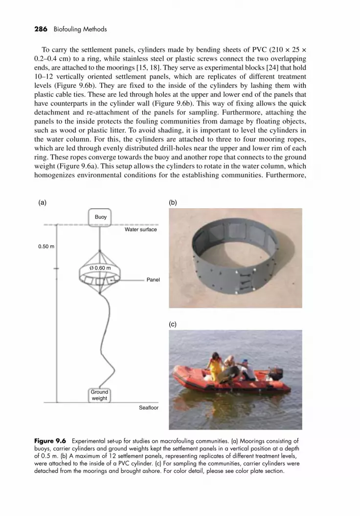
286 Biofouling Methods
To carry the settlement panels, cylinders made by bending sheets of PVC (210 × 25 × 0.2–0.4 cm) to a ring, while stainless steel or plastic screws connect the two overlapping ends, are attached to the moorings [15, 18]. They serve as experimental blocks [24] that hold 10–12 vertically oriented settlement panels, which are replicates of different treatment levels (Figure 9.6b). They are fixed to the inside of the cylinders by lashing them with plastic cable ties. These are led through holes at the upper and lower end of the panels that have counterparts in the cylinder wall (Figure 9.6b). This way of fixing allows the quick detachment and re-attachment of the panels for sampling. Furthermore, attaching the panels to the inside protects the fouling communities from damage by floating objects, such as wood or plastic litter. To avoid shading, it is important to level the cylinders in the water column. For this, the cylinders are attached to three to four mooring ropes, which are led through evenly distributed drill-holes near the upper and lower rim of each ring. These ropes converge towards the buoy and another rope that connects to the ground weight (Figure 9.6a). This setup allows the cylinders to rotate in the water column, which homogenizes environmental conditions for the establishing communities. Furthermore,
Figure 9.6 Experimental set-up for studies on macrofouling communities. (a) Moorings consisting of buoys, carrier cylinders and ground weights kept the settlement panels in a vertical position at a depth of 0.5 m. (b) A maximum of 12 settlement panels, representing replicates of different treatment levels, were attached to the inside of a PVC cylinder. (c) For sampling the communities, carrier cylinders were detached from the moorings and brought ashore. For color detail, please see color plate section.
Buoy
Water surface
Ø 0.60 m
0.50 m
Panel
Groundweight
Seafloor
(a) (b)
(c)

Assessing macrofouling 287
it holds the settlement panels in a constant water depth of 50 cm, which facilitates handling of the panels from a boat or while snorkeling (Figure 9.6c). At the same time, this is suffi-ciently deep to exclude gulls and it keeps the panels far enough from the buoys to prevent shading and scratching. During each sampling event, after detaching the settlement panels, the cylinders are cleaned from all fouling organisms that could otherwise interact with the experimental communities.
Buoys in sea areas with intense fouling pressure need regular cleaning to prevent them from sinking. Anchors for example, buckets filled with concrete, are placed on the seafloor in water depths between 3 and 10 m, while the connecting ropes are up to 15 m long, so that the buoys are not dragged under during high tides (Figure 9.6a). Up to 12 of these moorings are deployed per site at a distance of several meters apart, which prevents the cylinders from colliding during low tide [18, 25]. The placement of moorings should not follow any geometric pattern, while “Position of Block” (maximum number of levels: 12) can be included in the statistical modeling of the data as a random factor to account for spatial heterogeneity at the study sites [26, 27]. Heterogeneity in environmental conditions can result from differences between positions with regard to (i) small-scale hydrodynamics, (ii) the impact of predators, (iii) the presence of a point source of nutrients or freshwater or (iv) human activities such as fishing.
In field experiments, it is vitally important to control for the influence of predators, which can strongly bias experiments by the selective or non-selective consumption of fouling organisms. Predators of sessile marine biota can stem from the benthic, the pelagic or even from the terrestrial environment and not all of them can be excluded by the experimental setup. However, the moorings described above exclude almost all benthic predators, such as starfish, sea urchins, gastropods, and crustaceans. These animals cannot cover long distances swimming and usually fail to climb up ropes. However, if experiments are maintained for a long time they should be inspected regularly to ensure that no predators have reached the panels. Some of them can arrive as larvae and then grow, if undetected, to adult size. In one GAME project, sea urchin larvae established on the moorings, metamorphosed into adults and started to graze the panels (Joao Canning-Clode, personal communication).
Pelagic predators, such as fish, can only be excluded by nets or cages, which modify small-scale hydrodynamics and reduce water exchange and light supply. Furthermore, they can get clogged with drifting macroalgae or plastic litter and are often colonized by fouling organisms. To fight these problems, time consuming manual cleaning is required, which also constitutes a disturbance for the experimental assemblages. So far, in GAME projects nets were dispensable, because most sites lack pelagic species that feed on fouling biota [25]. Avian predators forage visually and can simply be excluded by placing the panels in a water depth of several tens of centimeters.
9.13.5 Step 5: Training the experimenters
GAME projects start with a one-month long preparative course at GEOMAR. The participating students are trained in methodological skills such as the use of identification keys and the visual inspection of macrofouling assemblages. Furthermore, all aspects of the planned study, including the experimental design and the statistics, are discussed among the participants and coordinating scientists. This training module serves to standardize the methods across all study sites and is therefore essential for the success of a global project.

288 Biofouling Methods
9.13.6 Step 6: Running experiments and collecting data
Field work starts immediately after the preparative course and continues for a maximum of six months. During this phase, all experimenters frequently report their activities to the coordinating researchers at GEOMAR, who safeguard adherence to the common protocol and communicate necessary modifications to all stations. Finally, all students return to GEOMAR for the synoptical analysis of the obtained data. This phase lasts for three months and includes several teaching modules on biostatistics and scientific communication.
Documenting the course of succession requires repeated samplings, of which all but the last needs to be non-destructive, which clearly restricts the assessment of biomass to one sampling event. For sampling, either the panels are detached from the cylinders or the cylinders are decoupled from the moorings and brought to shore where the panels are stored in seawater filled containers. They are then visually inspected either with the naked eye or with a stereo microscope (magnification 5–12 times). All sessile organisms larger than 1 mm are identified to the lowest possible taxonomic level, while smaller taxa, such as diatoms, are pooled and recorded as “biofilm”. Since non-destructive sampling is commonly required, specimens of species that remain unidentified are taken from the backside or margins of panels, or from the moorings and brought to a nearby laboratory for further inspection. Whenever the identification is doubtful, specimens preserved in formalin or photos of them are sent to experts.
Macrofouling assemblages usually constitute a mixture of solitary and modular organ-isms. While the first can be counted as single individuals, the second can only be assessed by their biomass or by the amount of substratum they occupy. In GAME the latter was adopted as the fastest and most appropriate method for analyzing solitary and modular species together. For this, a plastic grid is laid over each panel to facilitate the estimation of single abundances in 5% intervals. All species that cover less than 5% are recorded as 1% [15]. In case of multistrata growth, the different layers are projected separately onto the panel surface and added up so that total cover could exceed 100%. In some cases, panels were photographed and species’ abundances were analyzed with the free software package Image J [17, 22, 23, 28, 29].While inspecting the panels, a 1 cm margin to all sides is ignored to avoid the sampling of edge effects [26]. After the final sampling, to assess total dry weight, the entire biota including the 1 cm margin is scraped off the panels and dried in an electric oven at 60–70°C until the weight remains constant.
9.13.7 Step 7: Analyzing community data
Diversity metrics such as species richness, evenness and diversity indices, which combine the two, allow information on assemblage structure to be summarized as a single number, which can be analyzed by univariate statistical modelling. Furthermore, the use of sum parameters facilitates comparisons with other studies, but disregards a considerable amount of information contained in community data sets. Multivariate tools are an alternative here. Similarity (or dissimilarity) between communities can, inter alia, be quantified as the Bray–Curtis Similarity Index [30]. This information can be used for data exploration, such as nonmetric multidimensional scaling ordination (nMDS) and hierarchical clustering, or in null-hypothesis testing procedures like Analysis of Similarity (ANOSIM) or PERMANOVA [31, 32]. Both approaches, the uni- and the multivariate, allow the analysis of multifactorial designs, including the testing for interactions between factors. This enables researchers to use macrofouling communities

Assessing macrofouling 289
for studies on complex ecological problems, such as predicting the effects of climate change on marine benthic communities. The latter is one of the major current challenges for marine ecologists and macrofouling assemblages will presumably play a considerable role in this research.
Acknowledgements
All GAME studies presented in this chapter, apart from the pilot project, were generously funded by the Mercator Foundation, Essen, Germany.
References
1. Lawton, J.H. 2000. Community Ecology in a Changing World. Excellence in Ecology Vol. 11. Ecology Institute, Oldendorf/Luhe, Germany.
2. Dobretsov, S.V., Qian, P.Y., and Wahl, M. 2005. Effect of solar ultraviolet radiation on the formation of shallow, early successional biofouling communities in Hong Kong. Marine Ecology Progress Series, 290: 55–65.
3. Lotze, H.K., Worm, B., Molis, M., and Wahl, M. 2002. Effects of UV radiation and consumers on recruitment and succession of a marine macrobenthic community. Marine Ecology Progress Series, 243: 57–66.
4. Molis, M. and Wahl, M. 2004. Transient effects of solar ultraviolet radiation on macrobenthic community diversity at Lüderitz, Namibia. Journal of Experimental Marine Biology and Ecology, 302: 51–62.
5. Wahl, M., Molis, M., Davis, A., et al. 2004. UV effects that come and go: A global comparison of marine benthic community level impacts. Global Change Biology: 10, 1962–1972.
6. Wahl, M, Link, H., Alexandridis, N., et al. 2011. Re-structuring of marine communities exposed to environmental change: A global study on the interactive effects of species and functional richness. PLoS One, 6: e19514.
7. Lenz, M., da Gama, B.A.P., Gerner, N.V., et al. 2011. Non-native marine invertebrates are more tolerant towards environmental stress than taxonomically related native species. Results from a globally replicated study. Environmental Research, 111: 943–952.
8. Canning-Clode, J., Valdivia, N., Molis, M., et al. 2008. Estimation of regional richness in marine benthic communities: quantifying the error. Limnology and Oceanography: Methods, 6: 580–590.
9. Canning-Clode, J., Bellou, N., Kaufmann, M., and Wahl, M. 2009. Local–regional richness relationship in fouling assemblages – Effects of succession. Basic and Applied Ecology, 10: 745–753.
10. Canning-Clode, J., Maloney, K.O., McMahon, S.M., and Wahl, M. 2010. Expanded view on the local–regional richness relationship by incorporating functional richness and time – a large scale perspective. Global Ecology and Biogeography, 19: 875–885.
11. Freestone, A.L. and Osman, R.W. 2011. Latitudinal variation in local interactions and regional enrichment shape patterns of marine community diversity. Ecology, 92: 208–217.
12. Hillebrand, H. and Sommer, U. 1997. Response of epilithic microphytobenthos of the Western Baltic Sea to in situ experiments with nutrient enrichment. Marine Ecology Progress Series, 160: 35–46.
13. Witman, J.D., Etter, R. J., and Smith, F. 2004. The relationship between regional and local species diversity in marine benthic communities: A global perspective. Proceedings of the National Academy of Sciences of the USA, 101: 15664–15669.
14. Terlizzi, A. and Faimali, M. 2010. Fouling on artificial substrata. In: Biofouling (S. Dürr and J.C. Thomason). John Wiley & Sons, Ltd, Chichester, UK, pp. 170–179.
15. Valdivia, N., Heidemann, A., Thiel, M., et al. 2005. Disturbance and diversity in hard-bottom macrobenthic communities at the coast of Chile. Marine Ecology Progress Series, 299: 45–54.
16. Atalah, J., Otto, S., Anderson, M.J., et al. 2007. Temporal variance of disturbance did not affect diversity and structure of a marine fouling community in north-eastern New Zealand. Marine Biology, 153: 199–211.
17. Sugden, H., Lenz, M., Molis, M., et al. 2008. The interaction between nutrient availability and disturbance frequency on the diversity of benthic marine communities on the North East coast of England. Journal of Animal Ecology, 77: 24–31.

290 Biofouling Methods
18. Svensson, J.R., Lindegarth, M., Siccha, M., et al. 2007. Maximum species richness at intermediate frequencies of disturbance: consistency among levels of productivity. Ecology, 88: 830–838.
19. Jara, V.C., Miyamoto, J.H.S., da Gama, B.A.P., et al. 2006. Limited evidence of interactive disturbance and nutrient effects on the diversity of macrobenthic assemblages. Marine Ecology Progress Series, 308: 37–48.
20. Cifuentes, M., Krüger, I., Dumont, C.P., et al. 2010. Does primary colonization or community structure determine the succession of fouling communities? Journal of Experimental Marine Biology and Ecology, 395: 10–20.
21. Connell, S. D. 1999. Effects of surface orientation on the cover of epibiota. Biofouling, 14: 219–226.22. Sugden, H., Panusch, R., Lenz, M., et al. 2007. Temporal variability of disturbances: is this important
for diversity and structure of marine fouling assemblages? Marine Ecology, 28: 1–9.23. Vance, T., Lauterbach, L., Lenz, M., et al. 2008. Rapid invasion and ecological interactions
of Diplosoma listerianum in the North Sea, U.K. Marine Biodiversity Records. doi:10.1017/S1755267209000815.
24. Ruxton, G.D. and Colegrave, N. 2010. Experimental Design for the Life Sciences, 2nd edn. Oxford University Press, New York.
25. Valdivia, N., Stehbens, J.D., Hermelink, B., et al. 2008. Disturbance mediates the effects of nutrients on developing assemblages of epibiota. Austral Ecology, 33: 951–962.
26. Underwood, A.J. 1997. Experiments in Ecology: Their Logical Design and Interpretation Using Analysis of Variance. Cambridge University Press, Cambridge.
27. Zuur A.F., Ieno E.N., Walker N.J., et al. 2009. Mixed Effects Models and Extensions in Ecology with R. Springer, New York.
28. Meese, R.J. and Tomich, P.A. 1992. Dots on rocks, a comparison of percent cover estimation methods. Journal of Experimental Marine Biology and Ecology, 165: 59–73.
29. Dethier, M.N., Graham, E.S., Cohen, S., and Tear, L.M. 1993. Visual versus random-point percent cover estimations – objective is not always better. Marine Ecology Progress Series, 96: 93–100.
30. Clarke, K.R. and Warwick, R.M. 2001. Change in Marine Communities: An Approach to Statistical Analysis and Interpretation. Plymouth Marine Laboratory, Plymouth, UK.
31. Anderson, M.J. 2001. A new method for non-parametric multivariate analysis of variance. Austral Ecology, 26: 32–46.
32. Clarke, K.R. and Gorley, R.N. 2006. PRIMER v6. User manual/ tutorial. Plymouth routine in multivariate ecological research. Plymouth Marine Laboratory, Plymouth, UK.

Biofouling Methods, First Edition. Edited by Sergey Dobretsov, Jeremy C. Thomason and David N. Williams. © 2014 John Wiley & Sons, Ltd. Published 2014 by John Wiley & Sons, Ltd.
10 Efficacy testing of nonbiocidal and fouling-release coatings
Maureen E. Callow1, James A. Callow1, Sheelagh Conlan2, Anthony S. Clare3, and Shane Stafslien4
1 School of Biosciences, University of Birmingham, Birmingham, UK2 Natural Sciences and Psychology, Liverpool John Moores University, Liverpool, UK3 School of Marine Science and Technology, Newcastle University, Newcastle upon Tyne, UK4 Center for Nanoscale Science and Engineering, North Dakota State University, Fargo, ND, USA
Abstract
A number of organisms is routinely used in laboratory assays (i) to enable the down- selection of coating libraries and (ii) to test hypotheses in relation to settlement/adhesion on model/practical surfaces. Settlement and fouling-release assays are described for bacteria, algae (Ulva sp. and diatoms) and barnacles.
10.1 Introduction
The question whether there is a need for laboratory-scale assays is asked frequently. It is often argued that laboratory assays do not reflect the “real world”, but evaluating nonbioc-idal coatings in the “real world” is more complex than for biocidal coatings because all organisms have the potential to thrive and an assessment of fouling-release potential neces-sitates an evaluation of the adhesion strength of the dominant fouling species. Laboratory evaluation allows a rapid assessment of a coating or surface under controlled and reproduc-ible conditions, thus the challenge is not site-specific or seasonal in character. Laboratory-scale evaluation is relatively low cost, both in terms of facilities and the amount of test material required, which is an important factor where novel polymer systems or coating libraries are being investigated. Furthermore, it allows the different stages of settlement, attachment and fouling-release potential to be studied in detail. This is especially important, as the key to antifouling without biocides necessitates control of the settling stages (cells, spores or larvae), which are not considered in field tests that employ panels hung from rafts. Technical issues such as stability of coatings and adhesion to the substrate may also be revealed, thereby saving time and money on field trials that might turn out to be worthless. Laboratory assays allow model surfaces to be evaluated so that specific hypoth-eses can be tested. Data from such assays can inform the development of practical coatings, that is, those likely to be commercialized for specific end uses.

292 Biofouling Methods
A wide range of laboratory-based methods has been used in the area of antifouling research [1]. A range of test organisms has been employed, including bacteria, algae, and the larval and adult stages of invertebrates, especially barnacles, tubeworms and mussels (Figure 10.1) [2]. Many of the assays were developed to test the efficacy of active ingredients (biocides and natural products) against specific test organisms (Chapter 12) or to test specific hypotheses, for example, interactions between larvae and biofilms. This chapter does not set out to provide a comprehensive set of methods but focuses on those that have been modified or developed for evaluating a wide range of nonbiocidal coating technologies, particularly in programs supported by the European Commission and the US Office of Naval Research. These programs have necessitated bioassay methods that can be applied to large numbers of samples provided by chemists and polymer scientists. The main test organisms that have been used for testing the antifouling efficacy of nonbiocidal and fouling-release coatings are barnacles, especially Balanus amphitrite (syn. Amphibalanus amphitrite), the green macroalga Ulva (syn. Enteromorpha), and diatoms (unicellular algae that form biofilms (slimes)).
Interpretation of bioassay data requires knowledge of the properties of the coatings. However, the relationship between coatings’ properties and settlement/adhesion is not
(a)
(b) (f) (h)
(g) (i)
(j)
Individualplants of
Ulva
(c)
Bacteria
1 μm 10 μm
Swimming (b)and settled (c)spores of Ulva
100 μm
Barnaclecypris larva
Adult tube-worms
1 mm 10 mm 10 cm
DiatomTubeworm
larvaAdult
barnaclesMussel with
byssus threads(d) (e)
Figure 10.1 Representative fouling organisms used is laboratory assays: (a) bacteria (scanning electron micrograph); (b) false-color SEM of motile, quadriflagellate spores of the green alga (seaweed) Ulva; (c) false-color Environmental SEM image of settled spore of Ulva showing secreted annulus of swollen adhesive; (d) SEM of diatom (Navicula); (e) larva of tube worm, Hydroides elegans (Source: Brian Nedved, Hadfield Laboratory, Kewalo Marine Biology, Hawaii. Reproduced with permission of Brian Nedved.); (f) barnacle cypris larva (Balanus amphitrite) exploring a surface via its paired antennules (Source: Nicholas Aldred, School of Marine Science and Technology, Newcastle University, UK. Reproduced with permission of Nicholas Aldred.); (g) adult barnacles (image: A.S. Clare); (h) adult tubeworms (Hydroides elegans) (Source: Mike Hadfield, Hadfield Laboratory, Kewalo Marine Biology, Hawaii. Reproduced with permission of Mike Hadfield.); (i) adult mussels showing byssus threads attached to a surface (Source: Jonathan Wilker, Department of Chemistry, Purdue University, USA. Reproduced with permission of Jonathan Wilker.); (j) mature plants of Ulva. The diagram is intended to indicate relative scales rather than absolute sizes; individual species within a group can vary significantly in absolute size. Image from [2]. For color detail, please see color plate section.

Efficacy testing of nonbiocidal and fouling-release coatings 293
straightforward and it may vary between organisms or even between the developmental stages of the same organism. As a minimum, contact angle data (and preferably surface energy) are required (Chapter 11). Knowledge of other properties such as roughness, charge, and the bulk properties of the coatings may also be needed to interpret the biological data.
Finally, the importance of critical (microscopic) observation to generating meaningful data from bioassays should be emphasized. For example, a low attachment density of cells/larvae may be because the surface is genuinely antifouling, that is, inhibits settlement, but it may also be a consequence of toxicity or disintegration/delamination of the coating.
10.2 Test organisms
10.2.1 The green seaweed UlvaMature, reproductive plants (Figure 10.1) release vast numbers of motile, pear-shaped spores (zoospores), 5–8 µm in length. Spores are negatively photactic and also respond to a number of surface cues, for example, wettability, charge, topography and can “choose” where to settle (attach). Settlement (attachment) is enhanced by topographic features of similar dimensions to those of the spores (about 5 µm) [3] but can be inhibited by specific designs of smaller (2 µm) dimensions, for example, Sharklet™ [4]. In general, spore settle-ment is enhanced on hydrophobic surfaces [5].
Settlement involves rapid secretion of a glycoprotein adhesive and loss of the four fla-gella (Figure 10.1) resulting in permanent attachment to the substratum [6]. The secreted adhesive cures rapidly as shown by an increase in adhesion strength with time [7]. The settled spores germinate and grow into sporelings (young plants), which are approxi-mately 100 µm long after 5–6 days. Sporelings form the basis of the fouling-release assay described below.
10.2.2 Diatoms
Diatoms are unicellular algae characterized by the presence of an elaborately ornamented silica frustule and chloroplasts containing the pigment fucoxanthin, which masks the chlo-rophyll, hence their brown color (Figure 10.1). Cells range in size from a few to several hundred micrometers. Pennate diatoms have bilateral symmetry and are the abundant types in benthic habitats, particularly those genera which possess an elongate slit, the raphe, in one or both valves of the frustules. Raphid diatoms may be sessile or motile but, in both cases, extracellular polymeric substances (EPS) are secreted via the raphe(s), which in the former provides the means for adhesion whilst in the latter it provides the mechanism for both adhesion and motility by gliding [8]. Raphid diatoms are probably the most important biofilm algae, being instrumental in the primary colonization of submerged substrata and forming strongly adhered biofilms on fouling-release coatings [9]. Initial attachment is reversible as the cells adjust their position by gliding; secondary or permanent adhesion appears to be the result of the secretion of further EPS components via the raphe, along with reorganization and cross-linking reactions [8].
Diatom adhesion assays are employed because of the contribution of diatoms to the adherent slimes that colonize silicone-based fouling-release coatings and which are not “released” at the operating speeds of most vessels. Thus, improvements to current fouling-release technologies are aimed at reducing the adhesion strength of diatom slimes.

294 Biofouling Methods
10.2.3 Barnacles
Barnacles are widely accepted as one of the most important of the hard foulers, due in part to their size, shape and tenacity [10]. Antifouling and fouling-release assays are carried out using Balanus amphitrite in particular, though increasingly other species are being used. Barnacles are exclusively marine Crustacea of the infraclass Cirripedia and have two parts to their lifecycle: a sessile adult stage and planktonic (swimming) larval stages. Adults brood egg masses in the mantle cavity; once hatched the nonfeeding nauplii (stage I) are expelled into the ocean. After molting to stage 2, the nauplii begin to feed on phytoplankton and grow by undergoing five further molts to reach the specialized settlement stage, the cyprid (Figure 10.1). The cyprid is used in settlement assays. Cyprids use highly developed organs, the antennules, to sense the surface while “walking” on it using temporary adhesive and have been shown to select a surface based on, for example, its chemistry [11], wettability [12] and roughness on both the macro- and microscale [4, 13]. On selection of a suitable surface for settlement, permanent cyprid cement (produced in paired cement glands) is released to the surface via ducts in the antennules which exit from the attachment discs, resulting in permanent (irreversible) attachment [14]. After settlement the permanently attached cyprid undergoes metamorphosis after which it resembles the adult in miniature. Calcification and production of adult adhesive follow (in around 1 month for Semibalanus balanoides [15], a boreoarctic species, but only approximately 24 hours for the tropical/subtropical B. amphitrite [16]). Growth to a testable adult size (approximately 3–5 mm) is dependent upon species, temperature and feeding regime but in B. amphitrite is around 2–3 months, which is relatively quick (one reason it is commonly used as a test organism).
10.3 Test samples
Coatings are usually applied to glass microscope slides or deposited in multiwell plates, or individual small Petri dishes. Slides (76 × 26 mm) are a convenient size for assays and for use in apparatuses to measure adhesion strength. It is essential to include controls and stand-ards in assays. Fouling-release standards are typically PDMS elastomers such as Silastic® T2, Sylgard 184® and Intersleek®. Optimum data are obtained if coatings are smooth, of uniform thickness, and well-bonded to the substrate (essential for hydrodynamic assays). Bonding of the test coating to glass may necessitate the prior application of a tie-coat such as allyltriethoxysilane.
A multiwell plate format has been developed to accommodate the screening of large numbers of coatings in parallel, such as those generated with a combinatorial, high-through-put (HT) approach [17]. Commercially available 24-well polystyrene plates are modified by adhering discs of the appropriate material (e.g., glass, metal, plastic) to the bottom of the wells. These well modifications allow for the preparation of organic solvent-based coatings in the plates and enable the selection of the appropriate substrate to achieve optimal bonding of the coating system being investigated. Typically, 15 mm diameter marine grade aluminum discs (punched from panels) or glass coverslips are used to modify the plates. The discs are adhered to the bottom of the wells by dispensing 0.03 ml of adhesive (Dow Corning® 734 Flowable Sealant) to each well, setting each disc into the adhesive and applying light pres-sure with a cotton tipped swab. Coatings are typically reduced in the appropriate solvent (30–50 wt-%) and 0.2–0.3 ml of the coating solutions are dispensed into the wells to obtain smooth coatings of uniform thickness. Alternatively, coatings can be prepared on discs outside of the plates and adhered to the well bottoms after curing.

Efficacy testing of nonbiocidal and fouling-release coatings 295
Some coatings may need to be leached prior to the bioassay to remove compounds, for example, curing agents that may be toxic to the test organisms. This is usually accomplished by putting racks of slides in a tank of recirculating deionized water fitted with a carbon filter for 1–4 weeks. Coatings need to be equilibrated in seawater before being exposed to test organisms. Artificial seawater (ASW), for example, Tropic Marin® made up to manufactur-er’s instructions can be used for most purposes. Some coating types, for example, amphiphi-lic coatings, may need to be equilibrated for a period of days to allow surface restructuring before starting the bioassay.
10.4 “Antifouling” settlement assays
10.4.1 Assays with Ulva sp.Studies on the kinetics of spore settlement reveal a linear rate over approximately the first 60 minutes but thereafter the settlement rate progressively decreases [18, 19]. Departures from linearity were ascribed primarily to differences in competence of the zoospore population to settle with time under the assay conditions rather than saturation of binding sites. In addition, with time it is likely that the surface will become progressively conditioned by organic materi-als that are either present in the water in which the spores are released or which are secreted from the swimming spores – such conditioning materials may make surfaces either less or more attractive for settlement [19]. Finally, spores settle not just on the test surface but also on the surrounding container in which the test slides are immersed, thus progressively reducing the number of swimming spores in solution. A practical consequence of these kinetic features is that a meaningful comparison of settlement on different surfaces requires that the initial linear rate be assessed; typical assays are therefore conducted for about 45–60 minutes. It must also be emphasized that because the spores are obtained from “wild” plants, the absolute num-ber of spores that settle in an assay varies between batches and with season, thus the total number of spores settled per unit area cannot be directly compared across different sets of data.
Three replicates of each coating on microscope slides are required for spore settlement, a further three replicates if adhesion strength of spores is to be determined. Test slides are placed in individual compartments of Quadriperm dishes (Greiner Bio-One).
Fertile plants of Ulva sp. are collected from the seashore 3–5 days before the spring tide (i.e., corresponding to a new or full moon) to ensure maximum release of spores [20]. Plants that will release zoospores have cream-colored tips where spores have already been released and are dark green–brown for up to a few centimeters behind the pale region. Immediately after collection, squeeze out excess water and wrap in absorbent “kitchen” paper, put inside plastic bags and keep cool (on ice) until back at the laboratory. Plants will release spores for three days if kept in a refrigerator at 5–10 °C. A large volume of artificial seawater (ASW), for example,Tropic Marin®, is required for the assay.
Protocol of spore adhesion assay for coatings on microscope slides
1. Assemble apparatus before releasing spores: crushed ice, clean beakers, magnetic stirrer, funnel and three pieces of clean nylon mesh (pore size 100, 50 and 20 microns) to filter spore suspension, ASW, 10 ml pipette and tip, spectrophotometer, Quadriperm dishes each compartment containing a test slide.
2. Cut 50–100 fertile tips (dark green–brown) into a 500 ml glass beaker.3. Add enough ASW to cover the plants; move water gently.

296 Biofouling Methods
4. Filter into a clean beaker as soon as seawater becomes green with released spores (filter through three pieces of nylon net, pore size 100 (top), 50 and 20 microns). The meshes will remove any debris such as sand grains and diatoms.
5. To “clean up” and concentrate the filtered spore suspension, plunge beaker containing spores into crushed ice; zoospores swim to the bottom forming a dark green plume; gametes and spores stay in suspension.
6. Pipette spores from the concentrated plume into another beaker on a stirrer so the spores do not settle.
7. Dilute the spore suspension with ASW and read absorbance at 660 nm. Dilute to an Absorbance
660 of 0.15 (approximately 1 × 10⁶ spores ml–1).
8. Pipette 10 ml spore suspension into each dish compartment and transfer as quickly as possible to a dark cupboard or drawer to prevent spores responding to light (spores are negatively phototactic) or starting to settle.
9. Incubate dishes for 45–60 min in darkness at room temperature (about 20 °C).10. Wash vigorously in beaker of ASW to remove unattached (swimming) spores.11. Fix in 2.5% glutaraldehyde in ASW for 10–15 min, wash sequentially in ASW, ASW:
DW, 50:50, distilled water (DW), drain and allow to dry.12. Spores are quantified by fluorescence microscopy and image analysis*.13. Spores autofluoresce red with Texas Red filter set (546
ex590
emnm) due to the excitation
of chlorophyll. Count 30 fields of view on each of three replicates.
* The image analysis system used needs to be calibrated against manual counts at a range of spore densities to check that automatically generated counts are accurate. If the test surface is autofluorescent, it may not be possible to use automated counting. In this event, counts can be made using a grid placed over the computer screen provided the spores are clearly visible. If the coating is transparent, spores can be viewed by transmitted light.
Figure 10.2 shows an example of data produced by this assay using surfaces differing in wettability [21].
EG60H35°
EG60Me60°
EG60Et70°
EG60Pr97°
700
600
500
400
300
200
Spo
res
mm
–2
100
0
Figure 10.2 Example of settlement data for spores of Ulva linza in relation to surface wettability using a range of hexa(ethylene glycol)-containing undecanethiol self-assembled monolayers with different end-group terminations. Resulting differences in contact angle are shown. Reproduced in modified form from data in [21].

Efficacy testing of nonbiocidal and fouling-release coatings 297
10.4.2 Settlement assays with barnacle larvae
Settlement assays using B. amphitrite have been used to assess compounds and surfaces for over 30 years [22] and have proliferated in that time to a variety of formats. Most commonly assays use 24-well polystyrene plates, Petri dishes or glass slides. The use of Petri dishes is particularly common with other species, such as Elminius modestus (syn. Austrominius modestus) and B. improvisus, in order to remove any water/air meniscus, where cyprids of these species are prone to become trapped; a relatively rare occurrence with B.amphitrite. The age of the cyprids used in assays varies with species. B. amphitrite cyprids are stored routinely for three days at 6 °C, while E. modestus cyprids tend to be used immediately upon molting from stage IV nauplii. One unifying feature of settlement assays is the enumeration of settlement, which is almost exclusively done 24 and 48 hours after setting up. Absolute settlement will vary from one batch of cyprids to another and a laboratory standard (e.g., an untreated 24-well plate of a known brand) with allows comparison of batches of larvae.
Twelve replicate wells, or slides, are preferred (though often six replicates are used to provide a quick down-selection while reducing costs). Repeating any result with at least a second batch of cyprids is required to increase confidence in the results. If set-tlement is high, the same settled cyprids can be used for adult adhesion testing (when using slides). Testing newly metamorphosed juvenile barnacles (Section 10.5.3) requires large numbers (≥10 per slide) of settled individuals and generally a further 12 slides are needed.
Adult B. amphitrite are kept in the laboratory in well-aerated, filtered (1 µm), UV-irradiated seawater that is changed daily. They are fed freshly hatched Artemia sp. each day and microalgae around twice a month. To collect nauplii, adults are cleaned under running water and placed in clean seawater in the dark with a point cold light source at one end of the container. As nauplii are released by the adults they swim to the light source and can be collected by pipette. After collection they are transferred to 0.45 µm filtered aerated seawa-ter containing antibiotics, penicillin and streptomycin (21.9 and 36.5 mgl–1, respectively) and fed Tetraselmis suecica (approximately 2 × 10⁵ cells ml–1d–1) for 4–5 days until cyprids are seen. Cyprids are collected using a 260 µm mesh filter and stored in 0.2 µm filtered seawater at 6 °C for three days prior to use.
Protocol for B. amphitrite settlement assays for slide testing (24-well testing in parentheses)
Apparatus needed: crushed ice, clean evaporation dish, 0.2 µm filtered ASW, d3 cyprids, glass Pasteur pipettes and bulb, 2 ml automated pipette and tips, dissection microscope, untreated 24-well plate, Quadriperm dishes, each compartment containing a test slide (untreated 24-well plate with either 2 ml of diluted chemicals to be tested in 6–12 replicate wells, or 6–12 evenly coated wells).
1. Pour about 50 ml ASW into the evaporation dish, add approximately 500 cyprids, place on crushed ice, and add more cyprids from 6 °C storage as needed. NB: Do not leave cyprids on ice for more than three minutes at a time.
2. Add 2 ml ASW to each well of the 24-well plate (laboratory standard); add 10 cyprids in minimal volume of ASW to each of the wells.

298 Biofouling Methods
3. In an incubator set to 28 °C, create an area with high humidity. For example, wrap test dishes in deionized water-soaked laboratory roll and foil totally enclosing dishes.
4. Place a Quadriperm dish into the incubator and carefully pipette 1 ml of ASW onto each slide and add 20 (±2) cyprids in 0.5 ml ASW (for 24 well dishes add 10 (±1) cyprids to each well in minimal ASW).
5. Place the laboratory standard with the Quadriperm dishes (or the 24-well test plates) and fully wrap in foil and wet laboratory roll.
6. Leave for 24 h at 28 °C in the dark.7. Carefully remove test plates and use a dissection microscope to enumerate settlement
and mortality; direct light may be required for opaque coatings. (Figure 10.3a)8. Replace plates in the incubator for a further 24 h and re-count settlement and mortality.9. Data are presented as percent settlement and percent mortality at the two time points
(Figure 10.3b). Data are generally nonparametric even after arcsine transformation and the Kruskal Wallis test with a post hoc Dunn’s test is used to determine significance [23].
Problems ● Slide assay: can result in very different surface areas available for settlement due to dif-ferences in wettability; this must be taken into account when attempting to explain differ-ences seen. Highly hydrophobic and highly hydrophilic surfaces are difficult to test using the standard slide assay due to the high probability of the drop falling off the slide surface into the Quadriperm dish well.
● Twenty-four well assay: Cannot be used for established adhesion strength tests. If the volume of ASW added with the cyprids is not carefully controlled, the concentrations tested will vary. If there is a clear disparity between wells in terms of volume, data should be ignored and the assay repeated if necessary.
Figure 10.3 (a) Image of a settled cyprid and metamorphosed juvenile; (b) bar chart showing settlement and mortality data (±95% confidence intervals) produced by a settlement assay. Coating A prevents settlement due to toxicity, Coating B reduces settlement significantly from the control but is not toxic while Coating C has no significant effect, Coating D promotes settlement compared to the control. For color detail, please see color plate section.
(a)
Settled
Metamorphosed
(b)100
90
80
70
60
50
40
30
20
10
0A B C
Coating name
D Control
Mea
n pe
rcen
t
24h settlement
48h settlement24h mortality
48h mortality

Efficacy testing of nonbiocidal and fouling-release coatings 299
10.5 Fouling-release assays
Methods to measure critical removal stress of hard fouling organisms and the hydrodynamic methods to measure adhesion strength of algae and larvae described below have been devel-oped from various pieces of apparatus originally designed by Professor G. Swain’s group at the Florida Institute of Technology.
10.5.1 Assays with sporelings (young plants) of UlvaThis assay has been widely used to demonstrate the fouling-release potential of experimen-tal surfaces [24, 25, 26]. The release (assessed as % removal) of sporelings is quantified from samples prior to and after exposure to shear. Standards of PDMS, for example, Silastic T2 (Dow Corning) or Intersleek® (International Paint), are typically included as standards. Negative standards, for example, epoxy, may also be included. Biomass is quantified by autofluorescence of chlorophyll. It is helpful to combine this assay with the spore settlement assay described above so that differences in biomass can be correlated with the density of spores that attached to each surface. The bioassay requires six replicates of each test coating; an additional replicate of each test surface, treated in the same way but not exposed to spores, is needed as an instrument blank (see point 5 below).
Protocol of adhesion strength assay
1. Prepare six replicate slides as for the spore adhesion assay up to step 10.2. Return the washed slides with attached spores to cleaned Quadriperm dishes and add
10 ml of enriched seawater medium [27] to each compartment.3. Incubate dishes at 18 °C with a 16 h:8 h, light:dark cycle; irradiance of approximately
75 µmol m–2 s–1 from appropriate fluorescent tubes, for example, Sylvania F36wt8/2084.4. Change the medium every two days for 6–7 days, by which time the coatings should be
covered by a green lawn of sporelings.5. Quantify biomass as relative fluorescence units (RFU) on the surface in plate reader (e.g.,
Tecan Genios Plus) using filters for fluorescence of chlorophyll (430ex
/670em
nm). Blank the plate reader with a hydrated test sample. Measure a minimum of 70 points per sample.
6. Expose slides to turbulent flow either in a water channel or by exposure to the compres-sive forces delivered by a water jet (see below). The optimum flow regime needs to be determined from a pilot experiment.
7. Re-measure chlorophyll fluorescence only in the area exposed to shear if a water jet is used.8. Calculate percentage removal of biomass from the before shear and after shear values.
Figures 10.4 and 10.5 show examples of the ability of both the water jet and water channel assays to detect differences in fouling-release performance between individual coatings in compositional ladders [25, 28].
10.5.2 Adhesion assays with diatoms
Since diatom cells are not motile in the water column, cells reach the surface of the coating by sinking. Thus, at the end of an assay, every test sample has approximately the same number of cells in contact with the surface. Gentle washing after the attachment period (typically 2 h) removes cells that have not adhered to the surface and quantification of cells

300 Biofouling Methods
after washing provides the starting density for strength of attachment assays. Attachment strength is greatest on hydrophobic surfaces [9, 21].
Diatoms are cultured in enriched seawater medium, for example, Guillards F2 [29], using either natural or artificial seawater as the base. Navicula and Amphora species are widely
100
80
60
Rem
oval
(%
)
40
20
00 50 100
Water pressure (kPa)
150 200
PDMSe
SEBS
0.0Si_0.38EG
0.17Si_0.31EG
0.22Si_0.21EG
0.28Si_0.11EG
0.39Si_0.0EG
Figure 10.4 Percentage removal of 7-day-old sporelings from a range of amphiphilic coatings applied over a SEBS base layer, plotted as a function of surface water pressure (kPa) delivered from the water jet. The test coatings were based on mixtures of block copolymers containing different proportions of short side groups of PDMS (Si) and polyethylene glycol (EG) on a triblock copolymer backbone of polystyrene8K-block-poly(ethylene-ran-butylene)25K-block-polyisoprene20K applied over a base coat of SEBS (polystyrene-block-poly(ethylene-ran-butylene)-block-polystyrene), which was included as a negative standard. PDMSe is Silastic T2 (Dow Corning), which was included as a positive fouling-release standard. The data show the ability of the assay to identify the optimal composition. Figure from [28]. For color detail, please see color plate section.
Figure 10.5 Removal of sporeling biomass of Ulva from a range of ultrathin SiOx-like coatings by 30 Pa wall shear stress provided by a water channel (a) and correlation with γTot, total surface energy (b). Percentage removal from a PDMS standard (Silastic T2) included in the assay was 36.9%. Error bars = ± 2 × Standard Error, derived from arcsine transformed data.Source: Akesso et al. [25]. Reproduced with permission of Taylor and Francis.
(a)
50
40
30
Rem
oval
(%
)
20
10
0TCL 40 TCL 40a TCL 40b TCL 40bt
(b)55
50
45
40
35
30
Spo
relin
g re
mov
al (
%)
25
20
15
10
5
0
Surface energy (mN/m)
0 20 40 60
R2 = 0.9875

Efficacy testing of nonbiocidal and fouling-release coatings 301
used for bioassays. Cultures are maintained in 250 ml sterile conical flasks at 18 °C in an environmental cabinet with a 16:8 light:dark cycle. Stock cultures are subcultured on a weekly basis.
Protocol of diatom attachment and adhesion assay
1. Use log phase cells (4d after subculturing); pour away medium, then re-suspend cells adhered to the flask in fresh F2 medium to a density of 0.25–0.3 µg chlorophyll a per ml [30]. Keep cell suspension on a stirrer.
2. Pipette 10 ml culture into Quadriperm dishes containing test slides (as for Ulva spore assay). Leave in light on laboratory bench for two hours. Cells fall by gravity and cover the test surfaces.
3. Wash slides gently in ASW underwater, that is, without exposing to air; unattached cells are washed away leaving only those that have attached to the test surface.
4. Quantify cell density as for spore adhesion assay (steps 11–13); strength of attachment assays can be performed using either a flow channel or water jet depending on how strongly the cells are adhered to the surface.
10.5.3 Adhesion strength of attached cypris larvae
While adult adhesion strength is the most widely used fouling-release test it involves a con-siderable investment in terms of time and effort, and therefore cost, to grow from settled cyprids to adults (about 3 months). To reduce this time and cost a number of methods have been developed including testing earlier life cycle stages and the re-attachment assay (Section 10.6.3). The use of earlier settlement stages, i.e. permanently attached cyprids, newly metamorphosed juvenile barnacles and juvenile barnacles, is attracting increasing interest [31, 32]. Methods to test these stages are usually hydrodynamic in nature. Two such hydrodynamic systems are the water jet (akin to water blasting a surface [7, 33, 34, 35]; Section 10.7.2) and the flow cell (akin to the forces produced by the movement of a ship through water [31, 36, 37]; Section 10.7.1); these are discussed here. Both methods require similar protocols, so will be described together.
Cyprids are settled on the surfaces to be tested (coated microscope slides) over 24 hours. The position and settlement stage of each individual is determined and the slides tested using either the water jet (in batches of 12) or the flow cell (in batches of 7 or 14). Each settled individual is then checked for removal and any adhesive remaining is noted. The water jet impacts a settled individual in air and is a relatively immediate force. The force applied by the flow cell, on the other hand, is developed over 15 seconds and impacts an individual under water. The water jet also allows the test slide to be split into 36 lines across the width of the slide and, therefore, requires the area for spraying (i.e., the area of each slide that has settlement) to be entered, in terms of lines to spray, into the specialist computer software prior to testing. The whole slide is subject to shear in the flow cell.
Protocol of cyprid and juvenile barnacle adhesion assay
Apparatus needed: crushed ice, clean evaporation dish, 0.2 µm filtered ASW, glass Pasteur pipette and bulb, Quadriperm dishes with one test slide per well, 10–5 mol l–1 3-isobutyl-1-methylxanthine (IBMX), incubator at 28 °C, dissection and compound microscope,

302 Biofouling Methods
acetate grid with 36 horizontal lines “linked” to spray lines on the water jet software, water jet or flow cell (Sections 10.7.1 and 10.7.2).
1. Add around 50–100 cyprids to a drop of seawater on test slides in the wells of Quadriperm dishes. The drop of seawater containing the cyprids should be as large as possible to allow settlement over the whole of the slide surface. A settlement inducer (e.g., IBMX) is sometimes needed to obtain acceptable levels of settlement. Slides are incubated for 24 h in a dark, high humidity environment at 28 °C to allow settlement.
2. After 24 h, gently wash unsettled cyprids from the surface using ASW. The number, exact location, and stage of development of each settled individual should be noted (using a dissection microscope and a grid of 1 mm2 squares). Any slide with fewer than 10 indi-viduals should be discarded.
3. Place slides in the test apparatus ensuring the slide surfaces are all level (particularly important for the flow cell).
4. For the water jet apparatus the spray lines (areas) need to be entered for each slide (allowing at least one line above and below areas with settlement).
5. Test at desired impact pressure or wall shear stress (generally a small trial using 2–3 slides of test surfaces are used to determine ideal force for removal).
6. After testing, carefully examine surfaces using a dissection microscope to determine removal. Where removal is seen it should be checked using a compound microscope for any remaining adhesive on the surface (Figure 10.6).
7. Data are reported as average removal of each life stage and mean failures (adhesive and/or antennules remaining behind).
10.5.4 Adhesion strength of adult barnacles
Measures of barnacle adhesion strength on various surfaces have long been of interest. Initial studies often applied a tensile force (e.g., [38, 39] which is still used [34]). With the introduction of a standardized method (ASTM D5618 [40]) in 1994, the removal of barnacles of >5 mm diameter using a shear force applied using a handheld force gauge became the generally accepted method. The standard method has been built upon for laboratory use with many researchers using motorized systems to control the application rate of the
Edge of adhesive
Antennules
50 µm
Figure 10.6 Cyprid permanent cement with antennules embedded in the mass. For color detail, please see color plate section.

Efficacy testing of nonbiocidal and fouling-release coatings 303
force [41, 42] or purpose-built machines (Section 10.7.4 and [43]). Force for removal is normally reported as removal force (Newtons) per unit (mm2) basal area and is termed the Critical Removal Stress (CRS) [44].
In order to test adult barnacle adhesion on a surface, cyprids are settled and grown to adults. Often large numbers of cyprids, and/or a settlement inducer (e.g., IBMX), are required to obtain suitable levels of settlement. The settled barnacles are grown to adults. The juveniles are initially fed on microalgae followed by Artemia sp. nauplii.
Protocol of adult barnacle adhesion assay
Apparatus needed: crushed ice, clean evaporating dish, 0.2 µm filtered ASW, glass Pasteur pipette and bulb, Quadriperm dishes with one test slide per well, incubator at 28 °C, Tetraselmis suecica culture, freshly hatched Artemia sp., handheld force gauge (as per ASTM D5618), flat-bed scanner, Image J software, purpose built push-off machine.
1. Place approximately 50 cyprids, in around 1 ml of ASW, onto coated slides in Quadriperm dishes.
2. Allow cyprids to settle for 48 hours at 28 °C, in the dark, at high humidity.3. Rinse slides gently with ASW to remove nonsettled cyprids.4. To feed the juvenile barnacles, flood the Quadriperm wells with 15 ml of Tetraselmis
suecica culture (approximately 3 × 10⁵ cells ml–1).5. Feed every two days as water is changed and check for, and remove, any individuals that
are close to touching.6. Once the barnacles reach >2 mm in diameter (usually around 60 days) they can be fed
freshly hatched Artemia every two days.7. Barnacles are large enough to test once they reach ≥5 mm diameter.
To test using a handheld force gauge:
8. Remove the slide from the Quadriperm dish and clean using clean ASW; scan using a flat-bed scanner, ensuring the position of each barnacle on the slide is first noted.
9. Using the handheld force gauge, gently push the shearing probe against each individual barnacle, ensuring it does not come into contact with the test surface and remains close to the surface and parallel to it. Maintain slow, gentle, constant pressure on the barnacle until it is removed.
10. Once removed check the basis has been removed cleanly (if ≥10% remains discard the data) and make a note of the removal force in Newtons (convert units if required).
11. Calculate the basal area in mm2 of each barnacle using the scanned slide image and software (such as Image J). Divide the removal force by the basal area for each barnacle to obtain the CRS in megapascals (MPa).
To test using an automated machine [43]:
12. Remove the slide and clean, place in machine slide holder and capture the image.13. Begin the movement of the push-off bar, ensure the barnacles fall off the surface after
removal and are not crushed on subsequent barnacles.14. Once removed, check the basis has been removed cleanly (if ≥10% remains discard the
data) and make a note of the CRS as calculated by the machine.
304 Biofouling Methods
Data are usually presented as a mean of >30 individuals on each surface with 95% confi-dence interval error bars. The data are usually distributed normally and ANOVA is used to determine significance. Using the machine reduces variability introduced by the handler and results in the ability to test fewer, smaller individuals [43].
10.6 Adhesion assays for high-throughput screening
A high-throughput (HT) biological laboratory screening workflow has been developed to accommodate the performance evaluation of large numbers of coatings in parallel [35, 45]. This workflow has been effectively utilized to screen and identify new and potentially useful fouling-release coating technologies developed with a combinatorial approach. A suite of robotic tools and automated instrumentation is employed to enable rapid and reproducible adhesion measurements of bacteria, diatoms and adult barnacles on small-sized sample arrays (Section 10.3). A series of standard coatings (e.g., Intersleek®, polyurethane, polydi-methyl siloxane) is typically included to gauge the relative performance of the experimental coatings under investigation.
10.6.1 Adhesion of bacterial biofilms
Two different methods have been developed to assess the adhesion of bacterial biofilms to coatings prepared in multiwell plates. The first method is based on the measurement of biofilm surface coverage after drying and staining using the marine bacterium, Cellulophaga lytica [46, 47]. The second method relies on the use of a fully-automated, spinning water jet apparatus (Section 10.7.2) to apply a precisely controlled, pressur-ized stream of artificial sea water (ASW) to facilitate biofilm removal from the coating surfaces [48].
Retention and retraction of biofilms
Biofilm retraction is a phenomenon where biofilm retained on a coating surface after rinsing with water, to remove nonattached biomass, is redistributed into smaller, denser areas. This redistribution of biomass is a consequence of surface de-wetting during the process of drying on hydrophobic, fouling-release surfaces. Biofilm retraction is meas-ured by calculating percentage surface coverage from high resolution digital images using a custom software tool [47]. Coatings that exhibit a high degree of biofilm retrac-tion (i.e., low percentage surface coverage) are considered to have good anti-adhesive/fouling-release properties.
Cultures of Cellulophaga lytica (isolate from Dr Michael Hadfield, University of Hawaii) are maintained weekly on marine agar plates at 4 °C from cryopreserved stocks in marine broth (MB) containing 20% glycerol (v/v). One colony is inoculated into 10 ml of MB and cultured overnight at 28 °C with shaking. A subculture is prepared by transferring 0.5 ml of the overnight culture into 10 ml of fresh MB and incubating at 28 °C for 24 hours. Cells are harvested via centrifugation (4000 × g) for 10 minutes, washed three times in ASW and resuspended to 107 cells.ml–1 in biofilm growth medium (BGM) consisting of 35.5 g of sea salts (Sigma-Aldrich), 0.5 g pep-tone (Becton Dickinson Labware) and 0.1 g of yeast extract (EMD Chemicals) per liter of deionized water.

Efficacy testing of nonbiocidal and fouling-release coatings 305
Protocol of biofilm retention and retraction assay1. Add 1.0 ml of the 107 cells.ml–1 culture in BGM to each well in rows 2 through 4 of the
24-well plates (three replicate wells for each individual coating composition prepared in columns). The top row serves as an assay control for each coating and receives 1.0 ml of fresh BGM (one replicate well per individual coating composition).
2. Place lids on plates and transfer to a temperature controlled water bath or an incubator set at 28 °C for 24 hours under static conditions. If using a conventional incubator, a container of water should be placed in the incubator to maintain an appropriate degree of humidity to prevent evaporation of BGM from the wells.
3. Remove plates from the incubator and discard planktonic growth and spent BGM by inverting the plates over a waste reservoir. Rinse each well of the plate with 1.0 ml of deionized water by placing the tip of a pipette against the side of the well and gently delivering the water. Discard rinse water (invert over waste container) and repeat rinsing process two more times.
4. Invert plates and tap gently against a paper towel several times to remove any residual water remaining in the wells after rinsing. Let plates dry at ambient laboratory condi-tions for at least one hour.
5. Add 0.5 ml of crystal violet (CV) solution (0.3% w/v in water) to each well and incubate for 15 minutes at ambient laboratory conditions.
6. Repeat steps 3 and 4 to remove excess CV dye (discard, rinse three times, tap plates against paper towel and dry for at least one hour).
7. Take high-resolution digital images of each coating plate using a wide-zoom lens camera and use an appropriate software tool to measure CV pixel area and calculate percentage surface coverage on each coating surface [47].
8. After imaging, apply extraction templates [17] and add 0.5 ml of 33% glacial acetic acid to each well and incubate at ambient laboratory conditions for 15 minutes to extract CV dye from the biofilms. Shake plates gently every 2–3 minutes to ensure homogenization and complete extraction of the CV dye.
9. Transfer 0.15 ml of the resulting eluates into a 96-well plate and measure the absorb-ance at 600 nm using a multiwell plate spectrophotometer.
10. Absorbance values for each coating composition are reported as the mean absorb-ance values of three replicate samples minus the absorbance values of the assay control wells. Mean absorbance values are directly proportional to amount of bio-mass on coating surfaces. Error bars represent one standard deviation of the mean absorbance value.
Figure 10.7 provides an example of data produced by this assay using a series of polysi-loxane fouling-release coatings [46].
Water jet adhesion of biofilms
The water jet testing methodology referred to above (Section 10.5) has been adapted to accommodate the screening of bacterial biofilm adhesion on coatings prepared in multi-well plates [48]. Each unique coating composition is prepared in three columns of a 24-well plate (two unique coating compositions per plate with twelve replicate wells per coating) where four replicate wells (columns 1 and 4) are not treated with the water jet (0 kPa), four replicates (columns 2 and 5) are treated at a low impact pressure (e.g., 43 kPa) and four replicates (columns 3 and 6) are treated at a high impact pressure (e.g., 111 kPa). The CV

306 Biofouling Methods
colorimetric assay (Section 10.6.1.1) is used to quantify biofilm biomass before and after water jet treatments to enable the calculation of percent removal values.
Culture preparation is given in Section 10.6.1.1.
Protocol of water jet biofilm adhesion assay1. Add 1.0 ml of a 105–107 cells.ml–1 culture in BGM to each well in columns 2, 3, 5 and 6.
Add 1.0 ml of this suspension to rows 2 through 4 (three replicate wells) of columns 1 and 5. The first row of column 1 and 5 (one replicate well) will receive 1.0 ml of fresh BGM only and serve as an assay control.
2. Place lids on plates and transfer to a temperature controlled water bath or an incubator set at 28 °C for 24 hours under static conditions. If using a conventional incubator, a container of water should be placed in the incubator to maintain an appropriate degree of humidity to prevent evaporation of BGM from the wells.
3. Remove plates from the incubator and discard planktonic growth and spent BGM by inverting the plates over a waste reservoir. Rinse each well of the plate with 1.0 ml of
Figure 10.7 Cellulophaga lytica biofilm retention reported as (a) a crystal violet absorbance ratio to Dow Corning 3140 (DC) control coating and (b) percentage surface coverage on a series of polysiloxane fouling-release coatings. (c) Digital images of C. lytica biofilm retraction on the coating surfaces after rinsing, drying and staining with crystal violet. Biofilm retention data demonstrate that the total amount of biofilm is similar on all surfaces but has retracted on several coatings during the drying process, resulting in decreased percent surface coverage. Source: Modified form from data in Figures 7 and 9 in Stafslien et al. [46]. Reproduced with permission of Taylor and Francis. For color detail, please see color plate section.
0
0.2
0.4
0.6
0.8
1
1.2
1.4
1 2 3 4 5 6 7 8 9Bio
film
ret
entio
n as
rat
io to
DC
314
0 co
ntro
l
(a)
0
20
40
60
80
100
120
1 2 3 4 5 6 7 8 9 DC
C. l
ytic
a pe
rcen
t cov
erag
e
(b)
1 2 3
7 8 9
4 5 6
DC
(c)

Efficacy testing of nonbiocidal and fouling-release coatings 307
artificial seawater by placing the tip of a pipette against the side of the well and gently delivering the ASW. Do not discard ASW and place lids on the plates.
4. Transfer plates to the deck of the automated spinning water jet apparatus and treat columns 2 and 5 with a low impact pressure and columns 3 and 6 with a high impact pressure for five seconds.
5. Invert plates and tap gently against a paper towel several times to remove any residual water remaining in the wells after water jetting. Let plates dry at ambient laboratory conditions for at least one hour.
6. Carry out steps 5 through 9 described for the biofilm retraction protocol (Section 10.6.1.1).7. Total biomass before water jetting is reported as the average CV absorbance value of
rows 2 through 4 for column 1 (coating composition 1) and 4 (coating composition 2) minus the absorbance values of the assay control wells. Percentage removal values for each coating composition (both low and high impact pressures) are calculated as follows:
% Removal ABS /ABSJ NJ= ( )( )×1 100−
where ABSJ = mean absorbance of four replicate jetted wells, ABS
NJ = mean absorbance
of three replicate nonjetted wells. Error bars represent one standard deviation of the mean percentage removal value.
Figure 10.8 provides an example of data produced by this assay using a series of modified polysiloxane fouling-release coatings [45].
10.6.2 Attachment and adhesion of diatoms
This HT screening method developed for diatoms is an adaptation of the standard method described in Section 10.5.2 and uses the same multiwell plate layout as the bacterial biofilm adhesion assay (Section 10.6.1.2, Figure 10.8).
Culture preparation and maintenance is given in Section 10.5.2.
Protocol of diatom attachment and adhesion assay
1. Use log phase cells (4d after subculturing); pour away medium, then re-suspend cells adhered to the flask in fresh F2 medium to an optical density of 0.03 at 660 nm.
2. Add 1.0 ml of the F2 culture suspension to each well in columns 2, 3, 5 and 6. Add 1.0 ml of this suspension to rows 2 through 4 of columns 1 and 5. The first row of column 1 and 5 will receive 1.0 ml of fresh F2 medium and serve as an assay control.
3. Place lids on plates and let sit on the laboratory bench at ambient conditions for 2 h to allow gravity settlement and attachment to the coating surfaces.
4. Transfer plates to the deck of the automated spinning water jet apparatus and treat columns 2 and 5 with a low impact pressure and columns 3 and 6 with a high impact pressure for 10 seconds.
5. Invert plates and tap gently against a paper towel several times to remove any residual water remaining in the wells after water jetting.
6. Add 0.5 ml of dimethyl sulfoxide to each well, replace lids and incubate for 20 minutes in a dark cabinet to extract chlorophyll a from diatoms attached to the coating surfaces.

308 Biofouling Methods
7. Remove plates from the cabinet and gently shake the plates to ensure homogenization and complete extraction of chlorophyll a. Transfer 0.15 ml of the resulting eluates into a 96-well plate and measure fluorescence intensity (RFU) using a multiwell plate spectro-photometer (430
ex/670
em nm).
Figure 10.8 (a) Representative image of a 24-well plate containing two unique coating compositions after bacterial biofilm adhesion analysis using the automated spinning water-jet apparatus. NJ = column not treated with water jet; LP = column treated with low impact pressure; HP = column treated with high impact pressure. (b) Halomonas pacifica biofilm removal (103 and 172 kPa) on a series of modified polysiloxane fouling-release coatings. The dashed lines indicate the performance of the un-modified polysiloxane control coating (C) relative to the experimental coatings [1 to 24]. Source: Modified from Figure 8 in Stafslien et al. [45]. Reproduced with permission of Taylor and Francis. For color detail, please see color plate section.
Coating 1 Coating 2
NJ LP HP NJ LP HP
Assaycontrol
(a)
(b)
0
20
40
60
80
100
C 1 2 3 4 5 6 7 8 9 10 11 12 13 14 15 16 17 18 19 20 21 22 23 24
Rem
oval
(%
)
103 kPa
172 kPa
Efficacy testing of nonbiocidal and fouling-release coatings 309
8. Total biomass before water jetting is reported as the average fluorescence intensity value (RFU) of rows 2 through 4 for column 1 and 4 minus the fluorescence intensity value of the assay control wells. Percentage removal values for each coating composition (both low and high impact pressures) are calculated as follows:
% /Removal RFU RFUJ NJ= ( )( )1 100− ×
where; RFUJ = mean fluorescence intensity of four replicate jetted wells, RFU
NJ = mean
fluorescence intensity of three replicate nonjetted wells. Error bars represent one standard deviation of the mean percent removal value.
10.6.3 Adhesion of reattached adult barnacles
An alternative method for assessing the adhesion strength of adult barnacles (Section 10.5.4) has been developed to enable the evaluation of large coating sets in a relatively short period of time [45, 49, 50]. Adult barnacles, typically Balanus amphitrite, are dislodged from a silicone elastomer and reattached to experimental coating surfaces via two weeks of immersion in a laboratory aquarium system. Reattached barnacles are then assessed for adhesion strength in shear as described in Section 10.5.4 using a semi-automated device. This method is also useful in instances where coating toxicity, either intended (e.g., teth-ered biocides) or unintended (e.g., residual catalyst), may prevent or hamper the use of the cyprid settlement-based assay.
Prior to reattachment studies, adult barnacles must either be reared on an appropriate silicone elastomer coating in-house or obtained from a facility that can supply them (e.g., Duke University Marine Laboratory). It is important to note that only barnacles of the appropriate size (4–6 mm basal diameter) with good quality bases after initial removal from the rearing panel (i.e., no cracks, notches, holes or cupping) should be used for reattachment to experimental coatings. Typically, 10–20% of adult barnacles will result in poor quality bases after initial removal from the rearing panel and must be factored into the total number of barnacles required for a particular experiment.
Protocol of adult barnacle reattachment adhesion assay
1. Pre-equilibrate coatings in ASW for 24 hours prior to reattaching adult barnacles.2. Dislodge adult barnacles from silicone elastomer rearing panel using a hand held force
gauge by applying force parallel to the substrate at the edge plate of the base.3. Place the dislodged barnacles with intact, good quality base plates (see above) on the
surface of experimental and standard control coatings. A total of nine barnacles should be placed on each coating surface.
4. Transfer the coatings with newly placed barnacles into sealable plastic containers for 48 hours at ambient laboratory conditions to facilitate initial attachment. The containers should be lined with wet paper towels to maintain high humidity.
5. Remove coatings and place in a dry aquarium tank. Slowly add ASW to the tank until the coatings and initially attached barnacles are completely submerged. Use a bubbler to keep the aquarium tank aerated during the entire reattachment period.
6. Let barnacles reattach in the aquarium tank system for 14 days. Feed barnacles daily with freshly hatched brine shrimp nauplii. During feeding (1–4 hours), flow to the aquarium tank should be terminated (achieving static conditions). If using a static,

310 Biofouling Methods
noncirculating tank or container, ASW should be replaced every two to three days throughout the duration of reattachment.
7. Remove coatings with 14 day reattached barnacles and measure removal force of each reattached barnacle in shear using a handheld force gauge or automated device (Section 10.5.4).
8. Place dislodged barnacles on a digital scanner and capture image of barnacle base plates. Calculate the area of each barnacle base plate using an appropriate software package (e.g., Sigma Scan Pro).
9. Normalize removal force measurements to the basal areas for each barnacle to obtain adhesion strength values (Section 10.5.4). Average the adhesion strength values for all attached barnacles exhibiting a removal force value for each coating tested.
10. Barnacles that exhibit base plate damage during removal force measurements are not included in the adhesion strength calculations. Also, barnacles that do not exhibit a measureable removal force value are considered as nonattached and excluded from the adhesion strength calculations.
Figure 10.9 provides an example of data produced by this assay using a series of modified polysiloxane fouling-release coatings [45].
10.7 Apparatus
10.7.1 Turbulent flow channel
Since fouling-release coating systems do not prevent settlement, various methods to quan-tify the tenacity of adhesion of fouling organisms on these systems have been studied. One method, commonly used for low-form fouling, for example, algae, is the turbulent channel flow apparatus [36]. Schultz et al. [51] showed that measurements of the detachment strength of low form fouling from laboratory assays using the turbulent channel provided a
C 1 2 3 4 5 6 7 8 9 10 11 12 13 14 15 16 17 18 19 20 21 22 23 240
0.05
0.1
0.15
0.2
0.25
Adh
esio
n st
reng
th (
MP
a)
Figure 10.9 Reattached adult barnacle adhesion (A. amphitrite) on a series of modified polysiloxane fouling-release coatings. The dashed line indicates the performance of the un-modified polysiloxane control coating (C) relative to the experimental coatings (1 to 24). Source: Stafslien et al. [45]. Reproduced with permission of Taylor and Francis.

Efficacy testing of nonbiocidal and fouling-release coatings 311
good indicator of the conditions necessary for detachment of such organisms in a turbulent boundary layer at ship scale. The operation is that of a high aspect ratio, turbulent channel flow, since boundary layers around ships are turbulent in character. The fully-developed channel flow allows determination of accurate wall shear stress from a simple pressure gra-dient measurement. The flow channel holds six coated microscope slides. Turbulent flow is created in a 60 cm long low aspect ratio section of channel preceding the slides. Flows of ASW up to 4.9 m s–1 generate wall shear stresses up to 56 Pa. The setup cost of a turbulent flow channel is expensive (>US$ 50 000) and can only be justified if large numbers of sam-ples are to be evaluated. The flow channel used for barnacle testing is larger with a 2300 mm long test section, which holds up to 14 coated microscope slides (Figure 10.10). Wall shear stresses of up to 250 Pa can be developed.
10.7.2 Semi-automated water jet apparatus
The water jet developed by Swain and Schultz [33] for assessment of fouled panels in the field, uses perpendicular rather than parallel flow and delivers a greater force per unit area than the flow channels referred to above. Modifications to the original field apparatus have produced a semi-automated, standardized operation by computer-driven stepper motors that allows the jet nozzle to be raster-scanned across a batch of slides at a controlled rate, in a variety of reproducible patterns [7]. Although the initial impact force in the region of the
B
C
F
D
E
A
Figure 10.10 Flow cell used for testing ease of removal of barnacles: (A) seawater in large open system is pumped (B) through de-swirl plates prior to entering a 2D contraction (C) to a Perspex testing section measuring 2300 mm long by 250 mm wide and 10 mm high (D). Turbulence is generated within the testing section using sand roughness strips ensuring that the turbulence is fully developed at the slide testing area 2000 mm downstream (E). Flow rates are controlled by computer control (F) of the pump rpm. For color detail, please see color plate section.

312 Biofouling Methods
sample directly impinged by the water jet is perpendicular to the surface, the subsequent lateral spreading of the water also generates a lateral shear stress that can be modeled and used to determine a wall shear stress [7]. The instrument is typically operated at a speed of 10 mm s–1 for 10 swathes to remove algae, at the end of which an area of 500 mm2 in the mid-region of each slide has been exposed to the jet of water. The water supply is housed in a pressure resistant tank and pressurized using a compressed air supply from a conventional SCUBA tank. The relationship between regulator setting and impact pressure exerted at the surface is described in [7].
Barnacle cyprids are around 100 times larger than organisms previously tested using the water jet and cyprids do not cover set areas of the slides uniformly (as is usually the case with other test organisms such as bacteria, diatoms and Ulva zoospores). Due to these dif-ferences, a modification of the above design is used for barnacle testing at Newcastle University (Figure 10.11). The main adaptations are: a larger water reservoir due to increased areas to be spray tested, and software alterations allowing set areas of each of the 12 slides to be water jetted (allowing the jetting only on those areas with settlement) and pausing of runs to refill reservoir. The cost of a water jet apparatus is relatively inex-pensive (about US$ 15 000).
C
E
B
H
D
A E
G Slide holder
Jet nozzleF
Motorisedjet assembly
Figure 10.11 Water jet apparatus adapted for barnacles. Air from the standard scuba air cylinder (A) passes through the pressurized airline (C) and pressurizes the water (D) to the level set by the regulator (B). This controls the water passing through the pressurized water hose (E) and through the water jet nozzle (F) onto the slides (G). The impact pressure is thus controlled using the digital regulator (B) and the movement of the motorized jet assembly is controlled by the water jet software through a computer link (not shown). For color detail, please see color plate section.

Efficacy testing of nonbiocidal and fouling-release coatings 313
10.7.3 Spinning water jet apparatus
A modified version of the water jet described in Section 10.7.2 has been developed to assess the adhesion strength of microalgae and bacterial biofilms on coatings prepared in multiwell plates. The coated wells are inverted over a stationary nozzle that spins during operation. The nozzle is offset by 3.5 mm so that a 7 mm diameter circle is traversed over the 15 mm diameter coating surface by the impinging jet of water. The spinning of the nozzle is achieved by coupling a gear motor to a hydraulic shaft that rotates at a fixed speed of approximately 120 rpm. Water jet pressures of 40–688 kPa can be generated and precisely maintained dur-ing operation. Both a semi-automated and fully-automated version of this apparatus have been designed and fabricated [48, 52].
10.7.4 Force gauge methods for hard-fouling
Either a handheld force gauge or a purpose built automated system can be used. Handheld force gauges are of two main types: spring loaded and the now more commonly used digi-tal gauge. A mechanical gauge contains a spring that expands or contracts dependent upon the force applied to it and this is fed directly to a dial with a needle to measure the force exerted. Digital gauges use a load cell to convert the force applied into an electrical signal that is directly related to the force applied. Force in both cases is measured in either pounds of force (lbF), kilograms of force (KgF) or Newtons (N). Peak force (i.e., the maximum force measured) is used to determine the critical removal stress of adult barnacles in fouling release testing. The force range (and resolution) of handheld gauges can vary from 2 N (with resolution 0.001 N) to 1000 N (with resolution 1 N). Barnacles on fouling-release surfaces rarely require a force gauge with a force measure above 2–3 N (the maximum needed for removal of barnacles from T2, a relatively poor fouling-release material used as a standard). The automated system (Advanced Analysis and Integration Ltd, Manchester, UK) has been designed specifically to allow the rapid measurement of the critical removal stress of barnacles grown on different coatings in one easy step (for a fuller description of the system see [43]).
A camera images the barnacles and software recognizes the barnacle as a dark area against a light background and converts the pixels of the image to mm2 (±0.1 mm2). Lighting is extremely important in the accuracy of measurement and must be adjusted for each differ-ent set of coatings used. Once barnacles are measured, the platform holding the slide moves at a controlled speed (set to 90 mm min–1, which equates to the 4.5 N s–1 suggested by ASTM D5618 (1994) [40]) passing 0.1 mm above a flat fronted, 23 mm wide by 1.87 mm high push bar (termed the shearing probe in [40]). This bar contacts the barnacles and removes them, passing the force applied to an electric load cell, the output of which is converted to Newtons. The software identifies the peaks (a cut off can be set to remove low level noise) and uses the maximum force required to remove each barnacle to calculate the critical removal stress in megapascals (MPa).
Acknowledgements
The authors acknowledge awards from the Office of Naval Research and the European Commission that have facilitated the development of the methods discussed in this chapter. SS acknowledges Professor D. Rittschof for providing adults of Balanus amphitrite for reattachment assays.

314 Biofouling Methods
References
1. Briand, J.-F. 2009. Marine antifouling laboratory bioassays: an overview of their diversity. Biofouling, 25: 297–311.
2. Callow, J.A. and Callow, M.E. 2011. Trends in the development of environmentally friendly fouling-resistant marine coatings. Nat Commun, 2: 244.
3. Callow, M.E. and Callow, J.A. 2002. Marine biofouling: a sticky problem. Biologist, 49: 10–14.4. Schumacher, J.F., Carman, M.L., Estes, T.G., et al. 2007. Engineered antifouling microtopographies-
effect of feature size, geometry and roughness on settlement of zoospores of the green alga Ulva. Biofouling, 23: 55–62.
5. Callow, M.E., Callow, J.A., Ista, L.K., et al. 2000. The use of self-assembled monolayers of different wettabilities to study surface selection and primary adhesion processes of green algal (Enteromorpha) zoospores. Applied and Environmental Microbiology, 66: 3249–3254.
6. Callow, J.A. and Callow, M.E. 2006. The Ulva spore adhesive system. In: Biological Adhesives (eds A.M. Smith and J.A. Callow). Springer-Verlag, Berlin/Heidelberg, pp. 63–78.
7. Finlay, J.A., Callow, M.E., Schultz, M.P., et al. 2002. Adhesion strength of settled spores of the green alga Enteromorpha. Biofouling, 18: 251–256.
8. Molino, P.J. and Wetherbee, R. 2008. Mini-review: The biology of biofouling diatoms and their role in the development of microbial slimes. Biofouling, 24: 365–379.
9. Holland, R., Dugdale, T.M., Wetherbee, R., et al. 2004. Adhesion and motility of fouling diatoms on a silicone elastomer. Biofouling, 20: 323–329.
10. Anderson, C., Atlar, M., Callow, M.E., et al. 2003. The development of foul release coatings for sea going vessels. Proc Inst Mar Eng Sci Tech B, J Mar Design Operations, 4: 11–23.
11. Cao, X.Y., Pettit, M.E., Conlan, S.L., et al. 2009. Resistance of polysaccharide coatings to proteins, hematopoietic cells, and marine organisms. Biomacromolecules, 10: 907–915.
12. Finlay, J.A., Bennett, S.M., Brewer, L.H., et al. 2010. Barnacle settlement and the adhesion of protein and diatom microfouling to xerogel films with varying surface energy and wettability. Biofouling, 26(6): 657–666.
13. Aldred, N., Scardino, A., Cavaco, A., et al. 2010. Attachment strength is a key factor in the selection of surfaces by barnacle cyprids (Balanus amphitrite) during settlement. Biofouling, 26: 287–299.
14. Maruzzo, D., Aldred, N., Clare, A.S., and Høeg, J.T. 2010. Metamorphosis in the cirripede crustacean Balanus amphitrite. PLoS ONE, 7: e37408.
15. Walker, G. 1973. The early development of the cement apparatus in the barnacle, Balanus balanoides (L.) (Crustacea: Ciripedia). J Exp Mar Biol Ecol, 12: 305–314.
16. LeFurgey, A., Freudenrich, C.C., Wallace, N.R., et al. 1995. The onset of biomineralization during cyprid to juvenile metamorphosis of the barnacle (Balanus amphitrite amphitrite). FASEB J, 9: A639.
17. Stafslien, S.J., Bahr, J.A., Feser, J.M., et al. 2006. Combinatorial materials research applied to the development of new surface coatings I: A multiwell plate screening method for the high-throughput assessment of bacterial biofilm retention on surfaces. J Comb Chem, 8(2): 156–162.
18. Callow, M.E., Callow, J.A., Pickett-Heaps, J.D., and Wetherbee, R. 1997. Primary adhesion of Enteromorpha (Chlorophyta, Ulvales) propagules: quantitative settlement studies and video microscopy. J Phycol, 33: 938–947.
19. Thome, I., Pettitt, M.E., Callow, M.E., et al. 2010. Conditioning of surfaces by macromolecules and its implication for the settlement of zoospores of the green alga Ulva linza. Biofouling, 28: 501–510
20. Christie, A.O. and Evans, L.V. 1962. Periodicity in the liberation of gametes and zoospores of Enteromorpha intestinalis link. Nature, 193: 193–194.
21. Schilp, S., Kueller, A., Rosenhahn, A., et al. 2007. Settlement and adhesion of algal cells to hexa(ethylene glycol)-containing self-assembled monolayers with systematically changed wetting properties. Biointerphases, 2: 143–150.
22. Rittschof, D., Branscomb, E.S., Costlow, J.D. 1984. Settlement and behavior in relation to flow and surface in larval barnacles, Balanus amphitrite Darwin. J Exp Mar Biol Ecol, 82: 131–146.
23. Zar, J.H. 1998. Biostatistical Analysis, 4th edn. Prentice Hall.24. Martinelli, E., Agostini, S., Galli, G., et al. 2008. Nanostructured films of amphiphilic fluorinated block
copolymers for fouling release application Langmuir, 24: 13138–13147.25. Akesso, L., Pettitt, M.E., Callow, J.A., et al. 2009. The potential of nanostructured silicon oxide type
coatings deposited by PACVD for control of aquatic biofouling. Biofouling, 25: 55–67.

Efficacy testing of nonbiocidal and fouling-release coatings 315
26. Weinman, C.J., Finlay, J.A., Park, D., et al. 2009. ABC Triblock surface active block copolymer with grafted ethoxylated fluoroalkyl amphiphilic side chains for marine antifouling/fouling-release applications. Langmuir, 25: 12266–12274.
27. Starr, R.C. and Zeikus, J.A. 1987. The culture collection at the University of Texas. J Phycol, 23(Suppl): S1–S27.
28. Sundaraman, H.S., Cho, Y., Dimitriou, M.D., et al. 2011. Fluorine-free mixed amphiphilic polymers based on PDMS and PEG side chains for fouling release applications. Biofouling, 27: 589–602.
29. Guillard, R.L. and Ryther, J.H. 1962. Studies on marine planktonic diatoms. 1. Cyclotella nana Hustedt and Detonula confervacea (Cleve). Can J Microbiol, 8: 229–239.
30. Jeffrey, S.W. Humphrey, G.F. 1975. New spectrophotometric equations for determining chlorophylls a, b, c1 and c2 in higher plants, algae and natural phytoplankton. Biochemie und Physiologie der Pflanzen, 167: 191–194.
31. Zardus, J.D., Nedved, B.T., Huang, Y., et al. 2008. Microbial biofilms facilitate adhesion in biofouling invertebrates. Biol Bull, 214; 91–98.
32. Larsson, A.I., Mattsson-Thorngren, L., Granhag, L., and Berglin, M. 2010. Fouling release of barnacles from a boat hull with comparison to laboratory data of attachment strength. J Exp Mar Biol Ecol, 392; 107–114.
33. Swain, G.W. and Schultz, M.P. 1996. The testing and evaluation of non-toxic antifouling coatings. Biofouling, 10: 187–197.
34. Chisholm, B.J., Webster, D.C., Bennett J.C., et al. 2007. Combinatorial materials research applied to the development of new surface coatings VII. An automated system for adhesion testing. Rev Sci Instrum, 78: 072213.
35. Webster, D., Chisholm, B.J., Stafslien, S. 2009. High throughput methods for the design of fouling control coatings. In: Advances in Marine Antifouling Coatings and Technologies (eds C. Hellio and D.M. Yebra). Woodhead Publishing, Sawston, UK, pp. 365–392.
36. Schultz, M.P., Finlay, J.A., Callow, M.E., and Callow, J.A. 2000. A turbulent channel flow apparatus for the determination of the adhesion strength of microfouling organisms. Biofouling, 15: 243–251.
37. Stanley, M.S. and Callow, J.A. 2007. Whole cell adhesion strength of morphotypes and isolates of Phaeodactylum tricornutum (Bacillariophyceae). Euro J Phycol, 42(2); 191–197.
38. Griffith, J.R. and Bultman, J.D. 1978. Fluorinated Naval Coatings. Ind Eng Chem Prod Res Dev, 17(1): 8–9.
39. Yule, A.B. and Walker, G. 1984. The adhesion of the barnacle, Balanus balanoides, to slate surfaces. J Mar Biol Assoc UK, 64: 147–156.
40. ASTM D5618-94. 1994. Standard test method for measurement of barnacle adhesion strength in shear. American Standard for Testing and Materials. Paint-tests for formulated products and applied coatings, V 06.01. ASTM International, West Conshohocken, PA
41. Stein, J., Truby, K., Wood, C.D., et al. 2003. Structure-property relationships of silicone biofouling-release coatings: effect of silicone network architecture on pseudobarnacle attachment strengths. Biofouling, 19: 71–82.
42. Wendt, D.E., Kowalke, G.L., Kim, J., and Singer, I.J. 2006. Factors that influence the elastomeric coating performance: the effect of coating thickness on basal plate morphology, growth and critical removal stress of the barnacle Balanus amphitrite. Biofouling, 22: 1–9.
43. Conlan, S.L., Mutton, R.J., Aldred, N., and Clare, A.S. 2008. Evaluation of a fully automated method to measure the critical removal stress of adult barnacles. Biofouling, 24: 471–481.
44. Kavanagh, C.J., Schultz, M.P., Swain, G.W., et al. 2001. Variation in adhesion strength of Balanus eburneus, Crassostrea virginica and Hydroides dianthus to fouling release coatings. Biofouling, 17: 155–169.
45. Stafslien, S.J., Bahr, J., Daniels, J., et al. 2011. High-throughput screening of fouling-release properties: An overview. J Adhes Sci Technol, 25(17): 2239–2253.
46. Stafslien, S., Daniels, J., Mayo, B., et al. 2007. Combinatorial materials research applied to the development of new surface coatings IV: A high-throughput bacterial biofilm retention and retraction assay for screening fouling-release performance of coatings. Biofouling, 23(1): 45–54.
47. Ribeiro, E., Stafslien, S.J., Cassé, F., et al. 2008. Automated image-based method for laboratory screening of coating libraries for adhesion of algae and bacterial biofilms. J Comb Chem, 10(4): 586–594.
48. Stafslien, S.J., Bahr, J.A., Daniels, J.W., et al. 2007b. Combinatorial materials research applied to the development of new surface coatings VI: An automated spinning water jet apparatus for the high-throughput characterization of fouling-release marine coatings. Rev Sci Instrum, 78: 1–6.

316 Biofouling Methods
49. Rittschof, D., Orihuela, B., Stafslien, S., et al. 2008. Barnacle reattachment: a tool for studying barnacle adhesion. Biofouling, 24(1): 1–9.
50. Stafslien, S.J., Daniels, J., Bahr, J., et al. 2010. An improved laboratory reattachment method for the rapid assessment of barnacle adhesion strength to fouling-release marine coatings. J Coat Tech Res, 9(6): 651–665.
51. Schultz, M.P., Finlay, J.A., Callow, M.E., and Callow, J.A. 2003. Three models to relate detachment of low form fouling at laboratory and ship scale. Biofouling, 19(suppl): 17–26.
52. Cassé, F., Ribeiro, E., Ekin, A., et al. 2007. Laboratory screening of coating libraries for algal adhesion. Biofouling, 23: (3–4): 267–276.

Biofouling Methods, First Edition. Edited by Sergey Dobretsov, Jeremy C. Thomason and David N. Williams. © 2014 John Wiley & Sons, Ltd. Published 2014 by John Wiley & Sons, Ltd.
11 Contact angle measurements
Abstract
Surface energy has been shown to have a strong influence on biofouling. The first part of this chapter introduces surface energy theory and then gives methods for the measurement of surface energy using liquids on dry surfaces. In the second part of the chapter, the captive bubble method is described for determining the surface energy of immersed surfaces.

Biofouling Methods, First Edition. Edited by Sergey Dobretsov, Jeremy C. Thomason and David N. Williams. © 2014 John Wiley & Sons, Ltd. Published 2014 by John Wiley & Sons, Ltd.
11.1 Introduction
There have been many indications in earlier studies that surface energy and roughness have a crucial influence on marine biofouling [1–3]. Both are parameters that can be monitored to a certain extent by contact angle measurements. In this part of the chapter, firstly an intro-duction is given on how a liquid comes in contact with a solid. Then, different types of contact angle measurements are introduced and instructions for a reliable method with a common measuring device are given. By determining contact angles of different liquids with known surface tensions on the same solid, a measure for the surface energy of the solid can be calculated by using a model. This is discussed in the last section of this part of the chapter; it is deliberately very concise and is intended to facilitate an entry into the field. For a deeper understanding of the subject, the following, which increase in complexity and completeness are recommended Spori [4], de Gennes et al. [5] and Adamson [6].
11.2 Liquids in contact with solids
The most important parameters defining how a liquid will contact a solid are the surface tensions, γ, of the three phases in contact: γ
LG (liquid–gas), γ
LS (liquid–solid) and γ
GS (gas–
solid). The surface tensions are each a measure for the dislike between the two phases in contact, meaning a measure for the difference in the nature of interaction. For example, molecules in a liquid interact via intermolecular attraction forces (cohesion). A molecule at the gas–liquid interface loses about one half of its cohesive interactions and is, thus, in an unfavorable, higher-energy state. This causes a liquid suspended in a gas always to adopt a shape with the least surface area [5], which is a sphere. Therefore, drops on a surface are also always sections of a sphere, as long as the drop volume is small enough that distortions due to gravity can be neglected. For example, water, known for its strong cohesion (dipole–dipole interactions, hydrogen bonds and Van der Waals interactions), has a very high water–air surface tension γ
WA at room temperature.
Section 1 Surface characterization by contact angle measurements
Doris M. Fopp-Spori ETH Zürich, Zurich, SwitzerlandCurrently: Metrology Department, Oerlikon Balzers Coating AG, Balzers, Liechtenstein

Contact angle measurements 319
Depending on the surface energy of a solid, a drop of liquid contacting it will either fully spread or form a defined drop. Full spreading will occur when the surface tension of the solid γ
GS is larger and partial spreading when γ
GS is smaller than the sum of γ
LS and γ
LG [5].
Contact angle measurements can only be performed when droplet formation occurs. In the ideal case the contact angle θY of the drop is only defined by the surface tensions γ in contact, as described by Young’s equation (Figure 11.1) [7]:
cosθY GS LS
LG
=−γ γγ
Young’s equation is a force balance. The surface tensions γGS
and γLS
act entirely in-plane with the solid surface. Only the angle θY between γ
LG and the surface can be adjusted to
get the system in equilibrium. γLG
cos θY is the component of γLG
that also acts in the plane of the solid surface. The perpendicular fraction is compensated for by the stiffness of the solid.
A few preconditions for the ideal case are listed in Table 11.1.It is clear that the conditions in Table 11.1 can hardly be met. The closer the conditions
are to these ideal properties, the better the known physical equations fit such as Young–Laplace [8–10]. However, most real surfaces and liquids do not fulfil all of these requirements. This is not a serious problem, since much can be learned anyway from a given liquid–solid pairing. Contact angle measurements are very reliable and repeatable if performed carefully. It is important to recognize that the probing tool of the contact angle measurement is the moving contact line of the liquid, very much like the cantilever tip of an atomic force microscope (AFM).
γLG
γGSγLS θY
Figure 11.1 Drop on a surface: The force balance between the surface tensions g (G = gas, L = liquid, S = solid) define Young’s contact angle θY.
Table 11.1 Properties of a solid and liquid for an ideal contact angle measurement.
Ideal solid Ideal liquid
• Clean • Pure • Stiff and inelastic • Not evaporating • Ideally smooth • Low viscosity • Chemically homogeneous • (not poisonous) • Inert towards test liquid • No gas or vapor adsorbed on surface

320 Biofouling Methods
11.3 Reproducible contact angle measurements
Contact angle measurements were originally performed as static measurements only, as this was sufficient to fulfil Young’s equation. For this, a drop of liquid is gently placed on a surface and the contact angles on each side of the relaxed drop are measured. However, due to the fact that most surfaces are not perfect and exhibit a certain roughness or chemical heterogeneity, and liquids evaporate, any contact angle between a maximum (advancing contact angle θ
adv)
and a minimum (receding contact angle θrec
) value can be observed. Therefore, to fully and reproducibly characterize a surface with contact angle measurements, generally these two extremes are determined. The θ
adv provides the same information as the static contact angle but
is usually a few degrees larger than θstatic
and is mostly influenced by surface energy; but chemical heterogeneities and roughness also play a role. θ
rec is much more sensitive towards
order, chemical heterogeneity and roughness, and is therefore somewhat more complex to interpret and requires more experience. However, θ
rec data can yield significant insights,
especially with systems where attachment and detachment play a crucial role. In these cases it may make more sense to correlate the data with the contact angle hysteresis. Contact angle hysteresis is the angle difference between the advancing θ
adv and receding contact angle θ
rec:
∆θ θ θ= −adv rec
Sometimes, especially when drop retention plays a role, the following quantity is also referred to as contact angle hysteresis:
∆cos cos cosθ θ θ= −rec adv
This type of calculation has its origin in the fact that energy is lost between contacting and retrieving the surface. Therefore, it is a difference of the energy of work of adhesion, which is:
∆W W WLS LS rec LS adv LG rec LG adv LG= = +( ) +( ) =θ θ θ θ θ– cos – cos cosγ γ γ1 1 rrec adv– cosθ( )
There are different ways to measure contact angles (Figure 11.2). If it is necessary to measure static contact angle, care must be taken that the drop is always formed the same way. A good method is to produce a drop of 3–5 microliters, still clinging to the syringe and
θ θθ
(a) (b)
Static Dynamic
(c) (d)(e)
θθ
θ
Figure 11.2 Different ways of measuring contact angle: (a) static measurement; (b)–(e) dynamic measurements. (b) static advanced/receded; (c) advancing/receding; (d) undisturbed advancing and receding; (e) tilting.

Contact angle measurements 321
bringing it slowly in contact with the surface, carefully avoiding any additional kinetic energy. Upon contact, the drop will detach from the syringe. Once the contact line has come to a halt the contact angles are measured.
However, for a proper analysis, the two extremes, namely advancing and receding contact angle, are determined, as mentioned above. Therefore, the contact line of the drop has to be moved and these measurements are often called “dynamic” measurements. The speed of the contact line is chosen to be so low that the values achieved show the static condition and should not be confused with investigations in fluid dynamics (contact line speed should be below 0.025 mm/sec [11]).
The first dynamic method in Figure 11.2b illustrates the measurement of static advanced and static receded contact angles. This type of contact angles is sometimes also called static advancing and static receding, due to historic reasons. In this measurement a certain volume ΔV is added to the drop and the contact angles are measured after the contact line has come to a halt. This is repeated a few times and then the process is reversed, meaning liquid is sucked from the drop. Again, the measurement is performed each time after the contact line movement has stopped. The advantage of this method is that it does not require an auto-mated system, the disadvantage being that not every operator is patient enough to wait until all movement of the drop has stopped.
The contact angles obtained by the second method (Figure 11.2c) are simply called advancing and receding contact angles. For this experiment, the syringe remains within the drop and liquid is continuously and slowly added to increase the drop volume. The contact angle is constantly measured during this process and averaged in the end to yield the advanc-ing contact angle. For the receding contact angle, the process is reversed. This method is explained in more detail in the next section.
Upon tilting the substrate (Figure 11.2e), the drop will start to move at a certain tilt angle α. The moving force is gravity, thus the tilt angle α is strongly dependent on the weight of the drop and the drop retention on the surface [12]. Once the drop is in movement, the front angle is considered as the advancing contact angle and the back angle as the receding contact angle.
A fourth method has to be employed if the experimental drop profile is to be fitted with a theoretical profile predicted by the Laplace equation of capillarity [8–10]. This analysis requires an undisturbed profile of the drop, and to this end a hole is drilled in the sample and the syringe for liquid dispensing is fixed underneath (Figure 11.2d). The advantage of this method is that the fit has a theoretical background and is not just a tangent placed in the three-phase-contact point; however, in most cases, it is not very convenient to drill a hole in the substrate and to construct a sealed connection between the syringe and the substrate.
11.3.1 Protocol for dynamic measurement for advancing and receding contact angles (Figure 11.2c)
1. Make sure the contact angle device is ready (e.g., a DSA system from Krüss or an OCA system from Dataphysics). The system should consist of an appropriate light source, an automated liquid dosing system (syringes), a camera attached to the microscope and software that can extract and fit drop profiles reliably. If surface energy measurements are to be performed it is very convenient to have a dosing system with four syringes.
Add fresh liquid, or if it is a larger device with permanent liquid containers, rinse the syringes twice to be sure that you have clean liquid in a rinsed syringe. If you are unsure

322 Biofouling Methods
about the quality of your liquid, it may be possible to use your device to perform a pendant drop measurement, to ensure that the surface tension of your liquid is as expected from literature or specifications. Common liquids are ultrapure water (strong polar inter-actions, high surface tension), hexadecane (only apolar interactions, low surface tension), diiodomethane (only apolar interactions, relatively high surface tension, susceptible to decomposition upon light exposure), ethylene glycol (polar and apolar interactions in almost equal parts, relatively high surface tension).
2. Clean the sample appropriately.This step very much depends on your surface and the information you seek. Use
clean solvents (pro analysis, ultrapure water), dry the substrate with filtered nitrogen, never touch the area to analyze – neither with fingers nor with tweezers.
3. Perform contact angle measurements directly after cleaning (fresh samples). Dust, hydro-carbon adsorption from the air, oxidation processes may change your surface chemistry.
4. Suggested settings for an advancing and receding measurement are: – initial drop: 3–5 μl, depending on the surface tension of the liquid and / or the solid – volume speed: 15 μl/min (contact line speed below 0.025 mm/sec) – additional volume: 8 μl (final drop volume 11–13 μl) – recorded frames:
for the advancing roughly 100 (2.5 frames/sec)for the receding it needs more to have the chance to monitor the moving contact line,
try 250 with (2.5 frames/sec). This has to be adjusted to your experiment.5. Analysis model.
Analysis software usually contains a number of models to choose from. The best choice is a model that fits the tangent independently on each side and which is not based on a physical model (e.g., for a Krüss GmbH software: Tangent-2 method). Such a model is robust and will deliver reliable data and good fits, even when a drop is not perfectly axisymmetrical.
6. Evaluation.As mentioned above, the probing tool is the moving contact line. Thus, only the
images from the movie should be analyzed where the contact line was actually in movement. It can happen that the contact line of the drop is pinned on one side. This side only gives arbitrary numbers of contact angles – these values have to be discarded. The contact angles of the other, moving side, however, are valid and can easily be extracted with a method that sets the tangent independently on each side of the drop. With the settings mentioned above this corresponds to approximately 80–90 images for advancing. For receding it may vary from no image (extremely strongly pinning substrate) [4, 13], to a few images (strongly pinning substrate) to a similar number as achieved for the advancing.
7. Average and standard deviation.Generally, an average and standard deviation over the above mentioned “valid” con-
tact angles is presented. Standard deviations are presented with a precision of 1°. If stick–slip of the contact line occurred, then the average is calculated over the whole series; the stick–slip increasing the standard deviations drastically. In the data description it has to be mentioned if stick–slip occurred. Such data is most probably not suited for surface energy calculations, but delivers useful information when compared with other contact angle measurements. (In the case where during the measurement a transition from a metastable Cassie state [14] (superhydrophobic) to a Wenzel state [15] occurs then the average should be made over the two states separately).

Contact angle measurements 323
11.4 Surface energy calculations
As seen in Young’s equation for a “perfect” surface, only the surface tension of the phases in contact defines the contact angle of the liquid with the solid. Experimentally, only the surface tension of the liquid with the surrounding atmosphere (γ
LG) can be determined by
pendant drop measurements.In principle that leaves Young’s equation with two unknown variables, γ
LS and γ
GS, when
written for the specific triphasic equilibrium at the point of contact between the surface, the liquid and the ambient air. Thus, more information has to be gained. To resolve this equation, contact angles need to be measured on the same surface with a second liquid that has different properties than the first liquid. Additionally, assumptions have to be made on the surface free energy of the interaction between the test liquid and the surface γ
LS. Several approaches were
found, most of them involve partitioning of the interaction into simpler terms. The Zisman method [16] was the first of its kind. It is suitable to determine the surface tension γ
GS of
hydrophobic materials with pure alkanes as test liquids. It only determines apolar (dispersive) interactions. The Fowkes [17], the Owens/Wendt [18] and the Wu theories [6] are two-component approaches, meaning that they distinguish between dispersive and polar interac-tions. They evolved from a combination of Young’s equation [7] and the Girifalco-Good equation [19]. Fowkes and Owens/Wendt are mathematically identical but their specific inter-pretation makes the former (Fowkes) more suitable in situations where adhesion is of interest and the latter (Owens/Wendt) to surfaces with low charge and moderate polarity. In contrast to the Owens/Wendt theory, the Wu theory employs the harmonic instead of the geometric mean, which makes it somewhat more accurate but also slightly harder to interpret.
High-energy surfaces are wetted by most liquids in air. If this is the case, the Schultz method [20] can be used. For this, contact angle measurements are performed in a second liquid instead of air. However, due to the more complex interactions (interactions between the two liquids and the second liquid with the solid) the method is experimentally as well as mathematically more challenging.
The extended Fowkes method [21–23] and the van Oss method [24] are three-component methods. The extended Fowkes method additionally takes hydrogen bonds into account. The van Oss method divides the interaction into a dispersive part (as before) and subdivides the polar contribution into an acidic (electron donor) and a basic part (electron acceptor). Surfaces containing ions, organometallics and inorganics are surfaces that are best analyzed with this method. However, liquids with well characterized dispersive, acidic and basic contributions, and where these values are generally accepted, are rare.
Depending on the choice of the model, the experiment will lead to slightly different results. Therefore, for every investigation the most appropriate method has to be chosen. Most contact angle analysis programs have the models implemented. They all have in common that the contact angle measurements have to be performed with great care and reproducibility, as described above.
The closer the surface is to the “perfect” surface, the better are the results from such surface energy considerations. Again, it has to be emphasized that these are models and the results they deliver have to be interpreted with prudence. Indeed, often it may be more informative to look at the contact angles themselves, than to feed them into a model that is not completely free of all controversy [25–28]. For comparison with literature, ultrapure water should be taken. It may give more information to compare surfaces by measuring directly with the liquid of interest. Given the focus of this book, for some readers it may actually make sense to analyze the substrates directly with artificial sea water.

324 Biofouling Methods
References
1. Dexter, S.C., Sullivan, J.D., Williams, J. and Watson, S.W. 1975. Influence of substrate wettability on attachment of marine bacteria to various surfaces. Applied Microbiology, 30: 298–308.
2. Genzer, J. and Efimenko, K. 2006. Recent developments in superhydrophobic surfaces and their relevance to marine fouling: a review. Biofouling, 22: 339–360.
3. Muthukumar, T., Aravinthan, A., Lakshmi, K., et al. 2011. Fouling and stability of polymers and composites in marine environment. International Biodeterioration & Biodegradation, 65: 276–284.
4. Spori, D.M. 2010. Structural Influences on Self-cleaning Surfaces. Doctor of Science thesis, ETH Zurich, Switzerland.
5. de Gennes, P.G., Quéré, D., and Brochart-Wyart, F. 2004. Capillarity and Wetting Phenomena: Drops, Bubbles, Pearls, Waves. Springer Science + Business Media, Inc., New York.
6. Adamson, A.W. and Gast, A.P. 1997. Physical Chemistry of Surfaces. John Wiley & Sons, Inc, New York.
7. Young, T. 1805. An Essay on the Cohesion of Fluids. Philosophical Transactions of the Royal Society of London, 95: 65–87.
8. Butler, J.N. and Bloom, B.H. 1966. A curve-fitting method for calculating interfacial tension from the shape of a sessile drop. Surface Science, 4: 1–17.
9. Jennings, J.W. and Pallas, N.R. 1988. An efficient method for the determination of interfacial tensions from drop profiles. Langmuir, 4: 959–967.
10. Del Río, O.I., Kwok, D.Y., Wu, R., et al. 1998. Contact angle measurements by axisymmetric drop shape analysis and an automated polynomial fit program. Colloids and Surfaces A: Physicochemical and Engineering Aspects, 143: 197–210.
11. Kwok, D.Y. and Neumann, A.W. 1999. Contact angle measurement and contact angle interpretation. Advances in Colloid and Interface Science, 81: 167–249.
12. Furmidge, C.G. 1962. Studies at phase interfaces. 1. Sliding of liquid drops on solid surfaces and a theory for spray retention. Journal of Colloid Science, 17: 309–324.
13. Spori, D.M., Drobek, T., Zürcher, S., et al. 2008. Beyond the lotus effect: roughness influences on wetting over a wide surface-energy range. Langmuir, 24: 5411–5417.
14. Cassie, A.B.D. and Baxter, S. 1944. Wettability of porous surfaces. Transactions Of The Faraday Society, 40: 0546–0550.
15. Wenzel, R.N. 1936. Resistance of solid surfaces to wetting by water. Industrial and Engineering Chemistry, 28: 988–994.
16. Fox, H.W. and Zisman, W.A. 1952. The Spreading of liquids on low-energy surfaces. 3. Hydrocarbon surfaces. Journal of Colloid Science, 7: 428–442.
17. Fowkes, F.M. 1963. Additivity of intermolecular forces at interfaces. I. Determination of the contribution to surface and interfacial tensions of dispersion forces in various liquids. The Journal of Physical Chemistry, 67: 2538–2541.
18. Owens, D.K. and Wendt, R.C. 1969. Estimation of the surface free energy of polymers. Journal of Applied Polymer Science, 13: 1741–1747.
19. Girifalco, L.A. & Good, R.J. 1957. A Theory for the Estimation of Surface and Interfacial Energies. I. Derivation and Application to Interfacial Tension. The Journal of Physical Chemistry, 61: 904–909.
20. Schultz, J., Tsutsumi, K., and Donnet, J.-B. 1977. Surface properties of high-energy solids: II. Determination of the nondispersive component of the surface free energy of mica and its energy of adhesion to polar liquids. Journal Of Colloid And Interface Science, 59: 277–282.
21. Hata, T., Kitazaki, Y., and Saito, T. 1987. Estimation of the surface energy of polymer solids. The Journal of Adhesion, 21: 177–194.
22. Kitazaki, Y. and Hata, T. 1972. Surface-chemical criteria for optimum adhesion. The Journal of Adhesion, 4: 123–132.
23. Fowkes, F.M. 1964. Attractive forces at interfaces. Industrial and Engineering Chemistry, 56: 40–52.24. van Oss, C.J., Chaudhury, M.K., and Good, R.J. 1987. Monopolar surfaces. Advances in Colloid and
Interface Science, 28: 35–64.25. Di Mundo, R. and Palumbo, F. 2011. Comments regarding “An essay on contact angle measurements”.
Plasma Processes and Polymers, 8: 14–18.

Contact angle measurements 325
26. Montes Ruiz-Cabello, F.J., Angel Rodriguez-Valverde, M., and Cabrerizo-Vilchez, M.A. 2011. Additional comments on “An essay on contact angle measurements” by M. Strobel and C.S. Lyons. Plasma Processes and Polymers, 8: 363–366.
27. Mueller, M. and Oehr, C. 2011. Comments on “An essay on contact angle measurements” by Strobel and Lyons. Plasma Processes and Polymers, 8: 19–24.
28. Strobel, M. and Lyons, C.S. 2011. An essay on contact angle measurements. Plasma Processes and Polymers, 8: 8–13.

Biofouling Methods, First Edition. Edited by Sergey Dobretsov, Jeremy C. Thomason and David N. Williams. © 2014 John Wiley & Sons, Ltd. Published 2014 by John Wiley & Sons, Ltd.
11.5 Introduction
As a further development of the conventional contact angle measurement described by Fopp-Spori in Part 1 of this chapter, underwater measurements are increasing in importance. The captive bubble method has been long used in different fields, such as in the mining and metallurgy industry [1], for characterization of hydrogels [2] and membranes [3]. Contact lens materials include a range of materials from poly(methyl methacrylate) (PMMA) to hydrogels and silicone hydrogels that are routinely characterized by this method [4]. Marine biologists have used the captive bubble technique to characterize surfaces in the sea, including biofilms [5, 6]. It has also been a powerful characterization method in the development of new fouling control tech-nologies [2, 7, 8].
A good reason to measure contact angles underwater is that hydrophilic surfaces are best characterized when fully hydrated. The hydration state of hydrogels, for example, is difficult to control in air, as water will constantly evaporates from the material. Also, very low contact angles (i.e., <10°) are experimentally difficult to measure. Another good reason to measure contact angles underwater is that there is no evaporation of the test drop or test bubble with time as long as the test fluid is not soluble in the ambient fluid. As the test bubble is aging under the surface, any changes in the contact angle with time can be related to a surface change. Polymers, for example, will try to minimize their interfacial energy by exposing their more hydrophilic groups to water and their more hydrophobic groups to air or other hydrophobic fluids. Finally, the challenge of fouling control technologies is to understand the interfacial processes involved in marine fouling adhesion. As these processes takes place underwater on surfaces that are immersed in water for long periods of time and hydrated to their maximal extent, measuring the contact angle underwater is a sensible choice.
The captive bubble method can be described in the same way as for the standard contact angle measurement in air. The primary difference being that the ambient liquid will not be air but most likely water (which can be ultrapure water or artificial sea water)
Section 2 Underwater contact angle measurement by the captive bubble method
Pierre Martin-TanchereauM&PC Technology Centre, International Paint Ltd, Gateshead, Tyne & Wear, UK

Contact angle measurements 327
and the test fluid will be air or n-octane [9]. As air and n-octane have a lower density than water, measurements take place with the surface upside down in the ambient fluid. The use of fluids denser than water with coatings immersed facing up has also been reported [10].
The pros of the captive bubble method are:
● There is no change of contact angle with time caused by evaporation. ● If there is a time dependence of the contact angle it is only due to surface reorganization. ● Low water-in-air contact angles become high air-under-water contact angles and, there-fore, are easier to measure.
● The hydration state of the surfaces and in particular hydrogels is perfectly controlled.
The cons of the method are:
● Limited choice of captive bubble fluids to measure surface energy. ● Not suitable for surfaces that degrade or dissolve under water. ● Relative humidity inside the air bubble is not known. ● Surfaces may always retain a layer of the ambient fluid (water) at their surface [11].
11.6 Materials and requirements
Measuring any contact angle requires a contact angle goniometer, which is commercially available from different companies (e.g., Dataphysics Instruments GmbH, Krüss GmbH, First Ten Ångstrom, Attension, etc.). The specific tools for underwater contact angle are a cell to immerse the surfaces in and a U-shaped needle that can reach the under part of the solid surface immersed in the cell.
The cell will contain the ambient media (likely deionized water or artificial sea water) and should be big enough to fully immerse the surface, leaving sufficient space under the surface to move the needle to the targeted spot. UV transparent glass cells can be bought from different goniometer manufacturers but are mainly designed for the study of contact lenses and are generally too small to hold standard microscope slides (25 × 75 mm). It is advisable to custom build a cell using plain glass that will fit the dimensions of the substrates. Figure 11.3 is an example of cell with a design inspired by Dr Qi Zhao from Dundee University.
The needle should be curved so that it will blow the test fluid upwards instead of downwards and is usually described as a “U-shaped” needle. Any diameter (inner and outer diameter) will let air through without resistance; however, high viscosity fluids (e.g., silicone oils) may require bigger inner diameters. Pre-shaped needles with Luer-lock fitting can be purchased from the different goniometer manufacturers. As an example, Dataphysics provides a U-shaped needle with:
● Inner diameter 0.26 mm ● Outer Diameter 0.52 mm ● Length 57 mm ● Width 10 mm ● Upwards 7 mm

328 Biofouling Methods
It is, however, possible to bend straight needles at 90° at two different positions along the needle shaft to custom build a needle that will fit the dimensions of the substrates and the cell (Figure 11.4).
The ambient media will most likely be deionized water or Sea water depending on the information needed. The surface tension of deionized water is well characterized and will, therefore, be useful to access the surface tension of the coating. Sea water (likely artificial seawater) is more difficult to characterize and differences may exist depending on the mix of salts. It should be only reserved for direct comparison of the air under (sea) water contact angles across the different surfaces. Artificial sea water should be prepared by using ASTM D1141-98 instead of pre-made salts.
The obvious choice test fluid is air, as it will provide the same three-phase contact point as in air when using water. It is also inexpensive and will meet all the criteria above. Additional liquids can be used depending on the type of answer needed. n-octane is widely used as it is a purely dispersive liquid and is used in surface energy calculation underwater. A few preconditions for the ideal test fluids are:
● Pure ● Not soluble in the ambient media ● Low viscosity ● Ideally nontoxic ● Not interactive with the solid surface ● Density lower that the density of the ambient media (e.g., lower than 1)
Figure 11.3 Schematics of a slide (in green) fitted in an underwater contact angle cell. For color detail, please see color plate section.
Figure 11.4 Luer-lock syringe and custom-made needle. For color detail, please see color plate section.

Contact angle measurements 329
11.7 Method
Prerequisite: being proficient in the conventional contact angle technique and equipment (goniometer and software).
1. Make sure the contact angle goniometer is ready to operate and switch the software to captive bubble mode.
2. Fill the cell with water and transfer the surface upside down into the cell.3. Fit the U-shaped needle on the dispensing syringe and immerse it in the cell so that the
needle tip is under the surface and can be seen by the camera. The bubble at its biggest size should still be attached to the needle without touching the surface (approximately 10 mm).
4. Grow a drop between 1 and 3 µl on the needle tip, then move the needle upwards (manually or automatically). The bubble will approach the surface gently so that there is no kinetic energy transferred when contacting the surface.
5. When the bubble has spread under the surface, perform the contact angle analysis (Figure 11.5).
Contact angle analysis is very similar to that for conventional contact angle techniques and the same methods can be applied, the only difference being that the bubble is below the base-line. For example, the software SCA22 from Dataphysics GmbH can operate in “captive bub-ble” mode, which is designed to determine the baseline and the bubble shape upside down.
Polymeric surfaces tend to rearrange when in contact with water by exposing their most hydrophilic parts to the surface, in order to minimize the interfacial tension with water. When the air bubble (or any other test fluid) contacts the surface the same mechanism could occur. The experimenter should record the changes in contact angle with time over 3–5 minutes to determine when the contact angle should be measured after the bubble has entered into contact with the surface. In a similar way as measuring the contact angle
Figure 11.5 Computer analysis of an air captive bubble under water. For color detail, please see color plate section.

330 Biofouling Methods
in air, different authors have reported the possibility to measure dynamic advancing and receding contact angle under water [2, 12]. The ambient media should be changed as often as possible (e.g., when changing surface and when changing test fluid) as contamination is likely to occur.
11.8 Surface energy
Surface energy can be measured underwater using the same methodology as in air. The most common set of equations is derived from the Owens–Wendt method [13] and has been adapted for the underwater environment. In the Owens–Wendt method, contact angles with two different liquids are measured to measure the total, polar and nonpolar (or dispersive) components of the surface free energy. For underwater measurements, the solid surface free energy has been resolved using air and n-octane [14] under deionized water:
γ
γ γSurf AirPol Water Air Octane Air Octane
/. / / cos
=−( )× −( ) 1
2θ
44×γWater AirPolar
/
(11.1)
γ
γ θ γ γSurf AirDisp
Water Air Air Water AirPol
Sur
/.
/ /.cos
=× −( ) − ×1 2 ff Air
Pol
Water AirDisp
/.
/
( )×
2
4 γ (11.2)
From Equations 11.1 and 11.2:
γ γ γSurf Air Surf AirPol
Surf AirDisp
/ /.
/.= +
Values for the surface free energy of air, water and n-octane are shown in Table 11.2
Acknowledgements
I would like to thank Dr Lyndsey Tyson (International Paint Ltd – Akzo Nobel) and Dr Justin Perry (Northumbria University) for their valuable discussions concerning the prepa-ration of this chapter
Table 11.2 Surface free energy numerical values for air, water and n-octane.
Liquid γLiquid/Air γγ Surf AirPol
/. γγ Surf Air
Disp/.
Water 72.6 mN/m 50.8 mN/m 21.8 mN/mOctane 21.8 mN/m 0 mN/m 21.8 mN/m

Contact angle measurements 331
References
1. Taggart, A.F., Taylor, T.C., and Ince, C.R. 1930. Experiments with flotation reagents. Transactions of the American Institute of Mining Metallurgy Petroleum Engineering, 87, 285–368.
2. Dimitriou, M.D., Zhou, Z., Yoo, H.S., et al. 2011. A general approach to controlling the surface composition of poly(ethylene oxide)-based block copolymers for antifouling coatings. Langmuir, 27, 13762–13772.
3. Zhang, W. and Hallström, B. 1990. Membrane characterization using the contact angle technique I. Methodology of the captive bubble technique. Desalination, 79, 1–12.
4. Maldonado-Codina, C. and Morgan, P.B. 2007. In vitro water wettability of silicone hydrogel contact lenses determined using the sessile drop and captive bubble techniques. Journal of Biomedical Materials Research, 83A, 496–502.
5. Yousefi Rad, A., Ayhan, H., and Pişkin, E. 1998. Adhesion of different bacterial strains to low-temperature plasma-treated sutures. Journal of Biomedical Materials Research, 41, 349–358.
6. Thomason, J.C. and Davenport, J. 1995. The measurment of surface energy by video analysis of captive-bubble contact-angles. Journal of the Marine Biological Association of the United Kingdom, 75, 763–766.
7. Magin, C.M., Finlay, A.M., Clay, G., et al. 2011. Antifouling performance of cross-linked hydrogels: refinement of an attachment model. Biomacromolecules, 12, 915–922.
8. International Paint Ltd. 2013. Intercept 8000 LPP. Available at: http://www.international-marine.com/Literature/Intercept-8000-LPP-PIC.pdf (last accessed 15 March 2014).
9. Andrade, J.D., King, R.N., Gregonis, D.E., and Coleman, D.L. 1979. Surface characterization of poly(hydroxyethyl methacrylate) and related polymers. I. Contact angle methods in water. Journal of Polymer Science: Polymer Symposium, 66, 313–336.
10. Kobayashi, M., Terayama, Y., Yamaguchi, H., et al. 2012. Wettability and antifouling behavior on the surfaces of superhydrophilic polymer brushes. Langmuir, 28, 7212–7222.
11. Menzies, K.L. and Jones, L. 2010. The impact of contact angle on the biocompatibility of biomaterials. Optometry and Vision Science, 87, 387–99.
12. Drelich, J. 1996. The Effect of Drop (Bubble) Size on Advancing and Receding Contact Angles for Heterogeneous and Rough Solid Surfaces as Observed with Sessile-Drop and Captive-Bubble Techniques. Journal of Colloid and Interface Science, 179, 37–50.
13. Owens, D.K. and Wendt, R.C. 1969. Estimation of the surface free energy of polymers. Journal of Applied Polymer Science, 13, 1741–1747.
14. Roudman, A.R. and DiGiano, F.A. 2000. Surface energy of experimental and commercial nanofiltration membranes: effects of wetting and natural organic matter fouling. Journal of Membrane Science, 175, 61–73.

Biofouling Methods, First Edition. Edited by Sergey Dobretsov, Jeremy C. Thomason and David N. Williams. © 2014 John Wiley & Sons, Ltd. Published 2014 by John Wiley & Sons, Ltd.
12 Efficacy testing of biocides and biocidal coatings
Christine Bressy1, Jean-François Briand1, Chantal Compère2, and Karine Réhel31 Laboratoire MAPIEM, Université de Toulon, France2 Recherches et Développements Technologiques, IFREMER/Centre de Bretagne, Plouzané, France3 Laboratoire de Biotechnologie et Chimie Marine, Lorient, France
Abstract
This chapter describes a comprehensive array of laboratory tests and field methods for the measurement of the efficacy of biocides and biocide-containing coatings. Laboratory tests are bacterial adhesion, growth and viability assays, and clear guidelines for the field testing of antifouling coatings.
12.1 Introduction
European Directive (98/8/EC) concerning the placing of biocidal products on the market, including antifouling (AF) products (Product type 21), states that some assessment of the inherent activity of both the candidate active substance and an accompanying product is required before their possible inclusion in Annex I, IA or IB of the Directive. In addition, three types of efficacy data may be considered following laboratory assay, simulated field test and fields studies as summarized in the Technical Notes for Guidance (TNG) in Support of Directive 98/8/EC of the European Parliament and the Council Concerning the Placing of Biocidal Products on the Market. Unfortunately, no international procedure is to date stand-ardized for a complete AF efficacy evaluation.
Several standard test methods are available to obtain simulated field data using raft exposure of AF coatings. These standard practices cover the determination of antifoul-ing performance of coated panels in static immersion exposures [1–5], and the determi-nation of erosion rates for marine antifouling paint systems immersed in dynamic conditions [6, 7].
The methods presented in this chapter were mainly developed in the framework of two parallel French national programs (ECOPAINT and PAINTCLEAN, 2007–2010) dedicated to new AF paint research as well as the development of methods for evalua-tion of efficacy. Together they included three immersion sites, one in the Mediterranean Sea (Toulon) and two in the Atlantic Ocean (Lorient and Brest). Each program associ-ated one academic laboratory (MAPIEM from the University of Toulon in ECOPAINT

Efficacy testing of biocides and biocidal coatings 333
and LBCM from the University of Bretagne-Sud in PAINTCLEAN, respectively) to IFREMER and industrial entities.
One main point to keep in mind is that biofouling varies between immersion sites depending on latitude (especially temperate versus tropical) and the physicochemical characteristics of the ecosystems (salinity, pH, hydrodynamics, water stratification, nutrients, etc.). In addition, seasonal variation occurs corresponding to differences between temperate and tropical areas. The abundance, diversity and the dominant species that constitute biofouling, including micro- and macroorganisms, are dependent on spatiotemporal features. Consequently, AF assessment should be performed at more than one immersion site that display complementary characteristics. In addition, as required in the TNG, an indication of the type of waters where the AF coatings were considered efficient should be provided to the applicant.
The TNG are dedicated to all AF paints. The purpose here is only centered on biocidal coatings, as nonbiocidal coatings are dealt with in Chapter 10. In addition, the methods were only developed for a marine environment, although they could be easily adapted to freshwater ecosystems.
12.2 Laboratory assays for biocides
Following the TNG remit, laboratory assays could be used as screening tests for biocides before their incorporation into coatings. According to our experience, such tests based on a limited number of species and strains would be of high interest to select the most inter-esting candidates for field evaluation into coatings. These tests can be based on several organisms that are frequent colonizers of surfaces immersed in seawater, the main ones being bacteria, diatoms, algae spores, and barnacle larvae [8]. These organisms share some characteristics necessary for laboratory target organisms, such as the capacity to be maintained in culture and stocked, an easy way to quantify and manipulate and a substan-tial role in the biofouling process. Due to the aim to screen active molecules to prevent biofouling without having a toxic effect on nontargeted organisms, these assays should mainly be based on the inhibition of adhesion rather than toxicity. Indeed, it appeared unrealistic to find molecules or coatings with specific toxicity to some fouling organisms that would not be toxic to nontargeted organisms from the same groups. In addition, target species should have been isolated from artificial surfaces to be as close as possible to the ones that could colonize the coatings.
Presented here is an example of a laboratory assay based on the adhesion of pioneer or primo-colonizers marine bacteria isolated from biofilms on artificial substrates. This assay was initiated by Leroy et al. [9] and adapted to foul release coatings (FRC) by Stafslien et al. [10]. In addition to technical adaptation, the anti-adhesion assay was coupled with a toxicity test to define a selectivity index (SI, sometimes also reported as a therapeutic ratio) based on both activity and toxicity (LC
50/EC
50). It was assumed arbitrarily that a good SI
should be higher than five. Its reliability (repeatability and reproducibility) and ability to screen AF biocides was demonstrated. Commercial biocides as well as natural products purified from brown algae (Bifurcaria bifurcata, Dictyota sp.) or synthesis analogs have been screened using this method, leading to the identification of active compounds that are still under evaluation in coatings [11–13].
The adhesion of five strains of bacteria (TC4, 5 and 8, D41, 4M6), isolated from three French locations (Mediterranean Sea and two sites in the Atlantic Ocean), was monitored using fluorescence-based assay; toxicity was also evaluated. Eight biocides, including

334 Biofouling Methods
commercial (tributyl tin oxide (TBTO), Sea-Nine™ 211, Preventol® A4-S, Irgarol, copper sulfate), natural products (elegandiol, eleganolone purified from B. Bifurcata, [14], and naturally-derived products (TFA-Z), were tested. The commercial antifoulants TBTO and Sea-Nine™ 211 showed low EC
50 but high toxicity (IS <2, Figure 12.1). The noncommer-
cial product TFA-Z showed significant anti-adhesion activities and appeared to be non-toxic, suggesting a specific anti-adhesion mechanism (IS = 7 or 8 depending on the strains, Figure 12.1). Elegandiol and eleganolone also showed good activity but only for two of the strains. Consequently, their SI were actually ranged between good [12] and bad values [2–5] depending on the strains. In addition to these results, the strains could be classified depend-ing on their sensitivity to the molecules used, even if strain sensitivity also depended on the molecules tested. In conclusion, TFA-Z is a promising candidate as a nontoxic antifoulant and the results strengthen the need to perform antifouling bioassays with a panel of strains showing different response profiles [13].
Biocidal coatings could also be assessed using similar laboratory assays, as described by Stafslien et al. [10] for FRC. Indeed, it will not be surprising that an active biocide could loose its activity after incorporation in coatings. Tests are still in progress at the MAPIEM laboratory.
Some fouling diatoms (e.g., Amphora spp, Cylindrotheca closterium, Navicula spp. or Nitzschia spp.) have been used for anti-adhesion assays [15, 16]. The use of diatoms is all the more important, since many antifouling coatings fail to prevent microalga slimes domi-nated by diatoms [17]. The adhesion strength of the marine diatom Navicula perminuta to FRC has also been evaluated [18, 19].
However, we considered that the laboratory assays remains useful research tools, that is, present knowledge is insufficient for standardization. Overall, several issues are raised for laboratory bioassay whatever the target species used: (i) they are monospecific, which does not allow taking into account the interactions between species in the field; (ii) limited species were used, especially those that are cultivable. More specifically for our bacterial assay, and as outlined above, bacterial strains displayed different response profiles, also depending on compounds [13]. The interpretation of the results consequently depends on the choice of the number and profile of the strains. In addition, unspecific staining could
0
(a)
TBTOSea Nine
TFAZEleganolone
Eleganediol
Copper sulphate
PreventolTC4
TC8
D41
TC5
4M6
50
100
150
200
250
EC
50 (
µm) 300
350
400
450
500
(b)
TBTOSN
TFAZ
Eleganolone
Elegandiol
D41
TC5
4M6
LC50
(µm
)
0
50
100
150
200
250
300
Figure 12.1 (a) Adhesion response (EC50) for the five bacterial strains with all the biocides. (b) Toxicity (LC50) of active compounds to the three most sensitive strains.

Efficacy testing of biocides and biocidal coatings 335
sometimes occur depending on the compound tested with fluorochromes. This implies the need to adapt the protocol to several fluorochromes if necessary. Autofluorescent diatoms do not present the latter issue. Finally, the study of the relationship between bacterial adhe-sion assay data (EC
50) and global field efficacy after incorporation into coatings is still in
progress, even if the general tendency of the first study appeared promising (J.F. Briand, unpublished data).
12.2.1 Anti-adhesion assay
Materials and equipment required for the assay are shown in Table 12.1.
1. Bacterial strains isolated from marine biofilms developed on artificial surfaces should be grown in Vaatanen nine-salt solution (VNSS) at 20 °C under shaking conditions (120 rpm) and collected at the stationary phase. After centrifugation, cells should be suspended in sterile artificial sea water (ASW). Bacterial density for the inocula should be optimized for each strain to reach the highest fluorescence response, but remaining in the range where fluorescence is proportional to the bacterial density inoculated.
2. Microtiter plates (sterile black PS 96-wells flat-bottom) should be filled as follows: 100 μl at eight different concentrations in four replicates for each of the tested com-pounds (standard biocides, natural or naturally-derived products). After a preliminary test at 500 μM, eight concentrations should be chosen to range from 100–0% adhesion. All the concentrations are to be tested in triplicate and the fourth well filled for non-specific staining control (with the stain but without bacteria). The maximum percentage of solvent(s) used for the dilution of biocides should also be tested as additional control. For the bacterial adhesion control, 100 μl of ASW should be added to six wells. Then 100 μl of the bacterial suspension is to be inoculated in all the wells except the border-row wells. The latter should be filled to 200 μl with ASW and constituted the nonspecific staining control (“blank”).
3. After an optimized time for adhesion, which depends on the strain, the nonadhered bac-teria should be eliminated by three successive washes (36 g l–1 sterile NaCl solution). Then 200 μl of SytoRed61 at 1 μM should be directly added to the adhered bacteria for staining. After 20 minutes, the excess stain should be removed by three manual washes (36 g l–1 NaCl solution).
4. Fluorescence intensity (FI) should then be directly measured (λexc. = 628 nm, λem. = 645 nm) using an Infinit 200 microplate fluorescence reader (Tecan, Lyon, France).
Table 12.1 Anti-adhesion assay material and equipment required.
Material Equipment
• Bacterial strains isolated from biofilms from artificial surfaces
• Culture media: Vaatanen nine-salt solution (VNSS) and artificial sea water (ASW)
• Reference biocide (e.g., TBTO) • Sterile Microplates PS 96-well flat-bottom (black and transparent) (e.g., Nunc, Fisher Scientific, Illkirch, France)
• Fluorochromes (DAPI, SYTO, etc.)
• Microbiology laboratory (including incubator able to cool down to 20 °C)
• Microplate fluorescence and absorbance reader (e.g., Infinit 200 or 500 microplate fluorescence reader, Tecan, Lyon, France)
• Biostatistics software (e.g., GraphPad Prism 5 [GraphPad Software, San Diego, CA, USA] or XLSTAT [Addinsoft, Paris, France])

336 Biofouling Methods
5. EC50
should be calculated as follows:
( ) / ( )FIi nsCi Mean FIc Mean B− − ×100
where FIi = Fluorescence intensity in a treated well (tested compound + bacteria + SYTO), FIc = Fluorescence intensity in a control well (bacteria + SYTO), nsCi = nonspecific control (tested compound without bacteria + SYTO), and B = blank, that is, stain control (only SYTO).
After mean and standard deviation (SD) calculations for each triplicate for each con-centration, a sigmoid dose-response curve should be obtained by plotting the percentage of adhesion versus the log of compound concentrations, and hence the EC
50 should be
calculated.
12.2.2 Bacterial growth inhibition and viability assays (when EC50 lower than 100 μM)
6. The same bacterial strains should be grown on VNSS at 20 °C under shaking conditions (120 rpm) and collected during the exponential phase. After centrifugation, cells should be suspended in sterile VNSS (OD
600nm = 0.1).
7. 180 μl at eight concentrations for each tested compounds (standard biocides, natural or naturally-derived products) should be added to four wells of the microtiter plates (ster-ile transparent PS; Nunc, Fisher Scientific). All the concentrations should be tested in triplicate and the fourth well filled for control. The maximum percentage of solvent(s) used for the dilution of biocides should also be tested in triplicate as additional control. For the growth inhibition control, 180 μl of VNSS should be added in six wells. Then 20 μl of the bacterial suspension is to be inoculated on all the wells except the border-row wells and all the wells filled out to 200 μl with VNSS.
8. Turbidity (OD600nm
) must be measured every hour for eight hours.9. When the stationary phase is reached, resazurin (20 μM) is to be added in all the wells
and fluorescence measured after two hours (λexc
= 535 nm, λem
= 595 nm) using the microplate fluorescence reader.
10. The growth rate μ (h–1) should be calculated during the exponential phase for each strain, at each concentration: B = B
0 eμt, where B is the bacterial density at time t,
expressed as the OD, and B0 is the density of the inoculum. A percentage of growth
inhibition can be calculated:
µ µ µ ×i /−( )0 0 100
where μi = growth rate of the bacteria for a compound at a particular concentration,
μ0 = growth rate of the bacteria without any compound.Finally, after mean and SD calculation per triplicate for each concentration, a sig-
moid dose-response curve will be obtained when the percentage of growth inhibition versus the log of compound concentrations is plotted and the IC
50 (Inhibitory
Concentration for 50% of the bacteria) can be determined.11. Concerning the viability, the same methodology used with SYTO should be applied to
calculate a LC50
(Lethal Concentration for 50% of the bacteria) using resazurin FI.12. The selectivity index (SI) for each strain can finally be calculated:
SI LC /EC= 50 50

Efficacy testing of biocides and biocidal coatings 337
12.2.3 Trouble shooting hints and tips
● Strains chosen should have been demonstrated to give informative results relative to the field.
● All the bacterial strains could not be stained with all the available commercial stains. ● Molecules (or coatings) tested should not interact with the stain(s). ● The reproducibility of bacterial strain adhesion should be assessed. ● The sensitivity of the bacterial strains should be known for commercial molecules and their lack of modification regularly verified.
12.3 Field test methodology for biocidal coatings
In this section, an update of the French standard practice (NF T 34-552) [5] used to assess the AF performance of coatings in static exposure in natural seawater is described. This practice provides guidance for evaluating the AF performance of test panels covered with biocidal or chemically active coatings. These antifouling coatings can be categorized as insoluble, soluble, and self-polishing matrixes, and also hybrids of these different technolo-gies. Nonbiocidal fouling release coatings (FRCs) or topographically engineered surfaces are not considered here, as their mechanism of action relies on their ability to release fouling organisms under fluid shear forces.
This practice and the related evaluation methodology are designed for a relative assess-ment of the antifouling performance of coating systems rather than for predicting their “absolute” performance and their service life. As the antifouling and also the physical per-formances of coating systems depend on geographic location of test sites, a negative control (defined as an inert surface able to be heavily fouled) and a positive control (defined as an AF coating already known as an efficient coating) should be included. In addition, static raft testing with panels coated with a candidate coating should take place at a site appropriate to intended usage. Several parameters, including salinity, pH, temperature and flow of seawa-ter, were previously reported to affect the degree and type of fouling, and also the kinetic of the mechanisms involved in the release rate of active compounds from chemically active AF coatings [20–23]. These parameters should be recorded over time. It is recommended that inert panels are immersed periodically to define any seasonal biodiversity variation. In addi-tion, weather conditions and exposure starting time in the year would affect results in a given immersion site. The date of immersion needs to be recorded and a minimum of one year of immersion is required to assess the AF performance of coatings.
For validating the AF performance of the tested systems, the surface of inert panels should exhibit heavy fouling settlement relative to a chemically active AF coating proposed by the user as an AF coating efficient against the settlement of fouling organisms found in the fresh, estuarine or sea water.
The severity of the macrofouling is considered, as each type and category of fouling have various effects on the performance of the man-made structures painted with the candidate AF coating systems. Marine fouling can be divided into soft and hard fouling when consid-ering its impact on the performance of immersed structures. Soft fouling is typically slime layers consisting of bacteria, diatoms, fungi, and protozoa, and green, brown and red algae, tunicates, hydroids, and anemones. Hard fouling is organisms with calcareous or siliceous structure, which may decrease dramatically the performance of the coatings and the struc-ture. The dominant forms of hard fouling are barnacles, tubeworms, and bryozoans. Bivalves,

338 Biofouling Methods
such as mussels and oysters, are also defined as hard fouling. Composite fouling, which includes both hard and soft fouling organisms, should be taken into account for assessing the AF performance of candidate coatings (Figure 12.2). In this method, the assessment of the AF performances also takes into account the percentage of coverage as well as the type of fouling organisms that settle on the immersed surface. This method of evaluation differs from the one defined in the ASTM D6990-05(2011) standard [3] used for evaluating bio-fouling resistance and physical performance of marine coating systems. In the latter, the grading for antifouling performance of marine coating system relies on the generation of a fouling rating (FR), which essentially reflects the non-fouled area without taking into account the type of the fouling organisms that affects the severity.
12.3.1 Procedure for evaluating the antifouling performance of coatings
The first requirement to assess the AF performance of new candidate AF coatings is to immerse the coated panels in different immersion sites. Figure 12.3 shows the various foul-ing type and degree that could settle on control panels immersed at the same period in the Mediterranean Sea (Toulon) and in two different sites in Atlantic ocean (Brest and Lorient), after approximately 12 months of immersion. Macrofouling communities display very dif-ferent structures even for the two sites localized in Brittany (Brest and Lorient, Atlantic Ocean). One site seems to exhibit less fouling pressure, for example, Toulon. The protocol for immersing new AF coatings systems is summarized in Table 12.2; the methodologies of inspection and calculation of the AF efficacy parameter, N, are in the next two sections.
Inspection
1. Inspections of settled organisms are performed every month for at least one year before and after a gentle rinsing with a seawater jet (maximum pressure 2 bar). Rinsing of panels is recommended if necessary to remove silt although it may interfere with the assessment of the type of macrofouling and the percentage of each of them. Water used to rinse panels should be taken from the test site.
2. During inspection, the panels’ surface should be kept wet.3. The inspection of the surface should be done 1 cm from the border of the panel.
Encrusting sponges
Tunicates
Tubeworms
Figure 12.2 Composite fouling including hard and soft marine fouling organisms. For color detail, please see color plate section.

Efficacy testing of biocides and biocidal coatings 339
To. –12 months
Lo. –12 months Br. –11.5 months
Figure 12.3 Biodiversity of macrofouling settled on negative control (poly(vinylchloride) PVC panels) totally immersed at three sites for approximately 12 months; To. – France, Toulon; Br. – France, Brest; Lo. – France, Lorient. From October/November 2008 to October/November 2009. For color detail, please see color plate section.
Table 12.2 Summary of the protocol.
Immersion Type total immersion at least 1 m depthat least 1 year
Time total immersion at least 1 m depth
Type of exposure
Location To reportRack or panels orientation
To report(to sun and tide, GPS data)
Distance between rack Sufficient to avoid shadows
Panels Type of substrate steel, aluminum, organic materials, anticorrosive primer, etc.
Surface area at least 3 dm2 (panels coated on both sides)Replicates 2 panels at leastIdentification Label of each panel
Label of front and back sides
Calibration Water Temperature / Salinity or conductivitypH / Dissolved O2 / Chlorophyll a.Turbidity
Control panel at least 2 sand-blasted panels made of PVC (grey)
Inspection Frequency at least monthlyFouling organisms See Table 12.3 and related documents

340 Biofouling Methods
4. The inspection is required to report the estimated percentage of the surface covered by each type of fouling organism attached to the surface (Table 12.3). An intensity factor (IF) related to the percentage coverage and a severity factor (SF) for each type of foul-ing organism are defined. A numerical rating of increasing the intensity and the severity is assigned for both factors (Tables 12.4 and 12.5). Various documents may provide the reader with useful information on defining the type of fouling organisms found in the tested environment [24–31] and on how to estimate the percent of coverage of macro-fouling on a surface [3, 32].
5. The type of algae (e.g., brown, red, green), bryozoans (e.g., branching and encrusting) or sponges (e.g., solitary or encrusting) should be recorded if identified.
6. The percentage coverage of algae, branching bryozoans, anemones or tunicates should take into account the basal area where the organism is directly attached.
7. The total percentage of the surface covered by organisms should not exceed 100%. Only the primary layer of macrofouling attached directly to the coating surface should be considered.
8. The percentage coverage of biofilm is estimated before rinsing and could be up to 100%.
9. Color pictures of high quality shall be taken.10. Original color of marine coating on panel (prior to test exposure) and color at time of
each inspection shall be noted.
Calculation of the AF efficacy parameter N
The calculation of the AF performance takes into account the composite fouling, which includes both hard and soft fouling organisms through the assessment of an efficacy param-eter named, N, defined as:
N = ×Σ( )IF SF
where IF is the intensity factor related to the percentage coverage for each type of organism and SF is the severity factor for each of them. A numerical rating of increasing intensity and severity is assigned for both factors (Tables 12.4 and 12.5). Some photographs and the cor-responding N values are depicted in Figure 12.4, showing here the AF efficacy of the candi-date biocidal coating (blue coating) in comparison to the control panels and the AF reference (red coating).
Report
A comprehensive inspection report requires general information, which includes:
I. Testing Facility address.II. Name of customer.
III. Size and type of test substrate.IV. Designation of the AF reference (positive coating).V. Type of exposure (orientation of panel, and depth of exposure).
VI. Initial date of immersion and total number of months of exposure at time of latest inspection.
VII. Individual panel identification.

Table
12.3
In
spec
tion
guid
ance
.
Slim
eA
lgae
Nonen
crust
ing m
acr
oorg
anis
ms
Encr
ust
ing m
acr
oorg
anis
ms
SF1
aSF
3SF
4SF
6
Insp
ection
date
(%)
Gre
en
(%)
Bro
wn
(%)
Red
(%
)
Solit
ary
asc
idia
ns
(%)
Colo
nia
l asc
idia
ns
(%)
Solit
ary
sp
onges
(%)
Hydro
ids
(%)
Bra
nch
ing
bry
ozo
ans
(%)
Bry
ozo
ans
(%)
Barn
acl
es(%
)
Tube
worm
s(%
)Sp
onges
Biv
alv
es(%
)
a SF
= S
ever
ity fa
ctor
(def
ined
in T
able
12.
4.)

342 Biofouling Methods
VIII. Inspector’s name or initials.IX. Original color of marine coating on panel (prior to test exposure) and color at time of
each inspection.X. Range of water temperature, salinity or conductivity, pH, dissolved O
2, Chlorophyll a,
and turbidity.XI. Antifouling Performance Rating (N parameter) for the candidate coatings and controls.
XII. Report slime and macroorganism including percentage coverage information for each type of macroorganism.
XIII. Color pictures of each panel at each inspection.XIV. A record of degree of fouling at the test site on a monthly basis over one year.XV. Note all physical defects for marine coating systems before and during the immersion
test, that is, deteriorations such as blistering, rusting, cracking, flaking.
Trouble shooting hints and tips
● Static raft testing with panels coated with a candidate coating should take place at a site appropriate to the intended usage.
● A negative control (defined as an inert surface capable of being heavily fouled) and a positive control (defined as an AF coating already known as an efficient coating) should be included.
● A minimum of one year of immersion is required to assess the AF performance of coatings.
● Rinsing of panels is recommended if necessary to remove silt, although it may interfere with the assessment of the type of macrofouling and the percentage of each of them. (Water used to rinse panels should be taken from the test site.)
Table 12.4 Intensity factor (IF) used for calculating N; rating in order of increasing the degree of coverage
Percentage of area covered for each type of organisms IF
no fouling 00 – ≤10 110 – ≤20 220 – ≤40 340 – ≤60 460 – ≤100 5
Table 12.5 Severity factor (SF) used for calculating N; rating in order of increasing severity.
Type of organisms SF
Slime (biofilm) 1Algae (brown, green, red) 3Nonencrusting macroorganisms (ascidians, hydroids, solitary sponges, branched bryozoans)
4
Encrusting animal organisms (barnacles, bryozoans, tubeworms shellfish, coral algae, encrusting sponges)
6

Efficacy testing of biocides and biocidal coatings 343
References
1. ASTM D3623-78a. 2004. Standard Test Method for Testing Antifouling Panels in Shallow Submergence. ASTM International, West Conshohocken, PA.
2. ASTM D5479-94. 2007. Standard Practice for Testing Biofouling Resistance of Marine Coatings Partially Immersed. ASTM International, West Conshohocken, PA.
To. –12 months / N = 11
Lo. –12 months / N = 7 Br. –11.5 months / N = 8
Lo. –12 months / N = 5 Br. –11.5 months / N = 0
To. –12 months / N = 5
Figure 12.4 Pictures and the corresponding N values for the candidate biocidal coating (in blue) in comparison to the AF positive control (red coated panels) immersed for approximately 12 months in Toulon (To.), Brest (Br.), and Lorient (Lo.). Pictures of the negative control panels (PVC) are depicted in Figure 12.3 with N = 51 (To.), N = 41 (Br.), N = 37 (Lo.). For color detail, please see color plate section.

344 Biofouling Methods
3. ASTM D6990-05. 2011. Standard Practice for Evaluating Biofouling Resistance and Physical Performance of Marine Coating Systems. ASTM International, West Conshohocken, PA.
4. CEPE Antifouling Working Group. 1993. Antifouling coatings: Method of the generation of efficacy data. CEPE (European council of paint, printing inks and artist’s colours industry), Brussels.
5. NF T 34-552. 1996. Peintures et vernis – Systèmes de peintures pour la protection des ouvrages en acier – Essai d’immersion au radeau en eau de mer vive. Association Française de Normalisation (AFNOR), Saint-Denis, France.
6. ASTM D4938-89. 2007. Standard Test Method for Erosion Testing of Antifouling Paints Using High Velocity Water. ASTM International, West Conshohocken, PA.
7. ASTM D4939-89, 2007. Standard Test Method for Subjecting Marine Antifouling Coating to Biofouling and Fluid Shear Forces in Natural Seawater. ASTM International, West Conshohocken, PA.
8. Briand, J.F. 2009. Marine antifouling laboratory bioassays: an overview of their diversity. Biofouling, 25: 297–311.
9. Leroy, C., Delbarre-Ladrat, C., Ghillebaert F., et al. 2007. A marine bacterial adhesion microplate test using the DAPI fluorescent dye: a new method to screen antifouling agents. Letters in Applied Microbiology, 44: 372–378.
10. Stafslien, S., Daniels, J., Chisholm, B., and Christianson, D. 2007. Combinatorial materials research applied to the development of new surface coatings III. Utilization of a high-throughput multiwell plate screening method to rapidly assess bacterial biofilm retention on antifouling surfaces. Biofouling, 23: 37–44.
11. Viano, Y., Bonhomme, D., Camps, M., et al. 2009. Diterpenoids from the Mediterranean brown alga Dictyota sp. evaluated as antifouling substances against a marine bacterial biofilm. Journal of Natural Products, 72: 1299–1304.
12. Praud-Tabaries, A., Dombrowsky, L., Bottzeck, O., et al. 2009. Synthesis of a polyprenyl-type library containing 1,4-disubstituted-1,2,3-triazoles with anti-biofilm activities against Pseudoalteromonas sp. Tetrahedron Letters, 50: 1645–1648.
13. Camps, M., Briand, J.-F., Dombrowsky, L., et al. 2011. Antifouling activity of commercial biocides vs natural and natural-derived products assessed by marine bacteria adhesion bioassay. Marine Pollution Bulletin, 62: 1032–1040.
14. Ortalo-Magné, A., Culioli, G., Valls, R., et al. 2005. Polar acyclic diterpenoids from Bifurcaria bifurcata (Fucales, Phaeophyta). Phytochemistry, 66: 2316–2323.
15. Beveridge, C.M., Parr, A.C.S., Smith, M.J., et al. 1998. The effect of benzalkonium chloride concentration on nine species of marine diatom. Environmental Pollution, 103: 31–36.
16. Pettitt ME, Henry SL, Callow ME, et al. 2004. Activity of commercial enzymes on settlement and adhesion of cypris larvae of the barnacle Balanus amphitrite, spores of the green alga Ulva linza, and the diatom Navicula perminuta. Biofouling, 20: 299–311.
17. Molino, P.J. and Wetherbee, R. 2008. The biology of biofouling diatoms and their role in the development of microbial slimes. Biofouling, 24: 365–379.
18. Schultz, M.P., Finlay, J.A., Callow, M.E., and Callow, J.A. 2000. A turbulent channel flow apparatus for the determination of the adhesion strength of microfouling organisms. Biofouling, 15: 243–251.
19. Cassé, F, Stafslien, SJ, Bahr, JA, et al. 2007. Combinatorial materials research applied to the development of new surface coatings V. Application of a spinning water-jet for the semi-high throughput assessment of the attachment strength of marine fouling algae. Biofouling, 23: 121–130.
20. Yebra, D.M., Kiil, S., and Dam-Johansen, K. 2004. Antifouling technology – past, present and future steps towards efficient and environmentally friendly antifouling coatings. Progress in Organic Coatings, 50: 75–104.
21. Yebra, D.M., Kiil, S., Dam-Johansen, K., and Weinell, C.E. 2005. Reaction rate estimation of controlled-release antifouling paint binders: Rosin-based systems. Progress in Organic Coatings, 53: 256–275.
22. Yebra, D.M., Kiil, S., Dam-Johansen, K., and Weinell, C.E. 2006. Mathematical modeling of tin-free chemically-active antifouling paint behavior. AIChE Journal, 52(5): 1926–1940.
23. Bressy, C., Margaillan, A., Faÿ, F., et al. 2009. Tin-free self-polishing marine antifouling coatings. In: Advances in Marine Antifouling Coatings and Technologies (eds C. Hellio and D.M. Yebra). Woodhead Publishing, Cambridge, UK, pp. 445–491
24. OECD. 1961. Catalogue of Marine Fouling Organisms, Vol. 2. Polyzoa. Organisation for Economic Co-operation and Development.
25. OECD. 1963. Catalogue of Marine Fouling Organisms, Vol. 1. Barnacles. Organisation for Economic Co-operation and Development.

Efficacy testing of biocides and biocidal coatings 345
26. OECD. 1966. Catalogue of Marine Fouling Organisms, Vol. 3. Serpulids Organisation for Economic Co-operation and Development.
27. OECD. 1969. Catalogue of Marine Fouling Organisms, Vol. 5. Sponges of European waters. Organisation for Economic Co-operation and Development.
28. OECD. 1974. Catalogue of Marine Fouling Organisms, Vol. 4. Ascidians of European waters. Organisation for Economic Co-operation and Development.
29. OECD. 1980. Catalogue of Marine Fouling Organisms. Vol. 6. Algae of European waters. Organisation for Economic Co-operation and Development.
30. OECD. 1986. Catalogue of Marine Fouling Organisms, Vol. 7. Hydrozoa. Organisation for Economic Co-operation and Development.
31. NF X 40-504. 1969. Protection en milieu marin. Identification pratique des principales salissures de carènes. AFNOR, Paris, France.
32. ABS. 2007. Guidance notes on the inspection maintenance and the application of marine coatings systems, 3rd edn; Chapter 13: Assessment of coating breakdown. ABS (American Bureau of Shipping), Houston, TX, pp. 107–110.

Biofouling Methods, First Edition. Edited by Sergey Dobretsov, Jeremy C. Thomason and David N. Williams. © 2014 John Wiley & Sons, Ltd. Published 2014 by John Wiley & Sons, Ltd.
13 Commercialization
Abstract
This chapter describes the process required to commercialize antifouling research. The first part describes the route needed take a novel biocide through the complex regulatory system for approval for use in antifouling coatings. It provides the reader with a clear overview of the regulatory framework, risk assessment, and good laboratory practice. The second part provides clear guidance on coatings development, including bioassay screening, fitness for purpose testing, field performance testing, and test patch and vessel trials

Biofouling Methods, First Edition. Edited by Sergey Dobretsov, Jeremy C. Thomason and David N. Williams. © 2014 John Wiley & Sons, Ltd. Published 2014 by John Wiley & Sons, Ltd.
Section 1 Processing a new marine biocide from innovation through regulatory approvals towards commercialization
Lena LindblatI-Tech AB, Gothenburg, Sweden
13.1 Introduction
The need for change is the starting point for most new technologies. This is true also for marine biocides. The need for change can be driven by market forces or public requirements for better environmental solutions;more often it is a combination thereof. The overall discussion should focus on how innovations can be encouraged and, even more so, how innovations can be encouraged and supported towards a successful introduction to the harsh market where they are to compete with established technologies. The innovation is the first and necessary step towards change but even a brilliant idea is not guaranteed market success. The outcome is governed by parameters beyond the innovation process and relies more on long-term endurance in financing and regulatory affairs supported by the quality in the original innovation. In short, the endurance from people with the necessary competence, financial resources, and an understanding of the unpredictable nature of the process of translational development (i.e., the link between research and product development). This is, of course, true for all developments in the science field, not least for marine biocides, where most of the development is based on several years of efficacy testing in the field without the possibility to compromise long-term results and combined with a regulatory labyrinth adding up to a large number of uncertainties, both technical and economical. All of this is reflected in the low number of new marine biocides introduced to the European Union and USA markets. For the last ten years, only two new substances have been introduced with the support of a complete dossier, Econea® [1] (Tralopyril) from Janssen PMP in Belgium and Selektope® [2] (Medetomidine) from I-Tech AB in Sweden.
13.1.1 From academic research towards commercialization
Marine biofouling is characterized by a vast number of different species striving to colonize a ship hull. The broad classification into soft and hard fouling does not take into account the differences in the biology of the fouling organisms. As examples, the adhesive produced by mussels is quite different from the adhesive produced by barnacles, and algal zoospores

348 Biofouling Methods
cannot be compared with bryozoan larvae. The idea that one single substance will be able to keep the hull free from all the different types of fouling is not realistic due to the magnitude of biological mechanisms that have to be considered and combated.
The traditional biocidal mode of action is based on the administration of a lethal dose to the target species by means of the active substance being disseminated from the painted surface of a hull. Hence, it is a common truth within toxicology that the poison is in the dose, mean-ing that a highly toxic substance can be used in small quantities and a less toxic substance has to be used in larger quantities to exert an effect assuming a concentration-dependent release from the paint layer. Lethality is either dependent on high toxicity or high doses, especially to attain acute effects, which are obviously sought for when preventing fouling.
The most important aspect is not to kill the fouling organisms but to prevent permanent settlement. It is, therefore, necessary to rely on acute effects, since it is too late when the fouling organisms have settled. Ideally, the antifouling substance concentration should be high enough at the interface between the hull and the surrounding seawater but low enough to avoid an uncontrolled widespread release in the marine environment. In reality, substances that cannot be retained within the paint matrix and are released in large quantities too quickly are not viable for further development, not only due to environmental effects but also for the lack of long-term efficacy.
An approach built on modulating physiological parameters can be more effective than an approach built on lethality in that it will allow for attachment but prevent settlement, which is the main objective. Quite extensive research has been performed regarding the behavior of the barnacle larva at the surface [3]. The chemical cues that are important for the gregarious settlement behavior have been studied in detail. The barnacle cyprid larvae explores a surface by using their antennae and, while doing so, leave footprints (or more correctly, antennular prints) for other larvae to follow and settle in close proximity to conspecific barnacles [4, 5]. These pheromone footprints could possibly be a new lead for further developments of antifouling substances.
Since marine adhesives are made out of proteins, a novel approach has been to use enzymes that will cleave the bonds between the attaching organism and the surface but pos-sibly also erase the footprints of the early larvae explorers, as described above. Different available enzymes, both commercial and prototypes have been explored [6] for their ability to cleave bacterial, algal and invertebrate adhesives [7, 8]. The principle difficulty identified has been to incorporate the enzymes into a coating matrix and controlling enzyme stability [6]. Recently, it has been possible to covalently bind enzymes to a polymer without losing the enzymatic activity in marine applications [9] and this concept holds promise for further development.
A third approach is represented by Selektope (Medetomidine), pointing towards the possibility to use substances that exert a temporary and reversible effect, a principle very often used for pharmaceutical chemical entities. Selektope has the ability to hyperactivate barnacle larvae when approaching a treated surface, and thus immediately become deterred. The mode of action behind this phenomenon is that Selektope activates the octopamine receptors, which in turn induce motor activity of the anterior appendices – the legs [10]. Since the substance is potent at the receptor site and shortcuts behavioral cues, it is possible to use small quantities in a paint formulation, usually 0.1% to avoid barnacle settlement [11].
One of the key features of Selektope is the containment of an imidazole ring. Imidazole is a chemical entity that is found in many biological active molecules, such as the endogenous chemical transmitter histamine, a transformation product from the amino acid histidine. Imidazole rings are also found in numerous pharmaceutical substances, several of which

Commercialization 349
have been found to have an inhibiting effect on barnacle settlement [12]. But it was more of a surprise that the imidazoline ring would prove to be important in controlling the release and leakage rate of Selektope from a paint matrix. The imidazoline can chelate with metals and adhere to metal oxide particles, for example, zinc oxide or cuprous oxide [13, 14], which are both common components in marine antifouling paints. The imidazole ring can also take part in acid–base reactions to form salts, which is a potential way of forming ionic bonds between Selektope and polymers with acidic groups, for example, alkyd resins [15, 16]. Together, the different ways that Selektope can bind to various paint constituents will help to retain it in the paint and prohibit it from leaching out of the dry paint film prematurely. Under optimal self-polishing conditions, Selektope will leach at the same rate as the paint film is hydrolyzed and polished.
13.2 Basics about the regulatory landscape from the academic perspective
For marine biocides, special and critical interest is put on risk assessments for the marine environment. Since marine biocides disseminate directly and without discrimination between target and nontarget organisms into the recipient, it is an inherent challenge to balance the requirements of efficacy with environmental safety. The types of organisms that are to be combated are the same type as those that should be protected when defined as nontarget organisms. This is reflected in the environmental risk assessment, where the most sensitive species tested is used as reference in the risk evaluation; this is often the targeted organism. For an algicide, the environmental risk assessment outcome is based on toxicity towards algae, the same type of organism that is targeted for destruction at the ship hull. The key is to find substances that are very effective at the interface between the ship hull and the water but without long-lasting effects in the marine environment and this is the very essence of the regulatory review process.
When performing research with the purpose to find new antifouling substances, it is nec-essary to grasp the essentials of the regulatory processes and perform a preliminary risk assessment. An in-depth knowledge about the characteristics of the proposed marine biocide is essential in order to discriminate between hazard and risk and, equally important, is the ability to use that knowledge in the regulatory process. If to commercialize a new chemical entity, the research must be performed in a broader perspective, meaning taking into account the legal frameworks for a new chemical entity, for example the occupational hygiene legis-lation (Figure 13.1).
13.3 Risk, risk assessment and risk management
Risk is a difficult word and it is used most often without reflecting about its meaning. When approaching the regulatory legislation, it is of great help to use the vocabulary in its right context; see the ISO manual for definition for the risk vocabulary [17]. For example, hazard is a potential harm and the risk is related to the likelihood that the hazard would materialize. Risk is, therefore, always associated with unknowns. All regulatory efforts are directed towards limiting the unknown parameters and performing a risk assessment which includes: (i) risk identification; (ii) risk analysis, a valuation of nature and level of risk; and (iii) risk evaluation leading to a conclusion of whether the risks are acceptable or not. Risk assessment

350 Biofouling Methods
also includes a judgment of probability and consequences. Risks with high probability but with acceptable consequences are regarded differently than risks with low probability but with unacceptable consequences. Each antifouling substance carries its own specific risks due to the properties of the molecule. A number of requirements related to performance, such as stability, efficacy, compatibility with a paint matrix, and so on can be associated with higher risks meaning low degradability, toxicity and lipophilic properties. A perfect antifouling substance with no risk associated will never be found. Hence, the risk assessment forms the basis for the regulatory approvals. A risk assessment can come to the conclusion that the risks are unacceptable but with the introduction of risk management, for example protective clothing, the risks can be regarded as acceptable.
13.3.1 The basic of risk assessments
Risk assessment is the tool to find a concentration level where the use of a substance can be used and the probability for an adverse effect is low or the consequences are acceptable, but most often a combination thereof. All calculations are based on concentrations where no effect or no adverse effect has been seen and assessment factors are used to cover uncer-tainties. It may sound like a straightforward strategy but it all depends on which endpoint to choose and its No Observed Effect Concentration (NOEC). The common ground is to use the most sensitive endpoint among the tests performed. If there are few studies and, therefore, few endpoints, the uncertainty is regarded high, which is reflected by a high assessment factor.
13.3.2 Environmental risk assessment
The environmental risk assessment is based on three parameters: (i) the Predicted Environmental Concentration (PEC), most often according to the Marine Antifouling Model
Regulators
IndustrySociety
Industry develops approved products
Regulators issueauthorization
Society demandsefficacy and safety
CE
Figure 13.1 The Chemical Entity (CE) is surrounded by three important decision makers who interact with each other. Any research project with a new CE has to be aware of the interfaces and the different actions taking place with the different actors. For example, if a new societal requirement requests a new chemical entity to replace a harmful chemical, the industry and the regulators need to know society’s requirements on safety and the industry also needs to know the timelines with the regulatory bodies. None of the acting parties can stand alone in the process without knowing the intentions of the others. Therefore, communication and a deep understanding of each party’s role is perhaps the most essential element in transferring new substances towards the market. For color detail, please see color plate section.

Commercialization 351
to Predict Environmental Concentration (MAMPEC) [18] but there are also other models available; (ii) the number and type of studies; and (iii) their endpoints resulting in the Predicted No Effect Concentration (PNEC). These parameters will then be summarized as a ratio between PEC/PNEC. If that ratio is less than one, the risk is regarded acceptable (Figure 13.2).
13.3.3 Human risk assessment
Human risk assessment is based on similar principles. The different endpoints from mam-malian toxicological studies are scrutinized to find the most sensitive and relevant endpoint, the No Observed Adverse Effect Level (NOAEL). The NOAEL level is then combined with Assessment Factors to compensate for uncertainties, which are then compared with the expected systemic dose, calculated from exposure scenarios based on observation of anti-fouling paint application in practice. If the NOAEL is above the calculated systemic dose, the risk is regarded as acceptable (Figure 13.3).
13.3.4 Scientific studies or Good Laboratory Practice
The background to Good Laboratory Practice (GLP) was the discovery in the USA during the 1970s that chemical safety testing protocols were subjected to misconduct, poor quality and even fraud. To avoid further production of misleading data, a set of rules was proposed to assure quality and transparency and this set of rules was later defined in the OECD
(PEC/PNEC) × AF<1
PEC
PNEC
AF
•
•
MAMPEC
Leakagerate
•
•
StudiesUncertainties
• Endpoints
Figure 13.2 Environmental risk assessment and its input values as performed within the European Union’s Biocidal Products Directive. The risk assessment is summarized as the ratio between Predicted Environmental Concentration (PEC) and Predicted No Effect Concentration (PNEC). For an acceptable risk level, the ratio has to be less than one. The PEC is set out by using the MAMPEC model with parameters such as degradation, quantity applied, market shares, and leakage rate. The leakage rate can be calculated using the CEPE/ISO model. The Assessment Factor (AF), reflecting uncertainties, is based on the quality and quantity of the studies that have been performed; acute, long term and trophic level. The resulting AF if only three acute studies for three different trophic levels in the marine environment have been executed is 10 000 according to BPR as an example. The Predicted No Effect Concentration (PNEC) is the most sensitive endpoint in the ecotoxicology data set. For color detail, please see color plate section.

352 Biofouling Methods
Principles of GLP. A consensus document [19] was later adopted by the OECD council and is the backbone to all chemical safety testing and summarized in the definition:
“Good Laboratory Practice (GLP) is a quality system concerned with the organizational pro-cess and the conditions under which nonclinical health and environmental safety studies are planned, performed, monitored, recorded, archived and reported”.
Accreditation for GLP is performed by national accreditation authorities according to the OECD set standard. Within the OECD, there is a Mutual Acceptance of Data (MAD) agree-ment if the testing has been performed according to OECD guidelines and with GLP to avoid duplication of work and animal testing when applying for approval on different markets. Also, non-OECD countries, for example, Brazil and Argentina, have adhered to the MAD system.
Scientific and peer-reviewed studies that are not GLP compliant are not used for regula-tory risk assessments but are regarded as complementary information. Criticism has been voiced by scientists and NGO associations because of the limitation to GLP-studies for regu-latory risk assessments. The basis for the criticism is that the most sensitive endpoint will not be evaluated or that economic interest within industry may influence the evaluation. Since most of the studies executed at academic institutions are non-GLP, critics have suggested, therefore, that it is possible that industrial interests are favored at the expense of human and environmental safety [20]. The discussion regarding toxicological risk levels concerning Bisphenol A is an interesting example of the dispute. It might be possible that the outcome from the Bisphenol A dispute results in a general agreement among toxicologist on how to
NOAEL/AF>Expected systemic dose
NOAEL Animal toxicologytesting
Expectedsystemic
dose
AF
User scenariosPersonal ProtectiveEquipment (PPE)
UncertaintiesInterspeciesIntraspecies
PharmacodynamicsPharmacokinetics
Figure 13.3 The human risk assessment is similar to the environmental risk assessment in that it combines a number of different parameters to reach an acceptable systemic dose level. A No Observed Adverse Effect Level (NOAEL) is divided by Assessment Factors, usually 100 where a factor of 10 reflects interspecies differences and a factor of 10 reflects intraspecies differences, which are separated into unknowns in pharmacodynamics and pharmacokinetics of the substance. Usually a NOAEL is derived from animal testing using the most sensitive endpoints and then an AF of 100 is used. If a NOAEL is derived from human studies, the AF can be reduced to 10. From the different user scenarios employed to simulate the use of the products, an expected systemic dose can be calculated, dependent on the concentration of the active substance and personal protective equipment, PPE. For color detail, please see color plate section.

Commercialization 353
evaluate data in risk assessments evaluations based on the present work going on under consortium-based science performed under the NIEHS, USA [21, 22].
The main argument not to include academic research investigations in regulatory risk assessments is that protocols and methods are not validated and that reproducibility cannot be guaranteed in contrast to the OECD accepted test protocols performed under GLP. Further, when performing studies as demanded by regulatory authorities, a division regarding each party’s obligations is evident and transparent. What kind of study to perform is decided by the regulators and presented in Technical Notes of Guidance in Europe and in Environmental Protection Agency (EPA) instructions in the USA. The methodology is validated through OECD protocols (but it is possible to increase the testing scheme to use other protocols as long as they follow GLP) and a third party, the contract research organization (CRO), performs the actual study according to the quality assurance set out by GLP standard and the study protocols. Industry has the choice to engage any qualified CRO but has no influence over what core studies to undertake, nor how they are executed or evaluated. In most circumstances, the scientific community is alien to being forced to use a specific methodology and to open up for raw data evaluation and re-evaluation for a second opinion. Therefore, the regulatory system with shared responsibility and pre-set evaluation plans is a more open and legally secured process than relying on nonstandardized non-GLP data that may be difficult to repeat and interpret. It would be most useful if academic institutions would adapt to the GLP system to a greater extent to assure quality and the use of validated protocols, which would allow for a more flexible and up to date discussion regarding end points (environmental or toxicology) and how to use them in risk assessments.
It is a sad fact that in academic toxicology departments, a published nonobserved effect carries less academic merit, which drives the focus towards hazard assessment rather than risk assessment. The more hazards we are aware of, the more dangerous it will be regardless of probability and consequence. If hazards instead of risks are in focus, the best future substances may be lost for product development.
13.4 Future directions
Research in finding new marine biocides is often performed at different academic institu-tions with high quality standards and contributes to new perspectives. However, there is no common ground in how antifouling technologies should be evaluated to predict a possible viable commercial product. Each scientific investigation usually presents results based on very specific and unique methodologies to prove the candidate substance as an antifoulant. From an industrial perspective, it is difficult to predict how viable a concept is if some basic safety data is not associated with the new candidate. However, there are tools available, such as MAMPEC [18], ISO [23] and OECD guidelines [24], that can be used, and often for free, to perform a preliminary risk assessment to distinguish between candidates with good or poor regulatory prognosis.
13.4.1 Standardization of data – the link between academia and industry
A proposed route for standardization of data is described below but the most important fac-tor is a procedure that facilitates transparency and evaluation. Academic institutions are not always used to work with standardized methodology in relation to other investigational institutions. It is my personal belief that academic merit or degree of innovation are not

354 Biofouling Methods
hindered by using a standardized set of rules when searching for new chemical entities. It would facilitate communication between academia and industry and, thereby, enhance com-mon development.
Efficacy
Academic institutions have, through long-term investments in infrastructure and knowledge, been able to cultivate fouling species and the assays based on those cultures is a first and important starting point to evaluate proposed antifouling substances. If a substance is judged effective in a first set of laboratory assays, it should be tested without further delays in a paint matrix in the marine environment. However, such testing will be dependent on access to paint formulation capabilities. Since the marine paint industry holds the capability for paint formulation, it would be useful if the marine paint industry could agree on a test paint with an open recipe for scientists to use. Such a model paint will serve two purposes: for academic institutions to use for their evaluation and proof of concept studies and also to offer the possibility of comparing data from different studies and for different compounds. It may be argued that a single formulation cannot be used in all seas for all substances but, as a first step, a standardized paint formulation would be most useful even though not perfect or fully optimized. Paint optimization will always be the core knowledge of the paint industry and the basis for industrial research and development but, for proof of concept for a new chemical entity, a standardized paint would be valuable for standardized evaluations.
Toxicity testing – environment
It is absolutely possible to carry out a preliminary environmental risk assessment even with limited resources in terms of time and cost. There are tools available, such as the MAMPEC program, the leakage mass balance calculation, and short-term ecotoxicity tests. The test protocols and endpoints are freely available from OECD and the suggested tests and preferred species are presented in the regulatory guidelines. For preliminary testing, GLP would not be necessary and the studies can be done at most academic institutions performing marine research. By using the NOEC from the most sensitive endpoint and adding the AF (acute testing demands and an AF of 10 000 for the marine environment) it is possible to get an idea if a substance may be viable or not from an environmental point of view. Once more, a test paint formulation would be very valuable for the preliminary environmental risk assessment, although the mass balance calculation for leakage rates is based on data referred to the properties of a paint matrix.
Toxicity testing – human safety
Human safety is probably more problematic than efficacy and environmental testing. An acute toxicity testing scheme on mammals for a preliminary assessment is both costly and ethically doubtful. Instead it is possible to use in vitro testing. There are standardized cytotoxicity tests available from several providers that can serve as a first step. If field studies are available with a known effective concentration in paints, it is possible to estimate a safety dose level by calculating according to the user scenarios and then adding an AF of 100. If the cytotoxicity is above the estimated safety level, it might be less wise to continue

Commercialization 355
with further studies using mammals. A second well established screening test to perform would be Ames test, testing for mutagenicity. A substance with mutagenic potential is not viable from a health and safety perspective and should, therefore, be excluded early in the discovery process.
The tests suggested regarding human safety are not long-term tests and could be perfor-med either at the research bench or at a CRO for a limited cost, and it is a cost effective route to discriminate between possible and impossible chemical leads.
The concept of Minimum Information about a Bioactive Entity (MIABE)
One step further is to adapt the new concept called MIABE [25], which has the purpose to make the information regarding bioactive molecules available through public databases. Within the MIABE concept lies a standardized protocol presenting data for early stage development regarding new or old chemical entities. Whenever a substance is to be published in the scientific literature, a certain amount of information should be attached and declared by the authors. The archetype for MIABE is MIAME, Minimum Information about Micro-array Experiments, where journals and funding organizations now require from authors and applicants that a completed checklist is produced before publication or funding. The adoption and development of the proposed MIABE concept will have an impact in basic understanding of the chemical entity prospect as a new antifouling substance but also, and perhaps more importantly, it will facilitate the transfer of information from journals and funding organizations into a public database, which opens up for new information by learning from former research. It is perhaps even more important to add a MIABE list to those molecules that have been regarded as nonfunctional, as failures seldom find their way to the literature despite being equally important when building up a chemical database with biologically active substances.
Information in the MIABE list is a contact point between academia, regulatory bodies and industry and should include information regarding molecular properties, physiochemical properties, in vitro data and in vivo data. With an increasing amount of structured informa-tion provided to the list, it will improve the general knowledge regarding chemical entities and, since the MIABE guidelines will also propose the vocabularies and ontologies to describe the entities, it will also help to minimize any ambiguity regarding the interpretation of certain expressions.
13.5 Conclusions
The route from the laboratory bench to an authorized product is a long and costly process. The main issues are to secure efficacy and safety data that can be compared and understood by all parties involved – academic researchers, industrial partners, such as the chemical industry and the paint industry, and, in the end, the regulators representing society – to ensure safety. In order to facilitate the process, it would be most valuable to adopt a minimal standardization protocol involving a standardized paint proposed by the paint industry, some preliminary test as requested by the regulators and adherence to the MIABE list to increase the general knowledge and information availability about antifouling substances. If all of these measures are adopted, future endeavors in the field of research and developmental with the aim to develop new technologies will stand a better chance of unbiased evaluation and scrutiny (Figure 13.4).

356 Biofouling Methods
References
1. Janssen PMP. Home page, www.econea.com (last accessed 16 March 2014).2. I-Tech. Home page, www.i-tech.se (last accessed 16 March 2014).3. Lagersson, N.C. and Hoeg, J.T. 2002. Settlement behaviour and antennulary biomechanics in cypris
larvae of Balanus amphitrite (Crustacea: Thecostraca: Cirripedia). Marine Biol, 141: 513–526.4. Dreanno, C., Kriby, R.R., and Clare, A.S. 2006. Locating the barnacle settlement pheromone: spatial and
ontogenetic expression of the settlement-inducing protein complex of Balanus amphitrite. Proc R Soc B, 273: 2721–2728.
5. Dreanno, C., Kriby, R.R., and Clare, A.S. 2007. Involvement of the barnacle settlement-inducing protein complex (SIPC) in species recognition at settlement. J Exp Mar Bio Ecol, 351: 276–282
6. Olsen, S.M., Pedersen, L.T., and Hermann, M.H. 2009. Enzyme-based solution for marine antifouling coatings. In: Advances in Marine Antifouling Coatings and Technologies (eds C. Hellio and D. Yebra). Woodhead Publishing, Cambridge, UK, pp.623–643.
7. Pettitt, M.E., Henry, S.L., Callow, M.E., et al. 2004. Activity of commercial enzymes on settlement and adhesion of cypris larvae of the barnacle Balanus amphtrite, spores of the green alga Ulva linza, and the diatom Navicula perminuta. Biofouling, 20: 299–311.
8. Dobretsov, S., Xiong, H., Xu, Y., et al. 2007. Novel antifoulants: Inhibition of larval attachment by proteases. Marine Biotechnol, 9: 388–397.
9. Tasso, M., Conlan, S.L., Clare, A.S., and Werner, C. 2012. Active enzyme nanocoatings affect settlement of Balanus Amphitrite barnacle cyprids. Adv Funct Mater, 22: 39–47.
Academic researchChemical industry
Paint industry
Development3–5years
5–8years
Innovation
Innovation
Proof of conceptMode of action
Early regulatorytesting
MIABE
Early field testing –Standard paint
Paint formulationRegulatory approvalsProduction abilities
Static testing
Dynamic testingRegulatory dossierproductionDossier submission Commercialization
Figure 13.4 A schematic overview of processes involved in developing a new marine biocide and approximately the time spent between each transition phase. Each phase has to prove itself regarding certain parameters, described within the boxes. The developmental phase is the most critical since besides a technical transition, it also includes an Intellectual Property Right (IPR) transfer from academia towards commercial interests. The technological and the intellectual property transfer towards commercial interest must be synchronised if the project is to become successful. It may become difficult if the expectations are unrealistic by either part. It is therefore important for any research and development project that there is a common understanding and road map towards commercialisation. This can be achieved by using more standardised research and developmental procedures which are understood and accepted by any part. For color detail, please see color plate section.

Commercialization 357
10. Lind, U., Alm Rosenblad, M., Hasselberg Frank, L., et al. 2010. Octopamine receptors from the barnacle Balanus improvisus are activated by the α
2-adrenoceptor agonist medetomidine. Mol Pharmacol, 78:
237–248.11. Dahlström, M., Mårtensson, L.G.E., Jonsson, P.R., et al. 2000. Surface active adrenoceptor compounds
prevent the settlement of cyprid larvae of Balanus improvisus. Biofouling 16: 191–203.12. Dahlström, M., Lindgren, F., Berntsson, K., et al. 2005. Evidence for different pharmacological targets
for imidazoline compounds inhibiting settlement of the barnacle Balanus improvisus. J Exp Zool A Comp Exp Biol, 303: 551–562.
13. Fant, C., Handa, P., and Nydén, M. 2006. Complexation chemistry for tuning release from polymer coatings. J Phys Chem B, 110: 21808–21815
14. Shtykova, L., Fant, C., Handa, P., et al. 2009. Adsorption of antifouling booster biocides on metal oxide nanoparticles; Effect of different metal oxides and solvents. Prog Org Coat, 64: 20–26
15. Shtykova, L. S., Ostrovskii, D., Handa, P., et al. 2004. NMR diffusometry and FTIR in the study of the interaction between antifouling agent and binder in marine paints. Prog Org Coat, 51: 125–133.
16. Shtykova, L., Ostrovskii, D., Jacobsson, P., and Nydén, M. 2006. Interaction between medetomidine and alkyd resins: NMR and FTIR investigation of antifouling marine paint model systems. J Appl Polym Sci, 99: 2797–2809.
17. ISO. 2009. ISO Guide 73:2009: Risk management – Vocabulary. International Organization for Standardization (ISO), Geneva, Switzerland.
18. Deltares. MAMPEC (Marine antifoulant model to predict environmental concentrations). http://www.deltares.nl/en/software/1039844/mampec (last accessed 16 March 2014).
19. OECD. 1998. OECD Principles on Good Laboratory Practice. ENV/MC/CHEM(98)17, OECD Series on principles of good laboratory practice and compliance monitoring, Organisation for Economic Co-operation and Development (OECD), Paris, France.
20. Peterson Myers, J.P., vom Saal, F.S., Akingbemi, B.T., et al. 2009. Why public health agencies cannot depend on Good Laboratory Practices as a criterion for selecting data: The case of Bisphenol A. Environ Health Perspect, 117: 309–315.
21. Borell, B. 2010. The big test for bisphenol A. Nature, 464: 1122–1124.22. Birnbaum, L.S., Bucher, J.R., Collman, G.W., et al. 2012. Consortium-based science: The NIEHS’s
multipronged, collaborative approach to assessing the health effects of Bisphenol A. Environ Health Perspect, 120: 1640–1644.
23. ISO. 2012. ISO 13073-1:2012 Ships and marine technology – Risk assessment on anti-fouling systems on ships – Part 1: Marine environmental risk assessment method of biocidally active substances used for anti-fouling systems on ships. International Organization for Standardization (ISO), Geneva, Switzerland.
24. OECD. OECD Guidelines for the Testing of Chemicals. http://www.oecd.org/env/ehs/testing/oecdguidelinesforthetestingofchemicals.htm (last accessed 16 March 2014).
25. Orchad, S., Al-Lazikani, B., Bryant, S., et al. 2011. Minimum information about a bioactive entity (MIABE). Nat Rev Drug Discov, 10: 661–669.

Biofouling Methods, First Edition. Edited by Sergey Dobretsov, Jeremy C. Thomason and David N. Williams. © 2014 John Wiley & Sons, Ltd. Published 2014 by John Wiley & Sons, Ltd.
13.6 Introduction
The industrial process of moving from an idea for the prevention of fouling settlement to a successful fouling control coating technology in the form of a commercial product involves extensive testing, iterative development, and repeat validation. Successful laboratory devel-opment of practical coatings incorporating a new technology is followed by laboratory anti-fouling performance screening bioassays to down-select to the most promising candidates. Field immersion testing generates further antifouling performance data for the candidate coatings given exposure to diverse, global biofouling challenges. Fitness for purpose testing ensures that the technologies perform to the requirements of a commercial coating. Confidence built during these development stages supports a test-patch campaign to trial coatings on in-service vessels. Antifouling and product performance data are continuously collected from coated vessels throughout the lifetime of the successfully launched product and these data feed back into the industrial development process.
The time to move from an idea to development can vary depending on the specificity of the end-use for the coating. For a marine vessel commercial antifouling, which must provide good performance for 5+ years, the time from inception to product launch is 7–10 years. A pragmatic development approach typical in industry is outlined here.
13.7 Laboratory coating development
The product development timeline generally begins with a technology concept (Figure 13.5). This can range from an entirely new polymeric concept, to the substitution of an existing system that has been modified. Typically with an entirely novel system, several iterations of polymer development work are carried out, within a “screening” formulation, in order to obtain coating characteristics and performance data. At this early stage, an experimental design program may contain 20–30 systems, which are screened in order to set appropriate
Section 2 From laboratory to ship: pragmatic development of fouling control coatings in industry
Richie Ramsden and Jennifer LongyearM&PC Technology Centre, International Paint Ltd, Gateshead, Tyne & Wear UK

Commercialization 359
experimental limits for modifications. Several different methods of statistical analysis are used to analyze coating data and relate performance to modification via modelling and linear or nonlinear regression. The testing protocol is described in the next section.
13.8 Laboratory bioassay screening
13.8.1 Overview
The range of coatings developed in the laboratory must be tested for antifouling performance. Field immersion trials test performance against a diverse natural fouling challenge (Section 13.11) but require substantial resource. Thus, a pragmatic initial step is to screen coatings by laboratory bioassays and down-select before moving to immer sion trials.
For down-selection, laboratory bioassays have obvious advantages. Bioassays are:
● fast (days to months); ● convenient to carry out after the method and equipment have been established; ● controlled and reproducible; ● designed for clean statistical analysis; ● discriminatory.
13.8.2 Bioassay performance metrics
The indicator species chosen is usually a representative and reliably cultured fouling organ-ism that exhibits a clear and quantifiable biological response. However, biological variation precludes the isolated use of absolute response. Instead, performance of candidate technolo-gies is usually given as relative performance to a reference.
A control is a reference that is (typically) expected to have no antifouling performance. A control is included in an assay to verify that the organisms were healthy and to establish the baseline for normal biological behavior. Glass and tie-coat are two example control surfaces.
A standard is a reference technology that performs at the target level for the technology under test (generally). Intersleek 900 is a typical standard reference coating for nonbiocidal coating assays run by International Paint Ltd.
Bioassays at least screen out poor performing technologies, and at best rank the technolo-gies that show good performance.
Technology concept Experimental design Synthesis andformulation of coatings
Data collectionData analysisContinue to formulation
development stage
Figure 13.5 Flow process for technology concept development.

360 Biofouling Methods
13.8.3 Application-specific bioassays
In the development of biocidal coatings, bioassays are run to screen potential biocides for efficacy against target fouling organism groups. Toxicity assays check for biological response to a ladder of biocide concentrations, often over a number of time steps. The results are used to compute the concentration of biocide that is effective/lethal to some percentage of the test organisms, for example, 50% (EC
50/LC
50).
In the development of nonbiocidal coatings, assays screen for coatings that have biofoul ing settlement deterrence and anti-adhesion properties. Expert treatment of several foul-release coating bioassays important to academic and industry research is found in Chapter 12. Complementary bioassay results from the green seaweed Ulva sp. sporeling assays, barnacle Balanus amphitrite cyprid settlement assays, and additional bioassays build confidence that a coating has broad spectrum performance.
An in-depth overview of biofouling assays and relevant references can be found else-where [1].
13.8.4 Limitations of bioassays
UniversalityThe response of an indicator species is not necessarily the response of all similar fouling organisms.
DivergenceProperties of an organism in culture conditions can differ from the properties that organism would display in a natural environment.
VulnerabilityLaboratory cultures require resource to keep running and occasionally suffer population crashes.
ResourceAssays can be labor intensive, particularly when careful enumeration is involved (Chapter 12), so tested coatings are prioritized accordingly.
13.9 Fitness for purpose (FFP) testing
Once in situ laboratory testing has confirmed the antifouling performance for the candidate coatings, several other coating properties must be considered before prog-ressing to field trials. Most important of these are the application and mechanical properties:
13.9.1 Mechanical robustness
The coatings endure accelerated hot/cold cycling to amplify internal stress and strain factors within the scheme. This artificially harsh environment may lead to mechanical breakdown many times accelerated to that experienced in field, which allows us to rank, and ultimately optimize, mechanical robustness in the coating system.

Commercialization 361
13.9.2 Hold-up
Several forms of spray trial are carried out in order to understand the application properties at various temperatures, and conditions, including the maximum thickness a coating can be applied at before sagging occurs (hold-up). This testing also allows the optimum over-coat-ing thickness, intervals and environmental conditions to be defined.
13.9.3 Spraying properties
Ship yards around the world have a range of equipment for the application of coatings to marine substrates. Consequently, these must be mirrored in testing in order to identify any potential problems. Spray application is by far the most widespread coating application method. However, there are various lengths of line (which the paint travels down), various tip sizes (out of which the paint is sprayed), and different pressures (which provide the “push” for the paint to exit the tip). All these variables must be accounted for when testing a potential coating.
13.9.4 Storage
In an industrial marine coatings situation, paint can often be in transit, or storage, for long periods of time and, on many occasions, under extreme environmental conditions. Testing must reflect this in order to approve the fitness for transportation or storage over a sustained period of time. Secondly to this, the wet paint must pass a rigorous application test proce-dure to ensure the coating scheme is viable for use.
13.9.5 Adhesion/cohesion
The testing of adhesion of a candidate coating to potential substrates is imperative when designing new coating schemes, and testing must be carried out over multiple substrates to mirror the potential substrates experienced in the field. As well as fresh tie-coat/anticorrosive, several aged antifouling systems must be overcoated to check viability. Multiple adhesion tests are carried out under various conditions in order to understand the performance. Similarly, cohesion, or the ability of a coating to stick to itself, is also tested rigorously in this program. This program is carried out under semi-accelerated conditions; however, to complete, the program can take up to 10 months.
13.9.6 Leaching trials
Biocide leaching trials are imperative for building confidence in a coating system. Long-term biocide release rates can be observed under standard conditions, which provides long-term confidence that biocide release will be above the critical threshold release value required to deter fouling settlement. As this is the real-time leaching of biocides from test coatings under various conditions, this stage in the process can take a number of years to complete. However, the evidence of performance it provides is invaluable.
13.10 Field antifouling performance testing
Field immersion trials of candidate antifouling coatings generate time-referenced perfor-mance data sets that are used for further down-selection and for coating tuning. As with any biological field trial, clever experimental design that makes performance results maximally

362 Biofouling Methods
independent of local variability yields instructive data. At the same time, a variable real-world fouling challenge is the great advantage of field trials.
13.10.1 Fouling challenge diversity
Marine biofouling community diversity is driven globally and locally by physical, chemical, and biological environmental factors, including, but not exclusively, seasonality [2], light availability and attenuation with depth [3] (Cowie 2010), larval dispersal patterns [4] (McQuaid and Miller, 2010), food availability and water currents [3] (Cowie 2010), latitu-dinal gradients [5] (Witman et al 2004), pollution and competition from nonindigenous species [6] (Piola et al 2009), and substrate characteristics [7] (Prendergast 2010). Over 4000 macrofouling species have been reported worldwide [8] (Lewis 1998) and knowledge of microfouling diversity continues to accumulate.
13.10.2 Field immersion trial design
Global confidenceTo build confidence in coating performance against the diverse global fouling challenge, immersion trials should be run at multiple immersion sites, ideally in tropical, subtropical, and temperate waters.
Local confidenceThe local fouling challenge diversity generated by seasonality calls for an experimental design that samples fouling performance through time. This allows for comparisons between coatings immersed at periods of maximum and minimum local biofouling larval densities.
Pragmatic panel designTest validity: Panels should be designed to accommodate biological gradients and yield discriminating data
Practicalities: Substrates must be easy to work with, and panel size and weight manageable.
13.10.3 Field immersion test performance metrics
The biofouling community metrics that are most useful in pragmatic testing are:
● discriminatory; ● easily identifiable by nonspecialists; ● repeatable and/or have low observer bias; ● accurate representations of anti-fouling performance; ● measurable both in the field and remotely from high-resolution digital photographs of panels;
● comparable over time and between immersion sites; ● appropriately sampled in time.

Commercialization 363
13.10.4 Resource requirements
Immersion sitesA common approach is to site a floating platform in a local marina. This offers ease of access and local facilities for researchers during trial assessments as well as modest protection for panels.
PersonnelTeams will be required to assess panels and provide site maintenance. Frequency of assessment depends on the project. Teams typically visit Paint International’s immersion sites monthly to bimonthly for assessments. A site manager is invaluable at larger immersion facilities.
LogisticsPanels prepared at a central R&D laboratory must be packaged and shipped to immersion sites. Received materials must be correctly prepared and deployed. The loading at a site and any materials meant for discard must also be managed.
Data management systemTo track sites, trial timelines, panels, coatings, coating performance, antifouling perfor-mance, and relevant photographs, a well-planned data management system is essential.
13.10.5 Limitations of immersion trials
ResourceThe requirement is substantial and long term, so tested coatings must be prioritized.
Flow rateTrials are predominantly static panel immersions. Effectively, static flow differs from dynamic flow around ships underway. Alternative immersion trial platforms, such as drum rotors, can also be employed.
Sample areaPanel size is limited by logistics and is only a fraction of the size of a hull. In favorable foul-ing growth conditions, a small panel can quickly saturate to the point of returning no useful data. Edge effects can be substantial if fouling organisms attached to adjacent substrate encroach on a test area. Encrusting bryozoans and colonial ascidians, for example, often colonize test panels from adjacent initial attachment points.
Fouling challengeDue to seasonality, location, yearly variability in larval supply, or other environmental fac-tors, the immersion trial site may not experience an adequately severe or comprehensive fouling challenge.
13.11 Test patch and vessel trials
Test patches can be applied only when a coating has passed the extensive testing regime outlined in the preceding sections. However, they provide invaluable information into the performance of antifouling test coatings in the field. A test patch can vary in size signifi-cantly, from 1–2 m2 on small fishing vessels to >20 m2 patches on oil tankers or other

364 Biofouling Methods
large merchant vessels. Test patches are applied to various vessels, and so experience inherently different environmental conditions. For example, a fishing vessel trawling in the North Sea undergoes a vastly different set of environmental conditions to that of a liquid natural gas carrier operating between Japan and Australia. Differences in the envi-ronment (sea temperature, pH, salinity, etc.) are apparent. However, just as vital are dif-ferences in the vessel characteristics (size, hull area, etc.) and activity (speed profile, static periods, etc.).
13.11.1 Test patch data collection
Each patch is photographed several times, either via an underwater dive inspection or in a dry dock, and then an assessment is generated via an image analysis protocol. Obtaining data for coatings remains a challenge, as there are multiple barriers that need to be over-come; for example:
● Vessels moor at a dock side with the patches next to the wall, meaning a dive (and so inspection) is impossible due to insurance and practical reasons.
● Vessels run on a relatively flexible schedule. This means that vessels may be chartered at short notice, so do not dock.
● Dive inspections are limited in CCTV time by the amount of oxygen that the divers can carry. This is usually limited to about four hours, so any additional time is not only prob-lematic but also very expensive.
● Water quality in which the images are taken affects the validity of the images, as does the absence of certain wavelengths of light at increasing depths. This can be counter-acted by using filters and wavelength enhancers on some specialist underwater photog-raphy equipment.
13.12 Performance monitoring
Monitoring of the performance of the coating schemes (test patches and also commercial schemes) is vital in understanding several aspects of performance:
● How coating schemes work. ● Potential optimization routes. ● Track record of performance (technically and commercially). ● Understanding environmental variability. ● Understanding and assessing the risk of a coating system on a commercial vessel.
All of these attributes are vital not only to the development of new coatings systems but also to the commercial viability of existing products. International Paint Ltd monitors coating performance constantly and records data in a database called Dataplan, the largest marine coatings database in the world. Dataplan has been running since the mid-1970s, so is a valuable source of data for coating and vessel analysis. It contains millions of records concerning the performance of coatings, alongside environmental and physical characteristics of the vessels coated. This allows rigorous data mining and analysis to understand the factors which influence performance, and thus optimization.

Commercialization 365
13.13 Summary
The development of new antifouling coatings is a lengthy process that requires multiple replications at every stage in order to accurately assess the relationships between coating components and performance characteristics. Testing has evolved to mirror in-service con-ditions, and thus allow us to accurately predict in-field performance as well as develop new coating systems.
References
1. Briand, J.F. 2009. Marine antifouling laboratory bioassays: an overview of their diversity. Biofouling, 25(4): 297–313.
2. Berntsson, K.M. and Jonsson, P.R. 2003. Temporal and spatial patterns in recruitment and succession of a temperate marine fouling assemblage: A comparison of static panels and boat hulls during the boating season. Biofouling, 19(3): 187–195.
3. Cowie, P.R. 2010. Biofouling patterns with depth. In: Biofouling, 1st edn (eds S. Durr and J.C. Thomason). Blackwell Publishing Ltd, Oxford, pp. 87–95.
4. McQuaid, C.D. and Miller, K. 2010. Larval supply and dispersal. In: Biofouling, 1st edn (eds S. Durr and J.C. Thomason). Blackwell Publishing Ltd, Oxford, pp. 16–29.
5. Witman, J.D., Etter, J.R., and Smith, F. 2004. The relationship between regional and local species diversity in marine benthic communities: A global perspective. Proceedings of the National Academy of Sciences of the United States of America, 111(44): 15664–15669.
6. Piola, R.F., Dafforn, K.A., and Johnston, E.L. 2009. The influence of antifouling practices on marine invasion. Biofouling, 25(7): 633–644.
7. Prendergast, G.A. 2010. Settlement and behavior of marine fouling organisms. 2010 In: Biofouling, 1st edn (eds S. Durr and J.C. Thomason). Blackwell Publishing Ltd, Oxford, pp. 30–59.
8. Lewis, J.A. 1998. Marine biofouling and its prevention on underwater surfaces. Materials Forum, 22: 41–61.

Biofouling Methods, First Edition. Edited by Sergey Dobretsov, Jeremy C. Thomason and David N. Williams. © 2014 John Wiley & Sons, Ltd. Published 2014 by John Wiley & Sons, Ltd.
Achromobacter, 177, 209–11achromopeptidase, 10adenosine-5'-triphosphate (ATP), 52adhesion strength, 291, 293–5, 298, 299, 301–4,
309, 310, 313, 334aerobic, 50aerotolerance, 50agar, 46–50, 99, 103, 104, 117, 127, 129–31, 186,
304agarose, 9, 10, 120, 121, 127, 129–31alexa, 6, 18algae
brown, 192, 193, 333, 337, 340–342green, 193, 337, 341red, 192, 193, 337, 341
Amphora, 300, 334amplicon, 94, 97, 103–6, 120antibiotic, 52, 128, 140, 158, 163, 165, 297antifouling
coating, 271, 273, 279, 334, 337, 361, 365paint, 114, 226, 273, 332, 349, 351performance, 332, 337–43, 358–63
Artemia, 297, 303autofluorescence, 15, 21–3, 62, 70, 299autolysis, 33, 34automated ribosomal intergenic spacer analysis
(ARISA), 114–18, 121, 122, 368
bacteriaartificial chromosome, 125benthic, 6gram-negative, 153–4gram-positive, 7, 153high nucleic acid containing, 63low nucleic acid containing, 64–6, 72marine, 6, 50, 177, 214, 304, 333nitrifying, 27phylogeny, 16, 109planktonic, 6spore, 48, 59, 333
Baier curve, 182Balanus
B. amphitrite, 241, 292, 294, 297, 309, 360, 375B. improvisus, 241, 297
ballast water, 175–6, 178–9, 182, 212, 371barnacle, 226–9, 234, 236–7, 241, 254, 256, 277,
285, 292, 294, 297–8, 301–4, 309–13, 333, 337, 341, 342, 347–9, 360, 375, 378
beem capsule, 30, 31behavior, 223–38, 241–9benzalkonium chloride, 148–9, 370Bifurcaria bifurcate, 333bioassay screening, 359–60biocide
A4-S, 334copper sulphate, 334Econea®, 347efficacy, 59–62, 65, 67, 70–72, 77, 83, 332–43,
347, 360Irgarol, 62, 334Preventol®, 334Sea-Nine™, 334Tributyl tin oxide (TBTO), 334
biodiversity, 45, 96, 175, 264, 282, 337, 339, 379biofilm
adhesion, 304–7, 313assemblage, 169, 190, 215bacterial, 23, 35, 123, 175, 304–8, 313, 377biomass, 52, 190, 191, 193–4, 200, 304, 306community, 106, 114cultured, 15, 219dental, 18environmental, 16, 168–73, 215epilithic, 197natural, 22, 36, 215otitis media, 27photoautotrophic, 190, 192photosynthetic, 52, 190, 192, 215retention, 304–6, 377retraction, 304–7, 377thickness, 15, 52–4, 56waste water, 27weight, 52–5
biofoulingassemblagecommunity, 5, 214, 362, 366organism, 18, 45, 60, 271, 272, 275,
276, 347
Index

Index 367
biomass, 47, 52, 53, 62, 82, 90, 190, 191, 193–4, 200, 219, 254, 272, 274, 275, 283, 284, 288, 299, 300, 304–8
biosecurity risk, 271–9black band disease, 184, 185BLAST, 101, 102, 109bryozoa, 236, 277, 337, 340–342, 348, 363
carotenoid, 192, 193catalase, 50catalyzed reporter deposition fluorescent in situ
hybridization (CARD-FISH), 6–14, 16, 22cell
counts, 15, 61, 71, 259lysis, 88, 89, 91, 116membrane integrity, 59, 60, 62, 143size, 15, 59species, 16viability, 59, 61, 62, 70wall, 12, 27–9, 33, 37, 61, 98, 192
Cellulophaga lytica, 304, 306, 377chatter, 33, 34chlorophyll
a, 190, 192–6, 200, 201b, 192, 193, 200c, 192–4, 200
chlorophyll indexderivative analysis, 197Normalised Difference Vegetation Index
(NDVI), 196Perpendicular Vegetation Index (PVI), 196phytobenthos index, 196Ratio Vegetation Index (RVI), 196
chloroplast, 27, 102, 293cirripede see barnaclecitifluor, 19, 20, 23cloning, 95, 99–102, 125–7, 131, 155, 156coating
amphiphilic, 295, 300, 376antifouling, 53, 271, 273, 276, 279, 334, 337,
361, 365biocidal, 215, 291, 332–43, 360, 380foul/fouling release, 169, 210, 291–313, 333,
337, 360, 377non-biocidal, 214, 215, 218, 241, 242, 291–313,
333, 359, 360CodonCode Aligner, 101colony forming unit (CFU), 48–50, 159Comamonas terrigena, 117, 209, 210, 372combinatorial labeling and spectral imaging
FISH (CLASI-FISH), 18, 367confocal microscope, 15–17, 172contact angle
advancing, 320–322, 330analysis, 181, 209, 323, 329hysteresis, 320receding, 320–322, 330
contact time (CT), 77, 78, 80, 83contig sequence, 101continuous culture, 217CopyControl BAC Library Construction kit,
127, 131Coral Point Count, 258Corrosion Monitoring Unit (CMU™), 70, 79,
82, 83cristae, 33critical point drying (CPD), 37critical removal stress (CRS), 299, 303, 313critical surface tension (CST), 181, 182,
209culture
algae, 47axenic, 46bacteria, 26, 45, 47, 210–212continuous, 215, 217larvae, 224, 241liquid, 45, 47, 163plate method, 47
Cy3, 6, 11Cy5, 6cyanobacteria, 5, 59, 61, 63, 71, 118, 119, 184,
185, 191–3, 197, 198, 214, 366Cylindrotheca closterium, 334cyprid, 227, 228, 241–3, 245, 294, 297, 298,
301–3, 309, 312, 348, 360, 376cypris larvae see cyprid
denaturing gradient gel electrophoresis (DGGE), 114–22, 162, 368
4',6-diamidino-2-phenylindole (DAPI), 4, 9, 10, 19, 81, 143, 147
diatom, 5, 61, 169, 172, 192, 193, 197, 198, 214, 215, 218, 241, 292, 293, 296, 299–301, 304, 307–9, 312, 334, 335, 366, 375
Dictyota, 333dideoxynucleotide triphosphate, 95diversity
alpha, 94, 96, 108beta, 94, 96, 108–10index, 258 see also similarity coefficient
DNAisolation kit, 98polymerase, 93
DOPE-FISH, 22dosage
concentration, 77, 78, 80, 83frequency, 77, 78, 80, 83
double staining, 60drag, 52, 231dry weight, 52–5, 255, 257, 283, 288
elegandiol, 334eleganolone, 334Elminius modestus, 297

368 Index
Emiliania huxleyi, 63endonuclease, 116, 127enterobacteria, 46, 63, 211environmental SEM (ESEM), 30, 35, 292, 375EPS see Extracellular polymeric substance
(EPS)Escherichia coli, 50, 100, 158esterase, 67, 143, 147ethovision, 241, 242eucentric working distance, 40exopolymeric substance see extracellular polymeric
substance (EPS)extracellular polymeric substance (EPS), 293
fermentor, 214–19 see also Culturefield emission gun (FEG), 36FISH see Fluorescent in situ hybridization
(FISH)FITC, 185S rRNA, 94flagella, 27, 293flow cell, 70, 143, 146, 169, 177, 205–12, 301, 302,
311, 372, 378flow-through reactor, 22 see also Fermentorfluorescence
baseline, 22correlation spectroscopy, 140Lifetime Imaging, 140Recovery After Photobleaching, 140
fluorescent in situ hybridization (FISH), 6–8, 13, 15, 16, 18, 19, 22, 27, 78–83, 102
fluorophore, 16–18, 21, 22, 147, 367focused ion beam (FIB), 36formamide, 7, 10, 11, 19, 20, 22, 23, 115, 117, 120,
121, 181fosmid library, 125–31, 133fouling
assemblage see biofouling community see biofouling hard, 299, 337, 338, 347organism see biofouling soft, 337, 338, 340
free radical, 50freeze-thawing, 88fucoxanthin, 293functional group (FG), 261–4, 282fungi, 47, 337
GacS/GacA, 153–62gas-plasma treatment (GPT), 180Genbank, 101, 102gene expression, 15, 16, 126, 140, 145–6, 155genetic fingerprinting, 114–22Ginafit, 148glutaraldehyde, 9, 19, 23, 28, 29, 36, 37, 39, 66, 68,
70, 296glycocalyx, 29, 37
goniometer, 181, 327, 329greengenes, 22, 94, 107, 109
Haliclona (G.) cymaeformis, 50halophil/halophilic, 46heat exchanger, 52, 205heat shock protein, 94heavy metal, 34, 88hemocytometer, 48hemolytic activity, 126heteroduplex, 116hexamethyldisialzane, 37holoplakton, 226hybridization solution, 10, 11, 20, 23hydrogel, 326, 327hydroid, 236, 277, 292, 337, 341, 342, 375hydrophilic, 31, 179–81, 298, 326, 329hydrophobic, 179, 181, 293, 298, 300, 304, 322,
323, 326hyperspectral, 191, 194–5, 197, 199–202
IFM-GEOMAR, 281, 283, 287, 288immunogold labeling, 31ImageJ, 9, 35, 200, 242, 244–5, 258, 259IMARIS®, 143, 148, 149Imidazole, 348, 349immunohistochemistry, 16indole, 153inhibitory effect, 77in-service period, 273Intersleek®, 294, 299, 304, 359
kill curve, 77, 79
larval/larvaeavailability, 223–38behavior see behavior culture, 241distribution, 226net, 224, 226pump, 224–6, 228–31settlement, see settlement supply, 224–38, 244, 245, 363trap, 226, 232, 234, 236
laser scanning confocal microscopy (LSCM), 15–19, 21, 22
laser triangulation sensor, 52lectin, 140, 143, 144lincomycin, 63lipase, 126LIVE/DEAD® BacLight™, 60, 62live/dead determination see LIVE/DEAD®
BacLight™
luciferase, 53, 154–7luciferin, 53luminometer, 53, 56lysozyme, 10, 88–90

Index 369
macrofouling, 171, 214–17, 251–67, 282–9, 337–40, 342, 363
membrane blebbing, 39metagenome, 125, 126, 133metagenomics, 125–35methylene iodide, 181microaerophil, 50microarray, 22, 355microbial
ecology, 7, 18, 22, 115growth, 45, 80, 81, 216mat, 184, 185
microbially induced corrosion (MIC), 79, 82–4microfouling, 5, 169, 209, 214–18, 362microscope slides, 55, 56, 143, 169, 170, 177, 178,
180, 216, 218, 294, 295, 301, 311, 327mitochondria/mitochondrion, 27, 33multimodal laser scanning microscopy (M-LSM),
139–43, 145multiple-attenuated-internal-reflection infrared
(MAIR-IR) spectroscopy, 181–2, 209mussel, 175, 226, 228, 229, 236, 237, 254, 292,
338, 347
N-acylhomoserine lactone, 153nanoeukaryote, 62–5, 67–9, 72natural product, 292, 333, 334Navicula, 292, 300, 334Navicula perminuta, 334niche, 125, 135, 273–6, 278Nitzschia, 334non-indigenous species (NIS), 271, 276, 277, 362nucleic acid, 19, 23, 26, 60–64, 67, 68, 88–
91, 115, 140, 141, 143, 144, 186nucleus/nuclei, 5, 19, 23, 26, 27, 60–64, 67, 68,
88–91, 115, 140, 141, 143, 144, 186
octadecylsilane (ODS), 179octopamine, 348oil industry, 76, 77, 81, 82oligodeoxynucleotide, 164oligonucleotide, 6, 7, 10, 13, 16, 17, 19, 22, 93,
102, 109, 143optical section, 15organelle, 4, 5, 26, 27, 35ortholog, 153–6oyster, 338
paraformaldehyde, 10, 19, 23, 29, 37PCR see Polymerase chain reaction (PCR)periphyton, 62petrifilm count, 49phage, 127, 140, 154, 158phenol–chloroform extraction, 89photobleaching, 17, 18, 140photogrid, 258, 259photooxidation, 50
photoshop, 35, 258, 259photosynthetically active radiation (PAR), 63phycocyanin, 192, 193phycoerythrin, 60, 61, 192phylogenetic
analysis, 101–2, 114, 116, 121marker, 16, 94tree building, 100
phytoplankton, 59–69, 71, 226, 229, 294picocyanobacteria, 59picoeukaryote, 62, 63planctomycetales, 16plankton, 59, 61–2, 66, 217, 224–32, 244, 294 see
also phytoplankton; zooplanktonplasma membrane, 33, 60plastic embedding, 33, 36plate count, 46, 48–49, 67, 83, 141polydimethylsiloxane (PDMS), 209, 294,
299, 300polymerase chain reaction (PCR), 6, 27, 83, 89,
93–111, 114–18, 120–122, 126, 132, 155–8polysaccharide, 15, 22, 88, 97, 140, 144portable biofouling unit (PBU), 177,
207–10, 212port authority, 273probebase, 7, 22probecheck, 22Prochlorococcus, 59prokaryote, 27, 28, 62propidium iodide (PI), 60, 68, 143, 144propylene oxide, 31, 33protein, 16, 26, 29, 31, 36, 47, 70, 88, 91, 94, 97,
127–31, 139–43, 145, 146, 154, 155, 165, 177, 348
proteinase K, 88–91, 130, 131γ-proteobacteria, 153–5protista, 179protozoa/protozoan, 27, 175, 226, 337Pseudomonas aeruginosa, 7, 45, 145
QIIME, 106–10, 132quantitative gene expression, 15quorum sensing, 153–65
Raman spectroscopy, 16rDNA see RNA gene (rDNA)recruitment, 226, 228, 235–8, 263reflectance, 190, 192–202regional richness, 264–7reporter
csrB-luxCDABE, 154, 156, 158luminescent, 154–8, 162luxAB, 156PcsrB-luxCDABE, 158
rhodamine, 18Ribosomal Database Project (RDP), 101, 102,
107, 109
370 Index
risk assessmentMarine Antifouling Model to Predict
Environmental Concentration (MAMPEC), 350–351, 353, 354
No Observed Adverse Effect Level (NOAEL), 351, 352
Predicted Environmental Concentration (PEC), 350, 351
Predicted No Effect Concentration (PNEC), 351
RNA, 4, 6, 93, 95, 122, 154, 155, 187RNA gene (rDNA), 95, 96, 98, 104, 116RNAlater®, 187Robbins device, 22ruthenium red, 28, 29, 36, 37
Salmonella enterica, 155sampling
field, 254strategy, 253stratified, 254visual estimation, 253–5
Sanger method, 95scanning electron microscopy (SEM), 4, 27, 30,
35–40, 180, 209, 292screening
combinatorial, 294, 304high-throughput, 162, 304–10
sea chest, 277selektope, 347–9Semibalanus balanoides, 242, 294sequencher, 101sequencing
amplicon, 95, 102applied biosystems solid, 95DNA, 93–111dye-terminator, 95454 pyrosequencing, 95454 16S amplicon pyrotag, 95–6high-throughput, 95, 100, 104, 126, 127,
133, 135illumina (Solexa), 95, 132third-generation, 95
Serratia marcescens, 154, 156settlement
panel, 283–7plate, 237, 259
ship, 52, 175, 176, 179, 182, 209, 210, 261, 273, 275, 278, 301, 311, 347, 349, 358–65
shipping industry, 272Sidestream® Unit, 82, 83signal:noise ratio, 21Silastic® T2, 294, 299, 300SILVA, 22, 101, 102, 105, 107, 109, 110similarity coefficient
Bray–Curtis, 108, 134, 288
Jaccard, 108Sorenson, 108Yue & Clayton theta, 108
16S pyrotag, 9616S rRNA, 16, 22, 94, 96, 100, 110, 114, 115, 118,
132, 133sonication, 34, 88, 141spatial heterogeneity, 147, 170, 287species accumulation curve, 264–7species richness, 88, 95, 96, 108, 121, 263–7, 278,
282, 288species richness estimator, 265spectrometer
field, 190, 191, 194, 195, 199–201laboratory, 193, 201
spectrophotometry, 63, 193, 201, 228specular reflectance see Sun glintSphaerotilus natans, 27Spirobis borealis, 241spore see also Settlement
algae, 333macroalgal, 172
sporeling, 191, 293, 299, 300, 360sputter coater, 30, 38Staphylococcus aureus, 144, 148static immersion, 241, 332statistics
ANOSIM, 134, 288ANOVA, 134, 165, 304CANOCO, 121circular statistics, 247cluster analysis, 121discriminant function analysis, 249generalised linear modelling, 172, 173linear mixed modelling, 172MANOVA, 247, 249multidimensional scaling, 121, 134PERMANOVA, 134, 288PRIMER (software), 121, 197principal coordinate analysis, 110t-test, 12, 165
streak plate method, 47sulfate-reducing bacteria (SRB), 81, 84sun glint, 201superoxide dismutase, 50surface energy
Fowkes method, 323Owens–Wendt method, 323, 330
surface roughness, 247surface tension, 181, 182, 209, 318, 319, 322,
323, 328Sylgard 184, 206, 294Synechococcus, 59, 61–5SYTO 9, 60, 62, 64, 67–70, 144SYTO® 9, 62, 68, 143SYTO® 16, 68SYTOX Green, 60–65, 67, 69, 70, 73

Index 371
terminal-restriction fragment length polymorphism (T-RFLP), 114–18, 120–122
Tetraselmis sueccica, 297Thalassiosira weissflogii, 63thermophile/thermophilic, 46thiodiglycol, 181tie-coat, 294, 359, 361toluidine blue, 32topoisomerase, 94total carbon, 52, 53total organic carbon (TOC), 52, 53transmission electron microscopy (TEM), 26–35trial
application, 38, 361immersion, 214, 215, 359, 362, 363leaching, 361spray, 361test patch, 363–4vessel, 363–4
tubeworm, 292, 337, 342tunicate, 277, 337, 340two-photon excitation microscopy, 52tyramine, 6
Ultrasnap®, 56ultraviolet (UV), 4
radiation, 4, 63
Ulva, 292, 293, 295–6, 299–301, 312, 360unweighted pair-wise grouping with mathematical
averages (UPGMA), 121uranyl acetate, 31, 32, 34, 37, 39urea, 115, 117, 228
VAMPS, 132vectashield, 19, 20, 23Verrucomicrobiales, 16viable plate count, 48Vibrio
V. alginolyticus, 177, 209–11V. vulnificus, 155
videopoint, 242vessel see also ship
commercial, 271–3, 276, 364naval, 271recreational, 271type, 271, 273,274, 278
wastewater treatment, 63, 88wettability, 181, 293, 294, 298
xanthophyll, 192, 193x-ray spectroscopy, 27, 35
zooplankton, 224, 226, 229, 238

Biofouling Methods, First Edition. Edited by Sergey Dobretsov, Jeremy C. Thomason and David N. Williams.
© 2014 John Wiley & Sons, Ltd. Published 2014 by John Wiley & Sons, Ltd.
Length = 100.75 μm
Figure 1.1 Microfouling community dominated by different cyanobacteria, diatoms and bacteria under a light microscope. Magnification 100×. Picture by Julian Pirano.
0.01 mm
Figure 1.2 Bacterial cells stained with DAPI visualized under an epifluorescent microscope. Magnification 1000 × .

Figure 3.4 Flow cytometry data file analyzed in WinMDI 2.9 software (Joseph Trotter, http://facs.scripps.edu) showing SSC versus green fluorescence properties of the stained bacteria; (a) negative live control; (b) positive heat killed control; (c) biocide exposed sample. (Note: The majority of particles falling on the diagonal line in (c) are due to interaction of the biocide with the stains and/or seawater.)
100
101
102
103
104
Gre
en flo
ure
scence
R1
R2
Side scatter
100 101 102 103 104
(a)
100
101
102
103
104
Gre
en flo
ure
scence
R1
R2
R3
100 101 102 103 104
Side scatter
(b)
100
101
102
103
104
Gre
en flo
ure
scence
R1
R2
R3
100 101 102 103 104
Side scatter
(c)
Raw spectral image merge Taxon-assigned segmented image
Figure 1.5 Confocal images of CLASI-FISH-labeled human oral biofilm. Color in spectral images (left) represents the merge of six different fluorophore channels. Color in the segmented image (right) represents resulting false coloration of cells from each of the 15 taxa. Scale bar: 10 μm. Source: From Valm et al. [29] and reproduced with the permission of Proceedings of the National Academy of Sciences.

DNA extraction
PCR
T-RFLPDGGE ARISA
ITS16S16S
Separation based on size of ITS
Fluorescent label
Restriction digestion
Separation based on size of T-RFs
0 170 340 510 680 850
5400
3600
1800
0
Separation based on sequence
GC clamp
Fluorescent label
Figure 4.3 An overview of the different steps involved in microbial community analysis by DGGE, T-RFLP and ARISA techniques. Nucleic acids from an environmental sample are extracted, PCR amplified and the obtained bands are then analyzed. Note that the used primers amplify 16S rRNA in the case of DGGE and T-RFLP but its region in the case of ARISA.

(A) (B)
(C)(D)
Figure 5.1 Example of biofilm staining using different fluorescent markers. (A) Staphylococcus aureus ATCC 27217 biofilm stained with Syto9 and propidium iodide (Invitrogen). Green correspond to total cells and red/yellow correspond to membrane altered cells and also extracellular nucleic acids. (B) Staphylococcus aureus biofilm stained using Syto9 (total cells in green) and two lectins: ConA (red) and WGA (blue) (Invitrogen). (C) Amyloid fiber TasA stained with Thioflavine in Bacillus subtilis biofilms. (D) Bacillus subtilis 24-h biofilm of strain 168 carrying a GFP-hag transcriptional fusion and stained using the lipohilic marker FM4-64, which dye the cytoplasmic membrane in red (Invitrogen).

Norm
aliz
ed flu
ore
scence inte
nsity 1
ZS.aureus ATCC 6538 biofilm section
20 μm
Surface5 μm
10 μm
15 μm
0.5
0
0 60 120 180
t0
t30sec
t1min 30sec
t1 min
t2 min
240
Time (s)
(a)
(b)
Figure 5.2 (a) Quantification of Chemchrome V6 fluorescence intensity loss (membrane permeabilization) during benzalkonium chloride C14 treatment (0.5% w/v) at five different depths in a S. aureus ATCC 6538 biofilm. (b) Representation of fluorescence loss in the biofilm during the biocide treatment after 0, 30 s, 1 min, 1 min 30 s, and 2 min of application. Each image corresponds to the 3D reconstruction of fluorescence in biofilm using the IMARIS software (Bitplane®).

Suspension
cables
Slide
tray
Sediment
collection
Ballast H20
flow
through
Figure 6.3 Ballast Organic Biofilm [BOB] sampler used to acquire biofilm samples in ballast water tanks.
Figure 6.4 Photo of tray of test plates (left). As shown on the right, two of these trays fit into the BOB sampler.

Figure 7.2 Views of the Portable Biofouling Unit [PBU] showing two different styles of manifolds. In the photograph on the left, six parallel plate flow cells are installed, with water directed to the flow cells from the manifold on the opposite side of the unit. The electrical cord from the small submersible pump is seen at the lower right corner of the PBU.
(a) (b)
Figure 7.3 Examples of microscopic views of ocean biofilms after immunofluorescent staining: (a) Comamonas terrigena; (b) Vibrio alginolyticus; (c) Achromobacter; (d) Pseudomonas putrefaciens.
(a) (b)
(c) (d)

Figure 8.1 Boat-based pumping system with water being pumped though the corrugated hose into a small plankton net suspended from a PVC frame inside a shipping drum. Note the webbing straps securing the drum to the rail of the boat.
(A)
(B)
(C)
(D)
(E)
Figure 8.2 Blow-up schematic of larval trap with (A) rubber cap with the top cut out and secured with hose clamp that holds the funnel and plankton net in place, (B) funnel and ball valve, (C) small plankton net into which the funnel nests (opening is upward); the trap body is composed of a (D) large diameter PVC pipe with drainage holes glued to (E) a flat-bottomed PVC end cap. The trap is secured to the substrate with stainless steel brackets. A sleeve (not shown) can be sewn into the side of the plankton net and loaded with a formalin-impregnated chalk block to kill and fix captured larvae. For simplicity, the plankton net is illustrated as a shallow cup shape but should actually be deep enough that about 3 cm of the top edge can be folded down over the rim of the trap body (D) so that the net is firmly held in place by the rubber cap and hose clamp (A).
5 cm
PVC
sections
Screw
cap
0.6 cm dia.
baffle
1 cm dia.
baffles
Figure 8.3 Cylindrical tube trap constructed from conical tubes and flexible PVC tubing [19,20,32].

Mooring
line
Larval tube
traps attached
with cable ties
(not shown)
Line with longline
branch hangers
on each end for
attachment to
mooring line
threaded through
this pipe section
(not shown)
PVC cross to
which larval
tube traps are
attached
Figure 8.4 PVC crosses for deployment of cylindrical tube traps on moorings [32].
Figure 9.1 (a) Example of a fouling community on a PVC panel submerged for six months. (b) With overlaid grid points to estimate percentage cover. (c) Removal of all but one species using threshold color extraction; percentage cover of the individual species is estimated using a voxel counter technique on the remaining color. (d) Removal of panel background to estimate total percentage cover of the fouling community using a voxel counter technique.
(a) (b)
(c) (d)

Figure 9.6 Experimental set-up for studies on macrofouling communities. (a) Moorings consisting of buoys, carrier cylinders and ground weights kept the settlement panels in a vertical position in 50 cm water depth. (b) A maximum of 12 settlement panels, representing replicates of different treatment levels, were attached to the inside of a PVC cylinder. (c) For sampling the communities, carrier cylinders were detached from the moorings and brought ashore.
Buoy
Water surface
Ø 0.60 m
0.50 m
Panel
Ground
weight
Seafloor
(a) (b)
(c)

(a)
(b) (f) (h)
(g) (i)
(j)
Individual
plants of
Ulva
(c)
Bacteria
1 μm 10 μm
Swimming (b)
and settled (c)
spores of Ulva
100 μm
Barnacle
cypris larva
Adult tube-
worms
1 mm 10 mm 10 cm
DiatomTubeworm
larva
Adult
barnacles
Mussel with
byssus threads(d) (e)
Figure 10.1 Representative fouling organisms used is laboratory assays: (a) bacteria (scanning electron micrograph); (b) false-color SEM of motile, quadriflagellate spores of the green alga (seaweed) Ulva; (c) false-color Environmental SEM image of settled spore of Ulva showing secreted annulus of swollen adhesive; (d) SEM of diatom (Navicula); (e) larva of tube worm, Hydroides elegans (Source: Brian Nedved, Hadfield Laboratory, Kewalo Marine Biology, Hawaii. Reproduced with permission of Brian Nedved.); (f) barnacle cypris larva (Balanus amphitrite) exploring a surface via its paired antennules (Source: Nicholas Aldred, School of Marine Science and Technology, Newcastle University, UK. Reproduced with permission of Nicholas Aldred.); (g) adult barnacles (image: A.S. Clare); (h) adult tubeworms (Hydroides elegans) (Source: Mike Hadfield, Hadfield Laboratory, Kewalo Marine Biology, Hawaii. Reproduced with permission of Mike Hadfield.); (i) adult mussels showing byssus threads attached to a surface (Source: Jonathan Wilker, Department of Chemistry, Purdue University, USA. Reproduced with permission of Jonathan Wilker.); (j) mature plants of Ulva. The diagram is intended to indicate relative scales rather than absolute sizes; individual species within a group can vary significantly in absolute size. Image from [2].

Figure 10.3 (a) Image of a settled cyprid and metamorphosed juvenile; (b) bar chart showing settlement and mortality data (±95% confidence intervals) produced by a settlement assay. Coating A prevents settlement due to toxicity, Coating B reduces settlement significantly from the control but is not toxic while Coating C has no significant effect, Coating D promotes settlement compared to the control.
(a)
Settled
Metamorphosed
(b)100
90
80
70
60
50
40
30
20
10
0A B C
Coating name
D Control
Mean p
erc
ent
24h settlement
48h settlement
24h mortality
48h mortality
100
80
60
Rem
ova
l (%
)
40
20
00 50 100
Water pressure (kPa)
150 200
PDMSe
SEBS
0.0Si_0.38EG
0.17Si_0.31EG
0.22Si_0.21EG
0.28Si_0.11EG
0.39Si_0.0EG
Figure 10.4 Percentage removal of 7-day-old sporelings from a range of amphiphilic coatings applied over a SEBS base layer, plotted as a function of surface water pressure (kPa) delivered from the water jet. The test coatings were based on mixtures of block copolymers containing different proportions of short side groups of PDMS (Si) and polyethylene glycol (EG) on a triblock copolymer backbone of polystyrene
8K-block-poly(ethylene-ran-butylene)
25K-block-polyisoprene
20K applied over a base coat of SEBS
(polystyrene-block-poly(ethylene-ran-butylene)-block-polystyrene), which was included as a negative standard. PDMSe is Silastic T2 (Dow Corning), which was included as a positive fouling-release standard. The data show the ability of the assay to identify the optimal composition. Figure from [28].
Edge of adhesive
Antennules
50 μm
Figure 10.6 Cyprid permanent cement with antennules embedded in the mass.

Figure 10.7 Cellulophaga lytica biofilm retention reported as (a) a crystal violet absorbance ratio to Dow Corning 3140 (DC) control coating and (b) percentage surface coverage on a series of polysiloxane fouling-release coatings. (c) Digital images of C. lytica biofilm retraction on the coating surfaces after rinsing, drying and staining with crystal violet. Biofilm retention data demonstrate that the total amount of biofilm is similar on all surfaces but has retracted on several coatings during the drying process, resulting in decreased percentage surface coverage.Source: Modified form from data in Figures 7 and 9 in Stafslien et al. [46]. Reproduced with permission of Taylor and Francis.
0
0.2
0.4
0.6
0.8
1
1.2
1.4
1 2 3 4 5 6 7 8 9
ofilm
re
ten
tio
n a
s r
atio
to
DC
31
40
co
ntr
ol
(a)
0
20
40
60
80
100
120
1 2 3 4 5 6 7 8 9 DC
C. L
ytic
a perc
ent
covera
ge
(b)
1 2 3
7 8 9
4 5 6
DC
(c)
Figure 10.8 (a) Representative image of a 24-well plate containing two unique coating compositions after bacterial biofilm adhesion analysis using the automated spinning water-jet apparatus. NJ = column not treated with water jet; LP = column treated with low impact pressure; HP = column treated with high impact pressure. (b) Halomonas pacifica biofilm removal (103 and 172 kPa) on a series of modified polysiloxane fouling-release coatings. The dashed lines indicate the performance of the un-modified polysiloxane control coating (C) relative to the experimental coatings [1 to 24].Source: Modified from Figure 8 in Stafslien et al. [45]. Reproduced with permission of Taylor and Francis.
Coating 1 Coating 2
NJ LP HP NJ LP HP
Assay
control
(a)
(b)
0
20
40
60
80
100
C 1 2 3 4 5 6 7 8 9 10 1112 13 14 15 16 17 18 19 20 21 22 23 24
Rem
oval (%
)
103 kPa
172 kPa

B
C
F
D
E
A
Figure 10.10 Flow cell used for testing ease of removal of barnacles: (A) seawater in large open system is pumped (B) through de-swirl plates prior to entering a 2D contraction (C) to a Perspex testing section measuring 2300 mm long by 250 mm wide and 10 mm high (D). Turbulence is generated within the testing section using sand roughness strips ensuring that the turbulence is fully developed at the slide testing area 2000 mm downstream (E). Flow rates are controlled by computer control (F) of the pump rpm.
C
E
B
H
D
A E
G Slide holder
Jet nozzle
FMotorised
jet assembly
Figure 10.11 Water jet apparatus adapted for barnacles. Air from the standard scuba air cylinder (A) passes through the pressurized airline (C) and pressurizes the water (D) to the level set by the regulator (B). This controls the water passing through the pressurized water hose (E) and through the water jet nozzle (F) onto the slides (G). The impact pressure is thus controlled using the digital regulator (B) and the movement of the motorized jet assembly is controlled by the water jet software through a computer link (not shown).
Figure 11.3 Schematics of a slide (in green) fitted in an underwater contact angle cell.

Figure 11.4 Luer-lock syringe and custom-made needle.
Figure 11.5 Computer analysis of an air captive bubble under water.
Encrusting
sponges
Tunicates
Tubeworms
Figure 12.2 Composite fouling including hard and soft marine fouling organisms.
To. –12 months
Lo. –12 months Br. –11.5 months
Figure 12.3 Biodiversity of macrofouling settled on negative control (poly(vinylchloride) PVC panels) totally immersed at three sites for approximately 12 months; To. – France, Toulon; Br. – France, Brest; Lo. – France, Lorient. From October/November 2008 to October/November 2009.

To. –12 months / N = 11
Lo. –12 months / N = 7 Br. –11.5 months / N = 8
Lo. –12 months / N = 5 Br. –11.5 months / N = 0
To. –12 months / N = 5
Figure 12.4 Pictures and the corresponding N values for the candidate biocidal coating (in blue) in comparison to the AF positive control (red coated panels) immersed for approximately 12 months in Toulon (To.), Brest (Br.), and Lorient (Lo.). Pictures of the negative control panels (PVC) are depicted in Figure 12.3 with N = 51 (To.), N = 41 (Br.), N = 37 (Lo.).
Regulators
IndustrySociety
Industry develops approved products
Regulators issue
authorization
Society demands
efficacy and safety
CE
Figure 13.1 The Chemical Entity (CE) is surrounded by three important decision makers who interact with each other. Any research project with a new CE has to be aware of the interfaces and the different actions taking place with the different actors. For example, if a new societal requirement requests a new chemical entity to replace a harmful chemical, the industry and the regulators need to know society’s requirements on safety and the industry also needs to know the timelines with the regulatory bodies. None of the acting parties can stand alone in the process without knowing the intentions of the others. Therefore, communication and a deep understanding of each party’s role is perhaps the most essential element in transferring new substances towards the market.

(PEC/PNEC) × AF
<1
PEC
PNEC
AF
MAMPEC
Leakage
rate
Studies
Uncertainties
Endpoints
Figure 13.2 Environmental risk assessment and its input values as performed within the European Union’s Biocidal Products Directive. The risk assessment is summarized as the ratio between Predicted Environmental Concentration (PEC) and Predicted No Effect Concentration (PNEC). For an acceptable risk level, the ratio has to be less than one. The PEC is set out by using the MAMPEC model with parameters such as degradation, quantity applied, market shares, and leakage rate. The leakage rate can be calculated using the CEPE/ISO model. The Assessment Factor (AF), reflecting uncertainties, is based on the quality and quantity of the studies that have been performed; acute, long term and trophic level. The resulting AF if only three acute studies for three different trophic levels in the marine environment have been executed is 10 000 according to BPR as an example. The Predicted No Effect Concentration (PNEC) is the most sensitive endpoint in the ecotoxicology data set.
NOAEL/AF>
Expected systemic dose
NOAELAnimal toxicology
testing
Expected
systemic
dose
AF
User scenarios
Personal Protective
Equipment (PPE)
Uncertainties
InterspeciesIntraspecies
PharmacodynamicsPharmacokinetics
Figure 13.3 The human risk assessment is similar to the environmental risk assessment in that it combines a number of different parameters to reach an acceptable systemic dose level. A No Observed Adverse Effect Level (NOAEL) is divided by Assessment Factors, usually 100 where a factor of 10 reflects interspecies differences and a factor of 10 reflects intraspecies differences, which are separated into unknowns in pharmacodynamics and pharmacokinetics of the substance. Usually a NOAEL is derived from animal testing using the most sensitive endpoints and then an AF of 100 is used. If a NOAEL is derived from human studies, the AF can be reduced to 10. From the different user scenarios employed to simulate the use of the products, an expected systemic dose can be calculated, dependent on the concentration of the active substance and personal protective equipment, PPE.

Academic researchChemical industry
Paint industry
Development3–5
years
5–8
yearsInnovation
Innovation
Proof of concept
Mode of action
Early regulatory
testing
MIABE
Early field testing –
Standard paint
Paint formulation
Regulatory approvals
Production abilities
Static testing
Dynamic testing
Regulatory dossier
production
Dossier submission Commercialization
Figure 13.4 A schematic overview of processes involved in developing a new marine biocide and approximately the time spent between each transition phase. Each phase has to prove itself regarding certain parameters, described within the boxes. The developmental phase is the most critical since besides a technical transition, it also includes an Intellectual Property Right (IPR) transfer from academia towards commercial interests. The technological and the intellectual property transfer towards commercial interest must be synchronised if the project is to become successful. It may become difficult if the expectations are unrealistic by either part. It is therefore important for any research and development project that there is a common understanding and road map towards commercialisation. This can be achieved by using more standardised research and developmental procedures which are understood and accepted by any part.