(title of the thesis)* - qspace - queen's university

STANDARD AND MULTI-MATERIAL TOPOLOGY OPTIMIZATION

DESIGN FOR AUTOMOTIVE STRUCTURES

by

CHAO LI

A thesis submitted to the Department of Mechanical and Materials Engineering

In conformity with the requirements for

the degree of Doctor of Philosophy

Queen’s University

Kingston, Ontario, Canada

(June, 2015)

Copyright © Chao Li, 2015

i

Abstract

Lightweight design, drawing an increasing attention for structural design in automotive industry,

is recognized as an efficient and immediate way to improve fuel efficiency and reduce CO2

emissions. Topology optimization, by determining an optimum geometry and material distribution

of a structure at an early design stage, serves as the cornerstone for not only increasing the

performance of products but also streamlining the entire structural design process.

In this thesis, the theory, algorithm, implementation and application of both of the traditional

single-material topology optimization and an advanced multi-material topology optimization are

presented, which can solve real-world engineering problems in the automotive industry. This

research will advance structural optimization methods in academic research, and it is also expected

that the developed method and tool would make a profound impact in the design of automotive

parts and assemblies in the field.

In Chapter 2 and Chapter 3, the traditional single-material topology optimization is explained, and

it is applied to the design of an automotive engine cradle and a cross-car-beam (CCB). The

computational method helped an automotive tier-1 supplier company produce better engineering

products while reducing time and cost of the design process.

In Chapter 4, a multi-material topology optimization methodology and its numerical tool are

presented. This innovative approach can effectively deal with multiple, dissimilar materials in

structural design. Advanced mathematical algorithms, numerical implementation, and practical

ii

applications are discussed in detail, and effectiveness and efficiency of the methodology is

demonstrated with a variety of engineering problems.

Detailed discussions are included in Chapter 5, and recommendations for future work are discussed

in Chapter 6.

iii

Co-Authorship

Li C, Kim IY, Jeswiet J., Conceptual and detailed design of an automotive engine cradle by using

topology, shape, and size optimization, Structural and Multidisciplinary Optimization, 2015;

51(2): 547-564, DOI: 10.1007/s00158-014-1151-6.

Li C, Kim IY. Topology, size and shape optimization of an automotive cross car beam,

Proceedings of the Institution of Mechanical Engineers, Part D, Journal of Automobile

Engineering, (2014): 0954407014561279. DOI: 10.1177/0954407014561279.

iv

Acknowledgements

I cannot believe I am sitting in the library writing my thesis, exciting and relieved. Four years

passed as a blink. August 8th, 2011, the first day I landed in Canada and came to Kingston, was

like yesterday. The beautiful and friendly city has left me so much memory worth being

remembered for a life time. Everyone I know is truly amazing and helpful, without whom, my PhD

study would not be completed in success. They deserve all my heartfelt thanks for this wonderful

journey.

My utmost thanks would be given to my supervisor Prof. Il Yong Kim, whose knowledge, wisdom,

guidance and support have enabled me to explore the best of myself, not only to complete my

research, but to pursue a better life. I believe that the primary responsibility of a supervisor does

not limit to ‘tell’ a student ‘what’ to do, but ‘help’ a student understand ‘why’ to do and ‘how’ to

do. Prof. Il Yong Kim is this outstanding supervisor who helped me grow as a ‘thinker’. He is one

of the best supervisors I have ever met and I felt blessed and lucky to be mentored by him.

I would express my sincere gratitude to Dr. Justin Gammage and Mr. Balbir Sangha, from GM

Canada, for offering the opportunity of doing the on-site research in the Canadian Regional

Engineering Center (CREC). The achievement during the 7 months there was fruitful.

I would give my sincere thanks to Mr. Cheng Zeng and Mr. Sacheen Bekah, from KIRCHHOFF

Van-Rob Inc., for offering the opportunity to do internship for about 10 months in my first year of

PhD study. Thank you for the trust of providing me with various interesting and challenging

v

engineering tasks. The generosity of Mr. Oscar Jia for offering me the ride to work every day is

greatly appreciated.

Special thanks would be given to my colleagues from Structural and Multidisciplinary System

Design (SMSD) group. Their creativity, enthusiasm, and team work spirit have impressed me and

influenced me considerably.

I would not have gone this far without the endless and selfless love, encouragement and support

from my whole family, who are far away in China. I cannot thank more to them and feel truly sorry

for not being enough with them.

Again, thank you all for the incredible experience!

vi

Table of Contents

Abstract .......................................................................................................................................................... i

Co-Authorship.............................................................................................................................................. iii

Acknowledgements ...................................................................................................................................... iv

List of Figures ............................................................................................................................................ viii

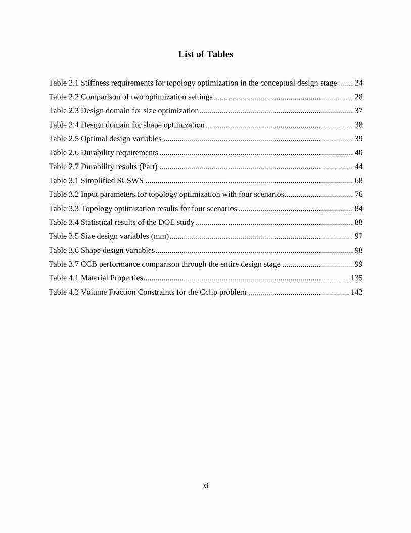
List of Tables ............................................................................................................................................... xi

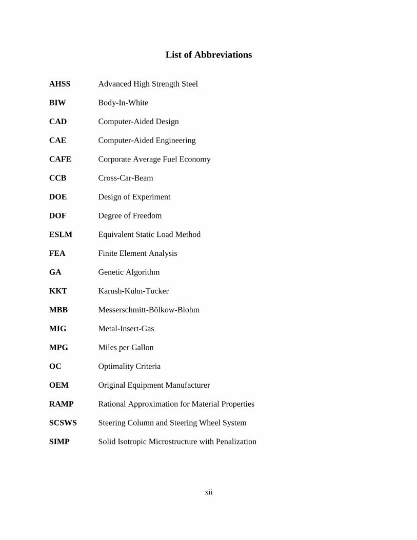
List of Abbreviations .................................................................................................................................. xii

Chapter 1 General Introduction ................................................................................................................ 1

1.1 Research Background ......................................................................................................................... 1

1.2 Current Lightweight Strategies ........................................................................................................... 2

1.2.1 Lightweight Materials .................................................................................................................. 2

1.2.2 Advanced Manufacturing Process ............................................................................................... 2

1.2.3 Design Optimization .................................................................................................................... 3

1.3 Structural optimization ........................................................................................................................ 3

1.3.1 Size optimization.......................................................................................................................... 4

1.3.2 Shape optimization ....................................................................................................................... 4

1.3.3 Topology optimization ................................................................................................................. 4

1.4 Motivation ........................................................................................................................................... 7

1.5 Primary Contribution .......................................................................................................................... 7

1.6 Structure Overview ............................................................................................................................. 8

Chapter 2 Conceptual and Detailed Design of an Automotive Engine Cradle by Using Topology,

Shape, and Size Optimization .................................................................................................................. 12

2.1 Introduction ....................................................................................................................................... 13

2.2 Mathematical Problem Statement of Engine Cradle Design Optimization ....................................... 18

2.3 Conceptual Design ............................................................................................................................ 19

2.3.1 Finite Element Modeling ........................................................................................................... 19

2.3.2 Topology Optimization .............................................................................................................. 25

2.3.3 Numerical Results of Topology Optimization in the Conceptual Design Stage ........................ 27

2.4 Detailed Design ................................................................................................................................. 33

2.4.1 Result Re-interpretation ............................................................................................................. 33

2.4.2 Finite Element Modeling ........................................................................................................... 35

2.4.3 Shape and Size Optimization and Numerical Results ................................................................ 39

2.5 Validation of the Optimum Design for Durability ............................................................................ 40

vii

2.6 Conclusions ....................................................................................................................................... 45

2.7 Limitation .......................................................................................................................................... 47

Chapter 3 Topology, Shape, and Size Optimization of an Automotive Cross Car Beam................... 54

3.1 Introduction ....................................................................................................................................... 55

3.2 Simplification of the Steering Column and Steering Wheel System (SCSWS) ............................... 65

3.3 Mathematical Problem Statement of CCB Design Optimization ..................................................... 68

3.4 Topology Optimization for CCB ...................................................................................................... 70

3.5 Size and Shape Optimization for Detailed Design ............................................................................ 86

3.6 Conclusions ..................................................................................................................................... 100

3.7 Limitations ...................................................................................................................................... 101

Chapter 4 Two-material Topology Optimization Based on Optimality Condition .......................... 109

4.1 Introduction ..................................................................................................................................... 109

4.2 Problem Definition .......................................................................................................................... 115

4.3 Theory of Two-Material Topology Optimization based on Optimality Condition ......................... 118

4.3.1 Interpolation function with two materials ................................................................................ 118

4.3.2 Two-material topology optimization statement of compliance minimization ......................... 120

4.3.3 Sensitivity derivation of compliance with respect to density variables ................................... 121

4.3.4 Update of design variables based on Optimality Condition (OC) ........................................... 123

4.3.5 Update of lagrangian multipliers based on monotonicity ........................................................ 124

4.3.6 Advanced sensitivity filtering for two-material topology optimization ................................... 128

4.4 Numerical Implementation of Two-Material Topology Optimization ........................................... 133

4.4.1 Implementation of two-material topology optimization on three classical examples .............. 135

4.4.1.1. Example I - 2D Cantilever ....................................................................................................... 136

4.4.2 Implementation of two-material topology optimization on three case studies with various

volume fraction ratios ....................................................................................................................... 140

4.5 Discussion ....................................................................................................................................... 155

4.6 Limitations and Future Work .......................................................................................................... 156

Chapter 5 General Discussion ................................................................................................................ 161

Chapter 6 Future Work .......................................................................................................................... 163

Appendix A In-house Tool of Multi-material Topology Optimization .................................................... 165

viii

List of Figures

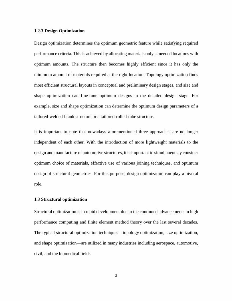
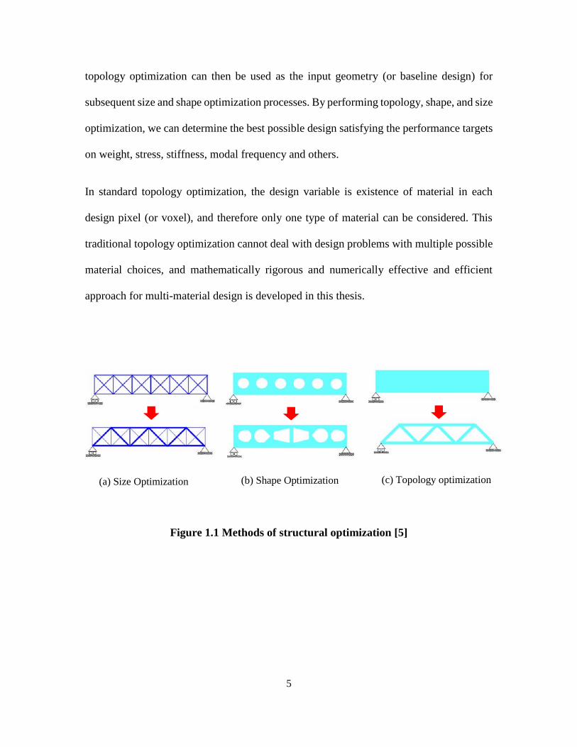
Figure 1.1 Methods of structural optimization ............................................................................... 5

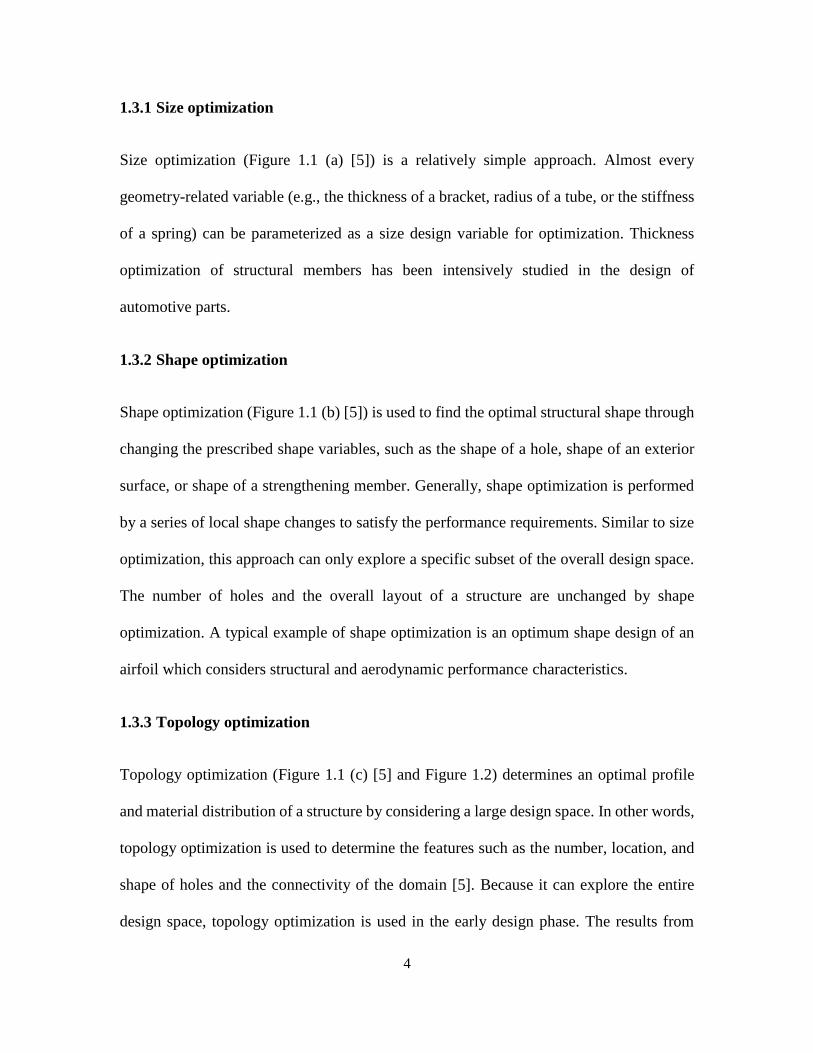
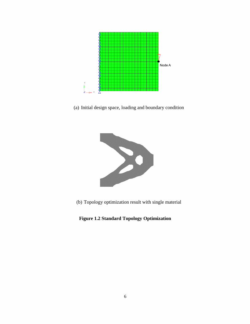
Figure 1.2 Standard Topology Optimization .................................................................................. 6

Figure 2.1 Solid space for engine cradle ....................................................................................... 20

Figure 2.2 Non-designable domains (yellow) ............................................................................... 21

Figure 2.3 Loading condition ........................................................................................................ 23

Figure 2.4 Extrusion constraints ................................................................................................... 28

Figure 2.5 Topology optimization results with different control parameters ............................... 30

Figure 2.6 Details of the topology structure with control parameters (Case B) ........................... 31

Figure 2.7 Topology optimization history for Case B (only 6 iteration snapshots shown here) .. 32

Figure 2.8 The history of the objective function (mass) during the topology optimization (Case

B)................................................................................................................................................... 32

Figure 2.9 Geometry extraction from topology optimization result (Case B) .............................. 34

Figure 2.10 Revised design ........................................................................................................... 34

Figure 2.11 Size optimization design variables ............................................................................ 37

Figure 2.12 Shape optimization design variables ......................................................................... 38

Figure 2.13 Stress contours for different loading conditions ........................................................ 43

Figure 2.14 Strain life with elastic and plastic lines (nCode Design Life 8.0) ............................. 44

Figure 2.15 Structural design process of an engine cradle .......................................................... 49

Figure 3.1 Structural optimization design process ........................................................................ 57

Figure 3.2 Production of vehicle from 2002 to 2012 .................................................................... 59

Figure 3.3 Simplified finite element model of the steering column and steering wheel system

(SCSWS) ....................................................................................................................................... 67

Figure 3.4 Two manufacturing processes and their respective possible design domains of a CCB

....................................................................................................................................................... 71

Figure 3.5 Design space for topology optimization ...................................................................... 72

Figure 3.6 Aluminum CCB with the simplified steering column and steering wheel attached.... 73

Figure 3.7 Locations of the CCB attachment points to its surrounding environment .................. 74

Figure 3.8 Topology results comparison ...................................................................................... 78

Figure 3.9 Topology optimization history for Case A-2 .............................................................. 79

ix

Figure 3.10 Topology result with identical parts (Case A-3) ....................................................... 80

Figure 3.11 Topology optimization history for Case A-3............................................................. 81

Figure 3.12 The history of the objective function during the topology optimization (Case A-3) 82

Figure 3.13 Topology Result (Case B) ......................................................................................... 83

Figure 3.14 New geometry after implementing a threshold of 0.7 and conducting results re-

interpretation ................................................................................................................................. 85

Figure 3.15 Parts allowed for size optimization (exploded view) ................................................ 86

Figure 3.16 Significant effects of thickness design variables to the responses ............................ 91

Figure 3.17 Final 10 size (thickness) design variables ................................................................. 92

Figure 3.18 Shape design variables (one side).............................................................................. 93

Figure 3.19 The history of the objective function of the shape and size optimization ................. 96

Figure 3.20 Complete design optimization procedure of a CCB ................................................ 103

Figure 4.1 Linear elastic continuum problem under static load.................................................. 116

Figure 4.2 A representative relationship between Young’s modulus and two normalized density

values for two materials .............................................................................................................. 119

Figure 4.3 An example of the relation between the total volume and the two Lagrangian

multipliers ................................................................................................................................... 126

Figure 4.4 An example of the relation between the volume of Material 1 and the Lagrangian

multiplier 1 ............................................................................................................................... 127

Figure 4.5 An example of dependence of the optimal solution on different mesh refinement.

Discretized elements for a) 2700, b) 4800 and c) 17200 ............................................................ 129

Figure 4.6 An example of checkerboard pattern ......................................................................... 129

Figure 4.7 Adjacent (neighbor) elements of the target element by one layer ............................. 132

Figure 4.8 Flow chart of two-material topology optimization implementation on the platform of

HyperWorks ................................................................................................................................ 134

Figure 4.9 Two-material topology optimization of the 2D cantilever problem .......................... 136

Figure 4.10 Objective function history of the 2D cantilever problem with two materials ......... 137

Figure 4.11 Topology changes of Material 1 and Material 2 during the first 14 iterations, for the

2D cantilever problem................................................................................................................. 137

Figure 4.12 Two-material topology optimization of the half MBB problem ............................. 138

Figure 4.13 Two-material topology optimization of the 3D cantilever ...................................... 139

x

Figure 4.14 Topology results of the first 14 iterations of the 3D cantilever problem ................ 139

Figure 4.15 Initial design space (finite element model) of the Cclip problem with boundary

conditions and loads .................................................................................................................... 142

Figure 4.16 Comparison of the optimum solutions of the Cclip problem .................................. 142

Figure 4.17 The optimum topology with two materials of each case (red-steel, green-aluminum).

All 6 designs have the same weight. ........................................................................................... 143

Figure 4.18 Performance (i.e. compliance) of 6 optimum solutions of the Cclip problem ........ 144

Figure 4.19 Initial design space (finite element model) of the Long Cantilever problem with

boundary conditions and loads.................................................................................................... 146

Figure 4.20 Comparison of the optimum solutions of the Long Cantilever problem ................. 147



Figure 4.22 Performance (i.e. compliance) of 6 optimum solutions of the Long Cantilever

problem ....................................................................................................................................... 149

Figure 4.23 Initial design space (finite element model) of the Control Arm problem with

boundary conditions and loads.................................................................................................... 151

Figure 4.24 Comparison of the optimum solutions of the Control Arm problem ...................... 152



Figure 4.26 Performance (i.e. compliance) of 6 optimum solutions of the Control Arm problem

..................................................................................................................................................... 155

xi

List of Tables

Table 2.1 Stiffness requirements for topology optimization in the conceptual design stage ....... 24

Table 2.2 Comparison of two optimization settings ..................................................................... 28

Table 2.3 Design domain for size optimization ............................................................................ 37

Table 2.4 Design domain for shape optimization ......................................................................... 38

Table 2.5 Optimal design variables .............................................................................................. 39

Table 2.6 Durability requirements ................................................................................................ 40

Table 2.7 Durability results (Part) ................................................................................................ 44

Table 3.1 Simplified SCSWS ....................................................................................................... 68

Table 3.2 Input parameters for topology optimization with four scenarios .................................. 76

Table 3.3 Topology optimization results for four scenarios ......................................................... 84

Table 3.4 Statistical results of the DOE study .............................................................................. 88

Table 3.5 Size design variables (mm) ........................................................................................... 97

Table 3.6 Shape design variables .................................................................................................. 98

Table 3.7 CCB performance comparison through the entire design stage ................................... 99

Table 4.1 Material Properties ...................................................................................................... 135

Table 4.2 Volume Fraction Constraints for the Cclip problem .................................................. 142

xii

List of Abbreviations

AHSS Advanced High Strength Steel

BIW Body-In-White

CAD Computer-Aided Design

CAE Computer-Aided Engineering

CAFE Corporate Average Fuel Economy

CCB Cross-Car-Beam

DOE Design of Experiment

DOF Degree of Freedom

ESLM Equivalent Static Load Method

FEA Finite Element Analysis

GA Genetic Algorithm

KKT Karush-Kuhn-Tucker

MBB Messerschmitt-Bölkow-Blohm

MIG Metal-Insert-Gas

MPG Miles per Gallon

OC Optimality Criteria

OEM Original Equipment Manufacturer

RAMP Rational Approximation for Material Properties

SCSWS Steering Column and Steering Wheel System

SIMP Solid Isotropic Microstructure with Penalization

1

Chapter 1

General Introduction

1.1 Research Background

With a rising cost of natural resources and growing concerns on the environment, energy

conservation and protection of the environment have become an important issue

worldwide. Both governments and customers demand more energy-efficient, cost-

effective, and environmentally friendly products. For example, the Corporate Average Fuel

Economy (CAFE) regulations in the United States mandate an improvement of the average

fuel economy of cars and light trucks up to 54.5 mile per gallon (mpg) by Model Year

2025. In Canada, the fuel economy target of passenger cars is 40.8 mpg by 2016 and 56.2

mpg by 2025; in the European Union, the target fuel economy of passenger cars is 42.3

mpg by 2015 and 57.9 mpg by 2025; in South Korea, 39.5 mpg by 2015 and 58.8 mpg by

2020; and in China, 37 mpg by 2015 and 56 mpg by 2025 [1]. Facing tremendous pressure

from governments and customers, improvement in fuel efficiency of the next generation

vehicles is a top priority for automakers.

There are several ways to improve fuel efficiency of a vehicle, such as improving the

powertrain efficiency or using a substitute energy, but one of the most promising

approaches is to reduce the weight of a vehicle. It has been demonstrated that with every

100 kg weight reduction, the fuel consumption will decrease by approximately 0.4 L per

100 km [2] and carbon dioxide (CO2) emissions will decrease by 8-11 g/km [3]. Therefore,

2

lightweight design of automobiles is an efficient and immediate way to improve fuel

efficiency and reduce CO2 emissions.

1.2 Current Lightweight Strategies

Current lightweight strategies can be categorized into three main approaches.

1.2.1 Lightweight Materials

The traditional low carbon steel can be substituted by lightweight materials, such as

aluminum, magnesium, plastics, and composites. The properties of different materials, in

terms of stiffness, strength, durability, corrosion, and formability, should be discreetly

taken into consideration. In automotive industry, traditional materials like low carbon steel

and iron have been gradually replaced by various lightweight materials over past decades.

A report by Ducker Worldwide [4] predicted that 26.6% of all body and closure parts for

light vehicles would be made of aluminum by 2025 in North America, whereas in 2015

only 6.6% is aluminum.

1.2.2 Advanced Manufacturing Process

Advanced manufacturing and production processes can be employed to reduce the extra

weight of joints. It is also important to develop methods that can join dissimilar materials

together. For example, the use of structural adhesives or overcasting can reduce the weight

of mechanical joints, and replacing metal-insert-gas (MIG) welding with laser welding can

avoid the introduction of extra material of solder, which will result in weight reduction.

Friction stir welding can join different dissimilar materials, like steel and aluminum.

3

1.2.3 Design Optimization

Design optimization determines the optimum geometric feature while satisfying required

performance criteria. This is achieved by allocating materials only at needed locations with

optimum amounts. The structure then becomes highly efficient since it has only the

minimum amount of materials required at the right location. Topology optimization finds

most efficient structural layouts in conceptual and preliminary design stages, and size and

shape optimization can fine-tune optimum designs in the detailed design stage. For

example, size and shape optimization can determine the optimum design parameters of a

tailored-welded-blank structure or a tailored-rolled-tube structure.

It is important to note that nowadays aforementioned three approaches are no longer

independent of each other. With the introduction of more lightweight materials to the

design and manufacture of automotive structures, it is important to simultaneously consider

optimum choice of materials, effective use of various joining techniques, and optimum

design of structural geometries. For this purpose, design optimization can play a pivotal

role.

1.3 Structural optimization

Structural optimization is in rapid development due to the continued advancements in high

performance computing and finite element method theory over the last several decades.

The typical structural optimization techniques—topology optimization, size optimization,

and shape optimization—are utilized in many industries including aerospace, automotive,

civil, and the biomedical fields.

4

1.3.1 Size optimization

Size optimization (Figure 1.1 (a) [5]) is a relatively simple approach. Almost every

geometry-related variable (e.g., the thickness of a bracket, radius of a tube, or the stiffness

of a spring) can be parameterized as a size design variable for optimization. Thickness

optimization of structural members has been intensively studied in the design of

automotive parts.

1.3.2 Shape optimization

Shape optimization (Figure 1.1 (b) [5]) is used to find the optimal structural shape through

changing the prescribed shape variables, such as the shape of a hole, shape of an exterior

surface, or shape of a strengthening member. Generally, shape optimization is performed

by a series of local shape changes to satisfy the performance requirements. Similar to size

optimization, this approach can only explore a specific subset of the overall design space.

The number of holes and the overall layout of a structure are unchanged by shape

optimization. A typical example of shape optimization is an optimum shape design of an

airfoil which considers structural and aerodynamic performance characteristics.

1.3.3 Topology optimization

Topology optimization (Figure 1.1 (c) [5] and Figure 1.2) determines an optimal profile

and material distribution of a structure by considering a large design space. In other words,

topology optimization is used to determine the features such as the number, location, and

shape of holes and the connectivity of the domain [5]. Because it can explore the entire

design space, topology optimization is used in the early design phase. The results from

5

topology optimization can then be used as the input geometry (or baseline design) for

subsequent size and shape optimization processes. By performing topology, shape, and size

optimization, we can determine the best possible design satisfying the performance targets

on weight, stress, stiffness, modal frequency and others.

In standard topology optimization, the design variable is existence of material in each

design pixel (or voxel), and therefore only one type of material can be considered. This

traditional topology optimization cannot deal with design problems with multiple possible

material choices, and mathematically rigorous and numerically effective and efficient

approach for multi-material design is developed in this thesis.

Figure 1.1 Methods of structural optimization [5]

(a) Size Optimization (b) Shape Optimization (c) Topology optimization

6

(a) Initial design space, loading and boundary condition

(b) Topology optimization result with single material

Figure 1.2 Standard Topology Optimization

7

1.4 Motivation

Theories and numerical techniques for size and shape optimization have been well

developed. Without proper choice of optimal topology, however, size and shape

optimization can make only limited performance improvement. Topology optimization

starts with a non-biased design, which means there is no need for input from a designer,

and the method determines a set of optimum load paths within the structure. Hence,

topology optimization is recognized as the most fundamental design process for structural

optimization, and it should be implemented in an early design stage, such as the conceptual

and preliminary design stages. The output from topology optimization can then be used in

the following detailed design stage, which can make a significant contribution to the

performance and quality of structural products.

Topology optimization has been traditionally used for structural design with only a single

material, which determines the existence of material within each design cell for a

prescribed material type. For a design problem with multiple materials, however, this

traditional topology optimization method cannot be used. As aforementioned, the use of

multiple materials for weight reduction is an important task in automotive industry, and the

current optimization technology is ill equipped for this challenge. Hence, it is imperative

to develop an effective multi-material topology optimization algorithm and numerical tool

that can deal with multiple materials for real-world design problems.

1.5 Primary Contribution

Not only will this research make a significant advancement in topology optimization

academically, but it will also provide automotive industry with a methodology and tool that

8

can produce innovative structural designs for lightweight design. Both of the single-

material and the multi-material topology optimization presented in this thesis can be used

in other industries such as railway and aerospace.

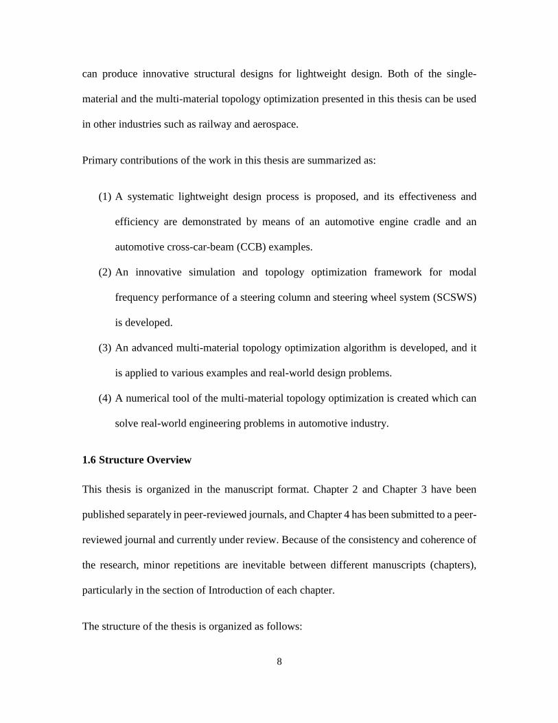
Primary contributions of the work in this thesis are summarized as:

(1) A systematic lightweight design process is proposed, and its effectiveness and

efficiency are demonstrated by means of an automotive engine cradle and an

automotive cross-car-beam (CCB) examples.

(2) An innovative simulation and topology optimization framework for modal

frequency performance of a steering column and steering wheel system (SCSWS)

is developed.

(3) An advanced multi-material topology optimization algorithm is developed, and it

is applied to various examples and real-world design problems.

(4) A numerical tool of the multi-material topology optimization is created which can

solve real-world engineering problems in automotive industry.

1.6 Structure Overview

This thesis is organized in the manuscript format. Chapter 2 and Chapter 3 have been

published separately in peer-reviewed journals, and Chapter 4 has been submitted to a peer-

reviewed journal and currently under review. Because of the consistency and coherence of

the research, minor repetitions are inevitable between different manuscripts (chapters),

particularly in the section of Introduction of each chapter.

The structure of the thesis is organized as follows:

9

Chapter 1 provides an overview of the entire work discussed in this thesis, including the

background, motivation, and contribution.

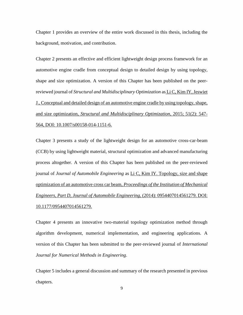
Chapter 2 presents an effective and efficient lightweight design process framework for an

automotive engine cradle from conceptual design to detailed design by using topology,

shape and size optimization. A version of this Chapter has been published on the peer-

reviewed journal of Structural and Multidisciplinary Optimization as Li C, Kim IY, Jeswiet

J., Conceptual and detailed design of an automotive engine cradle by using topology, shape,

and size optimization, Structural and Multidisciplinary Optimization, 2015; 51(2): 547-

564, DOI: 10.1007/s00158-014-1151-6.

Chapter 3 presents a study of the lightweight design for an automotive cross-car-beam

(CCB) by using lightweight material, structural optimization and advanced manufacturing

process altogether. A version of this Chapter has been published on the peer-reviewed

journal of Journal of Automobile Engineering as Li C, Kim IY. Topology, size and shape

optimization of an automotive cross car beam, Proceedings of the Institution of Mechanical

Engineers, Part D, Journal of Automobile Engineering, (2014): 0954407014561279. DOI:

10.1177/0954407014561279.

Chapter 4 presents an innovative two-material topology optimization method through

algorithm development, numerical implementation, and engineering applications. A

version of this Chapter has been submitted to the peer-reviewed journal of International

Journal for Numerical Methods in Engineering.

Chapter 5 includes a general discussion and summary of the research presented in previous

chapters.

10

Chapter 6 discusses the limitations of the research and the potential work that could be

carried out in the future.

11

REFERENCES

[1] http://www.theicct.org/info-tools/global-passenger-vehicle-standards

[2] Woisetschlaeger, E., Keine Monokultur. Automobile Entwicklung, 2001, pp. 130

[3] Wallentowitz H., Structural Design of Vehicles. Institute fur Kraftfahrwesen, Aachen,

2004

[4] http://www.drivealuminum.org/research-resources/PDF/Research/2014/2014-

ducker-report

[5] Bendsøe M. P. and Sigmund O. Topology Optimization: Theory, Methods and

Applications. Springer, 2003

http://www.google.ca/search?hl=zh-CN&tbo=p&tbm=bks&q=inauthor:%22Martin+P.+Bends%C3%B8e%22

12

Chapter 2

Conceptual and Detailed Design of an Automotive Engine Cradle by

Using Topology, Shape, and Size Optimization

An automotive engine cradle supports many crucial components and systems, such as an

engine, transmission, and suspension. Important performance measures for the design of

an engine cradle include stiffness, natural frequency, and durability, while minimizing

weight is of primary concern. This chapter presents an effective and efficient methodology

for engine cradle design from conceptual design to detailed design using design

optimization. First, topology optimization was applied on a solid model which only

contains the possible engine cradle design space, and an optimum conceptual design was

determined which minimizes weight while satisfying all stiffness constraints. Based on

topology optimization results, a design review was conducted, and a revised model was

created which addresses all structural and manufacturability concerns. Shape and size

optimization was then performed in the detailed design stage to further minimize the mass

while meeting the stiffness and natural frequency targets. Lastly, the final design was

validated for durability. The initial design domain had the mass of 82.6 kg; topology

optimization in conceptual design reduced the mass to 26.7 kg; and the detailed design task

involving shape and size optimization further reduced the mass to 21.4 kg.

13

2.1 Introduction

With new government regulations on automobiles, automotive manufacturers are under

tremendous pressure to improve vehicle fuel efficiency and reduce carbon emissions

drastically. As an example, automakers have to significantly improve vehicle mileage

through a series of steps beginning in 2016 through to 2025 due to the mandated Corporate

Average Fuel Economy (CAFE). There are several ways how to improve vehicle fuel

efficiency, such as improving the efficiency of power train, but one of the most promising

methods is to reduce the vehicle weight. It has been shown that with every 100 kg weight

reduction, the consumption of fuel will decrease by approximately 0.4 liters per 100 km

[1] and the emissions of CO2 will decrease by 8 g to 11 g per kilometer [2].

An engine cradle is a critical component of a car with multiple functions. The engine cradle

structurally supports the engine, transmission, and suspension; distributes high chassis

loads over a wider area; and reduces vibrations and shocks that are generated by the engine,

transmission, and roads. Engine cradles first appeared in the late 1960s and were used to

balance the riding comfort and handling ability for luxury cars. An engine cradle is

typically manufactured from welded steel stampings and is bolted to the vehicle body. By

adopting engine cradles, energy-absorption and force-distribution have also considerably

improved. Further, an engine cradle makes it possible to build the steering, engine, and

transmission assemblies in one location, and to install the finished product in the completed

vehicle in another location. This modular manufacturing process allows for the reduction

of assembly time and cost. The use of engine cradles also allows mechanics to remove

broken parts easily, which results in the reduction of repair time and maintenance cost.

14

Due to these benefits, engine cradles are used in various car segments, even in the compact

cars like Ford Focus, Toyota Corolla, and Volkswagen Lavida. Moreover, on account of

their advantages, a rear subframe that has a similar structure as the engine cradle has been

developed and widely adopted for the purpose of carrying the rear suspension and

transmission systems.

There are, however, two major drawbacks of adopting an engine cradle: 1) due to the

addition of an engine cradle, the weight of the vehicle increases, which results in inferior

fuel efficiency and increased carbon emissions; and 2) the design cycle time also becomes

longer—including CAD modeling, numerical analysis, physical testing, and re-design—

and this increases the cost of product development. It is therefore important for automakers

to have the ability to determine lightweight engine cradle designs with a short design cycle

time.

The current practice in automotive industry is not yet fully systematic or efficient. A

conceptual design is proposed based on the designer’s experience, which is often subjective

and sub-optimal. In the detailed design stage, a series of FEA (finite element analyses) are

performed with respect to several performance measures such as stiffness, natural

frequency, and durability (i.e. fatigue). If the target requirements cannot be met by fine

tuning of the design parameters, the conceptual design is revisited and new design concepts

are explored. This design iteration inevitably puts a significant strain on already tight

product development schedule and finances of the company.

A number of academic studies can be identified which attempt to improve the performance

of an engine cradle design. Triantos and Michaels [3] proposed the development of an

15

aluminum engine cradle, with different design criteria and structural performance

requirements, for GM midsize vehicles. Chen et al. [4] proposed a method of improving

energy absorption of an engine cradle. Kang et al. [5] applied artificial neural network to

predict multi-axial fatigue life of an automotive engine cradle. Kim et al. [6] applied the

hydroforming process to the manufacture of automotive engine cradles. Kim et al. [7]

conducted a parameter study of vibration characteristics of an engine cradle. Xu et al. [8]

introduced an approach for engine cradle fatigue analyses and tests.

These studies allowed for the improvement of engine cradle performance in one way or

another, but their contributions are limited because the application of the proposed

approaches took place in the detailed design stage, that is, after the overall design concept

is already selected. Truly effective designs could be determined, if a most promising engine

cradle design is sought in the conceptual design stage. Topology optimization is an

effective method for conceptual structural design. Due to significant computing power

improvement, we can nowadays solve topology optimization with high resolution—and

for simple geometries, topology optimization can determine optimum designs which really

do not require further shape and size optimization.

Theory of topology optimization is already well established for a number of performance

measures such as compliance, natural frequency, and stress. Topology optimization

determines optimal structural geometry by distributing material over the design domain—

the optimum geometry then can be considered as the most efficient load path network.

There are a very large amount of studies in topology optimization theory. Bendsøe and

Sigmund [9] summarized fundamentals of topology optimization in their book. Kim and


16

Kwak [10] proposed design space optimization in which the design domain (or the number

of design variables) is also considered as a design variable. Kim and Weck [11] applied the

concept of “adaptivity” to Genetic Algorithm-based topology optimization and

convergence criterion of topology optimization [12]. Forsberg and Nilsson [13] developed

an internal energy density method, avoiding the use of sensitivities, to apply topology

optimization to nonlinear problems. Topology optimization was also applied to the

simulation of the human bone adaptation process by Kim and his colleagues [14-15]. Lee

and Park [16] utilized the equivalent static method in nonlinear topology optimization.

Introducing topology optimization to the early design stage, such as the conceptual design

stage, can help effectively filter out inferior designs and produce the most promising

designs for the subsequent design stages. This could also reduce design cycle by

minimizing trial-and-error iterations. Due to these benefits, topology optimization has been

applied to the design of many automobile and aircraft parts such as chassis and body. Yang

and Chahande [17] introduce an in-house topology optimization software program, TOP,

and used it to optimize a simplified truck frame, a deck lid, and a space frame structure.

Lee and Lee [18] performed topology optimization to find the optimal layout of an

aluminum control arm to reduce the weight and improve the rigidity. Lee et al. [19] used

topology optimization to determine the material distribution of a door panel, and based on

the topology result, the panel was partitioned to multiple domains with different thickness

values that can be manufactured using tailor welded blanks. Chiandussi et al. [20] utilized

topology optimization to improve the structural performance of a rear suspension

subframe. Wang et al. [21] employed topology optimization and size optimization to

improve the overall stiffness of an existing car body. Torstenfelt and Klarbring [22] found

17

the conceptual design of the modular car product families using topology optimization.

Waquas et al. [23] applied topology optimization to the design of aircraft components.

Cavazzuti et al. [24] presented a methodology for automotive chassis design using topology

optimization, topometry optimization, and size optimization. Lee et al. [25] employed the

equivalent static loads method (ELSM) to determine the cross-section of the crashbox

using topology optimization to maximize the absorbed energy. Luo and Di [26] achieved

a lightweight optimal design of an in-wheel motor by using topology optimization and size

optimization.

Although an engine cradle adds a significant amount of weight and lengthens the design

cycle as aforementioned, the design of an engine cradle, especially in the conceptual design

stage, is currently done heuristically in industry; this is because a systematic and efficient

topology optimization approach has not been utilized for the design of engine cradles.

The objectives of this research are 1) to perform the conceptual design of a real-world

engine cradle based on a high-fidelity finite element (FE) model, using large-scale topology

optimization and 2) to further improve the design in the subsequent detailed design stage,

using shape and size optimization. By means of this work, the entire design process will be

done effectively and efficiently, and the important performance metrics such as stiffness

and natural frequency will be considered in design optimization. Manufacturability will be

considered after a promising concept is selected by topology optimization, and the final

optimum design will be validated for durability requirements.

Section 2.2 presents the design optimization problem statement for the entire design

process of an engine cradle. Section 2.3 shows the conceptual design task, which consists

18

of finite element modeling and topology optimization for mass minimization with stiffness

requirements. In Section 2.4, detailed design is performed: first, the optimum result by

topology optimization in the conceptual design stage is carefully interpreted and reviewed,

and a revised model is created. Shape and size optimization is conducted which considers

stiffness and natural frequency requirements while further minimizing the mass. Section

2.5 shows durability tests of the optimum design from the detailed design stage, in order to

confirm the design satisfies all fatigue requirements. Section 2.6 summarizes the study.

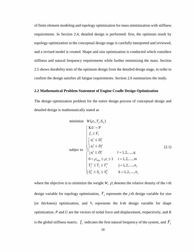
2.2 Mathematical Problem Statement of Engine Cradle Design Optimization

The design optimization problem for the entire design process of conceptual design and

detailed design is mathematically stated as

1 1

min

minimize ( , ,S )

subjec to 1,2,....,q

0 1 1,2,....,

j 1,2,...., n

k 1,2,....,

i j k

x x

l l

y y

l l

z z

l l

i

L U

j j j t

L U

k k k s

W T

U

f F

u D

u D

u D l

i m

T T T

S S S n

(2.1)

where the objective is to minimize the weight W, i denotes the relative density of the i-th

design variable for topology optimization, jT represents the j-th design variable for size

(or thickness) optimization, and Sk represents the k-th design variable for shape

optimization. P and U are the vectors of nodal force and displacement, respectively, and K

is the global stiffness matrix. 1f indicates the first natural frequency of the system, and 1F

19

is the lower bound for the first natural frequency. x

lu , y

lu andz

lu denote the x-, y- and z-

directional displacements of the l-th loading point, respectively. x

lD , y

lD and z

lD are the

corresponding upper bounds for x-, y-, and z-directional displacements of the l-th loading

point, respectively. q is the total number of loading points. min is the minimum allowable

bound for the density, which is implemented in order to avoid numerical difficulties. m, nt,

ns are the total number of design variables for topology optimization, size optimization,

and shape optimization, respectively. (L

jT , L

kS ) and (U

jT , U

kS ) are the lower bounds and upper

bounds for the corresponding size and shape design variables, respectively.

2.3 Conceptual Design

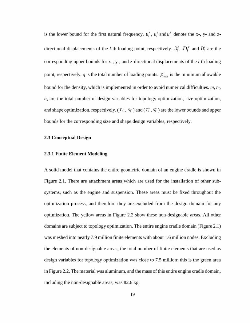
2.3.1 Finite Element Modeling

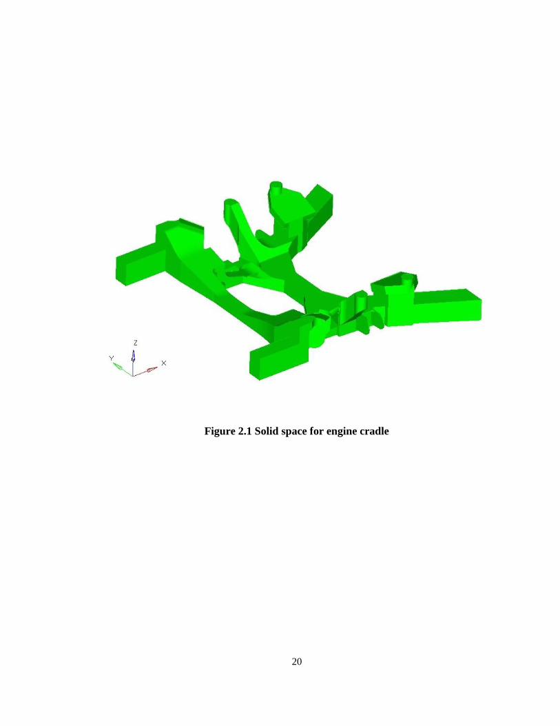
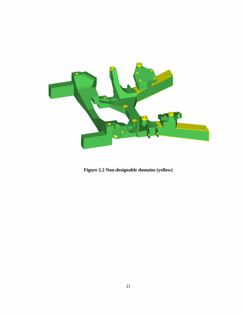
A solid model that contains the entire geometric domain of an engine cradle is shown in

Figure 2.1. There are attachment areas which are used for the installation of other sub-

systems, such as the engine and suspension. These areas must be fixed throughout the

optimization process, and therefore they are excluded from the design domain for any

optimization. The yellow areas in Figure 2.2 show these non-designable areas. All other

domains are subject to topology optimization. The entire engine cradle domain (Figure 2.1)

was meshed into nearly 7.9 million finite elements with about 1.6 million nodes. Excluding

the elements of non-designable areas, the total number of finite elements that are used as

design variables for topology optimization was close to 7.5 million; this is the green area

in Figure 2.2. The material was aluminum, and the mass of this entire engine cradle domain,

including the non-designable areas, was 82.6 kg.

20

Figure 2.1 Solid space for engine cradle

21

Figure 2.2 Non-designable domains (yellow)

22

Topology optimization was used in this conceptual design stage. The objective of the

topology optimization is to determine the most effective design that minimizes the mass of

the structure. Important performance requirements that must be considered through the

entire design process are the stiffness, natural frequency, and durability. Typically, it is

most difficult to satisfy stiffness targets among others. Hence, we chose the stiffness

requirement as the design constraint for topology optimization in this conceptual design

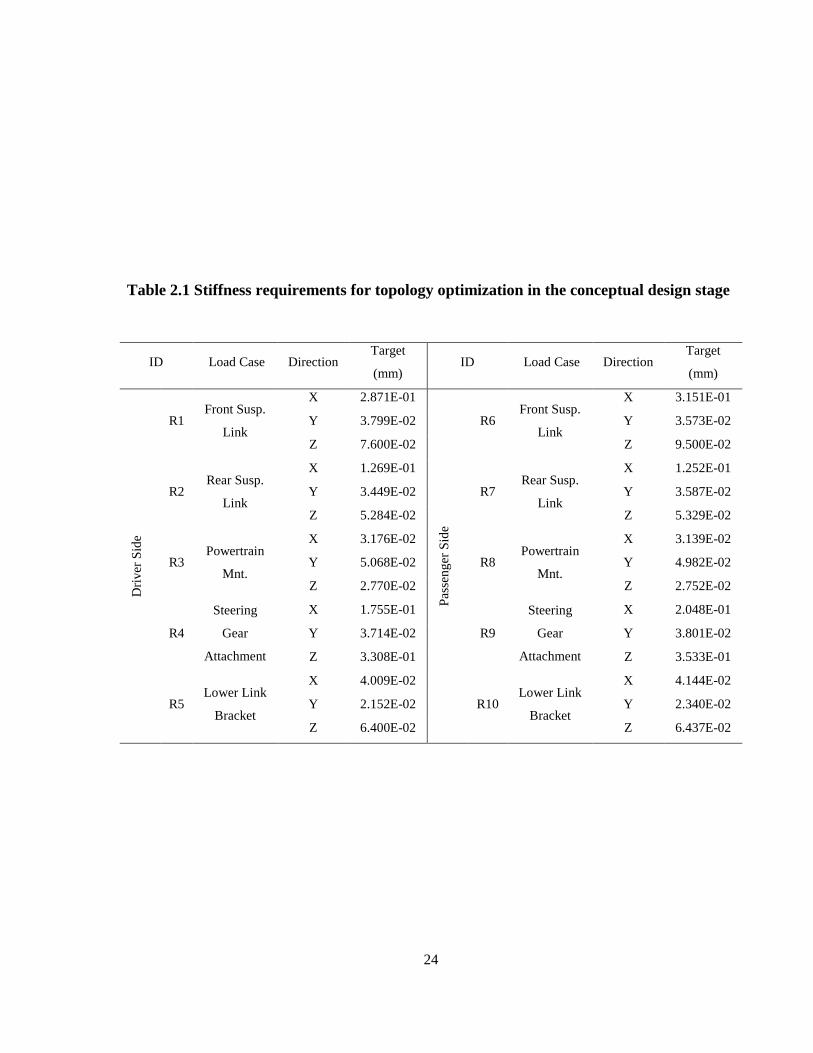
stage, while leaving other performance requirements for next-phase optimization tasks.

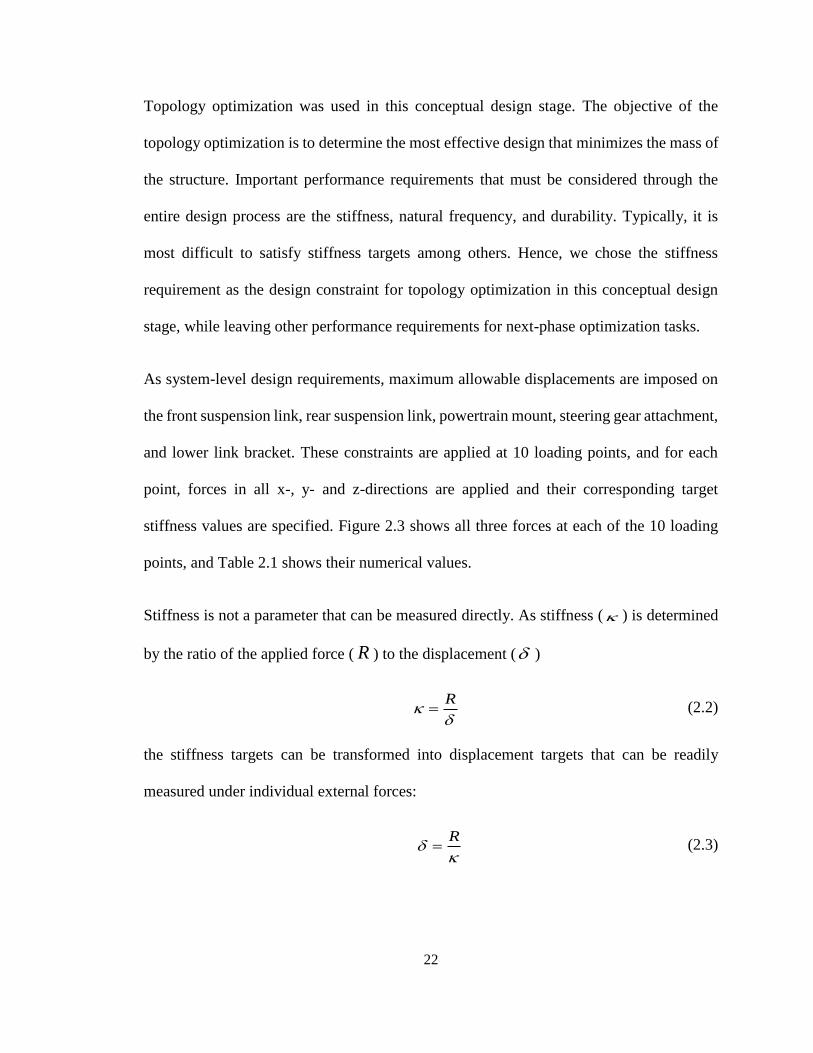
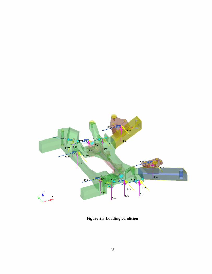
As system-level design requirements, maximum allowable displacements are imposed on

the front suspension link, rear suspension link, powertrain mount, steering gear attachment,

and lower link bracket. These constraints are applied at 10 loading points, and for each

point, forces in all x-, y- and z-directions are applied and their corresponding target

stiffness values are specified. Figure 2.3 shows all three forces at each of the 10 loading

points, and Table 2.1 shows their numerical values.

Stiffness is not a parameter that can be measured directly. As stiffness ( ) is determined

by the ratio of the applied force ( R ) to the displacement ( )

R

(2.2)

the stiffness targets can be transformed into displacement targets that can be readily

measured under individual external forces:

R

(2.3)

23

Figure 2.3 Loading condition

24

Table 2.1 Stiffness requirements for topology optimization in the conceptual design stage

ID Load Case Direction Target

(mm) ID Load Case Direction

Target

(mm)

Dri

ver

Sid

e

R1 Front Susp.

Link

X 2.871E-01

Pas

sen

ger

Sid

e

R6 Front Susp.

Link

X 3.151E-01

Y 3.799E-02 Y 3.573E-02

Z 7.600E-02 Z 9.500E-02

R2 Rear Susp.

Link

X 1.269E-01

R7 Rear Susp.

Link

X 1.252E-01

Y 3.449E-02 Y 3.587E-02

Z 5.284E-02 Z 5.329E-02

R3 Powertrain

Mnt.

X 3.176E-02

R8 Powertrain

Mnt.

X 3.139E-02

Y 5.068E-02 Y 4.982E-02

Z 2.770E-02 Z 2.752E-02

R4

Steering

Gear

Attachment

X 1.755E-01

R9

Steering

Gear

Attachment

X 2.048E-01

Y 3.714E-02 Y 3.801E-02

Z 3.308E-01 Z 3.533E-01

R5 Lower Link

Bracket

X 4.009E-02

R10 Lower Link

Bracket

X 4.144E-02

Y 2.152E-02 Y 2.340E-02

Z 6.400E-02 Z 6.437E-02

25

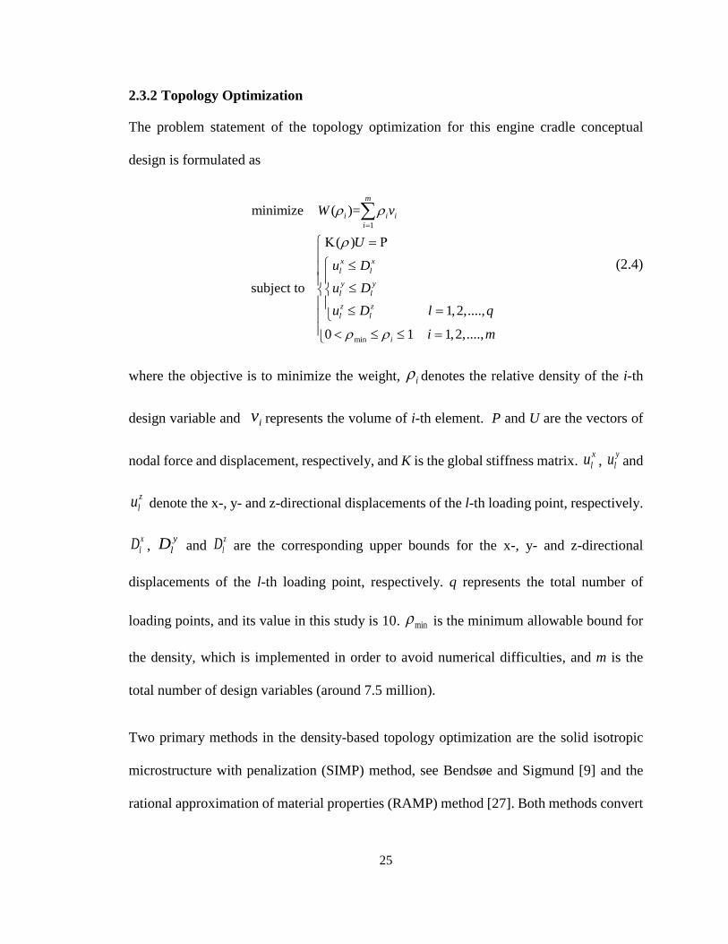
2.3.2 Topology Optimization

The problem statement of the topology optimization for this engine cradle conceptual

design is formulated as

1

min

minimize ( )=

( )

subject to

1,2,....,

0 1 1,2,....,

m

i i i

i

x x

l l

y y

l l

z z

l l

i

W v

U

u D

u D

u D l q

i m

(2.4)

where the objective is to minimize the weight, i denotes the relative density of the i-th

design variable and iv represents the volume of i-th element. P and U are the vectors of

nodal force and displacement, respectively, and K is the global stiffness matrix.

x

lu , y

lu and

z

lu denote the x-, y- and z-directional displacements of the l-th loading point, respectively.

x

lD , y

lD and z

lD are the corresponding upper bounds for the x-, y- and z-directional

displacements of the l-th loading point, respectively. q represents the total number of

loading points, and its value in this study is 10. min is the minimum allowable bound for

the density, which is implemented in order to avoid numerical difficulties, and m is the

total number of design variables (around 7.5 million).

Two primary methods in the density-based topology optimization are the solid isotropic

microstructure with penalization (SIMP) method, see Bendsøe and Sigmund [9] and the

rational approximation of material properties (RAMP) method [27]. Both methods convert


26

a continuous optimization model into a discretized model in which a penalty factor is used

to drive the intermediate density to converge to either 0 (void) or 1 (solid).

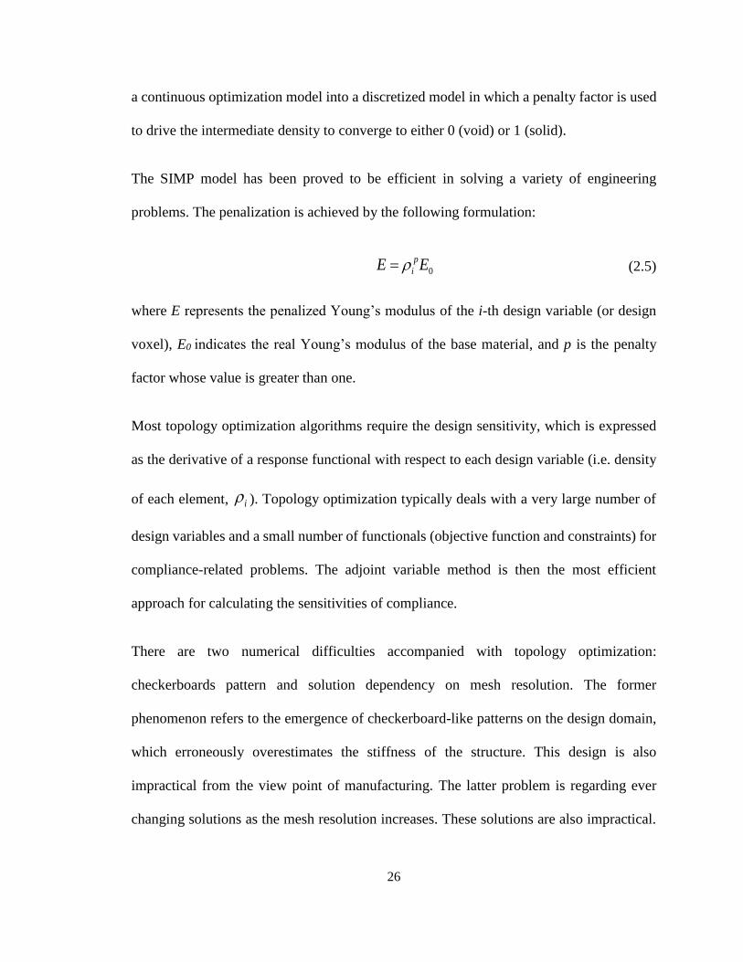
The SIMP model has been proved to be efficient in solving a variety of engineering

problems. The penalization is achieved by the following formulation:

0

p

iE E

(2.5)

where E represents the penalized Young’s modulus of the i-th design variable (or design

voxel), E0 indicates the real Young’s modulus of the base material, and p is the penalty

factor whose value is greater than one.

Most topology optimization algorithms require the design sensitivity, which is expressed

as the derivative of a response functional with respect to each design variable (i.e. density

of each element, i ). Topology optimization typically deals with a very large number of

design variables and a small number of functionals (objective function and constraints) for

compliance-related problems. The adjoint variable method is then the most efficient

approach for calculating the sensitivities of compliance.

There are two numerical difficulties accompanied with topology optimization:

checkerboards pattern and solution dependency on mesh resolution. The former

phenomenon refers to the emergence of checkerboard-like patterns on the design domain,

which erroneously overestimates the stiffness of the structure. This design is also

impractical from the view point of manufacturing. The latter problem is regarding ever

changing solutions as the mesh resolution increases. These solutions are also impractical.

27

The cause and solutions for both problems are well explained in the book by Bendsøe and

Sigmund [9].

2.3.3 Numerical Results of Topology Optimization in the Conceptual Design Stage

Topology optimization is performed using OptiStruct 11.0 [28]. Topology optimization

results are highly dependent on the choice of the penalty factor (for intermediate density

control) and sensitivity filtering factor (for checkerboards control). By using an effective

penalty factor, which is expressed as p in Equation (2.5), we can minimize unfavorable

intermediate-density elements in the final optimum results, and the choice of an optimum

sensitivity filtering factor can restrain the emergence of checkerboards in optimization.

There are two more control parameters that affect the optimum results: minimum member

size control and manufacturability control. Compared to bulky structures, thin structures

can usually support loads more efficiently with minimum mass. Minimum member size

control is a technique to keep such thin structures [29]. There are a number of

manufacturing processes used for mass production in the automotive industry, but

extrusion is particularly favorable because of its low cost and fast processing time.

Extrusion requires the elongated structure has the “same (i.e. constant)” cross-sectional

shape throughout the direction of extrusion (longitudinal direction). In the context of

topology optimization, the problem becomes a 2D optimization of a 3D structure

represented by a 3D finite element model, which means that all longitudinally-aligned

elements with the same coordinate on the cross-sectional plane must have the same density

value. This can be easily implemented in topology optimization.


28

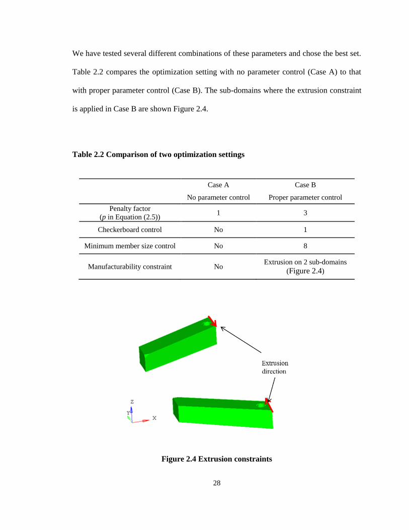
We have tested several different combinations of these parameters and chose the best set.

Table 2.2 compares the optimization setting with no parameter control (Case A) to that

with proper parameter control (Case B). The sub-domains where the extrusion constraint

is applied in Case B are shown Figure 2.4.

Table 2.2 Comparison of two optimization settings

Case A Case B

No parameter control Proper parameter control

Penalty factor

(p in Equation (2.5)) 1 3

Checkerboard control No 1

Minimum member size control No 8

Manufacturability constraint No Extrusion on 2 sub-domains

(Figure 2.4)

Figure 2.4 Extrusion constraints

29

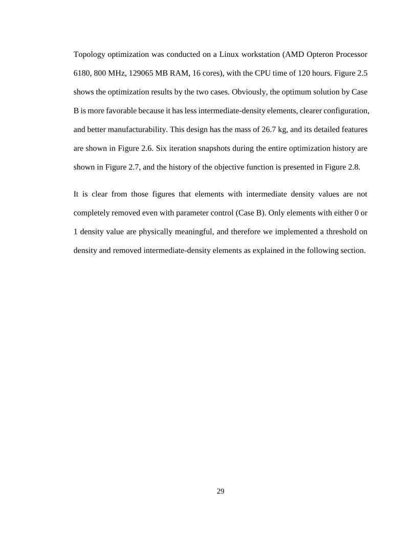
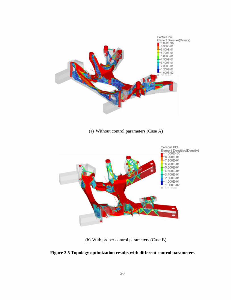
Topology optimization was conducted on a Linux workstation (AMD Opteron Processor

6180, 800 MHz, 129065 MB RAM, 16 cores), with the CPU time of 120 hours. Figure 2.5

shows the optimization results by the two cases. Obviously, the optimum solution by Case

B is more favorable because it has less intermediate-density elements, clearer configuration,

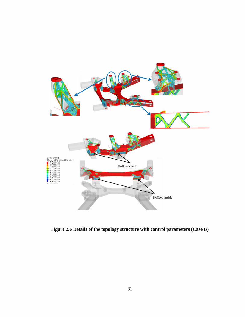
and better manufacturability. This design has the mass of 26.7 kg, and its detailed features

are shown in Figure 2.6. Six iteration snapshots during the entire optimization history are

shown in Figure 2.7, and the history of the objective function is presented in Figure 2.8.

It is clear from those figures that elements with intermediate density values are not

completely removed even with parameter control (Case B). Only elements with either 0 or

1 density value are physically meaningful, and therefore we implemented a threshold on

density and removed intermediate-density elements as explained in the following section.

30

(a) Without control parameters (Case A)

(b) With proper control parameters (Case B)

Figure 2.5 Topology optimization results with different control parameters

31

Figure 2.6 Details of the topology structure with control parameters (Case B)

32

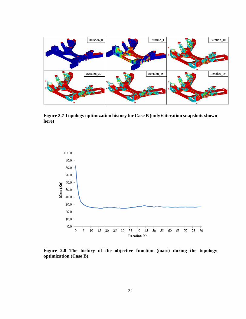
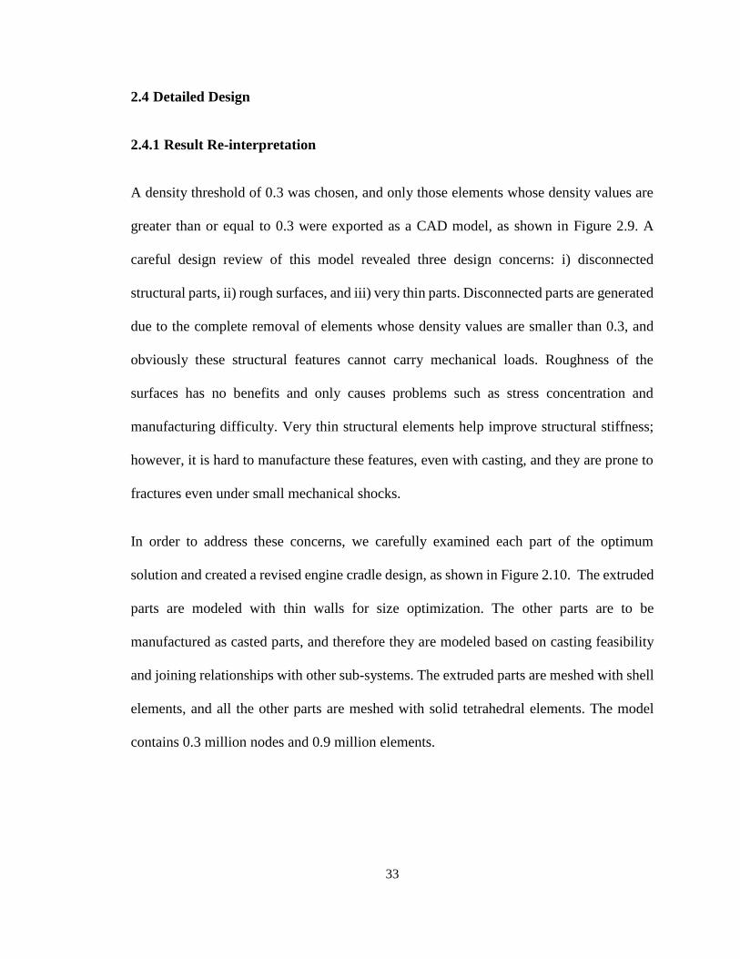
Figure 2.7 Topology optimization history for Case B (only 6 iteration snapshots shown

here)

Figure 2.8 The history of the objective function (mass) during the topology

optimization (Case B)

33

2.4 Detailed Design

2.4.1 Result Re-interpretation

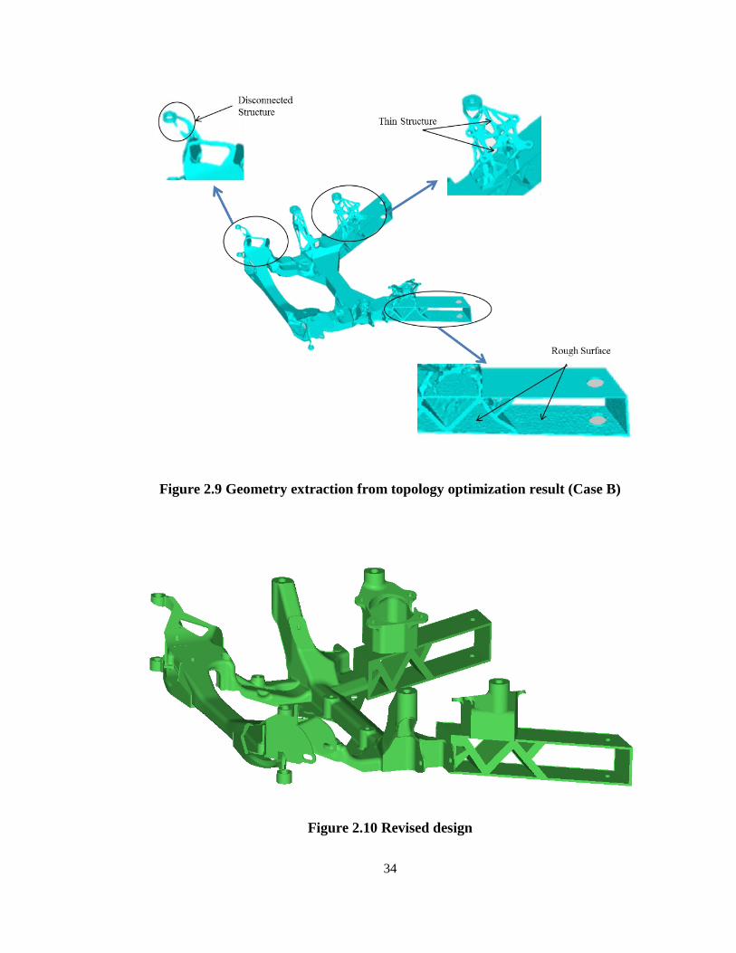
A density threshold of 0.3 was chosen, and only those elements whose density values are

greater than or equal to 0.3 were exported as a CAD model, as shown in Figure 2.9. A

careful design review of this model revealed three design concerns: i) disconnected

structural parts, ii) rough surfaces, and iii) very thin parts. Disconnected parts are generated

due to the complete removal of elements whose density values are smaller than 0.3, and

obviously these structural features cannot carry mechanical loads. Roughness of the

surfaces has no benefits and only causes problems such as stress concentration and

manufacturing difficulty. Very thin structural elements help improve structural stiffness;

however, it is hard to manufacture these features, even with casting, and they are prone to

fractures even under small mechanical shocks.

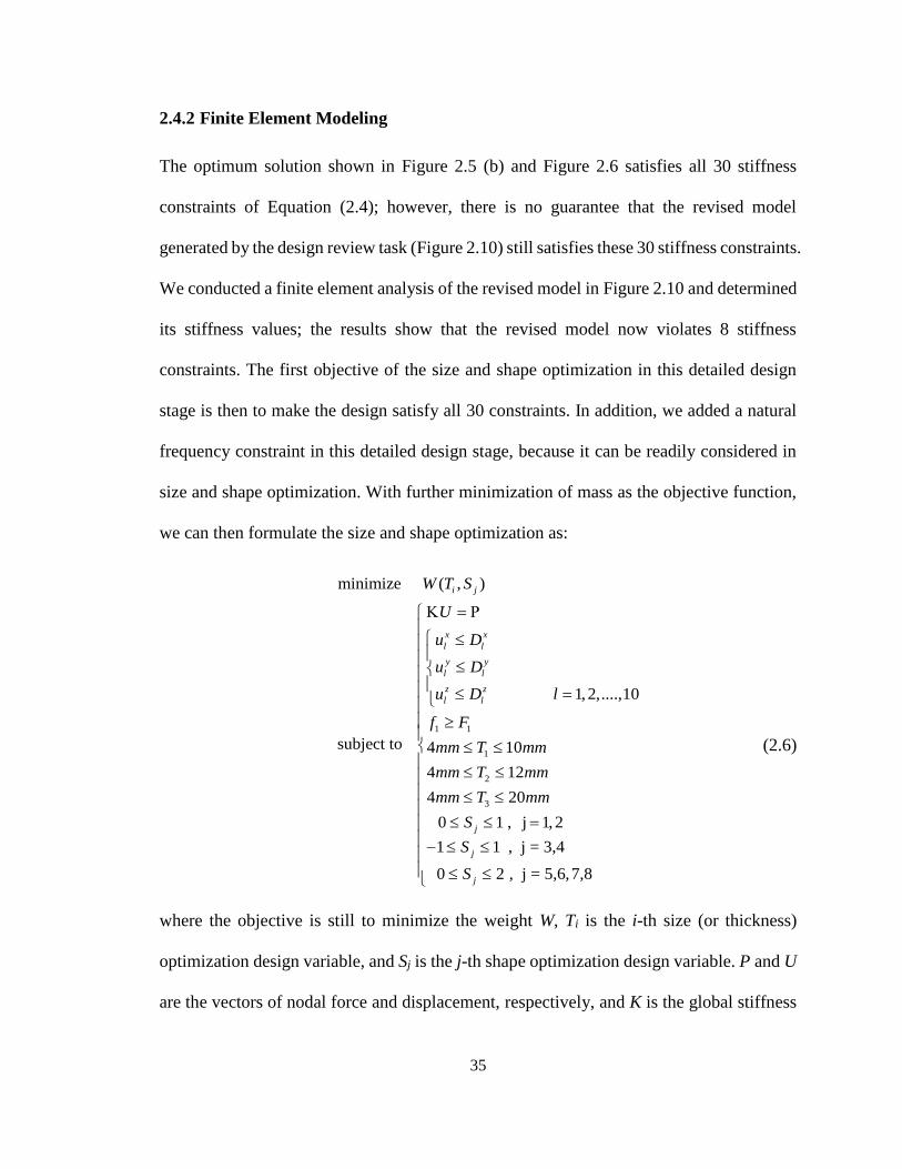
In order to address these concerns, we carefully examined each part of the optimum

solution and created a revised engine cradle design, as shown in Figure 2.10. The extruded

parts are modeled with thin walls for size optimization. The other parts are to be

manufactured as casted parts, and therefore they are modeled based on casting feasibility

and joining relationships with other sub-systems. The extruded parts are meshed with shell

elements, and all the other parts are meshed with solid tetrahedral elements. The model

contains 0.3 million nodes and 0.9 million elements.

34

Figure 2.9 Geometry extraction from topology optimization result (Case B)

Figure 2.10 Revised design

35

2.4.2 Finite Element Modeling

The optimum solution shown in Figure 2.5 (b) and Figure 2.6 satisfies all 30 stiffness

constraints of Equation (2.4); however, there is no guarantee that the revised model

generated by the design review task (Figure 2.10) still satisfies these 30 stiffness constraints.

We conducted a finite element analysis of the revised model in Figure 2.10 and determined

its stiffness values; the results show that the revised model now violates 8 stiffness

constraints. The first objective of the size and shape optimization in this detailed design

stage is then to make the design satisfy all 30 constraints. In addition, we added a natural

frequency constraint in this detailed design stage, because it can be readily considered in

size and shape optimization. With further minimization of mass as the objective function,

we can then formulate the size and shape optimization as:

1 1

1

2

3

minimize ( , )

1, 2,....,10

subject to 4 10

4 12

4 20

0 1 , j 1, 2

1 1 , j = 3,4

0 2 , j = 5,6,7,8

i j

x x

l l

y y

l l

z z

l l

j

j

j

W T S

U

u D

u D

u D l

f F

mm T mm

mm T mm

mm T mm

S

S

S

(2.6)

where the objective is still to minimize the weight W, Ti is the i-th size (or thickness)

optimization design variable, and Sj is the j-th shape optimization design variable. P and U

are the vectors of nodal force and displacement, respectively, and K is the global stiffness

36

matrix. x

lu , y

lu andz

lu denote the x-, y- and z-directional displacements of the l-th loading

point, respectively. x

lD , y

lD and z

lD are the corresponding upper bounds for those

displacements. The total number of loading points is 10 in this study. 1f indicates the first

natural frequency of the system, and 1F is the lower bound for the first natural frequency,

which is equal to 210 Hz in this study.

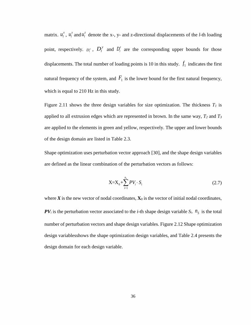
Figure 2.11 shows the three design variables for size optimization. The thickness T1 is

applied to all extrusion edges which are represented in brown. In the same way, T2 and T3

are applied to the elements in green and yellow, respectively. The upper and lower bounds

of the design domain are listed in Table 2.3.

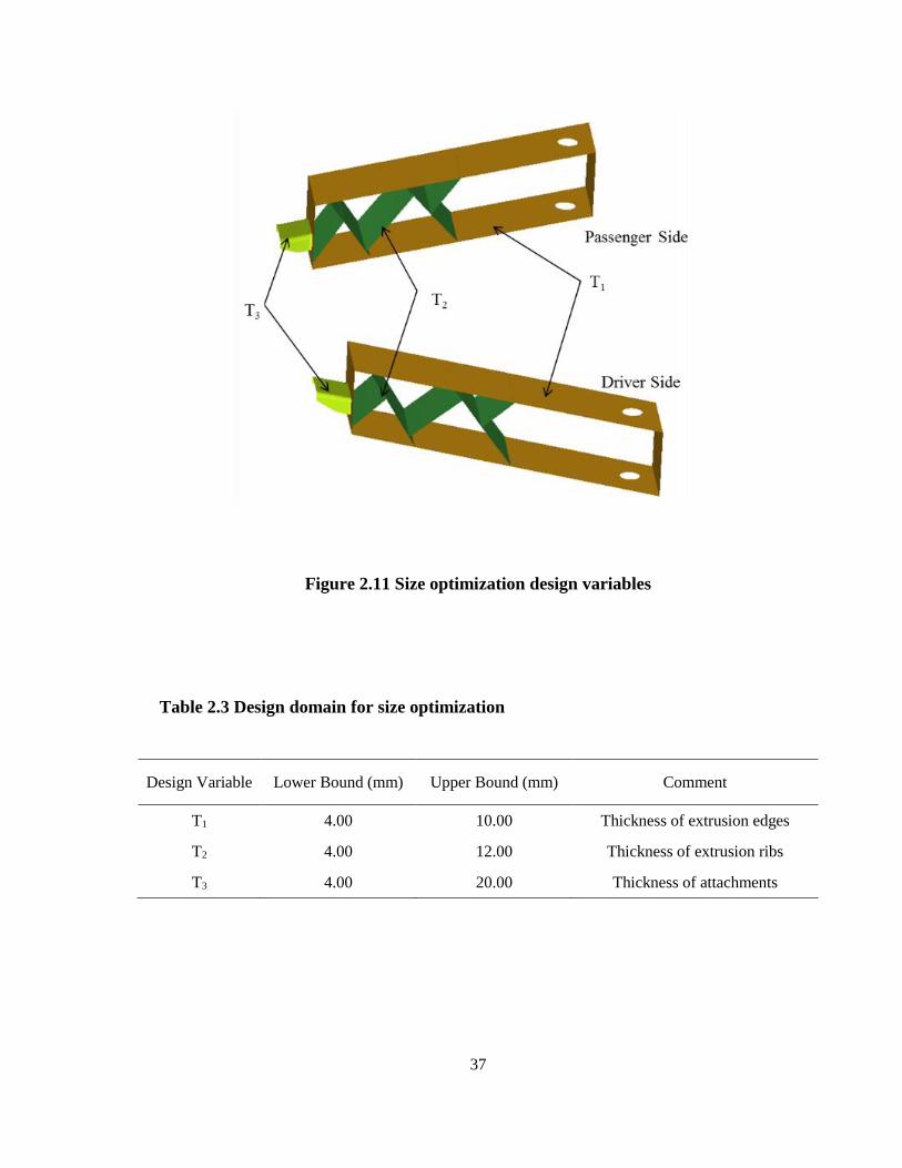
Shape optimization uses perturbation vector approach [30], and the shape design variables

are defined as the linear combination of the perturbation vectors as follows:

0

i=1

X=X +sn

i iPV S (2.7)

where X is the new vector of nodal coordinates, X0 is the vector of initial nodal coordinates,

PVi is the perturbation vector associated to the i-th shape design variable Si. Sn is the total

number of perturbation vectors and shape design variables. Figure 2.12 Shape optimization

design variablesshows the shape optimization design variables, and Table 2.4 presents the

design domain for each design variable.

37

Figure 2.11 Size optimization design variables

Table 2.3 Design domain for size optimization

Design Variable Lower Bound (mm) Upper Bound (mm) Comment

T1 4.00 10.00 Thickness of extrusion edges

T2 4.00 12.00 Thickness of extrusion ribs

T3 4.00 20.00 Thickness of attachments

38

Figure 2.12 Shape optimization design variables

Table 2.4 Design domain for shape optimization

Design Variable Lower Bound Upper Bound Perturbation Vector (mm)

S1 0.00 1.00 3.00

S2 0.00 1.00 3.00

S3 -1.00 1.00 5.00

S4 -1.00 1.00 5.00

S5 0.00 2.00 5.00

S6 0.00 2.00 5.00

S7 0.00 2.00 5.00

S8 0.00 2.00 5.00

39

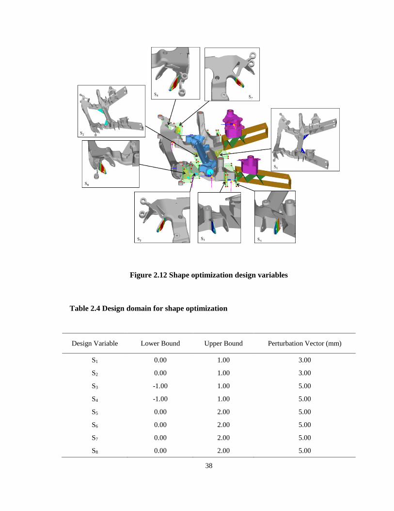
2.4.3 Shape and Size Optimization and Numerical Results

The objective of the shape and size optimization is to fine tune the local structure to further

minimize the weight while satisfying all 30 stiffness constraints and the first natural

frequency requirement. Size and shape optimization was conducted on Windows PC

(AMD Phenom II x6 1090T Processor, 3200MHz, 7392 MB RAM, 6 cores). After 6

iterations with the CPU time of about 1.5 hours, the optimization converged with all

constraints satisfied. The final mass of the engine cradle was 21.4 kg. The optimum values

of the design variables are listed in Table 2.5.

Table 2.5 Optimal design variables

Design Variable Optimal Values

T1 (mm) 10.00

T2 (mm) 11.20

T3 (mm) 17.92

S1 1.00

S2 0.00

S3 -1.00

S4 -1.00

S5 2.00

S6 2.00

S7 2.00

S8 2.00

40

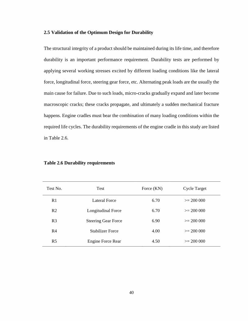
2.5 Validation of the Optimum Design for Durability

The structural integrity of a product should be maintained during its life time, and therefore

durability is an important performance requirement. Durability tests are performed by

applying several working stresses excited by different loading conditions like the lateral

force, longitudinal force, steering gear force, etc. Alternating peak loads are the usually the

main cause for failure. Due to such loads, micro-cracks gradually expand and later become

macroscopic cracks; these cracks propagate, and ultimately a sudden mechanical fracture

happens. Engine cradles must bear the combination of many loading conditions within the

required life cycles. The durability requirements of the engine cradle in this study are listed

in Table 2.6.

Table 2.6 Durability requirements

Test No. Test Force (KN) Cycle Target

R1 Lateral Force 6.70 >= 200 000

R2 Longitudinal Force 6.70 >= 200 000

R3 Steering Gear Force 6.90 >= 200 000

R4 Stabilizer Force 4.00 >= 200 000

R5 Engine Force Rear 4.50 >= 200 000

41

The cycle targets exceed 104 times, and this problem can be explained by high cycle fatigue

[31]. The Stress-Life (S-N) approach is frequently used, but this approach only focuses on

the cyclical stresses that are predominantly within the elastic range. There is a possibility

that the engine cradle is damaged with a plastic strain, which can then cause failure less

than 104 cycles. Hence, we chose the Strain-Life (E-N) approach which can deal with

plastic deformations occurring under the given cyclic loading.

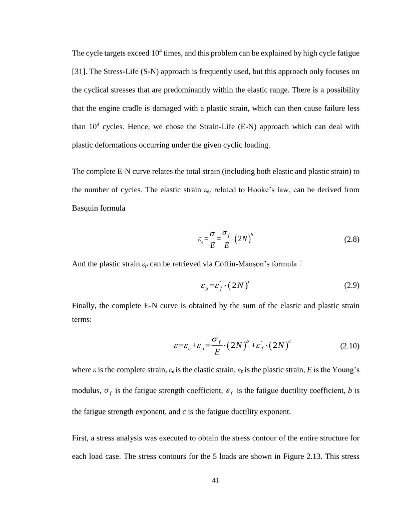
The complete E-N curve relates the total strain (including both elastic and plastic strain) to

the number of cycles. The elastic strain εe, related to Hooke’s law, can be derived from

Basquin formula

'

= = 2bf

e NE E

(2.8)

And the plastic strain εp can be retrieved via Coffin-Manson’s formula：

'

p = 2c

f N (2.9)

Finally, the complete E-N curve is obtained by the sum of the elastic and plastic strain

terms:

'

'

p= + = 2 + 2b cf

e fN NE

(2.10)

where ε is the complete strain, εe is the elastic strain, εp is the plastic strain, E is the Young’s

modulus, '

f is the fatigue strength coefficient, '

f is the fatigue ductility coefficient, b is

the fatigue strength exponent, and c is the fatigue ductility exponent.

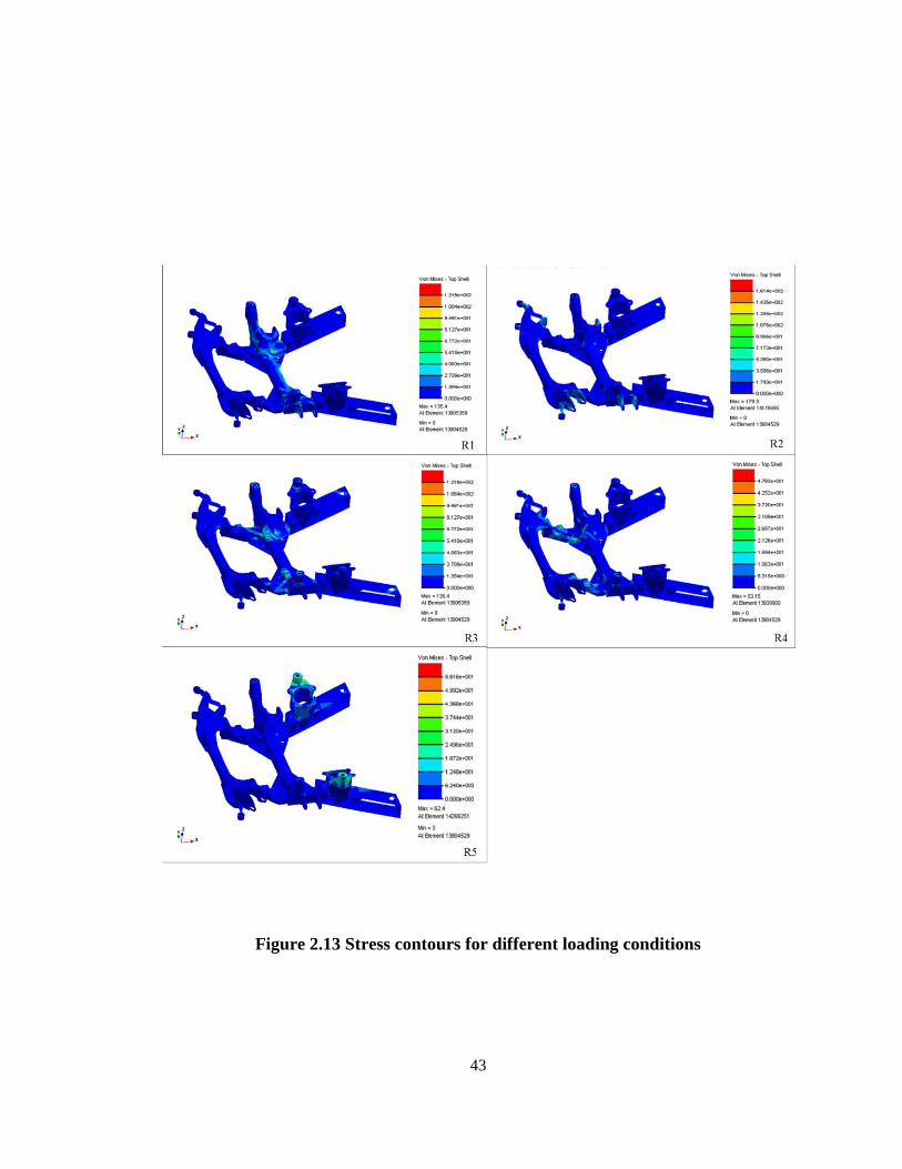
First, a stress analysis was executed to obtain the stress contour of the entire structure for

each load case. The stress contours for the 5 loads are shown in Figure 2.13. This stress

42

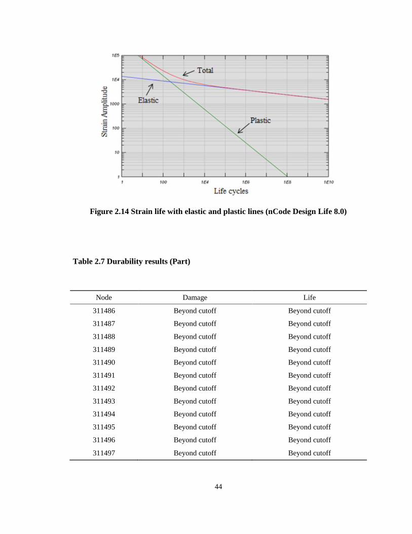
information was then utilized in the durability analysis which was implemented in nCode

Design Life 8.0 [32]. The E-N curve for the material is displayed in Figure 2.14. The cycle

numbers for all nodes in the structure were beyond “cutoff” (or minimum cycle limit), and

part of the results are shown in Table 2.7 as sample results. Thus, the current model

successfully passed the durability validation.

43

Figure 2.13 Stress contours for different loading conditions

44

Figure 2.14 Strain life with elastic and plastic lines (nCode Design Life 8.0)

Table 2.7 Durability results (Part)

Node Damage Life

311486 Beyond cutoff Beyond cutoff












45

It should be noted that our optimum design “passed” the durability test at once; however,

it is possible that in other applications the optimum design created by topology, shape and

size optimization does not meet the durability criteria. In this case, shape and size

optimization with the fatigue life as an inequality constraint should be run by considering

the overall shape change and local shape change (e.g. fillet radius). Generally, topology

optimization is ill-equipped for fatigue criteria because fatigue failures are heavily affected

by local shapes.

It is also meaningful to point out that there are other factors that affect fatigue life such as

manufacturing and machining operations, welding quality, surface treatment, surface

roughness, temperature, and corrosion. We do not have numerical methods that accurately

consider all these factors. Hence it is required to conduct experimental validation tests of

fatigue before proceeding to mass production.

2.6 Conclusions

This chapter presented an effective and efficient design process framework for automotive

engine cradles from conceptual design to detailed design by using design optimization.

Figure 2.15 shows the progress of design optimization tasks through the entire design

process. The initial design domain had the mass of 82.6 kg; topology optimization in

conceptual design produced an optimum design with the mass of 26.7 kg; and the detailed

design task involved shape and size optimization and further reduced the mass to 21.4 kg.

The topology optimization considered 30 stiffness constraints, and the size and shape

optimization implemented the same 30 stiffness constraints and an additional first natural

46

frequency constraint. As the last task, it was confirmed that the final optimum design

satisfies all durability constraints.

We solved the optimization problem in Equation (2.1) over two stages: topology

optimization and then shape and size optimization. The result is more than just finding a

“better” solution than the original design. We solved a practical, real-world optimization

problem in this chapter, and we are unable to discuss global optimality of our solution,

which will require the discussion of convexity (or all possible local minima) of the design

space and the satisfaction of KKT (Karush–Kuhn–Tucker) conditions. However, we

utilized state-of-the-art optimization methods and tools and ensured all convergence

criteria are properly met, and therefore it can be stated that our solution is one of the best

practical optimum designs that satisfy Equation (2.1).

The benefits of the proposed design process also include a shortened design cycle. Our

industrial partner, Van-Rob Inc., stated that the period of designing an automotive engine

cradle to the first-round technical review typically takes 10-12 weeks; however, by

introducing topology optimization, the period has been shortened to 5 weeks, which is a

massive time saving for product development in the fiercely competitive auto industry.

Further, compared to the traditional trial-and-error method, the geometrical configuration

of the lightweight design derived from topology optimization is more objective, reliable,

and economic. It was also a valuable experience for the designers to interpret the topology

optimization result and create a revised model which addresses all concerns of the “raw”

result from topology optimization. It should be noted that the methodology is not

47

constrained only for engine cradle development, but it can be extended to the design of

other products such as body-in-white structures, cross car beams, or control arms.

2.7 Limitation

In our research, we did not consider crashworthiness although it is one of the ultimate

performance criteria for automakers. There are two main challenges for crashworthiness

from the view point of design optimization of a component. First, crash safety regulations

are generally imposed onto the entire vehicle, except for bumper components. The problem

here is that it is hard to calculate crashworthiness of an entire vehicle based on

crashworthiness of separate components, because there are strong interactions among

components, sub-assemblies, and assemblies. A supplier can consider the behavior of a

particular component (in this research, engine cradle), but cannot consider interaction with

other components.

It should be noted that we did not make any assumption or approximation in the definition

of the loads. Our analysis and optimization was performed in collaboration with a Tier-I

supplier, who does the actual design work based on explicit requirements from its customer

(i.e. an OEM). The OEM as the customer gave the loading conditions to its supplier, and

once a final design is submitted to the OEM, it will perform crash analysis considering the

engine cradle and other components which are developed by many other suppliers.

Second, crash simulations have very high computing expense and the numerical analysis

is highly nonlinear. Therefore, it is not yet practical to include crashworthiness of an entire

vehicle in an optimization loop, which will require tens or hundreds of crash analyses.

Some techniques, such as the equivalent static load method (ESLM), make approximation

48

of crash behavior, and allow for the inclusion of some simplified crash behavior in an

optimization. Topology optimization for some crashworthiness studies have been seen

nowadays by using LS-TaSC and Genesis/ESLM together, and it is one of our future

directions. Once again, the Tier-I supplier is not required to consider crashworthiness,

because crash analyses will be done by an OEM considering many components from many

different suppliers. However, it would be advantageous for the supplier if it could consider

crashworthiness in its product development.

The objective of this chapter was to consider important performance metrics of an engine

cradle for a Tier-I supplier who actually design and manufacture the product. Hence,

crashworthiness was not considered in the current research, but left as future work which

will be conducted in collaboration with the OEM. Although it would be infeasible to

include crashworthiness of an entire vehicle in a design optimization loop, we would be

able to gain some meaningful insights by means of multiple crash simulations, and the

results will be incorporated back into our engine cradle design.

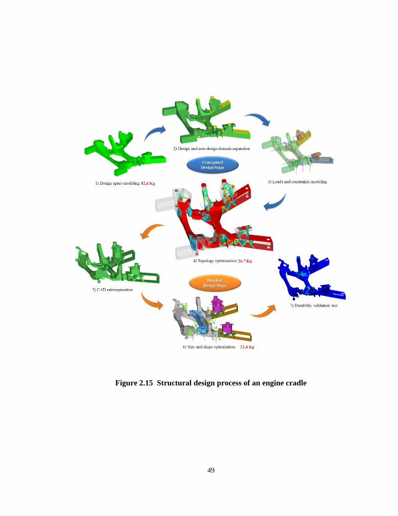
49

Figure 2.15 Structural design process of an engine cradle

50

ACKNOWLEDGMENT

The authors would like to express their thanks to the group of CAD & CAE department

and the members of Research & Development department from Van-Rob Inc. Their

suggestions are acknowledged and much appreciated.

REFERENCES

[1] Woisetschlaeger, E., Keine Monokultur. Automobile Entwicklung, 2001, pp. 130

[2] Wallentowitz H., Structural Design of Vehicles. Institute fur Kraftfahrwesen, Aachen,

2004

[3] Triantos D. and Michaels M., Design and Fabrication of an Aluminium Engine

Cradle for a General Motors Vehicle. SAE Technical Paper, 1999-01-0659

[4] Chen X. M., Mahmood H., Wagner, D. A., and Baccouche, M. R., Aluminium

Subframe Design for Crash Energy Management. SAE Technical Paper. 2004-01-

1775

[5] Kang J. Y., Choi B. I., Lee H. J., Kim J. S. and Kim K. J., Neural Network

Application in Fatigue Damage Analysis under Multiaxial Random Loadings.

International Journal of Fatigue, 2006; 28: pp. 132-140.

DOI:10.1016/j.ijfatigue.2005.04.012

[6] Kim K. J., Kim J. S., Choi, B. I., Kim K. H., Choi H. H., Kim C. W., Kang K.W.,

Song J. H., and Sung C.W., Development of Automotive Engine Cradle by

Hydroforming Process. Journal of Mechanical Science and Technology, 2007; 21:

pp. 1523-1527

[7] Kim B. S., Spiryagin M., Kim B. S. and Yoo H. H., Analysis of the Effects of Main

Design Parameters Variation on the Vibration Characteristics of a Vehicle Sub-

Frame. Journal of Mechanical Science and Technology, 2009; 23: pp. 960-963. DOI:

10.1007/s12206-009-0321-8

[8] Xu J. T., Song Y. D., Ding J. B. and Ding S. Q., Analysis of a Front Sub-Frame

Fatigue Strength Based on Miner Theory. 2010 International Conference on

51

Computer Application and System Modelling, 2010; pp. 191-193. DOI:

10.1109/ICCASM.2010.5623056

[9] Bendsøe M. P. and Sigmund O., Topology Optimization: Theory, Methods and

Applications. Springer, 2003

[10] Kim I. L. and Kwak B. M., Design Space Optimization Using a Numerical Design

Continuation Method, International Journal for Numerical Methods in Engineering,

2002; 53(8): pp. 1979-2002. DOI: 10.1002/nme.369

[11] Kim I. L. and Weck O. D., Variable Chromosome Length Genetic Algorithm for

Progressive Refinement in Topology Optimization. Struct. Multidiscip. Optim. 2005;

29: pp. 445-456. DOI: 10.1007/s00158-004-0498-5

[12] Kim S. Y., Kim I. L., and Mechefske C., A New Efficient Convergence Criterion for

Reducing Computational Expense in Topology Optimization: Reducible Design

Variable Method. International Journal for Numerical Methods in Engineering,

2012; 90(6), 752-783.

[13] Forsberg J. and Nilsson L.,Topology Optimization in Crashworthiness Design. Struct.

Multidiscp. Optim., 2007; 33: pp. 1-12. DOI: 10.1007/s00158-006-0040-z

[14] Jang I. G., Kim I. L., and Kwak B. M., Analogy of Strain Energy Density Based

Bone Remodeling Algorithm and Structural Topology Optimization. ASME Journal

of Biomechanical Engineering, 2009; 131(1), Article 011012.

DOI: 10.1115/1.3005202

[15] Boyle C. and Kim I. L., Three-dimensional Micro-level Computational Study of

Wolff’s law via Trabecular Bone Remodeling in the Human Proximal Femur Using

Design Space Topology Optimization. Journal of Biomechanics, 2011; 44: pp. 935–

942. DOI:10.1016/j.jbiomech.2010.11.029

[16] Lee H. A. and Park G. J., Topology Optimization for Structures with Nonlinear

Behaviour Using the Equivalent Static Loads Method. Journal of Mechanical Design,

2012; 134: pp. 031004-1-14

[17] Yang, R. J. and Chahande A. I., Automotive Applications of Topology Optimization.

Structural Optimization, 1995; 9, pp. 245-249. DOI: 10.1007/BF01743977

[18] Lee D. C. and Lee J. I., Structural Optimization Concept for the Design of an

Aluminium Control Arm. Proceedings of the Institution of Mechanical Engineers,

Part D: Journal of Automobile Engineering, 2003; 217(8): pp. 647-656.

DOI: 10.1243/09544070360692041

[19] Lee K. H., Shin J. K., Song S. I., Yoo Y. M., and Park G. J., Automotive Door Design

Using Structural Optimization and Design Of Experiments. Proceedings of the

http://dx.doi.org/10.1109/ICCASM.2010.5623056


52

Institution of Mechanical Engineers, Part D: Journal of Automobile Engineering,

2003; 217(10), pp. 855-865. DOI: 10.1243/095440703769683261

[20] Chiandussi G., Gaviglio I., and Ibba A., Topology Optimization of an Automotive

Component without Final Volume Constraint Specification. Advances in

Engineering Software, 2004; 35, pp. 609-617. DOI:

10.1016/j.advengsoft.2003.07.002

[21] Wang L. S., Basu P. K., and Leiva J. P., Automobile Body Reinforcement by Finite

Element Optimization. Finite Elements in Analysis and Design, 2004; 40, pp. 879-

893. DOI: 10.1016/S0168-874X(03)00118-5

[22] Torstenfelt B. and Klarbring A., Conceptual Optimal Design of Modular Car Product

Families Using Simultaneous Size, Shape and Topology Optimization. Finite

Elements in Analysis and Design, 2001; 43, pp. 1050-1061. DOI:

10.1016/j.finel.2007.06.005

[23] Waquas S., Fan Y. Q., and Wang Y. Q., Application of Topology Optimization and

Manufacturing Simulations – A New Trend in Design of Aircraft Components.

Proceedings of the International MultiConference of Engineers and Computer

Scientists, 2008; 2, pp. 19-21. ISBN: 978-988-17012-1-3

[24] Cavazzuti M., Baldini A., Bertocchi E., Costi D., Torricelli E., and Moruzzi P., High

Performance Automotive Chassis Design: a Topology Optimization Based Approach.

Struct. Multidisc. Optim., 2011; 44, pp. 45-56. DOI: 10.1007/s00158-010-0578-7

[25] Lee S. J., Lee H. A., Yi S. I., Kim D. S., Yang H. W., and Park G. J., Design Flow

for the Crash Box in a Vehicle to Maximize Energy Absorption. Proceedings of the

Institution of Mechanical Engineers, Part D: Journal of Automobile Engineering,

2013; 227(2), pp. 179-200. DOI: 10.1177/0954407012451545

[26] Luo Y. T. and Di T., Lightweight Design of an In-Wheel Motor Using the Hybrid

Optimization Method. Proceedings of the Institution of Mechanical Engineers, Part

D: Journal of Automobile Engineering, 2013; pp. 179-200. DOI:

10.1177/0954407013497194

[27] Stolpe M., and Svanberg K., An alternative interpolation scheme for minimum

compliance topology optimization. Struct. Multidisc. Optim., 2001; 22(2): 116-124.

DOI: 10.1007/s001580100129

[28] Altair OptiStruct 11.0 User Manual. Altair Engineering, 2001, Inc, Troy, MI

[29] Zhou M., Shyy Y. K. and Thomas H. L., Checkerboard and Minimum Member Size

Control in Topology Optimization. Struct. Multidisc. Optim., 2001; 21, pp. 152-158

53

[30] Samareh J. A., A survey of shape parameterization techniques. CEAS AIAA ICASE

NASA Langley International Forum on Aeroelasticity and Atructural Dynamics,

1999; pp. 333-343

[31] Hosford W. F., Mechanical Behavior of Materials. Cambrige University Press, 2005;

pp. 292

[32] HBM nNode, nNode Design Life 8.0 User Manual. HBM, 2011; Inc, Southfield, MI

54

Chapter 3

Topology, Shape, and Size Optimization of an Automotive Cross Car

Beam

An automotive cross car beam (CCB) supports instrument panels including the HVAC

(heating, ventilation, and air conditioning) system, knee airbags, steering column and

steering wheel system (SCSWS), and the central console. Avoiding resonant frequencies

and improving driving comfort is a major performance requirement in the design of a CCB.

Due to the nature of mass production in the automotive industry, the consideration of

manufacturability is important, and the current practice in the industry does grant detailed

information on the SCSWS to the CCB designer. The objective of this chapter is to perform

a complete topology, shape, and size optimization of a CCB by using a lightweight

material, considering two practical manufacturing processes (extrusion and casting), and

assuming the realistic situation where only limited information on the SCSWS is available

to the CCB designer. First, a simplified finite element (FE) model of the SCSWS was

developed, and it was calibrated using optimization such that important behavior of the

simplified FE model agrees with that of the real SCSWS. Topology optimization was

performed to determine the optimal material distribution for the parts that connect the

SCSWS and CCB. Then a geometry reinterpretation of the favorable topology result was

performed to address the concerns from the viewpoint of cost and manufacturability. A

sensitivity study was conducted subsequently to determine size optimization design

variables with significant effect on frequency performance. Finally, size and shape

55

optimization were performed together to further optimize the details of the CCB structure.

The weight of the optimal aluminum design was reduced by nearly 40% compared to the

steel design while the important performance requirements are met.

3.1 Introduction

Government regulations have become more and more stringent in the automotive industry

especially on fuel efficiency and carbon emissions. For example, the US regulation, the

Corporate Average Fuel Economy (CAFE), requires an automaker increase its corporate

average fuel efficiency to 54.5 miles per gallon (MPG) for passenger cars and light-duty

trucks by Model Year 2025. It is nearly as twice the fuel economy of the future vehicles as

that of 2012. It has been proved that with every 100kg weight reduction, the consumption

of fuel will be decreased by approximately 0.4 liters per 100 km [1] and the emissions of

CO2 will be reduced by 8g to 11g per kilometer [2]. Therefore, the lightweight design of

automobile is an efficient and immediate way to improve the fuel efficiency and reduce

CO2 emissions.

Currently, automotive lightweight strategies can be categorized into three approaches: 1)

Lightweight Material: the traditional low carbon steels can be replaced by high specific

strength materials or lighter materials, such as high strength steel, aluminum, magnesium,

and reinforced plastic composites. 2) Advanced Manufacturing: advanced manufacturing

and production processes are developed to reduce the weight of automobile. For example,

using structural adhesives will reduce the weight of joints, and to replace MIG welding

with laser welding could avoid introducing extra material of solders. 3) Design

Optimization: design optimization techniques can be used to minimize the material usage

56

without sacrificing performance requirements. For example, optimum designs of tailored-

welded-blanks and tailored-rolled-tubes can be determined by size optimization.

The process of a product design should be logical, effective, and efficient. Figure 3.1 [3]

gives an example of the entire structural design process of an automotive engine cradle.

The design process starts with a design space which encloses the possible design domain.

Design and non-design areas are intentionally separated considering the joining or

manufacturing requirements. Finite element (FE) modeling is performed to discretize the

continuous geometry and define loads and constraint conditions. Topology optimization is

then conducted to obtain the optimal material distribution. CAD re-interpretation is

executed next to generate a new geometry based on topology optimization results,

considering manufacturability and tooling costs. Size and shape optimization is used to fine

tune the local geometry. Finally, necessary performance tests are conducted to validate the

final optimal design.

Even using the most efficient optimization methods, however, weight saving is not large

enough if only pure steel is used, because of the ever stringent weight reduction

requirements. It has therefore become an inevitable strategy that lightweight materials such

as aluminum or magnesium are used more, despite their high costs. Reference [4] gave a

direct cost of weight savings as aluminum and advanced high strength steel (AHSS) added

to a pickup truck and as more aluminum is applied, the cost will increase rather nonlinearly.

Another important aspect is that as the use of multiple materials increases, the complexity

of the design increases, and it becomes more difficult to determine optimum designs.

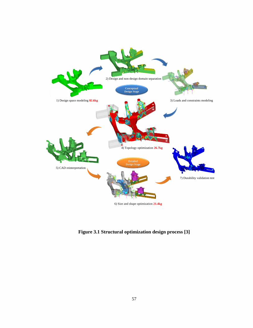
57

Conceptual

Design Stage

Detailed

Design Stage

1) Design space modeling 82.6kg

2) Design and non-design domain separation

3) Loads and constraints modeling

4) Topology optimization 26.7kg

5) CAD reinterpretation

6) Size and shape optimization 21.4kg

7) Durability validation test

Figure 3.1 Structural optimization design process [3]

58

A CCB functions as a structural support that holds all functional components housed in the

cockpit area, including the electronic parts (such as the HVAC system and the central

console) and safety parts (such as the knee bolsters and the airbags). In particular, the

SCSWS is mounted onto the CCB structure. If the natural frequency of the SCSWS / CCB

overlaps with the excited frequency coming from the engine, transmission, or other

sources, resonance will happen; this would cause discomfort to the driver because of high-

amplitude vibrations transmitting through the steering column to the steering wheel. An

important performance requirement for the CCB system is hence to maintain the first

vertical and first lateral natural frequencies above prescribed target values such that

resonance will not happen.

A CCB is a standard part to be equipped in a vehicle. The production of vehicles is

gradually increasing except during the economic recession period from 2008 to 2009.

Figure 3.2 shows the production of vehicles from 2001 to 2012 and the total number of

productions has passed 80 millions in 2012. The production statistics is referred to

‘Organisation Internationale des Constructeurs d’Automobiles’ (OICA) [5]. Due to the

nature of mass production in the automotive industry, every penny saved in cost will make

a considerable profit and every pound reduced in weight will have a significant contribution

in improving fuel efficiency and reducing carbon emissions of the entire fleet of cars.

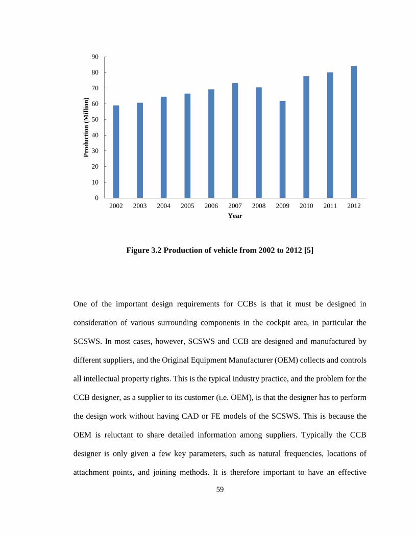
59

Figure 3.2 Production of vehicle from 2002 to 2012 [5]

One of the important design requirements for CCBs is that it must be designed in

consideration of various surrounding components in the cockpit area, in particular the

SCSWS. In most cases, however, SCSWS and CCB are designed and manufactured by

different suppliers, and the Original Equipment Manufacturer (OEM) collects and controls

all intellectual property rights. This is the typical industry practice, and the problem for the

CCB designer, as a supplier to its customer (i.e. OEM), is that the designer has to perform

the design work without having CAD or FE models of the SCSWS. This is because the

OEM is reluctant to share detailed information among suppliers. Typically the CCB

designer is only given a few key parameters, such as natural frequencies, locations of

attachment points, and joining methods. It is therefore important to have an effective

0

10

20

30

40

50

60

70

80

90

2002 2003 2004 2005 2006 2007 2008 2009 2010 2011 2012

Pro

du

ctio

n (

Mil

lio

n)

Year

60

method that allows the CCB designer to produce optimum designs when only limited

information on SCSWS is available. This chapter discusses a method to tackle this problem

in Section 3.2.

There is no universal principle to design an automotive part in a ‘most economic’ way. The

usual practice in the automotive industry depends on the knowledge and experience of

designers. Numerous trial-and-errors are performed to seek to find a ‘favorable’ design,

rather than the ‘optimum’ design, which meets the performance requirements. One of the

most evident drawbacks is that a considerable amount of time and cost are consumed by

the numerous re-designs and re-analyses. Therefore, structural optimization techniques

have been seen to be applied in the automotive design stage. Yildiz [6] developed a new

optimization approach based on Taguchi’s robust design approach and particle swarm

optimization algorithm and applied it to optimum design of a vehicle part. Yildiz and

Solanki [7] developed a new particle swarm-based optimization method to apply to multi-

objective crashworthiness optimization of a vehicle and demonstrated its effectiveness and

validity. Yildiz [8-10] utilized other heuristic optimization methods like genetic algorithm

or immune algorithm to apply onto the design of vehicle components. Durgun and Yildiz

[11] used Cuckoo search algorithm to perform the structural design optimization of vehicle

components. Craig et al. [12] created a response surface based screening method to

optimize the crashworthiness of an automobile body structure. Sinha [13] conducted

reliability-based multi-objective optimization on the vehicle structural crashworthiness

design considering occupant safety with the weight and the front door velocity as the

objectives. Jansson et al. [14] utilized the response surface methodology and space

mapping technique to optimize the draw-in for an automotive sheet metal part. Yim et al.

61

[15] constructed approximate functions to optimize the sections properties of a thin wall

beam including the area, the area moment of inertia and torsional constant. Baskar et al.

[16] used Taguchi method to optimize an automotive door hinge system to improve the

robustness of the vertical rigidity. Kim and Park [17] developed equivalent static loads

method to consider nonlinear dynamic loads at each time step with the generation of the

same response field. The method was applied to crashworthiness optimization of an

automobile frontal structure under a front impact.

Topology optimization is a powerful tool that determines the optimum design in the

conceptual design stage, and from the holistic view point of design, it produces most

promising designs that can be used as initial designs in subsequent shape and size

optimizations over the design procedure. Topology optimization can help improve the

performance of products and also reduce the design period considerably.

Both the theory and application of topology optimization have been advanced in the past

30 years. It is a very useful tool in finding the optimal material distribution within a given

design space under prescribed loads and boundary conditions. Many researchers and

engineers utilized topology optimization in their work: Yang and Chahande [18] introduced

an in-house topology optimization software, TOP, and used it to optimize a simplified truck

frame, a deck lid, and a space frame structure. Cavazzuti et al. [19] presented a

methodology for automotive chassis design using topology optimization, topometry

optimization, and size optimization. Forsberg and Nilsson [20] developed an internal

energy density method, avoiding the use of sensitivities, to apply topology optimization in

nonlinear problems. Lee and Park [21] developed the equivalent static load method in

62

nonlinear topology optimization. Wang et al. [22] employed topology optimization and size

optimization to improve the overall stiffness of an existing automobile body. Waqas et al.

[23] applied topology optimization to the design of aircraft components. Kim and Kwak

[24] developed a design space optimization method that extends the fixed design domain

problem to an alterable design space by overcoming the numerical discontinuity. Boyle

and Kim [25] compared different prosthesis shapes considering micro-level bone

remodeling and stress shielding criteria using three-dimensional design space topology

optimization. Maute and Frangopol [26] utilized topology optimization to design the

micro-electro-mechanical systems. Kim et al. [27] proposed a numerically efficient and

effective convergence criterion for topology optimization, and Kim et al. [28] applied

topology optimization to vibration problems to maximize damping effect on the structure.

Li and Kim [3] achieved an optimum lightweight design of an engine cradle systematically

and efficiently by using topology, size, and shape optimization. Yildiz and Saitou [29]

developed a topology optimization approach based on genetic algorithm for continuum

structures and applied to multi-component topology optimization of a vehicle floor frame.

Luo and Tan [30] employed size optimization and topology optimization for the in-wheel

motor to decrease the unsprung mass. Kim and Jang [31] performed topology optimization

using GENESIS to obtain the optimum layout of the frame structure of a flatbed trailer and

then utilized Taguchi method to further minimize the mass. Lee and Lee [32] performed

topology optimization on an aluminium control arm of a suspension to get the optimal

layout and utilized shape optimization to tune the details of the geometry. Lee and et al.

[33] achieved a better design of an automotive door in stiffness and natural frequency by

using topology, size and shape optimizations and design of experiments (DOE). Yildiz and

http://www.sciencedirect.com/science/article/pii/S0952197612001200#bib1

http://www.sciencedirect.com/science/article/pii/S0952197612001200#bib1

63

et al. [34] created an initial design concept of an engine mount bracket based on the optimal

structural layout from topology optimization. Yildiz [35] performed topology optimization

to achieve the optimal design of vehicle components. Jiang and et al. [36] obtained a

conceptual and basic design of a Mobile Harbor crane based on topology optimization and

shape optimization. Zhu and et al. [37] performed topology optimization on an assembled

aircraft structure to avoid the failure of the fastener joints. Oktay and et al. [38] utilized

topology optimization to achieve an optimum design of a wing of an unmanned aerial

vehicle under aerodynamic loads. Zhu and et al. [39] improved the stiffness and the

strength of the stretch-forming die through topology optimization under gravity and surface

loads. Bogomolny and Amir [40] achieved an optimal design of a reinforced concrete

structure modeled with elastoplastic material by using topology optimization.

Several optimization studies are identified for the design of a CCB. Hamid [41] minimized

the weight of a CCB under the constraints of the peak force and the intrusion in the side

impact of a car. Lam et al. [42] replaced a steel CCB with an aluminum design, by using

size optimization to satisfy the frequency and crashworthiness performance. Only size

optimization was used in this study, and the thickness of the aluminum structure had to

increase by 40%. Rita [43] discussed important issues in the early phase of a CCB concept

development, including the geometry and material choices, assembly solutions, and safety

regulations. Rahmani [44] utilized the particle swarm optimization (PSO) algorithm to

solve a multidisciplinary optimization problem of an existing aluminum CCB. These

studies introduced topology optimization to the design of a CCB in one way or another and

produced optimum designs; however, the impact is limited because those studies did not

look at the entire design process—including topology, shape, and size optimizations from

64

conceptual design to detailed design—especially when lightweight materials are to be used.

A second important limitation is that manufacturability was not considered in the design

process. For example, extrusion is one of the most favorable manufacturing processes in

the automotive industry because of its low cost in mass production, but none of the studies

considered manufacturing processes, including extrusion. Thirdly, these studies did not

discuss how to perform design optimization without having detailed information on the

SCSWS, which is a typical situation for the actual CCB designer.

The objective of this chapter is to perform a complete topology, shape, and size

optimization of a CCB by using a lightweight material, considering two practical

manufacturing processes, and assuming the realistic situation where only limited

information on the SCSWS is available to the CCB designer. A steel CCB will be

redesigned by using aluminum in order to achieve weight savings, while keeping most of

the original geometries and satisfying the natural frequency performance requirements. In

the preliminary design stage, topology optimization considering manufacturability will be

performed. Two manufacturing process will be compared: extrusion (which has small

design freedom for a low cost) versus casting (which has large design freedom for a high

cost). Based on the evaluation of weight reductions and manufacturability, a most favorable

design will be chosen for the subsequent detailed design stage. A sensitivity study will then

be conducted and most influential design variables will be selected. An advance tailored-

rolled-tube design will be considered, and size optimization and shape optimization will be

conducted to further reduce weight while meeting the performance targets.

65

3.2 Simplification of the Steering Column and Steering Wheel System (SCSWS)

As aforementioned, an OEM typically outsources many parts to various suppliers, and a

supplier typically provides products and services to various OEMs. Because of severe

competition and confidentiality, OEMs are reluctant to share detailed technical information

with their suppliers. A SCSWS is mounted on the CCB, and one of the most important

performance requirements for the CCB is to maintain minimum required natural

frequencies of the “steering column.” It is therefore essential for the CCB designer to be

able to predict the behavior of the SCSWS during the design optimization of the CCB. The

SCSWS is, however, normally designed and built by a different supplier, and its detailed

information (including the FE model) is not passed along to the company that designs the

CCB. This is the first challenge that a CCB designer faces, and this section discusses how

to build an approximate SCSWS model, only based on the available information.

The OEM typically provides the supplier (i.e. CCB designer) with the first natural

frequency (1 ) and second natural frequency (

2 ) of the “actual” SCSWS and its mounting

locations on the CCB. Here, 1 and

2 are associated with the first vertical mode shape

and the first lateral mode shape of the SCSWS, respectively. Note that we intentionally

show only a generic representation 1 and

2 in this chapter, instead of their actual

numerical values, due to confidentiality. In all actual analysis and optimization, however,

the actual numerical values were used.

We built a simplified FE model of the SCSWS by using beam elements, spring elements,

rigid elements, and concentrated mass elements, as shown in Figure 3.3. Spring and

concentrated mass elements were used to simulate the steering wheel; beam elements were

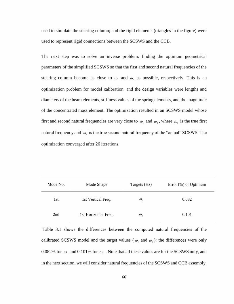
66

used to simulate the steering column; and the rigid elements (triangles in the figure) were

used to represent rigid connections between the SCSWS and the CCB.

The next step was to solve an inverse problem: finding the optimum geometrical

parameters of the simplified SCSWS so that the first and second natural frequencies of the

steering column become as close to 1 and

2 as possible, respectively. This is an

optimization problem for model calibration, and the design variables were lengths and

diameters of the beam elements, stiffness values of the spring elements, and the magnitude

of the concentrated mass element. The optimization resulted in an SCSWS model whose

first and second natural frequencies are very close to 1 and

2 , where 1 is the true first

natural frequency and 2 is the true second natural frequency of the “actual” SCSWS. The

optimization converged after 26 iterations.

Table 3.1 shows the differences between the computed natural frequencies of the

calibrated SCSWS model and the target values (1 and

2 ): the differences were only

0.082% for 1 and 0.101% for

2 . Note that all these values are for the SCSWS only, and

in the next section, we will consider natural frequencies of the SCSWS and CCB assembly.

Mode No. Mode Shape Targets (Hz) Error (%) of Optimum

1st 1st Vertical Freq. 1 0.082

2nd 1st Horizontal Freq. 2

0.101

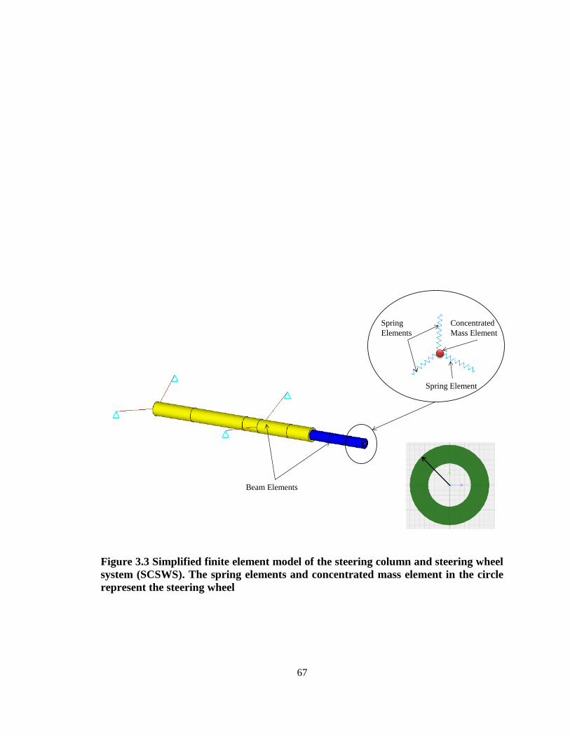
67

Concentrated

Mass Element

Spring

Elements

Spring Element

Beam Elements

Figure 3.3 Simplified finite element model of the steering column and steering wheel

system (SCSWS). The spring elements and concentrated mass element in the circle

represent the steering wheel

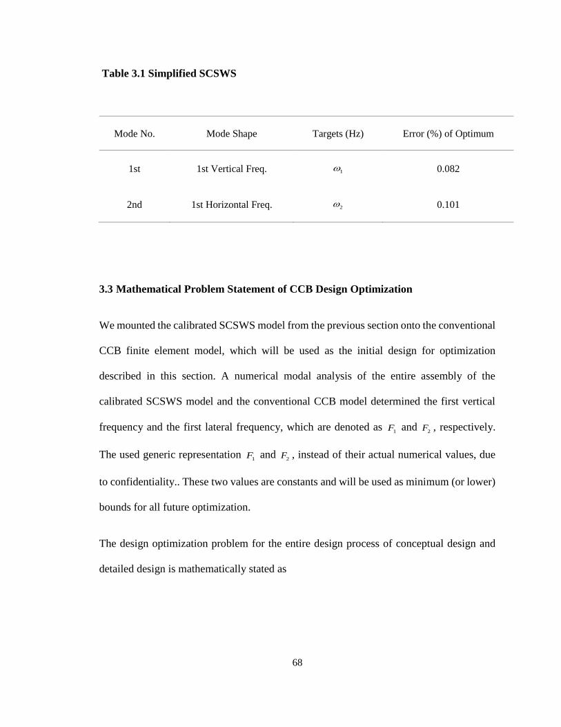
68

Table 3.1 Simplified SCSWS

3.3 Mathematical Problem Statement of CCB Design Optimization

We mounted the calibrated SCSWS model from the previous section onto the conventional

CCB finite element model, which will be used as the initial design for optimization

described in this section. A numerical modal analysis of the entire assembly of the

calibrated SCSWS model and the conventional CCB model determined the first vertical

frequency and the first lateral frequency, which are denoted as 1F and

2F , respectively.

The used generic representation 1F and

2F , instead of their actual numerical values, due

to confidentiality.. These two values are constants and will be used as minimum (or lower)

bounds for all future optimization.

The design optimization problem for the entire design process of conceptual design and

detailed design is mathematically stated as

Mode No. Mode Shape Targets (Hz) Error (%) of Optimum

1st 1st Vertical Freq. 1 0.082

2nd 1st Horizontal Freq. 2

0.101

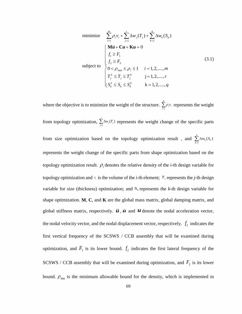
69

m

i=1 1 1

1 1

2 2

min

minimize ( ) ( )

0

subject to 0 1 1,2,....,

j 1,2,....,

k 1,2,....,

qr

i i j j k k

j k

i

L U

j j j

L U

k k k

v w T w S

f F

f F

i m

T T T r

S S S q

M C Ku u u

(3.1)

where the objective is to minimize the weight of the structure. m

i=1

i iv represents the weight

from topology optimization, 1

( )r

j j

j

w T

represents the weight change of the specific parts

from size optimization based on the topology optimization result , and 1

( )q

k k

k

w S

represents the weight change of the specific parts from shape optimization based on the

topology optimization result. i denotes the relative density of the i-th design variable for

topology optimization and iv is the volume of the i-th element; jT represents the j-th design

variable for size (thickness) optimization; and Sk represents the k-th design variable for

shape optimization. M, C, and K are the global mass matrix, global damping matrix, and

global stiffness matrix, respectively. u , u and u denote the nodal acceleration vector,

the nodal velocity vector, and the nodal displacement vector, respectively. 1f indicates the

first vertical frequency of the SCSWS / CCB assembly that will be examined during

optimization, and 1F is its lower bound. 2f indicates the first lateral frequency of the

SCSWS / CCB assembly that will be examined during optimization, and 2F is its lower

bound. min is the minimum allowable bound for the density, which is implemented in

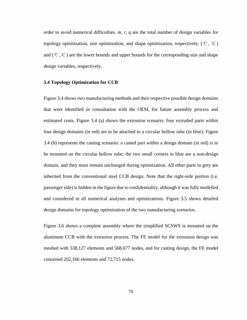
70

order to avoid numerical difficulties. m, r, q are the total number of design variables for

topology optimization, size optimization, and shape optimization, respectively. (L

jT , L

kS )

and (U

jT , U

kS ) are the lower bounds and upper bounds for the corresponding size and shape

design variables, respectively.

3.4 Topology Optimization for CCB

Figure 3.4 shows two manufacturing methods and their respective possible design domains

that were identified in consultation with the OEM, for future assembly process and

estimated costs. Figure 3.4 (a) shows the extrusion scenario: four extruded parts within

four design domains (in red) are to be attached to a circular hollow tube (in blue). Figure

3.4 (b) represents the casting scenario: a casted part within a design domain (in red) is to

be mounted on the circular hollow tube; the two small corners in blue are a non-design

domain, and they must remain unchanged during optimization. All other parts in grey are

inherited from the conventional steel CCB design. Note that the right-side portion (i.e.

passenger side) is hidden in the figure due to confidentiality, although it was fully modelled

and considered in all numerical analyses and optimizations. Figure 3.5 shows detailed

design domains for topology optimization of the two manufacturing scenarios.

Figure 3.6 shows a complete assembly where the simplified SCSWS is mounted on the

aluminum CCB with the extrusion process. The FE model for the extrusion design was

meshed with 538,127 elements and 568,677 nodes, and for casting design, the FE model

contained 202,166 elements and 72,715 nodes.

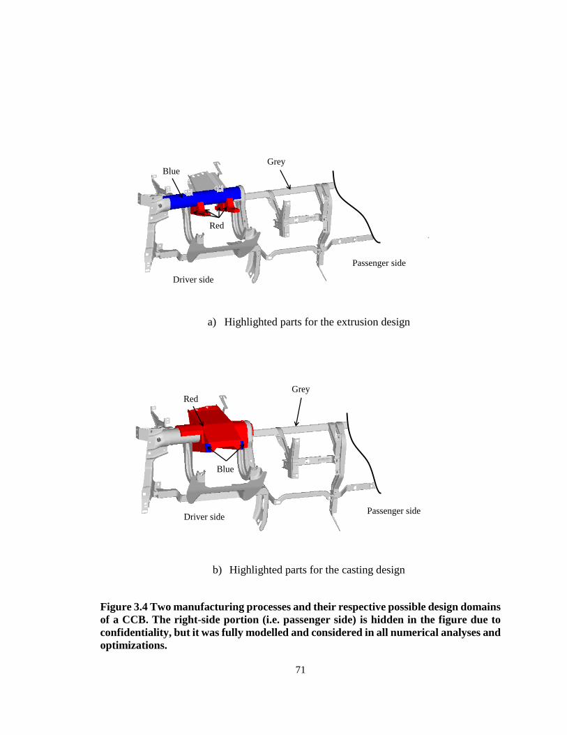
71

Driver side

Passenger side

Red

BlueGrey

a) Highlighted parts for the extrusion design

Driver sidePassenger side

Blue

RedGrey

b) Highlighted parts for the casting design

Figure 3.4 Two manufacturing processes and their respective possible design domains

of a CCB. The right-side portion (i.e. passenger side) is hidden in the figure due to

confidentiality, but it was fully modelled and considered in all numerical analyses and

optimizations.

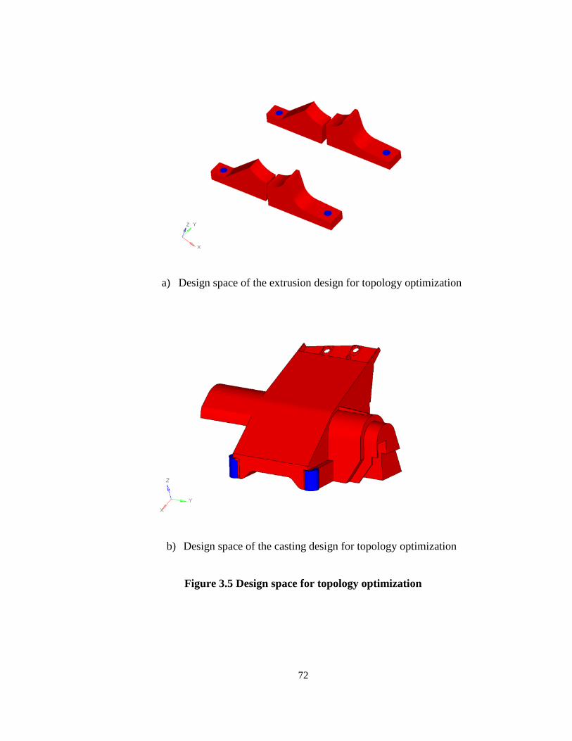
72

a) Design space of the extrusion design for topology optimization

b) Design space of the casting design for topology optimization

Figure 3.5 Design space for topology optimization

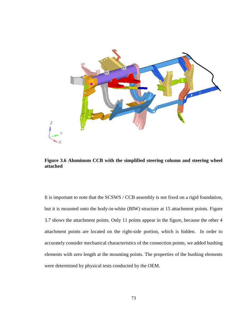
73

Figure 3.6 Aluminum CCB with the simplified steering column and steering wheel

attached

It is important to note that the SCSWS / CCB assembly is not fixed on a rigid foundation,

but it is mounted onto the body-in-white (BIW) structure at 15 attachment points. Figure

3.7 shows the attachment points. Only 11 points appear in the figure, because the other 4

attachment points are located on the right-side portion, which is hidden. In order to

accurately consider mechanical characteristics of the connection points, we added bushing

elements with zero length at the mounting points. The properties of the bushing elements

were determined by physical tests conducted by the OEM.

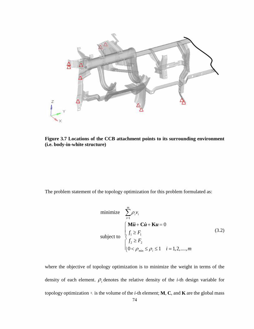
74

Figure 3.7 Locations of the CCB attachment points to its surrounding environment

(i.e. body-in-white structure)

The problem statement of the topology optimization for this problem formulated as:

m

i=1

1 1

2 2

min

minimize

0

subject to

0 1 1,2,....,

i i

i

v

f F

f F

i m

M C Ku u u (3.2)

where the objective of topology optimization is to minimize the weight in terms of the

density of each element. i denotes the relative density of the i-th design variable for

topology optimization iv is the volume of the i-th element; M, C, and K are the global mass

75

matrix, global damping matrix and global stiffness matrix. u , u and u denote the nodal

acceleration vector, the nodal velocity vector, and the nodal displacement vector,

separately. 1f indicates the first vertical frequency of the SCSWS / CCB assembly that

will be examined during optimization, and 1F is its lower bound. 2f indicates the first

lateral frequency of the SCSWS / CCB assembly that will be examined during

optimization, and 2F is its lower bound. min is the minimum allowable bound for the

density, which is implemented in order to avoid numerical difficulties, and m is the total

number of density design variables.

With respect to the topology optimization, two major constraints are the 1st order natural

frequency of the vertical mode shape and the 1st order natural frequency of the lateral mode

shape, as stated in Eq. (2). In addition, we also considered various numerical issues, the

penalty factor, checkerboard control, minimum member size control, and

manufacturability. Topology optimization was conducted using Altair OptiStruct11.0 [45].

Topology optimization results highly depend on the values of two control parameters: the

penalty factor and the checkerboard control factor. An appropriate penalty factor can

effectively remove elements with intermediate density values which are not practical from

the view point of manufacturing. A rational sensitivity filtering factor can restrain

emergence of checkerboard patterns and also help keep thin structural members which are

efficient from the view point of load transfer. In OptiStruct, minimum member size control

is a technique to keep such thin structural members [46]. In addition, we implemented

“extrusion manufacturing constraint” for the topology optimization with the extrusion

scenario (Figure 3.5 (a)).

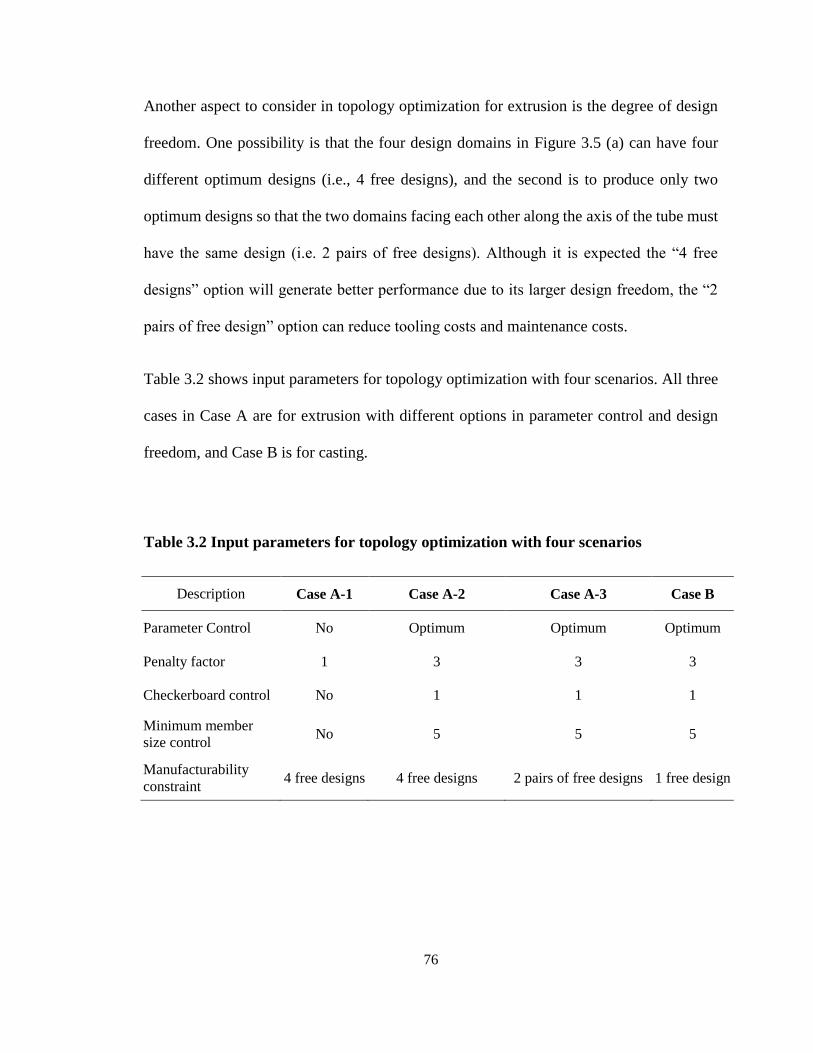
76

Another aspect to consider in topology optimization for extrusion is the degree of design

freedom. One possibility is that the four design domains in Figure 3.5 (a) can have four

different optimum designs (i.e., 4 free designs), and the second is to produce only two

optimum designs so that the two domains facing each other along the axis of the tube must

have the same design (i.e. 2 pairs of free designs). Although it is expected the “4 free

designs” option will generate better performance due to its larger design freedom, the “2

pairs of free design” option can reduce tooling costs and maintenance costs.

Table 3.2 shows input parameters for topology optimization with four scenarios. All three

cases in Case A are for extrusion with different options in parameter control and design

freedom, and Case B is for casting.

Table 3.2 Input parameters for topology optimization with four scenarios

Description Case A-1 Case A-2 Case A-3 Case B

Parameter Control No Optimum Optimum Optimum

Penalty factor 1 3 3 3

Checkerboard control No 1 1 1

Minimum member

size control No 5 5 5

Manufacturability

constraint 4 free designs 4 free designs 2 pairs of free designs 1 free design

77

Figure 3.8 shows the topology optimization for Case A-1 and Case A-2. It is clear that the

optimal topology layout from Case A-2 is more favorable because it has less intermediate-

density elements, clearer configuration, and better manufacturability. Topology

optimization of Case A-2 was conducted on a Windows PC (AMD Phenom II x6 1090T

Processor, 3200MHz, 7392 MB RAM, 6 cores), with the CPU time of 57 minutes and 18

seconds. Six iteration snapshots during the entire optimization history of Case A-2 are

shown in Figure 3.9.

The topology optimization result of the “2 pairs of free designs” option with proper

parameter control (i.e. Case A-3) is shown in Figure 3.10. Six iteration snapshots during

the entire optimization history are shown in Figure 3.11, and the history of the objective

function (mass within the design space) is presented in Figure 3.12.

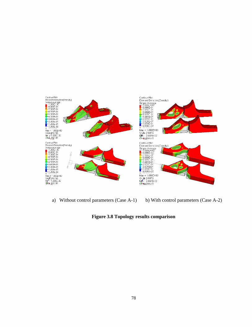
78

a) Without control parameters (Case A-1) b) With control parameters (Case A-2)

Figure 3.8 Topology results comparison

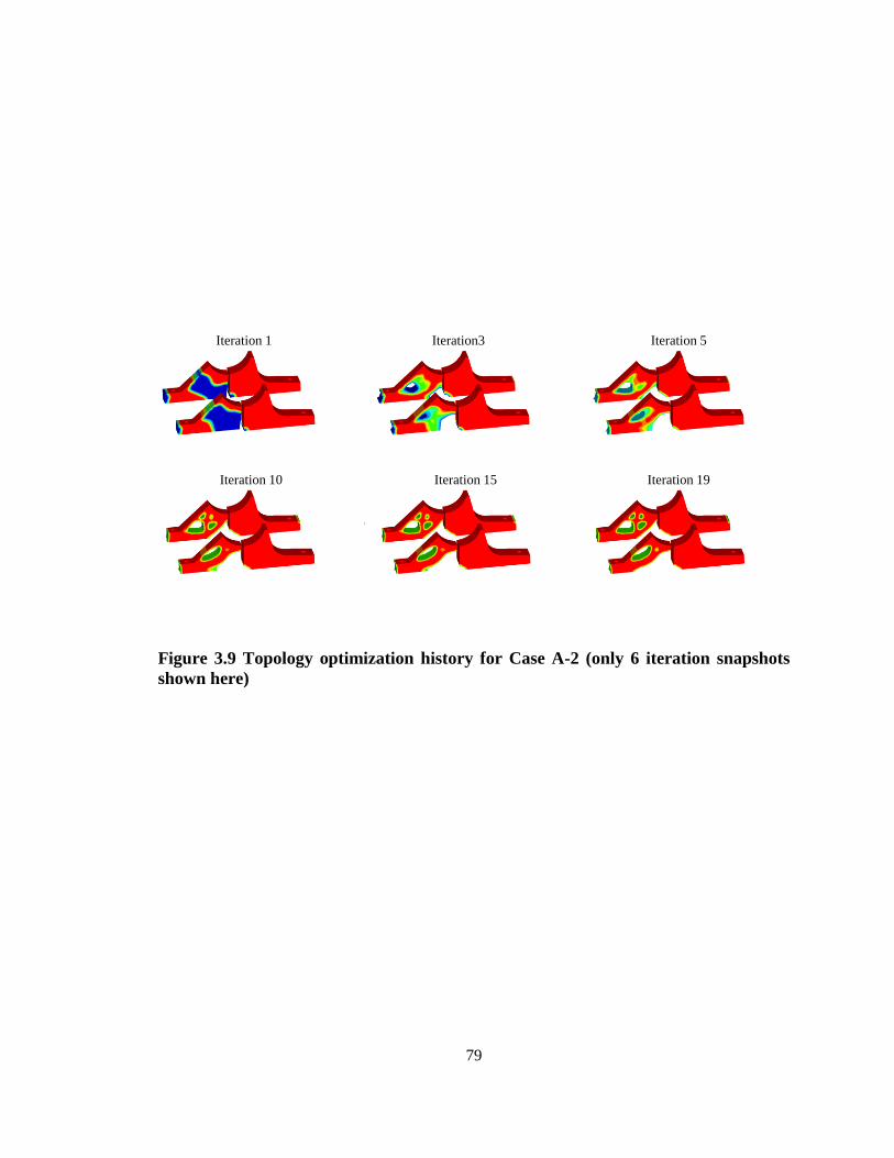
79

Iteration 1 Iteration3 Iteration 5

Iteration 10 Iteration 15 Iteration 19

Figure 3.9 Topology optimization history for Case A-2 (only 6 iteration snapshots

shown here)

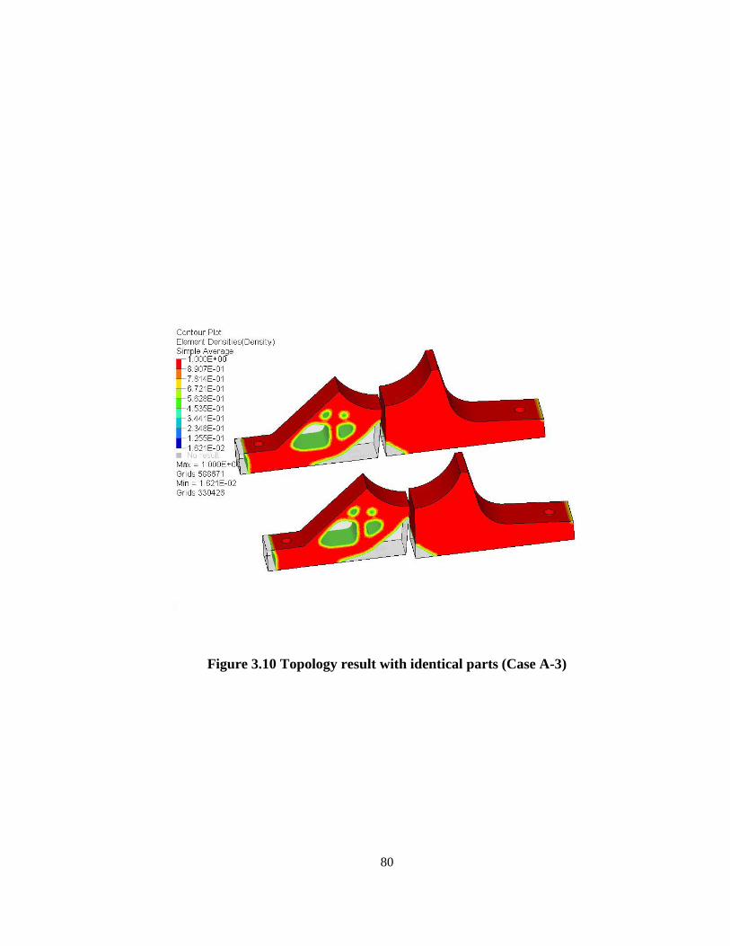
80

Figure 3.10 Topology result with identical parts (Case A-3)

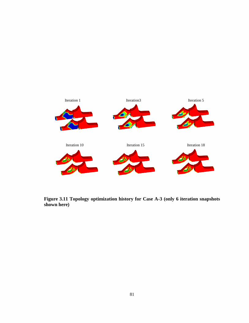
81

Iteration 1 Iteration3 Iteration 5

Iteration 10 Iteration 15 Iteration 18

Figure 3.11 Topology optimization history for Case A-3 (only 6 iteration snapshots

shown here)

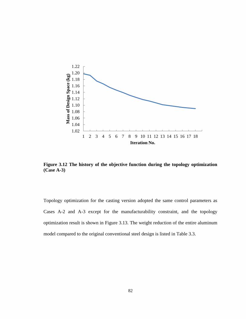
82

1.02

1.04

1.06

1.08

1.10

1.12

1.14

1.16

1.18

1.20

1.22

1 2 3 4 5 6 7 8 9 10 11 12 13 14 15 16 17 18

Mass

of

Des

ign

Sp

ace

(k

g)

Iteration No.

Figure 3.12 The history of the objective function during the topology optimization

(Case A-3)

Topology optimization for the casting version adopted the same control parameters as

Cases A-2 and A-3 except for the manufacturability constraint, and the topology

optimization result is shown in Figure 3.13. The weight reduction of the entire aluminum

model compared to the original conventional steel design is listed in Table 3.3.

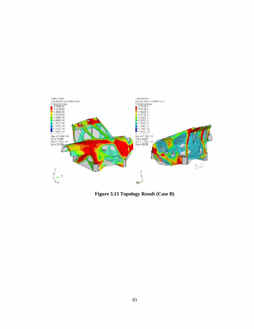
83

Figure 3.13 Topology Result (Case B)

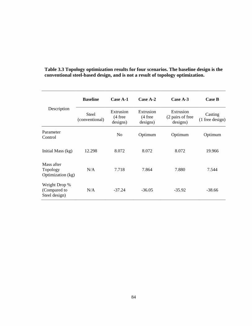
84

Table 3.3 Topology optimization results for four scenarios. The baseline design is the

conventional steel-based design, and is not a result of topology optimization.

Description

Baseline Case A-1 Case A-2 Case A-3 Case B

Steel

(conventional)

Extrusion

(4 free

designs)

Extrusion

(4 free

designs)

Extrusion

(2 pairs of free

designs)

Casting

(1 free design)

Parameter

Control No Optimum Optimum Optimum

Initial Mass (kg) 12.298 8.072 8.072 8.072 19.966

Mass after

Topology

Optimization (kg)

N/A 7.718 7.864 7.880 7.544

Weight Drop %

(Compared to

Steel design)

N/A -37.24 -36.05 -35.92 -38.66

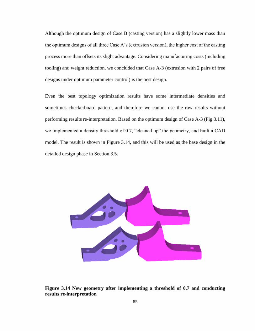
85

Although the optimum design of Case B (casting version) has a slightly lower mass than

the optimum designs of all three Case A’s (extrusion version), the higher cost of the casting

process more than offsets its slight advantage. Considering manufacturing costs (including

tooling) and weight reduction, we concluded that Case A-3 (extrusion with 2 pairs of free

designs under optimum parameter control) is the best design.

Even the best topology optimization results have some intermediate densities and

sometimes checkerboard pattern, and therefore we cannot use the raw results without

performing results re-interpretation. Based on the optimum design of Case A-3 (Fig 3.11),

we implemented a density threshold of 0.7, “cleaned up” the geometry, and built a CAD

model. The result is shown in Figure 3.14, and this will be used as the base design in the

detailed design phase in Section 3.5.

Figure 3.14 New geometry after implementing a threshold of 0.7 and conducting

results re-interpretation

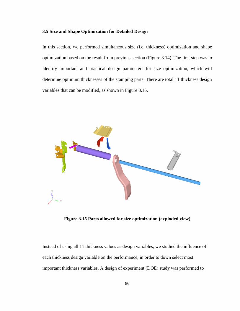
86

3.5 Size and Shape Optimization for Detailed Design

In this section, we performed simultaneous size (i.e. thickness) optimization and shape

optimization based on the result from previous section (Figure 3.14). The first step was to

identify important and practical design parameters for size optimization, which will

determine optimum thicknesses of the stamping parts. There are total 11 thickness design

variables that can be modified, as shown in Figure 3.15.

Figure 3.15 Parts allowed for size optimization (exploded view)

Instead of using all 11 thickness values as design variables, we studied the influence of

each thickness design variable on the performance, in order to down select most

important thickness variables. A design of experiment (DOE) study was performed to

87

calculate the effect of each thickness design variable change on the natural frequency

performance. The Latin HyperCube was adopted as the sampling method for the DOE

study. We chose 100 samples for each thickness design variable between the range of

1.5mm and 10mm. Therefore, there were 100 runs in total and the statistical results,

including the mean, the standard deviation, the absolute ratio of standard deviation to the

mean, and the variance, are listed in

Table 3.4.

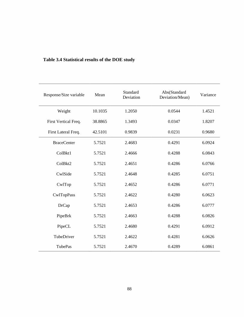
88

Table 3.4 Statistical results of the DOE study

Response/Size variable Mean Standard

Deviation

Abs(Standard

Deviation/Mean) Variance

Weight 10.1035 1.2050 0.0544 1.4521

First Vertical Freq. 38.8865 1.3493 0.0347 1.8207

First Lateral Freq. 42.5101 0.9839 0.0231 0.9680

BraceCenter 5.7521 2.4683 0.4291 6.0924

ColBkt1 5.7521 2.4666 0.4288 6.0843

ColBkt2 5.7521 2.4651 0.4286 6.0766

CwlSide 5.7521 2.4648 0.4285 6.0751

CwlTop 5.7521 2.4652 0.4286 6.0771

CwlTopPass 5.7521 2.4622 0.4280 6.0623

DrCap 5.7521 2.4653 0.4286 6.0777

PipeBrk 5.7521 2.4663 0.4288 6.0826

PipeCL 5.7521 2.4680 0.4291 6.0912

TubeDriver 5.7521 2.4622 0.4281 6.0626

TubePas 5.7521 2.4670 0.4289 6.0861

89

The quantitative effects of each thickness design variable on the frequency performance

are shown in Figure 3.16 (a) and (b). A total of 5 design variables were identified that have

significant effect on the first vertical frequency or first lateral frequency: BraceCenter,

CwlSide, DrCap, PipeBrk and TubeDriver. The other 6 design variables were given

predetermined thickness values and designated as fixed parameters.

Figure 3.16 (c) shows that one of the 5 design variables, TuberDriver, has the greatest

influence on mass, and we in consultation with the industry partner decided to build this

tube using the tailored-welded-tubes technique. For this, TubeDriver was partitioned into

6 pieces of welded tubes, and each piece can have an independent thickness design variable.

Thus, the thickness optimization of the CCB was defined with 10 design variables, as

shown in Figure 3.17.

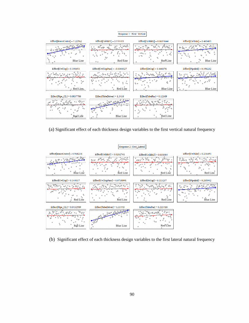
90

Blue Line Blue Line

Blue LineBlue Line

Blue Line

Red Line Red Line

Red Line Red Line

Red Line Red Line

(a) Significant effect of each thickness design variables to the first vertical natural frequency

Blue Line Red Line

Blue LineRed Line

Blue Line

Red Line Red Line

Red Line Red Line

Red Line Red Line

(b) Significant effect of each thickness design variables to the first lateral natural frequency

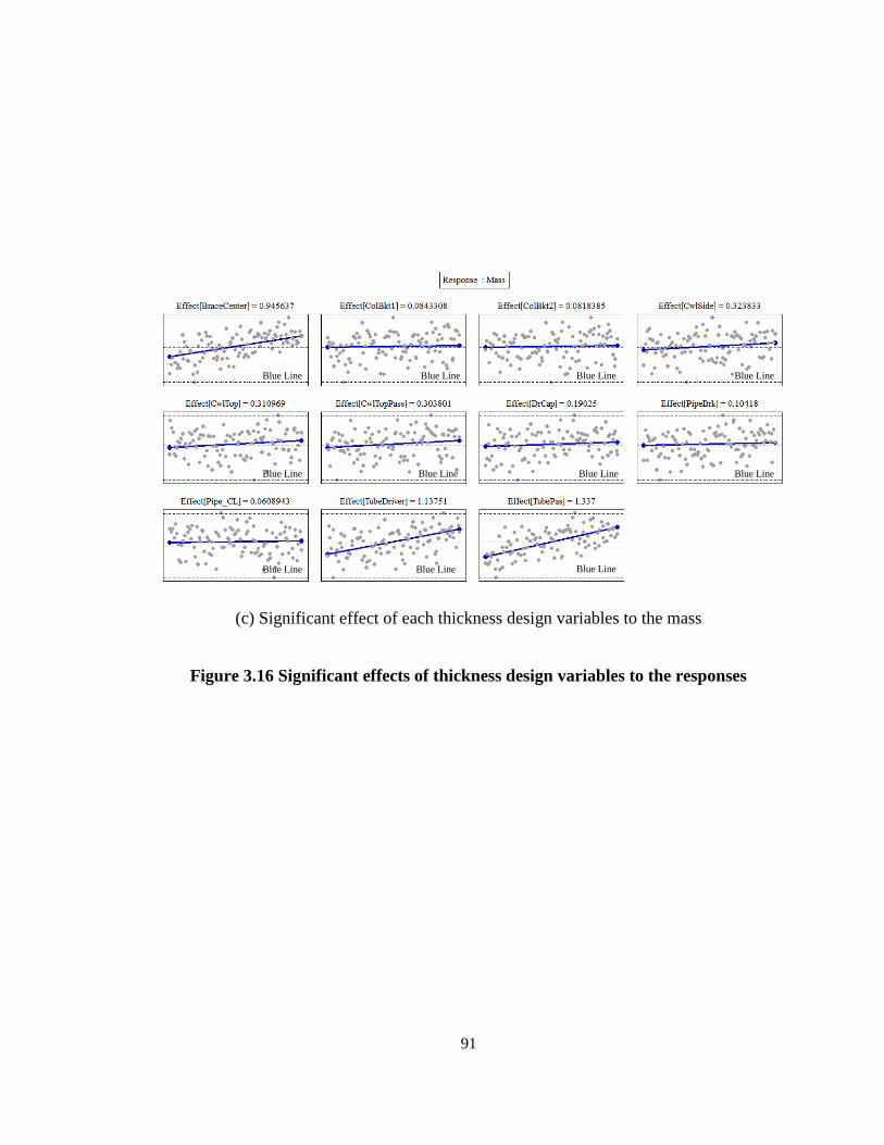
91

Blue Line Blue Line

Blue LineBlue Line

Blue Line

Blue Line Blue Line

Blue Line Blue Line

Blue Line Blue Line

(c) Significant effect of each thickness design variables to the mass

Figure 3.16 Significant effects of thickness design variables to the responses

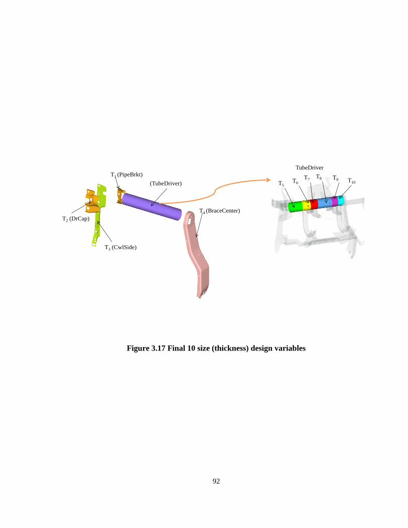
92

T5T6

T7T8 T9 T10

TubeDriver

T2 (DrCap)

T3 (CwlSide)

T1 (PipeBrkt)

(TubeDriver)

T4 (BraceCenter)

Figure 3.17 Final 10 size (thickness) design variables

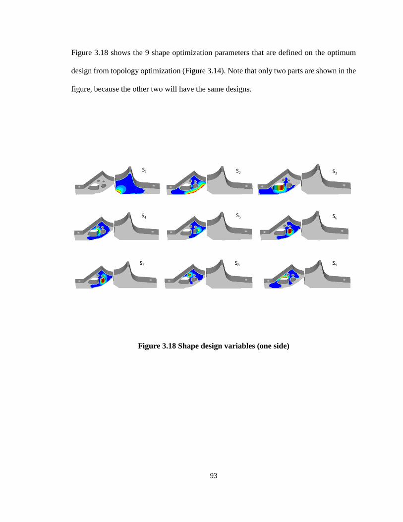
93

Figure 3.18 shows the 9 shape optimization parameters that are defined on the optimum

design from topology optimization (Figure 3.14). Note that only two parts are shown in the

figure, because the other two will have the same designs.

S1 S2 S3

S4 S5 S6

S7 S8 S9

Figure 3.18 Shape design variables (one side)

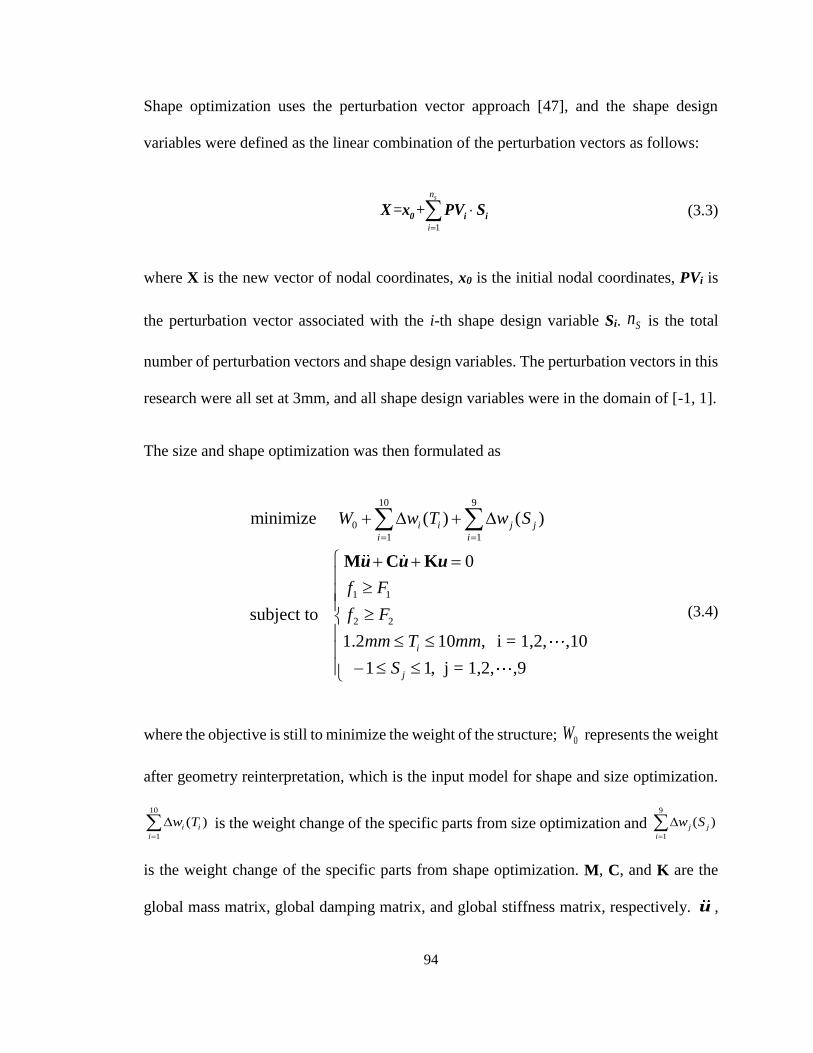
94

Shape optimization uses the perturbation vector approach [47], and the shape design

variables were defined as the linear combination of the perturbation vectors as follows:

1

= +sn

i

0 i iX x PV S (3.3)

where X is the new vector of nodal coordinates, x0 is the initial nodal coordinates, PVi is

the perturbation vector associated with the i-th shape design variable Si. Sn is the total

number of perturbation vectors and shape design variables. The perturbation vectors in this

research were all set at 3mm, and all shape design variables were in the domain of [-1, 1].

The size and shape optimization was then formulated as

10 9

0

1 1

1 1

2 2

minimize ( ) ( )

0

subject to

1.2 10 , i = 1,2, ,10

1 1, j = 1,2, ,9

i i j j

i i

i

j

W w T w S

f F

f F

mm T mm

S

M C Ku u u

(3.4)

where the objective is still to minimize the weight of the structure; 0W represents the weight

after geometry reinterpretation, which is the input model for shape and size optimization.

10

1

( )i i

i

w T

is the weight change of the specific parts from size optimization and 9

1

( )j j

i

w S

is the weight change of the specific parts from shape optimization. M, C, and K are the

global mass matrix, global damping matrix, and global stiffness matrix, respectively. u ,

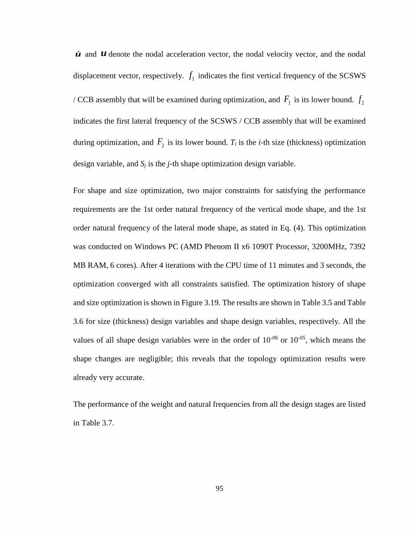
95

u and u denote the nodal acceleration vector, the nodal velocity vector, and the nodal

displacement vector, respectively. 1f indicates the first vertical frequency of the SCSWS

/ CCB assembly that will be examined during optimization, and 1F is its lower bound. 2f

indicates the first lateral frequency of the SCSWS / CCB assembly that will be examined

during optimization, and 2F is its lower bound. Ti is the i-th size (thickness) optimization

design variable, and Sj is the j-th shape optimization design variable.

For shape and size optimization, two major constraints for satisfying the performance

requirements are the 1st order natural frequency of the vertical mode shape, and the 1st

order natural frequency of the lateral mode shape, as stated in Eq. (4). This optimization

was conducted on Windows PC (AMD Phenom II x6 1090T Processor, 3200MHz, 7392

MB RAM, 6 cores). After 4 iterations with the CPU time of 11 minutes and 3 seconds, the

optimization converged with all constraints satisfied. The optimization history of shape

and size optimization is shown in Figure 3.19. The results are shown in Table 3.5 and Table

3.6 for size (thickness) design variables and shape design variables, respectively. All the

values of all shape design variables were in the order of 10-06 or 10-05, which means the

shape changes are negligible; this reveals that the topology optimization results were

already very accurate.

The performance of the weight and natural frequencies from all the design stages are listed

in Table 3.7.

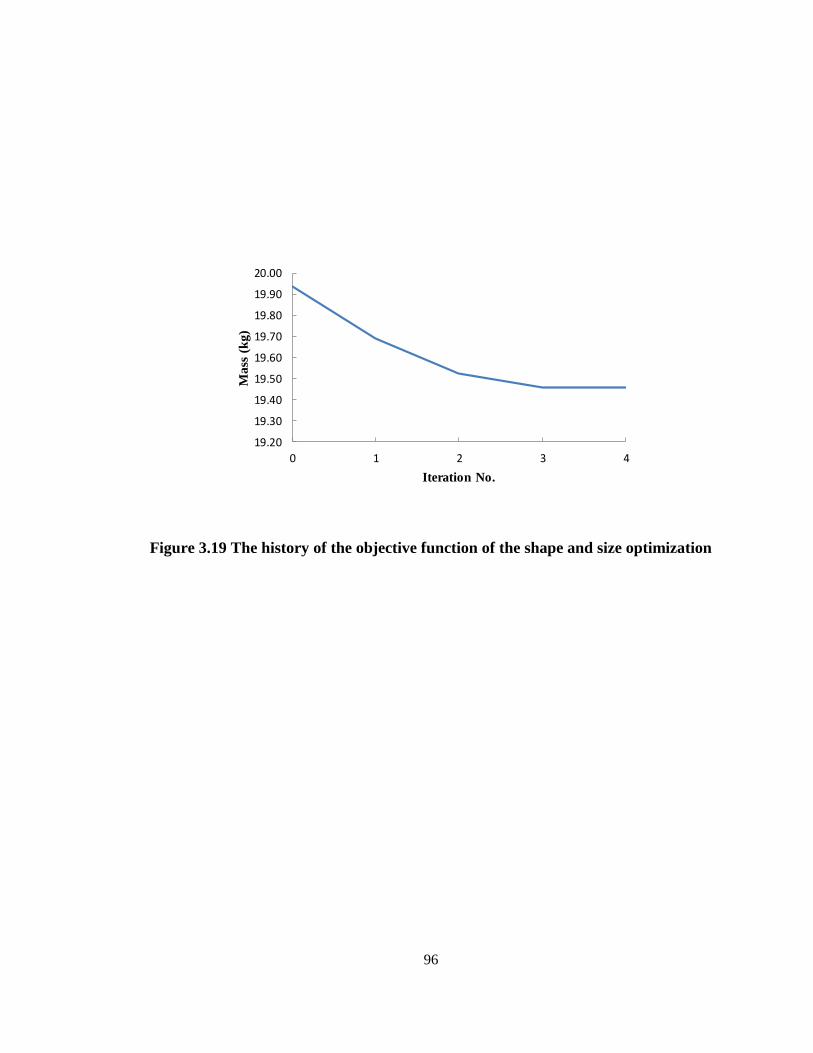
96

19.20

19.30

19.40

19.50

19.60

19.70

19.80

19.90

20.00

0 1 2 3 4

Ma

ss (

kg

)

Iteration No.

Figure 3.19 The history of the objective function of the shape and size optimization

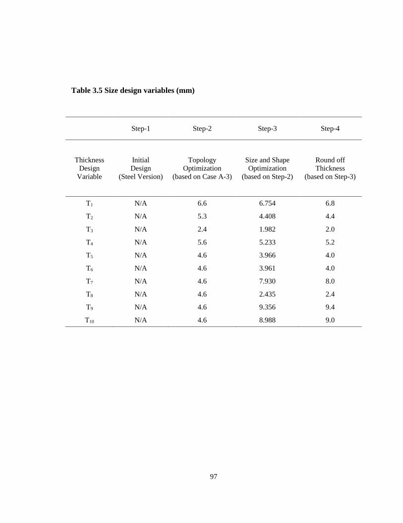
97

Table 3.5 Size design variables (mm)

Step-1 Step-2 Step-3 Step-4

Thickness

Design

Variable

Initial

Design

(Steel Version)

Topology

Optimization

(based on Case A-3)

Size and Shape

Optimization

(based on Step-2)

Round off

Thickness

(based on Step-3)

T1 N/A 6.6 6.754 6.8

T2 N/A 5.3 4.408 4.4

T3 N/A 2.4 1.982 2.0

T4 N/A 5.6 5.233 5.2

T5 N/A 4.6 3.966 4.0

T6 N/A 4.6 3.961 4.0

T7 N/A 4.6 7.930 8.0

T8 N/A 4.6 2.435 2.4

T9 N/A 4.6 9.356 9.4

T10 N/A 4.6 8.988 9.0

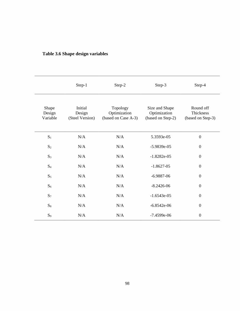
98

Table 3.6 Shape design variables


Shape

Design

Variable

Initial

Design

(Steel Version)

Topology

Optimization

(based on Case A-3)

Size and Shape

Optimization

(based on Step-2)

Round off

Thickness

(based on Step-3)

S1 N/A N/A 5.3593e-05 0

S2 N/A N/A -5.9839e-05 0

S3 N/A N/A -1.8282e-05 0

S4 N/A N/A -1.8627-05 0

S5 N/A N/A -6.9887-06 0

S6 N/A N/A -8.2426-06 0

S7 N/A N/A -1.6543e-05 0

S8 N/A N/A -6.8542e-06 0

S9 N/A N/A -7.4599e-06 0

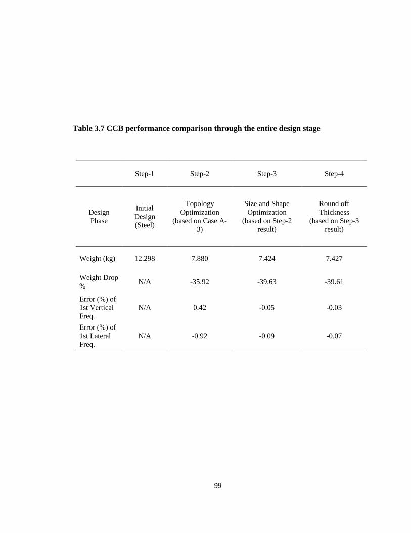
99

Table 3.7 CCB performance comparison through the entire design stage


Design

Phase

Initial

Design

(Steel)

Topology

Optimization

(based on Case A-

3)

Size and Shape

Optimization

(based on Step-2

result)

Round off

Thickness

(based on Step-3

result)

Weight (kg) 12.298 7.880 7.424 7.427

Weight Drop

% N/A -35.92 -39.63 -39.61

Error (%) of

1st Vertical

Freq.

N/A 0.42 -0.05 -0.03

Error (%) of

1st Lateral

Freq.

N/A -0.92 -0.09 -0.07

100

3.6 Conclusions

From the view point of lightweight strategies, this research utilized all three approaches

simultaneously: lightweight material, structural optimization, and advanced manufacturing

process to solve a real engineering problem. A completed design optimization of an

aluminum CCB from an already well-designed steel CCB by using topology, shape, and

size optimization for weight reduction was discussed explicitly. The final design had a

39.61% of weight savings compared to the baseline steel design.

Finite element analyses and optimization was conducted in order to build and calibrate an

approximate SCSWS model that represents the behavior of a real SCSWS with reasonable

accuracy. This approximation process can effectively address the typical challenge that

CCB supplier frequently faces: design optimization of a CCB needs to be performed, when

detailed information on the SCSWS is not available.

The entire optimization process in this research achieved significant weight savings;

moreover, the optimum design retained most of the original geometric parameters from the

conventional steel design with no changes. This means that time and cost for redesigning

the production line, the fabrication procedure, the assembly procedure, and packaging

could be saved significantly.

The initial mass of the aluminum extrusion design was 8.03kg; and topology, size, and

shape optimization reduced the mass to 7.43kg. The cost of aluminum is estimated to be

$2.2 per pound [48]. Therefore, the design optimization in this research saved material cost

by $2.91 per a unit of CCB with aluminum features. The number of units manufactured in

101

the automotive industry is very high—for example, hundreds of thousands—therefore, cost

savings due to the optimization would be substantial.

The entire design process of the aluminum CCB is shown in Figure 3.20. We maximized

the benefit of design optimization by doing topology optimization in the conceptual design

stage and shape/size optimization in the following detailed design stage. Two

manufacturing processes, extrusion and casting, were considered with various optimization

control parameters and design freedom options. All the process was conducted based on

the assumption that only limited information on the SCSWS is available, which is the

typical situation for the actual CCB designer. For this, a simplified FE model of the SCSWS

was built and calibrated.

It should be also noted that the use of topology, shape, and size optimization for the CCB

system development also allowed for considerable savings in design time and associated

costs. Our industrial partner has benefited greatly from the shortened design cycle. In

addition, the geometry layout resulted from topology optimization is more objective and

robust than that from the conventional trial-and-error. The methodology discussed in this

chapter could also be spread to the development of other automotive parts like engine

cradles or control arms.

3.7 Limitations

The limitation of this study is that crashworthiness of this CCB assembly was not

considered due to two major challenges. First, crashworthiness of a separate individual

assembly (in this research, cross car beam) could not truly reflect its deformation and

energy absorption behavior since there are strong interactions among components and

102

assemblies. This is the key reason why crashworthiness is mainly considered by the OEM.

Second, crashworthiness analysis of an automotive assembly involves geometry-

nonlinearity, material-nonlinearity and contact-nonlinearity. To include crashworthiness in

an optimization process is extremely time-consuming. Specially, topology optimization for

solving highly nonlinear problem is not well developed yet. Some techniques, such as the

equivalent static load method (ESLM), could linearize the nonlinear behavior, and have a

potential to improve the computational efficiency. In the future, after the OEM performed

crash test on a vehicle level, the feedback will be incorporated back into the model to

further improve the comprehensive performance of the CCB.

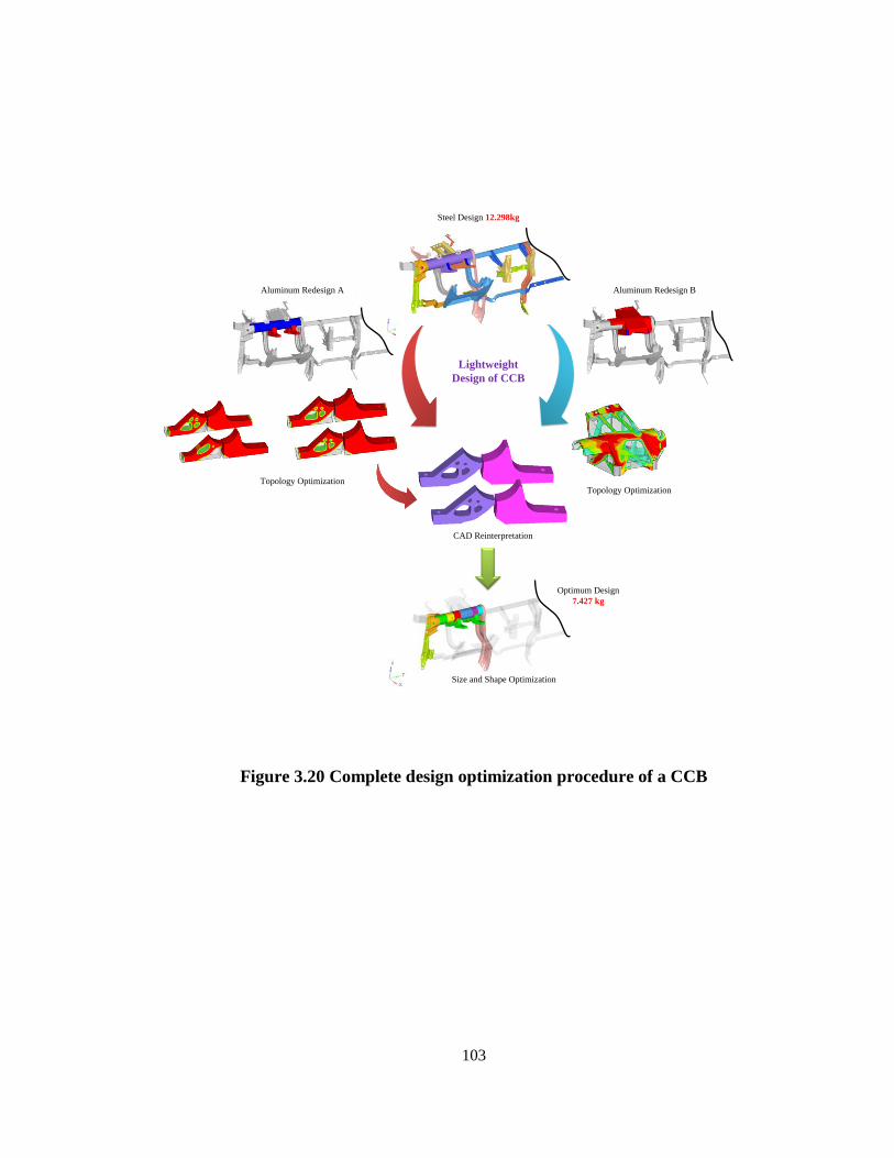
103

Lightweight

Design of CCB

Steel Design 12.298kg

Aluminum Redesign BAluminum Redesign A

Topology OptimizationTopology Optimization

CAD Reinterpretation

Size and Shape Optimization

Optimum Design

7.427 kg

Figure 3.20 Complete design optimization procedure of a CCB

104

ACKNOWLEDGEMENTS

The authors would like to thank the CAE group from Kirchhoff Van-Rob Inc. Their

suggestions are acknowledged and much appreciated.

REFERENCES

[1] Woisetschlaeger E. Keine Monokultur. Automobile Entwicklung, 2001, pp. 130

[2] Wallentowitz H. Structural Design of Vehicles. Institute fur Kraftfahrwesen, 2004,

Aachen

[3] Li C and Kim IY. Conceptual and Detailed Design of an Automotive Engine Cradle

by Using Topology, Shape and Size Optimization. Struct Multidisc Optim, 2014; 1-

18

[4] Schultz D. The Past, Present and Future of Aluminum in North American Light

Vehicles, Ducker Worldwide Michigan, October 16, 2012, pp. 20

[5] OICA, Organisation Internationale des Constructeurs d’Automobiles.

http://www.oica.net/category/production-statistics/

[6] Yildiz AR, A new hybrid particle swarm optimization approach for structural design

optimization in automotive industry, Proceedings of the Institution of Mechanical

Engineers, Part D: Journal of Automobile Engineering, 2012, 226 (10): 1340-1351

[7] Yildiz AR and Solanki KN, Multi-objective optimization of vehicle crashworthiness

using a new particle swarm based approach, International Journal of Advanced

Manufacturing Technology, 2012, 59(1-4): 367-376

[8] Yildiz AR, Öztürk N, Kaya N and Öztürk F, Hybrid multi-objective shape design

optimization using Taguchi’s method and genetic algorithm, Struct Multidisc Optim,

2007, 34 (4): 317-332

[9] Yildiz AR, Comparison of evolutionary based optimization algorithms for structural

design optimization, Engineering Applications of Artificial Intelligence, 2013, 26(1),

pp. 327–33

http://www.oica.net/category/production-statistics/

105

[10] Yildiz AR, A New Design Optimization Framework based on immune Algorithm

and Taguchi Method, Computers in Industry, 2009, 60(8): 613-620

[11] Durgun I and Yildiz AR, Structural design optimization of vehicle components

using Cuckoo search algorithm, Materials Testing, 2012, 54(3): 185-188

[12] Craig KJ, Stander Nielen, Dooge DA and Varadappa S, Automotive crashworthiness

design using response surface-based variable screening and optimization,

Engineering Computations, 2005, 22 (1): 38-61

[13] Sinha K, Reliability-based multiobjective optimization for automotive

crashworthiness and occupant safety, Struct Multidiscp Optim, 2007, 33: 255-268

[14] Jansson T, Andersson, A and Nilsson L., Optimization of draw-in for an automotive

sheet metal part: An evaluation using surrogate models and response surfaces,

Journal of Materials Processing Technology, 2005, 159: 426-434

[15] Yim HJ, Lee SB and Pyun SD, A study on optimum design for thin walled beam

structures of vehicles, SAE paper 2002-01-1987, 2002

[16] Baskar S, Kamat A and Lange R, Analytical robust door hinge system design

Taguchi approach, SAE paper 982306, 1998

[17] Kim YI and Park GJ, Nonlinear dynamic response structural optimization using

equivalent static loads, Comput. Methods Appl. Mech. Engrg. 2010, 199: 660-676

[18] Yang, RJ and Chahande AI. Automotive Applications of Topology Optimization.

Structural Optimization 1995; 9: 245-249. doi: 10.1007/BF01743977

[19] Cavazzuti M, Baldini A, Bertocchi E, and et al. High Performance Automotive

Chassis Design: a Topology Optimization Based Approach. Struct Multidisc Optim

2011; 44: 45-56. doi: 10.1007/s00158-010-0578-7

[20] Forsberg J and Nilsson L Topology Optimization in Crashworthiness Design. Struct

Multidiscp Optim 2007; 33: 1-12. doi: 10.1007/s00158-006-0040-z

[21] Lee HA and Park GJ. Topology Optimization for Structures with Nonlinear

Behaviour Using the Equivalent Static Loads Method. Journal of Mechanical Design

2012; 134: 1-14

[22] Wang LS, Basu PK, and Leiva JP. Automobile Body Reinforcement by Finite

Element Optimization. Finite Elements in Analysis and Design 2004; 40: 879-893.

doi: 10.1016/S0168-874X(03)00118-5

[23] Waquas S, Fan YQ, and Wang YQ. Application of Topology Optimization and

Manufacturing Simulations – A New Trend in Design of Aircraft Components.

Proceedings of the International MultiConference of Engineers and Computer

Scientists 2008; 2: 19-21. ISBN: 978-988-17012-1-3

106

[24] Kim IY and Kwak BM. Design Space Optimization Using a Numerical Design

Continuation Method) International Journal for Numerical Methods in Engineering

2002; 53(8): 1979-2002. doi: 10.1002/nme.369

[25] Boyle C and Kim IY. Three-dimensional Micro-level Computational Study of

Wolff’s law via Trabecular Bone Remodeling in the Human Proximal Femur Using

Design Space Topology Optimization. Journal of Biomechanics 2011; 44: 935–942.

doi:10.1016/j.jbiomech.2010.11.029

[26] Maute K and Frangopol DM. Reliability-based design of MEMS mechanisms by

topology optimization. Computers and Structures 2003; 81: 813-824.

doi:10.1016/S0045-7949(03)00008-7

[27] Kim SY, Kim IY, and Mechefske CK. A new efficient convergence criterion for

reducing computational expense in topology optimization: reducible design variable

method. International Journal for Numerical Method in Engineering 2012; 90: 752–

783.

[28] Kim SY, Mechefske CK, and Kim IY. Optimal damping layout in a shell structure

using topology optimization. Journal of Sound and Vibration 2013; 332: 2873-2883

[29] Yildiz AR and Saitou K, Topology Synthesis of Multicomponent Structural

Assemblies in Continuum Domains, ASME Journal of Mechanical Design, 2011,

133, 011008–011009

[30] Luo YT and Tan D, Lightweight design of an in-wheel motor using the hybrid

optimization method, Proceedings of the Institution of Mechanical Engineers, Part

D: Journal of Automobile Engineering, 2013, 227: 1590. doi:

10.1177/0954407013497194

[31] Kim JG and Jang GW, Development of a lightweight frame for a 40-foot flatbed

trailer by using CAE-based structural optimization, Proceedings of the Institution of

Mechanical Engineers, Part D: Journal of Automobile Engineering, 2011, 225: 643.

doi: 10.1177/0954407010395688

[32] Lee DC and Lee JI, Structural optimization concept for the design of an aluminium

control arm, Proceedings of the Institution of Mechanical Engineers, Part D: Journal

of Automobile Engineering, 2003; 217: 647. doi: 10.1243/09544070360692041

[33] Lee KH, Shin JK, Song SI, Yoo YM and Park GJ. Automotive door design using

structural optimization and design of experiments, Proceedings of the Institution of

Mechanical Engineers, Part D: Journal of Automobile Engineering, 2003; 217: 855.

doi: 10.1243/095440703769683261

[34] Yildiz AR, Kaya N and Öztürk F, Optimal design of vehicle components using

topology design and optimisation. International journal of vehicle design, 2004; 34

(4): 387-398

107

[35] Ali Riza Yildiz, Optimal structural design of vehicle components using topology

design and optimization. Materials Testing 50 (4), 224-228

[36] Jang IG, Kim KS, and Kwak BM. Conceptual and basic designs of the Mobile Harbor

crane based on topology and shape optimization. Struct Multidiscp Optim, 2014; 50:

505-515. doi: 10.1007/s00158-014-1073-3

[37] Zhu JH, Hou J, Zhang WH and Li Y. Structural topology optimization with

constraints on multi-fastener joint loads. Struct Multidiscp Optim, 2014; 50: 561-571.

doi: 10.1007/s00158-014-1071-5

[38] Oktay E, Hasan UA, and Onur TS. Three-dimensional structural topology

optimization of aerial vehicles under aerodynamic loads. Computers & Fluids 2014;

92: 225-232. doi: 10.1016/j.compfluid.2013.11.018

[39] Zhu, JH, Gu XJ, Zhang WH and Beckers P. Structural design of aircraft skin stretch-

forming die using topology optimization. Journal of Computational and Applied

Mathematics 2013: (246) 278-288. doi: 10.1016/j.cam.2012.09.001

[40] Bogomolny, M, and Amir O.Conceptual design of reinforced concrete structures

using topology optimization with elastoplastic material modeling. International

Journal for Numerical Methods in Engineering 2012; 90: 1578-1597. doi:

10.1002/nme.4253

[41] Hamid MS. Optimization of a Modular Cockpit Cross Car Beam for

Crashworthiness. SAE paper 2002-01-0938, 2002.

[42] Lam KP, Behdinan K, and Cleghorn WL. A Material and Gauge Thickness

Sensitivity Anallysis on the NVH and Crashworthiness of Automotive Instrument

Panel Support. Thin-Walled Structures 2003; 41: 1005-1018. doi:10.1016/S0263-

8231(03)00050-8

[43] Rita A. Early Phase of the Cross Car Beam Concept Development. Faculty of

Engineering, University of Porto. Dissertation for the degree of Master of

Engineering. Septemper 2013.

[44] Rahmani M. Multidisciplinary Design Optimization of Automotive Aluminum

Cross-Car Beam Assembly. Department of Mechanical and Industrial Engineering,

University of Toronto. Thesis for the degree of Masters of Applied Science. Nov.

2013

[45] Altair OptiStruct: OptiStruct 11.0 User Manual. Altair Engineering, 2011, Inc, Troy,

MI

[46] Zhou M, Shyy YK and Thomas HL. Checkerboard and Minimum Member Size

Control in Topology Optimization. Struct Multidisc Optim 2001; 21: 152-158

108

[47] Samareh JA. A survey of shape parameterization techniques. CEAS AIAA ICASE

NASA Langley International Forum on Aeroelasticity and Atructural Dynamics

1999; 333-343

[48] http://www.autonews.com/article/20140120/OEM04/301209910/fords-huge-bet-

on-aluminum#axzz2rj4YP4eP.

http://www.autonews.com/article/20140120/OEM04/301209910/fords-huge-bet-on-aluminum#axzz2rj4YP4eP

http://www.autonews.com/article/20140120/OEM04/301209910/fords-huge-bet-on-aluminum#axzz2rj4YP4eP

109

Chapter 4

Two-material Topology Optimization Based on Optimality Condition

This chapter conducted mathematical sensitivity formulations of two-material topology

optimization based on the adjoint variable method, and applied it to six structural

optimization problems. Commercial software programs were used for finite element

analysis including pre- and post-processing, and for multi-material topology optimization,

an in-house code was developed. Three simple, classical examples were solved for

compliance minimization, and then three case studies were performed by considering

various volume fractions. The optimum solutions by two-material topology optimization

were compared to optimum solutions determined by the standard single-material topology

optimization. All results showed that our two-material topology optimization algorithm

and computational tool can determine effective optimum solutions for various problem

statements, and optimum designs by the two-material topology optimization have better

performance than solutions by one-material topology optimization.

4.1 Introduction

Topology optimization was developed to determine important design features such as the

number, location, and shape of holes, and the connectivity of domains [1]. Due to its

effectiveness in exploring the design space, topology optimization is widely used for

preliminary design, and optimum solutions from topology optimization are then used as

baseline designs in subsequent detailed design stages.

110

The homogenization method is considered as a breakthrough of structural topology

optimization because it transforms a complicated discrete form-finding problem (e.g. truss-

like discretization) into a material distribution based continuous problem. The fundamental

concept of the homogenization method is to determine existence of the material within

each element of a structure. Cheng and Olhoff [2] first introduced a microstructure to

determine an optimum thickness distribution of elastic plates. Bendsøe and Kikuchi [3]

first applied the homogenization method to continuum structures with compliance as the

objective function and maximum allowable volume as the constraint.

The density method [4] has also developed over the last several decades, and it has been

successfully integrated into commercial software programs which can nowadays

effectively solve large-scale, real-world engineering topology optimization problems. The

density method assumes an explicit mathematical relationship between the relaxed

elemental density value and the elasticity tensor. The density method is an effective and

efficient method which does not require the homogenization process due to the introduction

of microstructures. There are two widely used density-elasticity interpolation models. The

first is the Solid Isotropic Material with Penalization (SIMP) model [5], which has been

successfully applied to a large number of problems and proven to be efficient and easy to

implement. The second is the Rational Approximation of Material Properties (RAMP)

model [6]. A penalty factor is implemented into the relation between the element density

and the elasticity in order to penalize intermediate densities, which drives the optimization

process to converge to the density value of either zero or one. During the past three decades,

tremendous progress has been made in the development of theories, various algorithms,

and application of these methods to a variety of real-world engineering and scientific

111

problems. Kim and his colleagues developed topology optimization based on the genetic

algorithms [7], proposed a numerically efficient convergence criterion which significantly

reduces computing cost [8], and solved a real-world automotive chassis design problem

considering manufacturability [9]. Li and Kim also performed conceptual and detailed

designs by using topology, shape, and size optimization [10-11].

With the rising cost of natural resources and concerns about the environment, energy

conservation and protection of the environment has become a very important issue

worldwide nowadays. Both governments and customers demand more energy-efficient,

cost-effective, and environmentally friendly products. As an example, the Corporate

Average Fuel Economy (CAFE) regulations in the United States require the average fuel

economy of cars and light trucks produced by an automaker be 54.5 mpg (mile per US

gallon) by Model Year 2025. Similarly, there is a tremendous demand for improved fuel

economy in the aerospace and rail industry as well. Reducing the weight of a vehicle is a

most effective and promising solution that improves fuel efficiency and decreases carbon

emissions.

There are three mainstream strategies for reducing weight: The first is to use lightweight

materials. The traditional low carbon steel is replaced by lightweight materials, such as

high strength steel, aluminum, magnesium, and plastic composites. Different material

properties—in terms of stiffness, strength, durability, corrosion, and formability—and cost

should be carefully taken into consideration. In the automotive industry, traditional

materials like low carbon steel and iron have been gradually replaced by various

112

lightweight materials over past decades [12]. There are however disadvantages in the use

of lightweight materials, and one of the major concerns is higher material cost [13].

The second strategy is to develop advanced manufacturing processes. For example, the use

of structural adhesives or overcasting can reduce the weight of mechanical joints, and if

MIG welding is replaced by laser welding, there is no need for solder, and weight can be

reduced. As the third strategy for weight reduction, various design optimization methods

can be used in the design process. Design optimization determines optimum geometric

features that minimize weight while satisfying important performance requirements.

Topology optimization finds most efficient structural layouts from the view point of weight

and structural integrity in conceptual and preliminary design stages. Size and shape

optimization can fine-tune optimum designs in the detailed design stage: for example, it

can determine optimum design parameters of tailored-welded-blanks and tailored-rolled-

tubes. It should be noted that design optimization alone—based on the traditional

material—does not achieve enough weight savings, given that energy efficiency

regulations become ever more stringent.

In order to maximize weight savings, those three lightweight approaches are adopted and

used altogether nowadays, and this introduces new challenges for design optimization. If

one or multiple lightweight materials are added to an automotive structure with traditional

low carbon steel as an example, the design work now becomes a multi-material

optimization problem. Therefore engineering designers have to deal with a much more

complex optimization problem, which must determine an optimum placement of multiple

materials as well as optimum geometric features of each respective materials. This design

113

problem has larger design freedom which would potentially allow for better optimum

solutions, but at the same time, it is more difficult to obtain optimum solutions because of

increased complexity, larger design space, and stronger interactions among various types

of design parameters. Topology optimization has been traditionally used for the design

with a single material, which basically determines the existence of material within each

design cell for a prescribed material type. Currently available topology optimization

theories and methods for this type of single material design are ill equipped for design

problems that consider multiple materials.

A limited number of studies are found in multi-material topology optimization. Ramani

[14] calculated a pseudo-sensitivity of each element based on the change of the objective

and constraint functions over consecutive iterations, keeping the design variables as

discrete parameters. Huang and Xie [15] proposed a ‘sensitivity number’ ranking scheme

based on their bi-directional evolutionary topology optimization method. Saxena [16] used

the genetic algorithm for multi-material topology optimization, which allowed for a binary

representation of the design variables. Han and Lee [17] utilized the evolutionary topology

optimization and changed the material type of elements based on strain energy values.

Stegmann and Lund [18] expressed the element constitutive matrix as a weighted sum of

constitutive matrices of candidate materials, and they solved composite shell structures

using the approach. Yin and Ananthasuresh [19] used normal distribution functions to

create a material interpolation model. Sensitivity calculation procedures in all these studies

are partially or completely heuristic. This means that computing cost could be potentially

very high for real-world problems which have large numbers of design variables. It is also

particularly important for those heuristic or semi-heuristic approaches to choose

114

“optimum” control parameters for simulations, which would require a number of trial-and-

errors. Yoon [20] developed a new patch stacking method to solve the multi-material

topology optimization based on an element connectivity parameterization (ECP) method.

This is a unique idea, but current limitations include use of higher number DOFs (degree-

of-freedoms) than the typical FE-based optimization method and checkerboard problems.

Stegmann and Erik used [21] a weighted sum interpolation of the element constitutive

matrices to perform a topology optimization of general composite laminate shell structures.

Gao and Zhang [22] solved structural topology optimization with multiphase material using

mass as constraint rather than volume. Thomsen [23] presented a stiffness maximization

of a structure which is composed of two isotropic materials by using the homogenization

technique. The material of each cell was modeled by a composite using its concentration

and orientation as design variables. Because the number of design variables of each cell

has been increased to 4, the computing cost of the proposed method is high. All these

previous studies typically solved simple two-dimensional classical problems, such as the

2D cantilever or the 2D MBB (Messerschmitt-Bölkow-Blohm) beams, based on the

assumption of plane stress and using small numbers of design variables. Applicability and

numerical efficiency for solving large-scale and complicated engineering problems have

not been proven yet.

The objectives of this chapter are (1) to perform mathematical sensitivity formulation of

two-material topology optimization based on the adjoint variable method and (2) to solve

2D and 3D topology optimization problems with two possible materials by using the

sensitivity information. All numerical implementation was conducted by using commercial

software programs as much as possible, which would allow industry to easily take up the

115

computational tool and utilize it for real-world problems. In order to verify accuracy and

effectiveness of the developed method, we first solved three classical topology

optimization problems, by considering two materials: 2D cantilever, half MBB, and 3D

cantilever structures. The method was then used to solve three case studies, including a 3D

Control Arm problem, which have more complex geometries, design and non-design

domains, and different element types. We compared the optimum solutions by the two-

material topology optimization with various volume fractions to the optimum solutions by

the standard single material optimization.

4.2 Problem Definition

A system of an elastic structure for the classical structural topology optimization problem

under a single static load case is graphically represented in Figure 4.1. The design domain

, 2 3Ω R R is defined as a 2D or 3D open set, with the essential boundary condition uΓ

and the natural boundary condition tΓ . The design domain can contain permanent void

domains (i.e. forbidden zones) and constant, non-designable domains (i.e. passive zones

with full of material). The essential boundary condition and the natural boundary condition

are mutually exclusive, and constitute the entire boundary ( Ω Γ ): u tΩ = Γ = Γ Γ

and u tΓ Γ .

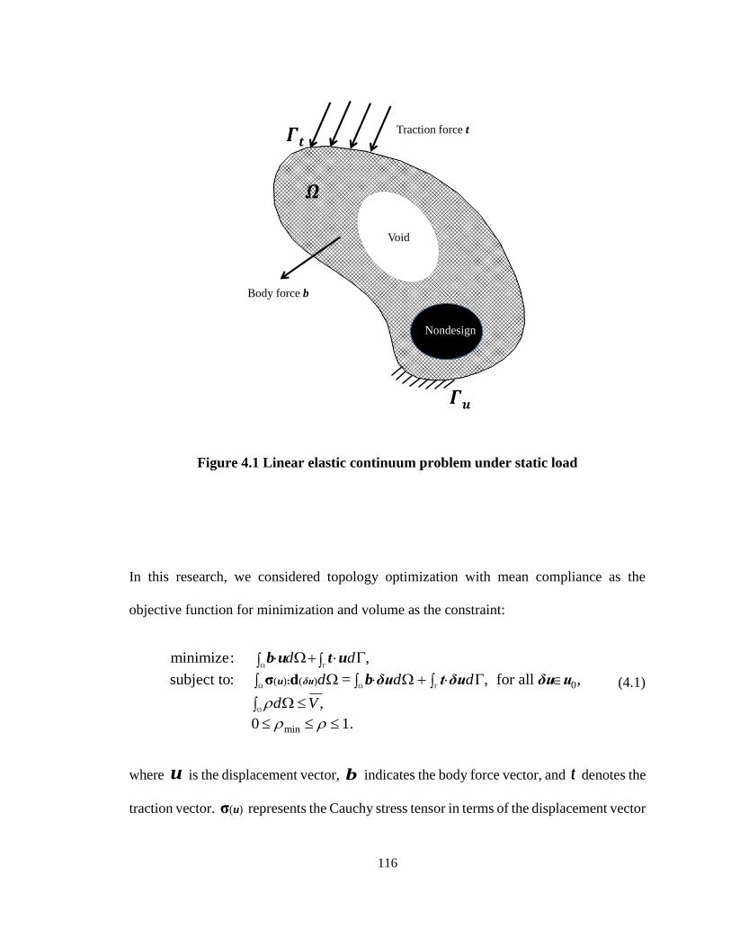
116

Void

Nondesign

Body force b

Traction force t

Figure 4.1 Linear elastic continuum problem under static load

In this research, we considered topology optimization with mean compliance as the

objective function for minimization and volume as the constraint:

( ) ( ) 0

min

minimize: ,

subject to: = , for all ,

,

0 1.

d d

d d d

d V

:σ du δu

b u t u

b δu t δu δu u

(4.1)

where u is the displacement vector, b indicates the body force vector, and t denotes the

traction vector. ( )σ u represents the Cauchy stress tensor in terms of the displacement vector

117

u , δu is the virtual displacement, and 0

u is the kinematically admissible space. is

the normalized density field, which is used as the design variable, and min

is its lower

bound. ( )d δu is the symmetric part of grad( )δu and can be derived as:

( ) : grad( ) ( ) : symm(grad( ))σ σu δu u δu

(4.2)

( )( )1 1( ) ( ) ( )

2 2

Tuu ji

x xj i

symm(grad( )) grad( ) grad ( ) dδu δu δu δu (4.3)

For linear elastic structures, the constitutive equation is ( ) : ( )σ C ερ u , where σ is the

Cauchy stress tensor, ( )ε u is the Euler-Almansi strain tensor, and ( )C ρ is the 4th-order

elasticity tensor.

Topology optimization ultimately determines the existence of material within each design

cell, and it has a binary (0-1 or void-solid) form of design variables. It is hard to solve this

type of discrete problems numerically, and therefore it is relaxed to a continuous problem

by introducing an interpolation scheme. We used the SIMP model which has been proved

to be effective for many real-world applications:

0( ) pC Cρ

(4.4)

where ( )C ρ is the (variable) elasticity tensor, whose value changes according to the

normalized density . 0C is the (constant) elasticity tensor of the base material. The

118

exponent p ( 1p ) is the penalty factor, and it drives the optimization to converge on either

zero value of design variables or one, by penalizing intermediate density values.

4.3 Theory of Two-Material Topology Optimization based on Optimality Condition

4.3.1 Interpolation function with two materials

In this chapter, we considered two different types of materials for structural topology

optimization. The interpolation function based on the SIMP model for bi-material topology

optimization is formulated as:

)=( [( (1 2

2 1 2 2( , ) ) (1 ) ) ]p p p

ijkl ijkl ijklC C C 1ρ ρ ρ ρ ρ (4.5)

where )2( ,ijklC1ρ ρ is the index representation of the (variable) elasticity tensor, whose

value changes according to the normalized densities 1ρ and 2ρ . The first normalized

density 1ρ represents existence of material within each design cell; and the second one 2ρ

is used to represent the portion of Material 1 with respect to Material 2. Further explanation

is given in Section 4.3.2 1

ijklC and 2

ijklC are the index representations of the (constant)

elasticity tensors of the Material 1 and Material 2, respectively. The exponent p is the

penalty factor, and it performs the same role as in the case of single-material topology

optimization in Equation (4.4). Figure 4.2 shows an example of the relation between

Young’s modulus and the two normalized density values for two different isotropic

materials.

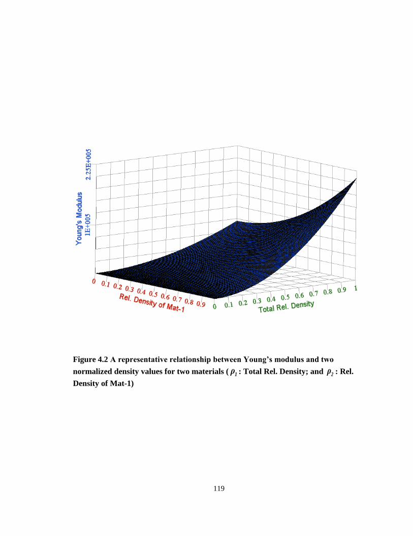
119

Figure 4.2 A representative relationship between Young’s modulus and two

normalized density values for two materials ( 1ρ : Total Rel. Density; and 2ρ : Rel.

Density of Mat-1)

120

4.3.2 Two-material topology optimization statement of compliance minimization

In order to solve the optimization problem, we use the finite element method, and now bi-

material topology optimization in the discrete form may be expressed as

)

)

1 Total_Max

1

1 2 1_Max

1

min 1

2

minimize ( ,

subject to ( ,

0 < 1, 1,2,..., ,...,

0 1, 1,2,..., ,...,

Ni i

i

Ni i i

i

i

i

C

v V

v V

i i N

i i N

K

1 2

1 2

ρ ρ

ρ ρ U F

(4.6)

where 1

i is the normalized density that determines the existence of the material (whether

it be Material 1 or Material 2) within the i-th design cell, and 2

i is the relative density that

determines the portion of Material 1 with respect to Material 2 within the i-th design cell.

This relative density ( 2

i ) has a valid physical meaning only if there is a material within

the i-th design cell (i.e. 1

i = 1). There are three physically meaningful cases for the i-th

design cell: (1) 1 21 and 1i i means that the cell is completely filled with Material 1; (2)

1 21 and 0i i means that the cell is completely filled with Material 2; and (3) 1 0i means

that the cell is empty. 1ρ and 2ρ are then the vector of the normalized density for material

existence and the vector of relative density for the portion of Material 1, respectively. iv

is the volume of the i-th design cell. Total_MaxV is the maximum, total allowable volume of

Material 1 and Material 2 combined, and 1_MaxV is the maximum allowable volume of

121

Material 1. C is compliance, which is used as the objective function for minimization. K

is the global stiffness matrix, U is the nodal displacement vector, and F is the external

force vector. N is the total number of the design variables.

4.3.3 Sensitivity derivation of compliance with respect to density variables

Topology optimization typically deals with a very large number of design variables and a

small number of functionals (objective function and constraints). The adjoint variable

method is hence the most efficient approach for calculating design sensitivities. The design

sensitivity by means of the adjoint variable method based on the SIMP model is written as

( ( )) =

= ( )

when

1, 2,... ,..., , 1, 2

T

i i

j j

T T

i

j

T T T

i i

j j

T T T

i

j

T

i

j

C

i i N j

K

Kλ K λ

Kλ = λ K λ

K

F U

F U U F

UF U

U F U

U U

(4.7)

where F is the external force vector, U is the nodal displacement vector, K is the global

stiffness matrix, and λ is the adjoint variable vector. N is the total number of the design

variables.

The sensitivity expression for each of the two materials, using the adjoint variable method

based on the SIMP model, is written as

122

( [( (1 1 2

1 2 2

1 1 1

) ) (1 ) ) ]T T i p i p T i p Tii ii i i

Cp

kKk k

i i i i i iU U u u u u u u

(4.8.1)

( ( 1 1 1 2

1 2 2

2 2 2

) [ ) ( ) ]T T i p i p T i p Tii ii i i

Cp p

kKk k

i i i i i iU U u u u u u u (4.8.2)

where K is the global element with the interpolated material property, ik is the stiffness

of the i-th element (or design cell), 1

ik is the element stiffness of the i-th element with the

properties of Material 1, and 2

ik is the element stiffness of the i-th element with the

properties Material 2. U is the global displacement vector, and iu is the displacement

vector of the i-th element. (Here, the i-th element is the same as the i-th design cell.)

It can be easily seen that 1

i

C

must be less than or equal to zero. For an actual numerical

implementation, we should implement a lower limit min min( 0) for each of 1

i in order

to avoid singularity; hence 1

i

C

is strictly non-positive and finite for non-singular

structures.

For 2

i

C

, the values of

1T

iki i

u u and 2T

iki i

u u will determine the sign of 2

i

C

. If

1 2T T

i ik ki i i i

u u u u , then 2

0i

C

; if

1 2T T

i ik ki i i i

u u u u , then 2

0i

C

. For the actual

numerical case studies in this chapter, we used steel for Material 1 and aluminum for

Material 2; therefore, we had 1 2T T

i ik ki i i i

u u u u , and therefore 2

i

C

was negative in all our

123

case studies. The negativity of 1

i

C

and

2

i

C

imply that as either density increases,

compliance of the structure decreases which means stiffness of the structure increases.

4.3.4 Update of design variables based on Optimality Condition (OC)

The Lagrangian function for problem stated in Equation (4.6):

1 2

1 2 1 2 1 1

1 1

1 2 3 4

min 1 1 2 2

1 1 1 1

( , ( ) ( ) ( )

( ) ( 1) (0 ) ( 1)

N Ni i i i i i i T

i i

N N N Ni i i i

i i i i

i i i i

L C v V v V

K) U F

(4.9)

where 1 , 2 , T , 1

i , 2

i , 3

i and 4

i are the Lagrange multipliers.

Sensitivities of the Lagrangian function with respect to 1

i and 2

i are derived as

1 2 1 2

2

1 1

1 3 4

1

2 2

1,2.,.., ,...,

T i i i

i ii i

T i i

i ii i

Lv v

i i NL

v

K

K

U U

U U

(4.10)

Dual feasibility and complementary slackness conditions are found as

1 2

1 2

1 2 1 1

1 1

1 2

1 2

min 1 1

3 4

3 4

2 2

0 0

( ) 0 ( ) 0

0 0 1,2.,.., ,...,

( ) 0 ( 1) 0

0 0

(0 ) 0 ( 1

N Ni i i i i

i i

i i

i i

i i

i i

i i

i i

v V v V

i i N

1,2.,.., ,...,) 0

i i N

(4.11)

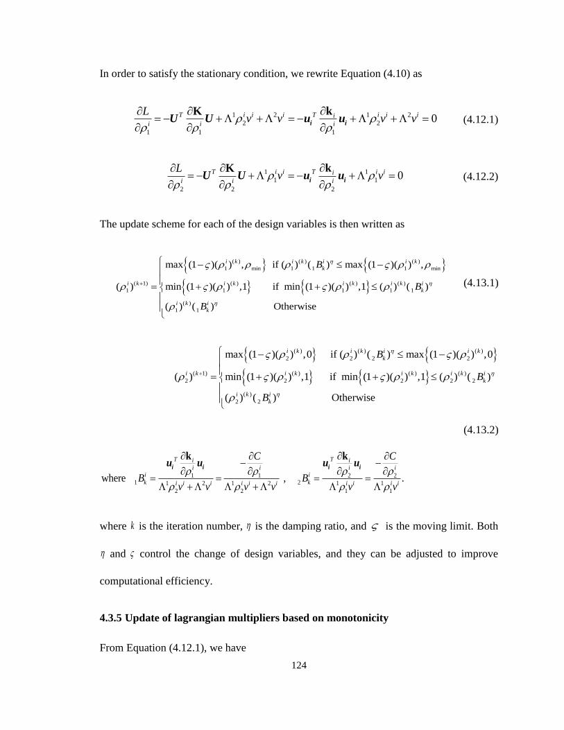
124

In order to satisfy the stationary condition, we rewrite Equation (4.10) as

1 2 1 2

2 2

1 1 1

0T i i i T i i ii

i i i

Lv v v v

kKi i

U U u u (4.12.1)

1 1

1 1

2 2 2

0T i i T i ii

i i i

Lv v

kKi i

U U u u (4.12.2)

The update scheme for each of the design variables is then written as

( ) ( ) ( )

1 min 1 1 1 min

( 1) ( ) ( ) ( )

1 1 1 1 1

( )

1 1

max (1 )( ) , if ( ) ( ) max (1 )( ) ,

( ) min (1 )( ) ,1 if min (1 )( ) ,1 ( ) ( )

( ) ( ) Otherwise

i k i k i i k

k

i k i k i k i k i

k

i k i

k

B

B

B

(4.13.1)

( ) ( ) ( )

2 2 2 2

( 1) ( ) ( ) ( )

2 2 2 2 2

( )

2 2

max (1 )( ) ,0 if ( ) ( ) max (1 )( ) ,0

( ) min (1 )( ) ,1 if min (1 )( ) ,1 ( ) ( )

( ) ( ) Otherwise

i k i k i i k

k

i k i k i k i k i

k

i k i

k

B

B

B

(4.13.2)

1 1 2 2

1 21 2 1 2 1 1

2 2 1 1

where , .

T Ti i

i i i ii i

k ki i i i i i i i i i

C C

B Bv v v v v v

i i i iu u u uk k

where k is the iteration number, is the damping ratio, and is the moving limit. Both

and control the change of design variables, and they can be adjusted to improve

computational efficiency.

4.3.5 Update of lagrangian multipliers based on monotonicity

From Equation (4.12.1), we have

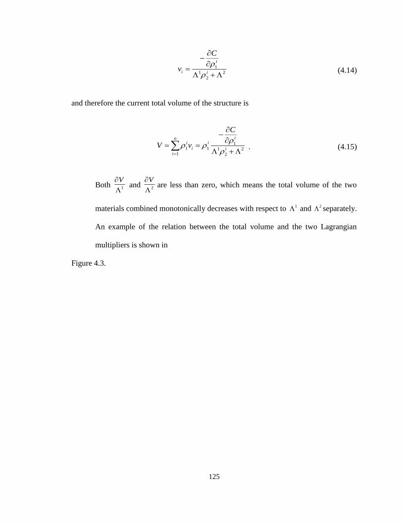
125

1

1 2

2

i

i i

C

v

(4.14)

and therefore the current total volume of the structure is

11 1 1 2

1 2

ini i

i ii

C

V v

.

(4.15)

Both 1

V

and 2

V

are less than zero, which means the total volume of the two

materials combined monotonically decreases with respect to 1 and 2 separately.

An example of the relation between the total volume and the two Lagrangian

multipliers is shown in

Figure 4.3.

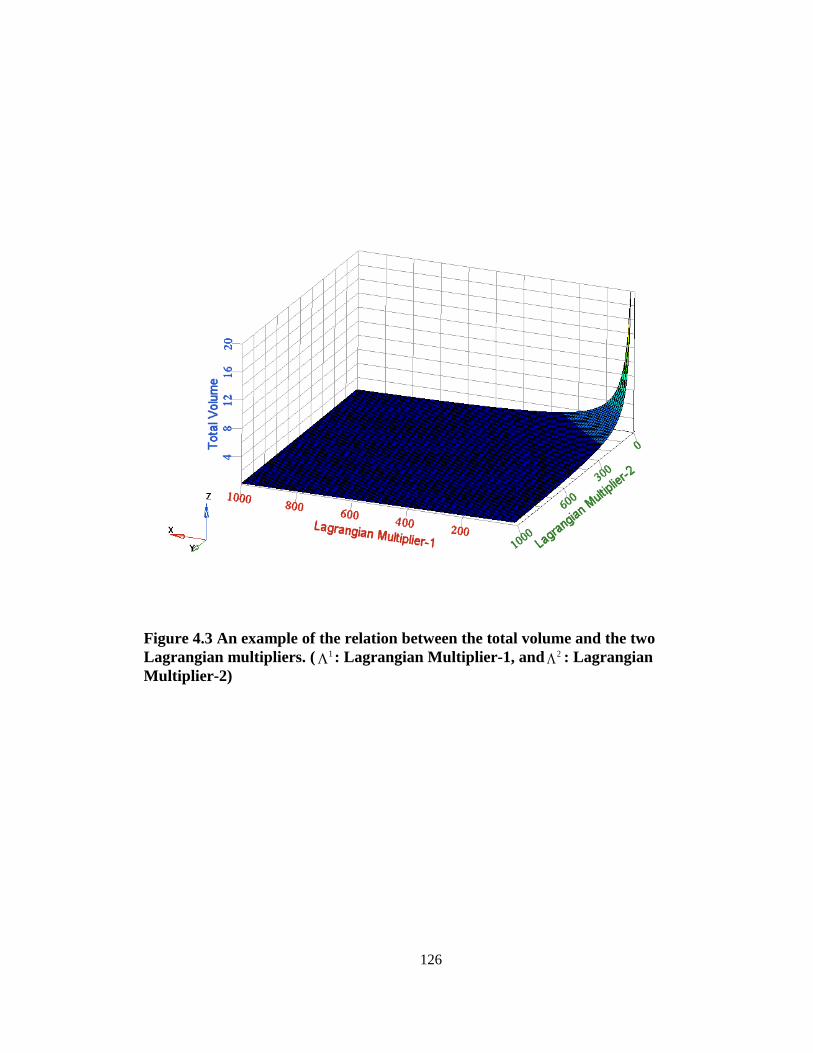
126

Figure 4.3 An example of the relation between the total volume and the two

Lagrangian multipliers. ( 1 : Lagrangian Multiplier-1, and 2 : Lagrangian

Multiplier-2)

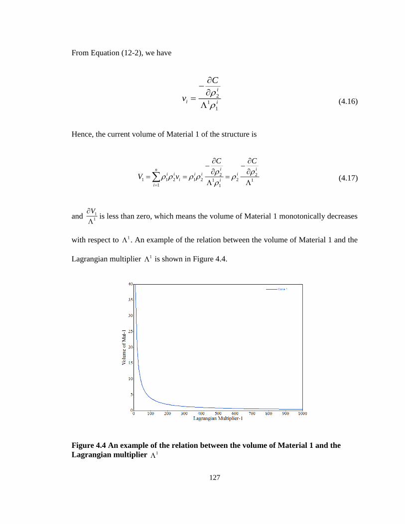
127

From Equation (12-2), we have

2

1

1

i

i i

C

v

(4.16)

Hence, the current volume of Material 1 of the structure is

2 21 1 2 1 2 21 1

1 1

i ini i i i i

i ii

C C

V v

(4.17)

and 1

1

V

is less than zero, which means the volume of Material 1 monotonically decreases

with respect to 1 . An example of the relation between the volume of Material 1 and the

Lagrangian multiplier 1 is shown in Figure 4.4.

Figure 4.4 An example of the relation between the volume of Material 1 and the

Lagrangian multiplier 1

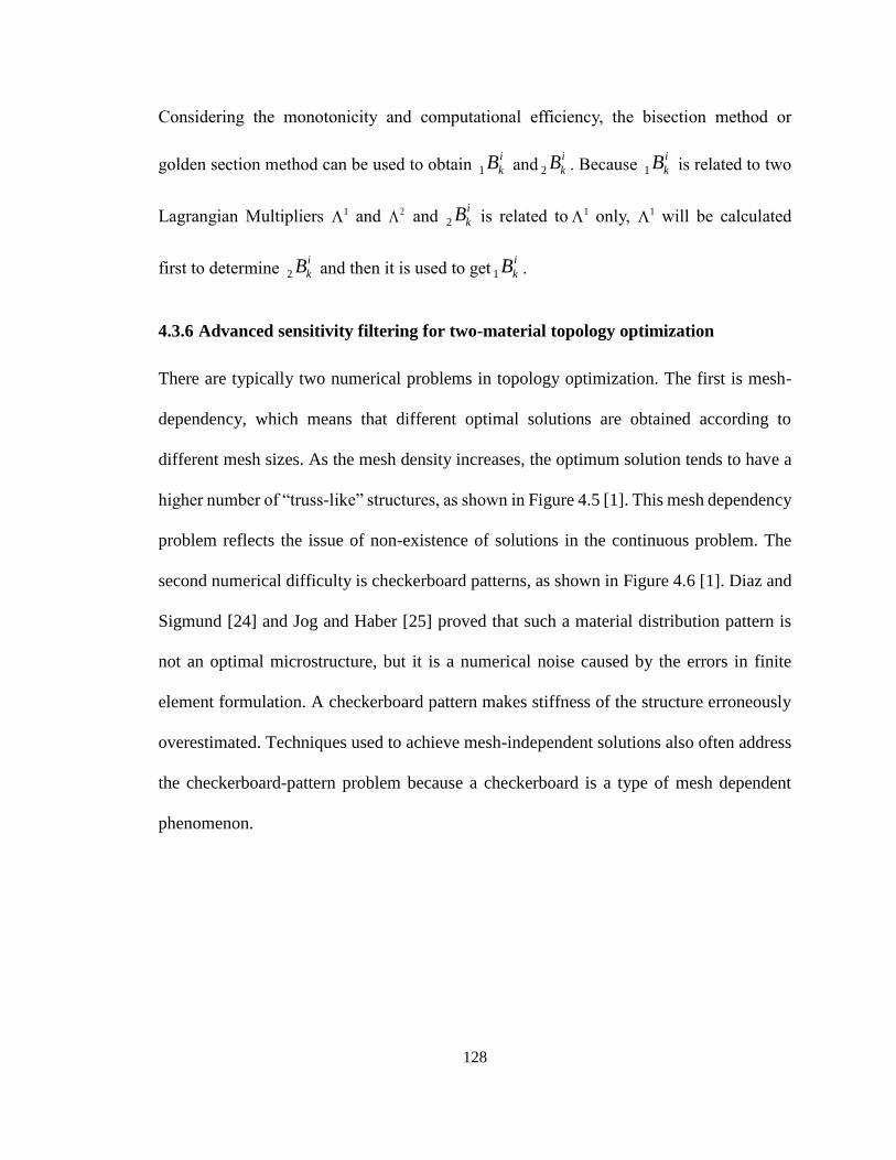
128

Considering the monotonicity and computational efficiency, the bisection method or

golden section method can be used to obtain 1

i

kB and 2

i

kB . Because 1

i

kB is related to two

Lagrangian Multipliers 1 and 2 and 2

i

kB is related to 1 only, 1 will be calculated

first to determine 2

i

kB and then it is used to get 1

i

kB .

4.3.6 Advanced sensitivity filtering for two-material topology optimization

There are typically two numerical problems in topology optimization. The first is mesh-

dependency, which means that different optimal solutions are obtained according to

different mesh sizes. As the mesh density increases, the optimum solution tends to have a

higher number of “truss-like” structures, as shown in Figure 4.5 [1]. This mesh dependency

problem reflects the issue of non-existence of solutions in the continuous problem. The

second numerical difficulty is checkerboard patterns, as shown in Figure 4.6 [1]. Diaz and

Sigmund [24] and Jog and Haber [25] proved that such a material distribution pattern is

not an optimal microstructure, but it is a numerical noise caused by the errors in finite

element formulation. A checkerboard pattern makes stiffness of the structure erroneously

overestimated. Techniques used to achieve mesh-independent solutions also often address

the checkerboard-pattern problem because a checkerboard is a type of mesh dependent

phenomenon.

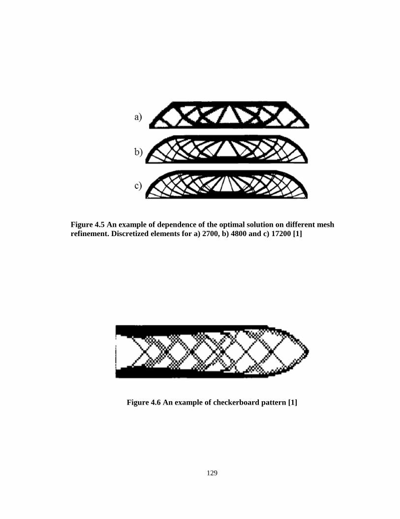
129

Figure 4.5 An example of dependence of the optimal solution on different mesh

refinement. Discretized elements for a) 2700, b) 4800 and c) 17200 [1]

Figure 4.6 An example of checkerboard pattern [1]

130

Several methods have been proposed to overcome these numerical difficulties. Perimeter

control [26] constrains the number of holes inside the structure, and density slope control

[27] constrains the local slope of the element densities. Sensitivity Filtering [28] uses a

weighted average of the sensitivities of neighbor elements. Because the sensitivity filtering

approach directly uses the sensitivity information derived for optimization, there is no extra

constraint brought into the optimization problem. A minimum member size of the structure,

which is often considered as a manufacturing constraint, can be also controlled via the

selection of the filtering radius.

A standard sensitivity filtering algorithm for minimum compliance topology optimization

with two materials is formulated as:

1 2

1 11 1 2 21 2

1 1

min min

ˆ ˆ1 1ˆ ˆ ˆ ˆ

ˆ ( , ), | ( , )

Q Qe e

e eQ Qi e i ei ie e

e e

e e

i

C C C CH H

H H

H r dist i e e Q dist i e r

(4.18)

where minr is the sensitivity filtering radius, elements i and e are the adjacent elements within

the radius. The index i is used to represent the target element for which the filtered

sensitivity is sought, and the index e is used for adjacent elements of the target element.

( , )dist i e denotes the distance between the target element i and the neighbor element e.

The sensitivity filtering method that uses a fixed filtering radius can effectively solve

simple problems such as 2D cantilever or MBB problems. In real-worlds problems that

have complex geometries and multiple types of elements, however, the filtering radius-

based approach could cause difficulties in numerical implementation. First, it is usually

131

difficult and time consuming to identify the neighboring elements within a prescribed

filtering radius when dealing with 3D structures that have complex, non-uniform mesh,

and multiple element types. Second, the number of neighboring elements within a filtering

radius can vary significantly according to the density of mesh in that area.

In our study, we chose neighbor elements based on “layers” instead of a “radius”. Figure

4.7 shows the selection of neighbor elements of a target element for 2D and 3D geometries.

Direct neighbor elements that share a side (for 2D) or a surface (for 3D) are shown in green,

and indirect neighbor elements that share a vertex (for 2D) or an edge (for 3D) are shown

in yellow. We considered both types to be neighbor elements. The modified filtered

sensitivity scheme is formulated as:

1 2

1 11 1 2 21 2

1 1

max

ˆ ˆ1 1ˆ ˆ ˆ ˆ

ˆ , |

e e

e e

e

Q QL Le e

e eQ Qi e i eL Li ie ee e

e e

L

e e e

C C C CH H

H H

H L e Q L L

(4.19)

where maxL indicates a prescribed number of layers for filtering, Q is the total number of

the adjacent elements within the maxL layer(s) from the target element i. eL is the number

of the layer where the respective neighbor element belongs to. For example, 1ˆ 1eH will be

used for all neighbor elements in the first layer and 2ˆ 2eH for all neighbor elements in the

second layer, if maxL = 2.

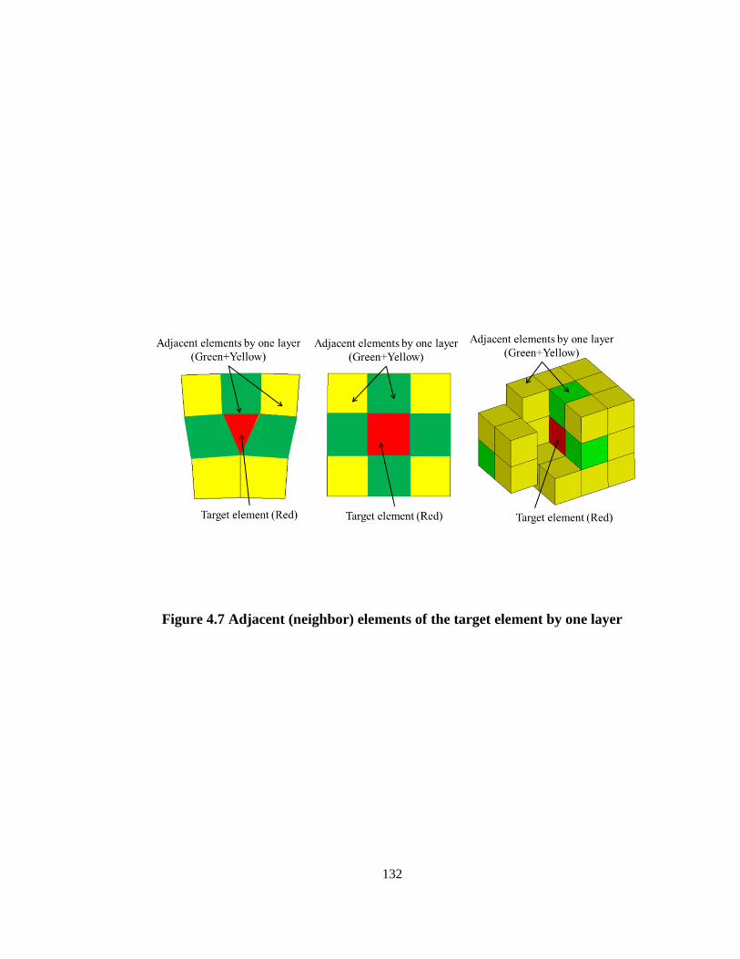
132

Figure 4.7 Adjacent (neighbor) elements of the target element by one layer

133

4.4 Numerical Implementation of Two-Material Topology Optimization

For simple design problems, it is possible and also practical to prepare in-house software

programs for all tasks required for multi-material topology optimization, including pre-

processor (including meshing), finite element analysis, post-processor, and optimization.

For real-world engineering problems, on the other hand, it is impractical to write in-house

codes for all these tasks because we have to deal with complex 3D geometries, loads, and

boundary conditions. In addition, it is less effective for technology transfer from academia

to industry if we stick to in-house codes–which are often limited to particular types of

physics and problems–for numerical tasks that currently available commercial software

can readily deal with.

For the actual case studies, we utilized a commercial software program for all finite element

analysis tasks; and for multi-material optimization which commercial programs cannot

solve, we implemented our own optimization platform. Figure 4.8 shows the flowchart and

use of software programs for each task. The OC (Optimality Criteria) method was

implemented and used.

We used Altair HyperMesh as a preprocessor to discretize the geometry, to assign material

and element properties, and to define boundary conditions and loads. RADIOSS was used

as the FE (finite element) solver, and HyperView was used as a postprocessor for

visualization of results. All these modules are integrated onto our optimization platform

which is written in a HyperWorks programming script language, HyperMath.

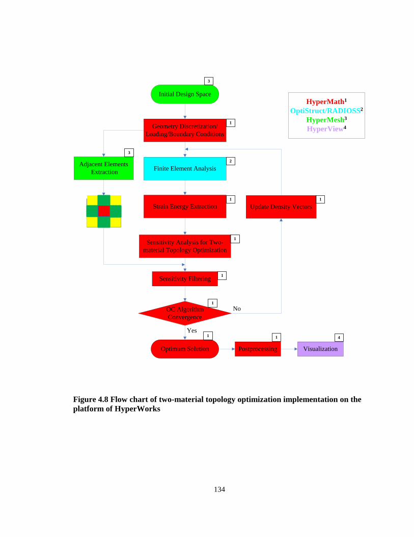
134

Geometry Discretization/

Loading/Boundary Conditions

Initial Design Space

Finite Element Analysis

Sensitivity Analysis for Two-

material Topology Optimization

OC Algorithm

Convergence

Optimum Solution

Update Density Vectors

No

Yes

Sensitivity Filtering

Strain Energy Extraction

Postprocessing Visualization

Adjacent Elements

Extraction

HyperMath1

OptiStruct/RADIOSS2

HyperMesh3

HyperView41

1 1

1

1

1

4

2

3

3

1 1

Figure 4.8 Flow chart of two-material topology optimization implementation on the

platform of HyperWorks

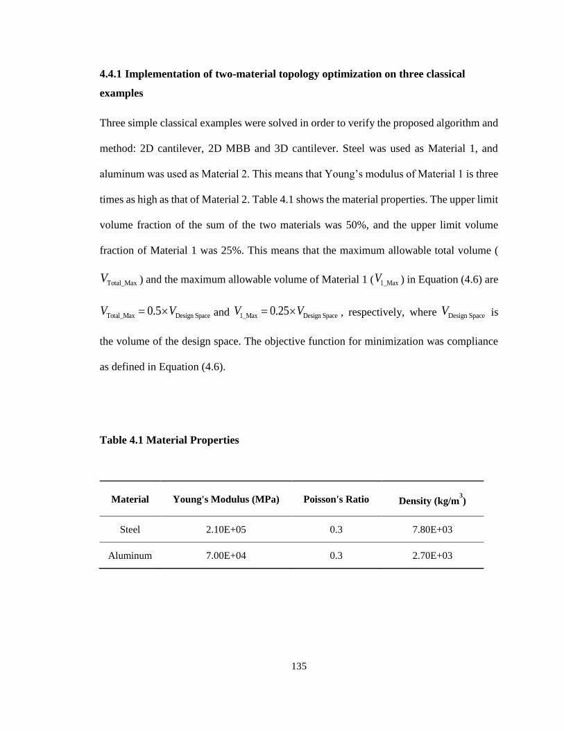
135

4.4.1 Implementation of two-material topology optimization on three classical

examples

Three simple classical examples were solved in order to verify the proposed algorithm and

method: 2D cantilever, 2D MBB and 3D cantilever. Steel was used as Material 1, and

aluminum was used as Material 2. This means that Young’s modulus of Material 1 is three

times as high as that of Material 2. Table 4.1 shows the material properties. The upper limit

volume fraction of the sum of the two materials was 50%, and the upper limit volume

fraction of Material 1 was 25%. This means that the maximum allowable total volume (

Total_MaxV ) and the maximum allowable volume of Material 1 ( 1_MaxV ) in Equation (4.6) are

Total_Max Design Space0.5V V and 1_Max Design Space0.25V V , respectively, where Design SpaceV is

the volume of the design space. The objective function for minimization was compliance

as defined in Equation (4.6).

Table 4.1 Material Properties

Material Young's Modulus (MPa) Poisson's Ratio Density (kg/m3)

Steel 2.10E+05 0.3 7.80E+03

Aluminum 7.00E+04 0.3 2.70E+03

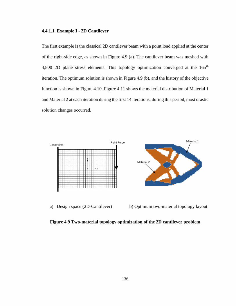
136

4.4.1.1. Example I - 2D Cantilever

The first example is the classical 2D cantilever beam with a point load applied at the center

of the right-side edge, as shown in Figure 4.9 (a). The cantilever beam was meshed with

4,800 2D plane stress elements. This topology optimization converged at the 165th

iteration. The optimum solution is shown in Figure 4.9 (b), and the history of the objective

function is shown in Figure 4.10. Figure 4.11 shows the material distribution of Material 1

and Material 2 at each iteration during the first 14 iterations; during this period, most drastic

solution changes occurred.

Point ForceConstraints

Material 1

Material 2

a) Design space (2D-Cantilever) b) Optimum two-material topology layout

Figure 4.9 Two-material topology optimization of the 2D cantilever problem

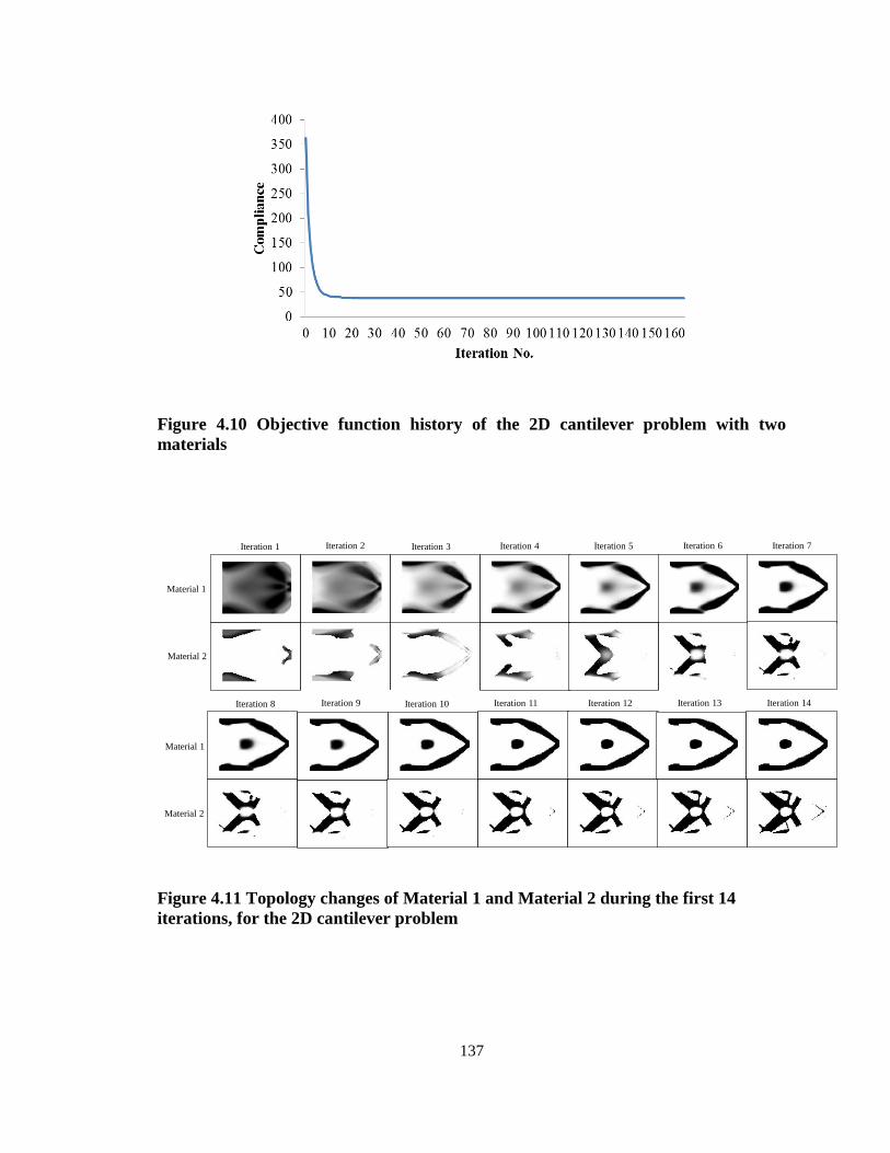
137

Figure 4.10 Objective function history of the 2D cantilever problem with two

materials

Iteration 1 Iteration 2 Iteration 3 Iteration 4 Iteration 5 Iteration 6 Iteration 7

Material 1

Material 2


Material 1

Material 2

Figure 4.11 Topology changes of Material 1 and Material 2 during the first 14

iterations, for the 2D cantilever problem

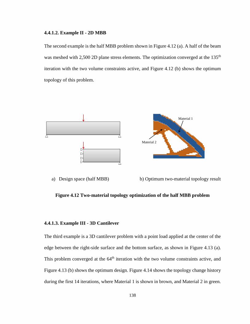
138

4.4.1.2. Example II - 2D MBB

The second example is the half MBB problem shown in Figure 4.12 (a). A half of the beam

was meshed with 2,500 2D plane stress elements. The optimization converged at the 135th

iteration with the two volume constraints active, and Figure 4.12 (b) shows the optimum

topology of this problem.

Material 1

Material 2

a) Design space (half MBB) b) Optimum two-material topology result

Figure 4.12 Two-material topology optimization of the half MBB problem

4.4.1.3. Example III - 3D Cantilever

The third example is a 3D cantilever problem with a point load applied at the center of the

edge between the right-side surface and the bottom surface, as shown in Figure 4.13 (a).

This problem converged at the 64th iteration with the two volume constraints active, and

Figure 4.13 (b) shows the optimum design. Figure 4.14 shows the topology change history

during the first 14 iterations, where Material 1 is shown in brown, and Material 2 in green.

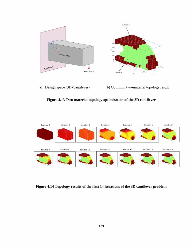
139

Point Force

Material 1

Material 2

a) Design space (3D-Cantilever) b) Optimum two-material topology result

Figure 4.13 Two-material topology optimization of the 3D cantilever



Figure 4.14 Topology results of the first 14 iterations of the 3D cantilever problem

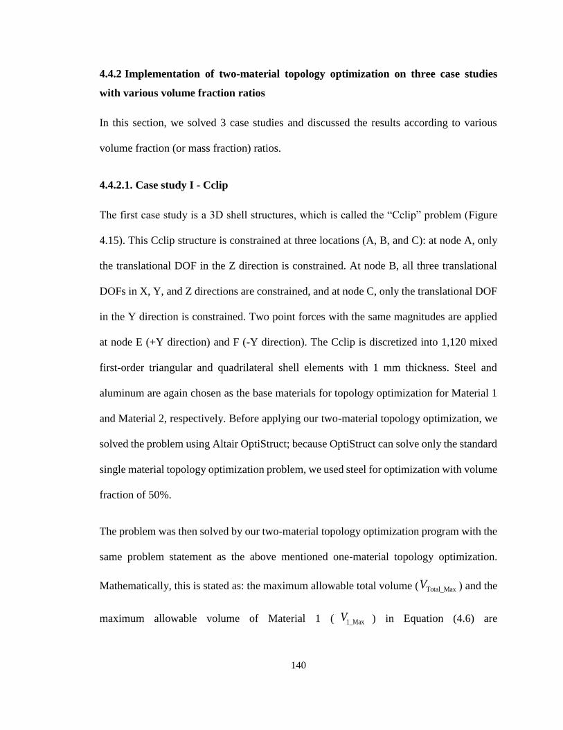
140

4.4.2 Implementation of two-material topology optimization on three case studies

with various volume fraction ratios

In this section, we solved 3 case studies and discussed the results according to various

volume fraction (or mass fraction) ratios.

4.4.2.1. Case study I - Cclip

The first case study is a 3D shell structures, which is called the “Cclip” problem (Figure

4.15). This Cclip structure is constrained at three locations (A, B, and C): at node A, only

the translational DOF in the Z direction is constrained. At node B, all three translational

DOFs in X, Y, and Z directions are constrained, and at node C, only the translational DOF

in the Y direction is constrained. Two point forces with the same magnitudes are applied

at node E (+Y direction) and F (-Y direction). The Cclip is discretized into 1,120 mixed

first-order triangular and quadrilateral shell elements with 1 mm thickness. Steel and

aluminum are again chosen as the base materials for topology optimization for Material 1

and Material 2, respectively. Before applying our two-material topology optimization, we

solved the problem using Altair OptiStruct; because OptiStruct can solve only the standard

single material topology optimization problem, we used steel for optimization with volume

fraction of 50%.

The problem was then solved by our two-material topology optimization program with the

same problem statement as the above mentioned one-material topology optimization.

Mathematically, this is stated as: the maximum allowable total volume ( Total_MaxV ) and the

maximum allowable volume of Material 1 ( 1_MaxV ) in Equation (4.6) are

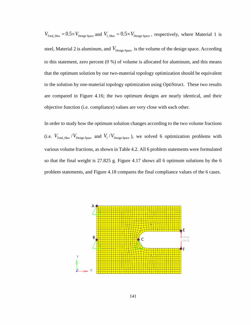
141

Total_Max Design Space0.5V V and 1_Max Design Space0.5V V , respectively, where Material 1 is

steel, Material 2 is aluminum, and Design SpaceV is the volume of the design space. According

to this statement, zero percent (0 %) of volume is allocated for aluminum, and this means

that the optimum solution by our two-material topology optimization should be equivalent

to the solution by one-material topology optimization using OptiStruct. These two results

are compared in Figure 4.16; the two optimum designs are nearly identical, and their

objective function (i.e. compliance) values are very close with each other.

In order to study how the optimum solution changes according to the two volume fractions

(i.e. Total_Max Design Space/V V and 1 Design Space/V V ), we solved 6 optimization problems with

various volume fractions, as shown in Table 4.2. All 6 problem statements were formulated

so that the final weight is 27.825 g. Figure 4.17 shows all 6 optimum solutions by the 6

problem statements, and Figure 4.18 compares the final compliance values of the 6 cases.

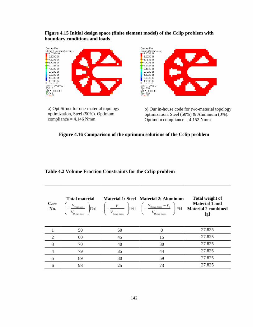
142

Figure 4.15 Initial design space (finite element model) of the Cclip problem with

boundary conditions and loads

Figure 4.16 Comparison of the optimum solutions of the Cclip problem

Table 4.2 Volume Fraction Constraints for the Cclip problem

Case

No.

Total material

Total_Max

Design Space

[%]V

V

Material 1: Steel

1

Design Space

[%]V

V

Material 2: Aluminum

Design Space 1

Design Space

[%]V V

V

Total weight of

Material 1 and

Material 2 combined

[g]

1 50 50 0 27.825

2 60 45 15 27.825

3 70 40 30 27.825

4 79 35 44 27.825

5 89 30 59 27.825

6 98 25 73 27.825

a) OptiStruct for one-material topology

optimization, Steel (50%). Optimum

compliance = 4.146 Nmm

b) Our in-house code for two-material topology

optimization, Steel (50%) & Aluminum (0%).

Optimum compliance = 4.152 Nmm

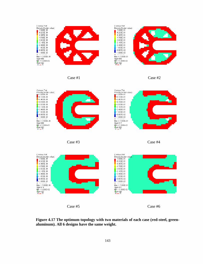
143

Case #1 Case #2

Case #3 Case #4

Case #5 Case #6

Figure 4.17 The optimum topology with two materials of each case (red-steel, green-

aluminum). All 6 designs have the same weight.

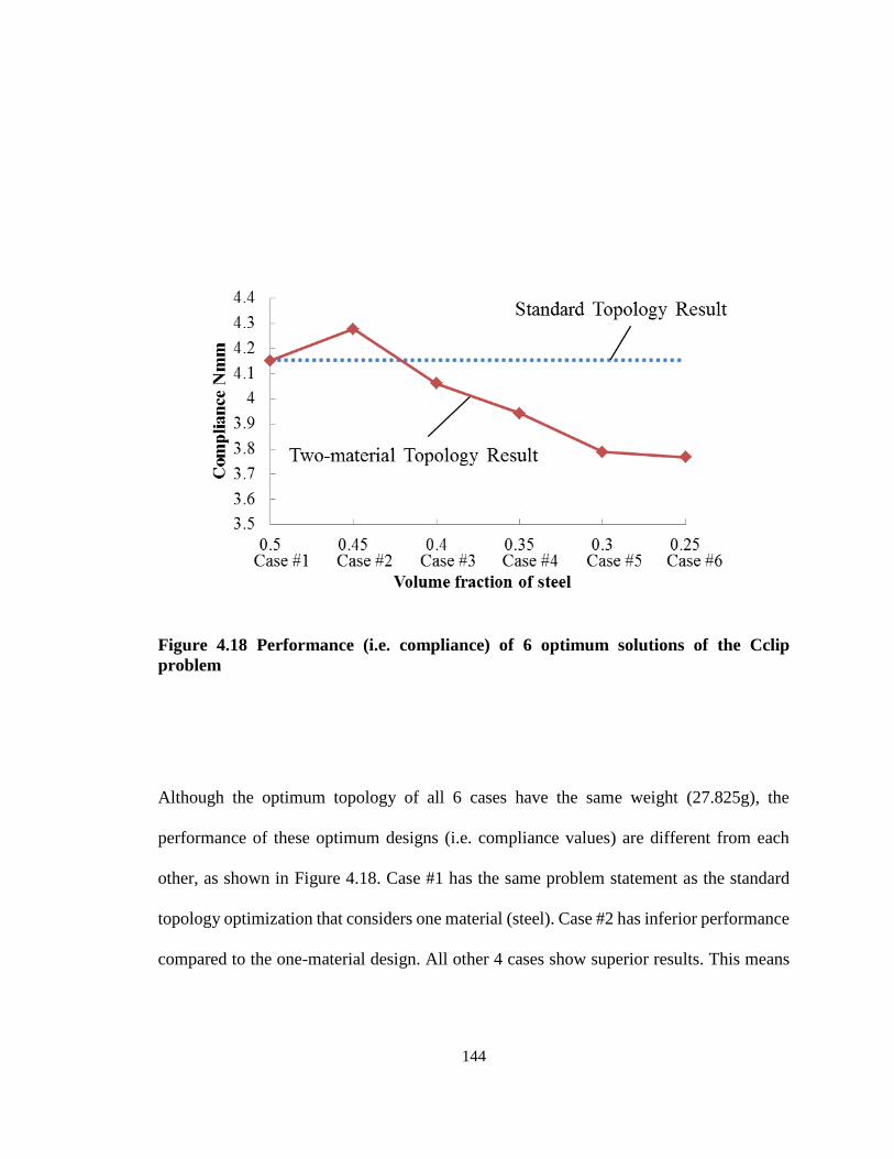
144

Figure 4.18 Performance (i.e. compliance) of 6 optimum solutions of the Cclip

problem

Although the optimum topology of all 6 cases have the same weight (27.825g), the

performance of these optimum designs (i.e. compliance values) are different from each

other, as shown in Figure 4.18. Case #1 has the same problem statement as the standard

topology optimization that considers one material (steel). Case #2 has inferior performance

compared to the one-material design. All other 4 cases show superior results. This means

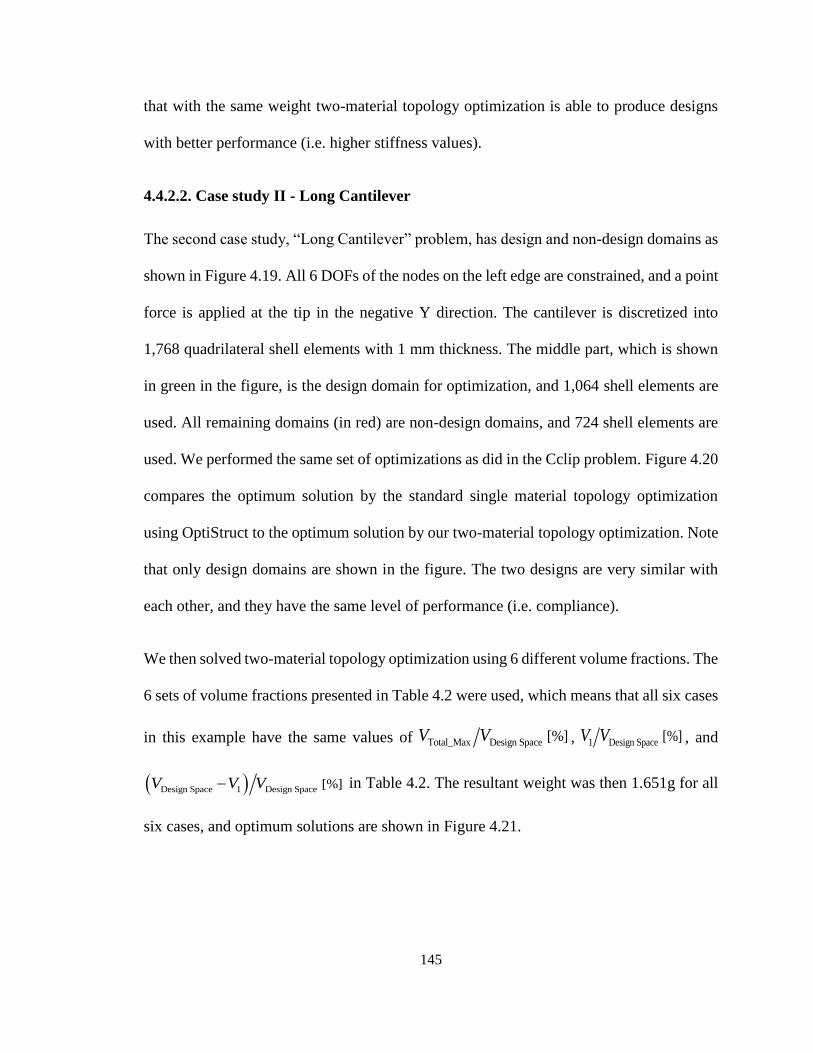
145

that with the same weight two-material topology optimization is able to produce designs

with better performance (i.e. higher stiffness values).

4.4.2.2. Case study II - Long Cantilever

The second case study, “Long Cantilever” problem, has design and non-design domains as

shown in Figure 4.19. All 6 DOFs of the nodes on the left edge are constrained, and a point

force is applied at the tip in the negative Y direction. The cantilever is discretized into

1,768 quadrilateral shell elements with 1 mm thickness. The middle part, which is shown

in green in the figure, is the design domain for optimization, and 1,064 shell elements are

used. All remaining domains (in red) are non-design domains, and 724 shell elements are

used. We performed the same set of optimizations as did in the Cclip problem. Figure 4.20

compares the optimum solution by the standard single material topology optimization

using OptiStruct to the optimum solution by our two-material topology optimization. Note

that only design domains are shown in the figure. The two designs are very similar with

each other, and they have the same level of performance (i.e. compliance).

We then solved two-material topology optimization using 6 different volume fractions. The

6 sets of volume fractions presented in Table 4.2 were used, which means that all six cases

in this example have the same values of Total_Max Design Space [%]V V , 1 Design Space [%]V V , and

Design Space 1 Design Space [%]V V V in Table 4.2. The resultant weight was then 1.651g for all

six cases, and optimum solutions are shown in Figure 4.21.

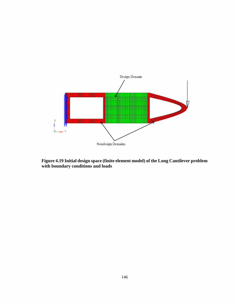
146

Figure 4.19 Initial design space (finite element model) of the Long Cantilever problem

with boundary conditions and loads

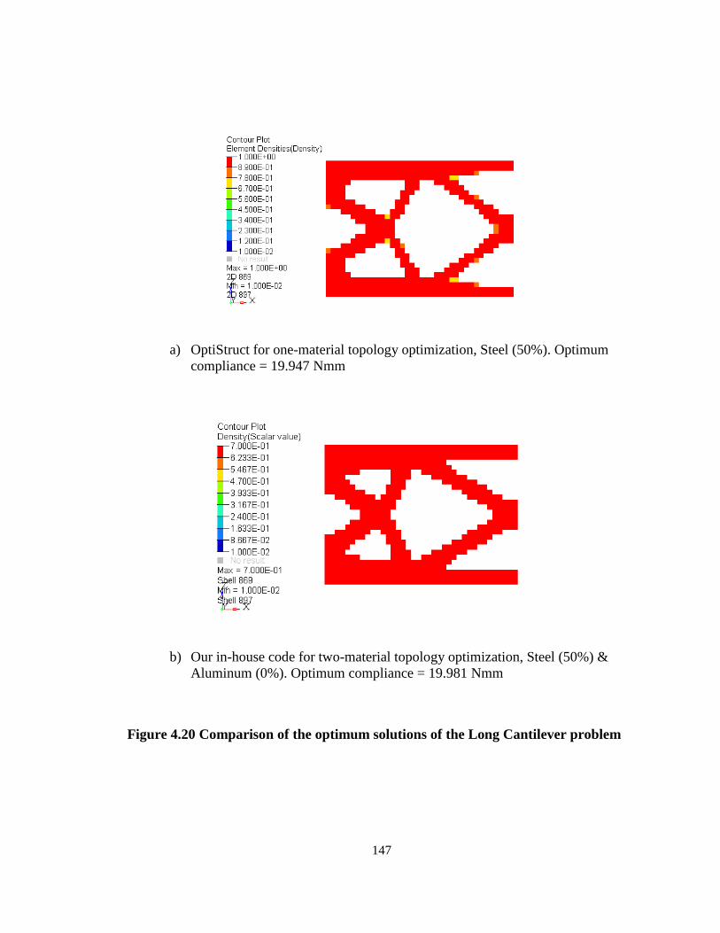
147

a) OptiStruct for one-material topology optimization, Steel (50%). Optimum


b) Our in-house code for two-material topology optimization, Steel (50%) &

Aluminum (0%). Optimum compliance = 19.981 Nmm

Figure 4.20 Comparison of the optimum solutions of the Long Cantilever problem

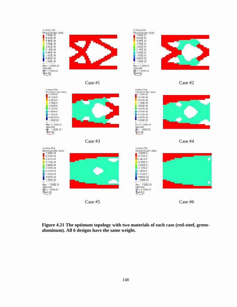
148

Case #1 Case #2

Case #3 Case #4

Case #5 Case #6



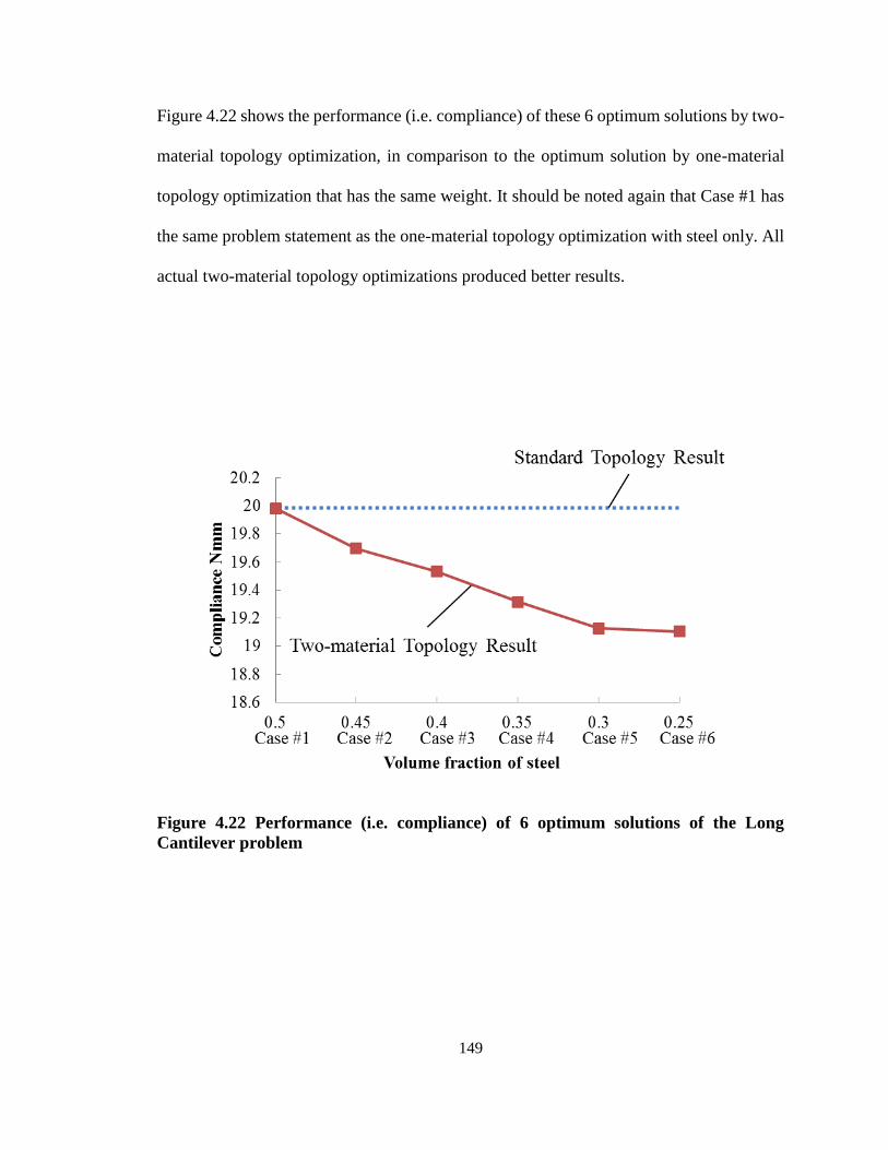
149

Figure 4.22 shows the performance (i.e. compliance) of these 6 optimum solutions by two-

material topology optimization, in comparison to the optimum solution by one-material

topology optimization that has the same weight. It should be noted again that Case #1 has

the same problem statement as the one-material topology optimization with steel only. All

actual two-material topology optimizations produced better results.

Figure 4.22 Performance (i.e. compliance) of 6 optimum solutions of the Long

Cantilever problem

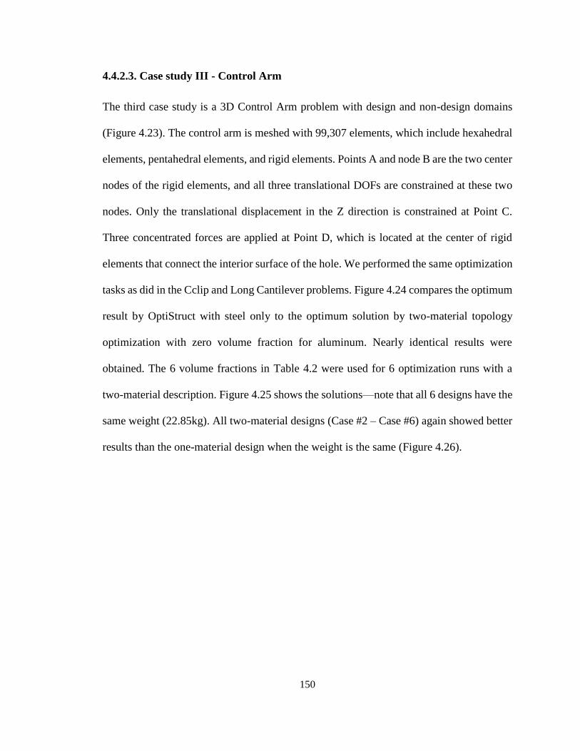
150

4.4.2.3. Case study III - Control Arm

The third case study is a 3D Control Arm problem with design and non-design domains

(Figure 4.23). The control arm is meshed with 99,307 elements, which include hexahedral

elements, pentahedral elements, and rigid elements. Points A and node B are the two center

nodes of the rigid elements, and all three translational DOFs are constrained at these two

nodes. Only the translational displacement in the Z direction is constrained at Point C.

Three concentrated forces are applied at Point D, which is located at the center of rigid

elements that connect the interior surface of the hole. We performed the same optimization

tasks as did in the Cclip and Long Cantilever problems. Figure 4.24 compares the optimum

result by OptiStruct with steel only to the optimum solution by two-material topology

optimization with zero volume fraction for aluminum. Nearly identical results were

obtained. The 6 volume fractions in Table 4.2 were used for 6 optimization runs with a

two-material description. Figure 4.25 shows the solutions—note that all 6 designs have the

same weight (22.85kg). All two-material designs (Case #2 – Case #6) again showed better

results than the one-material design when the weight is the same (Figure 4.26).

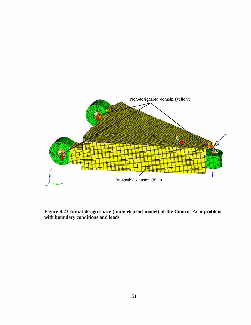
151

Figure 4.23 Initial design space (finite element model) of the Control Arm problem

with boundary conditions and loads

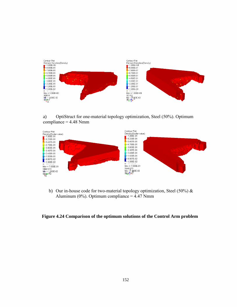
152

a) OptiStruct for one-material topology optimization, Steel (50%). Optimum


b) Our in-house code for two-material topology optimization, Steel (50%) &

Aluminum (0%). Optimum compliance = 4.47 Nmm

Figure 4.24 Comparison of the optimum solutions of the Control Arm problem

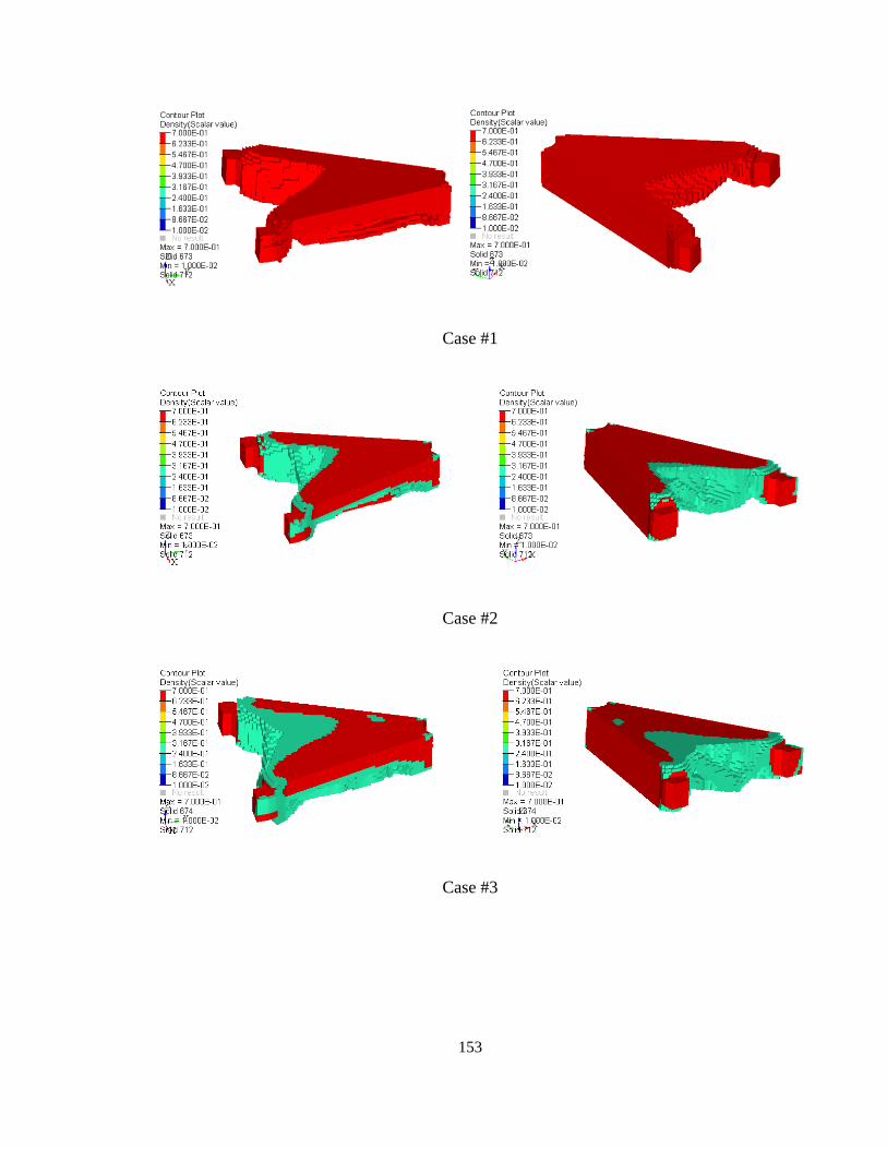
153

Case #1

Case #2

Case #3

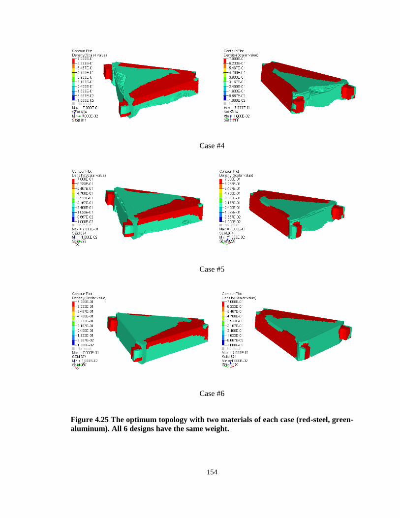
154

Case #4

Case #5

Case #6



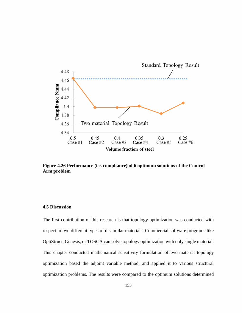
155

Figure 4.26 Performance (i.e. compliance) of 6 optimum solutions of the Control

Arm problem

4.5 Discussion

The first contribution of this research is that topology optimization was conducted with

respect to two different types of dissimilar materials. Commercial software programs like

OptiStruct, Genesis, or TOSCA can solve topology optimization with only single material.

This chapter conducted mathematical sensitivity formulation of two-material topology

optimization based the adjoint variable method, and applied it to various structural

optimization problems. The results were compared to the optimum solutions determined

156

by the standard single-material topology optimization. All three case studies showed that

two-material topology optimization can determine stiffer optimum designs than one-

material topology optimization, for a prescribed weight constraint. With this finding, we

can numerically confirm that two-material topology optimization can find lighter designs

than one-material topology optimization, for prescribed stiffness constraints.

The second contribution is that this chapter demonstrated that all tasks for multi-material

topology optimization could be conducted on a commercial software platform. We are

doing collaborative research projects with many automotive and aerospace companies, and

“technology transfer” is a very important aspect in the collaboration. For industry, it is of

little use if all tasks are implemented in the form of in-house codes, because pre- and post-

processors of in-house codes are not as powerful or user friendly as those by commercial

programs and also because commercial FEA solvers can deal with a wide variety of

engineering problems when most in-house codes cannot. We fully utilized HyperMesh,

HyperView, and RADIOSS, and all our mathematical optimization algorithms were

written in HyperMath. This means that our tool can solve problems that have complex

geometries, and complicated boundary conditions and loads.

4.6 Limitations and Future Work

The most important limitation of this study is that a user has to explicitly allocate a volume

fraction for each of Material 1 and Material 2. It would be more practical if there is only

one final weight constraint (i.e. total weight of Material 1 and Material 2 combined

together), and the optimizer automatically determines the optimum weight distribution

between Material 1 and Material 2 while minimizing compliance. Its dual problem, which

157

minimizes the total weight with stiffness constraints would be even more practical for

industry users. This requires more mathematical formulation and algorithm development,

and it is reserved as our immediate future work.

158

ACKNOWLEDGEMENT

Authors would like to thank Justin Gammage, Balbir Sangha, and colleagues at General

Motors of Canada for their technical advice and direction.

REFERENCES

[1] Bendsøe MP, Sigmund O. Topology Optimization: Theory, Methods and

Applications, Springer 2003.

[2] Cheng G.D, Olhoff N. An investigation concerning optimal design of solid elastic

plates. International Journal of Solids and Structures, 1982; 18: pp. 153-170, DOI:

10.1016/0020-7683(81)90065-2.

[3] Bendsoe MP, Kikuchi N. Generating Optimal Topology in Structural Design Using

a Homogenization Method. Computer Methods in Applied Mechanics and

Engineering, 1988; 71: 197-224, DOI: 10.1016/0045-7825(88)90086-2.

[4] Zhou M, Rozvany G. The COC algorithm, part II: Topological, geometry and

generalized shape optimization. Comput Methods Appl Mech Eng, 1991; 89: 309-

336, DOI: 10.1016/0045-7825(91)90046-9.

[5] Rozvany G, Bendsøe MP, Kirsch U. Layout optimization of structures. Applied

Mechanics Reviews, 1995, 48(2): 41-119, DOI:10.1115/1.3005097.

[6] Stolpe M, Svanberg K. An alternative interpolation scheme for minimum compliance

topology optimization. Struct Multidisc Optim, 2011; 22: 116-124, DOI:

10.1007/s001580100129.

[7] Kim IY, de Weck O. Variable Chromosome Length Genetic Algorithm for

Progressive Refinement in Topology Optimization. Structural and Multidisciplinary

Optimization, 2005: 29: 445-456.

[8] Kim SY, Kim IY, Mechefske C. A New Efficient Convergence Criterion for

Reducing Computational Expense in Topology Optimization: Reducible Design

Variable Method. International Journal for Numerical Methods in Engineering,

2012: 90: 752–783.


159

[9] Cristello N, Kim IY. Multidisciplinary design optimization of a zero emission vehicle

chassis considering crashworthiness and hydroformability. Proceedings of the

Institution of Mechanical Engineers, Part D, Journal of Automobile Engineering,

2007; 221: 511-526.

[10] Li C, Kim IY. Topology, size and shape optimization of an automotive cross car

beam. Proceedings of the Institution of Mechanical Engineers, Part D, Journal of

Automobile Engineering. Currently published online. DOI:

10.1177/0954407014561279.

[11] Li C, Kim IY, Jeswiet J. Conceptual and detailed design of an automotive engine

cradle by using topology, shape, and size optimization. Structural and

Multidisciplinary Optimizatio, 2015; 51(2): 547-564, DOI: 10.1007/s00158-014-

1151-6.

[12] Woisetschlaeger E. Keine Monokultur. Automobile Entwicklung, 2001, pp. 130.

[13] Wallentowitz H. Structural Design of Vehicles. Institute fur Kraftfahrwesen, 2004,

Aachen.

[14] Ramani A. A Pseudo-sensitivity Based Discrete-variable Approach To Structural

Topology Optimization With Multiple Materials. Struc Multidisc Optim, 2010;

41:913-934. DOI 10.1007/s00158-009-0455-4.

[15] Huang X, Xie YM. Bi-directional evolutionary topology optimization of continuum

structures with one or multiple materials. Comput Mech, 2009; 43:393-401.

[16] Saxena A. Topology design of large displacement compliant mechanisms with

multiple materials and multiple output ports, Struct Multidisc Optim, 2005; 30: 477-

490. DOI 10.1007/s00158-005-0535-z.

[17] Han SY, Lee SK, Development of a Material Mixing Method Based on Evolutionary

Structural Optimization. JSME International Journal Series A, 2005; 48(3): 132-135.

[18] Stegmann J, Lund E. Discrete material optimization of general composite shell

structures, Int. J. Numer. Mech. Engng, 2005; 62: 2009-2027.

DOI: 10.1002/nme.1259.

[19] Yin L, Ananthasuresh GK, Topology optimization of compliant mechanisms with

multiple materials using a peak function material interpolation scheme, Struct

Multidisc Optim, 2001; 23: 49-62. DOI: 10.1007/s00158-001-0165-z.

[20] Yoon, GH. Topology optimization for nonlinear dynamic problem with multiple

materials and material-dependent boundary condition. Finite Elements in Analysis

and Design, 2011;47(7):753-763.

160

[21] Stegmann, J., and Erik L. Discrete material optimization of general composite shell

structures. International Journal for Numerical Methods in Engineering, 2005;

62(14): 2009-2027.

[22] Gao, T., and Zhang WH. A mass constraint formulation for structural topology

optimization with multiphase materials. International Journal for Numerical

Methods in Engineering, 2011; 88(8): 774-796.

[23] Thomsen, J. Topology optimization of structures composed of one or two

materials. Structural optimization, 1992; 5(1-2): 108-115.

[24] Diaz AR, Sigmund O. Checkerboard patterns in layout optimization. Struct. Optim,

1995; 10, 40-45.

[25] Jog, CS, Haber, RB. Stability of finite element model for distributed parameter

optimization and topology design. Comp. Mech. Appl. Mech. Engrg, 1996; 130, 203-

226. DOI: 10.1016/0045-7825(95)00928-0.

[26] Haber RB, Jog CS, Bendsøe MP. A new approach to variable topology shape design

using a constraint on perimeter. Struct Optim, 1996; 11: 1-12.

[27] Sigmund O, Petersson J. Slope constrained topology optimization. Int J Number

Methods Eng, 1998; 41(8):1417-1434.

[28] Sigmund O. On the design of compliant mechanisms using topology optimization.

Mechan Struct Mach, 1997; 25(4): 495-526.

161

Chapter 5

General Discussion

This thesis discussed the theory, algorithm, numerical implementation, and application of

both standard single-material topology optimization and advanced multi-material topology

optimization. The effectiveness, efficiency, and contributions of the developed

methodology have been demonstrated through the study of a variety of engineering

problems. This research will not only benefit the theoretical development of topology

optimization, but will also have a significant effect on industrial applications. As opposed

to previous research, which only discussed simple benchmark problems, this thesis

distinguishes itself by closely integrating academic research and real-world engineering

problems to advance the structural design process for industry.

In Chapter 2, an effective and efficient design process framework for an automotive engine

cradle was presented by using topology, shape, and size optimization. Standard single-

material topology optimization was introduced to the preliminary design stage to find the

optimum material distribution for the desired detailed design. The proposed design

framework benefited our industrial partner by cutting the original design time in half.

Further, a design initiated from topology optimization is more objective and reliable, and

this proposed design methodology could be easily extended to the design of products in

other industries.

162

In Chapter 3, a lightweight design using lightweight material, structural optimization, and

advanced manufacturing techniques for an automotive CCB was discussed. The design

framework proposed in Chapter 2 was adopted for the development of this CCB, and

promising weight reduction and cost savings were achieved. Additionally, an innovative

simulation method was developed to approach the performance of a real SCSWS, which

successfully addressed the dilemma that a CCB supplier usually confronts: how to achieve

the optimum design of a CCB when detailed information about the SCSWS is not available.

In Chapter 4, topology optimization using two dissimilar materials was conducted to

accommodate the increasing demands from industry. Due to the difficulty in theoretical

development and numerical implementation, none of current commercial tools have solved

multi-material topology optimization problems. This chapter, as a breakthrough, discussed

the mathematical formulations of two-material topology optimization and successfully

implemented it to address various structural optimization problems. The results showed

that advanced two-material topology optimization could achieve more favorable designs

than standard single-material topology optimization. Specialists from our industrial partner

successfully tested our in-house tool and the technology-transfer effect between academia

and industry was substantial and profound.

Although this thesis attempted to cover all the work I have done for my PhD study, some

work was, unfortunately, not able to be presented for reasons of coherence, logic, and

confidentiality.

163

Chapter 6

Future Work

The work discussed in this thesis serves as the cornerstone for the advancement of topology

optimization and provides for a variety of promising research directions.

Current research on standard single-material topology optimization faces the dilemma of

how to improve the performance of product design and reduce the computational cost. High

fidelity and smooth-edged topology results with less, or even without any, geometric

reinterpretation is the ultimate goal, but this goal is currently constrained by the

computational capabilities and the financial tolerance of a company. Examining how to

effectively maintain manageable computational costs would be a promising direction for

future research.

Current research on multi-material topology optimization is limited in its ability to solve

compliance-minimization problems, which require designers to pre-allocate volume

fractions for different materials. To achieve a favorable design that satisfies all the

performance requirements, optimization might be performed more than once for the

purpose of tuning the volume fractions. Therefore, multi-material topology optimization

for weight-minimization would be a promising and exciting direction for industrial

engineers. Moreover, only metallic materials (steel and aluminum) were used in previous

studies. By introducing more non-metallic materials, like plastic, polymer, or carbon fiber,

164

into multi-material topology optimization, a revolutionary change to engineering design is

foreseeable.

Further, only a few manufacturing processes (e.g., extrusion and draw) have been

incorporated into current single-material and multi-material topology optimization.

Without considering manufacturability at an early design stage, topology results might

suffer from inferior designs that need an extensive geometric reinterpretation, which

impairs the strength of introducing topology optimization into the design framework.

Hence, the question of how to effectively incorporate more manufacturing processes into

topology optimization is drawing great research interest.

It is believed that more feasible research directions can be discovered and carried out to

advance topology optimization, and the growing influence of topology optimization in

structural design can be readily foreseen in various industrial fields.

165

Appendix A

In-house Tool of Multi-material Topology Optimization

The developed in-house tool for solving multi-material topology optimization problems is

programmed on HyperMath platform and contains about 4,000 lines. As a courtesy, main

code is shown as follows:

/////// Two-Material Topology Optimization/////////////

/////// Interface to .fem file defined by HyperMesh, ESE should be set as an output //////

////// The Filepath and FEAfile names will be modified if needed /////

////// Comments with '***' means this line could be modified depending on different models //////

////// If adjacent elements are needed for Sensitivity Filtering, then the attachedelements.txt is needed by using the .tcl macro. //////

ClearAll();

ReleaseMemory();

StartTime=CpuTime();

//////////// Definations for .fem File location and name ////////////

global Filepath;

global TOPfile;

global MATfile;

global FEAname;

Filepath="E:/Topology/ToDaoz/SampleModel_and_Code/"; // *** Location of .fem file Note: use backslash '/' here, since

it will be used in <NodesBetweenTwoMats.hml> for converting to .hm

FEAname="cclip2.fem" // *** .fem file name

//////////// Control factors for volfrac and penalty factor ////////////

global volfrac;

global volfracy;

global penal;

global MAXiteration;

volfrac=0.857; // *** Volume Fraction (Mat_1+Mat_2) of entire designable domain

volfracy=0.111; // *** Volume Fraction (Mat_2 only) of designable domain

penal=3; // *** Penalty Factor

MAXiteration=300; // *** Max iteration for OC

//////////// Initialization for the MAX element number and MAX node number //////////////////////////////////

global MAXcomp;

166

global MAXprop;

global MAXmat;

global MAXnode;

global DsgnMATID;

global CompDesignID;

global RBE2NO;

// MAXele=5000; // *** Assign the maximal element NO. to read

MAXnode=1207; // *** Assign the maximal node NO. to read

DsgnMATID=1; // *** MAT ID for designable elements

MAXcomp=30; // *** Assign the maximal component NO. to read

MAXprop=30; // *** Assign the maximal property NO. to read

MAXmat=30; // *** Assign the maximal material NO. to read

CompDesignID=[1]; // *** Designable Component IDs. Will be changed depending on different FE model. Could

be multiple IDs.

RBE2NO=0; // *** No. of RBE2 elements (will be extended to elements who does not have a strain energy) in

the model.

global EST;

global EAL;

global STEEL;

global AL;

EST=2.1e5; EAL=7e4 // *** Predefined INITIAL Young's Modulus for designable elements

STEEL=7.9e-9; AL=2.7e-9 // *** Predefined density for designable elements

//////////// Definations for .hml File (Codes) location and name ////////////

global Codepath;

Codepath="E:\\Topology\\ToDaoz\\SampleModel_and_Code\\HyperMathCode\\" // *** Location of .hml files

FEMrewritten=Codepath+"FEMrewrittenAdv_2D.hml"

// FEMrewrittenGrid=Codepath+"FEMrewrittenGrid.hml"

FEMrewrittenElement=Codepath+"FEMrewrittenElement_2D.hml"

// FEMrewrittenPropMat=Codepath+"FEMrewrittenPropMat.hml"

// AdjacentEle=Codepath+"AdjacentEleAdv2.hml"

AdjacentEle=Codepath+"AdjacentEleAdv2_2D.hml"

//AdjacentEleTest=Codepath+"TestRun_AdjacentElement.hml"

// AdjacentEleFiltered=Codepath+"AdjacentEleAdv2_Filtered.hml"

HyperMathOC=Codepath+"HyperMath_OC.hml"

Include(FEMrewritten)

Include(FEMrewrittenElement)

//FEMrewrittenTime=FEMrewrittenTime2-FEMrewrittenTime1;

//print("FEMwrittenTime:",FEMrewrittenTime);

// Include(AdjacentEle)

Include(AdjacentEle)

Include(HyperMathOC)

//OCTime=CpuTime();

//print("OCTime:",OCTime-FEMrewrittenTime);

167

Density4plot=Codepath+"Density4plot.hml";

Include(Density4plot) // To generate .txt files for ploting in HyperView, and new .fem file with seperate component

number of ST and AL.

TotalTime=CpuTime();

print("TotalElapsedTime:",TotalTime-StartTime);

////// Subroutine: FEMrewrittenAdv_2D.hml ////////

////// FEMrewritten for the new ***TOP.fem file, for 2D shell structure ////////

FEMrewrittenTime1=CpuTime();

////// To read once the original FEA file for gathering COMPONENT, PSHELL AND MAT1 info ///////

CompNo=0; // No. of total component

NodeTable={}; //+++ Store the each nodal coordinate

PropNo=0; PropTable={}; // No. of total Property, store original property in a table

PropMatID=0; // Original Mat ID in the original Prop Card

MatNo=0; MatTable={}; // No. of total Material, store original material in a table

CompInfo=Zeros(MAXcomp,5); // Component info: ComponentID, EleStrtA, EleEndA, EleStrtB, EleEndB (Max number

of row could be changed)

PropInfo=Zeros(MAXprop,2); // Property info: PropertyID, MaterialID (Max number of row could be changed)

MatInfo=Zeros(MAXmat,1); // Material info: MaterialID (Max number of row could be changed)

CompID=0; EleStrt=0; EleEnd=0;

global MaxEleID;

MaxEleStrt=0; MaxEleEnd=0; MaxEleID=0;

MaxEleStrtA=0;MaxEleStrtB=0; MaxEleEndA=0; MaxEleEndB=0;

GRIDPointer=0; ELEPointer=0;

PSOLIDPointer=0; PSHELLPointer=0; MAT1Pointer=0;

global FEAfile;

FEAfile=Filepath+FEAname // Name and location of original .fem file

fidFEAread=Open(FEAfile,'r+'); // Open the original .fem file

fidcomp=fidFEAread::read();

while fidcomp!=nil do

tok, rem=StrTok(fidcomp);

if StrCmp(tok,'$HMMOVE') then

CompID=StrSubrange(fidcomp,9,16)*1;

fidcomp=fidFEAread::read(); // Read next line including '1THRU100'

EleStrt=StrSubrange(fidcomp,9,16)*1; // Record the starting element ID in current component

EleEnd=StrSubrange(fidcomp,25,32); // Record the ending element ID in current component (Could be

empty since there is only one element in this component)

168

if EleEnd==' ' then

EleEnd=0; // If there is only one element in this component, assign 0 to EleEnd.

else

EleEnd=EleEnd*1;

end

if CompInfo(CompID,2)==0 then // To check if CompInfo(CompID,2) has already been filled.

CompInfo(CompID,1)=CompID;

CompInfo(CompID,2)=EleStrt;

CompInfo(CompID,3)=EleEnd;

else // If it has already been filled, then add another group of elements in

CompInfo(CompID,4), CompInfo(CompID,5)

CompInfo(CompID,4)=EleStrt;

CompInfo(CompID,5)=EleEnd;

end

end

CompNo=Max(CompInfo(:,1)); // Record component number

if StrCmp(tok,'PSHELL') then

PropNo=PropNo+1; // Record property number

PropID=StrSubrange(fidcomp,9,16)*1;

PropMatID=StrSubrange(fidcomp,17,24)*1;

PropInfo(PropNo,1)=PropID;

PropInfo(PropNo,2)=PropMatID;

PropTable(PropID)=fidcomp; // ATTENTION: Here using PropID to index PropTable

end

if StrCmp(tok,'MAT1') then

MatNo=MatNo+1; // Record material number

MatID=StrSubrange(fidcomp,9,16)*1;

MatInfo(MatNo)=MatID;

MatTable(MatNo)=fidcomp; // ATTENTION: Here using MatNo to index PropTable

end

fidcomp=fidFEAread::read(); // At the end, CompNo=Max number of comp, PropNo=Max number of Prop, and

MatNo=max number of Mat

end

MaxEleStrtA=Max(CompInfo(:,2)); MaxEleStrtB=Max(CompInfo(:,4));

MaxEleEndA=Max(CompInfo(:,3)); MaxEleEndB=Max(CompInfo(:,5));

MaxEleStrt=Max(MaxEleStrtA,MaxEleStrtB);

MaxEleEnd=Max(MaxEleEndA,MaxEleEndB);

MaxEleID=Max(MaxEleStrt,MaxEleEnd); // Aftering renumbering, element starts with ID 1 and with increment 1. Therefore,

MaxEleID=Total number of elements

Close(fidFEAread);

/////////////////////////////////////////////////////////////////////////////////////////////////////

169

////// To rewrite the original FEA .fem file into Top. fem File //////

////// To rewrite the ELEMENT part //////

CompDesignNo=Max(Size(CompDesignID)); // To get the Max number of designable comps

global DsgnEleNbr;

global NonDsgnEleNbr;

DsgnEleNbr=0;

NonDsgnEleNbr=0;

for i=1,CompDesignNo do

CompID=CompDesignID[i];

if CompInfo(CompID,4)>0 then // If: There are more than two groups of elements in this comp

DsgnEleNbr=DsgnEleNbr+Abs(CompInfo(CompID,3)-CompInfo(CompID,2))+1+Abs(CompInfo(CompID,5)-

CompInfo(CompID,4))+1;

else

DsgnEleNbr=DsgnEleNbr+Abs(CompInfo(CompID,3)-CompInfo(CompID,2))+1;

end

end

NonDsgnEleNbr=MaxEleID-DsgnEleNbr;

DsgnEleInfo=Zeros(DsgnEleNbr,2); //Designable Element info: ElementID, PropertyID (Max number of row could be

changed)

if NonDsgnEleNbr>0 then

NonDsgnEleInfo=Zeros(NonDsgnEleNbr,2); //Non-Designable Element info: ElementID, PropertyID (Max number of row

could be changed)

else

NonDsgnEleInfo=Zeros(DsgnEleNbr,2);

end

row=0; // For recording the location of the pointer at the original .fem file

elenr=0; // For Counting the number of element

gridnr=0; // For Counting the number of node

nbr=0; Nonnbr=0; // Pointer used in DsgnEleInfo and NonDsgnEleInfo

// MAXele=MaxEleID; // For storing total element number

for i=1, CompDesignNo do

CompID=CompDesignID(i);

EleStrtA=CompInfo(CompID,2); EleStrtB=CompInfo(CompID,4);

EleEndA=CompInfo(CompID,3); EleEndB=CompInfo(CompID,5);

///// To judge if current element is designable /////

if EleEndA>0 then // To Check if the number of element of this group in the current component is

bigger than 1

for i=EleStrtA,EleEndA do

170

nbr=nbr+1;

DsgnEleInfo(nbr,1)=i;

end

else // If the number of element in this group is equal to 1

nbr=nbr+1;

DsgnEleInfo(nbr,1)=EleStrtA;

end

if EleEndB>0 then // To Check if the number of element of this group in the current

component is bigger than 1

for i=EleStrtB,EleEndB do

nbr=nbr+1;

DsgnEleInfo(nbr,1)=i;

end

elseif EleStrtB>0 then // If the number of element in this group is equal to 1

nbr=nbr+1;

DsgnEleInfo(nbr,1)=EleStrtB;

else // If there is NO element in this group

nbr=nbr;

end

end

DsgnEleInfo(:,1)=Sort(DsgnEleInfo(:,1));

global ELEPROPID;

global CNode;

ELEPROPID=Zeros(2,MaxEleID); // 1st row is storing Element ID; 2nd row is storing the ORIGINAL Element Property

CNode=Zeros(MAXnode,3); // *** To record coordinates of each node

EleNode=Zeros(MaxEleID,4); // To record the node ID for each element. Assume it is First-order SHELL element here.

//EleCenter=Zeros(MaxEleID,3); // To record the coodinates of the center of each node

//////////// Define .fem File location and name, and to remake the TOP.fem file ////////////

// FEAfile=Filepath+FEAname // Name and location of original .fem file

global TOPfile;

TOPfile=StrSubs(FEAfile, ".fem","TOP.fem"); // New .fem file for topology optimization

GRIDfile=Filepath+"Grid.txt" // Element file

ELEfile=Filepath+"Element.txt" // Element file

PROPfile=Filepath+"Property.txt" // Material file

MATfile=Filepath+"Material.fem" // Material file

fidFEA=Open(FEAfile,'r+'); // Open the original .fem file

fidTOP=Open(TOPfile,'a+'); // Open the topology .fem file

fidGRID=Open(GRIDfile,'a+'); // Open the Grid .fem file

fidELE=Open(ELEfile,'a+'); // Open the Element .fem file

fidPROP=Open(PROPfile,'a+'); // Open the Property .fem file

fidMAT=Open(MATfile,'a+'); // Open the material .fem file

171

//////////// Create a new file for analysis //////////////////////

tline=fidFEA::read(); // Read the original file line by line

while tline!=nil do // To judge if it is the end of a file

tok, rem=StrTok(tline); // Trancate the first string and assign it to 'tok'

if !StrCmp(tok,'GRID') && !StrCmp(tok,'CTRIA3') && !StrCmp(tok,'CQUAD4') && !StrCmp(tok,'PSHELL')

&& !StrCmp(tok,'MAT1') then

fidTOP::write(tline,"\n"); // Copy the lines to **TOP.fem file except detecting lines with those exceptions

end

row=row+1; // Record the line number for the original .fem file

///// Judgement1: To get the coordinates of each node

if StrCmp(tok,'GRID') then

if GRIDPointer==0 then

GRIDPointer=1;

insert="INCLUDE Grid.txt";

fidTOP::write('\n\n\n\n\n\n','$$\n',insert,"\n");

end

fidGRID::write(tline,"\n");

gridnr=gridnr+1; // To count the grid number in the original .fem file

///// To store each node's coordinate in CNode Matrix./////

NodeID=StrSubrange(tline,9,16)*1; //+++ Get Node ID

NodeTable(NodeID)=tline; //+++ Put the entire "GRID..." line in the NodeTable

Cx=StrSubrange(tline,25,32); // Coordinates of each node. String format.

Cy=StrSubrange(tline,33,40);

Cz=StrSubrange(tline,41,48);

// if (StrFind(Cx,"-",2)~=nil) then

// Cx=StrSubrange(Cx,1,2)+StrSubs(StrSubrange(Cx,3,8),'-','e-');

// elseif (StrFind(Cx,"+")~=nil) then

// Cx=StrSubs(Cx,"+","e+");

// end

//

// if (StrFind(Cy,"-",2)~=nil) then

// Cy=StrSubrange(Cy,1,2)+StrSubs(StrSubrange(Cy,3,8),'-','e-');

// elseif (StrFind(Cy,"+")~=nil) then

// Cy=StrSubs(Cy,"+","e+");

// end

//

// if (StrFind(Cz,"-",2)~=nil) then

// Cz=StrSubrange(Cy,1,2)+StrSubs(StrSubrange(Cy,3,8),'-','e-');

172

// elseif (StrFind(Cz,"+")~=nil) then

// Cz=StrSubs(Cz,"+","e+");

// end

CNode(NodeID,1)=Cx*1; // Convert string to number

CNode(NodeID,2)=Cy*1;

CNode(NodeID,3)=Cz*1;

end

///// Judgement2: To get the element ID, each element will be assigned a unique property and material

if StrCmp(tok,'CTRIA3')|| StrCmp(tok,'CQUAD4') then

elenr=elenr+1; // To count the number of element assigned with material property, excluding

RBE2,SPRING,etc.

if ELEPointer==0 then

ELEPointer=1;

insert="INCLUDE Elementrewritten.txt";


end

tlineELE=tline;

ID=StrSubrange(tline,9,16); // ELEMENT ID is a string

ELEPROPID(1,ID*1)=ID*1; // Get element ID, which is a number now

ELEPROPID(2,ID*1)=StrSubrange(tline,17,24)*1; // Get element ORIGINAL Proterty ID

// To get the nodes ID of one element

N1=StrSubrange(tline,25,32)*1;



// N4=StrSubrange(tline,49,56)*1;

///// Change 1: CTRIA3 OR CQUAD4

if StrSubrange(tline,49,56)==' ' then

N4=0;

else


end

/////////////////////////////////////

// To store element node ID

EleNode(ID*1,1)=N1*1;




//To calculate the center of each element using the average of the coor of each node

// EleCenter(ID*1,1)=1/4*(CNode(N1*1,1)+CNode(N2*1,1)+CNode(N3*1,1)+CNode(N4*1,1));


173


// flag=0;

// for i=1, CompDesignNo do

// CompID=CompDesignID(i);

// EleStrtA=CompInfo(CompID,2); EleStrtB=CompInfo(CompID,4);

// EleEndA=CompInfo(CompID,3); EleEndB=CompInfo(CompID,5);

// ///// To judge if current element is designable /////

// if (EleStrtA<=ID*1 && ID*1<=EleEndA)||(EleStrtB<=ID*1 && ID*1<=EleEndB) then

// flag=1;

// nbr=nbr+1;

// DsgnEleInfo(nbr,1)=ID*1;

// DsgnEleInfo(nbr,2)=ID*1; // NEW Property ID same as designable Element ID

// for j=1,8 do

// tlineELE[16+j]=ID[j]; // Assign the Property ID to Element line

// end

// break;

// end

// end

// if flag==0 then

// Nonnbr=Nonnbr+1;

// NonDsgnPropID=MaxEleID+ELEPROPID(2,ID*1); // ELEPROPID(2,ID*1) stores the original property

ID

// NonDsgnEleInfo(Nonnbr,1)=ID*1;

// NonDsgnEleInfo(Nonnbr,2)=NonDsgnPropID; // NEW Property ID for non-designable elements. New

Property ID=MaxEleID + original Property ID

//

// NonDsgnPropID=StrFormat("%8s",NonDsgnPropID);

// for j=1,8 do

// tlineELE[16+j]=NonDsgnPropID[j]; // Assign the New Property ID to Element line

// end

// end

fidELE::write(tlineELE,"\n"); // This '+..' line is copied down.

end

///////////// The END of rewritting ELEMENT part/////////////////////////////////////////////

// Since there could be RBE2 or RBE3 elements in this model, nbr+Nonnbr!=MaxEleID //

EID=0; PID=0; NEWPROPID=0;

MID=0; PMATID=0;

////// Judgement3: To rewrite the PROPERTY part //////

if StrCmp(tok,'PSHELL')&& PSHELLPointer==0 then

PSHELLPointer=1;

insert="INCLUDE Property.txt";

174


///// Change the NEW Property ID to the same elementID for designable elements ///////

for p=1, DsgnEleNbr do

EID=DsgnEleInfo(p,1); // To get designable Element ID

PID=ELEPROPID(2,EID); // To get the Original Property ID

tlinePROP=PropTable(PID) // To call PropTable to get the needy original property line

NEWPROPID=StrFormat("%8d",EID) // To assign the Property ID same as current designaable Element

ID

for j=1,8 do

tlinePROP[8+j]=NEWPROPID[j]; // NEW Property ID

tlinePROP[16+j]=NEWPROPID[j]; // New Material ID

end

fidPROP::write(tlinePROP,"\n");

end

///// Change the NEWLY SCALED Property ID for NON-designable elements ///////

for q=1, PropNo do

PID=PropInfo(q,1); // Original Property ID

tlinePROP=PropTable(PID); // To call PropTable to get the needy original property line

MID=PropInfo(q,2); // Original MAT ID

PMATID=MaxEleID+MID*1; // Newly scaled MAT ID

PMATID=StrFormat("%8d",PMATID);

NEWPROPID=MaxEleID+PID*1; // To assign the SCALED Property ID stored in

NonDsgnEleInfo()

NEWPROPID=StrFormat("%8d",NEWPROPID);

for j=1,8 do

tlinePROP[8+j]=NEWPROPID[j]; // NEW Property ID

tlinePROP[16+j]=PMATID[j]; // nEW Material ID

end

fidTOP::write(tlinePROP,"\n");

end

end

MMATID=0;

///// Judgement4: To rewrite the MAT1 part ///////

if StrCmp(tok,'MAT1')&& MAT1Pointer==0 then

MAT1Pointer=1;

insert="INCLUDE Material.fem";


175

// DsgnEleInfo(:,1)=Sort(DsgnEleInfo(:,1));

// DsgnEleInfo(:,2)=Sort(DsgnEleInfo(:,2));

for t=1, DsgnEleNbr do

MMATID=DsgnEleInfo(t,1); // Get NEW MAT ID for deginable elements. MMAID= ID of

designable element

MMATID=StrFormat("%8d",MMATID);

tlineMAT=MatTable(DsgnMATID); // MAT line for designable elements

for j=1,8 do

tlineMAT[8+j]=MMATID[j];

end

fidMAT::write(tlineMAT, "\n"); // Write into Material.fem file

end

for t=1, MatNo do // ATTENTION: MatNo

tlineMAT=MatTable(t);

MMATID=MatInfo(t); // Get original MAT ID

MMATID=MaxEleID+MMATID;

MMATID=StrFormat("%8d",MMATID);

for j=1,8 do

tlineMAT[8+j]=MMATID[j];

end

fidTOP::write(tlineMAT, "\n"); //ATTENTION: Write into TOP.fem file

end

end

tline=fidFEA::read();

end

Close(fidFEA);

Close(fidTOP);

Close(fidGRID);

Close(fidELE);

Close(fidPROP);

Close(fidMAT);

//////////// Initialization for the element density //////////////////////////////////

global density; //

density=Zeros(DsgnEleNbr,1);

density([1:DsgnEleNbr],1)=STEEL; // *** Initial real density for each element.

176

////// Subroutine: AdjacentEleAdv_2D.hml ////////

///// This subroutine is to find 'one layer' ajacent elements of each element of a 2D SHELL structure /////////

///// This subroutine will use the attachedElems.txt file generated by using a findAttached.tcl macro/////////

//// Only export the adjacent elements for the designable elements using the macro from Altair ////////

global Adjele;

tt1=CpuTime();

Adjele=4; // Max columns for Adjacent solid elements

Adjacent=Zeros(DsgnEleNbr,Adjele); // There are max 4 unique adjacent elements for CQUAD or CTRIA (excluding corner

element)

global ELEPROPID;

CurrentID=0; AdjacentID=0;

TempNO=0; SetA=Zeros(1,4); SetB=Zeros(1,4); SameELENO=0;

///////// To find temp ajacent elements of each element (including duplicates)/////////

AdjElefile=Filepath+"attachedElems.txt"

fidtxt=Open(AdjElefile,"r")

// fidtxtcopy=Open("E:\\Temp\\Cantilever_3D\\AdjacentElems.txt","w")

AdjacentTemp = FReadText(fidtxt,'',1)

///////// Change 3:///////////////////

for e=1,DsgnEleNbr do // Current element

temp=0; // To count the adjacement element

CurrentID=DsgnEleInfo(e,1);

TempNO=AdjacentTemp(CurrentID,2); // Temp Adjacent Element Number

SetB=EleNode(CurrentID,:); // Element Node set of current element

// if EleNode(CurrentID,4)>0 then // To judge if it is a CQUAD element

for i=1,TempNO do

AdjacentID=AdjacentTemp(CurrentID,2+i);

SetA=EleNode(AdjacentID,:); // Element Node set of Adjacent element

SameELENO=Sum(Intersect(SetA,SetB)~=0) // To count the NO. of same element of the two sets. Rule out zeros.

if SameELENO==2 then // 2 nodes on each face of a CQUAD element

temp=temp+1; // Normally, Max value of temp should be 4.

Adjacent(e,temp)=AdjacentID; // Store the ajacent elements

end

end

// else // which means it is a CTETRA element

// for i=1,TempNO do

177

// AdjacentID=AdjacentTemp(CurrentID,2+i);

//

//

// SetA=EleNode(AdjacentID,:); // Element Node set of adjacent element

// //SetB=EleNode(CurrentID,:); // Element Node set of current element

//

// SameELENO=Sum(Intersect(SetA,SetB)~=0) // To count the NO. of same element of the two sets. Rule out zeros.

// if SameELENO==3 then // 3 nodes on each face of a CTETRA element

// temp=temp+1; // Normally, Max value of temp should be 4, if there is no T-

Shape feature of the geometry.

// Adjacent(e,temp)=AdjacentID; // Store the ajacent elements

// end

//

// end

// end

end

Close(fidtxt)

tt2=CpuTime();

print("Read original Adjacent Eles Time:",tt2-tt1);

////// Subroutine: HyperMath_OC ////////

///////// This subroutine is the Optimality Criteria Algorithm for Single Material /////////

function top(DsgnEleInfo,NonDsgnEleInfo,Adjacent,density,volfrac,volfracy,penal)

// function top(DsgnEleInfo,NonDsgnEleInfo,density,volfrac,volfracy,penal)

// function top(DsgnEleInfo,density,volfrac,volfracy,penal)

global x; // 'x' is the relative density vector to determine if current element will be assigned with material

global y; // 'y' is the relative density vector to determine if current element will be assigned with STEEL

global xnew;

global ynew;

global density;

global MAXiteration;

global StrainE;

global EST;

global EAL;

global STEEL;

global AL;

global DsgnEleNbr;

global NonDsgnEleNbr;

global MaxEleID;

178

global AlldensityX;

global AlldensityY;

global loop;

global RBE2NO;

x=Zeros(DsgnEleNbr,1); // To store the relative density for designable elements

y=Zeros(DsgnEleNbr,1);

xnew=Zeros(DsgnEleNbr,1);

ynew=Zeros(DsgnEleNbr,1);

StrainE=Zeros((MaxEleID-RBE2NO),2); // To store All the Strain Energy: Toal StrainE, Scaled StrainE

x([1:DsgnEleNbr],1)=volfrac; // Initialize density_1

y([1:DsgnEleNbr],1)=volfracy; // Initialize density_2

dca=Zeros(DsgnEleNbr,1); // To store the sensitivity of Mat_1

dcb=Zeros(DsgnEleNbr,1); // To store the sensitivity of Mat_2

AlldensityX=Zeros(DsgnEleNbr,MAXiteration); // To store the relative density_1 for all the iterations

AlldensityY=Zeros(DsgnEleNbr,MAXiteration); // To store the relative density_2 for all the iterations

AlldensityZ=Zeros(DsgnEleNbr,MAXiteration); // To store the relative density_3 for all the iterations, density_3 is not a design

variable.

AllSE=Zeros((MaxEleID-RBE2NO),MAXiteration); // To store the TOTAL strain energy for all the iterations

AllSEC=Zeros((MaxEleID-RBE2NO),MAXiteration); // To store the SCALED strain energy for all the iterations

loop=0; // To count the iteration number

scalefactor=0;

changeX=1.; changeY=1.; change=1.;

///// Define the output files //////

global Filepath;

Compliancefile=Filepath+"Output_Compliance.fem"

Changefile=Filepath+"Output_Change.fem"

DensityXfile=Filepath+"Output_EleDensityX.txt"

DensityYfile=Filepath+"Output_EleDensityY.txt" // Export relative density of STEEL

DensityZfile=Filepath+"Output_EleDensityZ.txt" // Export relative density of Aluminum

SEfile=Filepath+"Output_StrainEnergy_total.txt"

SECfile=Filepath+"Output_StrainEnergy_scaled.txt"

outputC=Open(Compliancefile,'a+');

outputCh=Open(Changefile,'a+');

fidDensityX=Open(DensityXfile,'a+');

fidDensityY=Open(DensityYfile,'a+');

fidDensityZ=Open(DensityZfile,'a+');

fidSE=Open(SEfile,'a+');

fidSEC=Open(SECfile,'a+');

global TOPfile;

// global OutfileName;

179

OutfileName=StrSubs(TOPfile,".fem",".h3d");

// OutfileName=StrSubs(TOPfile,".fem",".pch");

runanalysis="\"E:\\Altair12.0\\hwsolvers\\scripts\\radioss.bat\" "+TOPfile+" -dir" // Pay attention to the space

global Codepath;

// ReadSEfile=Codepath+"ReadSE_Advance.hml" // The file path of the ReadSE.hml subroutine

ReadSEfile=Codepath+"ReadSE_2D.hml"

DensityRewritten=Codepath+"UpdateDensity.hml" // The file path of the UpdateDensity.hml subroutine

global MATfile;

Objchange=1; // Percentage of change of the Compliance of the two consecutive iterations

cold=0; // Compliance

while (change>0.02 && loop<MAXiteration && Objchange>0.00001) do // && Objchange>0.002

// while (change>0.02 && loop<MAXiteration) do

////////////////////////////////////////////////////////////////////////////////

///// To call RADIOSS to run the analysis ///////

System(runanalysis)

////////////////////////////////////////////////////////////////////////////////

///////// To call ReadSE.hml /////////

Include(ReadSEfile)

StrainE=ReadSE(OutfileName); // To call the ReadSE() function

////////////////////////////////////////////////////////////////////////////////

loop=loop+1;

xold=x;

yold=y;

c=0;

AlldensityX(:,loop)=x; // To store the density by column

AlldensityY(:,loop)=y;

///// To calculate the Compliance for all CTRIA and CQUAD elements (excluding RBE2 or RBE3)

for ele=1,(MaxEleID-RBE2NO) do // *** Will be rewritten excluding RBE2 or RBE3 elements

// c=c+x(ele)^penal*StrainE(ele); // StrainE=1/2*compliance

c=c+StrainE(ele,1); // Strain Energy for the entire structure, Young's Modulus is the interpolated E

end

DsgnEledcID=0;

for ele=1,DsgnEleNbr do

// dc(ele)=-penal*x(ele)^(penal-1)*StrainE(ele);

DsgnEledcID=DsgnEleInfo(ele,1); // To obtain designable elementID, which is in ascending order

dca(ele)=-penal*2*StrainE(DsgnEledcID,1)/x(ele); // To calculate the sensitivity for designable element

if dca(ele)>0 then

dca(ele)=0;

180

//print("ElementNo.dcb: ", ele,"dcb:", dcb(ele), "SE: ", StrainE(ele,1),"Scaled SE: ", StrainE(ele,2))

end

scalefactor=EAL/(y(ele)^penal*EST+(1-y(ele)^penal)*EAL); // Scaled factor calculation

StrainE(DsgnEledcID,2)=scalefactor*StrainE(DsgnEledcID,1);

dcb(ele)=-penal*(2*StrainE(DsgnEledcID,1)-2*StrainE(DsgnEledcID,2))/y(ele); // To calculate the sensitivity

for designable element

if dcb(ele)>0 then

dcb(ele)=0;

//print("ElementNo.dcb: ", ele,"dcb:", dcb(ele), "SE: ", StrainE(ele,1),"Scaled SE: ", StrainE(ele,2))

end

end

// Filepath="E:/Temp/Engine_Cradle/";

// dcafile=Filepath+"dca.txt"

// dcbfile=Filepath+"dcb.txt"

// fiddca=Open(dcafile,'a+');

// fiddcb=Open(dcbfile,'a+');

// FWrite(fiddca,dca);

// FWrite(fiddcb,dcb);

// Close(fiddca);

// Close(fiddcb);

AllSE(:,loop)=StrainE(:,1); // To store the total strain energy by column

AllSEC(:,loop)=StrainE(:,2); // To store the scaled strain energy by column

dca,dcb=check(DsgnEleNbr,Adjacent,x,y,dca,dcb); // Call 'sensitivity filtering' function, dont need bracket '[ ]'

x,y=OC(DsgnEleNbr,x,y,volfrac,volfracy,dca,dcb); // Call 'Optimality Criteria' function, dont need bracket '[ ]'

////////////////////////////////////////////////////////////////////////////////

///// To rewrite the Material.fem file based on the new density/////////////////

Include(DensityRewritten)

////////////////////////////////////////////////////////////////////////////////

///// To screen output the results (iteration no., compliance, and change)

changeX=Max(Abs(x-xold)); // HyperMath does not support Max(Max()) structure

changeY=Max(Abs(y-yold));

change=Max(changeX,changeY);

Objchange=abs((cold-c)/c)*100; // Percentage of Change of Compliance

cold=c;

print("It.: ",loop, "Obj: ", c, "Vol.:", Sum(x)/DsgnEleNbr, "Vol_1.:", Sum(x.*y)/DsgnEleNbr, "Vol_2.:", Sum(x.*(1.-

y))/DsgnEleNbr, "ch.", change, "ch_X.", changeX, "ch_Y.", changeY, "Obj_ch.", Objchange)

outputC::write(c,"\n")

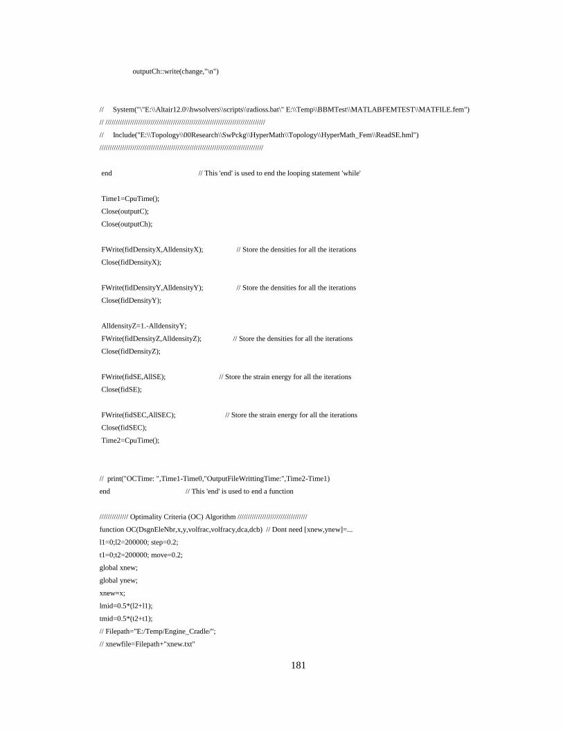
181

outputCh::write(change,"\n")

// System("\"E:\\Altair12.0\\hwsolvers\\scripts\\radioss.bat\" E:\\Temp\\BBMTest\\MATLABFEMTEST\\MATFILE.fem")

// //////////////////////////////////////////////////////////////////////////////

// Include("E:\\Topology\\00Research\\SwPckg\\HyperMath\\Topology\\HyperMath_Fem\\ReadSE.hml")

////////////////////////////////////////////////////////////////////////////////

end // This 'end' is used to end the looping statement 'while'

Time1=CpuTime();

Close(outputC);

Close(outputCh);

FWrite(fidDensityX,AlldensityX); // Store the densities for all the iterations

Close(fidDensityX);

FWrite(fidDensityY,AlldensityY); // Store the densities for all the iterations

Close(fidDensityY);

AlldensityZ=1.-AlldensityY;

FWrite(fidDensityZ,AlldensityZ); // Store the densities for all the iterations

Close(fidDensityZ);

FWrite(fidSE,AllSE); // Store the strain energy for all the iterations

Close(fidSE);

FWrite(fidSEC,AllSEC); // Store the strain energy for all the iterations

Close(fidSEC);

Time2=CpuTime();

// print("OCTime: ",Time1-Time0,"OutputFileWrittingTime:",Time2-Time1)

end // This 'end' is used to end a function

////////////// Optimality Criteria (OC) Algorithm //////////////////////////////////

function OC(DsgnEleNbr,x,y,volfrac,volfracy,dca,dcb) // Dont need [xnew,ynew]=...

l1=0;l2=200000; step=0.2;

t1=0;t2=200000; move=0.2;

global xnew;

global ynew;

xnew=x;

lmid=0.5*(l2+l1);

tmid=0.5*(t2+t1);

// Filepath="E:/Temp/Engine_Cradle/";

// xnewfile=Filepath+"xnew.txt"

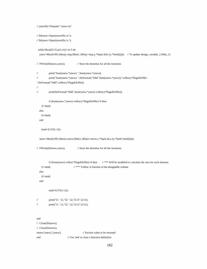
182

// ynewfile=Filepath+"ynew.txt"

// fidxnew=Open(xnewfile,'a+');

// fidynew=Open(ynewfile,'a+');

while Max((l2-l1),(t2-t1))>1e-5 do

ynew=Max(0.001,Max(y-step,Min(1.,Min(y+step,y.*Sqrt(-dcb./(x.*lmid)))))); // To update design_variable_2 (Mat_1)

// FWrite(fidynew,ynew); // Store the densities for all the iterations

// print("Sum(xnew.*ynew): ",Sum(xnew.*ynew))

// print("Sum(xnew.*ynew): ",StrFormat("%8d",Sum(xnew.*ynew)),"volfracy*DsgnEleNbr:

",StrFormat("%8d",volfracy*DsgnEleNbr))

//

// print(StrFormat("%8d",Sum(xnew.*ynew)-volfracy*DsgnEleNbr));

if (Sum(xnew.*ynew)-volfracy*DsgnEleNbr)>0 then

l1=lmid;

else

l2=lmid;

end

lmid=0.5*(l1+l2);

xnew=Max(0.001,Max(x-move,Min(1.,Min(x+move,x.*Sqrt(-dca./(y.*lmid+tmid))))));

// FWrite(fidxnew,xnew); // Store the densities for all the iterations

if (Sum(xnew)-volfrac*DsgnEleNbr)>0 then // *** Will be modified to calculate the area for each element.

t1=tmid; // *** Volfrac is fraction of the designable volume

else

t2=tmid;

end

tmid=0.5*(t1+t2);

// print("l1: ",l1,"l2: ",l2,"l2-l1",l2-l1);

// print("t1: ",t1,"t2: ",t2,"t2-t1",t2-t1);

end

// Close(fidynew);

// Close(fidxnew);

return [xnew], [ynew]; // Fuction value to be returned

end // Use 'end' to close a function definition

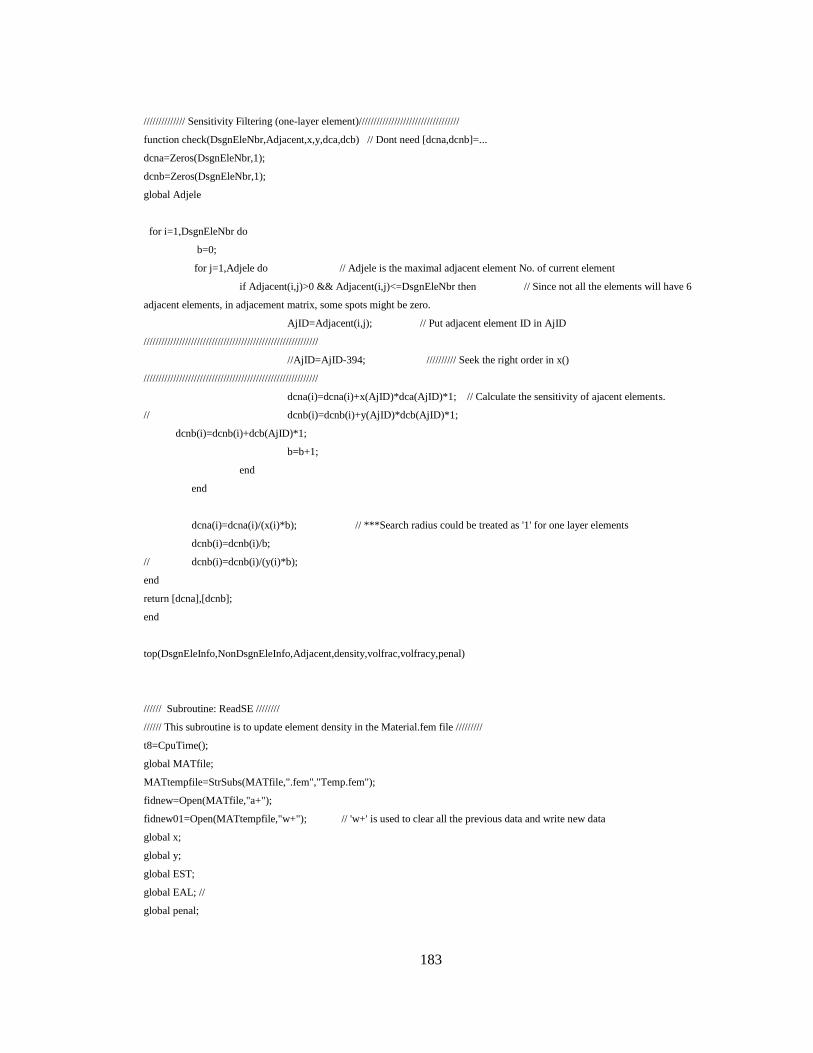
183

////////////// Sensitivity Filtering (one-layer element)//////////////////////////////////

function check(DsgnEleNbr,Adjacent,x,y,dca,dcb) // Dont need [dcna,dcnb]=...

dcna=Zeros(DsgnEleNbr,1);

dcnb=Zeros(DsgnEleNbr,1);

global Adjele

for i=1,DsgnEleNbr do

b=0;

for j=1,Adjele do // Adjele is the maximal adjacent element No. of current element

if Adjacent(i,j)>0 && Adjacent(i,j)<=DsgnEleNbr then // Since not all the elements will have 6

adjacent elements, in adjacement matrix, some spots might be zero.

AjID=Adjacent(i,j); // Put adjacent element ID in AjID

///////////////////////////////////////////////////////////

//AjID=AjID-394; ////////// Seek the right order in x()

///////////////////////////////////////////////////////////

dcna(i)=dcna(i)+x(AjID)*dca(AjID)*1; // Calculate the sensitivity of ajacent elements.

// dcnb(i)=dcnb(i)+y(AjID)*dcb(AjID)*1;

dcnb(i)=dcnb(i)+dcb(AjID)*1;

b=b+1;

end

end

dcna(i)=dcna(i)/(x(i)*b); // ***Search radius could be treated as '1' for one layer elements

dcnb(i)=dcnb(i)/b;

// dcnb(i)=dcnb(i)/(y(i)*b);

end

return [dcna],[dcnb];

end

top(DsgnEleInfo,NonDsgnEleInfo,Adjacent,density,volfrac,volfracy,penal)

////// Subroutine: ReadSE ////////

////// This subroutine is to update element density in the Material.fem file /////////

t8=CpuTime();

global MATfile;

MATtempfile=StrSubs(MATfile,".fem","Temp.fem");

fidnew=Open(MATfile,"a+");

fidnew01=Open(MATtempfile,"w+"); // 'w+' is used to clear all the previous data and write new data

global x;

global y;

global EST;

global EAL; //

global penal;

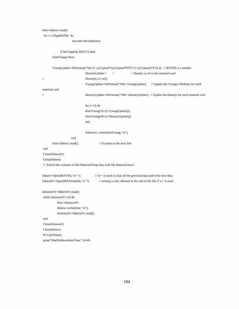
184

tline=fidnew::read()

for i=1,DsgnEleNbr do

tok,rem=StrTok(tline);

if StrCmp(tok,'MAT1') then

tlineYoung=tline;

YoungUpdate=StrFormat("%8.1e",x(i)^penal*(y(i)^penal*EST+(1-y(i)^penal)*EAL)); // MATID is a number

DensityUpdate=' '; // Density is nil in the material card

// Density(i,1)=x(i);

YoungUpdate=StrFormat("%8s",YoungUpdate); // Update the Young's Modulus for each

material card

// DensityUpdate=StrFormat("%8s",DensityUpdate); // Update the Density for each material card

for j=1,8 do

tlineYoung[16+j]=YoungUpdate[j];

tlineYoung[40+j]=DensityUpdate[j];

end

fidnew01::write(tlineYoung,"\n");

end

tline=fidnew::read(); // To point to the next line

end

Close(fidnew01)

Close(fidnew)

/// Switch the contents of file-MaterialTemp.fem with file Material.fem///

fidnew=Open(MATfile,"w+"); // 'w+' is used to clear all the previous data and write new data

fidnew01=Open(MATtempfile,"a+"); // writing is only allowed at the end of the file if 'a+' is used

tlinenew01=fidnew01::read();

while tlinenew01!=nil do

tline=tlinenew01;

fidnew::write(tline,"\n");

tlinenew01=fidnew01::read();

end

Close(fidnew01)

Close(fidnew)

t9=CpuTime();

print("MatFileRewrittenTime:",t9-t8)

(title of the thesis)* - qspace - queen's university

Documents