Working Paper No. 17

Tipping and Concentration in Markets with Indirect Network

Jean-Pierre Dubé University of Chicago Graduate School of Business

Günter J. Hitsch University of Chicago Graduate School of Business

Pradeep Chintagunta University of Chicago Graduate School of Business

Initiative on Global Markets The University of Chicago, Graduate School of Business

“Providing thought leadership on financial markets, international business and public policy”

Tipping and Concentration in Markets with Indirect NetworkEffects∗

Jean-Pierre DubéGraduate School of Business

University of Chicago

Günter J. HitschGraduate School of Business

University of Chicago

Pradeep ChintaguntaGraduate School of Business

University of Chicago

July 14, 2008First Version: July 1, 2007

Abstract

This paper develops a framework to measure “tipping”—the increase in a firm’s marketshare dominance caused by indirect network effects. Our measure compares the expectedconcentration in a market to the hypothetical expected concentration that would arisein the absence of indirect network effects. In practice, this measure requires a modelthat can predict the counter-factual market concentration under different parameter val-ues capturing the strength of indirect network effects. We build such a model for thecase of dynamic standards competition in a market characterized by the classic hard-ware/software paradigm. To demonstrate its applicability, we calibrate it using demandestimates and other data from the 32/64-bit generation of video game consoles, a canon-ical example of standards competition with indirect network effects. In our example, wefind that indirect network effects can lead to a strong, economically significant increase inmarket concentration. We also find important roles for beliefs on both the demand side,as consumer’s tend to pick the product they expect to win the standards war, and on thesupply side, as firms engage in penetration pricing to invest in growing their networks.

∗We are grateful to Dan Ackerberg, Lanier Benkard, Ariel Burstein, Tim Conley, Ron Goettler, WesHartmann, Ali Hortaçsu, Harikesh Nair, Amil Petrin, and Peter Rossi for helpful comments and suggestions.We also benefited from the comments of seminar participants at Duke University, Tillburg University, theUniversity of Minnesota, the University of Pennsylvania, the 2007 Invitational Choice Symposium at theWharton School, the 2007 QME Conference in Chicago, the 2007 SICS Conference at Berkeley and the 2008winter I.O. meetings at the NBER. We would like to acknowledge the Kilts Center for Marketing and theInitiative for Global Markets (IGM), both at the University of Chicago, for providing research funds. Thefirst author was also supported by the Neubauer Family Faculty Fund. All correspondence may be addressedto the authors at the University of Chicago, Graduate School of Business, 5807 South Woodlawn Avenue,Chicago, IL 60637; or via e-mail at jdube@gsb.uchicago.edu or guenter.hitsch@chicagogsb.edu.

1

1 Introduction

We study the diffusion of competing durable goods in a market exhibiting indirect networkeffects due to the classic hardware/software structure (Katz and Shapiro 1985). Of particularinterest is whether such markets are prone to tipping : “the tendency of one system to pull awayfrom its rivals in popularity once it has gained an initial edge” (Katz and Shapiro 1994) and,in some instances, to emerge as the de facto industry standard. Thus, tipping can create anatural form of market concentration in hardware/software markets. The potential for tippingcan also lead to aggressive standards wars between incompatible hardware products as theycompete for market dominance. These standards wars are widely regarded as a “fixture of theinformation age” (Shapiro and Varian 1999).

The extant literature has yet to provide an empirically practical measure of tipping. There-fore, we propose a dynamic framework with which to measure tipping, its relationship to indi-rect network effects and its ability to lead to market concentration in actual markets. We alsouse the framework to conduct computational exercises with which to understand the generalrole of expectations during a standards war, both on the supply and demand sides, and tosee how they can push a market to tip in favor of one standard. We expect the analysis oftipping and its natural tendency towards market concentration to be of general importanceboth to practitioners and to policy makers.1

The potential for tipping figures prominently in current antitrust discussions about hard-ware/software markets, as highlighted in the recent high-profile case surrounding the browserwar between Microsoft and Netscape (United States v. Microsoft, 87 F. Supp. 2d 30 andBresnahan 2001). However, existing antitrust policies and tools are often inadequate for ad-dressing the feedback dynamics in markets with indirect network effects (e.g. Evans 2003,Koski and Kretschmer 2004, Evans and Schmalensee 2007, and Rysman 2007). Since adop-tion decisions are not instantaneous, an empirically relevant model of a hardware/softwaremarket needs to incorporate dynamics in demand and supply. These dynamics constitute amethodological challenge and, consequently, much of the extant empirical literature eitherestimates the effects of indirect network effects using demand only, or treats the supply sideof the market as static (Gupta et al. 1999, Basu et al. 2003, Bayus and Shankar 2003, Ohashi2003, Dranove and Gandal 2003, Nair et al. 2004, Karaca-Mandic 2004, Park 2004, Rysman2004, Clements and O’Hashi 2005, Ackerberg and Gowrisankaran 2007, and Tucker and Ryan2007). Gandal et al. (2000) allow for forward-looking consumers; but they assume hardwaresponsors do not have a strategic role. More recently, Liu (2007) and, most closely-related to

1Herein, we focus only on the standardization that may emerge from competition. We do not considerthe role of formal standard-setting committees (e.g. Katz and Shapiro 1994) such as those that ultimatelysettled the standards war in the 56K modem market (Augereau et al 2006). We do not consider the role ofcompatibility which, in some instances, may eliminate the dominance of one of the hardware standards (Chen,Doraszelski and Harrington 2007).

2

our work, Jenkins, Liu, Matzkin, and McFadden (2004) allow for forward-looking hardwaremanufacturers. But, both papers treat consumers as myopic. In contrast, our paper allowsfor forward-looking consumer behavior and solves for an equilibrium in which consumers’ andfirms’ expectations are mutually consistent. We will demonstrate that the assumption ofstatic consumer behavior can strongly limit the empirical relevance of a model for measuringconcentration or “bad acts," as forward-looking consumer behavior can strongly exacerbatetipping.

Before discussing our empirical formulation of tipping, we first explain how indirect net-work effects can lead to tipping. In a hardware/software market structure, indirect networkeffects arise because consumers adopt hardware based on the current availability and theirbeliefs about the future availability of software, while the (third-party) supply of softwareincreases in the installed base of a given hardware standard (Chou and Shy 1992, Churchand Gandal 1993).2 Hence, each standard becomes more valuable to a consumer if it attainsa larger installed base. Due to positive feedback, a small initial market share advantage caneventually lead to large differences in the shares of the competing standards. This processis exacerbated by rational, self-fulfilling expectations, which allow consumers to coordinateon a standard that is widely adopted based on mutually consistent beliefs about the currentand future adoption decisions of other consumers.3 In an extreme case, two standards Aand B could be identical ex-ante, but due to self-fulfilling expectations either “all consumersadopt A” or “all consumers adopt B” could be an equilibrium. Hence, due to the emergenceof positive feedback and the role of expectations, markets with indirect network effects maybecome concentrated, i.e. tip towards one of the competing standards.

We now explain why the formulation of an empirically relevant definition of tipping isdifficult. Consider first the case of an ex-ante symmetric market where firms face identicaldemand functions, have the same production costs, etc. In this case, we could measure tippingby comparing the ex-post asymmetry in market shares with the perfectly symmetric outcomewhere all firms share the market equally.4 In actual markets, however, product differentiation,differences in costs, and other differences between standards frequently lead to asymmetricmarket outcomes, even in the absence of indirect network effects. Hence, we propose a measureof tipping that compares the expected concentration in a market to the hypothetical expected

2Rochet and Tirole (2003) argue that most network effects arise in an indirect manner.3The role of coordination and expectations in driving adoption decisions has been a central theme in the

theoretical literature on network effects since the seminal work of Katz and Shapiro (1985). For excellentsurveys, see Farrell and Klemperer (2006) and Katz and Shapiro (1994).

4Note that we focus herein on tipping and market dominance during a specific hardware generation. Arelated theoretical literature has also studied whether tipping can create inertia across hardware generationswhen there are innovations (e.g. Farrell and Saloner 1986, Katz and Shapiro 1992 and Markovitch 2004).Therein, tipping, or “excess inertia,” is defined by the willingness of consumers to trade-off the scale benefitsof a current standard with a large installed base in favor of a new technology without an installed base.Interestingly, in this type of environment, network effects may also serve as a potential barrier to entry(Cabral 2007).

3

concentration that would arise if the sources of indirect network effects were reduced oreliminated. The key insight is that tipping generally needs to be measured relative to a well-defined, counter-factual market outcome. For an empirical implementation of this measure,we need a model that captures indirect network effects, can be calibrated from actual data,and allows us to make predictions about the equilibrium adoption of the competing standardsunder various different parameter values capturing the strength of indirect network effects.

To implement the proposed measure of tipping, we build a dynamic model that capturesindirect network effects and gives consumer expectations a central role. Our model involvesthree types of players: consumers, hardware manufacturers, and software developers. Thedemand side of our model extends the framework of Nair et al. (2004) and allows for dynamicadoption decisions. Consumers are assumed to “single-home,” meaning they adopt at mostone of the competing hardware standards.5 The utility of each hardware standard increases inthe availability and variety of complementary software. Consumers form beliefs about futurehardware prices and software availability. These beliefs influence when consumers adopt (therate of diffusion) and which standard they adopt (the size of each installed base). On thesupply side, forward-looking hardware firms compete in prices while anticipating the impact ofhardware sales on the future provision of software and, hence, future hardware sales. Softwarefirms provide a variety of titles that is increasing in the installed base of a hardware standard.Our solution concept for this model is Markov perfect Bayesian equilibrium. The complexityof the model makes analytical solution methods intractable, and hence we solve the modelnumerically.

To demonstrate our model and how it can be used to measure tipping, we calibrate it withdemand parameter estimates and other market data from the 32/64-bit generation of videogame consoles.6 The video game console market is a canonical example of indirect networkeffects. Furthermore, from previous empirical research, the 32/64-bit generation is known toexhibit indirect network effects (Venkatesh and Bayus 2003, Clements and Ohashi 2005).

Demand estimation per se is not the main point of this paper. But we do need to overcomesome econometric challenges to obtain preference estimates that can be used to calibrate ourmodel. These challenges arise from the incorporation of forward-looking consumer behavior.A nested fixed point approach (Rust 1987) would impose a formidable computational burdenthat is exacerbated by the presence of indirect network effects in the model. Instead, we adaptthe two-step procedures of Bajari, Benkard and Levin (2007) (hereafter BBL) and Pesendorferand Schmidt-Dengler (2006) (hereafter PS-D) to solve our demand estimation problem. A

5Recent literature has begun to study the theoretical implications of multi-homing whereby consumers mayadopt multiple standards and software firms may create versions for multiple standards (Armstrong 2005).

6This approach follows in the tradition of Benkard (2004), Dubé, Hitsch, and Manchanda (2005), and Dubé,Hitsch, and Rossi (2007) by conducting counter-factual simulations of the market outcomes using empiricallyobtained parameters.

4

similar approach has recently been employed by Ryan and Tucker (2007).7

The calibrated model reveals that the 32/64 bit video game console market can exhibiteconomically significant tipping effects, given our model assumptions and the estimated pa-rameter values. The market concentration, as measured by the 1-firm concentration ratio inthe installed based after 25 periods, increases by at least 23 percentage points due to indirectnetwork effects. We confirm the importance of consumer expectations as an important sourceof indirect network effects; in particular, we find that tipping occurs at a (monthly) discountfactor of 0.9, but not for smaller discount factors. Our model also predicts penetration pricing(for small levels of the installed base) if indirect network effects are sufficiently strong. Inmarkets with strong network effects, firms literally price below cost during the initial periodsof the diffusion to invest in network growth.

2 Model

We consider a market with competing hardware platforms. A consumer who has adoptedone of the available technologies derives utility from the available software for that platform.Software titles are incompatible across platforms. Consumers are assumed to choose at mostone of the competing hardware platforms and to purchase software compatible with the chosenhardware, a behavior Rochet and Tirole (2003) term “single-homing.” There are indirectnetwork effects in this market, which are due to the dependence of the number of availablesoftware titles for a given platform on that platform’s installed based. The consumers in thismarket have expectations about the evolution of hardware prices and the future availability ofsoftware when making their adoption decisions. Correspondingly, the hardware manufacturersanticipate the consumer’s adoption decisions, and set prices for their platforms accordingly.The software market is monopolistically competitive, and the supply of software titles for anygiven platform is increasing in the platform’s installed base.

Time is discrete, t = 0, 1, . . . The market is populated by a mass M = 1 of consumers.There are J = 2 competing firms, each offering one distinct hardware platform. yjt ∈ [0, 1]denotes the installed base of platform j in period t, i.e., the fraction of consumers who haveadopted j in any period previous to t. yt = (y1t, y2t) describes the state of the market.

In each period, platform-specific demand shocks ξjt are realized. ξjt is private informationto firm j, i.e., firm j learns the value of ξjt before setting its price, but learns the demand shockof its competitor only once sales are realized. As we shall see later, ξjt can strongly influencethe final distribution of shares in the installed base. In particular, the realizations of ξjt in the

7An interesting difference is that Ryan and Tucker (2007) use individual level adoption data, which enablesthem to accommodate a richer treatment of ‘observed’ consumer heterogeneity. The trade-off from incorpo-rating more heterogeneity is that they are unable to solve the corresponding dynamic hardware pricing gameon the supply side.

5

initial periods of competition can lead the market to “tip” in favor of one standard. Also, ξjtwill typically ensure that the best response of each firm is unique, and thus the existence ofa pure strategy equilibrium.8 We assume that the demand shocks are independent and i.i.d.through time. φj(·) denotes the pdf of ξj , and φ(·) denotes the pdf of ξ = (ξ1, ξ2).

The timing of the game is as follows:

1. Firms learn their demand shock ξjt and set a product price, pjt.

2. Consumers adopt one of the available platforms or delay their purchase decisions.

3. For each platform j, software firms supply a given number of titles, njt.

4. Sales are realized, and firms receive their profits. Consumers derive utility from theavailable software titles and—in the case of new adopters—from the chosen platform.

Software Market

The number of available software titles for platform j in each period is a function of theinstalled base of platform j : njt = hj(yj,t+1). To see why njt is a function of yj,t+1 andnot yjt, note that yjt denotes the installed base at the beginning of period t, while yj,t+1

denotes the total installed base after the potential adopters have made a purchase decision.The software producers observe this total installed base before they supply a given numberof titles.

While this derivation may seem ad hoc, in Appendix A we show how this relationshipbetween njt and yj,t+1 can be derived from a structural model of monopolistic competition andCES software demand in the software market. These assumptions abstract away from someof the dynamic aspects of game demand (e.g. Nair 2006), but they retain the fundamentalinter-dependence between software and hardware.

Consumer Decisions

Consumers make their adoption decisions based on current prices and their expectation offuture prices and the availability of compatible software titles. Consumers expect that theinstalled hardware evolves according to yt+1 = fe(yt, ξt), and that firms set prices accordingto the policy function pjt = σej (yt,ξjt). Consumers observe both ξt and the current price vectorpt before making their decisions.

Consumer who have already adopted one of the platforms receive utility from the availablesoftware in each period. As the supply of software is a function of the installed base at the

8We are not able to prove this statement in general, but could easily verify it across all versions of ourmodel that we solved on a computer. In general, the right hand side of the firm’s Bellman equation, regardedas a function of pjt, has two local maxima. The realization of ξjt ensures that these local maxima are notequal.

6

end of a period, we can denote this utility as uj(yj,t+1) = γnjt = γhj(yj,t+1). The presentdiscounted software value is then defined as

ωj(yt+1) = E

[ ∞∑k=0

βkuj(yj,t+1+k)|yt+1

].

This value follows the recursion

ωj(yt+1) = uj(yj,t+1) + β

∫ωj(fe(yt+1, ξ))φ(ξ)dξ.

Consumers who have not yet adopted either buy one of the hardware platforms or delayadoption. The choice-specific value of adopting hardware platform j is given by

vj(yt, ξt, pt) = δj + ωj(fe(yt, ξt))− αpjt + ξjt. (1)

Here, δj is the value of owning a specific hardware platform, or the value of bundled software.α is the marginal utility of income. The realized utility from adopting j also includes arandom utility component εjt, which introduces horizontal product differentiation among thecompeting standards. That is, the total utility from the choice of j is given by vj(yt, ξt, pt)+εjt.We assume that εj is i.i.d. Type I Extreme Value distributed.

The value of waiting is given by

v0(yt, ξt) = β

∫max

v0(yt+1, ξ) + ε0,max

jvj(yt+1, ξ, σ

e(yt+1, ξ)) + εjφε(ε)φ(ξ)d(ε, ξ).

(2)In this equation, yt+1 = fe(yt, ξt).

Consumers choose the option that yields the highest choice-specific value, including εjt.That is, option j is chosen if and only if for all k 6= j, vj(yt, ξt, pt) + εjt ≥ vk(yt, ξt, pt) + εkt.

9

Given the distributional assumption on the random utility component, the market share ofoption j is

sj(yt, ξt, pt) =exp(vj(yt, ξt, pt))

exp(v0(yt, ξt)) +∑J

k=1 exp(vk(yt, ξt, pt)). (3)

Furthermore, the installed base of platform j evolves according to

yj,t+1 = yjt +

(1−

J∑k=1

ykt

)sj(yt, ξt, pt) = fj(yt, ξt, pt). (4)

9These inequalities involve some slight abuse of notation, as v0(y, ξ) is not a function of p.

7

Firms

Firms set prices according to the Markovian strategies pj = σj(y, ξj), i.e., prices dependonly on the current payoff-relevant information observed to each competitor. Firms expectthat the consumers make adoption decisions according to the value functions v0, . . . , vJ , andaccordingly that market shares are realized according to equation (3) and that the installedbase evolves according to (4).

The marginal cost of hardware production is cj , which we assume to be constant throughtime. The firms also collect royalty fees from the software manufacturers at the rate of rj perunit of software. Let qj(yt+1) be the total number of software titles sold in period t.10 Theper-period expected profit function is then given by

πj(y, ξj , pj) = (pj − cj) ·(

1−∑J

k=1ykt

)∫sj (y, ξj , ξ−j , pj , σ−j(y, ξ−j))φj(ξ−j)dξ−j

+ rj

∫qj (fj(y, ξj , ξ−j , pj , σ−j(y, ξ−j)))φj(ξ−j)dξ−j .

Each competitor maximizes the expected present discounted value of profits. Associatedwith the solution of the inter-temporal pricing problem is the Bellman equation

Vj(y, ξj) = suppj≥0

πj(y, ξj , pj) + β

∫Vj(f(y, ξj , ξ−j , pj , σ−j(y, ξ−j)), ξ′j)φ(ξ−j)φ(ξ′j)d(ξ−j , ξ′j)

.

(5)

Equilibrium

We seek a Markov perfect Bayesian equilibrium, where firms and consumers base their de-cision only on the current payoff-relevant information. Consumers have expectations aboutfuture hardware prices and the evolution of the installed base of platform and the associatedsupply of software. The adoption decisions are dependent on these expectations. Firms haveexpectations about the adoption decisions of the consumers, the evolution of the installedbase, and the pricing decisions of their competitors. Pricing decisions are made accordingly.In equilibrium, these expectations need to be mutually consistent.

Formally, a Markov perfect Bayesian equilibrium in pure strategies of the network gameconsists of consumer expectations fe and σe, consumer value functions vk, pricing policies σj ,and the firm’s value function Vj such that:

1. The consumer’s choice-specific value functions v1, . . . vJ satisfy (1), and the value ofwaiting, v0, satisfies (2).

10qj(yt+1) = qj(njt) · yj,t+1, where qj denotes the average number of titles bought by a consumer. See Ap-pendix A for the derivation of this equation within the context of a specific model. For our model simulations,we estimate qj(y) directly from the data.

8

2. The firm’s value functions V1, . . . , VJ satisfy the Bellman equations (5).

3. pj = σj(y, ξj) maximizes the right-hand side of the Bellman equation (5) for eachj = 1, . . . , J.

4. The consumer’s expectations are rational: σej ≡ σj for j = 1, . . . , J, and fe(y, ξ) =f(y, ξ, σ(y, ξ)), where f is as defined by equation (4).

In the Markov perfect equilibrium, all players—firms and consumers—act rationally giventheir expectations about the strategies of the other market participants. Furthermore, expec-tations and actually realized actions are consistent.

3 Estimation

To make our computational results more realistic, we calibrate them with data from thevideo game console market. While demand estimation per se is not the main objective ofthe paper, it is nevertheless helpful to discuss briefly some of the challenges involved inestimating preference parameters for a dynamic discrete choice model. The main difficultyarises from the incorporation of consumer beliefs, a crucial element for durable goods demandin general (Horsky 1990, Melnikov 2000, Song and Chintagunta 2003, Nair 2005, Prince2005, Carranza 2006, Gowrisankaran and Rysman 2006, and Gordon 2006). Once we includeconsumer beliefs in our console demand function, the derivation of the market shares, equation(3), requires us to compute the choice-specific value functions. Nesting the correspondingdynamic programming problem into the estimation problem is prohibitive due to the highdimension of the state space (yt, ξt and other exogenous states included in the empiricalspecification). In addition, the derivation of the density of market shares (or moments of thedensity) requires inverting the demand shocks, ξ, out of the market share function numerically.This step is also computationally costly since ξ enters the utility function non-linearly throughthe value functions ωj(fe(yt, ξt)) and v0(yt, ξt).11

Instead, we follow a recent tradition in the empirical literature on dynamic games andestimate the structural parameters of our model in two stages (e.g. BBL, PS-D, and Aguir-regabira and Mira 2002, 2006). The goal is to construct moment conditions that match theobserved consumer choices in the data with those predicted by our model. Rather than com-puting the choice-specific value functions needed to evaluate demand, we instead devise atwo-step approach to simulate them.

11As discussed in Gowrisankaran and Rysman (2006), since we do not know the shape of these value functionsa priori, it is unclear whether the market share function is invertible in ξ, let alone whether a computationallyfast contraction-mapping can be used to compute the inverse.

9

Stage 1

In the first stage, we estimate the consumer choice strategies along with the firms’ pricingstrategies and the software supply function. The supply function of software variety is specifiedas follows

log(njt) = Hj(yj,t+1; θn) + ηjt. (6)

where ηjt ∼ N(0, σ2

η

)captures random measurement. This specification is consistent with

the equilibrium software supply function derived in the Appendix, equation (9). The pricingstrategies are specified as follows

log (pjt) = Pj (yt, zpt ; θp) + λξjt, (7)

where ξjt ∼ N (0, 1). In equation (7) we let Pj be a flexible functional form of the statevariables. For the empirical model, we include exogenous state variables, zpt , that are observedby console firms in addition to yt and ξt, the state variables in the model of Section 2. Theseadditional states are discussed in Section 4. In equation (7), we assume that the video gameconsole manufacturers use only payoff-relevant information to set their prices. But we donot assume that their pricing strategies are necessarily optimal. This specification has theadvantage that it is consistent with the Bayesian Markov perfect equilibrium concept used inour model, but does not explicitly impose it.

Conditional on the model parameters, there is a deterministic relationship between theprice and installed base data and the demand unobservable, ξjt = Xj(yjt, pjt, zpt )12. Then,conditional on yt and pt, we can estimate the consumers’ optimal choice strategy in log-odds:

µjt ≡ log (sjt)− log (s0t)

= vj

(yt, ξt, pt, z

dt

)− v0

(yt, ξt, z

dt

)+ ζjt

= Lj(yt,X (yt, pt, z

pt ), zdt ; θµ

)+ ζjt, (8)

where ζjt ∼ N(0, σ2ζ ) is random measurement error and zdt denotes exogenous state variables

observed by the consumer. By including the control function X (yt, pt, zpt ) in the demand

equation, we also resolve any potential endogeneity bias that would arise due to the correlationbetween prices and demand shocks (this is the control function approach used in . The firststage consists then of estimating the vector of parameters Θ = (θn, θp, θµ, λ) via maximumlikelihood using the equations (6), (7), and (8).

12We can trivially invert ξ out of the price equation because of the additivity assumption in (7). This isa stronger condition than in BBL, but it is analogous to other previous work such as Villas-Boas and Winer(1999) and Petrin and Train (2005).

10

Stage 2

In the second stage, we estimate the consumers’ structural taste parameters, Λ, by construct-ing a minimum distance procedure that matches the simulated optimal choice rule for theconsumers to the observed choices in the data. The idea is to use the estimated consumerchoice strategies, (8) and the laws of motion for prices and software variety, (7) and (6),to forward-simulate the consumers’ choice-specific value functions, Vj

(yt, ξt, pt; Λ, Θ

)and

V0(y, ξ; Λ, Θ). The details for the forward-simulation are provided in the Appendix. Notethat while our two-step approach does not require us to assume that firms play the MarkovPerfect equilibrium strategies explicitly, we do need to assume that consumers maximize thenet present value of their utilities.

The minimum distance procedure forces the following moment condition to hold approxi-mately:

Qjt(Λ0, Θ) ≡ µjt −(Vj(y, ξ, p; Λ0, Θ)− V0(y, ξ; Λ0, Θ)

)= 0.

That is, at the true parameter values, Λ0, and given a consistent estimate of Θ, the simulatedlog-odds ratios should be approximately equal to the observed log-odds ratios for each of theobserved states in the data. The minimum distance estimator, ΛMD, is obtained by solvingthe following minimization problem:

ΛMD = minΛ

Q(Λ, Θ)′WQ(Λ, Θ)

,

where W is a positive semi-definite weight matrix.13 Wooldridge (2002) shows that theminimum distance estimator has an asymptotically normal distribution with the covariancematrix

Avar(ΛMD) =(∇ΛQ

′W∇ΛQ)−1∇ΛQ

′W∇ΘQΩ∇ΘQ′W∇ΛQ

(∇ΛQ

′W∇ΛQ)−1

,

where Ω = Avar(Θ), and ∇ΛQ and ∇ΘQ denote gradients of Q with respect to Λ and Θrespectively.

The approach is closest to PS-D. But, our implementation differs in two ways. First, weexamine a model with continuous states (PS-D look at a model with discrete states). Second,we adapt the approach to estimation of aggregate dynamic discrete choice demand, whereasPS-D focus on discrete choice at the individual level.

13We just set W equal to the identity matrix since it is unclear how to derive the efficient W in closed formfor our specific problem.

11

4 Data

For our calibration, we use data from the 32/64-bit generation of video game consoles, one ofthe canonical examples of indirect network effects. To understand the relevance of this casestudy to our model and our more general point about tipping in two-sided markets, we brieflyoutline some of the institutional details of the industry. We then discuss the data.

The US Videogame Console Industry

The market for home video game systems has exhibited a two-sided structure since the launchof Atari’s popular 2600 VCS console in 1977 (Williams 2002). Much like the systems today,the VCS consisted of a console capable of playing multiple games, each on interchangeablecartridges. While Atari initially developed its own proprietary games, ultimately more than100 independent developers produced games for Atari and more than 1,000 games were re-leased for Atari 2600 VCS (Coughlan 2001A). This same two-sided market structure hascharacterized all subsequent console generations, including the 32/64-bit generation we studyherein.

The 32/64-bit generation was novel in several ways. None of the consoles were backward-compatible, eliminating concerns about a previously-existing installed base of consumerswhich might have given a firm an advantage. This was also the first generation to adoptCD-ROM technology; although early entrants, Philips and 3DO, failed due to their high con-sole prices of $1000 and $700 respectively. In contrast, the September 1995 US launch ofSony’s 32-bit CD-ROM console, Playstation, was an instant success. So much so, that itscompetitors, Sega’s 32-bit Saturn console and later, Nintendo’s 64-bit N64 cartridge console,failed to recapture Sony’s lead. In fact, Sega’s early exit from the market implied a duopolyconsole market between Sony’s first-generation Playstation and Nintendo’s N64.

Playstation’s success reflected several changes in the management of the console side ofthe market. From the start, Sony’s strategy was to supply as many games as possible, a lessonit learned from its experience with Betamax video technology:

Sony’s primary goal with respect to Playstation was to maximize the number andvariety of games... Sony was willing to license any Playstation software that didn’tcause the hardware to “crash.” — Coughlan (2001b)

To stimulate independent game development, Sony charged substantially lower game royaltiesof $9, in contrast with Nintendo’s $18 (Coughlan 2001c). Sony’s CD-based platform alsolowered game development costs, in contrast with Nintendo’s cartridge based system. Whilethe Playstation console failed to produce any truly blockbuster games during its first year(Kirkpatrick 1996), after three months, Playstation’s games outnumbered those of Sega’s

12

Saturn by three-to-one. By 1998, more than 400 Playstation titles were available in the US.In addition, Sony engaged in aggressive penetration pricing of the console early on, hoping tomake its money back on game royalties (Cobb 2003).

In contrast, Nintendo maintained very stringent conditions over its game licensees, alegacy from its management of game licensees during earlier generations when Nintendo wasdominant.14 By Christmas of 1996, N64 only had eight games in contrast with roughly 200Playstation titles (Rigdon 1996). By June 1997, N64 still had only 17 games while Playstationhad 285. Nintendo insisted that it competed on quality, rather than quantity and in 1997 itsCEO claimed, “Sony could kill off the industry with all of ‘its garbage” ’ (Kunii 1998). In theend, the dominance of Sony Playstation in the 32/64-bit console generation was attributedprimarily to its vast library of games, rather than to specific game content.

Recall that our case study focuses only on the 32/64-bit console generation. The successof Playstation’s game proliferation strategy makes us comfortable with the assumption thatgame variety proxies meaningfully for the indirect network effects. This assumption would bemore tenuous for more recent console generations now that blockbuster games have becomemore substantial. For example, the blockbuster game Halo 3, for Microsoft’s Xbox 360,generated $300 million in sales during its first week (Blakely 2007) and, by November 2007,it represented over 17% of Xbox 360’s worldwide game sales according to NPD. At the sametime, monthly Xbox 360 console sales nearly doubled in contrast with two months previously,selling 527, 800 units in October 2007 (Gallagher 2007). Similarly, Playstation 3’s Spiderman3 grossed $151 million during its first week (Blakely 2007). The blockbuster games of the32/64-bit generation were smaller in magnitude. Only three N64 games garnered over 4% oftotal US game unit sales on the N64 platform, Goldeneye 007, Mario Kart 64 and Super Mario64, while an additional 21 games captured over 1% of total game sales. Only five Playstationtitles captured over 1% of total Playstation game sales, none capturing over 2%.15 Nair(2007) tests for Blockbuster game effects during this generation. He finds no material impacton sales or prices of games in the months leading-up to the launch of a best-selling game.Therefore, Nair (2007) ignores competitive effects in his analysis of video game pricing duringthis generation.

Data

Our data are obtained from NPD Techworld’s “Point of Sale” database. The database consistsof a monthly report of total sales and average prices for each video game consoles across a

14The dominance of Nintendo’s 8-bit NES console, during the 1980s, allowed it to command 20% royaltiesin addition to a manufacturing fee of $14 per game cartridge. Licensees were also restricted to 5 new NEStitles per year. Nevertheless, by 1991, less than 10% of titles were produced by Nintendo and the systemhad over 450 titles in the US. In addition, one in three US households had an NES console by 1991, with theaverage console owner purchasing 8 or 9 games (Coughlan 2001B).

15These numbers are based on US game sales data collected by NPD.

13

sample of participating US retailers from September 1995 to September 2002. NPD statesthat the sheer size of the participating firms represent about 84% of the US retail market. Wealso observe the monthly number of game titles available during the same period. We definethe potential market size as the 97 million US households as reported by the US Census.

In the data, we observe a steady decline in console prices over time. At first glance, thispattern seems inconsistent with the penetration-pricing motive one would expect from ourmodel. However, Playstation is estimated to have launched at a price roughly $40 belowmarginal cost (Coughlan 2001) and console prices have been documented to have fallen moreslowly than costs over time, the latter due to falling costs of chips (Liu 2006). The risingmargins over time are consistent with penetration pricing. Although we do not observemarginal costs, we control for falling costs by including a time trend as a state in the empiricalmodel. Thus, our empirical model is consistent with a richer game in which firms face fallingmarginal costs. We include this time trend in both zpt and zdt , which treats it as a commonly-observed state. In addition, we experiment with producer price indices (PPI’s), from the BLS,for computers, computer storage devices and audio/video equipment to control for technologycosts associated with a console. Finally, we also experiment with the inclusion of the exchangerate (Japanese Yen per US dollar) to control for the fact that parts of the console are sourcedfrom Japan. These two sets of cost-shifting variables, PPI’s and exchange rates, are includedin zpt . However, since we do not expect these costs to be observed by consumers when theymake console purchase decisions, we exclude them from zdt .

The empirical model also includes monthly fixed-effects to control for the fact that thereare peak periods in console demand (e.g. around Christmas). These states are observed byboth firms and consumers and, hence, enter both zpt and zdt . For the policy simulations, we willignore the effects of time, month and cost-shifters since they are incidental to our theoreticalinterest in tipping.

Descriptive statistics of the data are provided in Table 1. The descriptive statistics indicatea striking fact about competition between Sony Playstation and Nintendo 64. On average,the two consoles charged roughly the same prices. However, Sony outsold Nintendo by almost50%. At the same time, over 3.5 times as many software titles were available for Sony thanfor Nintendo. Of interest is whether Sony’s share advantage can be attributed to its largepool of software titles.

Identification

Like most of the extant literature estimating structural models of durable goods demand, ourdiffusion data contain only a single time-series for the US market16. The use of a single time-

16An interesting exception is Gupta et al (1999), who use panel data on individual HDTV adoption choicesobtained from a conjoint experiment.

14

series creates several generic identification concerns for durable goods demand estimationin general17. The first and most critical concern is the potential for sales diffusion datato exhibit dependence over time as well as inter-dependence in the outcome variables. Inaddition, the diffusion implies that any given state is observed at most once, a property thatcould complicate the estimation of beliefs. Finally, we also face the usual potential for priceendogeneity to bias demand parameters if prices are correlated with the demand shocks, ξ(Berry 1994). We now briefly discuss the intuition of our empirical identification strategy.

Diffusion data may naturally exhibit dependence over time in prices, pt, and an inter-dependence between prices and the other outcome variables, yt and nt. A concern is whetherwe can separately identify the price coefficient, α, and the software taste (i.e. the indirectnetwork effect), γ. Our solution consists of adding console cost-shifting variables, PPI’s andexchange rates, that vary prices but that are excluded from demand and from software supply.The exclusion restrictions introduce independent variation in prices and, hence, in the termαpt in the utility function. The exchange rates are particularly helpful in this regard becausethey introduce independent variation over time — past research has documented that short-run exchange rate innovations follow a random walk (e.g. Meese and Rogoff 1982 and Rogoff2007). The exclusion restrictions embody a plausible assumption that consumers do notobserve the PPI’s and exchange rates and, hence, they do not adjust their expectations inresponse to them.

A related concern is whether we can separately identify the role of product differentiation,δj (i.e. one standard has a higher share due to its superior technology), and the indirectnetwork effects, γ (i.e. one standard has a higher share due to its larger installed base whichin turn stimulates more software variety) on demand. Our assumption of “single-homing” (i.e.discrete choice), a reasonable assumption for this generation of video game consoles, enablesus to infer preferences from aggregate market shares. In addition, we hold each console’squality fixed over time. Thus, we can identify the current utility of software (i.e. the indirectnetwork effect) using variation in the beginning-of-period installed base, yt.

Finally, we face the usual concerns about endogeneity bias due to prices (e.g. Berry 1994).We do not have a specific console attribute or macro taste shock in mind when we include ξ inthe specification; but we include it as a precautionary measure. We are reasonably confidentξ is not capturing the impact of unmeasured blockbuster games18. Nevertheless, to the ex-tent that ξ captures demand information that is observed by firms, any resulting correlation

17Some argue that data containing multiple independent markets resolves some of the identification issues.Pooling markets would certainly resolve some of our identification concerns; however, it also raises others.Pooling markets requires the strong assumptions that all markets are in the same long-run equilibrium andthat all markets have the same parameters (e.g. consumer tastes are the same across markets) in order toestimate beliefs.

18We checked the correlation between the ξ estimates from our first stage and the 1-firm concentration ratioof video game sales for each console (based on NPD data). Game concentration explains less than 1% of thevariation in Playstation’s ξ, versus 11% of N64’s ξ.

15

between prices and ξ could introduce endogeneity bias. Our joint-likelihood approach to thefirst stage does provide a parametric solution to the endogeneity problem through functionalform assumptions. We have imposed a structure on the joint-distribution of the data whichprovides us with the relationship between prices and demand shocks, ξ. However, we canrelax this strong parametric condition by using our console cost-shifters. Both the exchangerate and the PPI’s provide sources of exogenous variation in prices that are excluded fromdemand and that are unlikely to be correlated with consumer tastes for video game consoles,i.e. ξ. In essence, the endogeneity is resolved by including the control function, X(yjt, pjt, z

pt ),

in the log-odds of choices, equation (8) (e.g. Villas-Boas and Winer 1999 and Petrin and Train2007).

5 Estimation Results

5.1 First Stage

During the first stage, we experiment with several specifications. In Table 2, we report thelog-likelihood and Bayesian information criterion (BIC) associated with each specification.

Our findings indicate that allowing the states to enter hj both linearly and quadraticallyimproves fit substantially based on the BIC predictive fit criterion (model 3 versus model2). Allowing for a time trend also improves fit moderately (model 2 versus model 1). Weuse a time-trend that is truncated after 65 periods since prices roughly level off after thatpoint (i.e. we do not expect costs to decline indefinitely). We also experimented with a moreflexible distributional assumption for the demand shocks, ξ. We use a mixture-of-normalsspecification to check whether the assumption of normality potentially biases our MLE’s.However, we find little change in fit from the 2-component mixture (model 4 versus model3). Moving to the last three rows, models 5, 6 and 7, we look at the implications of includingadditional cost proxies into the pricing function that are excluded from the game supply andfrom the consumer choices. Recall these are terms we include in zpt , but we do not include inzdt . We use a 3-month lag and 7-month lag in the exchange rate as they were found to explainmore price variation than the contemporaneous exchange rate, which is likely due to the factthat production is sourced in advance of sales. Overall, the inclusion of these terms in theprice equation improves the overall likelihood of the first stage (as seen by the BIC for model7).

Although not reported in the Tables, a regression of log-prices on the various price-shifters,including the PPI’s and the exchange rate, generates an R2 of 0.9. Similarly, the OLS re-gression for the game titles generates an R2 of 0.98. In the case of log-odds, the inclusion ofξ makes it hard to interpret an R2. Instead, we construct a distribution of ξ using a para-metric bootstrap from the asymptotic distribution of the parameters in the price regressions.

16

The mean R2 of a regression of log-odds on the observed states and the simulated ξ is 0.95.Overall, the first-stage model appears to fit the data well.

A critical aspect of the 2-step method is that the first-stage model captures the relationshipbetween the outcome variables and the state variables. To assess the fit of the first-stageestimates, in Tables 3, 4, and 5, we report all the first-stage estimates and their standarderrors. Most of the estimates are found to be significant at the 95% level. In Table 5, wefind a positive relationship between software variety and the installed base of each standard.Analogous findings are reported in Clements and O’Hashi (2005).

In the Figures 1, 2, and 3, we plot the true prices, log-odds and games under each standard.In each case, we plot the outcome variable for a standard against its own installed base(reported as a fraction of the total potential market, M = 97, 000, 000). In addition, wereport a 95% prediction interval for each outcome variables based on a parametric bootstrapfrom the asymptotic distribution of our parameter estimates19. In several instances, theobserved outcome variable lies slightly outside the prediction interval. But, overall, our first-stage estimates appear to do a reasonably good job preserving the relationship between theoutcome variables and the installed base.

5.2 Second Stage

We report the structural parameters from the second-stage in Table 6. Results are reportedfor two specifications: models 3 and 7 from the previous section. Recall that model 3 doesnot have any exclusion restrictions across equations in the first stage. Model 7, the best-fitting model overall in stage 1, includes PPI’s and exchange rates in the price equations. Toestimate the second stage of the model, we maintain the assumption that consumers do notobserve realizations of these costs. Instead, we assume they observe prices each period andcan integrate the innovations to prices out of their expected value functions20. The resultsare based on an assumed consumer discount factor of β = 0.9 and 60 simulated histories21

of length 500 periods each. Although not reported, we also included monthly fixed-effects intastes.

First, both model specifications each appear to yield qualitatively similar results. Whilethe point estimates suggest a slight preference for the Sony PlayStation console, the differencein tastes between the two consoles is statistically insignificant. This finding is consistent with

19The prediction intervals are constructed as follows. 5000 draws are generated from the asymptoticdistribution of the first-stage parameter estimates. We then compute the predicted log-price, log-odds andlog of game titles corresponding to each parameter draw. We then plot the 5th and 95th percentiles of thesevalues.

20To estimate the distributions of these various costs, we assume they all follow a random walk distributionwith drift. Thus, we regress each cost on its 1-period lag along with an intercept and an i.i.d. shock. For thePPI’s, we obtain an R2of 0.99, whereas for the exchange rates, we obtain an R2of 0.89.

21Since the second-stage estimator is linear in the simulation error, the choice of the number of draws onlyinfluences efficiency.

17

industry observers who noted that the improvements from 32 to 64 bit technology were muchless dramatic than in previous generations (Coughlan 2002). Rather, the variety of availabilityof games tended to be the main differentiator. Indeed, the taste for software variety, γ, ispositive and significant. In both specifications, γis roughly 0.1. The effective “network effect”in the model arises from the positive (and significant) software taste on the demand side, γ,and the positive (and significant) elasticity of each standard’s supply of software titles withrespect to its installed base, λSony and λNintendo (as in Table 5). The qualitative implicationsof these estimates are best understood in the context of our simulations in the followingsection.

6 Model Predictions

We now return to the main questions addressed in this paper regarding the ability to quan-tify “tipping” using our empirical estimates from the 32/64-bit video game console market.Throughout this section, we will base our simulations on Model 7, which was the best-fittingspecification in stage 1. We define tipping as the extent to which the economic mechanism ofindirect network effects leads to market concentration. Indirect network effects in our modelarise both through the consumers’ current marginal utility of complementary software, γ, andthrough their discount factor, β, which determines how the consumers’ expectations about thefuture availability of software for each standard impact on current adoption decisions. Usingour empirical example, we examine how γ and β lead to market concentration and tipping.

Our model abstracts from certain aspects of the 32/64 hardware market, in particu-lar learning-by-doing (declining production costs) and persistent heterogeneity in consumertastes. In this respect, we caution that our predictions should not be interpreted as attemptsto explain literally the observed, historic evolution of the market.

In the special case of a market with two symmetric competitors, we can define a measure oftipping by comparing the expected installed base share of the larger standard T periods afterthe product launch to a market share of 50% (i.e. to the the share in a “symmetric” outcome).That is, we measure tipping as the extent to which the cumulative 1-firm concentrationratio in period T exceeds 50%. In most actual markets, however, the expected share ofthe larger standard will exceed 50% even in the absence of indirect network effects, due toproduct differentiation, cost differences across the standards, etc. To assess tipping, we needto compare the expected share in the installed base to the hypothetical share that would ariseif one or more economic factors that cause indirect network effects were absent or smaller insize. Therefore, we need a model to predict counter-factual market outcomes, and define the(counter-factual) baseline case relative to which tipping is measured.22

22Note that due to demand shocks, the expected cumulative 1-firm concentration ratio could significantlyexceed 50% in a market with symmetric competitors even if there are no indirect network effects. In this

18

We now provide a formal definition of our tipping measure. Let ρjt be the share of standardj in the installed base t periods after product launch:

ρjt ≡yj,t+1

y1,t+1 + y2,t+1.

Here, remember that yj,t+1 is the installed base of standard j at the end of period t andthus includes the sales of j during period t. The cumulative 1-firm concentration ratio afterT periods is then given by

C(yT ) = maxρ1T , ρ2T .

The realization of C(yT ) depends on the model parameters, Θ, an equilibrium that existsfor these parameters, E(Θ), and a sequence of demand shocks, ξt. Given Θ and E(Θ), thedistribution of (yt)Tt=0 is well defined, and we can thus calculate the expected cumulative1-firm concentration ratio

C1(Θ, E(Θ)) ≡ E (C(yT )|Θ, E(Θ)) .

Let Θ′ be a variation of the model where one or more parameters that govern the strength ofindirect network effects are changed compared to the model described by Θ, and let E(Θ′) be acorresponding equilibrium. We can thus measure tipping, the increase in market concentrationdue to indirect network effects, as

∆C1 = C1(Θ, E(Θ))− C1(Θ′, E(Θ′)).

If we knew that the market under investigation was symmetric, then C1 ≈ 0.5 in the absenceof indirect network effects, and we could measure tipping by ∆C1 = C1(Θ, E(Θ))− 0.5.

To implement the tipping measure, we calibrate the model developed in Section 2 and useit to predict the evolution of the market. The parameters consist of the demand estimates andsoftware supply function estimates presented in section 5, along with industry estimates ofhardware console production costs and royalty fees.23 For a given set of parameter values, wesolve for a Markov perfect Bayesian equilibrium of the model, and then simulate the resultingequilibrium price and adoption paths.

situation, the difference between the cumulative 1-firm concentration ratio and 50% would not provide ameaningful measure of tipping even in the symmetric case.

23Cost and royalty data are reported in Liu (2007) and based on various industry reports. The marginalproduction costs are $147 (Sony) and $122 (Nintendo), and correspond to Liu’s cost estimates 20 months afterthe launch of Nintendo 64. The royalty fees per game sold are $9 (Sony) and $18 (Nintendo).

19

Preliminaries

We first summarize specific aspects of the model solutions and simulations. Firms and con-sumers make decisions at the monthly level. Throughout, we assume that firms discountfuture profits using the factor β = 0.9924. However, we will consider various consumer dis-count factors across the different simulations. To simplify the analysis, we also normalize themarket size to M = 125.

We summarize the firms’ equilibrium pricing strategies by the expected pricing policiesE(pjt|yt) = Eξj (σj(yt, ξj)|yt). Here, the expectation is taken over the firm’s private informa-tion, the transitory demand component ξj . The equilibrium evolution of the state vector issummarized by a vector field, where each state is associated with the expected state in thenext period.26 Thus, for a given current state yt, we calculate (and plot) a vector describingthe expected movement of the state between periods:

−→ζt = E(yt+1|yt)− yt = Eξ (f(yt, ξ, σ(yt, ξ)|yt)− yt.

Using the equilibrium policies and equilibrium state transitions, we can simulate a path ofprices, sales, and installed base values given an initial condition y0 and a sequence of demandshocks, ξt. For each set of parameter values, we generate 5, 000 simulations of the evolution ofthe market. Using the simulated values, we can then examine the distribution of prices overtime, and the distribution of shares in the total installed base at the end of each period, ρjt.

Measuring Tipping: Symmetric Competition

We first analyze a case of symmetric competition, where both competitors have identical de-mand functions, production costs, and royalty fee structures. In the symmetric case, it is easyto compare the predicted market concentration relative to the benchmark case, where bothcompetitors share the market equally. We assume that both competitors are characterizedby the parameter estimates that we obtained for Sony. As there are no ex ante differencesleft between Sony and Nintendo apart from the name, we refer to the two competitors as“Standard 1” and “Standard 2.”

We first examine how market outcomes are influenced by the consumers’ marginal utilityof software, γ. We use the parameter estimates obtained for the consumer discount factorβ = 0.9 and then scale the estimated software utility coefficient by the factors 0.25, 0.5, 0.75,and 1. Figure 4 displays the resulting equilibrium pricing policies and predicted expectedprice paths for the different software utility values. The expected price paths are conditionalon cases where Standard 1 sells at least as many consoles as Standard 2 by the end of period

24This discount factor corresponds to an annual interest rate of 12.8%.25Note that this normalization also requires re-scaling the parameters in the supply equation accordingly.26As before, the expectation is taken over the demand shock ξ.

20

T = 25, yT1 ≥ yT2. The marginal production costs are indicated by horizontal lines. Figure 5shows the vector field describing the expected evolution of the state, and the distribution ofshares in the installed base, ρjt, T = 25 months after both standards were launched.27

For the scale factors 0.25, 0.5, and 0.75, the results are similar. Prices rise over time,as firms compete more aggressively when they have not yet obtained a substantial share ofthe market. After 25 months, both firms have an approximately equal share of all adopters.Hence, market outcomes are approximately symmetric.

Now compare these results to the model solution obtained for the estimated softwareutility coefficient (scale factor equals 1), indicating a larger indirect network effect than inthe previous three model variations. Now, the equilibrium changes not only quantitativelybut also qualitatively. First, unlike in the previous cases, we are no longer able to find asymmetric equilibrium in pure strategies. However, there are at least two asymmetric purestrategy equilibria. The graphs at the bottom of Figure 5 display one of these equilibria, which“favors” Standard 1. In this equilibrium, before any consoles have been sold (y0 = (0, 0)),consumers expect that Standard 1 will obtain a larger market share than Standard 2 (notethe direction of the arrow at the origin). These expectations are self-fulfilling, and due to theimpact of the expected future value of software on adoption decisions, Standard 1 will, onaverage, achieve a larger share of the installed base than Standard 2. If, on the other hand,Standard 2 ever obtains a share of the installed base that is sufficiently larger than the shareof Standard 1 (due to a sequence of favorable demand shocks, for example), then consumers’expectations flip and Standard 2 is expected to win. The advantage due to self-fulfillingexpectations is increasing in the difference of shares in the installed base, yjt − y−j,t.

As a consequence of this equilibrium behavior, the market becomes concentrated, eventhough the standards are identical ex ante. The expected cumulative one-firm concentrationratio increases from C1 = 0.502 for the scale factor 0.25 to C1 = 0.833 for the scale factor 1(see Table 7). The distribution of shares in the installed base not only becomes disperse, butalso asymmetric: in about 55% of all simulations, Standard 1 “wins” the market, i.e. obtains alarger share of the installed base than Standard 2. Note that there is also another asymmetricequilibrium which “favors” Standard 2. This equilibrium exactly mirrors the one which favorsStandard 1; for example, Standard 2 has a 55% chance of “winning” the market, etc.

Another interesting aspect of the equilibrium is the impact of the magnitude of themarginal utility of software on firms’ pricing strategies. As can be seen at the bottom ofFigure 4, for a scale factor of 1, pricing becomes substantially more aggressive than under thesmaller scale factors. For small values of yjt, the firms engage in penetration pricing wherebyprices are set below costs (the per-console production cost in the simulations is $147).

Next, we examine how market outcomes change under different values of the consumers’27The red bar at the abscissa value ρ depicts the percent of all model simulations, i.e., approximately the

probability that Standard 1 accounts for a fraction ρ of all adopters at the end of T = 25.

21

discount factor, β. The discount factor influences how consumers value software that theyexpect to become available in the future, and thus determines the importance of expectationsin driving adoption decisions. We choose several discount factors (β = 0.6, 0.7, 0.8, 0.9) andsolve the model for each β, holding the other parameters that were estimated for the discountfactor β = 0.9 constant. Figure 6 shows that the equilibria obtained and the expectedconcentration of the market is highly sensitive to the magnitude of β. For the smaller discountfactors (β < 0.9), corresponding to relatively small indirect network effects, we obtain asymmetric equilibrium where the expected one-firm concentration ratio C1 is just slightlylarger than 0.5 (Table 7). For β = 0.9, however, we are unable to compute a symmetricequilibrium, and the expected market concentration increases to C1 = 0.833, as alreadydiscussed above.

Alternatively, we derive comparative static result for the same discount factors (β =0.6, 0.7, 0.8, 0.9), but solve the model at the parameter values that were estimated for eachcorresponding β. The results from this exercise are informative on how sensitive the predictedmarket outcomes are to the choice of the consumers’ discount factor, a parameter that istypically assumed and not estimated in applied work. The results are similar to the previousones where we only varied β, but not the other model parameters. In particular, Table 7shows that the market outcome is almost symmetric for the smaller discount factors, andthen becomes very concentrated for β = 0.9.

Measuring Tipping: The General Case

The symmetric case discussed in the previous section establishes the intuition for the modelpredictions. We now turn to the measurement of tipping due to indirect network effects in thegeneral case where firms are asymmetric ex ante. With heterogeneous competitors, marketscan obviously become concentrated even if indirect network effects are entirely absent. Hence,we measure tipping relative to a specific, counter-factual outcome where one or all mechanismsleading to indirect network effects are absent or small in size.

We first focus on the consumers’ software utility parameter, γ. As before in the symmetriccase, we scale this parameter by the factors 0.25, 0.5, 0.75, and 1.28 Figure 7 shows theexpected market evolution and distribution of shares in the installed base for the differentscale factors. Unlike in the case of symmetric competition, one standard, Nintendo, has apersistent advantage for all of the smaller scale factors (0.25, 0.5, and 0.75). In all 5,000 modelsimulations, Nintendo obtains a larger installed base share than Sony by the end of periodT = 25, and the expected one-firm concentration ratio, C1, ranges from 0.552 and 0.594(Table 7). At the estimated parameter values (scale factor = 1), however, we once againsee a big qualitative and quantitative change in the equilibrium. First, the market becomes

28The consumer discount factor is set to β = 0.9.

22

significantly more concentrated, C1 = 0.827. Second, Sony is now predicted to obtain a largerinstalled base share than Nintendo in 84% of all cases. That is, indirect network effectsstrongly increase the concentration of the market, and furthermore, the identity of the largerstandard changes. The reason for this difference in outcomes for different magnitudes of theindirect network effect is that, according to our estimates, Sony dominates Nintendo in termsof the quantity of software titles supplied at any given value of the installed base. On theother hand, Nintendo has a lower console production cost ($122 versus $147). For small valuesof the software utility, Nintendo’s cost advantage results in lower equilibrium prices and thusa market share advantage over Sony. Once the software utility gives rise to sufficiently largenetwork effects, however, Sony’s advantage in the supply of games becomes important andhelps it to “win” the standards war against Nintendo. The same argument also explains whyinitially, for the scale factors 0.25, 0.50, and 0.75, the concentration ratio C1 slightly decreases:Sony obtains a larger market share as its relative advantage due to indirect network effectsbecomes more pronounced.

Next, we examine the market outcomes under different consumer discount factors (β = 0.6,0.7, 0.8, 0.9). First, we vary β, but hold all other parameters constant at their estimatedvalues, which were obtained for a discount factor of 0.9. The results (Table 7 and Figure 8)show that the market concentration increases from C1 ≈ 0.59 for β < 0.9 to C1 = 0.827 forβ = 0.9. Furthermore, while—as we already discussed—Sony has a larger share of the installedbase than Nintendo in 84% of all cases when β = 0.9, Nintendo is always predicted to “win”for the smaller discount factors. These predictions remain qualitatively and quantitativelysimilar when we re-estimate all parameters for each separate consumer discount factor.

Finally, Table 8 shows our measure of tipping, ∆C1, for the model predictions at theestimated parameter values relative to several counter-factual models characterized by lowervalues of the software utility parameter, γ, or smaller values of the consumers’ discount factor,β. For example, compared to a market where the consumers’ flow utility from software is only25% of the estimated value, indirect network effects are predicted to increase the marketconcentration by 23 percentage points. Furthermore, relative to a market where consumersdiscount the future using β = 0.6, the increase in the market concentration is between 23and 26 percentage points, depending on the exact counter-factual chosen. Hence, for thisparticular market, we predict a large, quantitatively significant degree of tipping.

7 Conclusions

We provide a framework for studying the dynamics of hardware/software markets. Theframework enables us to construct an empirically practical definition of tipping: the levelof concentration relative to a counter-factual in which indirect network effects are reducedor eliminated. Computational results using this framework also provide several important

23

insights into tipping. Using the demand parameters from the video game industry, we findthat consumer expectations play an important role for tipping. In particular, tipping emergesas we strengthen the indirect network either by increasing the utility from software or byincreasing the degree of consumer patience. In some instances, this can lead to an increasein market concentration by 23 percentage points or more. Interestingly, tipping is not a nec-essary outcome of forward-looking behavior. For discount factors as high as 0.8, we observemarket concentration falling to roughly the level that would emerge in the absence of anyindirect network effects.

Studying other aspects of the equilibrium sheds some interesting managerial insights intothe pricing and diffusion. In particular, strengthening the indirect network effect toughensprice competition early on during the diffusion, leading firms to engage in penetration-pricing(pricing below marginal cost) to invest in the growth of their networks. When tipping arises,the market diffuses relatively quickly. Thus, an interesting finding is that increasing consumerpatience to the point of tipping leads to a more rapid diffusion of consoles.

Our approach to measuring tipping and its role as a source of market concentration shouldbe of interest to antitrust economists, academics and practitioners. For policy workers, ourcounter-factual approach provides an important method for assessing damages to “bad acts”in markets with indirect network effects. Our results relating consumer and firm beliefs andpatience to tipping should also be of interest to academics studying dynamic oligopoly out-comes in markets with durable goods, in particular with indirect network effects. Finally, forthe modeling framework constitutes a state-of-the-art quantitative paradigm for practition-ers to assess the long-run market share of new durable goods, in particular those exhibitingnetwork effects.

Our main goal herein is to study the role of consumer beliefs and expectations for tipping,not to explain the empirical diffusion of video game consoles per se. Therefore, even though wecalibrate the model with data from the 32/64-bit video game console market, we abstract fromcertain aspects of the industry. For instance, we do not account for declining production costsand persistent consumer heterogeneity when we simulate the market outcomes. Therefore,we caution that our model predictions should not be seen as an attempt to “explain” directlythe historical market outcome in the 32/64 bit video game console industry. Nevertheless,studying learning-by-doing, on the supply side, and consumer segmentation, on the demandside, are two interesting directions for future research in this area.

Another area for future research is the role of the game content for console adoption. Weintentionally chose the 32/64-bit generation of consoles to allow us to work with a simplermodel of the game side of the market. However, during subsequent generations, blockbustergames have become crucial for console adoption decisions. A very interesting direction forfuture research would be to extend the framework we provide herein to study the role ofmarket power and dynamics on the software side of the model. Similarly, as more recent

24

generations of game consoles become increasingly targeted (e.g. Nintendo Wii appeals tofamilies while Xbox 360 appeals more narrowly to adult males), households may begin topurchase multiple consoles. Thus, multi-homing may also be an interesting future extensionof our framework.

25

References

[1] Augereau, Angelique, Shane Greenstein and Marc Rysman (2006), “Coordination versusDifferentiation in a Standards War: 56K Modems,” The Rand Journal of Economics, 37,887-909.

[2] Basu, Amiya, Tridib Mazumdar and S.P. Raj (2003), “Indirect Network Externality Ef-fects on Product Attributes,” Marketing Science, 22, 209-221.

[3] Bajari, Patrick, Lanier Benkard and Jon Levin (2007), “Estimating Dynamic Models ofImperfect Competition,” Econometrica, 75 (5), 1331-1370.

[4] Benkard, Lanier (2004), “A Dynamic Analysis of the Market for Wide-Bodied CommercialAircraft,” Review of Economic Studies, 71 (3), 581-611.

[5] Blakely, Ryhs (2007), “Halo 3 Blows Away Rivals to Set Record,” Times Online, TimesNewspapers, October 4, 2007 .

[6] Cabral, Luis (2007), “Dynamic Price Competition with Network Effects,” Working Paper,New York University.

[7] Carranza, Juan Esteban (2006), “Estimation of Demand for Differentiated DurableGood,” manuscript, University of Wisconsin-Madison.

[8] Chen, Jiawei, Ulrich Doraszelski and Joseph E. Harrington (2007), “Avoiding MarketDominance: Product Compatibility in Markets with Network Effects,” Working Paper,UC Irvine.

[9] Chou, Chien-fu, and Oz Shy (1990), “Network Effects Without Network Externalities,”International Journal of Industrial Organization, 8, 259-270.

[10] Church, Jeffrey, and Neil Gandal (1993), “Complementary Network Externalities andTechnological Adoption,” International Journal of Industrial Organization, 11, 239-260.

[11] Clements, Matthew and Hiroshi O’Hashi (2005), “Indirect Network Effects and the Prod-uct cycle, Video Games in the US, 1994-2002,” Journal of Industrial Economics, 53,515-542.

[12] Cobb, Jerry (2003), “Video-game makers shift strategy,” 4:37 PM EST CNBC,http://moneycentral.msn.com/content/CNBCTV/Articles/TVReports/P47656.asp.

[13] Coughlan, Peter J. (2001a), “Competitive Dynamics in Home Video Games (A): The Ageof Atari”, Harvard Case, HBS 9-701-091.

[14] Coughlan, Peter J. (2001b), “Competitive Dynamics in Home Video Games (I): The SonyPlaystation,” Harvard Case, HBS 9-701-099.

26

[15] Coughlan, Peter J. (2001c), “Competitive Dynamics in Home Video Games (K): Playsta-tion vs. Nintendo64,” Harvard Case, HBS 9-701-101.

[16] Coughlan, Peter J. (2001), “Competitive Dynamics in Home Video Games (I): The SonyPlaystation,” Harvard Case, HBS 9-701-099.

[17] Erdem, Tulin, Susumu Imai and Michael Keane (2003), “A Model of Consumer Brandand Quantity Choice Dynamics under Price Uncertainty,” Quantitative Marketing andEconomics, 1, 5-64.

[18] Evans, David S. (2003), “The Antitrust Economics of Multi-Sided Platform Markets,”Yale Journal on Regulation, 20, 325-381.

[19] Evans, David S. and Richard Schmalenesee (2007), “The Industrial Organization of Mar-kets with Two-Sided Platforms,” Competition Policy International, 3, 151-179.

[20] Farrell, Joseph, and Paul Klemperer (2006), “Coordination and Lock-In: Competitionwith Switching Costs and Network Effects,” Handbook of Industrial Organization, Vol.III (forthcoming).

[21] Farrel J. and Saloner G. (1986), “Installed Base and Compatibility,” American EconomicReview, Vol. 76, 940-955.

[22] Gandal, Neil, M. Kende and R. Rob (2000), “The Dynamics of Technological Adoptionin Hardware/Software Systems: The Case of Compact Disc Players,” Rand Journal ofEconomics, 31-1.

[23] Gallagher, Dan (2007) “Video game sales blow away forecasts,” MarketWatch, October18, 2007 SAN FRANCISCO

[24] Gordon, Brett R. (2006), “A Dynamic Model of Consumer Replacement Cycles in thePC Processor Industry,” Working Paper, Carnegie Mellon.

[25] Gowrisankaran, Gautam and Marc Rysman (2006), “Dynamics of Consumer Demand forNew Durable Goods,” Working Paper, Washington University, St. Louis.

[26] Gupta, Sachin, Dipak C. Jain and Mohanbir S. Sawhney (1999), “Modeling the Evolutionof Markets with Indirect Network Externalities: An Application to Digital Television,”Marketing Science, 18, 396-416.

[27] Horsky, Dan (1990), “A Diffusion Model Incorporating Product Benefits, Price, Income,and Information,” Marketing Science, 9, 342-365.

[28] Jenkins, Mark, Paul Liu, Rosa L. Matzkin and Daniel L. Mcfadden (2004), “The BrowserWar – Econometric Analysis of Markov Perfect Equilibrium in Markets with NetworkEffects,” Working Paper, Stanford University.

27

[29] Karaca-Mandic, Pinar (2004), “Estimation and Evaluation of Externalities and Comple-mentarities,” Ph.D. dissertation, University of California, Berkeley.

[30] Katz, Michael L., and Carl Shapiro (1985), “Systems Competition and Network Effects,”Journal of Economic Perspectives, 8 (2), 93-115.

[31] Katz, Michael L., and Carl Shapiro (1986a), “Technology Adoption in the Presence ofNetwork Externalities,” The Journal of Political Economy, 94, 822-841.

[32] Katz, Michael L., and Carl Shapiro (1986b), “Product Market Compatibility Choice in aMarket with Technological Progress” Oxford Economic Papers, Special Issue on the NewIndustrial Economics, 38, 146-165.

[33] Katz, Michael L., and Carl Shapiro (1992), “Product Introduction with Network Exter-nalities,” The Journal of Industrial Economics, 94, 822-841.

[34] Koski, Heli and Tobias Kretschmer (2004), “Survey on Competing in Network Indus-tries: Firm Strategies, Market Outcomes, and Policy Implications,” Journal of Industry,Competition and Trade, Bank Papers, 5-31.

[35] Kunii, Irene (1998), “The Games Sony Plays; can it use Playstation to win mastery ofcyberspace?” Business Week, New York: June 15, 1998, Iss. 3582, 34.

[36] Liu, Hongju (2007), “Dynamics of Pricing in the Video Game Console Market: Skimmingor Penetration?” Working Paper, University of Chicago.

[37] Nair, Harikesh (2006), “Intertemporal Price Discrimination with Forward-looking Con-sumers: Application to the US Market for Console Video-Games,” forthcoming Quanti-tative Marketing and Economics.

[38] Nair, Harikesh, Pradeep Chintagunta and J.P. Dube (2004), “Empirical Analysis of In-direct Network Effects in the Market for Personal Digital Assistants,” Quantitative Mar-keting and Economics, 2, 23-58.

[39] Meese, Richard A. and Kenneth Rogoff (1982), “Empirical Exchange Rate Models of theSeventies, do they fit out of sample?” Journal of International Economics, 14, 3-24.

[40] Pesendorfer, Martin and Phillip Schmidt-Dengler (2006), “Asymptotic Least SquaresEstimators for Dynamic Games,” Working Paper, London School of Economics

[41] Petrin, Amil and Kenneth Train (2007), “Control Function Corrections for Omitted At-tributes in Differentiated Product Models,” Working Paper, University of Minnesota.

[42] Rigdon, Joana (1996), “Nintendo 64 revitalizes slumping video-game market,” Wall StreetJournal, Dec. 17.

28

[43] Rogoff, Kenneth (2007), “Comment on Exchange Rate Models Are Not as Bad as YouThink by Charles Engel, Nelson C. Mark, and Kenneth D. West,” For NBER Macroeco-nomics Annual 2007, Daron Acemoglu, Kenneth Rogoff and Michael Woodford, eds.

[44] Ryan, Stephen and Catherine Tucker (2007), “Heterogeneity and the Dynamics of Tech-nology Adoption,” Working Paper, MIT.

[45] Rust, John (1987), “Optimal Replacement of GMC Bus Engines: An Empirical Model ofHarold Zurcher,” Econometrica, 55 (5), 999-1033.

[46] Rysman, Marc (2004), “Competition Between Networks: A Study of the Market forYellow Pages,” Review of Economic Studies, 71, 483-512.

[47] Rysman, Marc (2004), “Empirics of Antitrust in Two-Sided Markets,” Competition PolicyInternational, 3, 483-512.

[48] Shankar, Venkatesh and Barry Bayus (2003), “Network Effects and Competition: AnEmpirical Analysis of the Home Video Game Market,” Strategic Management Journal,24, 375-384.

[49] Shapiro, Carl and Hal R. Varian (1999), “The Art of Standards Wars,” California Man-agement Review, 41, 8-32.

[50] Williams, Dmitri (2007), “Structure and Competition in the US Home Video Game In-dustry,” International Journal on Media Management, 4, 41-54.

29

Appendix A: Equilibrium Provision of Software

In this appendix, we illustrate how we can derive the hardware demand model based on tastesfor variety of software. We use a CES model of preferences for software and assume a spotmarket of monopolistically competitive software suppliers.

After purchasing a hardware platform j, a consumer i purchases an assortment of com-patible software each period, xit =

(xi1t, ..., xinjt

)′, by maximizing her software utility subjectto the budget constraint:

maxx1,...,xnjt

USWij(xi1, ..., xinjt , zi

)s.t.

njt∑k=1

ρkxik + zi = Ii − pjtQijt

where pjt is the price of hardware standard j in period t, and Qijt indicates whether theconsumer also purchases hardware that period (it is zero if they adopted hardware at sometime period prior to t). The term zi is a numeraire capturing expenditures on other goods,and ρk is the price of software k. We use CES preferences to model the consumer’s utility forsoftware:

USWij(xi1, ..., xinjt , zi

)=

( njt∑k=1

x1bik

) 1a

+ αzi, a ≥ 1, b > 1.

The corresponding individual demand for software k is:

x∗kt = (abα)ab

1−ab ρb

1−bk

( njt∑l=1

ρ1

1−bl

) ab−b1−ab

.

Turning to the software supply side, we assume that consumers dervive utility from soft-ware for only one period. Hence, a software firm earns profits on a software product for onlyone period. Let yjt+1 represent the installed base of consumers that have adopted hardwarestandard j prior to period (t+ 1). This installed base represents the potential demand attime t for a manufacturer of software compatible with hardware standard j. Each softwaretitle is treated as a separate firm. The profit function for a software firm k active in period tproducing a software title compatible with hardware j is:

πkt = (ρk − c) yjt+1x∗kt − F

where F is the fixed development cost and c is the marginal cost. The marginal costs consistof both royalties to the manufacturer and physical production costs (e.g. CDs and cartridgesfor Sony and Nintendo respectively). Since software firms are assumed to be ex ante identical,

30

there exists a symmetric price equilibrium in which each firm sets prices as follows:

ρ = αc.

This symmetry also allows us to simplify the demand function:

x∗kt = (abαρ)ab

1−ab nab−b1−abjtt

.

Under free entry, the equilibrium number of software firms, njt can be characterized by theinstalled base as follows:

log (njt) = κ+ λ log (yjt+1) (9)

where κ = ab−1ab−b

log(ρ−c)

F (abαρ)abab−1

= ab−1ab−b

log(c(α−1))

F (abα2c)abab−1

and λ = ab−1ab−b .

We now derive the aggregate sales of software for each standard. Total software sales willbe important in determining the software royalties that accrue to each hardware firm. Wecan substitute (9) to express individual demand for software k as follows:

x∗kt = (abαρ)ab

1−ab nab−b1−abjt

=(abα2c

) ab1−ab

(exp (κ) yλjt+1

)−1λ

=(abα2c

) ab1−ab

(exp

(−κλ

))y−1jt+1

We then obtain the corresponding Aggregate Demand for software k:

X∗kt = x∗ktyt

=(abα2c

) ab1−ab exp

(−κλ

)Finally, we obtain total software sales for the standard j:

Qjt =njt∑k=1

X∗kt

= Njt

[(abα2c

) ab1−ab exp

(−κλ

)]=[exp (κ) yλjt+1

] [(abα2c

) ab1−ab exp

(−κλ

)]= exp

(κ (1− λ)

λ

)(abα2c

) ab1−abjt

yλjt+1.

We can therefore estimate the elasticity of total software sales with respect to the installed

31

base as follows:log (Qjt) = φ+ λ log (yjt+1) .

32

Appendix B: Forward-Simulation of the Consumers’ Choice-SpecificValue Functions

We outline the procedure for using the first-stage estimates of the consumers’s choice strategy,(8), the console firms’ pricing strategies, (7), and the software supply, (6), to forward-simulatethe consumers’ choice-specific value functions.

Conditional on the first-stage estimates and some initial state, y0, we can simulate historiesof all variables affecting the consumers’ payoffs. For any period t with beginning-of-periodinstalled base yt, we draw recursively as follows:

ξjt ∼ N(0, 1), (j = 1, . . . , J)

pjt|yt, ξt = exp(Pj(yt; θp) + λξjt),

µjt|yt, ξt = Lj(yt, ξt; θµ),

sjt|µt =exp(µjt)

1 +∑J

k=1 exp(µkt),

yj,t+1|yt, st = fj(yt, ξt) = yjt +(

1−∑J

k=1ykt

)sjt,

njt|yj,t+1 = exp(Hj(yj,t+1; θn)).

In this manner, we can draw a sequence of states, yt, ξtTt=0, and corresponding prices, numberof software titles, and market shares.

Choice-specific value functions We first compute the software value functions. We as-sume the current software utility is given by

uj(yj,t+1) = γ exp(Hj(yj,t+1; θn)) = γnjt.

For any initial installed base y0, we draw a sequence of states y(r)t , ξ

(r)t Tt=0 and a sequence

of corresponding software titles, n(r)t Tt=0. Repeating this process R times, we calculate the

simulated expected PDV of software at state y = y(r)0 ,

Wj(y; Λ, Θ) =1R

R∑r=1

(T∑t=0

βtγn(r)jt

).

The consumers’ choice-specific value functions from adopting standard j can then be calcu-lated as

Vj(y, ξ, p; Λ, Θ) = δj +Wj(f(y, ξ); Λ, Θ)− αpj + ψξj .

Here, Λ = (δ, α, γ, ψ) is a vector containing all the stage 2 preference parameters to beestimated. Note that T needs to be chosen large enough such that βT is sufficiently small.

33

Value of waiting First, we define the expected per-period utility of a consumer who hasnot adopted at the beginning of period t, conditional on yt, pt, and ξt :

U(yt, ξt) = s0tE(ε0t|0) +J∑j=1

sjt(δj + γnjt − αpjt + ξjt + E(εjt|j)).

In this equation, st, pt, and nt are the choice probabilities, prices, and number of softwaretitles as implied by the first-stage estimates, conditional on the current states yt and ξt.

Furthermore, E(εjt|j) = − log(sjt) is the expected value of the Type I Extreme Value randomutility component, given that choice j is optimal.

Next, we definem0t as the probability that a consumer has not adopted one of the hardwarestandards prior to period t. Note that m01 = 1, because we want to calculate the value ofwaiting in period t = 0. Thereafter (t > 1), m0t evolves according to

m0t = s0,t−1m0,t−1.

mjt denotes the probability that a consumer has adopted standard j prior to period t. mj1 = 0,and for t > 1,

mjt = mj,t−1 + sj,t−1m0,t−1.

We now draw some sequence of states, y(r)t , ξ

(r)t Tt=0, with initial conditions (y, ξ) =

(y(r)0 , ξ

(r)0 ). Given a corresponding sequence of m(r)

0t and m(r)jt , define

J (r) =T∑t=1

βt

m(r)0t U(y(r)

t , ξ(r)t ) +

J∑j=1

m(r)jt (γn(r)

jt )

.

J (r) is the expected present discounted value from waiting, given that the market evolvesaccording to y(r)

t , ξ(r)t Tt=0. Averaging over R draws, we obtain the expected value from

waiting, conditional on (y, ξ) = (y(r)0 , ξ

(r)0 ) :

V0(y, ξ; Λ, Θ) =1R

R∑r=1

J (r).

34

Table 1: Descriptive Statistics

Console Mean SD Min MaxSales Playstation 275,409 288,675 26,938 1,608,967

Nintendo 192,488 201,669 1,795 1,005,166Price Playstation 119.9 30.3 55.7 200.6

Nintendo 117.6 33.9 50.3 199.9Game Titles Playstation 594.2 381.1 3 1,095

Nintendo 151.2 109.9 1 281

Table 2: Model Fit for Different Specifications

Model Log-Likelihood BIC1) Linear, ξ, 1-comp -187.88 679.402) Linear, time (t < 60), 1-comp -150.11 620.973) Quadratic, time (t < 60), 1-comp -79.38 514.014) Quadratic, time (t < 60), 2-comp -79.38 522.285) Quadratic, time (t < 60), 1-comp,

PPIs in prices -63.54 507.696) Quadratic, time (t < 60), 1-comp,

exchange rate in prices -25.43 422.947) Quadratic, time (t < 60), 1-comp,

exchange rate and PPI’s in prices -7.53 412.79

35

Table 3: First Stage Estimates: Pricing Policies Pj

Sony NintendoEstimate SE Estimate SE

Intercept 2.653 1.523 -1.592 4.051ySony -3.266 1.785 -0.861 2.490yN64 1.889 1.499 0.666 0.813y2Sony -0.320 0.218 -0.142 0.282y2N64 0.186 0.130 0.077 0.070Time (< 64) 0.005 0.003 0.000 0.002Jan 0.102 0.040 -0.054 0.016Feb 0.132 0.119 0.005 0.104Mar 0.118 0.053 -0.082 0.214Apr 0.136 0.057 -0.046 0.046May 0.045 0.032 -0.055 0.037Jun -0.012 0.003 -0.011 0.028Jul 0.000 0.026 -0.052 0.037Aug -0.001 0.012 -0.032 0.021Sep -0.049 0.074 -0.088 0.021Oct 0.011 0.048 -0.015 0.039Nov -0.026 0.019 -0.002 0.025PPI 1 -0.432 0.070 -0.285 0.154PPI 2 -0.546 0.351 -0.608 0.816PPI 3 -0.471 0.769 0.227 0.807Exchange rate (3 month lag) 0.434 0.509 0.397 0.159Exchange rate (7 month lag) -4.493 1.118 1.390 8.096log (λ) -4.511 0.123 -4.511 0.123

36

Table 4: First Stage Estimates: Log-odds of Market Shares, Lj

Sony NintendoEstimate SE Estimate SE

Intercept -13.826 2.539 -1.141 0.744ySony 1.456 4.669 0.065 0.012yN64 -7.670 5.884 -1.740 0.196y2Sony -0.334 0.432 -1.304 0.305y2N64 -0.684 0.571 -1.820 0.335Time (< 64) -0.003 0.008 -2.176 0.469Jan -1.367 0.154 -1.950 0.528Feb -1.345 0.159 -1.625 0.495Mar -1.813 0.475 -1.682 0.525Apr -2.442 0.351 -1.674 0.397May -2.596 0.463 -1.268 0.402Jun -1.947 0.395 -1.713 0.215Jul -1.805 0.470 -0.789 0.335Aug -1.871 0.392 -0.288 0.070Sep -1.496 0.426 0.085 0.135Oct -1.644 0.199 -0.406 0.150Nov -0.781 0.120 0.084 0.173ξSony -27.656 5.216 0.103 0.061ξN64 0.844 4.936 -0.220 0.083ξ2Sony -13.383 7.554 0.547 0.107ξ2N64 -0.660 0.416 -0.545 0.119

Table 5: First Stage Estimates: Equilibrium Game Provision, Hj

Estimate SEκSony -16.220 2.042κNintendo -24.349 1.992λSony 1.369 0.126λNintendo 1.810 0.126

37

Table 6: Second Stage Parameter Estimates

Model 3 Model 7Estimate SE Estimate SE

δSony -1.21 0.89 -1.119 0.971δN64 -1.34 0.87 -1.119 1.093α -1.94 0.52 -1.923 0.46Time (< 60) -0.04 0.01 -0.049 0.028γ (njt/1000) 0.09 0.04 0.09 0.04ψ (s.d. of ξjt) 0.05 0.09 0.028 1.95Notes: Model 7 uses PPI’s and exchange rates as IV’s in first stage.β = 0.9, no. simulations = 60

Table 7: Predicted One-Firm Concentration Ratios

Model Predictions:Symmetric Case (Parameter Estimates for Sony)

Scale Factor for γ 0.25 0.50 0.75 1.00C1 0.502 0.503 0.506 0.833

Discount Factor (β) 0.6 0.7 0.8 0.9C1

a 0.502 0.502 0.502 0.833C1

b 0.501 0.501 0.503 0.833

Model Predictions:Estimated Parameter Values

Scale Factor for γ 0.25 0.50 0.75 1.00C1 0.594 0.581 0.552 0.827

Discount Factor (β) 0.6 0.7 0.8 0.9C1

a 0.597 0.594 0.587 0.827C1

b 0.566 0.564 0.553 0.827

Note: (a) All estimated model parameters were obtained forβ = 0.9. (b) Predictions where the model parameters werere-estimated for each consumer discount factor, β.

38

Table 8: Predicted Degree of Tipping at Estimated Parameter Values (β = 0.9)

Scale Factor for γ 0.25 0.50 0.75∆C1 0.233 0.246 0.275

Discount Factor (β) 0.6 0.7 0.8∆C1

a 0.230 0.233 0.240∆C1

b 0.261 0.263 0.274

Note: The table displays the increase in market concentrationrelative to a specific counter-factual model, where either themarginal utility of software, γ, is scaled, or a different con-sumer discount factor β is chosen. (a) All estimated modelparameters were obtained for β = 0.9. (b) Predictions wherethe model parameters were re-estimated for each consumerdiscount factor, β.

0 0.05 0.1 0.15 0.2 0.250

50

100

150

200

Sony Playstation

Pric

e ($

)

installed base (1/M)

0 0.05 0.1 0.15 0.2 0.250

50

100

150

200

Nintendo 64

Pric

e ($

)

installed base (1/M)

true price5th Pctl95th Pctl

Figure 1: In-Sample Fit: Prices

39

0 0.05 0.1 0.15 0.2 0.25−8

−7

−6

−5

−4

−3Sony Playstation

Log−

Odd

s

installed base (1/M)

0 0.05 0.1 0.15 0.2 0.25−8

−7

−6

−5

−4

−3Nintendo 64

Log−

Odd

s

installed base (1/M)

true log−odds5th Pctl95th Pctl

Figure 2: In-Sample Fit: Log-Odds Ratios

0 0.05 0.1 0.15 0.2 0.250

200

400

600

800

1000

1200Sony Playstation

Gam

es (

#)

installed base (1/M)

0 0.02 0.04 0.06 0.08 0.1 0.12 0.14 0.160

50

100

150

200

250

300Nintendo 64

Gam

es (

#)

installed base (1/M)

true games5th Pctl95th Pctl

Figure 3: In-Sample Fit: Provision of Games

40

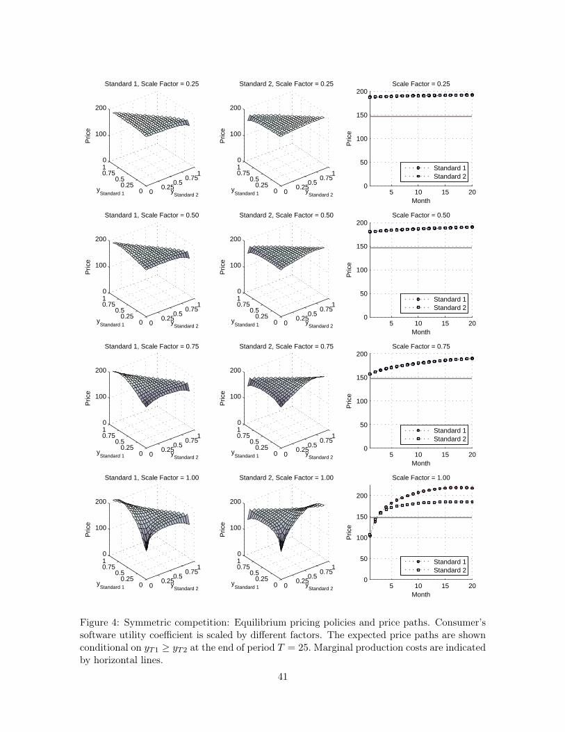
00.25

0.50.75

1

00.25

0.50.7510

100

200

yStandard 2

Standard 1, Scale Factor = 0.25

yStandard 1

Pric

e

00.25

0.50.75

1

00.25

0.50.7510

100

200

yStandard 2

Standard 2, Scale Factor = 0.25

yStandard 1

Pric

e

5 10 15 200

50

100

150

200

Month

Pric

e

Scale Factor = 0.25

Standard 1Standard 2

00.25

0.50.75

1

00.25

0.50.7510

100

200

yStandard 2

Standard 1, Scale Factor = 0.50

yStandard 1

Pric

e

00.25

0.50.75

1

00.25

0.50.7510

100

200

yStandard 2

Standard 2, Scale Factor = 0.50

yStandard 1

Pric

e

5 10 15 200

50

100

150

200

Month

Pric

e

Scale Factor = 0.50

Standard 1Standard 2

00.25

0.50.75

1

00.25

0.50.7510

100

200

yStandard 2

Standard 1, Scale Factor = 0.75

yStandard 1

Pric

e

00.25

0.50.75

1

00.25

0.50.7510

100

200

yStandard 2

Standard 2, Scale Factor = 0.75

yStandard 1

Pric

e

5 10 15 200

50

100

150

200

Month

Pric

eScale Factor = 0.75

Standard 1Standard 2

00.25

0.50.75

1

00.25

0.50.7510

100

200

yStandard 2

Standard 1, Scale Factor = 1.00

yStandard 1

Pric

e

00.25

0.50.75

1

00.25

0.50.7510

100

200

yStandard 2

Standard 2, Scale Factor = 1.00

yStandard 1

Pric

e

5 10 15 200

50

100

150

200

Month

Pric

e

Scale Factor = 1.00

Standard 1Standard 2

Figure 4: Symmetric competition: Equilibrium pricing policies and price paths. Consumer’ssoftware utility coefficient is scaled by different factors. The expected price paths are shownconditional on yT1 ≥ yT2 at the end of period T = 25.Marginal production costs are indicatedby horizontal lines.

41

0 0.2 0.4 0.6 0.8 10

0.2

0.4

0.6

0.8

1Scale Factor = 0.25

Standard 1

Sta

ndar

d 2

0.2 0.4 0.6 0.8 1.00

20

40

60

80

100Scale Factor = 0.25

Share of Total Installed Base

Per

cent

of S

imul

atio

ns

Standard 1Standard 2

0 0.2 0.4 0.6 0.8 10

0.2

0.4

0.6

0.8

1Scale Factor = 0.50

Standard 1

Sta

ndar

d 2

0.2 0.4 0.6 0.8 1.00

20

40

60

80

100Scale Factor = 0.50

Share of Total Installed Base

Per

cent

of S

imul

atio

ns

Standard 1Standard 2

0 0.2 0.4 0.6 0.8 10

0.2

0.4

0.6

0.8

1Scale Factor = 0.75

Standard 1

Sta

ndar

d 2

0.2 0.4 0.6 0.8 1.00

20

40

60

80

100Scale Factor = 0.75

Share of Total Installed Base

Per

cent

of S

imul

atio

ns

Standard 1Standard 2

0 0.2 0.4 0.6 0.8 10

0.2

0.4

0.6

0.8

1Scale Factor = 1.00

Standard 1

Sta

ndar

d 2

0.2 0.4 0.6 0.8 1.00

5

10

15

20

25

30Scale Factor = 1.00

Share of Total Installed Base

Per

cent

of S

imul

atio

ns

Standard 1Standard 2

Figure 5: Symmetric competition: Expected state evolution and distribution of shares in theinstalled base after 25 months. Consumer’s software coefficient is scaled by different factors.

42

0 0.2 0.4 0.6 0.8 10

0.2

0.4

0.6

0.8

1β = 0.6

Standard 1

Sta

ndar

d 2

0.2 0.4 0.6 0.8 1.00

20

40

60

80

100β = 0.6

Share of Total Installed Base

Per

cent

of S

imul

atio

ns

Standard 1Standard 2

0 0.2 0.4 0.6 0.8 10

0.2

0.4

0.6

0.8

1β = 0.7

Standard 1

Sta

ndar

d 2

0.2 0.4 0.6 0.8 1.00

20

40

60

80

100β = 0.7

Share of Total Installed Base

Per

cent

of S

imul

atio

ns

Standard 1Standard 2

0 0.2 0.4 0.6 0.8 10

0.2

0.4

0.6

0.8

1β = 0.8

Standard 1

Sta

ndar

d 2

0.2 0.4 0.6 0.8 1.00

20

40

60

80

100β = 0.8

Share of Total Installed Base

Per

cent

of S

imul

atio

ns

Standard 1Standard 2

0 0.2 0.4 0.6 0.8 10

0.2

0.4

0.6

0.8

1β = 0.9

Standard 1

Sta

ndar

d 2

0.2 0.4 0.6 0.8 1.00

5

10

15

20

25

30β = 0.9

Share of Total Installed Base

Per

cent

of S

imul

atio

ns

Standard 1Standard 2

Figure 6: Symmetric competition: Equilibrium pricing policies and price paths for differentconsumer discount factors (β).

43

0 0.2 0.4 0.6 0.8 10

0.2

0.4

0.6

0.8

1Scale Factor = 0.25

Sony

Nin

tend

o

0.2 0.4 0.6 0.8 1.00

20

40

60

80

100Scale Factor = 0.25

Share of Total Installed Base

Per

cent

of S

imul

atio

ns

0 0.2 0.4 0.6 0.8 10

0.2

0.4

0.6

0.8

1Scale Factor = 0.50

Sony

Nin

tend

o

0.2 0.4 0.6 0.8 1.00

20

40

60

80

100Scale Factor = 0.50

Share of Total Installed Base

Per

cent

of S

imul

atio

ns

0 0.2 0.4 0.6 0.8 10

0.2

0.4

0.6

0.8

1Scale Factor = 0.75

Sony

Nin

tend

o

0.2 0.4 0.6 0.8 1.00

20

40

60

80

100Scale Factor = 0.75

Share of Total Installed Base

Per

cent

of S

imul

atio

ns

SonyNintendo

SonyNintendo

SonyNintendo

0 0.2 0.4 0.6 0.8 10

0.2

0.4

0.6

0.8

1Scale Factor = 1.00

Sony

Nin

tend

o

0.2 0.4 0.6 0.8 1.00

10

20

30

40Scale Factor = 1.00

Share of Total Installed Base

Per

cent

of S

imul

atio

ns

SonyNintendo

Figure 7: Predictions from estimated parameter values: Expected state evolution and dis-tribution of shares in the installed base after 25 months. Consumer’s software coefficient isscaled by different factors.

44

0 0.2 0.4 0.6 0.8 10

0.2

0.4

0.6

0.8

1β = 0.6

Sony

Nin

tend

o

0.2 0.4 0.6 0.8 1.00

20

40

60

80

100β = 0.6

Share of Total Installed Base

Per

cent

of S

imul

atio

ns

SonyNintendo

0 0.2 0.4 0.6 0.8 10

0.2

0.4

0.6

0.8

1β = 0.7

Sony

Nin

tend

o

0.2 0.4 0.6 0.8 1.00

20

40

60

80

100β = 0.7

Share of Total Installed Base

Per

cent

of S

imul

atio

ns

SonyNintendo

0 0.2 0.4 0.6 0.8 10

0.2

0.4

0.6

0.8

1β = 0.8

Sony

Nin

tend

o

0.2 0.4 0.6 0.8 1.00

20

40

60

80

100β = 0.8

Share of Total Installed Base

Per

cent

of S

imul

atio

ns

SonyNintendo

0 0.2 0.4 0.6 0.8 10

0.2

0.4

0.6

0.8

1β = 0.9

Sony

Nin

tend

o

0.2 0.4 0.6 0.8 1.00

10

20

30

40β = 0.9

Share of Total Installed Base

Per

cent

of S

imul

atio

ns

SonyNintendo

Figure 8: Predictions from estimated parameter values: Equilibrium pricing policies and pricepaths for different consumer discount factors (β).

45