time delayed control of structural systems

EARTHQUAKE ENGINEERING AND STRUCTURAL DYNAMICSEarthquake Engng Struct. Dyn. 2003; 32:495–535 (DOI: 10.1002/eqe.228)

Time delayed control of structural systems

Firdaus E. Udwadia1;∗;†, Hubertus F. von Bremen2, Ravi Kumar3and Mohammad Hosseini2

1Department of Civil Engineering; Aerospace and Mechanical Engineering; Mathematics; and Information andOperations Management; University of Southern California; Los Angeles; CA 90089-1453; U.S.A.

2Department of Aerospace and Mechanical Engineering; University of Southern California; Los Angeles;CA 90089-1453; U.S.A.

3Structural Analysis and Research Corporation; 5000 McKnight Road; Pittsburgh; PA 15237; U.S.A.

SUMMARY

Time delays are ubiquitous in control systems. They usually enter because of the sensors and actuatorsused in them. Traditionally, time delays have been thought to have a deleterious eect on both thestability and the performance of controlled systems, and much research has been done in attempting toeliminate them, compensate for them, or nullify their presence. In this paper we take a dierent view. Weinvestigate whether purposefully injected time delays can be used to improve both the system’s stabilityand performance. Our analytical, numerical, and experimental investigation shows that this can indeedbe done. Analytical results of the eects of time delays on collocated and non-collocated control ofclassically damped and non-classically damped systems are given. Experimental and numerical resultsconrm the theoretical expectations. Issues of system uncertainties and robustness of time delayedcontrol are addressed. The results are of practical value in improving the performance and stabilityof controllers because these characteristics (performance and stability) improve dramatically with theintentional injection of small time delays in the control system. The introduction of such time delaysconstitutes a ‘minimal change’ to a controller already installed in a structural system for active control.Hence, from a practical standpoint, time delays can be implemented in a nearly costless and highlyreliable manner to improve control performance and stability, an aspect that cannot be ignored whendealing with the economics and safety of large structural systems subjected to strong earthquake groundshaking. Copyright ? 2003 John Wiley & Sons, Ltd.

KEY WORDS: time delayed control; structural systems; collocated and non-collocated control; classicallydamped and non-classically damped systems; stability; theory, experiment, and simulations; uncertainsystems and time delays

1. INTRODUCTION

The active control of large-scale structural systems usually requires the generation of largecontrol forces which often need to be provided at high frequencies. Actuator and sensor

∗ Correspondence to: Firdaus E. Udwadia, Department of Aerospace and Mechanical Engineering, University ofSouthern California, Los Angeles, CA 90089-1453, U.S.A.

† E-mail: [email protected]

Received 16 March 2001Revised 8 May 2002

Copyright ? 2003 John Wiley & Sons, Ltd. Accepted 8 June 2002

496 F. E. UDWADIA ET AL.

dynamics do not permit the instantaneous generation of such forces and hence the eectivecontrol gets delayed in time. Thus the presence of time delays in the control are inevitablewhen controlling building structures subjected to dynamic loads, such as those caused bystrong earthquake ground shaking. In order to accommodate for the time delays, the mathe-matical formulations of the problem of controlling building structures are usually more compli-cated than the formulations without time delays. The fact that the models are more complicatedwhen time delays are included and that in some cases the presence of time delays destabilizethe control has fueled the predominant view that time delays are an undesirable element in theactive control of structures. With this view in mind, methods to cancel out, reduce, or changethe eect of time delays have been developed. This paper proposes a dierent viewpoint:its central theme is that instead of considering time delays as always being injurious, onecould aim to exploit their presence, especially since they are ubiquitous. We show that theproper intentional introduction of time delays: (1) can stabilize even a non-colocated controlsystem (which may be unstable in the absence of time delays), and (2) may improve controlperformance.Extensive work has been done on the control of structural systems where no consideration

to time delays is given. The fact that the results do not include time delays does not underminetheir importance when controlling large building structures, since several of the concepts canbe used as a starting point when dealing with time-delayed problems. Feedback control ofstructural systems yields dierent stability characteristics depending on whether collocated ornon-collocated control is used. Direct velocity feedback (no time delay) control of a discretedynamical system with collocation of actuators and sensors is known to be stable for all valuesof the control gain [1; 2]. Balas [3] has investigated the potential of direct output feedbackcontrol for systems where sensors and actuators need not be collocated. When actuators’dynamics are considered, Goh and Caughey [4] and Fanson and Caughey [5] have shownthat position feedback is preferable to velocity feedback under collocated control. Cannonand Rosenthal [6] deal with experimental studies of collocated and non-collocated control ofexible structures. Based on these studies, it has been concluded that it is very dicult toachieve robust non-collocated control of exible structures.In practical feedback control systems, small time delays in the control action are inevitable

because of the involved dynamics of the actuators and sensors. As stated before, these timedelays become particularly signicant when the control eort demands large control forces,and=or high frequencies. It is therefore crucial to understand the eect of time delays on thecontrol of structural systems. Several papers in the literature treat the presence of time delaysas a negative factor. Yang et al. [7] show that time delays worsen performance for theirproposed controllers. Agrawal and Yang [8] show through simulations that the degradation ofthe control performance of an actively controlled structural system due to a xed time delayis not signicant until the delay reaches a critical value. Agrawal et al. [9] and Agrawaland Yang [10] indicated methods of compensation for time delay in the active control ofstructural systems. On the other hand, some previous studies suggest that time delays can beused to good advantage. Kwon et al. [11] show that the intentional use of time delays mayimprove the performance of the control system. Udwadia and Kumar [12] show that dislocatedvelocity control, which leads to instability in the absence of time delays, can be used to evenstabilize an MDOF system (for small gains) by an appropriate choice of time delays. In thepresent paper (Section 3) we show that the intentional injection of time delays can increasethe maximum gain for stability of a non-classically damped system (when compared with

Copyright ? 2003 John Wiley & Sons, Ltd. Earthquake Engng Struct. Dyn. 2003; 32:495–535

TIME DELAYED CONTROL OF STRUCTURAL SYSTEMS 497

the system with no time delays). Experimental results on a two-degree-of-freedom torsionalsystem (Section 4) conrm our analytical ndings and show that it is possible to choose timedelays which improve the controller’s performance when compared to the controlled systemwith no time delays.This paper is organized as follows. Section 2 of the paper deals with the time-delayed con-

trol of classically damped systems. Results for collocated as well as for non-collocated controlof undamped and underdamped systems are given. The theoretical expectations are conrmednumerically when applied to a building structure model which is subjected to an earthquake.Numerical results on the sensitivity of the control methodology to perturbations (a) of theparameters of a building structure, and (b) of the time delays used are also presented. Sec-tion 3 deals with more general, non-classically damped, linear systems. Section 4 presentsexperimental data on a two degree-of-freedom non-classically damped torsional system. Nu-merical results which corroborate the theoretical ndings obtained in the previous sectionsare also presented for comparison. Here we also show that it is possible for a non-systempole (a pole whose root locus does not start at an open loop pole of the structural system)to dictate the maximum gain for stability of the time-delayed, controlled system. Section 5presents robustness issues. It deals with the control of uncertain systems with uncertain timevarying delays in the control input. Our conclusions are presented in Section 6.

2. CLASSICALLY DAMPED STRUCTURAL SYSTEMS

This section deals with the time-delayed control of classically damped structures. Collocatedas well as non-collocated control of undamped and underdamped structures are considered.Most of the results apply to controllers of the PID type (proportional, integral, derivative).Numerical computations are used to conrm some of the theoretical expectations for a buildingstructure subjected to an earthquake. Most of the results apply only to the case when systempoles are considered (that is, for poles whose root locus originates at the open loop polesof the structural system). The sensitivity of the stability of the building structure when theparameters of the structure and the time delay are varied is explored numerically. It is shownnumerically that even under considerable perturbations (7–50%) of the parameter values thesystem remains stable. Details of some of the analytical results presented in this section canbe found in Udwadia and Kumar [12] and part of the numerical results can be found inUdwadia and Kumar [13].

2.1. System model and general formulation

Consider a linear classically damped structural system whose response x(t) is described bythe matrix dierential equation

Mx′′(t) + Cx′(t) + Kx(t)= g(t); x(0)=0; x′(0)=0 (1)

where M is the n× n positive denite symmetric mass matrix, C is the n× n symmetricdamping matrix, and K is the n× n positive denitive symmetric stiness matrix. The forcingfunction is given by the n-vector g(t).



Since the system is classically damped, it can be transformed to the diagonal system

z′′(t) + z′(t) + z(t)=T TM−1=2g(t); z(0)=0; z′(0)=0 (2)

where =diag(21; 22; : : : ; 2n); =diag(21; 22; : : : ;

2n), and the matrix T =[tij] is the or-

thogonal matrix of eigenvectors of M−1=2KM−1=2. Taking the Laplace transform of Equation(2) and solving, we get

x(s)=M−1=2TT TM−1=2g(s) (3)

where the wiggles indicate the transformed functions, and is given by

=diag((s2 + 21s+ 21)−1; (s2 + 22s+ 22)

−1; : : : ; (s2 + 2ns+ 2n)−1)

The open loop poles are given by the zeros of the equations

s2 + 2qs+ 2q=(s− +q)(s− −q)=0; q=1; 2; : : : ; n (4)

The poles have been denoted by ±q, the sign indicating the sign in front of the radical of thequadratic equations given in Equation (4). In this paper we assume the system to be genericand all poles to have multiplicity one (no repeated poles).The feedback control uses a linear combination of p responses xsk (t); k=1; 2; : : : ; p, which

are fed to a controller. In general, the responses are time-delayed by Tsk . The actuator willapply a force to the system, aecting the jth equation of Equation (1). When j∈sk : k=1; 2;: : : ; p the sensors and the actuator are collocated, and if j =∈sk : k=1; 2; : : : ; p the sensorsand the actuator are non-collocated (dislocated). The control methodology applied to a shearframe building structure is shown in Figure 1.

Figure 1. Shear frame building structure and control methodology.



Denoting the non-negative control gain by and the controller transfer function by c(s),the closed loop system poles are given by

A(s)x(s)= [Ms2 + Cs+ K]x(s)= g(s)− c(s)p∑k=1ask xsk (s) exp[−sTsk ]ej (5)

where ej is the unit vector with unity in the jth element and zeros elsewhere. The numbers askare the coecients of the linear combination of the responses fed to the controller. Movingthe last term on the right of Equation (5) to the left gives

A1(s)x(s)= g(s) (6)

where A1(s) is obtained by adding c(s)ask exp[−sTsk ] to the (j; sk)th element of A(s), fork=1; 2; : : : ; p.The closed loop poles are then given by the relation

det[A1(s)]=det[A(s)]1 + c(s)

p∑k=1ask exp[−sTsk ]x()sk ; j(s)

=0 (7)

where x()sk ; j(s) is the Laplace transform of the open loop response to an impulsive force appliedat node j at time t=0. The open loop response to the impulsive force is given by

x()sk ; j(s)=n∑i=1

t(M)sk ; i t(M)j; i

s2 + 2is+ 2i

where

t(M)sk ; r =n∑u=1m−1=2sk ; u tu; r

with m−1=2i; j being the (i; j)th element of M−1=2 and T (M) = M−1=2T =[t(M)i; j ].

The following set of conditions will be referred to as condition set C1. Given that the openloop poles of the system are ±q, we have

(1) c(±q) =0; for q=1; 2; : : : ; n

(2)p∑k=1ask exp[−±qTsk ]t(M)sk ; q =0; for q=1; 2; : : : ; n

(3) t(M)j; q =0; for q=1; 2; : : : ; n

The rst condition means that the open loop poles of the system are not also zeros of thecontroller transfer function. The second condition is a generalized observability conditionwhich requires that all mode shapes are observable from the summed, time-delayed sensormeasurements. The third condition is a controllability condition which requires that the con-troller cannot be located at any node of any mode of the system. Observe that if any of thethree conditions is not satised for one open loop pole q, then by Equation (7) the openloop pole q is also a closed loop pole. However, if C1 is satised, we have the followingresult.



Result 2.1When the open loop system has distinct poles and condition set C1 is satised, the open loopand the closed loop systems have no poles in common.If condition set C1 is satised, then by Result 2.1 and Equation (7), the closed loop poles

of the system are given by the values of s that satisfy the equation

1 + c(s)p∑k=1

n∑i=1ask exp[−sTsk ]

[t(M)sk ; i t

(M)j; i

s2 + 2is+ 2i

]=0 (8)

In general, Equation (8) may have an innite number of zeros due to the time delay term.As the parameter is varied, we obtain the root locus of the closed loop poles. The polesthat are on a root locus that starts at an open loop pole of the structural system will becalled system poles. The poles that do not originate at an open loop pole of the system willbe called non-system poles. To simplify matters, some of the following results deal with thesystem poles only. The simplication of dealing with the system poles only, allows us toobtain bounds on the gain and the time delay to guarantee stability. These results should beviewed with caution since in general there are an innite number of poles, and as shown inSection 4, a non-system pole may determine what is the maximum gain for stability for somesystems. It will be made clear when our results apply to all the poles considered, and whenonly to the system poles.The following result and all of its consequences apply to the case when only system poles

are considered. Multiplying Equation (8) by s2 + 2rs + 2r , then dierentiating with respectto and letting s→ ±r =−r ± i(2r − 2r)1=2 and → 0, we obtain

dsd

∣∣∣∣ →0s→±r

=− c(±r)±2i(2r − 2r)1=2

[ p∑k=1ask exp[−±rTsk ]t(M)sk ; r

]t(M)j; r (9)

Result 2.2A sucient condition for the closed loop system to remain stable for innitesimal gains isthat

Re

dsd

∣∣∣∣ →0s→±r

¡0; r=1; 2; : : : ; n (10)

Again, Result 2.2 applies only when system poles are considered, and in general the resultmay not be true when non-system poles are also considered.We now particularize the controller to be of the proportional, integral and derivative (PID)

form. The transfer function of the controller is then given by

c(s)=K0 + K1s+K2s

with K0; K1; K2¿0

The term K0 corresponds to proportional control, the term K1s corresponds to derivative controland the term K2=s corresponds to integral control. Next we specialize results for the undampedcase.



2.2. Undamped systems

The following set of results apply to undamped systems. When the damping matrix C=0,the open loop poles lie on the imaginary axis, and by Equation (10), the next resultfollows.

Result 2.3For undamped systems (C=0), condition (10) is a necessary and sucient condition forstability for small gains.For an undamped system, the open loop poles are of the form ±r = ± ir . Using Equations

(9) and (10) we can derive the following requirement for stability for small gains (this resultapplies to system poles only).

Re(

K0±ir + K1 −

K22r

)( p∑k=1ask exp[∓irTsk ]t(M)sk ; r t

(M)j; r

)¿0 (11)

for r=1; 2; : : : ; n.Using relation (11), we can derive the following result.

Result 2.4When using one sensor collocated with the actuator for an undamped system, the PID feedbackcontrol is stable (for small gains) if and only if

aj

−K0rsin(rTj) +

(K1 − K2

2r

)cos(rTj)

¿0 (12)

for r=1; 2; : : : ; n.

Result 2.5For undamped systems with one sensor collocated with the actuator, we have the followingconditions for stability for small gains.

(a) Velocity feedback (K0 =K2 = 0) is stable as long as the time delay is such thatTj¡=2max, where max is the highest undamped natural frequency of the system.

(b) Integral control (K0 =K1 = 0) is stable as long as the delay is such that Tj¡=2max.(c) Proportional control (K1 =K2 = 0) is stable as long as the delay is such that 0¡Tj¡=

max.(d) When K0 = 0 and the time delay is such that Tj¡=2max, the undamped system will

be stabilized when K1¿K2=2min and aj¿0, or K1¡K2=2max and aj¡0.

Result 2.6When the system is undamped, and

(1) condition set C1 is satised,(2) one sensor is used and is collocated with the actuator, and,(3) no time delay is used,



then the PID control, if stable for → 0+ is stable for all ¿0, provided

det[A(−K2K1

)]+ ajK0 det

[A2

(−K2K1

)]=0 (13)

for any positive , where A2 is obtained by deleting the jth row and the jth column of thematrix A.When velocity (or integral) feedback control is used, condition (13) is always satised,

hence we get the well-known result that stability is guaranteed for ¿0. The upper boundfor the stability of the system described in Result 2.6 can be obtained to be

¡−det[A(−K2=K1)]

ajK0 det[A2(−K2=K1)]

provided the right-hand side in the inequality is positive. If not, the system is stable for all¿0, provided it is stable for small gains. Result 2.6 and the above bound on the gain forstability apply to the case when all the poles are considered. The next result however onlyapplies when system poles are considered.

Result 2.7When the system is undamped, and

(1) condition set C1 is satised,(2) one sensor is used and it is collocated with the actuator, and(3) time delay Tj¡2max ,

then velocity feedback control will be stable as long as

¡1

ajK10∑n

i=1 [t(M)j; i ]2=(20 − 2i )

where 0 ==2Tj

The previous results have focused on collocated control. In the following results we willconsider the control of non-collocated (dislocated) systems. Results dealing with no timedelay are presented rst, and are followed by results for time-delayed systems.

Result 2.8When using a PID controller, where

(1) the sensors and the actuator are not collocated,(2) the time delays, Tsk ; k=1; 2; : : : ; p, are all zero,(3) the matrix M is diagonal, and(4) K1¿K2=2min or K1¡K2=

2max,

it is impossible to stabilize the undamped system for small gains.The next result gives necessary conditions for the stability of a system using a PID con-

troller.



Result 2.9When using a PID controller, where

(1) the sensors and the actuator are not collocated,(2) the time delays, Tsk ; k=1; 2; : : : ; p, are all zero, and(3) the matrix M is non-diagonal,

a necessary condition for the undamped system to be stabilized for small gains is

(a)∑p

k=1 askm−1sk ; j¿0 when K1¿K2=

2min, and

(b)∑p

k=1 askm−1sk ; j¡0 when K1¡K2=

2max.

Often building structures are modelled by tridiagonal stiness matrices. The following resultapplies to such structures.

Result 2.10If M and K are positive denite, M is diagonal and K is tridiagonal, having negative sub-diagonal elements, it is possible to nd a location j (for the actuator) and a location sl (forthe sensor), j = s1, so that the sequence t(M)s1 ; i t

(M)j; i ni=1 will only have one sign change.

Result 2.11When using an ID controller, for a system as dened in Result 2.10, where

(1) condition set C1 is satised,(2) one sensor is used and it is not collocated with the actuator,(3) the sign change in the sequence t(M)s1 ; i t

(M)j; i ni=1 occurs when i=m,

(4) time delay Ts1 (=2m−1)− , where is a small positive quantity and, Ts1m¿=2,(5) (max=m−1)63, and(6) K1¿K2=2min or K1¡K2=

2max,

it is possible to stabilize an undamped (open loop) system for small gains.

Result 2.12For the undamped system described in Result 2.11, velocity feedback control will bestable as long as ¡G, where G is the minimum of all positive Bl, for l=0; 1; 2; : : : ;where

Bl=−1

as1K1l sin(lTs1)∑n

i=1 (t(M)s1 ; i t

(M)j; i )=(2i − 2l )

and l=(2l+ 1)2Ts1

2.3. Underdamped systems

This section deals with underdamped systems. Specializing Equation (9) to underdampedsystems, and utilizing Result 2.2 we get the following result which is again applicable to thecase when only system poles are considered.



Result 2.13When using PID control for underdamped systems, i¡i; i=1; 2; : : : ; n, a sucient conditionfor the closed loop system to be stable for small gains is

− 1(2r − 2r)1=2

[K0 −

(K1 +

K22r

)r

]( p∑k=1ask exp[rTsk ] sin((

2r − 2r)1=2Tsk )t(M)sk ; r t

(M)j; r

)

+[K1 − K2

2r

]( p∑k=1ask exp[rTsk ] cos((

2r − 2r)1=2Tsk )t(M)sk ; r t

(M)j; r

)¿0

for r=1; 2; : : : ; n.

Result 2.14When the sensor and actuator are collocated and only one sensor is used, for PID control, if(K1 − K2=2r ) =0, for all r, a sucient condition for small gains stability is

aj

[K1 − K2

2r

]cos((2r − 2r)1=2Tsk + )¿0 for r=1; 2; : : : ; n

where

= tan−1[K0 − (K1 + (K2=2r ))r

(K1 − (K2=2r ))(2r − 2r)1=2]

Result 2.15When using one sensor, collocation of the sensor with an actuator of the given feedbackcontrol type will cause the closed loop system poles to move to the left in the s-plane, aslong as the given condition on the time delay is satised.

(a) For velocity feedback, the time delay needs to satisfy

Tj¡min∀r

[(=2) + (2r − 2r)1=2

]

where

= tan−1[

r(2r − 2r)1=2

]

(b) For integral feedback, the time delay needs to satisfy

Tj¡min∀r

[(=2)− (2r − 2r)1=2

]

where is as in part (a).(c) For proportional feedback, the time delay needs to satisfy

0¡Tj¡min∀r

[

(2r − 2r)1=2]



-16 -14 -12 -10 -8 -6 -4 -2 0 2-10

0

10

20

30

40

50

60

70

80

90

Real

Imag

inar

y ax

is

-10

0

10

20

30

40

50

60

70

80

90

Imag

inar

y ax

is

-15 -10 -5 0 5 10 15

Real (a) (b)

Figure 2. Root loci of closed loop system poles for collocated velocity feedback control withj=4; s1 = 4; a4 = 1, and time delay (a) T4 = 0 s, (b) T4 = 0:025 s.

(d) For a PID controller, the time delay needs to satisfy

Tj¡min∀r

[(=2)− (2r − 2r)1=2

]

where is as dened in Result 2.14, when K1¿K2=2min and aj¿0, or K1¡K2=2max

and aj¡0.

2.4. Numerical results

The numerical results are obtained for an undamped shear frame building structure (ve-degree-of-freedom system) shown in Figure 1. The mass and the stiness of each storey are1 and 1600 (taken in SI units), respectively. The root loci presented only show the systempoles. The controller’s gain has been varied from 0 to 100 units. Velocity feedback controlis used for all the results.The rst example deals with the collocated control of the structure with and without time

delay. The controller and the sensor are collocated at the fourth storey. Figure 2(a) shows theroot loci of the closed loop system poles for velocity feedback control with no time delay(T4 = 0 s). As expected from Result 2.6, the system is stable since the system’s closed looppoles have negative real parts. Figure 2(b) shows the root loci for the closed loop systempoles with velocity feedback control when a time delay of T4 = 0:025 s is used. Introducing atime delay of T4 = 0:025 s makes the system unstable even for very small gains, as predictedby Result 2.4.In the second example, the non-collocated control of the structure is studied with and

without time delay. The actuator is placed at mass 4 (fourth storey) and is fed the velocitysignal from location 5 (fth storey). Figure 3(a) shows the root loci for the closed loop systempoles for velocity feedback control with no time delay (T5 = 0 s) and j=4; s1 = 5; a5 = 1.As guaranteed by Result 2.8, even for vanishingly small gains, the third, fourth, and fthclosed loop system poles are in the right-half s-plane, hence causing instability. However, theintroduction of an appropriate time delay, such as T5 = 0:04 s makes the closed loop system



-1 0 -5 0 5 10-10

0

10

20

30

40

50

60

70

80

90

Real-14 -12 -10 -8 -6 -4 -2 0 2

-10

0

10

20

30

40

50

60

70

80

90

Real Axis

Imag

inar

y ax

is

Imag

inar

y ax

is

(a) (b)

Figure 3. Root loci of closed loop system poles for non-collocated velocity feedback control withj=4; s1 = 5; a5 = 1, and time delay (a) T5 = 0 s, (b) T5 = 0:04 s.

0 2 4 6 8 10-0.2

-0.15

-0.1

-0.05

0

0.05

0.1

0.15

0.2

Dis

plac

emen

t (m

)

Time (sec)

Gain=1No

Gain=10No control

Figure 4. Relative displacement response of mass 5 (j=4; s1 = 5; a5 = 1, andT5 = 0:04 s) for non-collocated velocity control.

poles remain in the left-half plane until a certain value of the controller gain. This is illustratedin Figure 3(b), where the closed loop system poles are shown for j = 4; s1 = 5; a5 = 1,and a time delay of T5 = 0:04 s. The upper bound on the gain for stability obtained by tracingthe root loci is the same as the one predicted by Result 2.12. This example shows that byappropriately injecting time delay into a system, it is possible to stabilize a system which isunstable for zero time delay.Figure 4 shows the displacement time history of mass 5 relative to the base, when the

structure is subjected to the ground motion of the S00E component of the Imperial ValleyEarthquake of 1940. The structural responses are numerically computed using a fourth-order



0 1 2 3 4 5 6 7 8 9 10-10

-8

-6

-4

-2

0

2

4

6

8

10

For

ce (

N)

Time (sec)

Incoming Force per storyControl Force (Gain=10)

Figure 5. Incoming force per storey and control force time histories (j=4; s1 = 5; a5 = 1, andT5 = 0:04 s) for non-collocated velocity control.

Runge–Kutta scheme. The response time histories are shown only for the rst 10 s. Theresponse is shown for no control (=0), and for =10 units, using non-collocated velocitycontrol with j=4; s1 = 5; a5 = 1, and T5 = 0:04s. The results on Figure 4 show that by usingintentional time-delayed velocity feedback, the displacement of the 5th mass is signicantlysmaller than the displacement of the mass when no control is used. Figure 5 shows thetime histories of the incoming force per storey (i.e. negative of storey mass times groundacceleration) and the control force required when the controller’s gain is =10 units.To explore the robustness of this control methodology, numerical results of the sensitivity

of the closed loop system poles to changes in the mass, stiness and time delay parameters(for the nominal system presented in the last example) are presented in the next section.

2.5. Sensitivity of the stability to perturbed parameters

There is always uncertainty about the exact values of the system’s parameters. The uncertaintymight come from not being able to measure or estimate the system parameters accurately.It may also come from variations of the system parameters caused by fatigue, structuraldegradation, etc. Changes in the parameter values will lead to changes in the closed looppoles, and thus changes in the performance of the system. This stresses the importance ofknowing how sensitive the time-delayed control is to parameter variations. Furthermore, wehave shown that the purposeful injection of time delays in non-collocated systems bringsabout stability. As the injection of such time delays in actual systems can at best be chosenonly approximately (because of the uncertainties in actuator dynamics, etc.) it is important toexamine the sensitivity of such a control technique to uncertainties in the time delays.These sensitivities are studied for the undamped shear frame building structure described in

Section 2.4 (see Figure 1). The results are for the non-collocated velocity feedback control,where the actuator is placed at mass 4, and the sensor takes delayed velocity readings from



0.02 0.025 0.03 0.035 0.04 0.045 0.051500

1520

1540

1560

1580

1600

1620

1640

1660

1680

1700

Time delay

Stif

fnes

s

5

5

5

5

5

5

10

10

10

10

10

10

20

20

20

20

20

20

30

30

30

30

30

30

35

35

35

35

35

35

40

40

40

40

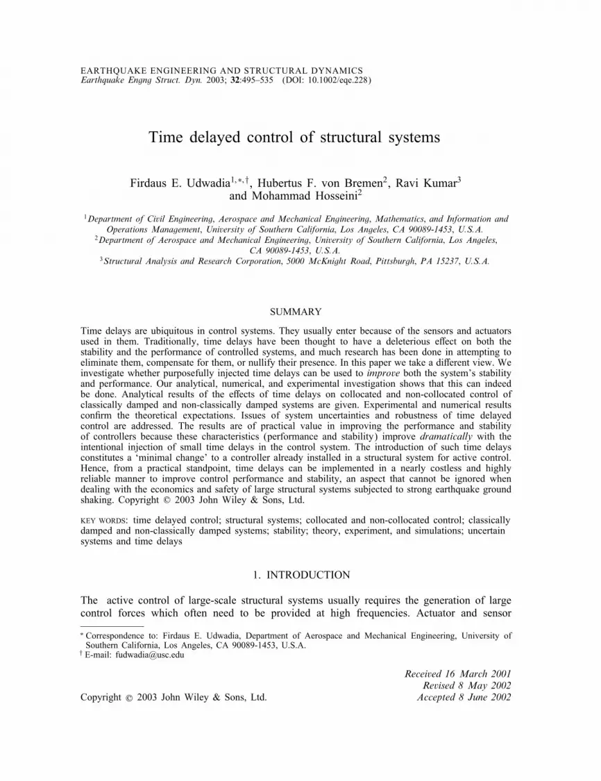
Figure 6. Sensitivity of the maximum gain for stability to changes in stinessand time delay for j=4; s1 = 5; a5 = 1, and mass=1.

0.025 0.03 0.035 0.04 0.045 0.050.5

0.6

0.7

0.8

0.9

1

1.1

1.2

1.3

Time delay

Mas

s

5

5

5

5

5

55 5

10

10

10

10

10

10

10

10 10

20

20

20

20

2020

20

20

25

25

25

25

2525

25

25

30

30

30

30

30

30

30

30

35

35

35

35

3535

40

40

40

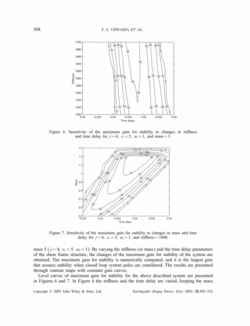
Figure 7. Sensitivity of the maximum gain for stability to changes in mass and timedelay for j=4; s1 = 5; a5 = 1, and stiness=1600.

mass 5 (j=4; s1 = 5; a5 = 1). By varying the stiness (or mass) and the time delay parametersof the shear frame structure, the changes of the maximum gain for stability of the system areobtained. The maximum gain for stability is numerically computed, and it is the largest gainthat assures stability when closed loop system poles are considered. The results are presentedthrough contour maps with constant gain curves.Level curves of maximum gain for stability for the above described system are presented

in Figures 6 and 7. In Figure 6 the stiness and the time delay are varied, keeping the mass



constant at 1 (SI units). Sensitivity to variations of the mass and the time delay are presentedon Figure 7, when the stiness is kept constant at 1600 (SI units).Both graphs show a continuous dependence of the maximum gain for stability on the chosen

parameters. The gures show that stable dislocated control brought about by the purposefulinjection of time delays could be made eective even in the presence of considerable uncer-tainties in the parameters that model the structural system. Further results on the stability ofcontrolled systems with uncertainties in the system parameters and time delay are presentedin Section 5. The next section deals with the control of more general linear systems whichinclude both non-classically and classically damped structures.

3. NON-CLASSICALLY DAMPED SYSTEMS

In the last section we presented results dealing with classically damped systems, where severalof the results apply when only system poles are considered. In this section we present aformulation that deals with more general systems, and the results apply to both, non-classicallydamped as well as to classically damped systems. Furthermore, the results apply when all thepoles are considered; they are not just limited to considering system poles. The importanceof having a formulation that deals with ‘all’ the poles of the control system with time delayswill be illustrated in Section 4 where it is shown that a pole not originating from an openloop pole dictates the stability of the system.We show that when all the open loop poles have negative real parts and the controller

transfer function is an analytic function, then given any time delays there exists a range inthe gain (which could depend on the time delays) for which the closed loop feedback systemis stable. The results are then specialized to systems with a single sensor. We show that undersome conditions there exists a range in the gain for which the closed loop system is stablefor all time delays. The section ends with the application of some of the results to a singledegree of freedom oscillator.

3.1. General formulation

The same general formulation given for classically damped systems (Section 2) will be usedin this section, except that the systems considered here are more general (also see von Bremenand Udwadia [14]). They include both classically damped and non-classically damped systems.Consider the following matrix equation corresponding to a structural system with the responsex(t) given as

Mx′′ + Cx′ + Kx= g(t); x(0)=0 and x′(0)=0 (14)

where M is an n by n mass matrix, C is the n× n damping matrix and K is the n× n stinessmatrix. The n-vector g(t) is the distributed applied force. The Laplace transform of the abovesystem is

A(s)x(s) = (Ms2 + Cs+ K)x(s) = g(s) (15)



As in Section 2, we use p responses in the feedback control. A linear combination of thesensed responses are fed to the controller which generates the control force. In general, thesystem may have several actuators; in this paper we will deal with one actuator. Supposewe have a control eort aecting the jth equation of Equation (15) given by (f(s); x(s))ej,where (f(s); x(s))=

∑ni=1 fi(s)xi(s); ej is a vector with 1 in the jth location and zero for

all other entries, and is the control gain. The function fi(s) contains the controller transferfunction which uses the signal from xi(s), and in the presence of a time delay Ti, it includesthe term exp[−sTi] as a factor. Equation (15) with the control eort becomes

A(s)x(s) = g(s)− (f(s); x(s))ej (16)

Moving the term (f(s); x(s))ej to the left-hand side of (16), we get the equation

A1(s)x(s) = g(s) (17)

The open loop poles of Equation (17) are given by Equation (18a) and the closed loop polesare given by Equation (18b) as follows:

det[A(s)] = 0 (18a)

det[A1(s)] = 0 (18b)

The equation for the closed loop poles can be written as

det[A1(s)] = det[A(s)] + n∑i=1fi(s)Aij(s) (19)

where Aij(s) is the cofactor of aij(s), in other words Aij(s) = (−1)(i+j)Minor(aij(s)), andthe matrix A is the one dened in Equation (15).

3.2. General analytical results

The stability of the system described in Equation (16) is dictated by the sign of the realpart of the closed loop poles. Using the argument principle, we can determine bounds on thegain so that the system described in Equation (16) is stable in the presence of time delays,provided the open loop poles of the system have negative real parts.The next result is similar to Result 2.1. It gives conditions so that the open and closed

loop systems have no poles in common.

Result 3.1Suppose the open loop poles are given by k , with k=1; 2; : : : ; 2n and the condition

q(k)=n∑i=1fi(k)Aij(k) =0 for k=1; 2; : : : ; 2n

is satised. Then the closed loop system and the open loop system have no poles in common.



ProofFor any k, clearly

det[A1(k)] = det[A1(k)] + n∑i=1fi(k)Aij(k)

= n∑i=1fi(k)Aij(k) =0

So no solution of Equation (18a) is shared by Equation (19), establishing the claim.For the stability of the closed loop system, we need the real part of the closed loop poles to

be negative. The next result gives bounds on the gain so that the closed loop system remainsstable.

Result 3.2For any given set of time delays, suppose the open loop poles 1; 2; : : : ; 2n all have negativereal parts and the following two conditions are satised:

(a) q(s)=∑n

i=1 fi(s)Aij(s) =0, and(b) q(s) is analytic,

for all s in the right-half complex plane and along the imaginary axis. Then there exists aninterval I∗ =[−∗; ∗], with ∗¿0, such that for any gain ∈ I∗ , the closed loop poles arein the left-half complex plane (i.e., the system is stable).

ProofWe will use the argument principle (see pp. 152–154 in Ahlfors [15]). Equation (19) can bevisualized as

det[A1(s)]= h(s)=p(s) + q(s)

where p(s)=det[A(s)], and q(s) is as above. Consider the contour given by the half-circle ofradius R in the right-half plane with boundary R and enclosing the region R, see Figure 8.

R

− R

Im (s)Γ

ΩR

Re (s)

Figure 8. Contour of integration.



For any xed R we have

h′(s)h(s)

=p′(s) + q′(s)p(s) + q(s)

=p′(s) + q′(s)

p(s)(1 + (q(s)=p(s)))

Now

11 + (q(s)=p(s))

=∞∑k=0

(−q(s)p(s)

)kfor all s∈R; provided

∣∣∣∣q(s)p(s)

∣∣∣∣¡1 or ||¡∣∣∣∣p(s)q(s)

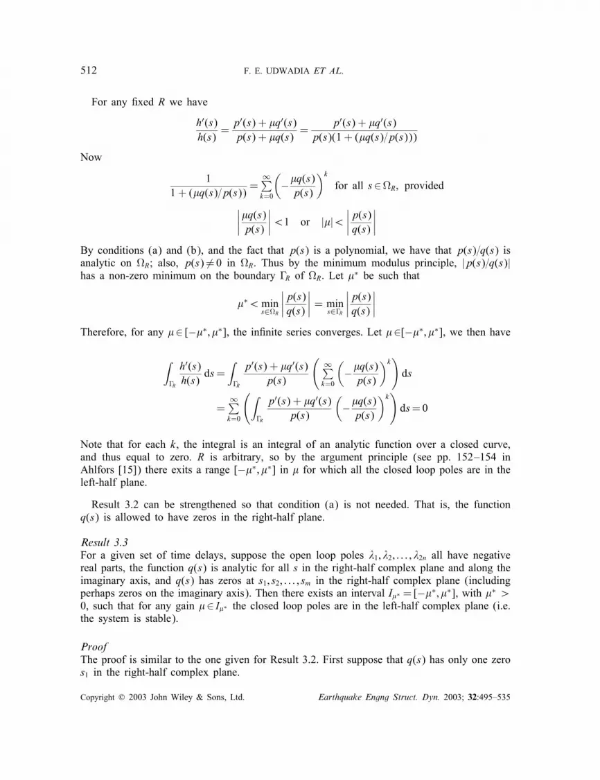
∣∣∣∣By conditions (a) and (b), and the fact that p(s) is a polynomial, we have that p(s)=q(s) isanalytic on R; also, p(s) =0 in R. Thus by the minimum modulus principle, |p(s)=q(s)|has a non-zero minimum on the boundary R of R. Let ∗ be such that

∗¡mins∈R

∣∣∣∣p(s)q(s)

∣∣∣∣ = mins∈R

∣∣∣∣p(s)q(s)

∣∣∣∣Therefore, for any ∈ [−∗; ∗], the innite series converges. Let ∈[−∗; ∗], we then have

∫R

h′(s)h(s)

ds=∫R

p′(s) + q′(s)p(s)

(∞∑k=0

(−q(s)p(s)

)k)ds

=∞∑k=0

(∫R

p′(s) + q′(s)p(s)

(−q(s)p(s)

)k)ds=0

Note that for each k, the integral is an integral of an analytic function over a closed curve,and thus equal to zero. R is arbitrary, so by the argument principle (see pp. 152–154 inAhlfors [15]) there exits a range [−∗; ∗] in for which all the closed loop poles are in theleft-half plane.

Result 3.2 can be strengthened so that condition (a) is not needed. That is, the functionq(s) is allowed to have zeros in the right-half plane.

Result 3.3For a given set of time delays, suppose the open loop poles 1; 2; : : : ; 2n all have negativereal parts, the function q(s) is analytic for all s in the right-half complex plane and along theimaginary axis, and q(s) has zeros at s1; s2; : : : ; sm in the right-half complex plane (includingperhaps zeros on the imaginary axis). Then there exists an interval I∗ =[−∗; ∗], with ∗ ¿0, such that for any gain ∈ I∗ the closed loop poles are in the left-half complex plane (i.e.the system is stable).

ProofThe proof is similar to the one given for Result 3.2. First suppose that q(s) has only one zeros1 in the right-half complex plane.



Im (s)

Re (s)

ΓR

ΩR,ε

Ce

Figure 9. Contour of integration.

Let R; be the contour given by R; =R ∪C, where R is the contour given by the halfcircle of radius R in the right-half plane, and C is the circle of radius centered about s1.Let R; be the region bounded by the circle C and the half circle R, see Figure 9.As in the proof of Result 3.2, det[A1(s)]= h(s)=p(s) + q(s). We need to show that

11 + (q(s)=p(s))

=∞∑k=0

(−q(s)p(s)

)kconverges for ∈ [−∗; ∗], where ∗ needs to be determined. In the region R; , the functionp(s)=q(s) is analytic, and thus |p(s)=q(s)| has a minimum on the boundary R; of R; (recallthat p has no zeros in the left-half plane, nor on the imaginary axis). The question is, whatwill occur when → 0? Since the minimum occurs on the boundary R; , it must either occuron R or on C. It will be shown that it must occur on R.The function q(s) can be expressed as q(s)= (s−s1)g(s). The function p(s)=g(s) is analytic

inside the closed disk bounded by C, so it has a non-zero minimum M= mins∈C |p(s)=g(s)|.Using the last observations we get

mins∈C

∣∣∣∣p(s)q(s)

∣∣∣∣ = mins∈C

∣∣∣∣ p(s)(s− s1)g(s)

∣∣∣∣¿mins∈C

∣∣∣∣p(s)q(s)

∣∣∣∣mins∈C1

|s− s1| =M1

Thus, if → 0, then mins∈C |p(s)=q(s)|→∞. Therefore, the minimum of |p(s)=q(s)| over theregion R; must occur on the boundary R. Using the fact the minimum occurs on R, wesee that the series

11 + (q(s)=p(s))

=∞∑k=0

(−q(s)p(s)

)kconverges. We can apply exactly the same argument given in the proof of Result 3.2, estab-lishing the result.When q(s) has more than one zero (even repeated zeros), a similar argument as the one

presented can be used to show that the minimum will occur on the boundary R, and hencethe series

11 + (q(s)=p(s))

=∞∑k=0

(−q(s)p(s)

)kconverges, and again the result follows.



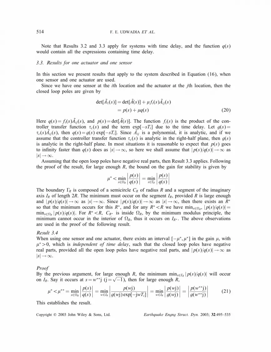
Note that Results 3.2 and 3.3 apply for systems with time delay, and the function q(s)would contain all the expressions containing time delay.

3.3. Results for one actuator and one sensor

In this section we present results that apply to the system described in Equation (16), whenone sensor and one actuator are used.Since we have one sensor at the ith location and the actuator at the jth location, then the

closed loop poles are given by

det[A1(s)] = det[A(s)] + fi(s)Aij(s)

=p(s) + q(s) (20)

Here q(s)=fi(s)Aij(s), and p(s)=det[A(s)]. The function fi(s) is the product of the con-troller transfer function c(s) and the term exp[−sTi] due to the time delay. Let g(s)=c(s)Aij(s), then q(s)= g(s) exp[−sTi]. Since Aij is a polynomial, it is analytic, and if weassume that the controller transfer function c(s) is analytic in the right-half plane, then g(s)is analytic in the right-half plane. In most situations it is reasonable to expect that p(s) goesto innity faster than q(s) does as |s|→∞, so here we shall assume that |p(s)=q(s)|→∞ as|s|→∞.Assuming that the open loop poles have negative real parts, then Result 3.3 applies. Following

the proof of the result, for large enough R, the bound on the gain for stability is given by

∗¡mins∈R

∣∣∣∣p(s)q(s)

∣∣∣∣ = mins∈R

∣∣∣∣p(s)q(s)

∣∣∣∣The boundary R is composed of a semicircle CR of radius R and a segment of the imaginaryaxis IR of length 2R. The minimum must occur on the segment IR, provided R is large enoughand |p(s)=q(s)|→∞ as |s|→∞. Since |p(s)=q(s)|→∞ as |s|→∞, then there exists an R∗

so that the minimum occurs for this R∗, and for any R∗¡R we have mins∈R∗ |p(s)=q(s)|=mins∈R |p(s)=q(s)|. For R∗¡R; CR∗ is inside R, by the minimum modulus principle, theminimum cannot occur in the interior of R, thus it occurs on IR∗ . The above observationsare used in the proof of the following result.

Result 3.4When using one sensor and one actuator, there exists an interval [−∗; ∗] in the gain , with∗¿0, which is independent of time delay, such that the closed loop poles have negativereal parts, provided all the open loop poles have negative real parts, and |p(s)=q(s)|→∞ as|s|→∞.

ProofBy the previous argument, for large enough R, the minimum mins∈R |p(s)=q(s)| will occuron IR. Say it occurs at s=w∗∗j (j=

√−1), then for large enough R,

∗¡∗∗= mins∈R

∣∣∣∣p(s)q(s)

∣∣∣∣ = minw∈IR

∣∣∣∣ p(wj)g(wj) exp[−jwTi]


∣∣∣∣p(wj)g(wj)

∣∣∣∣ =∣∣∣∣p(w∗∗j)g(w∗∗j)

∣∣∣∣ (21)

This establishes the result.



From the result, the bound ∗∗ can be obtained by considering the system with no timedelay and nding the minimum of |p(wj)=q(wj)| for w∈ IR. For some systems it may bepossible that ∗∗ is actually the maximum gain for stability for the system with no timedelay. This will be the case in Example 1 shown after Result 3.6 as well as for the controlsystems explored in Section 4. That is, for zero time delay one nds the maximum gain forstability using positive and negative feedback, and ∗∗ is the minimum of the two maximumgains. In general, however, it is not necessarily true that the minimum of the maximum gainsfor stability ∗∗ is achieved for the system with zero time delay. It is possible for somesystems that the maximum gain for stability of the system with zero time delay is larger thanthe gain that is independent of time delay. This case will be illustrated in Example 2.Since the bound ∗∗ occurs on the imaginary axis and it may not necessarily be the bound

for the maximum gain for stability for the system with no time delay, and it is a bound onthe gain for which the system is stable for all time delays, one might ask if ∗∗ will actuallybe the maximum gain for stability at some time delay. The following result answers thisquestion.

Result 3.5For systems with one sensor and one actuator, as described in Result 3.4, suppose ∗∗ occursat s = w∗∗j, then there exits a time delay T such that

p(w∗∗j) + ∗∗g(w∗∗j)e−w∗∗T j = 0:

That is, the bound of the maximum gain for stability independent of time delay given inResult 3.4 is achieved at some time delay T . The value of T will be given in the proof andit is derived from the system properties without time delay.

ProofLet the real and imaginary parts of p(w∗∗j) and q(w∗∗j) from Result 3.4 be given by

p(w∗∗j)=pR + pI j and g(w∗∗j)= gR + gI j (22)

Consider

pR + pI j + u∗∗(gR + gI j)(x − yj)=0Then

x − yj =−pRgR + pIgI∗∗(g2R + g

2I )

− pIgR − pRgI∗∗(g2R + g

2I )

(23)

Note that ∗∗=√(p2R + p

2I )=(g

2R + g

2I ) and x

2 +y2 = 1. Therefore we can take cos(w∗∗T )= xand sin(w∗∗T )=y, establishing the result.Result 3.5 indicates that there is a time delay at which the system will achieve the bound

on the maximum gain for stability given in Result 3.4. The result also indicates if the boundof the maximum gain for stability that is independent of time delay is actually achieved ornot for zero time delay. If x=1, then for the system with zero time delay the maximum gainfor stability will be reached with gain =∗∗. Similarly, if x=−1, then for the system withzero time delay the maximum gain for stability will be reached with gain =−∗∗. If |x| =1,then the maximum gain for stability of the system with zero time delay is larger than the



maximum gain for stability that is independent of time delay. The question of the uniquenessof the occurrence of poles at a gain of ∗∗ (for positive and negative feedback) is dealt within the next result.

Result 3.6For the case of a single actuator and a single sensor, suppose that a closed loop pole givenby (20) is at s=w∗j; =∗, and with a time delay of T =T ∗. Then there exist closed looppoles at s=w∗j; =−∗, with time delays T =T ∗ + ((2n+ 1)=w∗), for n=0; 1; 2; : : : ; andat s=w∗j; =∗, with time delays T =T ∗ + 2n=w∗, for n=1; 2; : : : .

ProofFor a pole on the imaginary axis, we have

p(wj) + g(wj) exp[−jwT ]=p(wj) + g(wj)(cos(wT )− j sin(wT ))=0 (24)

When the pole occurs at w=w∗; =∗, and T =T ∗, then Equation (24) is also satisedwith w=w∗, provided the time delay T satises the equations

cos(w∗T ∗)= cos(w∗T ) and sin(w∗T ∗)= sin(w∗T )

These equations are satised when T =T ∗ + (2n=w∗), for n=1; 2; : : : . Similarly, whenthe pole occurs at w=w∗; =∗, and T =T ∗, then Equation (24) is also satised withw=w∗; =−∗, provided the time delay T satises the equations

cos(w∗T ∗)=− cos(w∗T ) and sin(w∗T ∗)=− sin(w∗T )

And these equations are satised if T =T ∗ + ((2n+ 1)=w∗), for n=0; 1; 2; : : : .One consequence of this result is that the maximum gain for stability which is independent

of time delay (from Result 3.4) will be achieved for both positive and negative feedback,when an appropriate time delay is chosen. A time delay T ∗ at which the minimum value ofthe maximum gain for stability is achieved can be obtained using Result 3.6.In the next example, the bound on the maximum gain for stability that is independent of

time delay (given in Results 3.4) coincides with the maximum gain for stability of the systemwith zero time delay.

Example 1As a simple illustration of Results 3.4–3.6, consider a single degree of freedom oscillator withresponse x(t), and with mass m, damping c¿0, and stiness k¿0. The oscillator is controlledby using a time-delayed negative velocity feedback −x′(t−T ), with time delay T , and usinga control gain . The motion of the oscillator is described by the scalar dierential equation

mx′′(t) + cx′(t) + kx(t)=−x′(t − T ); x(0)=0; x′(0)=0 (25)

The Laplace transform of Equation (25) is

(ms2 + cs+ k + s exp[−sT ])x(s)=0 (26)

The closed loop poles of the system described by Equation (25) are the zeros of the equation

ms2 + cs+ k + s exp[−sT ]= 0 (27)



From Result 3.4, we have that the maximum gain for stability which is independent of timedelay occurs on the imaginary axis at some s= jw. Evaluation of Equation (27) at s= jwgives

−mw2 + cwj + k + jw(cos(wT ) + j sin(wT ))=0 (28)

The imaginary part of Equation (28) is

cw + w(cos(wT )=0 or cos(wT )=−c

(29)

Note that w=0 is not a solution, since it would violate Equation (28). Equation (29) has asolution only if |c=|61, that is ||¿c. Thus for ||¡c, Equation (28) has all poles in theleft-half complex plane (i.e. all solutions have negative real parts).For zero time delay (T =0) the closed loop poles are given by the zeros of the equation

ms2 + (c + )s+ k=0. From the Routh stability criterion, for negative feedback (¿0) thesystem will be stable for all gains. On the other hand, for positive feedback (¡0), thesystem has a cross-over pole at = − c and w=

√k=m.

Using Result 3.5 one can conrm this observation. From Result 3.5 we have

∗∗= minw∈IR



∣∣∣∣−mw2 + k + cwjwj

∣∣∣∣ = cand the minimum occurs at w∗∗ =

√k=m.

Additionally from Result 3.5, for negative feedback we have that x= cos(√k=mT )=−1

and y= sin(√k=mT )=0. The smallest time delay for which these equations are satised is

T =√m=k. Thus for negative feedback and zero time delay the bound on the maximum

gain for stability independent of time delay is not achieved. For positive feedback we havex= cos(

√k=mT )=1 and y= sin(

√k=mT )=0, and thus the bound on the maximum gain for

stability is reached at zero time delay.Using result 3.6 we have that for negative feedback the system will reach the minimum

bound for the gain for stability at w=√k=m for the time delays T =(2n + 1)

√m=k (for

n=0; 1; 2; : : :) with a gain of = c. For positive feedback the system will reach the minimumbound for the gain at w=

√k=m for the time delays T =2n

√m=k (for n=0; 1; 2; : : :) with a

gain of =−c.The next example shows the case where the maximum gain for stability of the system with

zero time delay is larger than the gain for stability that is independent of time delay, givenin Result 3.4.

Example 2Consider again a single degree of freedom oscillator with response x(t), and with mass m,damping c¿0, and stiness k¿0. This time the oscillator is controlled by using the negativefeedback time-delayed proportional control −x(t−T ), with time delay T , and a control gain. The motion of the oscillator is described by the scalar dierential equation

mx′′(t) + cx′(t) + kx(t)=−x(t − T ); x(0)=0 and x′(0)=0 (30)



After taking the Laplace transform of (30), the poles of the system are the zeros of theequation

ms2 + cs+ k + exp[−sT ]= 0 (31)

The bound on the maximum gain for stability that is independent of time delay can be obtainedusing Equation (21). When 2mk − c2¿0, we have

∗∗= minw∈IR


∣∣∣∣ = minw∈IR| −mw2 + cwj + k|=

√c2(4mk − c2)

4m2(32)

Where the minimum in Equation (32) occurs at w∗∗=√(2mk − c2)=2m2.

For zero time delay the closed loop poles are the zeros of the equation ms2+cs+(k+)=0.Based on the Routh stability criterion, the negative feedback system will be stable for all gains.In the case of positive feedback, the system will have a unique cross-over at w=0 and again of =−k. When 2mk − c2¿0 we have that ∗∗¡k. This indicates that the magnitudeof the maximum gain for stability of the system with zero time delay for positive feedbackis larger than the bound of the gain that is independent of time delay.The values for x and y in Equation (23) are

x= − c√4km− c2 and y=

√4km− 2c24km− c2 (33)

From Result 3.5 one can compute the time delay at which the bound on the gain for stabilitythat is independent of time delay is reached by the system. The smallest time delay at whichthe system reaches the bound on the gain for stability that is independent of time delay isthe smallest value of T that satises the equations

T = cos−1(x)=w∗∗ and T = sin−1(y)=w∗∗ (34)

Using Result 3.6, one can now obtain all the possible instances in which the system reachesthe bound on the gain that is independent of time delay for the system with positive andnegative feedback.Though the above simple examples illustrate Results 3.4–3.6 for classically damped sys-

tems, the results presented in this section apply to non-classically damped systems as well.We showed that when the open loop system has all poles with negative real parts, and thecontroller transfer function is an analytic function, then there is a range in the gain for whichthe closed loop system is stable (even in the presence of time delays).For the case of a single sensor with a single actuator, we showed that there is a range in

the gain for which the system is stable for all time delays. This is provided the open loopsystem has all poles with negative real parts, and the controller transfer function satises someconditions.The results imply that for the systems considered, all poles originate in the left complex

plane and any pole in the right-half complex plane can be traced to the left-half complexplane by varying the gain.The fact that for some systems the lower bound on the maximum gain for stability which is

independent of time delay is achieved when no time delay is present (Example 1), suggests



that the use of a time delay may actually increase the maximum gain for stability whencompared to the system with zero time delay for such systems. Therefore with an appropriatechoice of time delay one could increase the range in the gain for which the system is stable,thereby making the use of time delays desirable. From a control design point of view, thiscould improve the control performance dramatically for such systems.

4. EXPERIMENTS WITH A NON-CLASSICALLY DAMPED, 2-DOFTORSIONAL SYSTEM

The eect of time delay on the control of a 2-degrees-of-freedom (2-DOF) torsional bar isexplored experimentally and numerically. The maximum gain for stability is determined ex-perimentally over a range of time delays for collocated integral and non-collocated derivativecontrol and this is compared to analytical=numerical predictions based on a model of thesystem. For the case of collocated integral control, it is found both experimentally and nu-merically that a pole of the structural system, which does not originate from an open looppole, dictates the maximum gain for stability for some time delays. In this section we rstprovide a description of the apparatus including a mathematical model. Following this, theexperimental procedure is summarized. Finally, the experimental and numerical results arepresented. Additional experimental and numerical results on collocated and non-collocatedproportional, derivative and integral control of the torsional bar can be found in von Bremenet al. [16].In the absence of any time delays, the system has two-degrees-of-freedom (with 2 sets of

system poles). However, in the presence of time delays in the control loop, this seeminglysimple system has a complex behavior for it is no longer nite dimensional. It has an innitenumber of poles, and as the control gain increases from zero these poles ‘stream in’ from−∞ in the left half complex plane towards the imaginary axis. As we will show, their rootloci can ‘collide’ with those of the system poles, thereby leading to interesting behavior, andbifurcations.

4.1. Experimental setup and model

The setup (Figure 10) consists of 2 discs that undergo torsional vibrations. The inertial prop-erties of the disks can be altered by fastening additional weights to them. The control systemhas four primary components: (1) the real-time controller that generates the input trajectoryand computes the control algorithm, (2) the software for dening the controller, (3) the actu-ator at the lower disc, and (4) the optical sensors. The real-time controller is a digital signalprocessor-based single-board computer. The servo loop closure involves the computation ofthe user-supplied control algorithm, and these computations occur at a rate of once everysampling period (0:00442 s).The actuator that actuates the lower disk utilizes a brushless dc motor with electrical com-

mutation. Electrical commutation is accomplished by a sinusoidal switching scheme whichhas the advantage of reducing the magnitude of torque ripple. A sensor is secured to themotor shaft and reads its position. There are four incremental rotary shaft optical encoderson the system. Three are used to sense the position of the rotating disks. They have a



Figure 10. Experimental apparatus.

1J

2J

1c

2c

1k

2k

)(1 tθ

)(2 tθ

)(tT

Figure 11. Model of experimental apparatus.

resolution of 4000 pulses per revolution. The fourth encoder, with a resolution of 1000 pulsesper revolution, is connected to the motor.Accompanying the experimental results is a numerical study of the system. A model of the

experimental apparatus appears in Figure 11. The equations of motion of the two masses inFigure 10 are as follows:

J1′′1 + c1′1 + k1(1 − 2)=Tc(t)

J2′′2 + c2′2 + k1(2 − 1) + k22=0

(35)

Here, Ji; i=1; 2, are the mass moments of inertia of the disks; ci; i=1; 2, are the respectiveviscous damping coecients; ki; i=1; 2, are the stiness coecients; i; i=1; 2, are theangular displacements of the disks; and Tc(t) is the actuator torque.



Table I. Experimentally determined system parameters.

System parameter Experimental value

J1 0:00252 kg m2

J2 0:00194 kg m2

k1 2:830 N m=radk2 2:697 N m=radc1 0:00659 N m s=radc2 0:00229 N m s=rad

The actuator control torque for non-collocated derivative and for collocated integral controlis respectively of the form

Tc(t)=−′2(t − T ) and Tc(t)=−∫ t

01(− T ) d (36)

In both cases, is the control gain and T is the time delay in the control.The system parameters are estimated by clamping each disk, in turn, and measuring the

vibratory responses. These results are found in Table I. Though only a two degree-of-freedomsystem, it is non-classically damped.

4.2. Control procedure

Derivative control requires the estimation of the response derivative in real time. The followingnumerical approximation was used to compute the derivative ′2(t − T ):

′2(t − T )=12h

2(t − (2h+ T ))− 42(t − (h+ T )) + 32(t − T )+O(h2)

Here h=Ts (with Ts = 0:00442s) and T is the time delay. Using the above expression for thederivative, the control eort with control gain for non-collocated derivative control using atime delay of T becomes

Tc(t)=− 2Ts

2(t)− (2Ts + T ))− 42(t − (Ts + T )) + 32(t − T ) (37)

Integral control requires the estimation of the integral. The trapezoidal rule is used to approx-imate the integral as

∫ nh

01(− T ) d= h2

1(−T ) +

n−1∑j=11(jh− T ) + 1(nh− T )

+O(h2)

Again, h=Ts and T is the time delay. Recall that the system is initially at rest, so fort¡0; 1(t)≡ 0. Using the expression for the integral and the last observation, the control



eort for collocated integral control with a time delay of T is

Tc(t)=−Ts2

n−1∑j=11(jTs − T ) + 1(nTs − T )

(38)

In order to implement a time delay in the control, the control algorithm stores disk positionsfor previous sampling periods. Then, when dening the control law as in Equations (37) and(38), this past data is utilized. This means, however, that one is limited to time delays thatare multiples of the sampling period.The system described above is equipped with a safety feature which aborts control if the

exible shaft is over deected or if the speed of the motor is too high. This was takeninto account when the stability of the system was to be determined. A stable system wasone where the amplitudes of motion would decrease with time. An unstable system was onewhere the amplitudes of motion increased with time, often leading to the safety limits beingexceeded.

4.3. Experimental results

The maximum gain for stability of the system over a range of time delays is experimentallydetermined when using collocated integral control and non-collocated derivative control. Theseexperimental results are compared to numerical predictions of the maximum gain for stabilityof the system and, in general, there is close agreement for a wide range of time delays.We also present numerical results that help us understand the eect that time delays have

on the stability of the system. The numerical results presented deal with bifurcations, andthe fact that a non-system pole (a pole whose root locus does not originate at an open looppole of the structural system) can dictate the maximum gain for stability for the closed loopsystem. A system pole is simply a pole whose root locus originates at an open loop poleof the structural system. Non-system poles include poles that originate at the poles of thecontroller, and those caused by the presence of the time delay.When increasing the gain from zero, the pole that rst crosses the imaginary axis will be

called the dominant pole. This pole in essence limits the range of the gain for which thesystem is stable. Intuitively, one might expect that the dominant pole to be a system pole,because system poles are directly related to the physical structure and the non-system polesare induced by the controller and the time delay.The open loop poles of the system when using the experimental parameter values from

Table I are at s1;2 =−0:7482 ± 59:4029 i, and at s3;4 =−1:1495 ± 21:0010 i. Note that thepoles come in conjugate pairs, and this will be the case for all the poles including the non-system poles. On root loci plots, the location of the open loop poles will be denoted with thesymbol ‘*’ (making it easy to identify the root locus corresponding to a system pole). Thesystem poles will usually be traced using a thick line, while the non-system poles with a thinline. In this subsection, all the time delays are given in units of seconds, and frequencies inrads=s.Tracking the system poles as the gain changes is done simply by following the root loci

of the poles starting at an open loop pole. However, the task of tracking non-system poles isa dicult one, since we may have innitely many of them, and there is no systematic way



0 0.02 0.04 0.06 0.08 0.1 0.12 0.14 0.163

4

5

6

7

8

9

10

11

12

Time delay

Max

imum

gai

n fo

r st

abili

tyExperimental error bar

ExperimentalComputed

Figure 12. Experimental maximum gain for stability versus time delay for integral collocated control.

of selecting an initial location for all the poles‡ and tracing them by varying the gain (as forsystem poles). The non-system poles that originate at the poles of the controller or end at thezeros of the controller can, however, be traced in the usual way.Collocated integral control. Figure 12 represents a plot of the experimental results for timedelay versus the maximum gain for stability under collocated integral control. The solid lineon the plot is numerically determined using the system model described above. Accordingto the numerical results, then, a coordinate pair (time delay, gain) which nds itself abovethe line is unstable, and one below the line is stable. The experimental maximum gain forstability is also depicted on this graph as data points.The numerical results show a trend of increasing maximum gain for increasing time delay

until about 0:12 s. where the gain begins to decrease. The curve of the maximum gain forstability suggests that one can properly choose a time delay that can give the system a largermaximum gain for stability than the one the system has for no time delay.A root locus of a pole that starts (when the gain is close to zero) in the left-half complex

plane may cross the imaginary axis several times (as the gain is increased). The value of thepole (on a root locus) in the complex plane when it crosses from the left-half (complex) planeto the right-half (complex) plane for the rst time, as the gain is increased gradually fromzero, will be called the cross-over frequency. Figures 13 and 14 show the maximum gainfor stability and the cross-over frequency versus time delay for collocated integral control,when only system poles are considered. The points denoted by ‘o’ correspond to system polesoriginating at s1, and the points denoted by ‘*’ correspond to the system pole originating at s3(due to symmetry, the conjugates of these two system poles are also present in the system).Similar plots are given in Figures 15 and 16, which show the maximum gain for stability andthe cross-over frequencies versus time delay for collocated integral control, when all (systemand non-system) poles are considered. Even though the system does not satisfy all the requiredconditions of Result 3.4, the maximum gain for stability which is independent of time delay,

‡By means of Jensen’s formula (see Rudin [17; p:307]) it is possible to determine the magnitude of the non-systempoles at given gains and time delays for special systems.



0 0.0 0.0 0.0 0.0 0.1 0.1 0.1 0.10

20

40

60

80

100

120

140

Time

Max

imum

gai

n fo

r st

abili

ty

Figure 13. Maximum gain for stability versus time delay for collocatedintegral control using system poles only.

0 0.0 0.0 0.0 0.0 0.1 0.1 0.1 0.110

15

20

25

30

35

40

45

50

55

60

Time

Cro

ss-o

ver

freq

uenc

y

Figure 14. Cross-over frequency versus time delay for collocated integral controlsystem poles only data.

given by Result 3.4 is found to be 3.266. This is also exactly the numerically expected value(Figure 15) and it is very close to the experimentally observed value. We note that at zerotime delay, the smallest maximum gain for stability is achieved (see Figures 12, 13 and 15).Figures 15 and 16 are smooth continuous curves, while Figure 13 and 14 seem discontinuous

and present abrupt changes. The dierence between the system-poles data and the all-polesdata plots suggest that there is a range in the time delay where a non-system pole is thedominant pole. This expectation is conrmed by plots in Figures 17 and 18, which showthe root locus of the system poles (thick lines) and two non-system poles (thin lines) fortime delays of 0.11 and 0:13 s, respectively. The root loci are taken for values of the gain between 0 and 50, except for the portion of the root loci that lies on the horizontal axis,



0 0.02 0.04 0.06 0.08 0.1 0.12 0.14 0.163

4

5

6

7

8

9

10

11

12

Time delay

Max

imum

gai

n fo

r st

abili

ty

Figure 15. Maximum gain for stability versus time delay for collocatedintegral control, including all poles.

0 0.02 0.04 0.06 0.08 0.1 0.12 0.14 0.1610

12

14

16

18

20

22

Time delay

Cro

ss-o

ver

freq

uenc

y

Figure 16. Cross-over frequency versus time delay for collocated integral control, including all poles.

where the initial gain is larger than 0 in order to avoid problems of scaling. For the timedelay of 0:11s, two system poles cross the imaginary axis rst, that is, the dominant poles aretwo conjugate system poles (see Figure 17), while for a time delay of 0:13 s, two conjugatenon-system poles have become dominant (see Figure 18).The fact that there is an exchange of dominant pole status between a system pole and

a non-system pole, suggests the existence of a bifurcation. This bifurcation is presented inFigure 19 which shows the root loci for a system pole (thick line) and a non-system pole(thin line) at dierent time delays. The system pole root locus starts at a gain of zero, whilethe portion of the non-system pole displayed starts from the horizontal axis with a gain largerthan zero. The maximum gain is 50 for both poles. A bifurcation occurs at a time delay ofabout 0:11265 s. The poles selected are such that the system pole is the dominant pole fortime delays less than 0:112 s and the non-system pole is the dominant pole for time delay



Figure 17. Root locus of the system poles and two non-system poles for time a delayof 0:11 s, using collocated integral control.

Figure 18. Root locus of the system poles and two non-system poles for time a delayof 0:13 s, using collocated integral control.

greater than 0:113 s. Initially (for small time delays), the system pole is the dominant pole,as the time delay is increased the root loci of the two poles move closer until they touch(approximately at a time delay of 0:11265 s). This is the point where the bifurcation occurs.At the bifurcation, one ‘arm’ of the root loci is exchanged among the two poles. The systempole gives the ‘arm’ that dictates the maximum gain for stability to the non-system pole, andthe non-system poles gives the slow moving ‘arm’ to the system pole. After the exchangeof ‘arms’ at the bifurcation, the root loci of the two poles move apart as the time delay isincreased.To conrm that a non-system pole is actually the dominant pole, two experiments are

conducted on the two-degree-of-freedom torsional bar. The system is fed a sine wave witha given frequency, and the steady state amplitude of the response of disk 1 is recorded for



Figure 19. Root loci for dierent time delays showing bifurcation for collocated integral control.

dierent gains, while the control eort is active. The experiments are conducted using threedierent frequencies. These chosen frequencies are the cross-over frequencies for two of thesystem poles (originating from s1 and s2) and a non-system pole at a given time delay. Recallthat the cross-over frequency is dened as the purely imaginary value of a pole (moving alonga root locus, and starting in the left-half complex plane) when it rst crosses the imaginaryaxis, as the gain is gradually increased from zero. The time delays are taken to be 0:11 s inthe rst experiment and 0:13 s in the second. The objective is to experimentally conrm thelocation of points on the root locus.The results for a time delay of 0:11 s are shown in Figure 20. The frequencies of 13.2 and

59:7rad=s correspond to the cross-over frequencies of the system poles, while the frequency of43:6 rad=s is the cross-over frequency for the non-system pole. As expected, when the systemis excited near the frequency of the dominant pole, and at a gain close to the maximum gainfor stability, the amplitude of the response increases drastically. However, when the systemis excited at a frequency which is ‘far’ from the cross-over frequency, the amplitude of the



9 9.5 10 10.5

System Gain

Dis

k 1

Am

plitu

de, r

adiu

s

11 11.5 120

0.1

0.2

0.3

0.4

0.5

0.6

0.7

0.8

0.9

w=13.2 rad/secw=59.7 rad/secw=43.6 rad/sec

Figure 20. Amplitude of the steady state response of disk 1 versus gain for dierent frequencies of thesine wave using collocated integral control and a time delay of 0:11 s.

10 10.5 11

System Gain

Dis

k 1

Am

plitu

de, r

adia

ns

11.5 120

0.1

0.2

0.3

0.4

0.5

0.6

0.7

0.8

0.9

w=11.5 rad/secw=57.5 rad/secw=37 rad/sec

Figure 21. Amplitude of the steady state response of disk 1 versus gain for dierent frequencies of thesine wave using collocated integral control and a time delay of 0:13 s.

response does not increase greatly, even in the vicinity of the maximum gain for stability (asseen for the frequencies of 59.7 and 43:6 rad=s). This experiment conrms that for a timedelay of 0:11 s, the dominant pole is a system pole which crossed-over at a frequency ofabout 13:2 rad=s.The results for a time delay of 0:13 s are shown in Figure 21. The frequencies of 57.5 and

37 rad=s are the cross-over frequencies for the system poles and the frequency of 11:5 rad=sis the cross-over frequency of a non-system pole. The plot shows that the amplitude of theoscillations of disk 1 increases when the system is excited at the expected cross-over frequency



0 0.02 0.04 0.06 0.08

Time delay

Max

imum

gai

n fo

r st

abili

ty

0.1 0.12 0.14 0.160

0.01

0.02

0.03

0.04

0.05

0.06

0.07

0.08

0.09

0.1

Experimental error bar

ExperimentalComputed

Figure 22. Experimental maximum gain for stability versus time delayfor non-collocated derivative control.

of the non-system pole near the maximum gain for stability. On the other hand, when thesystem is excited at the cross-over frequencies of the system poles (which are not dominant),the amplitude of the response remains small and almost unchanged near the maximum gainfor stability corresponding to the dominant pole. This behavior conrms the expectation thatat a time delay of 0:13 s, a non-system pole is the dominant pole.The experimental results show that a non-system pole can be the dominant pole for col-

located integral control, and that our analysis can predict this behavior. Also, the maximumgain for stability with time delays is much higher than in the absence of a time delay. Thebehavior of the system can be theoretically explained in terms of bifurcation diagrams.Non-collocated derivative control. Figure 22 represents a plot of time delay versus the maxi-mum gain for stability for non-collocated derivative control. As before, the solid line depictsa numerically generated estimate of the maximum gain for stability as a function of timedelay. The data points represent experimentally determined values for the maximum gains forstability at various time delays.The numerical results show a trend of increasing maximum gain for increasing time delay

until about 0:04 s where the gain decreases. Thus a proper choice of time delay can give thesystem a much larger maximum gain for stability than if there were no time delay.Figure 23 shows the numerically determined maximum gain for stability versus time delay

for the torsional bar using non-collocated derivative control. For the time delays shown, thedominant pole is always a system pole. Again, points denoted by ‘o’ correspond to systempoles originating at s1, and the points denoted by ‘*’ correspond to the system pole originatingat s3. In the range of time delays shown, there are three instances in which the dominant polechanges from one system pole to another. The changes occur at time delays of about 0.04, 0.08and 0:125 s. Figure 24 shows the expected cross-over frequency (frequency of the dominantpole at the maximum gain for stability) versus time delay. The fact that the dominant polechanges from one system pole to another suggests the presence of bifurcations at the locationswhere the changes occurs.



0 0.02 0.04 0.06 0.08

Time delay

Max

imum

gai

n fo

r st

abili

ty

0.1 0.12 0.14 0.160

0.01

0.02

0.03

0.04

0.05

0.06

0.07

0.08

0.09

0.1

Figure 23. Expected maximum gain for stability versus time delayfor non-collocated derivative control.

0 0.02 0.04 0.06 0.08

Time delay

Cro

ss-o

ver

freq

uenc

y

0.1 0.12 0.14 0.1620

25

30

35

40

45

50

55

60

65

Figure 24. Expected cross-over frequency versus time delay for non-collocated derivative control,showing possible bifurcations at about 0.0396, 0.08 and 0:125 s.

The maximum gain for stability for non-collocated derivative control which is independentof time delay, given by Result 3.4 is 0.007988. When the time delay is zero, the above time-delay-independent maximum gain for stability is achieved (see Figures 22 and 23). There isclose agreement between the computational results from this section and the results from themethod of Section 3, with regards to the maximum gain for stability independent of timedelay.A bifurcation occurs at a time delay of about 0:0396 s. This bifurcation is shown on

Figure 25, which shows the root loci of two of the system poles for dierent time delays.



Figure 25. Root loci for dierent time delays showing bifurcation for non-collocated derivative control.

At the bifurcation, one ‘arm’ of the root loci is exchanged among the two system poles. Thethick line represents the root locus for the pole originating at the open loop pole s1, whilethe thin line is the root locus for the pole originating at s3. The root loci correspond to gainsbetween 0 and 0.12. The general behavior of the root loci of the poles at the bifurcation issimilar to the one for collocated integral control (see Figure 19). The main dierence betweenthe two cases is that for collocated integral control, a system pole and a non-system pole areinvolved, while for the present case, only system poles are involved. At a time delay of about0:08 s we have another bifurcation. However this bifurcation is less dramatic; there is nointersection of the root loci of the poles. The change of dominant pole occurs simply becausethere is a change in the rate at which the poles move across the complex plane.The experimental and numerical results presented in this section show that for collocated

integral control, there are time delays for which the dominant pole is a non-system pole.On the other hand, in the experiments with non-collocated derivative control, the dominantpole is a system pole (for the range in time delay considered). Good agreement between theexperimental and the numerically expected maximum gain for stability is observed. For both,



collocated integral control and non-collocated derivative control (see Figures 12 and 22), theintroduction of a suitable time delay, will yield a higher maximum gain for stability thanthe one for the system with no time delay. The next section deals with the control of timeinvariant systems with system uncertainties that include uncertainties in the time delay that isused. We model this uncertainty as a time-varying time delay.

5. CONTROL OF UNCERTAIN SYSTEMS

The models presented in Sections 2 and 3 do not include system uncertainties in the formula-tion. However, the numerical results presented in Section 2.5, suggest that structural systemsmay remain stable after the parameters of the system are slightly perturbed (or uncertain).This section deals with the robust state feedback control of time invariant dynamic systemswith time varying control delays and system uncertainties. Corless and Leitmann [18], Gutmanand Leitmann [19], and Chen and Chen [20] have worked on control systems which deal withuncertainties embedded in the system’s structure or with externally introduced uncertainties(like measurement noise). In this section we introduce a new set of uncertainties in the sys-tem, in terms of the time delay in the control. Here the time delay in the control is allowedto be a bounded function of time.Consider the system whose response x(t) is governed by the matrix dierential equation

x′(t)=Ax(t) +Ax(t) + Bu(t) +Bu(t) + Bu(t − h(t)) (39)

where the m-vector u(t) is the control function, the matrices A; B; B have uncertainentries and h(t) is the time-varying time delay. The matrices A, and A are n by n; B;Band B are n by m, and x(t) is an n-vector.The elements of the uncertain matrices could either have deterministic or stochastic forms.

Thus the stochastic uncertainties which are usually present in the stiness and damping ma-trices can be included in the matrices A.Assume that

A=BD with ‖D‖= k1; k1 ∈ [0;∞)B=BE with ‖E‖= k2; k2 ∈ [0; 1)B=BF with ‖F‖= k2; k2 ∈ [0;∞)

(40)

The above assumptions on the norms of the matrices can be interpreted as, the uncertaintiesin the system are bounded by known constants k1; k2 and k2. The restriction that k2 ∈ [0; 1)is interpreted as follows: the uncertainty in the control cannot be so severe as to reverse thedirection of the control action, for then one is not able to tell if the control is in the desireddirection.If the state feedback control u(t) is chosen as

u(t)=− 12 B

TPx(t) (41)

where P is the solution of the Lyapunov equation,

ATP + PA=−(Q +H); P; Q;H¿0 (42)



then the response of system (39) is stable, provided that the following conditions are satised.

h(t)¡h0; h′(t)6a¡1 and ¿42 (43a)

where

2 =k22‖BTP‖2

4(1− a)min(H) and =(1− k2)2min(Q)

k21

The control gain is chosen as

6(1− k2)2 +

; ¿0 (43b)

where is a positive constant which has to satisfy the condition,

− 222

1−√1−2¡¡ − 2

2

21 +

√1−

here

=22

− 22The result presented shows that systems with uncertainties in the parameters and in the time-delayed controller can be stabilized under special conditions. For a proof of the result andnumerical simulations which validate it, see Udwadia et al. [21] and Udwadia and Hos-seini [22].

6. CONCLUSIONS

In this paper we have studied time-delayed control of structural systems from several view-points. We show that the purposeful injection of time delays can indeed improve both thestability and performance characteristics of controlled systems. Rather than developing com-plex schemes to eliminate, compensate for, or nullify time delays (as has been the traditionalview), we show analytically, numerically, and experimentally that time delays can be pur-posefully and intentionally used to good advantage. This becomes more so important becausetime delays are indeed ubiquitous in control systems. Furthermore, we show that such timedelayed control can be made robust with respect to uncertainties in the system’s parametersand uncertainties in the implementation of the time delays themselves. We present next adetailed set of conclusions.Section 2 deals with the control of classically damped structural systems. Results for collo-

cated and non-collocated control of damped and undamped multi-degree-of-freedom systemswere given. For undamped and underdamped system, several analytical conditions on the timedelay that guarantees that the closed loop system poles move to the left in the complex planeare given. Since PID control is one of the most commonly used control laws in practice,we use this controller to obtain conditions when time delays can stabilize undamped systems.We illustrate our results using numerical computations. We show that non-collocated deriva-tive control that is unstable in the absence of time delays can be made stable through the



simple introduction of suitable, intentional time delays. The robustness of time delayed controlto variations in the values of the structural parameters (mass and stiness) and the time delayitself is numerically explored for non-collocated derivative control. The results show that evenunder considerable perturbations of the parameter values the system remains stable.General non-classically damped systems are treated in Section 3. The results presented deal

with the case of one actuator, and the transfer function of the controller is assumed to be ananalytic function. The main results can be summarized as follows: (1) When all the polesof the open loop system have negative real parts and the controller transfer function is ananalytic function, then for any given time delay there exists a range in the gain (which is, ingeneral, dependent on the given time delay) for which the closed loop system is stable. (2)For a single actuator and a sensor under the same conditions a before, there is an intervalof gain which is independent of time delay for which the system is stable. This gain can becomputed without knowledge of the time delay. (3) We show that through a proper choiceof time delay, one may obtain a larger maximum gain for stability than the one for thesystem with no time delay. Thus the injection of a time delay could signicantly improve theperformance of the control of such a system.Experimental and numerical results on the control of a two-degree-of-freedom torsional

bar are presented in Section 4. The main results are summarized as follows: (1) Experi-mental results showing the maximum gain for stability versus time delay, for both collo-cated integral control and non-collocated derivative control, exhibit close agreement with thenumerical=analytical expectations. Furthermore, the results show that the presence of a timedelay will actually increase the maximum gain for stability, when compared with the maxi-mum gain for stability when the system has no time delay. (2) For non-collocated derivativecontrol, we numerically nd that the dominant pole (the pole that dictates the maximum gainfor stability) is always a system pole (for the range of time delays analysed). For dierenttime delays the dominant pole may change from one system pole to another. At these timedelays we have bifurcations. (3) For collocated integral control, we numerically nd that thedominant pole can be a non-system pole. This result is corroborated by actual experiments. Aswith the non-collocated case, the dominant pole changes as the time delay is varied, and nowbifurcations involving system and non-system poles occur. We illustrate such a bifurcationboth experimentally and computationally.Finally, Section 5 deals with the robust state feedback control of time invariant structural

systems with time-varying time delays and system uncertainties. A state feedback controlis suggested that guarantees the stability of the system, provided, principally, the so-calledmatching conditions are met.Even though we have taken dierent approaches when dealing with the time-delayed con-

trol of structural systems, throughout this paper there is the recurring theme that under anappropriate choice of time delay, the maximum gain for stability could be greater than themaximum gain for stability obtained when no time delay is used. Since time delays are ubiq-uitous in the control of large scale structural systems, this strongly suggests the idea thatinstead of trying to eliminate=nullify time delays, we may actually want to introduce themappropriately in order to provide stable non-collocated control. We also show that this in-crease in the maximum gain for stability in the presence of delays can improve the controlperformance especially for non-collocated control.Our results, both experimental and analytical, indicate that the research presented in this

paper will be of practical value in improving the performance and stability of controllers.



Through the proper purposive injection of small time delays, it is possible to dramaticallyimprove the performance and stability of certain control systems. Furthermore, the injectionof small time delays can be easily implemented in a reliable and nearly costless way onan already installed controller. Thus the performance and stability of active control systemsthat are already installed in building structures can be enhanced in a nearly costless way byincluding appropriate and intentional time delays in the feedback loop. This makes the methodvery attractive from an economic and safety retro-t standpoint when dealing with the activecontrol of structural systems subjected to strong earthquake ground shaking.

REFERENCES

1. Auburn JN. Theory of the control of structures by low-authority controllers. Journal of Guidance and Control1980; 3:444–451.

2. Balas MJ. Direct velocity feedback control of large space structures. Journal of Guidance and Control 1979;2:252–253.

3. Balas MJ. Direct output feedback control of large space structures. The Journal of Astronomical Sciences 1979;XXVII(2):157–180.

4. Goh CJ, Caughey TK. On the stability problem caused by nite actuator dynamics in the collocated control oflarge space structures. International Journal of Control 1985; 41(3):787–802.

5. Fanson JL, Caughey TK. Positive position feedback control for large space structures. AIAA Journal 1990;28(4):717–724.

6. Cannon RH, Rosenthal DE. Experiments in control of exible structures with noncolocated sensors and actuators.Journal of Guidance and Control 1984; 7:546–553.

7. Yang JN, Akbarpour A, Askar G. Eect of time delay on control of seismic-excited buildings. Journal ofStructural Engineering (ASCE) 1990; 116(10):2801–2814.

8. Agrawal AK, Yang YN. Eect of xed time delay on stability and performance of actively controlled civilstructures. Earthquake Engineering and Structural Dynamics 1997; 26:1169–1185.

9. Agrawal AK, Fujino Y, Bhartia BK. Instability due to time delay and its compensation in active control ofstructures. Earthquake Engineering and Structural Dynamics 1993; 22:211–224.

10. Agrawal AK, Yang YN. Compensation of time-delay for control of civil engineering structures. EarthquakeEngineering and Structural Dynamics 2000; 29:37–62.

11. Kwon WH, Lee GW, Kim SW. Delayed state feedback controller for the stabilization of ordinary systems.Proceedings of the American Control Conference, vol. 1, Pittsburgh, Pennsylvania, 1989; 292–297.

12. Udwadia FE, Kumar R. Time delayed control of classically damped structural systems. International Journalof Control 1994; 60(5):687–713.

13. Udwadia FE, Kumar R. Time delayed control of classically damped structures. Proceedings of the 11th WorldConference of Earthquake Engineering, Acapulco, Mexico, 23–28 June, 1996.

14. von Bremen HF, Udwadia FE. Can time delays be useful in the control of structural systems? Proceedingsof the 41st AIAA=ASME=ASCE=AHS=ASC Structures, Structural Dynamics, and Materials Conference,Atlanta, GA, 3–6 April, 2000.

15. Ahlfors LV. Complex Analysis. McGraw-Hill: New York, 1979.16. von Bremen HF, Udwadia FE, Silverman MC. Eect of time delay on the control of a torsional bar. Proceedings

of the 42nd AIAA=ASME=ASCE=AHS=ASC Structures, Structural Dynamics, and Materials Conference,Seattle, Washington, 16–19 April, 2001.

17. Rudin W. Real and Complex Analysis. McGraw-Hill: New York, 1987.18. Corless MJ, Leitmann G. Continuous state feedback guaranteeing uniform ultimate boundedness for uncertain

dynamic systems. IEEE Transactions on Automatic Control 1981; AC-26(5):1139–1144.19. Gutman S, Leitmann, G. Stabilizing control for linear systems with bounded parameter and input uncertainty.

Proceedings of the 7th IFIP Conference on Optimization Techniques. Springer Verlag: Berlin, 1976.20. Chen YH, Chen JS. Adaptive robust control of uncertain systems. Control and Dynamic Systems 1992; 50:

175–222.21. Udwadia FE, Hosseini MAM, Chen YH. Robust control of uncertain systems with time varying delays in control

input. Proceedings of the 1997 American Control Conference, Albuquerque, New Mexico, 4–6 June, 1997.22. Udwadia FE, Hosseini MAM. Robust stabilization of systems with time delays. ASCE Proceedings of the

seventh specialty conference, Probabilistic Mechanics and Structural Reliability, Worchester, MA, 7–9 August,1996; 438–441.


time delayed control of structural systems

Documents