University of Nebraska at OmahaDigitalCommons@UNO

Student Work

4-1992

Framing Effects in Riskless Decisions: Discountingof Temporally Delayed OutcomesAdam B. ButlerUniversity of Nebraska at Omaha

Follow this and additional works at: https://digitalcommons.unomaha.edu/studentwork

Part of the Psychology Commons

This Thesis is brought to you for free and open access byDigitalCommons@UNO. It has been accepted for inclusion in StudentWork by an authorized administrator of DigitalCommons@UNO. Formore information, please contact unodigitalcommons@unomaha.edu.

Recommended CitationButler, Adam B., "Framing Effects in Riskless Decisions: Discounting of Temporally Delayed Outcomes" (1992). Student Work. 227.https://digitalcommons.unomaha.edu/studentwork/227

Framing Effects in Riskless Decisions: Discounting of Temporally Delayed Outcomes

A Thesis Presented to the

Department of Psychology and the

Faculty of the Graduate College University of Nebraska

In Partial Fulfillment of the Requirements for the Degree

Master of Arts University of Nebraska at Omaha

byAdam B. Butler April, 1992

UMI Number: EP72869

All rights reserved

INFORMATION TO ALL USERS The quality of this reproduction is dependent upon the quality of the copy submitted.

In the unlikely event that the author did not send a complete manuscript and there are missing pages, these will be noted. Also, if material had to be removed,

a note will indicate the deletion.

UMIDissertation Publishing

UMI EP72869

Published by ProQuest LLC (2015). Copyright in the Dissertation held by the Author.

Microform Edition © ProQuest LLC.All rights reserved. This work is protected against

unauthorized copying under Title 17, United States Code

uesf

ProQuest LLC.789 East Eisenhower Parkway

P.O. Box 1346 Ann Arbor, Ml 48106-1346

THESIS ACCEPTANCE

Acceptance for the faculty of the Graduate College, University of Nebraska, in partial fulfillment of the requirements for the degree Master of Arts, University of Nebraska at Omaha.

Committee

Name Department

i■S'-/' v — _____________ PSYCHOLOGY/ "/

[s y t'-'1______ I______________________________ PSYCHOLOGY

__________________ACCOUNTING

' LsC-JLi yyiChair

- i % - :\ \

Date

Acknowledgements

There are many people I would like to thank for their invaluable assistance on this project. First and foremost, I thank Dr. Lisa Scherer for her guidance, expertise, and continual effort to force me to conceptualize the problem better.

I am also grateful to the other members of my committee: Dr. Joseph Brown, Dr. Perrin Garsomke, andDr. C. Raymond Milllimet. All of the committee members assumed a very active role on this project, and I cannot thank them enough for their time and effort.

I would also like to thank Theresa Dethlefs for the preparation of figures, and for her comments on earlier drafts of this manuscript. I am grateful to Paul Pietig for his assistance in the data collection phase of this project.

Many thanks are also due to my friends and graduate student colleagues Vernon Peterson and David Yells for their scientific curiosity and willingness to discuss this project with me.

On a personal note, I would like to thank Patra Pakieser and my family for their moral support and encouragement of my education.

Table of Contents

List of Figures....................................... iiiAbstract .............................................. 2Choice With Delayed Outcomes........................... 5

Historical Perspective.......................... 5Preferences for Delayed Outcomes................ 6Personality Studies............................. 7Discounting Functions........................... 9Conclusions.....................................13

A Learning Model of Delayed Outcomes..................14The Matching Law............ 15The Matching Law and Irrational Choice........ 17

Prospect Theory 2 0The Evidence for Rational Choice...............20PT Value and Weighting Functions.............. 24Research Investigations of Framing.............25Probability as Delay in Repeated Gambles........33

The Proposed Investigation............................ 37Hypotheses......................................40

ii

Table of Contents (cont.)

Method.................................................42Subjects....................................... 42Apparatus...................................... 4 3Procedure...................................... 43Independent Variables.......................... 44Dependent Variables............................ 45

Results................................................45Results for Hypothesis.1...................... 45Results for Hypothesis.2...................... 54Results for Hypothesis 3 . . . .................. 56Additional Significant Results................ 59

Discussion.............................................60References.............................................71Footnotes..............................................80Appendix A .............................................81

iii

List of Tables and Figures

Table 1-Number of Subjects Choosing Advancedand Delayed Options/Chi Square Values........ 47

Table 2-Reflection in Individual Preferences..........51Table 3-Means and Standard Deviations for

Preference Ratings. ....................... 52Figure 2-Percentage Favoring Immediate and

Delayed Losses................................58Table 4-Analysis of Variance Table.................... 61Figure 3-Two-Way Interaction Between

Option B Delay and Outcome................... 62Figure 4-Two-Way Interaction Between

Option A Delay and Outcome 63Figure 5-Four-Way Interaction......................... 64

Discounting2

AbstractStudies of riskless choice in both cognitive (Stevenson, 1986) and behavioral paradigms (Chung & Herrnstein, 1967) have found that subjects prefer temporally delayed losses and temporally advanced gains. Analogously, studies of risky choice have found that subjects prefer risky losses and certain gains (Tversky & Kahneman, 1981). Because probability is conceptually identical to the inverse of delay, it was recently suggested that these findings were descriptions of the same choice process (Rachlin, Logue, Gibbon, & Frankel, 1986). There were two goals of the present investigation. The first was to replicate and extend, through the use of a within- subjects design, the finding that subjects prefer delayed gains and immediate losses. The second was to test the applicability of the prospect theory value function in a choice context involving temporally delayed financial options. Subjects showed strong preferences for immediate gains and delayed losses, but there was not support for the prospect theory value function in a riskless context involving temporal delays.

Discounting3

Framing Effects in Riskless Decisions: Discounting of Temporally Delayed Gains and Losses

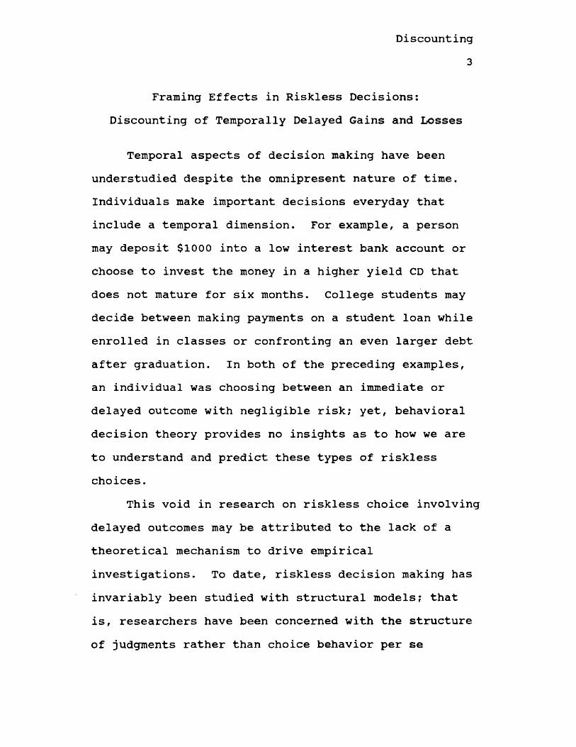
Temporal aspects of decision making have been understudied despite the omnipresent nature of time. Individuals make important decisions everyday that include a temporal dimension. For example, a person may deposit $1000 into a low interest bank account or choose to invest the money in a higher yield CD that does not mature for six months. College students may decide between making payments on a student loan while enrolled in classes or confronting an even larger debt after graduation. In both of the preceding examples, an individual was choosing between an immediate or delayed outcome with negligible risk; yet, behavioral decision theory provides no insights as to how we are to understand and predict these types of riskless choices.

This void in research on riskless choice involving delayed outcomes may be attributed to the lack of a theoretical mechanism to drive empirical investigations. To date, riskless decision making has invariably been studied with structural models? that is, researchers have been concerned with the structure of judgments rather than choice behavior per se

Discounting4

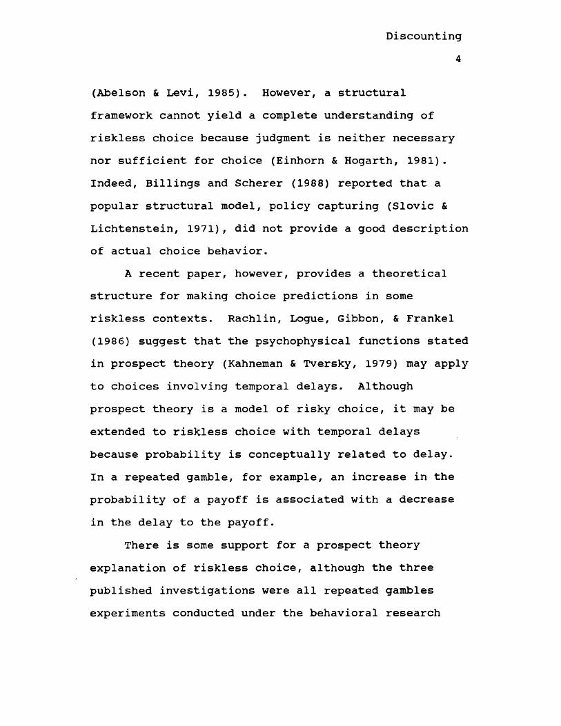
(Abelson & Levi, 1985). However, a structural framework cannot yield a complete understanding of riskless choice because judgment is neither necessary nor sufficient for choice (Einhorn & Hogarth, 1981). Indeed, Billings and Scherer (1988) reported that a popular structural model, policy capturing (Slovic & Lichtenstein, 1971), did not provide a good description of actual choice behavior.

A recent paper, however, provides a theoretical structure for making choice predictions in some riskless contexts. Rachlin, Logue, Gibbon, & Frankel (1986) suggest that the psychophysical functions stated in prospect theory (Kahneman & Tversky, 1979) may apply to choices involving temporal delays. Although prospect theory is a model of risky choice, it may be extended to riskless choice with temporal delays because probability is conceptually related to delay.In a repeated gamble, for example, an increase in the probability of a payoff is associated with a decrease in the delay to the payoff.

There is some support for a prospect theory explanation of riskless choice, although the three published investigations were all repeated gambles experiments conducted under the behavioral research

Discounting5

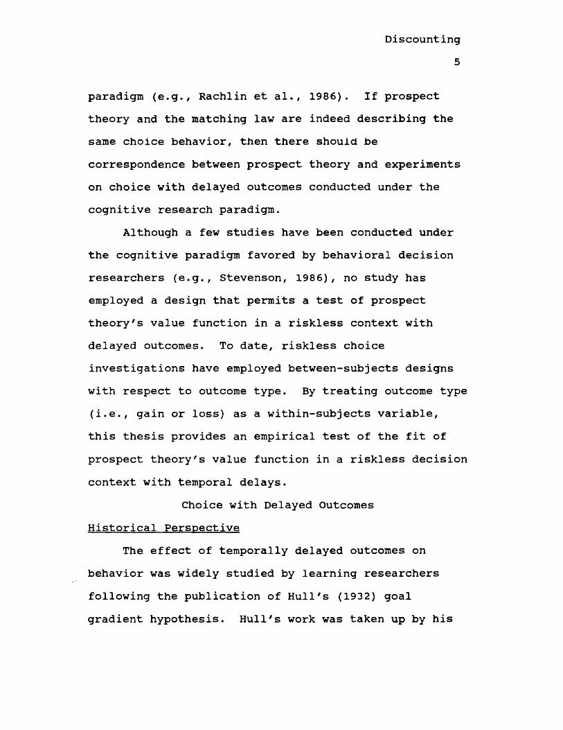
paradigm (e.g., Rachlin et al., 1986). If prospect theory and the matching law are indeed describing the same choice behavior, then there should be correspondence between prospect theory and experiments on choice with delayed outcomes conducted under the cognitive research paradigm.

Although a few studies have been conducted under the cognitive paradigm favored by behavioral decision researchers (e.g., Stevenson, 1986), no study has employed a design that permits a test of prospect theory's value function in a riskless context with delayed outcomes. To date, riskless choice investigations have employed between-subjects designs with respect to outcome type. By treating outcome type (i.e., gain or loss) as a within-subjects variable, this thesis provides an empirical test of the fit of prospect theory's value function in a riskless decision context with temporal delays.

Choice with Delayed Outcomes Historical Perspective

The effect of temporally delayed outcomes on behavior was widely studied by learning researchers following the publication of Hull's (1932) goal gradient hypothesis. Hull's work was taken up by his

Discounting6

student, Kenneth Spence, who proposed that learning involving delayed reinforcers occured through the presence of secondary reinforcers (Spence, 1947). The empirical work engendered by Hull (193 2) and Spence (1947) was plagued by its confinement to animal studies. Any studies that did use human subjects were limited to the effect of feedback delay on motor learning (Renner, 1964).

In the 1960's, personality researchers became interested in childrens' ability to delay rewards. Mischel and Metzner (1962) utilized psychoanalytic theory of personality development to predict that older children, having developed a reality-based secondary process, would be better able to delay gratification. Later, Mischel and Grusec (1967) utilized Rotter's (1954) expectancy value theory to hypothesize that delayed outcomes were associated with an implicit risk. Preferences for Delaved Outcomes

From an economic standpoint, it is always rational to choose more immediate gains over delayed gains because failure to do so represents opportunity costs (Yates & Watts, 1975). For example, money in the bank now is worth more than money in the bank a year from now because of the interest that may be earned. It is

Discounting7

also rational, in an inflationary economy, to defer debt payment because the loss, represented by commodities foregone, decreases with time (Yates & Watts, 1975). Methodologically sound research within both personality and learning paradigms has shown that people (and other animals) prefer advanced gains or rewards and delayed losses or punishments.Personality Studies

A number of individual and situational variables have been identified as covariates of delay of gratification. Mischel found that a preference for larger, delayed rewards was significantly correlated with need for achievement (Mischel, 1961a), a father in the home (Mischel, 1961b), social responsibility (Mischel, 1961c), age (Mischel & Metzner, 1962), and intelligence (Mischel & Metzner, 1962). In addition, the length of the delay interval was negatively correlated with a preference for delayed gratification (Mischel & Metzner, 1962).

Preferences for rewards and punishers. Mischel followed his original studies with investigations of preferences for delayed rewarding and aversive events. Mischel and Grusec (1967) found that children were more likely to choose immediate rewards as the delay to an

Discounting8

alternative reward increased. Surprisingly, choice of punishment was independent of delay. To explain their results, Mischel and Grusec (1967) stated that delayed rewards were associated with greater risk and were avoided. In a later publication, Mischel, Grusec, & Masters (1969) concluded that waiting for aversive outcomes was, in itself, aversive (Mischel, Grusec, & Masters, 19 69). As stated by Yates and Watts (1975), "It is as if the person faced with an unpleasant chore concludes, 'Well, I might as well get it over with and stop worrying about it” (p. 296).

To support their position, Mischel, Grusec, and Masters (1969) had adults and children choose between rewards and punishments of equal objective value that differed only in terms of the delay of their occurrence. As hypothesized, the subjective value of a reward decreased as delay increased. Delay had no influence on the subjective value of punishments for children, but delay consistently decreased the subjective value of punishments for adults. In other words, adults preferred immediate punishments.

Yates and Watts (1975), however, criticized the Mischel et. al. (1969) study on procedural grounds.They pointed out that while subjects were indeed

Discounting9

choosing between delayed aversive outcomes, participation in experiments was required for successful completion of a university course. Thus, the rewards for participating in the study (e.g., successful course completion) may have outweighed the aversive outcomes. In a replication that attempted to remove these procedural obstacles, Yates and Watts (1975) found that subjects were evenly split in their preferences for advanced or deferred aversive consequences. Yates and Watts (1975) concluded that their results generally supported a preference for delayed aversive outcomes because subjects that chose to advance may not have separated outcome from participation compensation.

Discounting of delaved outcomes. If delay of reinforcement is associated with an implicit risk, then a ratio discounting function should describe choice with temporally delayed alternatives (Ortendahl & Sjoberg, 1979; Stevenson, 1986). This model is specified as

p = sn/stwhere P is the psychological evaluation of the prospect, Sm is the subjective scale value for magnitude, and St is the subjective scale value for

Discounting10

time. A ratio discounting function indicates that temporally delayed outcomes are evaluated in proportion to the magnitude of the outcome. Therefore, ratio discounting reduces the subjective value of delayed gains and the aversiveness of delayed losses (Stevenson, 1986).

In contrast, if delay of negative outcomes is also aversive, as suggested by Mischel, Grusec, and Masters (1969), then a subtractive discounting function should describe choice (Ortendahl & Sjoberg, 1979; Stevenson, 1986). A subtractive model is specified as

p = Sm - St,such that discounting is independent of outcome magnitude. Therefore, subtractive discounting reduces the subjective value of delayed gains and increases the aversiveness of delayed losses (Stevenson, 1986).

Ortendahl and Sjoberg (1979) tested the fit of ratio and subtractive discounting functions to choices involving delayed outcomes. They found that different response measures tended to fit different functions.The ratio discounting model tended to fit best when magnitude estimates were elicited, while the subtractive model was the best fit when a rating of favorableness was used as the response measure

Discounting11

(Ortendahl & Sjoberg, 1979). Definitive conclusions were not forthcoming, however, as the results may have been due to a non-linear relation between the observed and modeled values.

Stevenson (1986) conducted a more definitive investigation of decisions with delayed outcomes. She tested the ratio and subtractive discounting functions in four experiments by collecting ratings on investment options from undergraduates. In the first experiment, financial decisions that varied in terms of the amount of risk (i.e., probability), delay, and magnitude were presented to undergraduates. A multiplicative combination (i.e., ratio) of the variables accounted for 99.07% of the variance in subjects' decisions.

Stevenson (1986) then sought to determine whether the multiplicative relation held when the risky component was dropped from the decision problem. She found that a ratio discounting function described choice for riskless investments with a delayed gain, but subjective scale values differed from the risky experiment (experiment 1). First, subjective scale values for the amount of return were higher when there was a component of risk. Second, the psychophysical function for time was negatively accelerated for

Discounting12

riskless investments? for example, the subjective difference between one month and two months is larger than the subjective difference between 24 months and 25 months. It will be recalled that the psychophysical function for time was linear when there was a component of risk.

To determine whether these differences between risky and riskless experiments were due to the task or the different subject samples, Stevenson (1986) did a within-subjects analysis using both risky and riskless investments. All subjects rated the risky investments from experiment one and the riskless investments in experiment two. The results from this experiment replicated those of the previous two experiments indicating that subjective scale differences were due to task rather than subject differences.

In the fourth and final experiment, Stevenson (1986) studied riskless decisions with delayed losses. She found, consistent with experiment two involving delayed gains, that a ratio discounting function described subjects' decisions. A temporal delay reduced the aversiveness of the investment loss. Therefore, Stevenson (1986) found converging evidence

Discounting13

for the ratio discounting model using both rewarding and aversive outcomes.Conclusions

A number of conclusions can be drawn from studies on preferences for delayed outcomes. As first suggested by Rotter (1954), delayed outcomes are associated with an implicit risk. The conception of delay as risky is supported by a ratio discounting function for time (Stevenson, 1986). This function reduces the value of gains and the aversiveness of losses. The effect of time, however, is a negatively accelerating function of real time (Chung & Herrnstein, 1967; Ortendahl & Sjoberg, 1979; Stevenson, 1986). In other words, the psychophysical difference between 3 months and 6 months is larger than the psychophysical difference between 21 and 24 months.

Consistent with the ratio discounting function, people generally prefer immediate gains (Kahneman & Snell, 1990; Mischel & Grusec, 1967; Stevenson, 1986) and delayed losses (Stevenson, 1986; Yates & Watts, 1975). However, this conclusion is based only on between-subjects tests. While Stevenson (1986) was prudent to use a within-subjects design to investigate decisions under risky and riskless circumstances, she

Discounting14

was remiss in using a between-subjects design to investigate preferences for gains and losses. With a between-subjects design it is impossible to know whether group differences are due to the variable manipulation (i.e., gain or loss) or to subject characteristics. This criticism is particularly cogent given the Yates and Watts (1975) finding that half of their subjects preferred advanced losses— a finding that is antithetical to Stevenson's (1986) conclusion.

An additional problem with the use of a between- subjects design is the inability to compare psychophysical functions for magnitude. While Stevenson (1986) states that a ratio discounting function describes choice for both gains and losses, the psychophysical value of magnitude cannot be compared for gains and losses despite considerable evidence in the decision literature that these two functions differ (Kahneman & Tversky, 1984). A within- subjects treatment of outcome type (gain vs. loss) is the ideal design for a comparison of the value function for gains and losses.

A Learning Model of Delayed OutcomesIt comes as no surprise that a ratio discounting

function describes choice for delayed outcomes.

Discounting15

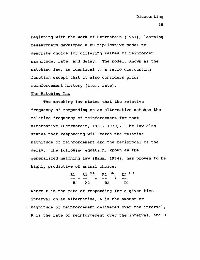
Beginning with the work of Herrnstein (1961), learning researchers developed a multiplicative model to describe choice for differing values of reinforcer magnitude, rate, and delay. The model, known as the matching law, is identical to a ratio discounting function except that it also considers prior reinforcement history (i.e., rate).The Matching Law

The matching law states that the relative frequency of responding on an alternative matches the relative frequency of reinforcement for that alternative (Herrnstein, 1961, 1970). The law also states that responding will match the relative magnitude of reinforcement and the reciprocal of the delay. The following equation, known as the generalized matching law (Baum, 1974), has proven to be highly predictive of animal choice:

B1 A1 SA R1 SR D2 SD B2 A2 R2 D1

where B is the rate of responding for a given time interval on an alternative, A is the amount or magnitude of reinforcement delivered over the interval, R is the rate of reinforcement over the interval, and D

Discounting16

is the delay of reinforcement. The exponents represent the organism's sensitivity to the variables.

The matching law was first demonstrated in an experiment with pigeons (Herrnstein, 1961). The pigeons were given the choice of pecking at two keys, both of which reinforced the response on variable interval schedules. Herrnstein (1961) found that the percentage of responses on a key equaled the relative percentage of reinforcers obtained from the key.

Chung and Herrnstein (1967) were the first to show that relative frequency of responding matched the relative immediacy of reinforcement. Pigeons decreased the rate of responding (i.e., pecking) on a key from .82 to .15 as the delay increased from 1 to 30 seconds. In addition, the response functions became less curved with increasing delays.

Subsequent to Herrnstein (1961), numerous researchers reported data confirming the matching law (Herrnstein, 1970). Matching was found when there were three response alternatives rather than two (Reynolds, 1963), when the reinforcers differed in magnitude rather than rate (Catania, 1963; Neuringer, 1967), when the response was standing on either side of an experimental chamber (Baum & Rachlin, 1969), and when

Discounting17

"yes" responses were plotted against the frequency or magnitude of reinforcement in signal detection studies with humans (Nevin, 1969). In fact, Herrnstein (1970) notes that matching is consistently found as long as responding and reinforcements are qualitatively equal. For example, it is unlikely that matching will be found if one of the response alternatives requires more work, or if one of the reinforcers is a preferred food (Herrnstein, 1970).

While pigeons are the subject of choice in matching law experiments, the equation has been demonstrated to adequately describe human choice as well. McDowell (1981) showed that a derivative of the matching law could account for 99% of the variance in the rate of self-injurious scratching. Piecre and Epling (1983) found that thirteen of sixteen studies of human responding on interval schedules conformed to the matching law.The Matching Law and Irrational Choice

The matching law shows, as one of its interesting predictions, the tendency for organisms to be temporally myopic in decision making (Herrnstein,1990). Animals, including humans, overwhelmingly show a preference for small, immediate rewards over larger,

Discounting18

delayed rewards. When animals act in this manner they are said to act impulsively (Herrnstein, 1990).

Unlike the Freudian and expectancy theories which form the basis of personality research on delayed outcomes, the matching law mathematically specifies this pervasive temporal myopia. The exponents for sensitivity to amount (SA) and sensitivity to delay (SD) represent the degree of discounting (Rachlin et al., 1986).

The mere discounting of deferred consequences is perfectly rational; the banker knows that money today is more valuable than money tomorrow because of the interest that may be earned. The matching law shows, however, that discounting fits a hyperbolic function. That is, animals downgrade the rate of discounting with increasing delays. As Herrnstein (1990, p. 359) points out, if discounting is rational, then the rate of discounting should remain fixed: "Fifteen percent aweek is 15% a week, now or next year, in the theory of rational choice."

This irrational method of discounting, caused by a negatively accelerating psychophysical function for time, yields some interesting preference reversals in choice. Consider the following example from Schwartz

Discounting19

and Lacey (1982). A hungry pigeon is given the choice of pecking a green key or a red key. Pecks at the green key result in four seconds of access to food after a four second delay. Pecks at the red key result in two seconds of access to food with no delay. As predicted by the matching equation, the pigeon will select (i.e., peck) the red key approximately 95% of the time. In other words, the pigeon acts impulsively by choosing the smaller, more immediate reward.

The preference reversal comes when the pigeons are presented with two white keys. Fifteen pecks at either key (FR15) cause a 10 second delay. If the left, white key is selected, the red and green keys are presented after the 10 second delay. Again, pecks at the red key result in two seconds of immediate food access while pecks at the green key result in four seconds of food access after a four second delay. If the right, white key is pecked only the green key (4 s access, 4 s delay) is presented after the 10 second delay. In accord with the matching law, the pigeon will choose to peck at the right, white key approximately 60% of the time. By selecting the key that results in the larger, delayed reward the pigeon has, in effect, delayed

Discounting20

gratification. The downgrading in the rate of temporal discounting results in a preference reversal.

There is nothing in the matching law to suggest that discounting for gains should be different from discounting for losses. A change in the rate of discounting for losses relative to gains would require a theoretical justification for changing sensitivity to amount (SA) (Rachlin et al.# 1986). Although some theories have been proposed (cf. Herrnstein, 1990), none have received wide support (Rachlin et al.# 1986). There is, however, descriptive justification for such a change. The value function for prospect theory (Kahneman & Tversky, 1979), a theory of risky choice, differs for gains and losses.

Prospect Theory The Evidence for Rational Choice

When choosing among different degrees of risk, a rational decision maker will consider only objective probabilities and values. The prescriptive formulation of rational choice, expected utility theory (Friedman & Savage, 1948), ignores subjective evaluations of risk. Instead, expected utility theory prescribes axioms necessary for rational choice. The descriptive viability of two of those axioms, invariance and

Discounting21

dominance, will be considered here. Then, a descriptive theory of risky choice will be reviewed for insights into decision makers' treatment of gains and losses.

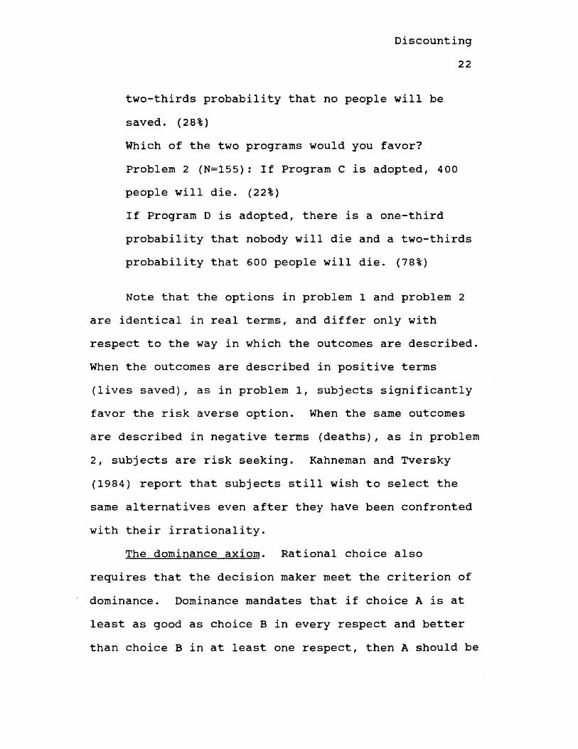
The invariance axiom. One requirement to be met by the rational decision maker is that of invariance. This requires that the preference order of choice should not change as a result of the way in which the options are described. As simple as the criterion of invariance may seem, Tversky and Kahneman (1981) report that it is consistently violated. Consider the following problem from Kahneman and Tversky (1984) (p.343) :

Problem 1 (N=152): Imagine that the U.S. is preparing for the outbreak of an unusual Asian disease, which is expected to kill 600 people.Two alternative programs to combat the disease have been proposed. Assume that the exact scientific estimates of the consequences of the programs are as follows:If Program A is adopted 200 people will be saved. (72%)If Program B is adopted, there is a one-third probability that 600 people will be saved and a

Discounting22

two-thirds probability that no people will be saved. (28%)Which of the two programs would you favor?Problem 2 (N=155): If Program C is adopted, 4 00 people will die. (22%)If Program D is adopted, there is a one-third probability that nobody will die and a two-thirds probability that 600 people will die. (78%)

Note that the options in problem 1 and problem 2 are identical in real terms, and differ only with respect to the way in which the outcomes are described. When the outcomes are described in positive terms (lives saved), as in problem 1, subjects significantly favor the risk averse option. When the same outcomes are described in negative terms (deaths), as in problem 2, subjects are risk seeking. Kahneman and Tversky (1984) report that subjects still wish to select the same alternatives even after they have been confronted with their irrationality.

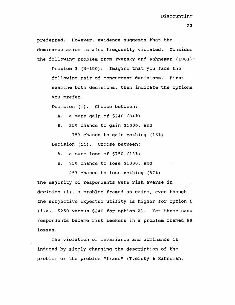
The dominance axiom. Rational choice also requires that the decision maker meet the criterion of dominance. Dominance mandates that if choice A is at least as good as choice B in every respect and better than choice B in at least one respect, then A should be

Discounting23

preferred. However, evidence suggests that the dominance axiom is also frequently violated. Consider the following problem from Tversky and Kahneman (1981)

Problem 3 (N=150): Imagine that you face thefollowing pair of concurrent decisions. First examine both decisions, then indicate the options you prefer.Decision (i). Choose between:A. a sure gain of $240 (84%)B. 25% chance to gain $1000, and

75% chance to gain nothing (16%)Decision (ii). Choose between:A. a sure loss of $750 (13%)B. 75% chance to lose $1000, and

25% chance to lose nothing (87%)The majority of respondents were risk averse in decision (i), a problem framed as gains, even though the subjective expected utility is higher for option B (i.e., $250 versus $240 for option A). Yet these same respondents became risk seekers in a problem framed as losses.

The violation of invariance and dominance is induced by simply changing the description of the problem or the problem "frame” (Tversky & Kahneman,

Discounting24

1981). Kahneman and Tversky (1984) conclude, "In their stubborn appeal, framing effects resemble perceptual illusions more than computational errors" (p. 343).This gives rise to the reflection effect (Kahneman & Tversky, 1979). That is, choice from negative prospects mirrors choice from corresponding positive prospects. The reflection effect is manifested as risk seeking of choices framed in terms of losses and risk avoidance of choices framed as gains (Kahneman & Tversky, 1979, 1984; Tversky & Kahneman, 1981).Prospect Theory's Value and Weighting Functions

Two characteristics of the human decision maker contribute to the reflection effect. The first is an S-shaped value function that is concave for gains and convex for losses. For example, the subjective difference between $10 and $20 is perceived as greater than the subjective difference between $110 and $120 (Tversky & Kahneman, 1981). In addition, the value function is steeper for losses than for gains which leads to a robust loss aversion effect. As stated by Tversky and Kahneman (1981), "The displeasure associated with losing a sum of money is generally greater than the pleasure associated with winning the same amount..."(p.454).

Discounting25

The second characteristic that contributes to the framing effect is the weighting of probabilities. Low probabilities are overweighted, and moderate and high probabilities are underweighted. In addition, certain outcomes are overweighted relative to probable outcomes. This phenomenon, labeled the certainty effect, means that certain gains will be highly attractive and certain losses highly aversive.Research Investigations of Framing

The framing effect described by Tversky and Kahneman (1981) is robust and is evinced by sophisticated and naive respondents alike (Kahneman & Tversky, 1984). Although research on framing effects is neither voluminous nor unequivocal, the findings generally support risk avoidance of gains and risk seeking of losses. A review of these studies and their findings follows.

Risk seeking of losses and risk aversion of gains were demonstrated in gambles with complete and incomplete information in a variety of tasks devised by Levin and his colleagues (Levin, Johnson, Russo, & Deldin, 1985; Levin, Johnson, Deldin, Carstens,Cressey, & Davis, 1986) . Specifically, it was found that subjects were more likely to accept gambles framed

Discounting26

in terms of probability of winning than probability of losing. When probability information was missing ("amount to be won” only) there was no effect for the frame. A further examination by Levin et al. (1986) revealed the locus of the framing effect to be in the decision weight associated with the probability. In other words, the problem frame appears to affect the subjective likelihood of winning or losing (Levin et al., 1986).

Decision frames have also been implicated in escalation of committment to a failing course of action (Northcraft & Neale, 1986). According to Northcraft and Neale (1986), the decision maker faced with the dilemma of pumping more money into a failing investment may consider the decision as a choice between a certain loss and a low probability of a gain or a high probability of an even greater loss. Because decision makers are risk seeking of losses and overestimate low probabilities (Kahneman & Tversky, 1979), it is expected that persistence in the failing course would occur. Northcraft and Neale (1986) obtained results consistent with this hypothesis. They also found that increasing the salience of opportunity costs decreased

Discounting27

persistence by rendering the certain loss less averse (Northcraft & Neale, 1986).

Not only may task characteristics produce a framing effect, but research supports a framing effect for role characteristics as well (Neale, Huber, & Northcraft, 1987). In sales negotiations, buyers may focus on the loss of money, while sellers may focus on dollar gain. Neale et al. (1987) found, in support oftheir hypothesis, that negotiator role framed the context and resulted in biased decisions.

The preference for risky alternatives may also be influenced by decision frames when groups make decisions (Schurr, 1987). Negotiating teams consisting of Masters of Business Administration (MBA) students selected more risky purchase alternatives when they were induced to think of losses as opposed to gains (Schurr, 1987). These results extend the findings of Tversky and Kahneman (1981) because the focus is on degree of risk taking rather than on risk seeking or aversion per se (Schurr, 1987).

The limits of information frames were tested by Levin, Schnittjer, and Thee (1988) who examined social and personal and moral decisions. They found that framing the incidence of cheating among college

Discounting28

students (65% cheated or 35% never cheated) affected the perceived incidence of cheating, but the frame had no effect on whether the subjects would report a cheater or cheat themselves. However, framing the success of a medical technique (50% success rate or 50% failure rate) affected the perceived effectiveness of the technique and the likelihood that the technique would be recommended to a friend and family member.This result is consistent with the finding that individuals are more likely to choose risky medical options framed positively (Wilson, Kaplan, & Schneiderman, 1987). Levin et al. attribute the difference obtained between the two decisions (i.e., cheating and medical technique) in their study to the amount of attention subjects must pay to the scenario to make an informed judgment in the medical technique decision.

Elliott and Achibald (1989) suggested that a weakness in framing research is that the frames are imposed on the subjects by the experimenter. In their studies, the choice outcomes were worded in a way such that subjects would impose their own frame. Results were consistent with the prospect theory prediction. Subjects who viewed the problem in terms of gains

Discounting29

avoided risk, whereas subjects who viewed the problem in terms of losses were risk seeking.

A study by Fagley and Miller (1987) called into question the robustness of the framing effect. In a decision problem concerning cancer treatments, most of the MBA students selected the risk averse option regardless of frame (lives saved versus deaths).Because the MBA subjects in the study had exposure to the concept of expected value, a replication was performed using graduate students in education.Framing effects consistent with prospect theory were obtained with the education students, but the proportion of subjects selecting the risk seeking option in the negative frame was significantly lower than the proportions reported by Tversky and Kahneman (1981).

One major problem with Kahneman and Tversky's (1979) demonstration of reflection is that preference reversals were measured across subjects. As Hershey and Shoemaker (1980) note, a between-subjects design showing risk aversion for gains with one group of subjects and risk seeking for losses with another group of subjects does not measure individual preference

Discounting30

reversals. Individual reversals may only be measured utilizing a within-subjects design.

Hershey and Shoemaker (1980) examined individual and group preferences in three separate experiments.In two of the experiments, preference reversals were inconsistent for both groups and individuals. In the third experiment, which had a very large sample size (n=2080), individual preference reversals consistent with prospect theory occurred in significantly more than 50% of the subjects for all problems. While reflection consistent with prospect theory was the most prevalent across all three experiments, Hershey and Shoemaker (1980) conclude that reflection is most likely to occur when prospects involve small amounts, extreme probabilities, or very large amounts.

Schneider and Lopes (1986) also examined the reflection effect both between and within subjects. Their study was unique, however, in that subjects were classified according to risk style (i.e., risk-averse or risk-seeking) and multi-outcome lotteries were used. Reflection for all subjects was irregular except for lotteries that were riskless (i.e., some amount would be won or lost). For both risk-averse and risk-seeking

Discounting31

subjects, riskless lotteries were preferred for gains but not for losses (Schneider & Lopes, 1986).

Cohen, Jaffray, and Said (1987) used a sample (n=134) of economics and computer science majors who made binary choices for gains and losses over a period of ten weeks. The choices involved large sums, and subjects were told that at least one payment would be made. They found that only 41% of their subjects behaved in accord with the reflection effect.Moreover, there was no correlation between attitudes on the gain side and attitudes on the loss side. Subjects also appeared to be insensitive to probabilities when losses were involved.

The Cohen et al. (1987) study appears to supply stronger evidence in opposition to the prospect theory value function, but there is reason to doubt the strength of their conclusions. First, their subjects, economics and computer science majors, had some background in probability theory. Second, the study was completed over a span of 10 weeks. It is likely that any subject who persisted in the study for 10 weeks had some interest in the topic under examination. It is not unreasonable to assume that the subjects discussed their choices among themselves. Third, there

Discounting32

is a special concern that the sample consisted, at least partially, of economics majors. Prospect theory was first published by Kahneman and Tversky (1979) in Econometrica. one of the leading economics journals. Conclusions

As was stated in the introduction, the research findings on generally support the framing effect, although the effect is not as robust as first reported by Tversky and Kahneman (1981). Reflection consistent with prospect theory seems most likely to occur when prospects involve very small or large amounts, when there are extreme probabilities, and when the prospect is riskless (i.e., some amount is certain to be won or lost). Any true test of the reflection effect must also be conducted utilizing a within-subjects design.A Comparison of Prospect Theory and the Matching Law

Rachlin, Logue, Gibbon, and Frankel (1986) published a paper in which Kahneman and Tversky's (1979) prospect theory was compared with Herrnstein's (1961) matching law. The paper is a seminal work in that it bridges the gap between the main cognitive and behavioral theories of choice.

Rachlin et al. (1986) argue that the two models of choice, prospect theory and the matching law, are

Discounting33

conceptually similar because of the correspondence between delay and probability. That is, probability may be viewed as the inverse of delay (Mazur, 1985; Rachlin, Castrogiovanni, & Cross, 1987; Rotter, 1954). As an example, if subjects were confronted with repeated choices between a gamble with a .5 chance of $10 and .25 chance of $20, the subject could expect a payoff every two choices for the .5 probability and every four choices for the .25 probability.

Because probability and the inverse of delay are conceptually similar, there is convergence between the findings in cognitive and behavioral studies. The finding in behavioral studies that animals sharply discount delayed positive reinforcement (e.g., Chung & Herrnstein, 1967) corresponds to Kahneman and Tversky's (1979) finding of risk aversion for gains. Conversely, the finding in behavioral studies that animals prefer delayed aversive stimuli (e.g., Deluty, Whitehouse, Mellitz, & Hineline, 1983) corresponds to Kahneman and Tversky's finding of risk seeking for losses. Probability as Delay in Repeated Gambles

Rachlin et al. (1986) empirically demonstrated howprobabilities function as delays to reinforcement.Their subjects were presented with two spinners and

Discounting34

were asked to choose one. The $100 spinner was called "the sure thing" and had a 17/18 chance of winning associated with it. The $250 spinner was the risky gamble which initially had a 7/18 chance of winning associated with it. A titration procedure was used such that if subjects selected the sure thing on one trial, the risky option was made more attractive by increasing the odds of winning by 1/18. Similarly, if subjects selected the risky option, it was made less attractive by decreasing the odds of winning by 1/18. Presumably, the titration procedure would serve to keep both options equally attractive. For one group of subjects the experiment was conducted as quickly as possible. A second group of subjects was required to wait 1.5 minutes between gambles. Results showed that long intervals between gambles resulted in risk averse choices, whereas short intervals between gambles resulted in risky choices. Thus, the long delays produced choices for near certain outcomes which may be seen as a form of impulsiveness.

Rachlin, Castrogiovanni, and Cross (1987) used a two-stage choice procedure to demonstrate that impulsiveness could be used to induce commitment to a gamble. They showed that when probability of advancing

Discounting35

to the second stage of a gamble (where money was available) was low, undergraduates committed to a chance to win a large, low probability award. However, when probability of advancing to the second stage was high, subjects preferred to commit to a gamble that allowed a choice between a small, high probability reward and a large, low probability award. When faced with this choice in the second stage, subjects significantly preferred the small, high probability reward. Their behavior was much like the pigeons that chose to peck at red and green keys: When the delay toreward choice is long (i.e., low probability), a large, delayed (i.e., large, low probability) reward is preferred. When the delay to choice is brief (i.e., high probability), a small, immediate (i.e., small, high probability) reward is preferred.

The Rachlin et al. (1986) study was replicated bySilberberg, Murray, Christensen, & Asano (1988), but a confound in the study was detected. Silberberg et al. noted that subjects who experienced a short interval between gambles may have expected more trials, and thus may have implicitly perceived that they had less to loose on each gamble. To control this potential confound, both long and short interval conditions were

Discounting36

restricted to 10 gambles. Under this restriction, there was no difference in risky choice between the two groups, suggesting that potential income affects risky choice. This explanation was tested directly by informing subjects that they had been given $10 or $10,000 before the repeated gambles had begun. Under these conditions, the high income group was significantly more likely to select the risky gamble.

The repeated gambles experiments described above provide some evidence that probability and delay are conceptually similar. The Silberberg et al. (1988) study suggests that income, either implicitly or explicitly stated, affects the value function for gains. Although the confound they identify has intuitive appeal, it seems likely that the results they report were due to experimenter demand, particularly when subjects were told that they had been given $10,000. Recall that the Rachlin, Castrogiovanni, and Cross (1987) study demonstrated convergence with animal studies of the matching law. Presumably, Silberberg and his colleagues would provide an account of a pigeon's preference for smaller, temporally advanced food rewards that refers to the pigeon's implicit

Discounting37

expectation of a greater opportunity to eat under these conditions.Conclusions

Rachiin's demonstration of convergence between cognitive and behavioral explanations of choice may, if valid, lead to a unification of these fields. Although the empirical evidence seems to demonstrate that risk is associated with delay, there is no evidence that the value functions obtained under conditions of risk are related to the value functions obtained under riskless conditions involving a delay. There is evidence that the reflection effect predicted by prospect theory is more likely to occur when there is a riskless component to choice (Schneider & Lopes, 1986); however, there has not been an empirical test of the prospect theory value function in a riskless context.

The Proposed Investigation

Experiments on delayed rewards and punishers support a discounting function in which delayed outcomes are evaluated in proportion to the magnitude of the return (Ortendahl & Sjoberg, 1979; Stevenson, 1986). A ratio discounting model implies that delay is treated as a risk; that is, temporal delay reduces the

Discounting38

value of gains and the aversiveness of losses (Stevenson, 1986). Therefore, a ratio discounting function predicts that individuals will prefer immediate gains and delayed losses.2

The matching law (Herrnstein, 1961), like a ratio discounting function, also states that delay influences choice through a multiplicative relationship.Herrnstein (1990) points out that the rate of discounting declines with time. Ortendahl and Sjoberg (1979) and Stevenson (1986) also found that the effect of time is a negatively accelerated function of real time.

There have not been any studies of individual preferences for delayed gains and losses with outcome type treated as a within-subjects variable. Stevenson (1986) found support for a ratio discounting function with both gains and losses, but the two experiments used different samples. Thus, the proposed investigation would be the first within-subjects comparison of individual preferences for both gains and losses.

In addition, there is not an accepted theoretical rationale offered by proponents of a ratio discounting function or matching law as to how a person's

Discounting39

discounting of gains should compare to the discounting of losses. Theoreticians have suggested, however, that the matching law and prospect theory (a theory of risky choice) are conceptually similar (Rachlin et al.,1986). Specifically, probability in prospect theory is equivalent to the inverse of delay in the matching law.

If the matching law and prospect theory simply explain the same phenomenon with different paradigmatic approaches, then the psychophysical values for delayed gains and losses should correspond to the prospect theory value function. The prospect theory value function is concave for gains and convex for losses, and it is steeper for losses than for gains.Translated to choice, this means that individuals are risk-averse for gains but risk-seeking for losses. The steeper curve for losses also contributes to a robust loss aversion effect. This would be expected to lead to a steeper discounting rate for delayed losses relative to delayed gains. In other words, the outcome frame should influence the rate of discounting.

Discounting40

HypothesesHypothesis 1, A ratio discounting function will

describe individual choice for both gains and losses.(a) Immediate gains will be preferred to delayed

gains.(b) Delayed losses will be preferred to immediate

losses.Hypothesis 2. Larger, delayed gains will be

preferred if the advanced, smaller gain is temporally removed.

Hypothesis 3. Preferences for delayed losses will be stronger than preferences for immediate gains.

Stevenson (198 6) found, using a between-subjects design, that a ratio discounting function described choice for gains and losses. Parts "a" and "b" of Hypothesis 1 represent an attempt to replicate and extend Stevenson's (1986) finding. This investigation improves upon Stevenson's study in two ways. First, outcome type (gain or loss) is a within-subjects variable in the present investigation. This is an important distinction as it permits a test of the ratio discounting function for both gains and losses without the potential confounding effects of subject differences. Second, both binary preferences and

Discounting41

preference ratings serve as dependent variables in the present investigation. Stevenson relied solely on preference ratings in her investigation, a design which lacks external validity for the study of choice behavior.

Numerous researchers have reported a negatively accelerating psychophysical function for time (Chung & Herrnstein, 1967; Herrnstein, 1990; Ortendahl &Sjoberg, 1979; Stevenson, 1986). Hypothesis 2 is an attempt to replicate and extend that finding. The present investigation is the first to utilize the cognitive paradigm with binary preference as the dependent variable.

Hypothesis 3 is a test of the Rachlin et al. (1986) proposition that prospect theory should apply to riskless choice. Because respondents are risk seeking in the domain of losses and risk averse in the domain of gains, and because the value function proposed by Kahneman and Tversky (1979) is steeper for losses, a negative frame should result in a steeper rate of discounting. That is, subjects should prefer delayed losses more than they prefer immediate gains. To paraphrase Kahneman & Tversky (1984, p. 342), a delayed

Discounting42

loss of $X is less aversive than an immediate gain of $X is attractive.

MethodOverview

The sample consisted of upper level accounting majors. The study was divided into two sessions. In the first session, subjects were presented with 64 two- option prospects involving delayed gains and losses. Preference was operationalized in the first session as binary choice which yielded nominal data. The second session was conducted a week later. In this session, subjects were presented with the same 64 two-option prospects, with choice operationalized as a preference rating. After completing the problems, open-ended questions were used to assess strategies in selecting and rating the options.Subjects

The subjects were upper level accounting majors enrolled in an information systems course. The study was completed in two sessions, and there was some subject mortality. In session 1 (binary choice), 31 subjects completed the study. Of this sample, 15 (48.4%) were male and 16 (51.6%) were female. Their ages ranged from 21 to 43 (M=28.29). In session 2

Discounting43

(preference rating), 2 6 subjects completed the study.Of this sample, 12 (46.2%) were male and 14 (53.8%) were female. They ranged in age from 21 to 43 (M=28.50).Apparatus

The packet of stimulus materials contained instructions for completion, examples, and 64 prospects requiring a choice by the subject. Each prospect contained two options. The choice was always between a larger, temporally delayed gain (loss) and a smaller, immediate or temporally advanced gain (loss). Presentation of the larger, temporally delayed option varied between option A and option B. (Note. For purposes of analysis, the problems were recoded such that option A was always the samller, immediate or temporally advanced option. Thus, all presentations of methodology and results which refer to option A or option B reflect this recoding.) The stimulus packets for sessions 1 and 2 appear in Appendix A and B, respectively.Procedure

The stimulus materials were administered following class periods. Two sessions were needed to complete the study. In the first session, subjects indicated

Discounting44

their preference by circling either the letter A or the letter B (binary choice). The second session was conducted a week after the first, and subjects indicated their preference by making a rating along a 17-point scale, where 8 on the left end indicated a strong preference for option A, 0 indicated indifference, and 8 on the right end indicated a strong preference for option B. After completing the 64 prospects, open-ended questions assessed the subjects' knowledge of temporal discounting, the strategies used to make choices for prospects involving gains and losses, and strategies used to make choices between outcomes with differing delays.

Independent variables. The four independent variables were magnitude of the outcome, outcome type, option A delay, and option B delay. There were four levels of magnitude ($100, 200, 400, and 800), two levels of outcome type (gain and loss), two levels of option A delay (immediate and half of option B delay), and four levels of option B delay (4, 10, 18, and 24 months). The magnitude of option A was held constant at 75% of the magnitude of option B. All four of the independent variables were within-subjects; thus, each

Discounting45

subject completed a total of 64 problems in each session.

Dependent variables. The two dependent variables were binary choice and preference rating. In the first session, subjects indicated their preference for each of the 64 problems by circling either the letter A orB. Subjects indicated their preferences in the second session, which was conducted a week after the first, by making a rating along a 17-point scale.

ResultsThe first open-ended question asked subjects to

indicate their knowledge of temporal discounting. Only the open-ended questions from the first session were content-coded because the majority of subjects did not complete these questions in the second session. Of the 31 subjects who participated in the first session, 25 (80.6%) reported having some knowledge of discounting,3 (9.7%) reported having no knowledge of discounting, and 3 (9.7%) did not answer.Results for Hypothesis 1

Hypothesis 1 stated that a ratio discounting function would describe choice for both gains and losses. This entailed two predictions: (a) Immediate

Discounting46

gains will be preferred to delayed gains; and (b) Delayed losses will be prefered to immediate losses.

This hypothesis was analyzed in three ways.First, frequency counts were made of subjects' binary choices, and the data were analyzed using the chi- square test. Second, preference ratings were analyzed using a within-subjects analysis of variance (ANOVA). Third, responses to the open-ended questions were content coded and frequency counts were made.

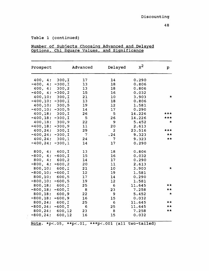
Binary Choice. There were 16 prospects in which subjects chose between an immediate and delayed gain. Subjects significantly preferred the smaller, immediate gain to the larger, delayed gain for 14 of those prospects. There were two prospects in which subjects showed no significant preference. Both of these involved relatively large magnitudes ($400 and $800) and relatively brief delays (4 months). These results are presented in Table 1.

There were also 16 prospects in which subjects chose between an immediate and delayed loss. Subjects significantly preferred the larger, delayed loss for nine of those prospects. The seven prospects for which the delayed loss was not significantly preferred all

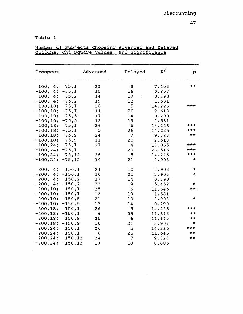
Discounting47

Table 1Number of Subjects Choosing Advanced and Delaved Options. Chi Square Values, and Significance

Prospect Advanced Delayed X2 p

100 4 75,1 23 8 7.258 **-100 4 -75,1 15 16 0.857100 4 75,2 14 17 0.290

-100 4 -75,2 19 12 1.581100 10 75,1 26 5 14.226 ***

-100 10 -75,1 11 20 2.613100 10 75,5 17 14 0.290

-100 10 -75,5 12 19 1.581100 18 75,1 26 5 14 .226 * * *

-100 18 -75, I 5 26 14.226 ***100 18 75,9 24 7 9 . 323 **

-100 18 -75,9 11 20 2.613100 24 75,1 27 4 17.065 ***

-100 24 -75,1 2 29 23.516 ***100 24 75, 12 26 5 14 . 226 ***

-100 24 -75,12 10 21 3 . 903 *200 4 150, I 21 10 3.903 *

-200 4 -150,I 10 21 3.903 *200 4 150, 2 17 14 0.290

-200 4 -150,2 22 9 5. 452 *200 10 150,1 25 6 11.645 **

-200 10 -150,I 12 19 1.581200 10 150, 5 21 10 3 .903 *

-200 10 -150,5 17 14 0.290200 18 150,1 26 5 14.226 * * *

-200 18 -150,1 6 25 11.645 **200 18 150, 9 25 6 11.645 **

-200 18 -150,9 10 21 3.903 *200 24 150,1 26 5 14.226 * * *

-200 24 -150,I 6 25 11.645 **200 24 150,12 24 7 9.323 **

-200 24 -150,12 13 18 0.806

Discounting48

Table 1 (continued)Number of Subjects Choosing Advanced and Delaved Options. Chi Square Values, and Significance

Prospect Advanced DelayedCMX P

400 4 300 I 17 14 0.290-400 4 -300 I 13 18 0. 806400 4 300 2 13 18 0.806

-400 4 -300 2 15 16 0.032400 10 300 I 21 10 3 .903 i f

-400 10 -300 I 13 18 0.806400 10 300 5 19 12 1.581

-400 10 -300 5 14 17 0.290400 18 300 I 26 5 14 . 226 i f i t i f

-400 18 -300 I 5 26 14.226 i f * i f

400 18 300 9 22 9 5.452 i f

-400 18 -300 9 11 20 2. 613400 24 300 I 29 2 23.516 i f * i f

-400 24 -300 I 7 . 24 9.323 i f i f

400 24 300 1 24 7 9.323 i f i f

-400 24 -300 1 14 17 0.290800 4 600 I 13 18 0. 806

-800 4 -600 I 15 16 0. 032800 4 600 2 14 17 0.290

-800 4 -600 2 20 11 2.613800 10 600 I 21 10 3.903 i f

-800 10 -600 I 12 19 1.581800 10 600 5 17 14 0. 290

-800 10 -600 5 19 12 1.581800 18 600 I 25 6 11.645 i f i f

-800 18 -600 I 8 23 7.258 i f i f

800 18 600 9 22 9 5.452 i f

-800 18 -600 9 16 15 0.032800 24 600 I 25 6 11.645 i f i f

-800 24 -600 I 6 25 11.645 i f i f

800 24 600 12 23 8 7.258 **-800 24 600 12 16 15 0. 032Note. *p<.05, **p<.01, ***p<. 001 (all two-tailed)

Discounting49

invloved relatively brief delays. When the delay to the larger loss was 4 months, there was no significant difference in preferences at three of the magnitude levels. The exception was the $200/$150 level; here, the larger, delayed loss was significantly preferred. When the delay to the larger loss was 10 months, there was no significant difference in preferences at all four magnitude levels. These results are reported in Table 1.

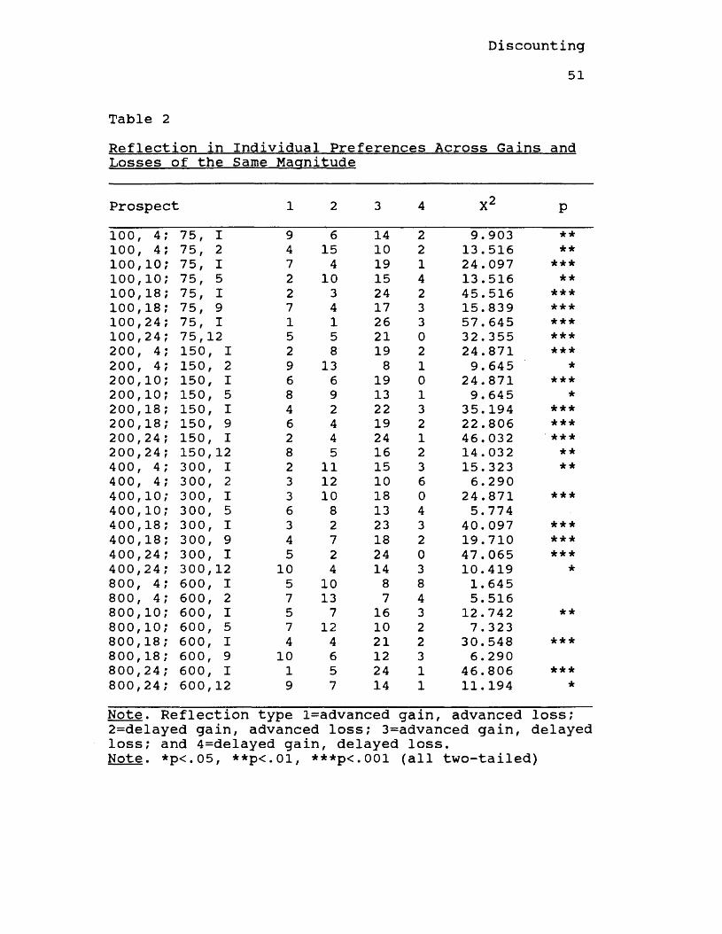
To assess individual preferences across gains and losses, subjects' responses were coded into one of four reflection types (across outcome) for each combination of magnitude and delay (i.e., advanced gain, advanced loss; delayed gain, advanced loss; advanced gain, delayed loss; and delayed gain, delayed loss). For 58 of the 64 prospects, reflection consistent with the prospect theory value function (i.e., advanced gain, delayed loss) was significantly more prevalent than any other reflection type. For the other six prospects, no single reflection type was significantly more prevalent than another. These prospects were of relatively high magnitude (i.e., $400 or $800) and brief delay (i.e., 4 or 10 months). In addition, the advanced, smaller option tended to be temporally removed in these

Discounting50

prospects. The single exception was the $800 in 4 months; $600 immediate prospect. These results are reported in Table 2.

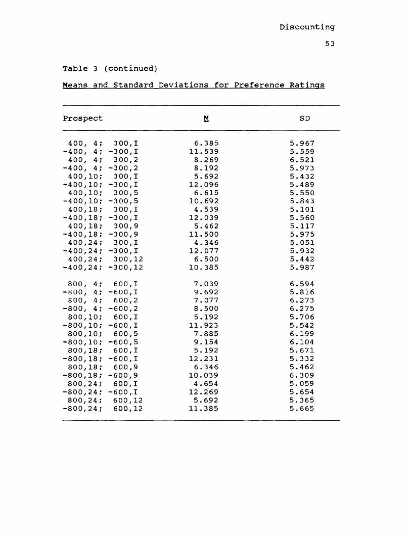
Preference ratings. Preference ratings were recoded such that a rating of 8 on the right end of the scale ("strong preference for option A") became 1, a rating of 0 (neutral) became 9, and a rating of 8 on the left end ("strong preference for option B") became 17. The analysis of subjects' preference ratings revealed a significant main effect for outcome type F(1,25)=7. 60, p=.011. Gains received significantly lower ratings (M=5.95) than losses (M=10.96).Individual t-tests for each prospect across gains and losses were not conducted because such a large number of analyses (32) would capitalize on chance. However, a visual inspection of the mean ratings reveals that every prospect, with one exception, that was described in terms of a loss received a higher rating (indicating a stronger preference for the delayed option) relative to the same prospect described as a gain. Means and standard deviations of preference ratings appear in Table 3. Figure 1 presents the preference ratings for all prospects involving an immediate option.

Discounting51

Table 2Reflection in Individual Preferences Across Gains andLosses of the Same Maanitude

Prospect 1 2 3 4 X2 P100 4 75, I 9 6 14 2 9.903 **100 4 75, 2 4 15 10 2 13.516 **100 10 75, I 7 4 19 1 24.097 * * *100 10 75, 5 2 10 15 4 13.516 **100 18 75, I 2 3 24 2 45.516 * * *100 18 75, 9 7 4 17 3 15.839 ***100 24 75, I 1 1 26 3 57.645 ***100 24 75, 12 5 5 21 0 32.355 ***200 4 150 I 2 8 19 2 24.871 * * *200 4 150 2 9 13 8 1 9.645 *200 10 150 I 6 6 19 0 24.871 ***200 10 150 5 8 9 13 1 9.645 *200 18 150 I 4 2 22 3 35.194 * * *200 18 150 9 6 4 19 2 22.806 * * *200 24 150 I 2 4 24 1 46.032 * * *200 24 150 12 8 5 16 2 14.032 **400 4 300 I 2 11 15 3 15.323 **400 4 300 2 3 12 10 6 6.290400 10 300 I 3 10 18 0 24.871 ***400 10 300 5 6 8 13 4 5.774400 18 300 I 3 2 23 3 40.097 * * *400 18 300 9 4 7 18 2 19.710 * * *400 24 300 I 5 2 24 0 47.065 * * *400 24 300 12 10 4 14 3 10.419 *800 4 600 I 5 10 8 8 1.645800 4 600 2 7 13 7 4 5.516800 10 600 I 5 7 16 3 12.742 **800 10 600 5 7 12 10 2 7.323800 18 600 I 4 4 21 2 30.548 * * *800 18 600 9 10 6 12 3 6.290800 24 600 I 1 5 24 1 46.806 * * *800 24 600 12 9 7 14 1 11.194 *Note. Reflection type l=advanced gain, advanced loss; 2=delayed gain, advanced loss; 3=advanced gain, delayed loss; and 4=delayed gain, delayed loss.Note. *p<.05, **p<.01, ***p<.001 (all two-tailed)

Discounting52

Table 3Means and Standard Deviations for Preference Ratings

Prospect M SD

100 4 75,1 6.154 5.641-100 4 -75,1 10.385 6.060100 4 75,2 7.654 5.912

-100 4 -75,2 10.231 6. 002100 10 75,1 5.885 6.002

-100 10 -75,1 11.115 5.764100 10 75,5 6.000 4.964

-100 10 -75,5 10.462 6. 107100 18 75,1 4.462 5.331

-100 18 -75,1 11.962 5.930100 18 75,9 5.731 4.904

-100 18 -75,9 11.462 5.874100 24 75,1 4 . 000 5. 192

-100 24 -75,1 12.654 5.462100 24 75, 12 5.731 5. 356

-100 24 -75,12 10.077 6. 105200 4 150, I 7.692 6. 329

-200 4 -150,I 11.654 5. 329200 4 150,2 7.885 6. 108

-200 4 -150,2 10.346 5.858200 10 150,1 5.423 5.529

-200 10 -150,1 10.962 5.834200 10 150, 5 6. 308 5. 342

-200 10 -150,5 10.808 5.755200 18 150,1 4.885 5. 187

-200 18 -150,I 12.039 5.956200 18 150,9 5. 654 5. 344

-200 18 -150,9 10.962 5.923200 24 150, I 4.539 5. 240

-200 24 -150,1 12.346 5. 192200 24 150,12 5. 692 5. 312

-200 24 -150,12 9.462 6. 048

Discounting53

Table 3 (continued)Means and Standard Deviations for Preference Ratings

Prospect M SD

400 4 300 I 6.385 5.967-400 4 -300 I 11.539 5.559400 4 300 2 8.269 6.521

-400 4 -300 2 8.192 5.973400 10 300 I 5.692 5.432

-400 10 -300 I 12.096 5.489400 10 300 5 6. 615 5.550

-400 10 -300 5 10.692 5.843400 18 300 I 4.539 5.101

-400 18 -300 I 12.039 5.560400 18 300 9 5. 462 5.117

-400 18 -300 9 11.500 5.975400 24 300 I 4. 346 5. 051

-400 24 -300 I 12.077 5.932400 24 300 12 6.500 5.442

-400 24 -300 12 10.385 5.987800 4 600 I 7.039 6.594

-800 4 -600 I 9. 692 5.816800 4 600 2 7.077 6. 273

-800 4 -600 2 8.500 6.275800 10 600 I 5.192 5.706

-800 10 -600 I 11.923 5.542800 10 600 5 7.885 6.199

-800 10 -600 5 9.154 6.104800 18 600 I 5.192 5.671

-800 18 -600 I 12.231 5.332800 18 600 9 6.346 5.462

-800 18 -600 9 10.039 6. 309800 24 600 I 4 .654 5. 059

-800 24 -600 I 12.269 5.654800 24 600 12 5.692 5. 365

-800 24 600 12 11.385 5. 665

Discounting54

Open-ended responses. After making their choices for the 64 prospects in session 1, subjects were asked to explain any rules or strategies they used in choosing between gains and losses. Twenty-four (77.4%) subjects responded to the query. For gains, 15 (62.5%) subjects indicated that their strategy was to choose the immediate or more advanced option, five (20.8%) subjects indicated that both magnitude and delay of the options played a role in their choices, two (8.3%) subjects indicated that they would wait to maximize their gain, and two subjects were ambiguous in their response.

For losses, 16 (66.7%) subjects indicated that their strategy was to choose the delayed option. Four (16.7%) subjects indicated that both magnitude and delay were considered in their choice, one (4.2%) subject indicated that a strategy which minimized the loss was used, and one subject responded ambiguously. Results for Hypothesis 2

Hypothesis 2 predicted that larger, delayed gains would be preferred if the advanced, smaller gain was temporally removed. This result would be expected if

Discounting55

the psychophysical value of time is a negatively accelerating function of real time.

Two methods were used to test this hypothesis. First, a chi-square test was used to analyze the binary choice data. Second, a within-subjects ANOVA was used to analyze the preference ratings. Although an open- ended question asked about strategies used in choosing between delays, very few subjects responded to the query? therefore, no content-coded data will be presented for this hypothesis.

Binary choice. This hypothesis was not supported by the binary choice data. When the length of the delay to the larger gain was four months, there was no significant difference in subjects' preferences at all four magnitude levels. When the delay to the larger gain was 10 months, there was no significant difference in preferences at three of the magnitude levels. The exception was the $200/$150 level, but the difference was opposite from the predicted direction. When the delay to the larger gain was 18 or 24 months, subjects significantly preferred the smaller, advanced gain at all magnitude levels. Thus, for relatively lengthy delays, subjects' preferences were opposite from the

Discounting56

predicted direction. These results are presented in Table 1.

Preference ratings. This hypothesis was not supported by the preference rating data. There was not a significant difference in ratings when the smaller magnitude option was immediate (M=8.53) or half the delay of the larger magnitude option (M=8.59) F(l,25)=0.79, p=.382.Results for Hypothesis 3

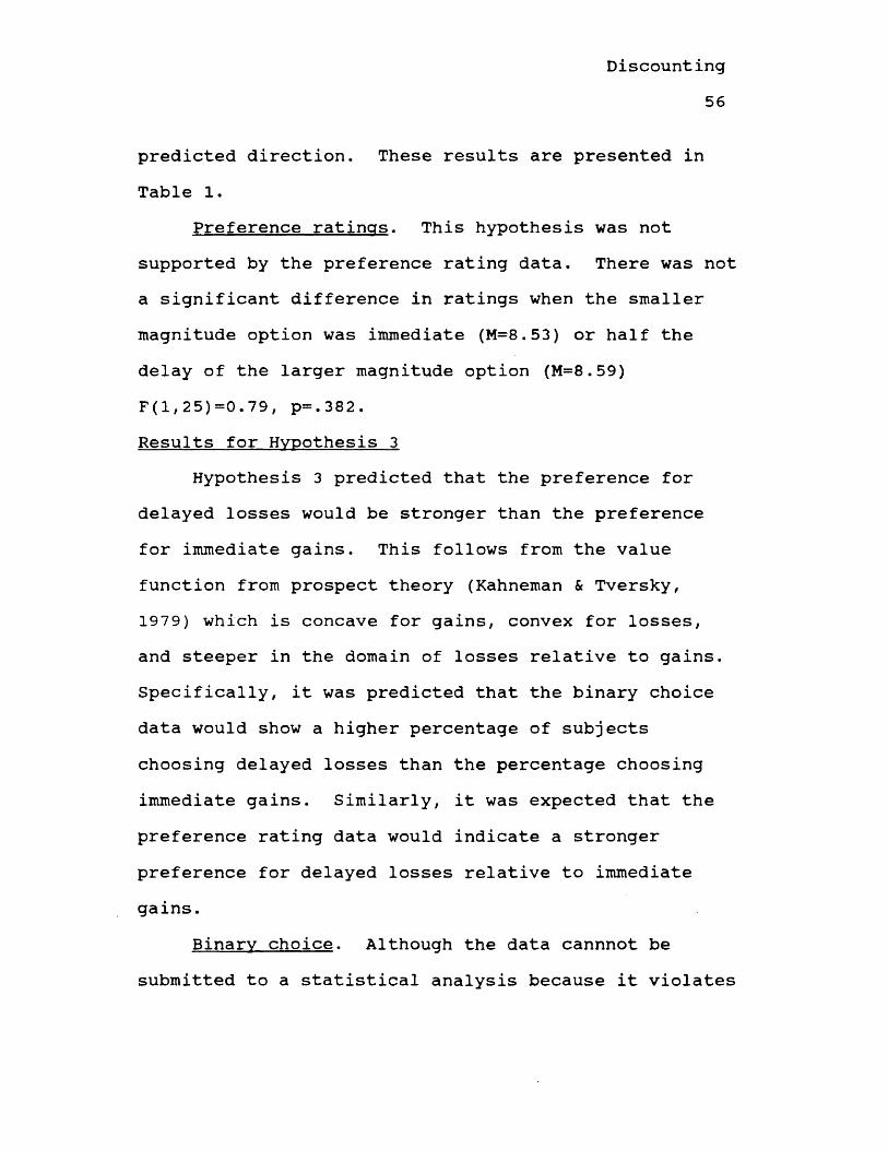
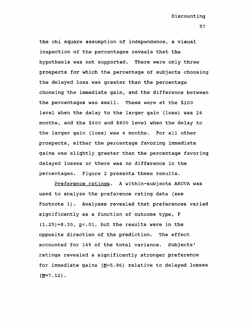
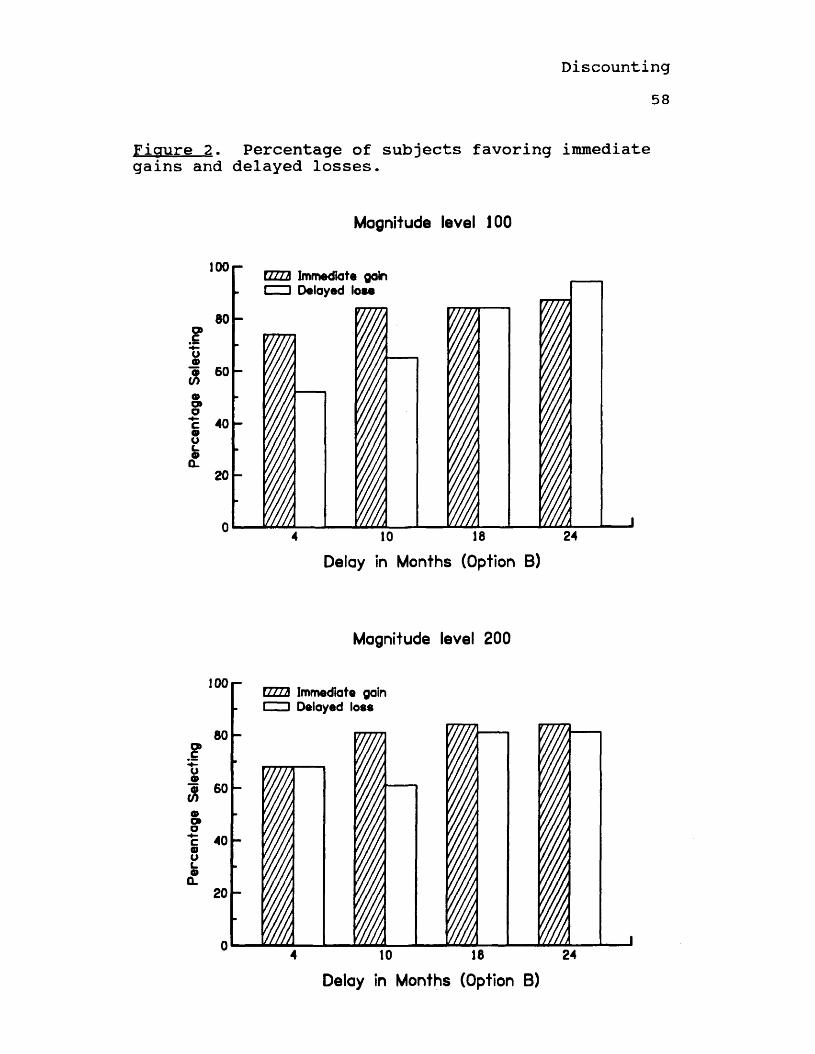
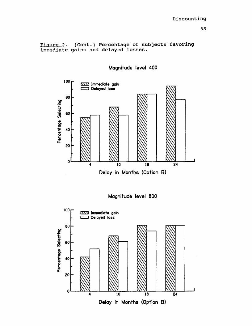
Hypothesis 3 predicted that the preference for delayed losses would be stronger than the preference for immediate gains. This follows from the value function from prospect theory (Kahneman & Tversky,1979) which is concave for gains, convex for losses, and steeper in the domain of losses relative to gains. Specifically, it was predicted that the binary choice data would show a higher percentage of subjects choosing delayed losses than the percentage choosing immediate gains. Similarly, it was expected that the preference rating data would indicate a stronger preference for delayed losses relative to immediate gains.

Binary choice. Although the data cannnot be submitted to a statistical analysis because it violates

Discounting57

the chi square assumption of independence, a visual inspection of the percentages reveals that the hypothesis was not supported. There were only three prospects for which the percentage of subjects choosing the delayed ioss was greater than the percentage choosing the immediate gain, and the difference between the percentages was small. These were at the $100 level when the delay to the larger gain (loss) was 24 months, and the $4 00 and $800 level when the delay to the larger gain (loss) was 4 months. For all other prospects, either the percentage favoring immediate gains was slightly greater than the percentage favoring delayed losses or there was no difference in the percentages. Figure 2 presents these results.

Preference ratings. A within-subjects ANOVA was used to analyze the preference rating data (see Footnote 1). Analyses revealed that preferences varied significantly as a function of outcome type, F(1,25)=8.30, pc.01, but the results were in the opposite direction of the prediction. The effect accounted for 14% of the total variance. Subjects' ratings revealed a significantly stronger preference for immediate gains (M=5.96) relative to delayed losses (M=7.12).

Discounting58

Figure 2. Percentage of subjects favoring immediate gains and delayed losses.

Magnitude level 100

too

a>a>oca>oc.oQ_

60

60

40

20

CZZZZ Immediate gain Delayed lose

10 18 24

Delay in Months (Option B)

Magnitude level 200

I

100

80

60

oOBoc 40atuL.0Q. 20

TTTTh Immediate gain Delayed loss

10 18 24

Delay in Months (Option B)

Perc

enta

ge

Selec

ting

Perc

enta

ge

Sele

ctin

g

Discounting58

Figure 2. (Cont.) Percentage of subjects favoring immediate gains and delayed losses.

Magnitude level 400

100EZZZ2) Immediate gain I 1 Delayed loss

Delay in Months (Option B)

Magnitude level 800

100 UZZ2 Immediate gain I l Delayed loss

Delay in Months (Option B)

Discounting59

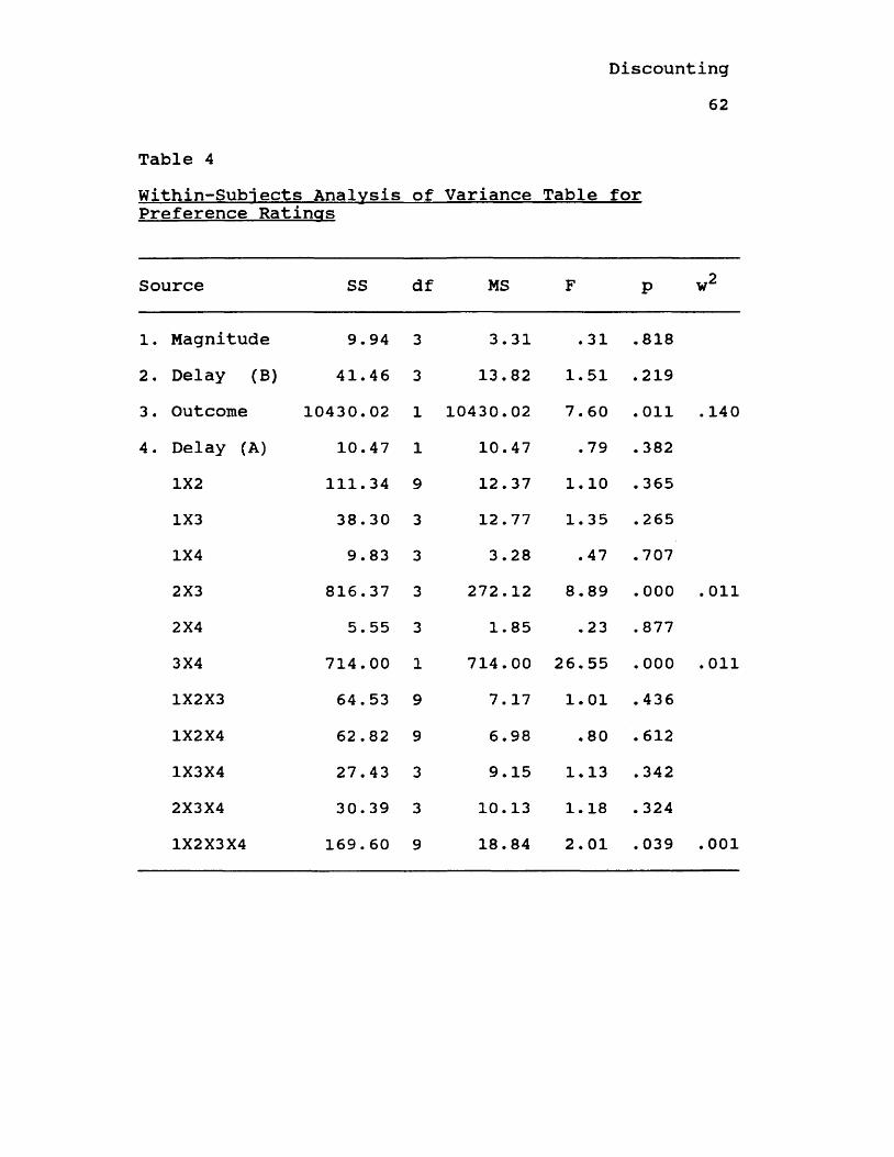
Additional Significant ResultsAs the analysis of variance results presented in

Table 4 reveal, there were some significant interactions that were not hypothesized. Effect sizes for each interaction were calculated assuming an additive model. Because none of the significant interactions accounted for more than 1.1% of the total variance, post hoc comparisons were not conducted.

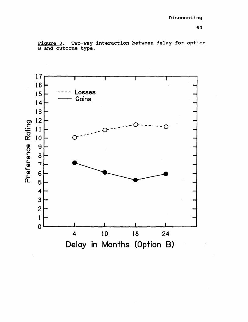
There was a significant two-way interaction between delay for option B and outcome which accounted for 1.1% of the total variance. For gains, analysis of ratings revealed a stronger preference for the smaller magnitude, immediate or advanced option with increasing delays. For losses, analysis showed a stronger preference for the larger magnitude, delayed option with increasing delays. This interaction is presented in Figure 3.

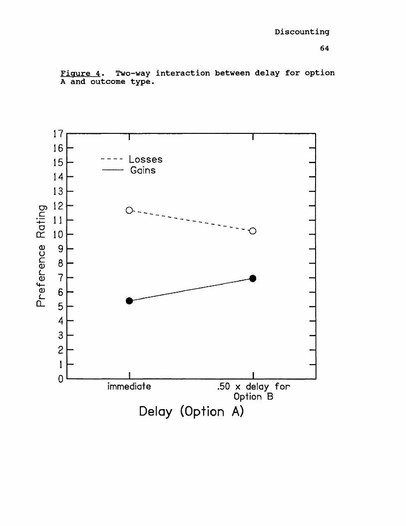
There was also a significant two-way interaction between delay for option A and outcome which accounted for 1.1% of the total variance. For gains, subjects showed a stronger preference for the smaller magnitude, advanced option when it was immediate (M=5.38) relative to when it was temporally removed (M=6.94). For losses, there was a stronger preference for the larger

Discounting

60

magnitude, delayed option when the smaller option was immediate (M=11.67) relative to when it was temporally removed (M=10.23). This interaction is presented in figure 4.

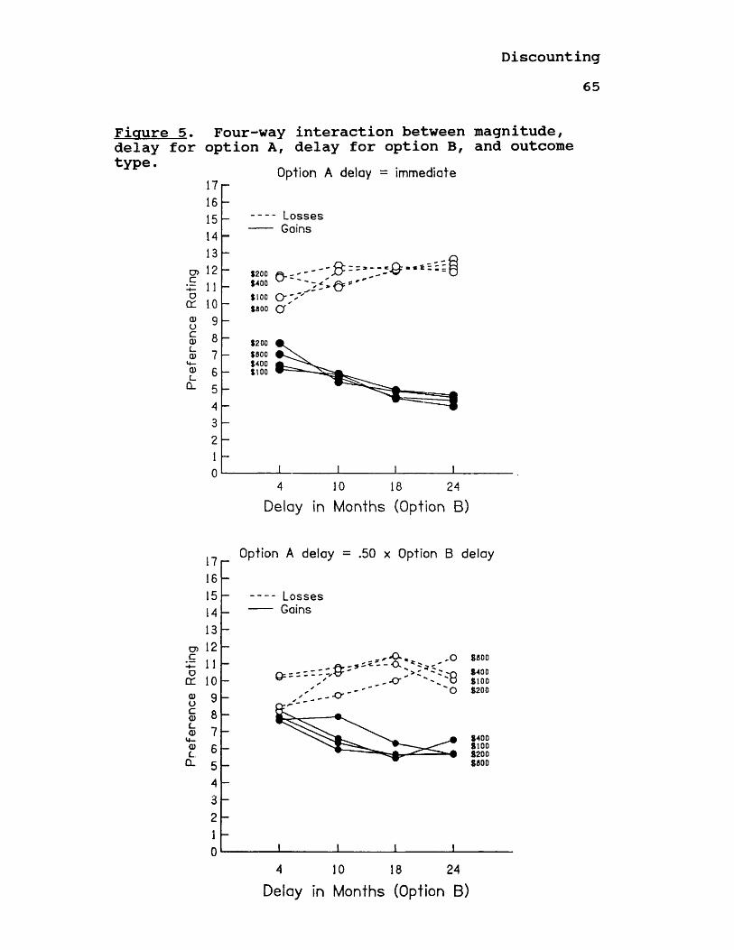
There was also a significant four-way interaction between magnitude, option B delay, outcome, and option A delay which accounted for 0.13% of the variance. Because of the large number of factors and levels involved (4 X 4 X 2 X 2), the interaction was impossible to interpret. This interaction is presented in figure 5.

DiscussionThe purpose of this study was to assess the

correspondence between cognitive and behavioral theories of choice as suggested by Rachlin, Logue, Gibbon, and Frankel (1986). The unique contribution of the study is that the prospect theory value function, which was derived from risky choice, was examined in a riskless context with temporal delays. The results of this thesis advance our understanding of prospect theory and choice under delay.

The results support the view that delay is associated with an implicit risk? that is, probability

Discounting61

corresponds to the inverse of delay. In general, subjects preferred immediate gains of smaller magnitude and delayed losses of larger magnitude. This finding is consistent with behavioral examinations of the matching law which show that animals prefer immediate

Discounting62

Table 4Within-Subi ects Analysis of Variance Table forPreference Ratinas

Source SS df MS F P w2

1. Magnitude 9.94 3 3.31 .31 .8182. Delay (B) 41.46 3 13.82 1.51 .2193. Outcome 10430.02 1 10430.02 7. 60 . 011 .1404. Delay (A) 10.47 1 10.47 .79 .382

1X2 111.34 9 12.37 1.10 .3651X3 38. 30 3 12.77 1. 35 .2651X4 9.83 3 3.28 .47 .7072X3 816.37 3 272.12 8.89 .000 .0112X4 5.55 3 1.85 .23 .8773X4 714.00 1 714.00 26.55 .000 .0111X2X3 64.53 9 7.17 1.01 .4361X2X4 62.82 9 6.98 .80 .6121X3X4 27.43 3 9.15 1.13 .3422X3X4 30.39 3 10.13 1.18 .3241X2X3X4 169.60 9 18.84 2.01 .039 .001

Pref

eren

ce

Ratin

gDiscounting

63

Figure 3. Two-way interaction between delay for option B and outcome type.

- - Losses — Gains

- " O ' O

O r ' "

3 -

4 10 18 24Delay in Months (Option B)

Pref

eren

ce

Rat

ing

Discounting

Figure 4. Two-way interaction between delay for option A and outcome type.

1716151413121 1109876543210

- - Losses -— Gains

immediate .50 x delay fo rOption B

Delay (Option A)

Discounting65

Figure 5. Four-way interaction between magnitude, delay for option A, delay for option B, and outcome type.

Option A delay = immediate

o>c-4—ocrQ)OcQ)C_Q)•+—Q)C_

CL

17 16 15 14 13 12 1 1 10 9 8 76b 5 4 3 2 1 0

LossesGains

*200 f % - ' *400 W '

* 1 0 0 O ' / "

*800 O '

*200*600*400*1 0 0

4 10 18 24Delay in Months (Option B)

1716151413

CD 12 £ 11 cr 10a)oc0)c_CD«4-a>L.Q.

9 8 7 6 5 43 h 2 1 0

Option A delay = .50 x Option B delay

- Losses- Gains

*600

*400 *1 0 0

' O *200

*400*1 0 0

% 8200 *600

4 10 18 24Delay in Months (Option B)

Discounting66

rewards and delayed punishments (see Rachlin et al., 1986). It is also consistent with cognitive examinations of prospect theory which show that people are risk averse with gains and risk seeking with losses (see Tversky & Kahneman, 1981).

The second hypothesis, that larger, delayed gains would be preferred if the advanced, smaller gain was temporally removed was not supported. Although numerous researchers (e.g., Ortendahl & Sjoberg, 1979; Stevenson, 1986) have reported that the psychophysical value of time is a negatively accelerating function of real time, the delay to the larger gain was obviously perceived as more aversive in this investigation even when the smaller gain was temporally removed.

This investigation was also the first to examine the correspondence of the prospect theory value function in a riskless context. No other study of choice with delayed outcomes, in either the cognitive or behavioral paradigms, has assessed outcome type (i.e., gains vs. losses) utilizing a within-subjects design. The prospect theory value function is concave for gains, convex for losses, and steeper for losses than for gains. The results of this study did not support a corresponding value function for choices

Discounting67

involving delayed outcomes. The findings of this study suggest that subjects' preferences for temporally advanced gains are stronger than their preferences for delayed losses. This is not consistent with a value function that is steeper in the domain of losses.

A fault of the present study is that there may have been an undetected carryover effect to the preference ratings given that all subjects completed binary choices a week prior to making ratings.Although a carryover effect is possible, subjects' binary choices (completed in the first session) were not congruent with the prospect theory value function. Thus, the value function from propsect theory is not consistent with the data even when there are no carryover effects. Nevertheless, any replication of the present study should include some form of counterbalancing for type of value elicitation (binary choice vs. preference ratings).The Limitations of Prospect Theory

The prospect theory value function was derived from risky choice but it did not fit with the riskless choices in this study even though the temporal dimension implied risk. This is consistent with the lack of support the value function has obtained from

Discounting68

within-subject examinations of risky choice (e.g., Hershey & Shoemaker, 1980). The present study and other methodologically sound examinations of prospect theory indicate that there is not a single value function that fits across all people and situational contexts. It is time that decision researchers moved away from a prospect theory analysis of choice and moved toward a person and situational analysis.

Schneider and Lopes (1986) provide a useful framework for a person and situation analysis of choice. They have found that propensity for risk taking is a good predictor of individual risky choice across gains and losses. Given the correspondence between probability and delay, it seems likely that this variable would influence choice with delayed outcomes as well.

Another potential individual difference variable that may predict choice in both risky contexts and riskless contexts involving delays is age (C. R. Millimet, personal communication, May, 1991). An older person may feel as if she or he cannot take risky gambles because there is not enough time to rebound should a loss occur. Similarly, an older person cannot

Discounting69

afford to make an investment that does not pay off for a long period of time.

There are many situational constraints that may influence both risky and riskless choices. A set of variables that is of interest to organizational researchers is personal and organizational goals. If an individual or organization aspired to maximize the gain from a prospect, it would make sense to be willing to take more risk or to wait a longer period of time for the outcome. The converse would be true if there was a stated goal to minimize losses.Overcoming Paradigmatic Limitations

A recent article by Baruch Fischoff (1991) highlights the false assumptions that can be made by strictly adhering to a single paradigmatic view of value elicitation. Fischoff places paradigms of value elicitation along a continuum from the philosophy of articulated values at one end to the philosophy of basic values at the other. The philosophy of articulated values holds that people have well-formed values and can provide researchers with reponses that accurately reflect these values. The philosophy of basic values holds that people have well-formed opinions on only a limited number of issues.

Discounting70

Fischoff (1991) notes that prospect theory operates from a partial perspective that is somewhere in-between articulated and basic values. Although a paradigm of value elicitation is useful in that it provides a framework for interpreting results, there is an inherent flaw in adhering to a single pardigmatic view. "...it is in the nature of paradigms that they provide clearer indications of relative rather than absolute success. That is, they show which applications of the set of accepted methods work better, rather than whether the set as a whole is up to the job" (Fischoff, 1991, p. 837).

With its partial perspectives of value elicitation, prospect theory straddles the center of the continuum of value elicitation paradigms. Prospect theory must be concerned with misunderstood questions that would prevent well articulated values from being expressed, but it must also be concerned with overinterpreting elicited responses from subjects who do not possess well-formed opinions (Fischoff, 1991).

The major problem with prospect theory is that it is a descriptive theory in search of a value function that is not robust. The question of how well a subject can articulate opinions about the value of goods is not

Discounting71

likely to be settled. However, research that addresses where values are well articulated would be very beneficial as well as informative (Fischoff, 1991). Conclusion

This investigation advances our knowledge in the understudied area of choices involving delays. It reveals that these types of choices are much too complex to be understood by a single value function. There is a tendency for subjects to prefer immediate gains and delayed losses, but this tendency seems to be stronger at lower magnitude levels and it is not consistent across all subjects. It would be fruitful to move from a perspective of modeling this tendency with value functions to understanding what factors affect individual's choices with delayed outcomes.

Discounting72

ReferencesAbelson, R. P., & Levi, A. (1985). Decision making and

decision theory. In G. Lindzey & E. Aronson (Eds.), The Handbook of Social Psychology (pp. 231-310).New York: Knopf.

Baum, W. M. (1974). On two types of deviation from the matching law: Bias and undermatching. Journal of the Experimental Analysis of Behavior. 22. 231-242.

Baum, W. M., & Rachlin, H. C. (1969). Choice as time allocation. Journal of the Experimental Anlvsis of Behavior. 12, 861-874.

Billings, R. S., & Scherer, L. L. (1988). The effects of response mode and importance on decision-making strategies: Judgment versus choice. Organizational Behavior and Human Decision Processes. 41. 1-19.

Catania, A. C. (1963). Concurrent performances:Reinforcement interaction and response independence. Journal of the Experimental Analysis of Behavior.6, 299-300.

Chung, S., & Herrnstein, R. J. (1967). Choice and delay of reinforcement. Journal of the Experimental Analysis of Behavior. 10. 67-74.

Discounting73

Cohen, M., Jaffray, J. Y., & Said, T. (1987).Experimental comparison of individual behavior under risk and under uncertainty for gains and for losses. Organizational Behavior and Human Decision Processes. 39. 1-22.

Deluty, M. Z., Whitehouse, W. G., Mellitz, M., &Hineline, P. N. (1983). Self-control and commitment involving aversive events. Behaviour Analysis Letters. 3, 213-219.

Elliott, C. S., & Archibald, R. B. (1989). Subjective framing and attitudes towards risk. Journal of Economic Psychology. 10. 321-328.

Fagley, N. S., & Miller, P. M. (1987). The effects of decision framing on choice of risky vs certain options. Organizational Behavior and Human Decision Processes. 39, 264-277.

Fischoff, B. (1991). Value elicitation: Is thereanything there? American Psychologist. 46. 835-847.

Friedman, M. & Savage, L. J. (1948). The utility analysis of choices inolving risk. Journal of Political Economy. 56, 279-304.

Discounting74

Hershey, J. C., & Shoemaker, P. J. H. (1980). Prospect theory's reflection hypothesis: A critical examination. Organizational Behavior and Human Performance. 25. 395-418.

Herrnstein, R. J. (1961). Relative and absolutestrength of response as a function of frequency of reinforcement. Journal of the Experimental Analysis of Behavior. A, 267-272.

Herrnstein, R. J. (1970). On the law of effect. Journal of the Experimental Analysis of Behavior. 13. 243- 266.

Herrnstein, R. J. (1990). Rational choice theory:Necessary but not sufficient. American Psychologist. 45, 356-367.

Hull, C. L. (1932). The goal gradient hypothesis and maze learning. Psychological Review. 39. 25-43.

Kahneman, D., & Snell, J. (1989). Predicting utility.In R. Hogarth (Ed.), Insights in decision making: A tribute to Hillel J. Einhorn (pp. 295-310). Chicago: University of Chicago Press.

Kahneman, D., & Tversky, A. (1979). Prospect theory: An analysis of decisions under risk. Econometrica. 47. 263-291.

Discounting75

Kahneman, D., & Tversky, A. (1984). Choices, value, and frames. American Psychologist. 39, 341-350.

Levin, I. P., Johnson, R. D., Deldin, P. J., Carstens, L. M., Cressey, L. J., & Davis, C. R. (1986).Framing effects in decisions with completely and incompletely described alternatives. Organizational Behavior and Human Decision Processes. 38, 48-64.

Levin, I. P., Johnson, R. D., Russo, C. P., & Deldin,P. J. (1985). Framing effects in judgment tasks with varying amounts of information. Organizational Behavior and Human Decision Processes. 37, 362-377.

Levin, I. P., Schnittjer, S. K., & Thee, S. T. (1988). Information framing effects in social and personal decisions. Journal of Experimental Social Psychology. 24. 520-529.

Mazur, J. E. (1985). Probability and delay ofreinforcement as factors in discrete-trial choice. Journal of the Experimental Analysis of Behavior.43, 341-351.

McDowell, J. J. (1981). On the validity and utility of Herrnstein's hyperbola in applied behavior analysis. In C. M. Bradshaw, E. Szabadi, & C. F. Lowe (Eds.), Quantification of steady state operant behavior. Amsterdam: Elsevier/North-Holland Biomedical Press.

Discounting76

Mischel , W. (1961a). Delay of gratification, need for achievement, and aquiesence in another culture. Journal of Abnormal and Social Psychology. 62, 543-552.

Mischel, W. (1961b). Father absence and delay ofgratification: Cross-cultural comparisons. Journal of Abnormal Social Psychology. 62, 116-124.

Mischel, W. (1961c). Preference for delayedreinforcement and social responsibility. Journal of Abnormal Social Psychology. 62, 1-7.

Mischel, W., & Grusec, J. (1967). Waiting for rewards and punishments: Effects of time and probability on choice. Journal of Personality and Social Psychology. 5, 24-31.

Mischel, W., Grusec, J., & Masters, J. C. (1969). Effects of expected delay time on the subjective value of rewards and punishments. Journal of Personality and Social Psychology. 11, 363-373.

Mischel, W., & Metzner, R. (1962). Preference fordelayed reward as a function of age, intelligence, and length of delay interval. Journal of Abnormal and Social Psychology. 64. 425-431.

Discounting77

Neale, M. A., Huber, V. L., & Northcraft, G. B. (1987). The framing of negotiations: Contextual versus task frames. Organizational Behavior and Human Decision Processes, 3.9, 228-241.

Neuringer, A. J. (1967). Effects of reinforcementmagnitude on choice and rate of responding. Journal of the Experimental Analysis of Behavior. 10, 417- 424.

Nevin, J. A. (19 69). Signal detection theory and operant behavior. [Review of Signal detection theory and psvchophvsicsl. Journal of the Experimental Analysis of Behavior. 12., 475-480.

Northcraft, G. B., & Neale, M. A. (1986). Opportunity costs and the framing of resource allocation decisions, organizational Behavior and Human Decision Processes. 37, 348-356.

Ortendahl, M., & Sjoberg, L. (1979). Delay ofoutcome and preference for different courses of action. Perceptual and Motor Skills. 48. 3-57.

Pierce, W. D., & Epling, W. F. (1983). Choice, matching, and human behavior: A review of the literature. The Behavior Analyst. 6, 57-76.

Discounting78

Rachlin, H., Castrogiovanni, A., & Cross, D. (1987). Probability and delay in commitment. Journal of the Experimental Analysis of Behavior. 48. 347-353.

Rachlin, H., & Green, L. (1972). Commitment, choice, and self-control. Journal of the Experimental Analysis of Behavior. 17, 15-22.

Rachlin, H., Logue, A. W., Gibbon, J., & Frankel, M.(1986). Cognition and behavior in studies of choice. Psychological Review. 93. 33-45.

Renner, K. E. (1964). Delay of reinforcement: Ahistorical review. Psychological Bulletin. 61. 341- 361.

Reynolds, G. S. (1963). On some determinants of choice in pigeons. Journal of the Experimental Analysis of Behavior. 6, 53-59.

Rotter, J. B. (1954). Social learning and clinical psychology. Englewood Cliffs, NJ: Prentice-Hall.

Schneider, S. L., & Lopes, L. L. (1986). Reflection in preferences under risk: Who and when may suggest why. Journal of Experimental Psychology: Human Perception and Performance. 12, 535-548.

Schurr, P. H. (1987). Effect of gain and loss decision frames on risky purchase negotiations. Journal of Apllied Psychology. 72, 351-358.

Discounting79

Silberberg, A., Murray, P., Christensen, J., & Asano,T. (1988). Choice in the repeated-gambles experiment. Journal of the Experimental Analysis of Behavior. 50, 187-195.

Slovic, P., & Lichtenstein, S. (1971). Comparison ofBayesian and regression approaches to the study of

information processing in judgment.Organizational Behavior and HumanPerformance. 6, 649-744.Spence, K. W. (1947). The role of secondary

reinforcement in delayed reward learning. Psychological Review. 54, 1-8.

Stevenson, M. K. (1986). A discounting model for decisions with delayed positive or negative outcomes. Journal of Experimental Psychology:General. 115. 131-154.

Tversky, A., & Kahneman, D. (1981, January). Theframing of decisions and the psychology of choice.

Science. pp. 453-458.Wilson, D. K., Kaplan,, R. M., & Schneiderman, L. J.

(1987). Framing of decisions and selections of alternatives in health care. Social Behavior. 2, 51-59.

Discounting80

Yates, J. F. , & Watts, R. A. (1975). Preferences for delayed losses. Organizational Behavior and Human Performance. 13, 294-306.

Discounting81

Footnotes1. To analyze this hypothesis, the data were recoded such that a rating of 1 in the domain of gains indicated a strong preference for the immediate or advanced option, and a rating of 1 in the domain of losses indicated a strong preference for the delayed option.

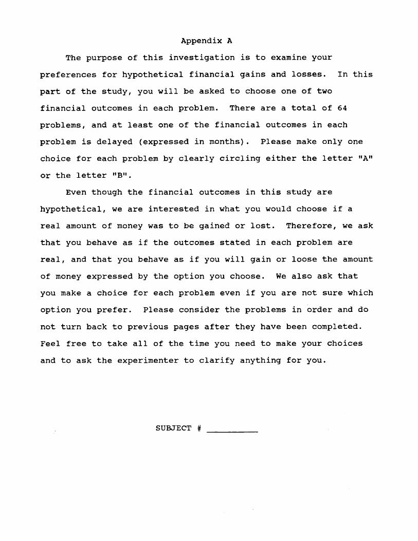
Appendix AThe purpose of this investigation is to examine your

preferences for hypothetical financial gains and losses. In this part of the study, you will be asked to choose one of two financial outcomes in each problem. There are a total of 64 problems, and at least one of the financial outcomes in each problem is delayed (expressed in months). Please make only one choice for each problem by clearly circling either the letter "A" or the letter MB".

Even though the financial outcomes in this study are hypothetical, we are interested in what you would choose if a real amount of money was to be gained or lost. Therefore, we ask that you behave as if the outcomes stated in each problem are real, and that you behave as if you will gain or loose the amount of money expressed by the option you choose. We also ask that you make a choice for each problem even if you are not sure which option you prefer. Please consider the problems in order and do not turn back to previous pages after they have been completed. Feel free to take all of the time you need to make your choices and to ask the experimenter to clarify anything for you.

SUBJECT #

The following is an example of a problem you might see wherethe choice is between two financial losses:

Option A Option BLose $500 in 8 months Lose $425 immediately

I prefer to lose (circle one): A BIn this sample problem you would be choosing between an immediate loss of $425 or a loss of $500 in eight months. If it helps, you might think of problems that involve losses as credit plan options for the payment of debts.

Here is a problem you might see where the choice is between two financial gains:

Option A Option BGain $425 in 3 months Gain $500 in 6 months

I prefer to gain (circle one): A BIn this sample problem you would be choosing between a gain of $425 in three months or a larger gain of $500 in six months. It may help to think of problems that involve gains as options in returns on an investment.

Please be sure that you know whether you are choosing between gains or losses for each problem and how many months it will take to gain or lose the money — This is VERY important!

Your participation in this study is greatly appreciated!

Option A Option BGain $100 in 4 months Gain $75 immediately

I prefer to gain (circle one): A B

Option A Option BGain $400 in 24 months Gain $300 in 12 months

I prefer to gain (circle one): A B

Option A Option BLose $600 in 5 months Lose $800 in 10 months

I prefer to lose (circle one): A B

Option A Option BLose $2 00 in 18 months Lose $150 immediately

I prefer to lose (circle one): A B

Option A Option BLose $300 in 2 months Lose $400 in 4 months

I prefer to lose (circle one): A B

Option A Option BGain $150 in 5 months Gain $200 in 10 months

I prefer to gain (circle one): A B

Option A Option BLose $7 5 immediately Lose $100 in 24 months

I prefer to lose (circle one): A B

Option A Option BGain $800 in 18 months Gain $600 immediately

I prefer to gain (circle one): A B

9. Option A Option BGain $300 in 5 months Gain $400 in 10 months

I prefer to gain (circle one): A B

10.

11.

12.

Option A Option BLose $2 00 in 24 months Lose $150 in 12 months

I prefer to lose (circle one): A B

Option A Option BGain $75 immediately Gain $100 in 10 months

I prefer to gain (circle one): A B

Option A Option BGain $800 in 24 months Gain $600 in 12 months

I prefer to gain (circle one): A B

13. Option A Option BLose $75 immediately Lose $100 in 18 months

I prefer to lose (circle one): A B

14.

15.

16.

Option A Option BGain $150 immediately Gain $200 in 4 months

I prefer to gain (circle one): A B

Option A Option BLose $8 00 in 4 months Lose $600 immediately

I prefer to lose (circle one): A B

Option A Option BLose $4 00 in 18 months Lose $300 immediately

I prefer to lose (circle one): A B

17.

18.

19.

Option A Option BLose $150 in 9 months Lose $200 in 18 months

I prefer to lose (circle one): A B

Option A Option BGain $300 immediately Gain $400 in 24 months

I prefer to gain (circle one): A B

Option A Option BLose $800 in 10 months Lose $600 immediately

I prefer to lose (circle one): A B

20. Option A Option BGain $75 in 2 months Gain $100 in 4 months

I prefer to gain (circle one): A B

21. Option A Option BGain $600 in 9 months Gain $800 in 18 months

I prefer to gain (circle one): A B

2 2.

23.

24.

Option A Option BLose $100 in 24 months Lose $75 in 12 months

I prefer to lose (circle one): A B

Option A Option BGain $2 00 in 10 months Gain $150 immediately

I prefer to gain (circle one): A B

Option A Option BLose $4 00 in 4 months Lose $3 00 immediately

I prefer to lose (circle one): A B

25.

26.

27.

Option A Option BGain $600 immediately Gain $800 in 24 months

I prefer to gain (circle one): A B

Option A Option BGain $100 in 10 months Gain $75 in 5 months

I prefer to gain (circle one): A B

Option A Option BLose $150 immediately Lose $200 in 24 months

I prefer to lose (circle one)s A B

28. Option A Option BGain $400 in 10 months Gain $300 immediately

I prefer to gain (circle one): A B

29. Option A Option BLose $2 00 in 4 months Lose $150 in 2 months

I prefer to lose (circle one): A B

30.

31.

32 .

Option A Option BLose $600 in 2 months Lose $800 in 4 months

I prefer to lose (circle one): A B

Option A Option BGain $200 in 4 months Gain $150 in 2 months

I prefer to gain (circle one)s A B

Option A Option BLose $100 in 18 months Lose $75 in 9 months

I prefer to lose (circle one): A B

33. Option A Option BGain $4 00 in 4 months Gain $3 00 immediately

I prefer to gain (circle one): A B

34.

35.

Option A Option BLose $600 in 12 months Lose $800 in 24 months

I prefer to lose (circle one): A B

Option A Option BLose $150 immediately Lose $200 in 10 months

I prefer to lose (circle one): A B

36. Option A Option BGain $7 5 in 9 months Gain $100 in 18 months

I prefer to gain (circle one): A B

37. Option A Option BGain $800 in 4 months Gain $600 in 2 months

I prefer to gain (circle one): A B

38.

39.

40.

Option A Option BLose $75 immediately Lose $100 in 10 months

I prefer to lose (circle one): A B

Option A Option BLose $4 00 in 2 4 months Lose $3 00 in 12 months

I prefer to lose (circle one): A B

Option A Option BGain $200 in 18 months Gain $150 in 9 months

I prefer to gain (circle one): A B

41. Option A Option BGain $600 immediately Gain $800 in 10 months

I prefer to gain (circle one): A B

42.

43.

44.

Option A Option BLose $100 in 4 months Lose $75 immediately

I prefer to lose (circle one): A B

Option A Option BGain $150 in 12 months Gain $200 in 24 months

I prefer to gain (circle one)s A B

Option A Option BLose $800 in 18 months Lose $600 in 9 months

I prefer to lose (circle one): A B

45.

46.

47.

Option A Option BGain $75 in 12 months Gain $100 in

I prefer to gain (circle one): A

Option A Option BLose $300 immediately Lose $400 in

I prefer to lose (circle one): A

Option A Option BGain $400 in 18 months Gain $300 in

I prefer to gain (circle one): A

24 months B

10 months B

9 months B

48. Option A Option BLose $3 00 in 9 months Lose $400 in 18 months

I prefer to lose (circle one): A B

49. Option A Option BGain $100 in 18 months Gain $75 immediately

I prefer to gain (circle one): A B

50.

51.

52.

Option A Option BLose $2 00 in 10 months Lose $150 in 5 months

I prefer to lose (circle one): A B

Option A Option BLose $800 in 24 months Lose $600 immediately

I prefer to lose (circle one): A B

Option A Option BLose $150 immediately Lose $200 in 4 months

I prefer to lose (circle one): A B

53.

54.

55.

Option A Option BLose $300 immediately Lose $400 in 24 months

I prefer to lose (circle one): A B

Option A Option BGain $200 in 18 months Gain $150 immediately

I prefer to gain (circle one): A B

Option A Option BLose $100 in 10 months Lose $7 5 in 5 months

I prefer to lose (circle one): A B

56. Option A Option BGain $600 immediately Gain $800 in 4 months

I prefer to gain (circle one): A B

57.

58.

59.

Option A Option BLose $400 in 10 months Lose $300 in 5 months

I prefer to lose (circle one): A B

Option A Option BGain $200 in 24 months Gain $150 immediately

I prefer to gain (circle one): A B

Option A Option BLose $75 in 2 months Lose $100 in 4 months

I prefer to lose (circle one): A B

60. Option A Option BGain $800 in 10 months Gain $600 in 5 months

I prefer to gain (circle one): A B

61. Option A Option BGain $400 in 18 months Gain $300 immediately

I prefer to gain (circle one): A B

62.

63.

64.

Option A Option BGain $300 in 2 months Gain $400 in 4 months

I prefer to gain (circle one): A B

Option A Option BLose $800 in 18 months Lose $600 immediately

I prefer to lose (circle one): A B

Option A Option BGain $75 immediately Gain $100 in 24 months

I prefer to gain (circle one): A B

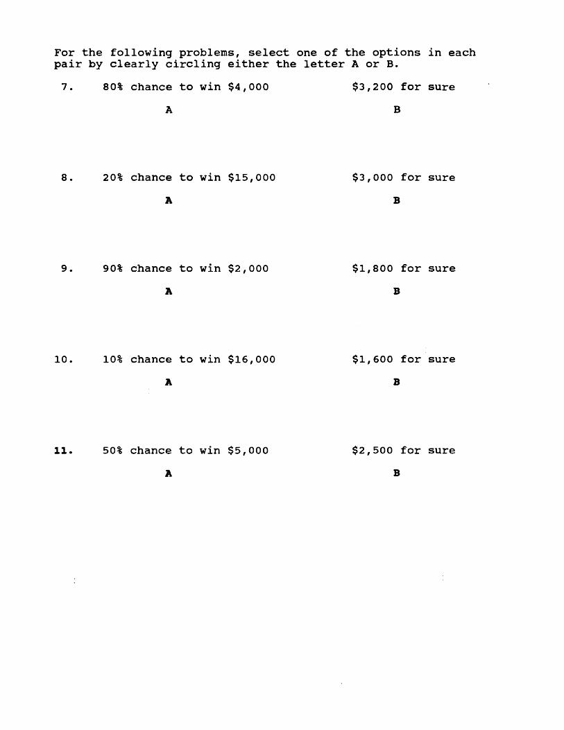
For the following problems, select one of the options in each pair by clearly circling either the letter A or B.7. 80% chance to win $4,000 $3,200 for sure

A B

8. 20% chance to win $15,000 $3,000 for sureA B

9. 90% chance to win $2,000 $1,800 for sureA B

10. 10% chance to win $16,000 $1,600 for sureA B

11. 50% chance to win $5,000 $2,500 for sure

Final QuestionsMale _____ Female _____Age _____Do you have any knowledge of discounting in accounting or finance? (If yes, please elaborate.)

Please explain any rules or strategies you used in choosing between gains in this study.

Please explain any rules or strategies you used in choosing between losses in this study.

Please explain any rules or strategies you used in choosing between different delays.