imc-pid controller design for improved disturbance rejection of time-delayed processes
TRANSCRIPT
IMC -PID Controller Design for Improved Disturbance Rejection ofTime-Delayed Processes
M. Shamsuzzoha and Moonyong Lee*
School of Chemical Engineering and Technology, Yeungnam UniVersity, Kyongsan 712-749, Korea
The IMC-PID tuning rules demonstrate good set-point tracking but sluggish disturbance rejection, whichbecomes severe when a process has a small time-delay/time-constant ratio. In this study, an optimal internalmodel control (IMC) filter structure is proposed for several representative process models to design aproportional-integral-derivative (PID) controller that produces an improved disturbance rejection response.The simulation studies of several process models show that the proposed design method provides betterdisturbance rejection for lag-time dominant processes, when the various controllers are all tuned to have thesame degree of robustness according to the measure of maximum sensitivity. The robustness analysis isconducted by inserting a perturbation in each of the process parameters simultaneously, with the resultsdemonstrating the robustness of the proposed controller design with parameter uncertainty. A closed-looptime constantλ guideline is also proposed for several process models to cover a wide range ofθ/τ ratios.
1. Introduction
The proportional-integral-derivative (PID) control algorithmis widely used in process industries because of its simplicity,robustness, and successful practical application. Althoughadvanced control techniques can provide significant improve-ments, a well-designed PID controller has proved to besatisfactory for a large number of industrial control loops. Thewell-known internal model control-PID (IMC-PID) tuningrules have the advantage of only using a single tuning parameterto achieve a clear tradeoff between closed-loop performanceand robustness to model inaccuracies. The IMC-PID controllerprovides good set-point tracking but has a sluggish disturbanceresponse, especially for the process with a small time-delay/time-constant ratio.1-9 However, because disturbance rejectionis much more important than set-point tracking for many processcontrol applications, a controller design that emphasizes dis-turbance rejection rather than set-point tracking is an importantdesign problem that has been the focus of renewed researchrecently.
The IMC-PID tuning methods by Rivera et al.,1 Morari andZafiriou,6 Horn et al.,3 Lee et al.,4 and Lee et al.9 and the directsynthesis methods by Smith et al.10 (DS) and Chen and Seborg5
(DS-d) are examples of two typical tuning methods based onachieving a desired closed-loop response. These methods obtainthe PID controller parameters by computing the controller thatgives the desired closed-loop response. Although this controlleris often more complicated than a PID controller, the controllerform can be reduced to that of either a PID controller or a PIDcontroller cascaded with a first- or second-order lag by someclever approximations of the dead time in the process model.
Several workers (Morari and Zafiriou,6 Lee et al.,4 Lee etal.,9 Chien and Fruehauf,2 Horn et al.,3 Chen and Seborg,5 andSkogestad8) have reported that the suppressing load disturbanceis poor when the process dynamics are significantly slower thanthe desired closed-loop dynamics.
In fact, regarding the disturbance rejection for lag-timedominant processes, the well-known old design method byZiegler and Nichols11 (ZN) shows better performance than the
IMC-PID design methods based on the IMC filterf ) 1/(λs +1)r. Horn et al.3 proposed a new type of IMC filter whichincludes a lead term to cancel out the process dominant poles.On the basis of this filter, they developed an IMC-PID tuningrule that leads to the structure of a PID controller with a second-order lead-lag filter. The performance of the resulting controllershowed a clear advantage over those based on the conventionalIMC filter. Chen and Seborg5 proposed a direct synthesis designmethod to improve disturbance rejection for several popularprocess models. To avoid excessive overshoot in the set-pointresponse, they utilized a set-point weighting factor. In order toimprove the set-point performance by including a set-point filter,Lee et al.4 proposed an IMC-PID controller based on both thefilter suggested by Horn et al.3 and a two-degree-of-freedom(2DOF) control structure. Lee et al.9 extended the tuning methodto unstable processes such as first- and second-order delayedunstable process (FODUP and SODUP) models and for the set-point performance 2DOF control structure proposed. Skogestad8
* Corresponding author. Tel.:+82-053-810-2512. Fax:+82-053-811-3262. E-mail: [email protected].
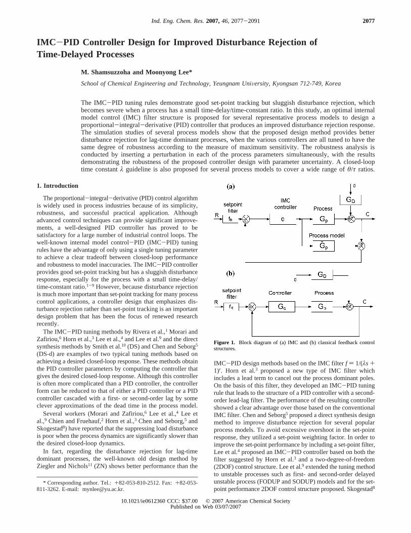
Figure 1. Block diagram of (a) IMC and (b) classical feedback controlstructures.
2077Ind. Eng. Chem. Res.2007,46, 2077-2091
10.1021/ie0612360 CCC: $37.00 © 2007 American Chemical SocietyPublished on Web 03/07/2007
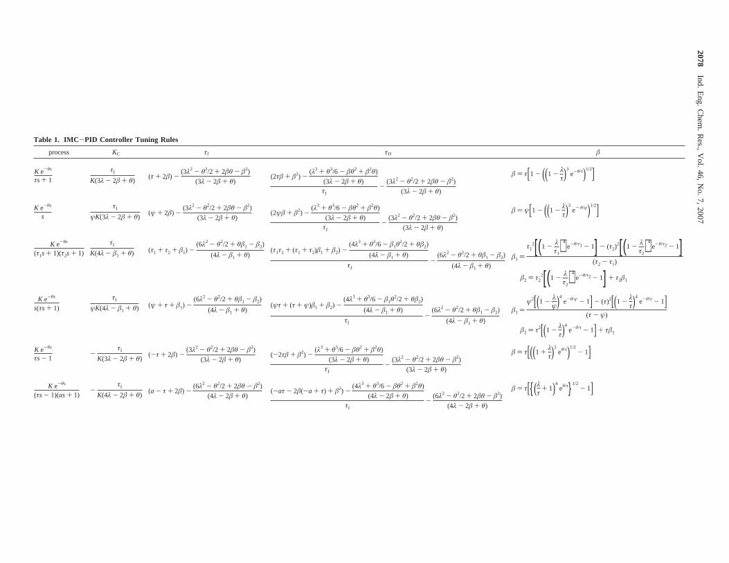
Table 1. IMC-PID Controller Tuning Rules
process KC τI τD â
K e-θs
τs + 1
τI
K(3λ - 2â + θ)(τ + 2â) -
(3λ2 - θ2/2 + 2âθ - â2)
(3λ - 2â + θ)(2τâ + â2) -
(λ3 + θ3/6 - âθ2 + â2θ)
(3λ - 2â + θ)τI
-(3λ2 - θ2/2 + 2âθ - â2)
(3λ - 2â + θ)
â ) τ[1 - ((1 - λτ)
3e-θ/τ)1/2]
K e-θs
s
τI
ψK(3λ - 2â + θ)(ψ + 2â) -
(3λ2 - θ2/2 + 2âθ - â2)
(3λ - 2â + θ)(2ψâ + â2) -
(λ3 + θ3/6 - âθ2 + â2θ)
(3λ - 2â + θ)τI
-(3λ2 - θ2/2 + 2âθ - â2)
(3λ - 2â + θ)
â ) ψ[1 - ((1 - λτ)
3e- θ/ψ)1/2]
K e-θs
(τ1s + 1)(τ2s + 1)
τI
K(4λ - â1 + θ) (τ1 + τ2 + â1) -(6λ2 - θ2/2 + θâ1 - â2)
(4λ - â1 + θ)(τ1τ2 + (τ1 + τ2)â1 + â2) -
(4λ3 + θ3/6 - â1θ2/2 + θâ2)
(4λ - â1 + θ)
τI-
(6λ2 - θ2/2 + θâ1 - â2)
(4λ - â1 + θ)â1 )
τ12[(1 - λ
τ1)4
e-θ/τ1 - 1] - (τ2)2[(1 - λ
τ2)4
e-θ/τ2 - 1](τ2 - τ1)
â2 ) τ22[(1 - λ
τ2)4
e-θ/τ2 - 1] + τ2â1
K e-θs
s(τs + 1)
τI
ψK(4λ - â1 + θ) (ψ + τ + â1) -(6λ2 - θ2/2 + θâ1 - â2)
(4λ - â1 + θ)(ψτ + (τ + ψ)â1 + â2) -
(4λ3 + θ3/6 - â1θ2/2 + θâ2)
(4λ - â1 + θ)
τI-
(6λ2 - θ2/2 + θâ1 - â2)
(4λ - â1 + θ)
â1 )ψ2[(1 - λ
ψ)4e-θ/ψ - 1] - (τ)2[(1 - λ
τ)4
e-θ/τ - 1](τ - ψ)
â2 ) τ2[(1 - λτ)
4e-θ/τ - 1] + τâ1
K e-θs
τs - 1-
τI
K(3λ - 2â + θ)(-τ + 2â) -
(3λ2 - θ2/2 + 2âθ - â2)
(3λ - 2â + θ)(-2τâ + â2) -
(λ3 + θ3/6 - âθ2 + â2θ)
(3λ - 2â + θ)τI
-(3λ2 - θ2/2 + 2âθ - â2)
(3λ - 2â + θ)
â ) τ[((1 + λτ)
3eθ/τ)1/2
- 1]
K e-θs
(τs - 1)(as+ 1)-
τI
K(4λ - 2â + θ)(a - τ + 2â) -
(6λ2 - θ2/2 + 2âθ - â2)
(4λ - 2â + θ)(-aτ - 2â(-a + τ) + â2) -
(4λ3 + θ3/6 - âθ2 + â2θ)
(4λ - 2â + θ)τI
-(6λ2 - θ2/2 + 2âθ - â2)
(4λ - 2â + θ)
â ) τ[{(λτ
+ 1)4eθ/τ}1/2
- 1]
2078Ind.
Eng.
Chem
.R
es.,V
ol.46,
No.
7,2007
proposed a model reduction technique to reduce the higher-order process model to a lower-order model and also developedthe SIMC-PID rule for improved disturbance rejection inseveral lag-time dominant processes.
It is clear that, in the IMC-PID approach, the performanceof the PID controller is mainly determined by the IMC filterstructure. In most previous works of IMC-PID design, the IMCfilter structure has been designed to be just as simple as to satisfya necessary performance of the IMC controller. For example,the order of the lead term in the IMC filter is designed to besmall enough to cancel out the dominant process poles, and thelag term is simply set to make the IMC controller proper.However, the performance of the resulting PID controller isbased not only on the IMC controller performance but also onhow closely the PID controller approximates the ideal controllerequivalent to the IMC controller, which mainly depends on thestructure of the IMC filter. Therefore, for the IMC-PID design,the optimum IMC filter structure has to be selected considering
the performance of the resulting PID controller rather than thatof the IMC controller.
In the present study, we have the following objectives:(1) Determine the optimum IMC filter, which gives the best
performance of the resulting PID controller (according toSkogestad,8 “best” could, for example, mean it minimizes theintegrated absolute error (IAE) with a specified value of thesensitivity peak, Ms) for several representative process models.This filter is used to design a PID controller for disturbancerejection and the corresponding analytical IMC-PID tuning rule.
(2) Provide the guidelines for selection of a closed-loop timeconstantλ for several process models to cover a wide range ofθ/τ.
(3) Conduct a robust study by inserting a perturbationuncertainty in each parameter simultaneously (for the worst-case model). Several illustrative examples are included todemonstrate the superiority of the proposed tuning methods.
2. IMC -PID Approach for PID Controller Design
Figure 1a shows the block diagrams of IMC control, whereGP is the process,GP is the process model, andq is the IMC
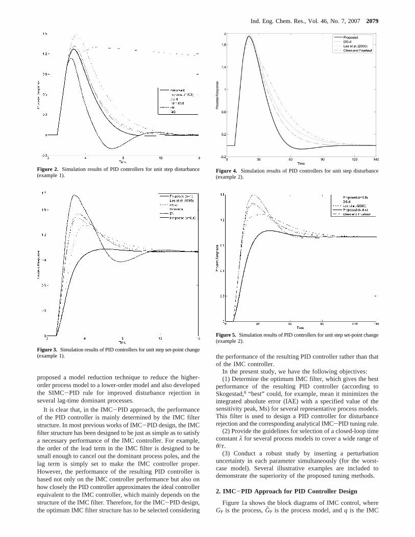
Figure 2. Simulation results of PID controllers for unit step disturbance(example 1).
Figure 3. Simulation results of PID controllers for unit step set-point change(example 1).
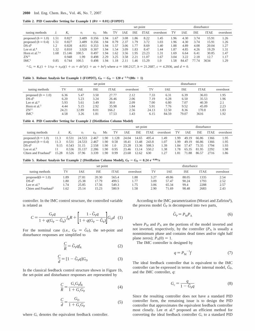
Figure 4. Simulation results of PID controllers for unit step disturbance(example 2).
Figure 5. Simulation results of PID controllers for unit step set-point change(example 2).
Ind. Eng. Chem. Res., Vol. 46, No. 7, 20072079
controller. In the IMC control structure, the controlled variableis related as
For the nominal case (i.e., GP ) GP), the set-point anddisturbance responses are simplified to
In the classical feedback control structure shown in Figure 1b,the set-point and disturbance responses are represented by
whereGc denotes the equivalent feedback controller.
According to the IMC parametrization (Morari and Zafiriou6),the process modelGP is decomposed into two parts,
wherePM and PA are the portions of the model inverted andnot inverted, respectively, by the controller (PA is usually anonminimum phase and contains dead times and/or right halfplane zeros);PA(0) ) 1.
The IMC controller is designed by
The ideal feedback controller that is equivalent to the IMCcontroller can be expressed in terms of the internal model,GP,and the IMC controller,q:
Since the resulting controller does not have a standard PIDcontroller form, the remaining issue is to design the PIDcontroller that approximates the equivalent feedback controllermost closely. Lee et al.4 proposed an efficient method forconverting the ideal feedback controllerGc to a standard PID
Table 2. PID Controller Setting for Example 1 (θ/τ ) 0.01) (FOPDT)
set point disturbance
tuning methods λ Kc τI τD Ms TV IAE ISE ITAE overshoot TV IAE ISE ITAE overshoot
proposed (b ) 1.0) 1.51 0.827 3.489 0.356 1.94 1.67 3.08 1.86 8.22 1.45 1.96 4.30 3.74 15.91 1.26proposed (b ) 0.4) 1.51 0.827 3.489 0.356 1.94 0.79 2.37 1.79 3.72 1.03 1.96 4.30 3.74 15.91 1.26DS-d5 1.2 0.828 4.051 0.353 1.94 1.57 3.06 1.77 8.69 1.40 1.88 4.89 4.08 20.04 1.27Lee et al.4 1.32 0.810 3.928 0.307 1.94 1.54 3.09 1.83 8.47 1.44 1.87 4.85 4.26 19.29 1.31Horn et al.3 a 1.68 15.146 100.5 0.497 1.94 1.62 3.56 1.95 23.23 1.31 1.69 6.64 6.41 30.85 1.47ZN11 0.948 1.99 0.498 2.29 3.25 3.58 2.21 11.07 1.67 3.04 3.22 2.18 12.7 1.17IMC1 0.85 0.744 100.5 0.498 1.94 1.18 2.11 1.46 15.29 1.0 1.58 84.47 77.74 3634 1.29
a Gc ) Kc(1 + 1/τIs + τDs)(1 + cs + ds2)/(1 + as + bs2) wherea ) 100.2127,b ) 21.2687,c ) 4.2936, andd ) 0.
Table 3. Robust Analysis for Example 1 (FOPDT),GP ) GD ) 120 e-1.2s/(80s + 1)
set point disturbance
tuning methods TV IAE ISE ITAE overshoot TV IAE ISE ITAE overshoot
proposed (b ) 1.0) 6.36 5.47 3.50 27.77 2.12 7.33 6.31 6.39 36.03 1.95DS-d5 6.20 5.23 3.24 26.46 2.06 7.19 6.28 6.50 35.53 1.96Lee et al.4 5.93 5.61 3.49 30.0 2.09 7.00 6.80 7.07 40.39 2.1Horn et al.3 4.44 5.15 2.92 35.98 1.84 5.91 7.76 9.52 45.09 2.23ZN11 24.21 12.89 8.01 166.2 2.56 24.13 12.50 8.36 170.8 1.83IMC1 4.58 3.26 1.81 17.53 1.43 6.15 84.59 79.07 3616 1.92
Table 4. PID Controller Setting for Example 2 (Distillation Column Model)
set point disturbance
tuning methods λ Kc τI τD Ms TV IAE ISE ITAE overshoot TV IAE ISE ITAE overshoot
proposed (b ) 1.0) 11.3 0.531 24.533 2.467 1.90 1.128 24.04 14.65 495.4 1.49 1.99 49.19 66.86 1366 1.95proposed (b ) 0.4) 11.3 0.531 24.533 2.467 1.90 0.58 18.41 13.48 243.8 1.07 1.99 49.19 66.86 1366 1.95DS-d5 9.15 0.543 31.15 2.558 1.90 1.0 23.28 13.36 508.3 1.39 1.84 57.47 73.35 1794 1.93Lee et al.9 11 0.536 35.137 2.286 1.90 0.95 23.46 13.14 550.2 1.38 1.78 65.35 81.95 2292 1.98Chien and Fruehauf2 15.28 0.526 37.96 3.339 1.90 0.99 23.68 12.62 630 1.27 1.81 71.88 86.57 2716 1.86
Table 5. Robust Analysis for Example 2 (Distillation Column Model),GP ) GD ) 0.24 e-8.88s/s
set point disturbance
tuning methods TV IAE ISE ITAE overshoot TV IAE ISE ITAE overshoot
proposed(b ) 1.0) 1.89 27.81 20.30 565.4 1.88 3.27 49.86 88.05 1335 2.54DS-d5 1.80 25.38 17.79 499.5 1.77 3.09 57.47 90.24 1793 2.52Lee et al.9 1.74 25.85 17.56 549.3 1.75 3.06 65.34 99.4 2288 2.57Chien and Fruehauf2 1.62 25.14 15.23 580.9 1.58 2.90 71.69 98.48 2683 2.43
C )GPq
1 + q(GP - GP)fRR + [ 1 - GPq
1 + q(GP - GP)]GDd (1)
CR
) GPqfR (2)
Cd
) [1 - GPq]GD (3)
CR
)GcGPfR
1 + GcGP(4)
Cd
)GD
1 + GcGP(5)
GP) PMPA (6)
q ) PM-1f (7)
Gc ) q1 - GPq
(8)
2080 Ind. Eng. Chem. Res., Vol. 46, No. 7, 2007
controller. SinceGc has an integral term, it can be expressed as
ExpandingGc in Maclaurin series ins gives
The first three terms of the above expansion can be interpretedas the standard PID controller, which is given by
where
3. IMC -PID Tuning Rules for Typical Process Models
This section proposes the tuning rules for several typical time-delayed process models.
3.1. First-Order Plus Dead Time Process (FOPDT).Themost commonly used approximate model for chemical processesis the FOPDT model as given below,
whereK is the gain,τ is the time constant, andθ is the timedelay. The optimum IMC filter structure is found asf ) (âs +1)2/(λs + 1)3. The resulting IMC controller becomesq ) (τs +1)(âs+ 1)2/K(λs+ 1)3. Therefore, the ideal feedback controller,which is equivalent to the IMC controller, is
The analytical PID formula can be obtained from eq 12 as
The value of the extra degree of freedomâ is selected so thatit cancels out the open-loop pole ats ) -1/τ that causes thesluggish response to the load disturbance. Thus,â is chosen sothat the term [1- Gq] has a zero at the pole ofGD. That is, wewant [1 - Gq]|s)-1/τ ) 0 and [1 - (âs + 1)2 e-θs/(λs +
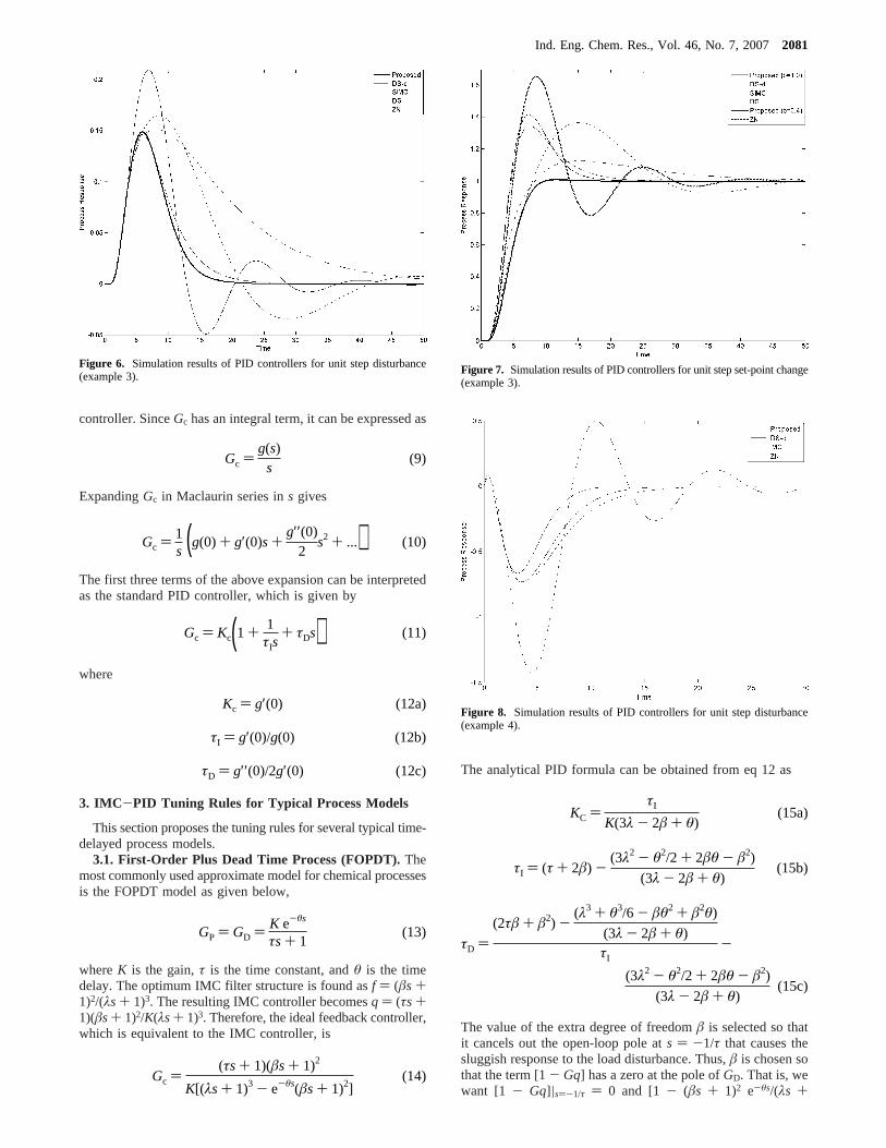
Figure 6. Simulation results of PID controllers for unit step disturbance(example 3).
Gc )g(s)
s(9)
Gc ) 1s (g(0) + g′(0)s +
g′′(0)2
s2 + ...) (10)
Gc ) Kc(1 + 1τIs
+ τDs) (11)
Kc ) g′(0) (12a)
τI ) g′(0)/g(0) (12b)
τD ) g′′(0)/2g′(0) (12c)
GP ) GD ) K e-θs
τs + 1(13)
Gc )(τs + 1)(âs + 1)2
K[(λs + 1)3 - e-θs(âs + 1)2](14)
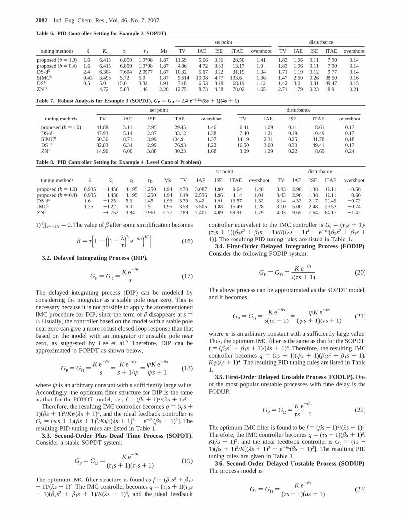
Figure 7. Simulation results of PID controllers for unit step set-point change(example 3).
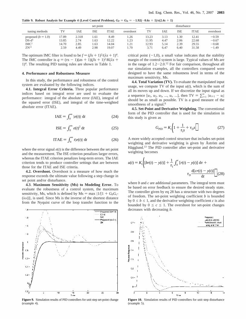
Figure 8. Simulation results of PID controllers for unit step disturbance(example 4).
KC )τI
K(3λ - 2â + θ)(15a)
τI ) (τ + 2â) -(3λ2 - θ2/2 + 2âθ - â2)
(3λ - 2â + θ)(15b)
τD )(2τâ + â2) -
(λ3 + θ3/6 - âθ2 + â2θ)
(3λ - 2â + θ)τI
-
(3λ2 - θ2/2 + 2âθ - â2)
(3λ - 2â + θ)(15c)
Ind. Eng. Chem. Res., Vol. 46, No. 7, 20072081
1)3]|s)-1/τ ) 0. The value ofâ after some simplification becomes
3.2. Delayed Integrating Process (DIP).
The delayed integrating process (DIP) can be modeled byconsidering the integrator as a stable pole near zero. This isnecessary because it is not possible to apply the aforementionedIMC procedure for DIP, since the term ofâ disappears ats )0. Usually, the controller based on the model with a stable polenear zero can give a more robust closed-loop response than thatbased on the model with an integrator or unstable pole nearzero, as suggested by Lee et al.9 Therefore, DIP can beapproximated to FOPDT as shown below,
whereψ is an arbitrary constant with a sufficiently large value.Accordingly, the optimum filter structure for DIP is the sameas that for the FOPDT model, i.e.,f ) (âs + 1)2/(λs + 1)3.
Therefore, the resulting IMC controller becomesq ) (ψs +1)(âs + 1)2/Kψ(λs + 1)3, and the ideal feedback controller isGc ) (ψs + 1)(âs + 1)2/Kψ[(λs + 1)3 - e-θs(âs + 1)2]. Theresulting PID tuning rules are listed in Table 1.
3.3. Second-Order Plus Dead Time Process (SOPDT).Consider a stable SOPDT system:
The optimum IMC filter structure is found asf ) (â2s2 + â1s+ 1)/(λs + 1)4. The IMC controller becomesq ) (τ1s + 1)(τ2s+ 1)(â2s2 + â1s + 1)/K(λs + 1)4, and the ideal feedback
controller equivalent to the IMC controller isGc ) (τ1s + 1)-(τ2s + 1)(â2s2 + â1s + 1)/K[(λs + 1)4 - e-θs(â2s2 + â1s +1)]. The resulting PID tuning rules are listed in Table 1.
3.4. First-Order Delayed Integrating Process (FODIP).Consider the following FODIP system:
The above process can be approximated as the SOPDT model,and it becomes
whereψ is an arbitrary constant with a sufficiently large value.Thus, the optimum IMC filter is the same as that for the SOPDT,f ) (â2s2 + â1s + 1)/(λs + 1)4. Therefore, the resulting IMCcontroller becomesq ) (τs + 1)(ψs + 1)(â2s2 + â1s + 1)/Kψ(λs + 1)4. The resulting PID tuning rules are listed in Table1.
3.5. First-Order Delayed Unstable Process (FODUP).Oneof the most popular unstable processes with time delay is theFODUP:
The optimum IMC filter is found to bef ) (âs + 1)2/(λs + 1)3.Therefore, the IMC controller becomesq ) (τs - 1)(âs + 1)2/K(λs + 1)3, and the ideal feedback controller isGc ) (τs -1)(âs + 1)2/K[(λs + 1)3 - e-θs(âs + 1)2]. The resulting PIDtuning rules are given in Table 1.
3.6. Second-Order Delayed Unstable Process (SODUP).The process model is
Table 6. PID Controller Setting for Example 3 (SOPDT)
set point disturbance
tuning methods λ Kc τI τD Ms TV IAE ISE ITAE overshoot TV IAE ISE ITAE overshoot
proposed (b ) 1.0) 1.6 6.415 6.859 1.9798 1.87 11.59 5.66 3.36 28.50 1.41 1.83 1.06 0.11 7.90 0.14proposed (b ) 0.4) 1.6 6.415 6.859 1.9798 1.87 4.86 4.72 3.63 13.17 1.0 1.83 1.06 0.11 7.90 0.14DS-d5 2.4 6.384 7.604 2.0977 1.87 10.82 5.67 3.22 31.19 1.34 1.71 1.19 0.12 9.77 0.14SIMC8 0.43 3.496 5.72 5.0 1.87 5.514 10.08 4.77 133.6 1.36 1.47 2.50 0.26 38.50 0.16DS10 0.5 5.0 15.0 3.33 1.91 7.18 6.53 3.28 68.19 1.12 1.42 3.0 0.31 49.47 0.15ZN11 4.72 5.83 1.46 2.26 12.75 8.73 4.88 78.02 1.65 2.71 1.79 0.23 18.9 0.21
Table 7. Robust Analysis for Example 3 (SOPDT),GP ) GD ) 2.4 e-1.2s/(8s + 1)(4s + 1)
set point disturbance
tuning methods TV IAE ISE ITAE overshoot TV IAE ISE ITAE overshoot
proposed (b ) 1.0) 41.88 5.11 2.95 29.45 1.46 6.41 1.09 0.11 8.61 0.17DS-d5 47.93 5.14 2.87 33.12 1.38 7.40 1.21 0.19 10.49 0.17SIMC8 50.36 8.71 3.99 104.9 1.37 14.19 2.31 0.25 31.78 0.18DS10 82.83 6.34 2.99 76.93 1.22 16.50 3.00 0.30 49.41 0.17ZN11 14.90 6.00 3.88 30.23 1.68 3.09 1.29 0.22 8.69 0.24
Table 8. PID Controller Setting for Example 4 (Level Control Problem)
set point disturbance
tuning methods λ Kc τI τD Ms TV IAE ISE ITAE overshoot TV IAE ISE ITAE overshoot
proposed (b ) 1.0) 0.935 -1.456 4.195 1.250 1.94 4.70 3.087 1.90 9.64 1.40 3.43 2.96 1.38 12.11-0.66proposed (b ) 0.4) 0.935 -1.456 4.195 1.250 1.94 1.49 2.536 1.96 4.14 1.01 3.43 2.96 1.38 12.11-0.66DS-d5 1.6 -1.25 5.3 1.45 1.93 3.70 3.42 1.91 13.57 1.32 3.14 4.32 2.17 22.49-0.72IMC1 1.25 -1.22 6.0 1.5 1.95 3.58 3.505 1.88 15.49 1.28 3.10 5.00 2.48 29.53-0.74ZN11 -0.752 3.84 0.961 2.77 2.89 7.401 4.09 59.91 1.79 4.03 9.65 7.64 84.17-1.42
â ) τ[1 - ((1 - λτ)3
e-θ/τ)1/2] (16)
GP ) GD ) K e-θs
s(17)
GP ) GD ) K e-θs
s) K e-θs
s + 1/ψ) ψK e-θs
ψs + 1(18)
GP ) GD ) K e-θs
(τ1s + 1)(τ2s + 1)(19)
GP ) GD ) K e-θs
s(τs + 1)(20)
GP ) GD ) K e-θs
s(τs + 1)) ψK e-θs
(ψs + 1)(τs + 1)(21)
GP ) GD ) K e-θs
τs - 1(22)
GP ) GD ) K e-θs
(τs - 1)(as+ 1)(23)
2082 Ind. Eng. Chem. Res., Vol. 46, No. 7, 2007
The optimum IMC filter is found to bef ) (âs + 1)2/(λs + 1)4.The IMC controller isq ) (τs - 1)(as + 1)(âs + 1)2/K(λs +1)4. The resulting PID tuning rules are shown in Table 1.
4. Performance and Robustness Measure
In this study, the performance and robustness of the controlsystem are evaluated by the following indices.
4.1. Integral Error Criteria. Three popular performanceindices based on integral error are used to evaluate theperformance: integral of the absolute error (IAE), integral ofthe squared error (ISE), and integral of the time-weightedabsolute error (ITAE).
where the error signale(t) is the difference between the set pointand the measurement. The ISE criterion penalizes larger errors,whereas the ITAE criterion penalizes long-term errors. The IAEcriterion tends to produce controller settings that are betweenthose for the ITAE and ISE criteria.
4.2. Overshoot.Overshoot is a measure of how much theresponse exceeds the ultimate value following a step change inset point and/or disturbance.
4.3. Maximum Sensitivity (Ms) to Modeling Error. Toevaluate the robustness of a control system, the maximumsensitivity, Ms, which is defined by Ms) max |1/[1 + GPGc-(iω)]|, is used. Since Ms is the inverse of the shortest distancefrom the Nyquist curve of the loop transfer function to the
critical point (-1,0), a small value indicates that the stabilitymargin of the control system is large. Typical values of Ms arein the range of 1.2-2.0.12 For fair comparison, throughout allour simulation examples, all the controllers compared weredesigned to have the same robustness level in terms of themaximum sensitivity, Ms.
4.4. Total Variation (TV). To evaluate the manipulated inputusage, we compute TV of the inputu(t), which is the sum ofall its moves up and down. If we discretize the input signal asa sequence [u1, u2, u3, ..., ui, ...], then TV) ∑i)1
∞ |ui+1 - ui|should be as small as possible. TV is a good measure of thesmoothness of a signal.8
4.5. Set-Point and Derivative Weighting.The conventionalform of the PID controller that is used for the simulation inthis study is given as
A more widely accepted control structure that includes set-pointweighting and derivative weighting is given by Åstro¨m andHagglund.13 The PID controller after set-point and derivativeweighting becomes
whereb andc are additional parameters. The integral term mustbe based on error feedback to ensure the desired steady state.The controller given by eq 28 has a structure with two degreesof freedom. The set-point weighting coefficientb is boundedby 0 e b e 1, and the derivative weighting coefficientc is alsobounded by 0e c e 1. The overshoot for set-point changesdecreases with decreasingb.
Table 9. Robust Analysis for Example 4 (Level Control Problem),GP ) GD ) -1.92(-0.6s + 1)/s(2.4s + 1)
set point disturbance
tuning methods TV IAE ISE ITAE overshoot TV IAE ISE ITAE overshoot
proposed (b ) 1.0) 17.89 2.318 1.61 8.49 1.26 13.23 3.13 1.30 12.41 -0.59DS-d5 13.85 2.74 1.63 12.22 1.23 11.95 4.47 2.06 22.68 -0.67IMC1 14.70 2.85 1.63 14.04 1.21 12.93 5.14 2.39 29.55 -0.68ZN11 2.59 4.49 2.98 19.07 1.70 3.71 6.47 6.40 31.58 -1.49
Figure 9. Simulation results of PID controllers for unit step set-point change(example 4).
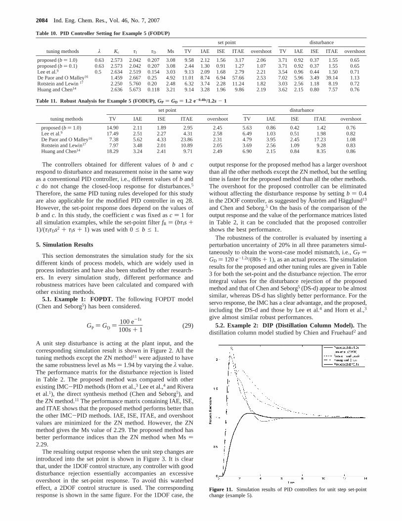
Figure 10. Simulation results of PID controllers for unit step disturbance(example 5).
GPID ) Kc(1 + 1τIs
+ τDs) (27)
u(t) ) Kc([br(t) - y(t)] + 1τI∫0
t[r(t) - y(t)] dτ +
τD
d[cr(t) - y(t)]dt ) (28)
IAE ) ∫0
∞ |e(t)| dt (24)
ISE ) ∫0
∞e(t)2 dt (25)
ITAE ) ∫0
∞t|e(t)| dt (26)
Ind. Eng. Chem. Res., Vol. 46, No. 7, 20072083
The controllers obtained for different values ofb and crespond to disturbance and measurement noise in the same wayas a conventional PID controller, i.e., different values ofb andc do not change the closed-loop response for disturbances.5
Therefore, the same PID tuning rules developed for this studyare also applicable for the modified PID controller in eq 28.However, the set-point response does depend on the values ofb andc. In this study, the coefficientc was fixed asc ) 1 forall simulation examples, while the set-point filterfR ) (bτIs +1)/(τIτDs2 + τIs + 1) was used with 0e b e 1.
5. Simulation Results
This section demonstrates the simulation study for the sixdifferent kinds of process models, which are widely used inprocess industries and have also been studied by other research-ers. In every simulation study, different performance androbustness matrices have been calculated and compared withother existing methods.
5.1. Example 1: FOPDT. The following FOPDT model(Chen and Seborg5) has been considered.
A unit step disturbance is acting at the plant input, and thecorresponding simulation result is shown in Figure 2. All thetuning methods except the ZN method11 were adjusted to havethe same robustness level as Ms) 1.94 by varying theλ value.The performance matrix for the disturbance rejection is listedin Table 2. The proposed method was compared with otherexisting IMC-PID methods (Horn et al.,3 Lee et al.,4 and Riveraet al.1), the direct synthesis method (Chen and Seborg5), andthe ZN method.11 The performance matrix containing IAE, ISE,and ITAE shows that the proposed method performs better thanthe other IMC-PID methods. IAE, ISE, ITAE, and overshootvalues are minimized for the ZN method. However, the ZNmethod gives the Ms value of 2.29. The proposed method hasbetter performance indices than the ZN method when Ms)2.29.
The resulting output response when the unit step changes areintroduced into the set point is shown in Figure 3. It is clearthat, under the 1DOF control structure, any controller with gooddisturbance rejection essentially accompanies an excessiveovershoot in the set-point response. To avoid this waterbedeffect, a 2DOF control structure is used. The correspondingresponse is shown in the same figure. For the 1DOF case, the
output response for the proposed method has a larger overshootthan all the other methods except the ZN method, but the settlingtime is faster for the proposed method than all the other methods.The overshoot for the proposed controller can be eliminatedwithout affecting the disturbance response by settingb ) 0.4in the 2DOF controller, as suggested by Åstro¨m and Hagglund13
and Chen and Seborg.5 On the basis of the comparison of theoutput response and the value of the performance matrices listedin Table 2, it can be concluded that the proposed controllershows the best performance.
The robustness of the controller is evaluated by inserting aperturbation uncertainty of 20% in all three parameters simul-taneously to obtain the worst-case model mismatch, i.e.,GP )GD ) 120 e-1.2s/(80s + 1), as an actual process. The simulationresults for the proposed and other tuning rules are given in Table3 for both the set-point and the disturbance rejection. The errorintegral values for the disturbance rejection of the proposedmethod and that of Chen and Seborg5 (DS-d) appear to be almostsimilar, whereas DS-d has slightly better performance. For theservo response, the IMC has a clear advantage, and the proposed,including the DS-d and those by Lee et al.4 and Horn et al.,3
give almost similar robust performances.5.2. Example 2: DIP (Distillation Column Model). The
distillation column model studied by Chien and Fruehauf2 and
Table 10. PID Controller Setting for Example 5 (FODUP)
set point disturbance
tuning methods λ Kc τI τD Ms TV IAE ISE ITAE overshoot TV IAE ISE ITAE overshoot
proposed (b ) 1.0) 0.63 2.573 2.042 0.207 3.08 9.58 2.12 1.56 3.17 2.06 3.71 0.92 0.37 1.55 0.65proposed (b ) 0.1) 0.63 2.573 2.042 0.207 3.08 2.44 1.30 0.91 1.27 1.07 3.71 0.92 0.37 1.55 0.65Lee et al.9 0.5 2.634 2.519 0.154 3.03 9.13 2.09 1.68 2.79 2.21 3.54 0.96 0.44 1.50 0.71De Paor and O Malley16 1.459 2.667 0.25 4.92 11.01 8.74 6.94 57.66 2.53 7.02 5.96 3.49 39.14 1.13Rotstein and Lewin17 2.250 5.760 0.20 2.48 6.32 3.74 2.28 11.24 1.82 3.03 2.56 1.18 8.19 0.72Huang and Chen14 2.636 5.673 0.118 3.21 9.14 3.28 1.96 9.86 2.19 3.62 2.15 0.80 7.57 0.76
Table 11. Robust Analysis for Example 5 (FODUP),GP ) GD ) 1.2 e-0.48s/1.2s - 1
set point disturbance
tuning methods TV IAE ISE ITAE overshoot TV IAE ISE ITAE overshoot
proposed (b ) 1.0) 14.90 2.11 1.89 2.95 2.45 5.63 0.86 0.42 1.42 0.76Lee et al.9 17.49 2.51 2.27 4.31 2.58 6.49 1.03 0.51 1.98 0.82De Paor and O Malley16 7.38 5.62 4.33 23.86 2.31 4.79 3.95 2.45 17.23 1.08Rotstein and Lewin17 7.97 3.48 2.01 10.89 2.05 3.69 2.56 1.09 9.28 0.83Huang and Chen14 18.29 3.24 2.41 9.71 2.49 6.90 2.15 0.84 8.35 0.86
GP ) GD ) 100 e-1s
100s + 1(29)
Figure 11. Simulation results of PID controllers for unit step set-pointchange (example 5).
2084 Ind. Eng. Chem. Res., Vol. 46, No. 7, 2007
Chen and Seborg5 was considered. The distillation columnseparates a small amount of a low-boiling material from thefinal product. The bottom level of the distillation column iscontrolled by adjusting the steam flow rate. The process modelfor the level control system is represented as the following DIPmodel, which can be approximated by the FOPDT model as
The method proposed by Chen and Seborg,5 Lee et al.,9 andChien and Fruehauf2 was used to design the PID controllers, asshown in Figure 4 and Table 4.λ ) 11.3 was chosen for theproposed method,λ ) 9.15 was chosen for Chen and Seborg,5
λ ) 11.0 was chosen for Lee et al.,9 andλ ) 15.28 was chosenfor Chien and Fruehauf,2 resulting in Ms) 1.90. Figure 4 showsthe output response, where the proposed tuning rule results inthe least settling time. Chien and Fruehauf’s method2 has theslowest response and requires the highest settling time. Theperformance matrix in Table 4 shows that the proposed methodhas the lowest error integral value while Chien and Fruehauf’s2
method has the highest value at an equal robustness level. Onthe basis of Table 4 and Figure 4, it is clear that the proposedmethod performs better than the other conventional methods.
The simulation results for the unit set-point change are shownin Figure 5. The overshoot for the proposed method is large,but the settling time is minimized for the 1DOF controller. Theovershoot can be minimized by using the 2DOF controller withb ) 0.4. The results in Table 4 and Figure 4 show the superiorperformance of the proposed method.
The robustness of the controller is evaluated by inserting aperturbation uncertainty of 20% in both parameters simultane-ously. The worst plant-model mismatch case after 20% pertur-bation isGP ) GD ) 0.24 e-8.88s/s. The simulation results forall tuning rules are given in Table 5. It is clear that the proposedmethod has better performance for disturbance rejection fol-lowed by DS-d and that by Lee et al.9 The set-point responsesof the DS-d and the methods by Lee et al.9 and Chien and Frue-hauf2 are almost similar and superior to the proposed method.
5.3. Example 3: SOPDT.Consider the SOPDT modeldescribed by Chen and Seborg:5
The proposed, DS-d (Chen and Seborg5), ZN, SIMC (Skoges-tad8), and DS (Smith et al.,10 Seborg et al.7) methods were used
to design the PID controller. The DS and IMC-PID (Rivera etal.1) methods give the exact same tuning formula for the SOPDTprocess. The parameters of the PID controller settings for theDS and ZN methods were taken from Chen and Seborg.5 Allthe other methods were adjusted to have the equal Ms value of1.87 for a fair comparison. Figure 6 shows the output responsefor all tuning methods mentioned above. The proposed methodhas a similar overshoot to that of the DS-d method, while theZN tuning method gives the highest peak. The settling time isthe lowest for the proposed method, whereas the DS methodshows the slowest response. Apart from the DS-d method, allthe other tuning methods have either higher overshoot or slowerresponse for disturbance rejection.
The simulation results for the unit set-point change are shownin Figure 7. The overshoot for the ZN method is the largestfollowed by that of the proposed method, but the settling timeis the lowest for the proposed method among all the 1DOFcontrollers. The overshoot can be minimized by using the 2DOFcontroller withb ) 0.4. On the basis of the performance shownin the above figures and the performance matrix in Table 6, theproposed method has the best performance.
To evaluate the robust performance, the worst plant-modelmismatch case was considered asGP ) GD ) 2.4 e-1.2s/(8s +1)(4s + 1) by inserting a perturbation uncertainty of 20% in all
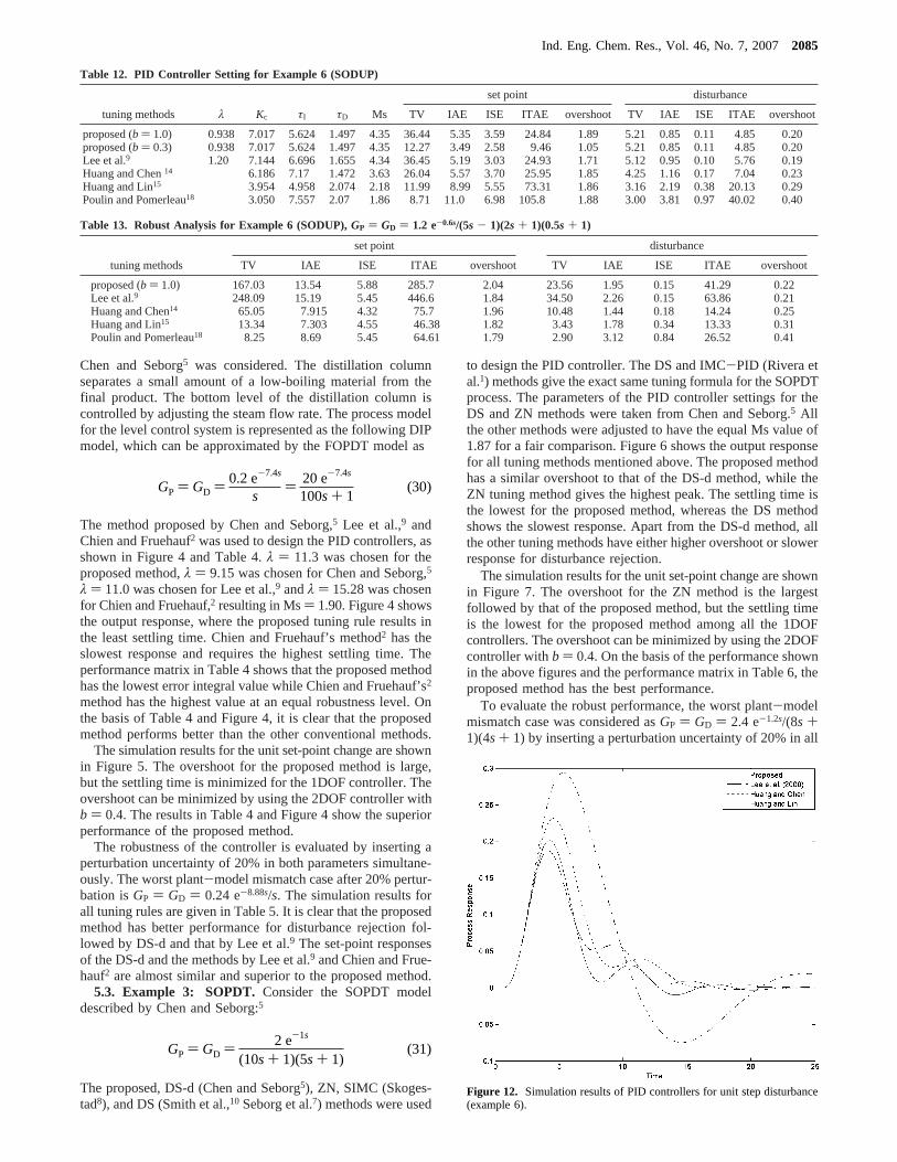
Table 12. PID Controller Setting for Example 6 (SODUP)
set point disturbance
tuning methods λ Kc τI τD Ms TV IAE ISE ITAE overshoot TV IAE ISE ITAE overshoot
proposed (b ) 1.0) 0.938 7.017 5.624 1.497 4.35 36.44 5.35 3.59 24.84 1.89 5.21 0.85 0.11 4.85 0.20proposed (b ) 0.3) 0.938 7.017 5.624 1.497 4.35 12.27 3.49 2.58 9.46 1.05 5.21 0.85 0.11 4.85 0.20Lee et al.9 1.20 7.144 6.696 1.655 4.34 36.45 5.19 3.03 24.93 1.71 5.12 0.95 0.10 5.76 0.19Huang and Chen14 6.186 7.17 1.472 3.63 26.04 5.57 3.70 25.95 1.85 4.25 1.16 0.17 7.04 0.23Huang and Lin15 3.954 4.958 2.074 2.18 11.99 8.99 5.55 73.31 1.86 3.16 2.19 0.38 20.13 0.29Poulin and Pomerleau18 3.050 7.557 2.07 1.86 8.71 11.0 6.98 105.8 1.88 3.00 3.81 0.97 40.02 0.40
Table 13. Robust Analysis for Example 6 (SODUP),GP ) GD ) 1.2 e-0.6s/(5s - 1)(2s + 1)(0.5s + 1)
set point disturbance
tuning methods TV IAE ISE ITAE overshoot TV IAE ISE ITAE overshoot
proposed (b ) 1.0) 167.03 13.54 5.88 285.7 2.04 23.56 1.95 0.15 41.29 0.22Lee et al.9 248.09 15.19 5.45 446.6 1.84 34.50 2.26 0.15 63.86 0.21Huang and Chen14 65.05 7.915 4.32 75.7 1.96 10.48 1.44 0.18 14.24 0.25Huang and Lin15 13.34 7.303 4.55 46.38 1.82 3.43 1.78 0.34 13.33 0.31Poulin and Pomerleau18 8.25 8.69 5.45 64.61 1.79 2.90 3.12 0.84 26.52 0.41
Figure 12. Simulation results of PID controllers for unit step disturbance(example 6).
GP ) GD ) 0.2 e-7.4s
s) 20 e-7.4s
100s + 1(30)
GP ) GD ) 2 e-1s
(10s + 1)(5s + 1)(31)
Ind. Eng. Chem. Res., Vol. 46, No. 7, 20072085
three parameters simultaneously. The simulation results for alltuning rules are given in Table 7. When compared to the othermethods, the error integral values for the proposed method arethe best for both set-point and disturbance rejection, and theovershoot for the proposed method is similar to those by theDS-d and DS methods. The ZN method has a higher overshootthan the other methods.
5.4. Example 4: FODIP (Reboiler Level Model).Considera level-control problem proposed by Chen and Seborg.5 It is anapproximate model for a liquid level in the reboiler of a steam-heated distillation column, which is to be controlled by adjustingthe control valve on the steam line. The process model is givenby
This kind of “inverse response time constant” (negative numera-tor time constant) can be approximated as a time delay such as(-θ0
invs + 1) ≈ e-θ0inv. This is reasonable since an inverse
response has a deteriorating effect on control, similar to that ofa time delay.8
Therefore, the above model can be approximated as
The above process model can be treated as FODIP, and thetuning parameters can be estimated by the analytical ruleproposed in Table 1.
Figure 8 shows the output response of the proposed tuningmethod and its comparison with the DS-d, IMC, and ZNmethods. The PID controller settings for all the other methodswere taken from Chen and Seborg.5 The valueλ ) 0.935 wasselected for the proposed method, which gives Ms) 1.94. Fromthe figure, the proposed output response has a small overshootand a fast settling time, followed by the DS-d and IMC methods,while the ZN method has a very aggressive response withsignificant overshoot and oscillation that takes a long time tosettle. The performance values are also listed in Table 8 whichindicates the clear advantage of the proposed method over othertuning rules.
The output responses for the unit set-point change are shownin Figure 9. The overshoot by the proposed method with the
1DOF structure is somewhat large but shows a fast settling timebefore reaching its final value. The overshoot can be drasticallyminimized by using the 2DOF controller. It is apparent fromFigure 8 and Table 8 that the proposed method is superior overthe other tuning methods for the disturbance rejection.
The robustness of the controller is evaluated considering theworst case under a 20% uncertainty in all three parameters asGP ) GD ) -1.92(-0.6s + 1)/s(2.4s + 1). The simulationresults for all tuning rules are given in Table 9. The error integraland overshoot values for the proposed method prove to be thebest. The overshoot and IAE of the ZN method is the highestamong the other tuning methods.
5.5. Example 5: FODUP.The following FODUP (Huang& Chen14 and Lee et al.9) was considered:
The closed-loop time constantλ ) 0.63 is selected for theproposed tuning method for Ms) 3.08. Settingλ ) 0.5 resultsin the same value of Ms) 3.08 for Lee et al.’s9 method, thusproviding a fair comparison. The controller setting parametersfor the other existing methods were taken from Lee et al.9 Figure10 shows the output response of all tuning methods, with theproposed method showing the clear advantage. In Table 10, theperformance and robustness matrices are listed for all tuningrules, and the proposed method shows a clear advantage overthe other methods.
The response for the unit set-point change of the 1DOFcontroller is shown in Figure 11 where every 1DOF controllershows a significant overshoot. By using the 2DOF controller,
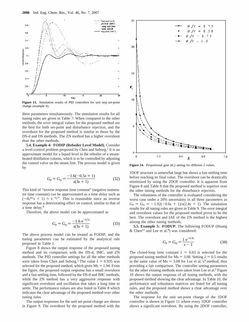
Figure 13. Simulation results of PID controllers for unit step set-pointchange (example 6).
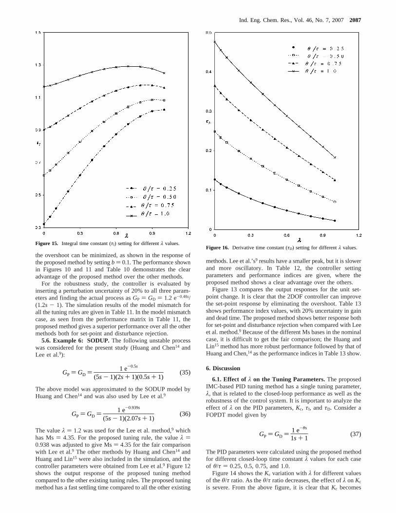
Figure 14. Proportional gain (Kc) setting for differentλ values.
GP ) GD ) 1 e-0.4s
s - 1(34)
GP ) GD )-1.6(-0.5s + 1)
s(3s + 1)(32)
GP ) GD ) -1.6 e-0.5s
s(3s + 1)(33)
2086 Ind. Eng. Chem. Res., Vol. 46, No. 7, 2007
the overshoot can be minimized, as shown in the response ofthe proposed method by settingb ) 0.1. The performance shownin Figures 10 and 11 and Table 10 demonstrates the clearadvantage of the proposed method over the other methods.
For the robustness study, the controller is evaluated byinserting a perturbation uncertainty of 20% to all three param-eters and finding the actual process asGP ) GD ) 1.2 e-0.48s/(1.2s - 1). The simulation results of the model mismatch forall the tuning rules are given in Table 11. In the model mismatchcase, as seen from the performance matrix in Table 11, theproposed method gives a superior performance over all the othermethods both for set-point and disturbance rejection.
5.6. Example 6: SODUP.The following unstable processwas considered for the present study (Huang and Chen14 andLee et al.9):
The above model was approximated to the SODUP model byHuang and Chen14 and was also used by Lee et al.9
The valueλ ) 1.2 was used for the Lee et al. method,9 whichhas Ms) 4.35. For the proposed tuning rule, the valueλ )0.938 was adjusted to give Ms) 4.35 for the fair comparisonwith Lee et al.9 The other methods by Huang and Chen14 andHuang and Lin15 were also included in the simulation, and thecontroller parameters were obtained from Lee et al.9 Figure 12shows the output response of the proposed tuning methodcompared to the other existing tuning rules. The proposed tuningmethod has a fast settling time compared to all the other existing
methods. Lee et al.’s9 results have a smaller peak, but it is slowerand more oscillatory. In Table 12, the controller settingparameters and performance indices are given, where theproposed method shows a clear advantage over the others.
Figure 13 compares the output responses for the unit set-point change. It is clear that the 2DOF controller can improvethe set-point response by eliminating the overshoot. Table 13shows performance index values, with 20% uncertainty in gainand dead time. The proposed method shows better response bothfor set-point and disturbance rejection when compared with Leeet al. method.9 Because of the different Ms bases in the nominalcase, it is difficult to get the fair comparison; the Huang andLin15 method has more robust performance followed by that ofHuang and Chen,14 as the performance indices in Table 13 show.
6. Discussion
6.1. Effect of λ on the Tuning Parameters.The proposedIMC-based PID tuning method has a single tuning parameter,λ, that is related to the closed-loop performance as well as therobustness of the control system. It is important to analyze theeffect of λ on the PID parameters,Kc, τI, andτD. Consider aFOPDT model given by
The PID parameters were calculated using the proposed methodfor different closed-loop time constantλ values for each caseof θ/τ ) 0.25, 0.5, 0.75, and 1.0.
Figure 14 shows theKc variation withλ for different valuesof theθ/τ ratio. As theθ/τ ratio decreases, the effect ofλ on Kc
is severe. From the above figure, it is clear thatKc becomes
Figure 15. Integral time constant (τI) setting for differentλ values.
GP ) GD ) 1 e-0.5s
(5s - 1)(2s + 1)(0.5s + 1)(35)
GP ) GD ) 1 e-0.939s
(5s - 1)(2.07s + 1)(36)
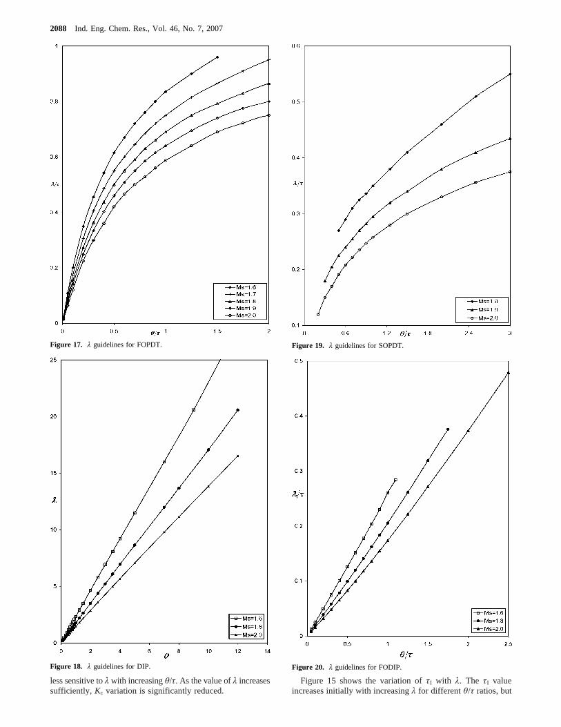
Figure 16. Derivative time constant (τD) setting for differentλ values.
GP ) GD ) 1 e-θs
1s + 1(37)
Ind. Eng. Chem. Res., Vol. 46, No. 7, 20072087
less sensitive toλ with increasingθ/τ. As the value ofλ increasessufficiently, Kc variation is significantly reduced.
Figure 15 shows the variation ofτI with λ. The τI valueincreases initially with increasingλ for differentθ/τ ratios, but
Figure 17. λ guidelines for FOPDT.
Figure 18. λ guidelines for DIP.
Figure 19. λ guidelines for SOPDT.
Figure 20. λ guidelines for FODIP.
2088 Ind. Eng. Chem. Res., Vol. 46, No. 7, 2007
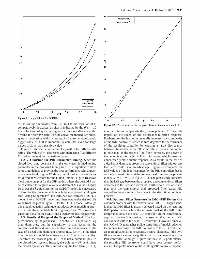
as theθ/τ ratio increases from 0.25 to 1.0, the variation ofτI
comparatively decreases, as clearly indicated by theθ/τ ) 1.0line. The trend ofτI increasing withλ reverses after a specificλ value for eachθ/τ ratio. For the above-mentionedθ/τ ratios,τI starts decreasing with increasingλ after some significantlybigger value ofλ. It is important to note that, even for largevalues ofλ, τI has a positive value.
Figure 16 shows the variation ofτD with λ for different θ/τratios. The value ofτD decreases with increasingλ at differentθ/τ ratios, maintaining a positive value.
6.2. λ Guideline for PID Parameter Tuning. Since theclosed-loop time constantλ is the only user-defined tuningparameter in the proposed tuning rule, it is important to havesomeλ guidelines to provide the best performance with a givenrobustness level. Figure 17 shows the plot ofλ/τ vs θ/τ ratiosfor different Ms values for the FOPDT model. Figure 18 showstheλ guideline plot for the DIP model, where the desiredλ canbe calculated for a givenθ value at different Ms values. Figure19 shows theλ guidelines for the SOPDT model. It is necessaryto describe the model reduction technique proposed by Skoges-tad.8 Using Skogestad’s8 half rule, we can convert a SOPDTmodel into a FOPDT model and then obtain the desiredλ/τvalue from the plot in Figure 19 for the SOPDT model. Althoughthis model reduction technique introduces some modeling error,it is within the acceptable limit. Figures 20 and 21 show theλguideline plots for the FODIP and FODUP models, respectively.
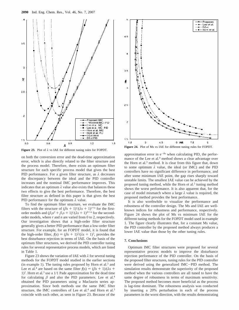
6.3. Beneficial Range of the Proposed Method.The loadperformance by the proposed PID controller is superior as lagtime dominates, but the superiority to that based on theconventional filter diminishes as dead time dominates. In thecase of a dead-time dominant process (i.e., θ/τ . 1), the filtertime constant should be chosen asλ ≈ θ . τ for stability.Therefore, the process pole at-1/τ is not a dominant pole inthe closed-loop system. Instead, the pole at-1/λ determinesthe overall dynamics. Thus, introducing the lead term (âs + 1)
into the filter to compensate the process pole at-1/τ has littleimpact on the speed of the disturbance-rejection response.Furthermore, the lead term generally increases the complexityof the IMC controller, which in turn degrades the performanceof the resulting controller by causing a large discrepancybetween the ideal and the PID controllers. It is also importantto note that, as the order of the filter increases, the power ofthe denominator term (λs + 1) also increases, which causes anunnecessarily slow output response. As a result, in the case ofa dead-time dominant process, a conventional filter without anylead term could have an advantage. Figure 22 compares theIAE values of the load responses by the PID controllers basedon the proposed filter and the conventional filter for the processmodelGP ) GD ) 10 e-θs/(1s + 1). The plot clearly indicatesthat the IAE gap between the proposed and conventional filtersdecreases as theθ/τ ratio increases. Furthermore, it is observedthat both the conventional and proposed filter based PIDcontrollers have similar robustness in the dead time dominantprocess.
6.4. Optimum Filter Structure for IMC -PID Design.Onecommon problem with the conventional IMC-PID approachesis that the IMC filter is usually selected based on the resultingIMC performance, while the ultimate goal of the IMC filterdesign is to obtain the best PID controller. In the conventionalapproach for the filter design, it is assumed that the best IMCcontroller results in the best PID controller. However, since allthe IMC-PID approaches utilize some kind of model reductiontechniques to convert the IMC controller to the PID controller,an approximation error necessarily occurs. Therefore, if the IMCfilter structure causes a significant error in conversion to thePID controller, although it gives the best IMC performance,the resulting PID controller could have poor control perfor-mance. The performance of the resulting PID controller depends
Figure 21. λ guidelines for FODUP.
Figure 22. Performance of the proposed filter vs the conventional filter.
Ind. Eng. Chem. Res., Vol. 46, No. 7, 20072089
on both the conversion error and the dead-time approximationerror, which is also directly related to the filter structure andthe process model. Therefore, there exists an optimum filterstructure for each specific process model that gives the bestPID performance. For a given filter structure, asλ decreasesthe discrepancy between the ideal and the PID controllerincreases and the nominal IMC performance improves. Thisindicates that an optimumλ value also exists that balances thesetwo effects to give the best performance. Therefore, the bestfilter structure as defined in this paper is that gives the bestPID performance for the optimumλ value.
To find the optimum filter structure, we evaluate the IMCfilters with the structure of (âs + 1)r/(λs + 1)r+n for the first-order models and (â2s2 + â1s + 1)r/(λs + 1)2r+n for the second-order models, wherer andn are varied from 0 to 2, respectively.Our investigation shows that a high-order filter structuregenerally gives a better PID performance than a low-order filterstructure. For example, for an FOPDT model, it is found thatthe high-order filter,f(s) ) (âs + 1)2/(λs + 1)3, provides thebest disturbance rejection in terms of IAE. On the basis of theoptimum filter structures, we derived the PID controller tuningrules for several representative process models, which are listedin Table 1.
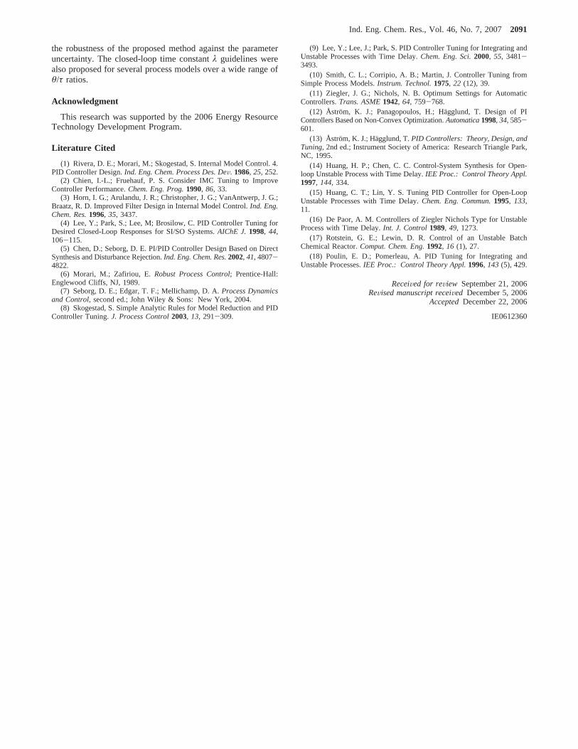
Figure 23 shows the variation of IAE withλ for several tuningmethods for the FOPDT model studied in the earlier sections(in example 1). The tuning rules proposed by Horn et al.3 andLee et al.4 are based on the same filterf(s) ) (âs + 1)/(λs +1)2. Horn et al.3 use a 1/1 Pade approximation for the dead timefor calculating â and also the PID parameters. Lee et al.4
obtained the PID parameters using a Maclaurin series ap-proximation. Since both methods use the same IMC filterstructure, the IMC controllers of Lee et al.4 and Horn et al.3
coincide with each other, as seen in Figure 23. Because of the
approximation error in e-θs when calculating PID, the perfor-mance of the Lee et al.4 method shows a clear advantage overthe Horn et al.3 method. It is clear from this figure that, downto some optimumλ value, the ideal (or IMC) and the PIDcontrollers have no significant difference in performance, andafter some minimum IAE point, the gap rises sharply towardunstable limits. The smallest IAE value can be achieved by theproposed tuning method, while the Horn et al.3 tuning methodshows the worst performance. It is also apparent that, for thecase of model mismatch where a largeλ value is required, theproposed method provides the best performance.
It is also worthwhile to visualize the performance androbustness of the controller design. The Ms and IAE are well-known indices for robustness and performance, respectively.Figure 24 shows the plot of Ms vs minimum IAE for thedifferent tuning methods for the FOPDT model used in example1. The figure clearly illustrates that, for a constant Ms value,the PID controller by the proposed method always produces alower IAE value than those by the other tuning rules.
7. Conclusions
Optimum IMC filter structures were proposed for severalrepresentative process models to improve the disturbancerejection performance of the PID controller. On the basis ofthe proposed filter structures, tuning rules for the PID controllerwere derived using the generalized IMC-PID method. Thesimulation results demonstrate the superiority of the proposedmethod when the various controllers are all tuned to have thesame degree of robustness in terms of maximum sensitivity.The proposed method becomes more beneficial as the processis lag-time dominant. The robustness analysis was conductedby inserting a 20% perturbation in each of the processparameters in the worst direction, with the results demonstrating
Figure 23. Plot of λ vs IAE for different tuning rules for FOPDT.Figure 24. Plot of Ms vs IAE for different tuning rules for FOPDT.
2090 Ind. Eng. Chem. Res., Vol. 46, No. 7, 2007
the robustness of the proposed method against the parameteruncertainty. The closed-loop time constantλ guidelines werealso proposed for several process models over a wide range ofθ/τ ratios.
Acknowledgment
This research was supported by the 2006 Energy ResourceTechnology Development Program.
Literature Cited
(1) Rivera, D. E.; Morari, M.; Skogestad, S. Internal Model Control. 4.PID Controller Design.Ind. Eng. Chem. Process Des. DeV. 1986, 25, 252.
(2) Chien, I.-L.; Fruehauf, P. S. Consider IMC Tuning to ImproveController Performance.Chem. Eng. Prog.1990, 86, 33.
(3) Horn, I. G.; Arulandu, J. R.; Christopher, J. G.; VanAntwerp, J. G.;Braatz, R. D. Improved Filter Design in Internal Model Control.Ind. Eng.Chem. Res.1996, 35, 3437.
(4) Lee, Y.; Park, S.; Lee, M; Brosilow, C. PID Controller Tuning forDesired Closed-Loop Responses for SI/SO Systems.AIChE J.1998, 44,106-115.
(5) Chen, D.; Seborg, D. E. PI/PID Controller Design Based on DirectSynthesis and Disturbance Rejection.Ind. Eng. Chem. Res.2002, 41, 4807-4822.
(6) Morari, M.; Zafiriou, E. Robust Process Control; Prentice-Hall:Englewood Cliffs, NJ, 1989.
(7) Seborg, D. E.; Edgar, T. F.; Mellichamp, D. A.Process Dynamicsand Control, second ed.; John Wiley & Sons: New York, 2004.
(8) Skogestad, S. Simple Analytic Rules for Model Reduction and PIDController Tuning.J. Process Control2003, 13, 291-309.
(9) Lee, Y.; Lee, J.; Park, S. PID Controller Tuning for Integrating andUnstable Processes with Time Delay.Chem. Eng. Sci.2000, 55, 3481-3493.
(10) Smith, C. L.; Corripio, A. B.; Martin, J. Controller Tuning fromSimple Process Models.Instrum. Technol.1975, 22 (12), 39.
(11) Ziegler, J. G.; Nichols, N. B. Optimum Settings for AutomaticControllers.Trans. ASME1942, 64, 759-768.
(12) Åstrom, K. J.; Panagopoulos, H.; Ha¨gglund, T. Design of PIControllers Based on Non-Convex Optimization.Automatica1998, 34, 585-601.
(13) Åstrom, K. J.; Hagglund, T.PID Controllers: Theory, Design, andTuning, 2nd ed.; Instrument Society of America: Research Triangle Park,NC, 1995.
(14) Huang, H. P.; Chen, C. C. Control-System Synthesis for Open-loop Unstable Process with Time Delay.IEE Proc.: Control Theory Appl.1997, 144, 334.
(15) Huang, C. T.; Lin, Y. S. Tuning PID Controller for Open-LoopUnstable Processes with Time Delay.Chem. Eng. Commun.1995, 133,11.
(16) De Paor, A. M. Controllers of Ziegler Nichols Type for UnstableProcess with Time Delay.Int. J. Control1989, 49, 1273.
(17) Rotstein, G. E.; Lewin, D. R. Control of an Unstable BatchChemical Reactor.Comput. Chem. Eng.1992, 16 (1), 27.
(18) Poulin, E. D.; Pomerleau, A. PID Tuning for Integrating andUnstable Processes.IEE Proc.: Control Theory Appl.1996, 143 (5), 429.
ReceiVed for reView September 21, 2006ReVised manuscript receiVed December 5, 2006
AcceptedDecember 22, 2006
IE0612360
Ind. Eng. Chem. Res., Vol. 46, No. 7, 20072091