tight performance bounds of cp-scheduling on out-trees

Journal of Combinatorial Optimization, 5, 445–464, 2001c© 2001 Kluwer Academic Publishers. Manufactured in The Netherlands.

Tight Performance Bounds of CP-Schedulingon Out-Trees

NODARI VAKHANIAScience Faculty, Morelos State University, Mexico

Received August 16, 1999; Revised October 12, 2000; Accepted February 9, 2001

Abstract. The worst-case behavior of the “critical path” (CP) algorithm for multiprocessor scheduling with anout-tree task dependency structure is studied. The out-tree is not known in advance and the tasks are releasedon-line over time (each task is released at the completion time of its direct predecessor task in the out-tree). Foreach task, the processing time and the remainder (the length of the longest chain of the future tasks headed by thistask) become known at its release time. The tight worst-case ratio and absolute error are derived for this stronglyclairvoyant on-line model. For out-trees with a specific simple structure, essentially better worst-case ratio andabsolute error are derived. Our bounds are given in terms of tmax , the length of the longest chain in the out-tree,and it is shown that the worst-case ratio asymptotically approaches 2 for large tmax when the number of processorsm = τ̃ (τ̃ + 1)/2 − 2, where τ̃ is an integer close to

√tmax . A non-clairvoyant on-line version (without knowledge

of task processing time and remainder at the release time of the task) is also considered and is shown that theworst-case behavior of width-first search is better or the same as that of the depth-first search.

Keywords: scheduling identical processors, tree-type precedence relations, worst-case ratio, release time,remainder

1. Introduction

In this paper, we address a multiprocessor scheduling problem in which the precedencerestrictions between the tasks are given by an out-tree T (a rooted tree, in which all arcsare directed from the root to the leaves). We are given m identical processors, however afinite set of n tasks and the precedence out-tree are not known in advance. A node i in T re-presents the unique task i (i is a non-negative integer). Each task becomes known (or ready)from the moment called its release (readiness) time. Each task, except the one associatedwith the root of T , becomes ready at the completion time of its direct predecessor, whereasthe former task is initially ready at time 0. Each released task is to be assigned to or scheduledon a processor from a given set of processors. Task i , once scheduled on a processor, takesa (real) processing time (or duration) pi , and it has a (real) remainder ti , which becomeknown by the release time of i ; ti is the total remaining processing time, originated by thelongest chain headed by task i in T (in practice, we assume that ti is predicted in someway).1 Task i , once assigned to a processor, is to be processed without any preemption. Aprocessor is idle at a moment t , if either no task has been assigned to that processor by themoment t or all the assigned tasks are already completed by that moment. A processor isbusy if it is not idle. A task can be assigned only to an idle processor, i.e., a processor canhandle at most one task at a time.

446 VAKHANIA

The precedence tree T is not known in advance and is generated on-line. Each timemoment when an already scheduled task i is finished, the tree is completed with the directsuccessors of this task (i is the direct predecessor of the former tasks). Hence each directsuccessor of i becomes ready at the completion time of i and can be scheduled from thismoment. One or more task is released initially at some moment t ≥ 0. These tasks are thedirect successors of the initial fictitious task 0 with p0 = t , released at time 0. An arc(i, j)∈ T , iff task i is the direct predecessor of task j . With an arc (i, j), the weightw(i, j) = pi is associated; for each task which has no successor, we introduce its ficti-tious direct successor task with 0 processing time, a leaf of T . Then the remainder of taski , ti is the length of a critical (longest) path from node i to a leaf in T .

A schedule is a mapping which assigns to each task a particular processor and a startingtime on that processor. A feasible schedule is a schedule satisfying the constraints statedabove (it assigns each released task i to an idle processor and executes it during pi timewithout interruption). An optimal schedule is a feasible schedule which minimizes themakespan, i.e., the maximal task completion time in a schedule.

For a given schedule, the performance ratio is the ratio of the makespan of this schedule tothe optimal makespan. The worst-case (performance) ratio for an algorithm is the maximalperformance ratio taken among all schedules, generated by this algorithm (for on-linealgorithms the term “competitive ratio” is commonly used). An absolute error estimatesa schedule in absolute terms and is equal to the difference between the makespan of thisschedule and an optimal one. A worst-case (absolute) error for an algorithm is definedsimilarly as worst-case ratio.

Numerous practical problems fit our model; for example, scheduling operations for par-allel execution of arithmetic expressions, different scheduling problems in parallel anddistributed systems with real-time tasks in which task processing times and remainders canbe predicted exactly or with some accuracy. The only on-line feature in our model is thelack of knowledge of the precedence tree and the jobs which arrive in future. According tothe classification from the survey articles of Chen et al. (1998) and Sgall (1998), the on-linemodels (algorithms), in which each task processing time is known by the release time of thistask are called clairvoyant (otherwise they are called non-clairvoyant). We call the on-linemodels (algorithms), in which besides task processing times, task reminders are known bythe release time of the tasks strongly (or precedently) clairvoyant (note that strong clairvoy-antness implies the precedence relations between the tasks). Besides, our model is on-lineover time since the tasks are released over time.2 Precedently clairvoyant models providemore insight than corresponding (normally) clairvoyant models and a reminder-dependentalgorithm can be applied for the former models. Unlike normal clairvoyant models, inprecedently clairvoyant models the task release times are schedule-dependent (since they,in general, depend on the order in which the ready tasks are scheduled).

Let us mention some basic results concerning the off-line version of our model (theprecedence tree and task processing times are known in advance). If there are no prece-dence relations, although the problem is NP-hard, it can be solved with a very good ap-proximation in polynomial time (Yue, 1990; Hochbaum and Shmoys, 1988) (the latteralgorithm works for more general case with uniform processors). The situation gets morecomplicated with precedence relations. With arbitrary precedence relations and equal-length

TIGHT PERFORMANCE BOUNDS 447

tasks the problem is again NP-hard (Ullman, 1975; Lenstra and Rinnoy Kan, 1978). Ef-ficient algorithms for equal-length tasks exist if the precedence relations are of the tree-type, or if m = 2 (Fuji et al., 1969; Coffman and Graham 1972; Gabow and Tarjan, 1985).Hu’s critical path (CP) algorithm (1961) is one of the classical (reminder-dependent) al-gorithms, which gives good approximability results and is optimal in certain cases (thealgorithm repeatedly determines a task with the longest remainder and schedules it ona machine with the minimal load). In particular, if all tasks are of equal length and theprecedence graph is a tree, the CP algorithm gives an optimal solution in linear time(Hsu, 1966; Sethi, 1976). We shall refer to Hu’s algorithm as the longest remainder (LR)algorithm.

For arbitrary precedence relations, the worst-case ratio of versions of LR algorithm ap-proaches 2 for large m, even if all tasks are of equal-length. In particular, LR algorithmgives the performance ratio of 2−1/(m −1) (Chen and Liu, 1975; Kunde, 1976). Coffmanand Graham’s algorithm (1972), which is optimal for m = 2, gives a slightly different per-formance ratio of 2 − 2/m (Lam and Sethi, 1977). Surprisingly, Graham’s on-line listscheduling algorithm for tasks with arbitrary durations (Graham, 1966) behaves almost asgood as the above two unit-task algorithms: for an arbitrary list schedule S and the re-spective optimal schedule S∗, L(S)/L(S∗) ≤ 2 − 1/m, where L(S) is the makespan ofS (Graham also gives an example proving that an LR schedule for arbitrary precedencerelations can be as bad as a list schedule). There were suggested on-line (over list) al-gorithms with a worst-case performance, better than Graham’s list scheduling algorithm.The first improvement of Graham’s bound is due to Galambos and Woeginger (1993).The performance ratio derived in Galambos and Woeginger (1993) still approaches 2 forlarge m. Later this result was improved by several authors which give the bounds, ap-proaching a number, less than 2 (for recent results see Karger et al., 1996 and Albers,1997).

Kaufman (1974) proved that for arbitrary task durations, LR algorithm provides a goodapproximation for in-trees. He gave an absolute error, showing that for any LR schedule Sand an optimal preemptive schedule S∗

p, the inequality L(S) ≤ L(S∗p) + pmax − [pmax/m]

holds, where pmax is the maximal task duration. Kunde (1981) investigates the worst-casebehavior of the LR algorithm in terms of performance ratio, and obtains the performanceratio 2 − 2/(m + 1) for in-trees. No worst-case ratio was obtained for out-trees, howeverit was shown that the worst-case behavior of the LR algorithm with out-trees is at least asbad as for in-trees.

In off-line models, the LR algorithm can be directly applied to the in-tree, obtained byreversing all arcs in the given out-tree. Then the resulted schedule, if read backwards, givesa feasible schedule for the original problem with the out-tree, as good as the former schedulefor the in-tree; hence the earlier mentioned results for in-trees also hold for out-trees. Foron-line models, the above cannot be done, and here we deal with this kind of situation. Weconsider the strongly clairvoyant on-line over time model and derive tight performance ratioand absolute error for the corresponding on-line version of the LR algorithm (OLR algorithmfor short). The absolute error for in-trees (Kaufman, 1974) does not hold, unfortunately theworst-case absolute error is much worse. Hu’s result for equal-length tasks (Hu, 1961) stillholds. An absolute error, comparable to that of Kaufman (1974) holds for arbitrary tasks, if

448 VAKHANIA

the out-tree has a special simple structure (we call such trees simple trees). Our worst-caseerror for simple trees is pmax −1, and the worst-case ratio is 1+ pmax/tmax , where tmax is thelength of a longest chain in the simple out-tree. The worst-case error and worst-case ratio forarbitrary trees are (

√tmax − 1−1)2 and 2−2

√tmax − 1/tmax , respectively. Unlike the earlier

bounds given in terms of m, our bounds are given in terms of tmax (note that tmax is an inputin our model).3 The behaviour of the LR algorithm does not unconditionally gets worse withthe increase of m or tmax . Our worst-case bounds are attained when m = τ̃ (τ̃ + 1)/2 − 2,where τ̃ is an integer, close to

√tmax (a precise definition of τ̃ is given in Section 4). Thus in

practice if the number m can be varied, we can choose an appropriate m to improve the worst-case behaviour of LR algorithm. For example, if m is large, the behaviour of LR algorithmwill not be indeed bad if tmax is small (although the total number of tasks might be verylarge).

We explore structural properties of out-trees which make the performance of LR algorithmpoor. As we show by an example, the worst-case ratio of OLR algorithm asymptoticallygoes to 3/2 (for an appropriate value of m) even if each task has a processing time 1 or 2.We also consider non-clairvoyant version of our problem and we study the bahaviour oftwo common search strategies, width-first and depth-first. In particular, we show that theworst-case behaviour of width-first search is better or the same as that of the depth-firstsearch.

In the next Section 2 we describe the OLR algorithm and give some other preliminarynotions. In Section 3 we derive the bounds for simple trees, in Section 4 we consider generalout-trees and derive tight performance bounds for OLR algorithm. In Section 5 we suggestthe non-clairvoyant on-line version and compare the worst-case behaviour of width-first anddepth-first strategies. In Section 6 we give concluding remarks and directions for furtherresearch.

2. Preliminary notions

We start this section with the description of OLR algorithm. We denote by sSi the starting

time of task i in schedule S, its completion time, cSi = sS

i + pi . Further, R+(i) (R−(i),respectively) is the set of direct successors (the direct predecessor, respectively) of task i .The algorithm consists of a finite number of iterations. With each iteration is associateda discrete time moment of completion of an already scheduled task. The time moments,corresponding to different consecutive iterations might be the same. At iteration 0 thefictitious task 0 is scheduled, and at each consequent iteration a single task, ready by thisiteration (i.e., by the corresponding time moment) is scheduled (so the total number ofiterations is n).

We denote by Sh (Th , respectively) the (partial) schedule (tree, respectively) generatedby iteration h and by Fh the set of yet unscheduled tasks, ready by iteration h. CP(Sh) is thecompletion time of processor P in Sh , that is, the completion time of the task, scheduledlast on P by iteration h; if no task is yet scheduled on P by iteration h, then CP(Sh) = 0.

OLR algorithm uses the “greatest remainder” rule for scheduling a task at iteration h.Iteratively, a released task i with the greatest remainder from Fh is scheduled on the processorwith the minimal completion time.The detailed formal description is given below.


Algorithm OLRStep 0 (Initialization) Schedule task 0 on processor 1 at time 0;

h := 0; Th := {0}; Fh := ∅;C1(Sh) := p0; Cl(Sh) := 0, l = 2, 3, . . . , m

Step 1 Among all processors, determine a processor P with the minimal completion timein Sh , such that either there is a ready task in Fh which can be scheduled on that processor,or the latest scheduled task on that processor has a successor;

IF there is no P THEN STOPELSE wait until the moment CP(Sh)

FOR each non-marked task i completed at time CP(Sh) in Sh

DO mark i ; Th := Th ∪ (i, j), for each j ∈ R+(i), w(i, j) := pi ;Fh := Fh ∪ R+(i);

among all processors, completed by time CP(Sh), determine the processor Q with theminimal index;

among all tasks of Fh , schedule next task j with the greatest remainder at the momentt = CQ(Sh) on processor Q (break ties by selecting the task, associated with the leftmostleaf of Th);

(i) CQ(Sh+1) := t + p j ;(ii) Cl(Sh+1) := max{t, Cl(Sh)}, for l �= Q, l = 1, 2, . . . , m;4

(iii) Fh+1 := Fh \ { j};(iv) h := h + 1; GOTO Step 1.

In a schedule S, a gap is a time interval on any of the given m processors, a subintervalof [0, L(S)], not occupied by any task. A gap is called internal on a processor, if a task isscheduled after this gap on that processor; otherwise, this gap is external (all processors arereleased at the same time in a schedule without external gaps; also note that we may have atmost one external gap on a processor). From the above description it can be easily seen, thatan OLR schedule can have both, internal and external gaps (each time the maximum betweent and Cl(Sh) in line (ii) Step 1 is t , an internal gap of length t −Cl(Sh) arises on processor l).

A chain (respectively, partial chain) C = (i0, i1, . . . , ik) is any path from the root i0 = 0to a leaf ik in T (respectively in Th , for some h); we number the chains from left to right,the total number of chains equals to the number of leaves. In the sequel, we use “chain”for both, “chain” and “partial chain.” A subchain C ′ = (il , il+1, . . . , i p) of a chain C is anypath from a node il ∈ C to a node i p ∈ C with l < p, 0 ≤ l, p ≤ k. L(C) is the length of C ,equal to the sum of the processing times of the tasks of C . A longest chain is a chain C in Twith the maximal L(C). In S a chain C is processed with delay, if there exists a task i ∈ Csuch that sS

i > cSj , j = R−(i). The remainder of a chain C at iteration h is the length of its

longest subchain which starts with the earliest (the closest to the root) yet unscheduled taskof C by that iteration.

Let C be a chain in T with a subchain (i1, i2), and let task i1 be scheduled on processorP in a schedule S. We say that C is broken at time cS

i1in S, if task i2 is not scheduled on

processor P right at the moment cSi1

in S. If S is an OLR schedule, then a task i3 �= i2 isscheduled at moment cS

i1on processor P in S and besides i3 has a reminder, no less than ti2

(in this case we will say that i3 interrupts chain C at moment cSi1

).

450 VAKHANIA

In the sequel S and S∗ stand for an OLR and an optimal schedule, respectively, generatedfor some problem instance P . We shall also use S(P) and S∗(P) when a problem instancematters.

The chains, and respectively tasks we divide into two classes, critical and non-critical.A critical chain is any longest chain in T . A chain is non-critical if it is not critical.The behaviour of OLR algorithm crucially depends on the number of chains, nestedin a particular way in T . Before we define nested chains, we give some auxiliarydefinitions.

Let the source node of T be the root of T if |R+(0)| ≥ 2; otherwise let it be the firstsuccessor of the root with 2 or more direct successors. We use r to denote the source node.Each node in T has its own level, equal to the number of its predecessors in T ; the root hasa level 0.

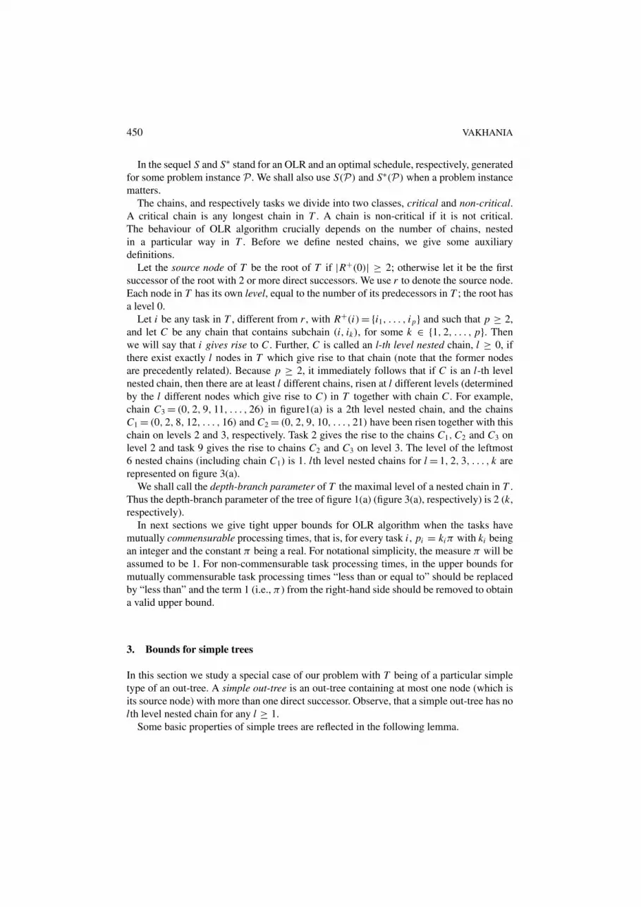
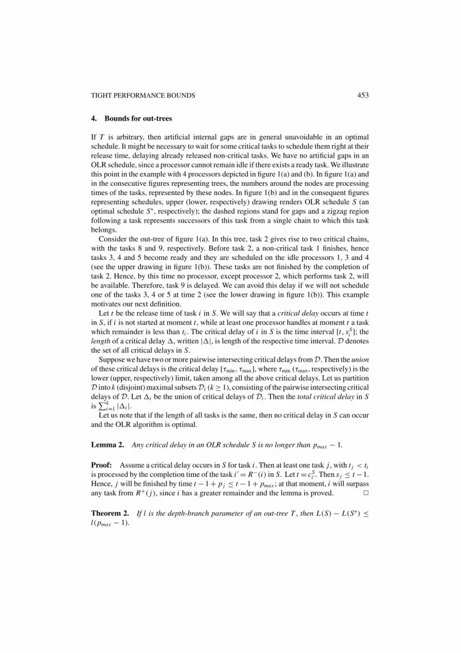
Let i be any task in T , different from r , with R+(i) = {i1, . . . , i p} and such that p ≥ 2,and let C be any chain that contains subchain (i, ik), for some k ∈ {1, 2, . . . , p}. Thenwe will say that i gives rise to C . Further, C is called an l-th level nested chain, l ≥ 0, ifthere exist exactly l nodes in T which give rise to that chain (note that the former nodesare precedently related). Because p ≥ 2, it immediately follows that if C is an l-th levelnested chain, then there are at least l different chains, risen at l different levels (determinedby the l different nodes which give rise to C) in T together with chain C . For example,chain C3 = (0, 2, 9, 11, . . . , 26) in figure1(a) is a 2th level nested chain, and the chainsC1 = (0, 2, 8, 12, . . . , 16) and C2 = (0, 2, 9, 10, . . . , 21) have been risen together with thischain on levels 2 and 3, respectively. Task 2 gives the rise to the chains C1, C2 and C3 onlevel 2 and task 9 gives the rise to chains C2 and C3 on level 3. The level of the leftmost6 nested chains (including chain C1) is 1. lth level nested chains for l = 1, 2, 3, . . . , k arerepresented on figure 3(a).

We shall call the depth-branch parameter of T the maximal level of a nested chain in T .Thus the depth-branch parameter of the tree of figure 1(a) (figure 3(a), respectively) is 2 (k,respectively).

In next sections we give tight upper bounds for OLR algorithm when the tasks havemutually commensurable processing times, that is, for every task i , pi = kiπ with ki beingan integer and the constant π being a real. For notational simplicity, the measure π will beassumed to be 1. For non-commensurable task processing times, in the upper bounds formutually commensurable task processing times “less than or equal to” should be replacedby “less than” and the term 1 (i.e., π ) from the right-hand side should be removed to obtaina valid upper bound.

3. Bounds for simple trees

In this section we study a special case of our problem with T being of a particular simpletype of an out-tree. A simple out-tree is an out-tree containing at most one node (which isits source node) with more than one direct successor. Observe, that a simple out-tree has nolth level nested chain for any l ≥ 1.

Some basic properties of simple trees are reflected in the following lemma.


Figure 1a. An out-tree with the depth-branch parameter 2.

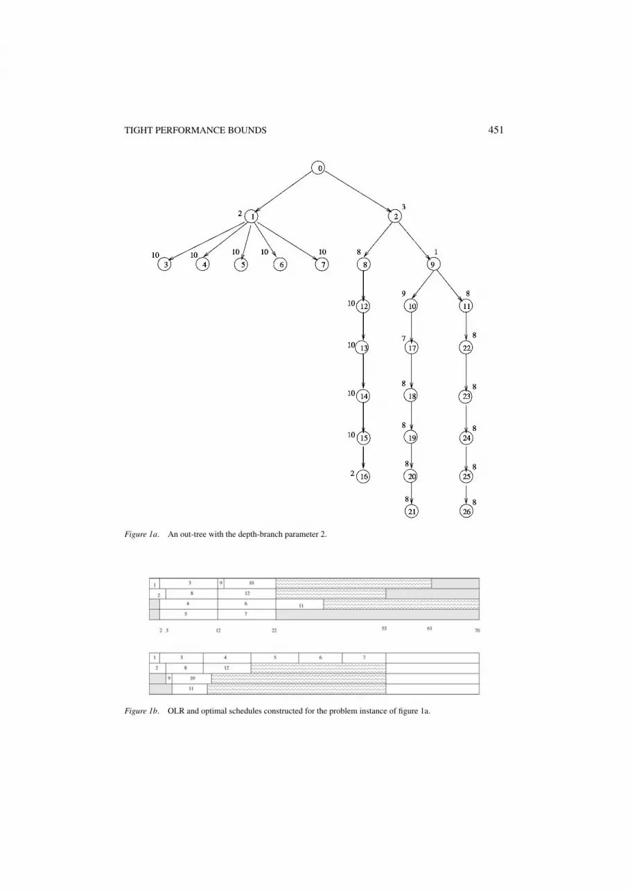
Figure 1b. OLR and optimal schedules constructed for the problem instance of figure 1a.

452 VAKHANIA

Lemma 1. Let T be a simple tree with the source node r , and let a critical chain of T bebroken in an OLR schedule S. Then in S:(i) there exists no internal gap after time cS

r ;(ii) no external gap is longer than pmax .

Proof: Suppose h is the earliest iteration on which a critical chain is broken in S. Let Cbe such a critical chain, interrupted by task j at moment cS

i . We claim that by iteration h,there can be no gap after time cS

r in S, since otherwise j would be scheduled earlier at thebeginning of this gap. Indeed, suppose before iteration h, there raised a gap on a processorP at time t in S, while j was not scheduled at that moment on P . Hence, j was not ready,i.e., a predecessor of j was not completed by time t . Let j ′ be the earliest such predecessorand l be the task, scheduled last on P by iteration h. Task j ′ has to be processed at momentt = cS

l , since otherwise j ′ would be scheduled on P at that moment. Assume both tasksl and j ′ are processed simultaneously on different processors. But the number of chainsis more than m, and hence there exists at least one more chain which is not processed atmoment t . Then a task of that chain would be scheduled at that moment on processor P .Thus, for iteration h, no gap may occur after the moment cS

r in S. Similarly, (i) holds forany subsequent iteration h′ > h.

Now we prove that (ii) holds for iteration h. Indeed, let Q be the processor on whichtask i is scheduled in S. By the definition of S, the completion time of Q is minimalat iteration h, that is, there exists no processor which is idle by time cS

i = CQ(Sh). Thisclearly implies that max{|Ck(Sh) − CQ(Sh)|, k = 1, 2, . . . , m} ≤ pmax . The latter inequalityrepresents condition (ii) for iteration h.

It remains to show that (ii) holds for any subsequent iteration h′. Indeed, if for it-eration h′ all critical chains are already broken, (ii) clearly holds. Now we show thatif there is a critical chain in T which is not broken by iteration h′ in S, then L(S)

≤ cSi + pmax . Indeed, starting from the time cS

i , in no more than pmax time, for eachcritical chain at least one task gets ready. Now since all critical chains have the samelength, at each consequent iteration, all critical chains will be broken before timecS

i + pmax . Thus no external gap will have a length more than pmax and the lemma isproved. ✷

Theorem 1. If T is a simple out-tree then(i) L(S) − L(S∗) ≤ pmax − 1 and

(ii) L(S)/L(S∗) ≤ 1 + pmax/tmax .

Proof: S is optimal if no critical chain is broken in it (because the makespan of S willbe equal to the length of a longest chain in T and it obviously cannot be less). Otherwise,Lemma 2 provides that there will exist no internal gap in S which is not in S∗, since all gapsbefore time cS

r are unavoidable in S∗. Besides, any external gap is no longer than pmax . Itcan be seen that this implies (i).

Since L(S) ≤ L(S∗) + pmax and L(S∗) ≥ tmax , for showing inequality (ii), we let L(S∗)= tmax . Then L(S) ≤ tmax + pmax and we obtain (ii). ✷


4. Bounds for out-trees

If T is arbitrary, then artificial internal gaps are in general unavoidable in an optimalschedule. It might be necessary to wait for some critical tasks to schedule them right at theirrelease time, delaying already released non-critical tasks. We have no artificial gaps in anOLR schedule, since a processor cannot remain idle if there exists a ready task. We illustratethis point in the example with 4 processors depicted in figure 1(a) and (b). In figure 1(a) andin the consecutive figures representing trees, the numbers around the nodes are processingtimes of the tasks, represented by these nodes. In figure 1(b) and in the consequent figuresrepresenting schedules, upper (lower, respectively) drawing renders OLR schedule S (anoptimal schedule S∗, respectively); the dashed regions stand for gaps and a zigzag regionfollowing a task represents successors of this task from a single chain to which this taskbelongs.

Consider the out-tree of figure 1(a). In this tree, task 2 gives rise to two critical chains,with the tasks 8 and 9, respectively. Before task 2, a non-critical task 1 finishes, hencetasks 3, 4 and 5 become ready and they are scheduled on the idle processors 1, 3 and 4(see the upper drawing in figure 1(b)). These tasks are not finished by the completion oftask 2. Hence, by this time no processor, except processor 2, which performs task 2, willbe available. Therefore, task 9 is delayed. We can avoid this delay if we will not scheduleone of the tasks 3, 4 or 5 at time 2 (see the lower drawing in figure 1(b)). This examplemotivates our next definition.

Let t be the release time of task i in S. We will say that a critical delay occurs at time tin S, if i is not started at moment t , while at least one processor handles at moment t a taskwhich remainder is less than ti . The critical delay of i in S is the time interval [t, sS

i ]; thelength of a critical delay �, written |�|, is length of the respective time interval. D denotesthe set of all critical delays in S.

Suppose we have two or more pairwise intersecting critical delays fromD. Then the unionof these critical delays is the critical delay [τmin, τmax], where τmin (τmax, respectively) is thelower (upper, respectively) limit, taken among all the above critical delays. Let us partitionD into k (disjoint) maximal subsetsDi (k ≥ 1), consisting of the pairwise intersecting criticaldelays of D. Let �i be the union of critical delays of Di . Then the total critical delay in Sis

∑ki=1 |�i |.

Let us note that if the length of all tasks is the same, then no critical delay in S can occurand the OLR algorithm is optimal.

Lemma 2. Any critical delay in an OLR schedule S is no longer than pmax − 1.

Proof: Assume a critical delay occurs in S for task i . Then at least one task j , with t j < tiis processed by the completion time of the task i ′ = R−(i) in S. Let t = cS

i ′ . Then s j ≤ t −1.Hence, j will be finished by time t − 1 + p j ≤ t − 1 + pmax ; at that moment, i will surpassany task from R+( j), since i has a greater remainder and the lemma is proved. ✷

Theorem 2. If l is the depth-branch parameter of an out-tree T , then L(S) − L(S∗) ≤l(pmax − 1).

454 VAKHANIA

Proof: Let C be the chain which ends with the latest scheduled task on a processor withthe maximal completion time in S. C has a level no more than l, i.e., there exist no morethan l nodes in T , giving rise to C . Let i ∈ C be any such node and i ′ be the directsuccessor of i from C . Note there may occur a critical delay for i ′ in C only if thereis another direct successor i ′′ of i (belonging a chain, different from C) and ti ′ ≤ ti ′′ .But there are in total l nodes giving rise to C . Hence, there may occur no more than ldelays in C . Each such delay is no longer than pmax − 1 (Lemma 3). Therefore, the totaldelay of chain C , and hence the difference between L(S) and L(S∗), is no more thanl(pmax − 1). ✷

In the following example we show that the inequality in Theorem 2 is attainable provingthat the bound is tight.

Example 1. Consider again the problem instance of figure 1(a). We have 4 processors, threecritical chains C1, C2 and C3 of equal length 53. Task 2 gives rise to all three critical chains,task 9 gives rise to critical chains C2 and C3; thus l = 2 and pmax = 10. The OLR schedule Swith the makespan 70 is represented in figure 1(b). The makespan of an optimal schedule,L(S∗) = tmax = 53 (see again figure 1(b)). In S∗, chains C1, C2 and C3 are scheduled onprocessors 2, 3 and 4 without any critical delay, and the rest of the tasks (tasks 1,3,4,5,6,7)are scheduled on processor 1. There is no external gap in S∗. We have three external gaps inS on processors 1, 2 and 4 with the lengths 9, 18 and 48, respectively. The first critical delayof the length 9 of chains C2 and C3 occurs at time c2 = 3 (task 9 is scheduled at time 12 onprocessor 1). The second critical delay of chain C3 is of the same length and occurs at timec9 = 13 (task 11 is scheduled on processor 3 at time 22), so L(S)− L(S∗) = l(pmax −1) = 2(10 − 1) = 18.

Thus the bound of Theorem 2, which depends linearly on the depth-branch para-meter l, a characteristic of T , is tight. Now we aim to give the worst-case absoluteerror and performance ratio of OLR-algorithm in terms of tmax. Before we study moreexamples.

Example 2. In our next example we have only two equal-length nested critical chainsand 3 processors (figure 2(a)). Task 2 gives rise to both nested critical chains in T with thelength tmax. Tasks 1 and 2 have the lengths 1 and 2, respectively. The duration of non-criticaltasks 3 and 4 is set to (tmax − 1)/2. The makespan of an optimal schedule S∗ is equal totmax (figure 2(b)). At the moment of completion of task 1, tasks 3 and 4 are scheduledon processors 1 and 3 causing the critical delay in S; the makespan of S is the releasetime of processor 1 equal to 1 + (tmax − 1)/2 + tmax − 2 = 3(tmax − 1)/2 (figure 2(b)). ThusL(S) − L(S∗) = (tmax − 3)/2 and L(S)/L(S∗) = 3/2 − 3/(2 tmax).

Example 3. Extending the problem instance of example 1, now we construct a class ofproblems with only two allowed processing times 1 and 2. The behaviour of OLR algorithmfor these problems remains weak, the total critical delay of S approaches [tmax/2]. As in theearlier examples, the makespan of an optimal schedule is tmax.


Figure 2a. An out-tree with two nested critical chains.

Figure 2b. Respective OLR and optimal schedules.

Relying on example 1, we make the following simple observations:

(i) Without violating the desired structure, the processing times of tasks 1 and 2 can betaken equal to 1 and 2, respectively (instead of 2 and 3);

(ii) The duration of any non-critical task which delays a critical chain (in our example anytask from R+(1)), must be no less than 2.

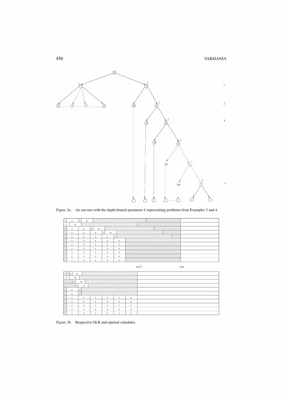
A problem instance and schedules S and S∗ are represented schematically in figure 3(a)and (b). Several problem characteristics which vary depending on tmax, such as the numberof successors of tasks 1 and 2, the number of processors and the critical chains, are notreflected on these figures. We will specify a bit later the number of critical chains and thenumber of processors in terms of tmax.

The structure of T (figure 3(a)) is somewhat similar to the tree of Example 1: R+(0) ={1, 2}, where task 2 gives rise to all critical chains in T , non-critical task 1 is the direct pre-decessor of all the rest of the non-critical tasks (denoted by y − s and z − s in figure 3(a)).These tasks have the duration 2. Each successor of task 2 giving rise to a critical chain is

456 VAKHANIA

Figure 3a. An out-tree with the depth-branch parameter k representing problems from Examples 3 and 4.

Figure 3b. Respective OLR and optimal schedules.


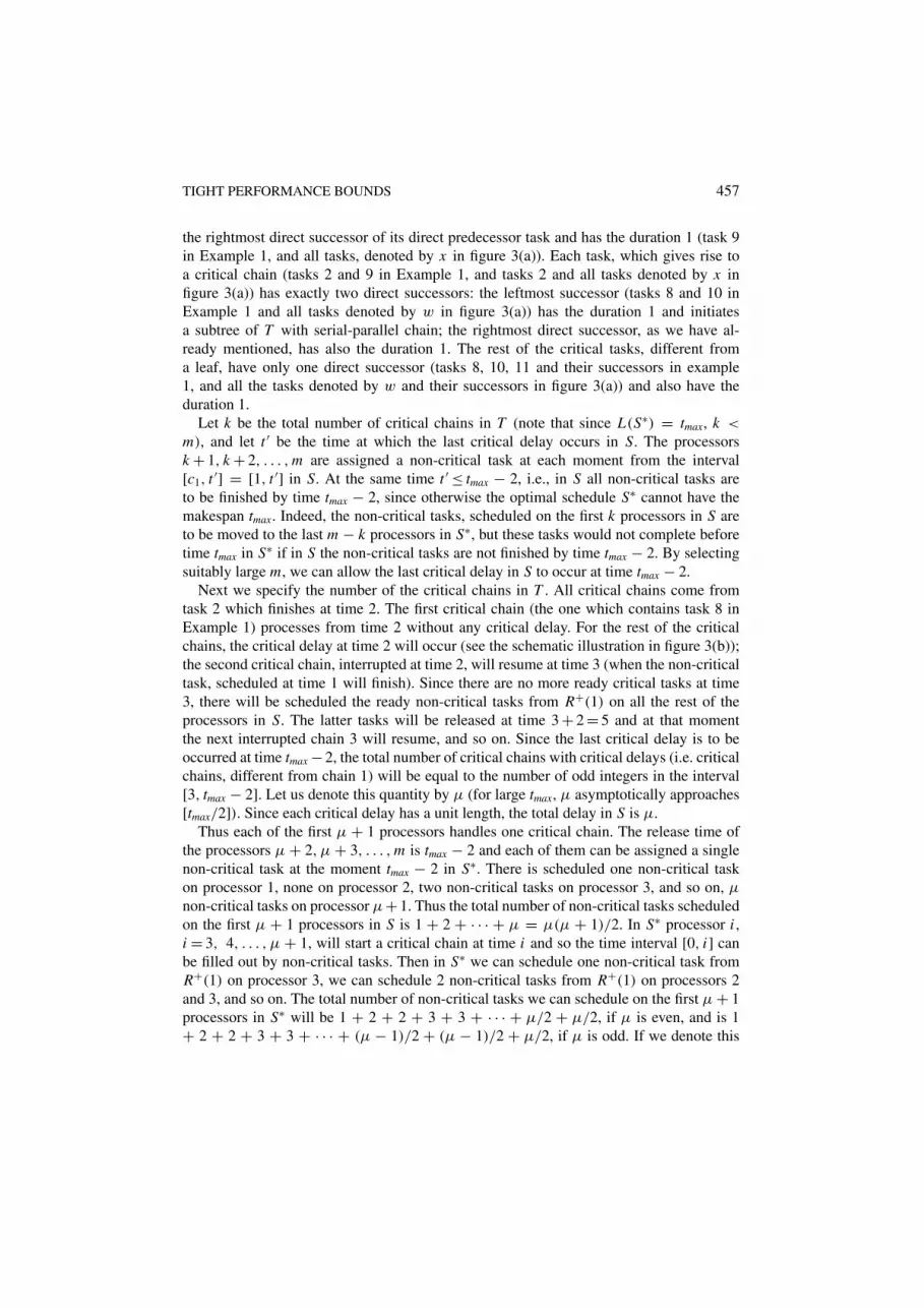
the rightmost direct successor of its direct predecessor task and has the duration 1 (task 9in Example 1, and all tasks, denoted by x in figure 3(a)). Each task, which gives rise toa critical chain (tasks 2 and 9 in Example 1, and tasks 2 and all tasks denoted by x infigure 3(a)) has exactly two direct successors: the leftmost successor (tasks 8 and 10 inExample 1 and all tasks denoted by w in figure 3(a)) has the duration 1 and initiatesa subtree of T with serial-parallel chain; the rightmost direct successor, as we have al-ready mentioned, has also the duration 1. The rest of the critical tasks, different froma leaf, have only one direct successor (tasks 8, 10, 11 and their successors in example1, and all the tasks denoted by w and their successors in figure 3(a)) and also have theduration 1.

Let k be the total number of critical chains in T (note that since L(S∗) = tmax, k <

m), and let t ′ be the time at which the last critical delay occurs in S. The processorsk + 1, k + 2, . . . , m are assigned a non-critical task at each moment from the interval[c1, t ′] = [1, t ′] in S. At the same time t ′ ≤ tmax − 2, i.e., in S all non-critical tasks areto be finished by time tmax − 2, since otherwise the optimal schedule S∗ cannot have themakespan tmax. Indeed, the non-critical tasks, scheduled on the first k processors in S areto be moved to the last m − k processors in S∗, but these tasks would not complete beforetime tmax in S∗ if in S the non-critical tasks are not finished by time tmax − 2. By selectingsuitably large m, we can allow the last critical delay in S to occur at time tmax − 2.

Next we specify the number of the critical chains in T . All critical chains come fromtask 2 which finishes at time 2. The first critical chain (the one which contains task 8 inExample 1) processes from time 2 without any critical delay. For the rest of the criticalchains, the critical delay at time 2 will occur (see the schematic illustration in figure 3(b));the second critical chain, interrupted at time 2, will resume at time 3 (when the non-criticaltask, scheduled at time 1 will finish). Since there are no more ready critical tasks at time3, there will be scheduled the ready non-critical tasks from R+(1) on all the rest of theprocessors in S. The latter tasks will be released at time 3 + 2 = 5 and at that momentthe next interrupted chain 3 will resume, and so on. Since the last critical delay is to beoccurred at time tmax − 2, the total number of critical chains with critical delays (i.e. criticalchains, different from chain 1) will be equal to the number of odd integers in the interval[3, tmax − 2]. Let us denote this quantity by µ (for large tmax, µ asymptotically approaches[tmax/2]). Since each critical delay has a unit length, the total delay in S is µ.

Thus each of the first µ + 1 processors handles one critical chain. The release time ofthe processors µ + 2, µ + 3, . . . , m is tmax − 2 and each of them can be assigned a singlenon-critical task at the moment tmax − 2 in S∗. There is scheduled one non-critical taskon processor 1, none on processor 2, two non-critical tasks on processor 3, and so on, µ

non-critical tasks on processor µ+ 1. Thus the total number of non-critical tasks scheduledon the first µ + 1 processors in S is 1 + 2 + · · · + µ = µ(µ + 1)/2. In S∗ processor i ,i = 3, 4, . . . , µ + 1, will start a critical chain at time i and so the time interval [0, i] canbe filled out by non-critical tasks. Then in S∗ we can schedule one non-critical task fromR+(1) on processor 3, we can schedule 2 non-critical tasks from R+(1) on processors 2and 3, and so on. The total number of non-critical tasks we can schedule on the first µ + 1processors in S∗ will be 1 + 2 + 2 + 3 + 3 + · · · + µ/2 + µ/2, if µ is even, and is 1+ 2 + 2 + 3 + 3 + · · · + (µ − 1)/2 + (µ − 1)/2 + µ/2, if µ is odd. If we denote this

458 VAKHANIA

quantity by π , then we obtain that the total number of processors m = µ+ 1 + (µ(µ+ 1)/

2 − π).

Example 4. In this example we construct the class of problems for which, as we willsee later, OLR algorithm shows its worst behavior. We keep the structure of T and thebasic features from Example 3, but we allow a task of R+(1) to take a processing time,different from 2 to maximize the overall critical delay in S. We use again figure 3(a) and(b) for the schematic representation of T and schedules S and S∗. In these figures y − sand z − s represent the non-critical tasks of R+(1), which are scheduled on the first kprocessors and on the last m − k processors, respectively in S (k again stands for thetotal number of critical chains). x − s represent critical tasks, different from task 2, givingrise to critical chains. As before, tasks 1 and 2 with durations 1 and 2 are scheduled onprocessors 1 and 2, respectively. Each w represents the direct successor of a task x or task2 and has the duration, equal to that of any non-critical task (we shall below specify thisvalue).

Processing time 2 of the non-critical tasks of R+(1) in Example 3, in general, does notyield the maximal critical delay for S. First observe, that since the makespan of an optimalschedule is tmax, no non-critical task can have a duration, more than (tmax − 1)/2 (recall thatnon-critical tasks from R+(1) cannot start earlier than at time 1 = cS

1 ); indeed, otherwise thenumber of processors should be the same as the number of critical chains plus the numberof all non-critical tasks, but in this case no critical delay can occur in S.

Next we show that the processing times of all non-critical tasks from R+(1) should bethe same. As we have observed in Example 3, in S there are scheduled i − 1 non-criticaltasks on processor i , i = 3, . . . , k, we have one non-critical task scheduled on processor 1and none on processor 2. These non-critical tasks are denoted by ys and we use Y to denotethe whole set of these tasks. To sustain a non-delay starting of each critical chain on thefirst k processors, we should move some tasks of Y to processors k + 1, . . . , m in S∗. Allnon-critical tasks, scheduled at the same moment in S should have equal duration, sinceotherwise the respective critical delay would be determined by task(s) with the smallestduration. Hence, each non-critical task, scheduled last on processors k + 1, . . . , m willfinish at the same time t ′. So the free available time slots, starting at time t ′ on each of theseprocessors, have the same length tmax − t ′. Since in S∗ these time slots are to be occupied bytasks of Y , the processing times of these tasks cannot exceed tmax − t ′; they can be less, butthis would not lead us to a greater critical delay in S. The latter tasks of Y will necessarilyinclude tasks scheduled at different time moments in S, which obviously implies that all thetasks of Y should have the same length p∗ = tmax − t ′. Then all the tasks of R+(1) shouldalso have the same length, as all tasks scheduled at the same time in S have equal duration.

Now we look for p∗ which yields the maximal overall critical delay in S. p∗ is to be somefraction of τ = tmax −1 and it cannot be more than τ/2, hence p∗ = τ/ν, ν ∈ {2, 3, . . .}. Tofind ν, note that the maximal possible overall critical delay δ in S will be (ν − 1)(τ/ν − 1),as each delay can last no more than τ/ν − 1 time (Lemma 3) and we can schedule no morethan ν − 1 non-critical tasks before time tmax on each processor in S. Using elementarycalculus, we can find that the maximum of the above expression is (

√τ − 1)2 achieved for

ν = √τ . Thus δ = (

√τ − 1)2 for ν = τ̃ , where τ̃ = √

τ , if the latter magnitude is integer


and otherwise it is the nearest integer, either �√τ� or �√τ�, maximizing the expression(√

τ − 1)2.It is easy to see that k = ν. As in Example 3, to determine m we let m − k = |Y | − π

(π being defined as in Example 3). Now in S∗ only on processors k − 1 and k a sin-gle non-critical task from R+(1) can be scheduled (p∗ got “essentially” longer thanin Example 3), hence π = 2. The non-critical tasks from Y , scheduled on processors1, 2, . . . , k before the critical chains in S and which cannot be scheduled on these pro-cessors in S∗, are moved to the available time slot [tmax − p∗, tmax] on each processork + 1, . . . , m. Now since |Y | = 1 + 2 + 3 + · · · + ν − 1 = ν(ν − 1)/2, we obtain that

m = ν + ν(ν − 1)/2 − 2 = ν(ν + 1)/2 − 2,

or in terms of tmax

m = τ̃ (τ̃ + 1)/2 − 2.

Theorem 3. For an arbitrary OLR schedule S and the respective optimal schedule S∗,L(S)− L(S∗) ≤ (

√tmax − 1 − 1)2 and L(S)/L(S∗) ≤ 2 − 2

√tmax − 1/tmax. These bounds

are tight.

Proof: In this prove we use S and S∗ for S(P) and S∗(P), respectively, where P is someproblem instance. Let first P be any problem instance with L(S∗) = tmax and let k ≥ 2 bethe total number of critical chains in T . Without loss of generality, let us assume that allnested chains in T are critical, for if some of them were non-critical, the maximal delaywould be obviously no more than that for P .

Let Pmax be a problem instance, such that L(S∗(Pmax)) = tmax and with the maximalpossible overall critical delay for this tmax. Let T ′ be the precedence tree of Pmax. Based onthe earlier considered examples, it can be easily verified the following. In T ′, R+(0) �= ∅and there must exist one non-critical task i1 (task 1 in our examples) and one critical task i2

(task 2 in our examples) giving rise to all nested critical chains in it (note that the existenceof 2 or more critical tasks giving rise to another critical chains would not increase the totalcritical delay). Besides, pi1 should have the minimal possible duration which is 1, and pi2

should have a minimal possible duration, greater than pi1 , which is 2. Let i be any criticaltask giving rise to a critical chain in T ′. We must have pi = 1 for i �= i2. The leftmost directsuccessor of each task i and task 2 (denoted by w − s in figure 3(a) and (b)) should becompleted no earlier than at the completion time of a corresponding non-critical task, sinceotherwise the next critical task (the next x) will be scheduled earlier than at the completiontime of that non-critical task and the total critical delay will be decreased as compared tothat of Example 4. So the processing time of each task w should be “large enough,” inparticular it suffices p∗. Further, it can be assumed that |R+(i)| = 2, since |R+(i)| > 2would imply two or more critical chains with the same critical delay in S(Pmax), whichagain would not lead us to a greater total critical delay in S(P ′). Hence, without loss ofgenerality, it might be assumed that R+(0) = {i1, i2}. Neither the existence of non-criticaltasks in R+(0), different from i1, can lead us to a greater overall critical delay. And without

460 VAKHANIA

loss of generality we can assume, that all non-critical tasks are the direct successors oftask 1. Thus problem Pmax belongs to the class of problems from Example 4 and hence thetheorem holds.

Now assume that P is such that L(S∗) > tmax. If there exists no non-critical task inT , then there will be no critical delay in S and S will be optimal. Suppose there arenon-critical tasks in P , and let Pc be the problem instance in which all these tasks areremoved from P (i.e., there are only the tasks of the longest chains in Pc). Either (i)L(S∗(Pc)) = tmax (i.e., all longest chains can be processed on the m processors withoutany delay) or (ii) L(S∗(Pc)) > tmax (i.e., some critical chain(s) must be processed after theothers are finished).

Case (i). Let P4 be the problem instance of Example 4 with L(S∗(P4)) = tmax, con-structed from P by suitably increasing the number of processors, and the number of non-critical tasks respectively. The theorem holds for P4. It will also hold for P if the totalcritical delay in S is no more than that in S(P4). Assume that this is not the case. Thenthere must occur a critical delay after moment tmax − 2 in S. Let σ ≥ 1 be the total criticaldelay occured after moment tmax − 2 in S. Using again Examples 3 and 4, we can easily seethat the makespan of S∗ will be more than σ time units longer than that of S∗(P4), whichimplies our claim.

The proof of the case (ii) is similar to the above case. Indeed, the number of nested criticalchains is more than m. This implies that at least one critical chain C is interrupted in S∗ andresumed at time tmax (when the first critical chain finishes). Let t ′ be the time of interruptionof C in S∗ and let P4 be the problem instance, defined as in case (i). The interruption of Cimplies the increase of the makespan of S∗ by at least tmax − t ′ in comparison with that ofS∗(P4). But the total critical delay, we may have after the moment tmax in S is again lessthan that.

We have seen in Example 4 that δ = (√

tmax − 1 − 1)2, besides, L(S) = L(S∗) + δ andL(S∗) = tmax. This imply that both inequalities are attainable. Thus the bounds are tightand the theorem is proved. ✷

5. Non-clairvoyant model

In this section we consider the non-clairvoyant version of our model. For this model wecannot apply any remainder-dependent algorithm, such as OLR. A random search randomlyselects a ready task at each iteration. It needs no information about ready tasks, except theset of ready tasks itself. Other rule of choice would be dependent on some extra taskdata, for example, on pi . In our model pi is not known by the release time of i . Even inthe clairvoyant version with known pi s the siltation does not gets essentially better, sincepi tells us a little about the real “urgency” of task i (hence a processing time dependentchoice would be very similar to a random search). We know for each moment t the releasetime of all released by that moment tasks. This gives us a choice among all released tasks(unlike on-line over list models, in on-line over time models, such as our model, a tasknot necessarily need to be scheduled immediately at its release time; also note that if tasksi, j ∈ T have different release times, then they have different direct predecessors in ourmodel).


We can use two basic release time dependent heuristics: (a) to serve first tasks with smallerrelease times (that is, to serve tasks in the order of their appearance) or (b) to serve first taskswith greater release times (that is, to serve tasks in the opposite order of their appearance).In terms of the trees, these two strategies (a) and (b) imply the width-first search (WS) anddepth-first search (DS), respectively. For WS we expand T level-by-level in width, while forDS we expand it in depth, extending latest generated nodes first. For the definiteness, assumethat the nodes, corresponding to the tasks with the equal readiness time are extended fromleft to right. We note that in both search strategies (like in OLR algorithm), no processorremains idle as long as there exists a ready task. Any such heuristic will give us a solutionwhich makespan is less than twice the makespan of an optimal schedule (Graham, 1996).

Here we compare WS and DS showing that the worst-case performance of WS is alwaysbetter or the same as that of DS, in the other words, WS never yields a worse schedulethan DS. There are several situations, when both search strategies give the same results, forexample, when all chains have equal length.

Intuitively, the search in width allocates tasks from all the branchings equally, givingthe same priority to all tasks, while the search in depth gives priority to the tasks of somebranchings, “forgetting” about the tasks from the other branchings. If DS would “guess”correctly the urgent branchings it could give a better result, however the latter would bea purely random event. On the other hand, the search in width gives the equal attentionto all chains and hence an urgent one cannot be completely “forgotten”. We illustrate thispoint in figure 4a and (b). In figure 4a is depicted the out-tree with unit-time tasks and onecritical chain (the last chain 4); the root is denoted by r , and the tasks of chain 1 (2, 3 and4, respectively) are denoted by xs (zs, ws and ys, respectively). The corresponding DS andWS schedules are represented in the upper and lower parts, respectively, of figure 4b. Aswe can see, WS schedule is better than DS schedule in this example.

To estimate the worst-case behavior of DS and WS we look for the problems, for whichDS and WS show their worst behavior. Denote by Pd and Pw a problem instance fromthe above “worst” type of problems for DS and WS, respectively; denote by Sd and Sw

depth-first and width-first, respectively schedule for problem Pd and Pw, respectively. Inboth, Sd and Sw, the critical chains have to be processed above all chains. Let T d be thetree of problem Pd . DS extends the branchings in depth, i.e., it schedules completely allthe chains it starts before it processes another chain, from left to right. It is easily seen thatT d should contain only one critical chain, say C , being the rightmost chain in T d . Clearly,if the total number of chains is more than m (if not, we obtain an optimal schedule by both,DS and WS), then there should exist a time moment τd in Sd such that all processors, exceptthe one performing C , are idle after that time (time 3 in the example of figure 4).

It is easily seen that Pw = Pd . Similarly, let τw be a time moment in Sw, after which allprocessors, except the one performing C , are idle (if there exists no τw, Sw is optimal). Letus compare L(Sw) and L(Sd). Let I = T \C , so τw (τd , respectively) is the total completiontime of tasks of I in Sw (Sd , respectively). There holds τd ≤ τw, since in Sw, besides tasksof I , l (0 ≤ l < k) tasks of C are scheduled before time τw. Denote the set of these tasksby I ′. Clearly, τd − τw ≤ ∑

i∈I ′ pi . After the moment τd , all l tasks from I ′ are scheduledon a single machine in Sd , while these tasks have been already scheduled by time τw in Sw.Then it obviously follows that L(Sw) ≤ L(Sd).

462 VAKHANIA

Figure 4a. An out-tree with one critical chain.

Figure 4b. Respective DS and WS schedules.

6. Concluding remarks

We have suggested two on-line models of multiprocessor scheduling with out-trees. For thefirst strongly clairvoyant model we obtained tight worst-case ratio and absolute error forOLR algorithm. Better bounds were found for simple out-trees. For the second


non-clairvoyant model we showed that the worst-case behavior of the width-first searchis never worse than that of the depth-first search.

The worst-case ratio for simple out-trees is close to 1 if tmax is sufficiently larger thanpmax. The worst-case ratio for general out-trees approaches 2 for large tmax, while we havea similar asymptotic bound for an arbitrary list schedule and arbitrary precedence relations.However, the situation is not as bad as it might seem from the first glance. As we haveseen in Section 3, our bound is reached for a specific values of m, in particular, whenm = τ̃ (τ̃ + 1)/2 − 2. If sufficiently large or sufficiently small value for m is selected, thenthe total critical delay decreases and the worst-case behaviour is better.

Is it possible to have a worst-case ratio, approaching a number, strictly less than 2 forgeneral trees, or for special tree-structures which are more general than simple trees? In anOLR schedule S, if non-critical jobs get released before some other critical jobs, then thenon-critical jobs, scheduled before the critical ones may cause a critical delay in S. Hence“artificial” internal gaps are, in general, unavoidable in an optimal schedule. If we wish toimprove the performance of the OLR algorithm, we have to deal with such internal gaps.An OLR algorithm with an incorporated waiting strategy may reduce the total critical delayand hence give better performance bounds. Allowing task restarts in OLR algorithm alsomight be beneficial (Akker et al., 2000) have recently shown the usefulness of restarts forthe makespan minimization in a clairvoyant on-line over time model with a single machine).

Acknowledgments

The author is grateful to Andrei Tchernykh for his initiative and to Klaus Ecker and DenisTrystram for their interest in this work. This work was supported by CONACyT grant28937A.

Notes

1. There is some similarity between a “reminder” and the commonly used in the scheduling literature term “tail”,although there is a basic difference, that unlike a tail, a reminder needs a processor time.

2. In scheduling over list a released from a list task is immediately scheduled on a processor, whereas in our modela released task not necessarily needs to be scheduled at its release time.

3. Our bounds can be also expressed in terms of m, since m can be expressed in terms of tmax .4. For the sake of conciseness of the description, here the definition of a processor completion time slightly differs

from the earlier given definition.

References

M. van den Akker, J. Hoogeveen, and N. Vakhania, “Restarts can help in on-line minimization of the maximumdelivery time on a single machine,” Journal of Scheduling, vol. 3, pp. 333–341, 2000.

S. Albers, “Better bounds for online scheduling,” Proc. of the 29th Ann. ACM Symp. on Theory of Computing,ACM, 1997, pp. 130–139.

N.F. Chen and C.L. Liu, “On a class of scheduling algorithms for multiprocessors computing systems,” ParallelProcessing, Lecture Notes in Computer Science, T.Y. Feng (Ed.), Springer: Berlin, vol. 24, pp. 1–16, 1975.

464 VAKHANIA

B. Chen, C.N. Potts, and G.J. Woeginger, “A review of machine scheduling: Complexity, algorithms and approx-imability,” Handbook of Combinatorial Optimization, vol. 3, D.Z. Du and P. Pardalos (Eds.). Kluwer AcademicPublishers: Dordrecht, 1998, pp. 21–169.

E.G. Coffman, Jr and R.L. Graham, “Optimal scheduling for two-processor systems,” Acta Informatica, vol. 1,pp. 200–213, 1972.

D.K. Freisen, “Tighter bounds for the multifit processor scheduling algorithm,” SIAM J. on Comput., vol. 13,pp. 170–181, 1984.

M. Fujii, T. Kasami, and K. Nimomiya, “Optimal sequencing of two equivalent processors,” SIAM J. Appl. Math.,vol. 14, pp.784–789, 1969.

H.N. Gabow and R.E. Tarjan, “A linear-time algorithm for a special case of disjoint set union,” J. Comput. SystemSci., vol. 30, pp. 209–221, 1985.

G. Galambos and G.J. Woeginger, “An on-line scheduling heuristic with better worst case ratio than Graham’s listscheduling,” SIAM J. Comput., vol. 22, pp. 349–355, 1993.

R.L. Graham, “Bounds for certain multiprocessing anomalies,” Bell Syst. Tech. J., vol. 45, pp. 1563–1581, 1966.R.L. Graham, “Bounds on multiprocessing timing anomalies,” SIAM J. Applied Math., vol. 17, pp. 416–429, 1969.D.S. Hochbaum and D.B. Shmoys, “A polynomial approximation scheme for scheduling on uniform processors:

Using the dual approximation approach,” SIAM J. Comput., vol. 17, no. 3, pp. 539–551, 1988.N.C. Hsu, “Elementary proof of Hu’s theorem on isotone mappings,” Proc. Amer. Math. Soc., vol. 17, pp. 11–114,

1966.T.C. Hu, “Parallel sequencing and assembly line problems,” Oper. Res., vol. 9, pp. 841–848, 1961.D.R. Karger, S.J. Phillips, and E. Torng, “A better algorithm for ancient scheduling problem,” J. of Algorithms,

vol. 20, pp. 400–430, 1996.M.T. Kaufman, “An almost-optimal algorithm for the assembly line scheduling problem,” IEEE Trarns. on

Computers, C-23, pp. 1170–1174, 1974.M. Kunde, “Beste Schranken biem LP-scheduling,” Institut fur Informatic und Prakt. Math., Bericht 7603,

Universitat Kiel, 1976.M. Kunde, “Nonpreemptive LP-scheduling on homogeneous multiprocessor system,” SIAM J. Comput., vol. 10,

pp. 151–173, 1981.S. Lam and R. Sethi, “Worst case analysis of two scheduling algorithms,” SIAM J. Comput., vol. 6, pp. 518–536,

1977.E.L. Lawler, J.K. Lenstra, A.H.G. Rinnooy Kan, and D.B. Shmoys, “Sequencing and scheduling: Algorithms

and complexity,” Handbooks in Operations Research and Management Science, vol. 4, S.C. Graves, A.H.G.Rinnooy Kan, and P. Zipkin (Eds.), North Holland: Amsterdam, 1993.

J.K. Lenstra and A.H.G. Rinnooy Kan, “Complexity of scheduling under precedence constraints,” Oper. Res.,vol. 26, pp. 22–35, 1978.

R. Sethi, “Algorithms for minimal-length schedules,” Computer and Job/Shop Scheduling Theory, E.G. CoffmanJr. (Ed.), Wiley: New York, 1976, pp. 51–59.

J. Sgall, “On-line scheduling—A servey,” A. Fiat and G.J. Woeginger (Eds.), Online algorithms: The state of theart, Springer, 1998.

J.D. Ullman, “NP-complete scheduling problems,” J. Computer System Sci., vol. 10, pp. 384–393, 1975.M. Yue, “On the exact upper bound for the multifit processor scheduling algorithm,” Ann. Oper. Res., vol. 24,

pp. 233–259, 1990.

tight performance bounds of cp-scheduling on out-trees

Documents