cp violation
TRANSCRIPT

CP Violation
P. Kooijman & N. Tuning
April 2011
The mirror on my wallCasts an image dark and smallBut I’m not sure at allIt’s my reflection
P.Simon“Flowers never bend with the rainfall”


ii

Table of contents
Introduction 1
1 CP Violation in the Standard Model 3
1.1 Parity transformation . . . . . . . . . . . . . . . . . . . . . . . . . . . . . . 3
1.1.1 The Wu-experiment: 60Co decay . . . . . . . . . . . . . . . . . . . . 4
1.1.2 Parity violation . . . . . . . . . . . . . . . . . . . . . . . . . . . . . 5
1.1.3 CPT . . . . . . . . . . . . . . . . . . . . . . . . . . . . . . . . . . . 7
1.2 C, P and T: Discrete symmetries in Maxwell’s equations . . . . . . . . . . 8
1.3 C, P and T: Discrete symmetries in QED . . . . . . . . . . . . . . . . . . . 9
1.4 CP violation and the Standard Model Lagrangian . . . . . . . . . . . . . . 12
1.4.1 Yukawa couplings and the Origin of Quark Mixing . . . . . . . . . . 12
1.4.2 CP violation . . . . . . . . . . . . . . . . . . . . . . . . . . . . . . . 15
2 The Cabibbo-Kobayashi-Maskawa Matrix 17
2.1 Unitarity Triangle(s) . . . . . . . . . . . . . . . . . . . . . . . . . . . . . . 17
2.2 Size of matrix elements . . . . . . . . . . . . . . . . . . . . . . . . . . . . . 20
2.3 Wolfenstein parameterization . . . . . . . . . . . . . . . . . . . . . . . . . 23
2.4 Discussion . . . . . . . . . . . . . . . . . . . . . . . . . . . . . . . . . . . . 26
3 Neutral Meson Decays 27
3.1 Neutral Meson Oscillations . . . . . . . . . . . . . . . . . . . . . . . . . . . 27
3.2 The mass and decay matrix . . . . . . . . . . . . . . . . . . . . . . . . . . 27
iii

iv Table of contents
3.3 Eigenvalues and -vectors of Mass-decay Matrix . . . . . . . . . . . . . . . . 29
3.4 Time evolution . . . . . . . . . . . . . . . . . . . . . . . . . . . . . . . . . 31
3.5 The Amplitude of the Box diagram . . . . . . . . . . . . . . . . . . . . . . 33
3.6 Meson Decays . . . . . . . . . . . . . . . . . . . . . . . . . . . . . . . . . . 37
3.7 Classification of CP Violating Effects . . . . . . . . . . . . . . . . . . . . . 38
4 CP violation in the B-system 41
4.1 β: the B0 → J/ψK0S decay . . . . . . . . . . . . . . . . . . . . . . . . . . . 42
4.2 βs: the B0s → J/ψφ decay . . . . . . . . . . . . . . . . . . . . . . . . . . . 47
4.3 γ: the B0s → D±
s K∓ decay . . . . . . . . . . . . . . . . . . . . . . . . . . . 49
4.4 Direct CP violation: the B0 → π−K+ decay . . . . . . . . . . . . . . . . . 51
4.5 CP violation in mixing: the B0 → l+νX decay . . . . . . . . . . . . . . . . 52
4.6 Penguin diagram: the B0 → φK0S decay . . . . . . . . . . . . . . . . . . . . 53
5 CP violation in the K-system 55
5.1 CP and pions . . . . . . . . . . . . . . . . . . . . . . . . . . . . . . . . . . 55
5.2 Description of the K-system . . . . . . . . . . . . . . . . . . . . . . . . . . 57
5.3 The Cronin-Fitch experiment . . . . . . . . . . . . . . . . . . . . . . . . . 58
5.3.1 Regeneration . . . . . . . . . . . . . . . . . . . . . . . . . . . . . . 60
5.4 Master Equations in the Kaon System . . . . . . . . . . . . . . . . . . . . 61
5.5 CP violation in mixing: ǫ . . . . . . . . . . . . . . . . . . . . . . . . . . . . 62
5.6 CP violation in decay: ǫ′ . . . . . . . . . . . . . . . . . . . . . . . . . . . . 63
5.7 CP violation in interference . . . . . . . . . . . . . . . . . . . . . . . . . . 65
6 Experimental Aspects and Present Knowledge of Unitarity Triangle 67
6.1 B-meson production . . . . . . . . . . . . . . . . . . . . . . . . . . . . . . 67
6.2 Flavour Tagging . . . . . . . . . . . . . . . . . . . . . . . . . . . . . . . . . 71
6.3 Present Knowledge on Unitarity Triangle . . . . . . . . . . . . . . . . . . 72
6.3.1 Measurement of sin 2β . . . . . . . . . . . . . . . . . . . . . . . . . 73

Table of contents v
6.3.2 Measurement of ǫK . . . . . . . . . . . . . . . . . . . . . . . . . . . 73
6.3.3 |Vub/Vcb| . . . . . . . . . . . . . . . . . . . . . . . . . . . . . . . . . 74
6.3.4 Measurement of ∆m . . . . . . . . . . . . . . . . . . . . . . . . . . 74
6.4 Outlook: the LHCb experiment . . . . . . . . . . . . . . . . . . . . . . . . 77
References 79

Introduction
In these lectures we will introduce the subject of CP violation. This subject is oftenreferred to with the more general term “Flavour Physics” since all the interesting stuffconcerning CP violation happens in the weak (charged current) interaction when onequark-flavour changes into another quark-flavour, q →Wq′, even between different fami-lies!
The charged current interactions q →Wq′ form a central element in the Standard Model.Out of the 18 free parameters in the Standard Model, no less than four are related to thecoupling constants of the interaction q → Wq′. In addition, we will see that the origin ofthese coupling constants is closely related (through the Yukawa couplings) to the massesof the fermions, which form another nine free parameters of the Standard Model. Both themasses of the fermions and the coupling strength of the charged-current quark-couplingsform an intruiging, hierarchial, pattern for which some underlying mechanism must exist...
The CP operation changes particles into anti-particles, and changes the coupling constantof q → Wq′ into its complex conjugate. It turns out that not all processes are invariantunder the CP operation and we will show how these complex numbers are determined.In fact, the observation of CP violation allows us to make a convention-free definitionof matter, with respect to anti-matter 1! Maybe not surprising, CP violation is indeedone of the requirements needed to create a universe that is dominated by matter (or byanti-matter for that matter...).
Although CP violation was first discovered in the K-system in 1964, in recent years mostexperimental and theoretical developments in the field of flavour physics occur in theB-system and as a result the term “B-physics” is intimately related to flavour physics.The study of B-mesons and their decays is not only interesting for the above mentionedreasons. Many observables in B-physics are dominated by higher order diagrams, andtherefore these measurements are extremely sensitive to extra contributions from new,virtual, heavy particles, such as the supersymmetric partners of the Standard Modelparticles.
1This could be of importance in a telephone call with aliens, before the first hand-shake. If they ask tomeet you, first ask them what the charge of the lepton is to which the neutral kaon preferentially decays.If that is equal to the charge of the orbiting leptons in atoms, you are in business and can savely fix theterm...
1

2 Table of contents
Very interesting topics such as baryogenesis, sphalerons, the strong CP problem, or neu-trino oscillations unfortunately fall beyond the scope of these lectures. These lectures willfocus on “normal” CP violation (also known as the Kobayashi Maskawa mechanism, forwhich these gentlemen were awarded the Nobel Prize in 2008), and its direct connectionto the Standard Model, see Fig. 1.
The lectures are organized as follows. We start with the Standard Model Lagrangian andsee where the flavour (and even family) changing interactions originate. This leads to thefamous CKM-matrix which is discussed in chapter 2. We continue with the description ofneutral mesons and their decays in chapter 3. This will be of importance for the discussionof measurements of some important B-decays in chapter 4. The historically importantbut less instructive K-system is discussed in chapter 5. We conclude with a discussion onexperimental aspects and the present status of knowledge of CP violation in the StandardModel.
Most facts in these notes are taken from two excellent books on the topic, Bigi & Sanda [1]and Branco & Da Silva [2].
Figure 1: “Nature’s grand tapestry”. [1]

Chapter 1
CP Violation in the Standard Model
1.1 Parity transformation
The parity operator, P, inverts all space coordinates used in the description of a physicalprocess. Consider for instance a scalar wavefunction ψ(x, y, z, t). Performing the parityoperation on this wavefunction will transform it to ψ(−x,−y,−z, t), or
Pψ(x, y, z, t) = ψ(−x,−y,−z, t)The parity transformation can be viewed as a mirroring with respect to a plane, (forinstance z → −z) followed by a rotation around an axis perpendicular to the plane (thez-axis). As angular momentum is conserved, physics will be invariant under the rotationand so the parity operation tests for invariance to mirroring w.r.t. a plane of arbitraryorientation. Parity conservation or P-symmetry implies that any physical process willproceed identically when viewed in mirror image. This sounds rather natural. After allwe would not expect a dice for instance to produce a different distribution of numbers ifone swaps the position of the one and the six on the dice.
Up until 1956 the general feeling was that all physical processes would conserve parity. Inthis year, however, a number of experiments were performed which showed that at leastfor processes involving the weak interaction this was not the case. For both experimentswhich will be discussed the properties of the transformation of spin by the parity operationplayed a crucial role, so let us consider how spin transforms.
Spin like angular momentum transforms as the cross product of a space vector and amomentum vector.
~L = ~r × ~p
P~r = −~rP~p = −~p
and soP ~L = ~L
3

4 Chapter 1 CP Violation in the Standard Model
In other words the parity operation leaves the direction of the spin unchanged. If one canthus find a process which produces an asymmetric distribution with respect to the spindirection one proves that P-symmetry is not conserved. Another way of looking at it isby considering helicity which is the projection of the spin of a particle onto its directionof motion,
h =1
2~σ � p
As helicity changes sign under parity transformation (~p → −~p) finding a process whichproduces a particle with a prefered helicity also proves that P-symmetry is violated.
1.1.1 The Wu-experiment: 60Co decay
The experiment performed by Wu [3] in 1956 took a 60Co source and placed it in amagnetic field. The 60Co nucleus has spin 5 and becomes polarised along the magneticfield lines. The experimental aparatus is shown in Fig. 1.1a. The experimental method
(a) (b)
Figure 1.1: (a) The experimental configuration of the Wu experiment. The NaI coun-ters monitor the state of polarisation by measuring the anisotropy of successive γ emis-sions produced through the polarisation technique. The anthracene crystal measures theβ-electrons. (b) The result of the Wu experiment. The top plot shows the rate as afunction of time for the two NaI counters, the center shows the degree of polarisationdetermined from the anisotropy. The lowest plot shows the measured β counting rates forpositive and negative magnetic field directions.

1.1 Parity transformation 5
ν_
ν_
Co60 Ni60
e
e
Co60 Ni60
A B
(S=5) (S=4) (S=5) (S=4)
Figure 1.2: The possible transitions of 60Co with spin 5 to 60Ni with spin 4. The openarrows denote the spin. Closed arrows denote the momentum vector. (a) The transitionwhich is forbidden in nature. (b) The allowed transition. The antineutrino is alwaysrighthanded.
was then to measure the rate of β-electrons from the decay:
6027Co →60
28 Ni + e− + νe
in a small counter placed at small angles with respect to the field lines. By inverting themagnetic field direction and thus the polarisation of the cobalt nucleus, a difference incounting rate could be detected, as shown in Fig. 1.1b. Several control counters were alsoread out so that the degree of polarisation and the absolute counting rate of the sourcecould be callibrated. The rate asymmetry shown in Fig. 1.1b was convincing evidence forthe violation of P-symmetry or parity.
It could be explained by the following argument: The transition from 60Co(spin 5) to60Ni(spin 4) as shown in Fig. 1.2a apparently does not occur, but the transition shownin Fig. 1.2b does. As the electron was known from other experiments to appear in naturein both helicity states (±1/2), the only remaining conclusion was that the anti-neutrinooccured only in one single helicity state, namely +1/2.
1.1.2 Parity violation
A more elegant experiment was performed a few weeks later by Lederman [4] whichallowed the observation of parity violation in charged pion decay. The experimental setupis shown in Fig. 1.3a. Charged pions of 85 MeV are created in pp collisions and separated

6 Chapter 1 CP Violation in the Standard Model
(a) (b)
Figure 1.3: (a) The experimental setup of the Lederman experiment. (b) The resultingrate variation as a function of the applied magnetic field.
magnetically according to their charge. They are then allowed to decay according to
π+ → µ+ + νµ
The remaining pions are absorbed. The penetrating muons are stopped in a carbon targetwhich is placed in a magnetic field, perpendicular to their line of flight. The muons willstart to precess in the magnetic field and after a while decay. The precession frequencyis given by
ωL =geB
2mµ(1.1)
with B the magnetic field, e the charge of the muon, mµ its mass and g the gyromagneticratio of the muon which for a spin 1/2 particle is approximately 2.
A counter placed at fixed angle w.r.t. the original flight direction is gated open with afixed delay after the entry of the muon into the carbon target. This counter detects thepositrons from the decay
µ+ → e+ + νe + νµ
The experiment was repeated for several different settings of the magnetic field and thusdifferent precession frequency. The resulting rate is shown in Fig. 1.3b. A clear oscillationis seen showing that the muons are produced with non-zero polarisation in the pion decay.So also in pion decay parity is not conserved. Again the assumption of a single helicityfor the neutrino can explain the result. As an aside the curves also show an asymmetryin the height of the oscillation caused by the violation of parity in the muon decay.Furthermore the wavelength of the oscillation allowed for the first time the measurementof the gyromagnetic moment of the muon, thus confirming the spin 1/2 nature of themuon.
Let us now take a closer look at the π decay. Fig. 1.4 shows the effect of the parityoperation on the decay of a π+, which yields an unphysical result. If we now perform

1.1 Parity transformation 7
µ+
νµ νµ-
µ-π-π+π+
CP
µ+
νµ
P C
Figure 1.4: The physical π+ decay is transformed via the parity operation to an unphysicaldecay, the charge conjugation operation transforms this to a physically allowed situationfor π− decay. The solid arrows denote momentum vectors, the open arrows the spin.
a second operation, that of charge conjugation, C, the final result is again a physicallyacceptable result. That this is correct could be verified by the Lederman experimentby the use of π− mesons. So the combined application of the parity operation togetherwith the operation of charge conjugation (or more precisely particle-antiparticle exchange)seems at least to provide a symmetry of nature.
1.1.3 CPT
Sofar we have come across two basic symmetries P and C which both are violated maxi-mally in the weak interaction. The neutrino has only one helicity state. A third symmetrywhich many find an appealing symmetry is that of time reversal, T. Certainly there is avery strong reason for requiring the combination of all three to be a symmetry of natureas it has been proven that any Lorentz invariant local field theory must have the combinedCPT symmetry. This is such a basic requirement that it is hard to imagine any theoryin particle physics which does not conform to this symmetry. One of the consequences ofthe CPT symmetry is that particle states i.e. mass eigenstates which are the solution of
Hψ −mψ = 0 (1.2)
will have an equivalent antiparticle mass eigenstate with the same mass eigenvalue. Theeasiest way of conserving the CPT invariance would clearly have been the invariance ofphysics to all three symmetries separately. As we have seen P-symmetry and C-symmetryare both violated but CP seems for the time being a valid symmetry. The notion of time-reversal invariance is thus closely coupled to that of CP invariance. If CP-invariance istrue then T invariance is also true, if CP symmetry is violated then so must timereversalinvariance be.
The discrete transformations parity (P), charge conjugation (C) and time reversal (T)will be discussed in more detail in the following sections.

8 Chapter 1 CP Violation in the Standard Model
1.2 C, P and T: Discrete symmetries in Maxwell’s
equations
Consider first how the electric and magnetic fields, currents and charges behave under P,C and T transformation. Under P transformation positions of charges will be exchangedand so the electric field will change sign. Currents will flow in opposite direction so theyalso will change sign. The magnetic field is proportional to ~j × ~r and so will conserve itssign:
~E(~x, t)P→ −~E(−~x, t)
~B(~x, t)P→ ~B(−~x, t)
~j(~x, t)P→ −~j(−~x, t)
∇ P→ −∇
Under T transformation the charges and positions will remain unchanged, whereas thecurrents will flow in opposite direction, so we get:
~E(~x, t)T→ ~E(~x,−t)
~B(~x, t)T→ − ~B(~x,−t)
~j(~x, t)T→ −~j(~x,−t)
∂
∂t
T→ − ∂
∂t
and using similar arguments, we get for the C transformation:
~E(~x, t)C→ −~E(~x, t)
~B(~x, t)C→ − ~B(~x, t)
~j(~x, t)C→ −~j(~x, t)
ρ(~x, t)C→ −ρ(~x, t)
Finally under the combined CPT transformation the charges and currents change signand electric and magnetic field retain their sign. These properties can be summarised interms of the scalar potential φ and vector potential ~A:
~A(~x, t)P→ − ~A(−~x, t), ~A(~x, t)
T→ − ~A(~x,−t), ~A(~x, t)C→ − ~A(~x, t).
φ(~x, t)P→ φ(−~x, t), φ(~x, t)
T→ φ(~x,−t), φ(~x, t)C→ −φ(~x, t).
1.3 C, P and T: Discrete symmetries in QED 9
1.3 C, P and T: Discrete symmetries in QED
In this section we will derive expressions for the P, C and T operators. By definition thetransformed states ψP (~x, t), ψC(~x, t) and ψT (~x, t) are constructed such that they satisfythe same equation of motions for free fields as ψ(~x, t). In the derivation of expressionsfor the P, C and T operators we start from the (correct) assumption that electromagneticinteractions are P, C and T symmetric. In other words, the Dirac equation should alsohold for the P, C and T transformed fields. Eventually we will see what CP invarianceimplies for the weak interactions.
Let us consider the Dirac equation of a particle with charge e in an electro-magnetic field(
iγµ∂
∂xµ− γµeAµ −m
)
ψ(~x, t) = 0, (1.3)
where ψ(~x, t) is a four component spinor and the matrices γµ are given by:
γi =
(
0 σi
−σi 0
)
for i = 1, 3; γ0 =
( 1 00 −1 )
,with :
σ1 =
(
0 11 0
)
; σ2 =
(
0 −ii 0
)
; σ3 =
(
1 00 −1
)
; 1 =
(
1 00 1
)
.
We now write out Eq. (1.3) as(
γ0
[
i∂
∂t− eφ(~x, t)
]
− γi[
i∂
∂xi− eAi(~x, t)
]
−m
)
ψ(~x, t) = 0 (1.4)
The Dirac equation after parity transformation becomes:(
γ0
[
i∂
∂t− eφ(−~x, t)
]
− γi[
i∂
∂(−xi)− eAi(−~x, t)
]
−m
)
ψ(−~x, t) = 0 (1.5)
And using the properties of the potential φ(−~x, t) = φ(~x, t) and ~A(−~x, t) = − ~A(~x, t):(
γ0
[
i∂
∂t− eφ(~x, t)
]
+ γi[
i∂
∂xi− eAi(~x, t)
]
−m
)
ψ(−~x, t) = 0 (1.6)
Now, ψ(−~x, t) is not a solution of the Dirac equation, due to the additional -sign in frontof γi. Multiplying the Dirac equation (after parity transformation) from the left by γ0,we obtain the Dirac equation again:
γ0
(
γ0
[
i∂
∂t− eφ(~x, t)
]
+ γi[
i∂
∂xi− eAi(~x, t)
]
−m
)
ψ(−~x, t) = 0
and then transport the γ0 through the equation using the anti-commutation rules γ0γi =−γiγ0 for i = 1, 2, 3 we get:
(
γ0
[
i∂
∂t− eφ(~x, t)
]
− γi[
i∂
∂xi− eAi(~x, t)
]
−m
)
γ0ψ(−~x, t) = 0 (1.7)

10 Chapter 1 CP Violation in the Standard Model
We now see that the spinor γ0ψ(−~x, t) obeys the (original) Dirac equation. We cometo the conclusion that the original Dirac equation is obeyed by the simultaneous paritytransformation in Lorentz space (~x → −~x) and the transformation in Dirac space of thespinor with γ0:
ψ(~x, t)P−→ ψP (~x, t) = γ0ψ(−~x, t) = Pψ(−~x, t)
Of course also eiφγ0ψ(−~x, t), with φ an arbitrary real phase, would provide a valid solution.
We will now take a look at the charge conjugation and investigate the interaction of aparticle of opposite charge with an electro-magnetic field. Starting again from Eq. (1.3)and exchanging e → −e we find that the charge conjugate wave-function ψC(~x, t) mustsatisfy:
(
γ0
[
i∂
∂t+ eφ(~x, t)
]
− γi[
i∂
∂xi+ eAi(~x, t)
]
−m
)
ψC(~x, t) = 0 (1.8)
For our particular representation of the γ matrices we have the following properties:γ0∗ =γ0, γ1∗ = γ1, γ2∗ = −γ2 and γ3∗ = γ3. So then taking the complex conjugate of Eq. (1.3)one obtains
(
−γ0
[
i∂
∂t+ eφ(~x, t)
]
+ γ1
[
i∂
∂x1+ eA1(~x, t)
]
− γ2
[
i∂
∂x2+ eA2(~x, t)
]
+γ3
[
i∂
∂x3+ eA3(~x, t)
]
−m
)
ψ∗(~x, t) = 0 (1.9)
Now multiplying from the left with γ2 and transporting it through the equation we get:(
γ0
[
i∂
∂t+ eφ(~x, t)
]
− γi[
i∂
∂xi+ eAi(~x, t)
]
−m
)
γ2ψ∗(~x, t) = 0 (1.10)
comparing this result with Eq. (1.8) we can readily identify
ψC(~x, t) = γ2ψ∗(~x, t)
Again we can use the arbitrary phase which we now take to be i, causing the combinationiγ2 to be real:
ψC(~x, t) = iγ2ψ∗(~x, t).
Rewriting this expression using ψT ≡ (ψ†γ0)T = γ0T (ψ†)T = γ0ψ∗ yields the widely used
expression for ψC(~x, t):
ψ(~x, t)C−→ ψC(~x, t) = iγ2ψ∗(~x, t) = iγ2γ0ψ
T(~x, t) = Cψ
T(~x, t)
Similarly, using C = iγ2γ0, we find C = −C−1 and ψ(~x, t) → −ψT (~x, t)C−1.
Finally we take a look at time reversal. We now again start from the complex conjugateequation and now multiply by γ1γ3 we then get
ψ(~x, t)T−→ ψT (~x, t) = iγ1γ3ψ∗(~x,−t) = Tψ∗(~x,−t)
1.3 C, P and T: Discrete symmetries in QED 11
where we again use the arbitrary phase to give the factor i.
For the CP operation we have:
CPψ(~x, t) = ieiφγ2γ0ψ∗(−~x, t)
and for CPTCPTψ(~x, t) = eiφγ5ψ(−~x,−t)
using γ5 = iγ0γ1γ2γ3. Check out the fact that the CP operation transforms an electroninto a positron with opposite momentum and opposite helicity.
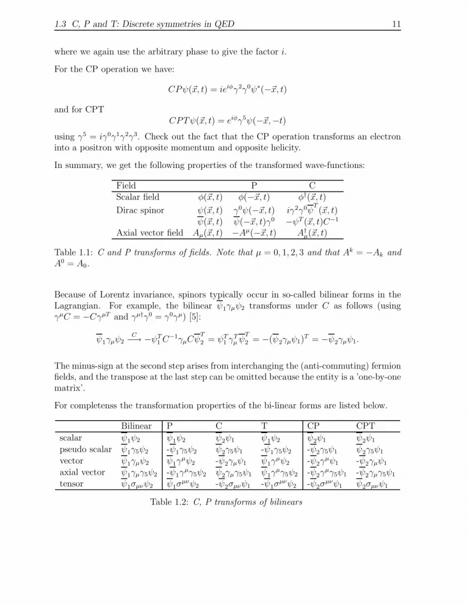
In summary, we get the following properties of the transformed wave-functions:
Field P CScalar field φ(~x, t) φ(−~x, t) φ†(~x, t)
Dirac spinor ψ(~x, t) γ0ψ(−~x, t) iγ2γ0ψT(~x, t)
ψ(~x, t) ψ(−~x, t)γ0 −ψT (~x, t)C−1
Axial vector field Aµ(~x, t) −Aµ(−~x, t) A†µ(~x, t)
Table 1.1: C and P transforms of fields. Note that µ = 0, 1, 2, 3 and that Ak = −Ak andA0 = A0.
Because of Lorentz invariance, spinors typically occur in so-called bilinear forms in theLagrangian. For example, the bilinear ψ1γµψ2 transforms under C as follows (usingγµC = −CγµT and 㵆γ0 = γ0γµ) [5]:
ψ1γµψ2C−→ −ψT1 C−1γµCψ
T
2 = ψT1 γTµψ
T
2 = −(ψ2γµψ1)T = −ψ2γµψ1.
The minus-sign at the second step arises from interchanging the (anti-commuting) fermionfields, and the transpose at the last step can be omitted because the entity is a ’one-by-onematrix’.
For completenss the transformation properties of the bi-linear forms are listed below.
Bilinear P C T CP CPT
scalar ψ1ψ2 ψ1ψ2 ψ2ψ1 ψ1ψ2 ψ2ψ1 ψ2ψ1
pseudo scalar ψ1γ5ψ2 -ψ1γ5ψ2 ψ2γ5ψ1 -ψ1γ5ψ2 -ψ2γ5ψ1 ψ2γ5ψ1
vector ψ1γµψ2 ψ1γµψ2 -ψ2γµψ1 ψ1γ
µψ2 -ψ2γµψ1 -ψ2γµψ1
axial vector ψ1γµγ5ψ2 -ψ1γµγ5ψ2 ψ2γµγ5ψ1 ψ1γ
µγ5ψ2 -ψ2γµγ5ψ1 -ψ2γµγ5ψ1
tensor ψ1σµνψ2 ψ1σµνψ2 -ψ2σµνψ1 -ψ1σ
µνψ2 -ψ2σµνψ1 ψ2σµνψ1
Table 1.2: C, P transforms of bilinears

12 Chapter 1 CP Violation in the Standard Model
1.4 CP violation and the Standard Model Lagrangian
1.4.1 Yukawa couplings and the Origin of Quark Mixing
Let us now have a close look at the Standard Model Lagrangian to see where CP violationoriginates. The full Standard Model Lagrangian consists of three parts:
LSM = Lkinetic + LHiggs + LY ukawa.
The kinetic term describes the dynamics of the spinor fields ψ
Lkinetic = iψ(∂µγµ)ψ,
where ψ ≡ ψ†γ0 and the spinor fields ψ are the three fermion generations, each consistingof the following five representations:
QILi(3, 2,+1/6), uIRi(3, 1,+2/3), dIRi(3, 1,−1/3), LILi(1, 2,−1/2), lIRi(1, 1,−1)
This notation [6] means that QILi(3, 2,+1/6) is a SU(3)C triplet, left-handed SU(2)L dou-
blet, with hypercharge Y = 1/6. The superscript I implies that the fermion fields areexpressed in the interaction basis. The subscript i stands for the three generations. Ex-plicitly, QI
Li(3, 2,+1/6) is a shorthand notation for:
QILi(3, 2,+1/6) =
(
uIg, uIr, u
Ib
dIg, dIr , d
Ib
)
i
=
(
uIg, uIr, u
Ib
dIg, dIr , d
Ib
)
,
(
cIg, cIr , c
Ib
sIg, sIr , s
Ib
)
,
(
tIg, tIr , t
Ib
bIg, bIr , b
Ib
)
.
The interaction terms are obtained by imposing gauge invariance by replacing the partialderivative by the covariant derivate
Lkinetic = iψ(Dµγµ)ψ (1.11)
with the covariant derivative defined as
Dµ = ∂µ + igsGµaLa + igW µ
b σb + ig′BµY,
with La the Gell-Mann matrices and σb the Pauli matrices. Gµa , W
µb and Bµ are the
eight gluon fields, the three weak interaction bosons and the single hypercharge boson,respectively.
We can now write out the charged current interaction between the (left-handed!) quarks:
Lkinetic,weak(QL) = iQILiγµ
(
∂µ +i
2gW µ
b σb)
QILi
= i(u d)IiLγµ(
∂µ +i
2gW µ
b σb)
(
ud
)I
iL
= iuIiLγµ∂µuIiL + idIiLγµ∂
µdIiL − g√2uIiLγµW
−µdIiL − g√2dIiLγµW
+µuIiL + ...

1.4 CP violation and the Standard Model Lagrangian 13
using W+ = 1√2(W1 − iW2) and W− = 1√
2(W1 + iW2).
Next, the W and Z bosons aquire their mass through the mechanism of spontaneoussymmetry breaking. For this, the Higgs scalar field and her potential is added to theLagrangian:
LHiggs = (Dµφ)†(Dµφ) − µ2φ†φ− λ(φ†φ)2 (1.12)
with φ an isospin doublet
φ(x) =
(
φ+
φ0
)
.
The coupling of the Higgs to the gauge fields follows from the covariant derivative in thekinetic term. However, the interactions between the Higgs and the fermions, the so-calledYukawa couplings, have to be added by hand:
−LY ukawa = YijψLi φ ψRj + h.c.
= Y dijQ
ILi φ d
IRj + Y u
ijQILi φ u
IRj + Y l
ijLILi φ l
IRj + h.c. (1.13)
with
φ = iσ2φ∗ =
(
φ0
−φ−
)
.
The matrices Y dij , Y
uij and Y l
ij are arbitrary complex matrices that operate in flavour space,giving rise to couplings between different families, or quark mixing, and thus to the fieldof flavour physics. It is interesting to note how intimately flavour physics is related to themass of the fermions, see Section 2.4. Since this is the crucial part of flavour physics, wespell out the term Y d
ijQILi φ d
IRj explicitly:
Y dijQ
ILi φ d
IRj = Y d
ij(u d)IiL
(
φ+
φ
)
dIRj =
Y11(u d)IL
(
φ+
φ0
)
Y12(u d)IL
(
φ+
φ0
)
Y13(u d)IL
(
φ+
φ0
)
Y21(c s)IL
(
φ+
φ0
)
Y22(c s)IL
(
φ+
φ0
)
Y23(c s)IL
(
φ+
φ0
)
Y31(t b)IL
(
φ+
φ0
)
Y32(t b)IL
(
φ+
φ0
)
Y33(t b)IL
(
φ+
φ0
)
�
dIRsIRbIR
After spontaneous symmetry breaking,
φ(x) =
(
φ+
φ0
)
sym.breaking−→ 1√2
(
0v + h(x)
)
,
the following mass terms for the fermion fields arise:
−LquarksY ukawa = Y dijQ
ILi φ d
IRj + Y u
ijQILi φ u
IRj + h.c.
= Y dijd
ILi
v√2dIRj + Y u
ijuILi
v√2uIRj + h.c.+ interaction terms
= Mdijd
ILid
IRj +Mu
ijuILiu
IRj + h.c.+ interaction terms

14 Chapter 1 CP Violation in the Standard Model
The interaction terms of the fermion fields to the Higgs field, qqh(x), are omitted.
To obtain proper mass terms, the matrices Md and Mu should be diagonalized. We dothis with unitary matrices V d as follows:
Mddiag = V d
LMdV d†
R
Mudiag = V u
LMdV u†
R
Using the requirement that the matrices V are unitary (V d†L V d
L = 1) the Lagrangian cannow be expressed as follows:
−LquarksY ukawa = dILi Mdij d
IRj + uILi M
uij u
IRj + h.c. + ...
= dILi Vd†L V d
LMdijV
d†R V d
R dIRj + uILi V
u†L V u
LMuijV
u†R V u
R uIRj + h.c.+ ...
= dLi (Mdij)diag dRj + uLi (Mu
ij)diag uRj + h.c.+ ...
where the matrices V are absorbed in the quark states, resulting in the following quarkmass eigenstates:
dLi = (V dL )ijd
ILj dRi = (V d
R)ijdIRj
uLi = (V uL )iju
ILj uRi = (V u
R )ijuIRj
Note that we can thus express the quark states as interaction eigenstates dI , uI or asquark mass eigenstates d, u.
If we now express the Lagrangian in terms of the quark mass eigenstates d, u instead ofthe weak interaction eigenstates dI , uI , the price to pay is that the quark mixing betweenfamilies (i.e. the off-diagonal elements) appears in the charged current interaction:
Lkinetic,cc(QL) =g√2uIiLγµW
−µdIiL +g√2dIiLγµW
+µuIiL + ...
=g√2uiL(V
uL V
d†L )ijγµW
−µdiL +g√2diL(V
dLV
u†L )ijγµW
+µuiL + ...
The unitary 3×3 matrixVCKM = (V u
L Vd†L )ij (1.14)
is the Cabibbo-Kobayashi-Maskawa (CKM) mixing matrix [7].
By convention, the interaction eigenstates and the mass eigenstates are chosen to be equalfor the up-type quarks, whereas the down-type quarks are chosen to be rotated, goingfrom the interaction basis to the mass basis:
uIi = uj
dIi = VCKMdj
or explicitly:
dI
sI
bI
=
Vud Vus VubVcd Vcs VcbVtd Vts Vtb
dsb
(1.15)

1.4 CP violation and the Standard Model Lagrangian 15
The connection between the charged current couplings and the quark masses will bediscussed further in Section 2.4.
From the definition of VCKM , see Eq. (1.14), follows that the transition from a down typequark to an up-type quark is described by Vud, whereas the transition from an up typequark to a down-type quark is described by V ∗
ud:
W−
d
u
Vud
W+
u
d
V∗ud
W+
d
u
V∗ud
W−
u
d
Vud
Figure 1.5: The definition of Vij and V ∗ij. Note that if the arrow of time points from left
to right, that the two right diagrams represent the situation for anti-quarks.
1.4.2 CP violation
CP violation shows up in the complex Yukawa couplings. We examine once more theYukawa part of the Lagrangian:
−LY ukawa = YijψLi φ ψRj + h.c.
= YijψLi φ ψRj + Y ∗ijψRj φ
† ψLi
The CP operation transforms the spinor fields as follows:
CP (ψLi φ ψRj) = ψRj φ† ψLi
So, LY ukawa remains unchanged under the CP operation if Yij = Y ∗ij .
Similarly, if we look at the charged current coupling in the basis of quark mass eigenstates,
Lkinetic,cc(QL) =g√2uiLVijγµW
−µdiL +g√2diLV
∗ijγµW
+µuiL (1.16)
and the CP-transformed expression,
LCPkinetic,cc(QL) =g√2diLVijγµW
+µuiL +g√2uiLV
∗ijγµW
−µdiL (1.17)
then we can conclude that the Lagrangian is unchanged if Vij = V ∗ij .
The complex nature of the CKM matrix is the origin of CP violation in the StandardModel. In the following chapter the properties of the CKM mixing matrix will be examinedin detail.

16 Chapter 1 CP Violation in the Standard Model

Chapter 2
The Cabibbo-Kobayashi-MaskawaMatrix
In the previous chapter we saw how the introduction of Yukawa couplings (i.e. the termswhere the Higgs couples to the fermions) led to off-diagonal elements in the 3×3 matrix be-tween the different families. By diagonalizing the 3×3 Yukawa matrix, these off-diagonalelements appear in the charged current coupling, in the Cabibbo-Kobayashi-Maskawa-matrix. The CKM-mechanism is the origin of CP violation, and earned Kobayashi andMaskawa the Nobel price in 2008, “for the discovery of the origin of the broken symmetrywhich predicts the existence of at least three families of quarks in nature”.
2.1 Unitarity Triangle(s)
In this section we will discuss the properties of the unitary 1 CKM matrix VCKM . Westart by counting the number of free parameters for the CKM-matrix.
1) A general n×n complex matrix has n2 complex elements, and thus 2n2 real param-eters.
2) Unitarity (V †V = 1) implies n2 constraints:
– n unitary conditions (unity of the diagonal elements);
– n2 − n orthogonality relations (vanishing off-diagonal elements).
3) The phases of the quarks can be rotated freely: uLi → eiφui uLi and dLj → eiφ
di dLj.
Since the overall phase is irrelevant, 2n− 1 relative quark phases can be removed.
1Remember from quantum mechanics the evolution of a wave function, |ψ(t)〉 = U(t)|ψ(0)〉. Theunitarity condition implies conservation of probability: 〈ψ(t)|ψ(t)〉 = 〈ψ(0)|U †U |ψ(0)〉 = 〈ψ(0)|ψ(0)〉,provided U †U = 1
17

18 Chapter 2 The Cabibbo-Kobayashi-Maskawa Matrix
Summarizing, the CKM-matrix describing the flavour couplings of n generations of upand down type quarks has 2n2 − n2 − (2n− 1) = (n− 1)2 free parameters. Subsequently,we can divide these free parameters into Euler angles and phases:
4) A general n × n orthogonal matrix can be constructed from 12n(n − 1) angles de-
scribing the rotations among the n dimensions.
5) The remaining free parameters are the phases: (n−1)2− 12n(n−1) = 1
2(n−1)(n−2).
For the Standard Model with three generations we find three Euler angles and one complexphase.
At this point we make a short historical excursion. Before the third family was known,Cabibbo suggested in 1963 the mixing between d and s quarks, by introducing the Cabibbomixing angle θC . This is the only free parameter for a 2×2 unitary matrix, and themixing matrix is a pure real matrix. To allow for CP violation the mixing matrix hasto contain complex elements, satisfying Vij 6= V ∗
ij . This requires at least three families.CP violation was first measured in 1964 by Cronin and Fitch (discussed in more detailin Section 5.3). Subsequently, Kobayashi and Maskawa suggested in 1973 the possibilitythat the existence of a third family could explain the CP violation within the StandardModel. This happened at the time that not even the second family was completed! The 4th
quark, the charm quark was only discovered a year later, in 1974, in the form of the J/ψresonance. The bottom and the top quark were discovered in 1977 and 1994 respectively.In 2008 Kobayashi and Maskawa were awarded the Nobel prize for the discovery of theorigin of the broken symmetry which predicts the existence of at least three families ofquarks in nature.
Let us now look at the consequences of the unitarity condition for the CKM-matrix:
V †V = V V † =
Vud Vus VubVcd Vcs VcbVtd Vts Vtb
V ∗ud V ∗
cd V ∗td
V ∗us V ∗
cs V ∗ts
V ∗ub V ∗
cb V ∗tb
=
1 0 00 1 00 0 1
(2.1)
This leads to the following three unitary relations:
VudV∗ud + VusV
∗us + VubV
∗ub = 1
VcdV∗cd + VcsV
∗cs + VcbV
∗cb = 1
VtdV∗td + VtsV
∗ts + VtbV
∗tb = 1 (2.2)
These relations express the so-called weak universality, because it shows that the squaredsum of the coupling strengths of the u-quark to the d, s and b-quarks is equal to theoverall charged coupling of the c-quark (and the t-quark). In addition, we see that thissum adds up to 1, meaning that “there is no probability remaning” to couple to a 4th
down-type quark. Obviously, this relation deserves continuous experimental scrutiny.

2.1 Unitarity Triangle(s) 19
V tbV ub*
VtsVus*
VtdVud*
φ1
φ2φ
3
Figure 2.1: One of the six unitarity triangles. VtdV∗ud = |VtdV ∗
ud|eiφ1, VtsV∗us = |VtsV ∗
us|eiφ2
and VtbV∗ub = |VtbV ∗
ub|eiφ3 .
The remaining relations are known as the orthogonality conditions:
VudV∗cd + VusV
∗cs + VubV
∗cb = 0
VudV∗td + VusV
∗ts + VubV
∗tb = 0
VcdV∗ud + VcsV
∗us + VcbV
∗ub = 0
VcdV∗td + VcsV
∗ts + VcbV
∗tb = 0
VtdV∗ud + VtsV
∗us + VtbV
∗ub = 0
VtdV∗cd + VtsV
∗cs + VtbV
∗cb = 0 (2.3)
Three of the six equations are simply the complex conjugate version. An additional threeinteresting equations arise from the unitarity relation V †V = 1:
V ∗udVus + V ∗
cdVcs + V ∗tdVts = 0
V ∗udVub + V ∗
cdVcb + V ∗tdVtb = 0
V ∗usVud + V ∗
csVcd + V ∗tsVtd = 0
V ∗usVub + V ∗
csVcb + V ∗tsVtb = 0
V ∗ubVud + V ∗
cbVcd + V ∗tbVtd = 0
V ∗ubVus + V ∗
cbVcs + V ∗tbVts = 0 (2.4)
Equations (2.3-2.4) give relations in which the complex phase is present. As these aresums of three complex numbers that must yield zero they can be viewed as a triangle inthe complex plane, see for example Fig. 2.1.
In the literature there are many different parameterizations of the CKM matrix. A con-venient representation uses the Euler angles θij with i, j denoting the family labels. Withthe notation cij = cos θij and sij = sin θij the following parameterization was introducedby Chau and Keung, and has been adopted by the Particle Data Group:
VCKM =
c12 s12 0−s12 c12 0
0 0 1
c13 0 s13e−iδ13
0 1 0−s13e
iδ13 0 c13
1 0 00 c23 s23
0 −s23 c23
=
c12c13 s12c13 s13e−iδ13
−s12c23 − c12s23s13eiδ13 c12c23 − s12s23s13e
iδ13 s23c13s12s23 − c12c23s13e
iδ13 −c12s23 − s12c23s13eiδ13 c23c13
(2.5)

20 Chapter 2 The Cabibbo-Kobayashi-Maskawa Matrix
The phase can be made to appear in many elements, and is chosen here to appear in thematrix describing the relation between the 1st and 3rd family.
2.2 Size of matrix elements
We will now briefly discuss the experimental evidence for the size of the matrix elementsof the CKM-matrix.
|Vud|: This matrix element is determined from comparing nuclear β-decay rates or neutrondecay rates to the µ-decay rate, see Fig. 2.2. In the calculations there are sometheoretical uncertainties due to binding energy corrections in nuclei. The best valueobtained by averaging many experiments is:
|Vud| = 0.97425 ± 0.00022
n
u
d
dp
u
W−
d
u
e−
νe
VudW−
µ− νµ
e−
νe
1
Figure 2.2: Diagrams important for determining Vud.
|Vus|: By analysing semi-leptonic K-decays, shown in Fig. 2.3, a value is obtained of
|Vus| = 0.2252 ± 0.0009
K− s
u
π0u
W−
u
e−
νe
Vus
W−
µ− νµ
e−
νe
1
Figure 2.3: Diagrams important for determining Vus.

2.2 Size of matrix elements 21
|Vcd|: Is obtained by the analysis of neutrino and anti-neutrino induced charm-particleproduction of the valence d-quark in a neutron (or proton) (see Fig. 2.4). whichthen yields
|Vcd| = 0.230 ± 0.011
n
u
d
d
W
νµ
c
u
d
µ−
Vcd
W−
µ− νµ
e−
νe
1
Figure 2.4: Diagrams important for determining Vcd.
|Vcs|: Is the matrix element relevant for the dominant decay modes of the charm quark.Here an analogous analysis is performed for D-decays as was done for K-decaysfor Vus. (see Fig. 2.5). The major uncertainty is due to the form-factor of theD-meson. The final result is
|Vcs| = 1.023 ± 0.036
D0 c
u
K−s
W+
u
e+
νe
V ∗cs
W−
µ− νµ
e−
νe
1
Figure 2.5: Diagrams important for determining Vcs.
|Vcb|: Is determined from the decay B → D∗l+νl (see Fig. 2.6). A large amount of data isavailable on these decays both from LEP and from lower energy e+e− acceleratorsgiving an average result of
|Vcb| = 0.0406 ± 0.0013
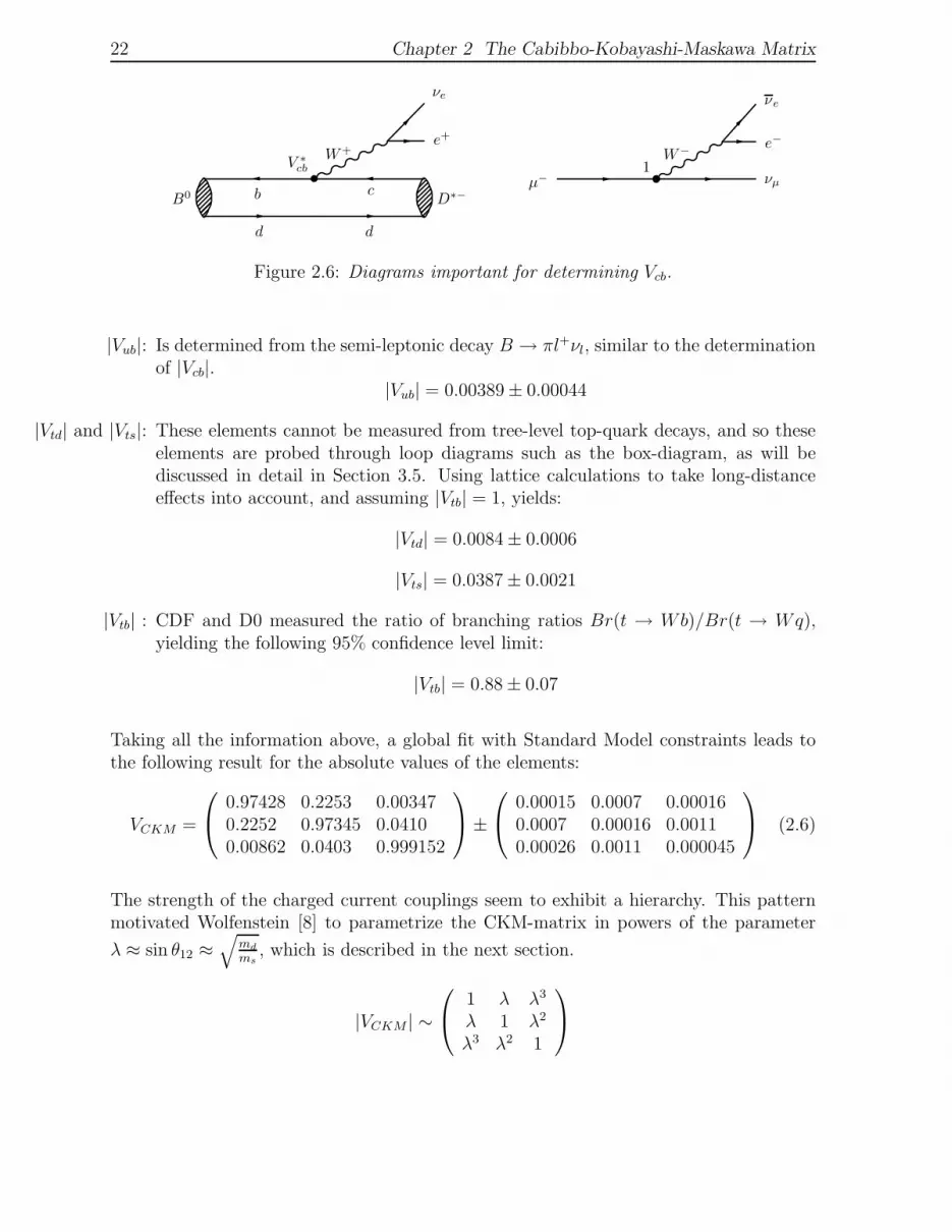
22 Chapter 2 The Cabibbo-Kobayashi-Maskawa Matrix
B0
d
D∗−cb
W+
d
e+
νe
V ∗cb
W−
µ− νµ
e−
νe
1
Figure 2.6: Diagrams important for determining Vcb.
|Vub|: Is determined from the semi-leptonic decay B → πl+νl, similar to the determinationof |Vcb|.
|Vub| = 0.00389 ± 0.00044
|Vtd| and |Vts|: These elements cannot be measured from tree-level top-quark decays, and so theseelements are probed through loop diagrams such as the box-diagram, as will bediscussed in detail in Section 3.5. Using lattice calculations to take long-distanceeffects into account, and assuming |Vtb| = 1, yields:
|Vtd| = 0.0084 ± 0.0006
|Vts| = 0.0387 ± 0.0021
|Vtb| : CDF and D0 measured the ratio of branching ratios Br(t → Wb)/Br(t → Wq),yielding the following 95% confidence level limit:
|Vtb| = 0.88 ± 0.07
Taking all the information above, a global fit with Standard Model constraints leads tothe following result for the absolute values of the elements:
VCKM =
0.97428 0.2253 0.003470.2252 0.97345 0.04100.00862 0.0403 0.999152
±
0.00015 0.0007 0.000160.0007 0.00016 0.00110.00026 0.0011 0.000045
(2.6)
The strength of the charged current couplings seem to exhibit a hierarchy. This patternmotivated Wolfenstein [8] to parametrize the CKM-matrix in powers of the parameter
λ ≈ sin θ12 ≈√
md
ms, which is described in the next section.
|VCKM | ∼
1 λ λ3
λ 1 λ2
λ3 λ2 1

2.3 Wolfenstein parameterization 23
2.3 Wolfenstein parameterization
Comparing the expressions (2.5) and (2.6) we see that typically the sin θij are smallnumbers and that sin θ12 ≫ sin θ23 ≫ sin θ13. This leads to a very popular approximateparameterization of the CKM matrix proposed by Wolfenstein.
sin θ12 = λ (2.7)
sin θ23 = Aλ2 (2.8)
sin θ13e−iδ13 = Aλ3(ρ− iη) (2.9)
where A, ρ and η are numbers of order unity. The CKM matrix then becomes O(λ3):
VCKM =
1 − 12λ2 λ Aλ3(ρ− iη)
−λ 1 − 12λ2 Aλ2
Aλ3(1 − ρ− iη) −Aλ2 1
+ δV (2.10)
The higher order terms in the Wolfenstein parametrization are of particular importancefor the Bs-system, as we will see in chapter 4, because the phase in |Vts| is only apparentat O(λ4):
δV =
−18λ4 0 0
12A2λ5(1 − 2(ρ+ iη)) −1
8λ4(1 + 4A2) 0
12Aλ5(ρ+ iη) 1
2Aλ4(1 − 2(ρ+ iη)) −1
2A2λ4
+ O(λ6) (2.11)
Let us now return to the six orthogonality relations that give rise to the six unitaritytriangles. Only two out of the six equations have terms with equal powers in λ.
VudV∗ub + VcdV
∗cb + VtdV
∗tb = 0
O(λ3) O(λ3) O(λ3) (2.12)
VtdV∗ud + VtsV
∗us + VtbV
∗ub = 0
O(λ3) O(λ3) O(λ3) (2.13)
These two triangles are relevant for B-decays. The other four equations contain termswith different powers of λ and hence give rise to “squashed” triangles.
The relation shown in Eq. 2.12 is known as the unitarity triangle. By dividing thethree sides by |VcdVcb| and subsequently rotating the whole triangle (i.e. rephasing allsides, without affecting the relative phases), yields the famous unitarity triangle shownin Fig. 2.7. One side now has unit length and points along the real axis. The apex of thetriangle is located by definition at (ρ, η) 2:
ρ+ iη ≡ VudV∗ub
VcdV∗cb
.
2Occasionally the generalized parameters ρ and η are defined in the literature as the approximationρ ≡ ρ(1 − 1
2λ2) and η ≡ η(1 − 1
2λ2) [9].

24 Chapter 2 The Cabibbo-Kobayashi-Maskawa Matrix
cdV Vcb*
VtdVtb*
ubVudV *
cdV Vcb*
Vub cdV V VtdVtbudV cb+ + = 0* * *
Re0 1
(ρ,η)
α
γ β
Im Vub V V V VtbV + + = 0* * *us cbcs ts
Vts Vtb*
csV Vcb*
csV Vcb*
ubVV *us Re1
0
Im
π−γ sβ
Figure 2.7: (a) “The” unitarity triangle. Shown in the complex plane is the relation1 + VtdV
∗tb/VcdV
∗cb + VudV
∗ub/VcdV
∗cb = 0. (b) The analogous unitarity triangle for the B0
s -system, with the d-quark replaced by the s-quark, 1 + VtsV
∗tb/VcsV
∗cb + VusV
∗ub/VcsV
∗cb = 0.
The parameters ρ, and η can be expressed in terms of the Wolfenstein parameters ρ andη as follows:
ρ = ρ(1 − 1
2λ2) + O(λ4) η = η(1 − 1
2λ2) + O(λ4) (2.14)
The angles in “the” unitarity triangle are defined as follows:
α ≡ arg
[
− VtdV∗tb
VudV∗ub
]
β ≡ arg
[
−VcdV∗cb
VtdV∗tb
]
γ ≡ arg
[
−VudV∗ub
VcdV∗cb
]
βs ≡ arg
[
−VtsV∗tb
VcsV∗cb
]
(2.15)Note that these definitions are convention independent: any phase added to a specificquark cancels out in either the product or the ratio of the CKM-elements. Equivalently,the CKM triangles can be rotated and scaled in the complex plane, without affecting theinternal angles of the triangles.
In the Wolfenstein parametrization a phase convention is used such that the elementsVtd, Vub and Vts have an imaginary component (to order O(λ4)), and VcdV
∗cb is real and
negative, see Fig. 2.8.
V Vtbtd*
V Vcd cb*
Vtdarg
Varg ub*
V V *cs cb
βs
Vtsarg
V Vcd cb*
V V *
V V *
ud ub
ts tb
π π
β Re
Im
Re
Im
Re
Imγ βsβ
γ=
Figure 2.8: The angles β, γ and βs using the phase convention as given by the Wolfensteinparameterization. (a) β (b) γ (c) βs.

2.3 Wolfenstein parameterization 25
The expressions for the angles now become:
β ≈ π + arg(VcdV∗cb) − arg(VtdV
∗tb) = π + π − arg(Vtd) = − arg(Vtd)
γ ≈ π + arg(VudV∗ub) − arg(VcdV
∗cb) = π − arg(Vub) − π = − arg(Vub)
βs ≈ π + arg(VtsV∗tb) − arg(VcsV
∗cb) = π + arg(Vts) − 0 = arg(Vts) + π
Alternatively, the Wolfenstein phase convention in the CKM-matrix elements can beshown as:
VCKM,Wolfenstein =
|Vud| |Vus| |Vub|e−iγ−|Vcd| |Vcs| |Vcb||Vtd|e−iβ −|Vts|eiβs |Vtb|
+ O(λ5) (2.16)
As mentioned earlier, CP violation requires Vij 6= V ∗ij , which is satisfied if the triangle
has a finite surface in the complex plane. In fact, it turns out that the surface of all sixunitarity triangles have equal surface area.
This quantity denoted as J , also known as the Jarlskog invariant, can be derived in asimple way from the CKM matrix. Remove one column and one row from the CKMmatrix and take the product of the diagonal elements with the complex conjugate of thenon-diagonal elements. The imaginary part of the product is then equal to J . In totalthere will be nine possible expressions for J which all give the same result:
J = ℑ(V11V22V∗12V
∗21) = ℑ(V22V33V
∗23V
∗32) = .... (2.17)
In the Wolfenstein parameterization the quantity J becomes
J = A2λ6η = 2 × area (2.18)
In the parameterization of Eq. (2.5) it is
J = c12c213c23s12s13s23 sin δ13 (2.19)
From this form it is clear why this quantity occurs in all CP violation effects. It is zero ifany one of the mixing angles is zero. This would reduce the CKM matrix essentially toa 2 × 2 matrix and allow the removal of the phase. Also if the complex phase would bezero no CP violation is possible. As a final comment the quantity J is just equal to thetwice the surface area of the unitarity triangle.

26 Chapter 2 The Cabibbo-Kobayashi-Maskawa Matrix
2.4 Discussion
The strong hierarchy in the size of the matrix elements of the quark mixing matrix isintriguing and its origin is not understood. To paraphrase Ikaros Bigi [10]: “ It has tocontain a message from nature - albeit in a highly encoded form.”
We have seen that the origin of the quark mixing matrix lies in the Yukawa couplingsbetween the Higgs field and the quark fields. At the same time, these Yukawa couplingsare responsible for the generation of the quark masses, which becomes obvious afterdiagonalizing the matrix that describes the Yukawa couplings. Also the values of the quarkmasses show a striking hierarchy, which makes the thought of an underlying connectionbetween the quark masses and the charged current quark couplings fascinating.
Yukawa Couplings
Couplings Masses
u
c
t
??
d s b
u
c
t
d
s
b
Figure 2.9: Both the charged current quark couplings and the quark masses originate fromthe Yukawa couplings and both the couplings and the masses show an intriguing hierarchy.Does this suggest an underlying connection between them?
.
We have now set the framework for the incorporation of CP violation in the StandardModel. The question remains of course whether all manifestations of CP violation can beexplained. Of course theoretically we can always incorporate new ideas such as supersym-metry or an increase in the number of families to explain any deviations. Experimentallyit is now important to verify the Standard Model description. When looking at the uni-tarity triangle we can see that the length of the sides of the triangle can be extractedfrom measurable quantities. It is now necessary to investigate whether the angles of thetriangle can be measured in an independent way. Disagreement between the angles andthe lengths of the side would necessarily signal New Physics. At present many experi-ments are either running or have been proposed which will be able to give answers to thequestions to a greater or lesser extent. In chapter 4 we will proceed to discuss the channelswhich are considered to be the prime candidates for further investigation of CP violation.Before that, we will introduce the concept of neutral meson oscillations, or mixing, whichplays a crucial role in many of the CP-measurements.

Chapter 3
Neutral Meson Decays
3.1 Neutral Meson Oscillations
The phenomenon of neutral meson oscillations is important for various reasons. Firstly, inmany measurements of CKM-parameters, the oscillations play a crucial role in providinga second transition amplitude from the initial state to a given final state. This secondamplitude is needed to determine the relative phase difference between two amplitudes,as described in chapter 4. Secondly, the observation of two K0 particles with largelyvarying lifetimes and the resulting discovery of CP violation is of historical importance,see chapter 5, and is described in terms of a superposition of |K〉-states and its quantum-mechanical evolution.
The formalism described in this section is valid for all weakly decaying neutral mesons:K0, D0, B0 and B0
s . We will outline the framework in terms of a generical meson P 0,which can be substituted at will by K0, D0, B0 or B0
s . Although we will see that thedifference in mass (and thus available phase space for the final state) and coupling strength(CKM-elements) results in dramatically different phenomenology.
3.2 The mass and decay matrix
The states |P 0〉 and |P 0〉 which are eigenstates of the strong and electromagnetic interac-tions with common mass m0 and opposite flavour content. Let us consider an arbitrarysuperposition of the P 0 and P 0 states, which has time-dependent coefficients a(t) andb(t) respectively:
ψ(t) = a(t)|P 0〉 + b(t)|P 0〉We can write ψ(t) in the subspace of P 0 and P 0 as follows
ψ(t) =
(
a(t)b(t)
)
27

28 Chapter 3 Neutral Meson Decays
The effective Hamiltonian that governs the time evolution is a sum of the strong, electro-magnetic and weak Hamiltonians.
H = Hst +Hem +Hwk
The wavefunction ψ must then obey
i∂ψ
∂t= Hψ
The Hamiltonian can then, in the (P 0, P 0) basis, be written as 2 × 2 complex matrix:
H = M − i
2Γ
where both M and Γ are Hermitian matrices. M will provide a “mass” term and due tothe −i, Γ will provide the exponential decay. Note that due to the i, H is not hermitianreflected in the property that the probability to observe either P 0 or P 0 is not conserved,but goes down with time:
d
dt
(
|a(t)|2 + |b(t)|2)
= − (a(t)∗b(t)∗)
(
Γ11 00 Γ22
) (
a(t)b(t)
)
If the weak part of the Hamiltonian did not exist the P system would be stable and so Hwould reduce to
H →M =
(
mP 0 00 mP 0
)
where mP 0 = 〈P 0|Hst + Hem|P 0〉 and mP 0 = 〈P 0|Hst + Hem|P 0〉 and the off-diagonalelements are 0 through flavour conservation. With the weak interaction responsible forthe decay we get:
i∂ψ
∂t= Hψ = (M − i
2Γ)ψ =
(
M11 − i2Γ11 0
0 M22 − i2Γ22
)
ψ
If we now allow for the transitions P 0 → P 0, the off-diagonal elements are introduced:
i∂ψ
∂t= Hψ = (M − i
2Γ)ψ =
(
M11 − i2Γ11 M12 − i
2Γ12
M21 − i2Γ21 M22 − i
2Γ22
)
ψ
The off-diagonal elements consist of two parts, M12 and 12Γ12, which describe different
ways of the P 0 → P 0 transition. M12 quantifies the short-distance contribution fromthe (calculable) box diagram as will be discussed in Section 3.5. Γ12 is a measure of thecontribution from the virtual, intermediate, decays to a state f , see Fig. 3.1.
If we now assume that CPT is valid then it follows that M11 = M22, M21 = M∗12 and
Γ11 = Γ22, Γ21 = Γ∗12 meaning that mass and total decay width of particle and antiparticle
are identical.
i∂ψ
∂t= Hψ = (M − i
2Γ)ψ =
(
M − i2Γ M12 − i
2Γ12
M∗12 − i
2Γ∗
12 M − i2Γ
)
ψ (3.1)

3.3 Eigenvalues and -vectors of Mass-decay Matrix 29
M12
−i Γ122
P0
P0P 0 f
P0
via on−shell states,
via off−shell states,weak box−diagram
Figure 3.1: The neutral meson oscillation consists of two contributions, namely throughoff-shell states and on-shell states.
.
In general there can be a relative phase between Γ12 and M12 [11]:
φ = arg(
− M12
Γ12
)
(3.2)
which is the relative phase difference between the on-shell (or dispersive) and off-shell (orabsorbative) transition. This leads to the relations
∆m = 2|M12| (3.3)
∆Γ = 2|Γ12| cosφ. (3.4)
If T is conserved then it follows that Γ∗12/Γ12 = M∗
12/M12 so that by introducing a freephase we can make Γ12 and M12 real.
Under these assumptions we can now find the eigenvalues and eigenvectors of the Hamil-tonian. These will describe the masses and decay widths and the P 0, P 0 superpositions,that describe the physical particles.
3.3 Eigenvalues and -vectors of Mass-decay Matrix
Given the Schrodinger equation (3.1) we find the eigenvalues of the mass-decay matrix,by solving the determinantal equation [12]:
∣
∣
∣
∣
M − i2Γ − λ M12 − i
2Γ12
M∗12 − i
2Γ∗
12 M − i2Γ − λ
∣
∣
∣
∣
= 0
Using the shorthand notation F =√
(M12 − i2Γ12)(M
∗12 − i
2Γ∗
12) we find the eigenvalues
λ± = M − i2Γ±F . Splitting the real and imaginary part by defining λ− = m1 + i
2Γ1 and

30 Chapter 3 Neutral Meson Decays
λ+ = m2 + i2Γ2, we obtain:
m1 +i
2Γ1 = M − ℜF − i
2(Γ − 2ℑF )
m2 +i
2Γ2 = M + ℜF − i
2(Γ + 2ℑF )
These expressions invite the use of the following notation:
∆m ≡ m2 −m1 = 2ℜF∆Γ ≡ Γ1 − Γ2 = 4ℑF
If we express the eigenstates P1 and P2 as:
|P1〉 = p|P 0〉 − q|P 0〉|P2〉 = p|P 0〉 + q|P 0〉
we find p and q by solving
(
M − i2Γ M12 − i
2Γ12
M∗12 − i
2Γ∗
12 M − i2Γ
) (
pq
)
= λ±
(
pq
)
yielding:
q
p= ±
√
M∗12 − i
2Γ∗
12
M12 − i2Γ12
The state |P1〉 is the mass eigenstate with mass m1 and lifetime Γ1. Similarly we obtainthe mass m2 and lifetime Γ2 for state |P2〉. The sign of q/p determines whether |P1〉 or|P2〉 is heavier. The choice of a positive value of ∆m gives:
q
p=
√
M∗12 − i
2Γ∗
12
M12 − i2Γ12
(3.5)
Note that we have chosen the sign here, such that ∆m > 0, but that does not implyanything for the sign of ∆Γ: experiment has to judge whether ∆Γ is positive or negative,relative to the sign of ∆m.
We can also relate q/p to the mixing phase as introduced in Eq.(3.2) [11]:
|Γ12||M12|
sinφ =∆Γ
∆mtanφ = 2
(
1 − |q||p|
)
. (3.6)
(This will turn out to be the size of a possible CP asymmetry for flavour-specific finalstates, afs.)
3.4 Time evolution 31
3.4 Time evolution
We define the two mass eigenstates of the neutral mesons as 1:
|PH〉 = p|P 0〉 + q|P 0〉|PL〉 = p|P 0〉 − q|P 0〉 (3.7)
where the subscripts 1 and 2 are replaced by H and L, indicating the heavy and lightmass eigenstate, respectively. We can then decompose the P 0 and P 0 states as
|P 0〉 =1
2p[|PH〉 + |PL〉]
|P 0〉 =1
2q[|PH〉 − |PL〉] (3.8)
The states |PH〉 and |PL〉 are mass eigenstates and from the Schrodinger equation (withdiagonal Hamiltonian) the usual time dependent wave functions are obtained:
|PH(t)〉 = e−imH t− 1
2ΓH t|PH(0)〉
|PL(t)〉 = e−imLt− 1
2ΓLt|PL(0)〉 (3.9)
By combining Eqs. (3.9), (3.8) and (3.7) we get:
|P 0(t)〉 =1
2p
{
e−imH t− 1
2ΓH t|PH(0)〉 + e−imLt− 1
2ΓLt|PL(0)〉
}
=1
2p
{
e−imH t− 1
2ΓH t(p|P 0〉 + q|P 0〉) + e−imLt− 1
2ΓLt(p|P 0〉 − q|P 0〉)
}
=1
2
(
e−imH t− 1
2ΓH t + e−imLt− 1
2ΓLt
)
|P 0〉 +q
2p
(
e−imH t− 1
2ΓH t − e−imLt− 1
2ΓLt
)
|P 0〉
= g+(t)|P 0〉 +
(
q
p
)
g−(t)|P 0〉 (3.10)
where we define the functions
g+(t) =1
2
(
e−imH t− 1
2ΓHt + e−imLt− 1
2ΓLt
)
=1
2e−iMt
(
e−i1
2∆mt− 1
2ΓH t + e+i
1
2∆mt− 1
2ΓLt
)
g−(t) =1
2
(
e−imH t− 1
2ΓHt − e−imLt− 1
2ΓLt
)
=1
2e−iMt
(
e−i1
2∆mt− 1
2ΓH t − e+i
1
2∆mt− 1
2ΓLt
)
1There are some subtleties concerning the sign (or phase) convention. Let us assume CP symmetry,|q/p| = 1. We can choose q/p = ±1 and CP |P 0〉 = ±|P 0〉. Once the sign of q/p is fixed, see Eq.(3.5),experiment decides if PH is the state that is (more) even or odd, which fixes CP |P 0〉 = ±|P 0〉. In principlethis can be different for K0, B0 and B0
s . We choose the sign convention ∆mK > 0 and CP |K0〉 = −|K0〉such that CP |KL〉 = −|KL〉 (or ∆ΓK = ΓS − ΓL > 0) according to experiment. This leads to the signconvention in Eq.(3.7), and implies ∆mK = mL−mS . Also in the B-system the heavier mass eigenstateBH is (more) CP odd, and the CP-even state in the Bs-system can decay to the final state D+
s D−s , and
has therefore a slightly shorter lifetime.

32 Chapter 3 Neutral Meson Decays
where M = (mH +mL)/2 and ∆m = mH −mL. Likewise, we get for the time evolutionof the state |P 0〉:
|P 0(t)〉 = g−(t)
(
p
q
)
|P 0〉 + g+(t)|P 0〉 (3.11)
If we start from a pure sample of |P 0〉 particles (e.g. produced by the strong interaction)then we can calculate the probability of measuring the state |P 0〉 at time t:
|〈P 0(t)|P 0〉|2 = |g−(t)|2(
p
q
)2
with
|g±(t)|2 =1
4
(
e−ΓH t + e−ΓLt ± e−Γt(e−i∆mt + e+i∆mt))
=1
4
(
e−ΓH t + e−ΓLt ± 2e−Γt cos ∆mt)
=e−Γt
2
(
cosh1
2∆Γt± cos ∆mt
)
(3.12)
where Γ = (ΓL +ΓH)/2 and ∆Γ = ΓH −ΓL. Here we see that Γ fulfills the natural role ofdecay constant, Γ = 1/τ , justifying the choice of 1
2in the hamiltonian in Eq. (3.1). The
sign of ∆m is by definition positive, but the sign of ∆Γ has to be determined experimen-tally.

3.5 The Amplitude of the Box diagram 33
3.5 The Amplitude of the Box diagram
The short distance contribution to the P 0 ↔ P 0 transitions of neutral meson oscillationsis described by ∆m and can be represented by a Feynman diagram known as the boxdiagram, and can be calculated in perturbation theory.
In this section we will calculate the value of ∆m by studying this so-called box diagram.We will investigate the process of K0 ↔ K0 using the CKM matrix. To describe mixingbetween a K0 which has strangeness S = 1 and a K0 which has S = −1 we must introducean amplitude which creates a ∆S = 2 transition. This must necessarily be a second orderweak interaction. The transition necessary for mixing is shown in Fig. 3.2. The calculationof the box diagram is quite complicated but we will illustrate some of the features in thecalculation of the K0
L −K0S mass difference.
The mass difference is given by
∆m = mK0L−mK0
S= 〈K0
L|H|K0L〉 − 〈K0
S|H|K0S〉 (3.13)
As we saw in the previous section, the mass eigenstates can be expressed as a linearcombination of the flavour eigenstates. The amplitude 〈K0|H|K0〉 can now be calculatedvia the box diagram of Fig. 3.2. As an example we use the Feynman rules to derive anexpression for the amplitude where both the intermediate quarks are u quarks:
Muu = i
(−igw2√
2
)4
(V ∗usVudV
∗usVud)
∫
d4k
(2π)4
(−igλσ − kλkσ/m2W
k2 −m2W
) (−igαρ − kαkρ/m2W
k2 −m2W
)
[
usγλ(1 − γ5)k/ +mu
k2 −m2u
γρ(1 − γ5)ud
] [
vsγα(1 − γ5)k/+mu
k2 −m2u
γσ(1 − γ5)vd
]
Here we readily recognise the weak coupling constant to the fourth power, the CKM matrixelements for the vertices, the W propagator terms, the quark and anti-quark spinors andthe factors for the intermediate fermion lines.
d
K0 K0
du, c, t
W
s
u, c, t
W
s
Vud,cd,tdV ∗us,cs,ts
Vud,cd,td V ∗us,cs,ts
d
K0 K0
dW
u, c, t
s
W
u, c, t
s
Vud,cd,tdV ∗us,cs,ts
Vud,cd,td V ∗us,cs,ts
Figure 3.2: Box diagrams responsible for K0 → K0 mixing.

34 Chapter 3 Neutral Meson Decays
Taking the sum of all amplitudes with all possible intermediate quark lines we get anamplitude which is proportional to (assuming k2 ≪ m2
W ).
M ∝∫
d4k kµkν
(
V ∗usVud
k2 −m2u
+V ∗csVcd
k2 −m2c
+V ∗tsVtd
k2 −m2t
)2
(3.14)
Which with the aid of the equation V ∗usVud + V ∗
csVcd + V ∗tsVtd = 0 we can rewrite as
M ∝∫
d4k kµkν
(
V ∗csVcd
[
1
k2 −m2c
− 1
k2 −m2u
]
+ V ∗tsVtd
[
1
k2 −m2t
− 1
k2 −m2u
])2
This then finally leads to an answer that has three terms [13], one term depending onm2c/m
2W , one term depending on m2
t/m2W and and a term which has a complicated depen-
dence on both m2c/m
2W and m2
t/m2W . The magnitude of the so-called Inami-Lim factor
these three terms is listed in Table 3.1, together with the size of the CKM-elementsinvolved in the box diagram.
This calculation only takes into account the quark level transitions and so the full calcu-lation must take into account the transition from K0 → ds and gluonic corrections andcolour factors. Because |VtdVts| << |VcdVcs| the charm contribution in the loop dominates,and the final answer becomes:
∆mK =G2Fm
2W
6π2ηQCDBKf
2KmK
[
S0(m2c/m
2W )|VcdVcs|2
]
(3.15)
where GF is the Fermi coupling constant, ηQCD is the QCD correction (≈ 0.85), B andf 2K
is the “bag-factor” and the decay constant, respectively, which describe the effect of thetransition from bound to free quarks and Vij are the CKM matrix elements.
In the B-system we have |VtdVtb| ∼ |VcdVcb|, but because mt >> mc now the top contri-bution in the loop dominates. By replacing the internal charm quark with the top quark,and replacing the strange flavour by the bottom quark we find for the B-system:
∆mB =G2Fm
2W
6π2ηQCDBBf
2BmB
[
S0(m2t/m
2W )|VtdVtb|2
]
(3.16)
Internal Inami-Lim CKM factorquarks factor K0 B0 B0
s
c, c 3.5 10−4 λ2 (2.7 10−2) A2λ6 (7.4 10−5) A2λ4 (1.4 10−3)c, t 3.0 10−3 A2λ6|1 − ρ− iη| (8.8 10−6) A2λ6|1 − ρ− iη| (7.3 10−5) A2λ4 (1.5 10−3)t, t 2.5 A4λ10|1 − ρ− iη|2 (1.1 10−7) A2λ6|1 − ρ− iη|2 (7.2 10−5) A2λ4 (1.5 10−3)
Table 3.1: The magnitude of the three terms contributing to the box diagram, expressed sep-arately for the Inami-Lim factors (depending on m2
q/m2W ) and for the CKM elements [14].
Clearly, the charm-quark contribution dominates in the K-system, where the CKM-factorcompensates for the small Inami-Lim factor. In the B-systems the top-quark contributiondominates.

3.5 The Amplitude of the Box diagram 35
0 0.1 0.2 0.3 0.4 0.5 0.6 0.7 0.8 0.9 10
0.2
0.4
0.6
0.8
1
0K
0 0.5 1 1.5 2 2.5 3 3.5 4 4.5 50
0.2
0.4
0.6
0.8
1
0D
0 0.5 1 1.5 2 2.5 3 3.5 4 4.5 50
0.2
0.4
0.6
0.8
1
0B
0 0.5 1 1.5 2 2.5 3 3.5 4 4.5 50
0.2
0.4
0.6
0.8
1
s0B
t (ns)0 0.1 0.2 0.3 0.4 0.5 0.6 0.7 0.8 0.9 1
Pro
babi
lity
0
0.2
0.4
0.6
0.8
1
0K
(t))0 K→(t)0P(K
(t))0
K →(t)0P(K
0K
t (ps)0 0.5 1 1.5 2 2.5 3 3.5 4 4.5 5
Pro
babi
lity
0
0.2
0.4
0.6
0.8
1
0D
(t))0 D→(t)0P(D
(t))0
D →(t)0P(D
0D
t (ps)0 0.5 1 1.5 2 2.5 3 3.5 4 4.5 5
Pro
babi
lity
0
0.2
0.4
0.6
0.8
1
0B
(t))0 B→(t)0P(B
(t))0
B →(t)0P(B
0B
t (ps)0 0.5 1 1.5 2 2.5 3 3.5 4 4.5 5
Pro
babi
lity
0
0.2
0.4
0.6
0.8
1
s0B
(t))s0 B→(t)
s
0P(B
(t))s
0B →(t)
s
0P(B
s0B
Figure 3.3: If one starts with a pure P 0-meson beam the probability to observe a P 0 or aP 0-meson at time t is shown, Prob(t) = e−Γt
2
(
cosh 12∆Γt± cos ∆mt
)
..
At this point we can see how the neutral mesons K0, D0, B0 and B0s in reality oscillate and
what the differences are. As mentioned earlier, the oscillations consist of two components,M12 and 1
2Γ12. As a general rule, all possible quark exchanges contribute to M12, but only
actual final states contribute to Γ12 [12]. The short-distance, off-shell contribution fromM12 depends on the size of the CKM-elements at the corners of the box-diagram, and onthe mass of the particles in the box. In the case of D0-mixing, the mass of the heaviestdown-type quark in the box, mb is not large enough to compensate the suppression ofthe CKM-elements |VubVcb|. As a result, the light quarks dominate the short-range D0-mixing and proceeds proportional to ∼ |VusVcs|2m2
s ∼ λ2m2s. As a consequence, the
mixing parameters are expected to be small, and the D-mesons decay before they havethe chance to oscillate.
The oscillation probability of D-mesons is clearly suppressed compared to B0-mixing,see Fig. 3.3, which is proportional to ∼ |VtbVtd|2m2
t ∼ λ6m2t . B0
s -mixing on the otherhand, is more pronounced, see Fig. 3.3d), due to the magnitude of Vts: ∼ |VtbVts|2m2
t ∼λ4m2
t . Finally, K0-oscillation is dominated by the (light) charm quark in the loop, ∼|VcdVcs|2m2
c ∼ λ2m2c . However, the kaons profit from the fact that their lifetime is much
higher compared to the B-mesons. Note that the sum of the B0 and B0 distributions inFig. 3.3 give a perfect exponential decay, because the mass eigenstates BH and BL happento have equal lifetimes, ∆Γ = 0. In contrast, the sum of the K0 and K0 distributionsresults in the sum of two exponential distributions, corresponding to the KS and KL withshort and long lifetime, respectively.

36 Chapter 3 Neutral Meson Decays
Often the dimensionless variables x and y are used to express the mixing behaviour,expressing the oscillation rate relative to the lifetime:
x =∆m
Γy =
∆Γ
2Γ
The oscillation parameters of the various neutral mesons are summarized in Table 3.2.
τ = 1/Γ ∆m x yK-system 0.26 × 10⁻⁹ s 1 5.29 ns−1 0.477 -1D-system 0.41 × 10⁻¹² s 0.0024 ps−1 0.0097 0.0078B-system 1.53 × 10⁻¹² s 0.507 ps−1 0.78 0.0015 2
Bs-system 1.47 × 10⁻¹² s 17.77 ps−1 26.1 0.06 2
Table 3.2: Oscillation parameters of the various neutral mesons.
1Note that the average lifetime Γ is not a very meaningful quantity in the K-system due to the largedifference between the lifetimes of the two mass-eigenstates Ks and KL.
2These numbers are theoretical values, rather than experimental measurements. The transitionT (B0
s → DsDs → B0s ) is the largest contribution and proceeds proportional to |Vcb|2. ∆ΓB0 < ∆ΓB0
s
because the transitions T (B0 → (DD), (ππ), (Dπ) → B0) are all Cabibbo suppressed.

3.6 Meson Decays 37
3.6 Meson Decays
In this section we extend the formalism of neutral meson oscillations, and include thesubsequent decay of the meson to a final state f . We consider the following four decayamplitudes
A(f) = 〈f |T |P 0〉 A(f) = 〈f |T |P 0〉A(f) = 〈f |T |P 0〉 A(f) = 〈f |T |P 0〉
and define the complex parameter λf (not be confused with the Wolfenstein parame-ter λ !):
λf =q
p
AfAf
, λf =1
λf, λf =
q
p
AfAf
, λf =1
λf(3.17)
The general expression for the time dependent decay rates, ΓP 0→f(t) = |〈f |T |P 0(t)〉|2,give us the probability that the state P 0 at t = 0 decays to the final state f at time t,and can now be constructed as follows, using Eqs. (3.10) and (3.11):
ΓP 0→f(t) = |Af |2(
|g+(t)|2 + |λf |2|g−(t)|2 + 2ℜ[λfg∗+(t)g−(t)]
)
ΓP 0→f(t) = |Af |2∣
∣
∣
∣
q
p
∣
∣
∣
∣
2(
|g−(t)|2 + |λf |2|g+(t)|2 + 2ℜ[λfg+(t)g∗−(t)])
ΓP 0→f(t) = |Af |2∣
∣
∣
∣
p
q
∣
∣
∣
∣
2(
|g−(t)|2 + |λf |2|g+(t)|2 + 2ℜ[λfg+(t)g∗−(t)])
ΓP 0→f(t) = |Af |2(
|g+(t)|2 + |λf |2|g−(t)|2 + 2ℜ[λfg∗+(t)g−(t)]
)
(3.18)
with
|g±(t)|2 =e−Γt
2
(
cosh1
2∆Γt± cos ∆mt
)
g∗+(t)g−(t) =e−Γt
2
(
sinh1
2∆Γt+ i sin ∆mt
)
g+(t)g∗−(t) =e−Γt
2
(
sinh1
2∆Γt− i sin ∆mt
)
(3.19)
The terms proportional |A|2 are associated with decays that occurred without oscillation,whereas the terms proportional to |A|2(q/p)2 or |A|2(p/q)2 are associated with decaysfollowing a net oscillation. The third terms, proportional to ℜg∗g, are associated to theinterference between the two cases.
Combining Eqs. (3.18) and (3.19) results in the following expressions for the decay rates

38 Chapter 3 Neutral Meson Decays
for neutral mesons, also known as the master equations:
ΓP 0→f(t) = |Af |2e−Γt
2(
(1 + |λf |2) cosh1
2∆Γt+ 2ℜλf sinh
1
2∆Γt+ (1 − |λf |2) cos ∆mt− 2ℑλf sin ∆mt
)
ΓP 0→f(t) = |Af |2∣
∣
∣
∣
p
q
∣
∣
∣
∣
2e−Γt
2(3.20)
(
(1 + |λf |2) cosh1
2∆Γt+ 2ℜλf sinh
1
2∆Γt− (1 − |λf |2) cos ∆mt + 2ℑλf sin ∆mt
)
The sinh- and sin-terms are associated to the interference between the decays with andwithout oscillation. Commonly, the master equations are expressed as:
ΓP 0→f(t) = |Af |2 (1 + |λf |2)e−Γt
2
(
cosh1
2∆Γt+Df sinh
1
2∆Γt+ Cf cos ∆mt− Sf sin ∆mt
)
ΓP 0→f(t) = |Af |2∣
∣
∣
∣
p
q
∣
∣
∣
∣
2
(1 + |λf |2)e−Γt
2
(
cosh1
2∆Γt+Df sinh
1
2∆Γt− Cf cos ∆mt + Sf sin ∆mt
)
(3.21)
with
Df =2ℜλf
1 + |λf |2Cf =
1 − |λf |21 + |λf |2
Sf =2ℑλf
1 + |λf |2. (3.22)
For a given final state f we therefore only have to find the expression for λf to fullydescribe the decay of the (oscillating) mesons. Examples of some final states will bepresented in chapter 4.
3.7 Classification of CP Violating Effects
The following classification between the various types of CP violation can be made [6].
1) CP violation in decay. This type of CP violation occurs when the decay rate ofa B to a final state f differs from the decay rate of an anti-B to the CP-conjugatedfinal state f :
Γ(P 0 → f) 6= Γ(P 0 → f)
This is obviously satisfied (see Eq. (3.18)) when∣
∣
∣
∣
AfAf
∣
∣
∣
∣
6= 1. (3.23)
An example of CP violation in decay for neutral mesons is decay B0 → K+π−. Asizeable CP-asymmetry has been observed
ACP =ΓB0→K+π− − ΓB0→K−π+
ΓB0→K+π− + ΓB0→K−π+
< 0

3.7 Classification of CP Violating Effects 39
In charged mesons there is no mixing, so this is the only type of CP violation thatcan occur in charged meson decays.
2) CP violation in mixing. This implies that the oscillation from meson to anti-meson is different from the oscillation from anti-meson to meson:
Prob(P 0 → P 0) 6= Prob(P 0 → P 0)
Experimentally this is searched for in the semi-leptonic decay of both the B0 andthe B0, coherently produced through Υ → B0B0. The b-quark inside the B0-mesondecays weakly to a positively charged lepton, and vice versa. So, an event with twoleptons with equal charge in the final state means that one of the two B-mesonsoscillated. So, the asymmetry in the number of two positive and two negative leptonsallows us to compare the oscillation rates.
ACP =N++ −N−−N++ +N−−
=|p/q|2 − |q/p|2|p/q|2 + |q/p|2
This type is violated if∣
∣
∣
∣
q
p
∣
∣
∣
∣
6= 1. (3.24)
In the B0- and B0s -system this is not the case, so |q/p| ≈ 1 both within the exper-
imental accuracy and theoretical expectation, but we will see that this type of CPviolation is active in the K-system, see chapter 5 2.
3) CP violation in interference between a decay with and without mixing,sometimes referred to as CP violation involving oscillations. This form of CP viola-tion is measured in decays to a final state that is common for the B0 and B0-meson.An interesting category are CP-eigenstates, f = f (an example of a non-CP eigen-state are the final states D±
s K∓ in the B0
s -system). CP is violated if the followingcondition is satisfied:
Γ(P 0(;P 0) → f)(t) 6= Γ(P 0
(;P 0) → f)(t)
A direct consequence of f = f is that there will be two amplitudes that contributeto the transition amplitude from the initial state |B0〉 to a final state f , namelyA(B0 → f) and A(B0 → B0 → f). If we consider the case that |q/p| = 1, thefollowing expression is obtained, using Eqs. (3.21):
ACP (t) =ΓP 0(t)→f − ΓP 0(t)→f
ΓP 0(t)→f + ΓP 0(t)→f
=2Cf cos ∆mt− 2Sf sin ∆mt
2 cosh 12∆Γt+ 2Df sinh 1
2∆Γt
(3.25)
2Normally expressed in terms of ǫ, for historical reasons: p = (1 + ǫ)/√
2(1 + |ǫ|2), q = (1 −ǫ)/
√
2(1 + |ǫ|2) and thus q/p = (1 − ǫ)/(1 + ǫ). The parameters p and q are normalized such that|p|2 + |q|2 = 1.

40 Chapter 3 Neutral Meson Decays
This simplifies considerably if the transition is dominated by only one amplitude, i.e.assuming that |Af | = |Af | (or |λf | = 1), so that Df = ℜλf , Cf = 0 and Sf = ℑλf :
ACP (t) =−ℑλf sin ∆mt
cosh 12∆Γt+ ℜλf sinh 1
2∆Γt
(3.26)
We conclude that CP violation can even occur when both |q/p| = 1 and |A(f)| =|Af |, namely when the following condition is satisfied:
ℑλf = ℑ(
q
p
AfAf
)
6= 0 (3.27)
Commonly an alternative classification of direct and indirect CP violation is made [6].Direct CP violation is defined as |A(f)| 6= |Af |. In terms of the above categories, directCP violation obviously appears in the CP violation in decay. In addition, the term directCP violation is used for the situation where Cf 6= 0, probed by the first term in Eq. (3.25),since |A(f)| 6= |Af | → |λf | 6= 1 → Cf 6= 0. Indirect CP violation is the type of CPviolation that involves mixing in any way, either through |q/p| 6= 1 or via the second termof Eq. (3.25). Historically this distinction originates from so-called superweak models thatpredicted CP violation to appear only in mixing diagrams. The discovery of direct CPviolation excluded these superweak models.
Finally, we comment on the relative size of CP violation in the interference of mixingand decay in the K and B system. The difference arises from the CKM-factor of thebox-diagram. The real part of the CKM-factor in the K-system is given by:
(VcdV∗cs)
2 = λ2
The imaginary part is proportional to A2λ6η. Therefore, we expect for the ratio of theCP violating part to the CP non-violating part of ∆mK to be
ℑ∆m
ℜ∆m∝ A2λ4η (3.28)
In the B system the CKM factor is given by
(VtdV∗tb)
2 = (1 − ρ− iη)2A2λ6
from which we can deduce that the ratio of CP violation to CP non-violation in the Bsystem is
ℑ∆m
|∆m| ∝η(1 − ρ)
(1 − ρ)2 + η2(3.29)
In the B system we then have the strength of CP violation of the same order as CPnon-violation, whereas in the K system it is suppressed by a factor of λ4 ≈ 2 10−3.

Chapter 4
CP violation in the B-system
In the previous chapter we have identified where CP violation occurs in the general for-malism of meson decays, and classified the various categories. In the coming sections wewill investigate a few special decays with which CP violation is measured and the phasesof the CKM elements are determined [9].
Remember the Wolfenstein parametrization, Eq. (2.16), since it so widely used. This pa-rameterization is very convenient to localize weak phase differences in Feynman diagrams:
VCKM,Wolfenstein =
|Vud| |Vus| |Vub|e−iγ−|Vcd| |Vcs| |Vcb||Vtd|e−iβ −|Vts|eiβs |Vtb|
+ O(λ5) (4.1)
In this chapter we will see how the angles β, βs and γ can be determined.
At first sight it might be remarkable that complex phases can be observed, because thecomplex phase in an amplitude A = |A|eiϕ disappears in the expectation value, AA† =|A|2ei(ϕ−ϕ) = |A|2. However, several decay amplitudes Ai = |Ai|eiϕi might contribute tothe total amplitude A [15]. Each phase consists of a CP-odd phase φi originating fromcomplex coupling constants, and a CP-even phase δi, typically originating from gluonexchange in the final state (and strong interactions are CP-conserving!). Therefore wehave for the CP-conjugated amplitude Ai = |Ai|ei(−φi+δi). Now we can calculate thedifference in the magnitude of the total amplitude |A(a → b)| and the CP-conjugate|A(a→ b)|:
|A|2 = |A1 + A2|2 = |A1|2 + |A2|2 + |A1A2|(
ei((φ1+δ1)−(φ2+δ2)) + ei(−(φ1+δ1)+(φ2+δ2)))
= |A1|2 + |A2|2 + 2|A1A2| cos(∆φ+ ∆δ)
|A|2 = |A1 + A2|2 = |A1|2 + |A2|2 + |A1A2|(
ei((−φ1+δ1)−(−φ2+δ2)) + ei(−(−φ1+δ1)+(−φ2+δ2)))
= |A1|2 + |A2|2 + 2|A1A2| cos(−∆φ + ∆δ)
An explicit example will be shown in Section 4.1.
41

42 Chapter 4 CP violation in the B-system
4.1 β: the B0 → J/ψK0S decay
In the case of decays into CP eigenstates (i.e. |f〉 = CP|f〉 = ηf |f〉, with ηf = ±1)only two independent amplitudes need to be considered: Af and Af . We define the CPasymmetry as (see Eq. (3.25)):
ACP (t) =ΓB0(t)→f − ΓB0(t)→f
ΓB0(t)→f + ΓB0(t)→f
Let us now concentrate on specific decays to get an idea where the CKM phase enters theasymmetry measurement. We start with the decay B0 → J/ψK0
S [16] and will investigateEq. (3.26) further.
The first observation is that at the quark level the B0 decay and the B0 decay have adifferent final state, B0 → J/ψK0 and B0 → J/ψK0. As a result, we need to considerthe mass eigenstates in the K system, see Eq. (3.7), to obtain the same final state ffor the B0 and B0 decay: |K0
S〉 = p|K0〉 + q|K0〉. (The details of the K-system will bediscussed in chapter 5.) Secondly, in the B0-system ∆Γ ≈ 0 (see Table 3.2), so Eq. (3.26)can simply be written as:
ACP (t) = −ℑλf sin(∆mt) (4.2)
For a given final state f , the magnitude and phase of λf fully describe the decay andoscillation of the B0 and the B0-meson. (If the final state is not a CP-eigenstate, we willalso need λf .) Starting from the definition of λf we write
λJ/ψK0S
=(q
p
)
B0
(
ηJ/ψK0S
AJ/ψK0S
AJ/ψK0S
)
= −(q
p
)
B0
(AJ/ψK0
AJ/ψK0
) (p
q
)
K0(4.3)
The three parts in this equation correspond to the mixing of the B0-meson, (q/p)B0 , thedecay of the B0 or B0, A/A, and the mixing of the K0-meson, (q/p)K0. These three partsare diagrammatically shown in Fig. 4.1. The factor ηJ/ψK0
Saccounts for the CP-eigenvalue
of the final state. The J/ψ has spin-1 and is CP-even, while KS has spin-0 and is (almost)CP-even. The B0 is spin-0, and thus the particles in the final state must have a relativeangular momentum l = 1. As a result the final state J/ψK0
S is CP-odd, ηJ/ψK0S
= −1 1.
The B0 ↔ B0 mixing is induced by the box diagram shown in Fig. 4.1a). We have seenthat the mass matrix element M12 ∝ V ∗
tbVtdV∗tbVtd, (see Eq. (3.16)), and that we can neglect
the term Γ12, see Table 3.2, and therefore:
(
q
p
)
B0
=
√
M∗12
M12
=V ∗tbVtdVtbV
∗td
(4.4)
1The analogous measurement can be performed with the decay B0 → J/ψK0L, with ηJ/ψK0
L
= +1.

4.1 β: the B0 → J/ψK0S decay 43
b_
d_
d
s
b
db
_
d_
s
s
c
_
_
V V
V VV
V
V
V
V
V
tb
tb
td
td
*
*
_
c
cb
cs*
cs
cs
cd
cd*
*
ab
c
Figure 4.1: The diagrams that enter in the phase of the decay B0 → J/ψK0S. (a) B0
mixing, (b) B0 decay and (c) K mixing..
For the ratio of the decay amplitudes we find on inspection of the diagram in Fig. 4.1b)that
(
A
A
)
=VcbV
∗cs
V ∗cbVcs
At this point we have however not produced a K0S but either a K0 or a K0 to finally make
a prediction of the CP violation in the decay B0 → J/ψK0S we also have to take into
account the K0 ↔ K0 mixing. This adds a factor in analogy to Eq. (4.4) (see Fig. 4.1c):
(
p
q
)
K
=
√
M12
M∗12
=VcsV
∗cd
V ∗csVcd
Taking everything together we find for the parameter λJ/ψK0S:
λJ/ψK0S
= −(V ∗
tbVtdVtbV
∗td
) (VcbV∗cs
V ∗cbVcs
) (VcsV∗cd
V ∗csVcd
)
= −V∗tbVtdVtbV
∗td
VcbV∗cd
V ∗cbVcd
(4.5)
and for its imaginary part
ℑλJ/ψK0S
= − sin
{
arg
(
V ∗tbVtdVcbV
∗cd
VtbV ∗tdV
∗cbVcd
)}
= − sin
{
2 arg
(
VcbV∗cd
VtbV ∗td
)}
≡ sin 2β, (4.6)
where β is defined as in Eq. (2.15). In short we can also write λJ/ψK0S
= −e−2iβ .
To recapitulate, the CP-asymmetry of the decay B0 → J/ψK0S is given by the imaginary
part of λJ/ψK0S:
ACP, B0→J/ψK0S(t) = − sin 2β sin(∆mt) (4.7)
Using the Wolfenstein parameterization we see that the CKM-element Vtd is the onlycomponent with a non-vanishing imaginary part, leading to Eq. (4.6). We conclude that

44 Chapter 4 CP violation in the B-system
the CP-asymmetry in the decay B0 → J/ψK0S arises from the phase difference of the
amplitudes B0 → J/ψK0S and B0 → B0 → J/ψK0
S. The phase difference arises from theCKM-elements Vtd (in the Wolfenstein parametrization) originating from the box-diagramthat is responsible for the B0 ↔ B0 oscillations.
The value of sin 2β has been determined very accurately by the BaBar and Belle experi-ments with the process e+e− → Υ → B0B0. A remarkable feature of this process is thatthe B0B0-pair is produced coherently, which means that the B0-clock only starts tickingwhen the B0 has decayed. The lifetime of the B0-meson is thus expressed as the timediffrence between the two decays, ∆t. The number of decaying B0-mesons is determinedby requiring that the other B had decayed as a B0. This number is called the number oftagged B0-mesons, NB0 . The asymmetry is given by:
ACP (∆t) =ΓB0(∆t)→f − ΓB0(∆t)→f
ΓB0(∆t)→f + ΓB0(∆t)→f
=Γtag=B0 − Γtag=B0
Γtag=B0 + Γtag=B0
= ηf sin 2β sin ∆m∆t.
After correcting for imperfect tagging, we see that the amplitude of the asymetry givesthe value of sin 2β. The present world average is: sin 2β = 0.68 ± 0.03.

4.1 β: the B0 → J/ψK0S decay 45
-5 0 5
Evt
s. /
0.4
ps
200
-5 0 5
Evt
s. /
0.4
ps
200 tags0B
tags0 B
a)
-5 0 5
Raw
asy
m.
-0.5
0
0.5
-5 0 5
Raw
asy
m.
-0.5
0
0.5 b)
-5 0 5
Evt
s. /
0.4
ps
100
-5 0 5
Evt
s. /
0.4
ps
100 tags0B
tags0 B
c)
-5 0 5
Raw
asy
m.
-0.5
0
0.5
-5 0 5
Raw
asy
m.
-0.5
0
0.5 d)
∆t (ps)
Figure 4.2: Number of ηf = −1 candidates (mainly J/ψK0S) in the signal region with
a B0 tag NB0 and with a B0 tag NB0 , and b) the raw asymmetry ACP (t) = (NB0 −NB0)/(NB0 + NB0), as functions of ∆t. Figs. c) and d) are the corresponding plotsfor the ηf = +1 mode J/ψK0
L. The shaded regions represent the estimated backgroundcontributions. From [17].
.

46 Chapter 4 CP violation in the B-system
Measuring complex numbers
Before we continue, we can reflect on the principle behind the measurement of the complexphase β. Let us show once more how the complex phase appears as an observable, startingfrom the |B0〉 wave function and the two decay amplitudes. Remember our wave functionof the decaying, oscillating neutral meson, Eq. (3.10):
|B0(t)〉 = g+(t)|B0〉+(
q
p
)
g−(t)|B0〉 = e−iMt−i 12∆Γt
(
cos∆mt
2|B0〉 + i sin
∆mt
2
(
q
p
)
|B0〉)
|B0(t)〉 = g−(t)
(
p
q
)
|B0〉+g+(t)|B0〉 = e−iMt−i 12∆Γt
(
i sin∆mt
2
(
p
q
)
|B0〉 + cos∆mt
2|B0〉
)
again using ∆Γ ≈ 0 for the B0 case, see Table 3.2. The factor qp
accounts for the
B0 → B0 oscillation. We saw that for the B0-mesons holds | qp| = 1, more specifically,
qp
= ei2β. How is this phase factor ei2β measurable, in general? If we would measure
the number of B0-mesons (i.e. produced as a B0) and compare that to the number ofB0-mesons (i.e. produced as a B0) at time t = π
2∆m, then both the unoscillated and the
oscillated amplitudes are of equal magnitude, and the CP asymmetry can be written as:
ACP
(
t =π
2∆m
)
=|1 + iei2β |2 − |ie−i2β + 1|2|1 + iei2β |2 + |ie−i2β + 1|2 = sin 2β (4.8)
The situation is schematically shown in Fig. 4.3. The total amplitude of the CP-conjugatedsituation will have a different magnitude if there are two phases, of which one flips signunder CP transformation!
B0
K0S
J/ψ
W+
WW
d
b
d, s
s, d
c
c
V ∗bc
VcsB0
K0S
J/ψ
u, c, t
W
b
W
du, c, t
W−
WW
b
d
d, s
s, d
c
c
Vtd Vbc
Vtd
V ∗cs
B0
K0S
J/ψ
W−
WW
d
b
d, s
s, d
c
c
Vbc
V ∗cs
B0
K0S
J/ψ
W
u, c, t
W
b
du, c, t
W+
W
Wb
d
d, s
s, d
c
c
V ∗td
V ∗bc
V ∗td
Vcs
Figure 4.3: Adding two amplitudes results in a Atot with different magnitude under CP..

4.2 βs: the B0s → J/ψφ decay 47
4.2 βs: the B0s → J/ψφ decay
The decay B0s → J/ψφ is the B0
s analogue of the decay B0 → J/ψK0S, with the spectator
d-quark replaced by an s-quark. However, there are four major differences:
I Vts vs Vtd. Since the spectator d-quark is replaced by an s-quark, the CKM-element responsible for the CP-asymmetry (in the Wolfenstein parameterization) isnow Vts, instead of Vtd, see Fig. 4.4. In contrast to Vtd the imaginary part of Vts isno longer of comparable size as the real part, see Eqs. (2.10-2.11), and the predictedCP asymmetry is therefore small, arg(Vts) ∼ ηλ2.
II No K-oscillations. The final state, containing the mesons J/ψ and φ, is the samefor the B0
s and the B0s -meson, and hence we do not need the extra K-oscillation
step as in the B0 system.
III ∆Γ 6= 0. In contrast to the B0 case, the B0s -system has non-vanishing ∆Γ. This
is caused by the existence of a final state common to B0s and B0
s , with a large
branching fraction around 5%, namely the CP-eigenstate D±(∗)s D
∓(∗)s . Since this
is a CP-eigenstate with eigenvalue +1 this decay channel is only accessible for theCP-even eigenstate Bs,H and not for Bs,L. Hence the different lifetime for Bs,H andBs,L with a predicted value of ∆Γ/Γ ∼ 0.1. (A similar situation for the B0 casedoes not occur, because the branching ratio for B0 → D±D∓ is Cabibbo suppressed,A ∼ |Vcd|.)
IV Vector-vector final state. The final state now contains two vector-particles withspin-1. As a result the final state is not a pure CP-eigenstate, in contrast to B0 →J/ψK0
S. The spin of the final state particles J/ψ and φ can be pointing parallel,
B0s
φ
J/ψ
W+
s
b
s
s
c
c
V ∗bc
VcsB0s
φ
J/ψ
u, c, t
W
b
W
su, c, t
W−
b
s
s
s
c
c
Vts Vbc
Vts
V ∗cs
Figure 4.4: The two interfering diagrams of the decay B0s → J/ψφ, with phase differ-
ence 2βs..

48 Chapter 4 CP violation in the B-system
orthogonal, or opposite, which need to be compensated by an orbital momentum,of l = 2, 1 and 0, respectively, to obtain the spin of the initial state, SBs
= 0. TheCP-eigenvalue of the final state now depends on the orbital momentum due to thefactor (−1)l in the total wave function;
CP|J/ψφ〉l = (−1)l|J/ψφ〉l
The fact that the predicted CP-asymmetry is so small in the Standard Model, makesthis decay particularly sensitive to new particles participating in the box-diagram. Anydeviation from the Standard Model value would signal New Physics.
The asymmetry for the decay of the B0s -meson to the common final state J/ψφ is given
by Eq. (3.26):
ACP (t) =ΓB0
s (t)→J/ψφ − ΓB0s (t)→J/ψφ
ΓB0s (t)→J/ψφ + ΓB0
s (t)→J/ψφ
=−ℑλJ/ψφ sin ∆mt
cosh 12∆Γt+ ℜλJ/ψφ sinh 1
2∆Γt
(4.9)
where
λJ/ψφ =(q
p
)
B0s
(
ηJ/ψφAJ/ψφAJ/ψφ
)
= (−1)l(V ∗
tbVtsVtbV
∗ts
) (VcbV∗cs
V ∗cbVcs
)
(4.10)
andℑλJ/ψφ = (−1)l sin(−2βs) (4.11)
By comparing Eqs. (4.6) and (4.11) a relative minus sign occurs due to the definition ofβ and βs: β is defined with Vtd in the denominator, whereas βs has Vts in the numerator,see Eqs. (2.15).
A complication arises from the above mentioned vector-vector final state. The contri-butions from the terms with different orbital momentum, A‖, A⊥ and A0, for values ofthe orbital momentum of 2, 1 and 0, respectively, need to be disentangled statisticallyby examining the angular distributions of the final state particles, J/ψ → µ+µ− andφ→ K+K−.

4.3 γ: the B0s → D±
s K∓ decay 49
4.3 γ: the B0s → D±
s K∓ decay
CP violation in interference between a decay with and without mixing is most simplyrealized by considering a final state that is a CP eigenstate. In that case the amplitudesB → f and B → B → f occur and interfere. In addition, the formulas simplify because|Af | = |Af | = |Af | = |Af |.
The decay B0s → D±
s K∓ is a final state that is not a CP eigenstate. The interference
can however occur when both the B0s and the B0
s decay to the same final state, albeitwith different amplitudes this time. We will first examine the pair B0
s → D−s K
+ andB0s → B0
s → D−s K
+ in a similar way as in the previous sections. This is then followed bythe pair B0
s → D+s K
− and B0s → B0
s → D+s K
−. The information from both pairs allowsfor the extraction of the angle γ in the unitarity triangle.
By examining Fig. 4.5 we see that the amplitude of the decay B0s → D−
s K+ proceeds
proportional to Af ∼ V ∗cbVus whereas the decay B0
s → D−s K
+ proceeds proportional toAf ∼ VubV
∗cs. At this point we should note three important aspects:
I Although both the B0s -decay and the B0
s -decay are equally Cabibbo suppressed,|AD−
s K+| ∼ λ3 and |AD−
s K+| ∼ λ3, nevertheless they are not completely equal|AD−
s K+| 6= |AD−
s K+|. If we split off the part from the weak couplings, and in-troduce the hadronic amplitude including effects from the strong interactions in thefinal state, A1 and A2, we get:
(AD−
s K+
AD−
s K+
)
=(VubV
∗cs
V ∗cbVus
)(A2
A1
)
(4.12)
II Both amplitudes will not only differ by their magnitude, but also by a relative
B0s
D−s
K+
W+
s
b
s
c
s
u
V ∗cb
Vus
B0s
K+
D−s
W−
u, c, t
WW
u, c, tb
s
s
u
c
s
Vub
V ∗cs
Vts
Vts
Figure 4.5: The two interfering diagrams of the decay B0s → D−
s K+, with phase difference
−γ + 2βs..

50 Chapter 4 CP violation in the B-system
phase γ, originating from Vub, see Eq. (4.1), and therefore
AD−
s K+
AD−
s K+
=|AD−
s K+||AD−
s K+|e−iγ. (4.13)
III In fact, since the transitions B0s → D−
s K+ and B0
s → D−s K
+ proceed in a differentway, an extra relative phase δs needs to be introduced, originating from stronginteractions in the final state,
AD−
s K+
AD−
s K+
=|AD−
s K+ ||AD−
s K+ |ei(δs−γ). (4.14)
(This complication is exactly the reason why we will need the second pair of decaysto the final state D+
s K−: to disentangle the two phases γ and δs.)
Combining these three points leads to the following expression:
λD−
s K+ =(q
p
)
B0s
(AD−
s K+
AD−
s K+
)
=∣
∣
∣
V ∗tbVtsVtbV ∗
ts
∣
∣
∣
∣
∣
∣
VubV∗cs
V ∗cbVus
∣
∣
∣
∣
∣
∣
A2
A1
∣
∣
∣ei(−2βs−γ+δs)) (4.15)
In a similar way we obtain the expression for the other pair, where the B0s decays to the
CP-conjugated final state, B0s → D+
s K− and B0
s → B0s → D+
s K− (see Fig. 4.6):
λD+s K−
=(q
p
)
B0s
(AD+s K−
AD+s K−
)
=∣
∣
∣
V ∗tbVtsVtbV
∗ts
∣
∣
∣
∣
∣
∣
V ∗usVcbVcsV
∗ub
∣
∣
∣
∣
∣
∣
A1
A2
∣
∣
∣ei(−2βs−γ−δs)) (4.16)
where we used |AD−
s K+ | = |AD+s K−
| ∼ A1.
B0s
K−
D+s
W+
s
b
s
u
s
c
V ∗ub
Vcs
B0s
D+s
K−
W−
u, c, t
WW
u, c, tb
s
s
c
u
s
Vcb
V ∗us
Vts
Vts
Figure 4.6: (a-b) The two interfering diagrams of the decay B0s → D+
s K−, with phase
difference −γ + 2βs..

4.4 Direct CP violation: the B0 → π−K+ decay 51
4.4 Direct CP violation: the B0 → π−K+ decay
An example of direct CP violation is given by the decay B0 → π−K+. A CP-asymmetryhas been observed in the processes B0 → π−K+ and its CP-conjugate B0 → π+K−,|Af | 6= |Af | [18]:
ACP =ΓB0→π−K+ − ΓB0(t)→π+K−
ΓB0(t)→π−K+ + ΓB0(t)→π+K−
= −0.098 ± 0.012 (4.17)
As before, a different magnitude of the total amplitude between a decay and its CP-conjugate only appears if the total amplitude AB0→π−K+ consists of two interfering am-plitudes with a phase difference. In addition, as before, this phase difference needs tohave two components of which one part is CP-odd and flips sign under the CP-operation,and one part that is CP-even and does not change sign under the CP-operation (oftendenoted as the strong phase, since this phase often arises from final state gluon exchange).
In the decays described in the previous sections, the second amplitude originated from thepossibility that the B-meson oscillated before its decay. That is not possible this time,because the decay B0 → B0 → π+K− results in a different final state.
The second amplitude is now given by the a so-called penguin-diagram, as shown inFig. 4.7. These penguin diagrams are notoriously difficult to calculate, and therefore itis difficult to interpret this results in terms of the CKM-angles. However, from Fig. 4.7it is clear that there is a weak phase difference between the tree (∼ V ∗
ubVus) and penguinamplitude (∼ V ∗
tbVts), and in general a different strong phase is expected. Intriguingly,no CP-asymmetry has been observed in the analogous decay B+ → π0K+, where thespectator d-quark is “simply” replaced by a u-quark, ACP = 0.050 ± 0.025 [18].
B0
π−
K+
W+
d
b
d
u
s
u
V ∗ub
Vus
B0
π−
K+
W
u, c, t
g
d
b
d
u
u
s
V ∗tb
Vts
Figure 4.7: (a-b) The two interfering diagrams of the decay B0 → π−K+..
52 Chapter 4 CP violation in the B-system
4.5 CP violation in mixing: the B0 → l+νX decay
In the previous sections we always assumed for the B0-mesons that |q/p| = 1, originatingfrom calculations of the box diagram responsible for B0 ↔ B0 oscillations. If |q/p| 6= 1that would mean that the probability to oscillate differ for the B0 and the B0:
Prob(B0 → B0) 6= Prob(B0 → B0)
The experimental confirmation has been measured using semi-leptonic decays. A semi-leptonically decaying b-quark proceeds as b → l−νX, whereas the anti-b quark decays asb→ l+νX. The charge of the lepton contains information whether the B-meson decayedas a B0 (containing a b-quark) or whether it oscillated and decayed as a B0 (containinga b-quark). At the B-factories with the BaBar and Belle experiments both a B0 and aB0-meson are produced simultaneously through the process e+e− → Υ → B0B0.
If the probability to oscillate would be larger for the B0 than for the B0, then the prob-ability to observe two negatively charged leptons (B0 → B0 → l−νX and B0 → l−νX)would be larger than to observe two positively charged leptons!
ACP =P (B0 → B0) − P (B0 → B0)
P (B0 → B0) + P (B0 → B0)=N++ −N−−
N++ +N−− =1 − |q/p|41 + |q/p|4
The combined value as measured at the B-factories yields:
∣
∣
∣
q
p
∣
∣
∣
B0= 1.0024 ± 0.0023 (4.18)
In other words, no CP violation in mixing is observed in the B0-system.
The energy at the B-factories is not large enough to produce B0s -mesons. The measure-
ment of |q/p| for the B0s -system has been done at the Tevatron with the D0 and CDF
experiments [18]:∣
∣
∣
q
p
∣
∣
∣
B0s
= 0.999 ± 0.004. (4.19)
Recent measurements of the flavour-specific asymmetry in semi-leptonic decays at the D0experiment seem to suggest however that |q/p| 6= 1, see Eq.(3.6).

4.6 Penguin diagram: the B0 → φK0S decay 53
4.6 Penguin diagram: the B0 → φK0S decay
Already in the decay B0 → π−K+ we introduced the loop diagram that is known asthe penguin diagram, see Section 4.4. On the one hand these diagrams are difficult tocalculate, but on the other hand, these loop diagrams are very interesting because new,heavy particles might run around in these loops, affecting the measurements. And becausethe particles in the loop are virtual, even very heavy particles can contribute.
A particularly interesting example is the decay B0 → φK0S, which caused excitement
in recent years. The two interfering diagrams are shown in Fig. 4.8. The situation iscompletely analogous as for the decay B0 → J/ψK0
S from Section 4.1: the B0 → B0
oscillation gives rise to the phase difference between the two diagrams (Vtd ∼ eiβ) and thetime dependent CP-asymmetry is again given by
ACP, B0→φK0S(t) = − sin 2β sin(∆mt)
Any difference in the measurement of sin 2β between the decays B0 → J/ψK0S and B0 →
φK0S might be attributed to new particles in the loop adding an extra phase. The value
of sin 2βφKSis slighly low compared to the value of sin 2βJ/ψKS
as measured with treediagrams, which is still a matter of debate:
sin 2βJ/ψKS= 0.68 ± 0.03
sin 2βφKS= 0.39 ± 0.17
B0
K0S
φ
W
u, c, t
g
W
Wd
b
d, s
s, d
s
s
B0
K0S
φ
u, c, t
W
b
W
u, c, t
W
u, c, t
g
W
Wb
d
d, s
s, d
s
s
Vtd
Vtd
Figure 4.8: The two interfering diagrams of the decay B0 → φK0S, with phase differ-
ence 2β..
54 Chapter 4 CP violation in the B-system

Chapter 5
CP violation in the K-system
CP violation was first discovered in the kaon system and struck the community with largesurprise. CP violation was discovered almost 10 years before the CKM-mechanism wasinvented, at the time that only the three quarks (u, d and s) were known. We will discussCP violation in the K-system because of its large historical importance.
The nomenclature used in the K-system has some small differences compared to theB-system, which we will introduce in this chapter. The connection in the K-systembetween CP violation and our well known Lagrangian and its short range couplings is lessstraightforward.
5.1 CP and pions
Before we dive into the K-system, we give the CP properties of the pion, which will berelevant when we will discuss the K-decay into pions.
The π0 is a pseudoscalar meson consisting of a quark and an antiquark. The total wave-function of the π0 must be symmetric as it has spin 0. It must however be antisymmetricunder the interchange of the spin of quark and anti-quark as these are fermions. Thereforethe wave function must also be antisymmetric under interchange of the positions of thequark and antiquark.
|π0〉 = |q ↑ q ↓ 〉 − |q ↓ q ↑ 〉 + |q ↑ q ↓ 〉 − |q ↓ q ↑ 〉
Performing the parity transformation then yields
P |π0〉 = |q ↓ q ↑ 〉 − |q ↑ q ↓ 〉 + |q ↓ q ↑ 〉 − |q ↑ q ↓ 〉 = −1 |π0〉
The π0 is thus an eigenstate of the Parity operation with eigenvalue -1. One says it hasnegative intrinsic parity.
55

56 Chapter 5 CP violation in the K-system
Performing the C-operation yields (check)
C|π0〉 = |π0〉
This can also be deduced from the fact that it decays into two photons. As a photon isnothing more than a combination of electric and magnetic fields and the C operation willinvert both components (why), so that
C|γ〉 = −1 |γ〉
from which it follows that
C|π0〉 = C|γγ〉 = (−1)2|γγ〉 = |π0〉
The combined transformation yields:
CP |π0〉 = −1 |π0〉 (5.1)
and so it is a CP eigenstate with eigenvalue -1 or it “has CP=-1” or “is CP-odd”.
The system |π0π0〉 must be symmetric under interchange of the two particles as theyare identical bosons. The CP operation will therefore be merely the product of the CPoperation on the two π0s separately
CP |π0π0〉 = (−1)2 |π0π0〉 = +1 |π0π0〉
For the |π+π−〉 system the C operation interchanges π+ and π− and the P operationchanges them back again so that the full CP operation is equivalent to the identity trans-formation:
CP |π+π−〉 = 1|π+π−〉 = +1 |π+π−〉All systems of two pions are eigenstates of CP with eigenvalue +1: they are thus “CP-even”.
The |π0π0π0〉 system is again simple because we are dealing with identical bosons the CPoperation is the product of the operation on the three pions separately:
CP |π0π0π0〉 = (−1)3 |π0π0π0〉 = −1 |π0π0π0〉
It is therefore a CP-odd system.
For the |π+π−π0〉 system the relative angular momenta come into play. Let us consider thesituation where the |π+π−〉 system is produced with angular momentum L = l then if thetotal angular momentum of the |π+π−π0〉 system is zero (we are heading for K0 decay)the relative angular momentum of π0 ↔ (π+π−) will also be L = l. Now performingthe CP operation will for the |π+π−〉 be the identity operation again, performing it onthe |π0〉 will give -1 and for the part of the wavefunction describing the relative angularmomentum L(π0 ↔ (π+π−)) = l one gets (−1)l (the wave function is proportional toPl(cos θ)). So for l even the system is CP-odd, and for l odd the system is CP-even.
Summarizing the results sofar we have:

5.2 Description of the K-system 57
Pion state CP eigenvalueπ0 -1π+π− +1π0π0 +1π0π0π0 -1π+π−π0 -1 (L(π+π−)↔π0 = 0, 2, ..)
+1 (L(π+π−)↔π0 = 1, 3, ..)
So if CP-symmetry holds then a particle will only be able to decay into a two pion systemif it is a CP eigenstate with eigenvalue +1.
5.2 Description of the K-system
As was introduced in chapter 3 we express the CP-eigenstates as follows:
|K0+〉 =
1√2
[
|K0〉 + |K0〉]
|K0−〉 =
1√2
[
|K0〉 − |K0〉]
The |K0+〉 and |K0
−〉 states have definite CP-eigenvalues
CP |K0+〉 = +1 |K0
+〉CP |K0
−〉 = −1 |K0−〉
If CP is conserved, the state |K0+〉 will only decay into π+π− or π0π0 ( or with a higher
angular momentum to π+π−π0) whereas the the state |K0−〉 is strictly forbidden to decay
into a two pion final state. Because the mass of the K0L/S is approximately 497.6 MeV and
the mass of a pion is about 139.6 MeV the available phasespace for the two pion decayis almost a factor 1000 larger than that available for the three pion decay. As a result,the lifetime of the CP-odd eigenstate of the K-system is very large, much larger than thelifetime of the CP-even eigenstate. This is the reason that the CP-eigenstates are referredto as the K0
S and K0L, where the subscripts stand for short and long, respectively, and not
referred to as heavy and light as is done in the B-system 1.
|K0S〉 =
1√2
[
|K0〉 + |K0〉]
|K0L〉 =
1√2
[
|K0〉 − |K0〉]
(5.2)
1The K0L corresponds to the heavy eigenstate, so could also have been named the KH ...

58 Chapter 5 CP violation in the K-system
5.3 The Cronin-Fitch experiment
Until 1964 all measurements were consistent with the notion of CP-symmetry, even thosewhich involve the weak interaction. In fact CP-symmetry was invoked to explain thelarge difference in lifetime between the K0
L and K0S. The experiment which unexpectedly
changed this situation was performed by Christensen, Cronin, Fitch and Turlay [19] in1964.
The experimental apparatus is shown in Fig. 5.1. It consisted of a Be-target placed ina π− beam. All particles produced in the interactions, including any K0s were allowedto decay in a low pressure He-tank. Decay products were detected in two magneticspectrometers placed roughly 20 m from the target. The distance of 20 m corresponds toapproximately 300 lifetimes for the K0
S. All decay products must therefore come from theK0L. All opposite charge combinations of particles, which had a reconstructed decay vertex
within the He-volume were analysed and their invariant mass was determined under theassumption that both detected particles were pions. Obviously one expects to observeinvariant mass combinations with a mass smaller than the K0 mass emanating from theK0L → π+π−π0 decay (M(π+π−) < M(K0
L) −M(π0)). However some background wasproduced in the experiment from the decays K0
L → πµν and K0L → πeν where the µ and
the e are misidentified as pions (check the mass limit for these decays). Fig. 5.2a) showsthe measured spectrum. The figure shows a Montecarlo prediction from all known decaysof the K0
L (e.g. the peak at about 350 MeV is from the K0L → π+π−π0 decay. At first
Figure 5.1: The experimental apparatus with which CP violation was first measured..

5.3 The Cronin-Fitch experiment 59
glance there is no real discrepancy between the measurements and the MC prediction.Certainly there is no indication of an excess of events at around 500 MeV. If we howeverplot the cosine of the angle between the flightpath of the K0 and the direction of themomentum sum of the two particles for 490 < M(π+π−) < 510 MeV we start to see anexcess appear for cos θ ∼ 1, see Fig. 5.2b). This is of course exactly what one expects forthe decay K0
L → π+π−. Fig. 5.2d) shows this in a little more detail. The forward peakis only present for 494 < M(π+π−) < 504 MeV. Outside this mass interval there is noindication for a forward enhancement. The enhancement contains 49±9 events. This wasafter many consistency checks finally taken as proof that the decay K0
L → π+π− occursin nature. After acceptance correction the experiment gave a branching ratio of:
BR(K0L → π+π−) =
Γ(K0L → π+π−)
Γ(K0L → all charged decay modes)
= 2.0 ± 0.4 × 10⁻³
This result proves then that CP-symmetry is violated in the decay of the K0L, of course
(a)
(b)
(c)
(d)
(e)
Figure 5.2: (a) The measured two “pion” mass spectrum. (b) The distribution of the cosineof the angle between the summed momentum vector of the two pions and the direction ofthe K0 beam. (c-e) The angular distribution for different ranges in the invariant mass.
.

60 Chapter 5 CP violation in the K-system
one has to be careful that the effect seen is indeed the decay of the K0L, as there are some
subtle effects that could affect the result.
5.3.1 Regeneration
Here we will discuss the effects of the passage through matter of a state which is asuperposition of |K0〉 and |K0〉. In the Hamiltonian we will now also have to take intoaccount the strong interactions of the state with the matter it is passing through. Wewill neglect any inelastic interactions as these will merely decrease the intensity. Weknow from experiment that the strong interactions of |K0〉 and |K0〉 are different. The|K0〉 (sd) contains an s-quark and can, in its interaction with matter, produce strangebaryon resonances, like K0 +n→ Λ+π0, whereas the K0 (sd) can not. So the total crosssection for K0 scattering will be smaller than for K0.
Suppose that a pure K0L beam would incident on matter where all K0 would be absorbed,
then the outgoing beam would be pure K0. Similar to a Stern-Gerlach filter, half of theoutgoing kaons would then decay as a K0
S and half as K0L, see Eq. 5.2:
|K0〉 =1√2
[
|K0S〉 + |K0
L〉]
In principle the effect seen in the Cronin experiment could have been due to regenerationof the K0
L beam. If this would be the case then clearly by introducing more material in thepath of the K0
L beam the effect would increase. The experiment was therefore repeatedwith liquid hydrogen instead of He in the decay path. The density and so the size of theregeneration then grows by a factor of 1000. The growth of the signal was found to bethe equivalent of 10 events. The experiment was also repeated with the He replaced byvacuum. The signal persisted, so that regeneration could be ruled out as the cause.
Finally one has to prove that the particle which decays into the π+π− state is in fact theK0L state. To prove this one determined that there existed interference between the state
decaying into π+π− and a regenerated K0S.
The only remaining conclusion was therefore that CP-symmetry is violated in weakinteractions.

5.4 Master Equations in the Kaon System 61
5.4 Master Equations in the Kaon System
In Section 3.7 a classification of the various types of CP violation was made. In thefollowing these various types will be examined in the kaon system. First, let us introducethe quantity η+− by starting from the familiar master equations.
ΓK0→f(t) = |Af |2(
|g+(t)|2 + |λf |2|g−(t)|2 + 2ℜ[λfg∗+(t)g−(t)]
)
ΓK0→f(t) = |Af |2∣
∣
∣
∣
p
q
∣
∣
∣
∣
2(
|g−(t)|2 + |λf |2|g+(t)|2 + 2ℜ[λfg+(t)g∗−(t)])
(5.3)
with
|g±(t)|2 =1
4
(
e−ΓSt + e−ΓLt ± e−Γt(e−i∆mt + e+i∆mt))
λfg∗+(t)g−(t) =
λf4
(
e−ΓSt − e−ΓLt + e−Γt(e−i∆mt − e+i∆mt))
(5.4)
yields
ΓK0→f(t) =|Af |2
4
(
e−ΓSt(1 + |λf |2 + 2ℜλf) + e−ΓLt(1 + |λf |2 − 2ℜλf) +
e−Γt((1 − |λf |2)(e−i∆mt + e+i∆mt) + 2ℜ(λf(e−i∆mt − e+i∆mt)))
)
=|Af |2
4
(
e−ΓSt(1 + λf )(1 + λ∗f ) + e−ΓLt(1 − λf )(1 − λ∗f) +
e−Γt((1 − |λf |2)(cos ∆mt) + 2ℑ(λf) sin ∆mt)))
∼(
e−ΓSt + e−ΓLt(1 − λf)(1 − λf)
∗
(1 + λf)(1 + λf)∗+
e−Γt((1 − |λf |2)
(1 + λf)(1 + λf)∗(2 cos∆mt) − 4
ℑ(λf )
(1 + λf )(1 + λf)∗sin ∆mt))
)
and finally
ΓK0→f(t) = N(
e−ΓSt + e−ΓLt|η+−|2 + 2e−Γt|η+−| cos(∆mt + φ+−))
ΓK0→f(t) = N(
e−ΓSt + e−ΓLt|η+−|2 − 2e−Γt|η+−| cos(∆mt + φ+−))
(5.5)
with η+− =1−λf
1+λf= |η+−e
iφ+−.

62 Chapter 5 CP violation in the K-system
5.5 CP violation in mixing: ǫ
It is clear that we can no longer identify the K0L with the K0
− and the K0S with the K0
+,as they are clearly no longer eigenstates of the full Hamiltonian, and therefore we write:
|K0S〉 = p|K0〉 + q|K0〉
|K0L〉 = p|K0〉 − q|K0〉
Historically, the CP violation was parameterized by introducing an arbitrary complexnumber ǫ, because the K0
S and K0L were almost CP-eigenstates:
|K0L〉 =
1√
1 + |ǫ|2(
|K0−〉 + ǫ|K0
+〉)
(5.6)
and
|K0S〉 =
1√
1 + |ǫ|2(
|K0+〉 − ǫ|K0
−〉)
(5.7)
where p = (1 + ǫ)/√
2(1 + |ǫ|2), q = (1 − ǫ)/√
2(1 + |ǫ|2) and thus q/p = (1 − ǫ)/(1 + ǫ).The parameters p and q are normalized such that |p|2 + |q|2 = 1.
Let us consider the decays K0 → π+π− and K0 → π+π− and define the parameter λf , asin Eq. (3.17) [2]:
λπ+π− =(q
p
)
K
Aπ+π−
Aπ+π−
(5.8)
The amount of CP violation is measured by determining the relative branching ratio ofBR(K0
L → π+π−) over BR(K0S → π+π−):
η+− ≡ 〈π+π−|T |K0L〉
〈π+π−|T |K0S〉
=pAπ+π− − qAπ+π−
pAπ+π− + qAπ+π−
=1 − λπ+π−
1 + λπ+π−
If η+− 6= 0 then that means |λπ+π−| 6= 1. In this way we have reduced the CP violation toCP violation in the mixing of the K0 and K0, whereas the interaction that describes thedecay is still CP-invariant. Only the part of the wavefunction that is CP-even will decayto the CP-even two pion states.
Similarly, for the decay to two neutral pions the parameter η00 is introduced. Theirmeasured values are:
|η+−| = (2.285 ± 0.019) × 10−3
|η00| = (2.275 ± 0.019) × 10−3
The value of ǫ is related to ǫ ≈ η+− and ǫ ≈ η00 (see next section) and amounts to|ǫ| = (2.229 ± 0.012) × 10−3 [20], yielding (compare to Eqs. (4.18-4.19)):
∣
∣
∣
q
p
∣
∣
∣
K0=
1 − ǫ
1 + ǫ= 0.995552± 0.000024. (5.9)
5.6 CP violation in decay: ǫ′ 63
If this is true this will have consequences for the semi-leptonic decay of the K0L. We
rewrite Eq. (5.6) as:
|K0L〉 =
1√
1 + |ǫ|2(
|K0−〉 + ǫ|K0
+〉)
=1
√
2(1 + |ǫ|2)[
(1 + ǫ)|K0〉 − (1 − ǫ)|K0〉]
The charge asymmetry in the decay of the K0L will then be
A+− =Γ(K0
L → e+π−νe) − Γ(K0L → e−π+νe)
Γ(K0L → e+π−νe) + Γ(K0
L → e−π+νe)
=|1 + ǫ|2 − |1 − ǫ|2|1 + ǫ|2 + |1 − ǫ|2 (5.10)
∼ 2ℜ ǫ
If the wavefunction of the K0L is indeed a superposition of the two CP-eigenstates then
there will be a difference in the rates. The measured asymmetry [20] is
A+− = 3.32 ± 0.06 × 10⁻³
confirming the above assumption (ǫ = |ǫ|eiφǫ, with φǫ = 43o). The size of the effect isconsistent with the two pion decay rates.
There is of course still the possibility that the decay of the CP-eigenstates, from whichthe K0
L is built, also violates CP-symmetry: i.e. the |K0−〉 part of the wavefunction decays
into π+π− in that case we speak of direct CP violation.
5.6 CP violation in decay: ǫ′
If the amount of CP violation would depend on the final state, then that obviously impliesthat the decay contributes to the CP violation. In other words, η+− 6= η00 implies directCP violation. We will see that this difference is expressed with the parameter ǫ′ [2]:
η00
η+−≈ ǫ− 2ǫ′
ǫ+ ǫ′≈ 1 − 3
ǫ′
ǫ
To investigate the possibility of direct CP violation in the K0 system we consider thetransition from the |K0〉 state to an eigenstate of the strong interaction and perform theCP transformation:
〈A|H|K0〉 CP−→ 〈A|(CP )−1H(CP )|K0〉 = 〈A|H|K0〉
Here we have used the arbitrary phase of the CP-transformation CP |K0〉 = +|K0〉. Forone transition amplitude this is always possible. However if a second transition can take

64 Chapter 5 CP violation in the K-system
place then this will have to follow the same phase-convention, and so if a transition isfound that has a non-zero phase with respect to the first then we will have CP violation.
The two pion system can occur in two distinct eigenstates of the strong interaction, namelyI = 0 and I = 2. So we can decompose the two-pion states emanating from the K0
L andK0S decay into the Isospin eigenstates:
|π+π−〉 =1√3
(√2|2π, I = 0〉 + |2π, I = 2〉
)
|π0π0〉 =1√3
(
|2π, I = 0〉 −√
2|2π, I = 2〉)
We can now define the amplitude for the transitions into the I = 0 state as:
〈2π, I = 0|T |K0〉 = 〈2π, I = 0|T |K0〉 = A0eiδ0
where we have added a phase shift due to the final state strong interactions in the I = 0state, δ0. For the I = 2 state we will in general then not have a real amplitude:
〈2π, I = 2|T |K0〉 = A2eiδ2
〈2π, I = 2|T |K0〉 = A∗2eiδ2
(δ2 is the final state strong interaction phaseshift for the I = 2 state.) Introducing thefollowing variables:
F = ei(δ2−δ0)
∆ =F√2
ℜA2
A0
ǫ′ =iF√
2
ℑA2
A0
we find for the amplitudes
η+− =〈π+π−|H|K0
L〉〈π+π−|H|K0
S〉= ǫ+ ǫ′(1 + ∆)−1
and
η00 =〈π0π0|H|K0
L〉〈π0π0|H|K0
S〉= ǫ− 2ǫ′(1 − 2∆)−1
so that, assuming that |∆| ≪ 1 and |ǫ′| ≪ 1 will be small, we find for the rate asymmetry∣
∣
∣
∣
η00
η+−
∣
∣
∣
∣
2
=R(K0
L → π0π0)
R(K0S → π0π0)
R(K0S → π+π−)
R(K0L → π+π−)
= 1 − 6ℜǫ′
ǫ
So if ǫ′ 6= 0 then ℑA2 6= 0 and so the phase of the transition to the I = 2 state is not equalto the phase of the transition to the I = 0 state and we will have direct CP violation.
The experimental result is
ℜǫ′
ǫ≈ ǫ′
ǫ= 1.65 ± 0.26 × 10⁻³ (5.11)

5.7 CP violation in interference 65
5.7 CP violation in interference
In Section 3.7 a classification of the various types of CP violation was made. We just sawhow CP is violated in the kaon system in decay, and in mixing:
1) CP violation in decay: ǫ′
2) CP violation in mixing: ǫ
3) CP violation in interference between a decay with and without mixing,
The CP violation in the interference between a decay with and without mixing obviouslydepends on the neutral meson mixing and is therefore time-dependent. Often this is thusreferred to as time-dependent CP-asymmetry. Interference occurs when there are twoamplitudes for a transition from a given initial state to a given final state. For this tohappen, we now need a final state that is a CP eigenstate in order to obtain the twoamplitudes K0 → fCP and K0 → K0 → fCP . An example of such a final state is simplyK0 → π+π−.
The time dependent CP asymmetry of K0 → π+π− and K0 → π+π− is shown in Fig 5.3b)and is compared to the time dependent CP asymmetry as measured in the B-system withB0 → J/ψKS.
CPLEAR
•: K0
◦: K0
(a) (b)
Figure 5.3: Number of B0 → J/ψK0S candidates with a B0 tag NB0 and with a B0 tag
NB0 , and below the asymmetry ACP (t) = (NB0 −NB0)/(NB0 +NB0), as functions of ∆t.From [17]. (b) Number of K0 → π+π− candidates. Open circles ◦ correspond to kaonsthat started as K0, wheras closed circles • correspond to K0 tags. From [21]
.

66 Chapter 5 CP violation in the K-system

Chapter 6
Experimental Aspects and PresentKnowledge of Unitarity Triangle
6.1 B-meson production
In principle b and b quarks are always made in pairs, the way they dress up into hadronsis however dependent on the specific production. At present there are three acceleratortypes, where significant results can be expected for CP violation.
• e+e− colliding beam machines at a CM energy of the Υ(4S)
• e+e− colliding beam machine at a large CM energy (p.e. LEP)
• Hadron colliders such as Tevatron (pp) or LHC (pp)
e+e− colliding beam machines at a CM energy of the Υ(4S)
The Υ(4S) resonance is the first bb resonance which can decay into “open” b. It decaysinto B0 B0 or B+B−-mesons, see Fig. 6.1. The CM energy (mass of the Υ(4S)) is suchthat only the B-mesons are produced. Most notably the mass of the B0
s is such that itcan not be produced in these collisions. Also additional hadrons (pions and kaons) arekinematically forbidden. In the CM system the B-mesons are produced essentially atrest. This means that the decay-length cannot be measured as the velocity of the mesonis to good approximation zero. This means that if a decay-length measurement is to bemade one must ensure that the CM system is in motion. For this reason the acceleratorsat Stanford (BaBaR) and KEK (Belle) employ asymmetric beam energies for the e+ ande− beams. It has a disadvantage for the machine as one needs two separate accelerators.BaBaR for instance has a 3.1 GeV e+ beam and a 9 GeV e− beam to produce a CMenergy of 10.56 GeV. The CM system thus has a βγ = 0.56 so that the mean decay length
67

68 Chapter 6 Experimental Aspects and Present Knowledge of Unitarity Triangle
Figure 6.1: B0B0 production via Υ(4S) decay..
of a B-meson (τ = 1.5 ps) produced at rest in the CM system is βγcτ ≈ 250 µm. Thereis also a disadvantage for the analysis as the actual production vertex is not known, sothat all CP asymmetries must be rewritten in terms of the difference of the lifetimes ofthe two B-mesons. Fig 6.2 shows an example of what an event could look like.
L1
L2µ
π
π
µν
µ-
+
+
-
+
Figure 6.2: Event topology for low energy B factories
e+e− colliding beam machine at a large CM energy
In this case the production goes via an intermediate photon or Z0 (see Fig. 6.3). Again abb-pair will be created but because of the available CM energy the hadronization will giveparticles in addition to the B-mesons. In addition, since the B-mesons do not originatefrom a Υ resonance, the B-mesons are not necessarily B0B0 combinations. All flavoursof B-mesons are in principle allowed (even baryons) as long as they contain one b quarkand one b quark. The advantage in this case is that the primary interaction vertex can bedetermined (see Fig. 6.4). Also the mean momentum of the B-mesons is about 35 GeV sothat βγ = 7 so that the mean decay length is βγcτ ≈ 3.2 mm. The disadvantage is that

6.1 B-meson production 69
γ,Z
e
e
+
-
b
b
_
hadrons
Figure 6.3: B B production in high energy e+e− interactions
B mesondecay
primaryvertex
B mesondecay
decayD meson
µ
µ π
π
+
−
−
+
Figure 6.4: Event topology at high energy e+e− machines
the B0s is very difficult to distinguish from the B0. An extremely good mass resolution
and particle identification is needed to accomplish this. Otherwise one has mixed effectsof the two flavours of mesons.
Hadron colliders such as Tevatron (pp) or LHC (pp)
The production mechanism for b and b quarks is the same in both pp and pp collisions.They are formed when a gluon from the proton fuses with a gluon of the (anti-)proton(see Fig. 6.5). From measurements in deep-inelastic scattering we know that the gluondensity in the (anti-)proton is largest at very small fractional momentum (x). In fact thegluon density behaves approximately as
g(x) ∝ x−3/2
This means that to produce a mass M(≈ 2mb) =√x1x2s, where s is the centre-of-mass
energy squared, the most probable situation is that either x1 or x2 is very small (and theother large). The b and the b are thus produced in the same hemisphere at small angles

70 Chapter 6 Experimental Aspects and Present Knowledge of Unitarity Triangle
_( )
hadrons
hadrons
b
b
_
p
p
Figure 6.5: B B production in high energy hadron machines through gluon-gluon fusion
to the beam and at quite high momentum. The momenta are in the range of 30 to 100GeV giving a mean decay distance of βγcτ ≈ 3 − 10 mm. In addition to the B-mesonsmany other particles are produced. A similar mixture of B-meson flavours occurs as inhigh energy e+e− collisions (see Fig. 6.6).
decay
B meson
primaryvertex
B mesondecay
µ
µπ
π
−
−
++
Figure 6.6: Event topology at high energy hadron machines
At these machines the interaction rate of events with no b quarks is so high that a selectionmust be performed in order not to be swamped by unwanted events. In fact at the LHCthe production rate of b quark containing events is so high that a large fraction have to befiltered away because they do not contain interesting decays. This question is obviouslya very subtle one and is too involved for the present lecture.

6.2 Flavour Tagging 71
6.2 Flavour Tagging
As we saw in chapter 4 many measurements depend on the knowledge whether the B-meson oscillated or not. In order to determine whether the B-meson was produced as aB or a B, the flavour at production needs to be tagged. In principle tagging is simple.All one has to do is identify the flavour of the B meson accompanying the one decayinginto a CP eigenstate. There are several methods which are or will be used.
• Complete reconstruction of the decay of a charged B-meson. This is the gold platedtagging method. It suffers however from efficiencies and branching ratios. Typicallythe decay in which one is interested has a branching ratio of less than 10−3. Com-bining this with a similar branching ratio for the tagging decay gives too small afraction of events. At the Υ this method is anyway excluded.
• Determination of the charge of the secondary vertex of the accompanying B-meson.Also not usable at the Υ.
• Semi-leptonic decay of the accompanying B-meson. The b-quark will decay intoa negatively charged lepton whereas the b-quark decays into a positively chargedlepton. If these semi-leptonic decays are of charged B-mesons detection of the leptonwill provide an unambiguous tag. If however the accompanying B-meson is neutralthen the tag only indicates the flavour at the time of the accompanying B-meson’sdecay and it can have oscillated. It is interesting to calculate that the time integratedCP asymmetry actually becomes zero at the Υ if only the difference in lifetimes andthe semi-leptonic tagging are used. In the high energy e+e− and hadron machinesthis method works, be it with some tagging inefficiency. This inefficiency has to bemeasured using other channels (p.e. double semi-leptonic decays) or estimated fromMonte Carlo. This method also suffers from misidentification due to semi-leptoniccharm decay in the decay of the accompanying B-meson. The lepton from this decayhas the opposite charge to the one from the original b decay and so will further washout the tagging information.
• Other methods include reconstruction of charm particles (the charge of the kaonin the decay provides an unambiguous tag, apart from B0 ↔ B0 oscillations) andcharge of the total opposite jet (at high energy e+e−)

72 Chapter 6 Experimental Aspects and Present Knowledge of Unitarity Triangle
6.3 Present Knowledge on Unitarity Triangle
At present there are several measurements which constrain the CKM unitarity triangle.Combining all these measurements in a global fit is a stringent test of the internal consis-tency of the Standard Model. The two best known groups that perform these global fitsare CKMfitter [22] and UTfit [23].
In this section we will present the input to the fit, of which the following four measurementsprovide the strongest constraints:
I sin2β The measurement of sin 2β constrains one of the three angles of the triangle.
II ǫK The measurement of ǫK provides a constraint that follows a hyperbola in the(ρ, η) plane.
III |Vub| The measurement of |Vub/Vcb| constrains one side of the triangle as it isproportional to
√
ρ2 + η2.
IV ∆m The measurements of ∆md and ∆ms for the B0 and B0s systems constrain
another side, as it is proportional to ((1 − ρ)2 + η2).
The first two measurements are direct proofs of CP violation, in the B and K-systemrespectively. The last two measurements however, provide strong constraints in the ρ, η-plane, but are no signs of CP violation on their own, since they allow for vanishingimaginary part of the CKM elements, η = 0, see Fig. 6.7.
γ
γ
α
α
dm∆Kε
Kε
sm∆ & dm∆
ubV
βsin 2
(excl. at CL > 0.95) < 0βsol. w/ cos 2
excluded at CL > 0.95
α
βγ
ρ−1.0 −0.5 0.0 0.5 1.0 1.5 2.0
η
−1.5
−1.0
−0.5
0.0
0.5
1.0
1.5excluded area has CL > 0.95
Moriond 09
CKMf i t t e r
ρ-1 -0.5 0 0.5 1
η
-1
-0.5
0
0.5
1γ
β
α
)γ+βsin(2
sm∆dm∆ dm∆
KεcbVubV
ρ-1 -0.5 0 0.5 1
η
-1
-0.5
0
0.5
1
Figure 6.7: Global fits to the unitarity triangle, by (a) CKMfitter [22] and (b) UTfit [23].

6.3 Present Knowledge on Unitarity Triangle 73
6.3.1 Measurement of sin 2β
The determination of the angle β as measured at the B factories with the BaBar andBelle experiments, has been extensively discussed in Section 4.1, which resulted in thepresent world average [18]:
sin 2β = 0.68 ± 0.03
sin(2βeff) ≡ sin(2φe1ff)
b→ccs
φ K0
η′ K0
KS KS KS
π0 KS
ρ0 KS
ω KS
f0 K0
π0 π0 KS
K+ K- K0
-1.6 -1.4 -1.2 -1 -0.8 -0.6 -0.4 -0.2 0 0.2 0.4 0.6 0.8 1 1.2 1.4 1.6
World Average 0.68 ± 0.03
Average 0.39 ± 0.17
Average 0.61 ± 0.07
Average 0.58 ± 0.20
Average 0.38 ± 0.19
Average 0.61 +-00..2257
Average 0.48 ± 0.24
Average 0.85 ± 0.07
Average -0.52 ± 0.41
Average 0.73 ± 0.10
H F A GH F A GLP 2007
PRELIMINARY
Figure 6.8: Average value of the measurement of sin 2β for BaBar and Belle for thevarious penguin channels.
.
6.3.2 Measurement of ǫK
The measurement of |ǫK | provides a constraint on the position of the apex of the univer-sality triangle in the (ρ, η) plane. The value of |ǫK | is a measure of the CP violation inK-mixing, and is thus related to the imaginary part of the box diagram contribution thatis responsible for the short range mixing of K0 ↔ K0: ǫ ∼ ℑM12/∆mK . Using the boxdiagram to calculate |ǫK |, see Eq. (3.15), one arrives at the following form [24]:
|ǫK | =G2
Fm2
W
12√
2π2
mKf2KBK
∆mKℑ
[
ηcS(xc)(V∗csVcd)
2 + ηtS(xt)(V∗tsVtd)
2 + 2ηctS(xc, xt)(V∗csVcdV
∗tsVtd)
]
=G2
Fm2
W
12√
2π2
mKf2KBK
∆mK[ηcS(xc)2ℜ(V ∗
csVcd)ℑ(V ∗csVcd) + ηtS(xt)2ℜ(V ∗
tsVtd)ℑ(V ∗tsVtd) −
ηctS(xc, xt)ℜ(V ∗csVcd)ℑ(V ∗
csVcd)]
here again the functions S(xq) have been derived by Inami and Lim [13] and quantifythe loop contributions from quark q, depending on xq = m2
q/m2W . The ηq include the

74 Chapter 6 Experimental Aspects and Present Knowledge of Unitarity Triangle
NLO QCD corrections for each function. The factors f 2KBK again parameterize the non-
perturbative strong corrections. The value of fK is well known from measurements ofcharged K decay, so that the most uncertain value is that of the bag-factor BK . Thethird term is evaluated as follows: (V ∗
csVcdV∗tsVtd) ≡ (λcλt) = (ℜλc + iℑλc)(ℜλt + iℑλt).
Using ℑλc ≈ −ℑλt and ℜλt ≪ ℜλc, we then find ℑ(V ∗csVcdV
∗tsVtd) ≈ −ℜ(V ∗
csVcd)ℑ(V ∗csVcd).
Using the Wolfenstein parameterization we find [2]:
|ǫK | =G2Fm
2W
12√
2π2
mKf2KBK
∆mK
A2λ6η[
ηcS(xc) − ηtS(xt)A2λ4(1 − ρ) − ηctS(xc, xt)
]
≈ 104 A2λ6η[
ηcS(xc) − ηtS(xt)A2λ4(1 − ρ) − ηctS(xc, xt)
]
.
With |Vcb| = Aλ2 and |Vus| = λ and the evaluation of the Inami-Lim functions S(xc) ≈2.4 × 10⁻⁴, S(xt) ≈ 2.6 and S(xc, xt) = 2.2 × 10⁻³ [25] we can rewrite as:
|ǫK | ≈ 104 η|Vcb|2|Vus|2[
2.4 × 10⁻⁴ + 2.6|Vcb|2(1 − ρ) − 2.2 × 10⁻³]
≈ 10−3 η [(1 − ρ)]
(6.1)
which becomes a hyperbolic band in the (ρ, η) plane, given in Fig. 6.7.
6.3.3 |Vub/Vcb|
The ratio |Vub/Vcb| provides a strong constraint on the unitarity triangle. The presentmeasurement is given by
|Vub/Vcb| = 0.090 ± 0.025
In the Standard Model in the Wolfenstein parameterization this quantity is given by
|Vub/Vcb| =λ
1 − λ2
√
(ρ2 + η2)
where ρ = (1 − λ2/2)ρ and η = (1 − λ2/2)η. This constraint is shown in Fig. 6.7 by thecircular band with its origin at (0,0) in the (ρ, η) plane. This band is a strong constraintin the (ρ, η) plane, but it is on its own not a measurement of CP violation: a solutionwith the apex of the unitarity triangle at η = 0 would be perfectly consistent with thisconstraint.
6.3.4 Measurement of ∆m
The mass difference ∆m of the two mass-eigenstates of a neutral meson system results inan oscillatory behaviour between the meson and anti-meson, B0 ↔ B0, as explained inchapter 3.

6.3 Present Knowledge on Unitarity Triangle 75
The oscillations of neutral B-mesons were first observed at the PETRA collider at DESYwith the ARGUS experiment in 1987 [26]. The oscillations were more rapid than expectedat that time, because the mass of the top quark was not expected to be that heavy. Infact, fortunately it turned out that the B0-meson has a fair chance to oscillate before shedecays. As a consequence of the determination of ∆md, a lower limit on the top quarkmass could be set, mt > 40 GeV 1
The mass difference ∆md has been very accurately determined by the B factories.
These decays can, as with semi-leptonic decays, only proceed from the B0 or B0 part ofthe wavefunction. In this case the tagging is done using muons detected in the oppositehemisphere to the particle under study. A clear oscillation is seen and the extracted massdifference is obtained
∆md = 0.577ps−1
In the Standard Model the calculation of the box-diagram yields the following expressionfor this mass difference, see Eq. (3.16):
∆md =G2F
6π2m2W ηCS(xt)A
2λ6[
(1 − ρ)2 + η2]
mBdf 2BdBBd
where S(xt) is again the Inami-Lim function [13], xt = m2t/m
2W , mt and mW are the top
quark and W masses, ηc = 0.55±0.01 is the NLO QCD correction to the box-diagram am-plitude and the most uncertain factor f 2
BdBBd
parameterizes the non-perturbative strongcorrections. Using the best estimates of all the parameters this translates into a limitingregion in the (ρ, η) plane. It is shown as the circular shaded band centered around (1, 0)in Fig. 6.7.
Recently the CDF and D0 experiments at the pp collider Tevatron at Fermilab havemeasured the mass difference in the B0
s system:
∆ms = 17.77ps−1
The ratio ∆md/∆ms will allow a determination of this radius which is theoretically lessuncertain, as this quantity is given by:
∆md
∆ms=mBd
f 2BdBBd
mBsf 2BsBBs
λ2[
(1 − ρ)2 + η2]
Here almost all corrections have cancelled and the ratio of the non-perturbative factors ismuch better under control, hence the narrow circular band inside the circle coming from∆md alone, see Fig. 6.7.
1This happened at the time that the TOPAZ e+e−-collider in Japan was about to become operationalwith the aim to discover the top quark up to a mass of about 40 GeV...
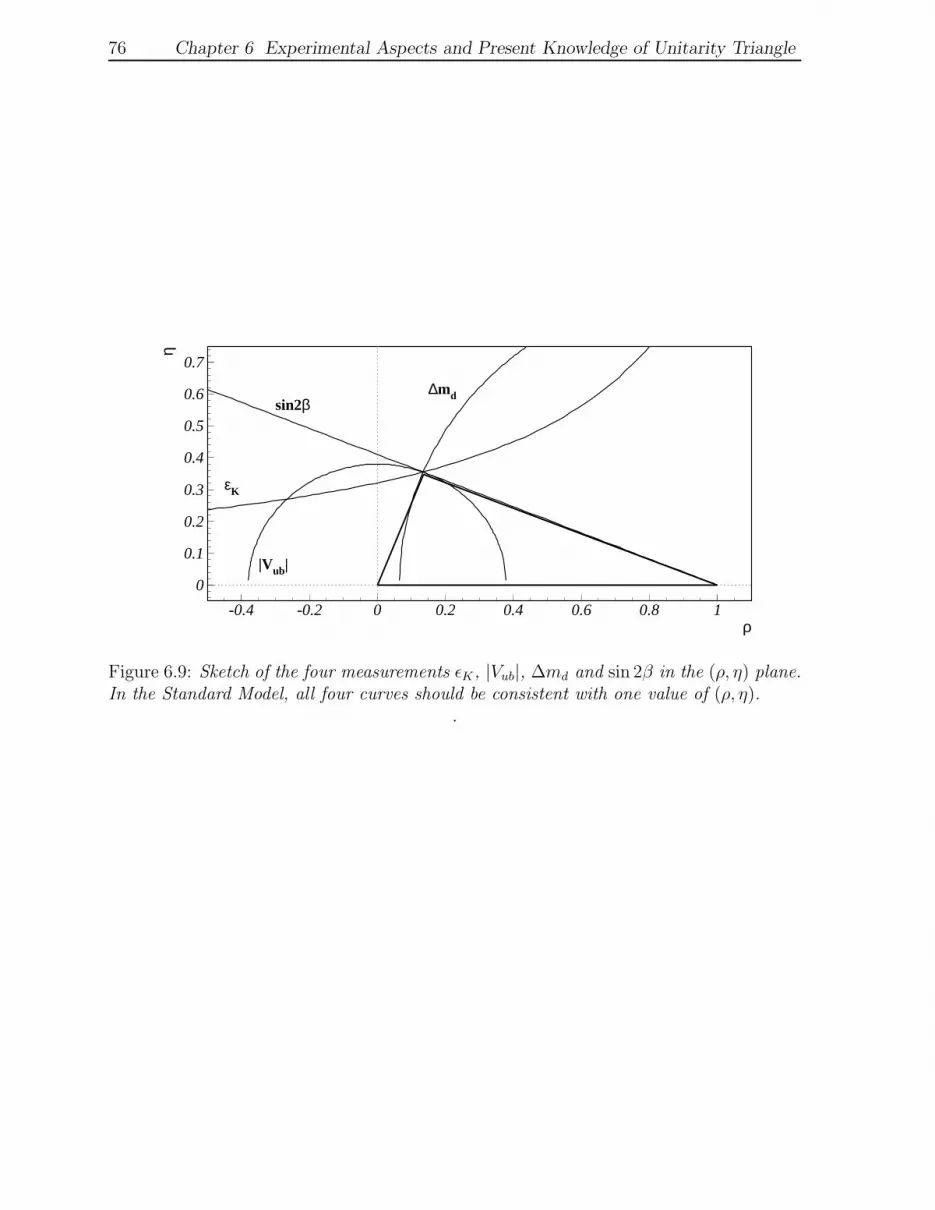
76 Chapter 6 Experimental Aspects and Present Knowledge of Unitarity Triangle
ρ
η
εK
|Vub|
∆mdsin2β
0
0.1
0.2
0.3
0.4
0.5
0.6
0.7
-0.4 -0.2 0 0.2 0.4 0.6 0.8 1
Figure 6.9: Sketch of the four measurements ǫK, |Vub|, ∆md and sin 2β in the (ρ, η) plane.In the Standard Model, all four curves should be consistent with one value of (ρ, η).
.

6.4 Outlook: the LHCb experiment 77
6.4 Outlook: the LHCb experiment
The B-factories at the SLAC (USA) and KEK (Japan) with the BaBar and Belle ex-periments have been extremely succesful in measuring CP violation in the B0 system,resulting in a very accurate determination of the angle β. However, the uncertainty onthe angle γ is still large. The angle βs has not been measured at all yet, although someclaims of new physics have been made [27, 28], based on the measurements at the CDFand D0 experiments with the Tevatron collider at Fermilab, Chicago. The B0
s system is todate very poorly constrained, and might hide interesting new physics effects in the b↔ stransition.
The LHCb detector aims at determining γ and βs at unprecedented precision. Two primeexamples are given in Sections 4.3 and 4.2 were γ and βs are extracted from the decaysB0s → D±
s K∓ and B0
s → J/ψφ, respectively. The B-factories run at the Υ(4S) resonancewhich does not provide enough energy to produce B0
s -mesons. On the other hand, B0s -
mesons are produced at the pp collider at Fermilab. But a relatively low bb cross sectionof 50µb at the center-of-mass energy of 2 TeV and a modest yearly collected luminosityof ∼ 1fb−1 only yields ∼ 3, 000 B0
s → J/ψφ events in the period from 2002-2008.
The LHCb experiment will operate at the LHC collider that will run at a center-of-massenergy of 14 TeV (with a bb cross section of 600µb) and a yearly luminosity of 2 fb−1. Asa result, the LHCb experiment is expected to collect about 100,000 B0
s → J/ψφ eventsper year. Not only due to the large amount of collected B0
s -mesons, but also due to theoptimized (forward) detector design, see Fig. 6.10, an accuracy of σβs
= 0.03 is expectedafter one year. The optimized detector design also comprises particle identification (to
Figure 6.10: Schematic view of the LHCb detector..

78 Chapter 6 Experimental Aspects and Present Knowledge of Unitarity Triangle
distinguish kaons from pions) and an efficienct hadron trigger, which places LHCb ina special situation compared to the other LHC experiments ATLAS and CMS. Due tothese two features, LHCb is expected to collect 5,400 B0
s → D±s K
∓ events, enabling todetermine γ with an accuracy better than σγ = 15o.
These new precision measurements will scrutinize the Standard Model and her CKM-mechanism. Together with the determination of angular distributions and branchingratios of rare decays such as B0 → K∗µ+µ− and B0
s → µ+µ− the measurements at LHCbmight reveal new particles inside virtual loops, complementary to the possible directproduction of new particles at ATLAS and CMS.

References
[1] I.I. Bigi and A.I. Sanda, CP Violation. Cambridge University Press, Cambridge,(England), 2000.
[2] G.C. Branco, L. Lavoura and J.P. Silva, CP Violation. Clarendon Press, Oxford,(England), 1999.
[3] C.S. Wu et al., Experimental test of parity conservation in beta decay. Phys. Rev.105, 1413 (1957).
[4] R.L.Garwin et al., Observations of the failure of conservation of parity and chargeconjugation in meson decays: The magnetic moment of the free muon. Phys. Rev.105, 1415 (1957).
[5] C.Jarlskog (editor), CP Violation, 1989, available onhttp://books.google.com/books?id=U5TC5DSWOmIC&vq=cp violation&pg=PR1.Published by World Scientific.
[6] Y. Nir, CP violation in meson decays. Preprint hep-ph/0510413, 2005.
[7] M.Kobayashi and K.Maskawa, CP violation in the renormalizable theory of weakinteraction. Prog. Theor. Phys. 49, 652 (1973).
[8] L. Wolfenstein, Parametrization of the kobayashi-maskawa matrix. Phys. Rev. Lett.51, 1945 (1983).
[9] R. Fleischer, Flavour physics and CP violation: Expecting the LHC. PreprintarXiv:0802.2882, 2008.
[10] I.Y. Bigi, Flavour dynamics & CP violation in the standard model: A crucial pastand an essential future. Preprint hep-ph/0701273, 2007.
[11] Lenz, A. and others, Anatomy of New Physics in B-Bbar mixing. Phys. Rev.D83, 036004 (2011), 1008.1593.
[12] W.E. Burcham and M. Jobes, Nuclear and Particle Physics. Longman House,Essex, (England), 1995.
79

80 References
[13] T. Inami and C. S. Lim, Effects of superheavy quarks and leptons in low-energyweak processes KL → µ+νµ, KL → µ−νµ, K
+ → π+νν and K0 ↔ K0. Prog. Theor.Phys. 65, 297 (1981).
[14] C. Gay, B mixing. Ann. Rev. Nucl. Part. Sci. 50, 577 (2000).
[15] M. Baak, Measurement of CKM-angle γ with charmed B0 meson decays. Ph.D.Thesis, Free University Amsterdam, 2007.
[16] I.Y. Bigi and A.I. Sanda, Notes on the observability of CP violations in B decays.Nucl. Phys. B193, 85 (1981).
[17] BaBar Coll., Aubert et al., Improved measurement of CP asymmetries inB0 → (cc)K0∗ decays. Phys. Rev. Lett. 94, 161803 (2005).
[18] Heavy Flavor Averaging Group (HFAG), E. Barberio, et al., Averages of b-hadronand c-hadron properties at the end of 2007. Preprint arXiv:0808.1297v3, 2008.
[19] J.H. Christenson et al., Evidence for the 2-π decay of the K02 meson. Phys. Rev.
Lett. 13, 138 (1964).
[20] Particle Data Group, C. Amsler et al., Review of particle physics. Phys. Lett.B667, 1 (2008).
[21] CPLEAR Coll., A.Angelopoulos, A determination of the cp violation parametereta+- from the decay of strangeness-tagged neutral kaons.
[22] CKMfitter Coll., J. Charles et al., CP violation and the CKM matrix: Assessing theimpact of the asymmetric B factories. Eur. Phys. J. C41, 1 (2005).
[23] UTfit Coll., M. Bona et al., The unitarity triangle fit in the standard model andhadronic parameters from lattice QCD: A reappraisal after the measurements of∆ms and BR(B → τν). JHEP 0610, 81 (2006).
[24] G. Buchalla, A.J. Buras and M.E. Lautenbacher, Weak decays beyond leadinglogarithms. Rev. Mod. Phys. 68, 1125 (1996).
[25] G. Colin, B mixing. Ann. Rev. Nucl. Part. Sci. 50, 577 (2000).
[26] ARGUS Coll., H. Albrecht et al., Observation of B0 - anti-B0 mixing. Phys. Rev.Lett. B192, 245 (1987).
[27] UTfit Coll., M. Bona et al., First evidence of new physics in b↔s transitions.Preprint arXiv:0803.0659, 2008.
[28] L. Silvestrini, First evidence of new physics in Bs mixing and its implications.Nucl. Phys. Proc. Suppl. 185, 41 (2008).

References 81
Acknowledgments
Special thanks to Tristan du Pree, Serena Oggero, Daan van Eijk, Jeroen van Leerdam,Kristof De Bruyn, Meike de With and Rob Knegjens for spotting mistakes in these lecturenotes, and for suggesting many improvements!