theory of robotics and mechatronics
TRANSCRIPT
TheoryofRoboticsandMechatronicsCoursenumber151‐0601‐00
InstructorsSascha Stoeter [email protected]
Petr Korba [email protected]
TeachingAssistantHong Ayoung [email protected] +41 44 632 86 76 CLA H 13
Prof.BradNelsonInstitute of Robotics and Intelligent Systems
SuggestedLiterature
G. Strang, “Linear algebra and its applications”, Academic Press, New York, USA, 1976
J. J. Craig, “Introduction to Robotics: Mechanics and Control”, 3rd ed., Prentice Hall, 2003.
R. M. Murray, Z. Li, and S. S. Sastry, “A Mathematical Introduction to Robotic Manipulation”, CRC Press, 1994.
M. Spong and M. Vidyasagar, "Robot Dynamics and Control", Wiley, 1989. P. McKerrow, "Introduction to Robotics", Addison‐Wesley, 1999.
T. Yoshikawa, "Foundations of Robotics: Analysis and Control", MIT Press, 1990.
J.‐P. Merlet, "Parallel Robots", Springer, 2001.
R. Siegwart and I. R. Nourbakhsh, “Introduction to Autonomous Mobile Robots”, MIT Press, 2004.
H. Choset, K. M. Lynch, S. Hutchinson, G. Kantor, W. Burgard, L. E. Kavraki, and S. Thrun, “Principles of Robot Motion: Theory, Algorithms, and Implementations”, MIT Press, 2005.
J. Borenstein, H. Everett, and L. Feng, Navigating Mobile Robots: Systems and Techniques, A. K. Peters, 1996.
G. Dukek and M. Jenkin, "Computational Principles of Mobile Robotics", Cambridge University Press, 2000.
D. Forsyth and J. Ponce, "Computer Vision — A Modern Approach", Prentice Hall, 2003.
1
Introduction
Institute of Robotics and Intelligent Systems
ETH Zurich
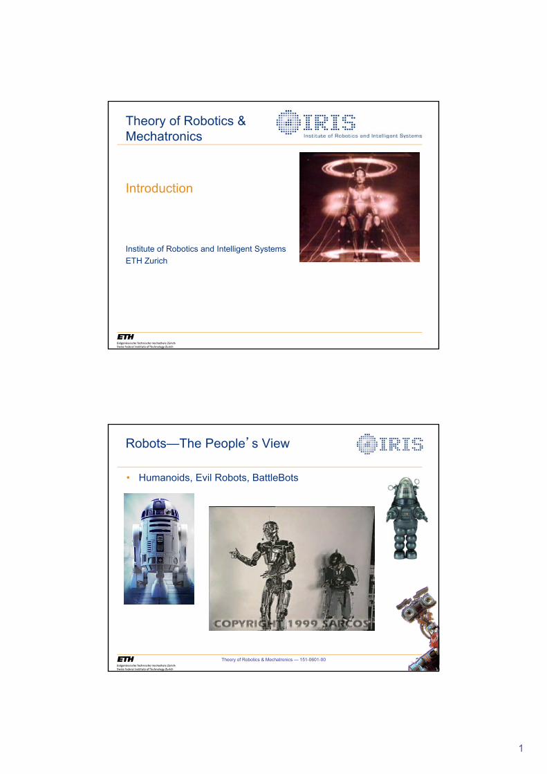
Theory of Robotics &Mechatronics
2Theory of Robotics & Mechatronics — 151-0601-00
Robots—The People’s View
• Humanoids, Evil Robots, BattleBots

2
Pierre Jaquet-Droz (1721–1790)
Swiss watchmaker and builder of automatons
Exercise
• Part 1: Get to know each other– Hello, my name is …
– Where are you from?
– What couldn’t be guessed about you?
– …
• Part 2: What is a robot?
3
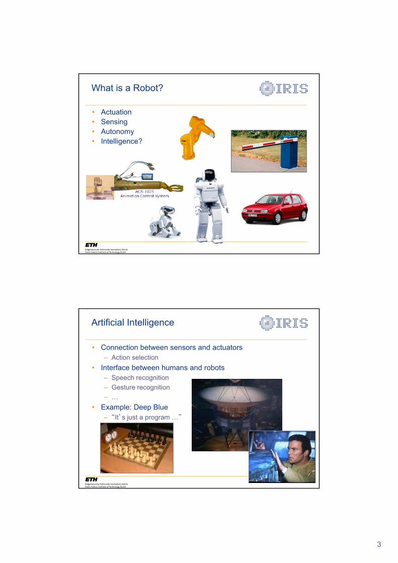
What is a Robot?
• Actuation
• Sensing
• Autonomy
• Intelligence?
Artificial Intelligence
• Connection between sensors and actuators
– Action selection
• Interface between humans and robots
– Speech recognition
– Gesture recognition
– …
• Example: Deep Blue
– “It’s just a program …”
4
7Theory of Robotics & Mechatronics — 151-0601-00
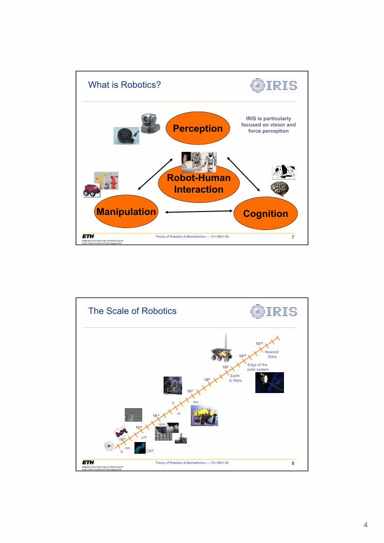
What is Robotics?
IRIS is particularly focused on vision and
force perception
Manipulation
Perception
Cognition
Robot-HumanInteraction
8Theory of Robotics & Mechatronics — 151-0601-00
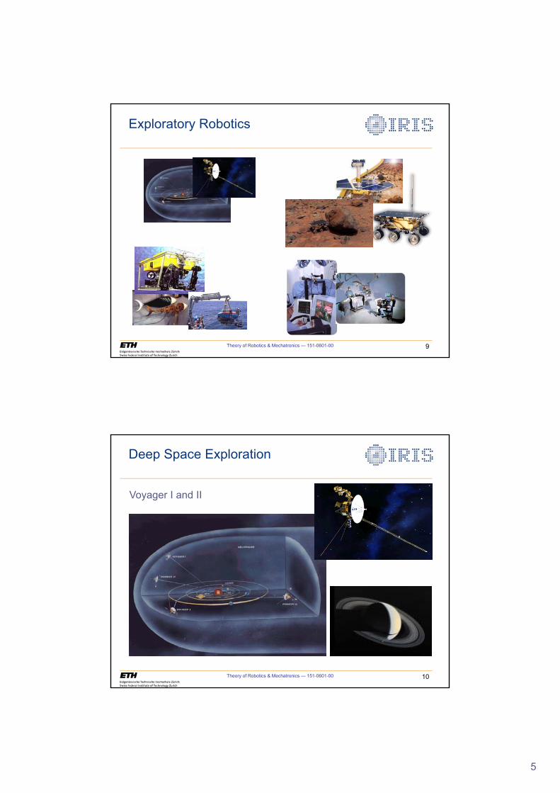
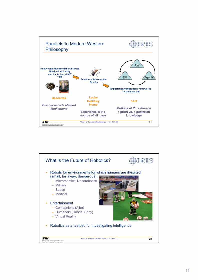
The Scale of Robotics
Å
10-9
10-6
10-3
1
103
106
109
1012
1015
nm
Pm
mm
m
km
Edge of the solar system
Earth to Mars
CNT
Nearest Stars
5
9Theory of Robotics & Mechatronics — 151-0601-00
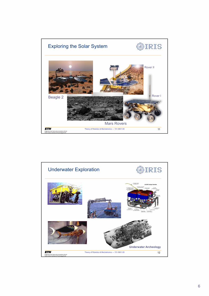
Exploratory Robotics
10Theory of Robotics & Mechatronics — 151-0601-00
Deep Space Exploration
Voyager I and II
6
11Theory of Robotics & Mechatronics — 151-0601-00
Exploring the Solar System
Mars Rovers
Beagle 2 Rover I
Rover II
12Theory of Robotics & Mechatronics — 151-0601-00
Underwater Exploration
Underwater Archeology
7
13Theory of Robotics & Mechatronics — 151-0601-00
Robotic Surgery
14Theory of Robotics & Mechatronics — 151-0601-00
Robotics for Exploring Life at a Cellular Level
8
15Theory of Robotics & Mechatronics — 151-0601-00
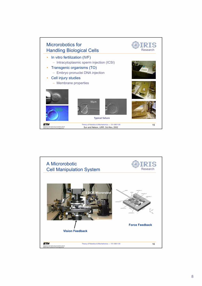
Microrobotics for Handling Biological Cells
• In vitro fertilization (IVF)
– Intracytoplasmic sperm injection (ICSI)
• Transgenic organisms (TO)
– Embryo pronuclei DNA injection
• Cell injury studies
– Membrane properties
Typical failure
Sun and Nelson, IJRR, Oct-Nov, 2002
50Pm
Research
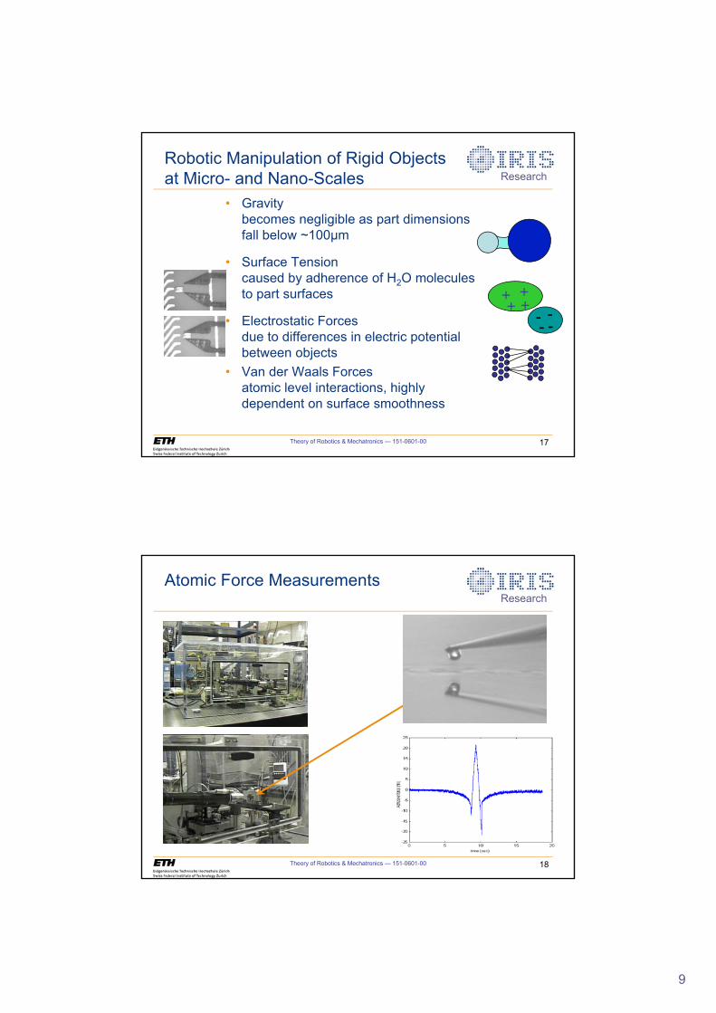
16Theory of Robotics & Mechatronics — 151-0601-00
A MicroroboticCell Manipulation System
3 DOF Microrobot
Vision Feedback
Force Feedback
Research
9
17Theory of Robotics & Mechatronics — 151-0601-00
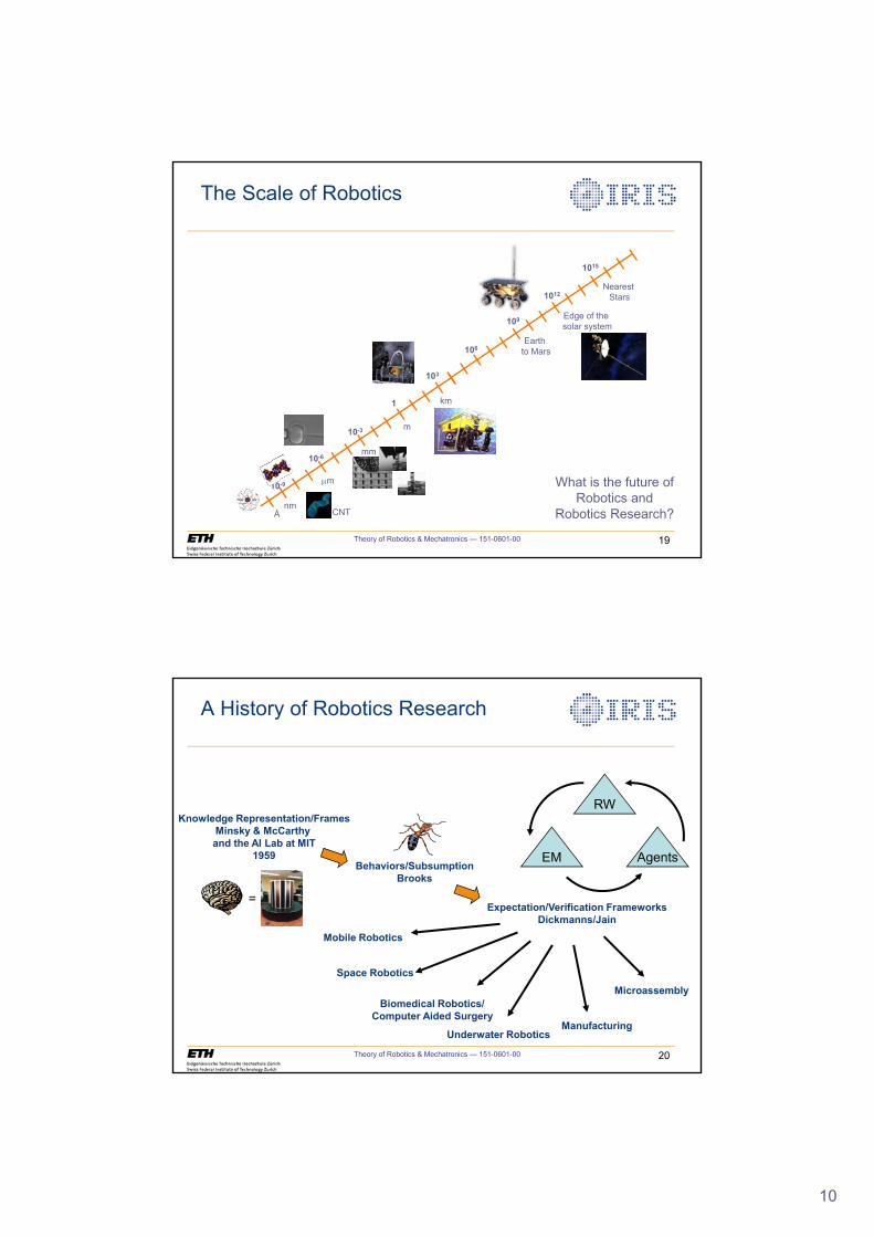
Robotic Manipulation of Rigid Objects at Micro- and Nano-Scales
• Gravity becomes negligible as part dimensions fall below ~100μm
• Surface Tensioncaused by adherence of H2O molecules to part surfaces
• Electrostatic Forcesdue to differences in electric potential between objects
• Van der Waals Forcesatomic level interactions, highly dependent on surface smoothness
+++
+---
-
Research
18Theory of Robotics & Mechatronics — 151-0601-00
Atomic Force MeasurementsResearch
10
19Theory of Robotics & Mechatronics — 151-0601-00
The Scale of Robotics
What is the future of Robotics and
Robotics Research?Å
10-9
10-6
10-3
1
103
106
109
1012
1015
nm
Pm
mm
m
km
Edge of the solar system
Earth to Mars
CNT
Nearest Stars
20Theory of Robotics & Mechatronics — 151-0601-00
Mobile Robotics
MicroassemblySpace Robotics
Underwater Robotics
Biomedical Robotics/Computer Aided Surgery
Manufacturing
A History of Robotics Research
Knowledge Representation/FramesMinsky & McCarthy and the AI Lab at MIT
1959Behaviors/Subsumption
Brooks
Expectation/Verification FrameworksDickmanns/Jain
AgentsEM
RW
=
11
21Theory of Robotics & Mechatronics — 151-0601-00
Parallels to Modern Western Philosophy
Knowledge Representation/FramesMinsky & McCarthy and the AI Lab at MIT
1959Behaviors/Subsumption
Brooks
Expectation/Verification FrameworksDickmanns/Jain
AgentsEM
RW
=
Descartes
Discourse de la MethodMeditations
LockeBerkeley
Hume
Experience is the source of all ideas
Kant
Critique of Pure Reasona priori vs. a posteriori
knowledge
22Theory of Robotics & Mechatronics — 151-0601-00
What is the Future of Robotics?
• Robots for environments for which humans are ill-suited (small, far away, dangerous)– Microrobotics, Nanorobotics
– Military
– Space
– Medical
• Entertainment– Companions (Aibo)
– Humanoid (Honda, Sony)
– Virtual Reality
• Robotics as a testbed for investigating intelligence
12
23Theory of Robotics & Mechatronics — 151-0601-00
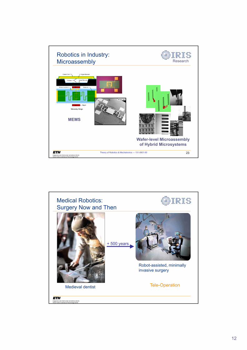
Robotics in Industry:Microassembly
Wafer-level Microassemblyof Hybrid Microsystems
MEMS
Research
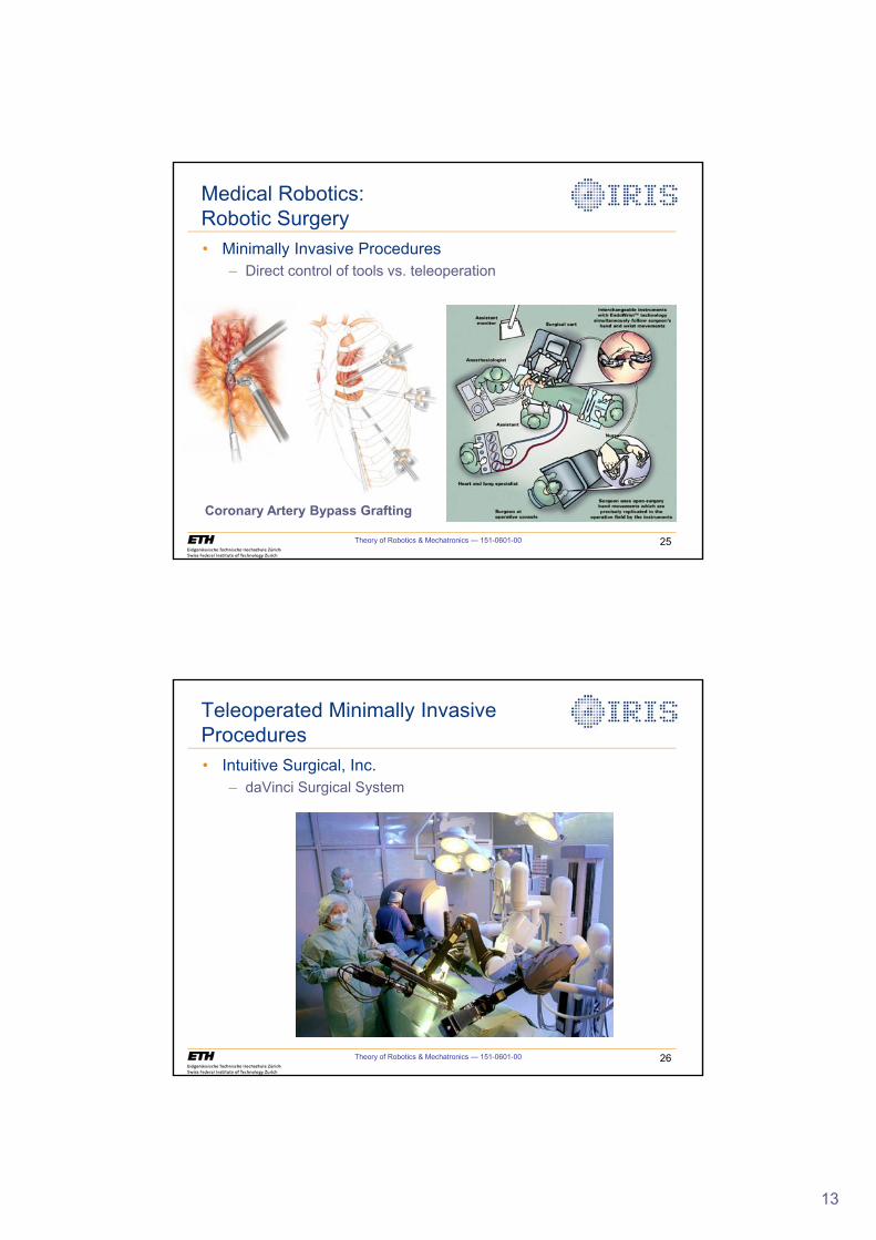
Medical Robotics:Surgery Now and Then
Medieval dentist
Robot-assisted, minimally invasive surgery
+ 500 years
Tele-Operation
13
25Theory of Robotics & Mechatronics — 151-0601-00
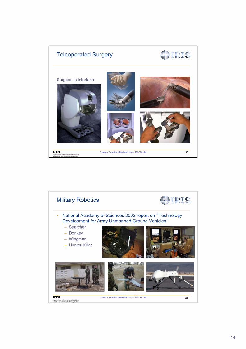
Medical Robotics: Robotic Surgery
• Minimally Invasive Procedures
– Direct control of tools vs. teleoperation
Coronary Artery Bypass Grafting
26Theory of Robotics & Mechatronics — 151-0601-00
Teleoperated Minimally Invasive Procedures
• Intuitive Surgical, Inc.
– daVinci Surgical System
14
27Theory of Robotics & Mechatronics — 151-0601-00
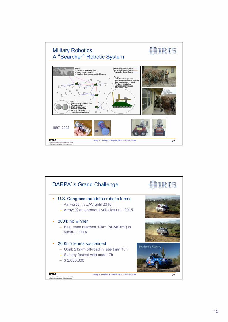
Teleoperated Surgery
Surgeon’s Interface
28Theory of Robotics & Mechatronics — 151-0601-00
Military Robotics
• National Academy of Sciences 2002 report on “Technology Development for Army Unmanned Ground Vehicles”
– Searcher
– Donkey
– Wingman
– Hunter-Killer
15
29Theory of Robotics & Mechatronics — 151-0601-00
Military Robotics: A “Searcher” Robotic System
1997–2002
30Theory of Robotics & Mechatronics — 151-0601-00
DARPA’s Grand Challenge
• U.S. Congress mandates robotic forces
– Air Force: ⅓ UAV until 2010
– Army: ⅓ autonomous vehicles until 2015
• 2004: no winner
– Best team reached 12km (of 240km!) in several hours
• 2005: 5 teams succeeded
– Goal: 212km off-road in less than 10h
– Stanley fastest with under 7h
– $ 2,000,000
Stanford’s Stanley
16
DARPA’s Urban Grand Challenge
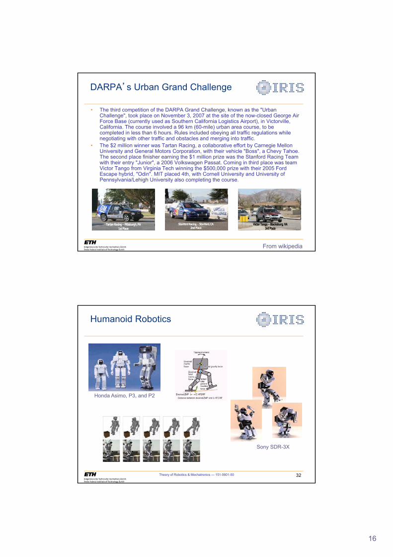
• The third competition of the DARPA Grand Challenge, known as the "Urban Challenge", took place on November 3, 2007 at the site of the now-closed George Air Force Base (currently used as Southern California Logistics Airport), in Victorville, California. The course involved a 96 km (60-mile) urban area course, to be completed in less than 6 hours. Rules included obeying all traffic regulations while negotiating with other traffic and obstacles and merging into traffic.
• The $2 million winner was Tartan Racing, a collaborative effort by Carnegie Mellon University and General Motors Corporation, with their vehicle "Boss", a Chevy Tahoe. The second place finisher earning the $1 million prize was the Stanford Racing Team with their entry "Junior", a 2006 Volkswagen Passat. Coming in third place was team Victor Tango from Virginia Tech winning the $500,000 prize with their 2005 Ford Escape hybrid, "Odin". MIT placed 4th, with Cornell University and University of Pennsylvania/Lehigh University also completing the course.
From wikipedia
32Theory of Robotics & Mechatronics — 151-0601-00
Humanoid Robotics
Sony SDR-3X
Honda Asimo, P3, and P2

17
33Theory of Robotics & Mechatronics — 151-0601-00
Humanoid Robotics
Sony SDR-3X
Honda Asimo, P3, and P2
The “Killer App” ??
34Theory of Robotics & Mechatronics — 151-0601-00
Nanorobotics: Manipulation of Carbon Nanotubes
18
35Theory of Robotics & Mechatronics — 151-0601-00
The PC Industry as a Metaphor for Robotics
• The Robotics Industry is at the same state now as the PC industry was in the late 1970’s (Brooks)
– Mainly expensive and used in industry
– PC kits — Robot kits
– PC’s for the home — Robots for the home
– The failure of conventional wisdom?
• The demise of the mainframe industry
36Theory of Robotics & Mechatronics — 151-0601-00
Future Robotics Research
• Distributed robotic systems
• Fusing multiple “orthogonal” sensing modalities
– e.g., manipulating deformable objects
• Radically new theories of intelligence
• Robots may not be what we think they are
– New types of Robot-Human Interaction
• The future of robotics is being determined by those that have both a vision and the energy to pursue their vision
19
37Theory of Robotics & Mechatronics — 151-0601-00
Social Impact of Robots
• Sometimes robots are the only way(e.g., hazardous environments)
• Mostly competes with manual labor
• Social tax on robots just like workers?
• Impact on human-human relationships?
Exercise
• Why don’t we use monkeys (humans, dolphins, …)?
20
39Theory of Robotics & Mechatronics — 151-0601-00
What we will learn
• Introduction
Overview of Robotics
• Mechanical Design of Robots
Types of robots, sensors, actuators, gearboxes, robot end-effectors, resolution, accuracy, precision.
40Theory of Robotics & Mechatronics — 151-0601-00
What we will learn
• The Mathematical Basics of Robotics Using a Classical Approach
– Describing the position and orientation of objects in 3D space
– Coordinate frames, position, orientation and velocity vectors in 3D, coordinate transformations.
– Applies directly to Computer Graphics
• The Mathematical Basics of Robotics Using Screw Theory
– A mathematical description of rigid body motion
– Eliminates deficiencies of the classical approach
21
41Theory of Robotics & Mechatronics — 151-0601-00
What we will learn
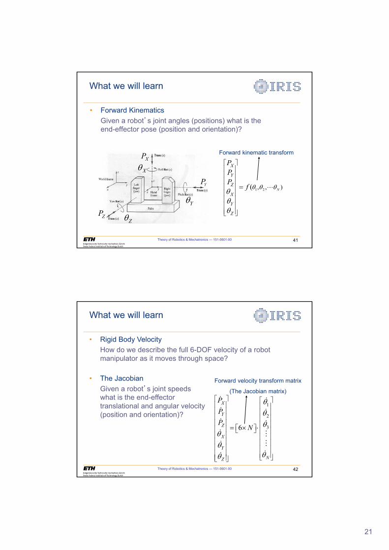
• Forward Kinematics
Given a robot’s joint angles (positions) what is theend-effector pose (position and orientation)?
1 2, , )( N
X
Y
Z
X
Y
Z
PPP f T T TTTT
ª º« »« »« »« »« »« »« »« »¬ ¼
�
XP
XT
YP
YT
ZPZT
Forward kinematic transform
42Theory of Robotics & Mechatronics — 151-0601-00
What we will learn
1
2
36
X
Y
Z
X
Y
NZ
PPP
N
TTT
TT
TT
ª º ª º« » « »« » « »« » « »« » « »ª º« » ¬ ¼ « »« » « »« » « »« » « »« » « »¬ ¼« »¬ ¼
u �
� �
� �
� �
� �� �
��
Forward velocity transform matrix
(The Jacobian matrix)
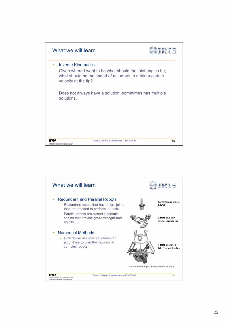
• The Jacobian
Given a robot’s joint speeds what is the end-effector translational and angular velocity (position and orientation)?
• Rigid Body Velocity
How do we describe the full 6-DOF velocity of a robot manipulator as it moves through space?
22
43Theory of Robotics & Mechatronics — 151-0601-00
What we will learn
• Inverse Kinematics
Given where I want to be what should the joint angles be; what should be the speed of actuators to attain a certain velocity at the tip?
Does not always have a solution, sometimes has multiple solutions.
44Theory of Robotics & Mechatronics — 151-0601-00
What we will learn
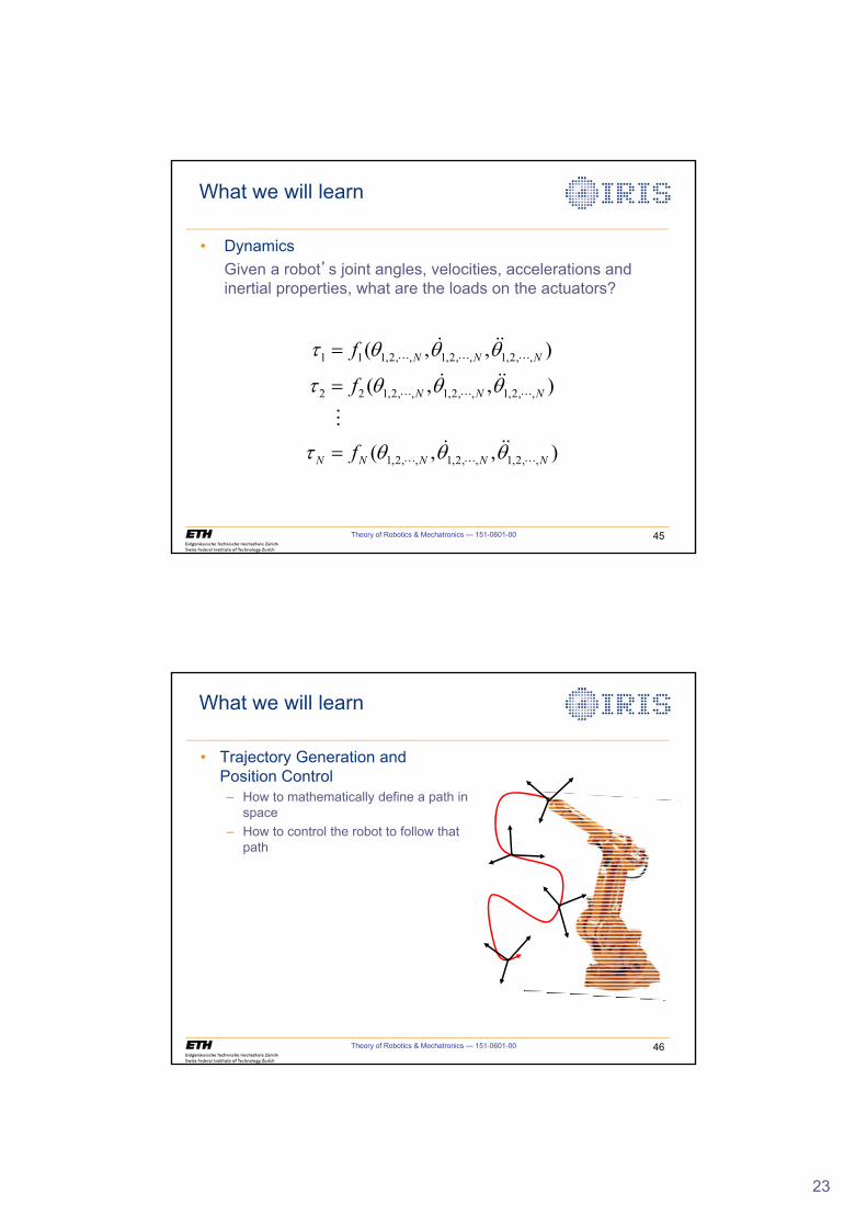
• Redundant and Parallel Robots– Redundant robots that have more joints
than are needed to perform the task
– Parallel robots are closed-kinematic chains that provide great strength and rigidity
• Numerical Methods– How do we use efficient computer
algorithms to plan the motions of complex robots
The SML Parallel Haptic Device (Uchiyama,Tsumaki)
23
45Theory of Robotics & Mechatronics — 151-0601-00
What we will learn
• Dynamics
Given a robot’s joint angles, velocities, accelerations and inertial properties, what are the loads on the actuators?
1 1 1,2, , 1,2, , 1,2, ,
2 2 1,2, , 1,2, , 1,2, ,
1,2, , 1,2, , 1,2, ,
( , , )
( , , )
( , , )
N N N
N N N
N N N N N
f
f
f
W T T T
W T T T
W T T T
� � �
� � �
� � �
� ��
� ��
�
� ��
46Theory of Robotics & Mechatronics — 151-0601-00
What we will learn
• Trajectory Generation and Position Control– How to mathematically define a path in
space
– How to control the robot to follow that path
24
47Theory of Robotics & Mechatronics — 151-0601-00
What we will learn
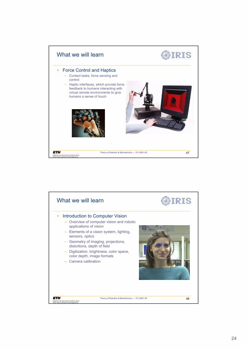
• Force Control and Haptics– Contact tasks, force sensing and
control
– Haptic interfaces, which provide force feedback to humans interacting with virtual remote environments to give humans a sense of touch
48Theory of Robotics & Mechatronics — 151-0601-00
What we will learn
• Introduction to Computer Vision– Overview of computer vision and robotic
applications of vision
– Elements of a vision system, lighting, sensors, optics
– Geometry of imaging, projections, distortions, depth of field
– Digitization, brightness, color space, color depth, image formats
– Camera calibration

25
49Theory of Robotics & Mechatronics — 151-0601-00
What we will learn
• Computer Vision Algorithms– Binary images, thresholding, histograms
– Area/moment statistics, morphological operations
– Segmentation, blob analysis, labeling
– Spatial operations and transformations:Pixel neighborhoods, convolution.
– Mean, Gaussian, Laplacian, gradient filters
– Edge detection, Canny, Hough transform
• Vision for Robotics– Visual servoing, image based, position based
– Tracking, snakes
– 3D vision: multi-camera geometry, stereo andmodel-based vision
– Range imaging and robotic applications
50Theory of Robotics & Mechatronics — 151-0601-00
What we will learn
• Introduction to Mobile Robotics
– Overview of mobile robotics, applications
– Sensors and estimation
– Distributed robotics
• Introduction to Micro- and Nano-robotics
– Overview of MEMS, scaling effects, micromanipulation
– Microscope optics, depth from defocus, focus measures
– Examples from current research
26
Robotics is …
• fun• an interdisciplinary area
• unsolved
51Theory of Robotics & Mechatronics — 151-0601-00
ICRA Video ProceedingsWinner 2006
52Theory of Robotics & Mechatronics — 151-0601-00
1
Mechanical Design of Robots
Theory of Robotics &Mechatronics
Institute of Robotics and Intelligent SystemsETH Zurich
Theory of Robotics & Mechatronics — 151-0601-00 2
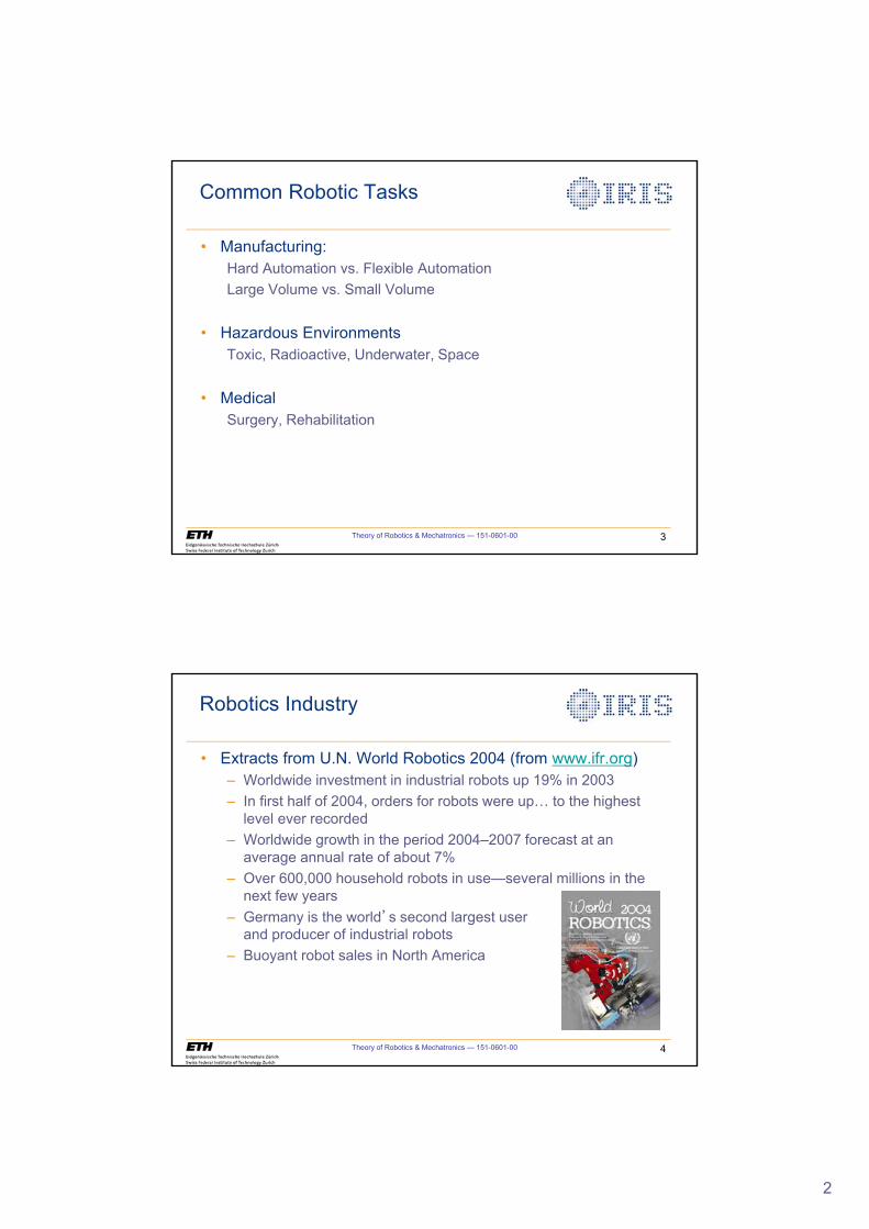
Robots—The Industrial View
• “A robot is a reprogrammable, multifunctional machine designed to manipulate materials, parts, tools, or specializeddevices, through variable programmed motions for theperformance of a variety of tasks.”
Definition of the Robotics Industries Association ( www.robotics.org )
2
Theory of Robotics & Mechatronics — 151-0601-00 3
Common Robotic Tasks
• Manufacturing:Hard Automation vs. Flexible AutomationLarge Volume vs. Small Volume
• Hazardous EnvironmentsToxic, Radioactive, Underwater, Space
• MedicalSurgery, Rehabilitation
Theory of Robotics & Mechatronics — 151-0601-00 4
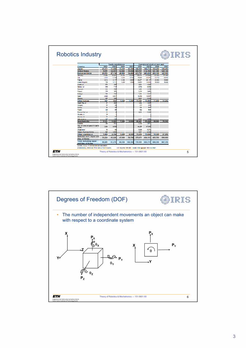
Robotics Industry
• Extracts from U.N. World Robotics 2004 (from www.ifr.org)– Worldwide investment in industrial robots up 19% in 2003– In first half of 2004, orders for robots were up… to the highest
level ever recorded– Worldwide growth in the period 2004–2007 forecast at an
average annual rate of about 7%– Over 600,000 household robots in use—several millions in the
next few years– Germany is the world’s second largest user
and producer of industrial robots– Buoyant robot sales in North America
3
Theory of Robotics & Mechatronics — 151-0601-00 5
Robotics Industry
Theory of Robotics & Mechatronics — 151-0601-00 6
Degrees of Freedom (DOF)
X
Y
Z
PX
TX
PYTY
PZ
TZ
X
Y
PY
T
PX
• The number of independent movements an object can make with respect to a coordinate system
4
Theory of Robotics & Mechatronics — 151-0601-00 7
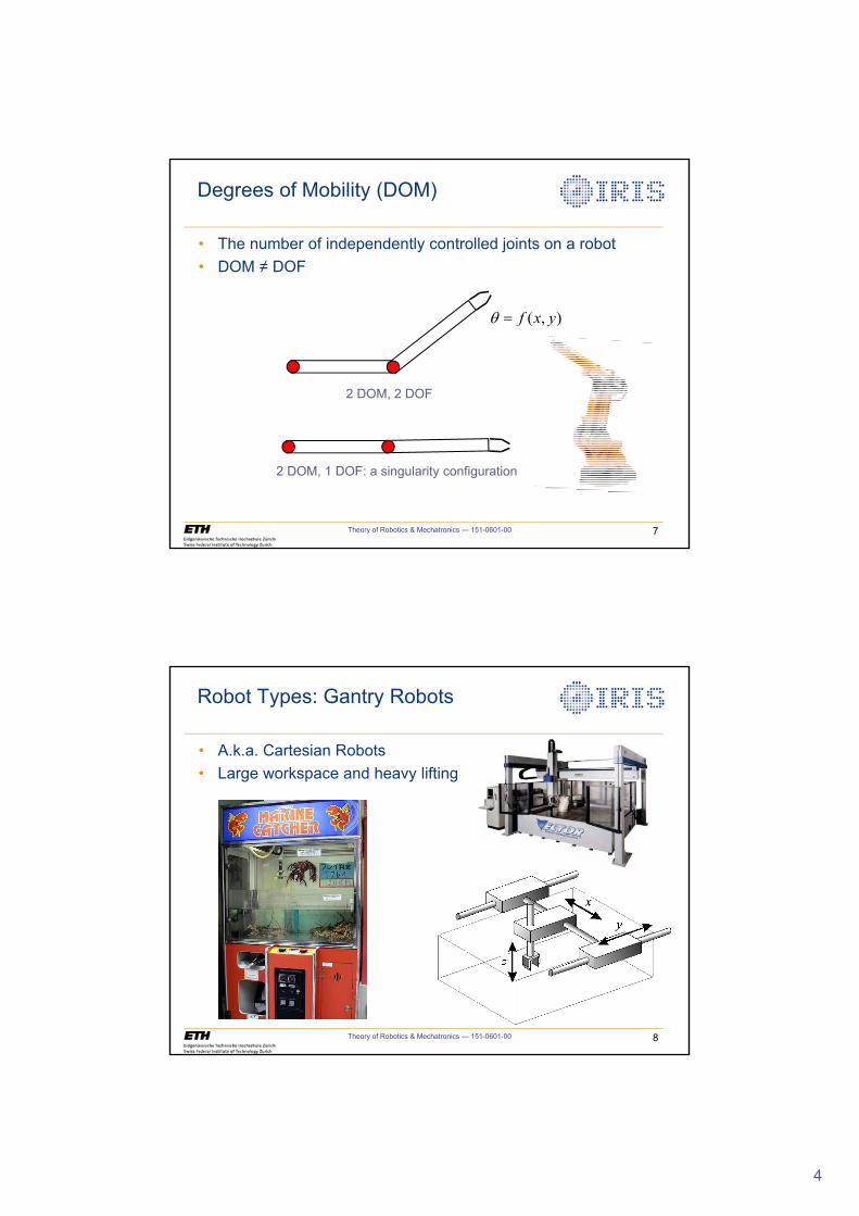
Degrees of Mobility (DOM)
• The number of independently controlled joints on a robot• DOM DOF
2 DOM, 2 DOF
2 DOM, 1 DOF: a singularity configuration
( , )f x yT
Theory of Robotics & Mechatronics — 151-0601-00 8
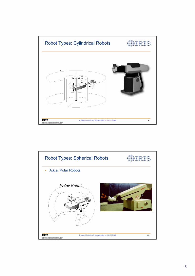
Robot Types: Gantry Robots
• A.k.a. Cartesian Robots• Large workspace and heavy lifting
5
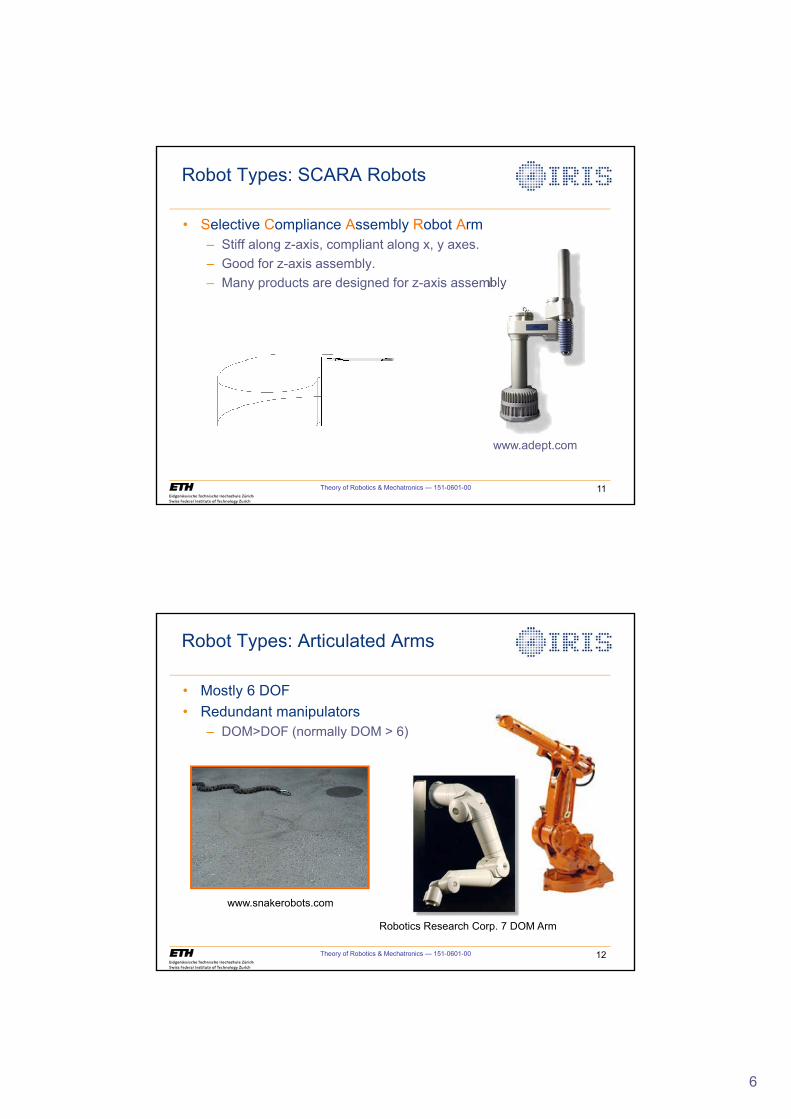
Theory of Robotics & Mechatronics — 151-0601-00 9
Robot Types: Cylindrical Robots
Theory of Robotics & Mechatronics — 151-0601-00 10
Robot Types: Spherical Robots
• A.k.a. Polar Robots
6
Theory of Robotics & Mechatronics — 151-0601-00 11
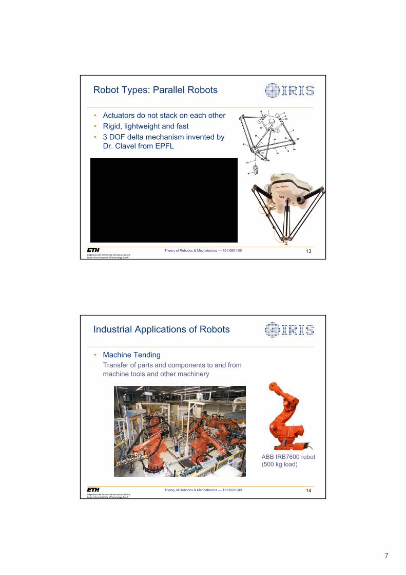
Robot Types: SCARA Robots
• Selective Compliance Assembly Robot Arm– Stiff along z-axis, compliant along x, y axes.– Good for z-axis assembly.– Many products are designed for z-axis assembly
www.adept.com
Theory of Robotics & Mechatronics — 151-0601-00 12
Robot Types: Articulated Arms
• Mostly 6 DOF• Redundant manipulators
– DOM>DOF (normally DOM > 6)
Robotics Research Corp. 7 DOM Arm
www.snakerobots.com
7
Theory of Robotics & Mechatronics — 151-0601-00 13
Robot Types: Parallel Robots
• Actuators do not stack on each other• Rigid, lightweight and fast• 3 DOF delta mechanism invented by
Dr. Clavel from EPFL
Theory of Robotics & Mechatronics — 151-0601-00 14
• Machine TendingTransfer of parts and components to and from machine tools and other machinery
Industrial Applications of Robots
ABB IRB7600 robot (500 kg load)
8
Theory of Robotics & Mechatronics — 151-0601-00 15
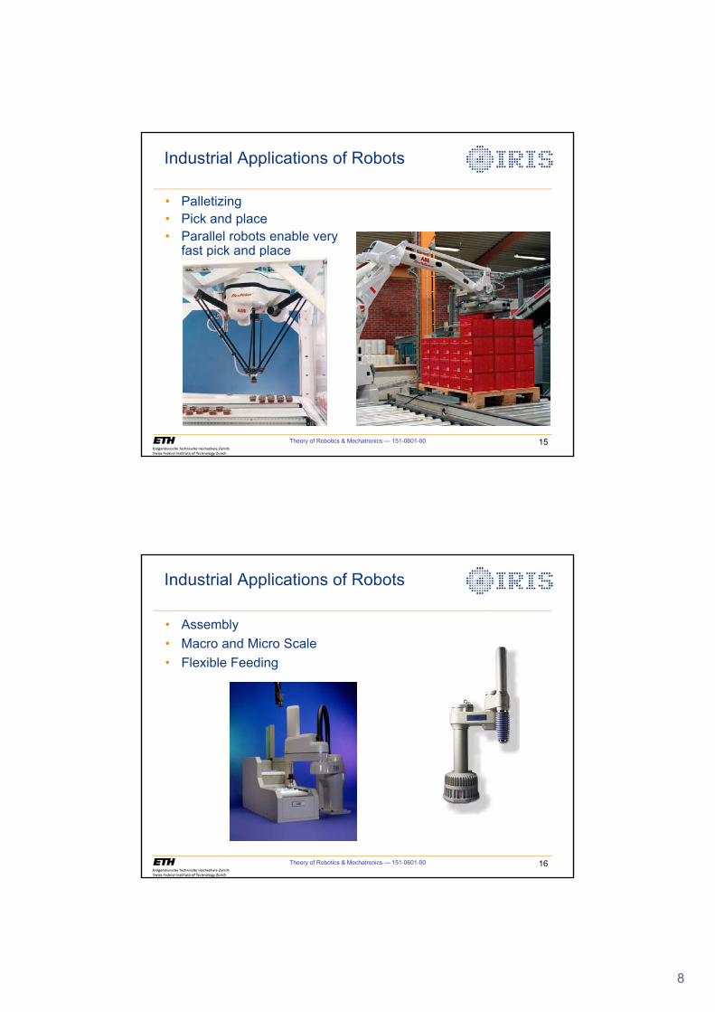
• Palletizing• Pick and place• Parallel robots enable very
fast pick and place
Industrial Applications of Robots
Theory of Robotics & Mechatronics — 151-0601-00 16
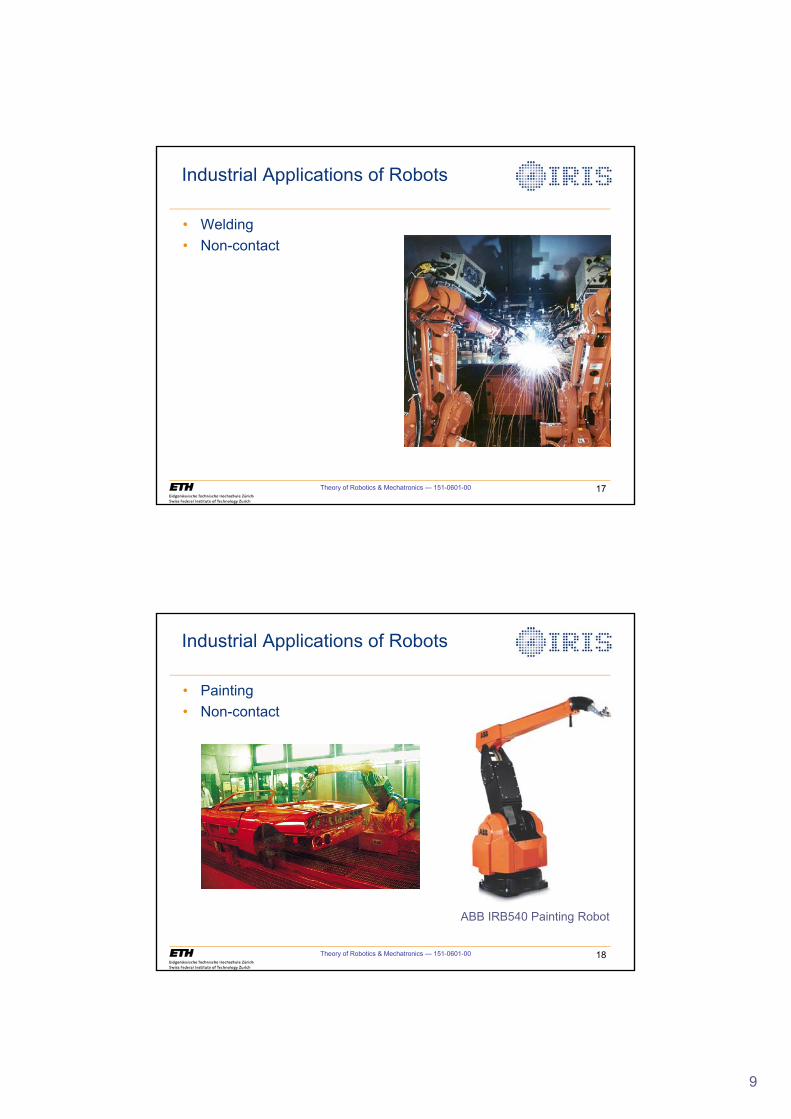
• Assembly• Macro and Micro Scale• Flexible Feeding
Industrial Applications of Robots
9
Theory of Robotics & Mechatronics — 151-0601-00 17
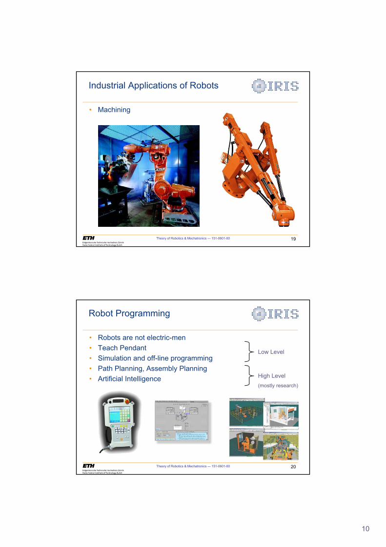
• Welding• Non-contact
Industrial Applications of Robots
Theory of Robotics & Mechatronics — 151-0601-00 18
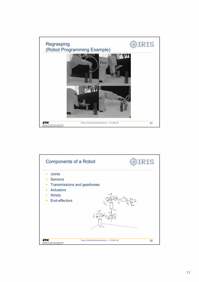
• Painting• Non-contact
Industrial Applications of Robots
ABB IRB540 Painting Robot
10
Theory of Robotics & Mechatronics — 151-0601-00 19
• Machining
Industrial Applications of Robots
Theory of Robotics & Mechatronics — 151-0601-00 20
Robot Programming
• Robots are not electric-men• Teach Pendant• Simulation and off-line programming• Path Planning, Assembly Planning • Artificial Intelligence
Low Level
High Level(mostly research)
11
Regrasping(Robot Programming Example)
Theory of Robotics & Mechatronics — 151-0601-00 21
Theory of Robotics & Mechatronics — 151-0601-00 22
• Joints• Sensors• Transmissions and gearboxes• Actuators• Wrists• End-effectors
Components of a Robot
12
Theory of Robotics & Mechatronics — 151-0601-00 23
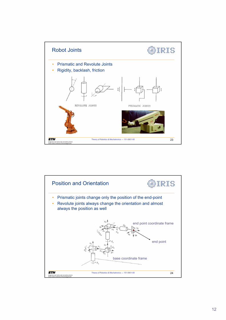
Robot Joints
• Prismatic and Revolute Joints• Rigidity, backlash, friction
Theory of Robotics & Mechatronics — 151-0601-00 24
Position and Orientation
• Prismatic joints change only the position of the end-point• Revolute joints always change the orientation and almost
always the position as well
end point
end point coordinate frame
base coordinate frame
13
Theory of Robotics & Mechatronics — 151-0601-00 25
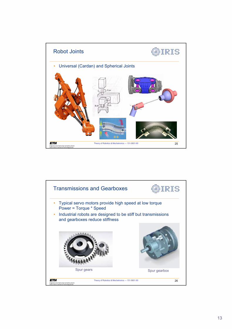
Robot Joints
• Universal (Cardan) and Spherical Joints
Theory of Robotics & Mechatronics — 151-0601-00 26
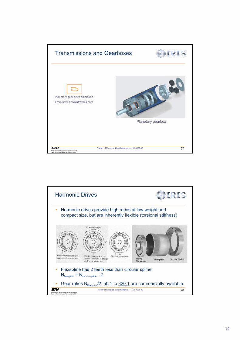
Transmissions and Gearboxes
• Typical servo motors provide high speed at low torquePower = Torque * Speed
• Industrial robots are designed to be stiff but transmissions and gearboxes reduce stiffness
Spur gears Spur gearbox
14
Theory of Robotics & Mechatronics — 151-0601-00 27
Transmissions and Gearboxes
Planetary gearbox
Planetary gear drive animation
From www.howstuffworks.com
Theory of Robotics & Mechatronics — 151-0601-00 28
Harmonic Drives
• Harmonic drives provide high ratios at low weight and compact size, but are inherently flexible (torsional stiffness)
• Flexspline has 2 teeth less than circular spline Nflexspline = Ncircularspline - 2
• Gear ratios Nflexspline/2. 50:1 to 320:1 are commercially available
15
Theory of Robotics & Mechatronics — 151-0601-00 29
Transmissions and Gearboxes
• Tendon Drives
Theory of Robotics & Mechatronics — 151-0601-00 30
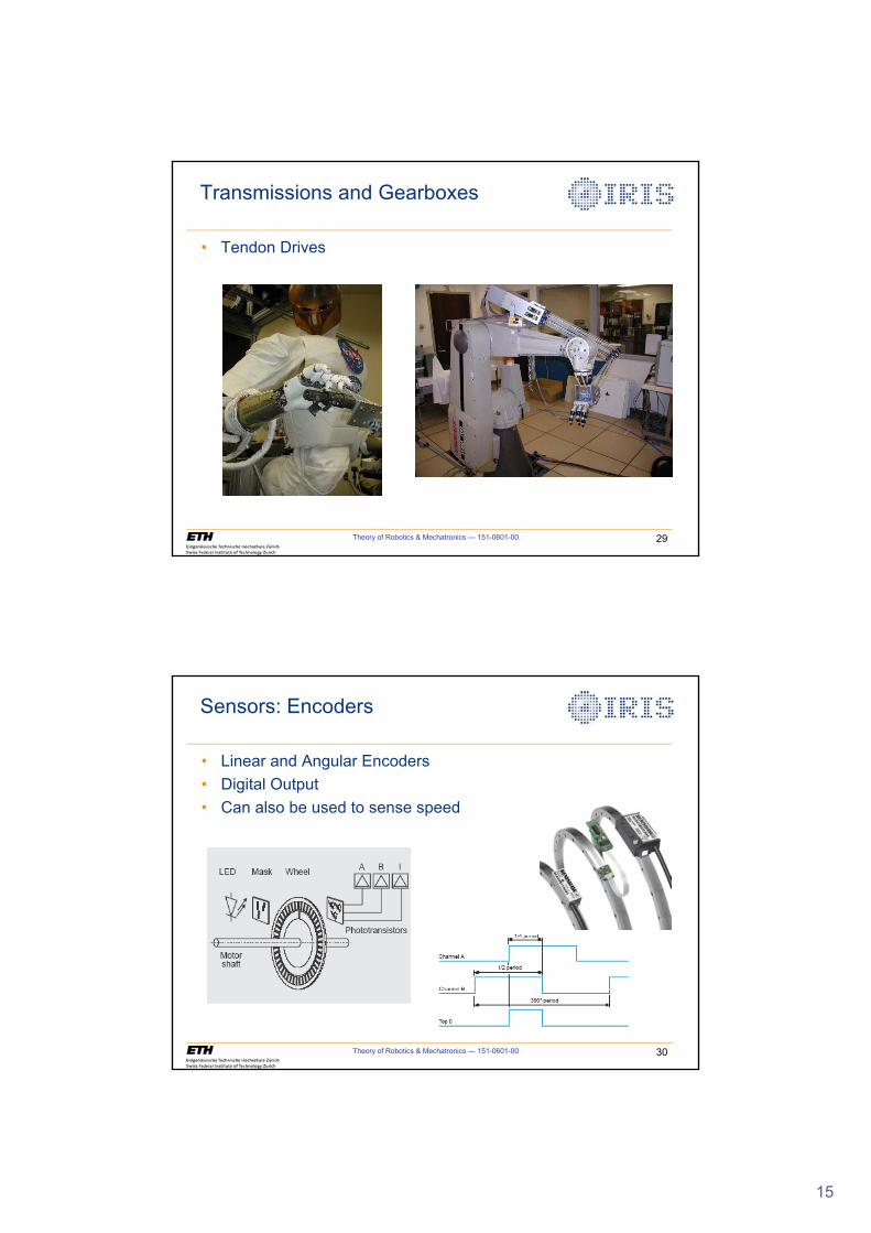
Sensors: Encoders
• Linear and Angular Encoders• Digital Output• Can also be used to sense speed
16
Theory of Robotics & Mechatronics — 151-0601-00 31
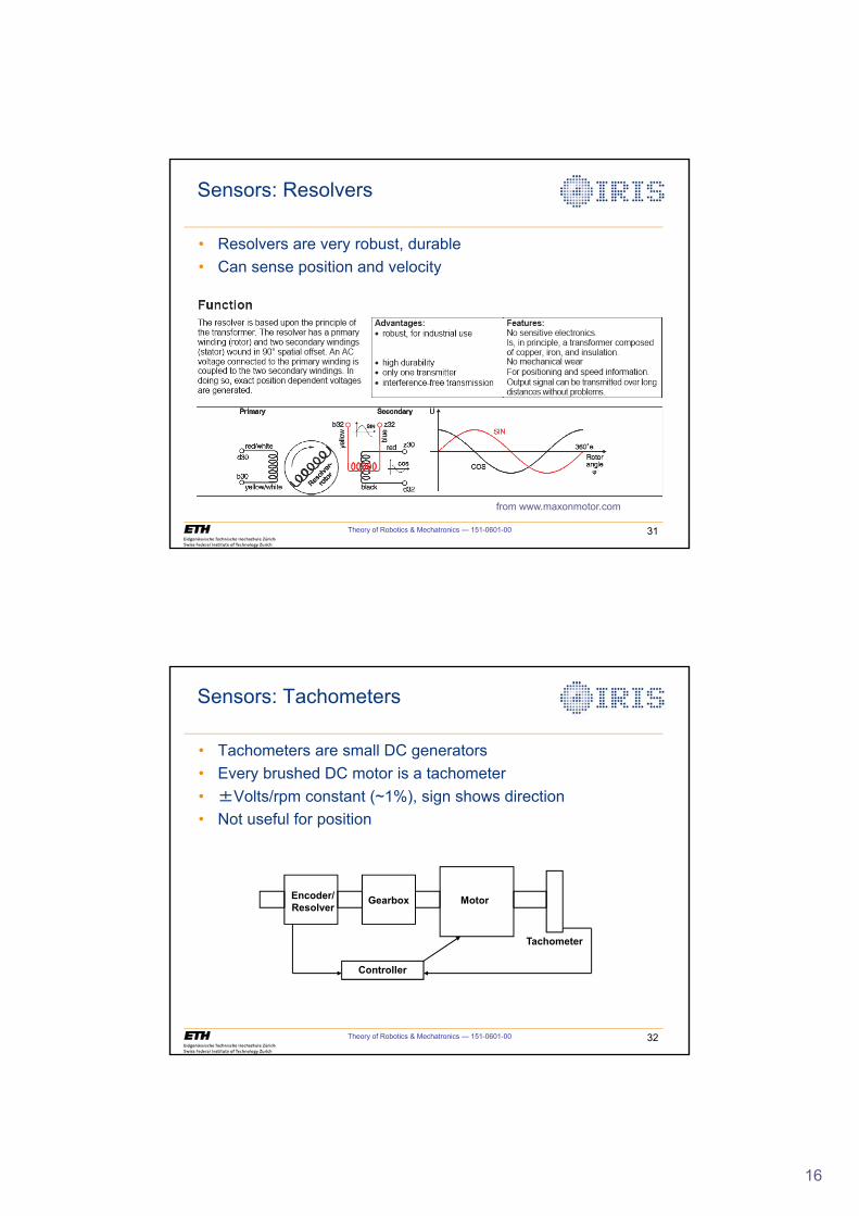
Sensors: Resolvers
• Resolvers are very robust, durable• Can sense position and velocity
from www.maxonmotor.com
Theory of Robotics & Mechatronics — 151-0601-00 32
Sensors: Tachometers
• Tachometers are small DC generators• Every brushed DC motor is a tachometer• Volts/rpm constant (~1%), sign shows direction• Not useful for position
MotorGearbox
Tachometer
Encoder/Resolver
Controller
17
Theory of Robotics & Mechatronics — 151-0601-00 33
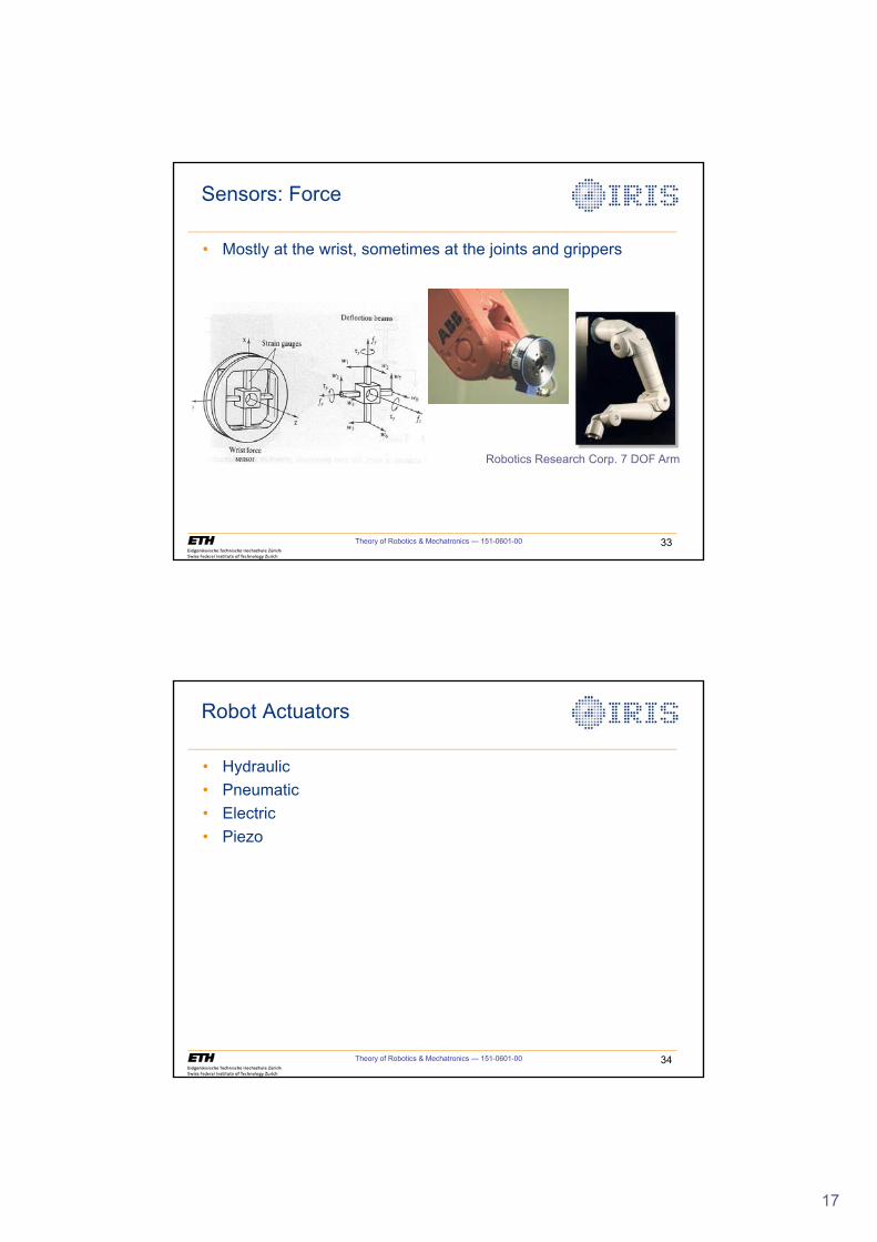
Sensors: Force
• Mostly at the wrist, sometimes at the joints and grippers
Robotics Research Corp. 7 DOF Arm
Theory of Robotics & Mechatronics — 151-0601-00 34
Robot Actuators
• Hydraulic• Pneumatic• Electric• Piezo
18
Theory of Robotics & Mechatronics — 151-0601-00 35
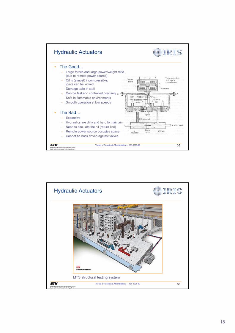
Hydraulic Actuators
• The Good…- Large forces and large power/weight ratio
(due to remote power source)- Oil is (almost) incompressible,
joints can be locked- Damage-safe in stall- Can be fast and controlled precisely- Safe in flammable environments- Smooth operation at low speeds
• The Bad…- Expensive- Hydraulics are dirty and hard to maintain- Need to circulate the oil (return line)- Remote power source occupies space- Cannot be back driven against valves
Theory of Robotics & Mechatronics — 151-0601-00 36
Hydraulic Actuators
MTS structural testing system
19
Theory of Robotics & Mechatronics — 151-0601-00 37
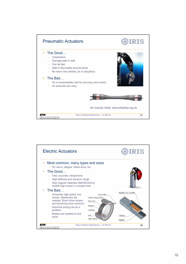
Pneumatic Actuators
• The Good…- Inexpensive- Damage-safe in stall- Can be fast - Safe in flammable environments- No return line needed, air is ubiquitous
• The Bad…- Air is compressible, bad for accuracy and control- Air exhausts are noisy
Air muscle robot, www.shadow.org.uk
Theory of Robotics & Mechatronics — 151-0601-00 38
Electric Actuators
• Most common, many types and sizes– DC servo, stepper, direct drive, etc.
• The Good…- Fast, accurate, inexpensive- High stiffness and dynamic range- New magnet materials (NdFeB,SmCo)
enable high torque in compact size.
• The Bad…- Inherently high speed, low
torque. Gearboxes areneeded. Direct drive motorsare becoming more common.
- Electrical arcing can be aproblem
- Brakes are needed to lockjoints
20
Theory of Robotics & Mechatronics — 151-0601-00 39
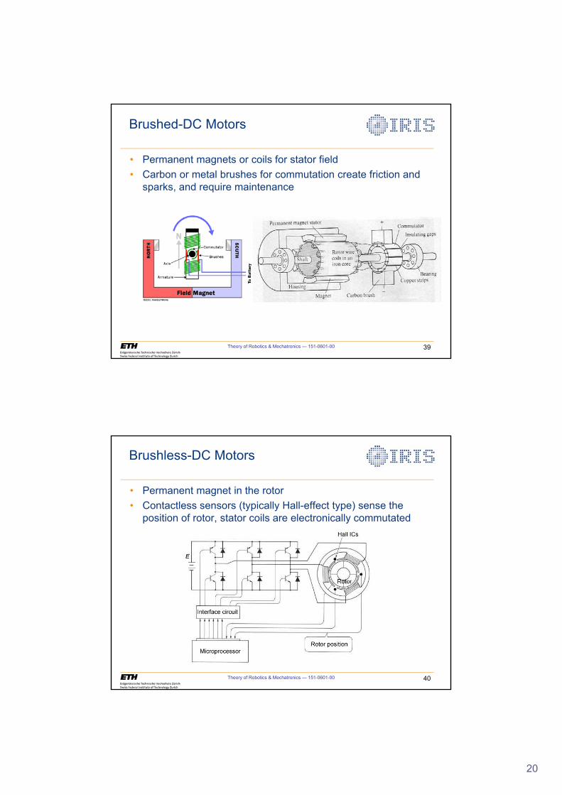
• Permanent magnets or coils for stator field• Carbon or metal brushes for commutation create friction and
sparks, and require maintenance
Brushed-DC Motors
Theory of Robotics & Mechatronics — 151-0601-00 40
• Permanent magnet in the rotor• Contactless sensors (typically Hall-effect type) sense the
position of rotor, stator coils are electronically commutated
Brushless-DC Motors
21
Theory of Robotics & Mechatronics — 151-0601-00 41
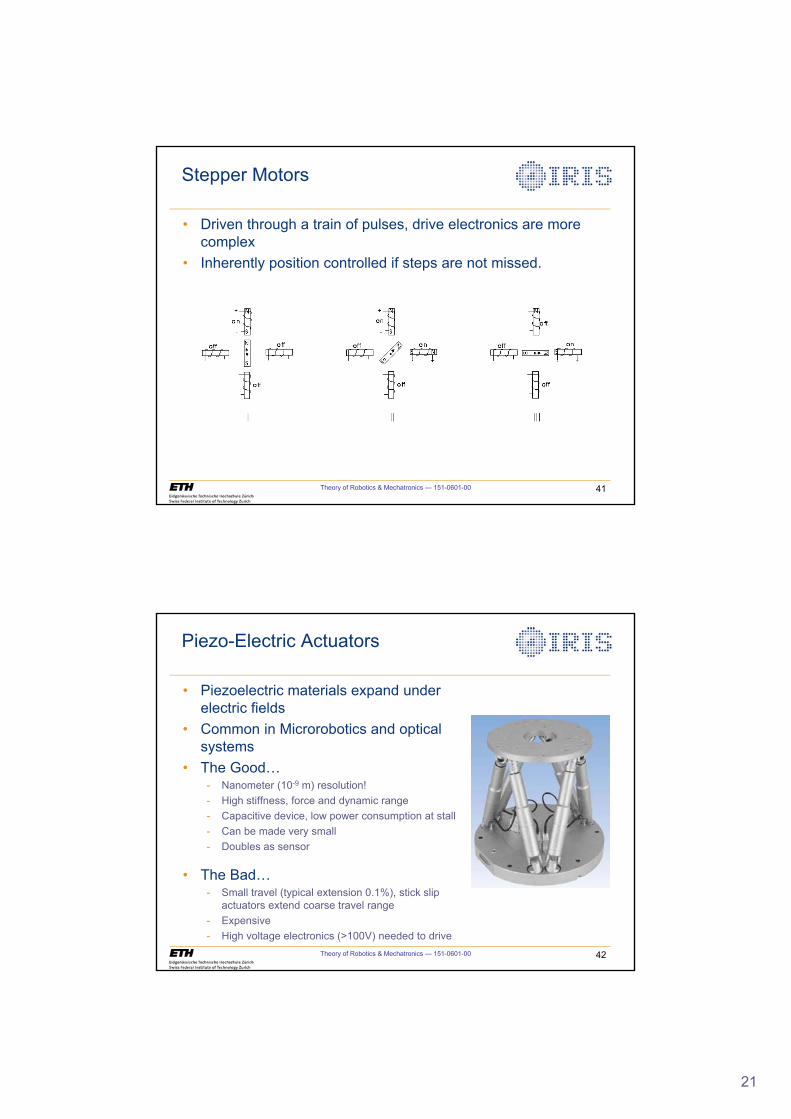
• Driven through a train of pulses, drive electronics are more complex
• Inherently position controlled if steps are not missed.
Stepper Motors
Theory of Robotics & Mechatronics — 151-0601-00 42
Piezo-Electric Actuators
• Piezoelectric materials expand under electric fields
• Common in Microrobotics and optical systems
• The Good…- Nanometer (10-9 m) resolution!- High stiffness, force and dynamic range- Capacitive device, low power consumption at stall- Can be made very small- Doubles as sensor
• The Bad…- Small travel (typical extension 0.1%), stick slip
actuators extend coarse travel range- Expensive- High voltage electronics (>100V) needed to drive
22
Theory of Robotics & Mechatronics — 151-0601-00 43
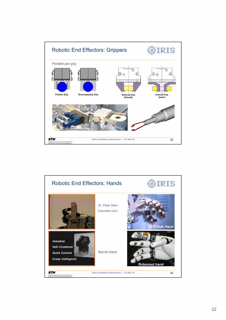
Robotic End Effectors: Grippers
Parallel jaw grip
Theory of Robotics & Mechatronics — 151-0601-00 44
Robotic End Effectors: Hands
Dr. Peter Allen
Columbia Univ.
Barret Hand
Robonaut hand
MIT-Utah Hand
23
Theory of Robotics & Mechatronics — 151-0601-00 45
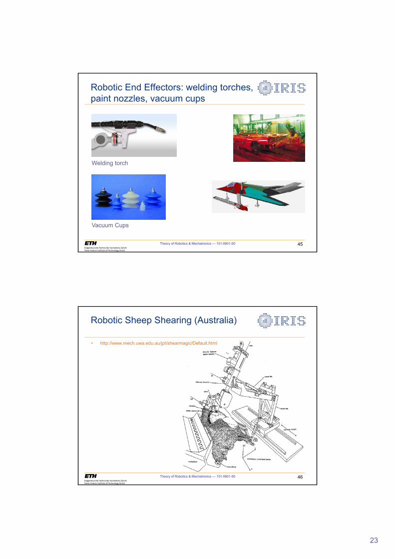
Robotic End Effectors: welding torches, paint nozzles, vacuum cups
Welding torch
Vacuum Cups
Theory of Robotics & Mechatronics — 151-0601-00 46
Robotic Sheep Shearing (Australia)
• http://www.mech.uwa.edu.au/jpt/shearmagic/Default.html
24
Theory of Robotics & Mechatronics — 151-0601-00 47
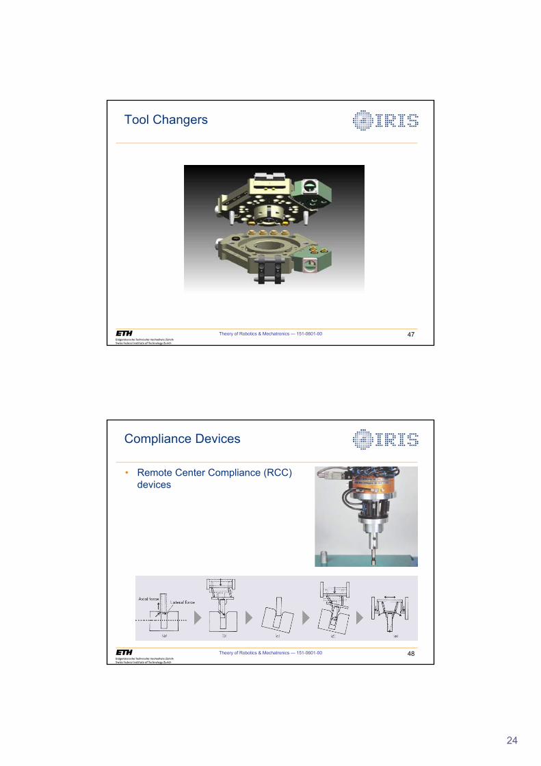
Tool Changers
Theory of Robotics & Mechatronics — 151-0601-00 48
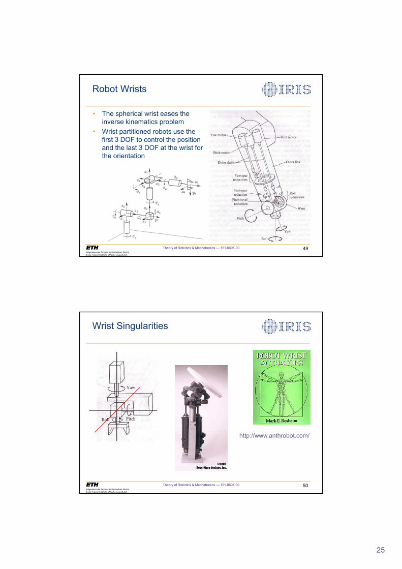
Compliance Devices
• Remote Center Compliance (RCC) devices
25
Theory of Robotics & Mechatronics — 151-0601-00 49
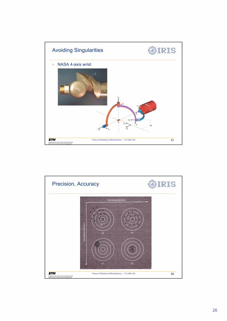
Robot Wrists
• The spherical wrist eases theinverse kinematics problem
• Wrist partitioned robots use thefirst 3 DOF to control the positionand the last 3 DOF at the wrist forthe orientation
Theory of Robotics & Mechatronics — 151-0601-00 50
Wrist Singularities
http://www.anthrobot.com/
26
Theory of Robotics & Mechatronics — 151-0601-00 51
Avoiding Singularities
• NASA 4-axis wrist
Theory of Robotics & Mechatronics — 151-0601-00 52
Precision, Accuracy
27
Theory of Robotics & Mechatronics — 151-0601-00 53
• Resolution of an actuator is the smallest commandable distance of travel (or angle of rotation)
• For a sensor it is the smallest measurable interval
Resolution
First Position
Adjacent PositionTargeted Position
Command Resolution
Accuracy
Theory of Robotics & Mechatronics — 151-0601-00 54
Spatial Resolution
• Actual spatial resolution of a manipulator may change depending on configuration, loads, etc.
First Position
Adjacent Position
Spatial Resolution
Mechanical Errors
Targeted Position
Accuracy
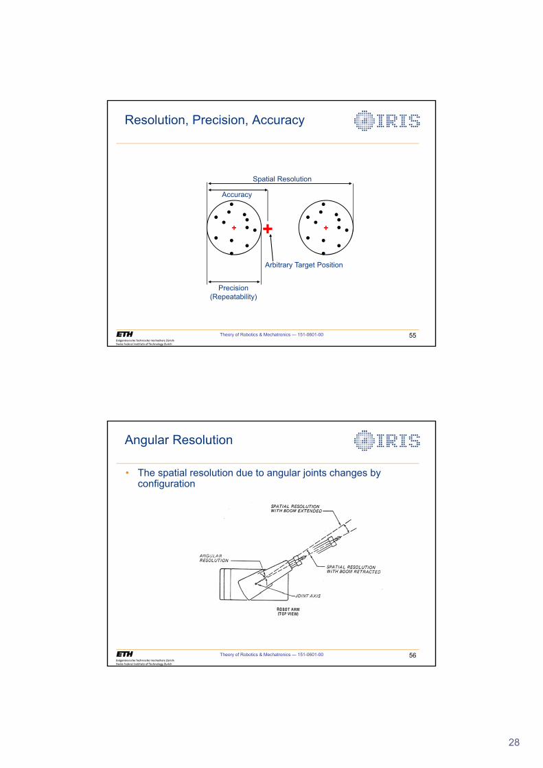
28
Theory of Robotics & Mechatronics — 151-0601-00 55
Resolution, Precision, Accuracy
+ ++
Spatial Resolution
Accuracy
Precision (Repeatability)
Arbitrary Target Position
Theory of Robotics & Mechatronics — 151-0601-00 56
Angular Resolution
• The spatial resolution due to angular joints changes by configuration

29
Theory of Robotics & Mechatronics — 151-0601-00 57
A Last Word on Robot Design
MIT’s COG
• Industrial robots are made to be rigid and accurate. This is good for positioning tasks.
• Not the ideal way for contact tasks.
1
Spatial Descriptions 1 (Classical Formulation)
Institute of Robotics and Intelligent Systems
ETH Zurich
Theory of Robotics &Mechatronics
Theory of Robotics & Mechatronics — 151-0601-00 2
Motivation
• What are we going to learn here?
– We want to deal with rigid bodies (not only with points)
– We want to deal even with multi-bodies connected together by prismaticor revolute joints, i.e. robots.
• Before we can deal (model, simulate, control) with complex kinematic links, we have to define their position,orientation, velocity and acceleration
…and we start with position in this lecture.
2
Theory of Robotics & Mechatronics — 151-0601-00 3
Location of Objects
What about orientation?
X0
Y0
Can we attach a reference point to an object to represent it?
00
0
XP
Y ª º« »¬ ¼
Simple 2D Case
• A point has a unique position in 2D space described with respect to (wrt) a coordinate frame. Two components are necessary to describe the position, a point has twodegrees-of-freedom in 2D space.
Theory of Robotics & Mechatronics — 151-0601-00 4
Location of Objects
X0
Y0
X1
Y1
• Solution: Attach a coordinate frame to the object
• Rigid ObjectÎ Every point on the object has fixed coordinates wrt its coordinate frame.
• Position + Orientation = Pose
3
Theory of Robotics & Mechatronics — 151-0601-00 5
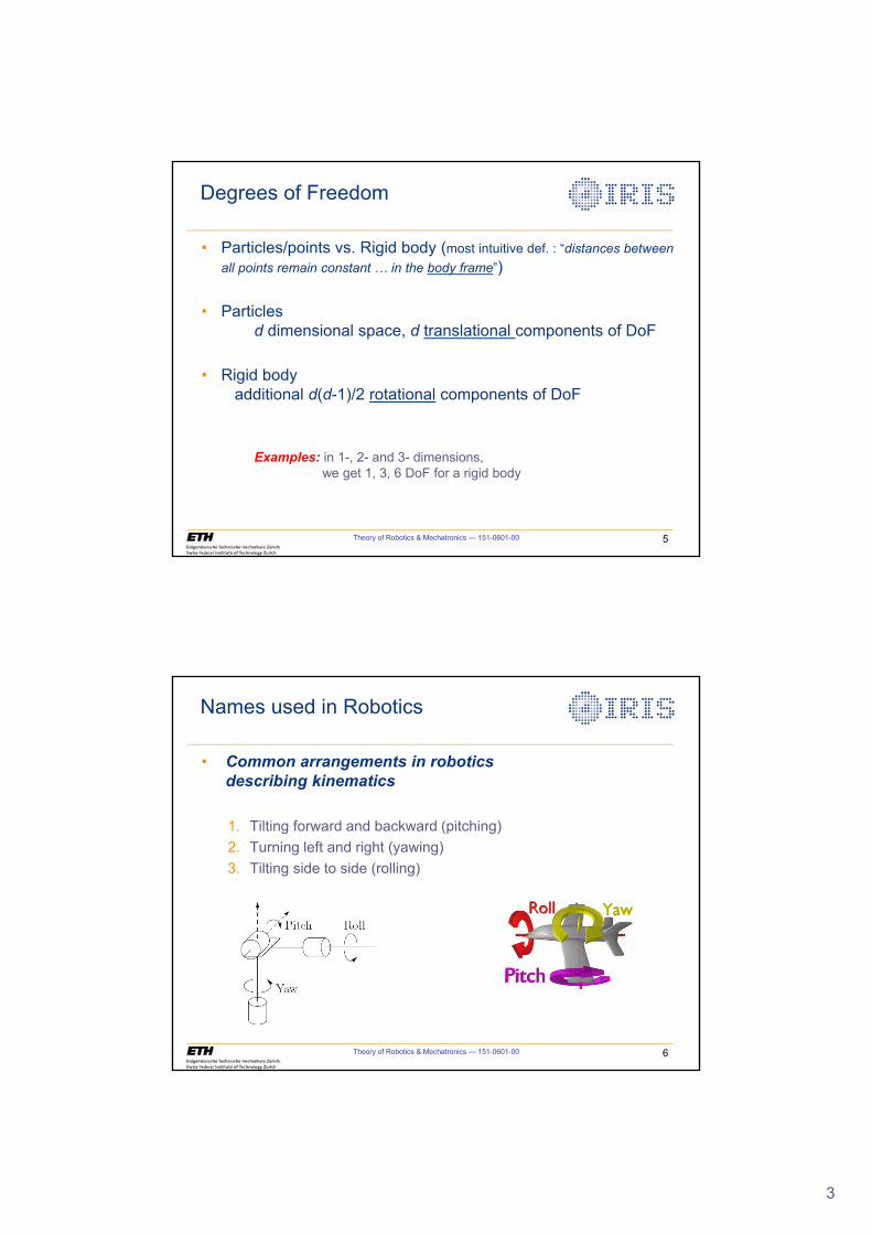
Degrees of Freedom
• Particles/points vs. Rigid body (most intuitive def. : “distances between all points remain constant … in the body frame”)
• Particles d dimensional space, d translational components of DoF
• Rigid body additional d(d-1)/2 rotational components of DoF
Examples: in 1-, 2- and 3- dimensions, we get 1, 3, 6 DoF for a rigid body
Theory of Robotics & Mechatronics — 151-0601-00 6
Names used in Robotics
• Common arrangements in robotics describing kinematics
1. Tilting forward and backward (pitching)
2. Turning left and right (yawing)
3. Tilting side to side (rolling)
4
Theory of Robotics & Mechatronics — 151-0601-00 7
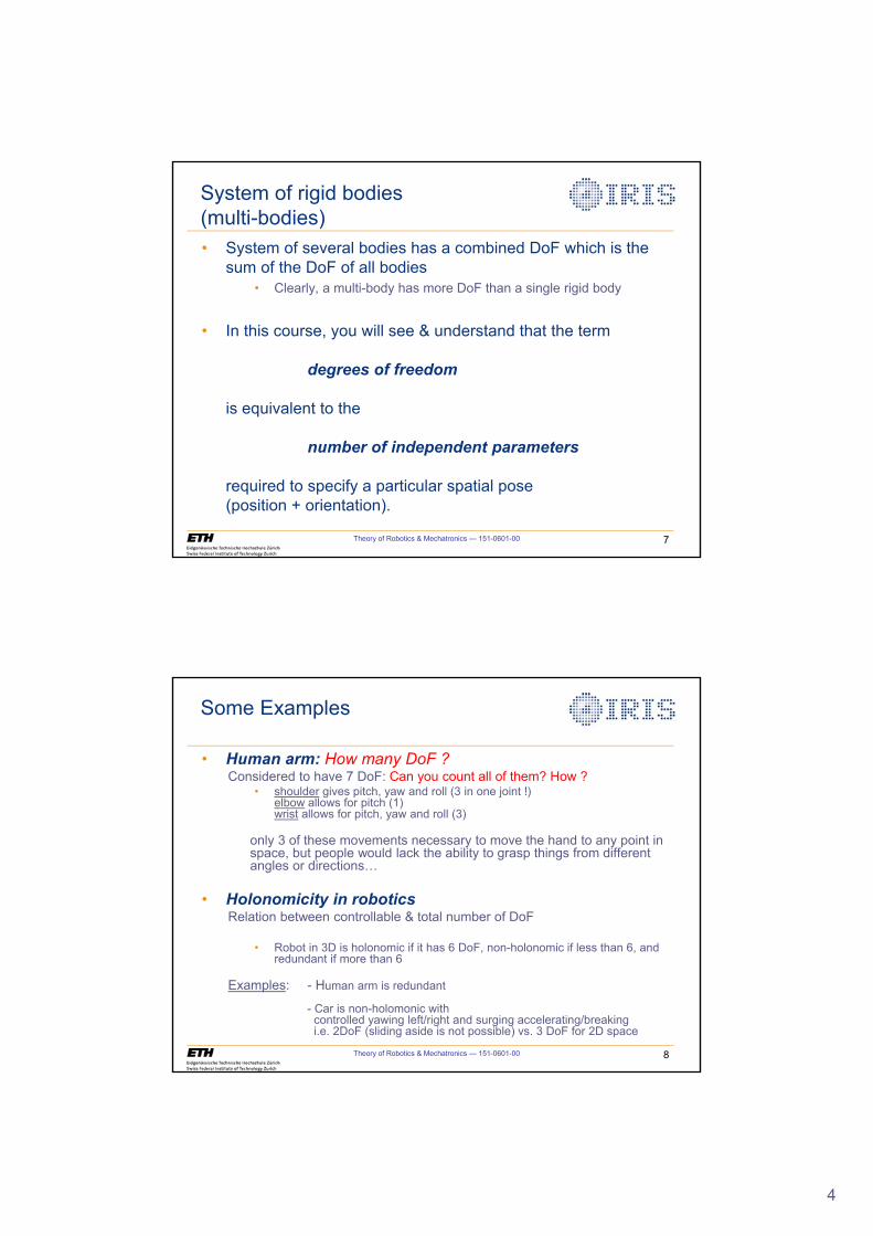
System of rigid bodies(multi-bodies)
• System of several bodies has a combined DoF which is the sum of the DoF of all bodies
• Clearly, a multi-body has more DoF than a single rigid body
• In this course, you will see & understand that the term
degrees of freedom
is equivalent to the
number of independent parameters
required to specify a particular spatial pose(position + orientation).
Theory of Robotics & Mechatronics — 151-0601-00 8
Some Examples
• Human arm: How many DoF ?Considered to have 7 DoF: Can you count all of them? How ?
• shoulder gives pitch, yaw and roll (3 in one joint !)elbow allows for pitch (1) wrist allows for pitch, yaw and roll (3)
only 3 of these movements necessary to move the hand to any point inspace, but people would lack the ability to grasp things from different angles or directions…
• Holonomicity in roboticsRelation between controllable & total number of DoF
• Robot in 3D is holonomic if it has 6 DoF, non-holonomic if less than 6, and redundant if more than 6
Examples: - Human arm is redundant
- Car is non-holomonic with controlled yawing left/right and surging accelerating/breaking i.e. 2DoF (sliding aside is not possible) vs. 3 DoF for 2D space
5
Theory of Robotics & Mechatronics — 151-0601-00 9
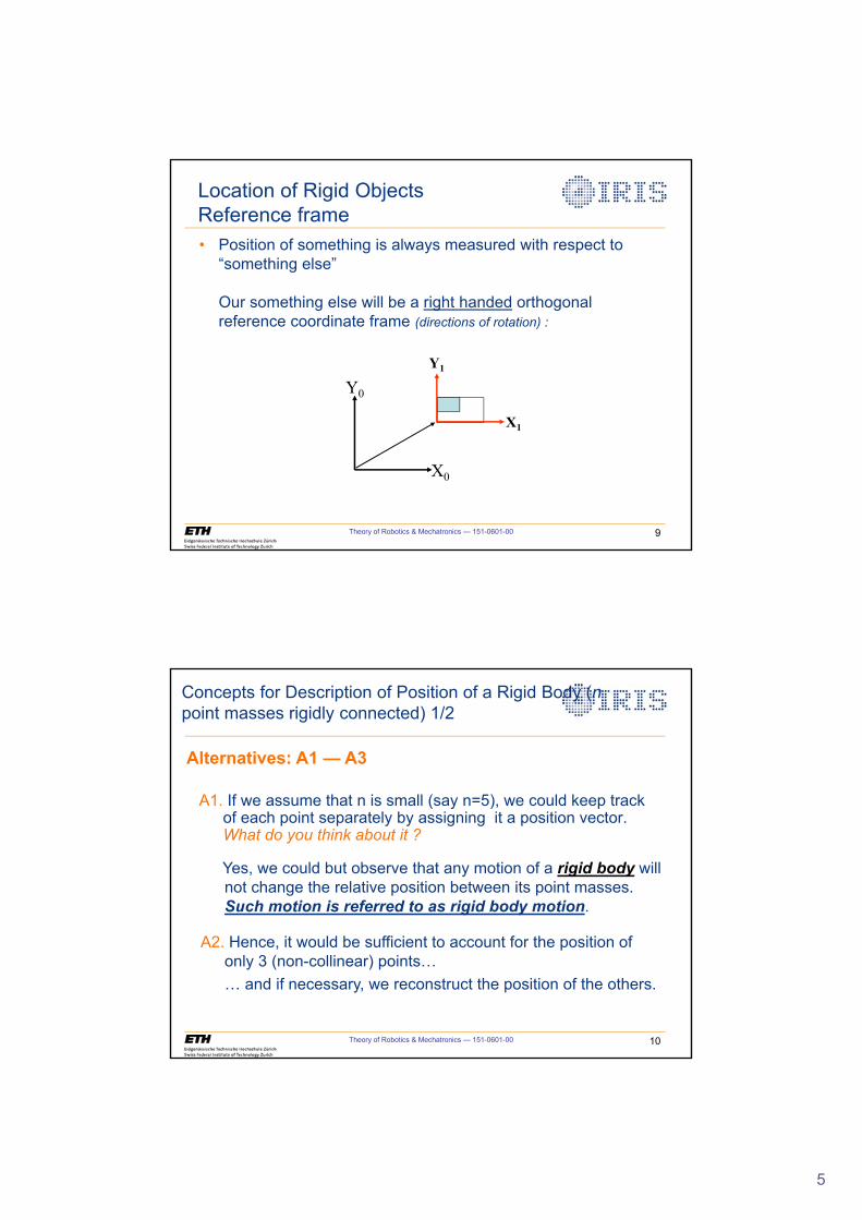
Location of Rigid ObjectsReference frame
X0
Y0
X1
Y1
• Position of something is always measured with respect to “something else”
Our something else will be a right handed orthogonal reference coordinate frame (directions of rotation) :
Theory of Robotics & Mechatronics — 151-0601-00 10
Concepts for Description of Position of a Rigid Body (npoint masses rigidly connected) 1/2
A1. If we assume that n is small (say n=5), we could keep track of each point separately by assigning it a position vector.What do you think about it ?
Yes, we could but observe that any motion of a rigid body will not change the relative position between its point masses. Such motion is referred to as rigid body motion.
A2. Hence, it would be sufficient to account for the position of only 3 (non-collinear) points…
… and if necessary, we reconstruct the position of the others.
Alternatives: A1 — A3
6
Theory of Robotics & Mechatronics — 151-0601-00 11
Concepts for Description of Position of a Rigid Body (n point masses rigidly connected) 2/2
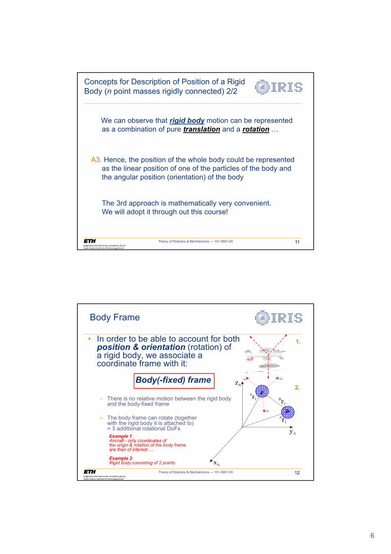
We can observe that rigid body motion can be representedas a combination of pure translation and a rotation …
A3. Hence, the position of the whole body could be represented as the linear position of one of the particles of the body and the angular position (orientation) of the body
The 3rd approach is mathematically very convenient.We will adopt it through out this course!
Theory of Robotics & Mechatronics — 151-0601-00 12
Body Frame
• In order to be able to account for both position & orientation (rotation) of a rigid body, we associate acoordinate frame with it:
Body(-fixed) frame
– There is no relative motion between the rigid bodyand the body-fixed frame
– The body frame can rotate (togetherwith the rigid body it is attached to) = 3 additional rotational DoFs
Example 1: Aircraft - only coordinates of the origin & rotation of the body frameare then of interest …
Example 2:Rigid body consisting of 2 points
1.
2.
7
Theory of Robotics & Mechatronics — 151-0601-00 13
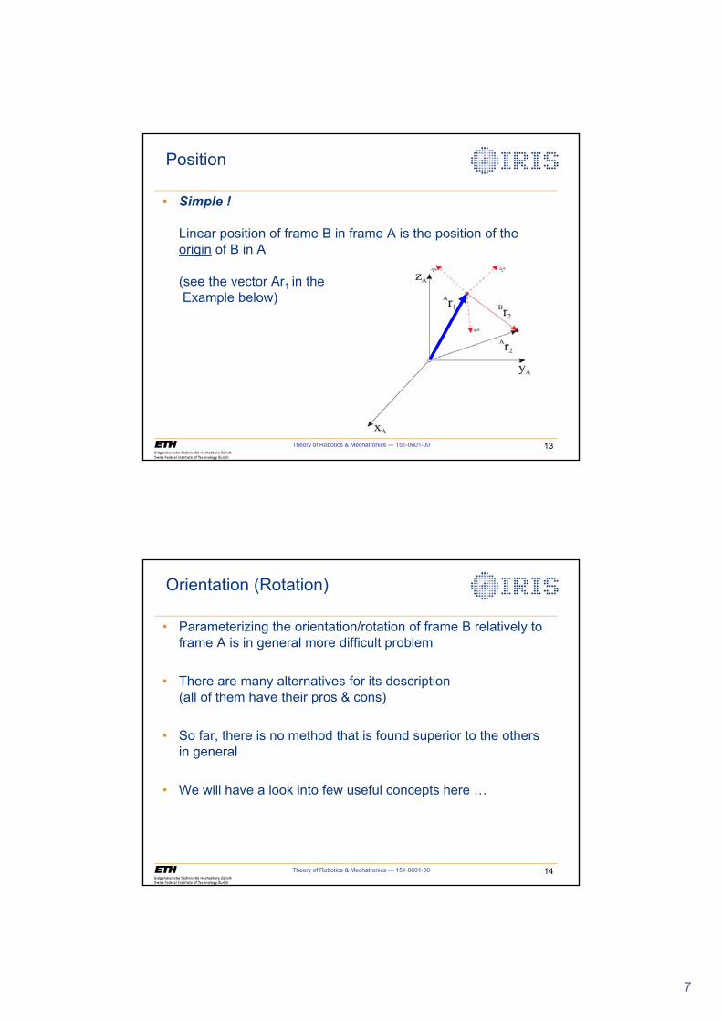
Position
• Simple !
Linear position of frame B in frame A is the position of the origin of B in A
(see the vector Ar1 in theExample below)
Theory of Robotics & Mechatronics — 151-0601-00 14
Orientation (Rotation)
• Parameterizing the orientation/rotation of frame B relatively to frame A is in general more difficult problem
• There are many alternatives for its description(all of them have their pros & cons)
• So far, there is no method that is found superior to the othersin general
• We will have a look into few useful concepts here …
8
Theory of Robotics & Mechatronics — 151-0601-00 15
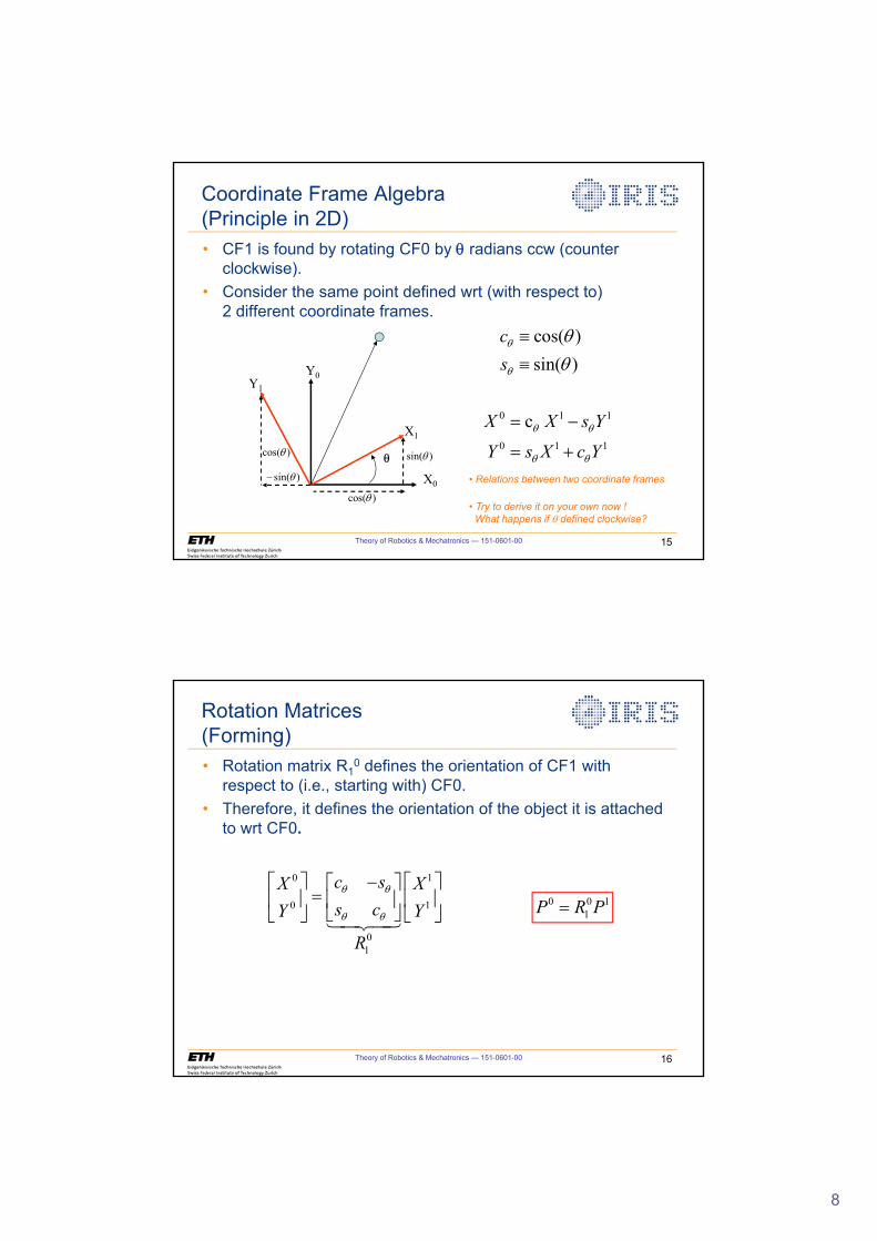
Coordinate Frame Algebra(Principle in 2D)
0 1 1
0 1 1
cX X s Y
Y s X c YT T
T T
�
�
cos( )sin( )
csT
T
TT
{
{Y1
T
X1
Y0
X0
cos( )T
sin( )T�
sin( )Tcos( )T
• CF1 is found by rotating CF0 by T radians ccw (counter clockwise).
• Consider the same point defined wrt (with respect to) 2 different coordinate frames.
• Relations between two coordinate frames
• Try to derive it on your own now ! What happens if T defined clockwise?
Theory of Robotics & Mechatronics — 151-0601-00 16
Rotation Matrices(Forming)
0 0 11P R P
0 1
0 1
01
c sX Xs cY Y
R
T T
T T
�ª º ª ºª º « » « »« »¬ ¼¬ ¼ ¬ ¼���
• Rotation matrix R10 defines the orientation of CF1 with
respect to (i.e., starting with) CF0.
• Therefore, it defines the orientation of the object it is attached to wrt CF0.
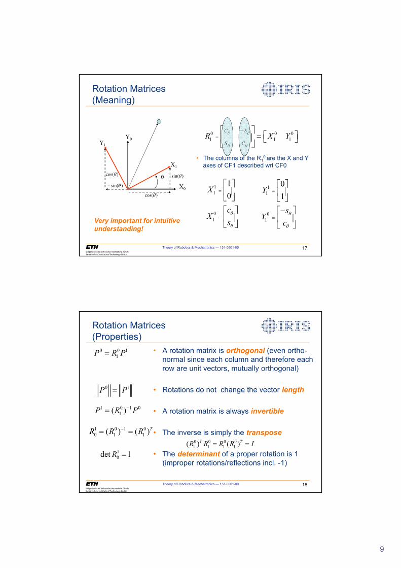
9
Theory of Robotics & Mechatronics — 151-0601-00 17
Rotation Matrices(Meaning)
Y1
T
X1
Y0
X0
cos( )T
sin( )T�
sin( )Tcos( )T
0 0 01 1 1
c sR X Y
s cT T
T T
�ª º
ª º « » ¬ ¼¬ ¼
• The columns of the R10 are the X and Y
axes of CF1 described wrt CF0
11
01
10
X
cX
sT
T
ª º« »¬ ¼ª º« »¬ ¼
11
01
01
Y
sY
cT
T
ª º« »¬ ¼�ª º« »¬ ¼Very important for intuitive
understanding!
• A rotation matrix is orthogonal (even ortho-normal since each column and therefore each row are unit vectors, mutually orthogonal)
• Rotations do not change the vector length
• A rotation matrix is always invertible
• The inverse is simply the transpose
• The determinant of a proper rotation is 1 (improper rotations/reflections incl. -1)
Theory of Robotics & Mechatronics — 151-0601-00 18
Rotation Matrices(Properties)
0 0 11P R P
1 0 1 01( )P R P�
1 0 1 00 1 1( ) ( )TR R R�
0 1P P
0 0 0 01 1 1 1( ) ( )T TR R R R I
1det 10 R
10
Theory of Robotics & Mechatronics — 151-0601-00 19
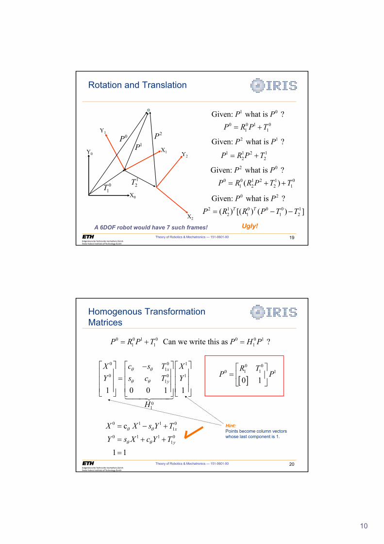
Rotation and Translation
0 0 1 01 1P R P T �
1 1 2 12 2P R P T �
1 0Given: what is ?P P
2 1Given: what is ?P PX1Y0
X0
Y1
X2
Y2
0P1P
2P
01T
12T
2 0Given: what is ?P P0 0 1 2 1 0
1 2 2 1( )P R R P T T � �
Ugly!
2 1 0 0 0 12 1 1 2( ) [( ) ( ) ]T TP R R P T T � �
0 2Given: what is ?P P
A 6DOF robot would have 7 such frames!
Theory of Robotics & Mechatronics — 151-0601-00 20
Homogenous Transformation Matrices
0 0 1 0 0 0 11 1 1 Can we write this as ?P R P T P H P �
0 0 11
0 0 11
01
1 0 0 1 1
x
y
X c s T XY s c T Y
H
T T
T T
ª º ª º ª º�« » « » « » « » « » « »« » « » « »¬ ¼ ¬ ¼ ¬ ¼�����
0 1 1 01
0 1 1 01
c
1 1
x
y
X X s Y T
Y s X c Y TT T
T T
� �
� �
> @0 01 10 1
0 1R T
P Pª º
« »¬ ¼
Hint:Points become column vectors whose last component is 1.
11
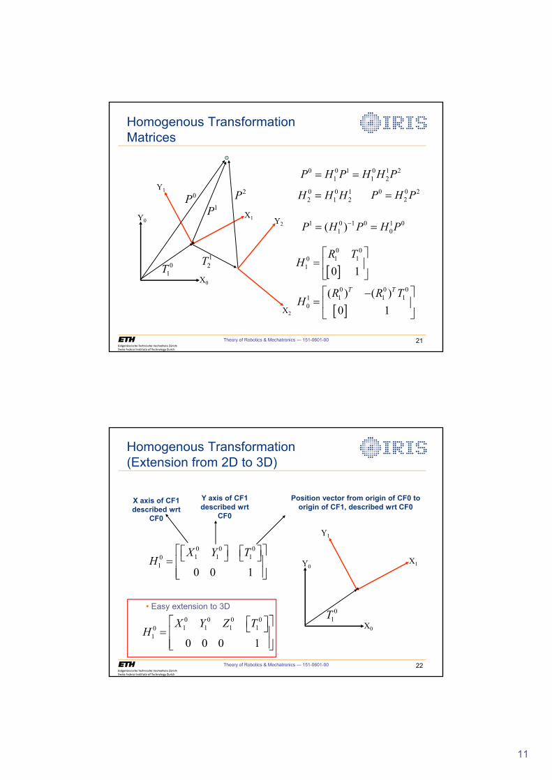
Theory of Robotics & Mechatronics — 151-0601-00 21
Homogenous Transformation Matrices
X1Y0
X0
Y1
X2
Y2
0P1P
2P
01T
12T
0 0 1 0 1 21 1 2 P H P H H P
0 0 12 1 2 H H H
1 0 1 0 1 01 0 ( )P H P H P�
> @
> @
0 01 10
1
0 0 01 1 11
0
0 1
( ) ( )0 1
T T
R TH
R R TH
ª º « »¬ ¼ª º�
« »¬ ¼
0 0 22 P H P
Theory of Robotics & Mechatronics — 151-0601-00 22
Homogenous Transformation(Extension from 2D to 3D)
0 0 01 1 10
10 0 1
X Y TH
ª ºª º ª º¬ ¼ ¬ ¼ « »« »¬ ¼
X axis of CF1 described wrt
CF0
Y axis of CF1 described wrt
CF0
Position vector from origin of CF0 to origin of CF1, described wrt CF0
X1Y0
X0
Y1
01T0 0 0 0
1 1 1 101
0 0 0 1
X Y Z TH
ª ºª º¬ ¼ « »« »¬ ¼
• Easy extension to 3D
12
Theory of Robotics & Mechatronics — 151-0601-00 23
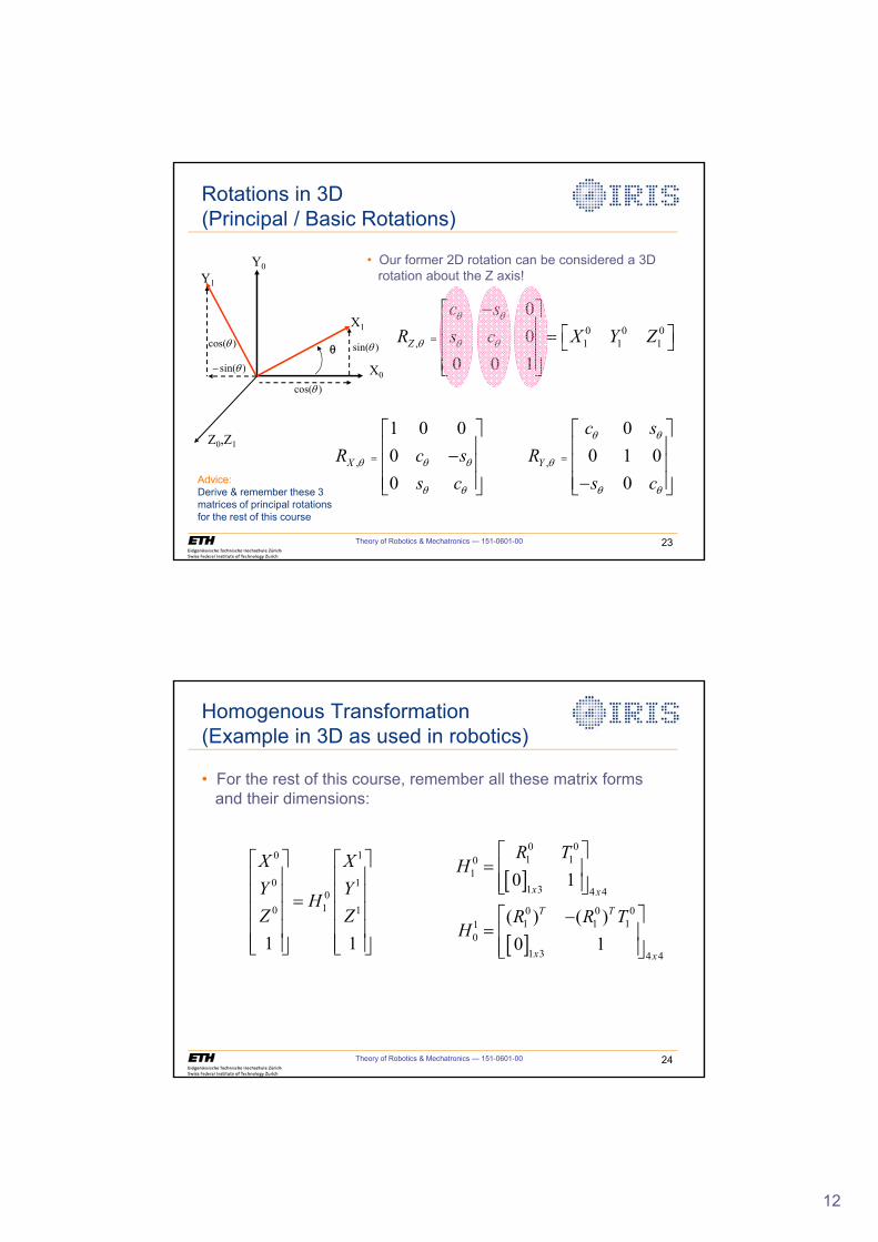
Rotations in 3D(Principal / Basic Rotations)
• Our former 2D rotation can be considered a 3Drotation about the Z axis!
0 0 0, 1 1 1
00
0 0 1Z
c sR s c X Y Z
T T
T T T
�ª º« » ª º ¬ ¼« »« »¬ ¼
,
1 0 000
XR c ss c
T T T
T T
ª º« »�« »« »¬ ¼
,
00 1 0
0Y
c sR
s c
T T
T
T T
ª º« »« »« »�¬ ¼
Y1
T
X1
Y0
X0
cos( )T
sin( )T�
sin( )Tcos( )T
Z0,Z1
Advice: Derive & remember these 3 matrices of principal rotations for the rest of this course
Theory of Robotics & Mechatronics — 151-0601-00 24
Homogenous Transformation(Example in 3D as used in robotics)
> @
> @
0 01 10
11 3 4 4
0 0 01 1 11
01 3 4 4
0 1
( ) ( )0 1
x x
T T
x x
R TH
R R TH
ª º « »« »¬ ¼
ª º� « »« »¬ ¼
0 1
0 1010 1
1 1
X XY Y
HZ Z
ª º ª º« » « »« » « » « » « »« » « »« » « »¬ ¼ ¬ ¼
• For the rest of this course, remember all these matrix formsand their dimensions:
13
Theory of Robotics & Mechatronics — 151-0601-00 25
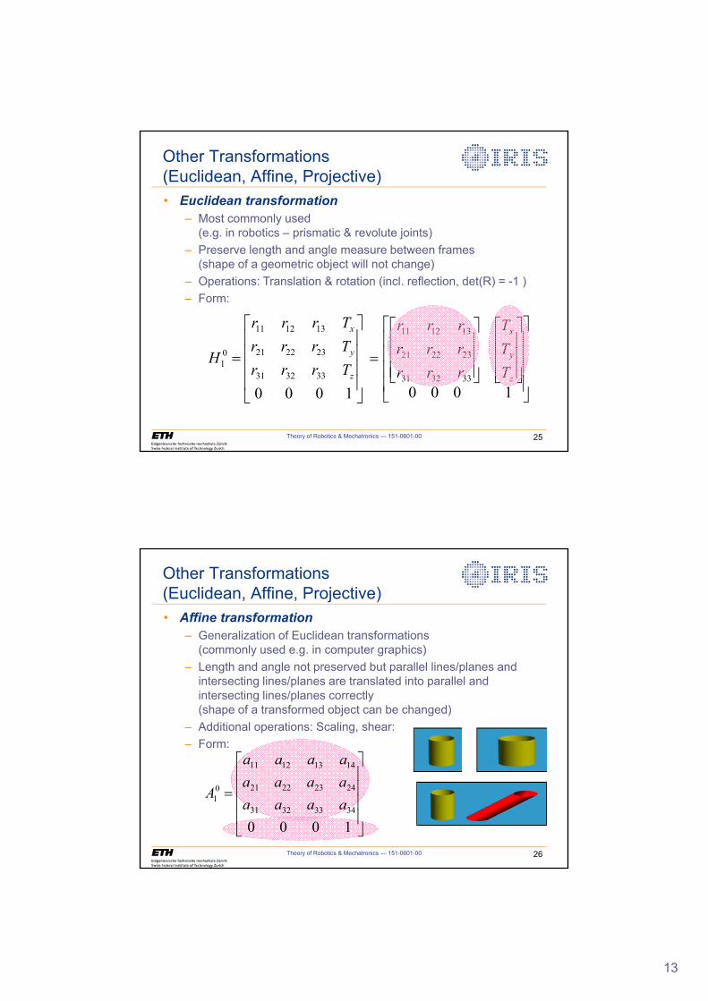
Other Transformations(Euclidean, Affine, Projective)
• Euclidean transformation– Most commonly used
(e.g. in robotics – prismatic & revolute joints)
– Preserve length and angle measure between frames(shape of a geometric object will not change)
– Operations: Translation & rotation (incl. reflection, det(R) = -1 )
– Form:
»»»»
¼
º
««««
¬
ª
1000333231
232221
131211
01
z
y
x
TrrrTrrrTrrr
H
»»»»
¼
º
««««
¬
ª
»»»
¼
º
«««
¬
ª
»»»
¼
º
«««
¬
ª
1000333231
232221
131211
z
y
x
TTT
rrrrrrrrr
Theory of Robotics & Mechatronics — 151-0601-00 26
Other Transformations(Euclidean, Affine, Projective)
• Affine transformation– Generalization of Euclidean transformations
(commonly used e.g. in computer graphics)
– Length and angle not preserved but parallel lines/planes and intersecting lines/planes are translated into parallel and intersecting lines/planes correctly(shape of a transformed object can be changed)
– Additional operations: Scaling, shear:
– Form:
»»»»
¼
º
««««
¬
ª
100034333231
24232221
14131211
01 aaaa
aaaaaaaa
A
14
Theory of Robotics & Mechatronics — 151-0601-00 27
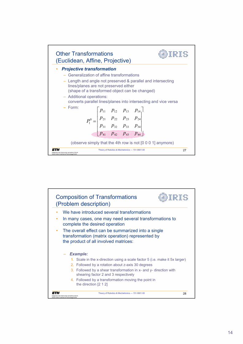
Other Transformations(Euclidean, Affine, Projective)
• Projective transformation– Generalization of affine transformations
– Length and angle not preserved & parallel and intersecting lines/planes are not preserved either (shape of a transformed object can be changed)
– Additional operations: converts parallel lines/planes into intersecting and vice versa
– Form:
(observe simply that the 4th row is not [0 0 0 1] anymore)
»»»»
¼
º
««««
¬
ª
44434241
34333231
24232221
14131211
01
pppppppppppppppp
P
Theory of Robotics & Mechatronics — 151-0601-00 28
Composition of Transformations(Problem description)
• We have introduced several transformations
• In many cases, one may need several transformations to complete the desired operation
• The overall effect can be summarized into a single transformation (matrix operation) represented by the product of all involved matrices:
– Example:1. Scale in the x-direction using a scale factor 5 (i.e. make it 5x larger)
2. Followed by a rotation about z-axis 30 degrees
3. Followed by a shear transformation in x- and y- direction with shearing factor 2 and 3 respectively
4. Followed by a transformation moving the point inthe direction [2 1 2]
15
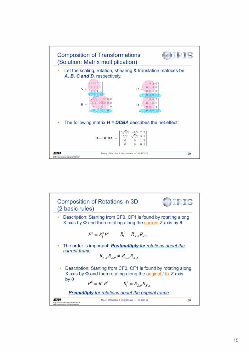
Theory of Robotics & Mechatronics — 151-0601-00 29
Composition of Transformations(Solution: Matrix multiplication)
• Let the scaling, rotation, shearing & translation matrices beA, B, C and D, respectively.
• The following matrix H = DCBA describes the net effect:
Theory of Robotics & Mechatronics — 151-0601-00 30
Composition of Rotations in 3D(2 basic rules)
• The order is important! Postmultiply for rotations about the current frame
• Description: Starting from CF0, CF1 is found by rotating along X axis by and then rotating along the current Z axis by
0 0 11P R P 0
1 , ,X ZR R RI T
, , , ,X Z Z XR R R RI T T Iz
• Description: Starting from CF0, CF1 is found by rotating along X axis by and then rotating along the original / fix Z axisby
0 0 11P R P 0
1 , ,Z XR R RT I
Premultiply for rotations about the original frame
16
Theory of Robotics & Mechatronics — 151-0601-00 31
Composition of Rotations in 3D(Example)
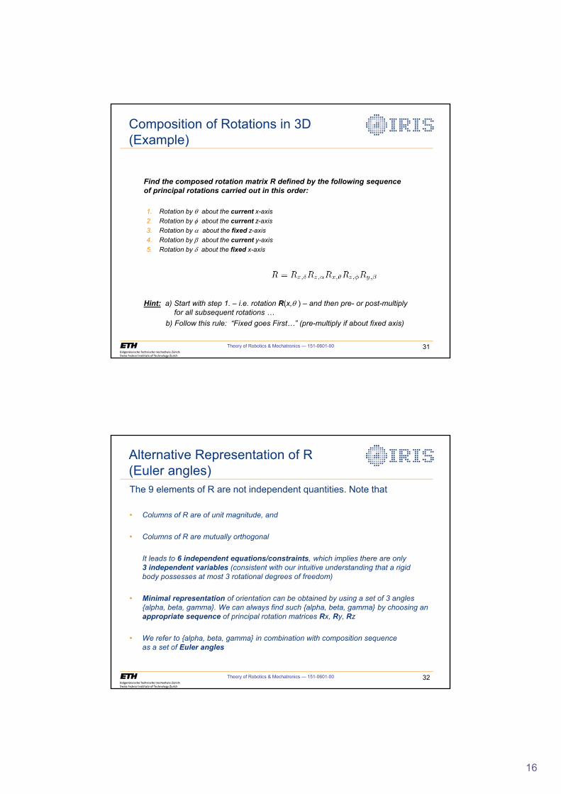
Find the composed rotation matrix R defined by the following sequenceof principal rotations carried out in this order:
1. Rotation by T about the current x-axis2. Rotation by I about the current z-axis3. Rotation by D about the fixed z-axis4. Rotation by E about the current y-axis5. Rotation by G about the fixed x-axis
Hint: a) Start with step 1. – i.e. rotation R(x,T ) – and then pre- or post-multiplyfor all subsequent rotations …
b) Follow this rule: “Fixed goes First…” (pre-multiply if about fixed axis)
Theory of Robotics & Mechatronics — 151-0601-00 32
Alternative Representation of R(Euler angles)
The 9 elements of R are not independent quantities. Note that
• Columns of R are of unit magnitude, and
• Columns of R are mutually orthogonal
It leads to 6 independent equations/constraints, which implies there are only3 independent variables (consistent with our intuitive understanding that a rigidbody possesses at most 3 rotational degrees of freedom)
• Minimal representation of orientation can be obtained by using a set of 3 angles{alpha, beta, gamma}. We can always find such {alpha, beta, gamma} by choosing an appropriate sequence of principal rotation matrices Rx, Ry, Rz
• We refer to {alpha, beta, gamma} in combination with composition sequenceas a set of Euler angles
17
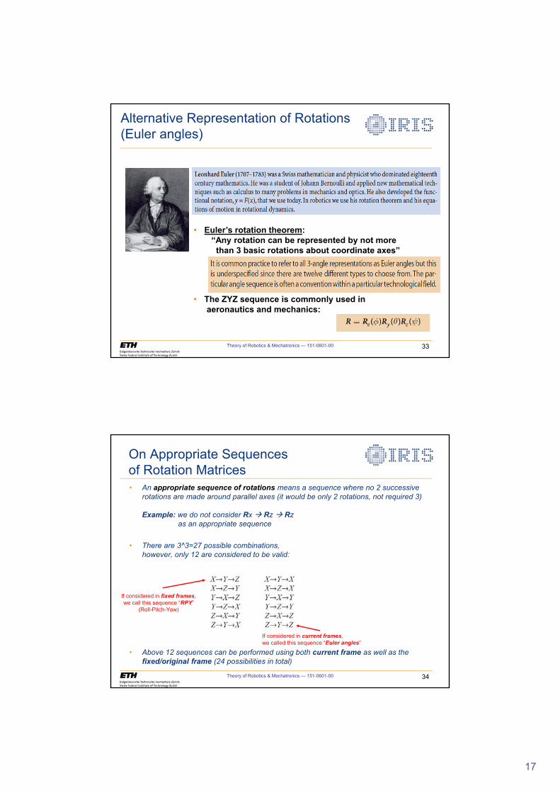
Theory of Robotics & Mechatronics — 151-0601-00 33
Alternative Representation of Rotations(Euler angles)
• Euler’s rotation theorem:“Any rotation can be represented by not morethan 3 basic rotations about coordinate axes”
• The ZYZ sequence is commonly used in aeronautics and mechanics:
Theory of Robotics & Mechatronics — 151-0601-00 34
On Appropriate Sequencesof Rotation Matrices• An appropriate sequence of rotations means a sequence where no 2 successive
rotations are made around parallel axes (it would be only 2 rotations, not required 3)
Example: we do not consider Rx Æ Rz Æ Rz as an appropriate sequence
• There are 3^3=27 possible combinations,however, only 12 are considered to be valid:
• Above 12 sequences can be performed using both current frame as well as the fixed/original frame (24 possibilities in total)
If considered in current frames, we called this sequence “Euler angles”
If considered in fixed frames,we call this sequence “RPY”
(Roll-Pitch-Yaw)
18
Theory of Robotics & Mechatronics — 151-0601-00 35
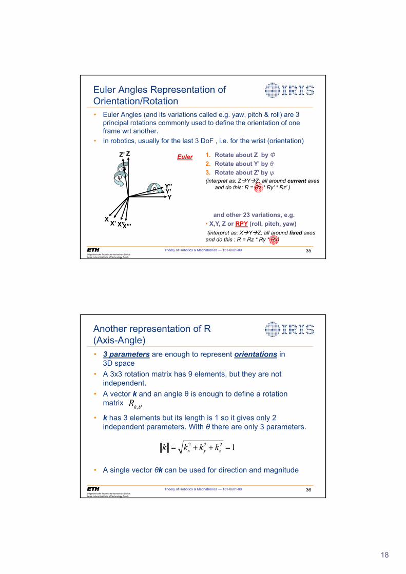
Euler Angles Representation of Orientation/Rotation
• Euler Angles (and its variations called e.g. yaw, pitch & roll) are 3 principal rotations commonly used to define the orientation of one frame wrt another.
• In robotics, usually for the last 3 DoF , i.e. for the wrist (orientation)
X
Y
Z 1. Rotate about Z by Φ2. Rotate about Y’ by θ3. Rotate about Z’ by ψ(interpret as: ZÆYÆZ; all around current axes
and do this: R = Rz * Ry’ * Rz’ )
and other 23 variations, e.g.• X,Y, Z or RPY (roll, pitch, yaw)(interpret as: XÆYÆZ; all around fixed axes
and do this : R = Rz * Ry * Rx)
Y’
Φ
X’
θ
X’’
Z’
ψ
X’’’
Y’’
Euler
Theory of Robotics & Mechatronics — 151-0601-00 36
• 3 parameters are enough to represent orientations in3D space
• A 3x3 rotation matrix has 9 elements, but they are not independent.
• A vector k and an angle is enough to define a rotationmatrix
• k has 3 elements but its length is 1 so it gives only 2 independent parameters. With θ there are only 3 parameters.
• A single vector θk can be used for direction and magnitude
Another representation of R(Axis-Angle)
2 2 2 1x y zk k k k � �
,kR T
19
Theory of Robotics & Mechatronics — 151-0601-00 37
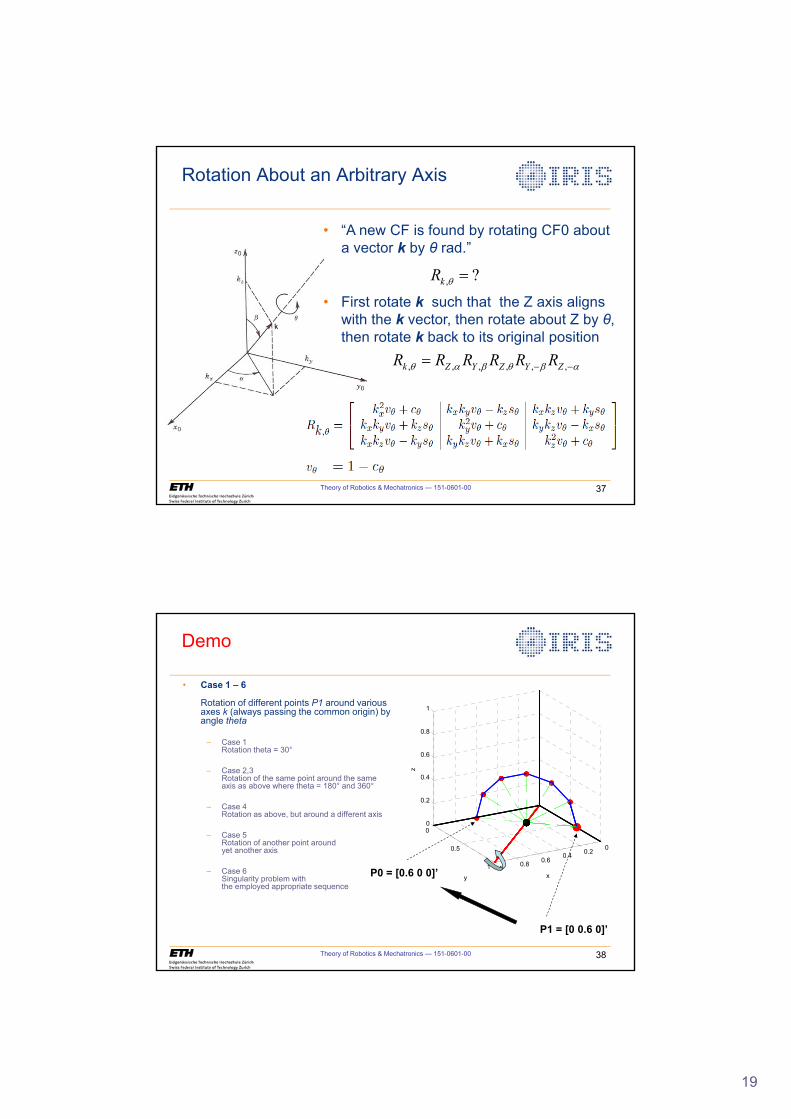
Rotation About an Arbitrary Axis
, ?kR T
, , , , , ,k Z Y Z Y ZR R R R R RT D E T E D� �
• “A new CF is found by rotating CF0 about a vector k by θ rad.”
• First rotate k such that the Z axis aligns with the k vector, then rotate about Z by θ, then rotate k back to its original position
Theory of Robotics & Mechatronics — 151-0601-00 38
Demo
• Case 1 – 6
Rotation of different points P1 around various axes k (always passing the common origin) by angle theta
– Case 1Rotation theta = 30°
– Case 2,3Rotation of the same point around the same axis as above where theta = 180° and 360°
– Case 4Rotation as above, but around a different axis
– Case 5Rotation of another point around yet another axis
– Case 6Singularity problem with the employed appropriate sequence
00.2
0.40.6
0.81
0
0.5
1
0
0.2
0.4
0.6
0.8
1
xy
z
P1 = [0 0.6 0]’
P0 = [0.6 0 0]’
20
Theory of Robotics & Mechatronics — 151-0601-00 39
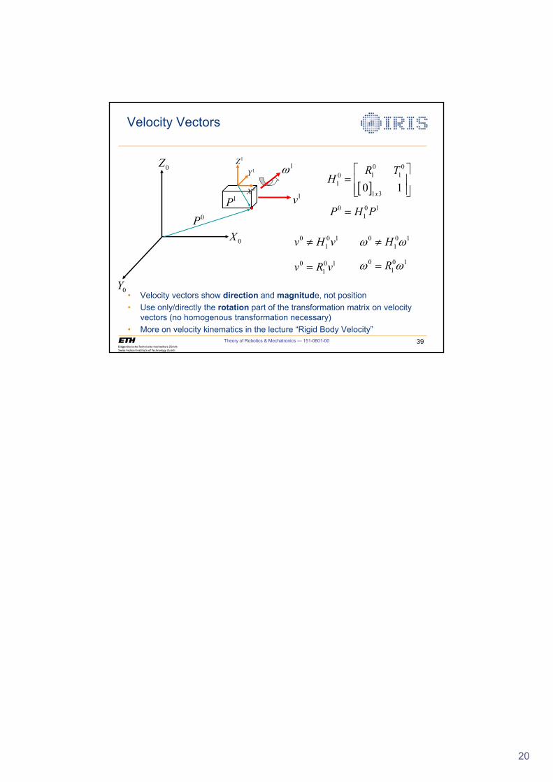
Velocity Vectors
0X
0Z
0Y
1Z1X
1Y
1Z
1v> @
0 01 10
11 3
0 1x
R TH
ª º « »« »¬ ¼
0 0 11P H P
1P0P
0 0 11v H vz 0 0 1
1HZ Zz
0 0 11v R v 0 0 1
1RZ Z
• Velocity vectors show direction and magnitude, not position
• Use only/directly the rotation part of the transformation matrix on velocity vectors (no homogenous transformation necessary)
• More on velocity kinematics in the lecture “Rigid Body Velocity”
1
Spatial Descriptions 2 (Screw Theory)
Institute of Robotics and Intelligent SystemsETH Zurich
Theory of Robotics &Mechatronics
Theory of Robotics & Mechatronics — 151-0601-00 2
Screw Theory (ST) in Robotics(Introduction to its application)
• There are alternatives for spatial descriptions in robotics– Recall drawbacks observed in classical approaches such as
• Euler angles - one singularity in any sequence• Angle-axis - axis not always defined (if T = 0 r kS for any k = 0,1,… )
• Screw Theory is mathematically elegant and powerful• Relatively new to robotics, many robotics researchers are not familiar with it• A lot of different words are used to described it:
(a) Screws (b) Twists (c) Product of matrix exponentials (POE)• The entire method is based on thorough understanding of
rigid-body motion rather than location
Observe the following:- Time was not included in previously introduced (homogeneous) transformations.- Since the screw theory will introduce the notion of time through a differential
equation, we move “from location to motion” now.
2
Theory of Robotics & Mechatronics — 151-0601-00 3
Classical Formulation vs. Screw Theory• Classical formulation is focused on expressing/transforming points &
vectors in one (arbitrary) robot-link frame with respect to another (different) robot-link frame, based on the current configuration
• This method (ST) has its advantages, but essentially treats each robot link directly as equally important (in base/world/spatial coordinates)
• We are typically most interested only in the last robot-link frame, usually called the tool frame
• Screw theory is very good for direct description of the configurationand motion of the tool frame with respect to the base coordinates (this will become more evident when we discuss rigid-body velocity)
• The other robot links are just elements which position the tool frame, and we have less information about them (although we could always calculate this information if necessary, see later the demo).
• Perhaps, this can be seen as the only disadvantage?
Theory of Robotics & Mechatronics — 151-0601-00 4
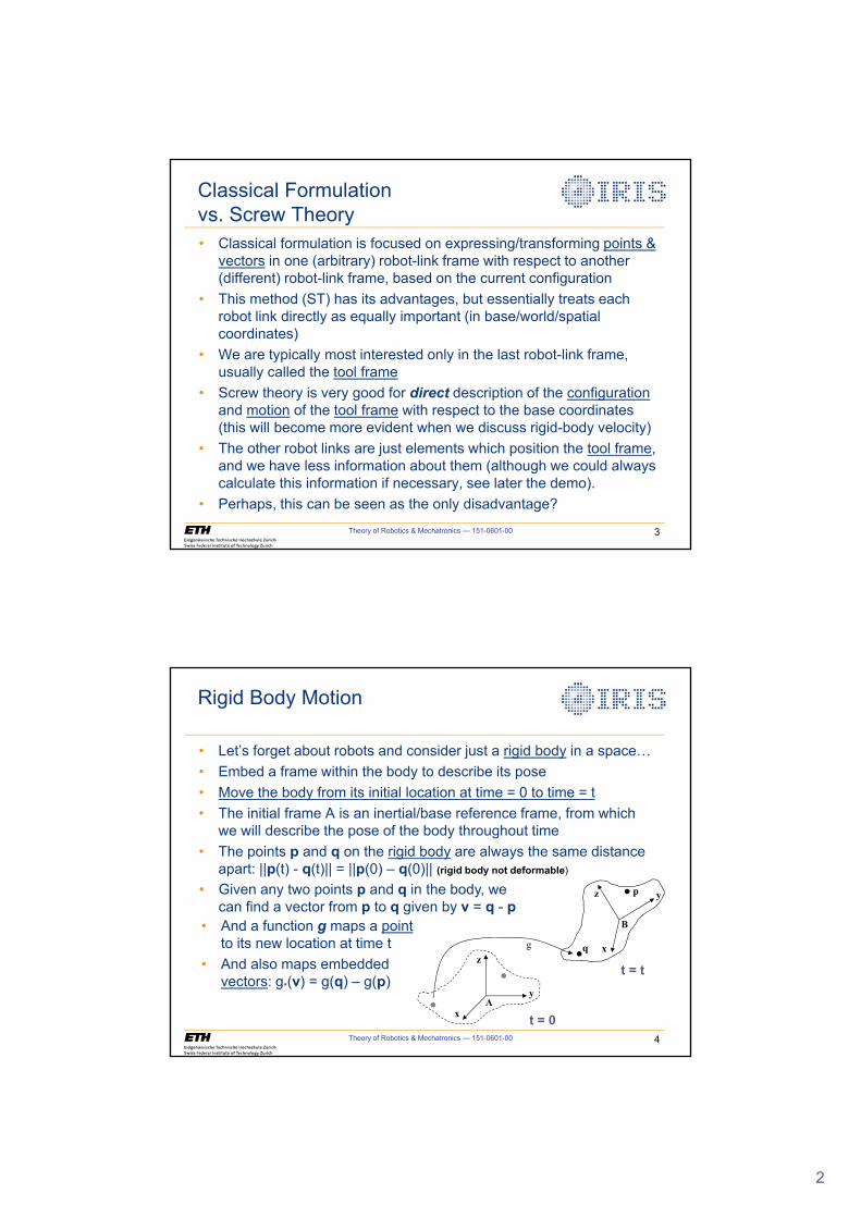
Rigid Body Motion
• Let’s forget about robots and consider just a rigid body in a space…• Embed a frame within the body to describe its pose• Move the body from its initial location at time = 0 to time = t• The initial frame A is an inertial/base reference frame, from which
we will describe the pose of the body throughout time• The points p and q on the rigid body are always the same distance
apart: ||p(t) - q(t)|| = ||p(0) – q(0)|| (rigid body not deformable)
x
y
z
A
x
yz
B
q
p• Given any two points p and q in the body, we can find a vector from p to q given by v = q - p
• And a function g maps a pointto its new location at time t
• And also maps embedded vectors: g*(v) = g(q) – g(p)
g
t = 0
t = t
3
Theory of Robotics & Mechatronics — 151-0601-00 5
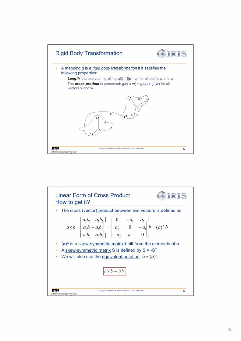
Rigid Body Transformation
• A mapping g is a rigid body transformation if it satisfies the following properties:– Length is preserved: ||g(p) - g(q)|| = ||p - q|| for all points p and q– The cross product is preserved: g*(v x w) = g*(v) x g*(w) for all
vectors v and w
x
y
zx
yz
A
B
q
p
g
Theory of Robotics & Mechatronics — 151-0601-00 6
Linear Form of Cross ProductHow to get it?
babaa
aaaa
babababababa
ba )^(0
00
12
13
23
1221
3113
2332
»»»
¼
º
«««
¬
ª
��
�
»»»
¼
º
«««
¬
ª
���
u
• The cross (vector) product between two vectors is defined as
• (a)^ is a skew-symmetric matrix built from the elements of a• A skew-symmetric matrix S is defined by S = -ST
• We will also use the equivalent notation )^(ˆ aa
4
Theory of Robotics & Mechatronics — 151-0601-00 7
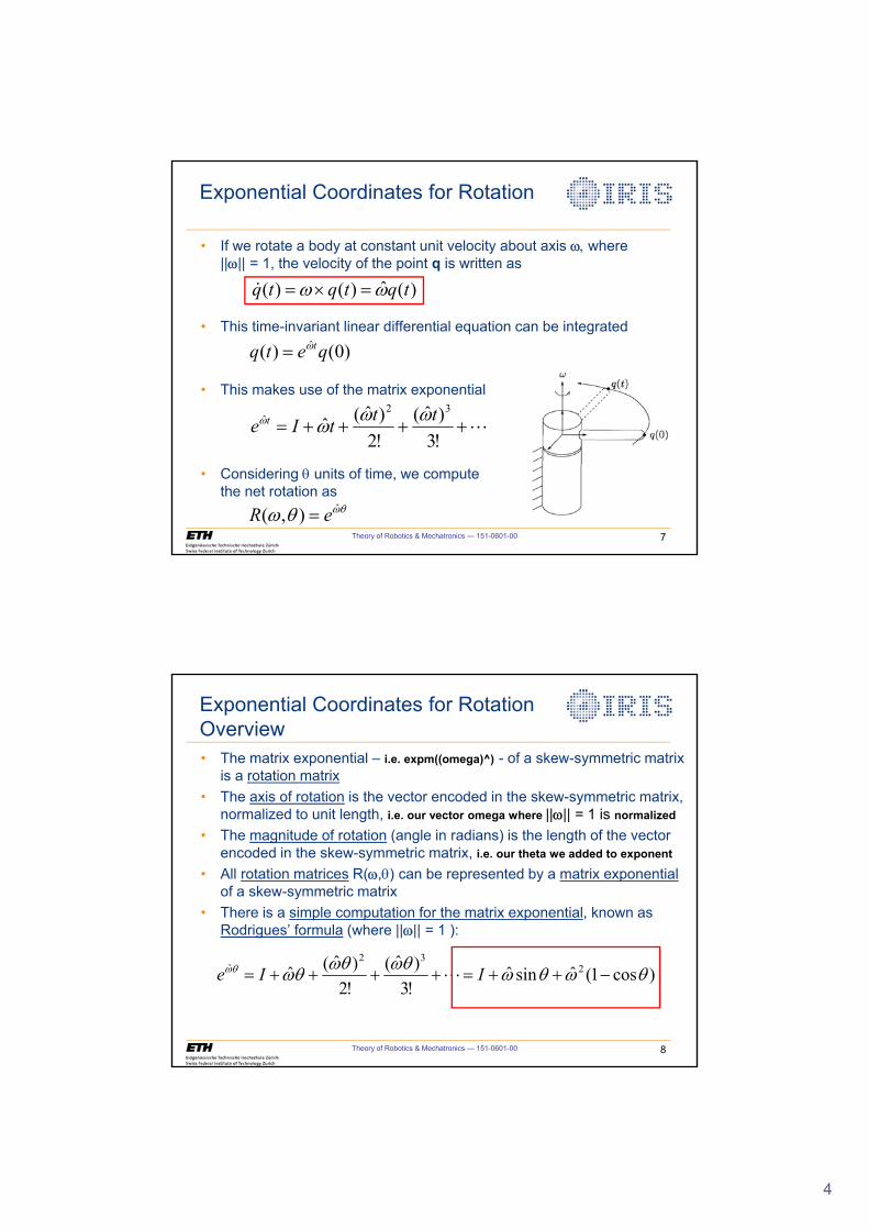
Exponential Coordinates for Rotation
• If we rotate a body at constant unit velocity about axis Z��where ||Z|| = 1, the velocity of the point q is written as
• This time-invariant linear differential equation can be integrated
• This makes use of the matrix exponential
• Considering T units of time, we compute the net rotation as
)(ˆ)()( tqtqtq ZZ u �
)0()( ˆ qetq tZ
����� !3)ˆ(
!2)ˆ(ˆ
32ˆ tttIe t ZZZZ
TZTZ ˆ),( eR
Theory of Robotics & Mechatronics — 151-0601-00 8
Exponential Coordinates for RotationOverview• The matrix exponential – i.e. expm((omega)^) - of a skew-symmetric matrix
is a rotation matrix• The axis of rotation is the vector encoded in the skew-symmetric matrix,
normalized to unit length, i.e. our vector omega where ||Z|| = 1 is normalized
• The magnitude of rotation (angle in radians) is the length of the vector encoded in the skew-symmetric matrix, i.e. our theta we added to exponent
• All rotation matrices R(Z,T) can be represented by a matrix exponentialof a skew-symmetric matrix
• There is a simple computation for the matrix exponential, known as Rodrigues’ formula (where ||Z|| = 1 ):
)cos1(ˆsinˆ!3)ˆ(
!2)ˆ(ˆ 2
32ˆ TZTZTZTZTZTZ ��� ���� IIe �
5
Theory of Robotics & Mechatronics — 151-0601-00 9
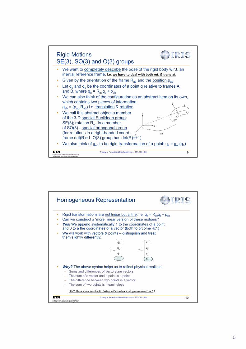
• We can also think of the configuration as an abstract item on its own, which contains two pieces of information: gab = (pab,Rab) i.e. translation & rotation
• We call this abstract object a memberof the 3-D special Euclidean group: SE(3); rotation Rab is a memberof SO(3) - special orthogonal group(for rotations in a right-handed coord.frame det(R)=1; O(3) group has det(R)=r1)
• We also think of gab to be rigid transformation of a point: qa = gab(qb)
Rigid MotionsSE(3), SO(3) and O(3) groups• We want to completely describe the pose of the rigid body w.r.t. an
inertial reference frame, i.e. we have to deal with both rot. & translat.
• Given by the orientation of the frame Rab and the position pab
• Let qa and qb be the coordinates of a point q relative to frames A and B, where qa = Rabqb + pab
Theory of Robotics & Mechatronics — 151-0601-00 10
Homogeneous Representation
• Rigid transformations are not linear but affine, i.e. qa = Rabqb + pab
• Can we construct a ‘more’ linear version of these motions?• Yes! We append systematically 1 to the coordinates of a point
and 0 to a the coordinates of a vector (both to brcome 4x1)• We will work with vectors & points – distinguish and treat
them slightly differently:
• Why? The above syntax helps us to reflect physical realities:– Sums and differences of vectors are vectors– The sum of a vector and a point is a point– The difference between two points is a vector– The sum of two points is meaningless
HINT: Have a look into the 4th “extended” coordinate being maintained 1 or 0 !
»»»»
¼
º
««««
¬
ª
13
2
1
qqq
q
»»»»
¼
º
««««
¬
ª
03
2
1
vvv
v
6
Theory of Robotics & Mechatronics — 151-0601-00 11
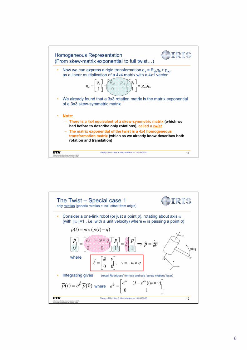
Homogeneous Representation(From skew-matrix exponential to full twist…)
• Now we can express a rigid transformation qa = Rabqb + pabas a linear multiplication of a 4x4 matrix with a 4x1 vector
• We already found that a 3x3 rotation matrix is the matrix exponential of a 3x3 skew-symmetric matrix
• Note: – There is a 4x4 equivalent of a skew-symmetric matrix (which we
had before to describe only rotations), called a twist.– The matrix exponential of the twist is a 4x4 homogeneous
transformation matrix (which as we already know describes both rotation and translation)
1 0 1 1a ab ab b
a ab b
q R p qq g qª º ª º ª º
{« » « » « »¬ ¼ ¬ ¼ ¬ ¼
)
Theory of Robotics & Mechatronics — 151-0601-00 12
• Consider a one-link robot (or just a point p), rotating about axis Z(with ||Z||=1 , i.e. with a unit velocity) where Z is passing a point q)
where
• Integrating gives (recall Rodrigues’ formula and see ‘screw motions’ later)
where
The Twist – Special case 1only rotation (generic rotation = incl. offset from origin)
))(()( qtptp �u Z�
ppppqp
[[ZZ ˆ
1ˆ
100ˆ
0 �»
¼
º«¬
ª »
¼
º«¬
ª»¼
º«¬
ª u� »
¼
º«¬
ª ��
qvv
u� »¼
º«¬
ª Z
Z[ ,
00
ˆˆ
)0()( ˆ petp t[ »¼
º«¬
ª u�
10))(( ˆˆ
ˆ veIee
ttt ZZZ[
7
)
• Consider a one-link robot, sliding on a prismatic joint with unit velocity
• Integrating gives
where
Theory of Robotics & Mechatronics — 151-0601-00 13
The Twist – Special Case 2only translation
vtp )(�
ppppvp
[[ ˆ1
ˆ100
00
�»¼
º«¬
ª »
¼
º«¬
ª»¼
º«¬
ª »
¼
º«¬
ª ��
)0()( ˆ petp t[ »¼
º«¬
ª
10ˆ vtIe t[
Theory of Robotics & Mechatronics — 151-0601-00 14
• A twist is a 4x4 matrix of the structure
• We can also extract the 6x1 twist coordinates [
• The twist is a characteristic of screw motions• Matrix exponential maps twist into screw motion
»¼
º«¬
ª »
¼
º«¬
ª
��
ZZ
[[vv
00
ˆˆ
»¼
º«¬
ª
00ˆˆ vZ
[
3x3 skew-symmetric matrix 3x1 vector
1x3 matrix of zeros
The Twist and Screw MotionStructure, Names, Notations
8
Theory of Robotics & Mechatronics — 151-0601-00 15
Screw Motions
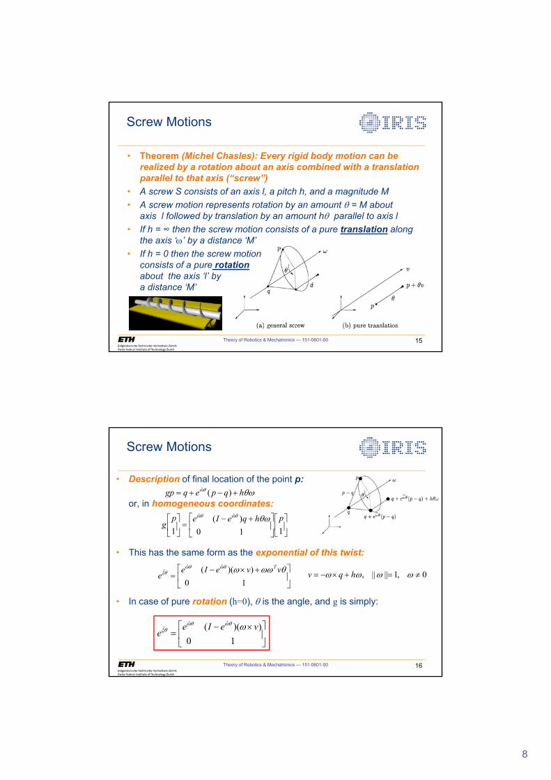
• Theorem (Michel Chasles): Every rigid body motion can be realized by a rotation about an axis combined with a translation parallel to that axis (“screw”)
• A screw S consists of an axis l, a pitch h, and a magnitude M• A screw motion represents rotation by an amount T = M about
axis l followed by translation by an amount hT parallel to axis l• If h = then the screw motion consists of a pure translation along
the axis ‘Z’ by a distance ‘M’• If h = 0 then the screw motion
consists of a pure rotationabout the axis ‘l’ bya distance ‘M’
Theory of Robotics & Mechatronics — 151-0601-00 16
Screw Motions
• Description of final location of the point p:
or, in homogeneous coordinates:
• This has the same form as the exponential of this twist:
• In case of pure rotation (h=0), T is the angle, and g is simply:
»¼
º«¬
ª»¼
º«¬
ª �� »
¼
º«¬
ª110
)(1
ˆˆ phqeIepg
TZTZTZ
TZTZ hqpeqgp ��� )(ˆ
»¼
º«¬
ª �u�
10))(( ˆˆ
ˆ TZZZTZTZT[ vveIee
T
0,1||||, z �u� ZZZZ hqv
»¼
º«¬
ª u�
10))(( ˆˆ
ˆ veIee
ZTZTZT[
9
Theory of Robotics & Mechatronics — 151-0601-00 17
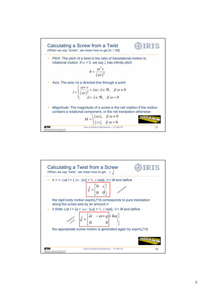
Calculating a Screw from a Twist(When we say “screw”, we mean how to get [h, l, M])
• Pitch: The pitch of a twist is the ratio of translational motion to rotational motion. If Z = 0, we say [ has infinite pitch
• Axis: The axis l is a directed line through a point
• Magnitude: The magnitude of a screw is the net rotation if the motion contains a rotational component, or the net translation otherwise
2||||ZZ vhT
¯®
z
0||,||0||,||
ZZZ
ifvif
M
°̄
°®
��
z���u
0,:
0,:|||| 2
ZOO
ZOOZZZ
ifv
ifvl
Theory of Robotics & Mechatronics — 151-0601-00 18
Calculating a Twist from a Screw(When we say “twist”, we mean how to get )
• h = : Let l = { Ov : ||v|| = 1, O real}, T = M and define
the rigid body motion expm([^T) corresponds to pure translation along the screw axis by an amount T
• h finite: Let l = {q + OZ : ||Z|| = 1, O real}, T = M and define
the appropriate screw motion is generated again by expm([^T)
»¼
º«¬
ª
000ˆ v
[
»¼
º«¬
ª �u�
00ˆˆ ZZZ
[hq
10
Theory of Robotics & Mechatronics — 151-0601-00 19
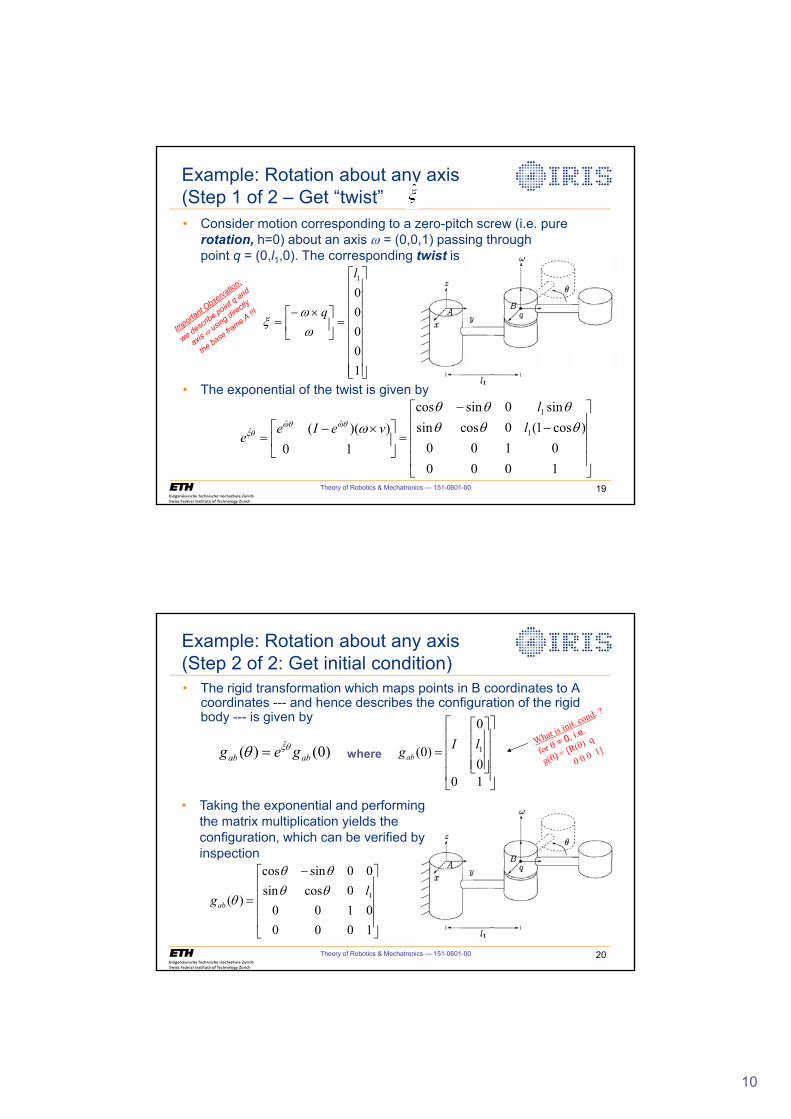
Example: Rotation about any axis(Step 1 of 2 – Get “twist” )• Consider motion corresponding to a zero-pitch screw (i.e. pure
rotation, h=0) about an axis Z = (0,0,1) passing throughpoint q = (0,l1,0). The corresponding twist is
• The exponential of the twist is given by»»»»»»»»
¼
º
««««««««
¬
ª
»¼
º«¬
ª u�
100001l
qZZ
[
»»»»
¼
º
««««
¬
ª�
�
»¼
º«¬
ª u�
10000100
)cos1(0cossinsin0sincos
10))(( 1
1ˆˆ
ˆ TTTTTT
ZTZTZT[ l
lveIe
e
Theory of Robotics & Mechatronics — 151-0601-00 20
Example: Rotation about any axis(Step 2 of 2: Get initial condition)• The rigid transformation which maps points in B coordinates to A
coordinates --- and hence describes the configuration of the rigid body --- is given by
»»»»
¼
º
««««
¬
ª �
10000100
0cossin00sincos
)( 1lgabTTTT
T
»»»»
¼
º
««««
¬
ª
»»»
¼
º
«««
¬
ª
100
0
)0( 1lIgab)0()( ˆabab geg T[T
• Taking the exponential and performing the matrix multiplication yields the configuration, which can be verified by inspection
where
11
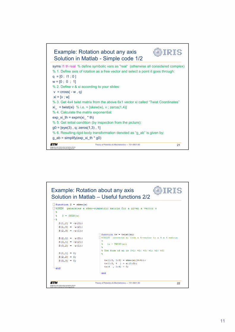
Theory of Robotics & Mechatronics — 151-0601-00 21
syms l1 th real % define symbolic vars as "real“ (otherwise all considered complex)% 1. Define axis of rotation as a free vector and select a point it goes through:q = [0 ; l1 ; 0 ] w = [0 ; 0 ; 1] % 2. Define v & xi according to your slides:v = cross( - w , q)xi = [v ; w]
% 3. Get 4x4 twist matrix from the above 6x1 vector xi called “Twist Coordinates”xi_ = twist(xi) % i.e. = [skew(w), v ; zeros(1,4)] % 4. Calculate the matrix exponential:exp_xi_th = expm(xi_ * th) % 5. Get initial condition (by inspection from the picture):g0 = [eye(3) , q; zeros(1,3) , 1]% 6. Resulting rigid body transformation denoted as “g_ab” is given by:g_ab = simplify(exp_xi_th * g0)
Example: Rotation about any axisSolution in Matlab - Simple code 1/2
Theory of Robotics & Mechatronics — 151-0601-00 22
Example: Rotation about any axisSolution in Matlab – Useful functions 2/2
12
Theory of Robotics & Mechatronics — 151-0601-00 23
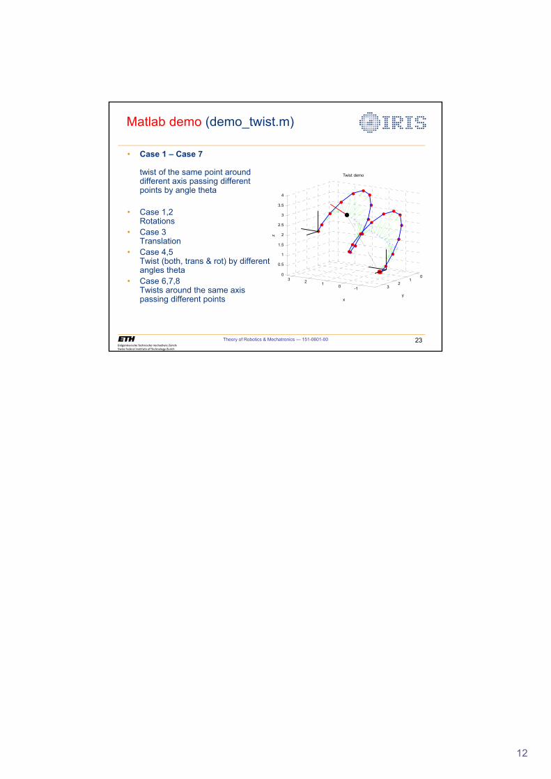
Matlab demo (demo_twist.m)
• Case 1 – Case 7
twist of the same point arounddifferent axis passing different points by angle theta
• Case 1,2Rotations
• Case 3Translation
• Case 4,5Twist (both, trans & rot) by different angles theta
• Case 6,7,8Twists around the same axis passing different points
-101230
12
3
0
0.5
1
1.5
2
2.5
3
3.5
4
y
Twist demo
x
z
1
Forward Kinematics
Institute of Robotics and Intelligent SystemsETH Zurich
Theory of Robotics &Mechatronics
Theory of Robotics & Mechatronics — 151-0601-00 2
Robot Forward Kinematics
• “ Given the joint angles, what is the position and orientation of the end-effector? ”
2
Theory of Robotics & Mechatronics — 151-0601-00 3
What have we learned?
• Body frame (BF) approach• 3rd approach to rigid body pose description
• BF rotation/orientation + translation of the BF origin in the world frame• 3 + 3 DoF i.e. 6 independent parameters
• Translation/position is rather simple to describe• Description of rotation/orientation more complex:
– Euler angles – 2x12 appropriate sequences (current vs. fixed frames), e.g. RPY– Advantage: Minimum representation (directly by means of only 3 parameters)– Drawback: Every sequence has 1x singularity
– Angle-axis representation – Advantage: Every sequence of rotations can be described as 1 rotation
about an axis Z going through the origin and by an angle T– 4 parameters (axis – 3x vector + 1x angle = 4; if axis normalized Æ 2x parameters)– Drawback: Axis not always defined (if T = Sk where k any integer)
• Screw theory (suitable for description of both translations & rotations)– Very elegant and powerful approach– No problems with singularities or undefined axes– More advantages coming up in this lecture (e.g. POE – Product Of Exponentials)
Theory of Robotics & Mechatronics — 151-0601-00 4
Robot Forward KinematicsWhat is the advantage of revolute joints?
• Dealing with them mathematically is more complicated than in case of prismatic joints (rotations vs. translations)– They result in large amount of coupling in
kinematics & dynamics of connected links(it leads to accumulation of errors and making control problems more difficult)
• Their advantage? Higher compactness & dexterity
1. Revolute joint can be made much smaller than a link with linear joint(i.e. manipulators made of revolute joints occupy a smaller space)
2. Robots with revolute joints are better able to maneuver aroundobstacles (i.e. there is a wider range of possible applications)
3
Theory of Robotics & Mechatronics — 151-0601-00 5
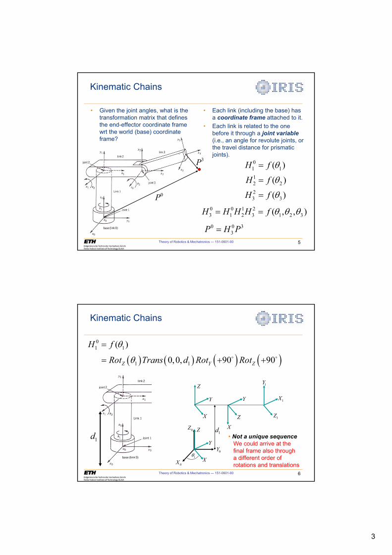
Kinematic Chains
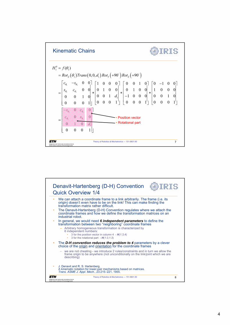
0P
3P 01 1
12 2
23 3
( )
( )
( )
H f
H f
H f
T
T
T
0 0 1 23 1 2 3 1 2 3( , , )H H H H f T T T 0 0 3
3P H P
• Given the joint angles, what is the transformation matrix that defines the end-effector coordinate frame wrt the world (base) coordinate frame?
• Each link (including the base) has a coordinate frame attached to it.
• Each link is related to the one before it through a joint variable(i.e., an angle for revolute joints, or the travel distance for prismatic joints).
Theory of Robotics & Mechatronics — 151-0601-00 6
Kinematic Chains
� � � � � � � �01 1
1 1
( )
0,0, 90 90Z Y Z
H f
Rot Trans d Rot Rot
T
T
� �$ $
0X
0Y
0Z
X
Y
Z
X
Y
Z
X
Y
Z
1X
1Y
1Z
1d
1T
• Not a unique sequenceWe could arrive at thefinal frame also througha different order ofrotations and translations
1d
4
Theory of Robotics & Mechatronics — 151-0601-00 7
� � � � � � � �1 1
1 1
1 1
1 1
01 1
1 1
1
1
( )
0,0, 90 90
0 0 1 0 0 0 0 0 1 0 0 1 0 00 0 0 1 0 0 0 1 0 0 1 0 0 0
0 0 1 1 0 0 0 0 0 1 00 0 1 00 0 0 1 0 0 0 1 0 0 0 10 0 0 1
0 0
0 0
0 1 00 0 0 1
Z Y Z
H f
Rot Trans d Rot Rot
c s
s cd
s c
c s
d
T T
T T
T T
T T
T
T
� �
�ª º �ª º ª º ª º« » « » « » « »« » « » « » « » « » « » « » « »�« » « » « » « »« » ¬ ¼ ¬ ¼ ¬ ¼¬ ¼�
$ $
ª º« »« »« »« »« »¬ ¼
Kinematic Chains
• Position vector• Rotational part
Theory of Robotics & Mechatronics — 151-0601-00 8
Denavit-Hartenberg (D-H) Convention Quick Overview 1/4• We can attach a coordinate frame to a link arbitrarily. The frame (i.e. its
origin) doesn’t even have to be on the link! This can make finding the transformation matrix rather difficult.
• The Denavit-Hartenberg (D-H) Convention regulates where we attach the coordinate frames and how we define the transformation matrices on an industrial robot.
• In general, we would need 6 independent parameters to define the transformation between two “neighboring” coordinate frames
– Arbitrary homogeneous transformation is characterized by6 independent numbers:
• 3 for the position vector in column 4 - H(1:3,4)• 3 for the rotational part - H(1:3,1:3)
• The D-H convention reduces the problem to 4 parameters by a clever choice of the origin and orientation for the coordinate frames
– we are not cheating - we introduce 2 rules/constraints and in turn we allow the frame origin to be anywhere (not unconditionally on the link/joint which we are describing)
• J. Denavit and R. S. Hartenberg. A kinematic notation for lower-pair mechanisms based on matrices. Trans. ASME J. Appl. Mech., 23:215–221, 1955.
5
Theory of Robotics & Mechatronics — 151-0601-00 9
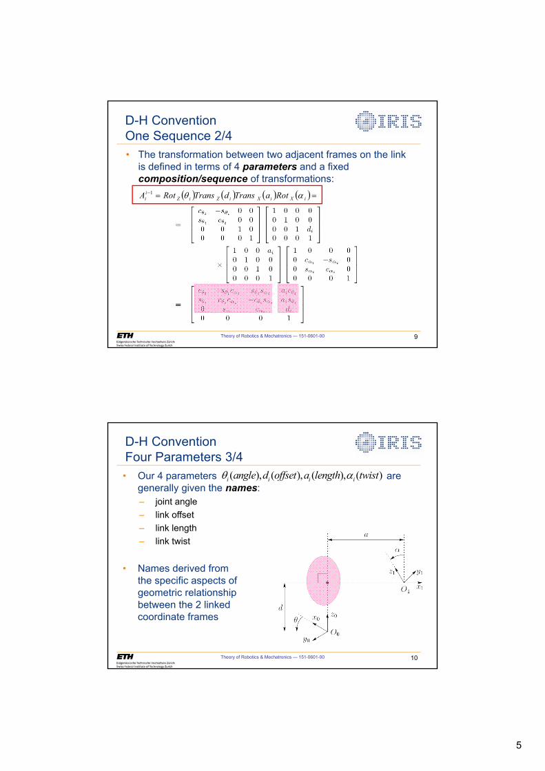
� � � � � � � � �1iXiXiZiZ
ii RotaTransdTransRotA DT
D-H ConventionOne Sequence 2/4• The transformation between two adjacent frames on the link
is defined in terms of 4 parameters and a fixedcomposition/sequence of transformations:
Theory of Robotics & Mechatronics — 151-0601-00 10
D-H ConventionFour Parameters 3/4• Our 4 parameters are
generally given the names:– joint angle – link offset– link length– link twist
• Names derived fromthe specific aspects ofgeometric relationshipbetween the 2 linkedcoordinate frames
( ), ( ), ( ), ( )i i i iangle d offset a length twistT D
6
Theory of Robotics & Mechatronics — 151-0601-00 11
• Depending on the type of joint, 1 parameter either Ti or di is the joint variable and the other 3 parameters are constant.
• Why not 6 parameters? To ensure that only 4 parameters are sufficient, the location and orientation of the coordinate frames are chosen by the following 2 rules:
D-H ConventionTwo Constraints 4/4
1. The axis Xi is perpendicular to Zi-1
2. The axis Xi intersects the axis Zi-1
Theory of Robotics & Mechatronics — 151-0601-00 12
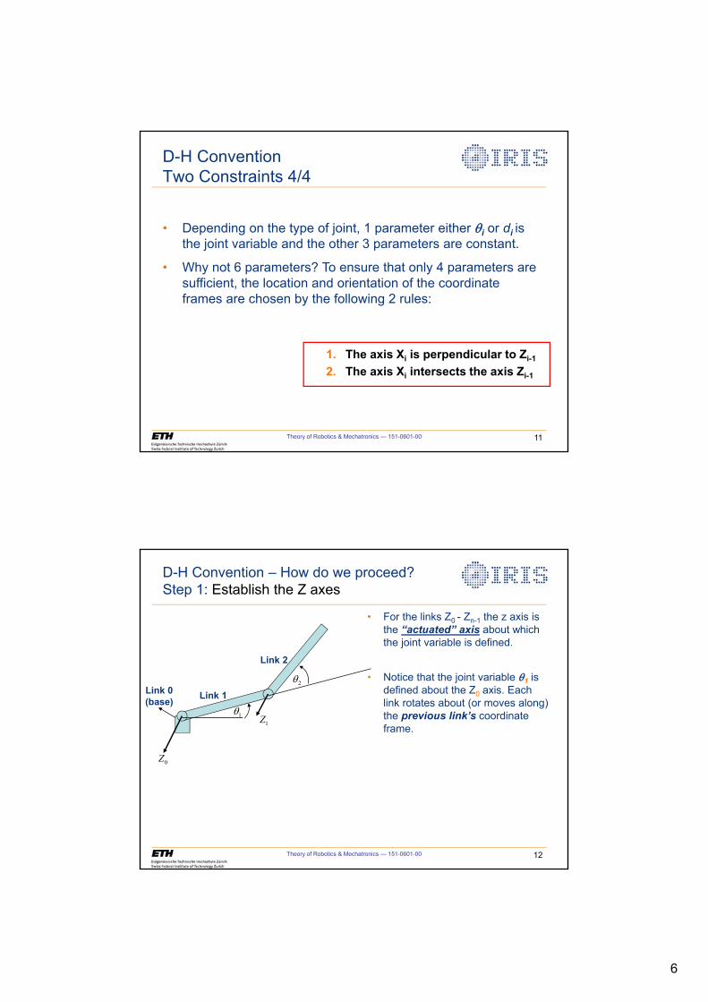
D-H Convention – How do we proceed?Step 1: Establish the Z axes
0Z
1Z
Link 1
Link 2
Link 0(base)
1T
2T
• For the links Z0 - Zn-1 the z axis is the “actuated” axis about which the joint variable is defined.
• Notice that the joint variable T1 is defined about the Z0 axis. Each link rotates about (or moves along) the previous link’s coordinate frame.
7
Theory of Robotics & Mechatronics — 151-0601-00 13
D-H Convention – How do we proceed? Step 2: Establish the Base frame
0Z
1Z
Link 1
Link 2
1T
2T
0X
0Y
• Locate the origin anywhere on the Z0 axis
the X0 and Y0 axes are then chosen conveniently to establisha right-hand orthonormal coordinate frame see next slides
Theory of Robotics & Mechatronics — 151-0601-00 14
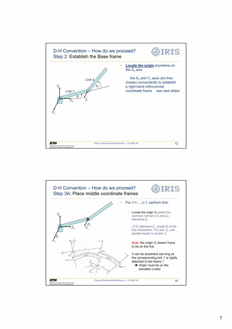
D-H Convention – How do we proceed? Step 3A: Place middle coordinate frames
0Z
1Z
1T
2T0X
0Y
• For i=1,…,n-1, perform this:
– Locate the origin Oi where the common normal to Zi and Zi-1intersects Zi.
( If Zi intersects Zi-1 locate Oi at the this intersection. If Zi and Zi-1 are parallel locate Oi at joint I ).
Note: the origin Oi doesn’t have to be on the link.
It can be anywhere (as long as the corresponding link ‘i’ is rigidly attached to the frame ‘i’ Î Origin must be on the
actuated z-axis!
8
Theory of Robotics & Mechatronics — 151-0601-00 15
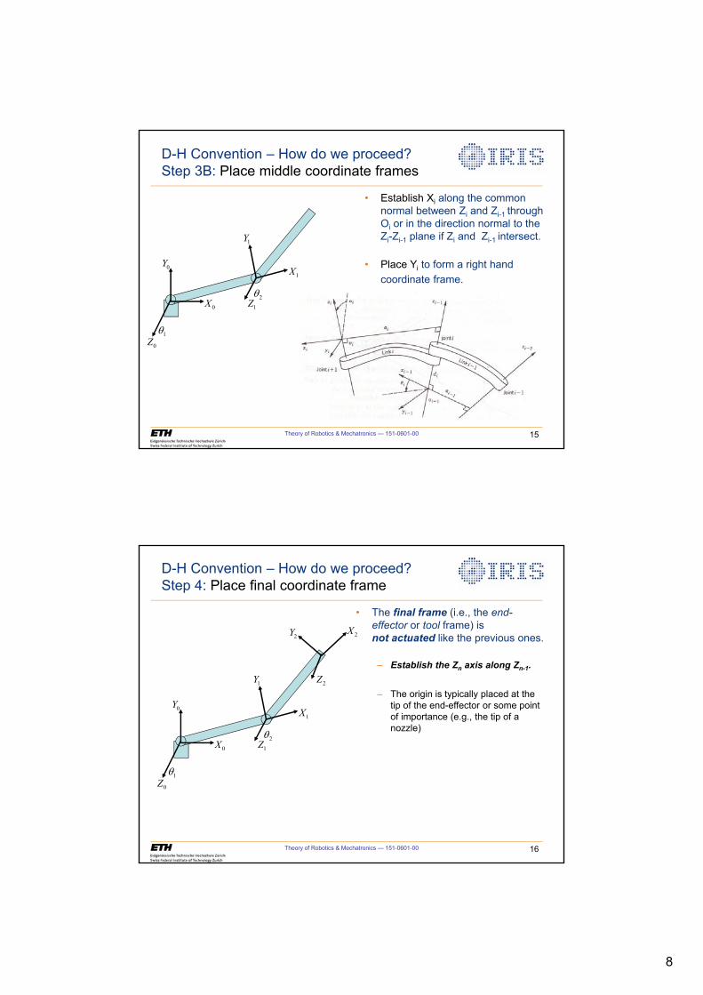
D-H Convention – How do we proceed? Step 3B: Place middle coordinate frames
0Z
1Z
1T
2T0X
0Y1X
1Y
• Establish Xi along the common normal between Zi and Zi-1 through Oi or in the direction normal to the Zi-Zi-1 plane if Zi and Zi-1 intersect.
• Place Yi to form a right hand coordinate frame.
Theory of Robotics & Mechatronics — 151-0601-00 16
D-H Convention – How do we proceed? Step 4: Place final coordinate frame
0Z
1Z
1T
2T
2Z
0X
0Y1X
1Y
2X2Y
• The final frame (i.e., the end-effector or tool frame) isnot actuated like the previous ones.
– Establish the Zn axis along Zn-1.
– The origin is typically placed at the tip of the end-effector or some point of importance (e.g., the tip of a nozzle)
9
Theory of Robotics & Mechatronics — 151-0601-00 17
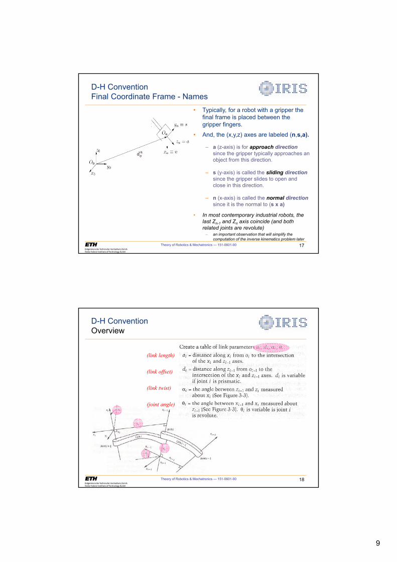
D-H ConventionFinal Coordinate Frame - Names
• Typically, for a robot with a gripper the final frame is placed between the gripper fingers.
• And, the (x,y,z) axes are labeled (n,s,a).
– a (z-axis) is for approach directionsince the gripper typically approaches an object from this direction.
– s (y-axis) is called the sliding directionsince the gripper slides to open and close in this direction.
– n (x-axis) is called the normal directionsince it is the normal to (s x a)
• In most contemporary industrial robots, the last Zn-1 and Zn axis coincide (and both related joints are revolute)
– an important observation that will simplify the computation of the inverse kinematics problem later
Theory of Robotics & Mechatronics — 151-0601-00 18
D-H ConventionOverview
(link length)
(link offset)
(link twist)
(joint angle)
10
Theory of Robotics & Mechatronics — 151-0601-00 19
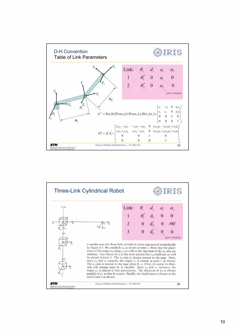
� � � � � � � �
»»»»
¼
º
««««
¬
ª���������
»»»»
¼
º
««««
¬
ª �
�
10000100
00
10000100
00
1122122121212121
1122122121212121
12
01
02
1
asascacsssccsccsacassacccsscsscc
AAH
sacscasc
RotaTransdTransRotA iiii
iiii
iXiXiZiZii DT
D-H Convention Table of Link Parameters
0Z
1Z
1T2T
2Z
0X
0Y1X
1Y
2X2Y
a1
a2
*1 1
*2 2
Link:
1 0 0
2 0 0
i i i id a
a
a
T D
T
T* joint variable
Theory of Robotics & Mechatronics — 151-0601-00 20
Three-Link Cylindrical Robot
*1 1
*2
*3
Link:
1 d 0 0
2 0 d 0 -90
3 0 d 0 0
i i i id aT D
T$
* joint variable

11
Theory of Robotics & Mechatronics — 151-0601-00 21
Spherical Wrist
*4
*5
*6 6
Link:
4 0 0 -90
5 0 0 +90
6 d 0 0
i i i id aT D
T
T
T
$
$
* joint variable
d6
Theory of Robotics & Mechatronics — 151-0601-00 22
The Stanford Manipulator
*1 1
*2 2
*3
*4
*5
Link:
1 d 0 -90
2 d 0 +90
3 0 d 0 0
4 0 0 -90
5 0
i i i id aT D
T
T
T
T
$
$
$
*6
0 +90
6 0 0 0T
$
x0
Could be d6 to place the coordinate frame between the gripper
12
Theory of Robotics & Mechatronics — 151-0601-00 23
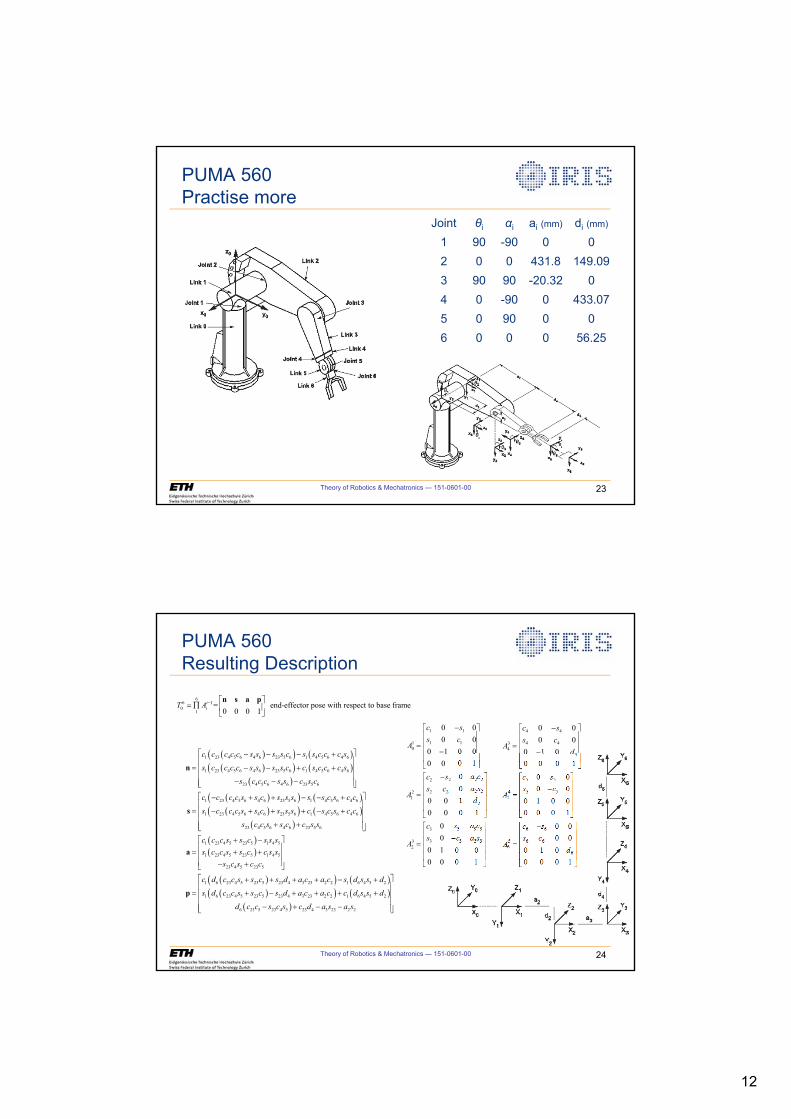
PUMA 560Practise more
Joint θi i ai (mm) di (mm)
1 90 -90 0 02 0 0 431.8 149.093 90 90 -20.32 04 0 -90 0 433.075 0 90 0 06 0 0 0 56.25
Theory of Robotics & Mechatronics — 151-0601-00 24
PUMA 560Resulting Description
1 1
1 110
2 2 2 2
2 2 2 221
2
3 3 3 3
3 3 3 332
0 00 0
0 1 0 00 0 0 1
00
0 0 10 0 0 1
00
0 1 0 00 0 0 1
c ss c
A
c s a cs c a s
Ad
c s a cs c a s
A
�ª º« »« » « »�« »¬ ¼
�ª º« »« » « »« »¬ ¼ª º« »�« » « »« »¬ ¼
4 4
4 434
4
5 5
5 545
6 6
6 656
6
0 00 0
0 1 00 0 0 1
0 00 0
0 1 0 00 0 0 1
0 00 0
0 1 00 0 0 1
c ss c
Ad
c ss c
A
c ss c
Ad
�ª º« »« » « »�« »¬ ¼ª º« »�« » « »« »¬ ¼
�ª º« »« » « »« »¬ ¼
66 1
01
= end-effector pose with respect to base frame0 0 0 1
iiT A � ª º
� « »¬ ¼
n s a p
� �� � � �� �� � � �
� �
� �� � � �� �� � � �
1 23 4 5 6 4 6 23 5 6 1 4 5 6 4 6
1 23 4 5 6 4 6 23 5 6 1 4 5 6 4 6
23 4 5 6 4 6 23 5 6
1 23 4 5 6 4 6 23 5 6 1 4 5 6 4 6
1 23 4 5 6 4 6 23 5 6 1 4 5 6 4 6
23 4
c c c c c s s s s c s s c c c s
s c c c c s s s s c c s c c c s
s c c c s s c s c
c c c c s s c s s s s s c s c c
s c c c s s c s s s c s c s c c
s c
ª º� � � �« »
� � � �« »« »� � �« »¬ ¼
� � � � � �
� � � � � �
n
s
� �� �� �
� �� � � �� �� � � �
5 6 4 6 23 5 6
1 23 4 5 23 5 1 4 5
1 23 4 5 23 5 1 4 5
23 4 5 23 5
1 6 23 4 5 23 5 23 4 3 23 2 2 1 6 4 5 2
1 6 23 4 5 23 5 23 4 3 23 2 2 1 6 4 5 2
6 23 5
c s s c c s s
c c c s s c s s ss c c s s c c s s
s c s c c
c d c c s s c s d a c a c s d s s d
s d c c s s c s d a c a c c d s s d
d c c
ª º« »« »« »� �« »¬ ¼ª º� �« » � �« »« »� �¬ ¼
� � � � � �
� � � � � �
a
p
� �23 4 5 23 4 3 23 2 2s c s c d a s a s
ª º« »« »« »� � � �« »¬ ¼
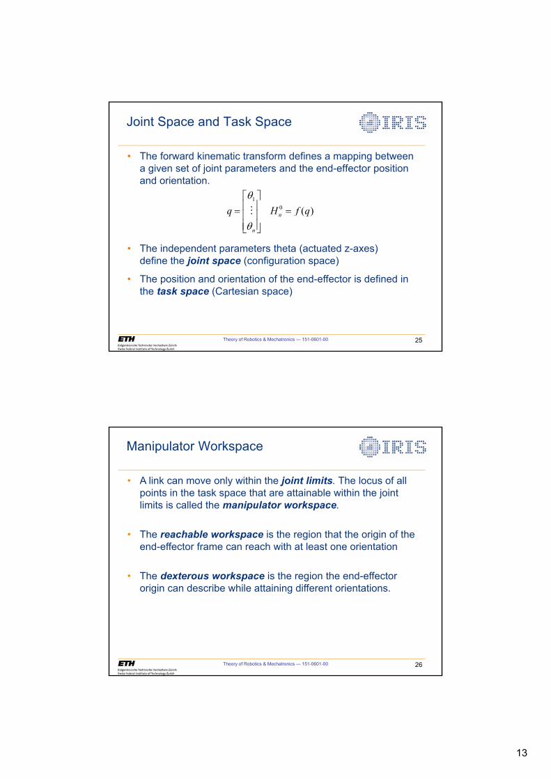
13
Theory of Robotics & Mechatronics — 151-0601-00 25
Joint Space and Task Space
10 ( )n
n
q H f qT
T
ª º« » « »« »¬ ¼
�
• The forward kinematic transform defines a mapping between a given set of joint parameters and the end-effector position and orientation.
• The independent parameters theta (actuated z-axes) define the joint space (configuration space)
• The position and orientation of the end-effector is defined in the task space (Cartesian space)
Theory of Robotics & Mechatronics — 151-0601-00 26
Manipulator Workspace
• A link can move only within the joint limits. The locus of all points in the task space that are attainable within the joint limits is called the manipulator workspace.
• The reachable workspace is the region that the origin of the end-effector frame can reach with at least one orientation
• The dexterous workspace is the region the end-effector origin can describe while attaining different orientations.
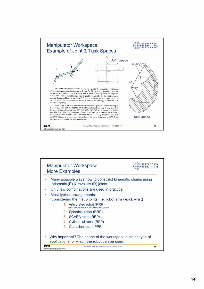
14
Theory of Robotics & Mechatronics — 151-0601-00 27
Manipulator WorkspaceExample of Joint & Task Spaces
0Z
1Z
1T
2T0X
0Y1X
1Y
Joint space
Task space
Theory of Robotics & Mechatronics — 151-0601-00 28
Manipulator WorkspaceMore Examples
• Many possible ways how to construct kinematic chains usingprismatic (P) & revolute (R) joints
• Only few combinations are used in practice• Most typical arrangements:
(considering the first 3 joints, i.e. robot arm / excl. wrist)1. Articulated robot (RRR)
some literature calls it “the elbow manipulator”
2. Spherical robot (RRP)3. SCARA robot (RRP)4. Cylindrical robot (RPP)5. Cartesian robot (PPP)
• Why important? The shape of the workspace dictates type of applications for which the robot can be used
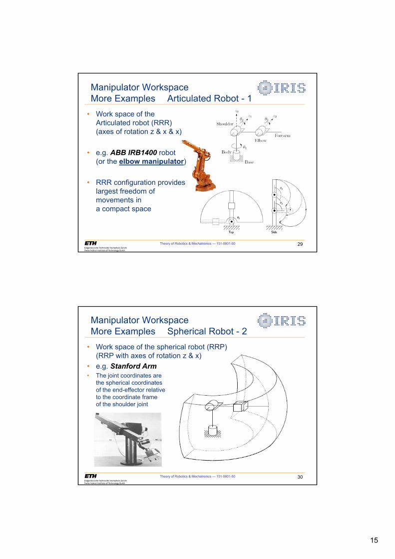
15
Theory of Robotics & Mechatronics — 151-0601-00 29
Manipulator WorkspaceMore Examples Articulated Robot - 1
• Work space of the Articulated robot (RRR)(axes of rotation z & x & x)
• e.g. ABB IRB1400 robot(or the elbow manipulator)
• RRR configuration provides largest freedom of movements in a compact space
Theory of Robotics & Mechatronics — 151-0601-00 30
Manipulator WorkspaceMore Examples Spherical Robot - 2
• Work space of the spherical robot (RRP) (RRP with axes of rotation z & x)
• e.g. Stanford Arm• The joint coordinates are
the spherical coordinatesof the end-effector relativeto the coordinate frameof the shoulder joint
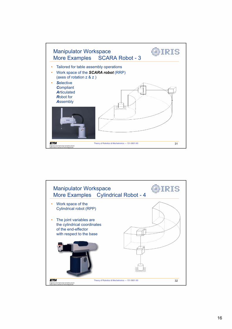
16
Theory of Robotics & Mechatronics — 151-0601-00 31
Manipulator WorkspaceMore Examples SCARA Robot - 3
• Tailored for table assembly operations• Work space of the SCARA robot (RRP)
(axes of rotation z & z )• Selective
Compliant ArticulatedRobot forAssembly
Theory of Robotics & Mechatronics — 151-0601-00 32
Manipulator WorkspaceMore Examples Cylindrical Robot - 4
• Work space of the Cylindrical robot (RPP)
• The joint variables arethe cylindrical coordinatesof the end-effector with respect to the base
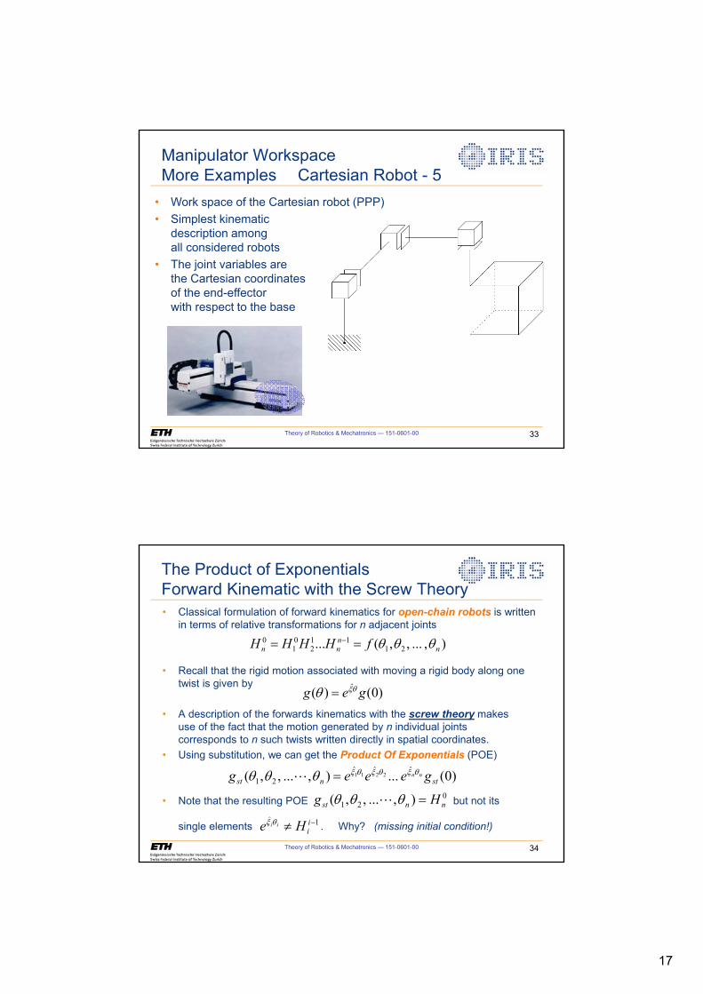
17
Theory of Robotics & Mechatronics — 151-0601-00 33
Manipulator WorkspaceMore Examples Cartesian Robot - 5
• Work space of the Cartesian robot (PPP)• Simplest kinematic
description amongall considered robots
• The joint variables are the Cartesian coordinatesof the end-effectorwith respect to the base
Theory of Robotics & Mechatronics — 151-0601-00 34
The Product of ExponentialsForward Kinematic with the Screw Theory• Classical formulation of forward kinematics for open-chain robots is written
in terms of relative transformations for n adjacent joints
• Recall that the rigid motion associated with moving a rigid body along one twist is given by
• A description of the forwards kinematics with the screw theory makesuse of the fact that the motion generated by n individual jointscorresponds to n such twists written directly in spatial coordinates.
• Using substitution, we can get the Product Of Exponentials (POE)
• Note that the resulting POE but not its
single elements . Why? (missing initial condition!)
)0()( ˆ geg T[T
),...,,(... 2111
201
0n
nnn fHHHH TTT �
)0(...),...,,( ˆˆˆ21
2211stnst geeeg nnT[T[T[TTT �
021 ),...,,( nnst Hg TTT �
1�z iiHe iiT[
�
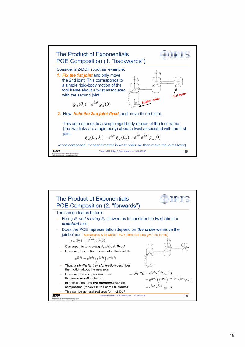
18
Theory of Robotics & Mechatronics — 151-0601-00 35
2. Now, hold the 2nd joint fixed, and move the 1st joint.
This corresponds to a simple rigid-body motion of the tool frame (the two links are a rigid body) about a twist associated with the first joint
(once composed, it doesn’t matter in what order we then move the joints later)
The Product of ExponentialsPOE Composition (1. “backwards”)Consider a 2-DOF robot as example:1. Fix the 1st joint and only move
the 2nd joint. This corresponds to a simple rigid-body motion of the tool frame about a twist associated with the second joint:
)0()( 22ˆ
2 stst geg T[T
)0()(),( 221111ˆˆ
2ˆ
21 ststst geegeg T[T[T[ TTT
The same idea as before: � Fixing T1 and moving T2 allowed us to consider the twist about a
constant axis� Does the POE representation depend on the order we move the
joints? (no - “Backwards & forwards” POE compositions give the same)
- Corresponds to moving T1 while T2 fixed - However, this motion moved also the joint T2
- Thus, a similarity transformation describesthe motion about the new axis
- However, the composition givesthe same result as before
- In both cases, use pre-multiplication ascomposition (resolve in the same fix frame)
- This can be generalized also for n>2 DoF Theory of Robotics & Mechatronics — 151-0601-00 36
The Product of ExponentialsPOE Composition (2. “forwards”)
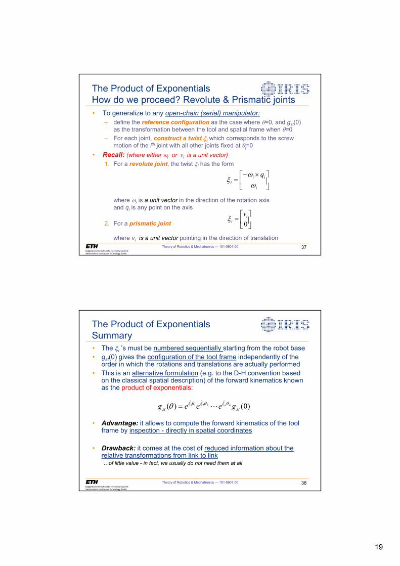
19
»¼
º«¬
ª
0i
i
v[
• To generalize to any open-chain (serial) manipulator:– define the reference configuration as the case where T=0, and gst(0)
as the transformation between the tool and spatial frame when T=0– For each joint, construct a twist [i which corresponds to the screw
motion of the ith joint with all other joints fixed at Tj=0• Recall: (where either Zi or vi is a unit vector)
1. For a revolute joint, the twist [i has the form
where Zi is a unit vector in the direction of the rotation axisand qi is any point on the axis
2. For a prismatic joint
where vi is a unit vector pointing in the direction of translationTheory of Robotics & Mechatronics — 151-0601-00 37
The Product of ExponentialsHow do we proceed? Revolute & Prismatic joints
»¼
º«¬
ª u�
i
iii
qZZ
[
Theory of Robotics & Mechatronics — 151-0601-00 38
The Product of ExponentialsSummary• The [i ’s must be numbered sequentially starting from the robot base• gst(0) gives the configuration of the tool frame independently of the
order in which the rotations and translations are actually performed• This is an alternative formulation (e.g. to the D-H convention based
on the classical spatial description) of the forward kinematics known as the product of exponentials:
• Advantage: it allows to compute the forward kinematics of the tool frame by inspection - directly in spatial coordinates
• Drawback: it comes at the cost of reduced information about the relative transformations from link to link…of little value - in fact, we usually do not need them at all
)0()(ˆˆˆ
2211stst geeeg nnT[T[T[T �
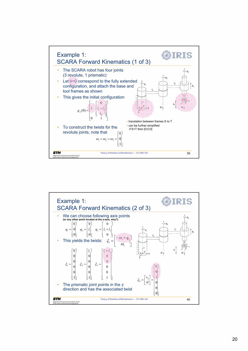
20
Theory of Robotics & Mechatronics — 151-0601-00 39
Example 1:SCARA Forward Kinematics (1 of 3)• The SCARA robot has four joints
(3 revolute, 1 prismatic)• Let T=0 correspond to the fully extended
configuration, and attach the base and tool frames as shown
• This gives the initial configuration
• To construct the twists for therevolute joints, note that
»»»»
¼
º
««««
¬
ª
»»»
¼
º
«««
¬
ª�
10
0
)0(0
21
lllIgst
»»»
¼
º
«««
¬
ª
100
321 ZZZ
• translation between frames S to T• can be further simplified
if S=T then [0;0;0]
Theory of Robotics & Mechatronics — 151-0601-00 40
Example 1:SCARA Forward Kinematics (2 of 3)• We can choose following axis points
(or any other point located at the z-axis, why?)
• This yields the twists:
• The prismatic joint points in the zdirection and has the associated twist
»»»
¼
º
«««
¬
ª�
»»»
¼
º
«««
¬
ª
»»»
¼
º
«««
¬
ª
0
0
0
0
000
213121 llqlqq
»»»»»»»»
¼
º
««««««««
¬
ª �
»»»»»»»»
¼
º
««««««««
¬
ª
»»»»»»»»
¼
º
««««««««
¬
ª
10000
10000
100000 21
3
1
21
lll
[[[
»»»»»»»»
¼
º
««««««««
¬
ª
»¼
º«¬
ª
000100
04
4
v[
»¼
º«¬
ª u�
i
iii
qZZ
[
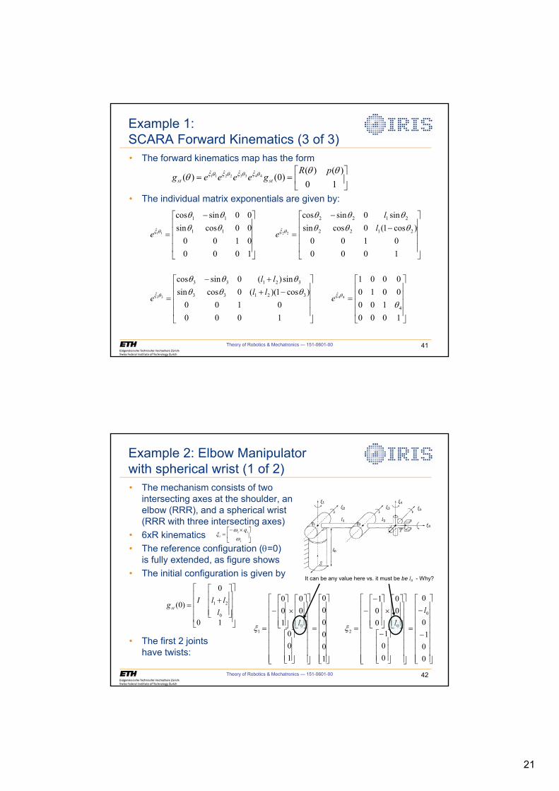
21
Theory of Robotics & Mechatronics — 151-0601-00 41
Example 1: SCARA Forward Kinematics (3 of 3)• The forward kinematics map has the form
• The individual matrix exponentials are given by:
»¼
º«¬
ª
10)()(
)0()( 44332211ˆˆˆˆ TT
T T[T[T[T[ pRgeeeeg stst
»»»»
¼
º
««««
¬
ª �
1000010000cossin00sincos
11
11
ˆ11
TTTT
T[e
»»»»
¼
º
««««
¬
ª�
�
10000100
)cos1(0cossinsin0sincos
2122
2122
ˆ22
TTTTTT
T[ ll
e
»»»»
¼
º
««««
¬
ª��
��
10000100
)cos1)((0cossinsin)(0sincos
32133
32133
ˆ33
TTTTTT
T[ llll
e
»»»»
¼
º
««««
¬
ª
1000100
00100001
4
ˆ44
TT[e
Theory of Robotics & Mechatronics — 151-0601-00 42
Example 2: Elbow Manipulatorwith spherical wrist (1 of 2)• The mechanism consists of two
intersecting axes at the shoulder, an elbow (RRR), and a spherical wrist (RRR with three intersecting axes)
• 6xR kinematics• The reference configuration (T=0)
is fully extended, as figure shows• The initial configuration is given by
• The first 2 jointshave twists:
»»»»
¼
º
««««
¬
ª
»»»
¼
º
«««
¬
ª�
10
0
)0(0
21
lllIgst
»»»»»»»»
¼
º
««««««««
¬
ª
�
�
»»»»»»»»
¼
º
««««««««
¬
ª
»»»
¼
º
«««
¬
ª�»»»
¼
º
«««
¬
ªu»»»
¼
º
«««
¬
ª��
»»»»»»»»
¼
º
««««««««
¬
ª
»»»»»»»»
¼
º
««««««««
¬
ª
»»»
¼
º
«««
¬
ª»»»
¼
º
«««
¬
ªu»»»
¼
º
«««
¬
ª�
001
0
0
001
00
001
100000
100
00
100
0
02
01
lll
[[
»¼
º«¬
ª u�
i
iii
qZZ
[
It can be any value here vs. it must be be l0 - Why?
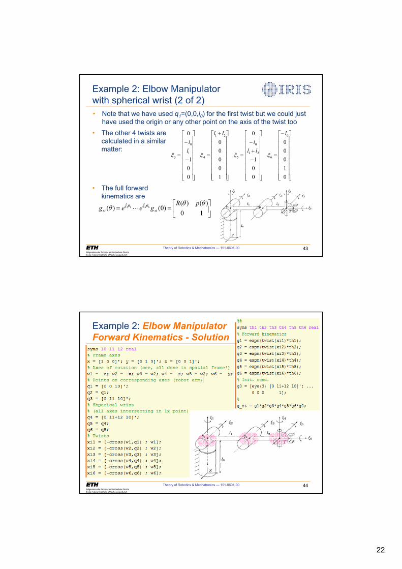
22
Theory of Robotics & Mechatronics — 151-0601-00 43
Example 2: Elbow Manipulatorwith spherical wrist (2 of 2)• Note that we have used q1=(0,0,l0) for the first twist but we could just
have used the origin or any other point on the axis of the twist too
»»»»»»»»
¼
º
««««««««
¬
ª�
»»»»»»»»
¼
º
««««««««
¬
ª
���
»»»»»»»»
¼
º
««««««««
¬
ª �
»»»»»»»»
¼
º
««««««««
¬
ª
�
�
01000
001
0
10000
001
0 0
621
0
5
21
41
0
3
l
lll
ll
ll
[[[[
»¼
º«¬
ª
10)()(
)0()( 6611ˆˆ TT
T T[T[ pRgeeg stst �
• The other 4 twists are calculated in a similar matter:
• The full forward kinematics are
Theory of Robotics & Mechatronics — 151-0601-00 44
Example 2: Elbow Manipulator Forward Kinematics - Solution
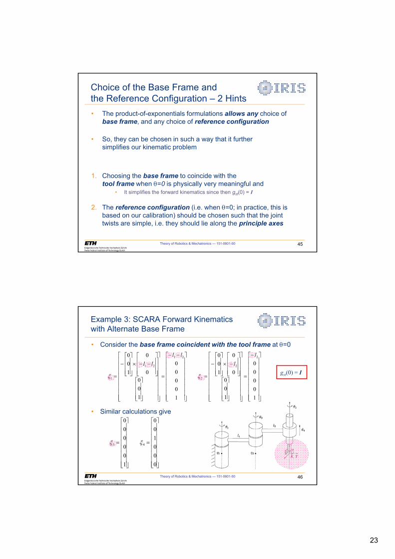
23
Theory of Robotics & Mechatronics — 151-0601-00 45
Choice of the Base Frame andthe Reference Configuration – 2 Hints• The product-of-exponentials formulations allows any choice of
base frame, and any choice of reference configuration
• So, they can be chosen in such a way that it further simplifies our kinematic problem
1. Choosing the base frame to coincide with the tool frame when T=0 is physically very meaningful and
• It simplifies the forward kinematics since then gst(0) = I
2. The reference configuration (i.e. when T=0; in practice, this is based on our calibration) should be chosen such that the joint twists are simple, i.e. they should lie along the principle axes
Theory of Robotics & Mechatronics — 151-0601-00 46
Example 3: SCARA Forward Kinematics with Alternate Base Frame
• Consider the base frame coincident with the tool frame at T=0
• Similar calculations give
»»»»»»»»
¼
º
««««««««
¬
ª�
»»»»»»»»
¼
º
««««««««
¬
ª
»»»
¼
º
«««
¬
ª»»»
¼
º
«««
¬
ª�u
»»»
¼
º
«««
¬
ª�
»»»»»»»»
¼
º
««««««««
¬
ª ��
»»»»»»»»
¼
º
««««««««
¬
ª
»»»
¼
º
«««
¬
ª»»»
¼
º
«««
¬
ª��u
»»»
¼
º
«««
¬
ª�
10000
100
0
0
100
10000
100
0
0
100 2
2
2
21
21
1
ll
llll
[[
»»»»»»»»
¼
º
««««««««
¬
ª
»»»»»»»»
¼
º
««««««««
¬
ª
000100
100000
43 [[
gst(0) = I
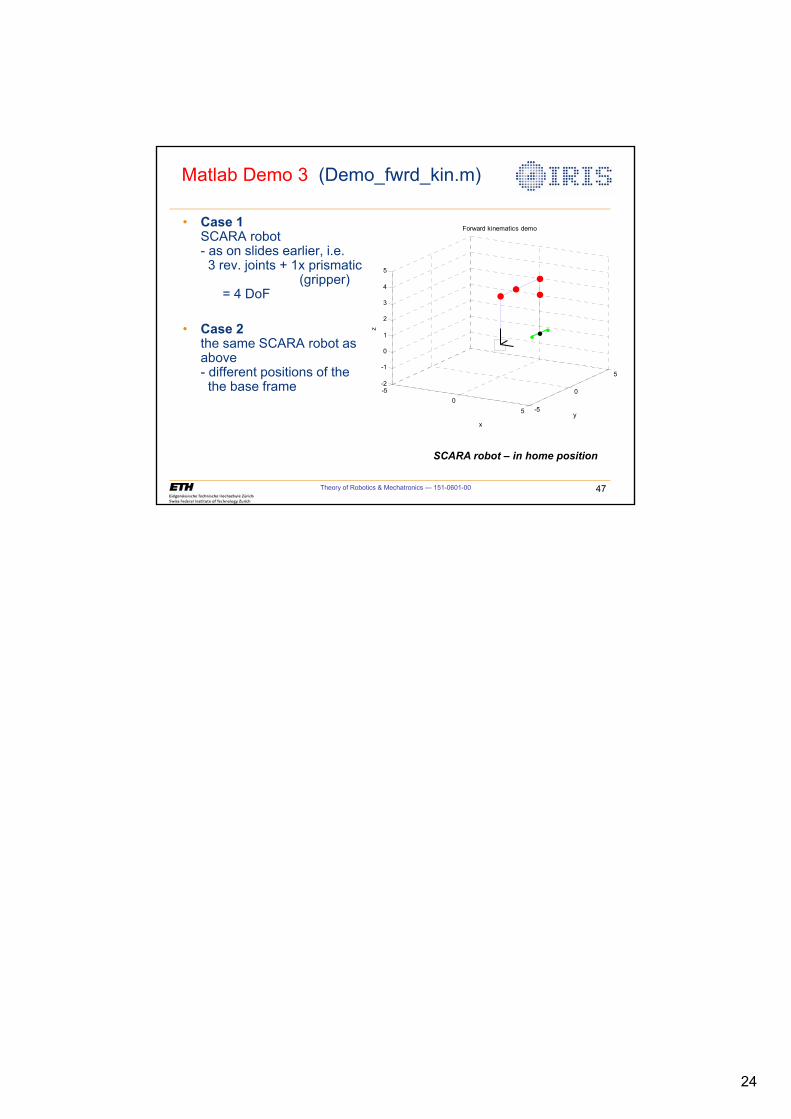
24
Theory of Robotics & Mechatronics — 151-0601-00 47
Matlab Demo 3 (Demo_fwrd_kin.m)
• Case 1SCARA robot - as on slides earlier, i.e.3 rev. joints + 1x prismatic
(gripper) = 4 DoF
• Case 2the same SCARA robot as above- different positions of thethe base frame
SCARA robot – in home position
-50
5 -5
0
5-2
-1
0
1
2
3
4
5
y
Forward kinematics demo
x
z
1
Rigid Body Velocity
Institute of Robotics and Intelligent SystemsETH Zurich
Theory of Robotics &Mechatronics
Theory of Robotics & Mechatronics — 151-0601-00 2
Main points covered in this lecture(Concepts to remember)• Linear & angular velocity
• Derivative of a rotation matrix R
• Skew symmetric matrices and groups O(3), so(3) / SO(3), se(3) / SE(3)
• What is spatial & body velocity – in SO(3) - rotational velocity: Z– in SE(3) - rigid body velocity: [v, Z] = [’
• Approach based on twists - Velocity of screw motion– Adjoint transformation– How to get spatial and body velocities from g(R,p) and the twist [– Transformation between frames
2
Theory of Robotics & Mechatronics — 151-0601-00 3
Rigid Body Position & Orientation(Review & prerequisites - 1)
• Important things to remember from previous lectures:
• There are alternative ways to represent mathematicallyposition of a rigid body:
1. Assign position vectors to all pointsof the rigid body. Aren’t they too many ?
2. Use position of three co-linear points on the body(and find a way how to reconstruct all the others out of them)
3. Attach a fix body frame to our rigid body and uselinear position (translation) of one point (frame origin)in combination with the angular position (rotation/orientation)
• We chose to use 3rd approach:• Mathematically most convenient
• In 3D, this results in 3 translational DoF and 3 rotational DoF,i.e. 6 independent parameters
Theory of Robotics & Mechatronics — 151-0601-00 4
Rigid Body Position & Orientation(Review & prerequisites - 2)
• Linear position (translation) of any point in 3D canbe represented by a vector r � R3 (3 independent parameters)
• Angular position (orientation/rotation) in 3D requiresanother 3 independent parameters and can be represented by:
– Rotation matrix (3 x 3 = 9 parameters but 6 constraints)What constraints?• All vectors orthogonal to each other (3) and scaled to unit length (3)
– Euler angles (3 parameters and composition sequence, i.e. this is directly the minimal realization/description)
– Axis & angle (3 +1 = 4 parameters with 1 constraint – unit scaling of axis ‘k’)
• Screw theory – twists describe both translation & rotationHow many parameters can we expect?
• 6 parameters• 1x axis (Z), 1x point (q), 1x angle (T) & pitch (h) = 3+3+1+1 = 8 > 6, however,• axis (only 2 since scaled) + point (only 2 since on the axis) + angle (1) + pitch (1) = 6
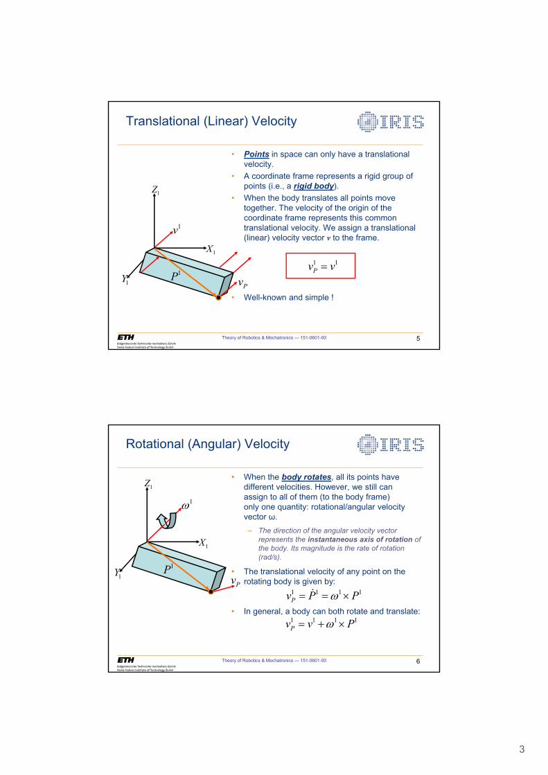
3
Theory of Robotics & Mechatronics — 151-0601-00 5
• Points in space can only have a translational velocity.
• A coordinate frame represents a rigid group of points (i.e., a rigid body).
• When the body translates all points move together. The velocity of the origin of the coordinate frame represents this common translational velocity. We assign a translational (linear) velocity vector v to the frame.
• Well-known and simple !
Translational (Linear) Velocity
1X
1Z
1Y
1v
1PPv
1 1Pv v
Theory of Robotics & Mechatronics — 151-0601-00 6
• When the body rotates, all its points have different velocities. However, we still canassign to all of them (to the body frame)only one quantity: rotational/angular velocity vector .
– The direction of the angular velocity vector represents the instantaneous axis of rotation of the body. Its magnitude is the rate of rotation (rad/s).
• The translational velocity of any point on the rotating body is given by:
• In general, a body can both rotate and translate:
Rotational (Angular) Velocity
1Z
1X
1Z
1Y
1 1 1 1Pv P PZ u�
1PPv
1 1 1 1Pv v PZ � u
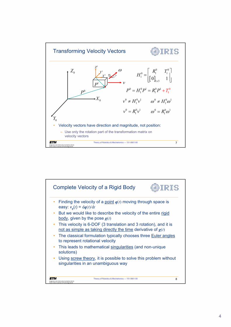
4
Theory of Robotics & Mechatronics — 151-0601-00 7
Transforming Velocity Vectors
0X
0Z
0Y
Z1X
1Y
1Z
v> @
0 01 10
11 3
0 1x
R TH
ª º « »« »¬ ¼
0 0 1 0 11
01 1P H P R P T�
1P0P
0 0 11v H vz 0 0 1
1HZ Zz
0 0 11v R v 0 0 1
1RZ Z
• Velocity vectors have direction and magnitude, not position:– Use only the rotation part of the transformation matrix on
velocity vectors
Theory of Robotics & Mechatronics — 151-0601-00 8
Complete Velocity of a Rigid Body
• Finding the velocity of a point q(t) moving through space is easy: vq(t) = dq(t)/dt
• But we would like to describe the velocity of the entire rigid body, given by the pose g(t)
• This velocity is 6-DOF (3 translation and 3 rotation), and it is not as simple as taking directly the time derivative of g(t)
• The classical formulation typically chooses three Euler anglesto represent rotational velocity
• This leads to mathematical singularities (and non-unique solutions)
• Using screw theory, it is possible to solve this problem without singularities in an unambiguous way
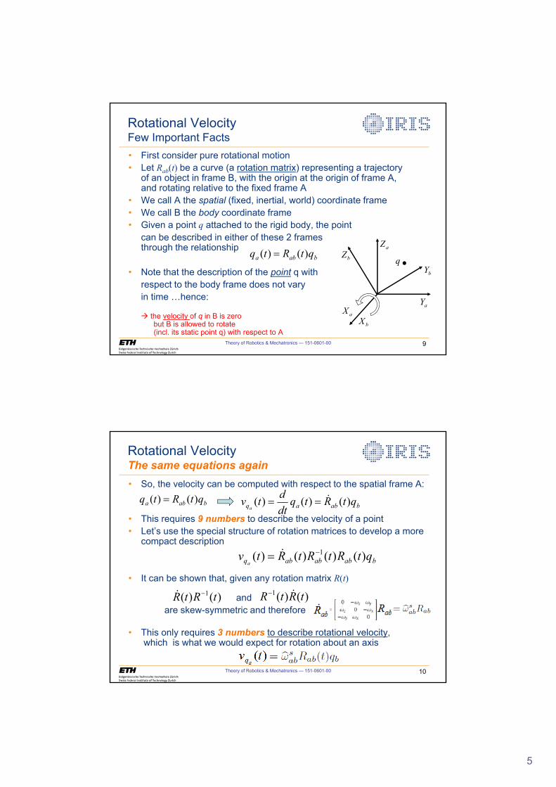
5
Theory of Robotics & Mechatronics — 151-0601-00 9
Rotational VelocityFew Important Facts• First consider pure rotational motion• Let Rab(t) be a curve (a rotation matrix) representing a trajectory
of an object in frame B, with the origin at the origin of frame A,and rotating relative to the fixed frame A
• We call A the spatial (fixed, inertial, world) coordinate frame• We call B the body coordinate frame• Given a point q attached to the rigid body, the point
can be described in either of these 2 framesthrough the relationship
• Note that the description of the point q with respect to the body frame does not vary in time …hence:
Æ the velocity of q in B is zerobut B is allowed to rotate (incl. its static point q) with respect to A
baba qtRtq )()(
aX
aZ
aY
bX
bZ
bYq
Theory of Robotics & Mechatronics — 151-0601-00 10
Rotational VelocityThe same equations again • So, the velocity can be computed with respect to the spatial frame A:
• This requires 9 numbers to describe the velocity of a point• Let’s use the special structure of rotation matrices to develop a more
compact description
• It can be shown that, given any rotation matrix R(t)
andare skew-symmetric and therefore
• This only requires 3 numbers to describe rotational velocity,which is what we would expect for rotation about an axis
babaq qtRtqdtdtv
a)()()( �
babababq qtRtRtRtva
)()()()( 1� �
)()( 1 tRtR �� )()(1 tRtR ��
baba qtRtq )()(
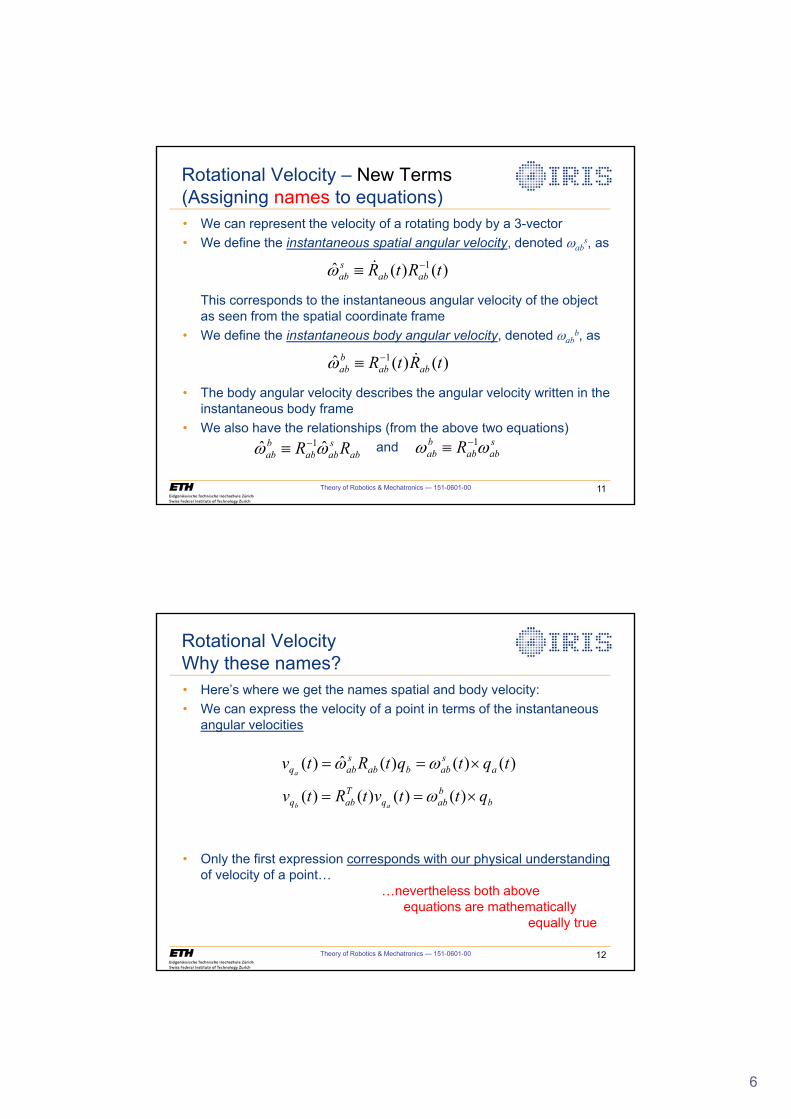
6
Theory of Robotics & Mechatronics — 151-0601-00 11
Rotational Velocity – New Terms(Assigning names to equations)• We can represent the velocity of a rotating body by a 3-vector• We define the instantaneous spatial angular velocity, denoted Zab
s, as
This corresponds to the instantaneous angular velocity of the object as seen from the spatial coordinate frame
• We define the instantaneous body angular velocity, denoted Zabb, as
• The body angular velocity describes the angular velocity written in the instantaneous body frame
• We also have the relationships (from the above two equations)and
)()(ˆ 1 tRtR ababsab
�{ �Z
)()(ˆ 1 tRtR ababbab
��{Z
absabab
bab RR ZZ ˆˆ 1�{ s
ababbab R ZZ 1�{
Theory of Robotics & Mechatronics — 151-0601-00 12
Rotational VelocityWhy these names?• Here’s where we get the names spatial and body velocity:• We can express the velocity of a point in terms of the instantaneous
angular velocities
• Only the first expression corresponds with our physical understandingof velocity of a point…
…nevertheless both aboveequations are mathematically
equally true
)()()(ˆ)( tqtqtRtv asabbab
sabqa
u ZZ
bbabq
Tabq qttvtRtv
abu )()()()( Z
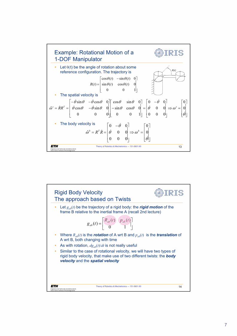
7
Theory of Robotics & Mechatronics — 151-0601-00 13
• Let T�t) be the angle of rotation about some reference configuration. The trajectory is
• The spatial velocity is
• The body velocity is
Example: Rotational Motion of a 1-DOF Manipulator
»»»
¼
º
«««
¬
ª �
1000)(cos)(sin0)(sin)(cos
)( tttt
tR TTTT
»»»
¼
º
«««
¬
ª �
»»»
¼
º
«««
¬
ª �
»»»
¼
º
«««
¬
ª�
»»»
¼
º
«««
¬
ª
���
T
ZTT
TTTT
TTTTTTTT
Z�
�
�
��
��
� 00
0000000
1000cossin0sincos
0000sincos0cossin
ˆ sTs RR
»»»
¼
º
«««
¬
ª �
»»»
¼
º
«««
¬
ª �
TZT
TZ
�
�
�
� 00
0000000
ˆ bTb RR
Theory of Robotics & Mechatronics — 151-0601-00 14
Rigid Body VelocityThe approach based on Twists• Let gab(t) be the trajectory of a rigid body: the rigid motion of the
frame B relative to the inertial frame A (recall 2nd lecture)
• Where Rab(t) is the rotation of A wrt B and pab(t) is the translation of A wrt B, both changing with time
• As with rotation, dgab(t)/dt is not really useful• Similar to the case of rotational velocity, we will have two types of
rigid body velocity, that make use of two different twists: the body velocity and the spatial velocity
»¼
º«¬
ª
10)()(
)(tptR
tg ababab
8
Theory of Robotics & Mechatronics — 151-0601-00 15
Body Velocity
• The body velocity is specified with a twist (we apply exactly the same approach to the twist as we did with pure rotations before )
• The velocity of a point q in the body frame is given by
• The action of the twist is to take a point in body coordinates and return the velocity of that point (with respect to the spatial frame) written in body coordinates, thus:– vab
b is the velocity of the origin of the body frame (relative to the spatial frame) written in the body coordinates
– and Zabb is the angular velocity of the body frame, written in the body
coordinates
� � »¼º
«¬
ª »
¼
º«¬
ª »
¼
º«¬
ª �
�
abTab
abTab
bab
babb
abab
Tabab
Tab
ababb
ab RRpRv
VpRRR
ggV�
����
Z00ˆ 1
babb
babb
babq vqqtVv
b�u Z)(ˆ
(4x4)(6x1)
Theory of Robotics & Mechatronics — 151-0601-00 16
Spatial Velocity
• The spatial velocity is specified with a twist
• The velocity of a point in the spatial frame is given by
• The action of this twist is to take a point of the body, but expressed in spatial coordinates, and return the velocity of that point written in spatial coordinates– vab
s (not very intuitive because of its more complex form) is not the velocity of the origin of the body frame but the velocity of a (possibly imaginary) point attached to the body frame and passing through the origin of the spatial frame, written in spatial coordinates…
– Zabs is the instantaneous angular velocity of the body as viewed in the
spatial frame (intuitive)
� � »¼
º«¬
ª �� »
¼
º«¬
ª »
¼
º«¬
ª �� �
�Tabab
ababTabab
sab
sabs
ababab
Tabab
Tabab
ababs
ab RRppRRv
VppRRRR
ggV�
������
Z00ˆ 1
saba
saba
sabq vqqtVv
a�u Z)(ˆ
(4x4) (6x1)(3x3) (3x1)
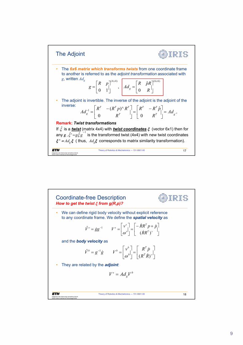
9
Theory of Robotics & Mechatronics — 151-0601-00 17
The Adjoint
• The 6x6 matrix which transforms twists from one coordinate frame to another is referred to as the adjoint transformation associated with g, written Adg
• The adjoint is invertible. The inverse of the adjoint is the adjoint of the inverse:
Remark: Twist transformationsIf is a twist (matrix 4x4) with twist coordinates [ (vector 6x1) then forany g , is the transformed twist (4x4) with new twist coordinates[�‘ �Adg [ ( thus, Adg[ corresponds to matrix similarity transformation).
)66()44(
0ˆ
,10
x
g
x
RRpR
AdpR
g »¼
º«¬
ª »
¼
º«¬
ª
1
0ˆ
0)^(1
� »¼
º«¬
ª � »
¼
º«¬
ª � �
gT
TT
T
TTT
g AdR
pRRR
RpRRAd
[̂gg[[ ˆ'ˆ 1
�
Theory of Robotics & Mechatronics — 151-0601-00 18
Coordinate-free DescriptionHow to get the twist [ from g(R,p)?
• We can define rigid body velocity without explicit referenceto any coordinate frame. We define the spatial velocity as
and the body velocity as
• They are related by the adjoint:
»¼
º«¬
ª �� »
¼
º«¬
ª
��
)(ˆ 1
T
T
s
sss
RRppRRv
VggV�
���
Z
»¼
º«¬
ª »
¼
º«¬
ª
��
)(ˆ 1
RRpRv
VggVT
T
b
bbb
�
��
Z
bg
s VAdV
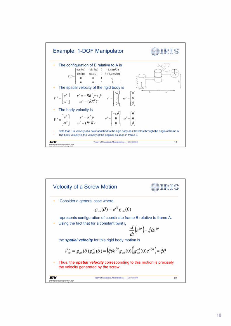
10
Theory of Robotics & Mechatronics — 151-0601-00 19
Example: 1-DOF Manipulator
• The configuration of B relative to A is
• The spatial velocity of the rigid body is
• The body velocity is
• Note that vs is velocity of a point attached to the rigid body as it traveles through the origin of frame A• The body velocity is the velocity of the origin B as seen in frame B
»»»»
¼
º
««««
¬
ª���
1000100
)(cos0)(cos)(sin)(sin0)(sin)(cos
)(0
21
2
ltlltt
tltt
tgTTTTTT
�
»¼
º«¬
ª
)( RRpRvv
VTb
Tb
b
bb
�
�
ZZ »»»
¼
º
«««
¬
ª
»»»
¼
º
«««
¬
ª�
TZ
T
�
�
00
00
2bb
lv
� ��
»¼
º«¬
ª
)( Ts
Ts
s
ss
RRppRRvv
V�
��
ZZ »»»
¼
º
«««
¬
ª
»»»
¼
º
«««
¬
ª
T
ZT
�
�
00
001
ss
lv
Theory of Robotics & Mechatronics — 151-0601-00 20
Velocity of a Screw Motion
• Consider a general case where
represents configuration of coordinate frame B relative to frame A.• Using the fact that for a constant twist [
the spatial velocity for this rigid body motion is
• Thus, the spatial velocity corresponding to this motion is precisely the velocity generated by the screw
)0()( ˆabab geg T[T
� � T[T[ T[ ˆˆ ˆ eedtd �
� �� � T[T[TT T[T[ ��� ˆ)0()0(ˆ)()(ˆ ˆ1ˆ1 ��� eggeggV ababababs
ab
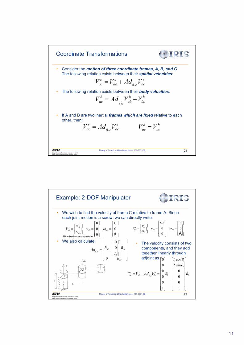
11
Theory of Robotics & Mechatronics — 151-0601-00 21
Coordinate Transformations
• Consider the motion of three coordinate frames, A, B, and C.The following relation exists between their spatial velocities:
• The following relation exists between their body velocities:
• If A and B are two inertial frames which are fixed relative to each other, then:
bbc
babg
bac VVAdV
bc� �1
sbcg
sab
sac VAdVV
ab�
sbcg
sac VAdV
ab b
bcb
ac VV
Theory of Robotics & Mechatronics — 151-0601-00 22
Example: 2-DOF Manipulator
• We wish to find the velocity of frame C relative to frame A. Since each joint motion is a screw, we can directly write:
• We also calculate1
0 00 00
absab ab ab
ab
vV v Z
ZT
ª º ª ºª º « » « » « » « » « »¬ ¼ « » « »¬ ¼ ¬ ¼�
1 2
2
00 00
bcsbc bc bc
bc
lv
V vT
ZZ
T
ª º ª ºª º « » « » « » « » « »¬ ¼ « » « »¬ ¼¬ ¼
�
�
»»»»
¼
º
««««
¬
ª
»»»
¼
º
«««
¬
ª
�
ab
ababg
R
Rl
RAdab
0
00
0
• The velocity consists of two components, and they add together linearly through adjoint as
2
11
11
1
1000
sincos
100000
T
TT
T ��
»»»»»»»»
¼
º
««««««««
¬
ª
�
»»»»»»»»
¼
º
««««««««
¬
ª
�
ll
VAdVV sbcg
sab
sac ab
AB v-fixed – can only rotate!
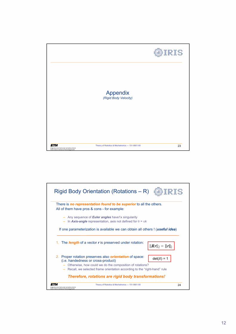
12
Theory of Robotics & Mechatronics — 151-0601-00 23
Appendix(Rigid Body Velocity)
Theory of Robotics & Mechatronics — 151-0601-00 24
Rigid Body Orientation (Rotations – R)
There is no representation found to be superior to all the others.All of them have pros & cons - for example:
– Any sequence of Euler angles have1x singularity– In Axis-angle representation, axis not defined for T = Sk
If one parameterization is available we can obtain all others ! (useful idea)
1. The length of a vector r is preserved under rotation:
2. Proper rotation preserves also orientation of space:(i.e. handedness or cross-product)
– Otherwise, how could we do the composition of rotations?– Recall, we selected frame orientation according to the “right-hand” rule
Therefore, rotations are rigid body transformations!
det(R) = 1
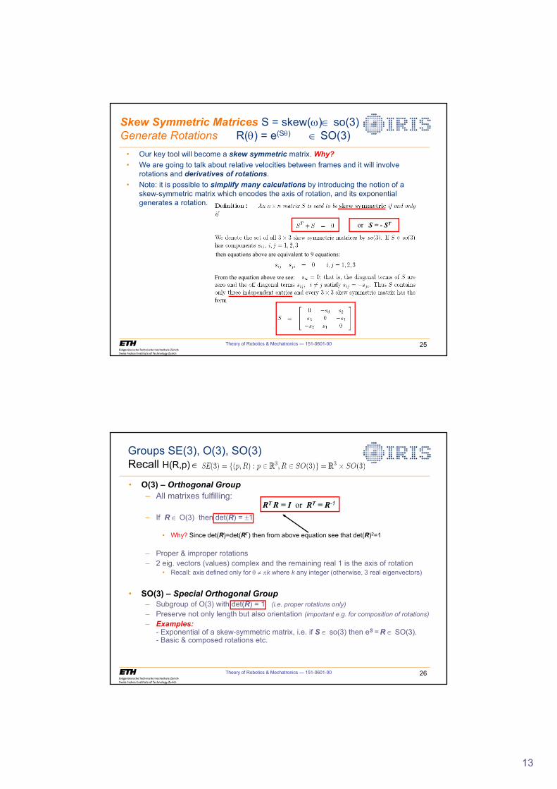
13
Theory of Robotics & Mechatronics — 151-0601-00 25
Skew Symmetric Matrices S = skew(Z)� so(3)Generate Rotations R(T) = e(ST) � SO(3)
• Our key tool will become a skew symmetric matrix. Why?• We are going to talk about relative velocities between frames and it will involve
rotations and derivatives of rotations.• Note: it is possible to simplify many calculations by introducing the notion of a
skew-symmetric matrix which encodes the axis of rotation, and its exponential generates a rotation.
or S = - ST
:
From the equation above we see:
then equations above are equivalent to 9 equations:
Theory of Robotics & Mechatronics — 151-0601-00 26
Groups SE(3), O(3), SO(3)Recall H(R,p) �
RT R = I or RT = R-1
• O(3) – Orthogonal Group– All matrixes fulfilling:
– If R � O(3) then det(R) = r1
• Why? Since det(R)=det(RT) then from above equation see that det(R)2=1
– Proper & improper rotations– 2 eig. vectors (values) complex and the remaining real 1 is the axis of rotation
• Recall: axis defined only for T z Sk where k any integer (otherwise, 3 real eigenvectors)
• SO(3) – Special Orthogonal Group– Subgroup of O(3) with det(R) = 1 (i.e. proper rotations only)– Preserve not only length but also orientation (important e.g. for composition of rotations)– Examples:
- Exponential of a skew-symmetric matrix, i.e. if S � so(3) then eS = R � SO(3).- Basic & composed rotations etc.
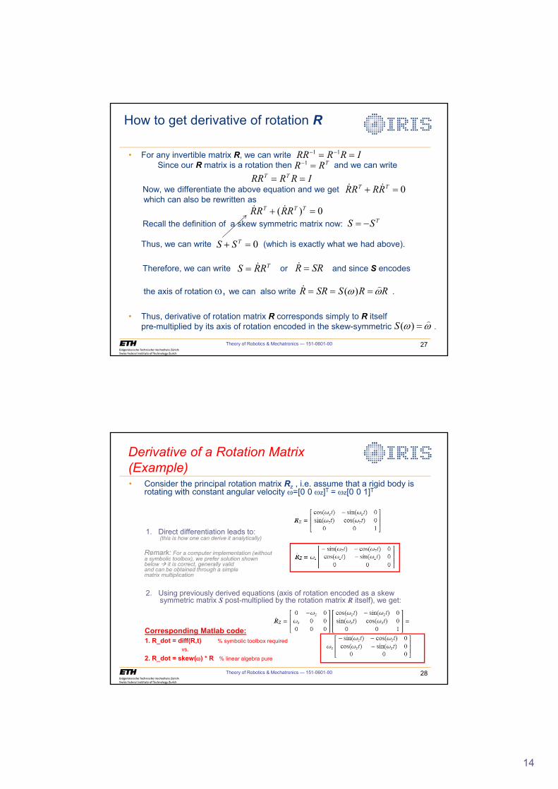
14
• For any invertible matrix R, we can write Since our R matrix is a rotation then and we can write
Now, we differentiate the above equation and we getwhich can also be rewritten as
Recall the definition of a skew symmetric matrix now:
Thus, we can write (which is exactly what we had above).
Therefore, we can write or and since S encodes
the axis of rotation Z, we can also write .
• Thus, derivative of rotation matrix R corresponds simply to R itself pre-multiplied by its axis of rotation encoded in the skew-symmetric .
Theory of Robotics & Mechatronics — 151-0601-00 27
How to get derivative of rotation R
IRRRR �� 11
IRRRR TT
TRR �1
0 � TT RRRR ��
0)( � TTT RRRR ��TSS �
0 � TSS
TRRS � SRR �
RRSSRR ZZ �� )(
ZZ � )(S
Theory of Robotics & Mechatronics — 151-0601-00 28
Derivative of a Rotation Matrix(Example)• Consider the principal rotation matrix Rz , i.e. assume that a rigid body is
rotating with constant angular velocity Z=[0 0 Zz]T = Zz[0 0 1]T
1. Direct differentiation leads to: (this is how one can derive it analytically)
Remark: For a computer implementation (withouta symbolic toolbox), we prefer solution shownbelow Æ it is correct, generally validand can be obtained through a simple matrix multiplication
2. Using previously derived equations (axis of rotation encoded as a skew symmetric matrix S post-multiplied by the rotation matrix R itself), we get:
Corresponding Matlab code:1. R_dot = diff(R,t) % symbolic toolbox required
vs.2. R_dot = skew(Z) * R % linear algebra pure
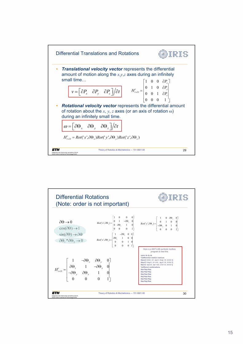
15
Theory of Robotics & Mechatronics — 151-0601-00 29
Differential Translations and Rotations
• Translational velocity vector represents the differential amount of motion along the x,y,z axes during an infinitely small time…
• Rotational velocity vector represents the differential amount of rotation about the x, y, z axes (or an axis of rotation Z) during an infinitely small time.
x y zv P P P tª º w w w w¬ ¼
x y z tZ ª º w4 w4 w4 w¬ ¼
1 0 00 1 00 0 10 0 0 1
x
ytt t
z
PP
HP�w
wª º« »w« » « »w« »¬ ¼
(' ', ) (' ', ) (' ', )tt t x y zH Rot x Rot y Rot z�w w4 w4 w4
Theory of Robotics & Mechatronics — 151-0601-00 30
Differential Rotations(Note: order is not important)
1 2
0cos( ) 1sin( )
* 0
w4ow4 ow4 ow4
w4 w4 o
1 01 0
1 00 0 0 1
z y
z xtt t
y x
H �w
�w4 w4ª º« »w4 �w4« » « »�w4 w4« »¬ ¼
1 0 0 00 1 0
(' ', )0 1 00 0 0 1
xx
x
Rot x
ª º« »�w4« »w4 « »w4« »¬ ¼
1 0 01 0 0
(' ', )0 0 1 00 0 0 1
z
zzRot z
�w4ª º« »w4« »w4 « »« »¬ ¼
1 0 00 1 0 0
(' ', )0 1 0
0 0 0 1
y
yy
Rot y
w4ª º« »« »w4 « »�w4« »¬ ¼
syms dx dy dz%differential rotation matricesRdx=[1 0 0 0 ; 0 1 -dx 0 ; 0 dx 1 0 ; 0 0 0 1]Rdy=[1 0 dy 0 ; 0 1 0 0 ; -dy 0 1 0 ; 0 0 0 1]Rdz=[1 -dz 0 0 ; dz 1 0 0 ; 0 0 1 0 ; 0 0 0 1]%different combinationsRdx*Rdy*RdzRdx*Rdz*RdyRdy*Rdx*RdzRdy*Rdz*RdxRdz*Rdx*RdyRdz*Rdy*Rdx
Here is a MATLAB symbolic toolbox program to test this
1
Jacobian
Institute of Robotics and Intelligent SystemsETH Zurich
Theory of Robotics &Mechatronics
Theory of Robotics & Mechatronics — 151-0601-00 2
Lecture outline
1. Introduction
2. How to get the Jacobian?
a. (SD 1) Classical approach based on homogeneous transformations
Forward kinematics formulation using DH convention
b. (SD 2) Screw Theory
Using twists and product of exponentials
3. What is the Jacobian good for in robotics ?
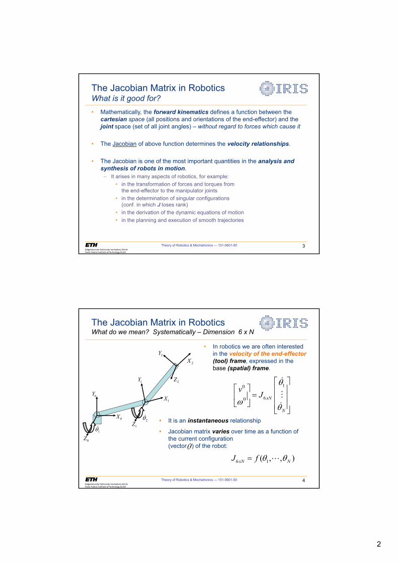
2
Theory of Robotics & Mechatronics — 151-0601-00 3
• Mathematically, the forward kinematics defines a function between the cartesian space (all positions and orientations of the end-effector) and thejoint space (set of all joint angles) – without regard to forces which cause it
• The Jacobian of above function determines the velocity relationships.
• The Jacobian is one of the most important quantities in the analysis and synthesis of robots in motion.
– It arises in many aspects of robotics, for example:• in the transformation of forces and torques from
the end-effector to the manipulator joints• in the determination of singular configurations
(conf. in which J loses rank)• in the derivation of the dynamic equations of motion• in the planning and execution of smooth trajectories
The Jacobian Matrix in RoboticsWhat is it good for?
Theory of Robotics & Mechatronics — 151-0601-00 4
The Jacobian Matrix in RoboticsWhat do we mean? Systematically – Dimension 6 x N
10
60 xN
N
vJ
T
ZT
ª ºª º « » « » « »¬ ¼ « »¬ ¼
�
��
• In robotics we are often interested in the velocity of the end-effector(tool) frame, expressed in the base (spatial) frame.
6 1( , , )xN NJ f T T �
• It is an instantaneous relationship
• Jacobian matrix varies over time as a function ofthe current configuration(vector ) of the robot:
0Z
1Z1T�
2T�
2Z
0X
0Y1X
1Y
2Y
2X
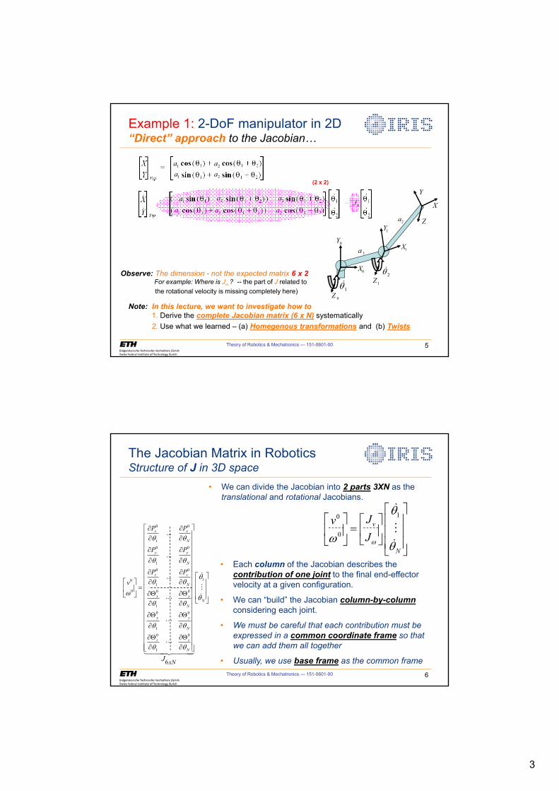
3
Theory of Robotics & Mechatronics — 151-0601-00 5
Example 1: 2-DoF manipulator in 2D“Direct” approach to the Jacobian…
Note: In this lecture, we want to investigate how to1. Derive the complete Jacobian matrix (6 x N) systematically2. Use what we learned – (a) Homegenous transformations and (b) Twists
Observe: The dimension - not the expected matrix 6 x 2For example: Where is JZ ? -- the part of J related to the rotational velocity is missing completely here)
0Z
1Z1T�
2T�0X
0Y1X
1Y
X
1a
2a
(2 x 2)
2a
2a
2a
2a2a
2a
1a
1a
1a
1a
Y
Z
Theory of Robotics & Mechatronics — 151-0601-00 6
The Jacobian Matrix in RoboticsStructure of J in 3D space
10
0v
N
JvJZ
T
ZT
ª ºª º ª º « » « » « » « »
¬ ¼¬ ¼ « »¬ ¼
�
��
• We can divide the Jacobian into 2 parts 3XN as the translational and rotational Jacobians.
• Each column of the Jacobian describes the contribution of one joint to the final end-effector velocity at a given configuration.
• We can “build” the Jacobian column-by-columnconsidering each joint.
• We must be careful that each contribution must be
expressed in a common coordinate frame so that
we can add them all together
• Usually, we use base frame as the common frame
0 0
1
0 0
1
0 0
101
0 0 0
1
0 0
1
0 0
1
6
...
...
...
x x
N
y y
N
z z
N
x xN
N
y y
N
z z
N
xN
P P
P P
P Pv
J
T T
T T
TT T
ZT
T T
T T
T T
ª ºw w« »w w« »« »w w« »w w« »
« »w w« » ª º« »w wª º « » « »« » « »w4 w4¬ ¼ « » « »¬ ¼« »w w« »w4 w4« »« »w w« »« »w4 w4« »w w« »¬ ¼
�
���
�
�
�������
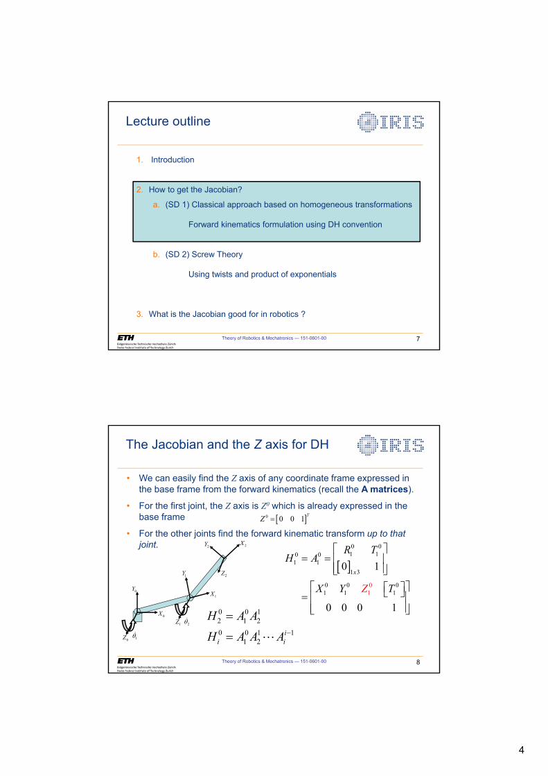
4
Theory of Robotics & Mechatronics — 151-0601-00 7
Lecture outline
1. Introduction
2. How to get the Jacobian?
a. (SD 1) Classical approach based on homogeneous transformations
Forward kinematics formulation using DH convention
b. (SD 2) Screw Theory
Using twists and product of exponentials
3. What is the Jacobian good for in robotics ?
Theory of Robotics & Mechatronics — 151-0601-00 8
• We can easily find the Z axis of any coordinate frame expressed in the base frame from the forward kinematics (recall the A matrices).
• For the first joint, the Z axis is Z0 which is already expressed in the base frame
• For the other joints find the forward kinematic transform up to that
joint.
The Jacobian and the Z axis for DH
0Z
1Z
1T�
2T�
2Z
0X
0Y1X
1Y
2X2Y
> @0 01 10
0
01 1
1 3
0 0 01 1 11
0 1
0 0 0 1
x
R TH A
X Y TZ
ª º « »
« »¬ ¼ª ºª º¬ ¼ « »« »¬ ¼
> @0 0 0 1 TZ
0 0 12 1 2
0 0 1 11 2
ii i
H A A
H A A A �
�
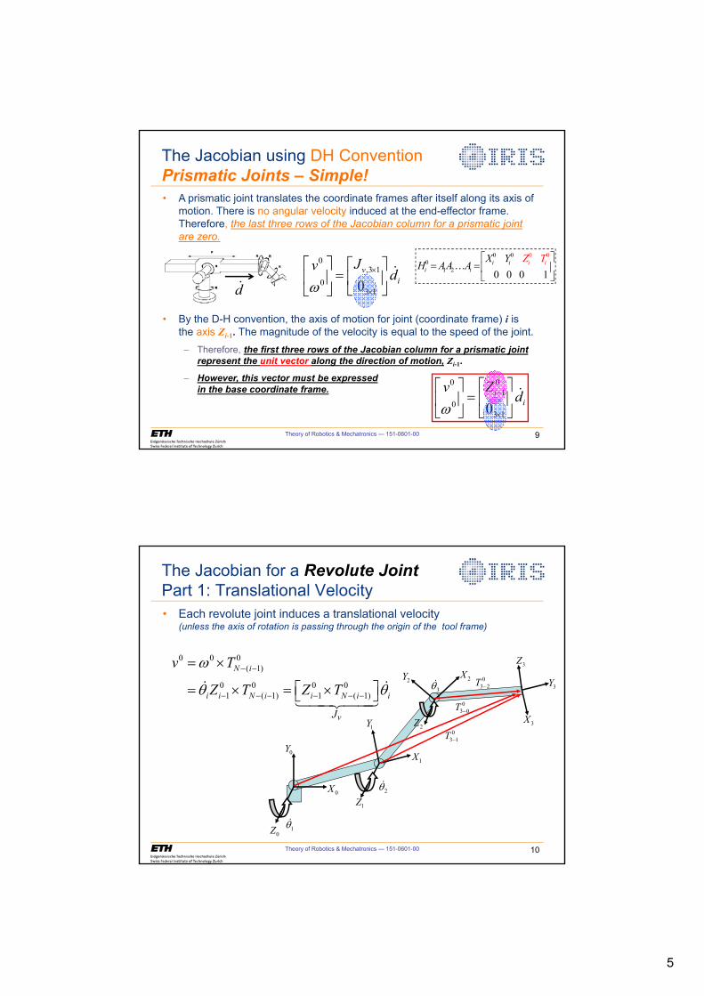
5
Theory of Robotics & Mechatronics — 151-0601-00 9
The Jacobian using DH ConventionPrismatic Joints – Simple!
0,3 1
03 10v
i
Jvd
Zu
u
ª º ª º « » « »¬ ¼¬ ¼
�
d�
001
03 10i
i
Zvd
Z�
u
ª ºª º « »« »
¬ ¼ ¬ ¼�
• A prismatic joint translates the coordinate frames after itself along its axis of motion. There is no angular velocity induced at the end-effector frame. Therefore, the last three rows of the Jacobian column for a prismatic joint
are zero.
• By the D-H convention, the axis of motion for joint (coordinate frame) i is the axis Zi-1. The magnitude of the velocity is equal to the speed of the joint.
– Therefore, the first three rows of the Jacobian column for a prismatic joint represent the unit vector along the direction of motion, Zi-1.
– However, this vector must be expressed in the base coordinate frame.
0 0 0 00
1 2 0 0 0 1i i
i ii iZX Y
H AA ATª º
« »¬ ¼
�
Theory of Robotics & Mechatronics — 151-0601-00 10
The Jacobian for a Revolute JointPart 1: Translational Velocity
0Z
1Z
1T�
2T�
2Z
0X
0Y1X
1Y
2X2Y3Z
3X
3Y3T�
03 1T �
03 0T �
03 2T �
0 0 0( 1)
0 0 0 01 ( 1) 1 ( 1)
N i
i i N i i N i i
vJ
v T
Z T Z T
Z
T T� �
� � � � � �
u
ª º u u¬ ¼� �
�����
• Each revolute joint induces a translational velocity (unless the axis of rotation is passing through the origin of the tool frame)
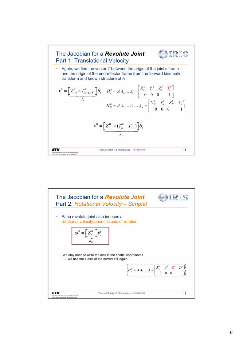
6
Theory of Robotics & Mechatronics — 151-0601-00 11
0 0 01 ( 1)i N i i
vJ
v Z T T� � �ª º u¬ ¼�
�����
0 00
1 2
0 00
2
0
00
1
0
0 0 0 1
0 0 0 1
i ii i
N N NN
i
Ni
i
N
Z TX YH A A A
X Y Z TH A A A A
ª º « »
¬ ¼ª º
« »¬ ¼
�
� �
0 0 0 01 1( )i N i i
vJ
v Z T T T� �ª º u �¬ ¼�
�������
• Again, we find the vector T between the origin of the joint’s frame and the origin of the end-effector frame from the forward kinematic transform and known structure of H
The Jacobian for a Revolute JointPart 1: Translational Velocity
• Each revolute joint also induces arotational velocity about its axis of rotation:
We only need to write the axis in the spatial coordinates– we use the z-axis of the correct HT again:
Theory of Robotics & Mechatronics — 151-0601-00 12
The Jacobian for a Revolute JointPart 2: Rotational Velocity – Simple!
,0 0
1i i
J
Z
Z
Z T�ª º ¬ ¼�
0 0 0 00
1 2 0 0 0 1i i
i ii iZX Y
H A A ATª º
« »¬ ¼
�Ti0
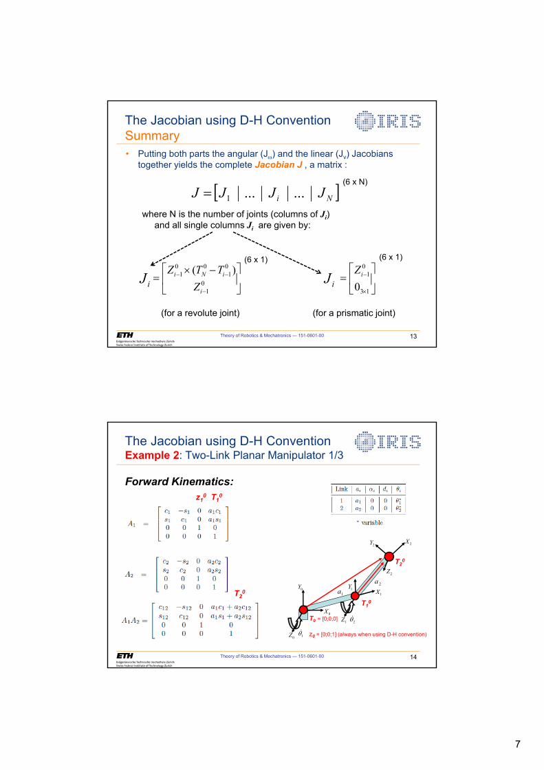
7
• Putting both parts the angular (JZ) and the linear (Jv) Jacobians together yields the complete Jacobian J , a matrix :
where N is the number of joints (columns of Ji)and all single columns Ji are given by:
or
(for a revolute joint) (for a prismatic joint)
Theory of Robotics & Mechatronics — 151-0601-00 13
The Jacobian using D-H Convention Summary
0 0 001 1
001
( )i N ii
i
Z T TvZ
TZ
� �
�
ª ºª º u � « »« »
¬ ¼ ¬ ¼�
001
03 10i
i
Zvd
Z�
u
ª ºª º « »« »
¬ ¼ ¬ ¼�
(6 x 1)
iJ iJ(6 x 1)
> @Ni JJJJ ......1 (6 x N)
Theory of Robotics & Mechatronics — 151-0601-00 14
The Jacobian using D-H ConventionExample 2: Two-Link Planar Manipulator 1/3
Forward Kinematics:z1
0 T10
T20
T0 = [0;0;0]
z0 = [0;0;1] (always when using D-H convention) 0Z
1Z
1T�
2T�
2Z
0X
0Y1X
1Y
2X2Y
T20
T10
2a
1a
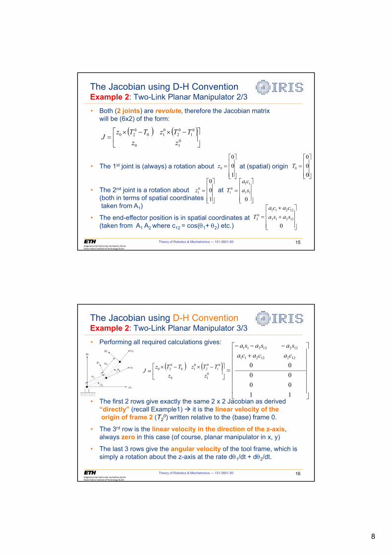
8
Theory of Robotics & Mechatronics — 151-0601-00 15
The Jacobian using D-H ConventionExample 2: Two-Link Planar Manipulator 2/3
• Both (2 joints) are revolute, therefore the Jacobian matrixwill be (6x2) of the form:
• The 1st joint is (always) a rotation about at (spatial) origin
• The 2nd joint is a rotation about at (both in terms of spatial coordinatestaken from A1)
• The end-effector position is in spatial coordinates at (taken from A1 A2 where c12 = cos(T1+ T2) etc.)
� � � �»¼
º«¬
ª �u�u
010
01
02
010
020
zzTTzTTz
J
»»»
¼
º
«««
¬
ª
000
0T»»»
¼
º
«««
¬
ª
100
0z
»»»
¼
º
«««
¬
ª
100
01z
»»»
¼
º
«««
¬
ª
011
110
1 saca
T
»»»
¼
º
«««
¬
ª��
0
12211
122110
2 sasacaca
T
• Performing all required calculations gives:
• The first 2 rows give exactly the same 2 x 2 Jacobian as derived “directly” (recall Example1) Æ it is the linear velocity of theorigin of frame 2 (T2
0) written relative to the (base) frame 0.
• The 3rd row is the linear velocity in the direction of the z-axis, always zero in this case (of course, planar manipulator in x, y)
• The last 3 rows give the angular velocity of the tool frame, which is simply a rotation about the z-axis at the rate dT1/dt + dT2/dt.
Theory of Robotics & Mechatronics — 151-0601-00 16
The Jacobian using D-H ConventionExample 2: Two-Link Planar Manipulator 3/3
»»»»»»»
¼
º
«««««««
¬
ª�
���
11000000
12212211
12212211
cacacasasasa
� � � �»¼
º«¬
ª �u�u
010
01
02
010
020
zzTTzTTz
J
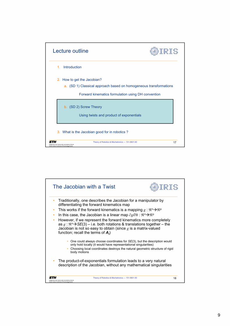
9
Theory of Robotics & Mechatronics — 151-0601-00 17
Lecture outline
1. Introduction
2. How to get the Jacobian?
a. (SD 1) Classical approach based on homogeneous transformations
Forward kinematics formulation using DH convention
b. (SD 2) Screw Theory
Using twists and product of exponentials
3. What is the Jacobian good for in robotics ?
Theory of Robotics & Mechatronics — 151-0601-00 18
The Jacobian with a Twist
• Traditionally, one describes the Jacobian for a manipulator by differentiating the forward kinematics map
• This works if the forward kinematics is a mapping g : �nÆ�p
• In this case, the Jacobian is a linear map wg/wT : �nÆ�p
• However, if we represent the forward kinematics more completely as g : �nÆSE(3) – i.e. both rotations & translations together – the Jacobian is not so easy to obtain (since g is a matrix-valued function; recall the terms of Ai)
• One could always choose coordinates for SE(3), but the description would only hold locally (it would have representational singularities)
• Choosing local coordinates destroys the natural geometric structure of rigid body motions
• The product-of-exponentials formulation leads to a very natural description of the Jacobian, without any mathematical singularities
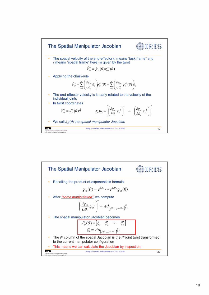
10
Theory of Robotics & Mechatronics — 151-0601-00 19
The Spatial Manipulator Jacobian
• The spatial velocity of the end-effector (t means “task frame” ands means “spatial frame” here) is given by the twist
• Applying the chain-rule
• The end-effector velocity is linearly related to the velocity of the individual joints
• In twist coordinates
• We call Jsts(T) the spatial manipulator Jacobian
)()(ˆ 1 TT � ststsst ggV �
TT �)(sstsst JV
»»¼
º
««¬
ª¸̧¹
·¨̈©
§ww
¸̧¹
·¨̈©
§ww
�
�
�
� 11
1
)( stn
stst
stsst ggggJ
TTT �
i
n
ist
i
stst
n
ii
i
stsst ggggV TT
TTT
T�� ¦¦
��
¸̧¹
·¨̈©
§ww
¸̧¹
·¨̈©
§ww
1
11
1
)()(ˆ
Theory of Robotics & Mechatronics — 151-0601-00 20
The Spatial Manipulator Jacobian
• Recalling the product-of-exponentials formula
• After “some manipulation”, we compute
• The spatial manipulator Jacobian becomes
• The ith column of the spatial Jacobian is the ith joint twist transformed to the current manipulator configuration
• This means we can calculate the Jacobian by inspection
)0()(ˆˆ
11stst geeg nnT[T[T �
> @� � ieei
nsst
iiAd
J[[[[[T
T[T[ 11ˆ11̂
21)(
�� c
cc
�
�
� � ieesti
stii
Adgg [T T[T[ 11ˆ11̂
1��
¸̧¹
·¨̈©
§ww
�
�
�
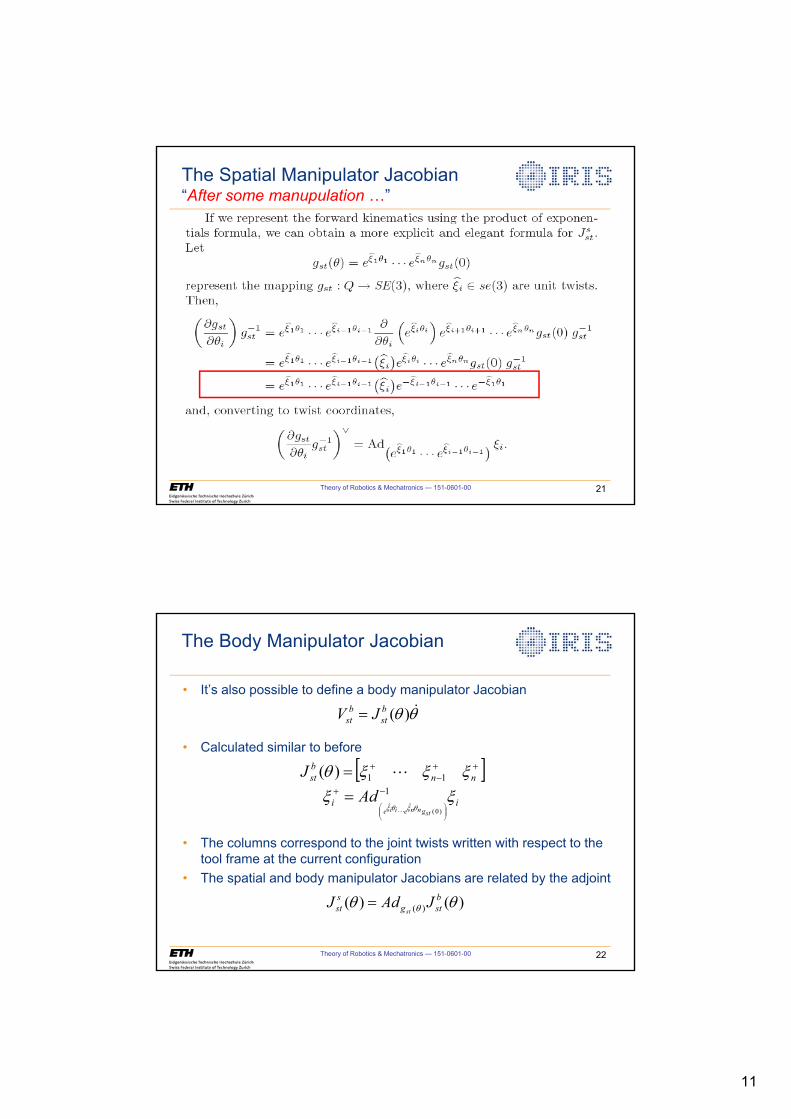
11
Theory of Robotics & Mechatronics — 151-0601-00 21
The Spatial Manipulator Jacobian“After some manupulation …”
Theory of Robotics & Mechatronics — 151-0601-00 22
The Body Manipulator Jacobian
• It’s also possible to define a body manipulator Jacobian
• Calculated similar to before
• The columns correspond to the joint twists written with respect to the tool frame at the current configuration
• The spatial and body manipulator Jacobians are related by the adjoint
TT �)(bstbst JV
> @ii
nnbst
stgnneiie
AdJ
[[[[[T
T[T[
111
)0(ˆˆ
)(��
���
�
¸̧¹
·¨̈©
§
�
�
)()( )( TT Tbstg
sst JAdJ
st
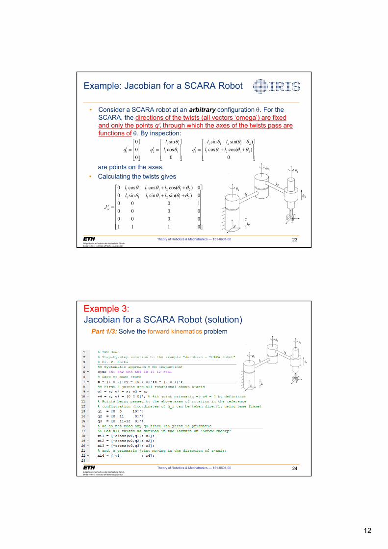
12
Theory of Robotics & Mechatronics — 151-0601-00 23
Example: Jacobian for a SCARA Robot
• Consider a SCARA robot at an arbitrary configuration T. For the SCARA, the directions of the twists (all vectors ‘omega’) are fixed and only the points q’i through which the axes of the twists pass are functions of T. By inspection:
1 1 1 1 2 1 2
1 2 1 1 3 1 1 2 1 2
0 sin sin sin( )0 cos cos cos( )0 0 0
l l lq q l q l l
T T T TT T T T
� � � �ª º ª º ª º« » « » « »c c c � �« » « » « »« » « » « »¬ ¼ ¬ ¼ ¬ ¼
»»»»»»»»
¼
º
««««««««
¬
ª����
01110000000010000)sin(sinsin00)cos(coscos0
2121111
2121111
TTTTTTTT
llllll
J sst
are points on the axes. • Calculating the twists gives
Theory of Robotics & Mechatronics — 151-0601-00 24
Example 3: Jacobian for a SCARA Robot (solution)
Part 1/3: Solve the forward kinematics problem
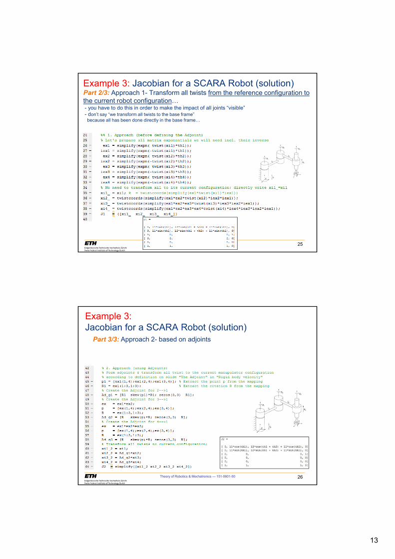
13
Theory of Robotics & Mechatronics — 151-0601-00 25
Example 3: Jacobian for a SCARA Robot (solution)Part 2/3: Approach 1- Transform all twists from the reference configuration to the current robot configuration…- you have to do this in order to make the impact of all joints “visible”- don’t say “we transform all twists to the base frame” because all has been done directly in the base frame…
Theory of Robotics & Mechatronics — 151-0601-00 26
Example 3: Jacobian for a SCARA Robot (solution)
Part 3/3: Approach 2- based on adjoints
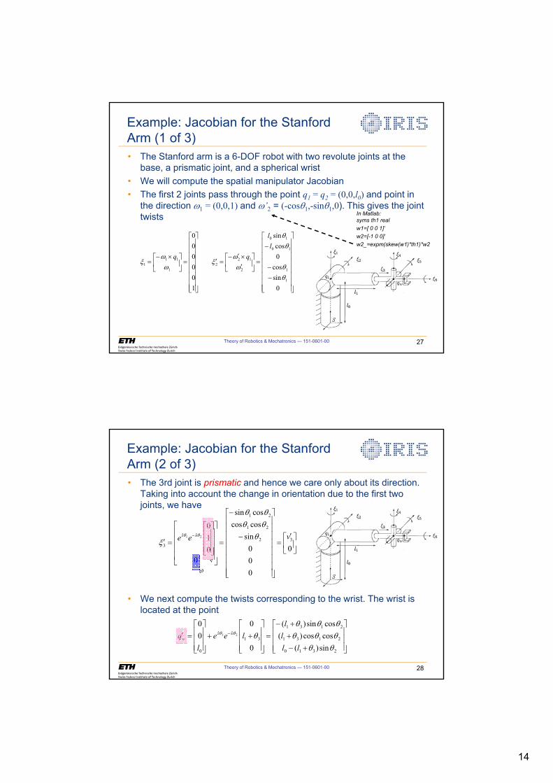
14
Theory of Robotics & Mechatronics — 151-0601-00 27
Example: Jacobian for the Stanford Arm (1 of 3)• The Stanford arm is a 6-DOF robot with two revolute joints at the
base, a prismatic joint, and a spherical wrist• We will compute the spatial manipulator Jacobian• The first 2 joints pass through the point q1 = q2 = (0,0,l0) and point in
the direction Z1 = (0,0,1) and Z’2 = (-cosT1,-sinT1,0). This gives the joint twists
»»»»»»»»
¼
º
««««««««
¬
ª
��
�
»¼
º«¬
ªcuc�
c
»»»»»»»»
¼
º
««««««««
¬
ª
»¼
º«¬
ª u�
0sincos
0cos
sin
100000
1
1
10
10
2
122
1
111
TT
TT
ZZ
[ZZ
[
ll
In Matlab:
syms th1 real
w1=[ 0 0 1]'
w2=[-1 0 0]'
w2_=expm(skew(w1)*th1)*w2
Theory of Robotics & Mechatronics — 151-0601-00 28
Example: Jacobian for the Stanford Arm (2 of 3)• The 3rd joint is prismatic and hence we care only about its direction.
Taking into account the change in orientation due to the first two joints, we have
• We next compute the twists corresponding to the wrist. The wrist is located at the point
»¼
º«¬
ª c
»»»»»»»»
¼
º
««««««««
¬
ª
�
�
»»»»
¼
º
««««
¬
ª
»»»
¼
º
«««
¬
ª
c�
0
000
sincoscoscossin
0010
32
21
21
ˆˆ
3
21 vee xz TTTTT
[TT
»»»
¼
º
«««
¬
ª
�����
»»»
¼
º
«««
¬
ª��
»»»
¼
º
«««
¬
ª c �
2310
2131
2131
31ˆˆ
0 sin)(coscos)(cossin)(
0
000
21
TTTTTTTT
TTT
llll
leel
q xzw
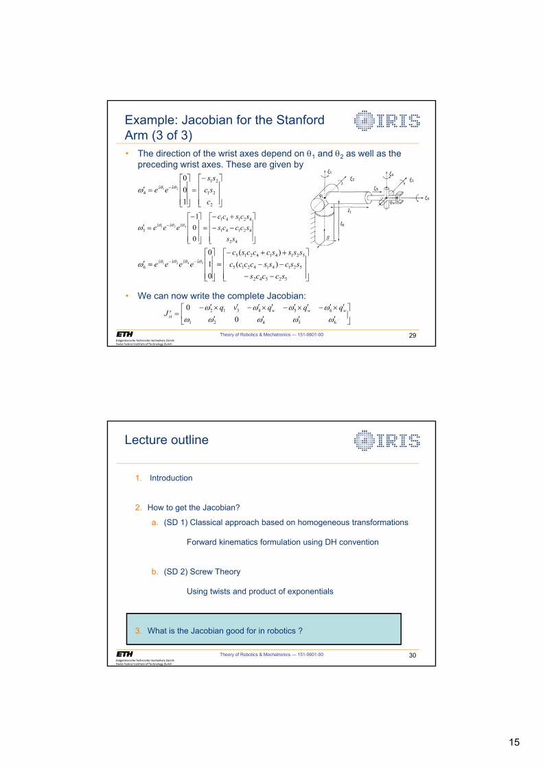
15
Theory of Robotics & Mechatronics — 151-0601-00 29
Example: Jacobian for the Stanford Arm (3 of 3)• The direction of the wrist axes depend on T1 and T2 as well as the
preceding wrist axes. These are given by
• We can now write the complete Jacobian:
»»»
¼
º
«««
¬
ª�
»»»
¼
º
«««
¬
ª c �
2
21
21ˆˆ
4
100
21
cscss
ee xz TTZ
»»»
¼
º
«««
¬
ª����
»»»
¼
º
«««
¬
ª� c �
42
42141
42141ˆˆˆ
5
001
421
ssscccsscscc
eee zxz TTTZ
»»»
¼
º
«««
¬
ª
�������
»»»
¼
º
«««
¬
ª c ��
52542
521414215
521414215ˆˆˆˆ
6 )()(
010
5421
scccssscssccccsssscccsc
eeee xzxz TTTTZ
»¼
º«¬
ªcccc
cuc�cuc�cuc�cuc�
65421
654312
00
ZZZZZZZZZ wwws
st
qqqvqJ
Theory of Robotics & Mechatronics — 151-0601-00 30
Lecture outline
1. Introduction
2. How to get the Jacobian?
a. (SD 1) Classical approach based on homogeneous transformations
Forward kinematics formulation using DH convention
b. (SD 2) Screw Theory
Using twists and product of exponentials
3. What is the Jacobian good for in robotics ?
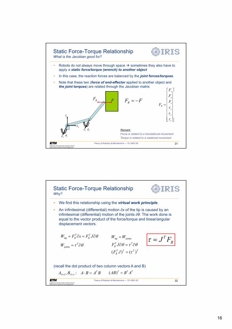
16
Theory of Robotics & Mechatronics — 151-0601-00 31
Static Force-Torque RelationshipWhat is the Jacobian good for?
0Z
1Z
1T�
2T�0X
0Y
FRF
x
y
zR
x
y
z
FFF
FWWW
ª º« »« »« »
« »« »« »« »« »¬ ¼
RF F �
• Robots do not always move through space Æ sometimes they also have to apply a static force/torque (wrench) to another object
• In this case, the reaction forces are balanced by the joint forces/torques.
• Note that these two (force of end-effector applied to another object and the joint torques) are related through the Jacobian matrix.
Remark:
Force is related to a translational movement
Torque is related to a rotational movement
Theory of Robotics & Mechatronics — 151-0601-00 32
• We find this relationship using the virtual work principle.
• An infinitesimal (differential) motion x of the tip is caused by an infinitesimal (differential) motion of the joints θ. The work done is equal to the vector product of the force/torque and linear/angular displacement vectors.
(recall the dot product of two column vectors A and B)
Static Force-Torque RelationshipWhy?
tipT TR RW F x F J T w w
1 1, : TN NA B A B A Bu u �
tip joints
( ) ( )
T TR
T T T TR
W W
F J
F J
T W T
W
w w
TRJ FW
( )T T TAB B A
jointsTW W T w
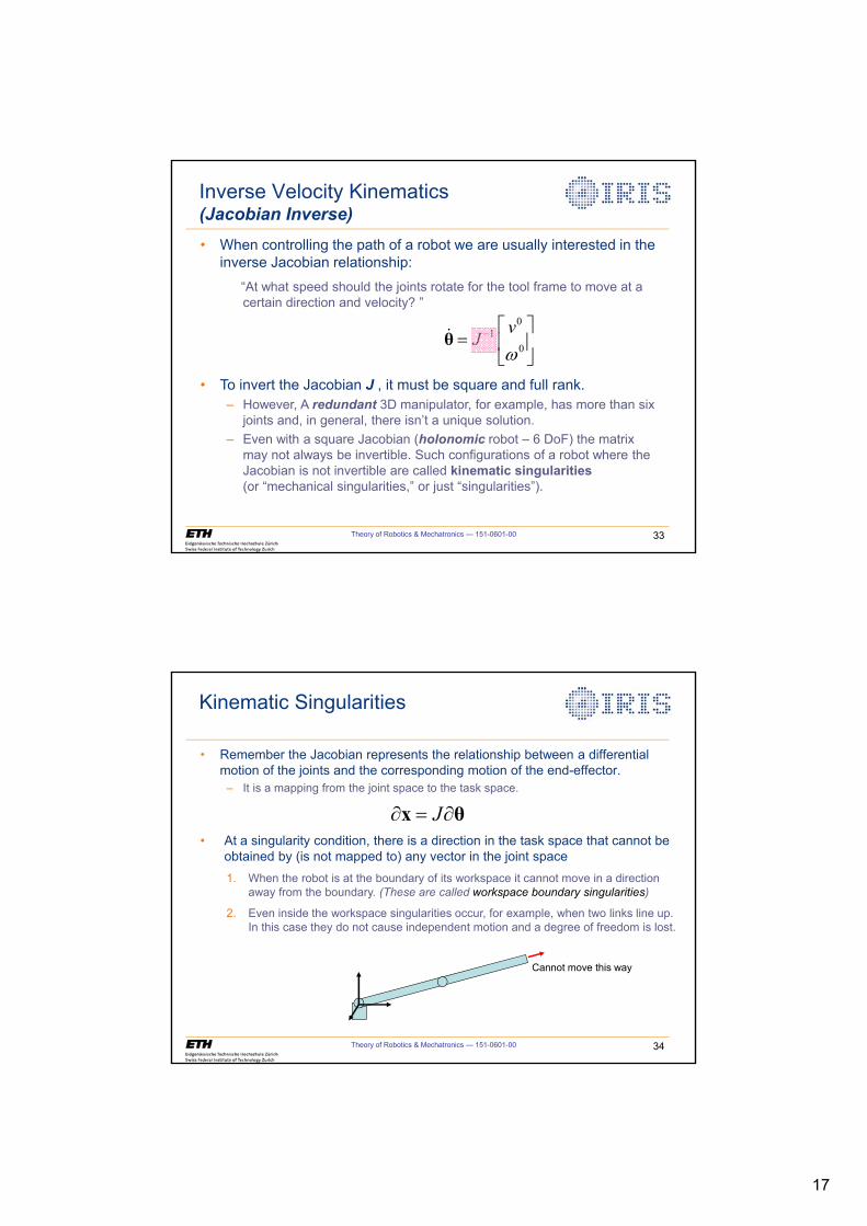
17
Theory of Robotics & Mechatronics — 151-0601-00 33
Inverse Velocity Kinematics(Jacobian Inverse)
01
0
vJ
Z� ª º
« »¬ ¼
θ�
• When controlling the path of a robot we are usually interested in the inverse Jacobian relationship:
“At what speed should the joints rotate for the tool frame to move at a certain direction and velocity? ”
• To invert the Jacobian J , it must be square and full rank.– However, A redundant 3D manipulator, for example, has more than six
joints and, in general, there isn’t a unique solution. – Even with a square Jacobian (holonomic robot – 6 DoF) the matrix
may not always be invertible. Such configurations of a robot where the Jacobian is not invertible are called kinematic singularities(or “mechanical singularities,” or just “singularities”).
Theory of Robotics & Mechatronics — 151-0601-00 34
Kinematic Singularities
• Remember the Jacobian represents the relationship between a differential motion of the joints and the corresponding motion of the end-effector.
– It is a mapping from the joint space to the task space.
Jw wx θ
Cannot move this way
• At a singularity condition, there is a direction in the task space that cannot be obtained by (is not mapped to) any vector in the joint space1. When the robot is at the boundary of its workspace it cannot move in a direction
away from the boundary. (These are called workspace boundary singularities)
2. Even inside the workspace singularities occur, for example, when two links line up. In this case they do not cause independent motion and a degree of freedom is lost.
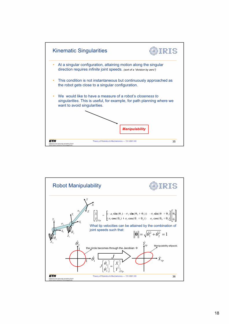
18
Theory of Robotics & Mechatronics — 151-0601-00 35
Kinematic Singularities
• At a singular configuration, attaining motion along the singular direction requires infinite joint speeds. (sort of a “division by zero”)
• This condition is not instantaneous but continuously approached as the robot gets close to a singular configuration.
• We would like to have a measure of a robot’s closeness to
singularities. This is useful, for example, for path planning where we want to avoid singularities.
Manipulability
TipYX
J »¼
º«¬
ª »
¼
º«¬
ª�
�
�
�
2
1
TT
Theory of Robotics & Mechatronics — 151-0601-00 36
Robot Manipulability
What tip velocities can be attained by the combination of joint speeds such that:
2 21 2 1T T � θ� � �
tipX�
tipY�
1T�
2T�
1
1
J
Manipulability ellipsoid.the circle becomes through the Jacobian Æ
2a
2a2a
2a1a
1a
0Z
1Z1T�
2T�0X
0Y1X
1Y
X
1a
2a
Y
Z
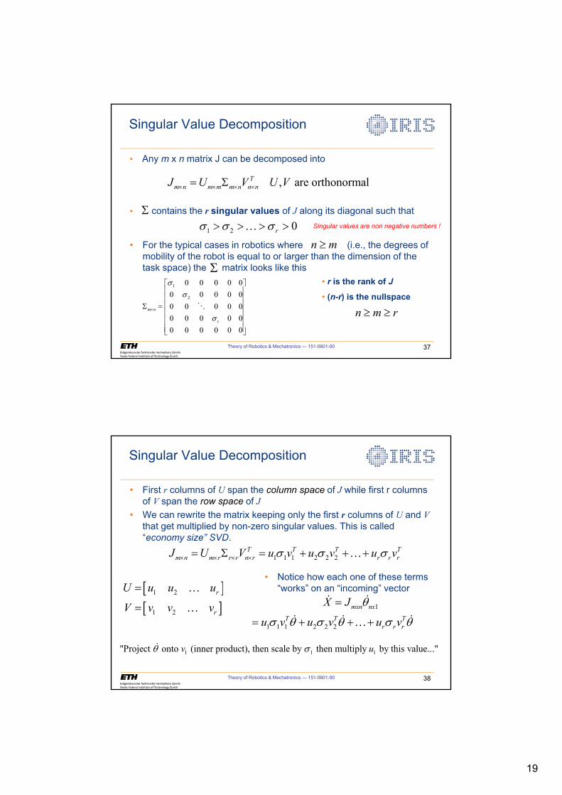
19
Theory of Robotics & Mechatronics — 151-0601-00 37
Singular Value Decomposition
• Any m x n matrix J can be decomposed into
, are orthonormalTm n m m m n n nJ U V U Vu u u u 6
1
2
0 0 0 0 00 0 0 0 00 0 0 0 00 0 0 0 00 0 0 0 0 0
m n
r
VV
Vu
ª º« »« »« »6 « »« »« »¬ ¼
�
• contains the r singular values of J along its diagonal such that
1 2 0rV V V! ! ! !�
n mt
6
6• r is the rank of J
• (n-r) is the nullspace
n m rt t
• For the typical cases in robotics where (i.e., the degrees of mobility of the robot is equal to or larger than the dimension of the task space) the matrix looks like this
Singular values are non negative numbers !
Theory of Robotics & Mechatronics — 151-0601-00 38
Singular Value Decomposition
> @> @
1 2
1 2
r
r
U u u u
V v v v
�
�
1 1 1 2 2 2T T T T
m n m r r r n r r r rJ U V u v u v u vV V Vu u u u 6 � � ��
1mxn nxX J T ��
1 1 1 2 2 2T T T
r r ru v u v u vV T V T V T � � �� � ��
1 1 1"Project onto (inner product), then scale by then multiply by this value..."v uT V�
• First r columns of U span the column space of J while first r columns of V span the row space of J
• We can rewrite the matrix keeping only the first r columns of U and Vthat get multiplied by non-zero singular values. This is called “economy size” SVD.
• Notice how each one of these terms “works” on an “incoming” vector
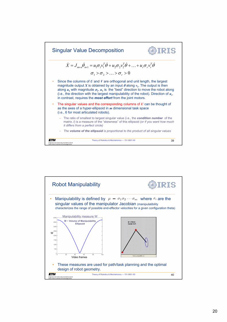
20
Theory of Robotics & Mechatronics — 151-0601-00 39
Singular Value Decomposition
1 2 0rV V V! ! ! !�
1 1 1 1 2 2 2T T T
m n n r r rX J u v u v u vT V T V T V Tu u � � �� � � �� �
• Since the columns of U and V are orthogonal and unit length, the largest magnitude output X is obtained by an input T along v1. The output is then along u1 with magnitude V1. u1 is the “best” direction to move the robot along (i.e., the direction with the largest manipulability of the robot). Direction of ur, in contrast, requires the most effort from the joint motors.
• The singular values and the corresponding columns of U can be thought of as the axes of a hyper-ellipsoid in m dimensional task space(i.e., 6 for most articulated robots).
– The ratio of smallest to largest singular value (i.e., the condition number of the matrix J) is a measure of the “skewness” of this ellipsoid (or if you want how much
it differs from a perfect circle)
– The volume of the ellipsoid is proportional to the product of all singular values
Theory of Robotics & Mechatronics — 151-0601-00 40
Robot Manipulability
Manipulability measure WW ~ Volume of Manipulability
Ellipsoid
Video frames
W
• These measures are used for path/task planning and the optimal design of robot geometry.
• Manipulability is defined by where are the singular values of the manipulator Jacobian (manipulatibility characterizes the range of possible end-effector velocities for a given configuration theta)
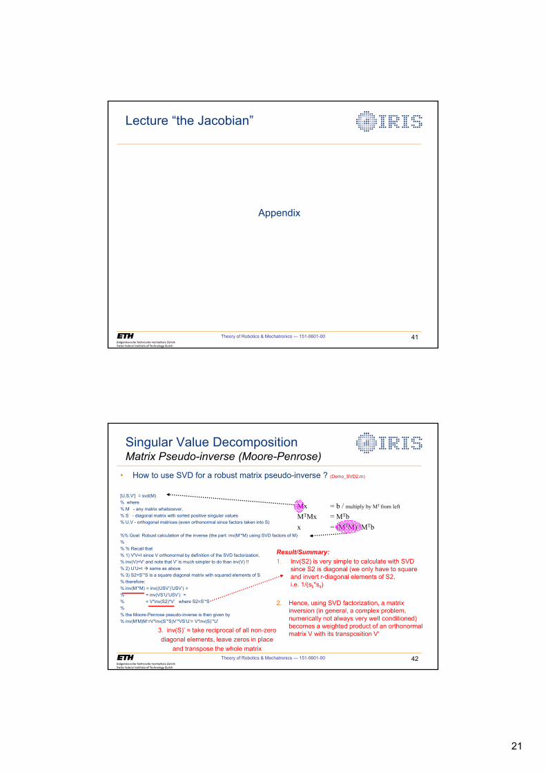
21
Theory of Robotics & Mechatronics — 151-0601-00 41
Lecture “the Jacobian”
Appendix
Theory of Robotics & Mechatronics — 151-0601-00 42
Singular Value DecompositionMatrix Pseudo-inverse (Moore-Penrose)
• How to use SVD for a robust matrix pseudo-inverse ? (Demo_SVD2.m)
[U,S,V'] = svd(M)% where % M - any matrix whatsoever,% S - diagonal matrix with sorted positive singular values% U,V - orthogonal matrices (even orthonormal since factors taken into S)
%% Goal: Robust calculation of the inverse (the part: inv(M‘*M) using SVD factors of M)%% % Recall that % 1) V'V=I since V orthonormal by definition of the SVD factorization, % inv(V)=V' and note that V' is much simpler to do than inv(V) !!% 2) U’U=I Æ same as above% 3) S2=S’*S is a square diagonal matrix with squared elements of S % therefore:% inv(M’*M) = inv((USV’)’USV’) =% = inv(VS’U’USV’) =% = V*inv(S2)*V’ where S2=S’*S% % the Moore-Penrose pseudo-inverse is then given by% inv(M’M)M’=V*inv(S’*S)V’*VS’U’= V*inv(S)’*U’
Result/Summary:1. Inv(S2) is very simple to calculate with SVD
since S2 is diagonal (we only have to squareand invert r-diagonal elements of S2,i.e. 1/(sii*sii)
2. Hence, using SVD factorization, a matrix inversion (in general, a complex problem, numerically not always very well conditioned) becomes a weighted product of an orthonormal matrix V with its transposition V‘
Mx = b / multiply by MT from left
MTMx = MTbx = (MTM)-1MTb
3. inv(S)’ = take reciprocal of all non-zero diagonal elements, leave zeros in place
and transpose the whole matrix
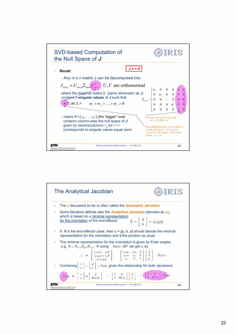
22
Theory of Robotics & Mechatronics — 151-0601-00 43
SVD-based Computation of the Null Space of J
• Recall:
- Any m x n matrix J can be decomposed into
where the diagonal matrix 6 (same dimension as J) contains r singular values of J such that
- matrix V= [ ] (the “bigger” one)
contains column-wise the null space of Jgiven by vectors/columns for i > r
(corresponds to singular values equal zero)
, are orthonormalTm n m m m n n nJ U V U Vu u u u 6
1
2
0 0 0 0 00 0 0 0 00 0 0 0 00 0 0 0 00 0 0 0 0 0
m n
r
VV
Vu
ª º« »« »« »6 « »« »« »¬ ¼
�
1 2 0rV V V! ! ! !�n m rt t
• This part of 6 “makes sure” thatJx = (U 6 V)x = 0
• The orthonormal basis of this subspace(called null space) of J is directlyencoded in “the bigger” orthonormalmatrix, i.e. in V
J x = 0
Theory of Robotics & Mechatronics — 151-0601-00 44
The Analytical Jacobian
TRRS � )(Z
• The J discussed so far is often called the Geometric Jacobian
• Some literature defines also the Analytical Jacobian (denoted as Ja)which is based on a minimal representation for the orientation of the end-effector
• If X is the end-effector pose, then D = [I, T, \] should denote the minimal representation for the orientation and d the position as usual
• The minimal representation for the orientation is given by Euler angles,e.g. Æ using we get Z as
• Combining gives the relationship for both Jacobians:
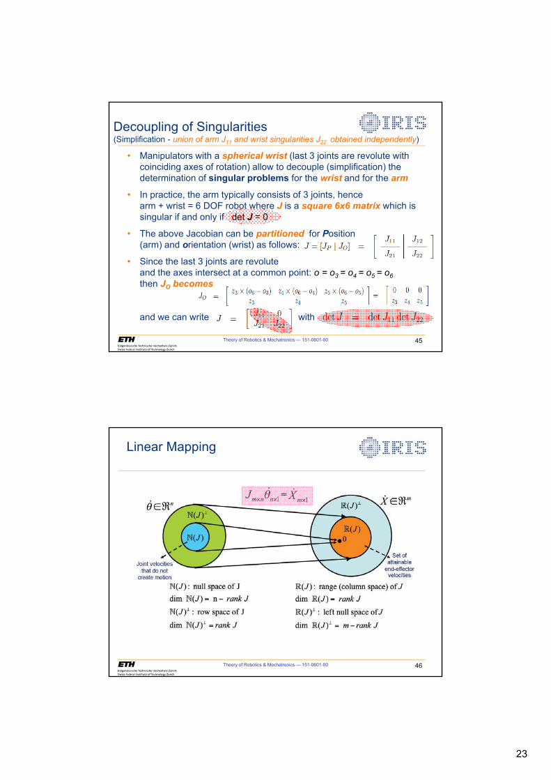
23
Theory of Robotics & Mechatronics — 151-0601-00 45
• Manipulators with a spherical wrist (last 3 joints are revolute with coinciding axes of rotation) allow to decouple (simplification) the determination of singular problems for the wrist and for the arm
• In practice, the arm typically consists of 3 joints, hencearm + wrist = 6 DOF robot where J is a square 6x6 matrix which is singular if and only if det J = 0
• The above Jacobian can be partitioned for Position(arm) and orientation (wrist) as follows:
• Since the last 3 joints are revoluteand the axes intersect at a common point: o = o3 = o4 = o5 = o6
then JO becomes
and we can write with
Decoupling of Singularities(Simplification - union of arm J11 and wrist singularities J22 obtained independently)
Theory of Robotics & Mechatronics — 151-0601-00 46
Linear Mapping
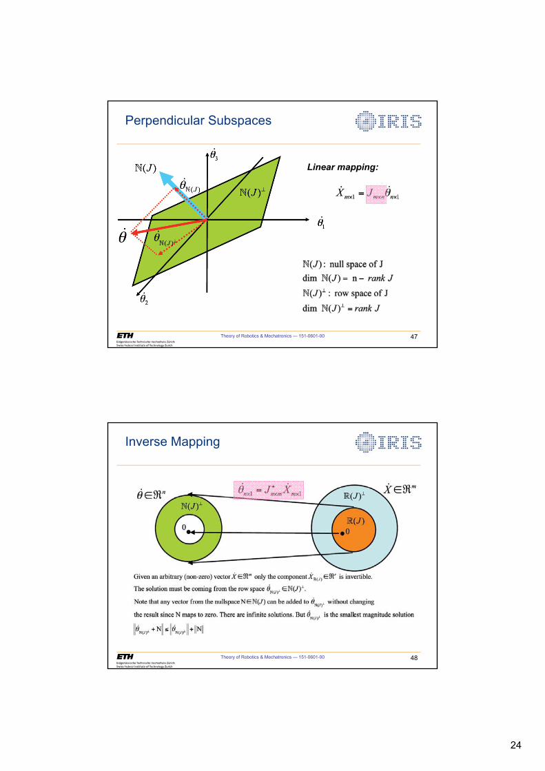
24
Theory of Robotics & Mechatronics — 151-0601-00 47
Perpendicular Subspaces
Linear mapping:
Theory of Robotics & Mechatronics — 151-0601-00 48
Inverse Mapping
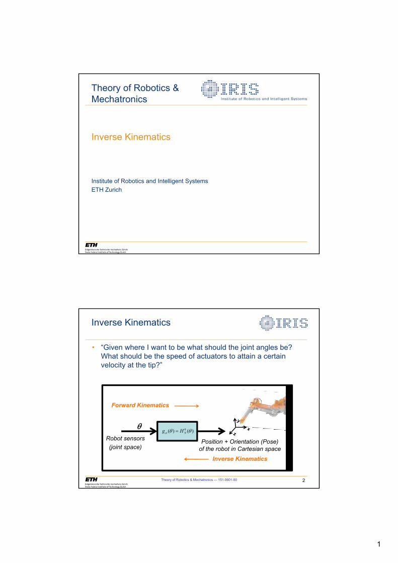
1
Inverse Kinematics
Institute of Robotics and Intelligent SystemsETH Zurich
Theory of Robotics &Mechatronics
Theory of Robotics & Mechatronics — 151-0601-00 2
Inverse Kinematics
• “Given where I want to be what should the joint angles be? What should be the speed of actuators to attain a certain velocity at the tip?”
TRobot sensors(joint space)
Position + Orientation (Pose)of the robot in Cartesian space
Inverse Kinematics
Forward Kinematics
)()( 0 TT Nst Hg
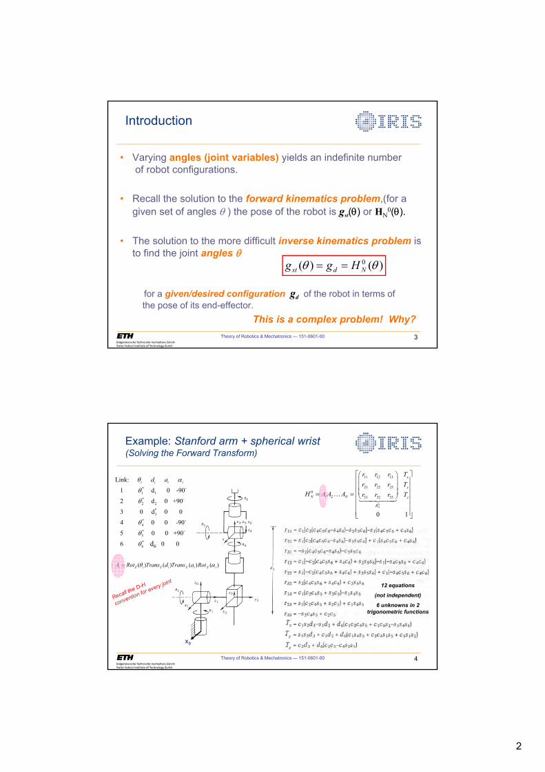
2
Theory of Robotics & Mechatronics — 151-0601-00 3
Introduction
• Varying angles (joint variables) yields an indefinite numberof robot configurations.
• Recall the solution to the forward kinematics problem,(for a given set of angles T ) the pose of the robot is gst(T) or HN
0(T).
• The solution to the more difficult inverse kinematics problem is to find the joint angles T
for a given/desired configuration gd of the robot in terms ofthe pose of its end-effector.
This is a complex problem! Why?
)()( 0 TT Ndst Hgg
Theory of Robotics & Mechatronics — 151-0601-00 4
Example: Stanford arm + spherical wrist (Solving the Forward Transform)
0
11 12 13
21 22 230
1 2 31 32 33
0 1N
x
y
N N z
R
r r r Tr r r T
H A A A r r r T
ª º§ ·« »¨ ¸« »¨ ¸¨ ¸« » © ¹« »« »« »¬ ¼
������
x0
*1 1
*2 2
*3
*4
*5
Link:
1 d 0 -90
2 d 0 +90
3 0 d 0 0
4 0 0 -90
5 0
i i i id aT D
T
T
T
T
$
$
$
*6
0 +90
6 0 0 0T
$
( ) ( ) ( ) ( )i Z i Z i X i X iA Rot Trans d Trans a RotT D
12 equations
(not independent)
6 unknowns in 2
trigonometric functions
d6
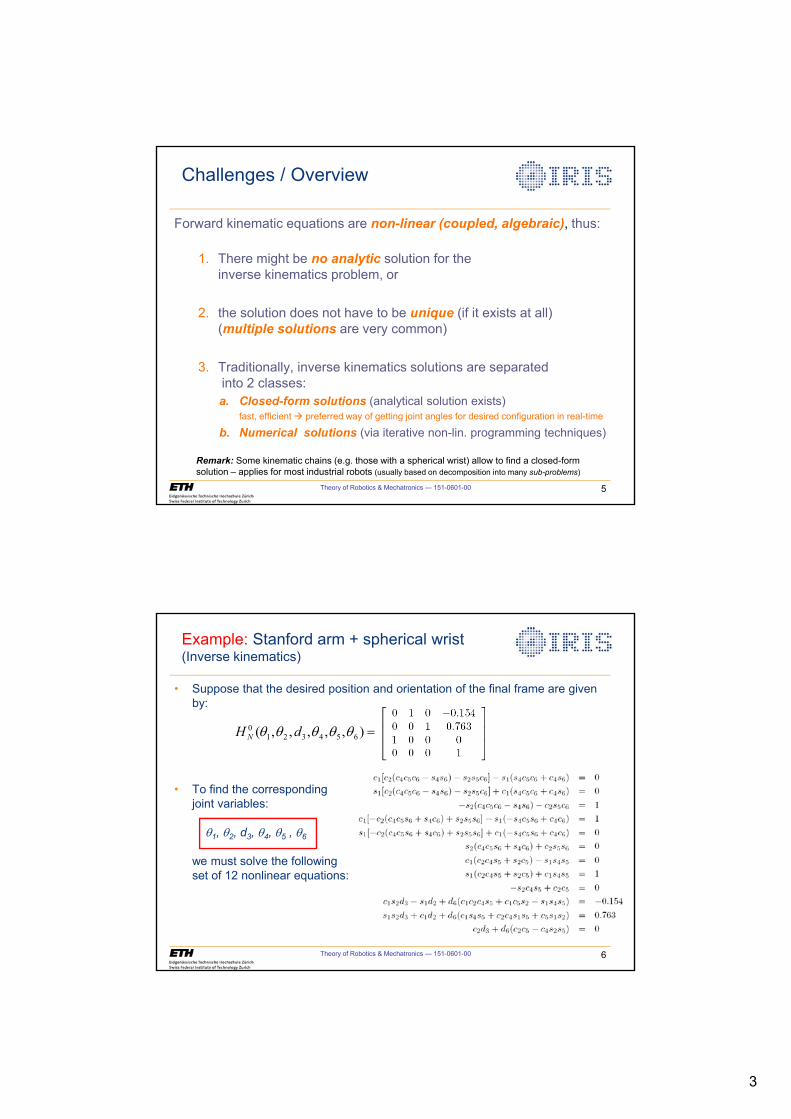
3
Theory of Robotics & Mechatronics — 151-0601-00 5
Challenges / Overview
Forward kinematic equations are non-linear (coupled, algebraic), thus:
1. There might be no analytic solution for the inverse kinematics problem, or
2. the solution does not have to be unique (if it exists at all)(multiple solutions are very common)
3. Traditionally, inverse kinematics solutions are separatedinto 2 classes: a. Closed-form solutions (analytical solution exists)
fast, efficient Æ preferred way of getting joint angles for desired configuration in real-time
b. Numerical solutions (via iterative non-lin. programming techniques)
Remark: Some kinematic chains (e.g. those with a spherical wrist) allow to find a closed-form solution – applies for most industrial robots (usually based on decomposition into many sub-problems)
Theory of Robotics & Mechatronics — 151-0601-00 6
Example: Stanford arm + spherical wrist(Inverse kinematics)
• Suppose that the desired position and orientation of the final frame are given by:
• To find the correspondingjoint variables:
T1, T2, d3, T4, T5 , T6
we must solve the followingset of 12 nonlinear equations:
),,,,,( 6543210 TTTTT dHN
4
Theory of Robotics & Mechatronics — 151-0601-00 7
Example: Stanford arm + spherical wrist(Numerical solution)
• One solution to this set of equations is given by:(for d1 = 0, d2 = 0.154 and d6 = 0.263)
+ any other solution satisfying T4 + T6 = S can be easily obtained(see the slide with robot and D-H table for more details)
• Even though you have not seen how this solution was derived,it is not difficult to verify that it satisfies the forward kinematics equations for the Stanford arm!
Theory of Robotics & Mechatronics — 151-0601-00 8
Overview - Inverse kinematicsWhat have we seen so far
• The inverse kinematics equations in this example were too difficult to solve directlyin close form – it is the case for most robots.
• Note, there are few efficient techniques which allow us to exploit several particular kinematic structures (see next slides)
• In general, we can say:1. Forward kinematics (FK) problem has always a unique solution that can be
obtained simply by evaluating the forward equations2. Inverse kinematics (IK) problem may or may not have a solution3. Even if a solution exists, it may or may not be unique4. Because the FK equations are in general complicated non-linear functions
(of joint variables), the solution(s) may be difficult to obtain even when it exists
– Solving the inverse kinematics problem, we are interested in findinga closed form (explicit solution) rather than a numerical oneWhy? Real-time, computational time, convergence problems etc.
– Finding a (closed form) solution means to get this explicit relationship:
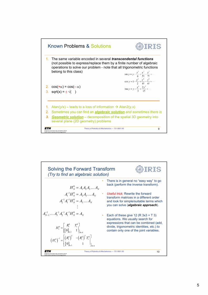
5
Theory of Robotics & Mechatronics — 151-0601-00 9
Known Problems & Solutions
1. The same variable encoded in several transcendental functions
(not possible to express/replace them by a finite number of algebraic operations to solve our problem - note that all trigonometric functions belong to this class)
2. cos(+D) = cos(– D) 3. sqrt(x) = r �( )
1. Atan(y/x) – leads to a loss of information Æ Atan2(y,x)2. Sometimes you can find an algebraic solution and sometimes there is3. Geometric solution – decomposition of the spatial 3D geometry into
several plane (2D geometry) problems
Theory of Robotics & Mechatronics — 151-0601-00 10
Solving the Forward Transform(Try to find an algebraic solution)
01 2 3
1 01 2 3
1 1 02 1 3
1 1 1 1 01 3 2 1
N N
N N
N N
N N N
H A A A A
A H A A A
A A H A A
A A A A H A
�
� �
� � � ��
�
�
�
�
�
> @
� � � � � �> @
0 01 10
11 3 4 4
0 0 01 1 1 10
1
1 3 4 4
0 1
0 1
T T
R TH
R R TH
u u
�
u u
ª º « »« »¬ ¼
ª º�« » « »¬ ¼
• There is in general no “easy way” to go back (perform the inverse transform).
• Useful trick: Rewrite the forward transform matrices in a different order and look for simple/suitable terms which you can solve (algebraic approach).
• Each of these give 12 (R 3x3 + T 3) equations. We usually search for expressions that can be combined (add, divide, trigonometric identities, etc.) to contain only one of the joint variables.
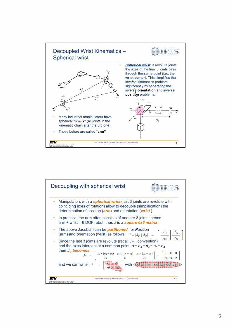
6
Theory of Robotics & Mechatronics — 151-0601-00 11
Decoupled Wrist Kinematics –Spherical wrist
06T
03T
d6
• Spherical wrist: 3 revolute joints, the axes of the final 3 joints pass through the same point (i.e., the wrist center). This simplifies the inverse kinematics problem significantly by separating the inverse orientation and inverse position problems.
• Many industrial manipulators have spherical “wrists” (all joints in the kinematic chain after the 3rd one)
• Those before are called “arm”
Theory of Robotics & Mechatronics — 151-0601-00 12
• Manipulators with a spherical wrist (last 3 joints are revolute with coinciding axes of rotation) allow to decouple (simplification) the determination of position (arm) and orientation (wrist )
• In practice, the arm often consists of another 3 joints, hencearm + wrist = 6 DOF robot, thus J is a square 6x6 matrix
• The above Jacobian can be partitioned for Position(arm) and orientation (wrist) as follows:
• Since the last 3 joints are revolute (recall D-H convention)and the axes intersect at a common point: o = o3 = o4 = o5 = o6then JO becomes
and we can write with
Decoupling with spherical wrist
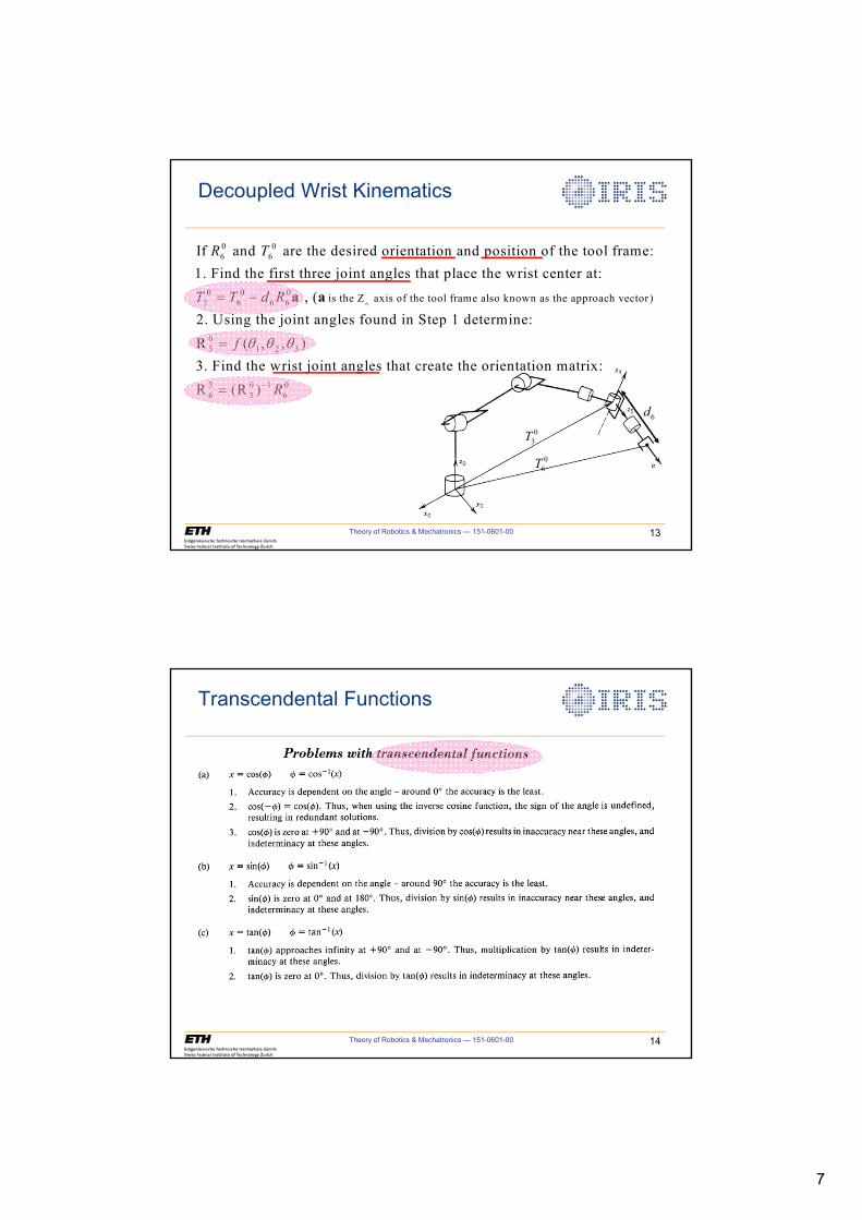
7
Theory of Robotics & Mechatronics — 151-0601-00 13
Decoupled Wrist Kinematics
6
0 06 6
0 0 03 6 6 6 is the Z axis of the tool frame also k
If and are the desired orientation and position of the tool frame:1. Find the first three joint angles that place the wrist center at:
, (
R T
T T d R � a a
03 1 2 3
3 0 1 06 3 6
nown as the approach vector )
2. Using the joint angles found in Step 1 determine:
R ( , , )3. Find the wrist joint angles that create the orientation matrix:
R (R )
f
R
T T T
�
06T
03T
6d
Theory of Robotics & Mechatronics — 151-0601-00 14
Transcendental Functions
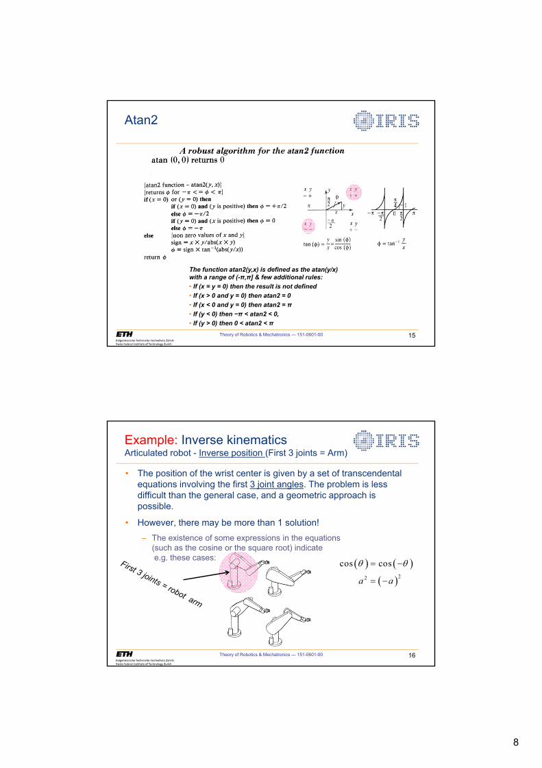
8
Theory of Robotics & Mechatronics — 151-0601-00 15
Atan2
The function atan2(y,x) is defined as the atan(y/x)
with a range of (-π,π] & few additional rules:
• If (x = y = 0) then the result is not defined
• If (x > 0 and y = 0) then atan2 = 0
• If (x < 0 and y = 0) then atan2 = π• If (y < 0) then −π < atan2 < 0,
• If (y > 0) then 0 < atan2 < π
Theory of Robotics & Mechatronics — 151-0601-00 16
Example: Inverse kinematicsArticulated robot - Inverse position (First 3 joints = Arm)
� � � �� �22
cos cos
a a
T T �
�
• The position of the wrist center is given by a set of transcendental equations involving the first 3 joint angles. The problem is less difficult than the general case, and a geometric approach is possible.
• However, there may be more than 1 solution!– The existence of some expressions in the equations
(such as the cosine or the square root) indicatee.g. these cases:
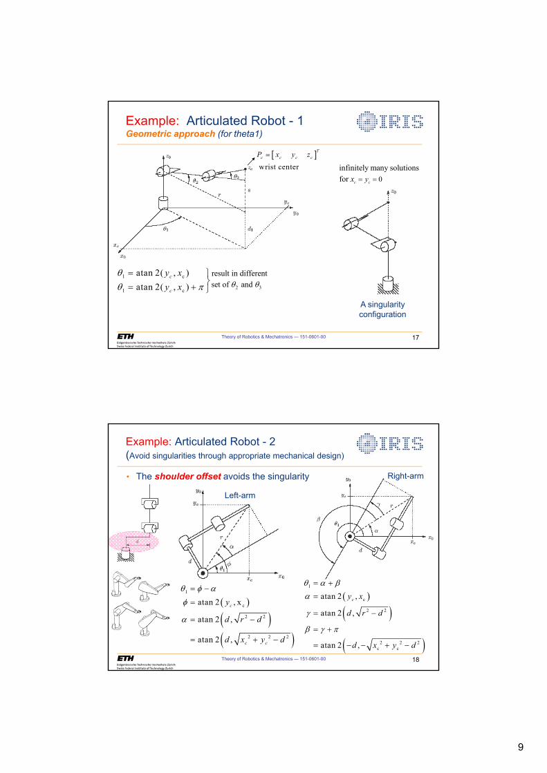
9
Theory of Robotics & Mechatronics — 151-0601-00 17
Example: Articulated Robot - 1Geometric approach (for theta1)
> @ wrist center
Tc c c cP x y z
1 c
1 c
atan 2( , )atan 2( , )
c
c
y xy x
TT S
½¾ � ¿ 2 3
result in differentset of and T T
0infinitely many solutionsfor c cyx
A singularity configuration
Theory of Robotics & Mechatronics — 151-0601-00 18
Example: Articulated Robot - 2(Avoid singularities through appropriate mechanical design)
• The shoulder offset avoids the singularity
� �
� �� �
1
c
2 2
2 2 2
atan 2 , x
atan 2 ,
atan 2 ,
c
c c
y
d r d
d x y d
T I DI
D
�
�
� �
� �
� �
� �
1
c
2 2
2 2 2c c
atan 2 ,
atan 2 ,
atan 2 ,
cy x
d r d
d x y d
T D ED
J
E J S
�
�
�
� � � �
Left-arm
Right-arm
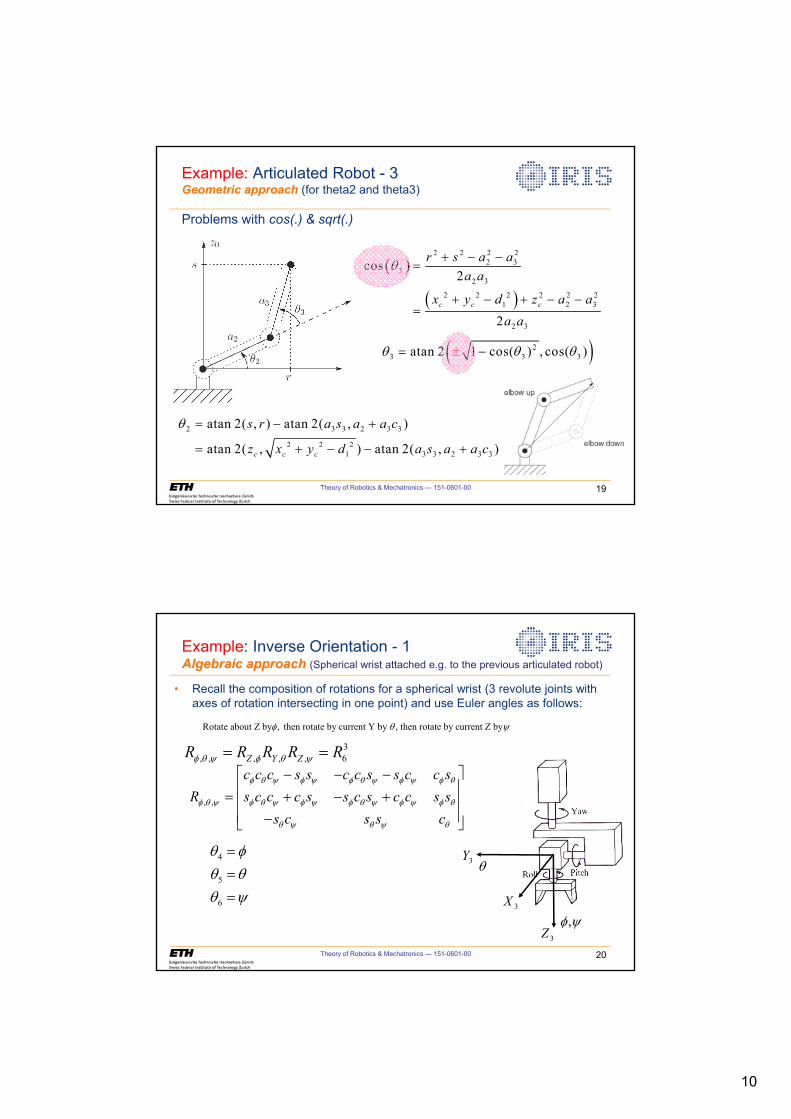
10
Theory of Robotics & Mechatronics — 151-0601-00 19
Example: Articulated Robot - 3Geometric approach (for theta2 and theta3)
Problems with cos(.) & sqrt(.)
� �
� �
2 2 2 22 3
32 3
2 2 2 2 2 21 2 3
2 3
cos2
2c c c
r s a aa a
x y d z a a
a a
T � � �
� � � � �
� �23 3 3atan 2 1 cos( ) , cos( )T T Tr �
2 3 3 2 3 3
2 2 21 3 3 2 3 3
atan 2( , ) atan 2( , )
atan 2( , ) atan 2( , )c c c
s r a s a a c
z x y d a s a a c
T � �
� � � �
Theory of Robotics & Mechatronics — 151-0601-00 20
Example: Inverse Orientation - 1 Algebraic approach (Spherical wrist attached e.g. to the previous articulated robot)
Rotate about Z by , then rotate by current Y by , then rotate by current Z byI T \
, ,
c c c s s c c s s c c sR s c c c s s c s c c s s
s c s s c
I T \ I \ I T \ I \ I T
I T \ I T \ I \ I T \ I \ I T
T \ T \ T
ª º� � �« » � � �« »« »�¬ ¼
3X
3Z
3Y T
,I \
4
5
6
T IT TT \
3, , , , , 6Z Y ZR R R R RI T \ I T \
• Recall the composition of rotations for a spherical wrist (3 revolute joints with axes of rotation intersecting in one point) and use Euler angles as follows:
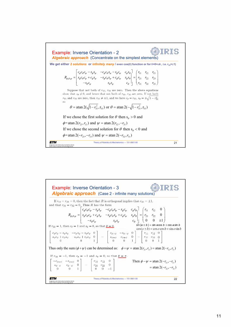
11
11 12 13
, , 21 22 23
31 32 33
c c c s s c c s s c c s r r rR s c c c s s c s c c s s r r r
s c s s c r r r
\ \ \ \I T I I T I I T
\ \ \ \I T \ I T I I T I I T
\ \T T T
ª º� � � § ·« » ¨ ¸ � � � « » ¨ ¸
¨ ¸« »� © ¹¬ ¼
Theory of Robotics & Mechatronics — 151-0601-00 21
2 233 33 33 33atan 2( 1 , r ) or atan 2( 1 , r )r rT T � � �
23 13 32 31
23 13 32 31
If we chose the first solution for then s 0 and = atan 2( , ) and atan 2( , )
If we chose the second solution for then s 0 and = atan 2( , ) and atan 2( , )
r r r r
r r r r
T
T
TI \
TI \
! �
�
� � �
We get either 2 solutions or infinitely many / even cos(T) function or for T=0+Sk , i.e. r33=r1)
Example: Inverse Orientation - 2 Algebraic approach (Concentrate on the simplest elements)
Theory of Robotics & Mechatronics — 151-0601-00 22
21 11 12 11Thus only the sum ( ) can be determined as: atan 2( ) atan 2( ), ,r r r rI \ I \� � �
11 12
, , 21 22
00
0 0 1
c c c s s c c s s c c s r rR s c c c s s c s c c s s r r
s c s s c
\ \ \ \I T I I T I I T
\ \ \ \I T \ I T I I T I I T
\ \T T T
ª º� � � § ·« » ¨ ¸ � � � « » ¨ ¸
¨ ¸« »� r© ¹¬ ¼
12 11
22 21
Then atan 2( )
atan 2( )
,,
r r
r r
I \� � �
� �
Example: Inverse Orientation - 3 Algebraic approach (Case 2 - infinite many solutions)
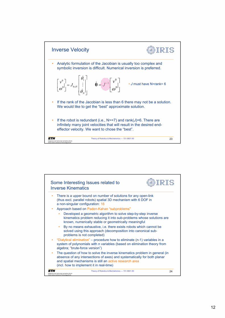
12
Theory of Robotics & Mechatronics — 151-0601-00 23
• Analytic formulation of the Jacobian is usually too complex and symbolic inversion is difficult. Numerical inversion is preferred.
• If the rank of the Jacobian is less than 6 there may not be a solution. We would like to get the “best” approximate solution.
• If the robot is redundant (i.e., N>=7) and rank(J)=6. There are infinitely many joint velocities that will result in the desired end-effector velocity. We want to chose the “best”.
Inverse Velocity
10
60 xN
N
vJ
T
ZT
ª ºª º « » « » « »¬ ¼ « »¬ ¼
�
��
01
0
vJ
Z� ª º
« »¬ ¼
θ� • J must have N=rank= 6
Theory of Robotics & Mechatronics — 151-0601-00 24
Some Interesting Issues related toInverse Kinematics• There is a upper bound on number of solutions for any open-link
(thus excl. parallel robots) spatial 3D mechanism with 6 DOF ina non-singular configuration: 16
• Approach based on Paden-Kahan “subproblems”• Developed a geometric algorithm to solve step-by-step inverse
kinematics problem reducing it into sub-problems whose solutions are known, numerically stable or geometrically meaningful
• By no means exhaustive, i.e. there exists robots which cannot be solved using this approach (decomposition into canonical sub-problems is not completed)
• “Dialytical elimination” – procedure how to eliminate (n-1) variables in a system of polynomials with n variables (based on elimination theory from algebra; “brute-force version”)
• The question of how to solve the inverse kinematics problem in general (in absence of any intersections of axes) and systematically for both planar and spatial mechanisms is still an active research area(incl. how to implement it in real-time)
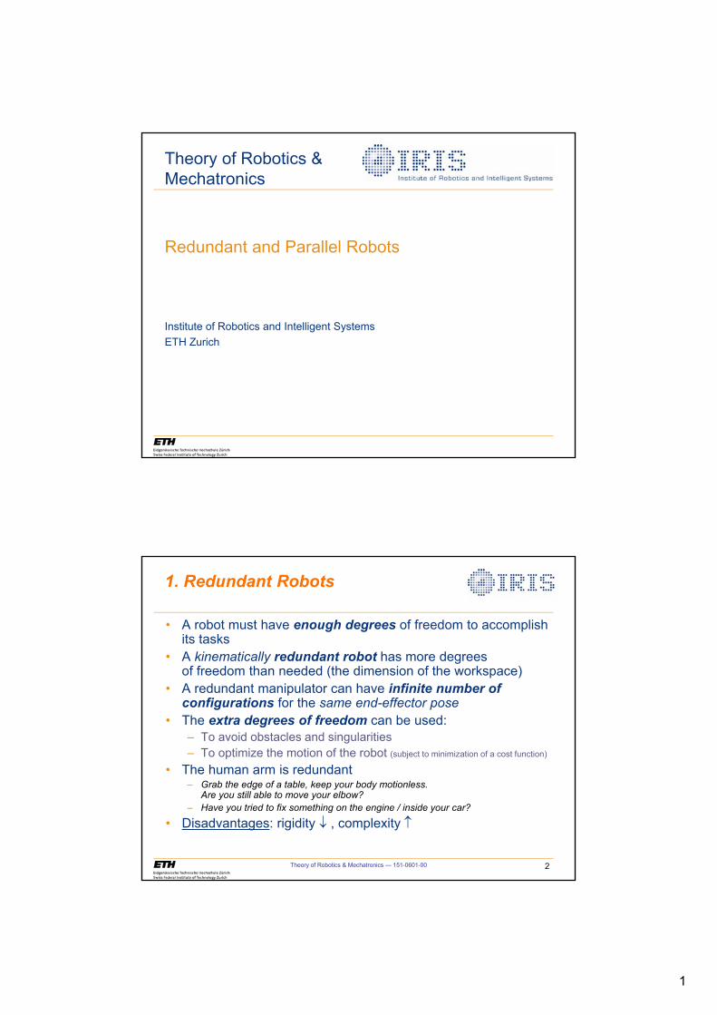
1
Redundant and Parallel Robots
Institute of Robotics and Intelligent SystemsETH Zurich
Theory of Robotics &Mechatronics
Theory of Robotics & Mechatronics — 151-0601-00 2
1. Redundant Robots
• A robot must have enough degrees of freedom to accomplish its tasks
• A kinematically redundant robot has more degreesof freedom than needed (the dimension of the workspace)
• A redundant manipulator can have infinite number of configurations for the same end-effector pose
• The extra degrees of freedom can be used:– To avoid obstacles and singularities– To optimize the motion of the robot (subject to minimization of a cost function)
• The human arm is redundant– Grab the edge of a table, keep your body motionless.
Are you still able to move your elbow?– Have you tried to fix something on the engine / inside your car?
• Disadvantages: rigidity p , complexity n
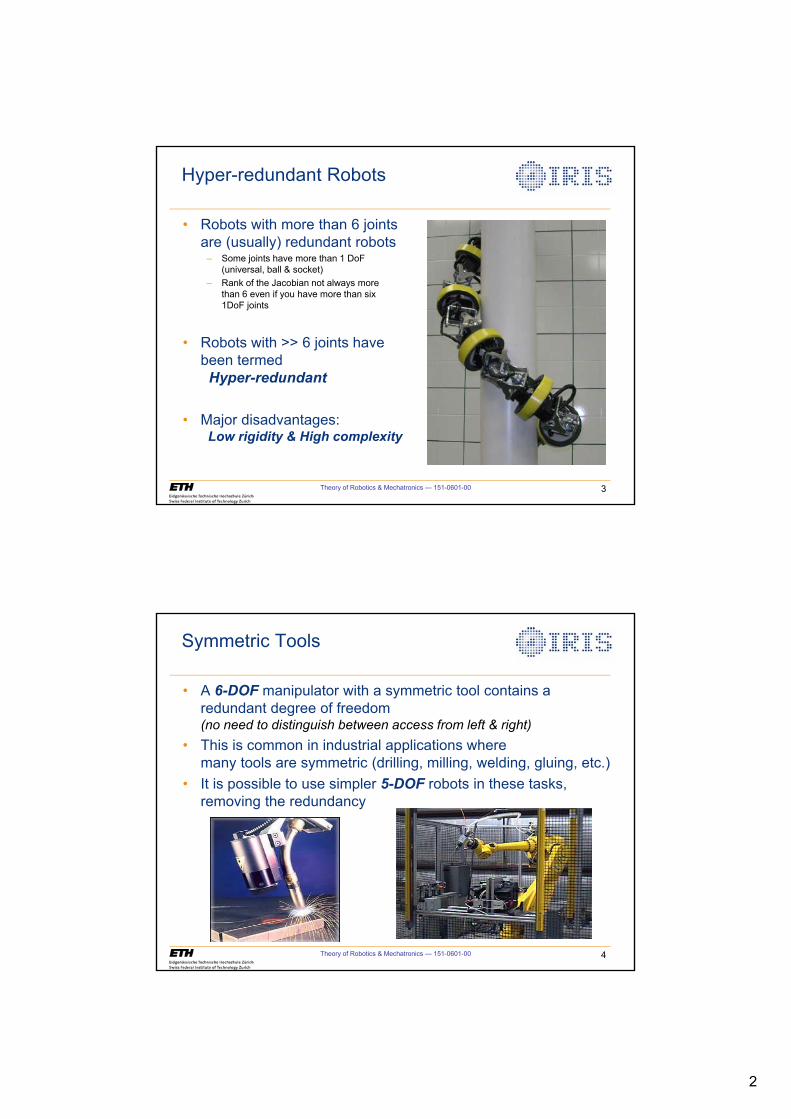
2
Theory of Robotics & Mechatronics — 151-0601-00 3
Hyper-redundant Robots
• Robots with more than 6 joints are (usually) redundant robots
– Some joints have more than 1 DoF(universal, ball & socket)
– Rank of the Jacobian not always morethan 6 even if you have more than six1DoF joints
• Robots with >> 6 joints have been termed
Hyper-redundant
• Major disadvantages: Low rigidity & High complexity
Theory of Robotics & Mechatronics — 151-0601-00 4
Symmetric Tools
• A 6-DOF manipulator with a symmetric tool contains a redundant degree of freedom (no need to distinguish between access from left & right)
• This is common in industrial applications where many tools are symmetric (drilling, milling, welding, gluing, etc.)
• It is possible to use simpler 5-DOF robots in these tasks, removing the redundancy
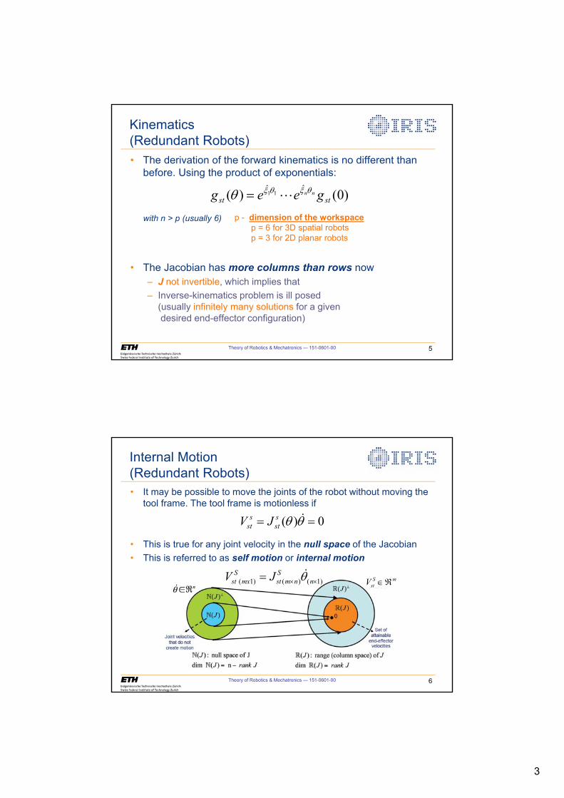
3
Theory of Robotics & Mechatronics — 151-0601-00 5
Kinematics(Redundant Robots)• The derivation of the forward kinematics is no different than
before. Using the product of exponentials:
with n > p (usually 6)
• The Jacobian has more columns than rows now – J not invertible, which implies that– Inverse-kinematics problem is ill posed
(usually infinitely many solutions for a givendesired end-effector configuration)
)0()( ˆˆ11
stst geeg nnT[T[T � p - dimension of the workspace
p = 6 for 3D spatial robotsp = 3 for 2D planar robots
Theory of Robotics & Mechatronics — 151-0601-00 6
Internal Motion(Redundant Robots)• It may be possible to move the joints of the robot without moving the
tool frame. The tool frame is motionless if
• This is true for any joint velocity in the null space of the Jacobian• This is referred to as self motion or internal motion
0)( TT �sst
sst JV
S mstV ��( 1) ( ) ( 1)
S Sst mx st m n nV J Tu u �
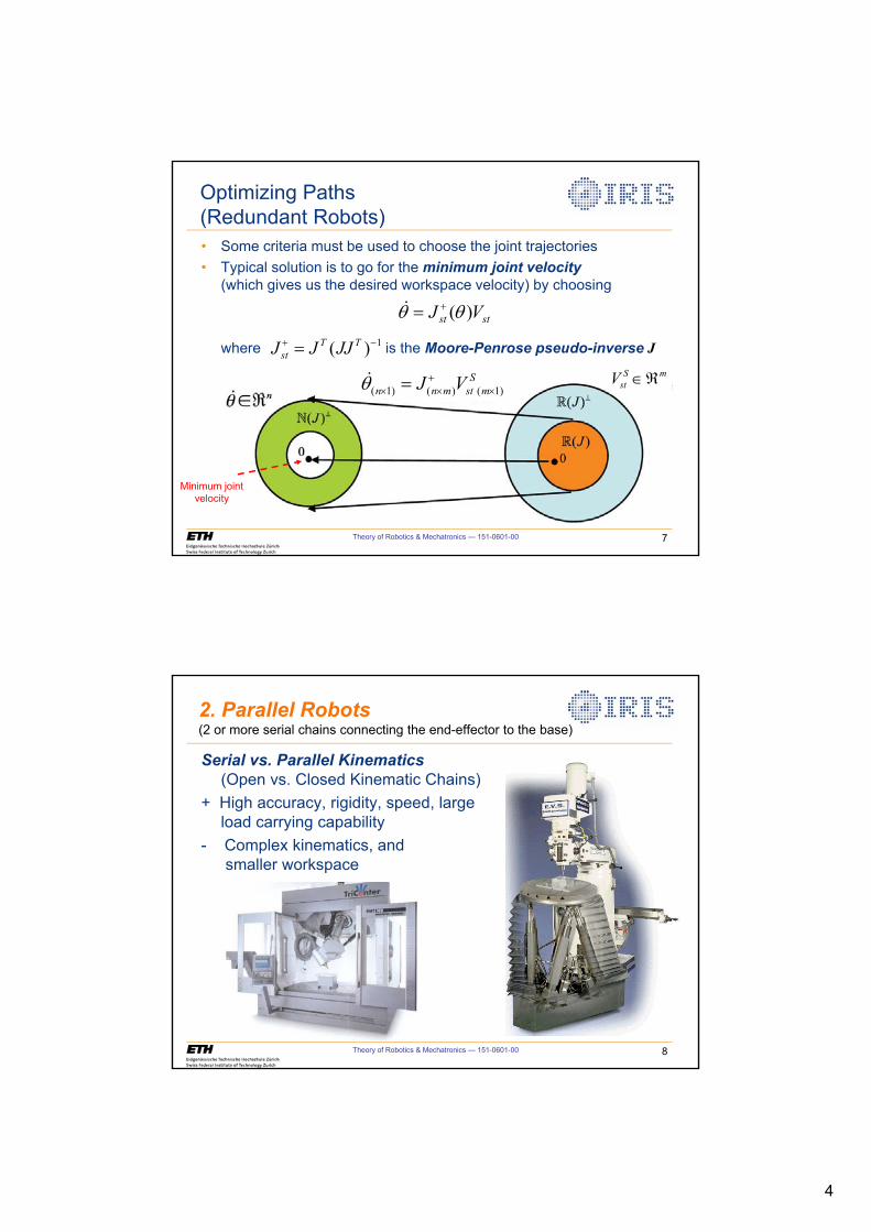
4
Theory of Robotics & Mechatronics — 151-0601-00 7
• Some criteria must be used to choose the joint trajectories• Typical solution is to go for the minimum joint velocity
(which gives us the desired workspace velocity) by choosing
where is the Moore-Penrose pseudo-inverse J1( )T TstJ J JJ� �
Optimizing Paths(Redundant Robots)
stst VJ )(TT � �
Minimum joint velocity
( 1) ( ) ( 1)S
n n m st mJ VT �u u u � S m
stV ��
Theory of Robotics & Mechatronics — 151-0601-00 8
2. Parallel Robots(2 or more serial chains connecting the end-effector to the base)
Serial vs. Parallel Kinematics(Open vs. Closed Kinematic Chains)
+ High accuracy, rigidity, speed, large load carrying capability
- Complex kinematics, andsmaller workspace
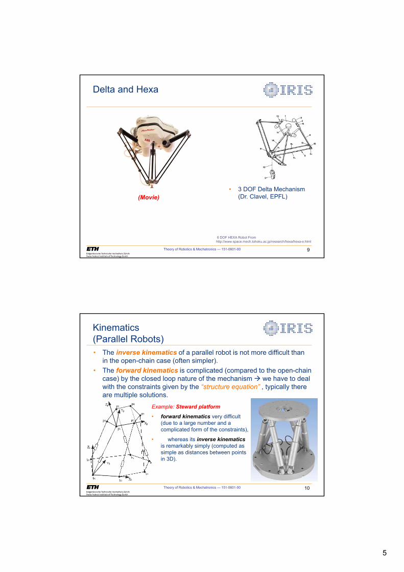
5
Theory of Robotics & Mechatronics — 151-0601-00 9
Delta and Hexa
6 DOF HEXA Robot From http://www.space.mech.tohoku.ac.jp/research/hexa/hexa-e.html
• 3 DOF Delta Mechanism (Dr. Clavel, EPFL)(Movie)
Theory of Robotics & Mechatronics — 151-0601-00 10
Kinematics(Parallel Robots)• The inverse kinematics of a parallel robot is not more difficult than
in the open-chain case (often simpler).• The forward kinematics is complicated (compared to the open-chain
case) by the closed loop nature of the mechanism Æ we have to deal with the constraints given by the “structure equation” , typically there are multiple solutions.
Example: Steward platform
• forward kinematics very difficult (due to a large number and a complicated form of the constraints),
• whereas its inverse kinematicsis remarkably simply (computed as simple as distances between points in 3D).
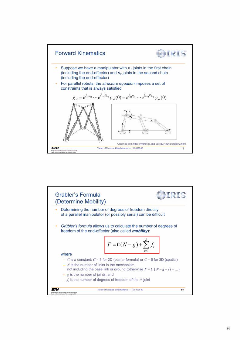
6
Theory of Robotics & Mechatronics — 151-0601-00 11
Forward Kinematics
• Suppose we have a manipulator with n1 joints in the first chain (including the end-effector) and n2 joints in the second chain (including the end-effector)
• For parallel robots, the structure equation imposes a set of constraints that is always satisfied
)0()0( 2222212111111111ˆˆˆˆ
ststst geegeeg nnnn T[T[T[T[ ��
Graphics from http://synthetica.eng.uci.edu/~curtis/project2.html
Theory of Robotics & Mechatronics — 151-0601-00 12
Grübler’s Formula(Determine Mobility)• Determining the number of degrees of freedom directly
of a parallel manipulator (or possibly serial) can be difficult
• Grübler’s formula allows us to calculate the number of degrees of freedom of the end-effector (also called mobility):
where – C is a constant: C = 3 for 2D (planar formula) or C = 6 for 3D (spatial)– N is the number of links in the mechanism
not including the base link or ground (otherwise F = C ( N – g – 1) + …)– g is the number of joints, and – fi is the number of degrees of freedom of the ith joint
¦
�� g
iifgNF
1)(6C
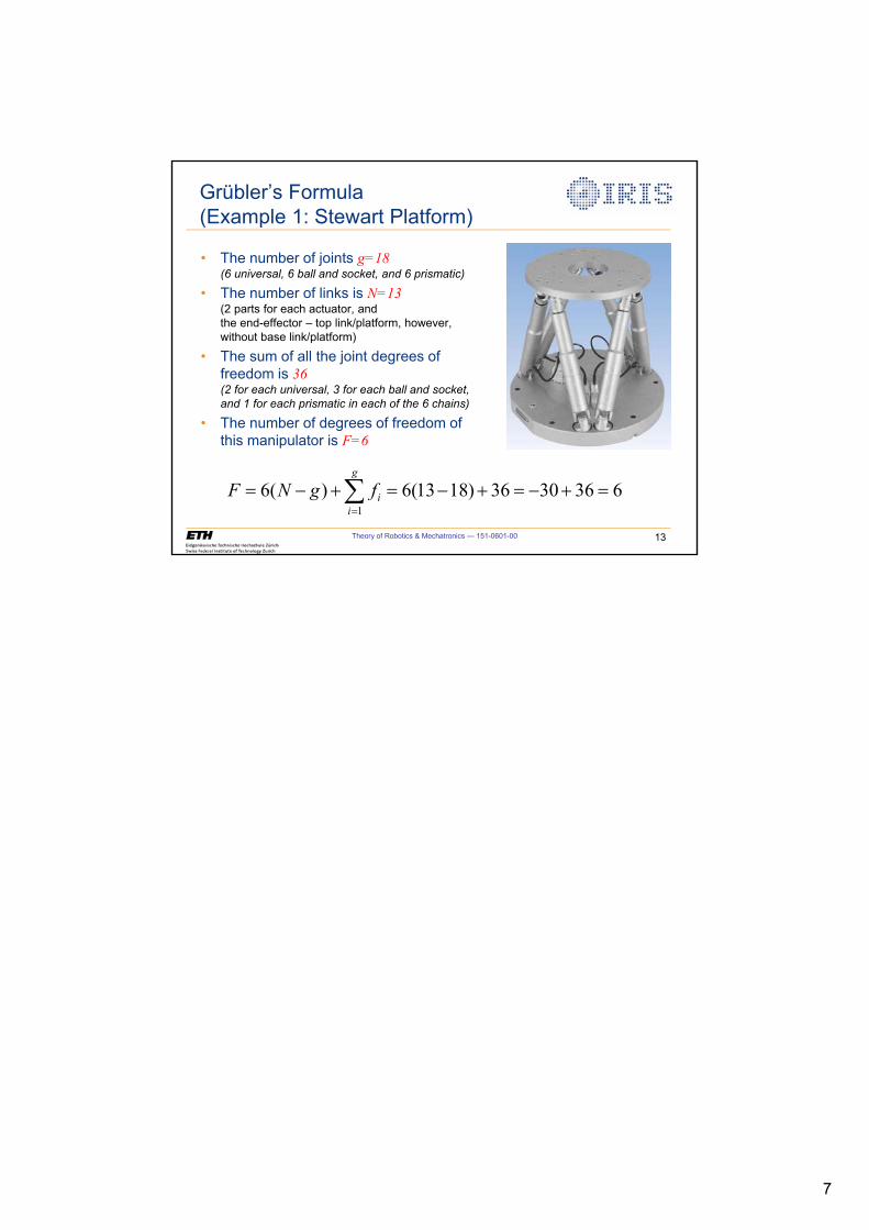
7
Theory of Robotics & Mechatronics — 151-0601-00 13
Grübler’s Formula(Example 1: Stewart Platform)
• The number of joints g=18(6 universal, 6 ball and socket, and 6 prismatic)
• The number of links is N=13(2 parts for each actuator, and the end-effector – top link/platform, however, without base link/platform)
• The sum of all the joint degrees of freedom is 36(2 for each universal, 3 for each ball and socket, and 1 for each prismatic in each of the 6 chains)
• The number of degrees of freedom of this manipulator is F=6
6363036)1813(6)(61
�� �� �� ¦
g
iifgNF
1
Numerical Methods
Institute of Robotics and Intelligent SystemsETH Zurich
Theory of Robotics &Mechatronics
Theory of Robotics & Mechatronics — 151-0601-00 2
Numerical Methods
• Inverse Kinematics– Linear approximation– Solving techniques– Calculating Jacobians– Other concerns
• Calibration– Methods
2
Theory of Robotics & Mechatronics — 151-0601-00 3
Inverse Kinematics
• Analytic solutions often not possible– Large solution space (redundancy)– Empty solution space (nonreachable goal)
• Need for numerical solutions
• Can be expensive
• Find numerical methods that are:– As fast as possible– Accurate– Robust
Theory of Robotics & Mechatronics — 151-0601-00 4
Inverse Kinematics
• is the desired pose, and is the actual set of joint angles to get to
• Forward Kinematics based on POE
• Inverse Kinematics
• How?– gst
-1 is nonlinear– find a linear approximation to gst
-1
)()0()( ˆˆˆ
2211
TT T[T[T[
std
stst
gggeeeg nn
�
)(1dgg
st
� T
dg T dg
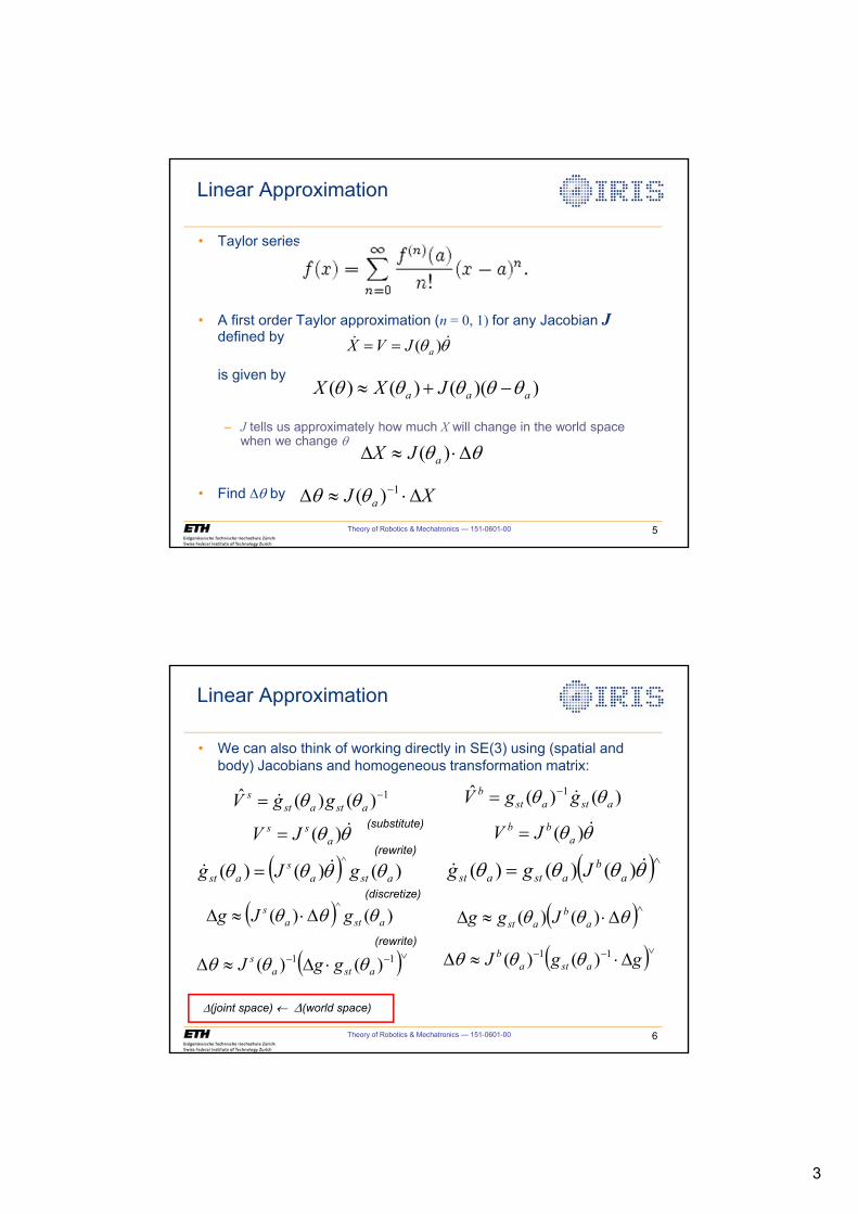
3
Theory of Robotics & Mechatronics — 151-0601-00 5
Linear Approximation
• Taylor series
• A first order Taylor approximation (n = 0, 1) for any Jacobian Jdefined by
is given by
– J tells us approximately how much X will change in the world space when we change T
• Find 'T by XJ a '�|' �1)(TT
TT '�|' )( aJX
TT �� )( aJVX
))(()()( aaa JXX TTTTT ��|
Theory of Robotics & Mechatronics — 151-0601-00 6
Linear Approximation
• We can also think of working directly in SE(3) using (spatial and body) Jacobians and homogeneous transformation matrix:
� � )()()(^
astas
ast gJg TTTT ��
1)()(ˆ � astasts ggV TT� )()(ˆ 1
astastb ggV TT ��
TT �)( abb JV TT �)( a
ss JV
� �� TTTT �� )()()( ab
astast Jgg
� ��'�|' TTT )()( ab
ast Jgg� � )()( ^asta
s gJg TTT '�|'
� ���� �'|' 11 )()( astas ggJ TTT � ���� '�|' ggJ asta
b 11 )()( TTT
(substitute)
(rewrite)
(discretize)
(rewrite)
'(joint space) m '(world space)
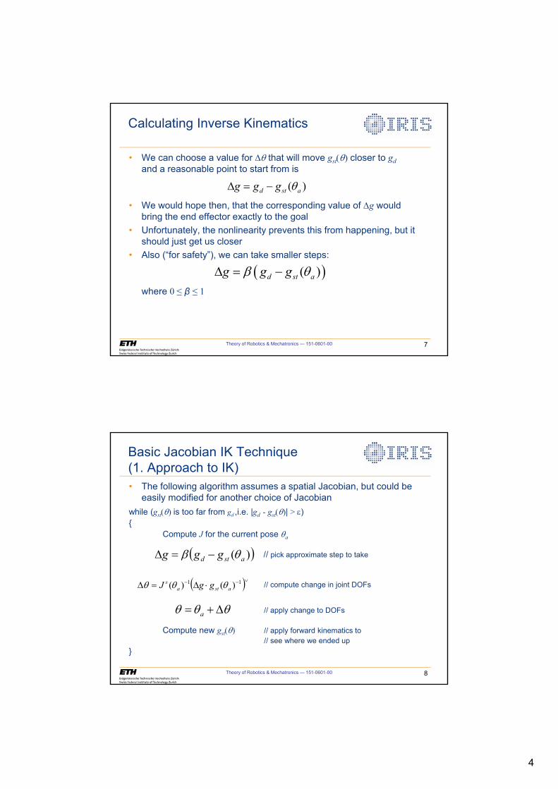
4
Theory of Robotics & Mechatronics — 151-0601-00 7
Calculating Inverse Kinematics
• We can choose a value for 'T that will move gst�T� closer to gdand a reasonable point to start from is
• We would hope then, that the corresponding value of 'g would bring the end effector exactly to the goal
• Unfortunately, the nonlinearity prevents this from happening, but it should just get us closer
• Also (“for safety”), we can take smaller steps:
where 0 ≤ ≤ 1
( )d st ag g g T' �
� �( )d st ag g gE T' �
Theory of Robotics & Mechatronics — 151-0601-00 8
Basic Jacobian IK Technique(1. Approach to IK)
while (gst�T� is too far from gd ,i.e. |gd - gst�T�| > H){
Compute J for the current pose Ta
// pick approximate step to take
// compute change in joint DOFs
// apply change to DOFs
Compute new gst�T� // apply forward kinematics to// see where we ended up
}
aT T T � '
• The following algorithm assumes a spatial Jacobian, but could be easily modified for another choice of Jacobian
� �)( astd ggg TE � '
� ���� �' ' 11 )()( astas ggJ TTT
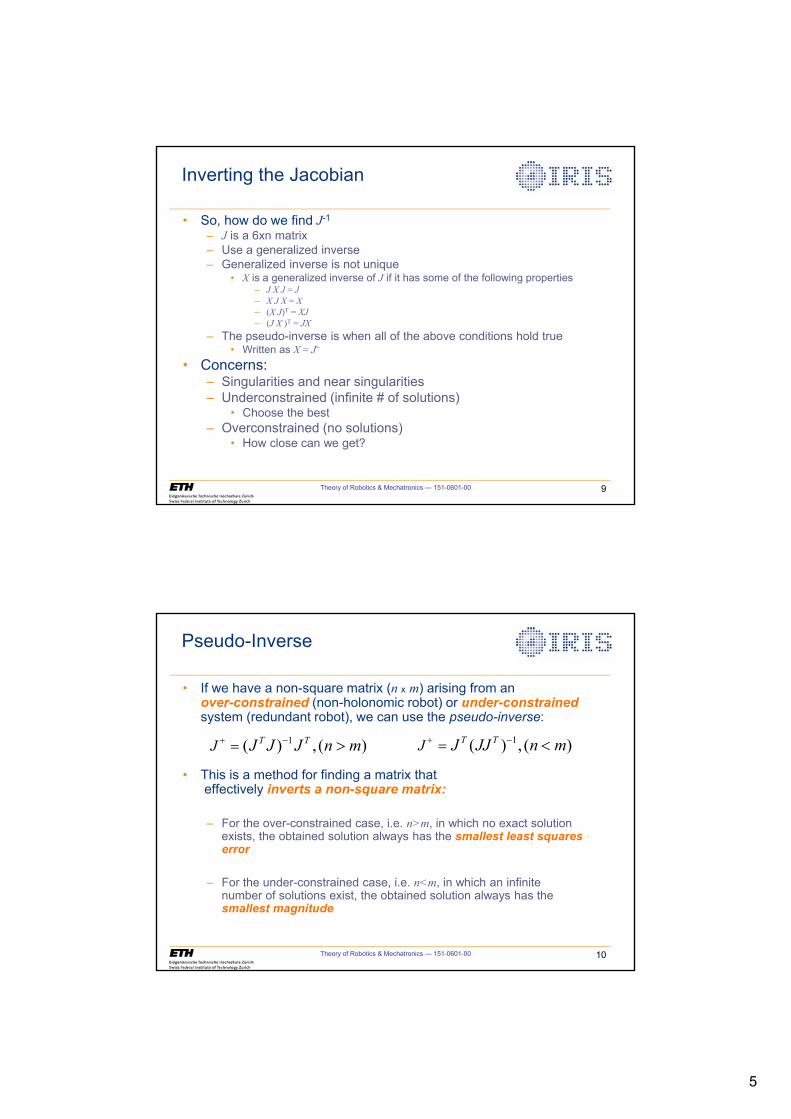
5
Theory of Robotics & Mechatronics — 151-0601-00 9
Inverting the Jacobian
• So, how do we find J-1
– J is a 6xn matrix– Use a generalized inverse– Generalized inverse is not unique
• X is a generalized inverse of J if it has some of the following properties– J X J = J– X J X = X– (X J)T = XJ– (J X )T = JX
– The pseudo-inverse is when all of the above conditions hold true• Written as X = J+
• Concerns:– Singularities and near singularities– Underconstrained (infinite # of solutions)
• Choose the best– Overconstrained (no solutions)
• How close can we get?
Theory of Robotics & Mechatronics — 151-0601-00 10
Pseudo-Inverse
• If we have a non-square matrix (n x m) arising from anover-constrained (non-holonomic robot) or under-constrainedsystem (redundant robot), we can use the pseudo-inverse:
• This is a method for finding a matrix thateffectively inverts a non-square matrix:
– For the over-constrained case, i.e. n>m, in which no exact solution exists, the obtained solution always has the smallest least squares error
– For the under-constrained case, i.e. n<m, in which an infinitenumber of solutions exist, the obtained solution always has the smallest magnitude
1( ) , ( )T TJ J J J n m� � ! 1( ) , ( )T TJ J JJ n m� � �
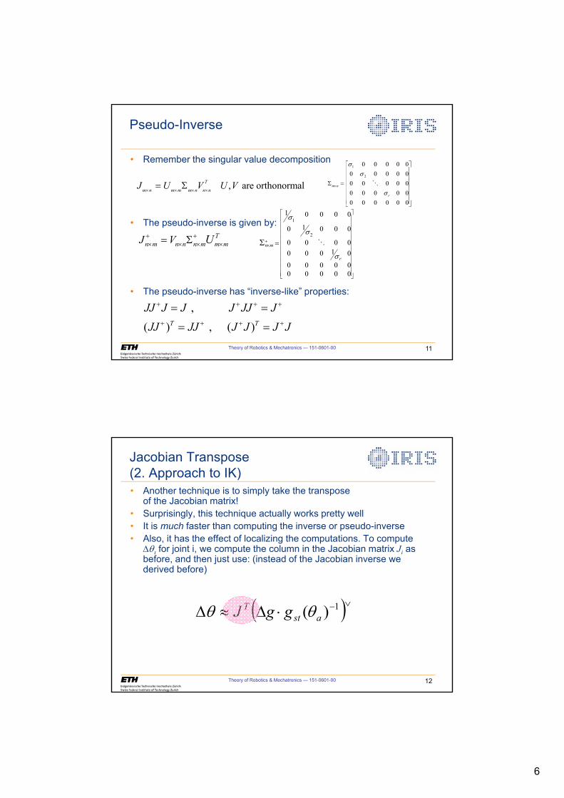
6
Theory of Robotics & Mechatronics — 151-0601-00 11
Pseudo-Inverse
, are orthonormalT
m n m m m n n nJ U V U Vu u u u 6
1
2
0 0 0 0 00 0 0 0 00 0 0 0 00 0 0 0 00 0 0 0 0 0
m n
r
VV
Vu
ª º« »« »« »6 « »« »« »¬ ¼
�
Tn m n n n m m mJ V U� �u u u u 6
1
2
1 0 0 0 0
10 0 0 0
0 0 0 010 0 0 0
0 0 0 0 00 0 0 0 0
n m
r
V
V
V
�u
ª º« »« »« »« »« »« »« »« »« »« »« »¬ ¼
6 �
, ( ) , ( )T T
JJ J J J JJ JJJ JJ J J J J
� � � �
� � � �
• Remember the singular value decomposition
• The pseudo-inverse is given by:
• The pseudo-inverse has “inverse-like” properties:
Theory of Robotics & Mechatronics — 151-0601-00 12
Jacobian Transpose(2. Approach to IK)• Another technique is to simply take the transpose
of the Jacobian matrix!• Surprisingly, this technique actually works pretty well• It is much faster than computing the inverse or pseudo-inverse• Also, it has the effect of localizing the computations. To compute
'TL for joint i, we compute the column in the Jacobian matrix Ji as before, and then just use: (instead of the Jacobian inverse we derived before)
� ����'|' 1)( astT ggJ TT
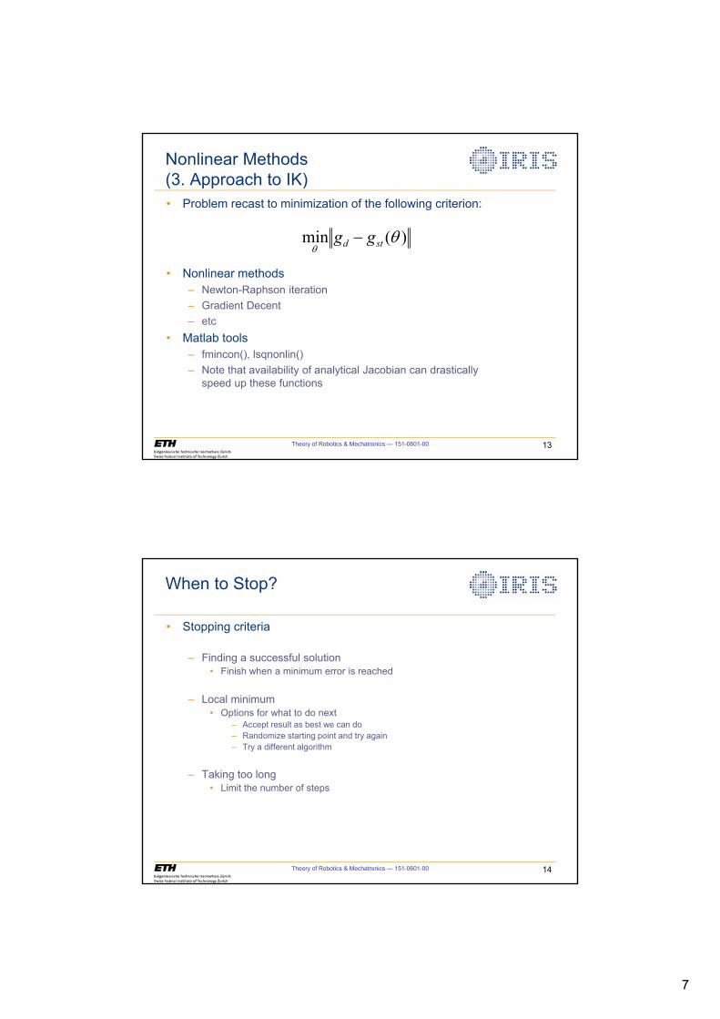
7
Theory of Robotics & Mechatronics — 151-0601-00 13
Nonlinear Methods(3. Approach to IK)• Problem recast to minimization of the following criterion:
• Nonlinear methods– Newton-Raphson iteration– Gradient Decent– etc
• Matlab tools– fmincon(), lsqnonlin()– Note that availability of analytical Jacobian can drastically
speed up these functions
)(min TT std gg �
Theory of Robotics & Mechatronics — 151-0601-00 14
When to Stop?
• Stopping criteria
– Finding a successful solution• Finish when a minimum error is reached
– Local minimum• Options for what to do next
– Accept result as best we can do– Randomize starting point and try again– Try a different algorithm
– Taking too long• Limit the number of steps
8
Theory of Robotics & Mechatronics — 151-0601-00 15
Units & Scaling(Potential numerical problems)• Rotational DOFs use radians and translational DOFs use
meters
• Can we combine their derivatives into the same matrix?
• If desired, we can scale any column (weighting factors) to adjust how much the numerical method will favorusing that DOF
Theory of Robotics & Mechatronics — 151-0601-00 16
Calibration
• Problem:– Due to manufacturing tolerances, a real robot does not exactly
match that of its model.– Thus, all forward and inverse kinematics calculated with these
models will contain inaccuracies• Goal:
– Can we calibrate our manipulator such that these inaccuracies will be minimized?
• How:– Move the robot to a variety of poses and collect truth values of
where the end effector actually is for each joint value– Use these values to correct the model
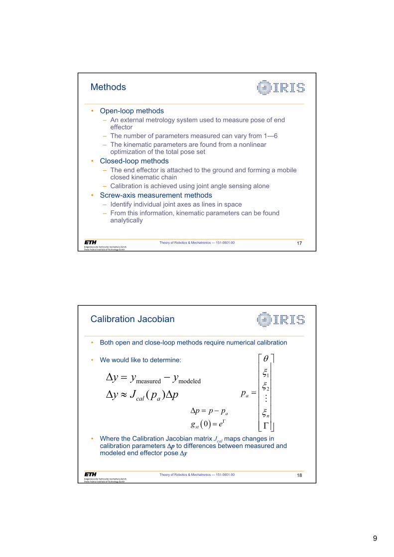
9
Theory of Robotics & Mechatronics — 151-0601-00 17
Methods
• Open-loop methods– An external metrology system used to measure pose of end
effector– The number of parameters measured can vary from 1—6– The kinematic parameters are found from a nonlinear
optimization of the total pose set• Closed-loop methods
– The end effector is attached to the ground and forming a mobile closed kinematic chain
– Calibration is achieved using joint angle sensing alone• Screw-axis measurement methods
– Identify individual joint axes as lines in space– From this information, kinematic parameters can be found
analytically
Theory of Robotics & Mechatronics — 151-0601-00 18
Calibration Jacobian
• Both open and close-loop methods require numerical calibration
• We would like to determine:
• Where the Calibration Jacobian matrix Jcal maps changes in calibration parameters 'p to differences between measured and modeled end effector pose 'y
measured modeled
( )cal a
y y yy J p p
' �
' | '
1
2a
n
p
T[[
[
ª º« »« »« »
« »« »« »« »*« »¬ ¼
�
� �0a
st
p p pg e*
' �
10
Theory of Robotics & Mechatronics — 151-0601-00 19
Calibration Jacobian
• After a long derivation:
• Now, we can use the same methods as for calculating inverse kinematics
� � � �� �
� � � �> @
11ˆ ˆ
0 0
1ˆ
0 0
1 2 3
0
| | | | |
i i i i
i i
ks
k ki
st
ns
Mi
cal n M
Q Ad e Ad e ds
g e
Q Ad e Ad e ds
J J Q Q Q Q Q
[ T [ T
[ T
T�
*
*
§ · ¨ ¸© ¹
§ · ¨ ¸© ¹
� ³
� ³�
Theory of Robotics & Mechatronics — 151-0601-00 20
Conclusions
• Numerical methods can generally help solve a variety of kinematic problems
• Important points– Speed,– Accuracy,– Robustness,– Convergence rate– Units

11
Theory of Robotics & Mechatronics — 151-0601-00 21
References
• K. Okamura and F. C. Park, Kinematic Calibration Using the Product of Exponentials Formula, Robotica, 1995.
• J. M. Hollerbach and C. W. Wampler, The Calibration Index and Taxonomy for Robotic Kinematic Calibration Methods , The International Journal of Robotics Research, 1996.
1
Dynamics
Institute of Robotics and Intelligent SystemsETH Zurich
Theory of Robotics &Mechatronics
Theory of Robotics & Mechatronics — 151-0601-00 2
Robot Dynamics
• “ Given a robot’s joint angles, velocities, accelerations and inertial properties, what are the loads on the actuators? ”
• We will learn two methods– The Newton-Euler Method– The Lagrangian Method
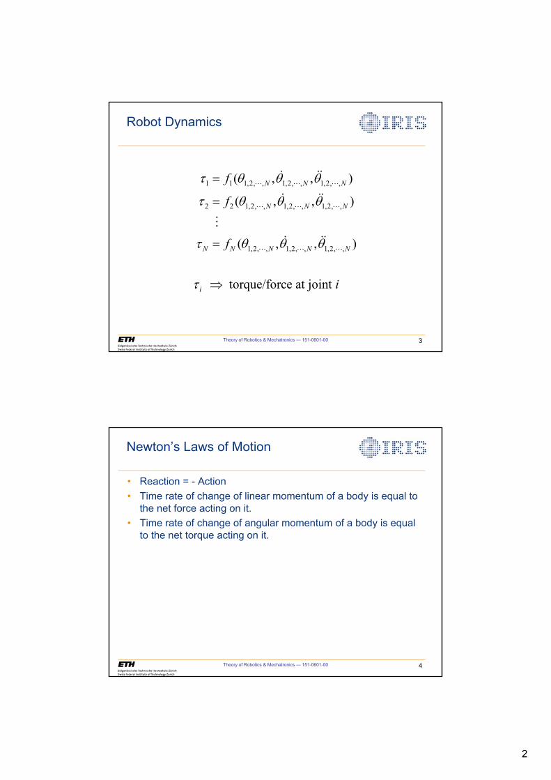
2
Theory of Robotics & Mechatronics — 151-0601-00 3
Robot Dynamics
1 1 1,2, , 1,2, , 1,2, ,
2 2 1,2, , 1,2, , 1,2, ,
1,2, , 1,2, , 1,2, ,
( , , )
( , , )
( , , )
torque/force at joint
N N N
N N N
N N N N N
i
f
f
f
i
W T T T
W T T T
W T T T
W
�
� � �
� � �
� � �
� ��
� ��
�
� ��
Theory of Robotics & Mechatronics — 151-0601-00 4
Newton’s Laws of Motion
• Reaction = - Action• Time rate of change of linear momentum of a body is equal to
the net force acting on it.• Time rate of change of angular momentum of a body is equal
to the net torque acting on it.
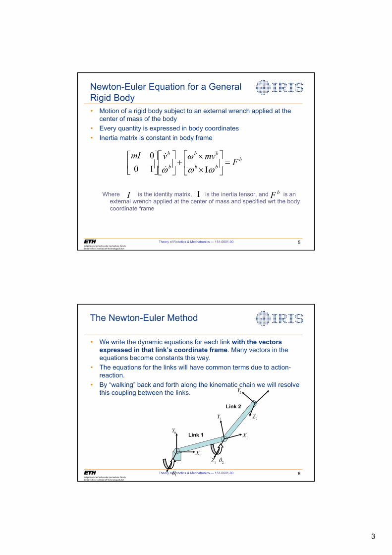
3
Theory of Robotics & Mechatronics — 151-0601-00 5
Newton-Euler Equation for a General Rigid Body• Motion of a rigid body subject to an external wrench applied at the
center of mass of the body• Every quantity is expressed in body coordinates• Inertia matrix is constant in body frame
Where is the identity matrix, is the inertia tensor, and is an external wrench applied at the center of mass and specified wrt the body coordinate frame
I
bbb
bb
b
b
FmvvmI
»¼
º«¬
ª
,uu
�»¼
º«¬
ª»¼
º«¬
ª, ZZ
ZZ��
00
, bF
Theory of Robotics & Mechatronics — 151-0601-00 6
The Newton-Euler Method
• We write the dynamic equations for each link with the vectors expressed in that link’s coordinate frame. Many vectors in the equations become constants this way.
• The equations for the links will have common terms due to action-reaction.
• By “walking” back and forth along the kinematic chain we will resolve this coupling between the links.
1Z
1T�
2T�
2Z
0X
0Y1X
1Y
2Y
Link 1
Link 2
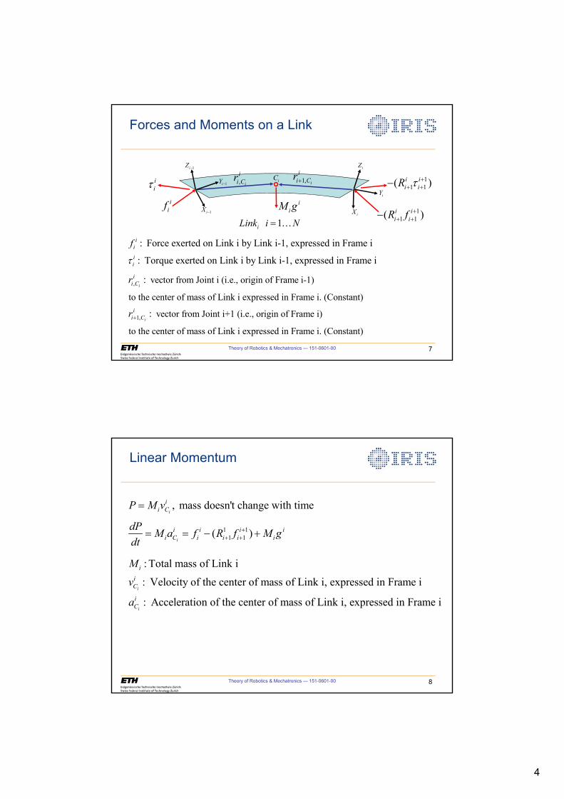
4
Theory of Robotics & Mechatronics — 151-0601-00 7
Forces and Moments on a Link
iiW
iif
11 1( )i i
i iR W �� ��
1iZ �
1iY �
1iX �
iZ
iY
iX
: Force exerted on Link i by Link i-1, expressed in Frame iiif
1iLink i N �
, i
ii Cr 1, i
ii Cr�
, vector from Joint i (i.e., origin of Frame i-1)
to the center of mass of Link i expressed in Frame i. (Constant)
: i
ii Cr
iC
iiM g
: Torque exerted on Link i by Link i-1, expressed in Frame iiiW
1, vector from Joint i+1 (i.e., origin of Frame i)
to the center of mass of Link i expressed in Frame i. (Constant)
: i
ii Cr�
11 1( )i i
i iR f �� ��
Theory of Robotics & Mechatronics — 151-0601-00 8
Linear Momentum
, mass doesn't change with timei
ii CP M v
1 11 1( )
i
i i i ii C i i i i
dP M a f R f M gdt
�� � � �
: Total mass of Link i
: Velocity of the center of mass of Link i, expressed in Frame i
: Acceleration of the center of mass of Link i, expressed in Frame ii
i
i
iC
iC
M
v
a
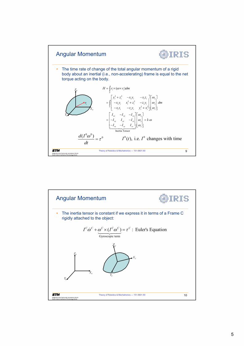
5
Theory of Robotics & Mechatronics — 151-0601-00 9
Angular Momentum
0X
0Z
0Y
ir
2 2
2 2
2 2
Inertia Tensor
( )
I
i iV
i i i i i i x
i i i i i i yV
i i i i i i z
xx xy xz x
xy yy zy y
xz zy zz z
H r r dm
y z x y x zx y x z z y dmx z z y y x
I I II I II I I
Z
ZZZ
ZZ ZZ
u u
ª º� � � ª º« » « » � � �« » « »« » « »� � � ¬ ¼¬ ¼
ª º� � ª º« » « » � � �« » « »« » « »� � ¬ ¼¬ ¼
³
³
�������
0 00( )d I
dtZ W 0 0( ), i.e. changes with timeI t I
• The time rate of change of the total angular momentum of a rigid body about an inertial (i.e., non-accelerating) frame is equal to the net torque acting on the body.
Theory of Robotics & Mechatronics — 151-0601-00 10
Angular Momentum
CX
CZ
CY
Gyroscopic term
( ) : Euler's EquationC C C C C CI IZ Z Z W� u ����
0X
0Z
0Y
• The inertia tensor is constant if we express it in terms of a Frame C rigidly attached to the object:
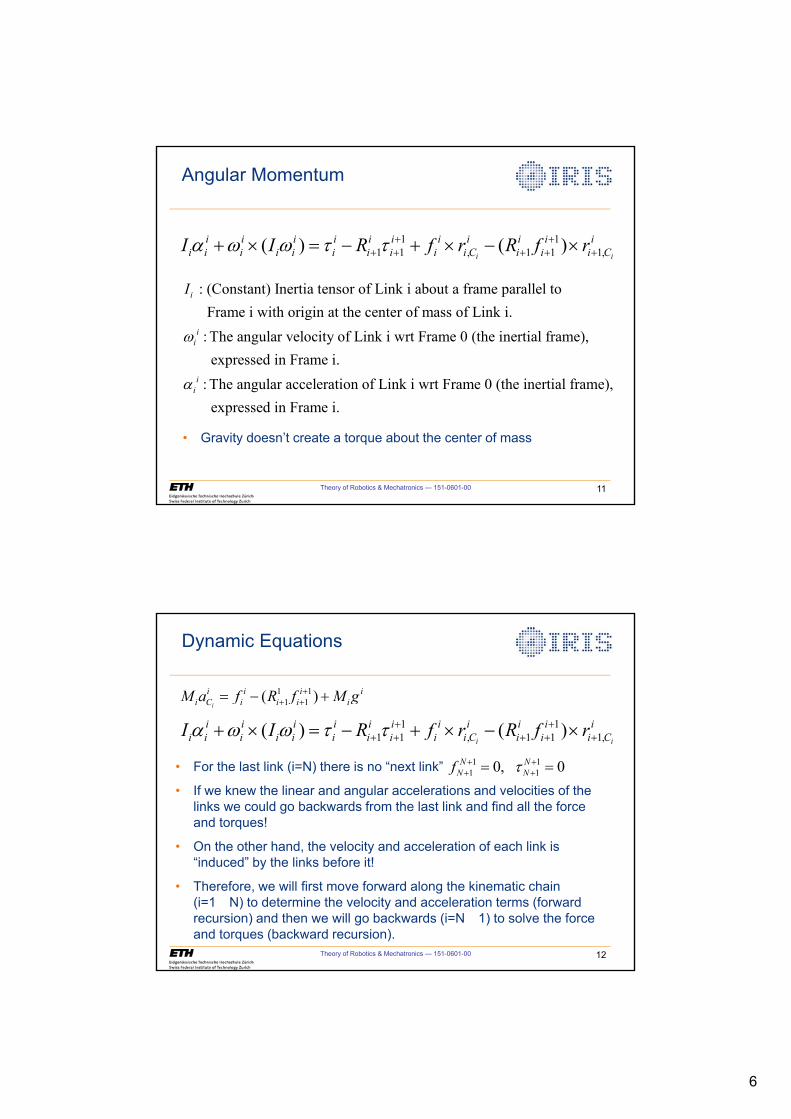
6
Theory of Robotics & Mechatronics — 151-0601-00 11
Angular Momentum
: (Constant) Inertia tensor of Link i about a frame parallel to Frame i with origin at the center of mass of Link i.
: The angular velocity of Link i wrt Frame 0 (the inertial frame),
i
ii
I
Zexpressed in Frame i.
: The angular acceleration of Link i wrt Frame 0 (the inertial frame), expressed in Frame i.
iiD
1 11 1 , 1 1 1,( ) ( )
i i
i i i i i i i i i i ii i i i i i i i i i C i i i CI I R f r R f rD Z Z W W � �
� � � � �� u � � u � u
• Gravity doesn’t create a torque about the center of mass
Theory of Robotics & Mechatronics — 151-0601-00 12
Dynamic Equations
1 11 1 , 1 1 1,( ) ( )
i i
i i i i i i i i i i ii i i i i i i i i i C i i i CI I R f r R f rD Z Z W W � �
� � � � �� u � � u � u
1 11 1( )
i
i i i ii C i i i iM a f R f M g�
� � � �
1 11 10, 0N N
N Nf W� �� � • For the last link (i=N) there is no “next link”
• If we knew the linear and angular accelerations and velocities of the links we could go backwards from the last link and find all the force and torques!
• On the other hand, the velocity and acceleration of each link is “induced” by the links before it!
• Therefore, we will first move forward along the kinematic chain (i=1 N) to determine the velocity and acceleration terms (forward recursion) and then we will go backwards (i=N 1) to solve the force and torques (backward recursion).
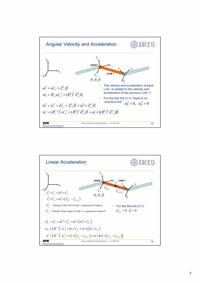
7
Theory of Robotics & Mechatronics — 151-0601-00 13
Angular Velocity and Acceleration
0X
0Y
0Z
iZ
iY iXLink i
1iZ �
, ,i i iT T T� ��
1iX �
1iY �
Joint i
0 0 01 1
1 0 01 1 1( )
i i i i
i i i Ti i i i i i
Z
R R Z
Z Z T
Z Z T� �
�� � �
�
�
�
�
0 0 0 0 0 01 1 1
1 1 0 0 0 01 1 1( ) ( ) [( ) ]
i i i i i i i i
i i T i T i Ti i i i i i i i i i
Z Z
R R Z R Z
Z D Z T Z T
D D T Z T� � �
� �� � �
� � u
� � u
�� �� �
�� �
0 00 00, 0Z D
• The velocity and acceleration of each Link i is related to the velocity and acceleration of the previous Link i-1
• For the first link (i=1), there is no “previous link”
Theory of Robotics & Mechatronics — 151-0601-00 14
Linear Acceleration
0X
0Y
0Z
iZ
iY iXLink i
1iZ �
, ,i i iT T T� ��
1iX �
1iY �
Joint iiC
� �0 0 0 0
1 ,
0 0 0 0 01 , 1,
0
01
0 0 0 0 0 01 ,
Velocity of the CM of Link i, expressed in Frame 0
Velocity of the origin of Link i-1, expressed in Frame 0
=
=
:
:
i i
i i
i
i i
C i i i C
i i i i C i C
C
i
C i i i C i i
v v r
v v r r
v
v
a a r r
Z
Z
Z Z Z
�
� �
�
�
� u
� u �
� u � u u� � �� � � �� � � � � �� �
0,
1 11 , ,
1 11 , 1, , 1,
i
i i i
i i i i i
i C
Ti i i i i i i iC i i i i C i i i C
Ti i i i i i i i i ii i i i C i C i i i C i C
a R a r r
a R a r r r r
Z Z Z
Z Z Z
� ��
� �� � �
� u � u u
� u � � u u �
�
�
, i
ii Cr
1, i
ii Cr�
• For the first link (i=1)
0
0 00, 00, 0Ca a
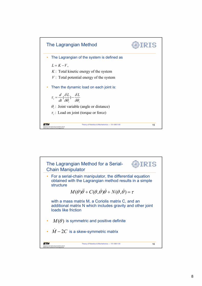
8
Theory of Robotics & Mechatronics — 151-0601-00 15
The Lagrangian Method
• The Lagrangian of the system is defined as
, : Total kinetic energy of the system: Total potential energy of the system
L K VKV
�
• Then the dynamic load on each joint is:
( )
: Joint variable (angle or distance): Load on joint (torque or force)
ii i
i
i
d L Ldt
G GWGT GT
TW
��
Theory of Robotics & Mechatronics — 151-0601-00 16
The Lagrangian Method for a Serial-Chain Manipulator• For a serial-chain manipulator, the differential equation
obtained with the Lagrangian method results in a simple structure
with a mass matrix M, a Coriolis matrix C, and an additional matrix N which includes gravity and other joint loads like friction
• is symmetric and positive definite
• is a skew-symmetric matrix
WTTTTTTT �� ),(),()( ����� NCM
)(TM
CM 2��
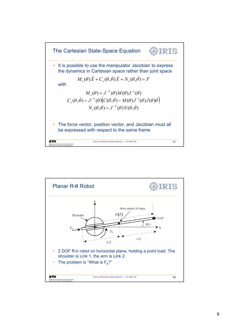
9
Theory of Robotics & Mechatronics — 151-0601-00 17
The Cartesian State-Space Equation
• It is possible to use the manipulator Jacobian to express the dynamics in Cartesian space rather than joint space
with
• The force vector, position vector, and Jacobian must all be expressed with respect to the same frame
FNXCXM xxx �� ),(),()( TTTTT �����
� �),()(),(
)()()(),()(),()()()()(
1
1
TTTTTTTTTTTTTT
TTTT
��
����
NJNJJMCJC
JMJM
Tx
Tx
Tx
�
��
��
�
Theory of Robotics & Mechatronics — 151-0601-00 18
Planar R-T Robot
• 2 DOF R-T robot on horizontal plane, holding a point load. The shoulder is Link 1, the arm is Link 2.
• The problem is “What is FA?”
( )r t
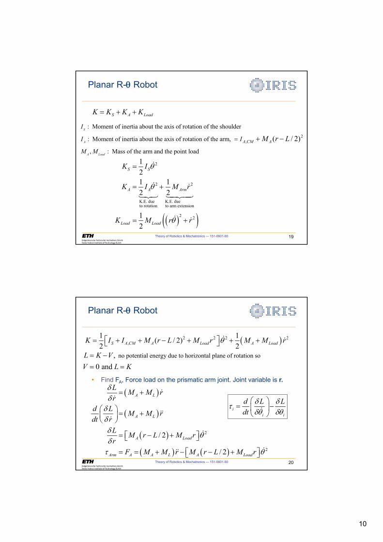
10
Theory of Robotics & Mechatronics — 151-0601-00 19
Planar R-T Robot
S A LoadK K K K � �
2,
: Moment of inertia about the axis of rotation of the shoulder
: Moment of inertia about the axis of rotation of the arm,
, : Mass of the arm and the point load
( / 2)S
A
A Load
A CM A
I
I I
M M
M r L � �
� �� �
2
2 2
K.E. due K.E. dueto rotation to arm extension
2 2
121 12 2
12
S S
A A Arm
Load Load
K I
K I M r
K M r r
T
T
T
�
�
�
� �� ���
� �
Theory of Robotics & Mechatronics — 151-0601-00 20
Planar R-T Robot
� �2 2 2 2,
1 1( / 2)
2 2S A CM A Load A LoadK I I M r L M r M M rTª º � � � � � �¬ ¼� �
no potential energy due to horizontal plane of rotation so, 0 and
L K VV L K �
� �
� �
� �
� � � �
2
2
/ 2
/ 2
A L
A L
A Load
Arm A A L A Load
L M M rr
d L M M rdt r
L M r L M rr
F M M r M r L M r
GG
GGG TGW T
�
§ · �¨ ¸© ¹
� �ª º¬ ¼
� � � �ª º¬ ¼
��
���
�
���
• Find FA, Force load on the prismatic arm joint. Joint variable is r.
ii i
d L Ldt
G GWGT GT§ ·
�¨ ¸© ¹�
11
Theory of Robotics & Mechatronics — 151-0601-00 21
Friction: A Parasitic Force in Robotics
• The accuracy of dynamic models are always limited by friction. Friction also limits robot precision.
• A papers of interest:– B. Armstrong-Helouvry, P. Dupont, and C. Canudas de Wit, “A
Survey of Models, Analysis Tools and Compensation Methods for the Control of Machines with Friction,” Automatica, vol. 30, no. 7, pp. 1083-1138, 1994.
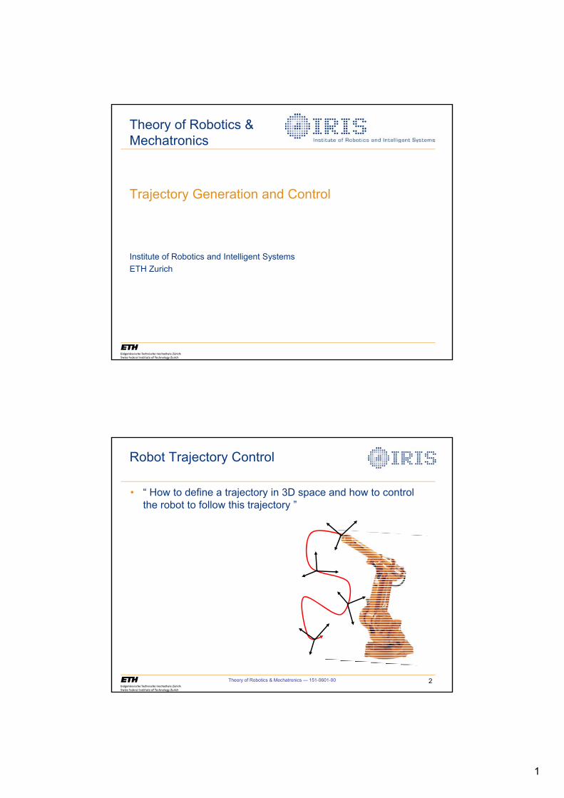
1
Trajectory Generation and Control
Institute of Robotics and Intelligent SystemsETH Zurich
Theory of Robotics &Mechatronics
Theory of Robotics & Mechatronics — 151-0601-00 2
Robot Trajectory Control
• “ How to define a trajectory in 3D space and how to control the robot to follow this trajectory ”
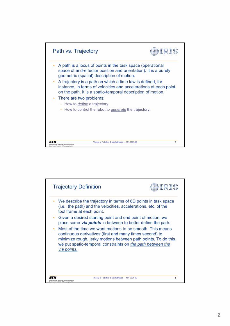
2
Theory of Robotics & Mechatronics — 151-0601-00 3
Path vs. Trajectory
• A path is a locus of points in the task space (operational space of end-effector position and orientation). It is a purely geometric (spatial) description of motion.
• A trajectory is a path on which a time law is defined, for instance, in terms of velocities and accelerations at each point on the path. It is a spatio-temporal description of motion.
• There are two problems:– How to define a trajectory.– How to control the robot to generate the trajectory.
Theory of Robotics & Mechatronics — 151-0601-00 4
Trajectory Definition
• We describe the trajectory in terms of 6D points in task space (i.e., the path) and the velocities, accelerations, etc. of the tool frame at each point.
• Given a desired starting point and end point of motion, we place some via points in between to better define the path.
• Most of the time we want motions to be smooth. This means continuous derivatives (first and many times second) to minimize rough, jerky motions between path points. To do this we put spatio-temporal constraints on the path between the via points.
3
Theory of Robotics & Mechatronics — 151-0601-00 5
Joint Space vs. Task Space Trajectories
• Using inverse kinematics we can convert from task space to joint space. The path points can be written in terms of joint variables, describing the trajectory in the joint space.
• Following the joint space trajectory, the end-effector will be at the desired position and orientation at the via points. However, in between the via points the generated path, while simple in joint space, may be complex in task space.
• Joint space trajectory generation is the easiest to compute and inherently avoids any singularities. However, we must make sure there are no obstacles in the resultingCartesian path.
Theory of Robotics & Mechatronics — 151-0601-00 6
Joint Space Trajectory Definition
• Consider the case of point-to-point motion between a start position and an end position. There are many smooth functions that may be used to interpolate the joint values.
0 0( ) , ( )f ft tT T T T • For example, a cubic polynomial function
may be used to add two constraints of velocity to achieve a smooth (in first derivative) function.
3 23 2 1 0
23 2 1
( )
( ) 3 2
t a t a t a t a
t a t a t a
T
T
� � �
� ��4 equations in 4 unknowns
0 0( ) , ( )f ft tT T T T � � � �
4
Theory of Robotics & Mechatronics — 151-0601-00 7
Polynomial Interpolation
5 4 3 25 4 3 2 1 0
4 3 25 4 3 2 1
3 25 4 3 2
( )
( ) 5 4 3 2
( ) 20 12 6 2
t a t a t a t a t a t a
t a t a t a t a t a
t a t a t a t a
T
T
T
� � � � �
� � � �
� � �
�
��
6 equations in 6 unknowns• Increasingly oscillatory path as the order increases
• Position, velocity and acceleration profile of a single cubic segment that starts and ends in rest.
• The desired velocity at each via point may be given by the user in terms of Cartesian (translational and angular) velocities. This definition is then translated to joint space velocities by the inverse Jacobian.
• To add acceleration constraints, we could go up to fifth order (quintic) polynomials.
Theory of Robotics & Mechatronics — 151-0601-00 8
Linear Segments withParabolic Blends (LSPB)• Appropriate for constant velocity point to point moves.• Between the via points, the joint velocity is constant, except at the beginning
and at the end where a quadratic polynomial is applied. • A blend time tb is defined to begin and end the quadratic interpolation.
bt0t f bt t� ft
22 1 0
2 1
2
( )
( ) 2
( ) 2
t a t a t a
t a t a
t a
T
T
T
� �
�
�
��
fT
0T
5
Theory of Robotics & Mechatronics — 151-0601-00 9
Linear Segments withParabolic Blends
bt0t f bt t� ft
fT
0Tht
fT
Half point
b Velocity at t
h bb
h b
tt tT TT �
�
��
�����
, constant acceleration during blendT��
b
20
Position at t
12 b btT T T� ��
�����
0
20 0
2
( ) 0f h
b f b f
t t t
t t t tT T T T
�
� � � � �� ��
2
02
0
0 00 ( ) 4 ( )( )2
4( )( )
2f
f
f
ffb
t tt tt
t t
T T T
T T
T
T
T
� � �
�t
�
� �
�� ��
�
��
�
• Given the joint positions and time at both ends, the blend time and the (constant) acceleration are related.
• Usually an acceleration is chosen and the blending time is computed. We cannot chose the acceleration too low otherwise the blending time will increase and the linear portion will “shrink” to zero.
2
Theory of Robotics & Mechatronics — 151-0601-00 10
Linear Segments withParabolic Blends• Multi-segment (i.e., with via points) linear path with blends.• Want to keep fixed velocity during each segment.
• Does not pass exactly through the via points except at the ends. The higher the acceleration, the closer the path to the exact via points.
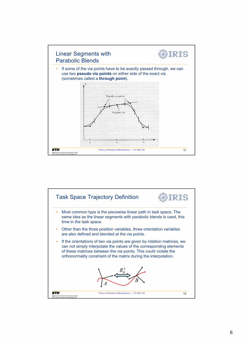
6
Theory of Robotics & Mechatronics — 151-0601-00 11
Linear Segments withParabolic Blends• If some of the via points have to be exactly passed through, we can
use two pseudo via points on either side of the exact via (sometimes called a through point).
Theory of Robotics & Mechatronics — 151-0601-00 12
Task Space Trajectory Definition
ABR
A B
• Most common type is the piecewise linear path in task space. The same idea as the linear segments with parabolic blends is used, this time in the task space.
• Other than the three position variables, three orientation variables are also defined and blended at the via points.
• If the orientations of two via points are given by rotation matrices, we can not simply interpolate the values of the corresponding elements of these matrices between the via points. This could violate the orthonormality constraint of the matrix during the interpolation.
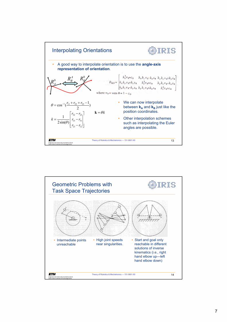
7
Theory of Robotics & Mechatronics — 151-0601-00 13
Interpolating Orientations
ABR
1 11 22 33
32 23
13 31
21 12
1cos ( )
2
12sin( )
r r r
r rk r r
r r
T
T
� � � �
�ª º« » �« »« »�¬ ¼
kT k
0AR
0BR
• A good way to interpolate orientation is to use the angle-axis representation of orientation.
• We can now interpolate between kA and kB just like the position coordinates.
• Other interpolation schemes such as interpolating the Euler angles are possible.
Theory of Robotics & Mechatronics — 151-0601-00 14
Geometric Problems withTask Space Trajectories
• Intermediate pointsunreachable
• High joint speedsnear singularities.
• Start and goal onlyreachable in differentsolutions of inversekinematics (i.e., righthand elbow up—left hand elbow down)
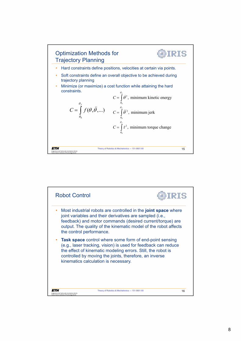
8
Theory of Robotics & Mechatronics — 151-0601-00 15
Optimization Methods forTrajectory Planning
0
( , ,...)f
C fT
T
T T ³ ��0
0
0
2
2
2
, minimum kinetic energy
, minimum jerk
, minimum torque change
f
f
f
C
C
C
T
T
T
T
T
T
T
T
W
³
³
³
�
���
�
• Hard constraints define positions, velocities at certain via points.
• Soft constraints define an overall objective to be achieved during trajectory planning
• Minimize (or maximize) a cost function while attaining the hard constraints.
Theory of Robotics & Mechatronics — 151-0601-00 16
Robot Control
• Most industrial robots are controlled in the joint space where joint variables and their derivatives are sampled (i.e., feedback) and motor commands (desired current/torque) are output. The quality of the kinematic model of the robot affects the control performance.
• Task space control where some form of end-point sensing (e.g., laser tracking, vision) is used for feedback can reduce the effect of kinematic modeling errors. Still, the robot is controlled by moving the joints, therefore, an inverse kinematics calculation is necessary.
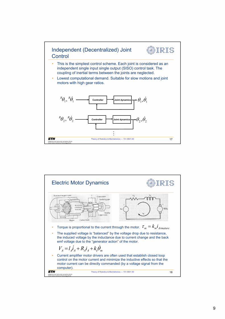
9
Theory of Robotics & Mechatronics — 151-0601-00 17
Independent (Decentralized) Joint Control• This is the simplest control scheme. Each joint is considered as an
independent single input single output (SISO) control task. The coupling of inertial terms between the joints are neglected.
• Lowest computational demand. Suitable for slow motions and joint motors with high gear ratios.
Joint dynamicsController1 1,R RT T� 1 1,T T�
Joint dynamicsController2 2,R RT T� 2 2,T T�
�
Theory of Robotics & Mechatronics — 151-0601-00 18
• Torque is proportional to the current through the motor.
• The supplied voltage is “balanced” by the voltage drop due to resistance, the induced voltage by the inductance due to current change and the back emf voltage due to the “generator action” of the motor.
Electric Motor Dynamics
m m Armaturek iW
A A A A A e mV l i R i k T � � ��
• Current amplifier motor drivers are often used that establish closed loop control on the motor current and minimize the inductive effects so that the motor current can be directly commanded (by a voltage signal from the computer).
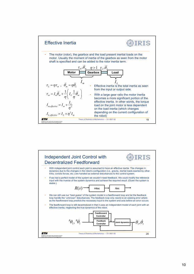
10
Theory of Robotics & Mechatronics — 151-0601-00 19
Effective Inertia
Motor Gearbox Load
mI LI
,m mW T�� ,L LW T��
, 2
2,
,
1 1L m m L
m m m L m
Lm effective m
L effective L m
I I
II I
I I I
W KW T KT
W T TK K
KK
§ · � ¨ ¸
© ¹
�
�
�� ��
�� ��
1K !
• The motor (rotor), the gearbox and the load present inertial loads on the motor. Usually the moment of inertia of the gearbox as seen from the motor shaft is specified and can be added to the rotor inertia term.
• Effective inertia is the total inertia as seen from the input or output side.
• With a large gear ratio the motor inertia becomes a more significant portion of the effective inertia. In other words, the torque load on the joint motor is less dependent on the load inertia (which changes depending on the current configuration of the robot)
Theory of Robotics & Mechatronics — 151-0601-00 20
Independent Joint Control with Decentralized Feedforward
G(s)1/G(s)( )R s
Joint dynamicsFeedbackController1 1,R RT T� 1 1,T T�
FeedforwardController
• With independent joint control each joint is assumed to have an effective inertia. The changes in dynamics due to the changes in the robot’s configuration (i.e., gravity, inertial loads exerted by other links, coriolis forces, etc.) are handled as external disturbances to the control system.
• If we had a perfect model of the system we wouldn’t need feedback. We could modify the reference input with the inverse of the system dynamics and achieve the required result. (Given the system is stable.)
• We can still use our “best guess” of the system model in a feedforward loop and let the feedback loop handle the “unknown” disturbances. The feedback loop only reacts to an existing error where as the feedforward loop predicts the necessary input to the system and acts before an error occurs.
• The feedforward loop is still decentralized in that it uses an independent model of each joint with an effective inertia, neglecting the true dynamics of the robot.
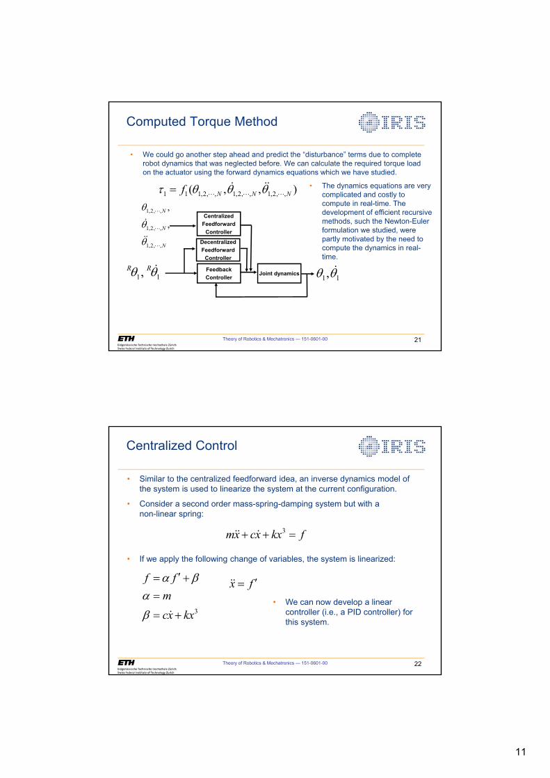
11
Theory of Robotics & Mechatronics — 151-0601-00 21
Computed Torque Method
Joint dynamicsFeedbackController1 1,R RT T� 1 1,T T�
DecentralizedFeedforward
Controller
CentralizedFeedforward
Controller
1 1 1,2, , 1,2, , 1,2, ,( , , )N N NfW T T T � � �� ��
1,2, ,
1,2, ,
1,2, ,
,
,N
N
N
T
T
T
�
�
�
�
��
• We could go another step ahead and predict the “disturbance” terms due to complete robot dynamics that was neglected before. We can calculate the required torque load on the actuator using the forward dynamics equations which we have studied.
• The dynamics equations are very complicated and costly to compute in real-time. The development of efficient recursive methods, such the Newton-Euler formulation we studied, were partly motivated by the need to compute the dynamics in real-time.
Theory of Robotics & Mechatronics — 151-0601-00 22
Centralized Control
3mx cx kx f� � �� �
3
f fm
cx kx
D ED
E
c �
��
x f c ��
• Similar to the centralized feedforward idea, an inverse dynamics model of the system is used to linearize the system at the current configuration.
• Consider a second order mass-spring-damping system but with a non-linear spring:
• If we apply the following change of variables, the system is linearized:
• We can now develop a linear controller (i.e., a PID controller) for this system.
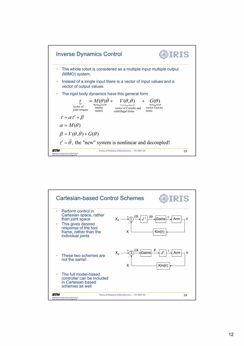
12
Theory of Robotics & Mechatronics — 151-0601-00 23
Inverse Dynamics Control
, , ,vector of Inertia vector Gravity vector of Coriolis andjoint torques matrix termscentrifugal terms
( ) ( , ) ( )M V GW T T T T T � ��� ��
( )
( , ) ( )
, the "new" system is nonlinear and decoupled!
M
V G
W DW ED T
E T T T
W T
c �
�
c
�
��
• The whole robot is considered as a multiple input multiple output (MIMO) system.
• Instead of a single input there is a vector of input values and a vector of output values.
• The rigid body dynamics have this general form
Theory of Robotics & Mechatronics — 151-0601-00 24
Cartesian-based Control Schemes
• Perform control in Cartesian space, rather than joint space
• This gives desired response of the tool frame, rather than the individual joints
• These two schemes are not the same!
• The full model-based controller can be included in Cartesian-based schemes as well
Xd
X Kin(T)
TArmWGX�B6
Xd
X Kin(T)
TArmWGX�B6
J-1 GT Gains
JTGains F
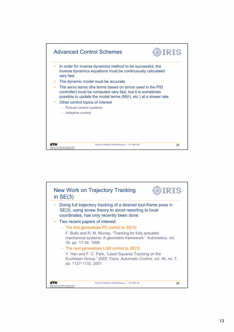
13
Theory of Robotics & Mechatronics — 151-0601-00 25
Advanced Control Schemes
• In order for inverse dynamics method to be successful, the inverse dynamics equations must be continuously calculated very fast.
• The dynamic model must be accurate.• The servo terms (the terms based on errors used in the PID
controller) must be computed very fast, but it is sometimes possible to update the model terms (M(T), etc.) at a slower rate
• Other control topics of interest– Robust control systems– Adaptive control
Theory of Robotics & Mechatronics — 151-0601-00 26
New Work on Trajectory Tracking in SE(3)• Doing full trajectory tracking of a desired tool-frame pose in
SE(3), using screw theory to avoid resorting to local coordinates, has only recently been done
• Two recent papers of interest:– The first generalizes PD control to SE(3):
F. Bullo and R. M. Murray, “Tracking for fully actuated mechanical systems: A geometric framework,” Automatica, vol. 35, pp. 17-34, 1999.
– The next generalizes LQR control to SE(3):Y. Han and F. C. Park, “Least Squares Tracking on the Euclidean Group,” IEEE Trans. Automatic Control, vol. 46, no. 7, pp. 1127-1132, 2001.

1
Force Control and Haptics
Institute of Robotics and Intelligent SystemsETH Zurich
Theory of Robotics &Mechatronics
Theory of Robotics & Mechatronics — 151-0601-00 2
Contact Tasks
• Mechanical part mating (assembly)• Contour Tracking• Machining
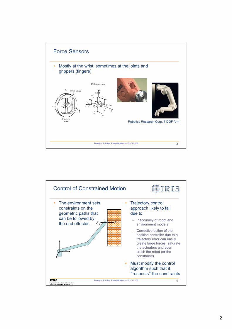
2
Theory of Robotics & Mechatronics — 151-0601-00 3
Force Sensors
• Mostly at the wrist, sometimes at the joints andgrippers (fingers)
Robotics Research Corp. 7 DOF Arm
Theory of Robotics & Mechatronics — 151-0601-00 4
Control of Constrained Motion
FRF
• The environment sets constraints on the geometric paths that can be followed by the end effector.
• Trajectory control approach likely to faildue to:– Inaccuracy of robot and
environment models
– Corrective action of the position controller due to a trajectory error can easily create large forces, saturate the actuators and even crash the robot (or the constraint!)
• Must modify the control algorithm such that it “respects” the constraints
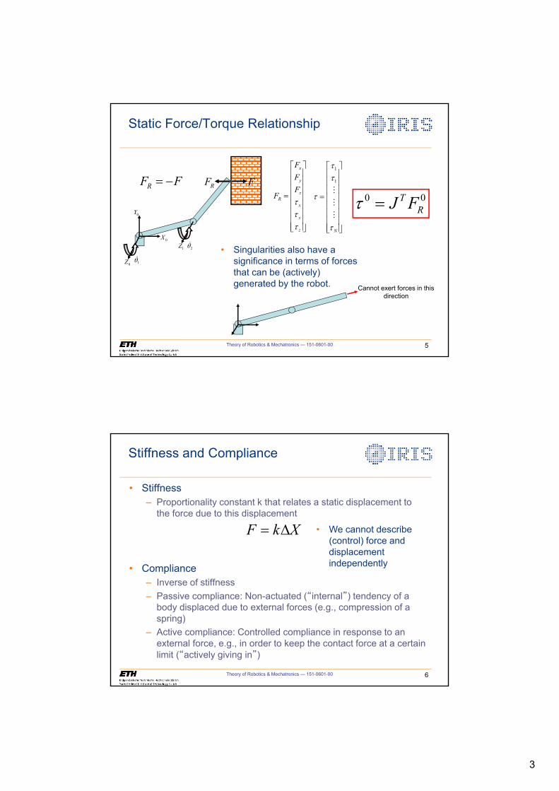
3
Theory of Robotics & Mechatronics — 151-0601-00 5
Static Force/Torque Relationship
0Z
1Z
1T�
2T�0X
0Y
x
y
zR
x
y
z
FFF
FWWW
ª º« »« »« »
« »« »« »« »« »¬ ¼
RF F �0 0T
RJ FW FRF
1
1
N
WW
W
W
ª º« »« »« »
« »« »« »« »« »¬ ¼
�
�
�
Cannot exert forces in this direction
• Singularities also have a significance in terms of forces that can be (actively) generated by the robot.
Theory of Robotics & Mechatronics — 151-0601-00 6
• Stiffness– Proportionality constant k that relates a static displacement to
the force due to this displacement
• Compliance– Inverse of stiffness– Passive compliance: Non-actuated (“internal”) tendency of a
body displaced due to external forces (e.g., compression of a spring)
– Active compliance: Controlled compliance in response to an external force, e.g., in order to keep the contact force at a certain limit (“actively giving in”)
Stiffness and Compliance
F k X ' • We cannot describe (control) force and displacement independently
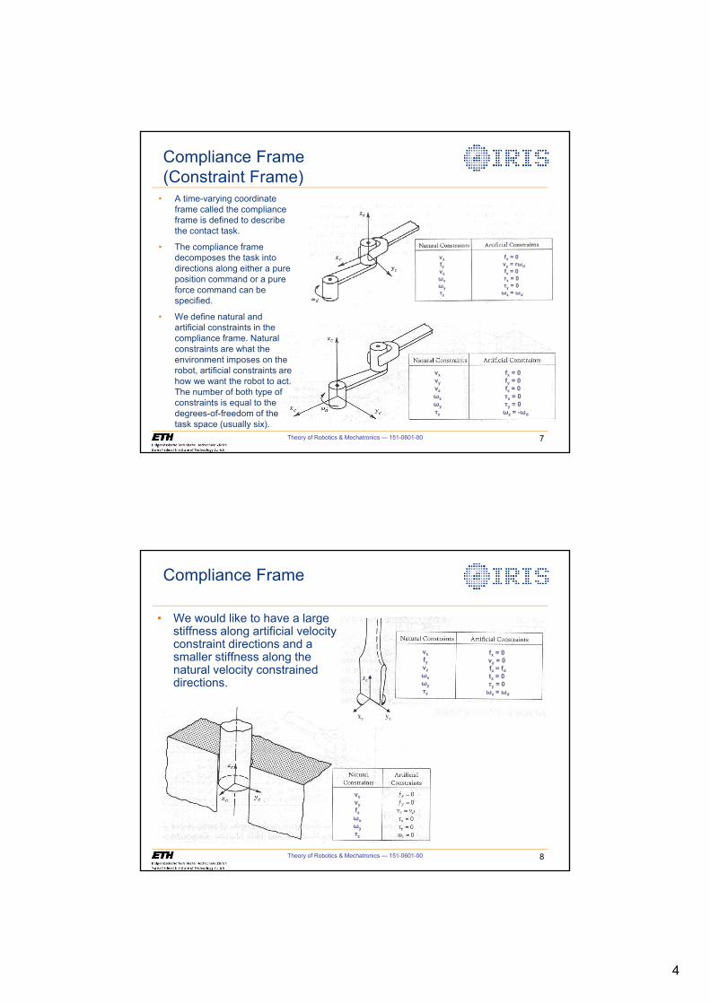
4
Theory of Robotics & Mechatronics — 151-0601-00 7
Compliance Frame(Constraint Frame)
Compliance frame defined at the end effector
Compliance frame defined at the axis of rotation of the crank
• A time-varying coordinate frame called the compliance frame is defined to describe the contact task.
• The compliance frame decomposes the task into directions along either a pure position command or a pure force command can be specified.
• We define natural and artificial constraints in the compliance frame. Natural constraints are what the environment imposes on the robot, artificial constraints are how we want the robot to act. The number of both type of constraints is equal to the degrees-of-freedom of the task space (usually six).
fx = 0vy = rωdfz = 0τx = 0τy = 0ωz = ωd
fx = 0fy = 0fz = 0τx = 0τy = 0ωz = -ωd
vxvyvzωxωyτz
vxfyvzωxωyτz
Theory of Robotics & Mechatronics — 151-0601-00 8
Compliance Frame
• We would like to have a large stiffness along artificial velocity constraint directions and a smaller stiffness along the natural velocity constrained directions.
vxfyvzωxωyτz
fx = 0vy = 0fz = fdtx = 0τy = 0ωz = ωd
yc
zc
xc
vxvyfzωxωyτz
5
Peg in Hole
Theory of Robotics & Mechatronics — 151-0601-00 9
z
Theory of Robotics & Mechatronics — 151-0601-00 10
Passive Compliance
• Center of compliance is the point on the tool where a force at that point creates a pure translation and a moment creates a pure rotation about that point.
• Remote Center Compliance (RCC) devices place the center of compliance at the tip of the tool with variable different stiffness along different directions of the compliance frame.
• High stiffness for translations along the vertical axis.
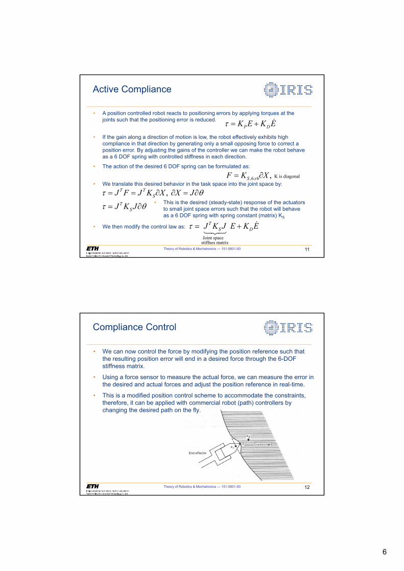
6
Theory of Robotics & Mechatronics — 151-0601-00 11
Active Compliance
P DK E K EW � �
,6 6 K is diagonal ,S xF K X w
, T TS
TS
J F J K X X J
J K J
W T
W T
w w w
w
Joint spacestiffnes matrix
TS DJ K J E K EW � �
�
• A position controlled robot reacts to positioning errors by applying torques at the joints such that the positioning error is reduced.
• If the gain along a direction of motion is low, the robot effectively exhibits high compliance in that direction by generating only a small opposing force to correct a position error. By adjusting the gains of the controller we can make the robot behave as a 6 DOF spring with controlled stiffness in each direction.
• The action of the desired 6 DOF spring can be formulated as:
• We translate this desired behavior in the task space into the joint space by:
• This is the desired (steady-state) response of the actuators to small joint space errors such that the robot will behave as a 6 DOF spring with spring constant (matrix) KS
• We then modify the control law as:
Theory of Robotics & Mechatronics — 151-0601-00 12
Compliance Control
• We can now control the force by modifying the position reference such that the resulting position error will end in a desired force through the 6-DOF stiffness matrix.
• Using a force sensor to measure the actual force, we can measure the error in the desired and actual forces and adjust the position reference in real-time.
• This is a modified position control scheme to accommodate the constraints, therefore, it can be applied with commercial robot (path) controllers by changing the desired path on the fly.
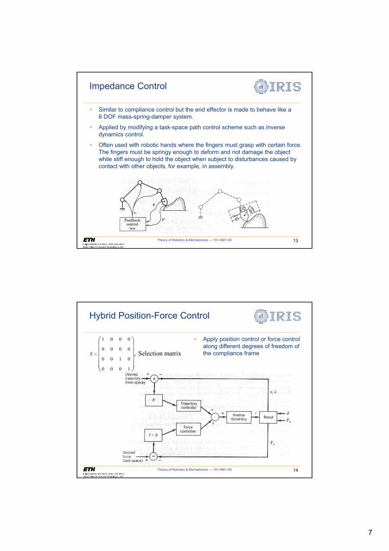
7
Theory of Robotics & Mechatronics — 151-0601-00 13
Impedance Control
• Similar to compliance control but the end effector is made to behave like a6 DOF mass-spring-damper system.
• Applied by modifying a task-space path control scheme such as inverse dynamics control.
• Often used with robotic hands where the fingers must grasp with certain force. The fingers must be springy enough to deform and not damage the object while stiff enough to hold the object when subject to disturbances caused by contact with other objects, for example, in assembly.
Theory of Robotics & Mechatronics — 151-0601-00 14
Hybrid Position-Force Control
• Apply position control or force control along different degrees of freedom of the compliance frame
1 0 0 0
0 0 0 0
0 0 1 0
0 0 0 1
, Selection matrixS
§ ·¨ ¸¨ ¸¨ ¸¨ ¸© ¹
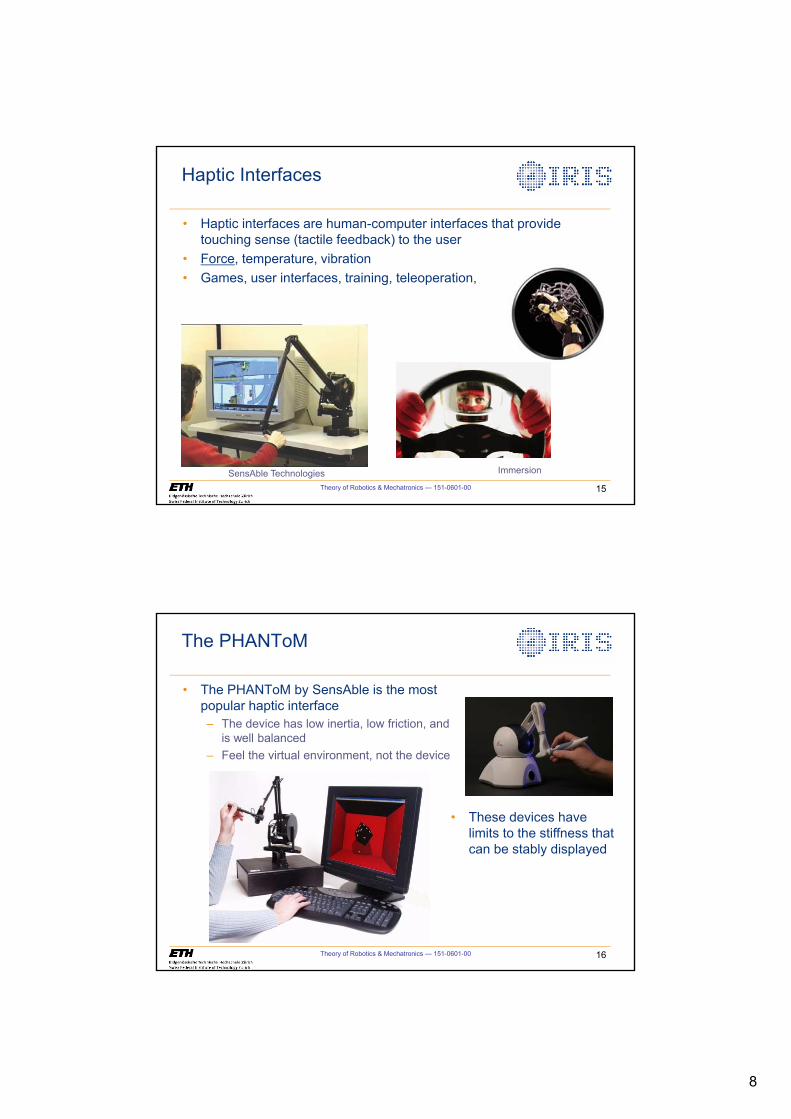
8
Theory of Robotics & Mechatronics — 151-0601-00 15
Haptic Interfaces
• Haptic interfaces are human-computer interfaces that provide touching sense (tactile feedback) to the user
• Force, temperature, vibration• Games, user interfaces, training, teleoperation,
SensAble Technologies Immersion
Theory of Robotics & Mechatronics — 151-0601-00 16
The PHANToM
• The PHANToM by SensAble is the most popular haptic interface– The device has low inertia, low friction, and
is well balanced– Feel the virtual environment, not the device
• These devices have limits to the stiffness that can be stably displayed
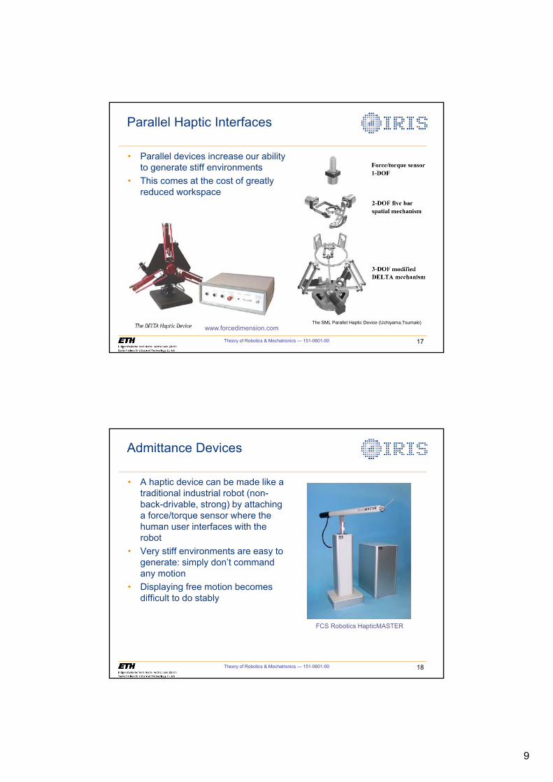
9
Theory of Robotics & Mechatronics — 151-0601-00 17
Parallel Haptic Interfaces
• Parallel devices increase our ability to generate stiff environments
• This comes at the cost of greatly reduced workspace
www.forcedimension.comThe SML Parallel Haptic Device (Uchiyama,Tsumaki)
Theory of Robotics & Mechatronics — 151-0601-00 18
Admittance Devices
• A haptic device can be made like a traditional industrial robot (non-back-drivable, strong) by attaching a force/torque sensor where the human user interfaces with the robot
• Very stiff environments are easy to generate: simply don’t command any motion
• Displaying free motion becomes difficult to do stably
FCS Robotics HapticMASTER
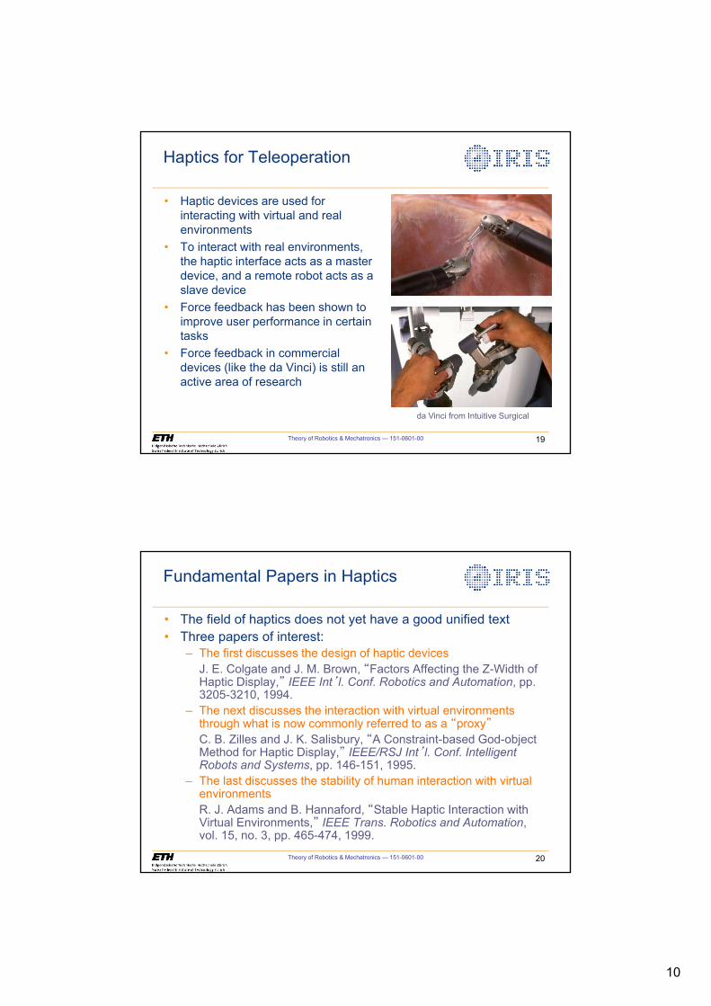
10
Theory of Robotics & Mechatronics — 151-0601-00 19
Haptics for Teleoperation
• Haptic devices are used for interacting with virtual and real environments
• To interact with real environments, the haptic interface acts as a master device, and a remote robot acts as a slave device
• Force feedback has been shown to improve user performance in certain tasks
• Force feedback in commercial devices (like the da Vinci) is still an active area of research
da Vinci from Intuitive Surgical
Theory of Robotics & Mechatronics — 151-0601-00 20
Fundamental Papers in Haptics
• The field of haptics does not yet have a good unified text• Three papers of interest:
– The first discusses the design of haptic devicesJ. E. Colgate and J. M. Brown, “Factors Affecting the Z-Width of Haptic Display,” IEEE Int’l. Conf. Robotics and Automation, pp. 3205-3210, 1994.
– The next discusses the interaction with virtual environments through what is now commonly referred to as a “proxy”C. B. Zilles and J. K. Salisbury, “A Constraint-based God-object Method for Haptic Display,” IEEE/RSJ Int’l. Conf. Intelligent Robots and Systems, pp. 146-151, 1995.
– The last discusses the stability of human interaction with virtual environmentsR. J. Adams and B. Hannaford, “Stable Haptic Interaction with Virtual Environments,” IEEE Trans. Robotics and Automation, vol. 15, no. 3, pp. 465-474, 1999.
1
Introduction to Computer Vision
Institute of Robotics and Intelligent Systems
ETH Zurich
Theory of Robotics &
Mechatronics
Theory of Robotics & Mechatronics — 151-0601-00 2
The Three Pillars of Robotics
Manipulation
Perception
Cognition
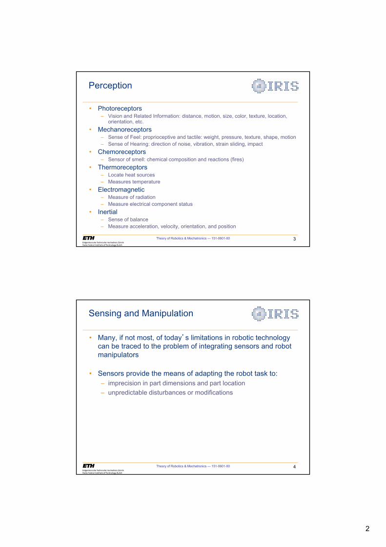
2
Theory of Robotics & Mechatronics — 151-0601-00 3
Perception
• Photoreceptors
– Vision and Related Information: distance, motion, size, color, texture, location,
orientation, etc.
• Mechanoreceptors
– Sense of Feel: proprioceptive and tactile: weight, pressure, texture, shape, motion
– Sense of Hearing: direction of noise, vibration, strain sliding, impact
• Chemoreceptors
– Sensor of smell: chemical composition and reactions (fires)
• Thermoreceptors
– Locate heat sources
– Measures temperature
• Electromagnetic
– Measure of radiation
– Measure electrical component status
• Inertial
– Sense of balance
– Measure acceleration, velocity, orientation, and position
Theory of Robotics & Mechatronics — 151-0601-00 4
Sensing and Manipulation
• Many, if not most, of today’s limitations in robotic technology
can be traced to the problem of integrating sensors and robot
manipulators
• Sensors provide the means of adapting the robot task to:
– imprecision in part dimensions and part location
– unpredictable disturbances or modifications
3
Theory of Robotics & Mechatronics — 151-0601-00 5
• Non-contact
• Large area of inspection possible
• Images are ambiguous; many variable parameters:
– Illumination
– Reflectivity, texture
– Surface orientation
– Sensor model
• Algorithms are computationally expensive
• We make it look easy but we do not understand how the
human visual system works.
• Computer technology changes continuously and so does
computer vision.
Vision as a Sensing Mode
Theory of Robotics & Mechatronics — 151-0601-00 6
A Picture is Worth a Thousand Words
• Goal of computer vision is to
write computer programs
that can interpret images
• Can computers match
human perception?
– computer vision is still no
match for human perception
– but catching up, particularly
in certain areas
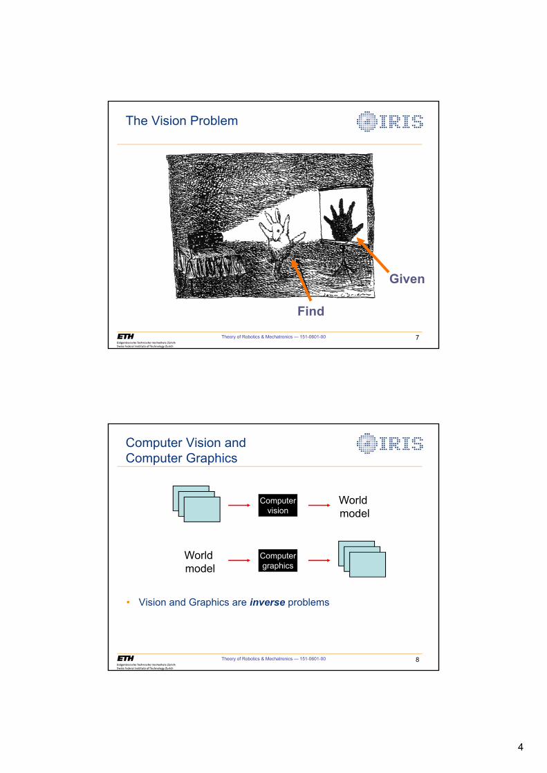
4
Theory of Robotics & Mechatronics — 151-0601-00 7
The Vision Problem
Find
Given
Theory of Robotics & Mechatronics — 151-0601-00 8
Computer Vision and
Computer Graphics
Computer
vision
World
model
Computer
graphics
World
model
• Vision and Graphics are inverse problems
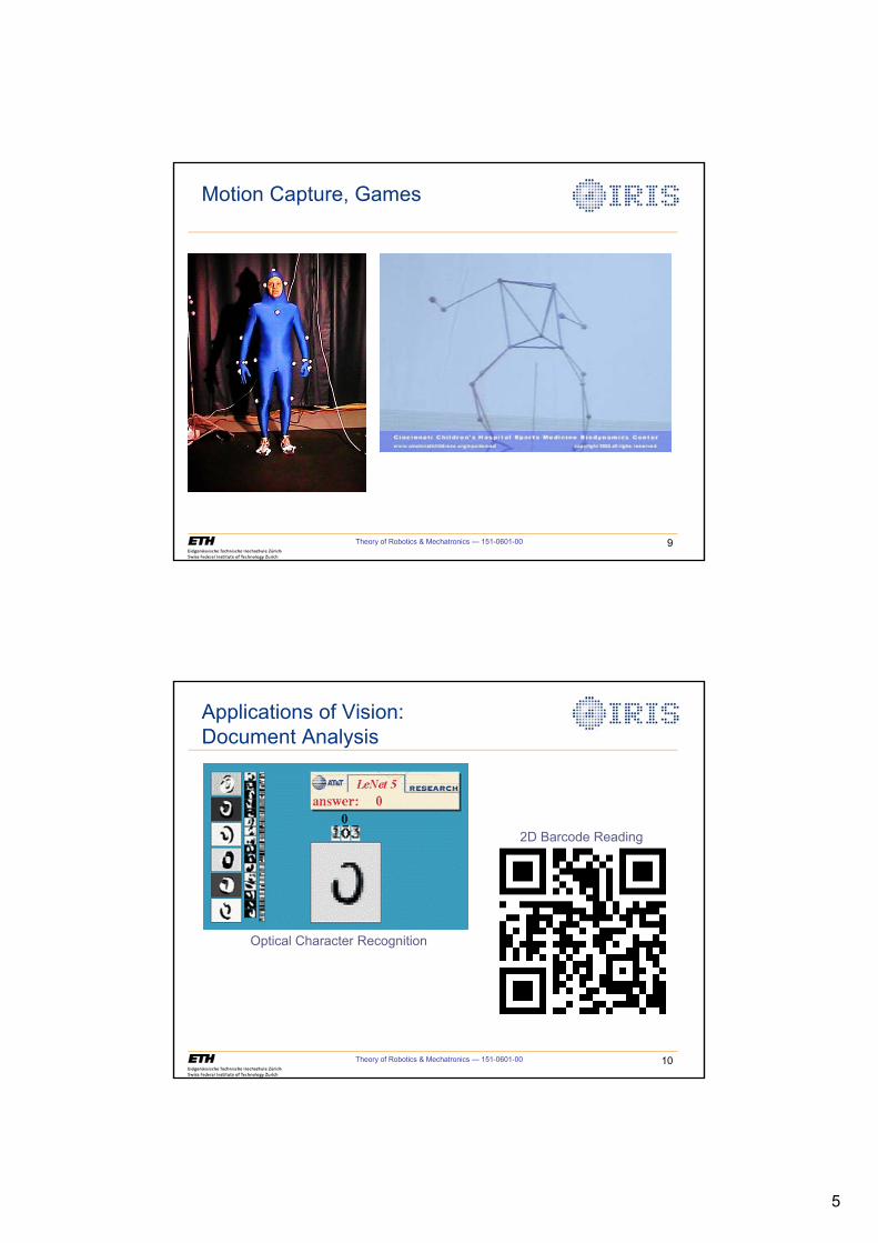
5
Theory of Robotics & Mechatronics — 151-0601-00 9
Motion Capture, Games
Theory of Robotics & Mechatronics — 151-0601-00 10
Applications of Vision:
Document Analysis
Optical Character Recognition
2D Barcode Reading

6
Theory of Robotics & Mechatronics — 151-0601-00 11
3D Scanning
Scanning Michelangelo’s “The David”• The Digital Michelangelo Project
• http://graphics.stanford.edu/projects/mich/
• 2 BILLION polygons, accuracy to .29mm
Theory of Robotics & Mechatronics — 151-0601-00 12
Medical Imaging, 3D Reconstruction,
Diagnostic Assistance
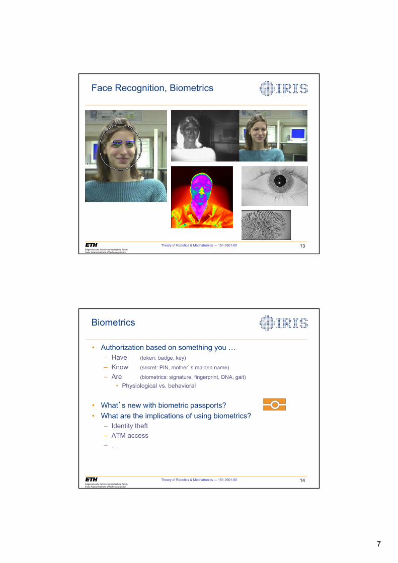
7
Theory of Robotics & Mechatronics — 151-0601-00 13
Face Recognition, Biometrics
Biometrics
• Authorization based on something you …
– Have (token: badge, key)
– Know (secret: PIN, mother’s maiden name)
– Are (biometrics: signature, fingerprint, DNA, gait)
• Physiological vs. behavioral
• What’s new with biometric passports?
• What are the implications of using biometrics?
– Identity theft
– ATM access
– …
Theory of Robotics & Mechatronics — 151-0601-00 14
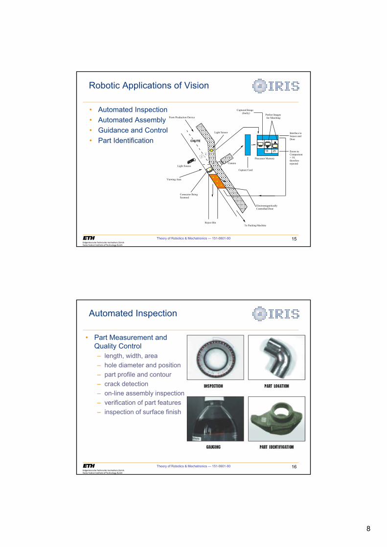
8
Theory of Robotics & Mechatronics — 151-0601-00 15
• Automated Inspection
• Automated Assembly
• Guidance and Control
• Part Identification
Robotic Applications of Vision
Reject Bin
Light Source
Light Sensor
Camera
Viewing Area
Connector Being Scanned
From Production Device
CHUTE
Capture Card
18 25
Processor Memory
Captured Image (faulty)
Perfect Images for Matching
Interface to Sensor and Door
To Packing Machine
Electromagnetically Controlled Door
Errors in Comparison > 10, therefore rejected
Theory of Robotics & Mechatronics — 151-0601-00 16
• Part Measurement and
Quality Control
– length, width, area
– hole diameter and position
– part profile and contour
– crack detection
– on-line assembly inspection
– verification of part features
– inspection of surface finish
Automated Inspection
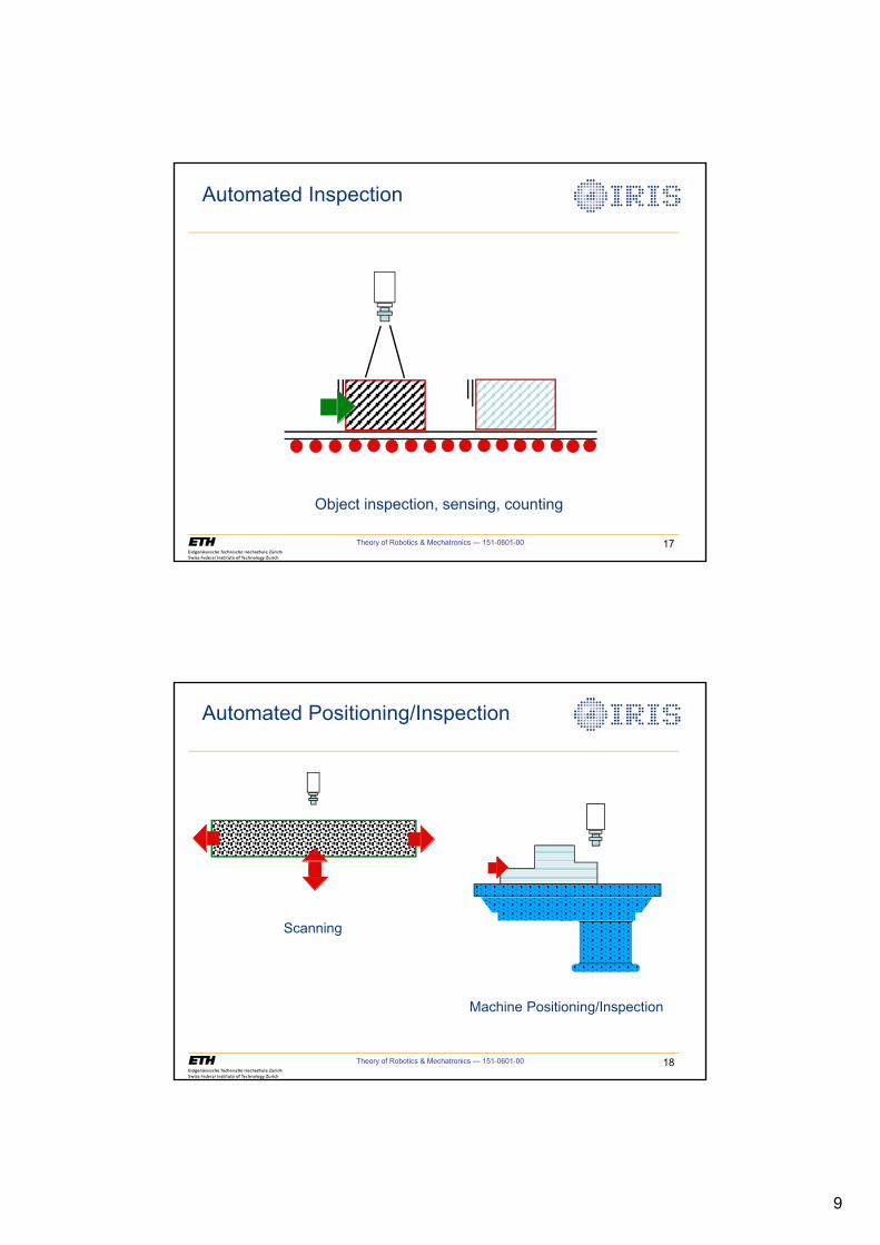
9
Theory of Robotics & Mechatronics — 151-0601-00 17
Object inspection, sensing, counting
Automated Inspection
Theory of Robotics & Mechatronics — 151-0601-00 18
Machine Positioning/Inspection
Automated Positioning/Inspection
Scanning
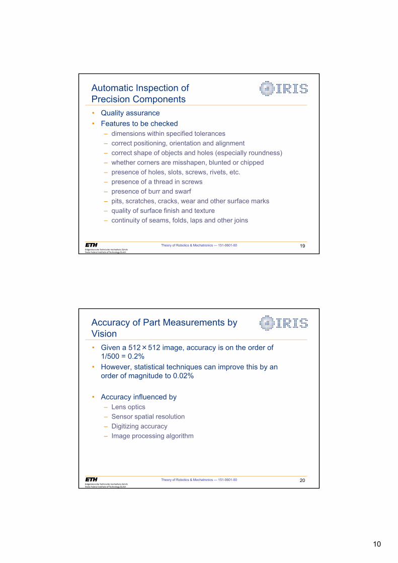
10
Theory of Robotics & Mechatronics — 151-0601-00 19
• Quality assurance
• Features to be checked
– dimensions within specified tolerances
– correct positioning, orientation and alignment
– correct shape of objects and holes (especially roundness)
– whether corners are misshapen, blunted or chipped
– presence of holes, slots, screws, rivets, etc.
– presence of a thread in screws
– presence of burr and swarf
– pits, scratches, cracks, wear and other surface marks
– quality of surface finish and texture
– continuity of seams, folds, laps and other joins
Automatic Inspection of
Precision Components
Theory of Robotics & Mechatronics — 151-0601-00 20
• Given a 512 512 image, accuracy is on the order of
1/500 = 0.2%
• However, statistical techniques can improve this by an
order of magnitude to 0.02%
• Accuracy influenced by
– Lens optics
– Sensor spatial resolution
– Digitizing accuracy
– Image processing algorithm
Accuracy of Part Measurements by
Vision
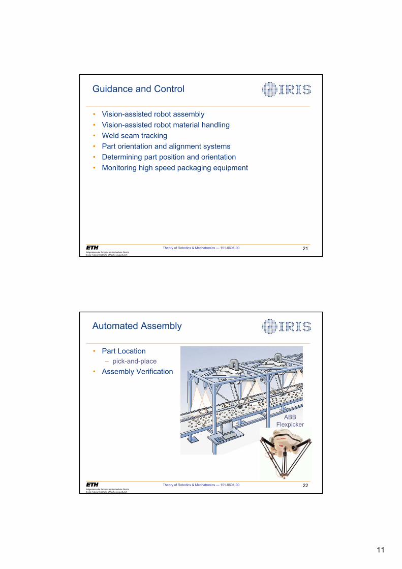
11
Theory of Robotics & Mechatronics — 151-0601-00 21
• Vision-assisted robot assembly
• Vision-assisted robot material handling
• Weld seam tracking
• Part orientation and alignment systems
• Determining part position and orientation
• Monitoring high speed packaging equipment
Guidance and Control
Theory of Robotics & Mechatronics — 151-0601-00 22
• Part Location
– pick-and-place
• Assembly Verification
Automated Assembly
ABB
Flexpicker
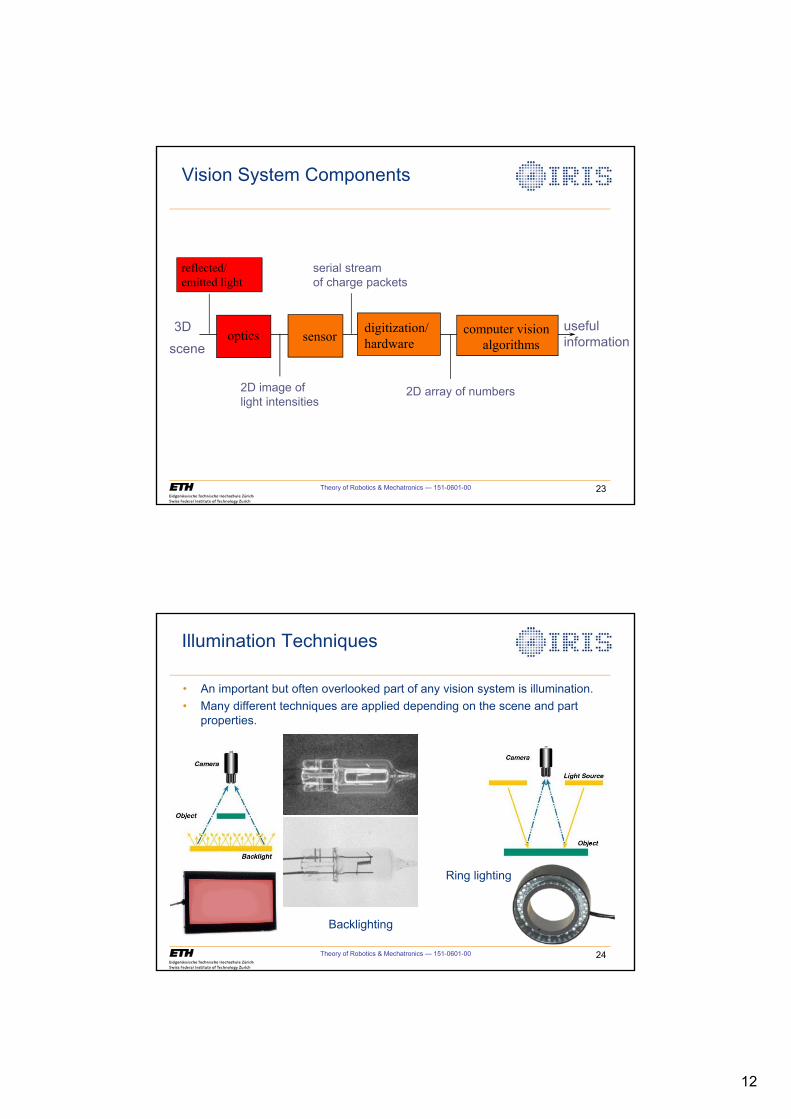
12
Theory of Robotics & Mechatronics — 151-0601-00 23
optics sensorcomputer vision
algorithms
3D
scene
useful
information
reflected/emitted light
2D image of
light intensities
serial stream
of charge packets
2D array of numbers
digitization/hardware
Vision System Components
Theory of Robotics & Mechatronics — 151-0601-00 24
Illumination Techniques
Backlighting
Ring lighting
• An important but often overlooked part of any vision system is illumination.
• Many different techniques are applied depending on the scene and part
properties.
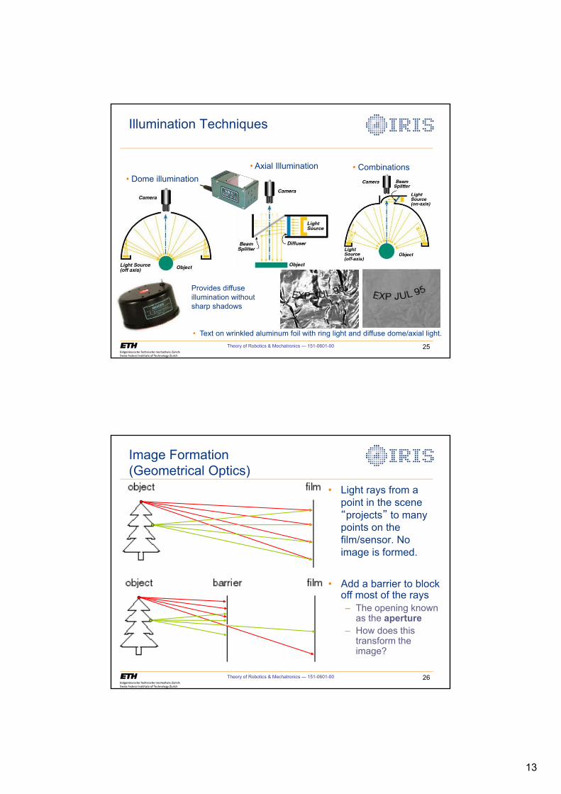
13
Theory of Robotics & Mechatronics — 151-0601-00 25
Illumination Techniques
• Dome illumination
• Axial Illumination
Provides diffuse
illumination without
sharp shadows
• Combinations
• Text on wrinkled aluminum foil with ring light and diffuse dome/axial light.
Theory of Robotics & Mechatronics — 151-0601-00 26
Image Formation
(Geometrical Optics)
• Light rays from a
point in the scene
“projects” to many
points on the
film/sensor. No
image is formed.
• Add a barrier to block
off most of the rays
– The opening known
as the aperture– How does this
transform the
image?
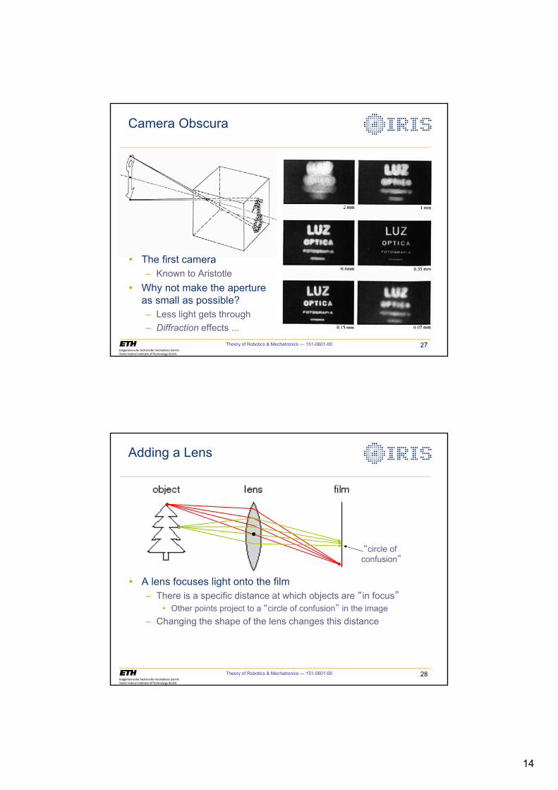
14
Theory of Robotics & Mechatronics — 151-0601-00 27
Camera Obscura
• The first camera
– Known to Aristotle
• Why not make the aperture
as small as possible?
– Less light gets through
– Diffraction effects ...
Theory of Robotics & Mechatronics — 151-0601-00 28
Adding a Lens
• A lens focuses light onto the film
– There is a specific distance at which objects are “in focus”
• Other points project to a “circle of confusion” in the image
– Changing the shape of the lens changes this distance
“circle of
confusion”
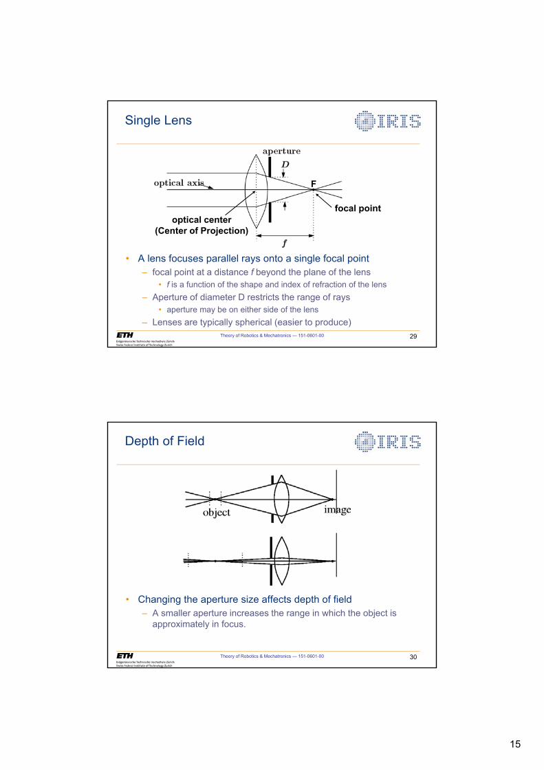
15
Theory of Robotics & Mechatronics — 151-0601-00 29
Single Lens
• A lens focuses parallel rays onto a single focal point
– focal point at a distance f beyond the plane of the lens
• f is a function of the shape and index of refraction of the lens
– Aperture of diameter D restricts the range of rays
• aperture may be on either side of the lens
– Lenses are typically spherical (easier to produce)
focal point
F
optical center(Center of Projection)
Theory of Robotics & Mechatronics — 151-0601-00 30
Depth of Field
• Changing the aperture size affects depth of field
– A smaller aperture increases the range in which the object is
approximately in focus.
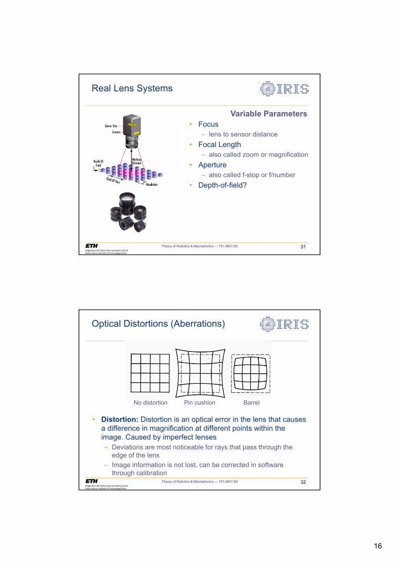
16
Theory of Robotics & Mechatronics — 151-0601-00 31
Real Lens Systems
• Focus
– lens to sensor distance
• Focal Length
– also called zoom or magnification
• Aperture
– also called f-stop or f/number
• Depth-of-field?
Variable Parameters
Theory of Robotics & Mechatronics — 151-0601-00 32
Optical Distortions (Aberrations)
No distortion Pin cushion Barrel
• Distortion: Distortion is an optical error in the lens that causes
a difference in magnification at different points within the
image. Caused by imperfect lenses
– Deviations are most noticeable for rays that pass through the
edge of the lens
– Image information is not lost, can be corrected in software
through calibration
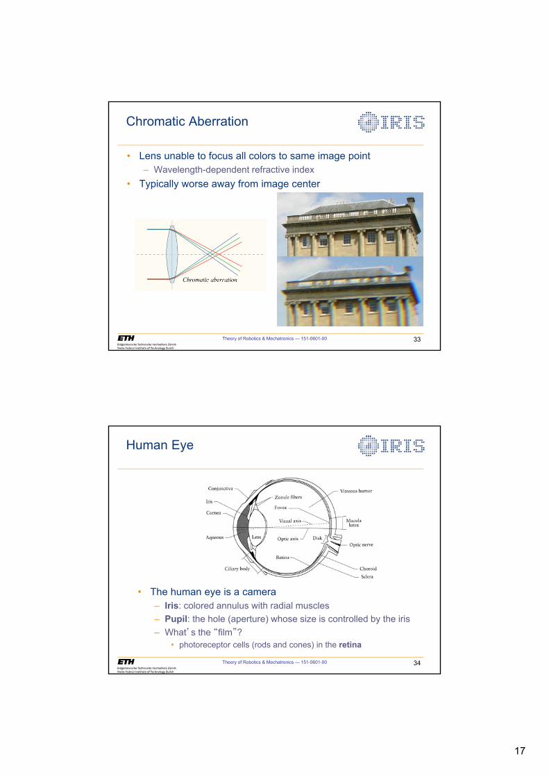
17
Chromatic Aberration
• Lens unable to focus all colors to same image point
– Wavelength-dependent refractive index
• Typically worse away from image center
Theory of Robotics & Mechatronics — 151-0601-00 33
Theory of Robotics & Mechatronics — 151-0601-00 34
Human Eye
• The human eye is a camera
– Iris: colored annulus with radial muscles
– Pupil: the hole (aperture) whose size is controlled by the iris
– What’s the “film”?
• photoreceptor cells (rods and cones) in the retina
18
Theory of Robotics & Mechatronics — 151-0601-00 35
optics sensordigitization/hardware
computer visionalgorithms
3D
Scene
Useful
Information
reflected/
emitted light
2D image of
light intensities
serial stream
of charge packets
2D array of numbers
CAMERAS
Cameras
Theory of Robotics & Mechatronics — 151-0601-00 36
• Incident photons are converted into electrons and accumulated
in a charge (potential) well.
• Imaging sensors are arrays of small (typ. ~10 10 μm squares)
pixels that collect the charge. They are spatial samplers of light
intensity.
+-
+-
photon
electron
battery
charged platecharged plate
boink!
The Photoelectric Effect
+e
-e-
e-
e-
e- e
-e
-e
-
+
Simple Photodetector
Potential Well
Silicon
Silicon dioxide
Polysilicon Gate
Electrical Connection
Incoming Light
19
Theory of Robotics & Mechatronics — 151-0601-00 37
CCD Sensors
• The charge on each pixel is
transferred from pixel to
pixel to an amplifier.
• High sensitivity, high
dynamic range (the ratio of
a pixel’s saturation level to
its signal threshold), better
signal to noise ratio.
• Expensive, needs off-chip
circuitry for clocking and
other functions.
• Used for high quality,
scientific imaging,
photography.
Theory of Robotics & Mechatronics — 151-0601-00 38
CMOS Sensors
Single-chip Integrated CMOS
sensor
13 13 mm square chip, the analog
output can directly drive a video monitor
without any other circuitry!
• Complementary Metal-Oxide
Semiconductor technology is
widely used for manufacturing
VLSI circuits.
• Similar to CCD in photon-to-
electron conversion but each
pixel has its own dedicated
buffer circuitry. All electronics
is integrated into a single chip.
• Better suited for complicated
functions, digital output, partial
output of the pixels
(windowing).
• Less costly (in quantity),
mostly used in low cost
imaging, security, web cams,
etc.
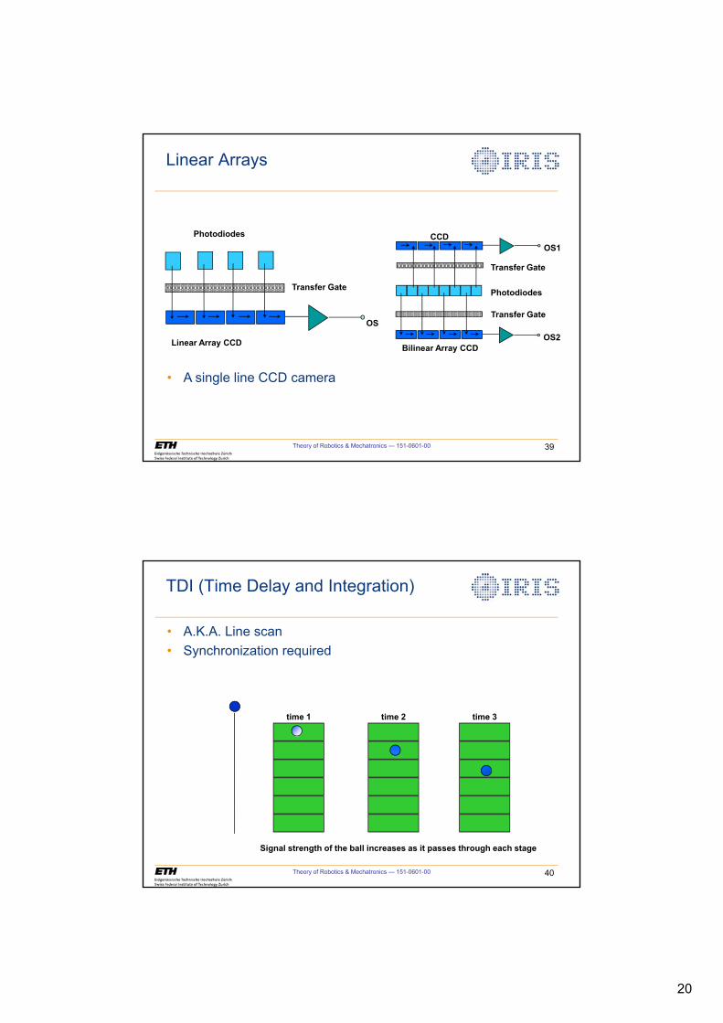
20
Theory of Robotics & Mechatronics — 151-0601-00 39
Photodiodes
Transfer Gate
OS
Linear Array CCD
Linear Arrays
CCDOS1
OS2
Transfer Gate
Photodiodes
Transfer Gate
Bilinear Array CCD
• A single line CCD camera
Theory of Robotics & Mechatronics — 151-0601-00 40
Signal strength of the ball increases as it passes through each stage
time 1 time 2 time 3
• A.K.A. Line scan
• Synchronization required
TDI (Time Delay and Integration)
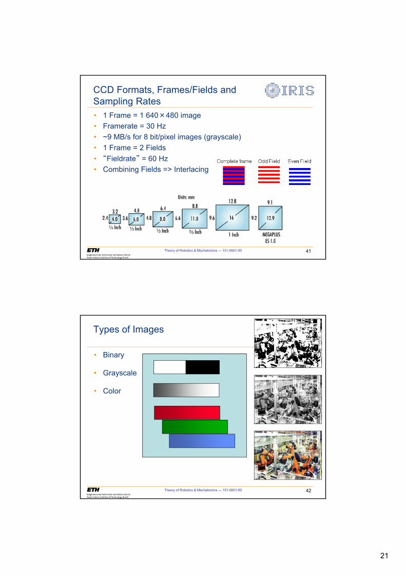
21
Theory of Robotics & Mechatronics — 151-0601-00 41
• 1 Frame = 1 640 480 image
• Framerate = 30 Hz
• ~9 MB/s for 8 bit/pixel images (grayscale)
• 1 Frame = 2 Fields
• “Fieldrate” = 60 Hz
• Combining Fields => Interlacing
CCD Formats, Frames/Fields and
Sampling Rates
Theory of Robotics & Mechatronics — 151-0601-00 42
• Binary
• Grayscale
• Color
Types of Images
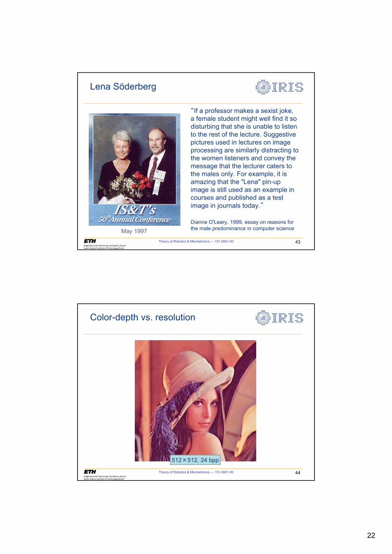
22
Lena Söderberg
“If a professor makes a sexist joke,
a female student might well find it so
disturbing that she is unable to listen
to the rest of the lecture. Suggestive
pictures used in lectures on image
processing are similarly distracting to
the women listeners and convey the
message that the lecturer caters to
the males only. For example, it is
amazing that the "Lena" pin-up
image is still used as an example in
courses and published as a test
image in journals today.”
Dianne O'Leary, 1999, essay on reasons for
the male predominance in computer science
Theory of Robotics & Mechatronics — 151-0601-00 43
May 1997
Color-depth vs. resolution
Theory of Robotics & Mechatronics — 151-0601-00 44
512 512, 24 bpp
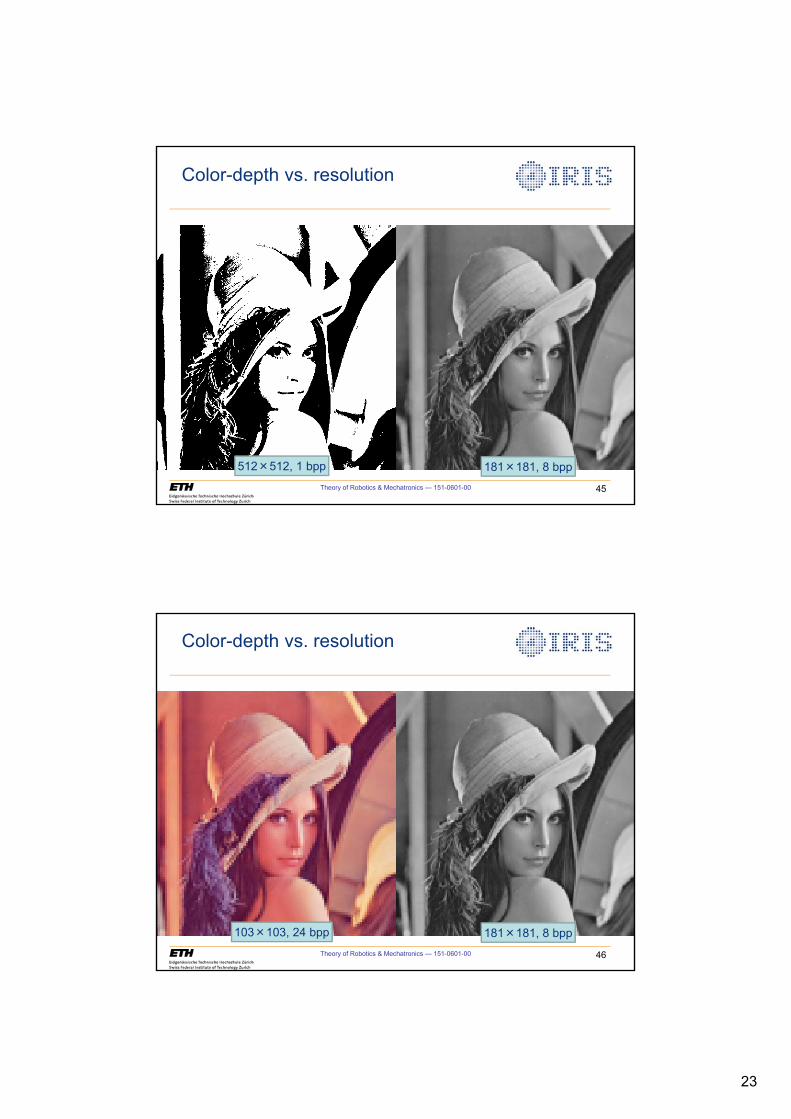
23
Color-depth vs. resolution
Theory of Robotics & Mechatronics — 151-0601-00 45
512 512, 1 bpp 181 181, 8 bpp
Color-depth vs. resolution
Theory of Robotics & Mechatronics — 151-0601-00 46
103 103, 24 bpp 181 181, 8 bpp
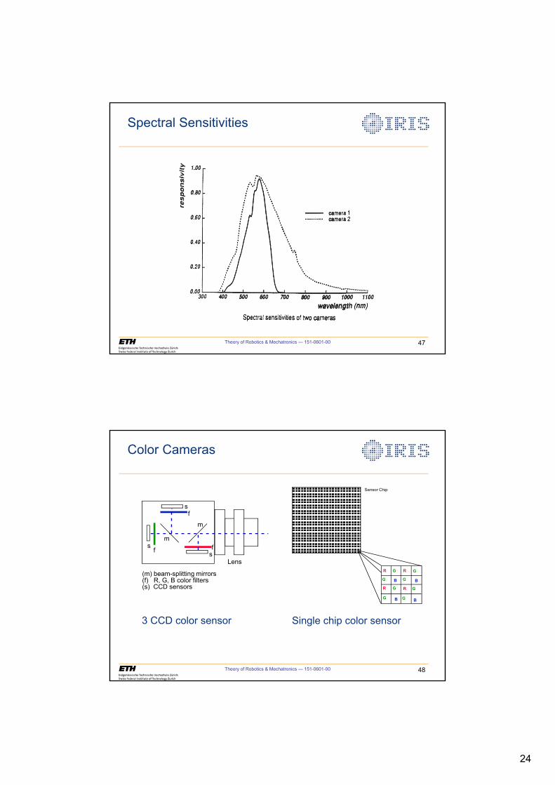
24
Theory of Robotics & Mechatronics — 151-0601-00 47
Spectral Sensitivities
Theory of Robotics & Mechatronics — 151-0601-00 48
Single chip color sensor
s
s
s
f
ff
m
m
(m) beam-splitting mirrors (f) R, G, B color filters (s) CCD sensors
Lens
Color Cameras
RR
RR
GG
GG
GG
G G
Sensor Chip
B B
B B
3 CCD color sensor
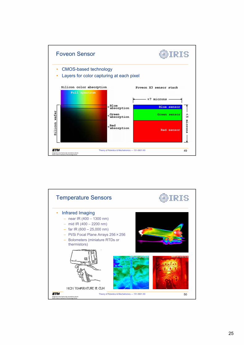
25
Foveon Sensor
• CMOS-based technology
• Layers for color capturing at each pixel
Theory of Robotics & Mechatronics — 151-0601-00 49
Theory of Robotics & Mechatronics — 151-0601-00 50
• Infrared Imaging
– near IR (400 – 1300 nm)
– mid IR (400 – 2200 nm)
– far IR (600 – 25,000 nm)
– Pt/Si Focal Plane Arrays 256 256
– Bolometers (miniature RTDs or
thermistors)
Temperature Sensors
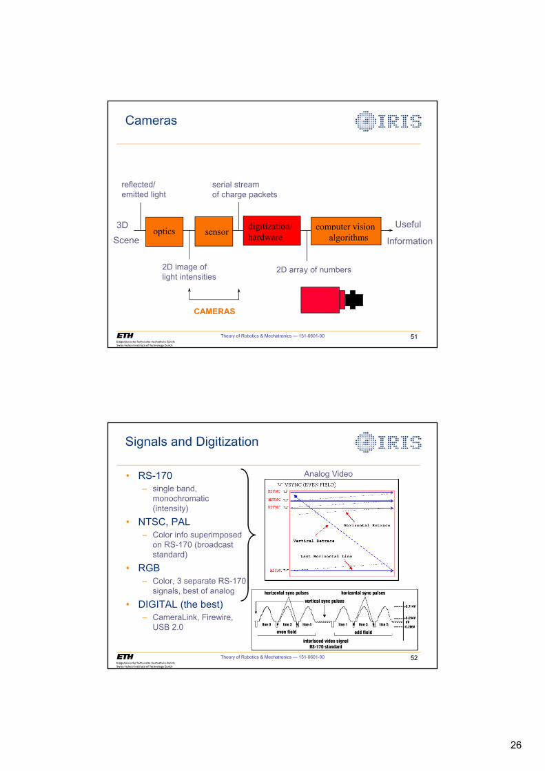
26
Theory of Robotics & Mechatronics — 151-0601-00 51
optics sensordigitization/hardware
computer visionalgorithms
3D
Scene
Useful
Information
reflected/
emitted light
2D image of
light intensities
serial stream
of charge packets
2D array of numbers
CAMERAS
Cameras
Theory of Robotics & Mechatronics — 151-0601-00 52
• RS-170
– single band,
monochromatic
(intensity)
• NTSC, PAL
– Color info superimposed
on RS-170 (broadcast
standard)
• RGB
– Color, 3 separate RS-170
signals, best of analog
• DIGITAL (the best)
– CameraLink, Firewire,
USB 2.0
Signals and Digitization
Analog Video
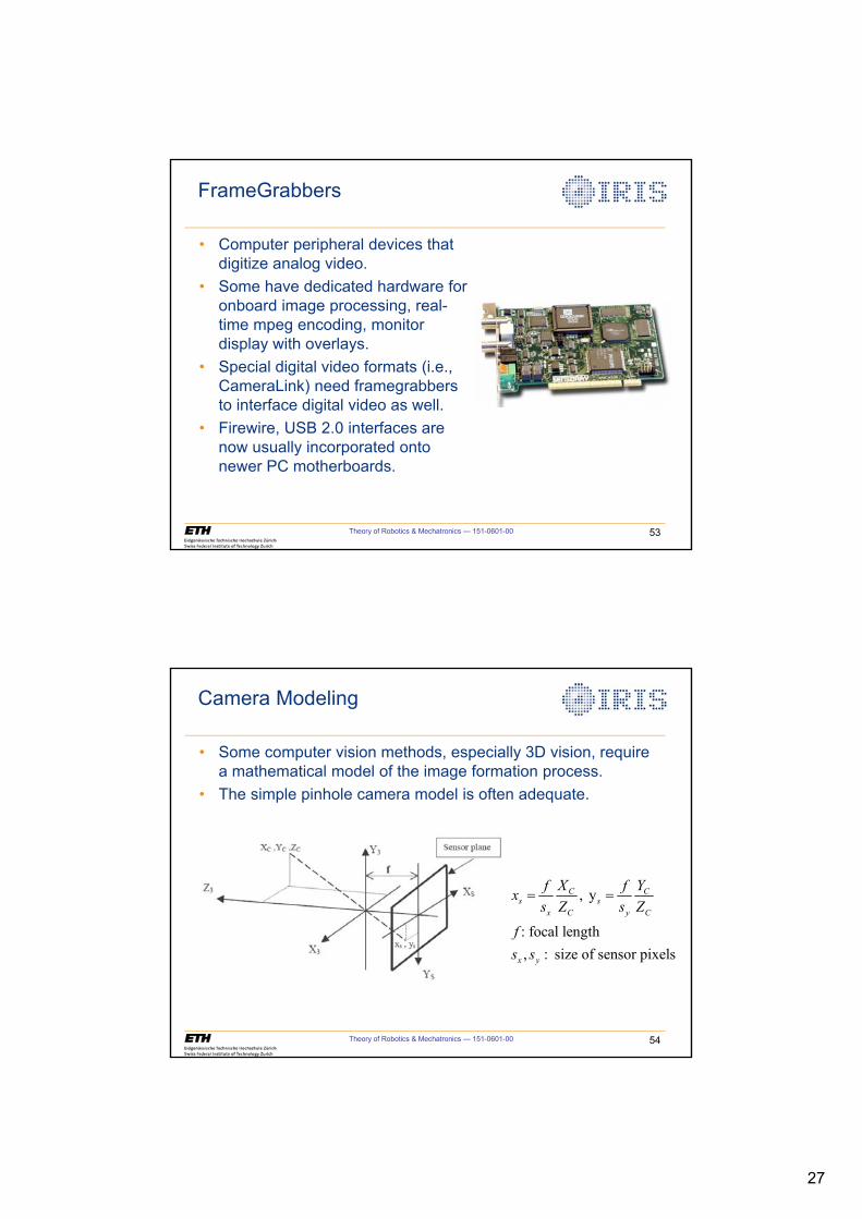
27
Theory of Robotics & Mechatronics — 151-0601-00 53
FrameGrabbers
• Computer peripheral devices that
digitize analog video.
• Some have dedicated hardware for
onboard image processing, real-
time mpeg encoding, monitor
display with overlays.
• Special digital video formats (i.e.,
CameraLink) need framegrabbers
to interface digital video as well.
• Firewire, USB 2.0 interfaces are
now usually incorporated onto
newer PC motherboards.
Theory of Robotics & Mechatronics — 151-0601-00 54
Camera Modeling
• Some computer vision methods, especially 3D vision, require
a mathematical model of the image formation process.
• The simple pinhole camera model is often adequate.
, y
: focal length
, : size of sensor pixels
C Cs s
x C y C
x y
X Yf fx
s Z s Z
fs s
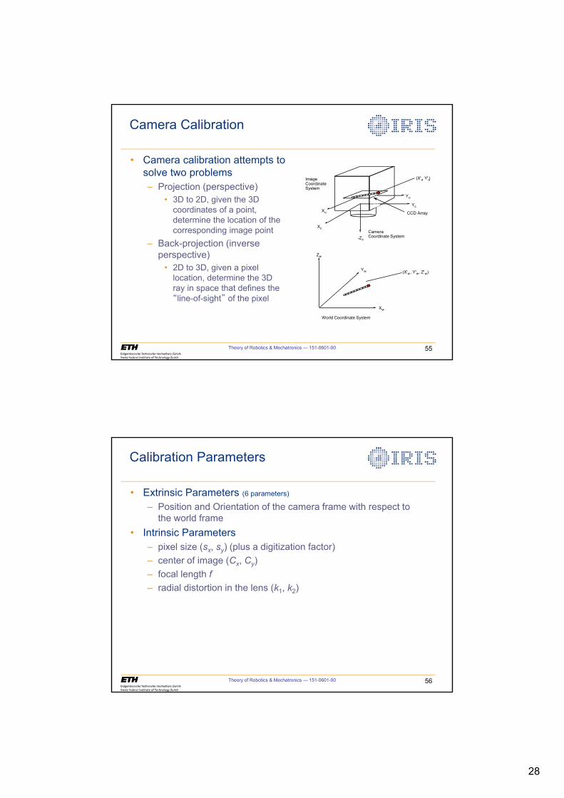
28
Theory of Robotics & Mechatronics — 151-0601-00 55
Zw
Yw
Xw
World Coordinate System
-Zc
Yc
Xc
Image
Coordinate
System
Xu
Yu
(X'w, Y'w, Z'w)
(X'u, Y'u)
Camera
Coordinate System
CCD Array
Camera Calibration
• Camera calibration attempts to
solve two problems
– Projection (perspective)
• 3D to 2D, given the 3D
coordinates of a point,
determine the location of the
corresponding image point
– Back-projection (inverse
perspective)
• 2D to 3D, given a pixel
location, determine the 3D
ray in space that defines the
“line-of-sight” of the pixel
Theory of Robotics & Mechatronics — 151-0601-00 56
• Extrinsic Parameters (6 parameters)
– Position and Orientation of the camera frame with respect to
the world frame
• Intrinsic Parameters
– pixel size (sx, sy) (plus a digitization factor)
– center of image (Cx, Cy)
– focal length f– radial distortion in the lens (k1, k2)
Calibration Parameters
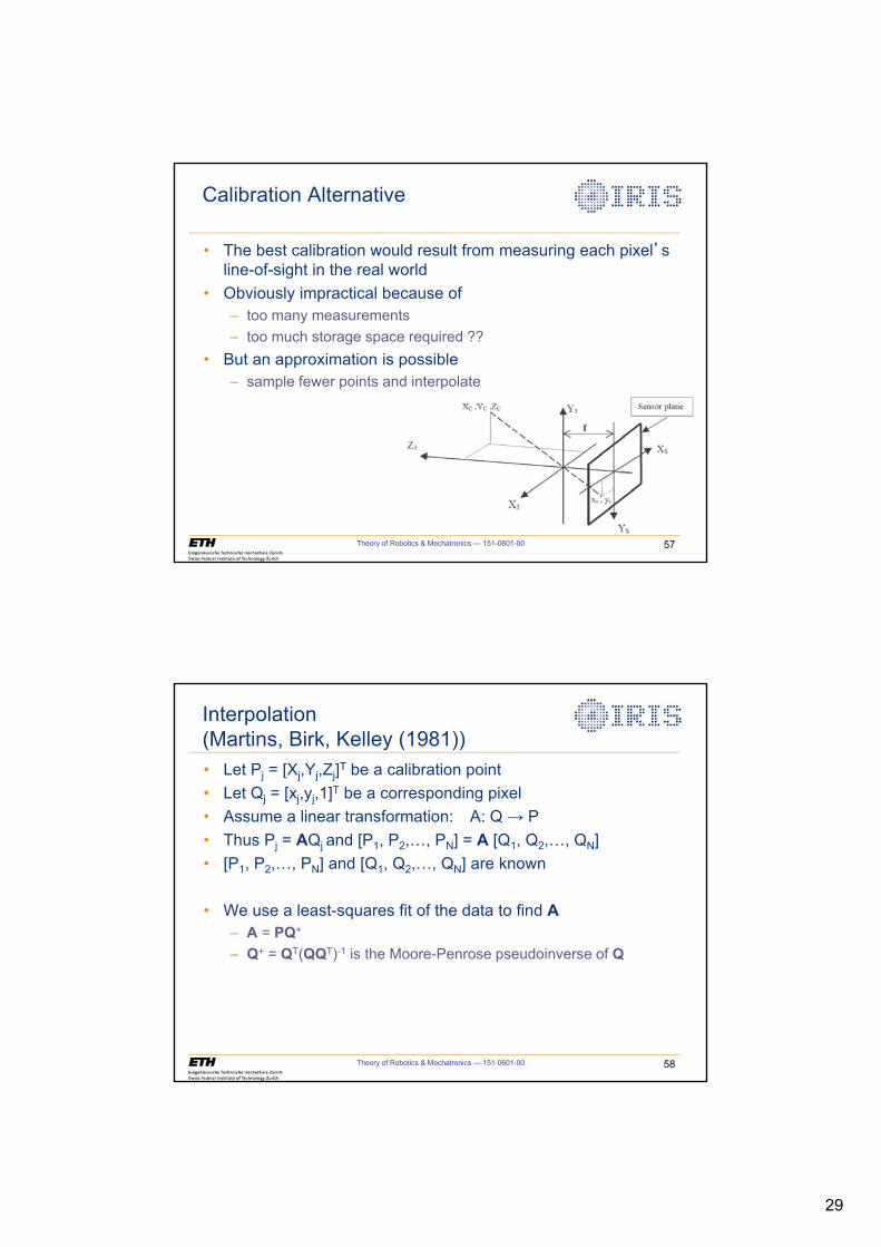
29
Theory of Robotics & Mechatronics — 151-0601-00 57
Calibration Alternative
• The best calibration would result from measuring each pixel’s
line-of-sight in the real world
• Obviously impractical because of
– too many measurements
– too much storage space required ??
• But an approximation is possible
– sample fewer points and interpolate
Theory of Robotics & Mechatronics — 151-0601-00 58
• Let Pj = [Xj,Yj,Zj]T be a calibration point
• Let Qj = [xj,yj,1]T be a corresponding pixel
• Assume a linear transformation: A: Q P
• Thus Pj = AQj and [P1, P2,…, PN] = A [Q1, Q2,…, QN]
• [P1, P2,…, PN] and [Q1, Q2,…, QN] are known
• We use a least-squares fit of the data to find A– A = PQ+
– Q+ = QT(QQT)-1 is the Moore-Penrose pseudoinverse of Q
Interpolation
(Martins, Birk, Kelley (1981))

30
Theory of Robotics & Mechatronics — 151-0601-00 59
Other calibration issues
• Calibration may vary with many camera parameters such as
– focus
– aperture
– zoom (variable focal length)
• Pan-tilt heads must be calibrated
• We haven’t considered
– color
– intensity
1
Computer Vision Algorithms
Institute of Robotics and Intelligent SystemsETH Zurich
Theory of Robotics &Mechatronics
Theory of Robotics & Mechatronics — 151-0601-00 2
optics sensordigitization/hardware
computer visionalgorithms
3DScene
Useful
Information
reflected/emitted light
2D image of light intensities
serial stream of charge packets
2D array of numbers
ALGORITHMS
Commonly Used Algorithms
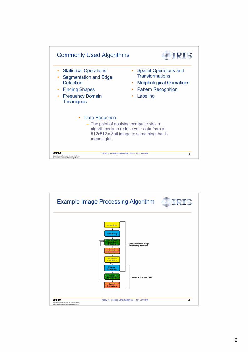
2
Theory of Robotics & Mechatronics — 151-0601-00 3
• Statistical Operations• Segmentation and Edge
Detection• Finding Shapes• Frequency Domain
Techniques
• Spatial Operations and Transformations
• Morphological Operations• Pattern Recognition• Labeling
Commonly Used Algorithms
• Data Reduction– The point of applying computer vision
algorithms is to reduce your data from a 512x512 x 8bit image to something that is meaningful.
Theory of Robotics & Mechatronics — 151-0601-00 4
Acquisition
Prefiltering
Recursive/ Adaptive Filtering
Image Segmentation
Geometric Operations
Feature Extraction
Image Classification
Image Evaluation
Special Purpose Image Processing Hardware
General Purpose CPU
Example Image Processing Algorithm
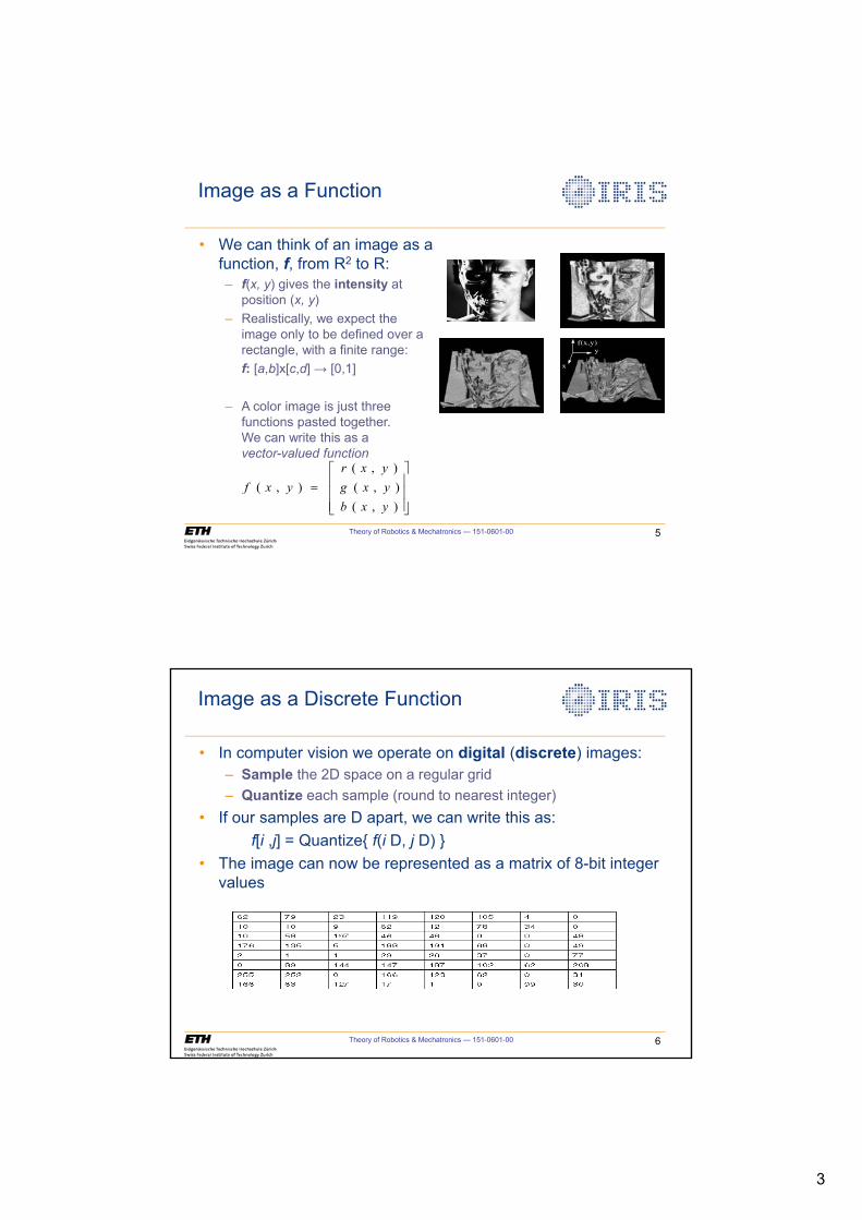
3
Theory of Robotics & Mechatronics — 151-0601-00 5
Image as a Function
• We can think of an image as a function, f, from R2 to R:– f(x, y) gives the intensity at
position (x, y) – Realistically, we expect the
image only to be defined over a rectangle, with a finite range:f: [a,b]x[c,d] [0,1]
– A color image is just three functions pasted together. We can write this as a vector-valued function
( , )
( , ) ( , )
( , )
r x yf x y g x y
b x y
ª º« » « »« »¬ ¼
x
yf(x,y)
Theory of Robotics & Mechatronics — 151-0601-00 6
Image as a Discrete Function
• In computer vision we operate on digital (discrete) images:– Sample the 2D space on a regular grid– Quantize each sample (round to nearest integer)
• If our samples are D apart, we can write this as:f[i ,j] = Quantize{ f(i D, j D) }
• The image can now be represented as a matrix of 8-bit integer values
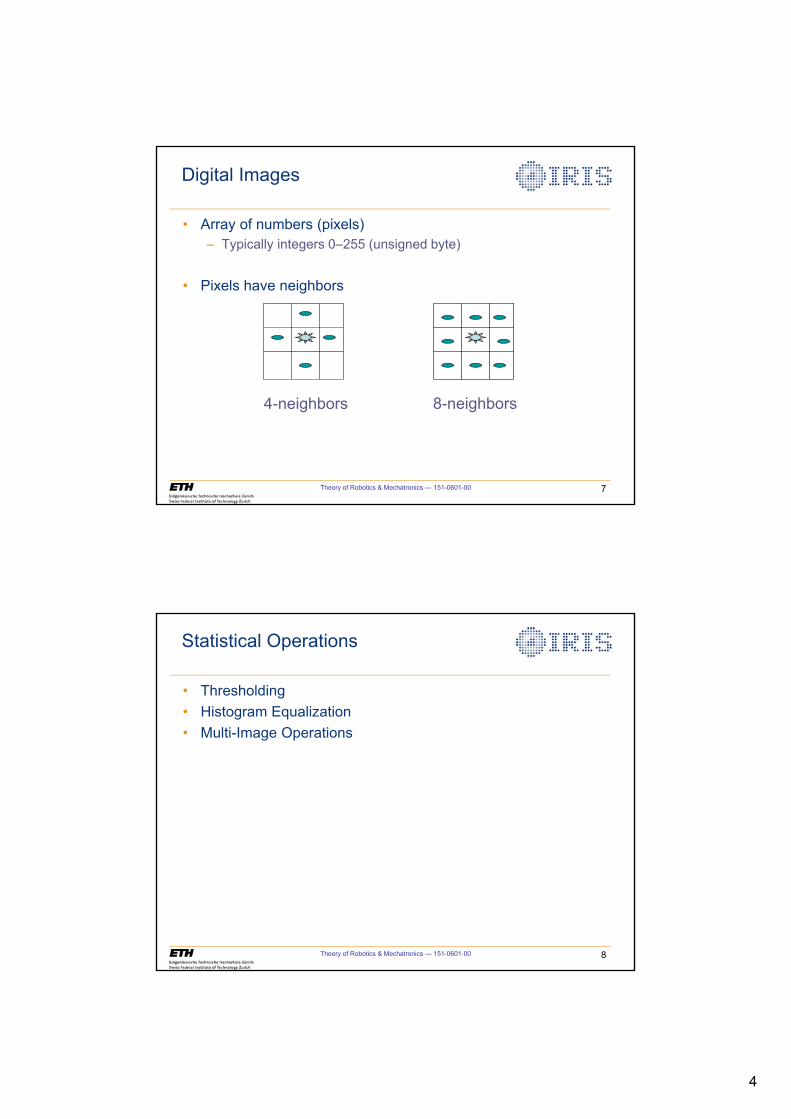
4
Theory of Robotics & Mechatronics — 151-0601-00 7
Digital Images
• Array of numbers (pixels)– Typically integers 0–255 (unsigned byte)
• Pixels have neighbors
4-neighbors 8-neighbors
Theory of Robotics & Mechatronics — 151-0601-00 8
• Thresholding• Histogram Equalization• Multi-Image Operations
Statistical Operations
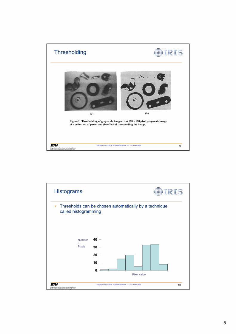
5
Theory of Robotics & Mechatronics — 151-0601-00 9
Thresholding
Theory of Robotics & Mechatronics — 151-0601-00 10
• Thresholds can be chosen automatically by a technique called histogramming
0
10
20
30
40
Pixel value
Number ofPixels
Histograms
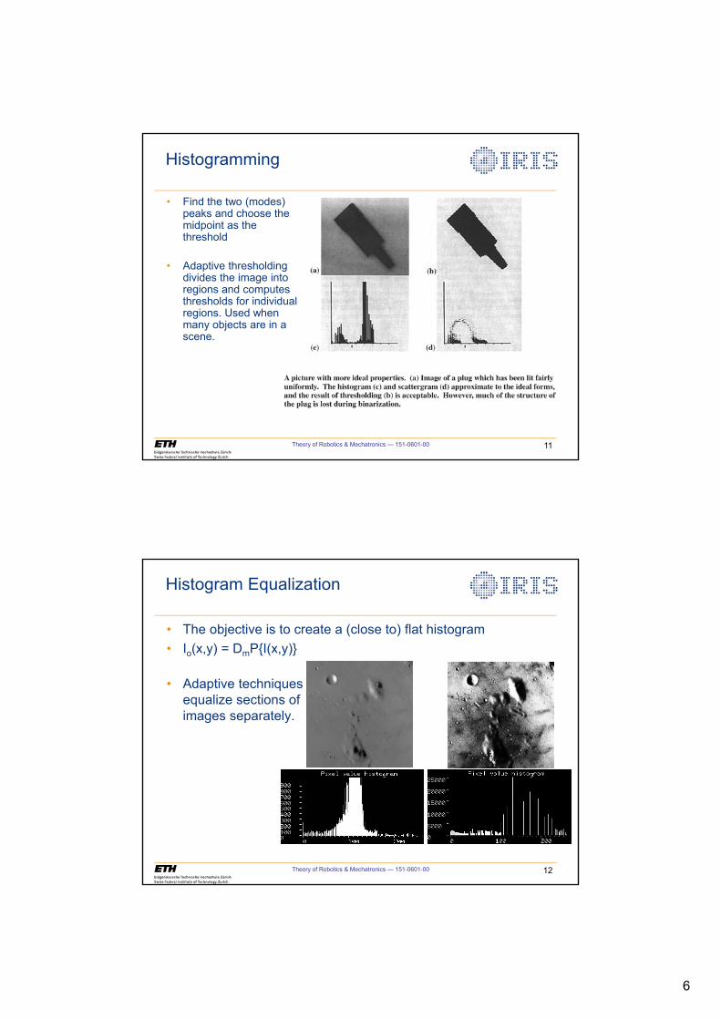
6
Theory of Robotics & Mechatronics — 151-0601-00 11
• Find the two (modes) peaks and choose the midpoint as the threshold
• Adaptive thresholding divides the image into regions and computes thresholds for individual regions. Used when many objects are in a scene.
Histogramming
Theory of Robotics & Mechatronics — 151-0601-00 12
• The objective is to create a (close to) flat histogram• Io(x,y) = DmP{I(x,y)}
• Adaptive techniquesequalize sections ofimages separately.
Histogram Equalization
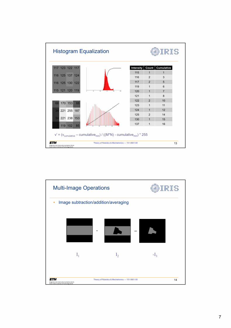
7
Histogram Equalization
Theory of Robotics & Mechatronics — 151-0601-00 13
117 123 122 117
116 125 137 124
116 125 130 122
115 121 120 119
Intensity Count Cumulative115 1 1
116 2 3
117 2 5
119 1 6
120 1 7
121 1 8
122 2 10
123 1 11
124 1 12
125 2 14
130 1 15
137 1 16
68 170 153 68
34 221 255 187
34 221 238 153
0 119 102 85
v’ = (vcumulative – cumulativemin) / ((M*N) - cumulativemin) * 255
Theory of Robotics & Mechatronics — 151-0601-00 14
• Image subtraction/addition/averaging
I1 I2 -I3
- =
Multi-Image Operations
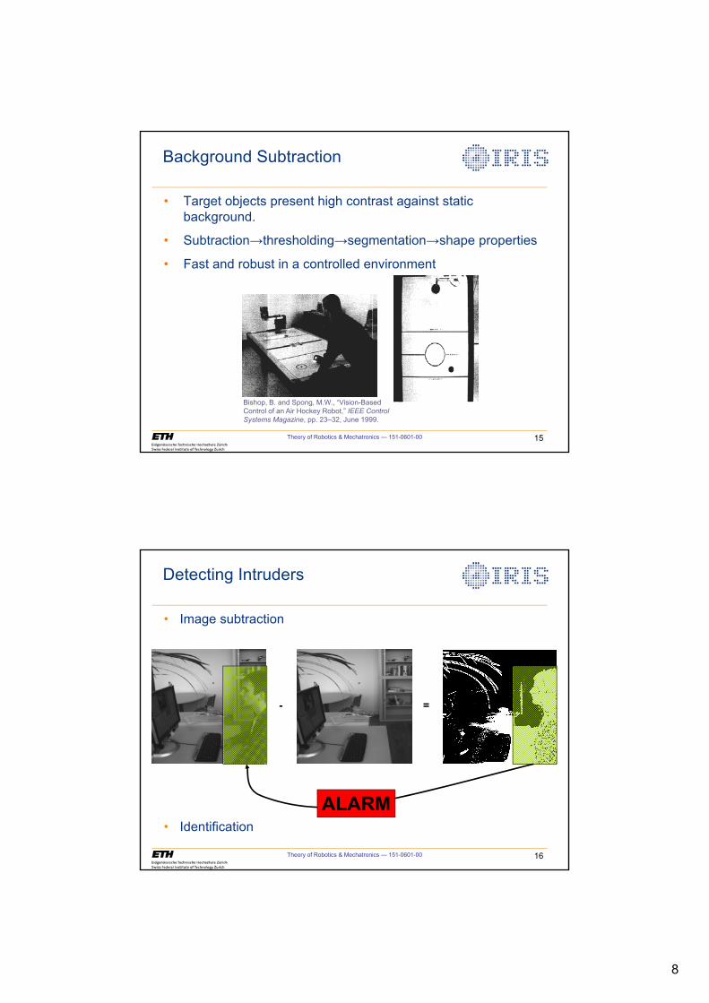
8
Theory of Robotics & Mechatronics — 151-0601-00 15
Background Subtraction
Bishop, B. and Spong, M.W., “Vision-Based Control of an Air Hockey Robot,” IEEE Control Systems Magazine, pp. 23–32, June 1999.
• Target objects present high contrast against static background.
• Subtraction thresholding segmentation shape properties
• Fast and robust in a controlled environment
Theory of Robotics & Mechatronics — 151-0601-00 16
=
Detecting Intruders
• Image subtraction
• Identification
-
ALARM
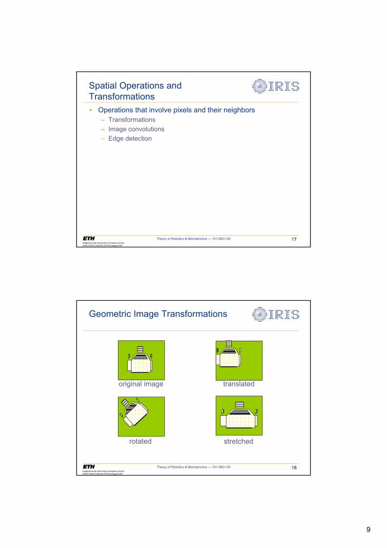
9
Theory of Robotics & Mechatronics — 151-0601-00 17
• Operations that involve pixels and their neighbors– Transformations– Image convolutions– Edge detection
Spatial Operations and Transformations
Theory of Robotics & Mechatronics — 151-0601-00 18
original image translated
rotated stretched
Geometric Image Transformations
10
Recording Blood Glucose Levels
Theory of Robotics & Mechatronics — 151-0601-00 19
Theory of Robotics & Mechatronics — 151-0601-00 20
f g f*g
f g f*g
In 1D
Convolution
11
Theory of Robotics & Mechatronics — 151-0601-00 21
2D Convolution and Filters
1
11
1
1 111
1
F
1/9
• Mean Filter: Replaces all pixels with the mean of the neighboring pixels
• 3×3 Mean Filtering kernel (mask)
Theory of Robotics & Mechatronics — 151-0601-00 22
Mean Filtered Gaussian Filtered
Image Smoothing
121242121
Original Image
The std. dev., V, of the Gaussian determines the amount of smoothing.
• Gaussian Filter gives more weight at the central pixel and less weights to the neighbors.
• The farther away the neighbors, the smaller the weight.
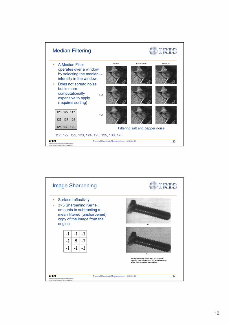
12
Theory of Robotics & Mechatronics — 151-0601-00 23
Median Filtering
3x3
5x5
7x7
Mean Gaussian Median
Filtering salt and pepper noise
• A Median Filter operates over a window by selecting the median intensity in the window.
• Does not spread noise but is more computationally expensive to apply (requires sorting)
123 122 117
125 137 124
125 130 122
117, 122, 122, 123, 124, 125, 125, 130, 170
Theory of Robotics & Mechatronics — 151-0601-00 24
Image Sharpening
-18-1
-1
-1 -1
-1-1
-1
• Surface reflectivity • 3×3 Sharpening Kernel,
amounts to subtracting a mean filtered (unsharpened) copy of the image from the original
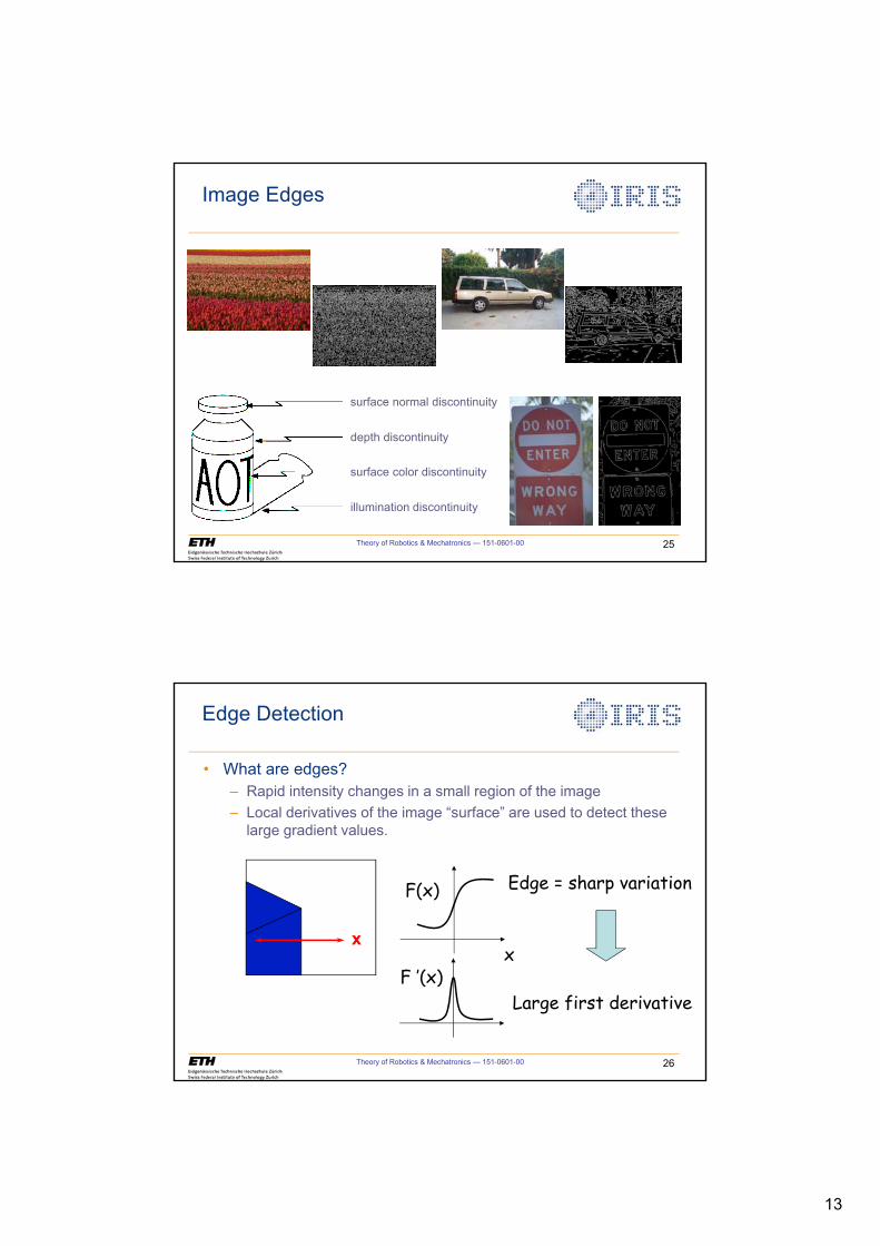
13
Theory of Robotics & Mechatronics — 151-0601-00 25
depth discontinuity
surface color discontinuity
illumination discontinuity
surface normal discontinuity
Image Edges
Theory of Robotics & Mechatronics — 151-0601-00 26
• What are edges?– Rapid intensity changes in a small region of the image– Local derivatives of the image “surface” are used to detect these
large gradient values.
Edge Detection
F(x)
xF ’(x)
Edge = sharp variation
Large first derivative
x
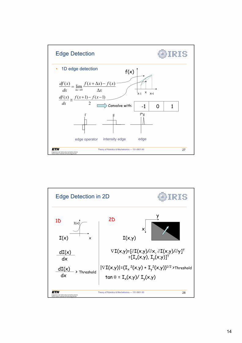
14
Theory of Robotics & Mechatronics — 151-0601-00 27
• 1D edge detection
Edge Detection
xxfxxf
dxxdf
x '�'�
o'
)()(lim
)(0
2
)1()1()( ���#
xfxfdxxdf
X
f(x)
X-1 X+1
-1 0 1Convolve with:
f g f*g
edge operator intensity edge edge
Theory of Robotics & Mechatronics — 151-0601-00 28
Edge Detection in 2D
1D 2D
I(x) I(x,y)
dI(x)dx
�I(x,y)=[wI(x,y)/wx, wI(x,y)/wy]T
=[Ix(x,y), Iy(x,y)]T
dI(x)dx
> Threshold|�I(x,y)|=(Ix
2(x,y) + Iy2(x,y))1/2 >Threshold
x
y
tan T = Ix(x,y)/ Iy(x,y)
I(x)
x
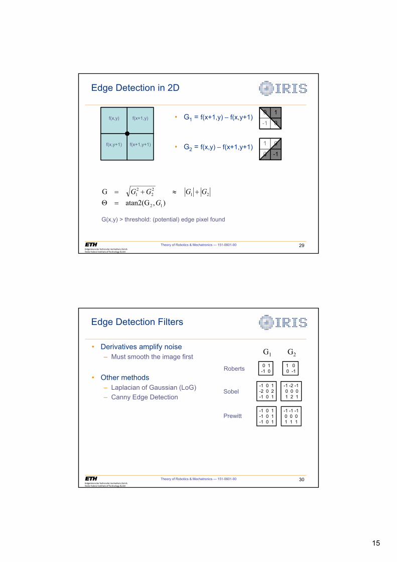
15
Edge Detection in 2D
Theory of Robotics & Mechatronics — 151-0601-00 29
f(x,y) f(x+1,y)
f(x,y+1) f(x+1,y+1)
),atan2(G
G
12
2122
21
GGGGG
4�|�
• G1 = f(x+1,y) – f(x,y+1)
• G2 = f(x,y) – f(x+1,y+1)
-1
0 1
0
0
1 0
-1
G(x,y) > threshold: (potential) edge pixel found
Theory of Robotics & Mechatronics — 151-0601-00 30
• Derivatives amplify noise– Must smooth the image first
• Other methods– Laplacian of Gaussian (LoG)– Canny Edge Detection
G1 G2
Edge Detection Filters
-1 0 1-2 0 2-1 0 1
-1 -2 -10 0 01 2 1
-1 0 1-1 0 1-1 0 1
-1 -1 -10 0 01 1 1
0 1-1 0
1 00 -1Roberts
Sobel
Prewitt
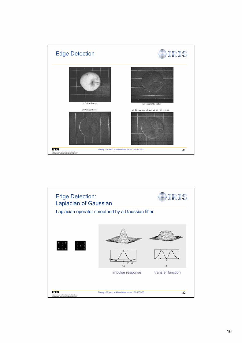
16
Theory of Robotics & Mechatronics — 151-0601-00 31
Edge Detection
Theory of Robotics & Mechatronics — 151-0601-00 32
0 -1 0-1 4 -10 -1 0
-1 -1 -1-1 8 -1-1 -1 -1
impulse response transfer function
Edge Detection:Laplacian of GaussianLaplacian operator smoothed by a Gaussian filter
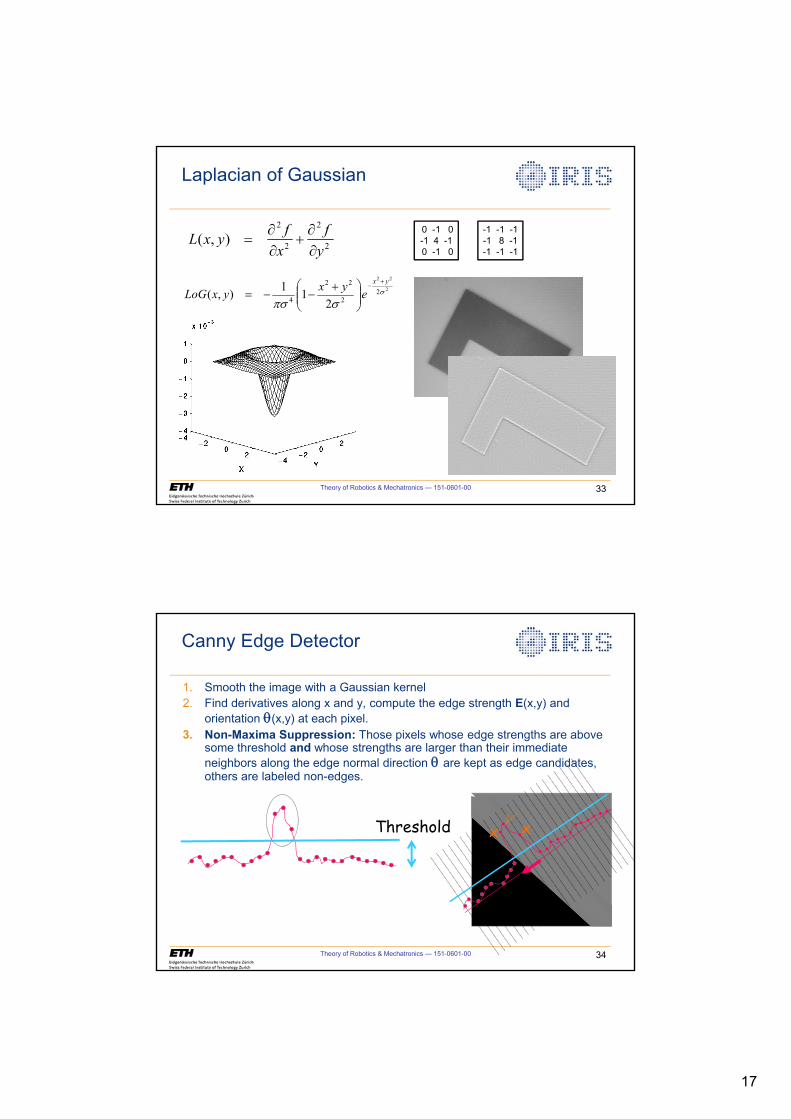
17
Laplacian of Gaussian
Theory of Robotics & Mechatronics — 151-0601-00 33
0 -1 0-1 4 -10 -1 0
-1 -1 -1-1 8 -1-1 -1 -12
2
2
2
),(yf
xf
yxLww
�ww
2
22
22
22
4 21
1),( V
VSV
yx
eyx
yxLoG�
�
¸̧¹
·¨̈©
§ ���
Theory of Robotics & Mechatronics — 151-0601-00 34
Canny Edge Detector
1. Smooth the image with a Gaussian kernel2. Find derivatives along x and y, compute the edge strength E(x,y) and
orientation T(x,y) at each pixel.3. Non-Maxima Suppression: Those pixels whose edge strengths are above
some threshold and whose strengths are larger than their immediate neighbors along the edge normal direction T are kept as edge candidates, others are labeled non-edges.
Threshold x x
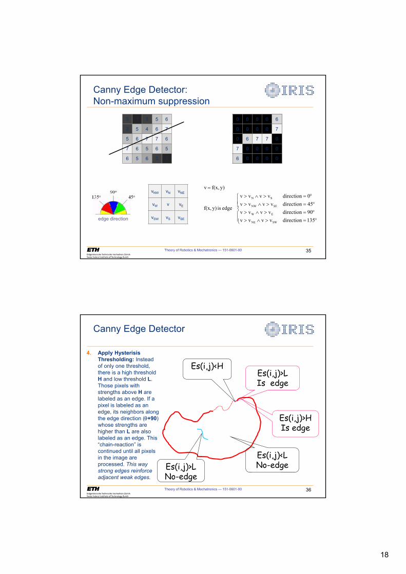
18
Canny Edge Detector:Non-maximum suppression
Theory of Robotics & Mechatronics — 151-0601-00 35
3 1 3 5 6
3 5 4 6 7
5 6 7 7 6
7 6 5 6 5
6 5 6 3 1
edge direction
vNW vN vNE
vW v vE
vSW vS vSE °°¯
°°®
q !�!q !�!q !�!q !�!
135directionvvvv
09directionvvvv
45directionvvvv
0directionvvvv
edge is y)f(x,
y)f(x, v
SWNE
EW
SENW
SN
7
0 0 0 0 6
0 0 0 0 7
0 6 7 7 0
7 0 0 0 0
6 0 0 0 0
Theory of Robotics & Mechatronics — 151-0601-00 36
Canny Edge Detector
Es(i,j)>HIs edge
Es(i,j)<HEs(i,j)>LIs edge
Es(i,j)<LNo-edgeEs(i,j)>L
No-edge
4. Apply Hysterisis Thresholding: Instead of only one threshold, there is a high threshold H and low threshold L. Those pixels with strengths above H are labeled as an edge. If a pixel is labeled as an edge, its neighbors along the edge direction (T+90) whose strengths are higher than L are also labeled as an edge. This “chain-reaction” is continued until all pixels in the image are processed. This way strong edges reinforce adjacent weak edges.
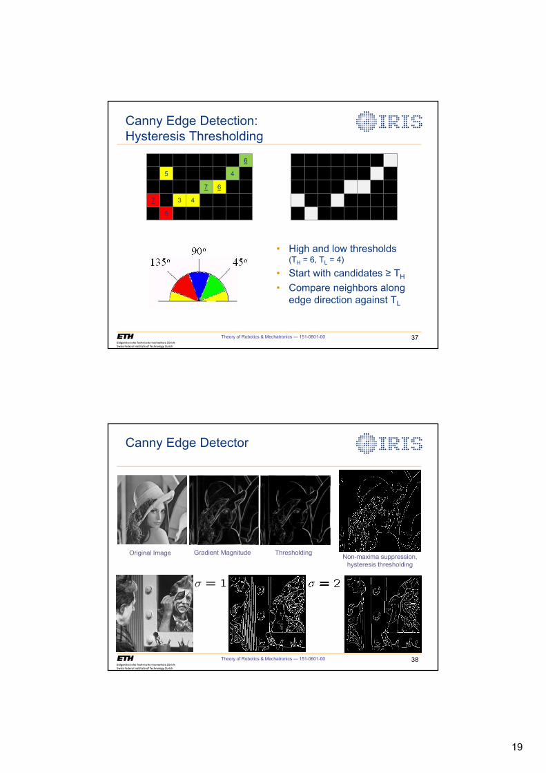
19
Canny Edge Detection:Hysteresis Thresholding
• High and low thresholds(TH = 6, TL = 4)
• Start with candidates TH
• Compare neighbors alongedge direction against TL
Theory of Robotics & Mechatronics — 151-0601-00 37
6
5 4
7 6
7 3 4
5
Theory of Robotics & Mechatronics — 151-0601-00 38
Canny Edge Detector
Original Image Gradient Magnitude Thresholding Non-maxima suppression,hysteresis thresholding
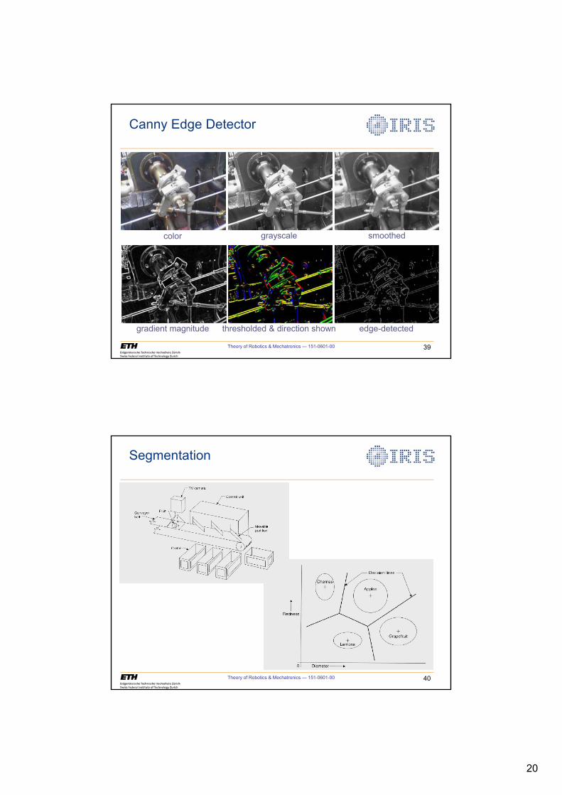
20
Canny Edge Detector
Theory of Robotics & Mechatronics — 151-0601-00 39
color grayscale smoothed
gradient magnitude thresholded & direction shown edge-detected
Theory of Robotics & Mechatronics — 151-0601-00 40
Segmentation
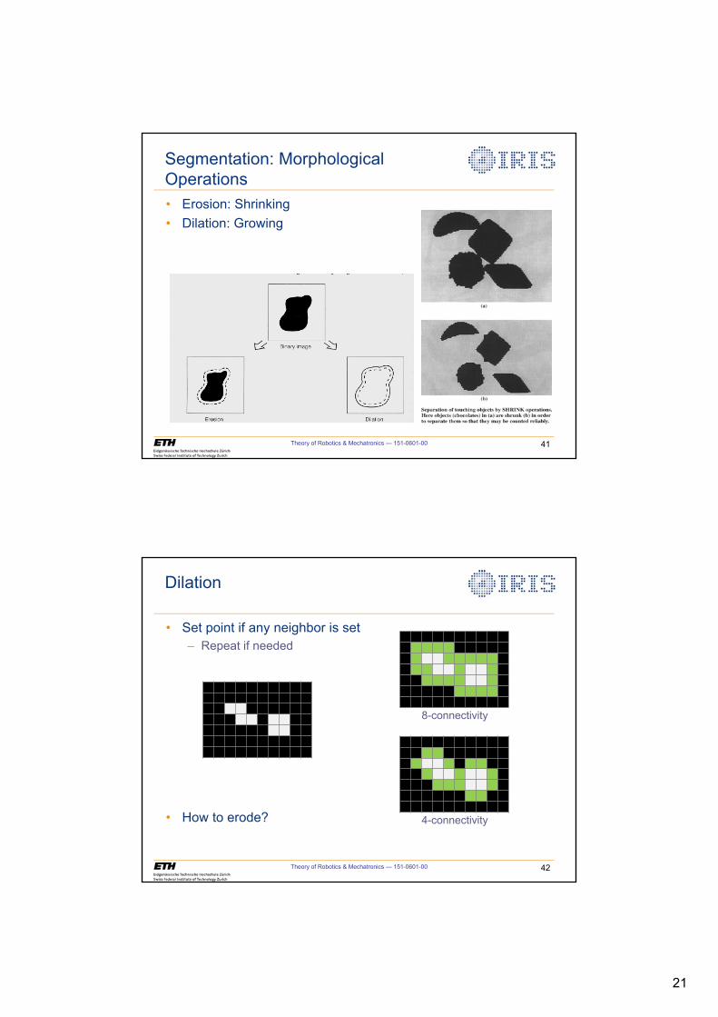
21
Theory of Robotics & Mechatronics — 151-0601-00 41
• Erosion: Shrinking• Dilation: Growing
Segmentation: Morphological Operations
Dilation
• Set point if any neighbor is set– Repeat if needed
• How to erode?
Theory of Robotics & Mechatronics — 151-0601-00 42
8-connectivity
4-connectivity
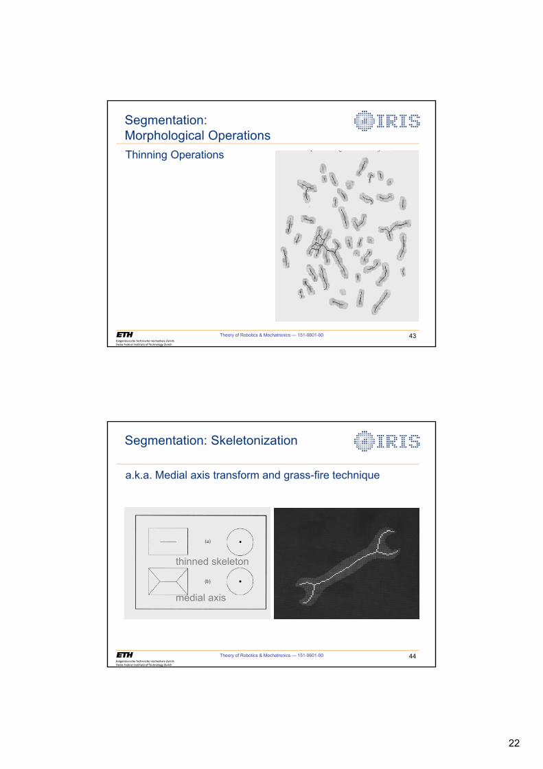
22
Theory of Robotics & Mechatronics — 151-0601-00 43
Thinning Operations
Segmentation:Morphological Operations
Theory of Robotics & Mechatronics — 151-0601-00 44
a.k.a. Medial axis transform and grass-fire technique
thinned skeleton
medial axis
Segmentation: Skeletonization
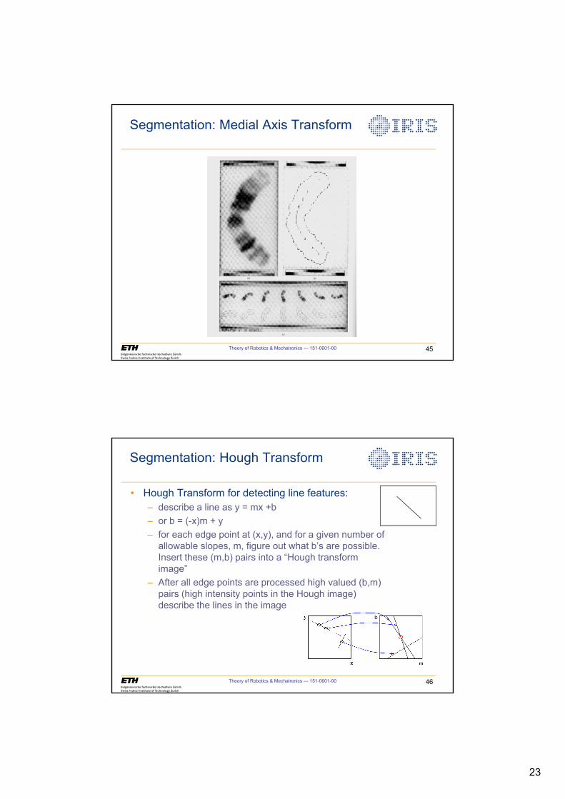
23
Theory of Robotics & Mechatronics — 151-0601-00 45
Segmentation: Medial Axis Transform
Theory of Robotics & Mechatronics — 151-0601-00 46
• Hough Transform for detecting line features:– describe a line as y = mx +b– or b = (-x)m + y– for each edge point at (x,y), and for a given number of
allowable slopes, m, figure out what b’s are possible. Insert these (m,b) pairs into a “Hough transform image”
– After all edge points are processed high valued (b,m) pairs (high intensity points in the Hough image) describe the lines in the image
Segmentation: Hough Transform
b
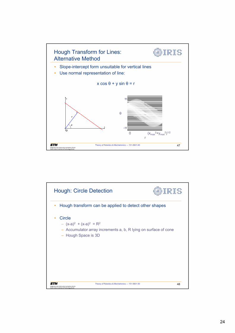
24
Hough Transform for Lines:Alternative Method• Slope-intercept form unsuitable for vertical lines• Use normal representation of line:
x cos + y sin = r
Theory of Robotics & Mechatronics — 151-0601-00 47
-0 (xmax
2+ymax2)1/2
r
Hough: Circle Detection
• Hough transform can be applied to detect other shapes
• Circle– (x-a)2 + (x-a)2 = R2
– Accumulator array increments a, b, R lying on surface of cone– Hough Space is 3D
Theory of Robotics & Mechatronics — 151-0601-00 48
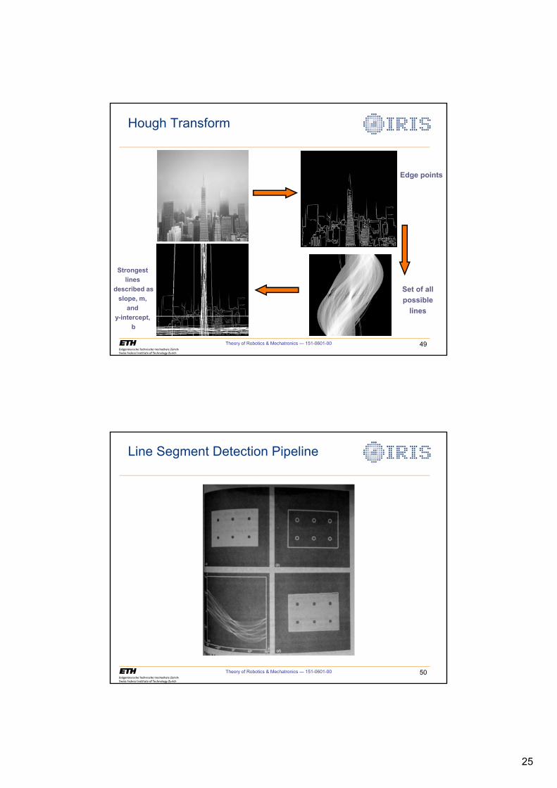
25
Theory of Robotics & Mechatronics — 151-0601-00 49
Hough Transform
Edge points
Strongest lines
described asslope, m,
and y-intercept,
b
Set of allpossible
lines
Line Segment Detection Pipeline
Theory of Robotics & Mechatronics — 151-0601-00 50
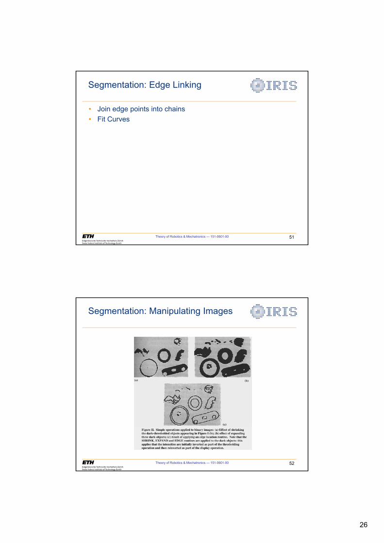
26
Theory of Robotics & Mechatronics — 151-0601-00 51
• Join edge points into chains• Fit Curves
Segmentation: Edge Linking
Theory of Robotics & Mechatronics — 151-0601-00 52
Segmentation: Manipulating Images
27
Theory of Robotics & Mechatronics — 151-0601-00 53
• Object measures– Area (number of points in region)
– Perimeter (number of points on edge)
– Length (ymax-ymin)
– Width (xmax-xmin)
– shape analysis• rectangularity• circularity
Object Classification
Theory of Robotics & Mechatronics — 151-0601-00 54
• Invariant moments– central moments (e.g., cog)
• x=1/n (x,y)∈R x– principal axes
• Shape descriptors– Fourier descriptors– medial axis transform
Object Measures
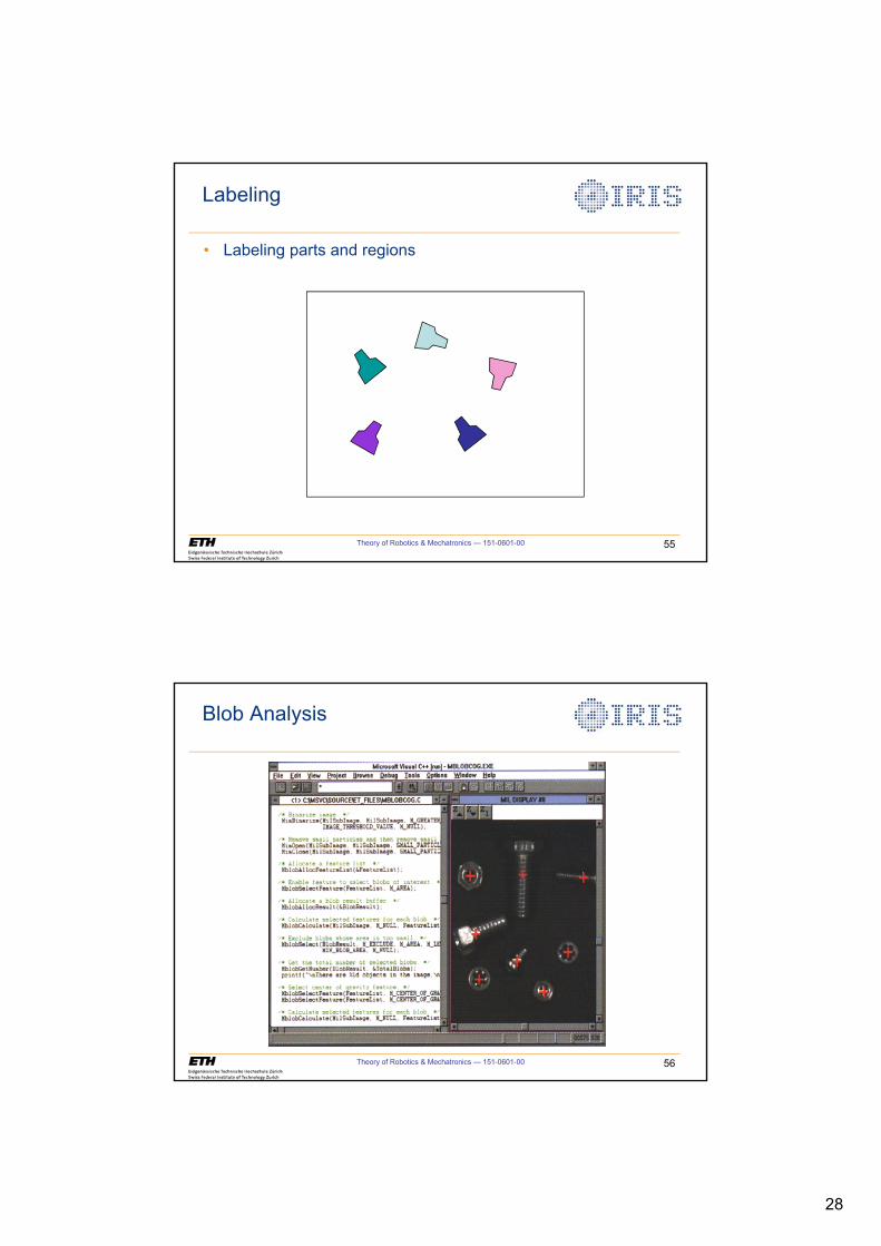
28
Theory of Robotics & Mechatronics — 151-0601-00 55
• Labeling parts and regions
Labeling
Theory of Robotics & Mechatronics — 151-0601-00 56
Blob Analysis
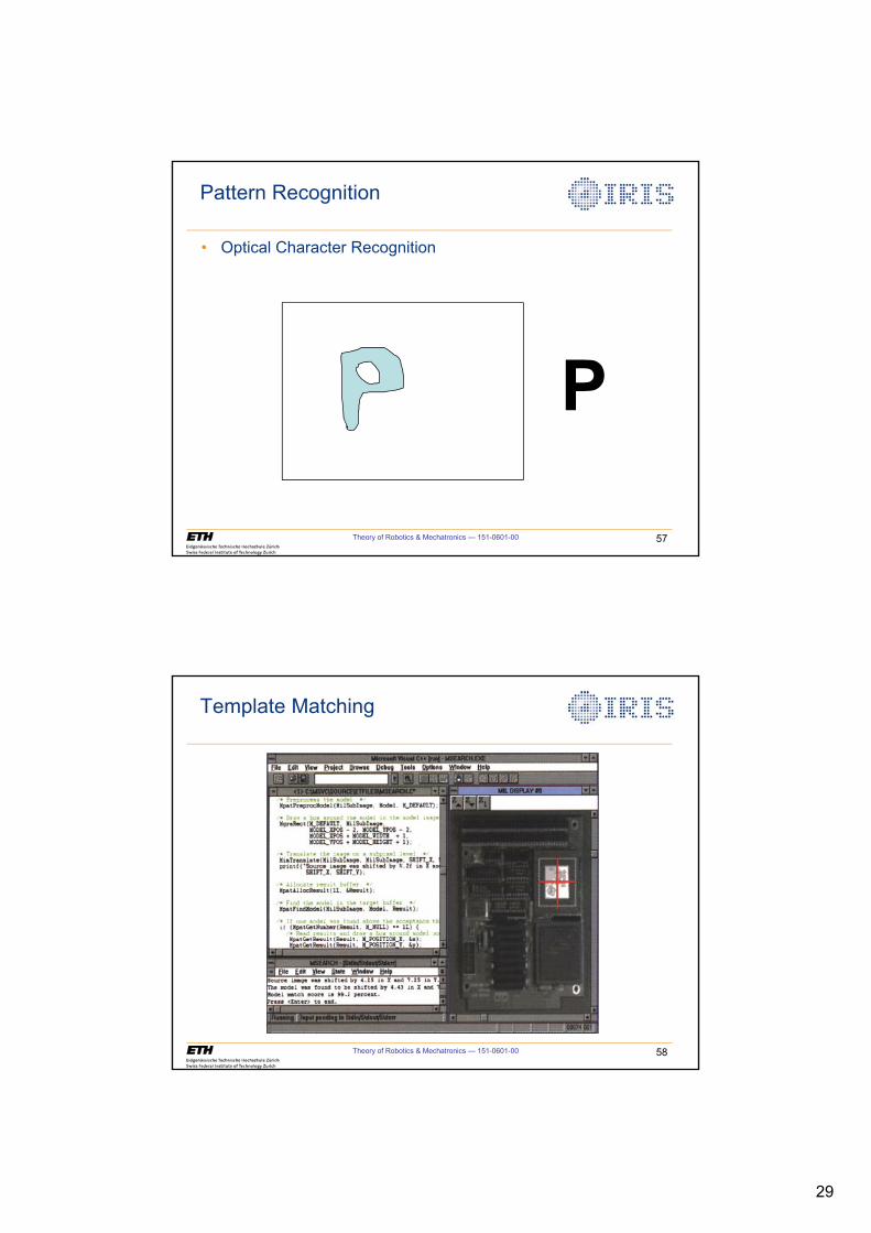
29
Theory of Robotics & Mechatronics — 151-0601-00 57
• Optical Character Recognition
P
Pattern Recognition
Theory of Robotics & Mechatronics — 151-0601-00 58
Template Matching
30
Theory of Robotics & Mechatronics — 151-0601-00 59
• Fourier Transform• Convolution = Multiplication in the Fourier domain• Low-pass filtering
Frequency Domain Techniques
Theory of Robotics & Mechatronics — 151-0601-00 60
Fourier Transform
31
Theory of Robotics & Mechatronics — 151-0601-00 61
Fourier Transform
• Fourier Series• Fourier Transform• Discrete Fourier Transform• Fast Fourier Transform• Properties of the Fourier Transform• The Convolution Theorem• Discrete Fourier Transform• Discrete Cosine Transform
Theory of Robotics & Mechatronics — 151-0601-00 62
It Isn’t Always Perfect
In fact it never is!

32
Theory of Robotics & Mechatronics — 151-0601-00 63
• Color image processing• Motion analysis• 3D image analysis (next class)
Things We Haven’t Talked About
1
Computer Vision for Robotics
Institute of Robotics and Intelligent SystemsETH Zurich
Theory of Robotics &Mechatronics
Theory of Robotics & Mechatronics — 151-0601-00 2
Vision for Robotics
• Visual Servoing• Visual Tracking• 3D Vision
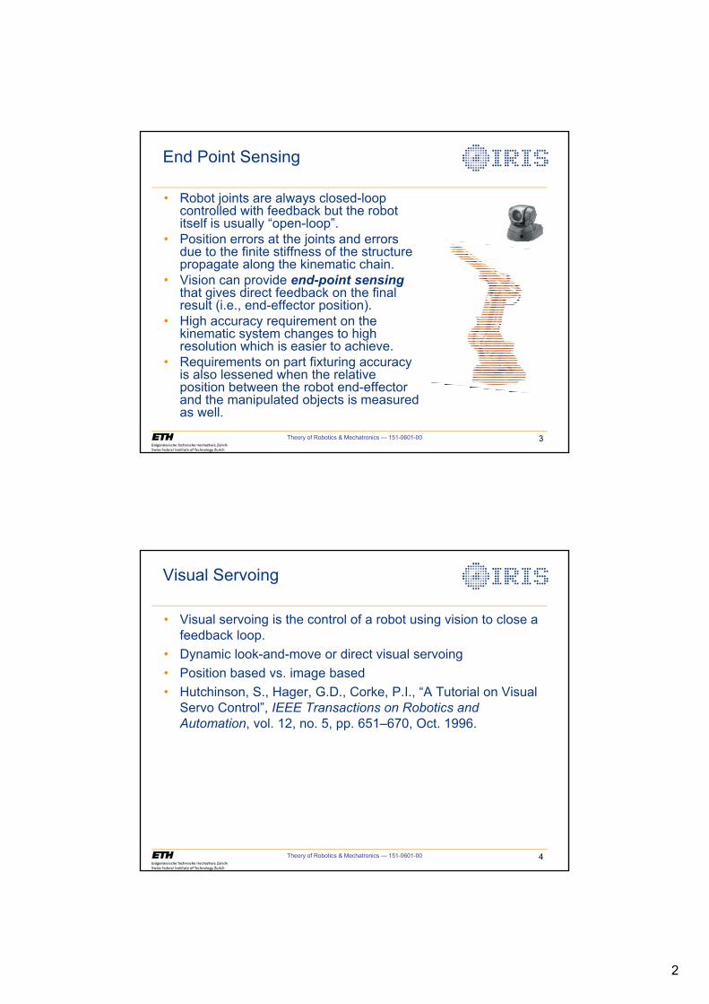
2
Theory of Robotics & Mechatronics — 151-0601-00 3
End Point Sensing
• Robot joints are always closed-loop controlled with feedback but the robot itself is usually “open-loop”.
• Position errors at the joints and errors due to the finite stiffness of the structure propagate along the kinematic chain.
• Vision can provide end-point sensingthat gives direct feedback on the final result (i.e., end-effector position).
• High accuracy requirement on the kinematic system changes to high resolution which is easier to achieve.
• Requirements on part fixturing accuracy is also lessened when the relative position between the robot end-effector and the manipulated objects is measured as well.
Theory of Robotics & Mechatronics — 151-0601-00 4
Visual Servoing
• Visual servoing is the control of a robot using vision to close a feedback loop.
• Dynamic look-and-move or direct visual servoing• Position based vs. image based• Hutchinson, S., Hager, G.D., Corke, P.I., “A Tutorial on Visual
Servo Control”, IEEE Transactions on Robotics and Automation, vol. 12, no. 5, pp. 651–670, Oct. 1996.
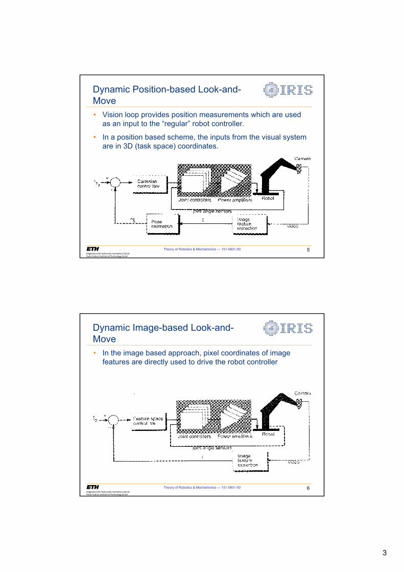
3
Theory of Robotics & Mechatronics — 151-0601-00 5
Dynamic Position-based Look-and-Move• Vision loop provides position measurements which are used
as an input to the “regular” robot controller.
• In a position based scheme, the inputs from the visual system are in 3D (task space) coordinates.
Theory of Robotics & Mechatronics — 151-0601-00 6
Dynamic Image-based Look-and-Move• In the image based approach, pixel coordinates of image
features are directly used to drive the robot controller
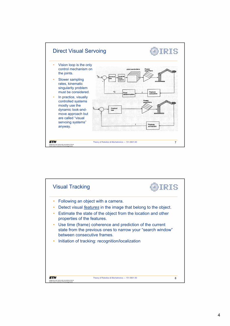
4
Theory of Robotics & Mechatronics — 151-0601-00 7
Direct Visual Servoing
• Vision loop is the only control mechanism on the joints.
• Slower sampling rates, kinematic singularity problem must be considered.
• In practice, visually controlled systems mostly use the dynamic look-and-move approach but are called “visual servoing systems” anyway.
Theory of Robotics & Mechatronics — 151-0601-00 8
Visual Tracking
• Following an object with a camera.• Detect visual features in the image that belong to the object.• Estimate the state of the object from the location and other
properties of the features.• Use time (frame) coherence and prediction of the current
state from the previous ones to narrow your “search window” between consecutive frames.
• Initiation of tracking: recognition/localization
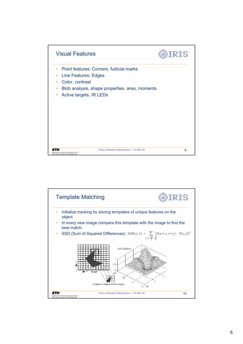
5
Theory of Robotics & Mechatronics — 151-0601-00 9
Visual Features
• Point features: Corners, fudicial marks• Line Features: Edges• Color, contrast• Blob analysis, shape properties, area, moments• Active targets, IR LEDs
Theory of Robotics & Mechatronics — 151-0601-00 10
Template Matching
• Initialize tracking by storing templates of unique features on the object.
• In every new image compare this template with the image to find the best match.
• SSD (Sum of Squared Differences)
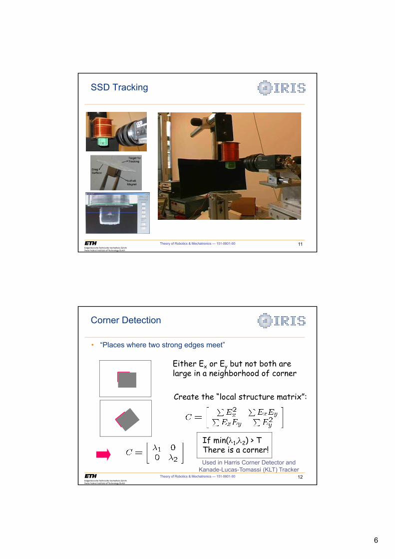
6
Theory of Robotics & Mechatronics — 151-0601-00 11
SSD Tracking
Theory of Robotics & Mechatronics — 151-0601-00 12
Corner Detection
• “Places where two strong edges meet”
Either Ex or Ey but not both are large in a neighborhood of corner
Create the “local structure matrix”:
If min(O1,O2) > TThere is a corner!Used in Harris Corner Detector and
Kanade-Lucas-Tomassi (KLT) Tracker
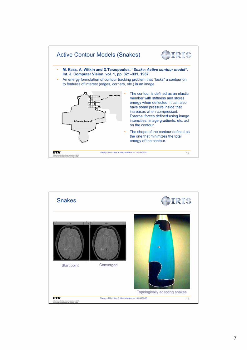
7
Theory of Robotics & Mechatronics — 151-0601-00 13
Active Contour Models (Snakes)
• M. Kass, A. Witkin and D.Terzopoulos, “Snake: Active contour model”, Int. J. Computer Vision, vol. 1, pp. 321–331, 1987.
• An energy formulation of contour tracking problem that “locks” a contour on to features of interest (edges, corners, etc.) in an image.
• The contour is defined as an elastic member with stiffness and stores energy when deflected. It can also have some pressure inside that increases when compressed. External forces defined using image intensities, image gradients, etc. act on the contour.
• The shape of the contour defined as the one that minimizes the total energy of the contour.
Theory of Robotics & Mechatronics — 151-0601-00 14
Snakes
Start point Converged
Topologically adapting snakes
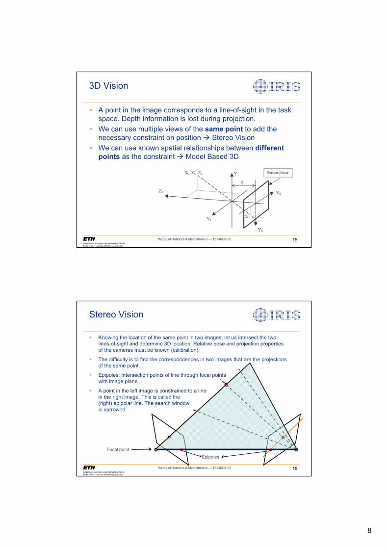
8
Theory of Robotics & Mechatronics — 151-0601-00 15
3D Vision
• A point in the image corresponds to a line-of-sight in the task space. Depth information is lost during projection.
• We can use multiple views of the same point to add the necessary constraint on position Æ Stereo Vision
• We can use known spatial relationships between different points as the constraint Æ Model Based 3D
Theory of Robotics & Mechatronics — 151-0601-00 16
Stereo Vision
Epipoles
• Knowing the location of the same point in two images, let us intersect the two lines-of-sight and determine 3D location. Relative pose and projection properties of the cameras must be known (calibration).
• The difficulty is to find the correspondences in two images that are the projections of the same point.
• Epipoles: Intersection points of line through focal pointswith image plane
• A point in the left image is constrained to a line in the right image. This is called the (right) epipolar line. The search window is narrowed.
Focal point
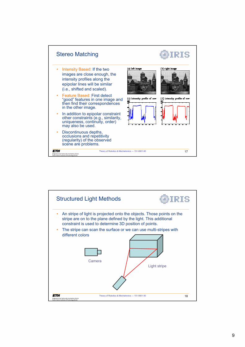
9
Theory of Robotics & Mechatronics — 151-0601-00 17
Stereo Matching
• Intensity Based: If the two images are close enough, the intensity profiles along the epipolar lines will be similar(i.e., shifted and scaled).
• Feature Based: First detect “good” features in one image and then find their correspondences in the other image.
• In addition to epipolar constraint other constraints (e.g., similarity, uniqueness, continuity, order) may also be used.
• Discontinuous depths, occlusions and repetitivity (regularity) of the observed scene are problems.
Theory of Robotics & Mechatronics — 151-0601-00 18
Structured Light Methods
CameraLight stripe
• An stripe of light is projected onto the objects. Those points on the stripe are on to the plane defined by the light. This additional constraint is used to determine 3D position of points.
• The stripe can scan the surface or we can use multi-stripes with different colors
10
Structured Light Implementation Options• Pattern can be black/white, color or IR• Multiple cameras to avoid obstructions
Theory of Robotics & Mechatronics — 151-0601-00 19
Kinect
Theory of Robotics & Mechatronics — 151-0601-00 20
11
Kinect
Theory of Robotics & Mechatronics — 151-0601-00 21
Theory of Robotics & Mechatronics — 151-0601-00 22
Model-Based Tracking
• Knowing the 3D spatial relationship (i.e., the model) between the points in the image, we can find the position and orientation of the rigid body constructed by those points.
• Matches between 3 non-collinear model and image points is enough to analytically solve the 6 DOF pose.
• Usually many more points are matched and a least-squares type solution is sought.
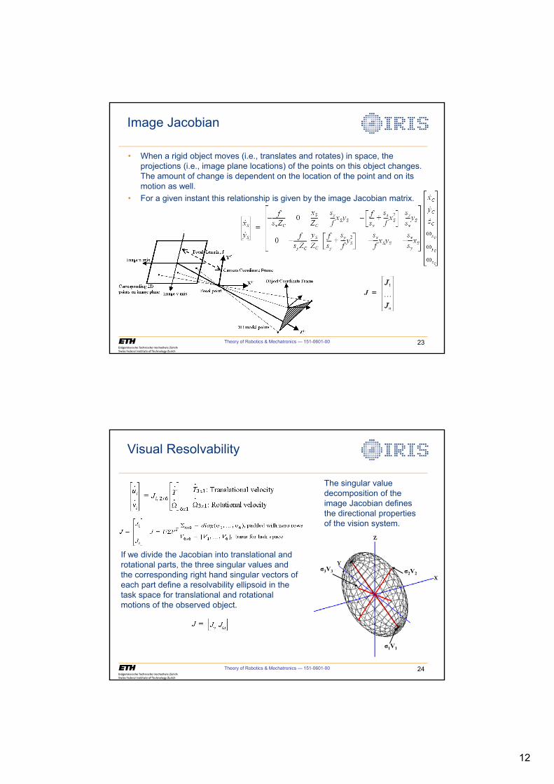
12
Theory of Robotics & Mechatronics — 151-0601-00 23
Image Jacobian
• When a rigid object moves (i.e., translates and rotates) in space, the projections (i.e., image plane locations) of the points on this object changes. The amount of change is dependent on the location of the point and on its motion as well.
• For a given instant this relationship is given by the image Jacobian matrix.
Theory of Robotics & Mechatronics — 151-0601-00 24
Visual Resolvability
The singular value decomposition of the image Jacobian defines the directional properties of the vision system.
If we divide the Jacobian into translational and rotational parts, the three singular values and the corresponding right hand singular vectors of each part define a resolvability ellipsoid in the task space for translational and rotational motions of the observed object.
1V1
2V23V3
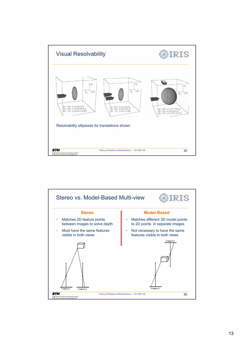
13
Theory of Robotics & Mechatronics — 151-0601-00 25
Visual Resolvability
Resolvability ellipsoids for translations shown
Theory of Robotics & Mechatronics — 151-0601-00 26
Stereo vs. Model-Based Multi-view
Camera 1 Camera 2 Camera 1
Camera 2
Stereo• Matches 2D feature points
between images to solve depth
• Must have the same features visible in both views
Model-Based• Matches different 3D model points
to 2D points in separate images
• Not necessary to have the same features visible in both views
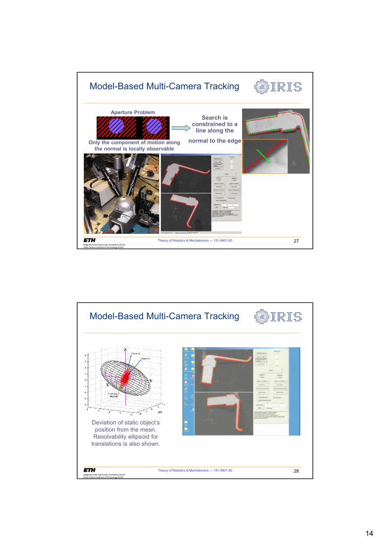
14
Theory of Robotics & Mechatronics — 151-0601-00 27
Model-Based Multi-Camera Tracking
Search is constrained to a
line along the
normal to the edgeOnly the component of motion along the normal is locally observable
Aperture Problem
Theory of Robotics & Mechatronics — 151-0601-00 28
Model-Based Multi-Camera Tracking
Deviation of static object’s position from the mean. Resolvability ellipsoid for
translations is also shown.
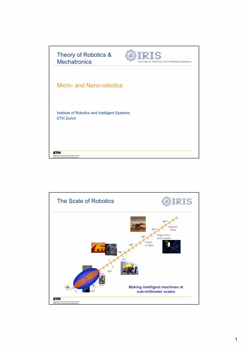
1
Micro- and Nano-robotics
Institute of Robotics and Intelligent SystemsETH Zurich
Theory of Robotics &Mechatronics
The Scale of Robotics
10-6
10-3
Pm
Å
10-9
1
103
106
109
1012
1015
nm
mm
m
km
Edge of the solar system
Earth to Mars
CNT
Nearest Stars
Making intelligent machines at sub-millimeter scales
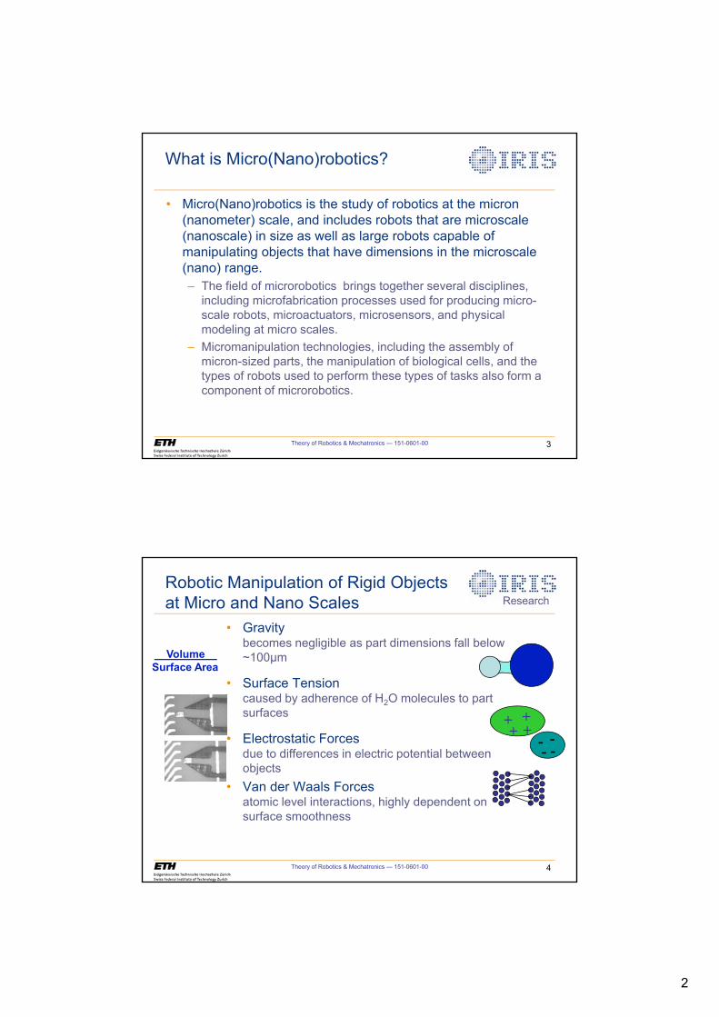
2
Theory of Robotics & Mechatronics — 151-0601-00 3
What is Micro(Nano)robotics?
• Micro(Nano)robotics is the study of robotics at the micron (nanometer) scale, and includes robots that are microscale (nanoscale) in size as well as large robots capable of manipulating objects that have dimensions in the microscale (nano) range. – The field of microrobotics brings together several disciplines,
including microfabrication processes used for producing micro-scale robots, microactuators, microsensors, and physical modeling at micro scales.
– Micromanipulation technologies, including the assembly of micron-sized parts, the manipulation of biological cells, and the types of robots used to perform these types of tasks also form a component of microrobotics.
Theory of Robotics & Mechatronics — 151-0601-00 4
Robotic Manipulation of Rigid Objects at Micro and Nano Scales
• Gravity becomes negligible as part dimensions fall below ~100μm
• Surface Tensioncaused by adherence of H2O molecules to part surfaces
• Electrostatic Forcesdue to differences in electric potential between objects
• Van der Waals Forcesatomic level interactions, highly dependent on surface smoothness
+++
+---
-
Research
Volume Surface Area
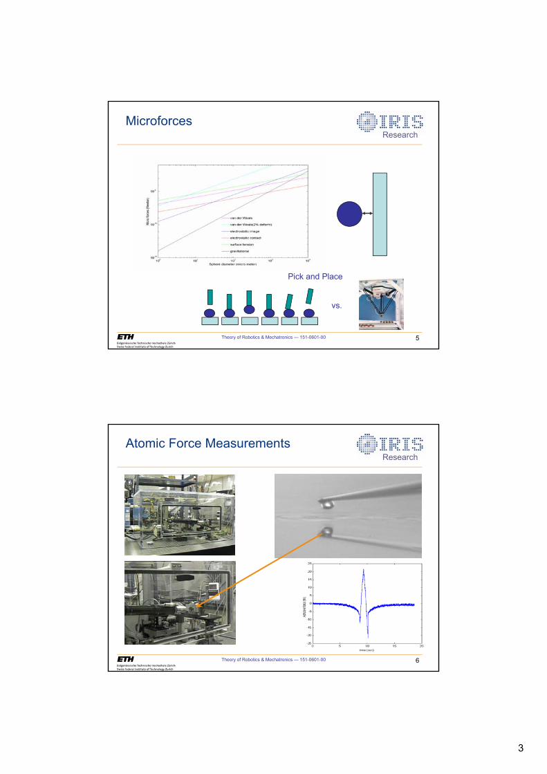
3
Theory of Robotics & Mechatronics — 151-0601-00 5
Microforces
Pick and Place
vs.
Research
Theory of Robotics & Mechatronics — 151-0601-00 6
Atomic Force MeasurementsResearch
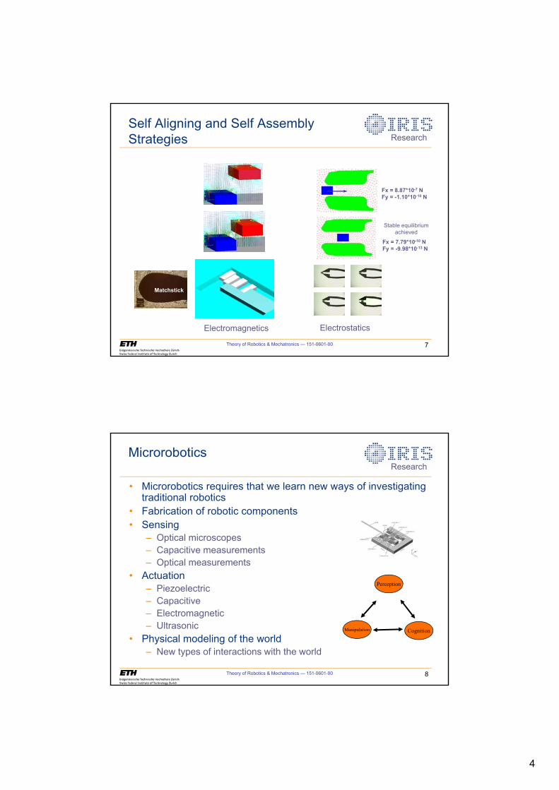
4
Theory of Robotics & Mechatronics — 151-0601-00 7
Self Aligning and Self Assembly Strategies
Fx = 8.87*10-7 NFy = -1.10*10-10 N
Fx = 7.79*10-10 NFy = -9.98*10-13 N
Stable equilibrium achieved
ElectrostaticsElectromagnetics
Matchstick
Research
Theory of Robotics & Mechatronics — 151-0601-00 8
Microrobotics
• Microrobotics requires that we learn new ways of investigating traditional robotics
• Fabrication of robotic components• Sensing
– Optical microscopes– Capacitive measurements– Optical measurements
• Actuation– Piezoelectric– Capacitive– Electromagnetic– Ultrasonic
• Physical modeling of the world– New types of interactions with the world
Manipulation
Perception
Cognition
Research
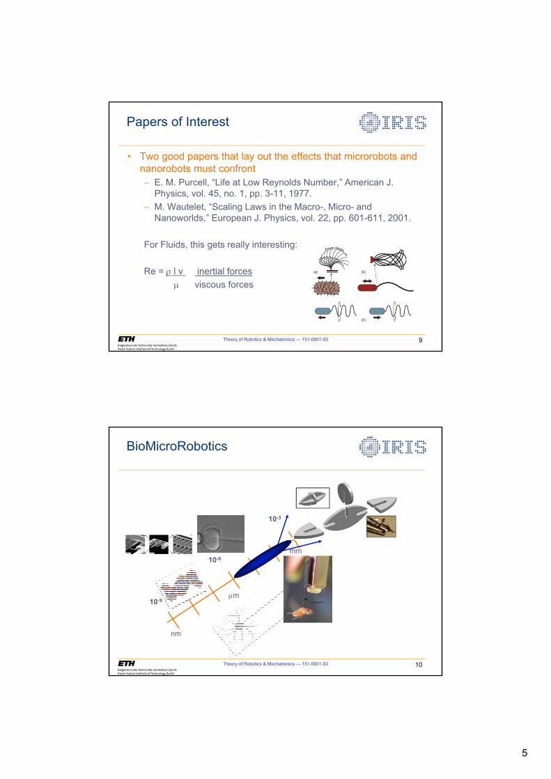
5
Theory of Robotics & Mechatronics — 151-0601-00 9
Papers of Interest
• Two good papers that lay out the effects that microrobots and nanorobots must confront– E. M. Purcell, “Life at Low Reynolds Number,” American J.
Physics, vol. 45, no. 1, pp. 3-11, 1977.– M. Wautelet, “Scaling Laws in the Macro-, Micro- and
Nanoworlds,” European J. Physics, vol. 22, pp. 601-611, 2001.
For Fluids, this gets really interesting:
Re = U�l v inertial forcesP viscous forces
Theory of Robotics & Mechatronics — 151-0601-00 10
10-9
10-6
10-3
nm
Pm
mm
BioMicroRobotics
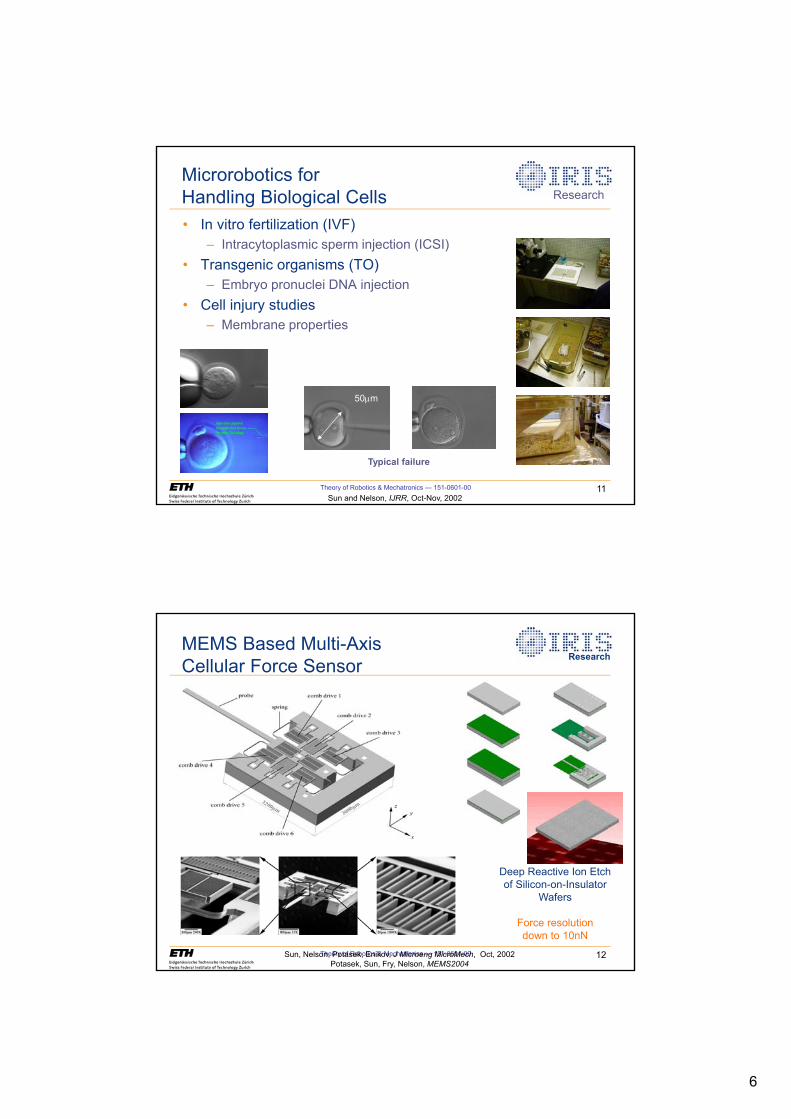
6
Theory of Robotics & Mechatronics — 151-0601-00 11
Microrobotics for Handling Biological Cells• In vitro fertilization (IVF)
– Intracytoplasmic sperm injection (ICSI)
• Transgenic organisms (TO)– Embryo pronuclei DNA injection
• Cell injury studies– Membrane properties
Typical failure
Sun and Nelson, IJRR, Oct-Nov, 2002
50Pm
Research
Theory of Robotics & Mechatronics — 151-0601-00 12
MEMS Based Multi-Axis Cellular Force Sensor
Deep Reactive Ion Etch of Silicon-on-Insulator
Wafers
Force resolution down to 10nN
Sun, Nelson, Potasek, Enikov, J Microeng MicroMech, Oct, 2002Potasek, Sun, Fry, Nelson, MEMS2004
Research
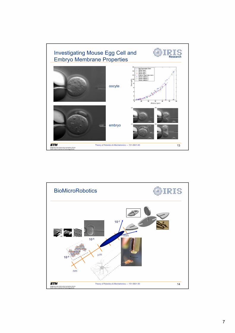
7
Theory of Robotics & Mechatronics — 151-0601-00 13
Investigating Mouse Egg Cell andEmbryo Membrane Properties
oocyte
embryo
Research
Theory of Robotics & Mechatronics — 151-0601-00 14
10-9
10-6
10-3
nm
Pm
mm
BioMicroRobotics
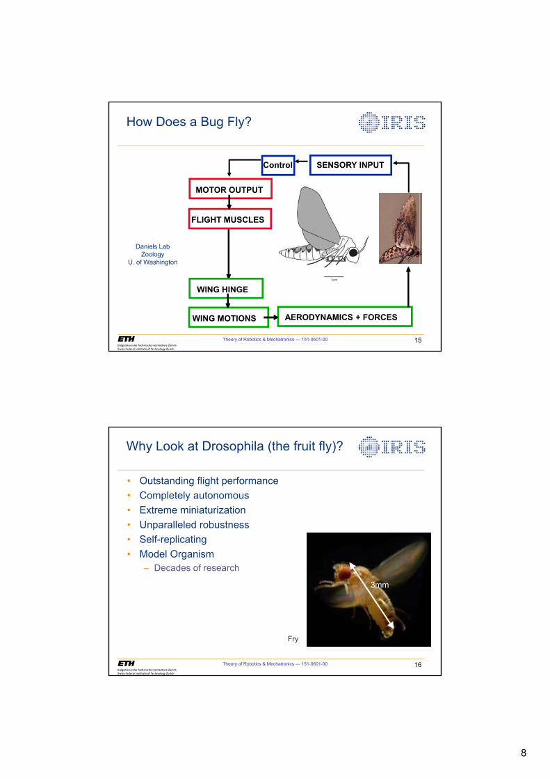
8
Theory of Robotics & Mechatronics — 151-0601-00 15
How Does a Bug Fly?
SENSORY INPUT
MOTOR OUTPUT
FLIGHT MUSCLES
WING HINGE
WING MOTIONS AERODYNAMICS + FORCES
Control
Daniels LabZoology
U. of Washington
Theory of Robotics & Mechatronics — 151-0601-00 16
Why Look at Drosophila (the fruit fly)?
• Outstanding flight performance • Completely autonomous • Extreme miniaturization • Unparalleled robustness • Self-replicating• Model Organism
– Decades of research
3mm
Fry
9
Theory of Robotics & Mechatronics — 151-0601-00 17
Fly Brain Structure
Institut für Biologie III der Albert-Ludwigs-Universität Freiburg
Theory of Robotics & Mechatronics — 151-0601-00 18
Fly Muscles
Dickinson
10
Theory of Robotics & Mechatronics — 151-0601-00 19
Neurons to Behaviors:Measurement of Flight Dynamics: Drosophila (Fruit Fly) Research
5000 frames/s
Wing beat frequencyof 200Hz
Lift forces as high as 35μN
Fry, Sayaman, and Dickinson, Science, 2003Sun, Potasek, Bell, Fry, and Nelson, JMEMS, 2004
Theory of Robotics & Mechatronics — 151-0601-00 20
Micromechanical Flying Insect (MFI) Ron Fearing UC-Berkeley
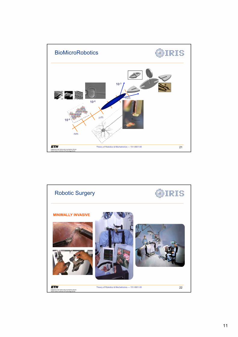
11
Theory of Robotics & Mechatronics — 151-0601-00 21
10-9
10-6
10-3
nm
Pm
mm
BioMicroRobotics
Theory of Robotics & Mechatronics — 151-0601-00 22
Robotic Surgery
MINIMALLY INVASIVE
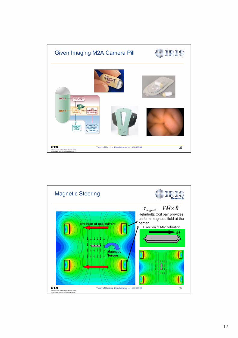
12
Theory of Robotics & Mechatronics — 151-0601-00 23
Given Imaging M2A Camera Pill
Theory of Robotics & Mechatronics — 151-0601-00 24
Helmholtz Coil pair provides uniform magnetic field at the centerdirection of coil current
Direction of Magnetization
Magnetic Steering
magnetic VM BW u& &
Magnetic Torque
M&
Research
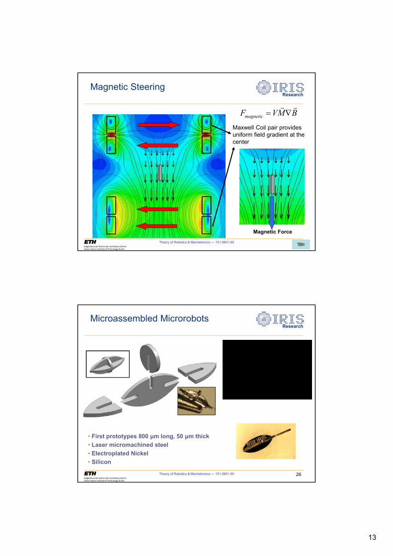
13
Theory of Robotics & Mechatronics — 151-0601-00 25
Maxwell Coil pair provides uniform field gradient at the center
Magnetic Steering
Magnetic Force
magneticF VM B �& &
Research
Theory of Robotics & Mechatronics — 151-0601-00 26
Microassembled Microrobots
• First prototypes 800 m long, 50 m thick• Laser micromachined steel• Electroplated Nickel• Silicon
Research
14
Theory of Robotics & Mechatronics — 151-0601-00 27
In Vivo Magnetic MicroRobots
• A MicroRobotic Platform for Investigating
– Microassembly– Microfabrication– Deposition of hard magnetic
materials for MEMS– Microsensors and
microactuators– Visual Servoing– Ultrasonic Servoing– New biomedical applications and
procedures
Wireless magnetically guided microrobots
Theory of Robotics & Mechatronics — 151-0601-00 28
NanoRobotics
• Miniaturization beyond MEMS (MicroElectro-MechanicalSystems) is needed
• NEMS (NanoElectro-MechanicalSystems) with novel nanoscale structures will enable many new nanosensors and nanoactuators
Nanoscrolls and NEMS
Telescoping CNTsand Hybrid NEMS
CNT-based NEMS
Top electrode
Ground electrode
IRIS Proprietary and Confidential
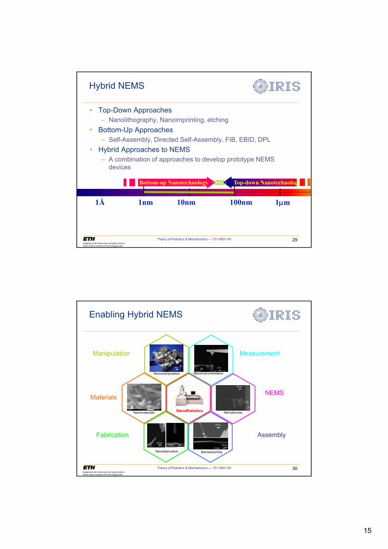
15
Theory of Robotics & Mechatronics — 151-0601-00 29
Hybrid NEMS
• Top-Down Approaches– Nanolithography, Nanoimprinting, etching
• Bottom-Up Approaches– Self-Assembly, Directed Self-Assembly, FIB, EBID, DPL
• Hybrid Approaches to NEMS– A combination of approaches to develop prototype NEMS
devices
1nm 10nm 100nm 1Pm1Å
Top-down NanotechnologyBottom-up Nanotechnology
Theory of Robotics & Mechatronics — 151-0601-00 30
Enabling Hybrid NEMS
NanoRobotics
Nanomanipulation
Nanodevices
1cm
100nm
Nanoinstrumentation
Nanofabrication Nanoassembly
100nm100nm
1Pm
100nm
100nm
Nanomaterials
100nm
Manipulation Measurement
AssemblyFabrication
MaterialsNEMS
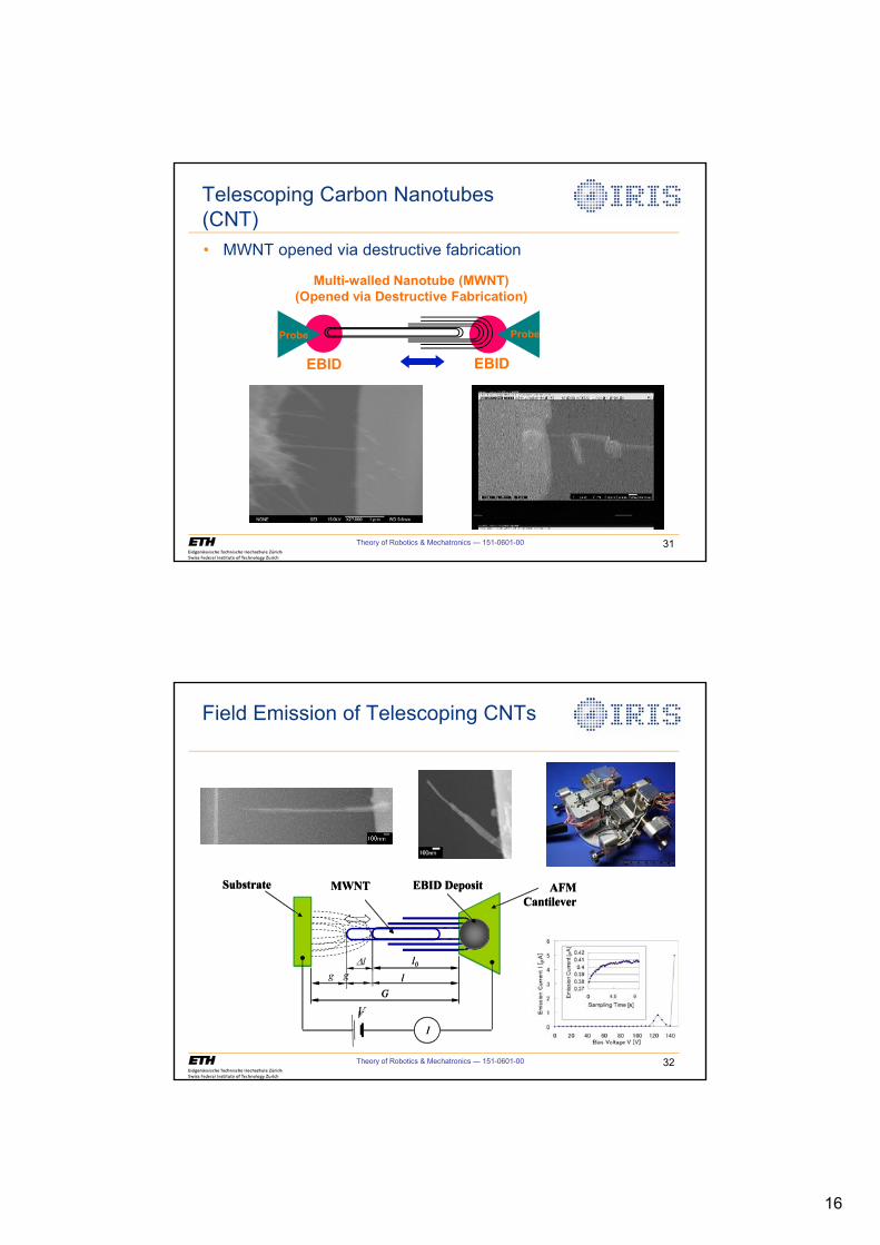
16
Theory of Robotics & Mechatronics — 151-0601-00 31
Telescoping Carbon Nanotubes (CNT)• MWNT opened via destructive fabrication
EBID EBID
Multi-walled Nanotube (MWNT)(Opened via Destructive Fabrication)
ProbeProbe
Theory of Robotics & Mechatronics — 151-0601-00 32
Field Emission of Telescoping CNTs
I
VG
lg'l l0
MWNT AFM Cantilever
EBID DepositSubstrate
IV
Glgl0
MWNT AFM Cantilever
EBID DepositSubstrate
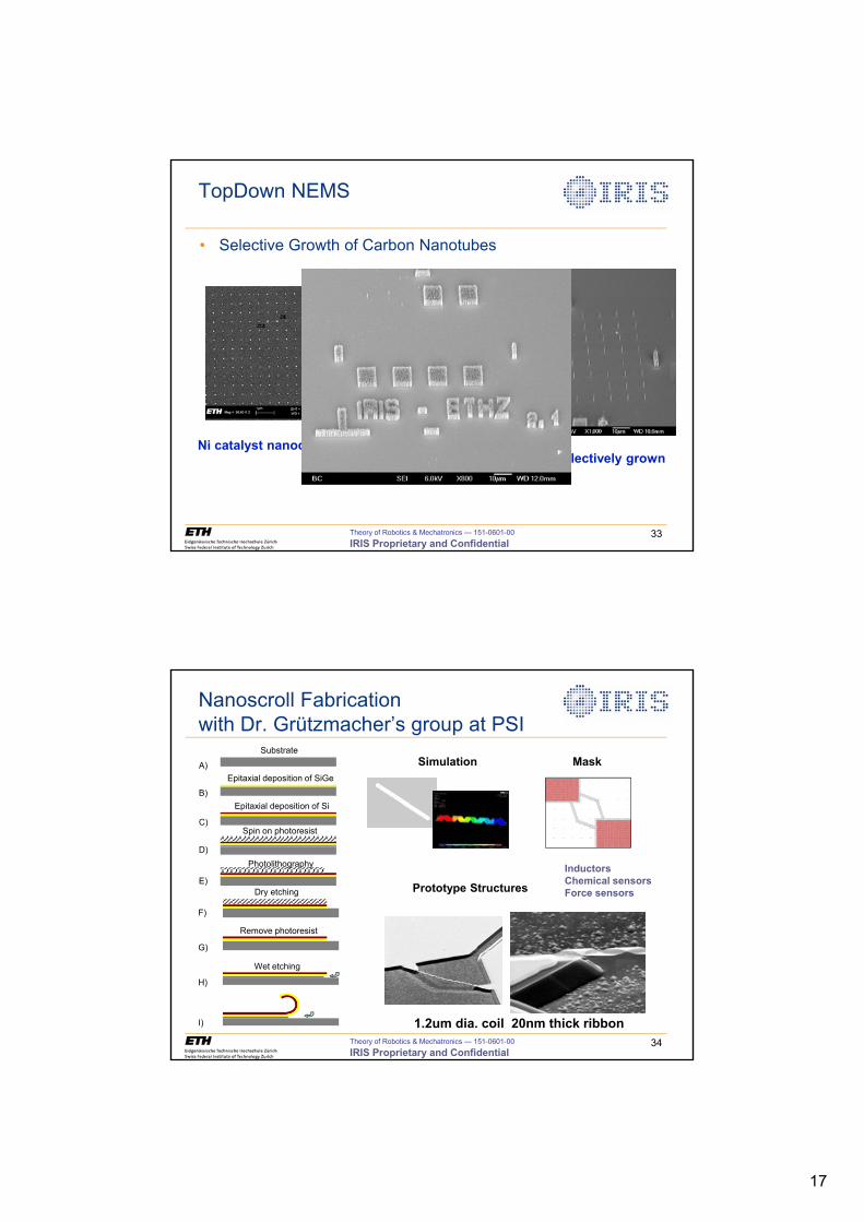
17
Theory of Robotics & Mechatronics — 151-0601-00 33
TopDown NEMS
• Selective Growth of Carbon Nanotubes
Ni catalyst nanodots (50nm dia.)Single CNTs selectively grown
IRIS Proprietary and Confidential
Theory of Robotics & Mechatronics — 151-0601-00 34
Nanoscroll Fabricationwith Dr. Grützmacher’s group at PSI
Substrate
Epitaxial deposition of SiGe
Epitaxial deposition of Si
Spin on photoresist
Photolithography
A)
B)
C)
D)
E)Dry etching
Remove photoresist
Wet etching
F)
G)
H)
I)
Simulation Mask
Prototype Structures
1.2um dia. coil 20nm thick ribbon
IRIS Proprietary and Confidential
InductorsChemical sensorsForce sensors
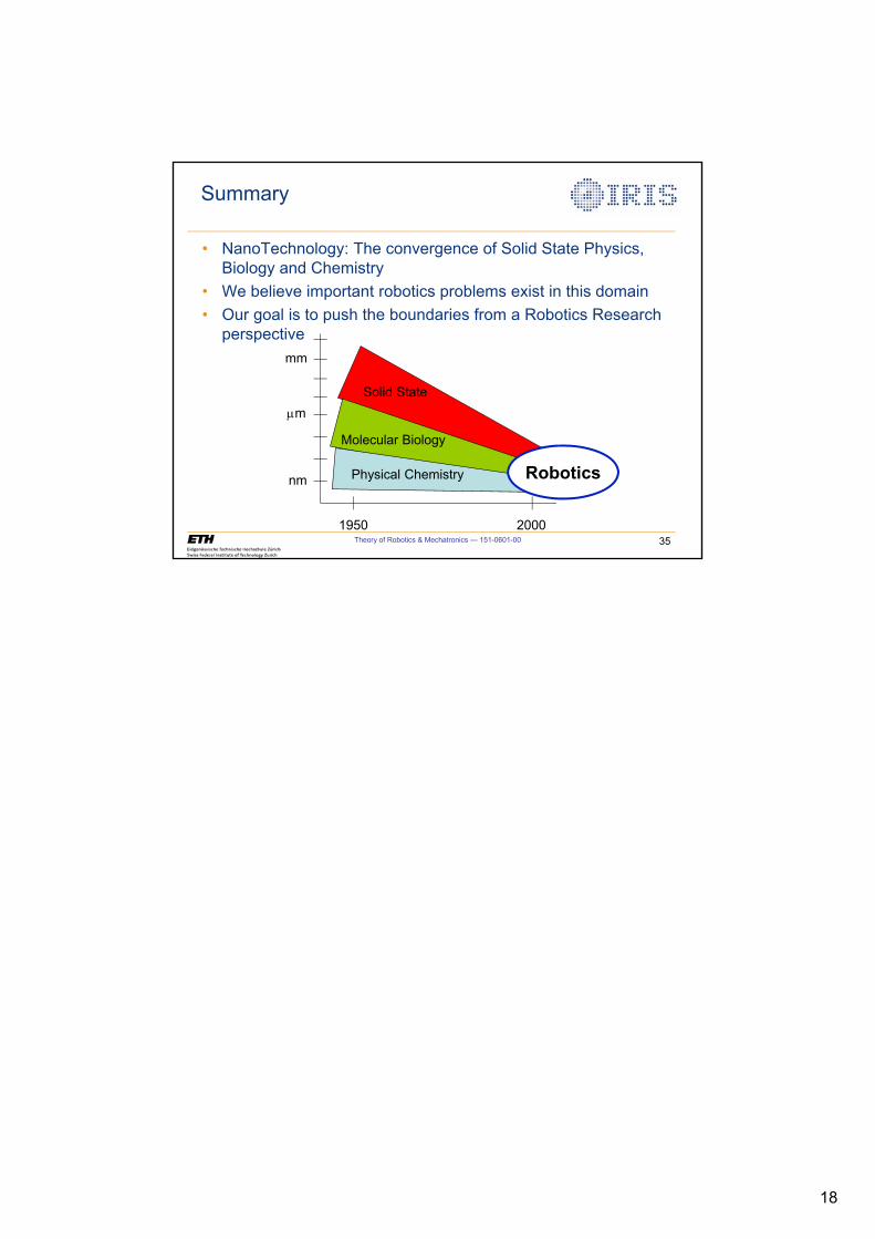
18
Theory of Robotics & Mechatronics — 151-0601-00 35
Summary
• NanoTechnology: The convergence of Solid State Physics, Biology and Chemistry
• We believe important robotics problems exist in this domain• Our goal is to push the boundaries from a Robotics Research
perspective
1950 2000
nm
Pm
mm
Solid State
Molecular Biology
Physical Chemistry Robotics
1
Institute of Robotics and Intelligent SystemsETH Zurich
Mobile Robotics
Theory of Robotics &Mechatronics
Theory of Robotics & Mechatronics — 151-0601-00 2
Overview
• Introduction• Mobility
– Kinematics– Types
• Control– Deliberate, – Reactive– Hierarchical– Behavioral
• Navigation– Sensors– Map Types
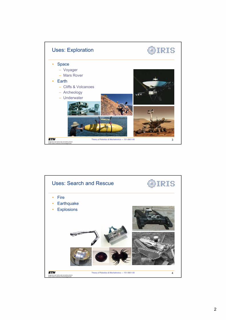
2
Theory of Robotics & Mechatronics — 151-0601-00 3
Uses: Exploration
• Space– Voyager– Mars Rover
• Earth– Cliffs & Volcanoes– Archeology– Underwater
Theory of Robotics & Mechatronics — 151-0601-00 4
Uses: Search and Rescue
• Fire• Earthquake• Explosions
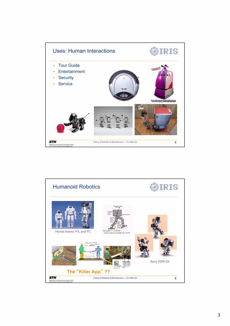
3
Theory of Robotics & Mechatronics — 151-0601-00 5
Uses: Human Interactions
• Tour Guide• Entertainment• Security• Service
6Theory of Robotics & Mechatronics — 151-0601-00
Humanoid Robotics
Sony SDR-3X
Honda Asimo, P3, and P2
The “Killer App” ??
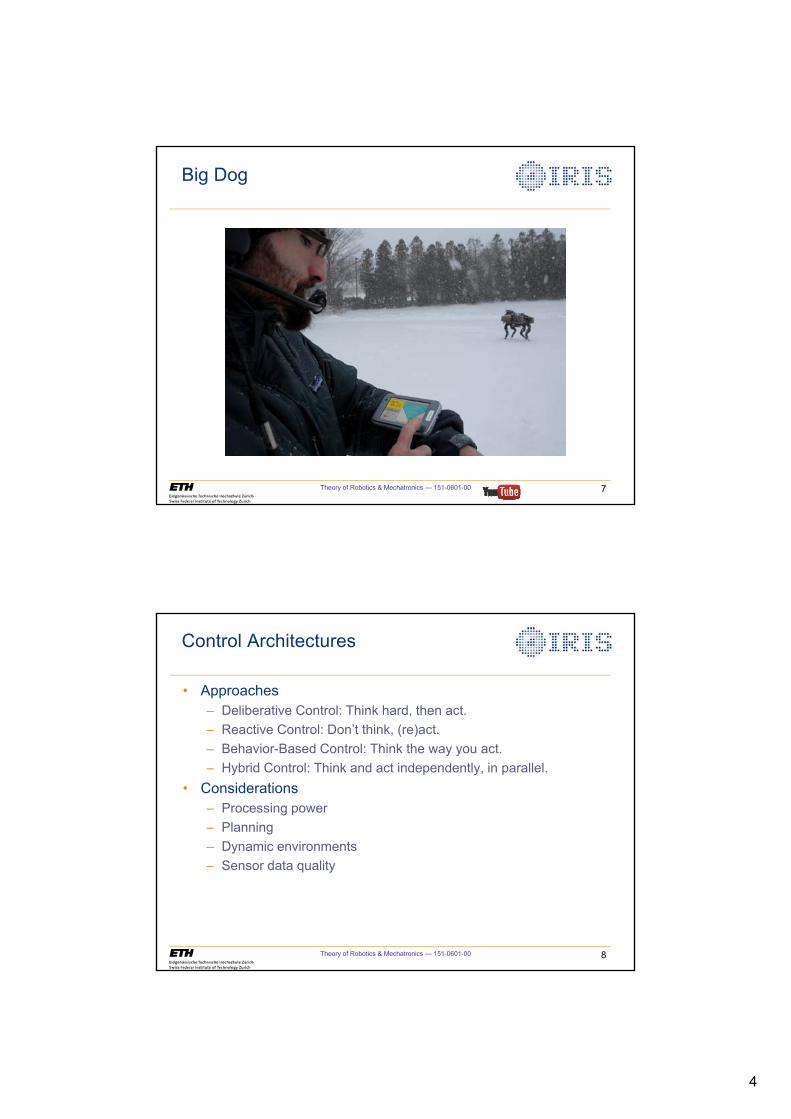
4
Theory of Robotics & Mechatronics — 151-0601-00 7
Big Dog
Theory of Robotics & Mechatronics — 151-0601-00 8
Control Architectures
• Approaches– Deliberative Control: Think hard, then act.– Reactive Control: Don’t think, (re)act.– Behavior-Based Control: Think the way you act.– Hybrid Control: Think and act independently, in parallel.
• Considerations– Processing power– Planning– Dynamic environments– Sensor data quality
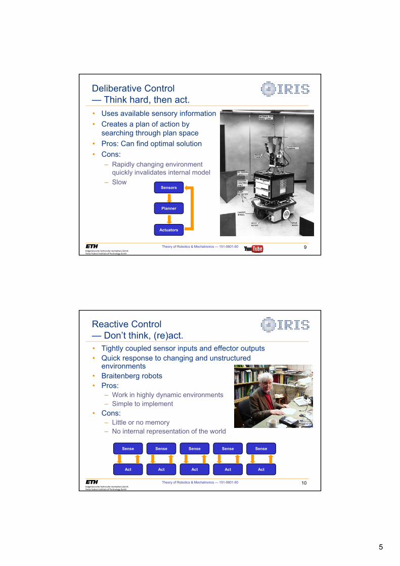
5
Theory of Robotics & Mechatronics — 151-0601-00 9
Deliberative Control— Think hard, then act.• Uses available sensory information• Creates a plan of action by
searching through plan space• Pros: Can find optimal solution• Cons:
– Rapidly changing environment quickly invalidates internal model
– Slow
Sensors
Actuators
Planner
Sensors
Actuators
Planner
Theory of Robotics & Mechatronics — 151-0601-00 10
Reactive Control— Don’t think, (re)act.• Tightly coupled sensor inputs and effector outputs• Quick response to changing and unstructured
environments• Braitenberg robots• Pros:
– Work in highly dynamic environments– Simple to implement
• Cons:– Little or no memory– No internal representation of the world
Sense
Act
Sense
Act
Sense
Act
Sense
Act
Sense
Act
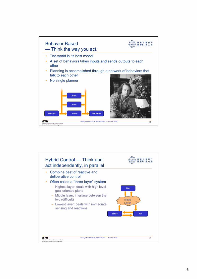
6
Theory of Robotics & Mechatronics — 151-0601-00 11
Behavior Based— Think the way you act.• The world is its best model• A set of behaviors takes inputs and sends outputs to each
other• Planning is accomplished through a network of behaviors that
talk to each other• No single planner
Sensors Level 0
Level 1
Level 2
Actuators
Theory of Robotics & Mechatronics — 151-0601-00 12
Hybrid Control — Think and act independently, in parallel• Combine best of reactive and
deliberative control• Often called a “three-layer” system
– Highest layer: deals with high level goal oriented plans
– Middle layer: interface between the two (difficult)
– Lowest layer: deals with immediate sensing and reactions
Sense
Plan
Act
Middle Layer
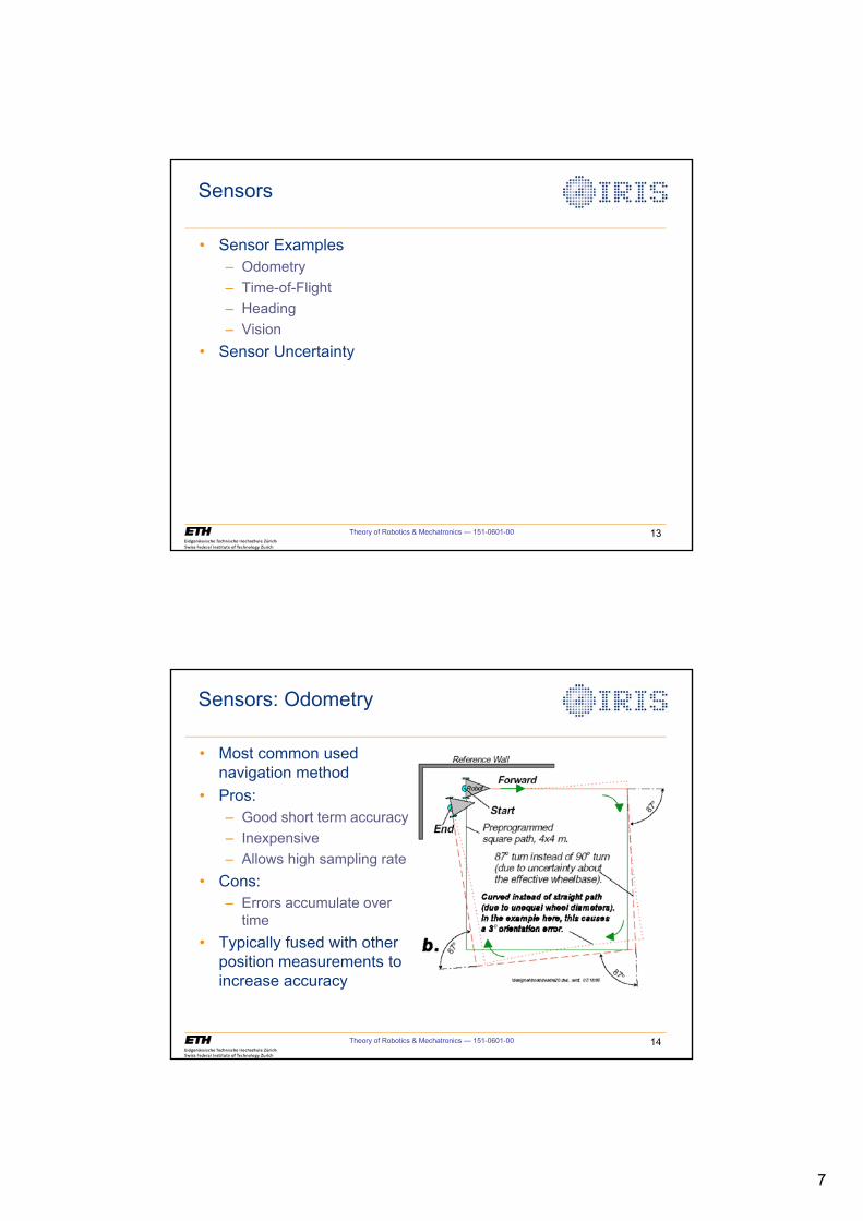
7
Theory of Robotics & Mechatronics — 151-0601-00 13
Sensors
• Sensor Examples– Odometry– Time-of-Flight– Heading– Vision
• Sensor Uncertainty
Theory of Robotics & Mechatronics — 151-0601-00 14
Sensors: Odometry
• Most common used navigation method
• Pros:– Good short term accuracy– Inexpensive– Allows high sampling rate
• Cons: – Errors accumulate over
time• Typically fused with other
position measurements to increase accuracy
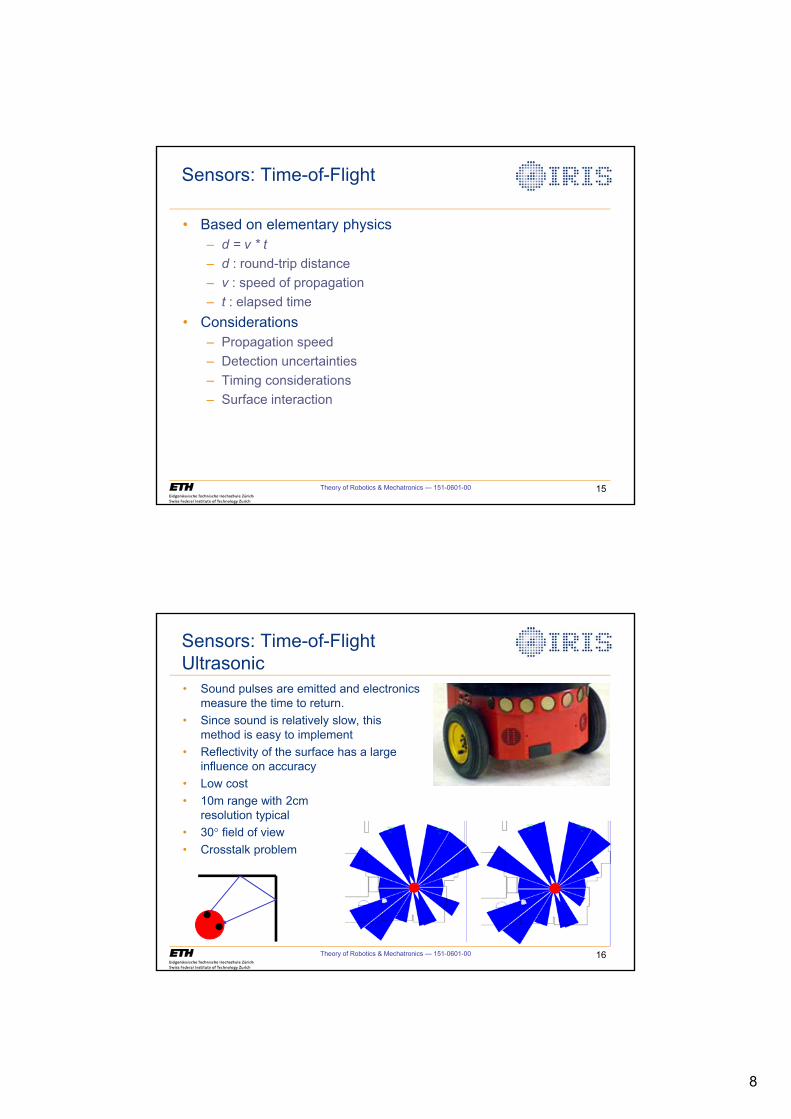
8
Theory of Robotics & Mechatronics — 151-0601-00 15
Sensors: Time-of-Flight
• Based on elementary physics– d = v * t– d : round-trip distance– v : speed of propagation– t : elapsed time
• Considerations– Propagation speed– Detection uncertainties– Timing considerations– Surface interaction
Theory of Robotics & Mechatronics — 151-0601-00 16
Sensors: Time-of-Flight Ultrasonic• Sound pulses are emitted and electronics
measure the time to return.• Since sound is relatively slow, this
method is easy to implement• Reflectivity of the surface has a large
influence on accuracy• Low cost• 10m range with 2cm
resolution typical• 30° field of view• Crosstalk problem
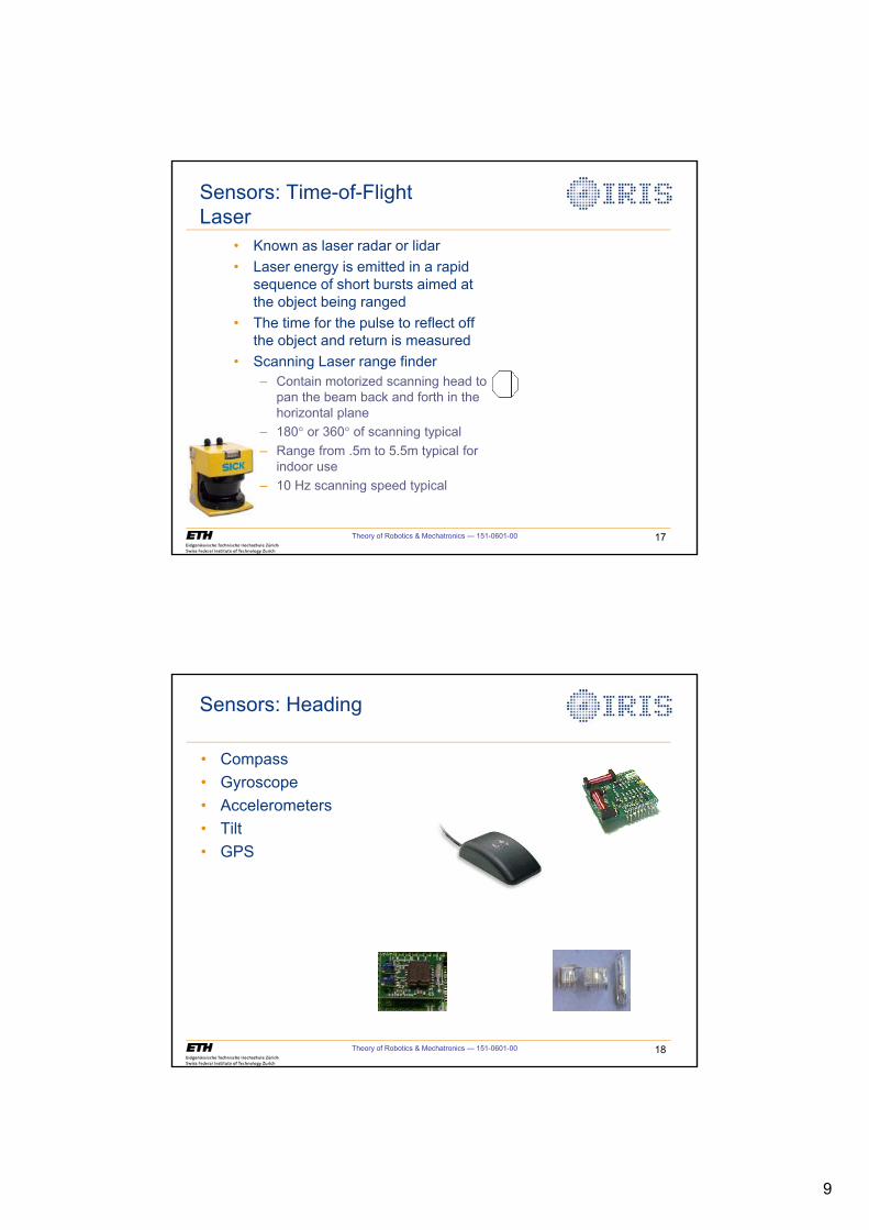
9
Theory of Robotics & Mechatronics — 151-0601-00 17
Sensors: Time-of-Flight Laser
• Known as laser radar or lidar• Laser energy is emitted in a rapid
sequence of short bursts aimed at the object being ranged
• The time for the pulse to reflect off the object and return is measured
• Scanning Laser range finder– Contain motorized scanning head to
pan the beam back and forth in the horizontal plane
– 180° or 360° of scanning typical – Range from .5m to 5.5m typical for
indoor use– 10 Hz scanning speed typical
Theory of Robotics & Mechatronics — 151-0601-00 18
Sensors: Heading
• Compass• Gyroscope• Accelerometers• Tilt• GPS
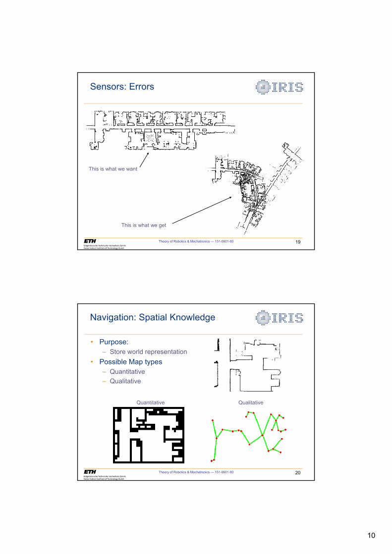
10
Theory of Robotics & Mechatronics — 151-0601-00 19
Sensors: Errors
This is what we want
This is what we get
Theory of Robotics & Mechatronics — 151-0601-00 20
Navigation: Spatial Knowledge
• Purpose:– Store world representation
• Possible Map types– Quantitative– Qualitative
QualitativeQuantitative
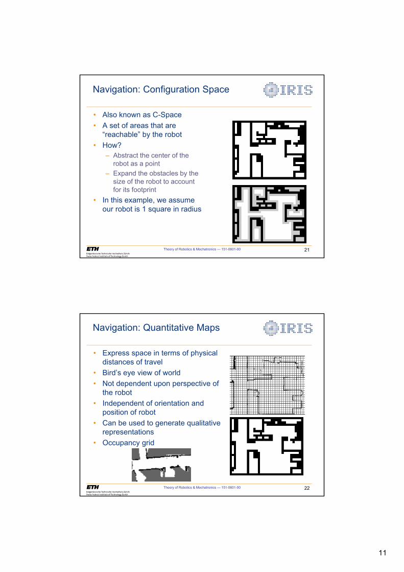
11
Theory of Robotics & Mechatronics — 151-0601-00 21
Navigation: Configuration Space
• Also known as C-Space• A set of areas that are
“reachable” by the robot• How?
– Abstract the center of the robot as a point
– Expand the obstacles by the size of the robot to account for its footprint
• In this example, we assume our robot is 1 square in radius
Theory of Robotics & Mechatronics — 151-0601-00 22
Navigation: Quantitative Maps
• Express space in terms of physical distances of travel
• Bird’s eye view of world• Not dependent upon perspective of
the robot• Independent of orientation and
position of robot• Can be used to generate qualitative
representations• Occupancy grid
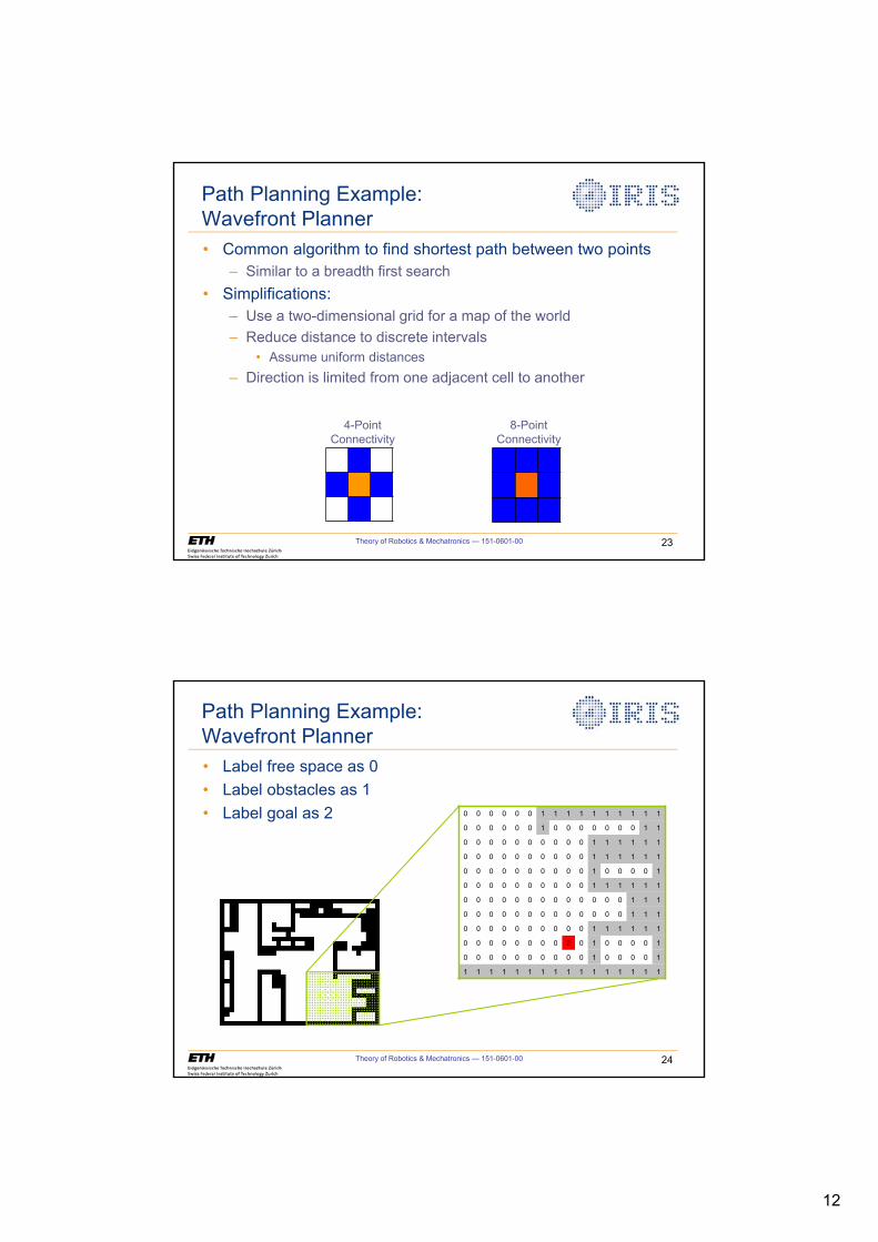
12
Theory of Robotics & Mechatronics — 151-0601-00 23
Path Planning Example: Wavefront Planner• Common algorithm to find shortest path between two points
– Similar to a breadth first search• Simplifications:
– Use a two-dimensional grid for a map of the world– Reduce distance to discrete intervals
• Assume uniform distances– Direction is limited from one adjacent cell to another
4-Point Connectivity
8-Point Connectivity
Theory of Robotics & Mechatronics — 151-0601-00 24
Path Planning Example: Wavefront Planner• Label free space as 0• Label obstacles as 1• Label goal as 2 0 0 0 0 0 0 1 1 1 1 1 1 1 1 1 1
0 0 0 0 0 0 1 0 0 0 0 0 0 0 1 1
0 0 0 0 0 0 0 0 0 0 1 1 1 1 1 1
0 0 0 0 0 0 0 0 0 0 1 1 1 1 1 1
0 0 0 0 0 0 0 0 0 0 1 0 0 0 0 1
0 0 0 0 0 0 0 0 0 0 1 1 1 1 1 1
0 0 0 0 0 0 0 0 0 0 0 0 0 1 1 1
0 0 0 0 0 0 0 0 0 0 0 0 0 1 1 1
0 0 0 0 0 0 0 0 0 0 1 1 1 1 1 1
0 0 0 0 0 0 0 0 2 0 1 0 0 0 0 1
0 0 0 0 0 0 0 0 0 0 1 0 0 0 0 1
1 1 1 1 1 1 1 1 1 1 1 1 1 1 1 1
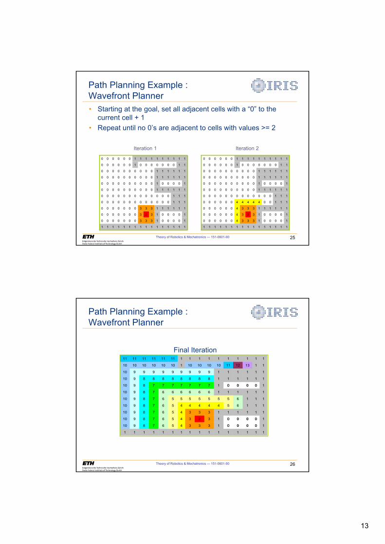
13
Theory of Robotics & Mechatronics — 151-0601-00 25
Path Planning Example : Wavefront Planner• Starting at the goal, set all adjacent cells with a “0” to the
current cell + 1• Repeat until no 0’s are adjacent to cells with values >= 2
0 0 0 0 0 0 1 1 1 1 1 1 1 1 1 1
0 0 0 0 0 0 1 0 0 0 0 0 0 0 1 1
0 0 0 0 0 0 0 0 0 0 1 1 1 1 1 1
0 0 0 0 0 0 0 0 0 0 1 1 1 1 1 1
0 0 0 0 0 0 0 0 0 0 1 0 0 0 0 1
0 0 0 0 0 0 0 0 0 0 1 1 1 1 1 1
0 0 0 0 0 0 0 0 0 0 0 0 0 1 1 1
0 0 0 0 0 0 0 0 0 0 0 0 0 1 1 1
0 0 0 0 0 0 0 3 3 3 1 1 1 1 1 1
0 0 0 0 0 0 0 3 2 3 1 0 0 0 0 1
0 0 0 0 0 0 0 3 3 3 1 0 0 0 0 1
1 1 1 1 1 1 1 1 1 1 1 1 1 1 1 1
0 0 0 0 0 0 1 1 1 1 1 1 1 1 1 1
0 0 0 0 0 0 1 0 0 0 0 0 0 0 1 1
0 0 0 0 0 0 0 0 0 0 1 1 1 1 1 1
0 0 0 0 0 0 0 0 0 0 1 1 1 1 1 1
0 0 0 0 0 0 0 0 0 0 1 0 0 0 0 1
0 0 0 0 0 0 0 0 0 0 1 1 1 1 1 1
0 0 0 0 0 0 0 0 0 0 0 0 0 1 1 1
0 0 0 0 0 0 4 4 4 4 4 0 0 1 1 1
0 0 0 0 0 0 4 3 3 3 1 1 1 1 1 1
0 0 0 0 0 0 4 3 2 3 1 0 0 0 0 1
0 0 0 0 0 0 4 3 3 3 1 0 0 0 0 1
1 1 1 1 1 1 1 1 1 1 1 1 1 1 1 1
Iteration 1 Iteration 2
Theory of Robotics & Mechatronics — 151-0601-00 26
Path Planning Example : Wavefront Planner
Final Iteration
1111111111111111
10000133345678910
10000132345678910
11111133345678910
11165444445678910
11165555555678910
11111166666678910
10000177777778910
11111188888888910
11111199999999910
11131211101010101101010101010
1111111111111111111111
1111111111111111
10000133345678910
10000132345678910
11111133345678910
11165444445678910
11165555555678910
11111166666678910
10000177777778910
11111188888888910
11111199999999910
11131211101010101101010101010
1111111111111111111111
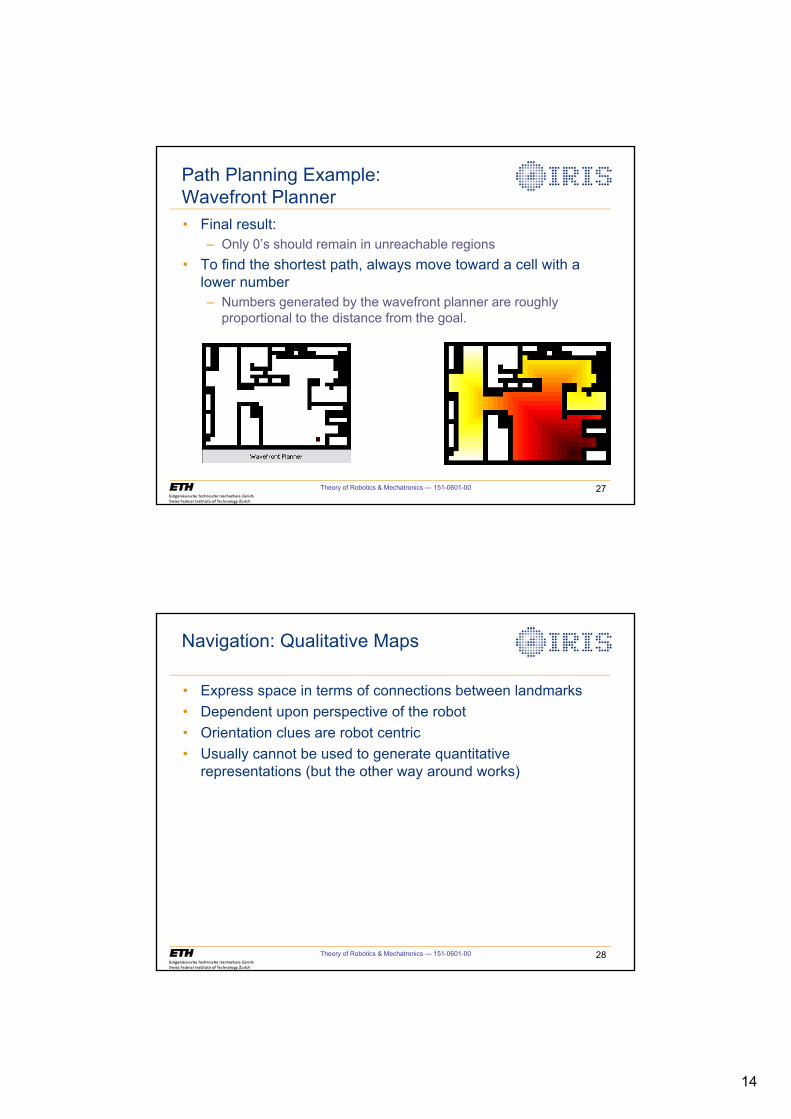
14
Theory of Robotics & Mechatronics — 151-0601-00 27
Path Planning Example: Wavefront Planner• Final result:
– Only 0’s should remain in unreachable regions• To find the shortest path, always move toward a cell with a
lower number– Numbers generated by the wavefront planner are roughly
proportional to the distance from the goal.
Theory of Robotics & Mechatronics — 151-0601-00 28
Navigation: Qualitative Maps
• Express space in terms of connections between landmarks• Dependent upon perspective of the robot• Orientation clues are robot centric• Usually cannot be used to generate quantitative
representations (but the other way around works)
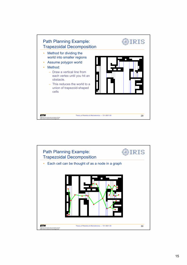
15
Theory of Robotics & Mechatronics — 151-0601-00 29
Path Planning Example: Trapezoidal Decomposition• Method for dividing the
world into smaller regions• Assume polygon world• Method:
– Draw a vertical line from each vertex until you hit an obstacle.
– This reduces the world to a union of trapezoid-shaped cells
Theory of Robotics & Mechatronics — 151-0601-00 30
Path Planning Example: Trapezoidal Decomposition• Each cell can be thought of as a node in a graph
16
Theory of Robotics & Mechatronics — 151-0601-00 31
Navigation: Maps
• Questions regarding map type:– How accurately and efficiently does the robot need to navigate?– Is navigation time-critical? Is a slightly sub-optimal route
acceptable?– What are the characteristics of the environment?– Are there landmarks to provide orientation clues?– What are the sources of information about the environment that
specify terrains, surface properties, obstacles, etc.?– What are the properties of the available sensors in the
environment?
Theory of Robotics & Mechatronics — 151-0601-00 32
Summary
• Actuators– Frame Assignment– Kinematics & Inverse Kinematics– Mobility Types
• Control– Deliberative Control: Think hard, then act.– Reactive Control: Don’t think, (re)act.– Behavior-Based Control: Think the way you act.– Hybrid Control: Think and act independently, in parallel.
• Perception– Sensors– Mapping & Localization
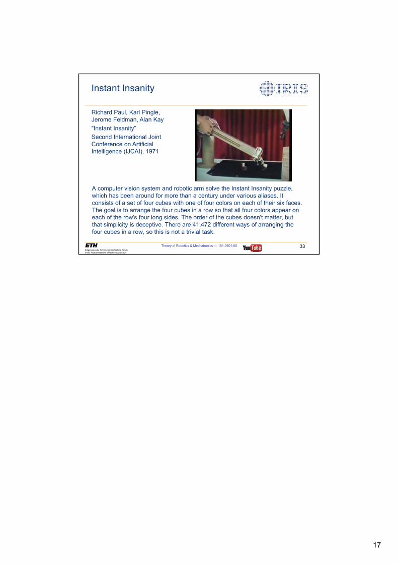
17
Instant Insanity
A computer vision system and robotic arm solve the Instant Insanity puzzle, which has been around for more than a century under various aliases. It consists of a set of four cubes with one of four colors on each of their six faces. The goal is to arrange the four cubes in a row so that all four colors appear on each of the row's four long sides. The order of the cubes doesn't matter, but that simplicity is deceptive. There are 41,472 different ways of arranging the four cubes in a row, so this is not a trivial task.
Theory of Robotics & Mechatronics — 151-0601-00 33
Richard Paul, Karl Pingle, Jerome Feldman, Alan Kay"Instant Insanity”Second International Joint Conference on Artificial Intelligence (IJCAI), 1971