theoretical and experimental investigation of bulk - middle

THEORETICAL AND EXPERIMENTAL INVESTIGATION OF BULK GLASS FORMING ABILITY IN BULK AMORPHOUS ALLOY SYSTEMS

A THESIS SUBMITTED TO THE GRADUATE SCHOOL OF NATURAL AND APPLIED SCIENCES

OF MIDDLE EAST TECHNICAL UNIVERSITY

BY

CAN AYAS

IN PARTIAL FULFILLMENT OF THE REQUIREMENTS FOR

THE DEGREE OF MASTER OF SCIENCE IN

METALLURGICAL AND MATERIALS ENGINEERING

JANUARY 2005

Approval of the Graduate School of Natural and Applied Science

Prof. Dr. Canan Özgen

Director I certify that this thesis satisfies all the requirements as a thesis for the degree of Master of Science.

Prof. Dr. Tayfur Öztürk

Head of Department This is to certify that we have read this thesis and that in our opinion it is fully adequate, in scope and quality, as a thesis for the degree of Master of Science.

Prof. Dr. Vedat Akdeniz Prof. Dr. Amdulla O. Mekhrabov

Co-Supervisor Supervisor Examining Committee Members Prof. Dr. Şakir Erkoç (METU, PHYS)

Prof. Dr. Amdulla O. Mekhrabov (METU, METE)

Prof. Dr. Vedat Akdeniz (METU, METE)

Prof. Dr. Macit Özenbaş (METU, METE)

Assoc. Prof. Dr. C. Hakan Gür (METU, METE)

I hereby declare that all information in this document has been obtained and presented in accordance with academic rules and ethical conduct. I also declare that, as required by these rules and conduct, I have fully cited and referenced all material and results that are not original to this work. Name, Surname: Can Ayas

Signature :

iii

ABSTRACT

THEORETICAL AND EXPERIMENTAL INVESTIGATION OF BULK GLASS FORMING ABILITY IN BULK

AMORPHOUS ALLOY SYSTEMS

Ayas, Can

M.S., Department of Metallurgical and Materials Engineering

Supervisor: Prof. Dr. Amdulla Mekhrabov

Co-Supervisor: Prof. Dr. Vedat Akdeniz

January 2005, 154 pages

In this study molecular dynamics simulation program in NVT ensemble using

Velocity Verlet integration was written in order to investigate the glass forming

ability of two metallic systems. The Zn-Mg system, one of the frontiers of simple

metal-metal metallic glasses and Fe-B, inquiring attention due to presence of

many bulk glass forming alloy systems evolved from this binary with different

alloying element additions.

In addition to this, atomistic calculations on the basis of ordering were carried out

for both Zn-Mg and Fe-B systems. Ordering energy values are calculated using

electronic theory of alloys in pseudopotential approximation and elements which

increase the ordering energy between atoms were determined. The elements

which increase the ordering energy most were selected as candidate elements in

order to design bulk amorphous alloy systems.

iv

In the experimental branch of the study centrifugal casting experiments were

done in order to see the validity of atomistic calculations. Industrial low grade

ferroboron was used as the master alloy and pure element additions were

performed in order to constitute selected compositions. Fe62B21Mo5W2Zr6 alloy

was successfully vitrified in bulk form using nearly conventional centrifugal

casting processing. Specimens produced were characterized using SEM, XRD,

and DSC in order to detect the amorphous structure and also the crystalline

counterpart of the structure when the cooling rate is lower. Sequential peritectic

and eutectic reaction pattern was found to be important for metallic glasses which

can be vitrified in bulk forms with nearly conventional solidification methods.

Keywords: Fe based alloys, Zn based alloys, Glass Forming Ability, Metallic

Glasses, Molecular Dynamics, Ordering, Centrifugal Casting

v

ÖZ

İRİ HACİMLİ METALİK CAMLARDA CAM OLUŞTURMA

YETENEĞİNİN TEORİK VE DENEYSEL YÖNTEMLERLE

İNCELENMESİ

Ayas, Can

Yüksek Lisans, Metalurji ve Malzeme Mühendisliği Bölümü

Tez Yöneticisi: Prof. Dr. Amdulla Mekhrabov

Ortak Tez Yöneticisi: Prof. Dr. Vedat Akdeniz

Ocak 2005, 154 sayfa

Bu çalışmada Zn-Mg be Fe-B metalik alaşımlarında bu sistemlerin cam

oluşturma yeteneğini incelemek için NVT bileşiminde Velocity Verlet integrali

kullanılarak moleküler dinamik simulasyonu programı yazılmıştır. Zn-Mg alaşımı

metal-metal olarak üretilmiş ilk amorf alaşımlardan biri olduğu için çalışmaya

dahil edilirken, Fe-B sistemi ise değişik alaşım elementleri eklenmesiyle birçok

iri ve hacimli metalik cam alaşımı oluşturması nedeniyle incelenmiştir.

Çalışma kapsamında ayrıca atomistik yaklaşım kullanılarak atomsal düzenlenme

Zn-Mg ve Fe-B sistemleri için incelenmiştir. Atomlar arası düzenlenme enerjileri

alaşımların elektronik teorisinin pseudopotansiyel yaklaşımında kullanılmasıyla

hesaplanmıştır. Belirtilen sistemlerde atomlar arası düzenlenme enerjisini en çok

arttıran elementler, iri hacimli amorf alaşımlar tasarlamak için aday elementler

olarak tayin edilmiştir.

vi

Çalışmanın deneysel kısmında atomistik hesaplamalarının geçerliliğini saptama

amacıyla santrifüjlü döküm deneyleri yapılmıştır. Alaşım hazırlama safhasında

endüstriyel ferrobor ve saf elementler kullanılarak seçilen kompozisyonlar

oluşturulmuştur. Fe62B21Mo5W2Zr6 alaşımı konvansiyonel benzereri döküm

yöntemiyle iri ve hacimli olarak amorf yapıda başarıyla üretilmiştir. Üretilen

alaşımlar, taramalı elektron mikroskobu, x-ışınları kırınımı ve thermal analiz

yöntemleriyle karakterize edilmiş ve amorf faz oluşumu tespit edilmiştir. Ayrıca

alaşımların daha yavaş soğuma hızlarında oluşturduklaru kristal yapılarda

incelenmiştir. Ardışık peritektik ve ötektik reaksiyonların iri ve hacimli cam

oluşturma kabiliyeti açısından önemli olduğu saptanmıştır.

Anahtar Kelimeler: Fe bazlı alaşımlar, Zn bazlı alaşımlar, Metalik Cam, Cam

Oluşturma Yeteneği, Moleküler Dinamik, Atomlar arası düzenlenme, Satrifüjlü

Döküm.

vii

ACKNOWLEDGMENTS

I express my deepest gratitude to my supervisor Prof. Dr. Amdulla Mekhrabov

and Prof. Dr. Vedat Akdeniz for their guidance, criticism, encouragements,

patience and insight throughout the research.

I am deeply grateful to my family for their love, encouragement and endless

belief on me through out my life.

I express my thanks to my lab friends Ali Abdelal, Hülya Arslan, Emrah Erdiller,

Selen Gürbüz and İlkay Saltoğlu for their various help and critics throughout the

study. I would also like to express my gratitude to my friend Fatih Şen for the

valuable discussions.

Special thanks to Nigel Robinson for reviewing the manuscripts, and to Ahmet

Peynircioğlu for his precious accompany in endless night shifts.

I would like to express my thanks to Cem Taşan for keeping me in the track and

always being at next door to share his synergy.

I am deeply indebted to Özlem Esma Güngör not only for her various help and

critics but more importantly for touching my soul from the deepest and

illuminating inspiration in every second we share.

This study was supported by the Scientific Research Projects Fund of Graduate

School of Engineering, Grant No: BAP-2003-07-02-00-57.

viii

TABLE OF CONTENTS

PLAGIARISM ………………………………………………………….....….. iii

ABSTRACT…………….....………………………………………………...... iv

ÖZ…………………………………………………………...……………….... vi

ACKNOWLEDGEMENTS..………………………………………..........…... viii

TABLE OF CONTENTS…………………………………………................... ix

LIST OF TABLES..…………………………………………………….......… xiii

LIST OF FIGURES......…………..……………………...........…..................... xiv

LIST OF SYMBOLS.……………………………………………………......... xix

CHAPTER

1 INTRODUCTION…………………………………...……................... 1

2 LITERATURE SURVEY…….....………………………………..…… 4

2.1 DESCRIPTION OF METALLIC GLASSES…………………... 4

2.2 HISTORICAL DEVELOPMENT OF METALLIC GLASSES. 4

2.3 AMORPHOUS NANOCRYSTALLINE MATERIALS …....... 8

2.4 PROPERTIES AND APPLICATIONS OF METALLIC

GLASSES ……….…………………………………………… 9

2.4.1 Mechanical Properties…………………………………… 10

2.4.2 Magnetic Properties ………………………………...…… 11

2.4.3 Applications of Metallic Glasses ………………………... 12

2.5 METHODS OTHER THAN RAPID SOLIDIFICATION FOR

THE PRODUCTION OF METALLIC GLASSES ……………….… 12

2.6 THEORY OF METALLIC GLASS FORMATION ……...…… 14

2.6.1 Glass Forming Ability…………………………………… 14

2.6.2 Thermodynamical Model ……………………...………… 21

2.6.3 Kinetic Model …………………………………………… 22

ix

2.6.4 Structural Model ………………………………………… 24

2.6.5 Semiempirical Criteria. ………………………………….. 24

2.6.6 Atomic Size Distribution Plot …………………………… 25

2.6.7 γ Criteria for Glass Forming Ability ...………………....... 27

2.6.8 Bulk Glass Forming Ability (BGFA)..………………....... 29

2.6.9 Structure of Amorphous Alloys………………………….. 29

2.7 MOLECULAR DYNAMICS IN ACCORDANCE WITH GFA... 33

3 METHODOLOGY ……………………………………………...…… 35

3.1 PSEUDOPOTENTIAL APPROXIMATION AND ONE

ELECTRON THEORY …………………………………….......…… 35

3.1.1 The Principals of the One Electron Theory …………..… 35

3.1.2 Nearly-Free Electron Model ……………………..……… 36

3.1.3 Calculation of Ordering Energies and Pairwise

Interatomic Interactions of Ternary Alloys ................................ 39

3.2 COMPUTER SIMULATION ........................................................ 41

3.2.1 Molecular Dynamics .......................................................... 43

3.2.1.1 Equations of Motion ........................................... 43

3.2.1.2 Sampling from Ensembles .................................. 45

3.2.1.3 Interatomic Potentials ......................................... 46

3.2.1.4 Molecular Dynamics Program ............................ 48

3.2.1.4.1 Initialization ......................................... 49

3.2.1.4.2 Force Calculation ................................. 50

3.2.1.4.3 Integration ............................................ 51

3.2.1.4.4 Boundary Conditions ........................... 51

4 EXPERIMENTAL PROCEDURE ...................................................... 54

4.1 THEORETICAL STUDIES .......................................................... 54

4.2 MD SIMULATION ....................................................................... 56

4.2.1 Initialization ....................................................................... 57

4.2.1.1 Initial Velocities ................................................. 58

4.2.1.2 Initial Positions ................................................... 62

x

4.2.2 Force Calculation ............................................................... 64

4.3 CASTING EXPERIMENTS ......................................................... 64

4.3.1 Alloy Selection .................................................................. 64

4.3.2 Alloy Preparation ............................................................... 65

4.3.3 Copper Molds .................................................................... 66

4.3.4 Crucible Production ........................................................... 67

4.3.5 Melting and Casting............................................................ 69

4.3.6 Characterization of Specimens .......................................... 69

4.3.6.1 Thermal Analysis ................................................ 69

4.3.6.2 Microstructural Investigations ........................... 70

4.3.6.3 X-Ray Diffraction ............................................... 70

4.3.6.4 Hardness Measurements ..................................... 71

5 RESULTS AND DISCUSSION ........................................................... 72

5.1 THEORETICAL CALCULATIONS …........................................ 72

5.1.1 Interatomic Potentials ........................................................ 72

5.1.2 Ordering Energy Calculations ........................................... 75

5.1.2.1 Ordering Energy Calculations for MgZn2 .......... 75

5.1.2.2 Ordering Energy Calculations for Fe3B ............. 81

5.1.3 Prediction of Glass Forming Compositions ....................... 86

5.2 MD SIMULATIONS...........................................…....................... 88

5.3 CENTRIFUGAL CASTING EXPERIMENTS...…....................... 95

5.3.1 C1 Fe75B25 alloy ................................................................ 100

5.3.2 C2 Fe75B25 alloy................................................................ 108

5.3.3 C4 Fe63B21Mo16 alloy ........................................................ 113

5.3.4 C6 Fe63B16Mo14W7 alloy.................................................... 118

5.3.5 C9 Fe62B21Mo5W2Zr6 alloy................................................ 123

5.3.6 C10 Fe62B21Mo5W2Zr6 alloy.............................................. 128

6 CONCLUSION ..................................................................................... 133

xi

REFERENCES .......................................................................................... 135

APPENDIX ................................................................................................ 140

APPENDIX A. MOLECULAR DYNAMICS CODE……….............. 140

APPENDIX B. BINARY PHASE DIAGRAMS FOR FE-MO, FE-

W, FE-ZR, B-MO, B-W, AND B-ZR SYSTEMS .............................. 152

xii

LIST OF TABLES

TABLE page

2.1

Typical bulk glassy alloy systems reported together with

the calendar years when the first paper or patent of each

alloy system was published [17]…………………………… 7

4.1 Composition and crucibles used for the alloys produced….. 65

4.2 Composition of industrial ferroboron……………………… 65

4.3 Chemical analysis of the Alumina plaster…………………. 68

5.2 Results of ordering energy calculation for Mg31Zn67X2 …….. 76

5.3 Results of ordering energy calculation for Mg31Zn67X2 …….. 77

5.4 The ordering energy calculations for Fe73B25X2 ……………. 82

5.5 The ordering energy calculations for Fe75B23X2 …………..... 83

5.6 Thermal data about C1 alloy………………………………. 102



5.9 EDS analysis results for the phases present in C4 alloy…… 115


5.11 EDS analysis results of C6 alloy…………………………... 121


5.13 EDS analysis results of C9 alloy…………………………... 126

5.14 Thermal data about C10 alloy……………………………... 129

xiii

LIST OF FIGURES

FIGURE page

2.1 Critical casting thickness of conventional glasses, for glass

formation as a function of the year corresponding alloy has

been discovered [9]..................................................................... 8

2.2 Change in the viscosity of a material upon crystallization and

amorphous phase formation [29]……………………………... 16

2.3

Relationship between the critical cooling rate, maximum

casting thickness and reduced glass transition temperature for

ordinary amorphous alloys, bulk amorphous alloys and oxide

glasses [23]…………………………………………………….. 18

2.4 Critical cooling rate as a function of Tg/Tm and Tg/Tl [31]……. 20

2.5 Time-transformation-temperature (TTT) graph of

Pd40Cu30Ni10P20 [9]…………………………………………….. 20

2.6 A Typical DSC trace of a glassy alloy [32]…………………… 22

2.7 Atomic size distribution of Ni75Nb5P16B4 with a critical

cooling rate around 104-106 K/s, and Nd60Fe30Al10 with a

critical cooling rate of around 10-1000 K/s [35]……………... 27

2.8 Total RDFs of liquid and amorphous and liquid Pd80Si20 alloy

[41]…………………………………………………………….. 30

2.9 Three types of BMGs and their atomic structures [34]……….. 31

3.1 Connection between simulation, theoretical, and experimental

techniques [55]………………………………………………… 42

3.2 Interatomic potential vs. distance plot for argon………………. 48

xiv

3.3 Two dimensional representation of periodic boundary

conditions……………………………………………………… 53

4.1 Standard hit and miss test circle ………………………………. 60

4.2 Hit miss ratio vs. Number of trials…………………………… 60

4.3 Random distribution of point in unit cube…………………….. 61

4.4 Initial fcc lattice constructed…………………………………... 63

4.5 Schematic drawing of copper mold……………………………. 66

4.6 Drawing of the alumina crucibles used for casting……………. 67

4.7 Sintering heat treatment program……………………………… 68

5.1 Interatomic interaction potential between Mg-Zn pairs of

atoms………………………………………………………… 73

5.2 Interatomic interaction potential between Fe-B pairs of atoms.. 74

5.3 Percent change in WMg-Zn due to addition of 2 at. % third

element in place of Mg………………………………………… 79

5.4 Percent change in WMg-Zn due to addition of 2 at. % third

element in place of Zn…………………………………………. 80

5.5 The representation of elements which increase the WMg-Zn on

periodic table…………………………………………………... 81

5.6 Percent change in WFe-B due to addition of 2 at. % third

element in place of Fe…………………………………………. 84

5.7 Percent change in WFe-B due to addition of 2 at. % third

element in place of B…………………………………………... 85

5.8 The representation of elements which increase the WFe-B on

periodic table…………………………………………………... 86

5.9 Total energy evolution of the system………………………….. 89

xv

5.10 Total energy evolution of the system for first few thousand

steps……………………………………………………………. 89

5.11 Temperature evolution of the system………………………….. 90

5.12 The distribution of atoms in the simulation box, a) at T = 1350

K b) at T = 2900 K …………………………………...……..… 92

5.13 Variation of translational order parameter…………………….. 93

5.14 Radial distribution function at 850 K and 2900 K…………….. 94

5.15 Non-equilibrium phase diagram of Fe-B system [71]…………. 96

5.16 Equilibrium phase diagram of Fe-B system [71]……………… 96

5.17 Unit cell of Fe3B………………………………………………. 98

5.18 Unit cell of MgZn2 …………………………………………….. 99

5.19 DSC trace of C1 with a scanning rate of 20 0C/sec……………. 102

5.20 DSC trace of C1 with a scanning rate of 20 0C/sec after

cooling slowly…………………………………………………. 103

5.21 X-ray diffraction pattern of C1 alloy………………….……….. 105

5.22 Secondary electron images of C1 alloy a) and b) are the

photographs taken from the thinnest section while c) and d) are

taken from the thickest section of the casting…………………. 106

5.23 Hardness profile of Fe75B25 alloy hardness measurements are

taken from the corresponding positions on the wedge given in

the figure………………………………………………………. 107

5.24 DSC curve of C2 alloy with a scanning rate 20 0C/min …….… 108

5.25 Secondary electron images of C2 alloy a) and b) are taken

from the thickest section, c) taken from the outer part middle

sections, d) taken from the thinnest section…………………… 110

xvi

5.26 X-ray Diffraction pattern for C2 alloy………………………… 111

5.27 Hardness profile of C2 alloy. Hardness measurements are

taken according to the wedge given in the figure…………….... 113

5.28 DSC curve of C4 alloy with a scanning rate 20 0C/min…….…. 114

5.29 SEM views of C4 alloy, a) secondary electron image, and b)

back scatter image……………………………………………... 115

5.30 X-ray Diffraction pattern for C4 alloy………………………… 117

5.31 DSC curve of C6 alloy with a scanning rate 20 0C/min………. 119


from the thickest region of the casting while c) and d) are

taken from the thinnest region…………………………………. 120

5.33 X-ray Diffraction pattern for C6 alloy. ……………………….. 122

5.34 DSC curve of C9 alloy with a scanning rate 20 0C/min………. 124

5.35 SEM images of C9 alloy a) and b) are taken from thick section

while c) is back scattered image of the thinnest section d) is the

secondary electron image of the thinnest section……………… 125

5.36 X-ray Diffraction pattern for C9 alloy. ……………………….. 127

5.37 DSC curve of C10 alloy with a scanning rate 20 0C/min……… 129


from thick section while c) and d) are taken from thin sections. 130

5.39 X-ray Diffraction pattern for C10 alloy……………………….. 131

5.40 Secondary electron fracture surface images of C10 alloy……... 132

A.1 Binary phase diagram for Fe-Mo system……………………… 152

A.2 Binary phase diagram for Fe-W system………………….……. 152

A.3 Binary phase diagram for Fe-Zr system…………..…………… 153

xvii

A.4 Binary phase diagram for B-Mo system…………….………… 153

A.5 Binary phase diagram for B-W system…………...…………… 154

A.6 Binary phase diagram for B-Zr system………...……………… 154

xviii

LIST OF SYMBOLS

Tg Glass Transition Temperature

Tx Crystallization Temperature

σy Yield Strength

E Young’s Modulus

∆Tx Supercooled Liquid Region

η Viscosity

Cp Heat Capacity

Rc Critical Cooling Rate

Trg Reduced Glass Transition Temperature

Tl Liquidus Temperature

Tm Solidus Temperature

∆G Gibbs Free Energy of Crystallization

∆H Enthalpy of Fusion

∆S Entropy of Fusion

∆Tr Reduced Undercooling

Iv Homogenous Nucleation Frequency

kn Kinetic Constant

η(T) Temperature Dependent Shear Viscosity

xix

Tr Reduced Temperature

α Dimensionless Parameter Related to Liquid/Crystal Interfacial Energy

β Dimensionless Parameter Related to Molar Entropy of Fusion

σ Molar Entropy of Fusion

N Avogadro Number

V Molar Volume of the Crystal

R Gas Constant

γ γ Criteria For GFA

Σstr Total Crystal Energy

U0 Volume Dependent Electronic Contribution to Total Energy

Ubs Structure Dependent Electronic Contribution to Total Energy

Ulattice Coulomb Repulsion Between The Ion Cores

gn Reciprocal Lattice Vector

q Ordinary Position Vector

k Wave Vector

Ω Volume of the Crystal

⎟⎠⎞

⎜⎝⎛→qκ Lindhard’s Function

ξ Ewald Parameter

Vcr(q) Crystal Potential

ωij Ordering Energy

xx

Wi0 (q) Form Factor of an Unscreened Pseudopotential of i ions

Fαβ(q) Characteristic Function of Partial Ordering Energy

S(q) Structure Factor

L(q,qk) Lagrangian Function

H(ri,pi) Hamiltonian Function

mi Mass of Particle i

ri Position of Particle i

pi Momentum of Particle i

vi Velocity of Particle i

ai Acceleration of Particle i

kb Boltzman Constant

U Total Potential Energy of a System

∆t Time Step

β Rescaling Factor

ε(q) Dielectric Constant

α Dimensionless Entropy

Hv Vickers Hardness

xxi

CHAPTER I

INTRODUCTION

Metallic glasses are amorphous metallic alloys with no long range order in the

distribution of atoms. Non-crystalline atomic configuration of metallic glasses

may arise from the non-equilibrium solidification of metallic melt. Upon rapid

solidification disordered atomic positions of the liquid are frozen while the

equilibrium reactions namely nucleation and growth of the crystals are at least

partially inhibited.

Metallic glasses can be formed by various different routes, such as solidification

from the liquid or vapor phases, deposition from a chemical solution or an

electrolyte and by high energy ion or neutron bombardment of crystalline

materials [1]. Mechanically alloying and severe deformation techniques have also

become an important production method for metallic glasses. However at present

rapid solidification techniques turn out to be the major production technique in

which intensive research is being conducted.

The technological importance of metallic glasses arises from the unique

properties due to the disordered structure. There are unique magnetic,

mechanical, electrical and corrosion behaviors which result from this amorphous

structure. For example, they can show soft magnetic characteristics, they are

exceptionally hard and have extremely high tensile strengths and in some alloys

the coefficient of thermal expansion can be made zero; they may also have

electrical resistivities which are three to four times higher than those of

conventional iron or iron-nickel alloys; and finally some of the amorphous alloys

are exceptionally corrosion resistant [1].

1

Metallic glasses although having very promising physical properties, haven’t yet

gained the wide commercial interest which they deserve. This arises from the

sophisticated techniques needed for their production. High quenching rates

adequate for vitrification impose geometrical constraints on the dimensions of the

samples produced. At least one dimension of the sample should not exceed a

critical value in order to remove heat rapidly upon cooling in limited time which

allows limited diffusion.

Glass forming ability (GFA) is the term used to specify the ease of glass

formation upon cooling form the melt. In this manner metallic systems have

rather poor glass forming abilities relative to oxide glasses.

The driving force for the development of this subject mostly became minimizing

the critical cooling rate and maximizing the sample thicknesses glass forming

metallic systems. With this criterion it is aimed to discover alloys systems with

high GFA, which can vitrify with nearly conventional casting methods. Recently

new amorphous multi-component alloys with much lower critical cooling rates

ranging from 0.100 K/s to several hundreds K/s have been explored.

Simultaneously, the maximum sample thickness for glass formation (tmax)

increases drastically from several millimeters to about one hundred millimeters. It

is to be noticed that the lowest Rc and largest tmax are almost comparable to those

for ordinary oxide glasses. Amorphous alloys with sizes greater than millimeter

scale are called bulk amorphous alloys or bulk metallic glasses (BMG). In

addition, current bulk amorphous alloy systems are multi component with the

number of constituents four or higher and usually availability and cost of at least

one component becomes a reason for hindering the wide commercialization of

the products.

Another scope of the active research on the subject is discovering the

fundamental physical parameters underlying the high glass formation of some

2

alloy systems. Semi-empirical criteria for high glass forming ability is proposed

by Inoue, however more general and theoretical rules should be established for

glass forming ability. Structural and thermal properties of metallic glasses are

also very important to develop theories of glass formation. Experimental

techniques to gain insight into glassy structure are employed widely such as high

resolution microscopy, diffraction techniques and thermal analysis. Besides the

huge experimental work reported in literature; computer simulations are also

conducted for this purpose. With the development of more powerful computers,

simulation studies up to several thousand atoms can now be run. Computer

simulation emerged as a new tool to design and develop new bulk amorphous

alloys with the light of condensed state physics and computational material

science. With the advancement of this research tool, computer simulations can

replace more expensive and time consuming traditional trial and error methods to

explore new bulk amorphous alloy systems.

The aim of this thesis is to design new bulk amorphous alloy compositions for

Zn-Mg and Fe-B systems by utilizing theoretical calculations, writing a general

molecular dynamics code for simulation studies of binary and ternary alloy

systems, simulating the amorphous phase formation and evaluation of GFA. In

the experimental part of the study it is aimed to synthesize bulk amorphous alloys

in Fe-B system by centrifugal casting according to the predictions made.

The literature survey of the subject and theory of glass formation is explained in

chapter two. In chapter three basics of pseudopotential theory and molecular

dynamics which forms the methodology of the simulation work is explained. In

chapter four theoretical calculations, simulations and casting experiments carried

out are given. Results obtained are given and discussed in chapter five, and

conclusions drawn are given in chapter six.

3

CHAPTER II

LITERATURE SURVEY

2.1 DESCRIPTION OF METALLIC GLASSES The amorphous phase may form within some metallic/intermetallic alloys during

solidification, where the cooling rates are high enough to suppress crystallization

in the melt and therefore at a critical temperature (glass transition temperature,

Tg) the liquid like structure of the melt is frozen into the solid state without

gaining the long range symmetry of the crystal. Although long range order is

absent there is experimental evidence that short range order exists in amorphous

metallic alloys [2]. Upon annealing in an amorphous phase, it is known that

crystal nuclei start to form and grow at a temperature which is called the

crystallization temperature (Tx). The temperature gap between the Tx and Tg is

defined as the supercooled liquid region, which is an indicator of the stability of

the amorphous phase to crystallization.

2.2 HISTORICAL DEVELOPMENT OF METALLIC GLASSES Metallic glasses and practical methods for processing these materials have been

developed over the past four decades. Historically, the first report in which a

range of amorphous metallic alloys were claimed to have been made was by

Kramer [3]. This was based on vapor deposition. Somewhat later Brenner et al.

[4] claimed to have made amorphous metallic alloys by electrodepositing nickel-

phosphorus alloys. They observed only one broad diffuse peak in the X-ray

scattering pattern in non-magnetic high phosphorus alloys. Such alloys have been

in use for many years as hard, wear and corrosion resistant coatings [1].

4

It was 1960 when Pol Duwez [5] at the California Institute of Technology

produced the first ribbons of metallic glasses, which had unusual mechanical

strength, magnetic behavior, and resistance to wear and corrosion that set them

apart from conventional crystalline materials. The processing method involved

chilling molten metal at rates in excess of 1,000,000 C0 per second, which was

called splat quenching. The first alloy system vitrified was a binary gold silicon

alloy.

Almost simultaneously Miroshnichenko and Salli [6] in the USSR reported on a

similar device for preparing amorphous alloys. In this technique the liquid alloy

drop is propelled on to a cold surface where it spreads into a thin film and is thus

rapidly solidified. Duwez actually propelled the liquid drop, whereas

Miroshnichenko and Salli propelled the two opposing pistons together with the

drop in between [1].

Production of a continuous long-length of ribbon was first reported by Pond and

Maddin [7]. This opened a new era in the subject, as the possibility of large scale

production has opened up and the interest of the scientific community is

increased on metallic glasses [1].

At the same time, Chen and Turnbull [8] were able to make amorphous spheres

of ternary Pd-Si-X with X= Ag, Cu, or Au. The alloy Pd77.5Cu6Si16.5 could be

made glassy and with the diameter of 0.5 mm and existence of glass transition

was demonstrated [9]. Chen [10] also made investigations about the formation

and stability of (Pd1-xMx)0.835Si0.165 , (Pd1-xTx)1-xpPxp and (Pt1-xNix)1-xpPxp,

compositions. Here T = Ni, Co, Fe and M = Rh, Au, Ag, Cu. It was able to

attain 1 mm as the critical casting size [11].

In the beginning of the 1980’s Turnbull et al. [12] studied on the Pd-Ni-P system

which is the first system vitrified in bulk form. Glassy ingots of Pd40Ni40P20 are

5

produced with a diameter of 5mm. Turnbull further increased the thickness of the

ingot to 1 cm by eliminating the heterogeneous nucleation sites by flux treatment

of boron oxide.

During the late 1990’s Inoue group investigated the use of rare-earth materials

with Al and ferrous metals. While studying rapid solidification in this system,

they found exceptional glass forming ability in La-AL-Ni and La-Al-Cu alloys

[13]. Cylindrical samples with diameters up to 5 mm or sheets with similar

thicknesses were made fully amorphous by casting La55Al25Ni20 (or later

La55Al25Ni10Cu10 up to 9 mm) into copper molds.

In 1991 the same group developed glassy Mg-Cu-Y and Mg-Ni-Y alloys with the

largest glass forming ability obtained in Mg65Cu25Y10 [14]. At the same time

Inoue group developed a family of Zr based Zr-Al-Ni-Cu alloys having a high

glass forming ability and thermal stability against crystallization [15]. The critical

casting thickness in these alloys ranged up to 155 mm and the supercooled region

was extended to 127 K0 for alloy Zr65Al7.5Ni10Cu17.5 [9].

With the significant success achieved by Inoue group, bulk amorphous alloys

became a popular research area. Johnson developed new compositions that could

be processed without rapid cooling in bulk or three-dimensional form (bulk forms

are more than 20 times thicker than the roughly 40-micrometer ribbons), suitable

for casting or possibly molding into complex shapes for precision parts, without

the costs or wastes associated with machining. Zr41.2Ti13.8Cu12.5Ni10Be22.5 has

been developed by Peker and Johnson [16] and named as Vitreloy 1.

Typical bulk amorphous alloys explored in the 1990’s are tabulated with the

calendar years by Inoue and is given in Table 2.1 below:

6

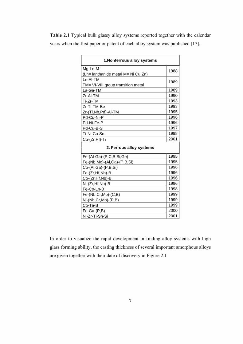
Table 2.1 Typical bulk glassy alloy systems reported together with the calendar

years when the first paper or patent of each alloy system was published [17].

1.Nonferrous alloy systems

Mg-Ln-M (Ln= lanthanide metal M= Ni Cu Zn)

1988

Ln-Al-TM TM= VI-VIII group transition metal

1989

La-Ga-TM 1989 Zr-Al-TM 1990 Ti-Zr-TM 1993 Zr-Ti-TM-Be 1993 Zr-(Ti,Nb,Pd)-Al-TM 1995 Pd-Cu-Ni-P 1996 Pd-Ni-Fe-P 1996 Pd-Cu-B-Si 1997 Ti-Ni-Cu-Sn 1998 Cu-(Zr,Hf)-Ti 2001

2. Ferrous alloy systems

Fe-(Al-Ga)-(P,C,B,Si,Ge) 1995 Fe-(Nb,Mo)-(Al,Ga)-(P,B,Si) 1995 Co-(Al,Ga)-(P,B,Si) 1996 Fe-(Zr,Hf,Nb)-B 1996 Co-(Zr,Hf,Nb)-B 1996 Ni-(Zr,Hf,Nb)-B 1996 Fe-Co-Ln-B 1998 Fe-(Nb,Cr,Mo)-(C,B) 1999 Ni-(Nb,Cr,Mo)-(P,B) 1999 Co-Ta-B 1999 Fe-Ga-(P,B) 2000 Ni-Zr-Ti-Sn-Si 2001

In order to visualize the rapid development in finding alloy systems with high

glass forming ability, the casting thickness of several important amorphous alloys

are given together with their date of discovery in Figure 2.1

7

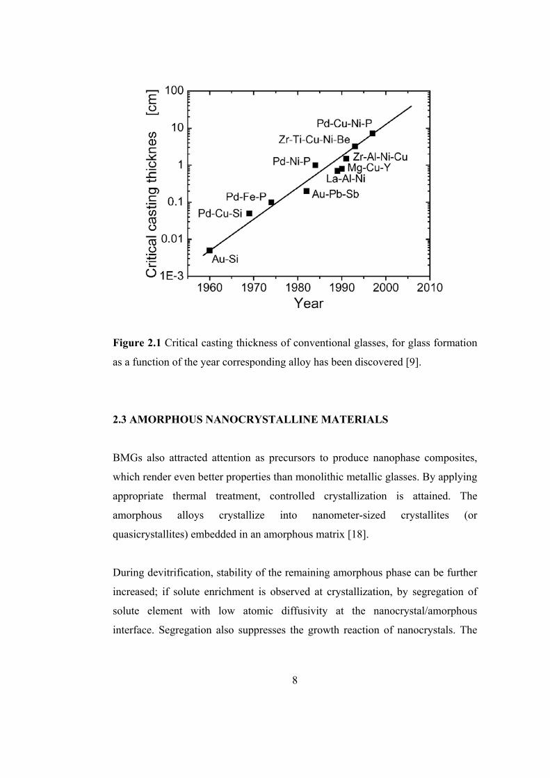
Figure 2.1 Critical casting thickness of conventional glasses, for glass formation

as a function of the year corresponding alloy has been discovered [9].

2.3 AMORPHOUS NANOCRYSTALLINE MATERIALS

BMGs also attracted attention as precursors to produce nanophase composites,

which render even better properties than monolithic metallic glasses. By applying

appropriate thermal treatment, controlled crystallization is attained. The

amorphous alloys crystallize into nanometer-sized crystallites (or

quasicrystallites) embedded in an amorphous matrix [18].

During devitrification, stability of the remaining amorphous phase can be further

increased; if solute enrichment is observed at crystallization, by segregation of

solute element with low atomic diffusivity at the nanocrystal/amorphous

interface. Segregation also suppresses the growth reaction of nanocrystals. The

8

final nanostructure is strongly dependent on the number of homogeneous

nucleation sites in the as-quenched glass. However, it has also been suggested a

possible control of heterogeneous nucleation mechanism by additional elements

occurring by formation of clusters or by the presence of quenched in nuclei. [18]

In addition to these, Inoue [19] also proposed that multistage crystallization is

also crucial for the formation of amorphous nanocrystalline materials.

2.4 PROPERTIES AND APPLICATIONS OF METALLIC GLASSES

The superior properties of metallic glasses arise from the absence of crystallanity

in the microstructure. In an amorphous microstructure, crystalline defects cannot

be present because of the nature of the amorphous state. The absence of

dislocations and grain boundaries renders different mechanical and magnetic

properties due to different mechanisms compared with the crystalline

counterparts of the amorphous alloys. Grain boundaries are the weak spots with

less atomic packing, where fractures can form corrosion starts. Misaligned planes

of atoms under sufficient stress and heat slip over each other easily, allowing

dislocations to move. As a result crystalline materials have a much lower strength

than their theoretical values [20].

Lack of grain boundaries is also one of the factors that make some amorphous

alloys more resistant towards corrosion; grain boundaries allow the diffusion of

oxygen due to their open structure. Another factor is that the amorphous phase in

many alloys is stabilized by B, P or Si. These elements are strong oxide formers

and may be the source for passivation in the same way as chromium in stainless

steel provides a protective layer against corrosion for the iron.

9

Pang and coworkers [21] experimentally verified that Fe43Cr16Mo16C15B10 and

Fe43Cr16Mo16C10B5P10 bulk glassy alloys exhibit passive behavior within

extremely corrosive environments, indicating that they have high corrosion

resistance. Corrosion resistance is higher for phosphorus containing alloys.

Atomic disorder is also the reason for high electrical resistance of amorphous

alloys, which is useful for suppressing eddy currents in high frequency magnetic

reversal applications [22].

2.4.1 Mechanical Properties

The mechanical properties of metallic glasses are in many cases superior to their

crystalline counterparts. In tensile loading, the elastic strain limit of metallic

glasses, εl, is 2% higher than that of common crystalline metallic alloys where εl

can reach 41%. Thus, the yield strength of amorphous alloys is relatively high in

tension and compression. In Vitreloy1 [9] (Zr41.2Ti13.8Cu12.5Ni10Be22.5), for

example, the tensile yield strength, σy is 1.9 GPa and Young’s modulus E, is 96

GPa. Upon yielding, metallic glasses often show plastic flow in absence of work-

hardening and a tendency towards work-softening leads to shear localization.

Under tensile conditions, the localization of plastic flow into shear bands limits

dramatically the overall plasticity, so that metallic glass specimens usually fail

catastrophically on one dominant shear band. This adverse property was recently

mitigated by the development of composites containing ductile crystals in a bulk

metallic glass matrix. Nanocomposites with improved plasticity ranging up to

2.5% in compression was obtained by the annealing of glassy precursor alloys in

the vicinity of Tx to allow some limited crystallization.

In another approach, researchers obtained a reinforced composite consisting of

ductile micrometer sized crystals in a glassy matrix via in situ processing, i.e.,

without additional annealing steps. The production of a composition in the

10

neighborhood of Vit1 (Zr56.2Ti13.8Nb5Cu7Ni5.5Be12.5) led to the precipitation of a

high-temperature, micrometer-sized β-ZrTi (bcc) phase upon cooling, which

shifted the composition of the remaining liquid close to that of Vitrealoy1. As a

consequence the remaining liquid solidified as a bulk metallic glass. The element

Nb was added to stabilize the ductile bcc phase over the β-ZrTi (hcp) phase. The

resulting two-phase microstructure effectively modifies shear band formation and

propagation. A high density of multiple shear bands evolves upon loading, which

results in a significant increase of ductility both in tension and compression,

toughness, and impact resistance compared to the monolithic glass. The overall

(tensile and compressive) plastic strain of this in situ composite is about 5%. The

tensile ductility is of particular importance for the use of bulk metallic glasses as

structural engineering materials [9].

2.4.2 Magnetic Properties

The unique properties of amorphous alloys stem from the lack of long-range

atomic order. The alloys do not exhibit magnetocrystalline anisotropy, thus some

of the alloys are extremely magnetically soft. The absence of grain boundaries,

which could otherwise pin the domain walls, also contributes to a low coercivity

[22].

Based on the three empirical rules for achievement of high glass forming ability

new bulk amorphous alloys with ferromagnetism at room temperature have been

developed. Soft ferromagnetic bulk amorphous alloys have been synthesized in

multicomponent Fe-(Al,Ga)-(P,C,B,Si), Co-Cr-(Al-Ga)-(P,B,C), Fe-(Co,Ni)-

(Zr,Nb,Ta)-B, and Co-Fe-(Zr,Nb,Ta,)-B systems [23].

11

2.4.3 Applications of Metallic Glasses

Metallic Glasses with promising properties can have a wide range of

technological applications. The combination of high strength, elasticity, hardness

and wear resistance has opened markets in a diverse spectrum of products.

Particularly important application fields are machinery/structural materials,

magnetic materials, acoustic materials, somatologic materials, optical machinery

materials, sporting good materials and electrode materials. Zr-Al-Ni-Cu and Zr-

Ti-Al-Ni-Cu alloys have already been commercialized as golf club materials [24].

Cell phone cases, surgical instruments, implants for bone replacement and other

medical devices are other application areas [9].

2.5 METHODS OTHER THAN RAPID SOLIDIFICATION FOR THE

PRODUCTION OF METALLIC GLASSES

The production of bulk amorphous alloys by consolidation of amorphous

powders has promising and important practical applications in the near-net-shape

fabrication of components. This flexible processing method substantially eases

the limitations in sample shape and size. The properties of the consolidated

amorphous product depend on the density and the bonding state that exists

between the powder particles, as well as the strength and ductility of the alloy.

The fabrication of bulk amorphous alloys with high strength by a warm extrusion

method requires full densification by flow under high pressure at temperatures

that are below the crystallization temperature (Tx), yet above the glass transition

temperature (Tg). Moreover, strong bonding between the powder particles should

occur by breaking of the surface films (e.g., oxide or nitride) during deformation

of the powders. These conditions imply that the amorphous alloy should have a

wide super-cooled liquid region (∆Tx = Tx-Tg) and high glass forming ability for

full densification without crystallization during extrusion [25].

12

In the supercooled liquid state, a metallic glass can be deformed under Newtonian

flow, where the viscosity is independent of the strain rate. At higher strain rates,

viscosity tends to decrease linearly and the deformation mode changes from a

homogeneous mode, where all volume elements contribute to total strain, to an

inhomogeneous mode, where strain is localized and deformation occurs in thin,

discrete shear bands. In the inhomogeneous mode, plastic flow in the shear bands

is high, but its contribution to global plasticity is very small. By maintaining

appropriate strain rates and thermal conditions, bulk metallic glasses may be

homogeneously deformed in their supercooled liquid state by conventional plastic

forming techniques such as warm extrusion and compression molding. Sordelet et

al. [25] examined the warm extrusion behavior and devitrification tendencies of

gas atomized Cu47Ti34Zr11Ni8 powders in their supercooled liquid state.

Amorphous powders are produced by gas atomization, where the cooling rate can

be very high for small atomized drops. Several warm extrusion experiments have

been conducted and successful consolidations predominantly to amorphous alloys

are reported [26].

Lee et al. [26] also reported, a fully amorphous Ni59Zr20Ti16Si2Sn3 alloy

successfully synthesized by warm extrusion. The extrusion temperature of 848 K

was selected from the T–T–T curve for the onset of crystallization of the

amorphous powders. The Ni based amorphous alloy exhibited high strength about

2 GPa, whereas the as cast Ni59Zr20Ti16Si2Sn3 alloy has a strength of 2.2 GPa.

Another route for forming amorphous powders is mechanical alloying, where

solid state amorphitization from the crystal powders is attained by ball milling.

Transition from crystalline to amorphous phase is observed when a sufficiently

high energy level is reached and kinetic conditions prevent the establishment of

equilibrium [27, 28].

13

2.6 THEORY OF METALLIC GLASS FORMATION

2.6.1 Glass Forming Ability

Liquid state is characterized by the absence of long-range order. When a metal or

alloy melts, the three dimensional lattice arrangements of atoms are destroyed,

and in the liquid the atoms vibrate about positions that are constantly and rapidly

interdiffusing. During melting, the crystal and liquid phases are in equilibrium

and for pure metals, the volume, enthalpy, and entropy undergo discontinuous

change; the enthalpy and entropy increase, the volume usually does also, except

where the atomic packing in the crystal is relatively open, as for semimetals.

Melting is therefore a first order phase transformation [29].

A liquid, at temperatures above the melting point, is in a state of internal

equilibrium and its structures and properties are independent of its thermal

history. It is characterized by the inability to resist shear stress [29]. On cooling,

for the solidification phase transformation to occur liquid must undercool below

the equilibrium crystallization temperature, due to an energy barrier to the

formation of nuclei. The degree of undercooling that occurs depends upon several

factors, including the initial viscosity of the liquid, the rate at which the viscosity

increases with decreasing temperature, the temperature dependence of the free

energy difference between the undercooled liquid and crystal phase, the

interfacial energy between the melt and crystal, the volume density and the

efficiency of heterogeneous nucleating particles and the imposed cooling rate.

Liquid transition metals such as iron, nickel and cobalt, in which the

heterogeneous nucleants have been largely removed with a flux, can be

undercooled in bulk by more than 200 K under slow cooling conditions.

However, the growth rates for crystals in metallic melts are very rapid once

nucleated and where the rate of heat removal to the surroundings is small, rapid

recalescence occurs [29].

14

For the formation of an amorphous phase by rapid solidification of the melt,

suppression of the nucleation and growth crystalline phases in the supercooled

region is required.

If a liquid metal is rapidly cooled below its melting temperature, the influence of

heterogeneous nucleants is increasingly delayed with the decrease of atomic

mobility, and as the cooling rate is increased, the undercooling is increased and

the recalecense decreased. Thus the temperature range over which crystallization

proceeds becomes increasingly depressed, leading to structural modifications [1].

The structure of alloys rapidly quenched from liquid state is always unusual in

some respect, even if the phases present are crystallographically the same as in

the equilibrium alloys. For example, binary alloys in which a complete series of

solid solutions exists, can be obtained with the highest degree of homogeneity.

With rapid cooling the refinement of microstructural features occur. Quenching

from liquid state also results in high concentration defects; the technique has been

used to study vacancy concentrations in quenched aluminum. However, the most

interesting application of the technique is by far, the synthesis of new alloy

phases which cannot be obtained neither under equilibrium conditions nor by

quenching from the solid state. These new phases can be classified into three

types; solid solutions extending beyond the equilibrium concentrations,

metastable crystalline phases and amorphous phases [30]. Amorphous phase is

formed when the cooling rate is sufficiently high, to suppress crystallization

because of insignificant growth or in the extreme nucleation. In this case, shear

viscosity (η) decreases continuously while in crystallization there is a

discontinuous jump in the viscosity value. The dependence of η to temperature

can be seen in Fig. 2.2.

15

Figure 2.2 Change in the viscosity of a material upon crystallization and

amorphous phase formation [29].

Although the driving force for nucleation is continually increasing, this is

opposed by rapidly decreasing mobility which at very high undercoolings,

dominates. Eventually, the atomic configuration of the liquid departs from

equilibrium and then shortly thereafter becomes homogeneously frozen, at the so

called glass transition temperature. This structural freezing to the glass state is by

convention, considered to occur when η is about 1013 poise [29].

Glass transition is characterized by significant loss of modulus and volume upon

heating. Glass transition is not one temperature but a relatively narrow range (10

degrees). Tg is not precisely measured, but is a very important characteristic.

Glass transition is a second order transformation which means at Tg the

16

temperature dependence of the volume and enthalpy decreases discontinuously,

Cp value decreases significantly due to the freezing of the structure. The

difference between the Cp values of crystal and vitrified liquid diminishes.

Glass formation occurs easily in some familiar cases of non-metallic materials

such as silicate glasses. In these the nature of atomic bonding severely limits the

capability of atomic or molecular rearrangement necessary for maintaining

thermodynamic equilibrium upon cooling. Thus the melt solidifies to a glass,

even at low rates of cooling, often less than 10-2 K/s. Metallic melts in contrast,

have non-directional bonding, so the atomic rearrangements occur very rapidly,

even at high degrees of cooling below their equilibrium freezing temperatures.

Hence, very high cooling rates (>105 K/s) must generally be imposed to form

metallic glasses [29].

Glass Forming ability (GFA) is the term used as a measure of the ease with which

an alloy melt can be undercooled below the glass transition temperature during

solidification. The most straightforward indicators of GFA are critical cooling

rate (Rc), and maximum casting thickness. Alloys with high GFA have a lower Rc

and greater maximum casting thickness. Although these indicators are

fundamental, they do not tell much about the potential of a system to be vitrified

into amorphous form. More advanced indicators of GFA are therefore needed.

Reduced glass transition temperature (Trg) which is defined as, Tg/Tl, is a widely

used as an indicator of GFA.

When the interval between Tg and Tl decreases, the value of Trg increases, so that

the probability of being able to cool through the interval between Tl and Tg

without crystallization is enhanced, therefore the GFA is increased. As the

alloying concentration is increased, Tg generally varies insignificantly, while Tl

often decreases more substantially. The ratio Tg/Tl also arises from the

requirement that the viscosity must be large at temperatures between the melting

17

point and Tg. The viscosity at Tg being constant, the higher the ratio of Tg/Tl, The

higher will be the viscosity at the nose of the TTT or CCT curves and hence

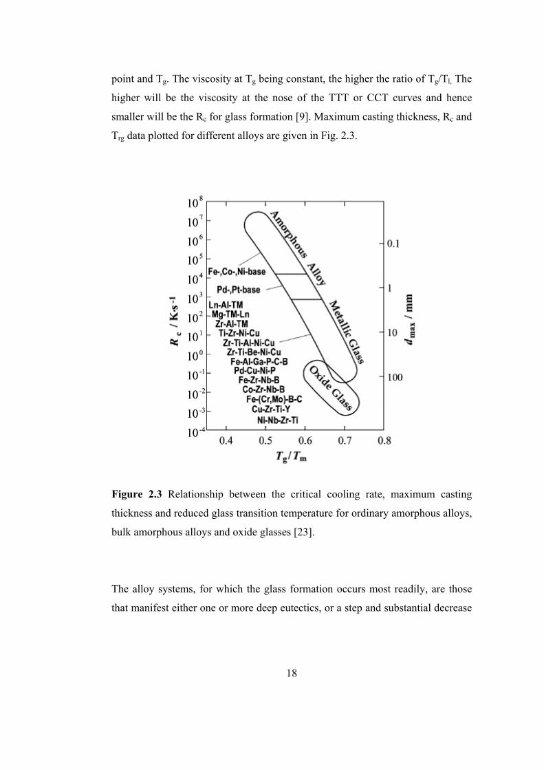
smaller will be the Rc for glass formation [9]. Maximum casting thickness, Rc and

Trg data plotted for different alloys are given in Fig. 2.3.

Figure 2.3 Relationship between the critical cooling rate, maximum casting

thickness and reduced glass transition temperature for ordinary amorphous alloys,

bulk amorphous alloys and oxide glasses [23].

The alloy systems, for which the glass formation occurs most readily, are those

that manifest either one or more deep eutectics, or a step and substantial decrease

18

in liquidus (Tl) with increasing percentage of solute, to a plateau over which Tl is

low in comparison with the melting point of the host metal [29].

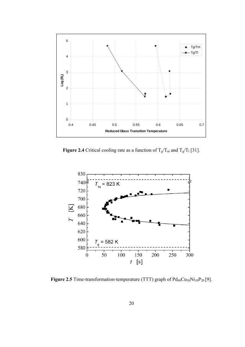
Although there are many Trg values reported in the literature, they are calculated

using both Tg/Tl and Tg/Tm interchangeably by the researchers. According to Lu

et. al. [31] the Tg/Tl parameter is more consistent to indicate GFA, while Tg/Tm

can have a less strong correlation with GFA. In their study, various bulk glass

forming alloys based on Zr, La, Mg, Pd and rare-earth elements are produced;

using thermal analysis their Tg, Tm (solidus temperature) and Tl (liquidus

temperature) values are determined. Accordingly, when Trg is calculated based

on Tg/Tm, while Trg is constantly increasing the critical cooling rate first shows a

decreasing trend, followed by an incremental trend. However, when Trg is

calculated based on Tg/Tl an increase in the Trg is always accompanied by a

decrease in the critical cooling rate. This arises mainly from the higher

dependency of Tl to composition while Tg and Tm are less composition

dependent. For Mg based alloys this behavior is shown in Fig. 2.4.

19

0

1

2

3

4

5

0.4 0.45 0.5 0.55 0.6 0.65 0.7

Reduced Glass Transition Temperature

Log

(Rc)

Tg/Tm

Tg/Tl

Figure 2.4 Critical cooling rate as a function of Tg/Tm and Tg/Tl [31].

Figure 2.5 Time-transformation-temperature (TTT) graph of Pd40Cu30Ni10P20 [9].

20

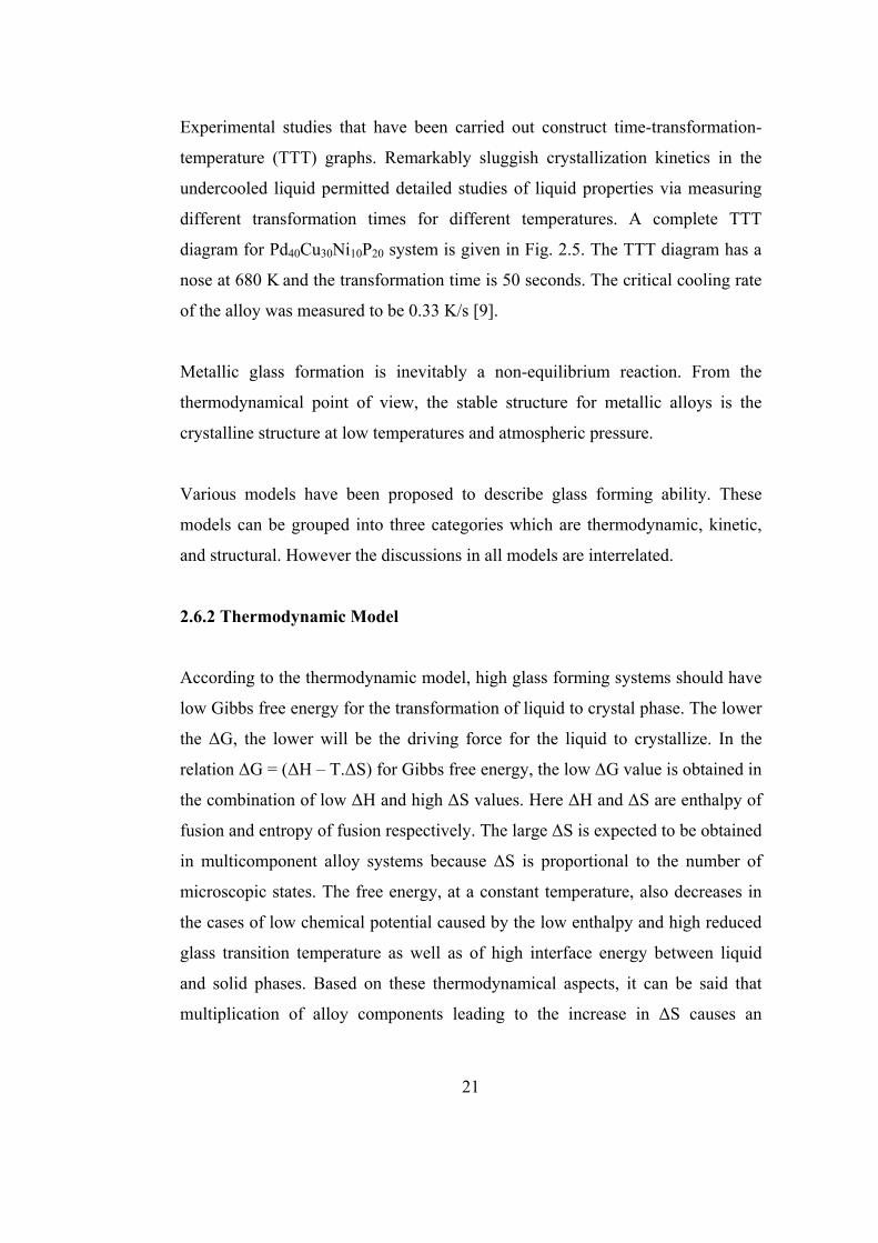
Experimental studies that have been carried out construct time-transformation-

temperature (TTT) graphs. Remarkably sluggish crystallization kinetics in the

undercooled liquid permitted detailed studies of liquid properties via measuring

different transformation times for different temperatures. A complete TTT

diagram for Pd40Cu30Ni10P20 system is given in Fig. 2.5. The TTT diagram has a

nose at 680 K and the transformation time is 50 seconds. The critical cooling rate

of the alloy was measured to be 0.33 K/s [9].

Metallic glass formation is inevitably a non-equilibrium reaction. From the

thermodynamical point of view, the stable structure for metallic alloys is the

crystalline structure at low temperatures and atmospheric pressure.

Various models have been proposed to describe glass forming ability. These

models can be grouped into three categories which are thermodynamic, kinetic,

and structural. However the discussions in all models are interrelated.

2.6.2 Thermodynamic Model

According to the thermodynamic model, high glass forming systems should have

low Gibbs free energy for the transformation of liquid to crystal phase. The lower

the ∆G, the lower will be the driving force for the liquid to crystallize. In the

relation ∆G = (∆H – T.∆S) for Gibbs free energy, the low ∆G value is obtained in

the combination of low ∆H and high ∆S values. Here ∆H and ∆S are enthalpy of

fusion and entropy of fusion respectively. The large ∆S is expected to be obtained

in multicomponent alloy systems because ∆S is proportional to the number of

microscopic states. The free energy, at a constant temperature, also decreases in

the cases of low chemical potential caused by the low enthalpy and high reduced

glass transition temperature as well as of high interface energy between liquid

and solid phases. Based on these thermodynamical aspects, it can be said that

multiplication of alloy components leading to the increase in ∆S causes an

21

increase in the degree of dense random packing which is favorable for the

decrease in ∆H and increase in solid/liquid interface energy [23].

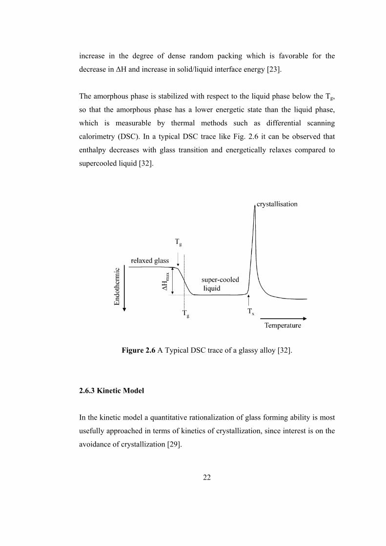
The amorphous phase is stabilized with respect to the liquid phase below the Tg,

so that the amorphous phase has a lower energetic state than the liquid phase,

which is measurable by thermal methods such as differential scanning

calorimetry (DSC). In a typical DSC trace like Fig. 2.6 it can be observed that

enthalpy decreases with glass transition and energetically relaxes compared to

supercooled liquid [32].

Figure 2.6 A Typical DSC trace of a glassy alloy [32].

2.6.3 Kinetic Model

In the kinetic model a quantitative rationalization of glass forming ability is most

usefully approached in terms of kinetics of crystallization, since interest is on the

avoidance of crystallization [29].

22

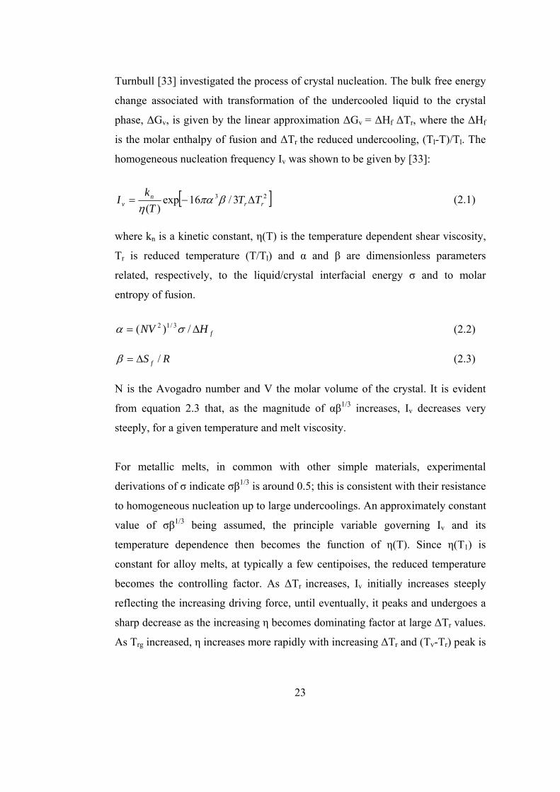
Turnbull [33] investigated the process of crystal nucleation. The bulk free energy

change associated with transformation of the undercooled liquid to the crystal

phase, ∆Gv, is given by the linear approximation ∆Gv = ∆Hf ∆Tr, where the ∆Hf

is the molar enthalpy of fusion and ∆Tr the reduced undercooling, (Tl-T)/Tl. The

homogeneous nucleation frequency Iv was shown to be given by [33]:

[ 23 3/16exp)( rr

nv TT

Tk

I ∆−= βπαη

] (2.1)

where kn is a kinetic constant, η(T) is the temperature dependent shear viscosity,

Tr is reduced temperature (T/Tl) and α and β are dimensionless parameters

related, respectively, to the liquid/crystal interfacial energy σ and to molar

entropy of fusion.

fHNV ∆= /)( 3/12 σα (2.2)

RS f /∆=β (2.3)

N is the Avogadro number and V the molar volume of the crystal. It is evident

from equation 2.3 that, as the magnitude of αβ1/3 increases, Iv decreases very

steeply, for a given temperature and melt viscosity.

For metallic melts, in common with other simple materials, experimental

derivations of σ indicate σβ1/3 is around 0.5; this is consistent with their resistance

to homogeneous nucleation up to large undercoolings. An approximately constant

value of σβ1/3 being assumed, the principle variable governing Iv and its

temperature dependence then becomes the function of η(T). Since η(T1) is

constant for alloy melts, at typically a few centipoises, the reduced temperature

becomes the controlling factor. As ∆Tr increases, Iv initially increases steeply

reflecting the increasing driving force, until eventually, it peaks and undergoes a

sharp decrease as the increasing η becomes dominating factor at large ∆Tr values.

As Trg increased, η increases more rapidly with increasing ∆Tr and (Tv-Tr) peak is

23

rapidly lowered and shifted to the higher Tr. Thus it becomes easier to avoid

nucleation [29].

2.6.4 Structural Model

It is well-established that as the size and valence differences between component

atoms increase, thus the electronegativity difference increases; the atomic

interaction, expressed by negative excess enthalpy and free enthalpy of mixing

also increases. Strong unlike atom interaction (ordering) leads to the formation of

stable intermetallic compound phases from eutectic reactions occurring at low

temperatures [29]. Upon solidification, ordered phases encounter growth

problems due to the complex structure arising from preferred heterocoordination.

This phenomenon increases the glass forming ability.

Also according to Inoue [24], the combination of the significant difference in

atomic sizes and negative heats of mixing is expected to cause an increase in

random packing density in the supercooled liquid which enables the achievement

of high liquid/solid interfacial energy as well as the difficulty of atomic

rearrangements leading to the decreases in atomic diffusivity and viscosity.

2.6.5 Semiempirical Criteria

According to Inoue [17] alloy systems with high glass forming ability obey the

following three empirical rules:

1. Multicomponent systems containing more than three elements

2. Significant difference in atomic size ratios above 12 % among the three main

constituent elements.

3. Negative heats of mixing among the main constituent elements.

24

According to confusion principle larger number of components in an alloy system

destabilizes competing crystalline phases which may form during cooling. This

effect frustrates the tendency of the alloy to crystallize by making the melt more

stable relative to crystalline phases [34]. The widely differing atomic radii and

the high number of different elements confuse the atoms so they don’t know

where to go to form crystal as they cool.

According to the data obtained for multicomponent amorphous alloys, it has been

stated that the amorphous alloys can have higher degrees of dense randomly

packed atomic configurations, which are different from those of the

corresponding crystalline phases, and the homogeneous atomic configuration of

the multicomponents on long-range scale [18].

2.6.6 Atomic Size Distribution Plot

Although there is a large amount of information about criterions of glass forming

ability, the task of exploring new alloy systems is still based on manual labor

intensive trial and error methods, where quite a number of compositions can be

rendered experimentally. In order to narrow the composition choice for research

Senkov at al. [35] investigated compositions and atomic radii of constituents in

amorphous alloys. Most amorphous metallic alloys have a characteristic

dependence of concentrations of alloying elements on their relative atomic radii,

where relative radius is defined as radius of solute atom divided by the radius of

the solvent atom.

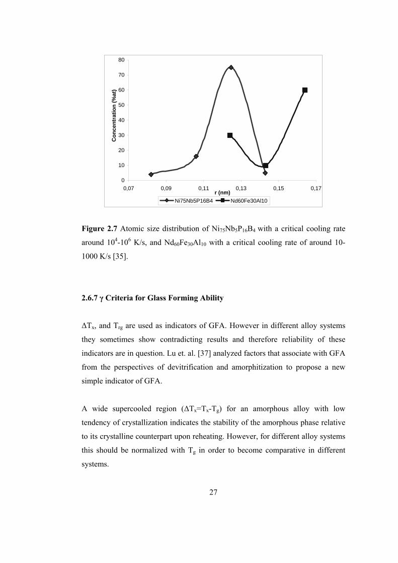
For a bulk amorphous alloy system, where the critical cooling rate is less than 103

K/s, usually the solvent element has the highest atomic size. Concentration

decreases for the solutes with lower atomic radii, exhibits a minimum and then

starts to increase for the elements with the smallest atomic radii. When the

concentration vs. atomic size (so called atomic size distribution) is plotted this

25

behavior is characterized with a concave upward shape. For ordinary amorphous

alloys with marginal glass forming ability a concave downward shape is observed

where the solvent atom has an intermediate size. Atomic size distributions of two

ordinary and bulk amorphous alloys are given in Fig. 2.7.

These characteristic atomic size distributions show correlation with the reported

low molar volume and high atomic packing of bulk amorphous alloys [35].

Concave upward shape provides a more close packing compared with the

concave downward behavior. It has been shown that a more compact structure

has a higher viscosity and lower diffusivity, which leads to a more difficult

nucleation and crystallization process which enhances glass forming ability

significantly [36].

A model has been developed in order to explain the concave upward shape of the

atomic size distribution in bulk amorphous alloys. Accordingly, when all the

alloying additions are smaller than the solvent element, some of them are located

at the substitutional sites while others at the interstitial sites. Substitutional and

interstitial atoms attract each other because of the different strain fields they

produce around them. This attraction produces short-ranged ordered clusters

which may stabilize the amorphous structure [36].

26

0

10

20

30

40

50

60

70

80

0,07 0,09 0,11 0,13 0,15 0,17r (nm)

Con

cent

ratio

n (%

at)

Ni75Nb5P16B4 Nd60Fe30Al10

Figure 2.7 Atomic size distribution of Ni75Nb5P16B4 with a critical cooling rate

around 104-106 K/s, and Nd60Fe30Al10 with a critical cooling rate of around 10-

1000 K/s [35].

2.6.7 γ Criteria for Glass Forming Ability

∆Tx, and Trg are used as indicators of GFA. However in different alloy systems

they sometimes show contradicting results and therefore reliability of these

indicators are in question. Lu et. al. [37] analyzed factors that associate with GFA

from the perspectives of devitrification and amorphitization to propose a new

simple indicator of GFA.

A wide supercooled region (∆Tx=Tx-Tg) for an amorphous alloy with low

tendency of crystallization indicates the stability of the amorphous phase relative

to its crystalline counterpart upon reheating. However, for different alloy systems

this should be normalized with Tg in order to become comparative in different

systems.

27

1−=−

g

x

g

gx

TT

TTT

(2.4)

From the above relation it can be comprehended that GFA is proportional with

the factor Tx/Tg .

From the perspective of amorphitization using non-isothermal crystallization

kinetics it is found that Tx/Tl ratio increases with the increasing viscosity of the

supercooled liquid, fusion entropy and activation energy of viscous flow and with

decreasing Tl. The dependence of the Tx/Tl ratio on the magnitudes of liquid

parameters is similar to those of critical cooling rate Rc. Therefore Tx/Tl ratio

becomes a reasonable indicator of high GFA.

1

,,−

⎟⎟⎠

⎞⎜⎜⎝

⎛⎟⎟⎠

⎞⎜⎜⎝

⎛

x

l

x

g

l

x

g

x

TT

TT

TT

TTGFA αα (2.5)

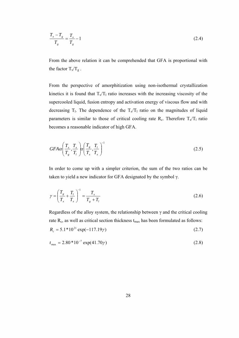
In order to come up with a simpler criterion, the sum of the two ratios can be

taken to yield a new indicator for GFA designated by the symbol γ.

lg

x

x

l

x

g

TTT

TT

TT

+=⎟⎟

⎠

⎞⎜⎜⎝

⎛+=

−1

γ (2.6)

Regardless of the alloy system, the relationship between γ and the critical cooling

rate Rc, as well as critical section thickness tmax has been formulated as follows:

)19.117exp(10*1.5 21 γ−=cR (2.7)

)70.41exp(10*80.2 7max γ−=t (2.8)

28

2.6.8 Bulk Glass Forming Ability (BGFA)

Recently Akdeniz et al. [38] investigated the bulk glass formation in accordance

with solidification behavior. It has been proposed that alloys having eutectic

peritectic reaction sequence are quite favorable for achieving rather high BGFA.

Characteristic DSC pattern, involving high temperature peritectic and subsequent

eutectic exothermic peaks are observed for this kind of alloys. When a high

temperature peritectic reaction produces a facet forming complex intermetallic

phase, on further cooling, this phase becomes one of the constituents of coupled

growth of subsequent eutectic reaction. The coupled zone becomes skewed

towards faceted phase and irregular eutectic formation occurs for equilibrium

cooling rates. However, upon rapid solidification, if the growth rate exceeds the

limiting growth rate of eutectic transition to amorphous phase instead of irregular

eutectic is observed

2.6.9 Structure of Amorphous Alloys

In order to understand the local atomic structure of amorphous alloys, the parent

liquid structure may be investigated. When a metallic melt is vitrified the liquid

structure is frozen however some structural relaxation occurs. Any model

constructed to describe atomic structure should be in accordance with radial

distribution function (RDF) which is the most valuable empirical data related

with the atomic structure for amorphous alloys. In RDF, the number of atoms at a

given distance r from a specified atom centre is compared with the number of

atoms at the same distance in an ideal gas at the same density. RDF can be

constructed from X-ray or neutron scattering experiments using Fourier

transforms to invert the structure factor from space to real space. →

q

Bernal [40] proposed a model depending on constituent atoms having high

coordination numbers, with surrounding atoms generally in contact. In the

29

proposed model the atoms were considered as hard spheres and their local

structure was determined by the restrictions on space filling consequent upon the

inability of two atoms to approach more closely than one diameter. The structural

unit of Bernal’s model was several small polyhedra. Gaskell adopted chemical

ordering and proposed trigonal prisms as the fundamental unit of structure.

Within this respect structure of metal-metalloid glasses were attempted to be

explained [39].

Figure 2.8 Total RDFs of liquid and amorphous Pd80Si20 alloy [41].

While modeling studies are continuously developing experimental RDFs can be

directly analyzed to interpret the local atomic configuration. Most of the binary

metallic glass shows a characteristic distinction from their liquid structure in RDF

plots, namely the splitting of the second peak. Also the sharpening of the peaks is

observed when liquid melt is vitrified. RDF of Pd80Si20 alloy is given in Fig. 2.8

as an example. Compared to the liquid, the atoms in the amorphous state are

30

relatively restricted movement. The basic arrangement of atoms in amorphous

state and liquid are similar, in which atoms are randomly distributed in nearly

closed packed structure and the mean free path is short and comparable to the

atomic size. This implies that the positional correlation of atoms is relatively

strong within the near neighbor region. However, the average atomic

configuration in the liquid is more homogeneous than that of the amorphous state

because the atomic vibration is high. In other words, the atomic configuration in

the amorphous state shows a slight inhomogenity, which frequently gives a

deformed sharp pattern with second peak splitting in RDF [42].

When the BMGs, emerged in the 1990’s are concerned the structure discussions

should be revisited. BMG were found to have a new type of glassy structure with

higher dense random packing. The densities of BMG’s are very near to their

crystalline counterparts, where the departure is more for ordinary metallic

glasses. [43]. Also the characteristic RDF pattern of ordinary metallic glasses are

not observed for BMGs.

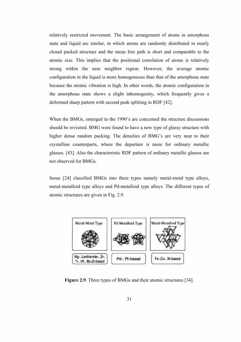
Inoue [24] classified BMGs into three types namely metal-metal type alloys,

metal-metalloid type alloys and Pd-metalloid type alloys. The different types of

atomic structures are given in Fig. 2.9.

Figure 2.9. Three types of BMGs and their atomic structures [34].

31

In metal-metal type alloys, TEM studies reveal that glass consists of icosahedral

clusters. When annealing is carried out in supercooled liquid range, the first

crystallization phase becomes the icosahedral quasicrystallines. At higher

temperatures transformation to stable crystalline phases occurs.

The structure provides a reasonable explanation of supreme GFA of BMGs. For

the ordinary metallic glasses, where the atomic structure of the amorphous phase

similar to the corresponding crystalline phase, the vitrification occurs at high

cooling rates. However, in alloy systems with BGFA at relatively low cooling

rates, still nucleation and growth of crystalline phases can be inhibited. Upon

cooling crystallization of BMGs need a substantial redistribution of the

component elements across the icosahedral liquid. The high dense randomly

packed structure of the BMG in its supercooled state results in extremely low

atomic mobility. Therefore, atomic redistribution becomes a harder task.

Icosahedral clusters having five-fold rotational symmetry are incompatible with

the translational symmetry of normal crystalline phases and this fundamental

structural discontinuity across the amorphous and crystalline phases suppress the

nucleation and growth. [34]

For metal-metaloid glasses, a network of atomic configurations consisting of

trigonal prisms which are connected with each other through glue atoms are

commonly found. The structural investigation shows that Pd–Cu–Ni–P BMGs

consist of two large clustered units of a trigonal prism capped with three half-

octahedra for the Pd–Ni–P and a tetragonal dodecahedron for the Pd–Cu–P

region [34].

32

2.7 MOLECULAR DYNAMICS IN ACCORDANCE WITH GFA

Molecular dynamics simulation method is one of the most powerful simulation

techniques to understand macroscopic material properties from an atomic

description of the system. A detailed explanation of the method is presented in

Chapter III. This powerful tool is starting to be more intimate with GFA; in order

to get insight about both amorphous metallic structure and theory of glass

formation. However, in order to mimic the rapid solidification process,

description of interatomic interactions in an alloy system is crucial. Ab-initio MD

calculations where quantum mechanical analyses employed for interaction at

atomic scale is still computationally expensive even with the modern powerful

computers. Therefore, the number of atoms that can be treated with this approach

is quite few. Different interaction potentials have been developed and

parameterized utilizing empirical and semi-empirical approaches.

Recently, Noya et.al. [44] studied constant temperature - constant therdynamical

tension MD for Ni3Al, NiAl, and NiAl3 alloys with using embedded atom model

(EAM). After melting the alloys at 2000 K, quenching with cooling rates 1013 K/s

and 4.1013 revealed the amorphous structure for all compositions.

Wang et. al. [45] used constant temperature – constant pressure MD to explore

the effect of atomic size mismatch on GFA. For this purpose starting from room

temperature Au, Au-Ag and AuCu systems were heated a few hundred degrees

above their melting temperature and quenched back to room temperature. Pure

Au and Au-Ag alloy formed a crystalline phase at all quench rates chosen, while

Au3Cu became amorphous when quenched with a cooling rate of 4.1012 K/s. Au-

Ag having similar atomic radii failed to form an amorphous phase. However Au-

Cu having dissimilar atomic radii revealed a higher GFA.

33

Qi et. al. [46] performed NPT molecular dynamics for PdNi3. After melting at

1700 K. Four different cooling rates were utilized; 1.1013 K/s, 6.1011 K/s, 5.1011

K/s and 1x1011 K/s in order to quench to room temperature. At high cooling rates,

cooling lead to continuous change in volume. Such characteristics indicate

amorphous phase formation. Tg of the alloy was determined as 950 K. In order to

analyze the local structure, pair analysis was carried out for the glassy alloys and

only a small percentage of fcc pairs were found indicating that fcc local orders

are insignificant. Nevertheless, the predominance of local icosahedral features

over crystalline short range packing was observed.

Kart et. al. [47] investigated diffusion properties of Pd0.8Ag0.2 alloy with NPT

MD. Sutton Chen potentials were used. Diffusion constant of the glassy alloy was

calculated using mean square distance. Accordingly it is found that upon heating

linear increase in the diffusion is found while an exponential decrease is observed

on cooling.

Wang et. al. [42] performed constant temperature – constant pressure MD to

explore the effect of quenching rates on medium range order (MRO). The main

feature of the MRO is the presence of a prepeak at structure factor. It occurs

before the main peak which is associated with short range order (SRO). When

heating is performed to Cu3Ni alloy, at temperatures below 1700 K a prepeak is

observed but above this temperature MRO ceases to exist. Effect of quenching is

examined by monitoring total structure factor at different temperatures. It is

observed that prepeak intensity increases with decreasing temperature, which

means greater number of clusters of MRO. On the other hand prepeak position is

unchanged which indicates, sizes of clusters are invariant but only the number is

increased.

34

CHAPTER III

METHODOLOGY

3.1 PSEUDOPOTENTIAL APPROXIMATION AND ONE ELECTRON

THEORY

3.1.1 The Principals of the One Electron Theory

Principally, any information about a crystal structure can be found by solving the

Schrödinger’s equation for a system of interacting nuclei and electrons that form

the crystal structure. This however requires some simplifications in the

Schrödinger’s equations, since it is too complicated, without these simplifications

to solve. The following simplifications are adopted to solve the problem in the

basis of one electron theory:

• It is generally assumed that nuclei are too massive to follow the rapidly

changing spatial distribution of the electrons. This is also named as “Adiabatic

Approximation”. Thus, this approximation divides Schrödinger’s equation into

two different equations; one for the electron and other for the nuclei.

• In the equation for the electrons, the individual motions of the electrons are

considered separately, not as a whole. Each electron will be thought of as moving

in the effective field of the (stationary) nuclei and all the other electrons. This

approximation is called the “Effective field Approximation”. Lastly, total

electron wave function ψ, is expressed in the terms of individual electron wave

functions ψi.

35

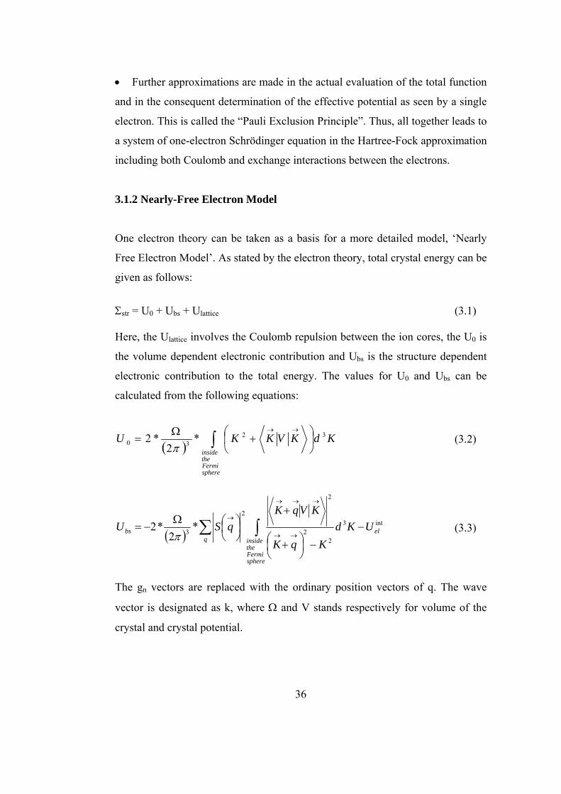
• Further approximations are made in the actual evaluation of the total function

and in the consequent determination of the effective potential as seen by a single

electron. This is called the “Pauli Exclusion Principle”. Thus, all together leads to

a system of one-electron Schrödinger equation in the Hartree-Fock approximation

including both Coulomb and exchange interactions between the electrons.

3.1.2 Nearly-Free Electron Model

One electron theory can be taken as a basis for a more detailed model, ‘Nearly

Free Electron Model’. As stated by the electron theory, total crystal energy can be

given as follows:

Σstr = U0 + Ubs + Ulattice (3.1) Here, the Ulattice involves the Coulomb repulsion between the ion cores, the U0 is

the volume dependent electronic contribution and Ubs is the structure dependent

electronic contribution to the total energy. The values for U0 and Ubs can be

calculated from the following equations:

( ) ∫ ⎟⎠

⎞⎜⎝

⎛ +Ω

=→→

sphereFermitheinside

KdKVKKU 3230 *

2*2

π (3.2)

( ) ∑ ∫ −−⎟

⎠⎞

⎜⎝⎛ +

+⎟⎠⎞

⎜⎝⎛Ω

−=→→

→→→

→

q

sphereFermitheinside

elbs UKdKqK

KVqKqSU int3

22

2

2

3 *2

*2π

(3.3)

The gn vectors are replaced with the ordinary position vectors of q. The wave

vector is designated as k, where Ω and V stands respectively for volume of the

crystal and crystal potential.

36

Above, U0 describes a ‘free’ electron gas with the inclusion of electron-electron

interaction. Moreover, Ubs is associated with band characteristics and named as

“Band Structure Energy”. Lastly, when calculating E(k), the interaction energy of

each electron pair contributes to the energy of each electron, meaning that the

electron-electron interaction energy is counted twice, while calculating the total

energy of the crystal. The term Uelint is used in order to get rid of this additional

energy calculated by subtracting it from the equation.

If the potential V is local, its form factor K is independent and can be taken out of

the K integral that appears then in Ubs. This solution is known as Lindhard’s

function:

( ) ∫ →→→

→

−⎟⎠⎞

⎜⎝⎛ +

Ω−=⎟

⎠⎞

⎜⎝⎛

sphereFermitheinside kqk

kdN

q2

2

3

3 *1*2

*2π

χ (3.4)

If the Fermi surface is assumed spherical, then the Eq. (3.4) becomes:

⎟⎟⎠

⎞⎜⎜⎝

⎛−+−

+⎟⎠⎞

⎜⎝⎛−=

−

xx

xxEZq F 1

1ln2

1132

4)(

21oχ (3.5)

In Eq. (3.5), x = k/2kF and EF

0= (3π2z/Ω0)2/3.

The electron-electron interaction energy may be represented [48] as a result

of interactions between the non-uniform part of the crystal electron density and

the potential, which is the difference between the crystal potential and the

initial potential of the system of ions. can be expressed in terms of the

form factor of V

intelU

crϑionϑ int

elU

cr (q), if a function, α( ) = →

q crion

ϑϑ , is set up in order to

characterize this potential.

37

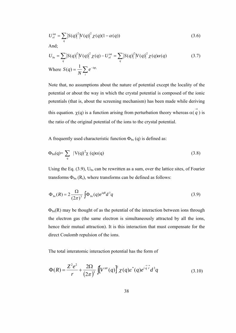
∑ −=q

el qqqVqSU ))(1)(()()( 22int αχ (3.6)

And;

∑ ∑=−=q q

elbs qqqVqSUqqVqSU )()()()()()()( 22int22 αχχ (3.7)

Where ∑ −=i

iqtieN

qS 1)(

Note that, no assumptions about the nature of potential except the locality of the

potential or about the way in which the crystal potential is composed of the ionic

potentials (that is, about the screening mechanism) has been made while deriving

this equation. χ(q) is a function arising from perturbation theory whereas α( ) is

the ratio of the original potential of the ions to the crystal potential.

→

q

A frequently used characteristic function Φbs (q) is defined as:

Φbs(q)= ∑ |V(q)|

q

2χ (q)α(q) (3.8)

Using the Eq. (3.9), Ubs can be rewritten as a sum, over the lattice sites, of Fourier

transforms Φbs (Ri), where transforms can be defined as follows:

∫ΦΩ

=Φ qdeqR iqRbsbs

33 )(

)2(2)(

π (3.9)

Φbs(R) may be thought of as the potential of the interaction between ions through

the electron gas (the same electron is simultaneously attracted by all the ions,

hence their mutual attraction). It is this interaction that must compensate for the

direct Coulomb repulsion of the ions.

The total interatomic interaction potential has the form of

( )[ ]∫

→→Ω+=Φ qdeqqqV

reZR rqistr 3*2

3

22

)()()(22)( εχπ

(3.10)

38

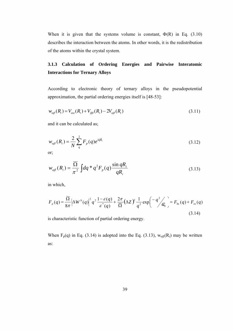
When it is given that the systems volume is constant, Φ(R) in Eq. (3.10)

describes the interaction between the atoms. In other words, it is the redistribution

of the atoms within the crystal system.

3.1.3 Calculation of Ordering Energies and Pairwise Interatomic

Interactions for Ternary Alloys

According to electronic theory of ternary alloys in the pseudopotential

approximation, the partial ordering energies itself is [48-53]:

)(2)()()( iiii RVRVRVRw αβββαααβ −+= (3.11)

and it can be calculated as;

∑=2

)(2)(q

Rqipi

ieqFN

Rwrr

αβ (3.12)

or;

∫Ω

=i

ipi qR

qRqFqdqRw sin)(*)( 22παβ (3.13)

in which,

( ) )()(4exp12

)()(1

)(8

)(2

22

*22

qFqFqq

ZqqqqWqF esbs

bp +=

⎠⎞

⎜⎝⎛ −∆

Ω+

−∆

Ω= ξ

πεε

π

(3.14) is characteristic function of partial ordering energy.

When Fp(q) in Eq. (3.14) is adopted into the Eq. (3.13), wαβ(Ri) may be written

as:

39

( )∫⎭⎬⎫

⎩⎨⎧

⎟⎠⎞

⎜⎝⎛−+

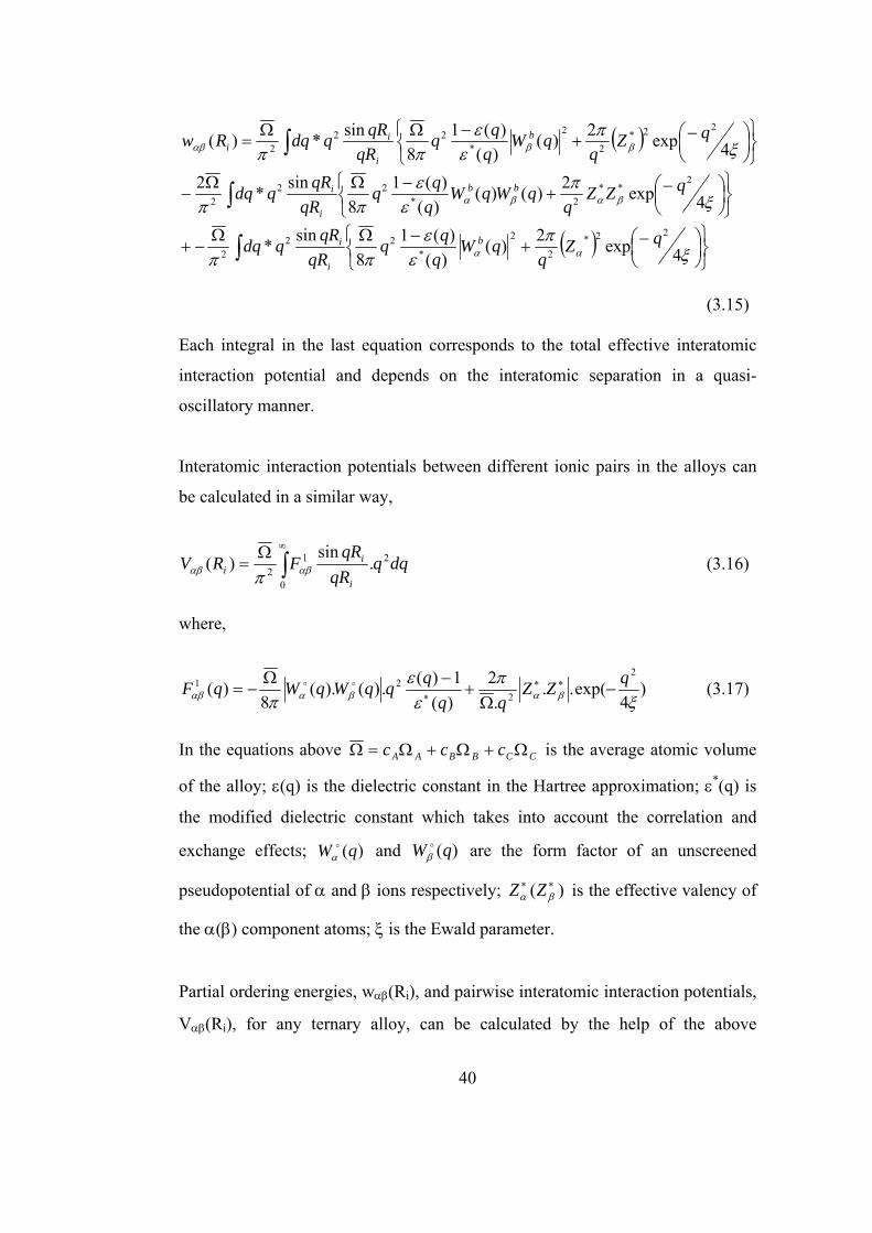
−ΩΩ= ξ

πεε

ππ ββαβ 4exp2)()()(1

8sin*)(

22*2

2

*22

2qZ

qqW

qqq

qRqRqdqRw b

i

ii

⎭⎬⎫

⎩⎨⎧

⎟⎠⎞

⎜⎝⎛−+

−ΩΩ− ∫ ξ

πεε

ππ βαβα 4exp2)()()()(1

8sin*2 2

**2*

222

qZZq

qWqWqqq

qRqRqdq bb

i

i

( )⎭⎬⎫

⎩⎨⎧

⎟⎠⎞

⎜⎝⎛−+

−ΩΩ−+ ∫ ξ

πεε

ππ αα 4exp2)()()(1

8sin*

22*2

2

*22

2qZ

qqW

qqq

qRqRqdq b

i

i

(3.15) Each integral in the last equation corresponds to the total effective interatomic

interaction potential and depends on the interatomic separation in a quasi-

oscillatory manner.

Interatomic interaction potentials between different ionic pairs in the alloys can

be calculated in a similar way,

∫∞Ω

=0

212 .

sin)( dqq

qRqRFRV

i

ii αβαβ π

(3.16)

where,

)4

exp(...

2)(1)(.)().(

8)(

2

221

ξπ

εε

π βαβααβqZZ

qqqqqWqWqF −

Ω+

−Ω−= ∗∗

∗oo (3.17)

In the equations above CCBBAA ccc Ω+Ω+Ω=Ω is the average atomic volume

of the alloy; ε(q) is the dielectric constant in the Hartree approximation; ε*(q) is

the modified dielectric constant which takes into account the correlation and

exchange effects; and are the form factor of an unscreened

pseudopotential of α and β ions respectively; is the effective valency of

the α(β) component atoms; ξ is the Ewald parameter.

)(qW oα )(qW o

β

)( ∗∗βα ZZ

Partial ordering energies, wαβ(Ri), and pairwise interatomic interaction potentials,

Vαβ(Ri), for any ternary alloy, can be calculated by the help of the above

40

equations from (3.12) to (3.17) as a function of interatomic distance, Ri when the

form factor of unscreened pseudopotentials, W°(q), and effective valances, Z*,

which are known for the ions involved, are provided.

3.2 COMPUTER SIMULATION

Computer simulation is a technique to represent the real world using a computer

program by imitating internal processes in a system. A simulation study of a

physical system requires a model which has the appearance and/or behavior of

the system without the reality [54].

There are only a handful of non-trivial, exactly soluble problems in statistical

mechanics. By this it is referred that a complete specification of microscopic

properties of a system leads directly and perhaps easily, to a set of interesting

results or macroscopic properties. Computer simulations have a valuable role to

play in providing essentially exact results for problems in statistical mechanics

which would otherwise only be soluble by approximate methods, or might be

quite intractable [55].

Along with the rapid increase in computer performance, computer simulations are

becoming a powerful investigation tool. With decreased time of running

simulation programs, well defined characteristics of systems are computed, while

in experimental methods, sometimes observing a single characteristic without

screening other parameters can be quite a difficult task.

Computer simulation methods fill the gap between the theoretical and

experimental methods. Eliminating the obligatory approximations in order to find

analytical solutions, validity of theoretical models can be tested and specific

parameters of a system can be computed without actually performing a physical

experiment. Due to this connecting role and the way in which simulations are

41

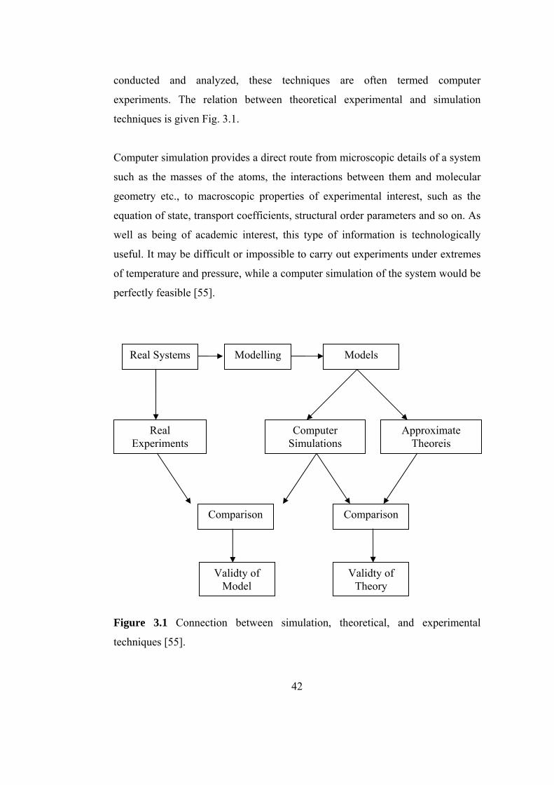
conducted and analyzed, these techniques are often termed computer

experiments. The relation between theoretical experimental and simulation

techniques is given Fig. 3.1.

Computer simulation provides a direct route from microscopic details of a system

such as the masses of the atoms, the interactions between them and molecular

geometry etc., to macroscopic properties of experimental interest, such as the

equation of state, transport coefficients, structural order parameters and so on. As

well as being of academic interest, this type of information is technologically

useful. It may be difficult or impossible to carry out experiments under extremes

of temperature and pressure, while a computer simulation of the system would be

perfectly feasible [55].

Figure 3.1 Connection between simulation, theoretical, and experimental

techniques [55].

Real Systems Models

Approximate Theoreis

Modelling

Real Experiments

Computer Simulations

Comparison Comparison

Validty of Model

Validty of Theory

42

A wide variety of simulation techniques have been developed up to date. The

most popular techniques used to study the molecular level details are Molecular

dynamics and Monte Carlo methods.

3.2.1 Molecular Dynamics

Simplest definition for the molecular dynamics (MD) method can be; solution of

classical equations of motion via numerical integration, to simulate the motion of

particles in a many-body system, with a predetermined interatomic potential for a

finite time. Solution of equation sets for all particles yield the trajectory of the

system which is the momenta and positions of all particles at all times.

Although at first glance utilizing classical mechanics for the nuclear motion of

atomic particles seems inappropriate, for quite a wide range of materials it

renders a good approximation. If De Broglie’s wavelength of the material is

much smaller than the typical interspacing between particles (λ << a), classical

mechanics can safely be used to describe the system. Only when light elements

such as He, H2 and/or low temperatures are involved; quantum effects should be

taken into account [56, 57].

MD simulations have played a key role in advanced materials research.

Generating the complete trajectory of a system allows one to study how atomistic

processes determine macroscopic materials properties [58].

3.2.1.1 Equations of Motion

In order to discuss further features of MD, firstly equations of motion should be

explored. Although there are several mathematical forms, Lagrangian equation

seems perhaps the most fundamental.

43

0)/()/( =∂∂−∂∂ ii rLrLdtd

& (3.18)

Lagrangian function is defined as follows

UKEqqL k −=),( & (3.19)

where KE and U are kinetic and potential energies respectively. Using the

classical definitions of kinetic energy, potential energy and equating the

conservative force to negative gradient of potential function U, Eq. 3.18 deduces

to Newton’s second law.

irrii fLLrm

ii=−∇=∇=&& (3.20)

where mi is the mass of an atom i and fi is the force on that atom. For a system

with N atoms computation of the trajectory of a system with N atoms involves the

solution of 3N second order differential equations [55].

Another way to formulate the classical equations of motion is Hamiltonian

dynamics. Hamiltonian is the function of position and velocities whose value is

constant in time, formally defined as,

∑ +=i

iiii rUpm

prH )(21),( 2 (3.21)

where pi is the momentum of the atom i. Hamiltonian equations are as follows,

i

iii

rprH

dtdp

∂∂

=),(

and i

iii

pprH

dtdr

∂∂

=),(

(3.22)

In order to work out the trajectory of a system with N atoms, this time solving 6N

first order differential equations of type Eq. 3.22 is necessary. When the

definition of momentum is substituted into Hamiltonian equations, it can be seen

that the two sets of equations (Eq. 3.22 and Eq. 3.20) are identical [57,59].

44

3.2.1.2 Sampling From Ensembles

The main objective of the MD simulation is obtaining the macroscopic material

properties from the information at microscopic level (trajectory) obtained during

the simulation. The connection between macroscopic and microscopic level is

established via statistical mechanics. With MD one can investigate

thermodynamic and kinetic phenomenon.

Microscopic state is characterized by atomic positions and momenta of N atoms.

Phase space is a 6N dimensional hyperspace where the positions and momenta of

the entire system can be represented by a point, when the coordinate axes are

components of position vectors and momentum vectors. As the positions and

momenta change with time, the point moves describing a trajectory in the 6N

dimensional phase space [59]. Therefore, with numerical integration of Newton’s

second law phase space trajectory is computed, which is the only information

needed to describe macroscopic features.

A physical experiment is carried out with extremely large numbers of atoms,

sampling an extremely large number of microscopic states. In statistical

mechanics, averages corresponding to experimental observables are ensemble

averages. An ensemble is a collection of all possible systems which have

different microscopic states but have an identical macroscopic or thermodynamic

state. An ensemble average is taken over a large number of replicas of the

ensemble considered simultaneously. Ensemble average of any observable A

which is expressed as a function of momenta (p) and position (r) is formally

defined as:

∫∫= ),(),( NNNNNNensemble

rprpAdrdpA ρ (3.23)

[ ] (3.24) TkrpHQ

rp bNNNN /),(exp1),( −=ρ

45

[∫∫ −= TkrpHdrdpQ bNNNN /),(exp ] (3.25)

In the above equations ρ is the probability function, H is the Hamiltonian, kB is

the Boltzmann constant and Q is the partition function. From the complexity of

integrals, it can be seen that ensemble averaging calculations are often extremely

difficult. On the other hand, while calculating a trajectory in a molecular

dynamics problem one can easily calculate the time average of an observable of

interest [60].

∑∫=

∞→≈=

M

t

NNNNt

ttimerpA

MdttrtpA

tA

10

),(1))(),((1lim (3.26)

At this stage ergodic hypothesis states that when a system is allowed to evolve for

an infinite time it will navigate within all possible states and time average of the

observable A will be equal to its ensemble average.

ensembletimeAA = (3.27)

In order to use ergodic hypothesis safely the number of time steps used in the

simulation (M in Eq. 3.26) should be reasonable high, which is restricted by the

computational performances of the hardware used.

3.2.1.3. Interatomic Potentials

At the microscopic level atoms interact with each other. Before performing a

simulation interatomic potential must be set in analytical form. Most of the time

in MD simulations for simplicity the potential is assumed to be pairwise additive,

in which the interaction among N atoms is a sum of isolated two-body

contributions.

∑∑=

i jjiruU )( , (3.28)

46

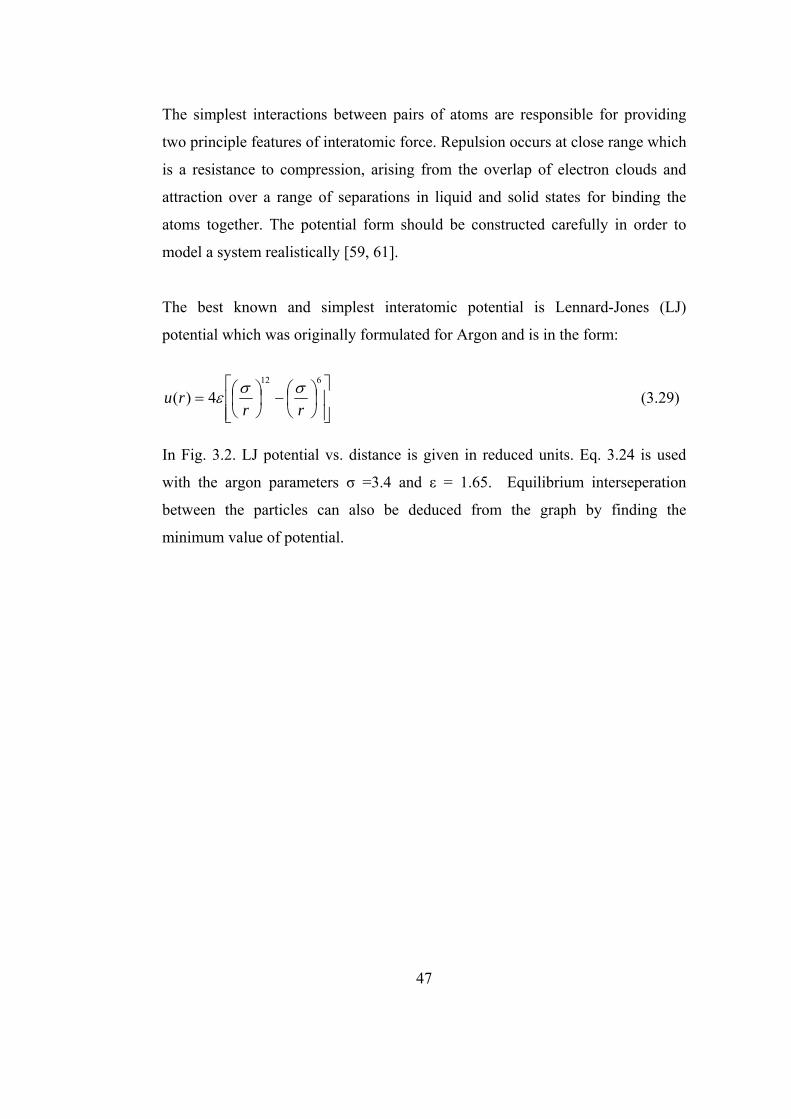
The simplest interactions between pairs of atoms are responsible for providing

two principle features of interatomic force. Repulsion occurs at close range which

is a resistance to compression, arising from the overlap of electron clouds and

attraction over a range of separations in liquid and solid states for binding the

atoms together. The potential form should be constructed carefully in order to

model a system realistically [59, 61].

The best known and simplest interatomic potential is Lennard-Jones (LJ)

potential which was originally formulated for Argon and is in the form:

⎥⎥⎦

⎤

⎢⎢⎣

⎡⎟⎠⎞

⎜⎝⎛−⎟

⎠⎞

⎜⎝⎛=

612

4)(rr

ru σσε (3.29)

In Fig. 3.2. LJ potential vs. distance is given in reduced units. Eq. 3.24 is used

with the argon parameters σ =3.4 and ε = 1.65. Equilibrium interseperation

between the particles can also be deduced from the graph by finding the

minimum value of potential.

47

Figure 3.2 Interatomic potential vs. distance plot for argon.

3.2.1.4. Molecular dynamics program

A simple molecular dynamics program can be constructed by following the steps:

1. The initial parameters are specified in order to model the initial condition of

the system (initial temperature, number of particles, density, and time step)

2. System is initialized, where the initial positions and initial velocities of atoms

are defined.

3. Forces between the atoms are calculated.

4. Newton’s laws of motion are integrated. This step and the previous one make

the core of the simulation. They are repeated until the desired length of time.

5. After the completion of the central loop, computations of average quantities are

carried out.

48

3.2.1.4.1 Initialization

In order to start a molecular dynamics simulation, initial positions and initial

velocities should be assigned to all particles. The particle positions are usually

chosen to be compatible with the structure that is aimed to simulate. In any event

particles should not be positioned at positions that result in appreciable overlap of

the atomic or molecular cores. This can be achieved by initially placing the

particles periodic crystal lattice. However it is also possible to choose initial

positions randomly but in this case a fictitious drag force should be included at

the start of the simulation in order to dampen the high velocities due to intensive

repulsive forces between too close atoms. This drag force is applied until all

velocities come to tolerable values [62].

In general, the easiest way of obtaining an initial configuration with the desired

configuration is to place particles a regular lattice. If temperature is high the

system will melt and become a liquid or even gas. Otherwise it will remain solid.

In addition to this, atomic movement can be easily traced when the starting point

is a lattice.

The velocity component of each particle should also be attributed. This can be

done by assigning random numbers to initial velocities from a meaningful

interval. Standard random numbers are independent realization values of the

random variable γ that is uniformly distributed in the interval 0 < x < 1. Such

numbers are necessary within molecular dynamics problems for assigning initial

velocities. However, random variable γ is an ideal mathematical abstraction and

trying to generate random numbers by deterministic methods is an exercise in

futility. Nevertheless this effort is worthy to generate at least pseudo-random

numbers with a prescribed formula that satisfy different requirements as if they

were true random numbers [63].

49

There are several commonly used methods of pseudo-random number generation

(PRNG), most of which are composed of recurrence relation and require a seed

value. Linear congurentional randomizers are some of the most popular PRNGs.

A linear congurentional generator is determined by [64]:

maxx ii mod1−= (3.30)

where xi is the ith member of the sequence of pseudo-random numbers, x0 being

the seed, a is a multiplier, m is a nonzero modulus. As standard pseudo-random

numbers, the fractions γi = xi/m are used [64]. The sequence is a periodic event

where the period is maximum m. Therefore, large moduli are selected. In order to

have an acceptable sequence, theoretical investigations are carried out for the

decision of seed, a, m integer triplet [63].

After assigning random numbers, the velocities should be shifted such that total

momentum of the system is equal to zero. Finally, the velocities should be scaled,

where the velocities are adjusted such that the mean kinetic energy comes to a

desired value. According to the kinetic theory:

∑=i

iib vmdN

Tk 21 (3.31)

where kb is Boltzman constant, T is the absolute temperature, d is the degrees of

freedom, N is the number of particles, mi is the mass of atom i and vi is the

velocity vector of atom i. Thus by multiplying each velocity by an appropriate

scaling factor, the initial temperature and mean initial kinetic energy can be

adjusted.

3.2.1.4.2 Force Calculation

This is the most computationally expensive and time consuming part of the

molecular dynamics simulation. Pairwise force calculations for each particle is

50

necessary. This means that for each time step calculation a total of N(N-1)/2

possible interactions should be considered. Dividing by two comes from

Newton’s third law. However because all kinds of interatomic potentials are

converging to zero at high distances, the efficiency of the force calculations is

increased considerably by assigning a cutoff distance for the force calculations.

In this case interatomic potential at distances higher than a critical value (cutoff

distance) are approximated to zero and this assumption does not contribute a

significant error into overall calculations.

3.2.1.4.3 Integration

After the force calculations are completed the atomic positions are calculated in

the integration step. Varying finite difference methods employing Taylor

expansion series for numerical integration of Newton’s equations are present in

the literature. These methods, algorithms and comparisons between different

methods can be found in related monograms [55, 59, 61]. Velocity Verlet

algorithm which is used in this study is one of the integration methods where

position and velocity vectors are calculated in the same time step. The related

equations are:

2)(5.0)()()( ttattvtrttr ∆+∆+=∆+ (3.32)

( )()(5.0)()( ttatatvttv )∆+++=∆+ (3.33)

3.2.1.4.4 Boundary Conditions

In a sample of macroscopic size, only a very small fraction of the atoms are close

enough to a wall to experience any deviation from the environment prevailing in

the interior. However, in a computer simulation because the number of atoms is

significantly small, surface effects are seriously high which makes the model far

from resembling reality.

51

A system that is bounded but free of physical walls can be constructed by

resorting to periodic boundary conditions. The introduction of periodic

boundaries is equivalent to considering an infinite space filling array of identical

copies of the simulation region. The two dimensional representation of the case is

given in Fig. 3.3, the box labeled as E is the real simulation box where the other 8

boxes are the copies. There are two consequences of this periodicity. The first, is

that an atom that leaves the simulation box through a particular bounding face

immediately reenters through the opposite face. The second, is that atoms lying

within a distance rc of boundary interact with atoms in an adjacent copy of the

system [61]. The second consequence, called the minimum image convention, is

that sometimes a replicate image of an atom is used as an interaction partner for

another atom. The position of any atom is checked and corrected if necessary

according to periodic boundary conditions during integration. Minimum image

convention is taken into account in force calculations when calculating the

separation distance between any atom pairs.

52

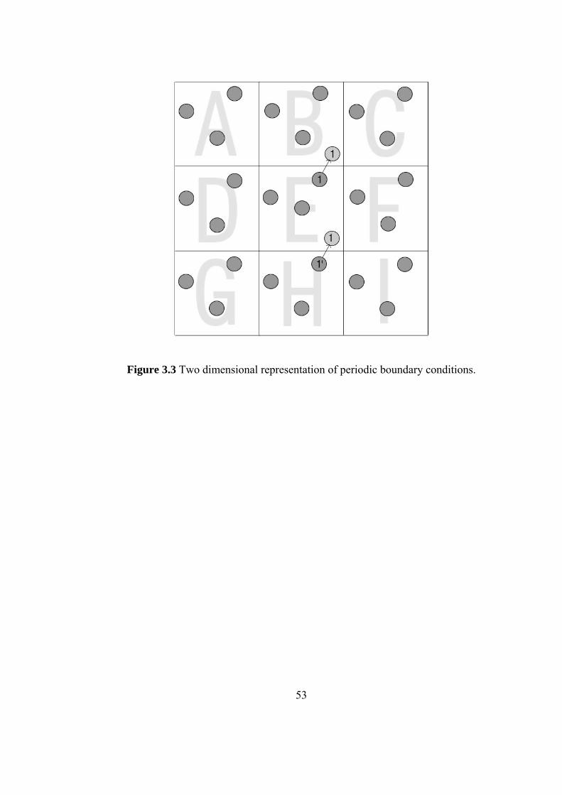
Figure 3.3 Two dimensional representation of periodic boundary conditions.

53

CHAPTER IV

EXPERIMENTAL PROCEDURE

This study consists of both theoretical and experimental parts. Simulation studies

were also carried out with an interconnecting role between the theoretical and

experimental tasks. Two systems were selected in order to investigate GFA. Zn-

Mg system being one of the frontiers of metal-metal binary glasses was

considered in order to investigate the Zn rich compositions. On the other hand Fe-

B system being potential bearing for the production of BMGs with alloying

additions was also selected to design new BMGs. In the theoretical branch

interatomic potentials and ordering energies were calculated Zn-Mg and Fe-B

binaries. For the systems considered the effect of the addition of a third element

to ordering energy was investigated. Subsequently in the light of these results,

MD simulations were carried out. In the experimental branch, centrifugal casting

experiments and the characterization of the specimens produced were carried out

for the Fe-B system. The theoretical findings form the basis of experimental work

carried out.

4.1 THEORETICAL STUDIES

In this part of the study ordering energies between magnesium and zinc atoms in

MgZn2 phase and ordering energy between iron and boron atoms in Fe3B phase

were calculated according to the nearly one electron theory in pseudopotential

approximation. Afterwards the variation of ordering energy between atoms in

alloys with ternary alloying element additions to MgZn2 and Fe3B compositions

were observed. All the calculations were done by utilizing computer programs

Meh1, Meh2, Meh3, Meh7, Meh 71, Meh72, written by Hamdullah Mekhrabov,

54

which are available in Metallurgical and Materials Engineering Department.

Ordering energies of the binary alloys were calculated by the Meh 7 program.

After this calculation, the ordering energy values between different pairs of atoms

in alloys with the addition of a third element were calculated for various alloying

elements. Elements considered in the study were, Ag, Au, Zn, Cd, Hg, Sc, Y, La,

Ti, Zr, Hf, V, Nb, Ta, Cr, Mo, W, Mn, Tc, Re, Fe, Ru, Os, Co, Rh, Ir, Ni, Pd, Pt,

Li, Na, K, Rb, Cs, Be, Mg, Ca, Ba, Zn, Cd, Hg, Al, Ga, In, Tl, Si, Ge, Sn, Pb, As,

Sb, Bi, Se, Te, Sr, B, C, P. For this purpose FORTRAN programs Meh1, Meh2,

and Meh3 were used. For an A-B binary system where X denotes the ternary

alloying element; Meh 1 program calculates the ordering energy between A and

B atoms (WAB), Meh2 program calculates the ordering energy between A and X

atoms (WAX), and Meh 3 program calculates the ordering energy between B and

X atoms (WBX).

From the outputs of the program runs, ordering energy can be read as a function

of interatomic distance. In order to determine an exact value the liquid

interatomic separation should be found and energy value should be extrapolated

for this separation. For Fe3B the distance between Fe and B atoms in the liquid

phase was found from literature as 2.21 Å [65]. This corresponds to 4.1763 in

atomic units. For the MgZn2 intermetallic, interatomic distance data for liquid

phase couldn’t be found in literature and therefore the distance is approximated to

the sum of atomic radii of Mg and Zn, which is 3.0075 Å [36]. This corresponds

to 5.6612 in atomic units. When the ordering energies were calculated between

one of the main elements and a ternary alloying addition element, interatomic

distance was taken as the distance between the main elements which introduces

another approximation.

Interatomic potentials for various atomic pairs were also calculated using the

nearly one electron theory in the pseudopotential approximation.

55

4.2 MD SIMULATION

Simulation studies were carried out in order to determine atomistic insight about

the motion of atoms during the rapid cooling from the liquid phase and the effect

of ternary alloying additions to alloys. In addition to these, macroscopic

thermodynamic parameters were intended to be explored. At this stage a main

FORTRAN program was written in order to form the basis of simulation studies.

FORTRAN language, which has been historically standard for scientific

purposes, was chosen due to its high computational efficiency. Small auxiliary

programs were written in MATHCAD because of the powerful visualization tools

available within the program.

The program written for MD purposes consists of a main program and several

subroutines. The code written is given in the Appendix A. The main program

starts by determining initial parameters and creating output files. Afterwards

subroutines INITIAL_VELOCITIIES and FCC were called for initialization. The

KIND_DETERMINATION subroutine was used in various places to identify the

types and masses of atoms. Initial interatomic forces were calculated by calling

the FORCE subroutine and flowing the main loop, which performs Velocity

Verlet type integration, starts within the main program for attaining the liquid

structure of the alloy. Periodic boundary conditions were employed for the new

coordinates. Force calculations were repeated at every time step. Temperature

scaling was done inside the integration loop. Atomic positions, velocities and

accelerations were recorded into relevant files. Also instantaneous temperature,

kinetic energy and potential energy were monitored during integration.

Translational order parameter and radial distribution functions (RDF) were also

calculated during integration by calling the subroutines ORDER and

RADIAL_DIST_FNC. After completing the first integration loop, the quenching

phase begins by again performing the integration loop but this time temperature

was constantly decreased by a specified rate to cool the alloy to room

56

temperature. The same kind of data which had been described previously was

collected during the integration.

4.2.1 Initialization

In order to start the simulation problem the following should be prescribed:

• number of particles

• initial temperature and therefore kinetic energy

• initial coordinates and velocities of particles

• and time step for integration

In this study the number of particles was chosen as 864. This choice arises from

optimization between execution time and resemblance to reality. As the number

of atoms increases the approximation of simulation to reality increases, however

at the same time execution time increases.

The objective of simulation was to perform rapid solidification from liquid state;

therefore initial temperature was determined as the liquidus temperature of the

system in concern. In order to determine the time step for integration, Eq. 4.1

deduced from conservation of total energy was used. In Eq. 4.1 m is the mass, r0

is the equilibrium spacing and ε0 is the equilibrium energy. In practice MD time

step was taken as ∆t/100 [66].

0

20

2εmrt =∆ (4.1)

In this study time step was taken as 1.5 femto seconds for all simulations, which

is much smaller than the values calculated using the above equation. Time step on

the order of femto seconds granted further stability to the system. Initialization of

positions and velocities will be discussed in the following sections.

57

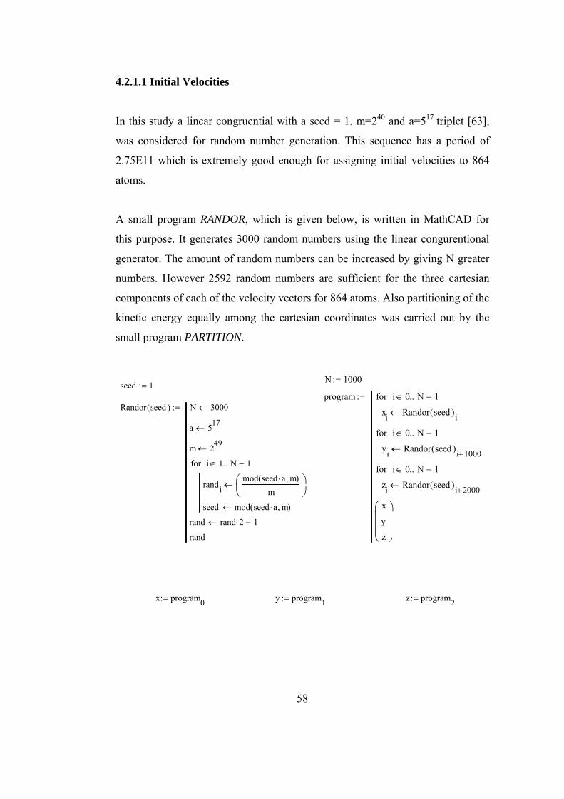
4.2.1.1 Initial Velocities

In this study a linear congruential with a seed = 1, m=240 and a=517 triplet [63],

was considered for random number generation. This sequence has a period of

2.75E11 which is extremely good enough for assigning initial velocities to 864

atoms.

A small program RANDOR, which is given below, is written in MathCAD for

this purpose. It generates 3000 random numbers using the linear congurentional

generator. The amount of random numbers can be increased by giving N greater

numbers. However 2592 random numbers are sufficient for the three cartesian

components of each of the velocity vectors for 864 atoms. Also partitioning of the

kinetic energy equally among the cartesian coordinates was carried out by the

small program PARTITION.

seed 1:=

Randor seed( ) N 3000←

a 517←

m 249←

randimod seed a⋅ m,( )

m⎛⎜⎝

⎞⎠

←

seed mod seed a⋅ m,( )←

i 1 N 1−..∈for

rand rand 2⋅ 1−←

rand

:=

N 1000:=

program

xi Randor seed( )i←

i 0 N 1−..∈for

yi Randor seed( )i 1000+←

i 0 N 1−..∈for

zi Randor seed( )i 2000+←

i 0 N 1−..∈for

x

y

z

⎛⎜⎜⎝

⎞

⎠

:=

x program0:= y program1:= z program2:=

58

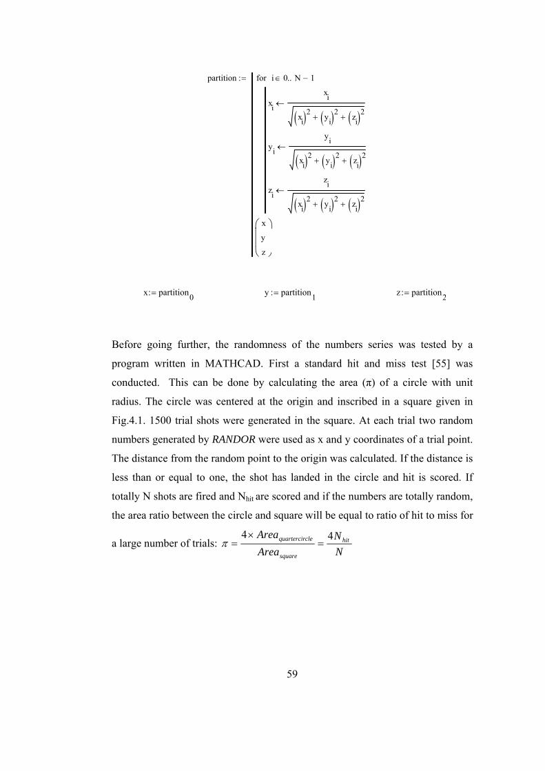
partition

xi

xi

xi( )2 yi( )2+ zi( )2+

←

yi

yi

xi( )2 yi( )2+ zi( )2+

←

zi

zi

xi( )2 yi( )2+ zi( )2+

←

i 0 N 1−..∈for

x

y

z

⎛⎜⎜⎝

⎞

⎠

:=

x partition0:= y partition1:= z partition2:=

Before going further, the randomness of the numbers series was tested by a

program written in MATHCAD. First a standard hit and miss test [55] was

conducted. This can be done by calculating the area (π) of a circle with unit

radius. The circle was centered at the origin and inscribed in a square given in

Fig.4.1. 1500 trial shots were generated in the square. At each trial two random

numbers generated by RANDOR were used as x and y coordinates of a trial point.

The distance from the random point to the origin was calculated. If the distance is

less than or equal to one, the shot has landed in the circle and hit is scored. If

totally N shots are fired and Nhit are scored and if the numbers are totally random,

the area ratio between the circle and square will be equal to ratio of hit to miss for

a large number of trials: NN

AreaArea hit

square

clequartercir 44=

×=π

59

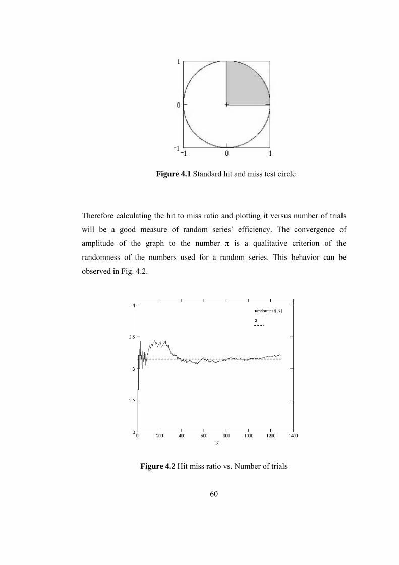
Figure 4.1 Standard hit and miss test circle

Therefore calculating the hit to miss ratio and plotting it versus number of trials

will be a good measure of random series’ efficiency. The convergence of

amplitude of the graph to the number π is a qualitative criterion of the

randomness of the numbers used for a random series. This behavior can be

observed in Fig. 4.2.

Figure 4.2 Hit miss ratio vs. Number of trials

60

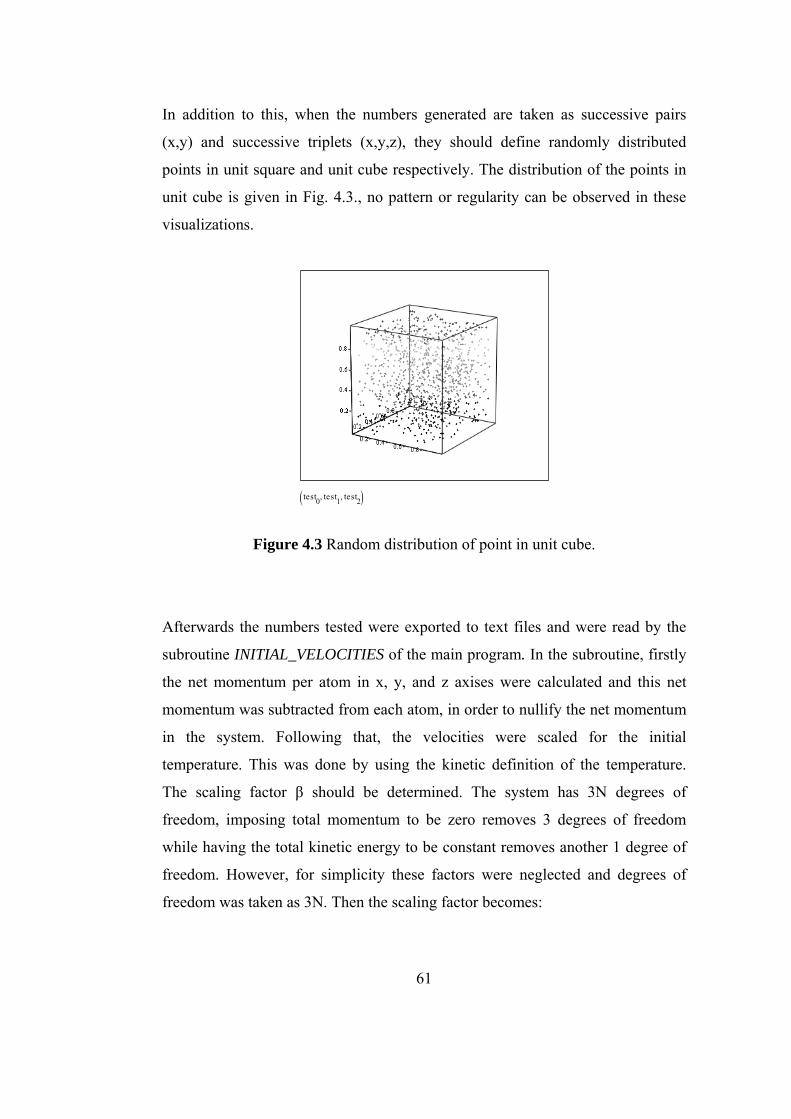
In addition to this, when the numbers generated are taken as successive pairs

(x,y) and successive triplets (x,y,z), they should define randomly distributed

points in unit square and unit cube respectively. The distribution of the points in

unit cube is given in Fig. 4.3., no pattern or regularity can be observed in these

visualizations.

test0 test1, test2,( )

Figure 4.3 Random distribution of point in unit cube.

Afterwards the numbers tested were exported to text files and were read by the

subroutine INITIAL_VELOCITIES of the main program. In the subroutine, firstly

the net momentum per atom in x, y, and z axises were calculated and this net

momentum was subtracted from each atom, in order to nullify the net momentum

in the system. Following that, the velocities were scaled for the initial

temperature. This was done by using the kinetic definition of the temperature.

The scaling factor β should be determined. The system has 3N degrees of

freedom, imposing total momentum to be zero removes 3 degrees of freedom

while having the total kinetic energy to be constant removes another 1 degree of

freedom. However, for simplicity these factors were neglected and degrees of

freedom was taken as 3N. Then the scaling factor becomes:

61

⎥⎥⎥

⎦

⎤

⎢⎢⎢

⎣

⎡=∑

iii

refb

vmTNk3

β (4.2)

For scaling, each velocity component was multiplied with β and the initial

velocity matrix was attained.

4.2.1.2 Initial Positions

Before giving the start up to the simulation, atoms were located to face centered

cubic lattice (fcc) by the subroutine FCC. This task was done by forming a loop

for generating periodic atom positions using the origin (0,0,0) and equivalent

positions (0,1/2,1/2; 1/2,0,1/2; 0,1/2,1/2) of fcc lattice The initial crystal lattice

can be seen in Fig. 4.4. The positions written into a text file were read by the

main program.

62

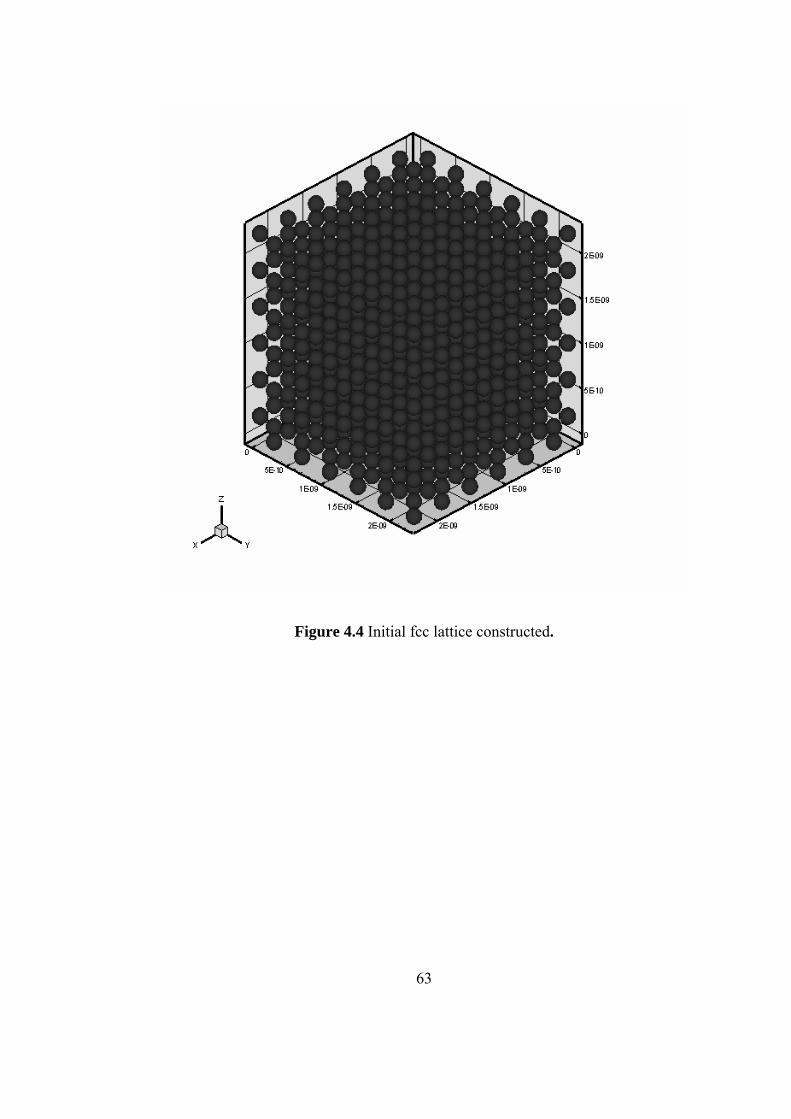
Figure 4.4 Initial fcc lattice constructed.

63

4.2.2 Force Calculation

Force calculation is a routine task which should be carried out in each step of

numerical integration. The subroutine FORCE at any time step calculates the

distance between all atoms, calls kind_determination subroutine in order to

identify the types of atoms, modifies the interatomic distances according to the

minimum image convention and finally calls the force functions for appropriate

atomic interaction to calculate the potential and force between these atoms.

4.3 CASTING EXPERIMENTS

4.3.1 Alloy Selection

The Fe-B system has been studied intensively for metallic glasses. Especially the

eutectic composition namely 83% Fe-17% B has been a focus. On the other hand

one of the constituents of the eutectic reaction Fe3B is a metastable intermetallic

phase which can also be a potential candidate to form metallic glasses with other

alloying additions. Fe3B being a facet forming intermetallic encounters crystal

growth problems and with alloying additives complex solidification behavior can

be induced. Under rapid solidification conditions this can yield a BGFA where

alloying elements which increase the ordering tendency are selected to modify

the composition. Binary to quinary alloys were produced during the course of

this study. Alloys which are beneficial to the discussion of GFA are given. The

compositions of these alloys are given in table 4.1.

64

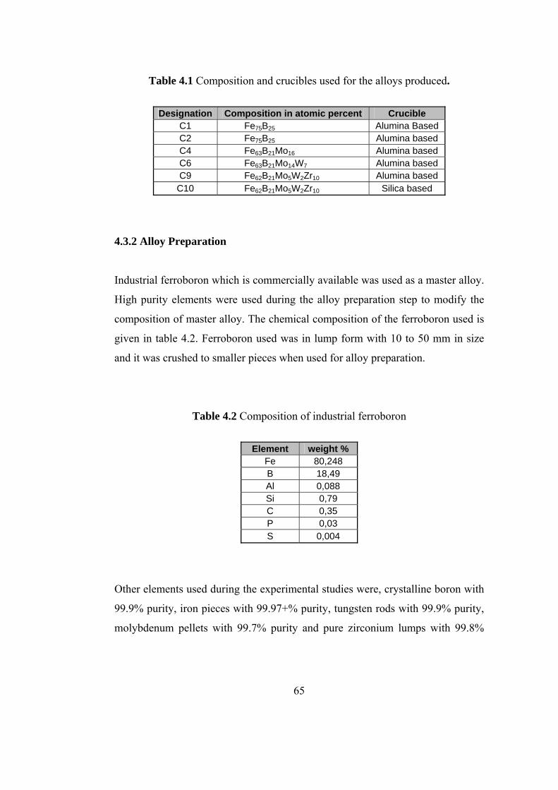
Table 4.1 Composition and crucibles used for the alloys produced.

Designation Composition in atomic percent Crucible

C1 Fe75B25 Alumina Based C2 Fe75B25 Alumina based C4 Fe63B21Mo16 Alumina based C6 Fe63B21Mo14W7 Alumina based C9 Fe62B21Mo5W2Zr10 Alumina based

C10 Fe62B21Mo5W2Zr10 Silica based

4.3.2 Alloy Preparation

Industrial ferroboron which is commercially available was used as a master alloy.

High purity elements were used during the alloy preparation step to modify the

composition of master alloy. The chemical composition of the ferroboron used is

given in table 4.2. Ferroboron used was in lump form with 10 to 50 mm in size

and it was crushed to smaller pieces when used for alloy preparation.

Table 4.2 Composition of industrial ferroboron

Element weight %

Fe 80,248 B 18,49 Al 0,088 Si 0,79 C 0,35 P 0,03 S 0,004

Other elements used during the experimental studies were, crystalline boron with

99.9% purity, iron pieces with 99.97+% purity, tungsten rods with 99.9% purity,

molybdenum pellets with 99.7% purity and pure zirconium lumps with 99.8%

65

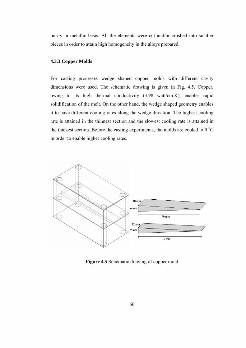
purity in metallic basis. All the elements were cut and/or crushed into smaller

pieces in order to attain high homogeneity in the alloys prepared.

4.3.3 Copper Molds

For casting processes wedge shaped copper molds with different cavity

dimensions were used. The schematic drawing is given in Fig. 4.5. Copper,

owing to its high thermal conductivity (3.98 watt/cm.K), enables rapid

solidification of the melt. On the other hand, the wedge shaped geometry enables

it to have different cooling rates along the wedge direction. The highest cooling

rate is attained in the thinnest section and the slowest cooling rate is attained in

the thickest section. Before the casting experiments, the molds are cooled to 0 0C

in order to enable higher cooling rates.

Figure 4.5 Schematic drawing of copper mold

66

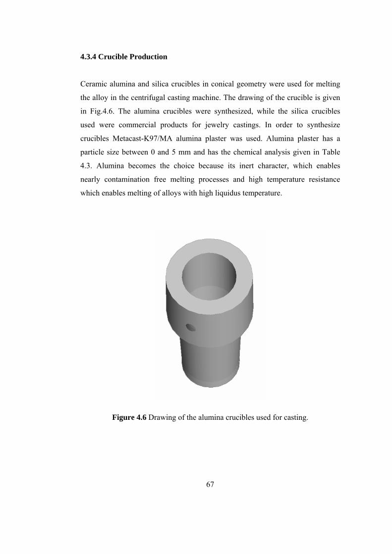
4.3.4 Crucible Production

Ceramic alumina and silica crucibles in conical geometry were used for melting

the alloy in the centrifugal casting machine. The drawing of the crucible is given

in Fig.4.6. The alumina crucibles were synthesized, while the silica crucibles

used were commercial products for jewelry castings. In order to synthesize

crucibles Metacast-K97/MA alumina plaster was used. Alumina plaster has a

particle size between 0 and 5 mm and has the chemical analysis given in Table

4.3. Alumina becomes the choice because its inert character, which enables

nearly contamination free melting processes and high temperature resistance

which enables melting of alloys with high liquidus temperature.

Figure 4.6 Drawing of the alumina crucibles used for casting.

67

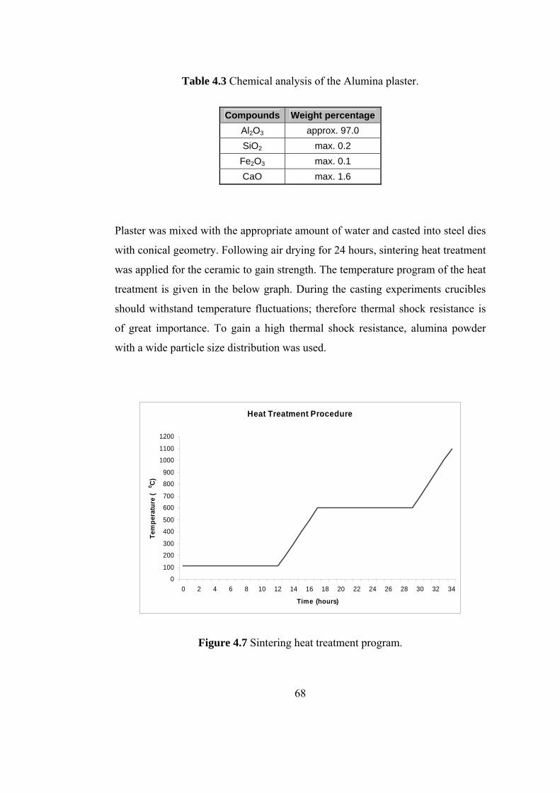
Table 4.3 Chemical analysis of the Alumina plaster.

Compounds Weight percentage

Al2O3 approx. 97.0 SiO2 max. 0.2

Fe2O3 max. 0.1 CaO max. 1.6

Plaster was mixed with the appropriate amount of water and casted into steel dies

with conical geometry. Following air drying for 24 hours, sintering heat treatment

was applied for the ceramic to gain strength. The temperature program of the heat

treatment is given in the below graph. During the casting experiments crucibles

should withstand temperature fluctuations; therefore thermal shock resistance is

of great importance. To gain a high thermal shock resistance, alumina powder

with a wide particle size distribution was used.

Heat Treatment Procedure

0

100

200

300

400

500

600

700

800

900

1000

1100

1200

0 2 4 6 8 10 12 14 16 18 20 22 24 26 28 30 32 34

Time (hours)

Tem

pera

ture

(0 C)

Figure 4.7 Sintering heat treatment program.

68

4.3.5 Melting and Casting

Melting and centrifugal castings were carried out using the Multihertz neutromag

digital induction casting machine. Melting was done by induction heating of the

alloy constituents in crucibles. Atmosphere control was accomplished by first

applying a vacuum and afterwards flushing spectrometric argon gas into the

system. Temperatures up to 2000 0C can be reached. Temperature control was

attained by the pyrometer. However, pyrometer measurements are sensitive

above 800 0C.

After the melting of alloy constituents, the alumina crucible with the opening

directed to a wedge shaped copper mold, which are both fixed on the main arm of

the machine are rotated at high speed and with the aid of centrifugal force the

metallic melt is injected into the copper mold, where it solidifies rapidly.

4.3.6 Characterization of the Specimens

For characterization studies differential scanning calorimetry, X-ray diffraction

and scanning electron microscopy were employed.

4.3.6.1 Thermal Analysis

Setaram SETSYS TGA-(DTA/DSC) thermal analyzer with facilities for

simultaneous TGA and DTA/DSC measurements was used for thermal analysis

of the specimens. For all alloys, small specimens around 25 mg were heated

above the melting point of the alloy in an argon atmosphere in a crucible

simultaneously with a blank sample crucible. Scanning rate of 20 0C/min was

used. Heat flow and temperature signals were obtained via computer and software

integrated with the DSC system. By analyzing heat flow vs. temperature graph,

the glass transition temperature can be determined, if exists due to specific

69

endothermic relaxation shape. Crystallization temperature, other phase

transformations and the enthalpy changes accompanying these transformations

were calculated.

4.3.6.2 Microstructural Investigations

Firstly, metallographic specimen preparation was performed. From the wedge

shaped as cast pieces, sections with varying cooling rate were mechanically cut

and mounted into bakelite by mount press at 140 0C and 4000 psi. Grinding was

carried out by 200, 400, 600, 800, 1200 SiC emery papers respectively in rotating

discs. In order to attain scratch free surfaces polishing with diamond paste and

alumina was performed step by step. Etchants 2% nital and 5% nital were used

for finalizing preparation.

Optical observations were carried out with Nikon Optihot microscope. SEM

investigations were carried out with JSM-6400 Electron Microscope (JEOL),

equipped with NORAN System 6 X-ray Microanalysis System & Semafore

Digitizer. Both secondary electron images and energy dispersive analysis (EDS)

were taken with the SEM facilities.

4.3.6.3 X-Ray Diffraction

X-ray diffraction studies were carried out with a 100 kV Philips twin tube X-ray

diffractometer (PW/1050). Cobalt Kα (λ = 1.79026 Å) radiation was used as the

incident beam. Diffractogrammes with diffraction angles (2θ) between 200 to

1000 were obtained for all specimens. The experimental parameters used for all

investigations were fixed to 30 kV voltage 8 mA current, 400 cps, 10/minute

speed for vigorous comparisons. From the diffractogrammes, 2θ values of peaks

were identified and the phases present were explored accordingly, using the

computer software PCPDFWIN.

70

4.3.6.4 Hardness Measurements

For the binary, alloy hardness test through out the wedge direction was carried

out. EMCO Universal Hardness Testing machine was used. Measurements were

carried out with Vickers indenter under 30 kgs load.

71

CHAPTER V

RESULTS AND DISCUSSION

Results obtained in this study will be given and discussed in three sections. These

sections are theoretical calculations, simulation results and casting experiments.

5.1 THEORETICAL CALCULATIONS

5.1.1 Interatomic Interaction Potentials:

According to the equations 3.1 to 3.17 results, of the interatomic interaction

potentials for the Zn-Mg, Mg-Mg, Zn-Zn, Fe-B, Fe-Fe and B-B pairs of atoms,

interactions were calculated for different interatomic spacings by using computer

programs, Meh7, Meh71 and Meh72. The results of Zn-Mg and Fe-B were plot as

examples in Fig. 5.1. and Fig. 5.2. However, because an analytical form of the

potential was needed, DataFit software was used to fit the data into a tenth order

polynomial.

72

Mg-

Zn

-0,2

-0,10

0,1

0,2

0,3

0,4

0,5

0,6 4,

55

5,5

66,

57

7,5

88,

59

9,5

1010

,511

dist

ance

(a.u

)

Interatomic Potential (a.u)

r 0

-ε

Figu

re 5

.1 In

tera

tom

ic in

tera

ctio

n po

tent

ial b

etw

een

Mg-

Zn p

airs

of a

tom

s

(1 a

.u(e

nerg

y) =

2 R

y =

27.2

eV

; 1.a

.u(le

ngth

) = 0

.529

177

Å).

73

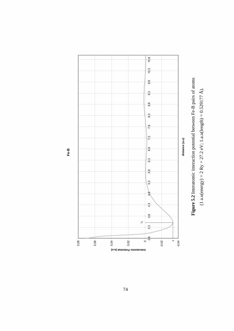
Fe-B

-0,0

4

-0,0

20

0,02

0,04

0,06

0,08

2,8

3,3

3,8

4,3

4,8

5,3

5,8

6,3

6,8

7,3

7,8

8,3

8,8

9,3

9,8

10,3

10,8

dist

ance

(a.u

)

Interatomic Potential (a.u)

ε

r 0

Figu

re 5

.2 In

tera

tom

ic in

tera

ctio

n po

tent

ial b

etw

een

Fe-B

pai

rs o

f ato

ms

(1 a

.u(e

nerg

y) =

2 R

y =

27.2

eV

; 1.a

.u(le

ngth

) = 0

.529

177

Å).

74

5.1.2 Ordering Energy Calculations

5.1.2.1 Ordering Energy Calculations for MgZn2

The results of ordering energy calculations are given for the MgZn2 intermetallic

composition. The ordering energy between Mg and Zn atoms is shown as WMg-Zn,

the ordering energy between the Mg and third element is shown as WMg-X and

ordering energy between Zn and third element is shown as WZn-X. The energy

values are given in atomic units. In Table 5.2 the calculations were carried out for

2 at. % third element replacement in place of iron, while in the Table 5.3.

calculations were done with replacing 2 at. % boron atoms with the third element

specified.

75

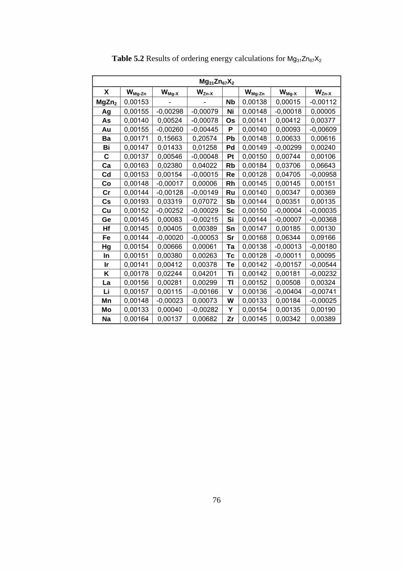
Table 5.2 Results of ordering energy calculations for Mg31Zn67X2

Mg31Zn67X2

X WMg-Zn WMg-X WZn-X WMg-Zn WMg-X WZn-X

MgZn2 0,00153 - - Nb 0,00138 0,00015 -0,00112 Ag 0,00155 -0,00298 -0,00079 Ni 0,00148 -0,00018 0,00005 As 0,00140 0,00524 -0,00078 Os 0,00141 0,00412 0,00377 Au 0,00155 -0,00260 -0,00445 P 0,00140 0,00093 -0,00609 Ba 0,00171 0,15663 0,20574 Pb 0,00148 0,00633 0,00616 Bi 0,00147 0,01433 0,01258 Pd 0,00149 -0,00299 0,00240 C 0,00137 0,00546 -0,00048 Pt 0,00150 0,00744 0,00106

Ca 0,00163 0,02380 0,04022 Rb 0,00184 0,03706 0,06643 Cd 0,00153 0,00154 -0,00015 Re 0,00128 0,04705 -0,00958 Co 0,00148 -0,00017 0,00006 Rh 0,00145 0,00145 0,00151 Cr 0,00144 -0,00128 -0,00149 Ru 0,00140 0,00347 0,00369 Cs 0,00193 0,03319 0,07072 Sb 0,00144 0,00351 0,00135 Cu 0,00152 -0,00252 -0,00029 Sc 0,00150 -0,00004 -0,00035 Ge 0,00145 0,00083 -0,00215 Si 0,00144 -0,00007 -0,00368 Hf 0,00145 0,00405 0,00389 Sn 0,00147 0,00185 0,00130 Fe 0,00144 -0,00020 -0,00053 Sr 0,00168 0,06344 0,09166 Hg 0,00154 0,00666 0,00061 Ta 0,00138 -0,00013 -0,00180 In 0,00151 0,00380 0,00263 Tc 0,00128 -0,00011 0,00095 Ir 0,00141 0,00412 0,00378 Te 0,00142 -0,00157 -0,00544 K 0,00178 0,02244 0,04201 Ti 0,00142 0,00181 -0,00232 La 0,00156 0,00281 0,00299 Tl 0,00152 0,00508 0,00324 Li 0,00157 0,00115 -0,00166 V 0,00136 -0,00404 -0,00741 Mn 0,00148 -0,00023 0,00073 W 0,00133 0,00184 -0,00025 Mo 0,00133 0,00040 -0,00282 Y 0,00154 0,00135 0,00190 Na 0,00164 0,00137 0,00682 Zr 0,00145 0,00342 0,00389

76

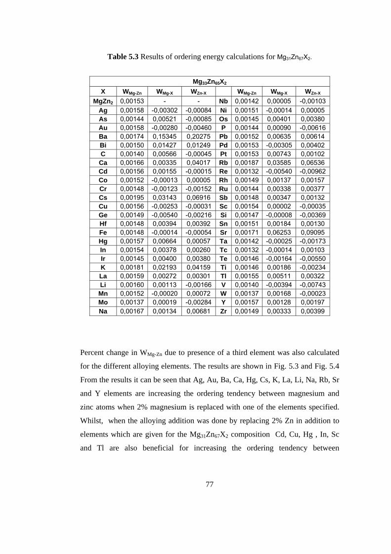
Table 5.3 Results of ordering energy calculations for Mg31Zn67X2.

Mg33Zn65X2

X WMg-Zn WMg-X WZn-X WMg-Zn WMg-X WZn-X

MgZn2 0,00153 - - Nb 0,00142 0,00005 -0,00103 Ag 0,00158 -0,00302 -0,00084 Ni 0,00151 -0,00014 0,00005 As 0,00144 0,00521 -0,00085 Os 0,00145 0,00401 0,00380 Au 0,00158 -0,00280 -0,00460 P 0,00144 0,00090 -0,00616 Ba 0,00174 0,15345 0,20275 Pb 0,00152 0,00635 0,00614 Bi 0,00150 0,01427 0,01249 Pd 0,00153 -0,00305 0,00402 C 0,00140 0,00566 -0,00045 Pt 0,00153 0,00743 0,00102

Ca 0,00166 0,00335 0,04017 Rb 0,00187 0,03585 0,06536 Cd 0,00156 0,00155 -0,00015 Re 0,00132 -0,00540 -0,00962 Co 0,00152 -0,00013 0,00005 Rh 0,00149 0,00137 0,00157 Cr 0,00148 -0,00123 -0,00152 Ru 0,00144 0,00338 0,00377 Cs 0,00195 0,03143 0,06916 Sb 0,00148 0,00347 0,00132 Cu 0,00156 -0,00253 -0,00031 Sc 0,00154 0,00002 -0,00035 Ge 0,00149 -0,00540 -0,00216 Si 0,00147 -0,00008 -0,00369 Hf 0,00148 0,00394 0,00392 Sn 0,00151 0,00184 0,00130 Fe 0,00148 -0,00014 -0,00054 Sr 0,00171 0,06253 0,09095 Hg 0,00157 0,00664 0,00057 Ta 0,00142 -0,00025 -0,00173 In 0,00154 0,00378 0,00260 Tc 0,00132 -0,00014 0,00103 Ir 0,00145 0,00400 0,00380 Te 0,00146 -0,00164 -0,00550 K 0,00181 0,02193 0,04159 Ti 0,00146 0,00186 -0,00234 La 0,00159 0,00272 0,00301 Tl 0,00155 0,00511 0,00322 Li 0,00160 0,00113 -0,00166 V 0,00140 -0,00394 -0,00743 Mn 0,00152 -0,00020 0,00072 W 0,00137 0,00168 -0,00023 Mo 0,00137 0,00019 -0,00284 Y 0,00157 0,00128 0,00197 Na 0,00167 0,00134 0,00681 Zr 0,00149 0,00333 0,00399

Percent change in WMg-Zn due to presence of a third element was also calculated

for the different alloying elements. The results are shown in Fig. 5.3 and Fig. 5.4

From the results it can be seen that Ag, Au, Ba, Ca, Hg, Cs, K, La, Li, Na, Rb, Sr

and Y elements are increasing the ordering tendency between magnesium and

zinc atoms when 2% magnesium is replaced with one of the elements specified.

Whilst, when the alloying addition was done by replacing 2% Zn in addition to

elements which are given for the Mg31Zn67X2 composition Cd, Cu, Hg , In, Sc

and Tl are also beneficial for increasing the ordering tendency between

77

magnesium and zinc atoms. The elements that increase the ordering energy are

represented on the periodic table in Fig. 5.5. Most of these elements are group 1A

and 2A elements. Apart from that 1A and 2A elements, are the ones with more

impact on the ordering energies. For example Cs causes nearly 26% increase.

Where the ordering energies between the main constituents and third elements are

concerned, Ba has an intensive increasing effect. These results correlate well with

the experimental founding in the literature [67,68]. GFA compositions according

to these results can be designed. However, two obstacles are present, one of them

is alkali and alkali-earth elements being quite reactive, such as even the humidity

in the air can trigger reactions involving them; so alloy preparation is compulsory

and severe differences between nominal and real compositions may arise. The

other obstacle is the melting temperature of the compositions for Mg-Zn system

is rather low, changing between 350-700 0C. Trg values are therefore low as a

consequence of this. For these reasons the Mg-Zn system was excluded from the

casting experiments part of the study. In the literature no bulk amorphous alloy

synthesized from Mg-Zn was reported. However, GFA ability of Mg-Zn alloys

were investigated and amorphous phase formation was reported by melt spinning

techniques in the literature [69, 70].

78

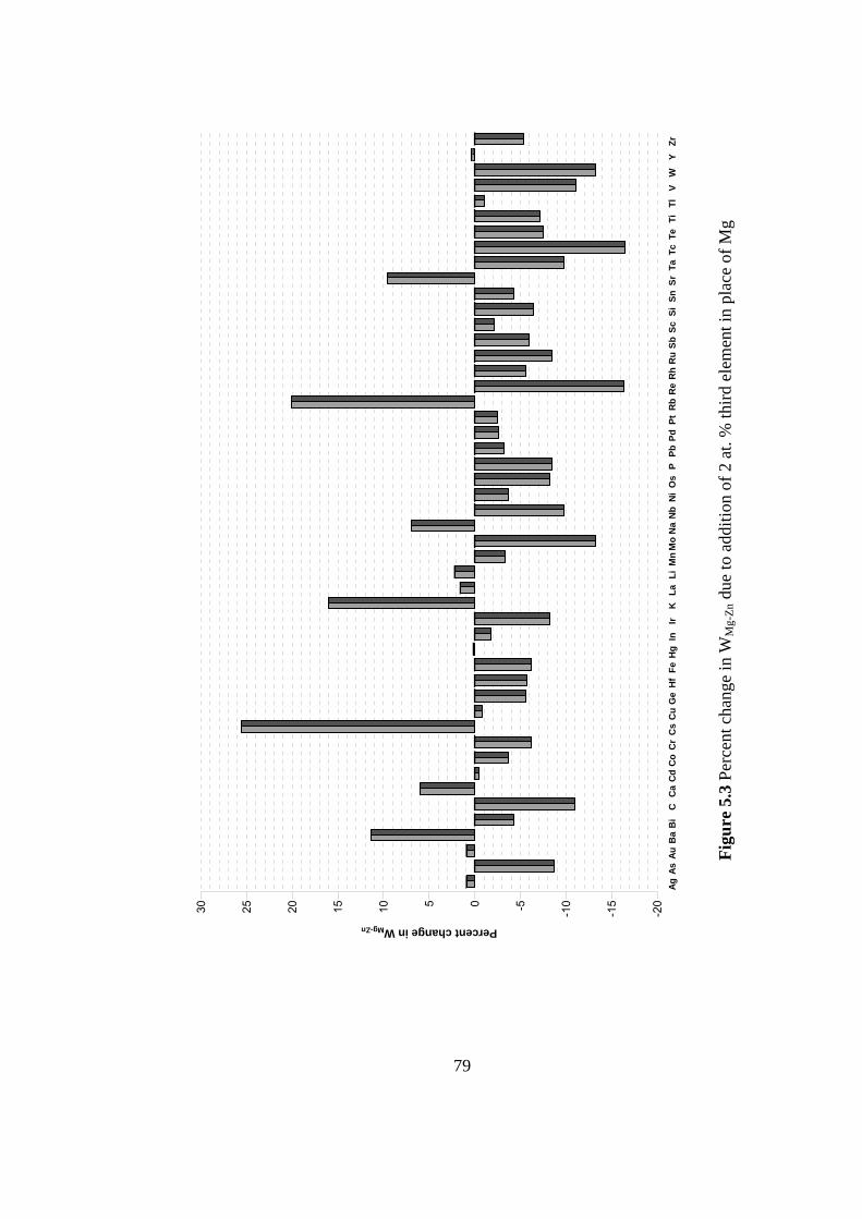
-20

-15

-10-5051015202530

Percent change in WMg-Zn

AgAs

AuB

aB

i C

Ca

Cd

Co

Cr

Cs

Cu

Ge

Hf

FeH

gIn

IrK

LaLi

Mn

Mo

Na

Nb

Ni

Os

PPb

PdPt

Rb

Re

Rh

Ru

SbSc

SiSn

SrTa

TcTe

TiTl

VW

YZr

Figu

re 5

.3 P

erce

nt c

hang

e in

WM

g-Zn

due

to a

dditi

on o

f 2 a

t. %

third

ele

men

t in

plac

e of

Mg

79

-15

-10-5051015202530

Percent change in WMg-Zn

AgAs

AuB

aB

i C

Ca

Cd

Co

Cr

Cs

Cu

Ge

Hf

FeH

gIn

IrK

LaLi

Mn

Mo

Na

Nb

Ni

Os

PPb

PdPt

Rb

Re

Rh

Ru

SbSc

SiSn

SrTa

TcTe

TiTl

VW

YZr

Figu

re 5

.4 P

erce

nt c

hang

e in

WM

g-Zn

due

to a

dditi

on o

f 2 a

t. %

third

ele

men

t in

plac

e of

Zn

80

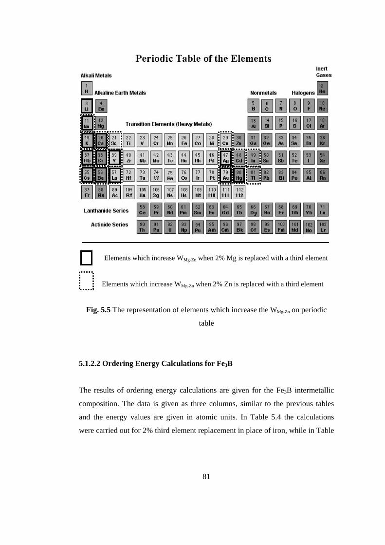
Elements which increase WMg-Zn when 2% Mg is replaced with a third element

Elements which increase WMg-Zn when 2% Zn is replaced with a third element

Fig. 5.5 The representation of elements which increase the WMg-Zn on periodic

table

5.1.2.2 Ordering Energy Calculations for Fe3B

The results of ordering energy calculations are given for the Fe3B intermetallic

composition. The data is given as three columns, similar to the previous tables

and the energy values are given in atomic units. In Table 5.4 the calculations

were carried out for 2% third element replacement in place of iron, while in Table

81

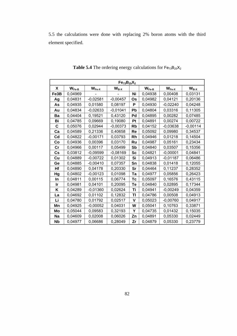
5.5 the calculations were done with replacing 2% boron atoms with the third

element specified.

Table 5.4 The ordering energy calculations for Fe73B25X2

Fe73B25X2

X WFe-B WFe-X WB-X WFe-B WFe-X WB-X

Fe3B 0,04969 - - Ni 0,04938 0,00408 0,03131 Ag 0,04831 -0,02581 -0,00457 Os 0,04982 0,04121 0,20136 As 0,04935 0,01580 0,08197 P 0,04930 -0,02240 0,04248 Au 0,04834 -0,02633 -0,01041 Pb 0,04804 0,03316 0,11305 Ba 0,04404 0,19521 0,43120 Pd 0,04895 0,00282 0,07485 Bi 0,04785 0,09669 0,19080 Pt 0,04891 0,00274 0,00722 C 0,05076 0,02944 -0,00373 Rb 0,04152 -0,03638 -0,00114 Ca 0,04589 0,21336 0,40658 Re 0,05092 0,09980 0,34537 Cd 0,04822 -0,00171 0,03793 Rh 0,04946 0,01218 0,14504 Co 0,04936 0,00396 0,03170 Ru 0,04987 0,05161 0,23434 Cr 0,04966 0,00117 0,05499 Sb 0,04840 0,03507 0,15356 Cs 0,03812 -0,09599 -0,08169 Sc 0,04821 -0,00001 0,04841 Cu 0,04889 -0,00722 0,01302 Si 0,04913 -0,01187 0,06486 Ge 0,04885 -0,00410 0,07357 Sn 0,04838 0,01418 0,12055 Hf 0,04890 0,04178 0,20330 Sr 0,04464 0,11237 0,28352 Hg 0,04802 -0,00123 0,01098 Ta 0,04977 0,05856 0,26423 In 0,04811 0,00115 0,06774 Tc 0,05097 0,16576 0,43115 Ir 0,04981 0,04101 0,20095 Te 0,04840 0,02895 0,17344 K 0,04289 -0,01360 0,02624 Ti 0,04941 -0,00249 0,04359 La 0,04692 0,01102 0,12832 Tl 0,04786 0,00508 0,04913 Li 0,04780 0,01792 0,02517 V 0,05023 -0,00760 0,04917

Mn 0,04925 -0,00052 0,04031 W 0,05041 0,10763 0,33871 Mo 0,05044 0,09583 0,32193 Y 0,04735 0,01432 0,15035 Na 0,04609 0,02008 0,06026 Zn 0,04891 0,05330 0,02449 Nb 0,04977 0,06686 0,28049 Zr 0,04879 0,05330 0,23779

82

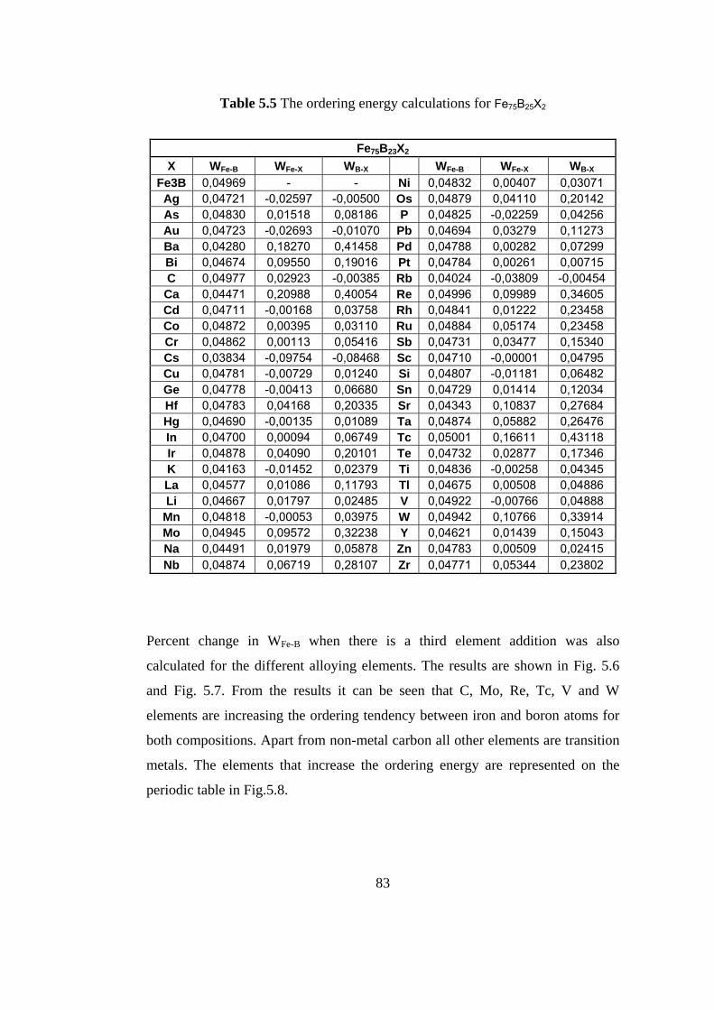
Table 5.5 The ordering energy calculations for Fe75B25X2

Fe75B23X2

X WFe-B WFe-X WB-X WFe-B WFe-X WB-X

Fe3B 0,04969 - - Ni 0,04832 0,00407 0,03071 Ag 0,04721 -0,02597 -0,00500 Os 0,04879 0,04110 0,20142 As 0,04830 0,01518 0,08186 P 0,04825 -0,02259 0,04256 Au 0,04723 -0,02693 -0,01070 Pb 0,04694 0,03279 0,11273 Ba 0,04280 0,18270 0,41458 Pd 0,04788 0,00282 0,07299 Bi 0,04674 0,09550 0,19016 Pt 0,04784 0,00261 0,00715 C 0,04977 0,02923 -0,00385 Rb 0,04024 -0,03809 -0,00454 Ca 0,04471 0,20988 0,40054 Re 0,04996 0,09989 0,34605 Cd 0,04711 -0,00168 0,03758 Rh 0,04841 0,01222 0,23458 Co 0,04872 0,00395 0,03110 Ru 0,04884 0,05174 0,23458 Cr 0,04862 0,00113 0,05416 Sb 0,04731 0,03477 0,15340 Cs 0,03834 -0,09754 -0,08468 Sc 0,04710 -0,00001 0,04795 Cu 0,04781 -0,00729 0,01240 Si 0,04807 -0,01181 0,06482 Ge 0,04778 -0,00413 0,06680 Sn 0,04729 0,01414 0,12034 Hf 0,04783 0,04168 0,20335 Sr 0,04343 0,10837 0,27684 Hg 0,04690 -0,00135 0,01089 Ta 0,04874 0,05882 0,26476 In 0,04700 0,00094 0,06749 Tc 0,05001 0,16611 0,43118 Ir 0,04878 0,04090 0,20101 Te 0,04732 0,02877 0,17346 K 0,04163 -0,01452 0,02379 Ti 0,04836 -0,00258 0,04345 La 0,04577 0,01086 0,11793 Tl 0,04675 0,00508 0,04886 Li 0,04667 0,01797 0,02485 V 0,04922 -0,00766 0,04888

Mn 0,04818 -0,00053 0,03975 W 0,04942 0,10766 0,33914 Mo 0,04945 0,09572 0,32238 Y 0,04621 0,01439 0,15043 Na 0,04491 0,01979 0,05878 Zn 0,04783 0,00509 0,02415 Nb 0,04874 0,06719 0,28107 Zr 0,04771 0,05344 0,23802

Percent change in WFe-B when there is a third element addition was also

calculated for the different alloying elements. The results are shown in Fig. 5.6

and Fig. 5.7. From the results it can be seen that C, Mo, Re, Tc, V and W

elements are increasing the ordering tendency between iron and boron atoms for

both compositions. Apart from non-metal carbon all other elements are transition

metals. The elements that increase the ordering energy are represented on the

periodic table in Fig.5.8.

83

-25

-20

-15

-10-505

Percent change in WFe-B

AgAs

AuB

aB

i C

Ca

Cd

Co

Cr

Cs

Cu

Ge

Hf

Hg

InIr

KLa

LiM

nM

oN

aN

bN

iO

sP

PbPd

PtR

bR

eR

hR

uSb

ScSi

SnSr

TaTc

TeTi

TlV

WY

ZnZr

Figu

re 5

.6 P

erce

nt c

hang

e in

WFe

-B d

ue to

add

ition

of 2

at.

% th

ird e

lem

ent i

n pl

ace

of F

e

84

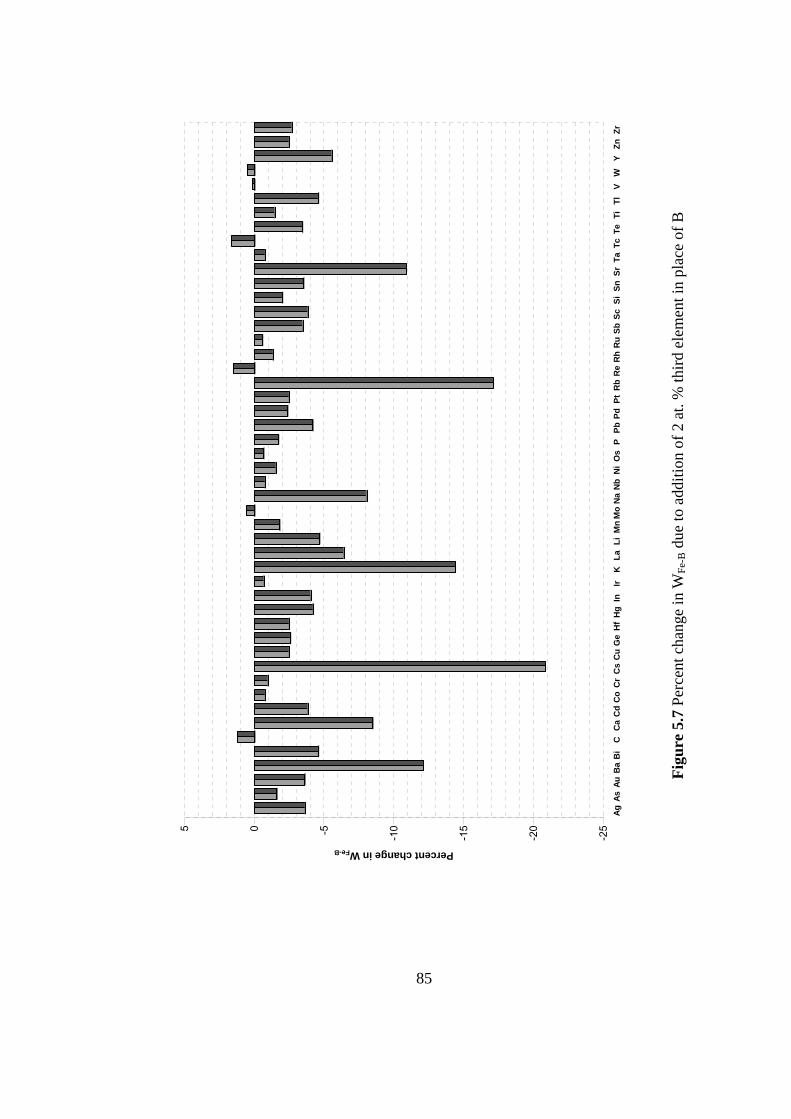
-25

-20

-15

-10-505

Percent change in WFe-B

AgAs

AuB

aB

i C

Ca

Cd

Co

Cr

Cs

Cu

Ge

Hf

Hg

InIr

KLa

LiM

nM

oN

aN

bN

iO

sP

PbPd

PtR

bR

eR

hR

uSb

ScSi

SnSr

TaTc

TeTi

TlV

WY

ZnZr

Figu

re 5

.7 P

erce

nt c

hang

e in

WFe

-B d

ue to

add

ition

of 2

at.

% th

ird e

lem

ent i

n pl

ace

of B

85

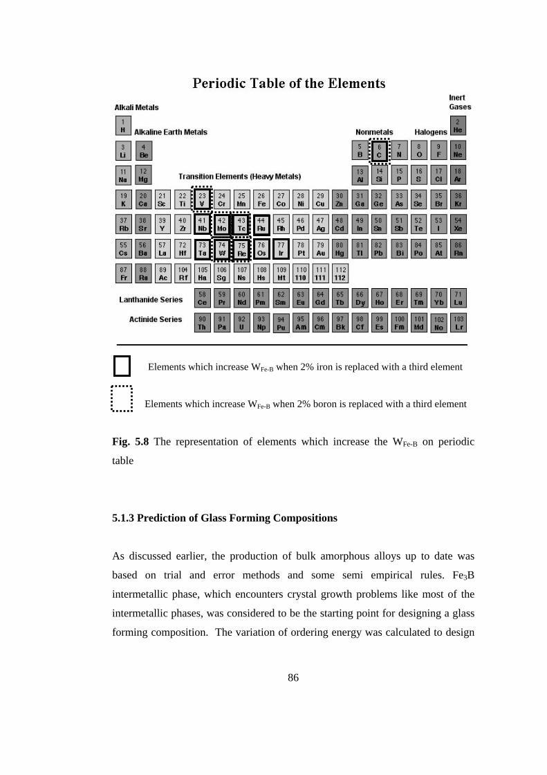
Elements which increase WFe-B when 2% iron is replaced with a third element

Elements which increase WFe-B when 2% boron is replaced with a third element

Fig. 5.8 The representation of elements which increase the WFe-B on periodic

table

5.1.3 Prediction of Glass Forming Compositions

As discussed earlier, the production of bulk amorphous alloys up to date was

based on trial and error methods and some semi empirical rules. Fe3B

intermetallic phase, which encounters crystal growth problems like most of the

intermetallic phases, was considered to be the starting point for designing a glass

forming composition. The variation of ordering energy was calculated to design

86

easily glass forming alloy compositions. The relationship between ordering

energy and glass forming compositions should be dealt with in accordance to

crystallization. Many alloy systems which are random solid solutions at elevated

temperatures become partially ordered when the temperature is lowered. The

amount of ordering energy between elements evaluates the degree of ordering.

High ordering energy means; high tendency of unlike atoms to become nearest

neighbors upon solidification because of the higher attractive potential for

heterocoordination. This preferred heterocoordination necessitates an excessive

amount of diffusion in the liquid phase when compared with a random solid

solution because preferred atomic bonding should be accomplished in order to

minimize the total energy. Therefore, elements which increase the ordering

energy, especially between the binary components and other possible atomic

matching combinations increase the needed undercooling for the crystal growth.

This condition favors the glass forming of the melt upon rapid solidification

because the suppression of the crystal growth becomes easier when the degree of

needed undercooling increases.

From the results of ordering energy calculations given above, W and Mo which

both increase WFe-B were chosen because of their availability. Although Tc and

Re are believed to be other good candidates, they were not used due to their high

cost and C was not selected as this study is centered on metallic alloying

additions. Zr on the other hand, while decreasing WFe-B when used as a third

element, it increases both WFe-Zr and WB-Zr considerably and therefore was chosen

as another alloying element during the studies.

Another parameter considered for the alloying element decision was the

equilibrium solidification route dictated by the phase diagrams. The alloying

elements which form complex intermetallics and undergo peritectic and eutectic

reactions involving these phases were selected. Also, the compositions of

87

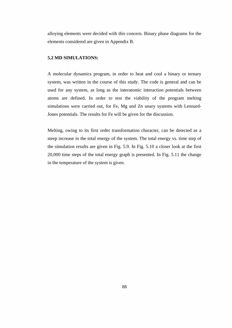
alloying elements were decided with this concern. Binary phase diagrams for the

elements considered are given in Appendix B.

5.2 MD SIMULATIONS:

A molecular dynamics program, in order to heat and cool a binary or ternary

system, was written in the course of this study. The code is general and can be

used for any system, as long as the interatomic interaction potentials between

atoms are defined. In order to test the viability of the program melting

simulations were carried out, for Fe, Mg and Zn unary systems with Lennard-

Jones potentials. The results for Fe will be given for the discussion.

Melting, owing to its first order transformation character, can be detected as a

steep increase in the total energy of the system. The total energy vs. time step of

the simulation results are given in Fig. 5.9. In Fig. 5.10 a closer look at the first

20,000 time steps of the total energy graph is presented. In Fig. 5.11 the change

in the temperature of the system is given.

88

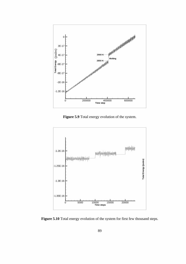
Time step

Tota

lEne

rgy

0 200000 400000 600000

-1.2E-16

-1E-16

-8E-17

-6E-17

-4E-17

-2E-17

0

Melting2850 K

2900 K(jo

ules

)

Figure 5.9 Total energy evolution of the system.

Time steps

Tota

lEne

rgy

(joul

es)

0 5000 10000 15000 20000

-1.35E-16

-1.3E-16

-1.25E-16

-1.2E-16

Figure 5.10 Total energy evolution of the system for first few thousand steps.

89

Time step

Tem

pera

ture

(K)

0 200000 400000 600000

1000

2000

3000

4000

Figure 5.11 Temperature evolution of the system.

From the Fig. 5.10 it can be seen that at each isotherm for 7000 time steps, total

energy fluctuates around a mean value especially at low temperatures, which is

an indication of the system evolving to the equilibrium. After the 7000th step of

each isotherm the total energy is perfectly constant. The reason for this behavior

is that after the 7000th step no velocity scaling is applied, however as the

temperature is monitored a small variance around the previously set temperature

is seen. This means the temperature is practically constant.

The estimation of melting point is an indicator for how the interatomic potential

correlates with the system. Therefore, the better the interatomic potential, smaller

will be the difference between the real and simulation melting temperature.

Experimentally, melting occurs at 1808 K for pure iron. However, for the MD

simulation melting occurs between 2850-2900 K. The reason for the melting

90

temperature being higher in simulation can be explained in terms of

configuration. The system under consideration in the simulation is homogeneous,

without any free surface due to periodic boundary conditions employed. In

addition because the initial configuration is a perfect fcc lattice, the system might

not generate the equilibrium number and distribution of defects, which are

usually the high energy sites available to trigger phase transformations. Although

there should be some overshooting, a difference in the order of 1000 K

necessitates the description of the system with Lennard-Jones potential is not the

most sophisticated way.

The coordinates of the system at several different time steps are also given in Fig.

5.12. It can be observed that the temperature increases, the initial lattice starts to

distort and after melting the complete long range order is lost.

91

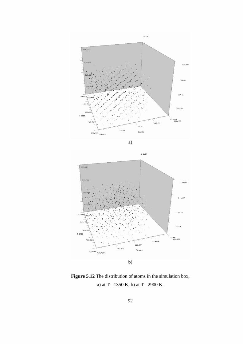
a)

b)

Figure 5.12 The distribution of atoms in the simulation box,

a) at T= 1350 K, b) at T= 2900 K.

92

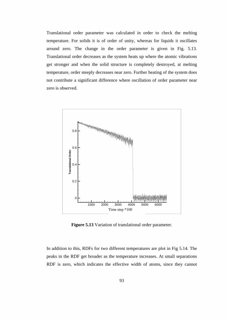
Translational order parameter was calculated in order to check the melting

temperature. For solids it is of order of unity, whereas for liquids it oscillates

around zero. The change in the order parameter is given in Fig. 5.13.

Translational order decreases as the system heats up where the atomic vibrations

get stronger and when the solid structure is completely destroyed, at melting

temperature, order steeply decreases near zero. Further heating of the system does

not contribute a significant difference where oscillation of order parameter near

zero is observed.

Tran

slat

iona

lOrd

er

1000 2000 3000 4000 5000 6000

0

0.2

0.4

0.6

0.8

Time step *100

Figure 5.13 Variation of translational order parameter.

In addition to this, RDFs for two different temperatures are plot in Fig 5.14. The

peaks in the RDF get broader as the temperature increases. At small separations

RDF is zero, which indicates the effective width of atoms, since they cannot

93

overlap. A number of obvious peaks are present for the RDF at 850 K. This

indicates a high degree of ordering present in crystalline state. However, for the

liquid structure, peaks are broader because of the thermal motion of atoms. At

very long range, RDF tends to a value of 1 because RDF describes the average

density at this range.

-1

0

1

2

3

4

0,4 2,2 4,0 5,8 7,7 9,5

r(A)

ρ (r)

T = 850 KT= 2900 K

Figure 5.14 Radial distribution functions at 850 K and 2900 K.

In order to perform simulations for binary systems, the interatomic potential

functions calculated, which are given in the previous section, were used to

describe pair wise interactions between atoms. However, the potential energy

drifts to large negative values shortly afterwards. This consequence is probably

due to polynomial interpolation of the function, which is not adequate for the data

at small separations. When the interpolation is carried out with exponential type

94

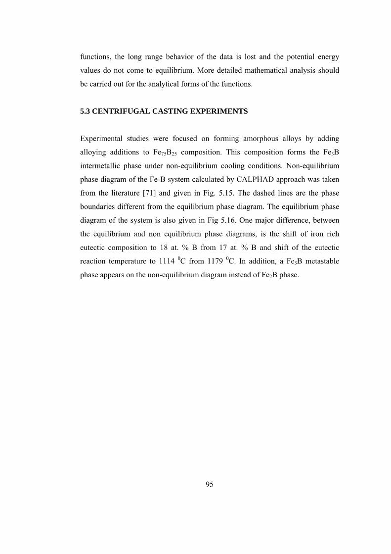
functions, the long range behavior of the data is lost and the potential energy

values do not come to equilibrium. More detailed mathematical analysis should

be carried out for the analytical forms of the functions.

5.3 CENTRIFUGAL CASTING EXPERIMENTS

Experimental studies were focused on forming amorphous alloys by adding

alloying additions to Fe75B25 composition. This composition forms the Fe3B

intermetallic phase under non-equilibrium cooling conditions. Non-equilibrium

phase diagram of the Fe-B system calculated by CALPHAD approach was taken

from the literature [71] and given in Fig. 5.15. The dashed lines are the phase

boundaries different from the equilibrium phase diagram. The equilibrium phase

diagram of the system is also given in Fig 5.16. One major difference, between

the equilibrium and non equilibrium phase diagrams, is the shift of iron rich

eutectic composition to 18 at. % B from 17 at. % B and shift of the eutectic

reaction temperature to 1114 0C from 1179 0C. In addition, a Fe3B metastable

phase appears on the non-equilibrium diagram instead of Fe2B phase.

95

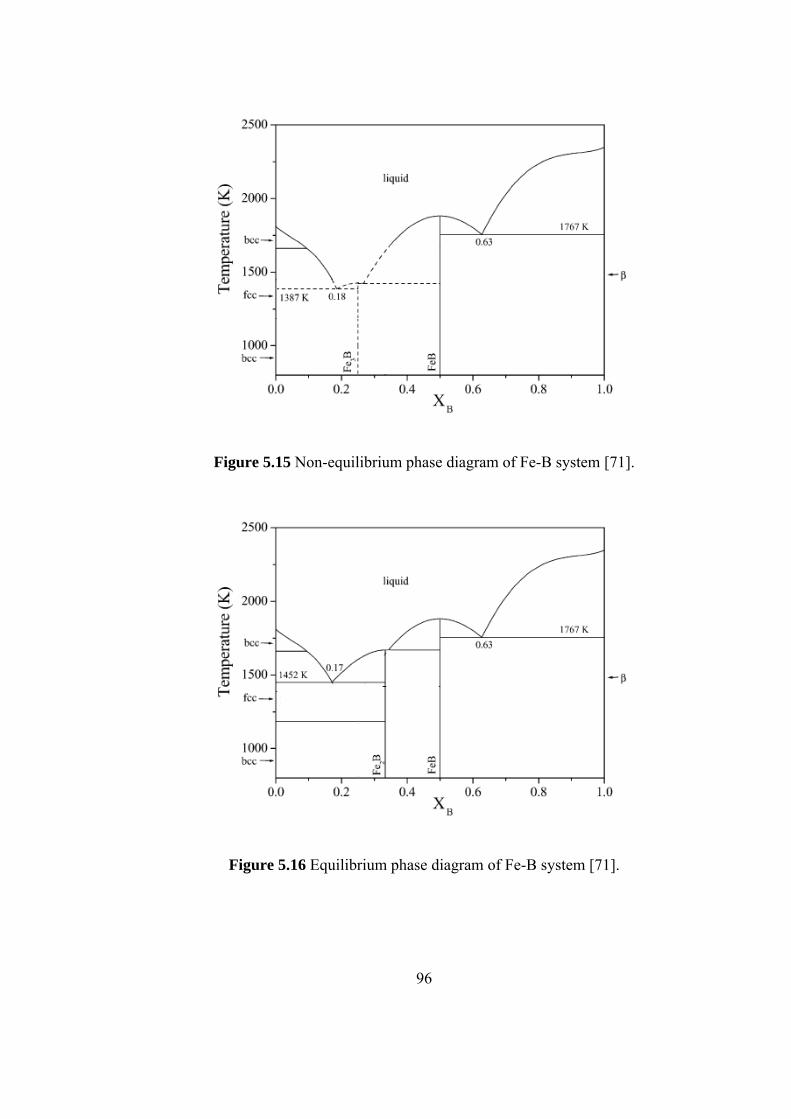
Figure 5.15 Non-equilibrium phase diagram of Fe-B system [71].

Figure 5.16 Equilibrium phase diagram of Fe-B system [71].

96

Fe3B is one of the constituents of the eutectic phase mixture (L → α + Fe3B). It is

generally believed that eutectic compositions are suitable for alloys with high

GFA due to the temperature gap being less between crystallization and glass

transition. However, intermetallic compositions should also be favorable for

amorphous alloy synthesis because of crystal growth problems encountered. For

Zr-Ni alloys, experimental findings state that eutectic Zr76Ni24 possess a higher

critical cooling rate than intermetallic Zr67Ni33 alloy [72]. Eutectics are generally

believed to be good glass forming compositions, however they can have poorer

GFA relative to intermetallic compositions, due to either the presence of

metastable phases competing with glass formation or low melt viscosity due to

lack of ordering in the melt. However, intermetallic compounds, owing to high

melt viscosity and slow nucleation and growth because of their complex

structure, can make them even better glass forming compositions. The

crystallization problems can be explained according to the solidification interface

morphology.

Two different growth morphologies are present for solid/liquid interfaces.

Faceted interfaces are planar angular surfaces which are atomically flat while

non-faceted interfaces are smooth and atomically rough. When the differences in

structure and bonding between solid and liquid phases are high, the transition

region between them becomes narrower in order to accommodate these

differences. Dimensionless entropy (α=∆S/R) is a good indicator for growth

morphology. When α value exceeds 2, solidification proceeds with facet forming

phase, like intermetallic phase growth. When α value is smaller than 2,

crystallization occurs on a non-faceted interface which is the case in pure metals.

An atomically flat interface will maximize the bonding between atoms in the

crystals and those in the interface. This kind of interface will close up the gaps in

the interface at the atomic scale and atomically flat surface will be favored. Such

an interface will expose few bonds to atoms arriving via diffusion through the

97

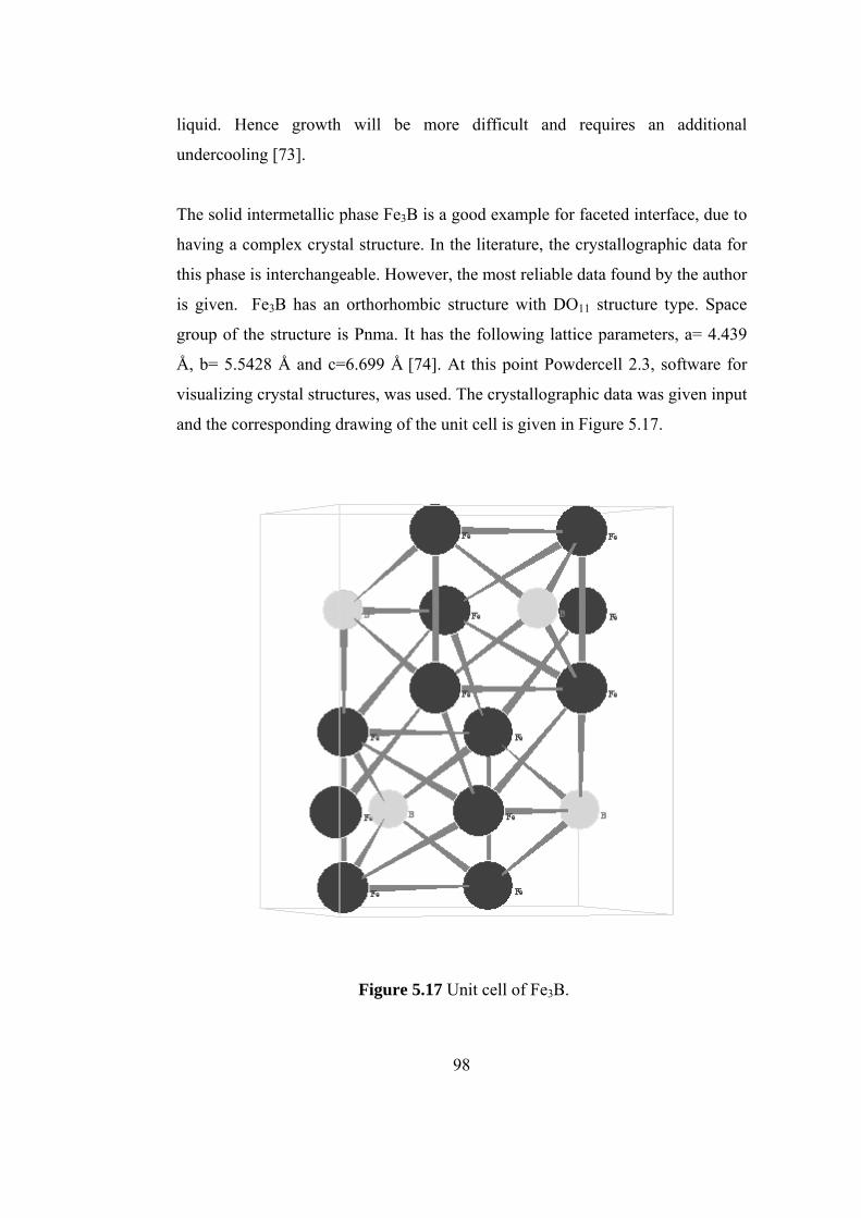
liquid. Hence growth will be more difficult and requires an additional

undercooling [73].

The solid intermetallic phase Fe3B is a good example for faceted interface, due to

having a complex crystal structure. In the literature, the crystallographic data for

this phase is interchangeable. However, the most reliable data found by the author

is given. Fe3B has an orthorhombic structure with DO11 structure type. Space

group of the structure is Pnma. It has the following lattice parameters, a= 4.439

Å, b= 5.5428 Å and c=6.699 Å [74]. At this point Powdercell 2.3, software for

visualizing crystal structures, was used. The crystallographic data was given input

and the corresponding drawing of the unit cell is given in Figure 5.17.

Figure 5.17 Unit cell of Fe3B.

98

When the other intermetallic compound MgZn2 is concerned, the same crystal

complexity is observed. MgZn2 has a hexagonal closed packed structure with C14

structure type. Space group of the structure is P63/mmc. It has the following

lattice parameter, a= 5.17 Å and c=8.50 Å [74]. By using the Powdercell software

the unit cell drawing of the MgZn2 intermetallic was found and given in Fig.

5.18.

Zn Zn

Zn Zn

Mg

Zn Zn

Mg

Zn

Zn Zn

Zn Zn

Zn

Mg

Zn Zn

Mg

Zn Zn

Zn Zn

Figure 5.18 Unit cell of MgZn2.

Another general remark to discuss before compiling the specific results for alloys

produced is the skewed eutectic zone phenomena. Although an intermetallic

binary composition was selected and modified with other alloying elements for

the casting experiments, that did not prevent the microstructure forming eutectic

phase mixtures in some specimens. Eutectic formation is an interacting

99

nucleation and cooperative growth of two solid phases. Under certain

undercoolings eutectic microstructure can be found in a composition range. The

coupled zone is defined as the range of alloy compositions and interface

temperatures in which the eutectic morphology lead the growth front. The extent

of the zone can be determined by comparing the growth velocities of eutectic and

primary phases [75]. There are two types of coupled zone for eutectic systems.

When the growth behaviors of two primary constituents are alike and regular

eutectic formation is observed, coupled zone originates itself symmetrically

around the eutectic point. On the other hand, a skewed coupled zone originates

when the eutectic growth is irregular, where one of the primary phases shows a

faceted solidification interface. That type of coupled zone is always skewed

towards the faceted phase, owing to growth difficulties even at high

undercoolings. Fe-B system having Fe3B as one of the eutectic constituents will

show this kind of coupled zone. According to Tan et al. [76] microstructural

evolution of a hypereutectic alloy as a function of cooling rate in alloy system

with skewed coupled zone is expected to be fully eutectic at the lowest cooling

rate, eutectic plus faceted primary phase when cooling rate is increased, fully

eutectic again when cooling rate is further increased, and finally eutectic plus

non-faceted primary face at the highest cooling rate. However when the Tg of the

alloy system is high enough, extremely high cooling rates result with fully

amorphous or partially amorphous plus faceted phase microstructures. When the

interface temperature of the eutectic is lower than Tg, eutectic growth will be

suppressed [73].

5.3.1. C1 Fe75B25 alloy

The first binary alloy synthesized was the binary Fe75B25 alloy. Ferroboron alloy

is used as the source of boron. Casting temperature of the alloy was 1200 0C.

Although centrifugal casting causes rapid solidification, no amorphous phase was

detected in the DSC trace, even at the thinnest section of the mold. This result

100

was however expected because it is known from the literature that crystallization

in binary alloys is suppressed only when very high cooling rates are employed.

According to previous studies in the lab, critical cooling rate for Fe75B25 alloy

was calculated as 7.3337E04 0C/sec [77]. From the DCS trace, which is given in

Fig. 5.19, it can be seen that the melting occurs at the onset of the endothermic

peak at 1187 0C. The enthalpy of melting is found to be 89.90 joules/gram. From

the phase diagram the melting temperature of metastable Fe3B phase is 1151 0C,

while the melting temperature of equilibrium Fe2B phase is 1179 0C. Two

possibilities are present for the heating curve of Fe75B25, either decomposition of

the metastable Fe3B to Fe2B and α-ferrite occurs with an exothermic peak in the

DSC signal or metastable melting of the Fe3B was observed. According to the

high temperature X-ray investigations reported in the literature, Fe3B is stable in

the temperature range 1157 0C and 1247 0C [78]. DSC traces reveal no

endothermic peak for the decomposition of Fe3B. However, to be on the safe side,

the DSC measurements were repeated after slowly cooling (20 0C/sec) the sample

in the DSC furnace. DSC scan of this experiment is given in Fig. 5.20. The only

significant difference between these two graphs are the endothermic peak at

around 953 0C that was present in the slowly cooled sample which is absent in the

original DSC curve. The consequence of this behavior will be discussed

following the evaluation of microstructural results.

101

-10

0

10

20

30

40

50

700 800 900 1000 1100 1200

Sample Temperature (0C)

Hea

t Flo

w (W

)

Melting

Figure 5.19 DSC trace of C1 with a scanning rate of 20 0C/sec.

Table 5.6 Thermal data about C1 alloy.

Melting Temperature Enthalpy of Melting 1187 0C 89.90 joules/gram

102

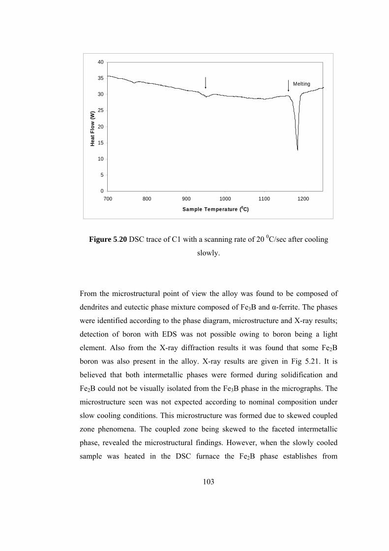
0

5

10

15

20

25

30

35

40

700 800 900 1000 1100 1200


Heat

Flo

w (W

)Melting

Figure 5.20 DSC trace of C1 with a scanning rate of 20 0C/sec after cooling

slowly.

From the microstructural point of view the alloy was found to be composed of

dendrites and eutectic phase mixture composed of Fe3B and α-ferrite. The phases

were identified according to the phase diagram, microstructure and X-ray results;

detection of boron with EDS was not possible owing to boron being a light

element. Also from the X-ray diffraction results it was found that some Fe2B

boron was also present in the alloy. X-ray results are given in Fig 5.21. It is

believed that both intermetallic phases were formed during solidification and

Fe2B could not be visually isolated from the Fe3B phase in the micrographs. The

microstructure seen was not expected according to nominal composition under

slow cooling conditions. This microstructure was formed due to skewed coupled

zone phenomena. The coupled zone being skewed to the faceted intermetallic

phase, revealed the microstructural findings. However, when the slowly cooled

sample was heated in the DSC furnace the Fe2B phase establishes from

103

decomposition of Fe3B and metastable melting of Fe2B was detected. Also, the

endothermic signal in the DSC trace can be explained by this phase

transformation.

The microstructure of the sample was analyzed through the wedge dimension in

order to observe the alterations due to different cooling rates. From the

micrographs it is seen that as the cooling rate increased eutectic phase separation

distance and the percentage of primary α-Fe phase were decreased. This

refinement arose due to decrease in time for the liquid phase to perform

composition partitioning on the eutectic reaction front when cooling rate was

increased. The secondary electron images of the alloy are given in Fig 5.22.

From the EDS analysis no elements other than Fe were detected. Although the

ferroboron alloy contains minute amounts of impurities, probably the alloy was

compositionally refined due to slag formation during casting and/or the amount

of impurities inside the alloy was insufficient for detection.

104

Figu

re 5

.21

X-r

ay d

iffra

ctio

n pa

ttern

of C

1 al

loy.

105

a) b)

c) d)

Figure 5.22. Secondary electron images of C1 alloy. a) and b) are the

photographs taken from the thinnest section while c) and d) are taken from the

thickest section of the casting.

In order to see mechanical consequences of the microstructural refinement,

results of hardness measurements are given for this alloy in Fig.5.23. It is seen

that hardness increases through the wedge direction when the cooling rate

increases. Also, it is seen that hardness and therefore strength of the specimen is

106

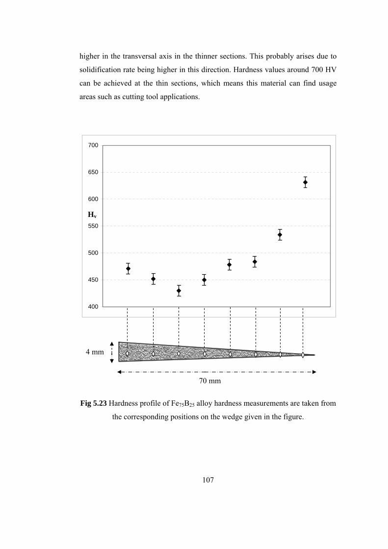
higher in the transversal axis in the thinner sections. This probably arises due to

solidification rate being higher in this direction. Hardness values around 700 HV

can be achieved at the thin sections, which means this material can find usage

areas such as cutting tool applications.

400

450

500

550

600

650

700

Hv

4 mm

70 mm

Fig 5.23 Hardness profile of Fe75B25 alloy hardness measurements are taken from

the corresponding positions on the wedge given in the figure.

107

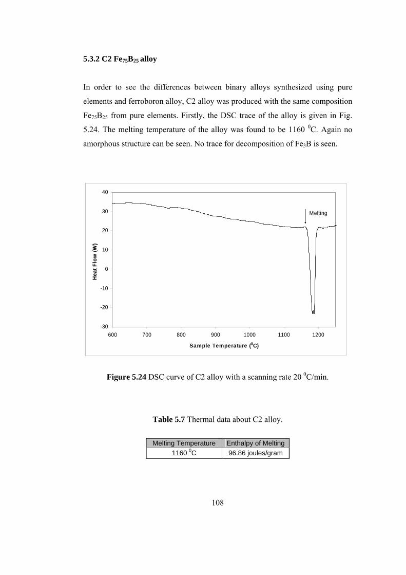
5.3.2 C2 Fe75B25 alloy

In order to see the differences between binary alloys synthesized using pure

elements and ferroboron alloy, C2 alloy was produced with the same composition

Fe75B25 from pure elements. Firstly, the DSC trace of the alloy is given in Fig.

5.24. The melting temperature of the alloy was found to be 1160 0C. Again no

amorphous structure can be seen. No trace for decomposition of Fe3B is seen.

-30

-20

-10

0

10

20

30

40

600 700 800 900 1000 1100 1200


Heat

Flo

w (W

)

Melting

Figure 5.24 DSC curve of C2 alloy with a scanning rate 20 0C/min.


Melting Temperature Enthalpy of Melting

1160 0C 96.86 joules/gram

108

When microstructural examinations were carried out for the C2 alloy, an

interesting phase selection occurred according to the cooling rate of the

examinations taken. At the thickest section of wedge, faceted primary Fe3B and

eutectic phase mixture consisting of Fe3B and α-Fe exist. When the examinations

were done on the mold wall, α-Fe dendrites become the primary phase together

with an irregular eutectic mixture. Also in some middle regions completely

eutectic microstructure can be seen. The SEM images of the alloy are given in

Fig. 5.25. In these images transition from 100% eutectic to primary α-Fe plus

eutectic can be seen, the upper right part of the picture c) is nearer to the mold

wall therefore cools more rapidly. X-ray results given in Fig. 5.26 show Fe2B,

Fe3B and α-Fe phases can be identified from the diffraction peaks.

109

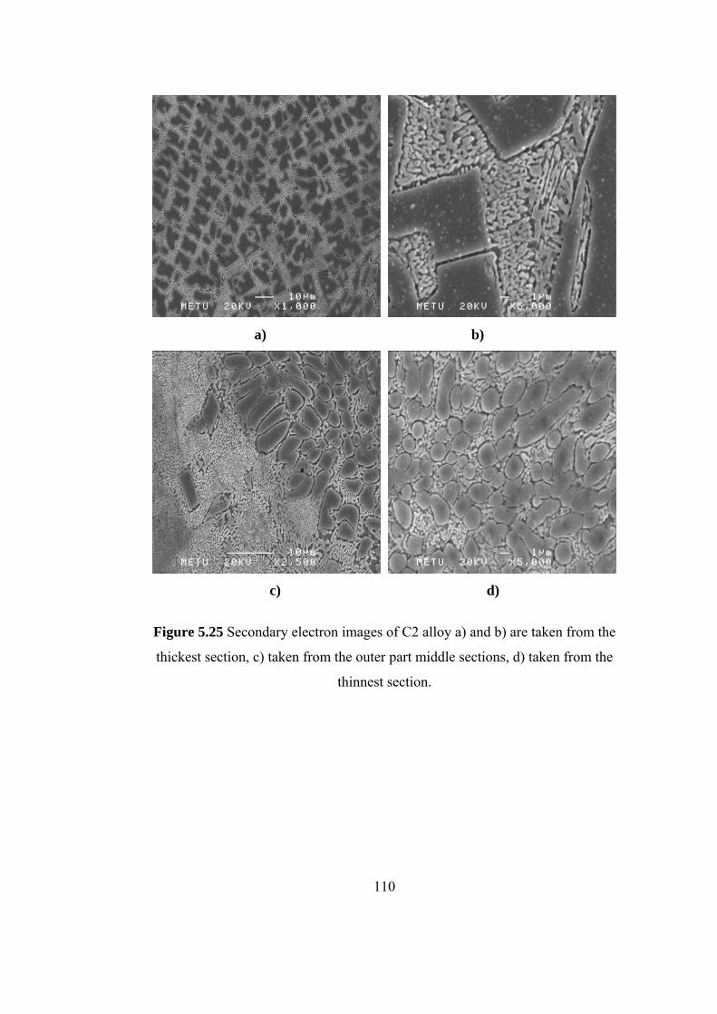
a) b)

c) d)

Figure 5.25 Secondary electron images of C2 alloy a) and b) are taken from the

thickest section, c) taken from the outer part middle sections, d) taken from the

thinnest section.

110

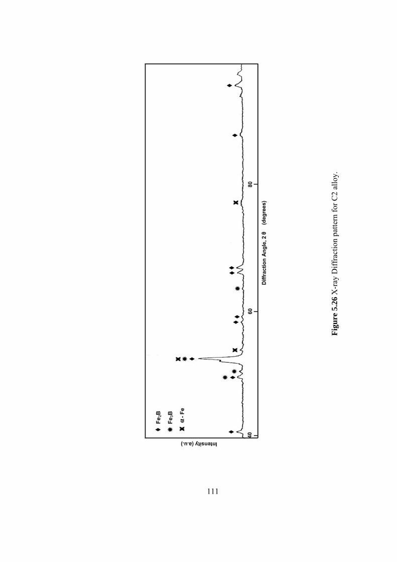
Figu

re 5

.26

X-r

ay D

iffra

ctio

n pa

ttern

for C

2 al

loy.

111

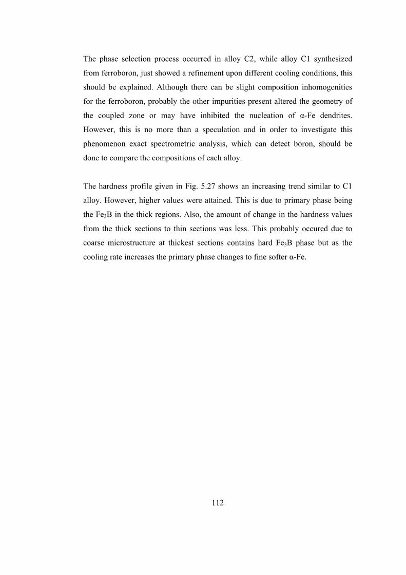
The phase selection process occurred in alloy C2, while alloy C1 synthesized

from ferroboron, just showed a refinement upon different cooling conditions, this

should be explained. Although there can be slight composition inhomogenities

for the ferroboron, probably the other impurities present altered the geometry of

the coupled zone or may have inhibited the nucleation of α-Fe dendrites.

However, this is no more than a speculation and in order to investigate this

phenomenon exact spectrometric analysis, which can detect boron, should be

done to compare the compositions of each alloy.

The hardness profile given in Fig. 5.27 shows an increasing trend similar to C1

alloy. However, higher values were attained. This is due to primary phase being

the Fe3B in the thick regions. Also, the amount of change in the hardness values

from the thick sections to thin sections was less. This probably occured due to

coarse microstructure at thickest sections contains hard Fe3B phase but as the

cooling rate increases the primary phase changes to fine softer α-Fe.

112

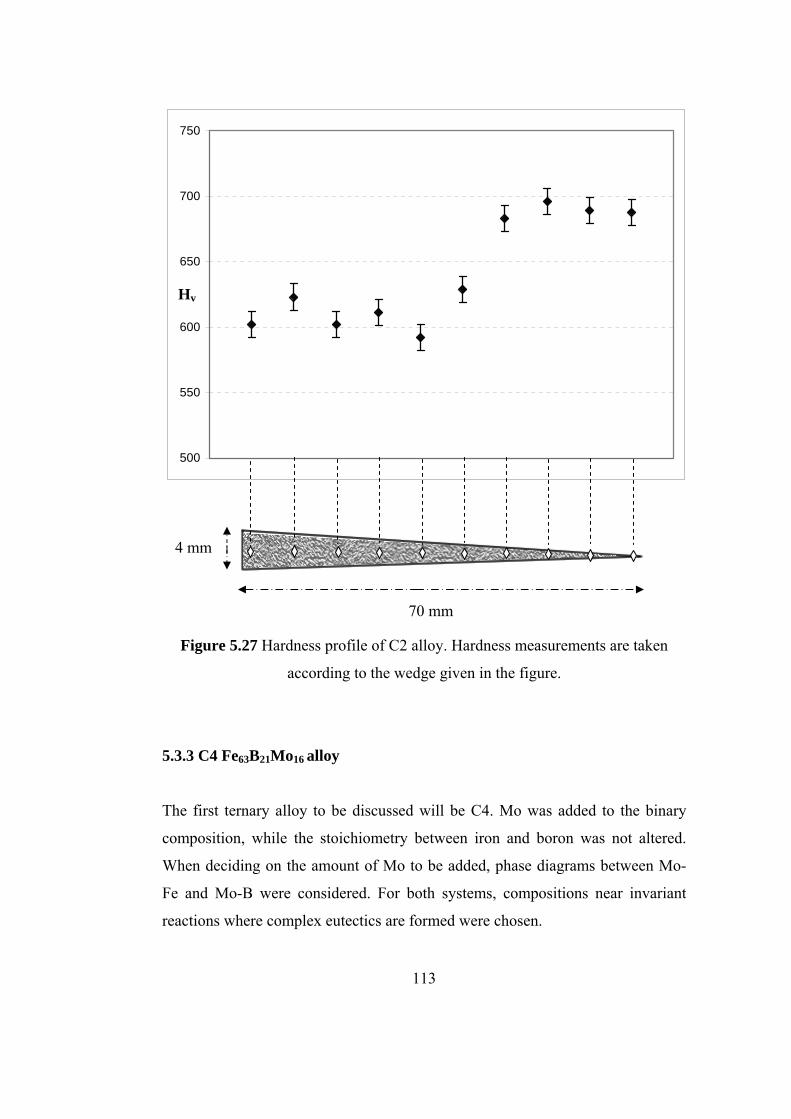
500

550

600

650

700

750

Hv

4 mm

70 mm

Figure 5.27 Hardness profile of C2 alloy. Hardness measurements are taken

according to the wedge given in the figure.

5.3.3 C4 Fe63B21Mo16 alloy

The first ternary alloy to be discussed will be C4. Mo was added to the binary

composition, while the stoichiometry between iron and boron was not altered.

When deciding on the amount of Mo to be added, phase diagrams between Mo-

Fe and Mo-B were considered. For both systems, compositions near invariant

reactions where complex eutectics are formed were chosen.

113

The casting temperature of the alloy was 1250 0C. The DSC trace taken for the

alloy is given in Fig. 5.28. From the DSC curve no glass transition and

crystallization behavior was observed. In other words, a fully crystalline alloy

was synthesized although it was rapidly cooled. The melting temperature, which

is the onset point of exothermic peak was found to be 1210 0C. The alloy formed

was very brittle and it was even hard to handle without fracture.

20

25

30

35

40

600 700 800 900 1000 1100 1200 1300


Heat

Flo

w (W

)

Melting


Table 5.8. Thermal data about C4 alloy.



114

In order to examine the microstructural evolution of the alloy, secondary electron

and back scatter images were taken. The SEM images of the alloy are given in

Fig. 5.29. EDS analyses of the phases are given in Table 5.9 for the phases

present. The phases on the micrograph are named as the X phase with the lightest

contrast, Y phase with the medium contrast and Z phase with the darkest contrast.

Z X Y

a) b)

Figure 5.29 SEM views of C4 alloy, a) secondary electron image, and b) back

scatter image

Table 5.9 EDS analysis results for the phases present in C4 alloy

X Y Z

weight percent

atomic percent

weight percent

atomic percent

weight percent

atomic percent

Fe 47,84 61,2 99,53 99,18 82,23 73,55 Mo 52,17 38,8 0 0,00 4,85 2,52 Al 0 0 0 0 12,93 23,93 S 0 0 0,47 0,82 0 0

115

When the X-ray results were examined, the phases that exist in the microstructure

were found to be Fe2B, Fe3B, FeB, Fe2Mo, Fe2MoB4 and Fe3Al. X-ray

diffractogramme of the alloy is given in Fig. 5.30. When this data was combined

with the EDS results, the Z phase was found to be Fe3Al phase. Aluminum should

have been reduced from the Al2O3 bearing crucible and altered the composition

of the alloy. Y phase is believed to be Fe2B and/or Fe3B and X phase is Fe2MoB4

and FeMo2

116

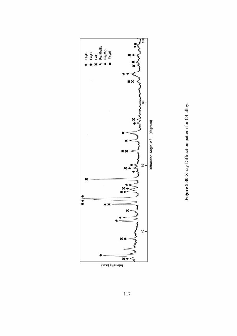
Figu

re 5

.30

X-r

ay D

iffra

ctio

n pa

ttern

for C

4 al

loy.

117

5.3.4 C6 Fe63B16Mo14W7 alloy

From the previous results, it is deduced that Mo addition didn’t increase the GFA

considerably. In order to increase GFA further, another alloying element W was

added to alloy according to the predictions based on ordering energy calculations.

The stoichiometry between the iron and boron was conserved to Fe75B25.

The casting temperature of this alloy was 1300 0C. However, DSC trace of this

alloy also ceases to show an amorphous phase. DCS curve of the alloy is given in

Fig. 5.31. In the DSC trace, around 880 0C, a Tg like Cp variation can be seen.

However, from the SEM observations no amorphous phase was detected for this

alloy. This behavior probably arises from some structural relaxation of rapidly

cooled phases. The melting temperature of the alloy was found to be 1280 0C.

Although the melting temperature of the alloy C6 is same as the C4 alloy, the

casting temperature has to be higher in our system due to the increased amount of

high melting point elements such as Mo and W. Melting temperature of Mo is

2620 0C, while the melting temperature of the W is 3400 0C. The increase in the

casting temperature is believed to be detrimental to glass forming of the alloy.

When the casting was carried out well above the melting temperature, cooling

rate decreases.

118

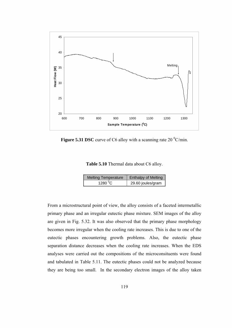
20

25

30

35

40

45

600 700 800 900 1000 1100 1200 1300


Heat

Flo

w (W

) Melting





From a microstructural point of view, the alloy consists of a faceted intermetallic

primary phase and an irregular eutectic phase mixture. SEM images of the alloy

are given in Fig. 5.32. It was also observed that the primary phase morphology

becomes more irregular when the cooling rate increases. This is due to one of the

eutectic phases encountering growth problems. Also, the eutectic phase

separation distance decreases when the cooling rate increases. When the EDS

analyses were carried out the compositions of the microconsituents were found

and tabulated in Table 5.11. The eutectic phases could not be analyzed because

they are being too small. In the secondary electron images of the alloy taken

119

from the thinnest region, even at 4000x magnification, the eutectic phase was not

resolved properly, however from element analyses it was confirmed that it has the

same composition with the eutectic in the thick regions of the sample. According

to this, it was comprehended that the eutectic morphology is distorted due to high

cooling rates.

a) b)

c) d)

Figure 5.32 Secondary electron images of C6 alloy a) and b) are taken from the

thickest region of the casting while c) and d) are taken from the thinnest region.

120

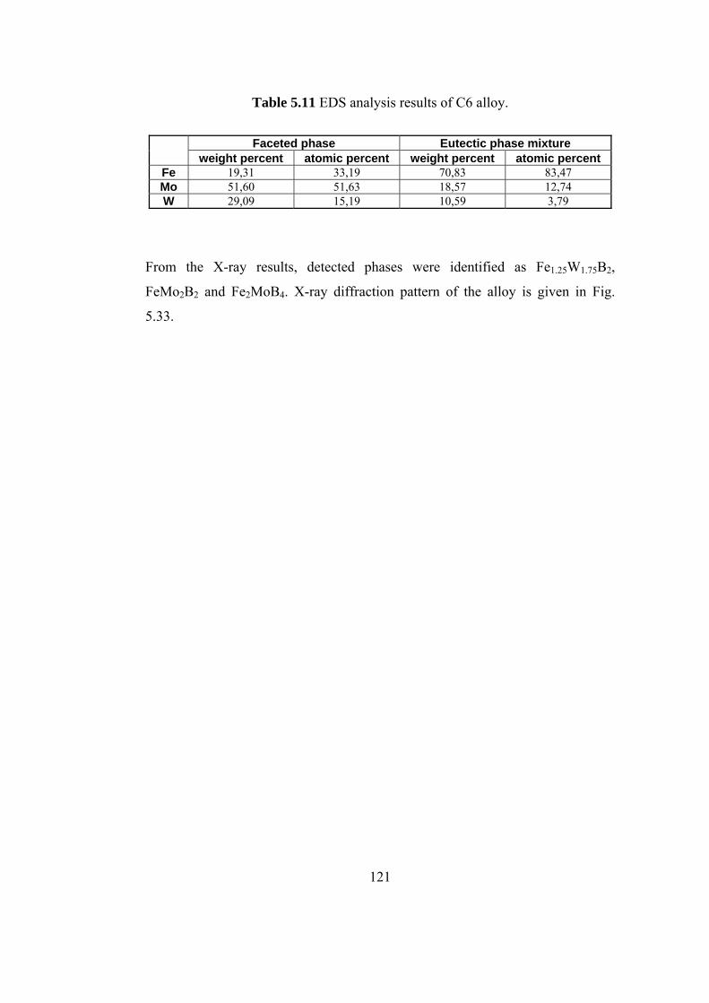
Table 5.11 EDS analysis results of C6 alloy.

Faceted phase Eutectic phase mixture

weight percent atomic percent weight percent atomic percent Fe 19,31 33,19 70,83 83,47 Mo 51,60 51,63 18,57 12,74 W 29,09 15,19 10,59 3,79

From the X-ray results, detected phases were identified as Fe1.25W1.75B2,

FeMo2B2 and Fe2MoB4. X-ray diffraction pattern of the alloy is given in Fig.

5.33.

121

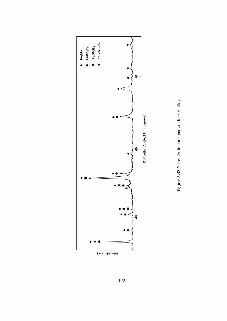
Figu

re 5

.33

X-r

ay D

iffra

ctio

n pa

ttern

for C

6 al

loy.

122

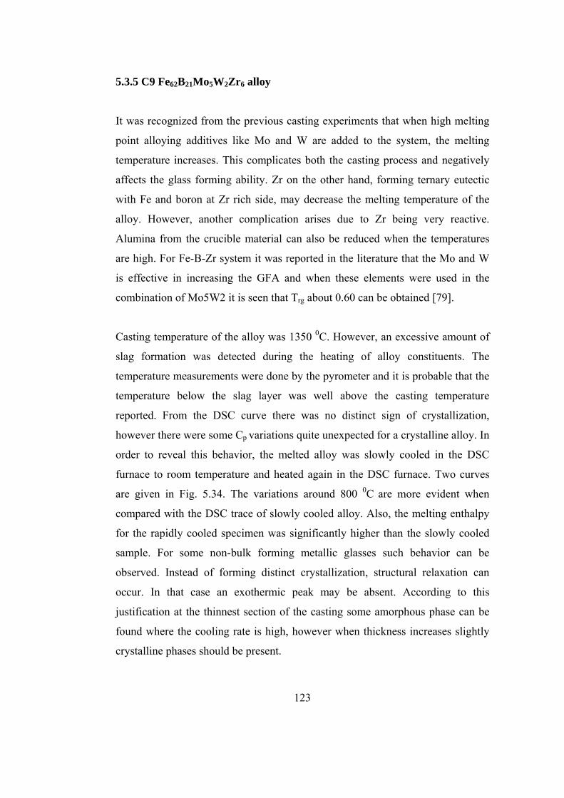
5.3.5 C9 Fe62B21Mo5W2Zr6 alloy

It was recognized from the previous casting experiments that when high melting

point alloying additives like Mo and W are added to the system, the melting

temperature increases. This complicates both the casting process and negatively

affects the glass forming ability. Zr on the other hand, forming ternary eutectic

with Fe and boron at Zr rich side, may decrease the melting temperature of the

alloy. However, another complication arises due to Zr being very reactive.

Alumina from the crucible material can also be reduced when the temperatures

are high. For Fe-B-Zr system it was reported in the literature that the Mo and W

is effective in increasing the GFA and when these elements were used in the

combination of Mo5W2 it is seen that Trg about 0.60 can be obtained [79].

Casting temperature of the alloy was 1350 0C. However, an excessive amount of

slag formation was detected during the heating of alloy constituents. The

temperature measurements were done by the pyrometer and it is probable that the

temperature below the slag layer was well above the casting temperature

reported. From the DSC curve there was no distinct sign of crystallization,

however there were some Cp variations quite unexpected for a crystalline alloy. In

order to reveal this behavior, the melted alloy was slowly cooled in the DSC

furnace to room temperature and heated again in the DSC furnace. Two curves

are given in Fig. 5.34. The variations around 800 0C are more evident when

compared with the DSC trace of slowly cooled alloy. Also, the melting enthalpy

for the rapidly cooled specimen was significantly higher than the slowly cooled

sample. For some non-bulk forming metallic glasses such behavior can be

observed. Instead of forming distinct crystallization, structural relaxation can

occur. In that case an exothermic peak may be absent. According to this

justification at the thinnest section of the casting some amorphous phase can be

found where the cooling rate is high, however when thickness increases slightly

crystalline phases should be present.

123

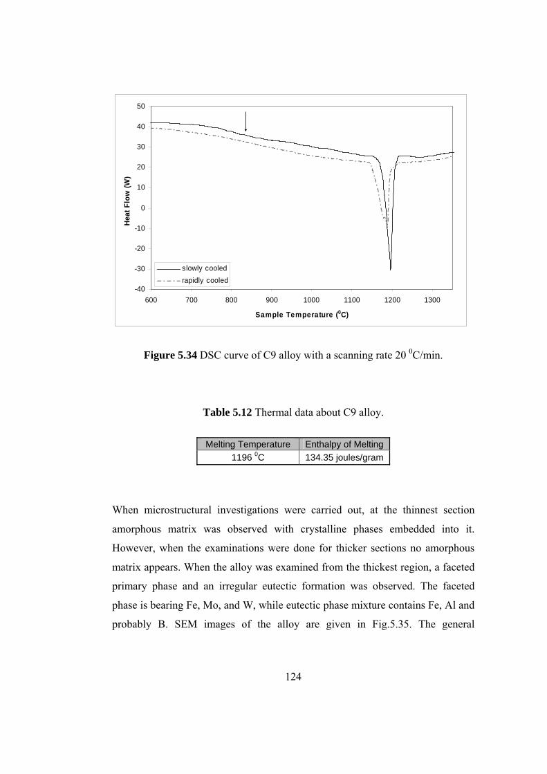
-40

-30

-20

-10

0

10

20

30

40

50

600 700 800 900 1000 1100 1200 1300


Heat

Flo

w (W

)

slowly cooledrapidly cooled





When microstructural investigations were carried out, at the thinnest section

amorphous matrix was observed with crystalline phases embedded into it.

However, when the examinations were done for thicker sections no amorphous

matrix appears. When the alloy was examined from the thickest region, a faceted

primary phase and an irregular eutectic formation was observed. The faceted

phase is bearing Fe, Mo, and W, while eutectic phase mixture contains Fe, Al and

probably B. SEM images of the alloy are given in Fig.5.35. The general

124

composition of the alloy according to EDS analysis was 11.41 % Al, 76.81 % Fe,

8.19% Mo and 3.59% W in atomic percents when boron is excluded.

a) b)

c) d)

Figure 5.35 SEM images of C9 alloy a) and b) are taken from thick section while

c) is back scattered image of the thinnest section d) is the secondary electron

image of the thinnest section.

125

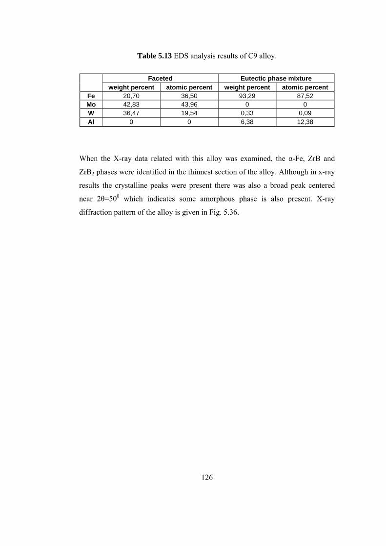
Table 5.13 EDS analysis results of C9 alloy.

Faceted Eutectic phase mixture

weight percent atomic percent weight percent atomic percent Fe 20,70 36,50 93,29 87,52 Mo 42,83 43,96 0 0 W 36,47 19,54 0,33 0,09 Al 0 0 6,38 12,38

When the X-ray data related with this alloy was examined, the α-Fe, ZrB and

ZrB2 phases were identified in the thinnest section of the alloy. Although in x-ray

results the crystalline peaks were present there was also a broad peak centered

near 2θ=500 which indicates some amorphous phase is also present. X-ray

diffraction pattern of the alloy is given in Fig. 5.36.

126

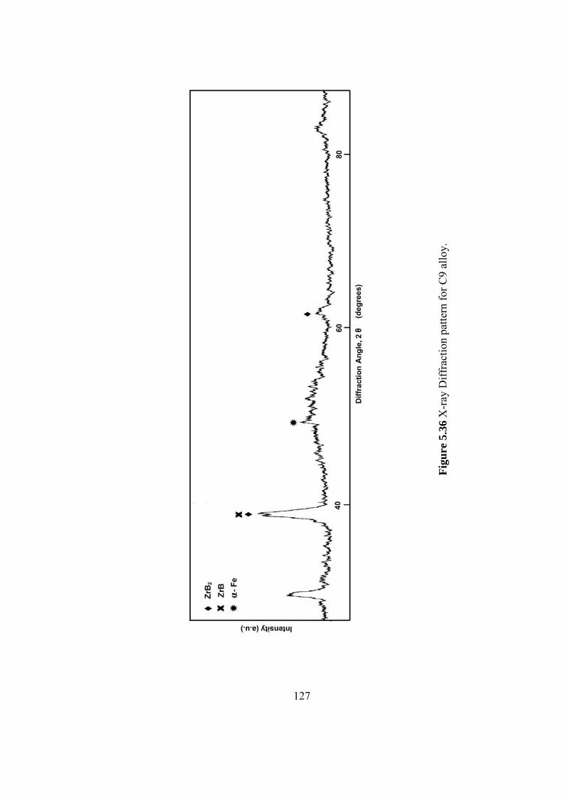
Figu

re 5

.36

X-r

ay D

iffra

ctio

n pa

ttern

for C

9 al

loy.

127

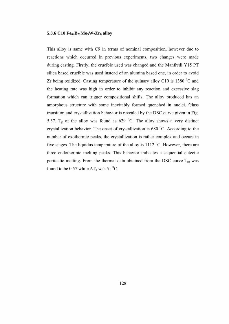
5.3.6 C10 Fe62B21Mo5W2Zr6 alloy

This alloy is same with C9 in terms of nominal composition, however due to

reactions which occurred in previous experiments, two changes were made

during casting. Firstly, the crucible used was changed and the Manfredi Y15 PT

silica based crucible was used instead of an alumina based one, in order to avoid

Zr being oxidized. Casting temperature of the quinary alloy C10 is 1380 0C and

the heating rate was high in order to inhibit any reaction and excessive slag

formation which can trigger compositional shifts. The alloy produced has an

amorphous structure with some inevitably formed quenched in nuclei. Glass

transition and crystallization behavior is revealed by the DSC curve given in Fig.

5.37. Tg of the alloy was found as 629 0C. The alloy shows a very distinct

crystallization behavior. The onset of crystallization is 680 0C. According to the

number of exothermic peaks, the crystallization is rather complex and occurs in

five stages. The liquidus temperature of the alloy is 1112 0C. However, there are

three endothermic melting peaks. This behavior indicates a sequential eutectic

peritectic melting. From the thermal data obtained from the DSC curve Trg was

found to be 0.57 while ∆Tx was 51 0C.

128

0

10

20

30

40

50

60

70

80

500 600 700 800 900 1000 1100 1200 1300 1400


Hea

t Flo

w (W

)

Crystallization

Peritectic Eutectic

Liquidus Tg

∆Tx



Tg Tx Te Tp TL ∆Ηx ∆Ηe ∆Ηp

629 0C 680 0C 1108 0C 1138 0C 1164 0C -65.87 (J/mol)

4.6544 (J/mol)

6.626 (J/mol)

Microstructural examination of the specimens showed that at the thin regions of

the alloy where cooling rate is high the amorphous matrix was formed. Small

crystals embedded in the matrix were α-Fe crystallites. At the thickest region of

the wedge, crystalline structure was seen. General composition of the alloy was

compared with the nominal composition to check the efficiency of casting. The

nominal and actual compositions were the same within the error limit of EDS

analyses. The SEM photographs taken are given in Fig. 5.38. The crystalline

phases present were a primary faceted phase and eutectic phase mixture.

129

a) b)

c) d)

Figure 5.38 Secondary electron images of C10 alloy a) and b) are taken from

thick section while c) and d) are taken from thin sections.

From the x-ray pattern given in Fig. 5.39, a broad peak was observed for thin

regions, which verifies the DSC results. Some crystalline peaks were also

identified. The presence of some crystalline phase was also seen from the SEM

observations, the size and percentage of the crystalline phases increase as the

cooling rate decreases.

130

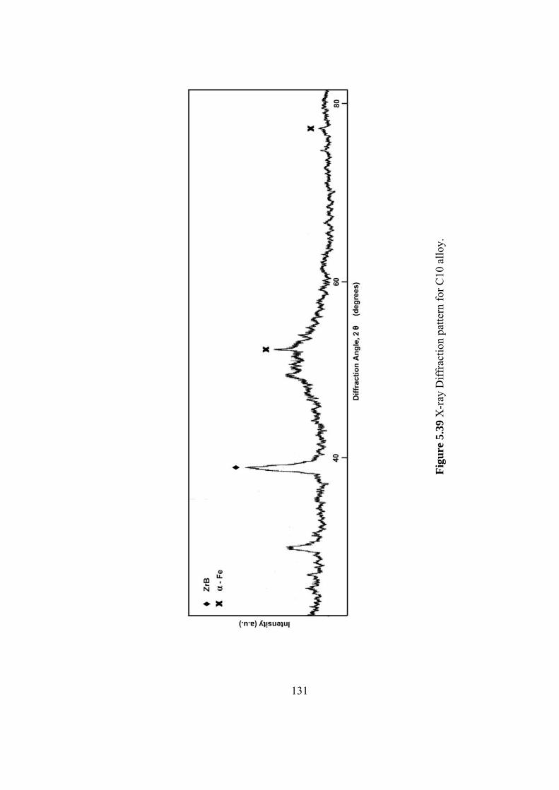
Figu

re 5

.39

X-r

ay D

iffra

ctio

n pa

ttern

for C

10 a

lloy.

131

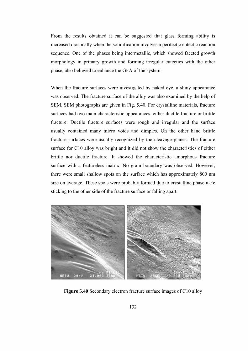
From the results obtained it can be suggested that glass forming ability is

increased drastically when the solidification involves a peritectic eutectic reaction

sequence. One of the phases being intermetallic, which showed faceted growth

morphology in primary growth and forming irregular eutectics with the other

phase, also believed to enhance the GFA of the system.

When the fracture surfaces were investigated by naked eye, a shiny appearance

was observed. The fracture surface of the alloy was also examined by the help of

SEM. SEM photographs are given in Fig. 5.40. For crystalline materials, fracture

surfaces had two main characteristic appearances, either ductile fracture or brittle

fracture. Ductile fracture surfaces were rough and irregular and the surface

usually contained many micro voids and dimples. On the other hand brittle

fracture surfaces were usually recognized by the cleavage planes. The fracture

surface for C10 alloy was bright and it did not show the characteristics of either

brittle nor ductile fracture. It showed the characteristic amorphous fracture

surface with a featureless matrix. No grain boundary was observed. However,

there were small shallow spots on the surface which has approximately 800 nm

size on average. These spots were probably formed due to crystalline phase α-Fe

sticking to the other side of the fracture surface or falling apart.

Figure 5.40 Secondary electron fracture surface images of C10 alloy

132

CHAPTER VI

CONCLUSIONS

Conclusions drawn from the study can be summarized as follows:

1. For the Zn-Mg system, the ordering energy between the atoms are

increased when Ag, Au, Ba, Ca, Hg, Cs, K, La, Li, Na, Rb, Sr and Y

elements are used as alloying additions in place of Mg. While Cd, Cu, Hg,

In, Sc, Tl, Ag, Au, Ba, Ca, Hg, Cs, K, La, Li, Na, Rb, Sr, Y are the

elements which increase the ordering energy when used as alloying

additions in place of Zn. For Zn-Mg system especially 1A and 2A metals

increase the GFA of the alloy and are potential alloying candidates for

designing new bulk glass forming systems.

2. For the Fe-B system, the ordering energy between the atoms are increased

when C, Mo, Re, Tc, V and W elements are used as alloying additions.

3. MD program developed can be used to investigate GFA and structure of

amorphous alloys. However, the interatomic potentials are crucial for the

results of simulation studies. Correct interpolation of interatomic potential

data is crucial for attaining analytical forms of potentials.

4. Centrifugal Casting process can be successfully used for producing bulk

amorphous alloys.

5. Silica based vessels are essential for melting when alloys containing

highly reactive elements such as Zr are being used.

133

6. Alloying addition of Zr to Fe-B system enhances the GFA significantly.

7. Fe62B21Mo5W2Zr6 alloy can be vitrified in bulk forms and the BGFA

related with this alloy is due to complex solidification behavior, with the

presence of sequential peritectic and eutectic reactions upon cooling. The

formation of amorphous phase is attained when the growth of faceted

intermetallic and irregular eutectic is suppressed due to high cooling rate.

134

REFERENCES

1. F.E. Luborsky in ‘‘Amorphous Metallic Alloys’’, Edited by F.E.

Luborsky, Butterworths Monographs in Materials, 1983.

2. N. Mattern, U. Kühn, H. Hermann, H. Ehrenberg, J. Neuefeind, J. Eckert,

Acta Materialia, 50 (2002) 305–314.

3. J. Kramer, Z. Phys., 106 (1937) 675.

4. A. Brenner, D. E.Couch and E. K. Williams, J. Res. Natn. Bur. Stand., 44

(1950) 109.

5. P. Duwez, Trans. Am. Soc. Metals, 60 (1967) 607.

6. I. S. Miroshienko and I. V. Salli, Ind. Lab. 25 (1959) 1463 in English;

Zav. Lab., 25 (1959) 1398.

7. R. (Jr.) Pond, and R. Maddin, TMS-AIME, 245 (1969) 2475

8. HS. Chen, D. Turnbull, Acta Metall 17 (1969) 1021-1031.

9. F. Jörg Löffer, Intermetallics, 11 (2003) 529-540.

10. HS. Chen, Acta Metall 22 (1974) 1505-1511.

11. B.X. Liu, W.S. Lai, Q. Zhang, Materials Science and Engineering, 29

(2000) 1-48.

12. H.W. Kui, A.L. Greer, D. Turnbull, Applied Physics Letters, 45 (1984)

615-616.

13. A. Inoue, T. Zhang, T. Masumoto, T. Mater Trans JIM 30(1989) 956-972.

14. A. Inoue, A. Karo, T. Zhang, S.G. Kim, T. Masumoto, T. Mater Trans

JIM 32(1991) 609-616.

15. T. Zhang, A. Inoue, T. Masumoto, Trans JIM 32(1991) 1005-1010.

16. A. Peker, W.L. Johnson, Applied Physics Letters 63 (1993) 2342-2344.

17. A. Inoue, A. Takeuchi, Materials Transaction, 43 (2002) 1982-1906.

18. J. Saida, M. Matsushita, A. Inoue, Intermetallics 10 (2002) 1089-1098.

19. A. Inoue, Acta Materialia 48 (2000) 279-306.

20. M. Telford, Materials Today, 36 (2004) 36-42.

135

21. S. J. Pang, T. Zhang, K. Asami, A. Inoue, Acta Materialia 50 (2002) 489-

497.

22. S. Linderoth, Proceedings of the 22nd Risø International Symposium on

Materials Science: Science of Metastable and Nanocrystalline Alloys,

Structure, Properties, and Modelling, Edited by A.R. Dinsen, M. Eldrup,

D. Juul Jensen, S. Linderoth, T.B. Pedersen, N.H: Pryds, A. Schroder

Pdersen, J. A. Werth, (2001) 69-88.

23. A. Inoue, Bulk Amorphous Alloys Preparation and Fundamental

Characteristics, Trans. Tech Publications, 1998.

24. A. Inoue, Acta Materialia 48 (2000) 279-306.

25. J. Daniel Sordelet, Elena Rozhkova, Matthew F. Besser, Matthew J.

Kramer. Journal of Non-Crystalline Solids 317 (2003) 137-143.

26. M. H. Lee, D.H. Bae, W.T. Kim, D.H. Kim, E. Rozhkova, P.B.

Wheelock, D.J. Sordelet, Journal of Non-Crystalline Solids 315 (2003)

89-96.

27. Z. P. Lu, H. Tan, Y. Li, S.C. Ng, Scripta Materialia 42 (2000) 667-673.

28. Z. P. Lu, H. Tan, Y Li, S.C. Ng, Journal of Non-Crystalline Solids 270

(2000) 103-114.

29. H.A Davies in “Amorphous Metallic Alloys” Edited by F.E. Luborsky,

Butterworths Monographs in Materials, 1983.

30. P. Duwez, Transactions of the ASM 60 (1967) 603-633.

31. Z.P. Lu, Y. Li, S.C. Ng, Journal of Non-Crystalline Solids 270 (2000)

103-114.

32. G. Shao, Intermetallics 11 (2003) 313-324.

33. D. Turnbull, Contemp. Physc., 10 (1969) 473.

34. W. H. Wang, C. Dong, C. H. Shek, Material Science and Engineering R,

44 (2004) 45-89.

35. O.N. Senkov, J.M. Scott, Scripta Materiala, 50 (2004) 449–452.

36. O.N. Senkov, D.B. Miracle, Materials Research Bulletin, 36 (2001) 2183-

2198.

136

37. Z.P. Lu, C.T. Liu, Acta Materialia 50 (2002) 3501-3512.

38. M. V. Akdeniz, Amdulla O. Mekhrabov, M. K. Pehlivanoğlu, Journal of

Alloys and Compounds, 386 (2005) 185-191.

39. J. L. Finney in “Amorphous Metallic Alloys” Edited by F. E. Lubrosky,

1984 42-57.

40. Bernal, J. D., Nature, 188,910 (1960)

41. K. Suzuki, in “Amorphous Metallic Alloys”, Edited. F. E. Luborsky,

1984, 74-100.

42. L. Wang, H. Cong, Y. Zhang, X. Bion, Physica B, 335 (2005) 140-146.

43. A. Inoue, A.R. Yavari, Mater. Trans. JIM 39 (1998) 318.

44. E. G. Noya, C. Rey and L. J. Gallego, Journal of Non-Crystalline Solids,

298 (2002) 60-66.

45. L. Wang, Y. Zhang, H. Yang and Y Chen, Physics Letters A, 317 (2003)

489-494.

46. L. Qi, H. F. Zhang, Z. Q. Hu and P. K. Liaw, Physics Letters A, 327

(2004) 506-511.

47. H.H. Kart, M. Uludoğan, T. Çağın and M. Tomak, Journal of Non-

Crystalline Solids, 342 (2004) 6-11.

48. V. Heine, M. L. Cohen, D. Weaine, Solid State Physics, vol. 24 Edited by

H. Ehrenreich et al., Academic Press, New York, 1970.

49. A. O. Mekhrabov and M. V. Akdeniz, Metallurgical and Materials

Transactions A, 34A (2003) 721.

50. A. O. Mekhrabov. and M. V. Akdeniz, Chemical Eng. Comm., 190 (2003)

898.

51. A. O. Mekhrabov and M. V. Akdeniz., Acta Materialia, 47-7 (1999) 2067.

52. A. O. Mekhrabov, M. V. Akdeniz and M. M. Arer, Acta Materialia, 45-3

(1997) 1077.

53. M. V. Akdeniz, A. O. Mekhrabov, Acta Materialia, 46- 4 (1998) 1185.

54. Robert E. Stephenson, Computer Simulation for Engineers, Harcourt

Brace Jovanovich 1971.

137

55. M.P. Allen, D.J. Tildesley, Computer Simulation of Liquids, Clarendon

Press, 1989.

56. D. Frenkel, B. Smit, Understanding molecular simulation: from

algorithms to applications, San Diego : Academic Press, 1996.

57. A. A. Selezenev, A. Yu. Aleynikov, N. S. Gantchuk, P. V. Yermakov, J.

K.Labanowski, A. A. Korkin, Computational Materials Science 28

(2003)107 –124.

58. F. Shimojo , T. J. Campbell, R. K. Kalia, A. Nakano, P. Vashishta, S.

Ogata, K. Tsuruta, Future Generation Computer Systems 17 (2000) 279–

291.

59. J. M. Haile, Molecular Dynamics Simulation Elementary Methods, A

Wiley-Interscience Publication, 1997.

60. J. A. McCammon, B. R. Gelin, M. Karplus, Nature (Lond.) 267 (1977)

585.

61. D. C. Raparot, The Art of Molecular Dynamics Simulation, Cambridge

University Press, 1995.

62. H. Gould, J. Tobochnik, An Introduction to Computer Simulation

Methods: Applications to Physical System. Jon Wiley and Sons, 2003.

63. I. M. Sobol, Y. L. Levitan, Computers and Mathematics with Applications

37 (1999) 33-40.

64. P. Gerald, Jr. Dwyer, K.B. Williams, Journal of Economic Dynamics &

Control 27 (2003) 645–650.

65. N. Cowlam, Journal of Non-Crystalline Solids, 205-207, (1996) 567.

66. Ş. Erkoç, Lecture Notes On Simulation of Many Particle Systems.

67. O. N. Senkov, J. M. Scott, Materials Letters, 58, 7-8 (2004) 1375-1378.

68. H. Men, Z. Q. Hu, J. Xu, Scripta Materialia, 46 10 (2002) 699-703.

69. N. Mingolo, Thermochimica Acta 302 (1997) 41-46.

70. M.V. Akdeniz, J. V. Wood, Journal of Material Science 31 (1996) 545-

550.

138

http://library.metu.edu.tr/cgi-bin/vtls.web.gateway?searchtype=title&conf=010000++++++++++++++&searcharg=Understanding+molecular+simulation+:+fro

http://library.metu.edu.tr/cgi-bin/vtls.web.gateway?searchtype=title&conf=010000++++++++++++++&searcharg=Understanding+molecular+simulation+:+fro

71. M. Plumbo, G. Cacciamani, E. Bosco, M. Baricco, Intermetallics 11

(2003) 1293-1299.

72. S. Banerjee, R.T. Savalia, G.K. Dey, Material Science and Engineering

A304-306 (2001) 26-33.

73. F. Kurtz, Fundamentals of Solidification, Trans Tech Publications, 1992.

74. W.B. Pearson, A Handbook of Lattice Spacings and Structures of Metals

and Alloys, Pergamon Press, 1967.

75. W. J. Yao, X.J. Han, B. Wei, Journal of Alloy and Compunds 348 (2003)

88-99.

76. H. Tan, Y. Zhang, D. Ma, Y.P. Feng, Y. Li, Acta Materialia 51 (2003)

4551-456.

77. S. Gürbüz, Synthesis and Characterization of Iron-Based Alloy Systems,

METU M.s Thesis, 2004.

78. B. Livio, A. Carlo, B. Marcell, Journal of Alloys and Compounds 247

(1997) 164-171.

79. K. Pehlivanoğlu, Production and Development of Bulk Metallic Glasses,

METU PhD. Thesis, 2003.

139

APPENDIX

A. MOLECULAR DYNAMICS CODE

PROGRAM MOLDYN IMPLICIT NONE INTEGER:: N COMMON N INTEGER:: I,J,T, TQ, NTIME1, NTIME2 !loop counter during integration COMMON I,J DOUBLE PRECISION:: TS, PE, TEMP_K, G, KE, M, A, KB, M_FE, M_B, KE1,V, VIR, P, K, PSET, SCALE COMMON TS, PE,TEMP_K DOUBLE PRECISION, DIMENSION(864):: VX, VY, VZ ! velocity arrays DOUBLE PRECISION, DIMENSION(864):: X, Y, Z ! position arrays COMMON X,Y,Z COMMON VX, VY, VZ DOUBLE PRECISION, DIMENSION(864):: AX, AY, AZ ! accelaration arrays DOUBLE PRECISION:: L_,W_,D_ !Length Width and Depth of the simulation box to be used DOUBLE PRECISION:: RESCALER, V_S CHARACTER (LEN=2):: ID ! identity of the atom COMMON ID DOUBLE PRECISION:: TMON ! Temperature monitored ! parameters are initialized N = 864 ! number of particles to be used in the simulation KE1 = 0 ! initial kinetic energy KE = 0 ! kinetic energy V_S = 0 ! initial unscaled kinetic energy TEMP_K = 800.0D0 ! Temperature in Kelvin !integration parameters TS = 1.5D-15 ! length of time step in seconds NTIME1 = 10000 ! number of time steps to be used in equilibration NTIME2 = 200000 ! number of steps to be use in the quenching phase SCALE = 8000 ! number of scale steps KB = 1.380658D-23 !Boltzmann constant in joule per Kelvin M_FE = 55.85/6.023D26 !mass of the IRON in kg M_B = 10.81/6.023D26 !mass of the B in kg M = 55.85/6.023D26 !mass of iron in kg PSET = 131325.0 A = 3.4300D-10 ! Lattice parameter of Fe3B OPEN (9, FILE = 'POSITION.OUT') OPEN (10, FILE = 'VELOCITY.OUT') OPEN (8, FILE = 'KINETIC_ENERGY.OUT')

140

OPEN (88,FILE ='TEMPERATURE.OUT') OPEN (77, FILE ='ACCELERATION.OUT') OPEN (99, file = 'PE.OUT') OPEN (100, FILE ='TOTE.OUT') OPEN (4,FILE='PRESSURE.OUT') !Velocity Verlet algorithm for the numerical integration of particles CALL INITIAL_VELOCITIES(N,TEMP_K,VX,VY,VZ, KB, M, M_FE, M_B) !Calculation of initial kinetic energy DO I=1,N CALL KIND_DETERMINATION(I,M,M_FE,M_B,ID) KE1 = KE1 + 0.5 * M * (VX(I)**2 + VY(I)**2 + VZ(I)**2) END DO WRITE(*,*) 'Initial kinetic energy of the system is',KE1 CALL FCC(A,K) !CALL BCC(A,K) !CALL SC(A,K) L_= A*(N/K)**(1.0/3.0) W_= A*(N/K)**(1.0/3.0) D_= A*(N/K)**(1.0/3.0) OPEN(55,FILE="FCC.TXT",FORM="FORMATTED",STATUS="OLD") DO I=1,N READ(55,20) X(I), Y(I), Z(I) 20 FORMAT(4X,F20.17,4X,F20.17,4X,F20.17) END DO T =1 ! initial time for the determination of initial forces CALL FORCE(N,X,Y,Z,T,A,AX,AY,AZ,M,M_FE,M_B,TEMP_K,PE,VIR,L_,W_,D_) WRITE(*,*) 'Initial potential energy of the system is', PE P = (N*KB*TEMP_K)/(L_*W_*D_) + VIR/(3*L_*W_*D_) DO T=1,NTIME1 KE = 0; V_S = 0 IF (MOD(T,100) == 0) THEN WRITE (9,*) T; WRITE (10,*) T END IF DO I=1,N CALL KIND_DETERMINATION(I,M,M_FE,M_B,ID) X(I) = X(I) + VX(I)*TS + AX(I)*(TS**2)/2.0 ! new positions IF (X(I) .LT. 0.0D0) X(I) = X(I) + L_ ! PBC IF (X(I) .GT. L_) X(I) = X(I) - L_ Y(I) = Y(I) + VY(I)*TS + AY(I)*(TS**2)/2.0 IF (Y(I) .LT. 0.0D0) Y(I) = Y(I) + W_ IF (Y(I) .GT. W_) Y(I) = Y(I) - W_ Z(I) = Z(I) + VZ(I)*TS + AZ(I)*(TS**2)/2.0 IF (Z(I) .LT. 0.0D0) Z(I) = Z(I) + D_ IF (Z(I) .GT. D_) Z(I) = Z(I) - D_ VX(I) = VX(I)+ 0.5*AX(I)*TS VY(I) = VY(I)+ 0.5*AY(I)*TS VZ(I) = VZ(I)+ 0.5*AZ(I)*TS

141

IF (MOD(T,100) == 0) THEN WRITE(9,*) ID, X(I), Y(I), Z(I) END IF END DO CALL FORCE(N,X,Y,Z,T,A,AX,AY,AZ,M,M_FE,M_B,TEMP_K,PE,VIR,L_,W_,D_) P = (N*KB*TEMP_K)/(L_*W_*D_) + VIR/(3*L_*W_*D_) WRITE(4,*) P

IF (MOD(T,100) == 0) THEN WRITE(77,*) AX,AY,AZ WRITE (*,*) 'potential energy =', PE END IF

DO I=1,N CALL KIND_DETERMINATION(I,M,M_FE,M_B,ID) VX(I) = VX(I) + (TS/2.0D0)*(AX(I)) ! new velocities VY(I) = VY(I) + (TS/2.0D0)*(AY(I)) VZ(I) = VZ(I) + (TS/2.0D0)*(AZ(I)) KE = KE + 0.5 * M *(VX(I)**2 + VY(I)**2 + VZ(I)**2) END DO IF (T<SCALE) THEN IF(MOD(T,10) == 1) THEN RESCALER=SQRT(3*REAL(N)*KB*TEMP_K)/DSQRT(2.0D0*KE) KE= 0 DO I=1,N CALL KIND_DETERMINATION(I,M,M_FE,M_B,ID) VX(I) = VX(I) * RESCALER VY(I) = VY(I) * RESCALER VZ(I) = VZ(I) * RESCALER KE = KE + 0.5*M*(VX(I)**2+VY(I)**2+VZ(I)**2) END DO END IF END IF IF (MOD(T,100) == 0) THEN CALL ORDER(X,Y,Z,A,N,T) IF (MOD(T,5000) == 0) THEN CALL RDF(N,X,Y,Z,L_,W_,D_,A,T) END IF END IF WRITE(99,*) PE TMON = 2*KE/((3*REAL(N)-4)*KB) WRITE(8,*) KE WRITE(88,*) TMON WRITE(100,*) KE+PE END DO ! end of equilibration phase ! ! quenching phase begins! WRITE(9,*) 'Quenching phase begins' WRITE(10,*) 'Quenching phase begins' DO TQ=1,20 !TEMP_K= TEMP_K-60 TEMP_K= TEMP_K+50 DO T=(NTIME1+1)+(TQ-1)*10000, (NTIME1+1)+(TQ)*(NTIME2/20) KE = 0; V_S = 0

142

IF (MOD(T,100) == 0) THEN WRITE (9,*) T; WRITE (10,*) T END IF DO I=1,N CALL KIND_DETERMINATION(I,M,M_FE,M_B,ID) X(I) = X(I) + VX(I)*TS + AX(I)*(TS**2)/2.0 IF (X(I) .LT. 0.0D0) X(I) = X(I) + L_ IF (X(I) .GT. L_) X(I) = X(I) - L_ Y(I) = Y(I) + VY(I)*TS + AY(I)*(TS**2)/2.0 IF (Y(I) .LT. 0.0D0) y(I) = y(i) + W_ IF (Y(I) .GT. W_) Y(I) = Y(I) - W_ Z(I) = Z(I) + VZ(I)*TS + AZ(I)*(TS**2)/2.0 IF (Z(I) .LT. 0.0D0) Z(I) = Z(I) + D_ IF (Z(I) .GT. D_) Z(I) = Z(I) - D_ IF (MOD(T,100) == 0) THEN WRITE(9,*) ID, X(I), Y(I), Z(I) END IF VX(I) = VX(I)+ 0.5*AX(I)*TS VY(I) = VY(I)+ 0.5*AY(I)*TS VZ(I) = VZ(I)+ 0.5*AZ(I)*TS END DO CALL FORCE(N,X,Y,Z,T,A,AX,AY,AZ,M,M_FE,M_B,TEMP_K,PE,VIR,L_,W_,D_) P = (N*KB*TEMP_K)/(L_*W_*D_) + VIR/(3*L_*W_*D_) WRITE(4,*) P IF (MOD(T,100) == 0) THEN WRITE(77,*) AX,AY,AZ WRITE (*,*) 'potential energy =', PE END IF DO I=1,N CALL KIND_DETERMINATION(I,M,M_FE,M_B,ID) VX(I) = VX(I) + (TS/2.0D0)*(AX(I)) VY(I) = VY(I) + (TS/2.0D0)*(AY(I)) VZ(I) = VZ(I) + (TS/2.0D0)*(AZ(I)) KE = KE + 0.5 * M *(VX(I)**2 + VY(I)**2 + VZ(I)**2) END DO IF (T<10000*tq+ SCALE) THEN IF (MOD(T,10) == 1) then RESCALER=SQRT(3*REAL(N)*KB*TEMP_K)/DSQRT(2.0D0*KE) KE= 0 DO I=1,N CALL KIND_DETERMINATION(I,M,M_FE,M_B,ID) VX(i) = VX(I) * RESCALER VY(i) = VY(i) * RESCALER VZ(i) = VZ(i) * RESCALER KE = KE + 0.5*M*(VX(I)**2+VY(I)**2+VZ(I)**2) END DO END IF END IF IF (MOD(T,100) == 0) THEN CALL ORDER(X,Y,Z,A,N,T) IF (MOD(T,5000) == 0) THEN

143

CALL RDF(N,X,Y,Z,L_,W_,D_,A,T) END IF END IF WRITE(99,*) PE TMON = 2*KE/((3*REAL(N)-4)*KB) WRITE(8,*) KE WRITE(88,*) TMON WRITE(100,*) KE+PE END DO END DO CALL CPU_TIME(G) OPEN (1,FILE = 'TIME.TXT') WRITE(1,*) G CLOSE (UNIT =8) CLOSE (UNIT =9) CLOSE (UNIT =10) CLOSE (UNIT =88) CLOSE (UNIT =77) END SUBROUTINE KIND_DETERMINATION(I,M,M_FE,M_B,ID) INTEGER, INTENT(IN):: I CHARACTER(LEN=2), INTENT(OUT):: ID DOUBLE PRECISION, INTENT(IN):: M_FE, M_B DOUBLE PRECISION, INTENT(OUT):: M IF (MOD(I,4)==1) THEN ID ='B' ELSE ID ='FE' END IF IF (ID=='FE') THEN M = M_FE ELSE M=M_B END IF END SUBROUTINE KIND_DETERMINATION SUBROUTINE INITIAL_VELOCITIES(N,TEMP_K,VX,VY,VZ, KB,M, M_FE, M_B) INTEGER, INTENT(IN):: N DOUBLE PRECISION, INTENT(IN):: TEMP_K, KB,M,M_FE,M_B DOUBLE PRECISION, DIMENSION(N), INTENT(OUT):: VX, VY, VZ INTEGER:: I DOUBLE PRECISION:: VXTOTAL, VYTOTAL, VZTOTAL, VXTOT2, VYTOT2, VZTOT2, V_S, RESCALER1, RESCALER CHARACTER(LEN=2):: ID OPEN(11,FILE='INITIAL_VELOCITIES.OUT') OPEN(66,FILE='RANDOM1.TXT') OPEN(67,FILE='RANDOM2.TXT') OPEN(68,FILE='RANDOM3.TXT') VXTOTAL = 0; VYTOTAL = 0; VZTOTAL = 0 ! random numbers generated by randor are read from text files

144

DO I=1,N READ(66,*) VX(I) VXTOTAL = VXTOTAL + VX(I) READ(67,*) VY(I) VYTOTAL = VYTOTAL+ VY(I) READ(68,*) VZ(I) VZTOTAL = VZTOTAL+ VZ(I) END DO VXTOT2 = VXTOTAL/REAL(N) VYTOT2 = VYTOTAL/REAL(N) VZTOT2 = VZTOTAL/REAL(N) !Adjust the total momentum of the system to zero DO I=1,N VX(I) = VX(I) - VXTOT2 VY(I) = VY(I) - VYTOT2 VZ(I) = VZ(I) - VZTOT2 END DO V_S = 0 DO I=1,N CALL KIND_DETERMINATION(I,M,M_FE,M_B,ID) V_S= V_S + 0.5*M*(VX(I)**2+VY(I)**2+VZ(I)**2) END DO RESCALER1= (3*REAL(N)*KB*TEMP_K)/(2*V_S) RESCALER = DSQRT(RESCALER1) DO I=1,N CALL KIND_DETERMINATION(I,M,M_FE,M_B,ID) VX(I) = VX(I) * RESCALER !kinetic energy of atoms are rescaled VY(I) = VY(I) * RESCALER VZ(I) = VZ(I) * RESCALER WRITE(11,*) ID,VX(I), VY(I), VZ(I) END DO CLOSE (UNIT = 11) RETURN END SUBROUTINE FCC(A,K) DOUBLE PRECISION, INTENT(IN):: A DOUBLE PRECISION, DIMENSION(864):: X, Y, Z DOUBLE PRECISION, DIMENSION(8):: X0, Y0, Z0 DOUBLE PRECISION, INTENT(OUT):: K INTEGER:: IX, IY, IZ K=4 OPEN (UNIT=55,FILE="FCC.TXT") X0(1)=0.0 Y0(1)=0.0 Z0(1)=0.0 X0(2)=0.5*A Y0(2)=0.5*A Z0(2)=0.0 X0(3)=0.5*A

145

Y0(3)=0.0 Z0(3)=0.5*A X0(4)=0.0 Y0(4)=0.5*A Z0(4)=0.5*A DO IX=0,5 DO IY=0,5 DO IZ=0,5 DO I=1,4 X(I)=IX*A+X0(I) Y(I)=IY*A+Y0(I) Z(I)=IZ*A+Z0(I) WRITE(55,10) X(I), Y(I), Z(I) 10 FORMAT(4X,F20.17,4X,F20.17,4X,F20.17) END DO END DO END DO END DO CLOSE (55) END SUBROUTINE FCC SUBROUTINE BCC(A,K) DOUBLE PRECISION, INTENT(IN):: A DOUBLE PRECISION, DIMENSION(1500):: X, Y, Z DOUBLE PRECISION, DIMENSION(2):: X0, Y0, Z0 DOUBLE PRECISION, INTENT(OUT):: K INTEGER:: IX, IY, IZ K=2 OPEN (UNIT=56,FILE="BCC.TXT") X0(1)=0.0 Y0(1)=0.0 Z0(1)=0.0 X0(2)=0.5*A Y0(2)=0.5*A Z0(2)=0.5*A DO IX=0,6 DO IY=0,6 DO IZ=0,6 DO I=1,2 X(I)=IX*A+X0(I) Y(I)=IY*A+Y0(I) Z(I)=IZ*A+Z0(I) WRITE(56,10) X(I), Y(I), Z(I) 10 FORMAT(4X,F18.16,4X,F18.16,4X,F18.16) END DO END DO END DO END DO CLOSE (56)

146

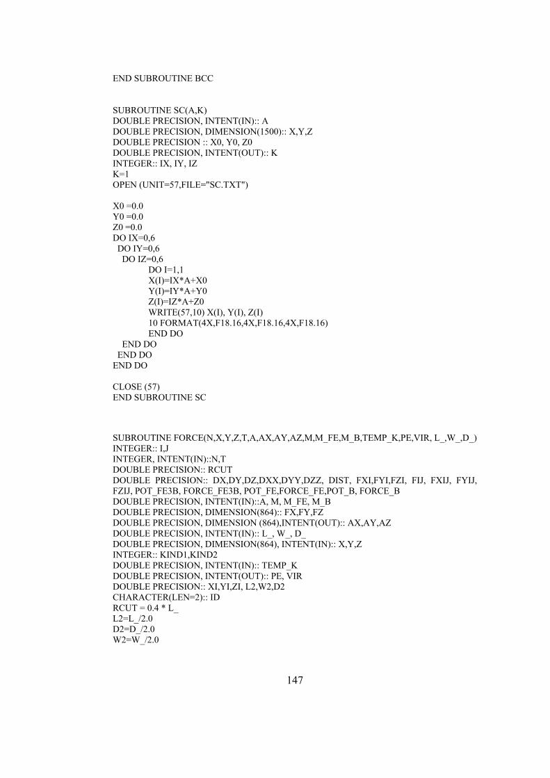
END SUBROUTINE BCC SUBROUTINE SC(A,K) DOUBLE PRECISION, INTENT(IN):: A DOUBLE PRECISION, DIMENSION(1500):: X,Y,Z DOUBLE PRECISION :: X0, Y0, Z0 DOUBLE PRECISION, INTENT(OUT):: K INTEGER:: IX, IY, IZ K=1 OPEN (UNIT=57,FILE="SC.TXT") X0 =0.0 Y0 =0.0 Z0 =0.0 DO IX=0,6 DO IY=0,6 DO IZ=0,6 DO I=1,1 X(I)=IX*A+X0 Y(I)=IY*A+Y0 Z(I)=IZ*A+Z0 WRITE(57,10) X(I), Y(I), Z(I) 10 FORMAT(4X,F18.16,4X,F18.16,4X,F18.16) END DO END DO END DO END DO CLOSE (57) END SUBROUTINE SC SUBROUTINE FORCE(N,X,Y,Z,T,A,AX,AY,AZ,M,M_FE,M_B,TEMP_K,PE,VIR, L_,W_,D_) INTEGER:: I,J INTEGER, INTENT(IN)::N,T DOUBLE PRECISION:: RCUT DOUBLE PRECISION:: DX,DY,DZ,DXX,DYY,DZZ, DIST, FXI,FYI,FZI, FIJ, FXIJ, FYIJ, FZIJ, POT_FE3B, FORCE_FE3B, POT_FE,FORCE_FE,POT_B, FORCE_B DOUBLE PRECISION, INTENT(IN)::A, M, M_FE, M_B DOUBLE PRECISION, DIMENSION(864):: FX,FY,FZ DOUBLE PRECISION, DIMENSION (864),INTENT(OUT):: AX,AY,AZ DOUBLE PRECISION, INTENT(IN):: L_, W_, D_ DOUBLE PRECISION, DIMENSION(864), INTENT(IN):: X,Y,Z INTEGER:: KIND1,KIND2 DOUBLE PRECISION, INTENT(IN):: TEMP_K DOUBLE PRECISION, INTENT(OUT):: PE, VIR DOUBLE PRECISION:: XI,YI,ZI, L2,W2,D2 CHARACTER(LEN=2):: ID RCUT = 0.4 * L_ L2=L_/2.0 D2=D_/2.0 W2=W_/2.0

147

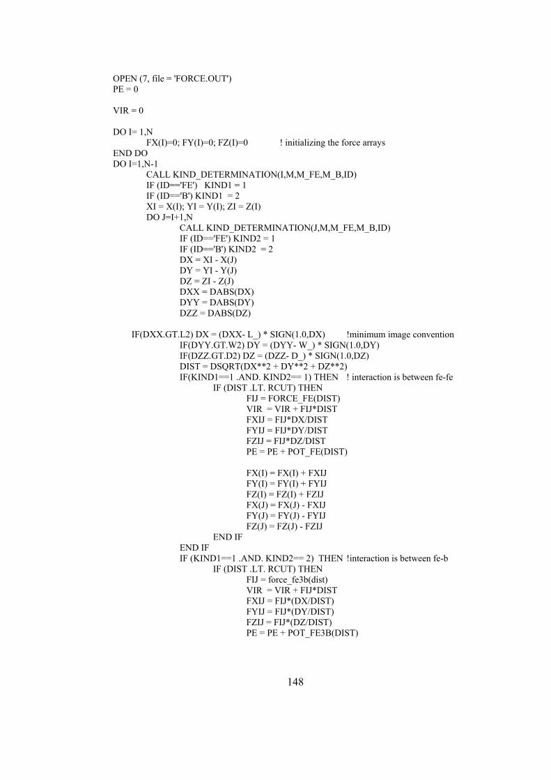
OPEN (7, file = 'FORCE.OUT') PE = 0 VIR = 0 DO I= 1,N FX(I)=0; FY(I)=0; FZ(I)=0 ! initializing the force arrays END DO DO I=1,N-1 CALL KIND_DETERMINATION(I,M,M_FE,M_B,ID) IF (ID=='FE') KIND1 = 1 IF (ID=='B') KIND1 = 2 XI = X(I); YI = Y(I); ZI = Z(I) DO J=I+1,N CALL KIND_DETERMINATION(J,M,M_FE,M_B,ID) IF (ID=='FE') KIND2 = 1 IF (ID=='B') KIND2 = 2 DX = XI - X(J) DY = YI - Y(J) DZ = ZI - Z(J) DXX = DABS(DX) DYY = DABS(DY) DZZ = DABS(DZ) IF(DXX.GT.L2) DX = (DXX- L_) * SIGN(1.0,DX) !minimum image convention IF(DYY.GT.W2) DY = (DYY- W_) * SIGN(1.0,DY) IF(DZZ.GT.D2) DZ = (DZZ- D_) * SIGN(1.0,DZ) DIST = DSQRT(DX**2 + DY**2 + DZ**2) IF(KIND1==1 .AND. KIND2== 1) THEN ! interaction is between fe-fe IF (DIST .LT. RCUT) THEN FIJ = FORCE_FE(DIST) VIR = VIR + FIJ*DIST FXIJ = FIJ*DX/DIST FYIJ = FIJ*DY/DIST FZIJ = FIJ*DZ/DIST PE = PE + POT_FE(DIST) FX(I) = FX(I) + FXIJ FY(I) = FY(I) + FYIJ FZ(I) = FZ(I) + FZIJ FX(J) = FX(J) - FXIJ FY(J) = FY(J) - FYIJ FZ(J) = FZ(J) - FZIJ END IF END IF IF (KIND1==1 .AND. KIND2== 2) THEN !interaction is between fe-b IF (DIST .LT. RCUT) THEN FIJ = force_fe3b(dist) VIR = VIR + FIJ*DIST FXIJ = FIJ*(DX/DIST) FYIJ = FIJ*(DY/DIST) FZIJ = FIJ*(DZ/DIST) PE = PE + POT_FE3B(DIST)

148

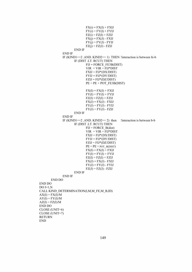
FX(i) = FX(I) + FXIJ FY(i) = FY(I) + FYIJ FZ(i) = FZ(I) + FZIJ FX(j) = FX(J) - FXIJ FY(j) = FY(J) - FYIJ FZ(j) = FZ(J) - FZIJ END IF END IF IF (KIND1==2 .AND. KIND2== 1) THEN !interaction is between fe-b IF (DIST .LT. RCUT) THEN FIJ = FORCE_FE3B(DIST) VIR = VIR + FIJ*DIST FXIJ = FIJ*(DX/DIST) FYIJ = FIJ*(DY/DIST) FZIJ = FIJ*(DZ/DIST) PE = PE + POT_FE3B(DIST) FX(I) = FX(I) + FXIJ FY(I) = FY(I) + FYIJ FZ(I) = FZ(I) + FZIJ FX(J) = FX(J) - FXIJ FY(J) = FY(J) - FYIJ FY(J) = FY(J) - FZIJ END IF END IF IF (KIND1==2 .AND. KIND2== 2) then !interaction is between b-b IF (DIST .LT. RCUT) THEN FIJ = FORCE_B(dist) VIR = VIR + FIJ*DIST FXIJ = FIJ*(DX/DIST) FYIJ = FIJ*(DY/DIST) FZIJ = FIJ*(DZ/DIST) PE = PE + POT_B(DIST) FX(I) = FX(I) + FXIJ FY(I) = FY(I) + FYIJ FZ(I) = FZ(I) + FZIJ FX(J) = FX(J) - FXIJ FY(J) = FY(J) - FYIJ FZ(J) = FZ(J) - FZIJ END IF END IF END DO END DO DO I=1,N CALL KIND_DETERMINATION(I,M,M_FE,M_B,ID) AX(I) = FX(I)/M AY(I) = FY(I)/M AZ(I) = FZ(I)/M END DO CLOSE (UNIT=6) CLOSE (UNIT=7) RETURN END

149

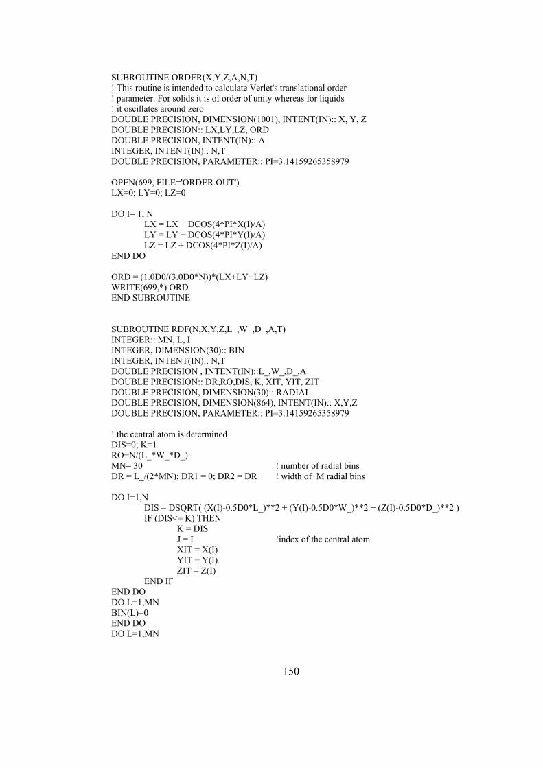
SUBROUTINE ORDER(X,Y,Z,A,N,T) ! This routine is intended to calculate Verlet's translational order ! parameter. For solids it is of order of unity whereas for liquids ! it oscillates around zero DOUBLE PRECISION, DIMENSION(1001), INTENT(IN):: X, Y, Z DOUBLE PRECISION:: LX,LY,LZ, ORD DOUBLE PRECISION, INTENT(IN):: A INTEGER, INTENT(IN):: N,T DOUBLE PRECISION, PARAMETER:: PI=3.14159265358979 OPEN(699, FILE='ORDER.OUT') LX=0; LY=0; LZ=0 DO I= 1, N LX = LX + DCOS(4*PI*X(I)/A) LY = LY + DCOS(4*PI*Y(I)/A) LZ = LZ + DCOS(4*PI*Z(I)/A) END DO ORD = (1.0D0/(3.0D0*N))*(LX+LY+LZ) WRITE(699,*) ORD END SUBROUTINE SUBROUTINE RDF(N,X,Y,Z,L_,W_,D_,A,T) INTEGER:: MN, L, I INTEGER, DIMENSION(30):: BIN INTEGER, INTENT(IN):: N,T DOUBLE PRECISION , INTENT(IN)::L_,W_,D_,A DOUBLE PRECISION:: DR,RO,DIS, K, XIT, YIT, ZIT DOUBLE PRECISION, DIMENSION(30):: RADIAL DOUBLE PRECISION, DIMENSION(864), INTENT(IN):: X,Y,Z DOUBLE PRECISION, PARAMETER:: PI=3.14159265358979 ! the central atom is determined DIS=0; K=1 RO=N/(L_*W_*D_) MN= 30 ! number of radial bins DR = L_/(2*MN); DR1 = 0; DR2 = DR ! width of M radial bins DO I=1,N DIS = DSQRT( (X(I)-0.5D0*L_)**2 + (Y(I)-0.5D0*W_)**2 + (Z(I)-0.5D0*D_)**2 ) IF (DIS<= K) THEN K = DIS J = I !index of the central atom XIT = X(I) YIT = Y(I) ZIT = Z(I) END IF END DO DO L=1,MN BIN(L)=0 END DO DO L=1,MN

150

DR1 = (L-1)*DR DR2 = (L)*DR DO I=1,N DIST= DSQRT((XIT-X(I))**2+(YIT-Y(I))**2+(ZIT-Z(I))**2) IF ((DR1 < DIST) .AND. (DIST <= DR2)) THEN BIN(L) = BIN(L) +1 END IF END DO END DO DO L=1,MN DR1 = (L-1)*DR DR2 = (L)*DR RADIAL(L)= BIN(L)/(RO*(4.0/3.0)*PI*(DR2**3-DR1**3)) END DO OPEN (51,FILE = 'RADIAL.OUT') WRITE (51,*) 'TIME STEP',T DO l=1,MN WRITE (51,*) L*DR*1.0D10,RADIAL(L) END DO END SUBROUTINE RDF

151

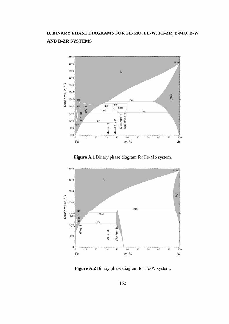
B. BINARY PHASE DIAGRAMS FOR FE-MO, FE-W, FE-ZR, B-MO, B-W

AND B-ZR SYSTEMS

Figure A.1 Binary phase diagram for Fe-Mo system.

Figure A.2 Binary phase diagram for Fe-W system.

152

Figure A.3 Binary phase diagram for Fe-Zr system.

Figure A.4 Binary phase diagram for B-Mo system.

153

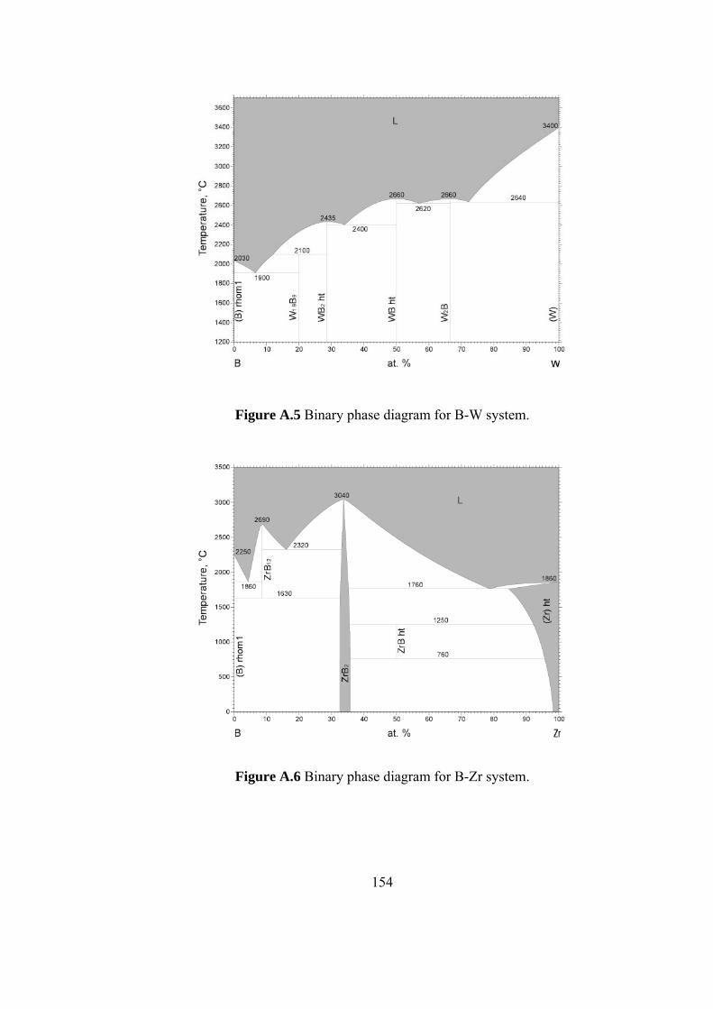
Figure A.5 Binary phase diagram for B-W system.

Figure A.6 Binary phase diagram for B-Zr system.

154

theoretical and experimental investigation of bulk - middle

Documents