the synergy between pav and adaboost
TRANSCRIPT
Machine Learning, 61, 71–103, 20052005 Springer Science + Business Media, Inc. Manufactured in The Netherlands.
DOI: 10.1007/s10994-005-1123-6
The Synergy Between PAV and AdaBoost
W. JOHN WILBUR [email protected] YEGANOVAWON KIMNational Center for Biotechnology Information, National Library of Medicine, National Institutes of Health,Bethesda, MD, U.S.A.
Editor: Robert SchapirePublished online: 08 June 2005
Abstract. Schapire and Singer’s improved version of AdaBoost for handling weak hypotheses with confidencerated predictions represents an important advance in the theory and practice of boosting. Its success results froma more efficient use of information in weak hypotheses during updating. Instead of simple binary voting a weakhypothesis is allowed to vote for or against a classification with a variable strength or confidence. The Pool AdjacentViolators (PAV) algorithm is a method for converting a score into a probability. We show how PAV may be appliedto a weak hypothesis to yield a new weak hypothesis which is in a sense an ideal confidence rated prediction andthat this leads to an optimal updating for AdaBoost. The result is a new algorithm which we term PAV-AdaBoost.We give several examples illustrating problems for which this new algorithm provides advantages in performance.
Keywords: boosting, isotonic regression, convergence, document classification, k nearest neighbors
1. Introduction
Boosting is a technique for improving learning by repeatedly refocusing a learner on thoseparts of the training data where it has not yet proved effective. Perhaps the most suc-cessful boosting algorithm is AdaBoost first introduced by Freund and Schapire (1997).Since its publication AdaBoost has been the focus of considerable study and in additiona large number of related boosting algorithms have been put forward for consideration(Aslam, 2000; Bennett, Demiriz, & Shawe-Taylor, 2000; Collins, Schapire, & Singer,2002; Duffy & Helmbold, 1999, 2000; Friedman, Hastie, & Tibshirani, 2000; Mason,Bartlett, & Baxter, 2000; Meir, El-Yaniv, & Ben-David, 2000; Nock & Sebban, 2001;Ratsch, Mika, & Warmuth, 2001; Ratsch, Onoda, & Muller, 2001; Schapire & Singer,1999)(see also http://www.boosting.org). Our interest in this paper is the form of AdaBoostusing confidence-rated predictions introduced by Schapire and Singer (1999). For claritywe will refer to this form of AdaBoost as CR(confidence-rated)-AdaBoost as opposed tothe binary form of AdaBoost originally introduced by Freund and Schapire (1997).
In the CR-AdaBoost setting a weak hypothesis not only votes for the category of adata point by the sign of the number it assigns to that data point, but it provides addi-tional information in the magnitude of the number it assigns. CR-AdaBoost combines theconfidence-rated weak hypotheses that are generated into a linear combination with constantcoefficients to produce its final hypothesis. While this approach works well in many cases,
72 W.J. WILBUR, L. YEGANOVA AND W. KIM
it is not necessarily ideal. A particular weak hypothesis may erroneously invert the orderof importance attached to two data points or if the order is not inverted it may still as-sign an importance that is not consistent between two data points. As a potential cure forsuch problems we here consider the Pool Adjacent Violators algorithm (Ayer et al., 1954;Hardle, 1991). This algorithm makes use of the ordering supplied by a weak hypothesis andproduces the isotonic regression which in a sense is the ideal confidence-rated predictionconsistent with the ordering imposed by the weak hypothesis. We show how this may beconverted into a resulting weak hypothesis which produces optimal improvements at eachstep of what we term PAV-AdaBoost. Our algorithm is a type of real AdaBoost, as Friedman,Hastie, and Tibshirani (2000) use the general term, but their realization involves trees, whileour development is in the direction of linearly ordered structures. Isotonic regression (PAV)could potentially play a role in other approaches to boosting provided the weak hypothesesgenerated have the appropriate monotonicity property. We chose CR-Adaboost because theconfidence of a prediction h(x) is assumed to go up with its magnitude and this is exactlythe condition where isotonic regression is appropriate.
In the most general setting PAV-AdaBoost may be applied exactly parallel to CR-AdaBoost. However, there are situations where one is limited to a certain fixed numberof weak hypotheses. To deal with this case we propose a modified form of PAV-AdaBoostwhich repeatedly cycles through this finite set of weak hypotheses until no more improve-ment can be obtained. The result is a type of back-fitting algorithm, as studied by Buja,Hastie, and Tibshirani (1989) but the fitting is nonlinear and convergence does not followfrom their results. For CR-AdaBoost with a fixed finite set of weak hypotheses, Collins,Schapire, and Singer (2002) have recently given a proof of convergence to the optimumunder mild conditions. While our algorithm does not satisfy their hypotheses we are ableto prove that it also converges to the optimum solution under general conditions.
The first part of this paper (Sections 2 and 3) deals with theoretical issues pertinent todefining the algorithm. Section 2 consists of an introduction to the PAV algorithm togetherwith pseudocode for its efficient implementation. Section 3 recalls CR-AdaBoost (Schapire& Singer, 1999), describes how PAV is used with CR-AdaBoost to yield the PAV-AdaBoostalgorithm, and proves several optimality results for PAV-AdaBoost. The second part ofthe paper (Sections 4 and 5) deals with the learning capacity and generalizability of thealgorithm. Section 4 gives three different examples where PAV-AdaBoost is able to learnon training data more successfully than confidence-rated AdaBoost. In its full general-ity PAV-AdaBoost has infinite VC dimension as shown in an appendix. In Section 5 weshow that an approximate form of PAV-AdaBoost has finite VC dimension and give errorbounds for this form of PAV-AdaBoost. All the results in this paper are produced usingthe approximate form of PAV-AdaBoost. The final sections present examples of successfulapplications of PAV-AdaBoost. In Section 6 we consider a real data set and a simulatedproblem involving two multidimensional normal distributions. Both of these examples in-volve a fixed small set of weak hypotheses. For these examples we find PAV-AdaBoostoutperforms CR-AdaBoost and compares favorably with several other classifiers tested onthe same data. The example in Section 7 deals with a real life document classificationproblem. CR-AdaBoost applied to decision tree weak hypotheses has given perhaps thebest overall document classification performance to date (Apte, Damerau, & Weiss, 1998;
PAV AND ADABOOST 73
Carreras & Marquez, 2001). The method by which CR-AdaBoost (Schapire & Singer, 1999)deals with decision tree weak learners is already optimized so that PAV-AdaBoost in thiscase does not lead to anything new. However, there are examples of weak learners unrelatedto decision trees and we consider two types for which PAV-AdaBoost is quite effective,but CR-AdaBoost performs poorly. Section 8 is a discussion of the practical limitations ofPAV-AdaBoost.
2. Pool adjacent violators
Suppose the probability p(s) of an event is a monotonically non-decreasing function ofsome ordered parameter s. If we have data recording the presence or absence of that eventat different values of s, the data will in general be probabilistic and noisy and the mono-tonic nature of p(s) may not be apparent. The Pool Adjacent Violators (PAV) Algorithm(Ayer et al., 1954; Hardle, 1991) is a simple and efficient algorithm to derive from thedata that monotonically non-decreasing estimate of p(s) which assigns maximal likeli-hood to the data. The algorithm is conveniently applied to data of the form {(si , wi , pi )}N
i=1where si is a parameter value, wi is the weight or importance of the data at i , and pi
is the probability estimate of the data associated with i . We may assume that no valuesi is repeated in the set. If a value were repeated we simply replace all the points thathave the given value si with a single new point that has the same value si , for whichpi is the weighted average of the contributing points, and for which wi is the sum ofthe weights for the contributing points. We may also assume the data is in order so thati < j ⇒ si < s j . Then the si , which serve only to order the data, may be ignored in ourdiscussion.
We seek a set of probabilities {qi }Ni=1 such that
i < j ⇒ qi ≤ q j (1)
and
N∏
i=1
qwi pi
i (1 − qi )wi (1−pi ) (2)
is a maximum. In other words we seek a maximal likelihood solution. If the sequence {qi }Ni=1
is a constant value q , then by elementary calculus it is easily shown that q is the weightedaverage of the p’s and this is the unique maximal likelihood solution. If the q’s are notconstant, they in any case allow us to partition the set N into K nonempty subsets definedby a set of intervals {(r ( j), t( j)}K
j=1 on each of which q takes a different constant value.Then we must have
qi =∑t( j)
k=r ( j) wk pk∑t( j)
k=r ( j) wk
, r ( j) ≤ i ≤ t( j) (3)
74 W.J. WILBUR, L. YEGANOVA AND W. KIM
by the same elementary methods already mentioned. We will refer to these intervals as thepools and ask what properties characterize them. First, for any k, r ( j) ≤ k ≤ t( j)
∑ki=r ( j) wi pi
∑ki=r ( j) wi
≥∑t( j)
i=r ( j) wi pi∑t( j)
i=r ( j) wi
≥∑t( j)
i=k wi pi∑t( j)i=k wi
. (4)
This must be true because if one of the ≥’s in inequality (4) could be replaced by < forsome k, then the pool could be broken at the corresponding k into two pools for which thesolutions as given by Eq. (3) would give a better fit (a higher likelihood) in Eq. (2). Let uscall intervals that satisfy the condition (4) irreducible. The pools then are irreducible. Theyare not only irreducible, they are maximal among irreducible intervals. This follows fromthe fact that each successive pool from left to right has a greater weighted average and theirreducible nature of each pool.
It turns out the pools are uniquely characterized by being maximal irreducible intervals.This follows from the observation that the union of two overlapping irreducible intervalsis again an irreducible interval. It remains to show that pools exist and how to find them.For this purpose suppose I and J are irreducible intervals. If the last integer of I plus oneequals the first integer of J and if
∑i∈I wi pi∑
i∈I wi≥
∑i∈J wi pi∑
i∈J wi(5)
we say that I and J are adjacent violators. Given such a pair of violators it is evident fromcondition (4), for each interval, and from condition (5) that the pair can be pooled (a unionof the two) to obtain a larger irreducible set. This is the origin of the PAV algorithm. Onebegins with all sets consisting of single integers (degenerate intervals) from 0 to N − 1. Allsuch sets are irreducible by default. Adjacent violators are then pooled until this process ofpooling is no longer applicable. The end result is a partition of the space into pools whichprovides the solution (3) to the order constrained maximization problems (1) and (2).
As an illustration of irreducible sets and pooling to obtain them consider the set of points:
w0 = 1, . . . , w5 = 1 and p0 = 1
4, p1 = 1
3, p2 = 1
5, p3 = 1
4, p4 = 1, p5 = 1
2
One pass through this set of points identifies two pairs {p1, p2} and {p4, p5} as adjacentviolators. When these are pooled they result in single points of weight 2 with the values 4
15and 3
4 , respectively. A second pass through the resulting set of four points shows that {p1, p2}and p3 are now adjacent violators. These may be pooled to produce the pool {p1, p2, p3}andthe value 47
180 . Examination shows that there are no further violations so that the irreduciblepools are {p0}, {p1, p2, p3}, and{p4, p5}.
In order to obtain an efficient implementation of PAV one must use some care in how thepooling of violators is done. A scheme we use is to keep two arrays of pointers of lengthN . An array of forward pointers, F , keeps at the beginning of each irreducible intervalthe position of the beginning of the next interval (or N ). Likewise an array of backward

PAV AND ADABOOST 75
pointers, B, keeps at the beginning of each interval the position of the beginning of theprevious interval (or −1). Pseudocode for the algorithm follows.
2.1. PAV algorithm
#InitializationA. Set F[k] ← k + 1 and B[k] ← k − 1, 0 ≤ k < N .
B. Set up two (FIFO) queues, Q1 and Q2, and put all the numbers, 0, . . . , N − 1, inorder into Q1 while Q2 remains empty.
C. Define a marker variable m and a flag.#ProcessingWhile (Q1 nonempty){
Set m ← 0.While (Q1 nonempty){
k ← dequeue Q1.If(m ≤ k){
Set flag ← 0.While (F[k] �= N and intervals at k and F[k] are adjacent violators){
Pool intervals beginning at k and F[k].Set u ← F[F[k]].Redefine F[k] ← u.If (u < N ) redefine B[u] ← k.Update m ← u.Update flag ← 1.
}}If (flag = 1 and B[k] ≥ 0) enqueue B[k] in Q2.
}Interchange Q1 and Q2.
}
This is an efficient algorithm because after the initial filling of Q1 an element is added toQ2 only if a pooling took place. Thus in a single invocation of the algorithm a total of nomore than N elements can ever be added to Q2 and this in turn limits the number of testsfor violators to at most 2N . We may conclude that both the space and time complexity ofPAV are O(N ). See also Pardalos and Xue (1999).
PAV produces as its output the pools described above and these define the solution as inEq. (3). It will be convenient to define p(si ) = qi , i = 1, . . . , N and we will generally referto the function p.
A simple example of the type of data to which the algorithm may be applied is a Bernoulliprocess for which the probability of success is a monotonic function of some parameter.Data generated by such a process could take the form of tuples such as (s, 3, 2/3). Here theparameter value is s and at this value there were 3 trials and 2 of these were a success. PAVapplied to such data will give us a prediction for the probability of success as a function

76 W.J. WILBUR, L. YEGANOVA AND W. KIM
of the parameter. The PAV algorithm may be applied to any totally ordered data set andassigns a probability estimate to those parameter values that actually occur in the data set.For our applications it will be important to interpolate and extrapolate from these assignedvalues to obtain an estimated probability for any parameter value. We do this in perhaps thesimplest possible way based on the values of p just defined on the points {si }N
i=1.
2.2. Interpolated PAV
Given the function p defined on the set {si }Ni=1, assume that the points come from a totally
ordered space, S, and are listed in increasing order. Then for any s ∈ S define p(s) by
Case 1. If s = si , set p(s) = p(si ).Case 2. If s < s1, set p(s) = p(s1).Case 3. If si < s < si+1, set p(s) = p(si )+p(si+1)
2 .Case 4. If sN < s, set p(s) = p(sN ).
While one could desire a smoother interpolation, 2.2 is general and proves adequate for ourpurposes. In cases where data is sparse and the parameter s belongs to the real numbers,one might replace Case 3 by a linear interpolation. However, there is no optimal solutionto the interpolation problem without further assumptions. The definition given has provedadequate for our applications and the examples given in this paper.
PAV allows us to learn a functional relationship between a parameter and the probabilityof an event. The interpolation 2.2 simply lets us generalize and apply this learning to newparameter values not seen in the training data.
3. AdaBoost
The AdaBoost algorithm was first put forward by Freund and Schapire (1997) but im-provements were made in Schapire and Singer (1999). We first review important aspectsof CR-AdaBoost as detailed in Schapire and Singer (1999), and then describe how PAVis used with AdaBoost. The AdaBoost algorithm as given in Schapire and Singer (1999)follows.
3.1. AdaBoost algorithm
Given training data {(xi , yi )}mi=1 with xi ∈ X and yi ∈ {1, −1}, initialize D1(i) = 1/m.
Then for t = 1, . . . , T :
(i) Train weak learner using distribution Dt .(ii) Get weak hypothesis ht : X → R.
(iii) Choose αt ∈ R.(iv) Update:
PAV AND ADABOOST 77
Dt+1(i) = Dt (i) exp(−αt yt ht (xi ))
Zt
where
Zt =m∑
i=1
Dt (i) exp(−αt yi ht (xi )). (6)
Output the final hypothesis:
H (x) = sign
(T∑
t=1
αt ht (x)
). (7)
Schapire and Singer establish an error bound on the final hypothesis.
Theorem 1. The training error of H satisfies:
1
m
∣∣{i |H (xi ) �= yi }∣∣ ≤
T∏
t=1
Zt . (8)
From inequality (8) it is evident that one would like to minimize the value of Zt at each stageof AdaBoost. Schapire and Singer suggest two basic approaches to accomplish this. Thefirst approach is a straightforward minimization of the right side of Eq. (6) by setting thederivative with respect to αt to zero and solving for αt . They observe that in all interestingcases there is a unique solution which corresponds to a minimum and may be found bynumerical methods. We shall refer to this as the linear form of AdaBoost because it yieldsthe sum
f (x) =T∑
t=1
αt ht (x) (9)
which is a linear combination of the weak hypotheses.The second approach to optimization presented in Schapire and Singer (1999) is appli-
cable to the special case when the weak learner produces a partition of the training spaceinto mutually disjoint nonempty sets {X j }N
j=1. Here α is absorbed into h, h is assumed tobe a constant c j on each set X j , and one asks how to define the c j in order to minimize Zin Eq. (6). Let us define a measure µ on all subsets of X by
µ(A) =∑
xi ∈A
D(i).

78 W.J. WILBUR, L. YEGANOVA AND W. KIM
Then we may set
W j+ = µ({xi | xi ∈ X j ∧ yi = 1})
W j− = µ({xi | xi ∈ X j ∧ yi = −1}) (10)
The solution (Schapire & Singer, 1999) is then given by
c j = 1
2ln
(W j
+W j
−
)(11)
and we may write
Z = 2N∑
j=1
√W j
+W j− = 2
N∑
j=1
√u j (1 − u j )µ(X j ) (12)
provided we define
u j = W j+
µ(X j )
3.2. PAV-AdaBoost algorithm
The AdaBoost Algorithm 3.1 is modified from step (iii) on. The weak hypothesis comingfrom step (ii) is assumed to represent a parameter so that si = ht (xi ). Each data point (xi , yi )may thus be transformed to a tuple
(si , Dt (i), (1 + yi )/2). (13)
PAV is applied to this set of tuples to produce the function pt (s). With the use of pt (s) wecan define another function
kt (s) = 1
2ln
(pt (s)
1 − pt (s)
). (14)
Clearly this function is monotonic non-decreasing because pt (s) is. There is one differ-ence, namely, kt (s) may assume infinite values. Through the formula (11) this leads to thereplacement of Eq. (9) by
f (x) =T∑
t=1
kt (ht (x)) (15)
PAV AND ADABOOST 79
and Eq. (12) becomes
Zt = 2∫ √
pt (s)(1 − pt (s)) dµ(s) = 2∫
σt (s) dµ(s) (16)
where µ(s) is the measure induced on ht [X ] by µ through ht . Based on Eq. (16) and theinequality
2√
p(1 − p) =√
1 − (1 − 2p)2 ≤ 1 − 2(p − 1/2)2
we may obtain the bound
Zt ≤ 1 − 2∫
(pt (s) − 1/2)2dµ(s).
Further we have the following theorem.
Theorem 2. Among all monotonic non-decreasing functions defined on ht [X ], kt is thatfunction which when composed with ht produces the weak hypothesis with minimum Zt .
Proof: By its construction pt (s) partitions the set ht [X ] into a family of subsets {Sj }mj=1
on each of which pt , and hence kt , is a constant. For each j set X j = h−1t [Sj ]. Then
referring to the defining relations (10) we see that the function W j+e−c + W j
−ec achievesits unique minimum when c is the constant value of kt on Sj . Now let g be a monotonicnon-decreasing function that when composed with ht produces the minimum Zt . We firstclaim that g is constant on each set Sj . Suppose that g is not constant on some Sj and letthe minimal value of g be c′ and maximal value of g be c′′ on Sj . Let S′ and S′′ be thosesubsets of Sj that map to c′ and c′′, respectively, under g. Then in turn set X ′ = h−1
t [S′]and X ′′ = h−1
t [S′′] and define W ′+ , etc., in the obvious way as in Eq. ( 10). Then we have
the inequality
W ′+
W ′−≥ W j
+W j
−≥ W ′′
+W ′′−
(17)
which follows from the constancy of pt on Sj (see inequality (4) above). Now suppose c′
is less than the constant value of kt on Sj . Then because the function W ′+e−c + W ′
−ec isconvex with a strictly positive second derivative it decreases in value in moving c from c′
to the value of kt as a consequence of inequality (17). Thus we can decrease the value of Zt
arising from g by increasing c′ to the next greater value of g or to kt whichever comes first.This contradicts the optimality of g. We conclude that c′ cannot be less then the value of kt
on Sj . Then c′′ must be greater than the constant value of kt on Sj . But the dual argumentto that just given shows that this is also impossible. We are forced to the conclusion that gmust be a constant on Sj . Now if g were not equal to kt on Sj , we could decrease the valueof Zt arising from g by changing its value on Sj to that of kt , which we know is optimal.
80 W.J. WILBUR, L. YEGANOVA AND W. KIM
This may cause g to no longer be monotonic non-decreasing. However if we make thischange for all Sj the result is kt , which is monotonic non-decreasing. The only conclusionthen is that kt is optimal.
There are practical issues that arise in applying PAV-AdaBoost. First, we find it useful tobound pt away from 0 and 1 by ε. We generally take ε to be the reciprocal of the size ofthe training set. This is the value used in Schapire and Singer (1999) for “smoothing” andhas the same purpose. If we assume that 0 < ε < 1/2 and define λ = ln[(1 − ε)/ε], thenthis approach is equivalent to truncating kt at size λ. Define
kλt (s) ={ kt (s), |kt (s)| ≤ λ
λ, λ < kt (s)−λ, −λ > kt (s).
(18)
Based on the proof of Theorem 2 we have the following corollary.
Corollary 1. Among all monotonic non-decreasing functions defined on ht [X ] andbounded by λ, kλt is that function which when composed with ht produces the weak hypoth-esis with minimum Zt .
Proof: Theorem 2 tells us that among monotonic non-decreasing functions, kt is thatfunction that minimizes Zt . Let W be a pool of points from ht [X ] on which kt takes theconstant value β(>λ). We already know that β minimizes the function
F(c) = W+e−c + W−ec. (19)
Because this function has a strictly positive second derivative and achieves its minimum at βthe value that minimizes it within [−λ, λ] is λ. A similar argument applies if β < −λ. Thuskλt must be that function which is monotonic non-decreasing and constant on each pooland minimizes Zt . The only question that remains is whether there could be a monotonicnon-decreasing function bounded by [−λ, λ] but not constant on the pools and which yieldsa smaller Zt . That this cannot be so follows by the same argument used in the proof of theTheorem.
In some applications we apply the weak learner just as outlined above. This seemsappropriate when there is an unlimited supply of weak hypotheses ht produced by the weaklearner. Just as for standard AdaBoost we try to choose a near optimal weak hypothesis oneach round. In other applications we are limited to a fixed set {h j }n
j=1 of weak hypotheses.In this case we seek a set {kλ j }n
j=1 of monotonic non-decreasing functions bounded by λ
that minimize the expression
m∑
i=1
exp
[−yi
n∑
j=1
kλ j (h j (xi ))
]. (20)
PAV AND ADABOOST 81
Because each kλ j in expression (20) acts on only the finite set h j [X ] and the result is boundedin the interval [−λ, λ], compactness arguments show that at least one set {kλ j }n
j=1 must existwhich achieves the minimum in (20). We propose the following algorithm to achieve thisminimum.
3.3. PAV-AdaBoost.finite algorithm
Assume a fixed set of weak hypotheses {h j }nj=1 and a positive real value λ. For any set
{kλ j }nj=1 of monotonic non-decreasing functions bounded by λ and where each kλ j is defined
on h j [X ] define
qi = exp
[−yi
n∑
j=1
kλ j (h j (xi ))
]. (21)
To begin let each kλ j be equal to the 0 function on h j [X ]. Then one round of updating willconsist of updating each kλ j , 1 ≤ j ≤ n, in turn (not in parallel) according to the followingsteps:
(i) Define
Di = qi exp[yi kλ j (h j (xi ))]
Z0(22)
where
Z0 =m∑
i=1
qi exp[yi kλ j (h j (xi ))]. (23)
(ii) Apply the PAV algorithm as described under 3.2 and Corollary 1 to produce the optimalkλ j which minimizes
∑mi=1 Di exp[−yi kλ j (h j (xi ))]. Replace the old by the new kλ j .
At each update step in this algorithm either kλ j is unchanged or it changes and the sum in(20) decreases. Repetition of the algorithm converges to the minimum for expression (20).
Theorem 3. Let {ktλ j }n
j=1denote the functions produced on the tth round of Algorithm 3.3.Let {k ′
λ j }nj=1 denote any set of functions that produces the minimum in expression (20). Then
we have
limt→∞
n∑
j=1
ktλ j ◦ h j =
n∑
j=1
k ′λ j ◦ h j (24)
pointwise on X.
82 W.J. WILBUR, L. YEGANOVA AND W. KIM
Proof: Clearly for {k ′λ j }n
j=1 the update procedure of Algorithm 3.3 can produce no change.Let {qt
i }mi=1 denote the result of (21) applied to {kt
λ j }nj=1, where t denotes the result of the
t th round. By compactness we may choose a subsequence {t(r )} for which each {kt(r )λ j }∞r=1
converges pointwise to a function kλ j . For this set of functions {kλ j }nj=1 let {q∗
i } denote thevalues defined by Eq. (21). We claim that the set {kλ j }n
j=1 is invariant under the updateprocedure of the algorithm. If not suppose that the update procedure applied to this set offunctions produces an improvement when kλ j ′ is updated and decreases the sum (20) by anε > 0. Then because the update procedure is a continuous process, there exists an integerM > 0 such that when r > M the update procedure applied in the t(r ) + 1th round to kt(r )
λ j ′
must produce an improvement in the sum (20) by at least ε/2. However, the sums∑m
i=1 qt(r )i
converge downward to∑m
i=1 q∗i so that we may choose an N > M for which r > N implies
m∑
i=1
qt(r )i −
m∑
i=1
q∗i <
ε
4(25)
It follows then that
m∑
i=1
qt(r )+1i <
m∑
i=1
q∗i . (26)
But this latter relation contradicts the fact that the sum∑m
i=1 q∗i must be a lower bound for
any such sum produced by the algorithm because of the monotonically decreasing natureof these sums in successive steps in the algorithm. We thus conclude that {kλ j }n
j=1 mustindeed be invariant under the algorithm’s update procedure.
The next step is to show that an invariant set under the algorithm’s update proceduredefines a unique function on X . For any α, 0 ≤ α ≤ 1, consider the set of functions{αk ′
λi + (1 − α)kλi }mi=1. This is again a set of monotonic functions to be considered in
taking the minimum of expression (20). Define
F(α) =m∑
i=1
exp
[−yi
n∑
j=1
{αk ′λ j (h j (xi )) + (1 − α)kλ j (h j (xi ))}
]. (27)
By assumption F(1) is the true minimum of (20) while F(0) = ∑mi=1 q∗
i . Let us supposethat F(1) < F(0). Because e−x is a convex function it follows that F is also and we have
F(α) ≤ αF(1) + (1 − α)F(0). (28)
From this relation it follows that
F ′(0) ≤ F(1) − F(0) < 0. (29)
PAV AND ADABOOST 83
Now define
G(α1, α2, . . . , αn) =m∑
i=1
exp
[−yi
n∑
j=1
{α j k′λ j (h j (xi )) + (1 − α j )kλ j (h j (xi ))}
](30)
and note that with α j = α, 1 ≤ j ≤ n, we have
F(α) = G(α1, α2, . . . , αn). (31)
It then follows that
F ′(0) =n∑
j=1
∂G
∂α j(0, 0, . . . , 0). (32)
Then some one of the partials of G in Eq. (32) must be negative, say the one correspondingto j ′. But then the nature of the derivative ensures that for some α > 0
G(0, 0, . . . , α j ′ (α), . . . , 0) < G(0, 0, . . . , 0). (33)
This, however, contradicts the invariance of the set {kλ j }nj=1 under the update procedure
applied at j ′. We are forced to the conclusion that F(0) = F(1). Now suppose there werean i with
n∑
j=1
k ′λ j (h j (xi )) �=
n∑
j=1
kλ j (h j (xi )). (34)
Then because e−x is strictly convex we would have for any α, 0 < α < 1, the relation
F (α) < αF (1) + (1 − α) F (0) = F (1) . (35)
But this contradicts the minimality of F(1). We conclude that inequality (34) does not occur.At this point we have shown that
limr→∞
n∑
j=1
kt(r )λ j ◦ h j =
n∑
j=1
k ′λ j ◦ h j (36)
where the convergence is pointwise on X . It now follows easily that convergence holdsas in Eq. (36) not just for the subsequence {t(r )}∞r=1, but also for the original sequence.If not we could choose a subsequence of the original sequence that for some particular xi
converged to a value other than∑n
j=1 k ′λ j (h j (xi )). By compactness we could then choose a
subsequence of this subsequence to take the place of {t(r )}∞r=1 in the above arguments. Theend result must then be a contradiction because inequality (34) must be true in this case.This establishes the convergence stated in Eq. (24).
84 W.J. WILBUR, L. YEGANOVA AND W. KIM
For evaluation purposes we generally work with f (x) as defined in Eq. (15) rather thanH (x) = sign( f (x)). In this way we not only use confidence-rated predictions as input,but produce a confidence-rated prediction as output. We believe this allows for a moresensitive analysis of performance. The function f (x) is used as a ranking function. Thisallows measures such as recall and precision to be applied. If there are a total of A itemswith label +1 and if among the r top scoring items there are a that have label +1, then theprecision and recall at rank r are calculated as
Pr = a
rand Rr = a
A(37)
Both precision and recall vary between 0 and 1, but not all values are taken for any given dataset. This has led to the concept of an interpolated precision corresponding to a prescribedrecall level. If R is any number between 0 and 1 the interpolated precision at recall level Ris defined
IPR = max{Pr | 1 ≤ r ≤ N&Rr ≥ R}. (38)
The 11-point average precision (Witten, Moffat, & Well, 1999) is defined as the average ofIPR over the eleven R values 0, 0.1, 0.2, . . ., 0.9, 1.0. In all the results that we will report herewe have applied the 11-point average precision as a summary statistic by which to judgeperformance. There is one minor problem. The score is used to rank but in some cases thesame score is repeated for a number of ranks. In that case the score does not completelydetermine the rank. Our approach is to divide the total number of objects labeled +1 inthose ranks by the number of ranks and consider this quotient as the precision at each of theranks. For example if three objects labeled +1 occur over ten ranks with the same score weconsider that 0.3 objects labeled +1 occur at each of the ten ranks. Finally, training givesexplicit values for pt on the set ht [X ]. We use the interpolation of 2.2 to extend pt (andhence kt ) to new values. In this way the hypothesis f (x) is defined over the entire space.
4. The PAV training advantage
From Theorem 2 we can expect that PAV-AdaBoost enjoys a training advantage over linearAdaBoost. This is not just an advantage in the speed with which PAV-AdaBoost learnsbut also in an absolute sense. PAV-AdaBoost can learn things (about the training set) thatlinear AdaBoost cannot learn at all. The purpose of this section is to give simple examplesillustrating this fact. Because we are not concerned here with the generalizability of learning,but rather with what can be learned about the training set, we will not need to consider atest space separate from the training space. The examples will involve a training space andwe will examine the performance on the training space.
One setting in which we find boosting useful is to combine several different scorings inan attempt to produce a scoring superior to any one of them. Suppose we are given a labeledtraining set X and a set of scoring functions {st }T
t=1 where each scoring function tendsto associate higher scores with the +1 label. Then we can apply the PAV-AdaBoost.finitealgorithm, 3.3, to combine the scores {st }T
t=1 to produce a final output score f as defined inEq. (15). Whether this is successful will depend on the scores {st }T
t=1, but we may expect
PAV AND ADABOOST 85
some success if they come from different sources or express different aspects of the datathat are important for distinguishing the two classes. For comparison purposes we alsooptimize linear AdaBoost by repeated application of the algorithm to the same limited setof scores (weak hypotheses) until convergence. In the case of linear AdaBoost convergenceis assured by a slight modification of the proof of Theorem 3 or by Collins, Schapire, andSinger (2002). We find there are many examples where PAV-AdaBoost is successful butlinear AdaBoost is not.
4.1. Example
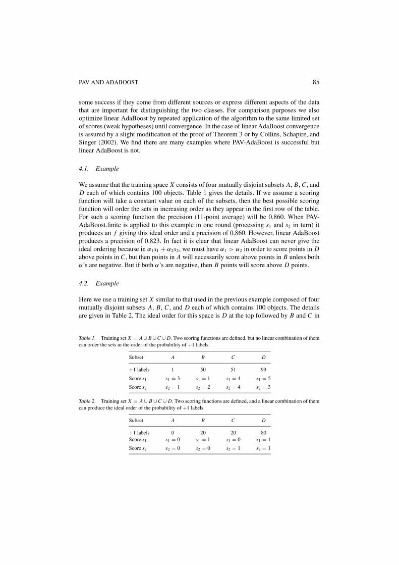
We assume that the training space X consists of four mutually disjoint subsets A, B, C , andD each of which contains 100 objects. Table 1 gives the details. If we assume a scoringfunction will take a constant value on each of the subsets, then the best possible scoringfunction will order the sets in increasing order as they appear in the first row of the table.For such a scoring function the precision (11-point average) will be 0.860. When PAV-AdaBoost.finite is applied to this example in one round (processing s1 and s2 in turn) itproduces an f giving this ideal order and a precision of 0.860. However, linear AdaBoostproduces a precision of 0.823. In fact it is clear that linear AdaBoost can never give theideal ordering because in α1s1 + α2s2, we must have α1 > α2 in order to score points in Dabove points in C , but then points in A will necessarily score above points in B unless bothα’s are negative. But if both α’s are negative, then B points will score above D points.
4.2. Example
Here we use a training set X similar to that used in the previous example composed of fourmutually disjoint subsets A, B, C , and D each of which contains 100 objects. The detailsare given in Table 2. The ideal order for this space is D at the top followed by B and C in
Table 1. Training set X = A ∪ B ∪ C ∪ D. Two scoring functions are defined, but no linear combination of themcan order the sets in the order of the probability of +1 labels.
Subset A B C D
+1 labels 1 50 51 99
Score s1 s1 = 3 s1 = 1 s1 = 4 s1 = 5
Score s2 s2 = 1 s2 = 2 s2 = 4 s2 = 3
Table 2. Training set X = A ∪ B ∪ C ∪ D. Two scoring functions are defined, and a linear combination of themcan produce the ideal order of the probability of +1 labels.
Subset A B C D
+1 labels 0 20 20 80Score s1 s1 = 0 s1 = 1 s1 = 0 s1 = 1
Score s2 s2 = 0 s2 = 0 s2 = 1 s2 = 1
86 W.J. WILBUR, L. YEGANOVA AND W. KIM
either order and lowest A. This order is produced in one round by PAV-AdaBoost.finite witha precision of 0.698. When linear AdaBoost is applied the α’s produced are zero leading toa random performance with a precision of 0.300.
4.3. Example
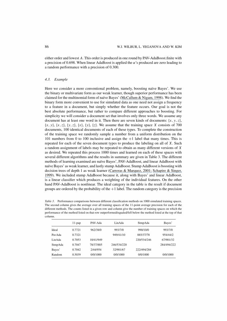
Here we consider a more conventional problem, namely, boosting naı̈ve Bayes’. We usethe binary or multivariate form as our weak learner, though superior performance has beenclaimed for the multinomial form of naı̈ve Bayes’ (McCallum & Nigam, 1998). We find thebinary form more convenient to use for simulated data as one need not assign a frequencyto a feature in a document, but simply whether the feature occurs. Our goal is not thebest absolute performance, but rather to compare different approaches to boosting. Forsimplicity we will consider a document set that involves only three words. We assume anydocument has at least one word in it. Then there are seven kinds of documents: {x, y, z},{x, y}, {x, z}, {y, z}, {x}, {y}, {z}. We assume that the training space X consists of 700documents, 100 identical documents of each of these types. To complete the constructionof the training space we randomly sample a number from a uniform distribution on the101 numbers from 0 to 100 inclusive and assign the +1 label that many times. This isrepeated for each of the seven document types to produce the labeling on all of X . Sucha random assignment of labels may be repeated to obtain as many different versions of Xas desired. We repeated this process 1000 times and learned on each of these spaces withseveral different algorithms and the results in summary are given in Table 3. The differentmethods of learning examined are naı̈ve Bayes’, PAV-AdaBoost, and linear AdaBoost withnaı̈ve Bayes’ as weak learner, and lastly stump AdaBoost. Stump AdaBoost is boosting withdecision trees of depth 1 as weak learner (Carreras & Marquez, 2001; Schapire & Singer,1999). We included stump AdaBoost because it, along with Bayes’ and linear AdaBoost,is a linear classifier which produces a weighting of the individual features. On the otherhand PAV-AdaBoost is nonlinear. The ideal category in the table is the result if documentgroups are ordered by the probability of the +1 label. The random category is the precision
Table 3. Performance comparisons between different classification methods on 1000 simulated training spaces.The second column gives the average over all training spaces of the 11-point average precision for each of thedifferent methods. The counts listed in a given row and column give the number of training spaces on which theperformance of the method listed on that row outperformed/equaled/fell below the method listed at the top of thatcolumn.
11-pap PAV-Ada LinAda StmpAda Bayes’
Ideal 0.7721 962/38/0 993/7/0 990/10/0 993/7/0
PavAda 0.7321 949/41/10 885/37/78 954/44/2
LinAda 0.7053 10/41/949 220/534/246 67/901/32
StmpAda 0.7047 78/37/885 246/534/220 284/494/222
Bayes’ 0.7042 2/44/954 32/901/67 222/494/284
Random 0.5039 0/0/1000 0/0/1000 0/0/1000 0/0/1000
PAV AND ADABOOST 87
produced by dividing the total number of +1 labels by 700. Examination of the data showsthat all the classifiers perform well above random. While PAV-AdaBoost seldom reaches theideal limit, in the large majority of training spaces it does outperform the other classifiers.However, one cannot make any hard and fast rules, because each classifier outperformsevery other classifier on at least some of the spaces generated.
5. The learning capacity and generalizability of PAV-AdaBoost
The previous examples suggest that PAV-AdaBoost is a more powerful learner than linearAdaBoost and the question naturally arises as to the capacity of PAV-AdaBoost and whetherPAV-AdaBoost allows effective generalization. First, it is important to note that the capacityof the individual hypothesis h(x) to shatter a set of points is never increased by the trans-formation to k(h(x)) where k comes from the isotonic regression of +1 labels on h(x). If hcannot distinguish points, then neither can h composed with a monotonic non-decreasingfunction. However, what is true of the output of a single weak learner is not necessarilytrue of the PAV-AdaBoost algorithm. In the appendix we show that the hypothesis spacegenerated by PAV-AdaBoost.finite, based on the PAV algorithm defined in 2.1 and the in-terpolation 2.2, has in many important cases infinite VC dimension. For convenience wewill refer to this as the pure form of PAV-AdaBoost. In the remainder of this section we willgive what we will refer to as the approximate form of PAV-AdaBoost. This approximateform produces a hypothesis space of bounded VC dimension and allows a correspondingrisk analysis, while yet allowing one to come arbitrarily close to the pure PAV-AdaBoost.
Our approximation is based on a finite set of intervals Bt = {I jt }nt
j=1 for each t , whichpartition the real line into disjoint subsets. For convenience we assume these intervals arearranged in order negative to positive along the real line by the indexing j . The Bt willbe used to approximate the pt (s)(defined earlier by 2.1 and 2.2) corresponding to a weakhypothesis ht . For each t the set Bt is assumed to be predetermined independent of whatsample may be under consideration. Generally in applications there is enough informationavailable to choose Bt intelligently and to obtain reasonable approximations.Assuming such a predetermined {Bt }T
t=1, then given {ht }Tt=1 define
bht (x) = j, ht (x) ∈ I jt , 1 ≤ j ≤ nt , 1 ≤ t ≤ T . (39)
The result is a new set of hypotheses, {bht }Tt=1, that approximate {ht }T
t=1. We simply applythe PAV-AdaBoost algorithms to this approximating set. The theorems of Section 3 applyequally to this approximation. In addition we can derive bounds on the risk or expected test-ing error for the binary classification problem. First we have a bound on the VC dimensionof the hypothesis space.
Theorem 4. Let {Bt }Tt=1 denote the set of partitions to be applied to T hypotheses {ht }T
t=1defined on a space X as just described. Let H denote the set of all hypotheses H (x) =sign
(∑Tt=1 kλt (bht (x))
)defined on X where {kλt }T
t=1 varies over all sets of monotonicallynondecreasing functions whose ranges are within [−λ, λ]. Then the VC dimension of Hsatisfies
88 W.J. WILBUR, L. YEGANOVA AND W. KIM
VC ≤T∏
t=1
nt . (40)
Proof: Define sets
Ar1,r2,...,rT =T⋂
t=1
bh−1t [rt ], 1 ≤ rt ≤ nt , 1 ≤ t ≤ T . (41)
Note that these sets partition the space X and that any function of the form H (x) =sign
(∑Tt=1 kλt (bht (x))
)is constant on each such set. Then it is straightforward for the
family of all such functions H (x) that we have the stated bound for the VC dimension.
Vapnik (1998), p. 161, gives the following relationship between expected testing error(R) and empirical testing error (Remp).
R ≤ Remp + E(N )
2
(1 +
√
1 + Remp
E(N )
)(42)
which holds with probability at least 1 − η, where E(N ) depends on the capacity of the setof functions and involves η and the sample size N .
Corollary 2. Let {Bt }Tt=1 denote the set of partitions to be applied to T hypotheses.
If S is any random sample of points from X of size N >∏T
t=1 nt and η > 0 and ifH (x) = sign
(∑Tt=1 kλt (bht (x))
)represents T rounds of PAV-AdaBoost learning or the
result of AdaBoost.finite applied to S, then with probability at least 1 − η the risk (R) orexpected test error of H satisfies inequality
R ≤ R′ + 1
2
(E ′ +
√E ′(E ′ + R′)
)(43)
where
E ′ = 4
N
[ T∏
t=1
nt(1 + log(2N ) −
T∑
t=1
log(nt ))) − log(η/4)
](44)
and
R′ =T∏
t=1
Zt (45)
PAV AND ADABOOST 89
in the case of PAV-AdaBoost or equivalently
R′ = N−1∑
x∈S
exp
[−y(x)
T∑
t=1
kλt (ht (x))
](46)
in the case of PAV-AdaBoost.finite.
Proof: First note that relation (42) can be put in the form (43) by a simple algebraicrearrangement where E(N ) corresponds to E ′ and Remp corresponds to R′. It is evident thatthe right side of (43) is an increasing function of both E ′ and R′ when these are nonnegativequantities. Vapnik (1998) , p. 161, gives the relationship
E(N ) = 4
N
{V C
[ln
(2N
V C
)+ 1
]− ln
(η
4
)}. (47)
The relation (43) then follows from inequality (40) and the bound on N , which insures thatE(N ) ≤ E ′ and the fact that Remp ≤ R′. The latter is true because relations (45) and (46)are simply different expressions for the same bound on the training error (empirical error)for PAV-AdaBoost, but only the second is defined for PAV-AdaBoost.finite.
In practice we use approximate PAV-AdaBoost with a fine partitioning in an attempt tominimize R′. This does not benefit E ′ but we generally find the results quite satisfactory.Two factors may help explain this. First, when the PAV algorithm is applied pooling maytake place and effectively make the number of elements in a partition Bt smaller than nt .Second, bounds of the form (43) are based on the VC dimension and ignore any specificinformation regarding the particular distribution defining a problem. Thus tighter boundsare likely to hold even though we do not know how to establish them in a particular case(Vapnik, 1998). This is consistent with (Burges, 1999; Friedman, Hastie, & Tibshirani,2000) where it is pointed out that in many cases bounds based on the VC dimension aretoo loose to have practical value and performance is much better than the bounds wouldsuggest. However, we note that even when N is not extremely large, E ′ can be quite smallwhen T is small. Thus the relation (43) may yield error bounds of some interest whenPAV-AdaBoost.finite is used to combine only two or three hypotheses.
6. Combining scores
We have applied PAV-AdaBoost to the real task of identifying those terms (phrases) intext that would not make useful references as subject identifiers. This work is part of theelectronic textbook project at the National Center for Biotechnology Information (NCBI).Textbook material is processed and phrases extracted as index terms. Special processing isdone to try to ensure that these phrases are grammatically well formed. Then the phrasesmust be evaluated to decide whether they are sufficiently subject specific to make usefulreference indicators. Examples of phrases considered useful as index terms are muscles,
90 W.J. WILBUR, L. YEGANOVA AND W. KIM
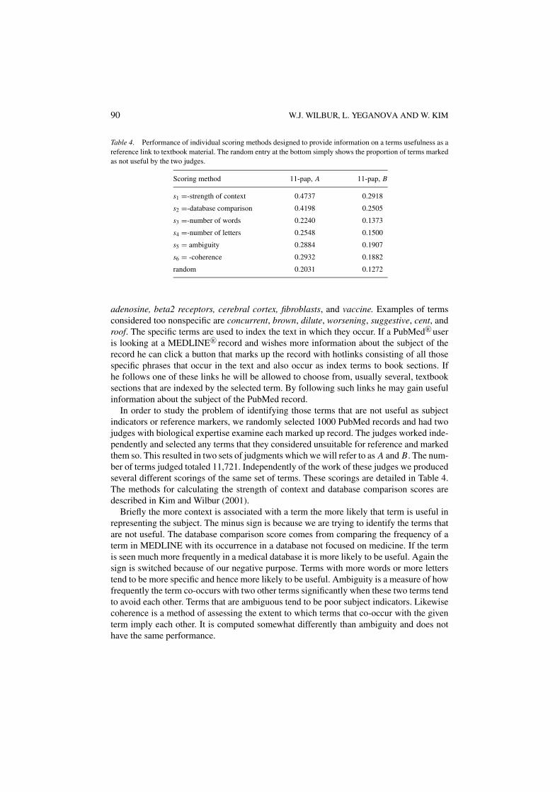
Table 4. Performance of individual scoring methods designed to provide information on a terms usefulness as areference link to textbook material. The random entry at the bottom simply shows the proportion of terms markedas not useful by the two judges.
Scoring method 11-pap, A 11-pap, B
s1 =-strength of context 0.4737 0.2918
s2 =-database comparison 0.4198 0.2505
s3 =-number of words 0.2240 0.1373
s4 =-number of letters 0.2548 0.1500
s5 = ambiguity 0.2884 0.1907
s6 = -coherence 0.2932 0.1882
random 0.2031 0.1272
adenosine, beta2 receptors, cerebral cortex, fibroblasts, and vaccine. Examples of termsconsidered too nonspecific are concurrent, brown, dilute, worsening, suggestive, cent, androof. The specific terms are used to index the text in which they occur. If a PubMed©R useris looking at a MEDLINE©R record and wishes more information about the subject of therecord he can click a button that marks up the record with hotlinks consisting of all thosespecific phrases that occur in the text and also occur as index terms to book sections. Ifhe follows one of these links he will be allowed to choose from, usually several, textbooksections that are indexed by the selected term. By following such links he may gain usefulinformation about the subject of the PubMed record.
In order to study the problem of identifying those terms that are not useful as subjectindicators or reference markers, we randomly selected 1000 PubMed records and had twojudges with biological expertise examine each marked up record. The judges worked inde-pendently and selected any terms that they considered unsuitable for reference and markedthem so. This resulted in two sets of judgments which we will refer to as A and B. The num-ber of terms judged totaled 11,721. Independently of the work of these judges we producedseveral different scorings of the same set of terms. These scorings are detailed in Table 4.The methods for calculating the strength of context and database comparison scores aredescribed in Kim and Wilbur (2001).
Briefly the more context is associated with a term the more likely that term is useful inrepresenting the subject. The minus sign is because we are trying to identify the terms thatare not useful. The database comparison score comes from comparing the frequency of aterm in MEDLINE with its occurrence in a database not focused on medicine. If the termis seen much more frequently in a medical database it is more likely to be useful. Again thesign is switched because of our negative purpose. Terms with more words or more letterstend to be more specific and hence more likely to be useful. Ambiguity is a measure of howfrequently the term co-occurs with two other terms significantly when these two terms tendto avoid each other. Terms that are ambiguous tend to be poor subject indicators. Likewisecoherence is a method of assessing the extent to which terms that co-occur with the giventerm imply each other. It is computed somewhat differently than ambiguity and does nothave the same performance.
PAV AND ADABOOST 91
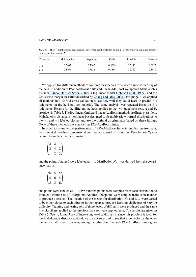
Table 5. The 11-point average precisions of different classifiers tested through 10-fold cross validation separatelyon judgment sets A and B.
Train/test Mahalanobis Log-linear Cmls Lin-Ada PAV-Ada
A/A 0.5402 0.5667 0.5634 0.5140 0.6023
B/B 0.3461 0.3632 0.3614 0.3520 0.3640
We applied five different methods to combine these scores to produce a superior scoring ofthe data. In addition to PAV-AdaBoost.finite and linear AdaBoost we applied Mahalanobisdistance (Duda, Hart, & Stork, 2000), a log-linear model (Johnson et al., 1999), and theCmls wide margin classifier described by Zhang and Oles (2001). For judge A we appliedall methods in a 10-fold cross validation to see how well they could learn to predict A’sjudgments on the held out test material. The same analysis was repeated based on B’sjudgments. Results for the different methods applied to the two judgement sets, A and B,are given in Table 5. The log-linear, Cmls, and linear AdaBoost methods are linear classifiers.Mahalanobis distance is nonlinear but designed to fit multivariate normal distributions tothe +1 and −1 labeled classes and use the optimal discriminator based on these fittings.None of these methods work as well as PAV-AdaBoost.finite.
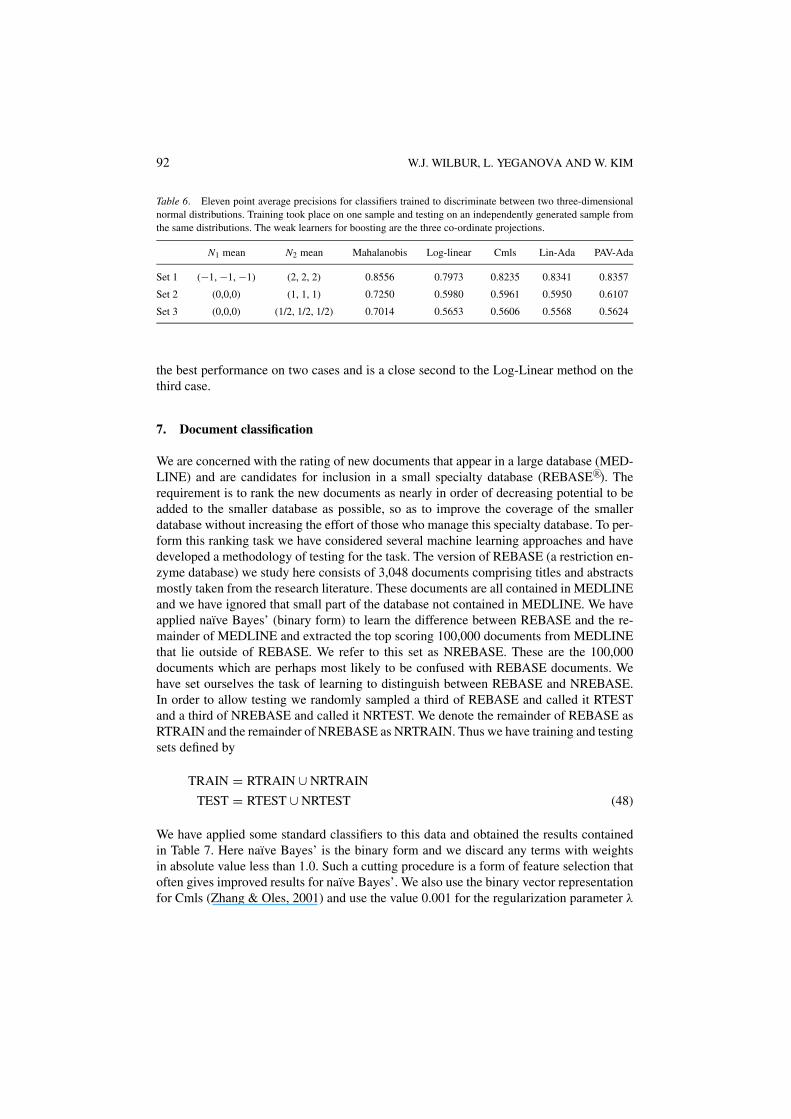
In order to examine the performance of PAV-AdaBoost.finite in another environment,we simulated two three dimensional multivariate normal distributions. Distribution N1 wasderived from the covariance matrix
2 2 1
2 4 2
1 2 2
and the points obtained were labeled as +1. Distribution N−1 was derived from the covari-ance matrix
6 5 5
5 6 5
5 5 6
and points were labeled as −1. Five hundred points were sampled from each distribution toproduce a training set of 1000 points. Another 1000 points were sampled in the same mannerto produce a test set. The location of the means for distribution N1 and N−1 were variedto be either closer to each other or farther apart to produce learning challenges of varyingdifficulty. Training and testing sets of three levels of difficulty were produced and the samefive classifiers applied to the previous data set were applied here. The results are given inTable 6. Sets 1, 2, and 3 are of increasing level of difficulty. Since this problem is ideal forthe Mahalanobis distance method, we are not surprised to see that it outperforms the othermethods in all cases. However, among the other four methods PAV-AdaBoost.finite gives
92 W.J. WILBUR, L. YEGANOVA AND W. KIM
Table 6. Eleven point average precisions for classifiers trained to discriminate between two three-dimensionalnormal distributions. Training took place on one sample and testing on an independently generated sample fromthe same distributions. The weak learners for boosting are the three co-ordinate projections.
N1 mean N2 mean Mahalanobis Log-linear Cmls Lin-Ada PAV-Ada
Set 1 (−1, −1, −1) (2, 2, 2) 0.8556 0.7973 0.8235 0.8341 0.8357
Set 2 (0,0,0) (1, 1, 1) 0.7250 0.5980 0.5961 0.5950 0.6107
Set 3 (0,0,0) (1/2, 1/2, 1/2) 0.7014 0.5653 0.5606 0.5568 0.5624
the best performance on two cases and is a close second to the Log-Linear method on thethird case.
7. Document classification
We are concerned with the rating of new documents that appear in a large database (MED-LINE) and are candidates for inclusion in a small specialty database (REBASE©R). Therequirement is to rank the new documents as nearly in order of decreasing potential to beadded to the smaller database as possible, so as to improve the coverage of the smallerdatabase without increasing the effort of those who manage this specialty database. To per-form this ranking task we have considered several machine learning approaches and havedeveloped a methodology of testing for the task. The version of REBASE (a restriction en-zyme database) we study here consists of 3,048 documents comprising titles and abstractsmostly taken from the research literature. These documents are all contained in MEDLINEand we have ignored that small part of the database not contained in MEDLINE. We haveapplied naı̈ve Bayes’ (binary form) to learn the difference between REBASE and the re-mainder of MEDLINE and extracted the top scoring 100,000 documents from MEDLINEthat lie outside of REBASE. We refer to this set as NREBASE. These are the 100,000documents which are perhaps most likely to be confused with REBASE documents. Wehave set ourselves the task of learning to distinguish between REBASE and NREBASE.In order to allow testing we randomly sampled a third of REBASE and called it RTESTand a third of NREBASE and called it NRTEST. We denote the remainder of REBASE asRTRAIN and the remainder of NREBASE as NRTRAIN. Thus we have training and testingsets defined by
TRAIN = RTRAIN ∪ NRTRAIN
TEST = RTEST ∪ NRTEST (48)
We have applied some standard classifiers to this data and obtained the results containedin Table 7. Here naı̈ve Bayes’ is the binary form and we discard any terms with weightsin absolute value less than 1.0. Such a cutting procedure is a form of feature selection thatoften gives improved results for naı̈ve Bayes’. We also use the binary vector representationfor Cmls (Zhang & Oles, 2001) and use the value 0.001 for the regularization parameter λ

PAV AND ADABOOST 93
Table 7. Results of some standard classifiers on the REBASE learning task.
Classifier Naı̈ve Bayes’ KNN Cmls
11-pap 0.775 0.783 0.819
as suggested in Zhang and Oles, (2001). KNN is based on a vector similarity computationusing IDF global term weights and a tf local weighting formula. If tf denotes the frequencyof term t within document d and dlen denotes the length of d (sum of all tf ′ for all t ′in d)then we define the local weight
lwt f = 1
1 + λt f −1 exp(α · dlen)(49)
where α = 0.0044 and λ = 0.7. This formula is derived from the Poisson model of termfrequencies within documents (Kim, Aronson, & Wilbur, 2001; Robertson & Walker, 1994)and has been found to give good performance on MEDLINE documents. The similarity oftwo documents is the dot product of their vectors and no length correction is used as thatis already included in definition (49). KNN computes the similarity of a document in thetest set to all the documents in the training set and adds up the similarity scores of all thosedocuments in the training set that are class +1 (in RTRAIN in this case) in the top K ranks.We use a K of 60 here.
One obvious weak learner amenable to boosting is naı̈ve Bayes’. We applied linearAdaBoost and obtained a result on the test set of 0.783 on the third round of boosting. Withnaı̈ve Bayes’ as the weak learner PAV-AdaBoost does not give any improvement. We willdiscuss the reason for this subsequently. Our interest here is to show examples of weaklearners where PAV-AdaBoost is successful.
One example where PAV-AdaBoost is successful is with what we will call the Cmassweak learner.
7.1. Cmass algorithm
Assume a probability distribution D(i) on the training space X = {(�xi , yi )}mi=1. Let P denote
that subset of X with +1 labels and N the subset with −1 labels. To produce h perform thesteps:
(i) Use D (i) to weight the points of P and compute the centroid �cp.(ii) Similarly weight the points of N and compute the centroid �cn .
(iii) Define �w = �cp − �cn and h(�x) = �w · �x for any �x .
With the Cmass weak learner PAV-AdaBoost gives the results depicted in Figure 1. PAV-AdaBoost reaches a peak score just above 0.8 after about 60 iterations. Since Cmass isvery efficient to compute it takes just under eleven minutes to produce one hundred rounds
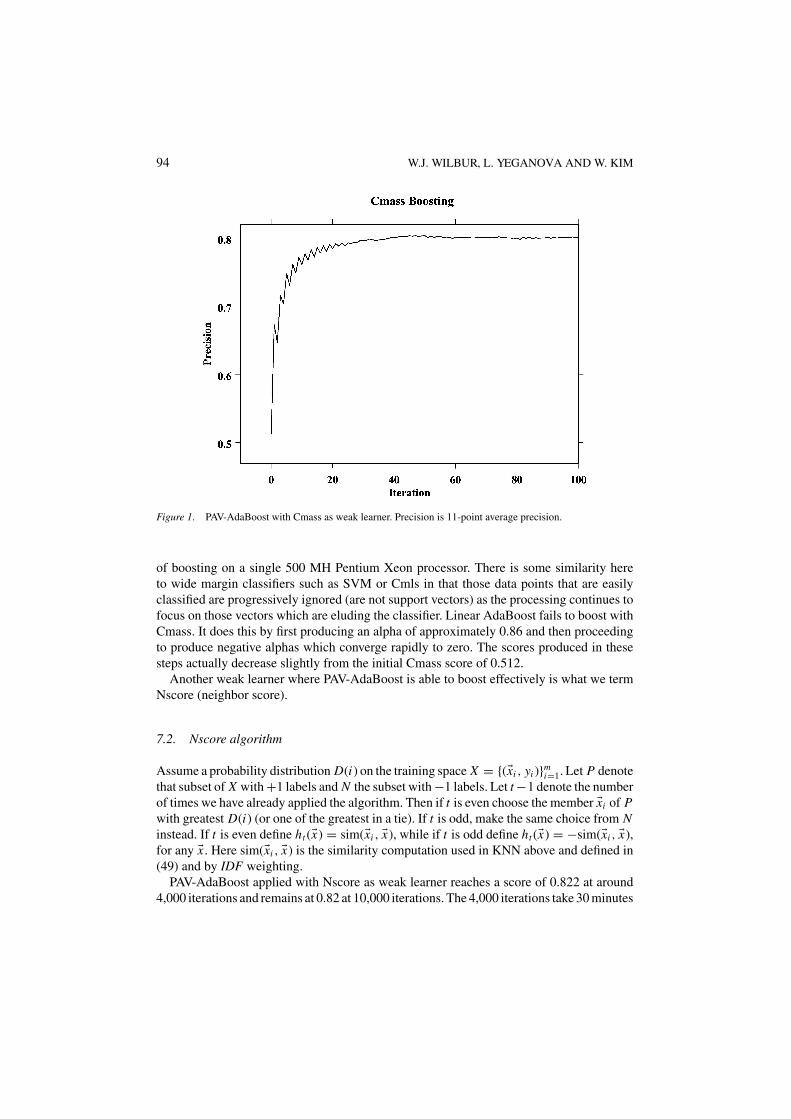
94 W.J. WILBUR, L. YEGANOVA AND W. KIM
Figure 1. PAV-AdaBoost with Cmass as weak learner. Precision is 11-point average precision.
of boosting on a single 500 MH Pentium Xeon processor. There is some similarity hereto wide margin classifiers such as SVM or Cmls in that those data points that are easilyclassified are progressively ignored (are not support vectors) as the processing continues tofocus on those vectors which are eluding the classifier. Linear AdaBoost fails to boost withCmass. It does this by first producing an alpha of approximately 0.86 and then proceedingto produce negative alphas which converge rapidly to zero. The scores produced in thesesteps actually decrease slightly from the initial Cmass score of 0.512.
Another weak learner where PAV-AdaBoost is able to boost effectively is what we termNscore (neighbor score).
7.2. Nscore algorithm
Assume a probability distribution D(i) on the training space X = {(�xi , yi )}mi=1. Let P denote
that subset of X with +1 labels and N the subset with −1 labels. Let t −1 denote the numberof times we have already applied the algorithm. Then if t is even choose the member �xi of Pwith greatest D(i) (or one of the greatest in a tie). If t is odd, make the same choice from Ninstead. If t is even define ht (�x) = sim(�xi , �x), while if t is odd define ht (�x) = −sim(�xi , �x),for any �x . Here sim(�xi , �x) is the similarity computation used in KNN above and defined in(49) and by IDF weighting.
PAV-AdaBoost applied with Nscore as weak learner reaches a score of 0.822 at around4,000 iterations and remains at 0.82 at 10,000 iterations. The 4,000 iterations take 30 minutes
PAV AND ADABOOST 95
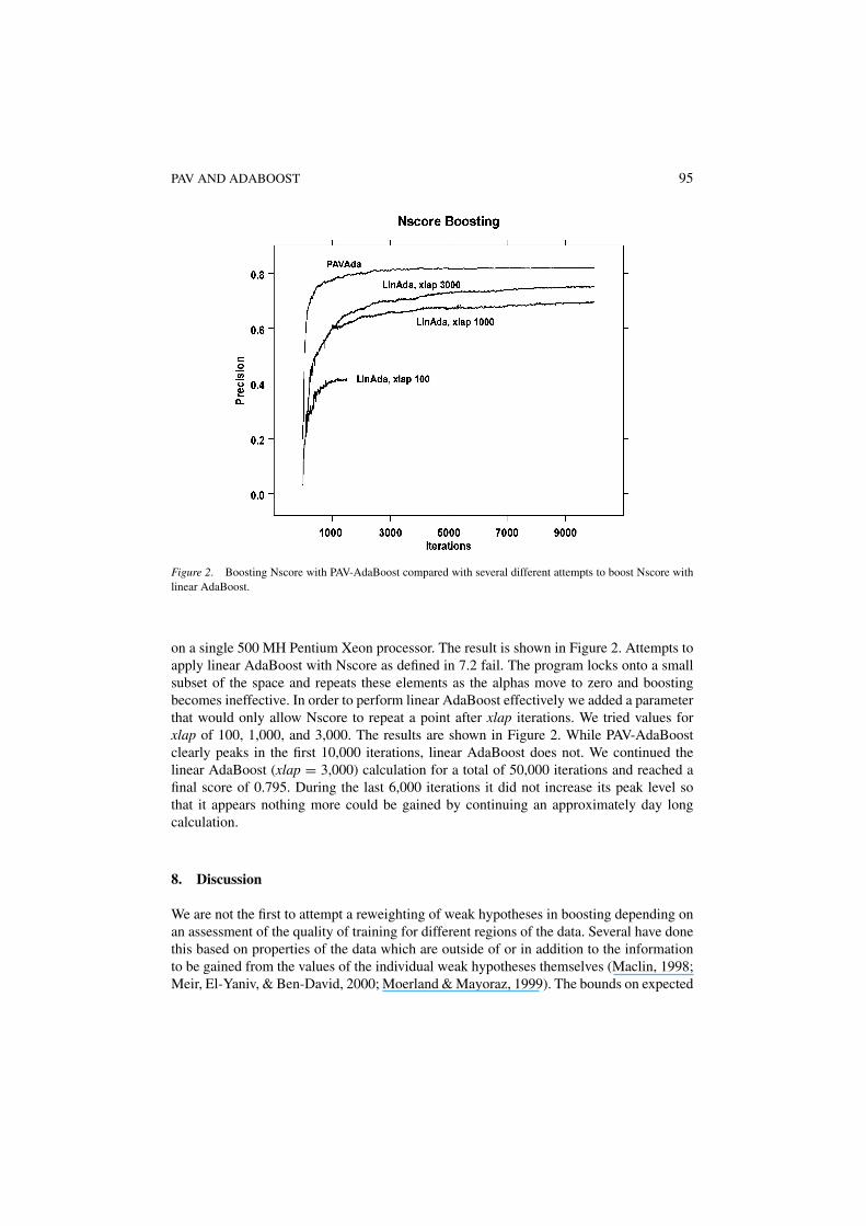
Figure 2. Boosting Nscore with PAV-AdaBoost compared with several different attempts to boost Nscore withlinear AdaBoost.
on a single 500 MH Pentium Xeon processor. The result is shown in Figure 2. Attempts toapply linear AdaBoost with Nscore as defined in 7.2 fail. The program locks onto a smallsubset of the space and repeats these elements as the alphas move to zero and boostingbecomes ineffective. In order to perform linear AdaBoost effectively we added a parameterthat would only allow Nscore to repeat a point after xlap iterations. We tried values forxlap of 100, 1,000, and 3,000. The results are shown in Figure 2. While PAV-AdaBoostclearly peaks in the first 10,000 iterations, linear AdaBoost does not. We continued thelinear AdaBoost (xlap = 3,000) calculation for a total of 50,000 iterations and reached afinal score of 0.795. During the last 6,000 iterations it did not increase its peak level sothat it appears nothing more could be gained by continuing an approximately day longcalculation.
8. Discussion
We are not the first to attempt a reweighting of weak hypotheses in boosting depending onan assessment of the quality of training for different regions of the data. Several have donethis based on properties of the data which are outside of or in addition to the informationto be gained from the values of the individual weak hypotheses themselves (Maclin, 1998;Meir, El-Yaniv, & Ben-David, 2000; Moerland & Mayoraz, 1999). The bounds on expected
96 W.J. WILBUR, L. YEGANOVA AND W. KIM
testing error in (Meir, El-Yaniv, and Ben-David, 2000) are based on a partition of thespace and show a dependency on the dimension of that space very similar to our results inTheorem 4 and Corollary 2. Our general approach, however, is more closely related to themethod of Aslam (2000) in that our reweighting depends only on the relative success ofeach weak hypothesis in training. Aslam evaluates success on the points with positive andnegative label independently and thereby decreases the bound on training error. In a sensewe carry this approach to its logical limit and decrease the bound on the training error asmuch as possible within the paradigm of confidence rated predictions. Our only restrictionis that we do not allow the reweighting to reverse the order of the original predictionsmade by a weak learner. Because our approach can be quite drastic in its effects there isa tendency to over train. Corollary 2 suggests that in the limit of large samples resultsshould be very good. However in practical situations one is forced to rely on experiencewith the method. Of course this is generally the state of the art for all machine learningmethods.
An important issue is when PAV-AdaBoost can be expected to give better performancethan linear AdaBoost. The short answer to this question is that all the examples in theprevious two sections where PAV-AdaBoost is quite successful involve weak hypothesesthat are intrinsic to the data and not produced by some optimization process applied to atraining set. As an example of this distinction let the entire space consist of a certain set Xof documents and let w be a word that occurs in some of these documents but not others.Suppose that some of these documents that are about a particular topic have the +1 labeland the remainder the -1 label. Then the function
hw(x) ={
1, w ∈ x
0, w /∈ x(50)
is what we are referring to as an intrinsic function. Its value does not depend on a sample fromX . On the other hand if we take a random sample Y ⊆ X which is reasonably representativeof the space, then we can define the Bayesian weight bw associated with w. If we define thefunction
h′w(x) =
{bw, w ∈ x
0, w /∈ x(51)
Then it is evident that h′w depends on the sample as well as the word w. It is not intrinsic to the
space X of documents. We believe this distinction is important as the non-intrinsic functionh′
w is already the product of an optimization process. Since PAV is itself an optimizationprocess it may be that applying one optimization process to the output of another is simplytoo much optimization to avoid over training in most cases.
We believe naı̈ve Bayes’ provides an instructive example in discussing this issue. Bayesianscores produced on a training set do not correspond to an intrinsic function because the samedata point may receive a different score if the sample is different. Thus it is evident thatthere is already an optimization process involved in Bayesian weighting and scoring. Inapplying PAV-AdaBoost with naı̈ve Bayes’ as weak learner we find poor performance.Because PAV-AdaBoost is a powerful learner, poor generalizability is best understood as
PAV AND ADABOOST 97
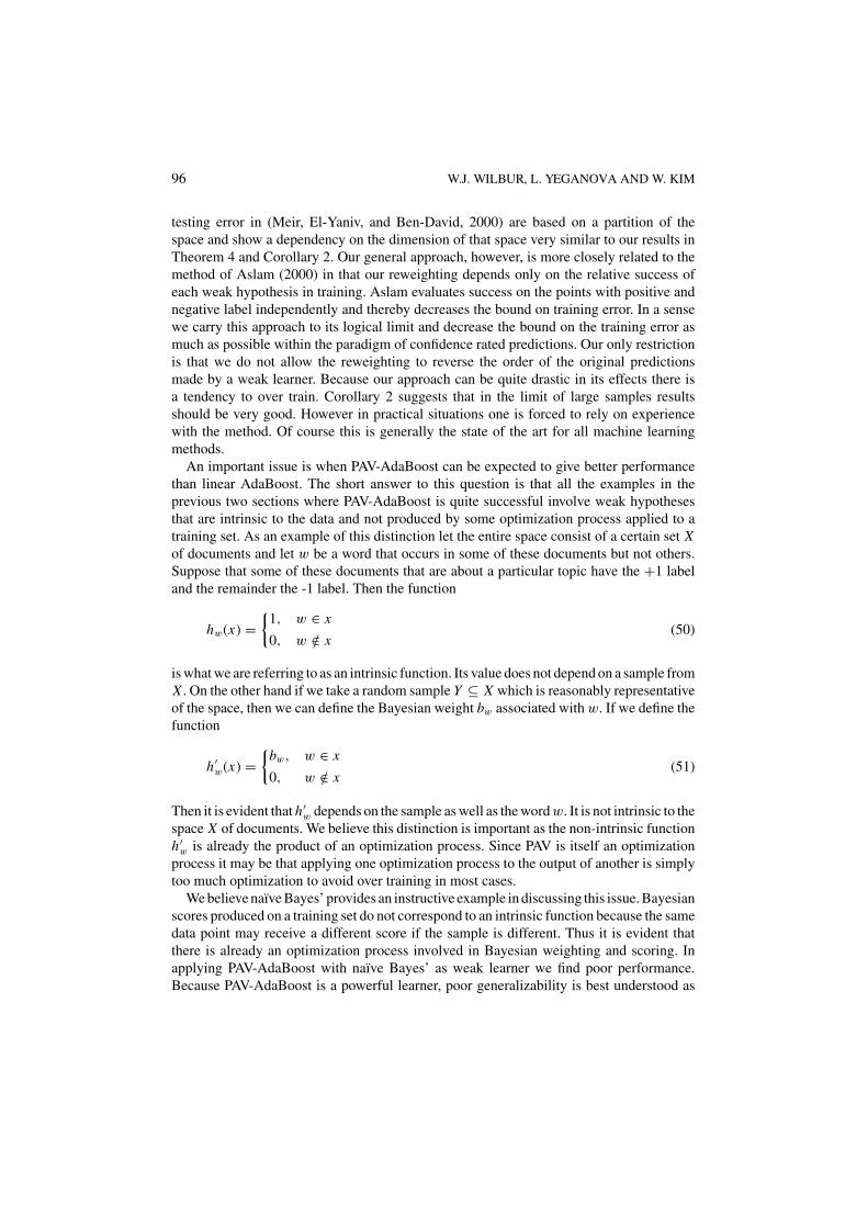
Figure 3. Probability of label class +1 as a function of score as estimated by PAV and by sigmoid curves. Thecurve marked Sigmoid is the estimate implicitly used by linear AdaBoost and is clearly not the optimal sigmoidminimizing Zt . SigmoidOpt is the result of optimization over both w and b in definition (52).
a consequence of overtraining. In the case of PAV-AdaBoost applied to naı̈ve Bayes’ suchovertraining appears as PAV approximates a generally smooth probability function with astep function that reflects the idiosyncrasies of the training data in the individual steps. Wemight attempt to overcome this problem by replacing the step function produced by PAVby a smooth curve. The PAV function derived from naı̈ve Bayes’ training scores (learnedon TRAIN) and a smooth approximation are shown in Figure 3. The smooth curve has theformula
σ (s) = (1 + e−(ws−b)
)−1(52)
and is the sigmoid shape commonly used in neural network threshold units (Mitchell, 1997).The parameters w and b have been optimized to minimize Z . If we use this function as wedo p(s) in definition (14) we obtain
k(s) = 1
2ln
(σ (s)
1 − σ (s)
)= 1
2(ws − b). (53)
Thus if we set b = 0 and optimize on w alone to minimize Z , we find that the function(52) gives the probability estimate used implicitly by linear AdaBoost with α = w/2. Theresultant sigmoid curve is also shown in Figure 3. From this picture it is clear that neitherPAV-AdaBoost nor linear AdaBoost are ideal for boosting naı̈ve Bayes’. PAV-AdaBoost
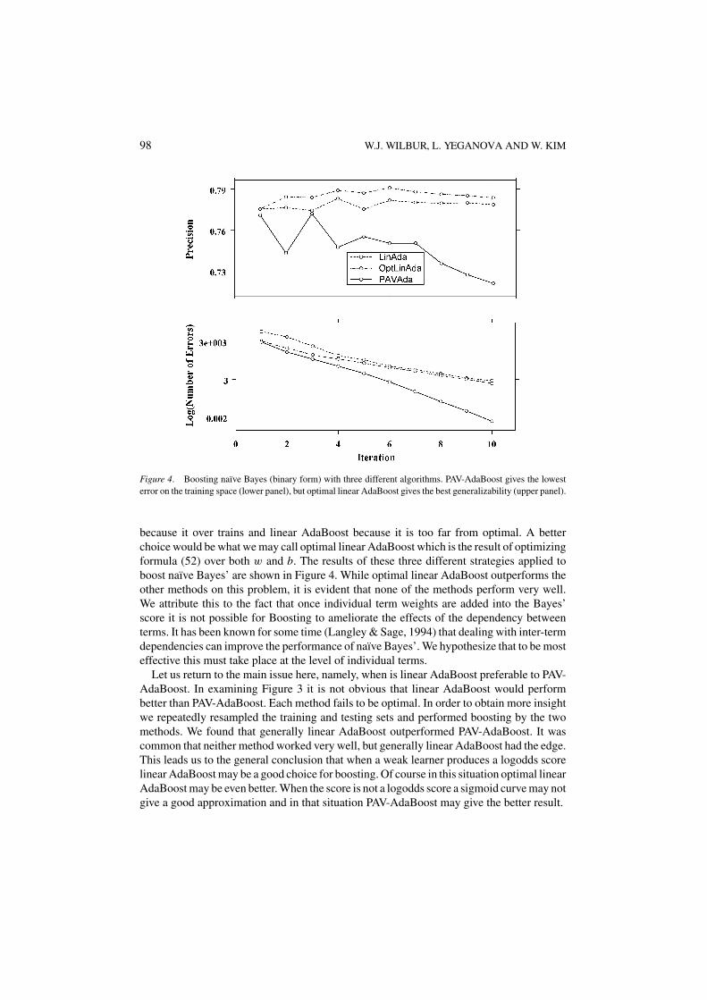
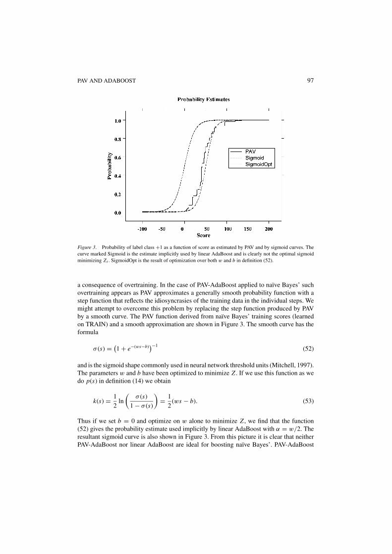
98 W.J. WILBUR, L. YEGANOVA AND W. KIM
Figure 4. Boosting naïve Bayes (binary form) with three different algorithms. PAV-AdaBoost gives the lowesterror on the training space (lower panel), but optimal linear AdaBoost gives the best generalizability (upper panel).
because it over trains and linear AdaBoost because it is too far from optimal. A betterchoice would be what we may call optimal linear AdaBoost which is the result of optimizingformula (52) over both w and b. The results of these three different strategies applied toboost naı̈ve Bayes’ are shown in Figure 4. While optimal linear AdaBoost outperforms theother methods on this problem, it is evident that none of the methods perform very well.We attribute this to the fact that once individual term weights are added into the Bayes’score it is not possible for Boosting to ameliorate the effects of the dependency betweenterms. It has been known for some time (Langley & Sage, 1994) that dealing with inter-termdependencies can improve the performance of naı̈ve Bayes’. We hypothesize that to be mosteffective this must take place at the level of individual terms.
Let us return to the main issue here, namely, when is linear AdaBoost preferable to PAV-AdaBoost. In examining Figure 3 it is not obvious that linear AdaBoost would performbetter than PAV-AdaBoost. Each method fails to be optimal. In order to obtain more insightwe repeatedly resampled the training and testing sets and performed boosting by the twomethods. We found that generally linear AdaBoost outperformed PAV-AdaBoost. It wascommon that neither method worked very well, but generally linear AdaBoost had the edge.This leads us to the general conclusion that when a weak learner produces a logodds scorelinear AdaBoost may be a good choice for boosting. Of course in this situation optimal linearAdaBoost may be even better. When the score is not a logodds score a sigmoid curve may notgive a good approximation and in that situation PAV-AdaBoost may give the better result.
PAV AND ADABOOST 99
Finally, there is the question of why PAV-AdaBoost applied to Nscore produces such agood result. The score of 0.822 is superior to the results in Table 7. We have only been able toproduce a higher score on this training-testing pair by applying AdaBoost to optimally boostover 20,000 depth four decision trees. By this means we have obtained a score just largerthan 0.84, but the computation required several days. While this is of theoretical interestit is not very efficient for an approximately 2% improvement. We believe the good resultwith PAV-AdaBoost applied to Nscore is a consequence of the fact that we are dealing witha large set of relatively simple weak learners that have not undergone prior optimization.We see the result of PAV-AdaBoost applied to Nscore as a new and improved version of theK-nearest neighbors algorithm.
Appendix
Here we examine the VC dimension of the set of hypotheses generated by the PAV-AdaBoost.finite algorithm based on the pure form of PAV defined by 2.1. This presupposes afixed set of weak hypotheses {ht }T
t=1 and the set of functions under discussion is all the func-tions H (x) = sign(
∑Tt=1 kλt (ht (x))) obtained by applying PAV-AdaBoost.finite to possible
finite training samples with any possible labeling of the sample points and then extendingthe results globally using the interpolation of 2.2. Let us denote this set of functions byH. Different weightings for points are allowed by PAV-AdaBoost.finite, but to simplify thepresentation we will assume that all points have weight 1.
To begin it is important to note that the algorithm actually acts on samples of the fixed setof points {(h1(x), h2(x), . . . , hT (x))}x∈X in Euclidean T -space. Thus for this purpose wemay disregard the set of weak hypotheses {ht }T
t=1 and focus our attention on finite subsetsof Euclidean T -space where the role of the weak hypotheses is assumed by the co-ordinateprojection functions. We may further observe that whether a set of points can be shatteredby H does not depend on the actual co-ordinate values, but only on the orderings of thepoints induced from their different co-ordinate values. Finally we observe that if a set ofpoints contains points A and B and A is less than or equal to B in all co-ordinate values,then H cannot shatter that set of points. The regressions involved must always score Bequal to or greater than A if B dominates A. It will prove sufficient for our purposes to workin two dimensions. In two dimensions the only way to avoid having one point dominateanother is to have the points strictly ordered in one dimension and strictly ordered in thereverse direction in the other dimension. Thus we may consider a set of N points to berepresented by the N pairs {(ri , b − rN−i+1)}N
i=1 where {ri }Ni=1 is any strictly increasing set
of real numbers and b is an arbitrary real number that may be determined by convenience.We will refer to the ordering induced by the first co-ordinate as the forward ordering, andthe ordering induced by the second co-ordinate as the backward ordering. For a given la-beling of such a set of points (which must contain both positive and negative labels) thePAV-AdaBoost.finite algorithm may be applied and will always yield a solution. This solu-tion will depend only on the number of points, the ordering, and the labels, but not on theactual numbers ri used to represent the points.
In order to shatter sets of points we must examine the nature of solutions coming fromPAV-AdaBoost.finite. Clearly for any labeling of the points we may consider the points

100 W.J. WILBUR, L. YEGANOVA AND W. KIM
as contiguous groups labeled negative or labeled positive and alternating as we move upthe forward order. Let the numbers of points in these groups be given by {mi }K
i=1. We willassume that the lowest group (m1) in the forward order is labeled negative and the highestgroup (mK ) is labeled positive. This will allow us to maintain sufficient generality for ourpurposes. Then K must be an even integer and it will be convenient to represent it by 2k −2.Our approach will be to assume a certain form for the solution of the PAV-AdaBoost.finitescoring functions and use the invariance of these functions under the algorithm to derive theiractual values. For the regression induced function k1obtained from the forward ordering weassume without loss of generality the form
k1(m p) =
α1, p = 1
αi , 2i − 2 ≤ p ≤ 2i − 1, 2 ≤ i ≤ k − 1
αk, p = 2k − 2
(54)
Here k1(m p) denotes the value of k1 on all the points in the group m p. Likewise the k2obtainedfrom the backward ordering is assumed to have the form
k2(m p) = βi , 2i − 1 ≤ p ≤ 2i, 1 ≤ i ≤ k − 1. (55)
By definition (54), αk corresponds to the single group m2k−2 with positive label. As a resultof the forward isotonic regression it follows that α1 = −λ and αk = λ. Now appealing tothe invariance of k1 and k2 under the algorithm (apply one round of PAV-AdaBoost.finiteand k1 and k2 are unchanged) we may derive the relations
α j = −1
2(β j−1 + β j ) + 1
2ln
(m2 j−2
m2 j−1
)
β j = −1
2(α j + α j+1) + 1
2ln
(m2 j
m2 j−1
) (56)
These relations are valid for α j , 2 ≤ j ≤ k − 1 and for all β j , 1 ≤ j ≤ k − 1. By simplyadding to the appropriate expressions in (56) we obtain expressions for the scores over thevarious mi .
score(m2 j−1) = α j + β j = 1
2(α j − α j+1) + 1
2ln
(m2 j
m2 j−1
)
= 1
2(β j − β j−1) + 1
2ln
(m2 j−2
m2 j−1
)
(57)
score(m2 j ) = α j+1 + β j = 1
2(α j+1 − α j ) + 1
2ln
(m2 j
m2 j−1
)
= 1
2(β j − β j+1) + 1
2ln
(m2 j
m2 j+1
)
PAV AND ADABOOST 101
The important observation here is that the odd and even groups will be separated providedthe α j+1 −α j are all positive and not overwhelmed by the log terms. If this can be arrangedproperly it will also guarantee that the regressions are valid as well. By repeated substitutionsusing Eqs. (57) it can be shown that
α j+1 − α j = 1
k − 1(αk − α1) + 1
k − 1
k−1∑
p=1
[ln
(m2 j
m2p
)+ ln
(m2 j−1
m2p−1
)](58)
One crucial result that comes from this relationship is that if all the mi are equal then all thelog terms disappear in Eq. (58) and because α1 = −λ and αk = λ we may conclude fromEqs. (57) that the score of all positive labeled elements is λ/(k − 1) while the score of allnegative labeled elements is −λ/(k − 1). If the mi are all equal to two, let us refer to theresulting function k1 + k2 as a binary solution. Such solutions may be used to shatter twodimensional sets of any number of points.
Let {si }Ni=1 be any strictly increasing set of real numbers and {(si , b − sN−i+1)}N
i=1 thecorresponding set of points in two dimensions. Let a labeling be given that divides theset into contiguous same label groups with the sizes {n j }J
j=1 as one moves up the forwardordering. For definiteness let the group corresponding to n1 have the positive label and thegroup corresponding to n J have the negative label. Our strategy is to sandwich each groupcorresponding to an n j between two elements that form a binary group in a new systemof points for which the binary solution defined above will apply. For any ε > 0 define thestrictly increasing set of numbers {ri }2J+4
i=1 by
ri = s1 + (i − 4)ε, i = 1, 2, 3
r2 j+2 = 2sk + sk+1
3
r2 j+3 = sk + 2sk+1
3
, k =
j∑
q=1
nq , 1 ≤ j < J
ri = sN + (i − 2J − 1)ε, i = 2J + 2, 2J + 3, 2J + 4
(59)
Label the two dimensional set of points coming from {ri }2J+4i=1 in groups of two starting
with negative from the left end and ending in positive at the far right end. Then this set ofpoints has a binary solution and its extension by the interpolation 2.2 separates the positivelabeled and negative labeled points of {(si , b − sN−i+1)}N
i=1 corresponding to the groupings{n j }J
j=1. The construction (59) will vary slightly depending on the labeling of the end groupsof {(si , b − sN−i+1)}N
i=1, but the same result holds regardless. We have proved the following.
Theorem 5. For any choice of λ and in any Euclidean space of dimension two or greater, ifall points have weight one and the weak hypotheses are the co-ordinate projections, then theVC dimension of the set H of all hypotheses that may be generated by PAV-AdaBoost.finiteover arbitrary samples with arbitrary labelings is infinite.
The construction of the sets of points {(si , b − sN−i+1)}Ni=1 and the set of points corre-
sponding to {ri }2J+4i=1 as defined in (59) can all be carried out within any open subset of E2
for any N by simply choosing ε small enough and adjusting b appropriately.
102 W.J. WILBUR, L. YEGANOVA AND W. KIM
Corollary 3. Let {ht }Tt=1 denote a fixed set of weak learners defined on a space X and define
U : X → ET by U (x) = (h1(x), h2(x), . . . , hT (x)). Assume that all points have weightone. If the image of X under U contains an open subset of a 2-dimensional hyperplaneparallel to two of the co-ordinate axes in ET , then for any λ the set of hypotheses comingfrom PAV-AdaBoost.finite applied to {ht }T
t=1 over all possible samples of X and arbitrarylabelings has infinite VC dimension.
Acknowledgments
The authors would like to thank the anonymous referees for very helpful comments inrevising this work.
References
Apte, C., Damerau, F., & Weiss, S. (1998). Text mining with decision rules and decision trees. ConferenceProceedings The Conference on Automated Learning and Discovery, CMU.
Aslam, J. (2000). Improving algorithms for boosting. Conference Proceedings 13th COLT. Palo Alto, California.Ayer, M., Brunk, H. D., Ewing, G. M., Reid, W. T., & Silverman, E. (1954). An empirical distribution function
for sampling with incomplete information. Annals of Mathematical Statistics, 26, 641–647.Bennett, K. P., Demiriz, A., & Shawe-Taylor, J. (2000). A column generation algorithm for boosting. Conference
Proceedings 17th ICML.Buja, A., Hastie, T., & Tibshirani, R. (1989). Linear smoothers and additive models. The Annals of Statistics, 17:2
453–555.Burges, C. J. C. (1999). A tutorial on support vector machines for pattern recognition (Available electronically
from the author): Bell Laboratories, Lucent Technologies.Carreras, X., & Marquez, L. (2001). September 5–7, 2001. Boosting trees for anti-spam email filtering. Conference
Proceedings RANLP2001, Tzigov Chark, Bulgaria.Collins, M., Schapire, R. E., & Singer, Y. (2002). Logistic regression, AdaBoost and Bregman distances. Machine
Learning, 48:1, 253–285.Duda, R. O., Hart, P. E., & Stork, D. G. (2000). Pattern Classification (2 edn.). New York: John Wiley & Sons,
Inc.Duffy, N., & Helmbold, D. (1999). Potential boosters? Conference Proceedings Advances in Neural Information
Processing Systems 11.Duffy, N., & Helmbold, D. (2000). Leveraging for regression. Conference Proceedings 13th Annual Conference
on Computational Learning Theory. San Francisco.Freund, Y., & Schapire, R. E. (1997). A decision-theoretic generalization of on-line learning and an application
to boosting. Journal or Computer and System Sciences, 55:1, 119–139.Friedman, J., Hastie, T., & Tibshirani, R. (2000). Additive logistic regression: A statistical view of boosting. The
Annals of Statistics, 38:2, 337–374.Hardle, W. (1991). Smoothing Techniques: With Implementation in S. New York: Springer-Verlag.Johnson, M., Geman, S., Canon, S., Chi, Z., & Riezler, S. (1999). Estimators for stochastic “unification-based”
grammars. Conference Proceedings Proceedings ACL’99. Univ. Maryland.Kim, W., Aronson, A. R., & Wilbur, W. J. (2001). Automatic MeSH term assignment and quality assessment.
Conference Proceedings Proc. AMIA Symp. Washington, D.C.Kim, W. G., & Wilbur, W. J. (2001). Corpus-based statistical screening for content-bearing terms. Journal of the
American Society for Information Science, 52:3, 247–259.Langley, P., & Sage, S. (1994). Induction of selective Bayesian classifiers. Conference Proceedings Tenth Confer-
ence on Uncertainty in Artificial Intelligence, Seattle, WA.Maclin, R. (1998). Boosting classifiers locally. Conference Proceedings Proceedings of AAAI.
PAV AND ADABOOST 103
Mason, L., Bartlett, P. L., & Baxter, J. (2000). Improved generalizations through explicit optimizations of margins.Machine Learning, 38, 243–255.
McCallum, A., & Nigam, K. (1998). A comparison of event models for naive bayes text classification. ConferenceProceedings AAAI-98 Workshop on Learning for Text Categorization.
Meir, R., El-Yaniv, R., & Ben-David, S. 2000. Localized boosting. Conference Proceedings 13th COLT. Palo Alto,California.
Mitchell, T. M. (1997). Machine learning. Boston: WCB/McGraw-Hill.Moerland, P., & Mayoraz, E. (1999). DynamBoost: combining boosted hypotheses in a dynamic way (Technical
Report RR 99-09): IDIAP Switzerland.Nock, R., & Sebban, M. (2001). A Bayesian boosting theorem. Pattern Recognition Letters, 22, 413–419.Pardalos, P. M., & Xue, G. (1999). Algorithms for a class of isotonic regression problems. Algorithmica, 23,
211–222.Ratsch, G., Mika, S., & Warmuth, M. K. (2001).On the Convergence of Leveraging (NeuroCOLT2 Technical
Report 98). London: Royal Holloway College.Ratsch, G., Onoda, T., & Muller, K.-R. (2001). Soft margins for AdaBoost. Machine Learning, 42, 287–320.Robertson, S. E., & Walker, S. (1994). Some simple effective approximations to the 2-Poisson model for prob-
abilistic weighted retrieval. Conference Proceedings 17th Annual International ACM SIGIR Conference onResearch and Development in Information Retrieval.
Schapire, R. E., & Singer, Y. (1999). Improved boosting algorithms using confidence-rated predictions. MachineLearning, 37:3, 297–336.
Vapnik, V. (1998). Statistical Learning Theory. New York: John Wiley & Sons, Inc.Witten, I. H., Moffat, A., & Bell, T. C. (1999). Managing Gigabytes (2 edn.). San Francisco: Morgan-Kaufmann
Publishers, Inc.Zhang, T., & Oles, F. J. (2001). Text categorization based on regularized linear classification methods. Information
Retrieval, 4:1, 5–31.
Received June 20, 2003Revised March 8, 2005Accepted March 10, 2005