the robo-investors from graham-doddsville - eth zürich

The Robo-Investors fromGraham-Doddsville

Applying Machine Learning to the Investment Choices ofWarren Buffett

Bachelor Thesis

Ernst Florian Schweizer-Gamborino

December, 2020

Advisors: Prof. Didier Sornette, Dongshuai Zhao, CFA

Department of Computational Sciences, ETH Zurich

Abstract

Recent advances in machine learning techniques have raised the hopes thatthe investment decisions of so-called super-investors could be replicated bycomplex algorithms. This thesis aims to determine how much of this hope iswell-founded. In particular, it investigates the performance of several well-established machine learning methods trained on the investment decisionsof Warren Buffett as reported by Berkshire Hathaway via their 13-F filingsfrom 1997 to 2019. The data underlying this binary classification task wascollected on all companies publicly traded in the US during the pertinenttime span, taking solely their fundamentals into account. The results showa definitive advantage of machine learning methods over using linear mod-els, possibly pushing this approach into the realm of feasible and profitableinvestment strategies.

Acknowledgements

To professor Didier Sornette, who introduced me to the art of rationallylooking at markets, and to my resourceful and patient advisor DongshuaiZhao, who handled the more technical parts of said introduction, I extendmy deepest gratitude. A special mention is deserved by Dr. Diana Gam-borino – my wife – who worked wonders on my motivation. AdditionallyI feel most thankful for the time and attention of Dr. Sarah Vermij and Dr.Ruya Yuksel, whose proof-reading and critique was vital to presenting athesis that has a running chance of being understood by any reader.

Contents

Contents iii

1 Introduction 1

2 Data Collection and Processing 52.1 Data Collection . . . . . . . . . . . . . . . . . . . . . . . . . . . 5

2.1.1 Warren Buffet Picks . . . . . . . . . . . . . . . . . . . . 52.1.2 Company Screening . . . . . . . . . . . . . . . . . . . . 52.1.3 Company Year Assignment . . . . . . . . . . . . . . . . 52.1.4 Company Data Collection . . . . . . . . . . . . . . . . . 6

2.2 Data Transformation . . . . . . . . . . . . . . . . . . . . . . . . 62.2.1 Company Data Cleaning . . . . . . . . . . . . . . . . . 62.2.2 Company Data Feature Engineering . . . . . . . . . . . 6

2.3 Splitting . . . . . . . . . . . . . . . . . . . . . . . . . . . . . . . 72.3.1 Train - Test Split . . . . . . . . . . . . . . . . . . . . . . 72.3.2 Data Layout so far . . . . . . . . . . . . . . . . . . . . . 7

2.4 Patterns in the Data . . . . . . . . . . . . . . . . . . . . . . . . . 82.4.1 Principal Component Analysis . . . . . . . . . . . . . . 82.4.2 Class-Conditioned Variable Correlation . . . . . . . . . 8

2.5 Advanced Statistical Properties . . . . . . . . . . . . . . . . . . 92.5.1 Averages . . . . . . . . . . . . . . . . . . . . . . . . . . . 92.5.2 Feature Importance . . . . . . . . . . . . . . . . . . . . . 102.5.3 Feature Importance by Obscuration . . . . . . . . . . . 112.5.4 Synopsis . . . . . . . . . . . . . . . . . . . . . . . . . . . 11

3 Methodology 173.1 Evaluation Metrics . . . . . . . . . . . . . . . . . . . . . . . . . 17

3.1.1 Accuracy, Recall, and Precision . . . . . . . . . . . . . . 173.1.2 Receiver Operator Characteristics and Area Under the

Curve . . . . . . . . . . . . . . . . . . . . . . . . . . . . . 18

iii

Contents

3.2 The Importance of Cross-Validation . . . . . . . . . . . . . . . 183.3 Models Used . . . . . . . . . . . . . . . . . . . . . . . . . . . . . 18

3.3.1 Baseline . . . . . . . . . . . . . . . . . . . . . . . . . . . 193.3.2 Support Vector Machine . . . . . . . . . . . . . . . . . . 193.3.3 Boosted Ensemble . . . . . . . . . . . . . . . . . . . . . 203.3.4 Neural Network . . . . . . . . . . . . . . . . . . . . . . 203.3.5 Hybrid Model . . . . . . . . . . . . . . . . . . . . . . . . 21

4 Results and Discussion 234.1 Performance and Comparison . . . . . . . . . . . . . . . . . . . 23

4.1.1 Baseline . . . . . . . . . . . . . . . . . . . . . . . . . . . 234.1.2 Support Vector Machine . . . . . . . . . . . . . . . . . . 244.1.3 Boosted Ensemble . . . . . . . . . . . . . . . . . . . . . 244.1.4 Neural Network . . . . . . . . . . . . . . . . . . . . . . 244.1.5 Hybrid Model . . . . . . . . . . . . . . . . . . . . . . . . 254.1.6 Comparison . . . . . . . . . . . . . . . . . . . . . . . . . 25

4.2 Discussion . . . . . . . . . . . . . . . . . . . . . . . . . . . . . . 25

A Appendix 31A.1 Variable Statistics . . . . . . . . . . . . . . . . . . . . . . . . . . 31

A.1.1 Average Differences . . . . . . . . . . . . . . . . . . . . 31A.1.2 Variable Importance by XGBoost . . . . . . . . . . . . . 33A.1.3 Implied Variable Importance . . . . . . . . . . . . . . . 35

A.2 Selected Companies . . . . . . . . . . . . . . . . . . . . . . . . 36A.2.1 Linear Model Predictions . . . . . . . . . . . . . . . . . 36A.2.2 SVM Predictions . . . . . . . . . . . . . . . . . . . . . . 41A.2.3 XGBoost Predictions . . . . . . . . . . . . . . . . . . . . 44A.2.4 Neural Network Predictions . . . . . . . . . . . . . . . 46A.2.5 Hybrid Model Predictions . . . . . . . . . . . . . . . . . 47

A.3 Code . . . . . . . . . . . . . . . . . . . . . . . . . . . . . . . . . 49

Bibliography 51

iv

Chapter 1

Introduction

If a business is worth a dollarand I can buy it for 40 cents,something good may happen tome.

Warren Buffett

For anyone working in a contemporary financial institution or an investmentfirm, they will most probably work with an abundance of data - data whichneeds collecting, processing, analysing, and most importantly, interpreting.All these stages need the attentive care of specialists, and every little steptowards furthering the productivity and accuracy of this process will con-tribute to the potential profitability of future investments. When it comes tothe analysis and interpretation of financial data, the conventional weaponof choice has been linear regression, or, if one has acquired unusually manydata-points on the usual amount of samples, its cousin sparsified linear re-gression. This is an efficient first approach that has yielded many importantresults that are easily interpretable, but often fails with the complex struc-ture and the noisiness of financial data. Due to the exponential growth ofcomputing power - modern-day laptops surpass supercomputers that havebeen in existence for a mere 20 years - we have access to machine learningmethods that were unimaginable only decades ago. These tools can dealwith massive amounts of data and can detect subtle, complex patterns thatsometimes escape the notice of the human eye, a feat that may revolutionisefinancial statement interpretation.

Machine learning algorithms have found widespread use in many fieldsincluding medical diagnosis, computer vision, and natural language under-standing. In finance and accounting their use has already been proven note-worthy in the areas of fraud detection, lending evaluation, risk assessment,

1

1. Introduction

and other fields. Their advantages compared to more conventional statisticalmodels are two-fold: Machine learning algorithms can potentially uncovernonlinear relationships and subtle patterns in the data, and easily deal withcases where two or more variables are highly collinear. A significant draw-back can be the risk of over-fitting, which means that due to the high dimen-sionality of its parameters, a machine learning algorithm can perfectly fit thetraining data yet predict nothing useful, an outcome that is exacerbated ifthe data exhibits high levels of noise. Despite the significant progress in theapplication of machine learning algorithms that study a plethora of financialfactors influencing the expected returns (Wang and Luo, 2012; Zimmerman,2016) [38, 27], this thesis will solely focus on the fundamentals of companiesand entirely disregard financial time series data, which exhibits a very lowsignal-to-noise-ratio. Another reason why we don’t directly use stock per-formance data as a learning target is that it might be heavily influenced bydecisions that have little to do with the intrinsic value of a company.

Historically we can trace back the beginnings of automated financial state-ment report classification to discriminate analysis, (Altman, 1968) [3] whichused several ratios to predict company bankruptcy. Other simple modelswere introduced later to detect financial fraud and earnings manipulation,combining several ratios into a predictive model (Beneish, 1997) [5]. Shortlyafterward, machine learning algorithms were proven to be more powerfuland useful when it comes to classification (Feroz et al., 2000; Lin et al., 2003;Kotsiantis et al., 2006; Perols, 2011) [14, 22, 21, 32], making the decision pro-cess more objective and exploiting the existing data more efficiently. Com-pared to conventional statistical models they don’t require time-consumingprocesses of proposing relations and then proving or disproving them.

An effective method of improving the signal-to-noise ratio in order to re-duce the risk of over-fitting is using domain expertise to enhance the finan-cial statement data. Therefore, the treatment of our data integrates previousinsights from accounting and finance research. Since Frazzini et al. (2016)[16] assessed that stock picking is indeed the central skill that drove theperformance of Berkshire Hathaways’ portfolio - and not solely Warren Buf-fett’s prowess leading private firms - we use various indicators that havebeen proven to be effective measures of a company’s success, returns, andrisks. Firms with a higher credit risk tend to under-perform (Altman, 1968;Ohlson, 1980; Campbell, Hilscher, and Szilagyi, 2008) [3, 28, 37]. Ou andOenman (1989) [30] show that certain ratios can indicate expected earnings,while Sloan (1996) [35] posits that firms with low accrual over-perform andfirms with high accrual conversely under-perform. Piotroski (2000, 2012)[33, 34] proposes the F-score, combining nine binary financial ratios, whichcorrelates with the expected returns, and Mohanram (2005) [25] propoundsthe G-Score, using eight accounting ratio signals, which predict high futurestock performance. Montier (2008) [26] reports that firms that manipulated

2

their statements have lower future earnings. Asness et al. (2019) [4] intro-duce a quality-minus-junk (QMJ) indicator, composed of 3 sub-indicatorswhich are in turn composed of 21 sub-factors, discerning low performingcompanies from extraordinarily performing companies. We included allthese indicators in our data set.

The central question of this thesis is whether it is possible to efficiently pre-dict whether companies will be picked by Warren Buffett by solely usingtheir financial statements. In order to do so, we collect and process thefinancial statement information of all companies that were traded on pub-lic exchanges in the US, and train several different machine learning algo-rithms on the outcome of whether they were selected by Warren Buffett ornot. As we maintained earlier, the fundamental information alone might notbe enough, thus we augment the data with the scores and ratios mentionedpreviously, giving an opportunity to check if traditionally efficient and pre-dictive ratios from asset pricing and accounting literature (Altman, 1968;Kotsiantis et al., 2006) [3, 21] can enhance the performance of our models.

While the list of stocks held by Warren Buffett, as well as the annual finan-cial reports of the respective companies are publicly available, making thisdata set a prime target for supervised learning, we have to add that WarrenBuffett not only possesses the fairly rare skill set of a super-investor - that hehumbly credits (1984) [6] to his education - allowing him to single out perti-nent information that is off the books, buried in the annual report footnotes,yet deducible by a wit sharp enough. These are factors that our models donot take into account (yet), so a one-to-one correspondence between our pre-dictions and the decisions of Warren Buffett would be highly surprising, ifnot deeply uncanny.

3

Chapter 2

Data Collection and Processing

2.1 Data Collection

2.1.1 Warren Buffet Picks

We collected the yearly reports of Berkshire Hathaway, which are requiredto list all investments according to the reporting requirements according tosection 13(f) of the securities exchange act of 1934. [2] Relying on this datais generally enough to mimic the behaviour of investors, especially whentheir focus is not centered on short trades. [9] We did this via the ThomsonReuters Eikon database [1], where data was available starting from 1997. Re-quests for data prior to this date directed to the SEC were met with longpauses interrupted by awkward periods of silence. We then transformedeach holding into a tuple of the company name and the year the stockwas first held, henceforth named ”pick” and ”pick year” Some companieswere duplicates since they issued different kinds of stock, in which case wedropped all entries but the first. Other holdings were ETF’s, which are sim-ply not conducive to the kind of analysis we intend to do. After this, wewere left with 187 unique company - year pairs.

2.1.2 Company Screening

For each year, starting from 1997, we then collected all companies publiclytraded at US exchanges and were reasonably financially active five yearsprior to each respective year. As a surrogate for ’reasonable financial activity’we took the fact whether a company has specified earnings before interest(EBIT) at the start and the end of this five-year period.

2.1.3 Company Year Assignment

Since we had many duplicate mentions of companies over the years, samplecontamination was going to be a problem: When the five year window of

5

2. Data Collection and Processing

financial information is just shifted by one year, one can easily figure out thepicks by checking which entries have no overlaps at all with other entries.To avoid this, if a company was assigned to be considered at a certain year,it can’t be assigned to any of the five following years yielding intervals con-taining unique financial information. The assignment to a year was donerandomly.

2.1.4 Company Data Collection

After assigning each financially active company to five-year intervals, wecollected their fundamentals as reported at the end of each financial yearvia the Thomson Reuters Eikon database. [1](c.f. appendix for a list of thefundamentals collected) Additionally, we collected information on the in-dustries the company was active in, and embedded it in a one-hot encoding,which means that if the company i is active in industry j, Xi,j would be 1.0,and 0.0 else.

2.2 Data Transformation

We scaled the whole data set to have 0 mean and a standard deviation of 1.0relative to each variable, making each variable somewhat comparable to theother. Generally, we used pandas [24] and NumPy [29] to process our data,while we made use of matplotlib [20] and seaborn [39] to visualise it.

2.2.1 Company Data Cleaning

Since some companies had a lot of missing entries, we deleted those thatmissed more than 65% of all entries. The 65% threshold was determinedin order to preserve as many positive samples as possible. Furthermore,we dropped columns that contained duplicate information but were lesscomplete (E.g. ”Revenue” vs. ”Total Revenue”) After this, we are left with140 positive samples and 6166 negative samples, or a class imbalance of2.14%.

2.2.2 Company Data Feature Engineering

Many machine learning algorithms cannot easily learn certain mathematicalfunctions, such as ratios, the difference between ratios, or counts of elementsabove a certain threshold. [19] Therefore, we enhanced the fundamentaldata with scores and ratios well-known and broadly used in financial anal-ysis: The f-score, which attempts to gauge the value of a company based onprofitability, leverage, liquidity, and source of funds, as well as on operatingefficiency (Piotroski 2000) [33] and the g-score, extending the idea behind

6

2.3. Splitting

the f-score, detecting growth signals, stability signals, and accounting con-servatism (Mohanram, 2005) [25]. The z-score represents the probability thata company will go bankrupt within two years (Altman, 1968) [3], while theo-score is a further refined indicator of bankruptcy (Ohlson 1980) [28]. Them-score detects whether a company has manipulated its statements (Beneish,1999) [5]. Additionally, we included ratios that were not directly incorpo-rated by the scores mentioned above, such as the current ratio, measuring acompany’s ability to pay off its short-term obligation, acidity which similarlymeasures how well cash, marketable securities, and accounts receivable cancover current liabilities, times interest earned (TIE), relating EBIT to interestexpenses, inventory turnover representing the number of times a company’sinventory is sold per year, fixed asset turnover accounting for how well a com-pany’s assets are used to generate income, and gross margin being the per-centage of gross profits in relation to net sales. Moreover, we implementedthe company quality measures as indicated by ’Quality minus junk’ (Asnesset al. 2019) [4] which ranks companies according to three sub-indicatorscorresponding to growth, safety, and profitability.

2.3 Splitting

2.3.1 Train - Test Split

If we were to naively take the entirety of our data and directly fitted ourmodels on it, we’d have a problem: How would we be able to tell whetherour models will be useful for predicting data in the future or whether theyjust make a very convoluted copy of the data set — useless for anything elsethan representing the data we already have? In order to assess the predictivepower of our models, we split our data into a training and a test set, suchthat 80% of it was used for training and the other 20% was set aside fortesting purposes. Of course we had to make sure that both sets containedpicks and non-picks in the same ratio. On top of that we also made surethat each 5-year interval roughly adhered to the same ratio of picks and non-picks, to avoid biasing the models (and their evaluation) toward recent orearlier picks.

2.3.2 Data Layout so far

Since we have fixed intervals, our data can be easily represented by theMatrix Xtrain respectively Xtest, with the pick results as the vector ytrain re-spectively ytest: For sample i, the j-th entry is comprised by xij while the pickdecision is represented by yi, yi = 1.0 when sample i is a pick, and yi = 0.0when sample i is a non-pick.

7


2.4 Patterns in the Data

Before we dive into the structure of our models, we want to explore how ourdata set looks like. As a quick way to gain insight into patterns in our data,we took the 5-year sample averages of all variables.

2.4.1 Principal Component Analysis

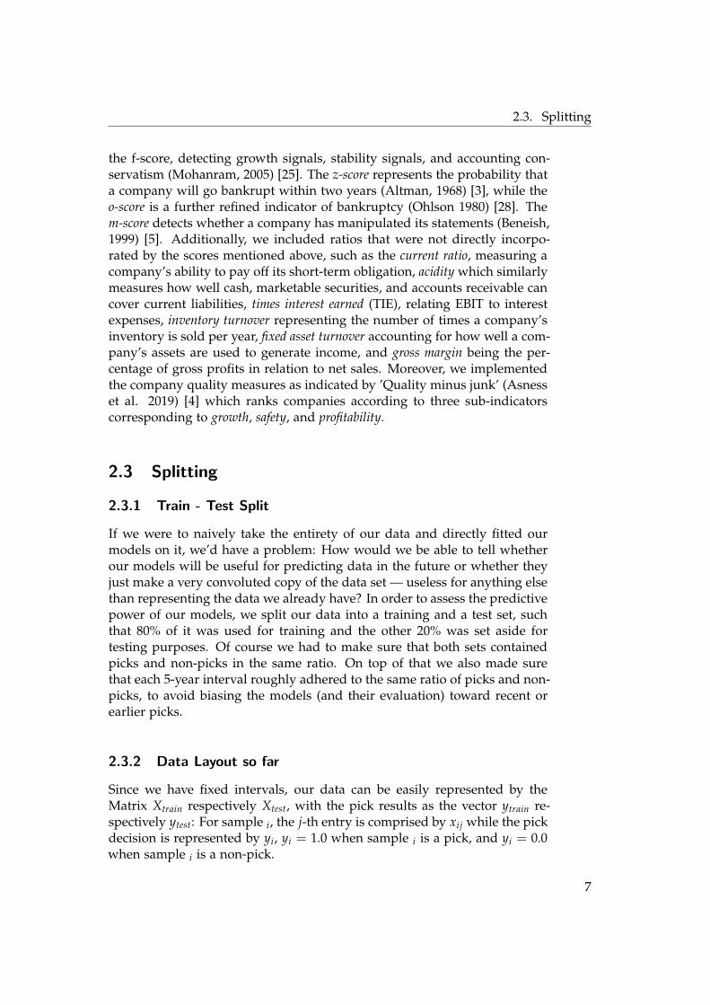
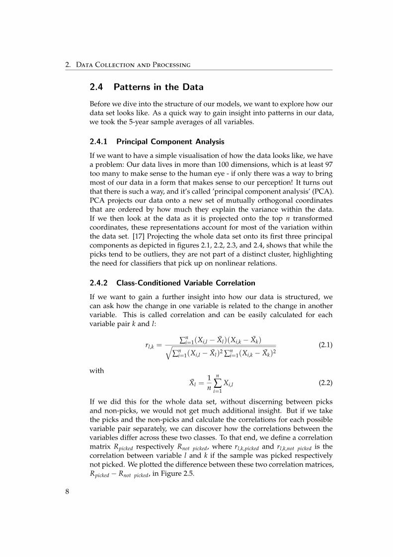
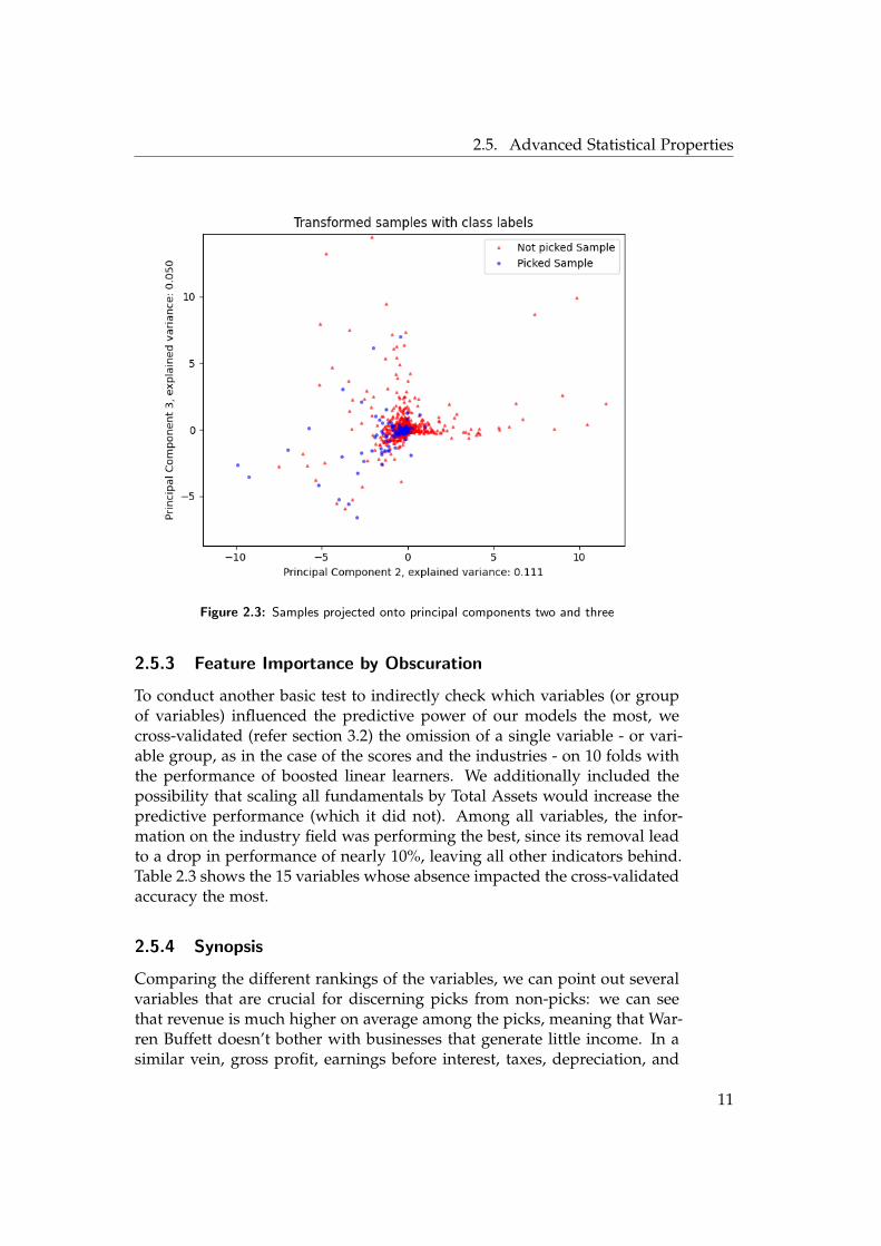
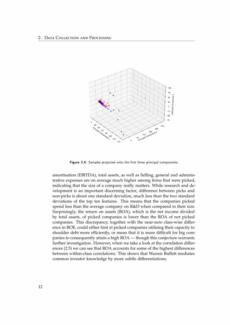
If we want to have a simple visualisation of how the data looks like, we havea problem: Our data lives in more than 100 dimensions, which is at least 97too many to make sense to the human eye - if only there was a way to bringmost of our data in a form that makes sense to our perception! It turns outthat there is such a way, and it’s called ’principal component analysis’ (PCA).PCA projects our data onto a new set of mutually orthogonal coordinatesthat are ordered by how much they explain the variance within the data.If we then look at the data as it is projected onto the top n transformedcoordinates, these representations account for most of the variation withinthe data set. [17] Projecting the whole data set onto its first three principalcomponents as depicted in figures 2.1, 2.2, 2.3, and 2.4, shows that while thepicks tend to be outliers, they are not part of a distinct cluster, highlightingthe need for classifiers that pick up on nonlinear relations.

2.4.2 Class-Conditioned Variable Correlation

If we want to gain a further insight into how our data is structured, wecan ask how the change in one variable is related to the change in anothervariable. This is called correlation and can be easily calculated for eachvariable pair k and l:

rl,k =∑n

i=1(Xi,l − Xl)(Xi,k − Xk)√∑n

i=1(Xi,l − Xl)2 ∑ni=1(Xi,k − Xk)2

(2.1)

with

Xl =1n

n

∑i=1

Xi,l (2.2)

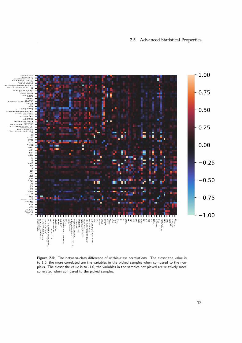
If we did this for the whole data set, without discerning between picksand non-picks, we would not get much additional insight. But if we takethe picks and the non-picks and calculate the correlations for each possiblevariable pair separately, we can discover how the correlations between thevariables differ across these two classes. To that end, we define a correlationmatrix Rpicked respectively Rnot picked, where rl,k,picked and rl,k,not picked is thecorrelation between variable l and k if the sample was picked respectivelynot picked. We plotted the difference between these two correlation matrices,Rpicked − Rnot picked, in Figure 2.5.

8

2.5. Advanced Statistical Properties

Figure 2.1: Samples projected onto principal components one and two

Surprisingly, many top-level engineered features such as the F-score and theG-score exhibited little to no differences in correlation, while some of theirunderlying engineered features yielded significant differences.

2.5 Advanced Statistical Properties

2.5.1 Averages

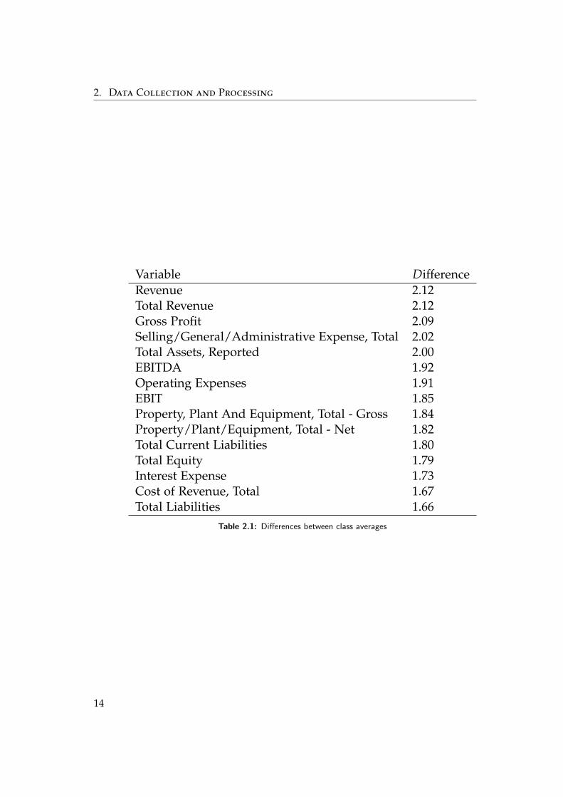
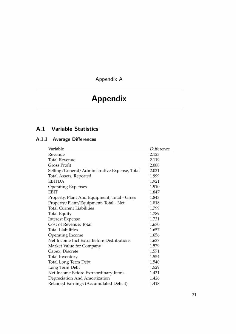
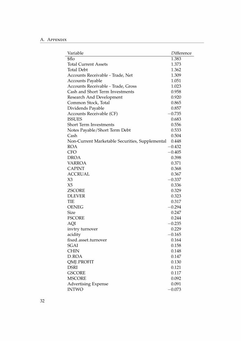
To see how the picks would differentiate themselves from the non-picks, wecalculated the class-wise mean of each variable and calculated the differencebetween these means. The variables with the most relative difference wereRevenue being income generated from ’normal’ business operations, Grossprofit, which is the revenue minus the costs associated with generating saidrevenue, Selling/General/Administrative Expenses, comprising all expenses ex-cept sales expenses necessary to generate revenue, and Total Assets, connot-ing the total of all economic resources belonging to the company. The vari-ables with the least relative differences were Principal Payments from Securi-

9


Figure 2.2: Samples projected onto principal components one and three

ties, Total Interest Expenses, Return on Equity — a ratio that specifies how muchnet income per shareholder’s equity a company generates — and ∆cash f low,which measures the yearly differences in cash-flow. On Table 2.1 we list thetop 15 variables sorted by descending absolute difference, the complete listcan be found in the appendix, which we provide for each variable compari-son.

2.5.2 Feature Importance

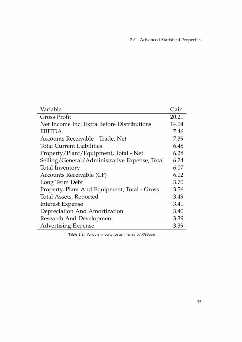
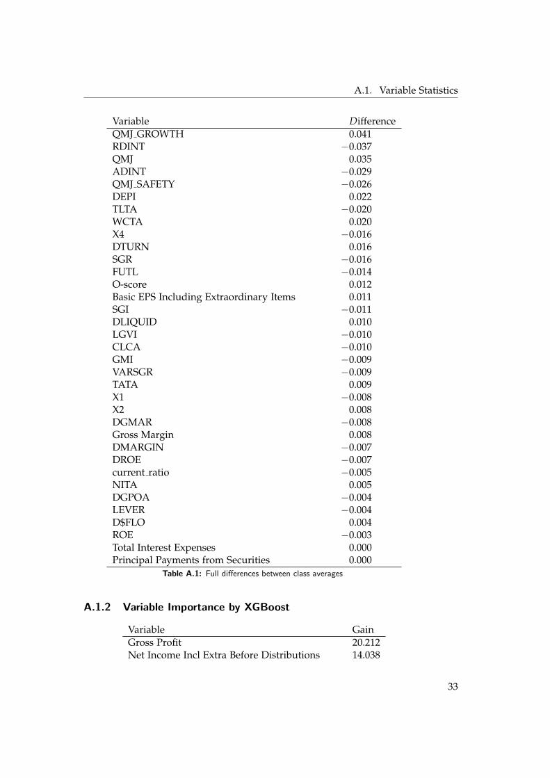
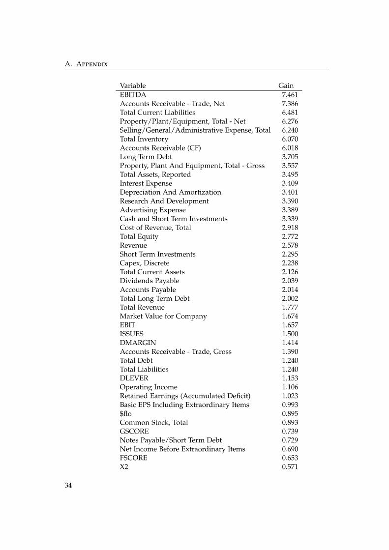
To further investigate the importance of single features, we made use of theXGBoost [7] library, which provides feature importance estimates by check-ing how often and how centrally a variable was used to split the boosteddecision trees. (Hastie, Tibsharani, Friedman, 2017) [18] Again, we list the16 most important variables in table 2.2 by descending order of importance.

10


Figure 2.3: Samples projected onto principal components two and three

2.5.3 Feature Importance by Obscuration

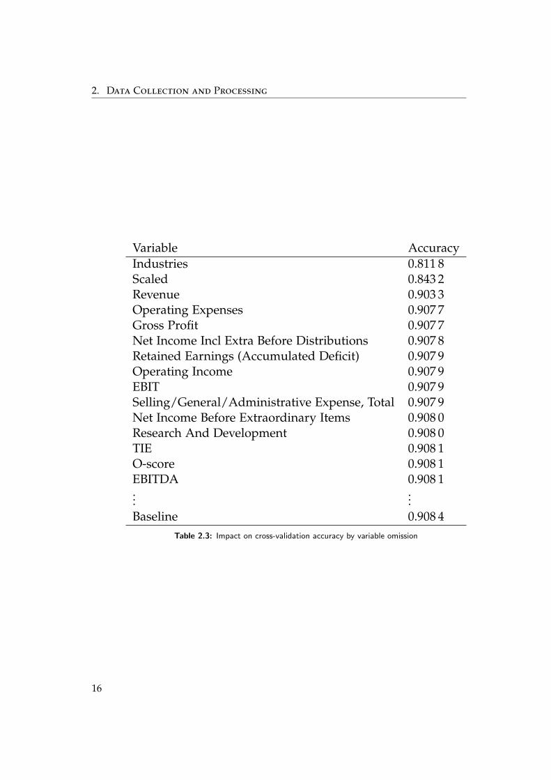
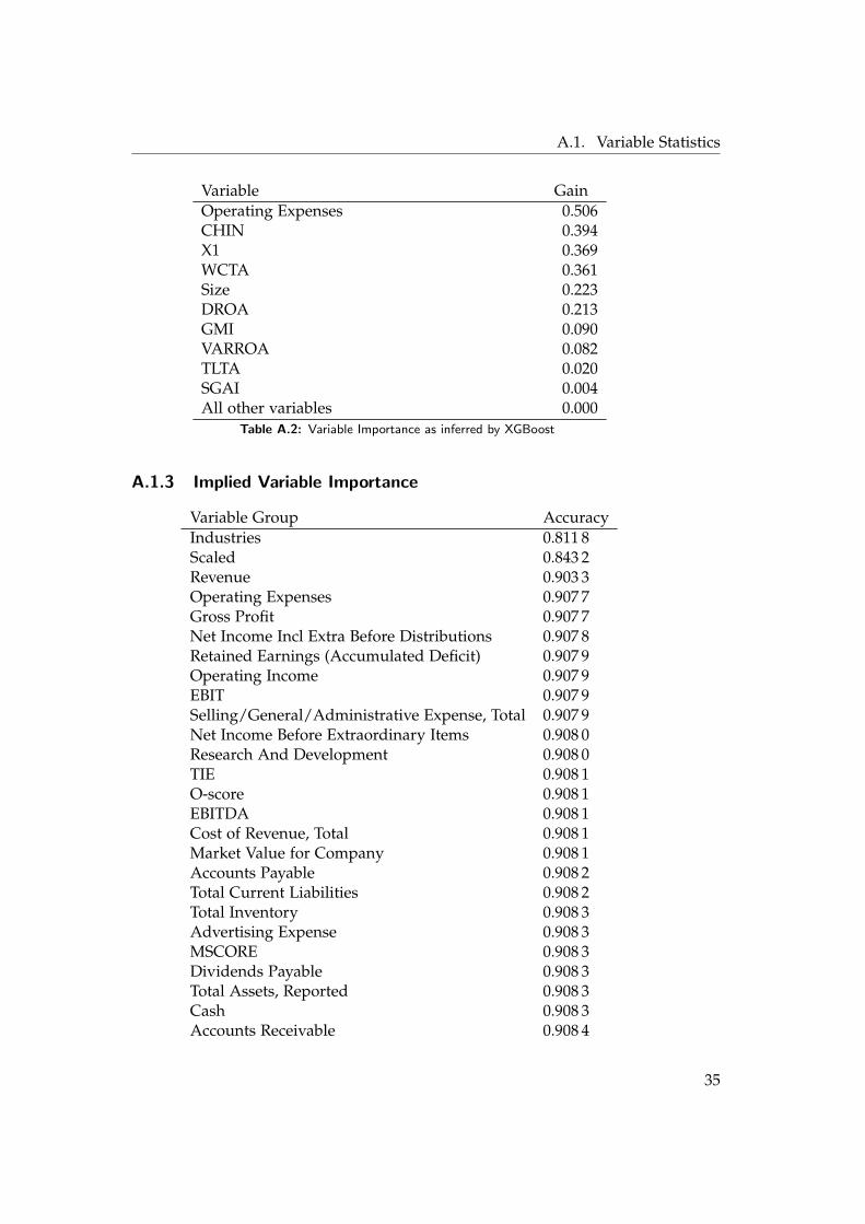
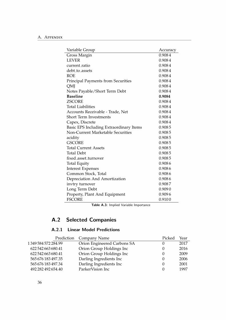
To conduct another basic test to indirectly check which variables (or groupof variables) influenced the predictive power of our models the most, wecross-validated (refer section 3.2) the omission of a single variable - or vari-able group, as in the case of the scores and the industries - on 10 folds withthe performance of boosted linear learners. We additionally included thepossibility that scaling all fundamentals by Total Assets would increase thepredictive performance (which it did not). Among all variables, the infor-mation on the industry field was performing the best, since its removal leadto a drop in performance of nearly 10%, leaving all other indicators behind.Table 2.3 shows the 15 variables whose absence impacted the cross-validatedaccuracy the most.

2.5.4 Synopsis

Comparing the different rankings of the variables, we can point out severalvariables that are crucial for discerning picks from non-picks: we can seethat revenue is much higher on average among the picks, meaning that War-ren Buffett doesn’t bother with businesses that generate little income. In asimilar vein, gross profit, earnings before interest, taxes, depreciation, and

11


Figure 2.4: Samples projected onto the first three principal components

amortisation (EBITDA), total assets, as well as Selling, general and adminis-trative expenses are on average much higher among firms that were picked,indicating that the size of a company really matters. While research and de-velopment is an important discerning factor, difference between picks andnon-picks is about one standard deviation, much less than the two standarddeviations of the top ten features. This means that the companies pickedspend less than the average company on R&D when compared to their size.Surprisingly, the return on assets (ROA), which is the net income dividedby total assets, of picked companies is lower than the ROA of not pickedcompanies. This discrepancy, together with the near-zero class-wise differ-ence in ROE, could either hint at picked companies utilising their capacity toshoulder debt more efficiently, or mean that it is more difficult for big com-panies to consequently attain a high ROA — though this conjecture warrantsfurther investigation. However, when we take a look at the correlation differ-ences (2.5) we can see that ROA accounts for some of the highest differencesbetween within-class correlations. This shows that Warren Buffett mediatescommon investor knowledge by more subtle differentiations.

12


Figure 2.5: The between-class difference of within-class correlations. The closer the value isto 1.0, the more correlated are the variables in the picked samples when compared to the non-picks. The closer the value is to -1.0, the variables in the samples not picked are relatively morecorrelated when compared to the picked samples.

13


Variable DifferenceRevenue 2.12Total Revenue 2.12Gross Profit 2.09Selling/General/Administrative Expense, Total 2.02Total Assets, Reported 2.00EBITDA 1.92Operating Expenses 1.91EBIT 1.85Property, Plant And Equipment, Total - Gross 1.84Property/Plant/Equipment, Total - Net 1.82Total Current Liabilities 1.80Total Equity 1.79Interest Expense 1.73Cost of Revenue, Total 1.67Total Liabilities 1.66

Table 2.1: Differences between class averages

14


Variable GainGross Profit 20.21Net Income Incl Extra Before Distributions 14.04EBITDA 7.46Accounts Receivable - Trade, Net 7.39Total Current Liabilities 6.48Property/Plant/Equipment, Total - Net 6.28Selling/General/Administrative Expense, Total 6.24Total Inventory 6.07Accounts Receivable (CF) 6.02Long Term Debt 3.70Property, Plant And Equipment, Total - Gross 3.56Total Assets, Reported 3.49Interest Expense 3.41Depreciation And Amortization 3.40Research And Development 3.39Advertising Expense 3.39

Table 2.2: Variable Importance as inferred by XGBoost

15


Variable AccuracyIndustries 0.811 8Scaled 0.843 2Revenue 0.903 3Operating Expenses 0.907 7Gross Profit 0.907 7Net Income Incl Extra Before Distributions 0.907 8Retained Earnings (Accumulated Deficit) 0.907 9Operating Income 0.907 9EBIT 0.907 9Selling/General/Administrative Expense, Total 0.907 9Net Income Before Extraordinary Items 0.908 0Research And Development 0.908 0TIE 0.908 1O-score 0.908 1EBITDA 0.908 1...

...Baseline 0.908 4

Table 2.3: Impact on cross-validation accuracy by variable omission

16

Chapter 3

Methodology

In this chapter we will introduce the general framework of our approach aswell as the tools and models used to analyse our dataset.

3.1 Evaluation Metrics

Defining the evaluation metrics is vital to understanding the performanceof our models.

3.1.1 Accuracy, Recall, and Precision

Since we have a binary prediction target, we have four possible outcomesfor each prediction: In the case that we are looking at a company that wasnot picked by Warren Buffett, our models can either (correctly) predict thatit will not be picked, yielding a true negative - TN - or (falsely) predict thatit will be picked, yielding a false positive, FP. Conversely, if we are lookingat a company that was picked by Warren Buffett, the prediction can eitherbe a true positive, TP, or a false negative, FN. From these outcomes, wecan construct our basic evaluation metrics. Since our data set is severelyimbalanced, accuracy as defined by TN+TP

TN+FP+FN+TP will deliver little insight,as an algorithm that consistently predicts negatives will yield an accuracyof 97.78%. An ameliorated version of this metric is balanced accuracy, wherewe weigh the predictions by the number of negative respective positive sam-ples: 0.5 ∗ ( TP

TP+F N + TNTN+FP ) Another pair of metrics we are interested in is

recall vs. precision: Recall - often also called sensitivity - measures how wellthe model identifies positive samples, and is defined by TP

TP+FN . Precisionmeasures how many of the samples labeled as positive are true positives,and is defined as TP

TP+FP These two metrics specifically interest us becausethe first tells us how well picks are identified, while the latter tells us howmuch Warren Buffett we should expect to be contained in a sample that islabeled ’Warren Buffett’.

17

3. Methodology

3.1.2 Receiver Operator Characteristics and Area Under the Curve

The former metrics depend on binary and discrete classifications. What ifwe want to evaluate our models on a more gradual scale, say probabilisticor ranked predictions? Following metrics do help us with these issues: [13]The Receiver Operating Characteristics (ROC) graph helps in determiningthe trade-off between recall and loss of specifity. While discrete classifierscan be situated on a single point on the ROC graph, its true evaluative powercomes from plotting the recall vs. the specifity of a classifier while varyingthe decision threshold. As Fawcett (2006) [13] notes, the curves generated inthis way have the property that they do not change when the class distribu-tion of the prediction targets changes, making the ROC graph a suitable anddesirable way to evaluate the performance of our models. Another interest-ing property is the Area Under the Curve (AUC) directly calculated fromthe ROC graph, which is at 0.5 for a completely random classifier, trans-lates into the probability that a randomly chosen positive sample will beranked higher than a randomly chosen negative sample. This makes it anexceptionally solid metric when determining the overall predictiveness of amodel [13]

3.2 The Importance of Cross-Validation

While training appropriate models, most of them will necessitate tuningparameters to account for the differences in underlying reality. If we were todirectly tune these parameters according to the performance on the test dataset, our models will most likely over-fit due to the richness encoded by theparameter space. Hence we we split our training data set into n folds - suchthat each fold contains the same proportion of positive to negative samples- and train our models, with varying parameters, n times on n − 1 foldswhile holding back the nth fold for validation. Averaging the scores acrossthe n folds will give us a robust estimate of the relatively best parameter set,while greatly reducing the risk of over-fitting and of selection bias. (Moreon cross-validation in Stone (1974) [36]) In the case of our simpler models,we chose n = 10, whilst we chose n = 5 for training our neural networks, inorder to reduce computation time.

3.3 Models Used

In the following subsections we will detail the models we used to analyseour data. Wherever our models were hampered by the imbalance of ourdata set described in 2.1, we solved this problem by weighing the samplesinversely to their prevalence. This means that the weights of picks vs. non-

18

3.3. Models Used

picks should maintain the ratio of 6166140 , which equals to saying that a positive

sample warrants 44 times more attention than a negative one.

3.3.1 Baseline

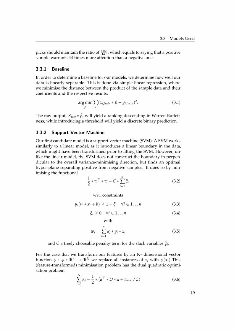
In order to determine a baseline for our models, we determine how well ourdata is linearly separable. This is done via simple linear regression, wherewe minimise the distance between the product of the sample data and theircoefficients and the respective results:

arg minβ

∑i(xi,train ∗ β− yi,train)

2. (3.1)

The raw output, Xtest ∗ β, will yield a ranking descending in Warren-Buffett-ness, while introducing a threshold will yield a discrete binary prediction.

3.3.2 Support Vector Machine

Our first candidate model is a support vector machine (SVM). A SVM workssimilarly to a linear model, as it introduces a linear boundary in the data,which might have been transformed prior to fitting the SVM. However, un-like the linear model, the SVM does not construct the boundary in perpen-dicular to the overall variance-minimising direction, but finds an optimalhyper-plane separating positive from negative samples. It does so by min-imising the functional

12∗ w> ∗ w + C ∗

n

∑i=1

ξi (3.2)

wrt. constraints

yi(w ∗ xi + b) ≥ 1− ξi ∀i ∈ 1 . . . n (3.3)

ξi ≥ 0 ∀i ∈ 1 . . . n (3.4)

with

wj =n

∑i=1

αji ∗ yi ∗ xi (3.5)

and C a freely choosable penalty term for the slack variables ξi.

For the case that we transform our features by an N- dimensional vectorfunction ϕ : ϕ : Rn → RN we replace all instances of xi with ϕ(xi) This(feature-transformed) minimisation problem has the dual quadratic optimi-sation problem

N

∑i=1

αi −12∗ (α> ∗ D ∗ α + αmax/C) (3.6)

19

3. Methodology

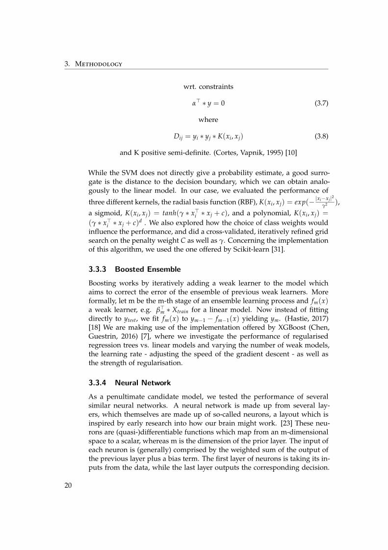
wrt. constraints

α> ∗ y = 0 (3.7)

where

Dij = yi ∗ yj ∗ K(xi, xj) (3.8)

and K positive semi-definite. (Cortes, Vapnik, 1995) [10]

While the SVM does not directly give a probability estimate, a good surro-gate is the distance to the decision boundary, which we can obtain analo-gously to the linear model. In our case, we evaluated the performance of

three different kernels, the radial basis function (RBF), K(xi, xj) = exp(− |xi−xj|2γ2 ),

a sigmoid, K(xi, xj) = tanh(γ ∗ x>i ∗ xj + c), and a polynomial, K(xi, xj) =

(γ ∗ x>i ∗ xj + c)d . We also explored how the choice of class weights wouldinfluence the performance, and did a cross-validated, iteratively refined gridsearch on the penalty weight C as well as γ. Concerning the implementationof this algorithm, we used the one offered by Scikit-learn [31].

3.3.3 Boosted Ensemble

Boosting works by iteratively adding a weak learner to the model whichaims to correct the error of the ensemble of previous weak learners. Moreformally, let m be the m-th stage of an ensemble learning process and fm(x)a weak learner, e.g. β>m ∗ Xtrain for a linear model. Now instead of fittingdirectly to ytest, we fit fm(x) to ym−1 − fm−1(x) yielding ym. (Hastie, 2017)[18] We are making use of the implementation offered by XGBoost (Chen,Guestrin, 2016) [7], where we investigate the performance of regularisedregression trees vs. linear models and varying the number of weak models,the learning rate - adjusting the speed of the gradient descent - as well asthe strength of regularisation.

3.3.4 Neural Network

As a penultimate candidate model, we tested the performance of severalsimilar neural networks. A neural network is made up from several lay-ers, which themselves are made up of so-called neurons, a layout which isinspired by early research into how our brain might work. [23] These neu-rons are (quasi-)differentiable functions which map from an m-dimensionalspace to a scalar, whereas m is the dimension of the prior layer. The input ofeach neuron is (generally) comprised by the weighted sum of the output ofthe previous layer plus a bias term. The first layer of neurons is taking its in-puts from the data, while the last layer outputs the corresponding decision.

20

3.3. Models Used

Training is done by iteratively propagating the input through each succes-sive layer (feed-forward), and then comparing the output of the final layerand the pick decision via a loss function giving an error. In a second step,this error then is differentiated with regard to the weights and biases of theprevious layer, which indicates the general direction of updating. These dif-ferentiations can then be done layer-wise going from the last to the first layer.(Cross, Harrison, Kennedy, 1995) [11] Different methods to implement or ap-proximate this gradient descent exist, and as our goal was to efficiently useexisting implementation of well-known algorithms, we decided to use thevery efficient NAdam optimiser (Dozat, 2015) [12] as implemented in keras.[8] Since our prediction target is binary, our final layer should produce asingle real scalar ranged from 0 to 1, corresponding to the probability of thesample being picked. We constructed a simple sequential neural networkwith n layers and a layer size of m that decreases by 2

3 by each subsequentlayer. For the number of layers we investigated a range between n ∈ 3, . . . , 17and for the number of neurons on the first layer a range of m ∈ 100, . . . , 7000,whereas the upper limit was given by machine memory restrictions. As net-works perform better under some circumstances when the output of the firstor second layer is fourier transformed, allowing for efficient convolution, wealso investigated the performance of this design feature. As candidate acti-vation functions we investigated Rectified Linear Unit (ReLU), tanh, andsigmoid. While the network size is an implicit source of regularisation byconstraining the set of possible parameters, one of the other ways to avoidover-fitting is dropout regularisation. This means that during training for agiven level of p ∈ [0, 1), any neuron is active with a probability of 1− p ordoes not activate with probability p. After shortly venturing into the terri-tory of p ∈ [0.7, 0.99] we quickly found out that such networks are barelytrainable under the constraints we were given and searched for appropriatep ∈ [0, 0.6].

3.3.5 Hybrid Model

Our final candidate was a very simple hybrid model which combined thepredictions of all the previously described models. This combination wasdone via a component-wise multiplication of the individual predictions. Inthe case of the SVM, we transformed the output with the logistic function inorder to make its predictions compatible with the other predictions, whichwere all probabilistic.

21

Chapter 4

Results and Discussion

Life is but a walking shadow, apoor playerThat struts and frets his hourupon the stageAnd then is heard no more.

W. Shakespeare

4.1 Performance and Comparison

4.1.1 Baseline

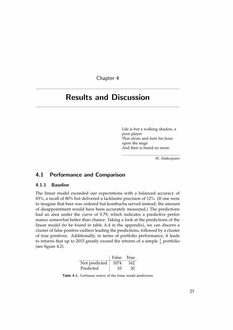
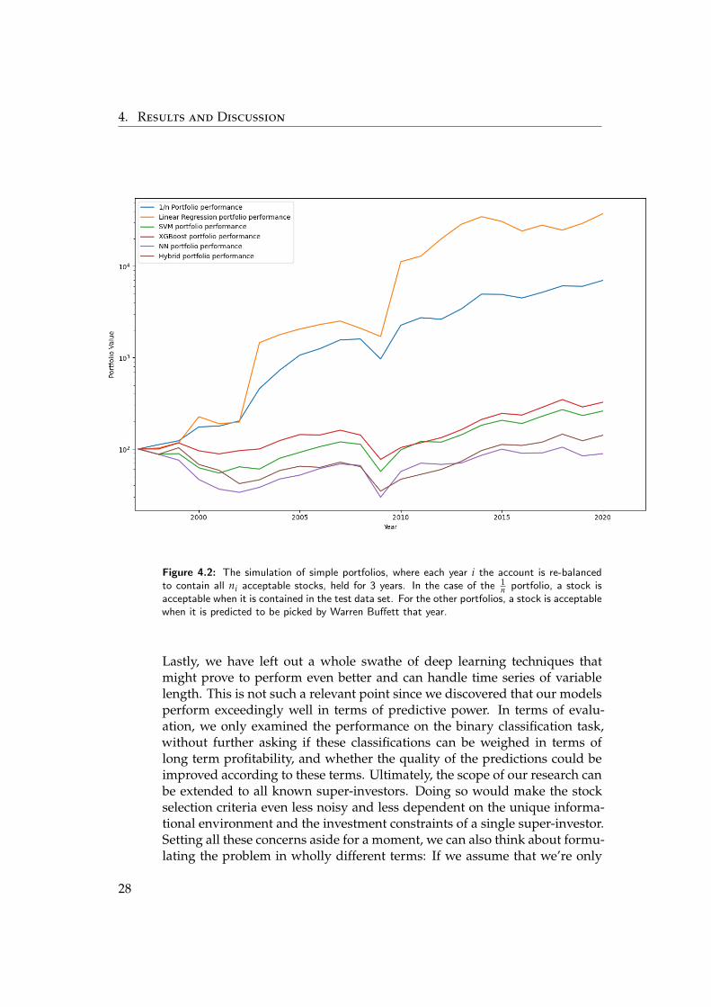
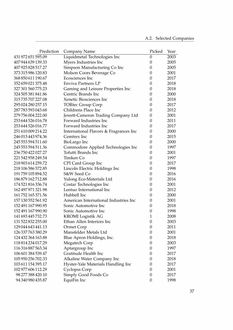
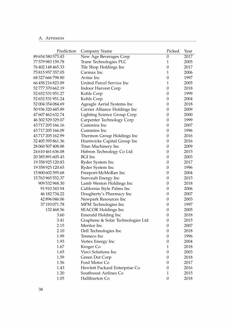
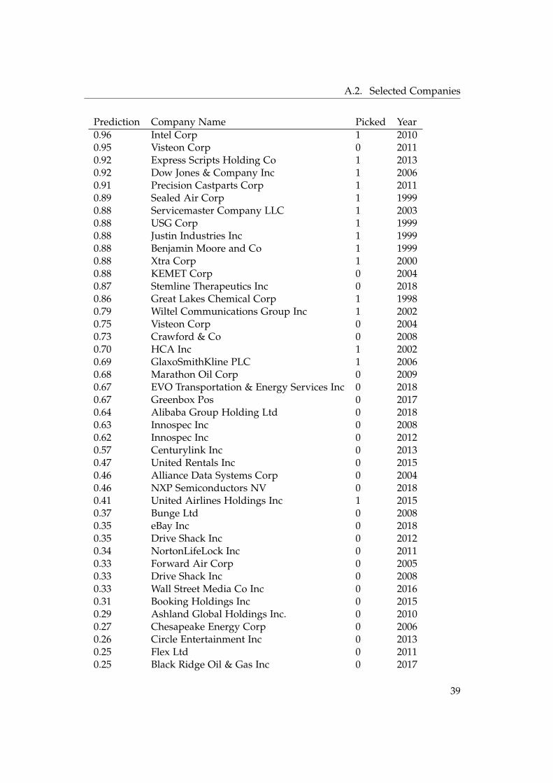
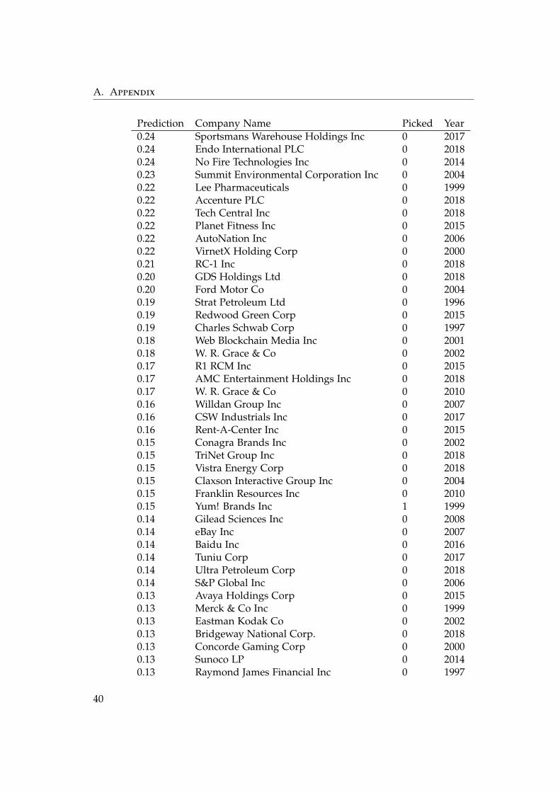
The linear model exceeded our expectations with a balanced accuracy of83%, a recall of 80% but delivered a lacklustre precision of 12%. (If one wereto imagine that beer was ordered but kombucha served instead, the amountof disappointment would have been accurately measured.) The predictionshad an area under the curve of 0.79, which indicates a predictive perfor-mance somewhat better than chance. Taking a look at the predictions of thelinear model (to be found in table A.4 in the appendix), we can discern acluster of false positive outliers leading the predictions, followed by a clusterof true positives. Additionally, in terms of portfolio performance, it leadsto returns that up to 2015 greatly exceed the returns of a simple 1

n portfolio(see figure 4.2).

False TrueNot predicted 1074 162Predicted 10 20

Table 4.1: Confusion matrix of the linear model predictions

23

4. Results and Discussion

4.1.2 Support Vector Machine

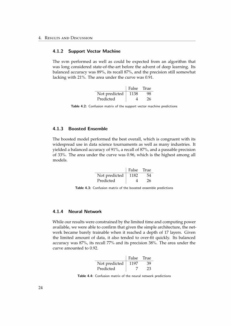
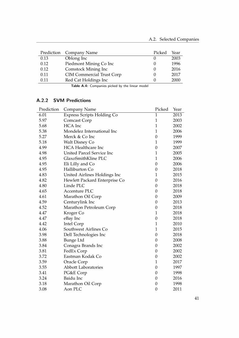
The svm performed as well as could be expected from an algorithm thatwas long considered state-of-the-art before the advent of deep learning. Itsbalanced accuracy was 89%, its recall 87%, and the precision still somewhatlacking with 21%. The area under the curve was 0.91.


Table 4.2: Confusion matrix of the support vector machine predictions

4.1.3 Boosted Ensemble

The boosted model performed the best overall, which is congruent with itswidespread use in data science tournaments as well as many industries. Ityielded a balanced accuracy of 91%, a recall of 87%, and a passable precisionof 33%. The area under the curve was 0.96, which is the highest among allmodels.


Table 4.3: Confusion matrix of the boosted ensemble predictions

4.1.4 Neural Network

While our results were constrained by the limited time and computing poweravailable, we were able to confirm that given the simple architecture, the net-work became barely trainable when it reached a depth of 17 layers. Giventhe limited amount of data, it also tended to over-fit quickly. Its balancedaccuracy was 87%, its recall 77% and its precision 38%. The area under thecurve amounted to 0.92.


Table 4.4: Confusion matrix of the neural network predictions

24

4.2. Discussion

4.1.5 Hybrid Model

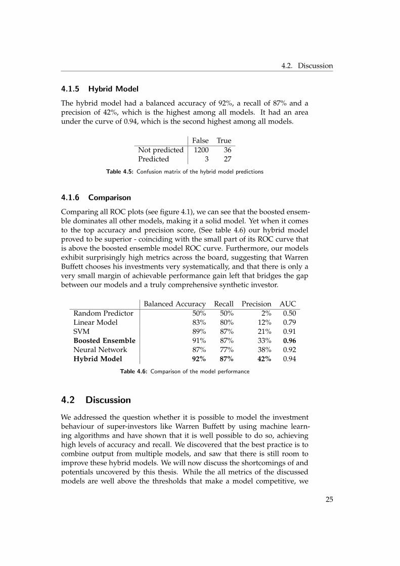
The hybrid model had a balanced accuracy of 92%, a recall of 87% and aprecision of 42%, which is the highest among all models. It had an areaunder the curve of 0.94, which is the second highest among all models.


Table 4.5: Confusion matrix of the hybrid model predictions

4.1.6 Comparison

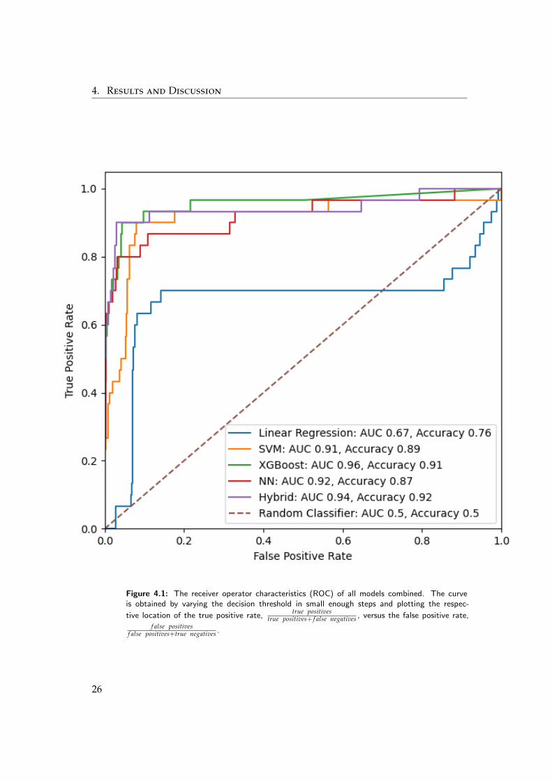
Comparing all ROC plots (see figure 4.1), we can see that the boosted ensem-ble dominates all other models, making it a solid model. Yet when it comesto the top accuracy and precision score, (See table 4.6) our hybrid modelproved to be superior - coinciding with the small part of its ROC curve thatis above the boosted ensemble model ROC curve. Furthermore, our modelsexhibit surprisingly high metrics across the board, suggesting that WarrenBuffett chooses his investments very systematically, and that there is only avery small margin of achievable performance gain left that bridges the gapbetween our models and a truly comprehensive synthetic investor.

Balanced Accuracy Recall Precision AUCRandom Predictor 50% 50% 2% 0.50Linear Model 83% 80% 12% 0.79SVM 89% 87% 21% 0.91Boosted Ensemble 91% 87% 33% 0.96Neural Network 87% 77% 38% 0.92Hybrid Model 92% 87% 42% 0.94

Table 4.6: Comparison of the model performance

4.2 Discussion

We addressed the question whether it is possible to model the investmentbehaviour of super-investors like Warren Buffett by using machine learn-ing algorithms and have shown that it is well possible to do so, achievinghigh levels of accuracy and recall. We discovered that the best practice is tocombine output from multiple models, and saw that there is still room toimprove these hybrid models. We will now discuss the shortcomings of andpotentials uncovered by this thesis. While the all metrics of the discussedmodels are well above the thresholds that make a model competitive, we

25


Figure 4.1: The receiver operator characteristics (ROC) of all models combined. The curveis obtained by varying the decision threshold in small enough steps and plotting the respec-

tive location of the true positive rate,true positives

true positives+ f alse negatives , versus the false positive rate,

f alse positivesf alse positives+true negatives .

26

4.2. Discussion

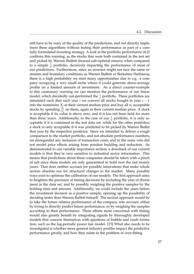
still have to be wary of the quality of the predictions, and not directly imple-ment these algorithms without testing their performance as part of a care-fully formulated investing strategy. A look at the portfolio performance (4.2)confirms this warning, as the stocks that were both contained in the test setand picked by Warren Buffett showed sub-optimal returns when comparedto a simple 1

n portfolio, decisively impacting the performance of most ofour predictions. Furthermore, since an investor might not face the same re-straints and boundary conditions as Warren Buffett or Berkshire Hathaway,there is a high probability we miss many opportunities due to e.g. a com-pany occupying a very small niche where it could generate above-averageprofits on a limited amount of investment. As a direct counter-exampleto this cautionary warning we can mention the performance of our linearmodel, which decidedly out-performed the 1

n portfolio. These portfolios aresimulated such that each year i we convert all stocks bought in year i − 1into the numeraire Xi at their current median price and buy all ni acceptablestocks by spending Xi

nion them, again at their current median price. A stock

is acceptable if its value is above zero, and if it has not been held for morethan three years. Additionally, in the case of our 1

n portfolio, it is only ac-ceptable if it is contained in the test data set, while for the other portfolios,a stock is only acceptable if it was predicted to be picked by Warren Buffetthat year by the respective predictor. Since we intended to deliver a roughcomparison to the market portfolio, and not absolute performance numbers,we disregarded any inclusion of transaction costs, and in the same vein didnot model price effects arising from position building and reduction. Asdemonstrated in our variable importance section, a drawback of our currentmodels is that they’re very sensitive to industrial sector information. Thismeans that predictions about these companies should be taken with a pinchof salt since these models are only guaranteed to hold over the last twentyyears. That does neither account for possible innovations that make wholesectors obsolete nor for structural changes in the market. Many possibleways exist to optimise the calibration of our models: The first approach aimsto heighten the precision of timing decisions by including the year of divest-ment in the data set, and by possibly weighing the positive samples by theholding time and amount. Additionally, we could include the years beforethe investment decision as a positive sample, opening up the possibility ofdeciding faster than Warren Buffett himself. The second approach would beto take the future relative performance of the company into account, eitherby trying to directly predict future performance, or by weighing the samplesaccording to their performance. These efforts more concerned with timingwould also greatly benefit by integrating signals by thoroughly developedmodels that concern themselves with questions of bubble and crash forma-tion, such as the log-periodic power law model. [15] What also needs to beinvestigated is whether more general industry profiles impact the predictiveperformance greatly, and how they relate to the problem of over-fitting.

27


Figure 4.2: The simulation of simple portfolios, where each year i the account is re-balancedto contain all ni acceptable stocks, held for 3 years. In the case of the 1

n portfolio, a stock isacceptable when it is contained in the test data set. For the other portfolios, a stock is acceptablewhen it is predicted to be picked by Warren Buffett that year.

Lastly, we have left out a whole swathe of deep learning techniques thatmight prove to perform even better and can handle time series of variablelength. This is not such a relevant point since we discovered that our modelsperform exceedingly well in terms of predictive power. In terms of evalu-ation, we only examined the performance on the binary classification task,without further asking if these classifications can be weighed in terms oflong term profitability, and whether the quality of the predictions could beimproved according to these terms. Ultimately, the scope of our research canbe extended to all known super-investors. Doing so would make the stockselection criteria even less noisy and less dependent on the unique informa-tional environment and the investment constraints of a single super-investor.Setting all these concerns aside for a moment, we can also think about formu-lating the problem in wholly different terms: If we assume that we’re only

28

4.2. Discussion

really certain about the companies that Warren Buffett did pick, throw in ad-ditional examples of very bad investment ideas, and, in a first step, set thedecision about all other companies as ’undecided’, we could come up with asemi-supervised learner that gradually discovers what makes great compa-nies valuable investment targets. To conclude, our research shows that usingmachine learning algorithms on the investment decisions of super-investorsis an exciting venue for future research.

29

Appendix A

Appendix

A.1 Variable Statistics

A.1.1 Average Differences

Variable DifferenceRevenue 2.123Total Revenue 2.119Gross Profit 2.088Selling/General/Administrative Expense, Total 2.021Total Assets, Reported 1.999EBITDA 1.921Operating Expenses 1.910EBIT 1.847Property, Plant And Equipment, Total - Gross 1.843Property/Plant/Equipment, Total - Net 1.818Total Current Liabilities 1.799Total Equity 1.789Interest Expense 1.731Cost of Revenue, Total 1.670Total Liabilities 1.657Operating Income 1.656Net Income Incl Extra Before Distributions 1.637Market Value for Company 1.579Capex, Discrete 1.571Total Inventory 1.554Total Long Term Debt 1.540Long Term Debt 1.529Net Income Before Extraordinary Items 1.431Depreciation And Amortization 1.426Retained Earnings (Accumulated Deficit) 1.418

31

A. Appendix

Variable Difference$flo 1.383Total Current Assets 1.373Total Debt 1.362Accounts Receivable - Trade, Net 1.309Accounts Payable 1.051Accounts Receivable - Trade, Gross 1.023Cash and Short Term Investments 0.958Research And Development 0.920Common Stock, Total 0.865Dividends Payable 0.857Accounts Receivable (CF) −0.735ISSUES 0.683Short Term Investments 0.556Notes Payable/Short Term Debt 0.533Cash 0.504Non-Current Marketable Securities, Supplemental 0.448ROA −0.432CFO −0.405DROA 0.398VARROA 0.371CAPINT 0.368ACCRUAL 0.367X3 −0.337X5 0.336ZSCORE 0.329DLEVER 0.323TIE 0.317OENEG −0.294Size 0.247FSCORE 0.244AQI −0.235invtry turnover 0.229acidity −0.165fixed asset turnover 0.164SGAI 0.158CHIN 0.148D ROA 0.147QMJ PROFIT 0.130DSRI 0.121GSCORE 0.117MSCORE 0.092Advertising Expense 0.091INTWO −0.073

32

A.1. Variable Statistics

Variable DifferenceQMJ GROWTH 0.041RDINT −0.037QMJ 0.035ADINT −0.029QMJ SAFETY −0.026DEPI 0.022TLTA −0.020WCTA 0.020X4 −0.016DTURN 0.016SGR −0.016FUTL −0.014O-score 0.012Basic EPS Including Extraordinary Items 0.011SGI −0.011DLIQUID 0.010LGVI −0.010CLCA −0.010GMI −0.009VARSGR −0.009TATA 0.009X1 −0.008X2 0.008DGMAR −0.008Gross Margin 0.008DMARGIN −0.007DROE −0.007current ratio −0.005NITA 0.005DGPOA −0.004LEVER −0.004D$FLO 0.004ROE −0.003Total Interest Expenses 0.000Principal Payments from Securities 0.000

Table A.1: Full differences between class averages

A.1.2 Variable Importance by XGBoost

Variable GainGross Profit 20.212Net Income Incl Extra Before Distributions 14.038

33

A. Appendix

Variable GainEBITDA 7.461Accounts Receivable - Trade, Net 7.386Total Current Liabilities 6.481Property/Plant/Equipment, Total - Net 6.276Selling/General/Administrative Expense, Total 6.240Total Inventory 6.070Accounts Receivable (CF) 6.018Long Term Debt 3.705Property, Plant And Equipment, Total - Gross 3.557Total Assets, Reported 3.495Interest Expense 3.409Depreciation And Amortization 3.401Research And Development 3.390Advertising Expense 3.389Cash and Short Term Investments 3.339Cost of Revenue, Total 2.918Total Equity 2.772Revenue 2.578Short Term Investments 2.295Capex, Discrete 2.238Total Current Assets 2.126Dividends Payable 2.039Accounts Payable 2.014Total Long Term Debt 2.002Total Revenue 1.777Market Value for Company 1.674EBIT 1.657ISSUES 1.500DMARGIN 1.414Accounts Receivable - Trade, Gross 1.390Total Debt 1.240Total Liabilities 1.240DLEVER 1.153Operating Income 1.106Retained Earnings (Accumulated Deficit) 1.023Basic EPS Including Extraordinary Items 0.993$flo 0.895Common Stock, Total 0.893GSCORE 0.739Notes Payable/Short Term Debt 0.729Net Income Before Extraordinary Items 0.690FSCORE 0.653X2 0.571

34

A.1. Variable Statistics

Variable GainOperating Expenses 0.506CHIN 0.394X1 0.369WCTA 0.361Size 0.223DROA 0.213GMI 0.090VARROA 0.082TLTA 0.020SGAI 0.004All other variables 0.000

Table A.2: Variable Importance as inferred by XGBoost

A.1.3 Implied Variable Importance

Variable Group AccuracyIndustries 0.811 8Scaled 0.843 2Revenue 0.903 3Operating Expenses 0.907 7Gross Profit 0.907 7Net Income Incl Extra Before Distributions 0.907 8Retained Earnings (Accumulated Deficit) 0.907 9Operating Income 0.907 9EBIT 0.907 9Selling/General/Administrative Expense, Total 0.907 9Net Income Before Extraordinary Items 0.908 0Research And Development 0.908 0TIE 0.908 1O-score 0.908 1EBITDA 0.908 1Cost of Revenue, Total 0.908 1Market Value for Company 0.908 1Accounts Payable 0.908 2Total Current Liabilities 0.908 2Total Inventory 0.908 3Advertising Expense 0.908 3MSCORE 0.908 3Dividends Payable 0.908 3Total Assets, Reported 0.908 3Cash 0.908 3Accounts Receivable 0.908 4

35

A. Appendix

Variable Group AccuracyGross Margin 0.908 4LEVER 0.908 4current ratio 0.908 4debt to assets 0.908 4ROE 0.908 4Principal Payments from Securities 0.908 4QMJ 0.908 4Notes Payable/Short Term Debt 0.908 4Baseline 0.9084ZSCORE 0.908 4Total Liabilities 0.908 4Accounts Receivable - Trade, Net 0.908 4Short Term Investments 0.908 4Capex, Discrete 0.908 4Basic EPS Including Extraordinary Items 0.908 5Non-Current Marketable Securities 0.908 5acidity 0.908 5GSCORE 0.908 5Total Current Assets 0.908 5Total Debt 0.908 5fixed asset turnover 0.908 5Total Equity 0.908 6Interest Expenses 0.908 6Common Stock, Total 0.908 6Depreciation And Amortization 0.908 6invtry turnover 0.908 7Long Term Debt 0.909 0Property, Plant And Equipment 0.909 6FSCORE 0.910 0

Table A.3: Implied Variable Importance

A.2 Selected Companies

A.2.1 Linear Model Predictions

Prediction Company Name Picked Year1 349 584 572 284.99 Orion Engineered Carbons SA 0 2017

622 542 663 680.41 Orion Group Holdings Inc 0 2016622 542 663 680.41 Orion Group Holdings Inc 0 2009565 676 183 497.35 Darling Ingredients Inc 0 2006565 676 183 497.34 Darling Ingredients Inc 0 2001492 282 492 654.40 ParkerVision Inc 0 1997

36

A.2. Selected Companies

Prediction Company Name Picked Year431 972 651 595.09 Liquidmetal Technologies Inc 0 2003407 944 639 139.33 Myers Industries Inc 0 2005407 925 828 517.27 Simpson Manufacturing Co Inc 0 2005373 315 986 120.83 Molson Coors Beverage Co 0 2001368 850 611 190.67 Ecosciences Inc 0 2017352 659 021 375.48 Enviva Partners LP 0 2018327 301 560 775.23 Gaming and Leisure Properties Inc 0 2018324 505 381 841.86 Centric Brands Inc 0 2000315 735 707 227.08 Xenetic Biosciences Inc 0 2018295 024 280 257.15 TORtec Group Corp 0 2017287 783 593 043.68 Childrens Place Inc 0 2012279 756 004 222.00 Jewett-Cameron Trading Company Ltd 0 2001253 644 526 016.78 Forward Industries Inc 0 2011253 644 526 016.77 Forward Industries Inc 0 2017251 610 009 214.22 International Flavors & Fragrances Inc 0 2000246 013 443 974.36 Cemtrex Inc 0 2015245 553 594 511.60 BioLargo Inc 0 2000245 553 594 511.36 Commodore Applied Technologies Inc 0 1997236 750 422 027.27 Tofutti Brands Inc 0 2001221 542 958 249.54 Timken Co 0 1997218 903 614 259.72 CPI Card Group Inc 0 2017218 106 586 572.85 Lincoln Electric Holdings Inc 0 1998191 759 105 894.52 S&W Seed Co 0 2016186 879 162 712.88 Yulong Eco-Materials Ltd 0 2016174 521 816 336.74 Costar Technologies Inc 0 2001162 497 971 321.98 Lentuo International Inc 0 2012161 752 165 371.56 Hubbell Inc 0 2000157 130 552 561.92 American International Industries Inc 0 2001152 491 167 990.95 Sonic Automotive Inc 0 2018152 491 167 990.90 Sonic Automotive Inc 0 1998141 693 445 732.73 KROMI Logistik AG 1 2008131 522 832 255.00 Ethan Allen Interiors Inc 0 2003129 044 643 441.13 Ormet Corp 0 2011126 337 763 380.29 Mansfelder Metals Ltd 0 2001124 432 364 163.88 Blue Apron Holdings, Inc. 0 2018118 814 234 017.29 Megatech Corp 0 2003116 316 887 563.34 Aptargroup Inc 0 1997106 601 384 539.47 Gratitude Health Inc 0 2017105 950 256 702.33 Alkaline Water Company Inc 0 2018103 611 154 395.17 Hyster-Yale Materials Handling Inc 0 2017102 977 606 112.29 Cyclopss Corp 0 200198 277 388 420.10 Simply Good Foods Co 0 201794 340 980 435.87 EquiFin Inc 0 1998

37

A. Appendix

Prediction Company Name Picked Year89 654 580 573.43 New Age Beverages Corp 0 201777 579 983 159.78 Trane Technologies PLC 1 200576 402 148 465.33 Tile Shop Holdings Inc 0 201775 815 957 357.05 Carmax Inc 1 200668 327 666 798.80 Avitar Inc 0 199766 458 216 823.09 United Parcel Service Inc 1 200552 777 370 662.19 Indoor Harvest Corp 0 201852 652 531 951.27 Kohls Corp 0 199952 652 531 951.24 Kohls Corp 0 200452 004 354 084.69 Ageagle Aerial Systems Inc 0 201850 936 320 445.89 Carrier Alliance Holdings Inc 0 200947 607 462 632.74 Lighting Science Group Corp 0 200046 302 529 329.07 Carpenter Technology Corp 0 199943 717 205 166.16 Cummins Inc 0 200743 717 205 166.09 Cummins Inc 0 199643 717 205 162.99 Thermon Group Holdings Inc 0 201632 405 395 861.36 Huntwicke Capital Group Inc 0 201628 060 507 408.88 Titan Machinery Inc 0 200924 610 461 636.08 Hebron Technology Co Ltd 0 201520 385 891 605.43 BGI Inc 0 200319 358 925 120.83 Ryder System Inc 0 201719 358 925 120.65 Ryder System Inc 0 199615 800 602 595.68 Freeport-McMoRan Inc 0 200415 763 965 552.37 Sunvault Energy Inc 0 2015

909 532 968.30 Lamb Weston Holdings Inc 0 201891 910 343.94 California Style Palms Inc 0 200646 182 734.22 Dougherty’s Pharmacy Inc 0 200742 896 046.06 Newpark Resources Inc 0 200337 193 071.78 MPM Technologies Inc 0 1997

132 468.56 SEACOR Holdings Inc 0 20053.60 Emerald Holding Inc 0 20183.41 Graphene & Solar Technologies Ltd 0 20152.15 Meritor Inc 0 20072.10 Dell Technologies Inc 0 20181.99 Tenneco Inc 0 19961.93 Vertex Energy Inc 0 20041.67 Kroger Co 1 20181.65 Viavi Solutions Inc 0 20031.59 Green Dot Corp 0 20181.56 Ford Motor Co 0 20171.43 Hewlett Packard Enterprise Co 0 20161.20 Southwest Airlines Co 1 20151.05 Halliburton Co 0 2018

38


Prediction Company Name Picked Year0.96 Intel Corp 1 20100.95 Visteon Corp 0 20110.92 Express Scripts Holding Co 1 20130.92 Dow Jones & Company Inc 1 20060.91 Precision Castparts Corp 1 20110.89 Sealed Air Corp 1 19990.88 Servicemaster Company LLC 1 20030.88 USG Corp 1 19990.88 Justin Industries Inc 1 19990.88 Benjamin Moore and Co 1 19990.88 Xtra Corp 1 20000.88 KEMET Corp 0 20040.87 Stemline Therapeutics Inc 0 20180.86 Great Lakes Chemical Corp 1 19980.79 Wiltel Communications Group Inc 1 20020.75 Visteon Corp 0 20040.73 Crawford & Co 0 20080.70 HCA Inc 1 20020.69 GlaxoSmithKline PLC 1 20060.68 Marathon Oil Corp 0 20090.67 EVO Transportation & Energy Services Inc 0 20180.67 Greenbox Pos 0 20170.64 Alibaba Group Holding Ltd 0 20180.63 Innospec Inc 0 20080.62 Innospec Inc 0 20120.57 Centurylink Inc 0 20130.47 United Rentals Inc 0 20150.46 Alliance Data Systems Corp 0 20040.46 NXP Semiconductors NV 0 20180.41 United Airlines Holdings Inc 1 20150.37 Bunge Ltd 0 20080.35 eBay Inc 0 20180.35 Drive Shack Inc 0 20120.34 NortonLifeLock Inc 0 20110.33 Forward Air Corp 0 20050.33 Drive Shack Inc 0 20080.33 Wall Street Media Co Inc 0 20160.31 Booking Holdings Inc 0 20150.29 Ashland Global Holdings Inc. 0 20100.27 Chesapeake Energy Corp 0 20060.26 Circle Entertainment Inc 0 20130.25 Flex Ltd 0 20110.25 Black Ridge Oil & Gas Inc 0 2017

39

A. Appendix

Prediction Company Name Picked Year0.24 Sportsmans Warehouse Holdings Inc 0 20170.24 Endo International PLC 0 20180.24 No Fire Technologies Inc 0 20140.23 Summit Environmental Corporation Inc 0 20040.22 Lee Pharmaceuticals 0 19990.22 Accenture PLC 0 20180.22 Tech Central Inc 0 20180.22 Planet Fitness Inc 0 20150.22 AutoNation Inc 0 20060.22 VirnetX Holding Corp 0 20000.21 RC-1 Inc 0 20180.20 GDS Holdings Ltd 0 20180.20 Ford Motor Co 0 20040.19 Strat Petroleum Ltd 0 19960.19 Redwood Green Corp 0 20150.19 Charles Schwab Corp 0 19970.18 Web Blockchain Media Inc 0 20010.18 W. R. Grace & Co 0 20020.17 R1 RCM Inc 0 20150.17 AMC Entertainment Holdings Inc 0 20180.17 W. R. Grace & Co 0 20100.16 Willdan Group Inc 0 20070.16 CSW Industrials Inc 0 20170.16 Rent-A-Center Inc 0 20150.15 Conagra Brands Inc 0 20020.15 TriNet Group Inc 0 20180.15 Vistra Energy Corp 0 20180.15 Claxson Interactive Group Inc 0 20040.15 Franklin Resources Inc 0 20100.15 Yum! Brands Inc 1 19990.14 Gilead Sciences Inc 0 20080.14 eBay Inc 0 20070.14 Baidu Inc 0 20160.14 Tuniu Corp 0 20170.14 Ultra Petroleum Corp 0 20180.14 S&P Global Inc 0 20060.13 Avaya Holdings Corp 0 20150.13 Merck & Co Inc 0 19990.13 Eastman Kodak Co 0 20020.13 Bridgeway National Corp. 0 20180.13 Concorde Gaming Corp 0 20000.13 Sunoco LP 0 20140.13 Raymond James Financial Inc 0 1997

40


Prediction Company Name Picked Year0.13 Oblong Inc 0 20030.12 Piedmont Mining Co Inc 0 19960.12 Comstock Mining Inc 0 20160.11 CIM Commercial Trust Corp 0 20170.11 Red Cat Holdings Inc 0 2000

Table A.4: Companies picked by the linear model

A.2.2 SVM Predictions

Prediction Company Name Picked Year6.01 Express Scripts Holding Co 1 20135.97 Comcast Corp 1 20035.68 HCA Inc 1 20025.38 Mondelez International Inc 1 20065.27 Merck & Co Inc 0 19995.18 Walt Disney Co 1 19994.99 HCA Healthcare Inc 0 20074.98 United Parcel Service Inc 1 20054.95 GlaxoSmithKline PLC 1 20064.95 Eli Lilly and Co 0 20064.95 Halliburton Co 0 20184.83 United Airlines Holdings Inc 1 20154.82 Hewlett Packard Enterprise Co 0 20164.80 Linde PLC 0 20184.65 Accenture PLC 0 20184.61 Marathon Oil Corp 0 20094.59 Centurylink Inc 0 20134.52 Marathon Petroleum Corp 0 20184.47 Kroger Co 1 20184.47 eBay Inc 0 20184.42 Intel Corp 1 20104.06 Southwest Airlines Co 1 20153.98 Dell Technologies Inc 0 20183.88 Bunge Ltd 0 20083.84 Conagra Brands Inc 0 20023.81 FedEx Corp 0 20023.72 Eastman Kodak Co 0 20023.59 Oracle Corp 1 20173.55 Abbott Laboratories 0 19973.41 PG&E Corp 0 19983.24 Baidu Inc 0 20163.18 Marathon Oil Corp 0 19983.08 Aon PLC 0 2011

41

A. Appendix

Prediction Company Name Picked Year3.07 NXP Semiconductors NV 0 20183.01 Flex Ltd 0 20113.01 Aptiv PLC 0 20162.84 Conagra Brands Inc 0 20072.67 Precision Castparts Corp 1 20112.61 iHeartMedia Inc 0 20152.46 Vistra Energy Corp 0 20182.40 Westrock Co 0 20162.34 PPL Corp 0 20082.31 Booking Holdings Inc 0 20152.30 Mylan NV 0 20142.30 Tenneco Inc 0 19962.29 AutoNation Inc 0 20062.20 US Foods Holding Corp 0 20162.19 JOYY Inc 0 20182.18 Qurate Retail Inc 0 20162.17 Masco Corp 0 20092.09 Ameren Corp 0 20102.06 News Corp 0 20161.93 Visteon Corp 0 20041.92 Ryder System Inc 0 20171.89 United Rentals Inc 0 20151.83 Ford Motor Co 0 20041.80 Chesapeake Energy Corp 0 20061.69 Halliburton Co 0 19991.64 eBay Inc 0 20071.64 Franklin Resources Inc 0 20101.62 Trane Technologies PLC 1 20051.58 Ford Motor Co 0 20171.56 Kohls Corp 0 20041.55 Autoliv Inc 0 20141.50 Enable Midstream Partners LP 0 20161.46 Yum! Brands Inc 1 19991.35 Discovery Inc 0 20121.33 Coty Inc 0 20181.32 Cummins Inc 0 20071.31 S&P Global Inc 0 20061.28 NetApp Inc 0 20151.27 NortonLifeLock Inc 0 20111.26 Taylor Morrison Home Corp 0 20181.16 Ameren Corp 0 20061.14 WPX Energy Inc 0 20141.14 California Resources Corp 0 2017

42


Prediction Company Name Picked Year1.09 Reliance Steel & Aluminum Co 0 20141.08 Huntsman Corp 0 20061.06 Ashland Global Holdings Inc. 0 20101.04 Brixmor Property Group Inc 0 20171.01 Centurylink Inc 0 20091.00 Servicemaster Company LLC 1 20030.99 USG Corp 1 19990.97 Avnet Inc 0 20070.91 Sirius XM Holdings Inc 1 20150.91 Interactive Brokers Group Inc 0 20130.89 Wiltel Communications Group Inc 1 20020.88 Park Hotels & Resorts Inc 0 20030.87 Office Depot Inc 1 20000.85 Expedia Group Inc 0 20150.84 Sealed Air Corp 1 19990.83 C.H. Robinson Worldwide Inc 0 20160.81 Great Lakes Chemical Corp 1 19980.80 Gilead Sciences Inc 0 20080.73 Crown Holdings Inc 0 20060.71 Dillard’s Inc 0 19970.70 Genuine Parts Co 0 19990.67 Apartment Investment and Management Co 0 20090.66 Fiserv Inc 1 20090.65 Dow Jones & Company Inc 1 20060.65 Eastman Chemical Co 0 19970.60 Western Midstream Partners LP 0 20170.58 Xtra Corp 1 20000.56 Ryder System Inc 0 19960.56 CME Group Inc 0 20080.51 RR Donnelley & Sons Co 0 19970.50 Meritor Inc 0 20070.49 Avaya Holdings Corp 0 20150.49 QEP Resources Inc 0 20180.45 Rent-A-Center Inc 0 20150.45 Eversource Energy 0 20070.42 Illumina Inc 0 20180.41 E. W. Scripps Co 0 20060.40 Visteon Corp 0 20110.38 Sonic Automotive Inc 0 20180.37 KEMET Corp 0 20040.36 Tyson Foods Inc 0 19980.36 Endo International PLC 0 20180.36 AMC Entertainment Holdings Inc 0 2018

43

A. Appendix

Prediction Company Name Picked Year0.35 CBL & Associates Properties Inc 0 20080.30 Benjamin Moore and Co 1 19990.29 Alibaba Group Holding Ltd 0 20180.25 Range Resources Corp 0 2012

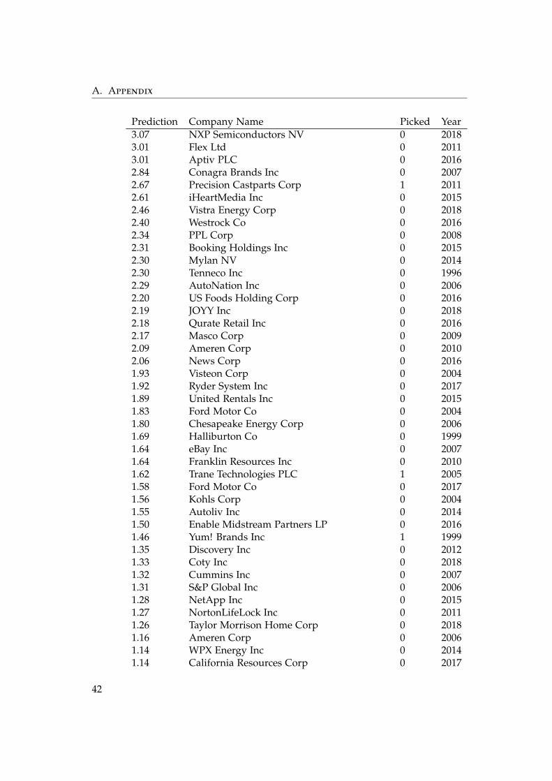
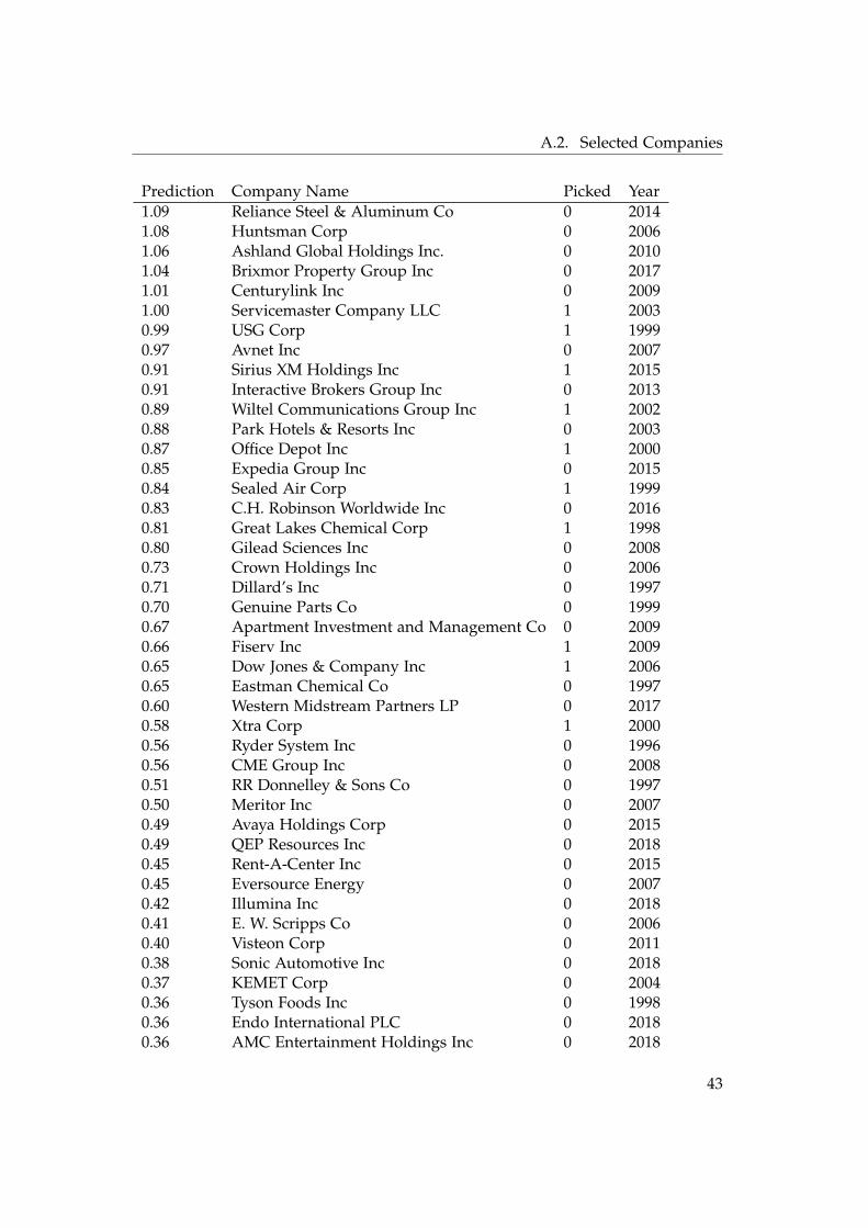
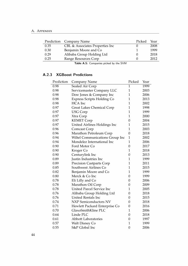
Table A.5: Companies picked by the SVM

A.2.3 XGBoost Predictions

Prediction Company Name Picked Year0.98 Sealed Air Corp 1 19990.98 Servicemaster Company LLC 1 20030.98 Dow Jones & Company Inc 1 20060.98 Express Scripts Holding Co 1 20130.98 HCA Inc 1 20020.97 Great Lakes Chemical Corp 1 19980.97 USG Corp 1 19990.97 Xtra Corp 1 20000.97 KEMET Corp 0 20040.97 United Airlines Holdings Inc 1 20150.96 Comcast Corp 1 20030.96 Marathon Petroleum Corp 0 20180.94 Wiltel Communications Group Inc 1 20020.94 Mondelez International Inc 1 20060.90 Ford Motor Co 0 20170.90 Kroger Co 1 20180.90 Centurylink Inc 0 20130.89 Justin Industries Inc 1 19990.89 Precision Castparts Corp 1 20110.85 Southwest Airlines Co 1 20150.82 Benjamin Moore and Co 1 19990.80 Merck & Co Inc 0 19990.78 Eli Lilly and Co 0 20060.78 Marathon Oil Corp 0 20090.78 United Parcel Service Inc 1 20050.76 Alibaba Group Holding Ltd 0 20180.76 United Rentals Inc 0 20150.74 NXP Semiconductors NV 0 20180.71 Hewlett Packard Enterprise Co 0 20160.70 GlaxoSmithKline PLC 1 20060.64 Linde PLC 0 20180.61 Abbott Laboratories 0 19970.57 Walt Disney Co 1 19990.55 S&P Global Inc 0 2006

44


Prediction Company Name Picked Year0.50 eBay Inc 0 20180.48 Lamb Weston Holdings Inc 0 20180.47 Mylan NV 0 20140.46 Stemline Therapeutics Inc 0 20180.42 HCA Healthcare Inc 0 20070.42 Yum! Brands Inc 1 19990.41 PPL Corp 0 20080.40 Aon PLC 0 20110.39 Halliburton Co 0 20180.39 Fiserv Inc 1 20090.38 Bunge Ltd 0 20080.38 Kohls Corp 0 20040.38 FedEx Corp 0 20020.36 Halliburton Co 0 19990.36 Ford Motor Co 0 20040.36 Chesapeake Energy Corp 0 20060.31 Conagra Brands Inc 0 20020.30 eBay Inc 0 20070.29 AutoNation Inc 0 20060.29 Franklin Resources Inc 0 20100.29 Baidu Inc 0 20160.28 Westrock Co 0 20160.27 Cummins Inc 0 20070.27 Qurate Retail Inc 0 20160.26 Accenture PLC 0 20180.24 Conagra Brands Inc 0 20070.23 Autozone Inc 0 19990.21 Autoliv Inc 0 20140.21 Trane Technologies PLC 1 20050.21 WPX Energy Inc 0 20140.21 Aptiv PLC 0 20160.21 Genuine Parts Co 0 19990.21 JOYY Inc 0 20180.20 Intel Corp 1 20100.20 Marathon Oil Corp 0 19980.20 Park Hotels & Resorts Inc 0 20030.19 Brown-Forman Corp 0 20100.19 Cummins Inc 0 19960.18 Dell Technologies Inc 0 20180.17 Vistra Energy Corp 0 20180.17 Cooper Tire & Rubber Co 0 19970.17 Oracle Corp 1 20170.17 Sirius XM Holdings Inc 1 2015

45

A. Appendix

Prediction Company Name Picked Year0.16 Eastman Kodak Co 0 20020.16 Ameren Corp 0 2010

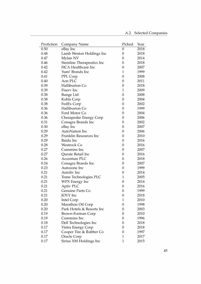
Table A.6: Companies picked by XGBoost

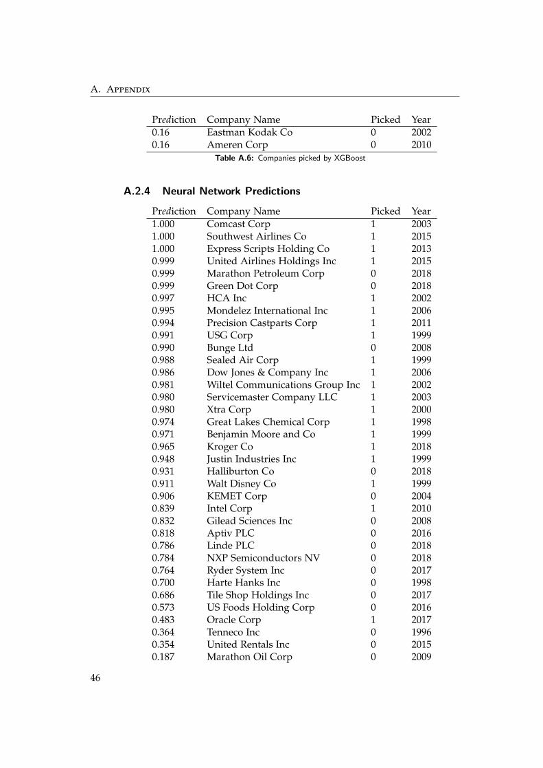
A.2.4 Neural Network Predictions

Prediction Company Name Picked Year1.000 Comcast Corp 1 20031.000 Southwest Airlines Co 1 20151.000 Express Scripts Holding Co 1 20130.999 United Airlines Holdings Inc 1 20150.999 Marathon Petroleum Corp 0 20180.999 Green Dot Corp 0 20180.997 HCA Inc 1 20020.995 Mondelez International Inc 1 20060.994 Precision Castparts Corp 1 20110.991 USG Corp 1 19990.990 Bunge Ltd 0 20080.988 Sealed Air Corp 1 19990.986 Dow Jones & Company Inc 1 20060.981 Wiltel Communications Group Inc 1 20020.980 Servicemaster Company LLC 1 20030.980 Xtra Corp 1 20000.974 Great Lakes Chemical Corp 1 19980.971 Benjamin Moore and Co 1 19990.965 Kroger Co 1 20180.948 Justin Industries Inc 1 19990.931 Halliburton Co 0 20180.911 Walt Disney Co 1 19990.906 KEMET Corp 0 20040.839 Intel Corp 1 20100.832 Gilead Sciences Inc 0 20080.818 Aptiv PLC 0 20160.786 Linde PLC 0 20180.784 NXP Semiconductors NV 0 20180.764 Ryder System Inc 0 20170.700 Harte Hanks Inc 0 19980.686 Tile Shop Holdings Inc 0 20170.573 US Foods Holding Corp 0 20160.483 Oracle Corp 1 20170.364 Tenneco Inc 0 19960.354 United Rentals Inc 0 20150.187 Marathon Oil Corp 0 2009

46


Prediction Company Name Picked Year0.155 Mylan NV 0 20140.065 Stemline Therapeutics Inc 0 20180.025 Meritor Inc 0 20070.020 Westrock Co 0 20160.016 AMC Entertainment Holdings Inc 0 20180.016 Merck & Co Inc 0 19990.012 Coty Inc 0 20180.011 Rent-A-Center Inc 0 20150.008 Sirius XM Holdings Inc 1 20150.007 Hibbett Sports Inc 0 20090.007 Chesapeake Energy Corp 0 20060.007 Hibbett Sports Inc 0 20050.006 Freeport-McMoRan Inc 0 20040.006 Illumina Inc 0 20180.006 Tofutti Brands Inc 0 20010.006 Ferroglobe PLC 0 20180.005 PPL Corp 0 20080.005 E. W. Scripps Co 0 20060.004 Centurylink Inc 0 20130.004 Office Depot Inc 1 20000.004 S&P Global Inc 0 20060.004 Eversource Energy 0 20070.004 United Parcel Service Inc 1 20050.004 Sequential Brands Group Inc 0 20180.003 Mesa Air Group Inc 0 2008

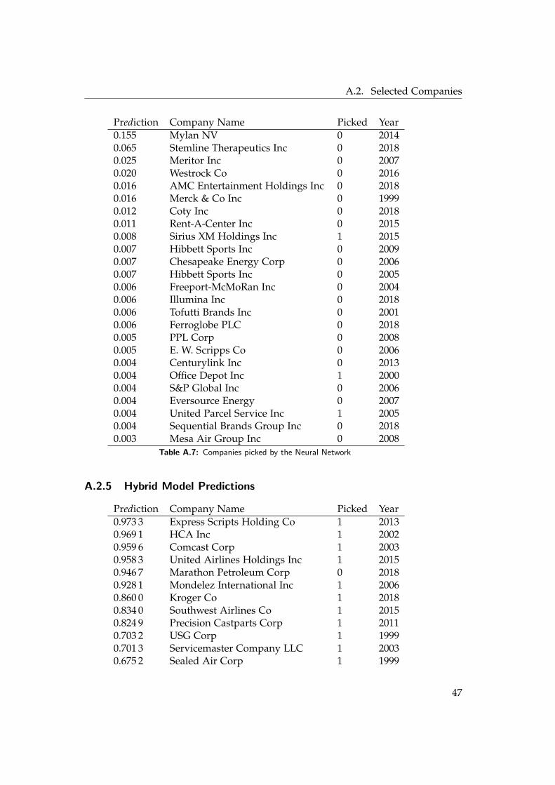
Table A.7: Companies picked by the Neural Network

A.2.5 Hybrid Model Predictions

Prediction Company Name Picked Year0.973 3 Express Scripts Holding Co 1 20130.969 1 HCA Inc 1 20020.959 6 Comcast Corp 1 20030.958 3 United Airlines Holdings Inc 1 20150.946 7 Marathon Petroleum Corp 0 20180.928 1 Mondelez International Inc 1 20060.860 0 Kroger Co 1 20180.834 0 Southwest Airlines Co 1 20150.824 9 Precision Castparts Corp 1 20110.703 2 USG Corp 1 19990.701 3 Servicemaster Company LLC 1 20030.675 2 Sealed Air Corp 1 1999

47

A. Appendix

Prediction Company Name Picked Year0.655 9 Great Lakes Chemical Corp 1 19980.655 5 Wiltel Communications Group Inc 1 20020.633 7 Dow Jones & Company Inc 1 20060.610 4 Xtra Corp 1 20000.556 2 NXP Semiconductors NV 0 20180.519 6 KEMET Corp 0 20040.517 4 Walt Disney Co 1 19990.499 1 Linde PLC 0 20180.465 6 Justin Industries Inc 1 19990.459 4 Benjamin Moore and Co 1 19990.367 6 Bunge Ltd 0 20080.359 0 Halliburton Co 0 20180.234 0 United Rentals Inc 0 20150.169 2 Intel Corp 1 20100.163 5 Aptiv PLC 0 20160.143 5 Marathon Oil Corp 0 20090.094 4 Ryder System Inc 0 20170.080 6 Oracle Corp 1 20170.069 4 Gilead Sciences Inc 0 20080.066 8 Mylan NV 0 20140.047 5 Tenneco Inc 0 19960.032 4 US Foods Holding Corp 0 20160.015 2 Green Dot Corp 0 20180.014 7 Stemline Therapeutics Inc 0 20180.012 6 Harte Hanks Inc 0 19980.012 4 Merck & Co Inc 0 19990.005 1 Westrock Co 0 20160.004 1 Tile Shop Holdings Inc 0 20170.003 9 Centurylink Inc 0 20130.002 8 United Parcel Service Inc 1 20050.002 0 Chesapeake Energy Corp 0 20060.001 9 Eli Lilly and Co 0 20060.001 9 PPL Corp 0 20080.001 6 S&P Global Inc 0 20060.001 5 eBay Inc 0 20180.001 3 GlaxoSmithKline PLC 1 20060.001 1 Aon PLC 0 20110.000 9 Sirius XM Holdings Inc 1 20150.000 9 Coty Inc 0 20180.000 7 AutoNation Inc 0 20060.000 7 Kohls Corp 0 20040.000 7 Hewlett Packard Enterprise Co 0 20160.000 6 Trane Technologies PLC 1 2005

48

A.3. Code

Prediction Company Name Picked Year0.000 6 AMC Entertainment Holdings Inc 0 20180.000 6 Halliburton Co 0 19990.000 5 Fiserv Inc 1 20090.000 5 Abbott Laboratories 0 19970.000 5 HCA Healthcare Inc 0 20070.000 5 Illumina Inc 0 20180.000 5 Yum! Brands Inc 1 1999

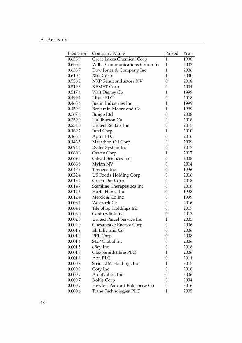
Table A.8: Companies picked by the Hybrid Model

A.3 Code

The entire code can be found on https://gitlab.com/Spatiality/PORTFOLIO2020/-/tree/master/03 thesis, the author’s GitLab page.

49

https://gitlab.com/Spatiality/PORTFOLIO2020/-/tree/master/03_thesis

https://gitlab.com/Spatiality/PORTFOLIO2020/-/tree/master/03_thesis

Bibliography

[1] Thomson reuters eikon.

[2] Rules and regulations under the securities exchange act of 1934. Securitiesand Exchange Commission, Washington, D.C, 1935.

[3] Edward I. Altman. Financial ratios, discriminant analysis and the pre-diction of corporate bankruptcy. Journal of Finance, 23(4):589–609, 1968.

[4] Clifford Asness, Andrea Frazzini, and Lasse Pedersen. Quality minusjunk. Review of Accounting Studies, 24(1):34–112, 2019.

[5] Messod D. Beneish. The detection of earnings manipulation. FinancialAnalysts Journal, 55(5):24–36, 1999.

[6] Warren Buffett. Warren Buffett on business : principles from the sage ofOmaha. John Wiley & Sons, Hoboken NJ, 2010.

[7] Tianqi Chen and Carlos Guestrin. XGBoost: A scalable tree boostingsystem. In Proceedings of the 22nd ACM SIGKDD International Conferenceon Knowledge Discovery and Data Mining, KDD ’16, pages 785–794, NewYork, NY, USA, 2016. ACM.

[8] Francois Chollet et al. Keras, 2015.

[9] S. Christoffersen, E. Danesh, and D. Musto. Why do institutions delayreporting their shareholdings? evidence from form 13f. 2015.

[10] Corinna Cortes and Vladimir Vapnik. Support-vector networks. Ma-chine Learning, 20(3):273–297, 1995.

[11] Simon Cross, Robert Harrison, and R Kennedy. Introduction to neuralnetworks. The Lancet, 346(8982):1075–9, 1995.

[12] Timothy Dozat. Incorporating nesterov momentum into adam. 2016.

51

Bibliography

[13] Tom Fawcett. An introduction to roc analysis. Pattern recognition letters,27(8):861–874, 2006.

[14] Ehsan Habib Feroz, Taek Mu Kwon, Victor S. Pastena, and KyungjooPark. The efficacy of red flags in predicting the sec’s targets: an artificialneural networks approach. Intelligent Systems in Accounting, Finance andManagement, 9(3):145–157, 2000.

[15] V. Filimonov and D. Sornette. A stable and robust calibration schemeof the log-periodic power law model. Physica A: Statistical Mechanics andits Applications, 392(17):3698 – 3707, 2013.

[16] Andrea Frazzini, David Kabiller, and Lasse Heje Pedersen. Buffett’salpha. Financial Analysts Journal, 74(4):35–55, 2018.

[17] Karl Pearson F.R.S. Liii. on lines and planes of closest fit to systems ofpoints in space. The London, Edinburgh, and Dublin Philosophical Magazineand Journal of Science, 2(11):559–572, 1901.

[18] Trevor Hastie. The elements of statistical learning : data mining, inference,and prediction. Springer series in statistics. Springer, New York NY, sec-ond edition, corrected at 12th printing 2017 edition, 2017.

[19] J. Heaton. An empirical analysis of feature engineering for predictivemodeling. In SoutheastCon 2016, pages 1–6, 2016.

[20] J. D. Hunter. Matplotlib: A 2d graphics environment. Computing inScience & Engineering, 9(3):90–95, 2007.

[21] Sotiris Kotsiantis, Euaggelos Koumanakos, Dimitris Tzelepis, andVasilis Tampakas. Predicting fraudulent financial statements with ma-chine learning techniques. In Advances in Artificial Intelligence: 4thHelenic Conference on AI, SETN 2006, Heraklion, Crete, Greece, May 18-20, 2006. Proceedings, volume 3955 of Lecture Notes in Computer Science,pages 538–542. Springer Berlin Heidelberg, Berlin, Heidelberg, 2006.

[22] Jerry W Lin, Mark I Hwang, and Jack D Becker. A fuzzy neural networkfor assessing the risk of fraudulent financial reporting. Managerial Au-diting Journal, 18(8):657–665, 2003.

[23] Warren S. McCulloch and Walter Pitts. A Logical Calculus of the IdeasImmanent in Nervous Activity, page 15–27. MIT Press, Cambridge, MA,USA, 1988.

[24] Wes McKinney. Data structures for statistical computing in python. InStefan van der Walt and Jarrod Millman, editors, Proceedings of the 9thPython in Science Conference, pages 51 – 56, 2010.

52

Bibliography

[25] Partha Mohanram. Separating winners from losers among lowbook-to-market stocks using financial statement analysis. Review of AccountingStudies, 10(2-3):133–170, 2005.

[26] James Montier. Cooking the books, or, more sailing under the blackflag. Mind Matters, June 2008.

[27] Benjamin Moritz and Tom Zimmermann. Tree-based conditional port-folio sorts: The relation between past and future stock returns. SSRNElectronic Journal, 2016.

[28] James A. Ohlson. Financial ratios and the probabilistic prediction ofbankruptcy. Journal of Accounting Research, 18(1):109–131, 1980.

[29] Travis Oliphant. NumPy: A guide to NumPy. USA: Trelgol Publishing,2006–. [Online; accessed ¡today¿].

[30] Jane A Ou and Stephen H Penman. Financial statement analysis and theprediction of stock returns. Journal of accounting & economics, 11(4):295–329, 1989.

[31] F. Pedregosa, G. Varoquaux, A. Gramfort, V. Michel, B. Thirion,O. Grisel, M. Blondel, P. Prettenhofer, R. Weiss, V. Dubourg, J. Vander-plas, A. Passos, D. Cournapeau, M. Brucher, M. Perrot, and E. Duch-esnay. Scikit-learn: Machine learning in python. Journal of MachineLearning Research, 12:2825–2830, 2011.

[32] Johan Perols. Financial statement fraud detection: an analysis of statis-tical and machine learning algorithms.(report). Auditing: A Journal ofPractice & Theory, 30(2):19, 2011.

[33] Joseph D. Piotroski. Value investing: the use of historical financial state-ment information to separate winners from losers. Journal of AccountingResearch, 38(SUPP):1–51, 2000.

[34] Joseph D. Piotroski and Eric C. So. Identifying expectation errors in val-ue/glamour strategies: A fundamental analysis approach. The Reviewof Financial Studies, 25(9):2841–2875, 2012.

[35] Richard Sloan. Do stock prices fully reflect information in accruals andcash flows about future earnings? The Accounting Review, 71(3):289,1996.

[36] M. Stone. Cross-validatory choice and assessment of statistical predic-tions. Journal of the Royal Statistical Society: Series B (Methodological),36(2):111–133, 1974.

53

Bibliography

[37] Jan Szilagyi, Jens Hilscher, and John Campbell. In search of distressrisk, 2008.

[38] Luo Y. Wang S. Signal processing: The rise of the machines. DeutscheBank Quantitative Strategy, Jun 2012.

[39] Michael Waskom, Olga Botvinnik, Drew O’Kane, Paul Hobson,Saulius Lukauskas, David C Gemperline, Tom Augspurger, YaroslavHalchenko, John B. Cole, Jordi Warmenhoven, Julian de Ruiter,Cameron Pye, Stephan Hoyer, Jake Vanderplas, Santi Villalba, GeroKunter, Eric Quintero, Pete Bachant, Marcel Martin, Kyle Meyer, Al-istair Miles, Yoav Ram, Tal Yarkoni, Mike Lee Williams, ConstantineEvans, Clark Fitzgerald, Brian, Chris Fonnesbeck, Antony Lee, andAdel Qalieh. mwaskom/seaborn: v0.8.1 (september 2017), September2017.

54

the robo-investors from graham-doddsville - eth zürich

Documents