the portability of new immigrants' human capital: language, education and occupational matching
TRANSCRIPT

Optimal Unemployment Insurance in GE: a Robust
Calibration Approach
Marco Cozzi, Queen’s University∗
April 2012
Abstract
This paper implements a simple Monte Carlo calibration approach to quantitatively study
the Hansen and Imrohoroglu (1992) economy, a GE model with uninsurable employment risk,
designed to assess the optimal replacement rate for a public Unemployment Insurance scheme.
The results of this sensitivity analysis are consistent with the original findings, but with
several caveats. One novel result in particular is that the sampling distribution of the optimal
UI is bimodal. Depending on the calibrated parameters, the optimal UI is in one of two regions:
a very generous scheme with high replacement rates, where insurance is mainly provided by
the UI scheme, or one with low replacement rates, where insurance is mainly achieved through
self-insurance. Even in the absence of moral hazard, it is never optimal to provide full insurance.
Moreover, for many plausible parameters’ configurations, the welfare maximizing replacement rate
does not decrease with the level of MH. The qualitative patterns and quantitative findings are
not altered substantially when considering an enlarged labor force, which includes the marginally
attached workers. Finally, the parameters representing the hours worked, the leisure share in
the households’ consumption bundle, and the risk aversion have a first order impact on the
average welfare. The determination of the optimal UI scheme depends heavily on them. This
finding suggests that extra caution should be paid when calibrating these parameters in similar
environments.
JEL Classification Codes: E21, D52, D58.
Keywords: Calibration methods, Unemployment Risk, Optimal Unemployment Insurance,
Heterogeneous Agents, Incomplete Markets, Computable General Equilibrium, Monte Carlo.
∗Contact details: Department of Economics, Queen’s University, 94 University Avenue, Kingston, ON K7L 3N6,
Canada. Tel: 1-613-533-2264, Fax: 1-613-533-6668, Email: [email protected]. Aknowledgements: I am
grateful to an anonymous referee for many useful suggestions. A shorter version is Forthcoming in the Economics
Letters.
1
1 Introduction
Unemployment Insurance (UI) programs are widespread systems designed to provide insurance to
workers experiencing unemployment spells. Public expenditures devoted to UI and assistance pro-
grams are sizeable in most OECD Countries, being in the order of 2-3% of GDP, as reported by Martin
(2002). Given their importance, several theoretical and applied studies have been analyzing the wel-
fare consequences of UI schemes, together with their effects on job search efforts and unemployment
duration.
A very influential paper in this area is Hansen and Imrohoroglu (1992). Arguably, this contribu-
tion started the theoretical and quantitative assessment of UI programs in models with Heterogeneous
Agents (HA), later studied by Hopenhayn and Nicolini (1997), Acemoglu and Shimer (1999), Abdulka-
diroglu, Kuruscu and Sahin (2002), Young (2004), Pollak (2007), Shimer and Werning (2008), Pavoni
(2009), Krusell, Mukoyama, and Sahin (2010), and Boostani, Gervais and Siu (2011), among others.
The purpose of this paper is to use a robust calibration procedure to quantify the optimal UI
scheme. To this end, a thorough robustness exercise for the environment proposed by Hansen and
Imrohoroglu (1992) will be performed. This global robustness check will implement a Monte Carlo
procedure. Relying on the methodology developed by Canova (1994), priors for the parameters’
distributions consistent with the available evidence are going to be postulated. The model is going
to be solved 1,000 times, each time with a different calibration drawn from the joint distribution of
parameters’ priors, delivering sampling distributions for the optimal UI program.
The overall message of Hansen and Imrohoroglu (1992) is confirmed, with several caveats: optimal
UI replacement rates tend to be quantitatively large, and the presence of Moral Hazard (MH) does
play a role in decreasing them. However, there are some additional novel findings.
First, the sampling distribution of the optimal UI appears to be bimodal. This implies that, even
in the absence of MH, there are many empirically plausible calibrations such that low replacement
rates are optimal. The 60% threshold seems to be the watershed of two different regions: one region
with high replacement rates, low precautionary savings and low consumption inequality, and another
one with the opposite outcomes. In the first case insurance is mainly provided by the UI scheme,
while in the second one consumption smoothing is achieved mainly through self-insurance.
Second, increasing the level of MH in the economy decreases the optimal UI. But this is only true
on average. Just like for the Hansen and Imrohoroglu (1992) calibration, for several cases, the higher
the MH, the lower the optimal replacement rate. However, in no less than 26% of the experiments,
the welfare maximizing replacement rate does not decrease below 60% with the level of MH. Even
with pervasive MH, there is still a large fraction of economies for which high replacement rates are
optimal.
2

Third, taking a different stand on the labor force composition leads to similar qualitative patterns
and quantitative findings. To this end, an enlarged labor force including also the marginally attached
workers is considered in the model economy.
Fourth, even in the absence of moral hazard, it is never optimal to provide full income insurance.
The increased taxation stemming from both a more generous scheme and higher unemployment rates
makes it too costly to give a 100% replacement rate. A basic trade-off between insurance and search
incentives prevents full insurance to be the welfare maximizing scheme.
Fifth, the number of hours worked, the leisure share in the households’ consumption bundle, and
the risk aversion have a first order impact on the determination of average welfare, hence on the
selection of the optimal UI scheme. This finding suggests that extra caution should be paid when
calibrating these parameters in similar environments and calls for some robustness checks with respect
to them.
The rest of the paper is organized as follows. Section 2 presents the theoretical model. Section
3 is devoted to the description of the Monte Carlo experiments. Section 4 presents the main results,
while Section 5 concludes. A series of appendices provide more details on the methodology together
with some additional results.
2 The Hansen and Imrohoroglu (1992) Economy
The economy is a GE one with incomplete markets and uninsurable employment risk, designed to
quantify the optimal UI program, with and without MH. The UI scheme is specified as a fixed
replacement rate of labor earnings, while MH arises because of limited observability of the unemployed
agents’ actions. This allows a fraction of unemployed workers rejecting employment opportunities to
be able to keep collecting UI benefits. Crucially, idiosyncratic employment shocks together with
incomplete markets and a no-borrowing constraint give a role for social insurance on top of self-
insurance. Time is discrete. The economy is populated by a measure one of infinitely lived ex-ante
identical agents.1
2.1 Preferences
Agents’ preferences are assumed to be represented by a time separable utility function u(.). Their
utility is defined over stochastic processes for consumption and leisure {ct, lt}∞t=0. Agents choose how
much to consume (ct), whether to work or not (when given the opportunity to choose) a fixed amount
1 In the interest of space, just a sketch of the model is going to be presented. For more details see Appendix A and
Hansen and Imrohoroglu (1992).
3

of hours 0 < h < 1 by setting their desired leisure(lt =
{1− h, 1
}), and how much to save in a
non interest bearing asset (mt+1) in each period of their lives, in order to maximize their objective
function. The agents’ problem can be defined as:
max{ct,lt,mt+1}∞t=0
E0u(c0, l0, c1, l1, ...) = max{ct,lt,mt+1}∞t=0
E0
∞∑
t=0
βtU (ct, lt)
where E0 represents the expectation operator over the employment opportunity shocks s ∈ S = {u, e},
and β ∈ (0, 1) is the subjective discount factor. Following Hansen and Imrohoroglu (1992), the per-
period utility function U (., .) is assumed to be strictly increasing, strictly concave, and to satisfy the
Inada conditions. The specific functional form is U (ct, lt) =(c1−σt lσt )
1−ρ−1
1−ρ , which has a RRA = ρ that
maps into its "consumption only" counterpart that is typically estimated with the transformation
ρ = 1− (1− σ) (1− ρ).
2.2 Endowments
Agents can be employed (e), or unemployed (u). Every agent is endowed with the same exogenous
efficiency units: when employed they all produce the same amount of output y, normalized to y = 1.
If employed, they earn a wage w = y and pay proportional taxes (τ) to finance the unemployment
benefit scheme. If unemployed, agents collect unemployment benefits, which are specified as a constant
replacement rate θ of the going wage, and pay proportional taxes (τ).
Employment opportunities are stochastic, and follow a two-state first-order Markov process. The
transition function of the employment opportunity state is represented by the matrix χ(s′,s) =
[χ (i, j)] , where each element χ(i,j) is defined as χ(i,j) = Pr {st+1 = i|st = j} , i, j = {u, e}. Once
the state s = e is realized, the agent can still reject this employment opportunity, by setting his labor
supply to zero. The unemployment rate and the unemployment duration in this economy are a mix of
choice and chance. The persistent stochastic process gives the agents the opportunity to work, while
at the same time the generosity of the UI scheme potentially gives disincentives for agents to accept
these jobs.
Agents can refuse employment opportunities and, because of imperfect monitoring, still receive
unemployment benefits, which leads to a form of MH to be present in the economy. The parameter
capturing the extent of this feature is π (η), namely the probability that an agent turning down a
job offer is not detected. This probability might depend on the agent’s previous employment status
η. Finally, UI eligibility is represented by µ, the workers with µ = 0 being the non eligible ones. If
eligible agents turning down a job are not detected, they can collect the UI benefits.2
2 In the applied section of the paper we are going to set π (e) = 0. It follows that MH matters only for the unemployed
agents.
4

There are no state-contingent markets to insure against the idiosyncratic employment risk, but
workers can self-insure by saving into the asset mt, while facing a no-borrowing constraint, so that
mt+1 ≥ 0.
3 (Monte Carlo) Calibration
Following Canova (1994), the model economy is parametrized with Monte Carlo methods. Several
combinations of parameters are drawn from a set of prior distributions, and the model is solved
for each realization of the parameters vector. Hence, this calibration procedure embeds in itself a
global sensitivity analysis. With this methodology it is possible to: 1) provide evidence on extensive
robustness checks, 2) have sampling distributions for the outcomes of interest, showing which results
are more likely to be relevant and which ones appear to be less plausible, 3) study which parameters
affect the determination of the computed equilibria the most, informing other researchers in the field
on what parameters should be calibrated more carefully.3
[Table (1) about here]
Table (1) provides the parameters’ list in the Hansen and Imrohoroglu (1992) economy, together
with their upper and lower values that are going to be used in the simulations. These values are chosen
to match some macroeconomic facts and to be consistent with the available empirical evidence. In
order to check if the findings are robust to relatively large changes in the parameters, and if they are
well behaved with respect to them, the parameters’ bounds are chosen to allow for a wide range of
possible calibrations. At the same time, an attempt is made to prevent the model to grossly miss
some quantitative implications. This could happen in several replications if the parameters’ ranges
were to be too wide.
There are six independent parameters: β, σ, ρ, h, and the two probabilities in the Markov chain,
χ(e′,e) and χ(e′,u). Canova (1994) provided an intuitive yet powerful procedure to implement global
robustness checks for fully parametrized quantitative models. The methodology acknowledges parame-
ters’ uncertainty and assumes prior distributions for the model’s parameters. At the simulation stage,
it repeatedly solves the model for many different calibrations, rather than computing the quantitative
implications of a theory for a unique set of calibrated parameters.
Specifying prior distributions to calibrate the model has some positive implications.
3For further details on this methodology applied to a standard HA model, and on the related issues, see Cozzi (2011).
5
First, it makes a global sensitivity analysis feasible. An alternative approach would be to discretize
the parameters’ space and consider all possible combinations of parameters’ grid points. Unfortunately,
for this class of models, this is not a viable option. With several parameters, six in this case, even
considering only 5 points in each dimension would lead to another manifestation of the curse of
dimensionality. This would generate 15,625 possible combinations: given the average computing time
of an optimal UI scheme, it would take no less than 50 days to complete each experiment on a top
of the line workstation. As in other applications, randomization can help in breaking the curse of
dimensionality.
The second implication is more grounded in economics. As stressed in the Bayesian literature, for
example by DeJong, Ingram, and Whiteman (2000) and An and Schorfheide (2007), specifying a set of
prior distributions for the parameters allows the researcher to exploit some of the available estimates,
giving more weight to the parameters’ values that are more likely to be empirically relevant.
Finally, standard calibration procedures tend to overlook parameters’ uncertainty. This can arise
from uncertainty on the moments the model should match, from the intrinsic uncertainty of the
estimates used to pin down a subset of the parameters, or by the unavoidable abstractions that a
model makes. These issues are tackled by the simple Monte Carlo methodology used here.
3.1 Calibration and Global Sensitivity Analysis
The calibration procedure consists of performing a series of Monte Carlo experiments, which rely on
two steps.
In the first step, the prior distributions from which the parameters are going to be drawn are
postulated. In the second step, 1,000 economies are simulated and solved. These economies differ
only in the parameters’ vector that is drawn at each replication i. For every economy, the equilibria
for all possible UI replacement rates θ are computed. Notice that the computation of the equilibrium
requires an iterative procedure on the tax rate τ until the government achieves a balanced budget.
Once the sequence of equilibria for the economies with all the different θ’s are computed, a welfare
measure comparison determines which UI scheme θ∗ is optimal, namely the one that achieves the
highest average steady-state welfare, with a utilitarian functional.4
As an additional robustness check, these experiments are repeated several times, with different
priors for the parameters’ distributions, with different assumptions on the degree of moral hazard (i.e.
how likely it is for unemployed workers to reject a job offer while keeping the entitlement to the UI
benefits), and with different assumptions on the nature of the labor market.
4The solution algorithm together with some computational aspects are explained in Appendices B and C.
6

[Table (2) about here]
Table (2) reports the list of experiments that are going to be considered. More in detail, four sets
of experiments (B1 -B4 ) are going to be reported.
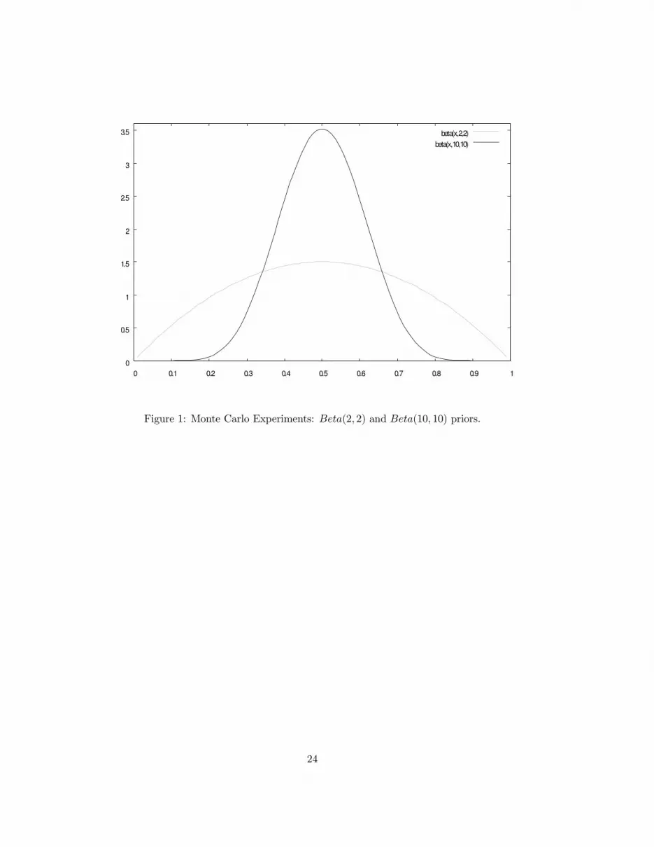
As for the parameters’ priors, two independent Beta distributions that vary in their dispersion are
specified: aBeta(10, 10) and aBeta(2, 2).5 The choice settled on these distributions for two reasons: 1)
with the priors centered around the Hansen and Imrohoroglu (1992) calibration, it is possible to assess
if there is a tendency for the outcomes to cluster around their results; 2) the Beta(10, 10) distribution
is substantially more concentrated than the Beta(2, 2) one, hence by increasing the dispersion of the
priors it is possible to appreciate the effect of relying on more extreme calibrations, that differ more
markedly from the benchmark one. Figure (1) shows the shape of the two Beta priors over the [0, 1]
interval.
[Figure (1) about here]
As for MH, three cases are going to be considered: a no MH case, with π (u) = 0%, a mild MH
case, with π (u) = 10%, and a more severe MH case, with π (u) = 50%. The first case is characterised
by perfect monitoring of the unemployed agents, because the UI agency never allows workers turning
down jobs to collect UI benefits. In the second and third cases there is a 10% and a 50% chance,
respectively, that an unemployed worker turning down a job opportunity will still be able to collect
UI benefits.
For each prior-MH combination, two different assumptions on the nature of the labor market are
going to be made. In the baseline model, the labor force is going to be the same as the one in Hansen
and Imrohoroglu (1992). In this case, considered in experiments B1 and B2, the underlying concept
of unemployment is the one defined and computed by the relevant statistical agencies, for example in
the U.S. by the Bureau of Labor Statistics. The alternative specification, considered in experiments
B3 and B4, takes a different stand on the nature of unemployment in the model economy, and on the
5More precisely, these distributions have four parameters: two shape parameters together with two location para-
meters. The location parameters allow to define the support of the distribution in an interval different from the [0, 1]
one, and they coincide with the upper and lower bounds reported in the last two columns of Table 1. For the other
two (shape) parameters that are needed to fully characterize the Beta distribution, two different set-ups are considered.
The former relies on the prior Beta(10, 10) for all the parameters, while the latter considers a Beta(2, 2) prior. These
specifications deal with Beta distributions which are symmetric around their means, because the two shape parameters
are equal. The pair (10, 10) implies a distribution which is substantially more concentrated around its mean, when
compared to the (2, 2) one.
7

related interpretation of the UI program. Jones and Riddell (1999) show that in the data it is hard
to distinguish between individuals who are genuinely unemployed and individuals who are formally
not unemployed, but they still are in the labor force. There is some evidence that workers who are
marginally attached to the labor force, namely those who are not actively looking for a job, have labor
market outcomes that are similar to the ones experienced by the workers that are formally counted
as unemployed. With these facts in mind, compared to the baseline model, it seems reasonable to
consider an enlarged labor force, where also the discouraged workers and people that are in the labor
force but would not be necessarily considered as unemployed workers are included into the labor
market figures. Accordingly, this alternative assumption calls for a different interpretation of the UI
scheme. In this case, it will implicitly refer to a broader concept of a public assistance program. The
main characteristics of this program are: a) its financing, obtained through general taxation, b) the
value of the benefits, which is tightly linked to the labor earnings of the employed workers, and c) the
recipients of the benefits, who are the workers who do not have a job.
The experiments B1 and B3 assume that all parameters are distributed according to aBeta(10, 10).
This is a symmetric and fairly concentrated distribution, whose average for every parameter is picked
to coincide with the values used in the calibration by Hansen and Imrohoroglu (1992). Case B1
will deal with the standard definition of the unemployment rate, while case B3 will deal with the
alternative definition, and it will target the employment rate instead.
The other experiments, denoted by B2 and B4, consider as the parameters’ priors the Beta(2, 2)
distribution. The averages of the priors are kept to the values that are consistent with the typical
calibrations of these models, the one used by Hansen and Imrohoroglu (1992) in particular.
More precisely: βavg = βHI92 = 0.995, σavg = σHI92 = 0.67, ρavg = ρHI92 = 2.5, havg = hHI92 =
0.45, χavg(e′,u) = χHI92(e′,u) = 0.5 and χavg(e′,e) = χ
HI92(e′,e) = 0.9681.
The upper and lower values for β,(β = 0.999 and β = 0.991
), imply a discount rate at the annual
frequency of 0.87% and 8.1%, while the average βavg = 0.995 implies a discount rate of 4.44%. Working
with a time period of six weeks opens the issue of how individuals discount future economic quantities
over short time horizons. Identification problems lead to a lack of consensus on the point estimates.
The available values for labor market environments, for example estimated by van den Berg (1990)
and Dey and Flinn (2005), suggest large ranges for the discount rates. This explains why a relatively
broad set of values for β is considered.6
As for σ and ρ, the main target pinning them down are the estimates of the Intertemporal Elasticity
of Substitution (IES), obtained by Attanasio, Banks, Meghir, and Weber (1999), among others. It
6Notice that, although this is a production economy, capital does not enter the production function. Hence, it is not
possible to set β for the economy to match the observed real interest rate or, equivalently, the capital/output ratio.
8

goes without saying that, given a value ρ for the RRA = 1IES
coefficient, there are infinite pairs of
σ and ρ that satisfy it. This consideration supports the view that an extensive sensitivity analysis is
needed. The upper and lower values for σ and ρ are chosen to satisfy a restriction on the adjusted
RRA (ρ), which has to lie in the [1.0, 2.5] interval.
[Figure (2) about here]
Figure (2) shows the distributions of the Relative Risk Aversion that are implied by the values of
σ and ρ that are used in the simulations. As it can be seen, ρ lies always in the [1.0, 2.5] interval,
which represents the range of available estimates for this parameter. As pointed out by Hansen and
Imrohoroglu (1992), it was also found that the results are quite sensitive to the specific value of the
RRA coefficient. This is shown in Figure (2): the outcomes, namely being in a high (θ∗ > 60%)
vs. low (θ∗ ≤ 60%) optimal UI regime, differ systematically with the average and the dispersion of
the RRA coefficient. The higher the RRA, the lower the likelihood that a low replacement rate is
optimal.7
As for the utility costs of working, the share of market time is represented by the parameter h.
Data from the American time use survey for the year 2009 show that on average employed people with
children spend (on working days) approximately 7.7 hours sleeping, and 8.7 working. The benchmark
calibration considered hHI92 = 0.45. This value was kept as the prior’s average, while the lower bound
was h = 0.35 (in this case sleeping is included in the definition of leisure, notice that 8.724 = 0.36), and
the upper bound was h = 0.55 (in this case only non-sleeping time is considered to be available for
market and non market activities, notice that 8.724−7.7 = 0.53).
Finally, the Markov chain parameters in the benchmark calibration(χHI92(e′,e) = 0.9681 and χHI92(e′,u) = 0.5
)
imply an unemployment rate of 6% and an unemployment duration of two model periods, namely 12
weeks.8 The model considers a stationary environment, hence the relevant labor market figures are
long-run averages. However, 1) labor market statistics vary wildly over the cycle, 2) in the last 20
years the long-run unemployment duration has increased. This explains the ranges that are considered
for χ(e′,e) and χ(e′,u). The upper and lower bounds for the latter imply an unemployment duration of
9 and 20 weeks. While the upper and lower values for the unemployment rate are 10.1% and 2.3%.
As argued above, it seems important to check the robustness of the results with respect to the
measurements in the labor market. These cases are denoted with E3, for the Beta(10, 10) priors, and
with E4, for the Beta(2, 2) priors.
7Figure (2) focuses on the B1-B2 experiments. The B3-B4 ones have similar graphs. Notice that the figure provides
the breakdown with respect to the degree of MH as well.8This is true only for the cases where employment opportunities are never turned down.
9

To achieve this target, a substantially different parametrization is going to be specified for the
Markov chain governing the employment opportunities. For these experiments, χavg(e′,e) = 0.87 and
χavg
(e′,u) = 0.4. Although these might seem to be pretty minor changes, quantitatively they imply
drastically higher unemployment rates and longer average unemployment durations, even for the
cases when no job opportunities are turned down. These values imply an employment rate of 75.7%,
which roughly matches the employment rate for the U.S. economy, and an unemployment duration
of two and half model periods, namely 15 weeks. The upper and lower bounds for χ(e′,u) imply a
(minimum) average unemployment duration of 10 and 30 weeks. While the upper and lower values
for the (potential) employment rate are 96.6% and 49.6%.
4 Results
This Section presents the main results. First, it documents how allowing for very flexible calibrations
does quantitatively alter the optimal UI replacement rates. Second, it provides a discussion on how
the endogenous variables, namely the aggregate asset holdings, the tax rate, and the variance of
consumption behave in this global robustness exercise.9
[Tables (3) and (4) about here]
Tables (3) and (4) report a set of statistics for the outcomes that are the focus of the analysis. The
minimum, maximum, mean, median and coefficient of variation are listed for all experiments, which
are a mix of parameters’ priors, degree of MH, and labor market definition.
Moreover, in order to provide a more intuitive summary of such a rich analysis, several figures are
included. Most figures show six panels. In these cases, each panel represents the non-parametric kernel
density estimate of an endogenous variable, for a particular prior-MH pair and a given definition of the
labor market. The figures presenting more panels show an additional breakdown of the experiments,
which are ordered according to the level of their optimal UI replacement rate θ∗.
4.1 Equilibrium Outcomes
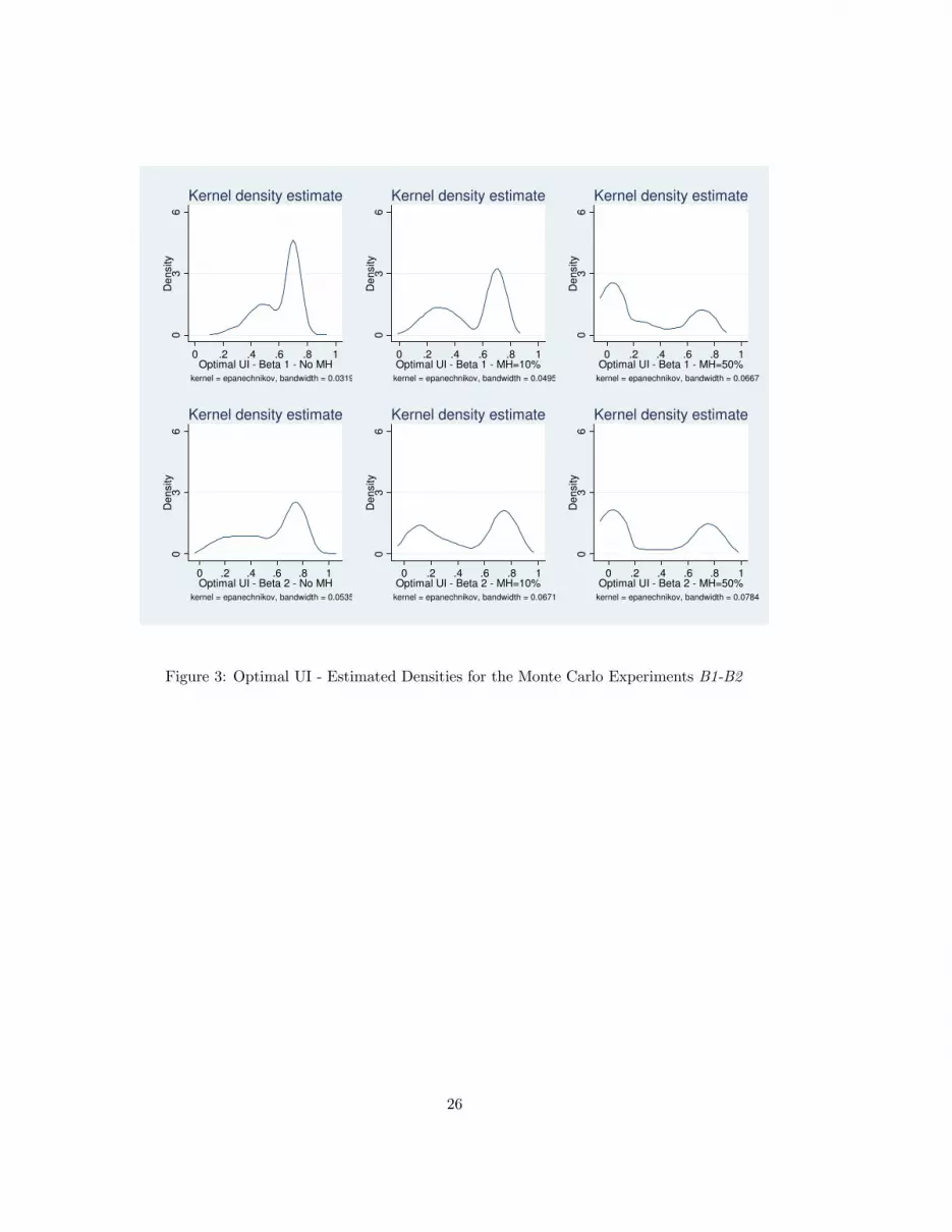
Figures (3) and (4) display the welfare maximizing UI replacement rates θ∗ coming from the solution
of the model, calibrated 1,000 different times for each experiment B1 -B4.
The first striking result is that the overall patterns are shared by all experiments.
9 In the interest of space, the results related to the employment rate and the difference between the employment
opportunity and the actual employment rate are reported in an appendix.
10

For any prior-MH-labor market triplet, the sampling distribution of the optimal UI is bimodal,
a fact that has a natural economic interpretation. Broadly speaking, there are two possible optimal
UI regions: one region is characterized by a high replacement rate, low precautionary savings and
low consumption inequality. In this region insurance is mainly provided by the UI. When the MH
and the utility costs of working are not too severe, it is inexpensive for the government to provide
generous UI benefits, which in turn lead to reasonable tax rates. On the other hand, the other optimal
regime entails the opposite outcomes. In this case, insurance is achieved mainly through self-insurance,
because the incentives to stay unemployed for too long a period, together with the high expenditure
per unemployed worker, make a generous UI system too costly in terms of taxation.
The 60% threshold seems to be the level of the replacement rate that separates the two different
regions. What is striking, is that the same threshold persists when moving to economies with a higher
level of MH, when moving to economies with more dispersed priors, and to economies with a different
underlying labor market.10
Quantitatively, the median θ∗ across experiments falls in the [60%, 70%] range, dropping sharply
to the [10%, 36%] range only for the high MH cases. Notice that the variability of θ∗, as represented
by its coefficient of variation, increases monotonically in the degree of MH, a result that is discussed
below.
[Figures (3), (4), (5) and (6) about here]
The results for the optimal UI sampling distributions are mirrored by the behavior of savings, of
consumption inequality and of the equilibrium tax rate. Detailed statistics about these endogenous
variables are provided in Tables (3) and (4).
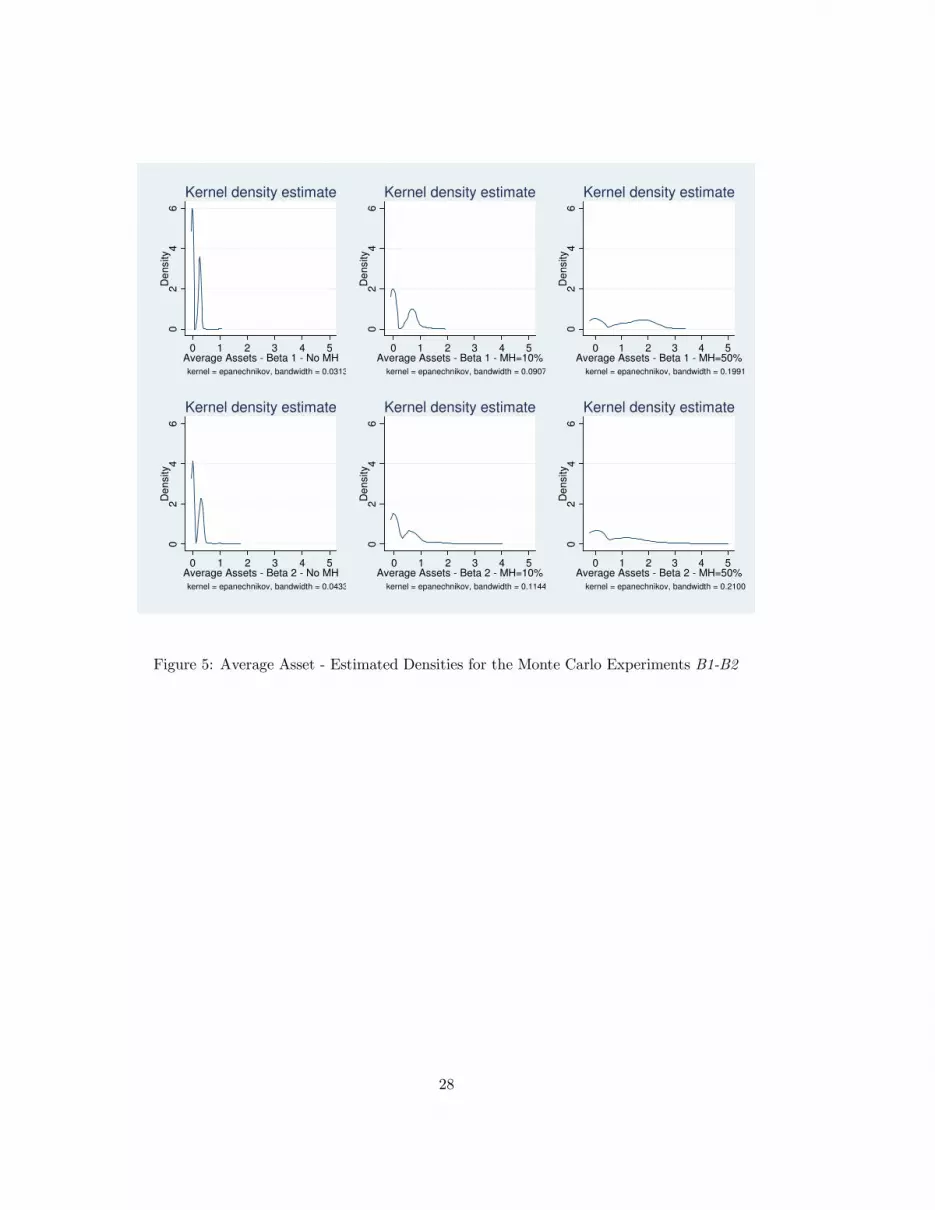
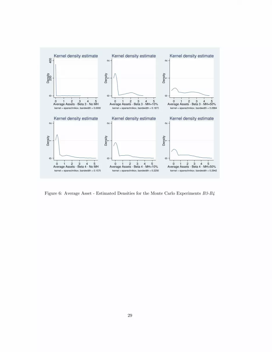
Figures (5) and (6) depict the sampling distributions of the average asset holdings. Also this
variable has bimodal distributions, because the households compensate with their savings behavior
the level of insurance provided by the UI system. A generous system induces low precautionary
savings, because being unemployed does not make consumption smoothing too difficult. Differently,
high precautionary savings are needed for all UI schemes that do not provide enough funds to achieve a
relatively flat consumption profile over all possible states. This also explains why savings are increasing
with the level of MH (moving left to right in either figure), and with the number of workers receiving
UI payments (case B3 or B4 in Figure 6 vis-à-vis case B1 or B2 in Figure 5). The median of the
10Figures (14) and (15) in the appendix confirm that this finding is not an artifact of the non-parametric kernel esti-
mation procedure. The very same patterns are present in the related histograms. Understanding why the distributions
are bimodal is challenging. A possible explanation could be related to the lumpiness of the labor supply choice.
11
aggregate asset holdings is zero, or close to zero, for most cases. The only exceptions being the cases
with the highest degree of MH. Furthermore, the variability of the aggregate asset holdings decreases
monotonically in the degree of MH, which, again, highlights the substitution that takes place between
public and self-insurance.
Figures (7) and (8) provide the tax rates sampling distributions. For the standard definition of
the labor market the distributions are not bimodal, and are fairly concentrated around the 4% value.
Even though for a given parameterization the equilibrium tax rates are monotonically increasing in
θ, their actual behavior depends on the optimal θ∗. This is why the tax distributions do not shift
to the right when a higher MH is considered. The decrease in the optimal θ∗ triggered by a more
pronounced MH prevents taxes to increase systematically, leading to a compression of the distribution
towards lower tax rates. This feature shows how the equilibrium nature of the model is crucial. MH
gives unemployed workers the chance to reject job offers. The higher the θ the more likely for workers
to turn down employment opportunities. Potentially, this would lead to a decrease in total output,
driving down the pool of resources that can be redistributed, and would drive up taxes. The only way
to prevent this from happening is to keep replacement rates relatively low. Quantitatively, for the
standard definition of the labor market, tax rates above 15% (with medians in the [1.1%, 4.4%] range)
are very rarely needed to finance the UI scheme. For the alternative definition of the labor market
tax rates as high as 42% (with medians in the [8.3%, 17.3%] range) are needed to achieve a balanced
budget. This could explain why public assistance programs granting high benefits are not observed
in reality. They could entail too high distortions and/or not pass a majority voting reform.
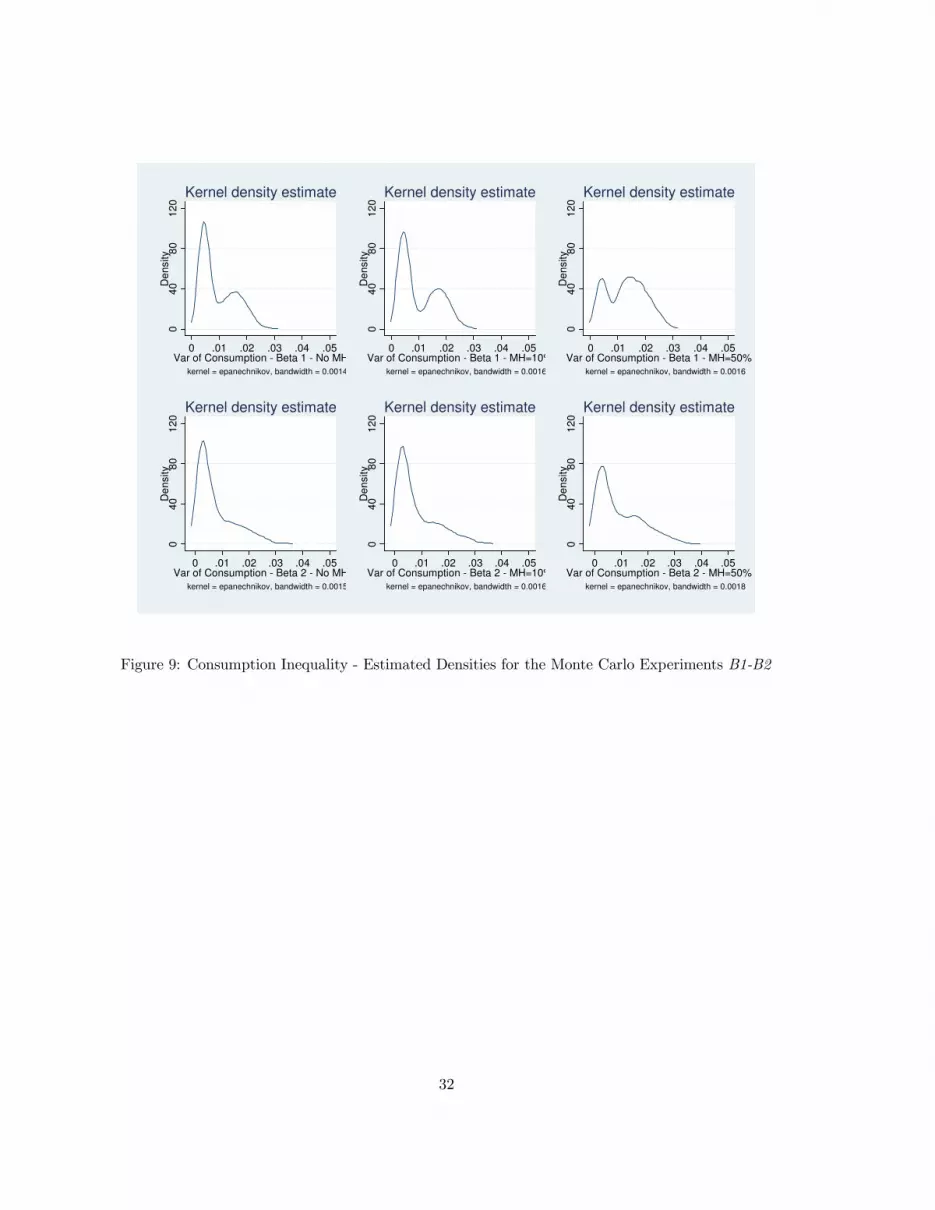
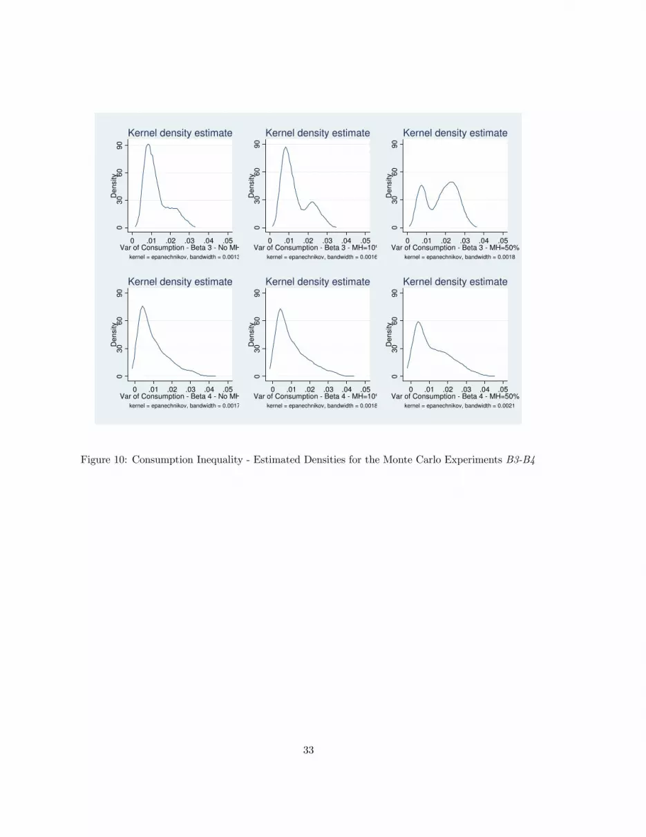
Finally, Figures (9) and (10) document the sampling distributions of the variance of consumption.
The economy displays a low degree of consumption inequality every time the UI scheme and self-
insurance are able to mitigate the market incompleteness, although the figures suggest that in many
instances market incompleteness does bite. Interestingly, more extreme calibrations lead to a lower
consumption inequality when MH is not too pervasive, as observed in cases B2 and B4.
[Figures (7), (8), (9) and (10) about here]
4.2 Optimal UI Replacement Rates and Moral Hazard
Another way of looking at the previous findings is to recognize that there are several empirically
plausible calibrations such that low replacement rates are optimal. This is an interesting outcome,
because it takes place even in the absence of MH, something that Hansen and Imrohoroglu (1992) did
not find, suggesting that their result stems from their specific calibration.
12

Increasing the level of MH in the economy does decrease the optimal UI, as Hansen and Imrohoroglu
(1992) reported. But this is true only on average. For several calibrations, when increasing the MH
there is still a large fraction of economies where high optimal replacement rates, even well above 75%,
survive.
Across experiments, a significant difference appears to be the share of economies with high optimal
UI schemes (namely with θ∗ > 60%). By comparing, say, the no MH case with the prior B1 to the
corresponding case with the prior B2 in Figure (3), it is clear that the mass of replications with
θ∗ > 60% is higher in the former experiment. The same pattern is found when moving from the cases
with the concentrated priors B1 (B3 ) to the corresponding case with the more dispersed priors B2
(B4 ).
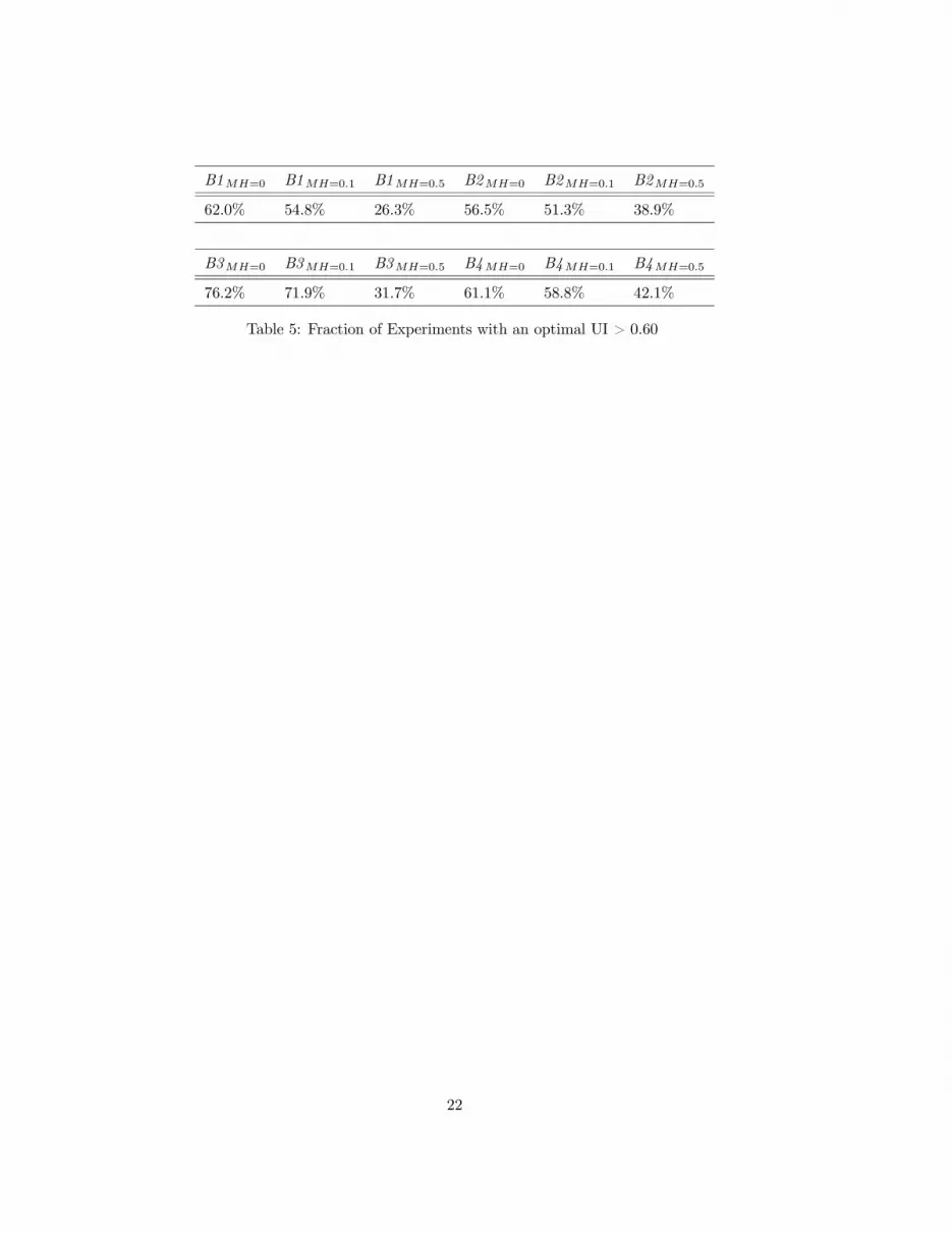
[Table (5) about here]
Table (5) provides a related statistic: the fraction of replications that display an optimal UI
replacement rate that is above 60%. This share ranges from 76.2% for the case B3 with no MH, to
26.3% for the case B1 with the highest MH.
It is also worth stressing that these shares are systematically higher for each case in the experiments
B3 (B4 ) than their counterparts in the experiments B1 (B2 ). Economies with worse employment
opportunities and higher unemployment durations command, on average, a higher θ∗. The rationale
for this result is as follows. The crucial aspect that allows high replacement rates to stay optimal in
these environments is the lack of incentives for unemployed agents to turn down an unemployment
offer, when they have one. Rejecting a job is a very risky choice, because the absence of full insurance
makes it costly (unless the disutility from working is particularly large). Jobs are relatively rare to
obtain, so MH has a lower influence in these cases. The experiments assuming enlarged labor markets
represent economies where aggregate welfare can improve by trading-off lower taxation for higher
public insurance, because individuals will not often turn down jobs. This can also be seen in the
behavior of the employment differential, namely the difference between the potential employment rate
(as driven by the Markov chain) and the actual one (as driven by both the Markov chain and the
agents’ choices): it decreases or remains stable with the degree of MH.11
Finally, even in the absence of moral hazard, it is never optimal to provide full income insurance.
The increased taxation stemming from higher unemployment rates makes it too costly to give a 100%
replacement rate. A basic trade-off between insurance and search incentives prevents full income
insurance to be the welfare maximizing scheme.
11See Figures (26)-(31) in the appendix.
13

4.3 Labor Force
The nature of the labor market, including the definition of the labor force, and the related labor
market risk seem to be key when assessing the welfare effects of UI schemes. Typically, in applied GE,
labor market risk is considered as pertaining to the most restrictive definition of the unemployment
rate. It is then interesting, in a robustness exercise, to consider the effects of an enlarged labor force,
which includes the marginally attached workers, and whose main characterization derives from the
employment rate data, as it was discussed above.
Taking a different stand on the labor force composition does lead to similar qualitative patterns.
However, comparing the results obtained from the enlarged labor force economies to the restricted
labor force ones highlights some differences in the quantitative findings.
Quantitatively, the former cases have higher optimal UI schemes (on average), coupled with higher
aggregate assets (on average). It goes without saying that the drawback of higher public insurance is
a higher taxation rate.
Higher labor market risk calls for more insurance, which is a combination of UI and asset hold-
ings. Overall, social and private insurance seem to work well, because they achieve relatively similar
distributions of consumption inequality in the two substantially different labor markets, as comparing
the statistics in Tables (3) and (4) show. Across experiments, the mean and median of the consump-
tion variance are surprisingly similar in the two definitions of the labor market. The range of the
mean (median) is [0.007, 0.013] ([0.005, 0.013]) in the experiments B1 -B2, while it is [0.010, 0.017]
([0.008, 0.019]) in the experiments B3 -B4.
4.4 Comparative Dynamics
The simulated economies form an artificial dataset that can be exploited to analyse how changes in the
parameters affect the endogenous variables. Moreover, it is possible to understand which parameters
have a stronger effect on the outcomes: with a Monte Carlo approach, regression analysis, instead of
calculus, allows for the study of comparative dynamics.
Table (6) provides the standardized beta coefficients of a Pooled OLS regression with the average
steady state utility on the LHS, and the six parameters on the RHS.12
[Table (6) about here]
12 In the table a "∗" symbol means that a parameter is not significant at the 10% level, and all regressions include a
constant term and the replacement rate as regressors, not reported. Several other specifications were tried, including a
Fixed Effect one (the FE being the replacement rate) and a SUR model with all the five endogenous variables as the
LHS. The estimated parameters in the expected utility equation were pretty robust.
14
There are several results that can be read from Table (6).
First, there are two trends in the explanatory power of this simple linear regressions. More in
detail, a substantial drop in the R2 of the regression is evident when comparing the experiments with
a more concentrated prior to the ones with a more disperse prior. This shows that, in the more
extreme calibrations, non linearities become important in the determination of the average steady-
state welfare. The second trend in the R2 is related to the degree of MH. When moving from the no
MH case to the most extreme case, a big drop can be seen (from 0.90 to 0.56 in experiment B1, for
example), possibly because of some effects starting to offset each other (e.g. the utility loss of working
vs. the partial loss of public insurance). With a high enough MH non linearities become predominant,
which suggests to take the following comments with caution for those cases.
Second, the standardized beta coefficients associated with the hours worked, the leisure share in
the households’ consumption bundle, and the intertemporal elasticity of substitution document that
these parameters have a first order impact on the determination of average welfare, hence on the
selection of the optimal UI scheme.
As for h, in the regressions with a good fit, its beta coefficient ranges between [−.735,−.594]:
this is the parameter that affects the average steady state utility the most. The other two important
parameters for the determination of aggregate welfare are σ, with a range of [−.613,−.167], and ρ,
which with a range of [−.414,−.345] shows also the most consistent effect.
Both χ(e′,e), the job retention probability, and χ(e′,u), the job finding probability, have negligible
effects in the experiments B1 and B2, while their quantitative importance in affecting the average
utility becomes larger in the experiments B3 and B4. This result could be accounted for by a level
effect. Very low probabilities for workers to keep their current job and find one while unemployed
mechanically determine a high unemployment rate. This leads a large chunk of the labor force to rely
on UI, making a generous system very expensive. Small changes in these probabilities can have first
order welfare effects due to the reduced need to save and reduced costs of in terms of taxes. This
interpretation seems to be confirmed by the decreasing importance of these parameters with respect
to the degree of MH.
Finally, the effect of β is always tiny, at least for the subset of the parameter’s space considered
here.
Further evidence on how the parameters affect the determination of the optimal UI system is given
in Figures (11) and (12).
[Figures (11) and (12) about here]
Figure (11) focuses on the parameter h, while Figure (12) focuses on σ, and they show several
15

distributions. Each Figure displays, at the very left, two panels. These represent the unconditional dis-
tributions of a parameter in a given experiment.13 As expected, given the high number of replications,
they approximate well the prior distributions from which they are sampled.
The other six panels (per experiment) condition the estimated parameters’ densities on the com-
puted optimal UI regime found in that replication, namely if θ∗ was less than 60% or if it was above
this threshold. Whenever the top distribution differs systematically from the bottom one, there is
some selection taking place. This implies that differences in that parameter are likely to induce a
different regime in the optimal UI scheme. Put it differently, the values of that parameter have a
major impact for the main outcome of the analysis.
For example, Figure (12) clearly shows that the UI schemes with θ∗ ≤ 60% come from a distribution
of the parameter σ that has a higher mean and a lower variance than the distribution of the same
parameter leading to optimal replacement rates θ∗ > 60%. Similarly, Figure (11) shows that the
distribution of the parameter h such that θ∗ ≤ 60% has consistently a higher mean than its counterpart
with θ∗ > 60%. These results seem important, because such clear patterns are not detected for the
other parameters.
These findings suggest where caution should be paid when calibrating similar environments. Other
researchers in the field should calibrate carefully the parameters h, σ and ρ, and perform robustness
checks with respect to them.
5 Conclusions
This paper applied Canova (1994) methodology to perform a thorough sensitivity analysis for the
Hansen and Imrohoroglu (1992) economy. This is a calibrated GE model with incomplete markets
and uninsurable employment risk, designed to quantify the size of the optimal replacement rate for a
government-run unemployment insurance scheme.
The results of this global robustness analysis are broadly consistent with the original findings. A
novel finding is that the sampling distribution of the optimal UI is bimodal. According to the 1,000
calibrations, for any degree of moral hazard considered, it is optimal for the UI to be in one of two
regions: a very generous scheme with a high replacement rate and low savings, or one with a low
replacement rate and high savings. In the first region insurance is mainly provided by the UI scheme,
while in the second one it is self-insurance that does the job.
One of the main findings of Hansen and Imrohoroglu (1992) is the sharp decrease of the optimal
13The labels hint that the densities refer to the no MH case. This is immaterial, because the other MH cases rely on
a fixed seed and have the exact same parameters’ draws, hence the same distributions. The Figures for the other cases
and parameters are in an appendix.
16
replacement rate when the economy is plagued by MH. Here it was found that, in no less than 26% of
the experiments, the welfare maximizing replacement rate did not decrease below 60% when the level
of MH was increased.
The paper shows how the findings are affected particularly by the calibration of three parameters:
the number of hours worked, the share of leisure in the households’ expenditure, and the curvature
of the per-period utility function. This suggests that similar studies based on a calibration approach
should pay special attention to the values assigned to these parameters, and should provide some
robustness checks with respect to them.
A positive message resulting from this paper, and from Cozzi (2011), is that more robust cali-
bration methods are feasible also for rich HA economies, usually used to perform (ex-ante) policy
evaluations. This methodology should be interpreted as complementary to full-blown structural esti-
mation techniques. Notice that an advantage of this analysis is the ability to provide ranges for the
outcomes of interest, which not only allows to better understand the mechanics of the model, but also
goes along the lines of Manski (1995) and Sims (2004).
A possible extension could be to consider fully Bayesian methods, proposed for example by De-
Jong, Ingram, and Whiteman (1996), even though computational limits might still be binding for
the computation of the likelihood function and the posterior distributions. More general UI policies
(specifying both the replacement rate and the maximum duration of the benefits), and a more general
GE set-up (for example with market clearing in the asset market as well) could also be studied. I
leave these modifications for future work.
17

Parameter Description Min Max
Model Period Six weeks
β Rate of time preference β = 0.991 β = 0.999
σ Leisure Share σ = 0.37 σ = 0.97
ρ Risk Aversion ρ = 1.5 ρ = 3.5
h Share of Market Time h = 0.35 h = 0.55
χ(e′,e) Job Retention Probability χ(e′,e) =
0.937, B1-B2
0.75, B3-B4χ(e′,e) =
0.999, B1-B2
0.99, B3-B4
χ(e′,u) Job Finding Probability χ(e′,u) =
0.3, B1-B2
0.2, B3-B4χ(e′,u) =
0.7, B1-B2
0.6, B3-B4
Table 1: Model parameters and their support
18

Experiment B1 Experiment B2 Experiment B3 Experiment B4
Parameters Priors Beta(10, 10; p, p) Beta(2, 2; p, p) Beta(10, 10; p, p) Beta(2, 2; p, p)
Labor MKT target Unemployment rate Unemployment rate Employment rate Employment rate
Table 2: Experiments - Prior Distributions over a generic parameter p and Labor market targets
19

Min Max Mean Med. C.V. Min Max Mean Med. C.V.
1) Opt. UI 2) Assets
B1MH=0 .14 .90 .604 .66 .234 0 1.020 .117 0 1.181
B1MH=0.1 .04 .82 .518 .65 .422 0 1.849 .341 0 1.177
B1MH=0.5 .02 .82 .280 .10 1.056 0 3.175 1.137 1.262 .774
B2MH=0 .02 .98 .559 .66 .423 0 1.699 .154 0 1.242
B2MH=0.1 .02 .90 .474 .62 .626 0 3.896 .388 0 1.323
B2MH=0.5 .02 .90 .346 .12 1.001 0 4.793 .835 .611 1.112
3) Tax 4) Var. of Cons.
B1MH=0 .018 .077 .042 .041 .240 .001 .030 .009 .006 .205
B1MH=0.1 .007 .087 .038 .038 .296 .001 .029 .010 .007 .671
B1MH=0.5 .001 .073 .019 .011 .909 .001 .030 .013 .013 .532
B2MH=0 .002 .185 .045 .044 .505 .0001 .034 .007 .005 .923
B2MH=0.1 .002 .310 .042 .038 .635 .0001 .035 .008 .005 .936
B2MH=0.5 .001 .253 .031 .022 .989 .0001 .038 .009 .006 .871
Table 3: Monte Carlo Results - Optimal UI, Assets, Tax Rate and Consumption Variance
20

Min Max Mean Med. C.V. Min Max Mean Med. C.V.
1) Opt. UI 2) Assets
B3MH=0 .02 .84 .595 .70 .392 0 3.084 .356 0 1.953
B3MH=0.1 .02 .84 .563 .70 .469 0 3.434 .546 0 1.685
B3MH=0.5 .02 .84 .382 .35 .746 0 4.395 1.380 1.124 .924
B4MH=0 .02 .92 .524 .70 .614 0 5.029 .552 0 1.672
B4MH=0.1 .02 .92 .497 .70 .685 0 5.015 .709 0 1.485
B4MH=0.5 .02 .94 .407 .36 .866 0 5.216 1.169 .736 1.113
3) Tax 4) Var. of Cons.
B3MH=0 .011 .305 .159 .173 .403 .003 .031 .012 .011 .500
B3MH=0.1 .007 .305 .151 .170 .475 .003 .033 .013 .011 .525
B3MH=0.5 .004 .280 .106 .098 .720 .003 .034 .017 .019 .453
B4MH=0 .005 .421 .142 .127 .677 .0003 .042 .010 .008 .776
B4MH=0.1 .005 .411 .135 .120 .742 .0003 .042 .010 .008 .787
B4MH=0.5 .002 .411 .113 .083 .872 .0003 .043 .012 .010 .760
Table 4: Monte Carlo Results - Optimal UI, Assets, Tax Rate and Consumption Variance
21
B1MH=0 B1MH=0.1 B1MH=0.5 B2MH=0 B2MH=0.1 B2MH=0.5
62.0% 54.8% 26.3% 56.5% 51.3% 38.9%
B3MH=0 B3MH=0.1 B3MH=0.5 B4MH=0 B4MH=0.1 B4MH=0.5
76.2% 71.9% 31.7% 61.1% 58.8% 42.1%
Table 5: Fraction of Experiments with an optimal UI > 0.60
22

B1MH=0 B1MH=0.1 B1MH=0.5 B2MH=0 B2MH=0.1 B2MH=0.5
EU
h −.622 −.610 −.147 −.606 −.612 −.225
β .012 .009 −.038 .021 .017 −.054
χ(e′,e) .028 .032 .037 .051 .064 .053
χ(u′,u) .004 −.001∗ −.001∗ −.003∗ −.012 −.010
σ −.580 −.613 −.219 −.256 −.336 −.189
ρ −.395 −.384 −.148 −.417 −.417 −.227
R2 0.90 0.92 0.56 0.55 0.60 0.33
B3MH=0 B3MH=0.1 B3MH=0.5 B4MH=0 B4MH=0.1 B4MH=0.5
EU
h −.735 −.622 −.205 −.594 −.501 −.274
β .012 .006 −.023 −.000∗ −.002∗ −.053
χ(e′,e) .181 .179 .017 .260 .239 .054
χ(u′,u) −.089 −.079 −.012 −.152 −.134 −.018
σ −.379 −.437 −.275 −.167 −.244 −.224
ρ −.414 −.345 −.133 −.406 −.351 −.230
R2 0.92 0.78 0.57 0.72 0.61 0.41
Table 6: Comparative Dynamics on Average Welfare - POLS Regressions
23
0
0.5
1
1.5
2
2.5
3
3.5
0 0.1 0.2 0.3 0.4 0.5 0.6 0.7 0.8 0.9 1
beta(x,2,2)
beta(x,10,10)
Figure 1: Monte Carlo Experiments: Beta(2, 2) and Beta(10, 10) priors.
24

02
46
De
nsity
1 1.5 2 2.5Param: RRA - Beta 1 - No MH
kernel = epanechnikov, bandwidth = 0.0275
Kernel density estimate
02
46
De
nsity
1 1.5 2 2.5Param: RRA - Beta 1 - No MH rr<0.6
kernel = epanechnikov, bandwidth = 0.0216
Kernel density estimate
02
46
De
nsity
1 1.5 2 2.5Param: RRA - Beta 1 - MH=10% rr<0.6
kernel = epanechnikov, bandwidth = 0.0197
Kernel density estimate
02
46
De
nsity
1 1.5 2 2.5Param: RRA - Beta 1 - MH=50% rr<0.6
kernel = epanechnikov, bandwidth = 0.0237
Kernel density estimate
02
46
De
nsity
1 1.5 2 2.5Param: RRA - Beta 1 - No MH rr>0.6
kernel = epanechnikov, bandwidth = 0.0258
Kernel density estimate
02
46
De
nsity
1 1.5 2 2.5Param: RRA - Beta 1 - MH=10% rr>0.6
kernel = epanechnikov, bandwidth = 0.0246
Kernel density estimate
02
46
De
nsity
1 1.5 2 2.5Param: RRA - Beta 1 - MH=50% rr>0.6
kernel = epanechnikov, bandwidth = 0.0287
Kernel density estimate
02
46
De
nsity
1 1.5 2 2.5Param: RRA - Beta 2 - No MH
kernel = epanechnikov, bandwidth = 0.0579
Kernel density estimate
02
46
De
nsity
1 1.5 2 2.5Param: RRA - Beta 2 - No MH rr<0.6
kernel = epanechnikov, bandwidth = 0.0414
Kernel density estimate
02
46
De
nsity
1 1.5 2 2.5Param: RRA - Beta 2 - MH=10% rr<0.6
kernel = epanechnikov, bandwidth = 0.0393
Kernel density estimate
02
46
De
nsity
1 1.5 2 2.5Param: RRA - Beta 2 - MH=50% rr<0.6
kernel = epanechnikov, bandwidth = 0.0426
Kernel density estimate
02
46
De
nsity
1 1.5 2 2.5Param: RRA - Beta 2 - No MH rr>0.6
kernel = epanechnikov, bandwidth = 0.0587
Kernel density estimate
02
46
De
nsity
1 1.5 2 2.5Param: RRA - Beta 2 - MH=10% rr>0.6
kernel = epanechnikov, bandwidth = 0.0577
Kernel density estimate
02
46
De
nsity
1 1.5 2 2.5Param: RRA - Beta 2 - MH=50% rr>0.6
kernel = epanechnikov, bandwidth = 0.0612
Kernel density estimate
Figure 2: CRRA - Estimated Densities for the Monte Carlo Experiments B1-B2
25
03
6D
en
sity
0 .2 .4 .6 .8 1Optimal UI - Beta 1 - No MH
kernel = epanechnikov, bandwidth = 0.0319
Kernel density estimate
03
6D
en
sity
0 .2 .4 .6 .8 1Optimal UI - Beta 1 - MH=10%
kernel = epanechnikov, bandwidth = 0.0495
Kernel density estimate
03
6D
en
sity
0 .2 .4 .6 .8 1Optimal UI - Beta 1 - MH=50%
kernel = epanechnikov, bandwidth = 0.0667
Kernel density estimate
03
6D
en
sity
0 .2 .4 .6 .8 1Optimal UI - Beta 2 - No MH
kernel = epanechnikov, bandwidth = 0.0535
Kernel density estimate
03
6D
en
sity
0 .2 .4 .6 .8 1Optimal UI - Beta 2 - MH=10%
kernel = epanechnikov, bandwidth = 0.0671
Kernel density estimate
03
6D
en
sity
0 .2 .4 .6 .8 1Optimal UI - Beta 2 - MH=50%
kernel = epanechnikov, bandwidth = 0.0784
Kernel density estimate
Figure 3: Optimal UI - Estimated Densities for the Monte Carlo Experiments B1-B2
26

03
6D
en
sity
0 .2 .4 .6 .8 1Optimal UI - Beta 3 - No MH
kernel = epanechnikov, bandwidth = 0.0168
Kernel density estimate
03
6D
en
sity
0 .2 .4 .6 .8 1Optimal UI - Beta 3 - MH=10%
kernel = epanechnikov, bandwidth = 0.0597
Kernel density estimate
03
6D
en
sity
0 .2 .4 .6 .8 1Optimal UI - Beta 3 - MH=50%
kernel = epanechnikov, bandwidth = 0.0644
Kernel density estimate
03
6D
en
sity
0 .2 .4 .6 .8 1Optimal UI - Beta 4 - No MH
kernel = epanechnikov, bandwidth = 0.0728
Kernel density estimate
03
6D
en
sity
0 .2 .4 .6 .8 1Optimal UI - Beta 4 - MH=10%
kernel = epanechnikov, bandwidth = 0.0769
Kernel density estimate
03
6D
en
sity
0 .2 .4 .6 .8 1Optimal UI - Beta 4 - MH=50%
kernel = epanechnikov, bandwidth = 0.0796
Kernel density estimate
Figure 4: Optimal UI - Estimated Densities for the Monte Carlo Experiments B3-B4
27
02
46
De
nsity
0 1 2 3 4 5Average Assets - Beta 1 - No MH
kernel = epanechnikov, bandwidth = 0.0313
Kernel density estimate
02
46
De
nsity
0 1 2 3 4 5Average Assets - Beta 1 - MH=10%
kernel = epanechnikov, bandwidth = 0.0907
Kernel density estimate
02
46
De
nsity
0 1 2 3 4 5Average Assets - Beta 1 - MH=50%
kernel = epanechnikov, bandwidth = 0.1991
Kernel density estimate
02
46
De
nsity
0 1 2 3 4 5Average Assets - Beta 2 - No MH
kernel = epanechnikov, bandwidth = 0.0433
Kernel density estimate
02
46
De
nsity
0 1 2 3 4 5Average Assets - Beta 2 - MH=10%
kernel = epanechnikov, bandwidth = 0.1144
Kernel density estimate
02
46
De
nsity
0 1 2 3 4 5Average Assets - Beta 2 - MH=50%
kernel = epanechnikov, bandwidth = 0.2100
Kernel density estimate
Figure 5: Average Asset - Estimated Densities for the Monte Carlo Experiments B1-B2
28
02
00
40
0D
en
sity
0 1 2 3 4 5Average Assets - Beta 3 - No MH
kernel = epanechnikov, bandwidth = 0.0006
Kernel density estimate
01
2D
en
sity
0 1 2 3 4 5Average Assets - Beta 3 - MH=10%
kernel = epanechnikov, bandwidth = 0.1873
Kernel density estimate
01
2D
en
sity
0 1 2 3 4 5Average Assets - Beta 3 - MH=50%
kernel = epanechnikov, bandwidth = 0.2884
Kernel density estimate
01
2D
en
sity
0 1 2 3 4 5Average Assets - Beta 4 - No MH
kernel = epanechnikov, bandwidth = 0.1576
Kernel density estimate
01
2D
en
sity
0 1 2 3 4 5Average Assets - Beta 4 - MH=10%
kernel = epanechnikov, bandwidth = 0.2256
Kernel density estimate
01
2D
en
sity
0 1 2 3 4 5Average Assets - Beta 4 - MH=50%
kernel = epanechnikov, bandwidth = 0.2942
Kernel density estimate
Figure 6: Average Asset - Estimated Densities for the Monte Carlo Experiments B3-B4
29

01
02
03
04
0D
en
sity
0 .15 .3 .45Tax Rate - Beta 1 - No MH
kernel = epanechnikov, bandwidth = 0.0022
Kernel density estimate
01
02
03
04
0D
en
sity
0 .15 .3 .45Tax Rate - Beta 1 - MH=10%
kernel = epanechnikov, bandwidth = 0.0026
Kernel density estimate
01
02
03
04
0D
en
sity
0 .15 .3 .45Tax Rate - Beta 1 - MH=50%
kernel = epanechnikov, bandwidth = 0.0039
Kernel density estimate
01
02
03
04
0D
en
sity
0 .15 .3 .45Tax Rate - Beta 2 - No MH
kernel = epanechnikov, bandwidth = 0.0050
Kernel density estimate
01
02
03
04
0D
en
sity
0 .15 .3 .45Tax Rate - Beta 2 - MH=10%
kernel = epanechnikov, bandwidth = 0.0054
Kernel density estimate
01
02
03
04
0D
en
sity
0 .15 .3 .45Tax Rate - Beta 2 - MH=50%
kernel = epanechnikov, bandwidth = 0.0062
Kernel density estimate
Figure 7: Tax Rate - Estimated Densities for the Monte Carlo Experiments B1-B2
30

04
8D
en
sity
0 .15 .3 .45Tax Rate - Beta 3 - No MH
kernel = epanechnikov, bandwidth = 0.0145
Kernel density estimate
04
8D
en
sity
0 .15 .3 .45Tax Rate - Beta 3 - MH=10%
kernel = epanechnikov, bandwidth = 0.0162
Kernel density estimate
04
8D
en
sity
0 .15 .3 .45Tax Rate - Beta 3 - MH=50%
kernel = epanechnikov, bandwidth = 0.0172
Kernel density estimate
04
8D
en
sity
0 .15 .3 .45Tax Rate - Beta 4 - No MH
kernel = epanechnikov, bandwidth = 0.0217
Kernel density estimate
04
8D
en
sity
0 .15 .3 .45Tax Rate - Beta 4 - MH=10%
kernel = epanechnikov, bandwidth = 0.0226
Kernel density estimate
04
8D
en
sity
0 .15 .3 .45Tax Rate - Beta 4 - MH=50%
kernel = epanechnikov, bandwidth = 0.0223
Kernel density estimate
Figure 8: Tax Rate - Estimated Densities for the Monte Carlo Experiments B3-B4
31
04
08
01
20
De
nsity
0 .01 .02 .03 .04 .05Var of Consumption - Beta 1 - No MH
kernel = epanechnikov, bandwidth = 0.0014
Kernel density estimate
04
08
01
20
De
nsity
0 .01 .02 .03 .04 .05Var of Consumption - Beta 1 - MH=10%
kernel = epanechnikov, bandwidth = 0.0016
Kernel density estimate
04
08
01
20
De
nsity
0 .01 .02 .03 .04 .05Var of Consumption - Beta 1 - MH=50%
kernel = epanechnikov, bandwidth = 0.0016
Kernel density estimate
04
08
01
20
De
nsity
0 .01 .02 .03 .04 .05Var of Consumption - Beta 2 - No MH
kernel = epanechnikov, bandwidth = 0.0015
Kernel density estimate
04
08
01
20
De
nsity
0 .01 .02 .03 .04 .05Var of Consumption - Beta 2 - MH=10%
kernel = epanechnikov, bandwidth = 0.0016
Kernel density estimate
04
08
01
20
De
nsity
0 .01 .02 .03 .04 .05Var of Consumption - Beta 2 - MH=50%
kernel = epanechnikov, bandwidth = 0.0018
Kernel density estimate
Figure 9: Consumption Inequality - Estimated Densities for the Monte Carlo Experiments B1-B2
32
03
06
09
0D
en
sity
0 .01 .02 .03 .04 .05Var of Consumption - Beta 3 - No MH
kernel = epanechnikov, bandwidth = 0.0013
Kernel density estimate
03
06
09
0D
en
sity
0 .01 .02 .03 .04 .05Var of Consumption - Beta 3 - MH=10%
kernel = epanechnikov, bandwidth = 0.0016
Kernel density estimate
03
06
09
0D
en
sity
0 .01 .02 .03 .04 .05Var of Consumption - Beta 3 - MH=50%
kernel = epanechnikov, bandwidth = 0.0018
Kernel density estimate
03
06
09
0D
en
sity
0 .01 .02 .03 .04 .05Var of Consumption - Beta 4 - No MH
kernel = epanechnikov, bandwidth = 0.0017
Kernel density estimate
03
06
09
0D
en
sity
0 .01 .02 .03 .04 .05Var of Consumption - Beta 4 - MH=10%
kernel = epanechnikov, bandwidth = 0.0018
Kernel density estimate
03
06
09
0D
en
sity
0 .01 .02 .03 .04 .05Var of Consumption - Beta 4 - MH=50%
kernel = epanechnikov, bandwidth = 0.0021
Kernel density estimate
Figure 10: Consumption Inequality - Estimated Densities for the Monte Carlo Experiments B3-B4
33

05
10
15
De
nsity
.3 .4 .5 .6Param: h - Beta 1 - No MH
kernel = epanechnikov, bandwidth = 0.0049
Kernel density estimate
05
10
15
De
nsity
.3 .4 .5 .6Param: h - Beta 1 - No MH rr<0.6kernel = epanechnikov, bandwidth = 0.0059
Kernel density estimate
05
10
15
De
nsity
.3 .4 .5 .6Param: h - Beta 1 - MH=10% rr<0.6
kernel = epanechnikov, bandwidth = 0.0057
Kernel density estimate
05
10
15
De
nsity
.3 .4 .5 .6Param: h - Beta 1 - MH=50% rr<0.6
kernel = epanechnikov, bandwidth = 0.0052
Kernel density estimate
05
10
15
De
nsity
.3 .4 .5 .6Param: h - Beta 1 - No MH rr>0.6kernel = epanechnikov, bandwidth = 0.0051
Kernel density estimate
05
10
15
De
nsity
.3 .4 .5 .6Param: h - Beta 1 - MH=10% rr>0.6
kernel = epanechnikov, bandwidth = 0.0051
Kernel density estimate
05
10
15
De
nsity
.3 .4 .5 .6Param: h - Beta 1 - MH=50% rr>0.6
kernel = epanechnikov, bandwidth = 0.0056
Kernel density estimate
02
46
8D
en
sity
.3 .4 .5 .6Param: h - Beta 2 - No MH
kernel = epanechnikov, bandwidth = 0.0102
Kernel density estimate
02
46
8D
en
sity
.3 .4 .5 .6Param: h - Beta 2 - No MH rr<0.6
kernel = epanechnikov, bandwidth = 0.0119
Kernel density estimate
02
46
8D
en
sity
.3 .4 .5 .6Param: h - Beta 2 - MH=10% rr<0.6
kernel = epanechnikov, bandwidth = 0.0118
Kernel density estimate
02
46
8D
en
sity
.3 .4 .5 .6Param: h - Beta 2 - MH=50% rr<0.6
kernel = epanechnikov, bandwidth = 0.0112
Kernel density estimate
02
46
8D
en
sity
.3 .4 .5 .6Param: h - Beta 2 - No MH rr>0.6kernel = epanechnikov, bandwidth = 0.0114
Kernel density estimate
02
46
8D
en
sity
.3 .4 .5 .6Param: h - Beta 2 - MH=10% rr>0.6
kernel = epanechnikov, bandwidth = 0.0114
Kernel density estimate
02
46
8D
en
sity
.3 .4 .5 .6Param: h - Beta 2 - MH=50% rr>0.6
kernel = epanechnikov, bandwidth = 0.0122
Kernel density estimate
Figure 11: Parameter h - Estimated Densities for the Monte Carlo Experiments B1-B2
34

07
14
De
nsity
.35 .55 .75 .95Param: Sigma - Beta 1 - No MHkernel = epanechnikov, bandwidth = 0.0147
Kernel density estimate
07
14
De
nsity
.35 .55 .75 .95Param: Sigma - Beta 1 - No MH rr<0.6
kernel = epanechnikov, bandwidth = 0.0104
Kernel density estimate
07
14
De
nsity
.35 .55 .75 .95Param: Sigma - Beta 1 - MH=10% rr<0.6
kernel = epanechnikov, bandwidth = 0.0103
Kernel density estimate
07
14
De
nsity
.35 .55 .75 .95Param: Sigma - Beta 1 - MH=50% rr<0.6
kernel = epanechnikov, bandwidth = 0.0118
Kernel density estimate
07
14
De
nsity
.35 .55 .75 .95Param: Sigma - Beta 1 - No MH rr>0.6
kernel = epanechnikov, bandwidth = 0.0114
Kernel density estimate
07
14
De
nsity
.35 .55 .75 .95Param: Sigma - Beta 1 - MH=10% rr>0.6
kernel = epanechnikov, bandwidth = 0.0103
Kernel density estimate
07
14
De
nsity
.35 .55 .75 .95Param: Sigma - Beta 1 - MH=50% rr>0.6
kernel = epanechnikov, bandwidth = 0.0081
Kernel density estimate
03
6D
en
sity
.35 .55 .75 .95Param: Sigma - Beta 2 - No MH
kernel = epanechnikov, bandwidth = 0.0302
Kernel density estimate
03
6D
en
sity
.35 .55 .75 .95Param: Sigma - Beta 2 - No MH rr<0.6
kernel = epanechnikov, bandwidth = 0.0203
Kernel density estimate
03
6D
en
sity
.35 .55 .75 .95Param: Sigma - Beta 2 - MH=10% rr<0.6
kernel = epanechnikov, bandwidth = 0.0203
Kernel density estimate
03
6D
en
sity
.35 .55 .75 .95Param: Sigma - Beta 2 - MH=50% rr<0.6
kernel = epanechnikov, bandwidth = 0.0223
Kernel density estimate
03
6D
en
sity
.35 .55 .75 .95Param: Sigma - Beta 2 - No MH rr>0.6
kernel = epanechnikov, bandwidth = 0.0219
Kernel density estimate
03
6D
en
sity
.35 .55 .75 .95Param: Sigma - Beta 2 - MH=10% rr>0.6
kernel = epanechnikov, bandwidth = 0.0198
Kernel density estimate
03
6D
en
sity
.35 .55 .75 .95Param: Sigma - Beta 2 - MH=50% rr>0.6
kernel = epanechnikov, bandwidth = 0.0183
Kernel density estimate
Figure 12: Parameter σ - Estimated Densities for the Monte Carlo Experiments B1-B2
35

References
Abdulkadiroglu, A., Kuruscu, B., and Sahin, A. (2002). "Unemployment Insurance and the Role of
Self-Insurance," Review of Economic Dynamics, Vol. 5, 681-703.
Acemoglu, D., and Shimer, R. (1999). "Efficient Unemployment Insurance," Journal of Political Econ-
omy, Vol. 107, 893-928.
An, S., and Schorfheide, F. (2007). "Bayesian Analysis of DSGE Models," Econometric Reviews, Vol.
26, 113-172.
Attanasio, O., Banks, J., Meghir, C., and Weber, G. (1999). "Humps and Bumps in Lifetime Con-
sumption," Journal of Business and Economic Statistics, Vol. 17, 22-35.
Boostani, R., Gervais, M., and Siu, H. (2011). "Optimal Unemployment Insurance in a Directed Search
Model," University of Southampton, mimeo.
Canova, F. (1994). "Statistical Inference in Calibrated Models," Journal of Applied Econometrics,
Vol. 9, S123-S144.
Cozzi, M. (2011). "Precautionary Savings and Wealth Inequality: a Global Sensitivity Analysis," QED
Working Paper n. 1270.
DeJong, D., Ingram, B. and Whiteman, C. (1996). "A Bayesian Approach to Calibration," Journal
of Business and Economic Statistics, Vol. 14, 1-9.
DeJong, D., Ingram, B. and Whiteman, C. (2000). "A Bayesian Approach to Dynamic Macroeco-
nomics," Journal of Econometrics, Vol. 98, 201-223.
Dey, M., and Flinn, C. (2005). "An Equilibrium Model of Health Insurance Provision and Wage
Determination," Econometrica, Vol. 73, 571-627.
Hansen, G. and Imrohoroglu, A. (1992). "The Role of Unemployment Insurance in an Economy with
Liquidity Constraints and Moral Hazard," Journal of Political Economy, Vol. 100, 118-142.
Hopenhayn, H., and Nicolini, J.P. (1997). "Optimal Unemployment Insurance," Journal of Political
Economy, Vol. 105, 412-438.
Krusell, P., Mukoyama, T., and Sahin, A. (2010). "Labour Market Matching with Precautionary
Savings and Aggregate Fluctuations," Review of Economic Studies, Vol. 77, 1477-1507.
36

Jones, S. and Riddell, C. (1999). "The Measurement of Unemployment: an Empirical Approach,"
Econometrica, Vol. 67, 147-162.
Manski, C. (1995). Identification Problems in the Social Sciences, Harvard University Press, Cam-
bridge (MA).
Martin, J. (2002). "What Works among Active Labour Market Policies: Evidence from OECD Coun-
tries’ Experiences," OECD Economic Studies, Vol. 30, 79-113.
Pavoni, N. (2009). "Optimal Unemployment Insurance, with Human Capital Depreciation, and Du-
ration Dependence," International Economic Review, Vol. 50, 323-362.
Pollak, A. (2007). "Optimal Unemployment Insurance with Heterogeneous Agents," European Eco-
nomic Review, Vol. 51, 2029-2053.
Shimer, R., and Werning, I. (2008). "Liquidity and Insurance for the Unemployed," American Eco-
nomic Review, Vol. 98, 1922-1942.
Sims, C. (2004). "Econometrics for Policy Analysis: Progress and Regress," De Economist, Vol. 152,
167-175.
van den Berg, G. (1990). "Nonstationarity in Job Search Theory," Review of Economic Studies, Vol.
57, 255-277.
Young, E. (2004). "Unemployment Insurance and Capital Accumulation," Journal of Monetary Eco-
nomics, Vol. 51, 1683-1710.
37

Appendix A - The Model and its Recursive Representation
6 Stationary Equilibrium
In this Section I first define the problem of the agents in their recursive representation, then I provide a
formal definition of the equilibrium concept used in this model, the recursive competitive equilibrium.
The individual state variables are asset holdings m ∈ M = [0,m], labor market status s ∈ S =
{u, e}, previous employment status η = {u, e} and UI eligibility µ = {0, 1}. The stationary distribution
is denoted by λ(m, s, η, µ).
6.1 Problem of the workers
The value function of an agent whose current asset holdings are equal tom, whose current labor status
is s, and whose previous employment status is η is denoted with V (m,s, η). The problem of these
agents can be represented as follows:
V (m, s, η) (1)
=
maxm′
U(m+ (1− τ) θy −m
′, 1) + β∑
s′
χ(s′,u)V (m′, s′, η′)
, s = u
max
maxm′
U(m+ (1− τ) y −m
′, 1− h) + β∑
s′
χ(s′,e)V (m′, s′, e)
,
π (η)
max
m′
U(m+ (1− τ) θy −m
′, 1) + β∑
s′
χ(s′,e)V (m′, s′, u)
+
[1− π (η)]
max
m′
U(m−m
′, 1) + β∑
s′
χ(s′,e)V (m′, s′, u)
, s = e
s.t. m′ ≥ 0
Agents have to set optimally their consumption/savings and their labor supply. They enjoy utility
38

from consumption, disutility from working and face some uncertain events in the future. In the next
period they could have an employment opportunity that they can turn down, which is going to affect
their chances of receiving the UI benefits. The production side of the model is represented by a linear
technology which relies on labor to produce the final output. Each employed worker produce the same
amount of output y. Notice that the interest rate is set to 0%.
6.2 Recursive Stationary Equilibrium
Definition 1 For a given UI policy θ, a recursive stationary equilibrium is a set of decision rules
{c(m, s, η, µ),m′(m, s, η, µ), η′(m, s, η)} , value functions V (m, s, η), a tax rate τ and stationary dis-
tributions λ(m, s, η, µ) such that:
• Given the tax rate τ , the individual policy functions {c(m, s, η, µ),m′(m,s, η, µ), η′(m, s, η)}
solve the household problem (1) and V (m, s, η) are the associated value functions.
• The goods market clears
∑yη′(m, s, η)λ(m, s, η, µ) =
∑c(m, s, η, µ)λ(m, s, η, µ)
• The government balances the budget
∑{(1− τ) θy [λ(m, e, η, 1) + λ(m,u, η, 1)]− τyη′(m, e, η)λ(m, e, η, 0)} = 0
• The stationary distributions λ(m, s, η, µ) satisfy
λ(m′, s′, η′, µ′) (2)
=
∑
s,η,µ,m:m′(m,s,η,µ)=m′
χ(s′,s)λ(m, s, η, µ), if s′ = u, µ′ = 1
∑
s,η,µ,m:m′(m,s,η,µ)=m′
χ(s′,s)λ(m, s, η, µ) {η′(.′) + [1− π (η′(.))] [1− η′(.′)]} , if s′ = e, µ′ = 1
∑
s,η,µ,m:m′(m,s,η,µ)=m′
χ(s′,s)λ(m, s, η, µ)π (η′(.)) [1− η′(.′)] , if s′ = e, µ′ = 0
0, if s′ = u, µ′ = 0
In equilibrium the measure of agents in each state is time invariant and consistent with individual
decisions, as given by the functional equation (2) above.
39

Appendix B - Computation
• All codes solving the economies were written in the FORTRAN 95 language, relying on the Intel
Fortran Compiler, build 11.1.048 (with the IMSL library). They were compiled selecting the
O3 option (maximize speed), and without automatic parallelization. They were run on a 64-bit
PC platform, running Windows 7 Professional Edition, with an Intel Q6600 Quad Core 2.4 Ghz
processor.
• Typically, each replication takes between 10 and 22 minutes. The actual computing time depends
essentially on the discount factor β that is drawn, how far the initial guess on the tax rate is from
the equilibrium one, and on how many iterations are needed to find the optimal value functions
and the stationary measures. This means that, for any prior distribution, the whole Monte Carlo
procedure takes between 7 and 15 days to complete. However, the Quad Core processor allows
to run at least four cases simultaneously, with a 100% load, without losing any computational
speed. Obviously, more recent Quad and Hexa Core CPU’s could handle even more simultaneous
simulations, that would be completed in less time. Running some simulations with a faster Intel
Core i7 2600-k Quad Core 3.4 Ghz processor approximately halved the computational time.
• In the actual solution of the model the continuous state variable m needs to be discretized
(the employment status and the UI eligibility are already discrete). An unevenly spaced grid
is allowed for. In order to keep the computational burden manageable, 301 grid points on the
asset space are used, the lowest value being the (no) borrowing constraint (mmin = 0) and the
highest one being a value mmax > m high enough for the saving functions to cut the 45 degree
line (mmax = 20).
• The model is solved with a ’successive approximation’ procedure on the set of value func-
tions. Non-differentiabilities in the value functions prevent from using faster Euler equation
and interpolation methods. I start from a set of guesses V (m, s, η)0. For each point in the
discretized state space I solve the constrained maximization problem and retrieve the policy
function, m′(m, s, η, µ). Notice that the agents’ asset holdings are restricted to belong to a dis-
crete set, hence there is no approximation between gridpoints. The procedure keeps on iterating
until a fixed point is reached, i.e. until two successive iterations satisfy:
Supm|V (m, s, η)n+1 − V (m, s, η)n| < 10
−8,∀s,∀η.
40
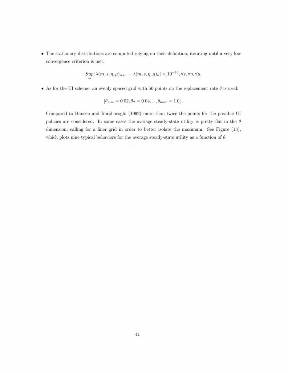
• The stationary distributions are computed relying on their definition, iterating until a very low
convergence criterion is met:
Supm|λ(m,s, η, µ)n+1 − λ(m, s, η, µ)n| < 10
−10,∀s,∀η,∀µ.
• As for the UI scheme, an evenly spaced grid with 50 points on the replacement rate θ is used:
[θmin = 0.02, θ2 = 0.04, ..., θmax = 1.0] .
Compared to Hansen and Imrohoroglu (1992) more than twice the points for the possible UI
policies are considered. In some cases the average steady-state utility is pretty flat in the θ
dimension, calling for a finer grid in order to better isolate the maximum. See Figure (13),
which plots nine typical behaviors for the average steady-state utility as a function of θ.
41

Appendix C - Monte Carlo Algorithm
The computational procedure used to solve the Monte Carlo experiments can be represented by
the following algorithm:
1. Draw 1,000 combinations of parameters from their prior distributions and store them.
2. Set the degree of moral hazard π (u) = {0, 0.1, 0.5} and the indicator i = 1.
3. Calibrate the model by reading the vector i of simulated parameters and begin the model
solution.
4. Generate a discrete grid over the UI replacement rate [θmin, ..., θmax] .
5. Set the UI replacement rate θj = θmin.
6. Generate a discrete grid over the asset space [0, ...,mmax] .
7. Guess on the tax rate τ0.
8. Get the value functions V (m,s, η; θj)i and the policy functions for savings m′(m, s, η, µ; θj)i and
labor supply η′(m, s, η; θj)i.
9. Compute the stationary distributions λ(m, s, η, µ; θj)i.
10. Get the aggregate unemployment rate.
11. Get the aggregate UI costs.
12. Check the government budget constraint; Get τ1.
13. Update τ ′0 = $τ0 + (1−$) τ1 (with bisection).
14. Iterate until the government budget constraint is satisfied.
15. Compute the average steady-state utility V (.; θj)i =∑
m,s,η,µ
λ(.; θj)iV (.; θj)i.
16. Consider the next point in the UI grid, until θj = θmax.
17. Compute the optimal UI scheme θ∗i as the steady-state utility maximizer, i.e. θ∗i ≡ Argmaxθj
{V (.; θj)i
}.
18. Save the output, set i = i+1 and repeat from step 3 for all the 1,000 combinations of simulated
parameters.
42

Appendix D - Additional Figures-.
85
-.8
-.7
5-.
7E
U
0 10 20 30 40 50Theta
-.5
05
-.5
-.4
95
EU
0 10 20 30 40 50Theta
-.5
45-
.54-
.53
5-.5
3-.5
25
EU
0 10 20 30 40 50Theta
-.4
56-.
45
4-.4
52-
.45-
.44
8E
U
0 10 20 30 40 50Theta
-.5
05
-.5
-.4
95
-.4
9E
U
0 10 20 30 40 50Theta
-.6
7-.
66
-.6
5-.
64-.
63
EU
0 10 20 30 40 50Theta
-.5
-.4
95
-.4
9-.
48
5E
U
0 10 20 30 40 50Theta
-.5
1-.5
08-.
50
6-.5
04-.
50
2E
U
0 10 20 30 40 50Theta
-.5
-.4
95-
.49-
.48
5-.4
8E
U
0 10 20 30 40 50Theta
Figure 13: Average Steady State Utility Vs. UI Scheme - Selected Calibrations
43
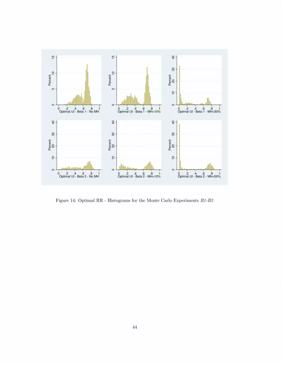
05
10
15
Pe
rce
nt
0 .2 .4 .6 .8 1Optimal UI - Beta 1 - No MH
05
10
15
Pe
rce
nt
0 .2 .4 .6 .8 1Optimal UI - Beta 1 - MH=10%
01
02
03
04
0P
erc
en
t
0 .2 .4 .6 .8 1Optimal UI - Beta 1 - MH=50%
01
02
03
04
0P
erc
en
t
0 .2 .4 .6 .8 1Optimal UI - Beta 2 - No MH
01
02
03
04
0P
erc
en
t
0 .2 .4 .6 .8 1Optimal UI - Beta 2 - MH=10%
01
02
03
04
0P
erc
en
t
0 .2 .4 .6 .8 1Optimal UI - Beta 2 - MH=50%
Figure 14: Optimal RR - Histograms for the Monte Carlo Experiments B1-B2
44

05
10
15
Pe
rce
nt
0 .2 .4 .6 .8 1Optimal UI - Beta 3 - No MH
05
10
15
Pe
rce
nt
0 .2 .4 .6 .8 1Optimal UI - Beta 3 - MH=10%
05
10
15
Pe
rce
nt
0 .2 .4 .6 .8 1Optimal UI - Beta 3 - MH=50%
01
02
03
04
0P
erc
en
t
0 .2 .4 .6 .8 1Optimal UI - Beta 4 - No MH
01
02
03
04
0P
erc
en
t
0 .2 .4 .6 .8 1Optimal UI - Beta 4 - MH=10%
01
02
03
04
0P
erc
en
t
0 .2 .4 .6 .8 1Optimal UI - Beta 4 - MH=50%
Figure 15: Optimal RR - Histograms for the Monte Carlo Experiments B3-B4
45

05
10
15
De
nsity
.3 .4 .5 .6Param: h - Beta 3 - No MH
kernel = epanechnikov, bandwidth = 0.0062
Kernel density estimate
05
10
15
De
nsity
.3 .4 .5 .6Param: h - Beta 3 - No MH rr<0.6kernel = epanechnikov, bandwidth = 0.0078
Kernel density estimate
05
10
15
De
nsity
.3 .4 .5 .6Param: h - Beta 3 - MH=10% rr<0.6
kernel = epanechnikov, bandwidth = 0.0076
Kernel density estimate
05
10
15
De
nsity
.3 .4 .5 .6Param: h - Beta 3 - MH=50% rr<0.6
kernel = epanechnikov, bandwidth = 0.0064
Kernel density estimate
05
10
15
De
nsity
.3 .4 .5 .6Param: h - Beta 3 - No MH rr>0.6kernel = epanechnikov, bandwidth = 0.0064
Kernel density estimate
05
10
15
De
nsity
.3 .4 .5 .6Param: h - Beta 3 - MH=10% rr>0.6
kernel = epanechnikov, bandwidth = 0.0065
Kernel density estimate
05
10
15
De
nsity
.3 .4 .5 .6Param: h - Beta 3 - MH=50% rr>0.6
kernel = epanechnikov, bandwidth = 0.0071
Kernel density estimate
02
46
8D
en
sity
.3 .4 .5 .6Param: h - Beta 4 - No MH
kernel = epanechnikov, bandwidth = 0.0127
Kernel density estimate
02
46
8D
en
sity
.3 .4 .5 .6Param: h - Beta 4 - No MH rr<0.6
kernel = epanechnikov, bandwidth = 0.0147
Kernel density estimate
02
46
8D
en
sity
.3 .4 .5 .6Param: h - Beta 4 - MH=10% rr<0.6
kernel = epanechnikov, bandwidth = 0.0144
Kernel density estimate
02
46
8D
en
sity
.3 .4 .5 .6Param: h - Beta 4 - MH=50% rr<0.6
kernel = epanechnikov, bandwidth = 0.0138
Kernel density estimate
02
46
8D
en
sity
.3 .4 .5 .6Param: h - Beta 4 - No MH rr>0.6kernel = epanechnikov, bandwidth = 0.0141
Kernel density estimate
02
46
8D
en
sity
.3 .4 .5 .6Param: h - Beta 4 - MH=10% rr>0.6
kernel = epanechnikov, bandwidth = 0.0142
Kernel density estimate
02
46
8D
en
sity
.3 .4 .5 .6Param: h - Beta 4 - MH=50% rr>0.6
kernel = epanechnikov, bandwidth = 0.0149
Kernel density estimate
Figure 16: Parameter h - Estimated Densities for the Monte Carlo Experiments B3-B4
46

07
14
De
nsity
.35 .55 .75 .95Param: Sigma - Beta 3 - No MHkernel = epanechnikov, bandwidth = 0.0145
Kernel density estimate
07
14
De
nsity
.35 .55 .75 .95Param: Sigma - Beta 3 - No MH rr<0.6
kernel = epanechnikov, bandwidth = 0.0095
Kernel density estimate
07
14
De
nsity
.35 .55 .75 .95Param: Sigma - Beta 3 - MH=10% rr<0.6
kernel = epanechnikov, bandwidth = 0.0093
Kernel density estimate
07
14
De
nsity
.35 .55 .75 .95Param: Sigma - Beta 3 - MH=50% rr<0.6
kernel = epanechnikov, bandwidth = 0.0112
Kernel density estimate
07
14
De
nsity
.35 .55 .75 .95Param: Sigma - Beta 3 - No MH rr>0.6
kernel = epanechnikov, bandwidth = 0.0117
Kernel density estimate
07
14
De
nsity
.35 .55 .75 .95Param: Sigma - Beta 3 - MH=10% rr>0.6
kernel = epanechnikov, bandwidth = 0.0114
Kernel density estimate
07
14
De
nsity
.35 .55 .75 .95Param: Sigma - Beta 3 - MH=50% rr>0.6
kernel = epanechnikov, bandwidth = 0.0099
Kernel density estimate
03
6D
en
sity
.35 .55 .75 .95Param: Sigma - Beta 4 - No MH
kernel = epanechnikov, bandwidth = 0.0311
Kernel density estimate
03
6D
en
sity
.35 .55 .75 .95Param: Sigma - Beta 4 - No MH rr<0.6
kernel = epanechnikov, bandwidth = 0.0181
Kernel density estimate
03
6D
en
sity
.35 .55 .75 .95Param: Sigma - Beta 4 - MH=10% rr<0.6
kernel = epanechnikov, bandwidth = 0.0185
Kernel density estimate
03
6D
en
sity
.35 .55 .75 .95Param: Sigma - Beta 4 - MH=50% rr<0.6
kernel = epanechnikov, bandwidth = 0.0220
Kernel density estimate
03
6D
en
sity
.35 .55 .75 .95Param: Sigma - Beta 4 - No MH rr>0.6
kernel = epanechnikov, bandwidth = 0.0226
Kernel density estimate
03
6D
en
sity
.35 .55 .75 .95Param: Sigma - Beta 4 - MH=10% rr>0.6
kernel = epanechnikov, bandwidth = 0.0221
Kernel density estimate
03
6D
en
sity
.35 .55 .75 .95Param: Sigma - Beta 4 - MH=50% rr>0.6
kernel = epanechnikov, bandwidth = 0.0196
Kernel density estimate
Figure 17: Parameter σ - Estimated Densities for the Monte Carlo Experiments B3-B4
47

02
00
40
0D
en
sity
.99 .995 1Param: betha - Beta 1 - No MHkernel = epanechnikov, bandwidth = 0.0002
Kernel density estimate
02
00
40
0D
en
sity
.99 .995 1Param: betha - Beta 1 - No MH rr<0.6
kernel = epanechnikov, bandwidth = 0.0003
Kernel density estimate
02
00
40
0D
en
sity
.99 .995 1Param: betha - Beta 1 - MH=10% rr<0.6
kernel = epanechnikov, bandwidth = 0.0002
Kernel density estimate
02
00
40
0D
en
sity
.99 .995 1Param: betha - Beta 1 - MH=50% rr<0.6
kernel = epanechnikov, bandwidth = 0.0002
Kernel density estimate
02
00
40
0D
en
sity
.99 .995 1Param: betha - Beta 1 - No MH rr>0.6
kernel = epanechnikov, bandwidth = 0.0002
Kernel density estimate
02
00
40
0D
en
sity
.99 .995 1Param: betha - Beta 1 - MH=10% rr>0.6
kernel = epanechnikov, bandwidth = 0.0002
Kernel density estimate
02
00
40
0D
en
sity
.99 .995 1Param: betha - Beta 1 - MH=50% rr>0.6
kernel = epanechnikov, bandwidth = 0.0002
Kernel density estimate
01
00
20
0D
en
sity
.99 .995 1Param: betha - Beta 2 - No MH
kernel = epanechnikov, bandwidth = 0.0004
Kernel density estimate
01
00
20
0D
en
sity
.99 .995 1Param: betha - Beta 2 - No MH rr<0.6
kernel = epanechnikov, bandwidth = 0.0005
Kernel density estimate
01
00
20
0D
en
sity
.99 .995 1Param: betha - Beta 2 - MH=10% rr<0.6
kernel = epanechnikov, bandwidth = 0.0005
Kernel density estimate
01
00
20
0D
en
sity
.99 .995 1Param: betha - Beta 2 - MH=50% rr<0.6
kernel = epanechnikov, bandwidth = 0.0004
Kernel density estimate
01
00
20
0D
en
sity
.99 .995 1Param: betha - Beta 2 - No MH rr>0.6
kernel = epanechnikov, bandwidth = 0.0005
Kernel density estimate
01
00
20
0D
en
sity
.99 .995 1Param: betha - Beta 2 - MH=10% rr>0.6
kernel = epanechnikov, bandwidth = 0.0005
Kernel density estimate
01
00
20
0D
en
sity
.99 .995 1Param: betha - Beta 2 - MH=50% rr>0.6
kernel = epanechnikov, bandwidth = 0.0005
Kernel density estimate
Figure 18: Parameter β - Estimated Densities for the Monte Carlo Experiments B1-B2
48

02
00
40
0D
en
sity
.99 .995 1Param: betha - Beta 3 - No MHkernel = epanechnikov, bandwidth = 0.0002
Kernel density estimate
02
00
40
0D
en
sity
.99 .995 1Param: betha - Beta 3 - No MH rr<0.6
kernel = epanechnikov, bandwidth = 0.0003
Kernel density estimate
02
00
40
0D
en
sity
.99 .995 1Param: betha - Beta 3 - MH=10% rr<0.6
kernel = epanechnikov, bandwidth = 0.0003
Kernel density estimate
02
00
40
0D
en
sity
.99 .995 1Param: betha - Beta 3 - MH=50% rr<0.6
kernel = epanechnikov, bandwidth = 0.0002
Kernel density estimate
02
00
40
0D
en
sity
.99 .995 1Param: betha - Beta 3 - No MH rr>0.6
kernel = epanechnikov, bandwidth = 0.0002
Kernel density estimate
02
00
40
0D
en
sity
.99 .995 1Param: betha - Beta 3 - MH=10% rr>0.6
kernel = epanechnikov, bandwidth = 0.0002
Kernel density estimate
02
00
40
0D
en
sity
.99 .995 1Param: betha - Beta 3 - MH=50% rr>0.6
kernel = epanechnikov, bandwidth = 0.0003
Kernel density estimate
01
00
20
0D
en
sity
.99 .995 1Param: betha - Beta 4 - No MH
kernel = epanechnikov, bandwidth = 0.0005
Kernel density estimate
01
00
20
0D
en
sity
.99 .995 1Param: betha - Beta 4 - No MH rr<0.6
kernel = epanechnikov, bandwidth = 0.0006
Kernel density estimate
01
00
20
0D
en
sity
.99 .995 1Param: betha - Beta 4 - MH=10% rr<0.6
kernel = epanechnikov, bandwidth = 0.0005
Kernel density estimate
01
00
20
0D
en
sity
.99 .995 1Param: betha - Beta 4 - MH=50% rr<0.6
kernel = epanechnikov, bandwidth = 0.0005
Kernel density estimate
01
00
20
0D
en
sity
.99 .995 1Param: betha - Beta 4 - No MH rr>0.6
kernel = epanechnikov, bandwidth = 0.0005
Kernel density estimate
01
00
20
0D
en
sity
.99 .995 1Param: betha - Beta 4 - MH=10% rr>0.6
kernel = epanechnikov, bandwidth = 0.0005
Kernel density estimate
01
00
20
0D
en
sity
.99 .995 1Param: betha - Beta 4 - MH=50% rr>0.6
kernel = epanechnikov, bandwidth = 0.0006
Kernel density estimate
Figure 19: Parameter β - Estimated Densities for the Monte Carlo Experiments B3-B4
49
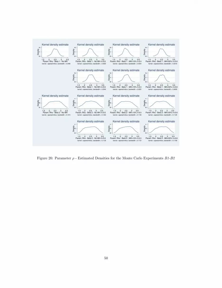
01
2D
en
sity
1.5 2 2.5 3 3.5Param: Rho - Beta 1 - No MH
kernel = epanechnikov, bandwidth = 0.0490
Kernel density estimate
01
2D
en
sity
1.5 2 2.5 3 3.5Param: Rho - Beta 1 - No MH rr<0.6
kernel = epanechnikov, bandwidth = 0.0555
Kernel density estimate
01
2D
en
sity
1.5 2 2.5 3 3.5Param: Rho - Beta 1 - MH=10% rr<0.6
kernel = epanechnikov, bandwidth = 0.0544
Kernel density estimate
01
2D
en
sity
1.5 2 2.5 3 3.5Param: Rho - Beta 1 - MH=50% rr<0.6
kernel = epanechnikov, bandwidth = 0.0516
Kernel density estimate
01
2D
en
sity
1.5 2 2.5 3 3.5Param: Rho - Beta 1 - No MH rr>0.6
kernel = epanechnikov, bandwidth = 0.0540
Kernel density estimate
01
2D
en
sity
1.5 2 2.5 3 3.5Param: Rho - Beta 1 - MH=10% rr>0.6
kernel = epanechnikov, bandwidth = 0.0551
Kernel density estimate
01
2D
en
sity
1.5 2 2.5 3 3.5Param: Rho - Beta 1 - MH=50% rr>0.6
kernel = epanechnikov, bandwidth = 0.0635
Kernel density estimate
0.5
1D
en
sity
1.5 2 2.5 3 3.5Param: Rho - Beta 2 - No MH
kernel = epanechnikov, bandwidth = 0.1010
Kernel density estimate
0.5
1D
en
sity
1.5 2 2.5 3 3.5Param: Rho - Beta 2 - No MH rr<0.6
kernel = epanechnikov, bandwidth = 0.1202
Kernel density estimate
0.5
1D
en
sity
1.5 2 2.5 3 3.5Param: Rho - Beta 2 - MH=10% rr<0.6
kernel = epanechnikov, bandwidth = 0.1190
Kernel density estimate
0.5
1D
en
sity
1.5 2 2.5 3 3.5Param: Rho - Beta 2 - MH=50% rr<0.6
kernel = epanechnikov, bandwidth = 0.1125
Kernel density estimate
0.5
1D
en
sity
1.5 2 2.5 3 3.5Param: Rho - Beta 2 - No MH rr>0.6
kernel = epanechnikov, bandwidth = 0.1126
Kernel density estimate
0.5
1D
en
sity
1.5 2 2.5 3 3.5Param: Rho - Beta 2 - MH=10% rr>0.6
kernel = epanechnikov, bandwidth = 0.1131
Kernel density estimate
0.5
1D
en
sity
1.5 2 2.5 3 3.5Param: Rho - Beta 2 - MH=50% rr>0.6
kernel = epanechnikov, bandwidth = 0.1199
Kernel density estimate
Figure 20: Parameter ρ - Estimated Densities for the Monte Carlo Experiments B1-B2
50

01
2D
en
sity
1.5 2 2.5 3 3.5Param: Rho - Beta 3 - No MH
kernel = epanechnikov, bandwidth = 0.0488
Kernel density estimate
01
2D
en
sity
1.5 2 2.5 3 3.5Param: Rho - Beta 3 - No MH rr<0.6
kernel = epanechnikov, bandwidth = 0.0645
Kernel density estimate
01
2D
en
sity
1.5 2 2.5 3 3.5Param: Rho - Beta 3 - MH=10% rr<0.6
kernel = epanechnikov, bandwidth = 0.0612
Kernel density estimate
01
2D
en
sity
1.5 2 2.5 3 3.5Param: Rho - Beta 3 - MH=50% rr<0.6
kernel = epanechnikov, bandwidth = 0.0529
Kernel density estimate
01
2D
en
sity
1.5 2 2.5 3 3.5Param: Rho - Beta 3 - No MH rr>0.6
kernel = epanechnikov, bandwidth = 0.0511
Kernel density estimate
01
2D
en
sity
1.5 2 2.5 3 3.5Param: Rho - Beta 3 - MH=10% rr>0.6
kernel = epanechnikov, bandwidth = 0.0519
Kernel density estimate
01
2D
en
sity
1.5 2 2.5 3 3.5Param: Rho - Beta 3 - MH=50% rr>0.6
kernel = epanechnikov, bandwidth = 0.0607
Kernel density estimate
0.5
1D
en
sity
1.5 2 2.5 3 3.5Param: Rho - Beta 4 - No MH
kernel = epanechnikov, bandwidth = 0.1016
Kernel density estimate
0.5
1D
en
sity
1.5 2 2.5 3 3.5Param: Rho - Beta 4 - No MH rr<0.6
kernel = epanechnikov, bandwidth = 0.1225
Kernel density estimate
0.5
1D
en
sity
1.5 2 2.5 3 3.5Param: Rho - Beta 4 - MH=10% rr<0.6
kernel = epanechnikov, bandwidth = 0.1215
Kernel density estimate
0.5
1D
en
sity
1.5 2 2.5 3 3.5Param: Rho - Beta 4 - MH=50% rr<0.6
kernel = epanechnikov, bandwidth = 0.1116
Kernel density estimate
0.5
1D
en
sity
1.5 2 2.5 3 3.5Param: Rho - Beta 4 - No MH rr>0.6
kernel = epanechnikov, bandwidth = 0.1120
Kernel density estimate
0.5
1D
en
sity
1.5 2 2.5 3 3.5Param: Rho - Beta 4 - MH=10% rr>0.6
kernel = epanechnikov, bandwidth = 0.1127
Kernel density estimate
0.5
1D
en
sity
1.5 2 2.5 3 3.5Param: Rho - Beta 4 - MH=50% rr>0.6
kernel = epanechnikov, bandwidth = 0.1235
Kernel density estimate
Figure 21: Parameter ρ - Estimated Densities for the Monte Carlo Experiments B3-B4
51

05
10
15
De
nsity
.4 .5 .6 .7 .8Param: x00 - Beta 1 - No MH
kernel = epanechnikov, bandwidth = 0.0100
Kernel density estimate
05
10
15
De
nsity
.4 .5 .6 .7 .8Param: x00 - Beta 1 - No MH rr<0.6
kernel = epanechnikov, bandwidth = 0.0128
Kernel density estimate
05
10
15
De
nsity
.4 .5 .6 .7 .8Param: x00 - Beta 1 - MH=10% rr<0.6
kernel = epanechnikov, bandwidth = 0.0122
Kernel density estimate
05
10
15
De
nsity
.4 .5 .6 .7 .8Param: x00 - Beta 1 - MH=50% rr<0.6
kernel = epanechnikov, bandwidth = 0.0108
Kernel density estimate
05
10
15
De
nsity
.4 .5 .6 .7 .8Param: x00 - Beta 1 - No MH rr>0.6
kernel = epanechnikov, bandwidth = 0.0105
Kernel density estimate
05
10
15
De
nsity
.4 .5 .6 .7 .8Param: x00 - Beta 1 - MH=10% rr>0.6
kernel = epanechnikov, bandwidth = 0.0105
Kernel density estimate
05
10
15
De
nsity
.4 .5 .6 .7 .8Param: x00 - Beta 1 - MH=50% rr>0.6
kernel = epanechnikov, bandwidth = 0.0123
Kernel density estimate
05
10
15
De
nsity
.4 .5 .6 .7 .8Param: x00 - Beta 2 - No MH
kernel = epanechnikov, bandwidth = 0.0199
Kernel density estimate
05
10
15
De
nsity
.4 .5 .6 .7 .8Param: x00 - Beta 2 - No MH rr<0.6
kernel = epanechnikov, bandwidth = 0.0233
Kernel density estimate
05
10
15
De
nsity
.4 .5 .6 .7 .8Param: x00 - Beta 2 - MH=10% rr<0.6
kernel = epanechnikov, bandwidth = 0.0227
Kernel density estimate
05
10
15
De
nsity
.4 .5 .6 .7 .8Param: x00 - Beta 2 - MH=50% rr<0.6
kernel = epanechnikov, bandwidth = 0.0217
Kernel density estimate
05
10
15
De
nsity
.4 .5 .6 .7 .8Param: x00 - Beta 2 - No MH rr>0.6
kernel = epanechnikov, bandwidth = 0.0225
Kernel density estimate
05
10
15
De
nsity
.4 .5 .6 .7 .8Param: x00 - Beta 2 - MH=10% rr>0.6
kernel = epanechnikov, bandwidth = 0.0230
Kernel density estimate
05
10
15
De
nsity
.4 .5 .6 .7 .8Param: x00 - Beta 2 - MH=50% rr>0.6
kernel = epanechnikov, bandwidth = 0.0245
Kernel density estimate
Figure 22: Parameter χ(u′,u) - Estimated Densities for the Monte Carlo Experiments B1-B2
52
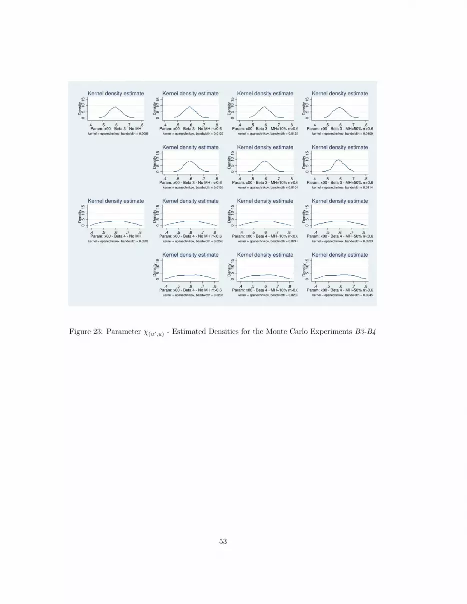
05
10
15
De
nsity
.4 .5 .6 .7 .8Param: x00 - Beta 3 - No MH
kernel = epanechnikov, bandwidth = 0.0098
Kernel density estimate
05
10
15
De
nsity
.4 .5 .6 .7 .8Param: x00 - Beta 3 - No MH rr<0.6
kernel = epanechnikov, bandwidth = 0.0132
Kernel density estimate
05
10
15
De
nsity
.4 .5 .6 .7 .8Param: x00 - Beta 3 - MH=10% rr<0.6
kernel = epanechnikov, bandwidth = 0.0128
Kernel density estimate
05
10
15
De
nsity
.4 .5 .6 .7 .8Param: x00 - Beta 3 - MH=50% rr<0.6
kernel = epanechnikov, bandwidth = 0.0109
Kernel density estimate
05
10
15
De
nsity
.4 .5 .6 .7 .8Param: x00 - Beta 3 - No MH rr>0.6
kernel = epanechnikov, bandwidth = 0.0103
Kernel density estimate
05
10
15
De
nsity
.4 .5 .6 .7 .8Param: x00 - Beta 3 - MH=10% rr>0.6
kernel = epanechnikov, bandwidth = 0.0104
Kernel density estimate
05
10
15
De
nsity
.4 .5 .6 .7 .8Param: x00 - Beta 3 - MH=50% rr>0.6
kernel = epanechnikov, bandwidth = 0.0114
Kernel density estimate
05
10
15
De
nsity
.4 .5 .6 .7 .8Param: x00 - Beta 4 - No MH
kernel = epanechnikov, bandwidth = 0.0208
Kernel density estimate
05
10
15
De
nsity
.4 .5 .6 .7 .8Param: x00 - Beta 4 - No MH rr<0.6
kernel = epanechnikov, bandwidth = 0.0248
Kernel density estimate
05
10
15
De
nsity
.4 .5 .6 .7 .8Param: x00 - Beta 4 - MH=10% rr<0.6
kernel = epanechnikov, bandwidth = 0.0247
Kernel density estimate
05
10
15
De
nsity
.4 .5 .6 .7 .8Param: x00 - Beta 4 - MH=50% rr<0.6
kernel = epanechnikov, bandwidth = 0.0233
Kernel density estimate
05
10
15
De
nsity
.4 .5 .6 .7 .8Param: x00 - Beta 4 - No MH rr>0.6
kernel = epanechnikov, bandwidth = 0.0231
Kernel density estimate
05
10
15
De
nsity
.4 .5 .6 .7 .8Param: x00 - Beta 4 - MH=10% rr>0.6
kernel = epanechnikov, bandwidth = 0.0232
Kernel density estimate
05
10
15
De
nsity
.4 .5 .6 .7 .8Param: x00 - Beta 4 - MH=50% rr>0.6
kernel = epanechnikov, bandwidth = 0.0245
Kernel density estimate
Figure 23: Parameter χ(u′,u) - Estimated Densities for the Monte Carlo Experiments B3-B4
53
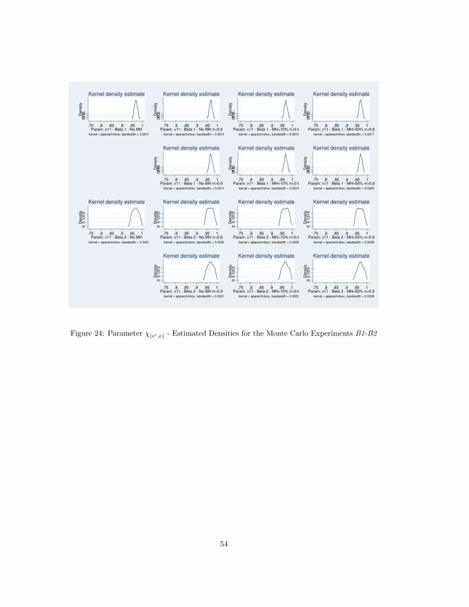
051
015
De
nsity
.75 .8 .85 .9 .95 1Param: x11 - Beta 1 - No MH
kernel = epanechnikov, bandwidth = 0.0016
Kernel density estimate
051
015
De
nsity
.75 .8 .85 .9 .95 1Param: x11 - Beta 1 - No MH rr<0.6
kernel = epanechnikov, bandwidth = 0.0018
Kernel density estimate
051
015
De
nsity
.75 .8 .85 .9 .95 1Param: x11 - Beta 1 - MH=10% rr<0.6
kernel = epanechnikov, bandwidth = 0.0018
Kernel density estimate
051
015
De
nsity
.75 .8 .85 .9 .95 1Param: x11 - Beta 1 - MH=50% rr<0.6
kernel = epanechnikov, bandwidth = 0.0017
Kernel density estimate
051
015
De
nsity
.75 .8 .85 .9 .95 1Param: x11 - Beta 1 - No MH rr>0.6
kernel = epanechnikov, bandwidth = 0.0018
Kernel density estimate
051
015
De
nsity
.75 .8 .85 .9 .95 1Param: x11 - Beta 1 - MH=10% rr>0.6
kernel = epanechnikov, bandwidth = 0.0018
Kernel density estimate
051
015
De
nsity
.75 .8 .85 .9 .95 1Param: x11 - Beta 1 - MH=50% rr>0.6
kernel = epanechnikov, bandwidth = 0.0020
Kernel density estimate
05
101
5D
en
sity
.75 .8 .85 .9 .95 1Param: x11 - Beta 2 - No MH
kernel = epanechnikov, bandwidth = 0.0033
Kernel density estimate
05
101
5D
en
sity
.75 .8 .85 .9 .95 1Param: x11 - Beta 2 - No MH rr<0.6
kernel = epanechnikov, bandwidth = 0.0038
Kernel density estimate
05
101
5D
en
sity
.75 .8 .85 .9 .95 1Param: x11 - Beta 2 - MH=10% rr<0.6
kernel = epanechnikov, bandwidth = 0.0038
Kernel density estimate
05
101
5D
en
sity
.75 .8 .85 .9 .95 1Param: x11 - Beta 2 - MH=50% rr<0.6
kernel = epanechnikov, bandwidth = 0.0036
Kernel density estimate
05
101
5D
en
sity
.75 .8 .85 .9 .95 1Param: x11 - Beta 2 - No MH rr>0.6
kernel = epanechnikov, bandwidth = 0.0037
Kernel density estimate
05
101
5D
en
sity
.75 .8 .85 .9 .95 1Param: x11 - Beta 2 - MH=10% rr>0.6
kernel = epanechnikov, bandwidth = 0.0037
Kernel density estimate
05
101
5D
en
sity
.75 .8 .85 .9 .95 1Param: x11 - Beta 2 - MH=50% rr>0.6
kernel = epanechnikov, bandwidth = 0.0039
Kernel density estimate
Figure 24: Parameter χ(e′,e) - Estimated Densities for the Monte Carlo Experiments B1-B2
54

05
10
15
De
nsity
.75 .8 .85 .9 .95 1Param: x11 - Beta 3 - No MH
kernel = epanechnikov, bandwidth = 0.0059
Kernel density estimate
05
10
15
De
nsity
.75 .8 .85 .9 .95 1Param: x11 - Beta 3 - No MH rr<0.6
kernel = epanechnikov, bandwidth = 0.0076
Kernel density estimate
05
10
15
De
nsity
.75 .8 .85 .9 .95 1Param: x11 - Beta 3 - MH=10% rr<0.6
kernel = epanechnikov, bandwidth = 0.0075
Kernel density estimate
05
10
15
De
nsity
.75 .8 .85 .9 .95 1Param: x11 - Beta 3 - MH=50% rr<0.6
kernel = epanechnikov, bandwidth = 0.0064
Kernel density estimate
05
10
15
De
nsity
.75 .8 .85 .9 .95 1Param: x11 - Beta 3 - No MH rr>0.6
kernel = epanechnikov, bandwidth = 0.0062
Kernel density estimate
05
10
15
De
nsity
.75 .8 .85 .9 .95 1Param: x11 - Beta 3 - MH=10% rr>0.6
kernel = epanechnikov, bandwidth = 0.0063
Kernel density estimate
05
10
15
De
nsity
.75 .8 .85 .9 .95 1Param: x11 - Beta 3 - MH=50% rr>0.6
kernel = epanechnikov, bandwidth = 0.0073
Kernel density estimate
05
10
15
De
nsity
.75 .8 .85 .9 .95 1Param: x11 - Beta 4 - No MH
kernel = epanechnikov, bandwidth = 0.0121
Kernel density estimate
05
10
15
De
nsity
.75 .8 .85 .9 .95 1Param: x11 - Beta 4 - No MH rr<0.6
kernel = epanechnikov, bandwidth = 0.0146
Kernel density estimate
05
10
15
De
nsity
.75 .8 .85 .9 .95 1Param: x11 - Beta 4 - MH=10% rr<0.6
kernel = epanechnikov, bandwidth = 0.0146
Kernel density estimate
05
10
15
De
nsity
.75 .8 .85 .9 .95 1Param: x11 - Beta 4 - MH=50% rr<0.6
kernel = epanechnikov, bandwidth = 0.0135
Kernel density estimate
05
10
15
De
nsity
.75 .8 .85 .9 .95 1Param: x11 - Beta 4 - No MH rr>0.6
kernel = epanechnikov, bandwidth = 0.0134
Kernel density estimate
05
10
15
De
nsity
.75 .8 .85 .9 .95 1Param: x11 - Beta 4 - MH=10% rr>0.6
kernel = epanechnikov, bandwidth = 0.0134
Kernel density estimate
05
10
15
De
nsity
.75 .8 .85 .9 .95 1Param: x11 - Beta 4 - MH=50% rr>0.6
kernel = epanechnikov, bandwidth = 0.0144
Kernel density estimate
Figure 25: Parameter χ(e′,e) - Estimated Densities for the Monte Carlo Experiments B3-B4
55

01
02
03
0D
en
sity
0 .2 .4 .6 .8 1E opportunity - Beta 1 - No MH
kernel = epanechnikov, bandwidth = 0.0030
Kernel density estimate
01
02
03
0D
en
sity
0 .2 .4 .6 .8 1E opportunity - Beta 1 - MH=10%
kernel = epanechnikov, bandwidth = 0.0030
Kernel density estimate
01
02
03
0D
en
sity
0 .2 .4 .6 .8 1E opportunity - Beta 1 - MH=50%
kernel = epanechnikov, bandwidth = 0.0030
Kernel density estimate
01
02
03
0D
en
sity
0 .2 .4 .6 .8 1E opportunity - Beta 2 - No MH
kernel = epanechnikov, bandwidth = 0.0065
Kernel density estimate
01
02
03
0D
en
sity
0 .2 .4 .6 .8 1E opportunity - Beta 2 - MH=10%
kernel = epanechnikov, bandwidth = 0.0065
Kernel density estimate
01
02
03
0D
en
sity
0 .2 .4 .6 .8 1E opportunity - Beta 2 - MH=50%
kernel = epanechnikov, bandwidth = 0.0065
Kernel density estimate
Figure 26: Employment Opportunity - Estimated Densities for the Monte Carlo Experiments B1-B2
56

05
10
De
nsity
0 .2 .4 .6 .8 1E opportunity - Beta 3 - No MH
kernel = epanechnikov, bandwidth = 0.0095
Kernel density estimate
05
10
De
nsity
0 .2 .4 .6 .8 1E opportunity - Beta 3 - MH=10%
kernel = epanechnikov, bandwidth = 0.0095
Kernel density estimate
05
10
De
nsity
0 .2 .4 .6 .8 1E opportunity - Beta 3 - MH=50%
kernel = epanechnikov, bandwidth = 0.0095
Kernel density estimate
05
10
De
nsity
0 .2 .4 .6 .8 1E opportunity - Beta 4 - No MH
kernel = epanechnikov, bandwidth = 0.0208
Kernel density estimate
05
10
De
nsity
0 .2 .4 .6 .8 1E opportunity - Beta 4 - MH=10%
kernel = epanechnikov, bandwidth = 0.0208
Kernel density estimate
05
10
De
nsity
0 .2 .4 .6 .8 1E opportunity - Beta 4 - MH=50%
kernel = epanechnikov, bandwidth = 0.0208
Kernel density estimate
Figure 27: Employment Opportunity - Estimated Densities for the Monte Carlo Experiments B3-B4
57

05
10
De
nsity
0 .2 .4 .6 .8 1Employment Rate - Beta 1 - No MH
kernel = epanechnikov, bandwidth = 0.0381
Kernel density estimate
05
10
De
nsity
0 .2 .4 .6 .8 1Employment Rate - Beta 1 - MH=10%
kernel = epanechnikov, bandwidth = 0.0391
Kernel density estimate
05
10
De
nsity
0 .2 .4 .6 .8 1Employment Rate - Beta 1 - MH=50%
kernel = epanechnikov, bandwidth = 0.0348
Kernel density estimate
05
10
De
nsity
0 .2 .4 .6 .8 1Employment Rate - Beta 2 - No MH
kernel = epanechnikov, bandwidth = 0.0640
Kernel density estimate
05
10
De
nsity
0 .2 .4 .6 .8 1Employment Rate - Beta 2 - MH=10%
kernel = epanechnikov, bandwidth = 0.0643
Kernel density estimate
05
10
De
nsity
0 .2 .4 .6 .8 1Employment Rate - Beta 2 - MH=50%
kernel = epanechnikov, bandwidth = 0.0642
Kernel density estimate
Figure 28: Employment Rate - Estimated Densities for the Monte Carlo Experiments B1-B2
58

05
10
De
nsity
0 .2 .4 .6 .8 1Employment Rate - Beta 3 - No MH
kernel = epanechnikov, bandwidth = 0.0127
Kernel density estimate
05
10
De
nsity
0 .2 .4 .6 .8 1Employment Rate - Beta 3 - MH=10%
kernel = epanechnikov, bandwidth = 0.0122
Kernel density estimate
05
10
De
nsity
0 .2 .4 .6 .8 1Employment Rate - Beta 3 - MH=50%
kernel = epanechnikov, bandwidth = 0.0117
Kernel density estimate
05
10
De
nsity
0 .2 .4 .6 .8 1Employment Rate - Beta 4 - No MH
kernel = epanechnikov, bandwidth = 0.0417
Kernel density estimate
05
10
De
nsity
0 .2 .4 .6 .8 1Employment Rate - Beta 4 - MH=10%
kernel = epanechnikov, bandwidth = 0.0416
Kernel density estimate
05
10
De
nsity
0 .2 .4 .6 .8 1Employment Rate - Beta 4 - MH=50%
kernel = epanechnikov, bandwidth = 0.0414
Kernel density estimate
Figure 29: Employment Rate - Estimated Densities for the Monte Carlo Experiments B3-B4
59
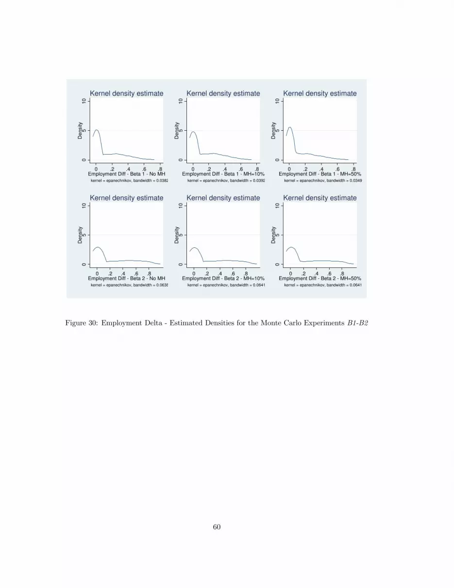
05
10
De
nsity
0 .2 .4 .6 .8Employment Diff - Beta 1 - No MH
kernel = epanechnikov, bandwidth = 0.0382
Kernel density estimate
05
10
De
nsity
0 .2 .4 .6 .8Employment Diff - Beta 1 - MH=10%
kernel = epanechnikov, bandwidth = 0.0392
Kernel density estimate
05
10
De
nsity
0 .2 .4 .6 .8Employment Diff - Beta 1 - MH=50%
kernel = epanechnikov, bandwidth = 0.0349
Kernel density estimate
05
10
De
nsity
0 .2 .4 .6 .8Employment Diff - Beta 2 - No MH
kernel = epanechnikov, bandwidth = 0.0638
Kernel density estimate
05
10
De
nsity
0 .2 .4 .6 .8Employment Diff - Beta 2 - MH=10%
kernel = epanechnikov, bandwidth = 0.0641
Kernel density estimate
05
10
De
nsity
0 .2 .4 .6 .8Employment Diff - Beta 2 - MH=50%
kernel = epanechnikov, bandwidth = 0.0641
Kernel density estimate
Figure 30: Employment Delta - Estimated Densities for the Monte Carlo Experiments B1-B2
60

05
10
De
nsity
0 .2 .4 .6 .8Employment Diff - Beta 3 - No MH
kernel = epanechnikov, bandwidth = 0.0158
Kernel density estimate
051
0D
en
sity
0 .2 .4 .6 .8Employment Diff - Beta 3 - MH=10%
kernel = epanechnikov, bandwidth = 0.0024
Kernel density estimate
051
0D
en
sity
0 .2 .4 .6 .8Employment Diff - Beta 3 - MH=50%
kernel = epanechnikov, bandwidth = 0.0013
Kernel density estimate
05
10
De
nsity
0 .2 .4 .6 .8Employment Diff - Beta 4 - No MH
kernel = epanechnikov, bandwidth = 0.0336
Kernel density estimate
05
10
De
nsity
0 .2 .4 .6 .8Employment Diff - Beta 4 - MH=10%
kernel = epanechnikov, bandwidth = 0.0334
Kernel density estimate
05
10
De
nsity
0 .2 .4 .6 .8Employment Diff - Beta 4 - MH=50%
kernel = epanechnikov, bandwidth = 0.0317
Kernel density estimate
Figure 31: Employment Delta - Estimated Densities for the Monte Carlo Experiments B3-B4
61