The Pass-Through of Sovereign Risk∗

Luigi Bocola

Northwestern University

and

Federal Reserve Bank of Minneapolis

Abstract

This paper examines the macroeconomic implications of sovereign credit risk in

a business cycle model where banks are exposed to domestic government debt. The

news of a future sovereign default hampers financial intermediation. First, it tightens

the funding constraints of banks, reducing their available resources to finance firms

(liquidity channel). Second, it generates a precautionary motive for banks to delever-

age (risk channel). I estimate the model using Italian data, finding that i) sovereign

credit risk was highly recessionary, and that ii) the risk channel was sizable. I then use

the model to evaluate the effects of subsidized long term loans to banks, calibrated to

the ECB’s Longer Term Refinancing Operations. The presence of strong precautionary

motives at the policy enactment implies that bank lending to firms is not very sensitive

to these credit market interventions.

Keywords: Sovereign Debt Crises, Occasionally Binding Leverage Constraints, Risk,

Credit Policies.

JEL: E32, E44, G01, G21

∗First version: August 2013. This version: May 2014. This paper is a revised version of Chapter 1 of myPhD dissertation at the University of Pennsylvania. I am indebted to Frank Schorfheide, Jesús Fernández-Villaverde, Iourii Manovskii and Dirk Krueger for their guidance and advice at each stage of this project. Ithank Saki Bigio, V.V. Chari, Alessandro Dovis, Marcus Hagedorn, Mark Gertler, Nils Gornemann, GuidoLorenzoni, Ellen McGrattan, Enrique Mendoza, Daniel Neuhann, Monika Piazzesi and Andrea Prestipinofor very helpful comments. I would also like to thank seminar participants at the Board of Governors, BostonUniversity, Brown, Cambridge University, Collegio Carlo Alberto, Columbia, Cornell, INSEAD, MinneapolisFed, Minnesota, Northwestern, NYU, Philadelphia Fed, Princeton, Stanford, UCLA, University of Chicago,University of Pennsylvania, and the 2013 MFM and Macroeconomic Fragility Conference. I thank the Becker-Friedman Institute and the Macroeconomic Modeling and Systemic Risk Research Initiative for financialsupport. The views expressed herein are those of the author and not necessarily those of the FederalReserve Bank of Minneapolis or the Federal Reserve System.

1

1 Introduction

At the end of 2009, holdings of domestic government debt by banks in European periph-eral countries - Greece, Italy, Portugal and Spain - were equivalent to 93% of banks’ totalequity. At the same time, domestic financial intermediaries in these economies were pro-viding roughly two-thirds of external financing of local firms. It is therefore not surprisingthat many empirical studies have documented a severe disruption of financial intermedi-ation and a substantial increase in the borrowing costs of firms during the sovereign debtcrisis.1 One proposed explanation of these findings is that the exposure to distressed gov-ernment bonds hurts the ability of banks to raise funds in financial markets, leading toa pass-through of their increased financing costs into the lending rates paid by firms.2

This view was at the core of policy discussions in Europe and was a motive for majorinterventions by the European Central Bank (ECB).

I argue, however, that this view is incomplete. A sovereign default can in fact bethe trigger of a severe recession and have adverse effects on the performance of firms.Consequently, as an economy approaches a sovereign default, banks may start perceivingfirms to be more “risky", and they may demand higher returns when lending to them asa fair compensation for holding this additional risk. If this mechanism is quantitativelyimportant, policies that address the heightened liquidity problems of banks but do notreduce the increased riskiness of firms may prove ineffective in encouraging bank lending.

I formalize this mechanism in a quantitative model with financial intermediation andsovereign default risk. In the model, the news that the government may default in thefuture has adverse effects on the funding ability of exposed banks (liquidity channel) and itraises the risks associated with lending to the productive sector (risk channel). I structurallyestimate the model on Italian data with Bayesian methods. I find that the risk channel isindeed quantitatively important: it explains up to 45% of the impact of the sovereigndebt crisis on the borrowing costs of firms. I then use the estimated model to assessthe consequences of credit market interventions adopted by the ECB in mitigating theimplications of increased sovereign default risk.

My framework builds on a business cycle model with financial intermediation, in thetradition of Gertler and Kiyotaki (2010) and Gertler and Karadi (2011, 2013). In the model,

1See, for example, the evidence in Klein and Stellner (2013) and Bedendo and Colla (2013) using corpo-rate bond data, the analysis of Bofondi et al. (2013) using Italian firm level data and Neri (2013) and Neriand Ropele (2013) for evidence using aggregate time series. See also ECB (2011).

2The report by CGFS (2011) discusses the transmission channels through which sovereign risk affectedbank funding during the European debt crisis. For example, banks in the Euro area extensively use gov-ernment bonds as collateral, and the decline in the value of these securities during the sovereign debt crisisreduced their ability to access wholesale liquidity. See also Albertazzi et al. (2012).

2

banks collect savings from households and use these funds, along with their own wealth(net worth), to buy long-term government bonds and to lend to firms. This intermedia-tion is important because firms need external finance to buy capital goods. The modelhas three main ingredients. First, an agency problem between households and banksgenerates a constraint in the borrowing ability of the latter. This constraint on bank lever-age binds only occasionally and typically when bank net worth is low. Second, financialintermediation is risky: bank net worth varies over time mainly because banks financelong-term risky assets with short-term riskless debt. Third, the probability that the gov-ernment will default on its debt in the future is time-varying and follows a reduced formrule.

To understand the key mechanisms of the model, consider a scenario in which agents’expectations of a future sovereign default rise. The anticipation of a future “haircut"on government bonds depresses their market value, lowering the net worth of exposedbanks. This tightens their leverage constraint and it has adverse consequences for finan-cial intermediation: banks’ ability to collect funds from households and their lending tothe productive sector decline, leading to a contraction of capital accumulation. This is aconventional liquidity channel in the literature.

In addition, the expectation of a future sovereign default has adverse effects on the will-ingness of banks to hold firms’ claims, even when banks are currently not facing fundingconstraints. The sovereign default, in fact, endogenously triggers a deep recession charac-terized by a severe decline in the payouts of firms. Thus, when the likelihood of this eventincreases, banks have a precautionary motive to deleverage in order to avoid these losses.More specifically, if the sovereign default happens in the future, the constraint on bankleverage will bind because of the large balance sheet losses associated with their positionin government bonds. Banks are thus forced to liquidate their holdings of firms’ claims.The associated decline in their market value leads to a further deterioration in bank networth, feeding a vicious loop. Ex-ante, forward-looking banks have a precautionary mo-tive to reduce their holdings of firms’ assets because they perceive these claims to be more“risky"- i.e. they pay out little precisely when banks are facing funding constraints andare mostly in need of wealth. I refer to this second mechanism, often overlooked in theliterature, as the risk channel.

I measure the quantitative importance of liquidity and risk by estimating the structuralparameters of the model with Italian data from 1999:Q1 to 2011:Q4. The major challengeis to separate these two propagation mechanisms since they have qualitatively similarimplications for indicators of financial stress commonly used in the literature (e.g., creditspreads). I demonstrate, however, that the Lagrange multiplier on the leverage constraint

3

of banks is a function of observable variables, specifically of the TED spread and of thefinancial leverage of banks. I construct a time series for the Lagrange multiplier andI use it in estimation, along with GDP growth, to measure the cyclical behavior of theleverage constraint. In addition, I use credit default swap spreads on Italian governmentbonds and data on holdings of domestic government debt by Italian banks to measurethe time-varying nature of sovereign risk and the exposure of banks to this risk.3 Thestructural estimation is complicated by the fact that the model features time-variation inrisk premia and occasionally binding financial constraints. I develop an algorithm for itsglobal solution based on projections and sparse collocation, and I combine it with theparticle filter to evaluate the likelihood function.

Having established the good fit of the model using posterior predictive analysis, I useit to answer two applied questions. First, I quantify the effects of the sovereign debt crisison the financing premia of firms and on output, and I assess the relative importance ofthe two propagation mechanisms. I estimate that the sovereign debt crisis in Italy wasresponsible for a rise in the financing premia of firms that reached 93 basis points in2011:Q4, with the risk channel explaining up to 45% of the overall effects. This increase inthe financing costs of firms was associated with a severe decline in real economic activity:output losses of the sovereign debt crisis in Italy cumulate to 1.75% by the end of 2011.

Second, I evaluate the effects of a major credit market intervention adopted by the ECBin the first quarter of 2012, the Longer Term Refinancing Operations (LTROs). I model thepolicy as a subsidized long-term loan offered to banks, and implement it conditioning onthe state of the Italian economy in 2011:Q4. I find that the effects of LTROs on credit tofirms and output are small when we average over the 2012:Q1-2014:Q4 period. This is dueto the fact that precautionary motives were sizable when the policy was enacted. Banksthus have little incentives to increase their exposure to firms and they mainly use LTROsto cheaply substitute liabilities they have with the private sector.

The general lesson from the policy evaluation is that the success of credit market inter-ventions crucially depends on the economic environment in which they are implemented,more specifically on the relative importance of liquidity and risk. Liquidity constraints,by definition, prevent banks from undertaking profitable investment. Policies that relaxthese constraints have sizable effects on bank lending to firms and capital accumulation.The risk channel, instead, is an indication that firms are perceived to be a “bad asset"in the future, and banks incentives to hold their claims are less responsive to this type

3A credit default swap (CDS) is a derivative used to hedge the credit risk of an underlying referenceasset. CDS spreads on government securities are typically used in the literature as a proxy of sovereign risk,see Pan and Singleton (2008).

4

of policies. The nonlinear model studied in this paper allows one to measure these twomechanisms in real time, a decomposition that provides useful information for predictingthe macroeconomic effects of credit market interventions.

1.1 Related literature

This research is related to several strands of the literature. I contribute to recent workstudying the macroeconomic implications of shocks to the balance sheet of financial inter-mediaries. I build on the framework developed in Gertler and Kiyotaki (2010) and Gertlerand Karadi (2011, 2013), where the limited enforcement of debt contracts leads to con-straints on intermediaries’ leverage. Differently from these papers, I study how changesin the expectation of this constraint being binding in the future influence the choices ofintermediaries to hold risky assets today. Technically, I capture these effects because Ianalyze the model using nonlinear methods. My analysis uncovers two important phe-nomena. First, intermediaries develop a precautionary motive to deleverage wheneverthey expect the constraint to bind in the future. Related effects have been emphasizedby Brunnermeier and Sannikov (2013), He and Krishnamurthy (2012a) and Bianchi andMendoza (2012). The novel insight is that in my set-up these precautionary motives areinduced by an increase in the default probability of an unproductive asset, the governmentbond. Intermediaries have lower incentives to hold productive assets because of conta-gion effects- i.e. their balance sheet endogenously generate a correlation in the payoffs ofproductive and unproductive assets. Second, I show that credit market interventions arehighly state and size dependent in this environment.4

This paper is also related to the research on sovereign debt crises. Many empirical anal-yses have documented a strong link between sovereign and private sector spreads, both inemerging economies and more recently in southern European countries.5 Several authorshave recognized the importance of this relationship in different settings, see Neumeyerand Perri (2005) and Uribe and Yue (2006) in the context of business cycles in emergingmarkets, and Corsetti et al. (2013) for the implications of the sovereign risk pass-throughfor fiscal multipliers. However, in these and related papers, the reasons underlying theconnection between sovereign spreads and private sector interest rate are left unmodeled.

4There are a number of papers that study the effects of credit market interventions in related environ-ments. See, Curdia and Woodford (2010), Del Negro et al. (2012) and Bianchi and Bigio (2013).

5For emerging market economies, Durbin and Ng (2005) and Borensztein et al. (2006) provide an empir-ical analysis of the “sovereign ceiling", the practice of agencies to rate corporations below their sovereign.Cavallo and Valenzuela (2007) document the effects of sovereign spreads on corporate bonds spreads. Seefootnote 1 and 2 for evidence on southern European economies.

5

Part of the contribution of this paper is to microfound this link in a fully specified dynamicequilibrium model.

In doing so, my paper relates to recent studies analyzing the relation between sovereigndefaults and domestic banking sector. Motivated by robust empirical evidence, Gennaioliet al. (2013b) and Sosa Padilla (2013) study the effects of sovereign defaults on domesticbanks, and the impact that the associated output losses have on the government’s in-centives to default.6 My research is complementary to theirs: I take sovereign defaultrisk in reduced form, but I explicitly model the behavior of private credit markets whensovereign risk increases. Differently from the above papers, the mere anticipation of afuture sovereign default is recessionary because of its effects on the ability and the incen-tives of banks to intermediate productive assets.7 Anticipation effects have been studiedin related environments by Acharya et al. (2013), Broner et al. (2014) and Mallucci (2013).However, their analysis abstract from the effects that a sovereign default has on the per-ceived riskiness of firms, the key novel mechanism of this paper.

Methodologically, I draw from the literature on the Bayesian estimation of dynamicequilibrium economies (Del Negro and Schorfheide, 2011), more specifically of mod-els where nonlinearities feature prominently (Fernández-Villaverde and Rubio-Ramírez,2007). The model decision rules are derived numerically using a projection algorithm andthe Smolyak sparse grid (Krueger and Kubler, 2003).8 The likelihood function is evaluatedusing the auxiliary particle filter of Pitt and Shephard (1999). To my knowledge, this isthe first paper that estimates a model with occasionally binding financial constraints us-ing global methods and nonlinear filters. However, there are other papers that use relatedtechniques in different applications (see Gust et al., 2013; Bi and Traum, 2012).

Finally, the shock to sovereign default probabilities considered in this paper is a formof time-varying volatility. As such, my research is related to the literature that studieshow different types of volatility shocks influence real economic activity (Bloom, 2009;Fernández-Villaverde et al., 2011). Rietz (1988) and Barro (2006) emphasize the role of largemacroeconomic disasters in accounting for asset prices and Gourio (2012) studies howchanges in the probability of these events affect risk premia and capital accumulation. The

6Kumhof and Tanner (2005) and Gennaioli et al. (2013a) document that banks are highly exposed todomestic government debt in a large set of countries. Reinhart and Rogoff (2011) and Borensztein andPanizza (2009) show that sovereign defaults typically occur in proximity of banking crises.

7In an empirical study, Levy-Yeyati and Panizza (2011) point out that anticipation effects are key tounderstand the unfolding of sovereign debt crises. See also Aguiar et al. (2009) and Dovis (2013) for modelswhere anticipation effects arise because of debt overhang problems.

8Christiano and Fisher (2000) is an early paper documenting the performance of projections in mod-els with occasionally binding constraints. See Fernández-Villaverde et al. (2012) for an application of theSmolyak sparse grid in a model where the zero bound constraint on nominal rates binds occasionally.

6

sovereign default studied in this paper can be seen as a potential source of macroeconomicdisasters.9

Layout. The paper is organized as follows. Section 2 presents the model, while Section3 discusses its main mechanisms using two simplified examples. Section 4 presents theestimation and an analysis of the model’s fit. Section 5 presents key properties of theestimated model that are useful to interpret the two quantitative experiments, which arereported in Section 6. Section 7 concludes.

2 Model

I consider a neoclassical growth model enriched with a financial sector as in Gertler andKiyotaki (2010) and Gertler and Karadi (2011). I introduce in this setting long term gov-ernment bonds to which financial intermediaries are exposed. These securities pay inevery state of nature unless the government defaults. The probability of this latter eventvaries over time according to a reduced form stochastic process.

The model economy is populated by households, final good producers, capital goodproducers and a government. Each household is composed of two types of members:workers and bankers. Workers supply labor to final good firms in a competitive factormarket, and their wages are made available to the household. Bankers manage the savingsof other households and use these funds to buy government bonds and claims on firms.The perfectly competitive non-financial corporate sector produces a final good using aconstant returns to scale technology that aggregates capital and labor. Firms rent laborfrom households and buy capital from perfectly competitive capital good producers. Theircapital expenses are financed by bankers. Finally, the government issues bonds and taxeshouseholds in order to finance government spending, and can default on its debt. Theactions of the government are determined via fiscal rules.

The key friction in this environment is the limited enforcement of debt contracts be-tween households and bankers: bankers can walk away with the assets of their franchise,and households can recover only a fraction of their savings when this event occurs. Thisfriction gives rise to constraints on the leverage of banks, with bank net worth being thekey determinant of their borrowing capacity. When these incentive constraints bind, orare expected to bind in the future, bankers’ ability to intermediate is hampered and creditto the productive sector declines. This has adverse consequences for capital accumulation.

9Arellano et al. (2012), Gilchrist et al. (2013) and Christiano et al. (2013) study the real effects of a differentform of time-varying volatility in models with financial frictions.

7

In this environment, sovereign credit risk has adverse effects on real economic activitybecause it alters both the ability and the incentives of bankers to lend to firms.

In the remainder of this section I describe the agents’ decision problems, derive theconditions characterizing a competitive equilibrium, and sketch the algorithm used for thenumerical solution of the model. In Section 3, I discuss the key mechanisms of interest.I denote by S the vector collecting the current value for the state variables and by S′ thefuture state of the economy.

2.1 Agents and their decision problems

2.1.1 Households

A household is composed of a fraction f of workers and a fraction 1− f of bankers. Thereis perfect consumption insurance between its members. I denote by Π(S) the net profitsthat the household receives from holdings of economic activities, and by W(S) the wagethat workers receive from supplying labor to final good firms. The household valuesconsumption c and dislikes labor l according to the flow utility u(c, l), and he discountsthe future at the rate β. The household makes contingent plans for consumption, laborsupply and savings b′ in order to maximize lifetime utility. Savings are managed byfinancial intermediaries that are run by bankers belonging to other households, and theyearn the risk free return R(S). Taking prices as given, a household solves

vh(b; S) = maxb′≥0,c≥0,l∈[0,1]

{u(c, l) + βES[vh(b′; S′)]

},

c +1

R(S)b′ ≤W(S)l + Π(S) + b− τ(S),

S′ = Γ(S).

τ(S) denotes the level of lump sum taxes while Γ(.) describes the law of motion for theaggregate state variables. Optimality is governed, at an interior solution, by the intra-temporal and inter-temporal Euler equations

ul(c, l) = uc(c, l)W(S), (1)

ES[Λ(S′, S)R(S)] = 1, (2)

where Λ(S′, S) = βuc(c′,l′)uc(c,l) is the household’s marginal rate of substitution.

For the empirical analysis I will use preferences that are consistent with balanced

8

growth, u(c, l) = log(c) − χ l1+ν−1

1+ν−1 , where ν parameterizes the Frisch elasticity of laborsupply.

2.1.2 Bankers

A banker uses his accumulated net worth, n, and households’ savings, b′, to buy govern-ment bonds and claims on firms.10 Let aj be asset j held by a banker and let Qj(S) andRj(S′, S) be, respectively, the price of asset j and its realized returns next period on a unitof numeraire good invested in asset j. The banker’s balance sheet equates total assets tototal liabilities:

∑j={B,K}

Qj(S)aj = n +b′

R(S), (3)

where subscript B refers to government bonds and K to firms’ claims. The banker makesoptimal portfolio choices in order to maximize the present discounted value of dividendspaid to his own household. The payment of dividends depends on the turnover of abanker. At any point in time there is a probability 1− ψ that a banker becomes a workerin the next period. When this happens, the banker transfers his accumulated net worth tothe household.11 A banker that continues running the business does not pay dividends,and he keeps on accumulating net worth. Therefore, the present discounted value ofdividends equals the present discounted value of the banker’s terminal wealth. Net worthnext period is given by the difference between realized returns on assets and the paymentspromised to households.

n′ = ∑j={B,K}

Rj(S′, S)Qj(S)aj − b′. (4)

Note that bad realizations of Rj(S′, S) lead to reductions in the net worth n′ of thebanker. Because of a financial friction, this variation in net worth can affect a banker’sborrowing ability. More specifically, I assume limited enforcement of contracts betweenhouseholds and bankers. At any point in time, a banker can walk away with a fraction λ

of the project and transfer it to his own household. If he does so, households can force himinto bankruptcy and recover a fraction (1− λ) of the banks’ assets. This friction definesan incentive constraint for the banker: the value of running his franchise must be higherthan its outside option, λ[∑j Qj(S)aj].

10A worker who becomes a banker this period obtains start-up funds from his households. These trans-fers will be specified at the end of the section.

11When a banker exits, a worker replaces him so that their relative proportion does not change over time.

9

Taking prices as given, the banker solves the following program

vb(n; S) = maxaB,aK ,b

ES{

Λ(S′, S)[(1− ψ)n′ + ψvb(n′; S′)

]},

n′ = ∑j={B,K}

Rj(S′, S)Qj(S)aj − b′,

∑j={B,K}

Qj(S)aj ≤ n +b′

R(S),

λ

∑j={B,K}

Qj(S)aj

≤ vb(n; S),

S′ = Γ(S).

Result 1 further characterizes this decision problem.

Result 1. A solution to the banker’s dynamic program is

vb(n; S) = α(S)n,

where α(S) solves

α(S) =ES{Λ(S′, S)[(1− ψ) + ψα(S′)]R(S)}

1− µ(S), (5)

and the Lagrange multiplier on the incentive constraint satisfies

µ(S) = max{

1−[

ES{Λ(S′, S)[(1− ψ) + ψα(S′)]R(S)}Nλ[QK(S)AK + QB(S)AB]

], 0}

, (6)

where N, AB and AK are, respectively, aggregate bankers’ net worth and aggregate bankers’ hold-ings of government bonds and firms assets.

Proof. See Appendix A.

This result clarifies why bank net worth plays a role in the model. Indeed, because ofthe linearity of the value function, we can rewrite the incentive constraint as

∑j={B,K} Qj(S)aj

n≤ α(S)

λ, (7)

implying that the leverage of a banker cannot exceed the time-varying threshold α(S)λ .

Bank net worth is thus a key variable regulating financial intermediation in the model:when net worth is low, the leverage constraint is more likely to bind and this limits theborrowing ability of a banker and, ultimately, his ability to intermediate.

10

The implications of this constraint for assets’ accumulation can be better understood bylooking at the Euler equation for risky asset j

ES[Λ(S′, S)Rj(S′, S)

]= ES

[Λ(S′, S)R(S)

]+ λµ(S), (8)

where Λ(S′, S) is the economy’s pricing kernel, defined as

Λ(S′, S) = Λ(S′, S)[(1− ψ) + ψα(S′)]. (9)

There are two main distinctions between this Euler equation and the one that wouldarise in a purely neoclassical setting. First, the leverage constraint limits the ability ofbanks to arbitrage away differences between expected discounted returns on asset j andthe risk free rate: this can be seen from equation (8), as the Lagrange multiplier generatesa wedge between these two returns. Second, the pricing kernel in equation (9) is notonly a function of consumption growth as in canonical neoclassical models, but also ofbank leverage. Indeed, as stated in equation (7), financial leverage is proportional to α(S)when µ(S) > 0. Adrian et al. (2013) provides empirical evidence in support of leverage-based pricing kernels for the U.S. economy and He and Krishnamurthy (2012b) discusstheir asset pricing implications in endowment economies. If the leverage constraint neverbinds, i.e. µ(S) = 0 ∀ S, equation (8) collapses to the neoclassical benchmark.12

Result 1 also implies that heterogeneity in bankers’ net worth and in their asset holdingsdoes not affect aggregate dynamics: this feature of the model makes its numerical analysistractable. For future reference, it is convenient to derive an expression for the law ofmotion of aggregate net worth

N′(S′, S) = ψ

∑j={B,K}

[Rj(S′, S)− R(S)]Qj(S)Aj + R(S)N

+ ω ∑j={B,K}

Qj(S′)Aj. (10)

Aggregate net worth next period equals the sum of the net worth accumulated bybankers who do not switch occupations today and the transfers that households maketo newly born bankers. These transfers are assumed to be a fraction ω of the assetsintermediated in the previous period, evaluated at current prices.

12Using equation (2), we can see that a solution to equation (5) is α(S) = 1 ∀ S whenever µ(S) = 0 ∀ S.

11

2.1.3 Capital good producers

The capital good producers build new capital goods using the technology Φ(

iK

)K, where

K is the aggregate capital stock in the economy and i the inputs used in production.They buy inputs in the final good market, and sell capital goods to final good firms atcompetitive prices. Taking the price of new capital Qi(S) as given, the decision problemof a capital good producer is

maxi≥0

[Qi(S)Φ

(iK

)K− i

].

Anticipating the market clearing condition, the price of new capital goods is

Qi(S) =1

Φ′(

I(S)K

) , (11)

where I(S) is equilibrium aggregate investment.

For the empirical analysis, I specify the production function for capital goods as Φ(x) =a1x1−ξ + a2, where ξ parametrizes the elasticity of Tobin’s q with respect to the investment-capital ratio.

2.1.4 Final good producers

Final output y is produced by perfectly competitive firms that operate a constant returnsto scale technology

y = kα(ezl)1−α, (12)

where k is the stock of capital goods, l stands for labor services, and z is a neutral tech-nology shock that follows an AR(1) process in growth

∆z′ = γ(1− ρz) + ρz∆z + σzε′z, ε′z ∼ N (0, 1). (13)

Labor is rented in competitive factor markets at W(S). Capital goods depreciate everyperiod at the rate δ. Anticipating the labor market clearing condition, profit maximizationimplies that equilibrium wages and profits per unit of capital are

W(S) = (1− α)Y(S)L(S)

, Z(S) = αY(S)

K, (14)

where Y(S) and L(S) are equilibrium aggregate output and labor.

12

Firms need external financing to purchase new capital goods. At the beginning of theperiod, they issue claims to bankers in exchange for funds.13 For each claim aK bankerspay QK(S) to firms.14 In exchange, bankers receive the realized return on a unit of thecapital stock in the next period:

RK(S′, S) =(1− δ)QK(S′) + Z(S′)

QK(S). (15)

Realized returns to capital move over time because of two factors: variation in firms’profits and variation in the market value of firms’ claims. These movements in RK(S′, S)induce variation in aggregate net worth, as equation (10) suggests.

2.1.5 The government

In every period, the government engages in public spending. Public spending as a fractionof GDP evolves as follows

log(g)′ = (1− ρg) log(g∗) + ρg log(g) + σgε′g, ε′g ∼ N (0, 1). (16)

The government finances public spending by levying lump sum taxes on householdsand by issuing long-term government bonds to financial intermediaries. Long term debtis introduced as in Chatterjee and Eyigungor (2013). In every period a fraction π ofbonds matures, and the government pays back the principal to investors. The remainingfraction (1− π) does not mature: the government pays the coupon ι, and investors retainthe right to obtain the principal in the future.15 I introduce risk of sovereign defaultby assuming that the government can default in every period and write off a fractionD ∈ [0, 1] of its outstanding debt. The parameter D can be interpreted as the “haircut"that the government imposes on bondholders in a default. Denoting by QB(S) the pricingfunction for government securities, tomorrow’s realized returns on a dollar invested ingovernment bonds are

RB(S′, S) =[1− d′D

] [π + (1− π) [ι + QB(S′)]QB(S)

], (17)

13While these claims are perfectly state contingent and therefore correspond to equity holdings, I interpretthem more broadly as privately issued paper such as bank loans.

14No arbitrage implies that the price of a unit of new capital equals in equilibrium the price of a claimissued by firms, Qi(S) = QK(S).

15The average duration of bonds is therefore 1π periods.

13

where d′ is an indicator variable equal to 1 if the government defaults next period. Real-ized returns on government bonds vary over time because of two sources. First, when thegovernment defaults, it imposes a haircut on bondholders. Second, RB(S′, S) is sensitiveto variation in the price of government securities: a decline in QB(S′), for example, lowersthe resale value of government bonds and reduces the returns on holding governmentdebt. This second effect is present even when the government does not default (d′ = 0),and to the extent that government debt has a maturity longer than one period (π < 1).

Denoting by B′ the stock of public debt, the budget constraint of the government isgiven by

QB(S)

B′ − (1− π)B[1− dD]︸ ︷︷ ︸Newly issued bonds

= [π + (1− π)ι] B[1− dD]︸ ︷︷ ︸Payments of principals and coupons

+ gY(S)− τ(S)︸ ︷︷ ︸Primary deficit

. (18)

Taxes respond to past debt according to the law of motion

τ(S)Y(S)

= t∗ + γτB

Y(S),

where γτ > 0.16

In order to close the model, we need to specify how sovereign risk evolves over time.As was the case for tax policy, sovereign credit risk follows a fiscal rule. In every periodthe government is hit by a shock εd that follows a standard logistic distribution. Thegovernment defaults on its outstanding debt if εd is sufficiently large. In particular, d′

follows

d′ =

1 if ε′d −Ψ(S; θ2) ≥ 0

0 otherwise,(19)

where θ2 is a vector of parameters. Given equation (19), we can write the conditionalprobability of a future sovereign default as follows

pd(S) ≡ Prob(d′ = 1|S) = exp{Ψ(S; θ2)}1 + exp{Ψ(S; θ2)}

. (20)

This formulation is intended to capture, in a flexible way, the considerations introducedby the research on the determinants of sovereign risk. In the literature on strategic debtdefault (Eaton and Gersovitz, 1981; Arellano, 2008), the government’s lack of commitment

16This formulation guarantees that the government does not run a Ponzi scheme and that its intertempo-ral budget constraint is satisfied in every state of nature. See Bohn (1995) and Canzoneri et al. (2001).

14

to repay his debt implies that default probabilities increase whenever the economy is ap-proaching states of the world where the government’s benefits to renege on his debt arelarger than their costs. In the literature on fiscal limits (Uribe, 2006; Bi, 2012), sovereignrisk moves whenever the current fiscal stance is forecasted to be incompatible with the sol-vency of the government. These approaches predict that sovereign credit risk responds tothe current state of the world. By appropriately choosing the function Ψ(S; θ2), one couldincorporate in the analysis key drivers of sovereign credit risk identified in the literature:for example, Ψ(S; θ2) could depend on the stock of debt, on total factor productivity or thenet worth of financial intermediaries. This allows us to keep the framework parimonious,and to focus on the economic mechanisms through which variation in pd(S) influencesreal economic activity, rather than those governing its determinants.

For the empirical application studied in the paper, though, I will consider the simplespecification Ψ(S; θ2) = s, with s being an AR(1) process

s′ = (1− ρs) log(s∗) + ρss + σsε′s, ε′s ∼ N (0, 1). (21)

This choice is motivated by two main considerations. First, there is substantial empiricalevidence that a large share of the variation in Italian sovereign spreads during the Eu-ropean crisis was driven by factors orthogonal to domestic fundamentals. For example,Bahaj (2013) documents that Italian sovereign spreads were very sensitive to political andsocial events in Cyprus, Greece, Ireland, Portugal and Spain during the European crisis:using a narrative approach, he finds that foreign events can account for up to 50% ofthe variation in Italian spreads.17 These empirical findings are consistent with the view,shared by economists and policymakers, that self-fulfilling beliefs (Conesa and Kehoe,2012; Lorenzoni and Werning, 2013) and contagion through common creditors (Arellanoand Bai, 2013) were key drivers of sovereign risk during the European crisis. The s-shock isintended to capture these considerations in a reduced form way. Second, exogenous vari-ations in the probability of a future sovereign default allow us to clearly isolate, withinthe model, the economic mechanisms driving the propagation of sovereign credit risk.

Importantly, as discussed in Section 4, the exogeneity of sovereign credit risk will notbe used as a restriction when estimating the structural model. Thus, the identification ofkey model parameters will not rely on this assumption.

17Di Cesare et al. (2013) show that economic fundamentals have limited predictive power in explainingthe behavior of Italian sovereign spreads, especially during the 2011-2012 period. Zoli (2013) points out thatforeign and domestic political event accounts for large part of the variation in Italian CDS spreads. See alsoGiordano et al. (2013) for an empirical analysis of contagion effects in European sovereign bonds markets.

15

2.2 Market clearing

Letting f (.) be the density of net worth across bankers, we can express the market clearingconditions as follows18

1. Credit market:∫

aK(n; S) f (n)dn = K′(S).

2. Government bonds market:∫

aB(n; S) f (n)dn = B′(S).

3. Market for households’ savings:∫

b′(n; S) f (n)dn = b′(S).

4. Market for final goods: Y(S)(1− g) = C(S) + I(S).

2.3 Equilibrium conditions and numerical solution

Since the non-stationary technology process induces a stochastic trend in several endoge-nous variables, it is convenient to express the model in terms of detrended variables. For agiven variable x, I define its detrended version as x = x

z .19 The state variables of the modelare S = [K, B, P, ∆z, g, s, d]. As I detail below, the variable P keeps track of aggregate banknet worth. The control variables {C(S), R(S), α(S), QB(S)} solve the residual equations(2), (5) and (8) (the last one for both assets).

The endogenous state variables [K, B, P] evolve as follows:

K′(S) ={(1− δ)K + Φ

[e∆z(

Y(S)(1− g)− C(S)K

)]K}

e−∆z, (22)

B′(S) =[1− dD]{π + (1− π)[ι + QB(S)]}Be−∆z + Y(S)

[g−

(t∗ + γτ

BY(S)

)]QB(S)

, (23)

P′(S) = R(S)[QK(S)K′(S) + QB(S)B′(S)− N(S)]. (24)

The state variable P measures the detrended cum interest promised payements of bankersto households at the beginning of the period, and it allows us to keep track of the evolutionof aggregate bankers’ net worth (See Appendix B). Finally, the exogenous state variables

18Note that we have anticipated earlier the market clearing condition for the labor market and for thecapital good market.

19The endogenous state variables of the model are detrended using the level of technology last period.

16

[∆z, log(g), s] follow, respectively, (13), (16) and (21), while d follows

d′ =

1 with probability exp{s}1+exp{s}

0 with probability 1− exp{s}1+exp{s} .

(25)

I use numerical methods to solve for the model decision rules. The algorithm for theglobal numerical solution of the model relies on projection methods (Judd, 1992; Heer andMaussner, 2009). In particular, let x(S) be the function describing the behavior of controlvariable x. I approximate x(S) using two sets of coefficients, {γx

d=0, γxd=1}. The law of

motion for x is then described by

x(d, S) = (1− d)γx0′T(S) + dγx

1′T(S),

where S = [K, B, P, ∆z, g, s] is the vector of state variables that excludes d, and T(.) is a vec-tor collecting Chebyshev’s polynomials. The coefficients {γx

d=0, γxd=1}x are such that the

residual equations are satisfied for a set of collocation points (di, Si) ∈ {0, 1}× S . I chooseS and the set of polynomial T(.) using the Smolyak collocation approach. Krueger andKubler (2003) and Krueger et al. (2010) provides a detailed description of the methodology.When evaluating the residual equations at the collocation points, I evaluate expectationsby “precomputing integrals" as in Judd et al. (2011). Finally, I adopt Newton’s methodto find the coefficients {γx

d=0, γxd=1}x satisfying the residual equations. Appendix B pro-

vides a detailed description of the algorithm and discusses the accuracy of the numericalsolution.

3 Two Simple Examples Illustrating the Mechanisms

It is now useful to describe the mechanisms that tie sovereign risk to the funding costs offirms and to real economic activity. An increase in the probability of a future sovereigndefault lowers capital accumulation via two distinct channels. First, it makes more difficultfor banks to raise funds from households, thus hampering their ability to intermediateproductive assets. Second, it signals that the economy is more likely to be in a bad stateof the world tomorrow: precautionary motives, then, reduce the willingness of bankers tointermediate the firms’ claims.

I illustrate these effects using two stylized versions of the model. First, I discuss themacroeconomic implications of a decline in the current net worth of bankers and a tighten-ing of their leverage constraint (Section 3.1). Second, I show that bad news about future net

17

worth leads bankers to act more cautiously and reduce their holdings of productive assetstoday. I also discuss how sovereign credit risk triggers these two propagation mechanismsin the full model. Section 3.3 explains the policy relevance of these mechanisms.

3.1 A decline in current net worth

I consider a deterministic economy with full depreciation (δ = 0), no capital adjustmentcosts (ξ = 0) and no government. Moreover, I assume that the transfers to newly bornbankers equal a fraction ω of current output, N = ωY and that bankers live only oneperiod (ψ = 0).

As in the neoclassical model with full depreciation and log utility, the saving rate isconstant in this economy. Specializing equation (6) to this particular parameterization, weobtain an expression for the Lagrange multiplier on the incentives constraint

µ =λσ−ω

λσ,

where σ is the saving rate. Using equation (8), we can solve for σ:

σ = min{

αβ + ω

1 + λ, αβ

}.

I assume that the leverage constraints is currently binding (λβα > ω), and I analyzethe implications of an unexpected transitory decline in the transfers to bankers.20 Whileanalytical solutions for this example can be easily derived, I illustrate the transition tosteady state using a numerical example.

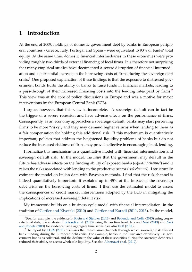
The top left panel of Figure 1 plots the equilibrium in the credit market prior to thedecline in ω. The supply of funds is derived from the bankers’ optimization problem:if the leverage constraint was not binding, bankers would be willing to lend at the riskfree rate R since this economy is non-stochastic. The supply of funds to firms is inelasticat K′ = α

λ N, the point at which the leverage constraint binds. The demand for credit isdownward sloping and equal to the expected marginal product of capital, αK′α−1

E[L′α].Since the leverage constraint binds, expected returns to capital equal R(1 + λµ).

The unanticipated decline in ω tightens the leverage constraint, and the inelastic partof the supply schedule shifts leftward. The right panels of the figure describe the adjust-

20More specifically, I assume that at time t = 1 the transfer to bankers ω declines, then goes back to itsprevious level at t = 2, and no further changes occur at future dates. Agents do not expect such a change,but are perfectly informed about the path of the transfer from period t = 1 ownward and they make rationalchoices based on this path.

18

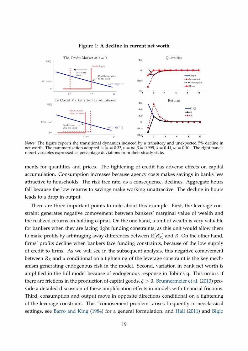
Figure 1: A decline in current net worth

Credit Supply

The Credit Market at t = 0

αK ′α−1E[L′1−α]

The Credit Market after the adjustment

αK ′α−1E[L′1−α]

Credit supplyafter the shock

0 2 4 6 8 10−1

−0.5

0

0.5Quantities

0 2 4 6 8 10−0.4

−0.2

0

0.2

0.4

0.6Returns

Output

Investment

Consumption

Hours

E[R′k]

R

Rk

R(1 + λμ)

Req(1 + λμeq)

E[R′k]

E[R′k]

K ′

K ′

Equilibrium priorto the shock

Net worthshock

R

Req

αλNα

λN ∗

αeq

λNeq

Equilibriumafter the shock

Notes: The figure reports the transitional dynamics induced by a transitory and unexpected 5% decline innet worth. The parametrization adopted is [α = 0.33, ν = ∞, β = 0.995, λ = 0.44, ω = 0.10]. The right panelsreport variables expressed as percentage deviations from their steady state.

ments for quantities and prices. The tightening of credit has adverse effects on capitalaccumulation. Consumption increases because agency costs makes savings in banks lessattractive to households. The risk free rate, as a consequence, declines. Aggregate hoursfall because the low returns to savings make working unattractive. The decline in hoursleads to a drop in output.

There are three important points to note about this example. First, the leverage con-straint generates negative comovement between bankers’ marginal value of wealth andthe realized returns on holding capital. On the one hand, a unit of wealth is very valuablefor bankers when they are facing tight funding constraints, as this unit would allow themto make profits by arbitraging away differences between E[R′K] and R. On the other hand,firms’ profits decline when bankers face funding constraints, because of the low supplyof credit to firms. As we will see in the subsequent analysis, this negative comovementbetween RK and α conditional on a tightening of the leverage constraint is the key mech-anism generating endogenous risk in the model. Second, variation in bank net worth isamplified in the full model because of endogenous response in Tobin’s q. This occurs ifthere are frictions in the production of capital goods, ξ > 0. Brunnermeier et al. (2013) pro-vide a detailed discussion of these amplification effects in models with financial frictions.Third, consumption and output move in opposite directions conditional on a tighteningof the leverage constraint. This “comovement problem" arises frequently in neoclassicalsettings, see Barro and King (1984) for a general formulation, and Hall (2011) and Bigio

19

(2012) for specific analysis in models with financial frictions.21

An increase in the probability of a future sovereign default in the model of Section 2triggers a decline in bank net worth and a tightening of their leverage constraint. Anincrease in s, in fact, implies a decline in the market value of government bonds becauseinvestors anticipate a future haircut. Thus, realized returns on government bonds de-cline. From equation (17) we can see that this effect is stronger the longer the maturityof bonds.22 Low realized returns on government bonds have a negative impact on banknet worth as we can see from equation (10). Thus, an s-shock can activate the process ofFigure 1 through its adverse effects on bank net worth. I will refer to this mechanism asthe liquidity channel.

3.2 Bad news about future net worth

Besides affecting the current constraint of financial intermediaries, an s-shock signals thatthe constraint is more likely to bind in the future. This affects bankers’ incentives tointermediate risky assets. It is helpful at this stage to derive an equilibrium relationdescribing the pricing of assets in the economy of Section 2. From equation (8) and (5) wefind that expected returns to asset j equal

ES[Rj(S′, S)− R(S)] =λµ(S)

ES[Λ(S′, S)]−

covS[Λ(S′, S), Rj(S′, S)]ES[Λ(S′, S)]

. (26)

Equation (26) defines the cross-section of assets’ returns. Expected excess returns tocapital typically carry a risk premium represented by covS[Λ(S′, S), RK(S′, S)]. As empha-sized by Ayiagari and Gertler (1999), this component reacts to changes in the expectationof how tight the leverage constraint will be in the future.

This can be illustrated with a simple modification of the previous set-up. I now allowψ to be greater than 0. Moreover, I assume that there are two regimes in the economy:

1. Normal times: transfers are fixed at their steady state, and the constraint on bankleverage is not binding.

21One way to restore comovement would be to allow the demand for labor to be directly affected by thetightenss of bank leverage constraint. This could be done, for example, by introducing working capital con-straint as in Mendoza (2010) and using preferences that mute the wealth effect on labor. While this extentionis straightforward to pursue in the current set up, I focus on a benchmark real model for comparability withprevious research.

22The parameter π also has an indirect effect on the elasticity of RB to the s-shock, since bond prices aremore responsive to this shock when the maturity is longer.

20

2. Financial crises: bankers are hit by the transitory decline in transfers described in theprevious section.

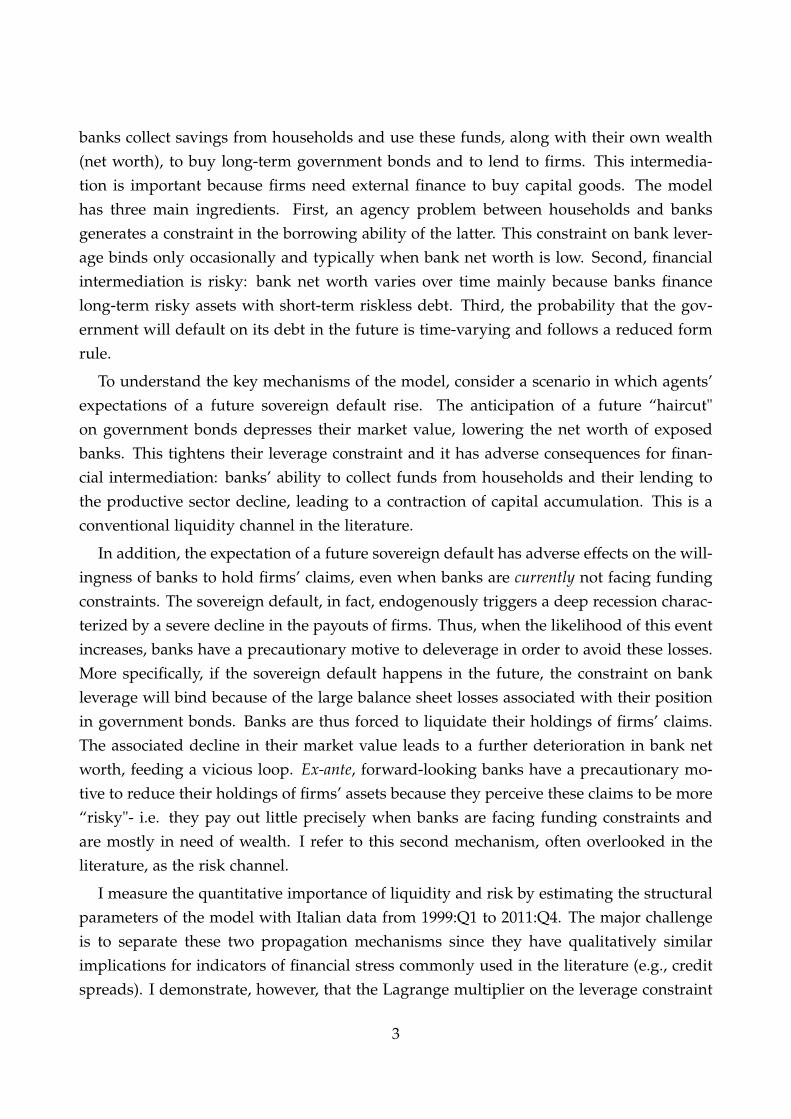
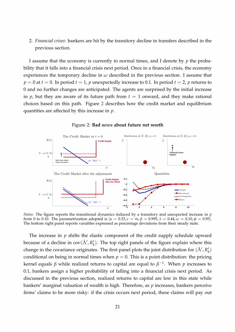
I assume that the economy is currently in normal times, and I denote by p the proba-bility that it falls into a financial crisis next period. Once in a financial crisis, the economyexperiences the temporary decline in ω described in the previous section. I assume thatp = 0 at t = 0. In period t = 1, p unexpectedly increase to 0.1. In period t = 2, p returns to0 and no further changes are anticipated. The agents are surprised by the initial increasein p, but they are aware of its future path from t = 1 onward, and they make rationalchoices based on this path. Figure 2 describes how the credit market and equilibriumquantities are affected by this increase in p.

Figure 2: Bad news about future net worth

αKα−1E[L1−α]

Credit Supply

The Credit Market at t = 0 Distribution of (Λ′, R′k), p = 0 Distribution of (Λ′, R′

k), p = 0.1

αKα−1E[L1−α]

Credit Supplyafter the shock

The Credit Market after the adjustment

0 2 4 6 8 10−0.4

−0.3

−0.2

−0.1

0

0.1

Quantities

Output

Investment

Consumption

Hours

K ′

K ′

R′k

R′k

Λ′ Λ′

Financial CrisesRegime

Bad news aboutfuture net worth

E[R′k]

E[R′k]

R - cov(Λ′ , R′k)

R - cov(Λ′ , R′k)

R

R

Notes: The figure reports the transitional dynamics induced by a transitory and unexpected increase in pfrom 0 to 0.10. The parametrization adopted is [α = 0.33, ν = ∞, β = 0.995, λ = 0.44, ω = 0.10, ψ = 0.95].The bottom right panel reports variables expressed as percentage deviations from their steady state.

The increase in p shifts the elastic component of the credit supply schedule upwardbecause of a decline in cov(Λ′, R′k). The top right panels of the figure explain where thischange in the covariance originates. The first panel plots the joint distribution for (Λ′, R′k)conditional on being in normal times when p = 0. This is a point distribution: the pricingkernel equals β while realized returns to capital are equal to β−1. When p increases to0.1, bankers assign a higher probability of falling into a financial crisis next period. Asdiscussed in the previous section, realized returns to capital are low in this state whilebankers’ marginal valuation of wealth is high. Therefore, as p increases, bankers perceivefirms’ claims to be more risky: if the crisis occurs next period, these claims will pay out

21

little precisely when bankers are most in need of wealth. For this reason, banks have aprecautionary motive to take out these claims from their balance sheet when the economyis approaching a financial crisis. The bottom right panel describes the macroeconomicconsequences of this increased precaution of bankers.

A sovereign default in the model of Section 2 resembles the financial crisis regimediscussed here: banks suffer large losses on their government bond holdings. Claims onfirms pay off badly in this state because of low firm profits and of a decline in their marketvalue. These low payouts are highly discounted by bankers because they are alreadyfacing large balance sheet losses, and their marginal value of wealth is high. When thelikelihood of this event increases, banks have a precautionary incentive to reduce theirholdings of firms’ claims because the economy is approaching a state where these assetsare not particularly valuable. This deleveraging leads to a decline in capital accumulation.I refer to this second mechanism through which sovereign credit risk propagates to thereal economy as the risk channel.

3.3 Policy relevance

While these two propagation mechanisms have similar implications for quantities andprices, they carry substantially different information. This can be seen by comparing thecredit markets in Figure 1 and Figure 2. In Figure 1, excess returns on firms’ claimsincrease because banks cannot rise enough funds to undertake profitable investment op-portunities: if they had an additional unit of wealth, they would invest it in firms’ claims.In Figure 2, instead, excess returns reflect fair compensation for increased risk: bank lever-age constraint are not binding, and there are no unexploited profitable opportunities.

This distinction has important implications for the evaluation of credit policies in themodel. For example, it is reasonable to expect that an injection of equity to the bankingsector may be more effective in stimulating banks’ lending when these latter are facingtight constraints on their leverage, while their aggregate implications may be muted whenprecautionary motives are strong. We will see in Section 5 that this intuition holds in themodel. First though, I move to the empirical analysis.

4 Empirical Analysis

The model is estimated using Italian quarterly data (1999:Q1-2011:Q4). This section pro-ceeds in three steps. Section 4.1 describes the data used in estimation. Section 4.2 illus-

22

trates the estimation strategy. I place a prior on parameters and conduct Bayesian infer-ence. Because of the high computational costs involved in solving the model repeatedly,I adopt a two-step procedure. In the first step, I estimate a version of the model withoutsovereign default risk on the 1999:Q1-2009:Q4 subsample. In the second step, I estimatethe parameters for the {st} shock using a time series for sovereign default probabilitiesfor the Italian economy. Section 4.3 presents basic diagnostics regarding model fit.

4.1 Data

While the previous section has described qualitatively the mechanisms of interest, theirquantitative relevance rests on the numerical value of the model parameters, in particu-lar those governing the stochastic properties of sovereign risk, the exposure of financialintermediaries to this risk and the macroeconomic implications of the financial frictionconsidered. I now describe the data series that I use to inform these model parameters.

First, I ensure that the time-varying nature of sovereign risk in the model is realistic.For this purpose, I use CDS spreads on Italian government securities with a five-yearmaturity. This time series is available at daily frequencies starting in January 2001 fromMarkit. See Appendix C.1 for further details.

Second, I measure the exposure of banks to this risk. I collect data on holdings ofdomestic government debt by the five largest Italian banks using the 2011 stress test of theEuropean Banking Authority.23 As detailed in Appendix C.2, these data include holdingsof domestic government securities, loans to central government and local authorities andother provisions, and these items are classified in terms of their maturity. Moreover,I correct for the possibility that banks insured against the risk of an Italian default bynetting out their positions in derivative contracts. I match this information with endof 2010 consolidated balance sheet data obtained from Bankscope, which allows me tomeasure how exposed were these five banks to the Italian government as a fraction oftheir total assets.

Third, I construct a model consistent indicator of agency costs. More specifically, I use asubset of the model’s equilibrium conditions to relate the Lagrange multiplier associatedto the leverage constraint of banks to a set of observable variables. As detailed in in Ap-pendix C.3, this Lagrange multiplier can be expressed as a function of financial leverage,levt, and of the spread between a risk free security that is traded only by bankers and the

23The five banks are: Unicredit, Intesa-San Paolo, MPS, BPI and UBI. Their total assets at the end of 2010accounted for 82% of the total assets of domestic banking groups in Italy.

23

risk free rate, R ft−Rt

R ft

µt =

[R f

t−RtRt

]levt

1 +[

R ft−RtRt

]levt

. (27)

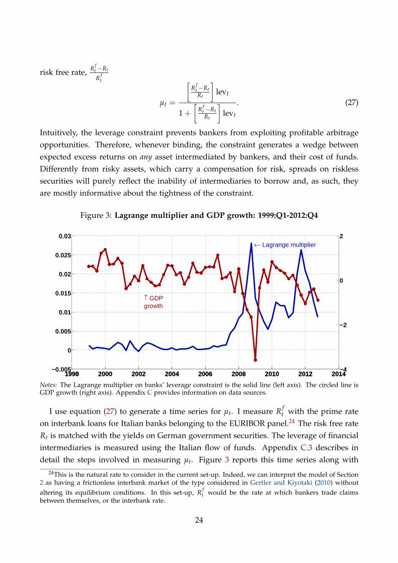
Intuitively, the leverage constraint prevents bankers from exploiting profitable arbitrageopportunities. Therefore, whenever binding, the constraint generates a wedge betweenexpected excess returns on any asset intermediated by bankers, and their cost of funds.Differently from risky assets, which carry a compensation for risk, spreads on risklesssecurities will purely reflect the inability of intermediaries to borrow and, as such, theyare mostly informative about the tightness of the constraint.

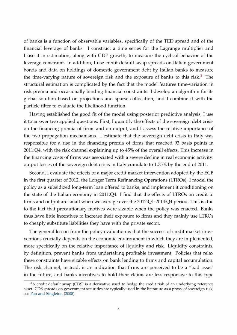
Figure 3: Lagrange multiplier and GDP growth: 1999:Q1-2012:Q4

1998 2000 2002 2004 2006 2008 2010 2012 2014−0.005

0

0.005

0.01

0.015

0.02

0.025

0.03← Lagrange multiplier

↑ GDP growth

1998 2000 2002 2004 2006 2008 2010 2012 2014−4

−2

0

2

Notes: The Lagrange multiplier on banks’ leverage constraint is the solid line (left axis). The circled line isGDP growth (right axis). Appendix C provides information on data sources.

I use equation (27) to generate a time series for µt. I measure R ft with the prime rate

on interbank loans for Italian banks belonging to the EURIBOR panel.24 The risk free rateRt is matched with the yields on German government securities. The leverage of financialintermediaries is measured using the Italian flow of funds. Appendix C.3 describes indetail the steps involved in measuring µt. Figure 3 reports this time series along with

24This is the natural rate to consider in the current set-up. Indeed, we can interpret the model of Section2 as having a frictionless interbank market of the type considered in Gertler and Kiyotaki (2010) withoutaltering its equilibrium conditions. In this set-up, R f

t would be the rate at which bankers trade claimsbetween themselves, or the interbank rate.

24

GDP growth. Two main facts stand out from a visual inspection of the figure. First,the Lagrange multiplier is countercyclical, rising substantially in periods in which GDPgrowth is markedly below average. Second, it is very close to 0 until 2007:Q2. Thus, theconstraint seems to bind only occasionally in sample.

Clearly, these three sets of data are not informative for all model parameters. Thus,I complement them with time series for the labor income share, the investment-outputratio, the government spending-output ratio and hours worked. Appendix C.4 providesdetailed definitions and data sources.

4.2 Estimation strategy

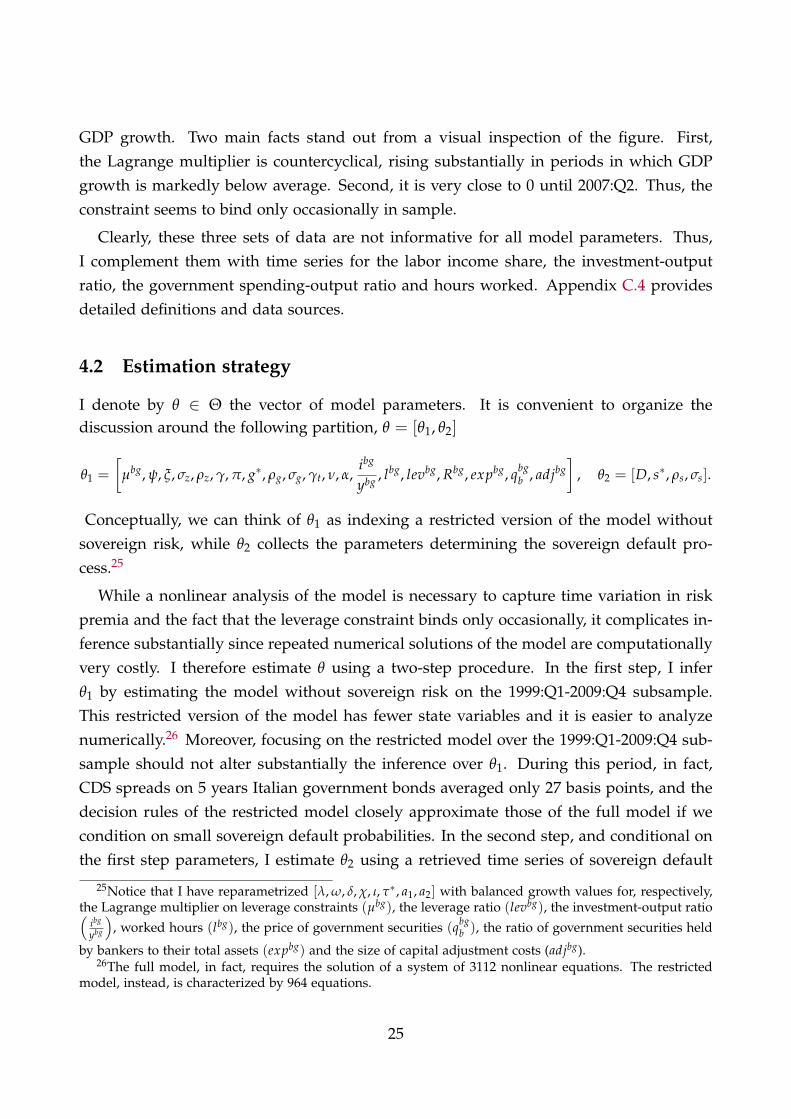
I denote by θ ∈ Θ the vector of model parameters. It is convenient to organize thediscussion around the following partition, θ = [θ1, θ2]

θ1 =

[µbg, ψ, ξ, σz, ρz, γ, π, g∗, ρg, σg, γt, ν, α,

ibg

ybg , lbg, levbg, Rbg, expbg, qbgb , adjbg

], θ2 = [D, s∗, ρs, σs].

Conceptually, we can think of θ1 as indexing a restricted version of the model withoutsovereign risk, while θ2 collects the parameters determining the sovereign default pro-cess.25

While a nonlinear analysis of the model is necessary to capture time variation in riskpremia and the fact that the leverage constraint binds only occasionally, it complicates in-ference substantially since repeated numerical solutions of the model are computationallyvery costly. I therefore estimate θ using a two-step procedure. In the first step, I inferθ1 by estimating the model without sovereign risk on the 1999:Q1-2009:Q4 subsample.This restricted version of the model has fewer state variables and it is easier to analyzenumerically.26 Moreover, focusing on the restricted model over the 1999:Q1-2009:Q4 sub-sample should not alter substantially the inference over θ1. During this period, in fact,CDS spreads on 5 years Italian government bonds averaged only 27 basis points, and thedecision rules of the restricted model closely approximate those of the full model if wecondition on small sovereign default probabilities. In the second step, and conditional onthe first step parameters, I estimate θ2 using a retrieved time series of sovereign default

25Notice that I have reparametrized [λ, ω, δ, χ, ι, τ∗, a1, a2] with balanced growth values for, respectively,the Lagrange multiplier on leverage constraints (µbg), the leverage ratio (levbg), the investment-output ratio(

ibg

ybg

), worked hours (lbg), the price of government securities (qbg

b ), the ratio of government securities held

by bankers to their total assets (expbg) and the size of capital adjustment costs (adjbg).26The full model, in fact, requires the solution of a system of 3112 nonlinear equations. The restricted

model, instead, is characterized by 964 equations.

25

probabilities.

Note that this two-step approach does not use the correlation between GDP growthand CDS spreads when estimating θ. This can be an attractive feature relative to a fullinformation approach. Because sovereign risk is assumed to be exogenous, in fact, themodel would interpret this moment as purely reflecting the causal effect of sovereignrisk on real economic activity and a full information approach would use it to informparameters values. Therefore, the two-step procedure adopted here is more robust topotential misspecifications of the sovereign default process described in Section 2.1.5.

4.2.1 Estimating the model without sovereign risk

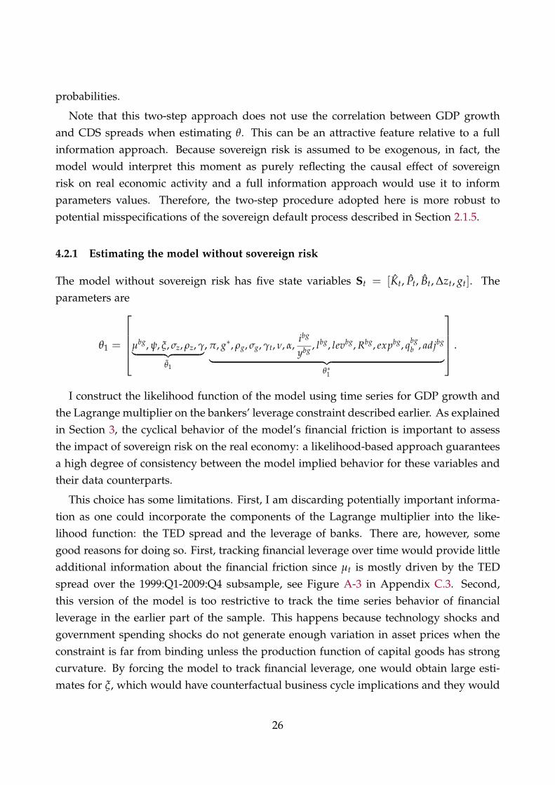
The model without sovereign risk has five state variables St = [Kt, Pt, Bt, ∆zt, gt]. Theparameters are

θ1 =

µbg, ψ, ξ, σz, ρz, γ︸ ︷︷ ︸θ1

, π, g∗, ρg, σg, γt, ν, α,ibg

ybg , lbg, levbg, Rbg, expbg, qbgb , adjbg︸ ︷︷ ︸

θ∗1

.

I construct the likelihood function of the model using time series for GDP growth andthe Lagrange multiplier on the bankers’ leverage constraint described earlier. As explainedin Section 3, the cyclical behavior of the model’s financial friction is important to assessthe impact of sovereign risk on the real economy: a likelihood-based approach guaranteesa high degree of consistency between the model implied behavior for these variables andtheir data counterparts.

This choice has some limitations. First, I am discarding potentially important informa-tion as one could incorporate the components of the Lagrange multiplier into the like-lihood function: the TED spread and the leverage of banks. There are, however, somegood reasons for doing so. First, tracking financial leverage over time would provide littleadditional information about the financial friction since µt is mostly driven by the TEDspread over the 1999:Q1-2009:Q4 subsample, see Figure A-3 in Appendix C.3. Second,this version of the model is too restrictive to track the time series behavior of financialleverage in the earlier part of the sample. This happens because technology shocks andgovernment spending shocks do not generate enough variation in asset prices when theconstraint is far from binding unless the production function of capital goods has strongcurvature. By forcing the model to track financial leverage, one would obtain large esti-mates for ξ, which would have counterfactual business cycle implications and they would

26

tend to increase the relative importance of the risk channel.27

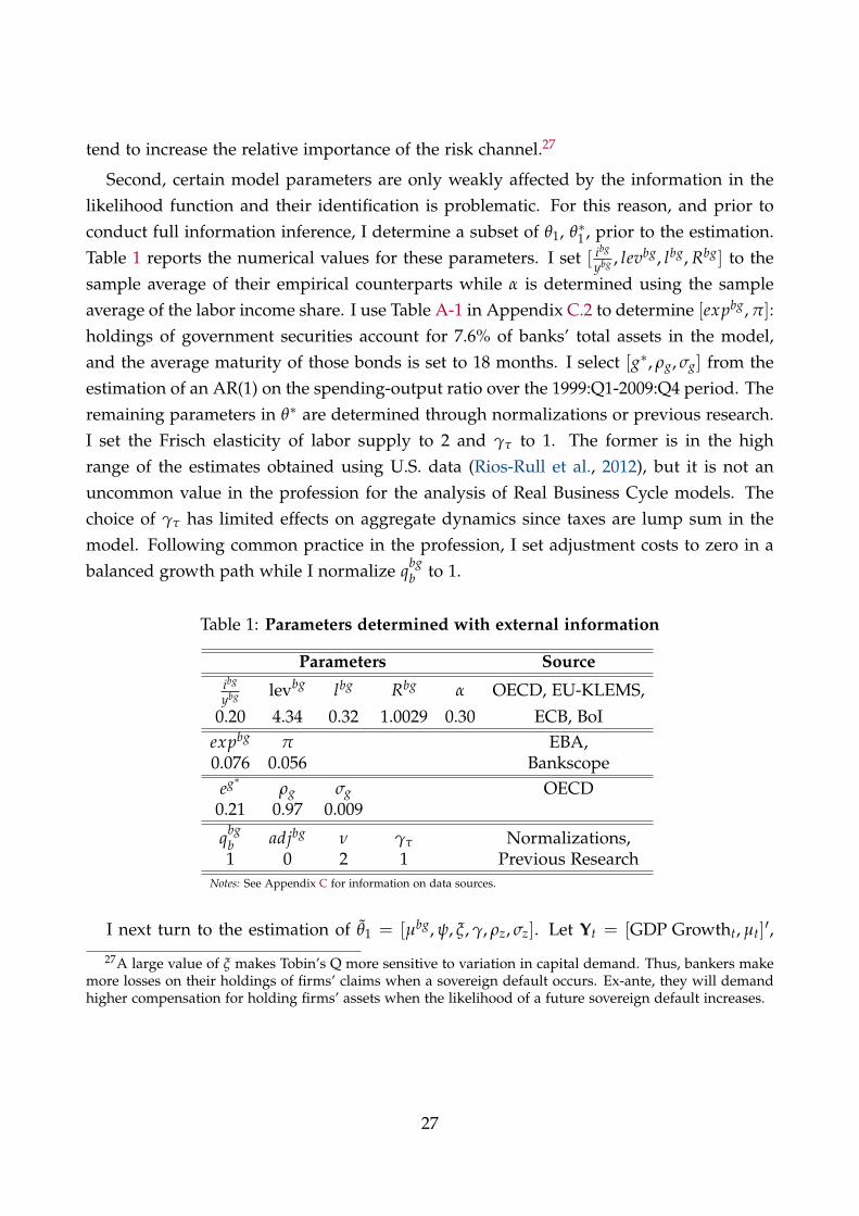
Second, certain model parameters are only weakly affected by the information in thelikelihood function and their identification is problematic. For this reason, and prior toconduct full information inference, I determine a subset of θ1, θ∗1 , prior to the estimation.Table 1 reports the numerical values for these parameters. I set [ ibg

ybg , levbg, lbg, Rbg] to thesample average of their empirical counterparts while α is determined using the sampleaverage of the labor income share. I use Table A-1 in Appendix C.2 to determine [expbg, π]:holdings of government securities account for 7.6% of banks’ total assets in the model,and the average maturity of those bonds is set to 18 months. I select [g∗, ρg, σg] from theestimation of an AR(1) on the spending-output ratio over the 1999:Q1-2009:Q4 period. Theremaining parameters in θ∗ are determined through normalizations or previous research.I set the Frisch elasticity of labor supply to 2 and γτ to 1. The former is in the highrange of the estimates obtained using U.S. data (Rios-Rull et al., 2012), but it is not anuncommon value in the profession for the analysis of Real Business Cycle models. Thechoice of γτ has limited effects on aggregate dynamics since taxes are lump sum in themodel. Following common practice in the profession, I set adjustment costs to zero in abalanced growth path while I normalize qbg

b to 1.

Table 1: Parameters determined with external information

Parameters Sourceibg

ybg levbg lbg Rbg α OECD, EU-KLEMS,0.20 4.34 0.32 1.0029 0.30 ECB, BoI

expbg π EBA,0.076 0.056 Bankscope

eg∗ ρg σg OECD0.21 0.97 0.009

qbgb adjbg ν γτ Normalizations,1 0 2 1 Previous Research

Notes: See Appendix C for information on data sources.

I next turn to the estimation of θ1 = [µbg, ψ, ξ, γ, ρz, σz]. Let Yt = [GDP Growtht, µt]′,

27A large value of ξ makes Tobin’s Q more sensitive to variation in capital demand. Thus, bankers makemore losses on their holdings of firms’ claims when a sovereign default occurs. Ex-ante, they will demandhigher compensation for holding firms’ assets when the likelihood of a future sovereign default increases.

27

and let Yτ = [Y1, . . . , Yτ]′. The model defines the nonlinear state space system

Yt = fθ1(St) + ηt ηt ∼ N (0, Σ)

St = gθ1(St−1, εt) εt ∼ N (0, I),

where ηt is a vector of measurement errors and εt are the structural shocks.28 I ap-proximate the likelihood function of this nonlinear state space model using sequentialimportance sampling (Fernández-Villaverde and Rubio-Ramírez, 2007).29 The posteriordistribution of model parameters is

p(θ1|YT) =L(θ1|YT)p(θ1)

p(YT),

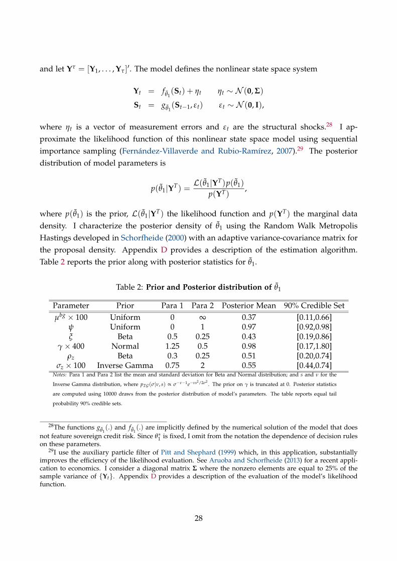
where p(θ1) is the prior, L(θ1|YT) the likelihood function and p(YT) the marginal datadensity. I characterize the posterior density of θ1 using the Random Walk MetropolisHastings developed in Schorfheide (2000) with an adaptive variance-covariance matrix forthe proposal density. Appendix D provides a description of the estimation algorithm.Table 2 reports the prior along with posterior statistics for θ1.

Table 2: Prior and Posterior distribution of θ1

Parameter Prior Para 1 Para 2 Posterior Mean 90% Credible Setµbg × 100 Uniform 0 ∞ 0.37 [0.11,0.66]

ψ Uniform 0 1 0.97 [0.92,0.98]ξ Beta 0.5 0.25 0.43 [0.19,0.86]

γ× 400 Normal 1.25 0.5 0.98 [0.17,1.80]ρz Beta 0.3 0.25 0.51 [0.20,0.74]

σz × 100 Inverse Gamma 0.75 2 0.55 [0.44,0.74]Notes: Para 1 and Para 2 list the mean and standard deviation for Beta and Normal distribution; and s and ν for the

Inverse Gamma distribution, where pIG (σ|ν, s) ∝ σ−ν−1e−νs2/2σ2. The prior on γ is truncated at 0. Posterior statistics

are computed using 10000 draws from the posterior distribution of model’s parameters. The table reports equal tail

probability 90% credible sets.

28The functions gθ1(.) and fθ1

(.) are implicitly defined by the numerical solution of the model that doesnot feature sovereign credit risk. Since θ∗1 is fixed, I omit from the notation the dependence of decision ruleson these parameters.

29I use the auxiliary particle filter of Pitt and Shephard (1999) which, in this application, substantiallyimproves the efficiency of the likelihood evaluation. See Aruoba and Schorfheide (2013) for a recent appli-cation to economics. I consider a diagonal matrix Σ where the nonzero elements are equal to 25% of thesample variance of {Yt}. Appendix D provides a description of the evaluation of the model’s likelihoodfunction.

28

The prior on the TFP process is centered using presample evidence while I center ξ

to 0.5, a conventional value in the literature. Priors on these three parameters are fairlydiffuse. I choose uniform priors over µbg and ψ, implying that the shape of the posterioris determined by the shape of the likelihood. Regarding posterior estimates, the Lagrangemultiplier is estimated to be close to 0 in a deterministic balanced growth path. Thissuggests that agency costs are fairly small on average in the model. This is not surprisinggiven the time series behavior of µt in Figure 3. Capital adjustment costs and the TFPprocess are in the range of what is typically obtained in the literature when using U.S.data.

4.2.2 Estimating sovereign risk

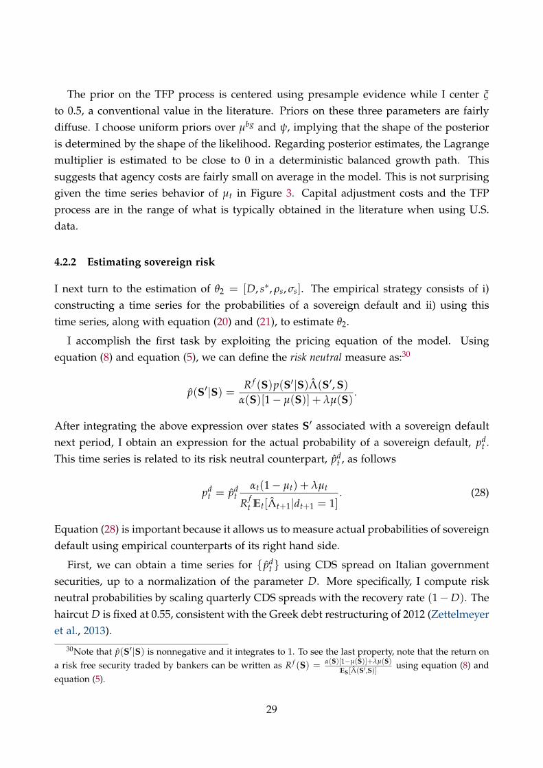
I next turn to the estimation of θ2 = [D, s∗, ρs, σs]. The empirical strategy consists of i)constructing a time series for the probabilities of a sovereign default and ii) using thistime series, along with equation (20) and (21), to estimate θ2.

I accomplish the first task by exploiting the pricing equation of the model. Usingequation (8) and equation (5), we can define the risk neutral measure as:30

p(S′|S) = R f (S)p(S′|S)Λ(S′, S)α(S)[1− µ(S)] + λµ(S)

.

After integrating the above expression over states S′ associated with a sovereign defaultnext period, I obtain an expression for the actual probability of a sovereign default, pd

t .This time series is related to its risk neutral counterpart, pd

t , as follows

pdt = pd

tαt(1− µt) + λµt

R ft Et[Λt+1|dt+1 = 1]

. (28)

Equation (28) is important because it allows us to measure actual probabilities of sovereigndefault using empirical counterparts of its right hand side.

First, we can obtain a time series for { pdt } using CDS spread on Italian government

securities, up to a normalization of the parameter D. More specifically, I compute riskneutral probabilities by scaling quarterly CDS spreads with the recovery rate (1−D). Thehaircut D is fixed at 0.55, consistent with the Greek debt restructuring of 2012 (Zettelmeyeret al., 2013).

30Note that p(S′|S) is nonnegative and it integrates to 1. To see the last property, note that the return ona risk free security traded by bankers can be written as R f (S) = α(S)[1−µ(S)]+λµ(S)

ES [Λ(S′ ,S)]using equation (8) and

equation (5).

29

Second, I construct a time series for Et[Λt+1|dt+1 = 1]. This is a difficult task because ofthe absence of a sovereign default in the sample. I indirectly use the model’s restrictionsto conduct this extrapolation. In particular, I approximate this object as follows

Et[Λt+1|dt+1 = 1] ≈ Et[Λt+1] + κVart[Λt+1]12 , (29)

where κ > 0 is a hyperparameter. The idea of equation (29) is that the marginal value ofwealth for bankers is above average in the event of a sovereign default because they aremore likely to face funding constraints: κ parameterizes the number of standard devia-tions by which Et[Λt+1|dt+1 = 1] is greater than Et[Λt+1].

I use the model restrictions to generate the terms {Et[Λt+1], Vart[Λt+1]12}. From equa-

tion (7) and (9), we can write Λt as a function of observables and of model parametersestimated in the first step

Λt = βe−∆ log(ct)[(1− ψ) + ψλlevt], (30)

where ∆ct is the growth rate of real personal consumption expenditure and levt is theleverage of financial intermediaries. I first estimate a first order Bayesian Vector Autore-gressive model on consumption growth and financial leverage, and I generate conditionalforecasts of [∆ct+1, levt+1]. I then use these conditional forecasts, the posterior mean of[β, ψ, λ] and equation (30) to generate {Et[Λt+1], Vart[Λt+1]

12}. Finally, I use these esti-

mates and equation (29) to approximate Et[Λt+1|dt+1 = 1]. The hyperparameter κ isselected with the help of the structural model. I consider a set of values κi ∈ {1, 3, 5} and Iselect the value that minimizes, in model simulated data, average root mean square errorsfor the approximation of Et[Λt+1|dt+1 = 1]. This gives a value of κ = 3.

Third, I combine the retrieved time series for {Et[Λt+1|dt+1 = 1]} with levt, µt and R ft

to generate the risk correction. I make use of the fact that the marginal value of wealth forbankers is proportional to financial leverage when the constraint binds, and measure therisk correction as follows:

λlevt(1− µt) + λµt

R ft {Et[Λt+1] + κVart[Λt+1]

12}

. (31)

Figure 4 plots {pdt } along with its decomposition of equation (28) for the different

values of κ. The top left panel reports the risk neutral probabilities, the bottom-left panelplots the risk correction and the right panel reports the time series for actual sovereigndefault probabilities. The estimates imply that roughly 30% of actual sovereign default

30

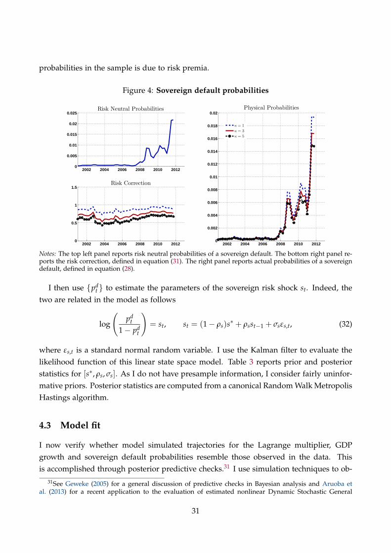
probabilities in the sample is due to risk premia.

Figure 4: Sovereign default probabilities

2002 2004 2006 2008 2010 20120

0.005

0.01

0.015

0.02

0.025Risk Neutral Probabilities

2002 2004 2006 2008 2010 20120

0.5

1

1.5Risk Correction

2002 2004 2006 2008 2010 20120

0.002

0.004

0.006

0.008

0.01

0.012

0.014

0.016

0.018

0.02Physical Probabilities

κ = 1

κ = 3

κ = 5

Notes: The top left panel reports risk neutral probabilities of a sovereign default. The bottom right panel re-ports the risk correction, defined in equation (31). The right panel reports actual probabilities of a sovereigndefault, defined in equation (28).

I then use {pdt } to estimate the parameters of the sovereign risk shock st. Indeed, the

two are related in the model as follows

log

(pd

t

1− pdt

)= st, st = (1− ρs)s∗ + ρsst−1 + σsεs,t, (32)

where εs,t is a standard normal random variable. I use the Kalman filter to evaluate thelikelihood function of this linear state space model. Table 3 reports prior and posteriorstatistics for [s∗, ρs, σs]. As I do not have presample information, I consider fairly uninfor-mative priors. Posterior statistics are computed from a canonical Random Walk MetropolisHastings algorithm.

4.3 Model fit

I now verify whether model simulated trajectories for the Lagrange multiplier, GDPgrowth and sovereign default probabilities resemble those observed in the data. Thisis accomplished through posterior predictive checks.31 I use simulation techniques to ob-

31See Geweke (2005) for a general discussion of predictive checks in Bayesian analysis and Aruoba etal. (2013) for a recent application to the evaluation of estimated nonlinear Dynamic Stochastic General

31

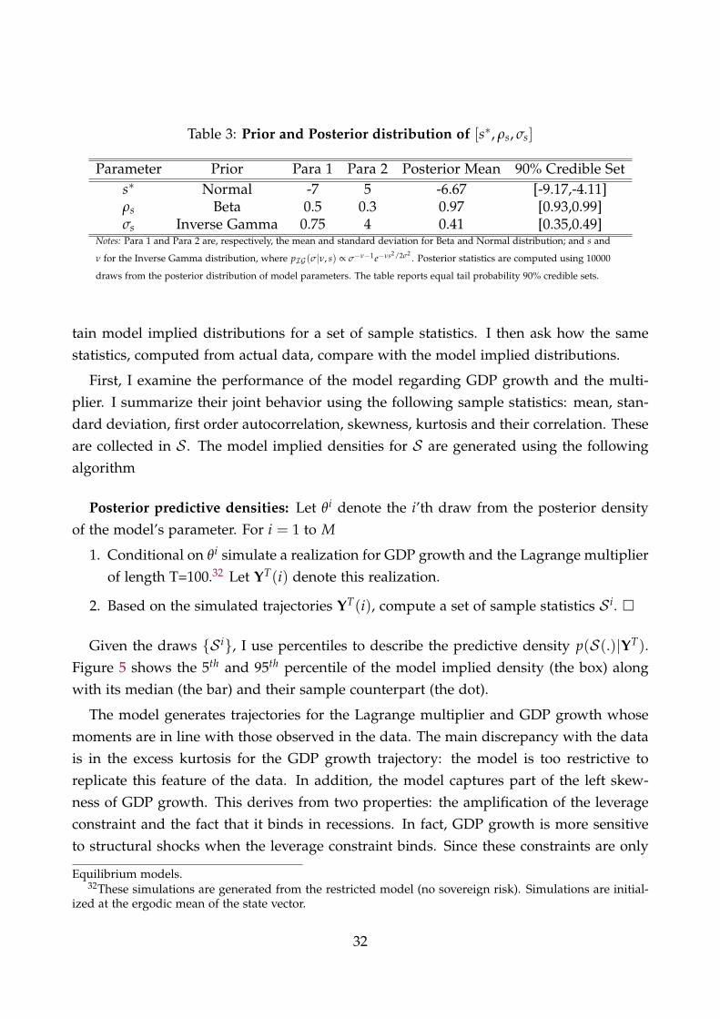
Table 3: Prior and Posterior distribution of [s∗, ρs, σs]

Parameter Prior Para 1 Para 2 Posterior Mean 90% Credible Sets∗ Normal -7 5 -6.67 [-9.17,-4.11]ρs Beta 0.5 0.3 0.97 [0.93,0.99]σs Inverse Gamma 0.75 4 0.41 [0.35,0.49]

Notes: Para 1 and Para 2 are, respectively, the mean and standard deviation for Beta and Normal distribution; and s and

ν for the Inverse Gamma distribution, where pIG (σ|ν, s) ∝ σ−ν−1e−νs2/2σ2. Posterior statistics are computed using 10000

draws from the posterior distribution of model parameters. The table reports equal tail probability 90% credible sets.

tain model implied distributions for a set of sample statistics. I then ask how the samestatistics, computed from actual data, compare with the model implied distributions.

First, I examine the performance of the model regarding GDP growth and the multi-plier. I summarize their joint behavior using the following sample statistics: mean, stan-dard deviation, first order autocorrelation, skewness, kurtosis and their correlation. Theseare collected in S . The model implied densities for S are generated using the followingalgorithm

Posterior predictive densities: Let θi denote the i’th draw from the posterior densityof the model’s parameter. For i = 1 to M

1. Conditional on θi simulate a realization for GDP growth and the Lagrange multiplierof length T=100.32 Let YT(i) denote this realization.

2. Based on the simulated trajectories YT(i), compute a set of sample statistics S i. �

Given the draws {S i}, I use percentiles to describe the predictive density p(S(.)|YT).Figure 5 shows the 5th and 95th percentile of the model implied density (the box) alongwith its median (the bar) and their sample counterpart (the dot).

The model generates trajectories for the Lagrange multiplier and GDP growth whosemoments are in line with those observed in the data. The main discrepancy with the datais in the excess kurtosis for the GDP growth trajectory: the model is too restrictive toreplicate this feature of the data. In addition, the model captures part of the left skew-ness of GDP growth. This derives from two properties: the amplification of the leverageconstraint and the fact that it binds in recessions. In fact, GDP growth is more sensitiveto structural shocks when the leverage constraint binds. Since these constraints are only

Equilibrium models.32These simulations are generated from the restricted model (no sovereign risk). Simulations are initial-

ized at the ergodic mean of the state vector.

32

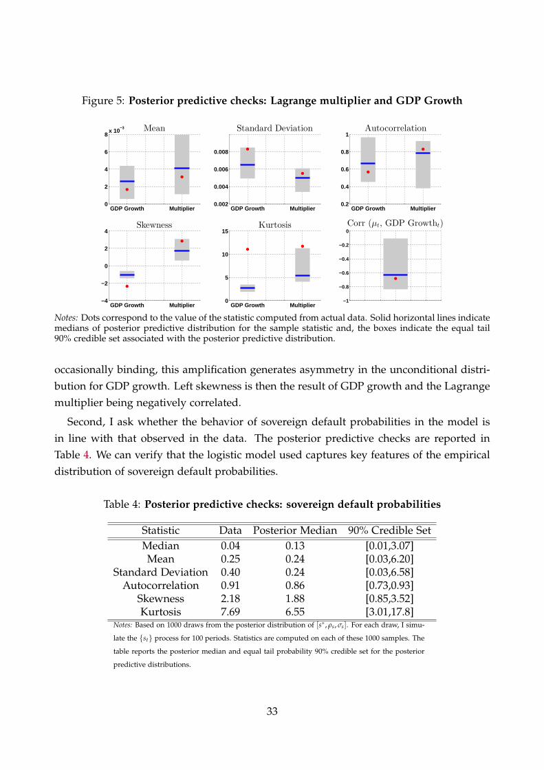
Figure 5: Posterior predictive checks: Lagrange multiplier and GDP Growth

GDP Growth Multiplier0

2

4

6

8x 10

−3 Mean

GDP Growth Multiplier0.002

0.004

0.006

0.008

Standard Deviation

GDP Growth Multiplier0.2

0.4

0.6

0.8

1Autocorrelation

GDP Growth Multiplier−4

−2

0

2

4Skewness

GDP Growth Multiplier0

5

10

15Kurtosis

−1

−0.8

−0.6

−0.4

−0.2

0Corr (μt, GDP Growtht)

Notes: Dots correspond to the value of the statistic computed from actual data. Solid horizontal lines indicatemedians of posterior predictive distribution for the sample statistic and, the boxes indicate the equal tail90% credible set associated with the posterior predictive distribution.

occasionally binding, this amplification generates asymmetry in the unconditional distri-bution for GDP growth. Left skewness is then the result of GDP growth and the Lagrangemultiplier being negatively correlated.

Second, I ask whether the behavior of sovereign default probabilities in the model isin line with that observed in the data. The posterior predictive checks are reported inTable 4. We can verify that the logistic model used captures key features of the empiricaldistribution of sovereign default probabilities.

Table 4: Posterior predictive checks: sovereign default probabilities

Statistic Data Posterior Median 90% Credible SetMedian 0.04 0.13 [0.01,3.07]Mean 0.25 0.24 [0.03,6.20]

Standard Deviation 0.40 0.24 [0.03,6.58]Autocorrelation 0.91 0.86 [0.73,0.93]

Skewness 2.18 1.88 [0.85,3.52]Kurtosis 7.69 6.55 [3.01,17.8]

Notes: Based on 1000 draws from the posterior distribution of [s∗, ρs, σs]. For each draw, I simu-

late the {st} process for 100 periods. Statistics are computed on each of these 1000 samples. The

table reports the posterior median and equal tail probability 90% credible set for the posterior

predictive distributions.

33

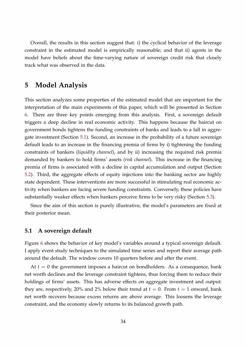
Overall, the results in this section suggest that: i) the cyclical behavior of the leverageconstraint in the estimated model is empirically reasonable; and that ii) agents in themodel have beliefs about the time-varying nature of sovereign credit risk that closelytrack what was observed in the data.

5 Model Analysis

This section analyzes some properties of the estimated model that are important for theinterpretation of the main experiments of this paper, which will be presented in Section6. There are three key points emerging from this analysis. First, a sovereign defaulttriggers a deep decline in real economic activity. This happens because the haircut ongovernment bonds tightens the funding constraints of banks and leads to a fall in aggre-gate investment (Section 5.1). Second, an increase in the probability of a future sovereigndefault leads to an increase in the financing premia of firms by i) tightening the fundingconstraints of bankers (liquidity channel), and by ii) increasing the required risk premiademanded by bankers to hold firms’ assets (risk channel). This increase in the financingpremia of firms is associated with a decline in capital accumulation and output (Section5.2). Third, the aggregate effects of equity injections into the banking sector are highlystate dependent. These interventions are more successful in stimulating real economic ac-tivity when bankers are facing severe funding constraints. Conversely, these policies havesubstantially weaker effects when bankers perceive firms to be very risky (Section 5.3).

Since the aim of this section is purely illustrative, the model’s parameters are fixed attheir posterior mean.

5.1 A sovereign default

Figure 6 shows the behavior of key model’s variables around a typical sovereign default.I apply event study techniques to the simulated time series and report their average patharound the default. The window covers 10 quarters before and after the event.

At t = 0 the government imposes a haircut on bondholders. As a consequence, banknet worth declines and the leverage constraint tightens, thus forcing them to reduce theirholdings of firms’ assets. This has adverse effects on aggregate investment and output:they are, respectively, 20% and 2% below their trend at t = 0. From t = 1 onward, banknet worth recovers because excess returns are above average. This loosens the leverageconstraint, and the economy slowly returns to its balanced growth path.

34

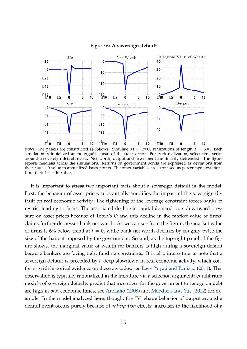
Figure 6: A sovereign default

−10 −5 0 5 10−60

−40

−20

0

20RB

−10 −5 0 5 10−60

−40

−20

0Net Worth

−10 −5 0 5 100

10

20

30

40Marginal Value of Wealth

−10 −5 0 5 10−8

−6

−4

−2

0QK

−10 −5 0 5 10−20

−15

−10

−5

0Investment

−10 −5 0 5 10−3

−2

−1

0Output

Notes: The panels are constructed as follows. Simulate M = 15000 realizations of length T = 300. Eachsimulation is initialized at the ergodic mean of the state vector. For each realization, select time seriesaround a sovereign default event. Net worth, output and investment are linearly detrended. The figurereports medians across the simulations. Returns on government bonds are expressed as deviations fromtheir t = −10 value in annualized basis points. The other variables are expressed as percentage deviationsfrom their t = −10 value.

It is important to stress two important facts about a sovereign default in the model.First, the behavior of asset prices substantially amplifies the impact of the sovereign de-fault on real economic activity. The tightening of the leverage constraint forces banks torestrict lending to firms. The associated decline in capital demand puts downward pres-sure on asset prices because of Tobin’s Q and this decline in the market value of firms’claims further depresses bank net worth. As we can see from the figure, the market valueof firms is 6% below trend at t = 0, while bank net worth declines by roughly twice thesize of the haircut imposed by the government. Second, as the top-right panel of the fig-ure shows, the marginal value of wealth for bankers is high during a sovereign defaultbecause bankers are facing tight funding constraints. It is also interesting to note that asovereign default is preceded by a deep slowdown in real economic activity, which con-forms with historical evidence on these episodes, see Levy-Yeyati and Panizza (2011). Thisobservation is typically rationalized in the literature via a selection argument: equilibriummodels of sovereign defaults predict that incentives for the government to renege on debtare high in bad economic times, see Arellano (2008) and Mendoza and Yue (2012) for ex-ample. In the model analyzed here, though, the “V" shape behavior of output around adefault event occurs purely because of anticipation effects: increases in the likelihood of a

35

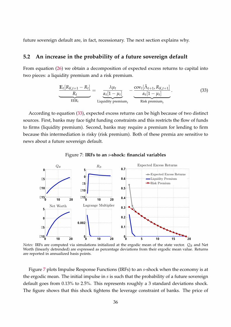
future sovereign default are, in fact, recessionary. The next section explains why.

5.2 An increase in the probability of a future sovereign default

From equation (26) we obtain a decomposition of expected excess returns to capital intotwo pieces: a liquidity premium and a risk premium.

Et[RK,t+1 − Rt]

Rt︸ ︷︷ ︸EERt

=λµt

αt[1− µt]︸ ︷︷ ︸Liquidity premiumt

− covt[Λt+1, RK,t+1]

αt[1− µt]︸ ︷︷ ︸Risk premiumt

. (33)

According to equation (33), expected excess returns can be high because of two distinctsources. First, banks may face tight funding constraints and this restricts the flow of fundsto firms (liquidity premium). Second, banks may require a premium for lending to firmbecause this intermediation is risky (risk premium). Both of these premia are sensitive tonews about a future sovereign default.

Figure 7: IRFs to an s-shock: financial variables

0 10 20−15

−10

−5

0QB

0 10 20−15

−10

−5

0

5RB

0 10 20−10

−5

0

5Net Worth

0 10 200

0.002

Lagrange Multiplier

0 5 10 15 200

0.1

0.2

0.3

0.4

0.5

0.6

0.7Expected Excess Returns

Expected Excess Returns

Liquidity Premium

Risk Premium

Notes: IRFs are computed via simulations initialized at the ergodic mean of the state vector. QB and NetWorth (linearly detrended) are expressed as percentage deviations from their ergodic mean value. Returnsare reported in annualized basis points.

Figure 7 plots Impulse Response Functions (IRFs) to an s-shock when the economy is atthe ergodic mean. The initial impulse in s is such that the probability of a future sovereigndefault goes from 0.13% to 2.5%. This represents roughly a 3 standard deviations shock.The figure shows that this shock tightens the leverage constraint of banks. The price of

36

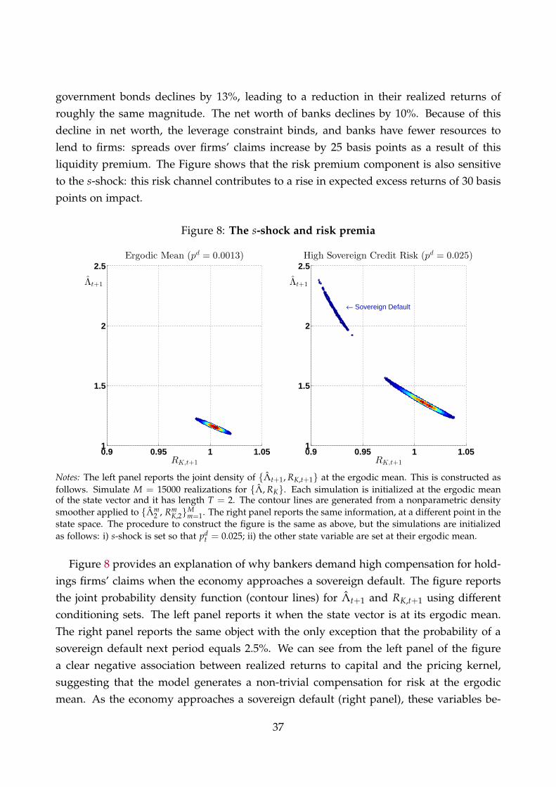
government bonds declines by 13%, leading to a reduction in their realized returns ofroughly the same magnitude. The net worth of banks declines by 10%. Because of thisdecline in net worth, the leverage constraint binds, and banks have fewer resources tolend to firms: spreads over firms’ claims increase by 25 basis points as a result of thisliquidity premium. The Figure shows that the risk premium component is also sensitiveto the s-shock: this risk channel contributes to a rise in expected excess returns of 30 basispoints on impact.

Figure 8: The s-shock and risk premia

Λt+1

RK,t+1

Ergodic Mean (pd = 0.0013)

0.9 0.95 1 1.051

1.5

2

2.5

Λt+1

RK,t+1

High Sovereign Credit Risk (pd = 0.025)

← Sovereign Default

0.9 0.95 1 1.051

1.5

2

2.5

Notes: The left panel reports the joint density of {Λt+1, RK,t+1} at the ergodic mean. This is constructed asfollows. Simulate M = 15000 realizations for {Λ, RK}. Each simulation is initialized at the ergodic meanof the state vector and it has length T = 2. The contour lines are generated from a nonparametric densitysmoother applied to {Λm

2 , RmK,2}M

m=1. The right panel reports the same information, at a different point in thestate space. The procedure to construct the figure is the same as above, but the simulations are initializedas follows: i) s-shock is set so that pd

t = 0.025; ii) the other state variable are set at their ergodic mean.

Figure 8 provides an explanation of why bankers demand high compensation for hold-ings firms’ claims when the economy approaches a sovereign default. The figure reportsthe joint probability density function (contour lines) for Λt+1 and RK,t+1 using differentconditioning sets. The left panel reports it when the state vector is at its ergodic mean.The right panel reports the same object with the only exception that the probability of asovereign default next period equals 2.5%. We can see from the left panel of the figurea clear negative association between realized returns to capital and the pricing kernel,suggesting that the model generates a non-trivial compensation for risk at the ergodicmean. As the economy approaches a sovereign default (right panel), these variables be-

37

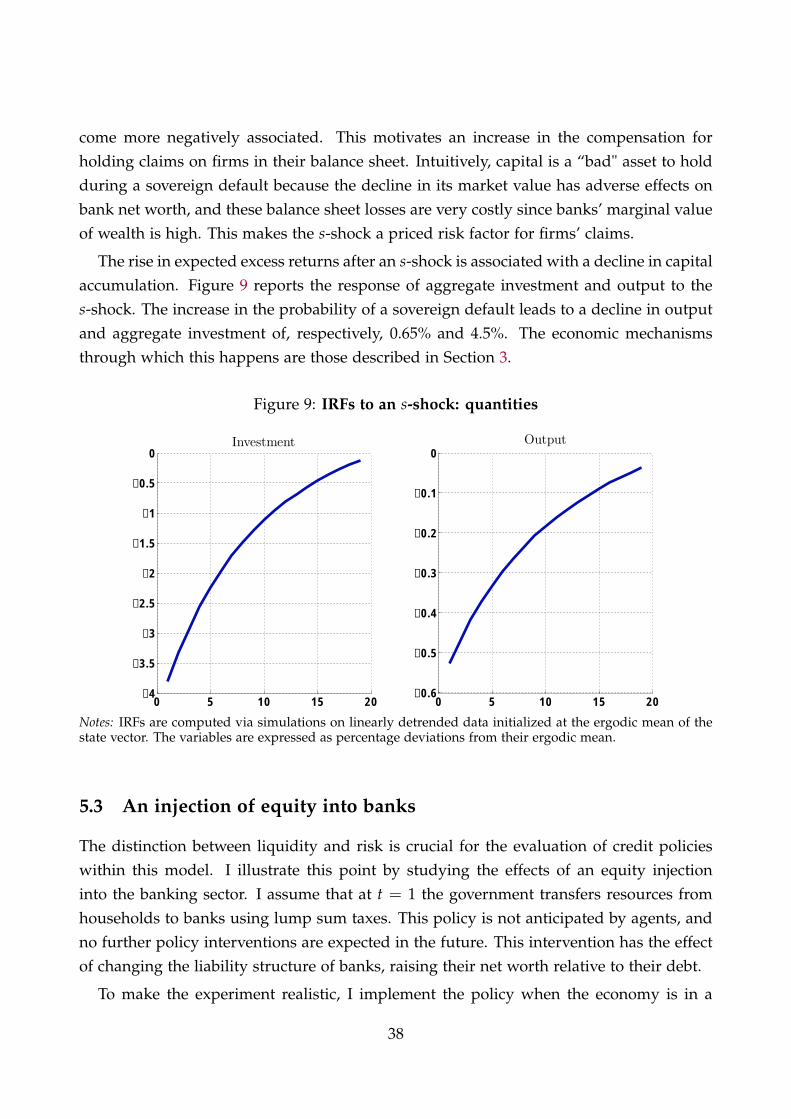
come more negatively associated. This motivates an increase in the compensation forholding claims on firms in their balance sheet. Intuitively, capital is a “bad" asset to holdduring a sovereign default because the decline in its market value has adverse effects onbank net worth, and these balance sheet losses are very costly since banks’ marginal valueof wealth is high. This makes the s-shock a priced risk factor for firms’ claims.

The rise in expected excess returns after an s-shock is associated with a decline in capitalaccumulation. Figure 9 reports the response of aggregate investment and output to thes-shock. The increase in the probability of a sovereign default leads to a decline in outputand aggregate investment of, respectively, 0.65% and 4.5%. The economic mechanismsthrough which this happens are those described in Section 3.

Figure 9: IRFs to an s-shock: quantities

0 5 10 15 20−4

−3.5

−3

−2.5

−2

−1.5

−1

−0.5

0Investment

0 5 10 15 20−0.6

−0.5

−0.4

−0.3

−0.2

−0.1

0Output

Notes: IRFs are computed via simulations on linearly detrended data initialized at the ergodic mean of thestate vector. The variables are expressed as percentage deviations from their ergodic mean.

5.3 An injection of equity into banks

The distinction between liquidity and risk is crucial for the evaluation of credit policieswithin this model. I illustrate this point by studying the effects of an equity injectioninto the banking sector. I assume that at t = 1 the government transfers resources fromhouseholds to banks using lump sum taxes. This policy is not anticipated by agents, andno further policy interventions are expected in the future. This intervention has the effectof changing the liability structure of banks, raising their net worth relative to their debt.

To make the experiment realistic, I implement the policy when the economy is in a

38

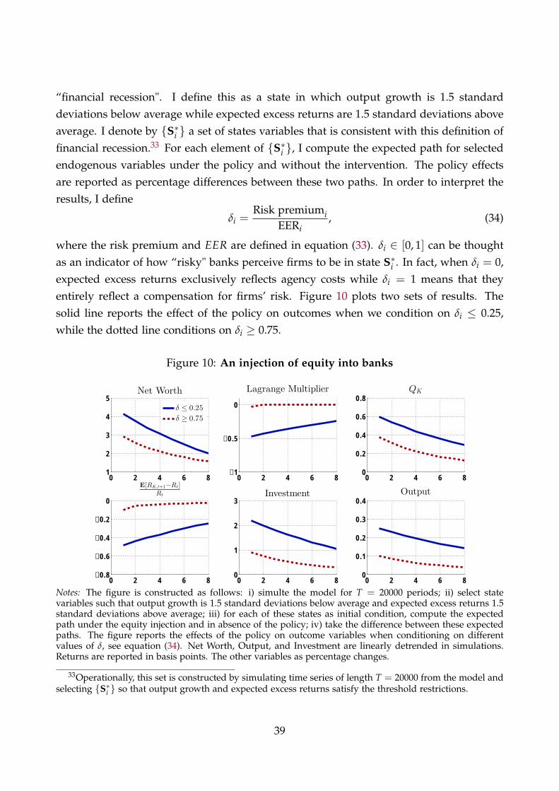
“financial recession". I define this as a state in which output growth is 1.5 standarddeviations below average while expected excess returns are 1.5 standard deviations aboveaverage. I denote by {S∗i } a set of states variables that is consistent with this definition offinancial recession.33 For each element of {S∗i }, I compute the expected path for selectedendogenous variables under the policy and without the intervention. The policy effectsare reported as percentage differences between these two paths. In order to interpret theresults, I define

δi =Risk premiumi

EERi, (34)

where the risk premium and EER are defined in equation (33). δi ∈ [0, 1] can be thoughtas an indicator of how “risky" banks perceive firms to be in state S∗i . In fact, when δi = 0,expected excess returns exclusively reflects agency costs while δi = 1 means that theyentirely reflect a compensation for firms’ risk. Figure 10 plots two sets of results. Thesolid line reports the effect of the policy on outcomes when we condition on δi ≤ 0.25,while the dotted line conditions on δi ≥ 0.75.

Figure 10: An injection of equity into banks

0 2 4 6 81

2

3

4

5Net Worth

δ ≤ 0.25

δ ≥ 0.75

0 2 4 6 8−1

−0.5

0

Lagrange Multiplier

0 2 4 6 80

0.2

0.4

0.6

0.8QK

0 2 4 6 8−0.8

−0.6

−0.4

−0.2

0

E[RK,t+1−Rt]Rt

0 2 4 6 80

1

2

3Investment

0 2 4 6 80

0.1

0.2

0.3

0.4Output

Notes: The figure is constructed as follows: i) simulte the model for T = 20000 periods; ii) select statevariables such that output growth is 1.5 standard deviations below average and expected excess returns 1.5standard deviations above average; iii) for each of these states as initial condition, compute the expectedpath under the equity injection and in absence of the policy; iv) take the difference between these expectedpaths. The figure reports the effects of the policy on outcome variables when conditioning on differentvalues of δ, see equation (34). Net Worth, Output, and Investment are linearly detrended in simulations.Returns are reported in basis points. The other variables as percentage changes.

33Operationally, this set is constructed by simulating time series of length T = 20000 from the model andselecting {S∗i } so that output growth and expected excess returns satisfy the threshold restrictions.

39

The figure shows that equity injections are particularly effective in stimulating realeconomic activity when agency costs are large (δ ≤ 0.25). The policy relaxes the constrainton bank leverage and leads to an increase in capital accumulation. The same policy hassubstantially weaker effects when implemented in regions of the state space where firms’risk is high (δ ≥ 0.75). The red dotted line reports this case. We can observe that theresponse of investment and output to the equity injection is 2.5 times smaller with respectto the previous case.

This state-dependence in the effects of equity injections has an intuitive explanation.Expected excess returns in the model can be high because of two reasons: liquiditypremia (low δ-regions) and risk premia (high δ-regions). Liquidity premia indicatesthat banks cannot undertake profitable investment opportunities because of funding con-straints. Therefore, policies that relax these constraints stimulate capital accumulationbecause they facilitate the flow of funds from households to firms. A large value of δ,instead, indicates that the observed high excess returns reflect mainly compensation forrisk: banks incentives to demand firms’ claims are less responsive to equity injectionsbecause these latter have only indirect effects on this risk.34

6 Measurement and Policy Evaluation

I now turn to the two main quantitative experiments of this paper. In Section 6.1, I mea-sure the effect of sovereign credit risk on the financing premia of firms and output, andI assess the contribution of the liquidity and risk channel. Section 6.2 proposes a quan-titative assessment of the Longer Term Refinancing Operations (LTROs) implemented bythe European Central Bank (ECB) in the first quarter of 2012. As we saw in the earliersection, credit market interventions are state and size dependent in this model due to itshighly nonlinear nature. Therefore, an integral part of the policy evaluation is to specifythe “initial conditions". I do so by estimating the state of the Italian economy in 2011:Q4using the particle filter. The evaluation of LTROs is conducted from an ex-ante perspective.

6.1 Sovereign risk, firms’ financing premia and output

What were the effects of sovereign credit risk on the financing premia of firms and onreal economic activity in Italy? What was the relative strength of liquidity and risk in

34By strengthening bank net worth, the policy provides a buffer when a sovereign default hits the econ-omy. This dampens the effects of a sovereign default on realized returns to capital and lowers risk premiaex-ante. The size of the equity injection is thus an important determinant of the policy effects.

40

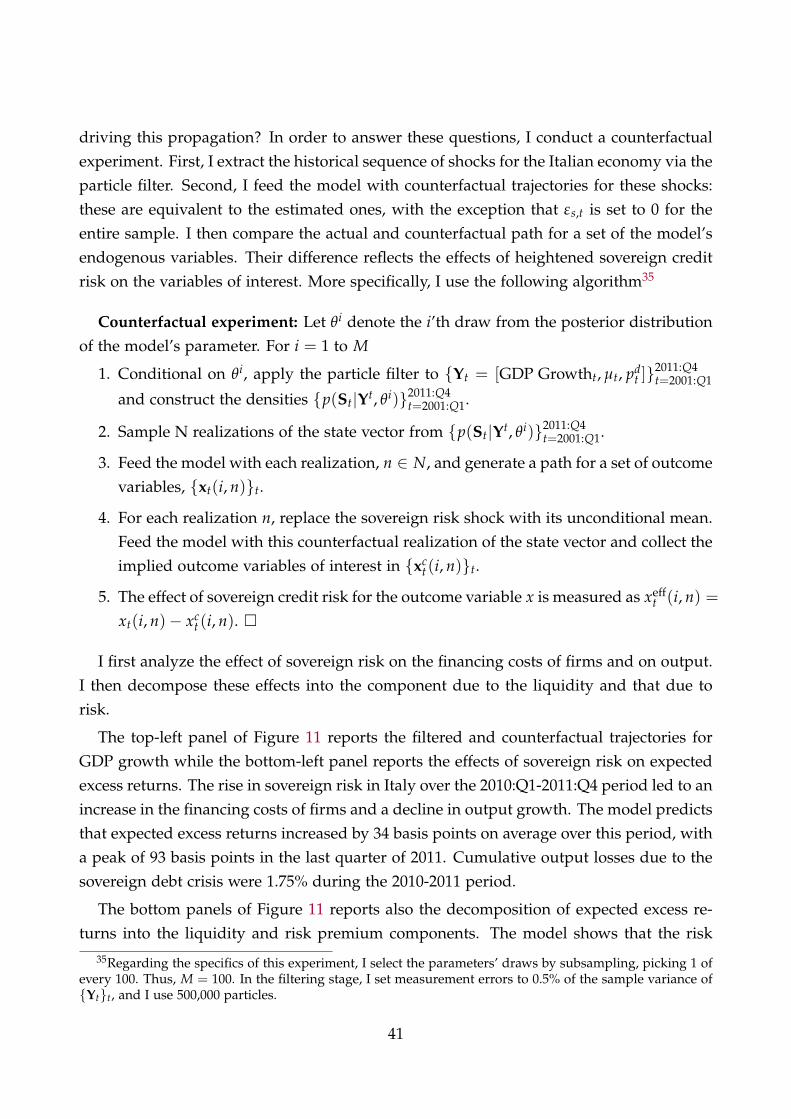
driving this propagation? In order to answer these questions, I conduct a counterfactualexperiment. First, I extract the historical sequence of shocks for the Italian economy via theparticle filter. Second, I feed the model with counterfactual trajectories for these shocks:these are equivalent to the estimated ones, with the exception that εs,t is set to 0 for theentire sample. I then compare the actual and counterfactual path for a set of the model’sendogenous variables. Their difference reflects the effects of heightened sovereign creditrisk on the variables of interest. More specifically, I use the following algorithm35

Counterfactual experiment: Let θi denote the i’th draw from the posterior distributionof the model’s parameter. For i = 1 to M

1. Conditional on θi, apply the particle filter to {Yt = [GDP Growtht, µt, pdt ]}

2011:Q4t=2001:Q1

and construct the densities {p(St|Yt, θi)}2011:Q4t=2001:Q1.

2. Sample N realizations of the state vector from {p(St|Yt, θi)}2011:Q4t=2001:Q1.

3. Feed the model with each realization, n ∈ N, and generate a path for a set of outcomevariables, {xt(i, n)}t.

4. For each realization n, replace the sovereign risk shock with its unconditional mean.Feed the model with this counterfactual realization of the state vector and collect theimplied outcome variables of interest in {xc

t(i, n)}t.

5. The effect of sovereign credit risk for the outcome variable x is measured as xefft (i, n) =

xt(i, n)− xct (i, n). �

I first analyze the effect of sovereign risk on the financing costs of firms and on output.I then decompose these effects into the component due to the liquidity and that due torisk.

The top-left panel of Figure 11 reports the filtered and counterfactual trajectories forGDP growth while the bottom-left panel reports the effects of sovereign risk on expectedexcess returns. The rise in sovereign risk in Italy over the 2010:Q1-2011:Q4 period led to anincrease in the financing costs of firms and a decline in output growth. The model predictsthat expected excess returns increased by 34 basis points on average over this period, witha peak of 93 basis points in the last quarter of 2011. Cumulative output losses due to thesovereign debt crisis were 1.75% during the 2010-2011 period.

The bottom panels of Figure 11 reports also the decomposition of expected excess re-turns into the liquidity and risk premium components. The model shows that the risk

35Regarding the specifics of this experiment, I select the parameters’ draws by subsampling, picking 1 ofevery 100. Thus, M = 100. In the filtering stage, I set measurement errors to 0.5% of the sample variance of{Yt}t, and I use 500,000 particles.

41

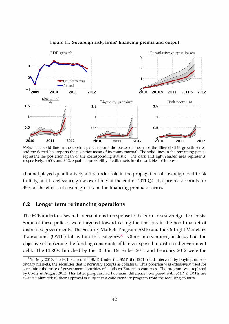
Figure 11: Sovereign risk, firms’ financing premia and output

2009 2010 2011 2012−4

−2

0

GDP growth

Cumulative output losses

2010 2010.5 2011 2011.5 20120

1

2

3

E[RK,t+1−Rt]Rt

2010 2011 20120

0.5

1

1.5Liquidity premium

2010 2011 20120

0.5

1

1.5Risk premium

2010 2011 20120

0.5

1

1.5

CounterfactualActual

Notes: The solid line in the top-left panel reports the posterior mean for the filtered GDP growth series,and the dotted line reports the posterior mean of its counterfactual. The solid lines in the remaining panelsrepresent the posterior mean of the corresponding statistic. The dark and light shaded area represents,respectively, a 60% and 90% equal tail probability credible sets for the variables of interest.

channel played quantitatively a first order role in the propagation of sovereign credit riskin Italy, and its relevance grew over time: at the end of 2011:Q4, risk premia accounts for45% of the effects of sovereign risk on the financing premia of firms.

6.2 Longer term refinancing operations

The ECB undertook several interventions in response to the euro-area sovereign debt crisis.Some of these policies were targeted toward easing the tensions in the bond market ofdistressed governments. The Security Markets Program (SMP) and the Outright MonetaryTransactions (OMTs) fall within this category.36 Other interventions, instead, had theobjective of loosening the funding constraints of banks exposed to distressed governmentdebt. The LTROs launched by the ECB in December 2011 and February 2012 were the

36In May 2010, the ECB started the SMP. Under the SMP, the ECB could intervene by buying, on sec-ondary markets, the securities that it normally accepts as collateral. This program was extensively used forsustaining the price of government securities of southern European countries. The program was replacedby OMTs in August 2012. This latter program had two main differences compared with SMP: i) OMTs areex-ante unlimited; ii) their approval is subject to a conditionality program from the requiring country.

42

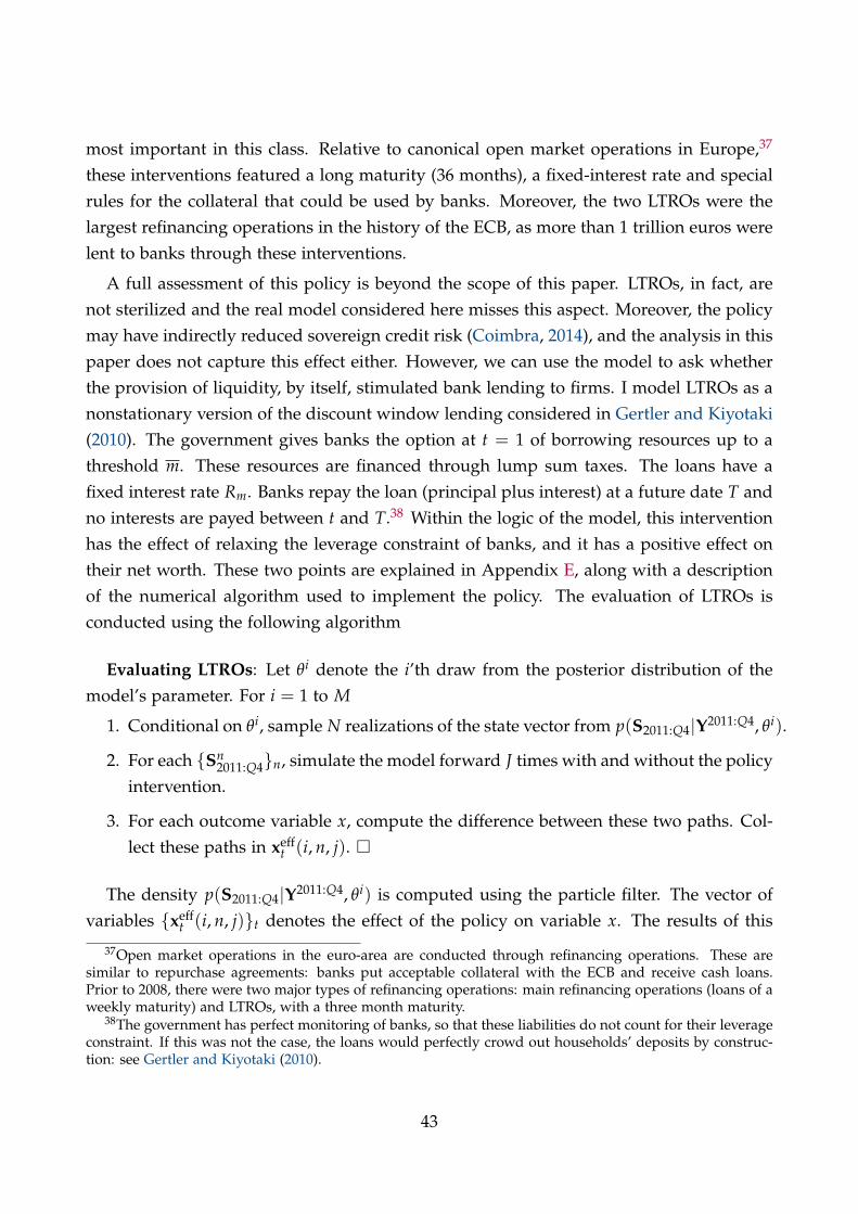
most important in this class. Relative to canonical open market operations in Europe,37

these interventions featured a long maturity (36 months), a fixed-interest rate and specialrules for the collateral that could be used by banks. Moreover, the two LTROs were thelargest refinancing operations in the history of the ECB, as more than 1 trillion euros werelent to banks through these interventions.

A full assessment of this policy is beyond the scope of this paper. LTROs, in fact, arenot sterilized and the real model considered here misses this aspect. Moreover, the policymay have indirectly reduced sovereign credit risk (Coimbra, 2014), and the analysis in thispaper does not capture this effect either. However, we can use the model to ask whetherthe provision of liquidity, by itself, stimulated bank lending to firms. I model LTROs as anonstationary version of the discount window lending considered in Gertler and Kiyotaki(2010). The government gives banks the option at t = 1 of borrowing resources up to athreshold m. These resources are financed through lump sum taxes. The loans have afixed interest rate Rm. Banks repay the loan (principal plus interest) at a future date T andno interests are payed between t and T.38 Within the logic of the model, this interventionhas the effect of relaxing the leverage constraint of banks, and it has a positive effect ontheir net worth. These two points are explained in Appendix E, along with a descriptionof the numerical algorithm used to implement the policy. The evaluation of LTROs isconducted using the following algorithm

Evaluating LTROs: Let θi denote the i’th draw from the posterior distribution of themodel’s parameter. For i = 1 to M

1. Conditional on θi, sample N realizations of the state vector from p(S2011:Q4|Y2011:Q4, θi).

2. For each {Sn2011:Q4}n, simulate the model forward J times with and without the policy

intervention.

3. For each outcome variable x, compute the difference between these two paths. Col-lect these paths in xeff

t (i, n, j). �

The density p(S2011:Q4|Y2011:Q4, θi) is computed using the particle filter. The vector ofvariables {xeff

t (i, n, j)}t denotes the effect of the policy on variable x. The results of this

37Open market operations in the euro-area are conducted through refinancing operations. These aresimilar to repurchase agreements: banks put acceptable collateral with the ECB and receive cash loans.Prior to 2008, there were two major types of refinancing operations: main refinancing operations (loans of aweekly maturity) and LTROs, with a three month maturity.

38The government has perfect monitoring of banks, so that these liabilities do not count for their leverageconstraint. If this was not the case, the loans would perfectly crowd out households’ deposits by construc-tion: see Gertler and Kiyotaki (2010).

43

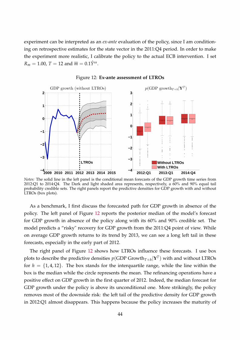
experiment can be interpreted as an ex-ante evaluation of the policy, since I am condition-ing on retrospective estimates for the state vector in the 2011:Q4 period. In order to makethe experiment more realistic, I calibrate the policy to the actual ECB intervention. I setRm = 1.00, T = 12 and m = 0.1Yss.

Figure 12: Ex-ante assessment of LTROs

GDP growth (without LTROs)

LTROs

2009 2010 2011 2012 2013 2014 2015−4

−3

−2

−1

0

1

2

2012:Q1 2013:Q1 2014:Q4−4

−3

−2

−1

0

1

2

3p(GDP growthT+h|YT )

Without LTROsWith LTROs

Notes: The solid line in the left panel is the conditional mean forecasts of the GDP growth time series from2012:Q1 to 2014:Q4. The Dark and light shaded area represents, respectively, a 60% and 90% equal tailprobability credible sets. The right panels report the predictive densities for GDP growth with and withoutLTROs (box plots).

As a benchmark, I first discuss the forecasted path for GDP growth in absence of thepolicy. The left panel of Figure 12 reports the posterior median of the model’s forecastfor GDP growth in absence of the policy along with its 60% and 90% credible set. Themodel predicts a “risky" recovery for GDP growth from the 2011:Q4 point of view. Whileon average GDP growth returns to its trend by 2013, we can see a long left tail in theseforecasts, especially in the early part of 2012.

The right panel of Figure 12 shows how LTROs influence these forecasts. I use boxplots to describe the predictive densities p(GDP GrowthT+h|YT) with and without LTROsfor h = {1, 4, 12}. The box stands for the interquartile range, while the line within thebox is the median while the circle represents the mean. The refinancing operations have apositive effect on GDP growth in the first quarter of 2012. Indeed, the median forecast forGDP growth under the policy is above its unconditional one. More strikingly, the policyremoves most of the downside risk: the left tail of the predictive density for GDP growthin 2012:Q1 almost disappears. This happens because the policy increases the maturity of

44

banks’ liabilities, and makes their balance sheet less sensitive to adverse shocks. As timegoes on and the repayment date approaches, though, GDP growth forecasts under LTROsbecome fairly similar to those in absence of this policy. At the scheduled repaymentdate, the predictive density for GDP growth is actually more left-skewed relative to thatobtained in absence of the policy.

In order to better understand the effects of LTROs, I report in Table 5 posterior statisticsof its effects on the level of output, expected excess returns and their decomposition intoliquidity and risk premia. On impact, the refinancing operations lower expected excessreturns and increases the level of output. The reduction in the firms’ financing costs ismainly due to lower liquidity premia: the policy, in fact, loosens the funding constraintsof intermediaries. However, the risk premium component is barely affected. Notice thatthese initial positive effects are reversed over time. One year after its implementation,the model places some probability of LTROs increasing the financing costs of firms andreducing the level of output. This result is driven by the behavior of the model at therepayment stage. At that stage, banks need to repay the loans they took on, and adversenet worth shocks at that date are very costly for them. The anticipation of the repaymentstage makes banks more cautious ex-ante and leads them to demand higher compensationfor bearing risk. This counteracts the initial positive effects of the policy. On average,LTROs lead to a reduction of private sector spreads of 20 basis points and an increase inthe level of output of 0.20%. Thus, these operations seems quite ineffective in stimulatingbank lending to firms once we condition on empirically reasonable regions of the statespace in 2011:Q4.

This result does not imply that refinancing operations are a bad policy instrument.Rather, that their effects depend on the economic environment in which they are imple-mented. In order to see this last point, I implement LTROs in a different region of the statespace, drawn from the density p(S2008:Q3|Y2008:Q3, θi). In contrast to the 2011:Q4 period,the model interprets the financial distress of 2008:Q3 as driven mainly by banks liquidityproblems. Results are reported in the bottom panel of Table 5. Two main differences standout compared to the previous analysis. First, the policy has a substantially stronger effecton the financing premia of firms and on output when implemented in 2008:Q3. Expectedexcess returns decline by 78 basis points on impact, while the level of output increases by0.45%. Second, the downside risk at the repayment stage is substantially reduced. Thiscan be seen by comparing the credible sets for output at the repayment stage for the twocases.

The reasons underlying this state dependence are related to the discussion of equityinjections in Section 5.3. In 2008:Q3, agency costs are estimated to be high. This indicates

45

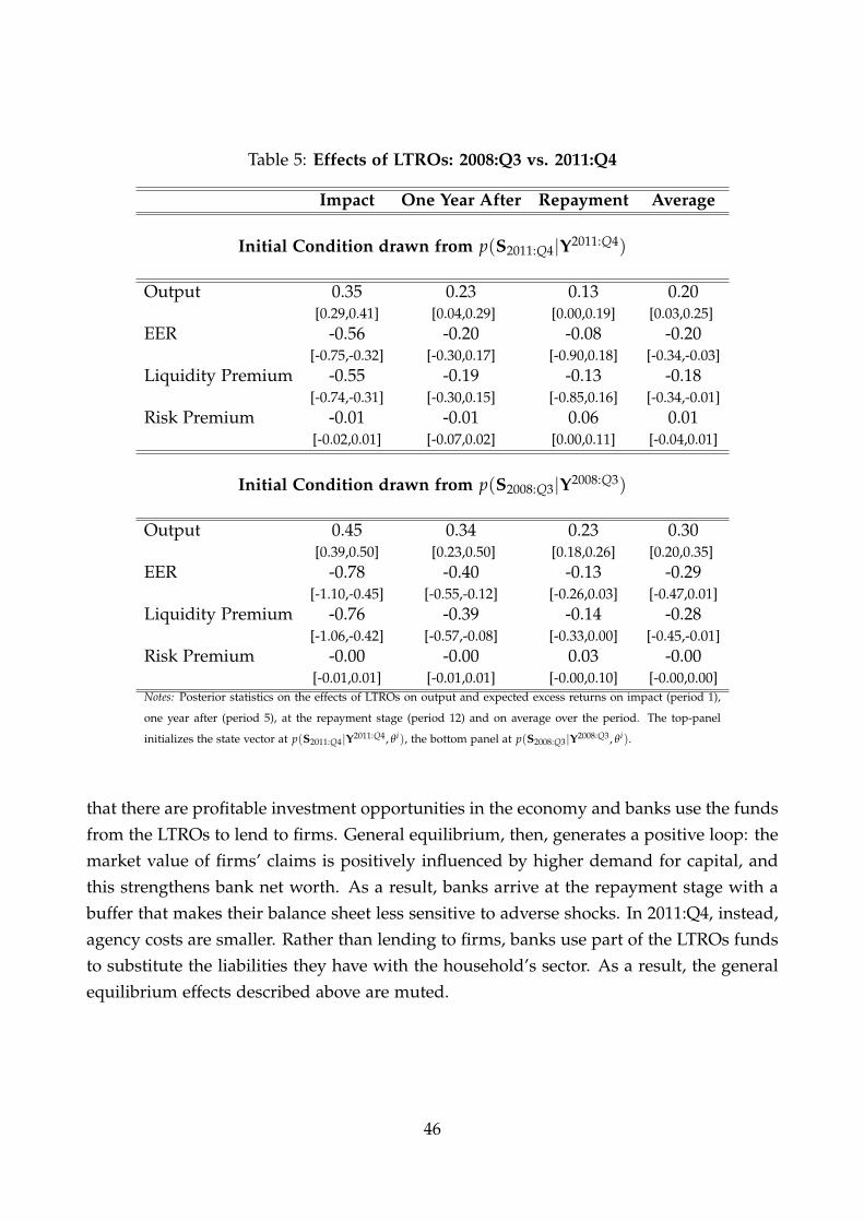
Table 5: Effects of LTROs: 2008:Q3 vs. 2011:Q4

Impact One Year After Repayment Average

Initial Condition drawn from p(S2011:Q4|Y2011:Q4)

Output 0.35 0.23 0.13 0.20[0.29,0.41] [0.04,0.29] [0.00,0.19] [0.03,0.25]

EER -0.56 -0.20 -0.08 -0.20[-0.75,-0.32] [-0.30,0.17] [-0.90,0.18] [-0.34,-0.03]

Liquidity Premium -0.55 -0.19 -0.13 -0.18[-0.74,-0.31] [-0.30,0.15] [-0.85,0.16] [-0.34,-0.01]

Risk Premium -0.01 -0.01 0.06 0.01[-0.02,0.01] [-0.07,0.02] [0.00,0.11] [-0.04,0.01]

Initial Condition drawn from p(S2008:Q3|Y2008:Q3)

Output 0.45 0.34 0.23 0.30[0.39,0.50] [0.23,0.50] [0.18,0.26] [0.20,0.35]

EER -0.78 -0.40 -0.13 -0.29[-1.10,-0.45] [-0.55,-0.12] [-0.26,0.03] [-0.47,0.01]

Liquidity Premium -0.76 -0.39 -0.14 -0.28[-1.06,-0.42] [-0.57,-0.08] [-0.33,0.00] [-0.45,-0.01]

Risk Premium -0.00 -0.00 0.03 -0.00[-0.01,0.01] [-0.01,0.01] [-0.00,0.10] [-0.00,0.00]

Notes: Posterior statistics on the effects of LTROs on output and expected excess returns on impact (period 1),

one year after (period 5), at the repayment stage (period 12) and on average over the period. The top-panel

initializes the state vector at p(S2011:Q4|Y2011:Q4, θi), the bottom panel at p(S2008:Q3|Y2008:Q3, θi).

that there are profitable investment opportunities in the economy and banks use the fundsfrom the LTROs to lend to firms. General equilibrium, then, generates a positive loop: themarket value of firms’ claims is positively influenced by higher demand for capital, andthis strengthens bank net worth. As a result, banks arrive at the repayment stage with abuffer that makes their balance sheet less sensitive to adverse shocks. In 2011:Q4, instead,agency costs are smaller. Rather than lending to firms, banks use part of the LTROs fundsto substitute the liabilities they have with the household’s sector. As a result, the generalequilibrium effects described above are muted.

46

7 Conclusion

In this paper I have conducted a quantitative analysis of the transmission of sovereigncredit risk to the borrowing costs of firms and real economic activity. I studied a modelwhere banks are exposed to risky government debt and they are the main source of fi-nance for firms. News about a future sovereign default hampers financial intermediationbecause of two mechanisms. First, by reducing the market value of government securities,higher sovereign credit risk reduces the net worth of banks and hampers their fundingability: their increased financing costs pass-through into the borrowing rates of firms (liq-uidity channel). Second, an increase in the probability of a future sovereign default raisesthe risks associated with lending to firms: if the default occurs in the future, in fact, claimson the productive sector will pay out little and banks will have to absorb these losses. Ireferred to this second mechanism as the risk channel. The structural estimation of themodel on Italian data suggests that the sovereign debt crisis significantly increased thefinancing premia of firms, with the risk channel explaining up to 45% of these effects.Moreover, the rise in the probability of a sovereign default had severe adverse conse-quences for the Italian economy: cumulative output losses were 1.75% at the end of 2011.In counterfactual experiments, I use the estimated model to evaluate the policy responseadopted by the ECB, with particular emphasis on the LTROs of the first quarter of 2012.The model estimates that this intervention, by itself, has limited effects on bank lendingto firms. This happens because firms were perceived to be risky at the time these policieswere implemented, and banks preferred to use the LTROs funds to cheaply refinance theirliabilities. More generally, the analysis shows that the stabilization properties of these in-terventions are state dependent in the model, and their aggregate effects depend on therelative strength of liquidity and risk.

There are a number of dimensions in which the model could be extended. First, itwould be interesting to introduce an optimizing government, and study its optimal defaultpolicy. Beside its importance for answering normative questions, understanding how thegovernment’s choice to default is affected by the wealth of the financial sector would allowfor a more complete evaluation of the policy responses adopted by the ECB. A secondextension would be that of considering an open economy. I believe that this dimensionwill help the empirical identification of the mechanisms discussed in this paper, since theyare likely to generate differential implications for international capital flows. While bothof these issues are challenging, and require a substantial departure from this framework,they represent exciting opportunities for future work.

Abstracting from the current application, recent research advocates the use of indica-

47

tors of credit spreads as observables when estimating quantitative models with financialintermediation. This paper adds to that by underscoring the importance of measuringthe sources driving the movements in these indicators of financial stress. Understandingwhether firms’ financing premia during crises are high because of “frictions" in financialmarkets or because of fair compensation for increased risk is a key information for policymakers. Incorporating the nonlinearities emphasized in this paper in larger scale modelsused for policy evaluation is technically challenging. Moreover, given the policy relevanceof these nonlinearities, there is a need for developing tools for their empirical validationin the data. I plan to address these issues in future work.

48

References

Acharya, Viral V., Itamar Dreschsler, and Philipp Schnabl, “A Phyrrhic Victory? BankBailouts and Sovereign Credit Risk,” Journal of Finance, 2013. forthcoming.

Adrian, Tobias, Erkko Etula, and Tyler Muir, “Financial Intermediaries and the Cross-Section of Asset Returns,” Journal of Finance, 2013. forthcoming.

Aguiar, Mark, Miguel Amador, and Gita Gopinath, “Investment Cycles and SovereignDebt Overhang,” Review of Economic Studies, 2009, 76, 1–31.

Albertazzi, Ugo, Tiziano Ropele, Gabriele Sene, and Federico M. Signoretti, “The Im-pact of the Sovereign Debt Crises on the Activity of Italian Banks,” 2012. Banca d’ItaliaOccasional Papers, No. 133.

Arellano, Cristina, “Default Risk and Income Fluctuations in Emerging Economies,” TheAmerican Economic Review, 2008, 98 (3), 690–712.

and Yan Bai, “Linkages across Sovereign Debt Markets,” 2013. Research DepartmentStaff Report 491, Federal Reserve Bank of Minneapolis.

, , and Patrick J. Kehoe, “Financial Frictions and Fluctuations in Volatility,” 2012.Federal Reserve Bank of Minneapolis, Staff Report No. 466.

Aruoba, Boragan S. and Frank Schorfheide, “Macroeconomic Dynamics Near the ZLB:A Tale of Two Equilibria,” 2013. Manuscript, University of Pennsylvania.

, Luigi Bocola, and Frank Schorfheide, “Assessing DSGE Model Nonlinearities,” 2013.Manuscript, University of Pennsylvania.

Ayiagari, Rao S. and Mark Gertler, “Overreaction of Asset Prices in General Equilib-rium,” Review of Economic Dynamics, 1999, 2, 3–35.

Bahaj, Saleem, “Systemic Sovereign Risk: Macroeconomic Implications in the Euro Area,”2013. Manuscript, University of Cambridge.

Barro, Robert, “Rare Disasters and Asset Markets in the Twentieth Century,” QuarterlyJournal of Economics, 2006, 121 (3), 823–866.

and Robert G. King, “Time-Separable Preferences and Intertemporal Substitution Mod-els of Business Cycles,” Quarterly Journal of Economics, 1984, 99 (4), 817–839.

Bartiloro, Laura, Riccardo Bonci, Massimo Coletta, Riccardo De Bonis, Valter Di Giac-into, and Gabriele Semeraro, I Conti Finanziari dell’Italia, Banca D’Italia, 2003.

Bedendo, Mascia and Paolo Colla, “Sovereign and Corporate Credit Risk: Spillover Ef-fects in the Eurozone,” 2013. Manuscript, Universita’ Bocconi.

49

Bi, Huixin, “Sovereign Default Risk Premia, Fiscal Limits and Fiscal Policy,” EuropeanEconomic Review, 2012, 56, 389–410.

and Nora Traum, “Estimating Sovereign Default Risk,” The American Economic Review,2012, 102, 161–166.

Bianchi, Javier and Enrique G. Mendoza, “Overborroving, Financial Crises and “Macro-prudential Policies",” 2012. Manuscript, University of Pennsylvania.

and Saki Bigio, “Banks, Liquidity Management and Monetary Policy,” 2013. Prelimi-nary Manuscript, Columbia Business School.

Bigio, Saki, “Liquidity Shocks and the Business Cycles: What next?,” 2012. Manuscript,Columbia Business School.

Bloom, Nicholas, “The Impact of Uncertainty Shocks,” Econometrica, 2009, 77 (3), 623–685.

Bofondi, Marcello, Luisa Carpinelli, and Enrico Sette, “Credit supply during a sovereigndebt crisis,” 2013. Temi di Discussione N. 909, Bank of Italy.

Bohn, Henning, “The Sustainability of Budget Deficits in a Stochastic Economy,” Journalof Money, Credit and Banking, 1995, 27, 257–271.

Borensztein, Eduardo and Ugo Panizza, “The Costs of Sovereign Default,” IMF StaffPapers, 2009, 9 (56), 683–741.

, Kevin Cowan, and Patricio Valenzuela, “Sovreign Ceiling “Lite"? The Impact ofSovereign Ratings on Corporate Ratings in Emerging Market Economies,” 2006. IMFWorking Paper No. 75.

Broner, Fernando, Aitor Erce, Alberto Martin, and Jaume Ventura, “Sovereign debt mar-kets in turbolent times: Creditor discrimination and crowding-out effects,” Journal ofMonetary Economics, 2014, 61, 114–142.

Brunnermeier, Markus and Yuliy Sannikov, “A Macroeconomic Model with a FinancialSector,” The American Economic Review, 2013. forthcoming.

, Thomas M. Eisenbach, and Yuliy Sannikov, “Macroeconomics with Financial Fric-tions: A Survey,” 2013. Advances in Economic and Econometrics, Tenth World Congressof the Econometric Society.

Canzoneri, Matthew B., Robert E. Cumby, and Behazad T. Diba, “Is the Price LevelDetermined by the Needs of Fiscal Solvency?,” The American Economic Review, 2001, 91,1221–1238.

Cavallo, Eduardo and Patricio Valenzuela, “The Determinants of Corporate Risk inEmerging Markets: An Option-Adjusted Spread Analysis,” 2007. IMF Working PaperNo. 228.

50

CGFS, “The Impact of Sovereign Credit Risk on Bank Funding Conditions,” CGFS Papers,BIS, 2011, 44.

Chatterjee, Satyajit and Burcu Eyigungor, “Maturity, Indebtedness and Default Risk,”The American Economic Review, 2013, 6, 2674–2699.

Christiano, Larry J. and Jonas D. M. Fisher, “Algorithms for Solving Dynamic Modelswith Occasionally Binding Constraints,” Journal of Economic Dynamics and Control, 2000,24 (8), 1179–1232.

, Roberto Motto, and Massimo Rostagno, “Risk Shocks,” 2013. NBER Working Paper,18682.

Coimbra, Nuno, “Sovereigns at Risk. A Dynamic Model of Sovereign Debt and BankingLeverage,” 2014. Manuscript, London Business School.

Conesa, Juan Carlos and Timothy J. Kehoe, “Gambling for Redemption and Self-Fulfilling Crises,” 2012. Research Department Staff Report 465, Federal Reserve Bank ofMinneapolis.

Corsetti, Giancarlo, Keith Kuester, Andre Meier, and Gernot J. Muller, “Sovereign Risk,Fiscal Policy and Macroeconomic Stability,” The Economic Journal, 2013, 123, 99–132.

Curdia, Vasco and Michael Woodford, “Credit Spreads and Monetary Policy,” Journal ofMoney, Credit and Banking, 2010, 42 (S1), 3–35.

Del Negro, Marco and Frank Schorfheide, “Bayesian Macroeconometrics,” in J. Geweke,G. Koop, and H. van Dijk, eds., The Oxford Handbook of Bayesian Econometrics, OxfordUniversity Press, 2011.

, Gauti Eggerston, Andrea Ferrero, and Nobuhiro Kiyotaki, “The Great Escape? AQuantitative Evaluation of the Fed’s Liquidity Facilities,” 2012. Federal Reserve Bank ofNew York Staff Report N. 520.

Di Cesare, Antonio, Giuseppe Grande, Michele Manna, and Marco Taboga, “Recentestimates of sovereign risk premia for euro-area countries,” 2013. Manuscript, Bank ofItaly.

Dovis, Alessandro, “Efficient Sovereign Default,” 2013. Manuscript, Penn State University.

Durbin, Erik and David T. Ng, “The Sovereign Ceiling and Emerging Market CorporateBond Spreads,” Journal of International Money and Finance, 2005, 24, 631–649.

Eaton, Jonathan and Mark Gersovitz, “Debt with potential repudiation: Theoretical andempirical analysis,” Review of Economic Studies, 1981, 48, 289–309.

ECB, “The Euro Area Bank Lending Survey,” 2011. October.

51

Fernández-Villaverde, Jesús and Juan Rubio-Ramírez, “Estimating MacroeconomicModels: A Likelihood Approach,” Review of Economic Studies, 2007, 74, 1059–1087.

, Gray Gordon, Pablo Guerrón-Quintana, and Juan Rubio-Ramírez, “Nonlinear Ad-ventures at the Zero Lower Bound,” 2012. Manuscript, University of Pennsylvania.

, Pablo Guerrón-Quintana, Juan Rubio-Ramírez, and Martin Uribe, “Risk Matters:The Real Effects of Volatility Shocks,” The American Economic Review, 2011, 101, 2530–2561.

Gennaioli, Nicola, Alberto Martin, and Stefano Rossi, “Banks, Government Bonds, andDefault: What do the data Say,” 2013. Manuscript, London School of Economics.

, , and , “Sovereign Default, Domestic Banks and Financial Institutions,” Journal ofFinance, 2013. forthcoming.

Gertler, Mark and Nobuhiro Kiyotaki, “Financial Intermediation and Credit Policy inBusiness Cycle Analysis,” in B. Friedman and M. Woodford, eds., Handbook of MonetaryEconomics, 3A, Elsevier, 2010.

and Peter Karadi, “A Model of Unconventional Monetary Policy,” Journal of MonetaryEconomics, 2011, 58, 17–34.

and , “QE 1 vs. 2 vs. 3...: A Framework for Analyzing Large-Scale Asset Purchasesas a Monetary Policy Tool,” International Journal of Central Banking, 2013, 9 (S1), 5–53.

Geweke, John, Contemporary Bayesian Econometrics and Statistics, Wiley, 2005.

Gilchrist, Simon, Jae W. Sim, and Egon Zakrajsek, “Uncertainty, Financial Frictions andIrreversible Investment,” 2013. Manuscript, Boston University.

Giordano, Raffaella, Marcello Pericoli, and Pietro Tommasino, “Pure or Wake-up-CallContagion? Another Look at the EMU Sovereign Debt Crisis,” International Finance,2013, 16 (2), 131–160.

Gourio, Francois, “Disaster Risk and Business Cycles,” The American Economic Review,2012, 102, 2734–2766.

Gust, Christopher, David Lopez-Salido, and Matthew E. Smith, “The Empirical Impli-cations of the Interest-Rate Lower Bound,” 2013. Manuscript, Federal Reserve Board.

Hall, Robert, “The High Sensitivity of Economic Activity to Financial Frictions,” The Eco-nomic Journal, 2011, 121 (5), 351–378.

He, Zhiguo and Arvind Krishnamurthy, “A Macroeconomic Framework for QuantifyingSystemic Risk,” 2012. Manuscript, Kellog Business School.

and , “Intermediary Asset Pricing,” The American Economic Review, 2012, 20, 1–42.

52

Heer, Burkhard and Alfred Maussner, Dynamic General Equilibrium Modeling: Computa-tional Methods and Applications, Springer, 2009.

Judd, Kenneth L., “Projection Methods for Solving Aggregate Growth Models,” Journal ofEconomic Theory, 1992, 58, 410–452.

, Lilia Maliar, and Serguei Maliar, “How to Solve Dynamic Stochastic Models Com-puting Expectations Just Once,” 2011. NBER working paper, No. 17418.

Klein, Christian and Christoph Stellner, “Does Sovereign Risk Matter? New Evidencefrom Eurozone Corporate Bond Ratings and Zero-Volatility Spreads,” Review of FinancialEconomics, 2013. forthcoming.

Krueger, Dirk and Felix Kubler, “Computing Equilibrium in OLG Models with StochasticProduction,” Journal of Economic Dynamics and Control, 2003, 28, 1411–1436.

, , and Benjamin A. Malin, “Solving the Multi-Country Real Business Cycle Modelusing a Smolyak-Collocation Method,” Journal of Economic Dynamics and Control, 2010,35, 289–309.

Kumhof, Michael and Evan Tanner, “Government Debt: A Key Role in Financial Inter-mediation,” 2005. IMF Working Paper.

Levy-Yeyati, Eduardo and Ugo Panizza, “The Elusive Costs of Sovereign Defaults,” Jour-nal of Development Economic, 2011, 94 (1), 95–105.

Lorenzoni, Guido and Ivan Werning, “Slow Moving Debt Crisis,” 2013. Manuscript,Northwestern University.

Mallucci, Enrico, “Sovereign Defaults, Wholesale Funding and Banking Crises,” 2013.Manuscript, London School of Economics.

Mendoza, Enrique G., “Sudden Stops, Financial Crises and Leverage,” The American Eco-nomic Review, 2010, 100, 1941–1966.

and Vivian Z. Yue, “A General Equilibrium Model of Sovereign Default and BusinessCycles,” Quarterly Journal of Economics, 2012, 127, 889–946.

Neri, Stefano, “The Impact of the Sovereign Debt Crises on Bank Lending Rates in theEuro Area,” 2013. Quaderni di Economia e Finanza, Bank of Italy.

and Tiziano Ropele, “The Macroeconomic Effects of the Sovereign Debt Crises in theEuro Area,” 2013. Manuscript, Bank of Italy.

Neumeyer, Pablo A. and Fabrizio Perri, “Business Cycles in Emerging Economies: theRole of Interest Rates,” Journal of Monetary Economics, 2005, 52 (2), 345–380.

Pan, Jun and Kenneth J. Singleton, “Default and Recovery Implicit in the Term Structureof Sovereign CDS Spreads,” Journal of Finance, 2008, 63 (5), 2345–2384.

53

Pitt, Michael K. and Neil Shephard, “Filtering via Simulation: Auxiliary Particle Filters,”Journal of the American Statistical Association, 1999, 94, 590–599.

Reinhart, Carmen M. and Kenneth S. Rogoff, “From Financial Crash to Debt Crisis,” TheAmerican Economic Review, 2011, 101 (5), 1676–1706.

Rietz, Thomas A., “The Equity Premium: a Solution,” Journal of Monetary Economics, 1988,22 (1), 117–131.

Rios-Rull, Jose-Victor, Frank Schorfheide, Cristina Fuentes-Albero, Maxym Kryshko,and Raul Santaeulalia-Llopis, “Methods versus Substance: Measuring the Effects ofTechnology Shocks,” Journal of Monetary Economics, 2012, 59 (8), 826–846.

Schorfheide, Frank, “Loss Function-Based Evaluation of DSGE Models,” Journal of AppliedEconometrics, 2000, 15, 645–670.

Sosa Padilla, Cesar, “Sovereign Defaults and Banking Crises,” 2013. Manuscript, McGillUniversity.

Uribe, Martin, “A Fiscal Theory of Sovereign Risk,” Journal of Monetary Economics, 2006,53, 1857–1875.

and Vivian Z. Yue, “Country Spreads and Emerging Countries: Who Drives Whom?,”Journal of International Economics, 2006, 69 (1), 6–36.

Zettelmeyer, Jeromin, Christoph Trebesh, and Mitu Gulati, “The Greek Debt Restructur-ing: An Autopsy,” 2013. CESifo Working Paper, No. 4333.

Zoli, Edda, “Italian Sovereign Spreads: Their Determinants and Pass-through to BankFunding Costs and Lending Conditions,” 2013. IMF working paper.

54

Online Appendix: The Pass-Through of Sovereign RiskLuigi Bocola

A Derivation of Results 1

Combine equation (3) and (4) to eliminate the demand for households’ savings from thedecision problem of the banker. The decision problem is then

vb(n; S) = maxaB,aK

ES{

Λ(S′, S)[(1− ψ)n′ + ψvb(n′; S′)

]},

n′ = ∑j={B,K}

[Rj(S′, S)− R(S)]Qj(S)aj + R(S)n,

λ

∑j={B,K}

Qj(S)aj

≤ vb(n; S),

S′ = Γ(S).

Guess that the value function is v(n, S) = α(S)n. Necessary and sufficient conditionsfor an optimum are

ES{

Λ(S′, S)[(1− ψ) + ψα(S′)

][Rj(S′, S)− R(S)]

}= λµ(S) j = {B, K}, (A.1)

µ(S)

α(S)n− λ ∑j={B,K}

Qj(S)aj

= 0. (A.2)

Substituting the guess in the dynamic program, and using the law of motion for n′, weobtain

vb(n, S) = maxaB,aK

∑j={B,K}

ES{

Λ(S′, S)[(1− ψ) + ψα(S′)][Rj(S′)− R(S)]}

Qj(S)aj

+

ES{

Λ(S′, S)[(1− ψ) + ψα(S′)]}

R(S)n.

Note that the first term on the right hand side of the above equation equals µ(S)α(S)n.Indeed, when the leverage constraint does not bind (µ(S) = 0), expected discountedreturns on assets held by bankers equal the discounted risk free rate by equation (A.1).This implies that the term equals 0. When the constraint binds (µ(S) > 0), instead, this

A-1

term can be written asλµ(S) ∑

j={B,K}Qj(S)aj.

Using the condition in (A.2), we can express λµ(S)∑j={b,k} Qj(S)aj as µ(S)α(S)n. Thus,the value function under the guess takes the following form:

α(S)n = µ(S)α(S)n + ES{

Λ(S′, S)[(1− ψ) + ψα(S′)]}

R(S)n.

Solving for α(S), we obtain

α(S) =ES{Λ(S′, S)[(1− ψ) + ψα(S′)]}R(S)

1− µ(S).

The guess is verified if µ(S) < 1. From equation (A.2) we obtain:

µ(S) = max

1− ES{Λ(S′, S)[(1− ψ) + ψα(S)]}R(S)nλ(

∑j={B,K} Qj(S)aj

) , 0

< 1.

Finally, notice that financial leverage equals across bankers whenever µ(S) > 0. Thisimplies that n

λ ∑j={B,K} Qjajis equal to N

λ[∑j={B,K} Qj Aj]when the constraint binds.

A-2

B Numerical Solution

B.1 Equilibrium conditions

The states of the model are S = [K, B, P, ∆z, g, s, d]. The controls {C(S), R(S), α(S), QB(S)}solve the residual equations

ES

[β

C(S)C(S′)

e−∆z′R(S)]− 1 = 0, (A.3)

ES

βC(S)C(S′)

e−∆z′ [(1− ψ) + ψα(S′)]

(1− δ)QK(S′) + α Y(S′)K′(S) e∆z′

QK(S)

− λµ(S) = 0, (A.4)

ES

{β

C(S)C(S′)

e−∆z′ [(1− ψ) + ψα(S′)][1− d′D

] [π + (1− π) [ι + Qb(S′)]QB(S)

]}− λµ(S) = 0, (A.5)

α(S)−(1− ψ) + ψR(S)ES

[β

C(S)C(S′) e−∆z′α(S′)

]1− µ(S)

= 0, (A.6)

where QK(S) is the market value of the capital stock and the multiplier µ(S) is given by

µ(S) = max

1−

ES

{β

C(S)C(S′) e−∆z′ [(1− ψ) + ψα(S′)]R(S)

}N(S)

λ[QK(S)K′(S) + QB(S)B(S)]

, 0

. (A.7)

The endogenous state variables [K, B, P] evolve as follows

K′(S) ={(1− δ)K + Φ

[e∆z(

Y(S)(1− g)− C(S)K

)]K}

e−∆z, (A.8)

B′(S) =[1− dD]{π + (1− π)[ι + QB(S)]}Be−∆z + Y(S)

[g−

(t∗ + γτ

BY(S)

)]QB(S)

, (A.9)

P′(S) = R(S)[Qk(S)K′(S) + Qb(S)B′(S)− N(S)]. (A.10)

The state variable P measures the detrended cum interest deposits that bankers pay tohouseholds at the beginning of the period and it is sufficient to keep track of the evolu-tion of aggregate bankers’ net worth. Indeed, the aggregate net worth of banks can be

A-3

expressed as

N(S) = ψ

{[QK(S) + α

Y(S)K

e∆z]

K + [1− dD] [π + (1− π) [ι + QB(S)]] B− P}(A.11)

+ω[QK(S)K + QB(S)B].

Using the intratemporal Euler equation of the household, we can express detrended out-put as

Y(S) =[

χ−1 (Ke−∆z)α

C(S)

] 1−αα+ν−1

(Ke−∆z)α. (A.12)

The exogenous state variables [∆z, log(g), s] evolve as follows

∆z′ = (1− ρz)γ + ρz∆z + σzε′z, (A.13)

log(g′) = (1− ρg)g∗ + ρg log(g) + σgε′g, (A.14)

s′ = (1− ρs)s∗ + ρss + σsε′s, (A.15)

while d follows

d′ =

1 with probability exp{s}1+exp{s}

0 with probability 1− exp{s}1+exp{s} .

(A.16)

It will be convenient to express detrended state and control variables as log-deviationsfrom their deterministic steady state. I denote this transformation for variable x as x.

B.2 Algorithm for numerical solution

I approximate the control variables of the model using piece-wise smooth functions,parametrized by γ = {γx

d=0, γxd=1}x={C,α,Qb,R}. The law of motion for a control variable x

is described byx(d, S) = (1− d)γx

d=0′T(S) + dγx

d=1′T(S), (A.17)

where S = [K, P, B, ∆z, g, s] and T(.) is a vector collecting Chebyshev’s polynomials.39 De-fineR(γc, {d, S}) to be a 4× 1 vector collecting the left hand side of the residual equations(A.3)-(A.6) for the candidate solution γc evaluated at {d, S}. The numerical solution of themodel consists in choosing γc so that R(γc, {d, S}) = 0 for a set of collocation points{d, Si} ∈ {0, 1} × S .

39The shocks are expressed as deviation from their mean.

A-4

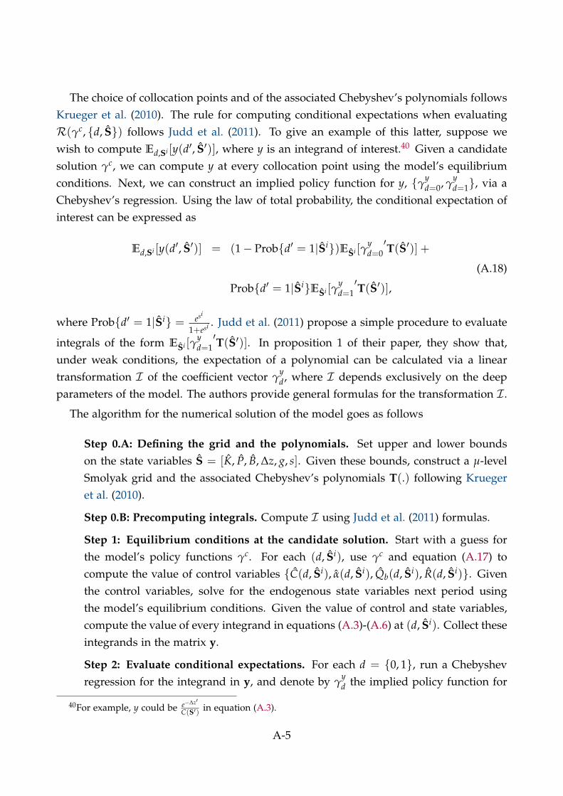
The choice of collocation points and of the associated Chebyshev’s polynomials followsKrueger et al. (2010). The rule for computing conditional expectations when evaluatingR(γc, {d, S}) follows Judd et al. (2011). To give an example of this latter, suppose wewish to compute Ed,Si [y(d′, S′)], where y is an integrand of interest.40 Given a candidatesolution γc, we can compute y at every collocation point using the model’s equilibriumconditions. Next, we can construct an implied policy function for y, {γy

d=0, γyd=1}, via a

Chebyshev’s regression. Using the law of total probability, the conditional expectation ofinterest can be expressed as

Ed,Si [y(d′, S′)] = (1− Prob{d′ = 1|Si})ESi [γyd=0′T(S′)] +

(A.18)

Prob{d′ = 1|Si}ESi [γyd=1′T(S′)],

where Prob{d′ = 1|Si} = esi

1+esi . Judd et al. (2011) propose a simple procedure to evaluate

integrals of the form ESi [γyd=1′T(S′)]. In proposition 1 of their paper, they show that,

under weak conditions, the expectation of a polynomial can be calculated via a lineartransformation I of the coefficient vector γ

yd, where I depends exclusively on the deep

parameters of the model. The authors provide general formulas for the transformation I .

The algorithm for the numerical solution of the model goes as follows

Step 0.A: Defining the grid and the polynomials. Set upper and lower boundson the state variables S = [K, P, B, ∆z, g, s]. Given these bounds, construct a µ-levelSmolyak grid and the associated Chebyshev’s polynomials T(.) following Kruegeret al. (2010).

Step 0.B: Precomputing integrals. Compute I using Judd et al. (2011) formulas.

Step 1: Equilibrium conditions at the candidate solution. Start with a guess forthe model’s policy functions γc. For each (d, Si), use γc and equation (A.17) tocompute the value of control variables {C(d, Si), α(d, Si), Qb(d, Si), R(d, Si)}. Giventhe control variables, solve for the endogenous state variables next period usingthe model’s equilibrium conditions. Given the value of control and state variables,compute the value of every integrand in equations (A.3)-(A.6) at (d, Si). Collect theseintegrands in the matrix y.

Step 2: Evaluate conditional expectations. For each d = {0, 1}, run a Chebyshevregression for the integrand in y, and denote by γ

yd the implied policy function for

40For example, y could be e−∆z′

C(S′) in equation (A.3).

A-5

an element y ∈ y. Conditional expectations are calculated using equation (A.19) andthe matrix I .

Step 3: Evaluate residual equations. Given conditional expectations, compute themultiplier using equation (A.7). Evaluate the residual equations R(γc, {d, Si}) atevery collocation point (d, Si). The dimension of the vector of residuals equals 4times the cardinality of the state space. Denote by r the Euclidean norm for thisvector.

Step 4: Iteration. If r ≤ 10−20, stop the algorithm. Else, update the guess and repeatStep 1-4. �

The specific for the algorithm are as follows

Choice of bounds. The bounds on [∆z, g] are +/- 3 standard deviations from theirmean. The bounds on s are larger and set to [−5,+5]. The bounds on the endoge-nous state variables S = [K, P, B] are set to +/- 4.5 their standard deviations in themodel without sovereign risk. The standard deviation is calculated by simulating athird order perturbation of the model without sovereign risk. A desirable extentionof the algorithm is to select different bounds depending on whether the economy isin a default state or not.

Smolyak grid. For tractability, I choose µ = 3 for the Smolyak grid. This impliesthat I have 389 distinct points in S .

Precomputation of integrals. I use Gaussian numerical quadrature for computingthe matrix I .

Iterative algorithm. I find the zeros of the residual equation using a variant of theNewton algorithm. To speed up computations, numerical derivatives are computedin parallel.

I denote the model solution by γ∗.

A-6

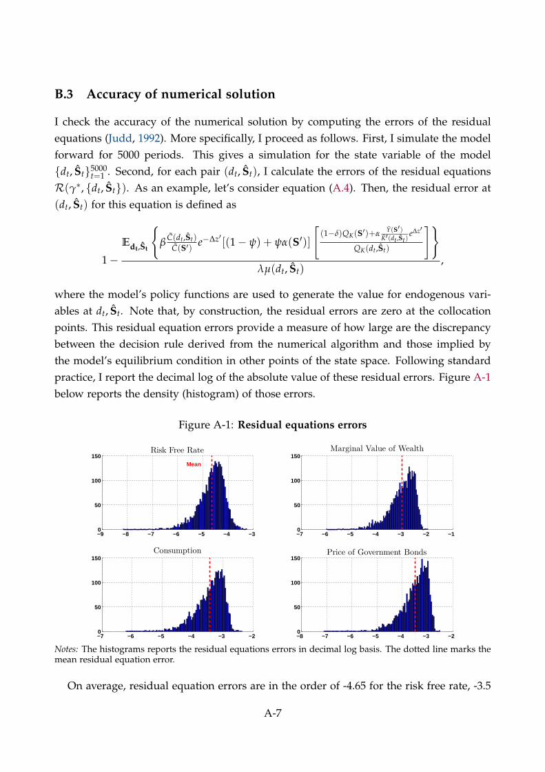
B.3 Accuracy of numerical solution

I check the accuracy of the numerical solution by computing the errors of the residualequations (Judd, 1992). More specifically, I proceed as follows. First, I simulate the modelforward for 5000 periods. This gives a simulation for the state variable of the model{dt, St}5000

t=1 . Second, for each pair (dt, St), I calculate the errors of the residual equationsR(γ∗, {dt, St}). As an example, let’s consider equation (A.4). Then, the residual error at(dt, St) for this equation is defined as

1−Edt,St

{β

C(dt,St)C(S′) e−∆z′ [(1− ψ) + ψα(S′)]

[(1−δ)QK(S′)+α

Y(S′)K′(dt ,St)

e∆z′

QK(dt,St)

]}λµ(dt, St)

,

where the model’s policy functions are used to generate the value for endogenous vari-ables at dt, St. Note that, by construction, the residual errors are zero at the collocationpoints. This residual equation errors provide a measure of how large are the discrepancybetween the decision rule derived from the numerical algorithm and those implied bythe model’s equilibrium condition in other points of the state space. Following standardpractice, I report the decimal log of the absolute value of these residual errors. Figure A-1below reports the density (histogram) of those errors.

Figure A-1: Residual equations errors

−9 −8 −7 −6 −5 −4 −30

50

100

150Mean

Risk Free Rate

−7 −6 −5 −4 −3 −2 −10

50

100

150Marginal Value of Wealth

−7 −6 −5 −4 −3 −20

50

100

150Consumption

−8 −7 −6 −5 −4 −3 −20

50

100

150Price of Government Bonds

Notes: The histograms reports the residual equations errors in decimal log basis. The dotted line marks themean residual equation error.

On average, residual equation errors are in the order of -4.65 for the risk free rate, -3.5

A-7

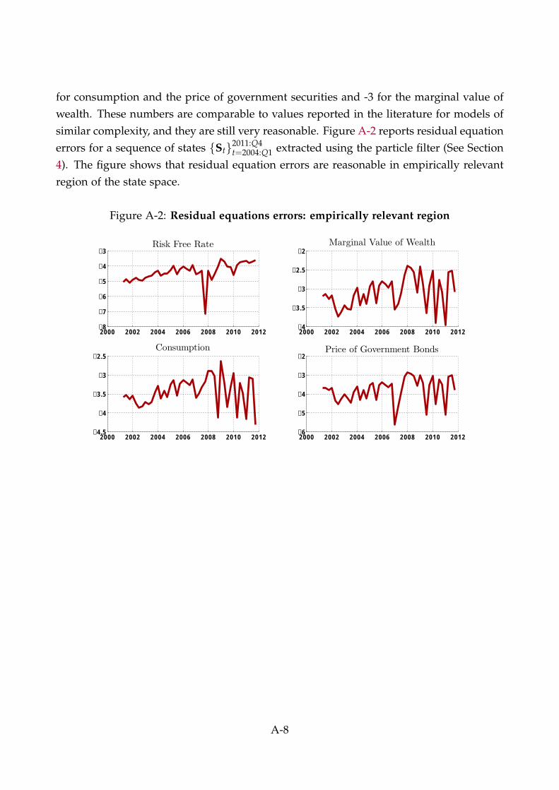
for consumption and the price of government securities and -3 for the marginal value ofwealth. These numbers are comparable to values reported in the literature for models ofsimilar complexity, and they are still very reasonable. Figure A-2 reports residual equationerrors for a sequence of states {St}2011:Q4

t=2004:Q1 extracted using the particle filter (See Section4). The figure shows that residual equation errors are reasonable in empirically relevantregion of the state space.

Figure A-2: Residual equations errors: empirically relevant region

2000 2002 2004 2006 2008 2010 2012−8

−7

−6

−5

−4

−3Risk Free Rate

2000 2002 2004 2006 2008 2010 2012−4

−3.5

−3

−2.5

−2Marginal Value of Wealth

2000 2002 2004 2006 2008 2010 2012−4.5

−4

−3.5

−3

−2.5Consumption

2000 2002 2004 2006 2008 2010 2012−6

−5

−4

−3

−2Price of Government Bonds

A-8

C Data source

C.1 Credit default swap (CDS) spread

Daily CDS spreads on 5 years Italian governmet securities (RED code: 4AB951). Therestructuring clause of the contract is CR (complete restructuring). The spread is denomi-nated in basis points and paid quarterly. The source is Markit, accessed from the WhartonResearch Data Services.

C.2 Banks’ exposure to the Italian government

The European Banking Authority (EBA) published information on holdings of govern-ment debt by European banks participating to the 2011 stress test. Five Italian bankswere in this pool: Unicredit, Intesa-San Paolo, Monte dei Paschi di Siena (MPS), BancoPopolare (BPI) and Unione di Banche Italiane (UBI). Results of the stress test for each ofthese five banks are available at http://www.eba.europa.eu/risk-analysis-and-data/

eu-wide-stress-testing/2011/results. I measure exposure of each bank to Italian cen-tral and local government as net direct long exposure (gross exposures net of cash shortposition of sovereign debt to other counterparties only where there is maturity matching)plus direct sovereign exposures in derivatives. This information is available by maturityof financial instrument, and it reflects positions as of 31st of December 2010. I match thesedata on exposure with end of 2010 total financial assets for each of the five institutions.This latter information is obtained using consolidated banking data from Bankscope, ac-cessed from the Wharton Research Data Service. Table A-1 reports these information.

C.3 Construction of the Lagrange multiplier

Result 2. In equilibrium, the multiplier on the incentive constraint of bankers is a function offinancial leverage and of the spread between a risk free security traded by bankers and the risk freerate

µt =

[R f

t−RtRt

]levt

1 +[

R ft−RtRt

]levt

. (A.19)

A-9

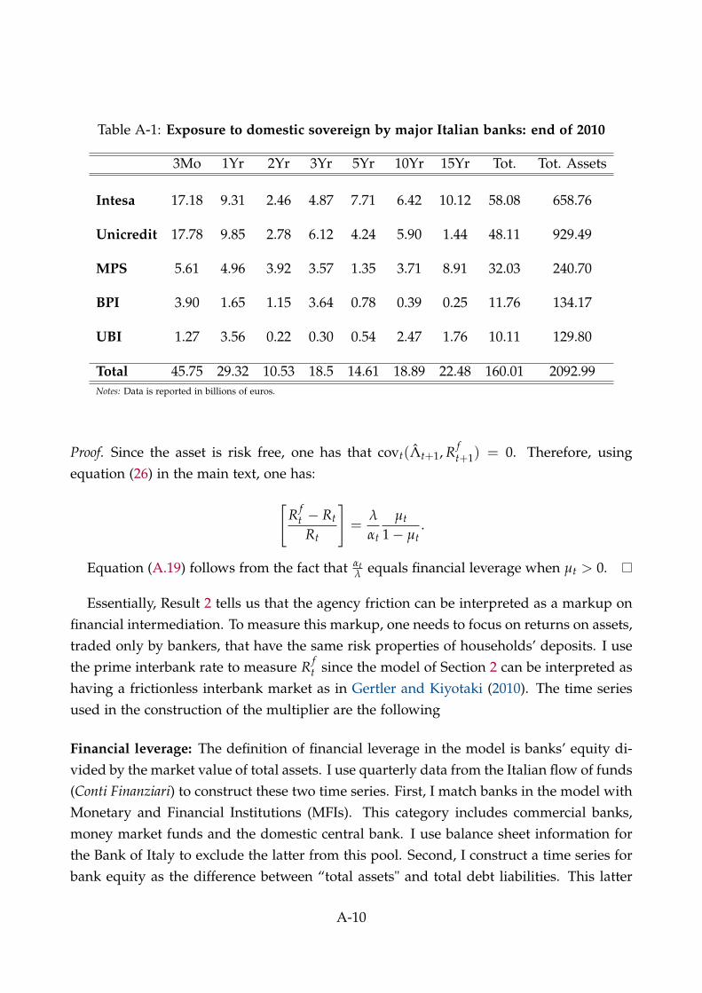
Table A-1: Exposure to domestic sovereign by major Italian banks: end of 2010

3Mo 1Yr 2Yr 3Yr 5Yr 10Yr 15Yr Tot. Tot. Assets

Intesa 17.18 9.31 2.46 4.87 7.71 6.42 10.12 58.08 658.76

Unicredit 17.78 9.85 2.78 6.12 4.24 5.90 1.44 48.11 929.49

MPS 5.61 4.96 3.92 3.57 1.35 3.71 8.91 32.03 240.70

BPI 3.90 1.65 1.15 3.64 0.78 0.39 0.25 11.76 134.17

UBI 1.27 3.56 0.22 0.30 0.54 2.47 1.76 10.11 129.80

Total 45.75 29.32 10.53 18.5 14.61 18.89 22.48 160.01 2092.99Notes: Data is reported in billions of euros.

Proof. Since the asset is risk free, one has that covt(Λt+1, R ft+1) = 0. Therefore, using

equation (26) in the main text, one has:

[R f

t − Rt

Rt

]=

λ

αt

µt

1− µt.

Equation (A.19) follows from the fact that αtλ equals financial leverage when µt > 0.

Essentially, Result 2 tells us that the agency friction can be interpreted as a markup onfinancial intermediation. To measure this markup, one needs to focus on returns on assets,traded only by bankers, that have the same risk properties of households’ deposits. I usethe prime interbank rate to measure R f

t since the model of Section 2 can be interpreted ashaving a frictionless interbank market as in Gertler and Kiyotaki (2010). The time seriesused in the construction of the multiplier are the following

Financial leverage: The definition of financial leverage in the model is banks’ equity di-vided by the market value of total assets. I use quarterly data from the Italian flow of funds(Conti Finanziari) to construct these two time series. First, I match banks in the model withMonetary and Financial Institutions (MFIs). This category includes commercial banks,money market funds and the domestic central bank. I use balance sheet information forthe Bank of Italy to exclude the latter from this pool. Second, I construct a time series forbank equity as the difference between “total assets" and total debt liabilities. This latter

A-10

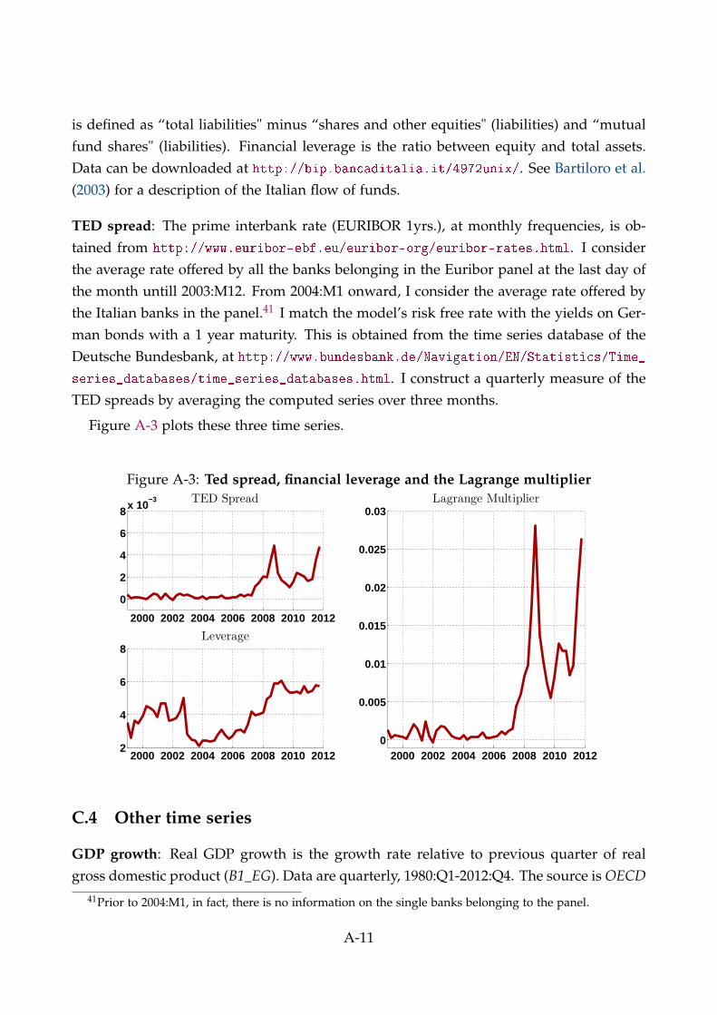
is defined as “total liabilities" minus “shares and other equities" (liabilities) and “mutualfund shares" (liabilities). Financial leverage is the ratio between equity and total assets.Data can be downloaded at http://bip.bancaditalia.it/4972unix/. See Bartiloro et al.(2003) for a description of the Italian flow of funds.

TED spread: The prime interbank rate (EURIBOR 1yrs.), at monthly frequencies, is ob-tained from http://www.euribor-ebf.eu/euribor-org/euribor-rates.html. I considerthe average rate offered by all the banks belonging in the Euribor panel at the last day ofthe month untill 2003:M12. From 2004:M1 onward, I consider the average rate offered bythe Italian banks in the panel.41 I match the model’s risk free rate with the yields on Ger-man bonds with a 1 year maturity. This is obtained from the time series database of theDeutsche Bundesbank, at http://www.bundesbank.de/Navigation/EN/Statistics/Time_series_databases/time_series_databases.html. I construct a quarterly measure of theTED spreads by averaging the computed series over three months.

Figure A-3 plots these three time series.

Figure A-3: Ted spread, financial leverage and the Lagrange multiplier

2000 2002 2004 2006 2008 2010 20122

4

6

8Leverage

2000 2002 2004 2006 2008 2010 2012

0

2

4

6

8x 10−3 TED Spread

2000 2002 2004 2006 2008 2010 20120

0.005

0.01

0.015

0.02

0.025

0.03Lagrange Multiplier

C.4 Other time series

GDP growth: Real GDP growth is the growth rate relative to previous quarter of realgross domestic product (B1_EG). Data are quarterly, 1980:Q1-2012:Q4. The source is OECD

41Prior to 2004:M1, in fact, there is no information on the single banks belonging to the panel.

A-11

Quarterly National Accounts.

Consumption growth: Consumption growth is the growth rate relative to previous quar-ter of real private final consumption expenditure (P31S14_S15). Data are quarterly, 1980:Q1-2012:Q4. The source is OECD Quarterly National Accounts.

Spending-Output ratio: Spending-output ratio is general government final consumptionexpenditure divided by gross domestic product. Both series are seasonally adjusted andin volume estimates. Data are quarterly, 1980:Q1-2012:Q4. The source is OECD QuarterlyNational Accounts.

Investment-Output ratio: Investment-output ratio is gross capital formation divided bygross domestic product. Both series are seasonally adjusted and in volume estimates. Dataare quarterly, 1980:Q1-2012:Q4. The source is OECD Quarterly National Accounts.

Labor income share: I obtain annual data (1970-2007) for and labor compensation (LAB)and value added (VA) from EU KLEMS database. Labor share is defined as LAB

VA . Data canbe downloaded at http://www.euklems.net/.

Worked hours: Average numbers of hours worked per year by person engaged. I scale theseries by (24− 8)× 7× 52. Data are annual (1970-2007), and obtained from EU KLEMS.Data can be downloaded at http://www.euklems.net/.

A-12

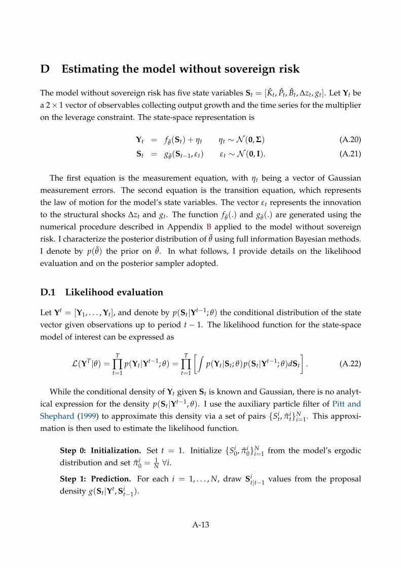
D Estimating the model without sovereign risk

The model without sovereign risk has five state variables St = [Kt, Pt, Bt, ∆zt, gt]. Let Yt bea 2× 1 vector of observables collecting output growth and the time series for the multiplieron the leverage constraint. The state-space representation is

Yt = fθ(St) + ηt ηt ∼ N (0, Σ) (A.20)

St = gθ(St−1, εt) εt ∼ N (0, I). (A.21)

The first equation is the measurement equation, with ηt being a vector of Gaussianmeasurement errors. The second equation is the transition equation, which representsthe law of motion for the model’s state variables. The vector εt represents the innovationto the structural shocks ∆zt and gt. The function fθ(.) and gθ(.) are generated using thenumerical procedure described in Appendix B applied to the model without sovereignrisk. I characterize the posterior distribution of θ using full information Bayesian methods.I denote by p(θ) the prior on θ. In what follows, I provide details on the likelihoodevaluation and on the posterior sampler adopted.

D.1 Likelihood evaluation

Let Yt = [Y1, . . . , Yt], and denote by p(St|Yt−1; θ) the conditional distribution of the statevector given observations up to period t− 1. The likelihood function for the state-spacemodel of interest can be expressed as

L(YT|θ) =T

∏t=1

p(Yt|Yt−1; θ) =T

∏t=1

[∫p(Yt|St; θ)p(St|Yt−1; θ)dSt

]. (A.22)

While the conditional density of Yt given St is known and Gaussian, there is no analyt-ical expression for the density p(St|Yt−1, θ). I use the auxiliary particle filter of Pitt andShephard (1999) to approximate this density via a set of pairs {Si

t, πit}N

i=1. This approxi-mation is then used to estimate the likelihood function.

Step 0: Initialization. Set t = 1. Initialize {Si0, πi

0}Ni=1 from the model’s ergodic

distribution and set πi0 = 1

N ∀i.

Step 1: Prediction. For each i = 1, . . . , N, draw Sit|t−1 values from the proposal

density g(St|Yt, Sit−1).

A-13

Step 2: Filtering. Assign to each Sit|t−1 the particle weight

πit =

p(Yt|Sit|t−1; θ)p(St|Si

t|t−1; θ)

g(St|Yt, Sit−1)

.

Step 3: Sampling. Rescale the particles {πit} so that they add up to unity, and denote

these rescaled values by {πit}. Sample N values for the state vector with replacement

from {Sit|t−1, πi

t}Ni=1. Call each draw {Si

t}. If t < T, set t = t + 1 and go to Step 1.Else, stop. �

The likelihood function of the model is then approximated as

L(YT|θ) ≈ 1N

(T

∏t=1

[1N

N

∑i=1

p(Yt|Sit|t−1; θ)

]).

Regarding the tuning of the filter, I set N = 20000. The matrix Σ is diagonal, and thediagonal elements equal 25% of the variance of the observable variables. The choice forthe proposal density g(St|Yt, Si

t−1) is more involved. I sample the structural innovationsεt from N (mt, I). Then, I use the model’s transition equation (A.21) to obtain Si

t|t−1. Thecenter for the proposal distribution for εt is generated as follows:

• Let St−1 be the mean for {Sit−1} over i.

• Set mt to the solution of this optimization program

argminε

{[Yt − fθ(gθ(St−1, ε))]′[Yt − fθ(gθ(St−1, ε))] + ε′Σ−1ε

}.

The first part of the objective function pushes ε toward values such that the state vectorcan rationalize the observation Yt. The second part of the objective function imposes apenalty for ε that are far away from their high density regions. I verify that this pro-posal density results in substantial efficiency gains relative to the canonical particle filter,especially when the model tries to fit extreme observations for Yt.

D.2 Posterior sampler

I characterize the posterior density of θ using a Random Walk Metropolis Hastings withproposal density given by

q(θp|θm−1) ∼ N (θm−1, cH).

The sequence of draws {θm} is generated as follows

A-14

1. Initialize the chain at θ1.

2. For m = 2, . . . , M, draw θp from q(θp|θm−1). The jump from θm−1 to θp is accepted(θm = θp) with probability min{1, r(θm−1, θp|YT)}, and rejected otherwise (θm =

θm−1). The probability of accepting the draw is

r(θm−1, θp|YT) =L(YT|θp)p(θp)

L(YT|θm−1)p(θm−1).

First, I run the chain for M = 10000 with H being the identity matrix and c = 0.001.The chain is initialized from an estimation of the model using the Method of SimulatedMoments.42 I drop the first 5000 draws, and I use the remaining draws to initialize asecond chain and to construct a new candidate density. This second chain is initializedat the mean of the 5000 draws. Moreover, the variance-covariance matrix H is set to theempirical variance-covariance matrix of these 5000 draws. The parameter c is fine tuned toobtain an acceptance rate of roughly 60%. I run the second chain for M = 20000. Posteriorstatistics are based on the latter 10000 draws.

42The moments used in this step are: i) mean, standard deviation and autocorrelation for GDP growthand the multiplier; ii) correlation between GDP growth and the multiplier.

A-15

E Policy Experiments

E.1 Refinancing operations

It is instructive to first consider the stationary problem. The government allows bankersto borrow up to m at the fixed interest rate Rm, and this intervention is financed throughlump-sum taxation. Moreover, these loans are not subject to limited enforcement prob-lems. The decision problem of the banker becomes

vb(n; S) = maxaB,aK ,b

ES{

Λ(S′, S)[(1− ψ)n′ + ψvb(n′; S′)

]},

n′ = ∑j={B,K}

[Rj(S′, S)− R(S)]Qj(S)aj + [Rm − R(S)]m− R(S)b,

∑j={B,K}

Qj(S)aj = n + b,

λ

∑j={B,K}

Qj(S)aj −m

≤ vb(n; S),

m ∈ [0, m],

S′ = Γ(S).

Assuming that m ≥ 0 does not bind,43 the first order condition with respect to m is

Es

{Λ(S′, S)

[(1− ψ) + ψ

∂vb(n′; S)∂n′

]}[R(S)− Rm] + λµ(S) = χ(S)

It can be showed, following a similar logic of Result 1, that vb(n; S) = α(S)n + x(S),with x(S) ≥ 0. The leverage constraint becomes

∑j Qj(S)aj

n≤ α(S)

λ+

x(S)λ

+ m

Notice that refinancing operations have two main direct effects on banks. First, theyrepresent an implicit transfer to banks. Indeed, to the extent that (Rm < R(S)), banksbenefit from the policy as their debt is subsidized. This has a positive effect on the networth of banks relative to what would happen in the no-policy case. Second, the policyrelaxes the leverage constraint of banks. This happens because of two distinct reasons: i)the loan from the government does not enter in the computation of the constrained level

43This is not a restriction, as the policy considered involves an Rm substantially below R, meaning thatbankers are willing to accept the loan.

A-16

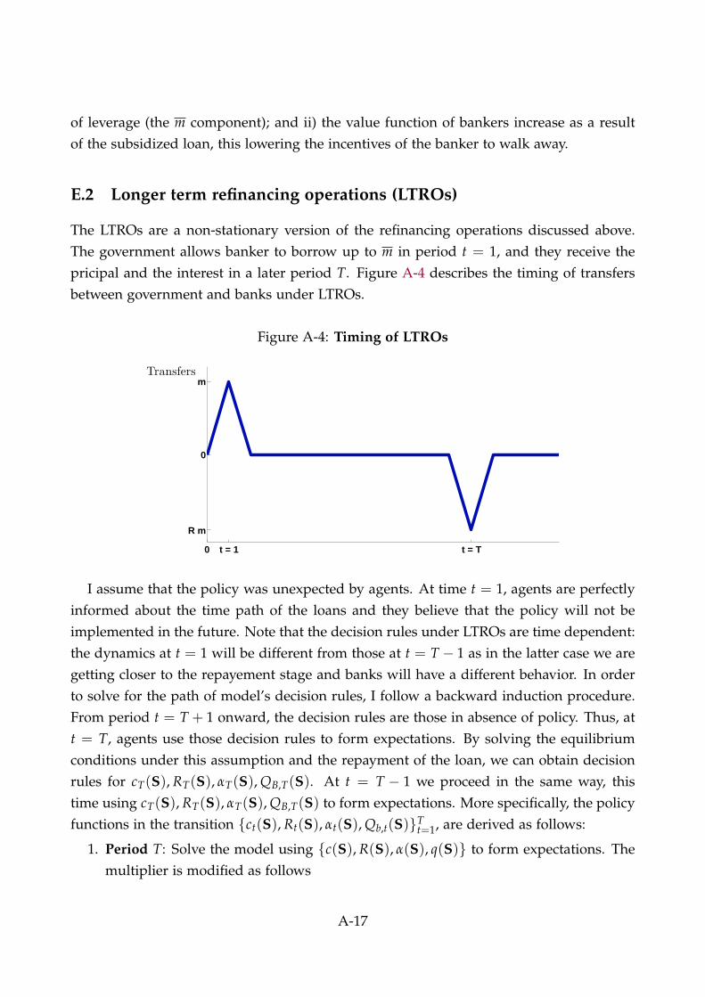
of leverage (the m component); and ii) the value function of bankers increase as a resultof the subsidized loan, this lowering the incentives of the banker to walk away.

E.2 Longer term refinancing operations (LTROs)

The LTROs are a non-stationary version of the refinancing operations discussed above.The government allows banker to borrow up to m in period t = 1, and they receive thepricipal and the interest in a later period T. Figure A-4 describes the timing of transfersbetween government and banks under LTROs.

Figure A-4: Timing of LTROs

0 t = 1 t = T

R m

0

mTransfers

I assume that the policy was unexpected by agents. At time t = 1, agents are perfectlyinformed about the time path of the loans and they believe that the policy will not beimplemented in the future. Note that the decision rules under LTROs are time dependent:the dynamics at t = 1 will be different from those at t = T − 1 as in the latter case we aregetting closer to the repayement stage and banks will have a different behavior. In orderto solve for the path of model’s decision rules, I follow a backward induction procedure.From period t = T + 1 onward, the decision rules are those in absence of policy. Thus, att = T, agents use those decision rules to form expectations. By solving the equilibriumconditions under this assumption and the repayment of the loan, we can obtain decisionrules for cT(S), RT(S), αT(S), QB,T(S). At t = T − 1 we proceed in the same way, thistime using cT(S), RT(S), αT(S), QB,T(S) to form expectations. More specifically, the policyfunctions in the transition {ct(S), Rt(S), αt(S), Qb,t(S)}T

t=1, are derived as follows:

1. Period T: Solve the model using {c(S), R(S), α(S), q(S)} to form expectations. Themultiplier is modified as follows

A-17

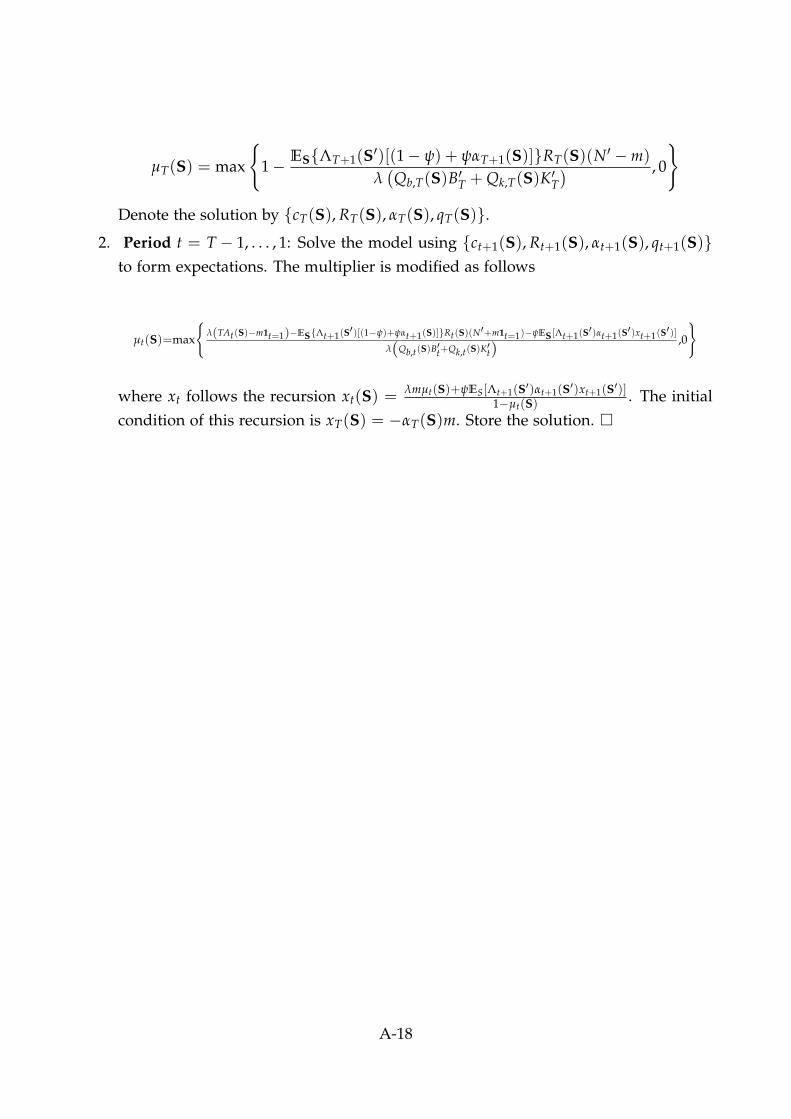
µT(S) = max

{1− ES{ΛT+1(S′)[(1− ψ) + ψαT+1(S)]}RT(S)(N′ −m)

λ(Qb,T(S)B′T + Qk,T(S)K′T

) , 0

}

Denote the solution by {cT(S), RT(S), αT(S), qT(S)}.2. Period t = T − 1, . . . , 1: Solve the model using {ct+1(S), Rt+1(S), αt+1(S), qt+1(S)}

to form expectations. The multiplier is modified as follows

µt(S)=max

{λ(TAt(S)−m1t=1)−ES{Λt+1(S

′)[(1−ψ)+ψαt+1(S)]}Rt(S)(N′+m1t=1)−ψES [Λt+1(S′)αt+1(S

′)xt+1(S′)]

λ(Qb,t(S)B′t+Qk,t(S)K′t)

,0

}

where xt follows the recursion xt(S) =λmµt(S)+ψES[Λt+1(S′)αt+1(S′)xt+1(S′)]

1−µt(S). The initial

condition of this recursion is xT(S) = −αT(S)m. Store the solution. �

A-18