A

ipTsni©

K

1

petornqtyfip

gh

1d

Journal of Photochemistry and Photobiology A: Chemistry 190 (2007) 228–240

The on-the-fly surface-hopping program system Newton-X:Application to ab initio simulation of the nonadiabatic

photodynamics of benchmark systems

Mario Barbatti a,∗, Giovanni Granucci b,∗, Maurizio Persico b,∗, Matthias Ruckenbauer a,Mario Vazdar c, Mirjana Eckert-Maksic c, Hans Lischka a,∗

a Institute for Theoretical Chemistry, University of Vienna, Waehringerstrasse 17, 1090-Vienna, Austriab Dipartimento di Chimica e Chimica Industriale, Universita di Pisa, v.Risorgimento 35, 56126 Pisa, Italy

c Laboratory for Physical-Organic Chemistry, Division of Organic Chemistry and Biochemistry, Rudjer Boskovic Institute, Zagreb, Croatia

Received 23 October 2006; accepted 1 December 2006Available online 15 December 2006

bstract

The great importance of ultrafast phenomena in photochemistry and photobiology has made dynamics simulations an essential methodologyn these areas. In this work, we present the Newton-X program package containing a new implementation of a direct dynamics approach toerform adiabatic (Born–Oppenheimer) and nonadiabatic simulations. The nonadiabatic dynamics is based on Tully’s surface hopping approach.

he program has been developed with the aim of (1) to create a flexible tool to be used in connection with a multitude of third-party electronic-tructure program packages and (2) to provide the most common options for excited-state dynamics simulations. Benchmark calculations on theonadiabatic dynamics are presented for the methaniminium, butatriene and pentadieniminium cations. The simulation of UV absorption spectras presented for the methaniminium cation and pyrazine.

2006 Elsevier B.V. All rights reserved.

hemis

lthtn(tcPt

eywords: Nonadiabatic phenomena; Excited state dynamics; Ultrafast photoc

. Introduction

In this paper we present computational methods and a newrogram system developed in our groups for the simulation ofxcited state dynamics. Illustrative examples are used to showhe capabilities of the program. The method is based on a “direct”n-the-fly approach for the computation of classical trajecto-ies with Tully surface hopping [1] using energy gradients andonadiabatic coupling vectors calculated by means of availableuantum chemical program systems. Ab initio direct calcula-ions of excited state dynamics have been performed in recent

ears by several groups [2–16]. The increasing interest in thiseld warrants the introduction of standardized and flexible com-utational tools, available to the scientific community.

∗ Corresponding author. Tel.: +43 1 4277 52757; fax: +43 1 4277 9527.E-mail addresses: mario.barbatti@univie.ac.at (M. Barbatti),

ranucci@dcci.unipi.it (G. Granucci), mau@dcci.unipi.it (M. Persico),ans.lischka@univie.ac.at (H. Lischka).

odsccca

e

010-6030/$ – see front matter © 2006 Elsevier B.V. All rights reserved.oi:10.1016/j.jphotochem.2006.12.008

try; On-the-fly surface-hopping dynamics; Ab initio dynamics

When choosing a method to simulate excited state molecu-ar dynamics one faces three main issues: the first one is howo solve the fixed nuclei electronic problem, the second one isow to treat the nuclear dynamics and its coupling to the elec-ronic dynamics, and the third issue is apparently a technicality,amely whether the computation of the potential energy surfacePES) should be dealt with beforehand or “on-the-fly”. In fact,his choice is conditioned by the previous ones and by the pro-esses to be investigated. The alternatives are to determine theES and couplings systematically in advance and to represent

hem analytically for use in the simulations (two-step strategy),r to compute them at each time step during the integration of theynamical equations as needed (direct or on-the-fly strategy). Ithould be stressed at this point that the calculation of electroni-ally excited states, analytic energy gradients and nonadiabaticoupling vectors is still a formidable problem and only few spe-

ialized methods and quantum chemical program systems arevailable for that purpose.

In the two-step approach, the number of single pointlectronic structure calculations to be executed increases

nd Ph

ewisseoaqbrPwrs

wnPsnftnFtpiptooltpfic

itsoatmtotb

cthbaa

asTHcogeftttitbipaiuocc

cmtac

2

2

stonbVati(toA

A

M. Barbatti et al. / Journal of Photochemistry a

xponentially with the dimensionality of the problem, i.e.ith the number of nuclear degrees of freedom that are taken

nto consideration. As a consequence, the application of thistrategy is severely restricted: a rigorous treatment is limited tomall molecules (5–6 atoms), and for larger systems one mustither select few internal coordinates and ignore the other ones,r resort to simplifying assumptions as to the form of the PESnd couplings. The analytic representation of the electronicuantities can be rather involved, and its parameterization wille quite a cumbersome task if the PESs do cross and/or severaleaction channels must be taken into account. The cusps of theES and divergences of the derivative couplings can be dealtith by resorting to effective Hamiltonians in a quasi-diabatic

epresentation [17,18] (see [19–21] for an application of thistrategy to the photofragmentation of azomethane).

All these difficulties are avoided in the direct approach,hich is therefore the most straightforward choice when severaluclear coordinates play non-trivial roles and the topology of theES is complicated. In all kinds of trajectory calculations (two-tep or direct), state energies, their gradients with respect to theuclear coordinates, and the nonadiabatic couplings are requiredor the given geometry at each time step. In the direct approach,he number of single point calculations is NS·NT, where NS is theumber of time steps and NT the number of trajectories to be run.or a single trajectory, the computational cost does not depend on

he number of internal coordinates (assuming the availability ofroper analytic gradients and nonadiabatic coupling vectors) buts proportional to the propagation time, i.e. the time length of therocess under investigation. Of course, the necessary number ofrajectories will depend on the problem. In particular in the casef ultrafast processes only a small number of internal degreesf freedom will be relevant for the sampling process. This facteads to a relatively small number of required trajectories. Thus,his approach is especially suited for the treatment of ultrafastrocesses, which require relatively short simulation times of aew ps. At this point we want to mention new approaches usingnterpolation techniques (see e.g. Ref. [22]) where the systematicomputation of energy grids is avoided.

Because of the non-local character of quantum mechanics,n principle the direct approach cannot be applied to quan-um wavepacket calculations and to adequately describe effectsuch as tunneling. However, by expanding the wavepacketsn localized travelling basis functions and introducing suitablepproximations, the direct approach becomes a viable alterna-ive, although the computational cost of a method such as the full

ultiple spawning (FMS) [6] increases more than linearly withhe propagation time. In fact, in the FMS procedure the numberf electronic calculations per run and per time step is withinhe range [Nb,Nb(Nb + 1)], where Nb is the number of travellingasis functions (increasing with time).

In this paper we shall describe computer software based onlassical trajectories that are most conveniently connected withhe direct calculation of electronic quantities. In particular, we

ave chosen Tully’s surface hopping (SH) method [1,10,23–29],ut other trajectory methods can be easily implemented, suchs mean-field (MF) [30–34] or intermediate (SH–MF) [35]pproaches.

wnci

otobiology A: Chemistry 190 (2007) 228–240 229

The implementation of direct dynamics methods can bechieved in several ways. One possibility is to tie all programteps closely together into one homogeneous program package.his approach will give maximum computational efficiency.owever, it will be strongly connected to a chosen quantum

hemical program system providing the electronic energies andther data as discussed before. These quantum chemical pro-ram sections are the most complex and extended parts of thentire program. Usually, the quantum chemical calculation per-ormed at each time step requires by far more computer timehan the numerical integration steps of Newton’s equations andhe integration of the electronic Schrodinger equation along therajectory. Thus, a modular approach appears to be more prof-table. There, the computational steps of the time integration andhe quantum chemical part are strictly separated, as describedelow. The big advantage of this modular approach is the fact thatt is only loosely linked to a given quantum chemical programackage. Since these quantum chemical program sections arelways in rapid development, insertion of new features are eas-ly achieved while keeping all remaining software environmentnchanged. The disadvantage of this approach is the introductionf computational overhead, which is, however, relatively smallompared to the large computer times of the quantum chemicalalculation.

The program Newton-X [36] to be described in this publi-ation has been developed in a joint effort along the concept ofodularity. As will be described below, the creation of interfaces

o the quantum chemical program section is straightforwardllowing the use of the most suitable method available in eachase.

. Method

.1. Dynamics implementation

In this section we give a short description of the standard clas-ical trajectory surface hopping (TSH) procedure [1,10,27,37]hat we have adopted in the Newton-X package, with emphasisn the options available to run ab initio on-the-fly dynamics. Theuclear motion is represented by classical trajectories, computedy numerical integration of Newton’s equations by the velocity-erlet algorithm [38,39]. The molecule is considered to be ingiven electronic state (the current state) at any time. While

he system is in the adiabatic state ψK the nuclear trajectorys driven by its PES, EK. Imposing the electronic wavefunctionexpanded in the basis of the first NA adiabatic states) to obey theime-dependent Schrodinger equation, we get the following setf coupled differential equations for the probability amplitudesK:

˙ K(t) = −NA∑L=1

AL(t) eiγKL Q hKL, (1)

here hγKL = ∫ t0 (EK − EL) dt′, Q is a vector collecting the

uclear velocities and hKL = 〈ψL|�QψK〉 is the nonadiabaticoupling vector between states K and L. From the numericalntegration of Eq. (1) the adiabatic populations PK(t) = |AK(t)|2

2 nd Photobiology A: Chemistry 190 (2007) 228–240

atoas[

tancrop[

A

U

w

Hpgaq

tpwcpotmactcTscbs

asttAddo

r(

oyatcet(

ddsoapteiantoa

30 M. Barbatti et al. / Journal of Photochemistry a

re obtained. The transition probability to jump from one poten-ial surface to another one is evaluated by looking at the variationf the PK(t)’s in time on the basis of Tully’s fewest switcheslgorithm [1,27,37] or alternatively using the modified fewest-witches algorithm proposed by Hammes–Schiffer and Tully25].

Several integration schemes have been implemented in ordero achieve high numerical stability together with time steps �ts long as possible. Contrary to the adiabatic energies EK, theonadiabatic couplings, as function of the nuclear coordinates,an undergo rather abrupt variations and even diverge. For thiseason, several algorithms have been provided for the integrationf Eq. (1). The main ones are the 6th-order Adams–Moultonredictor-corrector scheme [40], the 5th-order Butcher method41,42], and the unitary propagator U(t, �t):

(t +�t) ∼= U(t, �t)A(t), (2)

(t, �t) = exp

(B(t) + B(t +�t)

2�t

), (3)

here B is the antihermitian matrix BKL = exp(iγKL)Q·hKL.The integrators implemented usually give similar results.

owever, with multiple crossings the norm-conserving unitaryropagator is preferable. To further improve the numerical inte-ration of the electronic time-dependent Schrodinger equation,smaller timestep �t′ =�t/ms can be used, with the relevant

uantities EK(t), Q(t) and hKL(t) interpolated from t to t +�t.In previous work with semiempirical electronic wavefunc-

ions, Granucci et al. [43] have implemented a differentropagation algorithm, based on a local diabatization scheme,hich is inherently stable even in the case of narrowly avoided

rossings or in the proximity of conical intersections. We com-ared the performance of the Newton-X unitary scheme, basedn the evaluation of the nonadiabatic couplings, with those ofhe local diabatization procedure, as implemented in a develop-

ent version of the Mopac package [44]. The test case wasmodel neutral-ionic avoided crossing, and the semiempiri-

al parameters were varied so as to change the position ofhe crossing point and the value of the electronic neutral-ionicoupling H12. The results of the comparison are presented inable ST1 (supplementary material). As one can see, the twochemes gave similar results. Only for very weakly avoidedrossings, with transition probabilities greater than 95%, the dia-atic algorithm was superior (i.e. it allowed the use of larger timeteps).

In surface hopping dynamics the momentum has to bedjusted after the hopping in order to keep the total energy con-tant. In Newton-X it is possible to set this adjustment alonghe momentum direction, along the nonadiabatic coupling vec-or direction, or along the gradient difference vector direction.nother option refers to frustrated hopping (those hoppings thato not take place because there is no available kinetic energy too that). The most common options are to keep the momentum

r invert it. Both can be chosen in Newton-X.

The simulation of a photochemical or photophysical processequires the execution of a rather large number of trajectoriesa “swarm”), in case of ab initio dynamics preferably of the

Mttt

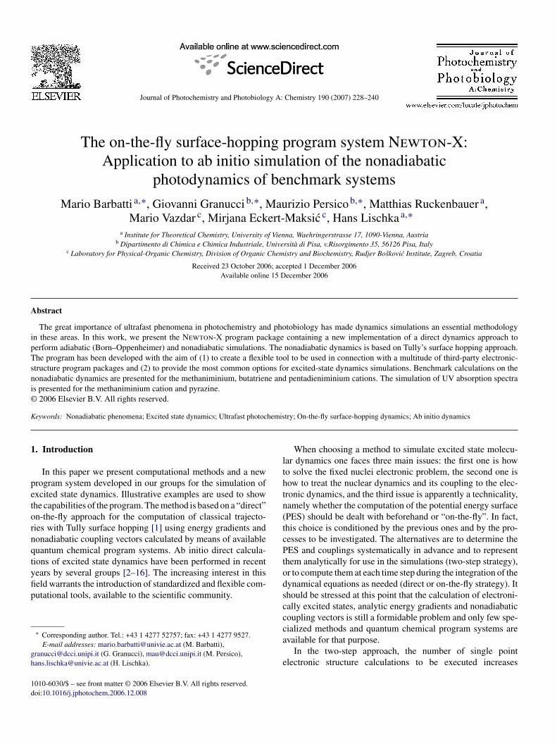
Fig. 1. Block structure of the Newton-X program.

rder of 100 or more. All quantities of interest, such as quantumields, state populations, energy disposal and transient spectra,re computed as averages over all trajectories. The number ofrajectories to be run depends on the statistical uncertainty thatan be accepted on the results, and on the probability of the rel-vant events. The program contains routines to control multiplerajectories and to perform the required statistical proceduresFig. 1).

As we have discussed in Section 1, Newton-X has beeneveloped in a highly modular way, with several indepen-ent programs communicating via files. The main moduli arechematically shown in Fig. 1. At each integration timestep (�t)f the Newton’s equations, the electronic quantities EK, �QEKnd hKL have to be calculated (see Fig. 1) by some externalrogram and provided to Newton-X. In principle, any ab ini-io program that could supply analytical energy gradients andventually nonadiabatic couplings is eligible. For the time being,nterfaces have been provided for the quantum chemistry pack-ges Columbus [45–48], with which it is possible to performonadiabatic and adiabatic dynamics using SA–CASSCF (forhe definition of acronyms see Section 2.3) and MR–CI meth-ds; Turbomole [49] (adiabatic dynamics with RI–CC2 [50,51]nd TD–DFT [52,53] methods); and the semiempirical packageopac [44] (nonadiabatic dynamics). Presently, an interface to

he Aces II package [54] is under development [55] allowinghe performance of adiabatic and nonadiabatic dynamics usinghe EOM–CCSD method.

nd Ph

2

mmsahmamivettsmt(fe

btic

pwp

P

wpf

sittTttmwlam

eIcest

ti

2

todcsmnpwtwr(tICwt

aef([

vmRpN

3

sdieniminium cation (see Scheme 1). The photodynamics of allof these systems provide interesting challenges and questionsand also may serve as benchmarks for testing new methods andprograms. The methaniminium cation dynamics dependence on

M. Barbatti et al. / Journal of Photochemistry a

.2. Initial conditions and absorption spectra

In Newton-X, the initial conditions (nuclear coordinates andomenta, and starting electronic state) are sampled so as toimic at best a quantum wavepacket, and to take into account in a

implified way the excitation process. Coordinates and momentare sampled according to their probability distributions in a givenarmonic vibrational state. Harmonic frequencies and normalodes can be imported from the Turbomole, Gamess [56]

nd Gaussian [57] packages. The sampling of coordinates andomenta can be either uncorrelated, i.e. they can be chosen by

ndependent random events, or correlated. In the former case, theirial theorem <Ekin> = <Epot> is fulfilled, but the initial totalnergy is strongly dispersed. For the vibrational ground state,his initial conditions distribution matches the Wigner distribu-ion for the quantum harmonic oscillator [58]. Alternatively, theampling of coordinates and momenta can be correlated, whicheans that after sampling coordinates, the momenta are scaled

o make the initial energy equal to the harmonic vibrational levelthe zero point energy, if v = 0). This method, however, does notulfill the virial theorem as it tends to overestimate the kineticnergy.

Some coordinates (normally the highest frequency ones) cane “frozen” in the sampling procedure, i.e. they can be fixedo equilibrium values with zero momenta: this may be useful,n order to reduce the total zero point energy and the artifactsonnected with it (see for instance [59,60]).

For each molecular geometry that is selected by the samplingrocedure, a stochastic algorithm can be executed to determinehether the trajectory will be started on the basis of the com-uted transition probability [61]:

K0 = (fK0/�E2K0)

max(fK0/�E2K0)

, (4)

here fK0 is the oscillator strength and�EK0 the energy gap. Therobability is normalized by the maximum value of computedK0/�E

2K0 ratios. In this way, the effect of an ultrashort pulse is

imulated, i.e. the creation of a “Franck–Condon” wavepacketn the excited electronic state without energy constraints. Notehat this procedure is beyond the Condon approximation, ashe oscillator strength is obtained for each molecular geometry.his feature can also be used to simulate the absorption spec-

rum, either by collecting in a histogram the number of acceptedransitions as a function of the transition energy (histogram

ethod) or by assigning to each transition a Gaussian functionith the height Pk0 and a width representing some phenomeno-

ogical broadening and plotting the sum of these Gaussianss a function of the transition energy (Gaussian broadeningethod).Additionally, the excitation can be restricted to a predefined

nergy window by imposing a constraint on the transition energy.n this case, instead of specifying the target excited state, one

hooses the excitation energy EX and a tolerance�EX. Then, forach sampled geometry, the procedure considers the electronictates K for which the transition energy EK − E0 falls withinhe interval EX ±�EX and starts a number of trajectories, dis-

otobiology A: Chemistry 190 (2007) 228–240 231

ributed among those states, according to the probability definedn Eq. (4).

.3. Computational details

Several electronic structure methods and levels of calcula-ion have been employed for the photodynamical simulationf the systems methaniminium cation, butatriene, and penta-ieniminium cations. Details on the methods and levels ofalculation are summarized in Table ST2. Complete active spaceelf-consistent field calculations with n electrons distributed in

orbitals (CASSCF(n, m)) have been performed on metha-iminium, butatriene, and pentadieniminium cations, and onyrazine. In all cases, a state averaging procedure has been usedith equal weights for all k states involved (SA-k). In the case of

he methaniminium cation, all configurations forming the CASere used as references for subsequent multireference configu-

ation interaction calculations with single and double excitationsMR–CISD). In the CI calculations the interacting space restric-ion [62] was applied and the 1s-core orbitals were kept frozen.n the case of the pentadieniminium cation, a subspace of theAS(6,6) was used as reference for MR–CIS calculations. It isorth noting that MR–CIS is considerably more flexible than

he conventional single reference CIS.The time-dependent density functional theory (TD–DFT)

nd resolution-of-identity coupled-cluster method with doublexcitations (RI–CC2) have also been employed. The B3–LYPunctional [63] was used in all TD–DFT calculations. Severalpolarized) double-zeta quality basis sets have been used: 3-21G64], 6–31G* [65], and SV(P) [66].

CASSCF and MR–CI gradients and nonadabatic couplingectors were obtained with the analytical tools [67–70] imple-ented in the COLUMBUS program system. TD–DFT andI–CC2 calculations were carried out with the TURBOMOLEackage. Dynamics calculations have been performed withewton-X.

. Applications

Dynamics simulations have been performed for a series ofystems, methaniminium cation, butatriene cation, and penta-

Scheme 1.

2 nd Photobiology A: Chemistry 190 (2007) 228–240

tclid3sIps

3

tfan[

C(PatbmrittotndSwscoo

tddasfsvaowflaq

FtS

di1Sa6t

f

FgjdlpbbBs

32 M. Barbatti et al. / Journal of Photochemistry a

he initial surface is the subject of Section 3.1. The butatrieneation dynamics and the effect of the electronic structure calcu-ation level and of the surface hopping algorithm are addressedn Section 3.2. The pentadieniminium cation dynamics depen-ence on the electronic structure method is discussed in Section.3. Furthermore (Section 3.4), simulations of the absorptionpectra of methaniminium cation and pyrazine are presented.n Table ST2 (supplementary material) the main computationalrocedures used in each one of the dynamics simulations areummarized.

.1. Methaniminium (CH2NH2+) cation

The methaniminium has been studied as prototype for pro-onated Schiff bases [71], for polar �-bonds [16,72–74], andor basic processes of dehydrogenation [75–77]. Its small sizend consequent reduced computational demands make metha-iminium always a good candidate to test new methodologies11,78].

Despite its apparent simplicity, the electronic structure ofH2NH2

+ shows an interesting complexity in terms of the ��*

S1) and ��* (S2) states not present in the larger member of theSB series CH2(CH)kNH2

+ [79,80]. It has been found by Michlnd Bonacic-Koutecky [72] that following the torsional motion,he ��* state is stabilized and crosses the S0 state at 90◦. Bar-atti et al. [16] have shown that additionally the CN stretchingode is of great importance for the photodynamics since it is

esponsible for a crossing between the S1 and S2 states. Prelim-nary dynamics simulations demonstrated a strong sensitivity ofhe dynamics on the initial state. Starting in the ��* (S2) statehe dynamics was following the CN stretch and a simultane-us bipyramidalization of the CH2 and NH2 groups and not theorsional motion. The origin of this stretching seemed to be con-ected to the acquired momentum along the CN bond-directionuring the initial motion on the S2 surface before crossing to1. One interesting question not explored in the previous workas the point whether the torsion dominates the dynamics of the

ystem excited into the S1 state. The aim of the present work is aomprehensive simulation study of the S1 and S2 state dynamicsf the methaniminium cation system using a much larger numberf trajectories and the MR–CISD method instead of CASSCF.

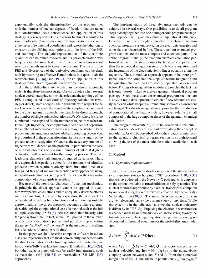
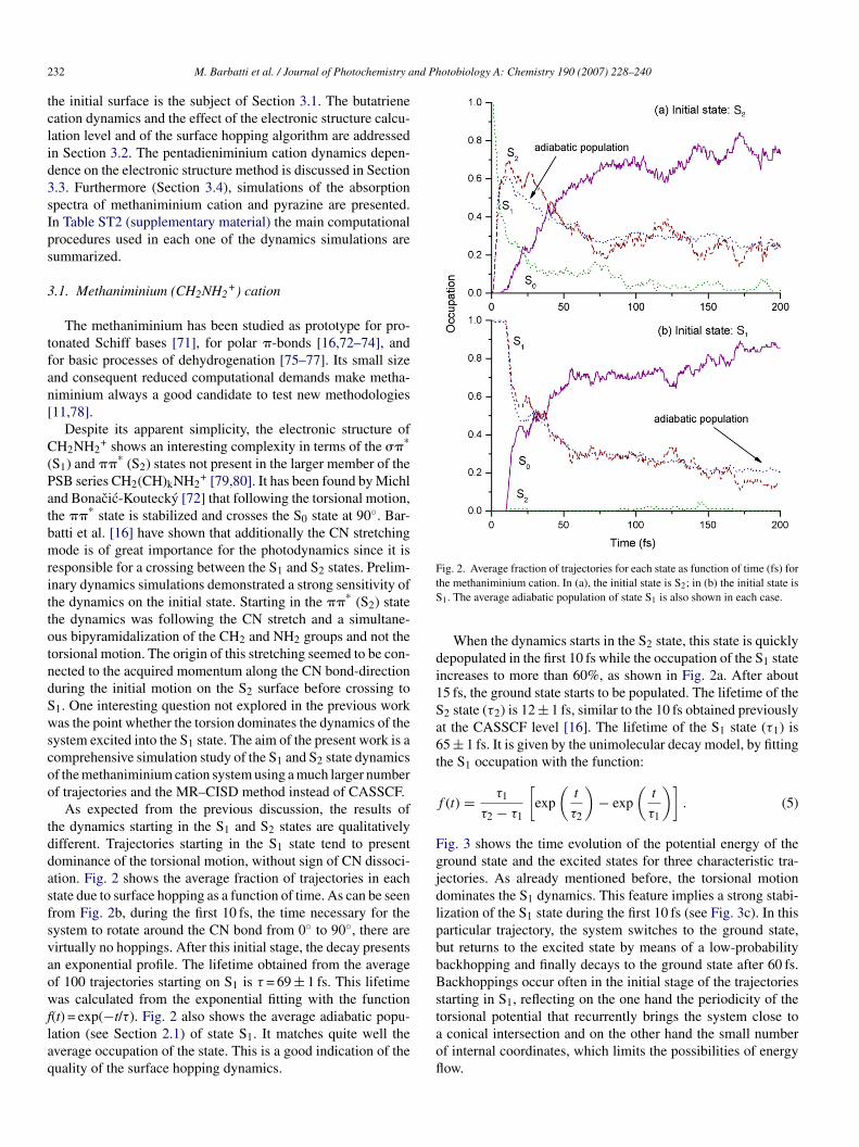
As expected from the previous discussion, the results ofhe dynamics starting in the S1 and S2 states are qualitativelyifferent. Trajectories starting in the S1 state tend to presentominance of the torsional motion, without sign of CN dissoci-tion. Fig. 2 shows the average fraction of trajectories in eachtate due to surface hopping as a function of time. As can be seenrom Fig. 2b, during the first 10 fs, the time necessary for theystem to rotate around the CN bond from 0◦ to 90◦, there areirtually no hoppings. After this initial stage, the decay presentsn exponential profile. The lifetime obtained from the averagef 100 trajectories starting on S1 is τ = 69 ± 1 fs. This lifetimeas calculated from the exponential fitting with the function

(t) = exp(−t/τ). Fig. 2 also shows the average adiabatic popu-ation (see Section 2.1) of state S1. It matches quite well theverage occupation of the state. This is a good indication of theuality of the surface hopping dynamics.

taofl

ig. 2. Average fraction of trajectories for each state as function of time (fs) forhe methaniminium cation. In (a), the initial state is S2; in (b) the initial state is

1. The average adiabatic population of state S1 is also shown in each case.

When the dynamics starts in the S2 state, this state is quicklyepopulated in the first 10 fs while the occupation of the S1 statencreases to more than 60%, as shown in Fig. 2a. After about5 fs, the ground state starts to be populated. The lifetime of the2 state (τ2) is 12 ± 1 fs, similar to the 10 fs obtained previouslyt the CASSCF level [16]. The lifetime of the S1 state (τ1) is5 ± 1 fs. It is given by the unimolecular decay model, by fittinghe S1 occupation with the function:

(t) = τ1

τ2 − τ1

[exp

(t

τ2

)− exp

(t

τ1

)]. (5)

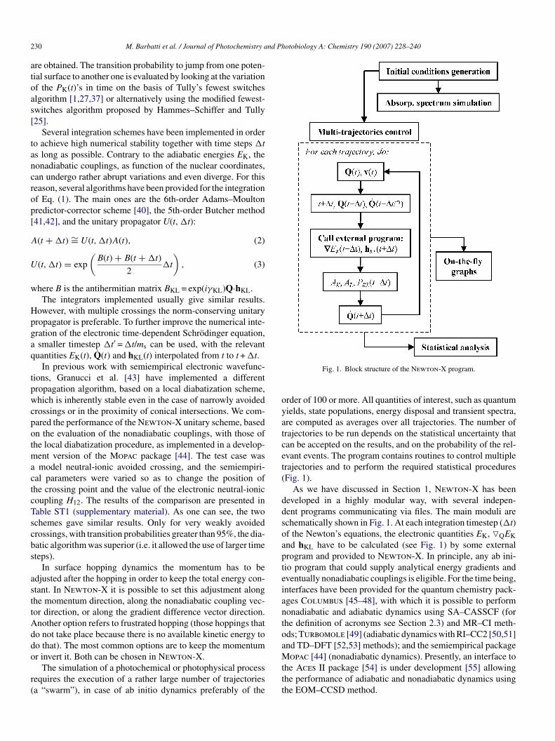
ig. 3 shows the time evolution of the potential energy of theround state and the excited states for three characteristic tra-ectories. As already mentioned before, the torsional motionominates the S1 dynamics. This feature implies a strong stabi-ization of the S1 state during the first 10 fs (see Fig. 3c). In thisarticular trajectory, the system switches to the ground state,ut returns to the excited state by means of a low-probabilityackhopping and finally decays to the ground state after 60 fs.ackhoppings occur often in the initial stage of the trajectories

tarting in S1, reflecting on the one hand the periodicity of the

orsional potential that recurrently brings the system close toconical intersection and on the other hand the small number

f internal coordinates, which limits the possibilities of energyow.

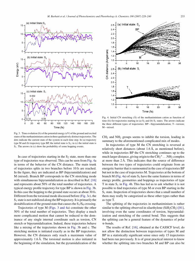
M. Barbatti et al. / Journal of Photochemistry and Photobiology A: Chemistry 190 (2007) 228–240 233

Fig. 3. Time evolution (fs) of the potential energy (eV) of the ground and excitedstates of the methaniminium cation in three qualitatively distinct trajectories. Thedots indicate the current state of the system in each time step. In (a) trajectorytS

tioIMwatIDSd

5mislsHat

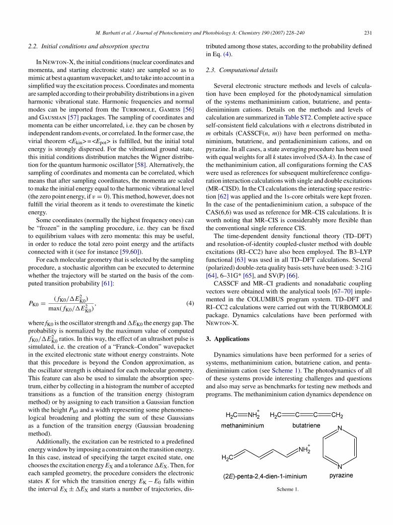
Fig. 4. Initial CN stretching (A) of the methaniminium cation as function ofttM

Cs

rwmabebbeTpSta

siit�

ype M and (b) trajectory type BP, the initial state is S2; in (c) the initial state is

1. The arrows in (c) show the probability of some hopping events.

In case of trajectories starting in the S2 state, more than oneype of trajectories was observed. This can be seen from Fig. 4an terms of the behavior of the CN distance. The main trunkf trajectories splits in two branches before 10 fs are reached.n the figure, they are indicated as BP (bipyramidalization) and

(mixed). Branch BP corresponds to the CN stretching modeith simultaneous bipyramidalization as described in Ref. [16]

nd represents about 50% of the total number of trajectories. Aypical energy profile trajectory for type BP is shown in Fig. 3b.n this case the hopping to the ground state occurs at about 30 fs.ifferent from the torsional mode discussed before (Fig. 3c), the1 state is not stabilized along the BP trajectory. It is primarily theestabilization of the ground state that causes the S1/S0 crossing.

Trajectories of type M (Figs. 3 and 4a) constitute the other0% of the total number of trajectories. They display a muchore complicated motion that cannot be reduced to the dom-

nance of any single internal coordinate such as torsion, CNtretch or bipyramidalization. Indeed, these trajectories behaveike a mixing of the trajectories shown in Fig. 3b and c. The

tretching motion is initiated exactly as in the BP trajectories.owever, the CN distances only reach a maximum value of

pproximately 1.6 A. The torsional motion is also initiated inhe beginning of the simulation, but the pyramidalization of the

nBhw

ime (fs) for trajectories starting in (a) S2 and (b) S1 states. The arrows indicatehe three different types of trajectories: BP—bipyramidalization; T—torsion;

—mixed.

H2 and NH2 groups seems to inhibit the torsion, leading inummary to the aforementioned complicated mix of modes.

In trajectories of type M the CN stretching is reversed atelatively short distances (about 1.6 A, as mentioned before),hile in trajectories BP the CN stretching continues up to theuch larger distance, giving origin to the CH2

+ . . .NH2 complext more than 2 A. This indicates that the source of differenceetween the two types of trajectories could originate from annergetic barrier that is surmounted in the case of trajectories BPut not in the case of trajectories M. Trajectories at the bottom ofranch M (Fig. 4a) of state S2 have the same features in terms ofnergy profile, geometries and hoppings as trajectories of typein state S1 in Fig. 4b. This has led us to ask whether it is not

ossible to find trajectories of type M or even BP starting in the1 state. Inspection of trajectories shows that a small number of

hem may really be categorized as these other types rather thans type T.

The splitting of the trajectories in methaniminium is ratherimilar to the splitting observed in silaethylene (SiH2CH2) [81],nvolving even the same coordinates of torsion, bipyramidal-zation and stretching of the central bond. This suggests thathe splitting can be a general feature of the dynamics of polar-bonds.

The results of Ref. [16], obtained at the CASSCF level, do

ot allow the distinction between trajectories of types M andP in a statistically significant sense since only 15 trajectoriesad been run previously. It is of great practical interest to knowhether the splitting into two branches M and BP can also be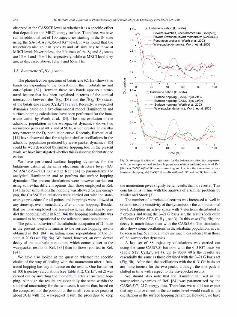

2 nd Photobiology A: Chemistry 190 (2007) 228–240

otrutMaa

3

botiodstart[acwc

b2adu[gaatda

iosdw[

ctocpsta

Fig. 5. Average fraction of trajectories for the butatriene cation in comparisonwith the wavepacket and surface hopping (population analysis) results of Ref.[f

tcM

ol5ddabo

u(e(as

34 M. Barbatti et al. / Journal of Photochemistry a

bserved at the CASSCF level or whether it is a specific effecthat depends on the MRCI energy surface. Therefore, we haveun an additional set of 100 trajectories starting in the S2 statesing the SA-3-CAS(4,3)/6–31G* level. It was found that therajectories also split in types M and BP similarly to those at

RCI level. Nevertheless, the lifetimes of the S2 and S1 statesre 13 ± 1 and 43 ± 1 fs, respectively, while at MRCI level theyre, as discussed above, 12 ± 1 and 65 ± 1 fs.

.2. Butatriene (C4H4+) cation

The photoelectron spectrum of butatriene (C4H4) shows twoands corresponding to the ionization of the � orbitals in- andut-of-plane [82]. Between these two bands appears a struc-ured feature that has been explained in terms of the conicalntersection between the 2B2u (D1) and the 2B2g (D0) statesf the butatriene cation (C4H4

+) [82,83]. Recently, wavepacketynamics based on a five-dimensional model Hamiltonian andurface hopping calculations have been performed for the buta-riene cation by Worth et al. [84]. The time evolution of thediabatic population in the wavepacket dynamics shows twoecurrence peaks at 40 fs and at 90 fs, which creates an oscilla-ory pattern in the D1 population curve. Recently, Barbatti et al.14] have observed that for ethylene similar oscillations in thediabatic population predicted by wave packet dynamics [85]ould be well described by surface hopping too. In the presentork, we have investigated whether this is also true for butatriene

ation.We have performed surface hopping dynamics for the

utatriene cation at the same electronic structure level (SA--CAS(5,6)/3–21G) as used in Ref. [84] to parameterize thenalytical Hamiltonian and to perform the surface hoppingynamics. The present simulations were however carried outsing somewhat different options than those employed in Ref.84]. In our simulations the hopping was allowed for any energyap, the CASSCF calculations were carried out with the state-verage procedure for all points, and hoppings were allowed atny timestep, even immediately after another hopping. Besideshat we have employed the fewest-switches algorithm to pre-ict the hopping, while in Ref. [84] the hopping probability wasssumed to be proportional to the adiabatic state population.

The general behavior of the adiabatic occupation of D1 staten the present results is similar to the surface hopping resultsbtained in Ref. [84], including some repopulation of the D1tate at 20 fs (see Fig. 5a). We found, however, an even slowerecay of the adiabatic population, which comes closer to theavepacket results of Ref. [83] than to those reported in Ref.

84].We have also looked at the question whether the specific

hoice of the way of dealing with the momentum after a frus-rated hopping has any influence on the results. One further setf 100 trajectory calculations (see Table ST2, C4H4

+, set 2) wasarried out by inverting the momentum after a frustrated hop-

ing. Although the results are essentially the same within thetatistical uncertainty for the two cases, it seems that, based onhe comparison of the position of the small recurrence peaks atbout 50 fs with the wavepacket result, the procedure to keep

wCto

84]. (a) CAS(5,6)/3–21G results inverting and keeping the momentum after arustrated hopping; (b) CAS(7,5) results with 6–31G* and 3–21G basis sets.

he momentum gives slightly better results than to revert it. Thisonclusion is in line with the analysis of a similar problem byuller and Stock [3].The number of correlated electrons was increased as well in

rder to test the sensitivity of the dynamics on the computationalevel. Adopting an active space with 7 electrons distributed inorbitals and using the 3–21 G basis set, the results look quite

ifferent (Table ST2, C4H4+, set 3). In this case (Fig. 5b), the

ecay is much faster than with the CAS(5,6). The simulationlso shows some oscillations in the adiabatic population, as cane seen in Fig. 5, although they are much less intense than thosef the wavepacket dynamics.

A last set of 88 trajectory calculations was carried outsing the same CAS(7,5) but now with the 6–31G* basis setTable ST2, C4H4

+, set 4). Up to about 40 fs the results aressentially the same as those obtained with the 3–21 G basis setFig. 5b). After that, the oscillations with the 6–31G* basis setre more intense for the two peaks, although the first peak ishifted in time with respect to the wavepacket results.

We should also note that the Hamiltonian used in theavepacket dynamics of Ref. [84] was parametrized by the

AS(6,5)/3–21G energy data. Therefore, we would not expect

hat any improvement in the ab initio level would result in thescillations in the surface hopping dynamics. However, we have

nd Photobiology A: Chemistry 190 (2007) 228–240 235

sti

3

SftSspRmam

mptraru

twfiorrtb3ai6Bt

tctsFtfτ

totτ

g

ar

F(

sdadMpd6a

masbfaac(a

gfb(odpMtaba

M. Barbatti et al. / Journal of Photochemistry a

een that increasing the number of correlated electrons and ofhe basis set have this effect. This question should be furthernvestigated using a higher quantum chemical level.

.3. Pentadieniminium (CH2(CH)4NH2+) cation

The all-trans-pentadieniminium-cation (PSB3, a protonatedchiff-base with three double bonds) can be used as a first modelor retinal, which is the central chromophore in the active cen-er of the light-sensitive protein bacteriorhodopsin. Protonatedchiff-bases of different length (PSBn) have been intensivelytudied in the last years [7,8,80–90]. Based on minimum energyath investigations [86] and on dynamics simulations [7,8],obb, Olivucci and co-workers have shown that the photoiso-erization of PSBn can be described in terms of two states, S0

nd S1, and two modes, the skeletal stretching and the torsionalotion around a double bond.In the present work, in addition to the selection of different

ultireference approaches and basis sets, we also chose twoopular single reference methods (TD–DFT and RI–CC2) withhe goal of testing their applicability for the photodynamics ofetinal models. Although these single-reference methods cannotdequately describe the multireference states appearing in theegions of crossing, in some cases they could be convenientlysed to describe the initial motion at low computational cost.

Five sets of trajectory calculations using different compu-ational levels concerning the electronic structure calculationere performed. They are summarized in Table ST2. In therst step, SA-2-CASSCF(6,6) were performed. Based on theserbitals MR–CIS calculations were carried out using a CAS(4,5)eference wave function. Test calculations had shown that thiseference space gave a good representation of the vertical exci-ation energies at a reduced computational cost. Two differentasis sets (3–21 G and 6–31 G*) were used. Even though the–21 G basis is of very limited size, it is worth testing whethert least principal features of a dynamics can be reproduced witht since it is computationally much less demanding than the–31G* basis. Trajectory calculations using TD–DFT with the3-LYP functional and the RI–CC2 method, in both cases with

he SV(P) basis set, were also performed.The occupation of the S1 state of the MR–CIS and CASSCF

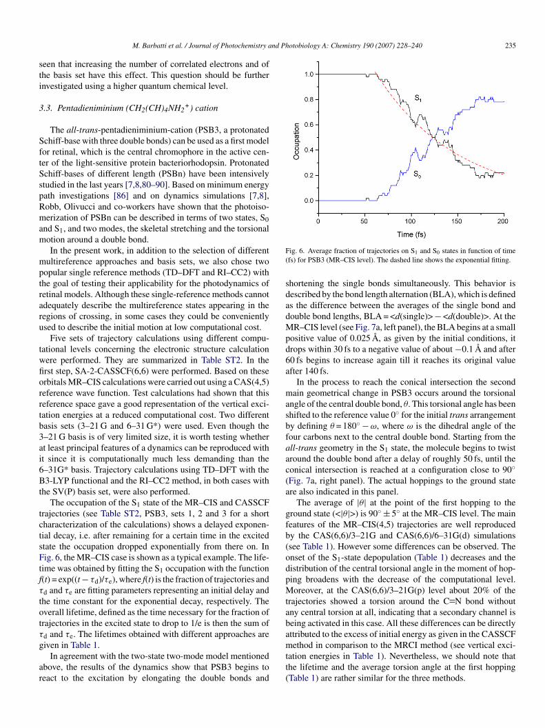
rajectories (see Table ST2, PSB3, sets 1, 2 and 3 for a shortharacterization of the calculations) shows a delayed exponen-ial decay, i.e. after remaining for a certain time in the excitedtate the occupation dropped exponentially from there on. Inig. 6, the MR–CIS case is shown as a typical example. The life-

ime was obtained by fitting the S1 occupation with the function(t) = exp((t − τd)/τe), where f(t) is the fraction of trajectories andd and τe are fitting parameters representing an initial delay andhe time constant for the exponential decay, respectively. Theverall lifetime, defined as the time necessary for the fraction ofrajectories in the excited state to drop to 1/e is then the sum ofd and τe. The lifetimes obtained with different approaches are

iven in Table 1.

In agreement with the two-state two-mode model mentionedbove, the results of the dynamics show that PSB3 begins toeact to the excitation by elongating the double bonds and

mtt(

ig. 6. Average fraction of trajectories on S1 and S0 states in function of timefs) for PSB3 (MR–CIS level). The dashed line shows the exponential fitting.

hortening the single bonds simultaneously. This behavior isescribed by the bond length alternation (BLA), which is defineds the difference between the averages of the single bond andouble bond lengths, BLA = <d(single)> − <d(double)>. At theR–CIS level (see Fig. 7a, left panel), the BLA begins at a small

ositive value of 0.025 A, as given by the initial conditions, itrops within 30 fs to a negative value of about −0.1 A and after0 fs begins to increase again till it reaches its original valuefter 140 fs.

In the process to reach the conical intersection the secondain geometrical change in PSB3 occurs around the torsional

ngle of the central double bond, θ. This torsional angle has beenhifted to the reference value 0◦ for the initial trans arrangementy defining θ = 180◦ −ω, where ω is the dihedral angle of theour carbons next to the central double bond. Starting from thell-trans geometry in the S1 state, the molecule begins to twistround the double bond after a delay of roughly 50 fs, until theonical intersection is reached at a configuration close to 90◦Fig. 7a, right panel). The actual hoppings to the ground statere also indicated in this panel.

The average of |θ| at the point of the first hopping to theround state (<|θ|>) is 90◦ ± 5◦ at the MR–CIS level. The maineatures of the MR–CIS(4,5) trajectories are well reproducedy the CAS(6,6)/3–21G and CAS(6,6)/6–31G(d) simulationssee Table 1). However some differences can be observed. Thenset of the S1-state depopulation (Table 1) decreases and theistribution of the central torsional angle in the moment of hop-ing broadens with the decrease of the computational level.oreover, at the CAS(6,6)/3–21G(p) level about 20% of the

rajectories showed a torsion around the C N bond withoutny central torsion at all, indicating that a secondary channel iseing activated in this case. All these differences can be directlyttributed to the excess of initial energy as given in the CASSCF

ethod in comparison to the MRCI method (see vertical exci-

ation energies in Table 1). Nevertheless, we should note thathe lifetime and the average torsion angle at the first hoppingTable 1) are rather similar for the three methods.

236 M. Barbatti et al. / Journal of Photochemistry and Photobiology A: Chemistry 190 (2007) 228–240

Table 1Vertical excitation energies (eV), averages of the absolute value of the central torsional angle (degrees) at the first hopping event, onset of the S1-state depopulation(τd, in fs), and the lifetime (τd + τe, in fs) obtained from the dynamics simulation of PSB3

Level Evert (eV) <|θ|> (degrees) τd (fs) Lifetime (fs)

MR–CIS(4,5)/3–21G 4.38 90 ± 5 62.5 149SA-2-CASSCF(6,6)/6–31G* 4.76 92 ± 10 47.5 130SA-2-CASSCF(6,6)/3–21G 4.85 91 ± 16a 32.5 153TR

nd.

adUt

a

FT

D–DFT(B3-LYP)/S V(P) 4.37I–CC2/SV(P) 4.39

a Including only the trajectories showing torsion around the central double bo

The lack of nonadiabatic coupling vectors in TD–DFT

nd RI–CC2 methods restricts the calculations to an adiabaticynamics, i.e. to a dynamics on the S1 surface in this case.nfortunately, the TD–DFT approach proved inadequate for

he PSB3 simulation even in the beginning of the dynamics,

lctR

ig. 7. Bond-length-alternation (BLA, in A) and central torsion angle (|θ|, in degreeshe diamonds in (a, right panel) indicate the first S1 → S0 hopping events.

– – –– – –

s can be observed from the BLA behavior shown in Fig. 7b,

eft panel. Similar conclusions was already drawn from the staticalculations of Refs. [80,87]. Moreover, a detailed analysis ofhe shortcomings of TD–DFT in this case has been given inef. [87]. Even more impressive is the complete lack of acti-

) for PSB3 for each trajectory with (a) MR–CIS, (b) TD–DFT, and (c) RI–CC2.

M. Barbatti et al. / Journal of Photochemistry and Photobiology A: Chemistry 190 (2007) 228–240 237

F4m

vp

teFsTlc

3

Udp[src

iamutcetmicpdgqa

Fsa

ssttGau

dncpfsbbcsta2wi

4

ac

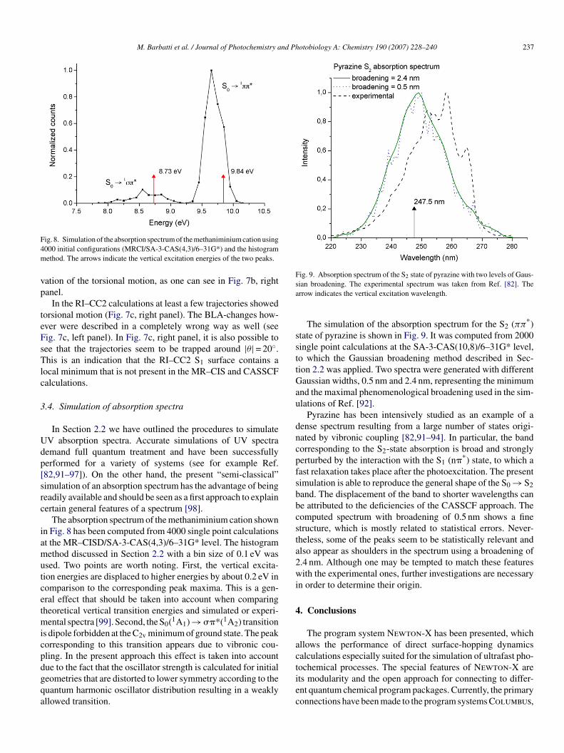
ig. 8. Simulation of the absorption spectrum of the methaniminium cation using000 initial configurations (MRCI/SA-3-CAS(4,3)/6–31G*) and the histogramethod. The arrows indicate the vertical excitation energies of the two peaks.

ation of the torsional motion, as one can see in Fig. 7b, rightanel.

In the RI–CC2 calculations at least a few trajectories showedorsional motion (Fig. 7c, right panel). The BLA-changes how-ver were described in a completely wrong way as well (seeig. 7c, left panel). In Fig. 7c, right panel, it is also possible toee that the trajectories seem to be trapped around |θ| = 20◦.his is an indication that the RI–CC2 S1 surface contains a

ocal minimum that is not present in the MR–CIS and CASSCFalculations.

.4. Simulation of absorption spectra

In Section 2.2 we have outlined the procedures to simulateV absorption spectra. Accurate simulations of UV spectraemand full quantum treatment and have been successfullyerformed for a variety of systems (see for example Ref.82,91–97]). On the other hand, the present “semi-classical”imulation of an absorption spectrum has the advantage of beingeadily available and should be seen as a first approach to explainertain general features of a spectrum [98].

The absorption spectrum of the methaniminium cation shownn Fig. 8 has been computed from 4000 single point calculationst the MR–CISD/SA-3-CAS(4,3)/6–31G* level. The histogramethod discussed in Section 2.2 with a bin size of 0.1 eV was

sed. Two points are worth noting. First, the vertical excita-ion energies are displaced to higher energies by about 0.2 eV inomparison to the corresponding peak maxima. This is a gen-ral effect that should be taken into account when comparingheoretical vertical transition energies and simulated or experi-

ental spectra [99]. Second, the S0(1A1) → ��*(1A2) transitions dipole forbidden at the C2v minimum of ground state. The peakorresponding to this transition appears due to vibronic cou-ling. In the present approach this effect is taken into account

ue to the fact that the oscillator strength is calculated for initialeometries that are distorted to lower symmetry according to theuantum harmonic oscillator distribution resulting in a weaklyllowed transition.

tiec

ig. 9. Absorption spectrum of the S2 state of pyrazine with two levels of Gaus-ian broadening. The experimental spectrum was taken from Ref. [82]. Therrow indicates the vertical excitation wavelength.

The simulation of the absorption spectrum for the S2 (ππ*)tate of pyrazine is shown in Fig. 9. It was computed from 2000ingle point calculations at the SA-3-CAS(10,8)/6–31G* level,o which the Gaussian broadening method described in Sec-ion 2.2 was applied. Two spectra were generated with differentaussian widths, 0.5 nm and 2.4 nm, representing the minimum

nd the maximal phenomenological broadening used in the sim-lations of Ref. [92].

Pyrazine has been intensively studied as an example of aense spectrum resulting from a large number of states origi-ated by vibronic coupling [82,91–94]. In particular, the bandorresponding to the S2-state absorption is broad and stronglyerturbed by the interaction with the S1 (n�*) state, to which aast relaxation takes place after the photoexcitation. The presentimulation is able to reproduce the general shape of the S0 → S2and. The displacement of the band to shorter wavelengths cane attributed to the deficiencies of the CASSCF approach. Theomputed spectrum with broadening of 0.5 nm shows a finetructure, which is mostly related to statistical errors. Never-heless, some of the peaks seem to be statistically relevant andlso appear as shoulders in the spectrum using a broadening of.4 nm. Although one may be tempted to match these featuresith the experimental ones, further investigations are necessary

n order to determine their origin.

. Conclusions

The program system Newton-X has been presented, whichllows the performance of direct surface-hopping dynamicsalculations especially suited for the simulation of ultrafast pho-

ochemical processes. The special features of Newton-X arets modularity and the open approach for connecting to differ-nt quantum chemical program packages. Currently, the primaryonnections have been made to the program systems Columbus,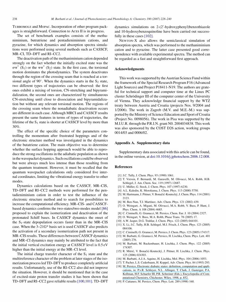

2 nd Ph

Ta

nptM

s�mtstodCttapl3

teowdibtqnm

TteibpptctMath

mmrtoT

daf

acsb

A

tLfcot1p(Mw0

A

i

R

38 M. Barbatti et al. / Journal of Photochemistry a

urbomole and Mopac. Incorporation of other program pack-ges is straightforward. Connection to Aces II is in progress.

The set of benchmark examples consists of the metha-iminium, butratriene and pentadieniminium cations, andyrazine, for which dynamics and absorption spectra simula-ions were performed using several methods such as CASSCF,

R–CI, TD–DFT and RI–CC2.The deactivation path of the methaniminium cation depended

trongly on the fact whether the initially excited state was the�* (S1) or the ��* (S2) state. In the first case, the torsionalotion dominates the photodynamics. The system deactivates

hrough the region of the crossing seam that is reached at a tor-ional angle of 90◦. When the dynamics starts in the S2 state,wo different types of trajectories can be observed: the firstnes exhibit a mixing of torsion, CN-stretching and bipyrami-alization, the second ones are characterized by simultaneousN-stretching until close to dissociation and bipyramidaliza-

ion but without any relevant torsional motion. The regions ofhe crossing seam where the nonadiabatic deactivation occursre different in each case. Although MRCI and CASSCF resultsresent the same features in terms of types of trajectories, theifetime of the S1 state is shorter at CASSCF level by more than0%.

The effect of the specific choice of the parameters con-rolling the momentum after frustrated hoppings and of thelectronic structure method was investigated in the dynamicsf the butatriene cation. The main objective was to determinehether the surface hopping approach would be able to repro-uce the strong oscillations in the adiabatic population as shownn the wavepacket dynamics. Such oscillations could be observedut were always much less intense than those resulting fromhe quantum treatment. However, it must be recalled that theuantum wavepacket calculations only considered five inter-al coordinates, limiting the vibrational energy transfer to otherodes.Dynamics calculations based on the CASSCF, MR–CIS,

D–DFT and RI–CC2 methods were performed for the pen-adieniminium cation in order to test the influence of thelectronic structure method and to search for possibilities toncrease the computational efficiency. MR–CIS- and CASSCF-ased dynamics confirms the two-states/two-modes model [86]roposed to explain the isomerization and deactivation of therotonated Schiff bases. In CASSCF dynamics the onset ofhe S1-state depopulation occurs faster than in the MR–CISase. When the 3–21G* basis set is used CASSCF also predictshe activation of a secondary isomerization path not present in

R–CIS results. These differences between CASSCF dynamicsnd MR–CI dynamics may mainly be attributed to the fact thathe initial vertical excitation energy at CASSCF level is 0.5 eVigher than the initial energy at the MR–CI level.

The initial charge transfer character of the S1 state and theultireference character of the problem at later stages of the iso-erization process led TD–DFT to produce completely artificial

esults. Unfortunately, use of the RI–CC2 also did not improvehe situation. However, it should be mentioned that in the casef excited-state proton transfer studies it has been shown thatD–DFT and RI–CC2 gave reliable results [100,101]. TD–DFT

otobiology A: Chemistry 190 (2007) 228–240

ynamics simulations on 2-(2′-hydroxyphenyl)benzothiazolend 10-hydroxybenzoquinoline have been carried out success-ully in these cases [102].

Newton-X also allows the semiclassical simulation ofbsorption spectra, which was performed to the methaniminiumation and to pyrazine. The latter case presented good corre-pondence with available experimental spectra. The method cane regarded as a fast and straightforward first approach.

cknowledgments

This work was supported by the Austrian Science Fund withinhe framework of the Special Research Program F16 (Advancedight Sources) and Project P18411-N19. The authors are grate-

ul for technical support and computer time at the Linux PCluster Schrodinger III of the computer center of the Universityf Vienna. They acknowledge financial support by the WTZreaty between Austria and Croatia (projects Nos. 9/2004 and/2006). The work in Zagreb (M.V. and M.E.-M.) was sup-orted by the Ministry of Science Education and Sport of CroatiaProject No. 0098056). The work in Pisa was supported by the

.I.U.R. through the P.R.I.N. grant N0. 2004034838. This workas also sponsored by the COST D26 action, working groups014/03 and 0006/02.

ppendix A. Supplementary data

Supplementary data associated with this article can be found,n the online version, at doi:10.1016/j.jphotochem.2006.12.008.

eferences

[1] J.C. Tully, J. Chem. Phys. 93 (1990) 1061.[2] T. Vreven, F. Bernardi, M. Garavelli, M. Olivucci, M.A. Robb, H.B.

Schlegel, J. Am. Chem. Soc. 119 (1997) 12687.[3] U. Muller, G. Stock, J. Chem. Phys. 107 (1997) 6230.[4] A.L. Kaledin, K. Morokuma, J. Chem. Phys. 113 (2000) 5750.[5] M. Hartmann, J. Pittner, V. Bonacic-Koutecky, J. Chem. Phys. 114 (2001)

2123.[6] M. Ben-Nun, T.J. Martınez, Adv. Chem. Phys. 121 (2002) 439.[7] O. Weingart, A. Migani, M. Olivucci, M.A. Robb, V. Buss, P. Hunt, J.

Phys. Chem. A 108 (2004) 4685.[8] C. Ciminelli, G. Granucci, M. Persico, Chem. Eur. J. 10 (2004) 2327.[9] O. Weingart, V. Buss, M.A. Robb, Phase Trans. 78 (2005) 17.

[10] A.W. Jasper, D.G. Truhlar, J. Chem. Phys. 122 (2005) 044101.[11] X. Li, J.C. Tully, H.B. Schlegel, M.J. Frisch, J. Chem. Phys. 123 (2005)

084106.[12] C. Ciminelli, G. Granucci, M. Persico, J. Chem. Phys. 123 (2005) 174317.[13] M. Barbatti, G. Granucci, M. Persico, H. Lischka, Chem. Phys. Lett. 401

(2005) 276.[14] M. Barbatti, M. Ruckenbauer, H. Lischka, J. Chem. Phys. 122 (2005)

174307.[15] R. Mitric, V. Bonacic-Koutecky, J. Pittner, H. Lischka, J. Chem. Phys.

125 (2006) 024303.[16] M. Barbatti, A.J.A. Aquino, H. Lischka, Mol. Phys. 104 (2006) 1053.[17] T. Pacher, L.S. Cederbaum, H. Koppel, Adv. Chem. Phys. 84 (1993) 293.

[18] M. Persico, Electronic diabatic states: definition, computation and appli-

cations, in: P.v.R. Schleyer, N.L. Allinger, T. Clark, J. Gasteiger, P.A.Kollman, H.F. Schaefer III, P.R. Schreiner (Eds.), Encyclopedia of Com-putational Chemistry, Chichester, Wiley, 1998, p. 852.

[19] P. Cattaneo, M. Persico, Chem. Phys. Lett. 289 (1998) 160.

nd Ph

M. Barbatti et al. / Journal of Photochemistry a

[20] P. Cattaneo, M. Persico, Theoret. Chem. Acc. 103 (2000) 390.[21] P. Cattaneo, M. Persico, J. Am. Chem. Soc. 123 (2001) 7638.[22] C.R. Evenhuis, X. Lin, D.H. Zhang, D. Yarkony, M.A. Collins, J. Chem.

Phys. 123 (2005) 134110.[23] R.K. Preston, J.C. Tully, J. Chem. Phys. 54 (1971) 4297.[24] J.C. Tully, R.K. Preston, J. Chem. Phys. 55 (1971) 562.[25] S. Hammes-Schiffer, J.C. Tully, J. Chem. Phys. 101 (1994) 4657.[26] J.C. Tully, Faraday Discuss. 110 (1998) 407.[27] D.S. Sholl, J.C. Tully, J. Chem. Phys. 109 (1998) 7702.[28] J.-Y. Fang, S. Hammes-Schiffer, J. Phys. Chem. A 103 (1999) 9399.[29] P.V. Parandekar, J.C. Tully, J. Chem. Phys. 122 (2005) 094102.[30] M. Desouter-Lecomte, J.C. Leclerc, J.C. Lorquet, Chem. Phys. 9 (1975)

147.[31] H.-D. Meyer, W.H. Miller, J. Phys. Chem. 70 (1979) 3214.[32] G.D. Billing, Int. Rev. Phys. Chem. 13 (1994) 309.[33] G. Stock, J. Chem. Phys. 103 (1995) 1561.[34] X. Sun, W.H. Miller, J. Chem. Phys. 106 (1997) 6346.[35] C. Zhu, S. Nangia, A.W. Jasper, D.G. Truhlar, J. Chem. Phys. 121 (2004)

7658.[36] M. Barbatti, G. Granucci, H. Lischka, M. Persico, M. Ruckenbauer,

Newton-X: a package for Newtonian dynamics close to the crossingseam, version 0.11b, www.univie.ac.at/newtonx, 2006.

[37] A. Ferretti, G. Granucci, A. Lami, M. Persico, G. Villani, J. Chem. Phys.104 (1996) 5517.

[38] L. Verlet, Phys. Rev. 159 (1967) 98.[39] W.C. Swope, H.C. Andersen, P.H. Berens, K.R. Wilson, J. Chem. Phys.

76 (1982) 37.[40] D.L. Bunker, Meth. Comput. Phys. 10 (1971) 287.[41] J. Butcher, J. Assoc. Comput. Mach. 12 (1965) 124.[42] N.S. Bakhvalov, Numerical Methods, Mir publishers, Moscow, 1977, p.

495.[43] G. Granucci, M. Persico, A. Toniolo, J. Chem. Phys. 114 (2001) 10608.[44] J.J.P. Stewart, Mopac 2000 and Mopac 2002. Fujitsu Limited, Tokio,

Japan.[45] H. Lischka, R. Shepard, F.B. Brown, I. Shavitt, Int. J. Quant. Chem.,

Quant. Chem. Symp. 15 (1981) 91.[46] R. Shepard, I. Shavitt, R.M. Pitzer, D.C. Comeau, M. Pepper, H. Lischka,

P.G. Szalay, R. Ahlrichs, F.B. Brown, J. Zhao, Int. J. Quant. Chem., Quant.Chem. Symp. 22 (1988) 149.

[47] H. Lischka, R. Shepard, I. Shavitt, R.M. Pitzer, M. Dallos, Th. Muller,P.G. Szalay, F.B. Brown, R. Ahlrichs, H.J. Bohm, A. Chang, D.C.Comeau, R. Gdanitz, H. Dachsel, C. Ehrhardt, M. Ernzerhof, P. Hochtl,S. Irle, G. Kedziora, T. Kovar, V. Parasuk, M.J.M. Pepper, P. Scharf,H. Schiffer, M. Schindler, M. Schuler, M. Seth, E.A. Stahlberg, J.-G.Zhao, S. Yabushita, Z. Zhang, M. Barbatti, S. Matsika, M. Schuur-mann, D.R. Yarkony, S.R. Brozell, E.V. Beck, J.-P. Blaudeau, Columbus,an ab initio electronic structure program, release 5.9.1 (2006, seehttp://www.univie.ac.at/columbus).

[48] H. Lischka, R. Shepard, R.M. Pitzer, I. Shavitt, M. Dallos, Th. Muller,P.G. Szalay, M. Seth, G.S. Kedziora, S. Yabushita, Z. Zhang, Phys. Chem.Chem. Phys. 3 (2001) 664.

[49] R. Ahlrichs, M. Bar, M. Haser, H. Horn, C. Kolmel, Chem. Phys. Letters162 (1989) 165.

[50] A. Kohn, C. Hattig, J. Chem. Phys. 119 (2003) 5021.[51] C. Hattig, J. Chem. Phys. 118 (2003) 7751.[52] R. Bauernschmitt, R. Ahlrichs, Chem. Phys. Lett. 256 (1996) 454.[53] F. Furche, R. Ahlrichs, J. Chem. Phys. 117 (2002) 7433.[54] J. Gauss, J.D. Watts, W.J. Lauderdale, R.J. Bartlett, Int. J. Quant. Chem.

Symp. 26 (1992) 879.[55] A. Tajti, M. Barbatti, P. G. Szalay, H. Lischka, in preparation.[56] M.W. Schmidt, K.K. Baldridge, J.A. Boatz, S.T. Elbert, M.S. Gordon, J.H.

Jensen, S. Koseki, N. Matsunaga, K.A. Nguyen, S.J. Su, T.L. Windus, M.Dupuis, J.A. Montgomery, J. Comput. Chem. 14 (1993) 1347.

[57] M.J. Frisch, G.W. Trucks, H.B. Schlegel, G.E. Scuseria, M.A. Robb, J.R.Cheeseman, J.A. Montgomery Jr., T. Vreven, K.N. Kudin, J.C. Burant,J.M. Millam, S.S. Iyengar, J. Tomasi, V. Barone, B. Mennucci, M. Cossi,G. Scalmani, N. Rega, G.A. Petersson, H. Nakatsuji, M. Hada, M. Ehara,K. Toyota, R. Fukuda, J. Hasegawa, M. Ishida, T. Nakajima, Y. Honda, O.

otobiology A: Chemistry 190 (2007) 228–240 239

Kitao, H. Nakai, M. Klene, X. Li, J.E. Knox, H.P. Hratchian, J.B. Cross,V. Bakken, C. Adamo, J. Jaramillo, R. Gomperts, R.E. Stratmann, O.Yazyev, A.J. Austin, R. Cammi, C. Pomelli, J.W. Ochterski, P.Y. Ayala,K. Morokuma, G.A. Voth, P. Salvador, J.J. Dannenberg, V.G. Zakrzewski,S. Dapprich, A.D. Daniels, M.C. Strain, O. Farkas, D.K. Malick, A.D.Rabuck, K. Raghavachari, J.B. Foresman, J.V. Ortiz, Q. Cui, A.G. Baboul,S. Clifford, J. Cioslowski, B.B. Stefanov, G. Liu, A. Liashenko, P. Piskorz,I. Komaromi, R.L. Martin, D.J. Fox, T. Keith, M.A. Al-Laham, C.Y.Peng, A. Nanayakkara, M. Challacombe, P.M.W. Gill, B. Johnson, W.Chen, M.W. Wong, C. Gonzalez, J.A. Pople, Gaussian 03, Gaussian Inc.,Wallingford CT, 2004.

[58] E. Wigner, Phys. Rev. 40 (1932) 749.[59] R. Van Harrevelt, M. Van Hemert, J.C. Schatz, J. Chem. Phys. 116 (2002)

6002.[60] D.M. Medvedev, S.K. Gray, E.M. Goldfield, M.J. Lakin, D. Troya, J.C.

Schatz, J. Chem. Phys. 120 (2004) 1231.[61] B.H. Bransden, C.J. Joachain, Physics of Atoms and Molecules, Long-

man, London and New York, 1983.[62] A. Bunge, J. Chem. Phys. 53 (1970) 20.[63] A.D. Becke, J. Chem. Phys. 98 (1993) 5648.[64] J.S. Binkley, J.A. Pople, W.J. Hehre, J. Am. Chem. Soc 102 (1980) 939.[65] W.J. Hehre, R. Ditchfield, J.A. Pople, J. Chem. Phys. 56 (1972) 2257.[66] A. Schafer, H. Horn, R. Ahlrichs, J. Chem. Phys. 97 (1992) 2571.[67] R. Shepard, H. Lischka, P.G. Szalay, T. Kovar, M. Ernzerhof, J. Chem.

Phys. 96 (1992) 2085.[68] H. Lischka, M. Dallos, R. Shepard, Mol. Phys. 100 (2002) 1647.[69] H. Lischka, M. Dallos, P.G. Szalay, D.R. Yarkony, R. Shepard, J. Chem.

Phys. 120 (2004) 7322.[70] M. Dallos, H. Lischka, R. Shepard, D.R. Yarkony, P.G. Szalay, J. Chem.

Phys. 120 (2004) 7330.[71] V. Bonacic-Koutecky, K. Schoffel, J. Michl, Theor. Chim. Acta 72 (1987)

459.[72] J. Michl, V. Bonacic-Koutecky, Electronic Aspects of Organic Photo-

chemistry, Wiley, New York, 1990.[73] S. El-Taher, R.H. Hilal, T.A. Albright, Int. J. Quant. Chem. 82 (2001)

242.[74] S. Zilberg, Y. Haas, Photochem. Photobiol. Sci. 2 (2003) 1256.[75] K.F. Donchi, B.A. Rumpf, G.D. Willett, J.R. Christie, P.J. Derrick, J. Am.

Chem. Soc. 110 (1998) 347.[76] E. Uggerud, Mass Spectrom. Rev. 18 (1999) 285.[77] T.H. Choi, S.T. Park, M.S. Kim, J. Chem. Phys. 114 (2001) 6051.[78] S. Yamazaki, S. Kato, J. Chem. Phys. 123 (2005) 114510.[79] P. Du, S.C. Racine, E.R. Davidson, J. Phys. Chem. 64 (1990) 3944.[80] A.J.A. Aquino, M. Barbatti, H. Lischka, Chem. Phys. Chem. 7 (2006)

2089.[81] G. Zechmann, M. Barbatti, H. Lischka, J. Pittner, V. Bonacic-Koutecky,

Chem. Phys. Lett. 418 (2006) 377.[82] G.A. Worth, L.S. Cederbaum, Annu. Rev. Phys. Chem. 55 (2004) 127.[83] Chr. Cattarius, G.A. Worth, H.-D. Meyer, L.S. Cederbaum, J. Chem. Phys.

115 (2001) 2088.[84] G.A. Worth, P. Hunt, M. Robb, J. Phys. Chem. A 107 (2003) 621.[85] A. Viel, R.P. Krawczyk, U. Manthe, W. Domcke, J. Chem. Phys. 120

(2004) 11000.[86] R. Gonzalez-Luque, M. Garavelli, F. Bernardi, M. Merchan, M.A. Robb,

M. Olivucci, Proc. Natl. Acad. Sci. U.S.A. 97 (2000) 9379.[87] M. Wanko, M. Garavelli, F. Bernardi, T.A. Niehaus, T. Frauenheim, M.

Elstner, J. Chem. Phys. 120 (2004) 1674.[88] A. Cembran, F. Bernardi, M. Olivucci, M. Garavelli, J. Am. Chem. Soc.

126 (2004) 16018.[89] J. Hufen, M. Sugihara, V. Buss, J. Phys. Chem. 108 (2004) 20419.[90] M. Garavelli, Theor. Chem. Acc. 116 (2006) 87.[91] T. Gerdts, U. Manthe, Chem. Phys. Lett. 295 (1998) 167.[92] A. Raab, G.A. Worth, H.-D. Meyer, L.S. Cederbaum, J. Chem. Phys. 110

(1999) 936.[93] M. Thoss, W.H. Miller, G. Stock, J. Chem. Phys. 112 (2000) 10282.[94] D.V. Shalashilin, M.S. Child, J. Chem. Phys. 121 (2004) 3563.[95] B. Schubert, H. Koppel, H. Lischka, J. Chem. Phys. 122 (2005) 184312.[96] W.J.D. Beenken, H. Lischka, J. Chem. Phys. 123 (2005) 144311.

2 nd Ph

40 M. Barbatti et al. / Journal of Photochemistry a

[97] A. Markmann, G.A. Worth, S. Mahapatra, H.-D. Meyer, H. Koppel, L.S.

Cederbaum, J. Chem. Phys. 123 (2005) 204310.

[98] J.P. Bergsma, P.H. Berens, K.R. Wilson, D.R. Fredkin, E.J. Heller, J. Phys.Chem. 88 (1984) 612.

[99] Y.J. Bomble, K.W. Sattelmeyer, J.F. Stanton, J. Gauss, J. Chem. Phys.121 (2004) 5236.

otobiology A: Chemistry 190 (2007) 228–240

[100] A.L. Sobolewski, W. Domcke, Phys. Chem. Chem. Phys. 1 (1999)

3065.

[101] A.J.A. Aquino, H. Lischka, C. Hattig, J. Phys. Chem. A 109 (2005)3201.

[102] R. de Vivie-Riedle, E. Riedle, A.J.A. Aquino, D. Tunega, M. Barbatti, H.Lischka, to be submitted for publication.