the morphology and development of folds a
TRANSCRIPT
THE MORPHOLOGY AND DEVELOPMENT OF FOLDS
A thesis submitted for the degree of Ph.D.
of the University of London
by
Peter John Hudleston
May 1969
2
ABSTRACT
This thesis is concerned with the description, classification, analysis
and interpretation of folds based on their morphologic properties.
Existing methods of geometrical fold analysis are critically examined.
Many are found to be impracticable. Two new analytical techniques are
presented, one based on the use of dip isogons and the other based on
harmonic analysis. A Visual method of rapid harmonic analysis is described
that involves no measurements.
Theories of fold development are discussed with particular reference
to folds developed by buckling in isolated competent layers embedded in
a less competent matrix. The geometric form of folds predicted by theory
are examined. Emphasis is placed on the geometric forms taken up by
buckle folds and by buckle folds modified by compression.
A series of buckling experiments in single viscous layers embedded
in a less viscous matrix at low viscosity contrasts are described.
Progressive development of the shape of the experimentally formed folds is
analysed and interpreted in terms of buckling theory.
Detailed analyses of minor folds, in small parts of the Moine rocks
in Scotland, the basement gneisses in the Swiss Alps and the Culm sediments
on the Cornish coast are described. In the rocks of each region the
geometric forms of the folds are shown to be different in each fold phase,
and are also shown to be related to differences in layer composition.
By analogy with the forms of folds predicted theoretically and observed
experimentally the geometric forms of the natural folds are accounted
for by processes of buckling and 'flattening'. Estimates of 'viscosity'
contrast and bulk deformation within the profile planes of the folds are
made in two instances.
3
CONTENTS Page
CHAPTER 1 INTRODUCTION
1.1 General Statement 7 1.2 Soto Definiticns of Terms 9 1.3 Symbols Used in the Text 10
CHAPTER 2 DESCRIPTIVE FOLD GEOMETRY
2.1 Introduction 12
2.2 General Geometry 12
2.3 Folded Layer Geometry 15 2.3.1 Thickness Parameters 16
2.3.2 Isogons 16 2.3.3 Isogon Plot - k against a 21 2.3.4 Relationship between ta l 0a, and a 22 2.3.5 Fold Classification 26 2.3.6 Errors in Measurement and Datum Fixing 35 2.3.7 Discussion 36
2.4 The Geometry of Single Folded Surfaces 39 2.5 Harmonic (Fourier) Analysis of Folds 42
2.5.1 Fourier Analysis in Geology 45 2.5.2 Fold Analysis using Harmonic Analysis 45 2.5.3 Theory 46 2.5.4 Selection of Coordinates for Analysis 50 2.5.5 Procedure for Analysis 51 2.5.6 Representation of Computed Coefficients 52 2.5.7 Visual Harmonic Analysis 63 2.5.8 Errors and Reproducibility 68
2.6 Techniques of Natural Fold Measurement 71
CILIPThii 3 THE THEORIES OF FOLD DEVELOPMENT AND GEOMETRIC FORM OF FOLDS.
3.1 Introduction 73
3.2 Passive Folds 74
3.3 Exact Mathematical Treatments 75
4
Page
3.4 The Shape of Buckled Layers 84
3.5 Homogeneous Flattening of Folds 86
3.5.1 Oblique Flattening in the Profile.Plane 99
3.6 Simultaneous Buckling and Flattening 99
CHAPTER 4 EXPERIMENTS ON BUCKLING
4.1 Introduction 107
4.2 Model Study Problems 109
4.3 Apparatus and Materials 110
4.4 Experimental Methods 118
4.5 Homogeneity of Strain and Boundary Effects 122
4.6 Results 127
4.6.1 Changes in Arc Length 127
4.6.2 Thickness Variation in the Buckled Layers 134
4.6.3 Wavelength/Thickness Ratios 135
4.6.4 Amplification 135
4.6.5 Harmonic Analysis of Fold Shape 138
4.6.6 aperimental Simultaneous Buckling and Flattening. 143
4.7 Interpretation 150
4.8 Discussion 154
4.9 Interpretation of Naturally Formed Folds 161
4.10 Conclusions 163
CHAPTER 5 AN ANALYSIS OF MINOR FOLDS IN THE MOINIAN ROCKS OF
MONAR, INVERNESS—SHIRE.
5.1 Introduction 164
5.2 Lithology 164
5.3 Metamorphism 170
5.4 Structural Geology 170
5.4.1 Rock Fabric 171
5.5 Descriptive Geometry 171
5
Page_
5.5.1 Size of Folds 174
5.5.2 Fold Order and Asymmetry 177
5.5.3 Isogon Patterns 180
5.5.4 Interlimb Angle Variation 180
5.5.5 Thickness/Dip Variations 185 5.5.6 Harmonic Analysis of Fold Shape 202
5.5.6.1 Analysis of b1 205
5.5.6.2 Analysis of b3/b1 208
5.6 Interpretation 223
5.6.1 Discussion 228
5.7 A Study of Wavelength/Thickness in Ptygmatic Folds in
Pegmatitic Veins 230
5.8 An Analysis of Deformed Lineations 239
5.9 Conclusions 248
CHAPTER 6 AN ANALYSIS OF MINOR FOLDS IN PART OF THE MAGGIA
NAPPE„ TICINO, SWITZERLAND
6.1 Introduction 250
6.1.1 Lithology and Mineralogy 253
6.1.2 Metamorphism 253
6.2 Structural Geology 254
6.2.1 Mineral Fabric 261
6.3 Descriptive Geometry 261
6.3.1 Isogon Plots and Thickness/Dip Relationships 262
6.3.2 Harmonic Analysis of Fold Shape 275
6.3.3 Refolded Folds 281
6.4 Interpretation 281
6.4.1 Discussion 289
6.5 A Wavelength/Thickness Study of F2 Folds 291
6.6 Conclusions 294
Page
CHAPTER 7 AN ANALYSIS OF MINOR FOLDS IN THE CULM MEASURES
AT BOSCASTLE, CORNWALL
7.1 Introduction 297
7.1.1 Lithology 297
7.2 Structural Geology 300
7.2.1 Fabric 306
7.3 Descriptive Geometry 307
7.3.1 Isogon Plots and Thickness/Dip Relationships 308
7.3.2 Harmonic Analysis of Fold Shape 318
7.3.3 Deformed Lineation Loci 321
7.3.4 Interlimb Angles and Limb Length Ratios 321
7.3.5 Miscellaneous Features 328
7.4 Interpretation and Discussion 328
7.5 Conclusions 336
CHAPTER 8 SYNTHESIS
8.1 A Comparison of the Results of the Three Detailed 337
Fold Studies 337
8.2 Summary and Conclusions 340
ACKNOWLEDGMENTS 342
REFERENCES 343
APPENDIX 352
6
CHAPTER 1
INTRODUCTION
1.1 GENERAL STATEMENT
In many zones where the earth's crust has been deformed the litho—
logical layers take up folded forms. For many years structural geologists
have speculated as to the processes by which solid rock may become deformed
by ductile flow without fracture, to form these familiar structures; and
in recent years this problem has received increasing attention. Interest
in the subject has followed several lines of approach, all of which have
led to a better understanding of folds and folding processes.
One approach has used mathematical analysis to provide a basis for
predicting the geometrical features of folds (and involved making many
simplifying assumptions for rock). A second approach has studied the
experimental development of folds, usually in materials with properties
scaled to simulate what are believed to be the properties of rock in the
earth's crust. A third approach has investigated the forms of natural
folds, using various methods of geometrical analysis in order to elucidate
the fold geometry. Perhaps the most significant progress in this
direction in recent years has been the elucidation of fold geometry in
zones of complex and repeated deformation (as in the Moine and Dalradian
rocks of Scotland).
It is an unfortunate fact that in natural folds it is seldom possible
to compute the sta- es of strain in the folded layers, and in most folds all
that is available to the structural geologist is the geometric form of
the bedding or foliation surfaces and tectonic structures such as cleavage
or schistosity. Even in the most favourable situation where the state
of strain may be evaluated in natural folds, it is impossible to know the
'strain path' by which the final fold form was attained (Ramsay, 1967,
P.343).
7
8
In any classification of folds their geometric form (in terms of the
shape of both folded layers and individual surfaces) is important, because
it is one feature of folds that is always available for study. Methods
of accurately describing these geometric features are necessary if analysis
and classification of folds are to be made. By use of methods of
accurate fold description a link between the three approaches to folding
referred to above may be made.
Some workers (e.g. Donath & Parker, 1964) consider that fold
classification should be placed on a genetic basis. Whilst this seems
to be the best way of classifying folds it is not practical because fold
genesis in rocks is imperfectly understood at the present time, and has to
be inferred from the end products of folding processes. It seems
advisable to distinguish between classifications based on fold geometry
and those based on folding processes.
In the past geologists have often described the geometrical forms of
folds in general impressions of fold shape and style. This practice has
never been very satisfactory because of the absence of agreed nomenclature,
and because no detailed analysis of fold shape can be made on this basis.
This thesis is primarily concerned with fold morphology and concerns
the problems of fold analysis and classification based upon the geometrical
properties of folds. An attempt is made to link theoretical and experim—
ental work to the interpretation of natural folds by means of detailed
geometrical analysis. Several new analytical techniques are presented
that have proved useful both in the determination of natural fold geometry
and as an aid in the interpretation of folds in terms of folding processes.
No attempt will be made to criticise or analyse the bulk of the
previous work on the subject of folding; the relevant work on each aspect
of folding considered in this thesis will be discussed at the beginning
9
of each Chapter. For general reviews and criticisms of the substantial
literature on folding the reader is referred to the works of Fleuty (1964),
Rast (1964), Whitten (1966a) and Ramsay (1967).
A critical review of the various methods of geometrical fold analysis
is given in Chapter 2, and two new analytical techniques are described.
A technique of harmonic analysis of fold shape is developed and a simple
method of visual harmonic analysis is presented that should be useful to
field geologists.
Theories of fold development and the geometric forms of folds predicted
by these theories are discussed in Chapter 3. Particular emphasis is
placed on the development of folds in a single competent layer embedded
in a less competent matrix. A series of buckling experiments at low
viscosity contrast are described in Chapter 4. By means of geometrical
analysis the results are interpreted in terms of the theories discussed
in Chapter 3. Chapters 5, 6 & 7 concern detailed studies cf minor folds in small parts of major fold belts of Caledonian, Alpine and Hercynian
ages respectively. In these studies systematic differences in fold
geometry are shown to exist between folds of different generations, and
are also shown to be related to differences in layer composition. In
all instances the geometric forms of the folds are shown to be consistent
with simple processes of fold development.
1.2 SOME DEFINITIONS OF TERMS
Many of the terms used in this thesis have generally accepted
meanings and will not be defined here.. The reader is referred to the
works of Turner & Weiss (1963), Fleuty (1964) and Ramsay (1967) for
definitions of these terms.
The domain of a single fold is given by Turner & Weiss (1963, p.105) to
include part of a folded surface between two adjacent inflexion lines
10
(see Turner & Weiss, 1963, fig. 4-15), and this is extended here to include
successive surfaces in a stack of folded layers. The following are
practical definitions of terms relating to the geometry of individual folds
(or two adjacent folds) in profile section.
Limb Length is defined as the distance measured along a single folded
surface between two adjacent hinge points.
Arc Length is defined as the distance measured along a single folded
surface between two inflexion points so as to include a third (this
length is roughly equivalent to two limb lengths). In Chapter 4 arc
length is taken to include several folds in a single folded surface.
Wavelength. A half-wavelength is taken as the straight line distance
between two adjacent inflexion points. In Chapters 4, 5 and 6, to comply
with current usage, the term wavelength is used for arc length in analyses
of arc length/thickness ratios.
Fold Size is taken as the mean of two adjacent limb lengths.
Tightness is defined by the interlimb angle; the angle between the
tangents to the fold surfaces at the inflexion points.
Asymmetry is defined as the ratio of two adjacent limb lengths.
The term strain-slip cleavage is used in Chapter 7 without genetic 4 m-1,1 4 eu,4-4 ..4.1041-vcd.va.v"00
1.3 SYMBOLS USED IN THE TEXT
t = orthogonal thickness of a folded layer.
T = layer thickness parallel to a fold axial surface
. limb dip
angle between an isogon and the normal to the parallel tangents
to the folded surfaces of a layer.
11
an = harmonic coefficients of a cosine series.
bn = harmonic coefficients of a sine series.
1-1 viscosity.
VR = viscosity ratio
X1 = maximum principal
X2 = minimum principal
V1/112
quadratic elongation.
quadratic elongation.
S strain ratio of h. 1 2
R = apparent strain ratio ofiX /f X j 2 1
A = fold amplitude
VT = fold wavelength
d dominant wavelength
natural logarithm
Xd = non—dimensional wavenumber
XI Y, Z axes of finite strain ellipsoid X Y).Z
CHAPTER 2
DESCRIPTIVE FOLD GEOMETRY
2.1 INTRODUCTION
Increasing attention is being paid by structural geologists to the
problem of accurately describing rock structures, and the last few years
have seen the publication of several new techniques of fold analysis.
It is the purpose of this Chapter to examine geometrical methods of fold
analysis and classification.
Section 262 deals briefly with the general features of fold geometry, and the main part of the Chapter is concerned with the geometrical features
of folds in profile section. Two new analytical techniques are
presented in sections 2.3 and 2.5, involving 'dip isogons' and harmonic
analysis respectively. These are discussed in relation to existing
techniques, and a critical appraisal of some of the more recent approaches
to the subject is made. The Chapter ends (sect. 2.6) with a short
account of the techniques used in the practical application of analytical
methods to natural folds.
2.2 GENERAL GEOMETRY
MUch of modern regional structural analysis is based upon the
assumption that folds are either cylindrical or can be - split into sub-
sections that are. The dimensions of most natural (e.g. Campbell, 1958;
Wilson, 1967) and experimentally produced (e.g. Ghodh & Ramberg, 1968)
non-cylindrical folds are usually much greater along the hinge lines than
in a direction normal to the axial surfaces, and adjacent hinge lines are usually within a few degrees of mutual parallelism. Conical folds are
considered to be rare in nature, and on geometrical grounds alone the
'ends' of folds are unlikely to be conical in form (Wilson, 1967), but
rather of a more complex non-cylindrical nature.
12
13
Many natural folds appear to be approximately cylindrical in form (i.e.
they persist with little changes in profile attitude or form, for
distances along their hinge lines that are large compared to their other
dimensions), and this is true for all the folds studied in the later
chapters of this thesis. The geometry of folds may now be considered
in two parts:
a) The attitude of the fold axis, axial surface. and bedding/
foliation surfaces in space.
b) The geometry of the fold in profile.
a) Spatial Attitude of Folds
The attitudes of lines (fold axes, lineations) and planes (axial
surfaces, bealinefoliation surfaces) are amenable to exact measurement
and have for a long time been used in structural geology (and petrofabrics)
as a basis for analysis in which the stereographic projection plays an
important role. Recently, statistical techniques have been established
to calculate the mean attitudes of lines and planes (e.g. Ramsay, 1967,
p.15), the best fit fold axis of cylindrical folds and best fit cone for
conical folds (Loudon, 1964; Whitten, 1966a; Ramsay, 1967, pp.18-27*;
Cruden, 1968; Kelley, 1968) and tedious statistical operations have been
made practical by use of computers (Loudon, 1964). The problem of
testing the significance of orientation data has been discussed by Flinn
(1958) and Stauffer (1966) on an empirical basis, and the methods of
testing observed data against theoretical models is reviewed by Watson
(1966).
Fleuty (1964) proposes terms to define the attitude of folds (i.e.
of axial surface and fold axis).
b) Fold Profile Geometry
Fundamental differences in fold shape have been recognised for some
14
time. Van Hise (1896) was the first to distinguish parallel and
similar folds, and these two types have since re—appeared in practically
all classifications of folds based on fold shape.
Ramsay (1967, pp.359-372) has shown that these are two special
classes of fold in an infinite field of possible shapes. The reason why,
until recently, little systematic study has been made on fold shape is
two—fold. First, most folds except the smallest are exposed in scattered
outcrops and rarely in anything near profile section. Secondly, until
recently few suitable methods have been available to use in such a study.
Considering the first reason, early workers, taking most folds to be
parallel used constructions involving concentric arcs (Busk, 1929),
evolutes and involutes (Mertie, 1940) or similar methods to construct
fold profiles from scattered data. Recently a method of establishing
profile geometry of proved cylindrical folds from scattered data has been
proposed that does not involve initial assumptions about geometry (Phillips
& Byrne, 1968). This problem will not be treated further here; all folds
considered in this thesis are of hand specimen or outcrop size in which
the whole ..fold is accessible for measurement. However, the methods
described in this chapter are all applicable to large folds with irregular
outcrop using similar techniques to those developed by Phillips and Byrne.
Coming to the second reason, several methods have now been proposed
(e.g. LouCon, 1964; Ramsay, 1962a, 1967) for quantitative description of
fold shapes in profile. These will be discussed in the sections below
and several new techniques will be introduced.
Ramsay (1967, ch.7) gives methods of description and classification
of fold geometry in profile and much of the following develops further
his approach. A fundamental and important distinction is made by Ramsay
between the geometry of a single folded surface or form surface (Turner &
15
Weiss, 1963, p.111) and the geometrical features of a layer (i.e. the
geometrical relationship between two or more form surfaces). The two
are to a large extent independent and should not be confused. For
instance, a parallel fold may be bounded by surfaces of an infinite
number of shapes. It should be noted that, except for similar folds
and folds in which the outer and inner arcs are the same shape but differ
in scale (non-congruent similar folds of Mertie, 1959), the shapes of
the inner and outer arcs of a folded layer must differ.
2.3 FOLDED LAYER GEOMETRY
Apart from the methods developed by Ramsay (1967, pp.359-372) few ways of accurately describing folded layer shape have appeared in the
literature. Mukhopadhyay (1964, 1965a) employs methods essentially the same as those of Ramsay. Mertie (1959) presents a classification of folds
based on the use of elliptical arcs in which he accounts for both similar
(his definition of the term 'similar' is looser than that generally
accepted and followed here) and parallel folds in a general treatment
that includes many complex layer shapes. His methods are however more
pertinent to a discussion of single folded surface geometry and are
difficult to interpret in terms of layer shape. They are also difficult
to apply. Williatis (1965, 1967) suggests that many folds are concentric
and may become modified to form folds with elliptical inner and outer
arcs; and Powell (1967) presents an analysis of fold shape on the assum-
ption that folds are either concentric ,or modified concentric. These
methods are restrictive, since they tie layer geometry to a special kind
of single surface geometry.
The most useful ways of describing the geometry of folded layers is
found to be by use of thickness parameters and by study of dip isogons
(Elliott, 1965). Both these topics are discussed at length by Ramsay
(1967, pp. 359-372). Use of Ramsay's thickness parameters, and the new
parameter Oa described below, allow layer geometry of folds to be
analysed separately from single surface geometry.
2.3.1 Thickness Parameters
Thickness of a folded layer is measured between tangents to the
bounding surfaces of the layer at apparent dip a (fig. 2.1a). The •
thickness can either be measured normal to the tangent, orthogonal thickness
t a , or parallel to the axial surface of the fold, Ta . The
relationship between these two is:
Ta cos a = to To = to is the thickness at the fold hinge, and the ratio
-Oa = to /to or
T'Ta /To may be plotted against a (Ramsay, 1967, p.361). For comparison with the 'isogon plot' introduced below, the fold in fig. 2.1a
is represented in fig. 2.2a on a t cl, /a graph.
2.3.2 Isogons
Dip isogons 1965, 1968) are very useful in the analysis of
fold profiles. They are lines of equal apparent dip on a fold section
and their relationship to folded layers and more specifically to relative
curvatures of the layer surfaces is explained in detail by Ramsay (1967,
p.363 et seq.). A discussion of the more general case of isogonic
surfaces is given by Elliott(1968) who uses isogons of pitch of lineation
in a plane in order to elucidate the geometry of 'early' cylindrical
folds that have been overprinted by a later deformation. Ickes (1923),
in determining the geometry of parallel, similar and neutral-surface
folding uses isogons in the same way as described here, although he does
not use the term isogon (see Ickes, fig. 8.5).
A most important feature of Ramsay's approach is his classification
of folded layer shape on the isogon pattern (Ramsay, 1967, p.363-372,
fig. 7.24). This classification is used throughout this thesis and the
main categories are given here:
16
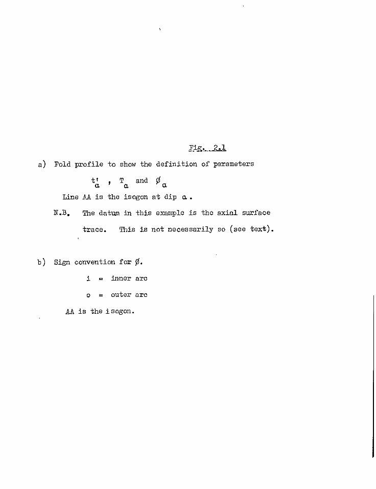
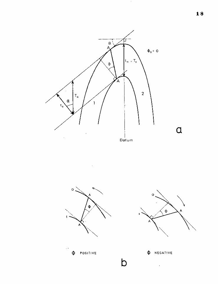
Fig. 2.1
a) Fold profile to show the definition of parameters
ta T
a and 0
a
Line AA is the isogon at dip a.
N.B. The datum in this example is the axial surface
trace. This is not necessarily so (see text).
b) Sign convention for 0.
i = inner arc
o = outer arc
AA is the isogon.
a Datum
1 POSITIVE
4.) NEGATIVE
b
18
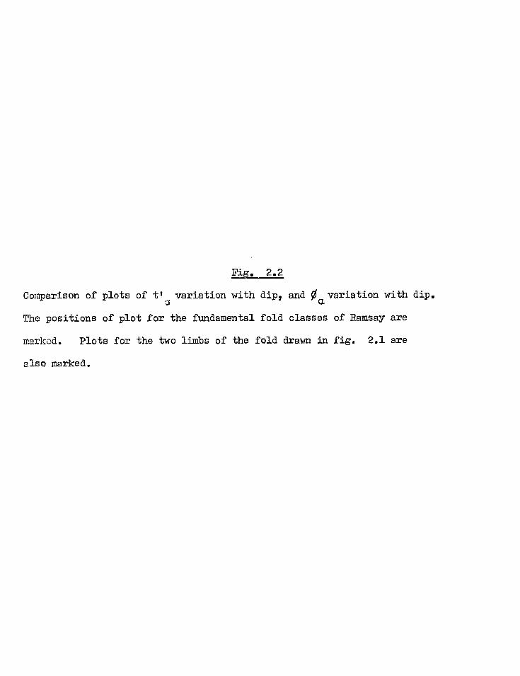
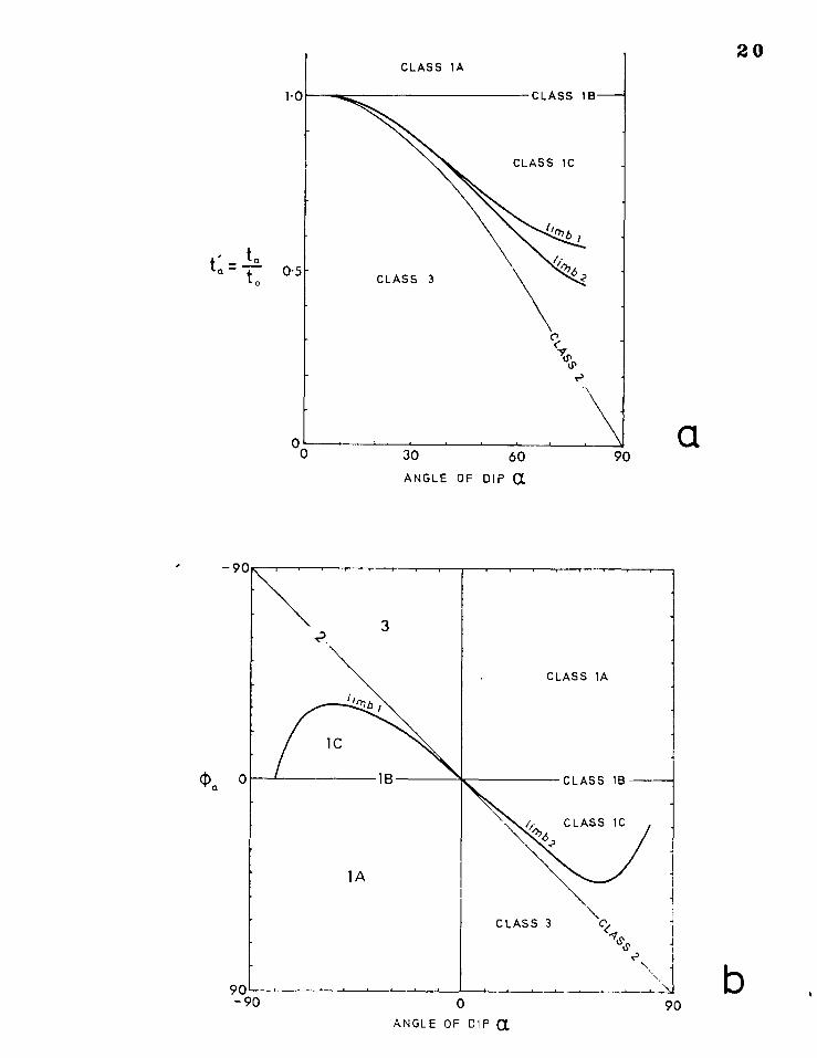
Elg. 2.2
Comparison of plots of -0o variation with dip, and 0o. variation with dip.
The positions of plot for the fundamental fold classes of Ramsay are
marked. Plots for the two limbs of the fold drawn in fig. 2.1 are
also marked.
b 0
ANGLE OF DIP a
CLASS 3
30 60 ANGLE OF DIP a
90
20
a
-90
3
90 -90
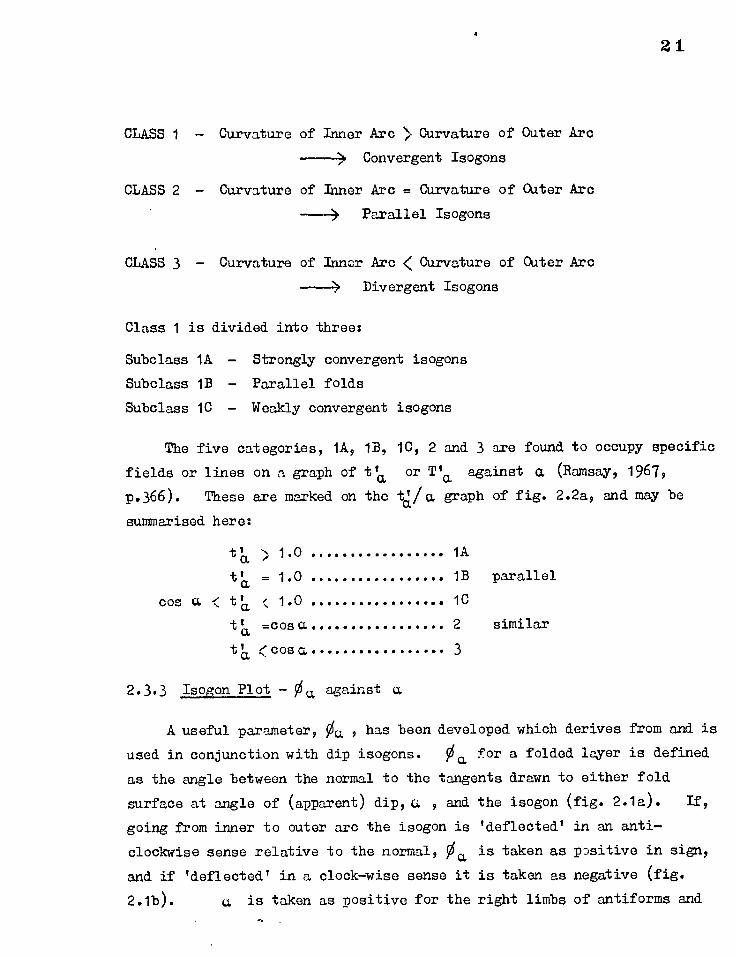
CLASS 1 - Curvature
CLASS 2 - Curvature
of Inner Arc > Curvature of Outer Arc
Convergent Isogons
of Inner Arc = Curvature of Outer Arc
Parallel Isogons
21
CLASS 3 - Curvature of Inncr Arc < Curvature of Outer Arc
----4 Divergent Isogons
Class 1 is divided into three:
Subclass 1A - Strongly convergent isogons
Subclass 1B - Parallel folds
Subclass IC - Weakly convergent isogons
The five categories, 1A, 1B, 1C, 2 and 3 are found to occupy specific fields or lines on a graph of t'a or T'a against a (Ramsay, 19679 p.366). These are marked on the V/(0, graph of fig. 2.2a9 and may be
summarised here:
t'a N 1.0 IA / t:), = 1.0 IB parallel
cos a / -0 ; . a 1.0 1C t'a =cos a 2 similar
to "cos a 3
2.3.3 Isogon Plot - a against a
A useful parameter, has been developed which derives from and is
used in conjunction with dip isogons. 0a for a folded layer is defined as the angle between the normal to the tangents drawn to either fold
surface at angle of (apparent) dip, a 9 and
going from inner to outer arc the isogon is
clockwise sense relative to the normal, 0a,
and if 'deflected' in a clock-wise sense it 2.1b). a is taken as positive for the
the isogon (fig. 2.1a). If,
'deflected' in an anti-
is taken as pDsitive in sign,
is taken as negative (fig.
right limbs of antiforms and
22
the left limbs of synforms, and negative for the other limbs. With
these sign conventions the fold in fig. 2.1a is represented in fig. 2.2b,
a plot of Oa against a . This should be compared with fig. 2.2a, a
plot of tla against a for the same fold.
Folds of the different geometrical classes 1A, 1B, 1C, 2 and 3 occupy
distinct fields or lines on this graph that are analogous to their
representation on a t( /c, graph. These fields are marked on fig. 2.2b
and are defined by values of 00, summarised below (for positive a):
4 0 1A
= 0 1B parallel
> 0 1C
= a 2 similar
>a 3
For practical purposes the signs of a and cla are reversed for plotted
points on the left half of fig. 2.2b and both limbs of a fold are
represented on the right hand side of this graph.
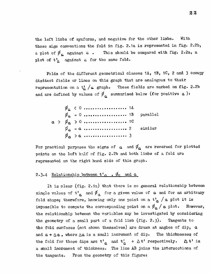
2.3.4 Relationship between -On , Om and a
It is clear (fig. 2.1a) that there is no general relationship between
single values of tta and 0a, for a given value of a and for an arbitrary fold shape; therefore, knowing only one point on a -Oa /a, plot it is impossible to compute tha corresponding point on a Oa/ a, plot. However, the relationship between the variables may be investigated by considering
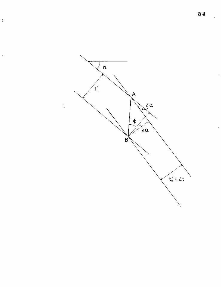
the geometry of a small part of a fold limb (fig. 2.3). Tangents to
the fold surfaces (not shown themselves) are drawn at angles of dip, a and a +60,, where nsLis a small increment of dip. The thicknesses of the fold for these dips are tta and t'a + Zstt respectively. Zst t is
a small increment of thickness. The line AB joins the intersections of
the tangents. From the geometry of this figure:
a >
00. 00. 00,
00. Oa

rig.. 2.3
To show the relationship between t and 0 a in a general case. Tangents
to the folded surfaces of a layer are drawn at two closely spaced values
of dip.
tt = orthogonal thickness at dip a
to -0 = 1 and so
a
24
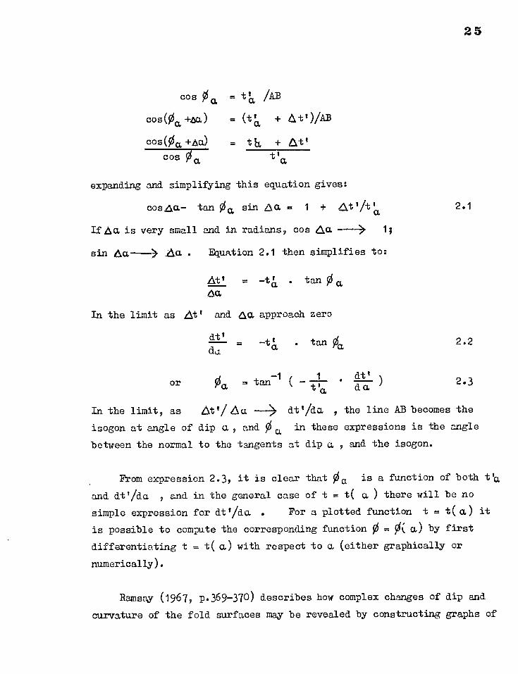
cos 0a = tie, /AB
cos (0a, +.0a) (t'a + At`)/AB
cos (00L +Au) = t b, + cos 0 t ' a a
expanding and simplifying this equation gives:
cos.61— tan Oa, sin Aa = 1 4- 6,-0/t 10,
IfAa is very small and in radians, cos &a 1;
sin 61 ---> . Equation 2.1 then simplifies to:
At' = -t& . tan 0 a 6a
In the limit as At' and eol approach zero
dt' . tan Oa du
Or Oa = tan-1 — 1 1 ' V • ddd'
) 2.3 a
In the limit, as 6.-0/6,a ---) dtlida , the line AB becomes the
isogon at angle of dip a, and O u in these expressions is the angle
between the normal to the tangents at dip a , and the isogon.
From expression 2.3, it is clear that 00. is a function of both t'cl,
and dti/da , and in the general case of t = t( a ) there will be no
simple expression for dtl/da . For a plotted function t = t(a) it
is possible to compute the corresponding function 0 91r( a) by first
differentiating t = t( a) with respect to a (either graphically or
numerically).
Ramsay (1967, p.369-370) describes how complex changes of dip and
curvature of the fold surfaces may be revealed by constructing graphs of
25
2.1
2.2
26
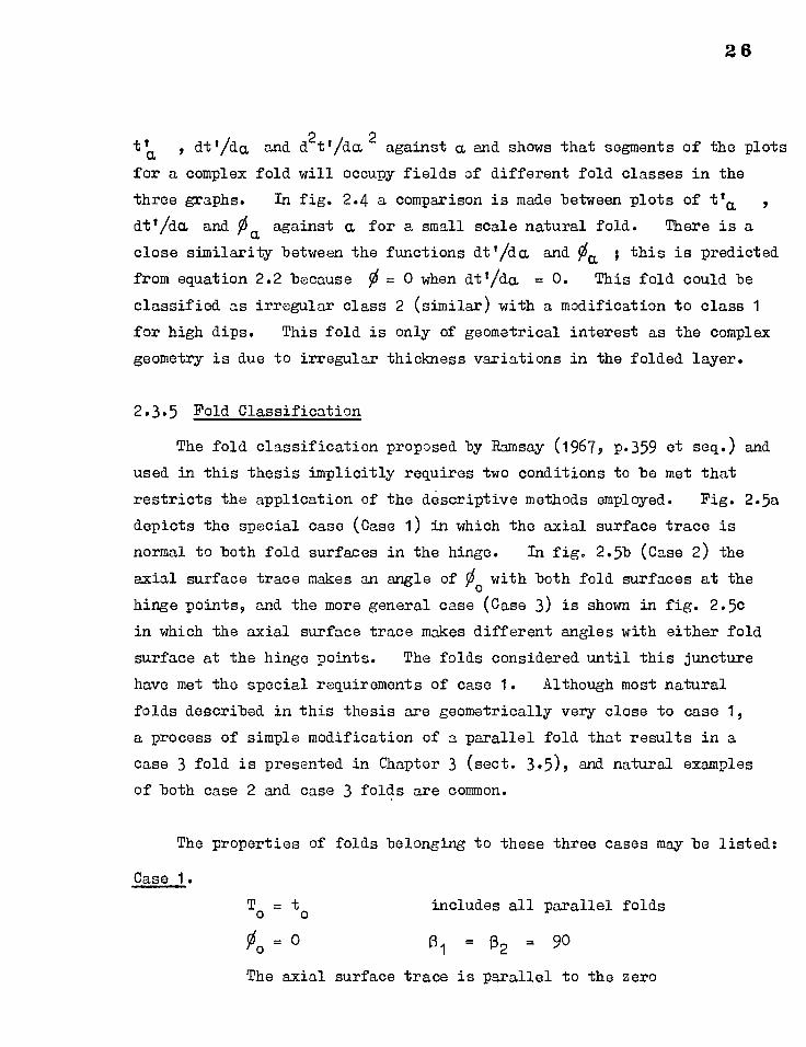
tt a , dtt/da and d2tt/da 2 against a and shows that segments of the plots
for a complex fold will occupy fields of different fold classes in the
three graphs. In fig. 2.4 a comparison is made between plots of tta
dtt/da and 0a against a for a small scale natural fold. There is a close similarity between the functions dtidct, and 0a ; this is predicted from equation 2.2 because 95 = 0 when dtt/do, = 0. This fold could be
classified as irregular class 2 (similar) with a modification to class 1
for high dips. This fold is only of geometrical interest as the complex
geometry is due to irregular thickness variations in the folded layer.
2.3.5 Fold Classification
The fold classification proposed by Ramsay (19679 p.359 et seq.) and
used in this thesis implicitly requires two conditions to be met that
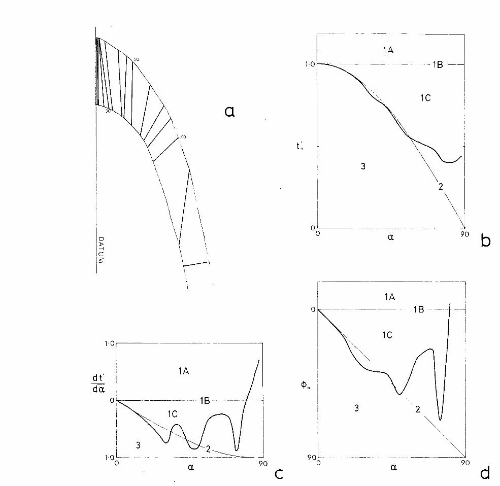
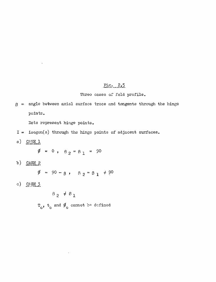
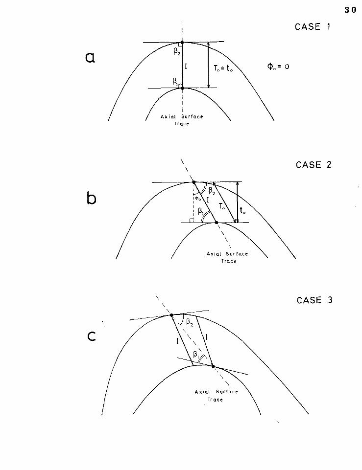
restricts the application of the descriptive methods employed. Fig. 2.5a
depicts the special case (Case 1) in which the axial surface trace is
normal to both fold surfaces in the hinge. In fig. 2.5b (Case 2) the
axial surface trace makes an angle of 00 with both fold surfaces at the
hinge points, and the more general case (Case 3) is shown in fig. 2.5c
in which the axial surface trace makes different angles with either fold
surface at the hinge points. The folds considered until this juncture
have met the special requirements of case 1. Although most natural
folds described in this thesis are geometrically very close to case 1,
a process of simple modification of a parallel fold that results in a case 3 fold is presented in Chapter 3 (sect. 3.5), and natural examples
of both case 2 and case 3 folds are common.
The properties of folds belonging to these three cases may be listed:
Case 1.
T = t 0 0
°o = 0
includes all parallel folds
°I = 02 = 90 The axial surface trace is parallel to the zero

Fig. 2.4
Comparison of various plots for a single fold.
a) Natural fold profile with isogons drawn at 5° intervals of dip
(except for a = 50).
Numbers refer to dip values for particular isogons
Datum line = Axial surface trace
b) c) and d) Various plots for the fold in a).
o > C \
t.
1.0
1A
0 9° b a
1A dt' da
901-- o a
C d 90
1.0
.\
N 90
70
a
Fig, 2.5
Three cases of fold profile.
. angle between axial surface trace and tangents through the hinge
points.
Dots represent hinge points.
= isogon(s) through the hinge points of adjacent surfaces.
a) CASE 1
0 = 0, 2 6 1 = 90
b) CASE 2
0 = 90 —6, 62=R1 90
c) CASE 3. 82 1
To,to and 0o cannot ba defined
I CASE 1
\ CASE 2
\ \ \
Axial Surface Trace
... (1).= 0
Axial Surface Trace
CASE 3
\
Axial Surface
Trace
30
isogon and perpendicular to the tangents at
the hinge points.
Case 2.
T o = t o sec O
0./0 1 = 0, ' 90
The axial surface trace is parallel to the zero
isogon and is oblique to the tangents at the hinge
points.
Case 3.
61 / 62
A zero isogon, To, to and 910 cannot be defined.
The tangents at the hinge points are not parallel.
The axial surface trace intersects the isogons.
To record changes in ta , T a and Oa with a it is necessary to select a datum tangent line, for which a = 0. For case 1 folds this is simple, the datum tangent is normal to the axial trace.
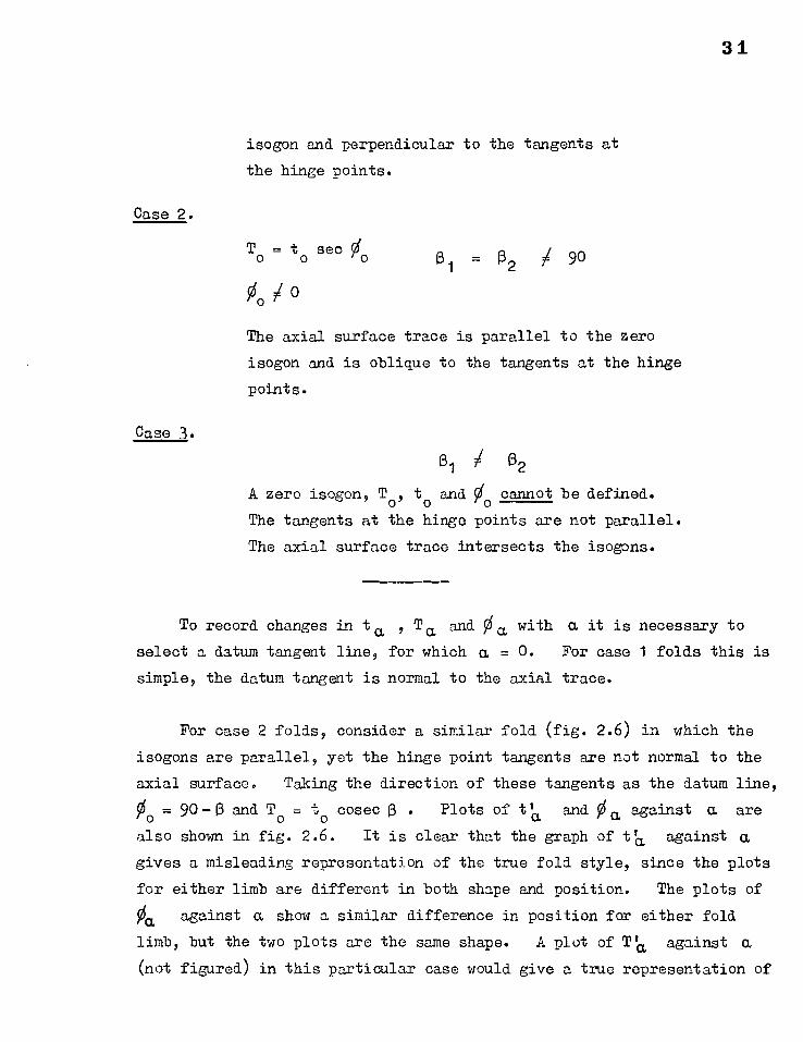
For case 2 folds, consider a similar fold (fig. 2.6) in which the
isogons are parallel, yet the hinge point tangents are not normal to the
axial surface. Taking the direction of these tangents as the datum line,
00 = 90-0 and To = to cosec 0 . Plots of tie. and O a against a are
also shown in fig. 2.6. It is clear that the graph of t'a against a gives a misleading representation of the true fold style, since the plots
for either limb are different in both shape and position. The plots of
Oa against a show a similar difference in position for either fold
limb, but the two plots are the same shape. A plot of Tia against a (not figured) in this particular case would give a true representation of
31

Fig. 2,6
Plots for a Case 2 'similar' fold, with the datum taken as the hinge
point tangents. Isogons are drawn at 20° intervals of dip on the fold
profile.
Note: the sign changes between limbs on the 0 Al plot
3
90
L
L
0 1- 0
1.0
1C t o
i- 90
ANGLE OF DIP a 90
0
34
the similar fold shape (11 = 1 for all a ). By taking as datum the
tangents to the fold surfaces for which Ta = tamax and 0a = 0, the fold
plots would be identical for either limb and would coincide with the plot
for a true similar fold on both the 0a / a and t'a / a graphs.
Considering case 3 folds it is impossible to define a single datum tangent line at the hinge of a fold (see fig. 2.5c). In the same way
as an alternative datum was found for a case 2 similar fold, a datum may
be defined where yf a, = 0 and ta is a maximum (or more rarely a minimum). By defining the datum in this way for natural folds it is found empirically
that plots of t'a against a for either limb of a fold match more closely than they do by defining a reference line in any other way. This
procedure of datum fixing has therefore been used in the fold studies
described in this thesis.
An important difference between a t'a / a and a Ora / a representation becomes apparent here. Because to /to is a ratio it is dependent
upon to , the datum value of ta ; so by varying the position of the
datum and hence the value of t o , the plots of against 04 constructed
for the various datum positions will differ in both shape and position.
00, on the other hand will take the same value whatever tangent plane is
taken for the datum, and so the shape of a 001a, plot will remain constant
however this datum is chosen. A change in datum merely means a
constant addition or subtraction to each a value and is reflected by
a horizontal displacement of the plot of 00. against a. on a Oa/ a graph. For the similar fold in fig. 2.6, the straight line plots of 00. against a
for either limb indicate the true geometry; the plots may be displaced
horizontally (bearing in mind the sign change for the left hand limb)
until the point 0 = 0 coincides with the origin of the graph. It is
clear that an arbitrary datum may be taken to construct a graph of 0a
against a .
All parallel folds must be case 1, even though the datum may be
35
difficult to define unambiguously. True similar folds must be either
case 1 or 2.
The situation may be complicated further by considering multiple
hinge folds (Ramsay, 1967, p.347). For a Oa / a representation these
folds present no problem because no fixed datum is required. If the
curvature of one hinge is much greater than that of the other(s), a datum
tangent line can usually be drawn in the way described above for single
hinged folds and for the purposes of measurement the subsidiary hinge(s)
may be ignored, and a plot of Volt against a may be made. However, if
the curvatures in each of the hinges are of the same order of magnitude,
then to define any single datum may be difficult. In this case a plot
of 00, against a should be made with an arbitrary datum.
The inner and outer arcs of folds should really be. treated as single
folded surfaces when considering curvature and in fact both the inner and
outer arcs of the fold drawn in fig. 2.4 are multiple hinged. However,
the curvature in the main.hing-e is much greater than the minor maxima of
curvature found on the limbs; also the main hinge is the only one for
which a datum tangent may be drawn (where 0 = 0). For practical purposes
this fold may be quite validly considered as a single hinged fold of case 1.
2.3.6 Errors in Measurement and Datum Fixing
If the bounding surfaces of a fold are both smooth, the plots of
and 0a against u for this fold should also be smooth curves. Slight non-systematic variations of plotted points from such smooth curves may be
predicted as a result measurement errors.
There is one kind of systematic error that can appear in these plots
that must be recognised, since when present it may indicate a false
difference in fold geometry between either limb of a fold for which a plot

36
of t'0, against cx has been constructed. The error is in the wrong
selection of the datum tangent and usually arises when the fold has a low
hinge curvature. Neglecting errors in thickness measurement the effect
of this error will be identical to that of choosing the hinge point
tangent as the datum for the fold in fig. 2.6. For a symmetrical fold it
causes the plots of t'a against a for either limb to be of different
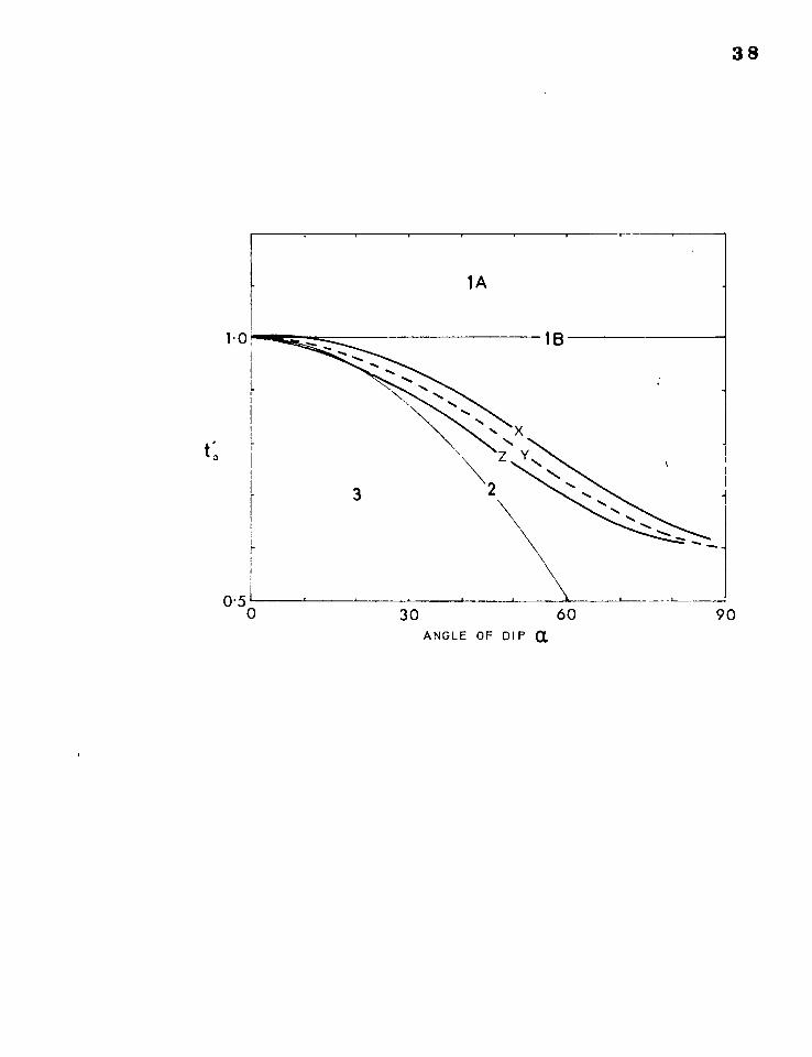
shape and position. A realistic size of error (5°) is included in the
plots of t'a against for an undrawn fold (fig. 2.7). The true plots
of either limb are identical, and are represented by the centre curve on
the graph. The features of this graph may be noted:
a) For an error of 5° in datum positioning, a 100 horizontal separation
of the plots for the two limbs appears.
b) The greater the change of t'ci. with a (i.e. the steeper the slope of
the curve) the greater the apparent separation of the plots for the
two limbs.
c) For small errors, the shapes of the plots for the two limbs are
similar to one another, and to the 'parent' or true plot. (cf.
the plots in fig. 2.7 with those of fig. 2.6).
Errors of this kind may be distinguished from real differences in
geometry between the limbs of a fold by plotting 0 a against a, . If the shapes of the plots for either limb differ on this graph, this indicates
a true difference in limb geometry.
2.3.7 Discussion
Layer geometry of folds has been considered in terms of two main
descriptive parameters, 0a and -Oa . T' has been omitted because it
depends directly upon t'a . Lot us consider the relative merits
of 0a/a and th /0, representations of fold geometry. Listing the
advantages of a 0a /a, representation:
Fig. 2.7
To show the effect on the plots of t' against a of wrongly selecting a
the datum for a symmetrical fold with identical thickness/dip variations
in either limb.
Y is the true plot for either limb
X and Z are the plots for either limb that result when the datum is
taken at an angle of 5° to the 'true' datum.
(The plot Y is for a parallel fold flattened by an
amount f x = 0.6).
30 60 ANGLE OF DIP .
90
c
38
39
a) The most distinct advantage to be gained by use of fei a rather than t'a is the independence of the shape of the Oala. plot on the datum
a used; whilst the correct location of the datum is most important
in constructing a t'a /a plot.
b) Because t'a is a ratio, measured values of ta must be converted to
. This takes time and introduces the possibility of errors.
The measured 0 0, are plotted directly against a.
c) The plotted function of Oa against a is more sensitive to changes in geometry than that of t'a against a (see fig. 2.4) because it
is more or less equivalent to the function dtio, /d a, .
The advantages of a -Oa / a representation are:
a) to is easier to measure than 95awhich requires careful positioning
of tangent points.
b) Errors in O mare larger than in -Oa , and are 'picked up' by the
more sensitive nature of the plot.
c) At high limb dips 0a becomes most inaccurate because the curvature
of the folded surfaces is low and the tangent points are difficult
to locate accurately; on the other hand the most useful part of a
t'a /a plot is that for the highest limb dips.
From these lists it appears that most of the disadvantages of a k /a plot are practical ones. If fold boundaries cannot be accurately defined
by a smooth curve, t'a is best used. is most accurate for folded
layers with clearly defined boundaries of high curvature, and must be used
for multiple hinged folds or folds with obscured hinges.
2.4 THE GEOMETRY OF SINGLE FOLDED SURFACES
Several different approaches have been made by a number of authors

40
to the problems of description of single surface fold morphology, and
these are discussed in this section. Most descriptions of fold style in
the literature are based upon a number of well known terms found in many
structural geology text books (e.g. Hills, 1963, p.215; Turner & Weiss,
1963, p.111). These terms have been reviewed by Fleuty (1964) and
Whitten (1966a). These authors make no distinction between the geometry
of layers and single surfaces.
The geometrical features of single folded surfaces may be considered
as a collection of several attributes that may be taken singly or together.
These include size, shape, tightness and asymmetry. Size is clearly an
independent attribute, shape may include both tightness and asymmetry;
their degree of interdependence depends upon the definitions used. Most
techniques involve more than one of these attributes and it is not
practical to treat them all separately. Working definitions of size,
asymmetry and tightness appear in section 1.2.
Ramsay (1967- P.347).considers the curvature-variations In graphed-
form, across a foldei1 surface; atechnique that. clearly brings out
features-of shape,--tightnessand asymmetry. He proposes the use of two
descriptive parameters, both functions of fold shape and tightness (see
Ramsay, p.350). Curvature is difficult to measure in practice and this
restricts the use of these parameters.
Mertie (1959) proposes the classification of fold shapes based on a
representation by elliptical arcs. A large number of fold shapes may be
represented by varying the eccentricity of the ellipses used and by forming
composite curves from ellipses of different eccentricities. However,
Mertie's method is concerned with fitting surfaces to scattered data
along a profile; for accurate representation of fold shape his methods
are unsuitable and many common fold styles (e.g. chevron and box fold)
find no place in his classification.
m1 = 1
2: cos2e. i 1 1 m2
a measure of attitude
2.4
a measure of tightness 2.5
fold The first two moments are: attribute.
. 1cose. 1
41
A quantitative description of fold shape based on statistical
techniques is proposed by Loudon (1963, 1964). He shows how information
on fold style may be obtained by taking statistical moments of the poles
to bedding, expressed as direction cosines (Loudon, 1964 and Whitten,
1966b). Loudon suggests that each moment is a measure of a particular
where O.1 is the angle between the line joining inflexion
points and a bedding pole.
N is the number of equi —spaced readings of ei.
Other moments and combinations of moments are suggested to give
measures of asymmetry, shape, skewness and kurtosis. These moments are
a series of scalar quantities, potentially useful for classification
purposes and for regional analyses of folds (see Whitten, 1966b; and
Whitten & Thomas, 1965). The biggest drawback of this technique lies
in its application. Sampling, as realised by Loudon, is of prime
importance and considerable care in data collection would be necessary
to get any meaningful results from regions of folded rooks. The only
application of these methods to date has been to a hypothetical region
of folded rocks (Whitten, 1966b; and Whitten & Thomas, 1965).
Although neither Loudon nor Whitten state this as being a necessary
restriction, the examples they consider are all folds of one or two
whole wavelengths; clearly any other sampled length (unless a multiple
of the wavelength or very large) would give very different results.
42
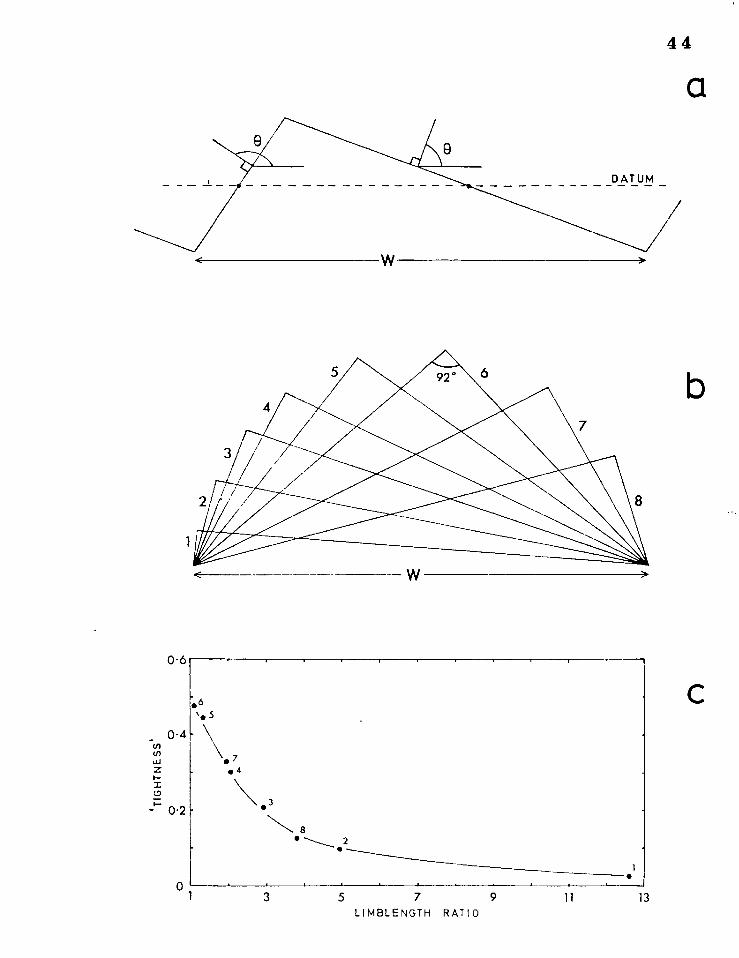
Another problem arises in interpretation of the statistical moments. For
instance, it can be shown that the measure of tightness, m2, is not
solely dependent on interlimb angle, but is closely related to asymmetry
as well. In fig. 2.8 eight chevron folds are drawn with the same wave—
length and interlimb angle, but with varying limblength ratios. For each
fold, m2 may be calculated according to eq. 2.5 (in which N = 47) and its
value is plotted against limblength ratio in fig. 2.8b. It is clear
that the moment, m2, is strongly related to asymmetry and its use as a
valid measure of tightness alone is considered unsound (cf. Whitten,
1966a, fig. 483, in which values of tightness are given for a number of
folds).
Loudon's method is thaqght to be of considerable potential in
structural analysis. However, considerable attentionnocdo to bo 'paid to the
problem of sampling and to the significance of the statistical moments
before this potential will be realised.
In a statistical analysis of fabric data, Kelley (1968) describes a
technique of finding the best fit fold axis to a number of bedding poles
by a trial and error method. He calculates the variance of the observed
measurements (poles to bedding) from the great circle normal to each trial
axis, for enough of such axes to enable him to draw a contoured map of
the variance on a stereogram. The shape of the contours will reflect
the shape and tightness of the folds and might be used for representing
fold shape. However, the method does not have the quantitative advantage
of Loudon's approach, whilst having the same problems of sampling.
The final method of analysis considered concerns the use of Fourier
(or harmonic) analysis, and the next section is devoted to this means of
analysis.
2.5 HARMONIC (FOURIER) ANALYSIS OF FOLDS
Harmonic, or Fourier, analysis is the representation of a function by
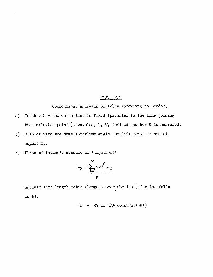
Fig. 2.8
Geometrical analysis of folds according to Loudon.
a) To show how the datum line is fixed (parallel to the line joining
the inflexion points), wavelength, W, defined and how 8 is measured.
b) 8 folds with the same interlimb angle but different amounts of
asymmetry.
c) Plots of Loudon's measure of Itightnessl
m2 = z_cos2 u.
i=l1=.1.
against limb length ratio (longest over shortest) for the folds
in b).
(N = 47 in the computations)
44
a
b
06
• 6 \.5
C
.7 .4
\•3
to
— 0.2
0
8 • ------,..2
3 5 7 9 11 13 LIMBLENGTH RATIO
45
the sum of a number of sine and cosine harmonics, and it provides a useful
and practical way of analysing and classifying single folded surfaces (here
in profile section) in a quantitative manner. A new method of application
of harmonic analysis to folds is described in this section; it presents
an alternative approach to those discussed in section 2.4, and has been
applied in natural fold studies described in the later chapters of the thesis.
2.5.1 Fourier Analrais in Geology
Fourier analysis is not new in geology and has been used mainly as
a tool in statistical studies. The technique finds wide application in
geophysics (e.g. Barber, 1966) including studies of gravity, seismic
and magnetic profiles. Recently, Fourier analysis has received much
attention as an alternative to the use of polynomials in calculating trend
surfaces or best fit surfaces to data showing areal variation (Krumbein,
1966; Agterberg, 1967). Fourier analysis of resistivity profiles in
stratigraphic correlation is described by Preston and Henderson (1964), its use in studying river meanders by Speight (1965) and in a study of
microrelief by Stone and Dugundji (1965).
In structural geology, until recently, no description of fold
morphology using Fourier analysis had been described.
2.5.2 Fold Analysis using Harmonic Analysis
Considering the obvious periodic nature of many folds it is perhaps
surprising that harmonic analysis has received such little attention in the
past. Norris (1963) noted the potential of the method, and in recent
years Chapple (1964, 1968), Harbaugh & Preston (1965) and Stabler (1968)
have described methods of fold analysis based on this technique. Other math-
ematical functions could be found to represent fold shapes, such as polynom-
ials or Bessel functions; however a Fourier representation seems intuitively
more useful as it is naturally periodic. Two possible uses of harmonic analysis
may be distinguished that are fundamentally different. The first is in the
46
study of single folds, to gain information about their 'Shape content'
(Chapple„ 1968), and the second is in the study of periodicity, involving
the analysis of long lengths of profile to include many folds. The
second approach is not taken here, but could prove useful in a study of
fold order, by the calculation of power spectra. The approach of Stabler
(1968) and of the writer restricts the analysis to single folds or segments
of folds. Chapple (1968), too, restricts his study to single folds,
but the function analysed is one of inclination (dip) against arclength.
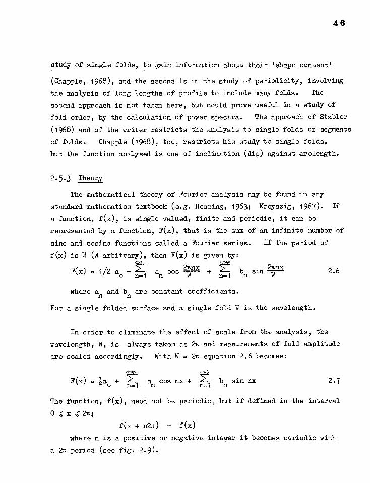
2.5.3 Theory
The mathematical theory of Fourier analysis may be found in any
standard mathematics textbook (e.g. Heading, 1963; Kreyszig, 1967). If
a function, f(x), is single valued, finite and periodic, it can be
represented by a function, F(x), that is the sum of an infinite number of
sine and cosine functions called a Fourier series. If the period of
f(x) is W (W arbitrary), then F(x) is given by: cys.
F(x) . 1/2 a + a cos 2nnx
o n=1 n n=1 nx
bn sin 2n 2.6
where an and bn are constant coefficients.
For a single folded surface and a single fold W is the wavelength.
In order to eliminate the effect of scale from the analysis, the
wavelength, W, is always taken as 2n and measurements of fold amplitude
are scaled accordingly. With W = 2n equation 2.6 becomes:
F(x) iso + CY4N -747 z-- a cos nx + b sin nx n=1 n n=1 n
2.7
The function, f(x), need not be periodic, but if defined in the interval
0 ‘ x 42n;
f(x + n2n) = f(x)
where n is a positive or negative integer it becomes periodic with
a 2n period (see fig. 2.9).
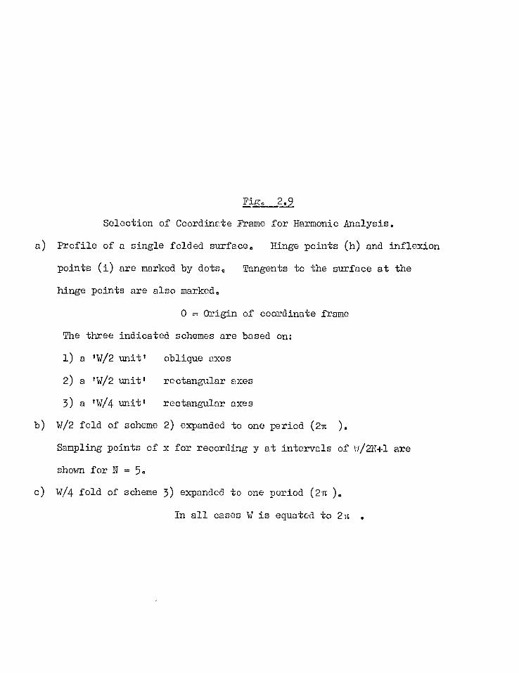
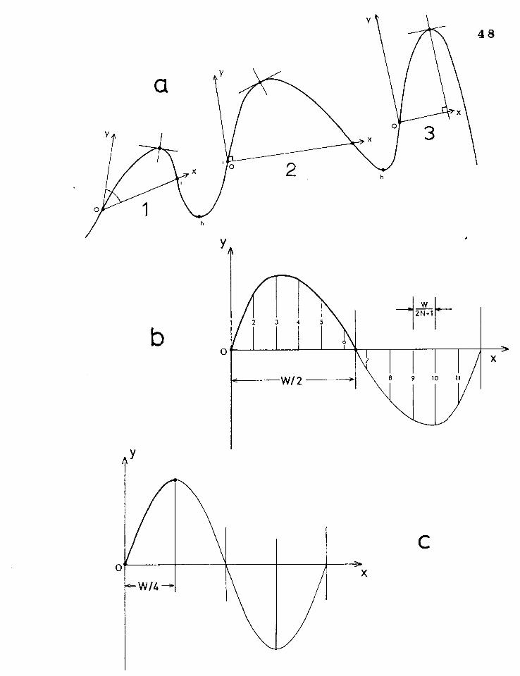
Selection of Coordinate Frame for Harmonic Analysis.
a) Profile of a single folded surface. Hinge points (h) and inflexion
points (i) are marked by dots. Tangents to the surface at the
hinge points are also marked.
0 . Origin of coordinate frame
The three indicated schemes are based on:
1) a 'W/2 unit' oblique axes
2) a 'W/2 unit' rectangular axes
3) a 'W/4 unit' rectangular axes
b) W/2 fcld of scheme 2) expanded to one period (2n ).
Sampling points of x for recording y at intervals of 11/2N+1 are
shown for N = 5.
c) W/4 fold of scheme 3) expanded to one period (2u ).
In all cases W is equated to 2u .
48
W/ 2
Y n
10 II
-,.
b
C X
{-W/4->
Y A
m - 2N+1 f(xp) sin
p=1
2n pm 2141
2 2.9b
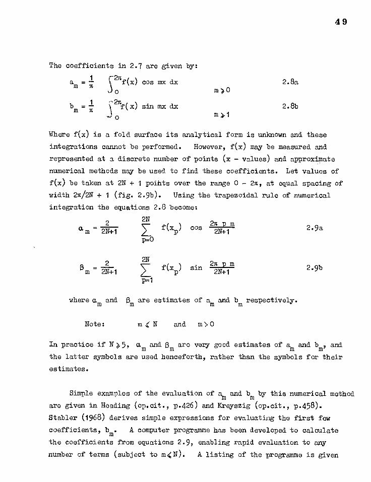
The coefficients in 2.7 are given by:
amn C2nf(x) cos mx dx 2.8a m)0
bm — 1
f (x)sin mx dx 2.8b 1 0
Where f(x) is a fold surface its analytical form is unknown and these
integrations cannot be performed. However, f(x) may be measured and
represented at a discrete number of points (x - values) and approximate
numerical methods may be used to find these coefficients. Let values of
f(x) be taken at 2N 1 poihts over the range 0 - 2n, at equal spacing of
width 2u/2N 1 (fig. 2.9b). Using the trapezoidal rule of numerical
integration the equations 2.8 become:
2N f(xp ) cos
49
2 a = m 2N+1
2.9a 2N+1
where am and am are estimates of am and bm respectively.
Note: m N and m'> 0
In practice if Er .,51 am and Om are very good estimates of am and bm, and
the latter symbols are used henceforth, rather than the symbols for their
estimates.
Simple examples of the evaluation of am and bm by this numerical method
aro given in Heading (op.cit., p.426) and Kreyszig (op.cit., p.458).
Stabler (1968) derives simple expressions for evaluating the first few
coefficients, bm. A computer programme has been developed to calculate the coefficients from equations 2.9, enabling rapid evaluation to any
number of terms (subject to m<N). A listing of the programme is given
50
in the appendix. Read into the computer are values of N, the 2N+1 values
of f(x•) and the wavelength W of the fold.
2.5.4 Selection of Co-ordinates for Analysis
An important requirement of an analysis is the selection of an
unambiguous frame of reference axes. Considering a section of a single
folded surface (fig. 2.9a) of a general kind it is clear that the invariant
points on the surface, the inflexion and hinge points, must be used as
reference points in any co-'ordinate scheme (this is not necessarily so for
polyclinal folds - see later). Considering any join of two adjacent
inflexion points to be a ,'half wavelength', AW, it is evident that if the
unit of fold for analysis were greater than -1-W, it would in general be
difficult to define an unambiguous frame of axes. Three reference axis
schemes are proposed (fig. 2.9).
1) & 2) Based on a -W unit with x-axis as the join of two inflexion
points.
1) oblique axes, y-axis normal to the tangent at the hinge point.
2) orthogonal axes, y-axis normal to x (usually y is not parallel
to the axial surface trace).
3) Based on a i--14 unit with y-axis normal to the tangent at the hinge,
and x-axis normal to y through the inflexion point.
In fig. 2.9b & c the examples of 2) and 3) are drawn with the unit lengths
of W/2 and W/4 respectively reproduced two and four times to constitute
one period of length W. In each case W would be equated to the period
2n to eliminate the difference in size. The three suggested schemes
have been tried and the third scheme based on the unit, W/4, is preferred
for the following reasons:
a) The largest number of natural folds cam be analysed this way; all
folds with limb dips 4 90°.
b) The origin, 0, is unambiguous. For both schemes 1 and 2 there are
two possible origins. (The origin could, however, always be
situated on the short limb).
c) Asymmetry is more or less separated from 'shape' and 'tightness'
(cf. fig. 2.9b & c), and may be evaluated by a comparison of co-
efficients for either 'half' of a fold.
d) The same segment of a fold is analysed as in a -00., or 0 a analysis.
All analyses described in this thesis are based on a w/4 unit - 'quarter
wavelength unit'.
For all three schemes described above, the functions analysed become
odd functions (i.e. f(x) = -f(-x) ); all sine waves are odd functions and
all cosine waves even (f(x) = f(-x) ). An odd function can only be
represented by odd harmonics and so am = 0 for all m. Further, in scheme
3, the even sine terms in the series will vanish as they are asymmetric
about the axial surface, and so b2m = 0 (m = 1,2,3 etc)., and only odd
terms remain in the series.
2.5.5 Procedure for Analysis
To analyse a single fold of a quarter wavelength, the following steps
should be taken (see fig. 2.9);
a) Locate hinge and inflexion points on the surface.
b) Draw a normal to the tangent line at the hinge through the hinge
point. This line, the y-axis, is usually parallel to the axial
surface trace.
c) Draw a normal to this line through the inflexion point, to form the
x-axis.
51
52
d) Divide the length, W/4, on the x-axis into N + 1 equal parts, to give
N + 1 sample points (see fig. 2.10).
e) Measure f(x) at each sample point. Because of the symmetry of the
fold, the 2N + 1 values of f(x) over the range O-W may be found from
the N + 1 values in the range 0 -11/4 (see fig. 2:10).
f) Measure W/4.
From the 211 + 1 values of f(x) and the value of W/4, the coefficients,
bm
may be calculated on the computer.
2.5.6 Representation of Computed Coefficients
The most diagnostic features of fold shape are brought out by the
first two coefficients, b1 and b3, and a plot of b3 against b1 (Stabler,
1968) proves a useful way of recording these (fig. 2.11). For comparison
of several coefficients a plot of log bm against log m, called here a
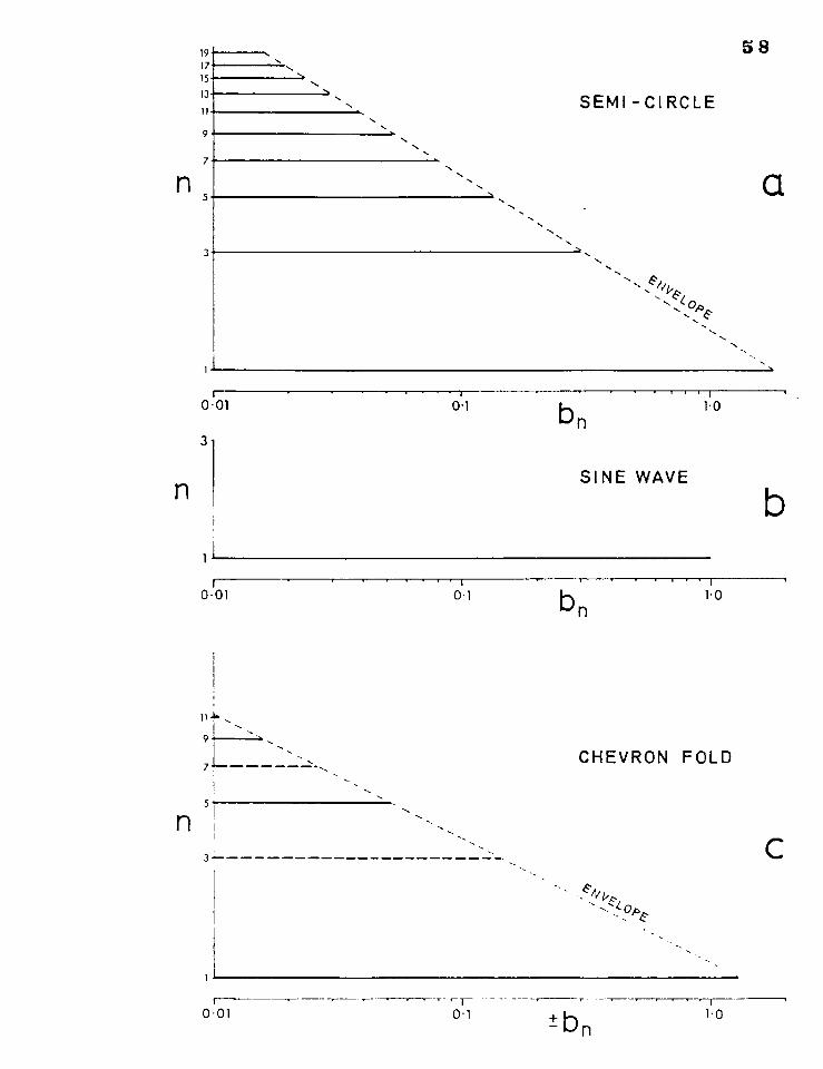
'spectral graph', is useful (fig. 2.12). This consists of a number of
discrete points of bm for each m.
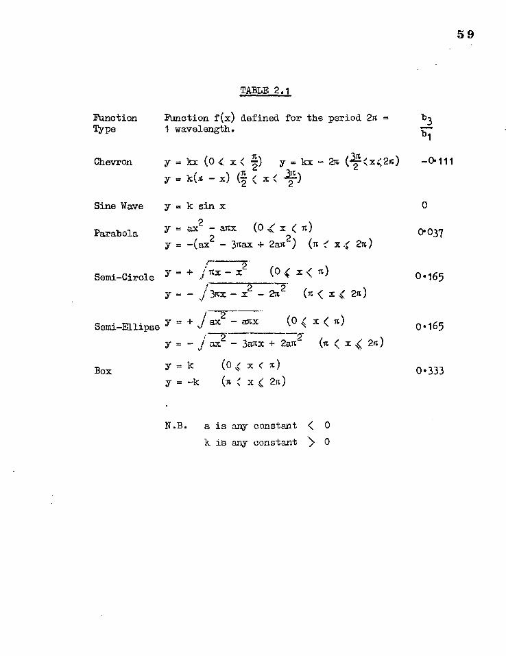
To investigate the significance of these plots it is instructive
to see how several ideal functions (Table 2.1) are broken down into their
harmonic components. The functions given in Table 2.1 are made periodic,
with period 2n. The chevron & semi-circular functions are drawn in fig.
2.13 and also the first 3 harmonic components of each, b1, b3 and b5.
First consider the spectral graphs for these functions (fig. 2.12),
for which specific values of the constants in Table 2.1 have been
introduced. (Note that the semi-circle is a special case of the semi-
ellipse where the constant a = 1). For each graph in fig. 2.12, and for
the similar graphs that may be constructed (but are not illustrated) for
each of the other functions in Table 2.1, straight line envelopes to the
odd values of bm may be drawn, irrespective of sign. The slope of
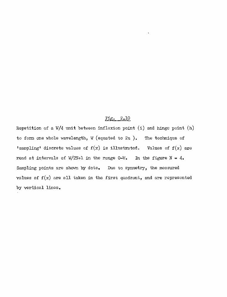
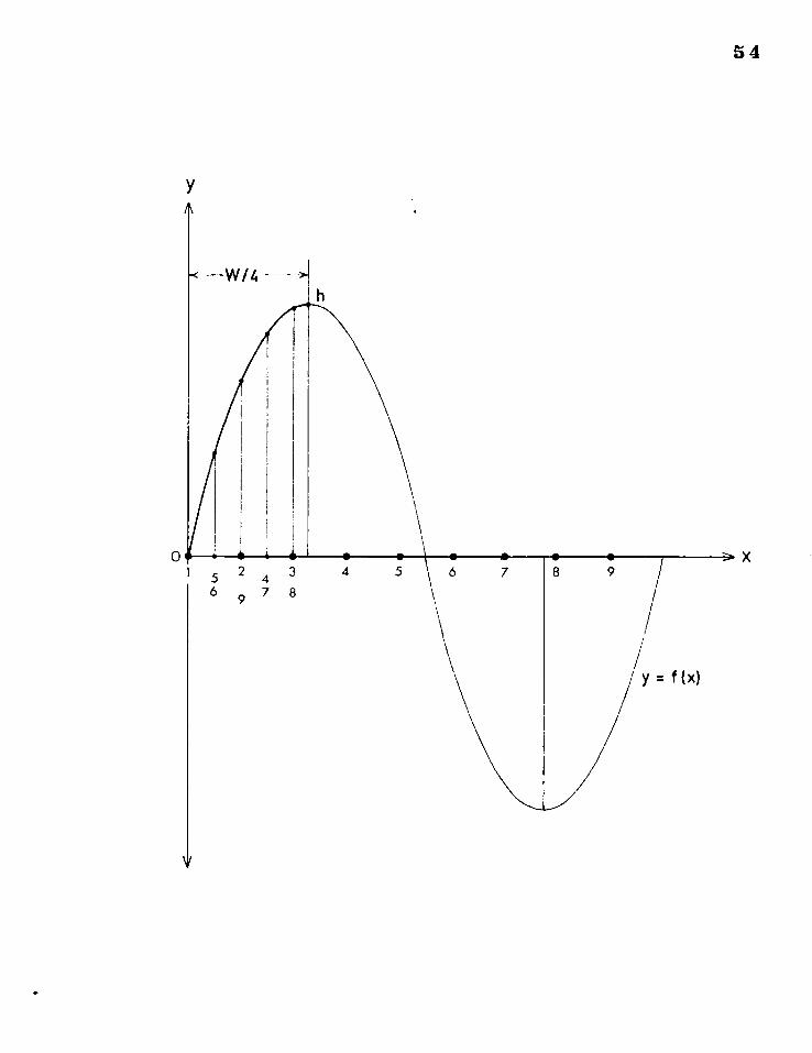
Fig. 2.10
Repetition of a W/4 unit between inflexion point (i) and hinge point (h)
to form one whole wavelength, W (equated to 2n ). The technique of
'sampling' discrete values of f(x) is illustrated. Values of f(x) are
read at intervals of W/2N+1 in the range O-W. In the figure N = 4.
Sampling points are shown by dots. Due to symmetry, the measured
values of f(x) are all taken in the first quadrant, and are represented
by vertical lines.
y
54
4 5 6 7 4 3 6 9 7 8
8 9
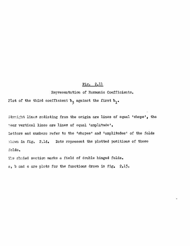
Fig. 2.11
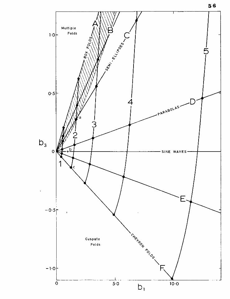
Rerresentation of Harmonic Coefficients.
Plot of the third coefficient b3 against the first bl.
Straioht lines radiating from the origin are lines of equal 'shape', the
--,ear vertical lines are lines of equal 'amplitude'.
Letters and numbers refer to the 'shapes' and 'amplitudes' of the folds
?hewn in fig. 2,14. Dots represent the plotted positions of these
folds.
Me shaded section marks a field of double hinged folds.
a, b and c are plots for the functions drawn in fig. 2.13.
Multiple
Folds 1-0
0.5
o,o.r).5
SINE WAVES
—0.5
56
Cuspate c(si,
Folds
A•s O!
—1.0
0
5.0 b, 10.0
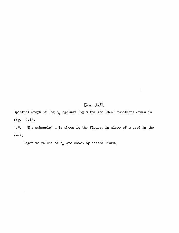
Fig, 2.12
Spectral Graph of log bra against log m for the ideal functions drawn in
fig. 2.13.
N.B. The subscript n is shown in the figure, in place of m used in the
text.
Negative values of bra are shown by dashed lines.
58 19 17 15 13 SEMI-CIRCLE II
9
7
3
FN opt
i t
0.01
3
0.1 b 1
1.0 n
SINE WAVE
0.01 0.1 " I
1.0 bn
11
9
7 CHEVRON FOLD
5
3
4 0p
-- 0.01 0- 1 +b, 1-0
Y = +
Y = -
1 2 f nx - (0< x< n)
/arm - x2 - 2n 2 (n < x 2n)
Y = + iax2 - anx (o 4 x ( n)
y = - y k y = -k
ax2 3anx + 2an
(0 x n) x 2n)
(lc x 2n)
N.B. a is any constant < 0 k 18 any constant > 0
Box 0.333
TABLE 2.1
Function Function f(x) defined for the period 2n = b3 Type 1 wavelength.
Chevron y = kx (0 4', x < 114 y = kx - 2sc (221<x(2n) -0.111 Y = k(n - x) < x 2)
59
Sine Wave
Parabola
Semi-Circle
Semi-Ellipse
y k sin x
y ax2 - anx (0 ,( x < n) = -(ax2 - 3nax + 2an2) x A 210
0
0'037
0.165
0.165
60
these envelopes is independent of the constants a and k in Table 2.1. The
sign reversals in the case of a chevron function are systematic (b2 3 are
all —ve for m = 0,1,2,3 etc). The effect of the size and sign of the
third and fifth harmonics (and by inference the higher harmonics) in
determining the fold shape may be seen in fig. 2.13. With all harmonics
positive (fig. 2.13a), they all tend to steepen and add to the limbs and
alternately to add and subtract from the hinge, to give an overall effect
of hinge roundness. The larger b3 /b1 9
the more pronounced will this
effect be. With b3 negative and higher harmonics alternating in sign
(fig. 2.13c), all the harmonics will add to the hinge and alternately
add and subtract from the limbs, to give an overall effect of a sharp
hinge and straight limbs.
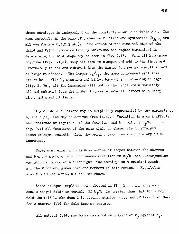
Any of these functions may be completely represented by two parameters,
b1
and b3/b1'
and may be derived from these. Variation in a or k affects
the amplitude or tightness of the function and b1, but not b3/b1. In
fig. 2.11 all functions of the same kind, or shape, lie on straight
lines or rays, radiating from the origin, away from which the amplitude
increases.
There must exist a continuous series of shapes between the chevron
and box end members, with continuous variation in b3/b1 and corresponding
variation in slope of the straight line envelope on a spectral graph.
All the functions given here are members of this series. Hyperbolas
also fit in the series but are not shown.
Lines of equal amplitude are plotted in fig. 2.11, and an area of
double hinged folds is marked. If b3/b1 is greater than that for a box
fold the fold breaks down into several smaller ones, and if less than that
for a chevron fold the fold becomes cuspate.
All natural folds may be represented on a graph of b3 against b1
.
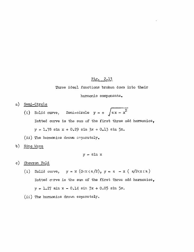
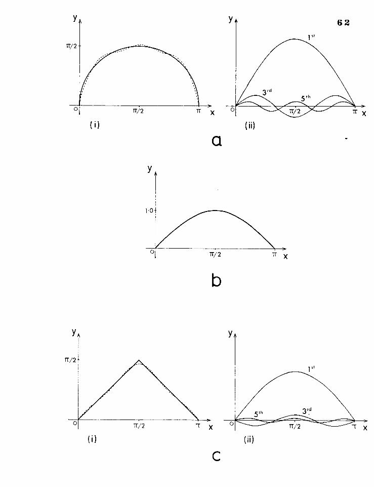
Fig, 2,13
Three ideal functions broken down into their
harmonic components.
a) Semi—Circle
(i) Solid curve Semi—circle y = +I Tu x — x2
Dotted curve is the sum of the first three odd harmonics,
y . 1.78 sin x + 0.29 sin 3x + 0.13 sin 5x.
(ii) The harmonics drawn separately.
b) Sine Wave
y = sin x
c) Chevron Fold
(i) Solid curve, y = x (0<x<1;/2), y x ( Tc/2<x(T‘ )
Dotted carve is the sum of the first three odd harmonics,
y = 1.27 sin x 0.14 sin 3x 0.05 sin 5x.
(ii) The harmonics drawn separately,
Y A
C (i)
Y
TT/ 2
0
(i)
a
)
b
63
Spectral graphs constructed for natural folds described in this thesis
(e.g. fig. 5.13 ) seem to display envelopes to the plotted values of bm
that are very nearly straight lines. These folds will be closely
matched in shape by a member of the series of ideal functions described
above.
This observation leads to a practical and rapid application of
harmonic analysis that is now to be described.
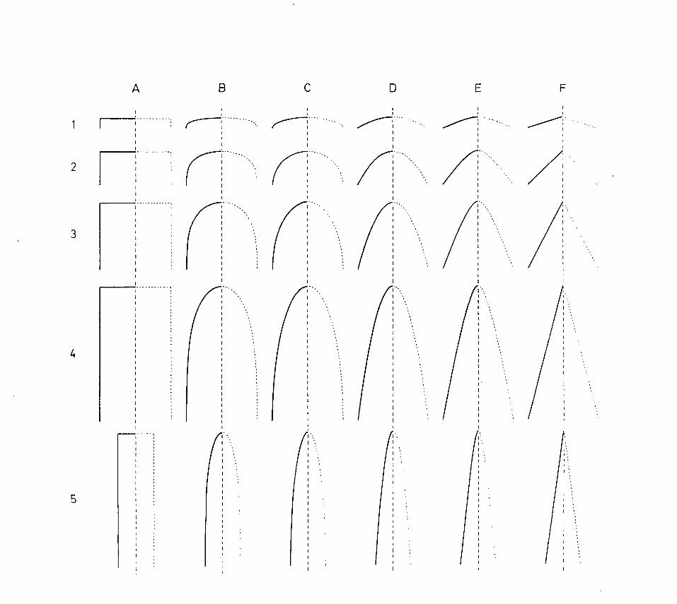
2.5.7 Visual Harmonic Analysis
On the basis of the continuous series of ideal functions described
above, 30 idealised fold forms have been constructed for 6 different 'shapes' (values of b
3/b1) in the series including the two end members, each at 5
/amplitudes' (see fig. 2.14). The position that each of these forms
occupies on a plot of b3 against b
1 is shown in fig. 2.11, and is given
by the intersection of a ray for a particular 'shape' with a line of a
particular 'amplitude'.
In order to compare natural fold shapes with these ideal forms, they
have been reproduced on a perspex sheet. A comparison is made in the
following way. The fold is observed in profile and estimates of the
positions of hinge and inflexion points are made. Each quarter wavelength
unit of the fold from inflexion to hinge point is compared with the forms
on the perspex sheet by looking through the sheet at the fold, and the
closest match is found. Folds may occupy intermediate positions between
the ideal forms.
Fig. 2.15 shows an-example and a simple graph on which results may be
plotted for a number of folds.
The method provides a rapid alternative to that described above and
involves no measurements or calculations. It does, however, require that
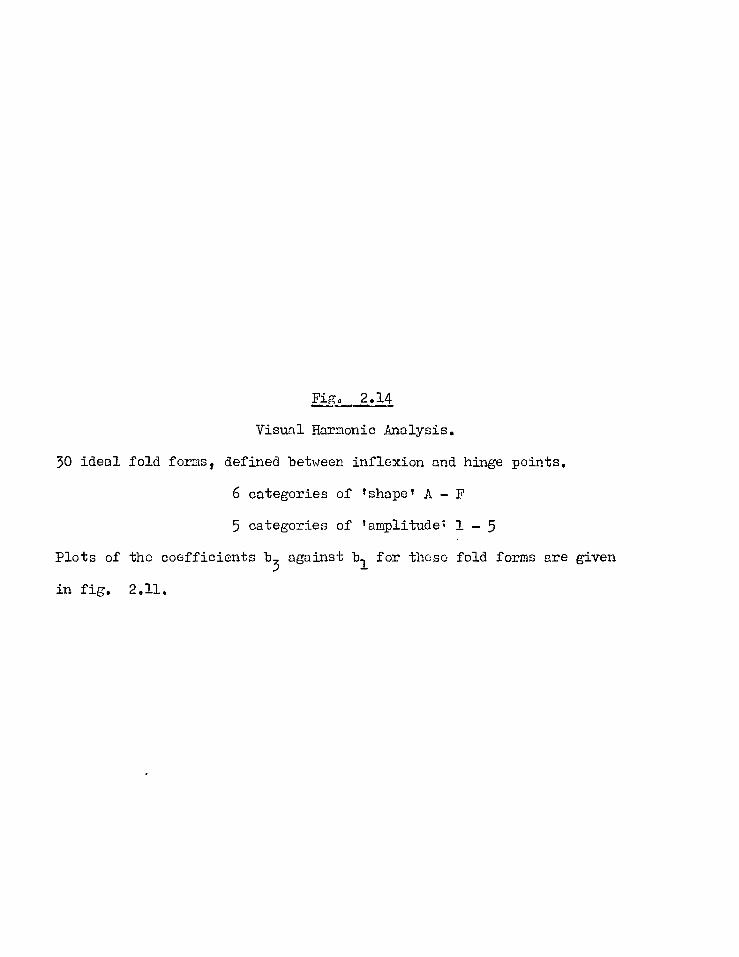
Fig. 2.14
Visual Harmonic Analysis.
30 ideal fold forms, defined between inflexion and hinge points.
6 categories of 'shape' A — F
5 categories of 'amplitude 1 — 5
Plots of the coefficients b3 against b1 for these fold forms are given
in fig. 2.11.
s
1
c
Z
L
d 8 V a D 3

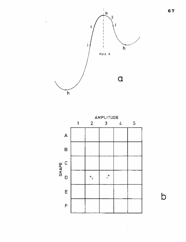
Fig. 2.15
a) Profile section of a single folded surface split into 'quarter
wavelength units' for classification.
inflexion point
h = hinge point
b) Box diagram of 'shape' against 'amplitude' for representation of
results.
The two limbs of Fold X are represented on this diagram.
, +2 +
A
B
w C a. < = (I)
D
E
F
b
67
AMPLITUDE 1
2 3 4
5
natural folds be closely represented by these ideal functions.
2.5.8 Errors and Reproducibility
Errors in the calculation of harmonic coefficients may arise in
several ways. Three kinds of error may be considered present in the values
of bm calculated for a single fold. These are:
1) Errors in measurement, with hinge & inflexion points, reference axes
and value of N fixed
2) Errors resulting from inadequate size of N.
3) Errors in the location of hinge and inflexion points and the reference
axes.
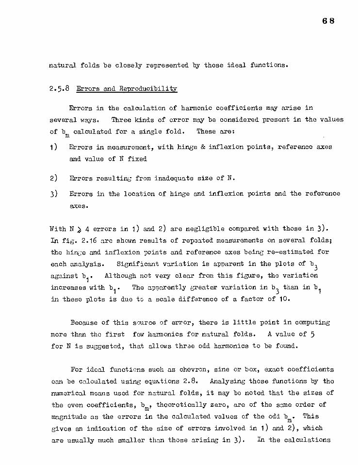
With N 4 errors in 1) and 2) are negligible compared with those in 3).
In fig. 2.16 are shown results of repeated measurements on several folds;
the hinge and inflexion points and reference axes being re-estimated for
each analysis. Significant variation is apparent in the plots of b3
against b1. Although not very clear from this figure, the variation
increases with b1. The apparently greater variation in b3 than in b1
in these plots is due to a scale difference of a factor of 10.
Because of this source of error, there is little point in computing
more than the first few harmonics for natural folds. A value of 5
for N is suggested, that allows three odd harmonics to be found.
For ideal functions such as chevron, sine or box, exact coefficients
can be calculated using equations 2.8. Analysing these functions by the
numerical means used for natural folds, it may be noted that the sizes of
the even coefficients, bra, theoretically zero, are of the some order of
magnitude as the errors in the calculated values of the odd bm. This
gives an indication of the size of errors involved in 1) and 2), which
are usually much smaller than those arising in 3). In the calculations
68

Fig, 2.16
Reproducibility of Harmonic Analysis.
The results of repeated harmonic analysis of two natural fold profiles
are shown on plots of b3 against b1. New estimates of hinge and
inflexion points were made for each analysis. One configuration of
coordinate axes and estimated hinge and inflexion points are shown on
each profile.
7 0 0.2
0.1
b3
0
Limb 2
- 0.1
02
Limb 1
. I
• • S.
••••
1.0 2.0 3.0 b1 0•l
b3
- 02 0
0
01 0 2.0 3.0
02
0.1
b3
0.1
02
1.0
b1
-r
Limb 3
• • •
• -
• s So
0 1.0 2.0 3.0 4.0
b1
7 1
for natural folds, the sizes of the even bm are regarded as an indication
of the size of error included in the values of the odd coefficients, for
a fixed co-ordinate frame.
2.6 TECHNIQUES OF NATURAL FOLD MEASUREMENT
The techniques outlined in this section were those used in the studies
of natural folds described in the later chapters of the thesis.
Material consisted of photographs of outcrops or of cut and polished
specimens in which the cut face was normal to the fold axis. The
photographs were all taken with the axis of the camera lens parallel to the
fold axis to within a few degrees. Outcrops were only photographed if
the outcrop surface was fairly smooth and nearly normal to the fold axis.
Measurements were made on the photographs themselves or on tracings
in which the fold surfaces were drawn as smooth curves.
A drawing machine was used in the construction of isogons and
thickness measurements were made with a small offset rule in conjunction
with this machine.
Arc lengths and curVed lines were measured with dividers or a map
measurer. Hinge points and inflexion points were estimated visually,
usually with the aid of isogons. The hinge points were taken as the
points of closest spacing of the isogons, and the inflexion points were
found by bisecting the lengths of arc in the fold limbs that were
approximately straight.
In the construction of plots of tL and against a the datum
tangent was taken in the way described in section 2.3.5 and values of t'a
and 00. were usually recorded at 100- dip intervals.
Harmonic analysis was carried out numerically or visually on well
defined single folded surfaces. For the numerical calculations N was
usually taken between 5 and 9.
72
CHLPTER
THE THEORIES OF FOLD DEVELOPMENT .AND GEOMETRIC FORM OF FOLDS
3.1 INTRODUCTION
There is considerable controversy in the literature concerning the
processes responsible for fold development, largely because the mechanical
behaviour of rocks over long periods of time under stress conditions that
exist in the earth's crust is unknown, and because the state of strain
within folded layers is usually indeterminate. Processes that have been
suggested attempt to explain the observed geometric form of folds and
related features such as cleavage, schistosity and lineations of various
kinds. For the most part they involve layer behaviour of one or more
of the following kinds:
a) Buckling (Timoshenko, 1960: Ramberg, 1963a).
Single layers embedded in a relatively more ductile medium, or a
stack of layers of varying ductilities may become mechanically unstable
when loaded parallel to the layering and this instability may lead to
the initiation of folds.
b) Passive Folding (Donath, 1963).
The layering plays no mechanical part in the deformation and acts
solely as a passive marker.
c) Kinking (Paterson & Weiss, 1962; Dewey, 1965; Ramsay, 1967, p.436 —
456).
Rocks with very well—developed layering (e.g. bedding, slaty cleavage,
schistosity) may develop an instability during deformation to form folds
in discrete zones with straight limbs and angular crests.
Ramberg (1963a), and Ramsay (1967) in particular, discuss the fold
geometry, strained state, and genesis of buckles and passive (Ramberg
uses the term bending) folds in detail. Kinking is not discussed further
7 3
74
and the reader is referred to the works listed above and to the papers
on conjugate folds by Johnson (1956) and Ramsay (1962b).
A. brief discussion of passive folds is given in section 3.2. This
is followed in section 3.3. by a discussion of the mathematical theories of buckling, with an erliphasis on those concerned with isolated layers.
The geometry of buckled layers is considered in section 3.4, the
modification of parallel folds by a homogeneous 'flattening' in section
3.5, and the effect of simultaneously buckling and flattening a layer is discussed in section 3.6.
3.2 PASSIVE FOLDS
One of the commonest situations in which passive folds develop is
in the zones of contact strain around buckled layers (Ramberg, 1963a),
where isogons alternately converge and diverge in adjacent hinges to give
folds of class 1 and class 3 geometries respectively (see Ramsay, 1967, P.416). Ramberg (1963a) describes similar kinds of folds that form
around boudins or conglomerate pebbles and refers to this type of folding
as bending.
'Similar' (class 2) folds aro usually considered to indicate passive
layer behaviour.
Where 'similar' folds persist over a large number of layers they
become difficult to account for mechanically, and the usual explanation
invoking heterogeneous simple shear acting parallel to the axial surfaces
of the folds is open to criticism on this account (Flinn, 1962, p.425). The near periodicity of many similar folds is particularly difficult to
account for by this hypothesis or by a hypothesis of differential flat-
tening producing differential shear that is transmitted through the rock-
mass to produce similar folds (Ramsay, 1962a). The explanation most
favoured by the writer is that suggested by Flinn (1962, p.425) and
75
Mukhopaahy.:.y (1965a) involving a large shortening component of finite
homogeneous strain across the axial surfaces of gently buckled layers or
initial irregularities in the layering. Nizichopadhyay shows how
similar folds may effectively be produced from originally parallel folds
in this way (see also Rancay, 1967, fig. 7-102). Slight systematic
departures from true similar geometry might be expected with this
hypothesis, and these have been observed by . Mukt_rildhyny(1964, 1965a)
and the present writer (Ch.5).
3.3 MOT MTHEMATICAL TREATMENTS
Precise mathematical analyses of folding are restricted to the case
of buckling, and a number of workers have approached the problem. The
early work in this field, discussed by Biot (1961) and Ramberg (1961a)
treated the problem as one of elasticity. Biot (1957, 1959, 1961, 1965a,
1965b) derives expressions for the buckling instability of layered
systems of general viscoelastic materials based on a principle of
correspondence t.j expressions obtained for true elastic materials. In
a series of papers, Ramberg (1961a, 1963b, 1964a) analyses the buckling behaviour of layered viscous (Newtonian) materials using the methods of
fluid mechanics. Currie, Patnode & Trump (1962) study the buckling of
elastic media, and Price (1967) extends an elastic buckling theory to
account for asymmetrical, straight—limbed folds.
Both Biot and Ramberg discuss the case of a single layer embedded
in a relatively more ductile medium, and various types of multilayered
sequences built up from layers of different thicknesses and different
ductilities. From the analytical equations expressing the deformation
behaviour of these different cases comes the concept of a dominant
wavelength (Biot, 1957); that is the wavelength in a single or multi—
layered system, of folds most likely to develop. It is the wavelength
of small sinusoidal irregularities that grow at the fastest rate.
76
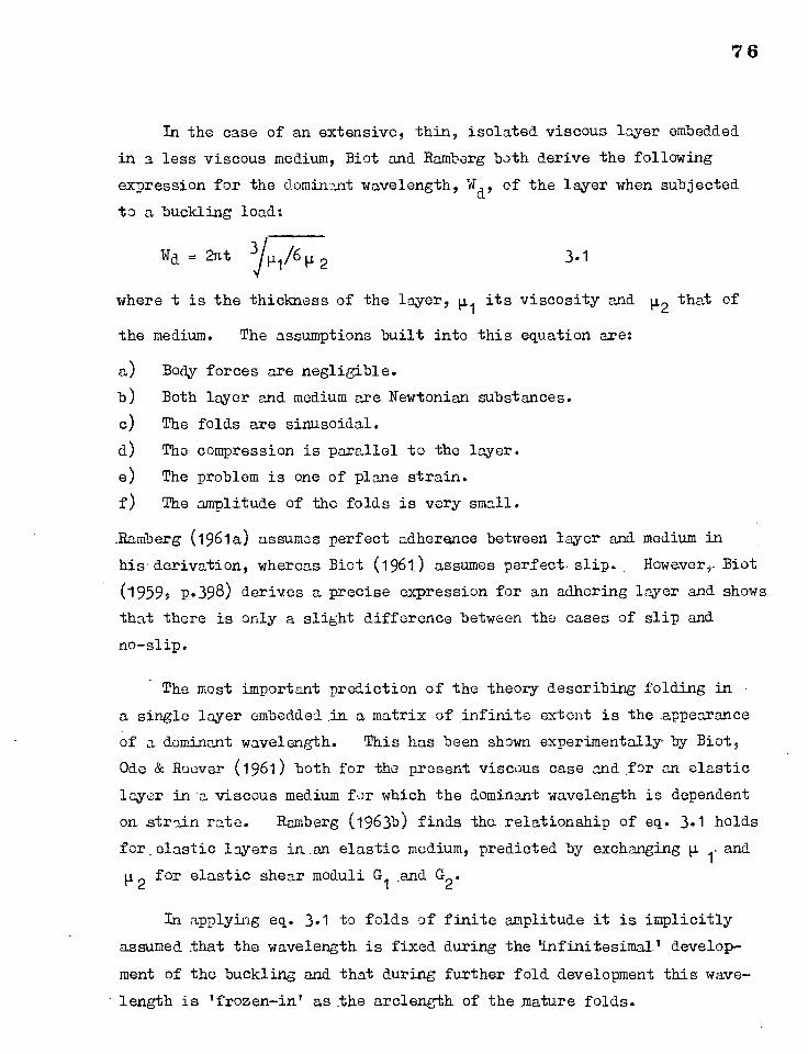
In the case of an extensive, thin, isolated viscous layer embedded
in a less viscous medium, Biot and Ramberg both derive the following
expression for the dominant wavelength, Wd, of the layer when subjected
to a buckling load:
Wa = 2nt Iµ1/6 2 3.1
where t is the thickness of the layer, j1 its viscosity and 42 that of
the medium. The assumptions built into this equation are:
a) Body forces are negligible.
b) Both layer and medium are Newtonian substances.
c) The folds are sinusoidal.
d) The compression is parallel to the layer.
e) The problem is one of plane strain.
f) The amplitude of the folds is very small.
_Ramberg (1961a) assumes perfect adherance between layer and medium in
his derivation, whereas Biot (1961.) assumes perfect-slip.. However,. Biot
(1959, p.398) derives a precise expression for an adhering layer and shows
that there is only a slight difference between the cases of slip and
no-slip.
The most important prediction of the theory describing folding in
a single layer embedded in a matrix of infinite extent is the appearance
of a dominant wavelength. This has been shown experimentally-by Biot,
Ode & Roover (1961) both for the present viscous case and for an elastic
layer in .a viscous medium for which the dominant wavelength is dependent
on strain rate. Ramberg (1963b) finds tha.relatianship of eq. 3.1 holds
for.elastic layers in.an elastic medium, predicted by exchanging 1-and
42 for elastic shear moduli Gi .and G2.
In applying eq. 3.1 to folds of finite amplitude it is implicitly
assumed that the wavelength is fixed during the 'infinitesimal.' develop-
ment of the buckling and that during further fold development this wave-
length is 'frozen-in' as.the arclength of the mature folds.
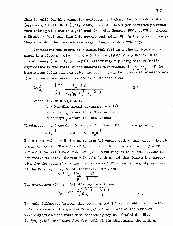
77
This is valid for high viscosity contrasts, but where the contrast is small
(approx. < 100:1), Biot (1961,13.1606) predicts that layer shortening without
much folding will become significant (see also Ramsay, 1967, p.379). Sherwin
& Chapple (1968) take this into account and modify Biot's theory accordingly.
They show that the dominant wavelength changes with shortening.
Considering the growth of a sinusoidal fold in a viscous layer cont-
ained in a viscous medium, Sherwin & Chapple (1968) modify Biot's 'thin
plate' theory (Biot, 1965a, p.426), effectively replacing time in Biot's
expressions by the ratio of the quadratic elongations, S =Jhl /N2 of the
homogeneous deformation on which the buckling may be considered superimposed.
They derive an expression for the fold amplification:
A In f ho dS — 3.2
ilo 3 ...!1 241/U2 + 3
where A = Fold amplitude.
N = Non-dimensional wavenumber = 2nt/w
subscript 0 refers to initial values
subscript refers to final values
Thickness, t, and wavelength, W, are functions of S, and are given by:
t tog and W WoS
For a fixed value of S, the expression 3.2 varies with ho and passes through
a maximum value. The vsJue of Ao for which this occurs is found by differ-
entiating the right hand side of 3.2 with respect to ho and setting the
derivative to zero. Sherwin & Chapple do this, and thus derive the expres-
sion for the wavenumler whose cumulative amplification is largest, in terms
of the final wavelength and thickness. This is: x f3 _ 12112 S2
5 +1 For comparison with eq. 3.1 this may be written:
Wd
2nt y .1 S 1 6u, 2 S2 3.3
The only difference between this equation and 3.1 is the additional factor
under the cube root sign, and from 3.3 the variation of the dominant
wavelength/thickness ratio with shortening may be calculated. Biot
(1965a, p.427) concludes that for small finite shortening, the dominant
7 8
wavelength does not alter greatly due to a compensatory effect in the
changes of thickness and wavelength. However, the ratio of the dominant
wavelength/thickness, important when only the final product is observed,
changes more rapidly than does the dominant wavelength alone, and the
effects are clear from the analysis of Sherwin & Chapple and cannot be
ignored. The relationship between amplification, dominant wavenutber
and shortening for different viscosity contrasts is shown in fig. 3.1,
reproduced from Sherwin & Chapple.
Biot (1961, p.1606) introduces the concept of explosive amplification,
Showing for a particular viscosity contrast that amplification increases
enormously at some stage in the shortening process. This is well illus-
trated by Ramsay's fig. 7-37 (1967, p.379) which is plotted from Biot's expression 5-15. Biot considers this effect will only be marked for
viscosity contrasts greater than about 100:1. However, it is the fold
initially amplified by the greatest amount (i.e. the fold whose-wavelength
is given by eq. 3.3 with S =.1,0) whose progressive amplifioation.is- recorded in.Biot's analysis. in fact at. successive stages of the.
deformation, folds of progressively changing wavelength/thickness ratios
will become those most amplified. Maximum amplification, for a variety
of viscosity contrasts, has bean evaluated at different values of S
by solving eq. 3.2 for a number of closely spaced values of xo ; the
highest value of these computed amplifications has then been taken as
an approximate maximum. Fig. 3.2 records the variation of maximum
amplification with shortening (measured as a percentage to enable
comparison with Ramsay's fig. 7-37), for a range of viscosity ratios.
For any viscosity contrast and for any amount of shortening, the value
of maximum amplification given by this graph is higher than that given
by Ramsay's graph; and so explosive amplification, defined by Blot to
occur at a value 2141o of about 1000, will take place at slightly lower
values of shortening than is calculated by Blot, if progressive changes
in dominant/thickness ratios are taken into account.
The effect of homogeneous shortening obviously becomes important at
Fig. 3,1
Amplification of the Dominant Wavelength Wa as a function of the
Dominant Wavenumber A d for various values of the viscosity ratio
µ 2 and the ratio S of the quadratic elongations of the uniform
shortening.
(After Sherwin & Chapple, fig. 5, 1968).
Pig. 3.2
Amplification of the Dominant Wavelength as a function of the uniform
shortening (expressed as % Compressive Strain), for various values of
the viscosity ratio.
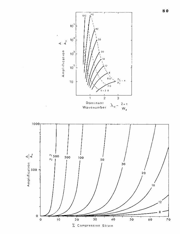
100
40
1 30
1
1 20 1
[12
105
< <
4 10
3 0 10
co
2 10
a
10
80
1 2 Dominant
Wavenumber
3
x d t
"d
10
20
30
40
50
60
70
% Compressive Strain
81
low viscosity ratios, and this is further discussed in the follow ingsChapter.
It is not possible, with the above theory, to predict changes in
layer thickness or changes in shape of the folded surfaces as the fold
develops.
Recently, Chapple (1964, 1968) extended the viscous infinitesimal
theory of Biot to an analysis of folds with large finite amplitudes.
Considering the competent layer to be thin (he took thickness as 1/40 of
the wavelength), inextensible and initially folded into a low—dip
sinusoidal shape, he was able to calculate progressive changes in finite
strain, strain rate and fold shape accompanying progressive shortening
across a block containing a single layer in a more ductile medium, defined
between two adjacent axial surfaces that remain plane and parallel
throughout the deformation (see Chapple, 1968, fig.1). He showed that
the 'path' of fold development depended only on the ratio of the actual
wavelength, W , to the predicted or dominant wavelength, Wd, and calculated
the changes in fold shape for three values of this ratio (fig. 3.3).
Shape and changes in shape were recorded by means of a harmonic analysis
of inclination (dip) against arclength. By representing shape this way,
Chapple was able to argue that beyond limb—dips of 150 the fold shape
is relatively independent of the initial irregularities and strongly
dependent on the ratio W/Wd and limb dip. Below limb dips of 150, the
wavelength selection mechanism described by Blot (1961, p.1604) operates.
Although in Chapple's treatment, a harmonic analysis of dip against
arclength proves more useful than the type described by the present writer
(section 2.5), the latter has boon found more nractical in the description
of natural fold shapes. Chapplo's results are presented on a plot of
third against first coefficients (fig. 3.3) of a harmonic analysis of
the kind described in Chapter 2, to enable comparison with results of
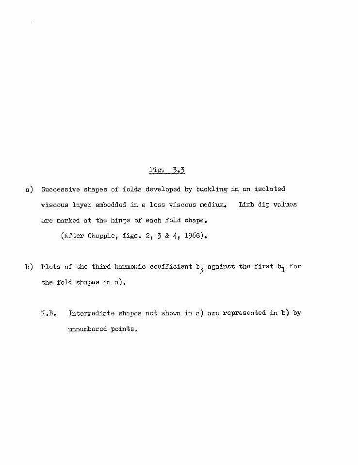
Fig, 3.3
a) Successive shapes of folds developed by buckling in an isolated
viscous layer embedded in a less viscous medium. Limb dip values
are marked at the hince of each fold shape.
(After Chapple2 figs. 2, 3 & 4, 1968).
b) Plots of The third harmonic coefficient b3
against the first b1 for
the fold shapes in a).
N.B. Intermediate shapes not shown in a) are represented in b) by
unnumbered points.
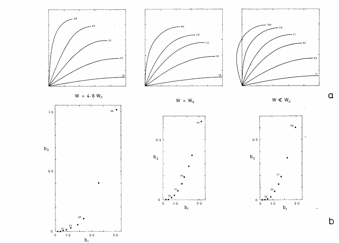
90 •
•
71 •
• 55 •
33 I •-• • •
1-0
b3
0.5
0•5
0 1 0 3.0 0 1.0 3.0 b1
0.5
b3
89 •
•
•
70 •
•
b3
56• 36 I •
0 ••
•
53 33• •
• • •
89 •
69 •
•
W = 4 • 6 Wd W = Wd W < Wd
a
0 1-0 3-0 5.0 b1
84
the studies on natural and experimentally produced folds. The plots of
fig. 3.3 indicate the same features as do Chapple's; a progressive departure of fold shape from sinusoidal, the crests becoming more rounded
as deformation progresses.
Chapple suggests that because the shapes of natural folds show a lack
of correspondence with his theoretical model, real rock materials may
follow non-linear rheological laws. This might alternatively be due to
the invalidity of the assumptions of inextensibility and thin-plate
theory applied to most natural folds. Studies of folds developed in
single competent layers made by Sherwin & Chapple (1968) and by the
writer (section 5.7) suggest that wavelength/thickness ratios of
most naturally formed folds are very much less than the figure used by
Chapple in his calculations and that layer parallel shortening must have
occurred during folding. Moreover, if the wavelength/thickness ratio
is small the shapes of the inner and outer arcs of the buckles will
follow different paths of progressive change.
The multilayer theories of Ramberg and Biot are quite different
from one another, and are more difficult to interpret physically than the
single layer case in terms of wavelength selection and amplification.
Potter (1967) has analysed confined folding in a micaeous bed in terms
of Biot's theory (1964, 1965b) of the buckling of confined multilayers.
Experiments in layered viscoelastic materials made by Ramberg (1963b,
1964a) and Ghosh (1968) show complex variations in shape of the members
of a multilayered sequence, ranging from chevron folds to folds with
rounded crests. These variations appear to depend upon layer spacing
and ease of slip between layers.
3.4 THE SHAPE OF BUCKLED L.YERS
Chapple's (1968) analysis predicts the shape of a buckled layer to
85
high amplitudes only where the layer, besides being thin and inextensible,
takes on a state of strain in which lines initially normal to the layer
remain as normals, and a concentric longitudinal strain (Ramberg, 1961b)
varies linearly across the layer. This is the kind of strain geometry
predicted for and observed in low amplitude elastic buckles; it is
called tangential longitudinal strain by Ramsay (1967, p. 397).
As the wavelenjth/tkickness ratio of folds decreases, however, there
is increasing likelihood of a shearing strain developing parallel to the
layering in the fold limbs (Ramberg, 1961b), and if a rock layer under-
going folding is well-laminated, the strain may be taken up entirely by
such a shearing strain, when the fold becomes a flexural slip or flexural
flow fold (Donath & Parker, 1964). The thickness of all layers remains
constant and the shearing strain is related directly to the apparent dip
(Ramsay, 1967, p.392).
Ramsay (1967, p.391 et seq.) discusses the geometry of the two types
of layer behaviour described above in considerable detail and considers
folds with composite behaviour, and Ramberg (1961b) also discusses the
relationship between the two kinds of strain within a sinusoidal low-
amplitude fold in a viscous material.
There is no analytical prediction offInitefold shape for thick
buckled layers, and models of the two idealised fold types are now
considered assuming a sinusoidal shape for the 'central' surface in the
case of the flexural flow fold, and for the neutral surface in the case
of the tangential longitudinal strain fold. For the latter the model of
Ramsay (1967y p.398) is employed.
It is probable in nature that the layer shape would not be sinusoidal
at the amplitudes considered here, but it is argued that the relative
differences in surface and layer shape apparent here between the two
86
models will be similar to those found where folds are of a more general
shape.
The folds are drawn in fig. 3.4 and changes in shape of the surfaces across the folded layers are compared by a harmonic analysis, using a
plot of the coefficients b3 against b1. From this plot it is clear that
the difference in surface shapes between the two models is slight, and that
a better distinction between them is made by a comparison of isogon
patterns, or of plots of t aagainst a . For thin layers the difference
between the two models is very slight.
It is apparent that unless the curvature remains constant, the
'normals' drawn for a tangential longitudinal strain fold are only normal
to the neutral surface, although for a thin layer they are almost normal
to all surfaces, and the thicknesses of the layers stay almost constant.
The tangential longitudinal strain model is probably only realistic
for thin layers, and the flexural flow model for layers with a very well-
developed layer-parallel lamination. Thick buckled layers will probably
accommodate the strain in a more complex manner that may or may not be
treated a a combination of these two ideal models.
3.5 HOMOGENEOUS FLATTENING OF FOLDS
Campbell (1951), de Sitter (1964) and Ramberg (1964b) briefly consider,
and Ramsay (1962a, 1967) and Ailkhopadhyay . (1965a) discuss in some detail,
the effect of a superposed finite homogeneous strain (referred to here
loosely as a 'flattening') on an initially parallel fold in terms of
thickness modification in the profile plane. The latter two authors
derive a family of curves on graphs of the thickness parameters, t'a , and T114 , against dip, a , that represent the plotted positions taken up by
an originally parallel fold modified by different amounts of flattening.
These curves enable determination of this flattening strain for natural
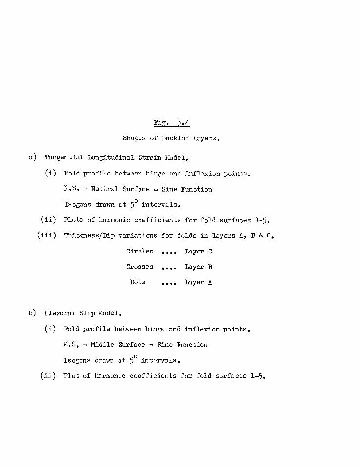
Fig. 3.4
Shapes of Buckled Layers.
a) Tangential Longitudinal Strain Model.
(i) Fold profile between hinge and inflexion points.
N.S. = Neutral Surface = Sine Function
Isogons drawn at 5° intervals.
(ii) Plots of harmonic coefficients for fold surfaces 1-5.
(iii) Thickness/Dip variations for folds in layers A, B & C.
Circles Layer C
Crosses .... Layer B
Dots Layer A
b) Flexural Slip Model.
(i) Fold profile between hinge and inflexion points.
M.S. = Middle Surface = Sine Function
Isogon drawn at 5° intervals.
(ii) Plot of harmonic coefficients for fold surfaces 1-5.
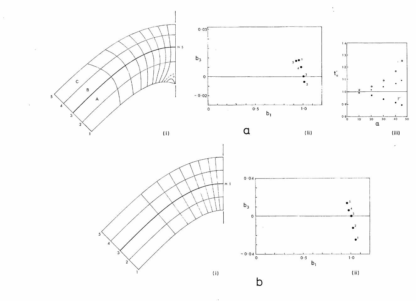
M S
0
a
1.0 b1
40 50 20 30
a 10
0.051-
N 14
13 b3 1
5 ••
4 • 12
3 a 1.1 •
2
10 - 0.02
1 0.9
0 80
0
o • 0 •
9 • •
• •
• •
0-04
b3
0
- 0.04 0
• 5
•4 3
0.5 1-0 b1
2
•1
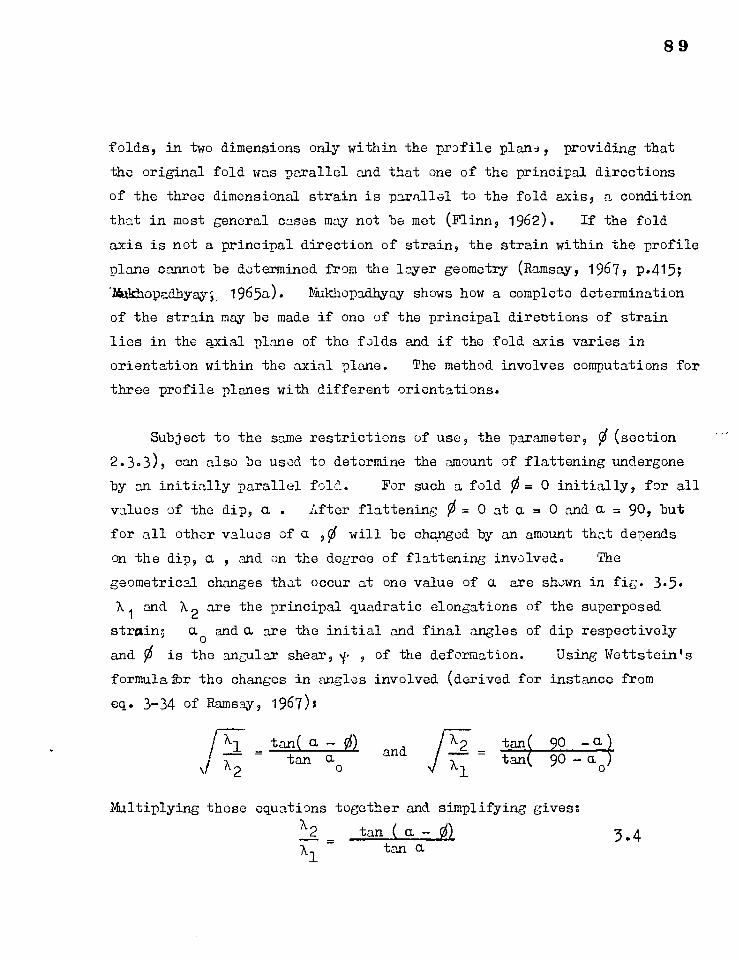
89
folds, in two dimensions only within the profile plane, providing that
the original fold was parallel and that one of the principal directions
of the three dimensional strain is parallel to the fold axis, a condition
that in most general cases may not be met (Flinn, 1962). If the fold
axis is not a principal direction of strain, the strain within the profile
plane cannot be determined from the layer geometry (Ramsay, 1967, p.415; -Nilkope.dhyan 1965a). MUkhopadhyay shows how a complete determination
of the strain may be made if one of the principal directions of strain
lies in the axial plane of the folds and if the fold axis varies in
orientation within the axial plane. The method involves computations for
three profile planes with different orientations.
Subject to the same
2.3.3), can also be used
by an initially parallel
values of the dip, a .
restrictions of use, the parameter, 0(section
to determine the amount of flattening undergone
folcl. For such a fold 0. 0 initially, for all
Lfter flattening 0. 0 at a = 0 and a = 90, but
for all other values of a 10 will be chapged by an amount that depends
on the dip, a , and on the degree of flattening involved. The
geometrical changes that occur at one value of a are shown in fig. 3.5.
the superposed
dip respectively
Using Wettstein's
instance from
A l and X2 are the principal quadratic elongations of
strain; ao and a are the initial and final angles of
and 0 is the angular shear, y, , of the deformation.
formula ffor the changes in angles involved (derived for
eq. 3-34 of Ramsay, 1967)%
ILL tan( a - 0) and / X
tan a
2 0
2 tan( 90 - ) X tan(90 - ao) 1
Multiplying these equations together and simplifying gives: X2
tan ( a - 0) tan a
3.4
Fig. 3.5
Modification of a parallel fold shape by a homogeneous 'flattening'
strain ix 2/x1 . 0.25.
a) Initial State AA = isogon at dip °, 0
b) Final State A'A' = deformed isogon at dip a
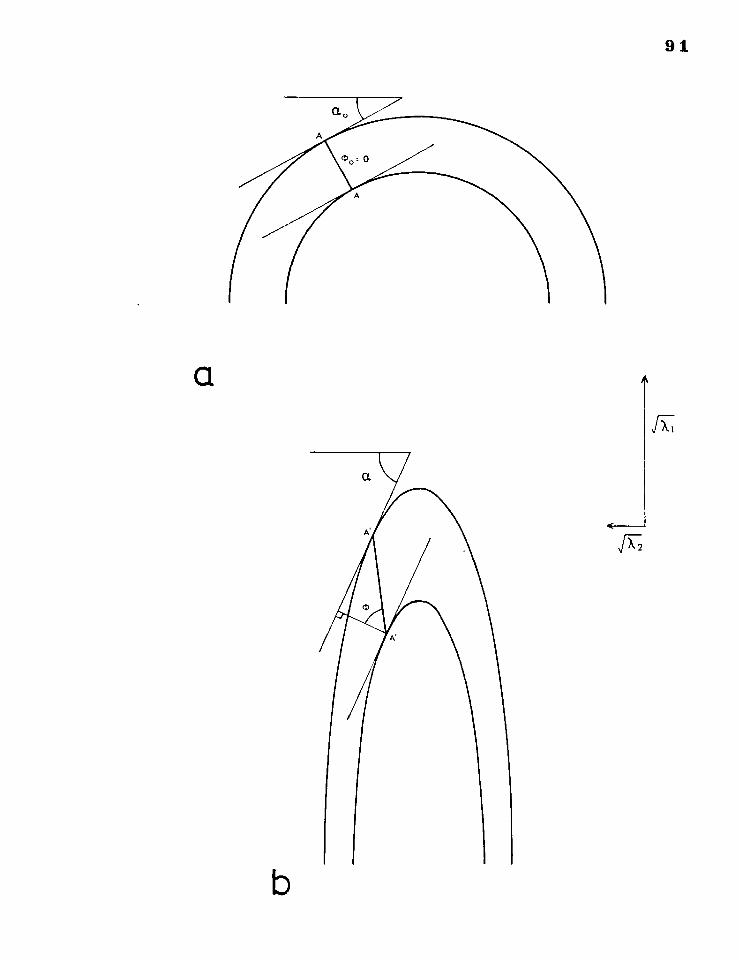
91

92
By substituting different values of X2/ xi into this equation curves
relating 0 and a for different amounts of flattening have been drawn
(fig. 3.6) which are directly comparable to those drawn by Ramsay (1962a; 1967, figs. 7-79 & 7-80) for the variation of t'a and T'a with a in
flattened parallel folds. The graph, fig. 3.6, is the mirror image
of one constructed by Breddin (1957, Table 5 fig.4) for strain determination
in fossils.
Because the value of /X2/ X1, determined from a plot of tta or
0 against a for a natural fold may not be atrue measure of strain, I will follow Mukhopadhyay (1965a) and refer to this value as an apparent
strain ratio, R (Fiukhopadhyay uses a symbol, a', the reciprocal of R).
R can be conaiclerad as an empirical parameter of fold shape that is only
directly related to a superposed strain in certain circumstances.
It is convenient to discuss hero a modification of the graphs of
and t'a against a that transform the family of curves of various x2/x1
values into straight lines. From equation 3.4 it is clear that a plot of tan( a - 0) against tan a will produce this transformaticn (fig. 3.7).
The relevant equation relating t'a , a and x2/x1
is given in Ramsay
-0 a 2
= xl A
X2 ( c _ X21 2 os a 3.5
J plot of t'a2 1
against cos2a will give a family of straight lines of
different slope for various values of X2/X1 (fig. 3.8).
The usefulness of a straight line representation lies in the fact
that plotted data for natural folds may be approximately re--resented by
best—fit straight lines using the familiar techniques of linear
regression by least squares. single fold may then be represented by
(1967, P.412):
Fig. 3.6
Variations of 0 with dip in flattened parallel folds for various values
of /2""l •
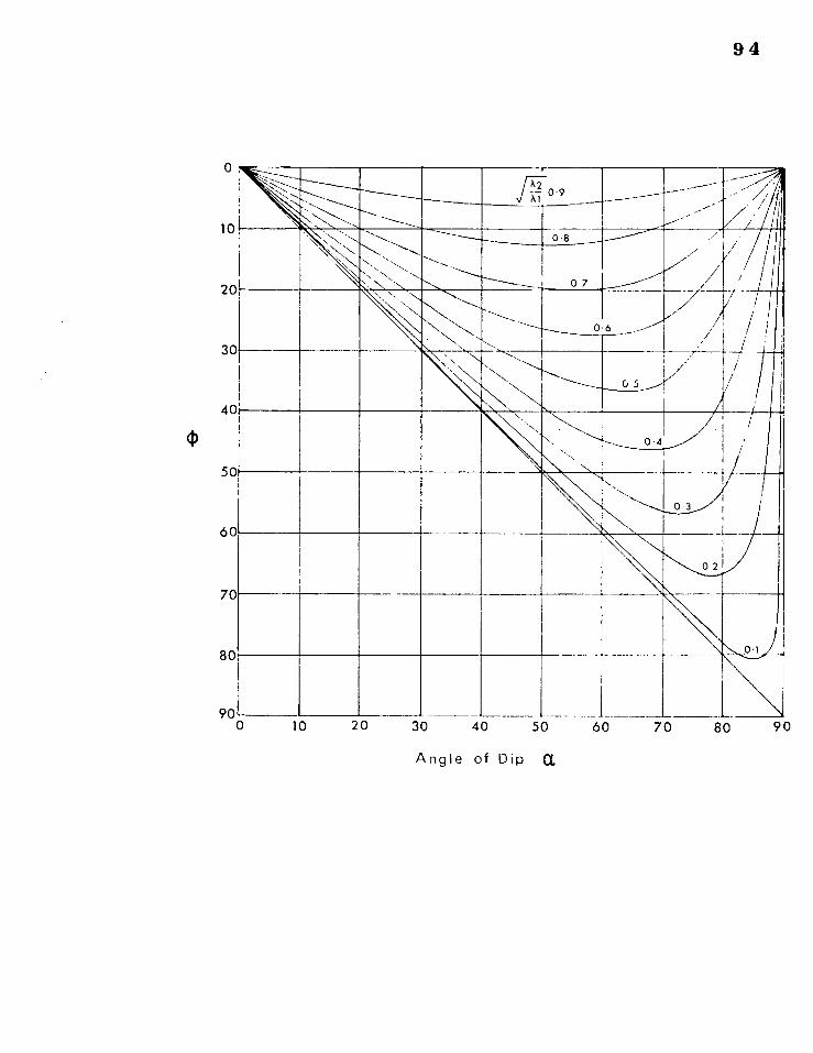
0 10 20 30 40 50 60 70 80 90
94
TT v 0 . 9 ----
!._
. - -- /1/
- - , / •
\ N...
---,
N ----..,„___________
--------__ 0 .8 .-----------
—__, 07
/'..-1.---'--------
___-------
I
. "
--, 0 6 ____-------
,,-
----------____ 0 5 , .,,, / r
.
\"-------„, o .3
N.Ns'''..\,.0 2
11441\ , 0 1
Angle of Dip a
0
10
2
3
4
5
6
7
8
90

Fig. 3.7
Straight line relationship in the variations of tan (a — 0) with tan a in
flattened parallel folds for various amounts of flattening.
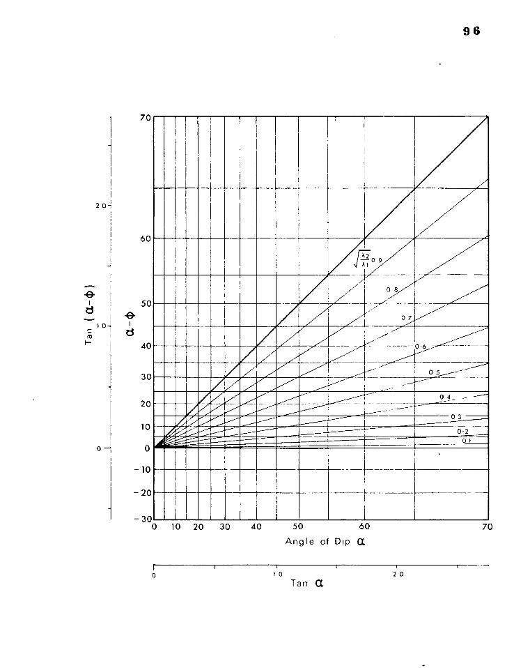
50
1 0-4 co 1- 40
30
20
10
0
10
- 20
- 30
60
96
A2 9 0
7 1 0 8 All
o7
1 I I WO Pr "
. _I-- 0 4 -
1------ - 0 3
0.2
1 :.0.036.--'...11111111111 0
0 10 20 30 40 50 60
70
Angle of Dip a
0
10 Tan a 2 0
70
I
2 0-
Fig. 3.8
Linear relationship in the variations of -02 with cos2o, in flattened
parallel folds for various amounts of flattening.
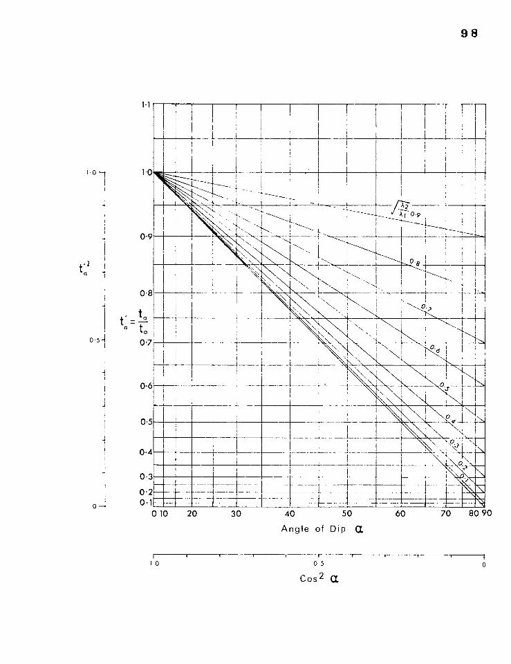
1.1
1 • 0 --I 10
to
09
0.8
ta =
07
06
05
O 4
O 3
O 2 O 1
0-5 -1
98
r
I L
I
1
-1-
,.. A , -4..
`..-- , , ',..
_l____ ----............„L ----..„..........
1--
A I 0-9 ' -- 1 ----i-, .....
-4--
4. .,
.., , J ---.9.1•<...,„
,,,, \ 1. .
1.-----1--
N NN
'N.
1-
1-
`‘
o.
1
, ....
010 20 30 40 50
60
70
80 90
Angle of Dip a
10 0 5
COS 2 a.
a single parameter, either the slope or the intercept of the best-fit
straight line
Plots of nearly all the natural folds measured by the writer are
closely approximated by straight lines on these graphs; the derived
parameters of slope and intercept, in the same way as R, may be considered
empirical and need not be related to flattening at all.
Since a graph of tan( a. -0) against tan a is infinite in two directions its use is best restricted to values of a less than 70°.
3.5.1 Oblique Flattening in the Profile Plane.
A single example of the effect of flattening a parallel fold will be
considered, to illustrate the general case in which two principal directions
of the superposed strain lie in the profile plane obliquely to the axial
surface trace. In fig. 3.9 a fold is drawn undeformed and at two finite
states of flattening,A2/xi. 0.5 and 0.25 the angle between the
principal axes of strain and the initial axial surface trace is 45°. In
the deformed states the originally 'symmetrical' fold with a straight
axial surface trace is transformed into an asymmetrical fold with a
curved axial surface trace (of the general case 3, section 2.3.5). This
is because the folded surfaces are different in shape, so that the hinge
points move around each deforming surface at a different rate.
Geometrically the effect is similar to that described by Schryver (1966),
of obliquely sectioning' cylindrical folds.
In nature, this kind of effect is likely to occur in parasitic folds
on the rotatinf, limbs of lar-er structures (Ramberg, 1963c).
3.6 SIMULTANEOUS BUCKLING AND FLATTENING.
Although de Sitter (1964) and Ramsay (1967, p.411) recognise that in
general unlimited shertenin of an actively folding layer maintaining a
99
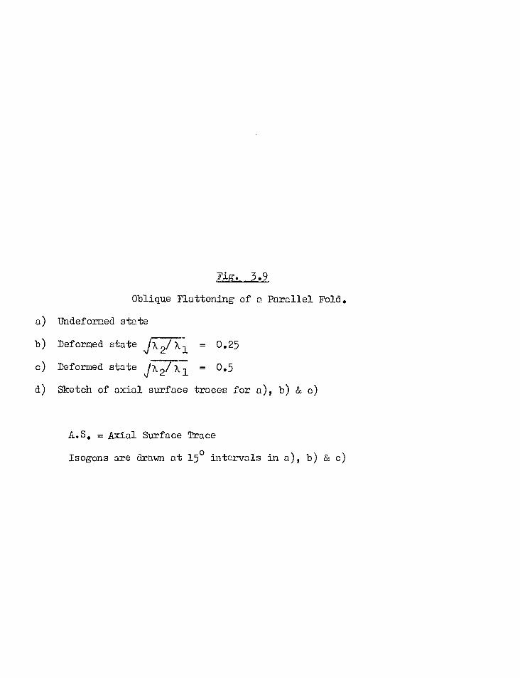
Fig. 3.9
Oblique Flattening of a Parallel Fold.
a) Undeformed state
b) Deformed state JA 2/ A l = 0.25
c) Deformed state IA 2/ A= 0.5
a) Sketch of axial surface traces for a), b) & c)
A.S. = Axial Surface Trace
Isogons are drawn at 15° intervals in a), b) & c)
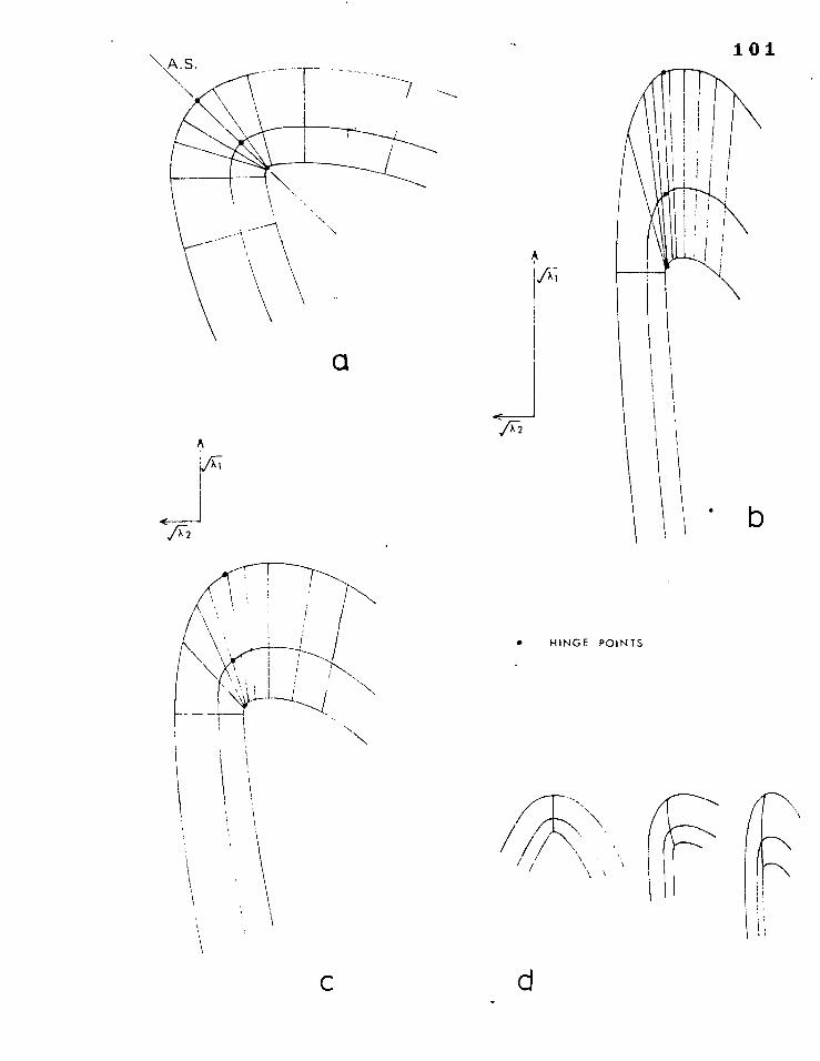
101
a
A
HINGE POINTS
c d
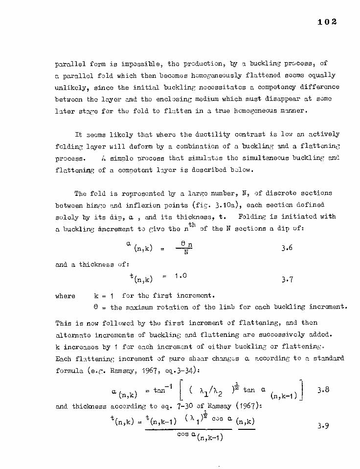
3.6 0n N
102
parallel form is impossible, the production, by a buckling process, of
a parallel fold which then becomes homogeneously flattened seems equally
unlikely, since the initial buckling necessitates a competency difference
between the layer and the enclosing medium which must disappear at some
later stage for the fold to flatten in a true homogeneous manner.
It seems likely that where the ductility contrast is low an actively
folding layer will deform by a combination of a buckling and a flattening
process. L. simple process that simulates the simultaneous buckling and
flattening of a competent layer is described below.
The fold is represented by a large number, N, of discrete sections
between hinge and inflexion points (fig. 3.10a), each section defined
solely by its dip, a , and its thickness, t. Folding is initiated with
a buckling increment to give the nth of the N sections a dip of:
a (n,k) =
and a thickness of:
t(n,k) 1.0 3.7
where k = 1 for the first increment.
= the maximum rotation of the limb for each buckling increment.
This is now followed by the first increment of flattening, and then
alternate increments of buckling and flattening are successively added.
k increases by 1 for each increment of either buckling or flattening.
Each flattening increment of pure
formula (e.g. Ramsay, 1967, eq.3-34):
—1 a (n,k) = tan
and thickness according to eq. 7-30
t(n,k) = t(nlk-1)
shear changes a according
1
( Al/A2 )2 tan
of Ramsay (1967): 1
( A1)2 cos (n,k)
to a standard
3.8 (a,k-1)
3.9 cos (n,k-1)
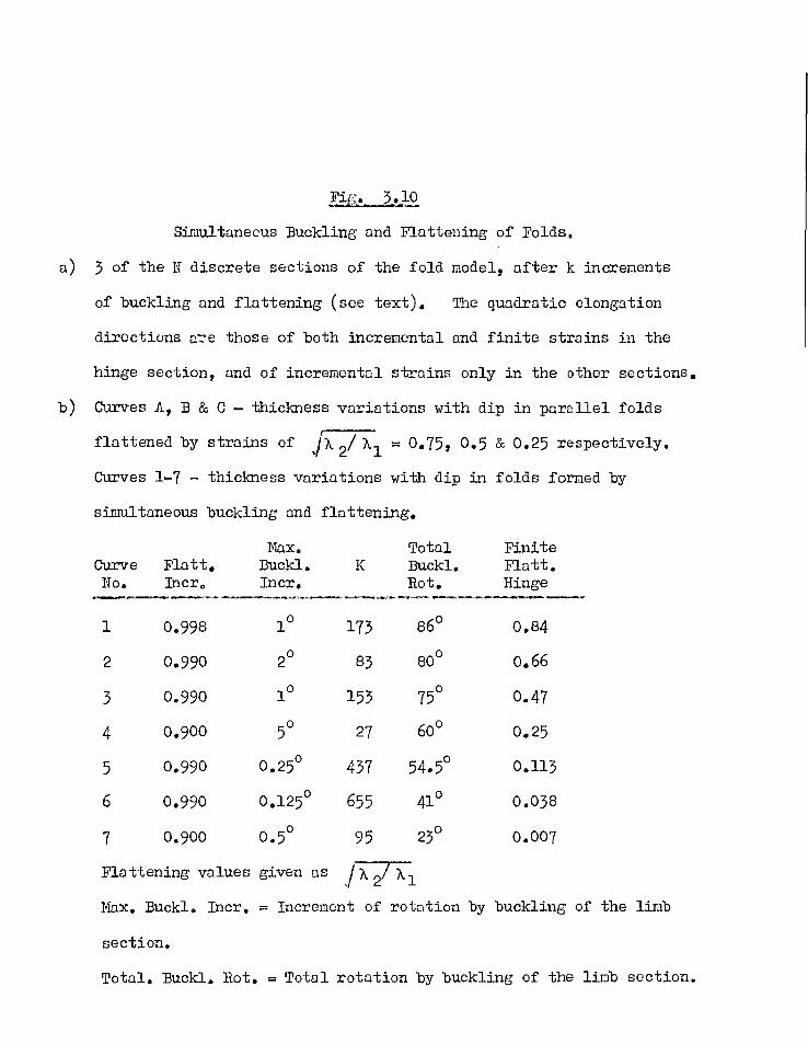
Fig. 3.10
Simultaneous Buckling and Flattening of Folds,
a) 3 of the N discrete sections of the fold model, after k increments
of buckling and flattening (see text). The quadratic elongation
directions are those of both incremental and finite strains in the
hinge section, and of incremental strains only in the other sections.
b) Curves A, B & C — thickness variations with dip in parallel folds
flattened by strains of IA 2/ 1 = 0.75, 0.5 & 0.25 respectively.
Curves 1-7 — thickness variations with dip in folds formed by
simultaneous buckling and flattening.
Curve No.
Flatt. Incr.
Max. Buckle Incr.
K Total Buckl. Rot.
Finite Flatt. Hinge
1 0.998 1o 173 86° 0.84
2 0.990 2° 83 80° 0.66
3 0.990 10 153 750 0.47
4 0.900 5° 27 6o° 0.25
5 0.990 0.25° 437 54.5° 0.113
6 0.990 0.125° 655 41° 0.038
7 0.900 0.5° 95 23° 0.007
Flattening values given as X2/ X1
Max. Buckl. Incr. = Increment of rotation by buckling of the limb
section.
Total. Buckl. Rot. = Total rotation by buckling of the limb section.
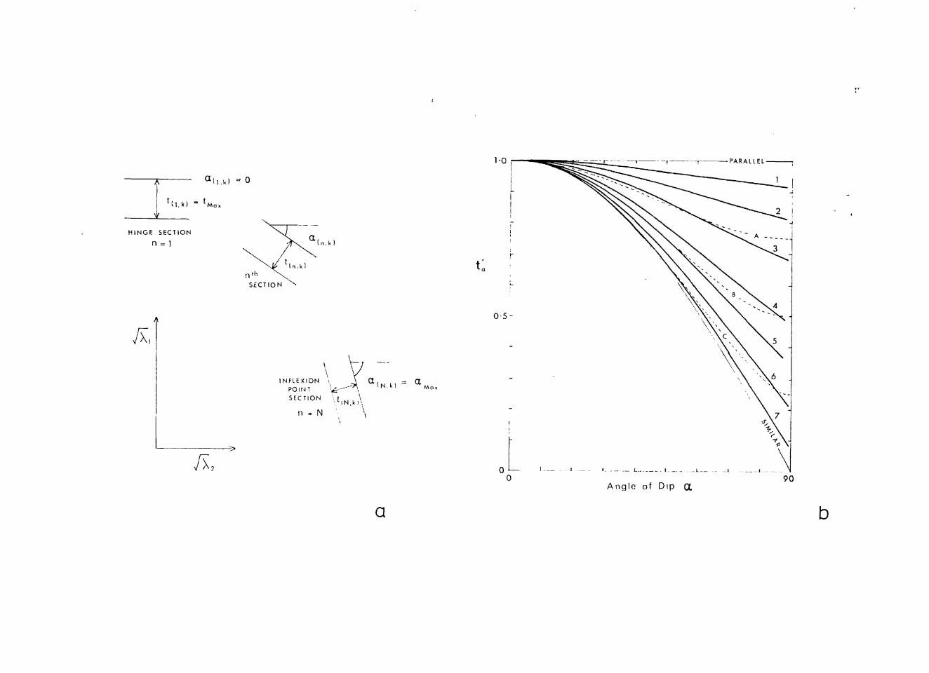
a
t (N,k
INFLEXION POINT SECTION
n N
IN a k I Max
A
HINGE SECTION
n =1
a(l.k) = 0
0 90
PARALLEL -7 1-0
0.5 -
0
Angle of Dip a,
t (Lk) tMax
A
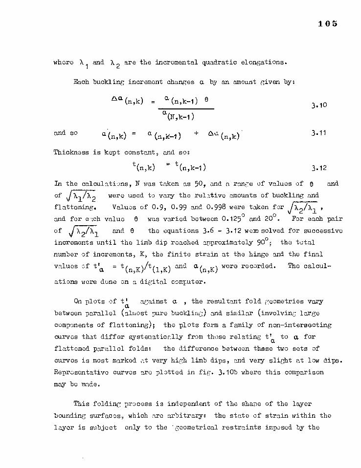
105
where X1 and X2 are the incremental quadratic elongations.
Each buckling increment changes a by an amount given by:
A (n k ) = a (n,k-1) 6 3.10 a (N k-1)
and so a (n, k) = a ) Au (n,k) 3.11
Thickness is kept constant, and so:
t(n,k) t(n,k_.1) 3.12
In the calculations, N was taken as 50, and a range of values of 0 and
of NIX1A2 were used to vary the relative amounts of buckling and
flattening. Values of 0.9, 0.99 and 0.998 were taken for fx2/xi ,
and for etch value 0 was varied between 0.125° and 20o. For each pair
of IX2A1 increments until the limb dip reached approximately 90°; the total
number of increments, K, the finite strain at the hinge and the final 0(1 K) and values of = t(n,K, 9
a(n,K) were recorded. The calcul-
ations were dune on a digital computer.
On plots of t' against a , the resultant fold geometries vary
between parallel (almost pure buckling) and similar (involving large
components of flattening); the plots form a family of non-intersecting
curves that differ systematically from those relating t'a to a for
flattened parallel folds: the difference between these two sets of
curves is most marked at very high limb dips, and very slight at low dips.
Representative curves are plotted in fig. 3.10b where this comparison
may be made.
This folding process is independent of the shape of the layer
bounding surfaces, which are arbitrary: the state of strain within the
layer is subject only to the 'geometrical restraints imposed by the
and 0 the equations 3.6 - 3.12 wem solved for successive
106
values of din and thickness and can therefore be accommodated in any
number of ways (not all of which are equally likely).
It must be stressed that there is no mechanical basis for choosing
this model, and the actual process will certainly be more complex.
However, the model proves useful, in a qualitative way, in the interpret—
ation of plots of tla against a for natural and experimentally produced folds (sections 5.7 and 4.8).
The reason why many natural folded competent layers appear to show
a geometrical relationship between t'a and a expected of ideal flattened
parallel folds may be due to:
a) Tho rheological contrast decreasing or vanishing during deformation
b) The resistance to continued buckling in the layer, imposed by the
enclosing medium, increasing as the fold tightens and the material
of the medium becomes extruded from the inner arc regions between
the limbs of the buckling layer (see Chapple, 1968). The
competent layer may then be forced to take up further deformation by
flattening.
c) A "tickling and flattening' process resulting in a fold whose geometry
is scarcely distinguishable from that produced by homogeneously
flattening a parallel fold.
The model proposed here is compatible with c) for small dips.
a) is thought to be unlikely as a general rule, and some combination of
the reasons given in b) and c) may account for the observed geometry of
many natural folds.
107
GRAPIER 4
EXPERIMENTS ON BUCKLING
4.1 INTRODUCTION
The existence of a buckling instability in many kinds of layered
systems (isolated beams, single layers set in a more ductile medium,
several layers of different ductilities forming a multilayered sequence)
shortened parallel to the layering has been well established experimentally
by a number of workers using a great variety of materials of a visco-
elastic or plastic nature. A brief summary of the relevant work is given
here.
The state of stress within and around buckled (less ductile) layers
at finite amplitudes has been studied using photoelastic techniques by
Bell & Currie (1964) and Currie, Patnode & Trump (1962), and the state
of finite strain within buckled layers by Ramberg (1963a).
Ramberg (1959) and Ghosh (1966) have studied the development of
buckles in layered systems undergoing simple shear. Experiments to
determine the relationship between the axial surface and fold axis and
the axes of bulk finite strain, where the buckling layers lie oblique to
the principal directions of strain, have produced ambiguous and controversial
results (see McBirney & Best, 1961; Ghosh, 1966, 1967; Singh, 1967).
Buckling experiments usually involve a maximum shortening parallel to
the layering in a bulk deformation of 'pure shear' type, resulting in more
or less symmetrical folds. The most important outcome of this work has
been the verification of the theory of Biot and Ramberg that predicts the
dominant wavelength of folds developed in a single layer embedded in a
relatively more ductile medium, where layer and medium are both Newtonian,
elastic or general viscoelastic bodies (see Section 3.3). The experimental
checks on the theory have treated the cases of viscous layer and medium,
108
elastic layer and viscous medium (Blot, Ode &Roever, 1961) and elastic
layer and medium (Ramberg, 1963b).
Ramberg (1963b), in a series of buckling experiments on elastic
multilayers has found that the observed wavelength/thickness ratios are the
same as the dominant wavelength/thickness ratios predicted theoretically for
viscous multilayers, by substituting elastic for viscous moduli in the
theoretical expressions. This might be expected from the rule of correspon—
dence between expressions derived for elastic and general viscoelastic
materials (Riot, 1957).
A series of experiments on the buckling of single layers of a viscous
material embedded in a less viscous medium, with low viscosity contrasts,
has been undertaken by the writer. These experiments are described in this
Chapter. This work was prompted by the apparent lack of correspondence between
a conclusion reached by Biot (1961, p.1607), who considered that no
significant folding would occur for a viscous layer embedded in a viscous
medium with a viscosity contrast of less than 100:1 (equivalent to a
dominant wavelength/thickness ratio of about 16:1), and the observed fact
that wavelength/thickness ratios of natural single layered folds are
frequently very much smaller than 16:1 (Sherwin & Chapple, 1968; sections
5.7 & 6.5 this thesis). At low viscosity contrasts shortening within the
competent layer becomes imnortant (Biot, 1961) and although the effects of
this have recently been theoretically evaluated in some detail by Sherwin
& Chapple (1968), they have not been verified experimentally.
The results of the experimonts described in this chapter will be
discussed in terms of the theories of Biot (1961) and Sherwin & Chapple (1968).
It was not found possible to determine accurately the viscosity contrasts
in the experiments, because of diffusional effects taking place between
layer and medium. The results could not therefore be used as a proper
109
quantitative check to the theory.
4.2 MODEL STUDY PROBLEMS
The problems of modelling tectonic processes are discussed by Hubbert
(1937), Donath (1963), Grovsky (1959), Beloussov (1960), Bell & Currie (1964)
and Ramberg (1967)f, the need to maintain similarity between a model and the
original (its prototype) by means of dimensional analysis is stressed by these
authors. Grovsky (1959) and Ramberg (1967) have attempted to simulate large
scale tectonic processes by employing fairly rigorous dimensional analyses, as
a basis for experimentation.
The present problem is the simulation of small scale folding in thin
isolated single layers in rock.
Geometrically the model will be about the same size as the prototype
folds. Beyond this, however, accurate modelling is impossible because the
rheological nature of the rock layer and its medium are unknown, the time
factor is indeterminate and the boundary conditions are also largely unknown
(see Heard, 1968).
Although rocks exposed at the earth's surface are clearly not viscous
substances, that rocks are able to deform very considerably by some kind of
flow over geological periods of time is indisputable from evidence of deformed
objects of known original shape and of folds themselves.
The treatment of rocks as Newtonian viscous bodies has several
advantages; mathematical analyses are generally simplified, and buckling
is theoretically independent of both absolute values of viscosity and rate
of deformation, Gay (1966) discusses at some length the validity of an
assumption of Newtonian viscosity for rocks, and he concludes that such an
assumption may be reasonably valid where stresses are applied for long periods
of time or where the rate of strain is slow. Flinn (1965) discusses the
nature of flow in rocks and the possible mechanisms by which it can be
110
accomplished. He considers diffusion to control deformation in metamorphism,
but thinks a true Newtonian viscosity unlikely. Reiner (1960, p.11)
considers all materials to possess all rheological properties at once, and
if stresses are maintained for a sufficient length of time Carey (1954)
considers that the effects of the viscous component of strain will exceed
all others.
Following Gay, I will assume that rocks probably behave as Newtonian
bodies (i.e. the stress/strain rate equations are linear) to a first
approximation, under conditions that are most likely to be met in areas of
regional metamorphism.
4.3 APPARATUS AND MATERIALS
The simplest type of experiment that will produce more or less
symmetrical folds is one in which the principal direction of shortening
is initially parallel to the layering, and remains parallel to the enveloping
surface of the folds as they develop. If in addition the fold axis is a
direction of no change the problem reduces to one of two dimensions. These
are the conditions usually met with in theoretical work; they can be
satisfied experimentally by use of a shear box that maintains plane strain
in pure shear. For the present series of experiments, a shear box was
designed and built to meet those requirements.
The shear box is shown in plate 1, and a plan is drawn in fig. 4.1.
It has four rigid L-shaped corner pieces made from Tufnel plate. From
the base of each of these protrudes a short steel peg that is free to
rotate, and which moves in a groove cut in the metal base plate of the box.
On two opposite sides of the box the corner units are connected by smooth
lubricated metal rods, free to slide through close-fitting tubes rigidly
attached to the corner units, and on the other two sides similar rods and
tubes are threaded to allow for a screw movement only. The connecting
rods ensure that the construction maintains a rectangular shape, and keeps
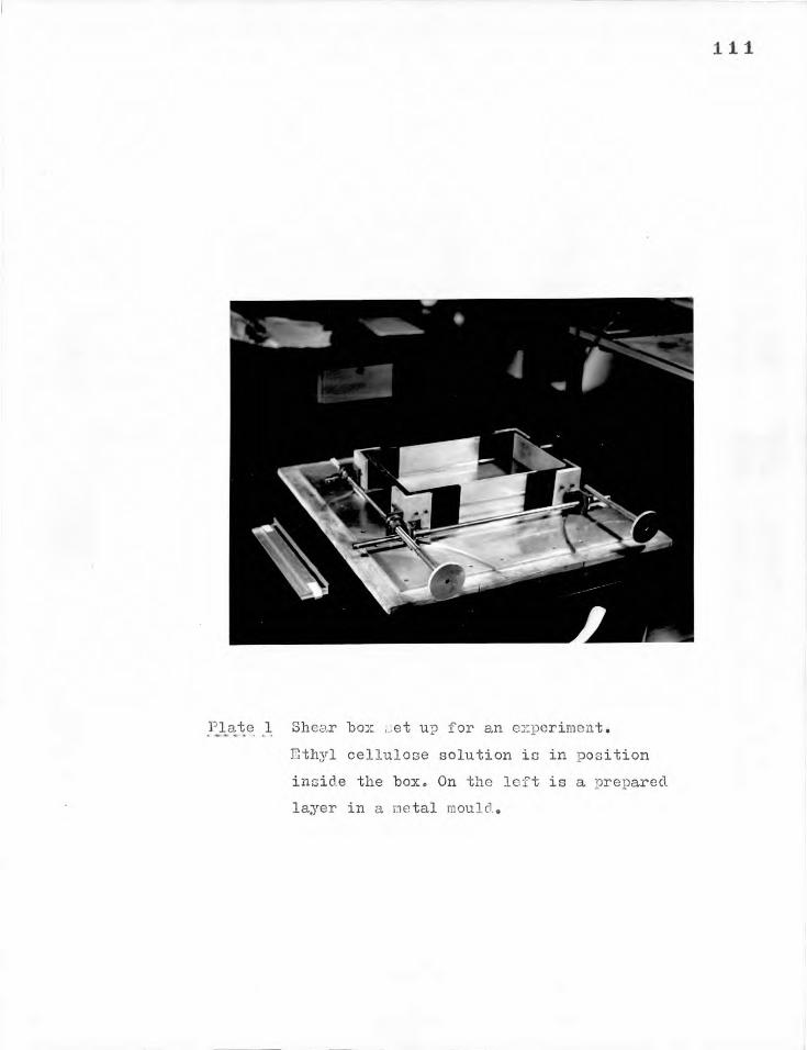
Plate .1 Shear box ;Jet up for an experiment.
Ethyl cellulose solution is in position
inside the box. On the left is a prepared
layer in a metal mould.

Fig. 4.1
Simplified plan of the shear box. Only two of the connecting rods are
shown. The box is symmetrical about the x axis.
A Base Plate
B Hyperbolic Groove
C Corner Piece
D Side Plate
E Connecting Rods
F Operating Handle
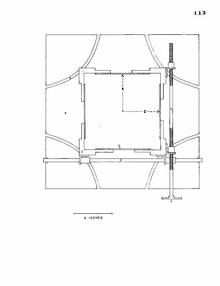
113
A
'7=
1
F
6 INCHES
114
the corner units in mutual alignment. They also allow for changes in
overall length of the box sides. Part of each side is formed by the
corner pieces, and the central part is a thin flat metal plate that rests
against and is able to slide over the corner pieces to allow for changes
in length of sidle. These plates are held in position by the material
in the box. The box is 4" deep. By turning the handles attached to the two threaded connecting rods the corners of the box move simultaneously along
their grooves, and the overall lengths of side progressively change, whilst
maintaining a rectangular fora. The grooves were cut in the base plate
such that the inside corners of the corner pieces move along hyperbolic
paths given by;
x z = k
where x and z are coordinates parallel to the sides of the box
with the cen-Le as origin, and k is a constant.
and so the area contained 'within' the box remains constant as the lengths
of side change.
The limiting ratios of lengths of two adjacent sides are 2:1 and 1:2
respectively.
If, during deformation, each material point in the box moves according
to:
x z - k' 4.
where k' and c are constants; k 1
Y = c varies with distance from the centre
of the box, k' k. c varies
ITith distance from the base.
The conditions of plane strain and pure shear would be fulfilled. The
maximum strain ratio (iX1/X2) expected would be 4:1.
Because the base plate is rigid and each side is compounded from three
rigid parts, considerable boundary effects may be expected to modify the
ideal behaviour of material deformed within the box. Their effects are
discussed in the next section.
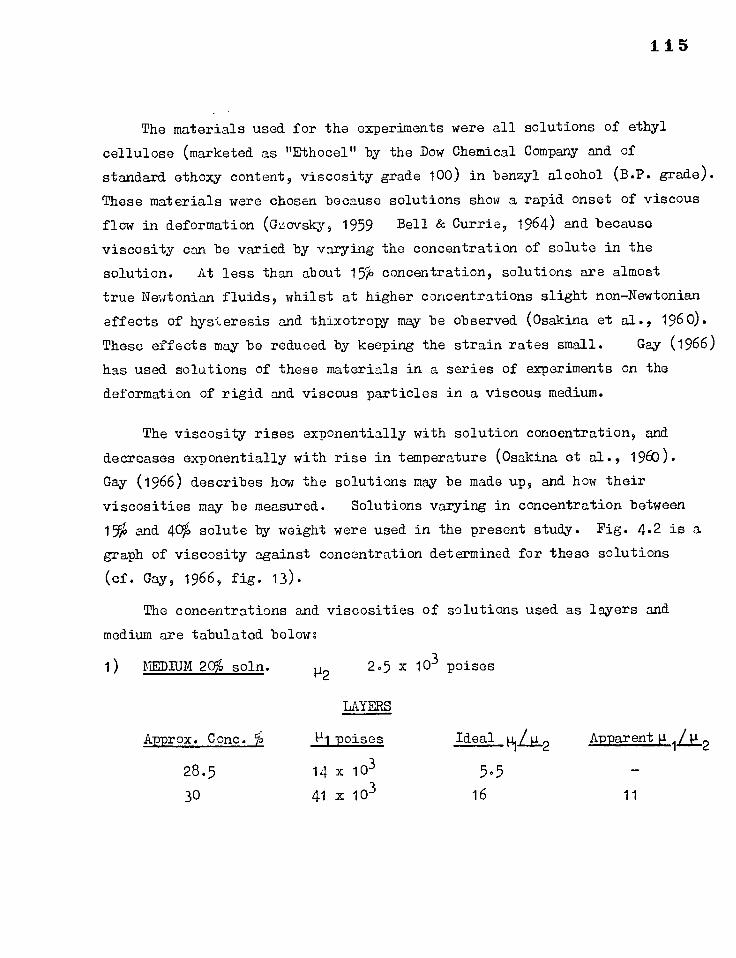
115
The materials used for the experiments were all solutions of ethyl
cellulose (marketed as "Ethocel" by the Dow Chemical Company and of
standard ethoxy content, viscosity grade 100) in benzyl alcohol (B.P. grade).
These materials were chosen because solutions show a rapid onset of viscous
flow in deformation (Grovsky, 1959 Bell & Currie, 1964) and because
viscosity can be varied by varying the concentration of solute in the
solution. At less than about 15% concentration, solutions are almost
true Newtonian fluids, whilst at higher concentrations slight non—Newtonian
effects of hysteresis and thixotropy may be observed (Osakina et . 196 0) . These effects may be reduced by keeping the strain rates small. Gay (1966)
has used solutions of these materials in a series of experiments on the
deformation of rigid and viscous particles in a viscous medium.
The viscosity rises exponentially with solution concentration, and
decreases exponentially with rise in temperature (Osakina et al., 1960).
Gay (1966) describes how the solutions may be made up, and how their
viscosities may be measured. Solutions varying in concentration between
15P and 40% solute by weight were used in the present study. Fig. 4.2 is a
graph of viscosity against concentration determined for these solutions
(cf. Gay, 1966, fig. 13).
The concentrations and viscosities of solutions used as layers and
medium are tabulated below:
1) MEDIUM 20% soln. 1-12
2.5 x 10³ poises
Approx. Conc. %
28.5
30
LAYERS
P1 poises
14 x 103
41 x 103
Apparent
11

Fig. 4.2
Relationship between viscosity and concentration of solutions of ethyl
cellulose (viscosity grade 100) in benzyl alcohol.
(cf. Gay, fig. 13, 1966).
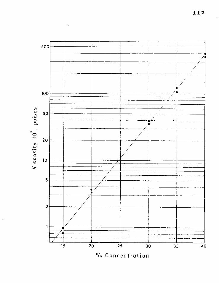
117
15
20
25
30
35
40
0/0 Concentration
/4
/4
/
•
L /
/ , I ,
/
t-•
-
50
100
2
1
r
20
5
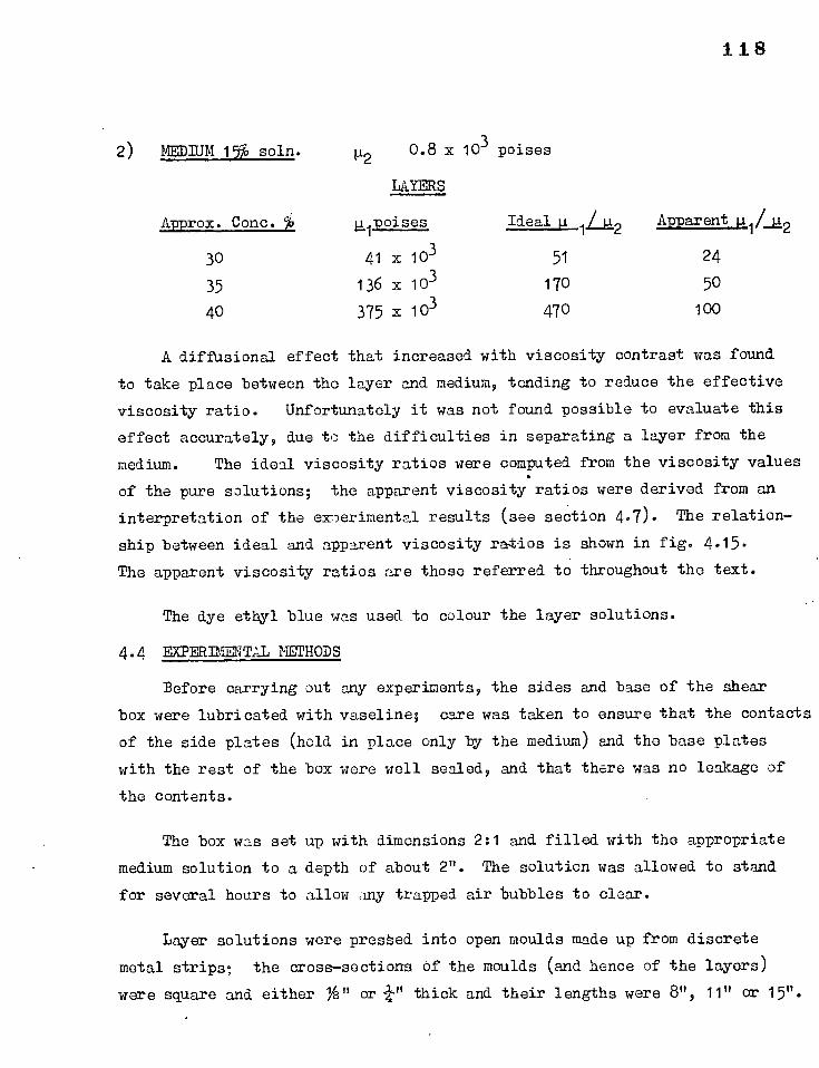
118
2) MEDIUM 15% soln. 112 0.8 x 10³ poises
LAYERS
Approx. Conc. % 1 Ideal u 1212 Apparent pl/j1,2
30 41 x 103 51 24
35 136 x 103 170 50
40 375 x 103 470 100
A diffusional effect that increased with viscosity contrast was found
to take place between the layer and medium, tending to reduce the effective
viscosity ratio. Unfortunately it was not found possible to evaluate this
effect accurately, due to the difficulties in separating a layer from the
medium. The ideal viscosity ratios were computed from the viscosity values
of the pure solutions; the apparent viscosity ratios were derived from en
interpretation of the ex1Derimental results (see section 4.7). The relation-
ship between ideal and apparent viscosity ratios is shown in fig. 4.15.
The apparent viscosity ratios are those referred to throughout the text.
The dye ethyl blue was used to colour the layer solutions.
4.4 EXPERIMENTAL METHODS
Before carrying out any experiments, the sides and base of the shear
box were lubricated with vaseline; care was taken to ensure that the contacts
of the side plates (held in place only by the medium) and the base plates
with the rest of the box were well sealed, and that there was no leakage of
the contents.
The box was set up with dimensions 2:1 and filled with the appropriate
medium solution to a depth of about 2". The solution was allowed to stand
for several hours to allow any trapped air bubbles to clear.
Layer solutions were pressed into open moulds made up from discrete
metal strips: the cross-sections of the moulds (and hence of the layers)
were square and either 1/A" ore thick and their lengths were 8", 11" or 15".
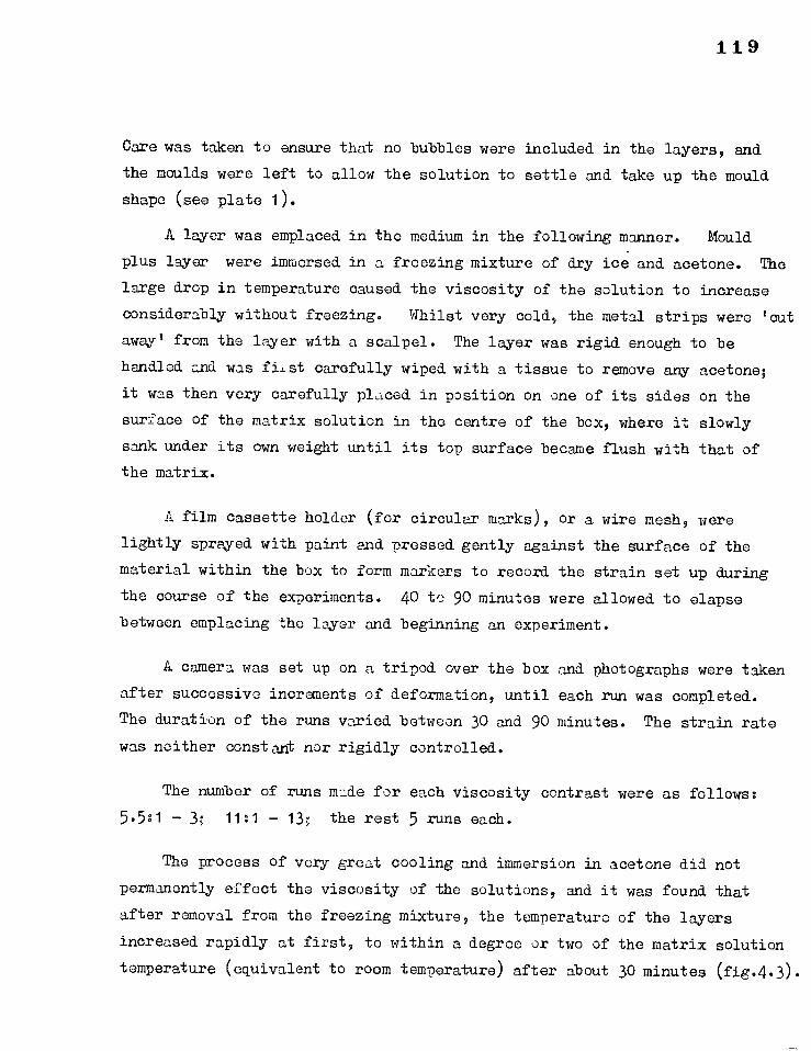
119
Care was taken to ensure that no bubbles were included in the layers, and
the moulds were left to allow the solution to settle and take up the mould
shape (see plate 1).
A layer was emplaced in the medium in the following manner. Mould
plus layer were immersed in a freezing mixture of dry ice and acetone. The
large drop in temperature caused the viscosity of the solution to increase
considerably without freezing. Whilst very cold, the metal strips were 'cut
away' from the layer with a scalpel. The layer was rigid enough to be
handled and was fist carefully wiped with a tissue to remove any acetone;
it was then very carefully placed in position on one of its sides on the
surface of the matrix solution in the centre of the box, where it slowly
sank under its own weight until its top surface became flush with that of
the matrix.
A film cassette holder (for circular marks), or a wire mesh, were
lightly sprayed with paint and pressed gently against the surface of the
material within the box to form markers to record the strain set up during
the course of the experiments. 40 to 90 minutes were allowed to elapse
between emplacing the layer and beginning an experiment.
A camera was set up on a tripod over the box and photographs were taken
after successive increments of deformation, until each run was completed.
The duration of the runs varied between 30 and 90 minutes. The strain rate
was neither constant nor rigidly controlled.
The number of runs made for each viscosity contrast were as follows:
5.5:1 — 3; 11:1 — 13; the rest 5 runs each.
The process of very great cooling and immersion in acetone did not
permanently effect the viscosity of the solutions, and it was found that
after removal from the freezing mixture, the temperature of the layers
increased rapidly at first, to within a degree or two of the matrix solution
temperature (equivalent to room temperature) after about 30 minutes (fig.4.3)•
Fig. 4.3
Temperature increase with time in a layer taken from a freezing mixture
(of dry ice and acetone), and placed in a host medium. (The bulb of a
thermometer was encased in a blob of a solution of 30% concentration so
that the solution formed a shell about 1/8" thick. Both blob and
thermometer were placed in the freezing mixture, left for 5 minutes, and
were then removed and placed in a solution of 20% concentration at room
temperature.).
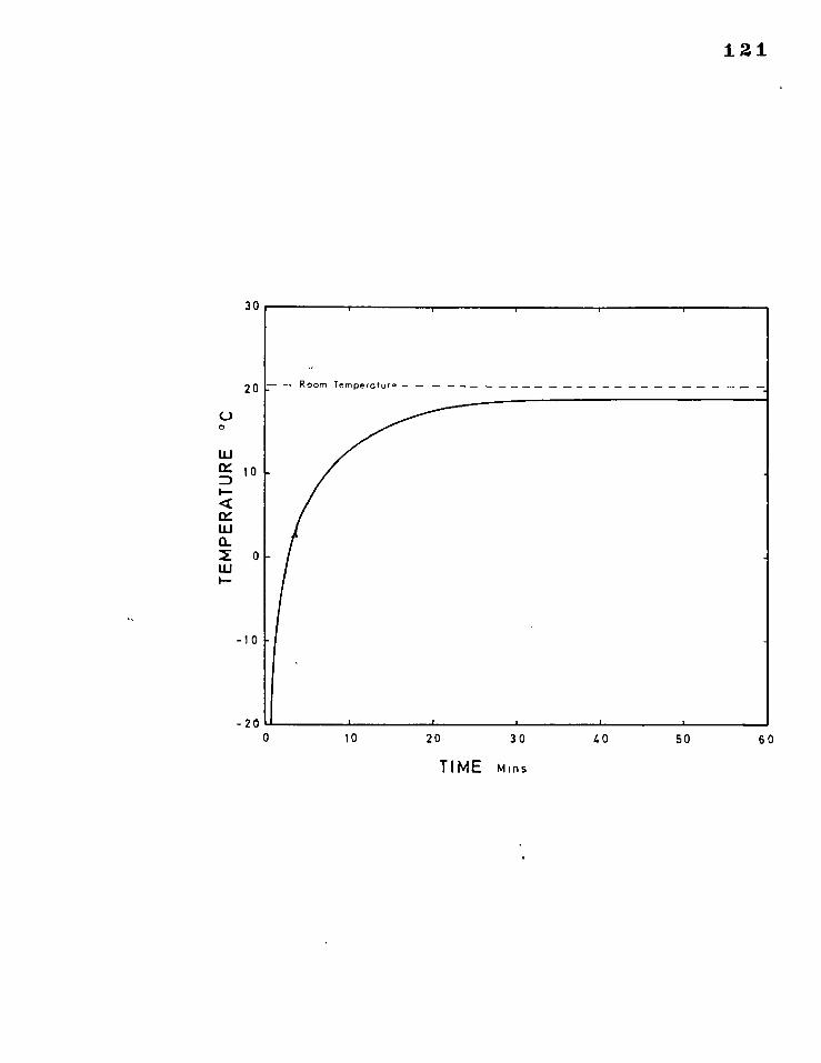
20 .7- — Room Temperotur ,!
121
30
10
—10
20 0
0
TEM
PER
ATU
RE
10 20 30 40 50 60
TIME Mans

122
The rate of further increase in temperature was very slow.
4.5 HOMOGENEITY OF STRAIN & BOUNDARY EFFECTS
I series of experimental runs were carried out with one solution only
in the box to determine the degree and extent of homogeneous deformation.
Fig. 4.4 is a drawing (traced from a photograph) showing the deformation
of originally circular markers) to form 'ellipses' with axial ratios of
about 4:1 near the centre of the box. The variations of strain near the
boundaries of the box (in the blank regions of fig. 4.4) were mite complex.
These variations involved increases in surface area along the two approaching
sides of the box and decreases along the receding sides. The strain at
the centre of the box (in an area bounded by lengths roughly half those of
the total length and breadth of the box at any one time), was however fairly
homogeneous, and measurements show that there was no surface area change
in this region. Moreover no significant differences in strain pattern could
be detected when the depth of material was varied between 1" and 2i".
It was concluded that the strain at the centre of the box for depths
of material between 1" and 2" was close to a two dimensional pure shear.
The relationship between the observed strain ratio (S =iX11x2) at the
centre of the box and that predicted from dimensional changes of the box
(the strain that would exist if deformation progressed according to
equations 4.1) was found to be consistent for all the runs mado5 data for
one run is shown in fig. 4.5a; measurements were recorded at equal
increments of predicted strain. The relationship between the observed
strain ratio and the predicted strain ratio was clearly not linear, and
the maximum observed strain ratio was almost twice that predicted.
The non—linear relationship is to be expected if the predicted
incremental strain ratio, IR 9 and the observed incremental strain ratio
IRo, are linearly related by:
ER = k1Ro
k = constant
FiE, 4- 4
Deformed circular narks on the surface of material in the shear box
after a strain of about jA,2/A l .--- 0.25.

124
,
Relationship between the strain, So, observed at the centre of the shear
box and the strain, Sp, predicted from shape changes of the box.
In a) each numbered dot marks each increment of deformation,
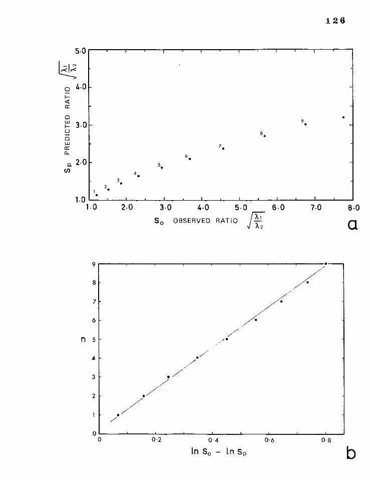
6.0 7.0 2.0 3.0 4.0 5.0
9
8
7
6
n 5
4
3
2
1
0 0.6 0.8 0
0.2 0.4
En so — In sp
126
So OBSERVED RATIO
1.0 1.0
a 2.0 U)
8.0
a
PRED
ICTED
RA
TIO
5.0
4.0
3.0
I
9
8•
7•
6• 5 •
4
3 26 1
•
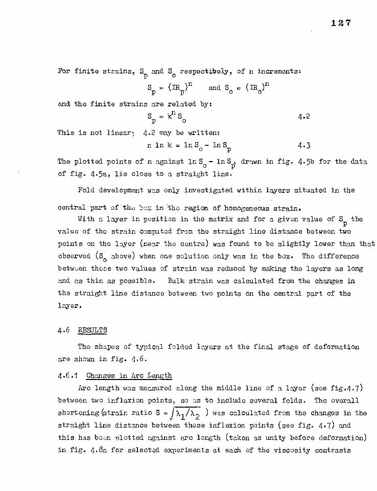
127
For finite strains, S and So respectibely, of n increments:
P = (IR P)n and So = (IRdn
and the finite strains are related by:
S = kn So 4.2
This is not linear; 4.2 may be written:
n ln k = ln So — ln S p 4.3
The plotted points of n against In So In Sp, drawn in fig. 4.5b for the data
of fig. 4.5a, lie close to a straight line.
Fold development was only investigated within layers situated in the
central part of -box in *the region of homogeneous strain.
With a layer in position in the matrix and for a given value of S the
value of the strain computed from the straight line distance between two
points on the layer (near the centre) was found to be slightly lower than that
observed (So above) when one solution only was in the box. The difference
between these two values of strain was reduced by making the layers as long
and as thin as possible. Bulk strain was calculated from the changes in
the straight line distance between two points on the central part of the
layer.
4.6 RESULTS
The shapes of typical folded layers at the final stage of deformation
are shown in fig. 4.6.
4.6.1 Changes in Arc Length
Arc length was measured along the middle line of a layer (see fig.4.7)
between two inflexion points, so as to include several folds. The overall
shortening(strain ratio S =1X1A2 ) was calculated from the changes in the
straight line distance between these inflexion points (see fig. 4.7) and
this has been plotted against arc length (taken as unity before deformation)
in fig. 4.8a for selected experiments at each of the viscosity contrasts
Fig. 4.6
Examples of Experimentally Produced Buckles.
a) Viscosity ratio of 24:1 bulk deformation S = 6.
b) Deformed rectangular grid constructed for a). N.B. The initial
spacing of the grid lines between the three discrete segments of
grid shown in a) is irregular.
c) Viscosity ratio of 100:1 , bulk deformation S = 6.
d) Viscosity ratio of 5,5:1 2 bulk deformation S = 6.5.
(the scale is the sane as that in b)).
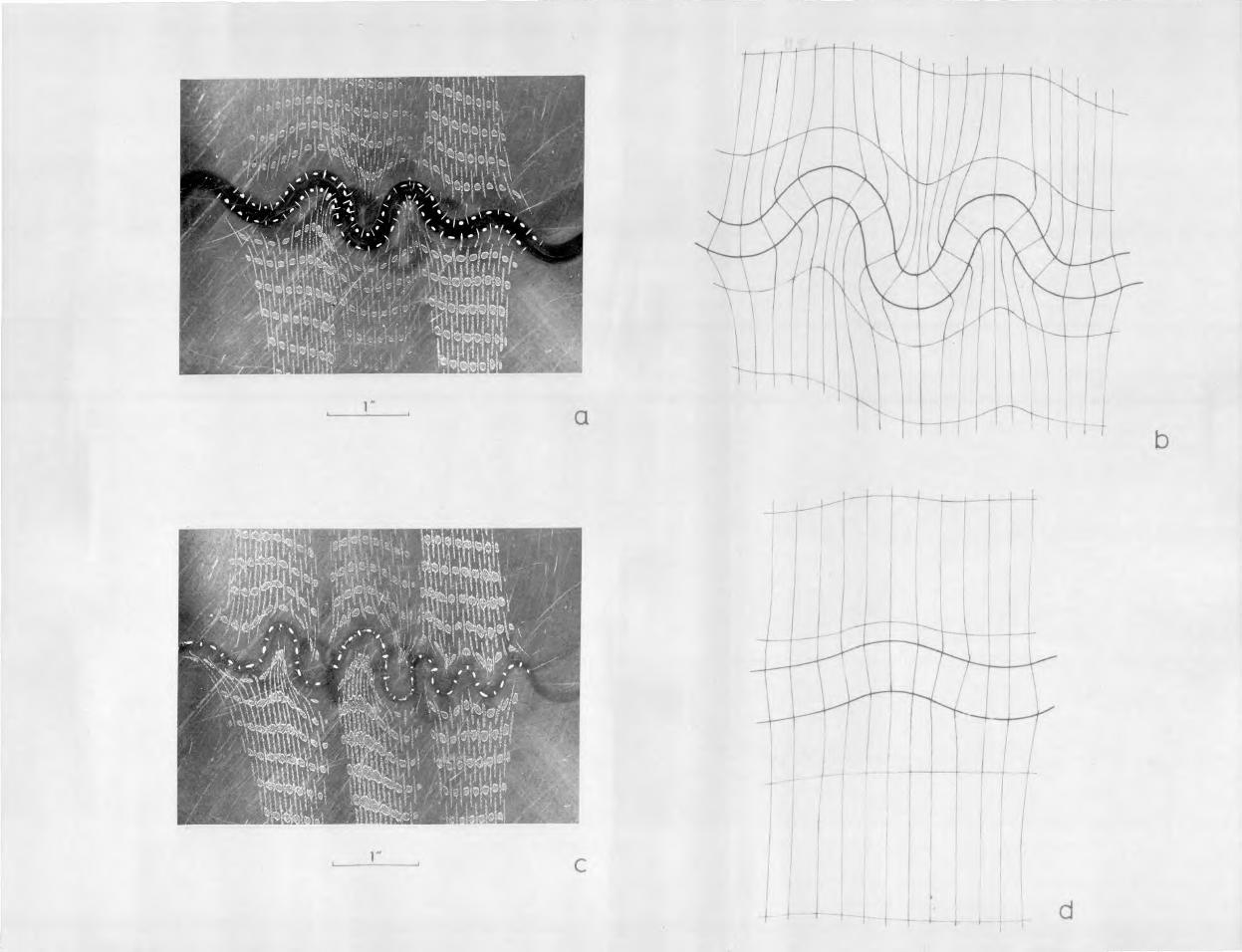
1
I
1" a
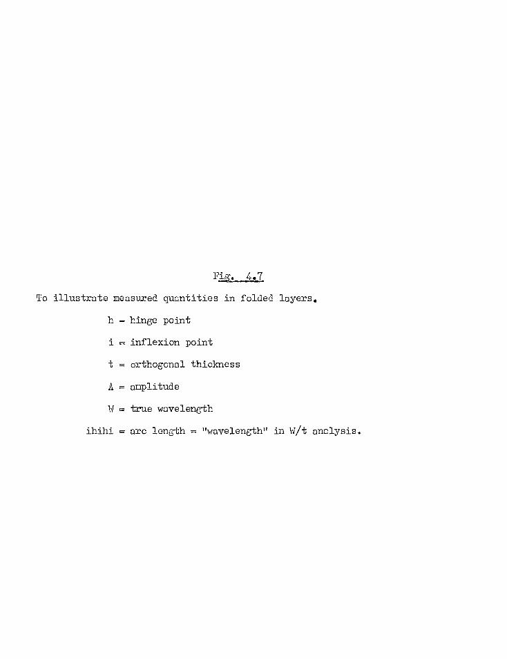
Fi. 4.7 To illustrate measured quantities in folded layers.
h — hinge point
i = inflexion point
t = orthogonal thickness
A = amplitude
W . true wavelength
ihihi = arc length = "wavelength" in w/t analysis.

131
!<
w
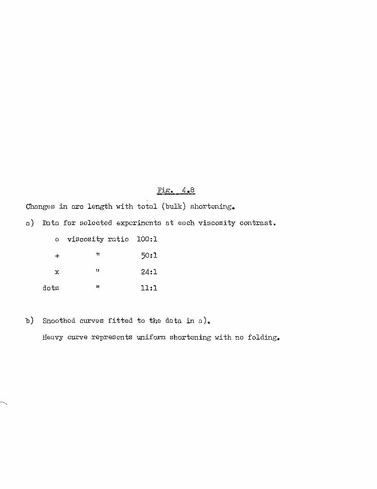
Fig. 4.8
Changes in arc length with total (bulk) shortening.
a) Data for selected experiments at each viscosity contrast.
o viscosity ratio 100:1
50:1
24:1
dots It 11:1
b) Smoothed curves fitted to the data in a).
Heavy curve represents uniform shortening with no folding.
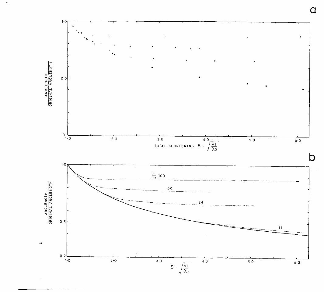
AR
CLE
NG
TH
AR
CLE
NG
TH
O
RIG
INA
L A
RC
LEN
GT
H
OR
IGIN
AL
AR
C L
EN
GT
H
9
0
0
+ 0
0
0
•
0
•
• •
0
•
134
(with the exception of the smallest). Smoothed curves for the same data
have been drawn in fig. 4.8b, together with a curve representing length
changes due to homogeneous shortening with no folding.
From this figure it is apparent that the initial shortening of a layer
or change of arc length is that of a homogeneous compressive strain.
However, a stage is reached where little further changes in arc length occur.
The stage (i.e. bulk strain ratio) at which the arc length becomes 'stable'
is different for each viscosity contrast. The maximum percentage shortening
undergone by the layer has been estimated in each experiment. The values
are listed below.
Viscosity ratio
shortening Mean
100 13 10 13 12 12.5 12
50 23 20 23.5 22 23 22
24 34 33 36.5 33 33 34
11 ? 50 — 60 for all expts.
The degree of correspondence between values of shortening in several
experiments at any one viscosity contrast is fairly close. Since the amount
of shortening possible in the shear box is limited to about 640, the estimates
for the lowest viscosity contrast,11:1, may be too small.
It was found that at the stages where the arc lengths became
'stabilised' (corresponding to the points of divergence of the experimentally
derived curves from the curve representing uniform shortening in fig. 4.8b),
the folds had mean limb dips of about 15° (varying between 5o and 30°) and
this value was found to be independent of viscosity contrast.
4.6.2 Thickness Variation in the Buckled Layers
No significant thickening in the hinges or thinning in the limbs was
observed in any of the folds developed in the experiments, for the whole
135
range of viscosity contrasts (see fig. 4.6). At the maximum deformation
attainable in the box, folds developed at a viscosity ratio of 11:1 rarely
attained limb dips greater than 30°. One experiment at this viscosity
contrast was continued beyond the limits imposed by the box, by crudely
compressing the folded layer between two plates to produce near isoclinal
folds (at a bulk strain ratio of about 20:1). These folds did show a
Certain amount of thickening in the hinges.
4.6.3 Wavelength/Thickness Ratios
The range in values of fold wavelengths developed at each viscosity
contrast was considerable.
The 'wavelength' (the arc length of mature folds, see section 1.2),
taken as twice the measured distance between adjacent hinges along the
middle line of the folded layer(fig. 4.7), and layer thickness were recorded
for each fold in each experiment, at a stage of the deformation when the arc
length had reached its stable value. For the viscosity contrast of 11:1,
these parameters were measured at a bulk strain of about S = 5.0. Wavelength/
thickness ratios were calculated, and frequency histograms of this ratio
have boon plotted in fig. 4.9 for each viscosity contrast. Examination
of this figure shows:
a) a considerable spread in w/t ratios for every viscosity contrast, and a
substantial overlap between the ranges of ratios observed for the different
viscosity contrasts.
b) mean values of W/t of 3.8, 6.8, 10.5, and 13.3 for viscosity contrasts
of 11, 24, 50 and 100:1 respectively.
c) similar relative spreads of the distributions as measured by the ratio
of standard deviation/mean.
4.6.4 Amplification
Progressive changes in amplitude during fold development were recorded
with increasing strain ratio, S, of the overall shortening. Amplitude, A,
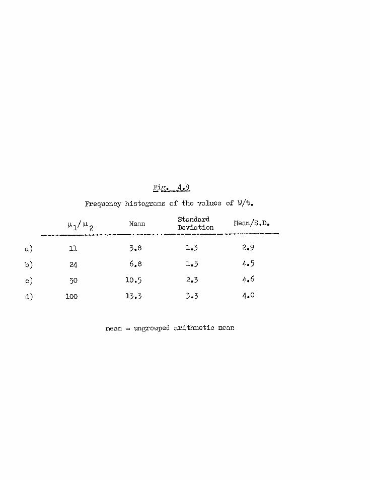
FiF. 4.9
Frequency histograms of the values of W/t.
Is/ 1/ R 2 Mean
Standard Deviation
Mean/S.D.
a) 11 3.8 1.3 2.9
b) 24 6.8 1.5 4.5
c) 50 10.5 2.3 4.6
d) 100 13.3 3.3 4.0
mean = ungrouped arithmetic mean
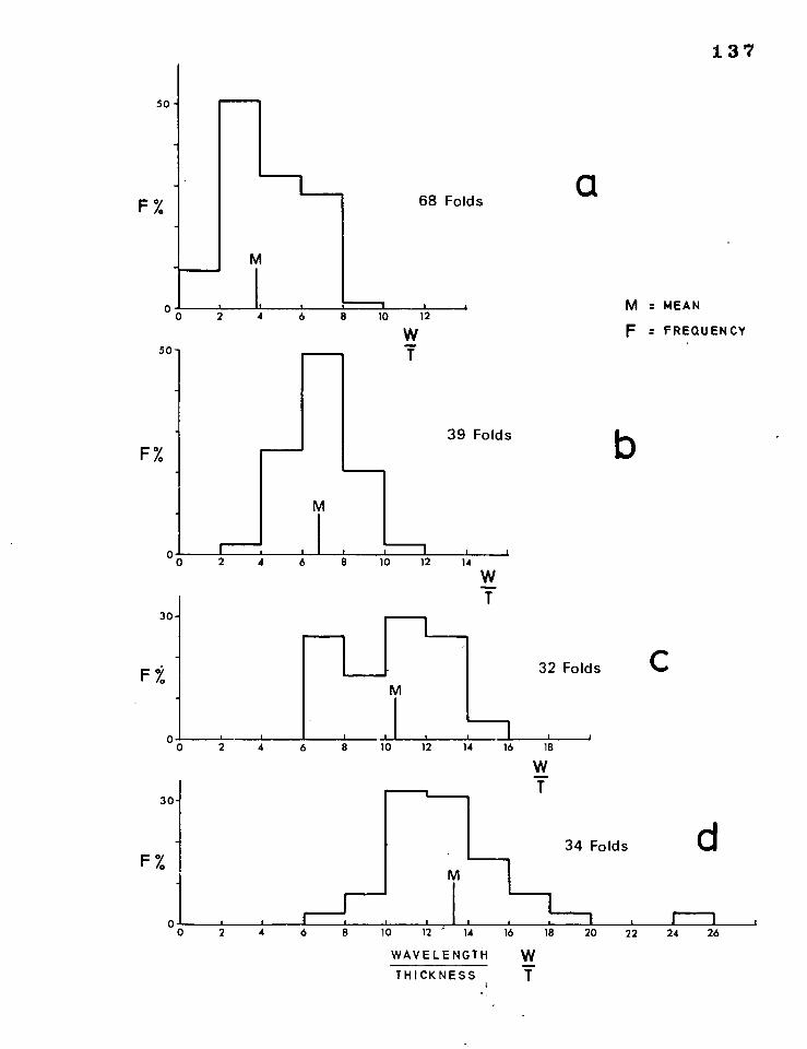
137
50 -
a 68 Folds F %
M = MEAN
F = FREQUENCY 2
I 10 12
50-
F% 39 Folds b
W T
1 . 1 6 8 10 12 14
w T
4 6 8 10 12 14
30-
F%
2
C 32 Folds
w T
34 Folds d
2 4 8 10
M
, I
WAVELENGTH
THICKNESS
1.".'"...-1
W T
12 " 14 16 18 20 I r - 1
22 24 26
30-
F%
138
of a single fold, was taken as half the measured distance between the
enveloping surfaces to one of the layer boundaries (see fig. 4.7) and its
value was divided by thickness to give a dimensionless measure.
Plots of amplitude against S were essentially similar for all the folds
measured, and selected plots for individual folds, developed in experiments
at each viscosity contrast, have been drawn in fig. 4.10 to show the slight
differences in amplification behaviour involved. From this figure we can
note that:
a) if points on each plot are joined by a smooth curve, A . f(S), in all
cases the second derivative, f"(S), would pass through a maximum
value. This represents the point at which the amplitude is growing
fastest.
b) the point of fastest amplitude growth occurs at progressively smaller
values of S with increase of viscosity contrast.
c) greater amplitudes are reached for progressively greater viscosity_
contrasts..
4.6.5 Harmonic Analysis of Fold Shape
The progressive development of fold shape may be studied using the
harmonic analysis described in section 2.5. A plot of the third harmonic
coefficient, b3, against the first, b1, for successive shapes in the
deformation progress of a single 'quarter wavelength unit' (see p. 51 )
of a folded layer will represent a 'deformation path' of fold shape.
Most individual folds analysed followed similar paths irrespective of
viscosity contrast and typical plots of b3 against b
1 have been drawn in
fig. 4.11. Both inner and outer arcs were analysed and have been
distinguished in this figure; from which may be noted:
a) The earliest measurable fold shape in any of the experiments is close
to sinusoidal (b3 is almost zero).
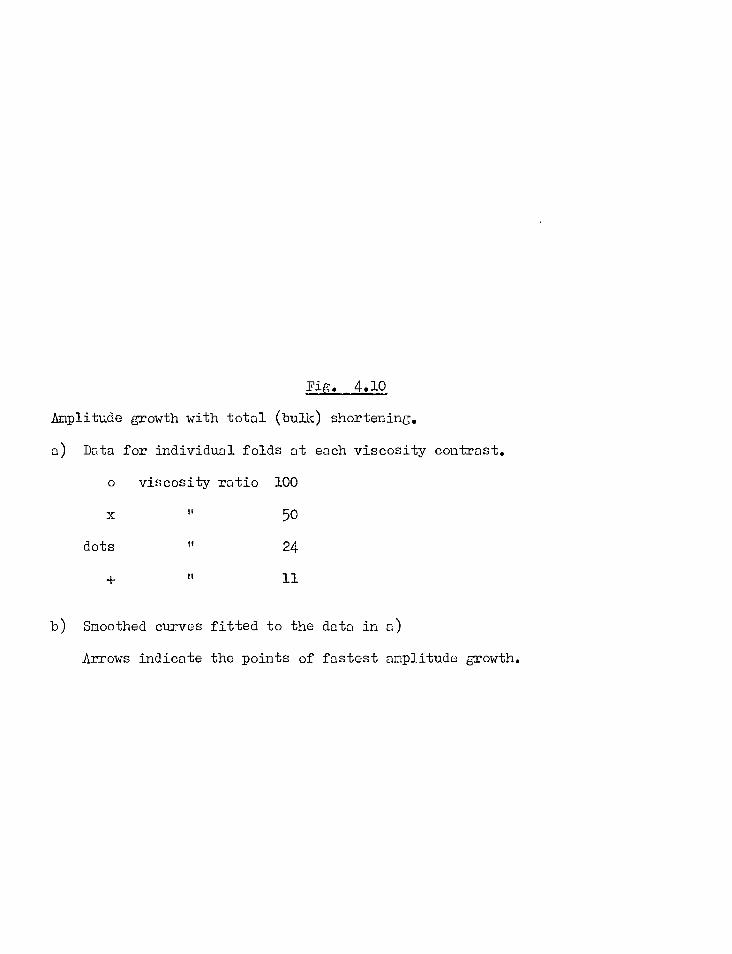
Fig. 4.10
Amplitude growth with total (bulk) shortening.
a) Data for individual folds at each viscosity contrast.
o viscosity ratio 100
50
dots If 24
11
b) Smoothed curves fitted to the data in a)
Arrows indicate the points of fastest amplitude growth.
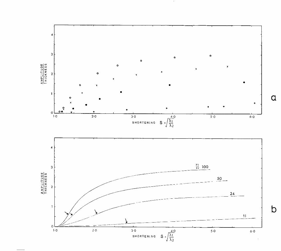
0 0 0
0 x
O x
•
• •
0 x o•
x
0
x
• +
2.0 3.0 4.0
SHORTENING S =, J A2
0
11
U)
z
0
SHORTENING
0 1-0
4
3
2
AM
PLITU
DE
T H
ICKN
ES
S
1
6.0 5.0
x

Fig. 4.11
Harmonic Analysis of Individual Folds through progressive deformation.
a) Successive shapes in the development of a single fold (p,i/ µ 2 = 100),
from the point where folds are first visible. Inflexion and hinge
points are marked by dots.
b) Plots of b3 against b1 for the left hand limbs of the folds in a).
c) d) Plots of b3 against b1 for successive shapes of folds developed at
a viscosity contrast of 50:1.
Note: Tie lines between two points relate inner and outer arcs
of a single fold at each stage of fold development.
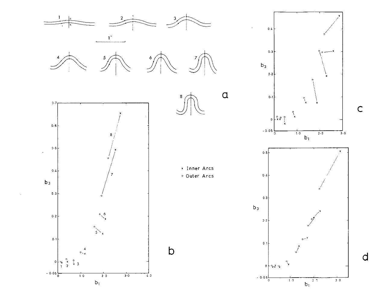
h
h
2 ----- 3 ----._
0-1.
1" -J
0.3 x
b3 0.2
0
x Inner Arcs
0 Outer Arcs
a
b 3
b
3.0 4 0
b
0.1 0 5(
x
0 x
-0.05 0 1.0 2.0 3.0
b1
b 3
-005 0
0-/.
0.2
0.5
03
01
0
1 0 2 b1
3 0
x
x
x
0
o-Y
x
0/
0
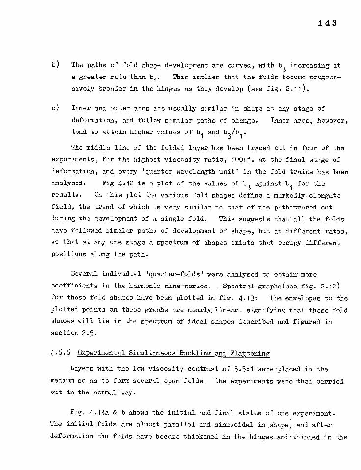
143
b) The paths of fold shape development are curved, with b3 increasing at
a greater rate than b1. This implies that the folds become progres-
sively broader in the hinges as they develop (see fig. 2.11).
c) Inner and outer arcs are usually similar in shape at any stage of
deformation, and follow similar paths of change. Inner arcs, however,
tend to attain higher values of b1 and b3/b1.
The middle line of the folded layer has been traced out in four of the
experiments, for the highest viscosity ratio, 100:1, at the final stage of
deformation, and every 'quarter wavelength unit' in the fold trains has been
analysed. Fig 4.12 is a plot of the values of b3 against b1 for the
results. On this plot the various fold shapes define a markedly-elongate
field, the trend of which is very similar to that of the path-traced out
during the development of a single fold. This suggests that - all the folds
have followed similar paths of development of shape, but at different rates,
so that at any one stage a spectrum of shapes exists that occupy_different
positions along the path.
Several individual 'quarter-folds' wereanalysed.to obtain- mare
coefficients in the .harmonic sine -series. • Spectral--gamaphs(see. fig. 2.12)
for those fold shapes have been plotted in fig. 4.13: the envelopes to the
plotted points on these graphs are nearlylinearl signifying that these fold
shapes will lie in the spectrum of ideal shapes described and figured in
section 2.5.
4.6.6 acperimental Simultaneous Buckling and Flattening
Layers with the low viscosity-contrast.of 5.5:1 -were -placed in the
medium so as to form several open folds: the experiments were carried
out in the normal way.
Fig. 4.14a & b shows the initial and final states_of one experiment.
The initial folds are almost parallel and sinusoidal in.shape, and after
deformation the folds have become thickened in the hinges-and-thinned in the
Fig. 4.12
Plots of b3
against b1 for 50 folds at the final stage of deformation
(S = 5.0 — 6.0) at a viscosity ratio of 100:1.
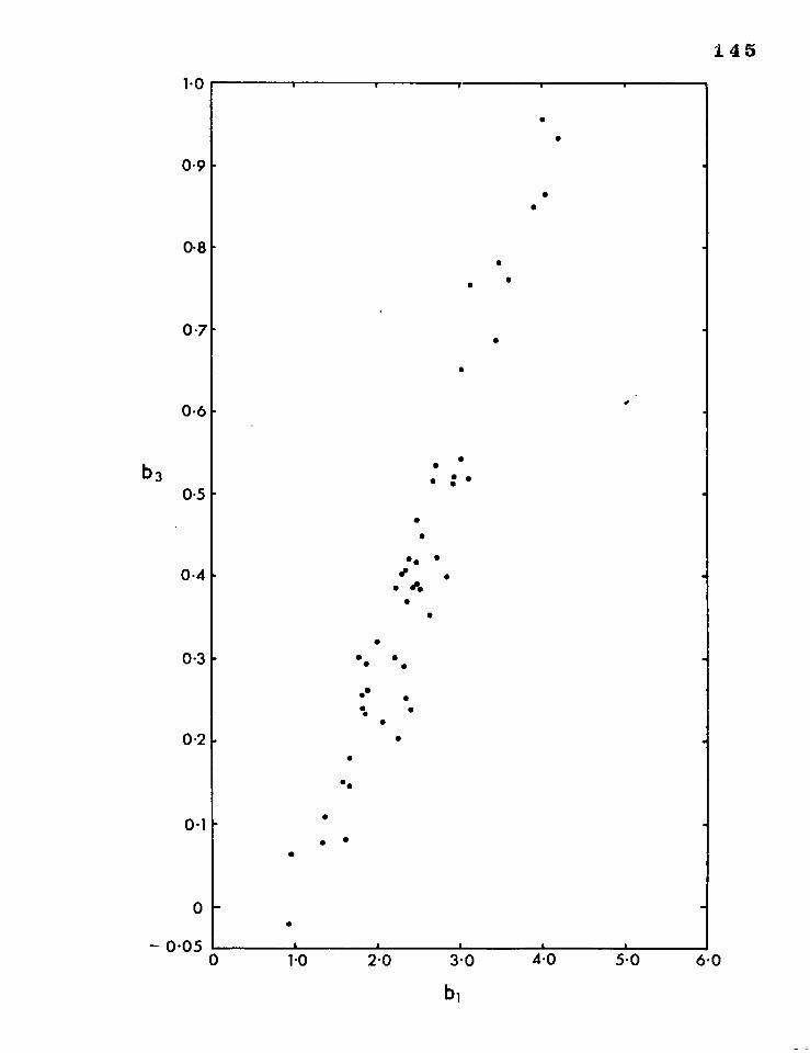
145
b1
•
• • •
b3 0.5
- 0.05 0
0.4
0.9
0.6
0.3
0.2
07
1.0
0-8
0.1
0
1.0 2.0 3.0 4.0 5.0 6.0
•
• •
•
•
•
•
. • : •
•
•
• .„
mr
0
•
•
•
•
•
•
•
..5 • • •
• •

Fig. 4.13
Spectral Graphs for individual folds (quarter wavelength units) at the
final stage of deformation.
a) Viscosity ratio = 50:1
b) = 100:1
c) 11 = 50:1. This is the outer arc of the fold whose
progressive deformation is traced in fig. 4.11d.
Note: each fold shape is an outer arc.
i = inflexion point
h = hinge point
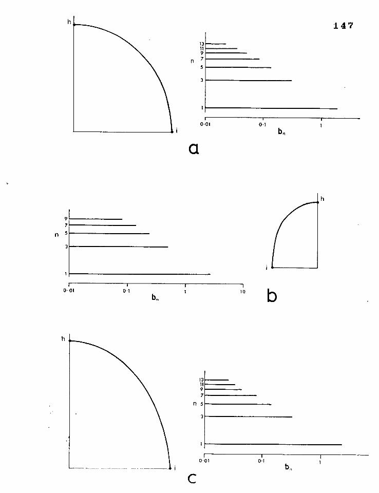
1 0.1 b„
147
13 11 9
n 7
5
3
1
0.01
a
b b, 1 10 0-01 0 1
0 - 01 0.1
3
n 5
1
13 11 9 7
b,
9 7 5
3
1 1
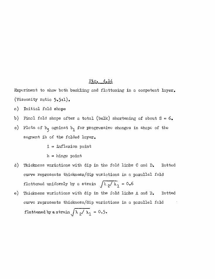
Fig. 4.14
Experiment to show both buckling and flattening in a competent layer.
(Viscosity ratio 5.5:1).
a) Initial fold shape
b) Final fold shape after a total (bulk) shortening of about S = 6.
c) Plots of b3 against bl for progressive changes in shape of the
segment ih of the folded layer.
i = inflexion point
h = hinge point
d) Thickness variations with dip in the fold limbs C and D. Dotted
curve represents thickness/dip variations in a parallel fold
flattened uniformly by a strain ps. 2/ Xi = 0.6
e) Thickness variations with dip in the fold limbs A and B. Dotted
curve represents thickness/dip variations in a parallel fold
flattened by a strain IX 2/ Al = 0.5.
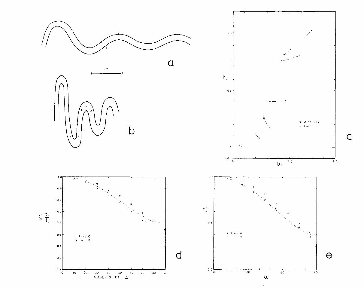
0 b, 50 9 0
• 0
0
0
• 0
•
0
o Limb C • D
I 0
05
b3
b
0 x
a
-0
O Oiitei Arc
• I ni,ei
0 x
O 8
07
O 6
80 70 90 0 10 20 30 40 50 60
ANGLE OF DIP a,
• •
• 0 N
• + `,0
o limb A 0
90 60 30
a
02 0
e
10
09
0.5
04
0.3
O 2
,0
In
0 6
d
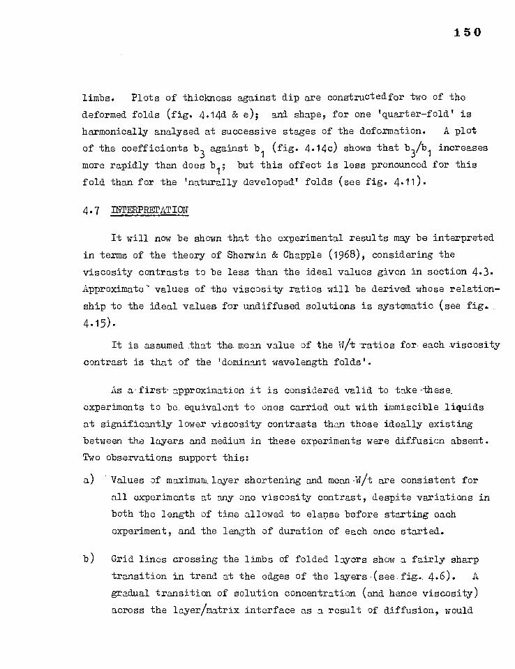
150
limbs. Plots of thickness against dip are constructedfor two of the
deformed folds (fig. 4.14d & e); and shape, for one 'quarter-fold' is
harmonically analysed at successive stages of the deformation. A plot
of the coefficients b3 against b
1 (fig. 4.14c) shows that
b3/b1 increases
more rapidly than does bi; but this effect is less pronounced for this
fold than for the 'naturally developed' folds (see fig. 4.11).
4.7 ItITERPRETAT ION
It will now be shown that the experimental results may be interpreted
in terms of the theory of Sherwin & Chapple (1968), considering the
viscosity contrasts to be less than the ideal values given in section 4.3. Approximate' values of the viscosity ratios will be derived whose relation-
ship to the ideal values for undiffused solutions is systematic (see fig..
4.15).
It is assumed that the- mean value of the W/t ratios for each viscosity
contrast is that of the 'dominant wavelength folds'.
As a-first-approximation it is considered valid to take-these.
experiments to be. equivalent to ones carried out with immiscible liquids
at significantly lower viscosity contrasts than those ideally existing
between the layers and medium in these experiments were diffusion absent.
Two observations support this:
a) 'Values of maximum. layer shortening and mean -W/t are consistent for
all experiments at any one viscosity contrast, despite variations in
both the length of time allowed to elapse before starting each
experiment, and the length of duration of each.once started.
b) Grid lines crossing the limbs of folded layers show a fairly sharp
transition in trend at the edges of the layers-(see.fig, 4.6). A
gradual transition of solution concentration (and hence viscosity)
across the layer/matrix interface as a result of diffusion, would

Fir.;. 4.15
Relationship between values of Apparent Viscosity Ratio and Ideal
Viscosity Ratio.
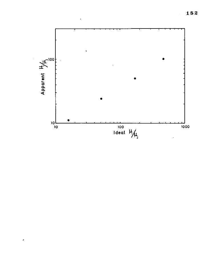
152
• •1111 111v
•
•
•
10 • • 11111 111•1
10 100 1000 Ideal PA
2
153
show in the experiments as a gradual transition in the trend of the
deformed grid lines.
Using the mean value of the observed w/t ratios (fig. 4.9) and the mean
limiting value of layer shortening, for each viscosity contrast used, an.
estimate may be made of the effective (apparent) viscosity ratio by
substituting these values into equation 3.3. In this way the figures in
row 5 of the table below were derived. Now, taking each of these estimates
of viscosity ratio and each mean limiting value of layer shortening, estimates
of amplification (of the dominant wavelength) may be read from the graph
in fig. 3.2. Those estim?.tes appear in row 6 of the table.
For all but the lowest viscosity contrast used, it appears that
shortening in the layers ceases when the limb dips of developing folds
reaches about 15°. Assuming the initial irregularities of all the layers
used in the experiments to be in the same order of size, the mean
amplification required to produce folds with 15° limb dips will be the same.
The values of amplification in row 6 of the above vary between 20 and
80. The mean value is 50, and taking this to be the best estimate of
amplification for all the viscosity contrasts used, a new estimate of each
effective viscosity ratio may be read from fig. 3.2, using the mean limiting
value of layer shortening and a value of 50 for the amplification.
The final estimate of the effective viscosity ratio is an average
of the first two estimates. (The values in row 9 of the table are the means of the values in rows 5 and 8). The final estimates of these ratios
are plotted against the ideal values for undiffused solutions in fig. 4.15.
see over
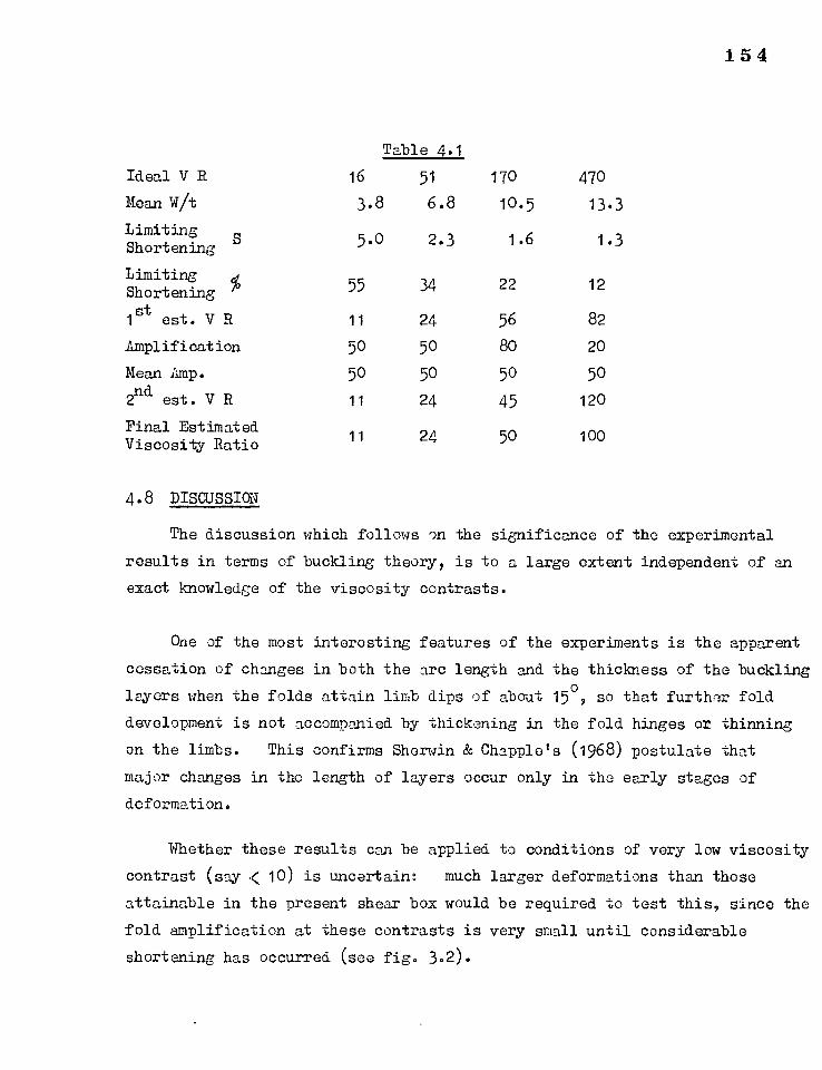
154
Table 4.1
Ideal V R 16 51 170 470
Mean W/t 3.8 6.8 10.5 13.3
Limiting S Shortening 5.0 2.3 1.6 1.3
Limiting Shortening % 55 34 22 12
1st est. V R 11 24 56 82
Amplification 50 50 80 20
Mean Amp. 50 50 50 50
2nd est. V R 11 24 45 120
Final Estimated Viscosity Ratio 11 24 50 100
4.8 DISCUSSION
The discussion which follows on the significance of the experimental
results in terms of buckling theory, is to a large extent independent of an
exact knowledge of the viscosity contrasts.
One of the most interesting features of the experiments is the apparent
cessation of changes in both the arc length and the thickness of the buckling
layers when the folds attain limb dips of about 1509 so that furthrx fold
development is not accompanied by thickening in the fold hinges or thinning
on the limbs. This confirms Sherwin & Chapple's (1968) postulate that
major changes in the length of layers occur only in the early stages of
deformation.
Whether these results can be applied to conditions of very low viscosity
contrast (say < 10) is uncertain: much larger deformations than those
attainable in the present shear box would be required to test this, since the
fold amplification at these contrasts is very small until considerable
shortening has occurred (see fig. 3.2).

155
It seems likely, however, with continuing deformation at very low
viscosity contasts, that further changes in arc length and thickness will
occur. These will be unequally distributed around the folded layer, and
may involve shortening along the layer in the hinge regions and extension
in the limbs (see Ramberg & Ghosh, 1968- ).
The large spread in wavelength/thickness ratios (fig. 4.9) suggests
that folding in these experiments is of low selectivity (see Biot, 1961,
p.1604). This feature is dependent upon the 'degree of flatness' of the
layers before deformation; the flatter the layers the more regular the
folds that develop (Biot, 1961, p.1605). assuming the amplification of
the folds (i.e. amplification of the dominant wavelength) up to the '15°
limb dip stage', to be the same for all the viscosity contrasts, selectivity
of the folding should also be the same, since it depends only upon
amplification to a first approximation (Biot, 1961, p.1605). For the
wavelength/thickness histograms of fig. 4.9, a measure of selectivity is given by the ratio of standard deviation/mean. Values of these ratios are
of the same order of size for the four distributions.
The final distribution of ?•d/t ratios, and therefore selectivity, is
probably 'fixed' at or before the 15° limb dip stage, and the amplification
required to attain this stage will depend upon the initial flatness of the
layer.
The relationship between'amplification and selectivity is illustrated
in fig. 4.16., where the variation of amplification with wavelength, at
different amounts of shortening, for a viscosity ratio of 16 is graphically
recorded. Equation 3.2 was used to derive these curves, and at each value
of shortening the maximum amplification has been set equal to unity to enable
comparison of the curve shapes.
Analysis of the experimental data shows that the change of amplitude
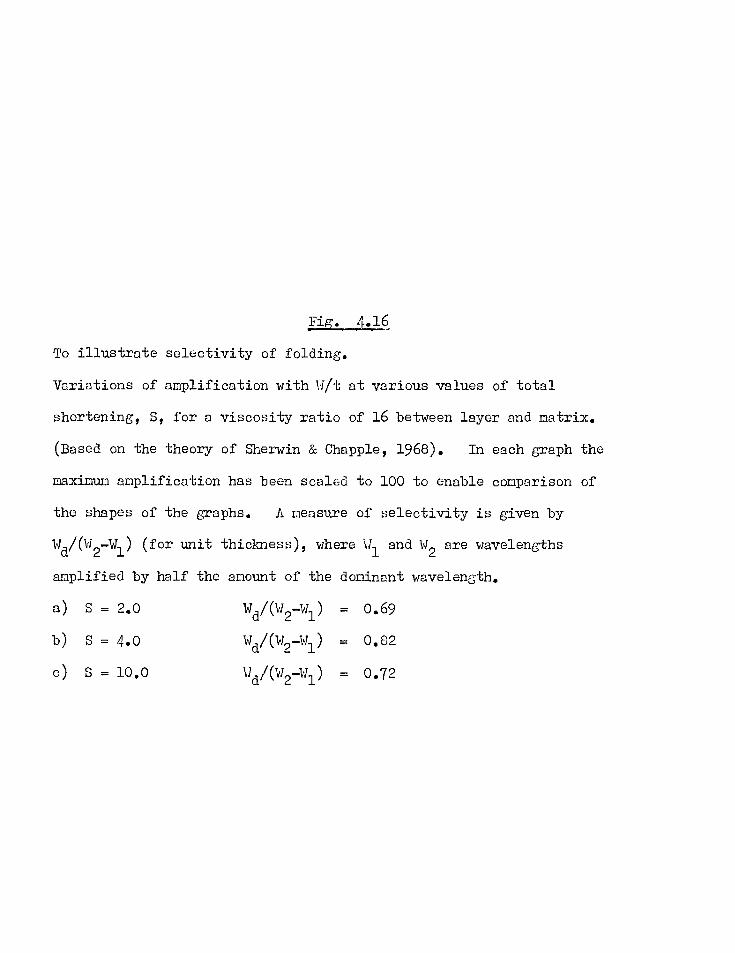
Fig. 4.16
To illustrate selectivity of folding.
Variations of amplification with W/t at various values of total
shortening, S, for a viscosity ratio of 16 between layer and matrix.
(Based on the theory of Sherwin & Chapple, 1968). In each graph the
maximum amplification has been scaled to 100 to enable comparison of
the shapes of the graphs. A measure of selectivity is given by
Wd/(W2—W) (for unit thickness), where W1 and W2 are wavelengths
amplified by half the amount of the dominant wavelength.
a) S = 2.0 Wd/(W2—W1) = 0.69
b) S = 4.0 Wd/(V—W1) = 0.82
c) S = 10.0 Wd/(W2—W1) = 0.72
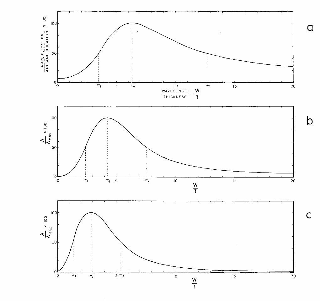
100 0 0
, a < I
50
0
0 0 100
lz z o o I- , a <
u_ =.1.1
5 0 u_ 71;
.‹
wi 5 Wd 10
w2 15
20 WAVELENGTH W THICKNESS
0 WI vvd 5 w2 10 15 20
100 0
0
< 50
"wd 5 W2 10
15 20
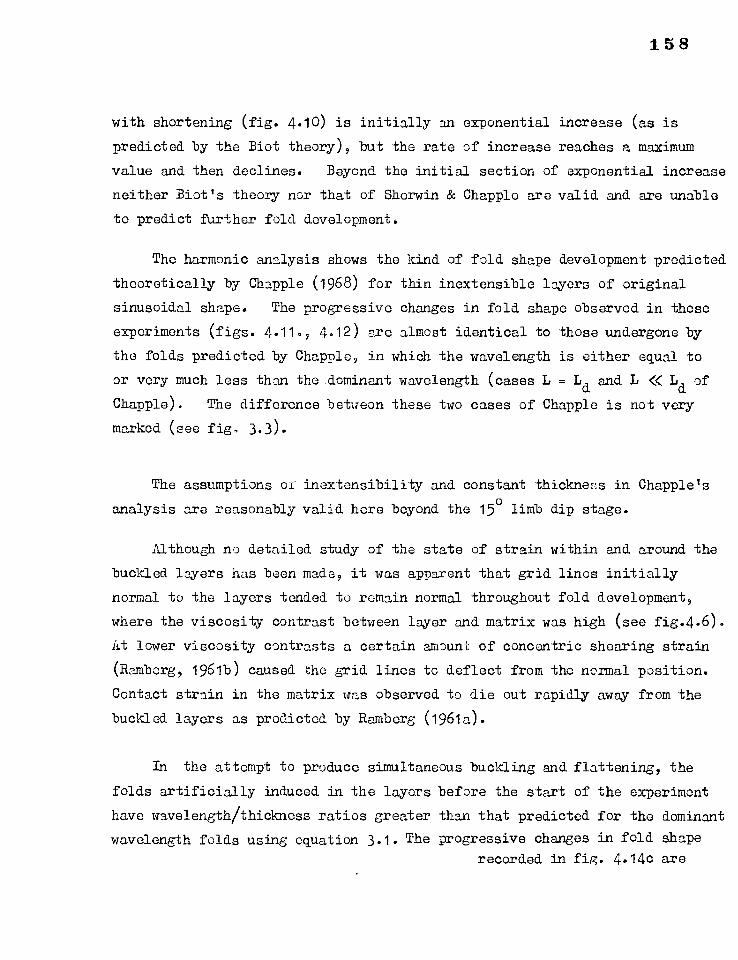
158
with shortening (fig. 4.10) is initially an exponential increase (as is
predicted by the Biot theory), but the rate of increase reaches a maximum
value and then declines. Beyond the initial section of exponential increase
neither Biot's theory nor that of Sherwin & Chapple are valid and are unable
to predict further fold development.
The harmonic analysis shows the kind of fold shape development predicted
theoretically by Chapple (1968) for thin inextensible layers of original
sinusoidal shape. The progressive changes in fold shape observed in these
experiments (figs. 4.11., 4.12) are almost identical to those undergone by
the folds predicted by Chapple, in which the wavelength is either equal to
or very much loss than the dominant wavelength (cases L = Ld and L << Ld of
Chapple). The difference between these two cases of Chapple is not very
marked (see fig, 3.3).
The assumptions of inextensibility and constant thickness in Chapple's
analysis are reasonably valid here beyond the 15° limb dip stage.
Although no detailed study of the state of strain within and around the
buckled layers has been made, it was apparent that grid lines initially
normal to the layers tended to remain normal throughout fold development,
where the viscosity contrast between layer and matrix was high (see fig.4.6).
lit lower viscosity contrasts a certain amount of concentric shearing strain
(Ramberg, 1961b) caused the grid lines to deflect from the normal position.
Contact strain in the matrix was observed to die out rapidly away from the
buckled layers as predicted by Ramberg (1961a).
In the attempt to produce simultaneous buckling and flattening, the
folds artificially induced in the layers before the start of the experiment
have wavelength/thickness ratios greater than that predicted for the dominant
wavelength folds using equation 3.1. The progressive changes in fold shape recorded in fig. 4.14c are
159
different for the inner and outer arcs, but are generally very similar to
those undergone by the 'weak plate' fold of Chapple (1968), for which the
wavelength is several times that predicted for the dominant wavelength
(L = 4.6 La in Chapple's analysis). However Chapple's assumptions of an
inextensible layer with no thickness changes do not hold for the case
considered here. Thickening of the hinges and thinning of the limbs have
occured during deformation and the relationship between thickness and dip
(fig. 4.14d & e) observed for a number of folds is very similar to that
expected for a fold formed by a combination of buckling and flattening
according to the model proposed in section 3.6. Other than by inspection
of this graph, the non-passive behaviour of these folds is indicated by the
rotation of the grid lines in the limbs, and by the progressive changes in
fold shape indicated in fig. 4.14c. In homogeneous flattening,
progressive changes in fold shape would trace out a straight line path on
this graph, radiating from the origin. For an isolated viscous layer in
a less viscous matrix, the effect of progressive layer shortening during the
early stages of buckling will be to alter the predicted value of the
dominant wavelength/thickness ratio according to equation 3.3. By
assuming layers to have initial irregularities of the same order of size,
and by assuming a particular value for the amplification needed to bring
folds to the stage at which shortening ceases (i.e. the 150 limb dip stage),
the degree to which the predicted value of the dominant wavelength/thickness
ratio will change from its initial value (given by equation 3.1) may be
evaluated. This has been done for several viscosity contrasts, taking a
value of 100 for the amplification. The results are shown in table 4.2.
see over
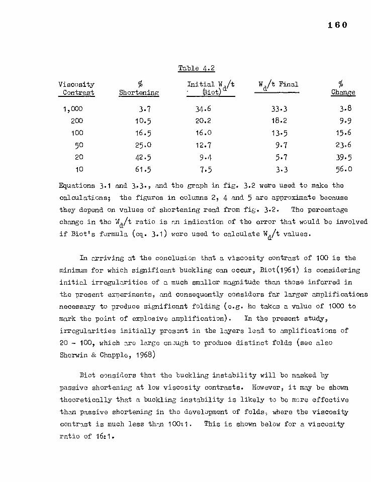
160
Table 4.2
Viscosity % Initial W /t Wd/t Final
Contrast Shortening • (Biot) d Change
1,000 3.7 34.6 33.3 3.8
200 10.5 20.2 18.2 9.9
100 16.5 16.0 13.5 15.6
50 25.0 12.7 9.7 23.6
20 42.5 9.4 5.7 39.5
10 61.5 7.5 3.3 56.0
Equations 3.1 and 3,3., and the graph in fig. 3.2 were used to make the
calculations; the figures in columns 2, 4 and 5 are approximate because
they depend on values of shortening read from fig. 3.2. The percentage
change in the Wd/t ratio is an indication of the error that would be involved
if Biot's formula (eq. 3.1) were used to calculate Wd/t values.
In arriving at the conclusion that a viscosity contrast of 100 is the
minimum for which significant buckling can occur, Biot(1961) is considering
initial irregularities of a much smaller magnitude than those inferred in
the present experiments, and consequently considers far larger amplifications
necessary to produce significant folding (e.g. he takes a value of 1000 to
mark the point of explosive amplification). In the present stuay,
irregularities initially present in the layers lead to amplifications of
20 — 100, which are large enough to produce distinct folds (see also
Sherwin & Chapple, 1968)
Biot considers that the buckling instability will be masked by
passive shortening at low viscosity contrasts. However, it may be shown
theoretically that a buckling instability is likely to be more effective
than passive shortening in the development of folds, where the viscosity
contrast is much less than 100:1. This is shown below for a viscosity
ratio of 16:1.
161
Considering a sinusoidal fold of unit amplitude at a finite state of
shortening, S = 7, an initial value of the fold amplitude can be found by
assuming the fold to have formed by
a) buckling (taking the fold to be the dominant wavelength fold at
S = 7, and applying Sherwin & Chapple's theory) and
b) passive flattening. Calculations show that the initial amplitude
needed to form the fold by passive shortening is over three orders of
magnitude larger than that needed to produce the fold by buckling, for a
viscosity ratio of 16. In this case buckling is 1000 times more effective
in fold development than passive deformation.
Sherwin & Chapple (1968), although recognizing that shortening occurs
in the early stages of buckling, extend their analysis to treat cases where
the amplitudes are very large, where the assumption of a flat plate, on which
their analysis depends, must be invalid.. , They estimate the amplification
of natural folds that have limb dips of 10°-20° upwards. Using this estimate
and the mean of the measured W/t ratios they obtain a rough value of
viscosity contrast by reference to a graph relating amplification, dominant
wavenumbor, shortening and viscosity ratio (see fig. 3.1, this thesis).
However, in the light of the present experimental results, it seems likely
that the W/t ratios become fixed when folds attain limb dips of about 15°.
The value of the mean W/t ratio should therefore be combined with an
estimate of the amplification required to produce folds with limb dips of
about 150, in order to estimate the viscosity contrast. Using this,rather
than Sherwin & Chapple's approach, slightly lower estimates of viscosity
contrast will be obtained.
4.9 INTERPRETATION OF NATURALLY FORT 2D FOLDS
Assuming that it is valid to compare naturally formed folds with those
developed experimentally (see section 4.2), several important geological
implications follow from the experimental results described 'above.
162
One implication is that the arc length of a folded layer cannot in
general be taken as the original length, even in the case where the orthog—
onal tlickness remains constant around the folds (see also Sherwin &
Chapple, 1968). Estimates of deformation based on the assumption that the
arc length is the initial lverbngth will in general be too small.
Slightly modified, the methods of Sherwin & Chapple (1968) will enable
estimates of total shortening (within the profile plane of the folds)
and viscosity contrast tolp made where 'suitable' natural folds exist.
Suitable folds are those that appear to meet the assumptions of the Biot
theory (see section 3.2).
The layers in these experiments are considered to have been amplified
by a factor of about 50 to attain limb dips of about 15°. Thin rock
layers or veins will probably have initial irregularities several times
larger than those of the layers used in these experiments, and values of
between 10 and 100 are suggested as amplifications likely to be required
to develop folds to the stage whore layer shortening effectively ceases.
Sherwin & Chapple's methods have been applied, in a modified form, in
natural fold studies described in sections 5.7 and 6.5.
In order to experimentally develop folds with significant amounts of
thickening in the hinge regions, it was found necessary to employ a low
viscosity contrast between layer and matrix, and to induce wavelengths in
the layer greater than the predicted dominant wavelength. Many natural
folds possess thickened hinges (see also section 3.6.), and this may be due
to:
a) a decreasing or vanishing viscosity contrast during deformation.
b) greater deformation occuring in nature than attained in these experiments,
reaching a stage of deformation not seen in the experiments.
163
c) an effect operating on individual competent layers within multilayered
sequences, in which some control of the development of folds is
exerted by other competent layers within the sequence. Such layers
will tend to form folds of larger wavelengths when part of a multi—
layered sequence, than when 'isolated' (Ramberg, 1961a; Biot, 1961),
and fold flattening (see section 3.5) may be facilitated in a multilayer.
d) non—linear rheological behaviour of rock.
4.10 CONCLUSIONS
A) Buckling may occur for values of viscosity contrast much smaller than
that of 100, suggested by Biot to be the minimum for which distinct
folding would occur.
B) Buckling in these experiments is adequately explained by a theory
based on those of Biot (1961), Chapple (1968) and Sherwin & Chapple
(1968).
C) Layer shortening occurs at the onset of deformation, but effectively
ceases when folds have attained limb dips of.about 150.
D) Deformation of folds at low viscosity contrasts, with induced wave—
lengths greater than the predicted dominant wavelength, appears to
take place by a combination of buckling and flattening.
E) The range of fold shapes present in a buckled layer at a given stage
of deformation appears to reflect the shape changes undergone by a
single fold in the course of progressive deformation.
164
CHAPWi 5
AN ANALYSIS OF MINOR FOLDS IN THE MOINIAN ROCKS OF MONAR, INVERNESS-pSHIRE
5.1 INTRODUCTION
Loch Monar is situated about 30 miles west of Inverness in the
Central Highlands of Scotland, the Moinian rocks exposed here forming a
central part of the Caledonia° fold belt. These rocks are metamorphosed
sediments; siliceous and micaceous granulites. The general area was
first studied by Peach &Othero (1913), and more recently the structural
and metamorphic history of the Moines has been summarised by Ramsay
(1963) and Johnson (1965). The area around Loch Monar has been mapped
in detail by Ramsay (1954, 1958). The geology of part of this area is
shown in fig. 5.1, and within this the locality under study is indicated.
The reason for selecting this small area is that minor folds (F2 of Ramsay)
are intensely developed here, and near-profile sections of these folds
are superbly exposed on glaciated pavement that has been washed clean
during a dam construction scheme.
A brief account of the general geology of the area is given in
sections 5.2-5.4. This is followed by a detailed geometrical analysis
of the minor F2 folds in section 5.5. Section 5.6 is concerned with
the interpretation of the fold geometry in terms of folding processes.
Specific studies oflitY gmatic folds in pegmatitic veins (section 5.7), and
of lineations deformed around F2 folds (section 5.8) are described at the
end of the Chapter. As a result of these studies, estimates of viscosity
contrast have been made, and information as to the orientation of the 'bulk
finite strain ellipsoid' of the F2 deformation has been obtained.
5.2 LITHOLOGY
The rocks exposed in the study area are psammites belonging to the
Monar psammitic group of Ramsay (1958, p.274). They are banded siliceous,

Fiff. 5.1
a) Geological nap of the area around the eastern end of Loch 'Abner.
(After Ramsay, 1958).
d = dam
A.S. = Axial Surface
The shaded area at the end of the loch is the region selected for
detailed fold study.
b) Map to show the location of nap a).
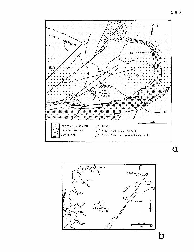
166
PSAMMIT IC MOINE ./ FAULT .."
PELITIC MOINE ..../.. A.S. TRACE Major F2 Fold LEW ISIAN "'". A.S. TRACE Loch Monar Synform
a
b
167
semi-pelitic and pelitic granulites. The bands or layers are essentially
composed of varying proportions of quartz, plagioclase feldspar and biotite
and muscovite micas and probably represent original sedimentary layers
of variable composition. Pegmatitic veins of quartzo-feldspathic
material, either concordant or slightly discordant to the layering, are
common. These are coarse-grained and consist mainly of quartz, potash
feldspar and plagioclase. Sheets of similar material are also found
parallel or slightly oblique to the axial surfaces of the minor F2 folds
(plate 2). These pegmatitic sheets are considered to have formed either
late in the history of development of the F2 folds, or after folding had
ceased. They will not be considered further. Both types of vein are
considered metamorphic-metasomatic in origin (Ramberg, 1952).
The quartz and feldspar in the granulites exist as fairly equant
grains, the size of most lying in the range 0.1mm - 1.0mm. In the
pegmatitic veins, however, these minerals are about an order of magnitude
larger and are cormonly several mm in size.
It is convenient in describing fold geometry to distinguish four
lithologies; politic, semi-politic, psammitic and pegmatitic quartze-
feldspathic. The first three, referred to collectively as the layered
'granulites' can be considered as members of a continuous sequence of
composition variation based on dark mineral (biotite) content. The
distinction made is:-
politic - abundant biotite
psammitic - sparse biotite
semi-politic - intermediate in biotite content.
This distinction, although somewhat subjective, is significant in con-
sidering detailed fold geometry. Only the early generations of
pegmatitic veins are involved in the F2 folding, and these veins make
up the fourth category.
Plate. 2 F2 folds (300X NOW. of the little dam on the S. shore
of Loch llonar). Pegmatitic veins of one age are folded,
while those of a later age lie in sheets parallel to the
axial surfaces of the folds.
Plate 1 Folic.tion surface dcformed by F2 folds. (Road
section at E. end of little dam).
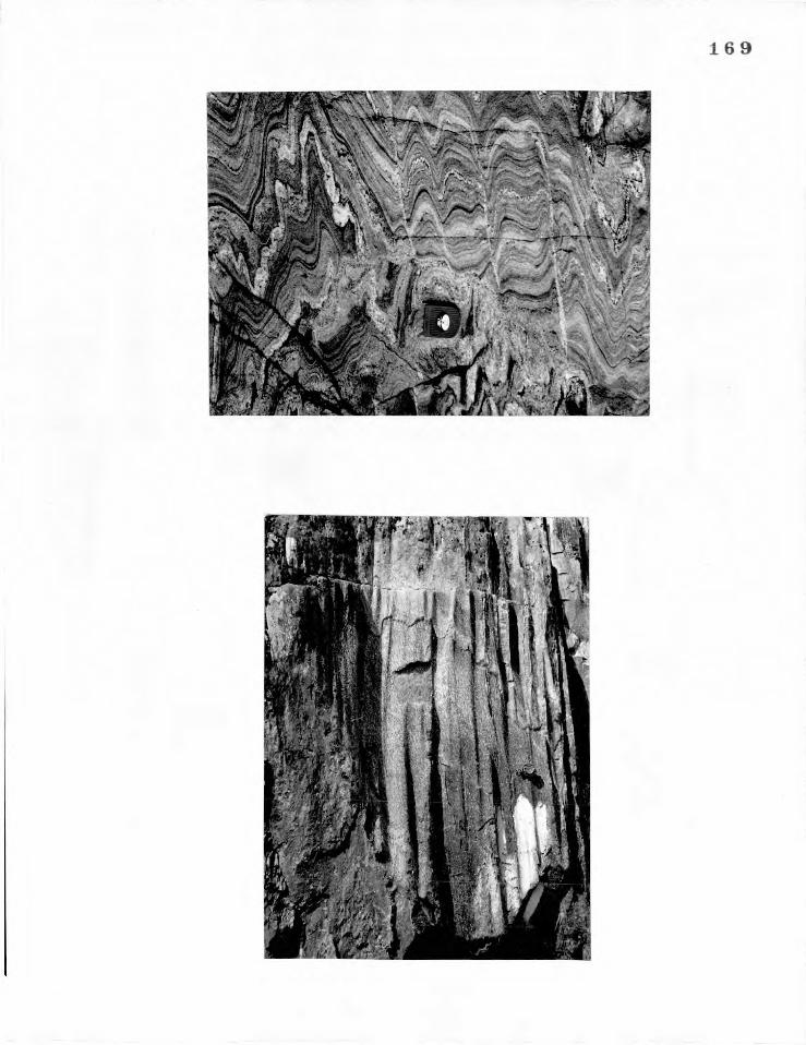
. ,. -;i, - . ' . :` ••'.- .,, -', \ \ - .... ., ' •
-• • - • • - .
. • • •"
• \
•-•,„
1111.'4' -144 ,
170
5.3 METAMORPHISM
Moine rocks appear to have undergone intense regional metamorphism,
accompanied by local migmatisation and the prodution of quartzo-feld-
spathic veins. Staurolite and kyanite are found in the Monar region
(Ramsay, 1954) and garnet is common in relitic rocks found to the south,
west and north of the area under discussion. The grade of metamorphism
is garnet-kyanite. There is evidence (Ramsay, 1963, p.168) of several
successive regional metamorphisms in parts of the Moines, all of about
this grade. That the grade of metamorphism stayed fairly constant through-
out the whole deformation history as seen at Monar, is suggested by the
presence of several generations of quartzo-feldspathic veins. The
earliest of these have been affected by the early fold phase movements,
whilst veins of a similar nature, parallel to the axial surfaces of the
second folds, are contemporaneous with or post-date these later fold
movements. The rocks may well have been in a near-migmatitic state
throughout this history.
5.4 STRUCTURAL GEOLOGY
Ramsay (1954, 1958) showed the existence of two major fold phases;
he demonstrated a close and consistent relationship between small-scale
folds and the larger structures throughout the region. The early phase
of deformation produced a series of major folds, overturned to the north,
with axial traces trending east-west, plunging gently to the west. The
later phase produced a series of major folds overturned in general to
the north-west, trending in a north-east south-west direction with
variable plunge. Ramsay (1954, 1958, p.291) showed how this plunge was
determined geometrically by the intersection of the second phase axial
surface (constant in orientation) with the fold limbs of the earlier
structures.
The area of interest (fig. 5.1) lies on the steeply dipping southern
limb of the Loch Monar synform, a major first phase fold. This limb has
171
been refolded by several major second folds. These folds trend north-
east south-west and their axial surfaces are near vertical, the fold axes
plunging steeply within them. The limbs and hinges of these major folds
are intensely puckered by small-scale structures, whose axes and axial
surfaces have attitudes in accord with the major structures. The fold
plunge, however, does vary locally where these folds are superimposed
on the minor folds of the early generation on the limb of the Loch Monar
synform. These second phase minor folds are the main objects of this
study.
Structural elements from the area are plotted on a stereogram in
fig. 5.2 (cf. Ramsay, 1958, figs. 3 & 4 sub-area 11).
The two fold phases of Monar are correlated with the second and
third phases of the general Moinian structural history (Ramsay, 1963).
Very tight isoclinal folds of the first Moinian deformation occur in the
Monar region. Those are not important in the present study and will
not be discussed further.
5.4.1 Rock Fabric
Ramsay (1958) showed that petrofabric girdles of quartz c-axes and
poles to basal planes of biotite closely matched the girdles of poles to
foliation planes in each of his sub-areas. The dominant visible feature
of the fabric is the well-developed mica schistosity which closely
parallels the axial surfaces of the F2 minor folds.
5.5. DESCRIPTIVE GEOMETRY
The material for this study consisted of a large number of field
photographs and specimens. devious analyses of folds from this and
adjacent areas are found in Ramsay (1962a) and Luahopadhyay (1964,
1965a). Their results will be considered later.
There is apparently no systematic variation in the spatial dis-
Fig. 5.2
Equal area stereographic plot of structural data for the area under
investigation.
0
Fl lineations (intersection of foliation
with an Fl schistosity).
F2 minor fold axes.
dots
Poles to F2 axial surfaces.
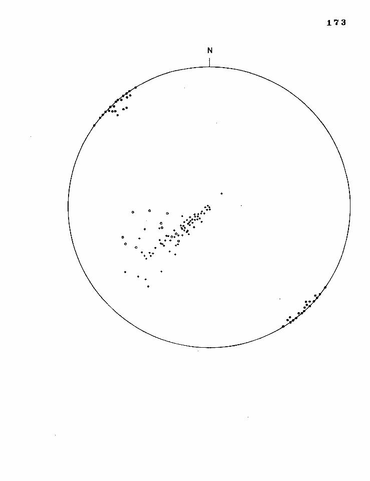
173
N
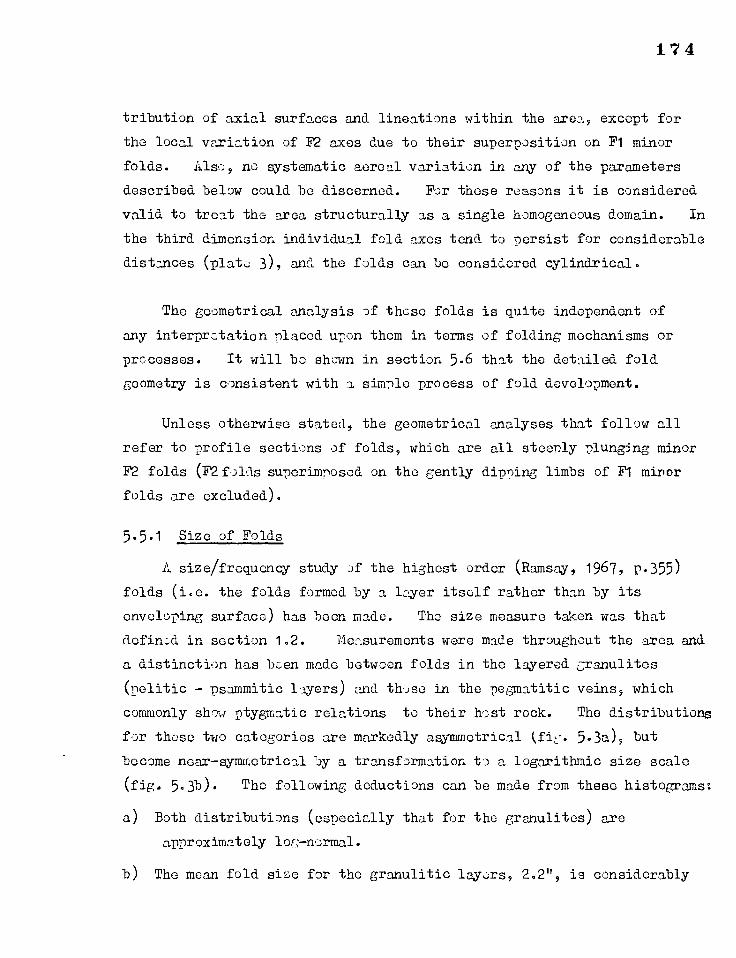
174
tribution of axial surfaces and lineations within the area, except for
the local variation of F2 axes due to their superposition on F1 minor
folds. Also, no systematic cereal variation in any of the parameters
described below could be discerned. For these reasons it is considered
valid to treat the area structurally as a single homogeneous domain. In
the third dimension individual fold axes tend to persist for considerable
distances (plato 3), and the folds can be considered cylindrical.
The geometrical analysis of these folds is quite independent of
any interpretation placed upon them in terms of folding mechanisms or
processes. It will be shown in section 5.6 that the detailed fold
geometry is consistent with a simple process of fold development.
Unless otherwise stated, the geometrical analyses that follow all
refer to profile sections of folds, which are all steeply plunging minor
F2 folds (F2 folds superimposed on the gently dipping limbs of Fl minor
folds are excluded).
5.5.1 Size of Folds
A size/frequency study of the highest order (Ramsay, 1967, p.355)
folds (i.e. the folds formed by a layer itself rather than by its
enveloping surface) has been made. Tho size measure taken was that
definod in section 1.2. Measurements wore made throughout the area and
a distinction has been made between folds in the layered granulites
(politic - psammitic layers) and thJse in the pegmatitic veins, which
commonly show ptygmatic relations to their host rock. The distributions
for those two categories are markedly asymmetrical (fir. 5.3a), but
become near-symmetrical 5y a transformation to a logarithmic size scale
(fig. 5.3b). The following deductions can be made from these histograms:
a) Both distributions (especially that for the granulites) are
approximately lor;-normal.
b) The mean fold size for the granulitic layers, 2.2", is considerably
Fig. _5.3
Frequency histograms of the size of F2 minor folds.
F = Frequency
a) & c) for 282 folds in the granulites.
b) & d) for 170 folds in the pegriatitic veins.
DI = Arithmetic (grouped) mean.
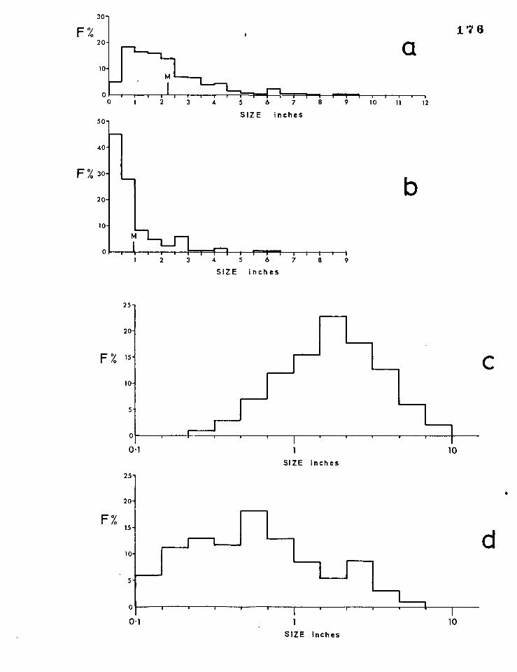
30-
F% 20-
10-
a
5 6 7 8 9 10 11 12 SIZE inches
b
4 5 6
SIZE inches
176
25-
20-
F% 15-
10-
I O1
10 SIZE inches
25-,
20-
F% 15-
10-
0
0
O 1 , I I
1
10 SIZE inches
177
greater than the mean for the pegmatitic veins, o.9".
An upper limit to the size of folds recorded is imposed by the scale of
the photographs on which measurements are made. A lower limit may also
be imnosed by the limiting visibility of the naked eye. The effect
of an upper size limit would be to truncate the 'tailing-off' of the
distribution, without otherwise affecting the overall shape. The
smallest fold sizes recorded here are of the same order of magnitude as
the grain size: folding on this scale becomes meaningless, and so the
lower limits of the distributions are the true limits of fold size.
5.5.2 Fold Order and Asymmetry.
The symmetry of the minor folds is always in accord with the geometry
of the larger structures, and between the highest order folds and the
major folds (fig. 5.1) exists a spectrum of sizes that do
form distinct fold orders of fixed wavelength magnitude,
order folds show considerable variation in symmetry about
mediate 'orders'. Asymmetry of the highest order folds,
ratio of the lengths of adjacent limbs (see section 1.2),
not seem to
The highest
these inter-
taken as the
has been
studied on folds taken more or less at random within the region. The
positions of the major folds can be seen from fig. 5.1a. A frequency
histogram of limb ratis, with 'S' and 'Z' sense of asymmetry distin-
guished, is plotted in fig. 5.4. For the sampled folds we can state:
a) 'Z' and 'S' folds are ap7)roximately equally common (45/0 'Z' and
55% 's')•
b) The distribution is fairly symmetrical about the ratio 1 : 1,
c) of all folds are asymmetrical in the range of ratios 1:1 - 3:1.
As in the study of fold size, an upper limit to the degree of asymmetry
recorded has been imposed by the scale of the photographs on which the
measurements were made. This has caused a truncation of the 'tails' of
the distribution. The shape of this distribution is largely due to

ag,__5.4 Asymmetry of F2 folds — frequency of limblength ratios.
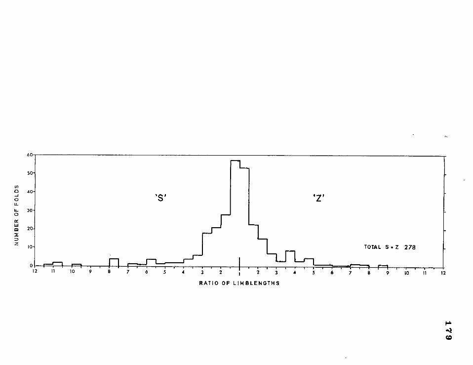
60
50-
40-
30-
20-
10- NU
MB
ER
OF
FO
LD
S
'S '
sz
TOTAL S . Z 278
r-r- 11 10 9 8 7 6 5 4 3 2
te r, 2 3 4 5 6 7 8 9 10 11 12
0 12
RATIO OF LIMBLENGTHS
180
the existence of a continuous spectrum of fold 'orders' that results
in frequent changes in the sense and amount of asymmetry of the smallest
scale folds.
5.5.3 Isogon Patterns
For a large proportion of the minor F2 folds, the geometry is very
nearly 'similar' (class 2), and the isogons run in near parallel lines,
concentrated in the hinge zones (see fig. 5.5a & b). Zones of near—similar folds usually occur where folded pegmatitic veins are sparse
or absent. Within those zones it is usually possible to detect slight
divergencies from class 2 geometry (see fig.. 5.5b, layer B — class 1C
geometry, layer A — class 3 geometry). Where such divergencioseccur politic layers take up class 3, and psammitic layers class 1C geometry. Folded pegmatitic veins tend to have ptygmatic form and disrupt the
'similar' isogon pattern (fig. 5.5c, d & e). They usually show a
pronounced class 1C geometry, and have greater limb dips than do the folds
in the enclosing layers, causing the isogons to form closed patterns
across the folded veins. In fig. 5.5d a series of closed patterns follows
a pegmatitic vein across the fold profile. Where strongly convergent
isogons are found in pegmatitic veins, strongly divergent ones also
occur in the adjacent layers (fig. 5.50, thus tending to maintain an
overall class 2 geometry.
5.5.4 Interlimb Angle Variation
The closed patterns of isogons described above are related to
changes in interlimb angle. 11 study of the variation of interlimb
angle along axial surface traces for folds in a layered sequence
containing pegmatitic veins reveals several features of interest (see
the example drawn in fig. 5.6):
a) The lowest values of interlimb angle occur within, or at the
bounding surfaces of the pegmatitic veins.
b) There is little difference between the values of this angle for
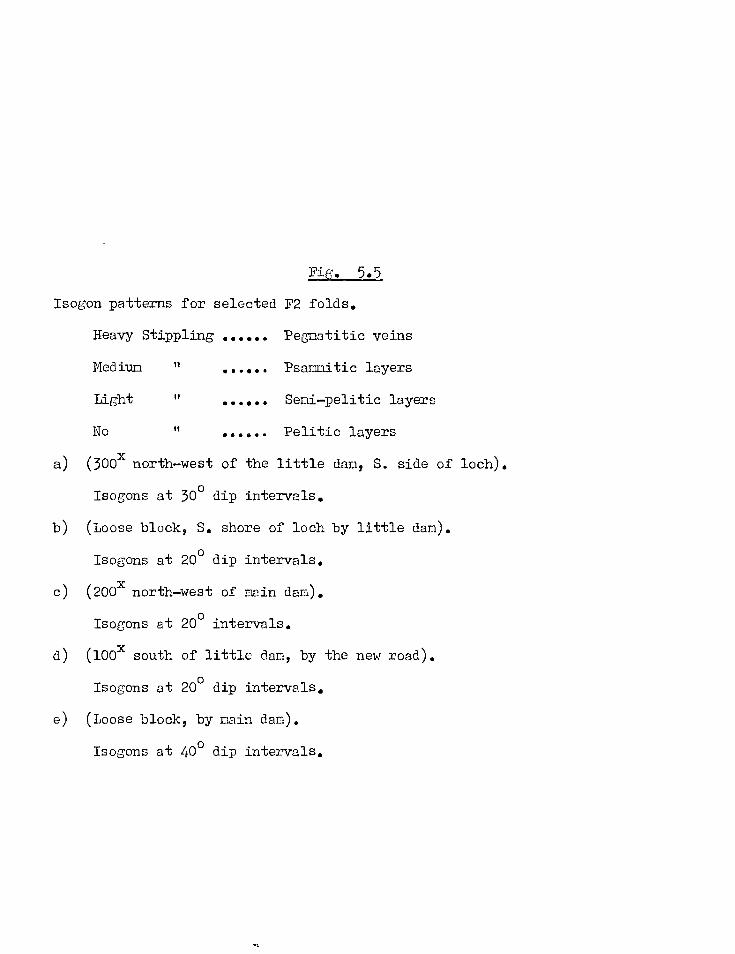
Fie. 5.5
Isogon patterns for selected F2 folds.
Heavy Stippling Pegmatitic veins
Medium 17 Psamnitic layers
Light Semi—pelitic layers
No Pelitic layers
a) (300X north—west of the little dam, S. side of loch).
Isogons at 30° dip intervals.
b) (Loose block, S. shore of loch by little dan).
Isogons at 20° dip intervals.
c) (200X north—west of main dam).
Isogons at 20° intervals.
d) (100X south of little dam, by the new road).
Isogons at 20° dip intervals.
e) (Loose block, by main dam).
Isogons at 40° dip intervals.
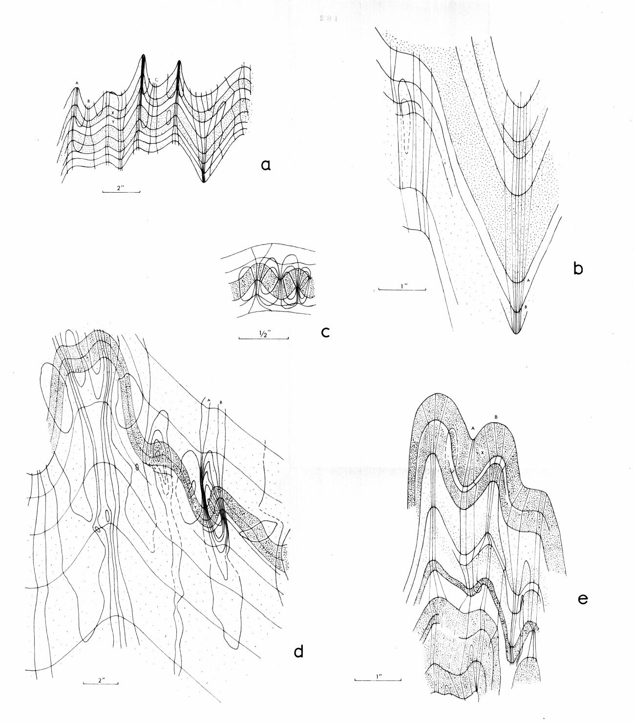

Fig. 5.6
Local Interlimb Jingle Variation.
a) Fold profile (part of the fold in fig. 5.5d) - pegtiatitic vein
stippled - axial surface traces narkec1 by dashed lines.
b) Plots of interlimb angle variation for the folds drawn in a) - the
"position" of the pegmatitic vein is shown by stippling.
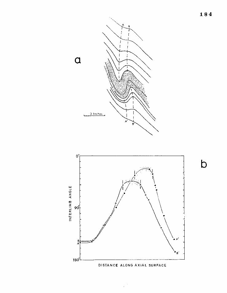
184
a
1 % .. • • / I I \
_1 tu
Z <
0\ \ .
co • 0 /I
0
:.; 9 0 ct f • w .2 /
A
o . 180
DISTANCE ALONG AXIAL SURFACE
185
either bounding surface of a pegmatitic vein.
c) The greatest rate of change of interlimb angle occurs in the layers
immediately adjacent to the pegmatitic veins.
In the example shown in fig. 5.6, interlimb angle is taken as the minimum
angle subtended by the fold limbs for a particular surface, and is
recorded as ordinate on a graph, with abscissa as the distance of this
surface from a datum point measured along the axial surface trace. The
variations in interlimb angle are fairly symmetrical on either side of the
layer.
In folded sequences containing several pegmatitic veins, an interlimb
angle variation curve shows peaks at positions where these veins are
crossed by the curve.
When variation of interlimb angle for one particular folded surface
is studied in a direction normal to the axial surface trace, there
appears to be no systematic change in its value from one fold to the next.
5.5.5 Thickness/Dip Variations
The techniques described in Chapter 2 have been applied in the study
of thickness variation with dip for
folds' (i.e. segments between hinge
analysed in detail. The thickness
been recorded as a function of dip,
2.2a and 3.8.
the F2 folds. About 350 'quqrter—
and inflexion points) have been
parameter used was , t'a which has
on graphs of the kind shown in figs.
In order to synthesise the data it was convenient to represent each
fold by a single parameter, the dope or intercept of the best fit
stright line on a graph of t t2a against cos2a . The degree of goodness of
fit of straight lines to the data was empirically found to be very good
for practically all the measured folds. A minimum of five pairs of tVa values were used in each analysis, and the computations were done on a
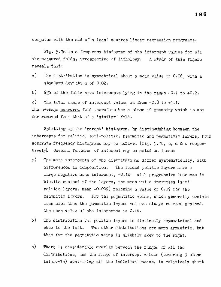
186
computer with the aid of a least squares linear regression programme.
Fig. 5.7a is a frequency histogram of the intercept values for all
the measured folds, irrespective of lithelogy. A study of this figure
reveals that:
a) the distribution is symmetrical about a mean value of 0.06, with a
standard deviation of 0.02.
b) 65% of the folds have intercepts lying in the range -0.1 to +0.2.
c) the total range of intercept values is from -0.8 to +1.1.
The average measured fold therefore has a class 1C geometry which is not
far removed from that of a 'similar' fold.
Splitting up the 'parent' histogram, by distingdshing between the
intercepts for pelitic, semi-politic, psammitic and pegmatitic layers, four
separate frequency histograms may be derived (fig. 5.7b, c, d & e respec-
tively). Several features of interest may be noted in these:
a) The moan intercepts of the distributions differ systematically, with
differences in composition. The folded politic layers have a
largo negative mean intercept, -0.14- with progressive decrease in
biotite content of the layers, the mean value increases (semi-
pelitic layers, mean -0.006) reaching a value of 0.09 for the
psammitic layers. For the pegmatitic veins, which generally contain
less mica than the psammitic layers and are always coarser grained,
the mean value of the intercepts is 0.16.
b) The distributim for politic layers is distinctly asymmetrical and
skew to the left. The other distributions are more symmetric, but
that for the pegmatitic veins is slightly skew to the right.
c) There is considerable overlap between the ranges of all the
distributions, Ind the range of intercept values (covering 3 class
intervals) containing all the individual means, is relatively short
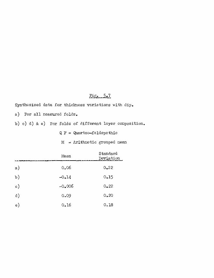
Fig. 5.7 Synthesised data for thickness variations with dip.
a) For all measured folds.
b) c) d) & e) For folds of different layer composition.
Q, F = Quartzo—feldspathic
M = Arithmetic grouped mean
Standard Mean Deviation
a) 0.06 0.22
b) —0.14 0.15
c) —0.006 0.22
d) 0.09 0.20
e) 0.16 0.18
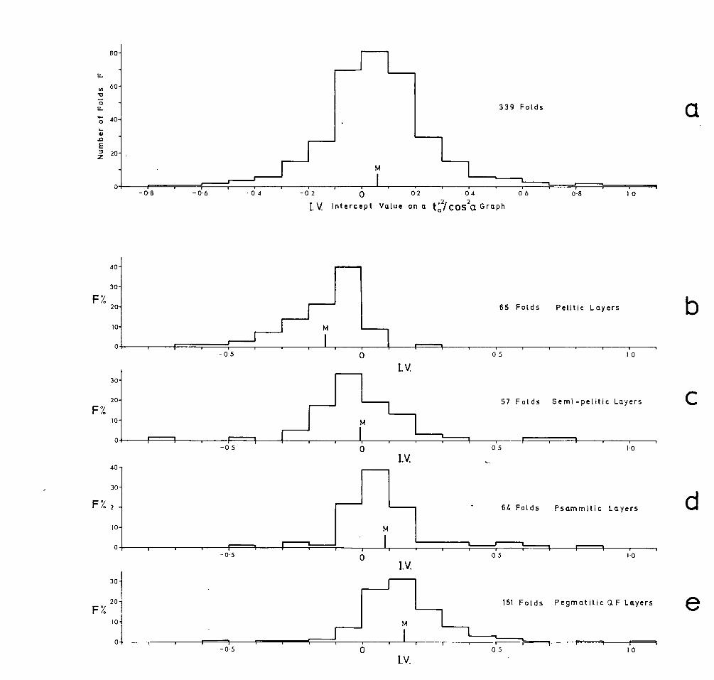
80-
u- 60-
40-
2 Nu
mb
er
of F
old
s
M
339 Folds
-0.8 -06 -04 -02 r 0 02 04 0 6 Or 8 0 1. V. Intercept Value on a tc,/cos2a. Graph
40-
30-
F% 20- 65 Folds Pelitic Layers
10- M
-05 0
d 5 1'0
I.V. 30-
20- 57 Folds Semi -pelitic Layers F%
10- M
-0 5 0
d5 1'0 I.V.
40-
30-
64 Folds Psammitic Layers
-0.5 0 05 I.V.
F% 2
10- M
F%
30
20
151 Folds Pegmatitic 0.F Layers
10
0
M
-0-5 0 05 10
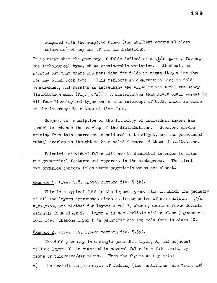
189
compared with the complete range (the smallest covers 10 class
intervals) of any one of the distributions.
It is clear that the geometry of folds defined on a tVo, graph, for any
one lithological type, shows considerable variation. It should be
pointed out that there are more data for folds in pegmatitto veins than
for any other rock typo. This reflects an observation bias in fold
measurement, and results in increasing the value of the total frequency
distribution mean (fib;. 5.7a). A distribution that gives equal weight to
all four lithological types has a mean intercept of 0.02, which is close
to the intercept for a true similar fold.
Subjective description of the lithology of individual layers has
tended to enhance the overlap of the distributions. However, errors
arising from this source are considered to be slight, and the pronounced
mutual overlap is thought to be a valid feature of these distributions.
Selected individual folds will now be described in order to bring
out geometrical features not apparent in the histograms. The first
two examples concern folds where pegmatitic veins are absent.
Example 1. (fig. 5.8, isogon pattern fig. 5.5b).
This is a typical fold in the layered granulites in which the geometry
of all the layers ap?roaches class 2, irrespective of composition. talc,
variations are plotted for layers A and B, whose geometric forms deviate
slightly from class 2. Layer A is semi—aelitic with a class 3 geometric fold form, whereas layer B is psammitic and its fold form is class 10.
Example 2. (fig. 5.9, isogon pattern fig. 5.5a).
The fold geometry in a single psammitic layer, X, and adjacent
politic layer, Y, is compared in several folds in a fold train, by
means of thickness/dip plots. From the figure we may note;
a) the overall cuspate style of folding (the 'antiforms' are tight and
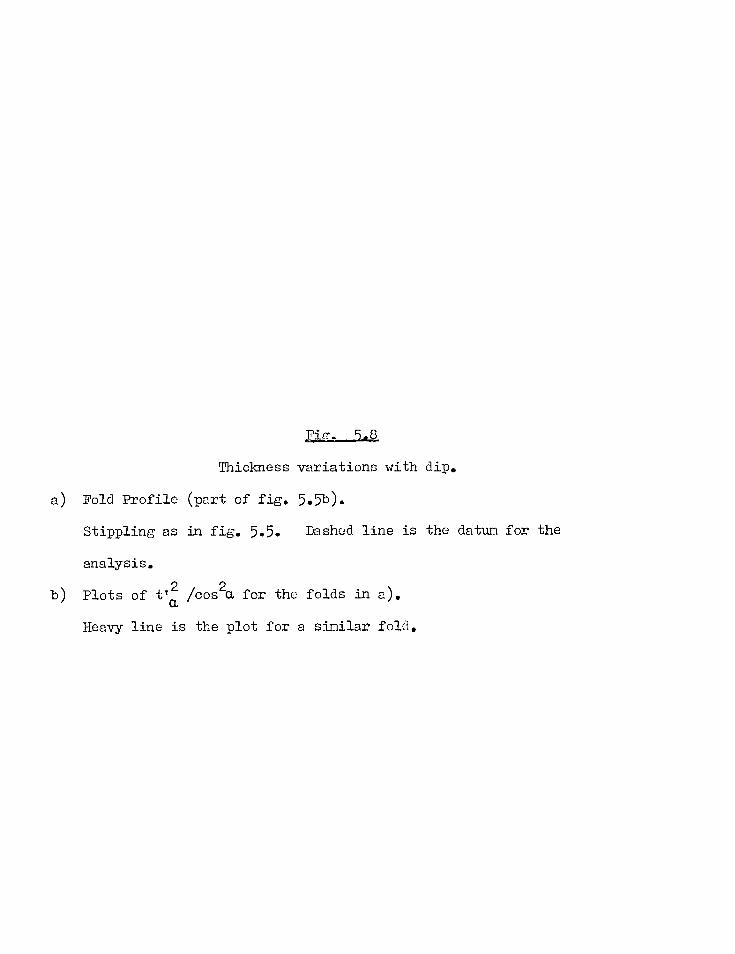
Fig. 5.8
Thickness variations with dip.
a) Fold Profile (part of fig. 5.5b).
Stippling as in fig. 5.5. Dashed line is the datum for the
analysis.
b) Plots of t'a2 /cos2a for the folds in a).
Heavy line is the plot for a similar fold.
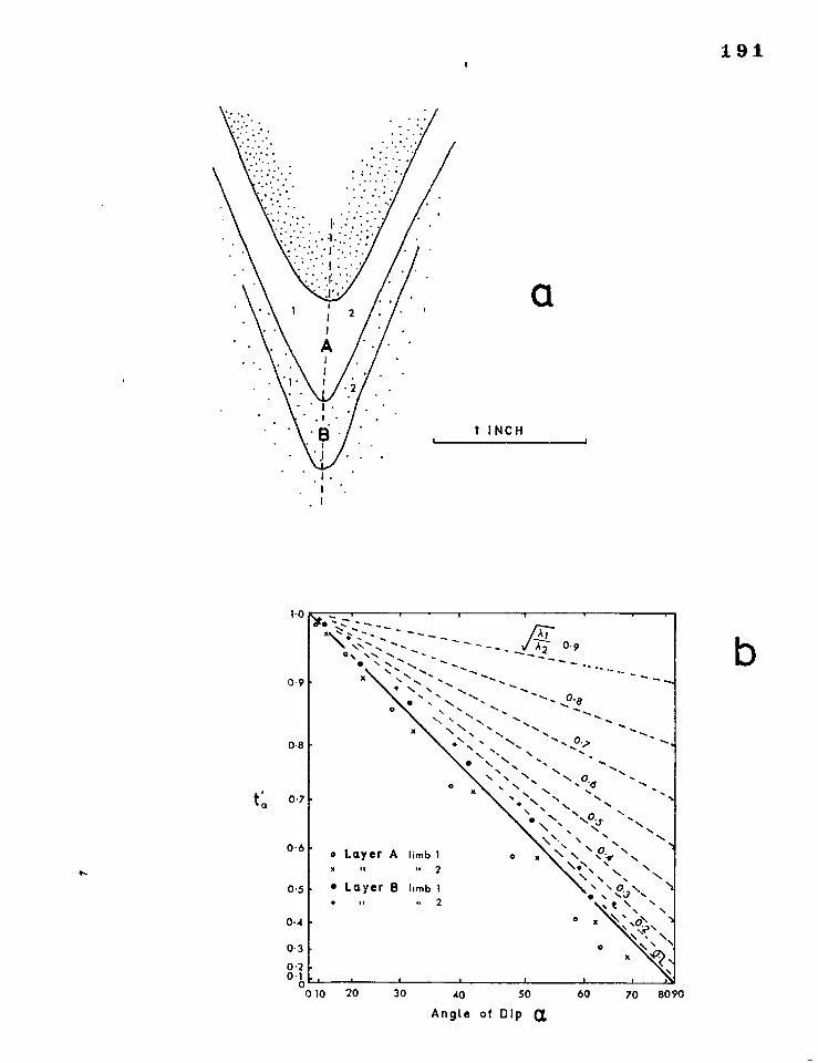
Naft. -zz-:—_____ x N •
• ' " .... ". ":" •.. N .... '. .... • " N N. N ,
". " N XN " ...., ". ... .....
S. .% ..... '`. ..... • N "•
N ' '. s N. .. 0 .8 • • N. .., ". ".
O " ' , .... N N ". N. "..,, 's .....
N ". ...
"*".. ".. N '.
, N ...., ...
▪ ... N.
' ". % N. 1) •,. • .. N "•- •• % \ ‘ ' • \
". % • N
". - % N. N N • ' , N. 0
,
o • N \ , ...s N
N. • ... N. • ♦ N. N. N.
• s• N. N • N N , N • N N. ....• ' ..... \ •' , N. N.
N N. .., \
N
., ...
0 • Layer A limb 1 o x \ "\ s• ir ss \
\ 0‘ % N . \ N
_ _ 2 0.9
x n 2 • •
• Layer B limb 1 • • 0.
t o 2 • S. 0
x O•
o • • N.• •
191
t INCH
a
1.0
0-9
0.8
Ca 0.7
0.6
0.5
0.4
0.3 0.2 0.1
0 0 10 20 30 40 50
Angle of DIp a 60 70 8090

Fig. 5,9
Thickness variations with dip.
a) Fold Profile (part of fig. 5.5a)
Stippling as in fig. 5.5. Dashed linos are the datum lines for
the analysis.
2 b) c) Plots of t'a /cos2u for the folds in a).
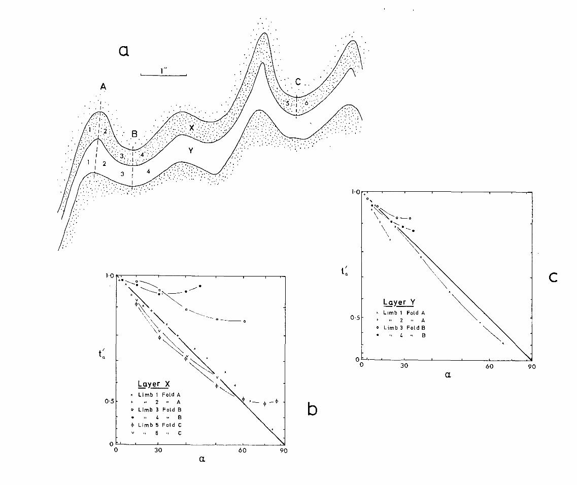
C
. a
0.5
Layer X x Limb 1 Fold A + .. 2 ,. A o Limb 3 Fold B • .. 4 ,. B (I) Limb 5 Fold C ✓ u 6 .. C
b
30
60
90 a
194
the 'synforms' open)
b) the considerable differences between the positions taken up by the
plotted points for each layer in different folds.
c) the similarity of the Wu relationships for either limb of the same
fold in a given layer.
d) that the plots for both layers in the 'antiforms' (i.e. fold A) are
bettor represented by straight lines than the plots for these layers
in the 'synforms' (folds B Sc c). Both plots for layer X in fold C
move from field 3 tc field 10 at high limb dips.
Example 3. (fig. 5.10, isogon pattern fig. 5.5d).
Folds I and B die cut away from a pegmatitic vein (see fig. 5.6, where
the interlimb angle variations for these folds are recorded). Thickness/
dip plots for the pegmatitic vein (layer Y) and for semi—pelitic layers X
and Z either side of the vein, are recorded. From the figure we may note
that:
a) the variations for layer Y are almost identical on both limbs of
folds A and B (R = 0.4, see section 3.5).
b) whore themmi—pelitic layers X and Z lie beyond the outer arcs of
the folded pegmatitic vein, they take on a class 10 fold geometry
(except for limb 1 of layer Z), and where these layers lie within
the inner arcs of the folded vein, their geometric form is class 3.
Example 4. (fig. 5.11, isogon pattern fig. 5.5e).
The profile drawn is part of a sequence of folded pegmatitic veins,
alternating with pelitic rock layers. to variations with dip are plotted
for the massive pegmatitic vein X. All the plots fall within field 10
on the graph.
Considering the two pegmatitic veins together c.)nstitute a single
unit, where vein X forms the inner arc of this unit its geometric form
Fig. 5.10
Thickness variations with dip.
a) Fold profile (part of fig. 5.5d).
Stippling as in fig. 5.5. Dashed lines are the datum lines for
the analysis.
b) c) d) Plots of t'(i /cos2a for the folds in a).
Dashed line in c) is the plot for a parallel fold flattened by a
strain of ik2/7\.1 = 0.4.
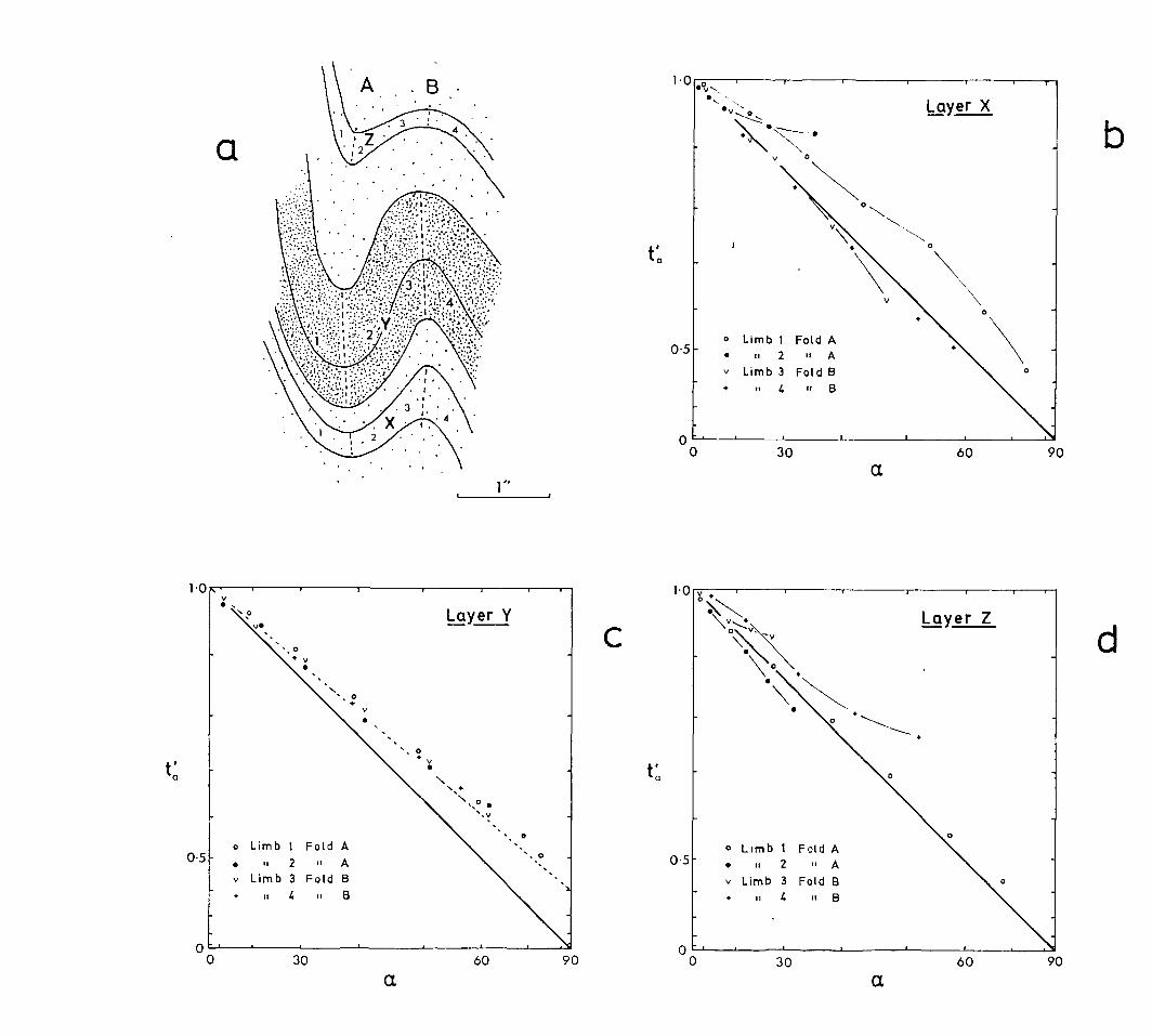
a
10
t "c,
0.5
0 0 30 60 90
a
1.0
0.5
0 0 30 60 90
t to
0 0 30 60 90
1.0
C
Limb I Fold A 2 A
Limb 3 Fold B 4 B
0-5
a a

Fig_. 5.11
Thickness variations with dip.
a) Fold profile (part of fig. 5.50.
Stippling as in fig. 5.5. Dashed lines are the datum lines for the
analysis.
b) Plots of t'c /cos2a for the folds in a).
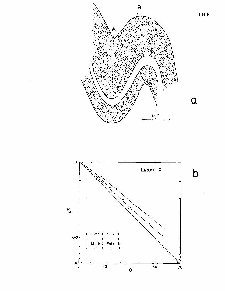
a
198
0 r ' 0
co •
O
• Limb 1 Fotd A o ir 2 ii A ✓ Limb 3 Fold B . ii 4 II g
30 60 a
10
0.5
•
Layer X b
NI 90
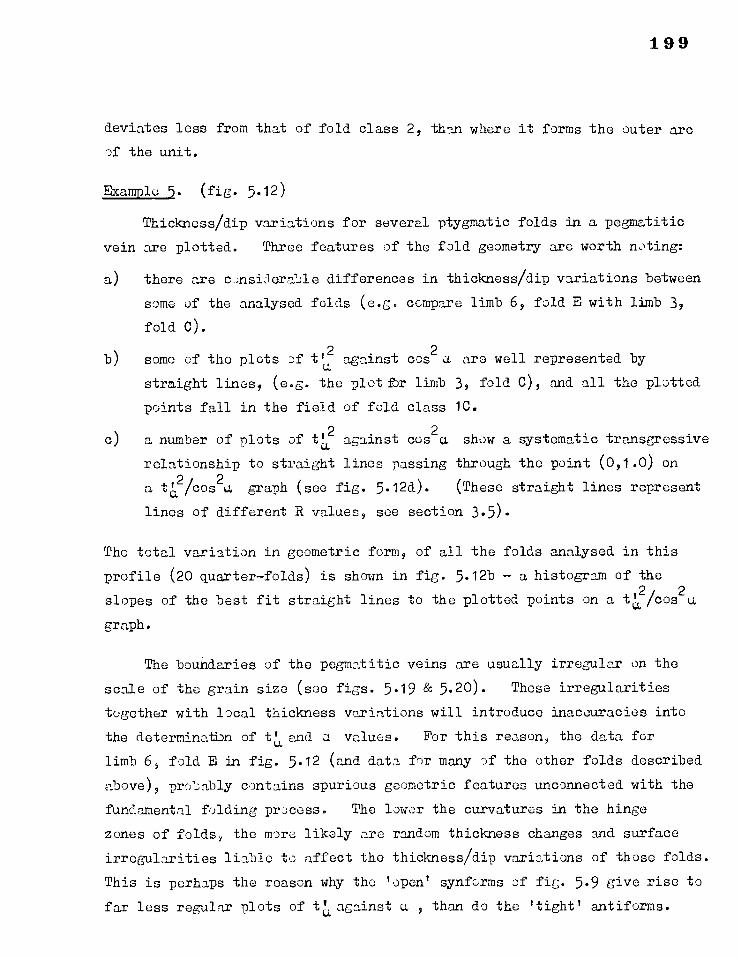
199
deviates less from that of fold class 2, than where it forms the outer arc
of the unit.
Example 5. (fig. 5.12)
Thickness/dip variations for several ptygmatic folds in a pegmatitic
vein are plotted. Three features of the fold geometry are worth noting:
a) there are c.)nsiaeralde differences in thickness/dip variations between
some of the analysed folds (e.g. compare limb 6, fold E with limb 39
fold C).
b) some of the plots of t t2 against cos are well represented by
straight lines, (e.g. the plot for limb 3, fold C), and all the plotted
points fall in the field of fold class 1C.
c) a number of plots of tot against cos2a show a systematic transgressive
relationship to straight lines passing through the point (0,1.0) on
a t'2/cos2a graph (see fig. 5.I2d). (These straight lines represent
linos of different R values, see section 3.5).
The total variation in geometric form, of all the folds analysed in this
profile (20 quarter—folds) is shown in fig. 5.12b — a histogram of the
slopes of the best fit straight lines to the plotted points on a t&/cos2a
graph.
The boundaries of the pegmatitic veins are usually irregular on the
scale of the grain size (see figs. 5.19 & 5.20). These irregularities
together with local thickness variations will introduce inaccuracies into
the determinatbn of tLand a values. For this reason, the data for
limb 6, fold E in fig. 5.12 (and data for many of the other folds described
above), proably contains spurious geometric features unconnected with the
fundamental folding process. The lower the curvatures in the hinge
zones of folds, the more likely are random thickness changes and surface
irregularities liable to affect the thickness/dip variations of those folds.
This is perhaps the reason why the 'open' synforms of fig. 5.9 give rise to
far less regular plots of tLagainst a , than do the 'tight' antiforms.

Fig. 5.12
Thickness variations with dip.
a) Fold Profile (300X east of main dam).
Pegmatitic vein (stippled) in pelitic rock. Dashed lines are the
datum lines for the analysis.
b) Histogram of the values of the slope of the best fit straight line
2 (on a -0a/cos
2 a,graph) for 20 folds in the profile shown in a).
c) d) Plots of -02 /cos2a for the folds in a). a
Dashed lines in d) are the plots for parallel folds flattened by
strains of JX2/X1 = 0.4 & 0.5.
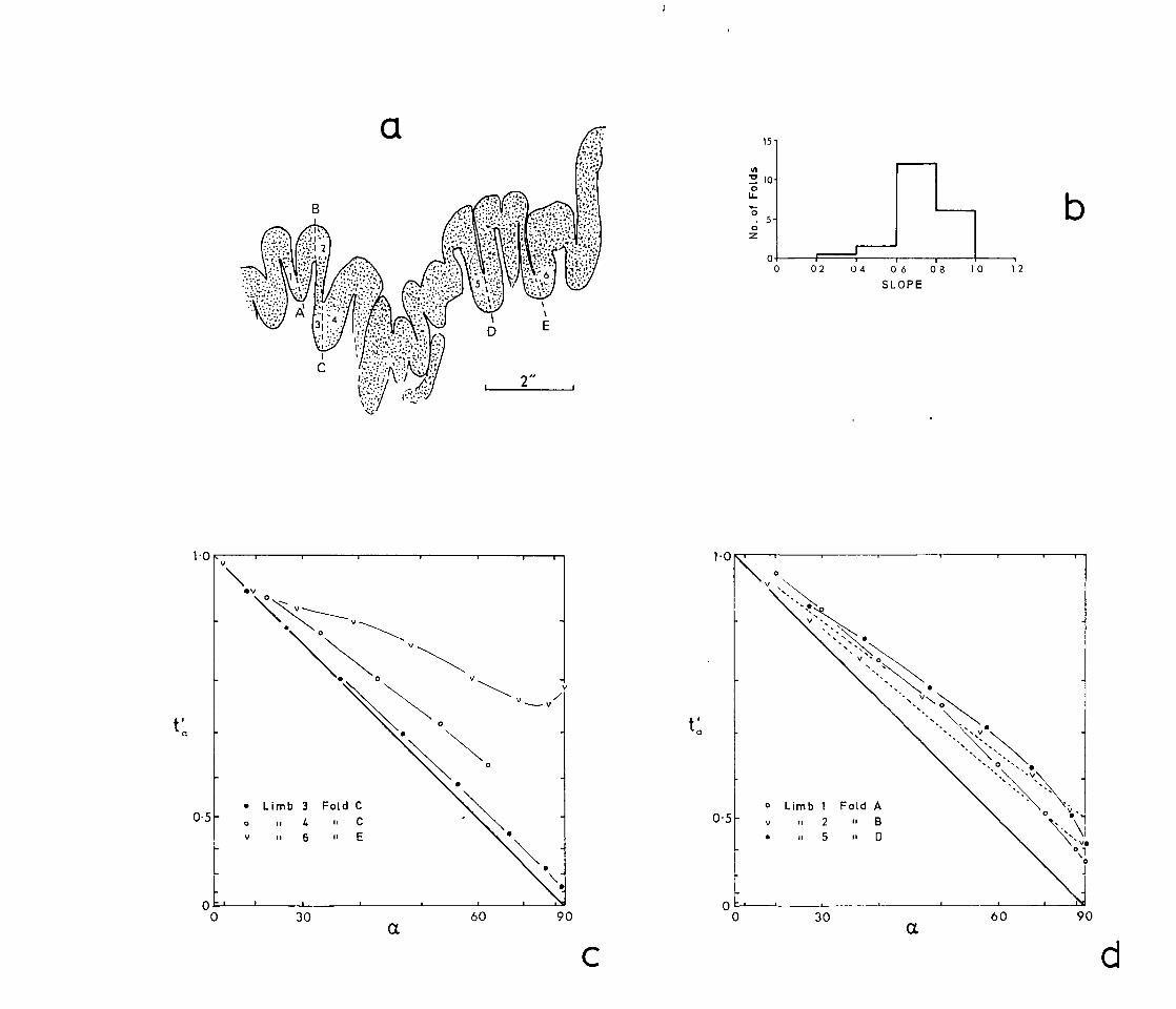
15
V 0
0 0 z
10
b 5-
0 2 12 0 4 10 06 08 8
SLOPE
30
tQ
• v
1.0
0-5 • Limb 3 Fold C o "
ii 4 6
I,
"
C E
N.
90 60 a a
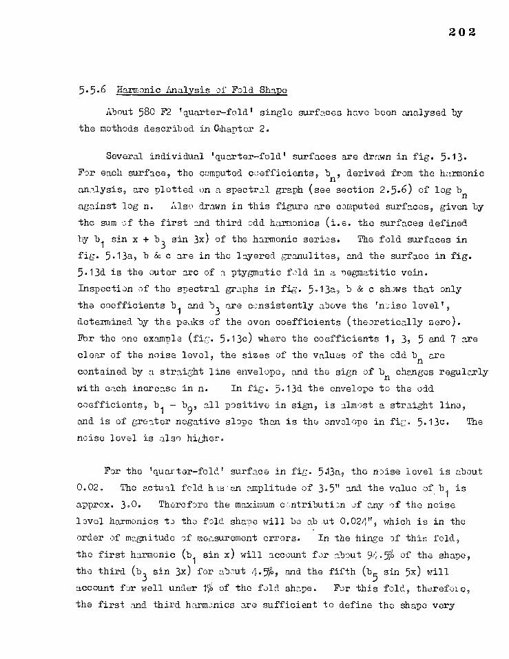
202
5.5.6 Harmonic Analysis of Fold Shape
About 580 F2 'quarter—fold' single surfaces have been analysed by
the methods described in Chapter 2.
Several individual 'quarter—fold' surfaces are drawn in fig. 5.13.
For each surface, the computed coefficients, bn, derived from the harmonic
analysis, are plotted on a spectral graph (see section 2.5.6) of log bn
against log n. Also drawn in this figure are computed surfaces, given by
the sum of the first and third odd harmonics (i.e. the surfaces defined
by b1 sin x + b
3 sin 3x) of the harmonic series. The fold surfaces in
fig. 5.13a, b do c are in the layered granulites, and the surface in fig.
5.13d is the outer arc of a ptygmatic fold in a 'egmatitic vein.
Inspection of the spectral graphs in fig. 5.13a, b (Si c shows that only
the coefficients b1 and b
3 are consistently above the 'noise level',
determined by the peaks of the oven coefficients (theoretically zero).
For the one example (fig. 5.13c) where the coefficients 1, 3, 5 and 7 are clear of the noise level, the sizes of the values of the odd bn are
contained by a straight line envelope, and the sign of bn changes regularly
with each increase in n. In fig. 5.13d the envelope to the odd
coefficients, b1 — b9, all positive in sign, is almost a straight line,
and is of greater negative slope than is the envelope in fig. 5.13c. The
noise level is also higher.
For the 'quarter—fold' surface in fig. 5.13a, the noise level is about
0.02. The actual fold hls'an amplitude of 3.5" and the value of b1 is
approx. 3.0. Therefore the maximum contribution of any of the noise
level harmonics to the fold shape will be about 0.024", which is in the
order of m.aguitude of measurement errors. In the hinge of this fold,
the first harwenic (b1 sin x) will account for about 94.51. of the shape,
the third (b3 sin 3x) for about 4.%, and the fifth (b
5 sin 5x) will
account for well under t; of the fold shape. For this fold, therefore,
the first and third harmonics are sufficient to define the shape very

Fig. 5.13
Individual 'quarter wavelength units' of F2 folds, and spectral graphs of
their harmonic components.
The solid curves are the actual fold shapes, and the dashed curves are
the sums of the first two odd harmonics; y = sin x + b3 sin 3x
The first of the two lithologies referred to in each case below lies on
the "inside" of the folded surfaces shown.
a) b) & c) are all folds in the granulites.
a) Folded surface between psanmitic and pelitic layers.
b) Surface between psamnitic and semi-pelitic layers.
c) Surface between semi-pelitic and pelitic layers.
d) Surface between a pegmatitic vein and a pelitic layer.
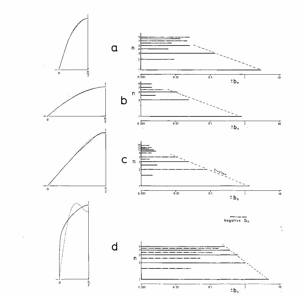
d
• 0
2 10
-bn 0 001 0 01 0'1
9 7
a
1 0
b
0 rt
2
0.001 0-'01 Oi 1 1 10
9 bn 7
n 5 3
1
0 001 0 01 0 1 10
2
C n
0 rr 2
- n
15 13 11 9
5
„, op
3
1
0 001 0.01 0.1 1 10
bn
N egative bn
5 4
3
2
9 7
5 n
1
•
205
closely. Higher harmonics have little significance, as their values are
of the same order of magnitude as the expected measurement errors.
The close match of the sums of the first and third harmonics to the
actual fold shapes is evident in fig. 5.13a, b & c. For nearly all the
folds in the layered granulites, the sum of the first two odd harmonics
were found to define the fold shape fairly accurately.
In fig. 5.13d the sum of the first and third harmonics is clearly
insufficient to define the fold shape; the coefficients decrease in size
at a much slower rate than they do for the folds in the granulites. For
this fold at least 10 harmonics would be required to define the shape with
any degree of accuracy. However, because the envelope to the computed
values of bra
is a straight line, it is valid to represent the fold shape
using only the first and third coefficients (see section 2.5.6), and the
shape will be closely matched by a member of the ideal series of fold
forms described in section 2.5.6.
Spectral graphs similar to that drawn in fig. 5.13d were obtained
for nearly all the analysed ptygmatic folds in pegmatitic veins.
In the analysis that follows only the coefficients b1 and b3 are
considered.
5.5.6.1 Analysis of bi.
The size of the coefficient bI is closely related to the fold
amplitude/wavelength ratio, or fold tightness (see section 2.5.6).
Frequency histograms of the size of b1 appear in fig. 5.14, for all the
analysed F2 folds. In drawing these histograms values of b1 for fold
surfaces in the granulites (fig. 5.14a) hwe been distinguished from those
in the pegmatitic veins (fig. 5.14b), and surfaces in those pegmatitic
veins with ptygmatic form have been treated as a separate category, (fig.
5.14c). Examination of fig. 5.14 reveals that:
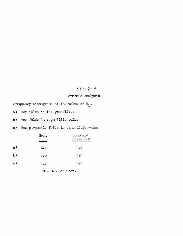
Fig. 5.14
Harmonic Analysis.
Frequency histograms of the value of b1.
a) For folds in the granulites
b) For folds in pegmatitic veins
c) For ptygmatic folds in pegnatitic veins
Mean Standard Deviation
a) 2.7 2.4
b) 3.5 1.9
c) 4.9 2.2
M = Grouped mean.
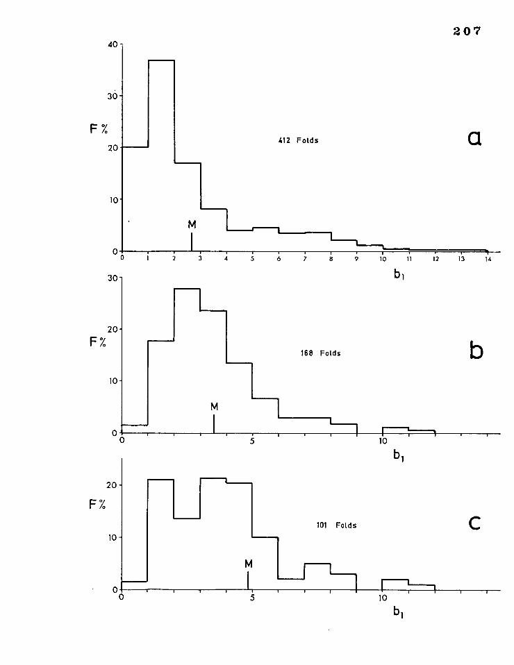
30 -
4 ; . 6 7. 8 9 10 11 12 13 14
b1
b 168 Folds
5 10 '
b1
C 101 Folds
207
30-
412 Folds
M
I f
10-
M
F%
10-
M
I I I I
5 10 '
b1
20-
F%
20-
a
40-
F%
20
10 -
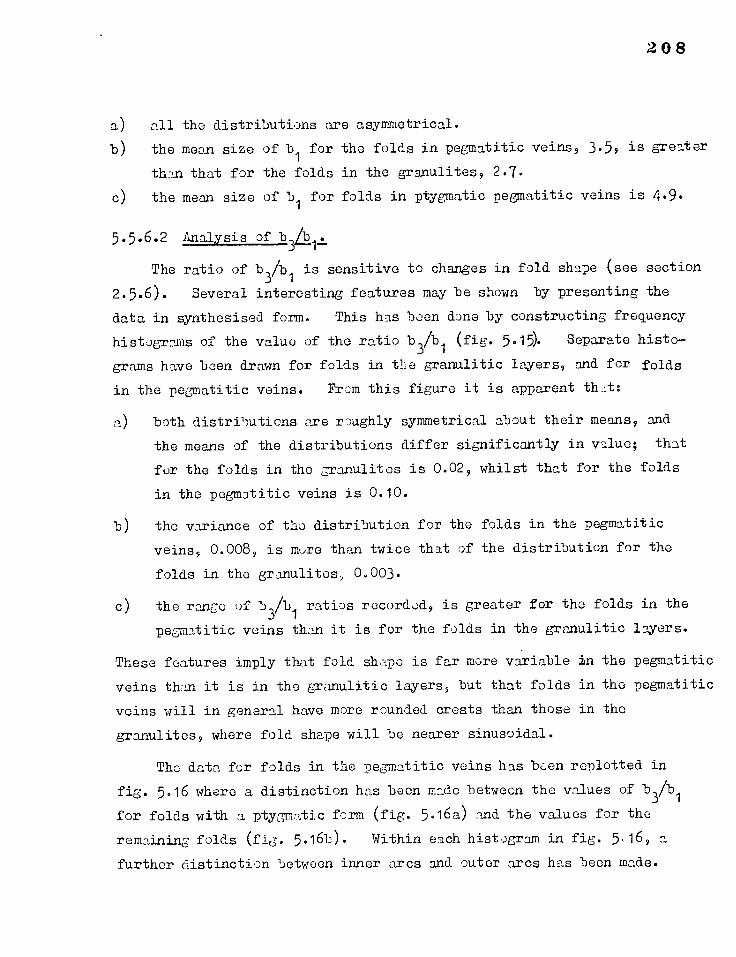
208
a)
all the distributions are asymmetrical.
b) the mean size
than that for
c) the mean size
of b1 for the folds in pegmatitic veins, 3.5, is greater
the folds in the granulites, 2.7. of b
1 for folds in ptygmatic pegmatitic veins is 4.9.
5.5.6.2 Analysis of b34.
The ratio of b31
is sensitive to changes in fold shape (see section
2.5.6). Several interesting features may be shown by presenting the
data in synthesised form. This has been done by constructing frequency
histograms of the value of the ratio b3/b1 (fig. 5.15). Separate histo-
grams have been drawn for folds in the granulitic layers, and for folds
in the pegmatitic veins. From this figure it is apparent that:
a) both distributions are roughly symmetrical about their means, and
the means of the distributions differ significantly in value; that
for the folds in the granulites is 0.02, whilst that for the folds
in the pegmatitic veins is 0.10.
b) the variance of the distribution for the folds in the pegmatitic
veins, 0.008, is more than twice that of the distribution for the
folds in the granulites, 0.003.
c) the range of b3/b1 ratios recorded, is greater for the folds in the
pegmatitic veins than it is for the folds in the granulitic layers.
These features imply that fold shape is far more variable in the pegmatitic
veins than it is in the granulitic layers, but that folds in the pegmatitic
veins will in general have more rounded crests than those in the
granulites, where fold shape will be nearer sinusoidal.
The data for folds in the pegmatitic veins has been replotted in
fig. 5.16 where a distinction has been made between the values of bibi
for folds with a ptygmatic form (fig. 5.16a) and the values for the
remaining folds (fig. 5.16b). Within each histogram in fig. 5,16,
further distinction between inner arcs and outer arcs has been made.
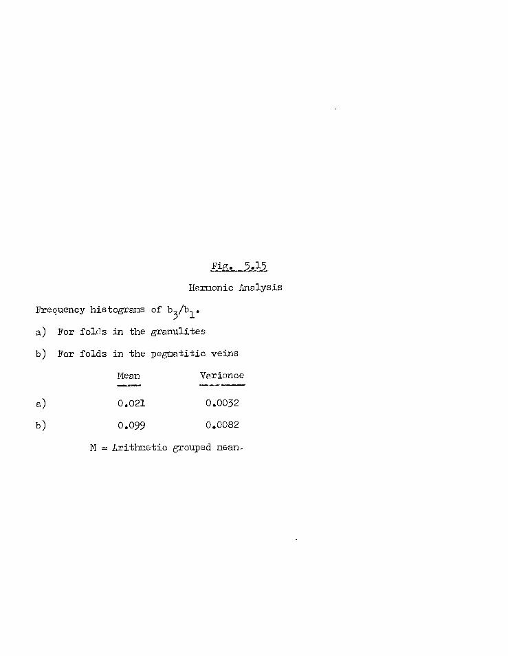
Fig. 5.15
Harmonic Analysis
Frequency histograms of b3/b1.
a) For folds in the granulites
b) For folds in the pegnatitic veins
Mean Variance
a) 0.021 0.0032
b) 0.099 0.0082
M = Arithmetic grouped mean,
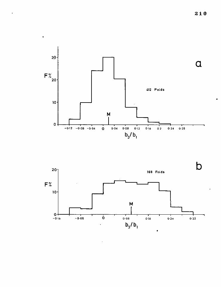
0 0.04 0.08 0.12 016 0.2 0.24 0.28 -0.12 -0.08 -0.04
210
b3/
168 Folds b
F%
0 0.08 0 0.08 0.16 0-24 0.32
b3/ 0.16
20-
10-
412 Folds
10 -
30-
F% 20 -
a
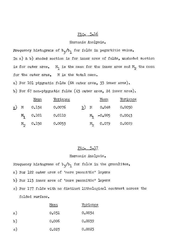
Fig. 5.16
Harmonic Analysis.
Frequency histograms of b3/b1 for folds in peguatitic veins.
In a) & b) shaded section is for inner arcs of folds, unshaded section
is for outer arcs. M1 is the mean for the inner arcs and M2 the mean
for the outer arcs. M is the total mean.
a) For 101 ptygmatic folds (68 cuter arcs, 33 inner arcs).
b) For 67 non-ptygnatic folds (43 outer arcs, 24 inner arcs).
Mean Variance Mean Variance
a) M 0.134 0.0076 b) M 0.048 0.0050
Ml 0.101 0.0110 -0.005 0.0043
M2 0.150 0.0053 M2 0.079 0.0029
Fir- 5.17 Harmonic Analysis.
Frequency histograms of b3/b1 for folds in the granulites.
a) For 122 outer arcs of 'more psamnitic' layers
b) For 113 inner arcs of 'more psammiticl layers
c) For 177 folds with no distinct lithological contrast across the
folded surface.
Mean Variance
a) 0.031 0.0034
b) 0.006 0.0039
c) 0.023 0.0023
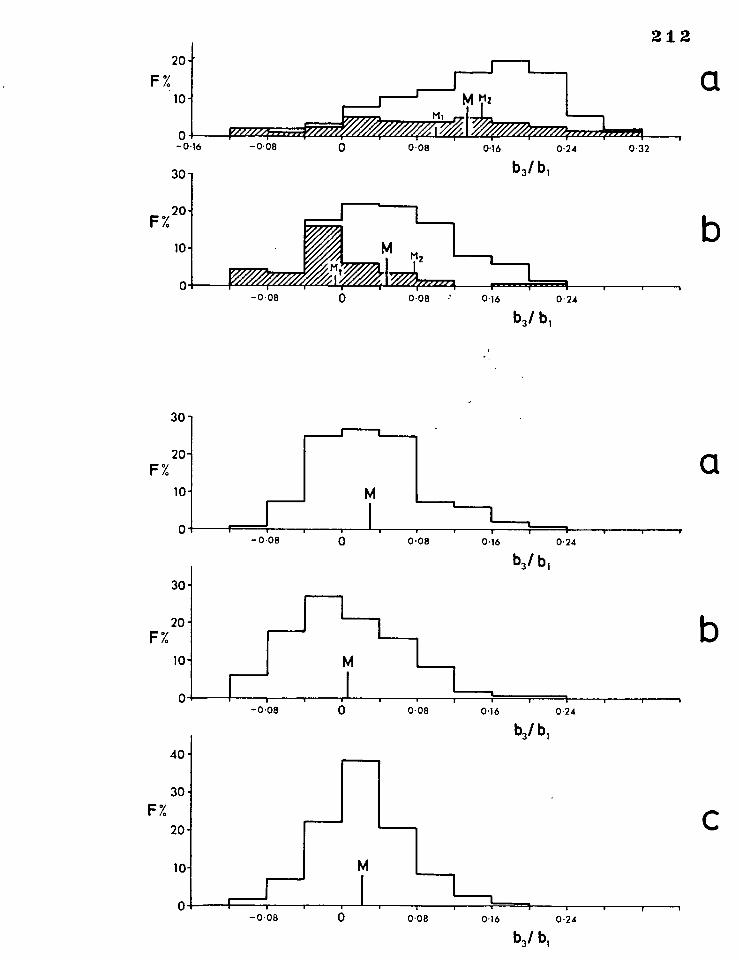
-0.08 0.08 016 0.24 0.32
- 0.08 0.08 0.16 0 24
b3/
b3 / b,
20
F% 10
0 -0 16
30
F%20
10
0
212
a
O 0.08
016
0.24
b3 / b,
30 -
20- F%
10 - a
- 0 08
30
20 - F%
10 - M b
-0:08 0 0.08 016 0.24
b3/b, 40 -
30-
F%
20 -
10-
-0.08 0 0.08 016 0.24
b3/
C
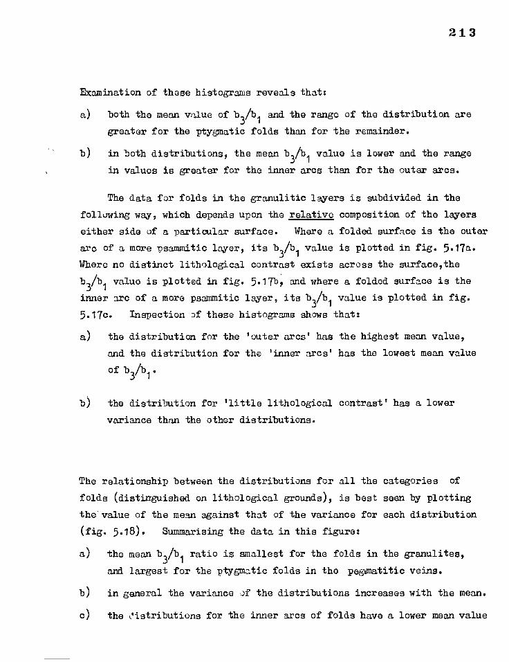
213
EXamination of these histograms reveals that:
a) both the mean value of b3/b1
and the range of the distribution are
greater for the ptygmatic folds than for the remainder.
b) in both distributions, the mean b3/b1 value is lower and the range
in values is greater for the inner arcs than for the outer arcs.
The data for folds in the granulitic layers is subdivided in the
following way, which depends upon the relative composition of the layers
either side of a particular surface. Where a folded surface is the outer
arc of a more psammitic layer, its b3/b1 value is plotted in fig. 5.17a.
Where no distinct lithological contrast exists across the surfacelthe
b3/b
1 value is plotted in fig. 5.17b, and where a folded surface is the
inner arc of a more psammitic layer, its b3/b1 value is plotted in fig.
5.17c. Inspection of these histograms shows that:
a) the distribution for the 'outer arcs' has the highest mean value,
and the distribution for the 'inner arcs' has the lowest mean value
of b3/b1.
the distribution for 'little lithological contrast' has a lower
variance than the other distributions.
The relationship between the distributions for all the categories of
folds (distinguished on lithological grounds), is best seen by plotting
the value of the mean against that of the variance for each distribution
(fig. 5.18). Summarising the data in this figure:
a) the mean b3/b1 ratio is smallest for the folds in the granulites,
and largest for the ptygmatic folds in the pegtmatitic veins.
b) in general the variance of the distributions increases with the mean.
c) the k'istributions for the inner arcs of folds have a lower mean value
Fig. 5.18
Harmonic Analysis.
Synthesis of data from figs. 5.15, 5.16 & 5.17.
For each distribution of the values of b3/b1 the arithmetic grouped mean
is plotted against the variance.
1 — For folds in the granulites
2 — For non—ptygmatic folds in pegnatitic veins
3 - For ptygmatic folds in pegmatitic veins
X Total of measured folds
triangles Inner arcs
dots Outer arcs
G No lithological contrast across the folded
surface.
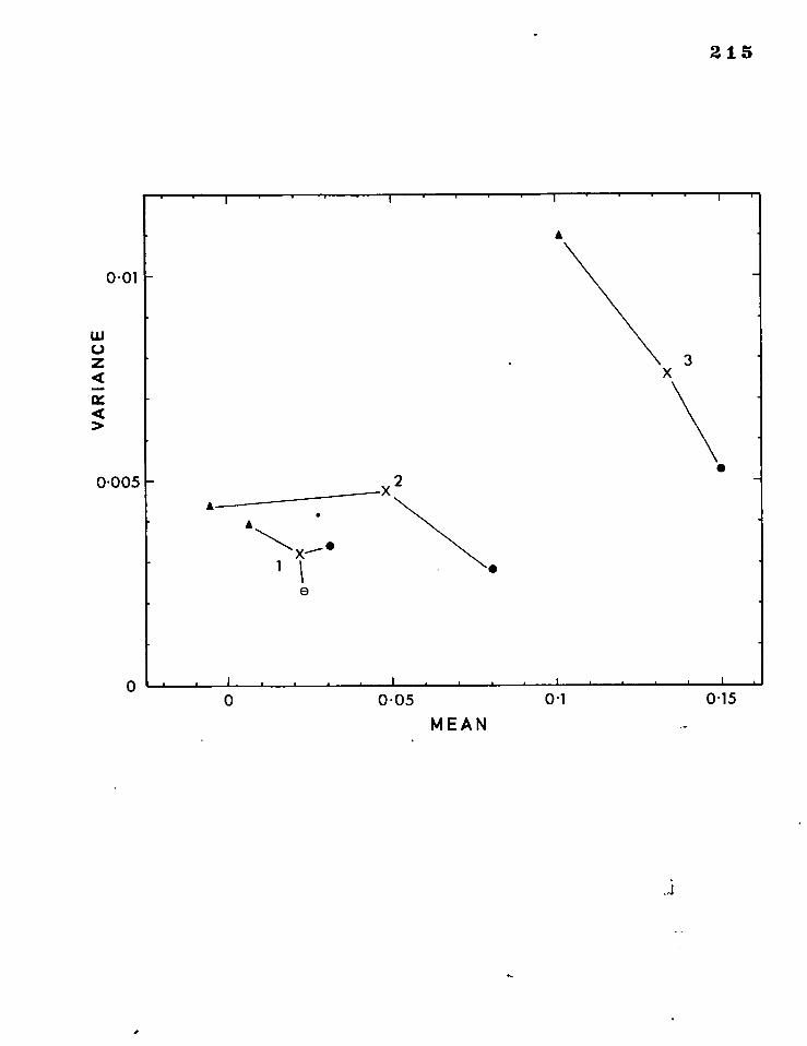
0.15 0.1 0-05 MEAN
0
j
215
VA
RI A
NC
E
0-005
0-01
0
216
but higher variance than those for the outer arcs.
d) the group of folded surfaces that shows least variation in b3/b1 ratio
is that for which there is no distinct lithological contrast across
the surfaces.
In general terms of fold style, these results imply that the inner
arcs of folds are usually sharper in the hinges yet more variable in shape
than the outer arcs, for a particular category of folds, The ptygmatic
folds in the pegmatitic veins have higher amplitudes, are in general more
rounded in the crests and are much more variable in shape than the folds
in the layered granulites.
The results of analyses of a number of individual folds will now be
described in order to bring out features not aroarent in the synthesised
data. The selected examples are shown in figs. 5.19 and 5.20, where the
data are presented in plots of b3
against b1.
Shape Variations related to Variations in Composition.
a) Differences in shape between folds in the pegmatitic veins and folds
in the granulitic layers.
The values of b1 and b3/b1, for ptygmatic folds in pegmatitic veins,
tend t, be high; and several plotted points for these folds on a graph of
b3 against b
1 tend to display a pronounced 'linear' trend (fig. 5.19a,b).
Values of b3 are seldom negative.
The plotted points of b31, determined from an analysis of folds in
the granulitic layers, tend to cluster about the line b3 = 0 (see fig.
5.19d and fig. 5.20a,c): occasionally a distinct linear trend is apparent
(fig. 5.20d).
Non—ptygmatically folded veins are present in fig. 5.19c. On a
graph of b3 against b1, the data for these folds occupy a field which is
intermediate in position between the field occupied by data for ptygmatic
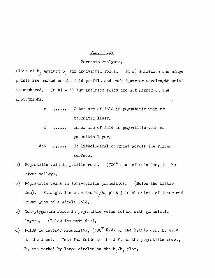
Fig. 5.19
Harmonic Analysis.
Plots of b3 against bl for individual folds. In a) inflexion and hinge
points are marked on the fold profile and each 'quarter wavelength unit'
is numbered. In b) d) the analysed folds are not marked on the
photographs.
o Outer arc of fold in pegmatitic vein or
psammitic layer.
x Inner arc of fold in pegmatitic vein or
psammitic layer.
dot No lithological contrast across the folded
surface.
a) Pegmatitic vein in pelitic rock. (700x east of main dam, in the
river valley).
b) Pegmatitic veins in semi—politic granulites. (Below the little
dam). Straight lines on the b5/b1 plot join the plots of inner and
outer arcs of a single fold.
c) Non—ptygmatic folds in pegmntitic veins folded with granulitic
layers. (Below the main dam).
d) Folds in layered granulites, (500x N.W. of the little dam, S. side
of the loch). Data for folds to the left of the pegmatitic sheet,
P, are marked by large circles on the b5/bI plot.
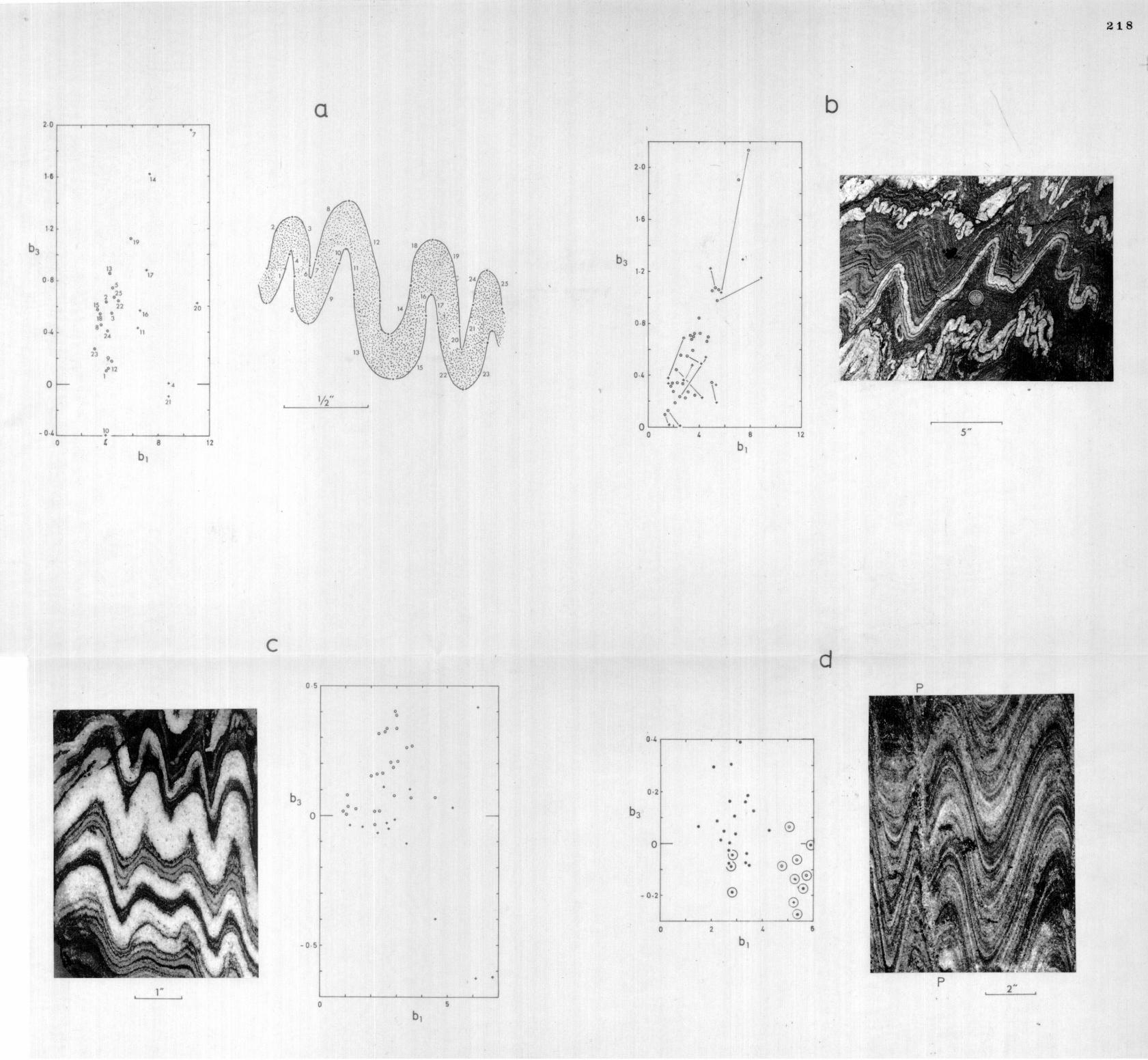
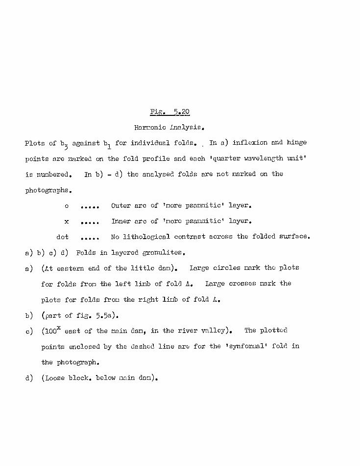
Fig. 5.20
Harmonic Lnalysis.
Plots of b3
against b1 for individual folds. In a) inflexion and hinge
points are narked on the fold profile and each 'quarter wavelength unit'
is numbered. In b) — d) the analysed folds are not narked on the
photographs.
o Outer arc of 'more psammitic' layer.
x Inner arc of 'more psanmitic' layer.
dot No lithological contrast across the folded surface.
a) b) c) d) Folds in layered granulites.
a) (Lt eastern end of the little dam). Large circles mark the plots
for folds from the left limb of fold A. Large crosses mark the
plots for folds from the right limb of fold A.
b) (part of fig. 5.5a).
c) (100x east of the main dam, in the river valley). The plotted
points enclosed by the dashed line are for the Isynfornall fold in
the photograph.
d) (Loose block, below main dam).
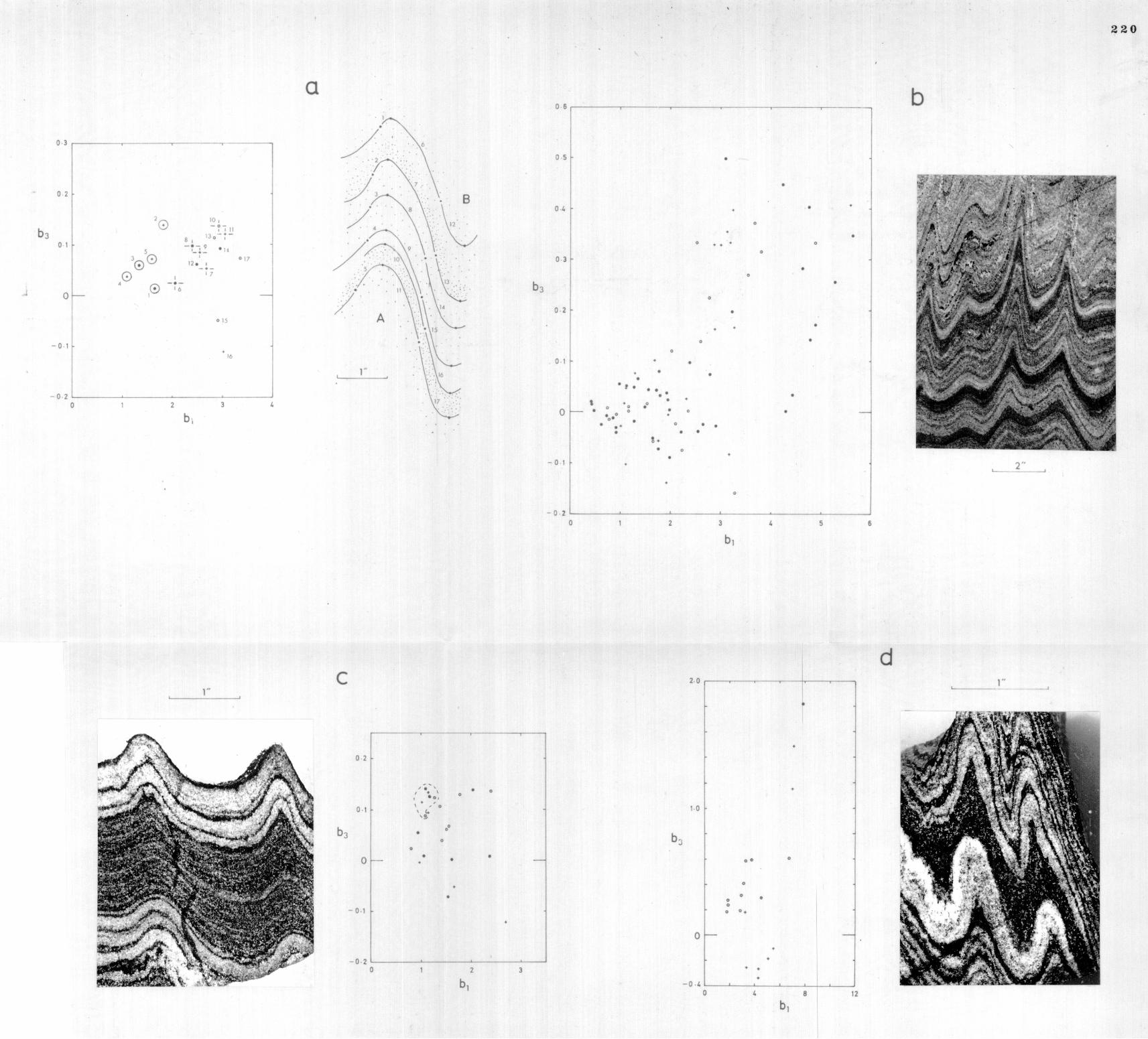
221
folds in pegmatitic veins (see fig. 5.19a,b), and that occupied by data
for the folds in the granulites.
b) Differences of shape of the inner and outer arcs of folded layers.
An analysis of folds in pegmatitic veins shows that the inner arcs are
far more variable in shape than the outer arcs (see the plots of b3
against
b1 in fig. 5.19a,b,c). This feature is either absent or slightly shown in
the folds in the granulites (see fig. 5.20a,b,c,d). In most of the plots
in figs. 5.19 & 5.20 both u1 b3
attain more extreme values
for the inner arcs of folds than they do for the outer.
Other Local Shape Variations.
a) Differences in shape between the limbs of the same fold.
In successive fold surfaces in fig. 5.20a, b1 takes on greater values
on ono limb of the fold A, than on the other.
b) Differences in shape between adjacent folds.
In fig. 5.20c, data for folds in the open 'synform' define a restricted
field on a graph of b3
against b1,
in contrast to the wide field defined
by the data for the tight adjacent tantiforms'.
In fig. 5.19d, there are distinctive differences between the positions,
on a graph of b3 against b1, taken up by the plotted points for fold
surfaces on either side of the pegmatitic sheet, P.
c) Progressive changes in fold shape along axial surfaces.
In the fold profile drawn in fig. 5.20b, there are progressive
changes in fold amplitude along the _axial surface traces. These changes
are reflected in the plots of b3
against b1.for a number of fold surfaces
in this profile. The plotted points for these surfaces on a graph of b3
against b1, fall in a broad field which displays an arcuate trend. For
222
low values of b1,
values of b3 are small, and either positive or negative
in sign: as the value of b1 increases,b
3 takes on positive values and
increases at a greater rate than b1.
d) Differences in shape between a number of ptygmatic folds in a single
layer.
In fig. 5.19a & b, the results are shown of analyses of a number of
folded surfaces in single layers with ptygmatic fold form. Picts of
the values of b3 against b1 for these folds fall in fields which show a
distinct linear trend. An increase in the values of both b1 and b
3 away
from the origin of the graph is accompanied by an increase in the value of
the ratio b3/b1. The trends do not appear to project through the origin
of the graph.
A summary of the features of folded surface geometry, brought out
by the harmonic analyses of individual folds drawn in figs. 5.19 & 5.20,
will now be made.
a) The existence of trends in some of the plots of b3 against b
1 has
been demonstrated: All the trends lead to an increase of b3/b1 with
b1'
implying that fold crests bocome more rounded as fold amplitude
increases.
b) Local differences in shape often exist between limbs of single folds
or between adjacent folds. The cuspate style of folding in fig.
5.20c has been 'brought out' by the harmonic analysis.
c) In any of the figured examples the spread in fold shapes present in
the analysed folded surfaces is large (i.e. the range in b3/b1
ratios is large).
d) The fold shape in the granulitic layers is usually fairly close to
being sinusoidal.
223
5.6 INTERPREMTION
The results of the geometrical analyses described above, all show
systematic variations in fold shape (both for layers and for single
surfaces) that can be related to variations in composition of the folded
layers. The layering in the rocks has not therefore behaved in a truly
passive manner (see section 3.2) throughout the deformation, and the folds
that have developed are not truly similar.
Nearly all the features brought out in the geometrical analysis are
compatible with a folding process that involves buckling of the more
competent layers in the rock, and a considerable amount of 'flattening'
(see section 3.5) of the whole folded sequence.
By analogy with buckling theory and the results of experiments on
folding (see Chapter 3), the relative competencies of the various rock
types may be determined by observation of isogon patterns (fig. 5.5), or
by inspection of the histograms of intercept values derived from -002,/cos2a
plots (fig. 5.7). The more competent a layer is with respect to its
neighbours in general the less will its geometric form depart from that 2 On a plot of -0a against cos
2a, , the most competent
layers will in general have intercept values closest to 1.0, and the least
competent layers values of intercept furthest removed from a value of 1.0.
Using these criteria we may rank the rock types according to competency:
pegmatitic veins > psammites > semi-pelites > pelites
Examination of fig. 5.5 shows that an overall class 2 fold geometry often results from alternating class 1C and class 3 fold geometries in individual layers. Ramsay (1967, p.432) describes this feature in a
folded phyllite.
The folds in the pegmatitic veins show features expected of buckle
folds that have been modified by a flattening deformation (section 3.5).
The geometric form of the folds in these veins is class 10, and on a plot
of
a parallel fold.
224
of a-02 against costa , the folds show a mean intercept of 0.16 (fig. 5.7).
Assuming that the profile plane of the folds is a principal plane of the
'bulk strain ellipsoid', that the folds were originally parallel and that
a flattening deformation followed the buckling, an estimate of ITT; = 0.4
for the mean value of flattening may be obtained from the value of the
mean intercept on a te/cos2a graph (see fig. 3.8).
Thickness variations with dip are for the most part very similar to
those predicted for parallel folds modified by a uniform flattening (i.e.
straight lines on a tDcos2a, plot; e.g. fig. 5.10). However, in fig.
5.12d several ptygmatic folds in a pegmatitic vein give rise to curves,
relating thickness to dip on a t'2/cos2 e, graph, that systematically trans—
gress the straight lines representing thickness/dip variations in flattened
parallel folds. The thickness/dip variations in these ptygmatic folds are
very similar to those theoretically predicted for a fold formed by a
process of combined buckling and flattening (section 3.6). It is not
possible to compute the relative amounts of buckling to flattening from
this data.
Adjacent to the folds in the pegmatitic veins, and especially around
the ptygmatic folds, are found geometrical features typical of the zones
of contact strain around buckled layers (Ramberg, 1961a; Ramsay, 1967,
P.416). The most dinstinctive feature of these zones is the increase
of interlimb away from the buckled layer. This is shown in isogon
patterns by the presence of closed isogonic lines (fig. 5.5c & d), and is
clearly brought out in the studies of interlimb angle variation (fig.5.6).
This feature is also apparent in the results of the harmonic analysis,
where the mean value of the first coefficient' b1, is greater for the folds
in the_pegmatitic veins than for the_folds in the granulites (fig. 5.14).
A second feature, typical of contact strain zones, is the difference
in the geometric form taken up by the incompetent layers near the inner
225
and outer arcs of the buckled layer (see Ramsay, 1967, P.416). In the
example described by Ramsay (1967, p.416), the folded incompetent layers
'within' the inner arcs of the buckled layer (itself a fold of class 1B
geometry) take up a class 3 fold geometry, whilst 'outside' the outer arcs of the buckled layer, these same layers take up a class 1A fold
geometry. A similar situation exists in the folds in fig. 5.10, except
that the 'buckled layer' itself shows a class 10 fold geometry and the
fold form of the incompetent layers outside the outer arcs of the 'buckled
layer' is also class 10. This is similar to the modified geometry that
would be produced by uniformly flattening a buckled layer and its contact
strain zone, where the original fo:..d geometry was of the kind described by
Ramsay.
There are features, more or less identical to those found in contact
strain zones, that occur whore no single competent (buckled) layer can be
identified as 'controlling' the fold geometry. Many cuspate folds (e.g.
fig. 5.9), often with different layer thicknesses in adjacent hinges (cf.
Ramsay, 1962a, figs. 10 & 11), are an example of such a feature. This
style of folding is nearly always associated with large local variations
in interlimb angle, and both features may result from the mutual inter-
ference of buckling layers within their zones of contact strain. A more
probable explanation of the cuspate style of folding, where apparently
outside the contact strain zone of an individual competent layer, is as
follows less competent layers in the contact strain zone of a competont
buckling lar,r will take up a cuspate fold style impised by the behaviour
of the more competent layer, and at the same time tend to buckle themselves.
In buckling, they may help to propagate the cuspate fold style away from
the contact strain zone of the original buckled layer.
With increasing amplitude, Chap le (1968) predicts that isolated
buckled layers will change their shape, to become more rounded in the fold
crests. This feature is observed in the ptygmatic folds in the pegmatitic
veins (fig. 5.19a & b), whore the ratio of harmonic coefficients b3rip1
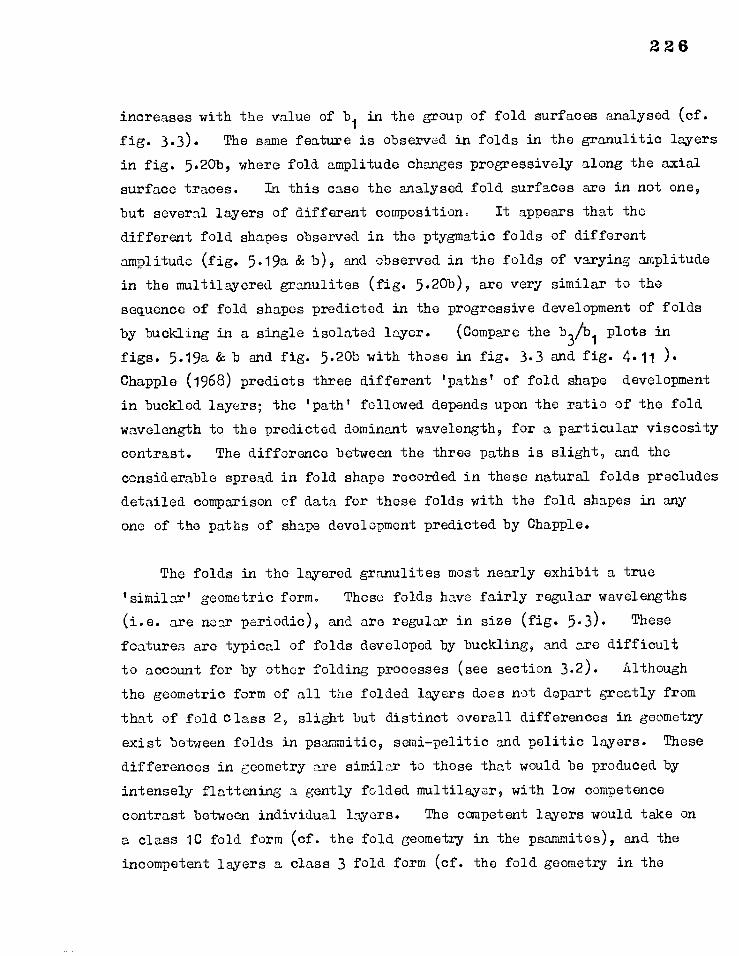
226
increases with the value of b1 in the group of fold surfaces analysed (cf.
fig. 3.3). The same feature is observed in folds in the granulitic layers
in fig. 5.20b, where fold amplitude changes progressively along the axial
surface traces. In this case the analysed fold surfaces are in not one,
but several layers of different composition. It appears that the
different fold shapes observed in the ptygmatic folds of different
amplitude (fig. 5.19a & b), and observed in the folds of varying amplitude
in the multilayered granulites (fig. 5.20b), are very similar to the
sequence of fold shapes predicted in the progressive development of folds
by buckling in a single isolated layer. (Compare the b3Al1 plots in
figs. 5.19a & b and fig. 5.20b with those in fig. 3.3 and fig. 4.11 ).
Chapple (1968) predicts three different 'paths' of fold shape development
in buckled layers; the 'path' followed depends upon the ratio of the fold
wavelength to the predicted dominant wavelength, for a particular viscosity
contrast. The difference between the three paths is slight, and the
considerable spread in fold shape recorded in these natural folds precludes
detailed comparison of data for these folds with the fold shapes in any
one of the paths of shape development predicted by Chapple.
The folds in the layered granulites most nearly exhibit a true
'similar' geometric form. Those folds have fairly regular wavelengths
(i.e. are near periodic), and are regular in size (fig. 5.3). These
features are typical of folds developed by buckling, and are difficult
to account for by other folding processes (see section 3.2). Although
the geometric form of all the folded layers does not depart greatly from
that of fold class 2, slight but distinct overall differences in geometry
exist between folds in psammitic, semi-pelitic and pelitic layers. These
differences in geometry are similar to those that would be produced by
intensely flattening a gently folded multilayer, with low competence
contrast between individual layers. The competent layers would take on
a class 1C fold form (cf. the fold geometry in the psammites), and the
incompetent layers a class 3 fold form (cf. the fold geometry in the
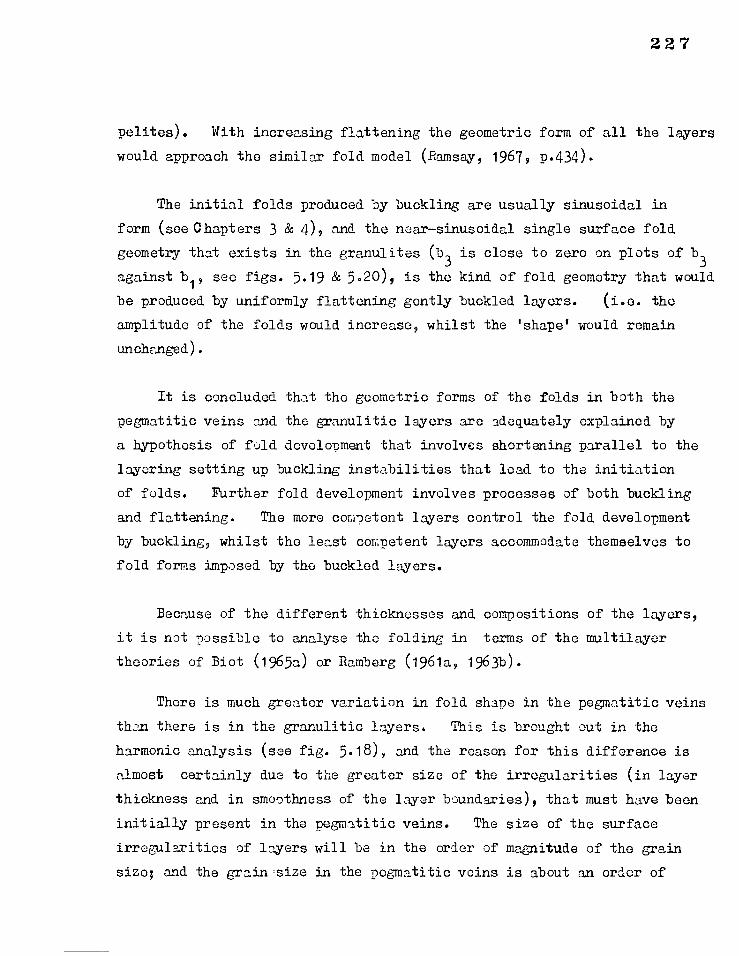
227
pelites). With increasing flattening the geometric form of all the layers
would approach the similar fold model (Ramsay, 19679 p.434).
The initial folds produced by buckling are usually sinusoidal in
form (see Chapters 3 & 4), and the near—sinusoidal single surface fold geometry that exists in the granulites (b3 is close to zero on plots of b
3 against b1, see figs. 5.19 & 5.20), is the kind of fold geometry that would
be produced by uniformly flattening gently buckled layers. (i.e. the
amplitude of the folds would increase, whilst the 'shape' would remain
unchanged).
It is concluded that the geometric forms of the folds in both the
pegmatitic veins and the granulitic layers are adequately explained by
a hypothesis of fold development that involves shortening parallel to the
layering setting up buckling instabilities that load to the initiation
of folds. Further fold development involves processes of both buckling
and flattening. The more competent layers control the fold development
by buckling, whilst the least coEpetent layers accommodate themselves to
fold forms imposed by the buckled layers.
Because of the different thicknesses and compositions of the layers,
it is not possible to analyse the folding in terms of the multilayer
theories of Biot (1965a) or Ramberg (1961a, 1963b).
There is much greater variation in fold shape in the pegmatitic veins
than there is in the granulitic layers. This is brought out in the
harmonic analysis (see fig. 5.18), and the reason for this difference is
almost certainly due to the greater size of the irregularities (in layer
thickness and in smoothness of the layer boundaries), that must have been
initially present in the pegmatitic veins. The size of the surface
irregularities of layers will be in the order of magnitude of the grain
size; and the grain'size in the pegmatitic veins is about an order of
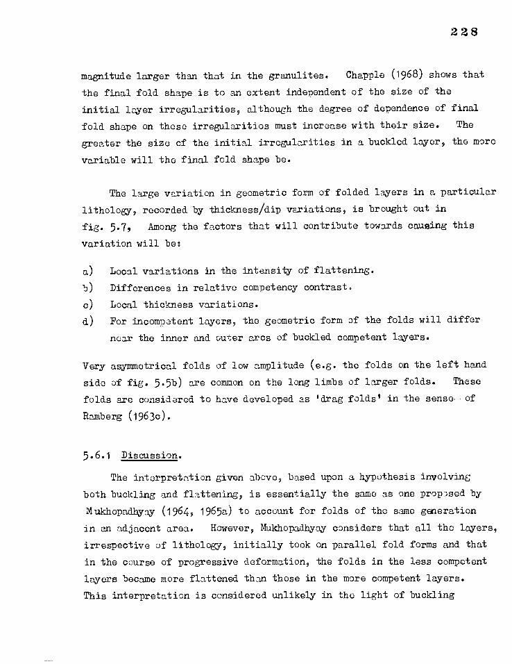
228
magnitude larger than that in the granulites. Chapple (1968) shows that
the final fold shape is to an extent independent of the size of the
initial layer irregularities, although the degree of dependence of final
fold shape on these irregularities must increase with their size. The
greater the size of the initial irregularities in a buckled layer, the more
variable will the final fold shape be.
The large variation in geometric form of folded layers in a particular
lithology, recorded by thickness/dip variations, is brought out in
fig. 5.7, Among the factors that will contribute towards causing this
variation will be:
a) Local variations in the intensity of flattening.
b) Differences in relative competency contrast.
c) Local thickness variations.
d) For incompetent layers, the geometric form of the folds will differ
near the inner and outer arcs of buckled competent layers.
Very asymmetrical folds of low amplitude (e.g. the folds on the left hand
side of fig. 5.5b) are common on the long limbs of larger folds. These
folds are considered to have developed as 'drag folds' in the sense. .of
Ramberg (1963c).
5.6.1 Discussion.
The interpretation given above, based upon a hypothesis involving
both buckling and flattening, is essentially the same as one proposed by
MukhoPad-hYaY (1964, 1965a) to account for folds of the same generation
in an adjacent area. However, Mukhopadhyay considers that all the, layers,
irrespective of lithology, initially took on parallel fold forms and that
in the course of progressive deformation, the folds in the less competent
layers became more flattened than those in the more competent layers.
This interpretation is considered unlikely in the light of buckling
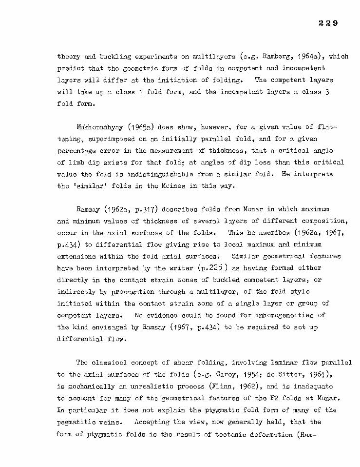
229
theory and buckling experiments on multilayers (e.g. Ramberg, 1964a), which
predict that the geometric form of folds in competent and incompetent
layers will differ at the initiation of folding. The competent layers
will take up a class 1 fold form, and the incompetent layers a class 3 fold form.
Mukhopadhyay (1965a) does show, however, for a given value of flat-
tening, superimposed on an initially parallel fold, and for a given
percentage error in the measurement of thickness, that a critical angle
of limb dip exists for that fold; at angles of dip less than this critical
value the fold is indistinguishable from a similar fold. He interprets
the 'similar' folds in the Moines in this way.
Ramsay (1962a, p.317) describes folds from Monar in which maximum
and minimum values of thickness of several layers of different composition,
occur in the axial surfaces of the folds. This he ascribes (1962a, 1967,
p.434) to differential flow giving rise to local maximum and minimum
extensions within the fold axial surfaces. Similar geometrical features
have been interpreted by the writer (p.225) as having formed either
directly in the contact strain zones of buckled competent layers, or
indirectly by propagation through a multilayer, of the fold style
initiated within the contact strain zone of a single layer or group of
competent layers. No evidence could be found for inhomogeneities of
the kind envisaged by Ramsay (1967, p.434) to be required to sot up
differential flow.
The classical concept of shear folding, involving laminar flow parallel
to the axial surfaces of the folds (e.g. Carey, 1954; de Sitter, 1964),
is mechanically an unrealistic process (Flinn, 1962), and is inadequate
to account for many of the geometrical features of the F2 folds at Monar.
In particular it does not explain the ptygmatic fold form of many of the
pegmatitic veins. Accepting the view, now generally held, that the
form of ptygmatic folds is the result of tectonic deformation (Rem-
230
berg, 1959) r:.thor than the result of the mode of vein emplacement
(e.g. Wilson, 1952), these folds are incompatible with a classical shear
hypothesis of fold formation, without invoking a strong shortening
parallel to the layering to cause buckling in the pegmatitic veins.
Ramsay (1967, p.430) discusses a modified differential shear hypothesis
in which flow lines converge in the development of similar folds. In
this process, a shortening along the layering is involved that could set
up buckling instabilities which might lead to the initiation of folds by
buckling in the more competent layers in the rock mass. However, the
development of buckles in this way obviates the need to invoke a differential
shear hypothesis in the first place.
If folds in the layered granulites were solely the result of a very
intense shortening along initially non-planar layering, causing accent-
uation of the irregularities present (Flinn, 1962), no regularity in the
size of the folds or in fold wavelength would be exnected. Irregular
folds of the kind described by Ramberg (1964b) would result.
It is concluded that alternative processes of fold development by
differential shear or by finite homogeneous flattening with no buckling,
are inadequate to account for many of the geometrical features of the
Monar F2 folds.
5.7 A STUDY OF WAVELENGTH/THICKNESS IN PPYGMATIC FOLDS IN PEGMiaITIC VEINS
If the ptygmatic folds in the pegmatitic veins are treated as folds
formed in isolated viscous layers in a less viscous matrix, then estimates
of the viscosity contrast between the veins and their matrix, and the total
deformation within the profile plane of the folds may be made. The folds
are assumed to have developed according to a theory based on those of Biot
(1961)t Sherwin & Chapple (1968) and Chapple (1968). These theories
have been discussed in some detail in sections 3.3. and 4.8.
The assumptions on which the basic Biot theory depends are listed in
231
section 3.3, and the degree to which these assumptions are met in the present
study will now be discussed. As the folds are small body forces may be
ignored. It is considered valid to treat rocks undergoing regional meta-
morphism as Newtonian viscous bodies to a first approximation (see section
4.2 ). The assumptions of sinusoidal fold shape and small amplitude concern
the infinitesimal development of folding and may be relaxed in considering
the final form of folds (see Sherwin & Chapple, 1968 ; Chapple, 1968). The
ptygmatic folds analysed are all symmetrical (i.e. the axial surfaces are
almost normal to the enveloping surfaces) and so the maximum compression is
considered to have acted parallel to the layering (or enveloping surface)
throughout fold development. The assumption of plane strain is not wholly
valid (see section 5.8). Lastly, none of the folded veins are truly 'isolates
Some are 'confined' between more massive layers (fig. 5.22), whilst others
are really part of a multilayer (see fig. 5.19c). Compared with the predic-
ted ratio of Wd/t for folds in an isolated layer, the Wd/t ratios of folds
in a 'confined' situation are theoretically reduced (Ramberg, 1963b), whilst
the Wd/t ratios of folds that are part of a multilayer are theoretically
increased (Ramberg, 1961a). However, no systematic differences of this kind
could be detected in the analysed folds, and closely confined folded veins,
and those forming part of a multilayer are not included in the analysis.
Where ptygmatic folds are developed in the pegmatitic veins, the matrix
is invariably pelitic (more rarely semi-pelitic) granulite, and is assumed
to be uniform in composition for the analysed folds.
The 'wavelength' considered is the arc length of the mature folds (see
section 1.2). The mean of the wavelength/thickness (w/t) ratios for a number
of folds is assumed to be the dominant wavelength/thickness (Wd/t) ratio.
The procedure of analysis followed is similar to that described by Sherwin
& Chapple (1968), with slight differences that will be described below.
A total of 157 'half-folds' (segments of a folded vein between
adjacent hinges) were analysed. For each 'half-fold', the arc length
(w/2), measured along the mid-line of the folded layer, and the thickness,
measured at several points along the layer were recorded. The mean value
of thickness was found. Folds wore measured in 17 specimens or photo-
graphs, and mean values of W/2 and t for the folds in each of these were
computed. Mean W/2 is plotted against mean t in fig. 5.21a, and the 157
individual W/t ratios are plotted in histogram form in fig. 5.21b (i).
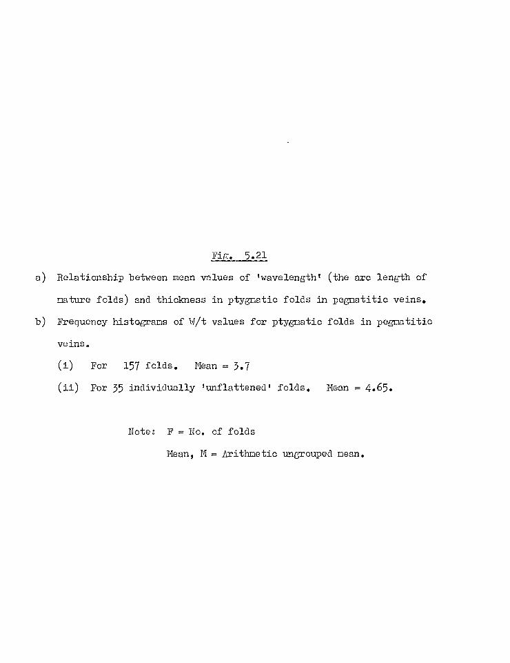
Fin. 5.21
a) Relationship between mean values of 'wavelength' (the arc length of
nature folds) and thickness in ptygmatic folds in pegmatitic veins.
b) Frequency histograms of WA values for ptygmatic folds in pegmatitic
veins.
(i) For 157 folds. Mean = 3.7
(ii) For 35 individually 'unflattened' folds. Mean = 4.65.
Note: F = No. of folds
Mean, M = Arithmetic ungrouped mean.
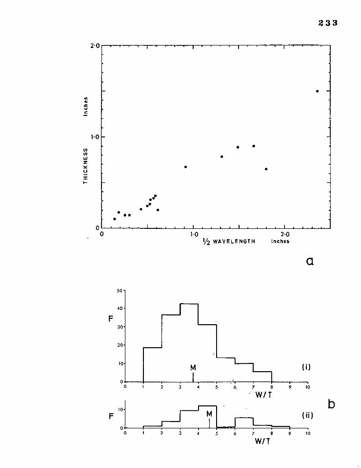
1•0
THI
CK
NE
SS
a
b
20
in u .0 u e
0
233
• • i
1 . I . 1 ' -r i .
• —
•
• •
•
• •
1..
• • • • •
•
I I • I • • I I . • II I • 1 1 1 I • 1 •
0
110 2.0 1/2 WAVELENGTH inches
50 -
40 -
F 30-
20-
10-
1 2 3 4
10- F
6. 7 8
• W/T
7
M
1
2 3 4
W/T
Fig. _ „5.22
To illustrate the confinement of a thin ptygmatically folded pegmatitic
vein, A, between more massive pegmatitic sheets.
Heavy stippling Pegnatitic veins
Pelitic rock.
Fig. 5.23
Theoretical variation of amplification with w/t for a viscosity ratio of
10 (between a single viscous layer and its less viscous matrix) at a
value of shortening given by S = 3.0.
No
?I
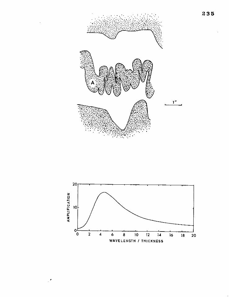
20
1"
235
2 4 6 8 10 12 14 16 18 20
WAVELENGTH / THICKNESS
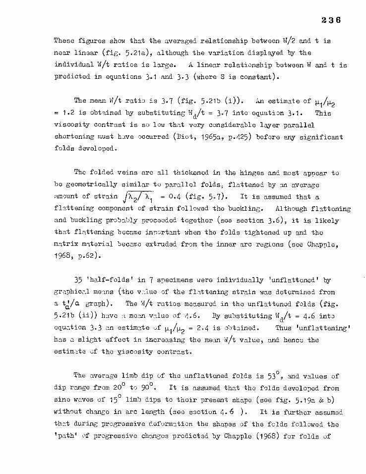
236
These figures show that the averaged relationship between W/2 and t is
near linear (fig. 5.21a), although the variation displayed by the
individual W/t ratios is large. A linear relationship between W and t is
predicted in equations 3.1 and 3.3 (where S is constant).
The mean W/t ratio is 3.7 (fig. 5.21b (i)). An estimate of ii1t12
= 1.2 is obtained by substituting Wd/t = 3.7 into equation 3.1. This
viscosity contrast is so low that very considerable layer parallel
shortening must have occurred (Blot, 1965a, p.425) before any significant
folds developed.
The folded veins are all thickened in the hinges and most appear to
be geometrically similar to parallel folds, flattened by an average
amount of strain jX2/ = 0.4 (fig. 5.7). It is assumed that a
flattening component of strain followed the buckling. Although flattening
and buckling probably proceeded together (see section 3.6), it is likely
that flattening became important when the folds tightened up and the
matrix material became extruded from the inner arc regions (see Chapple,
1968, p.62).
35 'half-folds' in 7 specimens were individually 'unflattened' by
graphical means (the value of the flattening strain was determined from
a tj/a graph). The W/t ratios measured in the unflattened folds (fig.
5.21b (ii)) have a mean value of 4.6. By substituting Wd/t = 4.6 into
equation 3.3 an estimate of 111/112 = 2.4 is obtained. Thus 'unflattening'
has a slight effect in increasing the mean Wit value, and hence the
estimate of the viscosity contrast.
The average limb dip of the unflattened folds is 53°, and values of
dip range from 20° to 90°. It is assumed that the folds developed from
sine waves of 15° limb dips to their present shape (see fig. 5.19a & b)
without change in arc length (see section 4.6 ). It is further assumed
that during progressive deformation the shapes of the folds followed the
'path' of progressive changes predicted by Chapple (1968) for folds of
2nt X - d w
1.35
111412 (Sherwin &
Chapple)
237
the dominant wavelength. The development of the 'average' fold, involving
an increase in limb dip from 15o to 53
o would be accomplished by a bulk
shortening of JX2A i = 0.65.
It remains to estimate the amplification required to produce folds
with 15° limb dips. Applying the theory of Sherwin & Chapple (1968), and
using a similar argument to theirs, it is considered that initial
irregularities in the veins would have had limb dips in the order of 1°,
and that amplifications of 10 to 20 would have been necessary in order to
develop folds with 15° limb dips (see the discussion in section 4.8 ).
Taking the value of fold amplification to lie between 10 and 20, and
taking the value Wa/t . 4.6, estimates of both viscosity contrast (between
the pegmatitic veins and the matrix granulites) and of shortening (up
until the 115° limb dip stage') may be read from the graph drawn in fig.
3.1, relating amplification, viscosity contrast, shortening and dominant
wavenum'Jer. The data and results are tabulated below.
T.,..BLE 5.1 D 1N V.J.LTES Tim UNFLTTENED FOLDS
Strain W/t Ratio - 3 Unflattened Flattening Folds
0.42 4.65
Strain Ratio - 2 Assumed Shortening Amp.
150 53°
Limb Dip 111/112 Unflattened (Biot) Folds
2.4 530
Strain Strain Ratio - 1 Ratio - Shortening Total -7x,-15° 1 x 2 x 3
0.65 10 - 20 10 0.33 0.09
238
The strain ratio is defined ast%.2A
1. The value of the total shortening
(equivalent to a strain ellipse ratio of ca. 11:1) of the bulk strain
in the profile plane of the folds, is found by multiplying together the
values of shortening for the three stages of fold development distinguished.
The estimated value of the viscosity contrast, read from the graph in
fig. 3.1, is about four times the value estimated when layer shortening
is not taken into account. By closely following the procedure of analysis
described by Sherwin and Chapple (without considering the stage of fold
development where the arc length remains unchanged), an amplification
of about 100 would be considered necessary in order to form folds with limb
dips of about 50°. The estimated viscosity contrast would then be about
16 and the total shortening aboutjA2A1 = 0.1.
The large variation in the measured values of Wit (fig. 5.21b (i))
indicates the low selectivity of the folding. This is consistent with
the low values of amplification considered necessary to produce folds
with 15° limb dips, since Biot (1961) shows that selectivity depends only
upon amplification to a first approximation. The theoretical variation
of amplification with W/t for a viscosity contrast of 10 at a value of
shortening of/A.2A I = 0.33 (values estimated in the present analysis)
is shown in fig. 5.23. Sherwin & Chapple consider that a frequency
histogram of N/t values should reflect the broad features of a graph
relating amplification to Vt. The histograms in fig. 5.21b (i) & (ii)
may be compared with fig. 5.23.
The mainly untestable nature of the assumptions on which the theory
is based, and the variability of the measured factors both indicate the
limitations of the analysis. The results are therefore considered to
give rough estimates only of the viscosity contrast between the pegmatitio
veins and the politic granulites, and the total amount of shortening
within the profile plane of the F2 folds.
239
5.8 l T ANALYSIS OF DEFORMbn LINEATIONS.
There are a series of linear structures developed parallel to the axes
of the early folds (the first folds of Ramsay, 1958) at Monar, that are
deformed about the minor F2 folds. The geometry of these deformed
lineations provides useful information concerning progressive fold develop—
ment. The commonest linear feature is a striping on Toliation surfaces
(plates 4 & 5). This is an intersection effect of the early cleavage with
the foliation.
The attitudes of deformed lineations were measured at several points
around a number of minor folds. Data for two examples has been plotted
on a stereogram in fig. 5.24a. It was not found possible to measure the
loci accurately enough to compare them with theoretical loci related to
various folding processes (Ramsay, 1967, Chapter 8). However, individual
loci are almost contained within planes. In the field, it was possible
to visually 'fit' a lineation locus into a plane (see Ramsay, 1967, p.472),
where the locus crossed the two limbs of a single fold, but this was not
possible where the lineation crossed several folds (see plate 5).
Assuming, as a first approximation, that individual lineation loci
are contained within planes, the intersections of the fold axial surfaces
with these planes may be found. These intersections are equivalent to
the 'a' directions of a classical simple shear hypothesis. They are
referred to here as 'a' directions without any genetic implications. On
a stereogram the 'a' directions show as a cluster of points within the
field containing the F2 minor fold axes (fig. 5.24b). Two distinct
types of lineation locus may be distinguished, depending on the relative
orientation of the F2 fold axis to the 'lineation locus plane' (see fig.
5.25.). The first type is the commonest, where the fold axis is near
vertical; and the second type is local, and is only found where F2 minor
folds are superimposed on the gentle limb of an F1 minor fold. Viewed
towards the north—east, the sense of relative displacement of the lineation
Plate 4 Coarse Fl lineations deformed around F2 folds.
(Road section, N. end of main dam).
Plate 5 Fl lineations on a foliation surface deformed by
F2 folds. (Road section at E. end of little dam).
The camera is pointed such that the lineations in
the centre of the photograph most nearly 'fit' into
planes.
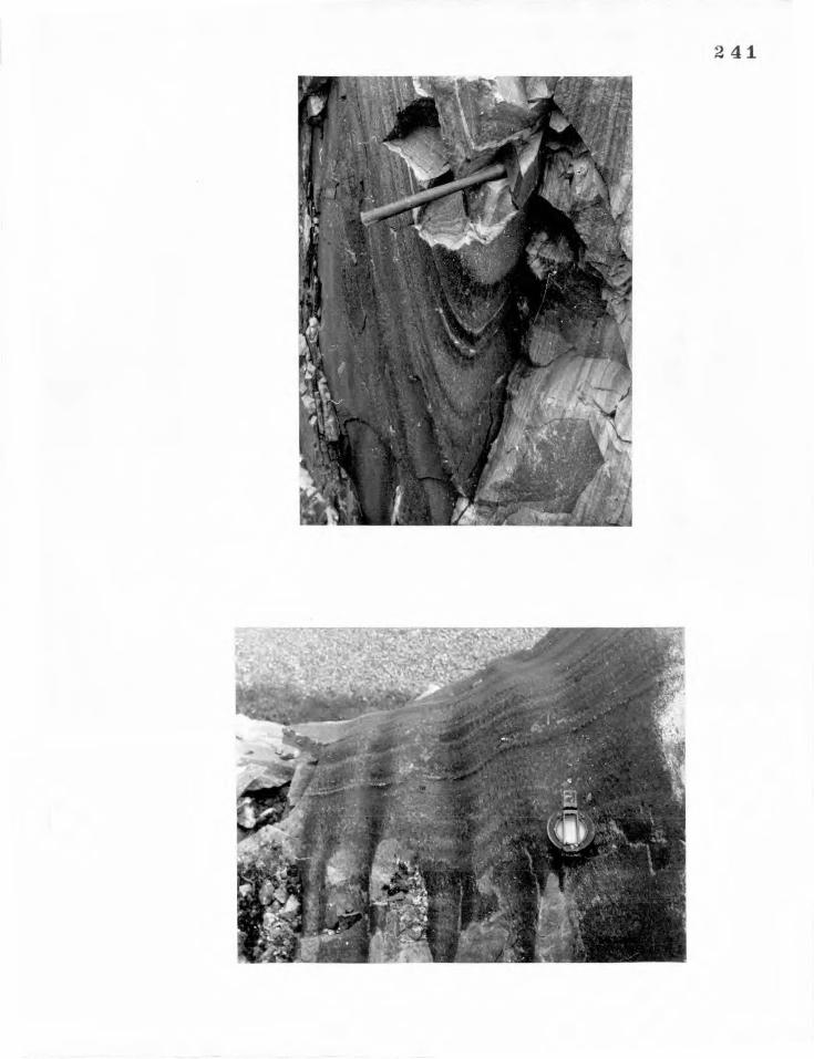
241
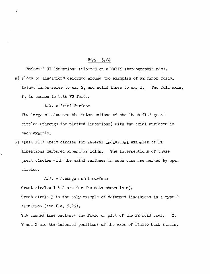
Kils2.JJA
Deformed Fl lineations (plotted on a Wulff stereographic net).
a) Plots of lineations deformed around two examples of F2 minor folds.
Dashed lines refer to ex. 2, and solid lines to ex. 1. The fold axis,
F, is common to both F2 folds.
A.S. = Axial Surface
The large circles are the intersections of the 'best fit' great
circles (through the plotted lineations) with the axial surfaces in
each example.
b) 'Best fit' great circles for several individual examples of Fl
lineations deformed around F2 folds. The intersections of these
great circles with the axial surfaces in each case are marked by open
circles.
A.S. = Average axial surface
Great circles 1 & 2 are for the data shown in a).
Great circle 3 is the only example of deformed lineations in a type 2
situation (see fig. 5.25).
The dashed line encloses the field of plot of the F2 fold axes. X,
Y and Z are the inferred positions of the axes of finite bulk strain.
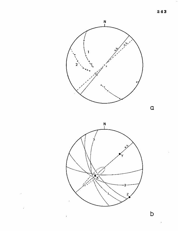
243
` • \ /
\ / • o
2 ‘ \o + • o. e F •, z • ... /
a
b
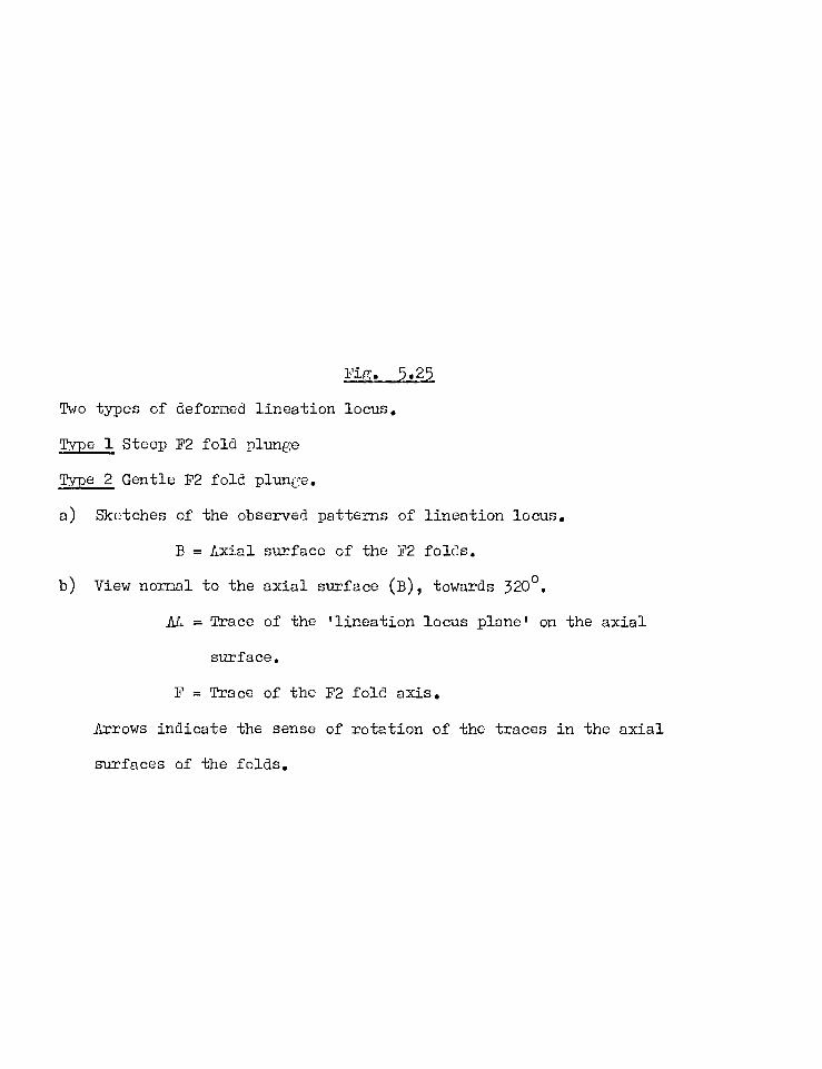
Fig. 5.25
Two types of deformed lineation locus.
Type 1 Steep F2 fold plunge
Type 2 Gentle F2 fold plunge.
a) Sketches of the observed patterns of lineation locus.
B = Axial surface of the F2 folds.
b) View normal to the axial surface (B), towards 3200.
AA = Trace of the 'lineation locus plane' on the axial
surface.
F = Trace of the F2 fold axis.
Arrows indicate the sense of rotation of the traces in the axial
surfaces of the folds.
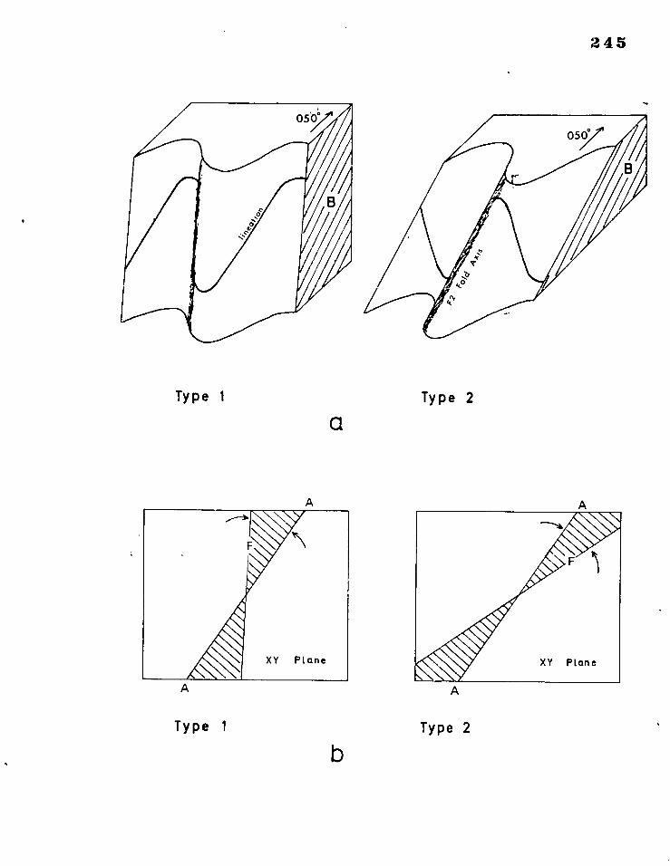
A A
245
Type 1
Type 2
a
A A
Type 1 Type 2
246
between the antiformal and synformal hinges is reversed (fig. 5.25) in
these two types.
On lineation geometry alone these patterns could be consistently
interpreted according to the classical simple shear hypothesis of fold
development. However, an alternative explanation will now be given
which is compatible with the interpretation of fold profile geometry
given in section 5.6.
It must be assumed that the F2 axial surfaces are parallel to a
principal plane of the bulk strain ellipsoid (considered for a volume of
rock that is much larger than the size of individual folds). This is
not generally agreed upon for folds formed by buckling (e.g. Ghosh, 1966,
1967; Singh, 1967); but the symmetry of fold geometry about the axial
surfaces, in terms of thickness/dip variations, and the presence of an
axial surface schistosity suggest that this assumption holds for the F2
minor folds at Monar.
The maximum shortening direction (Z) of the bulk strain ellipsoid
must be perpendicular to the axial surfaces of the folds. The deformed
lineations lie at low angles to F2 in the limbs of the folds but are
almost normal to F2 in the hinges. The lineations must therefore have
been normal to F2 in the hinges initially, or they would have rotated away
from this position in the course of the deformation (Flinn, 1962). The
'instability' of lines lying close to Z in progressive deformation may
account for the considerable s7)read in trend of the 'lineation locus planes' ,
(fig. 5.24h). The present pattern of relative displacement of the
lineations in adjacent synformal and antiformal hinges must be due to the
rotation of the minor F2 fold axes within their axial surfaces during
deformation to produce a shear component across the fold profiles. The
traces of the 'lineation locus planes' and the F2 fold axes on the axial
surfaces may be treated as line elements that have undergone homogeneous
247
strain within the XY plane of the bulk strain ellipsoid. The attitudes
of the traces of the 'lineation locus planes' and fold axes on the axial
surfaces are shown in fig. 5.25b, for the two types of lineation locus
distinguished. In either case both line elements must have rotated
towards the X direction of the bulk strain ellipsoid, which therefore lies
in the shaded zones of each of the figures in fig. 5.25b. The trace
of the 'lineation locus plane', or 'a' direction, is the only line in
common to both shaded zones. Assuming that the bulk deformation within
the region is homogeneous, the 'a' direction must be approximately
parallel to the X axis of the bulk strain ellipsoid.
Examination of the stereograms in figs. 5.24b and 5.2 shows that .
the 'at directions lie in the centre of the field in which the F2 fold axes
plot. Fold axes plotting either side of the 'a' direction cluster, are
those of the two types distinguished in fig. 5.25. The near-vertical
fold axes (type 1) lie very close to X. In one of the measured examples,
the angle between the fold axis and the 'a' direction was virtually
zero, and the deformed lineation lay on an almost unfolded surface (see
Ramsay, 1967, p.473).
Only a small buckling component would be necessary in order to initiate
folding, and thus form the fold axes and 'lineationlocueplanes t , which would subsequently behave more or less as passive elements throughout
progressive deformation. A buckling process equivalent to that of
oblique flexural slip (Ramsay, 1967, p.396) could initiate the lineation
locus in a plane or surface nearly parallel to the X direction of the
bulk strain ellipsoid, and at an acute angle to the fold axis. This
would account for the parallelism of the 'a' directions, irrespective of
the attitude of the fold axes.
From the data available, it is not possible to find the k- value
(Flinn, 1962) of the finite bulk strain. However, because lines have
rotated in the XY plane, k 0; and because the axial surfaces are
248
constant in orientation and there is a well-developed schistosity, k
The interpretation of the geometry of the deformed lineation loci
is more or less consistent with the interpretation of the geometric foxqn
of the fold profiles. All the folds analysed in profile section were in
the group with uear-vertical axes. It is apparent that the mean profile
plane of these folds is not a principal plane of the finite bulk strain
ellipsoid. Therefore the estimates of the deformation in the fold profile
planes made in sections 5.6 and 5.7 will be invalid (Makhopadhyay, 1965a;
Ramsay, 1967, p.415). It is impossible to compute the true strain in
the profile planes from the fold geometry, but because the profile planes
are within a few degrees of being normal to X, it is suggested that the
estimates of deformation made in sections 5.6 and 5.7 give a qualitative
indication of the strain in the YZ plane of the finite bulk strain ellipsoid.
5.9 CONCLUSIONS
A) A detailed geometrical analysis of the minor F2 folds shows that
systematic overall differences in the geometric forms of folds can
be related to differences in layer composition.
B) The total variation in the fold geometry of both single surfaces
and layers is large.
C) The fold geometry is more variable in the pegmatitic veins than in
the granulitic layers.
D) The relative competencies of different lithological types is found
to be: pegmatitic veins > psammites semi-pelites pelites.
E) The fold geometry is adeauately explained by a hypothesis of fold
development involving processes of buckling and flattening.
F) The viscosity ratio of the most competent rock type (pegmatitic
qualtzo-feldspathic veins) to the politic granulites is considered
to be about 10:1.
249
G) The steeply inclined F2 fold axes are almost parallel to the
principal extension axis (X) of the finite bulk strain ellipsoid,
and the profile planes of the folds are nearly parallel to the YZ
plane of the finite bulk strain ellipsoid.
An estimate of the two dimensional strain in the F2 fold deformation,
in the mean profile plane (roughly equivalent to the YZ plane of the
finite bulk strain ellipsoid) of the steeply inclined folds is
1- 2/ x - 0.09 •
250
CHAPTER 6
AN ANALYSIS OF MINOR FOLDS IN PART OF THE MiGGIA NAPPE, TICINO, SWITZERLAND
6.1 INTRODUCTION
An investigation of fold geometry was carried out in a small part of
one of the Lower Pennine nappes of the Swiss Alps on the same lines as the
study of folded Moinian rocks in the Scottish Caledonides described in
Chapter 5. The rocks in both areas are highly deformed and metamorphosed.
Unlike the situation at Monar, the structure and exposure of the rocks
studied here enable a geometric analysis of several successive generations
of folds to be made. A geometrical comparison of these fold phases forms
the main part of this chapter.
The selected area for study lies just north-east of Lago Sambuco and
below the ridge separating Valle Leventina from Val Sambuco (fig. 6.1),
where the rocks are superbly exposed on glaciated surfaces.
The rocks in this area are basement gneisses, forming part of the
Maggia nappe, which lies near the base cf the exposed nappe pile of the
whole mountain belt.
Hasler (1949) has described the geology of the area around Sambuco,
including the site of the present study, mainly from a petrographical/
petrological viewpoint; his tectonic analysis is brief and does not provide
an adequate frame of reference for the present work. The work of Heim (1921)
still provides one of the best descriptions of the major tectonics of the
Alps.
The area was chosen because several fold phases are developed more or
loss co-axially, about an almost vertical axis, to give near profile sections
on the glaciated outcrop surfaces.
The general geology of the area is described in this section (6.1) and
section 6.2. A detailed geometrical fold analysis is described in section
6.3, and the fold geometry is interpreted in terms of folding processes in
section 6.4. On the basis of an analysis of wavelength/thickness ratios,
in thin buckled layers estimates of viscosity contrasts and deformation in
the F2 folding episode are made in section 6.5.

Fir. 6.1
a) Geological nap of the Sambuco area
(After Hasler, 1949). The region selected for detailed study is
narked by diagonal shading.
b) Map to show the location of nap a).
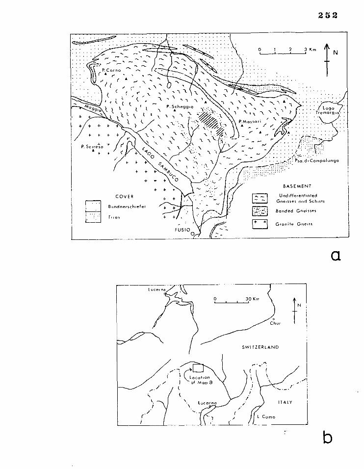
252
„.... ..,. ...... .."- ....
r- e... - • ...- ,••••• -... •-.- ... ..... ..... .,. ,..... ,.._
P. Cor no •-•
r A ,- • \ s -....
( • .... M. .4. . S.
< " C
( r' -,... ... "I ' 1- -1 1.
.., , ---'-<,,•,) ' r tc ( . -1 " ‘ N 1 • .-... Ala • - , t ''s
1 / P. Scheggia
1-
99/0 k t N • .. ). \ t I 1A 1 .‘ ''.7. . A
1 t- 1.-. • ) 1 -N. • 1
.. '.•..., .4p.- N-. .. A. ., .‘: _ \. \ .N* • N ' - ..,:‘• A -,,,„ 1.. 1. N..
1.. I_ • I .
A. k . ' . N N.:• • . A.,
-. ‘ -'-• * N
.. -,
COVER
Bundnerschiefer
Trios
FUSIO 0
+ 4- 4- +
P. Sciresa •
+
.... • .
.. 1 .. logo Tremorgto •
• • -•••• •
• • Pso di Campolungo
•
+ +
BASEMENT
Undifferentiated Gneisses arid Schists
Banded Gneisses
Granite Gneiss
a
253
6.1.1 Lithology and Mineralogy.
The basement rocks of this area are included in the group of 'banded
gneisses' recognised and mapped by Hasler (1949). They are variable
in composition and for the most part strongly banded; typically dark layers
of amphibolitic rock alternate with white layers composed of quartz and
feldspar.
Quartz, plagioclase and hornblende are the three principal minerals
that, in varying proportions, go to make up bands of different composition
and colour index. Chlorite and more especially apidote-clinozoisite
frequently make up a significant .proportion of the dark bands, and appear
also in the light bands. Biotite, usually rare, locally becomes an
important constituent of the dark layers. Garnets, and small crystals
of zircon and opaque minerals also occur.
The texture of the quartz-feldspar layers is granular and that of
the darker layers usually schistose.
For the purposes of fold analysis, the only practical division of
layer types is into 'dark', 'intermediate' and 'light', and in terms of
composition this is generally equivalent to:
dark predominantly hornblende epidote, biotite.
intermediate - between 'light' and 'dark' in dark mineral content.
light predominantly quartz and plagioclase.
Several cross-cutting basic dykes and other intrusive bodies appear
to have been emplaced between the first and second phases of deformation
described below.
6.1.2 Metamorphism.
The rocks in the Sambuco area have been affected by a strong Alpine
metamorphism (the metamorphic culmination of the Alpine orogeny was
254
centred in southern Ticino), the main part of which postdated the
formation of the nappes (Wenk, 1962), attaining garnet Iganite grade
over the general region of north Ticino. The Mesozoic sediments
(Bundnerschiefer), incorporated in the nappe movements, mantle the Maggie.
nappe (see fig. 6.1) and are also strongly metamorphosed.
The preferred orientation of hornblende in the banded gneisses is
for the most part parallel to the axial surfaces of the first phase folds
recognised here; and an axial surface schistosity is locally developed
in the second folds. The granular texture of the quartz and feldspar,
and the more or less strain-free nature of all minerals shows that
recrystallisation had gone on after deformation had ceased.
6.2 STRUCTURAL GEOLOGY
Three distinct phases of Alpine folding in the banded gneisses have
been recognised on the basis of the interference relationships of small
scale structures (plates 6 & 7). The interference patterns are all
Type 3 of Ramsay (1967, p.530).
The observable relationship between the basement gneisses and the
Bundnerschiefer around the Sambuco region and to the west around
Cristallina is complicated, suggesting a complex major structural
pattern. For present purposes, the relationship between the small scale
folds analysed in this study and the major structures is relatively
unimportant, and no proper attempt to analyse the major structures has
been made. It is not known whether the first generation folds observed
here were developed during or later than the nappe forming movements.
In the Lebendun nappe and Bundnerschiefer exposed near Basodino
(about 15 km west of Sambuco) Higgins (1964) has established a succession
of fold episodes similar to those described here; and in the Bundner-
schiefer and Mesozoic cover rocks of the Gotthard massif to the north of
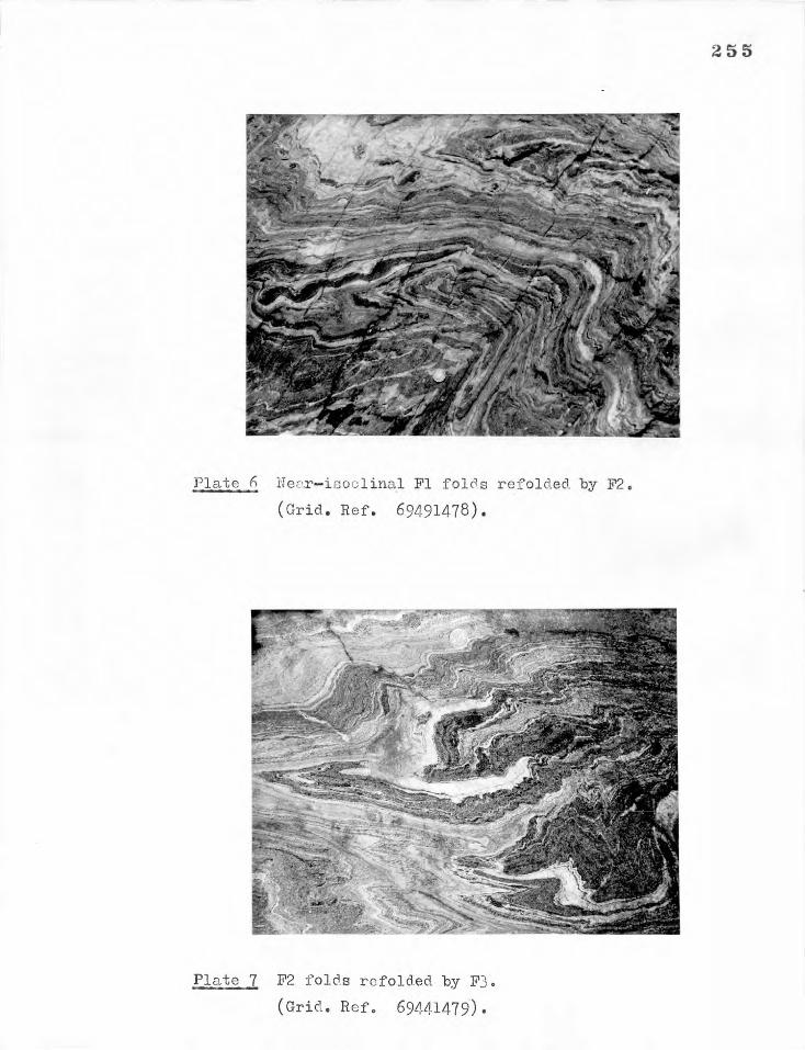
Plate 6 Near—isoclinal P1 folds refolded by F2.
(Grid. Ref. 69491478).
Plate 7 P2 folds refolded by P3.
(Grid. Ref. 69441479).
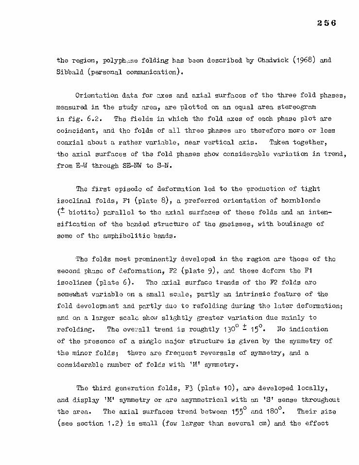
256
the region, polyphase folding has been described by Chadwick (1968) and
Sibbald (personal communication).
Orientation data for axes and axial surfaces of the three fold phases,
measured in the study area, are plotted on an equal area stereogram
in fig. 6.2. The fields in which the fold axes of each phase plot are
coincident, and the folds of all three phases arc therefore more or less
coaxial about a rather variable, near vertical axis. Taken together,
the axial surfaces of the fold phases show considerable variation in trend,
from Eql through SE-NW to S-N.
The first episode of deformation led to the production of tight
isoclinal folds, F1 (plate 8), a preferred orientation of hornblende
(± biotite) parallel to the axial surfaces of these folds and an inten-
sification of the banded structure of the gneisses, with boudinage of
some of the amphibolitic bands.
The folds most prominently developed in the region are those of the
second phase of deformation, F2 (plate 9), and these deform the Fl
isoclines (plate 6). The axial surface trends of the F2 folds are
somewhat variable on a small scale, partly an intrinsic feature of the
fold development and partly due to refolding during the later deformation;
and on a larger scale show slightly greater variation due mainly to
refolding. The overall trend is roughtly 1300 ± 15°. No indication
of the presence of a single major structure is given by the symmetry of
the minor folds; there are frequent reversals of symmetry, and a
considerable number of folds with 'MI symmetry.
The third generation folds, F3 (plate 10), are developed locally,
and display symmetry or are asymmetrical with an 'S' sense throughout
the area. The axial surfaces trend between 155° and 180°. Their size
(see section 1.2) is small (few larger than several cm) and the effect

Fig. 6.2
Equal area stereographic plot of structural data for the area under
investigation.
Poles to Axial surfaces.
triangles
dots
circles
Fold Axes.
0
Fl
F2
x F3
Fl
F2
F3
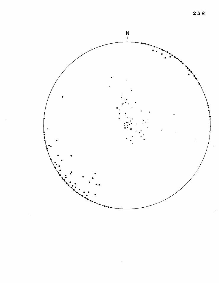
co an N
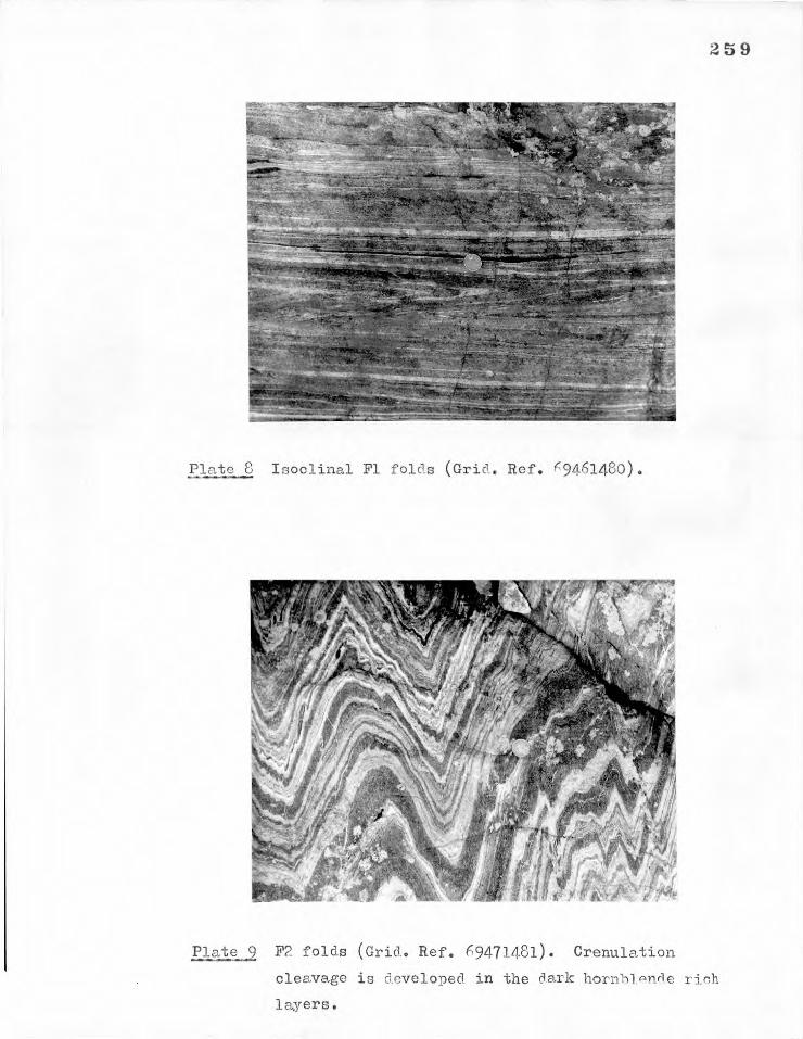
Plate 8 Isoclinal Fl folds (Grid. Ref. -9461480).
Plate 9 F2 folds (Grid. Ref. 69471481). Crenulation
cleavage is developed in the dark hornblnHe rich
layers.
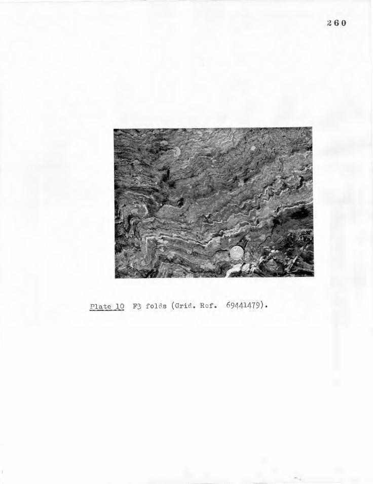
2 6 0
Plate 10 F3 folds (Grie. Ref. 69441479)•

261
they have on reorientating the earlier structures appears to be limited.
There is evidence of a further phase of folds with axial surfaces
roughly normal to those of F3. These structures are very local and their
relationship to F3 could not be determined. They do not enter into the
present discussion.
6.2.1 Mineral Fabric
The hornblende fabric parallel to the axial surfaces of Fl folds has
been mentioned above. A penetrative axial surface schistosity, formed
by the alignment of hornblende (and biotite when present) is present only
locally in the F2 folds. A common fabric, parallel to the F2 axial
surfaces, is a crenulation cleavage of kinking. It is only found in
the dark hornblende rich layers; tightly packed grains of hornblende
crystals initially parallel to the banding are responsible for its
localisation.
The development of F1 and F2 schistosities and the coaxial refolding
give rise to a common penetrative intersection lineation that is often
strongly developed parallel to the fold axes. The longest dimensions
of hornblende crystals often lie in this direction.
6.3 DESCRIPTIVE GEOMETRY
In many respects the variations in fold shape within and between
individual folded layers brought out in this study by use of harmonic
analysis, isogon plots and plots of thickness variation with dip, are
similar to those described in some detail in the Monar study. For this
reason individual examples of analysed folds are kept to a minimum, and
most data presented in this section, are in a synthesised form to Dhow
most clearly the overall differences in fold geometry between the fold
phases.
262
The direction of the 'common' fold axis is fairly constant, and no
systematic areal changes in either fold shape or fabric development were
observed within the region. For these reasons it is considered valid to
treat the area as a single homogeneous structural domain, although on
a smaller scale inhomogeneities may be apparent (e.g. the local development
of P3 folds).
Because many of the folds are small, irregularities in layer surfaces
on the scale of the grain size are significant; and so t a, rather
than0 a is used to record changes in layer shape with dip, being a less
sensitive parameter (see section 2.5.5).
Best fit straight lines to the values of -00,2 and cos
2a were
calculated for every measured fold and the value of the intercept of the
best fit line is used here as a parameter of fold shape (see section 3.5).
6.3.1 Isogon Plots and Thickness/Dip Relationships
Examples of F2 folds are taken to illustrate the irregular and
apparently inconsistent variations in fold geometry related to composition.
The same phenomena can be observed in all three fold phases; F2 however
affords the best examples.
Isogon plots are constructed for selected F2 folds in figs. 6.3a and
6.4a. In the former, the pattern of the isogons in the dark layers is
consistently convergent from outer to inner arc (class 10 geometry) and
in the light layers consistently divergent (class 3 geometry). In fig.
6.4a the patterns are reversed; the geometry of the isogons in the
light layers is class 10 and in the dark layers class 3.
These geometrical differences are equally apparent in plots of t'a
against cos2a . Fig. 6.5b is such a plot for both limbs of a fold in
adjacent light and dark layers. The two plots relating to either limb
Fig. 6.5
F2 folds (grid ref. 69491476).
a) Isogons at 30° dip intervals on the fold profile.
Heavy stipples • • • • Massive hornblende layer.
Light stipples • • • . Hornblende rich layer.
No stipples • • • • Quartz—feldspar layer.
2 b) Frequency histogram of the intercept values (on a t'a /cos
2 a graph)
for 35 folds in the profile shown in a).
Shaded section • • • • For folds in hornblende rich layers.
Unshaded section For folds in iCti-F layers.
F = Frequency
Note: Grid references for this and subsequent figures will be
found on the National Maps of Switzerland.
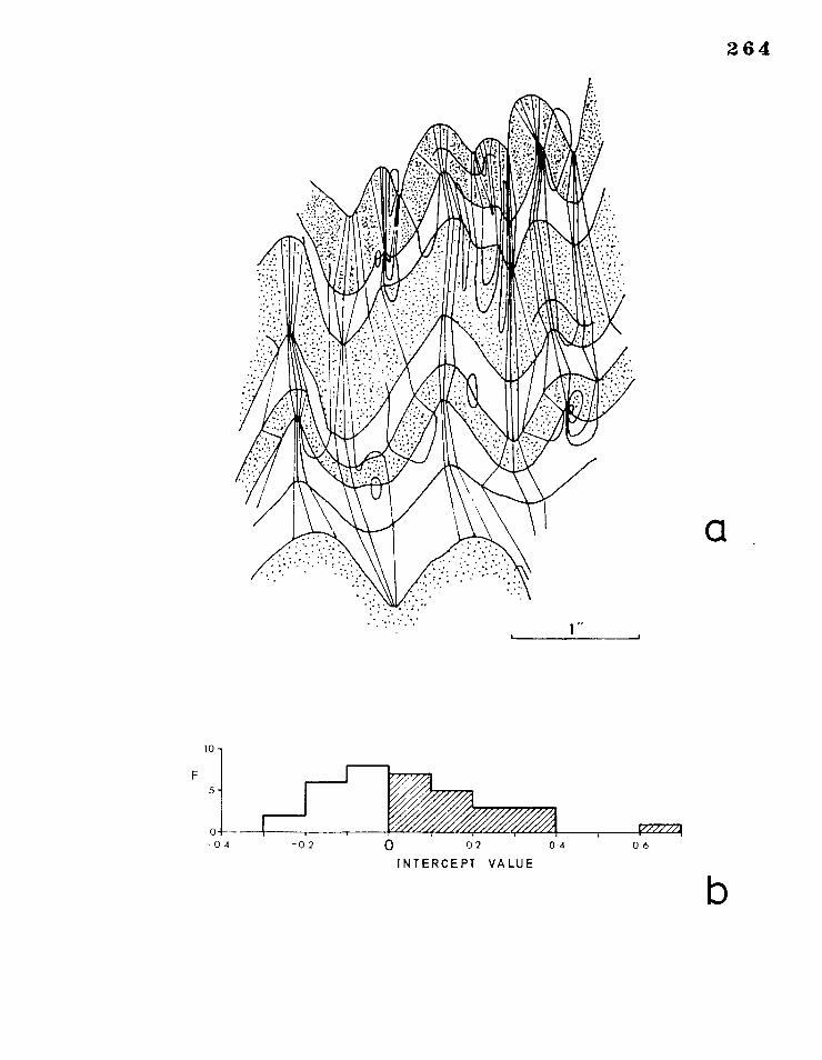
04 06 -04 -02 0 02
INTERCEPT VALUE
264
b
F
0
10-
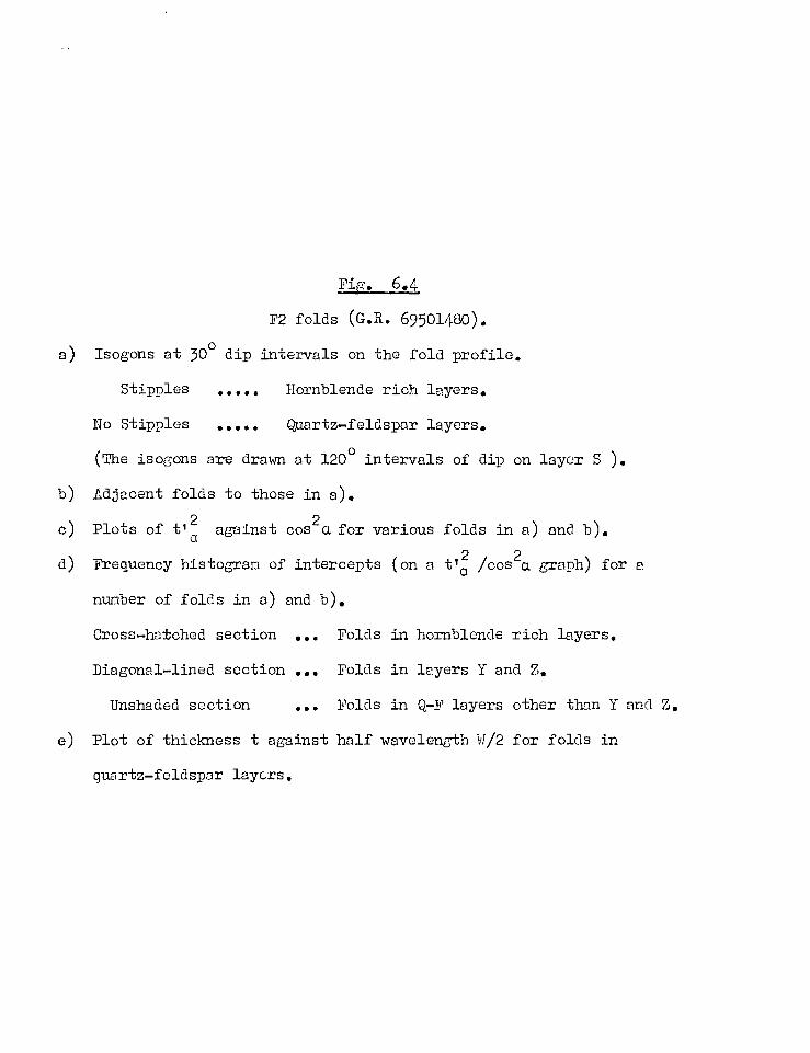
F2 folds (G.R. 69501480).
a) Isogons at 30° dip intervals on the fold profile.
Stipples Hornblende rich layers.
No Stipples Quartz-feldspar layers.
(The isogons are drawn at 120° intervals of dip on layer S ).
b) Adjacent folds to those in a).
c) Plots of t'2 against costa for various folds in a) and b). a
d) Frequency histogram of intercepts (on a tla2 /cos2a graph) for a
number of folds in a) and b).
Cross-ha±ched section ... Folds in hornblende rich layers.
Diagonal-lined section ... Folds in layers Y and Z.
Unshaded section Folds in Q-F layers other than Y and Z.
e) Plot of thickness t against half wavelength W/2 for folds in
quartz-feldspar layers.
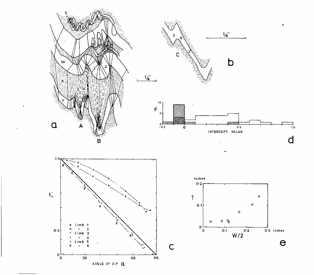
10
0 -02 0
1/4"
b
N.NNN.1 0-5
INTERCEPT VALUE 1-0
d
1/4"
• Limb 1 0, I; 2 + Limb 3 x I; 4 ✓ Limb 5 4, ii 6
0
C
03 inches
e 0.1 0-2
W/2
10
t "c,
0-5
Inches
0 2
T
0.1
0
•
0
0
0
0 0 21
30
60
90
ANGLE OF DIP a,

6
F2 folds (G.R. 69441480).
a) Fold profile.
Stippling Hornblende rich layer
No stippling Quartz—feldspar layer.
2 b) Plots of t'a against cos
2a for various folds in a).
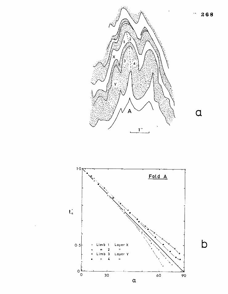
O 30 60 90
" 268
a ,
10
0.5
Fold A \.
\ \c, \\ • \
° \ \ • -
+ Limb 1 Layer X • it 2 • Limb 3 Layer Y
4 •
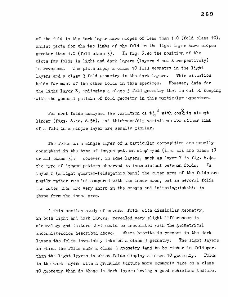
269
of the fold in the dark layer have slopes of less than 1.0 (fold class 1C),
whilst plots for the two limbs of the fold in the light layer have slopes
greater than 1.0 (fold class 3)• In fig. 6.4c the position of the
plots for folds in light and dark layers (layers W and X respectively)
is reversed. The plots imply a class 1C fold geometry in the light
layers and a class 3 fold geometry in the dark layers. This situation
holds for most of the other folds in this specimen. However, data for
the light layer Z, indicates a class 3 fold geometry that is out of keeping
-with the general pattern of fold geometry in this particular .sspecimen.
For most folds analysed the variation of t'a 2 with cos
2 a is almost
linear (figs. 6.4c, 6.5b), and thickness/dip variations for either limb
of a fold in a single layer are usually aimilar.
The folds in a single layer of a particular composition are usually
consistent in the type of isogon pattern displayed (i.e. all are class 1C
or all class 3). However, in some layers, such as layer Y in fig. 6.4a,
the type of isogon pattern observed is inconsistent between folds. In
layer Y (a light quartzo-feldspathic band) the outer arcs of the folds are
mostly rather rounded compared with the inner arcs, but in several folds
the outer arcs are very sharp in the crests and indistinguishable in
shape from the inner arcs.
A thin section study of several folds with dissimilar geometry,
in both light and dark layers, revealed very slight differences in
mineralogy and texture that could be associated with the geometrical
inconsistencies described above. Where biotite is present in the dark
layers the folds invariably take on a class 3 geometry. The light layers
in which the folds show a class 3 geometry tend to be richer in feldspar•
than the light layers in which folds display a class 10 geometry. Folds
in the dark layers with a granular texture more commonly take on a class
1C geometry than do those in dark layers having a good schistose texture.
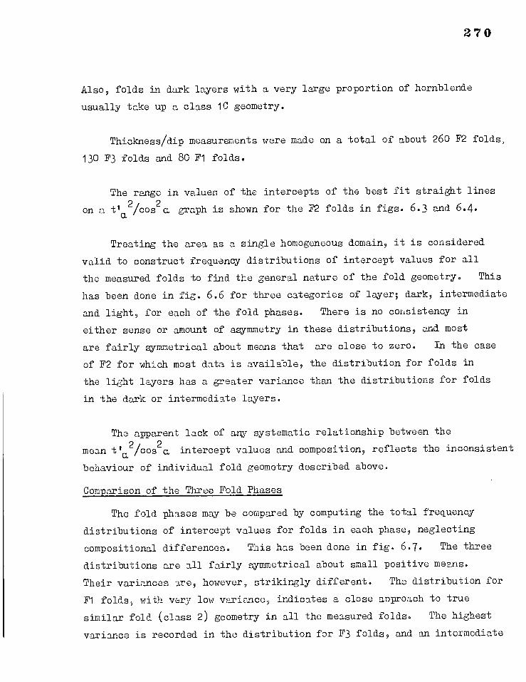
270
Also, folds in dark layers with a very large proportion of hornblende
usually take up a class 1C geometry.
Thickness/dip measurements were made on a total of about 260 F2 folds,
130 F3 folds and 80 F1 folds.
The range in values of the intercepts of the best fit straight lines
on a a2/cos2a graph is shown for the F2 folds in figs. 6.3 and 6.4.
Treating the area as a single homogeneous domain, it is considered
valid to construct frequency distributions of intercept values for all
the measured folds to find the general nature of the fold geometry. This
has been done in fig. 6.6 for three categories of layer; dark, intermediate
and light, for each of the fold phases. There is no consistency in
either sense or amount of asymmetry in these distributions, and most
are fairly symmetrical about means that are close to zero. In the case
of F2 for which most data is available, the distribution for folds in
the light layers has a greater variance than the distributions for folds
in the dark or intermediate layers.
The apparent lack of any systematic relationship between the
mean -0a2/cos2a intercept values and composition, reflects the inconsistent
behaviour of individual fold geometry described above.
Comparison of the Three Fold Phases
The fold phases may be compared by computing the total frequency
distributions of intercept values for folds in each phase, neglecting
compositional differences. This has been done in fig. 6.7. The three
distributions are all fairly symmetrical about small positive means.
Their variances are, however, strikingly different. The distribution for
F1 folds, with very low variance, indicates a close approach to true
similar fold (class 2) geometry in all the measured folds. The highest
variance is recorded in the distribution for F3 folds, and an intermediate
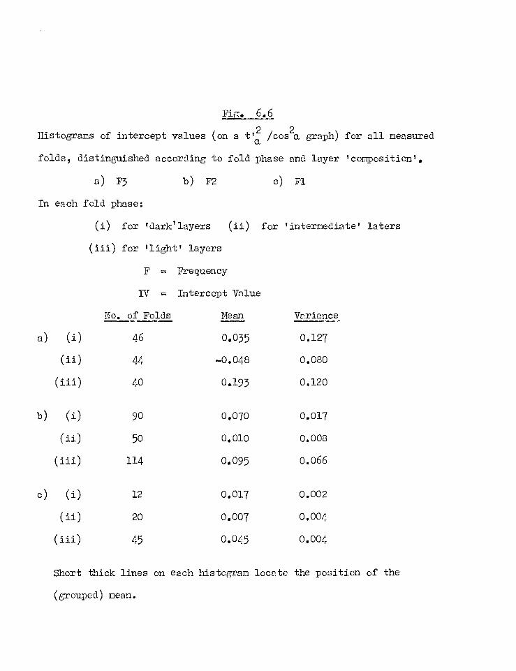
Fig. 6.6
Histograms of intercept values (on a 2 /cos2ia graph) for all measured
folds, distinguished according to fold phase and layer 'composition'.
a) F3 b) F2 c) Fl
In each fold phase:
(i) for 'dark'layers (ii) for 'intermediate' laters
(iii) for 'light' layers
F =
IV =
No. of Folds
Frequency
Intercept Value
Mean Variance
a) (i) 46 0.035 0.127
(ii) 44 —0.048 0.080
(iii) 40 0.193 0.120
b) (i) 90 0.070 0.017
(ii) 50 0.010 0.008
(iii) 114 0.095 0.066
e) (i) 12 0.017 0.002
(ii) 20 0.007 0.004
(iii) 45 0.045 0.004
Short thick lines on each histogram locate the position of the
(grouped) mean.
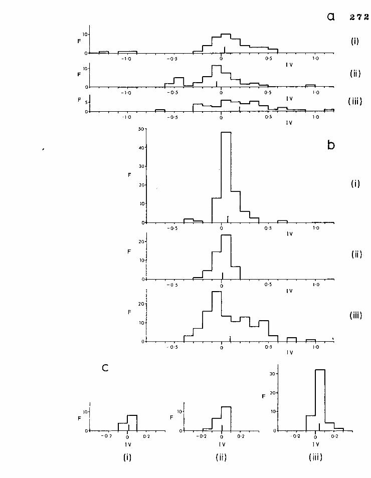
10 F
rI 1.0
5
- 1.0 - 0.5 0 0.5
I
F
0 I-1 - 1.0
r - 05 0 05 1.0
101
IV
F 10
30
F 20
10
0 -0.2 0
IV
0.2 - 0.2
IV
( i i i)
71--1 0.2
-10 -0.5 0 0.5
1.0 IV
b 50
40-
30-
F
20-
10-
0
-1 0.5 1.0
IV
0.5 1.0 I
- 0- 5
20.
F
10-
0 - 0 5
20-
F
10-
0 - 0.5 0 0.5 1.0
I
F 10
0
C
-02 0 2 0 IV
)
0.2
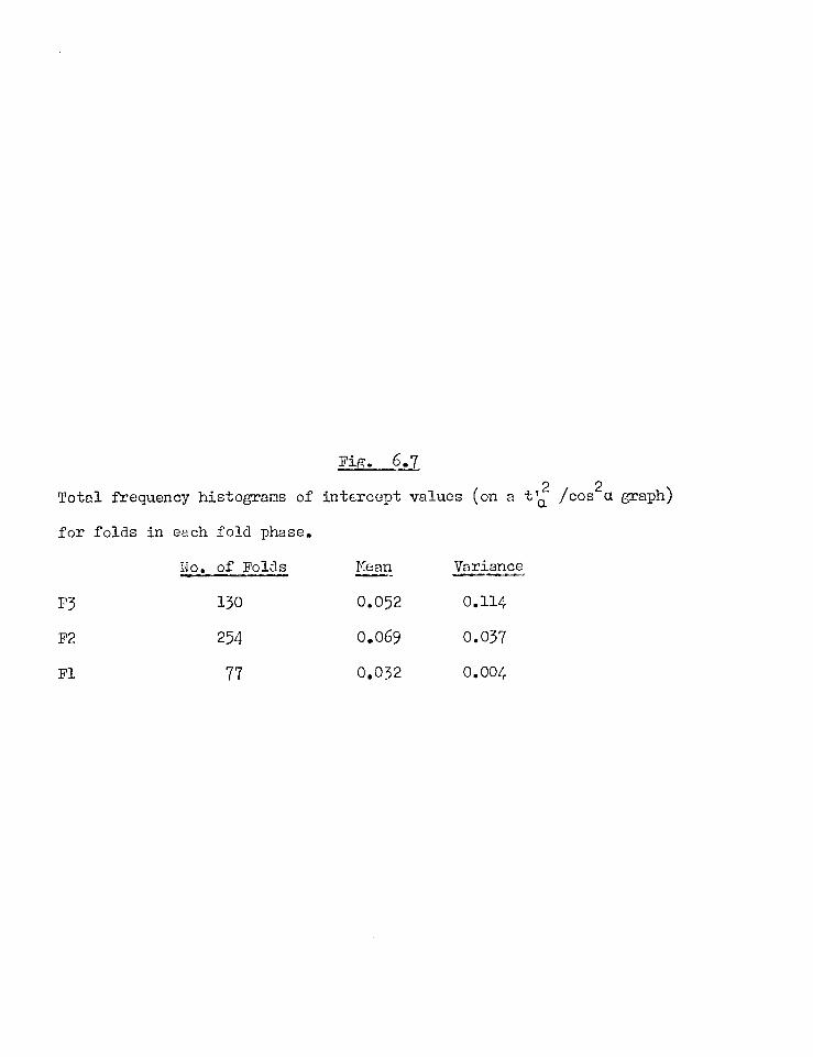
Fig. 6.7
2 Total frequency histograms of intercept values (on a tta /cost graph)
for folds in each fold phase.
No. of Folds Mean Variance
P3 130 0.052 0.114
F2 254 0.069 0.037
Fl 77 0.032 0.004
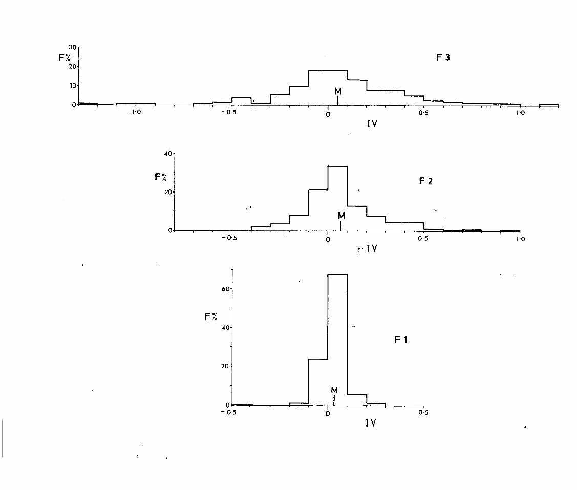
10- M I 0
-1.0 - 0.5 0 0:5 1.0
1
30-
F% 20-
F3
IV
40
F% F2 20-
0 - 0:5
M 1
0 0.5
p IV
11=111!11111111
1.0
60-
F% 40-
F1
20 -
o - 05 0:5
IV
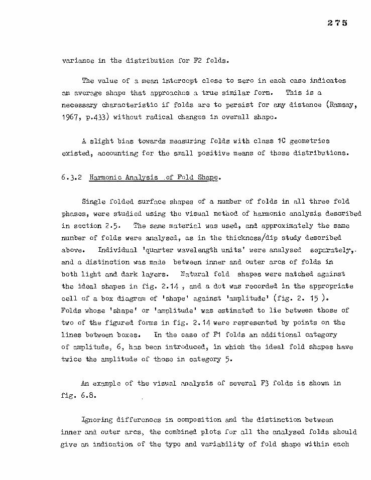
275
variance in the distribution for F2 folds.
The value of a mean intercept close to zero in each case indicates
an average shape that approaches a true similar form. This is a
necessary characteristic if folds are to persist for any distance (Ramsay,
1967, p.433) without radical changes in overall shape.
A slight bias towards measuring folds with class 1C geometries
existed, accounting for the small positive means of these distributions.
6.3.2 Harmonic Analysis .of Fold Shape.
Single folded surface shapes of a number of folds in all three fold
phases, were studied using the visual method of harmonic analysis described
in section 2.5. The same material was used, and approximately the same
number of folds were analysed, as in the thickness/dip study described
above. Individual 'quarter wavelength units' were analysed separatelyl-
and a distinction was made between inner and outer arcs of folds in
both light and dark layers. Natural fold shapes were matched against
the ideal shapes in fig. 2.14 , and a dot was recorded in the appropriate
cell of a box diagram of 'shape' against 'amplitude' (fig. 2. 15 ).
Folds whose 'shape' or 'amplitude' was estimated to lie between those of
two of the figured forms in fig. 2.14 were represented by points on the
lines between boxes. In the case of F1 folds an additional category
of amplitude, 6, has been introduced, in which the ideal fold shapes have twice the amplitude of those in category 5.
An example of the visual analysis of several F3 folds is shown in
fig. 6.8.
Ignoring differences in composition and the distinction between
inner and outer arcs, the combined plots for all the analysed folds should
give an indication of the type and variability of fold shape within each
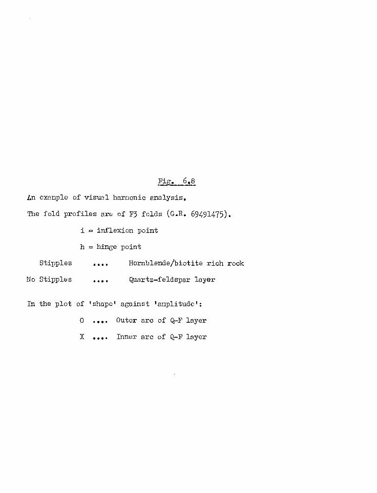
Fig. 6.8
Ln example of visual harmonic analysis.
The fold profiles are of F3 folds (G.R. 69491475).
i . inflexion point
h = hinge point
Stipples • • • • Hornblende/biotite rich rock
No Stipples • •• • Quartz—feldspar layer
In the plot of 'shape' against 'amplitude':
0 .... Outer arc of Q-F layer
X .... Inner arc of Q—F layer
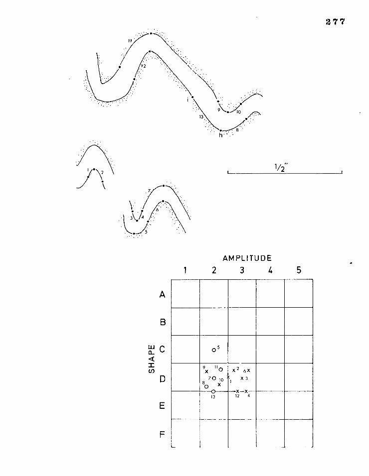
5
AMPLITUDE
2 3 4
277
1/2
1
A
B
w EL C
D (I)
E
F
(Ds
9 11 X ° 70 10
80 X
X 2 X
1
6X
X 3
13 X
12 X
4
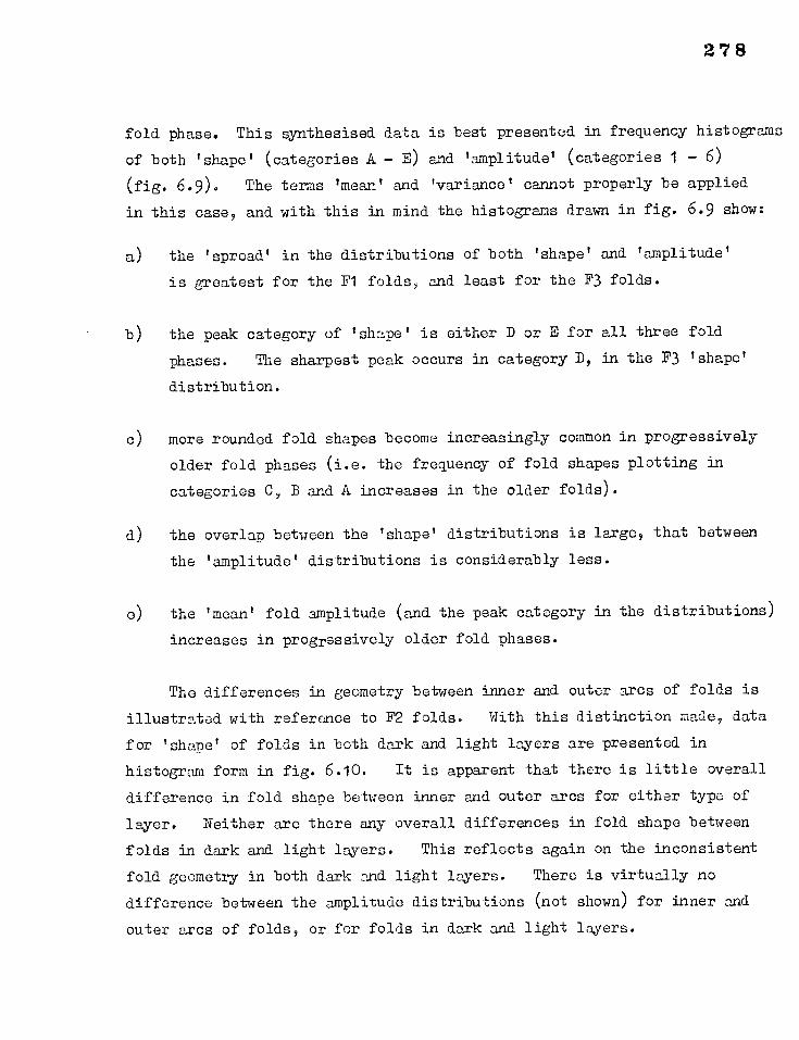
278
fold phase. This synthesised data is best presented in frequency histograms
of both 'shape' (categories A - E) and 'amplitude' (categories 1 - 6)
(fig. 6.9). The terms 'mean' and 'variance' cannot properly be applied
in this case, and with this in mind the histograms drawn in fig. 6.9 show:
a) the 'spread' in the distributions of both 'shape' and 'amplitude'
is greatest for the F1 folds, and least for the F3 folds.
b) the peak category of 'shape' is either D or E for all three fold
phases. The sharpest peak occurs in category D, in the F3 'shape'
distribution.
c) more rounded fold shapes become increasingly common in progressively
older fold phases (i.e. the frequency of fold shapes plotting in
categories C, B and A increases in the older folds).
d) the overlap between the 'shape' distributions is large, that between
the 'amplitude' distributions is considerably less.
e) the 'mean' fold amplitude (and the peak category in the distributions)
increases in progressively older fold phases.
The differences in geometry between inner and outer arcs of folds is
illustrated with reference to F2 folds. With this distinction made, data
for 'shape' of folds in both dark and light layers are presented in
histogram form in fig. 6.10. It is apparent that there is little overall
difference in fold shape between inner and outer arcs for either type of
layer. Neither are there any overall differences in fold shape between
folds in dark and light layers. This reflects again on the inconsistent
fold geometry in both dark and light layers. There is virtually no
difference between the amplitude distributions (not shown) for inner and
outer arcs of folds, or for folds in dark and light layers.
Fig. 6.9
Harmonic Analysis.
Frequency histograms of 'shape' and 'amplitude' of folds in each fold
phase. The totals of folds are:
Fl 81
F2 261
F3 154
Fig. 6.10
Harmonic Analysis.
Couparison between 'shape' distributions for inner and outer arcs of
folds in 'dark' layers (a) and 'light' layers (b). All are F2 folds.
Numbers of folds are:
Inner arcs Outer arcs
a) 72 92
b) 89 90
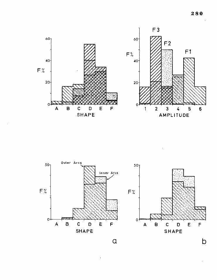
F%
50- Outer Arcs
\\.
F%
280
F3
Fl
3 4 5 AMPLITUDE
ABCD
SHAPE
AB C D
SHAPE
a
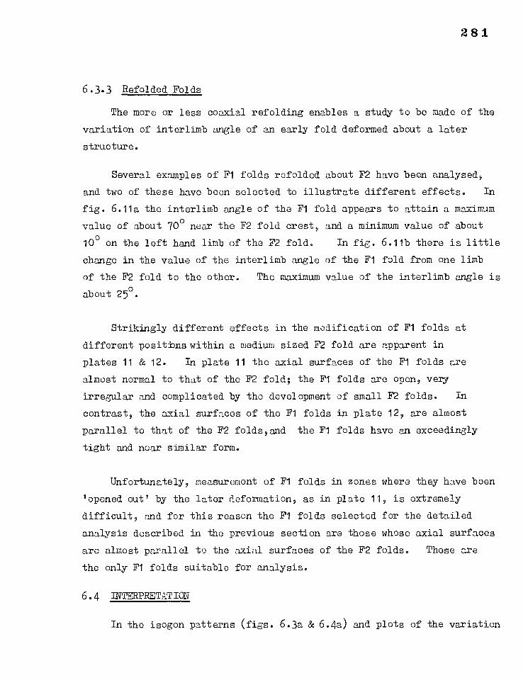
281
6.3.3 Refolded Folds
The more or less coaxial refolding enables a study to be made of the
variation of interlimb angle of an early fold deformed about a later
structure.
Several examples of F1 folds refolded about F2 have been analysed,
and two of these have been selected to illustrate different effects. In
fig. 6.11a the interlimb angle of the F1 fold appears to attain a maximum
value of about 70° near the F2 fold crest, and a minimum value of about
10° on the left hand limb of the F2 fold. In fig. 6.11b there is little
change in the value of the interlimb angle of the F1 fold from one limb
of the F2 fold to the other. The maximum value of the interlimb angle is
about 25°.
Strikingly different effects in the modification of F1 folds at
different positions within a medium sized F2 fold are apparent in
plates 11 & 12. In plate 11 the axial surfaces of the Fl folds are
almost normal to that of the F2 fold; the F1 folds are open, very
irregular and complicated by the development of small F2 folds. In
contrast, the axial surfaces of the Fl folds in plate 12, are almost
parallel to that of the F2 folds,and the F1 folds have an exceedingly
tight and near similar form.
Unfortunately, measurement of Fl folds in zones where they have been
'opened out' by the later deformation, as in plate 11, is extremely
difficult, and for this reason the Fl folds selected for the detailed
analysis described in the previous section are those whose axial surfaces
are almost parallel to the axial surfaces of the F2 folds. These are
the only Fl folds suitable for analysis.
6.4 INTERPRETATION
In the isogon patterns (figs. 6.3a & 6.4a) and plots of the variation
FiR. 6.11 Examples of Fl interlimb angle variation around F2 folds.
The folding is coaxial. Fl axial surface traces are shown by solid
lines, F2 axial surface traces by broken lines.
a) (G.R. 69471479)
b) (G.R. 69501477)
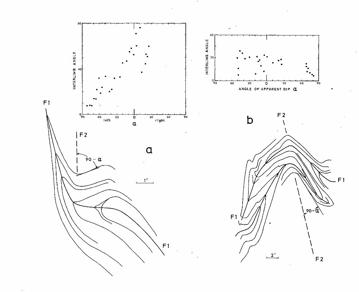
0 90 60 30
left Q 30 60
right
Fl
80
INTE
RLI
MB
AN
GLE
a 90
a
•
•
• •
•
• •
•
• • •
. • • • •
• •
• • •
•
• •
• • • .
........ 1
. ..
. • . • •• • • ••• • • .. . . • .
• •
• ..
40
20
0 90 60 30 0 30 60
ANGLE OF APPARENT DIP a. 90
•
b F2 I
Fl
Plates 11 & 12
Fl folds at different positions in a single F2 structure.
(Grid. Ref. 69501478).
Plate 11 The Fl fold axial surfaces are almost normal to that of
the F2 structure.
Plate 12 The Fl fold axial surfaces are almost parallel to that
of the F2 structure which is visible at the top of the
plate.
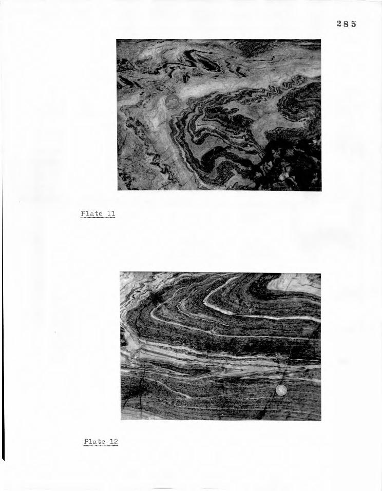
Plate 11
Plate 12
286
of -0112 with cos2a (figs. 6.4c & 6.5.b) there is ample evidence of
non-passive layer behaviour in the F2 folding. Similar evidence can be
produced for the Fl and F3 folds, and so the layering is considered
to have behaved non-passively in all three phases of deformation.
Isogon patterns give an indication of the relative ductility contrast
between adjacent folded layers (Chapter 5; Ramsay, 19679 p.416 & 432) and
in the present case this leads to the conclusion that in some situations
the dark amphibolitic layers have behaved in a more competent manner than
the light quartzo-feldspathic layers (e.g. fig. 6.3, 6.5). In other
situations the relative competency has been reversed, and the light layers
have behaved in a more competent manner (e.g. fig. 6.4). Rarely,
reversals in relative competence contrast appear to have taken place between
adjacent folded layers in neighbouring folds.
That these 'anomalous' variations in relative competence existed
throughout all three folding episodes is reflected in the lack of any
systematic differences between the overall -0(12/cos2a intercept distrib-
utions fcr dark, intermediate and light layers (fig. 6.6) in all three
fold phases. This is further shown for the F2 folds, by the similarity
of the 'shape' distributions for inner and outer arcs of folds in both
dark and light layers.
Using similar arguments to those developed in Chapter 5 it is
considered that buckling was the most important fold-forming process in
all three deformation episodes; the banded gneisses are thought to have
behaved as a complex multilayer in which either quartzo-feldspathic or
amphibolitic layers behaved as tile more competent units. As an
individual example of evidence for buckling, consider the F2 folds in
fig. 6.4. The folds in the thin light layer S can only be satisfactorily
explained by a buckling hypothesis. Fold wavelength in the light layers
in fig. 6.4a increases with layer thickness (fig. 6.4e). A direct
287
relationship between fold wavelength and layer thickness is characteristic
of buckling processes.
A component of flattening (see section 3.5), normal to the axial
surfaces, is inferred to have either followed or accompanied the buckling
in each episode of folding. This component has been greatest in the case
of the Fl folding, and least in the case of the F3 folding, accounting
for the differences between fold phases in the overall distributions of
both layer shape, based upon -02/ces2a intercept values (fig. 6.7) and
of 'amplitude' in the harmonic analysis (fig. 6.9). The larger the
flattening component of deformation the smaller the shapes of folded
layers depart from a class 2 geometry, and the higher the amplitude (taken
as the amplitude/wavelength ratio) becomes.
The variation of t' with a. observed in fold B in layer W in fig.
6.4c is similar to that predicted from a process of simultaneous
buckling and flattening (section 3.6).
Progressive changes in single surface fold shape during the
buckling of an isolated layer are discussed in Chapters 3 and 4. The
most distinct change observed is that the folds become progressively more
rounded in the crests with increasing deformation. In terms of the
visual harmonic analysis this implies changes in the closest matching
'shape' category from D or E through C to B, with increasing deformation.
In the overall distributions of 'shape' for the three fold phases (fig.
6.9), the frequencies of fold shapes in the categories C, B and A
increase in progressively older fold phases, together with progressively
higher amplitudes (and increasingly large components of inferred flat—
tening). By analogy with the isolated layer case, this is interpreted
to be the result of buckling of the more competent layers during the
deformation.
288
The frequency of folds with sharp crests (categories D and E) is
large in the distributions relating to F1 and F2, and this is considered
to be due to the flattening part of the deformation. In passive
flattening there is no change in fold 'shape' with increase in amplitude
(section 3. 5 ), and fold shapes initially near sinusoidal (categories D or E) would remain near sinusoidal throughout deformation.
The single surface fold 'shape' distributions are therefore taken
as evidence for simultaneous buckling and flattening in at least F1 and
F2 folding episodes.
Some of the deformation undergone by the Fl folds will have taken
place during the F2 phase of deformation (and perhaps during that of F3
as well). Since the measured F1 folds have axial surfaces almost
parallel to those of F2 and F3 (see sect. 6.3.3 and fig. 6.2), this
additional deformation will have been in the form _of a continued
shortening almost normal to the axial surfaces. Thus the measured F1
folds record rather more deformation than occurred in the Fl phase alone.
The extent to which F2 folds have been affected by F3 deformation outside
the zones of F3 fold development, is notthought to be great.
It is not possible to interpret the variations of the interlimb
angle of F1 folds, refolded by F2, unnnbiguously in terms of Ramsay's
(1967, p.491 et. seq.) idealised models of the modification of dihedral
angles in various types of refolding. However, the observed interlimb
angle variations (fig. 6.11) are compatible with a theory of buckling and
flattening. As a result of the flattening component the F1 folds would
tend to become opened out in the hinge regions of the F2 folds (figs.
6.11a & plate 11). Differences in the value of the maximum interlimb
angle attained near the F2 fold crests (cf. figs. 6.11a & b, and see
Ramsay, 1967, Chapter 9), would result from slight differences in
initially small interlimb angles becoming accentuated during the F2
289
flattening.
The kinking, or crenulation cleavage, developed in the amphibolitic
layers in F2 folds is thought to have played a small part in determining
fold size and geometry on the scale of the kinks themselves. There is
no evidence to suggest that these folds developed from conjugate kinks in
the manner described by Paterson & Weiss (1966). Paterson & Weiss (1968)
show how kinking can control the folding in more 'competent' layers which
take on fold geometries similar to those observed in buckling. However,
in this case there is no dependence of fold wavelength on the thickness
of the 'competent' layers, and zones of contact strain would not be present.
Buckling is thought to-be the primary process responsible for F2 fold
development, and kinking to be a secondary phenomenon.
F3 folds in some ways resemble the kinking in the amphibolitic bands
in the F2 folds; the whole stack of thin folded layers appear similar to
the kinks within a single amphibolitic band (compare plates 9 & 10). However, no sign of conjugate structures is apparent.
6.4.1 Discussion.
One of the biggest problems presented by the analysis, arises from
the conclusion that amphibolitic layers may behave either in a more or a
less competent manner than quartzo-feldspathic layers. If this conclusion
is correct it seems likely that the competency contrast is always very
small, and that very small differences in composition or texture, of the
kind described in section 6.3.1, will be sufficient to reverse the relative
competence of 'dark' and 'light layers.
It was not found possible to analyse the buckling, in any fold phase,
in terms of the precise multilayer theories of Biot (1964; 1965a; 1965b;
1965c) or Ramberg (1961a; 1963b; 1964a). Biot's (1964; 1965b) analysis
of the internal buckling of confined multilayers is probably the
290
theoretical treatment most applicable to the kind of folding observed here,
but it is not valid to very large deformations nor does it account for the
development of more than one order of folds. Ramberg (1964a) does
qualitatively discuss the simultaneous development of several fold orders
and is able to show that this phenomenon is a characteristic of buckling
in multilayers, where layers are of different ductility and thickness.
In the light of the series of experiments on multilayers made by
Ramberg (1963b) and Ghosh (1968) using viscoelastic materials, the
comparison made in tie interpretation above, between the development of
fold shape in isolated layers and multilayers, may not be valid. By
considering such factors as layer spacing, ease of slip between layers
(Ghosh) and the degree of confinement of the multilayer (Ghosh), these
authors show that a multilayer can behave as a single or a composite unit
and that folds may develop with rounded or angular crests. Ghosh shows
that kinking may occur under certain conditions (with a limited amount of
slip between layers).
Under metamorphic conditions, slip between layers (and therefore
kinking) is probably unimportant in fold development, and in the present
case it is considered that progressive changes in fold shape (in the
competent units) will be of the same relative kind as those undergone
during the buckling of a single isolated layer.
The fact that three phases of folding have developed coaxially is of
interest. Wynne—Edwards (1963) considers this kind of folding can occur
in a single continuous deformation involving fluid flow with convolution
of the flow lines. However, applied to the Sambuco folds, such a theory
does not account for the systematic nature of the refolding and has the
disadvantages of any theory involving heterogeneous simple shear (see
section 3.2). MUkhopadhyay (1965b) considers that examples of coaxial
refolding in the Moinian rocks of the Scottish Highlands are due to the
291
geometrical restraints imposed by the early structures on a subsequent
refolding which contains a strong flexural component. Such a restraint
would be expected to affect any type of superposed deformation that
involved buckling, and this may partly explain the coaxial refolding in
the Sambuco rocks.
6.5 A WAVELENGTH/THICKNESS STUDY OF F2 FOLDS
Certain thin layers have developed folds of the kind produced by
the buckling of competent layers isolated in a less competent medium, in
which a zone of contact strain dies out within a short distance of the
buckled layer. The layers may be either 'dark' amphibolitic bands embedded
in 'light' quartzo—feldspathic material, or 'light' quartz rich layers
surrounded by 'dark' hornblende and/or biotite rich rock (fig. 6.12a & b).
An analysis of these folds (all of the F2 phase) is made here, treating
them as buckles developed according to a modified theory of Sherwin &
Chapple (1968) (see Chapter 4 and section 5.7). Estimates of viscosity contrast and the amount of F2 deformation within the profile planes of the
folds will be made.
The procedure of analysis is identical to that described in section
5.79 and will not be repeated here.
The bulk F2 strain is assumed to be homogeneous within the area
studied; the effects of F3 are local and are assumed to be unimportant
away from the zones of F3 fold development. The basic assumptions of
the buckling theory (section 3.3) are for the most part difficult or
impossible to test. The validity of an assumption of Newtonian viscosity
for rocks undergoing metamorphism is discussed in section 4. 2 . The folded layers are never truly isolated and two effects are observed: one
is tLat of unfolded neighbouring layers acting as a confinement, tending
to reduce the dominant wavelength/thickness ratio (Ramberg, 1963b); and
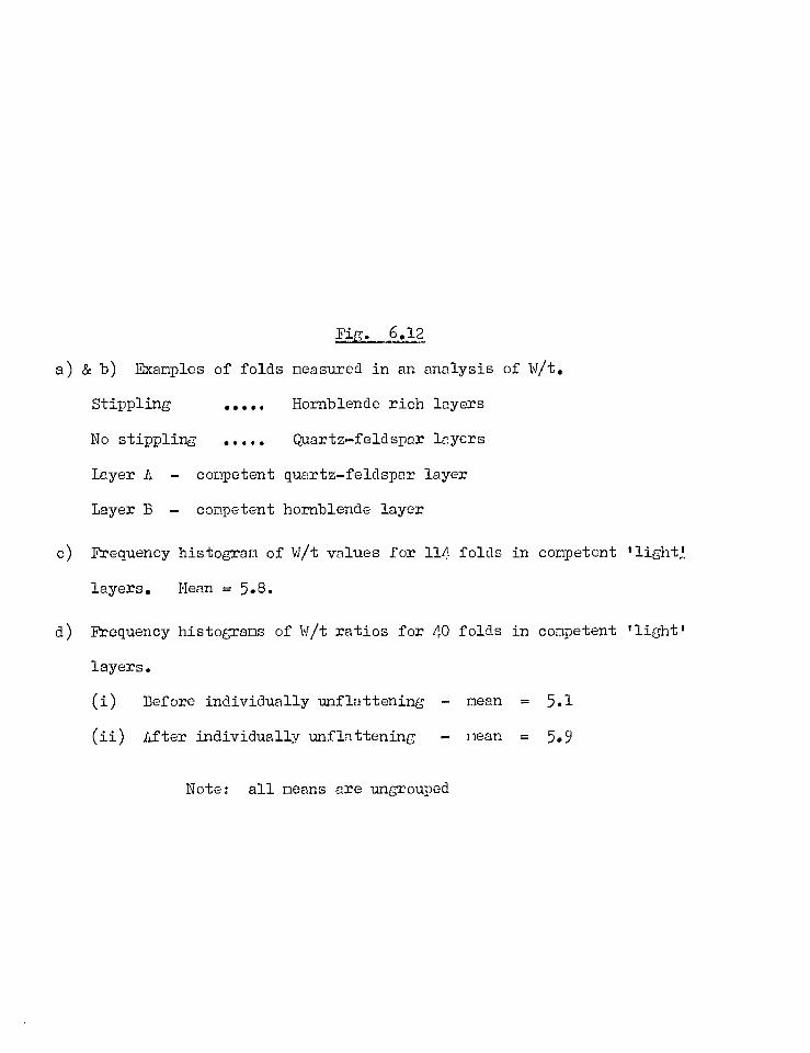
Fig. 6.12
a) & b) Examples of folds measured in an analysis of Wt.
Stippling Hornblende rich layers
No stippling Quartz—feldspar layers
Layer A — competent quartz—feldspar layer
Layer B — competent hornblende layer
c) Frequency histogram of W/t values for 114 folds in competent 'light?
layers. Mean = 5.8.
Frequency histograms of W/t ratios for 40 folds in competent 'light'
layers.
(i) Before individually unflattening mean = 5.1
(ii) After individually unflattening — mean = 5.9
Note: all means are ungrouped
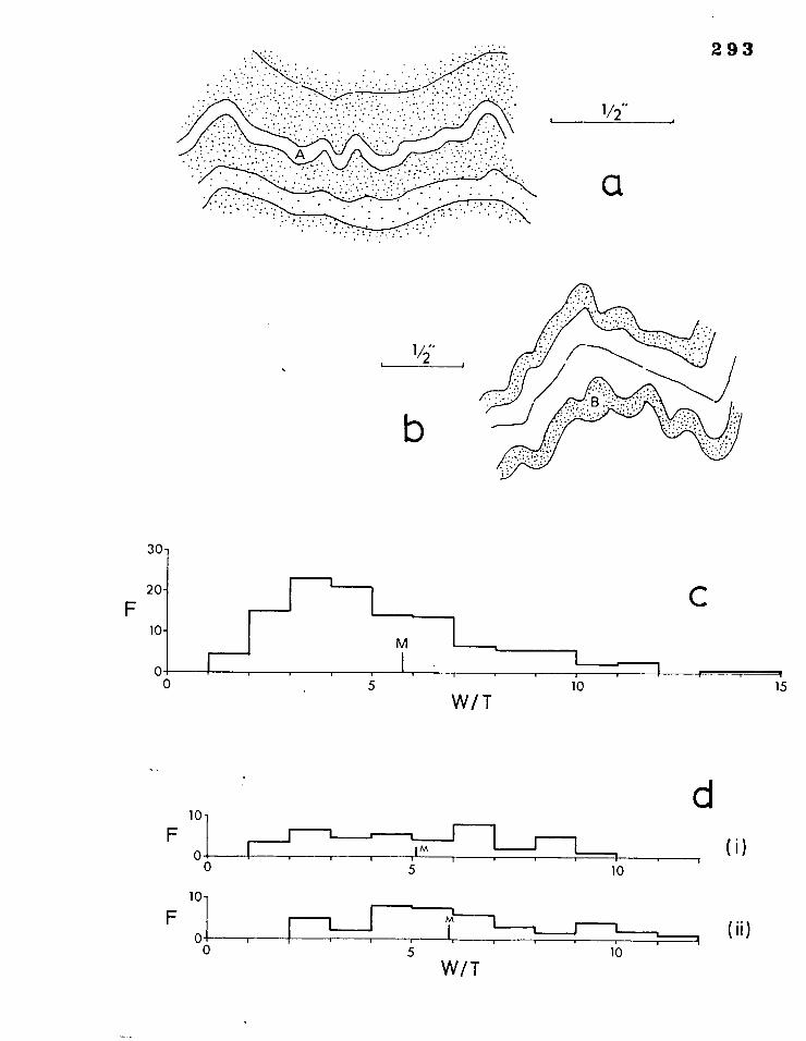
1/2-
293
a
vi
b
30
M
20- F
10-
C
5
F
F
10
0 0
10
0 0
1 I
I
10 15 W/T
d (i)
5 10
m I-1 , , 1 1
1 ( ii) 5 10
W/T
294
the other is a multilayer effect in which all the competent layers behave
in a similar fashion (Ramberg, 1961a) and the dominant wavelength/thickness
ratio tends to increase for a single competent member of the sequence.
These two effects are considered to 'neutralize' one another in the
calculation of mean wavelength/thickness ratios.
A frequency distribution of Wit ratios for isolated buckle folds in
'light' layers is drawn in fig. 6.12c. Nearly all the measured folds were
thickened in the hinges, and it was assumed that a component of homogeneous
flattening followed the buckling for the purposes of the analysis (but
see p.106)• To eliminate the effect of flattening, 35 folds in 'dark'
buckled layers and 40 folds in the 'light' buckled layers were individually
unflattened. Measurements of wavelength, thickness and limb dip were
made on each unflattened fold. The results are given in table 6.1.
The total shortening should be the same in the analyses of folds in
both 'dark' and 'light' layers. However, the calculated values of
Shortening are not quite the same, and are equivalent to strain ratios
(Jh1/ X2) of about 6:1 and. 5:1 respectively.
Because of the difficulties in both testing and meeting the assum—
ptions on which the theory is based, the results are only considered to
give rough estimates of the 'viscosity' contrast and the total amount of
shortening within the profile plane of the F2 folds.
6.6. CONCLUSIONS
A) Geometrical analyses of folds in all three fold phases show that
no systematic differences in fold geometry can be related to
different layer types (i.e. 'dark', 'intermediate' and 'light').
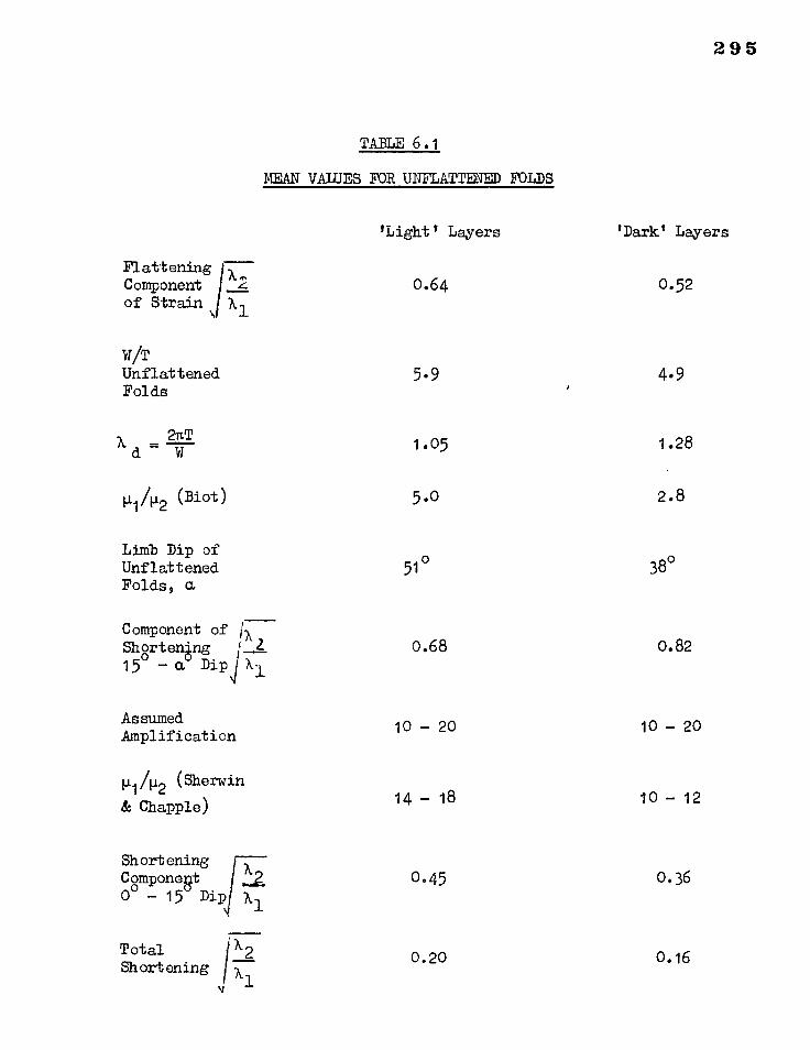
295
TABLE 6.1
MEAN VALUES FOR UNFLATTENED FOLDS
'Light' Layers
i
Flattening A
Component 2 0.64 of Strain X,
\ -1.
'Dark' Layers
0.52
W/T Unflattened Folds
2nT X=
5.9
1.05
5.0
51°
0.68
10 - 20
14 - 18
0.45
0.20
4.9
1.28
2.8
38°
0.82
10 - 20
10 - 12
0.36
0.16
d W
111/112 (Blot)
Limb Dip of Unflattened Folds,
Component of ix Shortening 15 - a Dip
Assumed Amplification
P1/112 (Sherwin
& Chapple)
Shortening Component 0 - 15° Dip
Total X2 Shortening x
1
296
B) Distinct differences in overall (synthesised) fold geometry exist
between the three fold phases.
C) The relative competence of the dark amphibolitic layers to the
light quartz-feldspar layers depends upon very slight differences
in composition and texture, and varies locally in all three fold
phases.
D) The fold geometry is adequately explained in all three folding
episodes by a hypothesis involving both buckling and flattening.
E) The geometrical differences between the three fold phases may be
accounted for by considering the folds in each fold phase to represent
different stages in progressive fold development by buckling and
flattening.
F) The 'viscosity' ratio of dark amphibolitic layers to light quartz-
feldspar layers is estimated to vary between about 11:1 to 1:16.
G) The bulk F2 deformation in the profile planes of the F2 folds is
estimated to be about JX2/X 1 = 0.18
297
CHAPTER
AN ANALYSIS OF MINOR FOLDS IN THE CULM MEASURES AT BOSCASTLE, CORNWALL.
7.1 INTRODUCTION
The sedimentary rocks of the Culm are generally unmetamorphosed,
although a few have slaty cleavage developed and show the effects of
extremely low grade metamorphism.
A small area was selected for study at Boscastle (fig. 7.1). just
within the southern margin of the extensive Culm outcrop. Good exposures
of rock are found here on Penally Hill and Penally Point, at the mouth
of the small harbour.
The rocks at Boscastle are a series of unfossiliferous alternating
dark slates and sandstones, generally considered to be Carboniferous in
age. Ashwin (1957) referred to them as the Boscastle Measures. Selwood
(1961) considered them to be part of the Upper Carboniferous, and placed
them in the Upper Culm.
At least two generations of folds have developed in the Boscastle
Measures, as a result of Hercynian deformation which has affected Devonian
and Carboniferous rocks throughout south-west England. Recent attempts
to elucidate the regional structural pattern have been made by Ashwin
(1957), Zwart (1964) and Freahney et al. (1966).
The general geology of the area is briefly discussed in sections
7.1 and 7,2, and this is followed in section 7.3 by a description of detailed geometrical analyses of the minor folds. The significance of
the fold geometry in terms of folding processes is discussed in section 7.4.
7.1.1 Lithology
In the area of interest around Boscastle harbour, the rocks consist

a) Geological nap of the area around Boscastle (After Dearnan &
Feshney, 1966).
b) Enlarged nap of Boscastle to show the area selected for detailed
fold investigation. This area is narked by diagonal shading.
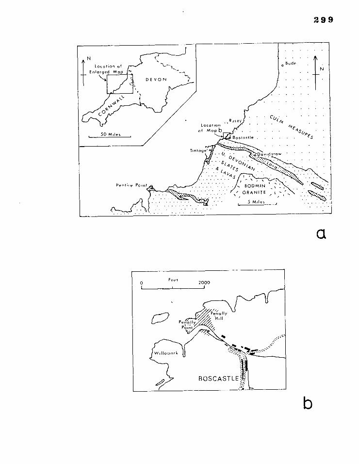
299
Loca ion of Enlarged Map
Penally iH II
300
of alternating slates, siltstones, sandstones and graywackes; their
sedimentary features have been described by Ashwin (1957). The rock
layers are in the form of continuous sheets, and the coarser sandstone
beds rarely exceed an inch in thickness. Within the coarser layers,
bedding laminations are often conscpicuous. Most layer boundaries are
well-defined surfaces and graded junctions are uncommon.
A simple division of layers into two types has been made for the
purpose of fold analysis:
'sandy' - sandstones, graywackes
'shaly' - slates
Nearly all the beds in which folds have been analysed, fall distinctly
into one or other of these categories.
7.2 STRUCTURAL GEOLOGY
Two distinct generations of minor folds were first recognised at
Boscastle by Ashwin (1957); and these have recently been described in some
detail by Dearman & Freshney (1966).
Fig. 7.2 is a stereographic plot of poles to axial surfaces and of
fold axes for both fold phases in the selected area.
Data for the early folds, F1, were collected on the long flat limbs
of the later folds, F2: the following description applies to F1 folds
situated on these long limbs of the F2 folds. The Fl folds (plate 13)
usually 11,1ve sharp crests and small interlimb angles. They are frequently
isoclinal. Their axial surfaces are either horizontal or dip gently
towards the north. The dominant axial trend is NNW-SSE, but locally E-W
trends are found, and some intermediate between these directions (see
fig. 7.2; and Dearman & Freshney, 1966, fig. 7a). The mutual relation-
ship between folds with different trends could not be determined. There
is, however, no evidence for the existence of more than a single fold
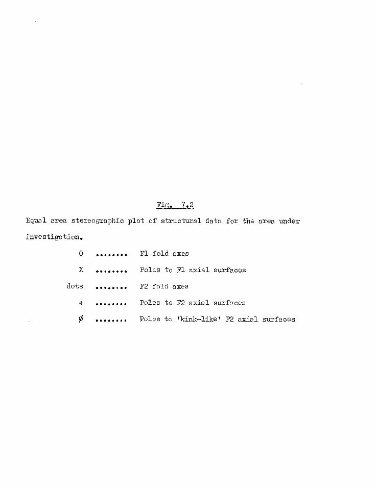
Fig. 7.2
Equal area stereographic plot of structural data for the area under
investigation.
0 Fl fold axes
X Poles to Fl axial surfaces
dots .. F2 fold axes
Poles to F2 axial surfaces
0 Poles to 'kink—like' F2 axial surfaces
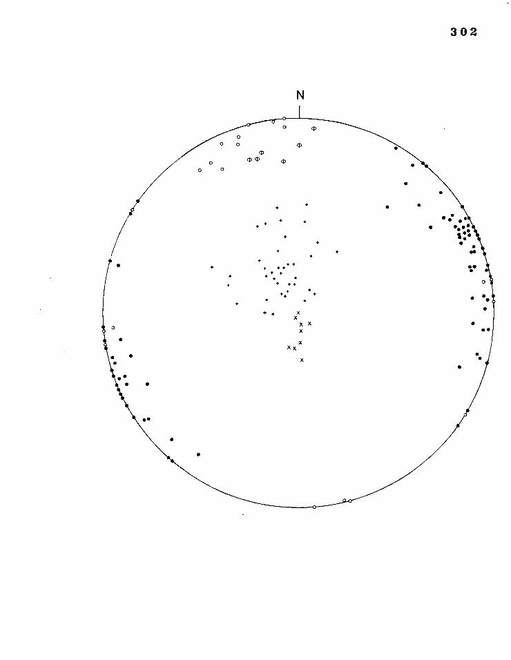
302
N
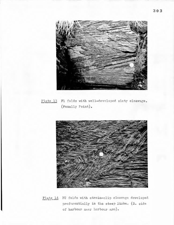
303
Plate 13 Fl folds with well—developed slaty cleavage.
(Penally Point).
Plated F2 folds with strain—slip cleavage developed
preferentially in the steel, limbs. (S. side
of harbour near harbour arm).
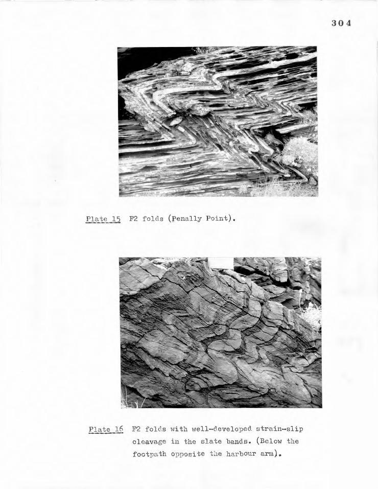
-;'''",1A01071116
4)A
304
Plate] F2 folds (penally Point).
Plate 16 F2 folds with well—developed strain—slip
cleavage in the slate bands. (Below the
footpath opposite the harbour arm).
305
phase (see Dearman & Freshney, 1966), and it appears that the different
trends are simply due to large variation of the hinge lines within the
flat axial surfaces. Viewed to the west or north, the symmetry of folds
with E-W or N-S axial trends respectively is either IS' or IZI, and Dearman
& Freshney consider all the long limbs to be the right way up, irrespective
of symmetry, implying a rather peculiar structural pattern (see Dearman
& Freshney, 1966, fig.3d).
The second folds, F2, refold the F1 structures and fold both bedding
and an F1 slaty cleavage. They are of a more open zig zag style, and
are developed locally in zones. Their axial surfaces and axes are
variable in orientation (see fig. 7.2). The axes are nearly horizontal
and trend between NE-SW and ESE-WNW. The axial surfaces have a variable
dip (between 0 and 60°) towards the SE or S. Variations in axial trend
of up to 50°, that are not th result of superimposed deformation, may be
measured along a single fold hinge in the space of a few feet (cf. Dearman
& Freshney, 1966, fig. 4e) where the folds have developed an 'en echelon'
pattern. The overall impression of fold symmetry is of 'SI type
viewed along the axes from west to east, although most folds occur in
zones of near 'M' symmetry. There is no evidence of large scale folds.
The general appearance of the F2 folds depends on the thickness of the
coarser sandstone layers involved in the folding (see plates 14, 15 & 16).
Individual superimposed structures have been described by Dearman &
Freshney; the only distinctive interference patterns observed are Type 3 of Ramsay (19679 p.530), where F2 folds refold Fl folds with an E-W trend.
The major structural pattern and interpretation of folds developed
in south-west England is complicated by the presence of northward-dipping
low-angle normal faults (see for e.g. Freshney et al. 1966). Two
recent attempts have been made to incorporate the structures observed
along the coastline between north Devon and Tintagel in Cornwall, into a
306
unified structural scheme.
Zwart (1964) correlates the two sets of structures observed at
Boscastle with two sets, both developed about E41 trending axes, occuring
in the main Culm outcrop to the north. He explains the regional structure
in terms of 'stockwerk' tectonics, according to which the folds occurring
at Boscastle and Tintagel were developed at deeper tectonic levels (forming
an infrastructure) than those occurring in the Culm to the north (forming
a suprastructure). Freshney et al. (1966) suggest an alternative
explanation, they consider that the major part of the Culm outcrop to the
north has been affected by a single phase of folding deformation only (and
that fanning of the axial surfaces of observed folds about major structures
accounts for the two fold phases of Zwart), and that these folds correlate
with the F1 folds of Boscastle. They consider that the F2 Boscastle
folds are associated with the development of the low-angle normal faults.
For a fuller discussion of the nroblem of major structures the reader is
referred to the works of Ashwin (1957), Zwart (1964) and Freshney et al.
(1966).
Neither Zwart's explanation nor that of Freshney et al. gives any
clear indication of the type of major structure to be expected in the region
of Boscastle; and despite the presence there of the minor Fl folds, there
appears to be a simple stratigraphic sequence from older beds to the
south-west of Boscastle through the Boscastle Measures to the Upper Culm
Measures appearing at Rusey to the north-east (see Selwood, 1961).
The nature of the major structure, if any, associated with the minor Fl
folds at Boscastle remains obscure.
The few F1 folds suitable for analysis and described in this Chapter
are all amongst those with axes trending nearly north-south.
7.2.1 Fabric
An intense slaty cleavage has developed in the shaly bands parallel
307
to the axial surfaces of the F1 folds (see plate 13), and because the
folds are often isoclinal, over large areas the cleavage is virtually
parallel to the bedding. It is in this situation that the F2 folds are
best developed.
Cleavage refracted through the coarser sandstone layers is a common
phenomenon. The intersection of bedding and cleavage produces a lineation
parallel to the F1 fold axes, and a mineral lineation parallel to this is
also developed on some cleavage faces and more particularly on bedding
surfaces. All these lineations are dominantly N-S in orientation.
A strain-slip cleavage has developed in the slates, either parallel
to, or fanning symmetricallyabutthe axial surfaces of the F2 folds
(plates 14 & 16). The intensity of development is variable; it is
always high in the crest regions of the folds, may be either high or low
in the limbs and often appears to be greater in the steeply dipping
short limbs of the folds than in the long limbs (plate 14).
7.3 DESCRIPTIVE GEOMETRY
Most of the data is presented in synthesised form and individual
examples have been selected to illustrate specific features of the fold
geometry.
Because F2 folds at Boscastle are frequently irregular and often en
echelon, care was taken to ensure that all the folds analysed were
approximately cylindrical, and could be measured in profile section.
The local variation of both F1 and F2 fold axis and axial surface
orientation is of the same order of magnitude as the total variation within
the region, and it is considered valid to treat the region as a single
homogeneous structural domain for both phases of deformation.
308
In F1 folds the layer boundaries are often ill-defined, and only in
a few examples could the:profile geometry be measured.
7.3.1 Isogon Plots and Thickness /Dip Relationships.
The variation of thickness with dip was measured in a total of 22 Fl
folds and 160 F2 folds; and for each fold the intercept of the best fit
straight line through the data plotted on a graph of tic_2 against costa
was computed. At least five pairs of t'a ,a values were used in each
calculation.
The synthesised data is presented in fig. 7.3a & b in the form of
frequency histograms of the value of the best fit straight line intercepts.
The intercept values for the Fl folds (fig. 7.3a) are all very close to
zero, indicating that the individual fold geometry is almost similar
(class 2) in all cases. The mean intercept is 0:005. In contrast the
range in values of intercept for the F2 folds is very large (from -0.8 to
1.0), reflecting a wide variation in folded layer geometry. In
addition, the distribution of intercepts is distinctly bimodal, one peak
greater than zero and the other less. By making a distinction between
intercepts for F2 folds in 'sandy' and 'shaly' layers, two separate
distributions may be constructed (fig. 7.3c) which are unimodal, with
virtually no mutual overlap. The intercepts relating to the folds in
tsandy' layers are all greater than 0 (fith a mean of 0.48), reflecting
a class 1 (and mostly 10) fold geometry; whilst those relating to the
folds in 'shaly' layers are predominantly less than 0 (with a mean of -0.15)
indicating a class 3 fold geometry.
Layers of sandstone and slate, with geometric fold forms of class 1C
and class 3 respectively, alternate in sequence to give an overall
similar (class 2) form to the F2 folds. Because the slate beds are
consistently thicker than the sandstones the separate distributions of
fig. 7.3c do not 'balance one another out', and the mean intercept of
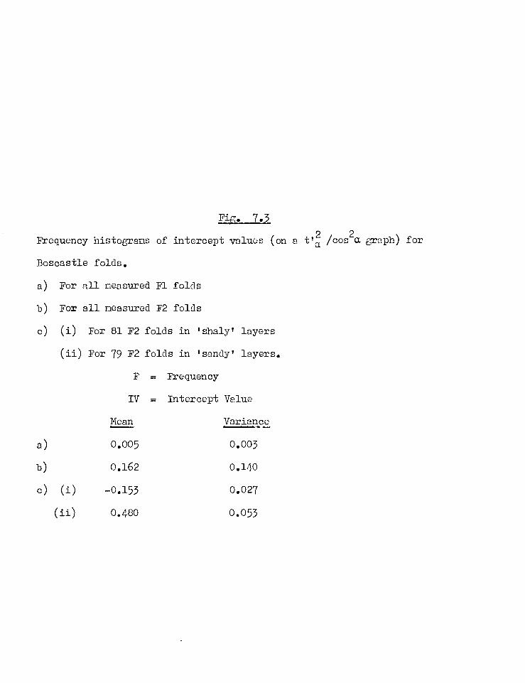
Fig. 7,3
Frequency histograms of intercept values (on a t'a2 /cos2a graph) for
Boscastle folds.
a) For all measured Fl folds
b) For all measured F2 folds
c) (i) For 81 F2 folds in 'shaly' layers
(ii) For 79 F2 folds in 'sandy' layers.
F = Frequency
IV = Intercept Value
Mean Variance
a) 0.005 0.003
b) 0.162 0.140
c) (i) -0.153 0.027
(ii) 0.480 0.053
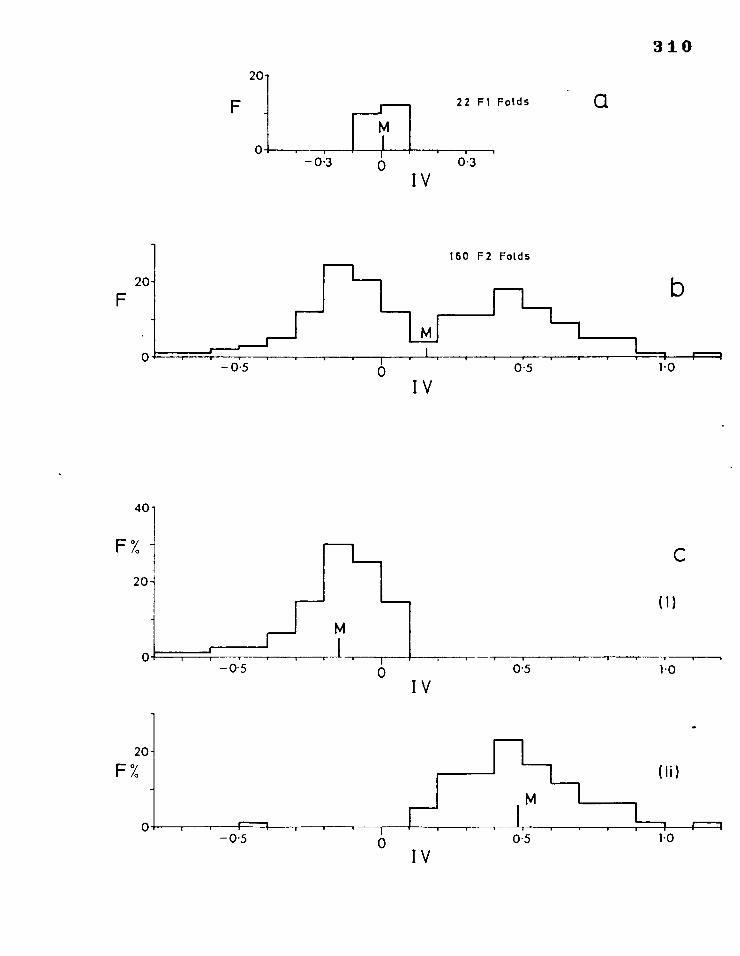
310
20
F 22 Fl Folds a
6.3 0
— 0:3 0 IV
160 F2 Folds
b 20F
-
— 0-5 0 0.5 1.0
IV
F%
20
40]
M
t a
0.5 —0:5 1.0 IV
20-
F%
— 0.5 0 0.5 I 1-0
IV
311
the combined distribution of fig. 7.3b is considerably greater than zero.
(mean 0.16).
It was not found -2-7actical to distinguish between 'shaly' and 'sandy'
layers in the case of the F1 folds.
An example of an Fl fold profile is shown in fig. 7.4. The isogon
plot and a graph of t 'a2 against cos 2a both reflect the very slight
differences in fold geometry that exist between the slate and the sandstone
layers. The fold geometry approaches class 2 in all layers and the tL2/
cost plot for the folded sandstone layer has a slightly smaller slope
than that for the slate layer.
In the case of F2 it is of interest to examine the variation of
geometry within the folded sandstone layers. Two examples are considered.
In fig. 7.5 the layer of interest is a massive sandstone bed within which there is little visible sign of bedding laminations. Isogons are
2 constructed on the fold profile, and a plot of t'a against cost a is
shown for a single fold in the massive layer. Both this graph and the
isogon pattern show that there is a considerable difference in geometry
between the inner and outer arc segments of the fold; the inner part is
nearly 'similar' (class 2) in geometry, whilst the outer part takes up
a class 1C fold form.
A similar situation exists in fig. 7.6, but here the sandstone layer
X, has a well-developed internal bedding structure. The isogons and the
tDcos2a plots for the selected fold in layer X show similar, though
less pronounced differences in geometry between the inner and outer parts
of the folded layer in the right-hand limb of the fold, and very little
difference in the left-hand limb. The complete fold has a class 10 fold
form.
t a2 /cos2a, data for a slate layer with a distinct class 3 geometry is also plotted in fig. 7.6c and the t'a2/cos2o, intercept values for folds

Fig. 7.4
Fl fold (between Penally Hill and Penally Point).
a) Isogons drawn at 30° intervals of dip on the fold profile.
Heavy stippling Quartz vein
Lighter stippling Sandstone beds
No stippling Slates
2 b) Plots of t'a against cos2a for folds in a).
Heavy line is the plot for a similar fold.
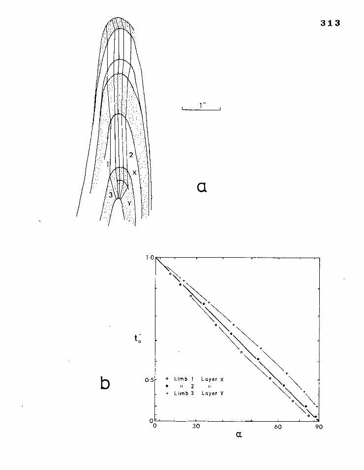
a.
313
1" I I
a
b
t a

FiF7. 7.5 F2 folds below the footpath opposite the harbour arm.
a) Isogons drawn at 20° intervals of dip on the fold profile.
Stippling Sandstone beds (except beds Y & Z that are
siltstones)
No stippling Slates.
b) Plots of -P02, against cos2a for fold A in the massive sandstone X.
Note: in fold A layer XI i is the inner arc segment and 0 is the
outer arc segment.
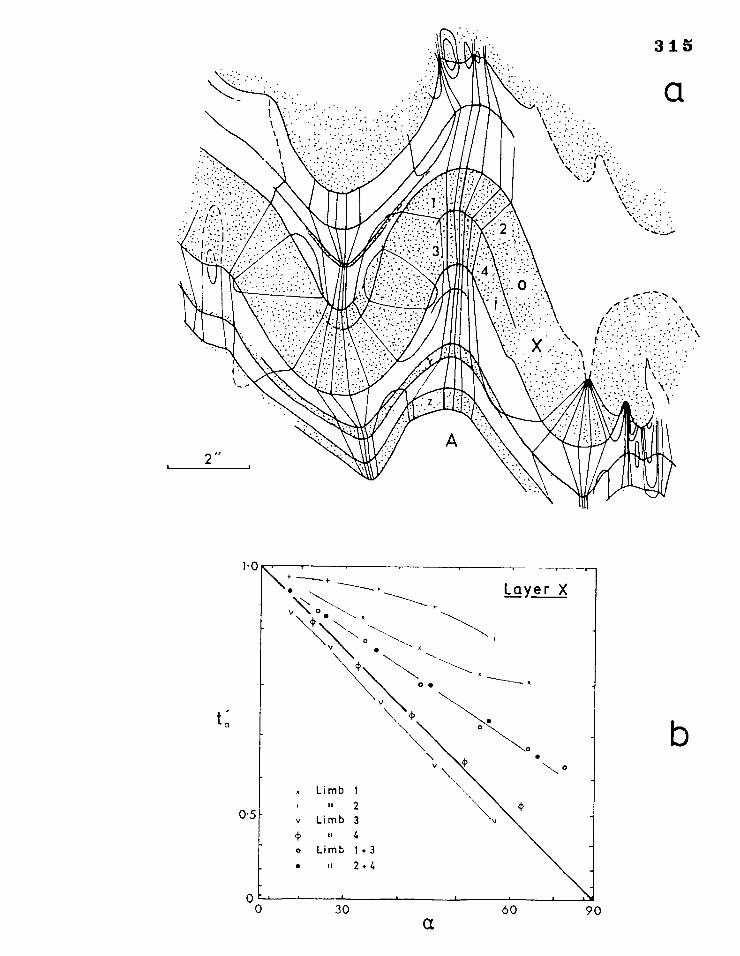
31 5
a
t b
30
60
90 a
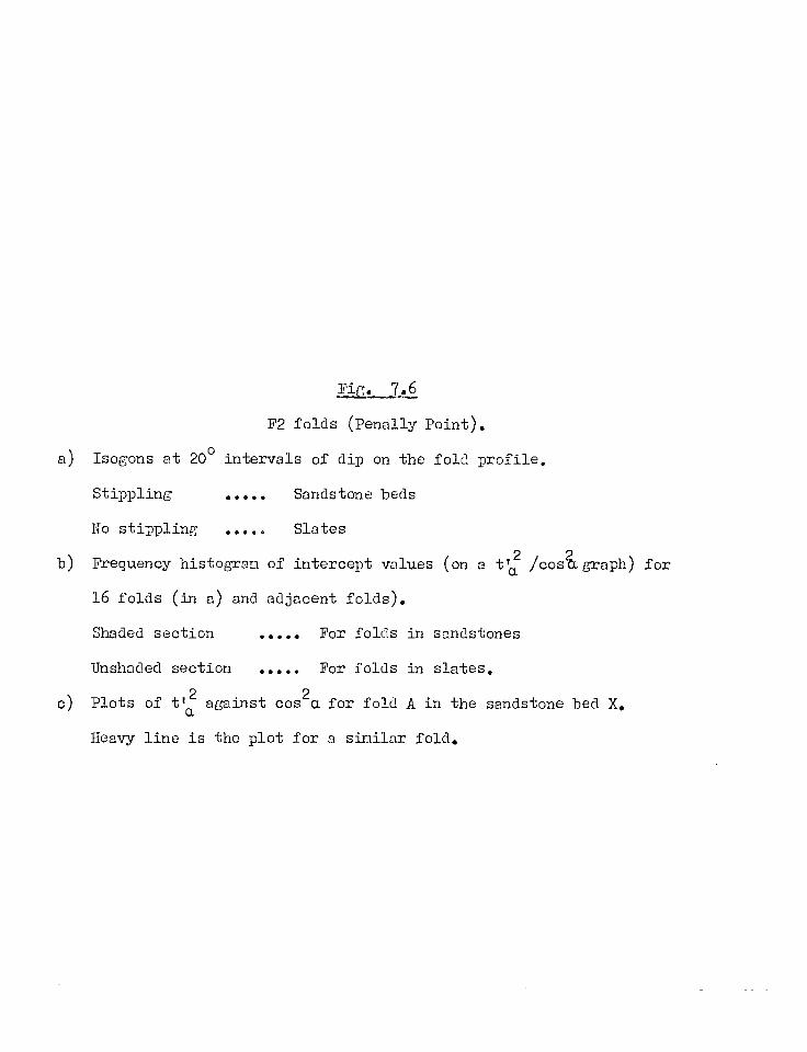
Fig. 7.6
F2 folds (Penally Point).
a) Isogons at 20° intervals of dip on the fold profile.
Stippling Sandstone beds
No stippling Slates
b) Frequency histogram of intercept values (on a t 2'a /coAgraph) for
16 folds (in a) and adjacent folds).
Shaded section For folds in sandstones
Unshaded section For folds in slates.
c) Plots of tla2 against cos2a for fold A in the sandstone bed X.
Heavy line is the plot for a similar fold.
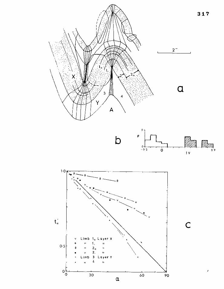
t o C
30 60 90
2-
317
a
5
F
b
- 0 3
0 09 Iv
318
in several "sandy' and 'shaly' layers from the same specimen are shown in
fig. 7.6b.
Most folds are well—represented by straight lines on a plot of t'a2
against costa (see figs. 7.4, 7.5, 7.6), and the thickness variations
with dip in the two limbs of a single fold in a layer are usually similar.
7.3.2 Harmonic Analysis of Fold Shape
Single surface fold geometry was investigated using the techniques
of visual harmonic analysis described in section 2.5 and utilised in
Chapter 6. The analysis is based on matching 'quarter wavelength units'
of folds with a series of idealised fold forms (see section 2.5). 35
and 166 quarter wavelength units of folds were analysed in the F1 and F2
fold phases respectively.
The synthesised data is presented in the form of frequency histograms
of 'shape' and 'amplitude' of both Fl (fig. 7.7a) and F2 (fig. 7.7b &c)
folds. In the case of F2 a distinction has been made between the inner
and outer arcs of folds in sandstone layers (which is roughly equivalent
to making the distinction between the outer and inner arcs respectively,
of folds in slaty layers). This distinction could not be made in
most F1 folds. In fig. 7.7c the data for folds in sandstone layers
whose thickness is small compared with their lidblengths (roughly with
a limblength/thickness ratio of greater than 20:1) have been separated
from the distribution in fig. 7.7b. The points of interest in these
distributions may be listed:
a) F1 and F2 folds all have sharp crests: in F2 'shape' categories
D, E and F predominate, and :in F1, E and F.
b) In F2 there is a distinct difference in the 'shape' distributions
between the inner and outer arcs of the folds in sandstone layers.
The outer arcs have more rounded crests (with a peak in the
'shape' category D) than the inner arcs (with a peak in category F).
Fif. 7.7
Harmonic Analysis.
Frequency histograms of 'shape' and 'amplitude'.
a) For 166 F2 folds (shaded distribution) and 37 Fl folds (unshaded).
b) For 87 inner arcs (shaded) and 79 outer arcs (unshaded) of F2 folds
in sandstone layers.
c) For 26 inner arcs (shaded) and 26 outer arcs (unshaded) of F2 folds
in thin sandstone layers.
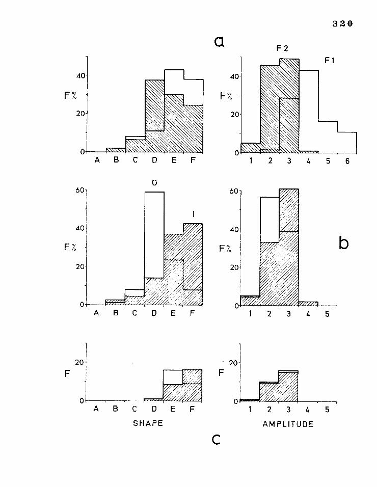
a F 2
F1
40 40-
F% F%
20-
0 1 2 3 4 5 6
320
0 60- 60-
40-
F% -
A B C D E F
20-
0
20F-
A BC DE F 1 2 3 4
SHAPE
AMPLITUDE
C
321
c) The distribution of outer arc 'shapes' in F2 is more restricted (and
the mode frequency is greater) than that of the inner arcs.
d) The distributions of 'shape' relating to the thin sandstones (fig.
7.70) in F2 show little difference between inner and outer arcs.
e) The 'amplitudes' of the F2 folds fall mainly in categories 2 and 3 (and the inner arcs tend to have slightly higher smplitudes than the
outer). The 'amplitudes' of the Fl folds fall mostly in the higher
categories 3, 4 and 5, and are more variable. (Note that the extra
'amplitude' category 6 has been included here as defined on page 275).
An example of data for several F2 folds in plate 16, is presented in
box diagram form in fig. 7.8, where the differences in position of plot
between outer and inner arcs of folds in sandstones layers is marked.
7.3.3 Deformed Lineation Loci
Several examples of an Fl mineral lineation deformed around individual
F2 folds of hand specimen size, were carefully measured to determine the
pattern of the deformed lineation loci. Data for two examples is
presented in fig. 7.9. In both these the measured Fl lineation lies
on the outer arc surface of a folded well-laminated sandstone bed, and in
both cases the angle between the F2 fold axis and the F1 lineation is
about 70°9 remaining faily constant about the F2 fold. The deformed
lineations appear to follow small circle paths on a stereogram.
7.3.4 interlimb Angles and Limb Length Ratios
About 160 F2 interlimb angles were measured on several folds in a
large number of specimens, and the results are presented in histogram
forb in fig. - 7.10a.. Tho mean interlimb angle is 61°, and the range is
rather large, from isoclinal to about 160°, with 85% of the values lying
in a 50° range between 350 and 850.
Fig. 7.8
Visual Harmonic Analysis.
Plots of 'shape' against 'amplitude' for a number of folds in plate 16.
0 Outer arcs of folds in sandstone beds.
X Inner arcs of folds in sandstone beds.
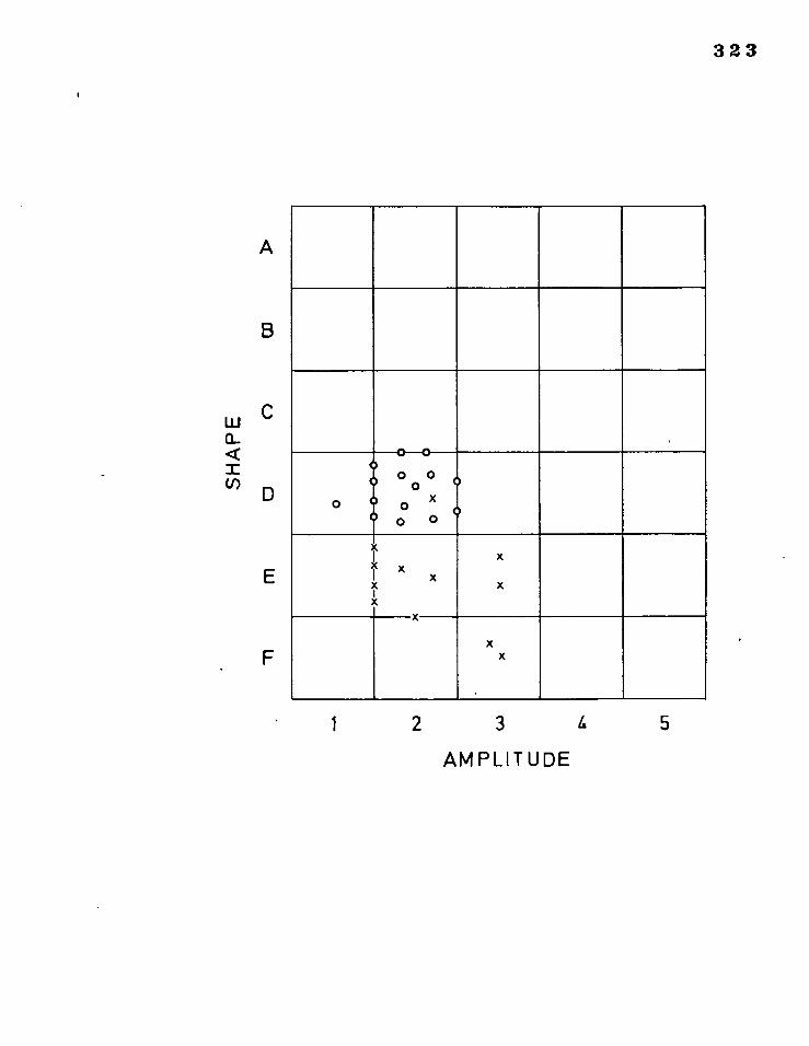
323
B
E
F
0 0 0 0
0 0
0 0 o
0 x C o 0
0
0
x x x x
x
x
x
x
x
•
x
1
2 3 4 5
AMPLITUDE
w C a_
U) D
aa2.2
Fl lineations (plotted on a Wulff stereographic net) deformed around
individual F2 minor folds.
L - Measured point on lineation locus
F F2 minor fold axis
A.S. - Axial surface
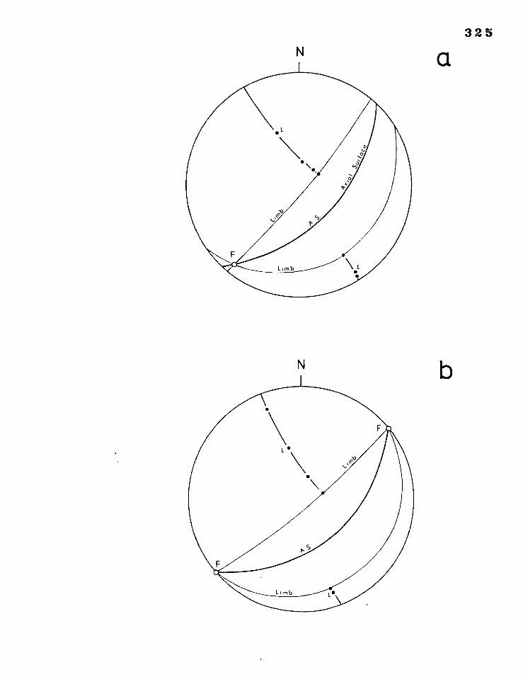
325 N a
N b
FiF. 7.10
a) Frequency histogram of interlimb angles of 160 F2 folds.
Grouped mean = 61°.
b) Frequency histogram of limb length ratios for 86 F2 folds.
(Note: the tails of this histogram have been truncated).
1.11
F2 folds (Penally Point), viewed towards the west.
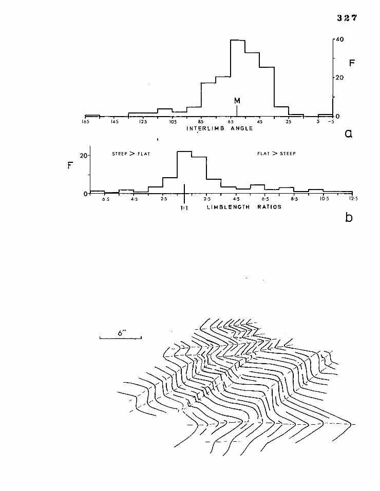
327
-40
F
M
II 165
r-1
145 125 105 8'565 4.5 INTERLIMB ANGLE
25 5 -5
a
20
I- 0
STEEP > FLAT FLAT > STEEP 20- F
65 4.5 25 25 4.5 6.5 8.5 105 12,5
1 1 LIMBLENGTH RATIOS
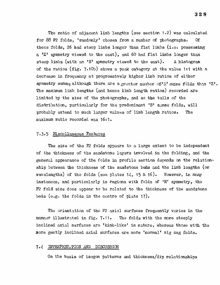
328
The ratio of adjacent limb lengths (see section 1.2) was calculated
for 88 F2 folds, 'randomly' chosen from a number of photographs. Of these folds, 26 had steep limbs longer than flat limbs (i.e. possessing
a 'Z' symmetry viewed to the east), and 60 had flat limbs longer than
steep limbs (with an 'S' symmetry viewed to the east). A histogram
of the ratios (fig. 7.10b) shows a peak category at the value 1:1 with a
decrease in frequency at progressively higher limb ratios of either
symmetry sense; although there are a,sTeater number ofISI =rise folds thnn
The maximum limb lengths (and hence limb length ratios) recorded are
limited by the size of the photographs, and so the tails of the
distribution, particularly for the predominant 'S' sense folds, will
probably extend to much larger values of limb length ratios. The
maximum ratio recorded was 16:1.
7.3.5 Miscellaneous Features
The size of the F2 folds appears to a large extent to be independent
of the thickness of the sandstone layers involved in the folding, and the
general appearance of the folds in profile section depends on the relation—
ship between the thickness of the sandstone beds and the limb lengths (or
wavelengths) of the folds (see plates 14, 15 & 16). However, in many
instances, and particularly in regions with folds of 'VP symmetry, the
F2 fold size does appear to be related to the thickness of the sandstone
beds (e.g. the folds in the centre of plate 17).
The orientation of the F2 axial surfaces frequently varies in the
manner illustrated in fig. 7.11. The folds with the more steeply
inclined axial surfaces are 'kink—like' in nature, whereas those with the
more gently inclined axial surfaces are more 'normal' zig zag folds.
7.4 INTERPRELITION AND DISCUSSION
On the basis of isogon patterns and thickness/dip relationships
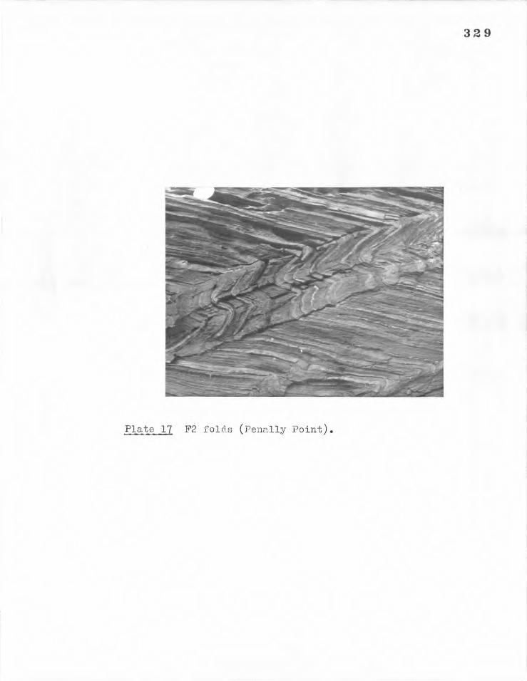
329
Plate 17 F2 folds (Penally Point).
330
(e.g. fig. 7.4), and using the criteria discussed in Chapter 5, there is
consistent evidence of slight non-passive layer behaviour during the Fl
deformation, the sandstone beds having behaved in a more competent manner
than the slates. The intensely developed slaty cleavage (usually
considered to form normal to the direction of maximum finite shortening
(see Ramsay, 1967, p.180)), the near-similar fold geometry and the tight
or isoclinal fold style are all consistent with a considerable shortening
normal to the axial surfaces of the folds. It is impossible to estimate
the amount of shortening that has occurred, but this seems almost
certainly greater than the 3C% compressive strain considered by Cloos
(1947) to be necessary in order to form slaty cleavage. The folds may
have initiated as buckles, and if so the angular fold style (indicated
in fig. 7.7) suggests that the shortening was not accompanied by further
buckling, which would have produced folds with more rounded crests.
The isogon patterns, thickness/dip plots and harmonic analysis of
the F2 folds provide evidence to suggest that the sandstone beds have
behaved in a much more competent fashion than the slates. Difficulties
in interpreting these folds arise because features of both buckling and
kinking are present. However, the folds are thought to have formed
essentially by a process of buckling in which slip between layers has
played an important role, accounting for the kink-like features observed.
This interpretation , and the problems that arise from it will now be
discussed. 'Let us first consider the features that are consistent
with a buckling hypothesis.
The fold geometry of the sandstone and slate layers is consistent
with class 1C and class 3 tyres respectively. This is a charactertistic
of buckled multilayers made up of alternating competent and incompetent
units, that have suffered a small amount of flattening (see section 3..5)
normal to the fold axial surfaces. Interpreted in this way, the mean
value of the flattening component affecting the F2 folds would be
331
,A2/.1' 1 = 0.7. This is determined for the folds in the sandstone beds
by taking the mean of the intercept distribution derived from tt(ficos20,
plots (fig. 7.3).
In the massive sandstone layer of fig. 7.5, the internal fold geometry
is that expected of a buckled layer in which deformation has been taken up
by tangential longitudinal strain, and modified by a flattening component.
(Compare fig. 7.5 with fig. 3.4a). In the well—laminated sandstone layer
of fig. 7.6, the internal geometry is closer to that expected of a buckled
layer in which the strain has beenactoommodatedby flexural slip or flow,
and again modified by a flattening component. (Compare fig. 7.6 with
fig. 3. 4b).
The loci of the early lineations deformed around folds in well—
laminated sandstone beds (fig. 7.9) are of a type produced by flexural
slip folding i.e. the angle between the F2 fold axis and the lineation
remains constant around the fold. A small component of superimposed
flattening would tend to increase this angle slightly in the fold limbs
and decrease it in the crests. This effect is seen in fig. 7.9a„ but
is not noticeable in fig. 7.9b.
In some zones of near—'M' symmetry the relationship between thickness
and wavelength in the sandstone layers suggests that fold development
was controlled by buckling.
The style of the folds is compatible with the buckling hypothesis
of Price (1967), who presents an analysis based on elastic theory that
accounts for the formation of asymmetrical folds with straight limbs and
angular or rounded crests (chevron and 'plastica' styles respectively).
Failure in the hinge regions of the buckles, in tension or in compression
(see Price, 1967, fig. 6), and subsequent 'rigid' rotation of the limbs
is the reason for the angular fold style. Price considers that this
332
process will operate in the deformation of competent and incompetent
sediments in the upper non—metamorphic parts of the crust. There is no
evidence of failure under tension in the hinges of the F2 folds, the fold
style in the competent sandstone layers is of the 'plastica' type,
produced by failure under compression in the fold hinges. In multilayers
slip between layers is a corollary of this type of buckling. In
assuming that the work done in rotating either limb of a single fold is
the same, the theory predicts greater rotation of the short limbs of
asymmetrical folds, and hence a greater slip between the layers in these
limbs. Price also predicts that the direction of the maximum principal
stress (of an 'average' stress field) will be normal to the axial surfaces
of the folds. The fold geometry within the competent beds will be
similar to that produced by tangential longitudinal strain. This is in
accord with the observations made above for the massive sandstone
beds, but not with those made for the well—laminated sandstones. The
fold geometry within the well—laminated sandstones is more consistent
with the development of chevron folds according to Ramsay (1967, Pp.440
447), who assumes that the strain is accommodated by flexural slip. Ramsay shows that chevron folds developed by flexural slip alone are
likely to 'lock' at interlimb angles of about 60° (the mean interlimb
angle of the F2 folds).
Let us now discuss the features of the F2 folds that are suggestive
of kinking (Dewey, 1965; Ramsay, 1967, p.447), and of kinking leading
to chevron folding (Paterson & Weiss, 1966).
The overall angularity of the folds, their asymmetry and development
in discrete zones are all characteristic of kinking. The occasional
occurrence of open kink structures related to more typical chevron folds
are compatible with the process of fold development described by Paterson
& Weiss (1966), by which conjugate folds form initially and with
progressive deformation interfere to form chevron folds whose axial
333
surfaces are normal to the direction of maximum compression. However,
only one of the two sets of initial kinks predicted by the theory is
actually observed among the F2 folds (see fig. 7.11)9 and there is no
evidence of interfering structures. Paterson & Weiss (1968) show how
kinking can control folding in quartz—rich layers in a phyllite. The
folds that develop in these layers show some charasteristics of buckled
competent bands, possessing rounded outer arcs and sharp inner arcs.
:according to this mode of formation, the fold size will be more or less
independent of the thicknesses of the 'competent' layers. There is often
little systematic relationship between F2 fold size and the thickness of
the 'competent' sandstone layers (plates 14, 15 & 16).
The folding process described by Paterson & Weiss(1966) provides
an alternative mode of chevron fold development to that proposed by Price
(1967). Paterson & Weiss predict that chevron folds formed in an 'ideal
foliated body' will have interlimb angles of 60°. (60° is also the
interlimb angle at which chevron folds developed, without kinking (Ramsay
1967, p.444), are prone to "lock").
It is apparent that many of the geometrical features of F2 folds
are compatible with theories of both buckling and kinking. It is
pertinent to consider the essential differences between buckling and
kinking in multilayers. In buckling the /theological contrast of the
layers is the cause of the folding instability, whereas in kinking it is
the anisotropic nature of the layering as a direction of weakness and
potential slip that can lead to a folding instability; there need be no
rheological contrast between the layers (as in kinking in a crystal).
In the case where the maximum compression acts parallel to the layering,
buckling would produce symmetrical folds with axial surfaces normal to the
compression; whereas kinking would produce asymmetrical folds with axial
surfaces inclined to the direction of maximum compression, and deformation
would be confined to the short limbs (kink zones). If multilayers pos—
sess both a rheological contrast between layers and a direction of
334
potential slip parallel to the layering, characteristics of both buckling
and kinking may appear when the multilayer is deformed. This is the case
in the series of experiments made by Ghosh (1968), and in those made by
Paterson & Weiss (1968). In both series of experiments the competent
members of the sequence displayed features of buckle folds (with rounded
outer arcs and sharp inner arcs) although the primary process of folding
was kinking leading to chevron folding.
The relationship between the orientation of the strain-slip cleavage
and the strain developed in the slates is critical to the interpretation
of these folds. The divergent fans of the strain-slip cleavage in slate
layers confined between folded sandstone beds (plates 14 & 16) are
identical to slaty cleavage fans that occur in incompetent material
sandwiched between buckled layers (see Ramsay, 1967, p.404-405). This
leads to the conclusion that the strain-slip cleavage formed normal to the
direction of maximum finite compression. The intensity of strain-slip
cleavage development, however, may not be valid indicator of the intensity
of deformation, since the presence of a slaty cleavage at a suitable
orientation to the deforming stresses is a prerequisite of strain-slip
cleavage development. !.t the stage of deformation when strain-slip
cleavage formed in the F2 folds, the short limbs may have been.in a more
suitable position than the long limbs for the development of this cleavage.
With this interpretation of the significance of the strain-slip
cleavage, the possibility that the F2 folds represent a single set of
kinks formed by shear deformation within the short limbs only, is ruled
out. The kinking/chevron folding process (Paterson & Weiss, 1966) is
unable to account for very asymmetric folds, since only one set of kinks
is likely to develop initially. It is possible that the folds developed
from a single set of kinks formed initially in discrete zones of localised
deformation, and that further deformation affected the whole rock mass so
that the direction of maximum finite shortening became normal to the
axial surface of the folds. This is the kind of interpretation made by
335
Roberts (1966) for somewhat similar structures in the Scottish Dalradian.
The interpretation for the development of the F2 folds and strain—
slip cleavage suggested here involves asymmetrical buckling (Price, 1967)
in the rock mass, and continued folding controlled in part by the
rheological contrast of the sandstones and slates, and in part by the planes
of weakness and potential slip parallel to the layering, to result in
chevron folds with axial surfaces normal to the direction of the maximum
finite compression. The strain in the competent layers (sandstones)
has been accommodated by flexural slip, tangential longitudinal strain or
in some less regular manner caused by local failure in the hinges of the
folds. In the slates, strain has been accommodated by slip on the
early slaty cleavage (mainly in the long limbs), or by some kind of
shortening along the slaty cleavage, associated with the production of
strain—slip cleavage (microfolding?). Slip between layers has been of
major importance in the long fold limbs. A small component of flattening
is thought to have affected the whole sequence. By ignoring the
'flattening', and assuming that the total length of the beds has remained
unchanged during folding, in the regions of best developed chevron folds
with interlimb angles of about 600, a shortening of about 50% normal
to the axial surfaces may be inferred.
The biggest problem with this interpretation is the degree of
asymmetry of some of the observed folds. This is certainly a primary
feature (see Breddin & Furtak, 1962), and strongly asymmetric folds are
difficult to account for by Price's theory.
Some of the difficulties in interpreting these folds would be
resolved through a better understanding of the folding processes in
multilayers with a rheological contrast between the layers, and a
direction of weakness and potential slip parallel to the layering.

336
7.5 CONCLUSIONS
A) There are systematic differences in fold geometry (slight in the Fl
folds, and very pronounced in the F2 folds) that can be related to
differences in layer composition.
B) Sandstones have consistently behaved in a more competent manner
than slates, in both folding episodes.
C) The geometric forms of the folds show features of both buckling
and kinking.
D) The primary process responsible for fold development is suggested
to be asymmetrical buckling.
E) Progressive folding has taken place by a combination of buckling
in the sandstones, and by slip between layers.
F) Strain-slip cleavage is considered to have developed normal to the
direction of the maximum finite compression in the rocks.
337
CHAPThli 8
SYNTHESIS
8.1 A COMPARISON OF RESULTS OF THE TRTTP. DETAILED FOLD STUDIES
Most of the features brought out in the geometric fold analyses
described in Chapter 5, 6 & 7 are common to folds in all three regions.
In each instance distinct overall differences in fold geometry can be
related to differences in layer composition. In the Moine rocks of Monar,
and more especially in the Culm sediments of Boscastle, differences in
fold geometry are related to distinct differences in rock composition.
In the gneisses of Sambuco, however, significant differences in the
geometric form of folds appear to be related to more subtle differences
in both composition and texture of the layers.
Both in the gneisses of Sambuco, and in the Culm of Boscastle overall
differences in the geometric form of folds exist between folds of different
generations. In progressively older fold phases, the amplitude/wavelength
ratio of folds is progressively greater, and the geometric forms of all
folds are closer to the 'similar' (class 2) fold form.
A conspicuous feature of folds in all three areas is the variable
nature of their geometric form. This is most apparent in the synthesised
data. The distributions of intercept values (on a t as 2/co/plot) for
folds in layers of different composition, or for folds of different
generations, have high values of variance and show considerable mutual
overlap. These same features are observed in the distributions of 'shape'
and 'amplitude' (of a harmonic analysis) of the inner and outer arcs of
folds in competent layers, and are also observed in the 'shape' and
'amplitude' distributions for folds of different generations.
Both in the Culm sediments and the Moine granulites, the relative
competence of layers of different composition (deduced from the fold
338
geometry) is distinct and consistent. In the metamorphic rocks of Monar,
competence decreases with an increase in the biotite content, and appears
to increase with increasing grain size. In the Culm sediments, sandstone
is much more competent than slate, and competence again appears to increase
with the grain size. In the Sambuco gneisses, however, competence vaxies
with slight changes in composition and texture of the rock. The main
compositional difference between the Sambuco gneisses and the Moine
granulites is the presence of hornblende in the former. Some property of
this mineral seems to be the major factor in determining the local change
in relative competence of the gneiss layers at Sambuco. In the meta—
morphic rocks of both Monar and Sambuco it is estimated that the maximum
'viscosity' contrast between layers of different composition is in the
order of 10:1 to 15:1.
In all instances the competent layers take on a geometric fold form
of class 1C, and the incompetent layers a variable fold form, but
predominantly one of fold class 3.
Variations of t'a2 with cos2a are nearly linear in all the measured
folds. The 'mean' fold shape of folds of different generations in each
region is close to a 'similar' (class 2) fold form. All the distributions
of intercept values (on a t'a2/cos2a graph) for all folds of any one
generation in each area are unimodal. The one exception is found in the F2
folds of Boscastle where the distribution is bimodal.
The most distinct differences between fold morphology in the three
regions is brought out in the harmonic analysis of single folded surfaces.
Most of the folds in the Monar granulites and the Sambuco gneisses match
the ideal fold forms (fig. 2.14) of 'shape' categories B, C, D & E,
indicating fold shapes varying between sinusoidal and forms very rounded
in the hinge regions. In contrast, the folds at Boscastle (of both
generations), having more angular hinges and straighter limbs, match
339
*shape' categories D, E and F. In all instances, both the inner and outer
arcs of folds in the most competent layers have the highest values of the
ratio b3/b1
(i.e. the folds are more rounded in the hinge regions). The
lower the competence contrast across a folded surface, the lower the value
of the ratio b3/b1 (and the more closely do the fold shapes approach a
sinusoidal form).
The higher the ratio of amplitude/wavelength of folds, the more
rounded are the folds in the hinge ,regions (with the exception of the Fl
folds of Boscastle).
In all three regions buckling is considered to have been the primary
process responsible for fold initiation. Continued fold development
is thoucht to have taken place by processes of both buckling and flattening.
The flattening either followed or accompanied the buckling. Where several
generations of folds are present in one region, the folds of older
generations appear to have undergone more flattening than younger
generation folds. The F2 folds of Boscastle show very little effects
of flattening. They also differ from all the other folds analysed in
that they show geometric features of both buckling and kinking. This is
attributed to the rock-mass having properties of both a rheological
contrast between the layers (of sandstone and slate), and a direction
of weakness and potential slip parallel both to the layering and the Fl
slaty cleavage.
In summary, the general pattern of fold geometry in the rocks of
these three regions is very much the same, and is consistent with a hypot-
hesis of fold development involving buckling in a multilayer (with layers
of different 'viscosity'), modified by varying amounts of flattening.
The folds in the Culm rocks of Boscastle, and particularly the F2 folds
there, do show a number of features not observed in folds in the other
regions. These features were probably produced by kinking. This
340
difference between the folds in the Culm and folds in the other regions
reflects the different mechanical state of the rocks, and the differences
in external conditions (of temperature and pressure)that existed at the
time of fold development .
8.2 SUICARY AND CONCLUSIONS
The principal concern of this thesis has been with fold morphology.
Attempts have been made to link theoretical and experimental work to
natural fold studies by means of accurate geometrical fold analysis.
The existing methods of geometrical fold analysis have been critically
reviewed; many were found to be impracticable. Two new analytical
techniques have been developed, one involving the use of dip isogons (and
concerned with folded layer geometry), and the other based on harmonic
analysis of single folded surfaces. A simple and rapid method of visual
harmonic analysis has been developed that should prove useful to the
field geologist.
Theories of fold development have been discussed with particular
emphasis on the predictions they make for fold shape and the development
of fold shape in an isolated competent layer embedded in a less competent
matrix.
A series of buckling experiments on single layers of a viscous
material embedded in a less viscous medium at low viscosity contrasts
have been described. The shape and progressive changes in shape of the
experimentally developed folds have been analysed and shown to be
consistent with buckling theory. The most important outcome of this work,
not predicted by the theory, was the observation that layer shortening
ceased when the developing folds attained limb dips of about 15°. This
appeared to be a geometrical effect and, in the range of viscosity
contrasts used, to be indelpendent of the value of the viscosity ratio.
341
Three detailed analyses of minor folds in fold belts of different
ages have been described. Systematic differences in fold geometry have
been shown to exist between folds of different generations, and have also
been related to differences in layer composition. The geometry of all
these folds was shown to be consistent with that of folds formed by
buckling and modified by flattening during or after the buckling. The
folds in the Culm sediments differ from the folds in the other regions
in their angular style, and in showing geometrical features of both buckling
and kinking. Estimates of the maximum 'viscosity' contrast in the rocks
of Sambuco and Monar, made from a study of isolated buckle folds, gave
values of 10:1 to 15:1. Estimates of shortening in the profile planes
of the folds were made in the same study. In the F2 folds of Monar, a
value of the ratioiXiA2 was estimated at 10, and in the F2 folds of
Sambuco, the estimated value of this ratio was 5.
In the one instance (Monar F2 folds) where the directions of the
principal axes of the finite bulk strain could be determined, the maximum
extension axis was found to lie at a small angle to the fold axes.
342
ACKNOWLEDGEMENTS
I should like to thank Prof. J. G. Ramsay for suggesting the topic
of research and for supervision during the course of the work.
Many other people have given advice and assistance at one time or
another and I gratefully acknowledge their help.
Drs. N. Gay and N. Price assisted in the design of the shear box
used in the experiments. Dr. D. Elliott, Mr. T. Sibbald and Mr. C. Stabler
were particularly helpful in discussing certain aspects of the work.
Mrs. L. Meadows did most of the typing and Mrs. J. Date helped with
the duplicating work.
The research was carried out under the tenure of a. University of
London Postgraduate Studentship which is gratefully acknowledged.

343
REFERENCES
Agterberg, P.P. 1967. Computer Techniques in Geology.
Earth-Sci. Rev., Vol. 3, pp. 47-77.
Ashwin, D. P. 1957. The Structure and Sedimentation of the Culm
Sediments between Boscastle & Bideford, North Devon. Unpublished
Ph.D. Thesis, Univ. of London.
Barber, N. F. 1966. Fourier Methods in Geophysics. in S.K. Runcorn (ed.),
Methods and Techniques in Geophysics, Vol. 2. pp. 123-204. Inter-
science Publ., New York.
Bell, R. T., and J. B. Currie. 1964. Photoelastic Experiments related
to Structural Geology. Proc. Geol. Ass. Canada, Vol. 15, pp. 33-51.
Beloussov, V. V. 1960. Toctonophysical Investigations. Geol. Soc. Am.
Bull., Vol. 71, pp. 1255-1270.
Biot, M. A. 1957. Folding Instability of a Layered Viscoelastic Medium
under Compression. Proc. Roy. Soc. (London), Ser. A, Vol. 242, pp.
444-454. Biot, M. A. 1959. On the Instability and Folding Deformation of a Layered
Viscoelnqtic Medium in Compression. J. Appl. Mechanics, Ser. E,
Vol. 26, pp. 393-400.
Biot, M.A. 1961. Theory of Folding of Stratifies,'. Viscoelastic Media
and Its Implications in Tectonics and Orogenesis. Geol. Soc. Am,
Bull., Vol. 72, pp. 1595-1620.
Biot, M. A., H. Ode, and W.L. Roever. 1961. Experimental Verification
of the Theory of Folding c.7 Stratified Viscoelastic Media. Geol.
Soc. Am. Bull., Vol. 72, pp. 1621-1630.
Biot, M.A. 1964. Theory of Viscous Buckling of a Confined Multilayered
Structure. Geol. Soc. Lm. Bull., Vol. 75, pp. 563-568.
344
Biot, M.A. 1965a. Mechanics of Incremental Deformation. John Wiley &
Sons, Inc., New York, 504 pp.
Biot, M.A. 1965b. Further Development of the Theory of Internal Buckling
of Multilayers. Geol. Soc. Am. Bull., Vol. 76, pp. 833-840.
Biot, M.A. 1965c. Theory of Similar Folding of the First and Second Kind.
Geol. Soc. Am. Bull., Vol. 76, pp. 251-258.
Breddin, H. 1957. Tektonische Fossil and Gesteinsdeformation im Gebiet
von St. Goarhausen. Decheniana, Vol. 110, pp. 289-350.
Breddin, H., and H. Furtak. 1962. Zur Geometrie asymmetrischer Falten.
Geol. Mitt. Aachen, Vol. 3, pp. 197-219.
Busk, H.G. 1929. Earth Flexures. Cambridge Univ. Press, London 106 pp.
Campbell, J.D. 1951. Some Aspects of Rock Folding by Shear Deformation.
Am. J. Sci., Vol. 249, pp. 625-639.
Campbell, J.D. 1958. En Echelon Folding. Econ. Geol., Vol. 53, PP.448-472.
Carey, S.W. 1954. The Rheid Concept in Geotectonics. J. Geol. Soc. Austr.
Vol. 1, pp. 67-117.
Chadwick, B. 1968. Deformation and Metamorphism in the Lukmanier Region,
Central Switzerland. Geol. Soc. Am. Bull., Vol. 79, pp.1123-1150.
Chapple, W.M. 1964. A Mathematical Study of Finite Amplitude Rock-Folding.
Unpublished Ph.D. Thesis. California Institute of Technology.
Chapple, W.M. 1968. A Mathematical Theory of Finite-Amplitude Folding.
Geol. Soc. Am. Bull., Vol. 79, pp. 47-68.
Cloos, E. 1947. Colite Deformation in the South Mountain Fold, Maryland.
Geol. Soc. Am. Bull., Vol. 58, pp. 843-918.
Cruden, D.M. 1968. Methods of Calculating the Axes of Cylindrical Folds:
Areview. Geol. Soc. Am. Bull., Vol. 79, PP. 143-148.
Currie, J.B., H.W. Patnode and R.P.Trump. 1962. Development of Folds
in Sedimentary Strata. Geol. Soc. Am. Bull., Vol. 73, pp. 655-674. Dearman, W.R. and E.C. Freshney. 1966. Repeated Folding at Boscastle,
North Cornwall, England. Proc. Geol. Assoc., Vol. 77, pp. 199-215.
345
de Sitter, L.U. 1964. Structural Geology. 2nd. Ed. McGraw-Hill Book Co.,
Yew York, 551 pp.
Dewey, J.F. 1965. Nature and Origin of Kink-Bands. Tectonophysics,
Vol. 1, pp. 459-494. Donath, F.A. 1963. Fundamental Problems in Dynamic Structural Geology.
in T.W. Donnelly (ea.), The Earth Sciences. pp. 83-103. Univ. of
Chicago Press, Chicago, Ill.
Donath, F.A. and R.B. Parker. 1964. Folds and Folding. Geol. Soc. Am.
Bull., Vol. 75, PP. 45-62.
Elliott, D. 1965. The Quantitative Mapping of Directional Minor
Structures. J. Geol., Vol. 73, pp. 865-880.
Elliott, D. 1968. Interpretation of Fold Geometry from Isogonic Maps.
J. Geol. Vol. 76, pp. 171-190.
Fleuty, M.J. 1964. The Description of Folds. Proc. Geol. Assoc., Vol.
75, 140. 461-492. Flinn, D. 1958. On Tests of Significance of Preferred Orientation in
Three Dimensional Fabric Diagrams. J. Geol., Vol. 66, pp. 526-539.
Flinn, D. 1962. On Folding during Three Dimensional Progressive Deformation.
Quart. J. Geol. Soc., Vol. 118, pp. 385-433.
Flinn, D. 1965. Deformation in Metamorphism. in W.S. Pitcher & G.W. Flinn
(eds.), Controls of Metamorphism. pp. 46-72. Oliver & Boyd, Edinburgh.
Freshney, M.C. McKeown, M. Williams, and W.R. Dearman. 1966.
Structural Observations in the Bude to Tintagel Area of the Coast
of North Cornwall, England. Geol. en Mijnb., Vol. 45, PP. 41-47.
Gay, N.C. 1966. The Deformation of Inhomogeneous Materials and Consequent
Geological Implications. Unpublished Ph.D. Thesis, Univ. of London.
Ghosh, S.K. 1966. Experimental Tests
Strain Ellipsoid in Simple Shear
Vol. 3, pp. 169-185.
Ghosh, S.K. 1967. Experimental Tests
Strain Ellipsoid in Simple Shear
physics, Vol. 4, PP. 341-343.
of Buckling Folds in Relation to
Deformations. Tectonophysics,
of Buckling Folds in Relation to
Deformations: a Reply. Tectono-
346
Ghosh, S.K., and H. Ramberg. 1968. Buckling Experiments on Intersecting
Fold Patterns. Tectonophysics, Vol. 5, pp. 89-105.
Ghosh, S.K. 1968. Experiments of Buckling of Multilayers which permit
Interlayer Gliding. Tectonophysics, Vol. 5, pp. 207-250.
Grovsky, M.V. 1959. The Use of Scale Models in Tectonophysics. Internat.
Geol. Rev., Vol. 1, pp. 31-47.
Harbaugh„ J.W., and F.W. Preston. 1965. Fourier Series Analysis in Geology.
Symposium Computer Applications in Mineral Exploration. Tuscon,
Arizona. V.I. pp. R1-R46.
Hasler, P. 1949. Geologie und Petrographie der Sambuco-Massari-
Gebirgsgruppe zwischen der oberen Valle Leventina und Valle Maggia
im nordlichen Tessin. Schweiz. Min. Petr. Mitt., Vol. 29, pp. 50-150.
Heading, J. 1963. Mathematical Methods in Science and Engineering. Edward
Arnold Ltd., London 628 pp.
Heard, H.C. 1968. Experimental Deformation of Rocks and the Problem of
Extrapolation to Nature. in R.E. Riecker (ed.), Rock Mechanics
Seminar. pp. 439-507. Spec. Report, Terr. Sci. Lab., Air Force
Cambridge Res. Labs., Bed., Massachusetts.
Heim, A. 1921. Geologie der Schweiz. II, Tauchnitz, Leipzig.
Higgins, A.K. 1964. The Structural and Metamorphic Geology of the Area
between Nufenenpass and Basodino, Tessin, South Switzerland.
Unpublished Ph.D. Thesis, Univ. of London.
Hills, E.S. 1963. Elements of Structural Geology. John Wiley & Sons Inc.,
New York, 483 pp.
Hubbert, M.K. 1937. Theory of Scale Models as Applied to the Study of
Geologic Structures. Geol. Soc. Am. Bull., Vol. 48, pp. 1459-1520.
Ickes, E.L. 1923. Similar, Parallel and Neutral Surface Types of Folding.
Econ. Geol., Vol. 18, pp. 575-591.
Johnson, M.R.W. 1956. Conjugate Fold Systems in the Moine Thrust Zone
in the Lochcarron and Coulin Forest Areas of Wester Ross. Geol.
Mag., Vol. 93, ' T.P. 345-350.
347
Johnson, M.R.W. 1965. Torridonian and Moinian. in G.Y. Craig (ed.),
The Geology of Scotland. pp. 79-113. Oliver & Boyd, Edinburgh.
Kelley, J.C. 1968. Least Squares Analysis of Tectonite Fabric Data.
Geol. Soc. Am. Bull., Vol. 79, pp. 223-240.
Kreyszig, E. 1967. Advanced Engineering Mathematics. 2nd Ed. John Wiley
& Sons, Inc., New York, 898 pp.
Krumbein, W.C. 1966. Classification of Map Surfaces based on the Structure
of Polynomial and Fourier Coefficient Matrices. Geol. Surv. Kansas,
Computer Contrib. No. 7, pp. 12-18.
Loudon, T.V. 1963. The Sedimentation and Structure in the Macduff District
of North Banffshire and Aberdeenshire. Unpublished Ph.D. Thesis,
Univ. of Edinbureh.
Loudon, T.V. 1964. Computer Analysis of Orientation Data in Structural
Geology. Tech. Report Geog. Branch Off. Naval Res., O.N.R. Task No.
389-135, Contr. No. 1228 (26), No. 13, pp. 1-130
McBirney, A.R., and M.G. Best. 1961. Experimental Deformation of Viscous
Layers in Oblique Stress Fields. Geol. Soc. Am. Bull., Vol. 72,
PP. 495-498. Mertie, J.B. 1940. Stratigraphic Measurements in Parallel Folds. Geol.
Soc. Am. Bull., Vol 51, pp. 1107-1134.
Mertie, J.B. 1959. Classification, Delineation and Measurement of
Non—parallel Folds. U.S. Geol. Surv. Profess. Paper 314 B, pp. 91-124.
mukhopadhiai, D. 1964. Caledonian Structure and Metamorphism in Eastern
Part of Glen Strathfarrar, Inverness—shire, Scotland. Unpublished
Ph.D. Thesis, Univ. of London.
MUkhopadhyay, D. 1965a. Effects of Compression on Concentric Folds and
Mechanism of Similar Folding. J. Geol. Soc. India, Vol. 6, pp. 27-41
NUkhopadhyay, D. 1965b. Some Aspects of Coaxial Refolding. Geo. Rund.,
Vol. 55, pp. 819-825.
Norris, D.K. 1963. Shearing Strain in Simple Folds in Layered Media.
Geol. Surv. Canada, Paper 63-2, pp. 26-27.
Osakina„ D.N., M.V. Grovsky, G.V. Vinogradov, and V.P. Pavlov, 1960.
Optical Polarisation Study of Plastic Deformation Processes with
348
the aid of Ethylcellulose Solutions and Gels. Kolloidnyi Zh.,
Vol. 22, pp. 434-441; English Translation: Colloid J. Vol. 22,
PP. 439-445. Paterson, M.S., and L.E. Weiss, 1962. Experimental Folding in Rocks.
Nature, Vol. 195, pp. 1046-1048.
Paterson, M.S. and L.E. Weiss. 1966. Experimental Deformation and Folding
in Phyllite. Geol. Soc. Am. Bull., Vol. 77, pn. 343-374.
Paterson, M.S. and L.E. Weiss. 1968. Folding and Boudinage of Quartz-Rich
Layers in Experimentally Deformed Phyllite. Geol. Soc. Am. Bull.,
Vol. 79, pp. 795-812.
Peach, B.N. and Others. 1913. The Geology of Central Ross-shire. Mem.
Geol. Surv. Scotland.
Phillips, A., and J.G. Byrne, 1968. Structural Analysis by the Construction
of Sections in Highly Deformed Rocks. (Abstract). in "Displacement
within Continents". Joint Symp. of Geol. Soc. Land., and Yorks.
Geol. Soc.
Potter, J.F. 1967. Deformed Micaceous Deposits in the Downtonian of the
Llandeilo Region, South Wales. Proc. Geol. Assoc., Vol. 78, pp.277-288.
Powell, C.M. 1967. Studies in the Geometry of Folding and Its Mechanical
Interpretation. Unpublished Ph.D. Thesis, Univ. of Tasmania.
Preston, F.W., and J.H. Henderson. 1964. Fourier Series Characterisation
of Cyclic Sediments for Stratigraphic Correlation. in D.F. Merriam
(ed.), Symposium on Cyclic Sedimentation. Kansas Geol. Surv. Bull.,
Vol. 2, pp. 415-425.
Price, N.J. 1967. The Initiation and Development of .Asymetrical Buckle
Folds in Non-Metamorphosed Competent Sediments. Tectonophysics,
Vol. 4, pp. 173-201.
Ramberg, H. 1952. The Origin of Metamorphic and Metasomatic Rocks. Univ.
Chicago Press, Chicago, 317 pp.
Ramberg, H. 1959. Evolution of Ptygmatic Folding. Norsk Geol. Tidsskr.,
Vol. 39, PP. 99-151.
349
Ramberg, H. 1961a. Contact Strain and Folding Instability of a Multi-
layered Body under Compression. Geol. Rund.,Vol. 51, pp. 405-439.
Ramberg, H. 1961b. Relationship between Concentric Longitudinal Strain
and Concentric Shearing Strain during Folding of Homogeneous Sheets
of Rock. Am. J. Sci., Vol. 259, Pp. 382-390.
Ramberg, H. 1963a. Strain Distribution and Geometry of Folds. Bull.,
Geol. Inst. Univ. Uppsala, Vol. 42, pp. 1-20.
Ramberg, H. 1963b. Fluid Dynamics of Viscous Buckling Applicable to
Folding of Layered Rocks. Bull. Am. Assoc. Petrol. Geol., Vol. 47,
PP. 484-515.
Ramberg, H. 1963c. Evolution of Drag Folds.
Geol. Mag., Vol. 100, pp. 97-106.
Ramberg H. 1964a. Selective Buckling of Composite Layers with Contrasted
Rhoological Properties: a Theory for Simultaneous Formation of
Several Orders of Folds. Tectonophysics, Vol. 1, pp. 307-341.
Ramberg, H. 1964b. Note on Model Studies of Folding of Moraines in
Piedmont Glaciers. J. Glaciology, Vol. 5, pp.207- 218.
Ramberg H, 1967. Gravity, Deformation and the Earth's Crust, as Studied
by Centrifuged Models. Academic Press, London 214 PP.
Ramberg, H., and S.K. Ghosh. 1968. Deformation Structures in the Hovin
Group Schists in the Hommelvik Hell Region (Norway). Tectonophysics,
Vol. 6, pp. 311-330.
Ramsay, J.G. 1954. The Stratigraphy, Structure and Metamorphism of the
Lewisian "Inlier" and Moine Rocks of Glen Strathfarrar, Ross-shire.
Unpublished Ph.D. Thesis, Univ. of London.
Ramsay, J.G. 1958. Superimposed Folding at Loch Monar, Inverness-shire
and Ross-shire. Quart. J. Geol. Soc., Vol.113, pp. 271-307.
Ramsay, J.G. 1962a. The Geometry and Mechanics of Formation of "Similar"
Type Folds. J. Geol. Vol. 70, pp. 309-327.
Ramsay, J.G. 1962b. The Geometry of Conjugate Fold Systems. Geol. Mag.,
Vol. 99, pp. 516-526
350
Ramsay, J.G. 1963. Structure and Metamorphism of the Moine and Lewisian
Rocks of the North-west Caledonides. in Johnson & Stewart (eds.),
The British Caledonides. pp. 143-175. Oliver & Boyd Ltd., Edinburgh.
Ramsay, J.G. 1967. Folding and Fracturing of Rocks. McGraw-Hill Book Co.,
New York, 568 pp.
Rast, N. 1964. Morphology and Interpretation of Folds - a Critical Essay.
Geol. J., Vol. 4 pp. 177-188. Reiner, M. 1960. Deformation, Strain and Flow. 2nd. Ea. H.K. Lewis and Co.,
London, 347 PP-
Roberts, J.L. 1966. The Formation of Similar Folds by Inhomogeneous
Plastic Strain, with Reference to the Fourth Phase of Deformation
Affecting the Dalradian Rocks in the Southwest Highlands of Scotland.
J. Geol., Vol. 74, pp. 831-855. Schryver, K. 1966. On the Measurement of the Orientation of Axial Planes
of Minor Folds. J. Geol., Vol. 74, PP. 83-84.
Selwood, E.B. 1961. The Upper Devonian and Lower Carboniferous Stratigraphy
of Boscrstle and Tintagel, Cornwall. Geol. Mag., Vol. 98, pp. 161-167.
Sherwin, J. and W.M. ChapDle, 1968. Wavelengths of Single Layer Folds:
a Comparison between Theory and Observation. Am. J. Sci., Vol. 266,
pp. 167-179.
Singh, R.P. 1967. Experimental Tests of Buckling Folds in Relation to
Strain Ellipsoid in Simple Shear Deformations: a Discussion.
Tectonophysics, Vol. 5, pp. 341-343.
Speight, J.G. 1965. Meander Spectra of the Augabunga River. J. Hydrol.,
Vol. 3, pp.1-15.
Stabler, C.L. 1968. Simplified Fourier Analysis of Fold Shapes.
Tectonophysics, Vol. 6, pp. 343-350.
Stauffer, M.R. 1966. An EMpirical-Statistical Study of Three-Dimensional
Fabric Diagrams as Used in Structural Analysis. Can. J. Earth Sci.,
Vol. 3, PP. 473-498.
Stone, R.O., and J. Dugundji. 1965. A study of Microrelief- Its Mapping,
Classification and Quantification by Means of a Fourier Analysis.
Eng. Geol., Vol. 1, pp. 89-187.
351
Timoshenko, S. 1960. Strength of Materials. Part 1. D. van Nostrand Co. Inc.,
Princeton, New Jersey, 442 pp.
Turner, F.J., and L.E. Weiss. 1963. Structural Analysis of Metamorphic
Tectonites. McGraw-Hill Book Co., New York, 545 pp.
van Hise, C.R. 1896. Principles of North American Pre-Cambrian Geology.
U.S. Geol. Surv. 16th Ann. Rept., part 1, pp. 571-843.
Watson, G.S. 1966. The Statistics of Orientation Data. J. Geol., Vol. 74,
pp. 786-797.
Wenk, E. 1962. Plagioclas als Indexmineral in den Zentralalpen. Schweiz.
Min. Petrogr. Mitt., Vol. 42, pp. 139-152.
Whitten, E.H.T., and J.J. Thomas. 1965. Geometry of Folds Portrayed by
Contoured by Maps: a New Method for Representing the Geographical
Variability of Folds. Geol. Soc. Am. Spec. Paper No . 87, p.186.
Whitten, E.H.T. 1966a. Structural Geology of Folded Rocks ▪ Rand McNally
& Co., Chicago, 663 pp.
Whitten, E.H.T. 1966b. Sequential Multivariate Regression Methods and
Scalars in the Study of Fold-Geometry Variability. J. Geol., Vol. 74,
PP• 744-763. Williams, E. 1965. The Deformation of Competent Granular Layers in
Folding. Am. J. Sci., Vol. 263, pp. 229-237.
Williams, E. 1967. Notes on the Determination of Shortening by Fle.Xure
Folding Modified by Flattening. Papers & Proc. Roy. Soc. Tasmania,
Vol. 101, pP. 37-41.
Wilson, G. 1952. rtYgmatic Structures and Their Formation. Geol. Mag.,
Vol. 89, pp. 1-21.
Wilson, G. 1967. The Geometry of Cylindrical and Conical Folds. Proc.
Geol. Assoc., Vol. 78, pp. 179-210.
Wynne-Edwards, H.R. 1963. Flow Folding. Am. J. Sci., Vol 261. pp. 793-814.
Zwart, H.J. 1964. The Development of Successive Structures in the
Devonian and Carboniferous of Devon and Cornwall. Geol. en Mijnb.
Vol. 43, PP. 516-526.
352
APPENDIX
PROGRAMME FOR THE CALCULATION OF HARMONIC COEFFICIENTS.
A listing is given of a programme to calculate the harmonic co-
efficients bn of a periodic function f(x) represented by discrete values
of f(x) in the period 2n. The IBM 'Share' subroutine FORIT is used to
calculate the values of the harmonic coefficients and is incorporated
in the programme. This is written in FORTRAN IV to run on an IBM 7094
computer under the IBSYS monitor.
The equations on which the calculations are based are given in
section 2.5. 2N+1 values of f(x) are taken over the range 0 - W, at
intervals of W/2N+1 (see figs. 2.9 & 2.10). For a 'quarter wavelength
unit' of a folded profile (see fig. 2.10) N+1 values of f(x) are measured
in the range 0 - WA (the origin is the first point taken). Data for
the programme are the value of N9 the number of coefficients M to be
computed (M less than or equal to N), the value of W/4 and N values
of f(x) in the range 0 - W/4 in increasing order of size (excluding
the value at the origin).
The comments on subroutine FORIT are part of the original 'Share'
programme.
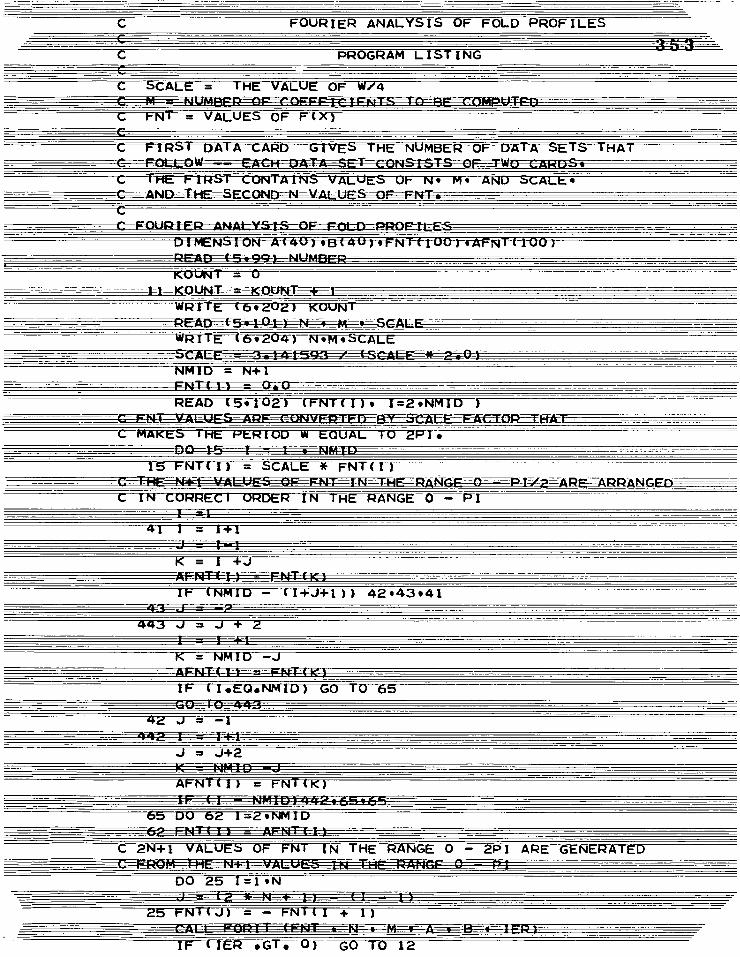
C
FOURIER ANALYSIS OF FOLD PROFILES
PROGRA LI IN
C SCALE = THE VALUE OF W/4 effirt-T-=zieVr--1;15-2
C FNT = VALUES OF f- ( X )
R-OF-DATA-SET-S- HA =FoLLiztvi-----_Eixa.v=pievrasFTefarikslEsTro
CON V A •
—At4E-THF=sEcOND_viaEur-o----E-isrr=•
FLI-14LECMEA;==ANAWitEFIES=00 0-/-r._E_,S DTMENSTON-A-(-401-0-81-4-01-vF NT-(-1-001-vAF (1-001
PEAC4-5=*-99=NUMBER
KOUts/T= WRITE (6.202)KOU
"ZI CALF
WRTTE-10204 ) N • M • SLALL
NMID = N+1
READ (5,102) (FNT(I), I=2,NMID ) •- MI:71 1 011 " Ll DMIVIVAIWA Vag • ft g '.M1 2 :
C MAKES THE PERIOD W EQUAL TO 2P1e
15 FNT(I) = SCALE * FNT(I) *MB: , — z • zf,..."1== Ai I I GE---n-7--PTZ2ffARE-7APRANGFA
C IN CORRECT ORDER IN THE RANGE 0 - PI
K = I +J
IF (NMID - (I+J+1)) 42043.41
443 J = J +
K = NMID -J Z!==i7-3
IF (I•EQ•NMID) GO TO 65
42 J = —1
J = J+2
AFNT(I) = FNT(K)
6b DO 62 1=2,NMID if M• W_ES
C 2N+1 VALUES OF FNT IN THE RANGE 0 - 2P1 APE GENERATED • '1' - -1== = I CI
DO 25 I=1,N
25 FNT(J) = - FNT(I + 1) -
IF (IER •GT• 0) GO TO 12
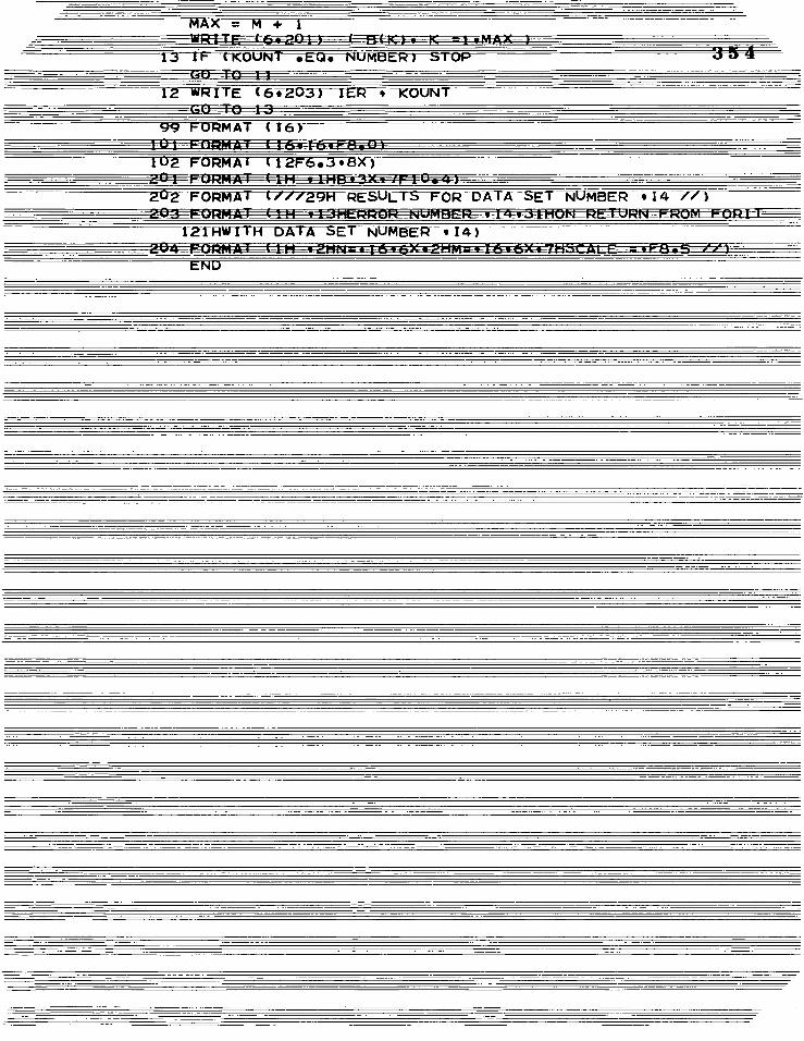
at)--E-01411tietET=4E14tiaallE4ZROINtftet
..=••==3/41.1112••1*/1Z=s11111. m401=13 It1U= .61'.:4
121HWIFH DATA SE' NUMBER 9 I4) wt
E.NU
MAX = M + 1
CKOUN MBERT—STOP
t4-1 f2 WRITE(692U3) IER KOUNT
etaMieM 99 FORMAT (I6)
V-0,---FORMA=1,6A=ECTHEFawIL) 102 FORMAT (12F6e398X) A4.1a r.. m. - n..•=u.ta 202 FORMAT (///29H RESULTS FOR DATA SE, NUMBER 914 //)
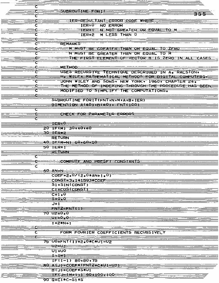
_-4ttBRoLET4tsriapnET C
C IER=0 NO ERROR C- RtA ERE
C IER=2 M LESS-THAN 0
C N MUST-BE-GREATER THAN UR LOUAL-TO-M
ER
e. • --.=i
C
USES
•
• •
0
•
:V= " = = - 2= pr.=. 03 Erg •
C JOHN-W1LEY-ANO-S
TER e4. 0 •
0 •
• 0
DEXTNG,M.HROUGHTHENvERROCEDUREBIHASBEEAEHE = 2 • '
C-- mocrI-F-1-ED-Tcy-sTmPL---rFY-T HE COMPUT rONS •
SUBROUTINE FORITTFNTITWICIAIB,IL.R, =.' a.;12 - - •
C C_ ____cHec uter-teRRo
C
20 IF(M) 30. 40+40
RETURN
0 IER=1
C
C 45_
COEF=24,0/1-20*AWT-101
SS-r-IN(CONST) Cl COS (CONS C=1.0
J=1 MX' — .7,==
70 U2=0.0
I=2*N+1
C FORM FOURIER COEFFICIENTS RECURSIVELY
7b U0=ENT(I)+2.0*c*u1-U2
80.80.75 2 I= 3.WE:=,- 'ark-Me:4 .z.":""
B(J)=COEF*5*u1
90 O=C1*C-5I*S
S=c 1 *S +Si *C C.—
..)== J+-1
ro-o—A-r-r crib __T=URN
END