the iir-ntu speaker diarization systems for rt 2009
TRANSCRIPT

The IIR-NTU Speaker
Diarization Systems for
RT 2009Trung Hieu Nguyen[1,2], Hanwu Sun [1], ShengKui Zhao [2],
Swe Zin Kalayar Khine [1] ,Huy Dat Tran [1], Tin Lay Nwe Ma [1],
Bin Ma[1], Eng Siong Chng [2], Haizhou Li [1,2]
[1] Institute for Infocomm Research, Singapore[2] Nanyang Technological University, Singapore
Outline
• System structures
• Results
• Performance analysis
• Conclusions

System Structures

Wiener Filtering
• Wiener filtering is applied to all audio channels for speech
enhancement. The implementation of Wiener filter is from
Qualcomm-ICSI-OGI front end [1].
[1] A. Adami, L. Burget, S. Dupont, H. Garudadri, F. Grezl, H. Hermansky, P. Jain, S. Kajarekar, N. Morgan, and S. Sivadas,
"Qualcomm-icsi-ogi features for asr," in Proc. ICSLP, vol. 1, 2002, pp. 4-7.
Beamforming
• The enhanced audio channels are then filtered and summed to produce
a beamformed audio channel with the BeamformIt tool-kit [2].
[2] BeamformIt acoustic beamformer. [Online]. Available: http://www.xavieranguera.com/beamformit/

TDOA Estimation (1/2) –
Microphone Pairs Selection
• Compute the histogram of all microphone pairs
50 100 150 200 250 300 350 400 450
33
42
47
55
DO
A e
stim
ate
time (sec)
DOA estimation vs. time for part of CMU_20061115-1030
33 42 47 550
2000
4000
6000
8000
10000
12000
14000
count
DOA values
Histogram of DOA values for part of CMU_20061115-1030

TDOA Estimation (2/2) –
Microphone Pairs Selection
• Find the number of peaks in the histogram for the given threshold below
• Find top 6 microphone pairs with highest detected number peaks if the possible
microphone pairs are greater than 6
• Use these 6 microphone pairs TDOA values for initial clustering.
33 42 47 550
2000
4000
6000
8000
10000
12000
14000
count
DOA values
Histogram of DOA values for part of CMU_20061115-1030
peak detection threshold
total # frames =
# histogram bins

a. Generate the 36 MFCC features (12 MFCC plus their first and second order derivatives) 30ms window with 20ms overlap
b. Select 10% highest energy with relative high zero cross rates frames as the initial speech guessing.
c. Select 20% lowest energy with relative low zero cross rates frames as the initial noise guessing
d. Train initial speech model λS and Non-speech model λNS via EM, the speech and noise model sizes are set to be 16 and 4, respectively.
e. Frame-wise maximum likelihood evaluation against λS and λNS
f. Retrain speech model λS and non-speech model λNS via MAP.
g. Compute the speech/non-speech frame ratio, if the percentage change of the ratio (compared to its previous ratio) is less than 1%, stop, otherwise go to step e.
Speech Activity Detection

Bootstrap Clustering (1/7) –
Within Pair Quantization
• Constructs a histogram of TDOA values for each selected microphone
pairs
33 42 47 550
2000
4000
6000
8000
10000
12000
14000
count
DOA values
Histogram of DOA values for part of CMU_20061115-1030
50 100 150 200 250 300 350 400 450
33
42
47
55
DO
A e
stim
ate
time (sec)
DOA estimation vs. time for part of CMU_20061115-1030

• Find the peaks in the histograms
33 42 47 550
2000
4000
6000
8000
10000
12000
14000
count
DOA values
Histogram of DOA values for part of CMU_20061115-1030
peak detection threshold
total # frames =
# histogram bins
Bootstrap Clustering (2/7) –
Within Pair Quantization

• Identifies centroids in histogram
Bootstrap Clustering (3/7) –
Within Pair Quantization
50 100 150 200 250 300 350 400 450
33
42
47
55
DO
A e
stim
ate
time (sec)
Quantized DOA estimation vs. time for part of CMU_20061115-1030

• Maps other values to nearest centroid
50 100 150 200 250 300 350 400 450
33
42
47
55
DO
A e
stim
ate
time (sec)
Quantized DOA estimation vs. time for part of CMU_20061115-1030
Bootstrap Clustering (4/7) –
Within Pair Quantization

• Using quantized TDOA from multiple microphone pairs
Bootstrap Clustering (5/7) –
Inter-Pair Quantization
33 42 47 550
2000
4000
6000
8000
10000
12000
14000
16000
count
DOA values
Histogram of DOA values for Pair 1
31 37 61 710
2000
4000
6000
8000
10000
12000
14000
16000
count
DOA values
Histogram of DOA values for Pair 2
Pair 1: Mic 1 & 2 Pair 2: Mic 1 & 3
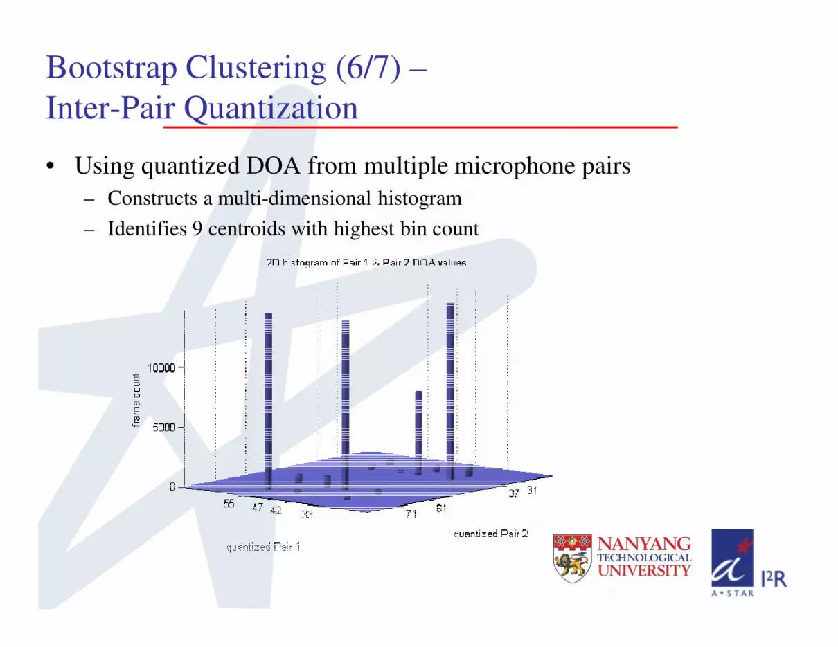
• Using quantized DOA from multiple microphone pairs
– Constructs a multi-dimensional histogram
– Identifies 9 centroids with highest bin count
Bootstrap Clustering (6/7) –
Inter-Pair Quantization

• Using quantized TDOA from multiple microphone pairs
– Constructs a multi-dimensional histogram
– Identifies 9 centroids with highest bin count (initial 9 clusters)
– Merges all other bins to the nearest centroids
• Centroids after merging are given unique labels
Bootstrap Clustering (7/7) –
Inter-Pair Quantization
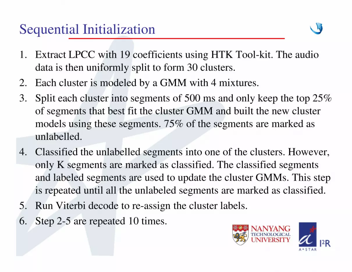
1. Extract LPCC with 19 coefficients using HTK Tool-kit. The audio
data is then uniformly split to form 30 clusters.
2. Each cluster is modeled by a GMM with 4 mixtures.
3. Split each cluster into segments of 500 ms and only keep the top 25%
of segments that best fit the cluster GMM and built the new cluster
models using these segments. 75% of the segments are marked as
unlabelled.
4. Classified the unlabelled segments into one of the clusters. However,
only K segments are marked as classified. The classified segments
and labeled segments are used to update the cluster GMMs. This step
is repeated until all the unlabeled segments are marked as classified.
5. Run Viterbi decode to re-assign the cluster labels.
6. Step 2-5 are repeated 10 times.
Sequential Initialization

Multi Stream Clustering (1/3)
• Two feature streams for clustering: TDOA and LPCC 19
• TDOA features: GMM with 2 mixtures. LPCCs: GMM with 16
mixtures. Standard agglomerative hierarchical clustering algorithm
with Viterbi re-segmentation as explained in [1].
• Modified version of CLR as the distance measure between clusters.
• The weighting algorithm is based on the Fisher distance.
• Stopping criterion: Ts criterion [2]
[1] C. Wooters and M. Huijbregts, "The ICSI RT07s speaker diarization system," Lecture Notes in Computer Science, vol.
4625, pp. 509-519, 2008.
[2] Trung Hieu Nguyen , Eng Siong Chng, Haizhou Li, “T-Test Distance and Clustering Criterion for Speaker Diarization”,
Interspeech, 2008.

Multi Stream Clustering (2/3) –
Automatic Stream Weight Selection
11 12 1, , ,K
λ λ λK 21 22 2, , , Kλ λ λK
( )( ) ( )( )1
1 1 1 1log | log |ij j i j UBMA P u P uλ λ= − ( )( ) ( )( )2
2 2 2 2log | log |ij j i j UBMA P u P uλ λ= −
1 i K≤ ≤
1 j N≤ ≤
1 2
1 2A w A w A= × + ×
{ }1 | , : ijS A i j frame j cluster i= ∀ ∈
{ }2 | , : ijS A i j frame j cluster i= ∀ ∉
K K

Multi Stream Clustering (3/3) –
Cluster Distance Measure
11 12,λ λ 21 22
,λ λ
( )( ) ( )( )1
1 1 1 1log | log |ij j i j UBMA P u P uλ λ= − ( )( ) ( )( )2
2 2 2 2log | log |ij j i j UBMA P u P uλ λ= −
1 2i≤ ≤
1 21 j N N≤ ≤ +
1 2
1 2A w A w A= × + ×
{ }1 | , : ijS A i j frame j cluster i= ∀ ∈
{ }2 | , : ijS A i j frame j cluster i= ∀ ∉
( )( ) ( )1 2 1 2
1 2
1 2
| |,
var( ) var( )
mean S mean S N Nd C C
S S
− +=
+
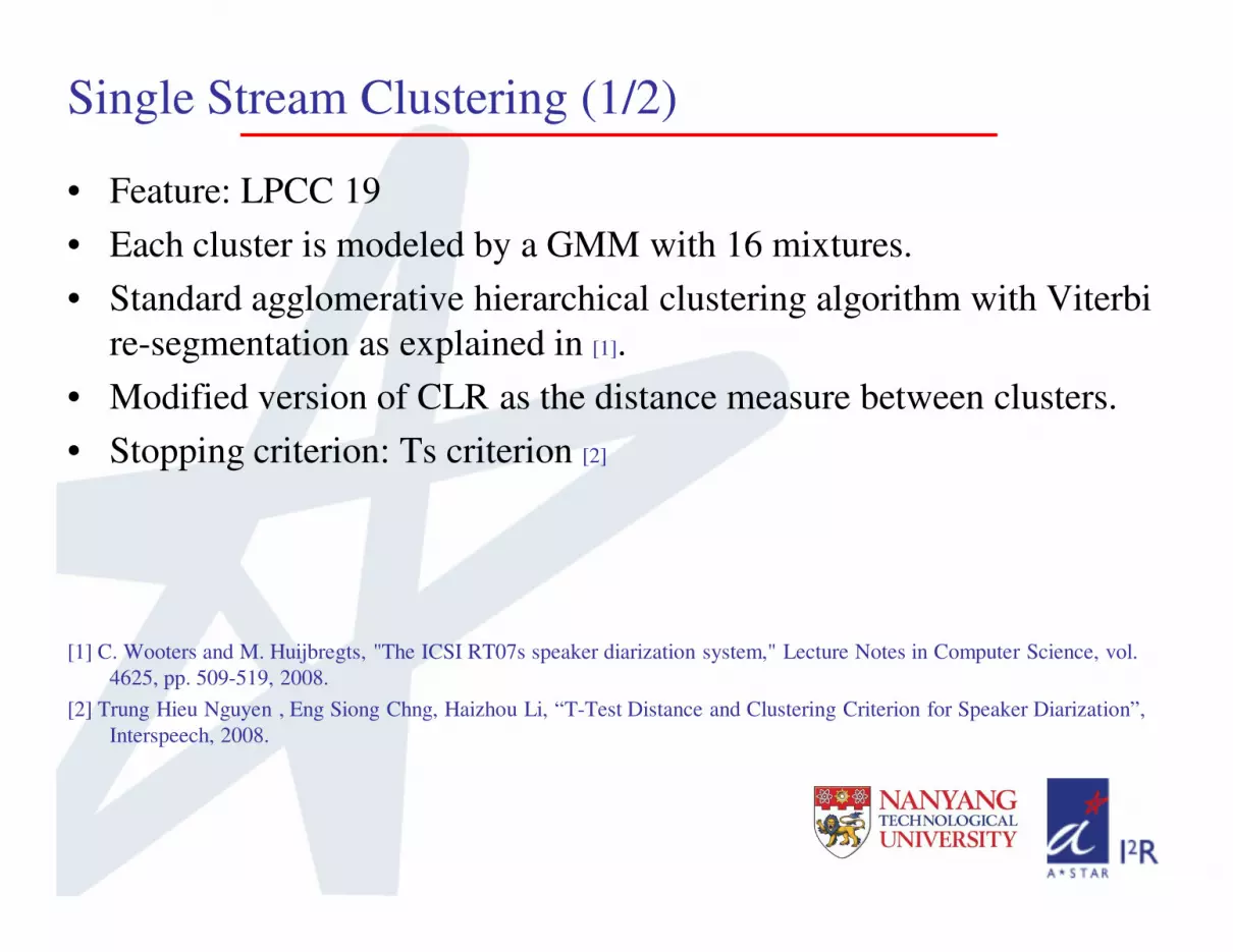
Single Stream Clustering (1/2)
• Feature: LPCC 19
• Each cluster is modeled by a GMM with 16 mixtures.
• Standard agglomerative hierarchical clustering algorithm with Viterbi
re-segmentation as explained in [1].
• Modified version of CLR as the distance measure between clusters.
• Stopping criterion: Ts criterion [2]
[1] C. Wooters and M. Huijbregts, "The ICSI RT07s speaker diarization system," Lecture Notes in Computer Science, vol.
4625, pp. 509-519, 2008.
[2] Trung Hieu Nguyen , Eng Siong Chng, Haizhou Li, “T-Test Distance and Clustering Criterion for Speaker Diarization”,
Interspeech, 2008.

Single Stream Clustering (2/2) –
Cluster Distance Measure
1 2,λ λ
( )( ) ( )( )log | log |ij j i j UBMA P u P uλ λ= −
1 2i≤ ≤
1 21 j N N≤ ≤ +
{ }1 | , : ijS A i j frame j cluster i= ∀ ∈
{ }2 | , : ijS A i j frame j cluster i= ∀ ∉
( )( ) ( )1 2 1 2
1 2
1 2
| |,
var( ) var( )
mean S mean S N Nd C C
S S
− +=
+

Results –
RT 2009 Evaluation
Mic. ConditionOverlap SPKR
Err.
Non-Overlap
SPKR Err.SAD
MDM 9.21 3.83 2.74
SDM 16.04 10.72 2.57

Performance Analysis (1/6) –
SDM Systems
System A System B System C System D System E
Feature MFCC 19 MFCC 19 LPCC 19 LPCC 19 LPCC 19
Duration
Constraint2s
0.5s with word
insertion
penalty of
-150
0.5s with word
insertion
penalty of
-150
0.5s with word
insertion
penalty of
-150
0.5s with word
insertion
penalty of
-150
Cluster
Distance
Measure
GLR GLR GLR Proposed Proposed
Initialization Uniform Uniform Uniform Uniform Sequential

Performance Analysis (2/6) –
SDM Systems
System A System B System C System D System E
RT 2005 15.57 13.00 11.95 10.88 12.08
RT 2006 27.08 20.68 17.04 18.78 19.63
RT 2007 16.96 13.54 13.25 11.94 10.92
DERs of various SDM systems with optimal stopping criterion
RT 2005 RT 2006 RT 2007
SAD (%) 3.00 4.50 3.01

Performance Analysis (3/6) –
Stopping Criteria
RT 2005 RT 2006 RT 2007
RT 2005 13.35 18.75 18.24
RT 2006 13.35 18.75 18.24
RT 2007 14.62 21.56 13.45
With GLR threshold as stopping criterion (DER)
RT 2005 RT 2006 RT 2007
DER(%) 9.94 15.21 11.78
With optimal stopping criterion

Performance Analysis (4/6) –
Stopping Criteria
RT 2005 RT 2006 RT 2007
RT 2005 12.47 28.73 25.22
RT 2006 22.78 22.94 28.23
RT 2007 17.58 35.57 20.64
With ICR threshold as stopping criterion (DER)
RT 2005 RT 2006 RT 2007
RT 2005 16.58 30.19 24.93
RT 2006 17.03 20.4 24.00
RT 2007 18.88 26.94 17.73
With BIC threshold as stopping criterion (DER)
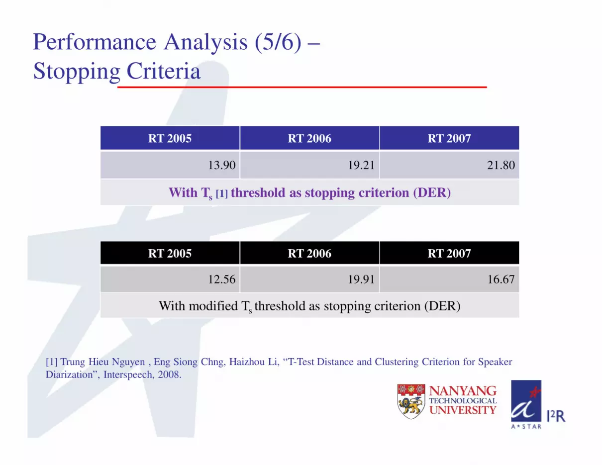
Performance Analysis (5/6) –
Stopping Criteria
RT 2005 RT 2006 RT 2007
13.90 19.21 21.80
With Ts [1] threshold as stopping criterion (DER)
RT 2005 RT 2006 RT 2007
12.56 19.91 16.67
With modified Ts threshold as stopping criterion (DER)
[1] Trung Hieu Nguyen , Eng Siong Chng, Haizhou Li, “T-Test Distance and Clustering Criterion for Speaker
Diarization”, Interspeech, 2008.

Performance Analysis (6/6) –
MDM Systems
RT 2005 RT 2006 RT 2007
Stream Weight
Selection using [1]9.08 14.37 9.59
Proposed Stream
Weight Selection8.93 12.94 9.30
DERs for MDM systems with different weighting schemes
[1] Anguera, X., Wooters, C., Pardo, J. M. and Hernando, J., Automatic Weighting for the Combination of TDOA and
Acoustic Features in Speaker Diarization for Meetings, in: Proc. ICASSP, Honolulu, 2007.
Conclusions
• Shorter duration constraint seems to improve the performance.
• It is not conclusive which acoustic features are good for speaker
diarization.
• MDM system is much better than SDM system, largely due to very
good initialization and correct stopping point.
• Performance of sequential initialization is not good. Need more
investigations.

THANK YOU !