optimization in static repositioning activities of bike ... - dr-ntu
TRANSCRIPT
This document is downloaded from DR‑NTU (https://dr.ntu.edu.sg)Nanyang Technological University, Singapore.
Optimization in static repositioning activities ofbike‑sharing systems
Zhu, Tiantian
2018
Zhu, T. (2018). Optimization in static repositioning activities of bike‑sharing systems.Doctoral thesis, Nanyang Technological University, Singapore.
http://hdl.handle.net/10356/75811
https://doi.org/10.32657/10356/75811
Downloaded on 04 Oct 2022 07:47:46 SGT

Optimization in Static Repositioning
Activities of Bike-Sharing Systems
Zhu Tiantian
School of Mechanical and Aerospace Engineering
Nanyang Technological University
This thesis is submitted for the degree of
Doctor of Philosophy
May 2018


I would like to dedicate this thesis to my dearest parents, my grandpa and myself.


Declaration
I hereby declare that except where specific reference is made to the work of others, the
contents of this dissertation are original and have not been submitted in whole or in part
for consideration for any other degree or qualification in this, or any other university. This
dissertation is my own work and contains nothing which is the outcome of work done in
collaboration with others, except as specified in the text and Acknowledgements. This
dissertation contains fewer than 65,000 words, including appendices, bibliography, footnotes,
tables and equations and has fewer than 150 figures.
Zhu Tiantian
May 2018


Acknowledgements
I would like to express the deepest gratitude to my previous supervisor, Prof. Xiaofeng
Nie, for his guidance, patience and encouragement. He suggested me to take several tough
doctoral level courses during the first and a half year of my PhD study, as my mathematical
background was not strong enough to conduct research in Operations Research. As a result, I
have acquired plenty of knowledge in the theories and methods of Operations Research and
become much more confident to do research. Moreover, his keen and vigorous academic
attitudes have greatly affected me.
A very special gratitude goes out to Prof. Andrea Raith from the University of Auckland
for her guidance and insightful recommendations to the second algorithm (in Chapter 5)
presented in this thesis. During the one-year visit at the University of Auckland, Andrea
gave me a lot of encouragement when the performance of new ideas was not as good as we
expected, so that I never stopped trying and improving. She also tried several times to reach
Bike-Sharing companies in order to get real-world data for my research.
I’m also very grateful to my current supervisor, Prof. Chun-Hsien Chen, who would like to
supervise me after my previous supervisor left and cared about my research progress during
my visiting study in Auckland, even if he was extremely busy.
I shall extend my thanks to my parents, my boyfriend, my best friends, especially Xiaofei
Qi and Guanyi Lv, and Prof. Duan Fei. They always understand me and have provided
encouragement and emotional supports in my PhD study and my life.
And finally, last but by no means least, many thanks to Nanyang Technological University
viii
and our School of Mechanical and Aerospace Engineering for providing me with the financial
support, the great environment and atmosphere to do research. Thank the University of
Auckland and their Department of Science Engineering for providing the access of NeSi Pan
Cluster and IT support for me to conduct the numerical experiment of my algorithm during
the one-year visiting.

Abstract
Bike-sharing systems have become increasingly popular in cities all over the world. Satisfying
the fluctuating and asymmetric demand is a crucial problem for bike-sharing systems. In
order to ensure a good quality of user service, repositioning activities are conducted by a fleet
of vehicles. This study focuses on the static repositioning problem, which usually happens at
night and assumes no demand occurs during the period of repositioning operations. The goal
is to determine the routes and loading instructions of vehicles with the minimal total time
cost.
In this thesis, first, new constraints are developed to speed up the Integer Programming
(IP) model of the static repositioning problem. Tests on the IP model and the IP model
with new constraints have been done to show the performance improvement by adding
these new constraints. Then, a novel IP model with two commodities is formulated, which
considers transferring both bikes and docking lockers, since movable docking stations are
in a developing trend. After conducting a numerical experiment with small-sized simulated
data, some patterns of computation time are pointed out and discussed.
As the static repositioning problem is NP-hard, in the following study, two novel heuristics
are put forward to handle larger-sized instances. One is called IP model based heuristic,
which includes forming an undirected graph with less costly arcs and running IP model by
setting the upper bound of decision variables based on the graph. The testing results of
this IP model based heuristic show that this method can efficiently handle medium-sized
instances with 40-90 stations. The other is called Set-Partitioning (SP) based heuristic, which

x
includes generating a pool of feasible routes, selecting the best combination of feasible routes
by SP model, modifying the solution of SP model, and rerunning the SP model after adding
new modified feasible routes back to the pool of feasible routes. The process of solution
modification and SP model rerun keeps repeating until the stopping criterion is reached. To
our best knowledge, it is the first time that the SP model is implemented in the repositioning
problem of bike-sharing systems. It is worth noting that the number of vehicles becomes an
output instead of input in this SP model based heuristic. As a result, the computation time
will not be affected by the increase of fleet size. In the numerical experiment, the maximum
size of tested instances is 500 stations with 10 vehicles needed. The computational results
show that all of the instances from 50 stations up to 200 stations can be solved in 7 minutes
with a gap less than 7%. For the instances with 300-500 stations, the maximum computation
time is up to 20 minutes.

Table of contents
List of figures xv
List of tables xvii
1 Introduction 1
1.1 Development of Bike-Sharing Systems . . . . . . . . . . . . . . . . . . . . 2
1.2 Rationale for Bike-Sharing . . . . . . . . . . . . . . . . . . . . . . . . . . 4
1.3 Motivation and Objective . . . . . . . . . . . . . . . . . . . . . . . . . . . 7
1.4 Contribution and Scope of the Thesis . . . . . . . . . . . . . . . . . . . . . 8
2 Literature Review 11
2.1 Strategic Planning of Bike-Sharing Systems . . . . . . . . . . . . . . . . . 11
2.1.1 System introduction, development history and directions, and regula-
tions . . . . . . . . . . . . . . . . . . . . . . . . . . . . . . . . . . 11
2.1.2 System design optimization . . . . . . . . . . . . . . . . . . . . . 13
2.2 Demand Analysis and Forecasting of Bike-Sharing Systems . . . . . . . . 14
2.3 Repositioning Problem of Bike-Sharing Systems . . . . . . . . . . . . . . 17
2.3.1 Static repositioning problem . . . . . . . . . . . . . . . . . . . . . 17
2.3.2 Dynamic repositioning problem . . . . . . . . . . . . . . . . . . . 21
2.3.3 Repositioning Problem of Free-floating Bike-Sharing Systems . . . 26

xii Table of contents
3 Integer Programming Model 29
3.1 Introduction and Monotonicity Assumption . . . . . . . . . . . . . . . . . 29
3.2 New Constraints for Integer Programming Model with One Commodity . . 33
3.3 Integer Programming Model with Two Commodities . . . . . . . . . . . . 34
3.4 Numerical Experiment . . . . . . . . . . . . . . . . . . . . . . . . . . . . 39
3.4.1 Numerical Experiments of New Constraints . . . . . . . . . . . . . 39
3.4.2 Illustrative Example of IP Model with Two Commodities . . . . . . 42
3.4.3 Numerical Experiments of IP Model with Two Commodities . . . . 45
3.5 Summary . . . . . . . . . . . . . . . . . . . . . . . . . . . . . . . . . . . 50
4 An Integer Programming Based Heuristic for Medium-Sized Problem 53
4.1 Algorithm Development . . . . . . . . . . . . . . . . . . . . . . . . . . . 55
4.2 Numerical Experiment . . . . . . . . . . . . . . . . . . . . . . . . . . . . 60
4.2.1 Data Generator . . . . . . . . . . . . . . . . . . . . . . . . . . . . 60
4.2.2 Methods to Speed up IP Model . . . . . . . . . . . . . . . . . . . . 60
4.2.3 Numerical Experiment of IPBH . . . . . . . . . . . . . . . . . . . 67
4.3 Summary . . . . . . . . . . . . . . . . . . . . . . . . . . . . . . . . . . . 69
5 A Set-Partitioning Based Heuristic for Large-Sized Problem 71
5.1 Algorithm Development . . . . . . . . . . . . . . . . . . . . . . . . . . . 72
5.1.1 Feasible Route Generation . . . . . . . . . . . . . . . . . . . . . . 75
5.1.2 Set-Partitioning Model and Solution Modification . . . . . . . . . . 78
5.2 Numerical Experiment . . . . . . . . . . . . . . . . . . . . . . . . . . . . 82
5.3 Summary . . . . . . . . . . . . . . . . . . . . . . . . . . . . . . . . . . . 88
6 Conclusion and Future Work 91
6.1 Conclusion . . . . . . . . . . . . . . . . . . . . . . . . . . . . . . . . . . 91
6.2 Future Work . . . . . . . . . . . . . . . . . . . . . . . . . . . . . . . . . . 93

Table of contents xiii
References 95
Appendix A Integer Programming Model with One Commodity 101

List of figures
1.1 a man looks at renting a BIXI bicycle in Montreal . . . . . . . . . . . . . . 1
1.2 growth in bicycle-sharing schemes and fleet . . . . . . . . . . . . . . . . . 2
1.3 the role of bike-sharing systems in urban mobility . . . . . . . . . . . . . . 5
3.1 a solution to balance the stations with allowing buffer station . . . . . . . . 31
3.2 a solution to balance the stations with allowing buffer station . . . . . . . . 31
3.3 all possible solutions to balance the stations with monitonoty assumption . . 32
3.4 the computation time of the IP model and with Constraints(19) and (20) for
20 - 40 stations . . . . . . . . . . . . . . . . . . . . . . . . . . . . . . . . 40
3.5 the gap comparison of the IP model and with Constraints (19) and (20) in 1
hour for 50 - 100 stations . . . . . . . . . . . . . . . . . . . . . . . . . . . 41
3.6 a simulated bike-sharing system with 20 stations, 1 depot and 2 vehicles . . 42
3.7 the optimal solution of two vehicles to re-balance the system . . . . . . . . 44
3.8 the computation time of 5-20 stations when the number of vehicle equals to
1 - 3 . . . . . . . . . . . . . . . . . . . . . . . . . . . . . . . . . . . . . . 49
3.9 the computation time of 4-10 stations and different vehicle capacities (C =
15−40) . . . . . . . . . . . . . . . . . . . . . . . . . . . . . . . . . . . . 50
4.1 the comparison of the optimal solution and a heuristic solution of a 20
station’s instance . . . . . . . . . . . . . . . . . . . . . . . . . . . . . . . 54

xvi List of figures
4.2 the deployment of a 20 station’s instance . . . . . . . . . . . . . . . . . . . 56
4.3 the MUAs of a 20 stations’ instance . . . . . . . . . . . . . . . . . . . . . 57
4.4 connect the left nodes to MUAs . . . . . . . . . . . . . . . . . . . . . . . 58
4.5 combine the closed paths for the 20 station’s instance . . . . . . . . . . . . 59
4.6 the final undirected graph for the 20 station’s instance . . . . . . . . . . . . 59
4.7 the percentage of the computation time of original IP for better modifications 62
4.8 the example that using one more vehicle has shorter travel cost . . . . . . . 66
4.9 the optimal solution comparison of the counter example . . . . . . . . . . . 66
5.1 the main structure of SPBH . . . . . . . . . . . . . . . . . . . . . . . . . . 74
5.2 the basic structure of Graph based Method . . . . . . . . . . . . . . . . . . 77
5.3 the flow path of SP model with solution modification rerun . . . . . . . . . 82
5.4 the performance deployment of computational tests for each step of SPBH . 86
List of tables
1.1 the evolution of bike-sharing systems . . . . . . . . . . . . . . . . . . . . . 4
1.2 the comparison of the exposure to traffic pollutants for motorists and cyclists 6
1.3 the comparison of key environmental indicators for different modes of public
transportation and private automobiles (for the same number of people/km) 6
2.1 summary of the scopes for the static repositioning problem . . . . . . . . . 18
2.2 summary of the methods and maximum testing sizes for static repositioning
problem . . . . . . . . . . . . . . . . . . . . . . . . . . . . . . . . . . . . 21
2.3 summary of the problem scope for the dynamic repositioning problem . . . 24
2.4 summary of the modelling and solving methods for dynamic repositioning
problem . . . . . . . . . . . . . . . . . . . . . . . . . . . . . . . . . . . . 25
3.1 the performance comparison between the IP model and IP model with addi-
tional Constraints . . . . . . . . . . . . . . . . . . . . . . . . . . . . . . . 40
3.2 the optimal values of decision variables x for vehicle 1 . . . . . . . . . . . 43
3.3 the optimal loading instructions of transiting bikes and lockers for vehicle 1 43
3.4 the optimal values of decision variables x for vehicle 2 . . . . . . . . . . . 44
3.5 the results of computation time & optimal objective value for different
parameters . . . . . . . . . . . . . . . . . . . . . . . . . . . . . . . . . . . 46
4.1 the computation time (seconds) of the IP model with different modifications 61

xviii List of tables
4.2 the computation time of the IP model with unsatisfied demands (IPUD) . . 65
4.3 the parameters used for testing IPBH . . . . . . . . . . . . . . . . . . . . . 68
4.4 the testing results of IPBH with medium-sized instances . . . . . . . . . . 68
5.1 the parameters used for testing feasible route generation methods . . . . . . 83
5.2 the performance comparison of three feasible route generation methods . . 83
5.3 the parameters used for testing SPBH . . . . . . . . . . . . . . . . . . . . 84
5.4 the testing results of the SPBH with large-sized instances . . . . . . . . . . 85
5.5 the performance of SPBH with large-sized instances . . . . . . . . . . . . . 87

Chapter 1
Introduction
Bike-sharing systems, also called public bicycle systems, public-use bicycles (PUBs) pro-
grams, or bicycle transit schemes, are a bank of bikes which can be borrowed and returned at
any self-served station across an urban area. The bikes are available to all general people and
the systems normally charge a small fee or for free.
Fig. 1.1 a man looks at renting a BIXI bicycle in MontrealSource: PRI’s The World[1]
For example, as shown in Figure 1.1, Toronto’s bike-sharing system, BIXI, is available to
everyone year round. To use the system, it takes the following steps. First, a user goes to a
pay station, chooses the bike icon, and then inserts his or her credit card (Visa, MasterCard,
or AMEX) for payment of a $250 deposit, which will be placed on his or her credit card for

2 Introduction
10 days. After the payment, the unlocking code, which is valid for 5 minutes, will be shown
on the screen. The user can choose one bike dock and enter the unlocking code on its keypad.
When the green light turns on, he or she can release the bike by pulling the handlebars firmly
toward him or her. And from now on, the user gets 30 included minutes for free. The user
can return the bike to any BIXI station by pushing the front wheel firmly into an empty dock
and ensuring that the green light turns on after locking the bike. To obtain a new unlocking
code, the user needs to go back to the first step. The system will recognize the user’s card
and there will be no additional fees charged if his or her previous trip is less than 30 minutes.
1.1 Development of Bike-Sharing Systems
The development of bike-sharing systems is very fast. Ten years ago, there were only five
bike-sharing programs with 4,000 bikes in total, operating in five counties, which were
Denmark, France, Germany, Italy, and Portugal. At present, it is estimated that there are
about 375 bike-sharing programs operating in 33 countries and the largest one is in Hangzhou,
China with a total fleet of 40,000 bikes. Figure 1.2 shows that the growth rate of bike-sharing
systems is very high, especially between 2008 and 2010.
Fig. 1.2 growth in bicycle-sharing schemes and fleetSource: Bicycle-sharing schemes: enhancing sustainable mobility in urban areas[2]

1.1 Development of Bike-Sharing Systems 3
There have been three generations of bike-sharing systems in total since 1964, when the
world’s first bike-sharing system, called White Bikes, was launched in Amsterdam. The
original purpose of this program was to decrease the bike theft, as people believed that free
and widely available bikes would have an active impact on reducing the number of stolen
private bikes. On the contrary, the program failed within days and ended up with almost all
of the bikes being stolen or used privately.
After nearly three decades, in 1991, the second generation of bike-sharing systems
was born in three small Danish cities, namely, Farsø, Grenå, and Nakskov. In order to
prevent bikes from being stolen, the parts of the bikes were designed differently and not
interchangeable with regular ones. Special tools were needed to install and remove the
parts of the bikes. Moreover, instead of being unlocked and free for anyone to use, these
bikes were locked at bike racks or public bike stations. Releasing a bike from the station
needed a coin and the deposit would be refunded when the bike was returned to a station.
One representative system, called Bycyklen, was launched in Copenhagen, the capital city
of Denmark, in 1995. Until now, the system had merely 2,000 bikes spread across 110
stations. In spite of using special parts and deposits, rampant theft and vandalism still exist
for Bycyklen. The system is helpless because no one shoulders the responsibility and the
system is anonymous. During the late 1990s, with the introduction of smart-card technology,
the third generation of bike-sharing systems emerged. The technology enabled bike-sharing
systems to become what they are like today. Unlike the previous ones, these so called smart
bikes would need user identification such as an electric card, a credit card, or a transit pass,
for avoiding theft. In 1998, Rennes of France launched "Vélo à la Carte", which was a
pioneering smart bike-sharing system. After that, other systems began to develop in France.
Lyon opened its bike-sharing system called Vélo’v in 2005, followed by Paris launching the
Vélib’ system in 2007. Nowadays, smart-cards, networked and self-served bike stations, and
radio frequency identification (RFID) technology for monitoring bikes’ locations come into

4 Introduction
use and many systems provide real-time information of bike availability at stations via web
sites.
Because of innovations such as solar-powered and movable docking stations, electric
bikes, and real-time availability applications on mobile phones, the potential fourth gener-
ation is already under development. The evolution and differences of each generation of
bike-sharing systems are summarized in Table 1.1.
Table 1.1 the evolution of bike-sharing systems
Year 1964 1992 1998 2005Generation First Generation Second Generation Third Generation Third Generation+
System Name Free bike Coin-deposit Smart-card Smart-card
Components Bikes Bikes Bikes BikesDocking Stations Docking Stations Docking Stations
Electric Bikes
Characteristics Distinct Bikes Distinct Bikes Distinct Bikes Distinct BikesUnlocked Bikes Locked Bikes Locked Bikes Locked Bikes
Coin Access Smart-card Access Smart-card AccessFree of Charge Free of Charge Free(first 30 min) Free(first 30 min)
No Station Special Stations Special Stations Special StationsAccess Kiosk Access Kiosk
Real Time AvailabilityGPS Tracking
Example Amsterdam Copenhagen Rennes LyonWhite bikes Bycyklen(city bikes) Vélo à la Carte Vélo’v
Source: Public bicycle schemes: applying the concept in developing cities [3]
1.2 Rationale for Bike-Sharing
Bike-sharing systems are becoming more and more attractive to cities as they can offer rapid
and flexible mobility for point-to-point and short-distance trips, acting as a good complement
for public transportation systems. As a result, bike-sharing offers four main benefits, namely,
mobility benefits, health benefits, environmental benefits, and safety benefits.
1.2 Rationale for Bike-Sharing 5
Mobility Benefits
Although the distance people would like to walk is different for different cities, the
average is up to 10 minutes. To complete the distance within 1 km to 5 km, bikes are faster
and more comfortable than walking, and more economical and flexible than automobiles.
When people are confronted with congestion and no parking in dense urban environments,
bikes are probably even faster than automobiles. Therefore, bikes are a good choice to fill
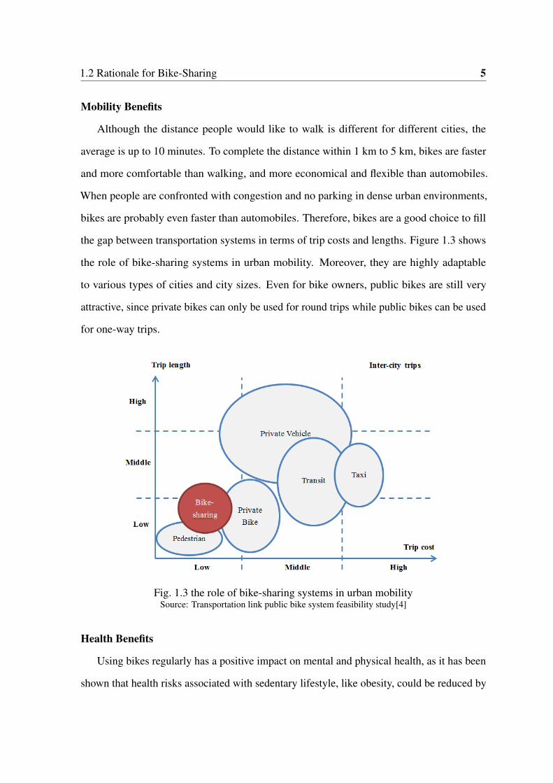
the gap between transportation systems in terms of trip costs and lengths. Figure 1.3 shows
the role of bike-sharing systems in urban mobility. Moreover, they are highly adaptable
to various types of cities and city sizes. Even for bike owners, public bikes are still very
attractive, since private bikes can only be used for round trips while public bikes can be used
for one-way trips.
Fig. 1.3 the role of bike-sharing systems in urban mobilitySource: Transportation link public bike system feasibility study[4]
Health Benefits
Using bikes regularly has a positive impact on mental and physical health, as it has been
shown that health risks associated with sedentary lifestyle, like obesity, could be reduced by

6 Introduction
regular bike use. Also, it has been shown that cyclists may get less exposure to traffic-related
pollutants than motorists. The comparison is shown in Table 1.2.
Table 1.2 the comparison of the exposure to traffic pollutants for motorists and cyclists
Traffic Pollutant Cyclists’ Exposure(µg/m3) Motorists’ Exposure(µg/m3)
Carbon monoxide (CO) 2670 6730Nitrogen dioxide (NO2) 156 277Toluene 72 373Xylene 46 193Benzene 23 138
Source: Exposure to carbon monoxide, repairable suspended particulates, and volatile organic compoundswhile commuting by bicycle [5]
Environmental Benefits
Among all the transportation modes of urban areas, bikes are the most energy efficient.
Table 1.3 shows the comparison of fossil fuels consumption and exhausts of toxic pollutant
and emissions (like greenhouse gases) for various modes of transportation. In the life-cycle
of a bike, the production and disposal energy costs are the only two vital costs, which are so
relatively small that they may be negligible. It is said that the energy costs of producing one
car is enough to produce 70 to 100 bikes.
Table 1.3 the comparison of key environmental indicators for different modes of publictransportation and private automobiles (for the same number of people/km)
Auto without Auto with Bus Train Airplane Bikecatalytic converter catalytic converter
Primary energy consumption 100% 100% 30% 34% 405% 0Space consumption 100% 100% 10% 6% 1% 8%Hydrocarbons 100% 15% 8% 2% 140% 0CO2 100% 100% 29% 30% 420% 0CO 100% 15% 2% 1% 93% 0NOx 100% 15% 9% 4% 290% 0Total atmospheric pollution 100% 15% 9% 3% 250% 0Accident risk 100% 100% 9% 3% 12% 2%
Source: The way ahead for towns and cities[6]Note: A catalytic converter will work only if the engine has warmed; on trips of short distance, the benefit of
pollution mitigating is insignificant.
1.3 Motivation and Objective 7
Safety Benefits
Bike-sharing systems can contribute to a "safety in number" effect, which means that the
increasing number of cyclists has a positive effect on reducing the probability of collision
with motorists, as documented by Jacobsen in 2003[7]. Though the safety problem is a main
factor inhibiting people from cycling, it can be reduced if the number of cyclists increases.
It can be generalized that bike-sharing systems may create a positive cycle by increasing
the number of bike users, which would improve safety and then would further increase the
number of cyclists.
1.3 Motivation and Objective
In practice, the unavailability of bikes and especially the unavailability of vacant lockers
at their destination stations are major complaints from users about bike-sharing systems.
There are two main causes of the unavailability, or so-called imbalance of the systems, which
can be summarized as follows. (1) The continuous cause of imbalance is that most of the
demands are one-way trips in a short period with a particular direction. One scenario is
some of the origin and destination points shift roles throughout the day (most of these shifts
happen in the afternoon). Also, the demands of picking and returning bikes are dynamic and
fluctuating. For example, an analysis of user behaviour in Barcelona’s bike-sharing system,
called "Bicing", is given by Froehlich et al. in 2009[8]. The results show that the availability
of bikes at downtown or midtown stations declines early in the morning when people ride to
work and goes up in the late afternoon. While in commercial districts, the stations show an
opposite pattern and are full during working hours. Another scenario is that stations located
at highland tend to have less bikes available, while the ones at lowland are more likely to
be full throughout the day. (2) Some discrete and unpredictable events, such as the sudden
change of the weather, can also cause imbalances. As a result, repositioning activities are
very crucial to ensure a good quality of services for users. With the redistribution of bikes by

8 Introduction
a fleet of vehicles, bike-sharing systems should have the ability to balance themselves, i.e., to
provide enough bikes for users to pick up and enough locker vacancies for them to return
bikes. Therefore, repositioning/redistribution activities of bikes are one of the key aspects for
a bike-sharing system to survive[9].
According to the importance of system usage rates, the operation of repositioning activi-
ties can be divided into two modes. One is called static repositioning problem, which means
that the system usage rate is insignificant to system performance and repositioning activities
usually happen at night. The other is called dynamic repositioning problem, which means
that the system’s status is changing fast and repositioning activities happen during the day.
This thesis focuses on the static repositioning problem for bike-sharing systems. We assume
there is one depot, a number of stations, and a fleet of identical vehicles in a bike-sharing
system. A particular number of lockers and bikes are set at each station. The repositioning
activities are conducted by the fleet of vehicles during the night, in order to set the system’s
status to the one that required in the next morning. Every station can be visited at most once
by each vehicle. There is also a vehicle capacity limit and an operation time limit for the fleet
of vehicles. The transportation routes of the vehicles and the loading/unloading instruction
for each vehicle at each station will be determined with the minimal total time cost. As a
result, by solving the static repositioning problem, the operation efficiency and facility usage
of bike-sharing systems will be enhanced. Also, customers’ satisfaction will be improved
and the survival chance of the bike-sharing systems will increase, which can bring a lot of
benefits to our environment and society.
1.4 Contribution and Scope of the Thesis
There are four main contributions in this thesis for static repositioning problem of bike-sharing
systems. First, new constraints are developed to fasten the original Integer Programming (IP)
model. Second, we formulated a new IP model with two commodities, defining repositioning

1.4 Contribution and Scope of the Thesis 9
activities as transporting both bike and lockers. Then, two heuristic approaches are proposed
to handle larger sized systems. One is called IP based heuristic, which is able to solve
medium-sized instances with up to 100 stations and 2 vehicles. The other is called Set-
Partitioning (SP) based heuristic, which is able to solve large size instances with up to 500
stations and 10 vehicles and is very competitive to a recent well-preformed method proposed
by Ho and Szeto et al.[10].
The rest of this thesis comprises five more chapters. Chapter 2 provides a comprehensive
summary of the previous research in bike-sharing systems. In Chapter 3, new constraints to
speed up the IP model for static repositioning problem are developed and tested. Then, a
novel IP model with two commodities is formulated, which considers repositioning both bikes
and lockers. An illustrative example is presented and small-sized numerical experiments of
this novel IP model are presented, which indicate the difficulty of this problem. In Chapter 4,
an IP model based heuristic is developed, which can efficiently solve medium-sized cases of
the static repositioning problem. Modifications of the original IP model are also put forward
for the purpose of getting better lower bounds as benchmarks for larger-sized instances.
Numerical experiments are conducted to show the performance of this algorithm. In order
to handle larger-sized cases, Chapter 5 presents a SP based heuristic and the numerical
experiments of this algorithm. For both of the heuristics in Chapter 4 and 5, the repositioning
activities are defined as transporting only bikes. In the end, Chapter 6 gives a conclusion of
this thesis and also points out some directions of future work.


Chapter 2
Literature Review
The need and importance of integrating bicycling into the transportation system is firstly
proposed and addressed in the work of Liu et al.[11] by analyzing the changes of transport
mode choice in large Chinese cities over the last 50 years. Since then, modern bike-sharing
systems have become more and more popular. Although the related existing literature is
relatively new and scarce, there are still some interesting and significant topics about bike-
sharing systems that have been put forward and studied. This chapter is the literature review
of the research and studies about bike-sharing systems, particularly in three major aspects:
strategic planning, demand analysis and forecasting, and repositioning activities.
2.1 Strategic Planning of Bike-Sharing Systems
2.1.1 System introduction, development history and directions, and
regulations
A detailed system introduction and the development history of bike-sharing systems can be
seen in DeMaio[12] and Midgley[2]. Additionally, DeMaio[12] gave a detailed examination
of previous models and a summation of their benefits and shortcomings. He also generated

12 Literature Review
some future development directions of bike-sharing systems including improved distribution,
ease of installation, powering stations, better tracking of bikes, pedal assistance, and various
business models. Midgley[2] studied how the bike-sharing system works financially. Policy
recommendations referring to information sharing, manuals, networks, and projections were
also put forward. The characteristics of bike-sharing system network in Biaystok were
studied by Dobrzynska et al.[13] with statistical methods. Different from our intuition, the
network of bike-sharing in Biaystok is more similar to a complete network and it does not
have the typical distributions characteristic of other transport networks. Furthermore, the
nodes in bike-sharing network are more likely to have fewer but stronger clusters, meaning
the network has steady state and low dynamics. In order to estimate the usability of bikes
in a bike-sharing system, Kaspi et al.[14] put forward a Bayesian model which was based
on the existing data and was continuously updated with online transactions data. With the
patterns of bike usability at each station, prioritizing maintenance and repositioning might
help to improve the service level of a bike-sharing system.
In addition, Midgley[2] pointed out that the redistribution of bicycles is one of the
key success factors in bike-sharing schemes. The vital meaning of redistribution was also
addressed by Richard and Jouannot[15]. They put forward three key factors (maintenance,
redistribution, and user information and monitoring) for bike-sharing systems to survive
by assessing the current systems in France. They also gave a possible sketch of the future
development of bike-sharing systems, but they questioned the competitive ability of bike-
sharing systems compared to private bikes. By analyzing the survey concerning bike-sharing
conducted in Singapore, Zhang et al.[16] also stated the importance of re-balancing issues in
the project planning of bike-sharing systems.
Some research showed the importance of regulation mechanisms, such as incentives, to
bike-sharing systems. Fricker and Gast[17] proposed a model of bike-sharing systems with
a finite number of stations and they show that even in a symmetric case, the performance

2.1 Strategic Planning of Bike-Sharing Systems 13
is still poor. After testing the system with simple incentives, they indicated that regulation
mechanisms are needed, such as repositioning of bikes by trucks. They also tested and
concluded that an optimal fleet size together with an incentive of returning bikes to the least
loaded stations will improve the system performance dramatically and the influence of simple
incentives is an exponential factor for the system performance. Ahillen et al.[18] analyzed
the 18-month data of bike-sharing systems in Washington DC and Brisbane Australia from
four perspectives, which are monthly ridership trends, daily ridership trends, trip duration and
length, and neighborhood performance. According to their results, we can see that although
these two systems have different utilization rates, their daily utilization patterns are similar,
such as morning and evening peaks on weekdays. They also suggested to expand the system
operation hours, provid helmets, reduce subscription price, and add stations at suburbs where
there are few or no station, in order to increase the ridership of bike-sharing systems, .
2.1.2 System design optimization
The research that has been done in the design of bike-sharing systems is mainly concerned
with determining the optimal number and location of stations, the optimal initial number of
bikes and lockers, and the optimal fleet size.
Lin et al.[19] presented an optimal design of bike-sharing systems, considering the
benefits for both users and investors. The mathematical model they built decides the number
and location of stations, as well as the paths between stations, and integrates users’ travel
costs, facility costs like docking lockers, setup costs of bike lanes, and service levels measured
by demand coverage levels. By testing the model on small examples, they also obtained the
importance of each parameter which makes a contribution to the strategic design of the system.
Simulation optimization approach had been applied for bike-sharing design to decide the
optimal locations for stations of the bike-sharing system by Romero et al.[20]. In their work,
they simulated the transport network and built a bi-level optimization model. Additionally,

14 Literature Review
Saharidis et al.[21] presented a model using pure Mixed Integer Linear Programming (MILP),
which determines the optimal locations of stations and the numbers of initial bikes and lockers.
The model was developed considering future demand patterns, bike popularity, and budget.
El-Assi et al.[22] also developed models, but using regression analysis, to forecast the total
monthly trip rates at potential station locations, which helps to choose a better location for
new stations with more total bike ridership.
Freund et al.[23] presented a polynomial-time algorithm to compute the optimal allocation
of bikes and docking lockers for bike-sharing systems with minimal unsatisfied demands.
In order to decide the optimal fleet size for the planning of a bike-sharing system, Sayar-
shad et al.[24] built a dynamic LP model which minimizes unsatisfied demand simultaneously.
Fricker and Gast[17] presented a stochastic model and a fluid approximation to determine
the optimal fleet size together with the rate of bike redistribution for the vehicles. They
also considered the influence of stations’ capacities, since they proved that the influence
of stations’ capacities cannot be neglected via analyzing the randomness of users’ choices
affected by their unsatisfied system-using experience. Lu[25] developed a robust bike fleet
allocation model, which determines the number of bikes to set at each station on each day of
a week and can be extended to a bike fleet planning model.
2.2 Demand Analysis and Forecasting of Bike-Sharing Sys-
tems
The demands of borrowing and returning bikes in bike-sharing systems are unknown and
changing all the time. In order to enhance the fulfillment of demands for bike-sharing
systems, there is an urgent need to know the demands in advance. Hence, some researchers
have already studied the patterns of the demands, the factors that affect the demands, and

2.2 Demand Analysis and Forecasting of Bike-Sharing Systems 15
how to forecast the demands, while most of them focus on the patterns of usage and travel
behaviors.
Kaltenbrunner et al.[26] detected some geographic and temporal patterns of mobility by
analyzing the human mobility data and the number of available bikes. They showed that
it is a good way to improve the bike-sharing system by predicting the number of available
bikes at each station using the mobility patterns and sharing the predictions to users. Vogel
et al. (2011) used data mining to seek the patterns of the imbalanced distribution of bikes.
These patterns regarding time periods and directions can be beneficial for setting more
suitable locations of the stations, which will make the system more efficient. Caggiani
and Ottomanelli[27, 28] developed a micro-simulation model to determine the optimal
redistribution flows, patterns, and time intervals for bike-sharing systems with dynamic
demand. They used a neural network to forecast the demands. The decision support system
they proposed can also be used for strategically designing the optimal layout of bike-sharing
systems. But the performance of the decision support system is poor in the congested
situations. Li et al.[29] implemented Markovian methods to compute relative user arrival
rates for bike-sharing stations. Then, the probabilities of full and empty stations were
computed. A data mining algorithm was developed by Bordagaray et al.[30] to study the
patterns of bike-sharing user behaviors. In their algorithm, the rental behaviors were divided
into five usage types, which are round rentals, interval duration reset, bike substitution,
perfectly symmetrical and non-perfectly symmetrical journeys. Via spatial and temporal
analysis, the features of commuting and casual users can be identified. Moreover, according
to the testing results of their algorithm, useful insights and valuable information could be
acquired for managing, improving and redesigning the bike-sharing system. Also, with data
mining tools, the users’ mobility patterns were presented by Jiménez et al.[31] to assist
managing and redesigning for bike-sharing systems. Unlike Bordagaray et al.[30], they
measured the mobility patterns with three ratios, which are the number of available bikes

16 Literature Review
ratio, the cumulative trips ratio and the turnover station ratio. As the bike trip data are
usually unavailable, Chen et al.[32] figured out an approach to identify the sparsity and
locality patterns of bike trip with the real-time bike and locker number in stations. According
to their data analysis, most of the rides happen between the stations of low geographical
distance, which is within 2km. In addition, the strong flow patterns retrieved from their
model would assist the real-time repositioning for bike-sharing systems. Morency et al.[33]
showed the bike-sharing usage patterns of BIXI in Montreal with its 6-year transaction data,
by examining several key indicators, such as accessibility to the network, system weekly
usage patterns, travel times distribution and balance ratios. Furthermore, they showed the
changing patterns of individual behaviors in different seasons via modelling the bike-sharing
usage by members.
Kim et al.[34] studied the factors that probably affect the travel behavior in bike-sharing
systems. It turns out that the total area of residential and commercial buildings, parks,
schools, and subway stations tend to increase the usage of the system, but to different
degrees. Weekday and rainfall have negative impact on bike-sharing usage. El-Assi et
al.[22] pointed out the influences of weather and built environment on demand by analyzing
station level of the bike-sharing system in Toronto. They showed a significant correlation
between temperature, land use and bike share trip. From the studies by Zhang et al.[16]
and Caulfield et al.[35], we can see that there is a great impact of weather on bike-sharing
demand. Morency et al.[33] also showed that adverse weather has significantly negative
influence on bike-sharing usage. However, the ’negative’ effects of the start-up and ending
of the system is completely removed during winter.
In terms of demand forecasting, Rudloff and Lackner[36] built a model to forecast the
demands considering the influences of weather and neighboring stations. Moreover, they
showed that their model is better than forecasting demand simply with historical demands.
Ashqar et al.[37] applied machine learning algorithms, which are Random Forest, Least-

2.3 Repositioning Problem of Bike-Sharing Systems 17
Squares Boosting and Partial Least-Squares Regression, to predict the bike availability at
each station of the bike-sharing system in the area of San Francisco Bay. Their testing results
showed that the optimal prediction period of their models with the least errors is 15 minutes.
It is worth noting that Urli[38] offered a technical report that describes how to generate a
static bike-sharing instance problem from the Citibike NYC data. His work is very helpful
for the studies of the static repositioning problem since it can provide realistic data for the
numerical experiments.
2.3 Repositioning Problem of Bike-Sharing Systems
As mentioned previously, redistribution is one of the key factors for bike-sharing systems to
survive. Indeed, the major complaint from bike-sharing users is the unavailability of bikes
and empty lockers, which makes the systems untrusted and possibly be abandoned by users
at last (see Shaheen and Guzman[39] and Brussel Nieuws[40].
Due to the importance of redistribution for bike-sharing systems, there are quite a few
works that have been done in this area. The majority of the research in balancing bike-sharing
systems can be divided into the static repositioning problem and the dynamic repositioning
problem. The static repositioning problem focuses on the repositioning activities happening at
night, meaning that the system usage rate is insignificant to system performance. The dynamic
repositioning problem focuses on the repositioning activities during the day, meaning that
the system’s status is changing continuously.
2.3.1 Static repositioning problem
Although in the research about static repositioning activities, the problem assumptions
about demand (numbers/intervals), depot (single/multiple), and vehicle (single/multiple)
are different, the static repositioning problem can be regarded as one commodity pickup
18 Literature Review
and deliver problem. Thus, most of the studies use Mixed Integer Programming (MIP) to
model the static repositioning problem. Since the static repositioning problem is NP-hard,
which was well explained in the work of Chemla et al.[41], using only MIP is not efficient
to solve large-sized instances. Therefore, besides optimization modelling, researchers also
make efforts to develop various approaches to solve the problem with larger size in shorter
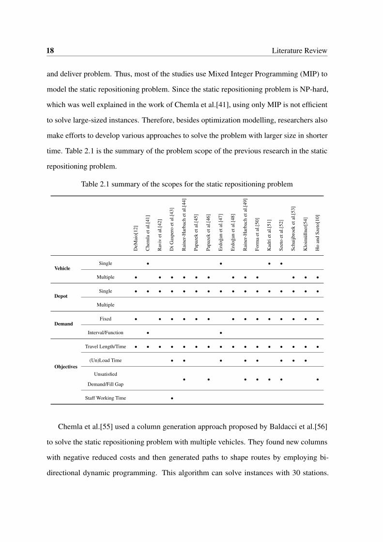
time. Table 2.1 is the summary of the problem scope of the previous research in the static
repositioning problem.
Table 2.1 summary of the scopes for the static repositioning problem
DeM
aio[
12]
Che
mla
etal
.[41]
Rav
ivet
al.[4
2]
DiG
aspe
roet
al.[4
3]
Rai
ner-
Har
bach
etal
.[44]
Papa
zek
etal
.[45]
Papa
zek
etal
.[46]
Erd
ogan
etal
.[47]
Erd
ogan
etal
.[48]
Rai
ner-
Har
bach
etal
.[49]
Form
aet
al.[5
0]
Kad
riet
al.[5
1]
Szet
oet
al.[5
2]
Schu
ijbro
eket
al.[5
3]
Klo
imül
lner
[54]
Ho
and
Szet
o[10
]
VehicleSingle • • • •
Multiple • • • • • • • • • • • •
DepotSingle • • • • • • • • • • • • • • • •
Multiple
DemandFixed • • • • • • • • • • • • • •
Interval/Function • •
Objectives
Travel Length/Time • • • • • • • • • • • • • • • •
(Un)Load Time • • • • • • • •
Unsatisfied• • • • • • •
Demand/Fill Gap
Staff Working Time •
Chemla et al.[55] used a column generation approach proposed by Baldacci et al.[56]
to solve the static repositioning problem with multiple vehicles. They found new columns
with negative reduced costs and then generated paths to shape routes by employing bi-
directional dynamic programming. This algorithm can solve instances with 30 stations.

2.3 Repositioning Problem of Bike-Sharing Systems 19
After that, Chemla et al.[41] developed a branch-and-cut algorithm with tabu search to solve
the problem with a single vehicle. The computational study shows that the algorithm they
proposed is able to handle instances with up to 100 stations. Erdogan et al.[47] also studied
the static bicycle relocation problem with a single vehicle, but using demand intervals. They
developed a branch-and-cut algorithm and a Benders decomposition to solve the problem
of size up to 50 stations. Dell’Amico et al.[57] treated the static repositioning problem
as a special pickup-and-delivery capacitated VRP for one commodity and provided four
different MILP formulations mainly based on the multiple traveling salesman problem.
They also developed a branch-and-cut algorithm which makes the third formulation able
to handle instances with 50 stations. Instead of using MILP, Gaspero et al.[43] solved the
static repositioning problem by developing two Constraint Programming (CP) models and
a Large Neighborhood Search (LNS) approach. They showed that pure CP is better than
MILP for large cases and the LNS approach performs competitively comparing with other
proposed methods. Some researchers applied inventory management concepts to help solve
the repositioning problem. A hub location inventory model for bike-sharing systems was
formulated by Lin et al.[58], who provided an integrated view of the concerns of different
costs and service quality. They proposed a heuristic method to find near-optimal solutions
within 2% optimality efficiently. But they did not count the check-in bikes in the calculation
of the bike inventory, which is unrealistic since the check-in bikes can be reused. Raviv et
al.[42] proposed a new inventory routing modelling approach with an introduction of a novel
convex objective function and the consideration of time. With acceptable optimal gaps, they
showed that their MILP formulation can handle instances of 60 stations.
Because of the complexity of this repositioning problem for bike-sharing systems and
more and more bike-sharing systems with large size in reality, many researchers focus on
developing efficient algorithms. Rainer-Harbach et al.[44] first developed a Variable Neigh-
borhood Search (VNS) approach embedded with a Variable Neighborhood Descend (VND)

20 Literature Review
algorithm to solve the static redistribution problem. Following their study, Papazek et al.[45]
improved the computing time by applying VND after the PILOT (Voßs et al[59])/Greedy
Randomized Adaptive Search Procedure (GRASP). With this approach, the model can deter-
mine the repositioning routes for a bike-sharing system with 700 stations. Papazek et al.[46]
later tried different ways, using path relink and simpler recombination operators, to hybridize
them for better computational improvement. A novel and efficient heuristic called 3-step
math heuristic was proposed by Forma et al.[50], which includes clustering and MIP. The
maximum instance size they tested is 200 stations with 3 vehicles. Ho and Szeto et al.[10]
developed a hybrid LNS with several removal and insertion operators and compared with the
3-step math heuristic proposed by Forma et al.[50]. They also showed that their hybrid LNS
heuristic performs better than the 3-step math heuristic. Moreover, they further increased
the handling size to 500 stations with 5 vehicles and the computation time was decreased
signicantly with quite small gaps. Different from other works, Alvarez-Valdes[60] solved the
balancing problem, considering multiple depots, multiple visits to one station by the same
vehicle, and also damaged bikes which need to be transported to a depot. Firstly, with the
previous and current demands information, they built an IP model to compute the number
of bikes needed and to be returned at each station within each time period. After that, an
heuristic algorithm based on Minimum Cost Flow Problem and insertion was proposed to
solve the balancing problem. Real small instances were tested, showing the effectiveness of
their algorithms and its potential solving ability for large cases.
Table 2.2 is the summary of performances of previous research in the static repositioning
problem. We can see that quite a few researchers applied Neighborhood Search method in
bike-sharing repositioning problem for large systems, [10] for instance, were able to show
that their hybrid heuristic performs well.

2.3 Repositioning Problem of Bike-Sharing Systems 21
Table 2.2 summary of the methods and maximum testing sizes for static repositioning problem
Article Method System Size Fleet Size
DeMaio[12] Branch-and-Cut 116 1
Model/ Raviv et al.[42] MIP 60 2
Exact Erdogan et al.[47] Branch-and-Cut and Bender’s Decomposition 50 1
Algorithm Erdogan et al.[48] Bender’s Cuts 60 1
Kadri et al.[51] Branch-and-Bound 30 1
Kloimüllner[54] Logic-based Benders Decomposition 70 3
Heuristic
Chemla et al.[41] Tabu Search 100 1
Di Gaspero et al.[43] CP and LNS 90 5
Rainer-Harbach et al.[44] VNS with VND 90 5
Papazek et al.[45] PILOT/GRASP Hybrid with VND 700 14
Papazek et al.[46] GRASP Hybrid with Path Relinking 500 15
Rainer-Harbach et al.[49] Combination of PILOT, GRASP and VNS 700 21
Forma et al.[50] 3-Step Matheuristic 200 3
Szeto et al.[52] Enhanced Chemical Reaction Optimization 300 20
Schuijbroek et al.[53] Cluster-First Route-Second 135 5
Ho and Szeto[10] Hybrid LNS 518 5
2.3.2 Dynamic repositioning problem
Comparing to the static repositioning problem, the dynamic repositioning problem is a more
normal but more complicated situation, since the demands of borrowing and returning bikes
are unknown and the status of stations is changing all the time. Hence, researchers develop
a range of modelling and solving approaches to solve it, such as MIP and CP. Some novel
22 Literature Review
ways have also been proposed to solve the problem, such as developing a direct algorithm,
using linear programming (LP), modelling from the perspective of control, and simulation.
Moreover, pricing and incentives schemes have also been considered as novel approaches for
balancing bike-sharing systems.
Nair and Miller-Hooks[61] formulated the problem with a stochastic MIP approach to
overcome the limitations of static or known demand assumptions. Since this stochastic
model has a non-convex feasible region, they presented a divide-and-conquer algorithm to
generate p-efficient points (PEPs) and transform the problem into a set of disjunctive, convex
MIPs. They also extended the concept of PEP to include dual-bounded chance constraints
and explored the trade-off between redistribution costs and service levels. Schuijbroek et
al.[62] proposed an MIP formulation and put forward a cluster first route second heuristic
to solve the dynamic case, unifying dual-bounded service level constraints and adding both
inventory flexibility and vehicle routing to their model. In order to achieve high computational
performance, they developed a novel maximum spanning star routing cost approximation
for the polynomial-size clustering problem. Then through comparing with the classical
full MIP model, they proved better performance of their model using cuts heuristic via CP.
Vogel et al. [63] treated determining the number of bikes and lockers at each station as a
resource allocation problem, which is interdependent with decisions on reallocation. They
also used MIP to build a dynamic model that can determine the optimal fill level of each
station. They developed a hybrid meta-heuristic integrating with LNS, which performs better
than CPLEX for small cases. Brinkman et al. [64] treated the dynamic repositioning problem
as an inventory routing problem. They defined the demands with the time-depended target
intervals and user activities, and using IP. They implemented a decomposition method to
solve the problem. VNS by meta-heuristics was used for the partitions of station assignment
and a cost-benefit inventory routing algorithm is presented for partition evaluation. By testing

2.3 Repositioning Problem of Bike-Sharing Systems 23
with real world data, it turns out that simulated annealing is much more suitable than tabu
search for large instances.
However, Raviv and Kolka[65] made progress by introducing a single station inventory
model with a convexity property which is suitable for the station management of bike-
sharing systems. They modeled the bike-sharing station as a double-ended queuing system
proposed by Kashyap [66]. They assumed that the arrivals of system users follow a non-
homogeneous Poisson arrival process. Since the model does not need the target level
assumption, they were able to impose time limit constraints. They also put forward an
efficient approximation method to get the expected station-dependent shortages. Instead of
stochastic modelling approaches, Angeloudis et al.[67] developed a repositioning algorithm
with the demand patterns summarized from real data, which can alleviate the imbalance of
the system significantly.
Shu et al.[68] developed a deterministic LP model to get a similar performance of the
stochastic bike-sharing systems and proved that it is very close to the actual performance
by testing it on the real data of Singapore Mass Rapid Transit ridership. Additionally, they
pointed out that the utilization rate of bikes, the repositioning of bikes and the number of
docks to set at each station are all vital problems for achieving good system performance.
From the control perspective, Labadi et al.[69] first introduced dynamic models based
on Petri nets into bike-sharing system for control purposes. After that, Benarbia et al.[70]
presented a modelling approach using Petri nets with variable arc weights to solve the
balancing problem for dynamic bike-sharing systems. They continued their study and
developed a new stochastic Petri nets model (Benarbia et al.[71]) based on a real-time alert
system and a new re-balancing policy for system control and performance evaluation.
Simulation is also used to study the dynamic repositioning problem. Wang and Wang[72]
simulated different redistribution strategies for bike-sharing systems to evaluate their per-
formances. They proved that even through the redistribution strategy is very simple it can

24 Literature Review
still improve the service quality of the system. They also showed that the service quality can
be well enhanced by exploiting real-time and historical rental data and applying real-time
and historical rental data to the models. Instead of the traditional simulation models, Jian
et al.[73] used a discrete-event simulation model and developed a variety of more efficient
gradient-like heuristic methods to optimize the bike and docking locker allocation for a
large-scale bike-sharing system with 466 stations.
Table 2.3 summary of the problem scope for the dynamic repositioning problem
Nai
rand
Mill
er-H
ooks
[61]
Con
tard
oet
al.[
74]
Con
tard
oet
al.[7
5]
Schu
ijbro
eket
al.[6
2]
Voge
leta
l.[63
]
Bri
nkm
anet
al.[6
4]
Ang
elou
dis
etal
.[67]
Shu
etal
.[68]
Wan
gan
dW
ang[
72]
Rav
ivan
dK
olka
[65]
Lab
adie
tal.[
69]
Ben
arbi
aet
al.[7
1]
Ben
arbi
aet
al.[7
0]
Vehicle Single
Multiple • • • • • • • • • • • •
Depot Single • • • • •
Multiple
Demand Function/Distribution • • • • • • Petri Nets
Stochastic Process • • • • (Control)
Objectives
Travel Length/Time • • • •
(Un)Load Time • Ensure Bikes
Unsatisfied • • • • • • • availabilityDemand/Fill Gap for pickup
Makespan of • and vacantSchedule lockers for
Waiting time • returnof Customers
Network Flow •
Table 2.3 is the summary of the problem scopes of the previous research in the dynamic
repositioning problem. Table 2.4 is the summary of the modelling and solving methods of
the previous research in the dynamic repositioning problem.
It is also worth mentioning that some other novel ideas about balancing the bike-sharing
system have been put forward instead of simply using vehicles to redistribute bikes. Vogel
and Mattfeld[76] presented two possible scenarios: distribution directly by the reposition of

2.3 Repositioning Problem of Bike-Sharing Systems 25
Table 2.4 summary of the modelling and solving methods for dynamic repositioning problem
Modelling Solving Methods
MIP(VRP Mode)
Divide-and-Conquer Algorithm
Column and Cut Generation
Dantzig-Wolfe Decomposition and BendersDecomposition
Cluster-First-Route-Second Heuristic& Maximum Spanning Star Routing Cost
Approximation
Hybrid Meta-heuristicIntegrating with LNS
Dynamic A Double-EndedApproximation MethodRepositioning Queuing System
Problem (Inventory Model)
IP (Inventory&Decomposition Method Tabu& Routing Model) Search/Simulated Annealing
Deterministic LP Heuristic Method
Dynamic Models Based on -Petri Nets (Control)
- Simulation
- Pricing & Incentives Schemes
bikes and distribution indirectly by incentives or pricing. Then, they formulated models by
introducing a nonlinear clearing function. Based on simulation experiments, they concluded
that spending more efforts on the redistribution of bikes can lead to better system performance
of demand satisfaction. Haider et al.[77] came up with a new way - pricing and incentive
schemes, to re-balance the bike-sharing system. They developed heuristics for their bi-level
optimization model. The heuristic, called iterative price adjustment scheme, can handle the
full network in only 87 seconds. They also showed that the cost of incentives is much less
than the cost of balancing the system with vehicles. But the assumption of the same value of
time for all customers is impractical.
26 Literature Review
2.3.3 Repositioning Problem of Free-floating Bike-Sharing Systems
Free-floating bike-sharing systems are very innovative, where there are no specific stations
and the bikes can be locked at any solid frame or standalone. A first study for the planning
and management was done by Pal and Zhang[78], in which a novel MILP was proposed to
solve static repositioning problem with single and multiple vehicles. They also developed a
hybrid nested LNS with VND algorithm for large-sized systems.
In summary, according to the previous studies of bike-sharing systems, it turns out that
research has been done at both the strategic planning level and the operational level. As
addressed at the beginning of this chapter, the balancing ability of bike-sharing systems
is vital to the survival of the systems and this redistribution problem is a variant of VRP.
Hence, it becomes more and more popular in Operations Research, but is still not well solved
because of its NP-hard characteristic.
For the static repositioning cases, most of the researchers study the single-depot bike-
sharing system with multiple vehicles, mostly via MIP, and little work has been done for
the multi-depot cases. Currently, the maximum handling size is about 700 stations with
21 vehicles (Alvarez-ValdesAlvarez-Valdes et al.[60]). However, they only compared the
performances between heuristic algorithms. The hybrid LNS algorithm proposed by Ho
and Szeto[10] solves cases with 500 stations and 5 vehicles. They showed the outstanding
performance of their algorithm by comparing with the optimal solution for the cases with up
to 200 stations. But both of the works above are still not able to solve the large bike-sharing
systems, such as the one in Hangzhou with 2700 stations in total. As to the dynamic cases,
which are more difficult than the static ones, there are mainly two ways of modelling the
unknown demands of bike-sharing systems according to the previous studies. One is using
probability distributions based on the patterns summarized from the real-world data. The
other is using Poisson processes. Although the approaches for dynamic cases are more
diversified comparing to the ones for static cases, they are also not practical and efficient

2.3 Repositioning Problem of Bike-Sharing Systems 27
enough for real bike-sharing systems. Thus, more efforts are needed to solve static and
dynamic repositioning problems for large-scale bike-sharing systems.
In addition, some of the researchers have addressed the importance and effectiveness of
incentives or pricing in balancing bike-sharing systems. Therefore, more future studies in
combining the incentives or pricing schemes with redistribution activities for balancing the
systems can be done.
More importantly, no matter the static or dynamic repositioning problem, all of the
previous research defines repositioning activities as transiting only one commodity - bikes.
However, in reality, there are systems, such as BIXI in Montreal, the docking lockers are
movable. Hangzhou’s public bike-sharing system even has mobile stations. The major
advantages of movable lockers are decreasing the initial fundamental facility costs and
significantly enhancing the flexibility and facility usage rate of the system. As a result, in
the next Chapter, a novel IP model will be developed defining repositioning activities as
transiting two commodities - bikes and lockers.

Chapter 3
Integer Programming Model
3.1 Introduction and Monotonicity Assumption
Due to the importance of repositioning activities for bike-sharing systems, the objective of
solving the repositioning problem is to determine the optimal redistribution plan. In general,
repositioning activities are defined as reallocating bikes. We assume that in this bike-sharing
system, there is one depot, a number of stations, and a fleet of vehicles. A particular number
of lockers and bikes are set at each station. The bikes will be transited by the vehicles among
the stations during the night in order to meet the required number of bikes at each station in
the morning. The demands realized during the night, which are negligible, are assumed to be
zero. After the repositioning activities, the starting conditions of stations will be improved
for the next day.
The depot is the starting point and ending point of each vehicle’s route and each station
can be visited at most once by each vehicle. The transportation routes of the vehicles and
the number of bikes at each station to be transited will be determined with the minimal total
costs, which include the traveling time costs of vehicles and the loading and unloading time
cost of bikes.

30 Integer Programming Model
The system can be represented as a complete directed graph, where vertices 1 to n are
stations and vertex 0 is the depot. The depot has no inventory and remains empty after the
repositioning activities. Each station i has initial numbers of bikes ibi and lockers ili before
the repositioning activities and required numbers of bikes f bi and lockers f li to be satisfied
(note: f li = ili). A fleet of identical vehicles M with capacity C at the depot is to transport
bikes and lockers among stations and each vehicle k must be back with no bikes and lockers.
The travel cost from station i to station j is wi j . Hence, the total travel cost is the summation
of the traveled arcs’ costs of all vehicles. There are also time costs bt , when staffs are loading
or unloading bikes and lockers at station i.
Eventually, the optimal route with minimal total travel costs, together with the operation
instructions (the number of bikes and lockers to be loaded or unloaded) at each visited station
for each vehicle will be determined.
Before formulating the model, an assumption of the monotonicity needs to be addressed,
which was firstly put forward by Rainer-Harbach et al.[44]. This monotonicity assumption,
which assumes each station can be visited by the same vehicle only once, cannot imply
that the number of bikes or lockers increases or decreases monotonically. We assume that
Vehicles are only allowed to load bikes at supplying stations and unload them at demanding
stations. In this way, the number of bikes or lockers increases or decreases monotonically.
As a result, the sequence of different vehicles visiting a single station does not matter. But
the counter example given by Rainer-Harbach et al.[49] does not clearly show that using a
station as a buffer can get better solution.
Here is a counter example we come up with (see Figure 3.1). Suppose there are four
stations (n = 4) to be balanced by one vehicle (m = 1) with capacity C = 3, meaning it can
load 3 bikes at most. Station 1 can provide 1 bike, station 2 needs 2 bikes, station 3 can
provide 3 bikes, and station 4 needs 2 bikes. The number on each arc in Figure 3.1 represents
the distance between two nodes.

3.1 Introduction and Monotonicity Assumption 31
n = 4m = 1C = 3
Depot 1 2
3
41 1 1
2
1√
2
2
3
√5
√2
Demands:d1 =−1d2 = 2d3 =−3d4 = 2
Fig. 3.1 a solution to balance the stations with allowing buffer station
If buffer station is allowed, we can find a route shown in Figure 3.2. The total travel
distance of the route is recorded in the left box of Figure 3.2. The loading instruction of the
vehicle is listed in the right box of Figure 3.2. For example, the vehicle will leave depot and
first visit station 1 to pick up 1 bike. We can see that the vehicle will visit station 2 twice to
pick up 1 bike first and drop 3 bikes later.
C = 3t = 6+
√2
Depot 1 2
3
41 1 1
2
1√
2
Depot → 1(+1)1 → 2(+1)2 → 4(-2)4 → 3(+3)3 → 2(-3)2 → Depot
Fig. 3.2 a solution to balance the stations with allowing buffer station
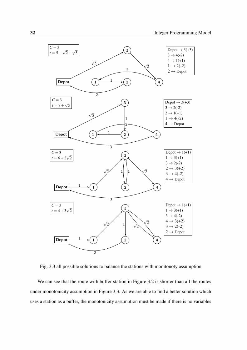
Figure 3.3 shows all the possible solutions to balance these stations with monotonicity
assumption. The total travel distance of each route is recorded in the left box near each route.
The loading instruction of the vehicle is listed in the right box near each route.
32 Integer Programming Model
C = 3t = 5+
√2+
√5
Depot 1 2
3
4
√5 √
22
1
2
Depot → 3(+3)3 → 4(-2)4 → 1(+1)1 → 2(-2)2 → Depot
C = 3t = 7+
√5
Depot 1 2
3
4
√5
1
1
2
3
Depot → 3(+3)3 → 2(-2)2 → 1(+1)1 → 4(-2)4 → Depot
C = 3t = 6+2
√2
Depot 1 2
3
41
√2 1 1
√2
3
Depot → 1(+1)1 → 3(+1)3 → 2(-2)2 → 3(+2)3 → 4(-2)4 → Depot
C = 3t = 4+3
√2
Depot 1 2
3
41
√2
√2√
21
2
Depot → 1(+1)1 → 3(+1)3 → 4(-2)4 → 3(+2)3 → 2(-2)2 → Depot
Fig. 3.3 all possible solutions to balance the stations with monitonoty assumption
We can see that the route with buffer station in Figure 3.2 is shorter than all the routes
under monotonicity assumption in Figure 3.3. As we are able to find a better solution which
uses a station as a buffer, the monotonicity assumption must be made if there is no variables

3.2 New Constraints for Integer Programming Model with One Commodity 33
tracking of the time or at least the sequence of vehicles visiting the same station in the model.
Otherwise, we cannot say it is the optimal solution of the repositioning problem.
3.2 New Constraints for Integer Programming Model with
One Commodity
The IP model with one commodity is presented in Appendix, which is similar to the Arc-
Indexed formulation developed by Raviv et al.[42]. The objective function of the Arc-Indexed
formulation contains not only the total time cost but also a convex penalty function, which is
different from here.
As in the testing of the IP Model with one commodity, we noticed that the computation
time will increase significantly if the fleet size increases, even if the added vehicles will not
be used. Therefore, for the purpose of speeding up the IP model, we created new constraints
related to vehicle, which are shown as follows.
∑ni=1 xk0i ≥ ∑
ni=1 x(k+1)0i ∀k ∈ [1, . . . ,m−1] (1)
Constraints (1) make sure that vehicle k+1 can be used only if vehicle k is in use. Adding
these constraints could reduce computation time is because if there are redundant vehicles,
the options of solution are reduced. For example, given vehicle 1, 2 and 3, if the optimal
solution only needs two vehicles, it is possible to use vehicle 1 and 2 or use vehicle 2 and 3 or
use vehicle 1 and 3. With Constraints (1), there will be only one option of optimal solution,
which is using vehicle 1 and 2.
∑ni=1 i · xk0i −0.5 ·∑n
i=1 xk0i ≥ ∑ni=1 i · x(k+1)0i ∀k ∈ [1, . . . ,m−1] (2)
34 Integer Programming Model
Constraints (2) aim to ensure that vehicle k+1 can be used only if vehicle k is in use,
and each route is assigned to a specific vehicle by making the first destination of vehicle k
larger (or smaller) than that of vehicle k+1. Constraints (2) further reduce the options of
optimal solution. Let’s continue with the previous example of vehicle 1, 2 and 3. If one route
starts with station 4 and the other route starts with station 9, there will still be two options of
the optimal solution, which are vehicle 1 starts with station 4 (vehicle 2 starts with station 9)
and vehicle 1 starts with station 9 (vehicle 2 starts with station 4). Constraints (2) not only
make sure using vehicle 1 and 2, but also ensure vehicle 1 starts with station 9 (vehicle 2
starts with stations 4).
3.3 Integer Programming Model with Two Commodities
Due to the importance of repositioning activities for bike-sharing systems, the objective of
solving the repositioning problem is to determine the optimal redistribution plan. Reposition-
ing activities are defined as reallocating both bikes and docking lockers in this chapter. It is
the novel point of the model presented in this chapter, as mentioned at the end of Chapter 2,
the previous research in balancing bike-sharing systems only considers transporting bikes.
Taking locker transit into consideration can bring a lot of benefits to the whole system. Firstly,
it can decrease the facility costs by lessening the number of lockers put at each station.
Secondly, it greatly improves the usage of the facilities and the flexibility of the whole system.
For example, assume that the lockers cannot be moved. If the demands of borrowing bikes
are beyond the number of lockers built at the station, there will be some demands being
unsatisfied, because the maximum number of bikes is equal to the number of lockers. And
the unsatisfied demands will bring penalty to the system. However, if the lockers can be
moved, more available bikes together with lockers can be transported from other stations to
satisfy the demands. Moreover, there are already movable lockers, such as the ones of BIXI
3.3 Integer Programming Model with Two Commodities 35
in Montreal, in use in reality. Therefore, defining repositioning activities as reallocating both
bikes and docking lockers is reasonable, meaningful and necessary to bike-sharing systems.
Here we assume the lockers and bikes are movable and will be transited by the vehicles
among the stations. Repositioning activities are defined as reallocating both bikes and
docking lockers. In this simplified bike-sharing system, there is one depot, a number of
stations, and a fleet of vehicles. A particular number of lockers and bikes are set at each
station. The lockers and bikes are movable and will be transited by the vehicles among
the stations during the night in order to meet the required number of lockers and bikes at
each station in the morning. The demand realized during the night, which is negligible, is
assumed to be zero. After the repositioning activities, the starting conditions of stations will
be improved for the next day.
The depot is the starting point and ending point of each vehicle’s route and each station
can be visited at most once by each vehicle. The transportation routes of the vehicles and
the number of bikes and docking lockers at each station to be transited will be determined
with the minimal total travel costs, which include the traveling time costs of vehicles and the
loading and unloading time cost of bikes and lockers.
Sets
V : set of stations including the depot, V = {0,1,2, . . . ,n}
V ⋆: set of stations excluding the depot, V ⋆ = {1,2,3, . . . ,n}
M: set of vehicles. M = {1,2,3, . . . ,m}
Inputs
n: number of stations
m: number of vehicles
C: capacity of each vehicle in terms of bikes
a: volume ratio between bikes and lockers
bt: time cost to load or unload one bike

36 Integer Programming Model
lt: time cost to load or unload one locker
ibi: initial number of bikes at station i, i ∈V ⋆
ili: initial number of lockers at station i, and ili ≥ ibi, i ∈V ⋆
f bi: final number of bikes at station i, i ∈V ⋆
f li: final number of lockers at station i, and f li ≥ f bi, i ∈V ⋆
wi j: travel cost between stations i and j in terms of time, i, j ∈V
T : time limitation for total operations.
Decision Variables
ubki: number of bikes unloaded by vehicle k at station i, i ∈V ⋆, k ∈ M
pbki: number of bikes picked up by vehicle k at station i, i ∈V ⋆, k ∈ M
ulki: number of lockers unloaded by vehicle k at station i, i ∈V ⋆, k ∈ M
plki: number of lockers picked up by vehicle k at station i, i ∈V ⋆, k ∈ M
vbki j: number of bikes on vehicle k when traveling from i to j, i, j ∈V , k ∈ M
vlki j: number of lockers on vehicle k when traveling from i to j, i, j ∈V , k ∈ M
xki j: binary decision varable. It equals to 1 when there is a path from station i to j for vehicle
k, otherwise, it equals to 0. i, j ∈V , k ∈ M
qki: auxiliary parameters, i ∈V ⋆, k ∈ M
Model
Minimize ∑ni=0 ∑
nj=0 wi j ∑
mk=1 xki j +bt ·∑m
k=1 ∑ni=0(ubki + pbki)+ lt ·∑m
k=1 ∑ni=0(ulki + plki)
s.t.
vbkii = vlkii = 0 ∀k ∈ M, i ∈V ⋆ (3)
vbk0i = vbki0 = vlk0i = vlki0 = 0 ∀k ∈ M, i ∈V ⋆ (4)
ubki ≤ ∑nj=0 vbk ji ∀k ∈ M, i, j ∈V ⋆ (5)
ulki ≤ ∑nj=0 vlk ji ∀k ∈ M, i, j ∈V ⋆ (6)
∑mk=1 pbki ≤ ibi ∀i ∈V ⋆ (7)
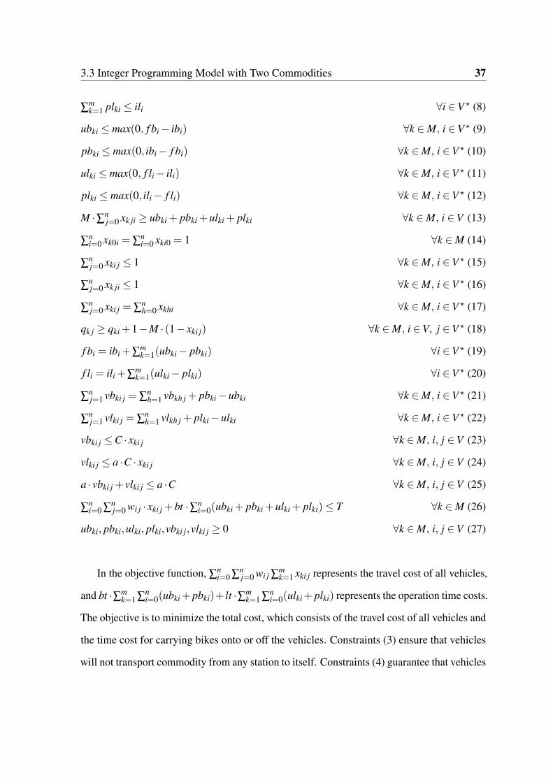
3.3 Integer Programming Model with Two Commodities 37
∑mk=1 plki ≤ ili ∀i ∈V ⋆ (8)
ubki ≤ max(0, f bi − ibi) ∀k ∈ M, i ∈V ⋆ (9)
pbki ≤ max(0, ibi − f bi) ∀k ∈ M, i ∈V ⋆ (10)
ulki ≤ max(0, f li − ili) ∀k ∈ M, i ∈V ⋆ (11)
plki ≤ max(0, ili − f li) ∀k ∈ M, i ∈V ⋆ (12)
M ·∑nj=0 xk ji ≥ ubki + pbki +ulki + plki ∀k ∈ M, i ∈V (13)
∑ni=0 xk0i = ∑
ni=0 xki0 = 1 ∀k ∈ M (14)
∑nj=0 xki j ≤ 1 ∀k ∈ M, i ∈V ⋆ (15)
∑nj=0 xk ji ≤ 1 ∀k ∈ M, i ∈V ⋆ (16)
∑nj=0 xki j = ∑
nh=0 xkhi ∀k ∈ M, i ∈V ⋆ (17)
qk j ≥ qki +1−M · (1− xki j) ∀k ∈ M, i ∈V, j ∈V ⋆ (18)
f bi = ibi +∑mk=1(ubki − pbki) ∀i ∈V ⋆ (19)
f li = ili +∑mk=1(ulki − plki) ∀i ∈V ⋆ (20)
∑nj=1 vbki j = ∑
nh=1 vbkh j + pbki −ubki ∀k ∈ M, i ∈V ⋆ (21)
∑nj=1 vlki j = ∑
nh=1 vlkh j + plki −ulki ∀k ∈ M, i ∈V ⋆ (22)
vbki j ≤C · xki j ∀k ∈ M, i, j ∈V (23)
vlki j ≤ a ·C · xki j ∀k ∈ M, i, j ∈V (24)
a · vbki j + vlki j ≤ a ·C ∀k ∈ M, i, j ∈V (25)
∑ni=0 ∑
nj=0 wi j · xki j +bt ·∑n
i=0(ubki + pbki +ulki + plki)≤ T ∀k ∈ M (26)
ubki, pbki,ulki, plki,vbki j,vlki j ≥ 0 ∀k ∈ M, i, j ∈V (27)
In the objective function, ∑ni=0 ∑
nj=0 wi j ∑
mk=1 xki j represents the travel cost of all vehicles,
and bt ·∑mk=1 ∑
ni=0(ubki+ pbki)+ lt ·∑m
k=1 ∑ni=0(ulki+ plki) represents the operation time costs.
The objective is to minimize the total cost, which consists of the travel cost of all vehicles and
the time cost for carrying bikes onto or off the vehicles. Constraints (3) ensure that vehicles
will not transport commodity from any station to itself. Constraints (4) guarantee that vehicles
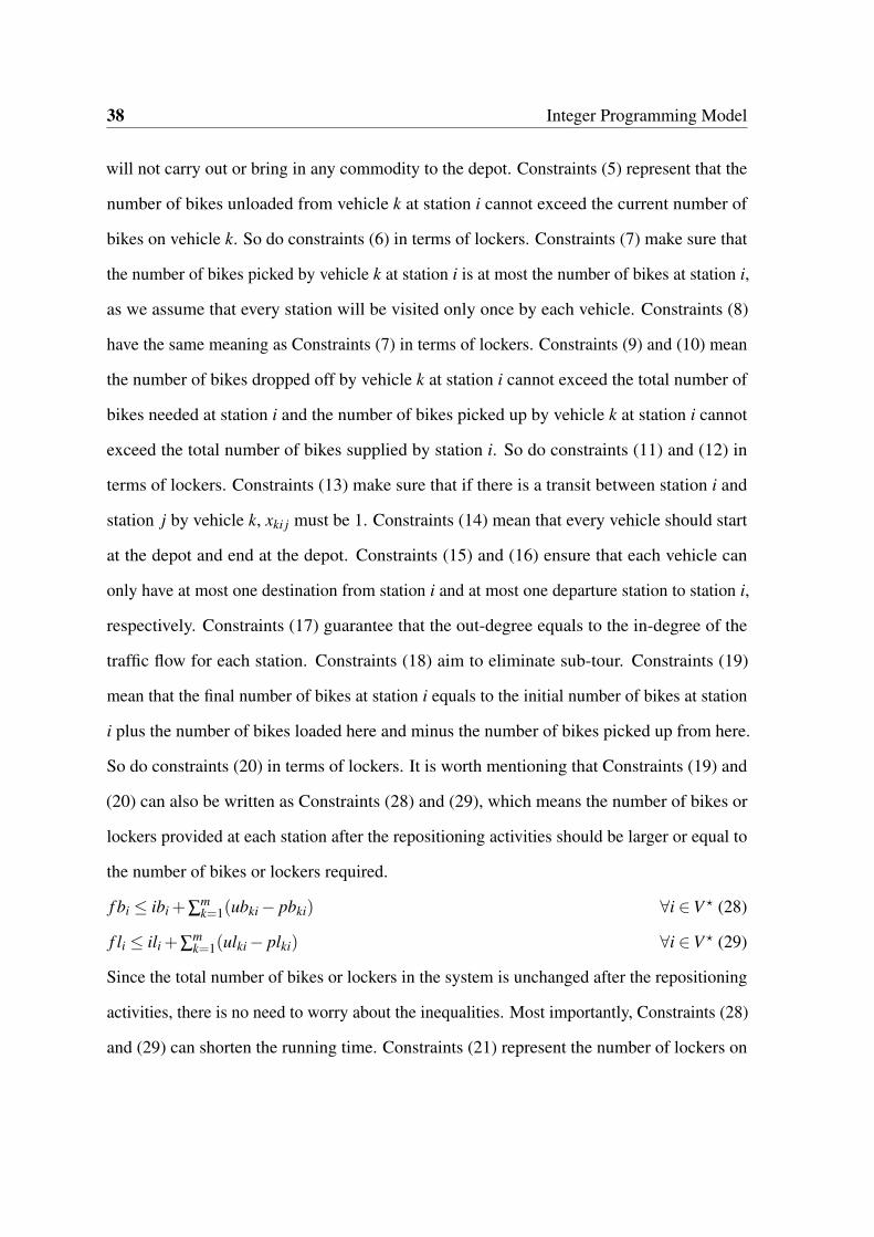
38 Integer Programming Model
will not carry out or bring in any commodity to the depot. Constraints (5) represent that the
number of bikes unloaded from vehicle k at station i cannot exceed the current number of
bikes on vehicle k. So do constraints (6) in terms of lockers. Constraints (7) make sure that
the number of bikes picked by vehicle k at station i is at most the number of bikes at station i,
as we assume that every station will be visited only once by each vehicle. Constraints (8)
have the same meaning as Constraints (7) in terms of lockers. Constraints (9) and (10) mean
the number of bikes dropped off by vehicle k at station i cannot exceed the total number of
bikes needed at station i and the number of bikes picked up by vehicle k at station i cannot
exceed the total number of bikes supplied by station i. So do constraints (11) and (12) in
terms of lockers. Constraints (13) make sure that if there is a transit between station i and
station j by vehicle k, xki j must be 1. Constraints (14) mean that every vehicle should start
at the depot and end at the depot. Constraints (15) and (16) ensure that each vehicle can
only have at most one destination from station i and at most one departure station to station i,
respectively. Constraints (17) guarantee that the out-degree equals to the in-degree of the
traffic flow for each station. Constraints (18) aim to eliminate sub-tour. Constraints (19)
mean that the final number of bikes at station i equals to the initial number of bikes at station
i plus the number of bikes loaded here and minus the number of bikes picked up from here.
So do constraints (20) in terms of lockers. It is worth mentioning that Constraints (19) and
(20) can also be written as Constraints (28) and (29), which means the number of bikes or
lockers provided at each station after the repositioning activities should be larger or equal to
the number of bikes or lockers required.
f bi ≤ ibi +∑mk=1(ubki − pbki) ∀i ∈V ⋆ (28)
f li ≤ ili +∑mk=1(ulki − plki) ∀i ∈V ⋆ (29)
Since the total number of bikes or lockers in the system is unchanged after the repositioning
activities, there is no need to worry about the inequalities. Most importantly, Constraints (28)
and (29) can shorten the running time. Constraints (21) represent the number of lockers on

3.4 Numerical Experiment 39
vehicle k at station i equals to the number of bikes on vehicle k before arriving station i plus
the bikes picked up or minus the number of bikes unloaded at station i. Constraints (22) have
the same meaning as Constraints (21) in terms of lockers. Constraints (23), (24) and (25) are
the vehicle capacity constraints. Constraints (26) ensure that for each vehicle, the travel time
plus the time of loading/unloading bikes does not exceed the limit of total operation time T .
Constraints (27) are the non-negative constraints.
3.4 Numerical Experiment
In this section, first, the test results of the new constraints created for the IP model with one
commodities will be presented. Then, an illustrative example will be explained for IP model
with two commodities, followed by the test results of IP model with two commodities. All
the tests in this section use simulated data.
3.4.1 Numerical Experiments of New Constraints
In order to see the computational improvement of Constraints (1) and Constraints (2), we test
them on cases with up to 100 stations and 3 vehicles. The tests are conducted in IBM ILOG
CPLEX Optimization Studio 12.6 on a computer with i7-4770 CPU and 8 GB RAM. The
data used in these tests is generated by the Data Generator describe in Chapter 4. The testing
results are listed in Table 3.1.
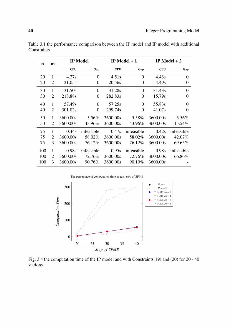
40 Integer Programming Model
Table 3.1 the performance comparison between the IP model and IP model with additionalConstraints
n m IP Model IP Model + 1 IP Model + 2
CPU Gap CPU Gap CPU Gap
20 1 4.27s 0 4.51s 0 4.43s 020 2 21.05s 0 20.56s 0 4.49s 0
30 1 31.50s 0 31.28s 0 31.43s 030 2 218.88s 0 282.83s 0 15.79s 0
40 1 57.49s 0 57.25s 0 55.83s 040 2 301.02s 0 299.74s 0 41.07s 0
50 1 3600.00s 5.56% 3600.00s 5.58% 3600.00s 5.56%50 2 3600.00s 43.96% 3600.00s 43.96% 3600.00s 15.54%
75 1 0.44s infeasible 0.47s infeasible 0.42s infeasible75 2 3600.00s 58.02% 3600.00s 58.02% 3600.00s 42.07%75 3 3600.00s 76.12% 3600.00s 76.12% 3600.00s 69.65%
100 1 0.98s infeasible 0.95s infeasible 0.98s infeasible100 2 3600.00s 72.76% 3600.00s 72.76% 3600.00s 66.86%100 3 3600.00s 90.76% 3600.00s 90.10% 3600.00s -
20 25 30 35 40
0
100
200
300
Step o f SPMB
Com
puta
tion
Tim
e
The percentage of computation time at each step of SPMB
IP,m = 1
IP,m = 2
IP+C(19),m = 1
IP+C(19),m = 2
IP+C(20),m = 1
IP+C(20),m = 2
Fig. 3.4 the computation time of the IP model and with Constraints(19) and (20) for 20 - 40stations

3.4 Numerical Experiment 41
50 60 70 80 90 100
0
20
40
60
80
Step o f SPMB
Com
puta
tion
Tim
e
The percentage of computation time at each step of SPMB
IP,m
IP,m+1
IP+C(19),m
IP+C(19),m+1
IP+C(20),m
IP+C(20),m+1
Fig. 3.5 the gap comparison of the IP model and with Constraints (19) and (20) in 1 hour for50 - 100 stations
According to Table 3.1, several patterns can be observed and are summarized as below.
1. The computation time of the IP model increases significantly when the number of
vehicles increases, even if the additional vehicle is redundant.
2. Mostly, adding Constraints (1) does not improve the computational performance of the
IP model.
3. For cases with single vehicle, adding Constraints (2) does not improve the computa-
tional performance of the IP model, which is reasonable because Constraints (2) are created
for multivehicle situations. For cases with up to 40 stations, the time of getting the optimal
solution reduces significantly by adding Constraints (2) (see Figure 3.4); for cases with 50 to
100 stations, within the same running time, the gap between the lower and upper bound gets
much smaller by adding Constraints (2) (see Figure 3.5).
4. Based on the current parameter settings of Data Generator for light demands, one
vehicle is probably able to handle 50 stations.
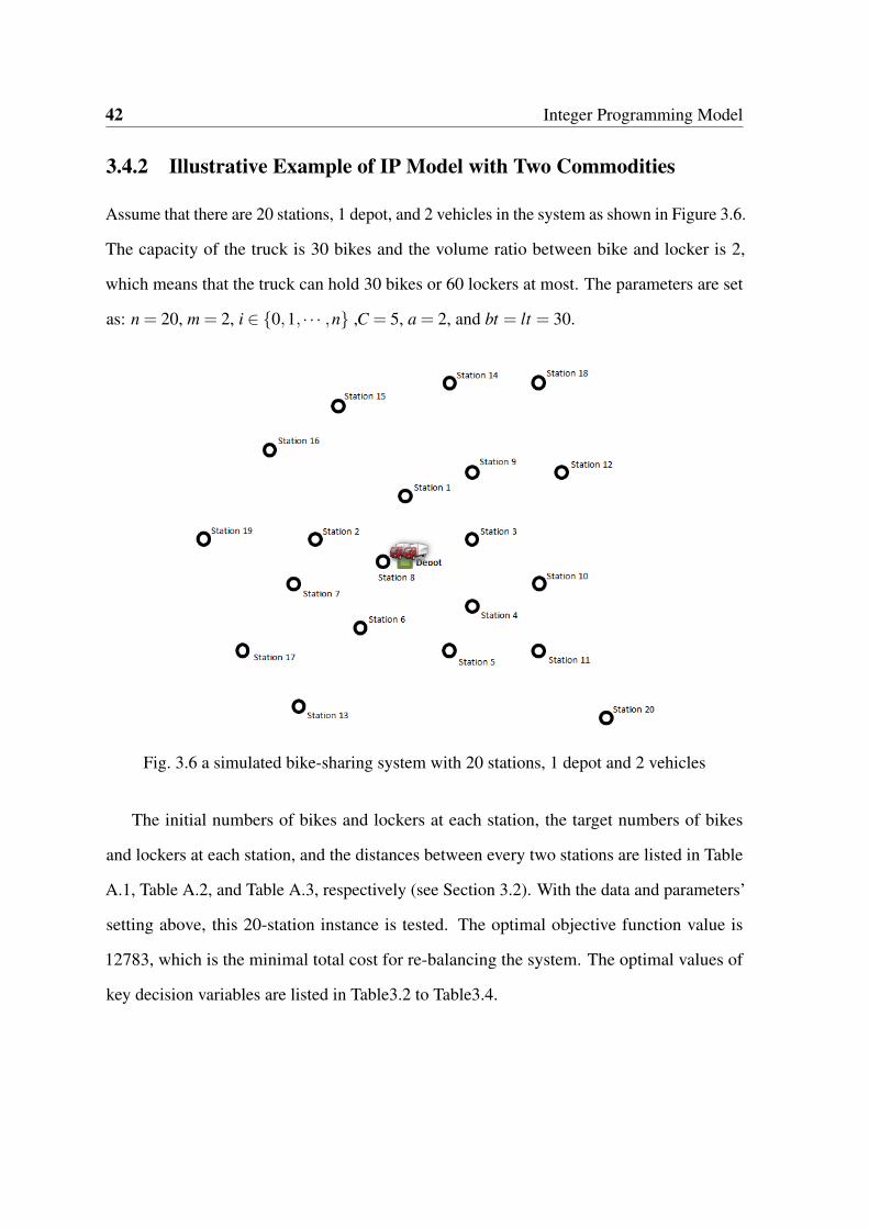
42 Integer Programming Model
3.4.2 Illustrative Example of IP Model with Two Commodities
Assume that there are 20 stations, 1 depot, and 2 vehicles in the system as shown in Figure 3.6.
The capacity of the truck is 30 bikes and the volume ratio between bike and locker is 2,
which means that the truck can hold 30 bikes or 60 lockers at most. The parameters are set
as: n = 20, m = 2, i ∈ {0,1, · · · ,n} ,C = 5, a = 2, and bt = lt = 30.
Fig. 3.6 a simulated bike-sharing system with 20 stations, 1 depot and 2 vehicles
The initial numbers of bikes and lockers at each station, the target numbers of bikes
and lockers at each station, and the distances between every two stations are listed in Table
A.1, Table A.2, and Table A.3, respectively (see Section 3.2). With the data and parameters’
setting above, this 20-station instance is tested. The optimal objective function value is
12783, which is the minimal total cost for re-balancing the system. The optimal values of
key decision variables are listed in Table3.2 to Table3.4.

3.4 Numerical Experiment 43
Table 3.2 the optimal values of decision variables x for vehicle 1
n 0 1 2 3 4 5 6 7 8 9 10 11 12 13 14 15 16 17 18 19 20
0 0 0 0 1 0 0 0 0 0 0 0 0 0 0 0 0 0 0 0 0 01 0 0 0 0 0 0 0 0 1 0 0 0 0 0 0 0 0 0 0 0 02 0 0 0 0 0 0 0 1 0 0 0 0 0 0 0 0 0 0 0 0 03 0 0 0 0 0 0 0 0 0 0 1 0 0 0 0 0 0 0 0 0 04 0 0 0 0 0 1 0 0 0 0 0 0 0 0 0 0 0 0 0 0 05 0 0 0 0 0 0 0 0 0 0 0 0 0 1 0 0 0 0 0 0 06 1 0 0 0 0 0 0 0 0 0 0 0 0 0 0 0 0 0 0 0 07 0 0 0 0 0 0 1 0 0 0 0 0 0 0 0 0 0 0 0 0 08 0 0 1 0 0 0 0 0 0 0 0 0 0 0 0 0 0 0 0 0 09 0 1 0 0 0 0 0 0 0 0 0 0 0 0 0 0 0 0 0 0 010 0 0 0 0 0 0 0 0 0 0 0 0 0 0 0 0 0 0 0 0 111 0 0 0 0 1 0 0 0 0 0 0 0 0 0 0 0 0 0 0 0 012 0 0 0 0 0 0 0 0 0 1 0 0 0 0 0 0 0 0 0 0 013 0 0 0 0 0 0 0 0 0 0 0 0 0 0 0 0 0 1 0 0 014 0 0 0 0 0 0 0 0 0 0 0 0 0 0 0 0 0 0 1 0 015 0 0 0 0 0 0 0 0 0 0 0 0 0 0 1 0 0 0 0 0 016 0 0 0 0 0 0 0 0 0 0 0 0 0 0 0 1 0 0 0 0 017 0 0 0 0 0 0 0 0 0 0 0 0 0 0 0 0 0 0 0 1 018 0 0 0 0 0 0 0 0 0 0 0 0 1 0 0 0 0 0 0 0 019 0 0 0 0 0 0 0 0 0 0 0 0 0 0 0 0 1 0 0 0 020 0 0 0 0 0 0 0 0 0 0 0 1 0 0 0 0 0 0 0 0 0
Table 3.3 the optimal loading instructions of transiting bikes and lockers for vehicle 1
n 1 2 3 4 5 6 7 8 9 10 11 12 13 14 15 16 17 18 19 20
Ub 0 3 0 0 0 6 7 0 5 0 0 2 7 0 0 0 5 0 0 3Pb 1 0 8 5 3 0 0 6 0 4 7 0 0 2 1 0 0 1 0 0Ul 0 2 0 8 0 5 7 0 4 0 0 0 5 0 0 0 4 0 0 0Pl 2 0 3 0 2 0 0 2 0 7 5 4 0 2 1 1 0 3 3 0
From Table 3.4, we can see vehicle 2 stays at the depot and is not involved the reposi-
tioning activities. The routes of the 2 vehicles (see Figure 3.7) can be drawn according to
Table 3.2 and 3.4.
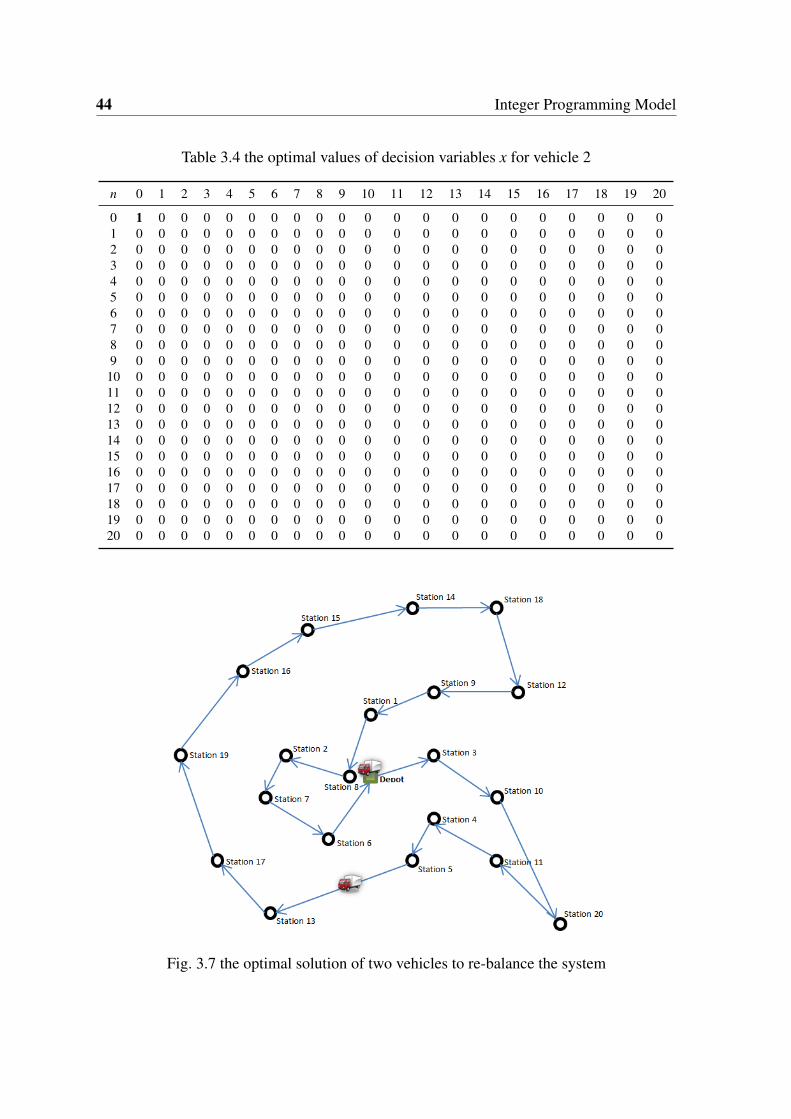
44 Integer Programming Model
Table 3.4 the optimal values of decision variables x for vehicle 2
n 0 1 2 3 4 5 6 7 8 9 10 11 12 13 14 15 16 17 18 19 20
0 1 0 0 0 0 0 0 0 0 0 0 0 0 0 0 0 0 0 0 0 01 0 0 0 0 0 0 0 0 0 0 0 0 0 0 0 0 0 0 0 0 02 0 0 0 0 0 0 0 0 0 0 0 0 0 0 0 0 0 0 0 0 03 0 0 0 0 0 0 0 0 0 0 0 0 0 0 0 0 0 0 0 0 04 0 0 0 0 0 0 0 0 0 0 0 0 0 0 0 0 0 0 0 0 05 0 0 0 0 0 0 0 0 0 0 0 0 0 0 0 0 0 0 0 0 06 0 0 0 0 0 0 0 0 0 0 0 0 0 0 0 0 0 0 0 0 07 0 0 0 0 0 0 0 0 0 0 0 0 0 0 0 0 0 0 0 0 08 0 0 0 0 0 0 0 0 0 0 0 0 0 0 0 0 0 0 0 0 09 0 0 0 0 0 0 0 0 0 0 0 0 0 0 0 0 0 0 0 0 0
10 0 0 0 0 0 0 0 0 0 0 0 0 0 0 0 0 0 0 0 0 011 0 0 0 0 0 0 0 0 0 0 0 0 0 0 0 0 0 0 0 0 012 0 0 0 0 0 0 0 0 0 0 0 0 0 0 0 0 0 0 0 0 013 0 0 0 0 0 0 0 0 0 0 0 0 0 0 0 0 0 0 0 0 014 0 0 0 0 0 0 0 0 0 0 0 0 0 0 0 0 0 0 0 0 015 0 0 0 0 0 0 0 0 0 0 0 0 0 0 0 0 0 0 0 0 016 0 0 0 0 0 0 0 0 0 0 0 0 0 0 0 0 0 0 0 0 017 0 0 0 0 0 0 0 0 0 0 0 0 0 0 0 0 0 0 0 0 018 0 0 0 0 0 0 0 0 0 0 0 0 0 0 0 0 0 0 0 0 019 0 0 0 0 0 0 0 0 0 0 0 0 0 0 0 0 0 0 0 0 020 0 0 0 0 0 0 0 0 0 0 0 0 0 0 0 0 0 0 0 0 0
Fig. 3.7 the optimal solution of two vehicles to re-balance the system

3.4 Numerical Experiment 45
According to Tables 3.2 and 3.3, in order to satisfy the required number of bikes and
lockers at each station and meanwhile follow the shortest route, only Vehicle 1 needs to
reallocate the bikes and lockers. Firstly, Vehicle 1 goes to Station 3 to pick 8 bikes and 3
lockers and then heads to Station 10. After picking 4 bikes and 7 lockers, Vehicle 1 reaches
Station 20 to unload 3 bikes. Then Vehicle 1 moves to Station 11 and picks 7 bikes plus 5
lockers. The next stop is Station 4. After taking 5 bikes and leaving 8 lockers, Vehicle 1
goes to Station 5 for picking 3 bikes and 2 lockers. Vehicle 1 then arrives at Station 13 and
drops 7 bikes and 5 lockers. After reaching Station 17 and leaving 5 bikes and 4 lockers,
Vehicle 1 moves to Station 19 for taking 3 lockers. After that, it goes to Station 16 to pick 1
locker. It continues to pick 1 bike and 1 lock at Station 15 and goes to Station 14 for taking
2 more bikes and 2 more lockers. Then Vehicle 1 picks 1 bike and 3 lockers at Station 18.
After reaching Station 12 and dropping 2 bikes and taking 4 lockers, it goes to Station 9 and
uploads 5 bikes and 4 lockers. Then it picks 1 bike and 2 lockers for Station 1 and moves to
Station 8 for 6 more bike and 2 more lockers. After it gives Station 2 3 bikes and 2 lockers, it
goes to Station 7 and leaves 7 bikes and 7 lockers. The final stop is Station 6, where Vehicle
1 drops 6 bikes and 5 lockers. In the end, it returns to the depot.
3.4.3 Numerical Experiments of IP Model with Two Commodities
More simulated cases are tested by the IP model with two commodities and are solved in
IBM ILOG CPLEX Optimization Studio 12.6.0.0 on an Intel (R) Core (TM) i5-3470 CPU
@3.2 GHZ with 4 GB of RAM. All the numerical experiments use CPLEX’s default settings
(the default optimality tolerance is 0.01%). The results of test computation time and optimal
objective value for different parameters are listed in Table 3.5.

46 Integer Programming Model
Table 3.5 the results of computation time & optimal objective value for different parameters
n C m = 1 m = 2 m = 3
4
3 Infeasible Unbounded or Infeasible 00.24s(3Vehicle,Obj.=5035)5 Infeasible 00.23s(2Vehicle,Obj.=3812) 00.32s(2Vehicle,Obj.=3812)10 00.12s(Obj.= 2531) 00.15s(1Vehicle,Obj.= 2531) 00.21s(1Vehicle,Obj.= 2531)15 00.17s(Obj.= 2531) 00.15s(1Vehicle,Obj.= 2531) 00.20s(1Vehicle,Obj.= 2531)20 00.12s(Obj.= 2531) 00.14s(1Vehicle,Obj.= 2531) 00.21s(1Vehicle,Obj.= 2531)25 00.12s(Obj.= 2531) 00.17s(1Vehicle,Obj.= 2531) 00.20s(1Vehicle,Obj.= 2531)30 00.12s(Obj.= 2531) 00.20s(1Vehicle,Obj.= 2531) 00.24s(1Vehicle,Obj.= 2531)35 00.12s(Obj.= 2531) 00.17s(1Vehicle,Obj.= 2531) 00.20s(1Vehicle,Obj.= 2531)40 00.12s(Obj.= 2531) 00.15s(1Vehicle,Obj.= 2531) 00.21s(1Vehicle,Obj.=2531)
5
3 Infeasible Unbounded or Infeasible 00.73s(3Vehicle,Obj.=7609)5 Infeasible 00.29s(2Vehicle,Obj.=5108) 00.37s(2Vehicle,Obj.= 5108)10 00.14s(Obj.= 3737) 00.23s(1Vehicle,Obj.=3737) 00.46s(1Vehicle,Obj.=3737)15 00.12s(Obj.= 3201) 00.21s(1Vehicle,Obj.= 3201) 00.29s(1Vehicle,Obj.= 3201)20 00.14s(Obj.= 3201) 00.18s(1Vehicle,Obj.= 3201) 00.46s(1Vehicle,Obj.= 3201)25 00.12s(Obj.= 3201) 00.21s(1Vehicle,Obj.= 3201) 00.37s(1Vehicle,Obj.= 3201)30 00.12s(Obj.= 3201) 00.18s(1Vehicle,Obj.= 3201) 00.35s(1Vehicle,Obj.= 3201)35 00.10s(Obj.= 3201) 00.29s(1Vehicle,Obj.= 3201) 00.35s(1Vehicle,Obj.= 3201)40 00.17s(Obj.= 3201) 00.18s(1Vehicle,Obj.= 3201) 00.32s(1Vehicle,Obj.= 3201)
6
3 Infeasible Unbounded or Infeasible 13.32s(3Vehicle,Obj.=8716)5 Infeasible 00.62s(2Vehicle,Obj.=6299) 16.82s(2Vehicle,Obj.=6299)10 00.17s(Obj.=4382) 00.43s(1Vehicle,Obj.= 4382) 00.73s(1Vehicle,Obj.= 4382)15 00.23s(Obj.=4005) 00.35s(1Vehicle,Obj.= 4005) 01.01s(1Vehicle,Obj.= 4005)20 00.15s(Obj.=3696) 00.21s(1Vehicle,Obj.= 3696) 00.53s(1Vehicle,Obj.= 3696)25 00.14s(Obj.= 3696) 00.29s(1Vehicle,Obj.= 3696) 00.45s(1Vehicle,Obj.= 3696)30 00.12s(Obj.= 3696) 00.21s(1Vehicle,Obj.= 3696) 00.54s(1Vehicle,Obj.= 3696)35 00.12s(Obj.= 3696) 00.23s(1Vehicle,Obj.= 3696) 00.47s(1Vehicle,Obj.= 3696)40 00.15s(Obj.= 3696) 00.20s(1Vehicle,Obj.= 3696) 00.48s(1Vehicle,Obj.= 3696)
7
3 Infeasible Unbounded or Infeasible 2min58.68s(3Vehicle,Obj.=9546)5 Infeasible 07.20s(2Vehicle,Obj.=6846) 48.02s(2Vehicle,Obj.=6846)10 00.18s(Obj.=4794) 01.10s(1Vehicle,Obj.=4794) 01.84s(1Vehicle,Obj.=4794)15 00.17s(Obj.=4263) 00.53s(1Vehicle,Obj.=4263) 01.79s(1Vehicle,Obj.=4263)20 00.20s(Obj.= 3954) 00.23s(1Vehicle,Obj.= 3954) 00.65s(1Vehicle,Obj.=3954)25 00.15s(Obj.= 3954) 00.26s(1Vehicle,Obj.= 3954) 01.20s(1Vehicle,Obj.= 3954)30 00.15s(Obj.= 3954) 00.23s(1Vehicle,Obj.= 3954) 02.21s(1Vehicle,Obj.= 3954)35 00.17s(Obj.= 3954) 00.26s(1Vehicle,Obj.= 3954) 01.09s(1Vehicle,Obj.= 3954)40 00.14s(Obj.= 3954) 00.34s(1Vehicle,Obj.= 3954) 00.54s(1Vehicle,Obj.= 3954)
8
3 Infeasible 09.47s(2Vehicle,Obj.=7714) 20min58.88s(2Veh.,Obj.=7714)5 Infeasible 24.53s(2Vehicle,Obj.=5842) 2min26.78s(2Vehicle,Obj.=5842)10 00.26s(Obj.=4417) 02.79s(1Vehicle,Obj.=4417) 08.67s(1Vehicle,Obj.=4417)15 00.15s(Obj.=3900) 00.46s(1Vehicle,Obj.= 3900) 03.63s(1Vehicle,Obj.= 3900)20 00.17s(Obj.=3900) 00.45s(1Vehicle,Obj.= 3900) 03.72s(1Vehicle,Obj.= 3900)25 00.15s(Obj.=3900) 00.39s(1Vehicle,Obj.= 3900) 03.19s(1Vehicle,Obj.= 3900)30 00.21s(Obj.=3900) 00.53s(1Vehicle,Obj.= 3900) 02.20s(1Vehicle,Obj.= 3900)35 00.20s(Obj.= 3900) 00.49s(1Vehicle,Obj.= 3900) 01.87s(1Vehicle,Obj.= 3900)40 00.18s(Obj.= 3900) 00.39s(1Vehicle,Obj.= 3900) 03.80s(1Vehicle,Obj.= 3900)
9
3 Infeasible 4min23.15s(2Vehicle,Obj.=7613) >45min5 00.20s(Obj.=6143) 2min49.95s(2Vehicle,Obj.=5757) 13min18.94s(2Veh.,Obj.=5757)10 00.48s(Obj.=4720) 07.86s(1Vehicle,Obj.=4720) 29.98s(1Vehicle,Obj.=4720)15 00.21s(Obj.= 4095) 00.96s(1Vehicle,Obj.=4095) 05.72s(1Vehicle,Obj.= 4095)20 00.17s(Obj.= 4095) 00.46s(1Vehicle,Obj.=4095) 04.07s(1Vehicle,Obj.=4095)25 00.18s(Obj.= 4095) 01.06s(1Vehicle,Obj.=4095) 05.61s(1Vehicle,Obj.= 4095)30 00.18s(Obj.= 4095) 00.76s(1Vehicle,Obj.=4095) 03.71s(1Vehicle,Obj.= 4095)35 00.20s(Obj.= 4095) 00.46s(1Vehicle,Obj.=4095) 03.66s(1Vehicle,Obj.= 4095)40 00.21s(Obj.= 4095) 00.67s(1Vehicle,Obj.=4095) 03.97s(1Vehicle,Obj.= 4095)
10
3 Infeasible 1min00.95s(2Vehicle,Obj.=6849) 5min58.42s(2Vehicle,Obj.=6849)5 00.42s(Obj.=6138) 7min07.48s(2Vehicle,Obj.=6069) >30min10 00.26s(Obj.=4716) 03.30s(1Vehicle,Obj.=4716) 15.24s(1Vehicle,Obj.=4716)15 00.21s(Obj.=4700) 04.64s(1Vehicle,Obj.=4700) 08.86s(1Vehicle,Obj.=4700)20 00.29s(Obj.=4700) 01.09s(1Vehicle,Obj.=4700) 13.27s(1Vehicle,Obj.=4700)25 00.20s(Obj.=4700) 02.93s(1Vehicle,Obj.=4700) 11.76s(1Vehicle,Obj.=4700)30 00.26s(Obj.=4700) 01.63s(1Vehicle,Obj.=4700) 15.25s(1Vehicle,Obj.=4700)35 00.24s(Obj.=4700) 02.82s(1Vehicle,Obj.=4700) 08.47s(1Vehicle,Obj.=4700)40 00.21s(Obj.=4700) 02.68s(1Vehicle,Obj.=4700) 08.54s(1Vehicle,Obj.=4700)

3.4 Numerical Experiment 47
n C m = 1 m = 2 m = 3
11
3 Infeasible Infeasible Infeasible5 Infeasible Unbounded or Infeasible >43min10 Infeasible >50min >59min15 04.14s(Obj.=7726) 2min44.88s(1Vehicle,Obj.=7726) >45min20 02.40s(Obj.=7039) 18.45s(1Vehicle,Obj.=7039) 1min26.01s(1Vehicle,Obj.=7039)25 00.93s(Obj.=6704) 09.45s(1Vehicle,Obj.=6704) 1min14.05s(1Vehicle,Obj.=6704)30 00.37s(Obj.=6590) 01.79s(1Vehicle,Obj.=6590) 15.21s(1Vehicle Obj.=6590)35 00.31s(Obj.=6590) 02.32s(1Vehicle,Obj.=6590) 20.50s(1Vehicle Obj.=6590)40 00.51s(Obj.=6590) 02.24s(1Vehicle,Obj.=6590) 18.72s(1Vehicle Obj.=6590)
12
3 Infeasible Infeasible Unbounded or Infeasible5 Infeasible Unbounded or Infeasible >55min10 Infeasible >52min >53min15 05.47s(Obj.=8839) >1h >38min20 03.72s(Obj.=8006) 2min29.78s(1Vehicle,Obj.=8006) 7min56.08s(1Vehicle,Obj.=8006)25 00.76s(Obj.=7635) 30.46s(1Vehicle,Obj.=7635) 1min39.71(1Vehicle,Obj.=7635)30 00.39s(Obj.=7451) 10.12s(1Vehicle,Obj.=7451) 16.06s(1Vehicle,Obj.=7451)35 00.40s(Obj.=7451) 03.35s(1Vehicle,Obj.=7451) 13.86s(1Vehicle,Obj.=7451)40 00.81s(Obj.=7451) 02.09s(1Vehicle,Obj.=7451) 16.72s(1Vehicle,Obj.=7451)
13
3 Infeasible Infeasible Unbounded or Infeasible5 Infeasible 1h24min07.71s(2V.,Obj.=8990) >43min10 Infeasible >1h >31min15 09.87s(Obj.=9905) >33min >1h20 14.38s(Obj.=8990) 3min34.01s(1Vehicle,Obj.=8990) 20min08.45s(1Veh.,Obj.=899025 04.80s(Obj.=8858) 1min15.67s(1Vehicle,Obj.=8858) 6min02.56s(1Vehicle,Obj.=8858)30 07.22s(Obj.=8817) 1min01.05s(1Veh.,Obj.=8817) 8min33.63s(1Veh.,Obj.=8817)35 00.35s(Obj.=8334) 1.90s(1Vehicle,Obj.=8334) 31.39s(1Vehicle,Obj.=8334)40 00.39s(Obj.=8334) 1.98s(1Vehicle,Obj.=8334) 19.48s(1Vehicle,Obj.=8334)
14
3 Infeasible Infeasible Unbounded or Infeasible5 Infeasible >38min >57min10 04.57s(Obj.=13331) >49min >1h15 15.45s(Obj.=11130) >42min >46min20 14.19s(Obj.=9865) 4min57.91s(1Veh.,Obj.=9865) 14min59.76s(1Veh.,Obj.=9865)25 08.06s(Obj.=9750) 2min37.73s(1Vehicle,Obj.=9750) 11min40.62s(1Veh.,Obj.=9750)30 12.09s(Obj.=9692) 2min24.82.s(1Veh.,Obj.=9692) 17min49.32s(1Veh.,Obj.=9692)35 00.43s(Obj.=9226) 15.95s(1Vehicle,Obj.=9226) 27.47s(1Vehicle,Obj.=9226)40 00.42s(Obj.=9226) 3.33s(1Vehicle,Obj.=9226) 1min38.14s(1Vehicle,Obj.=9226)
15
3 Infeasible Infeasible Unbounded or Infeasible5 Infeasible >54min >1h10 04.47s(Obj.=13231) >1h19min >43min15 39.23s(Obj.=11575) >42min >42min20 10.12s(Obj.=10456) 38min41.50s(1Veh.,Obj.=10456) 43min59.63s(1Veh.,Obj.=10456)25 01.59s(Obj.=10083) 2min08.65s(1Veh.,Obj.=10083) 3min23.37(1Veh.,Obj.=10083)30 04.88s(Obj.=10083) 1min14.60s(1Veh.,Obj.=10083) 14min41.13s(1V.,Obj.=16296)35 00.49s(Obj.=9806) 14.12s(1Vehicle,Obj.=9806) 33.37s(1Vehicle,Obj.=9806)40 00.51s(Obj.=9806) 10.82s(1Vehicle,Obj.=9806) 42.51s(1Vehicle,Obj.=9806)
16
3 Infeasible Unbounded or Infeasible Unbounded or Infeasible5 Infeasible >59min >1h1min10 14.14s(Obj.=12816) >40min >48min15 1min11.85s(Obj.=11616) >1h5min >1h17min20 1min03.21s(Obj.=10769) 49min29.56s(1Veh.,Obj.=10769) >49min25 36.24s(Obj.=10382) 7min07.05s(1Veh.,Obj.=10382) >44min30 21.65s(Obj.=10268) 11min53.11s(1V.,Obj.=10268) 20min27.61s(1V.,Obj.=10268)35 18.29s(Obj.=10225) 4min26.23s(1Veh.,Obj.=10225) 8min36.05(1Veh.,Obj.=10225)40 04.08s(Obj.=10091) 1min26.55s(1Veh.,Obj.=10091) 3min31.38s(1Veh.,Obj.=10091)
17
3 Infeasible Unbounded or Infeasible Unbounded or Infeasible5 Infeasible >1h26min >59min10 26.36s(Obj.=14886) >54min >1h59min15 3min23.91s(Obj.=13397) >1h >2h51min20 2min18.74s(Obj.=11945) >39min >59min25 35.35s(Obj.=11351) 17min01.52(1Veh.,Obj.=11351) >35min30 44.91s(Obj.=11202) 14min10.88s(1V.,Obj.=11202) 41min17.36s(1Veh.,Obj.=11202)35 22.21s(Obj.=10938) 4min27.47s(1Veh.,Obj.=10938) 10min55.96s(1Veh.,Obj.=10938)40 02.98s(Obj.=10713) 39.46s(1Vehicle,Obj.=10713) 11min46.11s(1Veh.,Obj.=10713)

48 Integer Programming Model
n C m = 1 m = 2 m = 3
18
3 Infeasible Infeasible Unbounded or Infeasible5 Infeasible >1h1min >2h35min10 16.47s(Obj.=15617) >59min >2h38min15 4min19.27s(Obj.=13978) >59min >2h42min20 10min11.68s(Obj.=12632) >45min >2h14min25 1min35.29s(Obj.=12066) >52min >2h36min30 1min01.16s(Obj.=11757) 59min26.51s(1V.,Obj.=11757) 5h35min52.12s(1V,Obj.=11757)35 39.42s(Obj.=11522) 3min41.32s(1Veh.,Obj.=11522) 3h29min42.15s(1V.,Obj.=11522)40 04.36s(Obj.=11204) 47.78s(1Vehicle,Obj.=11204) 7min00.26s(1Veh.,Obj.=11204)
19
3 Infeasible Infeasible Unbounded or Infeasible5 Infeasible >59min >1h42min10 12.79s(Obj.=15936) >1h >59min15 9min01.75s(Obj.=14409) >56min >50min20 14min29.00.s(Obj.=13055) >49min >42min25 1min59.48s(Obj.=12464) 1h46min27.69s(1V.,Obj.=12464) >46min30 3min25.76s(Obj.=12306) 55min55.78s(1V.,Obj.=12306) 6h27min42.73s(1V,Obj.=12306)35 1min52.58s(Obj.=12162) 35min22.77s(1Veh.,Obj.=12162) >2h40min40 22.99s(Obj.=11956) 4min53.26s(1Veh.,Obj.=11956) 41min23.83s(1Veh.,Obj.=11956)
20
3 Infeasible Infeasible Unbounded or Infeasible5 Infeasible Unbounded or Infeasible >1h10min10 Infeasible >56min >59min15 16min36.53s(Obj.=15033) >58min >59min20 19min42.74s(Obj.=13765) >36min >42min25 1min10.45s(Obj.=13041) 1h4min06.58s(Obj.=13041) >55min30 25.27s(Obj.=12926) 8min35.33s(1Veh.,Obj.=12926) 1h50min08.74(1V.,Obj.=12926)35 33.90s(Obj.=12925) 20min03.75s(1Veh.,Obj.=12925) 24min31.44s(1Veh.,Obj.=12925)40 10.31s(Obj.=12783) 8min56.42s(1Veh.,Obj.=12783) 34min24.95s(1Veh.,Obj.=12783)
According to the testing results in Table 3.5, some patterns and insights can be summa-
rized below.
1. Mostly, the computation time increases exponentially when the number of stations
increases. For example, when we fix the vehicle capacity (C = 25), Figure 3.8 shows the
changing trends of computation time as the number of stations increases when the number of
vehicle equals to 1−3. As expected, the computation time is exponentially increasing with
the growth of stations to serve. But there are little drop offs when the station numbers are 15
and 20.

3.4 Numerical Experiment 49
5 10 15 20
0
50
100
Number o f stations (n)
Com
puti
ngti
me(s
econ
ds)
The computing time when m = 1 and C = 25
m = 1
5 10 15 20
0
2,000
4,000
6,000
Number o f stations (n)
com
puti
ngti
me
The computing time when m = 2 and C = 25
m = 2
4 6 8 10 12 14
0
200
400
600
Number o f stations (n)
Com
puti
ngti
me(s
econ
ds)
The computing time when m = 3 and C = 25
m = 3
5 10 15 20
0
2,000
4,000
6,000
Number o f stations (n)
Com
puti
ngti
me(s
econ
ds)
The comparison of computing time with m = 1,2,3
m = 1m = 2m = 3
Fig. 3.8 the computation time of 5-20 stations when the number of vehicle equals to 1 - 3
2. The computation time increases tremendously when the number of vehicles increases,
even if the additional vehicle is redundant.
3. The computation time decreases when the vehicle capacity increases until the optimal
objective value does not change. We assume that m = 3, which means fixing the number
of vehicles for repositioning activities. The Figure 3.9 is to compare the computation time
for different number of stations (n = 4−10) and different vehicle capacities (C = 15−40).
For the same number of stations, the computation times are different with various vehicle
capacities. Figure 3.9 shows that the computation time does not always linearly increase or
decrease with the vehicle capacity, but there is still a trend that larger capacity takes less time
for a fixed number of stations until the capacity does not affect the objective value.
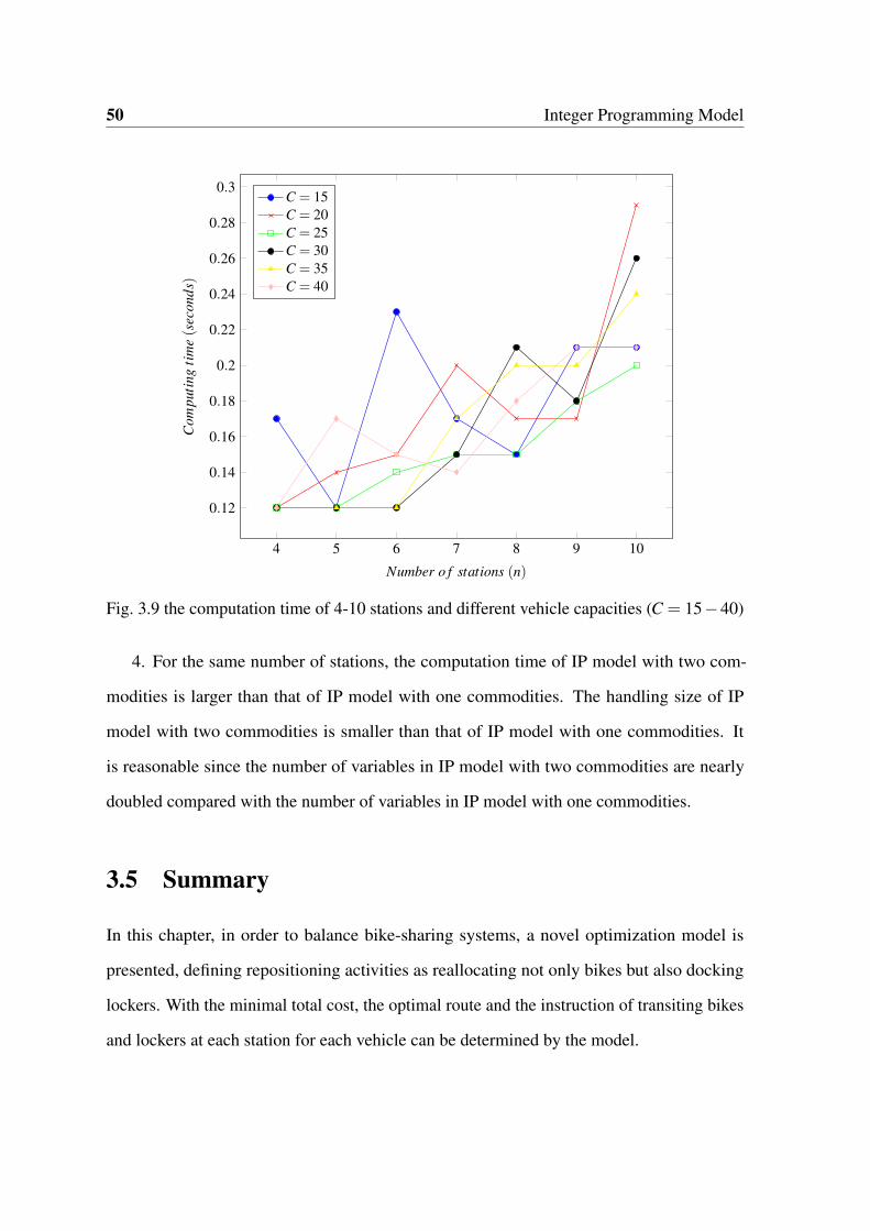
50 Integer Programming Model
4 5 6 7 8 9 10
0.12
0.14
0.16
0.18
0.2
0.22
0.24
0.26
0.28
0.3
Number o f stations (n)
Com
puti
ngti
me(s
econ
ds)
C = 15C = 20C = 25C = 30C = 35C = 40
Fig. 3.9 the computation time of 4-10 stations and different vehicle capacities (C = 15−40)
4. For the same number of stations, the computation time of IP model with two com-
modities is larger than that of IP model with one commodities. The handling size of IP
model with two commodities is smaller than that of IP model with one commodities. It
is reasonable since the number of variables in IP model with two commodities are nearly
doubled compared with the number of variables in IP model with one commodities.
3.5 Summary
In this chapter, in order to balance bike-sharing systems, a novel optimization model is
presented, defining repositioning activities as reallocating not only bikes but also docking
lockers. With the minimal total cost, the optimal route and the instruction of transiting bikes
and lockers at each station for each vehicle can be determined by the model.

3.5 Summary 51
After numerical experiments, the results of computation time show three major patterns.
1. the computation time is exponentially increasing with the growth of stations to serve; 2.
the computation time does not always linearly increase or decrease with the vehicle capacity,
but there is still a trend that larger capacity takes less time for a fixed number of stations
until the vehicle has surplus capacity; 3. and for multi-vehicle cases, the computation time
increases tremendously if the actual repositioning activities need more than one vehicle.


Chapter 4
An Integer Programming Based
Heuristic for Medium-Sized Problem
As pointed out at the end of Chapter 2, the static repositioning problem of bike-sharing system
is NP-hard. Therefore, in order to balance larger-scale systems, developing algorithms is
essential. In this chapter, we focus on static repositioning problem for bike-sharing system,
considering only transporting bikes. The construction of an IP based heuristic (IPBH) method
will be presented and the efficiency of IPBH for medium-sized instances will be shown by
the computation testing.
This algorithm was inspired by comparing the optimal solution for a 20 station’s case
with the solution from a heuristic that was developed earlier. The optimal solution and the
heuristic solution of this 20 station’s case are shown in Figure 4.1.

54 An Integer Programming Based Heuristic for Medium-Sized Problem
Depot
1
2
3
4 5
6
7
8
9
10
11
12 13
14
15
16
17
18
19
20
Depot
1
2
3
4 5
6
7
8
9
10
11
12 13
14
15
16
17
18
19
20
Fig. 4.1 the comparison of the optimal solution and a heuristic solution of a 20 station’sinstance
Comparing the heuristic solution on the right hand side of Figure 4.1 with the optimal one
on the left hand side, we can see that some arcs in the heuristic solution are very costly, such
as e8 14 and e20 17, where ei j means the arc from node i to node j, ∀i, j ∈ [0,n]. If we can find
a way to remove the costly arcs and provide the IP model with a graph that contains relatively
short arcs, the IP model will search the solution from this graph instead of a complete graph.
Then, the computation time will decrease, as the number of arcs are reduced.
The main idea of forming this undirected graph is to find some good arcs at first; then
spread these arcs and make them reach out to other nodes; in the meantime, take advantage
of those good arcs as much as possible until all nodes with non-zero demand are connected
by the undirected graph. The good arcs, which we called Must-Use-Arc (MUA), are defined
as follows: if either of any two nodes is the closest one to the other and both of their demands
are not zero, the undirected arc between them is a MUA.
In the following part of this Chapter, the detailed procedure of IPBH together with an
illustrative example are presented. Moreover, in order to get a better lower bound of the
objective value for performance comparison, some modifications for the original IP model
with one commodity in Chapter 3 were also developed and tested. At last, the numerical
experiments were conducted to show the performance of IPBH.

4.1 Algorithm Development 55
4.1 Algorithm Development
In this section, we will give a detail explanation of the IPBH development. The required
inputs of IPBH are listed as follows:
• Number of stations n
• Number of vehicles m
• Travel time between every two stations wi j, i, j ∈ [1,n]
• Initial and final number of bikes at each station, which are less than the number of
lockers at that station ibt , f bi
• Time of loading/unloading one bike bt
• Vehicle Capacity C
• Operation time limit T
The 20 station’s case, which is shown in Figure 4.2, will be used as an illustrative example.
In Figure 4.2, the black dot represents the depot and every vehicle must start and end with
depot with zero bike on itself. Each node represents a station and the number beside a node
is the demand of that corresponding station. The nodes with positive numbers represent
demanding stations, while the nodes with negative ones are supplying ones. The key idea of
IPBH is to form the undirected graph with less costly arcs, which connects to all stations. In
total, there are five steps to form the graph.

56 An Integer Programming Based Heuristic for Medium-Sized Problem
Depot
1
+3
2
−2
3
−1
4
−65
−2
6
−3
7 −3
8
+7
9 +3
10 −11
11
+7
12
+313
+1
14
+3
15
+1
160
17
+9
18+10
19−6
20 −13
Fig. 4.2 the deployment of a 20 station’s instance
Step 1 Pre-calculation:
• compute the demand of every station by di = f bi − ibi, i ∈ [1,n]. di > 0 refer to
demanding stations, while di < 0 refer to supplying ones;
• delete stations with zero demand from all stations in record;
• delete infeasible connections: from depot, vehicles can only visit supplying
stations in the next step; to depot, vehicles can only visit demanding stations
before returning to depot; for all stations, vehicles cannot visit two successive
stations that make the total number of their demanding or supplying bikes exceeds
vehicle capacity;
• for each station, sort its possible stations to be connected by distance (travel time)
from small to large.
Step 2 Search MUA:
• find the arcs where there are two nodes which are the closest to each other and
the number of MUA is recorded as l (the MUAs of the illustrative example are
the red lines shown in Figure 4.3);

4.1 Algorithm Development 57
• mark the stations which are not connected to MUAs as left unconnected nodes.
Depot
1
+3
2
−2
3
−1
4
−65
−2
6
−3
7 −3
8
+7
9 +3
10 −11
11
+7
12
+313
+1
14
+3
15
+1
160
17
+9
18+10
19−6
20 −13
Fig. 4.3 the MUAs of a 20 stations’ instance
Step 3 Connect the rest stations to MUAs:
• treat every MUA as a Closed Path, cpi, i ∈ [1, l], which contains nodes and arcs;
• for the left unconnected nodes, start with the one closest to any MUA as a merge
node and connect it to its nearest MUA to form a larger Closed Path cpi, i ∈ [1, l]
with minimal cost (see the blue lines on the left in Figure 4.4); if there are only
2 nodes in the Closed Path, just connect each of them with the merge node.
Otherwise, find the arc with minimal cost that connects merge node and the
Closed Path and connect the merge node with this arc;
• delete the merge node from the left unconnected nodes;
• repeat this process until all stations are connected to Closed Paths(the result of
Step 3 for the illustrative example is on the left in Figure 4.4).
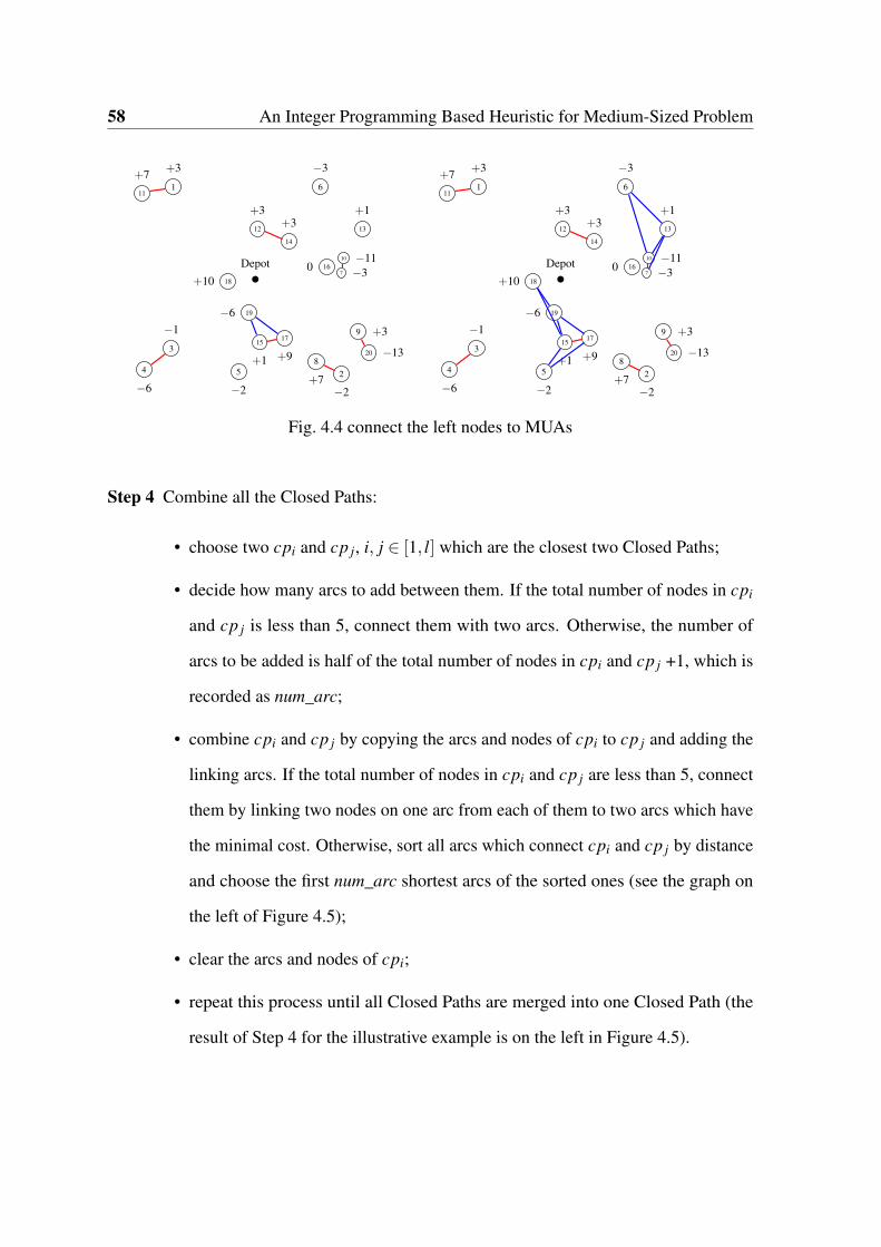
58 An Integer Programming Based Heuristic for Medium-Sized Problem
Depot
1
+3
2
−2
3
−1
4
−65
−2
6
−3
7 −3
8
+7
9 +3
10 −11
11
+7
12
+313
+1
14
+3
15
+1
160
17
+9
18+10
19−6
20 −13
Depot
1
+3
2
−2
3
−1
4
−65
−2
6
−3
7 −3
8
+7
9 +3
10 −11
11
+7
12
+313
+1
14
+3
15
+1
160
17
+9
18+10
19−6
20 −13
Fig. 4.4 connect the left nodes to MUAs
Step 4 Combine all the Closed Paths:
• choose two cpi and cp j, i, j ∈ [1, l] which are the closest two Closed Paths;
• decide how many arcs to add between them. If the total number of nodes in cpi
and cp j is less than 5, connect them with two arcs. Otherwise, the number of
arcs to be added is half of the total number of nodes in cpi and cp j +1, which is
recorded as num_arc;
• combine cpi and cp j by copying the arcs and nodes of cpi to cp j and adding the
linking arcs. If the total number of nodes in cpi and cp j are less than 5, connect
them by linking two nodes on one arc from each of them to two arcs which have
the minimal cost. Otherwise, sort all arcs which connect cpi and cp j by distance
and choose the first num_arc shortest arcs of the sorted ones (see the graph on
the left of Figure 4.5);
• clear the arcs and nodes of cpi;
• repeat this process until all Closed Paths are merged into one Closed Path (the
result of Step 4 for the illustrative example is on the left in Figure 4.5).

4.1 Algorithm Development 59
Depot
1
+3
2
−2
3
−1
4
−65
−2
6
−3
7 −3
8
+7
9 +3
10 −11
11
+7
12
+313
+1
14
+3
15
+1
160
17
+9
18+10
19−6
20 −13
Depot
1
+3
2
−2
3
−1
4
−65
−2
6
−3
7 −3
8
+7
9 +3
10 −11
11
+7
12
+313
+1
14
+3
15
+1
160
17
+9
18+10
19−6
20 −13
Fig. 4.5 combine the closed paths for the 20 station’s instance
Step 5 Connect depot to all the demanding and supplying stations ( Figure 4.6).
Depot
1
+3
2
−2
3
−1
4
−65
−2
6
−3
7 −3
8
+7
9 +3
10 −11
11
+7
12
+313
+1
14
+3
15
+1
160
17
+9
18+10
19−6
20 −13
Fig. 4.6 the final undirected graph for the 20 station’s instance
After generating the undirected graph, set the upper bound of the decision variable xi j of
the IP model (see Appendix) to 0, if ei j is not in the graph, and then run the IP model.
60 An Integer Programming Based Heuristic for Medium-Sized Problem
4.2 Numerical Experiment
In this section, we first present the method of generating the data for testing. After that,
the methods to assist the computation of the original IP model are proposed. Finally, the
results of numerical experiment for IPBH algorithm are summarized in order to show the
performance of IPBH algorithm.
4.2.1 Data Generator
Location of station:
For most successful bike-sharing systems, the average distance between stations should be
300 meters (see ITDP [79]). Therefore, the size of the square map size would approximately
be (√
n+1) ·300 meters. Assume average driving speed in city is 50km/h, which is the speed
limitation in Auckland City, and there is no traffic jam during night. Then we can get the
map size in terms of time, which is (√
n+1) ·21.6 seconds. Then within this square area, the
depot was set at the center point, and the coordinates of stations were randomly generated.
Number of bikes & docking lockers at station:
Based on the analysis of bicycles-to-population ratio and docks-per-bike ratio in various
cities by ITDP[79], we set the initial number of bikes at each station as 20, and the number of
lockers as 40. For the final number of bikes at each station, we generated it based on normal
distribution via the same method proposed by Forma et al.[50].
4.2.2 Methods to Speed up IP Model
In order to conduct the numerical experiment of IPBH and show the computation performance,
the optimal solution or at least a good lower bound for larger-sized instances should be
provided. We tried running larger-sized instances of 50 and 100 stations using the original IP
model (see Section 3.2) by Gurobi Optimizer 7.0.2 in Linux64 on one node of the NeSi Pan

4.2 Numerical Experiment 61
Cluster, which has 16 CPU Cores and 128 GB memory. However, after 48 hours, we could
not get the optimal solution for 50 stations’ case. Moreover, for 100 stations’ instance, not
even a feasible solution was found. Therefore, efforts must be made to assist the computation
of the original IP model.
Modify the original IP model
1 Add constraints ∑ni=1 xk0i ≥ ∑
ni=1 x(k+1)0i ∀k ∈ [1, . . . ,m−1] (1), which make sure that
vehicle k+1 can be used only if vehicle k is in use (see Section 3.2).
2 Add constraints ∑ni=1 i · xk0i −0.5 ·∑n
i=1 xk0i ≥ ∑ni=1 i · x(k+1)0i ∀k ∈ [1, . . . ,m−1] (2),
which aim to ensure that vehicle k+1 can be used only if vehicle k is in use, and each
route is assigned to a specific vehicle by making the first destination of vehicle k larger
(or smaller) than that of vehicle k+1 (see Section 3.2).
3 Remove the integer limitation of the decision variable vbki j, which is the number of bikes
on vehicle k when traveling from station i to station j. The number of bikes on vehicle
is computed by the number of bikes picked up or dropped off at each station, which
are both integers. Thus, the number of bikes on vehicle must be an integer.
Table 4.1 the computation time (seconds) of the IP model with different modifications
(m=2) 20-1 20-2 20-3 20-4 30-1 30-2 30-3 30-4
Original IP 15.45 28.16 15.51 54.39 372.26 3909.57 5373.89 11516.59IP+1 14.95 27.70 15.29 55.08 380.74 3938.60 5001.50 11986.17IP+2 6.08 18.46 1.81 7.91 40.84 244.78 37.44 1650.88IP+3 27.64 23.19 17.36 196.81 386.18 11900.99 25180.70 12083.01IP+1+2 6.02 18.68 1.71 7.70 40.78 250.86 38.04 1649.80IP+1+3 28.27 23.12 17.46 193.41 378.19 11282.84 23570.27 27377.04IP+2+3 1.39 8.18 2.19 2.98 13.84 242.36 53.76 1668.23IP+1+2+3 1.30 8.17 2.21 2.91 13.79 334.29 53.56 657.82
In order to see the performance of these modifications and decide which of them would
be used, we did a test on 20 and 30 stations’ cases. The results are shown in Table 4.1.

62 An Integer Programming Based Heuristic for Medium-Sized Problem
We can see that in most cases, the first and second modifications decrease the computation
time, especially the second one, which is adding Constraints (2). However, for the third
modification, it appears that it cannot accelerate the IP model, and may even make the IP
model much slower, such as case 30-3. But mostly, the third modification can improve the
performance when used together with the second modification.
1 2 3 4 5 6 7 8
0
20
40
60
80
100
120
Instance number
Tim
epe
rcen
tage
(%)
IP+1IP+2
IP+1+2IP+2+3
IP+1+2+3
Fig. 4.7 the percentage of the computation time of original IP for better modifications
Figure 4.7 shows the percentage of computation time by IP model, of IP+1, IP+2, IP+1+2,
IP+2+3, IP+1+2+3. It is obvious that the most outstanding ones are IP+2+3 and IP+1+2+3.
Since combining all of them seem to be more efficient and safer to improve the computation
ability of the original IP model, all three of these modifications will be used in the following
section for computing the optimal solution or at least a good lower bound for larger-sized
instances.
4.2 Numerical Experiment 63
Provide the IP model with an initial solution
Providing an initial solution is also a very efficient way to accelerate the original IP model.
For example, to a 50 stations’ instance, after adding an initial solution to the IP model, the
running time of getting the optimal solution is reduced from 1227.94 seconds to 134.78
seconds.
Consider unsatisfied demands
According to the literature of static repositioning problem for bike-sharing systems, we
noticed that large instances were tested by Forma et al.[50] and Ho and Szeto[10] and the
performances of their algorithms are very impressive. Especially, in the work of Ho and
Szeto[10], cases such as 200 stations with 3 vehicles can be solved within 34.37 seconds and
the gap is only 5.33%. But there is a key difference between our problem and theirs, which is
we aim to meet all demands of the system while they allowed unsatisfied demands. As we
explained earlier, the static repositioning happens at night. Thus, in our opinion, it is more
reasonable that the system can be set up exactly as the required status. However, in the work
of Forma et al.[50] and Ho and Szeto[10], as assuming not all demands must be fulfilled, the
objective function is to minimize the total travel cost together with the weighted unsatisfied
demands. Intuitively speaking, the problem with unsatisfied demands is likely to be easier
than exactly satisfying, because allowing unsatisfied demands has more flexibility. In order
to confirm our guessing, we modified the original IP model to allow unsatisfied demands and
then run some tests on it with small instances to compare with the original IP model. The
modifications are listed below.
1 Add Inputs
dw: weight of unsatisfied demand in the objective function
2 Add Decision Variables
duki: number of bikes, which should be but are not unloaded by vehicle k at station i,

64 An Integer Programming Based Heuristic for Medium-Sized Problem
i ∈V ⋆, k ∈ M
d pki: number of bikes, which should be but are not picked up by vehicle k at station i,
i ∈V ⋆, k ∈ M
3 Modify Objective Function
∑ni=0 ∑
nj=0 wi j ∑
mk=1 xki j+bt ·∑m
k=1 ∑ni=0(ubki+ pbki)+dw ·∑m
k=1 ∑ni=1(duki+d pki), where
the part, dw ·∑mk=1 ∑
ni=1(duki +d pki), represents the weighted cost of total unsatisfied
demands.
4 Modify Constraints
Modify the Constraints (13) in the Apendix to
f bi = ibi +∑mk=1(ubki +duki − pbki −d pki) ∀i ∈V ⋆ (28)
5 Add Constraints
duki ≤ max(0, f bi − ibi) ∀k ∈ M, i ∈V ⋆ (29)
d pki ≤ max(0, ibi − f bi) ∀k ∈ M, i ∈V ⋆ (30)
duki, d pki ≤ 0 ∀k ∈ M, i ∈V ⋆ (31)
It is obvious that if the weight of unsatisfied demands in the objective function is very
large, the solution of this problem would always be the same as that of our problem, where all
demands are satisfied. Because the model will automatically choose the solution that satisfies
all demands, since the cost of unsatisfied demand would be too large even if only one demand
is not fulfilled. Therefore, we tried changing the parameter dw to 100000. According to
the testing result in Table 4.2, we can see that even with dw = 100000, the performance of
the IP mode with unsatisfied demand is still better than the original one. As a result, the
fourth modification we decide to add to speed up our IP model is to allow unsatisfied demand
but with a very huge weight in the objective function. We also tried adding the previous
modification methods to the IP model that allows unsatisfied demand. We can also see the
efficiency of the modification methods.

4.2 Numerical Experiment 65
Table 4.2 the computation time of the IP model with unsatisfied demands (IPUD)
20-1 20-2 20-3 20-4
Original IP 15.45s 28.16s 15.51s 54.39sIPUD (dw=1000) 13.52s 16.27s 25.19s 52.80sIPUD (dw=100000) 14.08s 15.93s 18.36s 51.52sIPUD+1+2+3 (dw=100000) 1.70s 7.33s 2.64s 2.74s
Setting Fleet Size m
As pointed out in the numerical experiment in Chapter 2, the computation time will increase
a lot when fleet size increases by 1, even this additional vehicle will not be in use. In addition,
it is reasonable to use the least number of vehicles for the purpose of cutting the operation
costs. Thus, we could assume if the optimal solution to balance the system with k vehicles
exists, the optimal objective value with k+1 vehicles is no better than the optimal objective
value with k vehicles. However, we are not sure if the assumption is true all the time. Since
we have not figured out a way to prove it, we tried finding a counter example, which is if
the optimal solution to balance the system with k vehicles exists, the optimal objective value
with k+1 vehicles is better than the optimal objective value with k vehicles.
As a result, a simple program was built to try to find a counter example. In this program,
the number of stations is 6, the capacity of vehicle is 6, but the locations of stations are
randomly generated. Then run the IP model once, and if the optimal objective value of the
IP model with m = 1 is larger than that of the IP model with m = 2, stop. Otherwise, repeat
generating the coordinates of 6 stations and running the IP model. In the end, after 13078
times of repeating, a counter example was found. The deployment of the stations are shown
in Figure 4.8.

66 An Integer Programming Based Heuristic for Medium-Sized Problem
Depot
1
−5
2
+33
+2
4
−2
5
+4
6−2
Fig. 4.8 the example that using one more vehicle has shorter travel cost
Depot
1−5
2
+3 3
+2
4
−2
5
+4
6−2
Depot
1−5
2
+3 3
+2
4
−2
5
+4
6−2
Fig. 4.9 the optimal solution comparison of the counter example
Figure 4.9 shows the optimal solutions of the counter example with 1 and 2 vehicles. The
objective value of using a single vehicle to balance the system is 362, while the objective
value of using 2 vehicles is 361. However, the reason of one more vehicle having a better
objective value is actually caused by the rounding calculation of the distance between stations
with coordinates. According to the triangle inequality, 0->1 and 5->0 should be larger or
equal to 5->1. While in this case, because of the rounding, 0->1(14) + 5->0(31) = 45 is
smaller than 5->1(46).
Although it is not actually caused by the system deployment, we do have this situation
because of the way we computed the distance between every two stations. But we can take
4.2 Numerical Experiment 67
this case where the optimal objective value with k+ 1 vehicles is better than the optimal
objective value with k vehicles as a very rare circumstance.
According to the experiments above, we put forward a hypothesis as follows.
Hypothesis 1 (H1): If the optimal solution to balance the system with k vehicles exists and
increasing vehicle capacity will not affect the optimal object value, the optimal objective
value with k+1 vehicles is no better than the optimal objective value with k vehicles.
Because if the optimal solution to balance the system with k−1 vehicles does not exist,
the model will stop in seconds saying infeasible or unbounded. Thus, with Hypothesis 1, if
the IP model is infeasible or unbounded when m = k−1 and can start searching the optimal
solution with m = k, we say m = k is the right setting for fleet size and optimal solution of IP
model with m = k is the best solution of IPBH.
4.2.3 Numerical Experiment of IPBH
The main purpose of this section is to present the results of IPBH which is developed in
previous section with simulated data generated by the Data Generator described earlier. All
the simulated instances are generated by Visual Studio 2017 using C++. All the numerical
experiments of heuristic use Visual Studio 2017 by C++ and all the numerical experiments
concerning IP model are solved in APML calling Gurobi’s with default settings (the default
optimal tolerance is 0.01%) on an Intel (R) Core (TM) i7-4770 [email protected] GHZ with 8 GB
of RAM.
In order to show the efficiency of IPBH for medium-sized instances, instances with
50-100 stations are tested by IPBH. The parameter settings listed in Table 4.3 are referred to
the paper by Forma et al.[50].
If the optimal solution can be computed, the GAP is computed as
GAP =OBJ of IPBH - OBJ/BLB of IP model
OBJ/BLB of IP model(4.1)
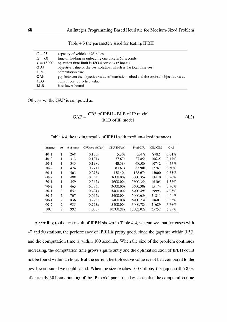
68 An Integer Programming Based Heuristic for Medium-Sized Problem
Table 4.3 the parameters used for testing IPBH
C = 25 capacity of vehicle is 25 bikesbt = 60 time of loading or unloading one bike is 60 secondsT = 18000 operation time limit is 18000 seconds (5 hours)OBJ objective value of the best solution, which is the total time costCPU computation timeGAP gap between the objective value of heuristic method and the optimal objective valueCBS current best objective valueBLB best lower bound
Otherwise, the GAP is computed as
GAP =CBS of IPBH - BLB of IP model
BLB of IP model(4.2)
Table 4.4 the testing results of IPBH with medium-sized instances
Instance m # of Arcs CPU(graph Part) CPU(IP Part) Total CPU OBJ/CBS GAP
40-1 1 268 0.166s 5.30s 5.47s 8782 0.04%40-2 1 313 0.181s 37.67s 37.85s 10645 0.15%50-1 1 345 0.198s 48.38s 48.58s 10742 0.39%50-2 1 424 0.271s 83.63s 83.90s 12782 0.50%60-1 1 403 0.275s 158.40s 158.67s 15000 0.75%60-2 1 488 0.353s 3600.00s 3600.35s 13410 0.96%70-1 1 459 0.347s 3600.00s 3600.35s 16405 1.38%70-2 1 463 0.383s 3600.00s 3600.38s 15174 0.96%80-1 2 652 0.494s 5400.00s 5400.49s 19993 4.07%80-2 2 707 0.645s 5400.00s 5400.65s 21811 4.61%90-1 2 836 0.726s 5400.00s 5400.73s 18601 3.62%90-2 2 935 0.775s 5400.00s 5400.78s 21689 5.76%100 2 992 1.036s 10300.98s 10302.02s 25752 6.85%
According to the test result of IPBH shown in Table 4.4, we can see that for cases with
40 and 50 stations, the performance of IPBH is pretty good, since the gaps are within 0.5%
and the computation time is within 100 seconds. When the size of the problem continues
increasing, the computation time grows significantly and the optimal solution of IPBH could
not be found within an hour. But the current best objective value is not bad compared to the
best lower bound we could found. When the size reaches 100 stations, the gap is still 6.85%
after nearly 30 hours running of the IP model part. It makes sense that the computation time

4.3 Summary 69
is still increasing exponentially with the increase of the MUAs, because IPBH is based on
the IP model. But what we can confirm is that the graph part is efficient, since for all the
cases the running time of the graph part are within 1 second except for the 100 station one.
Moreover, the generated graph contains good solution because the final gaps of the tested
instances are small. Although the gaps are increasing for larger cases, it may be mainly
caused by the IP model part, as we are not able to get the optimal solution or a better lower
bound for large instances. Nevertheless, more efforts need to be made to solve instances
larger than 100 stations.
4.3 Summary
In this chapter, a heuristic method, called IPBH, is developed to solve static repositioning
problem of bike-sharing systems. IPBH includes two parts, generating the graph and running
the IP model with the settings of the upper bound of decision variable xki j based on the
graph. In the numerical experiment, first, we present the data generator for the simulated
instances used in algorithm testing. Then, for the purpose of getting a better lower bound for
algorithm performance comparison, we tested several ways to speed up the original IP model.
In the end, the testing result of IPBH shows the satisfying performance for medium-sized
cases. The need of performance improvements has been indicated for large-sized instances
of bike sharing systems.


Chapter 5
A Set-Partitioning Based Heuristic for
Large-Sized Problem
The algorithm developed in this chapter is a Set-Partitioning based heuristic (SPBH). SPBH
is mainly used to solve the static repositioning problem for bike-sharing systems with more
than 100 stations.
SPBH is inspired by the work of Balinski and Quandt[80], which used Set-Partitioning
(SP) model to solve delivery problem. Using this formulation to solve routing problem has
two main advantages. First, column enumeration can save us from many complex route
constraints and it is very easy to manipulate routes as they are represented by columns.
Moreover, although this delivery problem belongs to IP problems, it can be easily solved
by formulating as a SP model. The main idea of SPBH is to take advantage of SP model
which is able to quickly pick up the best route(s) from thousands of routes and easily make
modifications to routes. But unfortunately, we are unable to enumerate every possible route
when n becomes large. Thus, one key part of SPBH is providing a pool of good feasible routes
within a short time, instead of enumerating all. It is also important to generate new better
feasible routes by creating effective modification operators, in order to keep the solution
improving. Thus, after modifying the solution of SP model by some operators and adding
72 A Set-Partitioning Based Heuristic for Large-Sized Problem
new better feasible routes to the pool, SP model will run again to select the current best
combination of routes. The process of route modification and SP model rerun repeats until
there is no further improvement of the solution or when the computation time limit is reached.
In the following sections, first we introduce the main structure of SPBH. Then the key
components of SPBH, which are generating a pool of feasible routes, SP model, modification
operators, are presented in details. The performance of SPBH is shown in the numerical
experiment, which is relatively good for large-sized instances. Moreover, according to the
numerical experiment of the IP model in Chapter 3, the running time increases tremendously
as the number of vehicles increases, even if some of the vehicles are not in use. However, in
reality, how many vehicles are actually needed to balance the system is unknown, especially
for large-sized problem. To our best knowledge, Set-Partitioning model has not been used
to solve repositioning problem for bike-sharing systems before. Moreover, the number of
vehicles is needed as an input in previous works. While the number of vehicles needed is
an output in SPBH so that the running time of SPBH will not be affected by the number of
vehicles.
5.1 Algorithm Development
The required inputs of SPBH are listed as follows:
• Number of stations n
• Travel time between every two stations wi j, i, j ∈ [0,n]
• Initial and final number of bikes at each station ibt , f bi, which are less than the number
of lockers at that station
• Time of loading/unloading one bike bt
• Vehicle Capacity C
5.1 Algorithm Development 73
• Operation time limit T
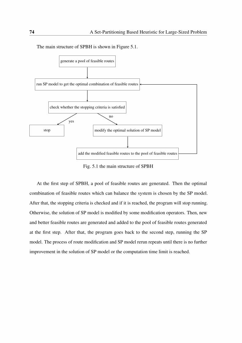
74 A Set-Partitioning Based Heuristic for Large-Sized Problem
The main structure of SPBH is shown in Figure 5.1.
generate a pool of feasible routes
run SP model to get the optimal combination of feasible routes
check whether the stopping criteria is satisfied
stop modify the optimal solution of SP model
add the modified feasible routes to the pool of feasible routes
yesno
Fig. 5.1 the main structure of SPBH
At the first step of SPBH, a pool of feasible routes are generated. Then the optimal
combination of feasible routes which can balance the system is chosen by the SP model.
After that, the stopping criteria is checked and if it is reached, the program will stop running.
Otherwise, the solution of SP model is modified by some modification operators. Then, new
and better feasible routes are generated and added to the pool of feasible routes generated
at the first step. After that, the program goes back to the second step, running the SP
model. The process of route modification and SP model rerun repeats until there is no further
improvement in the solution of SP model or the computation time limit is reached.

5.1 Algorithm Development 75
5.1.1 Feasible Route Generation
Feasible route is defined as a route travelled by a single vehicle, so that all or some of the
stations in the system will be visited and balanced by this vehicle. In the meantime, both of
vehicle capacity limit and operation time limit are not violated.
In the following part of this section, four methods, which are Enumerate Method, Random
Method, 10-Neighborhood-Search Method and Graph base Method, are proposed to generate
feasible routes. Every method will compute the total time cost of each generated feasible
route. The stopping criteria of Random Method, 10-Neighborhood-Search Method and Graph
based Method is reaching a running time limit or when no more feasible routes could be
generated. The performance comparison of these four methods are presented at Section 5.2.
Enumerate Method
In order to validate the SP model formulated in Section 5.1.2, we first tried enumerating all
the feasible routes. When all feasible routes are provided, if the SP model works correctly,
the optimal solution of the SP model should be the same as the optimal solution of the IP
model shown in Appendix. But this Enumerate Method can only work with cases of up to 10
stations due to the limit of computer memory. Thus, in order to test multi-vehicle situations,
we keep reducing the operation time limit until multiple vehicles are needed to balance 10
stations. In the end, both of the single and two-vehicle cases are tested and their optimal
solutions of the SP model are the same as the optimal solution of the IP model.
Random Method
Random Method is developed as a basic benchmark in order to show the performance
improvements by other methods of generating feasible routes. Instead of totally random
choosing a station to visit in the next step, we keep track of the unselected stations and

76 A Set-Partitioning Based Heuristic for Large-Sized Problem
randomly select the next station from them. Because when there are few stations left, it
would be very hard to get an unvisited station by random selection from all stations.
10-Neighborhood-Search Method
As Neighborhood Search is a common and reasonable method in solving VRP, we create this
10-Neighborhood-Search method to generate feasible routes by selecting the next destination
from the ten closest neighbors of the station currently visited. There are three main steps
of 10-Neighborhood-Search method. We define supplying station as a station that provides
bikes, where the required final number of bikes is larger than the initial number of bikes;
demanding station is a station that needs more bikes, where the required final number of
bikes is less than the initial number of bikes.
Step 1 Pre-calculation: 1. Delete stations with zero demand from all stations, as it does not
need to be visited. 2. Delete infeasible arcs. Vehicles starting at depot cannot visit
demanding stations in the next step, as the number of bikes on vehicles at depot is
zero. Therefore, the arcs between depot and demanding stations can be deleted. For
all stations except the depot, vehicles cannot visit two stations successively when the
sum of two demanding stations or the sum of two supplying stations exceeds vehicle
capacity. Thus, the arcs between such two stations can be deleted. 3. For each station,
sort every rest station by the distance of the arc between them.
Step 2 Start a feasible route with a random supplying station.
Step 3 Randomly choose the next station from the 10 neighborhoods of the current visiting
station.
Graph based Method
Graph based method is to generate feasible routes based on the graph formed by the approach
described in Section 4.1. Because according to the numerical tests of IPBH, we know that the
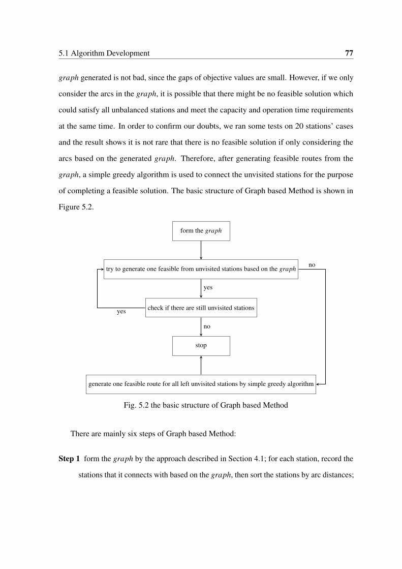
5.1 Algorithm Development 77
graph generated is not bad, since the gaps of objective values are small. However, if we only
consider the arcs in the graph, it is possible that there might be no feasible solution which
could satisfy all unbalanced stations and meet the capacity and operation time requirements
at the same time. In order to confirm our doubts, we ran some tests on 20 stations’ cases
and the result shows it is not rare that there is no feasible solution if only considering the
arcs based on the generated graph. Therefore, after generating feasible routes from the
graph, a simple greedy algorithm is used to connect the unvisited stations for the purpose
of completing a feasible solution. The basic structure of Graph based Method is shown in
Figure 5.2.
form the graph
try to generate one feasible from unvisited stations based on the graph
check if there are still unvisited stations
stop
generate one feasible route for all left unvisited stations by simple greedy algorithm
yes
no
no
yes
Fig. 5.2 the basic structure of Graph based Method
There are mainly six steps of Graph based Method:
Step 1 form the graph by the approach described in Section 4.1; for each station, record the
stations that it connects with based on the graph, then sort the stations by arc distances;

78 A Set-Partitioning Based Heuristic for Large-Sized Problem
Step 2 generate one feasible route from unvisited stations based on the graph, starting with
the closest supplying station that has not been visited;
Step 3 select the next station based on the arcs of the graph;
Step 4 check feasibility; if it is capacity feasible and operation time feasible, and the number
of bikes on the vehicle is 0, send the vehicle back to the depot, and if still operation
time is feasible, write down this feasible route; if it is capacity feasible and operation
time feasible, but the number of bikes on the vehicle is not 0, continue searching; if it
is not feasible, then go back to step 3 and select a different unvisited station;
Step 5 generate feasible routes based on the graph until no more feasible routes can be
generated;
Step 6 if there are still some unvisited stations left, greedily connect them and generate one
route, in order to complete a feasible solution.
The process of Graph based Method will stop when no more feasible routes are generated
or the running time limit is reached. The best feasible solution with least total cost is given at
the end of the program.
5.1.2 Set-Partitioning Model and Solution Modification
Set-Partitioning Model
Sets
L: set of feasible routes, L = {1,2, . . . , l}
V ⋆: set of stations excluding the depot, V ⋆ = {1,2,3, . . . ,n}
V 0: set of stations with zero demand

5.1 Algorithm Development 79
Inputs
l: number of feasible routes
n: number of stations
rwi: travel cost of feasible route i, i ∈ L
ri j: binary decision variable. It equals to 1 when station j is visited in feasible route i,
otherwise, it equals to 0. i ∈ L, j ∈V ⋆
Decision Variables
yi: binary decision variable. It equals to 1 when feasible route i is selected, otherwise, it
equals to 0. i ∈ L
Model
Minimize ∑li=1 rwi · yi
s.t.
∑ni=0 ri j · yi = 1 ∀ j ∈V ⋆ \V 0 (1)
The objective function is to minimize the total travel cost of the chosen feasible route(s).
Constraints (1) make sure that every station with non-zero demand must be visited by any of
the chosen feasible route(s).
Modification of SP Model Solution
After getting the current best combination of feasible routes from SP model, the solution will
be modified by the following operators in order to generate new feasible routes with smaller
travel cost.
Connect : connect any two of the feasible routes in the solution when the connection is still
feasible (does not exceed operation time limit) and also reduces travel cost.
80 A Set-Partitioning Based Heuristic for Large-Sized Problem
Re-order : re-order successive stations of the same type (all demanding or all supplying)
in one route. First, identify a sequence of successive stations of the same type. Then,
enumerate all possible sequences of these stations. At last, compute the travel cost of
each sequence, and re-order these stations as the sequence with minimal travel cost.
Record the route if any change has been made.
Switch : switch any two successive stations in one route. For example, the original sequence
of a route is · · ·−> a−> b−> c−> d−> · · · . Try switching b and c, then the new
sequence is · · ·−> a−> c−> b−> d−> · · · . If the switch makes the route shorter,
in other words, wac+wbd < wab+wcd , and still vehicle capacity feasible (vbi represents
the number of bikes on vehicle at station i, vbi ≥ 0 and vbi ≤C, i ∈ [a,c,b,d]), switch
b and c. After going through the whole route, record the new route if any switch has
been made.
Reposition : change the position of any station in one route. For example, we are trying to
reposition node f from · · ·−> a−> f−> b−> · · ·−> c−> d−> · · · to · · ·−>
a− > b− > · · ·− > c− > f− > d− > · · · . After going through all nodes and all
possible positions in this route, record the new route if it is vehicle capacity feasible
and also shorter than the original one.
Remove 1 : remove the crossing arcs in one route. Crossing arcs is defined as two arcs
having a crossing point on them. First, identify crossing arcs. The arcs that connect to
depot are also considered, while the only notable difference is that a route can only
start with supplying station and end with demanding one. Then try to re-arrange the
sequence of the nodes connected by these arcs.
Remove 2 : remove part of a route. Go through one route and compute the number of bikes
on vehicle at every station in it. If the number of bikes on vehicle are the same at two
different stations, for example, route · · ·− > a− > · · ·− > b− > · · · and vba = vbb,

5.1 Algorithm Development 81
the stations between these two stations can be removed from this route. Then a new
route · · ·−> a−> b−> · · · , which must be feasible, is formed and will be recorded.
All operators will be used on each route of SP model solution. The reason of modifying
the solution of SP model instead of all feasible routes that generated at the first place, is that
we can save computation time by improving the relatively good routes. Connect is the first
operator to be used. If a new route is generated by Connect Operator, it will be recorded
and the rest operators will also be used on this route. Re-order Operator is the second one
to be used on each route of the solution and the new routes generated by Connect Operator.
After that, for one route, use Remove 1 once. Then keep use Switch Operator until there
is no further decrease of travel cost. Then keep use Reposition Operator until there is no
further decrease of travel cost. The process of Remove 1, Switch and Reposition Operators
will repeat until no shorter route can be found and the current new route will be recorded.
In the end, use Remove 2 on the routes of SP model solution and the routes generated by
previous operators, and the generated routes will be recorded.
Set-Partitioning Model with Modified Solutions Rerun
As shown in Figure 5.3, after modifying the solution of SP model and generating shorter fea-
sible routes which can still balance the same stations, add the ones generated by modification
operators to the pool of feasible routes and rerun the SP model. Repeat this process until
there are no better feasible routes can be generated from the current SP model solution. Then
set the upper bound of previous solutions to zero for the purpose of preventing from selecting
the previous solutions, in other words, choosing the second best solution to modify. The
program will stop when the running time limit is reached or there is no more improvement of
all solutions selected by the SP model.

82 A Set-Partitioning Based Heuristic for Large-Sized Problem
run SP model
store the solution in S and modify it
check whether better feasible routes can be generated
add the modified ones to the poolset the upper bound of yi to 0, i ∈ S
check whether the stopping criteria is met
set the upper bound of all yi to 1, rerun SP model, and then stop
yes
no
no
yes
Fig. 5.3 the flow path of SP model with solution modification rerun
In the end, a current best solution will be given by SPBH which includes the overall total
cost, the number of feasible routes which is the exact number of vehicles needed to balance
the system, as well as the loading instruction at each station for each vehicle.
5.2 Numerical Experiment
In this section, a numerical experiment was conducted to evaluate the performance of SPBH.
The simulated data used in the numerical experiment were generated by the Data Generator
described in the section 4 of Chapter 5, in Visual Studio 2017 by C++. The feasible route
generating part was also programmed in Visual Studio 2017 using C++. The following parts
including the solution modifications and SP model rerun are performed in Python calling

5.2 Numerical Experiment 83
Gurobi with default settings (the default optimality tolerance is 0.01%). The computer
configuration is an Intel (R) Core (TM) i7-3470 [email protected] GHZ with 8 GB of RAM.
First, we did a simple test on three of the feasible route generation methods, which are
Random Method, 10-Neighborhood-Search Method and Graph based Method respectfully,
with instances of 20 stations. The parameters used for testing feasible route generation
methods are listed in Table 5.1. The testing results are shown in Table 5.2.
Table 5.1 the parameters used for testing feasible route generation methods
C = 30 capacity of vehicle is 30 bikesbt = 10 time of loading or unloading one bike is 10 secondsT = 18000 operation time limit is 18000 seconds (5 hours)OBJ optimal objective value, which is the minimal total time costCPU computation timeGAP gap between the objective value of heuristic method and the optimal objective value
Table 5.2 the performance comparison of three feasible route generation methods
Instance IP Model Random+SP 10-Neighbor+SP Graph+SP
20-1OBJ 1063 1076(200000 routes) 1099(200000 routes) 1104(737 routes)CPU 12.52s 26.31s+2.32s 23.00s+2.53s 0.11s+0.05sGAP 0 1.2% 3.3% 3.86%
20-2OBJ 1528 1706(300000 routes) 1672(300000 routes) 1555(298157 routes)CPU 28.01s 55.59s+13.69s 38.71s+13.90s 64.64s+7.96sGAP 0 10.4% 8.6% 1.77%
20-3OBJ 1421 1605(300000 routes) 1584(300000 routes) 1461(12984 routes)CPU 15.54s 54.70s+9.12s 40.48s+9.03s 2.31s+0.24sGAP 0 12.9% 10.3% 2.80%
20-4OBJ 1621 1891(300000 routes) 1806(300000 routes) 1624(934437 routes)CPU 55.90s 56.67s+14.50s 43.94s+10.11s 118.38s+33.00sGAP 0 16.7% 11.4% 0.19%
After running tests on small instances, we observed that 10-Neighborhood-Search Method
is better than Random Method all the time. We also noticed that the objective value will
be decreased slowly if the number of feasible routes to be generated increases by 10000.
Moreover, increasing the number of feasible routes generated by either random method or
10-Neighborhood-Search Method will not improve further, usually after it is 200000. But, as

84 A Set-Partitioning Based Heuristic for Large-Sized Problem
the gaps of Random Method and 10-Neighborhood-Search Method are large, both of them
are not good enough. However, we can see although for 20-1 case, the gap of Graph Method
is larger than the rest two methods, the overall gaps of Graph Method are relatively stable
and small. Therefore, we decided to use Graph based Method as the feasible route generation
part of SPBH.
The computation test of SPBH was performed on instances up to 500 stations with both
light and heavy demand settings. The parameters used for testing SPBH are listed in Table 5.3
and the testing results of SPBH are shown in Table 5.4 and Table 5.5.
Table 5.3 the parameters used for testing SPBH
C = 25 capacity of vehicle is 25 bikesbt = 60 time of loading or unloading one bike is 60 secondsT = 18000 operation time limit is 18000 seconds (5 hours)RT repeat times of SP model rerunOBJ optimal objective value, which is the minimal total time costCPU computation timePI percentage of objective value decreased by solution modification and SP model rerunBLB best lower bound of objective valueBGAP gap between the current lower bound and the objective value of the curent best solutionGAP gap between the objective value of SPBH and the optimal objective value
The GAP is computed as
GAP =OBJ of SPBH - OBJ/BLB of IP model
OBJ/BLB of IP model(5.1)

5.2 Numerical Experiment 85
Table 5.4 the testing results of the SPBH with large-sized instances
Instance FR generation SP model Mods + SP model rerun# of FRs CBS CPU OBJ CPU OBJ CPU RT m PI
50 light 75 15089 0.26s 15089 0.01s 14679 60.94s 159 1 2.7%50 light 59 14463 0.26s 14463 0.59s 14247 61.30s 143 1 1.5%50 heavy 41 14645 0.80s 14645 0.11s 14503 10.33s 57 1 1.0%50 heavy 40 15125 0.25s 15125 0.01s 14870 10.24s 62 1 1.2%75 light 89 21483 0.53s 21483 0.06s 21173 62.10s 91 2 1.4%75 light 172 20388 0.56s 20388 0.04s 19963 61.77s 85 2 2.1%75 heavy 85 24034 0.56s 24034 0.09s 23738 61.17s 109 2 1.2%75 heavy 16 21087 0.54s 21087 0.15s 21000 62.63s 101 2 0.4%100 light 130 24943 1.44s 24943 0.02s 24512 61.12s 129 2 1.8%100 light 141 30175 1.08s 30175 0.10s 29977 61.81s 74 2 0.7%100 heavy 159 28707 1.09s 28707 0.02s 28376 63.38s 79 2 1.2%100 heavy 116 32696 4.27s 32696 0.05s 32187 71.98s 60 2 1.6%200 light 415 60648 8.59s 60648 0.21s 59615 66.21s 33 5 1.7%200 light 246 62063 10.40s 62063 0.09s 61069 64.17s 46 3 1.6%200 heavy 260 58256 108.69s 58256 0.05s 57566 63.72s 43 4 1.2%200 heavy 167 55865 121.29s 55865 0.03s 55586 64.49s 52 4 0.5%300 light 223 91395 100.00s 91394 0.08s 90366 64.03s 36 7 1.1%300 light 275 89663 306.09s 89663 0.08s 88475 64.41s 33 6 1.3%300 heavy 1010 86520 128.77s 86478 0.57s 84615 64.19s 22 6 2.2%300 heavy 398 90622 151.39s 90580 0.08s 88900 63.43s 28 6 1.9%400 light 536 109118 300.00s 109118 0.10s 107296 64.83s 19 7 1.7%400 light 1090 121539 562.35s 121489 0.19s 118338 71.83s 15 8 2.6%400 heavy 213 126885 469.17s 126885 0.06s 124895 66.78s 26 9 1.6%400 heavy 29 122191 1108.95s 122191 0.08s 120652 1.40s 4 8 1.3%500 light 120 161209 366.97s 161205 0.03s 158832 11.99s 12 10 1.5%500 light 339 158660 353.84s 158660 0.07s 155993 12.56s 8 10 1.7%500 heavy 227 162406 346.81s 162406 0.04s 158998 12.47s 9 10 2.1%500 heavy 589 160785 301.03s 160785 0.10s 158854 17.21s 7 10 1.2%
According to the numerical experiment, we can see that the performances for 50 and 75
stations are not as good as IPBH, while the computation time is much less for 100 and 200
instances. More importantly, we noticed that at least four vehicles are needed in order to
satisfy all demands for the instances of large-sized system with 200 stations and also meet
the operation time limit. According to Table 5.4, for most of the cases, after the first time
running SP model, the objective value was not improved. Moreover, the combination of
feasible routes did not change after Solution Modifications and SP model rerun for 50 and
75 instances, which means the SP model did not make differences in medium sized cases.
However, for some cases, such as the first 300-light case, the objective value decreased after

86 A Set-Partitioning Based Heuristic for Large-Sized Problem
the first time running of SP model, and the final combination of feasible routes is different
from the one computed by FR generation part. Additionally, the increase of computation
time per SP model rerun is not as much as we expect with the increase of number of stations.
Therefore, it turns out that SPBH is efficient and more suitable to solve large sized instances.
1 1.5 2 2.5 3
100
200
300
400
Step o f SPMB
Com
puta
tion
Tim
e
The percentage of computation time at each step of SPMB
50−150−275−175−2100−1100−2200−1200−2
0 1 2 3 4
0
0.5
1
Step o f SPMB
Ob
ject
ive
Val
ue
The percentage of objective value decrease of each step of SPMB
50−150−275−175−2100−1100−2200−1200−2
Fig. 5.4 the performance deployment of computational tests for each step of SPBH
The left side of Figure 5.4 shows the percentage of running time at each step of SPMB.
For instances with 50 and 75 stations, although the number of initial feasible routes generated
by the first step of SPBH decreases, the time of the third step of SPBH still increases as the
number of station increases. The improvement of objective value at each step of SPBH for
these instances is shown at the right side of Figure5.4. According to the figure, first, we can
see that the third step, solution modifications and SP model rerun, indeed make a contribution
to improving performance. Moreover, for cases with less than 200 stations, the second step
of SPBH which is the first time running SP model does not decrease the objective value,
meaning the SP model does not make a contribution. For 50 and 75 stations, it is because
only a single vehicle is needed to balance the system. Thus, there is no combination of routes.
For one of the 100 station’s instances, the objective value decreases after first time running

5.2 Numerical Experiment 87
the SP model, which means the SP model chooses a better combination from the feasible
routes generated by the graph-based method.
Table 5.5 the performance of SPBH with large-sized instances
InstanceIP with New Constraints SPBH
OBJ / BLB CPU BGAP OBJ CPU GAP
50 light 14104.0 458.62s 0 14679 61.20s 4.08%50 light 13621.0 35996.00s 0.99% 14247 61.56s 4.60%50 heavy 13795.2 35995.00s 2.44% 14503 11.13s 5.13%50 heavy 14153.0 1454.51s 0 14870 10.49s 5.07%75 light 19948.4 215851.00s 10.5% 21173 62.63s 6.14%75 light 18995.3 215910.00s 10.6% 19963 62.33s 5.09%75 heavy 22646.9 215938.00s 16.7% 23738 61.73s 4.82%75 heavy 19910.0 215907.00s 12.2% 21000 63.17s 5.47%100 light 23184.7 215721.00s 7.91% 24512 62.56s 5.72%100 light 28299.5 215996.00s 7.95% 29977 62.89s 5.93%100 heavy 26834.1 215668.00s 7.93% 28376 64.47s 5.75%100 heavy 30425.7 215765.00s 12.1% 32187 76.25s 5.79%200 light 57319.7 250598.00s - 59615 74.80s 4.00%200 light 57911.2 247336.00s - 61069 74.57s 5.45%200 heavy 60317.7 250598.00s - 57566 172.41s 4.78%200 heavy 53912.4 251785.00s - 55586 185.78s 3.10%
In Table5.5, the IP model with Constraints (47) was conducted on NeSi Pan Cluster in
order to give a bench mark for SPBH to compare with. We can see that for all the tested
cases with 50 - 200 stations, the computation time of SPBH is much less than that of the
modified IP model. Moreover, for 200 stations’ cases, after running 70 hours, there is still
no feasible solution founded by the modified IP model, which also indicates the complexity
of static repositioning problem and the efficiency of SPBH. The gap between the objective
value of SPBH and that (or the best lower bound) of the modified IP model is within 7% all
the time. The gap even decreases a little when the size of the problem increases. In addition,
according to Table5.4 and Table5.5, we can conclude that the solution modification and SP
model rerun performs a little bit better when handling light cases rather than heavy cases in

88 A Set-Partitioning Based Heuristic for Large-Sized Problem
terms of computation time. But there is no obvious difference of the objective gap between
the light demand instances and the heavy ones.
According to the numerical experiment of SPBH, there are also some patterns observed:
1. Vehicle capacity feasibility matters a lot when generating better routes via the modification
operators. In other words, generating a shorter route and checking its feasibility at
the same time is much efficient than generating shorter routes without feasibility
check first. Because during the testing of modification operators without feasibility
check, thousands of shorter routes would have only several ones that are feasible.
Keeping the infeasible ones will not only consume much memories, but also waste
much computation time in running SP model.
2. Intuitively, we think modifying the second or third best solution of SP model would
increase routes’ variety and avoid repeating modifying the same solution. However,
mostly it did not improve the final objective value. The reason may be SPBH lacks of
randomness and does not have modifications between routes.
3. Changing the sequence of modification operators has effects on the objective value and
the final best solution. However, no best sequence has been found by our tests.
5.3 Summary
In this chapter, a novel SPBH algorithm is developed for the purpose of solving large-scale
static repositioning problem of bike-sharing systems. This heuristic has three main steps,
generating feasible routes by Graph based Method presented in Chapter 4, selecting the
best combination of feasible routes by SP model, and modifying the solution and rerunning
SP model after adding new modified feasible routes back to the pool of feasible routes
generated by Graph based Method. The process of step 3, solution modifications and SP
model rerun, will keep repeating until the stopping criterion, which is no more improvement
5.3 Summary 89
of the objective value or exceeding the running time limit, is reached. Instances with up to
500 stations have been tested and the effectiveness of SPBH has been shown by the numerical
experiment.


Chapter 6
Conclusion and Future Work
6.1 Conclusion
In this thesis, new constraints for speeding the IP model with one commodity, an IP model
with two commodities, and two novel heuristics have been put forward to solve the static
repositioning problem of bike-sharing systems.
In Chapter 3, new constraints (1) and (2) related to vehicle are created to reduce the
options of optimal solution. According to the numerical results, we can see adding Constraints
(2) is able to improve the performance of the original IP model. In addition, based on the
potential of removable docking lockers in reality, the novel IP model with transporting both
bikes and docking lockers has been formulated and tested. The result of the numerical
experiment shows that the computation time is exponentially increasing with the growth of
stations to serve and larger vehicle capacity takes less computation time for a fixed number
of stations until the vehicle capacity does not affect the objective value. For multi-vehicle
cases, the computation time increases tremendously if the actual repositioning activities need
more than one vehicle.

92 Conclusion and Future Work
Since the static repositioning problem is NP-hard, in Chapter 4 and 5, two novel heuris-
tics, IPBH and SPBH, have been presented to handle larger-scale bike-sharing systems by
transferring only bikes.
IPBH is developed to handle medium-sized instances by generating an undirected graph
with less costly arcs and running the IP model based on the graph. Additionally, several
methods to assist the computation of the original IP model have been put forward in order
to get an optimal solution or a good lower bound of large-sized instances for computation
performance comparison. The relative computation tests are also presented to show the
computation time improvement of IPBH. For 50 stations’ cases, the computation time is only
half a minute and the gap between the IPBH solution and the optimal one is only 0.16%.
However, since IPBH is based on the IP model, the computation time will still increase
exponentially. We can see that for the instances with larger than 75 stations, the performance
of IPBH is becoming poor.
Another heuristic, SPBH, is developed to handle instances larger than 100 stations. SPBH
consists of generating a pool of feasible routes, selecting the best combination of feasible
routes by SP model, modifying the solution of SP model, and rerunning the SP model after
adding new modified feasible routes to the pool. The process of solution modifications
and SP model rerun keeps repeating until the stopping criterion is reached. To our best
knowledge, this is the first time of implementing the SP model in repositioning problem of
bike-sharing systems. More importantly, the fleet size becomes an output instead of input in
this method, so that the computation time will not be affected by the increase of fleet size any
longer, which is a great advantage for solving the static repositioning problem of bike-sharing
systems. The computational results show that the performance of SPBH is relatively good
for large-sized instances. The maximum handling size of SPBH is extended to 500 stations
with 10 vehicles, which can be solved within 10 minutes. For 50 - 200 stations’ instances,
the computation time is less than 7 minutes and the gap is within 7%.
6.2 Future Work 93
6.2 Future Work
The research on the static repositioning problem of bike-sharing systems presented in this
thesis has a few works to be pursued. First, more efforts can be made to prove Hypothesis 1
(see Section 4.2.2). In the third step of SPBH, which is solution modification and SP model
rerun, more modification operators could be created and tested to see if the computation
performance can be further improved.
The heuristics proposed in this thesis can be extended to solve the static repositioning
problem that considers transporting two commodities. They can also be extended to solve
dynamic repositioning problem if we divide time into intervals and treat each interval as a
static problem.
As mentioned at the end of Chapter 2, some researchers have addressed the importance
and effectiveness of incentives or pricing schemes in balancing bike-sharing systems. It
would be very interesting and useful to study how to combine the incentives or pricing
schemes with the redistribution activities for balancing bike-sharing systems. In addition,
the free-floating bike-sharing systems are very innovative and there are few studies in the
operations management for these systems. Thus, another interesting research direction is to
decide the repositioning plan for free floating bike-sharing systems.


References
[1] B. Campbell, “Montreal’s bike community rallies around its financially strapped bikesharing program, bixi,” 1999.
[2] P. Midgley, “Bicycle-sharing schemes: enhancing sustainable mobility in urban areas,”United Nations, Department of Economic and Social Affairs, pp. 1–12, 2011.
[3] C. Dhingra and S. Kodukula, “Public bicycle schemes: Applying the concept in devel-oping cities,” GTZ Sustainbale Urban Project, New Delhi, 32pp, 2010.
[4] A. Curran, “Translink public bike system feasibility study,” Quay Communications Inc.,Vancouver, 2008.
[5] J. H. van Wijnen, A. P. Verhoeff, H. W. Jans, and M. van Bruggen, “The exposureof cyclists, car drivers and pedestrians to traffic-related air pollutants,” Internationalarchives of occupational and environmental health, vol. 67, no. 3, pp. 187–193, 1995.
[6] J. Dekoster and U. Schollaert, Cycling: the way ahead for towns and cities. EuropeanCommission, DG XI-Environment, Nuclear Safety and Civil Protection, 2000.
[7] P. L. Jacobsen, “Safety in numbers: more walkers and bicyclists, safer walking andbicycling,” Injury prevention, vol. 9, no. 3, pp. 205–209, 2003.
[8] J. Froehlich, J. Neumann, N. Oliver, et al., “Sensing and predicting the pulse of the citythrough shared bicycling.,” in IJCAI, vol. 9, pp. 1420–1426, 2009.
[9] B. Janett, M. Hendrik, B. Tim, G. Dana, et al., “Optimizing bike sharing in europeancities,” 2011.
[10] S. C. Ho and W. Szeto, “A hybrid large neighborhood search for the static multi-vehiclebike-repositioning problem,” Transportation Research Part B: Methodological, vol. 95,pp. 340–363, 2017.
[11] X. Liu, H. Wei, H. Guan, and J. Ma, “Repositioning bicycling in transportation policiesand strategies from the perspective of mode choice changes in large chinese cities,”TRB 82nd Annual Meeting2003: Washinton DC, United States, 2003.
[12] P. DeMaio, “Bike-sharing: History, impacts, models of provision, and future,” Journalof public transportation, vol. 12, no. 4, p. 3, 2009.
[13] E. Dobrzynska and M. Dobrzynski, “Structure and dynamics of a public bike-sharingsystem. case study of the public transport system in białystok,” Ekonomia i Zarzadzanie,vol. 8, no. 4, pp. 59–66, 2016.
96 References
[14] M. Kaspi, T. Raviv, and M. Tzur, “Detection of unusable bicycles in bike-sharingsystems,” Omega, vol. 65, pp. 10–16, 2016.
[15] O. Richard and T. Jouannot, “Bike sharing systems: part of public policies on sustain-able mobility,” in Transport Research Arena (TRA) 5th Conference: Transport Solutionsfrom Research to Deployment, 2014.
[16] J. Zhang, P. P. Koh, M. Meng, B. W. Leow, and Y. D. Wong, “Feasibility study of bikesharing in singapore,” in Proceedings of the Institution of Civil Engineers-EngineeringSustainability, pp. 1–7, Thomas Telford Ltd, 2017.
[17] C. Fricker and N. Gast, “Incentives and redistribution in homogeneous bike-sharingsystems with stations of finite capacity,” Euro journal on transportation and logistics,vol. 5, no. 3, pp. 261–291, 2016.
[18] M. Ahillen, D. Mateo-Babiano, and J. Corcoran, “Dynamics of bike sharing in wash-ington, dc and brisbane, australia: Implications for policy and planning,” Internationaljournal of sustainable transportation, vol. 10, no. 5, pp. 441–454, 2016.
[19] J.-R. Lin and T.-H. Yang, “Strategic design of public bicycle sharing systems withservice level constraints,” Transportation research part E: logistics and transportationreview, vol. 47, no. 2, pp. 284–294, 2011.
[20] J. P. Romero, A. Ibeas, J. L. Moura, J. Benavente, and B. Alonso, “A simulation-optimization approach to design efficient systems of bike-sharing,” Procedia-Socialand Behavioral Sciences, vol. 54, pp. 646–655, 2012.
[21] G. Saharidis, A. Fragkogios, and E. Zygouri, “A multi-periodic optimization modelingapproach for the establishment of a bike sharing network: A case study of the cityof athens,” in Proceedings of the International MultiConference of Engineers andComputer Scientists, vol. 2, 2014.
[22] W. El-Assi, M. S. Mahmoud, and K. N. Habib, “Effects of built environment andweather on bike sharing demand: a station level analysis of commercial bike sharing intoronto,” Transportation, vol. 44, no. 3, pp. 589–613, 2017.
[23] D. Freund, S. G. Henderson, and D. B. Shmoys, “Minimizing multimodular functionsand allocating capacity in bike-sharing systems,” in International Conference on IntegerProgramming and Combinatorial Optimization, pp. 186–198, Springer, 2017.
[24] H. Sayarshad, S. Tavassoli, and F. Zhao, “A multi-periodic optimization formulation forbike planning and bike utilization,” Applied Mathematical Modelling, vol. 36, no. 10,pp. 4944–4951, 2012.
[25] C.-C. Lu, “Robust multi-period fleet allocation models for bike-sharing systems,” Net-works and Spatial Economics, vol. 16, no. 1, pp. 61–82, 2016.
[26] A. Kaltenbrunner, R. Meza, J. Grivolla, J. Codina, and R. Banchs, “Urban cycles andmobility patterns: Exploring and predicting trends in a bicycle-based public transportsystem,” Pervasive and Mobile Computing, vol. 6, no. 4, pp. 455–466, 2010.

References 97
[27] L. Caggiani and M. Ottomanelli, “A modular soft computing based method for vehi-cles repositioning in bike-sharing systems,” Procedia-Social and Behavioral Sciences,vol. 54, pp. 675–684, 2012.
[28] L. Caggiani and M. Ottomanelli, “A dynamic simulation based model for optimalfleet repositioning in bike-sharing systems,” Procedia-Social and Behavioral Sciences,vol. 87, pp. 203–210, 2013.
[29] Q.-L. Li, R.-N. Fan, and Z.-Y. Qian, “A nonlinear solution to closed queueing networksfor bike sharing systems with markovian arrival processes and under an irreducible pathgraph,” arXiv preprint arXiv:1707.07551, 2017.
[30] M. Bordagaray, L. dell’Olio, A. Fonzone, and Á. Ibeas, “Capturing the conditionsthat introduce systematic variation in bike-sharing travel behavior using data miningtechniques,” Transportation research part C: emerging technologies, vol. 71, pp. 231–248, 2016.
[31] P. Jiménez, M. Nogal, B. Caulfield, and F. Pilla, “Perceptually important points ofmobility patterns to characterise bike sharing systems: The dublin case,” Journal ofTransport Geography, vol. 54, pp. 228–239, 2016.
[32] L. Chen, X. Ma, G. Pan, J. Jakubowicz, et al., “Understanding bike trip patternsleveraging bike sharing system open data,” Frontiers of computer science, vol. 11, no. 1,pp. 38–48, 2017.
[33] C. Morency, M. Trépanier, A. Paez, H. Verreault, and J. Faucher, “Modelling bikeshar-ing usage in montreal over 6 years,” tech. rep., 2017.
[34] D. Kim, H. Shin, H. Im, and J. Park, “Factors influencing travel behaviors in bikeshar-ing,” in Transportation Research Board 91st Annual Meeting, 2012.
[35] B. Caulfield, M. O’Mahony, W. Brazil, and P. Weldon, “Examining usage patterns of abike-sharing scheme in a medium sized city,” Transportation research part A: policyand practice, vol. 100, pp. 152–161, 2017.
[36] C. Rudloff and B. Lackner, “Modeling demand for bikesharing systems: neighboringstations as source for demand and reason for structural breaks,” Transportation ResearchRecord: Journal of the Transportation Research Board, no. 2430, pp. 1–11, 2014.
[37] H. I. Ashqar, M. Elhenawy, M. H. Almannaa, A. Ghanem, H. A. Rakha, and L. House,“Modeling bike availability in a bike-sharing system using machine learning,” in Modelsand Technologies for Intelligent Transportation Systems (MT-ITS), 2017 5th IEEEInternational Conference on, pp. 374–378, IEEE, 2017.
[38] T. Urli, “Balancing bike sharing systems (bbss): instance generation from the citibikenyc data,” arXiv preprint arXiv:1312.3971, 2013.
[39] S. Shaheen and S. Guzman, “Worldwide bikesharing,” Access Magazine, vol. 1, no. 39,2011.
[40] Brussel, “Villo-bevoorrading lijdt onder files,” 2010.

98 References
[41] D. Chemla, F. Meunier, and R. W. Calvo, “Bike sharing systems: Solving the staticrebalancing problem,” Discrete Optimization, vol. 10, no. 2, pp. 120–146, 2013.
[42] T. Raviv, M. Tzur, and I. A. Forma, “Static repositioning in a bike-sharing system:models and solution approaches,” EURO Journal on Transportation and Logistics,vol. 2, no. 3, pp. 187–229, 2013.
[43] L. Di Gaspero, A. Rendl, and T. Urli, “Constraint-based approaches for balancing bikesharing systems,” in International Conference on Principles and Practice of ConstraintProgramming, pp. 758–773, Springer, 2013.
[44] M. Rainer-Harbach, P. Papazek, B. Hu, and G. R. Raidl, “Balancing bicycle sharingsystems: A variable neighborhood search approach,” in European Conference onEvolutionary Computation in Combinatorial Optimization, pp. 121–132, Springer,2013.
[45] P. Papazek, G. R. Raidl, M. Rainer-Harbach, and B. Hu, “A pilot/vnd/grasp hybrid forthe static balancing of public bicycle sharing systems,” in International Conference onComputer Aided Systems Theory, pp. 372–379, Springer, 2013.
[46] P. Papazek, C. Kloimüllner, B. Hu, and G. R. Raidl, “Balancing bicycle sharing systems:an analysis of path relinking and recombination within a grasp hybrid,” in InternationalConference on Parallel Problem Solving from Nature, pp. 792–801, Springer, 2014.
[47] G. Erdogan, G. Laporte, and R. W. Calvo, “The static bicycle relocation problemwith demand intervals,” European Journal of Operational Research, vol. 238, no. 2,pp. 451–457, 2014.
[48] G. Erdogan, M. Battarra, and R. W. Calvo, “An exact algorithm for the static rebalancingproblem arising in bicycle sharing systems,” European Journal of Operational Research,vol. 245, no. 3, pp. 667–679, 2015.
[49] M. Rainer-Harbach, P. Papazek, G. R. Raidl, B. Hu, and C. Kloimüllner, “Pilot, grasp,and vns approaches for the static balancing of bicycle sharing systems,” Journal ofGlobal Optimization, vol. 63, no. 3, pp. 597–629, 2015.
[50] I. A. Forma, T. Raviv, and M. Tzur, “A 3-step math heuristic for the static repositioningproblem in bike-sharing systems,” Transportation research part B: methodological,vol. 71, pp. 230–247, 2015.
[51] A. A. Kadri, I. Kacem, and K. Labadi, “A branch-and-bound algorithm for solvingthe static rebalancing problem in bicycle-sharing systems,” Computers & IndustrialEngineering, vol. 95, pp. 41–52, 2016.
[52] W. Szeto, Y. Liu, and S. C. Ho, “Chemical reaction optimization for solving a static bikerepositioning problem,” Transportation research part D: transport and environment,vol. 47, pp. 104–135, 2016.
[53] J. Schuijbroek, R. C. Hampshire, and W.-J. Van Hoeve, “Inventory rebalancing andvehicle routing in bike sharing systems,” European Journal of Operational Research,vol. 257, no. 3, pp. 992–1004, 2017.

References 99
[54] C. Kloimüllner and G. R. Raidl, “Full-load route planning for balancing bike sharingsystems by logic-based benders decomposition,” Networks, vol. 69, no. 3, pp. 270–289,2017.
[55] D. Chemla, F. Meunier, and R. Wolfler-Calvo, “Balancing a bike-sharing system withmultiple vehicles,” in Proceedings of Congress annual de la société Française derecherche opérationelle et d’aidea la décision, ROADEF2011, Saint-Etienne, France,2011.
[56] R. Baldacci, N. Christofides, and A. Mingozzi, “An exact algorithm for the vehiclerouting problem based on the set partitioning formulation with additional cuts,” Mathe-matical Programming, vol. 115, no. 2, pp. 351–385, 2008.
[57] M. Dell’Amico, E. Hadjicostantinou, M. Iori, and S. Novellani, “The bike sharingrebalancing problem: Mathematical formulations and benchmark instances,” Omega,vol. 45, pp. 7–19, 2014.
[58] J.-R. Lin, T.-H. Yang, and Y.-C. Chang, “A hub location inventory model for bicyclesharing system design: Formulation and solution,” Computers & Industrial Engineering,vol. 65, no. 1, pp. 77–86, 2013.
[59] S. Voßs, A. Fink, and C. Duin, “Looking ahead with the pilot method,” Annals ofOperations Research, vol. 136, no. 1, pp. 285–302, 2005.
[60] R. Alvarez-Valdes, J. M. Belenguer, E. Benavent, J. D. Bermudez, F. Muñoz, E. Vercher,and F. Verdejo, “Optimizing the level of service quality of a bike-sharing system,”Omega, vol. 62, pp. 163–175, 2016.
[61] R. Nair and E. Miller-Hooks, “Fleet management for vehicle sharing operations,”Transportation Science, vol. 45, no. 4, pp. 524–540, 2011.
[62] J. Schuijbroek, R. Hampshire, and W.-J. van Hoeve, “Inventory rebalancing and vehiclerouting in bike sharing systems,” 2013.
[63] P. Vogel, B. A. N. Saavedra, and D. C. Mattfeld, “A hybrid metaheuristic to solve theresource allocation problem in bike sharing systems,” in International Workshop onHybrid Metaheuristics, pp. 16–29, Springer, 2014.
[64] J. Brinkmann, M. W. Ulmer, and D. C. Mattfeld, “Inventory routing for bike sharingsystems,” Transportation Research Procedia, vol. 19, pp. 316–327, 2016.
[65] T. Raviv and O. Kolka, “Optimal inventory management of a bike-sharing station,” IIETransactions, vol. 45, no. 10, pp. 1077–1093, 2013.
[66] B. R. Kashyap, “The double-ended queue with bulk service and limited waiting space,”Operations Research, vol. 14, no. 5, pp. 822–834, 1966.
[67] P. Angeloudis, J. Hu, and M. G. Bell, “A strategic repositioning algorithm for bicycle-sharing schemes,” Transportmetrica A: Transport Science, vol. 10, no. 8, pp. 759–774,2014.

100 References
[68] J. Shu, M. C. Chou, Q. Liu, C.-P. Teo, and I.-L. Wang, “Models for effective deploy-ment and redistribution of bicycles within public bicycle-sharing systems,” OperationsResearch, vol. 61, no. 6, pp. 1346–1359, 2013.
[69] K. Labadi, T. Benarbia, S. Hamaci, and A.-M. Darcherif, “Petri nets models for anal-ysis and control of public bicycle-sharing systems,” in Petri Nets-Manufacturing andComputer Science, InTech, 2012.
[70] T. Benarbia, K. Labadi, A. Omari, and J. Barbot, “Balancing dynamic bike-sharingsystems: A petri nets with variable arc weights based approach,” in Control, Decisionand Information Technologies (CoDIT), 2013 International Conference on, pp. 112–117,IEEE, 2013.
[71] T. Benarbia, K. Labadi, A. M. Darcherif, J.-P. Barbot, and A. Omari, “Real-timeinventory control and rebalancing in bike-sharing systems by using a stochastic petrinet model,” in Systems and Control (ICSC), 2013 3rd International Conference on,pp. 583–589, IEEE, 2013.
[72] I.-L. Wang and C.-W. Wang, “Analyzing bike repositioning strategies based on simula-tions for public bike sharing systems: simulating bike repositioning strategies for bikesharing systems,” in Advanced Applied Informatics (IIAIAAI), 2013 IIAI InternationalConference on, pp. 306–311, IEEE, 2013.
[73] N. Jian, D. Freund, H. M. Wiberg, and S. G. Henderson, “Simulation optimizationfor a large-scale bike-sharing system,” in Proceedings of the 2016 Winter SimulationConference, pp. 602–613, IEEE Press, 2016.
[74] C. Contardo, V. Hemmelmayr, and T. G. Crainic, “Lower and upper bounds for thetwo-echelon capacitated location-routing problem,” Computers & operations research,vol. 39, no. 12, pp. 3185–3199, 2012.
[75] C. Contardo, C. Morency, and L.-M. Rousseau, Balancing a dynamic public bike-sharing system, vol. 4. Cirrelt Montreal, 2012.
[76] P. Vogel and D. C. Mattfeld, “Modeling of repositioning activities in bike-sharingsystems,” in World conference on transport research (WCTR), 2010.
[77] Z. Haider, Inventory rebalancing through pricing in public bike sharing systems. StateUniversity of New York at Buffalo, 2014.
[78] A. Pal and Y. Zhang, “Free-floating bike sharing: Solving real-life large-scale static re-balancing problems,” Transportation Research Part C: Emerging Technologies, vol. 80,pp. 92–116, 2017.
[79] ITDP, “The bike-share planning guide,” 2013.
[80] M. L. Balinski and R. E. Quandt, “On an integer program for a delivery problem,”Operations Research, vol. 12, no. 2, pp. 300–304, 1964.
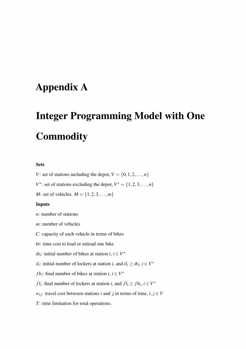
Appendix A
Integer Programming Model with One
Commodity
Sets
V : set of stations including the depot, V = {0,1,2, . . . ,n}
V ⋆: set of stations excluding the depot, V ⋆ = {1,2,3, . . . ,n}
M: set of vehicles. M = {1,2,3, . . . ,m}
Inputs
n: number of stations
m: number of vehicles
C: capacity of each vehicle in terms of bikes
bt: time cost to load or unload one bike
ibi: initial number of bikes at station i, i ∈V ⋆
ili: initial number of lockers at station i, and ili ≥ ibi, i ∈V ⋆
f bi: final number of bikes at station i, i ∈V ⋆
f li: final number of lockers at station i, and f li ≥ f bi, i ∈V ⋆
wi j: travel cost between stations i and j in terms of time, i, j ∈V
T : time limitation for total operations.

102 Integer Programming Model with One Commodity
Decision Variables
ubki: number of bikes unloaded by vehicle k at station i, i ∈V ⋆, k ∈ M
pbki: number of bikes picked up by vehicle k at station i, i ∈V ⋆, k ∈ M
vbki j: number of bikes on vehicle k when traveling from i to j, i, j ∈V , k ∈ M
xki j: binary decision variable. It equals to 1 when there is a path from station i to j for vehicle
k, otherwise, it equals to 0. i, j ∈V , k ∈ M
qki: auxiliary parameters, i ∈V ⋆, k ∈ M
Model
Minimize ∑ni=0 ∑
nj=0 wi j ∑
mk=1 xki j +bt ·∑m
k=1 ∑ni=0(ubki + pbki)
s.t.
vbkii = 0 ∀k ∈ M, i ∈V ⋆ (1)
vbk0i = vbki0 = 0 ∀k ∈ M, i ∈V ⋆ (2)
ubki ≤ ∑nj=0 vbk ji ∀k ∈ M, i, j ∈V ⋆ (3)
∑mk=1 pbki ≤ ibi ∀i ∈V ⋆ (4)
ubki ≤ max(0, f bi − ibi) ∀k ∈ M, i ∈V ⋆ (5)
pbki ≤ max(0, ibi − f bi) ∀k ∈ M, i ∈V ⋆ (6)
M ·∑nj=0 xk ji ≥ ubki + pbki ∀k ∈ M, i ∈V (7)
∑ni=0 xk0i = ∑
ni=0 xki0 = 1 ∀k ∈ M (8)
∑nj=0 xki j ≤ 1 ∀k ∈ M, i ∈V ⋆ (9)
∑nj=0 xk ji ≤ 1 ∀k ∈ M, i ∈V ⋆ (10)
∑nj=0 xki j = ∑
nh=0 xkhi ∀k ∈ M, i ∈V ⋆ (11)
qk j ≥ qki +1−M · (1− xki j) ∀k ∈ M, i ∈V, j ∈V ⋆ (12)
f bi = ibi +∑mk=1(ubki − pbki) ∀i ∈V ⋆ (13)
∑nj=1 vbki j = ∑
nh=1 vbkh j + pbki −ubki ∀k ∈ M, i ∈V ⋆ (14)
vbki j ≤C · xki j ∀k ∈ M, i, j ∈V (15)

103
∑ni=0 ∑
nj=0 wi j · xki j +bt ·∑n
i=0(ubki + pbki)≤ T ∀k ∈ M (16)
ubki, pbki,vbki j ≥ 0 ∀k ∈ M, i, j ∈V (17)
In the objective function, ∑ni=0 ∑
nj=0 wi j ∑
mk=1 xki j represents the travel cost of all vehicles,
and bt ·∑mk=1 ∑
ni=0(ubki + pbki) represents the operation time costs. The objective is to
minimize the total cost, which consists of the travel cost of all vehicles and the time cost for
carrying bikes onto or off the vehicles. Constraints (1) ensure that vehicles will not transport
commodity from any station to itself. Constraints (2) guarantee that vehicles will not carry
out or bring in any commodity to the depot. Constraints (3) represent that the number of
bikes unloaded from vehicle k at station i cannot exceed the current number of bikes on
vehicle k. Constraints (4) make sure that the number of bikes picked by vehicle k at station i
is at most the number of bikes at station i, as we assume that every station will be visited only
once by each vehicle. Constraints (5) and (6) guarantee that each vehicle is only allowed to
load bikes at pickup stations and unload them at delivery stations. Constraints (7) make sure
that xki j equals to 1 when vehicle k will visit station i for repositioning activities. Constraints
(8) mean that every vehicle should start at the depot and end at the depot. Constraints (9) and
(10) ensure that each vehicle can only have at most one destination from station i and at most
one departure station to station i, respectively. Constraints (11) guarantee that the out-degree
equals to the in-degree of the traffic flow for each station. Constraints (12) aims to eliminate
sub-tour, respectively. Constraints (13) mean that the final number of bikes at station i equals
to the initial number of bikes at station i plus the number of bikes loaded here and minus the
number of bikes picked up from here. It is worth mentioning that Constraints (13) can also
be written as Constraints (18), which means the number of bikes provided at each station
after the repositioning activities should be larger or equal to the number of bikes required.
f bi ≤ ibi +∑mk=1(ubki − pbki) ∀i ∈V ⋆ (18)
Since the total number of bikes in the system is unchanged after the repositioning activities,

104 Integer Programming Model with One Commodity
we do not need to worry about the inequalities. Most importantly, Constraints (18) can
shorten the running time.
Constraints (14) represent the number of lockers on vehicle k at station i equals to the
number of bikes on vehicle k before arriving station i plus the bikes picked up or minus the
number of bikes unloaded at station i. Constraints (15) make sure that if there is a transit
between station i and station j by vehicle k, xki j must be 1, which are also the capacity
constraints for vehicles. Constraints (16) ensure that for each vehicle, the travel time plus
the time of loading/unloading bikes does not exceed the limit of total operation time T . This
new time limitation constraint makes the computation slower even the operation time is far
less than T . Constraints (17) are the non-negative constraints.