the icecube prototype string in amanda
TRANSCRIPT

The ICECUBE prototype string in AMANDA
The AMANDA Collaboration
M. Ackermannd, J. Ahrensk, X. Bai a, M. Barteltt, S.W. Barwickj,R. Bayi, T. Beckak, J.K. Beckert, K.-H. Beckerb, E. Bernardinid,D. Bertrandc, D.J. Boersmad, S. Boserd, O. Botnerq, A. Bouchtaq,O. Bouhalic, J. Brauno C. Burgessr, T. Burgessr, T. Castermansm,
W. Chinowskyg, D. Chirking, J. Conradq, J. Cooleyo, D.F. Cowenh,A. Davourq, C. De Clercqs, T. DeYoungℓ, P. Desiatio, P. Ekstromr,T. Feserk, M. Gaugd, T.K. Gaissera, R. Ganugapatio, H. Geenenb,
L. Gerhardtj, A. Goldschmidtg, A. Großt, A. Hallgrenq, F. Halzeno,K. Hansono, R. Hardtkei, T. Harenbergb, T. Hauschildta,
K. Helbingg,∗, M. Hellwig k, P. Herquetm, G.C. Hill o, D. Huberts,B. Hugheyo, P.O. Hulthr, K. Hultqvistr, S. Hundertmarkr,
J. Jacobseng, K.H. Kampertb, A. Karleo, J.L. Kelleyo, M. Kestelh,G. Kohnenm, L. Kopkek, M. Kowalskid, M. Krasbergo, K. Kuehnj,H. Leichd, M. Leutholdd, I. Liubarskye, J. Ludvigg,1, J. Lundbergq,
J. Madsenp, P. Marciniewskiq, H.S. Matisg, C.P. McParlandg,T. Messariust, Y. Minaevar, P. Miocinovic i, R. Morseo,K.S. Municht, R. Nahnhauerd, J. Namj, T. Neunhofferk,P. Niessena, D.R. Nygreng, H. Ogelmano, Ph. Olbrechtss,
C. Perez de los Herosq, A.C. Pohlf , R. Porratai, P.B. Pricei,G.T. Przybylskig, K. Rawlinso, E. Resconid, W. Rhodet,
M. Ribordym, S. Richtero, S. Robbinsb, J. Rodrıguez Martinor,H.-G. Sanderk, S. Schlenstedtd, D. Schneidero, R. Schwarzo,
A. Silvestrij, M. Solarzi, J. Sopherg G.M. Spiczakp, C. Spieringd,M. Stamatikoso, D. Steeleo, P. Steffend, R.G. Stokstadg,
K.-H. Sulanked, I. Taboadan L. Thollanderr, S. Tilava, W. Wagnert,C. Walckr, M. Walterd, Y.-R. Wango, C. Wendto, C.H. Wiebuschb,
R. Wischnewskid, H. Wissingd, K. Woschnaggi, G. Yodhj
aBartol Research Institute, University of Delaware, Newark, DE 19716, USAbFachbereich C – Physik, BU Wuppertal, D-42119 Wuppertal, Germany
cUniversite Libre de Bruxelles, Science Faculty, Brussels, BelgiumdDESY-Zeuthen, D-15738 Zeuthen, Germany
eBlackett Laboratory, Imperial College, London SW7 2BW, UKfDept. of Chemistry and Biomedical Sciences, University of Kalmar,
S-39182 Kalmar, Sweden
Preprint submitted to Nucl. Instr. Meth. in Phys. Res. Sec. A October 4, 2005

gLawrence Berkeley National Laboratory, Berkeley, CA 94720, USAhDept. of Physics, Pennsylvania State University, University Park, PA 16802, USA
iDept. of Physics, University of California, Berkeley, CA 94720, USAjDept. of Physics and Astronomy, Univ. of California, Irvine, CA 92697, USA
kInstitute of Physics, University of Mainz, D-55099 Mainz, GermanyℓDept. of Physics, University of Maryland, College Park, MD 20742, USA
mUniversity of Mons-Hainaut, 7000 Mons, BelgiumnDept. de Fısica, Universidad Simon Bolıvar, Caracas, 1080, VenezuelaoDept. of Physics, University of Wisconsin, Madison, WI 53706, USApPhysics Dept., University of Wisconsin, River Falls, WI 54022, USA
qDiv. of High Energy Physics, Uppsala University, S-75121 Uppsala, SwedenrDept. of Physics, Stockholm University, SE-10691 Stockholm, SwedensVrije Universiteit Brussel, Dienst ELEM, B-1050 Brussels,Belgium
tInstitute of Physics, University of Dortmund, D-44221 Dortmund, Germany
Abstract
The AntarcticMuon And NeutrinoDetectorArray (AMANDA ) is a high-energy neutrinotelescope. It is a lattice of optical modules (OM) installedin the clear ice below theSouth Pole Station. Each OM contains a photomultiplier tube(PMT) that detects photonsof Cherenkov light generated in the ice by muons and electrons. ICECUBE is a cubic-kilometer-sized expansion of AMANDA currently being built at the South Pole. In ICE-CUBE the PMT signals are digitized already in the optical modulesand transmitted to thesurface. A prototype string of 41 OMs equipped with this new all-digital technology wasdeployed in the AMANDA array in the year 2000. In this paper we describe the technologyand demonstrate that this string serves as a proof of conceptfor the ICECUBE array. Ourinvestigations show that the OM timing accuracy is 5 ns. Atmospheric muons are detectedin excellent agreement with expectations with respect to both angular distribution andabsolute rate.
Key words: Neutrino telescope, AMANDA , ICECUBE, signal digitizationPACS:07.05.Hd, 07.07.Hj, 07.50.Qx, 29.40.Ka, 95.55.Vj, 95.85.Ry, 96.40.Tv
∗ Corresponding author: Klaus Helbing.Address: Physikalisches Institut, Uni-versity of Erlangen-Nurnberg, D-91058Erlangen, Germany; Phone: +49 91318528964, Fax: +49 69 13305370238
Email address:[email protected]
(K. Helbing).1 now at Stanford Research Systems, Sun-nyvale, CA 94089, USA
2

1 Introduction
The Antarctic Muon And NeutrinoDetectorArray (AMANDA ) [1] at thegeographic South Pole is a lattice ofphotomultiplier tubes (PMTs) each en-closed in a transparent pressure sphereto comprise an optical module (OM).The OMs are buried in the polar ice atdepths between 1500 m and 2000 m.The primary goal of AMANDA is todiscover astrophysical sources of highenergy neutrinos. High-energy muonneutrinos penetrating the earth fromthe Northern Hemisphere are identifiedby the secondary muons produced incharged current neutrino-nucleon in-teractions near or within the detector.AMANDA was the first neutrino tele-scope with an effective area in excessof 10000 m2 – with over 600 opticalmodules in place.
Large as it is, AMANDA is only capa-ble of seeing the brighter (and closer)sources of neutrinos. ICECUBE willbe an array of 4,800 optical moduleswithin a cubic kilometer of ice [2].Frozen into vertical holes 2.4 kmdeep, drilled by hot water, the opticalmodules will lie between 1450 m and2450 m below the surface. An instru-ment of this size is suited to studyneutrinos from distant astrophysicalsources [3].
The optical modules in AMANDA andICECUBE are arranged like strings ofbeads connected electrically and me-chanically to long cables leading upto a control room at the surface. ThePMT within the OM detects individualphotons of Cherenkov light generatedin the ice by muons and electrons
moving with velocities near the speedof light. Signal events consist primar-ily of up-going muons produced inneutrino interactions in the bedrock ofAntarctica or in the ice. In addition, thedetector will identify electromagneticand hadronic showers (“cascades”)from interactions ofνe and ντ insidethe detector volume provided theyare sufficiently energetic. Backgroundevents are mainly downward-goingmuons from cosmic ray interactionsin the atmosphere above the detector.For ICECUBE, the background willbe monitored for calibration purposesby the ICETOP air shower array [2]covering a 1 km2 area at the ice sur-face right above the in-ice OMs of theICECUBE detector. This backgroundwill also be used as a test beam forcommissioning the detector.
Unlike AMANDA , ICECUBE PMT sig-nals are digitized directly in the opti-cal module itself and then transmitteddigitally to the surface. This is donesuch that the arrival time of a pho-ton at an OM can be determined towithin a few nanoseconds. The elec-tronics at the surface determines whenan event has occurred (e.g., that a muontraversed or passed near the array) andrecords the information for subsequentevent reconstruction and analysis.
In the following we will discuss theperformance obtained with a string of41 Digital Optical Module (DOM) pro-totypes 12 m apart deployed in January2000 by the AMANDA Collaborationas the 18th string (STRING-18) of theAMANDA array.
3

2 Digital technology
The DOMs of STRING-18 were in-tended to demonstrate the advantagesand the feasibility of a purely digitaltechnical approach, in which PMT sig-nals are captured and digitized locally,within the optical module. The digitaldata are transmitted to the surface us-ing the twisted pair copper conductorsthat also bring power and control sig-nals to the DOMs. We will discuss thedesign, data taking and data analysisof STRING-18.
2.1 Concept
Very large high-energy cosmic neu-trino detectors require photomultipliertubes to be located far from the sig-nal processing center. The completedAMANDA detector represents an evo-lution of signal transmission technolo-gies from coaxial cable to twisted cop-per pair to optical fiber. In all thesecases, the analog signals are broughtto the surface, where they are digitizedand processed.
The longer cable lengths, the muchlarger number of PMTs of ICECUBE
and the requirements of a larger dy-namic range for PMT pulses and im-proved time resolution, as comparedto AMANDA , have led to the develop-ment of a data-acquisition technologywith the following features:
(1) Robust copper cable and connec-tors between the surface and themodules at depth.
(2) Digitization and time-stamping of
signals that are unattenuated andundispersed.
(3) Calibration methods (particularlyfor timing) that are appropriatefor a very large number of opticalmodules.
The PMT anode signal is digitizedand time-stamped already in the op-tical module. Waveform digitization,in which all the information in a PMTanode signal is captured, is incorpo-rated. The time calibration procedureis both accurate and automatic.
There are three fundamental elementsto the data acquisition architecture ofICECUBE and STRING-18:
• The Digital Optical Module (DOM),which captures the signals inducedby physical processes and preservesthe information quality through im-mediate conversion to a digital for-mat using an innovative ASIC, theAnalog Transient Waveform Digi-tizer (ATWD [4], see Sec. 2.2.4.1).
• A Network, which connects thehighly dispersed array of opticalmodules to the surface data acqui-sition system (DAQ) and providespower to them.
• A Surface DAQ, which maintains amaster clock time-base and providesall messaging, data flow, filtering,monitoring, calibration, and controlfunctions.
2.2 Digital optical module (DOM)
The basic elements of the DOM are thePMT for detection of Cherenkov light,a printed circuit board (PCB) for pro-
4

Figure 1. Schematic profile view of a STRING-18 Digital Optical Module, showing pres-sure sphere, optical coupling gel, photomultiplier, digital signal processing board (DOMPCB), LED flasher board, PMT base, and electrical penetrator.
cessing signals, a HV generator for thePMT, and an optical beacon consist-ing of LEDs for calibration purposesall within the glass pressure housing.The general physical layout of a DOMis shown in Fig. 1.
2.2.1 Pressure Housing
The spherical glass pressure housingsare standard items used in numerousoceanographic and maritime applica-tions. The most important qualitiesare mechanical reliability, cost, op-tical transmission, low radioactivity,and low scintillation of the glass. ForSTRING-18 “Benthospheres” are used,
a trade-name of Benthos, Inc.
2.2.2 Photomultiplier
The optical sensor of the DOM is alarge (8 inch diameter) hemispheri-cal 14-stage photomultiplier tube, theHamamatsu R5912-02 with a gain of4 · 108 at the typical operational volt-age of 1400 V. These large PMTs offergood time-resolution, as indicated bya transit-time-spread (TTS) for singlephotoelectron pulses of about 2.5 nsrms. Despite their large photocathodearea, these PMTs alone2 generate only
2 The dominant source of noise of theintegrated OM is the glass of the pres-
5

0
1000
2000
3000
4000
5000
6000
7000
0 10 20 30 40 50 60 70 80
coun
ts
charge [arb. units]
Figure 2. Measured integral charge distri-bution of DOM #1. Most of the histogramis single photoelectron noise pulses.
300 Hz or less of dark noise pulsesat temperatures below freezing and1400 V. The photocathode sensitivityextends well into the UV. The recep-tion of Cherenkov photons is limitedby the optical transmission of the glasspressure sphere at 350 nm. The PMTHV generator is a multi-stage voltagemultiplier with an oscillator runningat a few tens of kHz. It converts theelectrical power transmitted via cop-per cable down into the ice to a highvoltage for the PMT.
For each photon that produces a sin-gle photoelectron, the PMT producespulses that have characteristic rise (fall)times of 7 (11) ns. Due to the stochas-tic nature of the PMT’s electron multi-plication process, single photoelectronpulses display significant variations inpulse shape and amplitude. The mea-sured integrated charge distribution ofthe deepest DOM (DOM #1) is shownin Fig. 2. The peak to valley ratio isvery good for an 8 inch photomulti-plier.
sure sphere which leads to a total of about1 kHz noise pulse rate.
2.2.3 Optical beacon
Each of the STRING-18 DOMs isequipped with 6 GaN LEDs, whichemit predominantly in the near-UV at370 nm. The luminous intensity andthe pulsing rate may be varied over awide range under software control. Attheir brightest, these beacons can beseen by OMs up to distances of 200 m.The pulse width is 5 ns. The LEDs arebroad angular emitters, spaced at 60◦
around a vertical axis, and are cantedover by 45◦ to produce a roughlyhemispherical source.
2.2.4 Signal processing circuitry
Fig. 3 shows the principal componentsof the Digital Optical Module signalprocessing circuitry: the analog tran-sient waveform digitizer (ATWD), alow-power custom integrated circuitthat captures the waveform in 128 sam-ples at a rate3 of ∼ 600 MHz; a fastADC operating at3 ∼ 30 MHz cov-ering several microseconds; a FPGAthat provides state control, time stampsevents, handles communications, etc.;a low-power 32-bit ARM CPU witha real-time operating system. A verystable (δf/f ∼ 5 · 10−11 over∼ 5 s)Toyocom 16.8 MHz oscillator is usedto provide clock signals to severalcomponents. Short cables connectingadjacent DOM modules enable a lo-cal time coincidence (see Sec. 2.3.1),which eliminates most of the∼1 kHzof noise pulses when enabled.
The DOM is operated as a slave to the
3 The sampling speeds in ICECUBE aredifferent from those chosen for STRING-18.
6

Figure 3. Block diagram of the digital optical module signalprocessing circuitry.
surface DAQ. Upon power-up, it entersa wait state for an interval of a fewseconds, to permit downloading of newfirmware or software. If no messagesare received before time-out, the DOMwill boot from Flash memory and awaitcommands.
Normal operation of the DOM isdominated by a data-taking state (seeSec. 2.2.4.1). In addition, a local-timecalibration process is periodically in-voked, so that the local DOM timemay be ultimately transformed to mas-ter clock time with nanosecond accu-racy (see Sec. 3). The time calibrationprocess appears as a separately sched-uled thread, with no deleterious impactupon the data-taking state. Other activethreads are message receive/send anddata transmission, also invisible to thedata-taking process. There are several
calibration modes, such as runningoptical beacons, during which normaldata-taking of the respective DOM isinactive.
Low power consumption was a highpriority for the development of theDOM circuitry because electricalpower is limited at the South Pole.Each STRING-18 prototype DOM usesonly 3.5 W when booted up and trans-mitting data. An important feature inthis respect is the power consumptionspecific to the PMT pulse capture pro-cess since electronic devices operatedat high frequencies usually imposesignificant demands.
2.2.4.1 PMT pulse capture TheDOM is equipped with innovative cir-cuitry that is well-matched to the PMT
7

pulse characteristics and dynamicrange. The DOM concept takes advan-tage of the fact that, most of the time,no PMT pulses are present: The aver-age time between pulses is about2 ms.Circuit activity need occur only whenpulses appear. The waveform (pulseshape) capture capability is realizedthrough a custom switched capacitorarray based Application Specific In-tegrated Circuit (ASIC) designed atLawrence Berkeley National Labora-tory (LBNL), the Analog TransientWaveform Digitizer (ATWD) [4]. TheDOM has two such ATWDs with iden-tical tasks for fast switching from onedigitizing ATWD to the other ATWD.This minimizes the dead time due tothe digitization process.
The ATWD has four channels, eachwith 128 samples, that synchronouslyrecord different input waveforms. Itsemployment in the DOM is particu-larly advantageous because its powerconsumption is only 200 mW. TheATWD performance combination ofup to a GHz sampling speed with verylow power dissipation is unmatchedby any single commercial device forwaveform capture. The DOM proto-types in STRING-18 are equipped witha 15× and a 3× gain channel (seeFig. 3). The third channel is routedto an analog multiplexer (MUX) thatcan connect to various internal signalsfor diagnostic purposes. The fourthATWD channel in STRING-18 DOMsis permanently connected to the DOMinternal clock, for calibration and mon-itoring ofthe ATWD sampling speed.
The upper limit of linearity in pulseheight for the lower gain channel of theATWD was found to be about 150 pho-
0
100
200
300
400
500
600
700
800
900
0 20 40 60 80 100 120
sam
ple
valu
e (p
ulse
hig
ht)
sample number (time)
ATWD high gain channel
Figure 4. Waveform likely caused by adown-going muon recorded in the DOMclosest to a reconstructed track.
toelectrons for a single pulse. This wasachieved without extensive optimiza-tion of PMT voltages and threshold.
The waveform capture process is initi-ated by a “launch” signal derived froma discriminator connected to the signalpath. The capture process stores wave-form samples as analog voltages onfour internal linear capacitor arrays.A single DC current applied to theATWD controls the sampling speed.For STRING-18 we have chosen tocapture the pulse shape at 600 MHz(1.7 ns/sample). This high speed cap-ture is useful for characterizing PMTsignal shape with good resolution andfor other diagnostic purposes. All fourchannels within an ATWD are sam-pled syncronously, with aperture vari-ations between channels measured tobe less than 10 ps. Fig. 4 shows aparticularly feature-rich example of awaveform as recorded by an ATWDwith its high-gain channel. The datawere obtained with zero suppressionand data compression (see Sec. 2.3) inplace. Due to the zero suppression allvalues below the threshold of 2004
4 corresponding to a quarter of the aver-age single photoelectron amplitude with
8

are represented as the threshold value.The muon track reconstruction dis-cussed later in Sec. 5.2 indicates thatthe PMT signal was caused by a downgoing muon with this DOM being theclosest to the muon track. This plotdemonstrates the capability of separat-ing individual pulses and other detailswithin the ATWD waveform. Record-ing the full structure of waveforms willaid in reconstructing complex events.
For waveforms that exceed the ATWDcapture interval, sampling at a lowerfrequency is sufficient to capture rele-vant information at later times. For thispurpose, the DOM is equipped witha 10-bit low-power fADC5 , operatingat the DOM local clock frequency of33.6 MHz. The PMT signal in this pathis stretched to match the lower sam-pling rate.
2.2.4.2 Local time Each PMT hitmust be time-stamped such that cor-related hits throughout the detectormeet the relative timing accuracy re-quirement of 5 ns rms. This is accom-plished within the DOM using a two-stage method that produces a coarsetime-stamp and a fine time-stamp. TheSTRING-18 DOM FPGA maintains a54-bit local clock running at the DOM33.6 MHz clock frequency. Once datareach the surface, the local time unitsas defined by the local clock referenceare transformed to master clock units,and are ultimately linked to GPS (seeSec. 3). The 33.6 MHz is obtained by
respect to a baseline level of 100.5 This fADC is a fast, 10-bit, parallel-output, pipeline ADC
frequency-doubling the free-runningToyocom 16.8 MHz quartz oscillator.
The PMT signal triggers a discrimi-nator. The discriminator pulse is thenresynchronized to the next DOM clocktransition edge providing the coarsetime-stamp. At 33.6 MHz, this coarsetime-stamp has a time quantization of29.8 ns. The resynchronized pulse ofthe discriminator provides the ATWD“launch” signal. The synchronouslaunching causes the PMT signal toarrive within a one-clock-cycle widetime window at the ATWD. The lead-ing edge6 of the PMT signal wave-form within the ATWD record willoccur somewhere within this particu-lar 29.8 ns interval. This is the “finetime-stamp” which provides the de-sired time resolution of less than 5 ns.
For this to work, the PMT signal mustbe delayed sufficiently such that theleading edge of the signal always ap-pears well after the ATWD samplingaction has begun. An overall delay ofabout 75 ns is needed to accommo-date both the coarse time-stamp ran-dom delay and the propagation delayof the trigger processing path the cir-cuitry. In the STRING-18 DOM proto-types, a coil of coaxial cable of 15 mlength was employed for this purpose.
2.3 Network: Data link to the surface
All timing calibration, control, andcommunications signals between agiven DOM and the surface DAQ are
6 More sophisticated methods than theleading edge to determine the fine time-stamp can be easily envisaged.
9

provided by one conventional twistedpair of 0.9 mm diameter copper con-ductors. This pair also supplies powerto the DOM. The resulting cable linkis both cost-effective and robust, sincethe number of connections neededfor all functionality is minimal. Thetwisted pairs are assembled first indouble pairs, as “twisted quads”, andenclosed in a common sheath. Therequired number of twisted quadsper string are then wrapped around aKevlar strength member and coveredwith a protective sleeve. Breakouts ofindividual quads to facilitate connec-tions to the DOMs are introduced atthe appropriate positions.
The gross bandwidth across this 2.5 kmlong copper cable reached in STRING-18 was about 35 kilobytes/s. With twoATWD waveform channels of 128 10-bit sample values each and an fADCof 256 10-bit samples the data sizeof a hit is 640 bytes not accountingfor overhead. The hit rate in STRING-18 is about 500 Hz while the singlepulse rate is about 1 kHz.7 The result-ing data rate is in excess of 300 kB/swhich clearly exceeds the availablebandwidth.
We have developed two methods to re-duce the amount of data to be trans-fered from the DOM to the surface: lo-cal coincidence and data compression.
7 The discrepancy of the pulse and hitnoise rates is caused by the significant cor-relation of the noise - i.e. a single hit onaverage contains two pulses. The noise ismainly caused by radioactive decays inthe glass of the pressure spheres and sub-sequent luminescence. The slow decay ofthe luminescence gives rise to the intrinsiccorrelation of the noise.
2.3.1 Local coincidence
The DOM noise rate is approximately100 times greater than the rate inducedby high-energy muons. Unlike hits dueto high energy particles, noise hits inone DOM occur uncorrelated with hitsof neighboring DOMs, i.e. primarily asgeometrically isolated hits. A local co-incidence requirement, imposed in theice, selects predominantly only inter-esting hits for transmission to the sur-face. Each DOM communicates withits nearest neighbors by means of adedicated short copper wire pair. TheDOM is capable of sending and receiv-ing these short signals in a full duplexmode across these wires. Once a DOMhas triggered an ATWD, it sends sig-nals to each of its neighbors. Mean-while, a DOM is receptive to pulsesfrom either or both of its neighbors.In local coincidence mode, only whenthis pulse arrives, will the DOM dig-itize, store, and subsequently transmitthe time-stamped data to the surface.
2.3.2 Data compression
Since the local coincidence require-ment eliminates a small fraction of realevents [5], an alternative compressionof all data including the noise hits hasbeen developed. The waveforms cap-tured by a single ATWD channel or thefADC are similar to a facsimile scanline. The original facsimile encodingstandard [6] is based on “run-length”encoding followed by Huffman en-coding [7] with a fixed, immutable,Huffman code. The adaptation of thisidea to the digital waveform data hasled us to a 4 step algorithm:
10

I: Gain channel selection: In mostcases a waveform does not saturateor exceed the dynamic range of thehigh-gain channel of the ATWD.In these cases the low-gain channelinformation is redundant and dis-carded. However, should the high-gain channel saturate this channel isdiscarded and instead the low gainchannel data is preserved.
II: Zero suppression: The main pur-pose of this step is to reduce theentropy of the data set which makesthe subsequently applied compres-sion algorithms work more efficient.A threshold of a quarter of the av-erage single photoelectron pulseheight is applied to the data of thehighest gain channel. This equiva-lent of a discriminator threshold isthen subtracted from all sample val-ues. Resulting negative values areset to zero.
III: Run-length encoding: This com-pression step replaces sequences(“runs”) of consecutively repeatedvalues with a single number pre-fixed by the length of the run. Inthe standard definition of run-lengthencoding the prefix count denotesoccurrences and hence is alwaysnon-zero. In order to further gainefficiency for the compression in thesubsequentHuffman-lite algorithmwe choose to take the number ofconsecutive repetitions instead i.e.the prefix count is one less than withthe standard definition and samplevalues occurring only once are pre-fixed with a zero. As a consequenceabout 50% of the resulting code arezeros.
IV: Huffman-lite encoding: Huffmancoding simply uses shorter bit pat-terns as a replacement for more
frequent values in the input streamthan for rarely occurring values.We have reduced this concept toHuffman-lite in order to save com-puting resources. The bits used forzeros are minimized while we makeno attempt to compress finite val-ues. We convert a zero value “0” toa single bit ’0’. In order to identifyfinite values these are preceded bya single high bit ’1’.
For the STRING-18 configuration thiscompression reduces the data portionto 15 bytes per hit on average whichis a factor of 40 down from the un-compressed data volume. In STRING-18 this compression algorithm is exe-cuted by the CPU in the DOM.
The STRING-18 data presented inSecs. 4 and 5 have been obtained usingthe compression to save bandwidth butwithout the local coincidence criterionto maximize the number of contribut-ing DOMs and for straightforwardcomparison with the simulation basedon the AMANDA detector and its trig-ger logic (see Sec. 5.3).
2.4 Surface DAQ
At the surface, the copper cables lead-ing up from the DOMs are connected tocustom communications cards (DOM-COM cards) in five industrial PCs witha Linux operating system. Aside fromthe DOMCOM cards all componentsof the surface DAQ are commercialhardware. The DOMCOM cards canbe thought of as specialized serial portsfor communicating with the DOMswith additional functions for powering
11

on and off each DOM, and sendingand receiving time calibration pulses.The five DOMCom PCs and a sixth,master control PC are connected by anEthernet network. This network is thenaccessible via the South Pole stationLAN and, at certain times during theday, to the outside world via satelliteconnection. The principal task of thesurface DAQ is to allow one to takecontrol of and communicate with theDOMs in the ice for calibration andmonitoring purposes and to collectdata from the optical sensors.
FPGA logic in the DOMCOM boardsprovides input and output FIFOs con-nected to UARTs8 in the DOMCOM
boards. The UARTs in turn drive thecommunications circuits. Byte-wisecommunications of the DOMCOM in-terface to the DOMs is provided bya Linux kernel module device driver.By writing to and reading from FPGAregisters mapped to port addresses thekernel driver allows Linux programsto communicate with the DOMs.
A suite of DAQ programs has beenwritten to provide user interfaces formonitoring, control (HV settings, etc.)and data-taking purposes. Also, toolsare available to reconfigure STRING-18 in many respects. Almost all ofthe components in the DOM can bereprogrammed after it is deployed inthe ice. These include the DOM bootPROM, the code executed by its CPUs,and the FPGAs of both the DOMand the DOMCom card. For example,high speed communication and data
8 A UART or universal asynchronousreceiver-transmitter translates betweenparallel bits of data and serial bits.
DAQFront-End
DAQFront-End
DACFADC
������
���������������
���������������
����������������������������������������������������������������������������������������������������������������������������������������
twisted copper pairup to 3 km
free runnigoscillator
delta t
DOM
GPSGPS
δt
ttdown up
Figure 5. General concept of the Recipro-cal Active Pulsing (RAP) method for timecalibration.
compression in the DOM were imple-mented after the deployment and sub-stantially improved the performancefor physics data-taking.
3 Local to global time transforma-tion
The (local) time stamp for a photon ina DOM must be converted to a global,i.e., array-wide time base, in order tobe compared with hits in other DOMs.Correlation with events in nearby de-tectors, e.g. AMANDA and ICETOP,or much more distant detectors (satel-lites, other telescopes) requires con-verting the global time to universaltime. Therefore, a critical requirementis the ability to calibrate the DOM lo-cal oscillator against a master clock atthe surface.
12

3.1 Global time distribution
A GPS clock at the South Pole repre-sents this master-clock for STRING-18.Its 10 MHz output is coupled to a spe-cial phase-locked loop on a clock dis-tribution circuit. This PLL was set togive a frequency of 16.8 MHz in orderto match the frequency of the local os-cillators in the DOMs. The 16.8 MHzsignal is fed to each DOMCOM boardin the five DOMCOM PCs where anadditional PLL produces both 16.8 and33.6 MHz phase-locked signals. Thetime jitter introduced by the PLL distri-bution system was measured to be lessthan 1 ns.
3.2 Reciprocal Active Pulsing
Timing pulses sent down the string to aDOM at known time intervals are usedto determine relative frequency. In re-sponse to the calibration pulse receivedat the DOM, after a well-defined de-lay δt, a bipolar signal identical to theone sent down the string is sent backto the surface. With the pulses sent inboth directions the offset of the twoclocks at the surface and in the DOMare determined. The left part of Fig. 5depicts the transmission of the timingpulse from the surface down to theDOM while the right hand side showsthe transmission in the reverse direc-tion with the same DOM and DOM-COM combination. It is important thatthe circuitry for generation and record-ing of the timing pulse be identical atthe DOM and at the DOMCOM cardand that the treatment is the same inboth places. This way, the shapes of
-400
-300
-200
-100
0
100
200
300
400
500
600
0 50 100 150 200 250
sam
ple
valu
e (p
ulse
hig
ht)
sample number (time: 60 ns/sample)
cross over
leading edge
Figure 6. The timing pulse emitted by theDOMCOM card recorded over a 15µsperiod as received by the DOM.
the pulses sent down and up are iden-tical and can be analyzed in the sameway to determine the time mark. Thisprocedure yields an overall delaytrt
for the full round-trip. With the samesignal treatment at the surface and inthe DOM, one gets
tup = tdown =1
2(trt − δt) . (1)
This calibration method is called Re-ciprocal Active Pulsing (RAP) [8]. Itmaps the local clock counter values inthe DOM and the hit time-stamps tothe global time.
Fig. 6 shows the shape of the timingpulse observed by the DOM at the endof a∼2 km cable for a bipolar square-wave pulse injected by the DOMCOM
card. The pulse displays the effect ofcable attenuation and dispersion. Thepulses are recorded at surface and atdepth by fADCs whose sampling rates(16.8 MHz) are fixed by either the lo-cal oscillator in the DOM or the mas-ter clock on surface. The shapes of thepulses received by the DOMs and theDOMCOM cards are similar and in-deed allow for the identical treatment.
13

Two methods were used to determinea reference time mark on the pulse:
• The intersection of the baselinevoltage (linear fit) with the negative-going slope of the leading edge9 .
• The intersection of the crossoverpoint (linear fit) with the extrapo-lated baseline.
We found that leading edge timing isleast sensitive to variations in compo-nent values such as temperature vari-ations after powering up. Crossovertiming, however, gives better time res-olution and has less jitter from onetime calibration cycle to another. It wasfound that temperature drifts that showup in the cross over timing change thetimestup andtdown in identical amountsbecause the drifting electronic compo-nents affect both the up-going and thedown-going pulses in the same way.This implies that the effect cancels forthe calibration of the local time. More-over, the observed drifts are very slow,less than 15 ns in 1 hour. Therefore,we have used the crossover timing toobtain the local to global time cali-bration. Fig. 7 shows the measuredround-trip timetrt (see Eq. (1)) overa period of one hour for a DOM at2 km depth employing the cross overtiming. The jitter is 1.1 ns rms, whichis a relative error of only4 · 10−5.
Performing these clock calibrations au-tomatically every 10 seconds – as wasdone during data-taking with STRING-18 – consumes negligible bandwidth.We will demonstrate in Sec. 4.1 thatthis RAP method at this repetition rate
9 Tangent to the inflection point of a cubicfunction fit to the leading edge
28717
28718
28719
28720
28721
28722
0 10 20 30 40 50 60
t rt [n
s]
calibration start time [min]
Figure 7. Measured round-trip timetrt
from successive RAP calibrations for aDOM at 2 km depth.
provides a timing accuracy of betterthan 5 ns for the pulse times of a DOM.
4 Studies with optical beacons
To study the performance and uni-formity of STRING-18 we have per-formed various dedicated data-takingruns operating the optical beacons ofall available DOMs.
4.1 Timing accuracy
In order to determine the timing ac-curacy of the RAP calibration proce-dure described in Sec. 3 we have ob-served the light emitted by the LEDbeacon of one DOM by two neighbor-ing DOMs. The beacon is set to a verybright output operation mode. For shortdistances the light front created at thebeginning of a flash is to a good ap-proximation unaffected by scattering inthe ice as photons undergoing scatter-ing fall behind the front. As long asthere are enough photons as part of thelight front, this front moves with thespeed of light in the ice,c/n, wheren
14

is the refractive index. Hence, this lightflash provides a reference time signal.
0
10
20
30
40
50
60
70
80
90
-25 -20 -15 -10 -5 0 5 10 15 20 25
coin
cide
nce
coun
ts
time difference [ns]
Figure 8. Relative timing accuracy of apair of DOMs measured with a neighbor-ing flashing beacon.
Fig. 8 shows the measured time differ-ence of the arrival times of this lightfront at both DOMs corrected for thepropagation time of the light from oneDOM to the other. One observes a dis-tribution with a square root variance of7.5 ns. The jitter includes effects of thePMT timing and the RAP procedure.Accordingly, this provides an upperlimit for the timing accuracy of theRAP calibration process. Since bothDOMs contribute to the variance of theobserved time difference, the accuracyfor an individual DOM with respect tothe global surface time is about 5 ns.
4.2 Light propagation in the ice
We have studied the propagation of theLED light from the optical beacon (seeSec. 2.2.3) through the ice. From thebeginning of AMANDA operations, ithas been crucial to establish an under-standing of the properties of the glacialice at the South Pole [9]. Today the op-tical properties of the ice are mappedover the full relevant wavelength and
10
100
1000
10000
100000
100 150 200 250 300 350
coin
cide
nce
coun
ts
distance d from LED flasher [m]
λprop = 28.0 m +/- 1.5 m
DataFit via λprop
Figure 9. Attenuation of light from the op-tical beacon as a function of the distancefrom the source.
depth range [10] using the analog op-tical modules.
Using a configuration similar to theone discussed in Sec. 4.1 we haveused the flashing beacon in a DOMand observed the light in two otherDOMs, one being the next neighborto it. Here, the other observing DOMcan be any other one along the string.Fig. 9 shows the coincidence counts ofthe two observing DOMs as a functionof the distanced of the second ob-server DOM from a flasher at a depthof 1993 m below the ice surface. Thefirst observing DOM as a neighbor tothe beacon is close enough to observeevery emitted flash. For DOMs furtheraway photon counting in coincidencewith the neighbor DOM is possible.The combined effect of scattering andabsorption in the ice leads to a falloff of the light intensityI with an ef-fective propagation length parameterλprop: I(d) ∝ exp(−d/λprop)/d [11].Random coincidences of the twoobserving DOMs due to the darknoise of the distant DOM10 yields
10 The dark noise of the neighbor DOMcan be neglected compared to the highflash rate.
15

0
20
40
60
80
100
0 200 400 600 800 1000 1200
coun
ts
photon delay time distribution [ns]
t0 = -12 +/- 24 ns
χ2 / dof = 1.1
DataFit
Figure 10. LED photon arrival time distri-bution due to scattering through 143 m ofice
an additional offset c2 indepen-dent of the distance. From fittingc1 exp(−d/λprop)/d+ c2 via c1, c2 andλprop we obtainλprop = 28.0 ± 1.5 m.With the described setupλprop repre-sents a measurement of the averagepropagation length at depths between1750 m and 1880 m. This is in excel-lent agreement with previous findingswith the analog technology [10].
With the same setup we have also ob-served the arrival time distribution ofthe photons at the distant DOM (seeFig. 10). Here, the DOM next to thebeacon provides the reference for thetime of the flash. The time distribu-tion is shifted to account for the timeit takes light to traverse the ice with-out scattering from the beacon to thedistant DOM (delay time distribution).The arrival time distribution for theDOM next to the beacon can be ne-glected as discussed in Sec. 4.1. Fittedto the data is a gamma distribution
f(t|t0, α, β) = (t − t0)α−1βαe−β(t−t0)
Γ(α)(2)
for t − t0 > 0 with a shape parameterα > 0 and a scale parameterβ > 0.
Such a gamma function was found todescribe the arrival time distributionsreasonably well with scattering andabsorption in ice or water for the caseof an isotropic, monochromatic andpoint-like light source [12,13]. Theobserved time distribution with theDOM follows this known behavior. Asan additional parameter to the usualdefinition of a gamma distribution inEq. (2) we have introducedt0 to ac-count for possible timing errors of theDOM. It turns out thatt0 is compatiblewith zero which is consistent with theresults presented in Sec. 4.1.
5 Performance and analysis withatmospheric muons
Atmospheric muons provide a testbeam for neutrino telescopes, as wasdemonstrated by AMANDA [14]. Wewill use it here to demonstrate theperformance of STRING-18.
5.1 Down-going muons
The vast majority of the atmosphericmuons that reach the detector travel atnear the vacuum speed of light. Thezenith angle distribution is peaked inthe downward direction. We have com-pared the coincidence hit times of theDOMs with the hypothesis of a straightdown going muon, i.e. we have sub-tracted the time it takes the muon fromthe upper DOM to the lower one fromthe hit time differences. Fig. 11 showsthe distribution of these time differ-ences under the condition that at least4 DOMs of the string registered the
16

0
10
20
30
40
50
60
70
-1000 -500 0 500 1000
coun
ts
time differences [ns]
Single DOM pair 108 m apart
0
500
1000
1500
2000
2500
-1500 -1000 -500 0 500 1000 1500
coun
ts
time differences [ns]
All available DOM pair combinations
Figure 11. Time differences between pairs of DOMs correctedfor the down-going muonhypothesis. Left: single DOM pair 108 m apart, right: all available DOM pair combinationsaccumulated.
event. On the left of Fig. 11 we showthe distribution of time differences ofa particular pair of DOMs. The twoDOMs are 108 m apart. The right handside of Fig. 11 shows an accumula-tion of these diagrams for all availablepairs of DOMs. With the hypothesis ofa straight down-going muon, the peakcount should be at zero. The exact lo-cation of the peak at zero to within ananosecond, which can be seen by ex-amining the peak region in more detailthan shown, is another evidence for theaccurate timing and the proper func-tioning of the RAP calibration method.
The asymmetry of the tails of thedistribution towards negative timedifferences is a consequence of notquite straight down-going muons. Forsmall zenith angles of the muon trackthe Cherenkov light that reaches theDOMs does indeed cause hit timesthat proceed from top to the bottomof the string that appear faster thanthe vacuum speed of light. A muontrack at zenith angle90◦ − θC (θC isthe Cherenkov light emission angle)that intersects the string will cause all
DOMs located above the intersectionpoint to light up at once (neglectingscattering in the ice). By shifting thetime differences with the hypothesis ofa straight down going muon one ob-tains these negative time differences.We will see in Sec. 5.2 that these devia-tions can indeed be used to reconstructthe zenith angle of the muon track.
Fig. 12 shows the mean time differ-ences of all available pairs of DOMsas a function of the separation of theDOMs. For this plot the time differ-ences were not shifted for the down-going muon hypothesis and we re-quire that no fewer than 6 DOMs have“seen” the muon. A linear fit to thedata shows a slope compatible withstraight down-going muons travelingat the speed of light. The intercept ofthe fit at −2.3 ns± 7.2 ns is anotherindication that the local to global timetransformation works.
17

0
200
400
600
800
1000
1200
1400
1600
0 50 100 150 200 250 300 350 400 450
time
diffe
renc
e [n
s]
separation of DOM pair d [m]
Slope: 3.39 +- 0.07 ns/mIntercept: -2.3 +- 7.2 ns
Figure 12. Time differences between allavailable pair combinations of DOMs as afunction of the separation.
5.2 Zenith angle reconstruction
In the absence of scattering and ab-sorption in the Cherenkov medium thearrival time of the Cherenkov lightfrom the muon at the string takes thesimple analytic form of a hyperbolaas a function of the depthz along thestring [15]11 :
t = t0 +1
c
{
(z − z0) cos θ +√
(n2 − 1)[d2 + (z − z0)2 sin2 θ]}
(3)
Here, d is the minimum distance be-tween the string and the muon track;θ is the zenith angle of the muon;t0 and z0 are the time and the depthat which this closest approach ofthe muon occurs. Sincet0 is not di-rectly related to the observable hittimes of the DOMs we replace it bytfirst = t0 + d
√n2 − 1/c which is an
11 We have to caution that the approxima-tion presented as Eq. (5) in Ref. [15] iswrong for allz−z0 < 0. We have not usedthis approximation but the exact descrip-tion of the hyperbola with our Eq. (3).
estimate for the time when the Che-renkov light from the point(t0, z0)reaches the string12 .
The 4 parameterstfirst, z0, d andθ are tobe fitted to the data. We have used theGNU Scientific Library[16] to performthis nonlinear multiparameter fit. Com-puting the Jacobian matrix from ex-plicit derivatives greatly improves thenumerical stability and provides fit re-sults practically independent of the ini-tial guess of the parameters as longas they are chosen within a physicallyreasonable region – e.g.z0 in betweenthe actually hit DOMs. To calculate thederivatives we have used the computeralgebra systemMaxima [17]. For theinitial guess we have usedd = 0 andθ = 90◦. The guess forz0 was com-puted as the averagez of all hit DOMsweighted with the pulse charges. Theinitial value oft0 was set to the hit timeof the DOM next toz0. Eq. (3) holds forthe idealized situation without scatter-ing and absorption in the medium. Theice at the South Pole however showsscattering and absorption. By integrat-ing the gamma function mentioned inSec. 4.2 with the empirical parameterssuccessfully used in AMANDA [13] oneobtains that the mean speed of prop-agation of the light is about 11 ns/min contrast to the expectation of about5 ns/m based on the refractive indexof ice of n = 1.32. To account for thatwe have replacedn in Eq. (3) byneff ≃3.16. Note that the effective openingangle of the light cone13 of the pro-
12 This of course disregards the initial ori-entation of the Cherenkov light. Scatteringin the ice however largely voids this fea-ture.13 The initial emission angle of the Che-
18

0.01
0.1
1
0 5 10 15 20 25 30 35 40 45 50
# of
rec
onst
ruct
ed tr
acks
[(s
rad)
-1]
Zenith angle θ [deg]
Multiplicity 4: <θ> = 57.8o
Multiplicity 6: <θ> = 43.5o
Multiplicity 8: <θ> = 35.8o
Multiplicity 10: <θ> = 29.5o
Multiplicity 12: <θ> = 23.7o
Figure 13. Reconstructed zenith angle dis-tribution with STRING-18 for several mul-tiplicity conditions
duced Cherenkov light is reduced aswell. This is why a simple replacementof n by neff in Eq. (3) is consistent.
Fig. 13 shows the zenith angle dis-tribution as reconstructed with thismethod applied to STRING-18. Here, azenith angle of zero denotes a straightdown-going muon. One observes thatthe angular distribution falls off fasterwith higher required multiplicities ofthe number of hit DOMs. This is aneffect related to the acceptance chang-ing with increasing multiplicity. Dueto the absorption of the Cherenkovlight in the ice, only close by verticaltracks have a chance to be seen by allDOMs. However close a track mightbe, even when intersecting with thestring, a horizontal track has a verylow chance to light up more than onlya handful of DOMs.
renkov light is unaffected, of course.
5.3 Comparison with simulation
We have compared the observed ratesof muon tracks with a detailed simu-lation in order to verify that STRING-18 indeed performs with a homoge-neous efficiency. The acceptance formuon tracks agrees with the expecta-tions based on the parameters of thewhole light collection process i.e. theoptical coupling of the ice to the pres-sure sphere, the glass and gel transmis-sion and the quantum efficiency of thePMT. The simulation is based on theair shower generator CORSIKA [18], aprogram package for muon propaga-tion through matter MMC [19,20] andthe AMANDA detector simulation pro-gram AMASIM [21]. This simulationfor the full AMANDA detector was re-stricted to the STRING-18 geometry.
Besides generating hit times for theDOMs the simulation also providesthe zenith angle of the generated muontracks. By applying the reconstructionmethod of Sec. 5.2 to the simulatedhits one can study the performance ofthe reconstruction algorithm. It turnsout that the distribution of the devia-tion of the reconstructed zenith anglefrom the generated muon track angleroughly follows an exponential behav-ior ∝ exp(−∆θ/b) with b ≃ 22◦. Thiscorresponds to a median error of15◦.
This reconstruction technique is ofcourse inferior to the full AMANDAreconstruction [13]; the main limi-tation here stems from the reducedgeometry of a single string versus anarray of optical modules. Also the cho-sen approach to reconstruction is muchsimpler. It was not the primary aim of
19
0
0.05
0.1
0.15
0.2
0.25
0.3
0.35
0.4
0.45
0.5
10 20 30 40 50 60 70 80
# of
rec
onst
ruct
ed tr
acks
[(s
rad)
-1]
Zenith angle θ [deg]
Simulated data, mult. 10String-18 data, mult. 10
Simulated data, mult. 13String-18 data, mult. 13
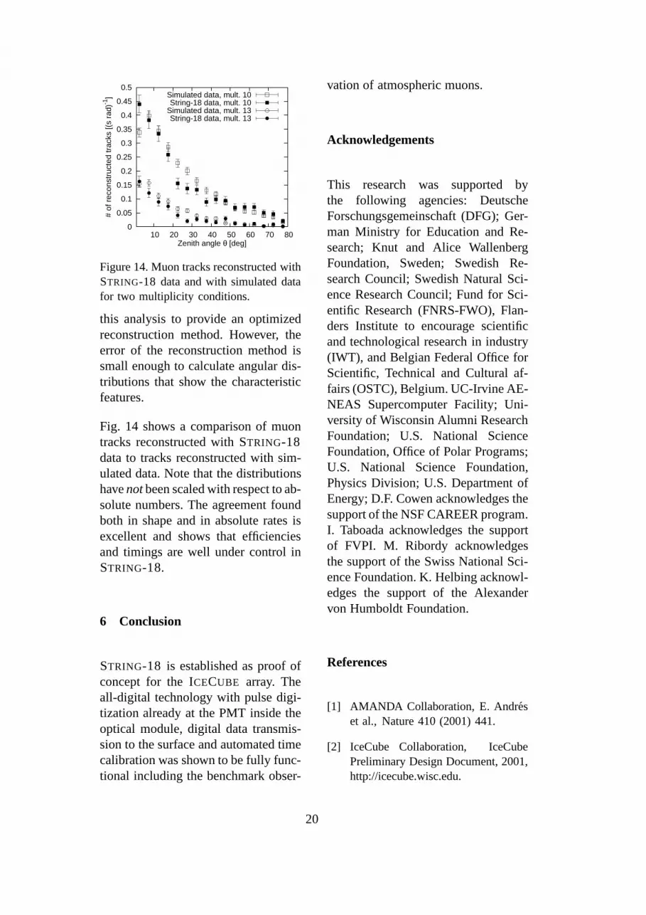
Figure 14. Muon tracks reconstructed withSTRING-18 data and with simulated datafor two multiplicity conditions.
this analysis to provide an optimizedreconstruction method. However, theerror of the reconstruction method issmall enough to calculate angular dis-tributions that show the characteristicfeatures.
Fig. 14 shows a comparison of muontracks reconstructed with STRING-18data to tracks reconstructed with sim-ulated data. Note that the distributionshavenotbeen scaled with respect to ab-solute numbers. The agreement foundboth in shape and in absolute rates isexcellent and shows that efficienciesand timings are well under control inSTRING-18.
6 Conclusion
STRING-18 is established as proof ofconcept for the ICECUBE array. Theall-digital technology with pulse digi-tization already at the PMT inside theoptical module, digital data transmis-sion to the surface and automated timecalibration was shown to be fully func-tional including the benchmark obser-
vation of atmospheric muons.
Acknowledgements
This research was supported bythe following agencies: DeutscheForschungsgemeinschaft (DFG); Ger-man Ministry for Education and Re-search; Knut and Alice WallenbergFoundation, Sweden; Swedish Re-search Council; Swedish Natural Sci-ence Research Council; Fund for Sci-entific Research (FNRS-FWO), Flan-ders Institute to encourage scientificand technological research in industry(IWT), and Belgian Federal Office forScientific, Technical and Cultural af-fairs (OSTC), Belgium. UC-Irvine AE-NEAS Supercomputer Facility; Uni-versity of Wisconsin Alumni ResearchFoundation; U.S. National ScienceFoundation, Office of Polar Programs;U.S. National Science Foundation,Physics Division; U.S. Department ofEnergy; D.F. Cowen acknowledges thesupport of the NSF CAREER program.I. Taboada acknowledges the supportof FVPI. M. Ribordy acknowledgesthe support of the Swiss National Sci-ence Foundation. K. Helbing acknowl-edges the support of the Alexandervon Humboldt Foundation.
References
[1] AMANDA Collaboration, E. Andreset al., Nature 410 (2001) 441.
[2] IceCube Collaboration, IceCubePreliminary Design Document, 2001,http://icecube.wisc.edu.
20

[3] IceCube, J. Ahrens et al., Astropart.Phys. 20 (2004) 507,astro-ph/0305196.
[4] S.A. Kleinfelder, IEEE Trans. Nucl.Sci. 50 (2003) 955.
[5] J. Jacobsen and R.G. Stokstad,Consequences of a local coincidencefor a large array in ice, 1998, LBNLINPA Internal Report, LBNL-41476.
[6] R. Hunterand A. Robinson, Proceedings of theIEEE 68 (1980) 854.
[7] D.A. Huffman, Proceedings ofthe Institute of Radio Engineers 40(1952) 1098.
[8] R.G. Stokstad et al., LBNL preprintLBNL-43200 (1998).
[9] AMANDA Collaboration, P.Askebjer et al., Geophys. Res. Lett.24 (1997) 1355.
[10] AMANDACollaboration, K. Woschnagg et al.,Nucl. Phys. Proc. Suppl. 143 (2005)343, astro-ph/0409423.
[11] P. Askebjer et al., Appl. Opt. 36(1997).
[12] D. Pandel, 1996, Diploma thesis,Humboldt University, Berlin.
[13] AMANDA Collaboration, J. Ahrenset al., Nucl. Instrum. Meth. A524(2004) 169, astro-ph/0407044.
[14] AMANDA Collaboration, E. Andreset al., Astropart. Phys. 13 (2000) 1.
[15] ANTARESCollaboration, E. Carmona, (2001),ICRC 2001, Hamburg.
[16] The GNU Project, GSL - GNUScientific Library,http://www.gnu.org/software/gsl/.
[17] Maxima - a sophisticated computeralgebra system,http://maxima.sourceforge.net/.
[18] J. Knapp and D. Heck, Nachr. Forsch.zentr. Karlsruhe 30 (1998) 27.
[19] D. Chirkin, Cosmic RayEnergy Spectrum Measurement withthe Antarctic Muon and NeutrinoDetector Array (AMANDA), PhDthesis, UC Berkeley, 2003.
[20] D. Chirkin and W. Rhode, (2004),hep-ph/0407075.
[21] S. Hundertmark, AMASIM neutrinodetector simulation program,Prepared for International Workshopon Simulations and Analysis Methodsfor Large Neutrino Telescopes,Zeuthen, Germany, 6-9 Jul 1998.
21