the health care system reform in china: effects on out-of-pocket expenses and saving

Electronic copy available at: http://ssrn.com/abstract=2343726

CEIS Tor Vergata RESEARCH PAPER SERIES

Vol. 11, Issue 14, No. 296 – October 2013

The health care system reform in China: effects on out-of-pocket

expenses and saving

Vincenzo Atella, Agar Brugiavini and Noemi Pace

This paper can be downloaded without charge from the

Social Science Research Network Electronic Paper Collection http://papers.ssrn.com/paper.taf?abstract_id=23437 26

Electronic copy available at: http://ssrn.com/abstr act=2343726


The health care system reform in China: e�ects on

out-of-pocket expenses and saving.�

Vincenzo Atellay Agar Brugiaviniz Noemi Pacex

October 21, 2013

Abstract

This paper aims at evaluating the impact of 1998 Chinese health care reform on

out-of-pocket expenditure and on saving. Existing evidence on the results achieved

by this reform in terms of reduction of out-of-pocket medical expenditures is still

mixed and contradictory, and very little is known about the impact of these mea-

sures on the consumption and saving behavior of the Chinese population. To shed

more light on this issue we use data collected by the Chinese Household Income

Project (CHIP), through a series of questionnaire-based interviews conducted in ur-

ban areas in 1995 and 2002. Contrary to previous evidence, our �ndings suggest that,

once properly accounting for unobserved heterogeneity (health status), out-of-pocket

medical expenses and saving rate are a�ected by the reform in a di�erentiated way.

In particular, we �nd that out-of-pocket expenses increase more for individuals with

poor health status and the saving rate increases only for individual with good health

status.

JEL: D14, I13, P36.

Keywords: China, Health Insurance, Health care system reform, Household Sav-

ing, Out-of-pocket expenditures.

�The authors gratefully thank Cinzia Di Novi, Henkelejda Havari and the participants at the 18thInternational Euro-Asia Research Conference held at the University Ca' Foscari of Venice for their usefulcomments and suggestions. The usual disclaimers apply.

yUniversity of Rome Tor Vergata, Department of Economics and Finance, CEIS Tor Vergata and CHP-PCOR Stanford University.

zUniversy Ca' Foscari of Venice, Department of Economics, and Venice International University.xUniversy Ca' Foscari of Venice, Department of Economics, and CEIS Tor Vergata.

1


1 Introduction

The characterization of the determinants of households' saving decisions is important both

for providing a framework to explain household wealth accumulation per se, as well as for

providing valuable information on a variety of welfare policies. Given the large size of the

Chinese economy and its importance at the international level, considerable e�ort has been

devoted in the economic literature to understand Chinese households' saving decisions.

In the `70s, China has launched several reforms a�ecting the economy and, in particular,

the social security system. The main objective of these reforms was to transform China's

stagnant, impoverished and centrally planned economic system into a more exible and

decentralized system capable of generating sustained economic growth and increasing the

well-being of Chinese citizens. The reforms began in 1978 and occurred in two stages.

The �rst stage, between the late `70s and the early `80s, involved the de-collectivization of

agriculture, the opening up of the country to foreign investments, and the permission for

entrepreneurs to start up businesses. However, most industries remained state-owned. The

second stage of the reform, between the late `80s and the `90s, involved the privatization

and contracting out of much state-owned enterprises (SOEs) and the removal of price

controls, protectionist policies, and redundant regulations, although state monopolies in

sectors such as banking and petroleum remained state-owned. Following these changes, the

private sector grew remarkably, accounting for as much as 70 percent of China's GDP by

2005, reaching a �gure larger than the GDP of Western nations. Along with the economic

reform, the period between the end of the `80s and the middle of the `90s was characterized

by high in ation and low real interest rate that might have induced an increase in saving

rate (Modigliani and Cao, 2004; Aaberge and Zhu, 2001; Nabar, 2011). Within the same

period, the Chinese government also implemented a series of reforms in the social security

sector, including the pension system.

The saving rate of urban Chinese households was basically at before the `70s, but

it started to increase as from 1978, until the beginning of the `90s and reached a per-

centage as high as 35 percent of GDP (Modigliani and Cao, 2004). The average saving

rate of urban households relative to their disposable income rose from 17 percent in 1995

to 24 percent in 2005 (Chamon and Prasad, 2011; Yang et al., 2010). Several studies,

based on classical models of saving have been used to explain the pattern of consump-

tion/saving in developed market economies. In particular, well established models, such

as the Modigliani-Brumberg's life-cycle theory and Friedman's permanent-income hypoth-

esis, are taken into account as theoretical ground to try to explain the Chinese household's

saving behavior. However, the results predicted by these theories are not supported by

the �ndings of empirical studies on the Chinese household saving behavior (Chow, 1985;

Qian, 1988; Wang, 1995; Modigliani and Cao, 2004). One challenging fact that hardly

2

reconciles with the life-cycle theory is the age-saving pro�le of the Chinese household: it

shows a U -shaped pattern (Chamon and Prasad, 2011; Brugiavini, Weber and Wu, 2013),

which is inconsistent with the hump-shaped pattern predicted by the life-cycle hypothesis.

Moreover, empirical studies have provided evidence of the increased uncertainty related to

income and consumption induced by the economic sector reforms and, as a consequence,

an increase of precautionary savings (Ma and Yi, 2010; Kraay, 2000). Other studies using

a simple growth model have shown that uninsured risk induced by the economic transition

partially altered the relation between the marginal propensity to consume and the perma-

nent income. Instead of consuming, the high income households prefer to save more (Wen,

2010; Wang and Wen, 2011).

The aim of this paper is to focus on the health care system reform undertaken in 1998

and on its potential e�ects on household out-of-pocket expenses and saving. We extend the

descriptive analysis provided in Atella, Brugiavini, Chen and Pace (2013) to investigate,

through an econometric analysis, the causal relationship between the health care reform

and out-of-pocket expenses and saving. To the best of our knowledge, this is the �rst

contribution addressing this speci�c research question.

Within this literature, several authors have investigated the e�ect of various determi-

nants of household saving rate (Chamon and Prasad, 2011; Brugiavini, Weber and Wu,

2013; Feng et al., 2011; Wei and Zhang, 2011) but to date there are no contributions study-

ing the relationship between the health care reforms and household out-of-pocket expenses

and saving using micro data. The only two papers that focus on the relationship between

the reforms in the health care sector and saving are Barnett and Brooks (2010) and Baldacci

et al. (2010) but they use macro data and cannot assess the role of heterogeneity.1

The remainder of this paper is organized as follows: section 2 reviews the institutional

background of the health care system; section 3 describes the data, the econometric model

and the estimation results. Finally, section 4 concludes.

2 The health care sector reform in urban China

Before 1998, the Chinese urban health insurance system consisted mainly of two insurance

schemes: i) the Labor Insurance Schemes (LIS) that bore all costs of medical treatment,

1Barnett and Brooks (2010) pool provincial data in China from 1994-2008 to exploit variations inprovincial spending on health and di�erences in saving rates. Their results suggest a statistically signi�cantnegative relationship between government health spending and saving in urban areas. Baldacci et al. (2010)examine the impact of expanding social programs on household consumption in China. They simulate thee�ects of alternative government social expenditure reforms on aggregate consumption using estimates ofthe age-speci�c marginal propensities to consume for di�erent income groups and estimates of the lifetimeamount of resources available to each cohort. They �nd that a 1 percentage point of GDP increase insocial expenditures allocated across pension, education and health would result in a permanent increasein household consumption of 1:2 percent of GDP.

3

medicine and hospitalization for the workers and for their dependents; and ii) the Gov-

ernment employee Insurance Scheme (GIS) under which medical costs were covered by

government budgetary allocation.2 While GIS and LIS have played an important role

in providing China's urban working population with health protection, several aspects of

the original schemes contributed to China's rapid health care cost in ation and ine�cient

resource allocation. First of all, GIS and LIS were third-party insurance, providing compre-

hensive bene�ts with minimal cost sharing. Second, insured individuals receive largely free

outpatient and inpatient services. This limited consumer �nancial responsibility for the

health services utilization, did not create incentives to seek the most cost-e�ective health

care. Moreover, both GIS and LIS bene�ciaries seek medical services from public hospitals,

which are usually reimbursed on a fee-for-service basis according to a government-set fee

schedule. This system gives providers incentive to over-provide services (Liu, 2002).

For this reason, during the `80s, China started to implement a whole series of reforms

in the urban health insurance system. During the �rst stage of the reforms (early `80s to

1991) the primary objective was cost containment and major reform measures include the

introduction of demand-side and supply-side cost sharing. During the second stage (1992-

1998), the health sector reforms addressed the issue of inadequate risk pooling. Two cities

in Jiangxi and Jiansu Province began pilot reforms that used a combination of individual

savings accounts and social risk-pooling funds to �nance medical expenditures. Before

an individual could access the social risk-pooling fund, however, he or she must �rst pay

deductibles from a �rst tier of individual medical savings account and a second tier of

direct deductible equal to 5 percent of annual income.

At the end of 1998, the Chinese government established a social insurance program for

urban workers that replaced the existing LIS and GIS in the cities, known as Basic Insur-

ance Scheme (BIS). The program is �nanced by premium contributions from employers (6

percent of the annual employee's wage) and employees (2 percent of their annual wage).3

Retired workers are exempt from premium contributions and the cost of their contributions

is to be borne by their former employers.4 Compared with the old GIS and LIS, the new

program expands coverage to private enterprises and smaller public enterprises. Moreover,

self-employed workers are allowed to enter the program. However, compared with the old

system of GIS and LIS, the bene�t structure under the new system has two major gaps in

coverage. First, the dependents of the urban workers, who used to receive partial coverage,

are no longer covered. Second, the new system has a ceiling on the insured amount of

2In this section we provide a short description of the health care system before and after the reformundertaken in the 1998. More details are provided in Wagsta� et al. (2009) and in Atella et al. (2013), towhich we refer interested readers.

3The amount of the employer's contribution was di�erent across provinces and cities. The average levelwas 6 percent of the employee's wage.

4Liu (2002) provides an extensive description of the characteristics of BIS.

4

the individual medical expenditures (equivalent to four times the annual average wage in

the region). Imposition of this ceiling is due to budget constraints as well as the political

emphasis on the wide coverage, but it leaves most catastrophic illnesses uncovered.

The Ministry of Labor and Social Security (1999) estimated that the premium contri-

bution based on the 8 percent of the current wage can only cover about 70 percent of the

total outlay under the old systems of GIS and LIS. Moreover, Gao et al. (2007) show that

the proportion of elderly covered by health insurance in urban China has declined over the

period 1998-2007.5

3 Data and empirical analysis

The empirical analysis of this paper is based on cross-sectional data obtained from the

Chinese Household Income Project surveys (CHIPs) conducted by the Chinese Academy of

Social Science (CASS) in 1988, 1995 and 2002. The surveys use sub-samples from the main

nationally representative household survey programme conducted by the Chinese National

Bureau of Statistics in the urban and rural areas, and are designed to be representative

of the whole Chinese population. For the scope of our analysis, we only focus on the

1995 and 2002 waves that represent respectively the pre-reform and post-reform periods.

We exclude from the analysis the 1988 wave because there are incomplete information on

income and expenditure. Furthermore, we do not consider the rural sample because the

Basic Insurance Scheme (BIS) was introduced only in the urban areas. The urban sample

included individuals and households from 11 provinces and municipalities.6 The purpose of

CHIPs urban data collection was to measure the distribution of personal income. Moreover,

the data provide a large set of information on each household member concerning his/her

social and economic status, including employment characteristics, wage, tax, and sources

of income, and demographic variables such as, age, gender, marital status, relationship to

5This may be attributed to the reform of state-owned enterprises, which has resulted in many enterprisesbeing closed and a substantial number of workers being laid o� (Gao et al., 2001). As only the minimumliving allowance was guaranteed, the elderly who were laid o� or whose employing enterprises were closedas a result of the ongoing economic reforms process may have lost their entitlements such as the healthinsurance.

6In the 1995 wave, the 11 provinces and municipalities are Anhui, Beijing, Gansu, Guangdong, Henan,Hubei, Jiangsu, Liaoning, Shanxi, Sichuan, and Yunnan. In the 2002 wave, Chongqing municipality isalso included. Since it was one city of Sichuan province and became the municipality in 1997, we combineChongqing and Sichuan together in the 2002 wave. These 11 provinces and municipalities cover all the 6geographical areas and can re ect the economic situation of China. In 2002, Guangdong ranked the �rstin GDP and Beijing municipality ranked the �rst in per capita GDP, whereas Gansu ranked the 25th inGDP over all the Chinese 31 provinces and was one of the lowest per capita GDP all over the country;Liaoning was heavy industry center, where petrochemical industry, machinery manufacturing industry andmetallurgy industry occupied 70 percent of total Liaoning gross industrial output value; Henan was themost important agriculture province, where cultivated area ranked the �rst all over the country (NationalBureau of Statistics of China, 2003).

5

the household head. Information is also gathered on household's expenditures and on their

living conditions.7

3.1 Data description

The empirical analysis will be performed at household level, with some information col-

lected at the head of the household level (socio-demographic and employment characteris-

tics) and some other at the household level (income, expenditures and saving). Given the

current structure of the Chinese health care assistance and our focus on saving behavior,

we restrict the sample to include only household heads aged 25-65. Moreover, to avoid

potential measurement errors, we dropped the extreme values of the saving rate (values of

the saving rate below the �rst percentile and above the 99th percentile). After performing

these selections we obtain a sample of 6; 496 households in 1995 and 6; 252 households in

2002. However, for our empirical analysis the sample size reduces to 5; 337 households in

1995 and to 4; 551 in 2002, as the survey contains a non negligible number of missing values

for the income and some employment characteristics variables used as regressors.

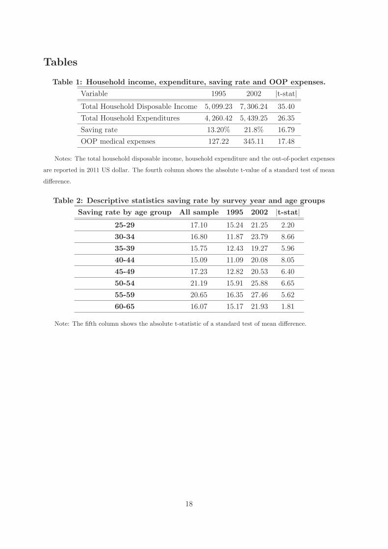
Table 1 reports summary statistics (based on the �nal sample) for household disposable

income, consumption, the resulting saving rates and out-of-pocket expenses.

Place Table 1 here

The measure of disposable income that we focus on includes labor income, property

income, transfers, and income from household sideline production minus income tax. The

consumption expenditure variable covers a broad range of categories.8 Out-of-pocket med-

ical expense is de�ned as the di�erence between total household's health care expenditure

and the amount of the reimbursement by any kind of health insurance. All ow variables

are expressed in 2011 U.S. dollars, PPP adjusted, and nominal variables in 2002 are de-

ated using the national CPI (base year 1995=100). Furthermore, we measure savings as

the di�erence between disposable income and consumption expenditure and we de�ne the

saving rate as the ratio between saving and disposable income. On average, we observe that

the household's total and disposable income increased signi�cantly in real terms from 1995

to 2002. Accordingly, also the household total expenditure increased signi�cantly, even

7In the 2002 wave, CHIPs provides two special data sets which investigate rural-to-urban migrantindividual and household information. However, such data do not exist in the 1995 wave. Therefore wedo not take these rural-to-urban migrant households into account in our analysis.

8Consumption expenditure includes food, clothing and footwear, household appliances, goods and ser-vices, medical care and health, transport and communications, recreational, educational and culturalservices and housing.

6

though the rate of growth of expenditure is lower than what we observe for the income

variables. Moreover, the average out-of-pocket medical expenses increased signi�cantly

from 1995 to 2002 which is consistent with the �ndings of Gao et al. (2001) and Wagsta�

and Linderlow (2008). Finally, the average ratio between out-of-pocket medical expenses

and disposable income is 0:025 in 1995 (ranging from 0 to 0:97) and 0:047 in 2002 (ranging

from 0 to 3:36). The household saving rate and the ratio between out-of-pocket medical

expenses and disposable income are the dependent variables in the econometric analysis

presented in the next section.

There are several possible explanations for the increase in total household expenditure,

but in our paper we stress two main reasons. First, in 1995 the health care costs of the

LIS and GIS bene�ciaries' dependents could be partially reimbursed, whereas in 2002 BIS

did not reimburse the dependents' health care costs any more. Second, during this period

there was a remarkable health care cost increase, which lead to higher household health

care expenses. Moreover, the proportion of the public insurance coverage decreased from

1995 to 2002 signi�cantly. This result is not surprising, since the Ministry of Labor and

Social Security (1999) reported that BIS could only cover 70 percent of the total outlay

under GIS and LIS. This may be attributed to the reform of SOEs which has resulted in

many enterprises being closed and a substantial number of workers being laid-o� (Gao et

al., 2001).

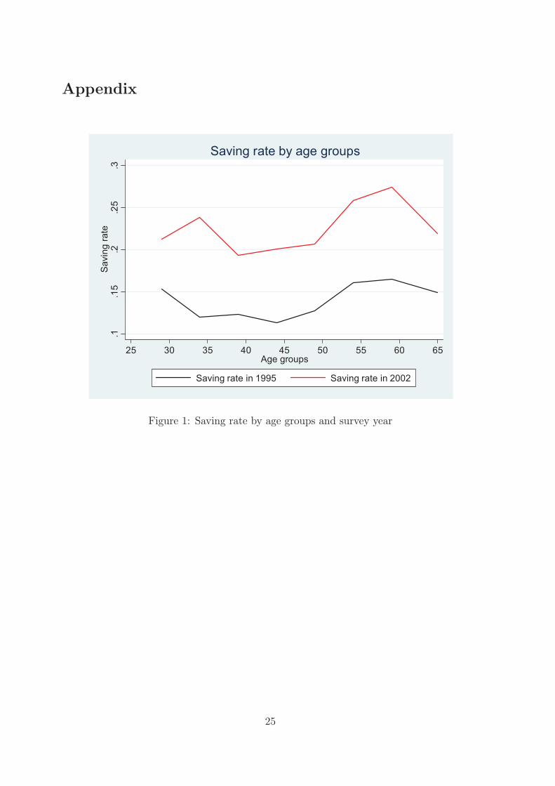
Table 2 and Figure 1 provide information on the average saving rate by age group. For

all age groups the saving rate is higher in 2002. Moreover, in both waves, the saving rate has

a U-shape pattern. Coherently with previous empirical analyses run by Yang et al. (2010),

Chamon and Prasad (2011), Brugiavini, Weber and Wu (2013), and Atella, Brugiavini,

Chen and Pace (2013), we also �nd that the lowest saving rate level are registered among

the 30-44 age group in 1995 and among the 35-49 age group in 2002.

Place Table 2 here

Another interesting aspect is to explore the evolution of saving rate by type of insurance

coverage. In China, the household head can be covered either by public insurance, private

insurance, or can remain uninsured. According to the data collected, in the 1995 wave,

public insurance was provided by either LIS or GIS, whereas in the 2002 wave it was

provided only by BIS. In 1995, 70:58 percent of household heads were covered by LIS or

GIS, 17:23 percent were covered by private health insurance, while the remaining 12:19

percent of households heads were not covered by any kind of health insurance. In 2002,

68:79 percent of household heads were covered by BIS, 5:31 percent was covered by private

health insurance while the remaining 25:9 percent of households heads were not covered

by any kind of health insurance.

7

Table 3 shows the average saving rate by survey, public health insurance coverage and

age groups. It is clear that in 2002 the saving rate is signi�cantly higher for households

whose household heads were covered by public health insurance and in the 40-54 age

group. Not statistically signi�cant di�erences can be found in 1995 with the only exception

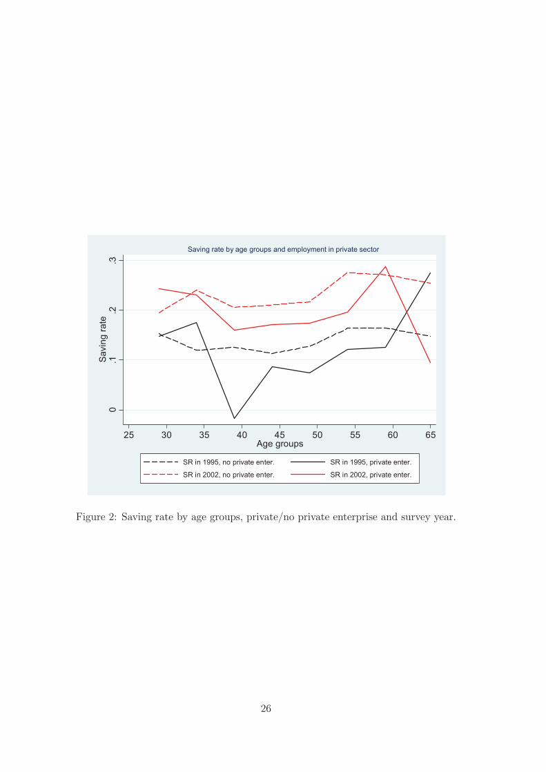
of the 30-34 age group. Figure 2 and 3 show the saving rate pro�le by age group and

working unit type. In Figure 2, we consider two categories of households, those with the

household head working in the private sector (employed in a private enterprise) and those

with the household head not working in the private sector (therefore working either in

public enterprises - State Owned Enterprises (SOE) at central or provincial level or local

SOE - or in government agencies or in public institutions). This �gure shows that the

saving rate pattern is smoother for employees not working in the private sector. Moreover,

while in 1995 the saving rate di�erence for those working in the private sector vs those not

working in the private sector was not statistically signi�cant, in 2002 it became signi�cantly

higher.

Place Table 3 here

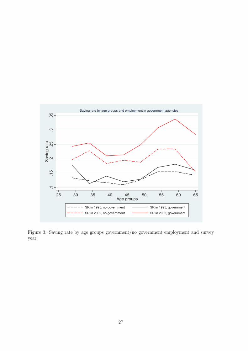
Figure 3 highlights a similar evidence: here we consider two categories of households,

those with the household head working in government agencies and government insitutions

and those with the household head working in enterprise (public or private) or in other

institutions. The result shows not statistically signi�cant di�erence in 1995. On the con-

trary, in 2002 household heads employed in government agencies or public institutions save

signi�cantly more than the others.

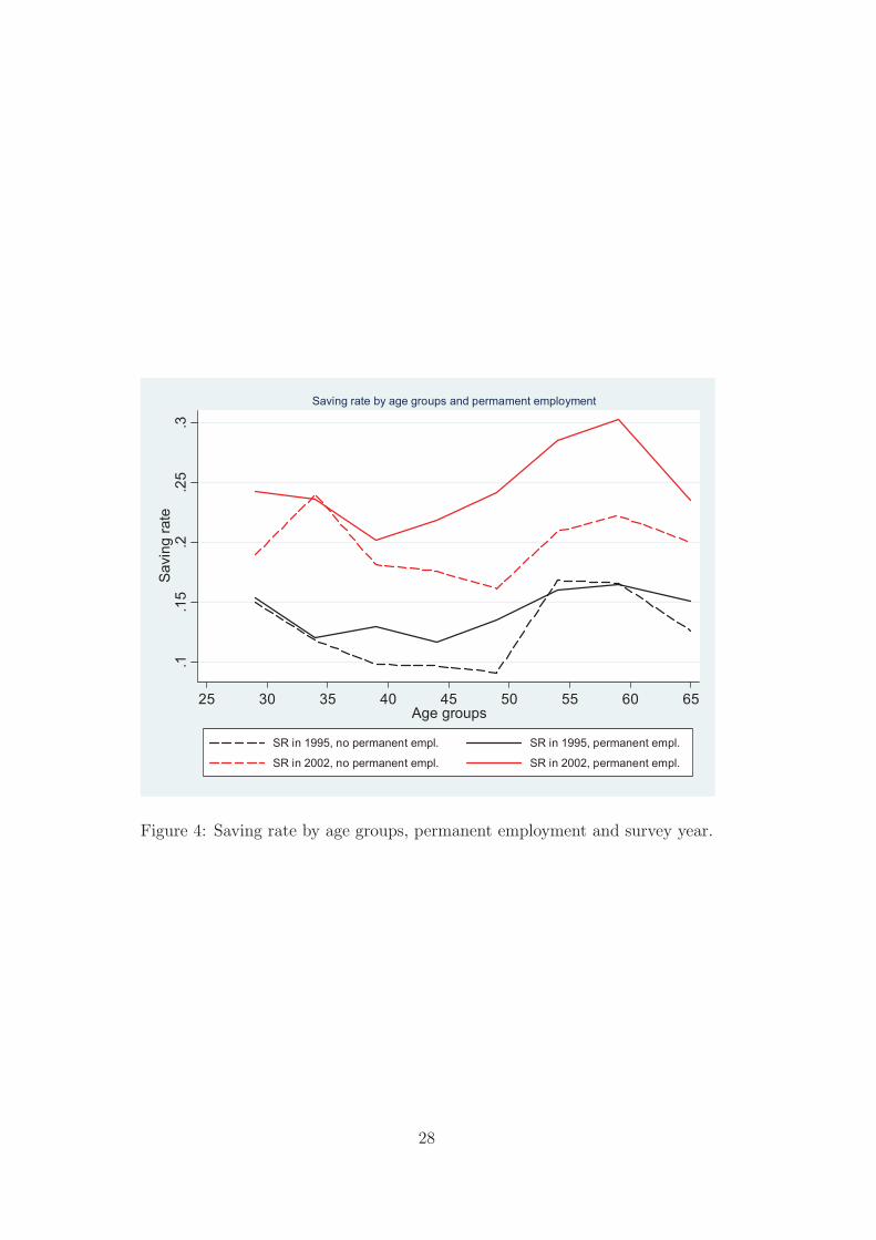
Figure 4 shows the saving age pro�le by age group and characteristics of the job contract.

In particular, we consider two categories of households, those with the household head

permanently employed in a working unit and those without a permanent contract. The

�gure shows that, in both waves, the saving rate of permanently employed household heads

is always higher than the saving rate of the households head with di�erent employment

contract.

Finally, descriptive statistics of other relevant variables are reported in Table 4. We

consider the age of the household head, the household composition (number of household

members aged less than 25, 25-49, 50+), the head's years of education and home own-

ership, and the employment characteristics, including working years in the current work

place, permanent employed or not, working in any enterprises or not, type of occupa-

tion and economic sectors. The data show that years of education and home ownership

increased signi�cantly between 1995 and 2002, suggesting a general improvement of the

living conditions of the Chinese population. Moreover, signi�cant changes are observed on

8

several indicators of the job position and occupational status. The fraction of employees

with permanent employment, the fraction of employees working in enterprises and the job

tenure decreased signi�cantly. In addition, in only seven years between 1995 and 2002 the

data show signi�cant changes also in the job sector. The fraction of individuals working

in the mineral, real estate and geological prospecting and irrigation administration de-

creased signi�cantly, while increased signi�cantly the fraction of individuals working in the

construction, �nance and insurance and social services.

Place Table 4 here

3.2 Empirical Results

As our aim is to estimate the e�ect of the 1998 health care reform on the saving rate and

OOP expenditure, we adopt a simple econometric strategy based on the estimation of the

following linear reduced form model:

(1) yi;t = �0 + �1PIi;t + �2PRi;t + �3Dt + Xi;t + �1PIi;t �Dt + �2PRi;t �Dt + �i;t

where yi;t is the household i0s saving rate or the ratio between out-of-pocket expenses

and disposable income, PIi;t is a dummy variable representing public insurance coverage

(it takes value 1 if the household head is covered by LIS or GIS in 1995, or by BIS in

2002, and takes value 0 otherwise), PRi;t is a dummy variable indicating private insurance

coverage, Dt is the time dummy indicating the pre-post reform wave, Xi;t is the vector of

control variables, which includes household head's demographic characteristics (age and

age square), household's composition variables (number of household members divided by

age groups), years of education, home ownership and employment characteristics (working

unit, permanent vs temporary contract, job tenure, occupation and economic sectors) and

the province dummies to take into account geographical heterogeneity. Furthermore, the

interaction terms PIi;t � Dt and PRi;t � Dt should capture the causal e�ect of the health

care reform on outcome variables. Finally, �i;t is the error term and t refers to time (with

t = 1995, 2002).9

The coe�cient estimates, obtained through simple OLS regressions, are reported in

Table 5. Columns from a to c show the estimated coe�cients for OOP expenses. Columns

from d to f show the estimated coe�cients for saving rate. We estimate di�erent model

speci�cations: the �rst includes only demographic characteristics and province dummies

9We also considered as dependent variable the log-normalized di�erence between disposable incomeand expenditure, controlling for the level of disposable income as additional regressor. However, the highcorrelation between years of education and income a�ects the estimated standard errors. For this reasonwe did not show the results that are available upon request.

9

(column a and d). The second adds years of education and home ownership (column b

and e). Finally, the third speci�cation, the most complete, adds the job characteristics of

the household head (column c and f ).10

Place Table 5 here

According to these results, the e�ect of the health care reform on the OOP expenses/income

ratio (columns a-c) is negative and statistically signi�cant. Furthermore, we �nd that the

interaction e�ect with survey year is negative and larger for those who are covered by pri-

vate insurance, although the di�erence is not statistically signi�cant. These results suggest

that after the reform, OOP expenses have increased, but both public and private insurance

prove to serve as a cushion against health risks, given that they do seem to reduce the OOP

expenses/income ratio. Furthermore, we �nd that a larger number of household members

aged 25+ signi�cantly increases the OOP expenses/income ratio. Years of education do

not have a signi�cant e�ect, but this may be due to its positive and signi�cant correlation

with disposable income (correlation coe�cient: 0.2295, P-value: 0.000). Moreover, the

employment characteristics do not play any role.

Looking at the saving rate model (columns d-f ), the results are in line with those

obtained for the OOP/income ratio. In this case we �nd that the interaction term between

public insurance coverage and post-reform dummy is positive and statistically signi�cant

at 1 percent and this result is robust across model speci�cations. This suggests that the

health care reform had an e�ect on saving rate for those individuals covered by public

health insurance or, put di�erently, that the public coverage induces households to save

between 3.7 to 4.8 percentage points more than households not covered by any kind of

health insurance.

In order to better describe the role of health shocks, we investigate how the saving rate

could be a�ected by health risks.

On the one hand saving may increase in response to unexpected future health shocks

which would cause higher health expenses (including OOP). Hence saving has an insurance

property vis-a-vis these risks. On the other hand if households are subject to liquidity

constraints, a health shock causing an increase in OOP would cause a reduction is current

saving. To account for these issues, we investigated the joint relationship between the

saving rate and OOP expenses by estimating a seemingly unrelated regressions (SUR)

system taking into account the contemporaneous cross-equation error correlation.11 In

10We estimate di�erent model speci�cations to check whether there are variables driving the e�ect onOOP/income and saving rate. However, since the coe�cients of the key variables do not change betweenmodel speci�cations, we can conclude that this concern is unfounded.11SUR produces more e�cient estimates than ordinary least square regression. It does this by weighting

the estimates by the covariance of the residuals from the individual regressions.

10

particular, we assume that current OOP enter the saving rate regression in order to capture

the idea that under liquidity constraints households have to reduce current saving to cope

with unexpected health expenditures.

In Table 6, we present the coe�cient estimates obtained from the two equation model,

one for the OOP expenses/income ratio (column a) and one for the saving rate (column b).

The two equations share the same set of regressors, but we add the OOP expenses/income

ratio as additional explanatory variable in the saving rate equation. As we can clearly see

in column b, the coe�cient of the OOP expenses/income ratio is negative and statistically

signi�cant, suggesting that high OOP expenses relative to income prevents households to

save. The interaction terms remain substantially unaltered with respect to the estimates

in Table 5, thus proving to be robust. Similarly, all other variables con�rm their role as in

Table 5.

Place Table 6 here

3.3 Data limitations: dealing with the unobserved heterogeneity

Although the analysis carried out so far present some interesting policy results, we are

aware of the existence of limitations in our data that may strongly in uence the estimates.

In particular, our dataset lacks information on individual health status and both OOP

expenses and saving rate are likely to be a�ected by the individual health status. Therefore,

if the health status is an important determinant of outcomes, this will lead to the existence

of some form of unobserved heterogeneity and our current estimate of the health insurance

coverage e�ect could, at best, be interpreted as an average e�ect across individuals with

poor and good health.12

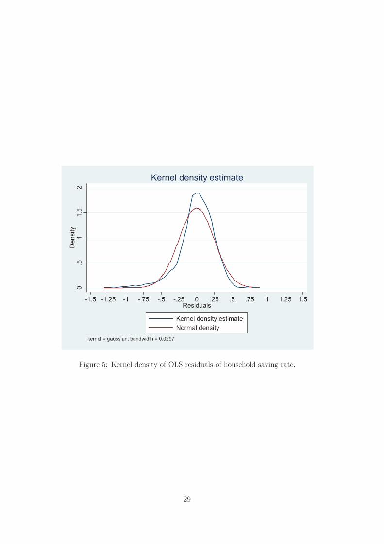
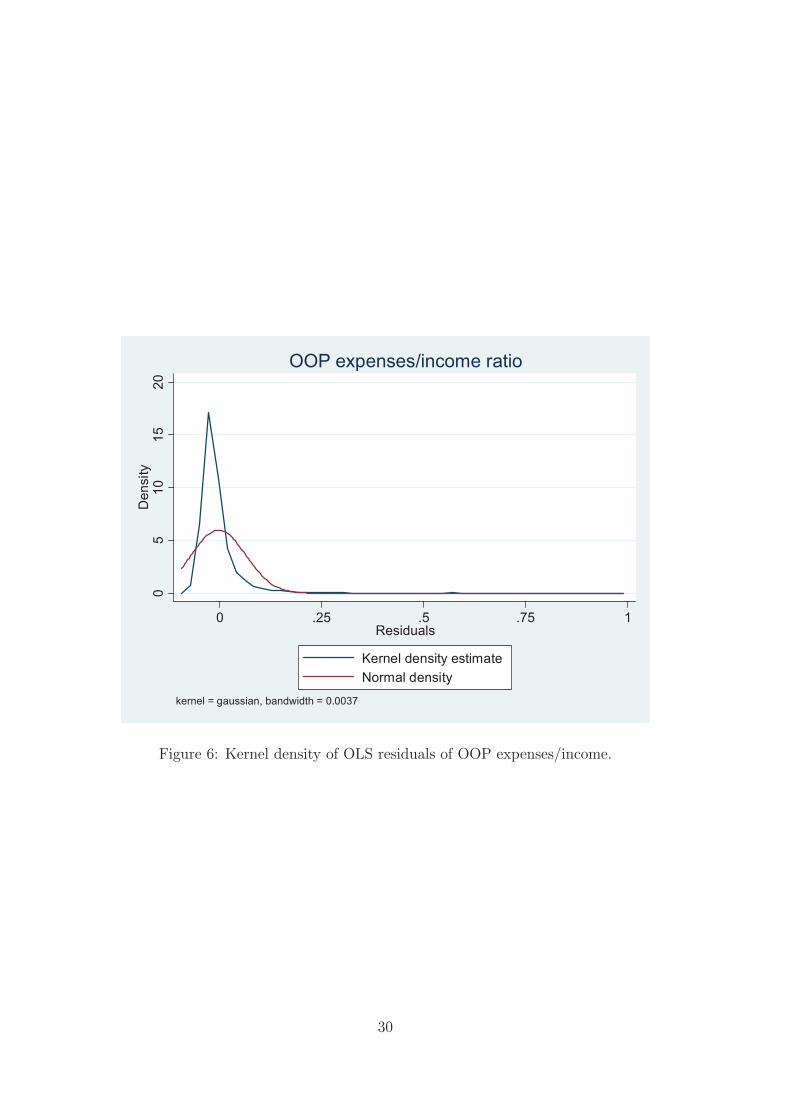
Indeed, evidence of the existence of some unobserved heterogeneity may be seen in

Figure 5 and 6. These �gures are kernel density estimates of the distribution of OLS resid-

uals from our models in equation 1. To take into account such unobserved heterogeneity,

we estimate a �nite mixture model. Finite Mixture Models (FMMs) are semiparametric

estimators that have received increasing attention both in the economics and statistics lit-

erature because there are di�erent areas in which such distributions are encountered. The

12What is available in the dataset is the number of sick leave days taken in the current year in 1995and a measure of self-perceived health status in 2002. These two pieces of information are not directlycomparable to obtain a synthetic and coherent measure of health status variation across the two waves.Theoretically, we could have constructed a coherent health status index based on the distribution of theanswers to both questions. However, the large number of missing values for the number of sick leave daysmakes this strategy useless as it would drastically reduce the sample size for the analysis.

11

FMMs provide a natural representation of heterogeneity in a �nite number of latent classes.

It concerns modeling any statistical distribution by a mixture of other distributions.13

Following Deb and Trivedi (1997), the density function for a C -component �nite mix-

ture is

(2) f(y j x; �1; �2; :::; �C ; �1; �2; :::; �C) =CX

j=1

�jfj(h j x; �j)

where 0 < �j < 1, and

CX

j=1

�j = 1 and fj denotes an appropriate density given the

characteristics of the error terms. In this contest normally distributed components appear

to be appropriate in the context of the outcome of interest. We estimate the model's

parameters using maximum likelihood. In addition, in post estimation, we calculate the

posterior probability that observation yi belongs to component c (the prior probability is

assumed to be a constant):

(3) Pr [yi 2 population c j xi; yi; �] =�CfC(yijxi;�C)CX

j=1

�jfj(yijxi;�j)

; c = 1; 2; ::C

which we use to explore the determinants of class membership, and especially to see if

these determinants are consistent with the idea that health status is the likely source of

unobserved heterogeneity.

By mean of the Akaike Information Criterion and Bayesian Information Criterion we

select a two component FMM. Parameter estimates of the �nite mixture model for OOP

expenses/income ratio (column a and b) and saving rate (column c and d) are reported

in Table 7. Di�erently from OLS estimates, our �ndings suggest that, once properly

accounting for unobserved heterogeneity (health status), out-of-pocket expenses and saving

rate are a�ected by the reform in a di�erentiated way. In particular, we �nd that the ratio

between out-of-pocket expenses and income increases more for component 1 individuals

compared to component 2 (0:072 vs 0:007) and saving rate increases only for component

2 individuals. Furthermore, we �nd that both public and private health insurances are

ine�ective to cushion individuals against the increase in out-of-pocket expenses, irrespective

of their group. In the case of the saving rate some positive statistically signi�cant (at 10

percent) e�ects could be found only for component 2 individuals.

These results support the prima facie evidence that the outcomes are generated by two

di�erent distributions where, potentially, individuals in component 1 have lower health

status than individuals in component 2.

13Atella and Deb (2013) provide a review of the contributions adopting the Finite Mixture approach.

12

In the model for OOP expenses/income ratio, the predicted mean in component 1 is

0:148 (std. dev. 0:048) ranging between 0:016 and 0:355, while the predicted mean in

component 2 is 0:02 (std. dev. 0:006) and ranges between 0:003 and 0:040. In the model

for saving rate, the predicted mean in component 1 is close to zero (mean �0:051, std.

dev. 0:093) and ranges between a negative value of �0:415 and a positive value of 0:335,

while the predicted mean in component 2 is 0:222 (std. dev. 0:076) and ranges between

0:004 and 0:486. The estimated class probabilities are informative vis-a-vis our speculative

hypothesis that the distributions are drawn from individuals with poor health and good

health, with the evidence suggesting that component 1 represents individuals with poor

health.

The posterior probabilities seem to support our hypothesis: in the model for OOP ex-

penses/income ratio the probability of being in component 1 is 14.4 percent while in the

model for saving rate the same probability is 19 percent. Although we have not been able

to obtain information on the health distribution for a population that is perfectly over-

lapping with our population, we feel comfortable to claim that the posterior probabilities

are consistent with some recent �ndings on health status distribution available in the lit-

erature (Zhao, 2008; Chatterji et al., 2008; Strauss et al., 2011; Mu, 2013). In particular,

according to Zhao (2008) 26 percent of the whole sample reported a poor and fair health

status ranging from 34.8 percent in the Hubei province and 13.4 percent in Heilongjiang.

Chatterji et al. (2008) show that 16 percent of the respondents in China reported having

at least one chronic diseases. Strauss et al. (2011) �nd that 22 percent of women and

30 percent of men reported poor general health. Finally, Mu (2013) �nds that 24 percent

of the sample self-report a poor health status. Given that our sample is younger than

the samples used by the authors listed above, we can conclude that our estimates suggest

that component 1 represents the group of individuals with poor health. If health status is

truly the unobserved variable a�ecting the results for both OOP expenditure/income and

saving rate, the results suggest a quite clear story: i) individuals with poor health tend to

pay out-of-pocket a larger share of their income and this direct disbursement reduces their

saving; ii) individuals with fair or good health tend to pay out-of-pocket a small share of

their income and can a�ord to save more.

Place Table 7 here

To better characterize class membership we estimate OLS regressions of the posterior

probabilities (multiplied by 100) of belonging to class 1 on a set of variable including age,

household income and a set of job characteristics (working unit, type of contract, tenure,

occupation). The results presented in Table 8 support the poor health/good health cate-

gorization. In both models for OOP expenses/income and saving rate, the coe�cients of

13

age is positive and statistically signi�cant, suggesting, as expected, that aging is associ-

ated with the worsening of health status. Moreover, the coe�cients of household income

(expressed either as a continuous or a categorized variable) and permanent employment

contract are negative and highly statistically signi�cant, suggesting that poorer families

with household head employed with temporary contract are more likely to have a poor

general health with respect to wealthier families with household head employed with a

permanent contract. Other job characteristics seem to be correlated with the posterior

probability of belonging to class 1: working in an enterprise and the number of years spent

in the current job place reduce the probability of a poor health status.14

Place Table 8 here

4 Conclusion

In this paper we have analyized the economic e�ects of the third stage of the health care

system reform occurred in 1998, when the Chinese government established a new public

insurance scheme, called the Basic Insurance Scheme (BIS) nationwide. In particular, we

have focused on the e�ects produced on OOP expenses and household's saving rate.

According to the literature, reforms which curtail health coverage and health provisions

should induce households to increase both oop expenses and the saving rate (in this last

case in view of future health expenditures). Using data from the 1995 and 2002 waves of

the Chinese Household Income Project Survey for the Chinese urban households, we have

estimated a DiD model to explore the e�ect of the 1998 reform. According to a �rst set

of results based on OLS estimation, the reform has positively a�ected both OOP expenses

and saving rate, con�rming the literature results. Furthermore, we found that both public

and private insurance prove to serve as a cushion against health risks, given that they do

seem to reduce the ratio of OOP expenses compared to disposable income.

We have further explored the robustness of these results by allowing for the existence of

unobserved heterogeneity in our data and made use of a Finite Mixture Model approach.

In this way we are able to isolate two distinct groups that, according to posterior probabil-

ity regression estimates, could be associated with "bad" and "good" health status. Once

properly accounted for this form of heterogeneity, the e�ects of this reform are quite dif-

ferent. In particular, we �nd that after the reform OOP expenses increase more for the

less healthy individuals, while the saving rate increases more for the healthy individuals.

14Also years of education is negatively associated to the posterior probability of beloning to class 1.However, we did not include this variable in the regression because is signi�cantly correlated with householdincome.

14

Furthermore, our results suggest that, after the reform, public and private insurances do

not serve as a cushion against health risks.

Overall, our results are somewhat surprising, if compared with the standard literature

developed for Western economies. Once attention is paid to the di�erent populations

re ected in the sample vis- �a -vis the di�erent health characteristics, the role of public

health provisions in protecting against current and future health shocks disappears. We

cannot say much about the speci�c reason for this failure, but a possible explanation is the

reduced coverage for dependent household members (spouse and children of the employee).

In future work we will focus on the speci�c role of each single health provision in order

to disentangle the di�erent explanations as to this lack of insurance properties.

15

References

Aaberge R. and Zhu Y. 2001. The Pattern of Household Savings during a Hyperin ation:

The Case of Urban China in the late 1980s. Review of Income and Wealth, Vol. 47, pp

181-202.

Atella V., Brugiavini A., Chen H. and Pace N. The Chinese health care system reforms

and household saving patterns: some stylized facts. In The Globalisation of Chinese busi-

ness; implications for multinational investors, edited by Taylor et al., Chandos publishing,

Oxford (forthcoming).

Atella V., Deb P. 2013. Heterogeneity in Long Term Health Outcomes of Migrants

within Italy. NBER Working Paper No. 19422.

Baldacci E., Callegari G., Coady D., Ding D., Kumar M., Tommasino P., Woo J. 2010.

Public Expenditures on Social Programs and Household Consumption in China. IMF

Working Paper 10/69.

Barnett S. and Brooks R. 2010. China: Does Government Health and Education Spend-

ing Boost Consumption?. IMF Working Paper 10/16.

Brugiavini A., Weber G., and Wu B. 2013. Saving Rates of Urban Households in China.

In The Chinese Economy, edited by G. Gomel et al., Springer-Verlag Berlin Heidelberg.

Chamon. M. D. and Prasad E. S. 2011. Why Are Saving Rates of Urban Households

in China Rising? American Economic Journal: Macroeconomics, Vol. 2(1), pp 93-130.

Chatterji S., Kowal P., Mathers C., Naidoo N., Verdes E., Smith JP. and Suzman R.

2008. The health of aging populations in China and India. Health A�airs, Vol. 27(4), pp

1052-1063.

Chow G. 1985. A Model of Chinese National Income Determination. Journal of Political

Economy, Vol. 93 (4), pp 782-792.

Deb P. and Trivedi P.K. 1997. Demand for Medical Care by the Elderly: A Finite

Mixture Approach. Journal of Applied Econometrics, Vol. 12, pp. 313-336.

Feng J., He L., and Sato H. 2011. Public pension and Household Saving: Evidence

from urban China. Journal of Comparative Economics, Vol. 39(4), pp 470-485.

Gao J., Raven J., and Tang S. 2007. Hospitalization among elderly in urban China.

Health Policy, Vol. 84, pp 210-219.

Gao J., Tang S., Tolhurst R. and Rao K. 2001. Changing access to health services in

urban China: implications for equity. Health Policy and Planning, Vol. 16(3), pp 302-312.

Kraay A. 2000. Household saving in China. World Bank Economic Review, Vol. 14(3),

pp 545-570.

Liu Y. 2002. Reforming China's urban health insurance system. Health Policy, Vol.

60, pp 133-150.

Ma G. and Yi W. 2010. China's high saving rate: myth and reality, BIS Working

16

Papers 312, Bank for International Settlements.

Ministry of Labor and Social Security 1999. The policy options for supplementary

medical insurance in China. Mimeo.

Modigliani F. and Cao S.L. 2004. The Chinese Saving Puzzle and the Life-Cycle Hy-

pothesis. Journal of Economic Literature, Vol. 42(1), pp 145-170.

Mu R. 2013. Regional disparities in self reported health: evidence from Chinese Older

Adults. Health Economics. doi: 10.1002/hec.2929.

Nabar M. 2011. Targets, Interest Rates, and Household Saving in Urban China. IMF

Working Paper 11/223.

National Bureau of Statistics of China 2003. The Chinese Statistical Yearbook 2003.

China Statistics Press.

Qian Y. 1988. Urban and Rural Household Saving in China. IMF Sta� Papers, Vol.

35(4), pp 592-627.

Strauss J., Lei X., Park A., Shen Y., Smith J., Yang Z., Zhao Y. 2011. Health Outcomes

and Socio-Economic Status Among the Elderly in China: evidence from the CHARLS pilot.

Journal of Population Ageing, Vol. 3, pp 111-143.

Wagsta� A. and Lindelow M. 2008. Can insurance increase �nancial risk? The curious

case of health insurance in China. Journal of Health Economics, Vol. 27(4), pp 990-1005.

Wagsta� A., Yip W., Lindelow M., Hsiao W. 2009. China's health system and its

reform: a review of recent studies. Health Economics. Vol. 18, S7-S23.

Wang Y. 1995. Permanent Income and Wealth Accumulation: A Cross-Sectional Study

of Chinese Urban and Rural Households. Economic Development and Cultural Change,

Vol. 43 (3), pp 522-550.

Wang X. and Wen Y. 2011. Can rising housing prices explain China's high household

saving rate?. Review 93(2), Federal Reserve Bank of San Louis.

Wei S.J. and Zhang X. 2011. The Competitive Saving Motive: Evidence from Rising

Sex Ratios and Savings Rates in China. Journal of Political Economy, Vol. 119, pp 511-564.

Wen Y. 2010. Saving and growth under borrowing constraints explaining the \high

saving rate" puzzle. Working Paper 2009-045C., Federal Reserve Bank of San Louis.

Yang D.T., Zhang J. and Zhou S. 2010. Why Are Saving Rates so High in China?,

Working Paper 16771, National Bureau of Economic Research.

Zhao Z. 2008. Health Demand and Health Determinants in China. Journal of Chinese

Economic and Business Studies, Vol. 6 (1), pp. 77-98.

17

Tables

Table 1: Household income, expenditure, saving rate and OOP expenses.

Variable 1995 2002 jt-statj

Total Household Disposable Income 5; 099:23 7; 306:24 35:40

Total Household Expenditures 4; 260:42 5; 439:25 26:35

Saving rate 13:20% 21:8% 16:79

OOP medical expenses 127:22 345:11 17:48

Notes: The total household disposable income, household expenditure and the out-of-pocket expenses

are reported in 2011 US dollar. The fourth column shows the absolute t-value of a standard test of mean

di�erence.

Table 2: Descriptive statistics saving rate by survey year and age groups

Saving rate by age group All sample 1995 2002 jt-statj

25-29 17:10 15:24 21:25 2:20

30-34 16:80 11:87 23:79 8:66

35-39 15:75 12:43 19:27 5:96

40-44 15:09 11:09 20:08 8:05

45-49 17:23 12:82 20:53 6:40

50-54 21:19 15:91 25:88 6:65

55-59 20:65 16:35 27:46 5:62

60-65 16:07 15:17 21:93 1:81

Note: The �fth column shows the absolute t-statistic of a standard test of mean di�erence.

18

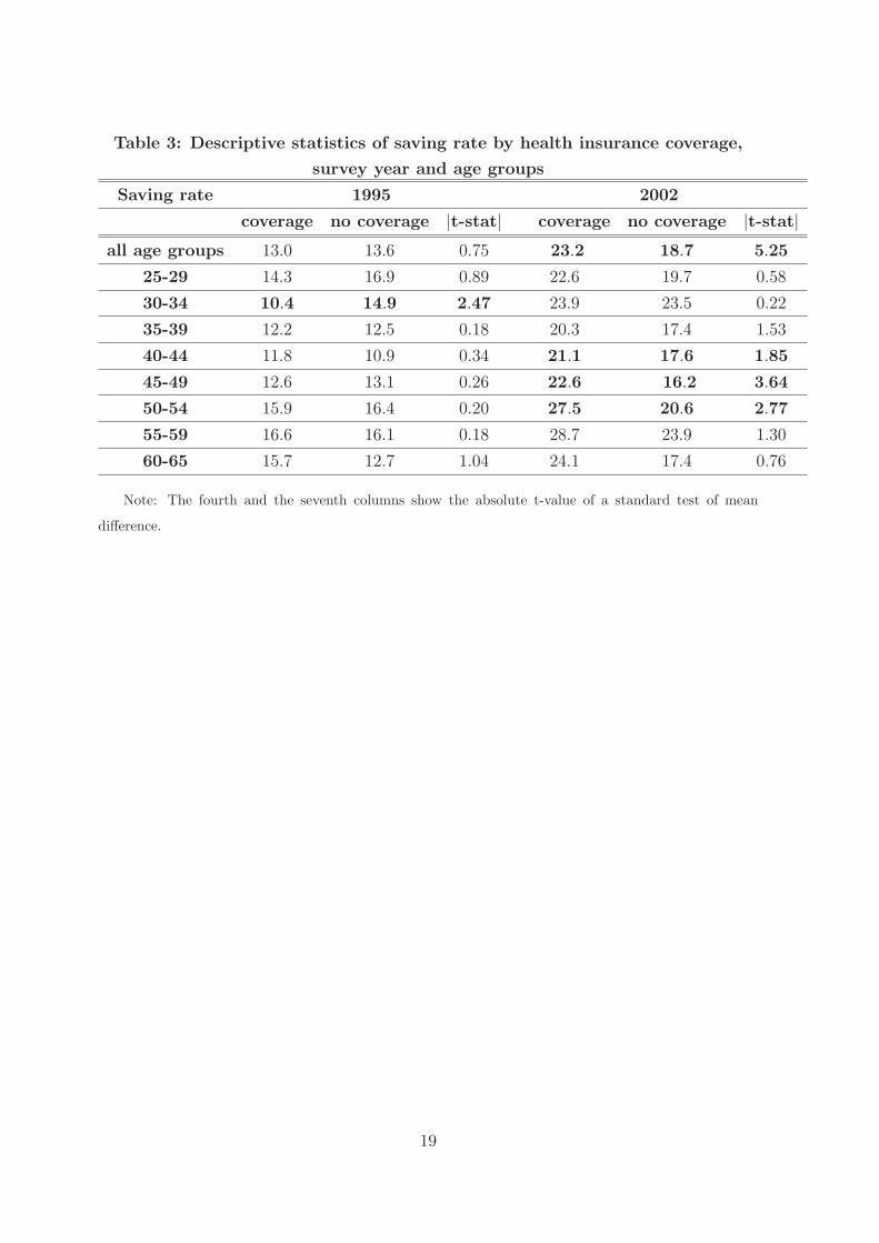
Table 3: Descriptive statistics of saving rate by health insurance coverage,

survey year and age groups

Saving rate 1995 2002

coverage no coverage jt-statj coverage no coverage jt-statj

all age groups 13:0 13:6 0:75 23:2 18:7 5:25

25-29 14:3 16:9 0:89 22:6 19:7 0:58

30-34 10:4 14:9 2:47 23:9 23:5 0:22

35-39 12:2 12:5 0:18 20:3 17:4 1:53

40-44 11:8 10:9 0:34 21:1 17:6 1:85

45-49 12:6 13:1 0:26 22:6 16:2 3:64

50-54 15:9 16:4 0:20 27:5 20:6 2:77

55-59 16:6 16:1 0:18 28:7 23:9 1:30

60-65 15:7 12:7 1:04 24:1 17:4 0:76

Note: The fourth and the seventh columns show the absolute t-value of a standard test of mean

di�erence.

19

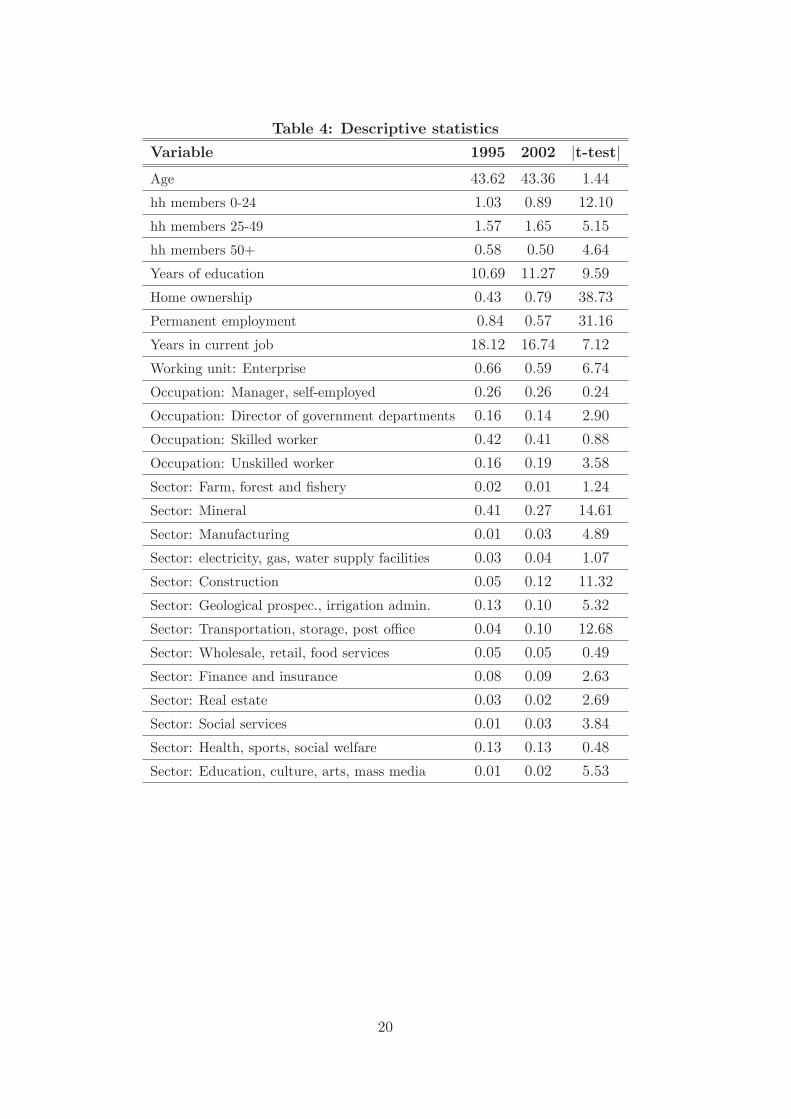
Table 4: Descriptive statistics

Variable 1995 2002 jt-testj

Age 43:62 43:36 1:44

hh members 0-24 1:03 0:89 12:10

hh members 25-49 1:57 1:65 5:15

hh members 50+ 0:58 0:50 4:64

Years of education 10:69 11:27 9:59

Home ownership 0:43 0:79 38:73

Permanent employment 0:84 0:57 31:16

Years in current job 18:12 16:74 7:12

Working unit: Enterprise 0:66 0:59 6:74

Occupation: Manager, self-employed 0:26 0:26 0:24

Occupation: Director of government departments 0:16 0:14 2:90

Occupation: Skilled worker 0:42 0:41 0:88

Occupation: Unskilled worker 0:16 0:19 3:58

Sector: Farm, forest and �shery 0:02 0:01 1:24

Sector: Mineral 0:41 0:27 14:61

Sector: Manufacturing 0:01 0:03 4:89

Sector: electricity, gas, water supply facilities 0:03 0:04 1:07

Sector: Construction 0:05 0:12 11:32

Sector: Geological prospec., irrigation admin. 0:13 0:10 5:32

Sector: Transportation, storage, post o�ce 0:04 0:10 12:68

Sector: Wholesale, retail, food services 0:05 0:05 0:49

Sector: Finance and insurance 0:08 0:09 2:63

Sector: Real estate 0:03 0:02 2:69

Sector: Social services 0:01 0:03 3:84

Sector: Health, sports, social welfare 0:13 0:13 0:48

Sector: Education, culture, arts, mass media 0:01 0:02 5:53

20

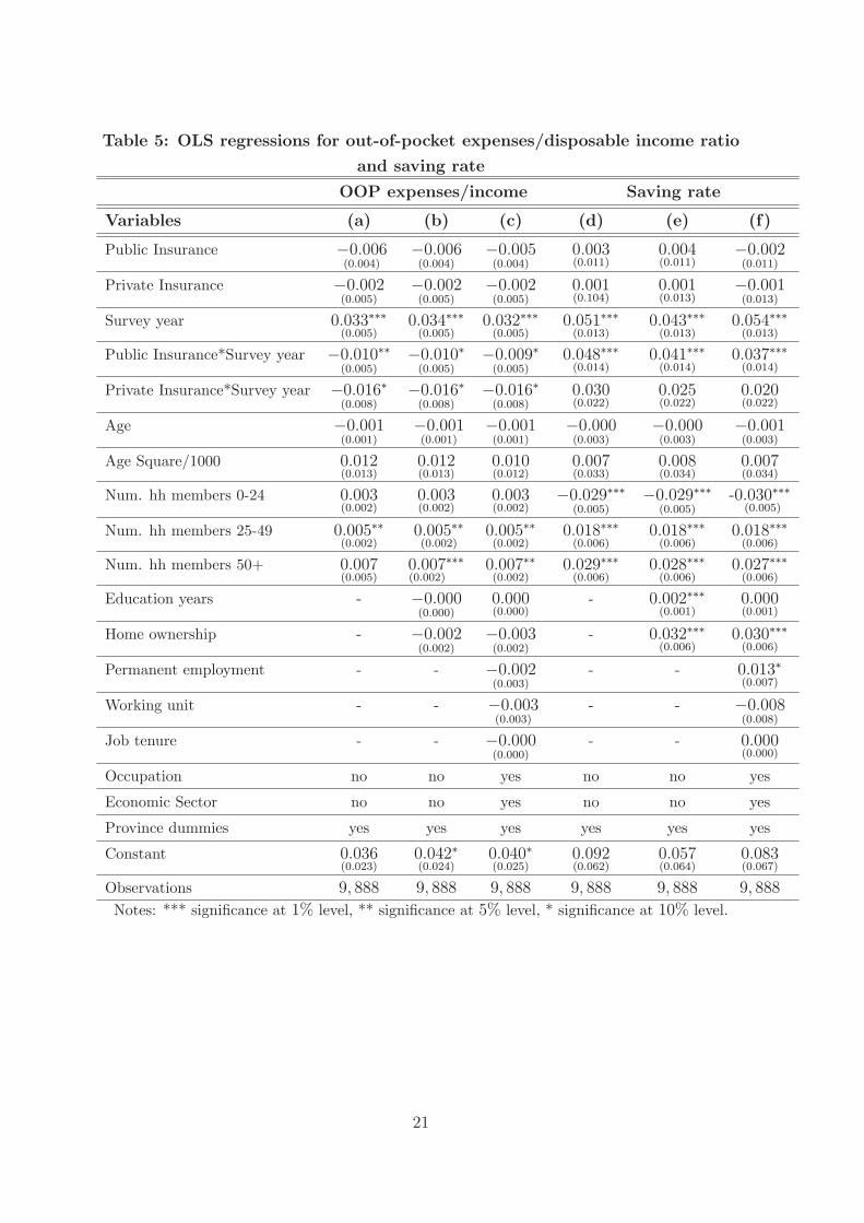
Table 5: OLS regressions for out-of-pocket expenses/disposable income ratio

and saving rate

OOP expenses/income Saving rate

Variables (a) (b) (c) (d) (e) (f)

Public Insurance �0:006(0:004)

�0:006(0:004)

�0:005(0:004)

0:003(0:011)

0:004(0:011)

�0:002(0:011)

Private Insurance �0:002(0:005)

�0:002(0:005)

�0:002(0:005)

0:001(0:104)

0:001(0:013)

�0:001(0:013)

Survey year 0:033��(0:005)

0:034��(0:005)

0:032��(0:005)

0:051��(0:013)

0:043��(0:013)

0:054��(0:013)

Public Insurance*Survey year �0:010��(0:005)

�0:010�(0:005)

�0:009�(0:005)

0:048��(0:014)

0:041��(0:014)

0:037��(0:014)

Private Insurance*Survey year �0:016�(0:008)

�0:016�(0:008)

�0:016�(0:008)

0:030(0:022)

0:025(0:022)

0:020(0:022)

Age �0:001(0:001)

�0:001(0:001)

�0:001(0:001)

�0:000(0:003)

�0:000(0:003)

�0:001(0:003)

Age Square/1000 0:012(0:013)

0:012(0:013)

0:010(0:012)

0:007(0:033)

0:008(0:034)

0:007(0:034)

Num. hh members 0-24 0:003(0:002)

0:003(0:002)

0:003(0:002)

�0:029��(0:005)

�0:029��(0:005)

-0:030��(0:005)

Num. hh members 25-49 0:005��(0:002)

0:005��(0:002)

0:005��(0:002)

0:018��(0:006)

0:018��(0:006)

0:018��(0:006)

Num. hh members 50+ 0:007(0:005)

0:007(0:002)

�� 0:007��(0:002)

0:029��(0:006)

0:028��(0:006)

0:027��(0:006)

Education years - �0:000(0:000)

0:000(0:000)

- 0:002��(0:001)

0:000(0:001)

Home ownership - �0:002(0:002)

�0:003(0:002)

- 0:032��(0:006)

0:030��(0:006)

Permanent employment - - �0:002(0:003)

- - 0:013�(0:007)

Working unit - - �0:003(0:003)

- - �0:008(0:008)

Job tenure - - �0:000(0:000)

- - 0:000(0:000)

Occupation no no yes no no yes

Economic Sector no no yes no no yes

Province dummies yes yes yes yes yes yes

Constant 0:036(0:023)

0:042�(0:024)

0:040�(0:025)

0:092(0:062)

0:057(0:064)

0:083(0:067)

Observations 9; 888 9; 888 9; 888 9; 888 9; 888 9; 888

Notes: *** signi�cance at 1% level, ** signi�cance at 5% level, * signi�cance at 10% level.

21

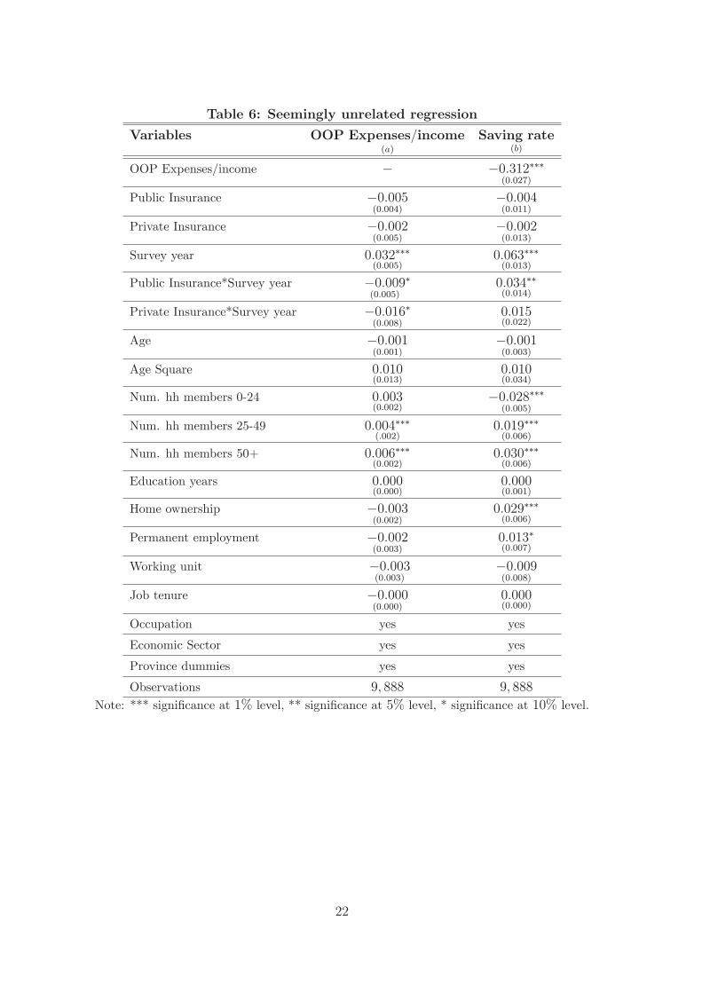
Table 6: Seemingly unrelated regression

Variables OOP Expenses=income(a)

Saving rate(b)

OOP Expenses/income � �0:312��(0:027)


�0:004(0:011)


�0:002(0:013)

Survey year 0:032��(0:005)

0:063��(0:013)

Public Insurance*Survey year �0:009(0:005)

� 0:034��(0:014)

Private Insurance*Survey year �0:016�(0:008)

0:015(0:022)

Age �0:001(0:001)

�0:001(0:003)

Age Square 0:010(0:013)

0:010(0:034)

Num. hh members 0-24 0:003(0:002)

�0:028��(0:005)

Num. hh members 25-49 0:004��(:002)

0:019��(0:006)

Num. hh members 50+ 0:006��(0:002)

0:030��(0:006)

Education years 0:000(0:000)

0:000(0:001)

Home ownership �0:003(0:002)

0:029��(0:006)

Permanent employment �0:002(0:003)

0:013�(0:007)

Working unit �0:003(0:003)

�0:009(0:008)

Job tenure �0:000(0:000)

0:000(0:000)

Occupation yes yes

Economic Sector yes yes

Province dummies yes yes

Observations 9; 888 9; 888

Note: *** signi�cance at 1% level, ** signi�cance at 5% level, * signi�cance at 10% level.

22

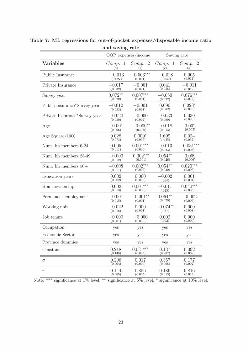
Table 7: ML regressions for out-of-pocket expenses/disposable income ratio

and saving rate


Variables Comp: 1(a)

Comp: 2(b)

Comp: 1(c)

Comp: 2(d)


�0:003��(0:001)

�0:028(0:049)

0:005(0:011)


�0:001(0:001)

0:041(0:058)

�0:011(0:012)

Survey year 0:072��(0:029)

0:007��(0:001)

�0:050(0:057)

0:076��(0:012)

Public Insurance*Survey year �0:012(0:032)

�0:001(0:001)

0:090(0:062)

0:023�(0:013)

Private Insurance*Survey year �0:020(0:050)

�0:000(0:002)

�0:033(0:099)

0:030(0:020)

Age �0:001(0:006)

�0:000��(0:000)

�0:018(0:013)

0:002(0:003)

Age Square/1000 0:028(0:073)

0:000�(0:000)

1:699(1:445)

0:024(0:032)

Num. hh members 0-24 0:005(0:011)

0:001��(0:000)

�0:013(0:023)

�0:031��(0:005)

Num. hh members 25-49 �0:000(0:012)

0:002��(0:001)

0:054��(0:026)

0:009(0:006)

Num. hh members 50+ �0:008(0:011)

0:002��(0:000)

0:054��(0:020)

0:020��(0:006)

Education years 0:002(0:002)

0:000(0:000)

�0:002(:004)

0:001(0:001)

Home ownership 0:002(0:013)

0:001��(0:000)

�0:011(:025)

0:040��(0:005)

Permanent employment �0:001(0:015)

�0:001��(0:001)

0:064��(0:029)

�0:002(0:006)

Working unit �0:022(0:018)

0:000(0:001)

�0:074��(:037)

0:000(0:008)

Job tenure �0:000(0:001)

�0:000(0:000)

0:002(:002)

0:000(0:000)

Occupation yes yes yes yes

Economic Sector yes yes yes yes

Province dummies yes yes yes yes

Constant 0:218(0:148)

0:031��(0:005)

0:137(0:287)

0:092(0:062)

� 0:206(0:004)

0:017(0:000)

0:357(0:008)

0:177(0:002)

� 0:144(0:005)

0:856(0:005)

0:186(0:013)

0:816(0:013)


23

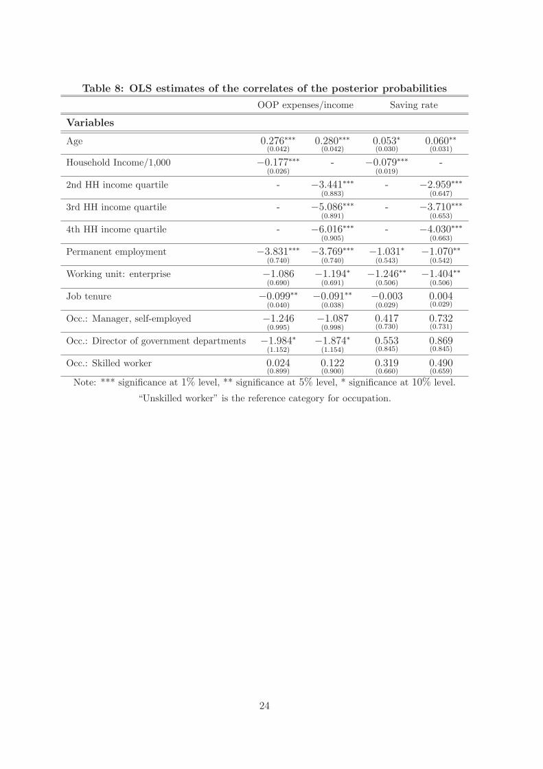
Table 8: OLS estimates of the correlates of the posterior probabilities


Variables

Age 0:276��(0:042)

0:280��(0:042)

0:053�(0:030)

0:060��(0:031)

Household Income/1,000 �0:177��(0:026)

- �0:079��(0:019)

-

2nd HH income quartile - �3:441��(0:883)

- �2:959��(0:647)

3rd HH income quartile - �5:086��(0:891)

- �3:710��(0:653)

4th HH income quartile - �6:016��(0:905)

- �4:030��(0:663)

Permanent employment �3:831��(0:740)

�3:769��(0:740)

�1:031�(0:543)

�1:070��(0:542)

Working unit: enterprise �1:086(0:690)

�1:194�(0:691)

�1:246��(0:506)

�1:404��(0:506)

Job tenure �0:099��(0:040)

�0:091��(0:038)

�0:003(0:029)

0:004(0:029)

Occ.: Manager, self-employed �1:246(0:995)

�1:087(0:998)

0:417(0:730)

0:732(0:731)

Occ.: Director of government departments �1:984�(1:152)

�1:874�(1:154)

0:553(0:845)

0:869(0:845)

Occ.: Skilled worker 0:024(0:899)

0:122(0:900)

0:319(0:660)

0:490(0:659)


\Unskilled worker" is the reference category for occupation.

24

Appendix

.1.1

5.2

.25

.3S

avin

g r

ate

25 30 35 40 45 50 55 60 65Age groups

Saving rate in 1995 Saving rate in 2002

Saving rate by age groups

Figure 1: Saving rate by age groups and survey year

25

0.1

.2.3

Savin

g r

ate

25 30 35 40 45 50 55 60 65Age groups

SR in 1995, no private enter. SR in 1995, private enter.

SR in 2002, no private enter. SR in 2002, private enter.

Saving rate by age groups and employment in private sector

Figure 2: Saving rate by age groups, private/no private enterprise and survey year.

26

.1.1

5.2

.25

.3.3

5S

avin

g r

ate

25 30 35 40 45 50 55 60 65Age groups

SR in 1995, no government SR in 1995, government

SR in 2002, no government SR in 2002, government

Saving rate by age groups and employment in government agencies

Figure 3: Saving rate by age groups government/no government employment and surveyyear.

27

.1.1

5.2

.25

.3S

avin

g r

ate

25 30 35 40 45 50 55 60 65Age groups

SR in 1995, no permanent empl. SR in 1995, permanent empl.

SR in 2002, no permanent empl. SR in 2002, permanent empl.

Saving rate by age groups and permament employment

Figure 4: Saving rate by age groups, permanent employment and survey year.

28

0.5

11.5

2D

ensity

-1.5 -1.25 -1 -.75 -.5 -.25 0 .25 .5 .75 1 1.25 1.5Residuals

Kernel density estimate

Normal density

kernel = gaussian, bandwidth = 0.0297


Figure 5: Kernel density of OLS residuals of household saving rate.

29

05

10

15

20

Density

0 .25 .5 .75 1Residuals


Normal density

kernel = gaussian, bandwidth = 0.0037

OOP expenses/income ratio

Figure 6: Kernel density of OLS residuals of OOP expenses/income.

30

RECENT PUBLICATIONS BY CEIS Tor Vergata Seasonality in smoking behaviour: Re-evaluating the effects of the 2005 public smoking ban in Italy Emilia Del Bono, Klaus Grünberger and Daniela Vuri CEIS Research Paper, 295,October 2013

Generalizing smooth transition autoregressions Emilio Zanetti Chini CEIS Research Paper, 294,October 2013

Italy’s Growth and Decline, 1861-2011 Emanuele Felice and Giovanni Vecchi CEIS Research Paper, 293,October 2013

Economic effects of treatment of chronic kidney disease with low-protein diet F.S. Mennini, S. Russo, A. Marcellusi, G. Quintaliani, D. Fouque CEIS Research Paper, 292,October 2013

The Legal Origins of Corporate Social Responsibility Leonardo Becchetti, Rocco Ciciretti and Pierluigi Conzo CEIS Research Paper, 291,October 2013

Generalised Linear Spectral Models Tommaso Proietti and Alessandra Luati CEIS Research Paper, 290,October 2013

Macroeconomic forecasting and structural analysis through regularized reduced-rank regression Emmanuela Bernardini and Gianluca Cubadda CEIS Research Paper, 289,October 2013

Three Elementary Forms of Economic Organization Leo Ferraris CEIS Research Paper, 288,October 2013

EuroMInd-C: a Disaggregate Monthly Indicator of Economic Activity for the

Euro Area and member countries Cecilia Frale, Stefano Grassi, Massimiliano Marcellino, Gianluigi Mazzi, Tommaso Proietti CEIS Research Paper, 287, October 2013

Environmental Policy and Macroeconomic Dynamics in a New Keynesian Model Barbara Annicchiarico and Fabio Di Dio CEIS Research Paper, 286, September 2013

DISTRIBUTION

Our publications are available online at www.ceistorvergata.it

DISCLAIMER

The opinions expressed in these publications are the authors’ alone and therefore do not necessarily reflect the opinions of the supporters, staff, or boards of CEIS Tor Vergata.

COPYRIGHT

Copyright © 2013 by authors. All rights reserved. No part of this publication may be reproduced in any manner whatsoever without written permission except in the case of brief passages quoted in critical articles and reviews.

MEDIA INQUIRIES AND INFORMATION

For media inquiries, please contact Barbara Piazzi at +39 06 72595652/01 or by e-mail at [email protected]. Our web site, www.ceistorvergata.it, contains more information about Center’s events, publications, and staff.

DEVELOPMENT AND SUPPORT

For information about contributing to CEIS Tor Vergata, please contact Carmen Tata at +39 06 72595615/01 or by e-mail at [email protected]

the health care system reform in china: effects on out-of-pocket expenses and saving

Documents