the flame preheating effect on numerical modelling of soot formation in a two-dimensional laminar...

NRC Publications Archive (NPArC)Archives des publications du CNRC (NPArC)

Web page / page Web

The flame preheating effect on numerical modelling of soot formation in a two-dimensional laminar ethylene-air diffusion flameGuo, Hongsheng; Liu, Fengshan; Smallwood, Gregory; Gulder, O.

Access and use of this website and the material on it are subject to the Terms and Conditions set forth athttp://nparc.cisti-icist.nrc-cnrc.gc.ca/npsi/jsp/nparc_cp.jsp?lang=en

Combustion Theory and Modelling, 6, 2, pp. 173-187, 2002Publisher’s version / la version de l'éditeur:

L’accès à ce site Web et l’utilisation de son contenu sont assujettis aux conditions présentées dans le site

http://dx.doi.org/10.1088/1364-7830/6/2/301http://nparc.cisti-icist.nrc-cnrc.gc.ca/npsi/ctrl?action=rtdoc&an=4213018&lang=enhttp://nparc.cisti-icist.nrc-cnrc.gc.ca/npsi/ctrl?action=rtdoc&an=4213018&lang=fr

LISEZ CES CONDITIONS ATTENTIVEMENT AVANT D’UTILISER CE SITE WEB.

READ THESE TERMS AND CONDITIONS CAREFULLY BEFORE USING THIS WEBSITE.

Contact us / Contactez nous: [email protected].

http://nparc.cisti-icist.nrc-cnrc.gc.ca/npsi/jsp/nparc_cp.jsp?lang=fr

PLEASE SCROLL DOWN FOR ARTICLE

This article was downloaded by: [Canada Institute for STI]On: 18 March 2009Access details: Access Details: [subscription number 908426518]Publisher Taylor & FrancisInforma Ltd Registered in England and Wales Registered Number: 1072954 Registered office: Mortimer House,37-41 Mortimer Street, London W1T 3JH, UK

Combustion Theory and ModellingPublication details, including instructions for authors and subscription information:http://www.informaworld.com/smpp/title~content=t713665226

The flame preheating effect on numerical modelling of soot formation in a two-dimensional laminar ethylene-air diffusion flameHongsheng Guo a; Fengshan Liu a; Gregory J. Smallwood a; Ömer L. Gülder b

a Combustion Research Group, Building M-9, Institute for Chemical Process and Environmental Technology,National Research Council of Canada, Ottawa, Ontario, Canada b Institute for Aerospace Studies, Universityof Toronto, Toronto, Ontario, Canada

Online Publication Date: 01 June 2002

To cite this Article Guo, Hongsheng, Liu, Fengshan, Smallwood, Gregory J. and Gülder, Ömer L.(2002)'The flame preheating effect onnumerical modelling of soot formation in a two-dimensional laminar ethylene-air diffusion flame',Combustion Theory andModelling,6:2,173 — 187

To link to this Article: DOI: 10.1088/1364-7830/6/2/301

URL: http://dx.doi.org/10.1088/1364-7830/6/2/301

Full terms and conditions of use: http://www.informaworld.com/terms-and-conditions-of-access.pdf

This article may be used for research, teaching and private study purposes. Any substantial orsystematic reproduction, re-distribution, re-selling, loan or sub-licensing, systematic supply ordistribution in any form to anyone is expressly forbidden.

The publisher does not give any warranty express or implied or make any representation that the contentswill be complete or accurate or up to date. The accuracy of any instructions, formulae and drug dosesshould be independently verified with primary sources. The publisher shall not be liable for any loss,actions, claims, proceedings, demand or costs or damages whatsoever or howsoever caused arising directlyor indirectly in connection with or arising out of the use of this material.

http://www.informaworld.com/smpp/title~content=t713665226

http://dx.doi.org/10.1088/1364-7830/6/2/301

http://www.informaworld.com/terms-and-conditions-of-access.pdf

INSTITUTE OF PHYSICS PUBLISHING COMBUSTION THEORY AND MODELLING

Combust. Theory Modelling 6 (2002) 173–187 PII: S1364-7830(02)28192-9

The flame preheating effect on numerical modelling of

soot formation in a two-dimensional laminar

ethylene–air diffusion flame

Hongsheng Guo1,3, Fengshan Liu1, Gregory J Smallwood1 and

Omer L Gulder2

1 Combustion Research Group, Building M-9, Institute for Chemical Process and Environmental

Technology, National Research Council of Canada, 1200 Montreal Road, Ottawa, Ontario,

Canada K1A 0R62 Institute for Aerospace Studies, University of Toronto, 4925 Dufferin Street, Toronto, Ontario,

Canada M3H 5T6

E-mail: [email protected]

Received 22 August 2001, in final form 21 January 2002

Published 18 March 2002

Online at stacks.iop.org/CTM/6/173

Abstract

Numerical modelling of soot formation is conducted for an axisymmetric,

laminar, coflow diffusion ethylene–air flame by two different methods to

investigate the effect of flame preheating. The first method cannot account for

the preheating effect, while the second one can. A detailed gas-phase reaction

mechanism and complex thermal and transport properties are used. The fully

coupled elliptic equations are solved. A simple two-equation soot model is

used to model the soot process coupled with detailed gas-phase chemistry. The

numerical results are compared with experimental data and indicate that the

flame preheating effect has a significant influence on the prediction of soot

yields. Both methods give reasonable flame temperature and soot volume

fraction distributions. However, quantitatively the second method results in

improved flame temperatures and soot volume fractions, especially in the

region near the fuel inlet, although the maximum flame temperatures from

both methods are slightly lower than that from the experiment.

1. Introduction

Soot is a by-product of incomplete hydrocarbon combustion. The detrimental effect of soot on

human health is a current concern and various restrictions are being placed on soot emissions

from various sources. From an operational point of view, soot formation is not desired in most

combustion devices. Therefore, a quantitative understanding of soot inception, growth and

3 Author to whom correspondence should be addressed.

1364-7830/02/020173+15$30.00 © 2002 IOP Publishing Ltd Printed in the UK 173

Downloaded By: [Canada Institute for STI] At: 19:47 18 March 2009

http://stacks.iop.org/ct/6/173

174 H Guo et al

oxidation mechanisms and the ability to model these processes are critical to the development

of strategies to control soot emissions.

Two-dimensional axisymmetric, laminar diffusion flames are the typical flames that have

been widely used to investigate soot formation and other flame characteristics. Numerous

experiments have been conducted in the last century and several numerical studies have

appeared in the past decade for these flames. An important step to exactly model this kind

of flame is the specification of appropriate boundary conditions. Unfortunately, it is usually

difficult to know the exact inlet temperature and velocity profiles due to the flame preheating

caused by heat transfer from the flame base to the burner nozzle and both fuel and air streams.

This preheating effect was, in general, neglected and instead uniform inlet temperature and

velocity were specified by most investigators [1–4]. In the modelling of soot formation in a

coflow, laminar diffusion flame, Smooke et al [5] raised both fuel and air inlet temperatures by

120 K, since they found that the flame temperatures were underpredicted by about 100–150 K

when the preheating was not accounted for. In order to minimize the uncertainty of inlet

conditions, McEnally et al [6] modelled a lifted flame by specifying the room temperature as

inlet temperatures for both air and fuel streams, and a parabolic velocity profile for the fuel

stream and a uniform velocity distribution for the air stream. However, most experiments

were conducted for burner stabilized flames. In the modelling of soot formation of a coflow,

laminar ethylene–air diffusion flame [7], we found that the temperatures in the lower centreline

region were significantly underpredicted, even though we increased both the fuel and air inlet

temperatures by 40 K to account for the flame preheating and a parabolic velocity profile was

specified for the fuel stream.

Apparently, difficulties exist for specifying an appropriate inlet boundary condition for the

simulation of this kind of flame. Although the prediction results can be improved by raising

both fuel and air inlet temperatures to a certain extent, it is usually hard to know the exact value

by which it is to be raised. Moreover, the extents of preheating of fuel and air streams may be

different due to different flow rates, and thus their inlet temperatures are generally different.

Thirdly, the inlet velocity profiles of both the fuel and air streams may be neither the general

shapes of fully developed laminar flows in a round pipe and a concentric space nor uniform

distributions, due to the preheating.

In this paper, we numerically model a two-dimensional axisymmetric laminar ethylene–

air diffusion flame by two different methods of dealing with the inlet conditions to identify the

effect of flame preheating on the numerical results, especially on the soot formation process.

The first method employed is similar to those used by most previous investigators, and thus can-

not accurately account for the influence of preheating. In the second method, we extend the sim-

ulation domain into the fuel nozzle a certain distance, and therefore the flame preheating effect

can be accounted for by simulation itself. Computationally, we employ the primitive variable

method in which the fully elliptic governing equations are solved with detailed gas-phase chem-

istry and complex thermal and transport properties. A simplified soot model is used to simulate

soot formation in the flame. The effects of soot inception, growth and oxidation on gas-phase

chemistry are taken into account. The radiation heat loss is accounted for by the discrete ordi-

nate method coupled to an SNBCK-based wide-band model for radiative properties of CO, CO2,

H2O and soot. The results are compared to those obtained in our laboratory by Gulder et al [8].

2. Numerical methods

2.1. Flame configuration

The investigated flame is a coflow, laminar ethylene–air diffusion flame in which a cylindrical

fuel (ethylene) stream is surrounded by a coflowing air jet.


Numerical modelling of soot formation 175

F Air

NozzleWall

NozzleWall

z

r

F Air

–4

0

4

8

–4

0

4

8

Figure 1. Burner configuration. Left: domain of simulation 1; right: domain of simulation 2.

We use two methods of dealing with the inlet conditions to simulate this flame. In the

simulation by the first method (simulation 1), the computational domain covers an area from 0

to 3.0 cm in the radial direction and from 0 to 11.0 cm in the axial direction. It has been checked

by a sensitivity calculation that this computational domain is enough and thus the boundary

location does not influence the simulation results. The inflow boundary (z = 0) corresponds

to the region immediately above the fuel nozzle exit. A uniform velocity of 3.54 cm s−1 is used

for the region from r = 0 to 0.545 cm (fuel nozzle exit) at z = 0, and that of 62.52 cm s−1 is

used for the region from r = 0.64 to 3.0 cm (air nozzle exit) at z = 0. The inlet temperatures

of both fuel and air streams are 300 K. For the region from r = 0.545 to 0.64 cm at z = 0,

a solid wall boundary condition is used. Symmetric and free-slip boundary conditions are

used for r = 0 and r = 3.0 cm, respectively. At z= 11.0 cm, a zero-gradient outlet boundary

condition is employed.

In the second simulation (simulation 2), the above computational domain is extended into

the fuel nozzle a certain distance where the nozzle wall temperature approximately reaches

room temperature, so that part of the fuel nozzle is included in the simulation domain. This

extended distance is 4 cm in the present simulation. The boundary conditions are the same

as those in simulation 1, except that the inlet of the domain is moved to z = −4 cm. By

specifying a linear temperature distribution (with values of 300 and 403 K at z = −4 and 0 cm,

respectively) along the axis direction for the solid wall of the fuel nozzle according to the

experimental measurements of Gulder et al [9], the conduction and convection heat transfer

from the wall of the fuel nozzle and flame base to both fuel and air streams is taken into account.

The radiation heat transfer from the nozzle wall is neglected, since the wall temperature is very

low (400 K).

Figure 1 shows the burner configuration and calculation domains for the two simulations.

2.2. Gas-phase equations

In cylindrical coordinates (r, z), the governing equations for the gas phase are [10] as follows.

Continuity:

∂

∂r(rρv) +

∂

∂z(rρu) = 0. (1)


176 H Guo et al

Axial momentum:

ρv∂u

∂r+ ρu

∂u

∂z= −

∂p

∂z+

1

r

∂

∂r

(

rµ∂u

∂r

)

+ 2∂

∂z

(

µ∂u

∂z

)

−2

3

∂

∂z

(

µ

r

∂

∂r(rv)

)

−2

3

∂

∂z

(

µ∂u

∂z

)

+1

r

∂

∂r

(

rµ∂v

∂z

)

+ ρgz. (2)

Radial momentum:

ρv∂v

∂r+ ρu

∂v

∂z= −

∂p

∂r+

∂

∂z

(

µ∂v

∂z

)

+2

r

∂

∂r

(

rµ∂v

∂r

)

−2

3

1

r

∂

∂r

(

µ∂

∂r(rv)

)

−2

3

1

r

∂

∂r

(

rµ∂u

∂z

)

+∂

∂z

(

µ∂u

∂r

)

−2µv

r2+

2

3

µ

r2

∂

∂r(rv) +

2

3

µ

r

∂u

∂z. (3)

Energy:

cp

(

ρv∂T

∂r+ ρu

∂T

∂z

)

=1

r

∂

∂r

(

rλ∂T

∂r

)

+∂

∂z

(

λ∂T

∂z

)

−

KK+1∑

k=1

[

ρcpkYk

(

Vkr

∂T

∂r+ Vkz

∂T

∂z

)]

−

KK+1∑

k=1

hkWkωk + qr . (4)

Gas species:

ρv∂Yk

∂r+ ρu

∂Yk

∂z= −

1

r

∂

∂r(rρYkVkr) −

∂

∂z(ρYkVkz) + Wkωk, k = 1, 2, . . . ,KK . (5)

u and v are the velocities in the axial (z) and radial (r) directions, respectively, T the temperature

of the mixture, ρ the density of the mixture (soot and gas), Wk the molecular weight of the

kth gas species, λ the mixture thermal conductivity, cp the specific heat of the mixture under

constant pressure, cpk the specific heat of the kth gas species under constant pressure and ωk

the mole production rate of the kth gas species per unit volume. It should be pointed out

that the production rates of gas species include the contribution due to soot inception, surface

growth and oxidation (see the next section). Quantity hk denotes the specific enthalpy of

the kth gas species, gz the gravitational acceleration in the z direction, µ the viscosity of the

mixture, Yk the mass fraction of the kth gas species, Vkr and Vkz the diffusion velocities of

the kth gas species in the r and z directions and KK the total gas-phase species number. The

quantities with subscript KK +1 correspond to those of soot. As an approximation, the thermal

properties, obtained from JANAF thermochemical tables [11], of graphite are used to represent

those of soot.

The last term on the right-hand side of equation (4) is the source term due to radiation heat

transfer. It is obtained by the discrete ordinate method coupled to an SNBCK-based wide-

band model for properties of CO, CO2, H2O and soot. The model is formulated by lumping

successive 20 narrow-bands (bandwidth 25 cm−1) to form a wide-band of 500 cm−1, based

on the band-lumping strategy described in [12]. A total of 20 wide-bands are considered in

the calculation to cover the infrared spectrum between 150 and 9100 cm−1. At each wide-

band, the blackbody radiation intensity and the absorption coefficient of soot are calculated

at the band centre. The absorption coefficients of the gas mixture containing CO, CO2 and

H2O at the Gauss quadrature points within each wide-band are obtained using the method

similar to the SNBCK technique in [13]. The approximate Malkmus band method based on

the expressions in the optically thin limit described by Liu et al [14] is used to treat the gas

mixture as a single radiating gas. The two-point Gauss quadrature is employed in the present

calculations to reduce the computing time while maintaining accuracy based on the findings

in [15]. The model parameters of the statistical narrow-band model for CO, CO2 and H2O are



those compiled recently by Soufiani and Taine [16] based on line-by-line calculations. The

spectral absorption coefficient of soot is obtained by Rayleigh’s theory for small particles and

the refractive index of soot due to Dalzell and Sarofim [17], and it turns out to be about 5.5fv/λ

(where fv is the soot volume fraction and λ the wavelength).

The diffusion velocity is written as

Vkxi = −1

YkDk

∂Yk

∂xi+ VT kxi + Vcxi , k = 1, 2, . . . ,KK, (6)

where VT kxi is the thermal diffusion velocity in the xi direction for the kth gas species and Vcxi

is the correction diffusion velocity used to ensure that the net diffusive flux of all gas species

and soot is zero [18] in the xi direction. In the current simulation, only the thermal diffusion

velocities of the H2 and H species are accounted for by [18]

VT kxi =Dk�k

Xk

1

T

∂T

∂xi, (7)

while those of all other gas species are set as zero. QuantityDk is related to the binary diffusion

coefficients through the relation

Dk =1 − Xk

∑KKj �=k Xj/Djk

, k = 1, 2, . . . ,KK, (8)

where �k is the thermal diffusion ratio of the kth species, Xk is the mole fraction of the

kth species and Djk is the binary diffusion coefficient.

2.3. Soot model

Modelling soot formation in practical combustion systems is an extremely challenging problem.

Although some detailed kinetic models of soot inception, growth and oxidation have been

derived, such as those in [19–21], it is currently still very difficult and time consuming to

implement this kind of model to the simulations of multidimensional combustion systems.

The applicability of purely empirical soot models is questionable under conditions different

from those under which they were originally formulated. Based on some semi-empirical

assumptions, Smooke et al [5] and McEnally et al [6] used the sectional model to simulate the

soot formation process. In addition to the momentum, energy and gas species conservation

equations, several soot section equations (usually more than ten) need to be solved. Leung et al

[22] and Fairweather et al [23] also conducted simulations of soot formation by a simplified

two-equation soot model based on similar semi-empirical assumptions. Except those of gas-

phase governing equations, only two additional equations need to be solved for the soot process

in this model. Therefore, it is used in this paper.

Two transport equations are solved for soot mass fraction and number density, respectively.

They are

ρv∂Ys

∂r+ ρu

∂Ys

∂z= −

1

r

∂

∂r(rρVT ,rYs) −

∂

∂z(ρVT ,zYs) + Sm, (9)

ρv∂N

∂r+ ρu

∂N

∂z= −

1

r

∂

∂r(rρVT ,rN) −

∂

∂z(ρVT ,zN) + SN , (10)

where Ys is the soot mass fraction and N is the soot number density defined as the particle

number per unit mass of mixture. Quantities VT ,r and VT ,z are the particle thermophoretic

velocities in the r and z directions, respectively. They are obtained by [24]

VT ,xi = −0.55µ

ρT

∂T

∂xi, xi = r, z. (11)


178 H Guo et al

The source term Sm in equation (9) accounts for the contributions of soot nucleation (ωn),

surface growth (ωg) and oxidation (ωO). Therefore,

Sm = ωn + ωg − ωO. (12)

The model developed by Leung et al [22] and Fairweather et al [23] is used to obtain

the three terms on the right-hand side of equation (12). It assumes the chemical reactions for

nucleation and surface growth, respectively, as

C2H2 → 2C(S) + H2, (R1)

C2H2 + nC(S) → (n + 2)C(S) + H2, (R2)

with the reaction rates given as

r1 = k1(T )[C2H2], (13)

r2 = k2(T )f (As)[C2H2], (14)

where f (As) denotes the functional dependence on soot surface area per unit volume. In this

paper, we simply assume that the functional dependence is linear, i.e. f (As) = As, which

means that surface growth has a linear dependence on soot particle surface area.

The oxidation processes are very important for accurate predictions of soot in flames. The

oxidation occurs primarily as a result of attack by molecular oxygen (O2) and the OH radical.

The radical O also contributes to soot oxidation in some regions [25]. We, therefore, account

for the soot oxidation by O2, OH and O, and assume the following reactions:

0.5O2 + C(S) → CO, (R3)

OH + C(S) → CO + H, (R4)

O + C(S) → CO. (R5)

The reaction rates for these three reactions are obtained by

r3 = k3(T )T1/2As[O2], (15)

r4 = ϕOHk4(T )T−1/2AsXOH, (16)

r5 = ϕOk5(T )T−1/2AsXO, (17)

where XOH and XO denote the mole fractions of OH and O, and ϕOH and ϕO are the collision

efficiencies for OH and O attack on soot particles. The collision efficiency of OH is treated

as that described by Kennedy et al [26], who accounted for the variation of the collision

efficiency of OH with time by assuming a linear relation between the collision efficiency and

a dimensionless distance from the fuel nozzle exit. A collision efficiency of 0.5 for radical O

attack on the particles is used [27].

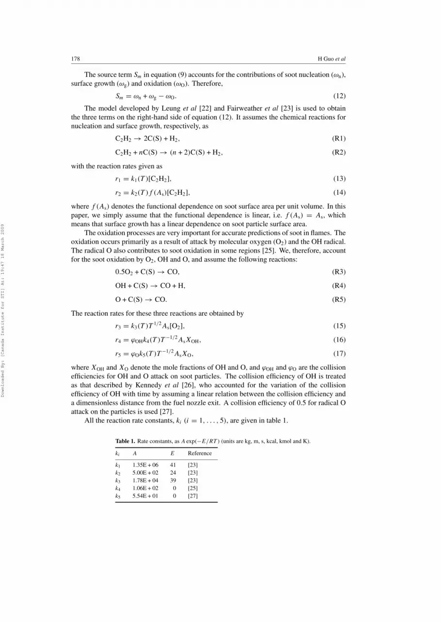
All the reaction rate constants, ki (i = 1, . . . , 5), are given in table 1.

Table 1. Rate constants, as A exp(−E/RT ) (units are kg, m, s, kcal, kmol and K).

ki A E Reference

k1 1.35E + 06 41 [23]

k2 5.00E + 02 24 [23]

k3 1.78E + 04 39 [23]

k4 1.06E + 02 0 [25]

k5 5.54E + 01 0 [27]



The source term SN in equation (10) accounts for the soot nucleation and agglomeration,

and is calculated as

SN =2

Cmin

NAR1 − 2Ca

(

6MC(S)

πρC(S)

)1/6 (

6κT

ρC(S)

)1/2

[C(S)]1/6[ρN ]11/6, (18)

where NA is Avogadro’s number (6.022 × 1026 particles kmol−1), Cmin is the number of

carbon atoms in the incipient carbon particle (9 × 104), κ is the Boltzmann constant

(1.38 × 10−23 J K−1), ρC(S) is the soot density (1800 kg m−3) and Ca is the agglomeration

rate constant for which a value of 3.0 [23] is used.

2.4. Numerical model

The governing equations are discretized using the control volume method. The SIMPLE

numerical scheme [28] is used to deal with the pressure and velocity coupling. The

diffusion and convective terms in the conservation equations are respectively discretized by the

central and upwind difference methods. The discretized equations of gas species, soot mass

fraction and soot number density are solved in a fully-coupled fashion on every grid to speed

up the convergence process [29], while those of momentum, energy and pressure correction

are solved using the TDMA method.

The computational meshes used in the two simulations are shown in figure 2. Totally

104×70 and 114×71 non-uniform grids are used for the two simulations, respectively. Finer

grids are placed in the primary reaction zone and near the fuel nozzle inlet region. It has been

Z

–4

0

0 1 2 3 0 1 2 3

4

8

Z

–4

0

4

8

r r

Figure 2. Computational meshes. Left: simulation 1; right: simulation 2.


180 H Guo et al

checked that the further increase of grid number does not significantly influence the simulation

results.

The chemical reaction mechanism used is essentially from GRI-Mech 3.0 [30], with the

removal of all the reactions and species related to NOX formation. The revised reaction scheme

consists of 36 species and 219 reactions. All the thermal and transport properties are obtained

by using the database of GRI-Mech 3.0 [30] and the algorithms given in [18, 31].

3. Results and discussions

3.1. Velocity and temperature profiles at the nozzle exit

Figure 3 illustrates the velocity and temperature profiles at the nozzle exit obtained by

simulation 2. The velocity profile of simulation 1 at z = 0 (specified) is also shown for

comparison. Since both fuel and air streams obtain energy from the fuel nozzle and flame

base, their temperatures are higher than room temperature (300 K), and the velocity profiles

are different from those of fully developed flows in a round pipe and a concentric space. The

average temperatures of fuel and air streams at the nozzle exit from simulation 2 are respectively

131 and 29 K higher than room temperature. Therefore, applying the same temperature increase

for both air and fuel streams to account for the preheating is not appropriate.

In the boundary layers next to the fuel nozzle, both fuel and air stream temperatures are

significantly increased. Their values are even higher than the nozzle temperature at z = 0

(403 K). Therefore, both fuel and air streams obtain energy directly from the flame at z = 0.

The temperatures of the air stream are higher than those of the fuel stream in the boundary

layers, since the position of the flame base is located at the outside of the fuel nozzle (as we

shall discuss below). However, due to the higher flow rate of the air stream compared to the

fuel stream, the preheated region of the air stream is only limited to a narrow layer, while that

of the fuel stream is extended to the centre of the fuel nozzle. Therefore, the predicted average

temperature of the fuel stream is much higher than that of the air stream.

The velocity profile of the fuel stream obtained by simulation 2 at the nozzle exit is neither

the general parabolic shape of a fully-developed flow in a round pipe nor a uniform distribution.

Radial position, cm

Velo

city, cm

/s

Tem

pera

ture

, K

300

400

500

600

700

800

900

1000

Velocity of simulation 2Temperature of simulation 2Velocity of simulation 1

0

10

20

30

40

50

60

70

1.51.00.50.0

Figure 3. Predicted axial velocity and temperature profiles at z = 0 cm.



It gradually increases with increasing radius, except in the boundary layer next to the wall.

The velocities of simulation 2 are higher than those of simulation 1 at z = 0, except in the

centreline region and the narrow boundary layer next to the fuel nozzle. Apparently, these are

due to the preheating. For the air stream, velocity increases quickly to a constant value with

increasing radial distance from the outside of the fuel nozzle.

3.2. Velocity profiles above the nozzle exit

Figure 4 shows the radial velocity profiles along the axial direction at r = 0.545 which is the

inner radius of the fuel nozzle. It illustrates that in simulation 1, air convects to the centreline

region faster than in simulation 2 at lower axial heights. This is caused by the uniform velocity

distribution of the air stream and the lower inlet fuel stream velocity in simulation 1. Although

the velocity data are not available from the experiments of [8], the flame base positions (see

the discussion in the next section) predicted by the two simulations show that this result is

qualitatively reasonable. As a result, axial velocities of simulation 1 soon become higher than

those of simulation 2 in the centreline region once z is greater than 0, as shown in figure 5,

although axial velocities of the fuel stream of simulation 1 are lower than those of simulation 2

in most regions at z = 0. Figure 5 shows that axial velocities of simulation 2 are higher than

those of simulation 1 in the centreline region once z becomes greater than 1 mm.

Since velocity affects the residence time, the differences of velocity profiles between two

simulations may affect the flame temperature and soot predictions.

3.3. Flame temperatures

The flame temperatures predicted by the two simulations and those measured by Gulder et al

[8], using CARS, are shown in figure 6. Figure 7 gives the radial temperature profiles at two

axial heights. It can be seen that both simulations capture the general feature of the flame,

Axial position, cm

0 2 4 6 8 10

Radia

l velo

city, cm

/s

Simulation 1Simulation 2

–40

–30

–20

–10

0

10

Figure 4. Radial velocity profiles along the axial direction at r = 0.545 cm.


182 H Guo et al

z = 1m

Radial position, cm

0.0 0.5 1.0 1.5

Radial position, cm

0.0 0.5 1.0 1.5

Axia

l ve

locity, cm

/s





z = 3 mm

Axi

al v

elo

city, c

m/s

z = 20 mm z = 40 mm

0

40

80

120

160

200

0

40

80

120

160

200

Radial position, cm

0.0 0.5 1.0 1.5

Axia

l ve

locity, cm

/s

0

40

80

120

160

200

Radial position, cm

0.0 0.5 1.0 1.5

Axia

l ve

locity, cm

/s

0

40

80

120

160

200

Figure 5. Axial velocity profiles at different axial heights.

–0.5 0 0.5

1

2

3

4

5

6

7300 1219 2138

Simulation 1

0 0.5

r, cmr, cmr, cm

1

2

3

4

5

6

7300 1219 2138

Simulation 2

–0.5 –0.50 0.5

1

2

3

4

5

6

7300 1219 2138

Measured

z,

cm

z,

cm

z,

cm

Figure 6. Flame temperatures (K).



Radial position, cm

0.0 0.2 0.4 0.6 0.8 1.0 1.2

Tem

pera

ture

, K

Simulation 1, z = 0.2 cmSimulation 2, z = 0.2 cmSimulation 1, z = 4 cmSimulation 2, z = 4 cmMeasured, z = 0.2 cmMeasured, z = 4 cm

300

600

900

1200

1500

1800

2100

Figure 7. Radial temperature profiles at two axial heights.

i.e. the temperature profiles have a maximum in the annular region of the lower part of the

flame, and these maximum temperature contours do not converge to the axis in the upper part

of the flame. This is due to the radiation cooling by soot, since a significant amount of soot

exists in the upper part of the flame (see the result below).

However, quantitatively simulation 2 (with the extended calculation domain) provides an

improved result, especially for the lower part of the flame. First, the predicted temperatures by

simulation 2 in the region immediately above the fuel nozzle are higher than those predicted

by simulation 1. The temperature on the centreline at 2 mm height above the fuel nozzle

exit is about 574 K, which is quite close to the value of 595 K from the experiment [8] at

the same position, while simulation 1 gives a much lower value (477 K) at that location.

Secondly, the radius of the flame base predicted by simulation 2 is closer to that obtained by the

experiment, while simulation 1 underpredicts this value. This is the result of different velocity

and temperature profiles at the nozzle exit in the two simulations. The higher temperatures at

the nozzle exit increase the axial velocities of the fuel stream at z = 0 in simulation 2. The

higher axial velocities of the fuel stream and the lower axial velocities of the air stream in the

boundary layer next to the outside surface of the fuel nozzle for simulation 2 allow the fuel

to move outwards along the radial direction, as shown by the radial velocity profiles at the

lower axial positions in figure 4. Finally, we also observe that the annular region of higher

temperatures predicted by simulation 2 is broader than that of simulation 1, although it is still

narrower than the experiment. Since soot is usually formed in the lower part of the flame,

we can expect that these differences may result in different soot volume fractions for the two

simulations.

For the upper half of the flame, both simulations give similar temperatures, which

are lower than the experimental result. This may be caused by the simplification of the

soot model. As indicated by Sunderland and Faeth [32], soot nucleation is a complex

process involving polycyclic aromatic hydrocarbons (PAH) that eventually become visible

soot particles, although it can be empirically correlated with C2H2 concentration alone, as

expressed by (R1). Moreover, not only C2H2 but also some other species may contribute to

the soot surface growth process, which can be described by the effects of various species on

active sites and parallel channels [32–34]. The simplifications in the current soot model need


184 H Guo et al

to be improved in the future simulation to account for the complex soot inception and surface

growth processes.

The peak flame temperature obtained by simulation 2 is only 7 K higher than that by

simulation 1, since different soot volume fractions are obtained in the two simulations.

3.4. Soot volume fraction

Figures 8 and 9 depict soot volume fractions from the experiment [8] and the two simulations.

Again, although both simulations capture the general features of soot in the flame, simulation 2

provides a more reasonable quantitative result. The peak soot volume fraction from

simulation 2 (7.2 ppm) is higher than that (6.2 ppm) from simulation 1 and closer to that

(8.0 ppm) from the experiment. Moreover, simulation 2 gives improved prediction in the

centreline region.

The reason why simulation 2 provides a more reasonable result can be explained by the

distributions of temperature and the mass fractions of acetylene from the two simulations.

Figure 10 shows the mass fractions of acetylene predicted by the two simulations.

As discussed above, the temperatures in the lower centreline region are raised and the

axial velocities there are lower in simulation 2. These cause the centreline fuel to decompose

earlier in simulation 2. Meanwhile, since the flame base (the reaction zone in the lowest region)

moves further away from the centreline in simulation 2, the fuel conversion region becomes

wider. In figure 10, one can observe that acetylene is formed earlier in the centreline region,

and the annular region with higher acetylene concentration is slightly wider in simulation 2.

–0.5 0 0.5

r, cmr, cmr, cm

1

2

3

4

5

6

7

z,

cm

z,

cm

z,

cm

Simulation 2

–0.5 0 0.5

1

2

3

4

5

6

70.0 4.0 7.9

Simulation 1

–0.5–0.5 0 0.5

1

2

3

4

5

6

70.0 4.0 7.9 0.0 4.0 7.9

Measured

Figure 8. Soot volume fractions (ppm).



Radial position, cm

0.0 0.2 0.4 0.6

So

ot

vo

lum

e f

ractio

n ×

10

6

0

1

2

3

4

5

6

7

Simulation 1, z = 2cmSimulation 2, z = 2cmSimulation 1, z = 4cmSimulation 2, z = 4cmMeasured, z = 2 cmMeasured, z = 4 cm

Figure 9. Radial soot volume fraction profiles at two axial heights.

–0.5 0 0.5

r, cm

0

1

2

3

4

5

6

70.0 3.7 7.4

Simulation 1

–0.5 0 0.5

r, cm

0

1

2

3

4

5

6

70.0 3.7 7.4

z,

cm

z,

cm

Simulation 2

Figure 10. Predicted acetylene (C2H2) mass fraction distribution (%).

Consequently, soot inception and growth time increase in simulation 2, and therefore finally

the soot yields increase.

We can therefore conclude that flame preheating results in a significant change in the

prediction of soot yields.


186 H Guo et al

4. Conclusions

An axisymmetric, laminar, coflow diffusion ethylene–air flame has been modelled by two

different methods to deal with the inlet boundary conditions. The first method cannot accurately

account for the influence of flame preheating, while the second one can.

The results show that the influence of flame preheating is important for the prediction of

the soot formation process. Although both simulations capture the general feature of the flame,

simulation 2 (which accounts for the influence of flame preheating) gives improved quantitative

results compared to simulation 1. The peak soot volume fraction obtained by simulation 2 is

about 1 ppm higher than that obtained by simulation 1 and is closer to the measured value. The

soot volume fraction prediction of the centreline region is improved by simulation 2. The use

of equal temperature increase for the fuel and air streams was found to be inappropriate. The

velocity profiles of the fuel and air streams at the nozzle exit are neither the general profiles of

fully developed flows in a round pipe and a concentric space nor uniform distributions.

References

[1] Smooke M D, Mitchell R E and Keys D E 1989 Combust. Sci. Technol. 67 85–122

[2] Xu Y, Smooke M D, Lin P and Long M B 1993 Combust. Sci. Technol. 90 289–313

[3] Bennett B A V and Smooke M D 1998 Combust. Theory Modelling 2 221–58

[4] Zhang Z and Ezekoye O A 1998 Combust. Sci. Technol. 137 323–46

[5] Smooke M D, Mcenally C S, Pfefferle L D, Hall R J and Colket M B 1999 Combust. Flame 117 117–39

[6] McEnally C S, Schaffer A M, Long M B, Pfefferle L D, Smooke M D, Colket M B and Hall R J 1998 27th Int.

Symp. Combustion (Pittsburgh, PA: The Combustion Institute) pp 1497–505

[7] Guo H, Liu F, Smallwood G J and Gulder O L 2001 ASME Paper NHTC2001-20126

[8] Gulder O L, Snelling D R and Sawchuk R A 1996 26th Int. Symp. Combustion (Pittsburgh, PA: The Combustion

Institute) pp 2351–7

[9] Gulder O L, Thomson K A and Snelling D R 2000 Proc. 2000 Spring Technical Meeting (Ottawa: Combustion

Institute/Canadian Section) pp 20.1–20.6

[10] Kuo K K 1986 Principles of Combustion (New York: Wiley)

[11] Chase M W, Davies C A, Downey J R, Frurlp D J, McDonald R A and Syverud A N 1985 JANAF Thermochemical

Tables 3rd edn (New York: American Chemical Society and American Institute of Physics)

[12] Liu F, Smallwood G J and Gulder O L AIAA Paper 99-3679

[13] Liu F, Smallwood G J and Gulder O L 2000 J. Thermophys. Heat Transfer 14 278–81

[14] Liu F, Smallwood G J and Gulder O L 2001 J. Quant. Spectrosc. Radiat. Transfer 68 401–17

[15] Liu F, Smallwood G J and Gulder O L 2000 Int. J. Heat Mass Transfer 43 3119–35

[16] Soufiani A and Taine J 1997 Int. J. Heat Mass Transfer 40 987–91

[17] Dalzell W H and Sarofim A F 1969 J. Heat Transfer 91 100–4

[18] Kee R J, Warnatz J and Miller J A Sandia Report SAND 83-8209

[19] Frenklach M, Clary D W, Gardiner W C and Stein S E 1984 20th Int. Symp. Combustion (Pittsburgh, PA: The

Combustion Institute) pp 887–901

[20] Frenklach M and Wang H 1990 23rd Int. Symp. Combustion (Pittsburgh, PA: The Combustion Institute) pp 1559–

66

[21] Frenklach M and Wang H 1994 Soot Formation in Combustion: Mechanisms and Models ed H Bockhorn

(Springer Series in Chemical Physics vol 59) (Berlin: Springer) pp 162–90

[22] Leung K M, Lindstedt R P and Jones W P 1991 Combust. Flame 87 289–305

[23] Fairweather M, Jones W P and Lindstedt R P 1992 Combust. Flame 89 45–63

[24] Talbot L, Cheng R K, Schefer R W M and Willis D R 1980 J. Fluid Mech. 101 737–58

[25] Neoh K G, Howard J B and Sarofim A F 1981 Particulate Carbon: Formation During Combustion ed D C Siegla

and G W Smith (New York: Plenum) p 261

[26] Kennedy I M, Yam C, Rapp D C and Santoro R J 1996 Combust. Flame 107 368–82

[27] Bradley D, Dixon-Lewis G, Habik S E and Mushi E M 1984 20th Int. Symp. Combustion (Pittsburgh, PA: The

Combustion Institute) pp 931–40

[28] Patankar S V 1980 Numerical Heat Transfer and Fluid Flow (New York: Hemisphere)

[29] Liu Z, Liao C, Liu C and McCormick S AIAA Paper 95-0205



[30] Smith G P, Golden D M, Frenklach M, Moriarty N W, Eiteneer B, Goldenberg M, Bowman C T, Hanson R K,

Song S, Gardiner W C Jr, Lissianski V V and Qin Z http://www.me.berkeley.edu/gri mech/

[31] Kee R J, Miller J A and Jefferson T H Sandia Report SAND 80-8003

[32] Sunderland P B and Faeth G M 1996 Combust. Flame 105 132–46

[33] Mauss F, Schafer T and Bockhorn H 1994 Combust. Flame 99 697–705

[34] Kennedy I M 1997 Prog. Energy Combust. Sci. 23 95–132


the flame preheating effect on numerical modelling of soot formation in a two-dimensional laminar...

Documents