nonlinear theory of flame front instability
TRANSCRIPT

arX
iv:p
hysi
cs/0
1080
57v1
[ph
ysic
s.fl
u-dy
n] 2
8 A
ug 2
001
Nonlinear theory of flame front instability
Kirill A. Kazakov1,2∗ and Michael A. Liberman1,3†
1Department of Physics, Uppsala University, Box 530, S-751 21, Uppsala, Sweden
2 Moscow State University, Physics Faculty, Department of Theoretical Physics,
117234, Moscow, Russian Federation
3P. Kapitsa Institute for Physical Problems, Russian Academy of Sciences,
117334, Moscow, Russian Federation
Abstract
Nonlinear non-stationary equation describing evolution of weakly curved pre-
mixed flames with arbitrary gas expansion, subject to the Landau-Darrieus
instability, is derived. The new equation respects all the conservation laws
to be satisfied across the flame front, as well as correctly takes into account
influence of vorticity, generated in the flame, on the flame front structure and
flame velocity. Analytical solutions of the derived equation are found.
82.33.Vx, 47.20.-k, 47.32.-y
Typeset using REVTEX
∗E-mail: [email protected]
†E-mail: [email protected]
1

I. INTRODUCTION
Description of premixed flame propagation is, in essential, the description of develop-ment of the Landau-Darrieus (LD) instability [1,2] of zero-thickness flames. Given arbitraryflame front configuration, its evolution is determined by the exponential growth of unstablemodes, eventually stabilized by the nonlinear mode interaction. By themselves, the nonlin-ear effects are not sufficient to stabilize flame propagation, since the spectrum of unstableperturbations of a zero-thickness flame is unbounded. In many cases, however, an upperbound for the mode wavenumber is provided by the heat conduction – species diffusionprocesses in the flame, which govern the evolution of short-wavelength perturbations [3].The flame propagation is thus described as the nonlinear propagation of interacting modesof zero-thickness front, with an effective short-wavelength cut-off described at the hydro-dynamic scale by means of an appropriate modification of the evolution equation and theconservation laws at the flame front [4].
In this purely hydrodynamic formulation, the flame dynamics is governed essentially bythe only parameter – the gas expansion coefficient θ, defined as the ratio of the fuel densityand the density of burnt matter. Unfortunately, in general it is very difficult to reduce thecomplete system of hydrodynamic equations governing flame dynamics to a single equationfor the flame front position. This is mainly because the nonlinearity of flame dynamicscannot be considered perturbatively. For instance, it can be shown that in the regime ofsteady flame propagation, the flame front slope can be considered small only if the gasexpansion is small (θ → 1), while for flames with θ = 6÷8 it is of the order 2÷3 (discussionof this issue can be found in Ref. [8]). At the early stages of development of the LD-instability, however, the perturbation analysis is fully justified, and the equation describingnonlinear propagation of the flame front can be obtained in a closed form. Within accuracyof the second order in the flame front slope such an equation was obtained by Zhdanov andTrubnikov (ZT) [5], without taking into account the influence of the effects related to finiteflame thickness, mentioned above. The latter were included in the ZT-equation ad hoc byJoulin [6].
Concerning the ZT-equation and its modification, we would like to note the following.1) Although this equation respects all the conservation laws to be satisfied across the
flame front, it was derived on the basis of a certain model assumption concerning the flowstructure downstream. Namely, it was assumed that the velocity field can be representedas a superposition of a potential mode and an “entropy wave”, so that the pressure fieldis expressed through the former by the usual Bernoulli equation. The generally nonlocalrelation between the pressure and velocity fields is thus rendered local algebraic, whichallows simple reduction of the system of hydrodynamic equations to the single equation forthe flame front position. Being valid at the linear stage of development of the LD-instability,this model assumption is, of course, unjustified in general.
2) It was assumed in the course of derivation of the ZT-equation that not only the frontslope, but also the value of the front position itself is a small quantity. As a result, the ZT-equation turns out to be non-invariant with respect to space translations in the direction offlame propagation. Practical consequence of this assumption is the unnecessary limitation ofthe range of validity of the equation: the space and time intervals should be taken sufficientlysmall to ensure that the deviation of the front position from the initial unperturbed plane
2

is small everywhere.The purpose of this paper is to show that the only assumption of smallness of the flame
front slope is actually sufficient to derive an equation describing the nonlinear developmentof the LD-instability to the leading (second) order of nonlinearity. Surprisingly, this equationturns out to be of a more simple structure than that of the ZT-equation. This simplificationis due to existence of a representation of the flow equations at the second order, which canbe called transverse. In this representation, the system of equations governing the flamepropagation can be brought into the form in which dependence of all dynamical quantitieson the coordinate in the direction of flame propagation is rendered purely parametric.
Let us consider the question of existence of this representation, and more generally,the meaning of the weak nonlinearity expansion, in more detail. First of all, the followingimportant aspect of the problem should be emphasized. The curved flame propagation is anessentially nonlocal process, in that the presence of vorticity produced in the flame impliesthat the relations between flow variables downstream generally cannot be put into the formin which the value of one variable at the front surface can be expressed entirely in terms ofother variables taken at the same surface. For instance, the value of the pressure field at theflame front depends not only on the gas velocity distribution along the front, but also on itsdistribution in the bulk. This means in turn that the equation describing the flame frontevolution cannot generally be written in a closed form, i.e., as an equation which expressesthe time derivative of the front position via its spatial gradients, because the gas dynamicsin the bulk depends, in particular, on the boundary conditions for the burnt matter. In theframework of the weak nonlinearity expansion, this non-locality shows itself as the necessityto increase the differential order of the equation for the flame front position. For example,it was shown in Ref. [8] that in order to take into account influence of the vorticity drift onthe structure of stationary flames with the accuracy of (θ− 1)4 in the asymptotic expansionfor θ → 1 (which is the relevant weak nonlinearity expansion in the stationary case), onehas to increase the differential order of the integro-differential equation by one as comparedto the Sivashinsky equation (the latter is of the second order in θ − 1, corresponding tothe approximation in which the gas flow is potential on both sides of the front). Roughlyspeaking, the nonlocal relations, being integral from the non-perturbative point of view, aretreated differential of infinite order in the framework of the weak nonlinearity expansion.
Let us now turn back to our present purpose of derivation of equation for the front po-sition at the second order of nonlinearity. Remarkably, it turns out that this approximationis exceptional in that the above-mentioned nonlocal complications do not arise in this case.We will give now a simple illustration of this important fact. Let us consider a weakly curvedflame propagating in z-direction with respect to an initially uniform fuel, and denote x thetransverse coordinates. If the flame front position is described by equation z = f(x, t), thenthe condition that front is only weakly curved implies that ∂f(x, t)/∂x is small, and so isthe gas velocity perturbation δv. From the continuity equation
divv = 0
and the Euler equations∂v
∂t+ (v∇)v = −
1
ρ∇P,
one has
3

∇2P = −ρ ∂ivk∂kvi , (1)
where summation over repeated indices is understood. Equation (1) implies
P (z,x, t) = −ρ∫
dz′dx′G(z,x, z′,x′, t)∂ivk(z′,x′, t)∂kvi(z
′,x′, t) + Ω(z,x, t) , (2)
where Ω(z,x, t) is a local function of the flow variables, satisfying ∇2Ω = 0, andG(z,x, z′,x′, t) is the Green function of the Laplace operator, appropriate to the givenboundary condition. Note that the latter, being a condition on the pressure jump across theflame, is imposed only at the flame front. Since the unperturbed velocity field is spatiallyuniform, one has from Eq. (2) for the curvature induced pressure variation δP
δP (z,x, t) = −ρ∫
dz′dx′G(z,x, z′,x′, t)∂iδvk(z′,x′, t)∂kδvi(z
′,x′, t) + δΩ(z,x, t) . (3)
Next, let us denote δx the characteristic length of the front perturbation. Then the corre-sponding length in z-direction
δz ∼
∣
∣
∣
∣
∣
∂f
∂x
∣
∣
∣
∣
∣
δx .
In other words, integration over z′ in Eq. (3) is effectively carried out for z′ ∈(f(x, t), f(x, t) + δz). Furthermore, as we will see in the sections below,
|δv| ∼
∣
∣
∣
∣
∣
∂f
∂t
∣
∣
∣
∣
∣
∼
∣
∣
∣
∣
∣
∂f
∂x
∣
∣
∣
∣
∣
.
Therefore, if one is interested in evaluating the pressure variation at the front, one canrewrite Eq. (3) with the accuracy of the second order
δP (f(x, t),x, t) = −ρ∫
dx′G(x,x′, t)∂iδvk(f(x′, t),x′, t)∂kδvi(f(x′, t),x′, t)
+ δΩ(f(x, t),x, t) , (4)
G(x,x′, t) ≡∫
dz′G(f(x, t),x, z′,x′, t) .
As we noted above, “boundary condition” for the pressure field is imposed only at the flamefront. Therefore, the Green function G is independent of any other conditions relevant tothe flow of the burnt matter (e.g., boundary conditions on the tube walls, in the case offlame propagation in a tube). The same is true for the function Ω, since the value of Ω at agiven point depends only on the value of flow variables at the same point. We thus see thatEq. (4) is an integral relation between local functions of the flow variables, defined on thefront surface, which is independent of the flow dynamics in the bulk. Furthermore, since theright hand side of Eq. (4) is of the second order, it is not difficult to show, using the lineardecomposition of the flow field into potential and vortex components, that z-derivatives ofthe velocity can be expressed via its derivatives along the flame front, bringing this equationinto the transverse representation. This implies that at the second order, there exists auniversal equation which describes the flame front dynamics in terms of the front positionalone. In practice, it is actually more convenient to work with the differential form of theflow equations, rather than integral. How their transverse representation can be derived willbe shown in detail in Sec. IIA. On the basis of this result, the nonlinear non-stationaryequation will be derived in Sec. III. Its analysis is carried out analytically using the methodof pole decomposition in Sec. IV. The obtained results are summarized in Sec. V.
4
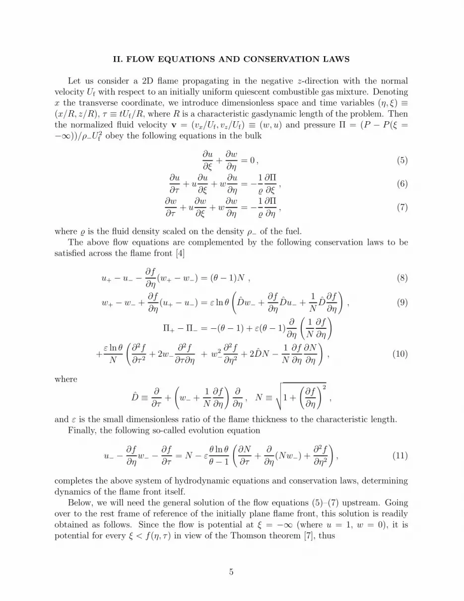
II. FLOW EQUATIONS AND CONSERVATION LAWS
Let us consider a 2D flame propagating in the negative z-direction with the normalvelocity Uf with respect to an initially uniform quiescent combustible gas mixture. Denotingx the transverse coordinate, we introduce dimensionless space and time variables (η, ξ) ≡(x/R, z/R), τ ≡ tUf/R, where R is a characteristic gasdynamic length of the problem. Thenthe normalized fluid velocity v = (vx/Uf , vz/Uf) ≡ (w, u) and pressure Π = (P − P (ξ =−∞))/ρ−U
2f obey the following equations in the bulk
∂u
∂ξ+∂w
∂η= 0 , (5)
∂u
∂τ+ u
∂u
∂ξ+ w
∂u
∂η= −
1
∂Π
∂ξ, (6)
∂w
∂τ+ u
∂w
∂ξ+ w
∂w
∂η= −
1
∂Π
∂η, (7)
where is the fluid density scaled on the density ρ− of the fuel.The above flow equations are complemented by the following conservation laws to be
satisfied across the flame front [4]
u+ − u− −∂f
∂η(w+ − w−) = (θ − 1)N , (8)
w+ − w− +∂f
∂η(u+ − u−) = ε ln θ
(
Dw− +∂f
∂ηDu− +
1
ND∂f
∂η
)
, (9)
Π+ − Π− = −(θ − 1) + ε(θ − 1)∂
∂η
(
1
N
∂f
∂η
)
+ε ln θ
N
(
∂2f
∂τ 2+ 2w−
∂2f
∂τ∂η+ w2
−
∂2f
∂η2+ 2DN −
1
N
∂f
∂η
∂N
∂η
)
, (10)
where
D ≡∂
∂τ+
(
w− +1
N
∂f
∂η
)
∂
∂η, N ≡
√
√
√
√1 +
(
∂f
∂η
)2
,
and ε is the small dimensionless ratio of the flame thickness to the characteristic length.Finally, the following so-called evolution equation
u− −∂f
∂ηw− −
∂f
∂τ= N − ε
θ ln θ
θ − 1
(
∂N
∂τ+
∂
∂η(Nw−) +
∂2f
∂η2
)
, (11)
completes the above system of hydrodynamic equations and conservation laws, determiningdynamics of the flame front itself.
Below, we will need the general solution of the flow equations (5)–(7) upstream. Goingover to the rest frame of reference of the initially plane flame front, this solution is readilyobtained as follows. Since the flow is potential at ξ = −∞ (where u = 1, w = 0), it ispotential for every ξ < f(η, τ) in view of the Thomson theorem [7], thus
5

u ≡ 1 + u = 1 +
+∞∫
−∞
dk uk exp(|k|ξ + ikη) , (12)
w = Hu , (13)
∂u
∂τ+ ΦΠ +
Φ
2(u2 + w2) = 0 , (14)
where the Hilbert operator H is defined by
(Hf)(η) =1
πp.v.
+∞∫
−∞
dζf(ζ)
ζ − η,
”p.v.” denoting the principal value. Equations (12), (13) represent the general form ofthe potential velocity filed satisfying the boundary conditions at ξ = −∞, while Eq. (14)is nothing but the Bernoulli equation. Note that the 2D Landau-Darrieus operator Φ issimply expressed through the Hilbert operator Φ = −∂H. Note also that although therelation w = Hu between the velocity components upstream is nonlocal, it is expressed interms of the transverse coordinate η only.
A. Bulk dynamics in transverse representation
Our next step is the reduction of the system of flow equations (5) – (7) to one equationin which the role of the coordinate ξ is purely parametric. For this purpose, it is convenientto introduce the stream function ψ via
u =∂ψ
∂η, w = −
∂ψ
∂ξ. (15)
The stream function satisfies the following equation
(
∂
∂τ+ v∇
)
∇2ψ = 0 . (16)
1. First order approximation
To perform the weak nonlinearity expansion, it is convenient to explicitly extract zero-order values of the flow variables downstream
u = θ + u , Π = −θ + 1 + Π . (17)
Then in the linear approximation, Eq. (16) takes the form
6

(
∂
∂τ+ θ
∂
∂ξ
)
∇2ψ(1) = 0 . (18)
Its general solution can be written as a superposition of the potential and vorticity modessatisfying, respectively,
∇2ψ(1)p = 0 , (19)
(
∂
∂τ+ θ
∂
∂ξ
)
ψ(1)v = 0 . (20)
General solution of Eq. (19) has the form analogous to Eqs. (12), (13)
up ≡ θ + up = θ +
+∞∫
−∞
dk uk exp(−|k|ξ + ikη) , (21)
wp = −Hup . (22)
Differentiating Eq. (20) with respect to η we obtain
1
θ
∂uv
∂τ=∂wv
∂η. (23)
Next, linearizing Eq. (6) and using the above equations for the potential and vorticity modes,one finds
−1
θ
∂up
∂τ+ Φ(Πp + up) = 0 , (24)
Πv = 0 . (25)
With the help of Eqs. (22), (23), and (25) equation (24) can be rewritten as
ΦΠ +∂w
∂η−
1
θ
∂u
∂τ= 0 . (26)
In this form, the flow equation governing dynamics downstream contains no explicit opera-tion with the ξ-dependence of the flow variables. In other words, this dependence is renderedpurely parametric. Let us now show that Eq. (26) can be generalized to take into accountinteraction of the perturbations.
2. Second order approximation
At the second order, Eq. (16) takes the form
(
∂
∂τ+ θ
∂
∂ξ
)
∇2ψ = −
(
u(1) ∂
∂ξ+ w(1) ∂
∂η
)
∇2ψ(1). (27)
7
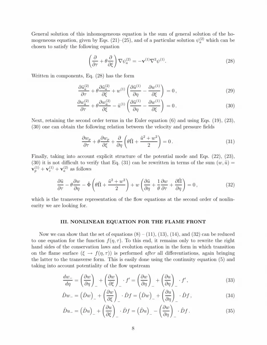
General solution of this inhomogeneous equation is the sum of general solution of the ho-mogeneous equation, given by Eqs. (21)–(25), and of a particular solution ψ(2)
a which can bechosen to satisfy the following equation
(
∂
∂τ+ θ
∂
∂ξ
)
∇ψ(2)a = −v(1)∇2ψ(1). (28)
Written in components, Eq. (28) has the form
∂u(2)a
∂τ+ θ
∂u(2)a
∂ξ+ w(1)
(
∂u(1)
∂η−∂w(1)
∂ξ
)
= 0 , (29)
∂w(2)a
∂τ+ θ
∂w(2)a
∂ξ− u(1)
(
∂u(1)
∂η−∂w(1)
∂ξ
)
= 0 . (30)
Next, retaining the second order terms in the Euler equation (6) and using Eqs. (19), (23),(30) one can obtain the following relation between the velocity and pressure fields
∂wp
∂τ+ θ
∂wp
∂ξ+
∂
∂η
(
θΠ +u2 + w2
2
)
= 0 . (31)
Finally, taking into account explicit structure of the potential mode and Eqs. (22), (23),(30) it is not difficult to verify that Eq. (31) can be rewritten in terms of the sum (w, u) =v(1)
p + v(1)v + v(2)
a as follows
∂u
∂τ− θ
∂w
∂η− Φ
(
θΠ +u2 + w2
2
)
+ w
(
∂u
∂η+
1
θ
∂w
∂τ+∂Π
∂η
)
= 0 , (32)
which is the transverse representation of the flow equations at the second order of nonlin-earity we are looking for.
III. NONLINEAR EQUATION FOR THE FLAME FRONT
Now we can show that the set of equations (8) – (11), (13), (14), and (32) can be reducedto one equation for the function f(η, τ). To this end, it remains only to rewrite the righthand sides of the conservation laws and evolution equation in the form in which transitionon the flame surface (ξ → f(η, τ)) is performed after all differentiations, again bringingthe latter to the transverse form. This is easily done using the continuity equation (5) andtaking into account potentiality of the flow upstream
dw−
dη=
(
∂w
∂η
)
−
+
(
∂w
∂ξ
)
−
· f ′ =
(
∂w
∂η
)
−
+
(
∂u
∂η
)
−
· f ′ , (33)
Dw− =(
Dw)
−+
(
∂w
∂ξ
)
−
· Df =(
Dw)
−+
(
∂u
∂η
)
−
· Df , (34)
Du− =(
Du)
−+
(
∂u
∂ξ
)
−
· Df =(
Du)
−−
(
∂w
∂η
)
−
· Df . (35)
8
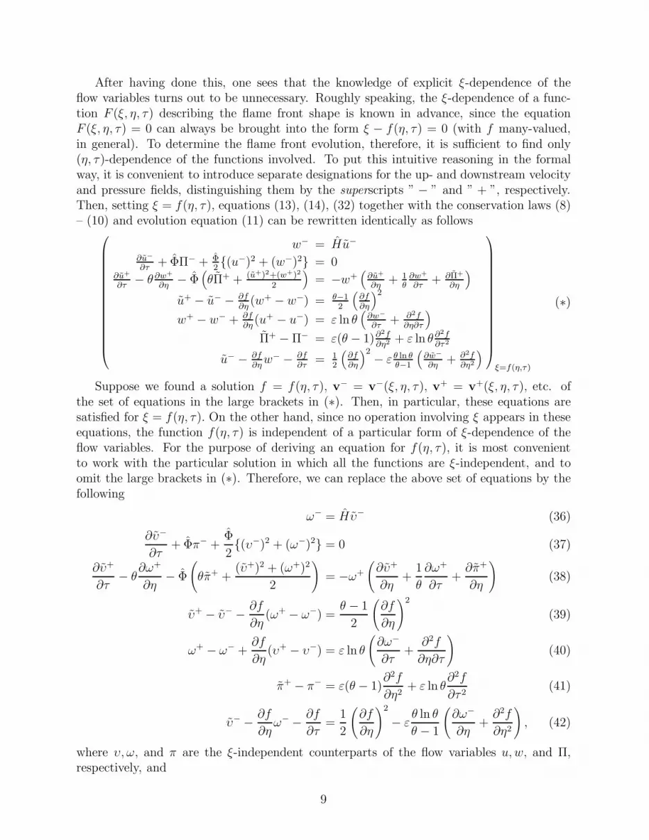
After having done this, one sees that the knowledge of explicit ξ-dependence of theflow variables turns out to be unnecessary. Roughly speaking, the ξ-dependence of a func-tion F (ξ, η, τ) describing the flame front shape is known in advance, since the equationF (ξ, η, τ) = 0 can always be brought into the form ξ − f(η, τ) = 0 (with f many-valued,in general). To determine the flame front evolution, therefore, it is sufficient to find only(η, τ)-dependence of the functions involved. To put this intuitive reasoning in the formalway, it is convenient to introduce separate designations for the up- and downstream velocityand pressure fields, distinguishing them by the superscripts ” − ” and ” + ”, respectively.Then, setting ξ = f(η, τ), equations (13), (14), (32) together with the conservation laws (8)– (10) and evolution equation (11) can be rewritten identically as follows
w− = Hu−
∂u−
∂τ+ ΦΠ− + Φ
2(u−)2 + (w−)2 = 0
∂u+
∂τ− θ ∂w+
∂η− Φ
(
θΠ+ + (u+)2+(w+)2
2
)
= −w+(
∂u+
∂η+ 1
θ∂w+
∂τ+ ∂Π+
∂η
)
u+ − u− − ∂f
∂η(w+ − w−) = θ−1
2
(
∂f
∂η
)2
w+ − w− + ∂f∂η
(u+ − u−) = ε ln θ(
∂w−
∂τ+ ∂2f
∂η∂τ
)
Π+ − Π− = ε(θ − 1)∂2f∂η2 + ε ln θ ∂2f
∂τ2
u− − ∂f
∂ηw− − ∂f
∂τ= 1
2
(
∂f
∂η
)2− ε θ ln θ
θ−1
(
∂w−
∂η+ ∂2f
∂η2
)
ξ=f(η,τ)
(∗)
Suppose we found a solution f = f(η, τ), v− = v−(ξ, η, τ), v+ = v+(ξ, η, τ), etc. ofthe set of equations in the large brackets in (∗). Then, in particular, these equations aresatisfied for ξ = f(η, τ). On the other hand, since no operation involving ξ appears in theseequations, the function f(η, τ) is independent of a particular form of ξ-dependence of theflow variables. For the purpose of deriving an equation for f(η, τ), it is most convenientto work with the particular solution in which all the functions are ξ-independent, and toomit the large brackets in (∗). Therefore, we can replace the above set of equations by thefollowing
ω− = Hυ− (36)
∂υ−
∂τ+ Φπ− +
Φ
2(υ−)2 + (ω−)2 = 0 (37)
∂υ+
∂τ− θ
∂ω+
∂η− Φ
(
θπ+ +(υ+)2 + (ω+)2
2
)
= −ω+
(
∂υ+
∂η+
1
θ
∂ω+
∂τ+∂π+
∂η
)
(38)
υ+ − υ− −∂f
∂η(ω+ − ω−) =
θ − 1
2
(
∂f
∂η
)2
(39)
ω+ − ω− +∂f
∂η(υ+ − υ−) = ε ln θ
(
∂ω−
∂τ+
∂2f
∂η∂τ
)
(40)
π+ − π− = ε(θ − 1)∂2f
∂η2+ ε ln θ
∂2f
∂τ 2(41)
υ− −∂f
∂ηω− −
∂f
∂τ=
1
2
(
∂f
∂η
)2
− εθ ln θ
θ − 1
(
∂ω−
∂η+∂2f
∂η2
)
, (42)
where υ, ω, and π are the ξ-independent counterparts of the flow variables u, w, and Π,respectively, and
9
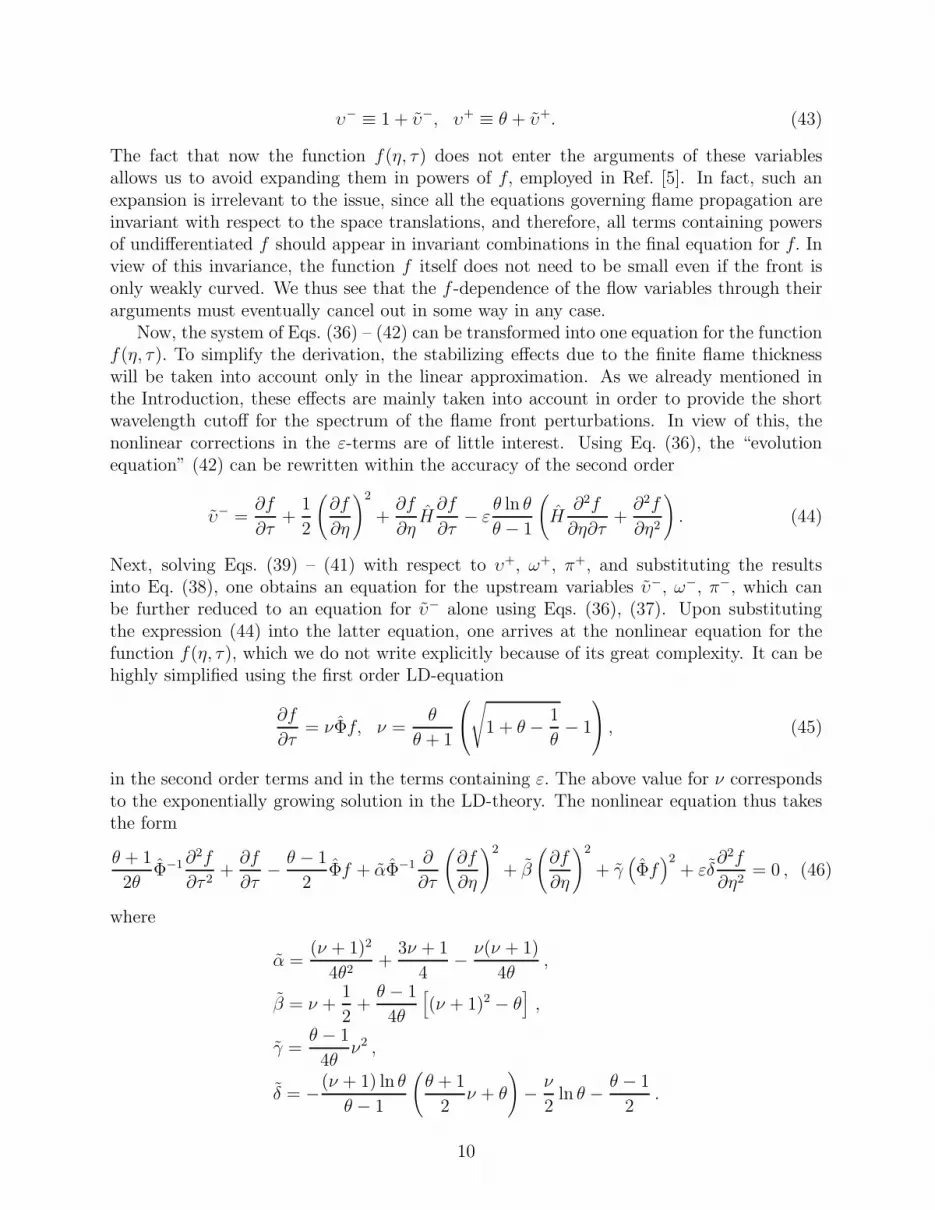
υ− ≡ 1 + υ−, υ+ ≡ θ + υ+. (43)
The fact that now the function f(η, τ) does not enter the arguments of these variablesallows us to avoid expanding them in powers of f, employed in Ref. [5]. In fact, such anexpansion is irrelevant to the issue, since all the equations governing flame propagation areinvariant with respect to the space translations, and therefore, all terms containing powersof undifferentiated f should appear in invariant combinations in the final equation for f. Inview of this invariance, the function f itself does not need to be small even if the front isonly weakly curved. We thus see that the f -dependence of the flow variables through theirarguments must eventually cancel out in some way in any case.
Now, the system of Eqs. (36) – (42) can be transformed into one equation for the functionf(η, τ). To simplify the derivation, the stabilizing effects due to the finite flame thicknesswill be taken into account only in the linear approximation. As we already mentioned inthe Introduction, these effects are mainly taken into account in order to provide the shortwavelength cutoff for the spectrum of the flame front perturbations. In view of this, thenonlinear corrections in the ε-terms are of little interest. Using Eq. (36), the “evolutionequation” (42) can be rewritten within the accuracy of the second order
υ− =∂f
∂τ+
1
2
(
∂f
∂η
)2
+∂f
∂ηH∂f
∂τ− ε
θ ln θ
θ − 1
(
H∂2f
∂η∂τ+∂2f
∂η2
)
. (44)
Next, solving Eqs. (39) – (41) with respect to υ+, ω+, π+, and substituting the resultsinto Eq. (38), one obtains an equation for the upstream variables υ−, ω−, π−, which canbe further reduced to an equation for υ− alone using Eqs. (36), (37). Upon substitutingthe expression (44) into the latter equation, one arrives at the nonlinear equation for thefunction f(η, τ), which we do not write explicitly because of its great complexity. It can behighly simplified using the first order LD-equation
∂f
∂τ= νΦf, ν =
θ
θ + 1
√
1 + θ −1
θ− 1
, (45)
in the second order terms and in the terms containing ε. The above value for ν correspondsto the exponentially growing solution in the LD-theory. The nonlinear equation thus takesthe form
θ + 1
2θΦ−1∂
2f
∂τ 2+∂f
∂τ−θ − 1
2Φf + αΦ−1 ∂
∂τ
(
∂f
∂η
)2
+ β
(
∂f
∂η
)2
+ γ(
Φf)2
+ εδ∂2f
∂η2= 0 , (46)
where
α =(ν + 1)2
4θ2+
3ν + 1
4−ν(ν + 1)
4θ,
β = ν +1
2+θ − 1
4θ
[
(ν + 1)2 − θ]
,
γ =θ − 1
4θν2 ,
δ = −(ν + 1) ln θ
θ − 1
(
θ + 1
2ν + θ
)
−ν
2ln θ −
θ − 1
2.
10

Following Zhdanov and Trubnikov [5], Eq. (46) can be further simplified by rewriting itslinear part in the form
θ + 1
2θΦ−1∂
2f
∂τ 2+∂f
∂τ−θ − 1
2Φf =
(
θ + 1
2θΦ−1 ∂
∂τ+θ − 1
2ν
)(
∂
∂τ− νΦ
)
f . (47)
Since we are only interested in the development of unstable modes of the front perturbations,which satisfy Eq. (45), we can transform the first factor in the right hand side of Eq. (47)as follows
θ + 1
2θΦ−1 ∂
∂τ+θ − 1
2ν→
θ + 1
2θν +
θ − 1
2ν=
√
1 + θ −1
θ.
Therefore, Eq. (46) becomes
∂f
∂τ− νΦf + αΦ−1 ∂
∂τ
(
∂f
∂η
)2
+ β
(
∂f
∂η
)2
+ γ(
Φf)2
+ εδ∂2f
∂η2= 0 , (48)
where
(α, β, γ, δ) =(α, β, γ, δ)√
1 + θ − 1θ
.
Finally, we would like to comment on the range of validity of the derived equation. Gen-erally speaking, Eq. (48) is only applicable for description of the early stages of developmentof the LD-instability, since it is obtained under the assumption of smallness of the frontslope. Even if the flame evolution is such that it smoothly ends up with the formation ofa stationary configuration (instead of spontaneous turbulization), this assumption becomesgenerally invalid whenever the process of flame propagation is close to the stationary regime.In fact, it can be easily shown that the assumptions of stationarity and weak nonlinearitycontradict each other (detailed discussion of this point can be found in Ref. [8]). Inciden-tally, the fact that the transition to the stationary regime in Eq. (48) is formally incorrectis clearly seen from its derivation given above. Namely, the stationary form of this equationdepends on the way the first order relation (45) is used in the second order terms beforetime derivatives are omitted. Only in the case of small gas expansion (θ → 1) is weak non-linearity approximation justified at all stages of development of the LD-instability, in whichcase Eq. (48) goes over to the well-known Sivashinsky equation [9]
∂f
∂τ+
1
2
(
∂f
∂η
)2
=θ − 1
2Φf − ε
∂2f
∂η2, (49)
since
β =1
2+O((θ − 1)2) , γ = O((θ − 1)3) , δ = −1 +O(θ − 1) , ν =
θ − 1
2+O((θ − 1)2) .
In this respect, a natural question arises as to what extent equation (48) is actually validwhen θ is arbitrary. Since the structure of higher order terms of the power expansion isunknown, it is very difficult to give even a rough estimate. Leaving this question aside, wewill simply assume in what follows, that this equation is formally valid for all times. It willbe shown below that at least in the case of flame propagation in narrow tubes, solutions tothe stationary version of Eq. (48) are in reasonable agreement with the results of numericalexperiments [14] for flames with the gas expansion coefficient up to θ ∼ 3.
11
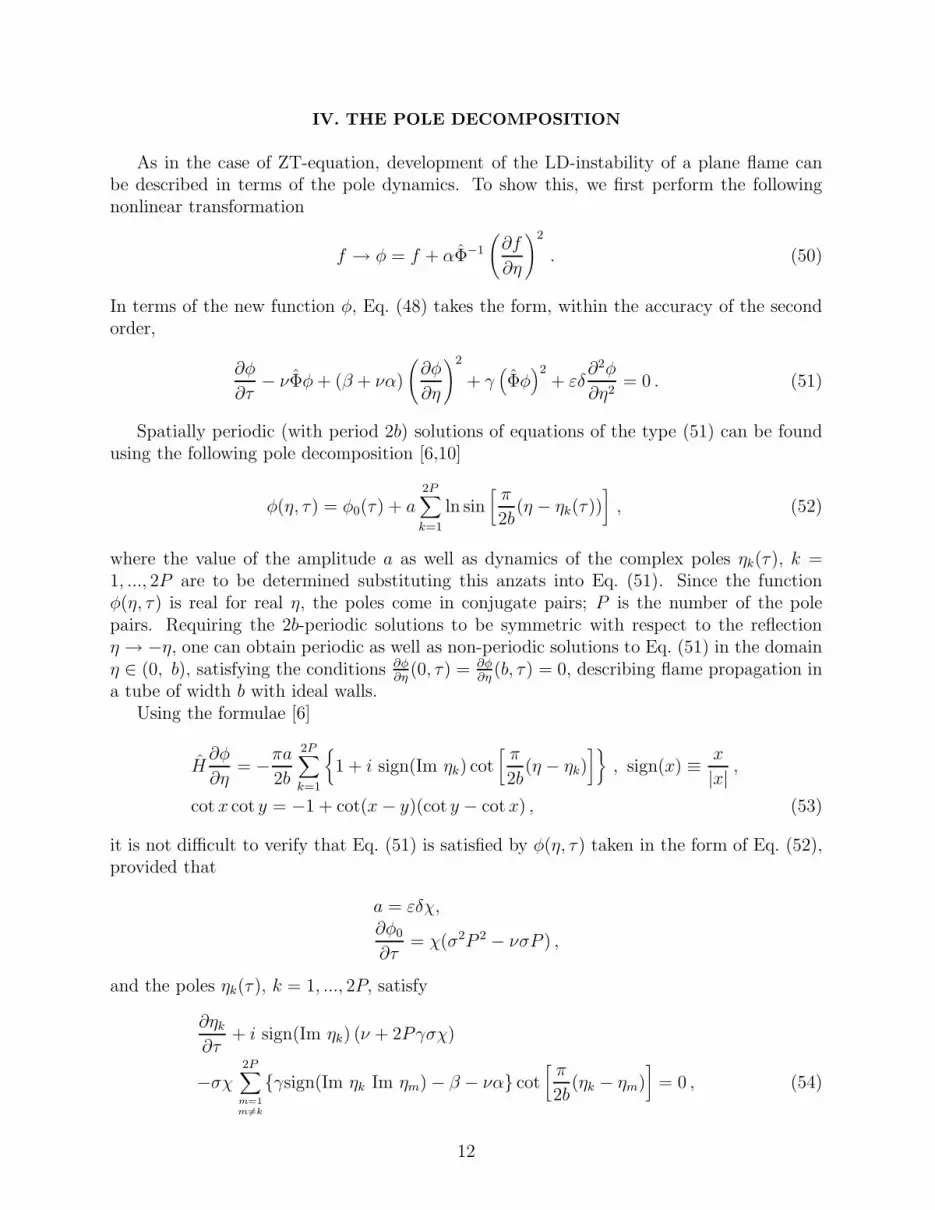
IV. THE POLE DECOMPOSITION
As in the case of ZT-equation, development of the LD-instability of a plane flame canbe described in terms of the pole dynamics. To show this, we first perform the followingnonlinear transformation
f → φ = f + αΦ−1
(
∂f
∂η
)2
. (50)
In terms of the new function φ, Eq. (48) takes the form, within the accuracy of the secondorder,
∂φ
∂τ− νΦφ+ (β + να)
(
∂φ
∂η
)2
+ γ(
Φφ)2
+ εδ∂2φ
∂η2= 0 . (51)
Spatially periodic (with period 2b) solutions of equations of the type (51) can be foundusing the following pole decomposition [6,10]
φ(η, τ) = φ0(τ) + a2P∑
k=1
ln sin[
π
2b(η − ηk(τ))
]
, (52)
where the value of the amplitude a as well as dynamics of the complex poles ηk(τ), k =1, ..., 2P are to be determined substituting this anzats into Eq. (51). Since the functionφ(η, τ) is real for real η, the poles come in conjugate pairs; P is the number of the polepairs. Requiring the 2b-periodic solutions to be symmetric with respect to the reflectionη → −η, one can obtain periodic as well as non-periodic solutions to Eq. (51) in the domainη ∈ (0, b), satisfying the conditions ∂φ
∂η(0, τ) = ∂φ
∂η(b, τ) = 0, describing flame propagation in
a tube of width b with ideal walls.Using the formulae [6]
H∂φ
∂η= −
πa
2b
2P∑
k=1
1 + i sign(Im ηk) cot[
π
2b(η − ηk)
]
, sign(x) ≡x
|x|,
cot x cot y = −1 + cot(x− y)(cot y − cot x) , (53)
it is not difficult to verify that Eq. (51) is satisfied by φ(η, τ) taken in the form of Eq. (52),provided that
a = εδχ,∂φ0
∂τ= χ(σ2P 2 − νσP ) ,
and the poles ηk(τ), k = 1, ..., 2P, satisfy
∂ηk
∂τ+ i sign(Im ηk) (ν + 2Pγσχ)
−σχ2P∑
m=1
m6=k
γsign(Im ηk Im ηm) − β − να cot[
π
2b(ηk − ηm)
]
= 0 , (54)
12

where the following notation is introduced
σ ≡ −εδπ
b> 0 , χ ≡ (β + να− γ)−1 .
Since the application of pole decomposition to Eq. (51) is quite similar to that given inRefs. [6,10], we will present below only final results, referring the reader to these works formore detail.
Following Ref. [10], we first consider two poles (η1, η2) in the same half plane of thecomplex η, which are fairly close to each other, so that their dynamics is unaffected by therest. Then one has from Eq. (54)
∂
∂τ(η1 − η2) =
4εδ
η1 − η2,
which indicates that the poles attract each other in the horizontal direction (parallel to thereal axis), and repel in the vertical direction, tending to form alignments parallel to theimaginary axis. Furthermore, assuming that the pole dynamics ends up with the formationof such a “coalescent” stationary configuration, and using the fact that γ < β + να (it isnot difficult to verify that actually γ/(β + να) < 1/3), the following upper bound on thenumber of pole pairs P can be easily obtained from Eq. (54)
P ≤1
2+
ν
2σ.
Still, for sufficiently wide tubes (such that σ < ν/3), the solution (52) is not unique: differentsolutions corresponding to different numbers P of poles are possible. To find the physicalones, it is necessary to perform the stability analysis. Noting that the functional structure ofEq. (51) is very similar to that of Eq. (49), the stability analysis of Refs. [11]– [13], where itwas carried out for the Sivashinsky equation, will be carried over the present case. Accordingto this analysis, for a given not-too-wide tube, there is only one (neutrally) stable solution.This solution corresponds to the number of poles that provides maximal flame velocity, i.e.,
Pm = Int(
ν
2σ+
1
2
)
,
Int(x) denoting the integer part of x. Thus, the flame velocity increase Ws ≡ |∂φ0/∂τ | ofthe stable solution can be written as
Ws = 4WmσPm
ν
(
1 −σPm
ν
)
, (55)
where
Wm =χν2
4. (56)
It is seen from Eq. (51) that the spectrum of front perturbations is effectively cut off atthe wavelength
λ =2πε|δ|
ν, (57)
13

representing the characteristic dimension of the flame cellular structure.Fig. 1 compares the theoretical dependence of the maximal flame velocity increase Wm
on the gas expansion coefficient, given by Eq. (56), with the results of numerical experiments[14]. For comparison, we show also the corresponding dependence calculated on the basis ofthe Sivashinsky equation. Dependence of the effective cut-off wavelength on the expansioncoefficient is shown in Fig. 2. We see that even beyond of its range of applicability, Eq. (51)provides reasonable qualitative description of flames with the expansion coefficients of prac-tical interest. Complete investigation of the LD-instability on the basis of this equation willbe given elsewhere.
V. CONCLUSIONS
The main result of our work is the nonlinear non-stationary equation (46) which describesdevelopment of the Landau-Darrieus instability in the second order of nonlinearity. We havederived this equation on the basis of the only assumption of smallness of the flame front slope.Thus, nonlinear evolution of the front perturbations generally obeys Eq. (46) which takeseven simpler form (51) if one is only interested in dynamics of the exponentially growingLD-solutions. It is important to stress that no assumption concerning the value of the flamefront position has been used in the derivation. Therefore, Eq. (46) can be applied not onlyto plane flames, but also to the problem of unstable evolution of any flame configuration,provided that the front slope is small.
It is also worth of emphasis that Eq. (46) is obtained without any assumptions about thestructure of the gas flow downstream. Thus, this equation is the direct consequence of theexact hydrodynamic equations for the flow fields in the bulk, and conservation laws at theflame front. We would like to stress also once again that the universal form of Eq. (46) isthe distinguishing property of the second order approximation. In the general case, equationfor the flame front should contain also information about the flow of the burnt matter inthe bulk. Indeed, as was shown in Ref. [8], the boundary conditions for the burnt matterare invoked in the course of derivation of the equation already at the third order. Thisuniversality of Eq. (46) allows it to be widely applied to the study of flames with arbitraryfront configuration, propagating in tubes with complex geometries.
ACKNOWLEDGMENTS
We are grateful to V. Lvov and G. Sivashinsky for interesting discussions. This researchwas supported in part by Swedish Ministry of Industry (Energimyndigheten, contract P12503-1), by the Swedish Research Council (contract E5106-1494/2001), and by the SwedishRoyal Academy of Sciences. Support form the STINT Fellowship program is also gratefullyacknowledged.
14

REFERENCES
[1] L. D. Landau, Acta Physicochimica URSS 19, 77 (1944).[2] G. Darrieus, unpublished work presented at La Technique Moderne, and at Le Congres
de Mecanique Appliquee, (1938) and (1945).[3] P. Pelce and P. Clavin, J. Fluid Mech. 124, 219 (1982).[4] M. Matalon and B. J. Matkowsky, J. Fluid Mech. 124, 239 (1982).[5] S. K. Zhdanov and B. A. Trubnikov, J. Exp. Theor. Phys. 68, 65 (1989).[6] G. Joulin, J. Exp. Theor. Phys. 73, 234 (1991).[7] L.D. Landau, E.M. Lifshitz, Fluid Mechanics (Pergamon, Oxford, 1987).[8] K. A. Kazakov, M. A. Liberman, physics/0106076.[9] G. I. Sivashinsky, Acta Astronaut., 4, 1177 (1977).
[10] O. Thual, U. Frish, and M. Henon, J. Phys. (France) 46, 1485 (1985).[11] M. Rahibe, N. Aubry, G. I. Sivashinsky, and R. Lima, Phys. Rev. E52, 3675 (1995).[12] M. Rahibe, N. Aubry, and G. I. Sivashinsky, Phys. Rev. E54, 4958 (1996).[13] M. Rahibe, N. Aubry, and G. I. Sivashinsky, Combust. Theory Modelling 2, 19 (1998).[14] V. V. Bychkov, S. M. Golberg, M. A. Liberman, and L. E. Eriksson, Phys. Rev. E54,
3713 (1996).
15

FIGURES
1 2 3 4 5 6 7 80
0.2
0.4
0.6
0.8
1
1.2
1.4
1.6
1.8
2
θ
Wm
FIG. 1. Maximal flame velocity increase Wm versus the gas expansion coefficient, given by
Eq. (56); the marks are according to Ref. [8]. Accuracy of the experimental results is about 20%.
5 10 15 200
10
20
30
40
50
60
θ
λ/ε
FIG. 2. The cut-off wavelength scaled on the flame thickness versus the expansion coefficient,
given by Eq. (57).
16