Documento de TrabajoISSN (edición impresa) 0716-7334

ISSN (edición electrónica) 0717-7593

The Evolution of the Intergenerational Mobility of Education in Chile by Cohorts: Facts and Possible Causes

Claudio Sapelli

Nº 348Enero 2009

www.economia.puc.cl

Versión impresa ISSN: 0716-7334 Versión electrónica ISSN: 0717-7593

PONTIFICIA UNIVERSIDAD CATOLICA DE CHILE INSTITUTO DE ECONOMIA Oficina de Publicaciones Casilla 76, Correo 17, Santiago www.economia.puc.cl THE EVOLUTION OF THE INTERGENERATIONAL MOBILITY OF EDUCATION IN CHILE BY COHORTS: FACTS AND POSSIBLE CAUSES

Claudio Sapelli*

Documento de Trabajo Nº 348

Santiago, Enero 2009

*csapelli@faceapuc.cl

INDEX ABSTRACT 2 1. INTRODUCTION 3 2. LITERATURE REVIEW (To be included) 3 3. THE DATA AND EMPIRICAL STRATEGY 4 4. EMPIRICAL RESULTS 5 5. HOW CAN WE EXPLAIN THESE PATTERNS? 10 6. CONCLUSIONS 14 REFERENCES 14 ANEXO DE TABLAS Y GRÁFICOS 15

1

THE EVOLUTION OF THE INTERGENERATIONAL MOBILITY

OF EDUCATION IN CHILE BY COHORTS: FACTS AND POSSIBLE

CAUSES

Claudio Sapelli*

Economics Department Pontificia Universidad Católica de Chile

We estimate the evolution of intergenerational mobility of education in Chile for synthetic cohorts born between 1930 and 1978. The correlation coefficient between children and parent education falls from 0.67 for the cohort born in 1930 to 0.41 for that born in 1956, followed by stagnation. We test three explanations for this evolution. The first that mobility was driven by laws that made further education mandatory. The second that mobility stopped because of a financial restriction either at age 18 or at birth. Finally, we test whether the increase in single parent households explains the stagnation in mobility. Keywords: Intergenerational mobility, Synthetic cohorts and Education JEL Classifications: J62, I20 *I would like to thank Pilar Alcalde for her efficient research assistance and her exceptional dedication. I would also like to thank the comments and suggestions received at the internal workshop of the Economics Department at the PUC and at the Meetings of the Chilean Economist Society 2007 and 2008.

2

ABSTRACT In this paper we estimate the evolution of the intergenerational mobility of education in Chile. Even though there have been estimates of the intergenerational mobility of education before, these estimates were for one single year. Here we estimate its evolution for synthetic cohorts born between 1930 and 1978. We do so for three different data sets and obtain practically identical results for all three. We find a sharp and continuous fall from 0.67 for the cohort born in 1930 to 0.41 for the cohort born in 1956, followed by a stagnation of the mobility from then on. To find an explanation for this we study the evolution of educational attainment and examine how it has evolved for children of parents with different educational levels. We conclude that one key factor in stopping the increase in educational mobility has been the difficulty in accessing college by children of parents with low educational attainment. The second part of the paper attempts to explain this evolution. We test three possible explanations. The first is that when mobility increased, mobility was driven by laws that made further education mandatory. We find this hypothesis has practically no explanatory power. The second tests the idea that mobility stopped increasing when increased mobility implied middle class children had to go into college and they faced a financial restriction. We test this hypothesis against the alternative hypothesis that what matters are financial restrictions around the date of birth (that, through a production function “a la Heckman” where human capital formation at all ages are strong complements implies very low rates of return to college). We find that the latter restriction is more important. Finally, our third hypothesis tests whether the increase in single parent households explains the stagnation in mobility. We find that when we use that series by itself to explain mobility it has substantial explanatory power. However, when we include this variable together with the financial restrictions at college entry age and at birth, these latter restrictions leave family composition with no explanatory power. Hence we find that the reason behind the stagnation lies in Chile’s economic stagnation in the years following the Second World War. Hence it could be expected that cohorts born beyond 1978 (cohorts we are not able to study) and in particular after the economic boom that started in the mid eighties may resume the increase in mobility followed up to the cohort born in 1956.

3

I. INTRODUCTION In this study we examine the evolution of intergenerational mobility of education for cohorts born between 1930 and 1978. These cohorts went through the educational system between 1936 and 2002. The key conclusion is that mobility has significantly improved and has reached levels that could be considered high in international comparison for those cohorts born from the mid fifties onwards. We also detect bottlenecks that have detained the increase in mobility, most importantly, access to college. To arrive at these conclusions we first estimate the regression coefficient of the child’s education on the parent’s education. We then complement this analysis by examining 1) how educational attainment has evolved: mean and distribution; and 2) how the educational attainment of children has evolved when examining it according to parent’s education. Our results show that the regression coefficient declines for cohorts born between 1930 and 1957, but this stops (the regression coefficient remains basically constant) for cohorts born between 1958 and 1978 (there is some further decline but it is small). These would have had to access tertiary education from 1976 to 1996. Through the analysis of the education data we examine we attribute this break in the increase of educational mobility to the difficulty of certain groups to access tertiary education. For the cohorts we study, access to tertiary education depends strongly on family background. It should be noted that there is an important development of scholarships and private supply of tertiary education (cheaper and/or with less requirements) that are not relevant for most of the cohorts we study here. We attempt to explain the evolution of access to tertiary education for children of parents with incomplete primary school and of parents with complete primary or incomplete secondary school. We find that the variable that best explains this evolution is the income of parents when children were born. These students enter the educational system with a low level of human capital which makes future investments less productive, and since the Chilean educational system is not able to make up for this handicap (and may even worsen it) these children arrive to the end of high school with low productivity of human capital investments. Hence tertiary education may not be profitable for them, i.e. they may be better off with on the job training. This paper is organized as follows. Section II presents a brief discussion of the existing literature in Chile and Latin America; Section III describes the data; Section IV presents the results of the empirical analysis for the evolution of educational mobility; Section V tests several hypothesis to explain that evolution; and Section VI concludes. II. LITERATURE REVIEW (To be included)

4

III. The Data and Empirical Strategy To study the evolution of educational mobility in Chile, we use the Encuesta de Protección Social (EPS) of 2002 and 2004. We also use the CASEN and the Encuesta de Movilidad Social de Chile (EMSC) but do not discuss these results since they are practically identical to those obtained by the EPS. We include all the cohorts born between 1931 and 1978. In total we have 73493 data for the education of the child and his parents1. What we do first is to estimate a regression between the education of the parent and his child. We report both the regression coefficient and the elasticity. This is what is most frequently done in the literature to analyze mobility. We then try to understand this evolution through a detailed analysis of the education data: 1) the evolution of the distribution of education in the population; and 2) educational attainment by educational level of the parents. We chose to analyze this data using four educational levels (the data does not permit us to study all levels individually so we need to aggregate). The aggregation is done using the results of Sapelli 2003, by aggregating years that have similar rates of return. This results in four educational levels: 1) incomplete primary education (1-6 years); 2) incomplete secondary school (we use here the old definition of high school: 7-11 years); 3) complete high school (at least 12 years); and 4) incomplete tertiary education (at least 13 years or more; this includes complete tertiary education). For each cohort we compute the percentage of children that achieve a certain level for each of the educational levels that the father has achieved. In some ways this can be assimilated to a transition matrix for education. We analyze this by looking at the educational attainment with respect to the entire cohort’s population (the unconditional attainment) and by looking at attainment with respect to the group that has achieved the level directly preceding (conditional attainment). Using these methods we are able to describe the evolution of education and the way its dependence with respect to family background has changed. This we do in the next section.

1 We work with three different data sets, but only report here the results for one of them. Two of the data sets (CASEN and EMSC) do not have sufficient data by cohort and hence require the aggregation of different cohorts to obtain statistically significant results. The third (the EPS) does allow us to work with each cohort individually and it is these results that we report. The results with the three data sets follow very similar patterns. We also study mobility of the child’s education with respect to both the father’s and the mother’s education, but only report here the results regarding the correlation with the father’s education. This is because when we include both parents’ education in the regression, only the father’s education is statistically significant. In any case, results for the mother and the father are very similar.

5

IV. Empirical Results a.- Description of the Changes in the Distribution of Education The mean education by cohort has increased from 6 years for the 1930 cohort to 11.7 for the 1978 cohort (see table 1 and figure 1). Figure 1b shows two different stages in this evolution, there is a sharp expansion of the mean between the cohorts born in 1930 and 1957. During this first stage the mean education for the cohort jumps from 6 to 10 years (at a rate of growth of 1.8% per year). For those cohorts born between 1958 and 1978 the rate of growth was much slower (0.8%). b.- Intergenerational correlation of education We run regressions both in levels and in logs. The coefficient (in levels) graphed in figure 3 (results in table 3), shows two stages. A first stage between 1930 and 1957 in which the coefficient drops from 0.67 to 0.41 (a decrease in the dependence of the education of the child on the education of the father, hence an increase in mobility). In a second stage from then to 1978, the coefficient drops only slightly and is practically constant. We find then that the stage where the mean grew substantially is also the stage when mobility increased. When the mean education grew more slowly, mobility stopped increasing. We also ran the regression in logs, and can look at the evolution of mobility in terms of elasticities (see table 4 and figure 4). The results are very similar, elasticity falls form 0.5 to 0.29 for the whole period. For the cohorts born between 1930 and 1957 the elasticity falls from 0.5 to 0.24; for cohorts born between 1958 and 1978 the elasticity moves in a narrow range (between 0.26 and 0.29). These elasticities can be compared to those estimated by Miranda and Nuñez (2006) with a different data set2. They find that the elasticity falls from 0.37 to 0.15 in a period we show a fall from 0.35 to 0.26. It should be noted that the level reached for the last cohort in the Miranda-Nuñez study is very low in international comparative terms. While this study concludes that the most recent cohorts have an educational mobility at par with the population mobility of Sweden, Australia or the USA, the Miranda Nuñez study would show mobility is substantially higher in Chile (for recent cohorts). We tested for nonlinearities in the correlation coefficient but found none. The relationship between parents and children education is linear and does not depend on the level of education of the parent. This would imply that restrictions that occur only for certain parents with certain characteristics like financial restrictions do not appear at first to be plausible explanations of the evolution of mobility. But this is something that requires further testing.

2 It is different from all three data sets we used; it is based on the employment survey of the U. de Chile where a question was added to inquire about the education of the parents of the persons being interviewed.

6

c.- Educational attainment of children according to parents’ attainment We estimate how many individuals in one cohort end up in one of the four educational levels according to the educational attainment of the parents. The four educational levels are: those we will say have incomplete primary (have one year of education or more); those that we will say have incomplete secondary (the percentage of the population that has 7 years of education or more), those that have complete secondary (12 years of education or more); and finally those that have incomplete tertiary (13 years of education or more). The results are presented in table 5 and figure 5. What first strikes when looking at the figure is the fact that attainment has grown for all the population. The percentage having at least one year of education grows from 89% to 99% of the population. Coverage of incomplete secondary grows from 29% in the cohort born in 1930 to 92% for the cohort born in 1978. Coverage of complete secondary also grows substantially (from 18% to 67%). That is, two thirds of the population of the last cohort studied had at least complete secondary. The percentage of the population that has at least one year of tertiary education also grows sharply: from 7% to 28%. These percentages grow in a similar pattern as the other data we have analyzed: first sharply and then much more moderately. In the first stage the rates of growth of the coverage percentage are: 0.3%, 3.6%, 3.5% and 3.1% for the four educational levels. In the second stage (1958-78) these percentages drop to 0%, 0.9%, 2% and 2.9%. The only rate of expansion that is not substantially lower and actually is similar in both stages is that for tertiary coverage (3.1 vs. 2.9%). Up to now all these different ways of looking at the data tell us a similar story but we have not yet been able to understand why this happened. Our first attempt at doing so will imply looking at this same data but classifying children’s coverage according to parents’ educational coverage. Children are classified in educational categories in such a way as to be present in the highest category they achieved and in all those categories bellow it. Parents’ coverage however is classified into non overlapping categories: only in the category which represents their highest level achieved. One of the issues we will pay attention to is whether the increase in coverage we described earlier is due to: 1) an increase in coverage independent of the education of the parents; 2) an increase in coverage only for children of parents with higher education levels; or 3) an increase in coverage due only to an increase in parents’ education, but with the probability of coverage unchanged once one controls for parents education. XXXXXX The results we obtain are as follows: For coverage of incomplete primary: Coverage increases for children of parents with all education levels, converging to 100% for all of them (except for children of parents with incomplete primary where it reaches

7

98%). Hence we can say that the probability of having at least one year of education is independent of family background. (see table 7, figure 7a). For coverage of incomplete secondary: Here we also observe a strong tendency to both increase and converge in time (see table 7 and figure 7b). The convergence is total for children of parents with 7-11, 12 and 13+ years of education. Even though convergence is strong for children of parents with 1-6 years of education for the cohort born in 1978 there still is a large gap in coverage. The level of coverage for the children of parents with the 3 higher levels of education (7+ years of education) converges to 98%. For the children of parents with 1-6 years of education the level of coverage reached for the cohort born in 1978 is 84%3. As all other data we have examined we find the same change of pace between cohorts born before and after 1957. This is particularly true for the increase of coverage for children of parents with 1-6 years of education. This implies that the overall rise in coverage occurs during the first stage principally because coverage grows for all levels of parental education, but then it continues growing only because parents change educational levels to a level with a higher probability of coverage. For coverage of complete secondary: Here we start seeing noticeable differences in how coverage evolves for children with different parental education. This translates into a lack of convergence. It is not as the previous two groups where convergence was practically complete or partial, we plainly see no convergence (see table 7 and figure 7c). Coverage grows but when we look at it conditional on parental education then coverage for the four groups rises in parallel lines. However, there is some convergence before 1957. Coverage grows at rates of 4.6%, 3%, 1.2% and 1.5% (for the four educational levels, ordered from less to more educated) showing a negative relationship between coverage growth and parental education that justifies the existence of convergence. In the second stage, for cohorts born between 1958 and 1978, the coverage differences by parental education tend to persist (or to close much more slowly). Coverage grows at rates of 1.8%, 0.3%, 1.1% and 0.2%. Coverage of incomplete tertiary: This is possibly the most interesting of all the tendencies we have analyzed (see table 7 and figure 7d). We do not see convergence but divergence (or stability followed by divergence). Coverage for children of parents with 1-6 years of education grows very slowly during the whole period, from 5% to 10%. Coverage for children of parents with 7-11 years of education grows form 14% to 33% and for those of parents with 12 years it grows from

3 The group of parents with 1-6 years of education is decreasing throughout the period under analysis. We are assuming that the mean parent quality in the group is the same throughout. However, it is possible that as the group gets smaller parent quality in the group declines. Since we have no way to control for this possible selection we will assume that parent quality is unchanged.

8

17% to 51%. The first two coverage rates double each other but the third triples itself. For children with parents with 13+ years of education the rate also more than doubles, from 37% to 81%. But possibly the most interesting differences do not occur from start to finish of the period under study, but in the second stage we have identified (i.e. cohorts born after 1957). The growth of coverage during the first stage is of 3.1%, 2.7%, 2.0% and 2.3% showing actually a small degree of convergence. In the second stage the rate of growth of coverage for the four levels of parental education are: 0.0%, 1.2%, 2.6% and 1.0%, showing divergence. If one compares the rates of change we have listed, one thing stands out: the relatively large increase in tertiary coverage for the children of parents with complete secondary. That is a key ingredient in the divergence between this group and the children of parents with lower than complete secondary. Conditional Coverage by parental education We define three conditional probabilities: 1) the probability of achieving incomplete secondary given you achieved incomplete primary; 2) the probability of achieving complete secondary given that you achieved incomplete secondary and 3) the probability of achieving incomplete tertiary given that you achieved complete secondary. Results are presented in table 8 and figure 8. Conditional coverage has not always increased (as all absolute coverage levels did). This is particularly true of the conditional coverage of tertiary education. The three conditional %s have grown at different rates that can be seen in the next table. Cohorts P(incomplete sec

/incomplete prim) P(complete sec/ Incomplete sec)

P(incomplete tertiary/ comp sec)

Born 1930-1957 3.1% 0.2% 0.1% Born 1958- 1978 0.8% 1.1% 0.9% As it can be seen the conditional coverage of tertiary education (and complete secondary) have grown very slowly for the whole period. Hence even though there is a large concentration of persons with complete secondary, the probability that they will go on to tertiary has not grown much in 50 years. (It increases from 36% to 41% in those 50 years). Table 9 and figures 9a to 9c show the evolution of conditional coverage by parental educational level. The conditional coverage of incomplete secondary is practically identical to the absolute coverage since the coverage of incomplete primary is practically 100% so we will not comment on it. Figure 9b shows the evolution of the probability of completing secondary given that you have initiated secondary.

9

The following table shows the growth in the conditional coverage of complete secondary for parents with different educational levels Parents with 1-6 Parents w/ 7-11 Parents w/ 12 Parents w/ 13+ Stage 1930-57 0.3% 0.0% 1.6% 1.1% Stage 1958-78 0.5% 0.0% 0.9% 1.8% The rates of conditional coverage diverge, more stronlgy in the second stage. For conditional coverage of incomplete tertiary: From cohorts born in 1944 onwards (the pattern beforehand is too variable to discuss) shows the following pattern (see table 9 and figure 9c). Conditional coverage for children of parents in the two lower educational level decreases, and for children of parents in the two higher educational levels it increases. Here the rates of conditional coverage diverge throughout. As we raise the level of parental educational attainment we find less and less convergence in rates, and for tertiary we actually find divergence. Access to tertiary education is blocked for children of parents with less than complete secondary education and has not increased substantially in the last 50 years. Absolute coverage has increased substantially and constantly along the period under study. But the advance does depend on the education of the father. The increase in opportunities is not the same for children of different educational backgrounds. In particular the increase in coverage of tertiary education has benefited those children of parents with more education. In the next section we will attempt to answer why this is so. Quantile analysis Several of the empirical findings imply that different parts of the distribution of education appear to experience different transition probabilities. We use quantile analysis to determine whether this is so. We run quantile regressions. Since our dependent variable is not continuous we use the method proposed by Machado and Santos (2005) to make a discrete variable continuous through a transformation of the form Z=Y+u, where Y is the original variable and u a random term with uniform distribution in the interval (0,1). We perform Montecarlo simulations with 100 repetitions. We find that the correlation coefficient increases for percentiles 5 and 10; is constant for percentile 15 and decreases for the rest of the distribution of education. During the period there is some interesting dynamics. At first the lowest percentiles showed much higher mobility and then this pattern completely reverses itself and it is the highest percentiles of the distribution of education that show higher mobility. The reversal occurs for cohorts born between 1949 and 1956. Hence the pattern of high mobility is the result of very high mobility at the lower levels of education and the pattern of stagnation corresponds to a period where the highest mobility is found for children of people with most education.

10

The pattern of the deterioration in the mobility of those less educated is interesting. Percentiles 5 to 45 show increased mobility for cohorts born from 1930 to 1946. From then on to cohorts born in 1956 there is a very sharp deterioration in mobility for the less educated (people that entered the educational system in the period 1952-1962). The other percentiles show mobility increasing persistently for the whole period but they show a jump for cohorts born in 1949-57 (entered the educational system in 1955-1963). There appears to have occurred something in the educational system in the fifties that sharply increased mobility for those more educated and decreased it for those less educated. This in turn implied that the sharp increase in mobility stopped. Even though it does not fully explain this latter pattern, there is the possibility that it was relatively easy for children of less educated parents to go from having some primary to having some secondary, but that completing secondary and even more so entering tertiary, was a completely different feat. Hence, when the rates of return to education increased after the reforms of the seventies, the ones that took advantage of them where the children of the more educated. Children born in the mid fifties where deciding whether to enter college or not when the reforms took place. V. How can we explain these patterns? Three different hypotheses will be tested in this section. The first is that the increase in mobility was only due to the laws that made completion of certain stages mandatory. Hence, since the law only imposed mandatory secondary education very recently (2003), that would be the reason why the increase in mobility lost steam. A second hypothesis is that credit constraints (either at birth or when the decision to enter college is taken) are behind the changes in the evolution of intergenerational mobility. Finally there is the possibility that the increase in single parent households has conspired against investment in human capital in the family. The Effect of the Laws that Impose Mandatory Minimum Education Levels The laws where approved in 1920 (4 year minimum); 1929 (6 year minimum); 1965 (8 year minimum); and 2003 (12 year minimum). To analyze the effect of these four laws on the evolution of mobility we concentrate on whether they have had an impact on coverage percentages by cohort. We look at this through three different tests. First, we look at the percentage of each cohort that abides by the mandatory minimum. Second, we do a regression analysis on the group that has 8 years or more (this is the law we have more data for). Finally, we do an event analysis to see whether the law does affect the time series of coverage. Before we proceed with each of these three analyses, we briefly discuss which cohort will be considered affected by the laws. The laws affect the children in the level immediately preceding the level that becomes mandatory. For example, the law that mandates a

11

minimum of 6 years of schooling affects those that are in the fifth year of primary school, who would not be able to choose whether to continue or not the next year. Since this law was approved in 1929, it affected those that were in fifth year of primary school at the time. That is, it affects those that where 11 years old in 1929, hence those born in 1918. To generalize, a law approved the year X that mandates level S of schooling will affect those that are 6+(S-1) years old; therefore the first cohort affected is that born in year Y, where year Y is estimated as X - (S-1) – 6, or X - S – 5. The number six introduced in the formula comes from the age of entry in primary school. This formula tells us then that the 1920 year law with a 4 year minimum affected all cohorts that where born from 1911 onwards; the 1929 law, those born from 1918 on; the 1965 law those born from 1952 on; and finally the 2003 law those born from 1986 on (this law cannot be studied with the present data set). Percentage of each cohort that abides by the mandatory minimum We can see the evolution of coverage in table 10 and figure 10 by cohort and in table 11 and figure 11 we can see the same data but ordered around the first cohort affected by the date of approval of the law (T=0). These figures apparently show that the laws have little to do with the evolution of coverage. For example, the law that established a mandatory minimum of 4 years of education even 26 years after its approval, the 1937 cohort had only 71% of the total abiding by the minimum. The law that established a 6 year minimum had, after 26 years (for the 1944 cohort), 66% of the total abiding by the law. The law that established an 8 year minimum shows acceleration in the percentage that abides by the minimum, but that precedes rather than follows the approval of the law. The graphs illustrate a situation that we now test empirically with a regression and an event analysis. Both are performed only for the 1965 law that imposes an 8 year minimum, since it is the law for which we have the most observations and the only one for which we have observations both for cohorts not affected and cohorts affected by the law. Regression analysis We test for changes in trend for the 1952 cohort and after. The change there is negative; we find that the rate of growth falls after the 1952 cohort. A second empirical work looks for all structural breaks and the analysis of the time series finds three structural breaks: for the cohorts born in 1944, 1953 and 1957. Table 12 shows the regression and figure 12 shows the changes in estimated trend. Again the trend found before 1953 has a higher rate of growth than the trend from that cohort on (up to the 1957 cohort). Event study This methodology (McKinlay 1997) is used in finance to study the impact of news, for example, on the value of a stock. Here we use the method to study the impact of the law on the time series of 8 year coverage by cohort. We fit a trend to the trajectory of the variable

12

previous to the event and test whether the true trajectory after the event deviates from the projection of the time trend followed before the event. Since the percentage of persons with at least eight years of schooling in a cohort is bound by 0 and 100 we fit a lognormal, transforming the dependent variable through a logistic function (Y=ln[X/(1-X)]). This transformation guarantees that the estimated trajectory will converge to 100%. The test, then is whether the law accelerated the convergence with respect to the trend followed before the approval of the law. We estimate the log normal function ln[X/(1-X)] = s + bT + cT2 + dT3 + eT4 Where X is the percentage of individuals in a cohort that have at least eight years of education, and T is simply a trend. We estimate this function for the data for cohorts born between 1930 and 1951 (before the event) so not to contaminate the trend with the event (this is standard). With this estimate we predict the percentage of coverage for the rest of the period 1952- 1978. We then estimate the prediction error for each cohort (the difference between the prediction and the realization). We test then whether the accumulation of errors is significantly different from zero. The results can be seen in table 13 and figure 13. After the cohort born in 1956 there is a significant deviation from the projected trend but it is not because the realized trend accelerated; the trend decelerated after the law. Hence we reject that the laws had any part in the acceleration of intergenerational mobility, and so the lack of new laws does not explain the stagnation of mobility in the most recent cohorts. The Credit Restriction Hypothesis The fact that we have attributed the stagnation of intergenerational mobility to a possible bottleneck in access to tertiary education lends itself to a test of the hypothesis that have been used in the US to explain the lack of growth in access to college while rates of return to college grew. Heckman (with different coauthors, see form example Carneiro and Heckman 2002) has postulated that the reason is lack of early investment in human capital (a restriction that occurs around the date of birth of the child). Others (Card, Krueger) have postulated credit constraints at the age of 18, when one decides whether to continue to college or not. Hence we examine whether either of these two credit constraints has an effect on access to tertiary education by children of parents with 1-11 years of schooling. Since we do not have wage data for the parents, what we will do is use a real wage series for non qualified workers (constructed by Diaz and Wagner…). Our dependant variables will be coverage of tertiary education for children of parents with 1-6 years of education and 7-11 years of education. Our explanatory variables will be permanent income at age 18 and at birth (age zero). Permanent income is estimated as the simple average of wages in the 10 years preceding the event (age 18 or zero). Results can be found in table 14 and figures 14a and 14b. Since we detect a structural break for cohorts born before and after 1956 we use this and hence test for differences in the elasticity of coverage to permanent income before and after that date. Our results are as follows: for the children of parents with 1-6 years of education, between 1930 and 1955 both incomes have a significant effect and of similar magnitude.

13

After 1956 only the permanent income at birth is statistically significant. Hence the moment when there is a change of trend also coincides with the moment where only the credit restriction at birth is binding. For children of parents with 7-11 years of education we find that before 1956 only income at 18 is statistically significant and after only income at birth is significant. Elasticities of coverage wrt permanent income (children of parents with 1-6 years) Cohorts born before 1955 Cohorts born after 1956 Income at birth 1.74 0.74 Income at age 18 1.56 ----- Elasticities of coverage wrt permanent income (children of parents with 7-11 years) Cohorts born before 1955 Cohorts born after 1956 Income at birth ----- 0.57 Income at age 18 0.78 ----- It is notable that in both cases in the period where we detect the stagnation only income at birth is statistically significant. Elasticities are always higher for the children of parents with the lowest education level. Is this due to the fact that contemporary financial restrictions where less important for children that made the decision to enter tertiary education from the mid seventies on? It is true that the financial sector was liberalized, but also tertiary education stopped being free. It is possible that a higher demand for tertiary education (due to the high rates of return) made previous accumulation of human capital more binding. Not until supply reacted strongly in a period beyond our time frame would this have stopped being so. The Effect of Family Structure Since what we have just proved is that income at birth plays a role in explaining the evolution of educational coverage, other forms of accumulation of human capital may also be important, such as growing up with both parents or only with one. Since the percentage of single parent families has increased strongly, we study if this played a role in the stagnation of intergenerational mobility of education. We first study whether coverage is a function of the percentage of single parent households. Results can be seen in table 15 and figures 15a and 15b (for children of parents with 1-6 years of education and 7-11 years of education). In both cases the percentage of single parent households has a negative and statistically significant effect on coverage. The effect is larger for children of parents with 1-6 years of education. However, we fin that the relationship is strong at the beginning and then fades out. What we do next is test this hypothesis together with the credit restriction hypothesis. When we do that (regression 5) the single parent variable loses explanatory power while the credit restriction variables continue to be statistically significant.

14

VI. Conclusions We study the evolution of intergenerational mobility for cohorts born between 1930 and 1978. We find a sharp increase in mobility followed by a long period of stagnation. We tie up this evolution to a bottleneck in the access to tertiary education (and to ending secondary education). This bottleneck appears to be associated strongly with financial constraints at the time of birth and reveals the importance of early interventions. References (incomplete) Becker, G. y Tomes, N. (1986), “Human Capital and the Rise and Fall of Families”, Journal of Labor Economics, Vol 4, N° 3.

Behrman, J., Birdsall, N. y Székely, M. (1998), “Intergenerational Schooling Mobility and Macro Conditions and Schooling Policies in Latin America”, Interamerican Development Bank, Working Paper N°386.

Behrman, J., Gaviria, A. y Székely, M. (2001), “Intergenerational Mobility in Latin America”, Interamerican Development Bank, Working Paper N°452.

Binder, M. y Woodruff, C. (2002), “Inequality and Intergenerational Mobility in Schooling: The Case of Mexico”, University of Chicago.

Bowles, S. y Gintis, H. (2002), “The Inheritance of Inequality”, Journal of Economic Perspectives, Vol 16, N° 3, pp 3-30.

Corak, M. y Heisz, A. (1999), “The Intergenerational Earnings and Income Mobility of Canadian Men: Evidence from Longitudinal Income Tax Data”, Journal of Economic Resources Vol 34, N°3, pp. 504-533.

Grawe, N. y Mulligan, C. (2002), “Economic Interpretations of Intergenerational Correlations”, Journal of Economic Perspectives, Vol 16, N° 3, pp 45-58.

Ham, S. y Mulligan, C. (2000), “Human Capital, Heterogeneity, and Estimated Degrees of Intergenerational Mobility”, NBER Working Paper N° 7678.

MacKinley, C. (1997), “Event Studies in Economics and Finance”, Journal of Economic Literature, Vol. XXXV (March), pp.13-39.

Miranda, L. y Núñez, J. (2006), “Recent Findings on Intergenerational Income and Educational Mobility in Chile”, Department of Economics, Universidad de Chile.

Solon, G (2002), “Cross-Country Differences in Intergenerational Earnings Mobility”, Journal of Economic Perspectives, Vol 16, N° 3, pp 59-66.

Spady, W (1967), “Educational Mobility and Access: Growth and Paradoxes”, The American Journal of Sociology, Vol 73, N°3, pp.273-286.

30 

 

ANEXO de Tablas y gráficos (por separado)

TABLA 0: Descripción de los datos disponibles en cada cohorte.

TABLA 1: Evolución de la Media de la Educación del Hijo y del Padre por cohorte, con intervalos de confianza.

GRÁFICO 1: Evolución de la Media de la Educación del Hijo y del Padre por cohorte, con intervalos de confianza.

GRÁFICO 1b: Evolución de la Media de la Educación del Hijo y Tendencia.

TABLA 2: Evolución de la Distribución de Educación del Hijo por cohorte.

GRÁFICO 2: Evolución de la Distribución de Educación del Hijo por cohorte.

REGRESIÓN 1: Regresión de la Educación del Hijo, usando la Educación del Padre como Variable Explicativa, por cohorte.

TABLA 3: Persistencia Intergeneracional estimada por cohorte, con intervalos de confianza.

GRÁFICO 3: Persistencia Intergeneracional estimada por cohorte, con intervalos de confianza.

TABLA 4: Elasticidad Intergeneracional estimada por cohorte, con intervalos de confianza.

GRÁFICO 4: Elasticidad Intergeneracional estimada por cohorte, con intervalos de confianza.

TABLA 5: Cobertura Absoluta de Niveles Educacionales para toda la Población.

GRÁFICO 5: Cobertura Absoluta de Niveles Educacionales para toda la Población.

TABLA 6: Porcentaje de Padres en cada nivel educativo.

TABLA 7: Cobertura Absoluta de Niveles Educacionales de acuerdo a la Educación del Padre.

GRÁFICO 7a: Cobertura Absoluta de Primaria Incompleta de acuerdo a la Educación del Padre.

GRÁFICO 7b: Cobertura Absoluta de Secundaria Incompleta de acuerdo a la Educación del Padre.

GRÁFICO 7c: Cobertura Absoluta de Secundaria Completa de acuerdo a la Educación del Padre.

GRÁFICO 7d: Cobertura Absoluta de Universitaria Incompleta de acuerdo a la Educación del Padre.

TABLA 8: Cobertura Condicional de Niveles Educacionales para toda la Población.

GRÁFICO 8: Cobertura Condicional de Niveles Educacionales para toda la Población.

TABLA 9: Cobertura Condicional de Niveles Educacionales de acuerdo a la Educación del Padre.

GRÁFICO 9a: Cobertura Condicional de Secundaria Incompleta de acuerdo a la Educación del Padre.

GRÁFICO 9b: Cobertura Condicional de Secundaria Completa de acuerdo a la Educación del Padre.

GRÁFICO 9c: Cobertura Condicional de Universitaria Incompleta de acuerdo a la Educación del Padre.

TABLA 10: Porcentaje de individuos en cada cohorte que cumple la escolaridad mínima, por cohorte de nacimiento.

GRÁFICO 10: Porcentaje de individuos en cada cohorte que cumple la escolaridad mínima, por cohorte de nacimiento.

TABLA 11: Porcentaje de individuos en cada cohorte que cumple la escolaridad mínima, por momento de promulgación de la ley.

31 

 

GRÁFICO 11: Porcentaje de individuos en cada cohorte que cumple la escolaridad mínima, por momento de promulgación de la ley.

REGRESIÓN 2: Análisis de Cambio Estructural en la Proporción de Individuos con al menos 8 años de Escolaridad.

TABLA 12: Tendencia para el Porcentaje de Individuos con 8 o más años de Educación

GRÁFICO 12: Tendencia para el Porcentaje de Individuos con 8 o más años de Educación

GRÁFICO 12b: Tendencia para el Porcentaje de Individuos con 8 o más años de Educación, selección.

TABLA 13: Estudio de Evento: Impacto de la Nueva Ley de Educación sobre el Porcentaje de Individuos con 8 o más años de Educación.

GRÁFICO 13: Estudio de Evento: Impacto de la Nueva Ley de Educación sobre el Porcentaje de Individuos con 8 o más años de Educación.

REGRESIÓN 3: Cobertura Absoluta vs. Ingresos al Nacer y a los 18.

TABLA 14: Cobertura Absoluta y Predicción usando los Ingresos al Nacer y a los 18.

GRÁFICO 14a: Cobertura Absoluta y Predicción para Hijos de Padres con 0-6 Años de Educación.

GRÁFICO 14b: Cobertura Absoluta y Predicción para Hijos de Padres con 7-11 Años de Educación.

REGRESIÓN 4: Cobertura Absoluta vs. Estructura Familiar.

TABLA 15: Cobertura Absoluta y Predicción usando la Estructura Familiar.

GRÁFICO 15a: Cobertura Absoluta y Predicción para Hijos de Padres con 0-6 Años de Educación.

GRÁFICO 15b: Cobertura Absoluta y Predicción para Hijos de Padres con 7-11 Años de Educación.

REGRESIÓN 5: Comparación de Hipótesis Alternativas.

32 

 

ANEXO 1 COMPARACIÓN DE DISTINTAS METODOLOGÍAS DE MOVILIDAD

ANEXO 2 RESULTADOS CASEN, EMSC, CON MADRES

 

TABLA 0DESCRIPCIÓN DE LOS DATOS DISPONIBLES POR COHORTE

Cohorte N Datos Ed Promedio Hijo Ed Promedio Padre1930 427 6.04 4.501931 304 6.08 4.681932 527 6.30 4.621933 321 6.11 4.401934 564 5.84 4.191935 460 6.48 4.551936 513 6.29 4.511937 687 6.28 4.291938 580 6.63 4.421939 692 6.55 4.391940 805 6.49 4.081941 588 7.13 4.701942 1,119 6.98 4.671943 725 7.18 4.971944 1,190 7.20 4.781945 879 7.31 4.731946 1,063 7.54 4.791947 1,141 7.83 4.891948 1,233 7.89 4.991949 1,087 8.15 4.941950 1,572 8.44 5.211951 1,112 8.71 5.411952 1,927 8.82 5.151953 1,352 9.31 5.441954 2,110 9.15 5.211955 1,596 9.60 5.651956 1,912 9.42 5.361957 2,114 9.88 5.74 0.018404811958 1,932 9.76 5.651959 2,030 9.70 5.541960 2,444 9.79 5.691961 1,899 10.19 6.091962 2,883 9.93 5.721963 2,288 10.13 6.041964 2,825 10.04 5.811965 2,332 10.12 5.991966 2,459 10.26 6.121967 2,364 10.37 6.091968 2,123 10.51 6.281969 2,098 10.82 6.541970 2,255 10.72 6.581971 1,814 11.05 6.971972 2,471 10.94 6.971973 1,976 11.32 7.251974 2,135 11.29 7.301975 1,892 11.47 7.581976 1,804 11.55 7.751977 1,691 11.71 8.041978 1,605 11.57 8.20 0.0085488

73,920

TABLA 1

Parámetro Parámetro1930 6.040 5.621 6.458 4.503 4.052 4.9531931 6.079 5.585 6.572 4.680 4.130 5.2301932 6.296 5.913 6.679 4.622 4.211 5.0341933 6.109 5.622 6.596 4.398 3.861 4.9341934 5.842 5.491 6.193 4.194 3.806 4.5831935 6.480 6.075 6.885 4.554 4.112 4.9961936 6.292 5.911 6.674 4.514 4.097 4.9311937 6.277 5.954 6.599 4.291 3.953 4.6291938 6.631 6.280 6.982 4.419 4.034 4.8041939 6.546 6.208 6.885 4.387 4.029 4.7451940 6.486 6.193 6.778 4.081 3.779 4.3841941 7.126 6.778 7.474 4.696 4.310 5.0811942 6.983 6.730 7.236 4.673 4.397 4.9491943 7.182 6.876 7.488 4.971 4.621 5.3221944 7.202 6.957 7.446 4.781 4.518 5.0441945 7.312 7.030 7.594 4.733 4.426 5.0401946 7.543 7.282 7.804 4.793 4.506 5.0811947 7.829 7.576 8.083 4.894 4.619 5.1681948 7.891 7.649 8.134 4.994 4.733 5.2561949 8.145 7.888 8.402 4.937 4.666 5.2081950 8.444 8.224 8.664 5.214 4.978 5.4501951 8.713 8.451 8.975 5.412 5.130 5.6941952 8.817 8.621 9.014 5.147 4.935 5.3601953 9.305 9.075 9.536 5.435 5.182 5.6881954 9.155 8.975 9.335 5.208 5.012 5.4041955 9.600 9.396 9.803 5.652 5.421 5.8831956 9.425 9.241 9.609 5.362 5.160 5.5631957 9.883 9.711 10.055 5.740 5.539 5.9421958 9.757 9.579 9.935 5.647 5.440 5.8541959 9.698 9.526 9.871 5.540 5.337 5.7441960 9.786 9.629 9.943 5.685 5.502 5.8681961 10.194 10.019 10.370 6.091 5.873 6.3081962 9.926 9.784 10.068 5.721 5.552 5.8901963 10.129 9.974 10.284 6.038 5.844 6.2321964 10.042 9.900 10.184 5.810 5.640 5.9801965 10.124 9.970 10.277 5.987 5.796 6.1791966 10.256 10.104 10.407 6.123 5.938 6.3071967 10.375 10.223 10.526 6.093 5.907 6.2791968 10.514 10.356 10.673 6.279 6.074 6.4831969 10.823 10.665 10.981 6.536 6.336 6.7371970 10.724 10.570 10.878 6.582 6.388 6.7771971 11.046 10.874 11.218 6.969 6.747 7.1911972 10.943 10.799 11.088 6.973 6.783 7.1641973 11.325 11.161 11.489 7.251 7.040 7.4631974 11.290 11.137 11.443 7.304 7.105 7.5041975 11.474 11.314 11.633 7.576 7.355 7.7971976 11.548 11.388 11.709 7.753 7.534 7.9721977 11.714 11.553 11.876 8.043 7.815 8.2701978 11.568 11.399 11.737 8.200 7.966 8.434

EVOLUCIÓN DE LA MEDIA DE EDUCACIÓN DEL HIJO Y DEL PADRE, CON INTERVALOS DE CONFIANZA

Educación Hijo Educación PadreIntervalo Confianza Intervalo Confianza

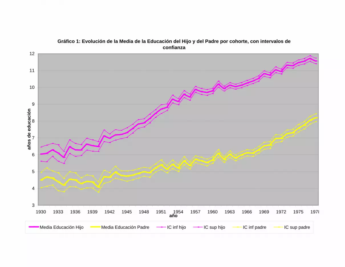
Gráfico 1: Evolución de la Media de la Educación del Hijo y del Padre por cohorte, con intervalos de confianza

3

4

5

6

7

8

9

10

11

12

1930 1933 1936 1939 1942 1945 1948 1951 1954 1957 1960 1963 1966 1969 1972 1975 1978año

años

de

educ

ació

n

Media Educación Hijo Media Educación Padre IC inf hijo IC sup hijo IC inf padre IC sup padre

Gráfico 1b: Evolución de la Media de la Educación del Hijo y tendencia

3

4

5

6

7

8

9

10

11

12

1930 1932 1934 1936 1938 1940 1942 1944 1946 1948 1950 1952 1954 1956 1958 1960 1962 1964 1966 1968 1970 1972 1974 1976 1978año

años

de

educ

ació

n

Media Educación Hijo IC inf hijo IC sup hijo Tendencia

TABLA 2EVOLUCIÓN DE LA DISTRIBUCIÓN DE EDUCACIÓN DEL HIJO

Cohorte MedianaValor

Percentil 10

Valor Percentil

25

Valor Percentil

75

Valor Percentil

90DesvEst Moda % Moda

Corr Ed PadreDesvEst

1930 6 0 3 8 12 4.40 6 24.4% 0.6682395 4.401931 6 0 3 8 12 4.37 6 21.4% 0.6191373 4.371932 6 0 3 9 12 4.47 6 23.0% 0.6152096 4.471933 6 1 3 9 12 4.44 6 18.4% 0.6510919 4.441934 6 0 3 8 12 4.25 6 22.3% 0.5508958 4.251935 6 1 3 9 12 4.42 6 21.5% 0.5568453 4.421936 6 1 3 9 12 4.40 6 21.1% 0.5640481 4.401937 6 1 3 9 12 4.30 6 23.6% 0.5576572 4.301938 6 1 3 10 12 4.30 6 23.1% 0.6090537 4.301939 6 1 3 10 12 4.54 6 19.9% 0.5980781 4.541940 6 2 3 9 12 4.22 6 24.8% 0.6446698 4.221941 6 2 4 10 12 4.29 6 20.2% 0.5334373 4.291942 6 2 4 10 12 4.31 6 25.5% 0.5386037 4.311943 6 3 4 10 12 4.19 6 24.3% 0.5179258 4.191944 6 2 4 10 12 4.30 6 24.1% 0.5339734 4.301945 6 2 4 11 12 4.26 6 22.0% 0.5015997 4.261946 6 3 4 11 12 4.34 6 20.6% 0.4937894 4.341947 6 3 5 12 13 4.37 6 22.1% 0.4913277 4.371948 7 3 5 12 13 4.34 6 22.2% 0.5075364 4.341949 7 3 5 12 13 4.32 6 21.0% 0.5361174 4.321950 8 3 6 12 15 4.45 6 18.9% 0.5208721 4.451951 8 3 6 12 15 4.45 12 18.3% 0.4811603 4.451952 8 3 6 12 14 4.39 12 23.2% 0.5023796 4.391953 10 3 6 12 15 4.32 12 25.7% 0.4832871 4.321954 10 3 6 12 14 4.22 12 25.0% 0.4946585 4.221955 10 4 6 12 15 4.14 12 27.2% 0.4383871 4.141956 10 4 6 12 14 4.10 12 26.9% 0.4760235 4.101957 10 4 7 12 15 4.03 12 28.6% 0.4072833 4.031958 10 4 7 12 15 3.99 12 28.9% 0.4432278 3.991959 10 4 8 12 14 3.96 12 28.3% 0.4230928 3.961960 10 4 8 12 14 3.96 12 30.4% 0.4264508 3.961961 11 5 8 12 15 3.90 12 32.1% 0.4073396 3.901962 11 5 8 12 15 3.88 12 30.3% 0.4354133 3.881963 11 5 8 12 15 3.78 12 31.0% 0.4020144 3.781964 11 5 8 12 14 3.85 12 32.2% 0.4132656 3.851965 11 5 8 12 15 3.78 12 32.5% 0.4035168 3.781966 12 5 8 12 15 3.83 12 34.3% 0.4264036 3.831967 12 6 8 12 15 3.75 12 32.8% 0.4203176 3.751968 12 6 8 12 15 3.72 12 34.7% 0.4066203 3.721969 12 6 8 12 16 3.69 12 33.4% 0.4092477 3.691970 12 6 8 12 16 3.73 12 31.4% 0.4079388 3.731971 12 6 8 13 16 3.73 12 31.3% 0.3962039 3.731972 12 6 8 13 16 3.67 12 30.8% 0.4110363 3.671973 12 6 9 13 16 3.72 12 32.6% 0.4295414 3.721974 12 7 9 13 16 3.61 12 33.5% 0.4023085 3.611975 12 7 9 13 16 3.53 12 36.0% 0.3573758 3.531976 12 7 9 14 16 3.48 12 34.4% 0.39707 3.481977 12 8 10 14 16 3.39 12 36.5% 0.4014908 3.391978 12 7 10 13 16 3.46 12 39.2% 0.4057428 3.46

2.0

2.5

3.0

3.5

4.0

4.5

5.0

1 4 7 10 13 16 19 22 25 28 31 34 37 40 43 46 490.0

0.1

0.2

0.3

0.4

0.5

0.6

0.7

0.8

DesvEst Corr Ed Padre, estimado sólo Padre

Gráfico 2: Evolución de la Distribución de Educación del Hijo

0

2

4

6

8

10

12

14

16

18

1930 1933 1936 1939 1942 1945 1948 1951 1954 1957 1960 1963 1966 1969 1972 1975 1978año

años

de

educ

ació

n

Percentil 10 Percentil 25 Mediana Percentil 75 Percentil 90 Media

REGRESIÓN 1

Number of obs 63445F(98, 63347) 6040.97Prob > F 0R-squared 0.8951Root MSE 3.4373

educ_hijo Coef. Std. Err. t P>|t|d1930 3.301 0.245 13.48 0 2.821 3.780d1931 3.382 0.319 10.60 0 2.756 4.007d1932 3.538 0.215 16.45 0 3.117 3.960d1933 3.368 0.303 11.11 0 2.774 3.963d1934 3.560 0.204 17.41 0 3.159 3.961d1935 4.115 0.253 16.26 0 3.619 4.612d1936 3.937 0.232 16.95 0 3.482 4.393d1937 4.070 0.207 19.70 0 3.665 4.475d1938 4.172 0.222 18.82 0 3.738 4.607d1939 4.046 0.201 20.12 0 3.652 4.440d1940 4.042 0.167 24.14 0 3.714 4.370d1941 4.755 0.239 19.87 0 4.286 5.224d1942 4.467 0.154 29.10 0 4.166 4.768d1943 4.780 0.203 23.58 0 4.383 5.177d1944 4.804 0.158 30.39 0 4.494 5.114d1945 5.121 0.198 25.88 0 4.733 5.509d1946 5.208 0.174 29.91 0 4.866 5.549d1947 5.607 0.184 30.55 0 5.248 5.967d1948 5.449 0.169 32.33 0 5.119 5.779d1949 5.699 0.183 31.22 0 5.341 6.057d1950 5.842 0.159 36.81 0 5.531 6.154d1951 6.284 0.199 31.64 0 5.894 6.673d1952 6.351 0.145 43.90 0 6.067 6.634d1953 6.857 0.184 37.27 0 6.496 7.217d1954 6.650 0.134 49.48 0 6.387 6.913d1955 7.226 0.165 43.73 0 6.902 7.549d1956 7.032 0.145 48.47 0 6.748 7.316d1957 7.723 0.141 54.92 0 7.447 7.999d1958 7.364 0.143 51.35 0 7.082 7.645d1959 7.510 0.138 54.52 0 7.240 7.780d1960 7.454 0.130 57.49 0 7.200 7.709d1961 7.781 0.146 53.38 0 7.495 8.067d1962 7.535 0.115 65.56 0 7.310 7.761d1963 7.802 0.133 58.65 0 7.541 8.063d1964 7.740 0.119 64.87 0 7.506 7.974d1965 7.834 0.132 59.27 0 7.575 8.093d1966 7.758 0.128 60.77 0 7.507 8.008d1967 7.897 0.131 60.25 0 7.640 8.154d1968 8.099 0.140 57.87 0 7.824 8.373d1969 8.216 0.142 57.95 0 7.938 8.494d1970 8.082 0.136 59.52 0 7.816 8.348d1971 8.315 0.153 54.17 0 8.014 8.616d1972 8.155 0.131 62.09 0 7.898 8.413d1973 8.215 0.150 54.70 0 7.921 8.509

[95% Conf. Interval]

REGRESIÓN DE LA EDUCACIÓN DEL HIJO, USANDO LA EDUCACIÓN DEL PADRE COMO VARIABLE EXPLICATIVA, POR COHORTE

d1974 8.404 0.149 56.27 0 8.111 8.697d1975 8.774 0.163 53.72 0 8.454 9.094d1976 8.507 0.164 51.82 0 8.185 8.828d1977 8.553 0.170 50.32 0 8.220 8.886d1978 8.281 0.174 47.57 0 7.940 8.622

edpadre1930 0.668 0.050 13.25 0 0.569 0.767edpadre1931 0.619 0.062 9.95 0 0.497 0.741edpadre1932 0.615 0.039 15.63 0 0.538 0.692edpadre1933 0.651 0.052 12.54 0 0.549 0.753edpadre1934 0.551 0.036 15.10 0 0.479 0.622edpadre1935 0.557 0.041 13.61 0 0.477 0.637edpadre1936 0.564 0.043 13.12 0 0.480 0.648edpadre1937 0.558 0.040 13.98 0 0.479 0.636edpadre1938 0.609 0.042 14.47 0 0.527 0.692edpadre1939 0.598 0.043 13.86 0 0.513 0.683edpadre1940 0.645 0.033 19.43 0 0.580 0.710edpadre1941 0.533 0.041 13.06 0 0.453 0.613edpadre1942 0.539 0.028 19.42 0 0.484 0.593edpadre1943 0.518 0.034 15.07 0 0.451 0.585edpadre1944 0.534 0.028 19.38 0 0.480 0.588edpadre1945 0.502 0.033 15.04 0 0.436 0.567edpadre1946 0.494 0.030 16.54 0 0.435 0.552edpadre1947 0.491 0.030 16.24 0 0.432 0.551edpadre1948 0.508 0.025 19.91 0 0.458 0.558edpadre1949 0.536 0.030 18.07 0 0.478 0.594edpadre1950 0.521 0.025 21.01 0 0.472 0.569edpadre1951 0.481 0.029 16.88 0 0.425 0.537edpadre1952 0.502 0.021 23.53 0 0.461 0.544edpadre1953 0.483 0.025 19.35 0 0.434 0.532edpadre1954 0.495 0.019 25.60 0 0.457 0.533edpadre1955 0.438 0.023 19.37 0 0.394 0.483edpadre1956 0.476 0.020 23.35 0 0.436 0.516edpadre1957 0.407 0.018 22.10 0 0.371 0.443edpadre1958 0.443 0.019 22.81 0 0.405 0.481edpadre1959 0.423 0.019 21.73 0 0.385 0.461edpadre1960 0.426 0.018 24.01 0 0.392 0.461edpadre1961 0.407 0.019 21.98 0 0.371 0.444edpadre1962 0.435 0.015 29.26 0 0.406 0.465edpadre1963 0.402 0.017 23.24 0 0.368 0.436edpadre1964 0.413 0.016 25.54 0 0.382 0.445edpadre1965 0.404 0.017 23.43 0 0.370 0.437edpadre1966 0.426 0.016 26.64 0 0.395 0.458edpadre1967 0.420 0.016 26.66 0 0.389 0.451edpadre1968 0.407 0.016 24.81 0 0.374 0.439edpadre1969 0.409 0.017 24.62 0 0.377 0.442edpadre1970 0.408 0.017 24.70 0 0.376 0.440edpadre1971 0.396 0.017 23.00 0 0.362 0.430edpadre1972 0.411 0.014 28.38 0 0.383 0.439edpadre1973 0.430 0.016 26.12 0 0.397 0.462edpadre1974 0.402 0.017 23.65 0 0.369 0.436edpadre1975 0.357 0.018 20.04 0 0.322 0.392edpadre1976 0.397 0.017 23.02 0 0.363 0.431edpadre1977 0.401 0.018 22.88 0 0.367 0.436edpadre1978 0.406 0.017 23.41 0 0.372 0.440

TABLA 3

Cohorte Parámetro IC inferior IC superior1930 0.668 0.564 0.7731931 0.619 0.490 0.7511932 0.615 0.535 0.6991933 0.651 0.544 0.7591934 0.551 0.476 0.6271935 0.557 0.472 0.6431936 0.564 0.473 0.6531937 0.558 0.474 0.6451938 0.609 0.523 0.6991939 0.598 0.508 0.6881940 0.645 0.576 0.7141941 0.533 0.447 0.6171942 0.539 0.481 0.5971943 0.518 0.446 0.5871944 0.534 0.478 0.5891945 0.502 0.431 0.5711946 0.494 0.433 0.5561947 0.491 0.428 0.5541948 0.508 0.455 0.5611949 0.536 0.475 0.5981950 0.521 0.470 0.5721951 0.481 0.421 0.5381952 0.502 0.457 0.5471953 0.483 0.432 0.5361954 0.495 0.453 0.5341955 0.438 0.392 0.4831956 0.476 0.434 0.5181957 0.407 0.369 0.4451958 0.443 0.403 0.4851959 0.423 0.382 0.4631960 0.426 0.389 0.4641961 0.407 0.370 0.4451962 0.435 0.405 0.4661963 0.402 0.367 0.4391964 0.413 0.380 0.4461965 0.404 0.369 0.4391966 0.426 0.394 0.4591967 0.420 0.389 0.4531968 0.407 0.372 0.4401969 0.409 0.374 0.4431970 0.408 0.374 0.4421971 0.396 0.359 0.4331972 0.411 0.381 0.4421973 0.430 0.395 0.4631974 0.402 0.366 0.4371975 0.357 0.322 0.3931976 0.397 0.361 0.4331977 0.401 0.364 0.4381978 0.406 0.369 0.441

Pendiente

PERSISTENCIA INTERGENERACIONAL ESTIMADA POR COHORTE, CON INTERVALOS DE CONFIANZA

Gráfico 3: Correlación entre la Educación del Hijo y la Educación del Padre, con intervalos de confianza

0.2

0.3

0.4

0.5

0.6

0.7

0.8

1930 1933 1936 1939 1942 1945 1948 1951 1954 1957 1960 1963 1966 1969 1972 1975 1978año

años

de

educ

ació

n

Correlación Hijo-Padre IC inf correlacion IC sup correlacion

Gráfico 3: Correlación entre la Educación del Hijo y la de su Padre y Tendencia

0.2

0.3

0.4

0.5

0.6

0.7

0.8

1930

1932

1934

1936

1938

1940

1942

1944

1946

1948

1950

1952

1954

1956

1958

1960

1962

1964

1966

1968

1970

1972

1974

1976

1978

año

años

de

educ

ació

n

xb_persistencia2 persistencia

TABLA 4

Cohorte Parámetro IC inferior IC superior1930 0.498 0.421 0.5761931 0.477 0.377 0.5781932 0.452 0.393 0.5131933 0.469 0.392 0.5461934 0.395 0.342 0.4501935 0.391 0.332 0.4521936 0.405 0.340 0.4681937 0.381 0.324 0.4411938 0.406 0.348 0.4661939 0.401 0.340 0.4611940 0.406 0.362 0.4491941 0.352 0.295 0.4071942 0.360 0.322 0.3991943 0.358 0.309 0.4061944 0.354 0.317 0.3911945 0.325 0.279 0.3701946 0.314 0.275 0.3531947 0.307 0.268 0.3461948 0.321 0.288 0.3551949 0.325 0.288 0.3621950 0.322 0.290 0.3531951 0.299 0.262 0.3341952 0.293 0.267 0.3191953 0.282 0.252 0.3131954 0.281 0.258 0.3041955 0.258 0.231 0.2841956 0.271 0.247 0.2951957 0.237 0.214 0.2591958 0.257 0.233 0.2801959 0.242 0.218 0.2641960 0.248 0.226 0.2701961 0.243 0.221 0.2661962 0.251 0.233 0.2681963 0.240 0.219 0.2621964 0.239 0.220 0.2581965 0.239 0.218 0.2591966 0.255 0.235 0.2741967 0.247 0.228 0.2661968 0.243 0.222 0.2631969 0.247 0.226 0.2671970 0.250 0.230 0.2711971 0.250 0.227 0.2731972 0.262 0.242 0.2811973 0.275 0.253 0.2971974 0.260 0.237 0.2831975 0.236 0.212 0.2601976 0.267 0.242 0.2901977 0.276 0.250 0.3001978 0.288 0.262 0.313

Pendiente

ELASTICIDAD INTERGENERACIONAL ESTIMADA POR COHORTE, CON INTERVALOS DE CONFIANZA

Gráfico 4: Elasticidad entre la Educación del Hijo y la Educación del Padre, con intervalos de confianza

0.1

0.2

0.2

0.3

0.3

0.4

0.4

0.5

0.5

0.6

0.6

1930 1932 1934 1936 1938 1940 1942 1944 1946 1948 1950 1952 1954 1956 1958 1960 1962 1964 1966 1968 1970 1972 1974 1976 1978año

años

de

educ

ació

n

Correlación Hijo-Padre IC inf correlacion IC sup correlacion

TABLA 5

Cohorte Primaria Incompleta

Secundaria Incompleta

Secundaria Completa

Universitaria Incompleta

1930 88.52% 29.27% 17.56% 7.03%1931 88.82% 32.24% 17.43% 6.25%1932 88.43% 32.83% 19.92% 6.64%1933 90.03% 32.71% 14.95% 7.79%1934 86.52% 29.08% 15.25% 5.85%1935 91.09% 35.87% 19.35% 6.96%1936 90.06% 33.14% 18.71% 7.41%1937 90.10% 33.48% 15.87% 5.97%1938 90.69% 38.10% 18.97% 6.03%1939 90.75% 37.28% 19.08% 8.38%1940 92.92% 33.79% 17.76% 6.96%1941 92.86% 43.54% 21.26% 7.31%1942 93.48% 38.87% 21.45% 7.77%1943 94.07% 42.90% 21.38% 8.28%1944 94.20% 41.34% 22.27% 8.66%1945 93.97% 44.37% 23.55% 8.65%1946 96.05% 46.19% 24.65% 9.88%1947 95.88% 49.52% 26.82% 10.60%1948 96.43% 50.45% 26.52% 10.79%1949 96.50% 52.25% 30.45% 11.04%1950 95.67% 56.68% 31.68% 13.87%1951 96.31% 59.80% 33.09% 14.75%1952 96.47% 60.92% 37.42% 14.22%1953 96.75% 69.23% 42.16% 16.49%1954 96.73% 68.53% 39.43% 14.45%1955 96.87% 74.25% 43.36% 16.17%1956 96.91% 73.01% 41.21% 14.33%1957 97.49% 77.48% 44.99% 16.41%1958 97.77% 76.81% 44.31% 15.42%1959 96.90% 78.23% 43.79% 15.47%1960 96.81% 79.58% 45.66% 15.30%1961 97.53% 82.10% 49.87% 17.80%1962 97.50% 80.89% 46.44% 16.13%1963 98.30% 82.69% 48.25% 17.26%1964 97.77% 80.71% 48.96% 16.78%1965 97.77% 83.06% 49.36% 16.81%1966 97.68% 82.35% 51.44% 17.12%1967 97.76% 84.56% 51.44% 18.61%1968 97.79% 84.88% 54.73% 20.07%1969 98.09% 86.89% 56.96% 23.59%1970 98.00% 86.65% 54.19% 22.79%1971 98.07% 88.92% 58.65% 27.34%1972 98.34% 87.82% 56.58% 25.74%1973 98.28% 89.57% 61.59% 28.95%1974 98.59% 90.16% 61.36% 27.87%1975 98.84% 91.86% 63.69% 27.64%1976 99.28% 91.96% 63.58% 29.21%1977 99.11% 92.79% 66.71% 30.22%1978 98.63% 91.96% 66.85% 27.66%

COBERTURA ABSOLUTA DE NIVELES EDUCACIONALES PARA TODA LA POBLACIÓN

Gráfico 5: Cobertura absoluta para toda la población.

0.00

0.10

0.20

0.30

0.40

0.50

0.60

0.70

0.80

0.90

1.00

1930 1933 1936 1939 1942 1945 1948 1951 1954 1957 1960 1963 1966 1969 1972 1975 1978

% cumplimiento 1-6 años % cumplimiento 7-11 años% cumplimiento 12 años % cumplimiento 13 años o más

TABLA 6PORCENTAJE DE PADRES EN CADA NIVEL EDUCATIVO

Cohorte Padres 0-6 años

Padres 7-11 años

Padres 12 años

Padres 13 o más años

1930 0.79 0.08 0.11 0.021931 0.77 0.11 0.10 0.031932 0.78 0.07 0.12 0.031933 0.81 0.06 0.09 0.041934 0.79 0.07 0.12 0.021935 0.81 0.06 0.09 0.041936 0.79 0.07 0.12 0.031937 0.81 0.08 0.09 0.021938 0.81 0.07 0.09 0.031939 0.79 0.09 0.09 0.031940 0.83 0.07 0.08 0.021941 0.77 0.09 0.11 0.031942 0.78 0.10 0.09 0.031943 0.77 0.09 0.09 0.041944 0.77 0.12 0.09 0.031945 0.77 0.11 0.09 0.031946 0.76 0.10 0.10 0.031947 0.75 0.12 0.10 0.031948 0.75 0.11 0.10 0.041949 0.76 0.11 0.11 0.021950 0.74 0.12 0.10 0.041951 0.72 0.13 0.11 0.041952 0.73 0.12 0.11 0.041953 0.72 0.13 0.12 0.041954 0.73 0.13 0.11 0.031955 0.71 0.13 0.12 0.041956 0.72 0.14 0.11 0.031957 0.69 0.15 0.13 0.041958 0.70 0.15 0.12 0.041959 0.71 0.14 0.11 0.041960 0.70 0.14 0.12 0.041961 0.66 0.16 0.14 0.051962 0.69 0.15 0.13 0.041963 0.66 0.16 0.13 0.051964 0.68 0.15 0.13 0.041965 0.67 0.16 0.13 0.051966 0.65 0.17 0.13 0.051967 0.65 0.18 0.12 0.051968 0.63 0.19 0.12 0.061969 0.60 0.21 0.14 0.061970 0.60 0.20 0.13 0.061971 0.57 0.20 0.15 0.081972 0.57 0.20 0.16 0.081973 0.53 0.23 0.15 0.091974 0.53 0.23 0.17 0.081975 0.49 0.24 0.18 0.101976 0.46 0.27 0.17 0.101977 0.44 0.28 0.17 0.111978 0.42 0.28 0.19 0.11

PORCENTAJE DE PADRES

Gráfico 6: Porcentaje de Padres en cada Nivel Educativo

0.00

0.10

0.20

0.30

0.40

0.50

0.60

0.70

0.80

0.90

1.00

1930 1933 1936 1939 1942 1945 1948 1951 1954 1957 1960 1963 1966 1969 1972 1975 1978

% cumplimiento 1-6 años % cumplimiento 7-11 años% cumplimiento 12 años % cumplimiento 13 años o más

TABLA 7COBERTURA ABSOLUTA DE NIVELES EDUCACIONALES DE ACUERDO A LA EDUCACIÓN DEL PADRE

Cohorte Padres 0-6 años

Padres 7-11 años

Padres 12 años

Padres 13 o más años

Padres 0-6 años

Padres 7-11 años

Padres 12 años

Padres 13 o más años

Padres 0-6 años

Padres 7-11 años

Padres 12 años

Padres 13 o más años

Padres 0-6 años

Padres 7-11 años

Padres 12 años

Padres 13 o más años

1930 0.8888889 0.96923077 0.973684 1 0.19713262 0.62962963 0.78947368 0.75 0.08960573 0.33333333 0.71052632 0.75 0.02867384 0.26153846 0.34210526 0.51931 0.8730159 0.98 1 1 0.21693122 0.65384615 0.79166667 0.875 0.11111111 0.30769231 0.54166667 0.625 0.04761905 0.14 0.16666667 0.3751932 0.8690808 0.96428571 0.962264 1 0.22005571 0.70967742 0.77358491 0.93333333 0.11977716 0.32258065 0.56603774 0.66666667 0.03342618 0.16666667 0.20754717 0.333333331933 0.8755981 1 1 1 0.23923445 0.6 0.79166667 0.90909091 0.0861244 0.13333333 0.54166667 0.81818182 0.04784689 0.15384615 0.16666667 0.545454551934 0.8443272 0.98913043 0.982456 1 0.16622691 0.71428571 0.68421053 1 0.07915567 0.34285714 0.43859649 0.875 0.03166227 0.16304348 0.14035088 0.1251935 0.9079365 0.94915254 0.971429 1 0.26349206 0.79166667 0.85714286 1 0.11428571 0.41666667 0.57142857 0.75 0.04126984 0.13559322 0.14285714 0.3751936 0.8928571 0.97435897 0.959184 1 0.24404762 0.75862069 0.69387755 1 0.10714286 0.34482759 0.51020408 0.91666667 0.04166667 0.16666667 0.20408163 0.51937 0.888651 1 1 1 0.25910064 0.72916667 0.76 0.75 0.11991435 0.25 0.48 0.5 0.04068522 0.17346939 0.3 0.166666671938 0.8883117 0.98701299 0.97619 1 0.30909091 0.8 0.85714286 0.86666667 0.14805195 0.17142857 0.61904762 0.6 0.03376623 0.16883117 0.23809524 0.466666671939 0.8953229 0.98039216 0.980769 0.93333333 0.28062361 0.68 0.75 0.93333333 0.10022272 0.42 0.57692308 0.8 0.04454343 0.24509804 0.28846154 0.533333331940 0.9165217 1 1 1 0.25913043 0.7755102 0.80769231 0.93333333 0.13217391 0.34693878 0.61538462 0.8 0.04173913 0.20792079 0.28846154 0.61941 0.9234973 0.95789474 0.960784 1 0.33333333 0.81818182 0.78431373 1 0.15027322 0.29545455 0.54901961 0.83333333 0.04098361 0.16842105 0.25490196 0.583333331942 0.9280868 0.97777778 0.977011 1 0.27272727 0.7311828 0.77011494 0.90322581 0.1302578 0.39784946 0.56321839 0.70967742 0.03256445 0.21666667 0.25287356 0.387096771943 0.9364035 0.97321429 0.964286 1 0.33552632 0.76785714 0.80357143 0.91666667 0.13157895 0.375 0.625 0.70833333 0.0504386 0.19642857 0.26785714 0.333333331944 0.9445876 0.96618357 0.966667 1 0.32345361 0.72649573 0.76666667 0.90322581 0.14819588 0.38461538 0.55555556 0.83870968 0.04381443 0.22705314 0.25555556 0.354838711945 0.9347443 0.97350993 0.955224 0.95238095 0.36684303 0.75 0.79104478 0.85714286 0.17813051 0.30952381 0.64179104 0.76190476 0.0617284 0.15231788 0.20895522 0.428571431946 0.9525926 0.98907104 1 1 0.37185185 0.77173913 0.79120879 0.85714286 0.16444444 0.31521739 0.61538462 0.57142857 0.06222222 0.20765027 0.25274725 0.321428571947 0.9589235 0.99029126 0.979592 0.96296296 0.40084986 0.7962963 0.80612245 0.96296296 0.1898017 0.44444444 0.64285714 0.7037037 0.06798867 0.24271845 0.26530612 0.333333331948 0.9580686 0.99545455 1 1 0.41423126 0.73504274 0.82524272 0.92105263 0.1905972 0.38461538 0.55339806 0.89473684 0.07242694 0.18636364 0.21359223 0.631578951949 0.9598278 0.99004975 1 1 0.44045911 0.80582524 0.84693878 0.95454545 0.23098996 0.52427184 0.7244898 0.77272727 0.05882353 0.29353234 0.34693878 0.409090911950 0.9497951 0.98657718 0.978417 0.98 0.47131148 0.83018868 0.89208633 0.9 0.22848361 0.4591195 0.69784173 0.82 0.08606557 0.25838926 0.30215827 0.621951 0.9640719 0.97747748 0.970874 1 0.51497006 0.84033613 0.84466019 0.94594595 0.23652695 0.55462185 0.63106796 0.83783784 0.09580838 0.27927928 0.30097087 0.621621621952 0.9577815 0.98680739 0.988636 0.96721311 0.51821192 0.87684729 0.91477273 0.93442623 0.26655629 0.65024631 0.74431818 0.8852459 0.08112583 0.29287599 0.30681818 0.573770491953 0.9632353 0.99647887 1 1 0.61764706 0.87755102 0.91240876 0.95 0.34436275 0.6462585 0.69343066 0.875 0.11397059 0.28873239 0.27737226 0.651954 0.9615385 0.99084668 0.989744 1 0.61312217 0.88016529 0.90769231 0.95918367 0.30090498 0.62809917 0.71794872 0.89795918 0.08974359 0.27688787 0.27692308 0.632653061955 0.9636552 0.98843931 0.988166 1 0.67912773 0.92090395 0.92899408 0.92857143 0.33229491 0.60451977 0.76923077 0.875 0.09449637 0.28612717 0.27218935 0.6251956 0.9667519 0.99036145 0.994475 1 0.67689685 0.9017094 0.93370166 0.95348837 0.32736573 0.60683761 0.74033149 0.93023256 0.08184143 0.2746988 0.32596685 0.767441861957 0.9699367 0.99204771 1 1 0.72231013 0.91078067 0.94871795 0.95890411 0.35996835 0.65799257 0.73504274 0.91780822 0.10522152 0.27833002 0.28205128 0.671232881958 0.9731136 0.99313501 0.994792 1 0.7085863 0.91428571 0.94791667 0.984375 0.34692108 0.63673469 0.71354167 0.90625 0.09887251 0.26086957 0.30729167 0.6718751959 0.9691558 0.99548533 1 0.96825397 0.73376623 0.91869919 0.95431472 0.93650794 0.3400974 0.66260163 0.75126904 0.85714286 0.09172078 0.29345372 0.3248731 0.650793651960 0.9640678 0.98207885 0.980159 0.98734177 0.74305085 0.93464052 0.92857143 0.97468354 0.35525424 0.66013072 0.75396825 0.92405063 0.08881356 0.27419355 0.31746032 0.696202531961 0.9700935 0.98347107 0.991266 0.98734177 0.7682243 0.9254902 0.94759825 0.97468354 0.37757009 0.69803922 0.76419214 0.92405063 0.09158879 0.30991736 0.31441048 0.68354431962 0.9710145 0.99419448 0.993789 1 0.74782609 0.94822888 0.96273292 0.98913043 0.36057971 0.64305177 0.78881988 0.94565217 0.09043478 0.30043541 0.33540373 0.673913041963 0.9838213 0.98963731 1 1 0.77041602 0.93457944 0.96124031 0.96629213 0.37904468 0.63862928 0.74806202 0.87640449 0.10015408 0.29188256 0.29844961 0.651685391964 0.9760909 0.98428571 0.987616 0.97777778 0.75552899 0.9204244 0.95665635 0.96666667 0.39210998 0.64456233 0.80495356 0.9 0.08846384 0.3 0.3498452 0.733333331965 0.9727479 0.99122807 0.996032 0.9787234 0.78728236 0.91823899 0.98015873 0.95744681 0.38909917 0.63207547 0.78968254 0.92553191 0.08327025 0.30175439 0.38095238 0.670212771966 0.9731884 0.98634294 0.989547 1 0.76304348 0.93817204 0.97212544 0.97959184 0.40289855 0.65053763 0.82578397 0.90816327 0.0942029 0.29742033 0.3554007 0.622448981967 0.9734513 0.98869144 1 1 0.78908555 0.93495935 0.98 1 0.40265487 0.68292683 0.804 0.93939394 0.10176991 0.29563813 0.324 0.737373741968 0.9722222 0.99298246 1 0.99038462 0.78819444 0.95639535 0.98672566 0.98076923 0.43142361 0.72674419 0.79646018 0.95192308 0.11284722 0.32105263 0.36283186 0.740384621969 0.9744991 0.99197432 0.995984 1 0.81238616 0.94652406 0.96385542 1 0.44444444 0.73529412 0.78714859 0.97029703 0.13661202 0.33065811 0.37751004 0.821782181970 0.9756098 0.98796992 0.984906 0.984 0.80487805 0.95 0.95471698 0.984 0.41547519 0.67 0.75471698 0.968 0.12279226 0.33684211 0.40754717 0.7761971 0.974359 0.98204668 0.987234 1 0.83500557 0.95341615 0.95744681 0.98425197 0.44593088 0.69565217 0.8212766 0.96062992 0.1393534 0.38779174 0.44680851 0.771653541972 0.9757282 0.98958333 0.997041 1 0.81391586 0.95581395 0.9704142 1 0.4263754 0.73023256 0.76923077 0.93678161 0.1302589 0.37369792 0.41420118 0.793103451973 0.9823009 0.97996918 0.988327 1 0.83960177 0.92602041 0.9766537 1 0.45353982 0.70918367 0.86770428 0.97350993 0.14048673 0.39137134 0.47859922 0.774834441974 0.9807107 0.99052774 0.990385 0.99328859 0.84263959 0.95081967 0.98076923 0.98657718 0.4680203 0.70725995 0.84935897 0.93959732 0.15228426 0.37618403 0.48397436 0.758389261975 0.9849246 0.99553571 0.996491 0.97419355 0.86055276 0.95607235 0.98947368 0.97419355 0.50251256 0.68475452 0.82105263 0.92258065 0.13316583 0.33184524 0.44210526 0.741935481976 0.9931129 0.99429387 0.988806 0.99342105 0.84710744 0.97921478 0.98134328 0.99342105 0.46969697 0.70207852 0.80597015 0.96052632 0.13774105 0.36091298 0.47014925 0.782894741977 0.988959 0.99394856 1 0.99363057 0.87697161 0.95599022 0.99206349 0.99363057 0.51419558 0.69193154 0.86507937 0.98726115 0.13880126 0.33888048 0.51190476 0.853503181978 0.9828767 0.98312883 0.988764 0.99371069 0.84417808 0.96103896 0.98501873 0.99371069 0.49143836 0.68051948 0.89513109 0.94968553 0.09931507 0.33128834 0.51310861 0.81132075

Cobertura de Primaria Incompleta Cobertura de Secundaria Incompleta Cobertura de Secundaria Completa Cobertura de Universitaria Incompleta

Gráfico 7a: Cobertura de primaria incompleta de acuerdo a la educación de los padres

0.00

0.10

0.20

0.30

0.40

0.50

0.60

0.70

0.80

0.90

1.00

1930 1933 1936 1939 1942 1945 1948 1951 1954 1957 1960 1963 1966 1969 1972 1975 1978

padres 1-6 padres 7-11 padres 12 padres 13 o más

Gráfico 7b: Cobertura de secundaria incompleta de acuerdo a la educación de los padres

0.0

0.1

0.2

0.3

0.4

0.5

0.6

0.7

0.8

0.9

1.0

1930 1933 1936 1939 1942 1945 1948 1951 1954 1957 1960 1963 1966 1969 1972 1975 1978

padres 1-6 padres 7-11 padres 12 padres 13 o más

Gráfico 7c: Cobertura de secundaria completa de acuerdo a la educación de los padres

0.00

0.10

0.20

0.30

0.40

0.50

0.60

0.70

0.80

0.90

1.00

1930 1933 1936 1939 1942 1945 1948 1951 1954 1957 1960 1963 1966 1969 1972 1975 1978

padres 1-6 padres 7-11 padres 12 padres 13 o más

Gráfico 7d: Cobertura de universitaria incompleta de acuerdo a la educación de los padres

0.00

0.10

0.20

0.30

0.40

0.50

0.60

0.70

0.80

0.90

1.00

1930 1933 1936 1939 1942 1945 1948 1951 1954 1957 1960 1963 1966 1969 1972 1975 1978

padres 1-6 padres 7-11 padres 12 padres 13 o más

TABLA 8

Cohorte Secundaria Incompleta

Secundaria Completa

Universitaria Incompleta

1930 0.330687831 0.6 0.41931 0.362962963 0.540816327 0.3584905661932 0.371244635 0.606936416 0.3333333331933 0.363321799 0.457142857 0.5208333331934 0.336065574 0.524390244 0.383720931935 0.393794749 0.539393939 0.3595505621936 0.367965368 0.564705882 0.3958333331937 0.371567044 0.473913043 0.3761467891938 0.420152091 0.497737557 0.3181818181939 0.410828025 0.511627907 0.4393939391940 0.363636364 0.525735294 0.3916083921941 0.468864469 0.48828125 0.3441942 0.415869981 0.551724138 0.36251943 0.45601173 0.498392283 0.3870967741944 0.438893845 0.538617886 0.3886792451945 0.472154964 0.530769231 0.3671497581946 0.480901077 0.533604888 0.4007633591947 0.516453382 0.54159292 0.3954248371948 0.52312868 0.525723473 0.4067278291949 0.541468065 0.582746479 0.3625377641950 0.592420213 0.558922559 0.4377510041951 0.620915033 0.553383459 0.4456521741952 0.631522324 0.614139693 0.3800277391953 0.71559633 0.608974359 0.391228071954 0.708476237 0.57538036 0.3665865381955 0.766494179 0.583966245 0.372832371956 0.753372909 0.564469914 0.3477157361957 0.794759825 0.580586081 0.3648790751958 0.785600847 0.576819407 0.3481308411959 0.807320793 0.559823678 0.3532058491960 0.822062553 0.57377892 0.3351254481961 0.841792657 0.607440667 0.3569165791962 0.829598008 0.574185249 0.3472740851963 0.841262783 0.583509514 0.3577898551964 0.825488776 0.606578947 0.3427331891965 0.849561404 0.594217863 0.3405734141966 0.84304746 0.624691358 0.3328063241967 0.864993509 0.608304152 0.3618421051968 0.868015414 0.644839068 0.3666092941969 0.885811467 0.655512891 0.4142259411970 0.884162896 0.625383828 0.4206219311971 0.906689151 0.659640422 0.4661654141972 0.893004115 0.644239631 0.4549356221973 0.911431514 0.687570621 0.4700082171974 0.914489311 0.680519481 0.4541984731975 0.929411765 0.693325662 0.4340248961976 0.926298157 0.69138035 0.4594594591977 0.936157518 0.718929254 0.4530141841978 0.932406822 0.72696477 0.413793103

COBERTURA CONDICIONAL DE NIVELES EDUCACIONALES PARA TODA LA POBLACIÓN

Gráfico 8: Cobertura condicional de niveles educacionales para toda la población

0.0

0.1

0.2

0.3

0.4

0.5

0.6

0.7

0.8

0.9

1.0

1930 1933 1936 1939 1942 1945 1948 1951 1954 1957 1960 1963 1966 1969 1972 1975 1978

secundaria incompleta secundaria completa universitaria incompleta

TABLA 9

Cohorte Padres 0-6 años

Padres 7-11 años

Padres 12 años

Padres 13 o más años

Padres 0-6 años

Padres 7-11 años

Padres 12 años

Padres 13 o más años

Padres 0-6 años

Padres 7-11 años

Padres 12 años

Padres 13 o más años

1930 0.22177419 0.64961787 0.81081081 0.75 0.45454545 0.52941176 0.9 1 0.32 0.78461538 0.48148148 0.666666671931 0.24848485 0.66718995 0.79166667 0.875 0.51219512 0.47058824 0.68421053 0.71428571 0.42857143 0.455 0.30769231 0.61932 0.25320513 0.73596177 0.80392157 0.93333333 0.5443038 0.45454545 0.73170732 0.71428571 0.27906977 0.51666667 0.36666667 0.51933 0.27322404 0.6 0.79166667 0.90909091 0.36 0.22222222 0.68421053 0.9 0.55555556 1 0.30769231 0.666666671934 0.196875 0.72213501 0.69642857 1 0.47619048 0.48 0.64102564 0.875 0.4 0.47554348 0.32 0.142857141935 0.29020979 0.83407738 0.88235294 1 0.43373494 0.52631579 0.66666667 0.75 0.36111111 0.32542373 0.25 0.51936 0.27333333 0.77858439 0.72340426 1 0.43902439 0.45454545 0.73529412 0.91666667 0.38888889 0.48333333 0.4 0.545454551937 0.29156627 0.72916667 0.76 0.75 0.46280992 0.34285714 0.63157895 0.66666667 0.33928571 0.69387755 0.625 0.333333331938 0.34795322 0.81052632 0.87804878 0.86666667 0.4789916 0.21428571 0.72222222 0.69230769 0.22807018 0.98484848 0.38461538 0.777777781939 0.31343284 0.6936 0.76470588 1 0.35714286 0.61764706 0.76923077 0.85714286 0.44444444 0.58356676 0.5 0.666666671940 0.28273245 0.7755102 0.80769231 0.93333333 0.51006711 0.44736842 0.76190476 0.85714286 0.31578947 0.59930111 0.46875 0.751941 0.36094675 0.85414585 0.81632653 1 0.45081967 0.36111111 0.7 0.83333333 0.27272727 0.57004049 0.46428571 0.71942 0.29385965 0.74780059 0.78823529 0.90322581 0.47761194 0.54411765 0.73134328 0.78571429 0.25 0.54459459 0.44897959 0.545454551943 0.35831382 0.78899083 0.83333333 0.91666667 0.39215686 0.48837209 0.77777778 0.77272727 0.38333333 0.52380952 0.42857143 0.470588241944 0.34242838 0.75192308 0.79310345 0.90322581 0.45816733 0.52941176 0.72463768 0.92857143 0.29565217 0.59033816 0.46 0.423076921945 0.39245283 0.77040816 0.828125 0.9 0.48557692 0.41269841 0.81132075 0.88888889 0.34653465 0.49210392 0.3255814 0.56251946 0.3903577 0.78026663 0.79120879 0.85714286 0.44223108 0.4084507 0.77777778 0.66666667 0.37837838 0.65875259 0.41071429 0.56251947 0.41802068 0.80410312 0.82291667 1 0.47349823 0.55813953 0.79746835 0.73076923 0.35820896 0.5461165 0.41269841 0.473684211948 0.43236074 0.73839909 0.82524272 0.92105263 0.4601227 0.52325581 0.67058824 0.97142857 0.38 0.48454545 0.38596491 0.705882351949 0.45889387 0.81392399 0.84693878 0.95454545 0.52442997 0.65060241 0.85542169 0.80952381 0.25465839 0.55988576 0.47887324 0.529411761950 0.49622438 0.84148376 0.91176471 0.91836735 0.48478261 0.5530303 0.78225806 0.91111111 0.37668161 0.56279305 0.43298969 0.756097561951 0.53416149 0.85969872 0.87 0.94594595 0.45930233 0.66 0.74712644 0.88571429 0.40506329 0.503549 0.47692308 0.741935481952 0.54105445 0.88856985 0.92528736 0.96610169 0.514377 0.74157303 0.8136646 0.94736842 0.30434783 0.45040777 0.41221374 0.648148151953 0.64122137 0.88065191 0.91240876 0.95 0.55753968 0.73643411 0.76 0.92105263 0.33096085 0.44677539 0.4 0.742857141954 0.63764706 0.88829615 0.91709845 0.95918367 0.49077491 0.71361502 0.79096045 0.93617021 0.29824561 0.44083464 0.38571429 0.704545451955 0.70474138 0.93167476 0.94011976 0.92857143 0.48929664 0.65644172 0.82802548 0.94230769 0.284375 0.47331317 0.35384615 0.714285711956 0.70017637 0.91048516 0.93888889 0.95348837 0.4836272 0.67298578 0.79289941 0.97560976 0.25 0.45267266 0.44029851 0.8251957 0.74469821 0.91808152 0.94871795 0.95890411 0.49835706 0.72244898 0.77477477 0.95714286 0.29230769 0.42299873 0.38372093 0.731343281958 0.72816399 0.92060566 0.95287958 0.984375 0.48959608 0.69642857 0.75274725 0.92063492 0.285 0.409699 0.43065693 0.741379311959 0.75711893 0.92286562 0.95431472 0.96721311 0.46349558 0.72123894 0.78723404 0.91525424 0.26968974 0.44288108 0.43243243 0.759259261960 0.77074543 0.95169601 0.94736842 0.98717949 0.47810219 0.70629371 0.81196581 0.94805195 0.25 0.4153625 0.42105263 0.753424661961 0.79190751 0.94104465 0.95594714 0.98717949 0.49148418 0.75423729 0.80645161 0.94805195 0.24257426 0.44398273 0.41142857 0.739726031962 0.77014925 0.95376599 0.96875 0.98913043 0.48217054 0.67816092 0.81935484 0.95604396 0.25080386 0.46720253 0.42519685 0.712643681963 0.78308536 0.94436561 0.96124031 0.96629213 0.492 0.68333333 0.77822581 0.90697674 0.26422764 0.45704537 0.39896373 0.743589741964 0.77403552 0.93511913 0.96865204 0.98863636 0.51898734 0.70028818 0.84142395 0.93103448 0.22560976 0.4654321 0.43461538 0.814814811965 0.80933852 0.926365 0.98406375 0.97826087 0.49423077 0.68835616 0.80566802 0.96666667 0.21400778 0.47740246 0.48241206 0.724137931966 0.78406552 0.95116212 0.98239437 0.97959184 0.52801519 0.69340974 0.84946237 0.92708333 0.23381295 0.45719159 0.43037975 0.68539326

Cobertura Condicional de Secundaria Incompleta Cobertura Condicional de Secundaria Completa Cobertura Condicional de Universitaria Incompleta

COBERTURA CONDICIONAL DE NIVELES EDUCACIONALES DE ACUERDO A LA EDUCACIÓN DEL PADRE

1967 0.81060606 0.94565333 0.98 1 0.51028037 0.73043478 0.82040816 0.93939394 0.25274725 0.43289868 0.40298507 0.784946241968 0.81071429 0.96315433 0.98672566 0.99029126 0.54735683 0.75987842 0.80717489 0.97058824 0.26156942 0.44176842 0.45555556 0.777777781969 0.83364486 0.95418203 0.96774194 1 0.5470852 0.77683616 0.81666667 0.97029703 0.30737705 0.44969502 0.47959184 0.846938781970 0.825 0.96156773 0.96934866 1 0.51619645 0.70526316 0.79051383 0.98373984 0.29554656 0.50274941 0.54 0.801652891971 0.85697941 0.97084606 0.96982759 0.98425197 0.53404539 0.72964169 0.85777778 0.976 0.3125 0.55745063 0.54404145 0.803278691972 0.83416252 0.96587515 0.97329377 1 0.52385686 0.76399027 0.79268293 0.93678161 0.30550285 0.51175192 0.53846154 0.846625771973 0.85472973 0.9449485 0.98818898 1 0.54018445 0.76584022 0.88844622 0.97350993 0.3097561 0.55186175 0.55156951 0.795918371974 0.85921325 0.95991221 0.99029126 0.99324324 0.55542169 0.74384236 0.86601307 0.95238095 0.32537961 0.53188934 0.56981132 0.807142861975 0.87372449 0.96035967 0.99295775 1 0.58394161 0.71621622 0.82978723 0.94701987 0.265 0.48461927 0.53846154 0.80419581976 0.85298197 0.98483438 0.99245283 1 0.55447154 0.71698113 0.82129278 0.96688742 0.29325513 0.51406356 0.58333333 0.815068491977 0.88676236 0.96181056 0.99206349 1 0.58633094 0.72378517 0.872 0.99358974 0.26993865 0.48976013 0.59174312 0.864516131978 0.85888502 0.97753105 0.99621212 1 0.5821501 0.70810811 0.90874525 0.9556962 0.20209059 0.48681684 0.57322176 0.85430464

0.04300110.00742768

Gráfico 9a: Cobertura condicional de secundaria incompleta de acuerdo a la educación de los padres

0.0

0.1

0.2

0.3

0.4

0.5

0.6

0.7

0.8

0.9

1.0

1930 1933 1936 1939 1942 1945 1948 1951 1954 1957 1960 1963 1966 1969 1972 1975 1978

padres 1-6 padres 7-11 padres 12 padres 13 o más

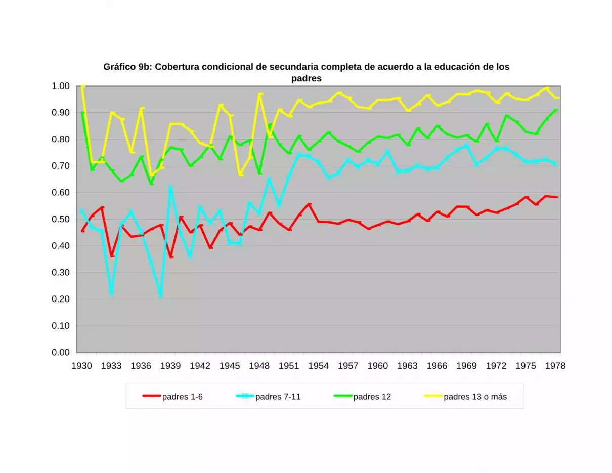
Gráfico 9b: Cobertura condicional de secundaria completa de acuerdo a la educación de los padres

0.00

0.10

0.20

0.30

0.40

0.50

0.60

0.70

0.80

0.90

1.00

1930 1933 1936 1939 1942 1945 1948 1951 1954 1957 1960 1963 1966 1969 1972 1975 1978

padres 1-6 padres 7-11 padres 12 padres 13 o más

Gráfico 9c: Cobertura condicional de universitaria incompleta de acuerdo a la educación de los padres

0.00

0.10

0.20

0.30

0.40

0.50

0.60

0.70

0.80

0.90

1.00

1930 1933 1936 1939 1942 1945 1948 1951 1954 1957 1960 1963 1966 1969 1972 1975 1978

padres 1-6 padres 7-11 padres 12 padres 13 o más

TABLA 10

Cohorte 4 o más años 6 o más años 8 o más años 12 o más años

1930 69.80% 53.60% 28.10% 17.60%1931 67.80% 53.60% 30.60% 17.40%1932 71.20% 55.80% 31.90% 19.90%1933 67.30% 51.10% 30.20% 15.00%1934 70.90% 51.40% 26.60% 15.20%1935 71.50% 57.40% 33.50% 19.30%1936 72.10% 54.20% 31.40% 18.70%1937 70.70% 57.10% 31.10% 15.90%1938 74.30% 61.20% 36.00% 19.00%1939 71.80% 57.20% 33.80% 19.10%1940 74.80% 58.60% 31.70% 17.80%1941 80.10% 63.80% 40.80% 21.30%1942 79.40% 64.30% 36.70% 21.40%1943 81.00% 67.20% 41.20% 21.40%1944 81.80% 65.50% 39.30% 22.30%1945 81.70% 66.30% 42.30% 23.50%1946 82.40% 66.80% 43.70% 24.60%1947 83.70% 71.60% 46.60% 26.80%1948 85.00% 72.70% 48.00% 26.50%1949 86.80% 73.20% 49.90% 30.50%1950 87.20% 75.60% 54.30% 31.70%1951 88.80% 78.00% 57.20% 33.10%1952 88.80% 77.10% 59.60% 37.40%1953 89.50% 80.70% 66.90% 42.20%1954 90.00% 80.10% 66.20% 39.40%1955 91.70% 84.20% 71.60% 43.40%1956 91.90% 82.60% 70.90% 41.20%1957 93.20% 86.20% 74.90% 45.00%1958 93.30% 84.70% 74.10% 44.30%1959 92.90% 85.10% 75.30% 43.80%1960 92.50% 86.30% 76.00% 45.70%1961 94.50% 88.60% 79.00% 49.90%1962 93.70% 87.30% 77.40% 46.40%1963 95.30% 88.10% 78.50% 48.30%1964 93.90% 87.60% 77.30% 49.00%1965 94.30% 88.50% 79.60% 49.40%1966 94.50% 88.40% 79.80% 51.40%1967 95.00% 90.10% 81.30% 51.40%1968 95.40% 90.30% 82.30% 54.70%1969 95.90% 91.20% 84.50% 57.00%1970 96.00% 91.40% 83.50% 54.20%1971 96.10% 92.20% 86.10% 58.70%1972 96.70% 92.60% 84.80% 56.60%1973 96.80% 93.40% 86.60% 61.60%1974 97.40% 93.90% 87.40% 61.40%1975 97.40% 94.70% 88.90% 63.70%1976 98.10% 94.80% 89.40% 63.60%1977 98.40% 95.70% 90.00% 66.70%1978 97.60% 95.00% 89.30% 66.90%

PORCENTAJE DE INDIVIDUOS EN CADA COHORTE QUE CUMPLE LA ESCOLARIDAD MÍNIMA, POR COHORTE DE NACIMIENTO

Gráfico 10: Porcentaje de individuos que cumple la escolaridad mínima, por cohorte de nacimiento

0.0

0.1

0.2

0.3

0.4

0.5

0.6

0.7

0.8

0.9

1.0

1930 1932 1934 1936 1938 1940 1942 1944 1946 1948 1950 1952 1954 1956 1958 1960 1962 1964 1966 1968 1970 1972 1974 1976 1978

4 años o más 6 años o más 8 años o más 12 años o más

TABLA 11

Momento 4 o más años 6 o más años 8 o más años 12 o más años

t-25 49.87%t-24 46.44%t-23 48.25%t-22 28.10% 48.96%t-21 30.59% 49.36%t-20 31.88% 51.44%t-19 30.22% 51.44%t-18 26.60% 54.73%t-17 33.48% 56.96%t-16 31.38% 54.19%t-15 31.15% 58.65%t-14 36.03% 56.58%t-13 33.82% 61.59%t-12 31.68% 61.36%t-11 40.82% 63.69%t-10 36.73% 63.58%t-9 41.24% 66.71%t-8 39.33% 66.85%t-7 42.32%t-6 43.74%t-5 46.63%t-4 48.01%t-3 49.86%t-2 54.26%t-1 57.19%t0 59.57%

t+1 66.94%t+2 66.21%t+3 71.55%t+4 70.92%t+5 74.88%t+6 74.12%t+7 75.32%t+8 76.02%t+9 79.04%

t+10 77.38%t+11 78.54%t+12 53.63% 77.31%t+13 53.62% 79.59%t+14 55.79% 79.83%t+15 51.09% 81.35%t+16 51.42% 82.34%t+17 57.39% 84.46%t+18 54.19% 83.55%t+19 69.79% 57.06% 86.05%t+20 67.76% 61.21% 84.82%t+21 71.16% 57.23% 86.59%t+22 67.29% 58.63% 87.35%t+23 70.92% 63.78% 88.90%t+24 71.52% 64.34% 89.36%t+25 72.12% 67.17% 90.01%t+26 70.74% 65.46% 89.35%

PORCENTAJE DE INDIVIDUOS EN CADA COHORTE QUE CUMPLE LA ESCOLARIDAD MÍNIMA, POR MOMENTO DE PROMULGACIÓN DE LA LEY

Gráfico 11: Porcentaje de individuos que cumple la escolaridad mínima, por momento de promulgación de la ley

0.0

0.1

0.2

0.3

0.4

0.5

0.6

0.7

0.8

0.9

1.0

T-25 T-22 T-19 T-16 T-13 T-10 T-7 T-4 T-1 T+2 T+5 T+8 T+11 T+14 T+17 T+20 T+23 T+26

4 años 6 años 8 años 12 años

REGRESIÓN 2

A. CAMBIO ESTRUCTURAL SÓLO EN T=0, 1952Number of obs 49F(4, 45) 25784.21Prob > F 0R-squared 0.9985Root MSE 0.02617

p8_ Coef. Std. Err. t P>|t|c 0.241 0.015 16.12 0 0.211 0.271

tendencia 0.012 0.001 10.61 0 0.010 0.015d1952 0.210 0.033 6.43 0 0.144 0.276

tend1952 -0.003 0.001 -2.15 0.037 -0.006 0.000

B. CAMBIO ESTRUCTURAL EN 1944 - 1953 - 1957Number of obs 49F(8, 41) 25724.86Prob > F 0R-squared 0.9994Root MSE 0.01701

p8_ Coef. Std. Err. t P>|t|c 0.270 0.013 20.95 0 0.244 0.296

tendencia 0.008 0.002 4.72 0 0.005 0.012d1944 -0.256 0.020 -12.78 0 -0.297 -0.216

tend1944 0.017 0.002 8.80 0 0.013 0.021d1953 0.232 0.103 2.24 0.031 0.023 0.441

tend1953 -0.008 0.004 -1.88 0.068 -0.016 0.001d1957 0.271 0.103 2.63 0.012 0.063 0.479

tend1957 -0.009 0.004 -2.36 0.023 -0.018 -0.001

[95% Conf. Interval]

[95% Conf. Interval]

ANÁLISIS DE CAMBIO ESTRUCTURAL EN LA PROPORCIÓN DE INDIVIDUOS CON AL MENOS 8 AÑOS DE ESCOLARIDAD

TABLA 12TENDENCIA PARA EL PORCENTAJE DE INDIVIDUOS CON 8 O MÁS AÑOS DE EDUCACIÓN

A. CAMBIO ESTRUCTURAL SÓLO EN T=0, 1952

Cohorte Parámetro IC inferior IC superior Parámetro IC inferior IC superior1930-1951 0.241 0.209 0.272 0.012 0.010 0.0151952-1978 0.451 0.391 0.511 0.009 0.008 0.011

B. CAMBIO ESTRUCTURAL EN 1944 - 1953 - 1957

Cohorte Parámetro IC inferior IC superior Parámetro IC inferior IC superior1930-1943 0.270 0.242 0.298 0.008 0.004 0.0121944-1952 0.014 -0.024 0.051 0.025 0.023 0.0271953-1956 0.245 -0.324 0.815 0.017 -0.005 0.0401957-1978 0.516 0.491 0.542 0.008 0.007 0.009

Constante Tendencia

Constante Tendencia

Gráfico 12: Tendencia para el Porcentaje de Individuos con 8 o más años de Educación

0.2

0.3

0.4

0.5

0.6

0.7

0.8

0.9

1.0

1930 1932 1934 1936 1938 1940 1942 1944 1946 1948 1950 1952 1954 1956 1958 1960 1962 1964 1966 1968 1970 1972 1974 1976 1978

8 o más años Tendencia

Gráfico 12: Tendencia para el Porcentaje de Individuos con 8 o más años de Educación, selección

0.30

0.35

0.40

0.45

0.50

0.55

0.60

0.65

0.70

0.75

0.80

1940 1942 1944 1946 1948 1950 1952 1954 1956 1958 1960 1962 1964

8 o más años Tendencia

TABLA 13

Cohorte Momento al Evento

Porcentaje de la Cohorte con 8 años o más de

educación

Predicción Error de Predicción

Error de Predicción Acumulado

Test θ

1930 -22 28.10% 29.48% -1.38% -1.38%1931 -21 30.60% 29.47% 1.13% -0.24%1932 -20 31.90% 29.65% 2.25% 2.01%1933 -19 30.20% 29.99% 0.21% 2.22%1934 -18 26.60% 30.48% -3.88% -1.66%1935 -17 33.50% 31.08% 2.42% 0.76%1936 -16 31.40% 31.79% -0.39% 0.37%1937 -15 31.10% 32.59% -1.49% -1.12%1938 -14 36.00% 33.47% 2.53% 1.41%1939 -13 33.80% 34.43% -0.63% 0.78%1940 -12 31.70% 35.47% -3.77% -2.99%1941 -11 40.80% 36.60% 4.20% 1.21%1942 -10 36.70% 37.82% -1.12% 0.08%1943 -9 41.20% 39.15% 2.05% 2.13%1944 -8 39.30% 40.61% -1.31% 0.82%1945 -7 42.30% 42.23% 0.07% 0.89%1946 -6 43.70% 44.02% -0.32% 0.57%1947 -5 46.60% 46.04% 0.56% 1.13%1948 -4 48.00% 48.31% -0.31% 0.82%1949 -3 49.90% 50.87% -0.97% -0.15%1950 -2 54.30% 53.77% 0.53% 0.38%1951 -1 57.20% 57.02% 0.18% 0.56%1952 0 59.60% 60.64% -1.04% -0.48% -0.4691721953 1 66.90% 64.63% 2.27% 1.79% 0.39113261954 2 66.20% 68.92% -2.72% -0.93% -0.3859651955 3 71.60% 73.43% -1.83% -2.75% -0.7444951956 4 70.90% 78.00% -7.10% -9.86% -2.0940681957 5 74.90% 82.47% -7.57% -17.43% -3.3008091958 6 74.10% 86.62% -12.52% -29.95% -5.1830161959 7 75.30% 90.27% -14.97% -44.91% -7.2270611960 8 76.00% 93.29% -17.29% -62.20% -9.4037691961 9 79.00% 95.62% -16.62% -78.82% -11.284181962 10 77.40% 97.31% -19.91% -98.74% -13.458081963 11 78.50% 98.45% -19.95% -118.69% -15.474341964 12 77.30% 99.17% -21.87% -140.56% -17.593481965 13 79.60% 99.58% -19.98% -160.54% -19.354091966 14 79.80% 99.81% -20.01% -180.55% -21.019711967 15 81.30% 99.92% -18.62% -199.16% -22.444311968 16 82.30% 99.97% -17.67% -216.83% -23.700271969 17 84.50% 99.99% -15.49% -232.32% -24.673491970 18 83.50% 100.00% -16.50% -248.81% -25.716571971 19 86.10% 100.00% -13.90% -262.71% -26.462431972 20 84.80% 100.00% -15.20% -277.91% -27.315641973 21 86.60% 100.00% -13.40% -291.31% -27.971811974 22 87.40% 100.00% -12.60% -303.91% -28.537961975 23 88.90% 100.00% -11.10% -315.01% -28.955581976 24 89.40% 100.00% -10.60% -325.61% -29.323521977 25 90.00% 100.00% -10.00% -335.61% -29.635641978 26 89.30% 100.00% -10.70% -346.31% -30.00729

ESTUDIO DE EVENTO: IMPACTO DE LA NUEVA LEY DE EDUCACIÓN SOBRE EL PORCENTAJE DE INDIVIDUOS CON 8 AÑOS O MÁS DE EDUCACIÓN

G_13

Page 40

Gráfico 13: Estudio de Evento, Impacto de la Ley de Educación sobre el Porcentaje de Individuos con 8 años o más de educación.

0.00

0.20

0.40

0.60

0.80

1.00

1.20

1930 1932 1934 1936 1938 1940 1942 1944 1946 1948 1950 1952 1954 1956 1958 1960 1962 1964 1966 1968 1970 1972 1974 1976 1978-3.75

-3.25

-2.75

-2.25

-1.75

-1.25

-0.75

-0.25

0.25

0.75

Porcentaje con 8 años o más Predicción Error de Predicción Acumulado

REGRESIÓN 3: COBERTURA ABSOLUTA VS INGRESOS AL NACER Y A LOS 18

A. SIN CAMBIO ESTRUCTURAL

Padres con 0-6 años de educaciónNumber of obs 49F( 2, 46) 112.49Prob > F 0R-squared 0.8782Root MSE 0.0127

Cobertura Abs Coef. Std.Err. t P>|t| [95%Conf. Interval]10 antes de na 4.11E-07 2.10E-07 1.96 0.056 -1.10E-08 8.33E-0710 antes de lo 1.43E-06 1.75E-07 8.18 0 1.08E-06 1.79E-06C -0.045189 0.0082717 -5.46 0 -0.0618392 -0.0285389

Medias Padres 0-6Variable Parámetro Elasticidad Parámetro Elasticidad Cobertura 0.082553110 antes de na 4.11E-07 0.28 8.04E-07 0.17 57060.3610 antes de 18 1.43E-06 1.26 2.69E-06 0.74 10 antes de 18 72744.05

Parámetros significativos al 95%

B. CON CAMBIO ESTRUCTURAL EN 1956

Padres con 0-6 años de educaciónNumber of obs 49F( 6, 43) 637.36Prob > F 0R-squared 0.9888Root MSE 0.01013

Cobertura Abs Coef. Std. Err. t P>|t| [95% Conf. Interval]10 antes de na 2.01E-06 6.76E-07 2.98 0.005 6.5E-07 3.4E-0610 antes de lo 1.52E-06 1.41E-07 10.8 0 1.2E-06 1.8E-06C -1.32E-01 3.45E-02 -3.83 0 -2.0E-01 -6.2E-021956_10 antes -7.57E-07 7.96E-07 -0.95 0.347 -2.4E-06 8.5E-071956_10 antes -1.45E-06 5.33E-07 -2.72 0.009 -2.5E-06 -3.7E-07D1956 1.54E-01 4.03E-02 3.83 0 7.3E-02 2.4E-01

Parámetros 1930-1955 1956-1978 1930-1955 1956-197810 antes de na 2.01E-06 1.25E-06 3.72E-06 2.79E-0610 antes de 18 1.52E-06 7.00E-08 2.84E-06 -5.50E-07

Elasticidad 1930-1955 1956-1978 1930-1955 1956-197810 antes de na 1.74 0.74 0.86 0.57 10 antes de 18 1.56 0.06 0.78 0.15-

Parámetros significativos al 95%

Padres 0-6 Padres 7-11

Padres 0-6 Padres 7-11

Padres 0-6 Padres 7-11

Padres con 7-11 años de educaciónNumber of obs 49F( 2, 46) 82.47Prob > F 0R-squared 0.7946Root MSE 0.03275

Cobertura Abs Coef. Std.Err. t P>|t| [95%Conf. Interval]10 antes de na 8.04E-07 4.13E-07 1.95 0.057 -2.66E-08 1.64E-0610 antes de lo 2.69E-06 3.26E-07 8.26 0 2.04E-06 3.35E-06C 0.0218168 0.0212166 1.03 0.309 -0.0208899 0.0645235

Padres 7-110.2635776

57060.3672744.05

Padres con 7-11 años de educaciónNumber of obs 49F( 6, 43) 2088.62Prob > F 0R-squared 0.991Root MSE 0.02756

Cobertura Abs Coef. Std. Err. t P>|t| [95% Conf. Interval]10 antes de na 3.72E-06 4.50E-06 0.83 0.413 -5.4E-06 1.3E-0510 antes de lo 2.84E-06 3.15E-07 9 0 2.2E-06 3.5E-06C -1.37E-01 2.25E-01 -0.61 0.545 -5.9E-01 3.2E-011956_10 antes -9.33E-07 4.51E-06 -0.21 0.837 -1.0E-05 8.2E-061956_10 antes -3.39E-06 4.48E-07 -7.56 0 -4.3E-06 -2.5E-06D1956 3.24E-01 2.25E-01 1.44 0.158 -1.3E-01 7.8E-01

Medias 1930-1955 1956-1978 1930-1955 1956-1978Cobertura 5.71E-02 1.11E-01 2.14E-01 3.20E-0110 antes de na 4.96E+04 6.55E+04 4.96E+04 6.55E+0410 antes de 18 5.87E+04 8.86E+04 5.87E+04 8.86E+04

Padres 0-6 Padres 7-11

Cohorte Cobertura Absoluta

Predicción Sin Cambio Estructural

Predicción Con Cambio Estructural

Cobertura Absoluta

Predicción Sin Cambio Estructural

Predicción Con Cambio Estructural

1930 0.02867384 0.05 0.0343444 0.26153846 0.20 0.1714281931 0.04761905 0.05 0.0366851 0.14 0.20 0.17574861932 0.03342618 0.05 0.037016 0.16666667 0.20 0.17635041933 0.04784689 0.05 0.0380079 0.15384615 0.20 0.17817741934 0.03166227 0.05 0.040419 0.16304348 0.20 0.18264861935 0.04126984 0.05 0.0416674 0.13559322 0.20 0.18493841936 0.04166667 0.05 0.0414754 0.16666667 0.19 0.18455351937 0.04068522 0.04 0.0397874 0.17346939 0.19 0.18138451938 0.03376623 0.04 0.0400845 0.16883117 0.19 0.1819111939 0.04454343 0.04 0.0416789 0.24509804 0.19 0.18486281940 0.04173913 0.04 0.0422254 0.20792079 0.19 0.18587131941 0.04098361 0.04 0.0422935 0.16842105 0.19 0.18600731942 0.03256445 0.05 0.0448714 0.21666667 0.19 0.19080541943 0.0504386 0.05 0.048834 0.19642857 0.20 0.19817681944 0.04381443 0.05 0.0505736 0.22705314 0.20 0.20141221945 0.0617284 0.05 0.0525021 0.15231788 0.20 0.20500321946 0.06222222 0.05 0.055323 0.20765027 0.21 0.21027491947 0.06798867 0.06 0.0600651 0.24271845 0.22 0.21912521948 0.07242694 0.07 0.067078 0.18636364 0.23 0.23221191949 0.05882353 0.07 0.0734171 0.29353234 0.24 0.24404241950 0.08606557 0.08 0.0796923 0.25838926 0.26 0.25576131951 0.09580838 0.09 0.0865627 0.27927928 0.27 0.26858541952 0.08112583 0.09 0.0948068 0.29287599 0.28 0.28394311953 0.11397059 0.10 0.1023464 0.28873239 0.30 0.29803021954 0.08974359 0.10 0.1004856 0.27688787 0.30 0.29459881955 0.09449637 0.10 0.0927568 0.28612717 0.29 0.28024741956 0.08184143 0.09 0.087599 0.2746988 0.28 0.27164831957 0.10522152 0.09 0.0876677 0.27833002 0.27 0.27375891958 0.09887251 0.08 0.08734 0.26086957 0.27 0.2755911959 0.09172078 0.08 0.0876201 0.29345372 0.26 0.27809761960 0.08881356 0.08 0.0891383 0.27419355 0.26 0.28243961961 0.09158879 0.08 0.0913372 0.30991736 0.25 0.28841511962 0.09043478 0.08 0.0922526 0.30043541 0.25 0.29107151963 0.10015408 0.08 0.0935248 0.29188256 0.25 0.29408681964 0.08846384 0.08 0.0965978 0.3 0.26 0.29784561965 0.08327025 0.09 0.1011657 0.30175439 0.28 0.30344591966 0.0942029 0.10 0.1075104 0.29742033 0.30 0.31409741967 0.10176991 0.11 0.1133529 0.29563813 0.32 0.32352361968 0.11284722 0.12 0.1194342 0.32105263 0.33 0.33397471969 0.13661202 0.12 0.1256338 0.33065811 0.34 0.34599891970 0.12279226 0.13 0.1315613 0.33684211 0.35 0.35792011971 0.1393534 0.13 0.1388956 0.38779174 0.36 0.37341931972 0.1302589 0.13 0.1392153 0.37369792 0.36 0.37406771973 0.14048673 0.13 0.1358262 0.39137134 0.35 0.36744271974 0.15228426 0.13 0.1335265 0.37618403 0.36 0.36168441975 0.13316583 0.13 0.1302517 0.33184524 0.36 0.35287981976 0.13774105 0.14 0.1260106 0.36091298 0.37 0.34107581977 0.13880126 0.14 0.1230096 0.33888048 0.37 0.33146831978 0.09931507 0.15 0.1216289 0.33128834 0.38 0.325247

Padres 0-6 Padres 7-11

TABLA 14: COBERTURA ABSOLUTA Y PREDICCIÓN USANDO LOS INGRESOS AL NACER Y A LOS 18

Gráfico 14a: Cobertura Absoluta y predicción para hijos de padres con 0-6 años de educación

0.00

0.02

0.04

0.06

0.08

0.10

0.12

0.14

0.16

1930 1933 1936 1939 1942 1945 1948 1951 1954 1957 1960 1963 1966 1969 1972 1975 197

Cobertura Absoluta Predicción Sin Cambio Estructural Predicción Con Cambio Estructural

Gráfico 14b: Cobertura Absoluta y predicción para hijos de padres con 7-11 años de educación

0.10

0.15

0.20

0.25

0.30

0.35

0.40

1930 1933 1936 1939 1942 1945 1948 1951 1954 1957 1960 1963 1966 1969 1972 1975 197

Cobertura Absoluta Predicción Sin Cambio Estructural Predicción Con Cambio Estructural

REGRESIÓN 4: COBERTURA ABSOLUTA VS. ESTRUCTURA FAMILIAR

A. Regresión sin Cambio Estructural

Padres con 0-6 años de educaciónNumber of obs 49F( 2, 47) 207.03Prob > F 0R-squared 0.8964Root MSE 0.02951

Cobertura Abs Coef. Std.Err. t P>|t| [95%Conf. Interval]padres solos 0.74- 0.12 -6.38 0 -9.76E-01 -5.08E-01C 0.15 0.01 13.13 0 0.1253886 0.1707635

Variable Parámetro Elasticidad Parámetro Elasticidad Cumplimientopadres solos -0.7417362 #REF! -1.602022 -0.53691322 Single parent

Parámetros significativos al 95%

B. Regresión con Cambio Estructural en 1968

Padres con 0-6 años de educaciónNumber of obs 49F( 4, 45) 481.9Prob > F 0R-squared 0.9563Root MSE 0.01957

Cobertura Abs Coef. Std.Err. t P>|t| [95%Conf. Interval]padres solos 0.57- 0.10 -5.84 0 -7.69E-01 -3.74E-01C 0.12 0.01 12.17 0 1.01E-01 1.41E-011968_padres 0.52 0.28 1.87 0.067 -3.88E-02 1.08E+00D_1968 0.01 0.02 0.71 0.484 -0.02579 0.0536568

padres solos 1930-1967 1968-1978 1930-1967 1968-1978Parámetro -0.571642 -0.0513976 -1.363519 0.198612 cumplimElasticidad #REF! -0.02936267 -0.52878927 0.04221201 single

Parámetros significativos al 95%

Padres 0-6 Padres 7-11

Padres 0-6 Padres 7-11

Padres con 7-11 años de educaciónNumber of obs 49F( 2, 47) 580.58Prob > F 0R-squared 0.9597Root MSE 0.05589

Cobertura Abs Coef. Std.Err. t P>|t| [95%Conf. Interval]padres solos 1.60- 0.19 -8.27 0 -1.99E+00 -1.21E+00C 0.41 0.02 21.51 0 0.3672022 0.4429897

0.26357760.0883373

Padres con 7-11 años de educaciónNumber of obs 49F( 4, 45) 835Prob > F 0R-squared 0.9808Root MSE 0.03943

Cobertura Abs Coef. Std.Err. t P>|t| [95%Conf. Interval]padres solos 1.36- 0.17 -7.91 0 -1.71E+00 -1.02E+00C 0.36 0.02 20.09 0 3.27E-01 4.00E-011968_padres 1.56 0.55 2.82 0.007 4.46E-01 2.68E+00D_1968 0.03- 0.04 -0.57 0.569 -0.1153769 0.064202

despues antes despues0.1312454 0.2377553 0.35278180.0749785 0.0922044 0.0749785

TABLA 15: COBERTURA ABSOLUTA Y PREDICCIÓN USANDO LA ESTRUCTURA FAMILIAR

Cohorte Cobertura Absoluta

Predicción Sin Cambio Estructural

Predicción Con Cambio Estructural

Cobertura Absoluta

Predicción Sin Cambio Estructural

Predicción Con Cambio Estructural

1930 0.02867384 0.08 0.0668598 0.26153846 0.25 0.23394341931 0.04761905 0.02 0.0208777 0.14 0.12 0.12426381932 0.03342618 0.09 0.0752046 0.16666667 0.28 0.2538481933 0.04784689 0.09 0.0774734 0.15384615 0.28 0.25925971934 0.03166227 0.05 0.0443322 0.16304348 0.19 0.1802091935 0.04126984 0.05 0.0487041 0.13559322 0.20 0.19063721936 0.04166667 0.03 0.0305777 0.16666667 0.15 0.1474011937 0.04068522 0.07 0.05765 0.17346939 0.23 0.21197561938 0.03376623 0.08 0.0680486 0.16883117 0.26 0.23677891939 0.04454343 0.05 0.0443443 0.24509804 0.19 0.18023791940 0.04173913 0.05 0.0469526 0.20792079 0.20 0.18645941941 0.04098361 0.05 0.0487041 0.16842105 0.20 0.19063721942 0.03256445 0.09 0.0762052 0.21666667 0.28 0.25623461943 0.0504386 0.08 0.0702503 0.19642857 0.26 0.24203071944 0.04381443 0.07 0.05765 0.22705314 0.23 0.21197561945 0.0617284 0.09 0.0733478 0.15231788 0.27 0.2494191946 0.06222222 0.06 0.0546958 0.20765027 0.22 0.20492891947 0.06798867 0.09 0.0736938 0.24271845 0.27 0.25024421948 0.07242694 0.07 0.0584696 0.18636364 0.23 0.21393051949 0.05882353 0.09 0.0775955 0.29353234 0.28 0.25955091950 0.08606557 0.09 0.0764407 0.25838926 0.28 0.25679651951 0.09580838 0.08 0.0678615 0.27927928 0.26 0.23633281952 0.08112583 0.09 0.0774254 0.29287599 0.28 0.25914511953 0.11397059 0.09 0.0769096 0.28873239 0.28 0.25791481954 0.08974359 0.08 0.0715161 0.27688787 0.27 0.24504991955 0.09449637 0.09 0.073529 0.28612717 0.27 0.24985111956 0.08184143 0.09 0.0736421 0.2746988 0.27 0.2501211957 0.10522152 0.10 0.0816514 0.27833002 0.29 0.26922521958 0.09887251 0.09 0.0738982 0.26086957 0.27 0.2507321959 0.09172078 0.10 0.0808577 0.29345372 0.29 0.26733211960 0.08881356 0.09 0.0764188 0.27419355 0.28 0.25674431961 0.09158879 0.10 0.0865208 0.30991736 0.31 0.28084011962 0.09043478 0.09 0.0763106 0.30043541 0.28 0.25648611963 0.10015408 0.10 0.0842062 0.29188256 0.30 0.27531911964 0.08846384 0.10 0.0821095 0.3 0.30 0.27031791965 0.08327025 0.09 0.0793091 0.30175439 0.29 0.26363831966 0.0942029 0.12 0.0966669 0.29742033 0.34 0.30504121967 0.10176991 0.11 0.0944891 0.29563813 0.33 0.29984671968 0.11284722 0.10 0.1317903 0.32105263 0.30 0.35067641969 0.13661202 0.11 0.1322501 0.33065811 0.32 0.34889971970 0.12279226 0.08 0.1301069 0.33684211 0.25 0.35718141971 0.1393534 0.11 0.1324498 0.38779174 0.32 0.34812791972 0.1302589 0.10 0.1318004 0.37369792 0.30 0.35063761973 0.14048673 0.07 0.1299711 0.39137134 0.25 0.35770641974 0.15228426 0.08 0.1302096 0.37618403 0.25 0.35678471975 0.13316583 0.10 0.1317497 0.33184524 0.30 0.35083341976 0.13774105 0.10 0.1316808 0.36091298 0.30 0.35109961977 0.13880126 0.09 0.1311973 0.33888048 0.28 0.35296811978 0.09931507 0.08 0.1304942 0.33128834 0.26 0.3556849

Padres 0-6 Padres 7-11

Gráfico 15a: Cobertura Absoluta y predicción para hijos de padres con 0-6 años de educación

0.00

0.02

0.04

0.06

0.08

0.10

0.12

0.14

0.16

1930

1932

1934

1936

1938

1940

1942

1944

1946

1948

1950

1952

1954

1956

1958

1960

1962

1964

1966

1968

1970

1972

1974

1976

1978

Cobertura Absoluta Predicción Sin Cambio Estructural Predicción Con Cambio Estructural

Gráfico 15b: Cobertura Absoluta y predicción para hijos de padres con 7-11 años de educación

0.10

0.15

0.20

0.25

0.30

0.35

0.40

1930

1932

1934

1936

1938

1940

1942

1944

1946

1948

1950

1952

1954

1956

1958

1960

1962

1964

1966

1968

1970

1972

1974

1976

1978

Cobertura Absoluta Predicción Sin Cambio Estructural Predicción Con Cambio Estructural

REGRESIÓN 5: COMPARACIÓN DE HIPÓTESIS ALTERNATIVAS

Padres con 0-6 años de educaciónNumber of obs 49F( 8, 41) 535.46Prob > F 0R-squared 0.9894Root MSE 0.01008

Cobertura Abs Coef. Std.Err. t P>|t| [95%Conf. Interval]10 antes de na 2.07E-06 6.37E-07 3.24 0.002 7.79E-07 3.35E-0610 antes de lo 1.55E-06 1.65E-07 9.39 0 1.21E-06 1.88E-06padres solos 2.85E-02 6.93E-02 0.41 0.683 -1.12E-01 1.69E-01C -1.39E-01 3.41E-02 -4.08 0 -2.08E-01 -7.01E-021956_10 ante -1.02E-06 8.17E-07 -1.25 0.219 -2.67E-06 6.30E-071956_10 ante -1.73E-06 5.58E-07 -3.1 0.004 -2.86E-06 -6.01E-071968_padres 1.74E-01 1.36E-01 1.28 0.209 -1.01E-01 4.48E-01D1956 1.90E-01 4.12E-02 4.61 0 1.07E-01 2.73E-01

Padres con 7-11 años de educaciónNumber of obs 49F( 8, 41) 1832.86Prob > F 0R-squared 0.9915Root MSE 0.02743

Cobertura Abs Coef. Std.Err. t P>|t| [95%Conf. Interval]10 antes de na 3.17E-06 4.58E-06 0.69 0.493 -6.08E-06 1.24E-0510 antes de lo 2.58E-06 3.88E-07 6.64 0 1.80E-06 3.36E-06padres solos -2.87E-01 2.72E-01 -1.06 0.297 -8.37E-01 2.62E-01C -6.52E-02 2.54E-01 -0.26 0.799 -5.78E-01 4.47E-011956_10 ante -1.10E-06 4.42E-06 -0.25 0.804 -1.00E-05 7.82E-061956_10 ante -3.72E-06 5.97E-07 -6.23 0 -4.93E-06 -2.52E-061968_padres 5.09E-01 3.15E-01 1.62 0.113 -1.27E-01 1.14E+00D1956 3.53E-01 2.28E-01 1.55 0.129 -1.07E-01 8.13E-01