the engineering merit of the
TRANSCRIPT

Earthquake and Structures, Vol. 4, No. 4 (2013) 397-428 397
The engineering merit of the “Effective Period” of bilinear isolation systems
Nicos Makris1 and Georgios Kampas2
1Division of Structures, Department of Civil Engineering, University of Patras, Greece
2 Robertou Galli 27, Athens 11742, Greece
(Received July 5, 2012, Revised September 12, 2012, Accepted October 16, 2012)
Abstract. This paper examines whether the ―effective period‖ of bilinear isolation systems, as defined invariably in most current design codes, expresses in reality the period of vibration that appears in the horizontal axis of the design response spectrum. Starting with the free vibration response, the study proceeds with a comprehensive parametric analysis of the forced vibration response of a wide collection of bilinear isolation systems subjected to pulse and seismic excitations. The study employs Fourier and Wavelet analysis together with a powerful time domain identification method for linear systems known as the Prediction Error Method. When the response history of the bilinear system exhibits a coherent oscillatory trace with a narrow frequency band as in the case of free vibration or forced vibration response from most pulselike excitations, the paper shows that the ―effective period‖ = Teff of the bilinear isolation system is a dependable estimate of its vibration period; nevertheless, the period associated with the second slope of the bilinear system = T2 is an even better approximation regardless the value of the dimensionless strength, Q/(K2 uy) = 1/α – 1, of the system. As the frequency content of the excitation widens and the intensity of the acceleration response history fluctuates more randomly, the paper reveals that the computed vibration period of the systems exhibits appreciably scattering from the computed mean value. This suggests that for several earthquake excitations the mild nonlinearities of the bilinear isolation system dominate the response and the expectation of the design codes to identify a ―linear‖ vibration period has a marginal engineering merit.
Keywords: seismic isolation; equivalent linearization; bilinear behavior; system identification; health
monitoring; earthquake protection
1. Introduction
Starting in the late 1950s researchers began recognizing the importance of studying the
response of structures deforming into their inelastic range and this led to the development of the
inelastic response spectrum. In parallel with the development of inelastic response spectra in the
1960s (Veletsos and Newmark 1960, Veletsos et al. 1969, Veletsos and Vann 1971), there has been
significant effort in developing equivalent linearization techniques (Caughey 1960, 1963, Roberts
and Spanos 2003, Crandall 2006) in order to define equivalent linear parameters (natural periods
and damping ratios) of equivalent linear systems that exhibit comparable response values to those
of the nonlinear systems (Iwan and Gates 1979, Iwan 1980).
Corresponding author, Professor, E-mail: [email protected]

Nicos Makris and Georgios Kampas
In the mid 1970s seismic base isolation has emerged as a practical and economical alternative
to conventional structural design (Kelly et al. 1977, Kelly 1986, Buckle and Mayes 1990). Given
that the two most practical and widely accepted type of isolation bearings are the lead rubber
bearing and the spherical sliding bearing which both exhibit a bilinear behavior, the bilinear
hysteretic system is by now the most widely used model in describing the nonlinear behavior of
practical seismic isolated systems. Despite that the behavior of the most practical seismic isolation
systems is bilinear, the fundamental concept of seismic isolation, as expressed in most current
design codes (AASHTO 1991, NZMWD 1983, FEMA 1998, Eurocode 2009 among others), is that
an isolation system shall offer a flexible support so that the period of vibration is lengthen
sufficiently to reduce the force response. Accordingly, while the behavior of the most practical
isolation systems is bilinear, all design codes invariably ask the design engineer to work with a
vibration period –that is the ―isolation‖ period. In view of this demand the concept of equivalent
linear parameters has become central in the analysis and design of seismic isolated structures and
this led to the wide acceptance of the ―effective period‖ and the associated ―effective stiffness‖.
The main scope of this work is to access the engineering merit of these quantities.
This work has been mainly motivated from system identification studies on seismic isolated
structures in which modal periods and damping ratios are expected to be extracted from recorded
response histories above and below isolators. This work shows that there are appreciable
differences between the first modal period extracted with identification techniques and the
―effective period‖ which according to the design codes is expected to be the ―period of vibration‖.
During the effort to uncover these differences this work also concludes that when the response
history of the bilinear system has a coherent oscillatory trace with a narrow frequency band, the
effective period, Teff as derived from the non-existing effective stiffness, Keff ,of the bilinear system
(in which iterations are needed to be determined) is a dependable estimate of its vibration period;
nevertheless, the period associated with the second slope of the bilinear system = T2 is an even
better approximation of the vibration period regardless the value of the dimensionless strength,
Q/(K2 uy) = 1/α – 1. Accordingly, whenever the concept of a vibration period is meaningful, the
effective period, Teff can be replaced with T2 which is known a priori.
Initially, the ―effective stiffness‖ = Keff, was introduced by practicing engineers in an effort to
reach an estimate for the peak forces that develop in seismic isolated structures with bilinear
(inelastic) behavior by simply employing a statically equivalent linear analysis. At present, Keff,
together with the corresponding effective period, Teff and the associated effective damping
coefficient, ξeff, consist the most widely used quantities for estimating through an iterative
procedure peak inelastic displacements and the associated peak shear forces/overturning moments
according to most current design codes (AASHTO 1991, FEMA 1998, Eurocode 2009 among
others).
The main challenges that Teff is facing are: (a) that it depends on the unknown peak inelastic
displacement; and therefore, iterations on the design spectrum are required to reach convergence,
(b) in seismic isolation applications it has not been established to what extent the effective period,
effeff KmT /2 , (what appears in the horizontal axis of the design spectrum) is indeed the
vibration period (the time needed to complete one cycle) of a mass, m, supported on a system with
bilinear behavior (mass isolated on lead rubber or spherical sliding bearings) and (c) that in several
occasions there are significant departures of the peak inelastic deformation/force of the bilinear
system from the elastic displacement/force of the ―effective‖ linear system.
The concerns with challenge (b) have been expressed indirectly in several review-type
398
The engineering merit of the “Effective Period” of bilinear isolation systems
publications and textbooks (Naeim 2001, Naeim and Kelly 1999) where, while they introduce,
effeff KmT /2 as the ―vibration period‖ of a structure isolated on bearings with bilinear
behavior (T1 = Teff — what appears in the horizontal axis of the spectrum); for the case of spherical
sliding bearings (where the first slope is 200 to 500 times larger than the second slope—a much
more aggressive bilinear behavior), the concept of the effective period, effeff KmT /2 is
suddenly abandoned, and the isolation period (vibration period), is derived from the second slope
of the system, gRTTI /22 . Fig. 1 (left) plots typical bilinear force displacement loops
that correspond to a lead rubber bearing (say strength Q = 0.05 mg, period that corresponds to the
second slope, K2, is 2.5 sec, and K1 / K2 = 1 / α = 10); while Fig. 1 (right) plots the corresponding
force displacement loops from a spherical sliding bearing (TI = 2.5s → R = 1.55 m, uy = 0.00025 m
and coefficient of friction f = 0.05; therefore K1 / K2 = 1/α = 1 + fR / uy = 311).
The above inconsistency, where the entire concept of the effective period is abandoned in the
very case where the bilinear behavior is most pronounced (large difference between K1 and K2)
remains confusing to the non-expert and most importantly uncovers potential technical weaknesses
in the concept of the ―effective period‖, Teff. This paper revisits the practical significance and
engineering merit of the ―effective period‖, Teff, while investigates to what extent it expresses the
oscillatory characteristics of an isolated structure. In this regard, the dynamic response of several
bilinear hysteretic systems (with different normalized strengths and second slopes) is investigated
for three types of excitation: free vibration, pulse-type forced vibration and earthquake forced
vibration. The investigation methods include: similitude, Fourier spectrum response analysis,
wavelet response analysis and the Prediction Error Method response analysis.
2. Review of design codes and related past publications
The currently available design specifications AASHTO (1991), FEMA (1998), IBC (2000),
Eurocode (2009) among others use invariably the equivalent linear static procedure. Details on the
specific steps followed by the most widely accepted codes can be found in Mayes et al. (1991),
Hwang and Sheng (1993, 1994) as well as and in the original documents of the abovementioned
design specifications. Below we only revisit the main steps followed by the 1991 AASHTO Guide
Specification for Seismic Isolation Design given that all subsequent design specifications follow a
similar approach.
2.1 The AASHTO guide specifications
The code specifications that established the quantity, Keff, of the bilinear system shown in Fig. 1
as a key quantity for the response analysis of seismically isolated structures is apparently the 1991
AASHTO Guide Specifications for Seismic Isolation Design. At that time the code did not make a
distinction between the Design Base Earthquake (DBE) and the Maximum Credible Earthquake
(MCE) and merely offers the design spectrum presented in Fig. 2. According to the AASHTO
Guide specification the statically equivalent seismic force is given by
ieff dKF (1)
where ΣKeff is the sum of the effective linear stiffnesses of all bearings supporting the
399

Nicos Makris and Georgios Kampas
Fig. 1 The hysteretic loops of lead rubber bearings (left, say uy = 2 cm = 20 mm) and spherical-sliding
bearings (right, say uy = 0.25 mm) together with the inconsistent code definition of the isolation
period, TI, as the yield displacement decreases (Keff is abandoned in the right plot)
Fig. 2 The AASHTO Acceleration spectrum
superstructure and di is the displacement across the isolation bearings given by
A
effeffi
Di ST
B
TASSd
2
2
4
10
(2)
where A, Si and B are the acceleration, site and damping coefficients offered in the AASHTO
Guide specifications and the effective period, Teff is given by
gK
WT
eff
eff 2 (3)
400
The engineering merit of the “Effective Period” of bilinear isolation systems
The effective linear stiffness Keff of the isolators used in the analysis shall be calculated at the
design displacement, however iterations on the design spectrum are needed given that the effective
period Teff as offered by Eq. (3) updates the maximum displacement as defined by Eq. (2).
The conceptual weakness of the Statically Equivalent Seismic Force Procedure offered by Eqs.
(1)-(3) is that while its ultimate goal is to reach an estimate for the peak design ―static‖ forces, the
estimation of the isolators displacement di = SD involves the effective period, Teff given by Eq. (3).
By involving the effective period, Teff, the ―static‖ procedure also takes a stand on the oscillatory
character of the bilinear system; and the effective period, Teff, which originates from the
non-existing, Keff, is silently upgraded with unsubstantiated liberty to a real physical quantity–that
is the time needed for the isolated structure to complete one cycle of vibration. This technically
weak concept is rooted to such an extent in the profession that several documents show values of
Teff with superficial precision up to two decimal digits. Part of the motivation of this study is to
investigate to what extent the effective period, Teff, may express the oscillatory response of a
system with bilinear behavior.
2.2 Simple geometric relations
With reference to Fig. 1 (left) one can derive via the use of similar triangles a relation between
the effective stiffness, Keff and the first slope of the bilinear model, K1.
)1(11
KKeff (4)
and in terms of periods Eq. (4) gives
)1(1
Ieff TT (5)
In the above equations, μ = umax / uy is the displacement ductility and α = K2 / K1 is the
second-to-the-first stiffness ratio. Eqs. (4) and (5) are well known in the literature (Hwang and
Sheng (1993, 1994) and references reported therein). They are popular geometric relations which
are valid for any value of the parameters K1, α and μ. Nevertheless, while the expression given by
Eq. (5) is geometrically correct, its physical value remains feeble since there is no physical
argument that associates the results of Eq. (5) with the vibration period of mass supported on a
bilinear hysteretic system.
Fig. 3 plots with a solid line the values of the period shift, Teff / T1, as given by Eq. (5) as a
function of the displacement ductility μ. The top-left plot of Fig. 3 is for values of α = K2 / K1 =
0.15 ≈ 1/6.5, which is the value of α recommended by the New Zealand Ministry of Works and
Development (NZMWD 1983) for lead rubber bearings. Fig. 3 (bottom-left) plots the results of Eq.
(5) for the widely used value of α = 0.05 (Hwang and Sheng 1993, 1994); while, Fig. 3 (right)
plots the results of Eq. (5) when spherical sliding bearings are used. With reference to Fig. 1, K1 =
(Q + K2uy) / uy and therefore
14
11
12
2
2
22
1
T
um
Q
uK
Q
K
K
yy
(6)
401

Nicos Makris and Georgios Kampas
Fig. 3 Values of the period shift, Teff / TI, as a function of the displacement ductility μ = umax / uy as they result
from similar triangles and other approximate expression presented in the literature
For a typical spherical sliding bearing Q/m = 0.05 g, uy = 0.25 mm = 0.00025 m (Mokha et al.
1990, Constantinou et al. 1990), sgRT 5.2/22 , Eq. (6) yields a value of α = 0.0032. In the
interest of completeness Table 1 offers the values of α = K2 / K1 for the typical values of strength,
Q/m, second period, T2, and values of yield displacement uy ranging from spherical sliding
bearings to lead rubber bearings. Fig. 3 shows that regardless of the value of, α = K2 / K1, the
period shift, Teff / T1, eventually tends asymptotically to the value /1/ 12 TT as the value of
the ductility μ increases. This asymptotic trend in association that in spherical sliding bearings
(SSB) the ductility μ is very large was probably the reason that several review type publications
and textbooks (Naeim 2001, Naeim and Kelly 1999) abandoned the concept of the effective period,
effeff KmT /2 and they introduce, to the surprise of the non-expert, that for SSB,
gRTTI /22 – not Teff. Assuming a common inelastic displacement, umax, for lead rubber
and spherical sliding bearings, Fig. 3 shows that the effective period Teff as offered by Eq. (5)
approaches the value of T2 in a comparable way (when we look to the corresponding values of
ductilities for LRB and SSB). Accordingly the question that rises is whether T2 may also replace
402

The engineering merit of the “Effective Period” of bilinear isolation systems
Table 1 Values of α = K2 / K1 for typical values of isolation strength, Q/m and yield displacement, uy
α = K2 / K1
Q/m = 0.03 g
Q/m = 0.05 g
Q/m = 0.07 g
uy (cm) uy (cm) uy (cm)
T2 (s)
0.025 0.5 1.0 2.0 0.025 0.5 1.0 2.0 0.025 0.5 1.0 2.0
2.0 0.0083 0.1435 0.2509 0.4012 0.0050 0.0913 0.1674 0.2867 0.0036 0.0670 0.1256 0.2231
2.5 0.0053 0.0968 0.1766 0.3001 0.0032 0.0604 0.1140 0.2046 0.0023 0.0439 0.0842 0.1552
3.0 0.0037 0.0693 0.1296 0.2295 0.0022 0.0428 0.0820 0.1516 0.0016 0.0309 0.0600 0.1132
3.5 0.0027 0.0519 0.0986 0.1795 0.0016 0.0318 0.0616 0.1160 0.0012 0.0229 0.0448 0.0857
Teff in the case of lead rubber bearings as well. Part of the scope of this paper is to offer an answer
to this question.
Returning now to Eq. (4), the reader recognizes that as the yield displacement decreases, Eq.
(4) combines very large (K1 and μ) and very small (α) numbers. At the limiting case of a spherical
sliding bearing, the first stiffness yuQK1 – that is the elasticity of the teflon layer of the
articulated slider before sliding occurs, is a very large quantity and totally indifferent to the design
engineer while the corresponding value of α = K2 / K1 is a very small number as shown in Table 1.
Accordingly, the reader shall recognize that as the value of the ductility, yuumax , of the
bilinear system increases, Eqs. (4) and (5) while they remain correct as geometric relations, their
engineering value becomes marginal. What is much more interesting is to multiply and divide Eq.
(4) by the second slope of the system, K2; therefore, relating Keff and K2 via the equation
)1(12
KKeff (7)
In terms of periods Eq. (7) becomes
)1(12
TTeff (8)
In studying the response of isolated structures, the displacement ductility yuumax may
vary either because the maximum displacement, umax, increases or because the yield displacement
decreases when shifting from lead rubber bearings to spherical sliding bearings and in this case the
ratio α = K2 / K1 varies as well. Accordingly, the behavior of Eq. (8) as the value of the ductility
increases depends on the values that the product αμ assumes (not just the values of μ). Therefore, it
is worth investigating the behavior of the product αμ as μ increases.
With reference to Fig. 1, K1uy = Q + K2uy; therefore
yy uKQuK
22
(9)
Dividing Eq. (9) by the elastic force that develops in the isolation system = K2umax, it yields
403

Nicos Makris and Georgios Kampas
1
1
max2
uK
Q
(10)
and
Q
uK
elfor
max2
arglim
(11)
Eq. (11) shows that for large values of the displacement ductility, yuumax , the term, αμ,
becomes a constant equal to the ratio of the elastic forces that develop in the isolation system,
K2umax, to the strength of the isolation system, Q. Accordingly, for large values of μ and after
taking that 1 – α ≈ 1 Eq. (8) gives
2
max2
arg1
1T
uK
QT
elfor
eff
(12)
when 1max2 uKQ , Eq. (11) can be expanded into a Taylor series,
2
max2max22 8
3
2
11
uK
Q
uK
Q
T
Teff (13)
In the event that one insists on using the concept of the effective period, Teff, Eq. (12) (or Eq.
(15)) has much more physical meaning than Eq. (5) (or Eq. (10)) since the displacement ductility,
μ, is a quantity of marginal interest in seismic isolation.
Given the introduction of the effective stiffness maxmax uFKeff by the aforementioned
design codes, the main motivation of this paper is to examine to what extent Eq. (5) (or Eq. (10))
which is a geometric relation that has been derived solely from similar triangles reflects indeed a
physical reality – that is whether it expresses to a satisfactorily extent the oscillatory character of a
bilinear system.
2.3 The work of Iwan and Gates (1979) and Iwan (1980)
Early theoretical work of the effective period and damping of stiffness-degrading structures
was presented by Iwan and Gates (1979). The hysteretic model examined by Iwan and Gates
(1979) is a collection of linear elastic and Coulomb slip elements which can approximate the
phenomenon of cracking, yielding and crushing. A special case of their hysteretic model is the
bilinear model that is of interest in this study. What is important to emphasize is that the Iwan and
Gates (1979) study was motivated by the yielding response of traditional concrete and steel
structures where the initial elastic stiffness, K1, is a dominant parameter of the model; while, the
displacement ductility assumes single digit values (say μ ≤ 8). Iwan and Gates (1979) observed
that the average inelastic response spectra resemble the linear response spectra except for a
translation along an axis of constant spectral displacement. The above observation was a major
contribution at that time for it indicates that the effective period of each corresponding linear
404

The engineering merit of the “Effective Period” of bilinear isolation systems
system would be of some constant multiple of the first period of the hysteretic system.
Ieff CTT (14)
Eq. (14) is similar to Eq. (5); however, in the work of Iwan and Gates (1979) the constant, C,
appearing in Eq. (14) is not an outcome from similar triangles (which result by assuming that Keff
is the slope of the line that connects the axis origin with the point on the backbone curve where we
anticipate the maximum displacement to occur), but is the outcome from minimizing the root
mean square (RMS) of the difference between the spectral displacements of a bilinear system and
a family of potentially equivalent linear systems.
In a subsequent publication (Iwan (1980)), the period shift, Teff / T1, was graphed as a function
of the ductility, μ. The least square log-log fit of these data resulted for a bilinear system with, α =
K2 / K1 = 0.05, the following expression
8,])1(121.01[ 939.0 Ieff TT (15)
It is worth mentioning that the work of Iwan and Gates (1979) and Iwan (1980) examined
bilinear systems which exhibit values of displacement ductility up to μ = 8.
Fig. 3 (bottom-left) plots with a heavy solid line the values of the period shift, Teff / T1, as
offered by Eq. (15) for α = 0.05 and up to values of ductility, μ = 8. These values are compared
with the results from AASHTO (1991) geometric relation given by Eq. (5). As indicated earlier,
the minimization procedure presented by Iwan and Gates (1979) and Iwan (1980) results an
appreciably smaller period shift, Teff / T1, that what is predicted by the geometric relation given by
Eq. (5).
2.4 The work of Hwang and Shang (1993, 1994) and Hwang and Chiou (1996)
While the work of Iwan and Gates (1979) investigated the effective period and damping of a
bilinear system that approximates the nonlinear behavior of traditional concrete and steel
structures (moderate values of the displacement ductility, μ < 8); Hwang and Sheng (1993, 1994)
investigated the effective period of the bilinear system that approximates the nonlinear behavior of
lead rubber isolation bearings where the displacement ductility can reach the value of μ = 25or
greater.
Initially, Hwang and Sheng (1993, 1994) argued that the effective stiffness and the associated
effective period of the bilinear system as suggested by the 1991 AASHTO Guide Specifications for
seismic isolation (Eq. (5)) is an unrealistic representation of what happens in reality and suggested
the following expression for the effective period for all practical values of α = K2 / K1
Ieff TT ]})1(13.01ln[1{ 137.1 (16)
The predictions of Eq. (16) which was presented later as the Caltrans Method (Hwang and
Chiou 1996) are also shown in Fig. 3 (top-left) with a thin solid line.
Eq. (16) as well as any empirical equation that attempts to offer an estimate on the effective
period Teff shall also satisfy the constraint – that the proposed period Teff shall always be less than
or equal to the period T2 which corresponds to the second slope of the bilinear system.
Accordingly,
405
Nicos Makris and Georgios Kampas
12 II
eff
T
T
T
T (17)
Fig. 3 (top-left) shows that for α = K2 / K1 = 0.15 Eq. (16) proposed by Hwang and Sheng (1993,
1994) violates the physical constraint given by Eq. (17) for values μ > 20; whereas, Fig. 3
(bottom-left) shows that for α = K2 / K1 = 0.05 Eq. (16) offers an isolation period that is even
shorter than the isolation period which results from the geometric relation given by Eq. (5) adopted
by AASHTO 1991.
In a subsequent publication, Hwang and Chiou (1996) proposed a refined model for lead rubber
bearings where the effective period is offered by the following equation
12
1737.01
)1(1TTeff
(18)
Eq. (18) is merely the geometric relation adopted by AASHTO (1991) given by Eq. (5)
modified by the multiplication factor 1 – 0.737(μ – 1)/μ2. The predictions of Eq. (18) (dashed line)
are also offered in Fig. 3 (left) which is relevant to lead rubber bearings. Note that the predictions
of Eq. (18) follow very closely the geometric relation adopted by AASHTO (1991), revealing that
the multiplication factor 1 – 0.737(μ – 1)/μ2 has a minor effect. The proximity of Eq. (18) that was
finally proposed by Hwang and Chiou (1996) to the predictions of Eq. (5) adopted by AASHTO
(1991) leaves the reader perplexed given the initial comments of Hwang and Sheng (1993, 1994)
that the effective period of the bilinear system as suggested by the 1991 AASHTO Guide
Specifications is an unrealistic representation of what happens in reality.
3. The relative importance of the parameters of the bilinear model associated with
the behavior of seismic isolation bearings
Before proceeding with the evaluation of the engineering merit of the ―effective period‖ of the
bilinear system, in this section we discuss the relative significance of the parameters of the bilinear
system. With reference to Fig. 1 (left) the bilinear model is fully described with any three of the
five parameters shown in Fig. 1, which are the strength, Q, the initial stiffness, K1, the yield force,
Fy, the yield displacement, uy, and the second stiffness, K2.
The main difference between the behavior of bilinear isolation bearings and the behavior of
traditional steel and reinforced concrete structures which also exhibit a bilinear behavior is in the
values of strength and peak inelastic deformation. Isolation bearings have intentionally lower
strength (say 0.03 ≤ Q /mg ≤ 0.09); and therefore, experience large values of inelastic
displacements. Accordingly, the behavior of bilinear isolation bearings is primarily controlled by
the strength, Q, and the second stiffness, K2; while, the yield displacement, uy, and the associated
first stiffness, K1 have marginal significance. The marginal significance of the yield displacement,
uy, in the peak response of a bilinear isolation system has been shown in the past via parametric
studies (Makris and Chang (2000)) and subsequently through formal dimensional analysis (Makris
and Black (2004), Makris and Vassiliou (2011)). Given the marginal significance of the yield
displacement, uy, the displacement ductility μ = umaxuy is also of marginal interest in seismic
isolation and should be avoided as a dimensionless quantity (see Eq. (12) or (13)).
406

The engineering merit of the “Effective Period” of bilinear isolation systems
Now while the design codes on seismic isolation do not state explicitly the marginal
significance of the first stiffness, K1, the iterative procedure proposed by the design codes
introduced in the previous section to converge on the effective stiffness, Keff, involves only the
strength, Q , and the second stiffness, K2 (the first stiffness, K1, and the yield displacement, uy, are
immaterial in estimating umax). Accordingly, the behavior of the bilinear model is described in a
robust way by the controlling parameters, Q and K2 together with one of the marginal parameters
K1, uy or Fy. In this study, for the third parameter we select uy. Its value ranges from 0.25 mm
(spherical sliding bearing, Mokha et al. (1990)) up to 2 cm or even higher (for lead rubber
bearings).
4. Free-vibration period of a bilinear system
Our evaluation on the engineering merit of the effective period, Teff, commences with the
free-vibration response analysis of a mass m supported on a mechanical system with bilinear
behavior. Given that the bilinear behavior is fully described by the normalized strength, Q /m, the
normalized second stiffness K2/m and the yield displacement, uy, the free vibration period – that is
the isolation period, TI is a function of
m
Ku
m
QfT yI
2,, (19)
The four variables appearing in Eq. (19) ][TTI , 2[][[ TLmQ ][Lu y , 2
2 ][ TmK involve only two reference dimensions; that of length [L] and time [T]. According to
Buckingham‘s Π-theorem, the number of independent dimensionless products that describe the
problem is the number of total physical variables = 4 minus the number of reference dimensions =
2. Therefore, the number of dimensionless products that describe the problem is 4 – 2 = 2. Since
the repeating variables need to have independent dimensions, the choice for the repeating variable
is the period associated with the second slope; ][2 22 TKmT and the yield displacement
uy= [L]. Consequently, the two dimensionless products are 22 2 KmTTTIT and
)()()1()( 22 yyQ uKQKmumQ . With the two dimensionless Π-products established
Eq. (19) reduces to
2
22
2
)()(
2
TuK
QT
uK
Q
K
m
T
y
I
y
I
(20)
Eq. (20) indicates that the free-vibration period of the bilinear system is equal to the period
associated with the second slope, 22 2 KmT , while being modified by some function
φ(Q/(K2uy)). In order to find the expression of the function φ(Q/(K2uy)) we conduct a series of
numerical runs to compute the free-vibration response of the bilinear system. A rigid mass
supported on bilinear bearings with second slope K2 is set away from equilibrium at a given initial
displacement (say u0 = 20 cm, 30 cm and 40 cm) and zero initial velocity and is let free to undergo
free vibration.
407
Nicos Makris and Georgios Kampas
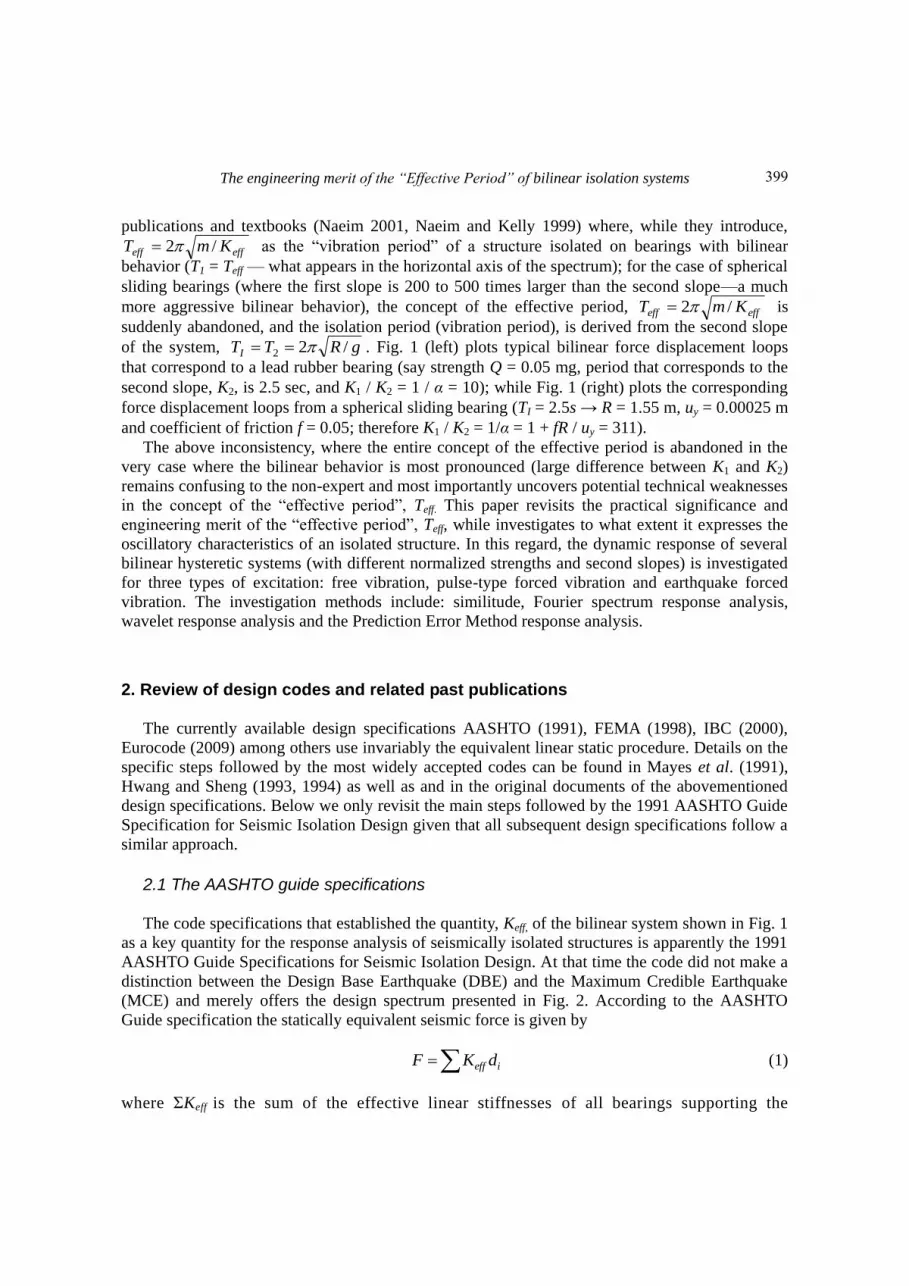
Fig. 4 Selective force-displacement loops from the free vibration response of bilinear isolation systems (T2 =
2.5s) and the associated Fourier spectra
408

The engineering merit of the “Effective Period” of bilinear isolation systems
4.1 Fourier analysis
In our investigation only runs where a full cycle or more was completed were retained and the
free-vibration period was defined as the period where the peak value in the Fourier spectrum
happens. Fig. 4 shows selective force displacement loops of the bilinear system under free
vibration response together with the corresponding Fourier spectra. The vibration period of the
system, TI, is extracted at the period where the maximum of the Fourier spectrum happens. Fig. 5
(left) plots the computed isolation period, TI, normalized to the period associated with the second
slope, 22 KmTI , as a function of the dimensionless product ПQ = Q/(K2 uy) = K1 / K2 – 1 = 1
/ α – 1. Regression analysis from all the data yields a mean value for TI / T2 = 0.99, indicating that
the function φ(Q/(K2uy)) appearing in Eq. (19) is merely a constant with value, φ = 0.99 ≈ 1. The
remarkable finding from this analysis is that the vibration period of a bilinear isolation system is
precisely the period associated with the second slope = T2. Furthermore, the standard deviation of
the computed values from the mean value TI / T2 = 0.99 is very small, SD = 0.045, showing that the
computed data are strongly correlated with the vibration period T2. Fig. 5 (right) plots the
computed isolation period, TI, from the Fourier analysis normalized to the effective period, Teff. In
this calculation the effective stiffness, Keff = Fmax / u0 was computed as the ratio of the peak force
Fmax, that develops at the peak initial displacement, u0, prior to the initiation of the motion which is
a calculation that selects the longest possible Teff. The regression analysis from all data yields a
mean value for TI / Teff = 1.06, and a very small standard deviation, SD = 0.053, indicating that Teff
is a dependable approximation of the vibration period of the bilinear system; nevertheless, the
period associated with the second slope, T2 is an even better approximation (see Fig. 5 left).
4.2 Wavelet analysis
The result offered by Fig. 5 – that the free-vibration period of the bilinear system is essentially
free-vibration response histories with wavelet analysis. Over the last two decades, wavelet the
Fig. 5 Values of the vibration period of bilinear isolation systems during free vibrations extracted with
Fourier analysis
409

Nicos Makris and Georgios Kampas
period associated strictly with the second slope, is further confirmed by analyzing the transform
analysis has emerged as a unique new time-frequency decomposition tool for signal processing
and data analysis. There is a wide literature available regarding its mathematical foundation and its
applications (Mallat 1999, Addison 2002 and references reported therein). Wavelets are simple
wavelike functions localized on the time axis. For instance, the second derivative of the Gaussian
distribution, 2/2te , known in seismology literature as the symmetric Ricker wavelet (Ricker 1943,
1944 and widely referred as the ―Mexican Hat‖ wavelet, Addison 2002)
2/2 2
)1()( tett (21)
is a widely used wavelet. Similarly the time derivative of Eq. (21) or a one cycle cosine function
are also wavelets. A comparison on the performance of various symmetric and antisymmetric
wavelet to fit acceleration records is offered in Vassiliou and Makris (2011). In order for a
wavelike function to be classified as a wavelet, the wavelike function must have: (a) finite energy
dttE2
)( (22)
and (b) a zero mean. In this work we are merely interested to achieve a local matching of the
response history of a bilinear system with a wavelet that will offer the best estimates of period, TI.
Accordingly, we perform a series of inner products (convolutions) of the acceleration response
history of the bilinear system, )(tu with the wavelet )(t by manipulating the wavelet through a
process of translation (i.e., movement along the time axis) and a process of dilation-contraction
(i.e., spreading out or squeezing of the wavelet)
dt
s
ttuswsC
)()(),( (23)
The values of s = S and ξ = Ξ for which the coefficient, C(s, ξ) becomes maximum offer the
scale and location of the wavelet )()( stsw that locally matches best the free-vibration
response history, )(tu . Eq. (23) is the definition of the wavelet transform. The quantity w(s)
outside the integral in Eq. (23) is a weighting function. Typically, w(s) is set equal to s1 in
order to ensure that all daughter wavelets )()()(, stswts at every scale s have the
same energy. The same energy requirement among all the daughter wavelets ψs,ξ(t) is the default
setting in the MATLAB wavelet toolbox (2002) and what is used in this analysis. A detail analysis
on the role of the weighting function in the definition of the wavelet transform is presented in
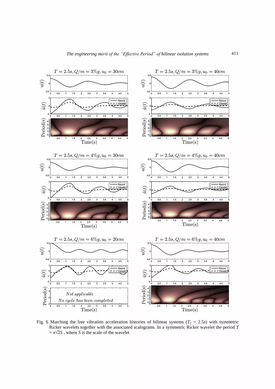
Vassiliou and Makris (2011). Each set of plots in Fig. 6 show the best matching Ricker wavelet on
selected free vibration responses of bilinear isolation systems (center); while, the associated
scalogram (bottom) shows contours of the value of C(s, ξ) as defined by Eq. (23) for all locations, t,
and all scales, ξ. The maximum value C(s, ξ) happens at the most bright location of the contour.
Similar to Fig. 5 (left), Fig. 7(left) plots the computed isolation period TI normalized to the
period associated with the second slope 22 KmTI , as a function of the dimensionless
product ПQ = Q / (K2uy) = K1 / K2 – 1 = 1 / α – 1 as extracted with wavelet analysis. In Fig. 7 the
period of free vibration of the bilinear system has been extracted with the symmetric Ricker
410
The engineering merit of the “Effective Period” of bilinear isolation systems
Fig. 6 Matching the free vibration acceleration histories of bilinear systems (T2 = 2.5s) with symmetric
Ricker wavelets together with the associated scalograms. In a symmetric Ricker wavelet the period T
= π√2̄S , where S is the scale of the wavelet
411
Nicos Makris and Georgios Kampas
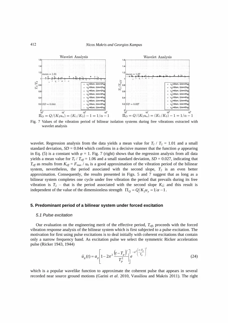
Fig. 7 Values of the vibration period of bilinear isolation systems during free vibrations extracted with
wavelet analysis
wavelet. Regression analysis from the data yields a mean value for TI / T2 = 1.01 and a small
standard deviation, SD = 0.044 which confirms in a decisive manner that the function φ appearing
in Eq. (5) is a constant with φ = 1. Fig. 7 (right) shows that the regression analysis from all data
yields a mean value for TI / Teff = 1.06 and a small standard deviation, SD = 0.027, indicating that
Teff as results from Keff = Fmax / u0 is a good approximation of the vibration period of the bilinear
system, nevertheless, the period associated with the second slope, T2 is an even better
approximation. Consequently, the results presented in Figs. 5 and 7 suggest that as long as a
bilinear system completes one cycle under free vibration the period that prevails during its free
vibration is T2 – that is the period associated with the second slope K2; and this result is
independent of the value of the dimensionless strength 112 yQ uKQ .
5. Predominant period of a bilinear system under forced excitation
5.1 Pulse excitation
Our evaluation on the engineering merit of the effective period, Teff, proceeds with the forced
vibration response analysis of the bilinear system which is first subjected to a pulse excitation. The
motivation for first using pulse excitations is to deal initially with coherent excitations that contain
only a narrow frequency band. As excitation pulse we select the symmetric Ricker acceleration
pulse (Ricker 1943, 1944)
2
22
2
221)(
p
p
T
Tt
p
p
pg eT
Ttatu
(24)
which is a popular wavelike function to approximate the coherent pulse that appears in several
recorded near source ground motions (Garini et al. 2010, Vassiliou and Makris 2011). The right
412

The engineering merit of the “Effective Period” of bilinear isolation systems
hand side of Eq. (24) is merely the mother Ricker wavelet given by Eq. (21) which has been
magnified with an acceleration amplitude ap dilated by a scale 22 pTs and translated by Tp.
The forced vibration response of the bilinear system is fully described by the three parameter
mentioned before which describe its bilinear behavior–that is the normalized strength, mQ , the
normalized second slope, 22 2 KmT , and the yield displacement, uy; together with the two
parameters that describe the pulse excitation–that is the pulse acceleration, ap, and the pulse
period, Tp. Accordingly, the period that dominates the forced vibration response of the bilinear
system – that is the isolation period, TI, is a function of
ppyI TaTu
m
QfT ,,,, 2 (25)
The six variables appearing in Eq. (26) TI = [T], Q/m = [L][T]-2
, uy = [L],
][2 22 TKmT , ap = [L][T]-2 and Tp = [T] involve again only two reference dimension that
of length [L] and time [T]; therefore, the number of dimensionless products that describe the
problem is 6-2=4. As in the previous sections the choice for the repeating variables is the period
associated with the second slope, ][2 22 TKmT and the yield displacement, uy = [L].
Based on this organization the dependent dimensionless product
2T
T II (26)
is a function only of the independent dimensionless products
y
QuK
Q
2
(27)
2T
Tp
T (28)
y
p
au
Ta2
2 (29)
While the first two dimensionless products ПQ and ПT have a clear engineering significance, the
engineering significance of Пa is not clear. Nevertheless, the quantity, Пa / ПQ = 4π2map / Q which
is the ratio of the inertia forces to the strength of the system has a clear engineering significance.
Accordingly, the dimensionless product given by Eq. (29) is replaced with the dimensionless
product
Q
map
Q
aaq
24
1
(30)
and Eq. (27) is reduced to
413

Nicos Makris and Georgios Kampas
2
22222
),,(),,( TQ
ma
T
T
uK
QT
Q
ma
T
T
uK
Q
T
T pp
y
I
pp
y
I (31)
As in the free vibration case, Eq. (31) indicates that the period which prevails during force
vibration–that is the isolation period is equal to the period associated with the second
slope 22 2 KmT , while being modified by some function QmaTTuKQ ppy ,, 22 .
The dynamic response of a mass, m, supported on isolation bearings with bilinear behavior as
described in Fig. 1 is governed by
)()()(2
2 tutzm
Qtuu g
(32)
where u(t) = relative to the ground displacement history, )(tug ground acceleration, Q/m =
specific strength, ω2 = 2π/T2 and z(t) = hysteretic dimensionless quantity with 1)( tz that is
governed by
0)()()()()()()(1
tutztutztztutzunn
y (33)
The model given by Eqs. (32) and (33) is the Bouc-Wen model (Wen 1975, 1976) in which β, γ
and n are dimensionless quantities that control the shape of the hysteretic loop. Fig. 8 plots with a
solid line the acceleration responses above isolators of two different isolation systems subjected to
a Ricker pulse excitation shown below.
5.1.1 Wavelet analysis
The identification of the vibration period of bilinear isolation systems subjected to pulse
excitation is first achieved with the wavelet analysis introduced in the previous section. Fig. 8
(left) plots with a dashed line the best matching wavelet (Vassiliou and Makris 2011) on the
acceleration response history above isolators with bilinear behavior. A number of bilinear systems
and Ricker pulse excitations have been selected to cover a wide range of the dimensionless
products given by Eqs. (27), (28) and (30). Fig. 9 (left) plots the computed isolation period TI
normalized to the period associated with the second period 22 2 KmT as a function of the
dimensionless products ПQ = Q/(K2 uy) = K1 / K2 – 1 = 1/α – 1 as extracted with wavelet analysis in
which the daughter wavelet is the Mavroeidis and Papageorgiou (M&P) wavelet (Vassiliou and
Makris 2011). Regression analysis from all data yields a mean value for TI / T2 = 1.05, indicating
that the function QmaTTuKQ ppy ,, 22 appearing in Eq. (19) is a constant with value φ =
1.05. At the same time it shall be recognized that the standard deviation now is SD = 0.082 which
is two times larger than the value of the standard deviation computed during the free vibration
response (see Fig. 5 and 7). Fig. 9 (right) plots the computed vibration (isolation) period, TI, with
wavelet analysis normalized to the effective period, Teff. In this calculation the effective stiffness,
Keff = Fmax / umax was computed by finding the peak force developed at the peak inelastic
displacement umax identified during the response history and regression analysis from all data
yields a mean value for TI / Teff = 1.15 and a standard deviation SD = 0.076. Accordingly, this
analysis shows that Teff as given by Eq. (5) is a dependable approximation of the vibration period
of the bilinear system; nevertheless, the period associated with the second slope, T2, is an even
better approximation.
414
The engineering merit of the “Effective Period” of bilinear isolation systems
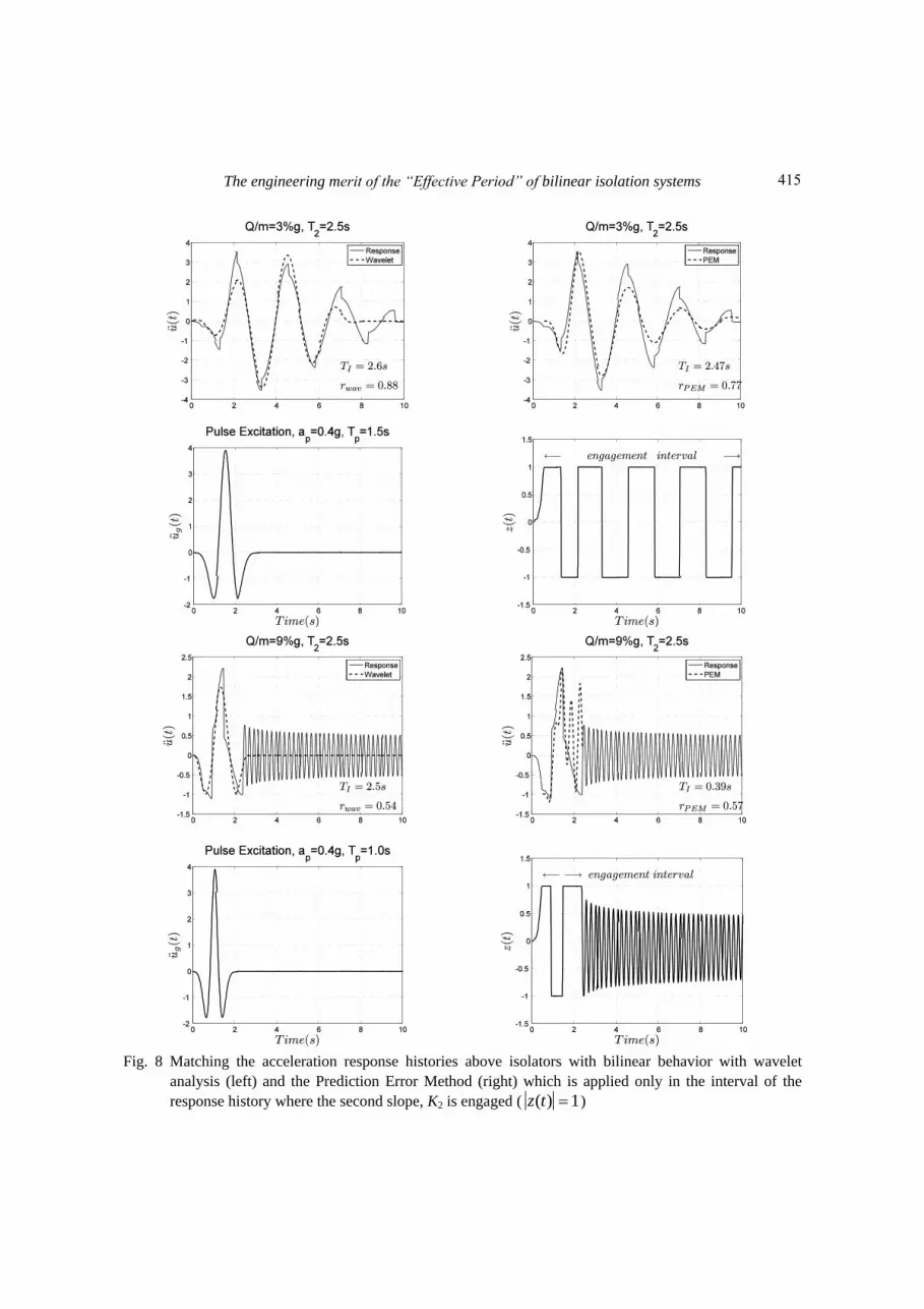
Fig. 8 Matching the acceleration response histories above isolators with bilinear behavior with wavelet
analysis (left) and the Prediction Error Method (right) which is applied only in the interval of the
response history where the second slope, K2 is engaged ( 1)( tz )
415
Nicos Makris and Georgios Kampas
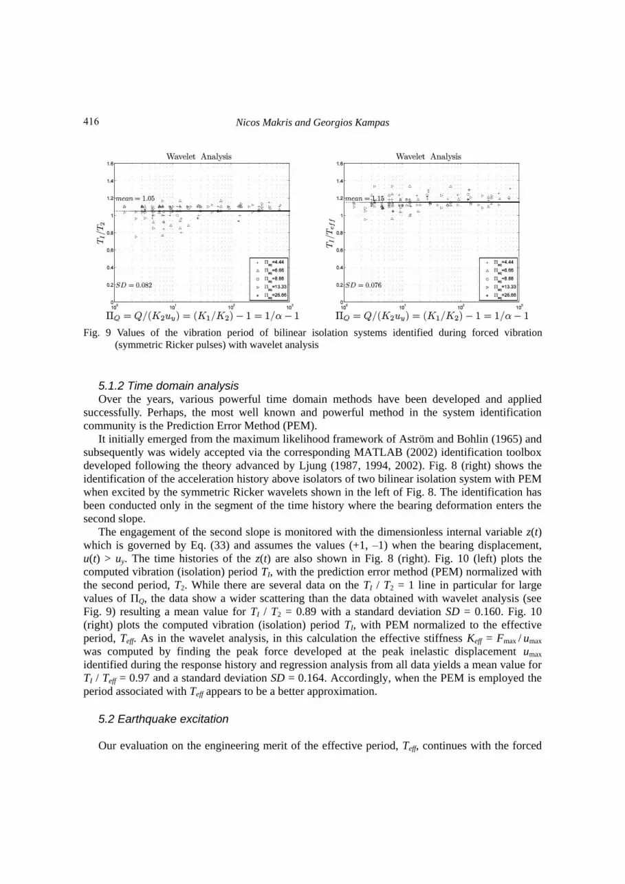
Fig. 9 Values of the vibration period of bilinear isolation systems identified during forced vibration
(symmetric Ricker pulses) with wavelet analysis
5.1.2 Time domain analysis Over the years, various powerful time domain methods have been developed and applied
successfully. Perhaps, the most well known and powerful method in the system identification
community is the Prediction Error Method (PEM).
It initially emerged from the maximum likelihood framework of Aström and Bohlin (1965) and
subsequently was widely accepted via the corresponding MATLAB (2002) identification toolbox
developed following the theory advanced by Ljung (1987, 1994, 2002). Fig. 8 (right) shows the
identification of the acceleration history above isolators of two bilinear isolation system with PEM
when excited by the symmetric Ricker wavelets shown in the left of Fig. 8. The identification has
been conducted only in the segment of the time history where the bearing deformation enters the
second slope.
The engagement of the second slope is monitored with the dimensionless internal variable z(t)
which is governed by Eq. (33) and assumes the values (+1, –1) when the bearing displacement,
u(t) > uy. The time histories of the z(t) are also shown in Fig. 8 (right). Fig. 10 (left) plots the
computed vibration (isolation) period TI, with the prediction error method (PEM) normalized with
the second period, T2. While there are several data on the TI / T2 = 1 line in particular for large
values of ПQ, the data show a wider scattering than the data obtained with wavelet analysis (see
Fig. 9) resulting a mean value for TI / T2 = 0.89 with a standard deviation SD = 0.160. Fig. 10
(right) plots the computed vibration (isolation) period TI, with PEM normalized to the effective
period, Teff. As in the wavelet analysis, in this calculation the effective stiffness Keff = Fmax / umax
was computed by finding the peak force developed at the peak inelastic displacement umax
identified during the response history and regression analysis from all data yields a mean value for
TI / Teff = 0.97 and a standard deviation SD = 0.164. Accordingly, when the PEM is employed the
period associated with Teff appears to be a better approximation.
5.2 Earthquake excitation
Our evaluation on the engineering merit of the effective period, Teff, continues with the forced
416
The engineering merit of the “Effective Period” of bilinear isolation systems
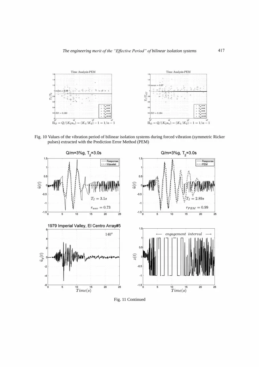
Fig. 10 Values of the vibration period of bilinear isolation systems during forced vibration (symmetric Ricker
pulses) extracted with the Prediction Error Method (PEM)
Fig. 11 Continued
417
Nicos Makris and Georgios Kampas
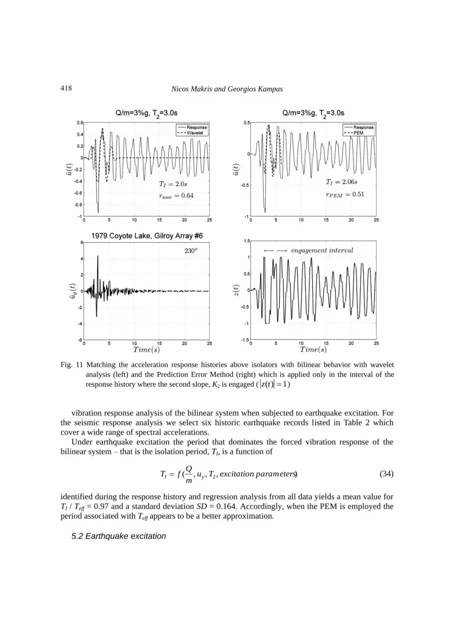
Fig. 11 Matching the acceleration response histories above isolators with bilinear behavior with wavelet
analysis (left) and the Prediction Error Method (right) which is applied only in the interval of the
response history where the second slope, K2 is engaged ( 1)( tz )
vibration response analysis of the bilinear system when subjected to earthquake excitation. For
the seismic response analysis we select six historic earthquake records listed in Table 2 which
cover a wide range of spectral accelerations.
Under earthquake excitation the period that dominates the forced vibration response of the
bilinear system – that is the isolation period, TI, is a function of
),,,( 2 parametersexcitationTum
QfT yI (34)
identified during the response history and regression analysis from all data yields a mean value for
TI / Teff = 0.97 and a standard deviation SD = 0.164. Accordingly, when the PEM is employed the
period associated with Teff appears to be a better approximation.
5.2 Earthquake excitation
418

The engineering merit of the “Effective Period” of bilinear isolation systems
Table 2 Earthquake records selected for this study
Earthquake Record station Magnitude, Mw PGA(g)
1979 Coyote Lake, CA Gilroy Array #6 230 5.7 0.43
1979 Imperial Valley, CA El Centro Array #5 140 6.5 0.52
1986 El Salvador Geot. Inv. Center 180 5.5 0.48
1992 Erzincan, Turkey 95 Erzincan 6.9 0.52
1992 Cape Mendocino, CA Cape Mendocino/000 7.2 1.49
1995 Aigion, Greece OTE Building 6.2 0.54
Our evaluation on the engineering merit of the effective period, Teff, continues with the forced
vibration response analysis of the bilinear system when subjected to earthquake excitation. For the
seismic response analysis we select six historic earthquake records listed in Table 2 which cover a
wide range of spectral accelerations.
Under earthquake excitation the period that dominates the forced vibration response of the
bilinear system – that is the isolation period, TI, is a function of
),,,( 2 parametersexcitationTum
QfT yI (34)
In analogy to the dimensional analysis presented for the case of forced vibrations under pulse
excitation (see Eq. (33)), Eq. (34) can be expressed in terms of dimensionless products
)parameters excitation essdimensionluK
Q
T
T
y
I ,(22
(35)
As in the case of pulse excitation, Eq. (35) indicates that the period which prevails during force
vibration – that is the isolation period is equal to the period associated with the second
slope 22 2 KmT , while being modified by some function yuKQ 2( , essdimensionl )parameters excitation .
The identification of the ―vibration‖ period of bilinear isolation systems subjected to
earthquake excitation is first achieved with wavelet analysis.
Fig. 11 (left) plots with a dashed line the best matching Mavroeidis and Papageorgiou (M&P)
wavelet (Vassiliou and Makris 2011) on the acceleration response history of a bilinear system with
strength Q/m = 0.03 g and period that corresponds to the second slope T2 = 3s when subjected to
the El Centro Array#5 ground motion recorded during the 1979 Imperial Valley earthquake. A
number of bilinear systems have been selected to cover a wide range of the dimensionless product
ПQ = Q/K2 uy = 1 / α – 1 and values of yield strength Q/(mg) = 3%, 5%, 7% and 9%. Fig. 12 (left)
plots the computed isolation period TI normalized to the period associated with the second slope
22 2 KmT as a function if the dimensionless product ПQ = 1 / a – 1 as extracted with
wavelet analysis in which the daughter wavelet is the M&P wavelet (Vassiliou and Makris 2011).
Fig. 12 (left) shows that the mean value of TI / T2 = 0.94 is close to unity; nevertheless, the
scattering of the data from the mean value is now appreciable yielding a value for the standard
deviation, SD = 0.310.
419
Nicos Makris and Georgios Kampas
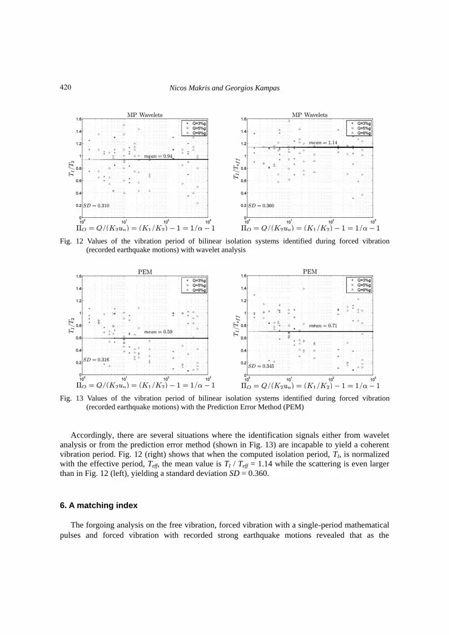
Fig. 12 Values of the vibration period of bilinear isolation systems identified during forced vibration
(recorded earthquake motions) with wavelet analysis
Fig. 13 Values of the vibration period of bilinear isolation systems identified during forced vibration
(recorded earthquake motions) with the Prediction Error Method (PEM)
Accordingly, there are several situations where the identification signals either from wavelet
analysis or from the prediction error method (shown in Fig. 13) are incapable to yield a coherent
vibration period. Fig. 12 (right) shows that when the computed isolation period, TI, is normalized
with the effective period, Teff, the mean value is TI / Teff = 1.14 while the scattering is even larger
than in Fig. 12 (left), yielding a standard deviation SD = 0.360.
6. A matching index
The forgoing analysis on the free vibration, forced vibration with a single-period mathematical
pulses and forced vibration with recorded strong earthquake motions revealed that as the
420

The engineering merit of the “Effective Period” of bilinear isolation systems
frequency content of the excitation widens and the intensity of the excitation fluctuates the
standard deviations of the predicted ―linear vibration period‖ of the bilinear system increases
regardless whether this vibration period, TI, is approximated with either the effective period,
)(11 max22 uKQTTeff or merely with the period associated with the second slope, TI, –
which in general offers superior results. The wide scattering of some data points from the mean
values of TI / T2 or TI / Teff in Figs. 9-13 is because in the corresponding response histories the
nonlinearities associated with the bilinear behavior dominate the response; therefore, the concept
of associating a ―vibration period‖ as required by the current design codes is meaningless.
Interestingly, the scattering of data does not show any correlation with the normalized strength of
the system. For instance, Fig. 11 (bottom-left) plots with dashed line the best matching M&P
wavelet on the acceleration response history of a bilinear system with strength Q/mg = 0.03 and T2
= 3s when subjected to the 1979 Coyote Lake, Gilroy Array #5 record; while Fig. 11 (right) plots
with a dashed line the response of the best matching equivalent linear system, as identified with
PEM during the time interval that the second slope of the bilinear system is engaged. With the
wavelet identification TI = 2.0s (TI / T2= 0.66 and TI / Teff = 0.81) while with the PEM identification
TI = 2.06s (TI / T2 = 0.69 and TI / Teff = 0.83). The ratios for TI / T2 or TI / Teff given above in
association with the assessment after visual observation of the scattering of all data in Figs. 12 and
13 suggest that the idea of associating a vibration period in several occasions should be abandoned.
Consequently, we reach the conclusion that for bilinear isolation systems the ―period of vibration‖
as expressed in most current design codes (AASHTO (1991), NZMWD (1983), FEMA (1998),
Eurocode (2009) among others) can be identified only for certain combination of bilinear systems
and ground motions. There is a class of response histories above isolators that are not capable to
reveal any ―vibration period‖. In this section we attempt to identify this class of response histories
by proposing a matching index.
The idea behind developing a dependable matching index is that the wavelet signal or the PEM
signal that is derived from the identification algorithms introduced earlier need to match to a
reasonable extent the acceleration history of the bilinear system (accelerations above isolators).
Accordingly, we introduce a matching index rwav and a matching index rPEM as the ratio of the
inner product of the best matching signal with the record normalized by the energy of the record
10,
)]([
)()(
0
2
0
wavT
b
T
b
wav r
dttu
dttut
re
e
and 10,
)]([
)()(
0
2
0
PEMT
b
T
b
PEM r
dttu
dttuta
re
e
(36)
where ψ(t) is the best matching wavelet, a(t) is the acceleration history of the resulted PEM signal
and )(tub is the acceleration history of the bilinear system above isolators. Clearly, both rwav and
rPEM assume values between zero and one. Fig. 14 (top) plots the vibration periods of a wide range
of bilinear systems identified during forced vibrations (pulse and earthquake excitations) with
wavelet analysis (all data appearing in Figs. 9 and 12), where now they are plotted as a function of
the matching index rwav defined by Eq. (36). Fig. 14 (top) reveals that regardless if the data are
normalized with T2 or Teff their dispersion decreases as rwav increases. Fig. 14 (bottom) plots the
standard deviation of the data shown in Fig. 14 (top) for any given value of rwav up to rwav = 1. For
421
Nicos Makris and Georgios Kampas
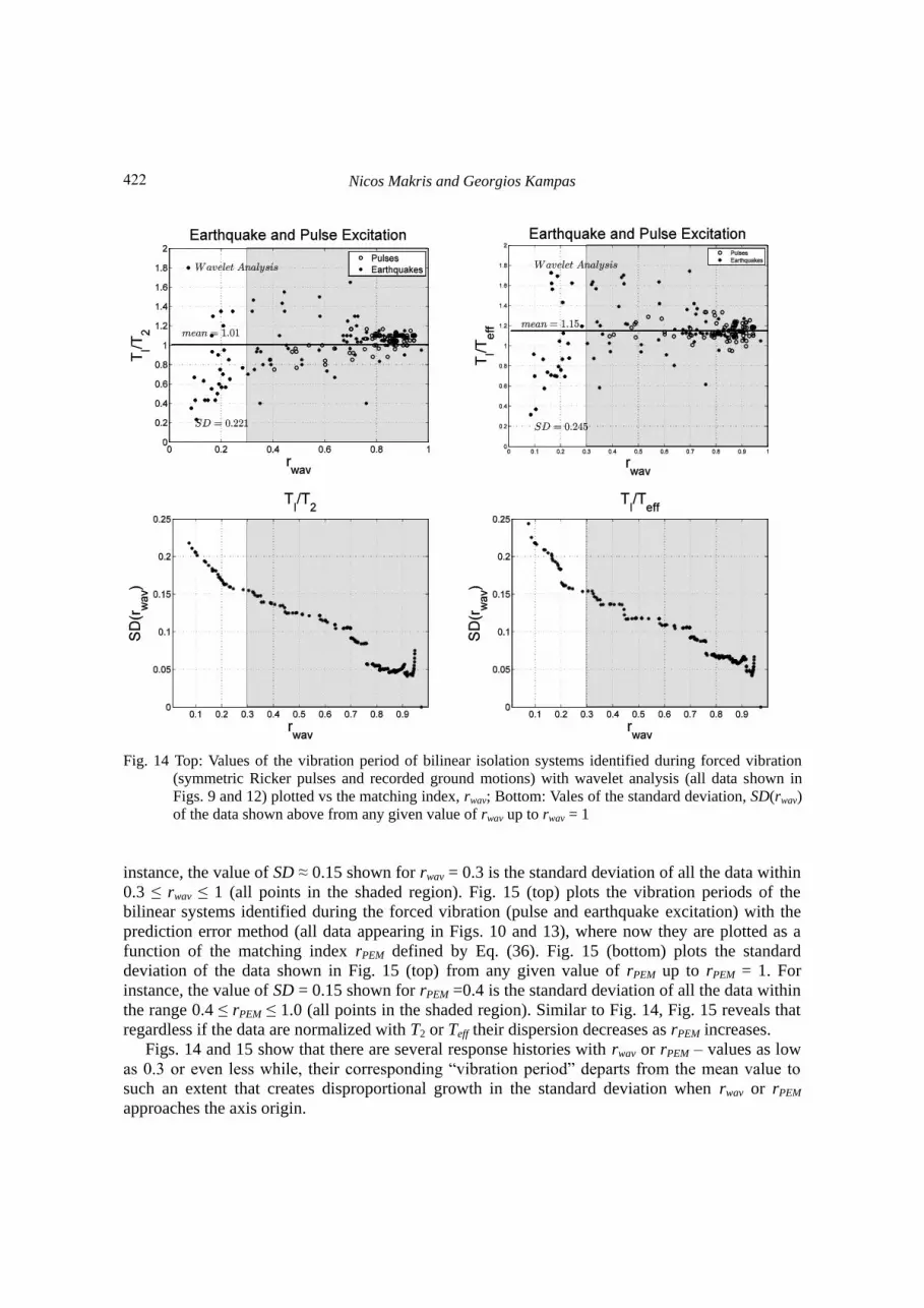
Fig. 14 Top: Values of the vibration period of bilinear isolation systems identified during forced vibration
(symmetric Ricker pulses and recorded ground motions) with wavelet analysis (all data shown in
Figs. 9 and 12) plotted vs the matching index, rwav; Bottom: Vales of the standard deviation, SD(rwav)
of the data shown above from any given value of rwav up to rwav = 1
instance, the value of SD ≈ 0.15 shown for rwav = 0.3 is the standard deviation of all the data within
0.3 ≤ rwav ≤ 1 (all points in the shaded region). Fig. 15 (top) plots the vibration periods of the
bilinear systems identified during the forced vibration (pulse and earthquake excitation) with the
prediction error method (all data appearing in Figs. 10 and 13), where now they are plotted as a
function of the matching index rPEM defined by Eq. (36). Fig. 15 (bottom) plots the standard
deviation of the data shown in Fig. 15 (top) from any given value of rPEM up to rPEM = 1. For
instance, the value of SD = 0.15 shown for rPEM =0.4 is the standard deviation of all the data within
the range 0.4 ≤ rPEM ≤ 1.0 (all points in the shaded region). Similar to Fig. 14, Fig. 15 reveals that
regardless if the data are normalized with T2 or Teff their dispersion decreases as rPEM increases.
Figs. 14 and 15 show that there are several response histories with rwav or rPEM – values as low
as 0.3 or even less while, their corresponding ―vibration period‖ departs from the mean value to
such an extent that creates disproportional growth in the standard deviation when rwav or rPEM
approaches the axis origin.
422

The engineering merit of the “Effective Period” of bilinear isolation systems
Accordingly, there is a need to develop a procedure to separate the ―good‖ response histories
where the concept of associating a ―vibration period‖ as required by the current design codes is
meaningful. This separation is most useful in system identification studies which attempt to extract
the isolation period of seismically isolated bridges from recorded signals above and below
isolators.
7. Selection of the “Good” response histories
The final goal of this paper is to separate the response histories of bilinear systems where the
concept of associating a ―vibration period‖ as required by the current design codes is meaningful;
from the response histories where the concept of associating a vibration period is meaningless.
This separation can be achieved if one observes the plots of the standard deviations, SD(rwav) and
SD(rPEM), shown in Figs. 14 (bottom) and 15 (bottom) which exhibit a growing values of SD when
rwav < 0.3 or when rPEM < 0.4. Our aim is to take the best elements offered by the wavelet analysis
and by the Prediction Error Method (PEM). We return now to Fig. 11 (bottom) where the isolation
system with Q/mg = 0.03 and T2 = 3s when excited by the 1979 Coyote Lake, Gilroy Array#6
record experienced few and small displacements beyond the yield displacement uy (see the few and
small plateaus in the z-history). In such situations the response history above isolators contains
poor information regarding the isolation period, T2, associated with the second slope of the bilinear
system. Accordingly, when evaluating a response history we need also to include a measure that
indicates to what extent the second slope of the bilinear system was engaged. This need is served
with the engagement ratio ΣNiplateau/ΣNi where Niplateau are the number of data points within
the segment where 1)( tz and Ni are all the data points between the first and last yielding of the
system during the excitation.
Our selection process proceed by taking only the data in Fig. 14 with rwav > 0.3 or the data in
Fig. 15 with rPEM > 0.4 and re-evaluate them by computing an improved matching index which
incorporates the engagement ratio
10,2
1 22,
rrrN
Nr PEMwav
i
plateaui (37)
Any response history with either rwav > 0.3 or rPEM > 0.4 is retained as a potentially ―good‖
response history and its identified vibration period appears in Fig. 16.
Accordingly, Fig. 16 (top) shows the vibration periods extracted from the responses of bilinear
systems that passed the first screening (rwav > 0.3 or rPEM > 0.4) and are plotted as a function of the
improved matching index, r, given by Eq. (37). Therefore, the number of data shown in Fig. 16 is
smaller than the number of the data appearing in Fig. 14 or Fig. 15. It is interesting to note in Fig.
16, several response histories which passed the first screening (rwav > 0.3 or rPEM > 0.4) their
improved r index is now poor (r > 0.3)–therefore, the need for a more refine selection. Fig. 16
(bottom) plots the standard deviation of the data shown in Fig. 16 (top) from any given value of r
423

Nicos Makris and Georgios Kampas
Fig. 15 Top: Values of the vibration period of bilinear isolation systems identified during forced vibration
(symmetric Ricker pulses and recorded ground motions) with PEM (all data shown in Figs. 10 and
13) plotted vs the matching index, rPEM; Bottom: Vales of the standard deviation, SD(rPEM) of the
data shown above from any given value of rPEM up to rPEM = 1
Fig. 16 Continued
424
The engineering merit of the “Effective Period” of bilinear isolation systems
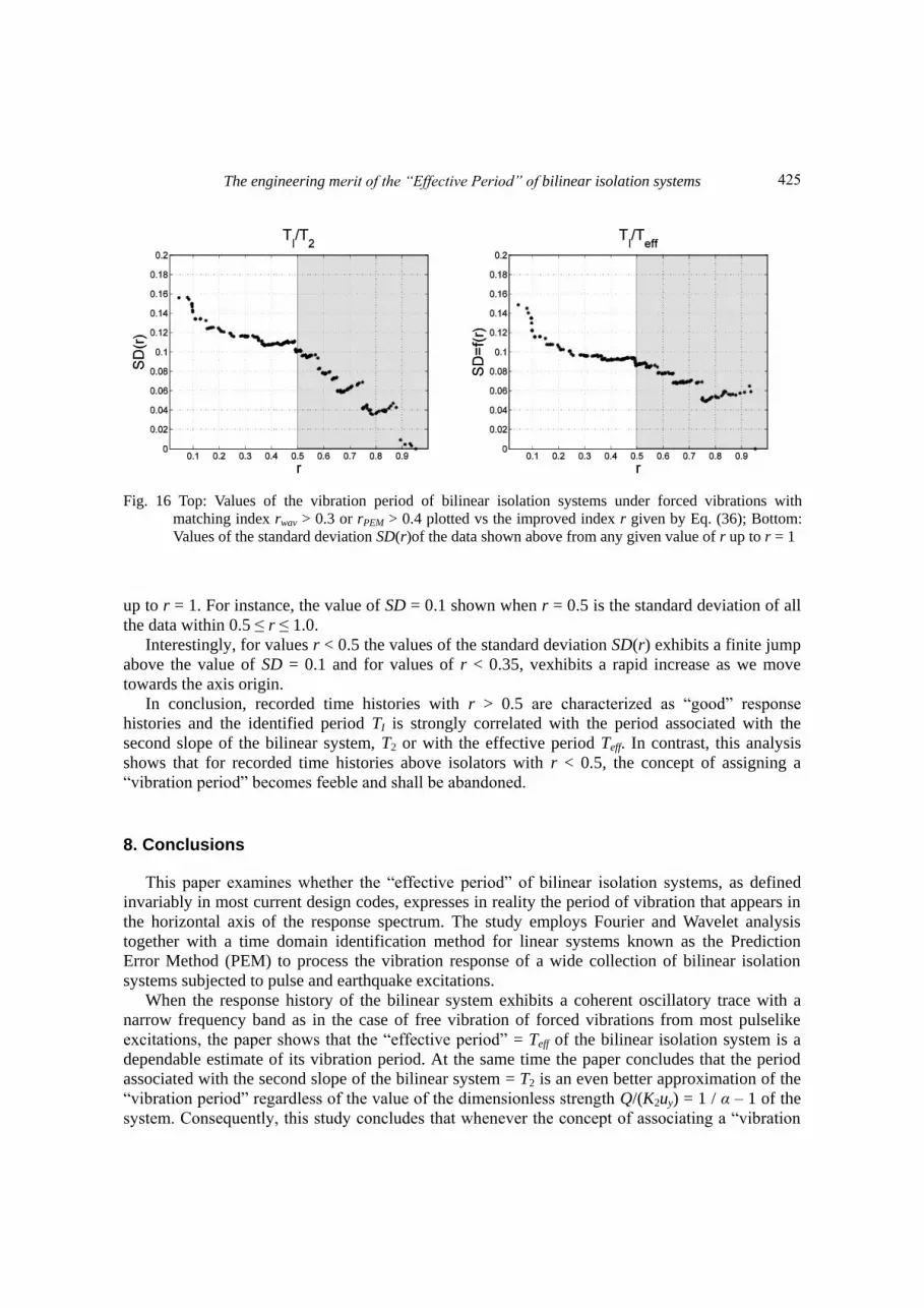
Fig. 16 Top: Values of the vibration period of bilinear isolation systems under forced vibrations with
matching index rwav > 0.3 or rPEM > 0.4 plotted vs the improved index r given by Eq. (36); Bottom:
Values of the standard deviation SD(r)of the data shown above from any given value of r up to r = 1
up to r = 1. For instance, the value of SD = 0.1 shown when r = 0.5 is the standard deviation of all
the data within 0.5 ≤ r ≤ 1.0.
Interestingly, for values r < 0.5 the values of the standard deviation SD(r) exhibits a finite jump
above the value of SD = 0.1 and for values of r < 0.35, vexhibits a rapid increase as we move
towards the axis origin.
In conclusion, recorded time histories with r > 0.5 are characterized as ―good‖ response
histories and the identified period TI is strongly correlated with the period associated with the
second slope of the bilinear system, T2 or with the effective period Teff. In contrast, this analysis
shows that for recorded time histories above isolators with r < 0.5, the concept of assigning a
―vibration period‖ becomes feeble and shall be abandoned.
8. Conclusions
This paper examines whether the ―effective period‖ of bilinear isolation systems, as defined
invariably in most current design codes, expresses in reality the period of vibration that appears in
the horizontal axis of the response spectrum. The study employs Fourier and Wavelet analysis
together with a time domain identification method for linear systems known as the Prediction
Error Method (PEM) to process the vibration response of a wide collection of bilinear isolation
systems subjected to pulse and earthquake excitations.
When the response history of the bilinear system exhibits a coherent oscillatory trace with a
narrow frequency band as in the case of free vibration of forced vibrations from most pulselike
excitations, the paper shows that the ―effective period‖ = Teff of the bilinear isolation system is a
dependable estimate of its vibration period. At the same time the paper concludes that the period
associated with the second slope of the bilinear system = T2 is an even better approximation of the
―vibration period‖ regardless of the value of the dimensionless strength Q/(K2uy) = 1 / α – 1 of the
system. Consequently, this study concludes that whenever the concept of associating a ―vibration
425
Nicos Makris and Georgios Kampas
period‖ is meaningful the ―effective‖ period, Teff can be replaced with T2 which is a period that is
known a priori (no iterations are needed) and offers in general superior results. This finding serves
both simplicity and a more rational estimation of maximum displacement. Simplicity is served
because instead of looking for Teff – a quantity that derives from the non-existing Keff, for which
iterations are needed to be approximated, the paper shows that the period associated with the
second slope of the bilinear system = T2 (that is known a priori – no iterations are needed) is a
better single-value descriptor of the frequency content of the dynamic response of a bi-linear
isolation system. Given that T2 is always longer than Teff the peak inelastic displacement does no
run the risk to be underestimated.
Most importantly, the paper shows that as the frequency content of the excitation widens and
the intensity of the acceleration response history fluctuates more randomly the computed vibration
period of the bilinear isolation system exhibits appreciable scattering from the computed mean
value. This scattering of the identified period values is due to the nonlinear nature of the response
signal; and therefore, for this class of response histories the expectation of the design codes to
identify a ―linear vibration period‖ has marginal engineering merit.
The paper develops a physically motivated matching index that permits the separation of the
response histories of bilinear systems where the concept of associating a ―vibration period‖ is
meaningful from those where the concept of associating a ―vibration period‖ is feeble.
In conclusion, the engineering merit of the effective period Teff of bilinear isolation systems as
given by Eq. (5) is marginal given that: (a) whenever the concept of associating a ―vibration
period‖ is meaningful (r > 0.5), this ―vibration period‖ can be approximated in a superior way with
the period associated with the second slope = T2 as (see Figs. 5,7 and 9) and (b) when the matching
index r is low (say r < 0.5) the concept of associating a ―vibration period‖ has marginal
engineering value.
Acknowledgements
Partial financial support has been provided by the EU research project ―DARE‖
(―Soil-Foundation-Structure Systems Beyond Conventional Seismic Failure Thresholds:
Application to New or Existing Structure and Monuments‖), which is – Advanced Grant, under
contract number ERC-2---9-AdG228254-DARE to Prof. G. Gazetas.
References Addison, P.S. (2002), The illustrated wavelet transform handbook, Institute of Physics Handbook.
Anti-seismic devices (2009), European standard, FprEN 15129, Eurocode.
Aström, K.J. and Bohlin, T. (1965), ―Numerical identification of linear dynamic systems from normal
operating records‖, IFAC Symposium on Self-Adaptive Systems, Teddington, England.
Buckle, I.G. and Mayes, R.L. (1990), ―Seismic isolation: History, application and performance – A world
view‖, Earthq. Spectra J., 6(2), 161-201.
Caughey, T.K. (1960), ―Random excitation of a system with bilinear hysteresis‖, J. Appl. Mech., 27(4),
649-652.
Caughey, T.K. (1963), ―Equivalent linearization techniques‖, J. Acoust. Soc. Am., 35(11), 1706-1711.
Constantinou, M.C., Mokha, A.S. and Reinhorn, A.M. (1990), ―Teflon bearing in base isolation. II:
modeling‖, J. Struct. Eng.-ASCE, 116(2), 455-474.
426

The engineering merit of the “Effective Period” of bilinear isolation systems
Crandall, S.H. (2006), ―A half-century of stochastic equivalent linearization‖, J. Struct. Contr. Health
Monitor., 13(1), 27-40.
Design of lead-rubber bearings (1983), Civil division publication 818/A, New Zealand Ministry of Works
and Development, Wellington, New Zealand.
FEMA 310 (1998), Handbook for the seismic evaluation of buildings – A prestandard, ASCE.
Garini, E., Gazetas, G. and Anastasopoulos, I. (2010), ―Accumulated assymetric slip caused by motions
containing severe ‗Directivity‘ and ‗Fling‘ pulses‖, Geotechnique, 61(9), 733-756.
Guide specifications for seismic isolation design (1991), American association of state highway and
transportation officials, Washington, D.C.
Hwang, J.S. and Chiou, J.M. (1996), ―An equivalent linear model of lead-rubber seismic isolation bearings‖,
J. Eng. Struct., 18(7), 528-536.
Hwang, J.S. and Sheng, L.H. (1993), ―Equivalent elastic seismic analysis of base-isolated bridges with
lead-rubber bearings‖, J. Eng. Struct., 16(3), 201-209.
Hwang, J.S. and Sheng, L.H. (1994), ―Effective stiffness and equivalent damping of base-isolated bridges‖,
J. Struct. Eng., 119(10), 3094-3101.
International Code Council (2000), International building code.
Iwan, W.D. and Gates, N.C. (1979), ―The effective period and damping of a class of hysteretic structures‖, J.
Earthq. Eng. Struct. D., 7(3), 199-211.
Iwan, W.D. (1980), ―Estimating inelastic response spectra from response spectra‖, J. Earthq. Eng. Struct. D.,
8(4), 375-388.
Kelly, J.M., Eidinger, J.M. and Derham, C.J. (1977), A practical soft story system, Report No.
UCB/EERC-77|27, Earthquake Engineering Research Center, University of California, Berkeley, CA,
USA.
Kelly, J.M. (1986), ―A seismic base isolation: Review and bibliography‖, J. Soil Dyn. Earthq. Eng., 5(4),
202-216.
Ljung, L. (1987), System identification-theory for the user, Prentice-Hall, New Jersey.
Ljung, L. (1994), ―State of the art in linear system identification: Time and frequency domain methods‖,
Proceedings of ’04 American Control Conference, 1, 650-660.
Ljung, L. (2002), ―Prediction error estimation methods‖, Circ. Syst. Signal Pr., 21(1), 11-21.
Makris, N. and Black, C.J. (2004a), ―Dimensional analysis of rigid-plastic and elastoplastic structures under
pulse-type excitations‖, J. Eng. Mech., 130(9), 1006-1018.
Makris, N. and Black, C.J. (2004b), ―Dimensional analysis of bilinear oscillators under pulse-type
excitations‖, J. Eng. Mech., 130(9), 1019-1031.
Makris, N. and Black, C. (2004c), ―Evaluation of peak ground velocity as a ‗‗good‘‘ intensity measure for
near-source ground motions‖, J. Eng. Mech.-ASCE, 130(9), 1032-1044.
Makris, N. and Chang, S. (2000), ―Effect of viscous, viscoplastic and friction damping on the response of
seismic isolated structures‖, J. Earthq. Eng. Struct. D., 29(1), 85-107.
Makris, N. and Vassiliou, M.F. (2011), ―The existence of ‗complete similarities‘ in the response of seismic
isolated structures subjected to pulse-like ground motions and their implications in analysis‖, J. Earthq.
Eng. Struct. D., 40(10), 1103-1121.
Mallat, S.G. (1999), A wavelet tour of signal processing, Academic Press.
MATLAB (2002), High-performance language software for technical computation, The MathWorks, Inc:
Natick, MA, USA.
Mayes, R.L., Buckle, I.G., Kelly, T.E. and Jones, L.R. (1991), ―AASHTO seismic isolation design
requirements for highway bridges‖, J. Struct. Eng., 118(1), 284-304.
Mokha, A.S., Constantinou, M.C. and Reinhorn, A.M. (1990), ―Teflon bearing in base isolation. I: Testing‖,
J. Struct. Eng.-ASCE, 116(2), 438-454.
Naeim, F. and Kelly, J.M. (1999), Design of seismic isolated structures, New York: Wiley Publications.
Naeim, F. (2001), The seismic design handbook, Springer.
Ricker, N. (1943), ―Further developments in the wavelet theory of seismogram structure‖, B. Seismol. Soc.
Am., 33(3), 197-228.
427
Nicos Makris and Georgios Kampas
Ricker, N. (1944), ―Wavelet functions and their polynomials‖, Geophysics, 9(3), 314-323.
Roberts, J.B. and Spanos, P.D. (2003), Random vibration and statistical linearization, New York, Dover
Publications.
Vassiliou, M.F. and Makris, N. (2011), ―Estimating time scales and length scales in pulselike earthquake
acceleration records with wavelet analysis‖, B. Seismol. Soc. Am., 101(2), 96-618.
Veletsos, A.S. and Newmark, N.M. (1960), Effect of inelastic behavior on the response of simple systems to
earthquake motions, University of Illinois, IL, USA.
Veletsos, A.S., Newmark, N.M. and Chelepati, C.V. (1969), ―Deformation spectra for elastic and
elastoplastic systems subjected to ground shock and earthquake motions‖, Proceedings of the 3rd World
Conference on Earthquake Engineering, II, Wellington, New Zealand: 663-682.
Veletsos, A.S. and Vann, W.P. (1971), ―Response of ground-excited elastoplastic systems‖, J. Struct.
Div.-ASCE, 97(ST4), 1257-1281.
Wen, Y.K. (1975), ―Approximate method for nonlinear random vibration‖, J. Eng. Mech., 101(4), 389-401.
Wen, Y.K. (1976), ―Method for random vibration of hysteretic systems‖, J. Eng. Mech., 102(2), 249-263.
SA
428