The dynamics of the real exchange rate: aBayesian DSGE approach

R. Cristadoro, A. Gerali, S. Neri, M. Pisani∗

Incomplete - This draft August, 21 2006

Abstract

This paper empirically analyzes the importance of various features introduced inmodels belonging to the new open economy macroeconomics (NOEM) literature inreproducing the main stylised facts of the real exchange rate and accounting for itsdynamics. Different models are estimated using euro-area and US data. First, thedata support the model featuring incomplete pass-through due to a combination ofnominal rigidities and distribution costs. Second, international price discriminationand home bias are the main determinants of real exchange rate dynamics. Third,shocks to either the uncovered interest rate parity condition (UIP) or to preferencesare necessary to reproduce the negative correlation between the real exchange rateand consumption differentials (the well-known Backus-Smith correlation). Finally,the volatility of the real exchange rate is mainly explained by the UIP shock and,to a smaller extent, by shocks to preferences. Fundamentals are, on the contrary,mostly explained by technology and preference shocks.

JEL classification: F32, F33, F41, C11

Keywords: Real exchange rate; Distribution Costs; Bayesian Estimation.

∗We owe a special thank to Fabio Canova, Gianluca Benigno, Pierpaolo Benigno, Paul Bergin, LeifBrubakk, Gunter Coenen, Luca Dedola, Gabriel Fagan, Jordi Gali, S. Schun, Frank Smets, Mattias Villaniand participants at the workshops “New Models for Forecasting and Policy Analysis” hosted by the Bankof Italy, “Recent Developments in Macroeconomic Modelling” hosted by the South African Reserve Bank,“Dynamic Macroeconomics” hosted by the University of Bologna, at the seminars at Harvard University,Boston College and the Federal Reserve Bank of Boston.

1 Introduction

Three main stylized facts of the open economy are related to the real exchange rate. Itsfluctuations are extremely volatile and persistent but they do not affect significativelyother macroeconomic variables (the so-called “exchange rate disconnect”). Several con-tributions in the new open economy macroeconomics (NOEM) literature have extendedthe Obstfeld and Rogoff sticky-price general equilibrium model, in which the real ex-change rate is constant and the purchasing power parity (PPP henceforth) holds, toaccount for the above mentioned stylized facts (see Obstfeld and Rogoff, 1995). Theseextensions include, among others, sticky prices (Chari, Kehoe and McGrattan, 2004) andwages (Hau, 2000 and Obstfeld and Rogoff, 2000), pricing-to-market (Betts and Devereux,2000), non-traded goods (Hau, 2000 and Obstfeld and Rogoff, 2000) and distribution ser-vices (Corsetti and Dedola, 2005). The use of Bayesian techniques for estimating generalequilibrium models have also allowed researchers to estimate NOEM models (see amongothers, Bergin, 2003, Lubik and Schorfheide, 2005, de Walke, Smets and Wouters, 2005and Rabanal and Tuesta, 2006). Even more recently, these models have been developedat central banks such as the Riksbank, the Federal Reserve, the European Central Bankand the Bank of Canada.

The goal of this paper is to empirically investigate these extensions by estimating aclass of models using Bayesian techniques and data on euro-area and US macroeconomicvariables. In the first model (“complete” model) we relax all the three assumptions atthe basis of the PPP condition: international law of one price, symmetric preferences,tradability of all goods.

We make two assumption to remove the international law of one price and introduceinternational price discrimination. One is the local currency pricing (LCP) assumption.Contrary to the producer currency pricing (PCP) case, exporters face costs of adjustingprices not only in their own currency, but also in the currency of the importing country.Hence, import prices are sticky in the currency of the destination market. Chari et al.(2004) show that a high degree of sticky prices is necessary to reproduce the volatilityof the real exchange rate when there are monetary shocks.1 The other source is thatof distribution services intensive in local nontradable goods (Corsetti and Dedola, 2005).Distribution services induce differences in demand elasticity across countries.2 Thus, withmonopolistic producers the law of one price does not hold in general, even in a flexibleprice equilibrium. Hence, firms in the tradable sector would optimally charge differentwholesale prices in the two countries. The advantage of introducing distribution servicesis that, when combined with standard preferences, they contribute to generate a low price

1Kollman (2001) studies a small open economy model in which nominal prices and wages are set twoor four periods in advance, and in which monetary shocks are the dominant source of exchange ratefluctuations. His model generates variability in the real and nominal exchange rate not much differentfrom that in the data.

2Campa and Goldberg (2004) provide evidence that the presence of distribution services helps explaina lower exchange rate pass-through at the consumer level than at the producer level.

2

elasticity of imports. Thanks to the price discrimination, fluctuations in the nominalexchange rate are not fully transmitted to the price of imports (assumption of incompleteexchange rate pass-through into import prices). Hence, large exchange-rate swings do nottranslate into large consumer prices movements.

We also relax the assumption of symmetric preferences, imposing home bias in con-sumption. Finally we assume that some goods are nontradable.3 All these assumptionscan contribute to increasing the volatility of the real exchange rate.

We also assume that financial markets are incomplete and introduce a shock to theuncovered interest parity (UIP from now on) as a stochastic change in the cost of holdingforeign bonds along the lines of Turnovsky (1987) and Benigno (2001). In fact, incompleteexchange rate pass-through and nominal rigidities per se are not sufficient to replicatethe high volatility of the real exchange rate. When international financial markets arecomplete, there is a risk sharing condition linking the real exchange rate to the cross-country ratio of consumption marginal utilities. According to this condition, the volatilityof the real exchange rate is proportional to that of the fundamentals. The risk sharingcondition can be removed by assuming that only a riskless bond is internationally traded.Incomplete financial market are not able to reproduce the high volatility of the exchangerate. In fact, the uncovered interest rate parity links real exchange rate fluctuations tothe real interest rate differential; the related tilting of the consumption path and currentaccount adjustment will limit the volatility of the real exchange rate. One possible solutionis to assume that the coefficient of risk aversion is high as in Chari et al. (2004). Anotheris to introduce a low elasticity of intratemporal substitution between domestic tradableand imported goods using, as we do, distribution services. Alternatively, it is possibleto add an uncovered interest parity shock that drives a wedge between the real interestrates. The result is the weakening of the link between exchange rate and fundamentals.The introduction of the UIP shock is justified by the empirical evidence on the failure ofthe UIP condition as well as by its long-standing use in the theoretical literature.4

To help the model in reproducing the persistence of the real exchange rate, we as-sume the existence of nominal rigidities and inertia in interest rate setting by the centralbanks. Benigno (2004) shows that with staggered prices and inertial monetary policy thereal exchange rate is persistent because the adjustment of the interest rate differential issmoothed over time.

We consider two alternative models. In the first, incomplete pass-through is due only

3The role of non tradable goods in the explanation of the observed behaviour of prices and exchangerates is still debated. Chari et al. (2004) observe that empirically the real exchange rate dynamics ismainly determined by rigidities in tradable goods prices so that the inclusion of a non tradable sectorin a model is unnecessary. Burnstein, Eichenbaum and Rebelo (2005) reach opposite conclusions. Giventhis lack of consensus, and the presence of distribution services intensive in local nontradable goods inour model, we include them.

4Duarte and Stockman (2001), Jeanne and Rose (2002), Devereux and Engel (2002) show how de-viation from the UIP condition, as well as from the complete pass-through assumption, are required toreproduce the high real exchange rate volatility in a monetary model.

3

to local currency pricing (LCP) and there are no distribution services. In the second thepass-through is complete because we assume that prices are set in the currency of theproducer (PCP).

The main results of the estimation are the following. First, incomplete pass-throughresulting from LCP and distribution services is the aspect which is more supported bythe data. Second, the decomposition of the variance of the real exchange rate into itsmain economic determinants shows that international price discrimination – and henceincomplete pass-through – and home bias are the main determinants of real exchangerate deviations from PPP, at least for the complete and LCP models. The PCP modelexplains the dynamics of the exchange rate by exploiting the home bias, which becomesso high that it limits effects of import prices, fully reacting to exchange rate movements,onto consumer prices. Third, in the three models the relative price of nontradable goods(the internal real exchange rate) plays a very small role in generating real exchange ratefluctuations. However nontradable goods cannot be dismissed. Indeed, in the completemodel (the one that better fits the data) the estimate of the distribution margin is around50 per cent, suggesting that distribution services are an important component in the finalsale price of tradables and hence an important source of international price discrimination.Finally, the decomposition of the variance of the forecast error shows that in the completemodel about 75 per cent of the real exchange rate variability is explained by the shock tothe UIP, and the rest by shocks to preferences. Consumptions, inflation rates and short-term interest rates are, on the contrary, mostly explained by technology and preferenceshocks.

The paper is organized as follows. Section 2 illustrates the setup of the model. Section3 illustrates the relationship between the features we have in the models and the momentsof the real exchange rate. Section 4 describes the solution of the model and its estimationprocedure. Section 5 reports the results. Section 6 concludes.

2 The Model

The world economy is composed by two large countries of equal size (Home and For-eign country). The two countries are symmetric in terms of technology and tastes, withthe exception of home bias in preferences for consumption goods. Each representativehousehold maximizes her utility with respect to leisure and a composite good resultingfrom the aggregation of non tradable and tradable commodities. The latter can be eitherimported or produced at home. Monopolistic firms in the two sectors produce a differen-tiated variety of either tradable or nontradable goods using labor as the only productiveinput.

4

2.1 The representative household

2.1.1 Preferences

In each country there is a continuum [0, 1] of households. The expected value of householdj lifetime utility is given by:

E0

{ ∞∑t=0

βtZp,t

[Ct (j)1−σ

1− σ− κ

τLt (j)τ

]}σ, κ, τ > 0

where E0 denotes the expectation conditional on information set at date 0 and β is theintertemporal discount rate (0 < β < 1) The household obtains utility from consumptionC (j) ( 1/σ is the elasticity of intertemporal substitution), and receives disutility fromlabor supply L (j). Each household is a monopolistic supplier of differentiated laborservices to firms. The shock Zp is a country-specific preference shifter, common to allhouseholds, that scales the overall period utility and follows an autoregressive process oforder one:

ln Zp,t = ρZp ln Zp,t−1 + εp,t

where 0 < ρp < 1 and εP,t is an independently and identically distributed shock withmean and variance respectively equal to 0 and σ2.5

The aggregate consumption index Ct (j) is defined as follows:

Ct (j) =[aT CT,t (j)

1−φφ + (1− aT ) CN,t (j)

1−φφ

] φ1−φ

φ > 0 (1)

CT,t (j) is the bundle of tradable goods, while CN,t (j) is the that of nontradable goods.The parameter φ is the elasticity of substitution between the two bundles. The parametersaT and (1 − aT ) are the weights on the consumption of traded and nontraded goods,respectively. The index of traded goods CT (j) is given by:

CT,t (j) =[aHCH,t (j)

1−ρρ + (1− aH) CF,t (j)

1−ρρ

] ρ1−ρ

ρ > 0 (2)

where ρ is the elasticity of substitution between the consumption of the Home goodCH(j)and the Foreign good CF (j).

The parameter aH (aH > 1/2) weighs the consumption of “local” tradables in thehome and foreign countries This assumption of “mirror symmetric” baskets generates a

5We do not model money explicitly, but we interpret this model as a cash-less limiting economy, in thespirit of Woodford (1998), in which the role of money balances in facilitating transactions is negligible.

5

home bias in consumption tradable goods.6 The elasticity of substitution among brandsin both Home and Foreign tradable sectors is θT > 1 while θN > 1 is the elasticity ofsubstitution among brands in the nontradable sectors.

2.1.2 Budget Constraint

Households in the home country can invest their financial wealth in two risk-free bondswith a one-period maturity. One is denominated in domestic currency and the other inForeign currency. In contrast, foreign households can allocate their wealth only in thebond denominated in the foreign currency.

The budget constraint of household j in the Home country is:7

BH,t (j)

(1 + Rt)+

StBF,t (j)

(1 + R∗t )Φ(

StBF,t

Pt)ZUIP,t

(3)

−BH,t−1 (j)− StBF,t−1 (j)

≤∫ 1

0

Πt (h) dh +

∫ 1

0

Πt (n) dn

+Wt (j) Lt (j)− PtCt (j)− ACWt Wt (j) Lt (j)

where BH (j) is household j’s holding of the risk-free one-period nominal bond denomi-nated in units of Home currency. This bond pays a nominal interest rate Rt. The holdingof the risk-free one-period nominal bond denominated in units of foreign currency is de-noted with BF (j). St is the nominal exchange rate, expressed as a number of Homecurrency units per unit of Foreign currency. It pays a nominal interest R∗

t . The nominalrates Rt and R∗

t are paid at the beginning of period t + 1 and are known at time t. Theyare directly controlled by the national monetary authorities. Following Benigno (2001),

the function Φ(StBF,t

Pt) captures the costs of undertaking positions in the international as-

set market for home country households. As borrowers, they will be charged a premiumon the foreign interest rate; as lenders, they will receive a remuneration lower than theforeign interest rate.8 We introduce this additional cost to pin down a well defined steadystate.9 The payment of this cost is rebated to agents belonging to the Foreign country.We adopt the following function form:

6The variables CH,t (j), CF,t (j), CN,t (j) are indexes of consumption across the continuum of dif-ferentiated goods produced respectively in the home tradable, foreign tradable and home nontradablesectors.

7See Benigno (2001) for a similar financial structure.8The function Φ(StBF,t

Pt) depends on real holdings of the foreign assets in the entire home economy.

Hence, domestic households take it as given when deciding on the optimal holding of the foreign bond.We require that Φ(0) = 1 and that Φ(.) = 1 only if BF,t = 0. Φ(.) is a, differentiable, (at least) decreasingfunction in the neighborhood of zero. See also Schmitt-Grohe and Uribe (2003).

9See Turnovsky (1985).

6

Φ(StBF,t

Pt

) = exp(φB1StBF,t

Pt

)

where 0 ≤ φB1 ≤ 1. The parameter φB1 controls the speed of convergence to the steadystate.

A risk premium shock Zu,t is added to the model to allow for exogenous variations ininternational financial markets conditions. It evolves as:

ln Zu,t = ρu ln Zu,t−1 + εu,t

where 0 < ρZu < 1 and εZu,t is an independently and identically distributed shock withmean and variance respectively equal to 0 and σ2

u.

Households derives income from two sources: nominal wages Wt (j) and profits of

domestic tradable and nontradable firms, respectively∫ 1

0Πt (h) dh and

∫ 1

0Πt (n) dn. The

consumer price index (CPI from now on) for the home country is denoted by Pt. Changesof nominal wages are subjeted to quadratic adjustment costs:

ACWt (j) =

κW

2

(Wt(j)

Wt−1(j)− 1

)2

κW ≥ 0 (4)

where the parameter κW measures the degree of nominal wage rigidity.

We assume that all the households belonging to the same country have the same initiallevel of wealth and share the profits of domestic firms in equal proportion. Hence, withina country all the households face the same budget constraint. In their optimal decisions,they will choose the same path of bonds, consumption and wages.

2.2 Firms

2.2.1 Production

There is a [0, 1] continuum of firms in each sector. Home firm x’s output at time t isdenoted by yS

t (x), x = H, N (H is for home tradable sector, N for Home nontradablesector) and is obtained using the following technology:

ySt (x) = ZX,tLt (x) x = h, n; X = H, N (5)

where ZX,t is a technology shock common to all the firms belonging to the same sectorthat follows a stationary autoregressive process:

ln ZX,t = ρX ln ZX,t−1 + εZX,t

7

where 0 < ρZX< 1 and εZX

is an independently and identically distributed shock withmean and variance respectively equal to 0 and σ2

Zx. The labour input used in the pro-

duction is a CES combination of differentiated labor inputs (where θL,t the elasticity ofsubstitution among labor inputs, is subject to an independently and identically distributedshock with mean and variance respectively equal to 0 and σ2

L). Firms take the wages asgiven. Cost minimization also yields the following marginal cost MCt(x) function:

MCt(x) =Wt

ZX,t

which is the same for all firms belonging to a given sector.

2.2.2 Price setting

All firms face a quadratic price adjustment denoted (following Rotemberg, 1982) byACp

X,t (x):

ACpX,t (x) =

κpX

2

(pt (x)

pt−1 (x)− 1

)2

x = h,f ,n X = H,F ,N

where the parameter κpX ≥ 0 measures the degree of price rigidity.

Nontradable sector Each firm n in the nontradable sector takes into account thedemand for its product and sets the nominal price pt(n) by maximizing the present dis-counted value of real profits. Demand comes not only from consumers but also from thefirms in the local competitive distribution sector. These firms purchase home and foreigntradable goods and distribute them domestically using a Leontief technology: they com-bine one unit of the tradable good with η ≥ 0 units of a basket of nontradable goods. Thedistribution costs introduce a wedge between wholesale and consumer prices. It followsthat:

pt (h) = pt (h) + ηPN,t

where p is the consumer price of a tradable good, p its wholesale price and PN,t the priceof the non-tradeable good.

Tradable sector Firm producing the generic brand h optimally set a price pt(h) (inHome currency) in the home market subject to the demand constraint

Cdt (h) =

(pt (h) + ηPN,t

PH,τ

)−θT(∫ 1

0

CDt (h, j) dj

)

8

and a price p∗t (h) (in foreign currency) in the foreign market, subject to the demandconstraint:

Cd∗t (h) =

(p∗t (h) + ηP ∗

N,t

P ∗H,t

)−θT (∫ 1

0

CDt (h, j∗) dj∗

)

and face a quadratic cost for adjusting their prices.

From the optimal pricing conditions it is possible to derive a measure of the degreeof the pass-through of nominal exchange rate changes into import prices (ERPT), otherthings equal. Starting from these optimality conditions and after some algebra, a structuralcoefficient measuring the pass-through at the border can be derived:

p∗H,t = ...− θT w1

pH + ηpN

{[κp∗

H (1 + β)] + θT pH

[(ηpN + w)

(pH + ηpN)2

]}−1

St (6)

which shows that the law of one price does not hold for two reasons. First, prices are stickyin the currency of the consumer (LCP). Second, distribution services intensive in localnontradable goods implies that the elasticity of demand for any brand is not necessarilythe same across markets. Hence pass-through is less than complete even if prices are fullyflexible.

2.3 Monetary policy

In the each country, the monetary authority sets the nominal interest according to thefollowing rule:

(1 + Rt

1 + R

)=

(1 + Rt−1

1 + R

)ρR(

Pt

Pt−1

)(1−ρR)ρπ(

Yt

Y

)(1−ρR)ρY (1−ρR)ρπ(

St

St−1

)(1−ρR)ρS

ZR,t

(7)

where Rt is the short-term nominal interest rate, Pt/Pt−1 is the inflation rate based onthe consumer price index, Yt is total output and the coefficient, St/St−1 is depreciationrate of the nominal exchange rate, R and Y are the steady state levels of interest rateand output, respectively. The parameter ρR, which assumes values between zero andone, captures inertia in conducting monetary policy: the higher the coefficient, the moreinertial is the monetary policy. The monetary policy shock is denoted with Zr,t and followsan i.i.d process with variance equal to σ2

R. A similar monetary policy function holds forthe foreign country.

9

3 The determinants of the real exchange rate

In this Section we analyse the implication of our model for the real exchange rate dynamicsand we discuss a decomposition of the real exchange rate deviations from PPP in theirthree major determinants (international price discrimination, relative price of nontradablegoods, home-bias). Next we draw attention on the implications of assuming incompleteinternational financial markets for the real exchange rate.

3.1 The components of real exchange rate fluctuations

The real exchange rate (RSthenceforth) can be defined as:

RS ≡ StP∗t

Pt

(8)

while the CPI of the home country Pt is equal to:

Pt =[aT P 1−φ

T,t + (1− aT ) P 1−φN,t

] 11−φ

where PT,t is consumer price of tradable goods in the Home country and PN,t that of thenontradable goods.The price indexes of tradable and non tradable goods in the Homeand Foreign countries, PT,t, PN,t, P ∗

T,t and P ∗N,t, are defined by a similar CES aggregators

(with import price elasticity of substitution given by ρ and home bias governed by theparameter aH).

The assumption of distribution services intensive in local nontraded good introduces anon trivial distinction between wholesale (producer) and retail (consumer) prices for thetraded good; hence, in the case of the Home tradable good (similar relations hold for theForeign traded good), we can write:

PH,t = PH,t + ηPN,t , P ∗H,t = P ∗

H,t + ηP ∗N,t

Given that there is market segmentation, the law of one price for tradable goods doesnot hold; hence at the wholesale level we have PF,t 6= StP

∗F,t and P ∗

H,t 6= PH,t/St. Similarinequalities hold at the consumer level.

The above relations can be used to decompose the real exchange rate into its maindeterminants (see Benigno and Thoenissen, 2006). After log-linearizing the price indexesaround the steady state and some algebraic manipulation we obtain:

∆RSt = (1− aT )(π∗N,t − π∗T,t)− (1− aT )(πN,t − πT,t) + (9)

+(2aH − 1)(πF,t − πH,t)

+aH

(∆St + π∗F,t − πF,t

)+ (1− aH)

(∆St + π∗H,t − πH,t

)

10

where ∆RSt and ∆St are the percentage change in the real and nominal exchange ratebetween period t and t − 1, πT,t, πH,t, πF,t, πN,t represent, respectively, the consumerprice inflation rates in the home country of tradable, home tradable, foreign tradable andnontradable goods.10 The variables with a star are the corresponding inflation rates in theForeign country. The first two terms in equation (9) can be called “Home” and “Foreign”internal real exchange rate, respectively; the second row is the home-bias; finally, the lasttwo terms show the deviations from the international law of one price for the Foreignand Home tradable good, respectively. In the absence of non tradables (aT = 1), withouthome bias (aH = 1

2) and assuming that the law of one price holds (no market segmentation

∆St + π∗F,t = πF,t and ∆St + π∗H,t = πH,t) one would have a constant real exchange rate(PPP). We now consider each of the components responsible for the deviation from PPPin our theoretical model.

3.1.1 The internal real exchange rate

The two terms in the first row of equation (9) represent the part of deviation from thePPP due to nontradable goods, their presence into the bundle of the agents limits thetransmission of nominal exchange rate fluctuations to the relative prices faced by theconsumers.11 Hence larger real exchange rate fluctuations are needed for an economywith a high share of nontradable goods ((1− aT ) in our model) in order to achieve thesame degree of relative price adjustment which accommodates asymmetric shocks. Notethat in our model, the prices of nontradable goods affect the internal real exchange ratenot only directly, but also indirectly through changes in tradables prices, induced bydistribution costs intensive in local nontraded goods.

3.1.2 Home-bias

The second term in equation (9), (2aH−1)(πF,t−πH,t), measures the home-bias componentof the real exchange rate dynamics. When the parameter aH equals 0.5 (no home-bias)this term vanishes; when aH is greater than 0.5 then the higher the home-bias, the widerare the changes in the real exchange rate induced by changes in the relative price of theimported good.12

3.1.3 International price discrimination

The term aH

(∆St + π∗F,t − πF,t

)+ (1− aH)

(∆St + π∗H,t − πH,t

)in equation (9) is a mea-

sure of international price discrimination: if the law of one price holds (so that the priceof a tradable good, when expressed in a common currency, is the same in each country),each of the two terms would be equal to zero. In our model the law of one price does not

10We use the following definition: π.,t ≈ ln (1 + π.,t) ≡ ln (P.,t/P.,t−1).11See Hau (2000, 2002) and Benigno and Thoenissen (2006).12See Warnock(2003).

11

hold because of the assumptions of market segmentation (distribution costs and nominalrigidities in local currency).

3.2 Incomplete financial markets and elasticities of substitution

Several authors have shown the assumption of complete international financial marketlimits the ability of a model in replicating the real exchange rate dynamics.13 Whena complete set of state contingent nominal assets is traded, the following risk-sharingcondition holds in every state of nature:

RSt = Γ0

(Ct

C∗t

)σ

where Γ0 is a constant that depends on initial conditions (the assumption of power utilitycan be relaxed and the argument would still hold). Log-linearizing around a given steady-state, we get:

RSt = σ(Ct − C∗t )

where the hat “ˆ” denotes log-deviation from the steady-state value. This condition saysthat the real exchange rate is proportional to the relative marginal utility of consump-tion, and hence, given the specification of preferences, to the relative consumption. Thedrawback is that it is hard to replicate the exchange rate volatility without assuming asufficiently high level of the coefficient of risk aversion σ (i.e., a relatively low intertemporalelasticity of substitution).

We weaken the risk-sharing condition by assuming that international financial marketare incomplete, so that the relation between the real exchange rate and marginal utilitiesof consumption holds only in expected values. In fact, the combination of the Home andForeign agent’s (log-linearized) first order conditions with respect to the internationallytraded bond BF,t gives:

Et

[RSt+1 − RSt

]= Et

[σ(Ct+1 − Ct)− (ln Zp,t+1 − ln Zp,t)

]− (10)

Et

[σ(C∗

t+1 − C∗t )− (

ln Z∗p,t+1 − ln Z∗

p,t

)]

+φ

(StBF,t

Pt

)− ln Zu,t

where Zp,t, Z∗p,t and Zu,t are, respetively, preference shocks in the home and foreign country

and the shock to the UIP condition. The assumption of incomplete markets has other

13See Chari et al. (2004) and Devereux and Engel (2002).

12

two advantages. These shocks, together with the assumption of incomplete markets, maybe of help help in generating a negative correlation between the real exchange rate andconsumption differentials as it is in the data (Backus and Smith, 1993). However, the signof the correlation depends also on the values of some parameters such as the elasticityof substitution between home and imported tradable goods and the degree of home bias.Corsetti et al. (2004) show that, under incomplete markets, a high degree home-bias andlow import price elasticity are key to make the real exchange rate volatile and to obtaina negative correlation with relative consumption. Given the import price elasticity ofsubstitution at the consumer level, ρ, distribution services reduce the price elasticity oftradable goods of the producers’ level, which is equal to

ρ

(1− η

PN

PH

)

where PN and PH are set at their steady state values.

All these features, which are present in the model we estimate, contribute to generatingvolatility and persistence in the real exchange rate. The estimation of the model willsuggest which of these modeling assumptions is more important in matching the stilisedfacts of the real exchange rate.

4 The empirical analysis

Our analysis is based on the estimation of three models. We compare the complete model- whose setup has been described in the previous sections - with two downsized versions:one without distribution services (international price discrimination being the result ofonly local currency pricing) and the other in which the PCP holds and pass-through iscomplete.

4.1 Model solution

Since a closed form solution is not possible, the model is solved by taking a loglinearapproximation of the equations in the neighborhood of a deterministic steady state. Inthis steady state the shocks are set to their mean values, price inflation, wage inflation andexchange rate depreciation are set to zero, interest rates are equal to the agents’ discountrate, consumption is equalized across countries and the trade balance is zero. Given thepresence of distribution costs, price of nontradable goods is different from that of tradedgoods; however, prices are symmetric between countries and the real exchange rate is one.The elasticities of substitution between tradable brands (θT ) and between nontradables(θN) are calibrated so that the steady state mark-ups are equal across sectors.

13

4.2 The Bayesian estimation

The estimation procedure consists of various steps: the transformation of the data intoa form suitable for the computation of the likelihood function using the stationary state-space representation of the model; the choice of appropriate prior distributions; the esti-mation of the posterior distribution with Monte Carlo methods. These steps are discussedin turn in this section.

The Bayesian approach starts form the assertion that both the data Y and of the pa-rameters Θ are random variables. From their joint probability distribution P (Y, Θ) onecan derive the fundamental relationship between their marginal and conditional distribu-tions known as Bayes theorem:

P (Θ|Y ) ∝ P (Y |Θ) ∗ P (Θ)

The Bayesian approach reduces to a procedure for combining the a priori informationwe have on the model, as summarized in the prior distributions for the parameters P (Θ),with the information that comes from the data, as summarized in the likelihood functionfor the observed time series P (Y |Θ). The resulting posterior density of the parametersP (Θ|Y ) can then be used to draw statistical inference either on the parameters themselvesor on any function of them or of the original data.

The computation of the posterior distribution of the estimated parameters cannot bedone analytically and thus we resort to Monte Carlo simulations in order to obtain asample of draws from this distribution that can be used to compute all moments andquantities of interest.14 We use a Metropolis-Hastings algorithm to explore the parameterspace starting from a neighborhood of the posterior mode (found by maximizing the ker-nel of the posterior using a numerical routine) and then moving around using a randomwalk ”jump distribution” whose covariance matrix is chosen so as to achieve an efficientexploration of the posterior. The algorithm defines a Markov Chain which eventually gen-erates draws coming from the posterior distribution, although the sequence of draws willbe correlated; keeping one every n-th draws results in a sub-sample of almost uncorrelateddraws which can be used to approximate the posterior distribution.15

4.2.1 The data

The home country is the euro-area and the foreign country are the US. Estimation is basedon nine quarterly key macroeconomic variables sampled over the period 1983:1-2005:2:real consumption, CPI inflation, nontradable inflation and nominal short-term interestrates for both countries the euro-area and the US) and the euro-dollar real exchange rate.

14See An and Schorfheide (2005) for a review of Bayesian methods for estimation of DSGE models.15Geweke (1999) reviews regularity conditions that guarantee the convergence to the posterior distri-

bution of the Markov chains generated by the Metropolis-Hastings algorithm. More details on Bayesiantechniques and DSGE models are in Del Negro et al. (2004), Schorfheide (2000), DeJong et al. (2000).

14

Figure 1 shows all the used data. The model has implications for the log deviations fromsteady state of all these variables, and thus we transformed them before estimating themodel. All series are demeaned and real consumption is detrended by fitting a linear trendto the original series. Seasonality has been removed from those series that were availableonly in unadjusted form regressing them on a set of seasonal dummies. The euro-area isthe home country.

4.2.2 Prior distributions and calibrated parameters

A very small number of parameters are calibrated. They are reported in Table 1A. Thediscount factor β is calibrated at 0.99, implying an annual steady-state real interest of 4%;the elasticity of substitution between nontradable varieties, θN , is set equal to 6, while theelasticity of substitution between tradable varieties, θT , is endogenously determined sothat θT = θN (1 + η), which assures that markups are equal across sectors; the parameterof labour disutility, τ , is set equal to 2; the elasticity of substitution between labourvarieties, θW , to 4.3.

The prior distributions for the estimated parameters in the complete model are shownin Table 1B. All prior distributions are assumed to be independently distributed.

The mean of the prior distribution of the share of tradables in the consumption basket,aT , is set equal to 0.45 while the standard deviation is set to 0.1 .16 The prior mean ofthe share of the home produced goods in the home tradable composite good, aH , is set isset equal to 0.8 and the standard deviation to 0.1. The mean of intratemporal elasticityof substitution between home and foreign tradable goods, φ, is set equal to 1.14, whilethe mean of intratemporal elasticity of substitution between tradable and non tradablegoods ρ is equal to 0.74. The elasticity of marginal utility with respect to consumptionσC has a mean value equal to 2 and a standard deviation of 0.2.

The priors on the coefficients in the monetary policy reaction functions are standard:the persistence coefficient mean is set to 0.8 (standard deviation equal to 0.1) the responseto inflation has a mean of 1.5 (standard deviation equal to 0.1) in order to avoid indeter-minacy when solving the model. The mean of the response to output and the changes inthe nominal exchange rate are set to, respectively, 0.1 and 0.

All the parameters measuring the costs for adjusting prices have the same mean value,equal to 5.6, with standard deviation equal to 10. Those measuring the degree of wagestickiness have a mean value equal to 63, with standard deviation equal to 40. Thesemean values are taken from Corsetti, Dedola and Leduc (2006).

The autoregressive parameters of the shocks have a beta distribution with mean valuesset to 0.9 and standard deviations of 0.05. Finally, the standard errors of the innovationsto the shock processes have non informative distributions.

16Stockman and Tesar (1995) suggest that the share of nontradables in the consumption basket of theseven largest OECD countries is roughly 50 percent.

15

5 Estimation results

In this Section we report the results of the estimation of the benchmark model and wecompare them to those obtained for the LCP and PCP models. First, we analyze theposterior distribution of some key parameters. We then proceed to assessing the ability ofthe different models in replicating some selected stylised facts concerning the real exchangerate and to decomposing its dynamics using equation. Finally the role of the differentshocks in driving the fluctuations of the main variables of the model is discussed.

5.1 Posterior distributions of the parameters

The summary statistics for the marginal posterior distributions of the structural param-eters of the complete model are reported in Table 2. Those of the LCP and PCP modelsare reported in Tables 3 and 4. All the tables report the 2.5, 50 and 97.5 percentiles of themarginal posterior distributions as well as the mean and the standard deviation. Table 5presents a comparison of the medians. The median values are pretty stable across modelswith the exception of the parameters measuring the degree of nominal prices and wagesrigidities and the degree of home bias, which tends to be larger in the models withoutdistribution services (LCP and PCP).

The means of the degree of home-bias are large ranging from 0.9 in the completemodel to 0.97 in the PCP model. These large values are to be expected since they help inmatching the volatility of the real exchange. The extremely high value in the case of thePCP model could be possibly interpreted as a sign of mis-specification: the high home-bias substitutes exchange rate pass-through incompleteness as feature for increasing thevolatility of the real exchange rate without augmenting that of the economic fundamentals.Previous attempts to estimate or calibrate this parameter ended up with similar values:both Rabanal and Tuesta (2006) and Lubik and Schorfheide (2005) find a value of 0.87,while Chari et al. (2004) calibrate this parameter to 0.984 in their analysis. The mean ofthe share of nontradable goods has a not negligible median weight, (1− aT ), that rangesfrom 0.37 (PCP model) to 0.46 (LCP model). The value in the complete model is equalto 0.38.

In all the models the data tend to push the import elasticity of substitution of tradablegoods, ρ, only slightly above its prior mean (1.1) to 1.2. The mean of the parameterthat measures the weight of distribution services is equal to 1.08 while the 90 percentprobability interval ranges from 0.92 and 1.27. Corsetti et al. (2006), following Bursteinet al. (2003), set η equal to 1.22, to match the share of the retail price of traded goodsaccounted for by local distribution services in the US (approximately equal to 50 percent).

Given our estimates, the producer price import elasticity of tradables, ρ(1− η PN

PH

), is

more or less equal to 0.58. This low value contributes to match the high volatility of thereal exchange rate in the complete model.

16

Data are also informative about the degree of substitutability between tradable andnontradable goods φ: the mean is pushed below the prior mean (1.2) to 0.91 in thecomplete model and 0.75 in respectively the LCP and PCP models. This result is inline with the 0.74 estimated by Mendoza (1991) for a sample of industrialized countries.The coefficient of relative risk aversion σ is slightly higher than 2 in all three models.This value is lower than that used by Chari et al. (2004) to reproduce the exchange ratevolatility. Lubik and Schorfheide (2005) estimate a posterior mean value of σ slightlybelow 4.0.

Posterior estimates of the price-adjustment cost parameters for exporting firms (κ∗H foreuro-area exporters and κF for US exporters in Table 2) in the complete model suggeststhat US import prices at the border change on average once every two quarters, whilein the euro-area import prices change once every quarter (1.5 in the PCP model). Ournumbers are roughly half of those found for the US by Gopinath and Rigobon (2006),who report a trade-weighted average price duration of four quarters for imports; for theeuro-area Choudri et al. (2004) in a vector autoregressive analysis report an averageduration of import prices of around three quarters. Nontradable prices are, as expected,more rigid than tradable ones in both countries The estimates of import price rigiditiesare lower than those usually found in the literature on empirical NOEM models. Thesecontributions, however, consider only tradable goods and disregard nontradability anddistribution services. The results we get for import price stickiness suggest that the lackof these features may severely distort the importance of nominal frictions for import prices.

The ability of the model to reproduce the persistence of the real exchange rate andof other variables hinges, among other things, on the interplay between the degree ofmonetary policy inertia, the degree of nominal rigidities and the persistence providedexogenously by the shocks. In both countries the parameter regulating nominal interestrate inertia is pushed up by the data, while they are not informative on the response ofUS monetary policy to inflation and output.

The means of the persistence parameters of the structural shocks are rather large andtheir volatilities are in line with values used in the literature. In particular, the variancesof technology shocks and preferences have roughly the same magnitude as in Stockmanand Tesar (1995).

5.2 Evaluating the alternative models

In this Section we first compare the models in terms of their ability of fitting the data bycomputing their marginal densities and then we evaluate them by using a more standardanalysis of the second moments.17

Table 6 reports the marginal densities of the model. The complete model has thehighest marginal density, followed by the PCP model and LCP model. According to

17In computing the marginal densities we use Geweke’s (1999) harmonic mean estimator.

17

Jeffreys’ (1961) rule, the evidence is clearly in favour of one alternative if the differencein the marginal densities is of order 100, that is 4.6 in log terms (see also Fernandez-Villaverde and Rubio-Ramırez, 2004). This rule suggests only weak support for the LCPmodel compared with the PCP one. On the other hand, the model with distributionservices seems to be favoured by the data against the LCP and PCP alternative models.

The results of the analysis of the second moments of the real exchange rate are reportedin Table 7. We compute them using respectively, the 2.5, 50 and 97.5 percentiles ofthe marginal posterior distribution of the parameters and for each of these staistics wesimulated 10,000 time series of length equal to that of the data. This strategy allowsto save on time compared to the one in which we use all the draws from the posteriordistribution of each of the parameters.

The estimated models are able to replicate the main stylized facts of the real exchange.The relatively high volatility of the real exchange rate is always matched as well as itspersistence. In the latter case, however, the value in the data lies at the very end ofthe posterior distribution of the persistence of the exchange rate. The models are alsoable to match the negative correlation between the real exchange rate and consumptiondifferentials. All the models are relatively uncertain on the sign of the correlations betweenthe real exchange rate and the different inflation rates as they can be either positive ornegative depending on the precise percentiles used in computing the statistics. variables.This is expected, given that the shocks are not cross-correlated. We also considered themodel without the shock to the UIP condition. This is able to replicate the volatility ofthe real exchange rate but at the cost of inducing higher volatility in the fundamentals.

Since we considered a model with a relatively large set of structural shocks, it isinteresting to understand their role in driving the dynamics of the real exchange rate andits correlation with relative consumptions. To this end we computed the second momentsfor the real exchange rate shutting down some of the structural shocks. In particular,we simulated the model assuming no shocks to the UIP condition, no preference shocks,only monetary policy shocks and finally only technology shocks. The results are reportedin Table 8A and 8B. Chari et al. (2004) showed that a two country model with onlytradable goods is able to replicate the volatility and persistence of the exchange rate withonly monetary shocks only when the coefficient of risk aversion is relatively large. As faras the volatility of the exchange rate is concerned, Table 8A suggests that shocks to theUIP condition are necessary to obtain a high volatility while preference shocks do not playa significant role. On the other hand, assuming only monetary policy or technology shocksis not enough to achieve a real exchange rate as volatile as in the data. Its persistence issimilar to the data in all the cases with the only exception when monetary shocks are theonly driving forces in the model. Finally, concerning the Backus-Smith correlation (Table8B), when only technology and monetary shocks are assumed to be driving the model,we are not able to generate a negative correlation just as in Chari et al. (2004). In orderto match it, the model must include either shocks to the UIP condition or shocks to theutility function, as it is clear by staring at equation (11).

18

5.3 The dynamics of the real exchange rate

In order to quantify the relevance of international price discrimination, non tradeablegoods and home bias for the dynamics of the real exchange rate, we first decomposeits variance using equation 9 and the estimates of the home bias aH and the weightof tradables goods in the consumer price index aT . The variances and covariances areobtained by simulation the model. The main results reported in Table 9 are that thecomponent of the variance of the real exchange rate that is due to international pricediscrimination explains around 56 per cent of the whole variance. The contribution ofthe home bias is also not negligible, 7.5 per cent. The covariance between the home-biasand international price discrimination terms also explains a large fraction of the variance.The contribution of the internal real exchange rate is negligible as shown by its varianceand the covariance terms it is involved. These results are in line with Chari et al. (2004)but in our case the importance of nontradable goods is also related to international pricediscrimination via price setting decisions in tradables sector.

Figure 2 reports graphically the decomposition of the real exchange rate between theeuro-area and the US. based on the estimated parameters and equation (7). The graphconfirms the results based on the variance decomposition of the real exchange rate thatprice discirmination and, to a smaller extent home bias, play a crucial role in shaping thedynamics of the real exchange rate as these two components track pretty well its timeseries.

Given the importance of international price discrimination, we compute the responsesof different prices to a one percent change in the nominal exchange rate using the shockto the uncovered interest parity condition to see how this feature affects the transmissionof shocks into prices (see Figure 3). First, pass-through incompleteness at the border isconfirmed by the reaction of import prices p∗(h) and p(f), which is lower than that ofthe nominal exchange rate. Second, ERPT is even lower at the consumer level: consumerprices of imported goods p∗(h) and p(f) move less than their border counterparts, giventhe presence of distribution costs. Finally, domestic prices of tradable goods, contrary toexport prices, are not significantly affected by exchange rate shock.

5.4 The role of the different shocks in driving fluctuations

One result of the above analysis is the importance of international price discriminationfor the dynamics of the real exchange rate. In this Section we quantify the contributionof each of the shocks we considered in the model to fluctuations in the main variables ofthe model. To this end we compute the asymptotic forecast error variance decompositionin the complete model. The results are reported in Table 10.

As far as the exchange rate is concerned, its main driving force is the shock to theuncovered interest parity condition which accounts for more than three quarters of itsvariance. The residual variance is accounted for by preference shocks. In a well-known

19

paper, Meese and Rogoff (1983) showed that a range of macroeconomic models wereunable to beat a random walk in forecasting the nominal exchange rate; along the samelines, Flood and Rose (1999) recommend abandoning the attempt of explaining exchangerates in terms of macroeconomic variables. The importance of the UIP shock is in line withthese empirical findings. The estimated model suggests the existence of strong deviationsfrom the uncovered interest parity condition and may be also indicating that the assumedstructure for international financial markets is not able to capture well portfolio shifts,which might be affecting the exchange rate. The results on the role of shocks to preferenceand to the UIP condition for the real exchange rate may suggest that the data containnonlinearities involving marginal utilities and risk premiums that are omitted from thelinear approximation of the model.

Technology and monetary policy shocks are not relevant for the real exchange rateSimilar results are obtained by Rabanal and Tuesta (2006). In their analysis both de-mand and technology shocks are important for the volatility of the real exchange rate.Fluctuations in consumption and the nominal interest rate are mainly driven by domesticpreference shocks, while inflation rates by domestic technology shocks, in particular bythe domestic technology shock in the tradable sector. Shocks to the mark-up in the labourmarket are not important at all, while monetary policy shocks are, to some extent, onlyrelevant for the domestic interest rate. In the model without the UIP shock, the prefer-ence shock is the mainly determinant of the dynamics of the real exchange rate dynamics,a result that is not surprising given what equation (11) suggests.

6 Concluding remarks

We have estimated four two-country NOEM models using euro-area and US data toreplicate the high volatility and persistence of the real exchange rate. The models differfor assumption on degree of exchange rate pass-through into import prices and for thepresence of an UIP shock. We find that the model that better fits the data is the onehaving LCP and incomplete pass–through. The models with the worst fit are the one inwhich the assumption of complete pass-through holds and that without the UIP shock.Hence, incomplete pass-through and UIP shock can be thought as crucial features toreproduce the high exchange rate volatility without any implications for the volatility ofother macroeconomic aggregates. The relevance of the UIP shock for the real exchangerate fluctuation is confirmed by the forecast error variance decomposition. We also findthat all the models are able to replicate the persistence of the real exchange rate thanksto staggered prices and wages and monetary policy conducted in an inertial way.

The empirical relevance of the two estimated features suggests that the switching effectof changes in the nominal exchange rate is relatively low for consumer prices. However,the size of the effect can be higher at the border, for import prices.

These results stimulate further work. In this paper, we have focused on the role of pass-through for the real exchange rate volatility and persistence. However, the capability of a

20

model to replicate the persistence of real exchange rate could be improved by introducingphysical capital. This feature should also improve the matching of the negative correlationbetween relative consumption and real exchange rate (the Backus Smith puzzle). Moregeneral preferences could be introduced to increase persistence. For example, translogpreferences, or habit in consumption and in labor.

Finally, the empirical estimates could be used as a starting point for a microfoundedtwo-country welfare analysis. Incomplete pass-through, in fact, modify the relative strengthof substitution and wealth effect of a given change in the nominal exchange rate. Thespillovers and the related welfare-improving policy measures could be not obvious.

21

INCOMPLETE

References

[1] An, Sungbae, and Frank Schorfeide (2005). “Bayesian Analysis of DSGE Models”,University of Pennsylvania, unpublished.

Adolfson, Malin, Stefan Laseen, Jesper Linde, and Mattias Villani (2004). “BayesianEstimation of an Open Economy DSGE Model with Incomplete Pass-Through,”Manuscript, Sveriges Riksbank.

[2] Backus, David K. and Gregory W. Smith (1993). ”Consumption and Real ExchangeRate in Dynamic Economies with Non Traded Goods”, Journal of International Eco-nomics, Vol. 35, pp. 297-316.

[3] Batini, Nicoletta, Alejandro Justiniano, Paul Levine, and Joseph Pearlman (2005).“Model Uncertainty and the Gains from Coordinating Monetary Rules”, unpublished.

[4] Benigno Gianluca (2004). “Real Exchange Rate Persistence and Monetary PolicyRules,” Journal of Monetary Economics, 51, 473-502.

[5] Benigno, Pierpaolo (2001). “Price Stability with Imperfect Financial Integration,”New York University, unpublished.

[6] Benigno, Gianluca and Christoph Thoenissen (2006) “Consumption and Real Ex-change Rates with Incomplete Markets and Non-Traded Goods”, CEP DiscussionPapers.

[7] Bergin, Paul R. (2003). “Putting the ‘New Open Economy Macroeconomics’ to aTest,” Journal of International Economics, 60, 3-34.

[8] Bergin, Paul R. (2004). “How Well Can the New Open Economy MacroeconomicsExplain the Exchange Rate and the Current Account?,” Journal of InternationalMoney and Finance.

[9] Burstein, Ariel, Martin Eichenbaum and Sergio Rebelo (2005) “The Importance ofNontradable Goods’ Prices in Cyclical Real Exchange Rate Fluctuations”, Septem-ber, mimeo.

[10] Burstein, Ariel T., Jo2dcao Neves, and Sergio Rebelo (2003). “Distribution Costsand Real Exchange Rate Dynamics During Exchange-Rate-Based Stabilizations,”Journal of Monetary Economics, 50: 1189–1214.

[11] Campa, Jose M. and Linda S. Goldberg (2004). “Do Distribution Margins Solve theExchange-Rate Disconnect Puzzle?”, (unpublished; New York: Federal Reserve Bankof New York).

22

[12] Choudhri, Ehsan U. & Faruqee, Hamid & Hakura, Dalia S. (2005). “Explaining theexchange rate pass-through in different prices”, Journal of International Economics,vol. 65(2), pages 349-374.

[13] Chari, V.V., Patrick Kehoe, Ellen McGrattan (2002). “Can Sticky Price ModelsGenerate Volatile and Persistent Real Exchange Rate,” Review of Economic Studies,69, 533-563.

[14] Corsetti, Giancarlo, Luca Dedola and Sylvain Leduc (2004). “International Risk-Sharing and The Transmission of Productivity Shocks”, Manuscript, European Uni-versity Institute.

[15] Corsetti, Giancarlo, Luca Dedola and Sylvain Leduc (2006). “DSGE models withhigh exchange rate volatility and low pass-through”, International Finance DiscussionPapers of the Federal Reserve Board, no. 845.

[16] Dedola, Luca, and Sylvain Leduc (2001). “Why Is the Business-Cycle Behavior ofFundamentals Alike across Exchange-Rate Regimes?,” International Journal of Fi-nance & Economics, 6(4), 401-19.

[17] DeJong, David N., Beth F. Ingram, and Charles H. Whiteman (2000). “A BayesianApproach to Dynamic Macroeconomics,” Journal of Econometrics 98, 203-223.

[18] Del Negro, Marco, Frank Schorfheide, Frank Smets, and Raf Wouters (2004). “Onthe Fit and Forecasting Performance of New-Keynesian Models,” Federal ReserveBank of Atlanta, manuscript.

[19] Devereux, Michael B., and Charles Engle (2002). “Exchange Rate Pass-Though, Ex-change Rate Volatility and Exchange Rate Disconnect”, Journal of Monetary Eco-nomics, Vol. 49, pp. 913-940.

[20] Duarte, Margarida, and Alan Stockman (2005). “Rational Speculation and ExchangeRates”, Journal of Monetary Economics 52 (2005) 3–29.

[21] Geweke, John (1999). “Using Simulation Methods for Bayesian Econometric Models:Inference, Development and Communication,” Econometric Reviews, 18, 1-126.

[22] Gopinath, Gita, and Roberto Rigobon (2006). “Sticky Borders”, Feb 2006.

[23] Hairault, Jean-Olivier and Franck Portier (1993). “Money, New-Keynesian macroe-conomics and the business cycle,” European Economic Review, 37(8), 1533-1568.

[24] Hau, Harald (2000) “Exchange Rate Determination under Factor Price Rigidities”Journal of International Economics, Vol. 50 (2000), No. 2, 421-447.

[25] Hau, Harald (2002) “Real Exchange Rate Volatility and Economic Openness: Theoryand Evidence” Journal of Money, Credit and Banking, Vol. 34 (2002), No. 3, 611-630.

23

[26] Ireland, Peter (1997). “A small, structural, quarterly model for monetary policyevaluation”, Carnegie-Rochester Conference Series on Public Policy, 47, 83-108.

[27] Ireland, Peter (2004). “A Method for Taking Models to the Data,” Journal of Eco-nomic Dynamics and Control 28(6), 1205-1226.

[28] Jeanne, Olivier, and Adrew Rose (2002). “Noise Trading and Exchange RateRegimes”, Quarterly Journal of Economics, May, Vol. 117, No. 2: 537-569.

[29] Justiniano, Alejandro and Bruce Preston (2004). “Small Open Economy DSGE Mod-els - Specification, Estimation, and Model Fit,” Manuscript, International MonetaryFund and Department of Economics,Columbia University.

[30] Kim, Jinill, (2000). “Constructing and estimating a realistic optimizing model ofmonetary policy,” Journal of Monetary Economics 45, 329-359.

[31] Lubik, Thomas, and Frank Schorfheide (2005). “A Bayesian Look at New OpenEconomy Macroeconomics,” NBER Macroeconomics Annual.

[32] Mendoza, Enrique (1991). “Real Business Cycles in a Small Open Economy,” Amer-ican Economic Review 81(4), 797-818.

[33] Obstfeld, Maurice, and Kenneth Rogoff (1995). Exchange rate dynamics redux. Jour-nal of Political Economy 103, 624–660.

[34] Rabanal, Pau and Vicente Tuesta (2006). “Euro-Dollar Real Exchange Rate Dynam-ics in an Estimated Two-Country Model: What Is Important and What Is Not”,International Monetary Fund Working Paper No. 06/177, July.

[35] Rotemberg, Julio (1982). “Monopolistic Price Adjustment and Aggregate Output,”Review of Economic Studies 49, 517-31.

[36] Schmitt-Grohe, Stephanie and Martin Uribe (2003). “Closing small open economymodels,” Journal of International Economics, 61, 163-185.

[37] Schorfheide, Frank (2000). “Loss Function-Based Evaluation of DSGE Models,” Jour-nal of Applied Econometrics, 15, 645-670.

[38] Smets, Frank and Raf Wouters (2003) “An Estimated Stochastic Dynamic GeneralEquilibrium Model for the euro area,” Journal of the European Economic Association,1, 1123-1175.

[39] Smets, Frank and Raf Wouters (2005). “Comparing Shocks and Frictions in US andeuro-area Business Cycles: A Bayesian DSGE Approach,” Journal of Applied Econo-metric, 20, 161–183.

[40] Stockman, Alan C., and Linda Tesar (1995). “Tastes and Technology in a Two-Country Model of the Business Cycle: Explaining International Comovements,”American Economic Review, 83, 473-86.

24

[41] Tesar, Linda (1993). “International Risk Sharing and Non-Traded Goods,” Journalof International Economics, 35 (1-2), 69-89.

[42] Turnovsky, S.J. (1987). “Domestic and Foreign Disturbances in an Optimizing Modelof Exchange-Rate Determination”. Journal of International Money and Finance 4(1),151-171.

[43] Warnock, Francis (2003). “Exchange rate dynamics and the welfare effects of mone-tary policy in a two-country model with home-product bias,” Journal of InternationalMoney and Finance, 22, 343-363.

[44] Woodford, Michael (1998). “Doing without Money: Controlling Inflation in a Post-monetary World”, Review of Economic Dynamics, 1, 173-219.

25

euro area real consumption

1983 1985 1987 1989 1991 1993 1995 1997 1999 2001 2003 2005-0.036

-0.024

-0.012

-0.000

0.012

0.024

0.036

U. S. real consumption

1983 1985 1987 1989 1991 1993 1995 1997 1999 2001 2003 2005-0.04

-0.03

-0.02

-0.01

0.00

0.01

0.02

0.03

euro area consumer price inflation

1983 1985 1987 1989 1991 1993 1995 1997 1999 2001 2003 2005-0.0075

-0.0050

-0.0025

0.0000

0.0025

0.0050

0.0075

0.0100

0.0125

0.0150

U. S. consumer price inflation

1983 1985 1987 1989 1991 1993 1995 1997 1999 2001 2003 2005-0.0100

-0.0075

-0.0050

-0.0025

0.0000

0.0025

0.0050

0.0075

0.0100

0.0125

euro area non-tradeable inflation

1983 1985 1987 1989 1991 1993 1995 1997 1999 2001 2003 2005-0.010

-0.005

0.000

0.005

0.010

0.015

0.020

U. S. non-tradeable inflation

1983 1985 1987 1989 1991 1993 1995 1997 1999 2001 2003 2005-0.006

-0.004

-0.002

0.000

0.002

0.004

0.006

0.008

euro area short-term interest rate

1983 1985 1987 1989 1991 1993 1995 1997 1999 2001 2003 2005-0.015

-0.010

-0.005

0.000

0.005

0.010

0.015

U. S. short-term interest rate

1983 1985 1987 1989 1991 1993 1995 1997 1999 2001 2003 2005-0.0105

-0.0070

-0.0035

-0.0000

0.0035

0.0070

0.0105

0.0140

Real exchange rate

1983 1985 1987 1989 1991 1993 1995 1997 1999 2001 2003 2005-0.32

-0.16

0.00

0.16

0.32

0.48

0.64

Figure 1. Data

26

RER internal RER price discr. home bias

1983 1985 1987 1989 1991 1993 1995 1997 1999 2001 2003 2005-0.60

-0.48

-0.36

-0.24

-0.12

0.00

0.12

0.24

0.36

Figure 2. Decomposition of the real exchange rate between the euro-area and the US:Complete model

27

−0.7

−0.6

−0.5

−0.4

−0.3

−0.2

−0.1

0

U. S. wholesaleimport prices

−0.35

−0.3

−0.25

−0.2

−0.15

−0.1

−0.05

0U. S. import prices

−0.01

0

0.01

0.02

0.03

0.04

euro area wholesale domestic tradable prices

0 10 200

0.2

0.4

0.6

0.8

1

euro area wholesaleimport prices

quarters after shock0 10 20

0

0.1

0.2

0.3

0.4euro area import prices

quarters after shock0 10 20

−0.04

−0.03

−0.02

−0.01

0

0.01

U. S. wholesale domestictradable prices

quarters after shock

Figure 3. Exchange rate pass-through: Shock to the UIP condition

28

Table 1A. Calibrated parameters

parameter symbol valueintertemporal discount factor β 0.99labour disutility τ 2elasticity of substitution (NON tradables) θN 6elasticity of substitution (labour inputs) θW 4.3

Table 1B. Prior distributions of the estimated parameters

param type mean st. devκ0 Gamma 0.01 0.005ρ Gamma 1.14 0.10φ Gamma 0.74 0.10σ Gamma 2.0 0.20ρR Beta 0.80 0.10ρπ Gamma 1.50 0.10ρY Normal 0.0 0.10ρS Normal 0.0 0.10ρ∗R Beta 0.80 0.10ρ∗π Gamma 1.50 0.10ρ∗Y Normal 0.0 0.10ρ∗S Normal 0.0 0.10κH Gamma 5.6 10.0κF Gamma 5.6 10.0κN Gamma 5.6 10.0κ∗H Gamma 5.6 10.0κ∗F Gamma 5.6 10.0κ∗N Gamma 5.6 10.0κW Gamma 63.0 40.0κ∗W Gamma 63.0 40.0

param type mean st. devρp Beta 0.90 0.05ρ∗p Beta 0.90 0.05ρu Beta 0.90 0.05ρ∗T Beta 0.90 0.05ρ∗N Beta 0.90 0.05ρ∗T Beta 0.90 0.05ρ∗N Beta 0.90 0.05σp Uniform[0,10] 5 0.29σ∗p Uniform[0,10] 5 0.29σu Uniform[0,10] 5 0.29σ∗R Uniform[0,10] 5 0.29σ∗R Uniform[0,10] 5 0.29σ∗T Uniform[0,10] 5 0.29σ∗N Uniform[0,10] 5 0.29σ∗T Uniform[0,10] 5 0.29σ∗N Uniform[0,10] 5 0.29σW Uniform[0,10] 5 0.29σ∗W Uniform[0,10] 5 0.29eta Gamma 1.20 0.10aH Beta 0.80 0.10aT Beta 0.45 0.10

29

Table 2. Statistics for the posterior distribution: Complete model

posterior priorparameter 2.5 50 97.5 mean st. dev. mean st. dev.

κ0 0.0045 0.0100 0.0184 0.0105 0.0041 0.01 0.005ρ 1.0487 1.2247 1.4125 1.2265 0.0919 1.14 0.10φ 0.6932 0.9130 1.1687 0.9176 0.1226 0.74 0.10σ 1.9910 2.3470 2.7513 2.3529 0.1929 2.00 0.20ρR 0.8324 0.8685 0.8997 0.8678 0.0172 0.80 0.10ρπ 1.4670 1.6678 1.8816 1.6700 0.1065 1.50 0.10ρY 0.1037 0.1952 0.2892 0.1954 0.0470 0.10 0.10ρS -0.0506 -0.0174 0.0201 -0.0169 0.0179 -0.0 0.10ρ∗R 0.8621 0.8992 0.9326 0.8987 0.0180 0.80 0.10ρ∗π 1.3337 1.5184 1.7165 1.5203 0.0976 1.50 0.10ρ∗Y -0.1033 0.0991 0.2974 0.0986 0.1018 0.10 0.10ρ∗S -0.0623 -0.0168 0.0345 -0.0160 0.0243 -0.0 0.10κH 3.3856 10.1310 27.1556 11.4883 6.1898 5.6 10.0κF 1.6086 3.2680 6.9822 3.5346 1.4088 5.6 10.0κN 22.5164 53.6298 113.5779 57.3492 23.6343 5.6 10.0κ∗H 7.9886 22.6502 60.4401 25.7234 13.6383 5.6 10.0κ∗F 1.9055 2.8267 4.4724 2.9305 0.6874 5.6 10.0κ∗N 8.4375 26.7870 73.6306 30.6272 17.2781 5.6 10.0κW 162.1143 283.8806 491.3413 295.8850 84.5535 63.0 40.0κ∗W 197.6208 348.9554 550.3467 355.6547 90.6009 63.0 40.0ρ∗p 0.8883 0.9231 0.9525 0.9224 0.0164 0.9 0.05ρp 0.8888 0.9253 0.9561 0.9245 0.0172 0.9 0.05ρu 0.8998 0.9311 0.9569 0.9304 0.0147 0.9 0.05ρ∗T 0.8499 0.9169 0.9614 0.9137 0.0289 0.9 0.05ρ∗N 0.8588 0.9183 0.9611 0.9161 0.0266 0.9 0.05ρ∗T 0.8387 0.8918 0.9345 0.8904 0.0244 0.9 0.05ρ∗N 0.8958 0.9426 0.9715 0.9402 0.0195 0.9 0.05σp 0.0229 0.0286 0.0378 0.0291 0.0039 5.0 8.33σ∗p 0.0186 0.0240 0.0334 0.0245 0.0039 5.0 8.33σu 0.0031 0.0044 0.0062 0.0045 0.0008 5.0 8.33σ∗R 0.0009 0.0010 0.0012 0.0011 0.0001 5.0 8.33σ∗R 0.0009 0.0011 0.0013 0.0011 0.0001 5.0 8.33σ∗T 0.0144 0.0216 0.0358 0.0226 0.0056 5.0 8.33σ∗N 0.0054 0.0088 0.0152 0.0092 0.0026 5.0 8.33σ∗T 0.0135 0.0167 0.0213 0.0169 0.0020 5.0 8.33σ∗N 0.0031 0.0054 0.0096 0.0056 0.0017 5.0 8.33σW 0.0938 0.4609 1.1555 0.5035 0.2785 5.0 8.33σ∗W 0.0749 0.4130 1.0963 0.4583 0.2687 5.0 8.33η 0.9167 1.0816 1.2659 1.0840 0.0882 1.2 0.10

aH 0.8616 0.8960 0.9298 0.8959 0.0174 0.8 0.10aT 0.5406 0.6149 0.6925 0.6153 0.0389 0.45 0.10

30

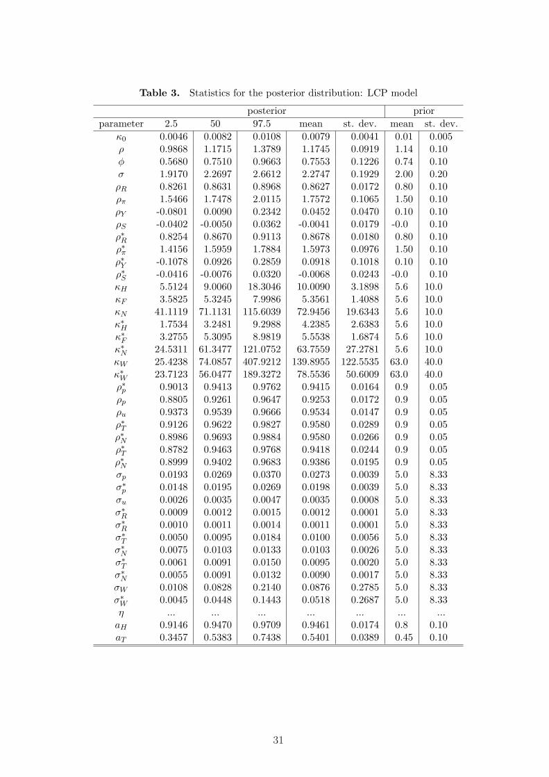
Table 3. Statistics for the posterior distribution: LCP model

posterior priorparameter 2.5 50 97.5 mean st. dev. mean st. dev.

κ0 0.0046 0.0082 0.0108 0.0079 0.0041 0.01 0.005ρ 0.9868 1.1715 1.3789 1.1745 0.0919 1.14 0.10φ 0.5680 0.7510 0.9663 0.7553 0.1226 0.74 0.10σ 1.9170 2.2697 2.6612 2.2747 0.1929 2.00 0.20ρR 0.8261 0.8631 0.8968 0.8627 0.0172 0.80 0.10ρπ 1.5466 1.7478 2.0115 1.7572 0.1065 1.50 0.10ρY -0.0801 0.0090 0.2342 0.0452 0.0470 0.10 0.10ρS -0.0402 -0.0050 0.0362 -0.0041 0.0179 -0.0 0.10ρ∗R 0.8254 0.8670 0.9113 0.8678 0.0180 0.80 0.10ρ∗π 1.4156 1.5959 1.7884 1.5973 0.0976 1.50 0.10ρ∗Y -0.1078 0.0926 0.2859 0.0918 0.1018 0.10 0.10ρ∗S -0.0416 -0.0076 0.0320 -0.0068 0.0243 -0.0 0.10κH 5.5124 9.0060 18.3046 10.0090 3.1898 5.6 10.0κF 3.5825 5.3245 7.9986 5.3561 1.4088 5.6 10.0κN 41.1119 71.1131 115.6039 72.9456 19.6343 5.6 10.0κ∗H 1.7534 3.2481 9.2988 4.2385 2.6383 5.6 10.0κ∗F 3.2755 5.3095 8.9819 5.5538 1.6874 5.6 10.0κ∗N 24.5311 61.3477 121.0752 63.7559 27.2781 5.6 10.0κW 25.4238 74.0857 407.9212 139.8955 122.5535 63.0 40.0κ∗W 23.7123 56.0477 189.3272 78.5536 50.6009 63.0 40.0ρ∗p 0.9013 0.9413 0.9762 0.9415 0.0164 0.9 0.05ρp 0.8805 0.9261 0.9647 0.9253 0.0172 0.9 0.05ρu 0.9373 0.9539 0.9666 0.9534 0.0147 0.9 0.05ρ∗T 0.9126 0.9622 0.9827 0.9580 0.0289 0.9 0.05ρ∗N 0.8986 0.9693 0.9884 0.9580 0.0266 0.9 0.05ρ∗T 0.8782 0.9463 0.9768 0.9418 0.0244 0.9 0.05ρ∗N 0.8999 0.9402 0.9683 0.9386 0.0195 0.9 0.05σp 0.0193 0.0269 0.0370 0.0273 0.0039 5.0 8.33σ∗p 0.0148 0.0195 0.0269 0.0198 0.0039 5.0 8.33σu 0.0026 0.0035 0.0047 0.0035 0.0008 5.0 8.33σ∗R 0.0009 0.0012 0.0015 0.0012 0.0001 5.0 8.33σ∗R 0.0010 0.0011 0.0014 0.0011 0.0001 5.0 8.33σ∗T 0.0050 0.0095 0.0184 0.0100 0.0056 5.0 8.33σ∗N 0.0075 0.0103 0.0133 0.0103 0.0026 5.0 8.33σ∗T 0.0061 0.0091 0.0150 0.0095 0.0020 5.0 8.33σ∗N 0.0055 0.0091 0.0132 0.0090 0.0017 5.0 8.33σW 0.0108 0.0828 0.2140 0.0876 0.2785 5.0 8.33σ∗W 0.0045 0.0448 0.1443 0.0518 0.2687 5.0 8.33η ... ... ... ... ... ... ...

aH 0.9146 0.9470 0.9709 0.9461 0.0174 0.8 0.10aT 0.3457 0.5383 0.7438 0.5401 0.0389 0.45 0.10

31

Table 4. Statistics for the posterior distribution: PCP model

posterior priorparameter 2.5 50 97.5 mean st. dev. mean st. dev.

κ0 0.0033 0.0054 0.0099 0.0058 0.0018 0.01 0.005ρ 1.0443 1.2241 1.4237 1.2261 0.0972 1.14 0.10φ 0.5627 0.7426 0.9585 0.7471 0.1006 0.74 0.10σ 1.8347 2.1661 2.5411 2.1725 0.1799 2.00 0.20ρR 0.8267 0.8640 0.8962 0.8633 0.0177 0.80 0.10ρπ 1.4533 1.6522 1.8535 1.6516 0.1029 1.50 0.10ρY 0.1467 0.2250 0.3189 0.2268 0.0439 0.10 0.10ρS -0.0537 -0.0212 0.0133 -0.0209 0.0169 -0.0 0.10ρ∗R 0.8697 0.9100 0.9462 0.9095 0.0196 0.80 0.10ρ∗π 1.2981 1.4856 1.6867 1.4876 0.0992 1.50 0.10ρ∗Y -0.0933 0.0998 0.2971 0.1005 0.0994 0.10 0.10ρ∗S -0.0608 -0.0095 0.0499 -0.0083 0.0277 -0.0 0.10κH 2.2296 3.5239 5.0725 3.5505 0.7812 5.6 10.0κF ... ... ... ... ... ... ...κN 10.9219 19.6154 43.4611 21.5959 8.3378 5.6 10.0κ∗H ... ... ... ... ... ... ...κ∗F 1.6033 3.3061 6.5133 3.4854 1.271 5.6 10.0κ∗N 0.7014 5.6455 24.7722 7.4513 6.6511 5.6 10.0κW 210.2401 342.2764 519.6272 348.1872 79.475 63.0 40.0κ∗W 252.8069 366.3486 507.3019 370.0352 65.4145 63.0 40.0ρ∗p 0.8815 0.9134 0.9382 0.9125 0.0145 0.9 0.05ρp 0.8705 0.9079 0.9384 0.9069 0.0173 0.9 0.05ρu 0.9267 0.9463 0.9635 0.9460 0.0094 0.9 0.05ρ∗T 0.9209 0.9627 0.9805 0.9590 0.0159 0.9 0.05ρ∗N 0.9188 0.9498 0.9720 0.9486 0.0136 0.9 0.05ρ∗T 0.8601 0.9048 0.9362 0.9031 0.0195 0.9 0.05ρ∗N 0.9372 0.9718 0.9854 0.9692 0.0122 0.9 0.05σp 0.0221 0.0270 0.0336 0.0273 0.0029 5.0 8.33σ∗p 0.0176 0.0227 0.0307 0.0231 0.0033 5.0 8.33σu 0.0028 0.0038 0.0052 0.0038 0.0006 5.0 8.33σ∗R 0.0009 0.0010 0.0012 0.0010 0.0001 5.0 8.33σ∗R 0.0010 0.0011 0.0014 0.0011 0.0001 5.0 8.33σ∗T 0.0040 0.0052 0.0071 0.0053 0.0008 5.0 8.33σ∗N 0.0041 0.0053 0.0074 0.0054 0.0009 5.0 8.33σ∗T 0.0050 0.0066 0.0094 0.0067 0.0011 5.0 8.33σ∗N 0.0018 0.0028 0.0053 0.0030 0.0009 5.0 8.33σW 0.1792 0.2771 0.3785 0.2744 0.0546 5.0 8.33σ∗W 0.1094 0.2223 0.3743 0.2249 0.0724 5.0 8.33η ... ... ... ... ... ... ...

aH 0.9635 0.9738 0.9817 0.9735 0.0046 0.8 0.10aT 0.5039 0.6336 0.7151 0.6268 0.0551 0.45 0.10

32

Table 5. Comparison of median values of parameters

parameter Complete LCP PCPκ0 0.0100 0.0082 0.0054ρ 1.2247 1.1715 1.2241φ 0.9130 0.7510 0.7426σ 2.3470 2.2697 2.1661ρR 0.8685 0.8631 0.8640ρπ 1.6678 1.7478 1.6522ρY 0.1952 0.0090 0.2250ρS -0.0174 -0.0050 -0.0212ρ∗R 0.8992 0.8670 0.9100ρ∗π 1.5184 1.5959 1.4856ρ∗Y 0.0991 0.0926 0.0998ρ∗S -0.0168 -0.0076 -0.0095κH 10.1310 9.0060 3.5239κF 3.2680 5.3245 ...κN 53.6298 71.1131 19.6154κ∗H 22.6502 3.2481 ...κ∗F 2.8267 5.3095 3.3061κ∗N 26.7870 61.3477 5.6455κW 283.8806 74.0857 342.2764κ∗W 348.9554 56.0477 366.3486ρ∗p 0.9231 0.9413 0.9134ρp 0.9253 0.9261 0.9079ρu 0.9311 0.9539 0.9463ρ∗T 0.9169 0.9622 0.9627ρ∗N 0.9183 0.9693 0.9498ρ∗T 0.8918 0.9463 0.9048ρ∗N 0.9426 0.9402 0.9718σp 0.0286 0.0269 0.0270σ∗p 0.0240 0.0195 0.0227σu 0.0044 0.0035 0.0038σ∗R 0.0010 0.0012 0.0010σ∗R 0.0011 0.0011 0.0011σ∗T 0.0216 0.0095 0.0052σ∗N 0.0088 0.0103 0.0053σ∗T 0.0167 0.0091 0.0066σ∗N 0.0054 0.0091 0.0028σW 0.4609 0.0828 0.2771σ∗W 0.4130 0.0448 0.2223η 1.0816 ... ...

aH 0.8960 0.9470 0.9738aT 0.6149 0.5383 0.6336

33

Table 6. Marginal densities

Model Marginal density

Complete 2977

LCP 2970

PCP 2974

Notes: The marginal density is computed using the harmonic mean estimator (Geweke, 1999).

Table 7. Selected second moments of the real exchange rate

Moment Data Complete LCP PCP

percentiles 2.5 50 97.5 2.5 50 97.5 2.5 50 97.5

σ (RSt) 20.74 7.41 14.32 33.01 8.57 14.10 23.09 7.94 14.46 26.73

ρ (RSt) 0.97 0.92 0.92 0.94 0.91 0.93 0.94 0.91 0.93 0.94

ρ(RSt,

Ct

C∗t

)-0.48 -0.32 -0.39 -0.37 -0.29 -0.28 -0.29 -0.39 -0.51 -0.63

Notes: Each figure is computed using the percentiles of the marginal posterior distribution of the pa-rameters reported in in the first row (’percentiles’) and simulating 10,000 time series the variables of themodel of length equal to that of the data and dropping the first 1000 observations.

Table 8A. Selected second moments of the observable variables: Complete model

σ ρ

Data All σu = 0 σp = 0 σR 6= 0 σZ 6= 0 All σu = 0 σp = 0 σR 6= 0 σZ 6= 0RS 0.97 14.32 6.12 13.37 1.30 2.56 0.92 0.96 0.92 0.78 0.96πc 0.75 0.50 0.49 0.46 0.05 0.44 0.64 0.65 0.59 0.68 0.60π∗c 0.40 0.45 0.44 0.42 0.06 0.41 0.48 0.47 0.42 0.80 0.40πn 0.85 0.42 0.42 0.37 0.04 0.36 0.79 0.78 0.75 0.86 0.75π∗n 0.57 0.35 0.34 0.31 0.06 0.30 0.74 0.74 0.71 0.86 0.70R 0.98 0.48 0.48 0.32 0.14 0.28 0.95 0.95 0.91 0.75 0.95R∗ 0.97 0.35 0.35 0.24 0.16 0.17 0.93 0.92 0.87 0.78 0.93C 0.49 1.35 1.32 0.79 0.33 0.67 0.84 0.84 0.91 0.75 0.94C∗ 0.96 1.15 1.13 0.66 0.44 0.42 0.84 0.83 0.87 0.78 0.94

Notes: Each figure in the table is computed using the median of the marginal posterior distribution ofthe parameters and simulating 10,000 time series the variables of the model of length equal to that of thedata and dropping the first 1000 observations.

34

Table 8B. Selected second moments of the observable variables: Complete model

All σu = 0 σp = 0 σR 6= 0 σZ 6= 0

ρ(RSt,

Ct

C∗t

)-0.39 -0.29 -0.35 1.00 0.85

Notes: Each figure in the table is computed using the median of the marginal posterior distribution ofthe parameters and simulating 10,000 time series the variables of the model of length equal to that of thedata and dropping the first 1000 observations.

Table 9. Real exchange rate fluctuations: Economic decomposition

(Percentage of variance of the real exchange rate)

Complete LCP PCP

component 2.5 50 97.5 2.5 50 97.5 2.5 50 97.5

σ(Internal Rexc) 0.86 0.24 0.06 1.87 0.67 0.22 0.85 0.24 0.13

σ(Home bias) 12.17 7.55 4.87 36.24 35.68 32.03 93.91 96.60 98.08

σ(IPD) 45.71 55.71 65.35 18.19 25.06 32.63 0.00 0.00 0.00

σ(Int. Rexc, home bias) -1.07 -0.08 -0.00 7.31 1.78 -0.29 5.28 3.16 1.82

σ(Int. Rexc, IPD) 4.39 2.34 0.96 4.85 1.91 0.62 0.00 0.00 0.00

σ(Home bias, IPD) 37.94 34.22 28.74 31.47 34.83 34.73 0.00 0.00 0.00

Notes: Each figure in the table is computed using the median, the 2.5 and the 97.5 percentiles of themarginal posterior distribution of the parameters and simulating 10,000 time series the variables of themodel of length equal to that of the data and dropping the first 1000 observations.

35

Table 10. Decomposition of the asymptotic forecast error variance: Complete model

Variable zH z∗F zN z∗N zR z∗R zU z∗U zU zW z∗W Total

euro-area

C 10.2 0.3 13.3 0.0 5.4 0.0 63.9 0.7 5.9 0.3 0.0 100πc 47.8 0.4 29.3 0.0 0.7 0.1 15.5 0.2 4.8 1.1 0.0 100πnt 14.8 0.0 59.7 0.0 0.8 0.0 21.6 0.2 1.7 1.2 0.0 100R 16.7 0.1 16.2 0.0 8.4 0.0 56.2 0.2 1.8 0.4 0.0 100

re 1.5 0.6 0.5 0.3 0.2 0.3 11.1 8.0 77.5 0.0 0.0 100

US

C 0.8 3.8 0.0 8.3 0.0 13.1 1.4 64.2 8.2 0.0 0.2 100πc 0.4 53.0 0.0 28.0 0.0 1.7 0.7 10.4 4.4 0.0 1.4 100πnt 0.1 8.2 0.0 64.2 0.0 2.4 1.1 17.2 5.2 0.0 1.7 100R 0.1 7.6 0.0 14.2 0.0 18.2 1.1 53.1 5.4 0.0 0.3 100

Notes: Each figure in the table is computed using the median of the marginal posterior distribution ofthe parameters.

36