the discriminative bilateral filter: an enhanced denoising filter for electron microscopy data

Journal of

www.elsevier.com/locate/yjsbi

Journal of Structural Biology 155 (2006) 395–408

StructuralBiology

The discriminative bilateral filter: An enhanced denoising filterfor electron microscopy data

Radosav S. Pantelic a, Rosalba Rothnagel a, Chang-Yi Huang b, David Muller b,David Woolford a, Michael J. Landsberg a, Alasdair McDowall a,c, Bernard Pailthorpe d,

Paul R. Young b, Jasmine Banks e, Ben Hankamer a,*, Geoffery Ericksson f

a Institute for Molecular Bioscience, University of Queensland, Brisbane, Qld 4072, Australiab School of Molecular and Microbial Sciences, University of Queensland, Brisbane, Qld 4072, Australia

c Centre for Microscopy and Microanalysis, University of Queensland, Brisbane, Qld 4072, Australiad School of Physical Sciences, University of Queensland, Brisbane, Qld 4072, Australia

e Advanced Computational Modelling Centre, University of Queensland, Brisbane, Qld 4072, Australiaf Queensland Brain Institute, University of Queensland, Brisbane, Qld 4072, Australia

Received 12 October 2005; received in revised form 23 March 2006; accepted 30 March 2006Available online 19 May 2006

Abstract

Advances in three-dimensional (3D) electron microscopy (EM) and image processing are providing considerable improvements in theresolution of subcellular volumes, macromolecular assemblies and individual proteins. However, the recovery of high-frequency infor-mation from biological samples is hindered by specimen sensitivity to beam damage. Low dose electron cryo-microscopy conditionsafford reduced beam damage but typically yield images with reduced contrast and low signal-to-noise ratios (SNRs). Here, we describethe properties of a new discriminative bilateral (DBL) filter that is based upon the bilateral filter implementation of Jiang et al. (Jiang,W., Baker, M.L., Wu, Q., Bajaj, C., Chiu, W., 2003. Applications of a bilateral denoising filter in biological electron microscopy. J. Struc.Biol. 128, 82–97.). In contrast to the latter, the DBL filter can distinguish between object edges and high-frequency noise pixels throughthe use of an additional photometric exclusion function. As a result, high frequency noise pixels are smoothed, yet object edge detail ispreserved. In the present study, we show that the DBL filter effectively reduces noise in low SNR single particle data as well as cellulartomograms of stained plastic sections. The properties of the DBL filter are discussed in terms of its usefulness for single particle analysisand for pre-processing cellular tomograms ahead of image segmentation.� 2006 Elsevier Inc. All rights reserved.

Keywords: Electron microscopy; Electron cryo-microscopy; Cryo-electron microscopy; Single particle analysis; Tomography; Image; Impulse noisereduction; Denoising; Filter; Bilateral; Anisotropic

1. Introduction

Advances in electron cryo-microscopy (cryo-EM) andimage processing are resulting in the capture and recoveryof structural information at rapidly increasing levels of

1047-8477/$ - see front matter � 2006 Elsevier Inc. All rights reserved.

doi:10.1016/j.jsb.2006.03.030

* Corresponding author. Fax: +61 7 334 62101.E-mail address: [email protected] (B. Hankamer).

1 Abbreviations used: 3D, three-dimensions/-dimensional; EM, electron microdiscriminative bilateral filter; FEG, field emission gun; GroEL, GroE chapchromatography; SNR, signal-to-noise ratio; TEM, transmission electron mic

resolution. Specifically, EM1 tomography, single particleanalysis, and electron crystallography are resolving thestructures of subcellular volumes, macromolecular assem-blies, and individual proteins, to �50 A (Baumeister,2002), �6 A (Ludtke et al., 2004), and �1.8 A (Gonen

scope/microscopy; CTF, contrast transfer function correction; DBL filter,eronin; KLH, keyhole limpet haemocyanin; FPLC, fast protein liquid

roscopy; CCD, charge coupled device; MSE, mean square error.

mailto:[email protected]

396 R.S. Pantelic et al. / Journal of Structural Biology 155 (2006) 395–408

et al., 2005), respectively. Furthermore, with the implemen-tation of a new generation of electron microscopes fittedwith 300 keV field emission guns (FEGs) and integratedaberration correction technology, current resolutions of�0.7 A (Zeneka and Van Mastrigt, 2005) have beenachieved. Given further improvements in biological datacollection methods (e.g. optimization of liquid helium(He) cooled stages, phase plates and increased data set siz-es), considerable advances in structural resolution can beexpected in the future.

Due to the sensitivity of biological samples to damageinduced by high levels of electron exposure, images are typ-ically collected at low doses (�10–30 e�/A2) using a liquidnitrogen (N2) (�77 K) or liquid He (�6–20 K) cooled stageto aid energy dissipation (van Heel et al., 2000). Howeverthe combined effect of imaging low contrast objects (suchas individual macromolecular protein assemblies in vitre-ous ice) under low dose conditions is the capture of noisy,low contrast data. Relatively high noise levels across awhole range of frequencies occur due to the difference inice thickness in which the sample is embedded, beam dam-age to the sample, incoherence in the electron beam (vanHeel et al., 2000), shot noise (Downing and Hendrickson,1999), cosmic rays, X-rays (Brink and Chiu, 1994; Down-ing and Hendrickson, 1999), and the point spread functionof the detector (Downing and Hendrickson, 1999). Report-ed examples of high-frequency noise include hard X-rayevents, which produce a signal near saturation over 1–3pixels, and soft X-rays, which generate a signal correspond-ing to tens of electrons usually in one or two adjacent pixels(Downing and Hendrickson, 1999). The combined contri-bution of noise across the full frequency range of the imageis clearly seen in the CTF graphs in which the noise level isrepresented by the plot connecting the minima (e.g., Sanderet al. (2005)).

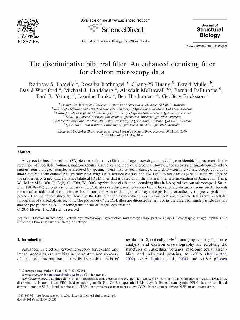
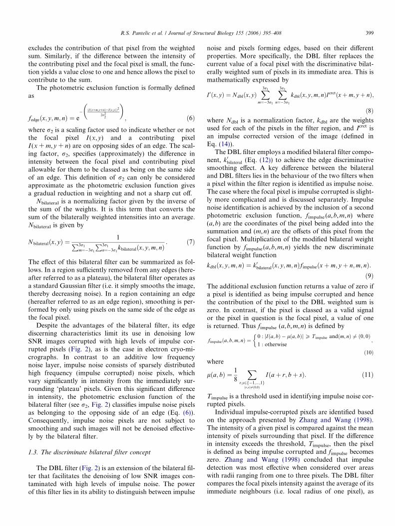
Fig. 1. The Gaussian and bilateral filters. (A) Gaussian filter. The ‘chicken-wirunder the peak of the Gaussian filter is defined as the focal pixel (coordinates x

pixel based on the weighted intensities of surrounding pixels under the mask (coand the spatial weighting of the surrounding pixels (m,n). In a plateau region,The ‘chicken-wire mesh’ describes the shape of the bilateral filter. The central pi(coordinates x,y). In a local region containing an edge, the bilateral filter calcusurrounding pixels under the mask (coordinates m,n) and on the same side of ththe left are excluded from the filtering process. The bilateral filter therefore pinterpret impulse noise spikes as forming an edge.

Central to the ability to resolve a 3D structure from suchnoise contaminated images is the ability to resolve the sig-nal component. To date, electron crystallography hasattained the highest resolution 3D reconstructions fromany transmission electron microscopy (TEM) images(Mitsuoka et al., 1999). This is largely due to the periodicproperties of 2D crystals, which allow the effective separa-tion of signal (as diffraction spots) from noise by use ofFourier space techniques. In contrast, aperiodic objects,such as single particles, require alternative image denoisingmethods to facilitate the accurate detection, alignment andsubsequent 3D reconstruction of individual molecular pro-jections (van Heel et al., 2000). In the case of tomographicdata sets, the presence of noise not only masks high-resolu-tion detail, but also hampers automated image segmenta-tion, which has the potential to accelerate the annotationof discrete subcellular volumes (Bartesaghi et al., 2005;Roerdink and Meijster, 2000; Volkmann, 2002).

Recently, Jiang et al. (2003) developed a bilateral filter(Fig. 1), based on the earlier work of Tomasi and Mandu-chi (1998). The most important property of this filter is itsability to reduce noise while preserving edge detail. In thisrespect Jiang et al. suggest that the bilateral filter is similarto anisotropic diffusion filters, and distinct from Gaussianfilters (Fig. 1A) which smooth both noise and edge detail.The bilateral filter was shown to effectively denoise 3Dreconstructions as well as electron cryo-micrographs oflarge particles such as rice dwarf virus (�50 nm diameter)and, to a more limited extent intermediate sized molecularassemblies such as the GroE chaperonin, GroEL(�850 kDa). However, large macromolecular assembliesyield higher SNR images than small molecules imagedunder similar conditions, and such low SNR conditionslimit the utility of the bilateral filter. This is because thebilateral filter identifies high amplitude/high frequency

e mesh’ describes the shape of the Gaussian filter. The central pixel located,y). During the filtering process, a new intensity is calculated for the focalordinates m,n). The radius of the mask adjusts both the width of the mask,the bilateral filter functions as a normal Gaussian filter. (B) Bilateral filter.xel located under the peak of the Gaussian filter is defined as the focal pixellates the new focal pixel’s intensity based upon the weighted intensities ofe edge. In this illustration the focal pixel is to the right of the edge. Pixels toreserves edge detail. The bilateral filter has the limitation that it can also

R.S. Pantelic et al. / Journal of Structural Biology 155 (2006) 395–408 397

noise pixels (referred to here as impulse noise) as edges, andhence excludes the high frequency noise from the smooth-ing process.

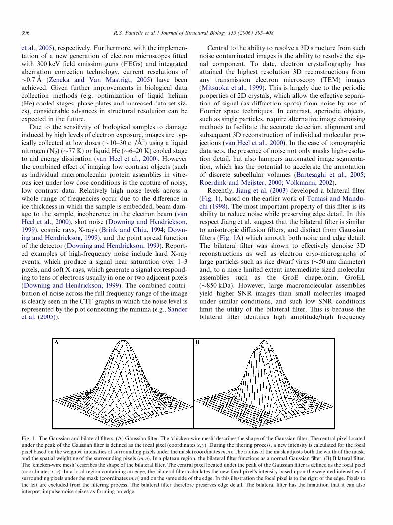
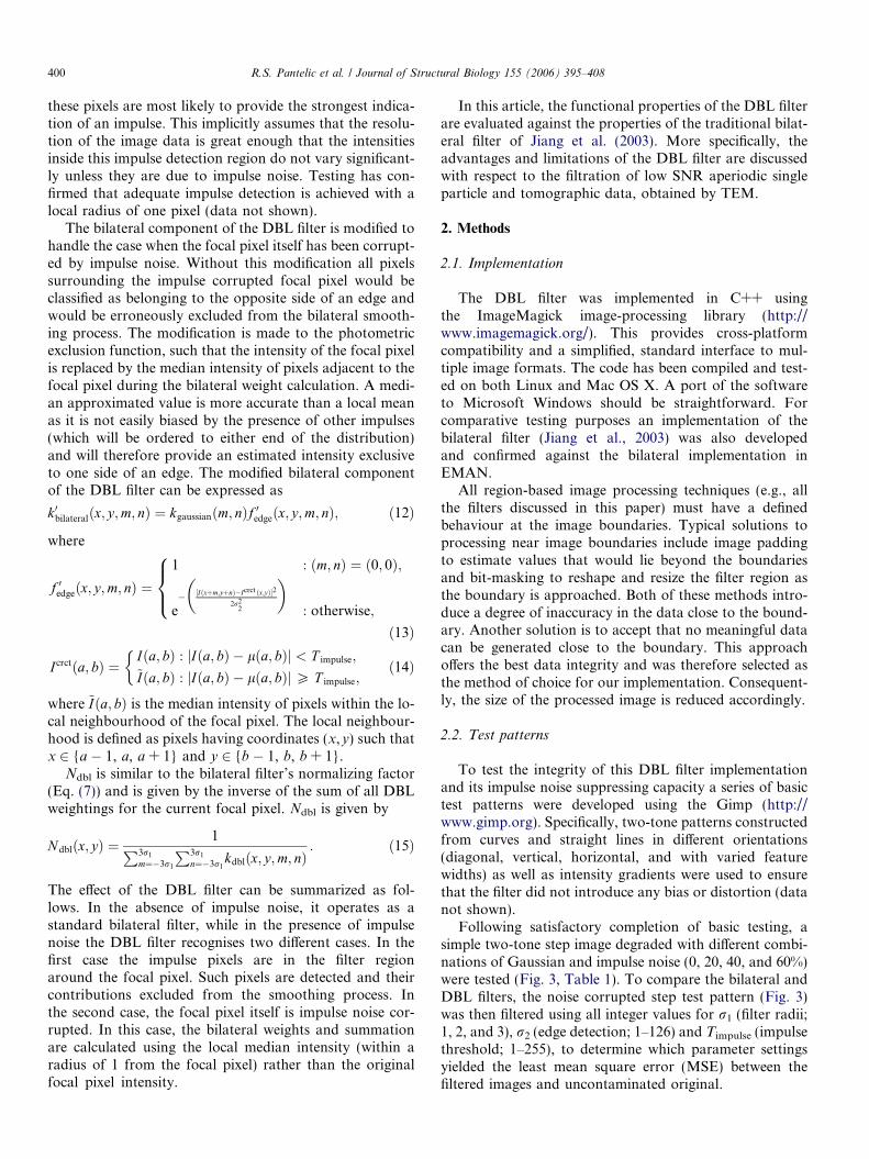
The focus of this paper is the extension of the bilateralfilter with a kernel component to reduce high-amplitude/high-frequency noise that can be modelled by impulsespikes (Fig. 2). We have called this filter, which includesan additional photometric exclusion component, the dis-criminative bilateral (DBL) filter, because of its ability todiscriminate between impulse noise pixels, and pixels thatbelong to object edges. It has enhanced denoising capabil-ities under low SNR conditions, while retaining the benefitsof the bilateral filter under higher SNR conditions. Theo-retically, the DBL filter can extend the detection limit(and detection certainty) of small molecules into the lowermolecular weight range (<500 kDa). The edge preservingand denoising properties of the DBL filter have the poten-tial to enhance the accuracy of 3D image reconstructionand aid the development of more automated segmentationprocesses for tomographic images.

Before describing the structure and enhancements of theDBL filter, the design of the Gaussian and the bilateralfilters on which this filter is based are summarized.

1.1. The Gaussian filter

The purpose of a Gaussian filter is to smooth an imageand hence remove noise. The filter works by replacing thecurrent value of a focal pixel with the weighted sum of pix-els in its immediate area (Fig. 1A). The new intensity for afocal pixel, I 0 (x,y), at the coordinates (x,y), can be mathe-matically expressed as

I 0ðx; yÞ ¼ N Gaussian

X3r1

m¼�3r1

X3r1

n¼�3r1

kGaussianðm; nÞIðxþ m; y þ nÞ;

ð1Þwhere m,n are the coordinates of the filter weightsand the coordinates (0, 0) correspond to the focal pixel.kGaussian (m,n) represents the individual weights which aremultiplied against the intensities of the pixels falling withinthe filter’s region. The weighting applied to each contribut-ing pixel is based on its distance from the focal pixel, withpixels further away having a weaker contribution. Theweights are determined by

kGaussianðm; nÞ ¼ e� m2þn2

2r21

� �; ð2Þ

where r1 specifies the distance over which the weights aresignificant.

NGaussian (x,y) is a normalizing factor which convertsthe sum of Gaussian weighted pixels into an average.NGaussian (x,y) is given by the inverse of the sum of allGaussian weights, as expressed by

NGaussian ¼1P3r1

m¼�3r1

P3r1

n¼�3r1kGaussianðm; nÞ

: ð3Þ

If the filter is viewed as a probability distribution, thenr1 can be interpreted as a standard deviation. The widthof the filter’s region is normally set to 3 times thestandard deviation either side of the focal pixel. Hencem and n range from �3r1 to 3r1. It should be noted thatlarger values of r1 increase the degree of smoothingapplied.

The disadvantage of the Gaussian filter is that it is indis-criminate, with the result that all pixel intensities within thefilter region are included in the weighted sum. This indis-criminate smoothing process can result in the loss of edgedetail. For the purpose of this paper, we define an edge tobe a large difference in pixel intensity within a local regionof the image (i.e. high local contrast). In a region containingan edge, calculation of a new focal pixel value using Eq. (1)will result in a weighted summation of high and low inten-sity values, from either side of the edge. The result issmoothing of pixel values over the edge, leading to a lossof image contrast and diminished edge definition.

1.2. The bilateral filter

The bilateral filter is used to smooth out noise whilemaintaining edge detail by being more selective in the pixelsallowed to contribute to the weighted sum. The filter worksby replacing the current value of a focal pixel with thebilaterally weighted sum of pixels in its immediate area.The bilateral weights are calculated such that pixels onthe same side of an edge contribute to the new focal pixelvalue, while those on the opposing side effectively do not(Fig. 1B). By this mechanism the edge is maintained. Math-ematically this can be expressed as

I 0ðx; yÞ ¼ Nbilateralðx; yÞX3r1

m¼�3r1

X3r1

n¼�3r1

kbilateralðx; y;m; nÞIðxþ m; y þ nÞ;

ð4Þ

where Nbilateral is a normalization factor (Eq. (7)) andkbilateral (Eq. (5)) are the weights for each of the pixels inthe filter region.

To achieve the smoothing objective, the bilateral filteremploys kGaussian (m,n) (Eq. (2)) to calculate a set of Gauss-ian weights. The selective inclusion of pixel intensities in theweighted sum is achieved by multiplying the Gaussianweight function with a photometric exclusion functionfedge (x,y,m,n) to yield the bilateral weight calculationfunction,

kbilateralðx; y;m; nÞ ¼ kGaussianðm; nÞfedgeðx; y;m; nÞ: ð5Þ

The photometric exclusion function is inversely propor-tional to differences in intensity. Thus, if the difference inintensity between the focal pixel at coordinates (x,y) anda pixel within the filter region at coordinates(x + m,y + n) is large, then the photometric exclusionfunction yields a near zero value (Eq. (6)). This effectively

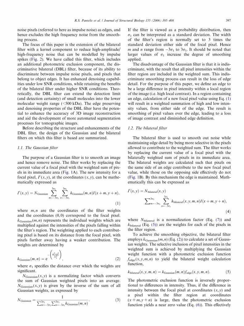
Fig. 3. Step test evaluation of DBL and bilateral filter performance. (A) Original grey-scale test image. (B) Step shown in (A) contaminated with 20%Gaussian: 60% impulse noise. (C and D) Noise corrupted step image shown in B after bilateral (C) and DBL (D) filtering. In both cases the least MSEresults are shown, after evaluating all integer settings values for r1 (filter radii; 1, 2, and 3), r2 (edge detection, 1–126) and Timpulse (1–255). Note that whenTimpulse is 255, the DBL filter functions as a bilateral filter. (E–H) Colour contour plots of A–D. Both the bilateral (G) and DBL (H) filtered images show amarked improvement in MSE (bilateral—1595; DBL—644), over that of the noise corrupted image shown in F (MSE—5907). However both visualinspection and the MSE values show that the DBL filtered image (D and H), most closely correlates with the original (A and E). (I–L) J–L show auto-equalized difference images between the original grey-scale image (A) and its noise corrupted (B) and filtered counterparts (C and D). I is the control (i.e.,A minus A). J (B minus A) shows the noise component of image B, which can be seen to be markedly reduced in K and L. As I–L have all been auto-equalized for clarity of reproduction, and the noise level of the DBL filtered images is considerably lower in the DBL filtered image, L may incorrectlysuggest that the DBL filter has resulted in more blurring of the edge than the bilateral filter. (M) The difference image between K and L clearlydemonstrates that this is not the case. Furthermore the ability of the DBL filter to remove impulse noise means that smaller r1 settings can often be used,to achieve better edge preservation.

Fig. 2. The DBL filter concept. This diagram is a 3D representation of a 2D image with physical dimensions (X and Y axes) and pixel intensities (Z axis)plotted. The background pixel intensities are represented by a horizontal black bar. The signals (e.g., projection images of single particles of differingintensity) protrude out of the background intensity and are represented by black vertical columns while impulse noise spikes are represented in blue. TheDBL filter passes over the image a pixel at a time and calculates a new focal pixel value based on the settings of r1, r2 and Timpulse. r1, not depicted, definesthe filter radius which is usually set to 3r1. The exact value of r1 determines the degree of spatial smoothing that the image undergoes. r2 is a photometricparameter of both the DBL and bilateral filters. r2 effectively defines the difference in intensity values that will be considered to be on the same side of anedge as the focal pixel. The green band depicts the intensity range (Z axis), which will be part of the same plateau region. To discriminate between edgesand impulse noise a local threshold parameter, Timpulse, has been incorporated into the DBL filter. This parameter is depicted by the red bars. To a firstapproximation, the action of this threshold is that pixels differing in intensity by more than Timpulse from the focal pixel are defined as impulse noise. In thepresence of impulse noise the DBL filter recognises two different cases. In the first case the impulse pixels are in the filter region around the focal pixel. Suchpixels are detected and excluded from the smoothing process. In the second case, the focal pixel itself is impulse noise corrupted. In this case the bilateralweights are calculated using the local median intensity (within a radius of r1 from the focal pixel) in place of the focal pixel intensity.



excludes the contribution of that pixel from the weightedsum. Similarly, if the difference between the intensity ofthe contributing pixel and the focal pixel is small, the func-tion yields a value close to one and hence allows the pixel tocontribute to the sum.

The photometric exclusion function is formally definedas

fedgeðx; y;m; nÞ ¼ e� ðIðxþm;yþnÞ�Iðx;yÞÞ2

2r22

� �; ð6Þ

where r2 is a scaling factor used to indicate whether or notthe focal pixel I (x,y) and a contributing pixelI (x + m,y + n) are on opposing sides of an edge. The scal-ing factor, r2, specifies (approximately) the difference inintensity between the focal pixel and contributing pixelallowable for them to be classed as being on the same sideof an edge. This definition of r2 can only be consideredapproximate as the photometric exclusion function givesa gradual reduction in weighting and not a sharp cut off.

Nbilateral is a normalizing factor given by the inverse ofthe sum of the weights. It is this term that converts thesum of the bilaterally weighted intensities into an average.Nbilateral is given by

Nbilateralðx; yÞ ¼1P3r1

m¼�3r1

P3r1

n¼�3r1kbilateralðx; y;m; nÞ

: ð7Þ

The effect of this bilateral filter can be summarized as fol-lows. In a region sufficiently removed from any edges (here-after referred to as a plateau), the bilateral filter operates asa standard Gaussian filter (i.e. it simply smooths the image,thereby decreasing noise). In a region containing an edge(hereafter referred to as an edge region), smoothing is per-formed by only using pixels on the same side of the edge asthe focal pixel.

Despite the advantages of the bilateral filter, its edgediscerning characteristics limit its use in denoising lowSNR images corrupted with high levels of impulse cor-rupted pixels (Fig. 2), as is the case in electron cryo-mi-crographs. In contrast to an additive low frequencynoise layer, impulse noise consists of sparsely distributedhigh frequency (impulse corrupted) noise pixels, whichvary significantly in intensity from the immediately sur-rounding ‘plateau’ pixels. Given this significant differencein intensity, the photometric exclusion function of thebilateral filter (see r2, Fig. 2) classifies impulse noise pixelsas belonging to the opposing side of an edge (Eq. (6)).Consequently, impulse noise pixels are not subject tosmoothing and such images will not be denoised effective-ly by the bilateral filter.

1.3. The discriminate bilateral filter concept

The DBL filter (Fig. 2) is an extension of the bilateral fil-ter that facilitates the denoising of low SNR images con-taminated with high levels of impulse noise. The powerof this filter lies in its ability to distinguish between impulse

noise and pixels forming edges, based on their differentproperties. More specifically, the DBL filter replaces thecurrent value of a focal pixel with the discriminative bilat-erally weighted sum of pixels in its immediate area. This ismathematically expressed by

I 0ðx; yÞ ¼ Ndblðx; yÞX3r1

m¼�3r1

X3r1

n¼�3r1

kdblðx; y;m; nÞIcrctðxþ m; y þ nÞ;

ð8Þwhere Ndbl is a normalization factor, kdbl are the weightsused for each of the pixels in the filter region, and Icrct isan impulse corrected version of the image (defined inEq. (14)).

The DBL filter employs a modified bilateral filter compo-nent, k0bilateral (Eq. (12)) to achieve the edge discriminativesmoothing effect. A key difference between the bilateraland DBL filters lies in the behaviour of the two filters whena pixel within the filter region is identified as impulse noise.The case where the focal pixel is impulse corrupted is slight-ly more complicated and is discussed separately. Impulsenoise identification is achieved by the inclusion of a secondphotometric exclusion function, fimpulse (a,b,m,n) where(a,b) are the coordinates of the pixel being added into thesummation and (m,n) are the offsets of this pixel from thefocal pixel. Multiplication of the modified bilateral weightfunction by fimpulse (a,b,m,n) yields the new discriminatebilateral weight function

kdblðx; y;m; nÞ ¼ k0bilateralðx; y;m; nÞfimpulseðxþ m; y þ n;m; nÞ:ð9Þ

The additional exclusion function returns a value of zero ifa pixel is identified as being impulse corrupted and hencethe contribution of the pixel to the DBL weighted sum iszero. In contrast, if the pixel is classed as a valid signalor the pixel in question is the focal pixel, a value of oneis returned. Thus fimpulse (a,b,m,n) is defined by

fimpulseða; b;m; nÞ ¼0 : jIða; bÞ � lða; bÞjP T impulse andðm; nÞ 6¼ ð0; 0Þ1 : otherwise

�;

ð10Þwhere

lða; bÞ ¼ 1

8

Xr;s2f�1;...;1gðr;sÞ6¼ð0;0Þ

Iðaþ r; bþ sÞ: ð11Þ

Timpulse is a threshold used in identifying impulse noise cor-rupted pixels.

Individual impulse-corrupted pixels are identified basedon the approach presented by Zhang and Wang (1998).The intensity of a given pixel is compared against the meanintensity of pixels surrounding that pixel. If the differencein intensity exceeds the threshold, Timpulse, then the pixelis defined as being impulse corrupted and fimpulse becomeszero. Zhang and Wang (1998) concluded that impulsedetection was most effective when considered over areaswith radii ranging from one to three pixels. The DBL filtercompares the focal pixels intensity against the average of itsimmediate neighbours (i.e. local radius of one pixel), as


these pixels are most likely to provide the strongest indica-tion of an impulse. This implicitly assumes that the resolu-tion of the image data is great enough that the intensitiesinside this impulse detection region do not vary significant-ly unless they are due to impulse noise. Testing has con-firmed that adequate impulse detection is achieved with alocal radius of one pixel (data not shown).

The bilateral component of the DBL filter is modified tohandle the case when the focal pixel itself has been corrupt-ed by impulse noise. Without this modification all pixelssurrounding the impulse corrupted focal pixel would beclassified as belonging to the opposite side of an edge andwould be erroneously excluded from the bilateral smooth-ing process. The modification is made to the photometricexclusion function, such that the intensity of the focal pixelis replaced by the median intensity of pixels adjacent to thefocal pixel during the bilateral weight calculation. A medi-an approximated value is more accurate than a local meanas it is not easily biased by the presence of other impulses(which will be ordered to either end of the distribution)and will therefore provide an estimated intensity exclusiveto one side of an edge. The modified bilateral componentof the DBL filter can be expressed as

k0bilateralðx; y;m; nÞ ¼ kgaussianðm; nÞf 0edgeðx; y;m; nÞ; ð12Þ

where

f 0edgeðx; y;m; nÞ ¼1 : ðm; nÞ ¼ ð0; 0Þ;

e� ½Iðxþm;yþnÞ�Icrct ðx;yÞ�2

2r22

� �: otherwise;

8><>:

ð13Þ

Icrctða; bÞ ¼Iða; bÞ : jIða; bÞ � lða; bÞj < T impulse;

~Iða; bÞ : jIða; bÞ � lða; bÞjP T impulse;

�ð14Þ

where ~Iða; bÞ is the median intensity of pixels within the lo-cal neighbourhood of the focal pixel. The local neighbour-hood is defined as pixels having coordinates (x,y) such thatx 2 {a � 1, a, a + 1} and y 2 {b � 1, b, b + 1}.

Ndbl is similar to the bilateral filter’s normalizing factor(Eq. (7)) and is given by the inverse of the sum of all DBLweightings for the current focal pixel. Ndbl is given by

Ndblðx; yÞ ¼1P3r1

m¼�3r1

P3r1

n¼�3r1kdblðx; y;m; nÞ

: ð15Þ

The effect of the DBL filter can be summarized as fol-lows. In the absence of impulse noise, it operates as astandard bilateral filter, while in the presence of impulsenoise the DBL filter recognises two different cases. In thefirst case the impulse pixels are in the filter regionaround the focal pixel. Such pixels are detected and theircontributions excluded from the smoothing process. Inthe second case, the focal pixel itself is impulse noise cor-rupted. In this case, the bilateral weights and summationare calculated using the local median intensity (within aradius of 1 from the focal pixel) rather than the originalfocal pixel intensity.

In this article, the functional properties of the DBL filterare evaluated against the properties of the traditional bilat-eral filter of Jiang et al. (2003). More specifically, theadvantages and limitations of the DBL filter are discussedwith respect to the filtration of low SNR aperiodic singleparticle and tomographic data, obtained by TEM.

2. Methods

2.1. Implementation

The DBL filter was implemented in C++ usingthe ImageMagick image-processing library (http://www.imagemagick.org/). This provides cross-platformcompatibility and a simplified, standard interface to mul-tiple image formats. The code has been compiled and test-ed on both Linux and Mac OS X. A port of the softwareto Microsoft Windows should be straightforward. Forcomparative testing purposes an implementation of thebilateral filter (Jiang et al., 2003) was also developedand confirmed against the bilateral implementation inEMAN.

All region-based image processing techniques (e.g., allthe filters discussed in this paper) must have a definedbehaviour at the image boundaries. Typical solutions toprocessing near image boundaries include image paddingto estimate values that would lie beyond the boundariesand bit-masking to reshape and resize the filter region asthe boundary is approached. Both of these methods intro-duce a degree of inaccuracy in the data close to the bound-ary. Another solution is to accept that no meaningful datacan be generated close to the boundary. This approachoffers the best data integrity and was therefore selected asthe method of choice for our implementation. Consequent-ly, the size of the processed image is reduced accordingly.

2.2. Test patterns

To test the integrity of this DBL filter implementationand its impulse noise suppressing capacity a series of basictest patterns were developed using the Gimp (http://www.gimp.org). Specifically, two-tone patterns constructedfrom curves and straight lines in different orientations(diagonal, vertical, horizontal, and with varied featurewidths) as well as intensity gradients were used to ensurethat the filter did not introduce any bias or distortion (datanot shown).

Following satisfactory completion of basic testing, asimple two-tone step image degraded with different combi-nations of Gaussian and impulse noise (0, 20, 40, and 60%)were tested (Fig. 3, Table 1). To compare the bilateral andDBL filters, the noise corrupted step test pattern (Fig. 3)was then filtered using all integer values for r1 (filter radii;1, 2, and 3), r2 (edge detection; 1–126) and Timpulse (impulsethreshold; 1–255), to determine which parameter settingsyielded the least mean square error (MSE) between thefiltered images and uncontaminated original.

http://www.imagemagick.org/

http://www.imagemagick.org/

http://www.gimp.org

http://www.gimp.org

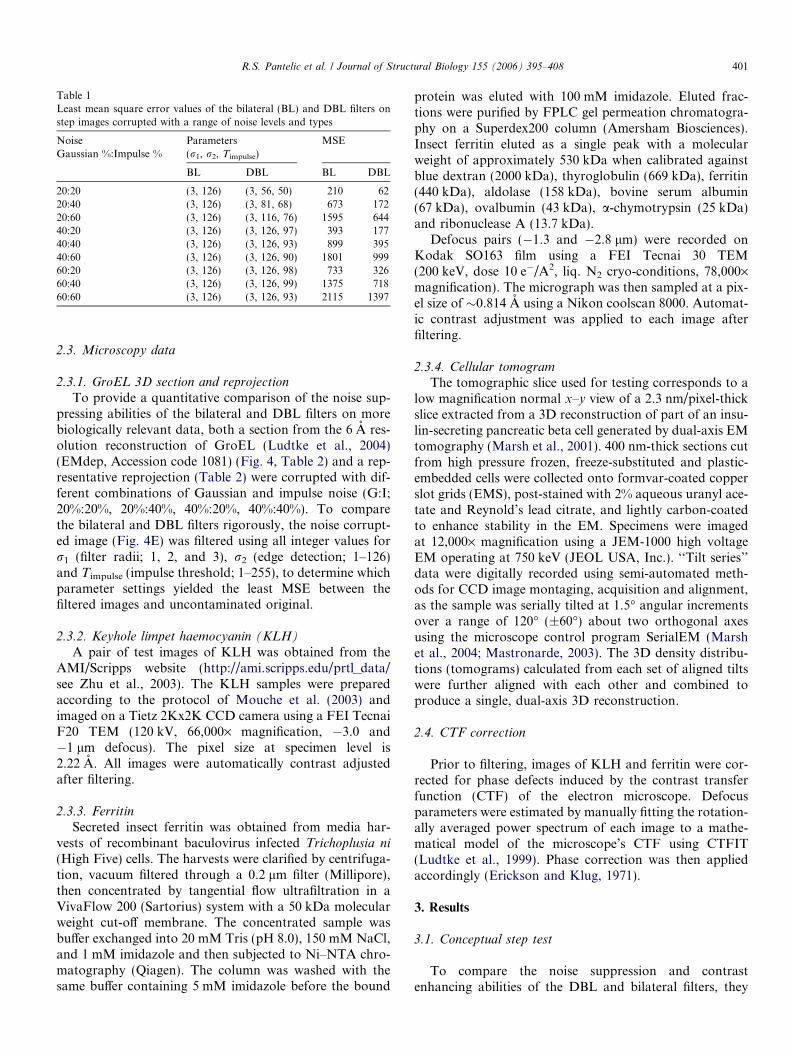
Table 1Least mean square error values of the bilateral (BL) and DBL filters onstep images corrupted with a range of noise levels and types

NoiseGaussian %:Impulse %

Parameters(r1, r2, Timpulse)

MSE

BL DBL BL DBL

20:20 (3, 126) (3, 56, 50) 210 6220:40 (3, 126) (3, 81, 68) 673 17220:60 (3, 126) (3, 116, 76) 1595 64440:20 (3, 126) (3, 126, 97) 393 17740:40 (3, 126) (3, 126, 93) 899 39540:60 (3, 126) (3, 126, 90) 1801 99960:20 (3, 126) (3, 126, 98) 733 32660:40 (3, 126) (3, 126, 99) 1375 71860:60 (3, 126) (3, 126, 93) 2115 1397


2.3. Microscopy data

2.3.1. GroEL 3D section and reprojection

To provide a quantitative comparison of the noise sup-pressing abilities of the bilateral and DBL filters on morebiologically relevant data, both a section from the 6 A res-olution reconstruction of GroEL (Ludtke et al., 2004)(EMdep, Accession code 1081) (Fig. 4, Table 2) and a rep-resentative reprojection (Table 2) were corrupted with dif-ferent combinations of Gaussian and impulse noise (G:I;20%:20%, 20%:40%, 40%:20%, 40%:40%). To comparethe bilateral and DBL filters rigorously, the noise corrupt-ed image (Fig. 4E) was filtered using all integer values forr1 (filter radii; 1, 2, and 3), r2 (edge detection; 1–126)and Timpulse (impulse threshold; 1–255), to determine whichparameter settings yielded the least MSE between thefiltered images and uncontaminated original.

2.3.2. Keyhole limpet haemocyanin (KLH)

A pair of test images of KLH was obtained from theAMI/Scripps website (http://ami.scripps.edu/prtl_data/see Zhu et al., 2003). The KLH samples were preparedaccording to the protocol of Mouche et al. (2003) andimaged on a Tietz 2Kx2K CCD camera using a FEI TecnaiF20 TEM (120 kV, 66,000· magnification, �3.0 and�1 lm defocus). The pixel size at specimen level is2.22 A. All images were automatically contrast adjustedafter filtering.

2.3.3. Ferritin

Secreted insect ferritin was obtained from media har-vests of recombinant baculovirus infected Trichoplusia ni(High Five) cells. The harvests were clarified by centrifuga-tion, vacuum filtered through a 0.2 lm filter (Millipore),then concentrated by tangential flow ultrafiltration in aVivaFlow 200 (Sartorius) system with a 50 kDa molecularweight cut-off membrane. The concentrated sample wasbuffer exchanged into 20 mM Tris (pH 8.0), 150 mM NaCl,and 1 mM imidazole and then subjected to Ni–NTA chro-matography (Qiagen). The column was washed with thesame buffer containing 5 mM imidazole before the bound

protein was eluted with 100 mM imidazole. Eluted frac-tions were purified by FPLC gel permeation chromatogra-phy on a Superdex200 column (Amersham Biosciences).Insect ferritin eluted as a single peak with a molecularweight of approximately 530 kDa when calibrated againstblue dextran (2000 kDa), thyroglobulin (669 kDa), ferritin(440 kDa), aldolase (158 kDa), bovine serum albumin(67 kDa), ovalbumin (43 kDa), a-chymotrypsin (25 kDa)and ribonuclease A (13.7 kDa).

Defocus pairs (�1.3 and �2.8 lm) were recorded onKodak SO163 film using a FEI Tecnai 30 TEM(200 keV, dose 10 e�/A2, liq. N2 cryo-conditions, 78,000·magnification). The micrograph was then sampled at a pix-el size of �0.814 A using a Nikon coolscan 8000. Automat-ic contrast adjustment was applied to each image afterfiltering.

2.3.4. Cellular tomogram

The tomographic slice used for testing corresponds to alow magnification normal x–y view of a 2.3 nm/pixel-thickslice extracted from a 3D reconstruction of part of an insu-lin-secreting pancreatic beta cell generated by dual-axis EMtomography (Marsh et al., 2001). 400 nm-thick sections cutfrom high pressure frozen, freeze-substituted and plastic-embedded cells were collected onto formvar-coated copperslot grids (EMS), post-stained with 2% aqueous uranyl ace-tate and Reynold’s lead citrate, and lightly carbon-coatedto enhance stability in the EM. Specimens were imagedat 12,000· magnification using a JEM-1000 high voltageEM operating at 750 keV (JEOL USA, Inc.). ‘‘Tilt series’’data were digitally recorded using semi-automated meth-ods for CCD image montaging, acquisition and alignment,as the sample was serially tilted at 1.5� angular incrementsover a range of 120� (±60�) about two orthogonal axesusing the microscope control program SerialEM (Marshet al., 2004; Mastronarde, 2003). The 3D density distribu-tions (tomograms) calculated from each set of aligned tiltswere further aligned with each other and combined toproduce a single, dual-axis 3D reconstruction.

2.4. CTF correction

Prior to filtering, images of KLH and ferritin were cor-rected for phase defects induced by the contrast transferfunction (CTF) of the electron microscope. Defocusparameters were estimated by manually fitting the rotation-ally averaged power spectrum of each image to a mathe-matical model of the microscope’s CTF using CTFIT(Ludtke et al., 1999). Phase correction was then appliedaccordingly (Erickson and Klug, 1971).

3. Results

3.1. Conceptual step test

To compare the noise suppression and contrastenhancing abilities of the DBL and bilateral filters, they

http://ami.scripps.edu/prtl_data/

Fig. 4. Evaluation of DBL and bilateral filter performance using a section of a 3D GroEL reconstruction contaminated with increasing levels of Gaussianand impulse noise. (A) Section of a 3D reconstruction of GroEL (EMdep, http://www.ebi.ac.uk/msd/index.html). (B–E) Section shown in A contaminatedwith different percentages of Gaussian (G) and impulse (I) noise. The MSE of each noise contaminated image is shown in the bottom right hand corner ofB–E (black text), with respect to the original (A). (F–I) The results of bilaterally filtering B–E, respectively, using the optimum settings of r1 and r2 (whitetext top right hand corner of B–E). Optimal settings were identified after evaluating all integer settings values for r1 (filter radii; 1, 2, and 3), r2 (edgedetection, 1–126) and Timpulse (1–255), based on the least MSE value (see Fig. 5). In all cases bilateral filtering markedly reduced the MSE values (blacktext) from those observed for the noise contaminated images. (J–M) The results of DBL filtering B–E respectively, using the optimum settings of r1, r2 andTimpulse (white text top right hand corner of B–E) based on the least MSE value. In all cases considerably lower MSE values (black text) were obtained forthe DBL filtered images than for the bilaterally filtered images.


were passed over a step image which had been contam-inated with different combinations of Gaussian andimpulse noise. Fig. 3 shows one example (Fig. 3A andE) contaminated with 20% Gaussian: 60% impulse noise(Fig. 3B and F). This was used as a stringent test toassess bilateral (Fig. 3C and G) and DBL (Fig. 3Dand H) filter performance under extreme conditions,typically encountered in low dose cryo-EM images. Inboth cases the filtered images in Fig. 3 represent theoptimal results in terms of MSE, compared to the ori-

ginal step image, found via exhaustive testing of theparameter settings (see methods). The improved perfor-mance of the DBL filter is shown by a considerablylower MSE value (Fig. 3H, MSE 644) than that ofthe bilateral filter (Fig. 3G, MSE 1595). Similarimprovements were observed over a wide range ofGaussian and impulse noise conditions (20–60%, seeTable 1). These results indicate that the enhanced per-formance of the DBL filter is due to its additional abil-ity to recognize and eliminate impulse corrupted pixels,

http://www.ebi.ac.uk/msd/index.html

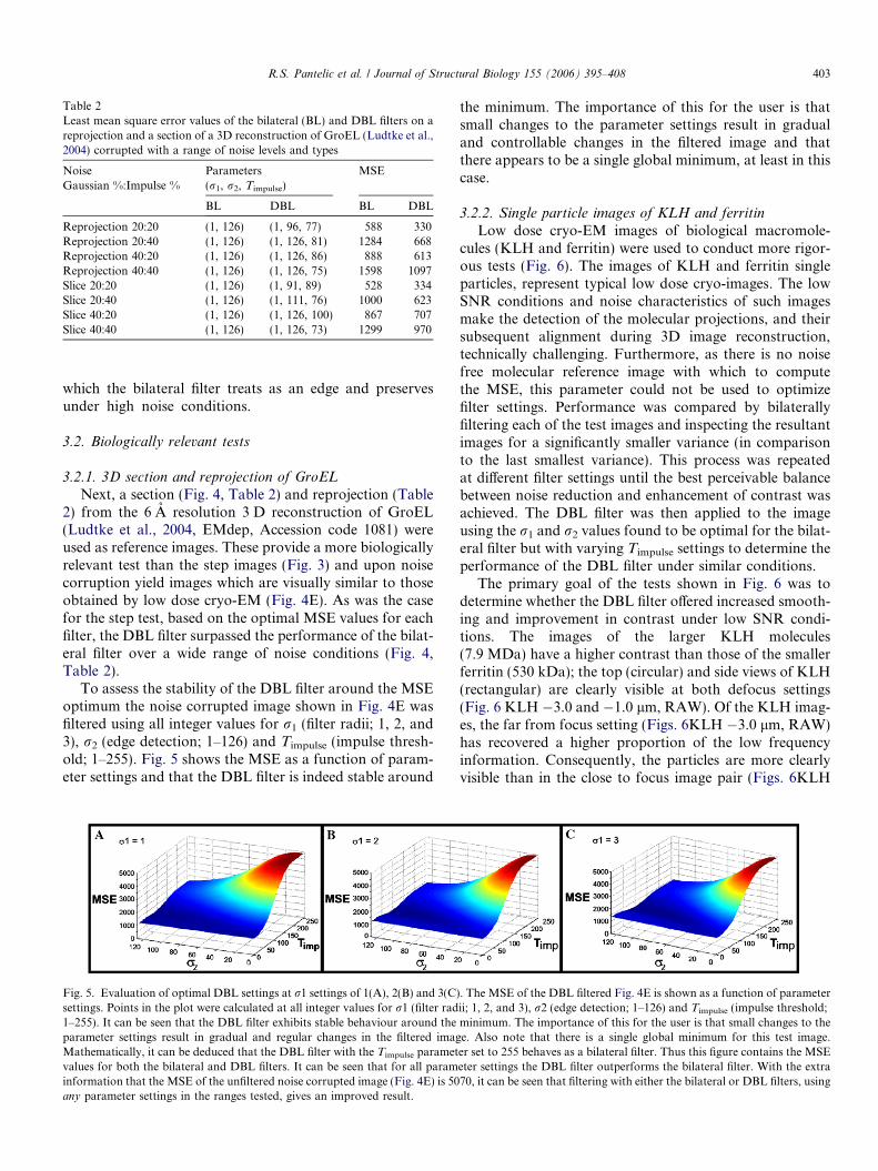
Table 2Least mean square error values of the bilateral (BL) and DBL filters on areprojection and a section of a 3D reconstruction of GroEL (Ludtke et al.,2004) corrupted with a range of noise levels and types

NoiseGaussian %:Impulse %

Parameters(r1, r2, Timpulse)

MSE

BL DBL BL DBL

Reprojection 20:20 (1, 126) (1, 96, 77) 588 330Reprojection 20:40 (1, 126) (1, 126, 81) 1284 668Reprojection 40:20 (1, 126) (1, 126, 86) 888 613Reprojection 40:40 (1, 126) (1, 126, 75) 1598 1097Slice 20:20 (1, 126) (1, 91, 89) 528 334Slice 20:40 (1, 126) (1, 111, 76) 1000 623Slice 40:20 (1, 126) (1, 126, 100) 867 707Slice 40:40 (1, 126) (1, 126, 73) 1299 970


which the bilateral filter treats as an edge and preservesunder high noise conditions.

3.2. Biologically relevant tests

3.2.1. 3D section and reprojection of GroEL

Next, a section (Fig. 4, Table 2) and reprojection (Table2) from the 6 A resolution 3 D reconstruction of GroEL(Ludtke et al., 2004, EMdep, Accession code 1081) wereused as reference images. These provide a more biologicallyrelevant test than the step images (Fig. 3) and upon noisecorruption yield images which are visually similar to thoseobtained by low dose cryo-EM (Fig. 4E). As was the casefor the step test, based on the optimal MSE values for eachfilter, the DBL filter surpassed the performance of the bilat-eral filter over a wide range of noise conditions (Fig. 4,Table 2).

To assess the stability of the DBL filter around the MSEoptimum the noise corrupted image shown in Fig. 4E wasfiltered using all integer values for r1 (filter radii; 1, 2, and3), r2 (edge detection; 1–126) and Timpulse (impulse thresh-old; 1–255). Fig. 5 shows the MSE as a function of param-eter settings and that the DBL filter is indeed stable around

Fig. 5. Evaluation of optimal DBL settings at r1 settings of 1(A), 2(B) and 3(C)settings. Points in the plot were calculated at all integer values for r1 (filter rad1–255). It can be seen that the DBL filter exhibits stable behaviour around theparameter settings result in gradual and regular changes in the filtered imagMathematically, it can be deduced that the DBL filter with the Timpulse parametvalues for both the bilateral and DBL filters. It can be seen that for all paraminformation that the MSE of the unfiltered noise corrupted image (Fig. 4E) is 50any parameter settings in the ranges tested, gives an improved result.

the minimum. The importance of this for the user is thatsmall changes to the parameter settings result in gradualand controllable changes in the filtered image and thatthere appears to be a single global minimum, at least in thiscase.

3.2.2. Single particle images of KLH and ferritin

Low dose cryo-EM images of biological macromole-cules (KLH and ferritin) were used to conduct more rigor-ous tests (Fig. 6). The images of KLH and ferritin singleparticles, represent typical low dose cryo-images. The lowSNR conditions and noise characteristics of such imagesmake the detection of the molecular projections, and theirsubsequent alignment during 3D image reconstruction,technically challenging. Furthermore, as there is no noisefree molecular reference image with which to computethe MSE, this parameter could not be used to optimizefilter settings. Performance was compared by bilaterallyfiltering each of the test images and inspecting the resultantimages for a significantly smaller variance (in comparisonto the last smallest variance). This process was repeatedat different filter settings until the best perceivable balancebetween noise reduction and enhancement of contrast wasachieved. The DBL filter was then applied to the imageusing the r1 and r2 values found to be optimal for the bilat-eral filter but with varying Timpulse settings to determine theperformance of the DBL filter under similar conditions.

The primary goal of the tests shown in Fig. 6 was todetermine whether the DBL filter offered increased smooth-ing and improvement in contrast under low SNR condi-tions. The images of the larger KLH molecules(7.9 MDa) have a higher contrast than those of the smallerferritin (530 kDa); the top (circular) and side views of KLH(rectangular) are clearly visible at both defocus settings(Fig. 6 KLH �3.0 and �1.0 lm, RAW). Of the KLH imag-es, the far from focus setting (Figs. 6KLH �3.0 lm, RAW)has recovered a higher proportion of the low frequencyinformation. Consequently, the particles are more clearlyvisible than in the close to focus image pair (Figs. 6KLH

. The MSE of the DBL filtered Fig. 4E is shown as a function of parameterii; 1, 2, and 3), r2 (edge detection; 1–126) and Timpulse (impulse threshold;minimum. The importance of this for the user is that small changes to thee. Also note that there is a single global minimum for this test image.er set to 255 behaves as a bilateral filter. Thus this figure contains the MSEeter settings the DBL filter outperforms the bilateral filter. With the extra70, it can be seen that filtering with either the bilateral or DBL filters, using


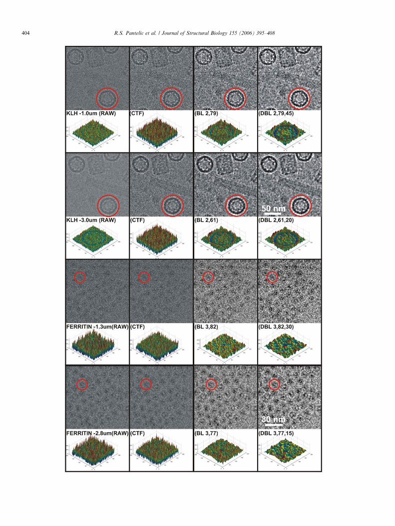
�1.0 lm, RAW). In comparison with KLH, the smallerferritin molecules are much less clearly defined, partlydue to their smaller size, and are less clearly visible evenin the more highly defocused image (Fig. 6FER �1.6 lm,RAW), when the contrast is set to display the full rangeof intensity values which are dominated by impulse noise.

Cryo-images are routinely CTF corrected for aberra-tions of the electron microscope prior to single particleanalysis. After CTF correction, the KLH particles in boththe close to and far from focus images (Fig 6KLH�1.0 lm, CTF) appear to be more clearly defined com-pared to the raw image (Fig 6KLH �1.0 and �3 lm,RAW), as the inverted frequency components have largelybeen recovered. Although the CTF correction step appearsto improve the contrast to a limited extent, the far andclose to focus KLH images (Fig. 6KLH, CTF) remain cor-rupted with dense impulse noise, making fine contour detailhard to distinguish. In contrast, neither the close to and farfrom focus ferritin images (Fig. 6FERRITIN �1.3 and�2.8 lm, CTF) have gained any perceivable improvementin contrast after CTF correction.

The application of the bilateral and DBL filters to allCTF corrected images in Figs. 6 (DBL and BL) in all casesremoved noise and improved the perceivable contrast.However, closer inspection shows that the DBL filterimproved the contrast to a greater degree. Surface plotsof the sections highlighted with a red ring show the greaterdegree of noise reduction in the DBL filtered image. Fig. 6therefore demonstrates, using real low SNR cryo-EM datathat the DBL filter outperforms the bilateral filter using r1

and r2 settings at which the bilateral filter was operating asclose to optimal as we could ascertain.

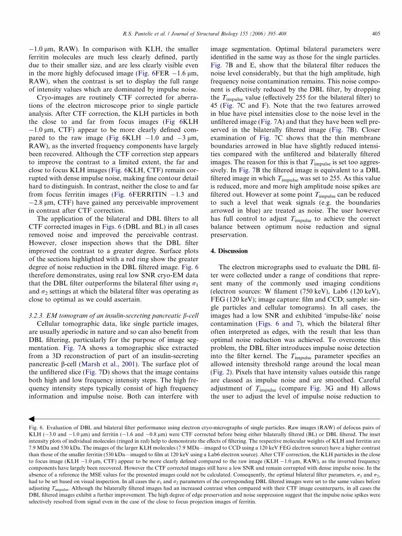
3.2.3. EM tomogram of an insulin-secreting pancreatic b-cell

Cellular tomographic data, like single particle images,are usually aperiodic in nature and so can also benefit fromDBL filtering, particularly for the purpose of image seg-mentation. Fig. 7A shows a tomographic slice extractedfrom a 3D reconstruction of part of an insulin-secretingpancreatic b-cell (Marsh et al., 2001). The surface plot ofthe unfiltered slice (Fig. 7D) shows that the image containsboth high and low frequency intensity steps. The high fre-quency intensity steps typically consist of high frequencyinformation and impulse noise. Both can interfere with

Fig. 6. Evaluation of DBL and bilateral filter performance using electron cryoKLH (�3.0 and �1.0 lm) and ferritin (�1.6 and �0.8 lm) were CTF correctintensity plots of individual molecules (ringed in red) help to demonstrate the e7.9 MDa and 530 kDa. The images of the larger KLH molecules (7.9 MDa—imthan those of the smaller ferritin (530 kDa—imaged to film at 120 keV using a Lto focus image (KLH �1.0 lm, CTF) appear to be more clearly defined compcomponents have largely been recovered. However the CTF corrected images sabsence of a reference the MSE values for the presented images could not be chad to be set based on visual inspection. In all cases the r1 and r2 parameters oadjusting Timpulse. Although the bilaterally filtered images had an increased coDBL filtered images exhibit a further improvement. The high degree of edge preselectively resolved from signal even in the case of the close to focus projectio

b

image segmentation. Optimal bilateral parameters wereidentified in the same way as those for the single particles.Fig. 7B and E, show that the bilateral filter reduces thenoise level considerably, but that the high amplitude, highfrequency noise contamination remains. This noise compo-nent is effectively reduced by the DBL filter, by droppingthe Timpulse value (effectively 255 for the bilateral filter) to45 (Fig. 7C and F). Note that the two features arrowedin blue have pixel intensities close to the noise level in theunfiltered image (Fig. 7A) and that they have been well pre-served in the bilaterally filtered image (Fig. 7B). Closerexamination of Fig. 7C shows that the thin membraneboundaries arrowed in blue have slightly reduced intensi-ties compared with the unfiltered and bilaterally filteredimages. The reason for this is that Timpulse is set too aggres-sively. In Fig. 7B the filtered image is equivalent to a DBLfiltered image in which Timpulse was set to 255. As this valueis reduced, more and more high amplitude noise spikes arefiltered out. However at some point Timpulse can be reducedto such a level that weak signals (e.g. the boundariesarrowed in blue) are treated as noise. The user howeverhas full control to adjust Timpulse to achieve the correctbalance between optimum noise reduction and signalpreservation.

4. Discussion

The electron micrographs used to evaluate the DBL fil-ter were collected under a range of conditions that repre-sent many of the commonly used imaging conditions(electron sources: W filament (750 keV), Lab6 (120 keV),FEG (120 keV); image capture: film and CCD; sample: sin-gle particles and cellular tomograms). In all cases, theimages had a low SNR and exhibited ‘impulse-like’ noisecontamination (Figs. 6 and 7), which the bilateral filteroften interpreted as edges, with the result that less thanoptimal noise reduction was achieved. To overcome thisproblem, the DBL filter introduces impulse noise detectioninto the filter kernel. The Timpulse parameter specifies anallowed intensity threshold range around the local mean(Fig. 2). Pixels that have intensity values outside this rangeare classed as impulse noise and are smoothed. Carefuladjustment of Timpulse (compare Fig. 3G and H) allowsthe user to adjust the level of impulse noise reduction to

-micrographs of single particles. Raw images (RAW) of defocus pairs ofed before being either bilaterally filtered (BL) or DBL filtered. The inset

ffects of filtering. The respective molecular weights of KLH and ferritin areaged to CCD using a 120 keV FEG electron source) have a higher contrastab6 electron source). After CTF correction, the KLH particles in the closeared to the raw image (KLH �1.0 lm, RAW), as the inverted frequency

till have a low SNR and remain corrupted with dense impulse noise. In thealculated. Consequently, the optimal bilateral filter parameters, r1 and r2,f the corresponding DBL filtered images were set to the same values beforentrast when compared with their CTF image counterparts, in all cases theservation and noise suppression suggest that the impulse noise spikes weren images of ferritin.

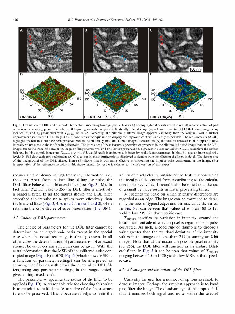
Fig. 7. Evaluation of DBL and bilateral filter performance using tomographic sections. (A) Tomographic slice extracted from a 3D reconstruction of partof an insulin-secreting pancreatic beta cell (Original grey-scale image). (B) Bilaterally filtered image (r1 = 1 and r2 = 36). (C) DBL filtered image usingidentical r1 and r2 parameters with Timpulse set to 45. Generally, the bilaterally filtered image appears less noisy than the original, with a furtherimprovement seen in the DBL image. (A–C) have been auto equalized to display the improved contrast as clearly as possible. The red arrows in (A)–(C)highlight fine features that have been preserved well in the bilaterally and DBL filtered images. Note that in (A) the features arrowed in blue appear to haveintensity values close to those of the impulse noise. The intensities of these features appear better preserved in the bilaterally filtered image than in the DBLimage, due to the trade-off between the degree of impulse removal and fine feature preservation. However the user can adjust Timpulse to achieve the desiredbalance. In this example increasing Timpulse towards 255, would result in an increase in intensity of the features arrowed in blue, but also an increased noiselevel. (D–F) Below each grey-scale image (A–C) a colour intensity surface plot is displayed to demonstrate the effects of the filters in detail. The deeper blueof the background of the DBL filtered image (F) shows that it was more effective at smoothing the impulse noise component of the image. (Forinterpretation of the references to color in this figure legend, the reader is referred to the web version of this paper.)


recover a higher degree of high frequency information (i.e.,the step). Apart from the handling of impulse noise, theDBL filter behaves as a bilateral filter (see Fig. 3I–M). Infact when Timpulse is set to 255 the DBL filter is effectivelya bilateral filter. In all the figures shown, the DBL filtersmoothed the impulse noise spikes more effectively thanthe bilateral filter (Figs 3, 4, 6, and 7, Tables 1 and 2), whileretaining the same degree of edge preservation (Fig. 3M).

4.1. Choice of DBL parameters

The choice of parameters for the DBL filter cannot bedetermined on an algorithmic basis except in the specialcase where the noise free image is already known. In allother cases the determination of parameters is not an exactscience, however certain guidelines can be given. With theextra information that the MSE of the unfiltered noise cor-rupted image (Fig. 4E) is 5070, Fig. 5 (which shows MSE asa function of parameter settings) can be interpreted asshowing that filtering with either the bilateral or DBL fil-ters, using any parameter settings, in the ranges tested,gives an improved result.

The parameter r1 specifies the radius of the filter to beapplied (Fig. 1B). A reasonable rule for choosing this valueis to match it to half of the feature size of the finest struc-ture to be preserved. This is because it helps to limit the

ability of pixels clearly outside of the feature upon whichthe focal pixel is centred from contributing to the calcula-tion of its new value. It should also be noted that the useof a small r1 value results in faster processing times.

r2 specifies the scale on which intensity differences areregarded as an edge. The image can be examined to deter-mine the sizes of typical edges and this size value then used.In Fig. 5 it can be seen that values of r2 from 80 to 126yield a low MSE in that specific case.

Timpulse specifies the variation in intensity, around thelocal mean, outside of which a pixel is regarded as impulsecorrupted. As such, a good rule of thumb is to choose avalue greater than the standard deviation of the intensityvalues in the image and less than 255 (assuming an 8 bitimage). Note that at the maximum possible pixel intensity(i.e. 255), the DBL filter will function as a standard Bilat-eral filter. In Fig. 5 it can be seen that values of Timpulse

ranging between 50 and 120 yield a low MSE in that specif-ic case.

4.2. Advantages and limitations of the DBL filter

Currently the user has a number of options available todenoise images. Perhaps the simplest approach is to bandpass filter the image. The disadvantage of this approach isthat it removes both signal and noise within the selected


frequency domain. Another commonly used approach is toapply a median filter. Median filters are effective at removinghigh frequency noise, but have the disadvantage that theyindiscriminately change intensity values in the image regard-less of whether or not the pixels are corrupted. It thereforeintrinsically results in the degradation of high frequencyinformation and thus median filtered images are oftensubjected to a subsequent edge sharpening stage. One ofthe advantages of the DBL filter is that it captures the bene-fits of the median filter’s reduction in high-frequency noisewithout losing genuine high frequency information. TheDBL filter achieves this by only replacing a noise corruptedfocal pixel with the local median value and excluding neigh-bouring impulses, prior to the application of the bilateralfilter component of the kernel. This discriminative behaviouris one of the key differences between using the DBL filter asopposed to using a median filter followed by a bilateral filter.Furthermore, the DBL achieves its effect in one pass.

Another advantage of the DBL filter is that it appears tobe less affected by the use of smaller filter sizes, as morestringent Timpulse thresholds are able to compensate. Thissuggests that the DBL filter may be more effective in filter-ing smaller structures with low SNRs, as noise suppressionis less affected by filter size. The DBL filter should thus pro-vide more focussed smoothing than either the Gaussian orbilateral filters.

In comparison to the median filter, both the bilateraland DBL filters are relatively slow in execution. Giventhe real space nature of the bilateral and DBL filters, onepossible method to decrease processing time is to conductparallel, segment based filtering (Jiang et al., 2003).

4.3. Potential applications

The noise reducing capabilities of the DBL filter willallow it to be used to improve a wide range of applications.For example, Fig. 6 suggests that DBL filtering low dosecryo images may assist in the detection of small proteincomplexes as well as their automatic selection.

In single particle analysis, noise also affects the initialparticle alignment and classification stages. For example,Sander et al. (2005) showed that the removal of the noisy,high frequency domain of single particle images by lowpass filtering results in much more accurate particle align-ment. This is because cross correlation based algorithmsare affected to a degree, by high frequency noise, as thecross correlation value is based on the full frequency rangeused. Consequently the use of DBL filtered images in whichthe high frequency noise is markedly reduced could assistin the accurate determination of initial class sums. Theassignment of Euler angles using the sinogram (van Heelet al., 2000) or related approaches, may benefit in a similarway.

With the rapid advances in high-resolution cellulartomography, automated image segmentation is alsobecoming increasingly important. While there are a num-ber of segmentation algorithms available (Bartesaghi

et al., 2005; Roerdink and Meijster, 2000; Volkmann,2002), each generally benefits from a noise suppressionpre-filtering step (Fig. 7). The properties of the DBLfilter may make it a valuable pre-processing tool in thisrespect.

5. Conclusions

The DBL filter has been shown to be particularly usefulfor denoising low SNR images corrupted with impulsenoise, such as low dose electron cryo-micrographs, whilepreserving important edge detail. In contrast to the bilater-al filter, the DBL filter is able to distinguish between objectedges and impulse noise pixels through the use of a furtherphotometric exclusion function. The value of the DBL fil-ter is clearly shown in Figs 3–7, which demonstrate its effi-cacy in suppressing strong impulse noise while preservingcontour (i.e., edge detail). More specifically, the DBL filterhas been shown to denoise low SNR single particle dataand cellular tomograms. In terms of single particle analysis,the properties of the DBL filter could prove to be a usefultool to assist single particle detection, classification, align-ment and 3D image reconstruction. In the context oftomography, the DBL filter may assist in automatic imagesegmentation.

Acknowledgements

We gratefully acknowledge the financial support of thiswork by the Australian Research Council, (Grant Nos.DP0452362 and DP0556547) and the Australian Partner-ship for Advanced Computing. We particularly thankYuanxin Yhu, Bridget Carragher, and Clint Potter (AMI,The Scripps Research Institiute) for providing us with theKLH data via the http://ami.scripps.edu/prtl_data/site,and Brad Marsh (Institute for Molecular Bioscience) forkindly providing us with the tomographic slice of part ofan insulin-secreting pancreatic b-cell for testing purposes.We also thank Steve Ludtke and his colleagues (NationalCenter for Macromolecular Imaging, Baylor College ofMedicine) for making available their 6 A resolution 3Dreconstruction of GroEL via EMDep (http://www.ebi.ac.uk/msd/index.html).

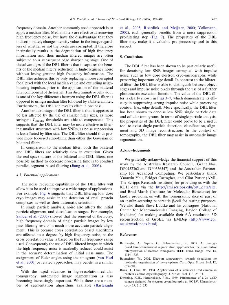
References

Bartesaghi, A., Sapiro, G., Subramaniam, S., 2005. An energy-based three-dimensional segmentation approach for the quantitativeinterpretation of electron tomograms. IEEE Trans. Image Proc. 14,1314–1323.

Baumeister, W., 2002. Electron tomography: towards visualizing themolecular organization of the cytoplasm. Curr. Opin. Struct. Biol. 12,679–684.

Brink, J., Chiu, W., 1994. Applications of a slow-scan Ccd camera inprotein electron crystallography. J. Struct. Biol. 113, 23–34.

Downing, K.H., Hendrickson, F.M., 1999. Performance of a 2k CCDcamera designed for electron crystallography at 400 kV. Ultramicros-copy 75, 215–233.

http://ami.scripps.edu/prtl_data/site




Erickson, H.P., Klug, A., 1971. Measurement and compensation ofdefocusing and aberrations by Fourier processing of electronmicrographs. Phil. Trans. R. Soc. Lond. Ser. B—Biol. Sci. 261,105.

Gonen, T., Cheng, Y., Sliz, P., Hiroaki, Y., Fujiyoshi, Y., Harrison, S.,Walz, T., 2005. Lipid–protein interactions in double-layered two-dimensional AQPO crystals. Nature 438, 633–638.

Jiang, W., Baker, M.L., Wu, Q., Bajaj, C., Chiu, W., 2003. Applications ofa bilateral denoising filter in biological electron microscopy. J. Struct.Biol. 144, 114–122.

Ludtke, S.J., Baldwin, P.R., Chiu, W., 1999. EMAN: semiautomatedsoftware for high-resolution single-particle reconstructions. J. Struct.Biol. 128, 82–97.

Ludtke, S.J., Chen, D.H., Song, J.L., Chuang, D.T., Chiu, W., 2004.Seeing GroEL at 6 A resolution by single particle electron cryomi-croscopy. Structure 12, 1129–1136.

Marsh, B.J., Mastronarde, D.N., Buttle, K.F., Howell, K.E., McIn-tosh, J.R., 2001. Organellar relationships in the Golgi region ofthe pancreatic beta cell line, HIT-T15, visualized by highresolution electron tomography. Proc. Natl. Acad. Sci. USA 98,2399–2406.

Marsh, B.J., Volkmann, N., McIntosh, J.R., Howell, K.E., 2004. Directcontinuities between cisternae at different levels of the Golgi complexin glucose-stimulated mouse islet beta cells. Proc. Natl. Acad. Sci.USA 101, 5565–5570.

Mastronarde, D.N., 2003. SerialEM: a program for automated tilt seriesacquisition on Tecnai microscopes using prediction of specimenposition. Microsc. Microanal. 9, 1182–1183.

Mitsuoka, K., Hirai, T., Murata, K., Miyazawa, A., Kidera, A., Kimura,Y., Fujiyoshi, Y., 1999. The structure of bacteriorhodopsin at 3.0

angstrom resolution based on electron crystallography: Implication ofthe charge distribution. J. Mol. Biol. 286, 861–882.

Mouche, F., Zhu, Y.X., Pulokas, J., Potter, C.S., Carragher, B., 2003.Automated three-dimensional reconstruction of keyhole limpet hemo-cyanin type 1. J. Struct. Biol. 144, 301–312.

Roerdink, J.B.T.M., Meijster, A., 2000. The watershed transform:definitions, algorithms, and parallellization strategies. IEEE Trans.Image Proc. 14, 187–228.

Sander, B., Golas, M.M., Stark, H., 2005. Advantages of CCDdetectors for de novo three-dimensional structure determinationin single-particle electron microscopy. J. Struct. Biol. 151,92–105.

Tomasi, C., Manduchi, R., 1998. Bilateral filtering for gray and colorimages. In: Proceedings of IEEE International Conference on Com-puter Vision, Bombay, India, pp. 59–66.

van Heel, M., Gowen, B., Matadeen, R., Orlova, E.V., Finn, R., Pape, T.,Cohen, D., Stark, H., Schmidt, R., Schatz, M., Patwardhan, A., 2000.Single-particle electron cryo-microscopy: towards atomic resolution.Quat. Rev. Biophys. 33, 307–369.

Volkmann, N., 2002. A novel three-dimensional variant of the watershedtransform for segmentation of electron density maps. J. Struct. Biol.138, 123–129.

Zeneka, D., Van Mastrigt, C., 2005. FEI announces world’s mostadvanced electron microscope, FEI Company, News for immediaterelease, Hillsboro.

Zhang, D.P., Wang, Z., 1998. Impulse noise removal using polynomialapproximation. Opt. Eng. 37, 1275–1282.

Zhu, Y., Carragher, B., Mouche, F., Potter, C., 2003. Automatic particledetection through efficient Hough transforms. IEEE Trans. Med.Imaging 22, 1053–1062.

the discriminative bilateral filter: an enhanced denoising filter for electron microscopy data

Documents