Discriminative k-Means Clustering

Ognjen ArandjelovicCentre for Pattern Recognition and Data Analytics

Deakin University, Australiaognjen.arandjelovic@gmail.com

Abstract— The k-means algorithm is a partitional clusteringmethod. Over 60 years old, it has been successfully used for avariety of problems. The popularity of k-means is in large parta consequence of its simplicity and efficiency. In this paper weare inspired by these appealing properties of k-means in thedevelopment of a clustering algorithm which accepts the notionof “positively” and “negatively” labelled data. The goal is todiscover the cluster structure of both positive and negative datain a manner which allows for the discrimination between thetwo sets. The usefulness of this idea is demonstrated practicallyon the problem of face recognition, where the task of learningthe scope of a person’s appearance should be done in a mannerwhich allows this face to be differentiated from others.

I. INTRODUCTION

IN data analysis, clustering refers to the process of dis-covering groups (clusters) of similar data points. Being a

vital tool in the exploration, sparsification and dimensionalityreduction of data, it is unsurprising to observe that clusteringis intensively used in a wide range of applications, fromprotein sequencing [1] to astronomical surveys of the sky [2].The use of clustering is even more ubiquitous in imageand multimedia processing: at the lowest level, clusteringis used to build vocabularies of low-level features usedto represent individual objects [3], [4], [5], images [6] orelementary motions [7]; at medium-level, clustering may beused to list the cast of a movie [8] or detect coherentlymoving objects [9], [10]; at the highest level, video clipsor images may themselves be clustered by the similarity oftheir content [11], [12].

Despite continuing major research efforts, clustering re-mains a most challenging problem. The application-specificnotion of what a good cluster is, the volume and dimension-ality of data, its sparsity and structure, and the number ofclusters, are only some of the factors which govern one’schoice of the clustering methodology. Popular algorithmsinclude those based on spectral approaches [13], various non-parametric formulations e.g. using the Dirichlet process [14],information theoretic ideas [15], and many others [16].

Yet, notwithstanding the cornucopia of sophisticated clus-tering models described in the literature, to this day the mostpopular and widely used clustering approach remains to bethe simple k-means algorithm [17].

II. K-MEANS CLUSTERING

Let X = {x1, x2, . . . , xn} be a set of d-dimensionalpoints. The k-means algorithm partitions the points into Kclusters, X1, . . . , XK , so that each datum belongs to one andonly one cluster. In addition, an attempt is made to minimize

the sum of squared distances between each data point and theempirical mean of the corresponding cluster. In other words,the k-means algorithm attempts to minimize the followingobjective function:

J(X1, . . . , Xk) =

k∑i=1

∑x∈Xi

‖ci − x‖2, (1)

where the empirical cluster means are calculated as:

ci =∑x∈Xi

x /∣∣Xi

∣∣. (2)

The exact minimization of the objective function in Eq. (1)is an NP-hard problem [18]. Instead, the k-means algorithmonly guarantees convergence to a local minimum. Startingfrom an initial guess, the algorithm iteratively updates clustercentres and data-cluster assignments until (i) a local min-imum is attained, or (ii) an alternative stopping criterionis met (e.g. the maximal desired number of iterations or asufficiently small sum of squared distances).

The k-means algorithm starts from an initial guess ofcluster centres c

(0)1 , c

(0)2 , . . . , c

(0)k . Often, this is achieved

simply by choosing k data points at random as the centres ofthe initial clusters, although more sophisticated initializationmethods have been proposed [19], [20]. Then, at eachiteration t = 0, . . . the new datum-cluster assignment iscomputed:

X(t)i = {x : x ∈ X ∧ argmin

j

∥∥x− c(t)j

∥∥2 = i}. (3)

In other words, each datum is assigned to the cluster withthe nearest (in Euclidean sense) empirical mean. Lastly, thelocations of cluster centres are re-computed from the newassignments by finding the mean of the data assigned to eachcluster:

c(t+1)i =

∑x∈X(t)

i

x /∣∣X(t)

i

∣∣. (4)

The algorithm is guaranteed to converge because neither ofthe updates in Eq. (3) nor Eq. (4) can ever increase theobjective function of Eq. (1).

Various extensions of the original k-means algorithm in-clude fuzzy c-means [21], k-medoid [22], kernel k-means[23]. Their relevance to the topic of the present paper istangential and the interested reader is referred to the citedpublications for further information.

III. EXTENDED K-MEANS CLUSTERING

In the present paper we are interested in the problem ofclustering data which comprises two types of data points,which we will call “positively labelled” and “negativelylabelled”, and which should be clustered in such a way toallow for the two types to be discriminated between. Ourgoal is to inherit the simple ideas underlying the classical k-means algorithm, while extending the algorithm to deal withthis novel complexity in the data.

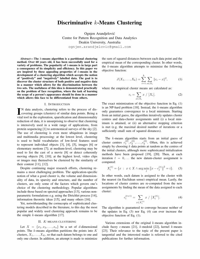
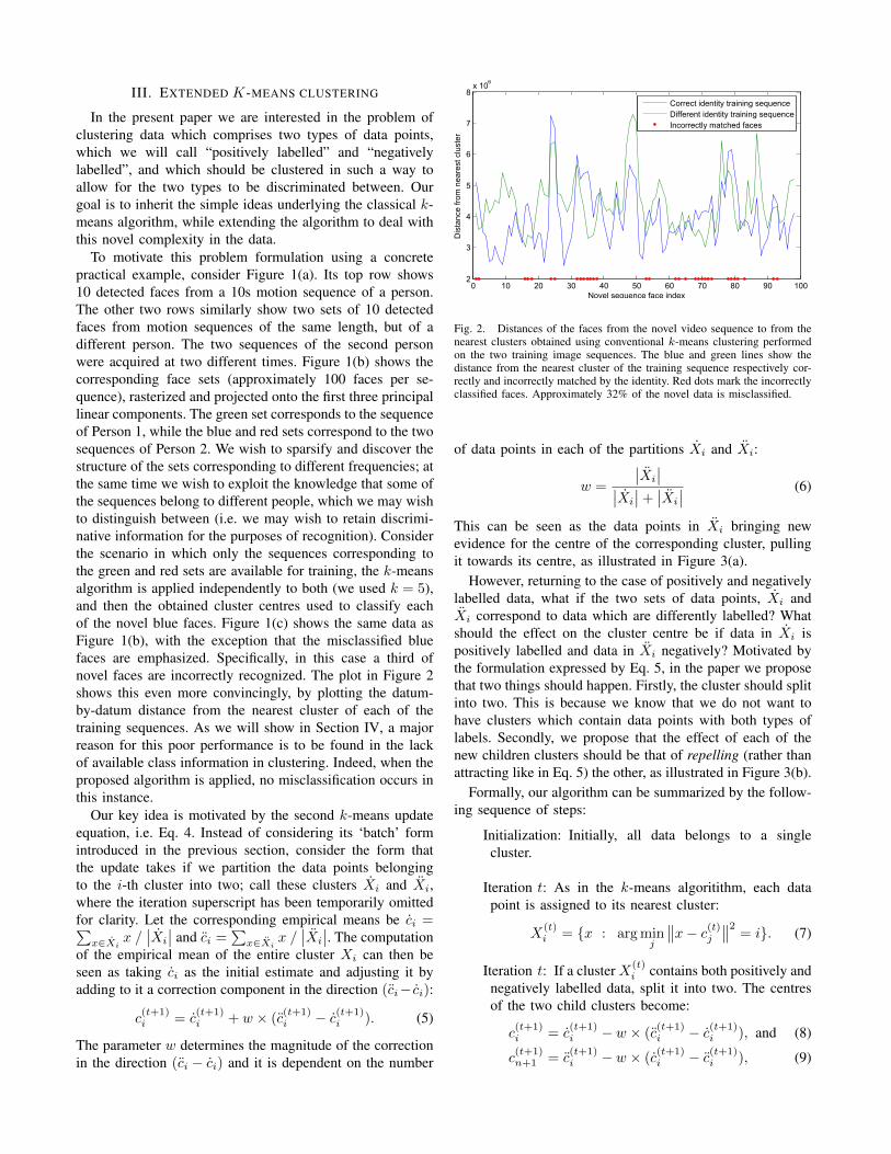
To motivate this problem formulation using a concretepractical example, consider Figure 1(a). Its top row shows10 detected faces from a 10s motion sequence of a person.The other two rows similarly show two sets of 10 detectedfaces from motion sequences of the same length, but of adifferent person. The two sequences of the second personwere acquired at two different times. Figure 1(b) shows thecorresponding face sets (approximately 100 faces per se-quence), rasterized and projected onto the first three principallinear components. The green set corresponds to the sequenceof Person 1, while the blue and red sets correspond to the twosequences of Person 2. We wish to sparsify and discover thestructure of the sets corresponding to different frequencies; atthe same time we wish to exploit the knowledge that some ofthe sequences belong to different people, which we may wishto distinguish between (i.e. we may wish to retain discrimi-native information for the purposes of recognition). Considerthe scenario in which only the sequences corresponding tothe green and red sets are available for training, the k-meansalgorithm is applied independently to both (we used k = 5),and then the obtained cluster centres used to classify eachof the novel blue faces. Figure 1(c) shows the same data asFigure 1(b), with the exception that the misclassified bluefaces are emphasized. Specifically, in this case a third ofnovel faces are incorrectly recognized. The plot in Figure 2shows this even more convincingly, by plotting the datum-by-datum distance from the nearest cluster of each of thetraining sequences. As we will show in Section IV, a majorreason for this poor performance is to be found in the lackof available class information in clustering. Indeed, when theproposed algorithm is applied, no misclassification occurs inthis instance.

Our key idea is motivated by the second k-means updateequation, i.e. Eq. 4. Instead of considering its ‘batch’ formintroduced in the previous section, consider the form thatthe update takes if we partition the data points belongingto the i-th cluster into two; call these clusters Xi and Xi,where the iteration superscript has been temporarily omittedfor clarity. Let the corresponding empirical means be ci =∑

x∈Xix /∣∣Xi

∣∣ and ci =∑

x∈Xix /∣∣Xi

∣∣. The computationof the empirical mean of the entire cluster Xi can then beseen as taking ci as the initial estimate and adjusting it byadding to it a correction component in the direction (ci− ci):

c(t+1)i = c

(t+1)i + w × (c

(t+1)i − c

(t+1)i ). (5)

The parameter w determines the magnitude of the correctionin the direction (ci − ci) and it is dependent on the number

0 10 20 30 40 50 60 70 80 90 1002

3

4

5

6

7

8x 10

6

Novel sequence face index

Dis

tanc

e fr

om n

eare

st c

lust

er

Correct identity training sequenceDifferent identity training sequenceIncorrectly matched faces

Fig. 2. Distances of the faces from the novel video sequence to from thenearest clusters obtained using conventional k-means clustering performedon the two training image sequences. The blue and green lines show thedistance from the nearest cluster of the training sequence respectively cor-rectly and incorrectly matched by the identity. Red dots mark the incorrectlyclassified faces. Approximately 32% of the novel data is misclassified.

of data points in each of the partitions Xi and Xi:

w =

∣∣Xi

∣∣∣∣Xi

∣∣+ ∣∣Xi

∣∣ (6)

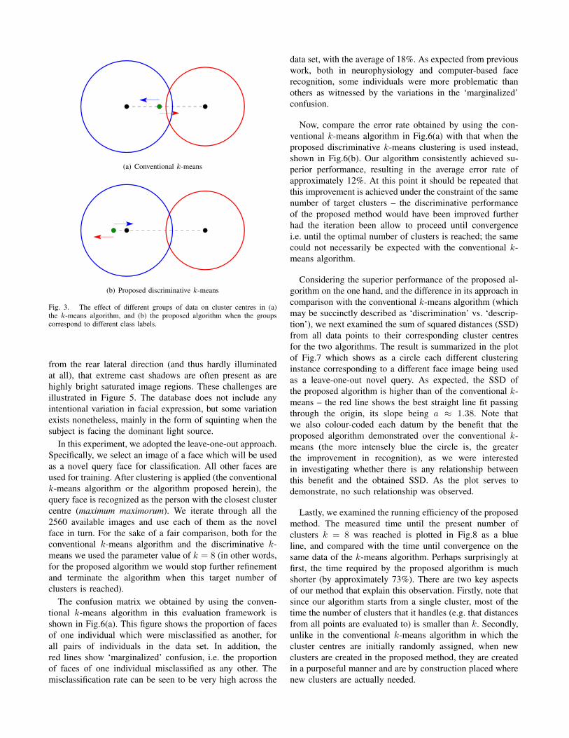
This can be seen as the data points in Xi bringing newevidence for the centre of the corresponding cluster, pullingit towards its centre, as illustrated in Figure 3(a).

However, returning to the case of positively and negativelylabelled data, what if the two sets of data points, Xi andXi correspond to data which are differently labelled? Whatshould the effect on the cluster centre be if data in Xi ispositively labelled and data in Xi negatively? Motivated bythe formulation expressed by Eq. 5, in the paper we proposethat two things should happen. Firstly, the cluster should splitinto two. This is because we know that we do not want tohave clusters which contain data points with both types oflabels. Secondly, we propose that the effect of each of thenew children clusters should be that of repelling (rather thanattracting like in Eq. 5) the other, as illustrated in Figure 3(b).

Formally, our algorithm can be summarized by the follow-ing sequence of steps:

Initialization: Initially, all data belongs to a singlecluster.

Iteration t: As in the k-means algoritithm, each datapoint is assigned to its nearest cluster:

X(t)i = {x : argmin

j

∥∥x− c(t)j

∥∥2 = i}. (7)

Iteration t: If a cluster X(t)i contains both positively and

negatively labelled data, split it into two. The centresof the two child clusters become:

c(t+1)i = c

(t+1)i − w × (c

(t+1)i − c

(t+1)i ), and (8)

c(t+1)n+1 = c

(t+1)i − w × (c

(t+1)i − c

(t+1)i ), (9)

Person 2Sequence 1

Person 1Sequence 1

Person 2Sequence 2

(a)

80007000

60005000

4000

3000

2000

1000

0

1000

2000

3000

4000

Principal component 1Principal component 2

Prin

cipa

l com

pone

nt 3

(b)

4000

50006000

70008000

01000

20003000

1000

2000

3000

4000

Principal component 1Principal component 2

Prin

cipa

l com

pone

nt 3

(c)

Fig. 1. (a) Three 10s long face motion sequences (due to space constraints only every 10th detected face is shown). (b) The three sets of rasterized faceimages shown projected to the first three principal components. (c) Misclassified faces of the blue set (32% misclassification rate) when the green and redsets are used for training and the k-means algorithm is used to represent the corresponding manifold structures.

where n is the previous number of clusters, c(t+1)i

is the mean of positively labelled data in X(t)i and

c(t+1)i is the mean of negatively labelled data in X

(t)i ,

and w a non-negative weight.

Iteration t: If a cluster X(t)i contains only positively or

negatively labelled data, update its empirical mean asin the k-means algorithm:

c(t+1)i =

∑x∈X(t)

i

x /∣∣X(t)

i

∣∣. (10)

Termination: Terminate when the maximal desirednumber of clusters is reached or when the algorithmhas converged (guaranteed in a similar manner to theconventional k-means algorithm.

IV. EVALUATION

A. Synthetic dataWe start this section by illustrating the operation of the

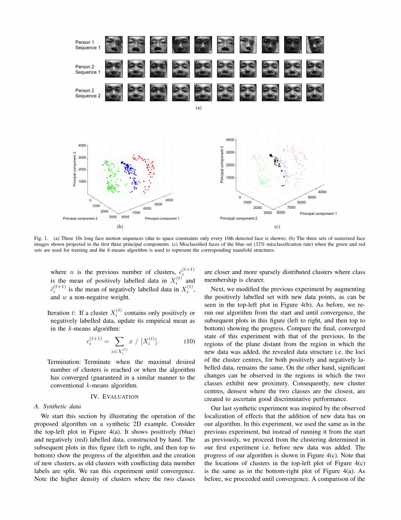
proposed algorithm on a synthetic 2D example. Considerthe top-left plot in Figure 4(a). It shows positively (blue)and negatively (red) labelled data, constructed by hand. Thesubsequent plots in this figure (left to right, and then top tobottom) show the progress of the algorithm and the creationof new clusters, as old clusters with conflicting data memberlabels are split. We ran this experiment until convergence.Note the higher density of clusters where the two classes

are closer and more sparsely distributed clusters where classmembership is clearer.

Next, we modified the previous experiment by augmentingthe positively labelled set with new data points, as can beseen in the top-left plot in Figure 4(b). As before, we re-run our algorithm from the start and until convergence, thesubsequent plots in this figure (left to right, and then top tobottom) showing the progress. Compare the final, convergedstate of this experiment with that of the previous. In theregions of the plane distant from the region in which thenew data was added, the revealed data structure i.e. the lociof the cluster centres, for both positively and negatively la-belled data, remains the same. On the other hand, significantchanges can be observed in the regions in which the twoclasses exhibit new proximity. Consequently, new clustercentres, densest where the two classes are the closest, arecreated to ascertain good discriminative performance.

Our last synthetic experiment was inspired by the observedlocalization of effects that the addition of new data has onour algorithm. In this experiment, we used the same as in theprevious experiment, but instead of running it from the startas previously, we proceed from the clustering determined inour first experiment i.e. before new data was added. Theprogress of our algorithm is shown in Figure 4(c). Note thatthe locations of clusters in the top-left plot of Figure 4(c)is the same as in the bottom-right plot of Figure 4(a). Asbefore, we proceeded until convergence. A comparison of the

(a) Experiment 1: Synthetic data set 1

(b) Experiment 2: Synthetic data set 2 (expanded synthetic data set 1)

(c) Experiment 3: Synthetic data set 2, algorithm run from the final state of Experiment 1

Fig. 4. The evaluation of the proposed method in three experiments on synthetic data. (a) The result on the first synthetic data set until convergence.(b) The result on the second synthetic data set (first set augmented with novel positively labelled data) until convergence. (c) The result on the secondsynthetic data set, initialized with the clustering result of the first experiment, until convergence.

final results of this and the previous experiments reveals aremarkable agreement between the determined cluster centresloci.

B. Face recognition

Next, we evaluated the proposed algorithm on a chal-lenging problem of immense practical significance: facerecognition across illumination. As particularly appropriatefor this experiment, we used the Extended YaleB database.This is a most difficult data set used as a standard benchmark

for the comparison of face recognition algorithms in terms oftheir robustness to severe illumination changes. It contains 40people and 64 images per person, each image correspondingto a different illumination. The variation in the direction ofthe dominant light source illuminating a face is extreme: itsazimuth varies from -130◦ to 130◦, and its elevation from-40◦ (i.e. pointing upwards) to 90◦ (i.e. directly overhead,pointing downwards), giving a total of 64 different illumina-tion conditions. Notice that the face is sometimes illuminated

(a) Conventional k-means

(b) Proposed discriminative k-means

Fig. 3. The effect of different groups of data on cluster centres in (a)the k-means algorithm, and (b) the proposed algorithm when the groupscorrespond to different class labels.

from the rear lateral direction (and thus hardly illuminatedat all), that extreme cast shadows are often present as arehighly bright saturated image regions. These challenges areillustrated in Figure 5. The database does not include anyintentional variation in facial expression, but some variationexists nonetheless, mainly in the form of squinting when thesubject is facing the dominant light source.

In this experiment, we adopted the leave-one-out approach.Specifically, we select an image of a face which will be usedas a novel query face for classification. All other faces areused for training. After clustering is applied (the conventionalk-means algorithm or the algorithm proposed herein), thequery face is recognized as the person with the closest clustercentre (maximum maximorum). We iterate through all the2560 available images and use each of them as the novelface in turn. For the sake of a fair comparison, both for theconventional k-means algorithm and the discriminative k-means we used the parameter value of k = 8 (in other words,for the proposed algorithm we would stop further refinementand terminate the algorithm when this target number ofclusters is reached).

The confusion matrix we obtained by using the conven-tional k-means algorithm in this evaluation framework isshown in Fig.6(a). This figure shows the proportion of facesof one individual which were misclassified as another, forall pairs of individuals in the data set. In addition, thered lines show ‘marginalized’ confusion, i.e. the proportionof faces of one individual misclassified as any other. Themisclassification rate can be seen to be very high across the

data set, with the average of 18%. As expected from previouswork, both in neurophysiology and computer-based facerecognition, some individuals were more problematic thanothers as witnessed by the variations in the ‘marginalized’confusion.

Now, compare the error rate obtained by using the con-ventional k-means algorithm in Fig.6(a) with that when theproposed discriminative k-means clustering is used instead,shown in Fig.6(b). Our algorithm consistently achieved su-perior performance, resulting in the average error rate ofapproximately 12%. At this point it should be repeated thatthis improvement is achieved under the constraint of the samenumber of target clusters – the discriminative performanceof the proposed method would have been improved furtherhad the iteration been allow to proceed until convergencei.e. until the optimal number of clusters is reached; the samecould not necessarily be expected with the conventional k-means algorithm.

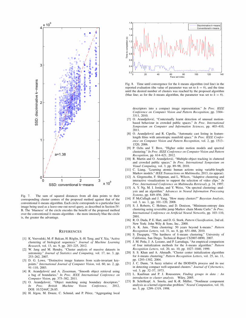
Considering the superior performance of the proposed al-gorithm on the one hand, and the difference in its approach incomparison with the conventional k-means algorithm (whichmay be succinctly described as ‘discrimination’ vs. ‘descrip-tion’), we next examined the sum of squared distances (SSD)from all data points to their corresponding cluster centresfor the two algorithms. The result is summarized in the plotof Fig.7 which shows as a circle each different clusteringinstance corresponding to a different face image being usedas a leave-one-out novel query. As expected, the SSD ofthe proposed algorithm is higher than of the conventional k-means – the red line shows the best straight line fit passingthrough the origin, its slope being a ≈ 1.38. Note thatwe also colour-coded each datum by the benefit that theproposed algorithm demonstrated over the conventional k-means (the more intensely blue the circle is, the greaterthe improvement in recognition), as we were interestedin investigating whether there is any relationship betweenthis benefit and the obtained SSD. As the plot serves todemonstrate, no such relationship was observed.

Lastly, we examined the running efficiency of the proposedmethod. The measured time until the present number ofclusters k = 8 was reached is plotted in Fig.8 as a blueline, and compared with the time until convergence on thesame data of the k-means algorithm. Perhaps surprisingly atfirst, the time required by the proposed algorithm is muchshorter (by approximately 73%). There are two key aspectsof our method that explain this observation. Firstly, note thatsince our algorithm starts from a single cluster, most of thetime the number of clusters that it handles (e.g. that distancesfrom all points are evaluated to) is smaller than k. Secondly,unlike in the conventional k-means algorithm in which thecluster centres are initially randomly assigned, when newclusters are created in the proposed method, they are createdin a purposeful manner and are by construction placed wherenew clusters are actually needed.

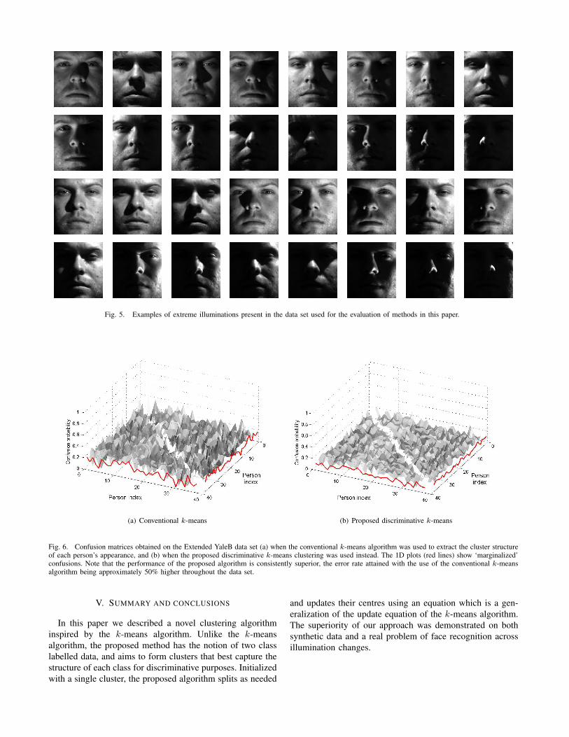
Fig. 5. Examples of extreme illuminations present in the data set used for the evaluation of methods in this paper.

(a) Conventional k-means (b) Proposed discriminative k-means

Fig. 6. Confusion matrices obtained on the Extended YaleB data set (a) when the conventional k-means algorithm was used to extract the cluster structureof each person’s appearance, and (b) when the proposed discriminative k-means clustering was used instead. The 1D plots (red lines) show ‘marginalized’confusions. Note that the performance of the proposed algorithm is consistently superior, the error rate attained with the use of the conventional k-meansalgorithm being approximately 50% higher throughout the data set.

V. SUMMARY AND CONCLUSIONS

In this paper we described a novel clustering algorithminspired by the k-means algorithm. Unlike the k-meansalgorithm, the proposed method has the notion of two classlabelled data, and aims to form clusters that best capture thestructure of each class for discriminative purposes. Initializedwith a single cluster, the proposed algorithm splits as needed

and updates their centres using an equation which is a gen-eralization of the update equation of the k-means algorithm.The superiority of our approach was demonstrated on bothsynthetic data and a real problem of face recognition acrossillumination changes.

0 1 2 3x 10

9

0

1

2

3

4x 10

9

SSD: conventional k−means

SS

D: d

iscr

imin

ativ

e k−

mea

ns

a=1.38

Fig. 7. The sum of squared distances from all data points to theircorresponding cluster centres of the proposed method against that of theconventional k-means algorithm. Each circle corresponds to a particular faceimage being used as a leave-one-out novel query, as described in Section IV-B. The ‘blueness’ of the circle encodes the benefit of the proposed methodover the conventional k-means algorithm – the more intensely blue the circleis, the greater the advantage.

REFERENCES

[1] K. Voevodski, M.-F. Balcan, H. Roglin, S.-H. Teng, and Y. Xia, “Activeclustering of biological sequences.” Journal of Machine LearningResearch, vol. 13, no. 9, pp. 203–225, 2012.

[2] W. Jang and M. Hendry, “Cluster analysis of massive datasets inastronomy.” Journal of Statistics and Computing, vol. 17, no. 3, pp.253–262, 2007.

[3] D. G. Lowe, “Distinctive image features from scale-invariant key-points.” International Journal of Computer Vision, vol. 60, no. 2, pp.91–110, 2003.

[4] R. Arandjelovic and A. Zisserman, “Smooth object retrieval usinga bag of boundaries.” In Proc. IEEE International Conference onComputer Vision, pp. 375–382, 2011.

[5] O. Arandjelovic, “Object matching using boundary descriptors.”In Proc. British Machine Vision Conference, 2012,DOI: 10.5244/C.26.85.

[6] H. Jegou, M. Douze, C. Schmid, and P. Perez, “Aggregating local

0 20 40 60 80 100 120 1400.2

0.4

0.6

0.8

1

1.2

1.4

1.6

1.8

Face set index

Tim

e to

com

plet

ion

(s)

Discriminative k−meansConventional k−means

Fig. 8. Time until convergence for the k-means algorithm (red line) in thereported evaluation (the value of parameter was set to k = 8), and the timeuntil the desired number of clusters was reached by the proposed algorithm(blue line; as for the k-means algorithm, the parameter was set to k = 8).

descriptors into a compact image representation.” In Proc. IEEEConference on Computer Vision and Pattern Recognition, pp. 3304–3311, 2010.

[7] O. Arandjelovic, “Contextually learnt detection of unusual motion-based behaviour in crowded public spaces.” In Proc. InternationalSymposium on Computer and Information Sciences, pp. 403–410,2011.

[8] O. Arandjelovic and R. Cipolla, “Automatic cast listing in feature-length films with anisotropic manifold space.” In Proc. IEEE Confer-ence on Computer Vision and Pattern Recognition, vol. 2, pp. 1513–1520, 2006.

[9] P. Ochs and T. Brox, “Higher order motion models and spectralclustering.” In Proc. IEEE Conference on Computer Vision and PatternRecognition, pp. 614–621, 2012.

[10] R. Martin and O. Arandjelovic, “Multiple-object tracking in clutteredand crowded public spaces.” In Proc. International Symposium onVisual Computing, vol. 3, pp. 89–98, 2010.

[11] C. Liang, “Learning atomic human actions using variable-lengthMarkov models.” IEEE Transactions on Multimedia, 2013, (to appear).

[12] A. Girgensohn, F. Shipman, and L. Wilcox, “Adaptive clustering andinteractive visualizations to support the selection of video clips.” InProc. International Conference on Multimedia Retrieval), p. 34, 1997.

[13] A. Y. Ng, M. I. Jordan, and Y. Weiss, “On spectral clustering: anal-ysis and an algorithm.” Advances in Neural Information ProcessingSystems, pp. 849–856, 2001.

[14] P. McCullagh and J. Yang, “How many clusters?” Bayesian Analysis,vol. 3, no. 1, pp. 101–120, 2008.

[15] S. J. Roberts, C. Holmes, and D. Denison, “Minimum-entropy dataclustering using reversible jump Markov chain Monte Carlo.” In Proc.International Conference on Artificial Neural Networks, pp. 103–110,2001.

[16] R. O. Duda, P. E. Hart, and D. G. Stork, Pattern Classification, 2nd ed.New York: John Wily & Sons, Inc., 2000.

[17] A. K. Jain, “Data clustering: 50 years beyond k-means.” PatternRecognition Letters, vol. 31, no. 8, pp. 651–666, 2010.

[18] S. Dasgupta, “The hardness of k-means clustering.” University ofCalifornia, San Diego, Technical Report CS2007-0890, 2007.

[19] J. M. Pena, J. A. Lozano, and P. Larranaga, “An empirical comparisonof four initialization methods for the k-means algorithm.” PatternRecognition Letters, vol. 20, no. 10, pp. 1027–1040, 1999.

[20] S. S. Khan and A. Ahmadb, “Cluster center initialization algorithmfor k-means clustering.” Pattern Recognition Letters, vol. 25, no. 11,pp. 1293–1302, 2004.

[21] J. C. Dunn, “A fuzzy relative of the ISODATA process and its usein detecting compact well-separated clusters.” Journal of Cybernetics,vol. 3, pp. 32–57, 1973.

[22] L. Kaufman and P. J. Rousseeuw, Finding groups in data : Anintroduction to cluster analysis. Wiley, 2005.

[23] B. Scholkopf, A. Smola, and K.-R. Muller, “Nonlinear componentanalysis as a kernel eigenvalue problem.” Neural Computation, vol. 10,no. 5, pp. 1299–1319, 1998.