The Development and Structure of Financial

Systems∗

Shankha Chakraborty† Tridip Ray‡

Abstract

We introduce monitored bank loans and non-monitored tradeable securities as

sources of external finance for firms in a dynamic general equilibrium model. Due

to frictions arising from moral hazard, access to credit and each type of financial in-

strument are determined by the wealth distribution. We study the depth of credit

markets (financial development) and conditions under which the financial system re-

lies more on either type of external finance (financial structure). We identify initial

inequality, investment size and institutional factors as key determinants of financial

development, while an economy’s financial structure is shaped by its investment tech-

nology and legal and financial institutions. The model’s predictions are consistent with

historical and recent development experience.

Keywords: Financial Development, Financial Structure, Bank Finance, Market Fi-

nance, Credit Frictions.

JEL Classification: E44, G20, G30, O15, O16

∗For helpful comments and suggestions we thank Joydeep Bhattacharya, Nancy Chau, Sudipto Dasgupta,

Chris Edmond, Claudian Kwok, Raoul Minetti, Dilip Mookherjee, Kunal Sengupta, Yong Wang and seminar

participants at various places this paper was presented. All remaining errors are ours.†Department of Economics, University of Oregon, Eugene, OR 97403-1285. Email:

shankhac@oregon.uoregon.edu‡Department of Economics, Hong Kong University of Science & Technology, Clear Water Bay, Kowloon,

Hong Kong. Email: tridip@ust.hk

1

1 Introduction

Researchers concerned with institutions and economic development seek to understand the

dynamic process by which institutions evolve and interact with the rest of the economy. This

paper analyzes the evolution of one such institution, the financial system, with the objective

of isolating factors that shape its development and long-run character.

The role of a financial system in development depends on the degree to which indus-

trialization benefits from external finance and is naturally determined by access to credit

markets.1 But in a second-best world infested with credit frictions, access to credit is con-

strained by wealth levels and internal asset positions of individuals and firms. There is thus

an intimate connection between the wealth distribution and financial development.

We construct a dynamic model that incorporates this interdependence and allows for a

sufficiently rich financial structure. Manufacturing industries require large-scale investment,

an amount that cannot be funded simply from internal assets. Potential entrepreneurs may

borrow using monitored bank loans (bank finance) or non-monitored sources like bonds and

equities (market finance). Credit frictions arise from an agency problem: owner-managers

of manufacturing firms may choose an inferior technology in order to enjoy private benefits.

The incentive to do so is greater the lower the personal stake an owner has in her investment

project (Holmstrom and Tirole, 1997).

In presence of this moral hazard, wealth thresholds determine who invests, using what

type of financial instrument. Poorer individuals do not obtain any funding since they cannot

guarantee lenders the required return. They work instead for a wage. Others who obtain

loans produce capital using a risky technology. When investment succeeds, these capitalists

hire workers to operate the machinery and produce a final good. Among capitalists, wealth

thresholds again determine how they borrow. Individuals of medium wealth levels are able to

borrow only through a combination of intermediated (bank) and unintermediated (market)

finance. Bank finance entails monitoring that partially eliminates the incentive problem;

perceiving this, direct lenders are willing to lend.2 Capitalists who are wealthy enough, on

the other hand, do not need to be monitored and use only market finance.

The wealth distribution thus determines access to credit markets (financial depth) as

well as dependence on each type of external finance (financial structure). Those that are

1An extensive literature exists on the role of financial systems in development. See Gerschenkron (1962),

Goldsmith (1969) and Gurley and Shaw (1955) for early work, and Levine (1997) for a survey of more recent

contributions.2Costly monitoring makes bank finance a more expensive, but necessary, alternative to market finance.

2

rationed out of the credit market, the wage earners, may ultimately accumulate enough assets

to become capitalists. Whether or not they are able to do so depends on how high their

income is, that is, on the extent of industrialization. At the same time, today’s capitalists

may find themselves denied access to credit in the future if they suffer losses on their current

investment.

This dynamic interplay of the wealth distribution and borrowing choices determines the

path of financial development and structure. We identify initial inequality, investment size

and institutional factors as key determinants of financial development, while an economy’s

financial structure is shaped by its investment technology and legal and financial institutions.

An unequal distribution, specifically a large peasant population relative to capitalists, is

inimical to financial development. When few individuals obtain credit, sparse industrializa-

tion prevents workers from earning enough to access credit markets in the future. Low to

moderate degrees of inequality, on the other hand, see the emergence of developed financial

systems. Even then, financial depth is negatively related to inequality, a prediction consistent

with evidence from a cross-section of countries. Initial inequality also impacts an economy’s

historical financial structure — by reducing dependence on monitored finance it results in

more market-oriented financial systems, a pattern we observed during industrialization in

Western Europe.

The investment technology plays a crucial role. When investment requirements are too

large relative to average wealth levels, fewer individuals obtain credit — industrialization

and financial development remain low. An implication is that poorer countries that are

characterized by high inequality, such as Latin America and sub-Saharan Africa, ought to

rely more on small- and medium-scale industries that do not require large setup costs. An

emphasis on import-substituting heavy industries, for instance, would be counterproductive

in the long-run.

Larger capital requirements of industry also promote a bank-based financial system, at

least during the initial stages of financial development. This outcome too matches well West-

ern Europe’s historical experience. In particular, the British industrial revolution occurred

in industries, textiles for example, that did not call for enormous investments (Landes, 1969).

Germany, in contrast, was involved in heavy manufacturing and chemicals, both of which

required large injections of external capital. Such technological differences could have played

a key role in Britain’s historical reliance on market finance and Germany’s dependence upon

its banking systems (Baliga and Polak, 2002).3

3Using monitored and non-monitored debt in a static model of moral hazard, Baliga and Polak (2002) too

3

Although agents are risk-neutral in our model investment risk influences financial struc-

ture by affecting wealth dynamics. In particular, riskier technologies are more conducive to

market-based systems because a larger fraction of capitalists can accumulate enough assets

to be able to shed their reliance on bank intermediation. This result provides an interesting

counterpoint to the typical portfolio effects analyzed in the corporate finance literature, al-

though there is no consensus whether risk diversification is better handled in bank-based or

market-based financial systems (Levine, 1997, Allen and Gale, 2001).

Institutional factors like agency costs shape a financial system in intuitively plausible

ways. Bank-based systems result when bank monitoring is particularly efficient in resolving

agency problems, although it depends upon monitoring costs as well. Our theoretical results

lend credence to recent empirical evidence, LaPorta et al. (1997, 1998) and Levine (2002) in

particular, that shows institutional and legal factors to be crucial determinants of financial

structure.

This paper contributes to the emerging literature pioneered by Banerjee and Newman

(1993) and Galor and Zeira (1993) on the dynamic link between credit frictions and wealth

distribution. Recent work in this area include Aghion and Bolton (1997), Piketty (1997),

Ghatak and Jiang (2002) and Mookherjee and Ray (2002, 2003). Similar to some of these

papers, an important aspect of our analysis lies in the dependence of factor prices on wealth

distribution. It is well-known that such factor price dependence may give rise to compli-

cated non-linear dynamics, preventing one from drawing substantive conclusions about the

economy. An advantage of our framework is its ability to circumvent this problem and flesh

out interesting and empirically plausible predictions regarding financial development.

The key innovation we bring to the above literature is a rich financial structure. Treat-

ment of financial systems in the existing literature has been somewhat incomplete since its

primary goal has been to characterize distributional dynamics. What is missing, specifically,

is the variety of financing choices that firms typically face. In contrast, our interest lies,

first and foremost, in the development and structure of financial systems. A big part of

the policy debate on developing and transition country financial institutions has centered on

the pros and cons of bank-finance versus market-finance (Allen and Gale, 2000, Holmstrom,

1996, Demirgüc-Kunt and Levine, 2001a). An explicit dynamic model of financial structure

is, therefore, a necessary starting point to address such policy issues. While firm financing

cite the influence of investment size on the Anglo-Saxon and German financial systems. Our results differ

in one key respect: investment size affects only the initial financial structure and has no persistent effect in

an industrialized society. Allen and Gale (2000) document how financial systems seem to be converging in

recent decades with even traditionally bank-based economies moving toward financial markets.

4

choices are at the heart of corporate finance research, the literature there deals primarily

with static (and often partial equilibrium) models of developed financial systems. Conclu-

sions about developing societies are hard to infer without an understanding of how financial

institutions evolve in the process of development. Our paper bridges the gap between these

two strands of the literature.

We draw insights especially fromDiamond (1991) and Holmstrom and Tirole (1997), both

of which analyze the link between firm financing choices and some form of asset distribution.

Diamond (1991) considers how firms switch from expensive (and monitored) bank finance

to cheaper forms such as public debt as they develop better reputations.4 Holmstrom and

Tirole (1997), whose incentive structure we adopt here, observe how incentive problems,

and hence access to different types of external finance, depend on a firm’s internal assets.

However, neither of these papers incorporate the feedback that macro-fundamentals have on

financing choices.

The paper is organized as follows. The model is developed in section 2 and optimal

financial contracts characterized in section 3. Section 4 looks at the static general equilib-

rium while section 5 analyzes the dynamics and discusses model implications for financial

development and structure. We conclude in section 6 indicating some possible extensions.

2 The Model

Consider a small open economy populated by a continuum of agents of measure one. Time

is continuous and successive generations are connected by a bequest motive.

An agent is born with an initial wealth, a, received as bequest from her parent and a

labor time endowment of one unit. This labor can be either supplied inelastically to the

labor market, or used to oversee an investment project that produces capital. Inheritance is

the sole source of heterogeneity among newly borns. We denote the cumulative distribution

of agents at instant-t by Gt(a) and assume that the initial distribution G0 is continuous and

differentiable.

Preferences are given by the “warm-glow” utility function:

ut = cβt b1−βt , β ∈ (0, 1),

where c denotes consumption and b denotes bequest left to offspring. Given a realized income

4Reputation is, of course, a form of asset.

5

z, optimal consumption and bequests are linear functions of z:

ct = βzt, bt = (1− β)zt. (1)

The indirect utility function is then also linear in income, Ut = ϕzt with ϕ ≡ ββ(1− β)1−β,

implying that agents are risk-neutral.

Our formalization of the generational structure follows Banerjee and Newman (1993).

Newly born agents become economically active only when they become ‘mature’; time to

maturity, T , is distributed exponentially with the density function h(T ) = ηe−ηT , η > 0,

across members of the same cohort. All economic activity occurs at the instant an agent

becomes mature: she chooses her occupation and earns income accordingly, gives birth to

one offspring, consumes, leaves bequests and dies.5 There is thus no population growth and

members of a cohort do not all die at the same time. Without loss of generality we set η = 1

so that agents live for a unit length of time on average.6

2.1 Production and Occupation

Whether or not an individual is a worker or a capitalist is determined by access to external

finance. Production of capital requires an indivisible investment of size q. Only individuals

able to raise the requisite funds (from internal and external sources) become capitalists, the

rest join the labor force.

A worker supplies her unit labor endowment to the labor market, earning a wage income

wt. A capitalist’s income, on the other hand, is uncertain. In particular the investment

project is risky — a successful project yields capital amounting to θq (θ > 1), while failure

yields nothing. Successful capitalists become producers of final goods by hiring workers to

operate the capital. This capital depreciates completely upon use.

Markets for the final good and for labor are perfectly competitive. For reasons that will

become evident later, we assume an Arrow-Romer type technological spillover in the final

goods sector. Specifically, for a successful capitalist j, the private technology for producing

the unique consumption good is constant returns to scale in private inputs:

Y jt =¡Kjt

¢α(AtN

jt )1−α, α ∈ (0, 1), (2)

5In other words, successive generations are non-overlapping, a framework quite distinct from continuous

time OLG models such as Yaari (1965) or Burke (1996).6Our motivation for using such a non-standard generational structure in continuous time is the same

as Banerjee and Newman’s: it avoids complicated dynamics that could arise purely from a discrete time

specification and simultaneous demographics. See also footnote 17 in section 5 below.

6

Here At denotes time-dependent labor-efficiency that is common to all final goods produc-

ers. Labor efficiency A depends upon capital per worker, k, through a learning-by-doing

externality:

At = Akt. (3)

Productivity improvements in any particular firm spills over instantaneously to the rest of

the economy, becoming public knowledge. The social (intensive-form) production function

is thus an Ak type technology yt = Akt, where A ≡ A1−α.It remains to characterize the investment decision facing a potential capitalist. An indi-

vidual with assets at < q can become a capitalist only if she is able to borrow the shortfall

q − at. To obtain a rich financial structure, we introduce an agency problem similar to thatin Holmstrom (1996) and Holmstrom and Tirole (1997).

Specifically, the probability of success of investment depends upon an unobserved action

taken by the capitalist — her choice on how to spend q. She can spend it on an efficient tech-

nology that yields θq units of capital with probability πG, but uses up all of q. Alternatively,

she can spend it on one of two inefficient technologies. One of these technologies is a low

moral hazard project, costing q−vq, leaving vq for the capitalist to appropriate. This projecttoo yields θq units of capital when it succeeds, but it succeeds less often, with probability

πB < πG. The other inefficient technology is a high moral-hazard project, costing q − V q.This leaves V q in private benefits.

Both inefficient technologies carry the same probability of success, πB, but since 0 < v <

V < 1 by assumption, the capitalist would prefer the high moral-hazard project over the

low moral-hazard one. Only the efficient technology is, however, economically viable.7 The

table below summarizes these investment choices.

Table 1

Project Good Low Moral Hazard High Moral Hazard

(low pvt. benefit) (high pvt. benefit)

Private Benefit 0 vq V q

Success Probability πG πB πB

7To ensure this we make the following parametric assumption:

πGαAθq − r∗q > 0 > πBαAθq − r∗q + V q, (Assumption 1)

where r∗ is the world return on investment and, additionally, we anticipate that a successful capitalist’s

return per unit capital produced, ρt, equals αA in equilibrium (see equation (11) below).

7

3 The Financial Sector

Capital is perfectly mobile across borders so that this small open economy has free access

to the international capital market. The time-invariant (gross) world rate of return on

investment, r∗, is taken as given.

Supply of loans in the domestic financial sector comes from two sources: through financial

intermediaries or banks, and directly from workers and international investors. Workers

are indifferent between bank deposits, lending directly to capitalists and investing on the

international capital market as long as all three yield a return of r∗. In other words, r∗ is the

return that banks promise their depositors as also the guaranteed return on direct lending.

On the demand side, loans are obtained by individuals who invest in the production of

capital; they invest their entire wealth, borrowing the remainder from the domestic financial

sector. Credit-constrained agents work for the capitalists. They deposit their wealth with

banks or lend directly to domestic capitalists or the international capital market.

Capitalists face a perfectly elastic supply curve of loanable funds since they can freely

access the international capital market. Availability of domestic investable resources is thus

not an issue that concerns us. What is crucial is where capitalists obtain their loans from.

Direct borrowing from domestic (workers) and foreign investors will be referred to as direct

(or market) finance, and should be thought of as occurring through the purchase of one-

period corporate bonds and equities. Borrowings intermediated by the banking sector will

be called indirect (or bank) finance.

Bank finance plays a specific role. Banks are assumed to have a monitoring technology

that allows them to inspect a borrowing capitalist’s activities and ensure that she conforms

to the terms agreed upon in the financial contract (Hellwig, 1991; Holmstrom and Tirole,

1997). Direct lenders (workers and foreign investors) do not possess this technology. Thus,

as in Diamond (1984, 1991), banks are the delegated monitors.

Bank monitoring partially resolves the moral hazard problem and reduces a capitalist’s

opportunity cost of being diligent. By choosing to monitor borrowers, banks are able to

eliminate the high moral-hazard project but not the low moral-hazard one (see Holmstrom,

1996 and Holmstrom and Tirole, 1997). For instance, a bank could stipulate conditions that

prevent the firm from implementing the high moral-hazard project when it negotiates a loan

contract with the bank. But such monitoring is privately costly for the bank and requires

it to spend a nonverifiable amount γ per unit invested by the capitalist. Evidently, bank

monitoring will be an optimal arrangement only if the gains from resolving the incentive

problem is commensurate with monitoring costs.

8

The distinction between the two types of external finance is being kept relatively simple

for reasons of tractability. The literature on corporate finance and financial intermediation

discusses several aspects of bank- and market-finance (see Hellwig, 1991, Levine, 1997, Allen

and Gale, 2000 and the references therein). But the key issue for us is that banks (or bank-

like institutions) exist primarily to perform certain services that dispersed investors on the

financial market do not or cannot provide. The Holmstrom-Tirole framework is a convenient

way to capture this, without worrying too much about the specifics of the two types of

external finance.

3.1 Optimal Contracts

Faced with the incentive problem outlined above, a capitalist will behave diligently to the

extent that she receives an incentive-compatible expected payoff and whether or not she is

monitored. Consider the financing options a prospective capitalist faces in borrowing from

banks or from the market.

Since banks monitor firms while outside investors do not, we shall find it convenient to

refer to the former as informed investors. We consider optimal contracts that induce invest-

ment in the good project.

Direct Finance

An optimal contract between a capitalist and direct financiers has a simple structure. Capitalist-

i invests her entire wealth, ait, on her own project since that yields a strictly higher return

than she would otherwise obtain. Direct lenders provide the remaining, q−ait. Neither partyis paid anything if the investment fails. When the project succeeds, the capitalist earns an

amount xCt > 0 while uninformed investors are paid xUt > 0. Denote a successful capitalist’s

rate of return per unit capital produced by ρt. Since a successful project produces θq units

of capital, we have xCt + xUt = ρtθq.

8

In order to invest in the good project, capitalist-i must earn an incentive compatible ex-

pected income. Moreover, the contract should satisfy each lender’s participation constraint,

8Since project returns are observable and verifiable, optimal contracts between direct financiers and

capitalists may be interpreted either as debt or as outside equity. For an equity contract, the capitalist sells

a share st of her project return, xUt = st (ρtθq). For a debt contract, the capitalist borrows q−at, promisingto repay a return of r∗ in case of success. The implicit return on equity has to be r∗ for both assets to be

held simultaneously, that is, st(ρtθq) = r∗(q−at). Again, what matters is that neither of these is monitored

lending.

9

that is, lenders should be guaranteed at least as much as they would earn on the interna-

tional capital market. Combining these two constraints, we obtain (refer to Appendix A.1

for details) that only capitalists with wealth exceeding at would be able to obtain direct

finance, where

at ≡ q

r∗

·πG

πG − πBV − {πGρtθ − r∗}

¸. (4)

Indirect Finance

Indirect or intermediated finance entails three parties to the contract: the bank, besides

uninformed investors and the capitalist. An optimal contract here too stipulates that no one

earns anything when the project fails. In case of success, total returns, ρtθq, are divided up

as xCt + xUt + x

Bt = ρtθq, with x

Bt denoting the bank’s returns.

Besides the incentive compatibility constraint of the capitalist and the participation con-

straint of the uninformed investors, we have to take into account an additional incentive

compatibility constraint, that for bank monitoring. At the same time the loan size has

to be chosen optimally so as to maximize bank profits subject to the capitalist’s incentive

constraint and the bank’s incentive and resource constraints. Moreover, in a competitive

equilibrium, the banking sector earns zero profits. Together these have the following impli-

cations (see Appendix A.1): (i) bank finance is relatively more expensive than direct finance

(due to monitoring costs), that is, the (gross) loan rate charged by the bank, rLt , is greater

than r∗

rLt =

µπGπB

¶r∗ > r∗, (5)

and (ii) capitalists with wealth at > ait ≥ at, where

at ≡q

r∗

·πGv

πG − πB− {πGρtθ − (1 + γ)r∗}

¸, (6)

are able to convince uninformed investors to supply the remaining funds for the investment

project only after the bank lends an amount (and agrees to monitor)9

lit = γ

µπB

πG − πB

¶q. (7)

9In order that the loan size does not exceed investment size, that is lit ≤ q, monitoring costs should notbe so high as to make it impossible for bank intermediation to resolve agency problems. Hence, we restrict

monitoring cost such that:

γ ≤ (πG − πB)/πB. (Assumption 2)

Also, it is natural to assume that at > at, or else there will be no demand for intermediation since monitoring

would be too costly to be socially useful. This is true as long as the expected gain from monitoring exceeds

10

Capitalists with wealth level below at cannot obtain any external finance, direct or indirect.

3.2 Occupational Incomes

Denote individual-i’s income by zit. Consider the case where i does not obtain any external

finance since her wealth is too small, ait ≤ at. Her income consists of labor earnings andreturns on investment in the domestic and/or international capital market

zit = wt + r∗ait.

Next consider those who borrow both from banks and the market, that is, using mixed

finance. For these capitalists with ait ∈ [at, at), equations (5) and (7) imply that income froma successful project would be

zit = ρtθq − rLt lit − r∗[q − lit − ait] = [ρtθ − (1 + γ)r∗] q + r∗ait.

Failure gives them zero returns.

Finally, capitalists with adequate wealth, ait ≥ at, borrow only from the market and earn

zit = ρtθq − r∗£q − ait

¤= (ρtθ − r∗)q + r∗ait,

from a successful project. Of course, we are assuming that the rate of return from the project

(ρtθ) is high enough for the capitalist’s participation constraint to be satisfied. That is, we

require that the capitalist’s expected income πGzit is greater than r∗ait, what she could earn

for sure by investing her entire wealth on the domestic and international capital markets.

This will be true under appropriate restrictions on θ and the final goods technology (α, A).

Earnings for each type of economic agent are thus given by

zit(ait) =

wt + r∗ait, for ait ∈ [0, at)

[ρtθ − (1 + γ)r∗] q + r∗ait, with prob. πG0, otherwise

)for ait ∈ [at, at)

(ρtθ − r∗)q + r∗ait, with prob. πG0, otherwise

)for ait ∈ [at,∞)

(8)

its cost: ·πG

πG − πB

¸(V − v) ≥ γr∗. (Assumption 3)

11

To summarize properties of optimal loan contracts and external financing choices, we note

that given q > ait and the wealth distribution Gt,

(i) individuals with ait < at are unable to obtain any external finance and work as laborers;

(ii) individuals with ait ∈ [at, at) obtain external finance from banks as well as households:they borrow an amount lit from banks at the loan rate rLt , given by (5) and (7) above,

agree to being monitored, and raise the remaining (q − lit − ait) directly from investorsat the rate r∗; optimal contracts guarantee these capitalists incentive compatible pay-

ments such that they behave diligently;

(iii) individuals with ait ≥ at borrow only from investors, paying them a return of r∗; here

too, incentive compatible payments to these capitalists ensure that investments occur

in the good project; and

(iv) income in each case is given by (8) above.

4 Static Equilibrium

Given the wealth distribution Gt, occupational choices determine incomes according to (8).

An agent’s occupational choice depends upon her wealth relative to the cutoffs at and at. In-

dividuals sort themselves into three categories: those who work, those who become capitalists

by borrowing through intermediated and unintermediated loans (mixed-finance capitalists),

and those who become capitalists by borrowing solely from the market (market-finance cap-

italists).

Parametric assumptions we make below ensure that workers earn a strictly lower income

than either type of capitalist. Moreover, market-finance capitalists earn a higher expected

income than mixed-finance capitalists (see equation (8)). Which of the three occupations an

individual “chooses” is thus solely determined by her wealth. If wealth were not a constraint,

all agents would want to become market-finance capitalists.

Consider the static equilibrium at time t. Denote the fractions of the three types of

agents by (f1t, f2t, f3t), where

f1t = Gt(at), f2t = Gt(at)−Gt(at), f3t = 1−Gt(at).

ClearlyP

` f`t = 1, and at any instant t, there are f1t workers and 1− f1t capitalists. Giventhe law of large numbers, πG proportion of these capitalists succeed in producing capital,

12

amounting to Kjt = θq each. The aggregate capital stock is then Kt = πGθq(1− f1t) and the

workforce Nt = f1t. Capital per worker is, thus,

kt = πGθq

·1− f1tf1t

¸. (9)

Since all successful capitalists produce the same amount of capital, given wt, they hire the

same number of workers

N jt =

f1tπG(1− f1t) .

Note the private technology (2). In equilibrium, substituting for the labor augmenting

technological progress ((3) and (9)) into this production function gives output produced by

a successful capitalist as Y jt = Aθq.

Under competitive markets, the equilibrium wage rate is given by the private marginal

product of capital,

wt = (1− α)Akt = (1− α)πGAθq

·1− f1tf1t

¸. (10)

A successful capitalist then earns the income bY jt = αAθq, net of wage payments wtNjt , from

her capital θq. The (gross) rate of return on capital, which we defined as ρt above, is clearly

equal to αA, the private marginal product of capital, that is,

ρt = αA. (11)

Due to overall constant returns to capital, this return is time-invariant. Since all successful

capitalists earn the same return on their capital, we assume, without loss of generality, that

they produce final goods using only their own capital.

Using the equilibrium return on capital from (11) the cutoff wealth levels defined by (6)

and (4) now do not depend upon time:

a = δ1q, a = δ2q, (12)

where10

δ1 ≡ [vπG/(πG − πB)− {πGαθA− (1 + γ)r∗}] /r∗,δ2 ≡ [V πG/(πG − πB)− {πGαθA− r∗}] /r∗.

It remains to check whether or not a worker earns lower income than a capitalist. This

is by no means guaranteed. For instance, when there are “too few” workers, the marginal

10Assumptions 1 and 3 ensure that δ1 < δ2 < 1.

13

product of labor may be so high that even individuals who could have obtained external

finance choose to work. It turns out that this happens when the proportion of credit-

constrained agents falls below ef1, where ef1 satisfies(1− α)πGαA

"1− ef1ef1

#+ r∗a = πG [{αAθ − (1 + γ)r∗} q + r∗a] .

We restrict ourselves to empirically plausible distributions, those that are positively skewed.

We assume hence that G0 satisfies f10 > ef1. This ensures that occupational “choice” is stableover time, and we can simply focus on the proportions of the three types of agents without

having to worry about the effect of income on occupational dynamics.

5 Dynamics of Financial Development and Structure

The financial system, by which we mean the degree to which an economy relies upon external

finance in general, and bank and market-finance in particular, is determined by access to

credit markets. Our purpose is to trace the evolution of the financial system and isolate fac-

tors that influence its dynamics and character. Drawing upon the instantaneous equilibrium

from the previous section, we now turn to this analysis.

Given an initial wealth distribution G0, wealth thresholds a and a determine the propor-

tion of individuals able to invest and the relative composition of bank- and market-finance

in aggregate investment. These investment choices lead to income realizations that deter-

mine the subsequent distribution through bequests. The process continues recursively, with

financial development tracking the wealth distribution through time.

Substituting labor and capital’s equilibrium returns into (8), and using optimal bequests

(1), we obtain the intergenerational law of motion:

bt =

(1− β)hr∗at + (1− α)πGAθq

³1−f1tf1t

´i, for at ∈ [0, a)

(1− β) [r∗at + {αAθ − (1 + γ)r∗}q] , with prob. πG0, otherwise

)for at ∈ [a, a)

(1− β) [r∗at + (αAθ − r∗)q] , with prob. πG0, otherwise

)for at ∈ [a,∞)

(13)

Figure 1 depicts this wealth dynamics for various possibilities (see below); the dotted lines

represent expected income from investment.

14

To ensure that this mapping is convergent we need a particular assumption. All three

regimes of (13) are piecewise linear, with slopes equal to (1 − β)r∗. In order to rule out a

dynasty from becoming arbitrary rich over time by simply reinvesting its wealth, we require

that

(1− β)r∗ < 1. (Assumption 4)

We would also like to rule out a dynasty from being able to self-finance its entire invest-

ment. When investment succeeds, the fixed-point of the mapping for at ∈ [a,∞) is given byaU = (1− β)(αAθ − r∗)q/[1− (1− β)r∗]. For this to be less than q, we assume that

(1− β)αAθ < 1. (Assumption 40)

Investment is undertaken only if the return from it, αAθ, is greater than the return to be

paid to lenders, r∗. Assumption 40 is sufficient to ensure that Assumption 4 is satisfied. We

maintain it henceforth and, without loss of generality, restrict ourselves to distributions on

the domain [0, aU ].

In tracing the evolution of the financial system we first note that distributional dynamics

are essentially nonlinear. The current wealth distribution and the threshold a determine

the size of the working class (f1t) which then determines equilibrium wages through (10).

This endogeneity of the wage rate gives rise to nonlinear dynamics since the future wealth

distribution depends upon wages via optimal bequests.

It is well-known that there are no general mathematical methods for analyzing such

nonlinear dynamics and the dynamic behavior of such systems can be quite complex. But

in tracking the financial system our objective is somewhat modest. We do not need to

completely characterize wealth dynamics, simply tracking the evolution of (f1t, f2t, f3t) is

sufficient for our purpose.11 Besides, a couple of specific features of our model greatly

simplifies the analysis. In the first place, there is no feedback from the wealth distribution

to a and a, which are independent of time.12 This eases the task of analyzing the dynamics

of (f1t, f2t, f3t). Secondly, constant returns to capital at the aggregate level (ρt = αA)

guarantees that recursion dynamics for wealth levels exceeding a is independent of time.13

11We are interested in two features of a financial system, its depth and structure. Financial depth is

captured by (1−f1t), the proportion of unconstrained borrowers, while the financial structure is characterizedby the relative measure of capitalists relying on bank-finance (f2t) and market-finance (f3t).12This is a feature our paper shares with Banerjee and Newman (1993) and Galor and Zeira (1993). See

also Ghatak and Jiang (2002).13See Aghion and Bolton (1997) and Piketty (1997) for models where returns to capital depend upon the

wealth distribution.

15

Specifically, wealth dynamics for the two upper categories are not affected by the endogeneity

of the wage rate which impacts only working-class dynamics. By exploiting the investment

technology, the feature that investment failure yields zero returns, here too we are able to

precisely characterize the dynamics.

5.1 Financial Development

The degree of credit rationing among potential capitalists determines the depth of a financial

system. The simplest measure of financial development hence comes from observing the

movement of f1.

We begin by reconsidering Figure 1.14 Suppose that a λt fraction of the f1t working

dynasties leave bequests exceeding a. This implies that the offsprings of these λtf1t workers

are able to borrow and become capitalists, once they are economically active. Figures 1(a)-(c)

differ only in the position of the lowest regime relative to a, and hence, in λt.

In Figure 1(a), the wealth recursion line for [0, a) lies entirely above a so that λt = 1.

This happens when the wage rate is high enough, that is, when there are fewer workers:

f1 ≤ f1 ≡·1 +

a

(1− β)(1− α)πGAθq

¸−1.

We characterize dynamics on the two-dimensional unit simplex in (f1, f3). SinceP

` f` = 1,

this is sufficient to determine the time-path of f2t. Suppressing time subscripts, transition

dynamics when f1 ≤ f1 is given by the pair of differential equations

f1 = (1− πG) (f2 + f3)− f1 = (1− πG)− (2− πG)f1,

f3 = πGf2 − (1− πG)f3 = πG(1− f1)− f3.

The first equation follows from noting that the outflow from the stock of workers is f1whereas the inflow comes from the fraction (1− πG) of capitalists who suffer losses on their

investment and lose their entire wealth. The mass of workers, f1, decreases or increases over

time according to whether f1 exceeds (1− πG)(f2 + f3). The second differential equation is

obtained similarly: the stock of market-finance capitalists increases as long as mixed-finance

capitalists moving up, πGf2, are more numerous than market-finance capitalists suffering

losses, (1 − πG)f3. Now turn to Figure 2 for the phase-plane: when f1 ≤ f1, the f1 = 0

14We assume, for now, that returns from successful investment are high enough; specifically, successful

mixed-finance capitalists become wealthy enough so that their offsprings are able to borrow using market

finance only.

16

locus is given by the equation f1 = (1 − πG)/(2 − πG) while the f3 = 0 locus is given by

f3 = πG(1− f1).Figure 1(b) looks at another possibility, where the lowest regime of the transition mapping

lies entirely below a. None of the working dynasties leave bequests exceeding a here which

means λt = 0. This happens when the wage rate is low enough, that is, workers are more

numerous:

f1 > f1 ≡·1 +

a[1− (1− β)r∗](1− β)(1− α)πGAθq

¸−1.

The corresponding transition dynamics is given by:

f1 = (1− πG) (f2 + f3) = (1− πG) (1− f1) ,f3 = πGf2 − (1− πG)f3 = πG(1− f1)− f3.

In Figures 2(a) and (b), the f1 = 0 locus is given by f1 = 1 and the f3 = 0 locus by

f3 = πG(1− f1), when f1 > f1.15A third possibility arises when the wealth recursion line on [0, a) lies neither fully above

nor fully below a. This occurs for f1 < f1 < f1. In Figure 1(c), working dynasties distributed

on [eat, a) leave bequests exceeding a, those on [0,eat) do not. For a scenario like this, λt woulddepend upon the exact distribution on [0, a) in general. But a moment’s reflection shows we

do not need details about the distribution on this interval; information about f1t alone is

sufficient to determine the dynamics.

To see this, we establish first that λt is a monotonically decreasing function of f1t. An

increase in f1t lowers the wage rate by increasing the supply of labor; this raises eat and, ceterisparibus, lowers λt. Obviously how an increase in f1t gets distributed on [0, a) matters, which

is why detailed information about Gt may be necessary. But recall that investment failure

yields zero income, which means all new workers start out with zero wealth. The pool of

workers increases when the influx of capitalists whose investments have failed exceeds the

outflux of workers who have accumulated wealth beyond a. This means an increase in f1tresults in a bulging of the distribution at zero; hence such an increase further reduces λt.16

In addition, λt is a continuous function of f1t. The continuous time demographic struc-

ture17 and a continuous initial distribution imply that changes in Gt and f1t (and hence in

15f1 > f1 since (1− β)r∗ < 1.16Note the crucial role played by the investment technology. If failure resulted in low, but positive, returns,

we would need more information about the distribution to determine how λt responds to Gt.17A discrete-time framework would have led to several complications. For example, optimal trajectories

of f1t could be oscillatory even if convergent. Since such behavior would arise solely from a discrete time

specification, we have adopted a continous-time formalization instead.

17

eat) occur in a continuous fashion. Thus λt, defined by 1−Gt(eat)/f1t, also moves continuouslywith f1t.

We can therefore specify the dynamics corresponding to Figure 1(c) by the differential

equations:

f1 = (1− πG)(1− f1)− λ(f1)f1,

f3 = πG(1− f1)− f3.

Appendix A.2 demonstrates the existence of the f1 = 0 locus for a continuous λ(f1t). Multiple

such loci are possible but, generically, there will be an odd number of these.

Figures 2(a) and (b) illustrate dynamics under one and three such loci respectively. In

both cases, when f10 ≤ f1, point D represents a locally stable stationary distribution, while

point L is a locally stable stationary distribution for f10 > f1. Point D, in fact, represents a

well-developed financial system and is given by (f∗1 , f∗2 , f

∗3 ) =

³1−πG2−πG ,

1−πG2−πG ,

πG2−πG

´. Point L

likewise represents a less-developed financial system. Indeed, there we have (f∗∗1 , f∗∗2 , f

∗∗3 ) =

(1, 0, 0), that is, a complete collapse of the financial structure.

In Figure 2(a), bf1 acts as a threshold. For values of f10 below bf1, the economy convergesto the developed financial system, whereas for values above bf1, the long-run outcome is theprimitive system. For three loci (fa1 , f

b1 , f

c1), as in Figure 2(b), the intermediate one acts as a

local attractor for f10 ∈ (fa1 , f c1). In addition to the developed and underdeveloped financialsystems, we now have a third kind, a moderately developed financial structure, at point M .

The complete collapse of the financial system at point L is an unattractive outcome, a

consequence of there being no way out of the working class when f1 > f1. Following Banerjee

and Newman (1993), perhaps it makes sense to get rid of this extreme result by perturbing

the dynamics slightly. We do so by allowing a very small probability (ξ) of moving up from

the working- to the middle-class. This probability corresponds to winning a lottery or some

other form of windfall gain not captured by the model.

The phase diagram for one such perturbation is Figure 2(c). When f1 ≤ f1, this pertur-bation does not alter the wealth dynamics since λt = 1. When f1 > f1, perturbed wealth

dynamics is given by

f1 = (1− πG) (f2 + f3)− ξf1 = (1− πG)− (1 + ξ − πG)f1,

f3 = πG(1− f1)− f3.

The perturbed locus f1 = 0 (when f1 > f1) lies to the left of the original one while the

f3 = 0 locus remains unchanged. The stationary distributions are now represented by D

18

and L0, both of which are locally stable. L0 still represents a very under-developed financial

structure, but we now have both f∗∗2 and f∗∗3 > 0.

Thus developed, underdeveloped and even moderately-developed financial systems may

emerge depending upon the initial measure of credit-constrained individuals, f10. High

values of f10 are particularly inimical to financial development. For low to moderate values,

a developed financial system results in the long-run, but even here, the degree to which it

develops may depend upon initial conditions.

Recall that f10 ≡ G0(a). Clearly, f10 depends on the initial distribution (G0) and on thefactors that determine a — investment size (q) and institutional parameters (v and γ).18 We

consider these determinants one by one.

Inequality and Financial Development

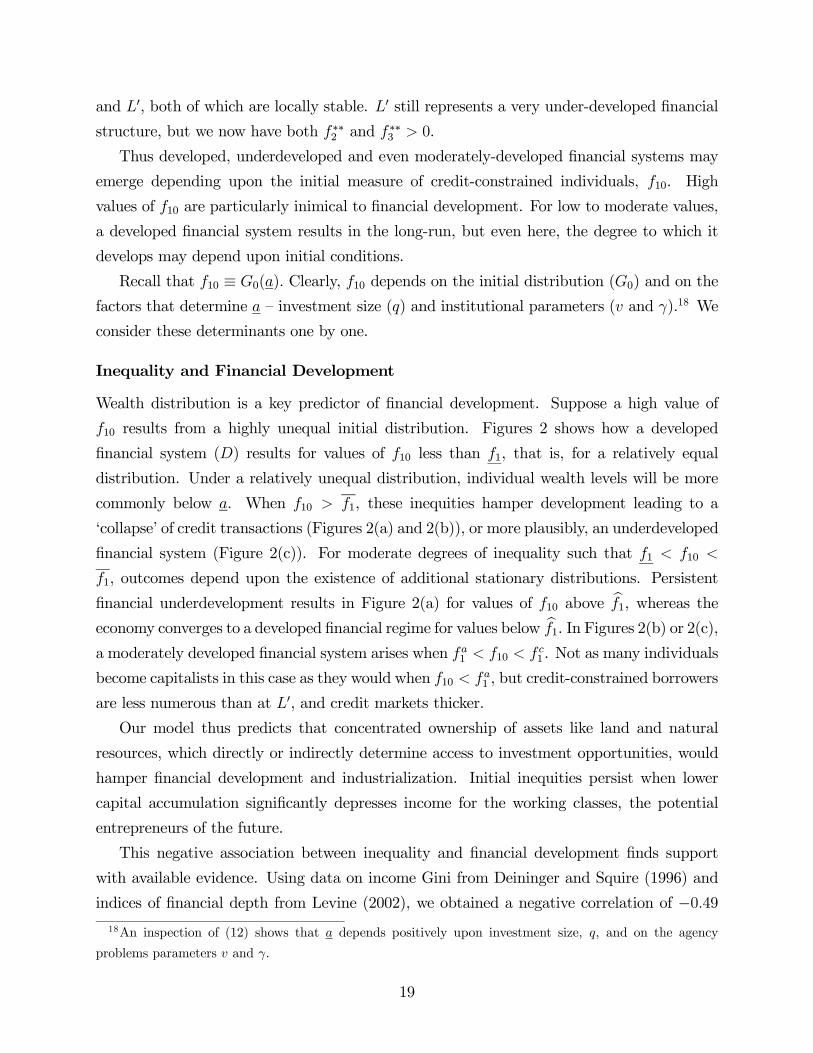
Wealth distribution is a key predictor of financial development. Suppose a high value of

f10 results from a highly unequal initial distribution. Figures 2 shows how a developed

financial system (D) results for values of f10 less than f1, that is, for a relatively equal

distribution. Under a relatively unequal distribution, individual wealth levels will be more

commonly below a. When f10 > f1, these inequities hamper development leading to a

‘collapse’ of credit transactions (Figures 2(a) and 2(b)), or more plausibly, an underdeveloped

financial system (Figure 2(c)). For moderate degrees of inequality such that f1 < f10 <

f1, outcomes depend upon the existence of additional stationary distributions. Persistent

financial underdevelopment results in Figure 2(a) for values of f10 above bf1, whereas theeconomy converges to a developed financial regime for values below bf1. In Figures 2(b) or 2(c),a moderately developed financial system arises when fa1 < f10 < f

c1 . Not as many individuals

become capitalists in this case as they would when f10 < fa1 , but credit-constrained borrowers

are less numerous than at L0, and credit markets thicker.

Our model thus predicts that concentrated ownership of assets like land and natural

resources, which directly or indirectly determine access to investment opportunities, would

hamper financial development and industrialization. Initial inequities persist when lower

capital accumulation significantly depresses income for the working classes, the potential

entrepreneurs of the future.

This negative association between inequality and financial development finds support

with available evidence. Using data on income Gini from Deininger and Squire (1996) and

indices of financial depth from Levine (2002), we obtained a negative correlation of −0.4918An inspection of (12) shows that a depends positively upon investment size, q, and on the agency

problems parameters v and γ.

19

between inequality and financial development.19 Indeed, some of the financially least devel-

oped countries in Levine (2002) (mostly from Latin America and Africa) are, at the same

time, characterized by severe distributional problems.

This is all the more evident when we contrast middle-income countries in East Asia and

Latin America. East Asia’s better asset and income distribution has received considerable

attention in the development literature;20 our model relates how this difference may have

been vital for their financial development. Latin American nations like Argentina, Brazil,

Chile, Peru and Venezuela are by and large financially underdeveloped while Hong Kong,

Malaysia, South Korea, Taiwan, Thailand and Singapore’s financial systems are comparable

to those in Western Europe and North America.21

Investment Size

Consider next the effect of investment size (q). An increase in q raises the cutoff a, given the

wealth distribution. This could lead to financial underdevelopment if the economy is pushed

over bf1 or f c1 . An immediate implication is that poorer countries which are characterized byhigh inequality, such as Latin America and sub-Saharan Africa, ought to rely more on small-

and medium-scale industries for their development. An emphasis on import-substituting

heavy industries, for instance, would be counterproductive in the long-run.

Institutional Factors

Individuals do not differ in terms of their innate abilities in our model and access to credit

markets is limited solely by informational asymmetries and costs. A relevant question is how

better institutions mitigate these asymmetries and what that implies for financial structure.

A simple way to interpret institutions here is through the parameters γ, v and V . These

parameters affect the depth and structure of a financial system through the nature and

magnitude of agency problems and costs of controlling it.

As noted earlier, the degree of credit-rationing, f10, depends positively upon the institu-

tional parameters γ and v through a. When legal and financial institutions are too inefficient

19For financial development, we use Levine’s (2002) “Finance Aggregate” measure (Column 4, Table 2),

constructed using indicators of financial activity, size and efficiency over the period 1980-95. For Levine’s

sample of 48 countries this index ranges from −2.2 to 1.88. For this sample of 48 countries, income Gini rangesfrom 24.9 to 62.5. We use income Gini for the year 1980 (as close as possible, permitted by availability) as

a proxy for initial inequality. Details available upon request.20Income Gini was 34.6 in East Asia and 53 in Latin America during the 1960s; land Ginis were 44.8 and

82 respectively (Deininger and Squire, 1998, Tables 1 and 2).21See Table 2 in Levine (2002) and Table 3.12 in Demirgüc-Kunt and Levine (2001b).

20

(f10 > bf1 or f10 > f c1), the financial system remains underdeveloped in the long run; efficientinstitutions lead to financial development in the long-run. This prediction is along the lines

of recent studies of the ‘legal-based’ view of financial development in LaPorta et al. (1997,

1998), where the quality and nature of legal rules and law enforcements protecting share-

holders and creditors are seen as fundamental to financial activity. Systematic empirical

support for this view, covering a wide range of countries, is offered by Levine (2002).

Inefficient institutions are more widespread and informational problems more acute in

poorer countries presumably because better institutions are costly to implement. In our

model, one way to get around such institutional bottlenecks is through a temporary income

redistribution that relaxes credit constraints for a sizeable number of potential entrepreneurs.

The benefits of such a redistribution will be persistent if it pushes f10 below the relevant

threshold, and in fact, could be politically more palatable than permanent distributive poli-

cies such as land reforms.

5.2 Financial Structure

Financial structure refers to the combination of financial instruments, markets and insti-

tutions operating in an economy (Goldsmith, 1969). A change in that structure towards

the ideal mode assumed in competitive general equilibrium theory is an essential feature of

financial development.

Turning to the model’s implications for financial structure, we consider the relative im-

portance of market- and bank-finance, ψt ≡ f3t/f2t, as an index of structure and study itsevolution.

In the analysis so far we have implicitly allowed high investment returns to ensure that

successful mixed-finance capitalists move up to the next wealth category. What if that

were not the case? We illustrate such a scenario in Figure 4 which depicts wealth recursion

dynamics for f1 ≤ f1 (the other two cases would parallel Figures 1(b) and (c)). It turns outthat the nature of the transition dynamics does not change here although the composition

of the stationary distribution does.

Transition dynamics corresponding to Figure 4 is given by:

when f1 ≤ f1,

f1 = (1− πG)− (2− πG)f1,

f3 = −(1− πG)f3;

21

when f1 > f1,

f1 = (1− πG) (1− f1) ,f3 = −(1− πG)f3;

and when f1 < f1 < f1,

f1 = (1− πG)(1− f1)− λ(f1)f1,

f3 = −(1− πG)f3.

In Figure 5(a), when f10 ≤ f1, D represents a locally stable stationary distribution with a‘developed’ financial system, where (f∗1 , f

∗2 , f

∗3 ) =

³1−πG2−πG ,

12−πG , 0

´. As before, when f10 > f1,

point L represents a locally stable stationary distribution representing a ‘less-developed’

financial system with (f∗∗1 , f∗∗2 , f

∗∗3 ) = (1, 0, 0), and when f

a1 < f10 < f

c1 , point M represents

a moderately developed financial system. Not surprisingly, the long-run distribution has no

capitalist relying purely on market finance since middle-class capitalists cannot move up.

As before, such an outcome can be avoided with perturbations that allow workers to move

up to the middle-class with a small probability (ξ), and middle-class capitalists to move up

with a similar probability (ε). Under perturbation, the stationary distributions in Figure

5(b) are represented by D0 when f10 ≤ f1, L0 when f10 > f1 and M 0 when fa1 < f10 < fc1 .

All three points are locally stable.

Compare now the financial structure of D (or D0) in Figures 2 and 5 under different

rates of return. When investment returns are low, all (or a very large proportion of) eligible

capitalists go through bank intermediation in the long-run. That is, bank-finance is relatively

more important when investment returns are lower (this would be true even for a moderately

developed financial system). The long-run financial structure is, hence, more market-based

for a configuration like Figure 1 and more bank-oriented for a situation like Figure 4.

A market-based system (Figure 1) occurs when the height of C exceeds a, that is when,

(1− β) r∗·

πGv

πG − πB+ (1− πG)αAθ

¸≥ πGV

πG − πB− (απGAθ − r∗) . (14)

This is more likely to occur when V is relatively low and v relatively high, or when θ

is relatively high but πG low (holding πGθ constant).22 On the other hand a bank-based

financial system (Figure 4) results when the height of H is less than a. This happens if

(1− β) r∗ [(1− πG)αAθ − γr∗] <µ

πGπG − πB

¶[1− (1− β) r∗]V − πGαAθ + r

∗. (15)

22We allow for a proportionate decrease in πB as well.

22

This inequality is more likely when V and γ are relatively high, or, holding πGθ constant,

when θ is relatively low and πG high.23

Thus, the financial structure of an economy is determined by the investment technology

(πG, θ) and institutional factors (γ, v and V ). We consider these issues next.

Investment Risk

Although banks and individuals are risk-neutral in our model, investment risk affects financial

structure through its effect on wealth dynamics. We begin by contrasting two types of

investment that yield the same expected return, πGθ: type-I projects yield a high θ but are

riskier since πG is low, while type-II projects succeed more often but realize low θ.24

Suppose now that the two project types differ significantly in their riskiness so that

Figure 1 depicts wealth dynamics for type-I projects while that for type-II projects is given

by Figure 4. From (14) and (15) we know that Figure 1 is more likely to occur when θ is

relatively high but πG low (holding πGθ constant) while Figure 4 is more likely to occur for

the opposite case.

Figures 1 and 4 lead to dynamics shown by Figures 2 and 5 respectively. We draw two

conclusions on the role of investment risk. First, lower πG leads to higher f∗1 so that credit

rationing is more widespread in the long-run. Secondly, when investment is less risky, all or

a large proportion of eligible capitalists go through bank intermediation in the long-run. In

other words, bank-finance is relatively more important for safer technologies, whereas market

finance gains importance for riskier ones.

This dependence of financial structure on risk is quite distinct from, but complementary

to, the ones commonly analyzed in the finance literature. Specifically, since agents are risk-

neutral our analysis misses the typical portfolio effect discussed in the literature.25 At the

same time it brings to the analysis the macroeconomic feedback that investment risk has on

asset positions and financing dynamics, an effect entirely absent from the existing literature.

Institutional Quality

Institutional parameters also affect long run financial structure in the model. Recall that a

market-based system is more likely to occur (that is, (14) holds) when V is relatively low and

v relatively high. On the other hand, a bank-based system (condition (15)) is more likely

23Again, we change πB by the same proportion as πG.24We allow for a proportionate change in πB between the two project types.25Risk averse agents would clearly make the analysis much less tractable. It is to be noted, though, that

the literature is not unequivocal about whether banks or markets diversify risks better, suggesting only that

both are important. Levine (1997) and Allen and Gale (2001) discuss these issues.

23

to occur when V and γ are relatively high. It is quite intuitive that a bank-based system

is more likely when the residual moral hazard under bank monitoring (v) is low relative to

what incentives would be in the absence of monitoring (V ). This conclusion is consistent

with Demirguc-Kunt and Levine’s (2001b) finding that countries with strong shareholder

rights relative to creditor rights and strong accounting systems (that is, low V relative to v)

tend to have more market-based systems.

It may seem surprising that higher monitoring costs, γ, lead to a more bank-oriented

systems even though these costs are borne by the banking sector. This is easy to understand

once we recognize that wealth and financing dynamics depend upon investment earnings.

A higher cost of monitoring means that banks need to inject a larger amount of their own

resources into the investment project. This forces mixed-finance capitalists to rely more

heavily on expensive intermediated finance; consequently less of them are able to move up

to become market-finance capitalists.

5.3 Historical Implications

Several of the model’s implications shed light on the historical development of financial

systems during the Industrial Revolution.

Inequality and Financial Structure

Consider, for example, the effect of initial inequality on financing choices. For convenience,

assume that the initial distribution is lognormal with mean µ0 and variance σ20, where a <

µ0 < a. In Appendix A.3 we establish that an increase in σ20 tends to raise f10, lower f20 but

increase f30. Higher inequality leads to thinner capital markets since 1 − f10 is lower. Butamong those who obtain loans, there is a shift toward market finance and away from bank

finance, increasing the ratio ψ0. Historical reliance upon the two types of finance may, in

other words, depend upon inequality. This prediction seems to be corroborated by what we

know about England and Germany during the industrial revolution.

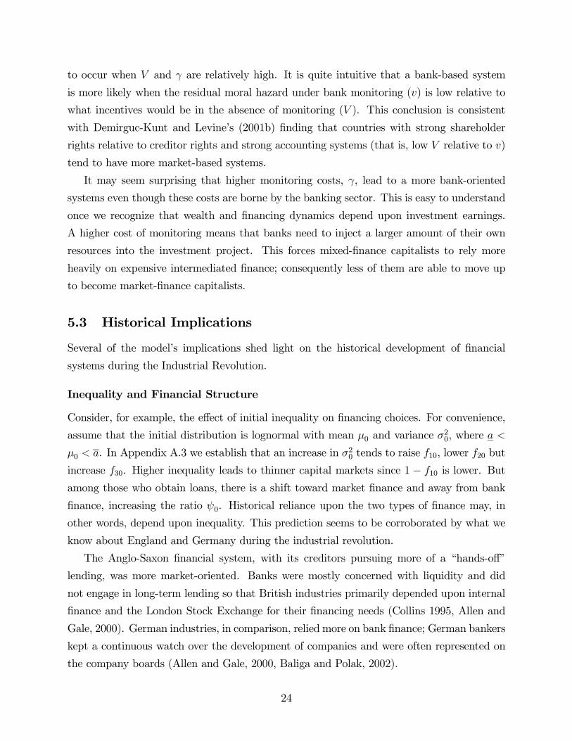
The Anglo-Saxon financial system, with its creditors pursuing more of a “hands-off”

lending, was more market-oriented. Banks were mostly concerned with liquidity and did

not engage in long-term lending so that British industries primarily depended upon internal

finance and the London Stock Exchange for their financing needs (Collins 1995, Allen and

Gale, 2000). German industries, in comparison, relied more on bank finance; German bankers

kept a continuous watch over the development of companies and were often represented on

the company boards (Allen and Gale, 2000, Baliga and Polak, 2002).

24

At the same time, substantial evidence suggests England had a more unequal land dis-

tribution than Germany (and France) (Clapham, 1936, Soltow, 1968). Landes (1969) also

notes that a large number of British industrialists were “men of substance”, having accumu-

lated significant wealth from merchant activities. This distributional difference between the

two regions could partly explain why the Anglo-Saxon and German financial systems have

historically differed. Indeed, this also explains why other societies with better distributions

than England, for instance France and Japan (or the newly industrializing East Asian coun-

tries), have traditionally relied more on bank-finance (see Allen and Gale, 2000). While a

systematic analysis covering a broad sample of countries is clearly required, the model indi-

cates the kind of macro-fundamentals that could prove useful in explaining paths of financial

development.26

Investment Size and Financial Structure

Investment size has an impact on initial or historical financial structure. With a higher q,

fewer individuals are able to obtain loans either from markets or from banks. At the same

time, the shortfall q − ai that has to be raised through external finance is higher for thosewho do invest. The Holmstrom-Tirole incentive structure has a straightforward implication:

due to limited liability, a borrower’s incentive to be diligent is weaker the less her personal

stake in the project, that is, the more she needs to borrow. The only way to attenuate this

is through increased monitoring.

Larger scale investments would hence push an economy towards bank finance. But

whether or not this happens depends also on the wealth distribution. A higher q raises

the importance of bank-finance under two conditions: when the initial wealth distribution

among capitalists is more equitable, that is when f30/f20 is low; and when banks are par-

ticularly effective at resolving incentive problems (δ1 << δ2 in (12)) so that the measure of

individuals above a is sizeable.27

Historical evidence, once again, provides some support in favor of this story. Similar

to their financial systems, a distinction is often made between England and Germany’s in-

dustrialization patterns. The British process of industrialization mainly relied upon small-

and medium-scale industries, textile manufacturing being a prime example. Germany, on26At the same time, as long as two societies converge to developed financial systems (D), inequality does

not have a permanent effect on financial structure. Interestingly, Allen and Gale (2000) point out how even

traditionally bank-oriented societies such as France, Germany or Japan have been moving toward market

finance since the 1980s. One could interpret this as a convergence in industrialized country financial systems,

though, policy shifts would have clearly played a key role.27This follows from noting that ∂ψ0/∂q < 0 whenever δ2(1 + f20/f30)g0(a) > δ1g0(a).

25

the other hand, largely utilized heavy manufacturing and chemical industries for its devel-

opment, both requiring far greater investment than in the case of England (see Landes,

1969, and related references in Baliga and Polak, 2002). Consistent with the evidence, our

model suggests that this technological difference would be reflected in a greater German re-

liance on intermediated finance especially if banks are efficient intermediaries and the wealth

distribution is more equitable.

Using a static model of monitored and non-monitored debt, Baliga and Polak (2002)

too stress the role of investment size for Western Europe’s financial structure. Importantly

though, our dynamic model suggests that long-run differences in financial structure are

neutral with respect to investment size. As long as f10 < bf1 (or less than fa1 ), differences inf10 do not translate into differences in the stationary distribution, that is, point D. This is

because q affects threshold wealth requirements (a and a) as well as expected income from

investment. In the short-run, a higher q could increase reliance upon bank-finance but it

also enables successful capitalists to earn more. When more of the middle-class capitalists

move above a, they do not need to be monitored so that reliance upon bank finance declines.

6 Conclusion

This paper has analyzed the evolution of a financial system and identified factors determin-

ing its development and structure. We introduced monitored bank loans and non-monitored

tradeable securities in a dynamic general equilibrium model and showed how the path to

financial development exhibits non-ergodic behavior — underdeveloped financial systems per-

sist in highly unequal societies or in societies with inefficient legal and financial institutions,

whereas societies with more equitable wealth distribution or better financial institutions

experience financial development. We examined how the investment technology (size and

riskiness) and institutional qualities influence the structure of financial systems. Finally, we

showed that some of the model’s implications are consistent with the historical development

of financial systems during the Industrial Revolution.

This paper continues in the tradition of several works like Banerjee and Newman (1993),

Galor and Zeira (1993), Aghion and Bolton (1997), Piketty (1997) and Mookherjee and Ray

(2002, 2003) in studying the dynamic interaction between credit markets and the wealth

distribution. Existing research has mainly studied the nature of distributional dynamics,

credit market imperfections, occupational choice and possibilities of poverty traps. In con-

trast, our goal has been to obtain a clearer understanding of what drives the development

26

and structure of financial systems. Thus, an important contribution of this paper lies in

extending the literature by incorporating a richer financial structure, one that may be used

to analyze the design and effectiveness of financial systems in developing societies.

We conclude by considering several extensions for future work. Throughout the paper

we focused on the demand side of financial systems. We did this primarily for tractability

given the nonlinear nature of the dynamics. A natural extension would be to consider how

important the supply of loanable funds is to financial structure, for example, by looking at a

closed economy version of the model. A more challenging extension would be to capture the

emergence of different financial institutions (institutions like banks and markets are taken

as given in our story). For instance, if there are fixed costs to setting up an intermediary (as

in Jovanovic and Greenwood, 1990), the extent to which banks emerge and monitor lending

will depend upon, and affect, the pattern of wealth accumulation. It will be also interesting

to endogenize the interest rate, allowing the wealth distribution to affect financial structure

through returns to bank and market-finance.

Another institutional aspect we have ignored, and one likely to be important in devel-

opment, is the quality of bank monitoring. In particular, banks do not face any incentive

problems vis-a-vis depositors in our model. Extensions incorporating agency problems within

the banking sector may be used to examine how the “quality” of bank-finance itself changes

over time and with respect to macro-fundamentals.

27

References

[1] Aghion, Philippe and Patrick Bolton (1997), “A Theory of Trickle-Down Growth and

Development”, Review of Economic Studies, vol. 64, pp. 151-172.

[2] Allen, Franklin and Douglas Gale (2000), Comparing Financial Systems, Cambridge,

MA, MIT Press.

[3] Allen, Franklin and Douglas Gale (2001), “Comparative Financial Systems: A Sur-

vey”, forthcoming in Bhattacharya, Sudipto, Boot, Arnoud and Anjan Thakor (eds.)

Financial Intermediation, Oxford University Press.

[4] Baliga, Sandeep and Ben Polak (2002), “The Emergence and Persistence of the Anglo-

Saxon and German Financial Systems,” forthcoming, Review of Financial Studies.

[5] Banerjee, Abhijit and Andrew Newman (1993), “Occupational Choice and the Process

of Development", Journal of Political Economy, vol. 101, pp. 274-298.

[6] Burke, Jonathan L. (1996), “Equilibrium for Overlapping Generations in Continuous

Time”, Journal of Economic Theory, vol. 70, no. 2, pp. 364-90.

[7] Clapham, John Harrold (1936), The Economic Development of France and Germany,

1815-1914, Cambridge University Press.

[8] Collins, Michael (1995), Banks and industrial finance in Britain, 1800-1939, Cambridge

University Press.

[9] Deininger, Klaus and Lyn Squire (1996), “Measuring Income Inequality: A New Data-

Base,” World Bank Economic Review, vol. 10, no. 3 (September), pp. 565-91.

[10] Deininger, Klaus, and Lyn Squire (1998), “New Ways of Looking at Old Issues: In-

equality and Growth,” Journal of Development Economics, vol. 57, no. 2, pp. 259-287.

[11] Demirgüc-Kunt, Asli and Ross Levine eds. (2001a) Financial Structure and Economic

Growth, MIT Press, Cambridge, MA.

[12] Demirgüc-Kunt, Asli and Ross Levine (2001b), “Bank-based and Market-based Finan-

cial Systems: Cross-country Comparisons”, in Asli Demirgüc-Kunt and Ross Levine

(eds.) Financial Structure and Economic Growth, MIT Press, Cambridge, MA.

28

[13] Diamond, Douglas (1984), “Financial Intermediation and Delegated Monitoring,” Re-

view of Economic Studies, vol. 51, pp. 393-414.

[14] Diamond, Douglas (1991), “Monitoring and Reputation: The Choice between Bank

Loans and Directly Placed Debt”, Journal of Political Economy, vol. 99, pp. 689-721.

[15] Galor, Oded and Joseph Zeira (1993), “Income Distribution and Macroeconomics,”

Review of Economic Studies, vol. 60, pp. 35-52.

[16] Gerschenkron, Alexander (1962), Economic Backwardness in Historical Perspective,

Cambridge, MA: Harvard University Press.

[17] Ghatak, Maitreesh and Neville Nien-Huei Jiang (2002), “A Simple Model of Inequality,

Occupational Choice and Development”, Journal of Development Economics, vol. 69,

pp. 205-226.

[18] Goldsmith, Raymond (1969), Financial Structure and Development, Yale University

Press, New Haven, CT.

[19] Greenwood, Jeremy and Boyan Jovanovic (1990), “Financial Development, Growth and

the Distribution of Income”, Journal of Political Economy, vol. 98, no. 5, pp. 1076-107.

[20] Gurley, John and E. Shaw (1955), “Financial Aspects of Economic Development,”Amer-

ican Economic Review, vol. 45, pp. 515-38.

[21] Hellwig, Martin (1991), “Banking, Financial Intermediation and Corporate Finance”, in

European Financial Integration, (eds.) Alberto Giovannini and Colin Mayer, Cambridge

University Press, U.K.

[22] Holmstrom, Bengt (1996), “Financing of Investment in Eastern Europe,” Industrial and

Corporate Change, vol. 5, pp. 205-37.

[23] Holmstrom, Bengt and Jean Tirole (1997), “Financial Intermediation, Loanable Funds,

and the Real Sector,” Quarterly Journal of Economics, vol. 112, pp. 663-91.

[24] La Porta, Rafael, Florencio Lopez-de-Silanes, Andrei Shleifer and Robert Vishny (1997),

“Legal Determinants of External Finance,” Journal of Finance, vol. 52, pp. 1131-50.

[25] La Porta, Rafael, Florencio Lopez-de-Silanes, Andrei Shleifer and Robert Vishny (1998),

“Law and Finance,” Journal of Political Economy, vol. 106, pp. 1113-55.

29

[26] Landes, D. (1969), The Unbound Prometheus, Technological Change and Industrial De-

velopment in Western Europe from 1750 to the Present, Cambridge, Cambridge Uni-

versity Press.

[27] Levine, Ross (1997), “Financial Development and Economic Growth: Views and

Agenda”, Journal of Economic Literature, vol. 35, pp. 688-726.

[28] Levine, Ross (2002), “Bank-based or Market-Based Financial Systems: Which is Bet-

ter?”, Journal of Financial Intermediation, vol. 11, pp. 1-30.

[29] Mookherjee, Dilip and Debraj Ray (2002), “Contractual Structure and Wealth Accu-

mulation”, American Economic Review, vol. 92, no. 4, pp. 818-849.

[30] Mookherjee, Dilip and Debraj Ray (2003), “Persistent Inequality”, Review of Economic

Studies, vol. 70, pp. 369-93.

[31] Piketty, Thomas (1997), “The Dynamics of the Wealth Distribution and the Interest

Rate with Credit Rationing”, Review of Economic Studies, vol. 64, pp. 173-189.

[32] Soltow, Lee (1968), “Long-Run Changes in British Income Inequality”, Economic His-

tory Review, Second Series, 21, 17-29.

[33] Yaari, Menahem E. (1965), “Uncertain Lifetime, Life Insurance, and the Theory of the

Consumer”, Review of Economic Studies vol. 32, pp. 137-50.

30

Appendix

A.1. Optimal Contracts

Direct Finance

We have xCt + xUt = ρtθq.

Capitalist-i’s incentive compatibility constraint (choosing the good project) is given by

πGxCt + (1− πG) .0 ≥ πBx

Ct + (1− πB) .0 + V q.

Direct lender’s participation constraint is

πGxUt + (1− πG) .0 ≥ r∗

¡q − ait

¢.

Capitalist’s incentive compatibility constraint implies

xCt ≥V q

πG − πB⇒ xUt = ρtθq − xCt ≤ ρtθq −

V q

πG − πB.

Using this, the lender’s participation constraint gives

r∗ (q − ait) ≤ πGxUt ≤ πG

·ρtθq −

V q

πG − πB

¸

⇒ ait ≥ at ≡q

r∗

·πG

πG − πBV − {πGρtθ − r∗}

¸.

Indirect Finance

Under indirect finance we have xCt + xUt + x

Bt = ρtθq. Here the optimal contracts need to

satisfy the following three constraints:

(i) capitalist-i’s incentive compatibility constraint (choosing the good project):

πGxCt + (1− πG) .0 ≥ πBx

Ct + (1− πB) .0 + vq,

(ii) bank’s incentive constraint (for monitoring):

πGxBt + (1− πG) .0− r∗γq ≥ πBx

Bt + (1− πB) .0,

assuming that banks discount monitoring costs at their opportunity cost, r∗,

31

(iii) participation constraint of the uninformed investors:

πGxUt + (1− πG) .0 ≥ r∗

¡q − lit − ait

¢,

where lit is the amount that the bank lends to capitalist-i.

The bank’s expected return from lending lit to capitalist-i is

πGxBt = r

Lt lit, (16)

where rLt is the (gross) loan rate charged to borrowers.

But bank’s incentive constraint implies

πGxBt ≥

·πG

πG − πB

¸r∗γq. (17)

Since bank finance is relatively more expensive than direct finance (due to monitoring

costs), borrowers accept only the minimum amount necessary so that

rLt lit = πGx

Bt =

·πG

πG − πB

¸r∗γq

⇒ lit(rLt ) =

r∗γqπG(πG − πB) rLt

. (18)

Capitalist’s incentive compatibility constraint implies xCt ≥vq

πG − πB. Then

xCt + xBt ≥

(v + r∗γ) qπG − πB

⇒ xUt = ρtθq −¡xCt + x

Bt

¢ ≤ ρtθq −(v + r∗γ) qπG − πB

.

Using this, the uninformed investors’ participation constraint gives

r∗¡q − lit − ait

¢ ≤ πGxUt ≤ πG

·ρtθq −

(v + r∗γ) qπG − πB

¸.

It follows that only capitalists with wealth

ait ≥ at ≡ q − lit(rLt )−qπGr∗

·ρtθ −

v + γr∗

πG − πB

¸(19)

are able to convince uninformed investors to supply enough funds for the investment project.

32

The Bank’s Problem

The aggregate demand for bank loans is

Lt =

Zi∈Itlit(r

Lt )dGt =

·γπGr

∗q(πG − πB) rLt

¸ Zi∈ItdGt,

where It denotes the subset of individuals using intermediated finance. The total monitoring

cost borne by the banking sector is then

γq

Zi∈ItdGt =

(πG − πB) rLt Lt

πGr∗.

Let Dt denotes the flow of deposits into the banking sector. Then banking profits are

ΠBt = rLt Lt − r∗Dt. (20)

Banks face the resource constraint that total loans cannot exceed total deposits net of mon-

itoring costs:

Lt ≤ Dt − γq

Zi∈ItdGt. (21)

The banking sector’s optimization problem in period t is to choose Lt so as to maximize ΠBtsubject to the capitalist’s incentive constraint and the constraints (17) and (21).

Since bank profits are increasing in total loans, (21) holds with equality:

Lt = Dt − γq

Zi∈ItdGt = Dt − (πG − πB) r

Lt Lt

πGr∗. (22)

Moreover, in a competitive equilibrium, the banking sector earns zero profits. From (20) we

then have

rLt Lt = r∗Dt, (23)

It follows from equations (22) and (23) that

Lt =

µπBπG

¶Dt,

and

rLt =

µπGπB

¶r∗. (24)

Hence, using (18), we observe that

lit = γ

µπB

πG − πB

¶q. (25)

33

In other words, for all i ∈ It, banks finance a fixed proportion of the borrower’s investment,irrespective of ait.

Taking into account the optimal loan size (25), the lower wealth cut-off (19) becomes

at =q

r∗

·πGv

πG − πB− {πGρtθ − (1 + γ)r∗}

¸. (26)

A.2. Existence of f1 = 0 locus when f1 < f1 < f1

In the text we have already established that λt is a continuous and monotonically decreasing

function of f1t. Now define

z(f1) ≡ (1− πG)/[1− πG + λ(f1)]− f1on the interval [f1, f1]. Since λ(f1) is continuous on [f1, f1],z is also continuous on [f1, f1].Wehave z(f1) = (1−πG)/(2−πG)−f1 < 0 since f1 > (1−πG)/(2−πG) and z(f1) = 1−f1 > 0,since f1 < 1. Hence, using the Intermediate Value Theorem, since z is continuous on [f1, f1]and since 0 ∈ [z(f1),z(f1)], we can find an u ∈ [f1, f1] such that z(u) = 0. In other words,z(f1) = 0 for at least one value of f1 ∈ [f1, f1]. Figure 3(a) illustrates this when the line(1−πG)/[1−πG+λ(f1)] intersects f1 once, at bf1. Multiple such intersections are also possible,but, generically, these have to be in odd numbers. Figure 3(b) depicts three intersections.

Figures 2(a) and (b) illustrate dynamics under one and three such intersections respectively.

A.3. Effect of an increase in initial inequality on financing choices

Suppose that the initial distribution G0 is lognormal with mean µ0 and variance σ20. Re-

call that the lognormal cumulative distribution is given by Φ [(lnx− µ)/σ], where Φ is thestandard Normal cumulative distribution function. Then:

∂G0(a)

∂σ0= −φ0

µln a− µ0

σ0

¶·ln a− µ0

σ20

¸,∂G0(a)

∂σ0= −φ0

µln a− µ0

σ0

¶·ln a− µ0

σ20

¸.

When ln a < µ0 < ln a, the first derivative is positive, the second derivative negative. More-

over,

∂[G0(a)−G0(a)]∂σ0

= −φ0µln a− µ0

σ0

¶·ln a− µ0

σ20

¸+ φ0

µln a− µ0

σ0

¶·ln a− µ0

σ20

¸,

is also negative in this case. Thus, as long as ln a < µ0 < ln a, we have

∂f10∂σ0

> 0,∂f20∂σ0

< 0,∂f30∂σ0

> 0.

34

tb

o45

AB

CH

EF

a

a

a a ta

Figure 1(a): Recursion Dynamics of Wealth Accumulation when 11 ff ≤

tb

o45

A B

CH

EF

a

a

a a ta

Figure 1(b): Recursion Dynamics of Wealth Accumulation when 11 ff >

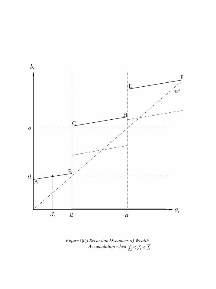
tb

o45

A

B

CH

EF

a a tata~

a

a

Figure 1(c): Recursion Dynamics of Wealth Accumulation when

111 fff <<

3f

Figure 2(a): Phase Diagram for a single Threshold

1

D

L

12

GG

ππ

−−

1f 1f

)(when 0 111 fff ≤=

03=f

)(when 0 111 fff >=

1f

)(when 0 1111 ffff <<=

1

Gπ

1f0

3f

Figure 2(b): Phase Diagram for two Thresholds

1

D

L

12

GG

ππ

−−

Gπ

1f 1f

)(when 0 111 fff ≤=

03=f

)(when 0 111 fff >=

)(when 0 1111 ffff <<=

M

af1

bf1

cf1

1

1f0

3f

Figure 2(c): Phase Diagram with Perturbed Wealth Dynamics

1

D

L

12

GG

ππ

−−

Gπ

1f1f 1f

)(when 0 111 fff ≤=

03=f

)(when 0 1111 ffff <<=

M

af1

bf1

cf1

L

)(when 0 111 fff >=

1

0

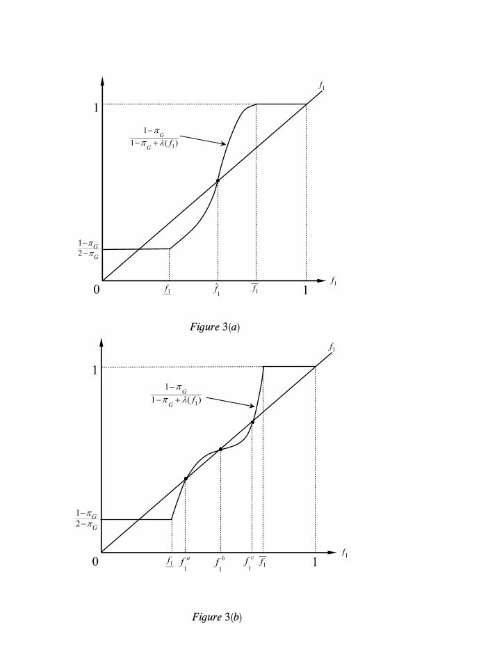
0 1f1

1

1f 1f

12

GG

ππ

−−

1f

1f

)(11

1fG

Gλπ

π+−

−

Figure 3(a)

0 11f 1f

12

GG

ππ

−−

1f

)(11

1fG

Gλπ

π+−

−

cf1

bf1

af1

1

1f

Figure 3(b)

tb

AB

CH

EF

a a ta

o45

a

a

Figure 4: Wealth Dynamics with Low Return on Investment )( 11 ff ≤

3f

1

1L

12

GG

ππ

−−

1f 1f

)(when 0 111 fff ≤=

03=f

)(when 0 111 fff >=

)(when 0 1111 ffff <<=

af1

bf1

cf1

D M1f0

Figure 5(a): Phase Diagram (for two Thresholds) with Low Investment Return

3f

1

1L

12

GG

ππ

−−

1f1f 1f

)(when 0 111 fff ≤=

03=f

)(when 0 1111 ffff <<=

af1

bf1

cf1

D

D ML

)(when 0 111 fff >=

0

Figure 5(b): Phase Diagram for the Perturbed Wealth Dynamics with Low Investment Return