TE

SI

DO

CTO

RA

L U

PF

/2

02

1T

ES

I DO

CTO

RA

L UP

F/

20

21

Essa

ys in

Fin

anci

al E

cono

mic

sJu

an F

elip

e Im

bet

Jim

énez

Essays in Financial Economics

Juan Felipe Imbet Jiménez

“mainupf” — 2021/6/1 — 2:06 — page i — #1

Essays in Financial Economics

Juan Felipe Imbet Jimenez

TESI DOCTORAL UPF / Year 2021

THESIS SUPERVISORDr. Javier Gil-BazoDepartment Department of Economics and Business

“mainupfv2” — 2021/6/1 — 20:22 — page i — #1

Sometimes Science is More Art Than Science, Morty.

Rick Sanchez

i

“mainupfv2” — 2021/6/1 — 20:22 — page ii — #2

A mi abuelo Jairo.

ii

“mainupfv2” — 2021/6/1 — 20:22 — page iii — #3

Acknowledgements

The outcome of this dissertation would have not been possible withoutthe support of many people across two continents. I thank my advisorJavier Gil-Bazo for his support and guidance, which started back when Iwas pursuing my master’s degree. He always went beyond his duties andresponsibilities as an advisor and taught me valuable lessons that I willtake with me for the rest of my life. I thank him for his constant encoura-gement to ask deep research questions, and for always reminding me thatacademic research is a service to society and therefore requires the highestcode of ethics.

I thank Filippo Ippolito, Roberto Steri, and Winston Dou for their aca-demic and personal support. Despite none of them being an official thesiscoadvisor, they always showed an incredible interest and commitment tohelp me improve my research. I thank Filippo for serving as the academicbridge between UPF and the University of Pennsylvania which allowedme to visit the Wharton School in 2020, and for funding my last monthsin the doctorate. I thank Roberto Steri for introducing me to the worldof structural estimation, and for all his help during the last years of myPh.D. while coming up with a job market paper. I also thank him for helpme finance my last years of Ph.D. through the University of Luxembourg.Finally, I thank Winston Dou for having sponsored my academic visit tothe Wharton School at UPenn. I am thankful to Winston for constantlymeeting me, even after the unfortunate COVID situation forced me to lea-ve Philadelphia. My job market paper improved substantially after everydiscussion we had.

I thank my family, Pito, Mita, Alejandro, Locky and Ginebra for alwaysencouraging me to pursue my dreams, and specially for their support indifficult times. Being away from my family has always been hard, butknowing that I could always count with them made everything orders ofmagnitude easier. I also thank Mune, Marlon, Tita, Dani, Pau, Luli, and allmy close relatives that supported me during these last seven years abroad.

I thank Ines Xavier, Kinga Tchorzewska, and Natalia Perry for beingmy second family in Barcelona, and specially to Camille DeFrancq andher family in France who have been a personal a professional lighthouseduring these last years. I thank my closest friends Raffaele Manini, MennaEl Hefnawy, Dagny Pawlak, Anna Porta, Karolis Liaudinskas, GianmarcoRuzzier, Sandra Kaya, Thomas Woiczyk, Sampreet Goraya, Adil Ismailov,Ilja Kantorovich, and Chris Evans as well as the wonderful members of thePhD rock band White Noise: Derrick Kanngiesser, Niko Schoell, Shohei

iii

“mainupfv2” — 2021/6/1 — 20:22 — page iv — #4

Yamamoto, and Giaccomo Caracciolo for all the amazing gigs and timewe played together.

I thank all the talented people I met during these last years in the PhDprogram, Angelo Gutierrez, Andrea Fabiani, Milena Djourelova, Sebasti-an Ellingsen, Josep Gisbert, Lukas Hoesch, Andre Souza, as well as to thefaculty who supported me, Xavier Freixas, Eulalia Nualart, Andrea Polo,Mircea Epure, Javier Gomez, Dmitry Kuvshinov, Bjorn Richter, and Vic-toria Vanasco. I also thank all the marvelous and talented PhD studentsand Faculty I met at Wharton, specially Andreas Brogger and AlexanderKronies who were an incredible office companion. I am particularly thank-ful to the faculty at ESADE Business School for their support specially toVicente Bermejo, Anna Bayona, and Carlo Sala. I thank the administra-tive team at UPF and the Barcelona GSE, specially Marta Araque, LauraAgustı, and Marta Ledesma for always helping me understand the bure-aucratic sea of paperwork which is studying abroad. I thank my friendsfrom the master’s in finance program at the Barcelona GSE, Berenice Ra-mirez, Jaime Lopez, Jelena Skaric, Octavi Castells and Nuria Mata. I alsothank my friends in Yerevan - Armenia, specially Sona Ghahramanyan.

Last but not least I thank all the students in the Barcelona GSE that Ihad the opportunity to be a TA for. I owe them my passion for teaching,and it fills me with joy that today despite the distance I can call some ofthem my friends.

Juan Felipe Imbet Jimenez, 2021

iv

“mainupfv2” — 2021/6/1 — 20:22 — page v — #5

Abstract

This dissertation studies the role of uncertainty and information in finan-cial markets, and its consequences for firms’ and investors’ capital alloca-tion decisions. It contains three chapters. Chapter one revisits the rela-tionship between policy uncertainty, investment and stock returns. I findthat the uncertainty about future energy policies covaries positively withinvestment, aggregate consumption growth, and its innovations carry anegative price of risk. Chapter two investigates the use of social media inthe asset management industry. The results suggest that managers usesocial media to persuade investors rather than to alleviate informationasymmetries. Chapter three develops a model of information disclosurefor a market of mutual funds in which fund managers strategically trans-mit qualitative information. I find that fund flows as a result, increasewith the tone of the signal, while reputation and verification costs affectthe probability of funds manipulating information.

Resum

Aquesta tesi doctoral estudia el paper de la incertesa i la informacio enels mercats financers, i les seves consequencies en les decisions d’inversiod’empreses i inversors. El primer capıtol estudia la relacio entre la in-certesa polıtica, la inversio i els retorns de les accions. La incertesa so-bre la realitzacio de polıtiques energetiques futures es relaciona amb ma-jor inversio, major creixement de consum i les seves innovacions com-porten un preu de risc negatiu. En el segon capıtol s’investiga l’us deles xarxes socials per part de gestores de capital. Els resultats suggerei-xen que els directius d’aquestes gestores poden utilitzar les xarxes socialsper persuadir inversors en comptes d’utilitzar-les per alleujar problemesd’asimetria d’informacio. El tercer capıtol desenvolupa un model de di-vulgacio d’informacio en un mercat de fons d’inversio en el qual infor-macio de caracter qualitatiu pot ser divulgada estrategicament. Com aresultat, els costos de reputacio i verificacio afecten la probabilitat que elsfons manipulin la informacio que transmeten.

v

“mainupfv2” — 2021/6/1 — 20:22 — page vi — #6

“mainupfv2” — 2021/6/1 — 20:22 — page vii — #7

Contents

List of figures xiv

List of tables xv

1 Stroke of a Pen: Investment and Stock Returns under Energy Pol-icy Uncertainty 51.1 Introduction . . . . . . . . . . . . . . . . . . . . . . . . . . . . 61.2 Literature Review . . . . . . . . . . . . . . . . . . . . . . . . . 111.3 A Stylised Model of Investment and Stock Returns under

Factor Uncertainty . . . . . . . . . . . . . . . . . . . . . . . . 131.4 Data . . . . . . . . . . . . . . . . . . . . . . . . . . . . . . . . . 18

1.4.1 Firm Accounting and Financial Data . . . . . . . . . . 181.4.2 Financial and Macroeconomic Data . . . . . . . . . . 191.4.3 Political Data . . . . . . . . . . . . . . . . . . . . . . . 20

1.5 Measuring Energy Policy Uncertainty . . . . . . . . . . . . . 221.6 Cross-sectional differences in investment under uncertainty 241.7 Energy Policy Uncertainty, Consumption, and Aggregate

Returns . . . . . . . . . . . . . . . . . . . . . . . . . . . . . . . 271.8 Energy Policy Uncertainty and the Cross-section of Expected

Stock Returns . . . . . . . . . . . . . . . . . . . . . . . . . . . 301.9 Robustness Analysis . . . . . . . . . . . . . . . . . . . . . . . 34

1.9.1 Robustness on the measure of Energy Policy Uncer-tainty . . . . . . . . . . . . . . . . . . . . . . . . . . . . 34

1.9.2 A quasi-natural experiment, The 2014 OPEC Announce-ment . . . . . . . . . . . . . . . . . . . . . . . . . . . . 35

1.9.3 Does lobbying decrease the exposure to energy pol-icy uncertainty? . . . . . . . . . . . . . . . . . . . . . . 36

1.9.4 Robustness tests on the Information Set . . . . . . . . 371.10 Conclusion . . . . . . . . . . . . . . . . . . . . . . . . . . . . . 39

vii

“mainupfv2” — 2021/6/1 — 20:22 — page viii — #8

2 Tweeting for money: Social media and mutual fund flows 552.1 Introduction . . . . . . . . . . . . . . . . . . . . . . . . . . . . 552.2 Data . . . . . . . . . . . . . . . . . . . . . . . . . . . . . . . . . 612.3 Determinants of Twitter activity by mutual fund families . . 642.4 Twitter activity and fund flows . . . . . . . . . . . . . . . . . 662.5 Analysis of inflows and outflows . . . . . . . . . . . . . . . . 702.6 Alternative hypotheses . . . . . . . . . . . . . . . . . . . . . . 712.7 Further evidence of social media as a persuasion tool . . . . 732.8 Conclusions . . . . . . . . . . . . . . . . . . . . . . . . . . . . 74

3 Learning from Quant (Qual)-itative Information 953.1 Introduction . . . . . . . . . . . . . . . . . . . . . . . . . . . . 953.2 The Model . . . . . . . . . . . . . . . . . . . . . . . . . . . . . 99

3.2.1 Preliminaries . . . . . . . . . . . . . . . . . . . . . . . 993.2.2 Fund flows under perfect competition and inelastic

capital supply . . . . . . . . . . . . . . . . . . . . . . . 1043.2.3 Optimal Portfolio Choice in the presence of qualita-

tive information . . . . . . . . . . . . . . . . . . . . . . 1063.3 Strategic transmission of qualitative information . . . . . . . 108

3.3.1 The game . . . . . . . . . . . . . . . . . . . . . . . . . 1093.4 Conclusion . . . . . . . . . . . . . . . . . . . . . . . . . . . . . 111

A Appendix - Stroke of a Pen: Investment and Stock Returns underEnergy Policy Uncertainty 117A.1 Energy Price Uncertainty and Investment - Alternative For-

mulation . . . . . . . . . . . . . . . . . . . . . . . . . . . . . . 117A.2 Robustness Analysis to the Information Set . . . . . . . . . . 119

A.2.1 Theoretical Setup . . . . . . . . . . . . . . . . . . . . . 119A.2.2 Estimation . . . . . . . . . . . . . . . . . . . . . . . . . 122A.2.3 Mathematical Appendix . . . . . . . . . . . . . . . . . 129

B Appendix - Tweeting for Money: Social Media and Mutual FundFlows 133B.1 Tweet Classification and Examples . . . . . . . . . . . . . . . 133B.2 Data pre-processing and Machine Learning algorithms . . . 138

B.2.1 Tweet Tokenization . . . . . . . . . . . . . . . . . . . . 138B.2.2 Part of Speech Tagger . . . . . . . . . . . . . . . . . . 140B.2.3 Notation . . . . . . . . . . . . . . . . . . . . . . . . . . 141B.2.4 Tweets from financial media accounts . . . . . . . . . 145B.2.5 Tweets from asset management companies . . . . . . 147B.2.6 Nonfinancial tweets . . . . . . . . . . . . . . . . . . . 148

viii

“mainupfv2” — 2021/6/1 — 20:22 — page ix — #9

C Appendix - Learning from Quant (Qual)-itative Information 149C.1 Mathematical Appendix . . . . . . . . . . . . . . . . . . . . . 149

ix

“mainupfv2” — 2021/6/1 — 20:22 — page x — #10

“mainupfv2” — 2021/6/1 — 20:22 — page xi — #11

List of Figures

1.1 Theoretical relation between Energy Policy Uncertainty andInvestment . . . . . . . . . . . . . . . . . . . . . . . . . . . . . 40

1.2 Energy policy uncertainty between 1985m1-2018m12, com-pared with the EPU index of Baker et al. (2016) . . . . . . . . 41

1.3 Number of Energy related U.S. Executive Order signed peryear together with the most common topic inferred from itstext . . . . . . . . . . . . . . . . . . . . . . . . . . . . . . . . . 42

1.4 Differences in energy policy uncertainty betas across port-folios sorted on size and book-to-market . . . . . . . . . . . . 49

1.5 Average impact of lobby on policy uncertainty exposure byindustry . . . . . . . . . . . . . . . . . . . . . . . . . . . . . . 50

1.6 Differences in the average energy policy uncertainty betabetween oil and non oil related firms . . . . . . . . . . . . . . 52

2.1 Evolution of tweets by fund families through time. Thefigure shows the number of tweets by fund families permonth. The solid black line shows the total number of tweetsobtained based on the fund family identifier mgmt cd forthe entire CRSP database. The dot-dashed line and the dashedline represent out of the entire sample the number of tweetsclassified as positive and negative, respectively. . . . . . . . 76

3.1 Prior (solid) and posterior (dashed) distributions after re-ceiving a good signal about α, α ¡ µ . . . . . . . . . . . . . . 103

3.2 Prior (solid) and posterior (dashed) distributions after re-ceiving a bad signal about α, α µ . . . . . . . . . . . . . . . 103

xi

“mainupfv2” — 2021/6/1 — 20:22 — page xii — #12

3.3 Theoretical flow performance relation when qualitativeinformation is neutral, good, or bad with respect to theposterior after the quantitative signal r1. The solid linecorresponds to the case in which investors receive neutralqualitative information α α0 ω

γω r1, the dashed line cor-responds to the case in which investors receive a good qual-itative signal with respect to the posterior expected abilityafter receiving the quantitative signal r1, α α0 ω

γω r1 0.02 and finally the dot-dashed line corresponds to bad qual-itative with respect to the posterior expected ability after re-ceiving the quantitative signal r1 α α0 ω

γω r1 0.02. Theparameters are a 1, ω 39.06, γ 156.25, α0 0.03 andf 0.01.The fund return is r1 α ε1 where α Npα0, 1

γqis the prior about managerial ability, and ε1 Np0, 1

ω q is thei.i.d. noise over time and across funds. . . . . . . . . . . . . . 112

3.4 Theoretical flow performance relation when qualitativeinformation is neutral, good, or bad with respect to theposterior after the quantitative signal r1. The solid line cor-responds to the case in which investors receive neutral qual-

itative information α σ2ε

σ20σ2

εα0 σ2

0σ2

0σ2εr1, the dashed line

corresponds to the case in which investors receive a goodqualitative signal with respect to the posterior expected abil-

ity after receiving the quantitative signal r1, α σ2ε

σ20σ2

εα0

σ20

σ20σ2

εr1 0.02 and finally the dot-dashed line corresponds

to bad qualitative with respect to the posterior expected abil-

ity after receiving the quantitative signal r1 α σ2ε

σ20σ2

εα0

σ20

σ20σ2

εr1 0.02. The parameters are σ0 0.08, σe 0.16,

α0 0.03 and γ 1.The fund return is r1 α ε1 whereα Npα0, σ2

0 q is the prior about managerial ability, andε1 Np0, σ2

e q is the i.i.d. noise over time and across funds. . 113

xii

“mainupfv2” — 2021/6/1 — 20:22 — page xiii — #13

3.5 Expected utility loss when a fund issues a qualitative sig-nal with parameter α ∆ and the investor takes this sig-nal at face value. The solid line corresponds to the trueexpected utility of the investor EUpX, r1, αq, the dashed linecorresponds to the expected utility being maximized by theinvestor EUpX, r1, α∆q. The investor allocates too much ofhis wealth to the fund and losses the difference EUpXpr1, αq, r1, αqEUpXpr1, α ∆q, r1, αq. The parameters are: σ0 0.08, σε 0.16, α0 0.03, γ 1, r1 0.1, W1 0, α 0.05 and ∆ 0.05.114

3.6 Probabilities of the mixed Nash equilibrium after investorsobserve return r1 and a signal α. The graph shows how theprobability of funds manipulating information (p) and theprobability of investors believing the signal issued by funds(q). The parameters are σ0 0.08, σε 0.16, α0 0.03,γ 1, W0 0, δ 0.05. The good qualitative signal isgiven by α1 0.02, the neutral qualitative signal is α1, andthe bad qualitative signal is α1 0.02. Probabilities pi wherei P tG, N, Bu are the probabilities of a fund manipulating thequalitative information if it is good, neutral or bad respec-tively. Probabilities qi where i P tG, N, Bu are the probabil-ities that a investor process the signal at face value if thequalitative information is good, neutral or bad respectively. 115

B.1 Example of a financial tweet posted by Bloomberg @busi-ness on September 27 2017, 14:00. . . . . . . . . . . . . . . . . 135

B.2 Tweet classified as financial with a confidence of 1. Thetweet corresponds to The Wall Street Journal (@wsj) writ-ten on February 22 of 2011. The tweet was included in thedatabase after mentioning the asset management companyJ.P. Morgan (@jpmorgan) in the text. . . . . . . . . . . . . . . 145

B.3 Tweet classified as financial with a confidence of 0.67 (4 of 6algorithms agreed on the financial topic). The tweet corre-sponds to Seeking Alpha (@SeekingAlpha) written on June27 2016. The tweet was included in the database after men-tioning the asset management company J.P. Morgan (@jp-morgan) in the text. . . . . . . . . . . . . . . . . . . . . . . . 145

B.4 Tweet classified as positive with a confidence of 1. Thetweet corresponds to Financial News (@FinancialNews) writ-ten on December 12 2016. The tweet was included in thedatabase after mentioning the asset management companyGoldman Sachs (@GoldmanSachs) in the text. . . . . . . . . . 145

xiii

“mainupfv2” — 2021/6/1 — 20:22 — page xiv — #14

B.5 Tweet classified as negative with a confidence of 0.67 (4 of6 algorithms agreed on the negative tone). The tweet cor-responds to Financial News (@FinancialNews) written onOctober 9 2017. The tweet was included in the database formentioning Vanguard Group (@Vanguard Group) in the text. 146

B.6 Tweet classified as negative with a confidence of 1. Thetweet was written by asset management company North-ern Trust (@NorthernTrust) on October 1 2013. . . . . . . . . 147

B.7 Tweet classified as positive with a confidence of 1. Thetweet was written by asset management company State Farm(@StateFarm) on November 11 2008. . . . . . . . . . . . . . . 147

B.8 Tweet classified as financial with a confidence of 0.67 (4 of6 algorithms agreed on the topic). The tweet was writtenby asset management company PaxWorld (@PaxWorld) onNovember 18 2015. PaxWorld funds are adviced by ImpaxAsset Management LLC, formerly Pax World ManagementLLC . . . . . . . . . . . . . . . . . . . . . . . . . . . . . . . . . 148

B.9 Tweet classified as nonfinancial with a confidence of 0.67 (4of 6 algorithms agreed on the tone). The tweet was writtenby asset management company JP Morgan (@jpmorgan) onJanuary 10 2019. . . . . . . . . . . . . . . . . . . . . . . . . . . 148

xiv

“mainupfv2” — 2021/6/1 — 20:22 — page xv — #15

List of Tables

1.1 Descriptive Statistics . . . . . . . . . . . . . . . . . . . . . . . 421.2 Investment Cross-sectional Regressions . . . . . . . . . . . . 431.3 Return predictability regressions . . . . . . . . . . . . . . . . 441.4 Probability Model regressions . . . . . . . . . . . . . . . . . . 451.5 Consumption growth regressions . . . . . . . . . . . . . . . . 461.6 Cross-sectional return regressions . . . . . . . . . . . . . . . . 471.7 Regressions of oil and gas betas on energy political betas . . 511.8 Difference-in-Differences regressions of energy policy un-

certainty betas on the 2014 OPEC announcement . . . . . . . 53

2.1 Descriptive Statistics, Fund Family characteristics . . . . . . 772.2 Determinants of Twitter Activity . . . . . . . . . . . . . . . . 792.3 Flows and Twitter Activity . . . . . . . . . . . . . . . . . . . 812.4 Flows and Positiveness (Fund family level) . . . . . . . . . . 832.5 Flows, Positiveness and Other Information . . . . . . . . . . 852.6 Flows, Positiveness and Timing . . . . . . . . . . . . . . . . . 872.7 Inflows, Outflows, and Positiveness . . . . . . . . . . . . . . 892.9 Predictive Regressions . . . . . . . . . . . . . . . . . . . . . . 902.8 Predictive Regressions . . . . . . . . . . . . . . . . . . . . . . 912.10 Flows, Positiveness, and Family Characteristics . . . . . . . 93

A.1 Return predictability regressions - Complete Information Set 123A.2 Consumption growth regressions - Complete Information Set 124A.3 Cross-sectional return regressions - Complete Information Set126A.4 Investment Cross-sectional Regressions - Complete Infor-

mation Set . . . . . . . . . . . . . . . . . . . . . . . . . . . . . 128

B.1 Manual classification of tweets in the training sample . . . . 136B.2 Algorithm classification of tweets by fund families . . . . . . 137

xv

“mainupfv2” — 2021/6/1 — 20:22 — page xvi — #16

“mainupfv2” — 2021/6/1 — 20:22 — page 1 — #17

Introduction

This doctoral dissertation lies at the intersection between Asset Pricing,and Corporate Finance. It aims to improve our understanding of the roleof uncertainty and information in financial markets and the consequencesfor both firms’ and investors’ capital allocation decisions. It contains threechapters: Chapter 1 studies the reaction of firms and financial markets tothe uncertainty about future energy policies using a q-theory approach,and state of the art quantitative methods in asset pricing. Chapter 2 andChapter 3 study both from a theoretical and empirical perspective howfirms strategically disclose voluntary information, and its impact on in-vestors’ demand for financial assets.

This dissertation contains both a theoretical and empirical contribu-tion to these fields. From a theoretical perspective, it introduces novelmodelling techniques such as the disclosure of qualitative information ina mutual fund market (Chapter 3), or the use of energy as a factor of pro-duction in a corporate-based asset pricing model (Chapter 1). From anempirical perspective, this dissertation’s contribution consists of collect-ing, processing and studying novel data to improve our knowledge onhow information and uncertainty impact firms’ and investors’ capital al-location decisions. In Chapter 2 (joint with Javier Gil-Bazo) we create thefirst asset management database of social media communications and usemachine learning (ML) algorithms to analyze their content contributing toa growing literature using ML in Finance (e.g. Gu et al. 2020; Bianchi et al.2020; DeMiguel et al. 2021).

The dissertation also contributes to developing an energy related pol-icy uncertainty index. This index is the first to explicitly use historicalpolitical data such as executive orders and public laws to measure pol-icy uncertainty objectively and multi-dimensionally. It associates policyuncertainty with the difficulty of forecasting policy decisions, and standsapart from the existing text and news based approach to measuring pol-icy uncertainty (Baker et al. 2016), which is highly aggregated and relieson a general perception of uncertainty rather than on the randomness of

1

“mainupfv2” — 2021/6/1 — 20:22 — page 2 — #18

policy decisions. I use this index of policy uncertainty on Chapter 1 totest the empirical predictions of a q-theory model with capital and brownenergy. In this chapter, I am the first to empirically document a positive re-lation between policy uncertainty and investment. In order to rationalizethese findings, I propose and test that firms invest in energy efficient cap-ital when the level of policy uncertainty is high in order to hedge againsthigher energy costs in the future, in particular in state of natures with highmarginal utility. The main contribution of each chapter can be summa-rized as follows:

Chapter 1 revisits the relation between policy uncertainty, investmentand stock returns. In particular I focus on a novel type of policy uncer-tainty, the uncertainty about future energy policies, which I refer to as en-ergy policy uncertainty. This uncertainty - measured as the uncertaintyabout the U.S. President signing an energy related executive order in thefuture - covaries positively with investment and aggregate consumptiongrowth, and its innovations carry a negative price of risk. In order to ra-tionalize my findings, I propose and test a q-theory explanation in whichfirms can invest in energy-efficient capital in order to hedge against higherenergy costs product of a tighter regulation in the future. Consistent withmy model, as uncertainty increases, the average firm invests more, andthe differences in investment between value and growth firms are ampli-fied. As the benefits to invest increase, aggregate expected consumptiongrowth decreases creating a predictable pattern in the stochastic discountfactor and therefore in expected returns. I find that without explicitly in-cluding an investment factor in cross-sectional asset pricing regressions,policy uncertainty betas explain cross-sectional variations in stock returnsacross portfolios that differ in their growth opportunities.

In Chapter 2, joint with Javier Gil-Bazo, we study the voluntary trans-mission of information and how it impacts financial markets. More specif-ically we investigate the use of Twitter by asset management firms usinga novel database of 1.4 million Twitter posts between 2009 and 2017 com-bined with machine learning (ML) algorithms. We find that larger andyounger fund families use Twitter more intensively. Investors do not reactto the amount of social media activity, but to the tone of the informationposted. This relation is economically significant; a one standard deviationincrease in the positiveness of a fund family’s tweets in a given monthincreases its assets under management by 15 basis points or 11 millionUSD in the following month. We provide evidence suggesting that assetmanagers use social media to persuade investors rather than to alleviateinformation asymmetries, since the positive tone of tweets do not predicthigher subsequent fund performance.

2

“mainupfv2” — 2021/6/1 — 20:22 — page 3 — #19

Chapter 3 presents a model for the market of mutual funds in whichinvestors learn about managerial ability from two types of signals: a stan-dard noisy signal from which investors learn following Bayes rule; anda qualitative signal from which investors learn following a more generalPseudo-Bayesian rule. Using recent developments in the axiomatic deci-sion making literature, I embed the learning process into a portfolio selec-tion program and study how capital allocation is affected by the presenceof both type of signals. The model predicts that i) flows are increasing onthe tone of the qualitative signal, ii) reputation costs decrease the proba-bility of investors verifying information, and iii) verification costs and riskaversion decrease the probability of funds manipulating information.

3

“mainupfv2” — 2021/6/1 — 20:22 — page 4 — #20

“mainupfv2” — 2021/6/1 — 20:22 — page 5 — #21

Chapter 1

Stroke of a Pen: Investment andStock Returns under EnergyPolicy Uncertainty

This paper shows novel evidence that Energy policy uncertainty - asmeasured by uncertainty about the U.S. President signing an energyrelated executive order in the future - covaries positively with corpo-rate investment and aggregate consumption growth, and its innova-tions carry a negative price of risk. I propose and test a q-theory ex-planation in which firms invest in energy-efficient capital when fac-ing energy policy uncertainty. This uncertainty amplifies differencesin investment between growth and value companies as the benefitsof substituting energy for capital increase with growth opportunities.As investment grows, aggregate current consumption decreases rela-tive to future consumption, creating time varying expected variationin aggregate market returns and consumption growth. Without an in-vestment factor, uncertainty betas explain cross-sectional variation instock returns across portfolios that differ in their growth opportuni-ties. However, since investment reacts to uncertainty endogenously,an asset pricing model that accounts for an investment factor absorbsthe cross-sectional differences in expected returns explained by thispolicy uncertainty. My findings suggest that uncertainty about futureenergy policies in the last four decades can explain firms’ adoption ofenergy-efficient capital.

5

“mainupfv2” — 2021/6/1 — 20:22 — page 6 — #22

1.1 Introduction

The impact of policy uncertainty on the real economy has been the sub-ject of debate among academics and market participants in the last decade(Bloom 2009; Bloom et al. 2018; Baker et al. 2016). In April 2020 the levelof policy uncertainty had a fivefold increase compared to 20 years ago,triggered by a global pandemic, U.S. political and demographic tensions,and a global trade war.1 As policy decisions become harder to anticipate,firms’ investment generally dampens and financial markets become morevolatile (Bloom 2009; Kelly et al. 2016; Gulen and Ion 2015). While thereis a growing body of literature on the impact of policy uncertainty intofirms’ total factor productivity (Pastor and Veronesi 2012, 2013), much lessis known about how policy uncertainty affects the demand of non-capitalfactors of production such as energy.2 Since the impact of policy uncer-tainty on energy demand depends theoretically on the level of risk aver-sion and substitutability in the economy (Stewart 1978), how this uncer-tainty affects firms’ decisions and asset prices is ultimately an empiricalquestion. This study is the first to examine how uncertainty about futureenergy policies impacts investment and stock returns. More specificallyI address these questions: How does investment react to the uncertaintyabout future energy policies? Do investors require compensation for hold-ing equity from firms exposed to this uncertainty? Does this uncertaintycapture patterns in consumption and aggregate returns?3

In recent decades there has been an increase in the supply of brownenergy sources (e.g. oil or coal), due to technological changes and OPECcountries failing to control an increasing supply of oil (Gilje et al. 2016; Douet al. 2020b), while simultaneously experiencing worldwide environmen-tal concerns that have increased the demand for cleaner energy sourcesand environmentally friendly companies (Pastor et al. 2019). Given the im-portance of energy in the economy, it is not uncommon for governments to

1The Economic Policy Uncertainty index of Baker et al. (2016), a standard measure ofpolicy uncertainty shows that in April 2020 its level more than quintupled from 80 to 423over two decades. https://www.policyuncertainty.com/

2See, for example, Riem (2016); Snowberg et al. (2007); Colak et al. (2017); Mattozzi(2008); Brogaard and Detzel (2015). The empirical evidence exploring the relation be-tween uncertainty and investment is ambiguous, and its sign depends on the source ofthe uncertainty e.g. productivity vs growth-opportunities quality (Dou 2017). Uncer-tainty shocks to productivity might have a different effect as firms temporarily pauseinvestment and hiring (Bloom 2009; Bai et al. 2011; Bloom et al. 2018)

3The idea that factor uncertainty can trigger capital investment goes back to Stewart(1978). Risk averse managers exploit the substitution between capital and non-capitalfactors, to dial up investment when the price of a non-capital factor is uncertain.

6

“mainupfv2” — 2021/6/1 — 20:22 — page 7 — #23

intervene when energy-related events jeopardize the economy.4 Moreover,energy has become such an important point in the political agenda, thatenergy and environmental policies are as cyclical as the economic policiesbetween political parties.5

In this study I use energy-related U.S. executive orders to measure en-ergy policy uncertainty, U.S. executive orders are difficult to anticipate,making them a suitable tool to study the impact of policy uncertainty onfirms’ behavior and financial markets. This contrasts with public laws forexample, which can be highly anticipated given the long process requiredfor their approval and media coverage. Moreover, executive orders cap-ture the way that the incumbent U.S. President manages the country ona daily basis. Also, executive orders provide the President with a toolto make unilateral policy decisions with minimal interference from eitherCongress or the courts just with the “stroke of a pen” (Palmer 2002).6

Formally, I define energy policy uncertainty as the conditional volatil-ity in a rolling probability model that forecasts, from the viewpoint of aneconomic agent, the occurrence of an energy related executive order inthe future. Based on a topic analysis, I model the economic agent’s infor-mation set as consisting of oil, business cycle, and political information.However, for robustness, I show that the main results do not depend onhow the information set is modelled. Using an almost complete informa-tion set as in Jurado et al. (2015) yields qualitative similar results in all

4In 2017 U.S. President Donald J. Trump signed an Executive Order to increaseArctic drilling by 2022. Despite a judge in Alaska ruling that the Executive Orderwas unconstitutional, by August 2020 Trump’s administration finalized the plan toopen oil drilling in the Arctic https://www.nytimes.com/2020/08/17/climate/alaska-oil-drilling-anwr.html

5As an example, in 2010 U.S. President Barack Obama signed Executive Order 13543creating the National Commission on the BP Deepwater Horizon Oil Spill and OffshoreDrilling suggesting new regulations to mitigate the impact of offshore drilling. On theother hand, U.S. President Donald Trump signed in 2019 Executive Order 13868 promot-ing the Energy Infrastructure and Economic Growth by facilitating Oil and Gas pipelines.Time varying energy and/or environmental policies can be the result of a political cycleinduced by time-varying risk aversion (Pastor and Veronesi 2017) as well as an envi-ronmental concern in the spirit of Pastor et al. (2019) similar to the inequality aversionmodelled in Pastor and Veronesi (2018).

6Palmer (2002) states that the phrase stroke of a pen is defined by Safire’s PoliticalDictionary as ”by executive order; action that can be taken by a Chief Executive withoutlegislative action.”. Its use has been traced to a nineteenth-century poem Wanted - AMan by the American poet Edmund Clarence. ”Give us a man of God’s own mold, Bornto marshal his fellow-men; One whose fame is not bought and sold At the stroke of apolitician’s pen; Give us the man of thousands ten, Fit to do as well as to plan; Give us arallying-cry, and then, Abraham Lincoln, give us a Man!”

7

“mainupfv2” — 2021/6/1 — 20:22 — page 8 — #24

empirical specifications.To rationalize these empirical findings, I extend a production-based

asset pricing model to consider firms that require energy and capital toproduce a good. In the model, to hedge against higher energy costs inbad times, managers substitute energy for energy-efficient capital. Thisbehavior is larger across firms with higher marginal q (marginal benefitof investing), and therefore amplifies cross-sectional differences in invest-ment between growth and value companies. Since investment correlatesnegatively with expected returns in the cross-section, uncertainty ampli-fies valuations between growth and value companies. Finally, given thatincentives to invest increase with uncertainty, under reasonable preferenceassumptions, households substitute current for future consumption as ex-pected returns decrease. I therefore formulate the following hypotheses.

Hypothesis 1: Cross-sectional differences in investment explained byfirms’ growth opportunities are amplified when uncertainty is high. Totest this hypothesis, I run cross-sectional investment-Q regressions (Galaet al. 2019) in which I interact energy policy uncertainty with variablesproxying for growth opportunities. Consistent with the hypothesis, acrossU.S. public firms, differences in investment between small and large com-panies, and companies with high and low average Q are amplified whenuncertainty increases. In particular, a one standard deviation increase inthe unconditional level of uncertainty covaries with an increase in the re-gression coefficient between investment and average Q of 15 percent, and20 percent between investment and size. Moreover, this increment in un-certainty covaries with a 1.2 percent increase in quarterly corporate invest-ment or 480 million USD for the average firm.

Hypothesis 2: If firms invest more when uncertainty is high, under rea-sonable assumptions on households’ intertemporal preferences, currentconsumption is substituted with current investment. If firms’ growth op-portunities decrease over time, future expected consumption increases.This predictable pattern in marginal utility can be tested by forecastingaggregate returns and consumption (Papanikolaou 2011; Kogan and Pa-panikolaou 2014). Predictability regressions of the U.S. monthly compoundedvalue weighted CRSP return on energy policy uncertainty, and controlvariables documented to capture expected return variation show a neg-ative and significant relationship between energy policy uncertainty andaggregate expected returns for horizons up to one year. A one standard de-viation increase in energy policy uncertainty from its unconditional mean,covariates with a one percent decrease in the monthly aggregate expected

8

“mainupfv2” — 2021/6/1 — 20:22 — page 9 — #25

return. Moreover, this finding is not explained by time-varying risk aver-sion across the political cycle (Pastor and Veronesi 2017), nor the dynamicsof oil prices (Jones and Kaul 1996). Similarly, I also investigate if energypolicy uncertainty predicts consumption growth. Given the endogene-ity between aggregate market returns and consumption growth in a con-sumption based asset pricing model (Lucas 1978; Rubinstein 1976), I fol-low a similar methodology to Harvey (1988) and simultaneously predictthe aggregate market return as well as consumption growth. For horizonsup to six years, energy policy uncertainty positively predicts consump-tion growth. A one standard deviation increase in the unconditional levelof energy policy uncertainty captures an increase in consumption growthbetween 17 and 24 percent per year for horizons of up to 6 years.

Hypothesis 3: Given that investment differences are amplified with en-ergy policy uncertainty, expected returns should vary across firms withdifferent uncertainty betas. However, controlling for investment, differ-ences in uncertainty exposure should not help explain differences in ex-pected returns since ceteris paribus, investment negatively correlates withreturns in the cross-section. To test this hypothesis, I run cross-sectionallinear asset pricing regressions in which one of the factors consists of theinnovations to energy policy uncertainty. Following Maio and Santa-Clara(2012) in an intertemporal capital asset pricing model (ICAPM) (Merton1973) framework, I extend common asset pricing models with innovationsto energy policy uncertainty. Since the cross-sectional differences in invest-ment are captured across firms’ growth opportunities, I use the 25 size andbook-to-market testing portfolios in Fama and French (1992, 1993). Assetpricing models that do not consider an investment factor yield negativeand significant prices of risk for the uncertainty. However, in the presenceof an investment factor the magnitude of the price of risk decreases andeven becomes insignificant. Fama and French’s five factor model (Famaand French 2015) extended with the innovations to energy policy uncer-tainty significantly reduces the magnitude of the price of risk, while usingthe q4 and q5 model of Hou et al. (2014) and Hou et al. (2020) completelyabsorbs the uncertainty price of risk.

I perform an extensive robustness analysis to ensure that the method-ology used to estimate energy policy uncertainty does not drive my mainresults. In particular, I use a quasi-natural experiment to examine howenergy policy uncertainty betas change between energy and non-energysensitive companies: the OPEC announcement in November 2014 to notcut oil supply despite the increasing supply of oil from non-OPEC coun-tries as studied in Dou et al. (2020b). The difference-in-differences esti-

9

“mainupfv2” — 2021/6/1 — 20:22 — page 10 — #26

mator of the uncertainty beta between oil and non-oil related companies,shows that after the announcement, the energy policy uncertainty beta ofoil related companies increased by 100%. Additionally, using lobbyingdata available since the 1990s, I show that firms in energy related sectorswith higher lobby expenditures have lower energy policy uncertainty be-tas. This provides indirect evidence on the risk management benefits oflobbying by energy-policy sensitive companies. Finally, to ensure my re-sults are not driven by my choice of the information set, I follow Juradoet al. (2015) and use a data-rich methodology to estimate energy policyuncertainty to show that the main results of the paper are robust to a moregeneral specification of the economic agent’s information set.

My study provides an investment-based explanation for a series of re-cent examined empirical patterns regarding climate risk and financial mar-kets. Bolton and Kacperczyk (2021) find that stocks from companies withhigher CO2 emissions earn higher expected returns that are not explainedby their exposure to common factors, suggesting that investors are alreadyconsidering compensation for carbon emissions risk. In my framework,companies exposed to CO2 risk are those with a lower degree of substitu-tion between energy and capital. As these companies invest less to hedgeagainst future volatility on energy costs, all things equal, they generatehigher expected returns. Pastor et al. (2019) develop a demand-side modelin which environmentally friendly stocks under-perform brown stocks.Equivalently, since in my framework these companies invest more rela-tive to brown companies in order to hedge energy risks in the future, theyearn lower expected returns. Finally, this study provides an indirect andinvoluntary mechanism in which government decisions impact the adop-tion and accumulation of energy-efficient capital.

The remainder of this paper is organized as follows, section (1.2) re-views the literature. Section (1.3) presents a stylised model of corporate in-vestment used to develop the main testable hypotheses. The data sourcesand variable construction used herein and through the robustness tests aredescribed in section (2.2). Section (1.5) builds the main measure of energypolicy uncertainty. Section (1.6) empirically investigates how energy pol-icy uncertainty amplifies cross-sectional differences in investment. Section(1.7) studies empirically the predictability power of energy policy uncer-tainty into aggregate market returns and consumption growth. The mar-ket reaction to energy policy uncertainty is studied in section (1.8) whilesection (1.9) presents all robustness tests. Finally, concluding remarks areprovided in section (1.10).

10

“mainupfv2” — 2021/6/1 — 20:22 — page 11 — #27

1.2 Literature Review

I contribute to the literature on the relation between political (policy) un-certainty and asset prices (Pastor and Veronesi 2012, 2013; Kelly et al. 2016;Fuss and Bechtel 2008; Mattozzi 2008; Bialkowski et al. 2008; Brogaard andDetzel 2015; Dopke and Pierdzioch 2006).7 My paper is closest to Brogaardand Detzel (2015) who show that innovations to the News Based EconomicPolicy Uncertainty index of Baker et al. (2016) earn a negative price of risk.Different to theirs, I study the mechanism driving these results by study-ing how firms react to uncertainty. Moreover, the negative price of riskfound by the authors in the cross-section of expected stock returns is notconsistent with the negative impact that policy uncertainty has on corpo-rate investment (e.g. Gulen and Ion 2015).

I also contribute to the literature by proposing a new proxy for pol-icy uncertainty. There is a growing literature studying the relation amongpolicy uncertainty, financial markets, and investment. However, policyuncertainty is unobservable to the researcher. Because of this, it has beenstudied indirectly by either looking at periods that are known to have highpolicy uncertainty (Kelly et al. 2016), or by using more general measuresof uncertainty that indirectly capture policy uncertainty (Baker et al. 2016).To the best of my knowledge extant measures of policy uncertainty do notdirectly exploit political data which is nowadays widely available. Stud-ies exploiting events such as elections to study how political uncertaintyaffect financial markets and corporate decisions include Kelly et al. (2016),Bialkowski et al. (2008), Colak et al. (2017), Fuss and Bechtel (2008), Good-ell and Vahamaa (2013), and Li and Born (2006). These studies have docu-mented the pervasive effect that this uncertainty has on investment as wellon making financial markets more volatile. However, the low frequencyof these events only captures a small source of policy uncertainty, focus-ing exclusively on the uncertainty regarding structural changes that comeafter a change in the political party in power.8

Other studies rely on proxies available at higher frequencies allowingthe study of financial markets and firms’ behaviour as policy uncertaintyevolves. Among these measures The News-Based Economic Policy Uncer-tainty Index (EPU) of Baker et al. (2016) has been highly used in academicresearch. The energy policy uncertainty index developed in this paper

7Other studies have focused on the reaction of firms to political (policy) uncertaintyin the form of lobbying (Grotteria 2019)

8Other authors such as Mattozzi (2008) study the performance of portfolios expectedto perform different depending on the result of the Bush vs Gore election in 2000 showingthat a fraction of the political uncertainty during that period could have been hedged.

11

“mainupfv2” — 2021/6/1 — 20:22 — page 12 — #28

complements the EPU index of Baker et al. (2016) as it focus only on en-ergy related matters, and its shown that impacts firms in a different way.In fact, from Figure (1.2) we see that both measures complement each otherwith a correlation of 0.18. Given that the information set used to computethe uncertainty depends on oil and political variables, my measure of un-certainty covariates with EPU only in moments of time in which these twovariables are relevant, the gulf war, the financial crisis, and the recent in-crease in the supply of oil by non OPEC members.

I also contribute to the literature studying the relation between uncer-tainty and investment. Among the most important studies are (Pastor andVeronesi 2006, 2009; Bloom 2009; Bai et al. 2011; Bloom et al. 2018; Bach-mann and Bayer 2014; Dou 2017; Dou et al. 2020a).9 Similar to my find-ings, Dou (2017) studies the impact of two types of idiosyncratic uncer-tainties that affect assets in place and growth opportunities separately. Hedevelops a general equilibrium model in which under poor risk sharingconditions that avoid the idiosyncratic volatility of the quality of growthoptions to be diversified, higher uncertainty increases the valuation ofgrowth companies and increases investment in equilibrium. The mech-anism studied in this paper is similar, with the main difference being thatenergy policy uncertainty is not diversifiable.

Since my paper studies how corporate investment and market valua-tions react to energy policy uncertainty, I also contribute to the literature inenergy economics that studies the relation between the energy sector andenergy-efficient investment in firms. A non exhaustive list of papers inthis literature include Reuter et al. (2012); Hassett and Metcalf (1993); Bar-radale (2010); Chassot et al. (2014); Margolis and Kammen (1999). Thisliterature studies regulation that encourages firms to invest in energy-efficient capital either by imposing carbon taxes, feed-in-tarifs, or tax in-centives for energy related R&D. My main finding suggests that uncer-tainty regarding future energy policies has a similar impact on investmentfor firms, regardless the industry where they operate. Contrary to moststudies in this literature who focus on firms in the utilities sector.

Additionally, I contribute to the literature that relates policy uncer-tainty with the macro-economy. Some of the most relevant studies includeKarnizova and Li (2014); Demir et al. (2018); Li and Zhong (2020); Kloßnerand Sekkel (2014); Gulen and Ion (2015); Liu and Zhang (2015). Finally Icontribute to the literature studying energy and environmental concernssuch as climate risk into financial markets and firm’s decisions. Papers in

9Other studies include Bai et al. (2011); Christiano et al. (2010, 2014); Basu and Bundick(2012)

12

“mainupfv2” — 2021/6/1 — 20:22 — page 13 — #29

this branch include Gilje et al. (2016); Jin and Jorion (2006); Chiang et al.(2015); Pastor et al. (2019); Dou et al. (2020b); Hong et al. (2019); Boltonand Kacperczyk (2021); Brøgger and Kronies (2020). Bolton and Kacper-czyk (2021) show that companies with higher CO2 emissions earn higherexpected returns, which they interpret as investors requiring a compensa-tion for holding Climate Risk. Pastor et al. (2019) develop a general equi-librium model in which green companies, companies with a higher ESGscore, earn lower returns in equilibrium. My framework provides an alter-native supply-side interpretation of these results. Companies with higherCO2 emissions, or lower ESG scores, are companies that do not invest inenergy-efficient capital. As this companies invest less in equilibrium, theyearn higher expected returns.

1.3 A Stylised Model of Investment and StockReturns under Factor Uncertainty

In this section I present a stylised dynamic model to study how corporateinvestment and expected returns vary in the presence of uncertainty aboutenergy prices (factor uncertainty). The model builds on the InvestmentCAPM presented in Zhang (2017) extended to consider two inputs to thefirms’ production technology: capital and energy. The model preservesthe classical characteristics of the neoclassical paradigm as it contains ra-tional expectations, absence of market frictions, and firms maximize theirequity value. The model is in partial equilibrium, firms take the pricingkernel as given, and the government acts exogenously by randomly set-ting energy prices. As a result, uncertainty regarding future energy prices,amplifies cross-sectional differences in investment and expected returnscaptured by the q theory of investment (Kaldor 1966; Tobin 1969; Hayashi1982; Cochrane 1991; Liu et al. 2009; Zhang 2017).10 The appendix pro-vides all mathematical details.

Consider a two dates economy, t and t 1 with a continuum of hetero-geneous firms indexed by i P r0, 1s. Firms produce an homogeneous goodthat requires capital K (e.g. Property, Plant and Equipment - PPE) andenergy E (e.g. electricity) using a Cobb-Douglas technology Y KαEβ

where α ¡ 0, β ¡ 0, and α β 1, after deciding optimally all otherrequired inputs such as labor, intangible capital, or raw materials. Thistechnology implies an inverse relation between capital and energy given

10This is contrary to models that explicitly model the government’s optimization prob-lem as in Pastor and Veronesi (2012, 2013)

13

“mainupfv2” — 2021/6/1 — 20:22 — page 14 — #30

output E pYKαqp1βq, and equivalently a substitution between energyand capital BEBK 0.

This assumption is consistent with the evidence reported in the liter-ature on energy economics. For instance, Tovar and Iglesias (2013), findthat elasticity regressions between production costs and factors such ascapital, energy, labor, and intermediate materials in the US yield nega-tive estimates of cross-price elasticities between energy and capital, whichsuggests a systematic adoption of energy efficient technology in recentdecades for U.S. firms.11 The price of energy wt, is randomly drawn froma stationary distribution with constant mean Erwt1s µ and varianceVarpwt1q σ2

e . The volatility of energy price σe captures energy policyuncertainty in the model. Firm i starts period t with an amount of cap-ital Kit and energy demand Eit to produce output Yit. I assume that thefirm’s PPE configuration is not instantaneously adjustable, and since thereare no shocks to the TFP of firms, capital and output are determined inadvance. Firms face convex investment adjustment costs apIKqK2 (e.g.Zhang 2005; Kogan and Papanikolaou 2012). where a ¡ 0. All firms oper-ate in both dates with a liquidation value of zero, and a depreciation rateof 100 %.

Firms take as given the stochastic discount factor (SDF) in the economyMt,t1. I assume that the price of energy wt1 covaries positively with theSDF with a constant correlation such that covpMt,t1, wt1q ρσmσe ¡ 0,where σm a

VarpMt,t1q. This assumption although restrictive, is con-sistent with empirical evidence: Edelstein and Kilian (2009) show thatenergy-price shocks have a negative impact on real consumption of unan-ticipated changes in discretionary income, shifts in precautionary savings,and changes in the operating cost of energy durables.12

Given current output Yit, capital Kit, energy demand Eit, energy priceper unit wt, and the stochastic discount factor Mt,t1, firm i chooses invest-ment and future output to maximize shareholder’s value which equals

11As agents dislike uncertainty regarding energy prices, induced innovation towardsenergy-efficient technology is more likely to occur (See Popp 2002). The discussion ofwhether capital and energy are substitutes or complements in firms’ production func-tions is extensive with the literature on energy economics presenting mixed evidence. Acommon approach is to assume complementarity in the short run and substitution in thelong run. See Haller and Hyland (2014) for a detailed discussion.

12Unreported monthly regressions of the natural logarithm of oil prices (1980m1-2019m12) and gas prices (1997m1-2019m12), report a positive correlation with themonthly NBER recession dummies, the probability of recession and the Sahm Rule es-timated by the FRED at St Louis. This confirms the empirical evidence that energy pricesincrease in bad times.

14

“mainupfv2” — 2021/6/1 — 20:22 — page 15 — #31

current market price plus dividends

Pit Dit maxIit,Yi,t1

!Yit wtpYitKα

it qp1βq Iit a2

Iit

Kit

2Kit

E

Mt1

Yt1 wt1pYt1Kα

t1qp1βq) (1.1)

The first order condition with respect to future output Yi,t1 is

Ii,t Y1β

αi,t1

R f t

βE

Mt1wt1

βα (1.2)

where R f t ErMt1s1 is the gross risk free rate in the economy. Equiva-lently, the first order condition with respect to future capital Ki,t1 is

1 a Iit

Kit

α

βI

αββ

i,t Y1β

i,t1E

Mt1wt1

qpYi,t1, Iitq (1.3)

Equation (1.2) shows that given optimal future output Yi,t1, investmentincreases with the present market value of the cost per energy ErMt,t1wt1s,while Equation (1.3) states that in the optimum, firms invest up to thepoint in which the marginal investment cost equals marginal q.13 Follow-ing Cochrane (1991) I can express the firm’s first order conditions with-out the SDF, given the ex-dividend equity value Pit E

Mt1

Yt1

wt1pYt1 Iαi,t q

1β

, and the gross return definition Ri,t1

Pi,t1Di,t1q

Pit

as follows

E

Ri,t1

α

β

Y1β

β

i,t1 I α

β

i,t µ 1Iit

Yi,t1

1 a Iit

Kit

α

βR f t

(1.4)

Given equations (1.2), (1.3), and (1.4) I derive testable predictions to studyhow investment and stock returns relate with energy policy uncertainty.I start by deriving the standard results in any q theory model regardinginvestment and expected returns, and then show how these relations areamplified in the presence of factor uncertainty. The following propositionrelates uncertainty with investment

13The assumption of a stochastic discount factor is required to study the asset pricingimplications of uncertainty, but is not required to study investment. For instance Stewart(1978) shows that if risk averse managers receive utility for consuming a fraction of div-idends, non-capital factor uncertainty increases investment when capital can substituteother factors in the production function as shown in the appendix.

15

“mainupfv2” — 2021/6/1 — 20:22 — page 16 — #32

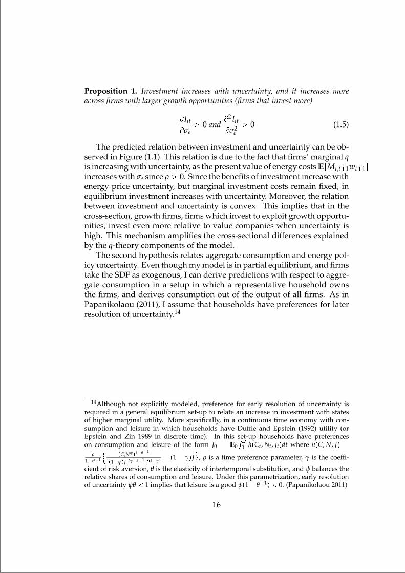
Proposition 1. Investment increases with uncertainty, and it increases moreacross firms with larger growth opportunities (firms that invest more)

BIit

Bσe¡ 0 and

B2 Iit

Bσ2e¡ 0 (1.5)

The predicted relation between investment and uncertainty can be ob-served in Figure (1.1). This relation is due to the fact that firms’ marginal qis increasing with uncertainty, as the present value of energy costs ErMt,t1wt1sincreases with σe since ρ ¡ 0. Since the benefits of investment increase withenergy price uncertainty, but marginal investment costs remain fixed, inequilibrium investment increases with uncertainty. Moreover, the relationbetween investment and uncertainty is convex. This implies that in thecross-section, growth firms, firms which invest to exploit growth opportu-nities, invest even more relative to value companies when uncertainty ishigh. This mechanism amplifies the cross-sectional differences explainedby the q-theory components of the model.

The second hypothesis relates aggregate consumption and energy pol-icy uncertainty. Even though my model is in partial equilibrium, and firmstake the SDF as exogenous, I can derive predictions with respect to aggre-gate consumption in a setup in which a representative household ownsthe firms, and derives consumption out of the output of all firms. As inPapanikolaou (2011), I assume that households have preferences for laterresolution of uncertainty.14

14Although not explicitly modeled, preference for early resolution of uncertainty isrequired in a general equilibrium set-up to relate an increase in investment with statesof higher marginal utility. More specifically, in a continuous time economy with con-sumption and leisure in which households have Duffie and Epstein (1992) utility (orEpstein and Zin 1989 in discrete time). In this set-up households have preferenceson consumption and leisure of the form J0 E0

³80 hpCt, Nt, Jtqdt where hpC, N, Jq

ρ

1θ1

! pC,Nψq1θ1

rp1ψqJspγθ1qp1γq p1 γqJ

), ρ is a time preference parameter, γ is the coeffi-

cient of risk aversion, θ is the elasticity of intertemporal substitution, and ψ balances therelative shares of consumption and leisure. Under this parametrization, early resolutionof uncertainty ψθ 1 implies that leisure is a good ψp1 θ1q 0. (Papanikolaou 2011)

16

“mainupfv2” — 2021/6/1 — 20:22 — page 17 — #33

Proposition 2. Uncertainty on future energy prices σe positively predicts aggre-gate consumption growth

Bgt1

Bσe¡ 0 where gt1 ErCt1

Cts Er Yt1

Yt Its (1.6)

where C, Y and I represent aggregate consumption, output and investment.

This proposition states that all things equal, an increase in uncertaintycovaries with aggregate consumption growth. Moreover, this predictabil-ity on consumption growth gets translated into SDF predictability (Har-vey 1988), and therefore firm returns are negatively predicted in the time-series.

Proposition 3. Uncertainty negatively predicts returns in the time series

BErRi,t1sBσe BErRi,t1s

BIit

BIit

Bσe 0 (1.7)

given the standard inverse relation between investment and expected returns inthe q-theory of investment BErRi,t1s

BIit 0

Finally, I derive a prediction regarding the cross-section of expectedreturns similar to a CCAPM beta representation which relates firm char-acteristics to firm’s beta

Proposition 4. Uncertainty amplifies cross-sectional differences in expected re-turns captured by investment

ErRi,ts r f t βSitλt (1.8)

where the firm’s consumption beta is defined as

βSit α

β

pYi,t1A q

1ββ I

αβ

i,tAIit

Yi,t1

1 a Iit

Kit

α

βR f t

ρσe

σM (1.9)

and λ is the price of consumption risk λt R f tpσMq2.

This proposition shows that differences in expected returns capturedby the firm’s consumption beta are amplified when energy policy uncer-tainty increases. Firms that invest more in equilibrium have a more nega-tive betas, and earn lower expected returns. These differences in expected

17

“mainupfv2” — 2021/6/1 — 20:22 — page 18 — #34

returns between companies with low and high investment, or equivalentgrowth and value companies, is amplified when energy policy uncertaintyis higher. Finally, I show that since a firm’s CCAPM beta is amplified bythe same magnitude (σe), investment absorbs the cross-sectional variationacross firms with different exposure to energy policy uncertainty

Proposition 5. Given future output Yt1, investment explains the cross-sectionalvariation in expected returns as proposition (9) can be rewritten as

ErRi,ts r f t βIitλ

et

where the firm’s investment beta is defined as

βIit α

β

pYi,t1A q

1ββ I

αβ

i,tAIit

Yi,t1

1 a Iit

Kit

α

βR f t

and the price of risk takes into account both consumption risk and energy priceuncertainty λe

t ρσeσMR f t.

1.4 Data

1.4.1 Firm Accounting and Financial Data

Accounting and Financial data comes from CRSP and the Compustat Quar-terly Database. From the quarterly Compustat database I download allfirm-quarter observations up to 2019q4 (1,789,987). I keep only observa-tions with ISO currency code in US dollars (curcdq), drop observationswith missing assets (atq) or stockholders’ equity (seqq) for a total of (1,235,343observations). Accounting variables are defined as follows: Market equityis defined as the number of common shares outstanding (cshoq) times thecalendar close price in the quarter (prccq). Size is the natural logarithm ofmarket equity, book-to-market is the ratio of Stockholder’s equity (seqq) tomarket equity. Book debt is defined as the sum of debt in current liabilities(dlcq) and long-term debt (dlttq). Profitability is the quarterly operatingincome after depreciation (oiadpq) over the sum of book debt and marketequity. Leverage is defined as the book value of debt over the book valueof debt plus market equity.

From the monthly CRSP database I download all observations fromDecember 1961 up to December 2019 (4,230,439). I keep only companiestrading in the NYSE AMEX or Nasdaq universe (exchcd 1, 2, and 3) with

18

“mainupfv2” — 2021/6/1 — 20:22 — page 19 — #35

sharecodes (shrcd) equal to 10 or 11 for a total of 3,223,430 observations.I use the WRDS linking table between gvkey and permno identifiers tomatch the Compustat database with CRSP. I lag accounting variables by 2months following Campbell et al. (2008) to correct for look-ahead bias. Themerged database contains 2,355,017 firm-month observations. To computemarket betas I download the Daily CRSP database between January 1965and December 2019 (86,115,478 observations) and define market beta fol-lowing Dimson (1979) computing intra-monthly regressions with respectto current, lagged, and led market returns as in Bali et al. (2019). Dailymarket excess return and daily risk free rates are obtained from Prof. Ken-neth French’s website.15

1.4.2 Financial and Macroeconomic Data

To construct the macro-finance data needed as a robustness test to modelthe investors’ information set I rely on the methodology presented in Ju-rado et al. (2015) which I update until 2019. Jurado et al. (2015) presenta Big Data methodology for uncertainty estimation using 147 macroeco-nomic and financial variables. Macroeconomic variables come from theFRED-MD database (McCracken and Ng 2015), financial variables are con-structed following Jurado et al. (2015), and Ludvigson and Ng (2007, 2009).For details on the construction of the financial variables see the Appendixfor Updates of Uncertainty Data available from Prof. Sydney Ludvigsonwebsite.16 I replicate the construction of all the 147 time series except fromthe VXO index which is available from the FRED-MD database, and theCochrane-Piazzesi factor (Cochrane and Piazzesi 2005) which I excludegiven that it does not cover the same sample as the rest of the variables.Portfolio data for the construction of the variables comes from Prof. Ken-neth French’s website, dividend data comes from the monthly index CRSPdatabase, and aggregate earnings data comes from Prof. Robert Shillerwebsite.

The analysis in this paper relies heavily on oil and gas price data, aswell as macroeconomic data commonly used in the predictability litera-ture (Fama and French 1989, 1988; Stambaugh 1999; Campbell and Yogo2006) such as the term and default spread, the aggregate dividend yieldand the aggregate payout ratio. Oil prices correspond to the West TexasIntermediate standard price per barrel, gas prices correspond to the Henry

15https://mba.tuck.dartmouth.edu/pages/faculty/ken.french/data_library.html

16https://www.sydneyludvigson.com/data-and-appendixes

19

“mainupfv2” — 2021/6/1 — 20:22 — page 20 — #36

Hub Natural Gas Spot price. Oil and gas information are obtained fromthe FRED at St. Louis.

The term spread is defined as the difference between the monthly aver-age of the 10 year and 1 year risk free rate (DGS10-DGS1) and the defaultspread as the difference between the monthly average of the rate on BAAand AAA bonds obtained as well from the FRED at St. Louis. The divi-dend price ratio is the natural logarithm of the fraction of aggregate div-idends inferred using the CRSP value weighted return with and withoutdividends (vwretd, vwretx) which is averaged across the last 12 monthsover an aggregate price index (See the Appendix of Jurado et al. 2015 fora detailed explanation). The aggregate dividend to earnings ratio is ob-tained from Prof. Robert Shiller’s website.17

1.4.3 Political Data

The main political data used in this paper contains U.S. executive ordersclassified into 20 topics from the Comparative Agendas Project.18 To en-sure the consistency of the data I double check all executive orders in thedatabase from public sources to ensure the database has no timing mis-takes. First I check that the total number of executive orders available inthe dataset from the Comparative Agendas project correspond to the totalnumber of executive orders reported by official sources. To determine thetrue number of executive orders that were issued in a particular month Irecollect data from the national archives and check for consistency.19 Al-though prior to the first half of the 20th century presidents used executiveorders in their mandates, these executive orders were not documented andarchived until the 1940s. I am able to obtain 974 executive orders from1937 to 2019, and count the number of executive orders issued each monthwhich corresponds almost entirely with the dataset provided by the com-parative agendas project.

The Comparative Agendas Project also contains data on public lawspassed by the Senate and the House of Representatives which are used ascontrol variables in the robustness test. The database contains a randomsubsample of all public laws starting in 1948. These public laws and ex-ecutive orders are classified into 20 different policy topics based on thevariable (pap majortopic).

17http://www.econ.yale.edu/˜shiller/18https://www.comparativeagendas.net/19https://www.archives.gov/federal-register/executive-orders/

disposition

20

“mainupfv2” — 2021/6/1 — 20:22 — page 21 — #37

The dataset containing the subsample of public laws does not containinformation about the month within each year in which the public law wasissued before 1973. In order to determine the month in which the publiclaw was issued I use two methodologies. First, I use the id of the publiclaw provided in the database and web-scrape the information about themonth from one of three sources. The library of congress contains infor-mation on all public laws issued since the period of George Washington,up to 1951.20 Public laws from 1952 to 1973 are available from the LegisWork website.21 Finally public laws from 1974 to nowadays are availablefrom the US congress website.22

To determine the exact month in which the public law was issued theid of each law contains the number of the congress. Congresses have anumber assigned since the first congress in 1789. Congresses from 1948 to1951 correspond to numbers 80 to 81, congresses from 1952 to 1973 corre-spond to congresses 82 to 92 and congresses from 1974 to 2019 correspondto congresses 93 to 115. The Legis Work website organizes public laws intoVolumes and not congress numbers. Congresses have mostly 2 volumesof laws which are normally split into half during the legislative mandate.Congresses from 1952 to 1973 correspond to volumes 65 to 86.

Once all public laws are downloaded from these websites the secondstep consists of assigning the law to the month and year when it wassigned. From the library of congress this can be done by searching for thename of the month, year and date within the description of each law. Forpublic laws from 1952 to 1973 obtained from Legis Work this is done bysearching for sentences with words containing month names and obtainthe year by looking at all words inside each sentence. Finally the congresswebsite provides a more friendly format to obtain the date of each law.

The information of some of the public laws is not digitalized in thesethree sources. For these laws, I download the original text in image format.Using Optical Character Recognition (OCR) algorithms, I isolate the textof each law and using textual analysis isolate the part of the Public Lawcontaining the year and month. I check that the year inferred from theOCR algorithm corresponds to the year provided by the original datasetfor robustness of the OCR algorithm. I also collect information regardingthe political party in power from the data-planet website. I collect data onthe party of the president of the United States, as well as the political party

20https://www.loc.gov/law/help/statutes-at-large21http://legisworks.org/sal/22https://www.congress.gov/public-laws/

21

“mainupfv2” — 2021/6/1 — 20:22 — page 22 — #38

holding majority in the Senate and the House of Representatives.23

1.5 Measuring Energy Policy Uncertainty

In this section I construct a measure of energy policy uncertainty by fittinga probability model to estimate how likely it is to have an energy relatedexecutive order signed by a U.S. President in the future. Define by Nt thenumber of energy related executive orders signed in month t. The randomvariable defined as

Yt #

1 if Nt ¡ 00 if Nt 0

(1.10)

has a conditional Bernoulli distribution with probability PrpYt 1q pt.The estimation of probability pt is performed as follows: Given an infor-mation set It1 available for an economic agent at time t 1, and assumingthe process Yt is stationary, she estimates a probability model based on thehistory of realizations of tYsut

s0.

pt ProbpYt 1|It1q f pIt1, θq (1.11)

Where f is the functional form of a Probit model. The uncertainty aboutthe value of variable Yt1 before its realization can be seen as its condi-tional standard deviation

Ut a

VarpYt1|Itq b

pt1p1 pt1q. (1.12)

This measure provides time varying uncertainty on Ut due to changes inthe information set as well as new realizations of Yt which updates theparameters in the underlying probability model f pIt, θq. To model the in-formation set required to fit the probability model I start with a base spec-ification that includes the level and return of the West Texas Intermediateprice per barrel, the aggregate dividend price ratio, and the PresidentialDummy of Santa-Clara and Valkanov (2003).

I show in robustness tests that the choice of the agents’ informationset does not qualitatively change the main results in the paper. However,there is evidence that the environmental and energy agenda of politiciansdiffer between Republican and Democratic mandates (Gustafson et al. 2020),governments are more likely to change existing policies in bad times (Pastorand Veronesi 2012, 2013), oil and financial markets are strongly interde-pendent (Jin and Jorion 2006), and textual analysis of the text in executive

23https://data-planet.libguides.com/politicalpartycontrol

22

“mainupfv2” — 2021/6/1 — 20:22 — page 23 — #39

orders suggest oil behaviour triggers the occurrence of energy policies. Asseen in Figure (1.3) during the 1970s and 1980s Oil is one of the topics mostdiscussed within the text of executive orders given its importance and theconsequences of the oil crisis.

Table (1.4) provides estimations of the probability model in which theleft hand side variables is the probability of having at least one energyrelated executive order in the following 1, 3, 6, and 12 months. The returnon oil, more than the level of the WTI predicts the occurrence of energyrelated executive orders for horizons of more than 3 months (Columns 2-4). The business cycle captured by the dividend price ratio predicts theoccurrence for energy related executive orders for all specifications in aninverse u-shape depending on the horizon considered. Energy policies aremore likely to occur after low market valuations, and finally they are morelikely to occur under Democrat mandates.

The uncertainty used in the rest of the paper assumes a forecastinghorizon of one month. In particular I fit a probit model as follows:

pt Φpβ0 β1wtit1 β2Roilt1 β3pd pqt1 β4Republicant1q (1.13)

where tβ0, β1, β2, β3, β4u are computed recursively using Maximum Likeli-hood Estimation based on information tYs, wtis, Roil

s , pd pqs, Republican sut1s0,

wti is the West Texas Intermediate oil price per barrel relative to the pricein 1970, Roil

t is the return on wtit between month t 1 and t, pd pq isthe CRSP Value Weighted log dividend price ratio, and Republican is adummy variable that takes the value of one if the U.S. President in powerat month t has a Republican affiliation, and Φp.q is the standard normalcdf.

The first estimation corresponds to January 1980 using informationavailable since January 1970.24 Each estimation is done recursively usingall information available until month t 1. Figure (1.2) plots the evolu-tion of energy policy uncertainty starting from January 1985 to December2018 plotted against the EPU index of Baker et al. (2016). My index com-plements the aggregate EPU index by isolating uncertainty variation inenergy related events. As a result my measure has a transitory spike dur-ing the Iraqi invasion of Kuwait in august 1990, then it increased in 1993when the OPEC failed to agree to cut production decreasing consistentlyduring the 2000s. During the financial crisis the energy policy uncertainty

24Oil prices before 1973 were highly regulated and do not exhibit significant time-seriesvariation. I only use information since 1970 despite having executive orders starting in1950 since most likely energy related decisions in the 50s and 60s were related to NuclearEnergy and Coal which probably not as relevant as they used to be.

23

“mainupfv2” — 2021/6/1 — 20:22 — page 24 — #40

increased with aggregate uncertainty, and declining in 2017 following aregularization in the Supply of oil by the OPEC. My measure of energypolicy uncertainty strongly rejects the null of unit root with a z-statisticof -3.78 (p=0.003) under a standard Dickey and Fuller (1979) test, whichdecreases the likelihood of biasing the its coefficient in predictability andcross-sectional regressions due to correlation between regression residualsand innovations to energy policy uncertainty (Stambaugh 1999).

So far I have only described the time-series behaviour of energy policyuncertainty and its ability to capture underlying changes in the world en-ergy supply. However, if this uncertainty is anticipated by the market, itshould be incorporated into asset prices. In order to study the asset pric-ing consequences of this uncertainty I use the unexpected component ofthe uncertainty estimation in cross-sectional asset pricing regressions lateron. I fit an AR(1) process into the conditional variance of random variableYt as follows

ptp1 ptq φ0 φ1pt1p1 pt1q ut (1.14)

after estimating φ0 and φ1 via OLS, and define ut is the unexpected compo-nent of uncertainty. As in Dou et al. (2020b) and Bansal and Yaron (2004)I assume that the variances follow an AR(1) process. The OLS estimatorof φ1 is 0.96 significant at the 1 percent level, and rejects the null of unitroot with a z-statistic of -22.8. The first sub-table in Table (1.1) presentssummary statistics of the number of energy related executive orders permonth Nt, the indicator variable Yt, as well as summary statistics of theenergy political uncertainty index Ut and its innovations ut. In average,between January 1980 and December 2018 there were 0.1 executive orderssigned per month, with executive orders occurring in average in 7 percentof the months in the sample.

1.6 Cross-sectional differences in investment un-der uncertainty

In this section I study how cross-sectional differences in investment acrossfirms are amplified when energy policy uncertainty is high. The mainresult in the q-theory of investment states that marginal q is a sufficientstatistic of firms’ asset growth, as it captures firms’ investment opportuni-ties (Hayashi 1982). The first hypothesis developed in section (1.3) showsthat energy policy uncertainty should amplify differences in investmentexplained by firms’ marginal q. Substitution between energy and capi-tal, or equivalently investment in energy-efficient technology should be

24

“mainupfv2” — 2021/6/1 — 20:22 — page 25 — #41

profitable for all firms when energy policy uncertainty is high, but moreprofitable for firms with higher investment opportunities.

I begin by extending an otherwise standard investment-Q regressionin which growth opportunities are proxied by size (Gala et al. 2019) andTobin’s average Q (Tobin 1969; Hayashi 1982; Cochrane 1991), and growthopportunities and profitability are sufficient statistics for investment.25 Inparticular I estimate the following panel regression for public U.S. firms

Invit a b Sizeit cQit d Profitabilityit γ Ut εit (1.15)

where investment (Inv) is defined as capital expenditures (the quarterlychange of reported annual compustat item capxy for quarters 2, 3, and4) over total assets. I use capital expenditures as proxying for energy-efficient capital investment following Brinkerink et al. (2019) who suggestthat energy-efficiency is improved after capital expenditures and not bychanges in fixed assets. I also estimate the above specification interactinggrowth opportunities (Size and Average Q) with my measure of energypolicy uncertainty. If energy policy uncertainty triggers investment in cap-ital, and this behaviour is more prominent for growth firms we shouldexpect b 0, c ¡ 0, and the interaction with uncertainty amplifying theimpact in the same direction.

Table (1.2) presents the results of estimating the above equation withand without industry fixed effects at the four SIC digits level to accountfor the fact that the impact that energy policy uncertainty can have on afirm’s growth opportunities depends on the industry it operates. Columns1 and 2 present the baseline result with industry fixed effects in which dif-ferences in investment are captured by profitability and growth opportu-nities and the level of energy political uncertainty. The baseline specifi-cation is consistent with Gala et al. (2019). Smaller firms and firms withhigher average Q invest more. Both significant at the 1% level. Otherthings equal, a one standard deviation increase in firm’s size translatesinto a decrease in average investment from 1.9 to 1.56 percent of total as-sets, for the average firm, or a 22% reduction in investment. Equivalently,a one standard deviation increase in average Q, translates into an increasein monthly investment for the average firm between 1.9 to 2.26 percent oftotal assets or an increase of 18 percent for the average firm. Moreover, thiscolumn confirms that aggregate investment increases when energy policy

25Extending Q regressions with ad-hoc variables has been widely used in the literaturemainly to study the role of financial frictions in driving differences between marginaland average Q (Gomes 2001; Cooper and Ejarque 2003; Abel and Eberly 1994; Barnettand Sakellaris 1998; Bolton et al. 2011)

25

“mainupfv2” — 2021/6/1 — 20:22 — page 26 — #42

uncertainty is higher. A one standard deviation increase in the level ofenergy policy uncertainty from its unconditional mean covaries with a 1.2percent increase in quarterly investment. For an average quarterly capexover assets of 1.9 percent and the average firm in the sample having 10.4USD Billions in total assets, this increase in uncertainty results in quarterlyinvestments of 480 million USD for the average firm.

Columns 2 and 3 present the estimation results of interacting energypolicy uncertainty with the first measure of firms’ growth opportunities,average Q. A one standard deviation increase in energy policy uncertaintyfrom its unconditional mean between March 1980 and October 2018, in-creases the marginal relation between average Q and investment acrossall firms by 15 % (from 0.19 to 0.22) a magnitude that is significant at the1% percent level. This amplification in the relation between average Qand investment also occurs across firms within the same industry at the 1% level, for which the marginal relation increases by 13.5% (from 0.22 to0.23).

In columns 4 and 5, I interact the second measure of firm’s growth op-portunities, firm size, with energy policy uncertainty in the cross-sectionalinvestment regressions. Across all firms in the sample, an increase of a onestandard deviation in energy policy uncertainty above its unconditionalmean between March 1980 and October 2018, amplifies the marginal rela-tion between size and investment by 21 % (from -0.23 to -0.28) both acrossall firms and within the same industry. Both results are significant at the 1% level. These results confirm the hypothesis that an increase in the levelof energy policy uncertainty, increases the incentives to invest by thosefirms with larger growth-opportunities - firms with larger average Q andsmaller firms.

26

“mainupfv2” — 2021/6/1 — 20:22 — page 27 — #43

1.7 Energy Policy Uncertainty, Consumption, andAggregate Returns

In this section I study the relation between the level of energy policy un-certainty, aggregate market returns and household consumption. If theincentives of growth firms to invest in capital are sufficiently high whenenergy policy uncertainty increases, one can expect an overall increase inaggregate investment as confirmed in Table (1.2). This increase in aggre-gate investment should decrease ceteris paribus aggregate consumption inthe current period as more output is used for investment rather than con-sumption. If this impact is transitory, and consumption and investmentpatterns are expected to reverse in the future, this creates a forecastablepattern in consumption, and expected returns (Lucas 1978; Rubinstein1976).

The idea that incentives to growth firms to invest in capital creates fore-castable patterns in expected returns and consumption has been exploredextensively in a recent literature (e.g. Papanikolaou 2011; Kogan and Pa-panikolaou 2013, 2014; Dou 2017). These papers suggest that these pat-terns in investment are caused by investment-specific shocks that decreasethe per-unit cost of capital investment, as well as improving the quality ofgrowth opportunities. Although, the mechanism that I test has a similarimpact on aggregate investment, in my setup, firms invest more in capi-tal when energy policy uncertainty is high, not because capital goods arecheaper, nor because managers expect higher returns to investment, butrather because the market value of the the cost incurred if not investing inenergy-efficient capital is larger.26

To test this hypothesis I follow the literature on return predictability(e.g. Campbell and Yogo 2006; Stambaugh 1999; Fama and French 1988,1989; Cochrane 2008) and fit the following time-series model

RtÑtk a δUt γXt εtÑtk (1.16)

where RtÑtk is the log cumulative return between month t and t k ofthe CRSP Value Weighted portfolio including dividends, Ut is the levelof energy policy uncertainty at time t regarding the possibility of an en-ergy executive order at time t 1, and Xt is a vector of variables docu-mented to capture expected return variation such as the log dividend yield

26In unreported tests I find that energy policy uncertainty does not help explain cross-sectional differences in expected investment growth, which shades light on the transitoryimpact of the uncertainty on investment. Interacting energy policy uncertainty with av-erage Q, operating cash flows, and changes in return on equity in similar investmentgrowth regressions of Hou et al. (2020) yield no significant results.

27

“mainupfv2” — 2021/6/1 — 20:22 — page 28 — #44

(Cochrane 2008; Fama and French 1989), the term and default spreads(Fama and French 1988), and the return on oil prices (Jones and Kaul 1996;Ready 2017). I also control for time varying risk aversion proxied by thepolitical party in power (Pastor and Veronesi 2017, 2018) by including adummy variable for those months in which the U.S. president is a repub-lican (Santa-Clara and Valkanov 2003).

According to one of the hypotheses presented in Section (1.3), if house-holds have a preference for late resolution of uncertainty, current aggre-gate consumption decreases at time t as investment becomes more atrac-tive. Since investment translates into future output, agents expect con-sumption to grow and therefore lower marginal utility in the future, whichcaptures lower expected returns (δ 0) as in the CCAPM. Table (1.3)presents OLS estimates with Newey and West (1987) standard errors withk lags to account for residual autocorrelation due to overlapping returns.For horizons of one month, one quarter, and one year, energy policy uncer-tainty negatively predicts market expected returns, above and beyond thevariability captured by the dividend yield, the term and default spreads,the presidential dummy and oil returns.

As a common finding in predictability regressions, the magnitude ofthe coefficient of most variables and R2s in the regression increases withthe horizon (Cochrane 2008). However the coefficient of energy policy un-certainty has a different behaviour and becomes not significant for hori-zons larger than one year. For horizons of up to one year, energy policyuncertainty negatively captures expected return variation with a signif-icance of 1% accounting for residual autocorrelation. The magnitude ofthis predictability is also economically significant. A one standard devi-ation increase in the level of energy policy uncertainty translates into adecrease in expected returns of 1.3 % in one month, 0.9 % monthly withinone quarter and 1% per month within one year.

The dividend price ratio remains a significant predictor of expected re-turns for all horizons consistent with Fama and French (1988) and Cochrane(2008). My results are also robust to the political party in power in the U.S.Results of regressions with horizons up to one year, show that the coef-ficient of the dummy capturing a Republican mandate, are negative andsignificant at the 1% level, which replicates the finding of Santa-Clara andValkanov (2003) in our sample, democrat presidencies tend to have higherexpected returns.27

27Pastor and Veronesi (2017) propose a rational explanation for the presidential puzzle(Santa-Clara and Valkanov 2003). The fact that under democrat U.S. presidential man-dates stock returns are higher than under republican mandates, is a consequence that

28

“mainupfv2” — 2021/6/1 — 20:22 — page 29 — #45

Next I test if energy policy uncertainty captures changes in expectedconsumption growth. This is a more direct way to test the hypothesiswhich states that when energy policy uncertainty is high, aggregate in-vestment increases at the expense of consumption. Testing for predictabil-ity on consumption growth is not trivial. In the consumption CAPM (Ru-binstein 1976; Breeden and Litzenberger 1978; Lucas 1978; Breeden 1979),expected consumption growth is a function of expected aggregate returns,which are simultaneously a function of the model primitives. To over-come this problem I estimate simultaneously the following two equationsvia GMM as in Harvey (1988)

lnctk

ct

γ0 γ1Ut γ2RtÑtk γ3termt υtÑtk

RtÑtk δ0 δ1pd pqt δ2termt δ3deft εtÑtk

(1.17)

where ct are the US monthly personal consumption expenses. I estimatethe system of equations with similar moment conditions as for an OLSestimation, for parameters θ tγ0, γ1, γ2, δ0, δ1, δ2, δ3, δ4u

gpθq 1T

¸t

!ln

ctkct

γ0 γ1Ut γ2RtÑtk γ3termt

RtÑtk δ0 δ1pd pqt δ2termt δ3deft

) Zt 0

(1.18)with instruments Zt tConstant,Ut, RtÑtk, termt, deft, pd pqtu, and aninitial identity matrix in the first stage of the GMM estimation.28 Table (1.5)presents the results of the two step GMM estimation, for horizons of one,three, five and six years. I choose yearly horizons for two reasons: First iteliminates the seasonal component of consumption, and second it allowsthe regressions to have higher volatility in the left hand side since it isknown that consumption patterns are smooth and consumption growth isnot volatile enough to meet the Hansen and Jagannathan (1991) bound.29

As observed in columns 1 to 4, the coefficient γ1 capturing the pre-dictability power of energy political uncertainty on expected consumptiongrowth is positive and significant for all horizons. Point estimates increasewith the prediction horizon and is significant at the 1% level except for the

democrats are more likely to be elected when risk aversion is higher. In particular, if highenergy uncertainty coincides with republican mandates where risk aversion is lower, andas a consequence expected returns.

28When using returns in GMM regressions it is common to obtain numerically singularcovariance matrices in the first step of the GMM estimation, which can be solved bygiving equal importance to every single moment condition (Cochrane 2009).

29See Bulusu and Gomez Biscarri (2012) and references inside for a discussion on thedifficulty of using consumption data in testing the CCAPM.

29

“mainupfv2” — 2021/6/1 — 20:22 — page 30 — #46

one year horizon for which is significant at the 5% level. The magnitude ofthis finding is also economically significant. A one standard deviation in-crease in the level of energy policy uncertainty translates into an expectedincreases in yearly consumption growth of 17, 43, 23 and 36 percent forhorizons of 1, 3, 5, and 6 years.

All together the predictability pattern in consumption and aggregatemarket returns supports the hypothesis that in periods of time with highenergy policy uncertainty, aggregate consumption decreases relative to fu-ture consumption which gives room for a forecastable pattern in expectedmarginal utility that translates into return and consumption growth pre-dictability. As shown in robustness tests, this finding survives a more com-plete specification of the information set when computing energy policyuncertainty.

1.8 Energy Policy Uncertainty and the Cross-sectionof Expected Stock Returns

In this section I show that innovations to energy policy uncertainty arepriced in the cross-section of portfolio returns sorted on growth oppor-tunities. Moreover, I show empirically that since investment reacts tothe level of energy policy uncertainty, differences in investment shouldcapture the cross-sectional variation explained by energy policy uncer-tainty betas. If energy policy uncertainty anticipates future states of lowmarginal utility, assets that appreciate in relative terms following an unan-ticipated shock should earn lower expected returns. Given that marketvaluations of growth companies appreciate with unexpected news aboutenergy policy uncertainty (positive betas), the price of risk of this innova-tions should be negative. To test this hypothesis I follow a standard assetpricing approach in which I extend a linear asset pricing model with theinnovations to energy policy uncertainty.

Given that my interest is to relate expected returns among firms withdifferent investment opportunities across size (Gala et al. 2019) and aver-age Q (Hou et al. 2014), I use as testing portfolios the 25 portfolios sortedon size and book-to-market (Fama and French 1992, 1993, 1995) whichproxy for differences in investment opportunities. I follow the intertempo-ral capital asset pricing model (ICAPM) of Merton (1973) to relate energypolicy uncertainty with state variables capturing changes in the invest-ment opportunity set and perform GMM estimations of the price of risk

30

“mainupfv2” — 2021/6/1 — 20:22 — page 31 — #47

following Maio and Santa-Clara (2012).30 In particular, given a linear assetpricing model with factors fit, I estimate the price of risk of energy policyuncertainty from the following expected return-covariance formulation

ErRej s γCovpRi, Rmq

¸i

γfi CovpRi, fiq γuCovpRi, uq (1.19)

where Rej corresponds to the expected excess return of testing portfolio j,

Rm corresponds to the market factor, u corresponds to the innovations onenergy policy uncertainty, and γ

fi is the covariance price of risk of factor i.

As a robustness test to check if my results are consistent with an ICAPMexplanation, I show that my results satisfy the restrictions in Maio andSanta-Clara (2012): The ICAPM predicts that the covariance price of mar-ket risk γ should be a feasible estimate of the representative agent’s riskaversion, and since energy policy uncertainty negatively predicts expectedreturns it must follow that γu 0.31

In the empirical analysis I extend some standard asset pricing modelswith innovations to energy policy uncertainty. I use the CAPM model ofSharpe (1964), Lintner (1965), and Mossin (1966), the 3 factor model (FF3F)of Fama and French (Fama and French 1992, 1993, 1996), the 5 factor model(FF5F) of Fama and French (2015) which includes both an investment andprofitability factor, the q4 model of Hou et al. (2014) which also relate ex-pected returns with profitability and investment as FF5F but the factorsconstruction differs, and finally, the q5 model in Hou et al. (2014) and Houet al. (2020).

30To avoid a fishing-license (Fama 1991) arising from using a data rich environment inasset pricing regressions, I follow Maio and Santa-Clara (2012) and test if energy polit-ical uncertainty satisfies 3 restrictions. First, for energy political uncertainty to capturechanges in the investment opportunity set, it should predict the distribution of aggregatereturns. In particular, the first or second moment of the return distribution. Second, in-novations to energy political uncertainty must earn a significant price of risk in the cross-section of expected returns with the sign of the price of risk equal to the sign obtained inthe predictability regressions. Third, the market price of covariance risk obtained fromthe cross-sectional regressions should be a reasonable estimate of the Relative Risk Aver-sion (RRA) of the representative agent in the economy. Finally, I check that the absolutevalue of the z-statistic in a GMM regression are close to the threshold in Harvey et al.(2016) in at least one of the specifications studied. Since the predictability power of en-ergy political uncertainty was assured in the last section I focus on the estimation of thecovariance price of risk as well as the estimates for the relative risk aversion coefficient.

31Maio and Santa-Clara (2012) point that in equilibrium the covariance price of marketrisk equals the Relative Risk Aversion coefficient of the representative agent γ W VWW

VW,

where W is aggregate wealth, and V is the Value Function result of the representativeinvestor’s optimization problem.

31

“mainupfv2” — 2021/6/1 — 20:22 — page 32 — #48

I use the above mentioned factors to achieve two goals. Standard as-set pricing models such as the CAPM and FF3F, allow me to test if in-vestors price unexpected innovations to energy policy uncertainty andhow they adjust their market valuations. This result is derived directlyif investors consider energy policy uncertainty a relevant state variable asin the ICAPM. The second set of asset pricing models (FF5F, q4, and q5),which include factors related to investment and profitability, have a differ-ent use. They test if changes in the investment policy of firms after changesin energy policy uncertainty, is enough to explain cross-sectional differ-ences across firms with lower and higher exposure to u. They allow meto test if differences in expected returns across companies with differentu betas, can be explained because systematically some of these companiesinvest relatively more or less intensively. Naturally, if firms adjust their in-vestment policy in the presence of uncertainty, magnitudes and z-statisticsof the price of risk in u should be higher across the first set of asset pricingmodels. Across the CAPM, FF3F, FF5F asset pricing models, factors mktrftsmbt, hmlt, cmat, rmwt and momt which are factors related to the market,size, book-to-market, investment, and profitability, are obtained from Prof.Kenneth French website. On the other hand, across the q4 and q5 models,the Rme, RIA, Rroe, Reg, factors related to market equity, investment-over-assets, return on equity and expected growth are obtained from Prof. LuZhang’s website.

The above models can be estimated with the following N K momentconditions following Maio and Santa-Clara (2012)

gTpθq 1T

T

t1

!pRit R f tq °K

k1 γkpRit R f tqp fkt µkqp fkt µkq

) 0

Where N is the number of testing portfolios, K is the number of factorsin the model, fk corresponds to a factor in each specification, and µk isthe unconditional average of the factor. The vector of parameters θ ptγkuK

k1, tµkuKk1q is then estimated using a one step GMM procedure (Hansen

1982) using an identity matrix as optimal weighting matrix. Followingthe original methodology by Maio and Santa-Clara, I add to the 25 testingportfolios the market return to merge the cross-sectional component of theICAPM with the time-series aggregate risk-return trade-off.

Using equally weighted moments is equivalent to running an ordinaryleast squares (OLS) cross-sectional regression of average excess returns onfactor covariances (right-hand side variables), however the GMM estima-tor accounts for residual correlation among testing assets. Moreover, thismethodology allows me to account for estimation error in the factor means

32

“mainupfv2” — 2021/6/1 — 20:22 — page 33 — #49

as in Cochrane (2009)[Chapter 13] and Yogo (2006).32 33

Table (1.6) provides estimates of GMM cross-sectional regressions. Col-umn 1 to 5 present the expected value and price of risk of energy pol-icy uncertainty together with the factor means after the GMM estimation.Columns 1 to 2 present the base specifications extending the CAPM andFF3F models. The covariance price of risk of energy policy uncertainty issignificant and negative across all five specifications, which suggest thatportfolio with assets that perform better when energy policy uncertaintyis unexpectedly high, are preferred by investors, and therefore earn lowerexpected returns. Finally, as shown in Columns 4 and 5, the price of riskearned by innovations to energy policy uncertainty is completely capturedby the portfolio exposure to the q factors, as studied in Section (1.3) of thepaper. The investment policy of firms reacts to energy policy uncertainty,and its a sufficient measure to explain the cross-sectional differences inexpected returns. Finally, I report the Mean Absolute Error (MAE) in thecross-sectional regressions which equals the average of the absolute valueof pricing errors. The q4 and q5 models yield the lowest MAE of all fivespecifications, with MAEs of 0.11 and 0.09 percent respectively. 34

A potential concern that can arise is that z statistics in the cross-sectionanalysis are not high enough to overcome potential biases caused by data-snooping and publication biases (Harvey et al. 2016, 2019). I tackle thispotential concern in two ways. First I show in the robustness test, that thisis caused by the conservative selection of variables in the information setused to estimate energy policy uncertainty. By considering a large batteryof variables into this information set, some z statistics in the first set of as-set pricing models overcome the threshold of 3 in Harvey et al. (2016) orremain slightly below while remaining significant. Second, the objectiveof the paper is to understand how energy policy uncertainty shapes firms’investment decisions, and how these decisions can be translated into dif-ferences in expected returns.

To ensure that portfolios of firms with larger growth opportunities arein fact earning higher expected returns when energy policy uncertainty

32As pointed by Maio and Santa-Clara (2012) this procedure is more convenient whenestimating an asset pricing in expected return-covariance form instead of expectedreturn-beta form Brennan et al. (2004)

33Recall that factor premia must be estimated jointly when the factor considered isnot a portfolio, since the factor does not price itself in the cross-section, see (Cochrane2009[Chapter 13])

34In unreported tests I extend the model of Stambaugh and Yuan (2016), which containstwo anomaly factors, and find that the factor also digests the price of risk of energy polit-ical uncertainty. Given the fact that the object of interest in the paper are the investmentopportunities of firms, I exclude it from the analysis.

33

“mainupfv2” — 2021/6/1 — 20:22 — page 34 — #50

is un expectedly large, I compute the portfolio betas using the model incolumn 1 of Table (1.6) but presented in a expected return beta form Re

it a bmktrft βut εit, and report them in Figure (1.4).35 As expected,portfolios of companies with more growth opportunities, small companiesand companies with lower book-to-market ratios, tend to have a largerbeta than value companies. Portfolios mainly of small companies, andcompanies with low book to market ratios have larger and positive u betas.

1.9 Robustness Analysis

In this section I provide robustness analysis supporting the main findingsin the paper. First, I provide more evidence that the measure of energypolicy uncertainty developed, is in fact capturing uncertainty about fu-ture energy policies. Second, I show that qualitatively the main resultsof the paper, are robust to a more complete modelling of the investors’information set to compute energy policy uncertainty.

1.9.1 Robustness on the measure of Energy Policy Uncer-tainty

I study if companies that operate in businesses that are more sensitive toenergy policies, such as companies whose cash-flows are energy-price sen-sitive, are also exposed to my measure of energy policy uncertainty. I de-fine energy exposure following Jin and Jorion (2006) as the sensitivity ofstock returns with respect to oil and gas returns controlling for aggregatemarket returns. In particular I use a 60 month rolling window for eachcompany to fit regressions

Rit a bRmt βoilRoilt εit (1.20)

andRit a bRmt βgasRgas

t εit (1.21)

together with an energy policy uncertainty beta.

Rit a bRmt βenergyut εit (1.22)

and study if energy sensitive companies coincide with companies whosestocks are sensitive to uncertainty regarding energy policies. I run cross

35Results are similar when computing the betas based on any specification in whichthe price of risk of innovations to energy policy uncertainty are significant.

34

“mainupfv2” — 2021/6/1 — 20:22 — page 35 — #51

sectional regressions between oil and gas betas on βenergy and market lever-age to account for equity risk as follows

βoil,gasit δ0 δ1β

energyit δ2Leverage δ3βit εit (1.23)

Where βoil,gasit represents either the oil or gas beta, leverage is the market

debt ratio of the firm, and βit is the company equity’s market beta. Ta-ble (1.7) presents results of estimating the above regression allowing forfixed variation at the time, industry, and firm level. Clustered standarderrors at the month level are presented in parenthesis. Consistent withthe nature of the uncertainty, companies sensitive to energy policy uncer-tainty coincide mostly with oil-sensitive companies while the relation togas sensitive companies is weak, although coefficients in columns 4 and5 are significant, they are economically insignificant. As seen in columns2, and 3, this is not due to these companies operating in energy sensitivesectors. Results including the industry fixed effect suggest that within in-dustry, companies more exposed to oil fluctuations are in fact companiesmore exposed to innovations on energy policy uncertainty. Additionally,the fact that the coefficient δ1 survives the inclusion of firm fixed effectssuggest that this relation is not firm specific.

1.9.2 A quasi-natural experiment, The 2014 OPEC Announce-ment

Oil and gas betas are noisy estimates of the reaction of firms’ valuations tooil and gas prices. To better study the energy policy uncertainty betas ofoil-sensitive companies I use a quasi-natural experiment recently used by(Dou et al. 2020b): the 2014 OPEC announcement to not cut the supply ofoil. In November 2014 in the 166 OPEC Meeting leaded by Saudi-Arabia,the OPEC decided to not cut oil production despite the increasing supplyfrom non-OPEC countries, which lead to a decrease of 10 percent in oilprices in one day, and persistent high volatility for the next years.36 Giventhe persistent increase in the volatility of oil prices, energy-sensitive com-panies should experience an increase in their energy policy uncertaintybeta. To estimate this impact, I run the following difference in differences

36I thank Winston Dou for referring me to his work with Leonid Kogan and Wei Wu,which allowed me to implement the quasi-natural experiment in my analysis.

35

“mainupfv2” — 2021/6/1 — 20:22 — page 36 — #52

regression

βenergyit a bOil related dummyit cAfter OPEC announcement dummyt

dOil related dummyit After OPEC announcement dummyt εit(1.24)

where Oil related dummyit is equal to one if the SIC code provided byCompustat equals to 1311, 1381, 1389, 2911, or 5172 as in (Chiang et al.2015 ).After OPEC announcement dummyt equals one if the current month t ¥2014m11. The difference-in-differences estimator d captures how the en-ergy policy uncertainty beta of oil-related companies changed after theannouncement. Table (1.8) provides OLS estimates with double clusteredstandard errors at the year-month and firm (gvkey) level. I keep a symmet-ric estimation sample of 4 years before and after the announcement, andprovide in column 1 the standard specification while in column 2 I includetime fixed effects and remove the after OPEC announcement dummy. Es-timator d is economically and statistically significant with a value of 0.84.Figure (1.10) plots the average β

energyit for oil related companies in solid

black line, and for non oil related companies in dashed line. The aver-age energy policy uncertainty beta of oil related companies before the an-nouncement is 0.66 and becomes 1.32 for the four years after the announce-ment. As expected, non oil related companies did not suffer a change intheir energy policy uncertainty betas after their announcement.

1.9.3 Does lobbying decrease the exposure to energy pol-icy uncertainty?

If firms have the ability to create political connections and lobby, energy-sensitive betas of companies that actively incur in lobbying should experi-ence a systematic reduction in their exposure to energy policy uncertainty.In order to test this hypothesis. I use a conditional beta model similar toJin and Jorion (2006), and model political uncertainty betas as a functionof lobby expenditures as follows.

Rit ai biRmt

βenergyi γi

Lit

Ai,t1

ut εit (1.25)

where Lit corresponds to lobby expenditures, and Ai,t1 corresponds tofirm’s total assets in the period before. Lobby expenditures are queried viathe LobbyView API using the Compustat gvkey of the firms in my sample,

36

“mainupfv2” — 2021/6/1 — 20:22 — page 37 — #53

and firms with missing lobby expenditures are treated as zero. Lobbyingexpenses are winsorized at the one percent level.37 If lobby expendituresof ex-ante exposed companies reduce the exposure to political uncertaintywe would expect γi 0 for energy sensitive companies. I estimate theabove equation using the entire sample for which lobby expenditures areavailable between 1997 and 2018. I aggregate coefficients γi using a sim-ple average scaling for the fraction of lobby expenditures per total assetswithin companies in the same industry

γj lj 1|Ij|

¸iPIj

γi li (1.26)

where li corresponds to the average lobby expenditures over assets of firmi, and Ij is the set containing all firms in industry j. I aggregate usingthe 12 industries definitions in Prof. Kenneth French’s website. Resultsof the impact of lobbying into systematic exposure to energy policy un-certainty as well as the zero lobby betas, the betas for companies with nolobby expenses, are presented in Figure (1.5). As expected, firms in sectorssuch as energy, durables, manufacture and health benefit from lobbyingto decrease their exposure to energy policy uncertainty, with energy be-ing the sector with the largest reduction in exposure to uncertainty giventheir lobby expenditures. Not surprisingly, the exposure of zero lobbyingenergy firms to uncertainty is the largest across these sectors. This doesnot only contribute to ensure my measure of energy policy uncertainty isin fact robust, but it also provides evidence that lobby is an effective riskmanagement tool in the presence of policy uncertainty.

1.9.4 Robustness tests on the Information Set

I perform robustness analysis to ensure that the main results in the paperare not driven by the specification of the information set presented in Sec-tion (1.5). I model the information set following Jurado et al. (2015) andperform a data-rich forecasting exercise in which I forecast the existenceof at least one energy related executive order in the future. The detailsof the forecasting procedure are presented in the appendix. I refer to thismeasure of energy policy uncertainty as the ”complete measure”.

I repeat the main three econometric specifications with this measure totest the hypotheses developed in Section (1.3). First I repeat aggregate

37I thank Marco Grotteria for sharing his code to perform the API requests from theLobyView website using the Compustat gvkeys.

37

“mainupfv2” — 2021/6/1 — 20:22 — page 38 — #54

return and consumption growth predictability regressions. Table (A.1)presents results over forecasting horizons of one month, one quarter, oneyear, and three years. For this specification I modify the control variablesin two ways. First, I exclude the level of the West Texas Intermediate oilprice, given that the construction of the complete measure uses data avail-able since the 1950s, and oil prices were strongly regulated until de mid1970s. Second, following Maio and Santa-Clara (2012) I include two morecontrol variables, corresponding to the state variables whose innovationscorrespond to the factors smb and hml of Fama and French (1993) (seeMaio and Santa-Clara 2012 for variable construction), since they have beendocumented to capture expected return variation for horizons starting inthe 1960s, and finally Republican dummies over the majority in the Senateand the House of Representatives to account for differences in the politicalagenda in the legislative branch of power not considered before.

The complete measure of energy policy uncertainty negatively cap-tures expected return variation for horizons between one quarter and threeyears. This result is stronger than the one presented in the main paperwhere predictability was only documented for horizons of up to one year.

Second, I study if this measure of uncertainty captures variation in ex-pected consumption growth. Repeating GMM regressions presented inSection (1.7), Table (A.2) shows that the complete measure of energy policyuncertainty positively predicts expected consumption growth for horizonsbetween one and six years. Thirdly, I study if its innovations are priced inthe cross-section of expected returns following Section (1.8). Extendingthe five asset pricing models considered with innovations to the completemeasure of energy policy uncertainty yield negative and significant pricesof risk. Moreover, the price of risk for the first set of asset pricing modelsthat exclude the investment factor, yield z statistics larger than 3 which de-crease the likelihood of any data-snooping concerns in my analysis (Har-vey et al. 2016). Finally, I study if differences in investment captured bya firm’s growth opportunities are amplified when using this measure ofuncertainty. Table (A.4) presents results of interacting investment-Q re-gressions with the firms average Q. I show that within each industry, thecross-sectional differences in investment are amplified when the completemeasure of energy policy uncertainty is higher. These robustness tests en-sure that my measure of energy policy uncertainty is capturing relevantstate variables for energy-sensitive companies, and that results do not de-pend on the specification of the information set used to construct the un-certainty.

38

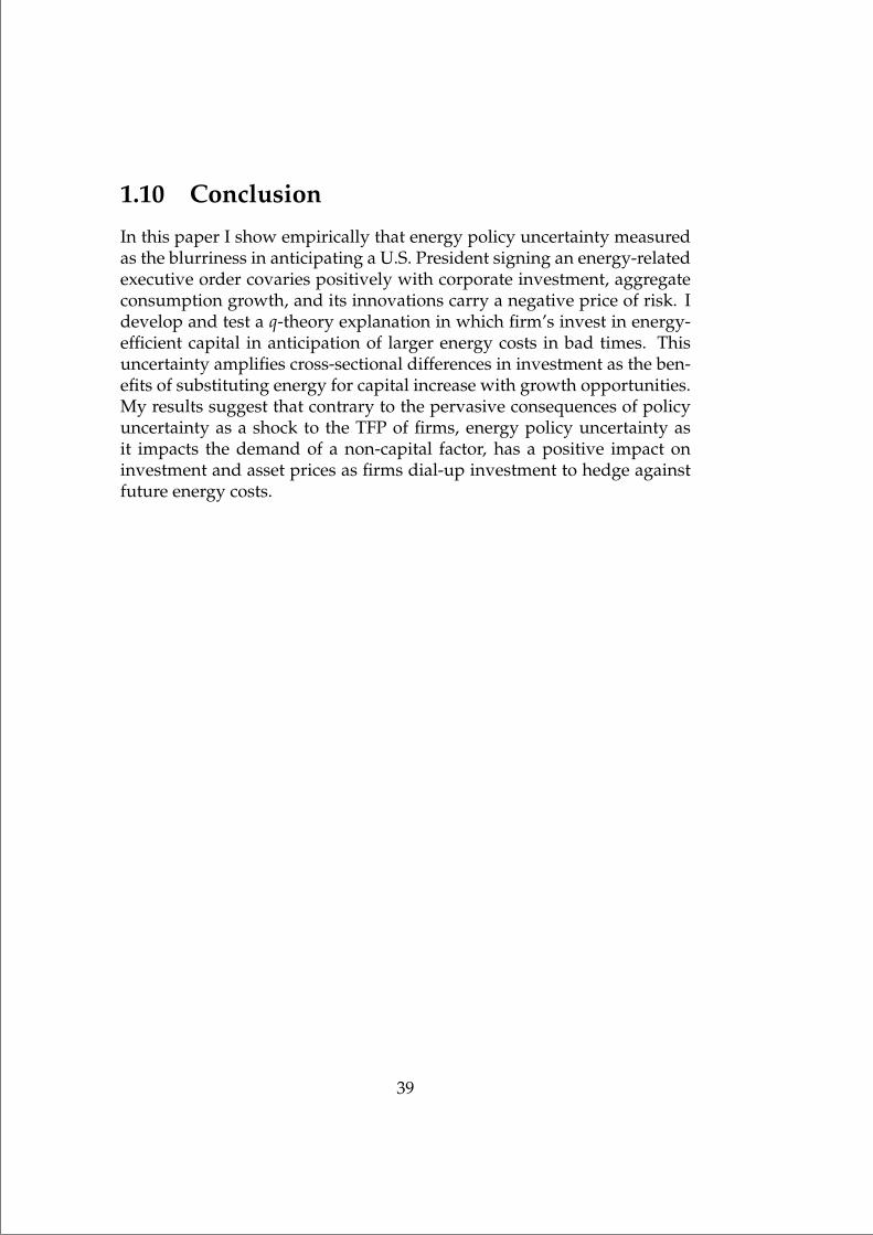
“mainupfv2” — 2021/6/1 — 20:22 — page 39 — #55

1.10 Conclusion

In this paper I show empirically that energy policy uncertainty measuredas the blurriness in anticipating a U.S. President signing an energy-relatedexecutive order covaries positively with corporate investment, aggregateconsumption growth, and its innovations carry a negative price of risk. Idevelop and test a q-theory explanation in which firm’s invest in energy-efficient capital in anticipation of larger energy costs in bad times. Thisuncertainty amplifies cross-sectional differences in investment as the ben-efits of substituting energy for capital increase with growth opportunities.My results suggest that contrary to the pervasive consequences of policyuncertainty as a shock to the TFP of firms, energy policy uncertainty asit impacts the demand of a non-capital factor, has a positive impact oninvestment and asset prices as firms dial-up investment to hedge againstfuture energy costs.

39

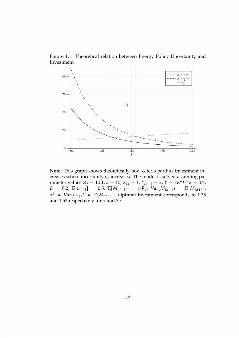
“mainupfv2” — 2021/6/1 — 20:22 — page 40 — #56

Figure 1.1: Theoretical relation between Energy Policy Uncertainty andInvestment

Note: This graph shows theoretically how ceteris paribus investment in-creases when uncertainty σe increases. The model is solved assuming pa-rameter values R f 1.01, a 10, Ki,t 1, Yi,t1 2, Y 2KαEβ α 0.7,β 0.2, Erwt1s 0.5, ErMt,t1s 1R f , VarpMt,t1q ErMt,t1s,σ2 Varpwt1q ErMt,t1s. Optimal investment corresponds to 1.35and 1.53 respectively for σ and 3σ.

40

“mainupfv2” — 2021/6/1 — 20:22 — page 41 — #57

Figure 1.2: Energy policy uncertainty between 1985m1-2018m12, com-pared with the EPU index of Baker et al. (2016)

41

“mainupfv2” — 2021/6/1 — 20:22 — page 42 — #58

Figure 1.3: Number of Energy related U.S. Executive Order signed peryear together with the most common topic inferred from its text

Table 1.1: Descriptive Statistics

(1)µ σ p1 p50 p99

Nt 0.1 0.3 0.0 0.0 2.0Yt 0.07 0.26 0.00 0.00 1.00Ut 0.36 0.05 0.26 0.35 0.50ut 0.00 0.02 -0.05 0.00 0.05Observations 468

Note: This table presents summary statistics regarding the total num-ber of energy related executive orders signed by a US president Nt(pap majortopic 8 in the Comparative Agendas database), and dummyvariable Yt that takes the value of 1 if Nt ¡ 0 and 0 otherwise. The condi-tional volatility of variable Yt captured by variable Ut, and its innovationsut defined as the residual of AR(1) process U 2

t1 φ0 φ1U 2t ut1. De-

scriptive statistics are computed from January 1980 to December 2018.

42

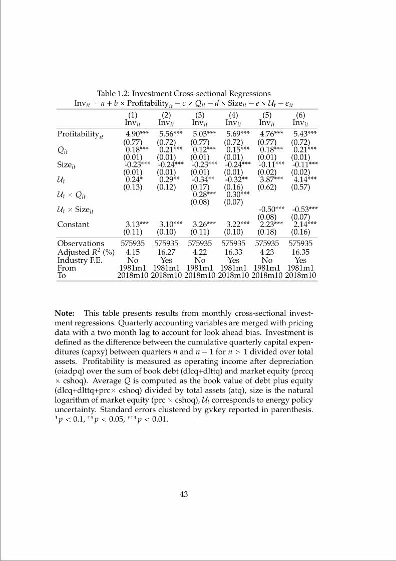
“mainupfv2” — 2021/6/1 — 20:22 — page 43 — #59

Table 1.2: Investment Cross-sectional RegressionsInvit a b Profitabilityit cQit d Sizeit e Ut εit

(1) (2) (3) (4) (5) (6)Invit Invit Invit Invit Invit Invit

Profitabilityit 4.90*** 5.56*** 5.03*** 5.69*** 4.76*** 5.43***(0.77) (0.72) (0.77) (0.72) (0.77) (0.72)

Qit 0.18*** 0.21*** 0.12*** 0.15*** 0.18*** 0.21***(0.01) (0.01) (0.01) (0.01) (0.01) (0.01)

Sizeit -0.23*** -0.24*** -0.23*** -0.24*** -0.11*** -0.11***(0.01) (0.01) (0.01) (0.01) (0.02) (0.02)

Ut 0.24* 0.29** -0.34** -0.32** 3.87*** 4.14***(0.13) (0.12) (0.17) (0.16) (0.62) (0.57)

Ut Qit 0.28*** 0.30***(0.08) (0.07)

Ut Sizeit -0.50*** -0.53***(0.08) (0.07)

Constant 3.13*** 3.10*** 3.26*** 3.22*** 2.23*** 2.14***(0.11) (0.10) (0.11) (0.10) (0.18) (0.16)

Observations 575935 575935 575935 575935 575935 575935Adjusted R2 (%) 4.15 16.27 4.22 16.33 4.23 16.35Industry F.E. No Yes No Yes No YesFrom 1981m1 1981m1 1981m1 1981m1 1981m1 1981m1To 2018m10 2018m10 2018m10 2018m10 2018m10 2018m10

Note: This table presents results from monthly cross-sectional invest-ment regressions. Quarterly accounting variables are merged with pricingdata with a two month lag to account for look ahead bias. Investment isdefined as the difference between the cumulative quarterly capital expen-ditures (capxy) between quarters n and n 1 for n ¡ 1 divided over totalassets. Profitability is measured as operating income after depreciation(oiadpq) over the sum of book debt (dlcq+dlttq) and market equity (prccq cshoq). Average Q is computed as the book value of debt plus equity(dlcq+dlttq+prc cshoq) divided by total assets (atq), size is the naturallogarithm of market equity (prc cshoq), Ut corresponds to energy policyuncertainty. Standard errors clustered by gvkey reported in parenthesis.p 0.1, p 0.05, p 0.01.

43

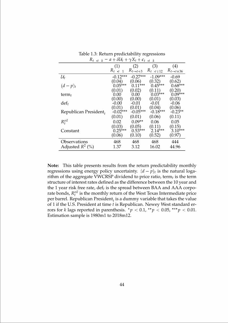
“mainupfv2” — 2021/6/1 — 20:22 — page 44 — #60

Table 1.3: Return predictability regressionsRtÑtk a δUt γXt εtÑtk

(1) (2) (3) (4)RtÑt1 RtÑt3 RtÑt12 RtÑt36

Ut -0.12*** -0.27*** -1.09*** -0.69(0.04) (0.06) (0.32) (0.62)

pd pqt 0.05*** 0.11*** 0.45*** 0.68***(0.01) (0.02) (0.11) (0.20)

termt 0.00 0.00 0.03*** 0.09***(0.00) (0.00) (0.01) (0.03)

deft -0.00 -0.01 -0.01 -0.06(0.01) (0.01) (0.04) (0.06)

Republican Presidentt -0.02*** -0.05*** -0.18*** -0.23**(0.01) (0.01) (0.06) (0.11)

Roilt 0.02 0.09** 0.06 0.05

(0.03) (0.05) (0.11) (0.15)Constant 0.25*** 0.53*** 2.14*** 3.10***

(0.06) (0.10) (0.52) (0.97)Observations 468 468 468 444Adjusted R2 (%) 1.37 3.12 16.02 44.96

Note: This table presents results from the return predictability monthlyregressions using energy policy uncertainty. pd pqt is the natural loga-rithm of the aggregate VWCRSP dividend to price ratio, termt is the termstructure of interest rates defined as the difference between the 10 year andthe 1 year risk free rate, deft is the spread between BAA and AAA corpo-rate bonds, Roil

t is the monthly return of the West Texas Intermediate priceper barrel. Republican Presidentt is a dummy variable that takes the valueof 1 if the U.S. President at time t is Republican. Newey West standard er-rors for k lags reported in parenthesis. p 0.1, p 0.05, p 0.01.Estimation sample is 1980m1 to 2018m12.

44

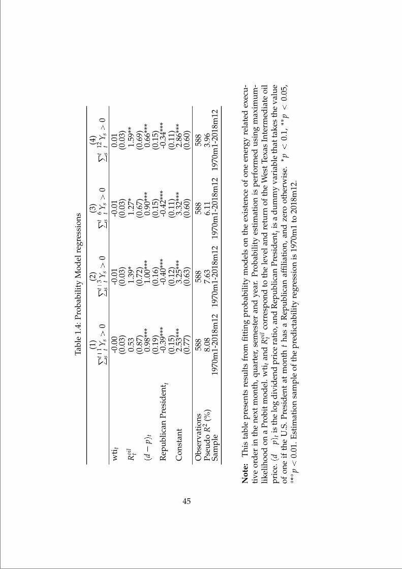
“mainupfv2” — 2021/6/1 — 20:22 — page 45 — #61

Tabl

e1.

4:Pr

obab

ility

Mod

elre

gres

sion

s

(1)

(2)

(3)

(4)

° t1 st

Y s¡

0° t3 s

tY s¡

0° t6 s

tY s¡

0° t1

2s

tY s¡

0w

tit

-0.0

0-0

.01

-0.0

10.

01(0

.03)

(0.0

3)(0

.03)

(0.0

3)R

oil

t0.

531.

39*

1.27

*1.

59**

(0.8

7)(0

.72)

(0.6

7)(0

.69)

pd

pqt

0.98

***

1.00

***

0.90

***

0.66

***

(0.1

9)(0

.16)

(0.1

5)(0

.15)

Rep

ublic

anPr

esid

ent t

-0.3

9***

-0.4

0***

-0.4

2***

-0.3

4***

(0.1

5)(0

.12)

(0.1

1)(0

.11)

Con

stan

t2.

53**

*3.

25**

*3.

32**

*2.

86**

*(0

.77)

(0.6

3)(0

.60)

(0.6

0)O

bser

vati

ons

588

588

588

588

Pseu

doR

2(%

)8.

087.

636.

113.

96Sa

mpl

e19

70m

1-20

18m

1219

70m

1-20

18m

1219

70m

1-20

18m

1219

70m

1-20

18m

12

Not

e:Th

ista

ble

pres

ents

resu

lts

from

fitti

ngpr

obab

ility

mod

els

onth

eex

iste

nce

ofon

een

ergy

rela

ted

exec

u-ti

veor

der

inth

ene

xtm

onth

,qua

rter

,sem

este

ran

dye

ar.

Prob

abili

tyes

tim

atio

nis

perf

orm

edus

ing

max

imum

-lik

elih

ood

ona

Prob

itm

odel

.wti

tan

dR

oil

tco

rres

pond

toth

ele

vela

ndre

turn

ofth

eW

estT

exas

Inte

rmed

iate

oil

pric

e.pd

pqt

isth

elo

gdi

vide

ndpr

ice

rati

o,an

dR

epub

lican

Pres

iden

t tis

adu

mm

yva

riab

leth

atta

kes

the

valu

eof

one

ifth

eU

.S.P

resi

dent

atm

onth

tha

sa

Rep

ublic

anaf

filia

tion

,and

zero

othe

rwis

e.

p

0.1,

p

0.05

,

p

0.01

.Est

imat

ion

sam

ple

ofth

epr

edic

tabi

lity

regr

essi

onis

1970

m1

to20

18m

12.

45

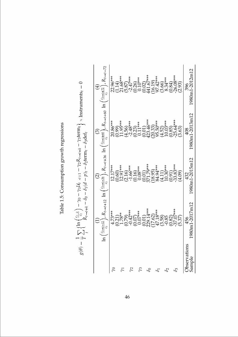
“mainupfv2” — 2021/6/1 — 20:22 — page 46 — #62

Tabl

e1.

5:C

onsu

mpt

ion

grow

thre

gres

sion

s

gpθq

1 T

¸ t

! ln c t

k

c t

γ

0

γ1U

tÑt

1

γ2R

tÑt

k

γ3t

erm

t

RtÑ

tk

δ 0

δ 1pd

pqt

δ 2te

rmt

δ 3de

f t

) In

stru

men

tst

0

(1)

(2)

(3)

(4)

ln c t

Ñt

12c t

,RtÑ

t12

ln c t

Ñt

36c t

,RtÑ

t36

ln c t

Ñt

60c t

,RtÑ

t60

ln c t

Ñt

72c t

,RtÑ

t72

γ0

4.73

***

12.1

7***

20.8

6***

22.9

6***

(0.2

1)(0

.60)

(0.9

9)(1

.14)

γ1

1.78

**12

.91*

**11

.95*

**21

.68*

**(0

.79)

(2.1

6)(4

.56)

(5.8

7)γ

2-0

.42*

**-1

.66*

**-2

.48*

**-2

.47*

**(0

.07)

(0.1

6)(0

.23)

(0.2

6)γ

30.

07**

*0.

08**

*0.

11**

*0.

10**

*(0

.01)

(0.0

1)(0

.01)

(0.0

2)δ 0

229.

14**

*37

1.79

***

423.

46**

*44

1.67

***

(17.

62)

(18.

95)

(20.

33)

(16.

19)

δ 147

.18*

**84

.94*

**95

.50*

**97

.42*

**(3

.58)

(4.1

1)(4

.52)

(3.6

6)δ 2

-0.8

510

.30*

**10

.03*

**8.

34**

*(0

.82)

(0.9

1)(0

.85)

(0.8

4)δ 3

-37.

07**

*-3

3.83

***

-25.

64**

*-2

6.08

***

(5.3

7)(4

.09)

(3.6

3)(2

.93)

Obs

erva

tion

s45

643

240

839

6Sa

mpl

e19

80m

1-20

17m

1219

80m

1-20

15m

1219

80m

1-20

13m

1219

80m

1-20

12m

12

46

“mainupfv2” — 2021/6/1 — 20:22 — page 47 — #63

Note: Parameters θ tγ0, γ1, γ2, γ3, δ0, δ1, δ2, δ3u minimize gpθq1 Igpθq andInstruments: Constant, Ut, term, d p, def. And, I is the identity ma-trix. This table presents results from the return and consumption growthpredictability regressions on energy policy uncertainty. Parameters are es-timated via GMM. RtÑtk is the cumulative log return of the VWCRSPportfolio between month t and t k. Ut is the level of energy policy un-certainty. Controls include the log dividend to price ration pd pqt, theterm structure (termt), the default spread (deft). lnpctkctq is the growthon consumption between month t and t k measured as aggregate per-sonal consumption expenses. p 0.1, p 0.05, p 0.01. Estimationsample of the predictability regression is 1980m1 to 2018m12.

47

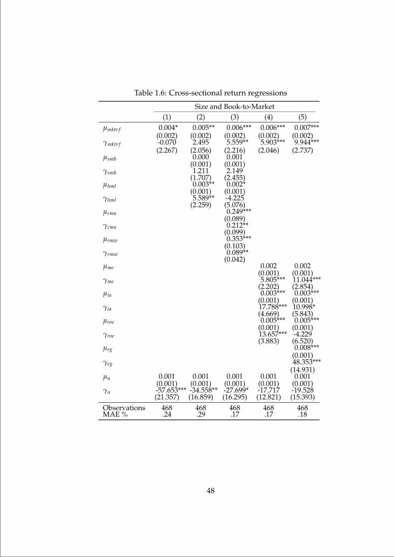
“mainupfv2” — 2021/6/1 — 20:22 — page 48 — #64

Table 1.6: Cross-sectional return regressions

Size and Book-to-Market(1) (2) (3) (4) (5)

µmktr f 0.004* 0.005** 0.006*** 0.006*** 0.007***(0.002) (0.002) (0.002) (0.002) (0.002)

γmktr f -0.070 2.495 5.559** 5.903*** 9.944***(2.267) (2.056) (2.216) (2.046) (2.737)

µsmb 0.000 0.001(0.001) (0.001)

γsmb 1.211 2.149(1.707) (2.455)

µhml 0.003** 0.002*(0.001) (0.001)

γhml 5.589** -4.225(2.259) (5.076)

µcma 0.249***(0.089)

γcma 0.212**(0.099)

µrmw 0.353***(0.103)

γrmw 0.089**(0.042)

µme 0.002 0.002(0.001) (0.001)

γme 5.805*** 11.044***(2.202) (2.854)

µia 0.003*** 0.003***(0.001) (0.001)

γia 17.788*** 10.998*(4.669) (5.843)

µroe 0.005*** 0.005***(0.001) (0.001)

γroe 13.657*** -4.229(3.883) (6.520)

µeg 0.008***(0.001)

γeg 48.353***(14.931)

µu 0.001 0.001 0.001 0.001 0.001(0.001) (0.001) (0.001) (0.001) (0.001)

γu -57.653*** -34.558** -27.699* -17.717 -19.528(21.357) (16.859) (16.295) (12.821) (15.393)

Observations 468 468 468 468 468MAE % .24 .29 .17 .17 .18

48

“mainupfv2” — 2021/6/1 — 20:22 — page 49 — #65

Note: This table presents results from estimating the price of energypolicy uncertainty in expected return - covariance form by extending theCAPM model, Fama and French three and five factor models, and theq4 and q5 models with its innovations (ut). Estimations are performedvia GMM in which factor loadings (covariances) and covariance prices ofrisk are estimated jointly. Factors smb, hml, cma, rmw, correspond to theFama and French factors related to size, book-to-market, investment andprofitability. Factors, me, ia, roe, and eg, correspond to factors related tosize, investment, profitability, and expected investment growth. p 0.1,p 0.05, p 0.01. Estimation sample of the cross-sectional regres-sion is 1980m1 to 2018m12.

49

“mainupfv2” — 2021/6/1 — 20:22 — page 50 — #66

Figure 1.4: Differences in energy policy uncertainty betas across portfoliossorted on size and book-to-market

Note: This figure provides estimates for each portfolio sorted on sizeand book-to-market of running the following time series regression Rit a b pRmt r f tq βut εt, where Rmt r f t is the excess return of theCRSP value weighted portfolio over the one month risk free rate. Portfolioreturns Rit for each quintile in the double sorting of size and book to mar-ket firms are obtained from Prof. Kenneth French’s website, me1 to me5correspond to quintiles 1 to 5 on size, and bm1 to bm5 correspond to quin-tiles1 to 5 on book to market. Estimation sample is 1980m1 to 2018m12.

50

“mainupfv2” — 2021/6/1 — 20:22 — page 51 — #67

Figure 1.5: Average impact of lobby on policy uncertainty exposure byindustry

Note: These figures present the equally weighted average by industryof the zero-lobbying exposure to energy policy uncertainty β

energyi and the

risk reduction of lobbying γi li from estimating equation Rit ai biRmt pβenergy

i γi ¯litqut εit for each firm in the sample where lit is the averagelobby expenses over lagged total assets of firm i. Estimation sample is1997m1 2018m10.

51

“mainupfv2” — 2021/6/1 — 20:22 — page 52 — #68

Table 1.7: Regressions of oil and gas betas on energy political betas

(1) (2) (3) (4) (5) (6)βoil

it βoilit βoil

it βgasit β

gasit β

gasit

βenergyit 4.72*** 4.42*** 3.90*** 0.07 -0.04 -0.06***

(0.11) (0.10) (0.08) (0.05) (0.03) (0.02)βit100 5.12 10.26* -1.79 -4.79 -2.24 -3.21

(7.85) (5.69) (4.25) (6.27) (3.80) (2.89)Leverageit 0.96* -0.13 1.54*** 0.69*** -1.91*** -3.17***

(0.50) (0.40) (0.50) (0.25) (0.17) (0.34)Constant -1.90*** -1.69*** -2.06*** 0.33*** 0.88*** 1.17***

(0.15) (0.11) (0.13) (0.09) (0.05) (0.08)Observations 404520 404520 404470 197236 197236 197219Adjusted R2 (%) 18.92 28.26 55.72 1.41 21.72 56.86Time F.E. Yes Yes Yes Yes Yes YesIndustry F.E. No Yes Yes No Yes YesFirm F.E. No No Yes No No YesFrom 1974m6 1974m6 1974m6 2002m1 2002m1 2002m1To 2018m10 2018m10 2018m10 2018m10 2018m10 2018m10

Note: This table presents results from regressing firm level gas and oilbetas on market beta, energy policy uncertainty beta and leverage. Thebeta from energy is computed using a 60 month rolling window of run-ning firm’s returns on the market return and innovations on the energypolicy uncertainty measure. Rit a bRmt βenergyut εit where Rmt isthe return on the CRSP Value Weighted Market Portfolio, and ut is theinnovation on energy policy uncertainty. Oil beta βoil is defined as theslope of regressing firm returns on the market return and the West TexasIntermediary monthly return using a 60 month rolling window. Rit a bRmt βoilRoil

t εit. Gas betas are computed using the return on themonthly Henry Hub Natural Gas Spot price Rit a bRmt βoilRgas

t εit,β is computed using daily returns within each month and is defined as thesum of coefficients β b1 b2 b3 from estimating the following regres-sion month by month: Re

is a b1Rmei,s1 b2Rme

is b3Rmei,s1 εis for

all days s within month t and Rem is the daily market excess return over the

daily risk free rate. Leverage is computed as total debt = Compustat Quar-terly items (dlcq+dlttq) over total debt plus market equity (prc cshoq).Oil and gas prices come from the Federal Reserve Economic Data at St.Louis. Clustered standard errors at the month level reported in parenthe-sis. p 0.1, p 0.05, p 0.01.

52

“mainupfv2” — 2021/6/1 — 20:22 — page 53 — #69

Announcement OPEC

-.50

.51

1.5

2En

PU B

eta

2010m1 2012m1 2014m1 2016m1 2018m1Year-Month

Figure 1.6: Differences in the average energy policy uncertainty beta be-tween oil and non oil related firms

53

“mainupfv2” — 2021/6/1 — 20:22 — page 54 — #70

Tabl

e1.

8:D

iffer

ence

-in-

Diff

eren

ces

regr

essi

ons

ofen

ergy

polic

yun

cert

aint

ybe

tas

onth

e20

14O

PEC

anno

unce

-m

ent

(1)

(2)

βen

ergy

βen

ergy

Oil

rela

ted

dum

my it

0.21

***

0.21

***

(0.0

2)(0

.02)

Aft

erO

PEC

anno

unce

men

tdum

my t

0.07

***

(0.0

1)A

fter

OPE

Can

noun

cem

entd

umm

y t

Oil

rela

ted

dum

my it

0.84

***

0.84

***

(0.0

4)(0

.04)

Con

stan

t-0

.14*

**-0

.11*

**(0

.00)

(0.0

0)O

bser

vati

ons

1030

2110

3021

Adj

uste

dR

2(%

)2.

182.

75Ti

me

F.E.

No

Yes

From

2010

m1

2010

m1

To20

18m

1020

18m

10

Not

e:Th

ista

ble

pres

ents

Clu

ster

edst

anda

rder

rors

atth

em

onth

,firm

,and

mon

th-fi

rmle

velr

epor

ted

inpa

ren-

thes

is.

p

0.1,

p

0.05

,

p

0.01

.

54

“mainupfv2” — 2021/6/1 — 20:22 — page 55 — #71

Chapter 2

Tweeting for money: Social mediaand mutual fund flows

Joint with Javier Gil-Bazo

In contrast to mandatory information disclosures, social media of-fer companies the opportunity to communicate with investors withfew constraints on frequency, content, and format. To investigate theuse of social media by asset management firms, we collect a databaseof 1.4 million Twitter posts by mutual fund families offering equityfunds in the US from 2009 to 2017 and analyze their content usingmachine learning algorithms. We find that larger and younger fam-ilies use Twitter more intensively. Investors do not respond to theamount of social media activity of a fund family but to the tone of itsposts. A one standard deviation increase in the positiveness of a fam-ily’s tweets in a given month increases its assets under managementby 15 basis points, or USD 11 million, in the following month. How-ever, tweets with a positive tone do not predict higher subsequentfund performance. These results suggest that asset managers use so-cial media to persuade investors rather than to alleviate informationasymmetries by either lowering search costs or disclosing privatelyobserved information. Consistently with this explanation, familiesfacing more difficulties in raising assets benefit the most from posi-tive posts on Twitter.

2.1 Introduction

As of April 2021, more than 4 billion people in the world, 70% of the pop-ulation aged 13 years and older, were using social media to communicate

55

“mainupfv2” — 2021/6/1 — 20:22 — page 56 — #72

with others, entertain themselves, and stay informed.1 The growing pop-ularity of social media has raised concerns about their potential to misin-form the public and manipulate individuals’ opinions and behavior (e.g.,Abramowitz, 2017; Aral and Eckles, 2019). In the context of financial mar-kets, the online activities of some high-profile individuals have promptedinvestigations by the Securities and Exchange Commission (SEC).2 If so-cial media can be used to influence investors’ perceptions, then companiesissuing securities to the public have strong incentives to become activeparticipants. In this paper we focus on the market for mutual funds andstudy whether asset managers use social media to attract money from in-vestors.

As argued by Mullainathan et al. (2008), persuasion in finance involvesexploiting investors’ biases to change their perceptions. In this sense, so-cial media is an ideal tool for persuasion for asset management firms, as itallows them to communicate with current and prospective investors with-out the strict constraints imposed by mandatory information disclosureson the timing, content, and framing of information.3 For instance, firmsmay choose to communicate only positive information. They may alsotime their communications to maximize the impact on investors’ deci-sions. And they may frame information in the most favorable way pos-sible.

Asset managers have strong incentives to use social media in order to

1Data from datareportal.com (Global Social Media Stats).2Mohamed (2021),“Big Short’ investor Michael Burry says he’ll stop tweeting after

SEC regulators paid him a visit,” Businessinsider.com, (https://markets.businessinsider.com/currencies/news/big-short-investor-michael-burry-stop-tweets-sec-regulators-visit-2021-3-1030222890); SEC (2018),“ElonMusk Charged With Securities Fraud for Misleading Tweets,” (https://www.sec.gov/news/press-release/2018-219); ; Spichak (2021), “Elon Musk Hopes SEC WillInvestigate Him over Dogecoin Tweets: ’It Would Be Awesome’,” Newsweek, (https://www.newsweek.com/elon-musk-sec-investigation-dogecoin-bitcoin-cryptocurrency-tweets-1572290).

3Note, however, that advertisement and retail investor communication by asset man-agement companies must comply with SEC rule 482 and FINRA rule 2210. In 2003, SECrule 482 modified the Securities Act of 1933-Section 5 that stated that all fund advertise-ment must have information that is contained in the statutory prospectus. With rule 482,investment companies are allowed to include information not included in the statutoryprospectus. This allows investment companies to include up-to-date information in rule-482 advertisements, such as information about current economic conditions that are notcommonly included in a fund’s prospectus. FINRA Rule 2210 governs communicationswith the public including communications with retail and institutional investors. Therule provides standards for the content, approval, recordkeeping and filing of communi-cations with FINRA. The rule prohibits false, exaggerated, unwarranted, and misleadinginformation communications, as well as projections of future performance.

56

“mainupfv2” — 2021/6/1 — 20:22 — page 57 — #73

influence investors’ perceptions and increase their assets under manage-ment. However, it is unclear whether they will succeed in this endeavor.The mutual fund market is highly regulated and abundant hard infor-mation is already available through mandatory disclosures, such as fundprospectuses and statements of additional information. Also, if investorsunderstand the ability of asset management firms to strategically selectand frame information, any attempts to influence investors could be self-defeating.

The mutual fund industry is an ideal laboratory to study the role ofsocial media communication in financial markets. First, thousands of ac-tively managed mutual funds compete for investors’ money. Second, thereis asymmetric information about managerial ability and other determi-nants of fund performance. While asset management companies can closelymonitor portfolio managers’ decisions and influence their performancethrough the allocation of resources within the firm, investors can onlylearn about funds’ future expected performance from public informationsuch as past returns and infrequently disclosed portfolio holdings. An-other important advantage of the mutual fund setting is that open-endmutual fund shares trade at their net asset value, which makes it possiblefor researchers to observe directly investors’ response to firms’ actions bylooking at flows of money into and out of mutual funds.

Twitter is also particularly appropriate for our purposes given its ris-ing popularity among investors. Indeed, a number of studies have shownevidence that Twitter activity can predict prices of stocks and other assetclasses (Bollen et al., 2011; Ranco et al., 2015; You et al., 2017; Gholam-pour and van Wincoop, 2017; Gu and Kurov, 2020). Also, the presence ofasset management firms in Twitter has grown at a very fast pace in thelast years. In our sample, the number of posts on Twitter (tweets) by allmutual fund families went from almost zero prior to 2009 to over 20,000tweets per month in 2017.

To investigate whether asset management companies influence investors’decisions through social media communications, we build a database ofTwitter posts by mutual fund families managing domestic diversified eq-uity funds in the US between January 2009 and October 2017. We thenemploy machine learning algorithms to classify tweets into positive ornegative and compute the positiveness of the tone of asset managementfirms’ tweets in a given month. Finally, we merge these data with theCRSP Survivor-Bias-Free US Mutual Fund database, which contains infor-mation on fund, manager and family characteristics.

Our results can be summarized as follows. First, 241 of 785 firms man-aging US diversified equity funds have a Twitter account and post at least

57

“mainupfv2” — 2021/6/1 — 20:22 — page 58 — #74

one tweet during our sample period. Families that use Twitter tend tomanage more assets, more funds, and funds in more investment cate-gories than families that do not use Twitter, which suggests that economiesof scale play a role in the decision to implement a social media strat-egy. Among those firms that use Twitter, more frequent users tend to beyounger and to manage more assets and funds with higher past perfor-mance, higher expenses, higher loads, and lower volatility.

We find no association between the number of tweets by a family in agiven month and flows of money to funds in that family in the followingmonth, controlling for fund performance, observable fund and fund fam-ily characteristics that have been documented to predict fund flows, andtime-invariant fund and family characteristics.

However, we find that a more positive tone in a family’s tweets in agiven month predicts significantly higher flows to the family’s funds inthe following month. The increase in flows to the family’s funds followingtweets with a positive tone is economically significant. A one standarddeviation increase in the tone of tweets is associated with an increase inassets under management of 15 basis points (bp) in the following month,or 11 USD million for the average family. This result is robust to differ-ent ways of modelling the flow-performance relationship, to controllingfor previously documented determinants of mutual fund flows, and to theinclusion of time, fund, and fund family fixed effects. To rule out the possi-bility that fund families tweet about events that are public knowledge andmay be trigger fund flows, we repeat the analysis controlling for knownevents, such as manager turnover, social media mentions by third par-ties, and the fraction of funds with very recent stellar performance in thefamily. In all cases, the association between recent tweets and fund flowssurvives.

To further investigate the mechanism through which Twitter activityinfluences fund flows, we obtain data on share purchases and share re-demptions from SEC filings, and run separate regressions for inflows andoutflows. We find that positive Twitter posts both increase inflows anddecrease outflows.

Our results are consistent with asset management firms using socialmedia to persuade investors, consistent with the theory of Mullainathanet al. (2008). However, we consider two alternative explanations for theresults documented in this paper. First, building on the work of Sirri andTufano (1998), Hortacsu and Syverson (2004), and Huang et al. (2007), as-set management companies could use social media to reduce search costsfor investors. This can be achieved by directing investors to informationabout fund offerings, fees, or past performance, that is already available

58

“mainupfv2” — 2021/6/1 — 20:22 — page 59 — #75

but difficult to locate for investors. Under this hypothesis, we would ex-pect the amount of social media activity to increase flows, since a reductionin search costs increases the number of new investors who are willing topay the cost to learn about a mutual fund and become a potential buyer.4

Our finding that the number of tweets does not predict flows does notsupport this prediction.

Second, we explore whether asset management companies use socialmedia to convey to investors information that is not available to the pub-lic. More specifically, the model of Dumitrescu and Gil-Bazo (2016) ofstrategic communication by asset managers predicts that asset manage-ment companies will communicate information that is favorable for futurefund performance and which is not already publicly available. Since thisinformation is both new and truthful, favorable communications have apositive impact on flows of new money. But the model also implies thatasset manager communications have predictive power with respect to fu-ture performance, controlling for publicly available information. To testthis prediction, we investigate whether more positive tweets predict supe-rior fund performance controlling for well-documented predictors of per-formance, including possible diseconomies of scale (Berk and Green, 2004;Chen et al., 2004; Pastor et al., 2015; Zhu, 2018). We find that the positive-ness of an asset management company’s tweets does not predict futurefund performance. This evidence contradicts the information hypothesis.

In sum, the empirical evidence documented in this paper does not sup-port the notion that social media communications of asset managementfirms alleviate information asymmetries between mutual fund companiesand investors by either reducing search costs or conveying new informa-tion to investors.

If the purpose of social media communications is to persuade investors,we would expect social media activity to benefit more those asset man-agers that experience more difficulties in attracting investors’ money. Con-sistently with this prediction, we find that the link between positive tweetsand asset growth is stronger for fund families with fewer assets undermanagement, managing fewer funds, and with lower recent flows intothe family. We also find that flows to funds that cater to retail investorsare three times more sensitive to the tone of asset managers’ posts, whichgives further credence to the persuasion hypothesis.

By unveiling the role of social media communications on mutual fund

4Of course, many investors who learn about a mutual fund may not find the funda desirable investment. However, since open-end mutual funds cannot be shorted, theimpact of lower search costs on net purchases is necessarily positive.

59

“mainupfv2” — 2021/6/1 — 20:22 — page 60 — #76

investors’ decisions, our paper contributes to a large literature on the de-terminants of mutual fund flows (see Christoffersen et al. 2014, for a sur-vey). More specifically, our paper is related to a number of studies thatinvestigate the role of advertising in the mutual fund industry. Sirri andTufano (1998) show that marketing effort, as proxied by fund fees, in-creases fund flows. Jain and Wu (2000) study a sample of 294 funds thatare advertised either in Barron’s or in Money magazine and find that eventhough the pre-advertisement performance of these funds is better thanthe performance of their benchmark, there is no superior performance inthe post-advertisement period. Cronqvist (2006) investigates the contentof mutual fund advertisements in Sweden and finds that most fund adsare not informative about fund quality. Nevertheless, fund ads influenceindividuals’ portfolio decisions, steering them towards high-fee funds, lo-cally concentrated portfolios, and funds investing in sectors with high re-cent performance. Gallaher et al. (2015) show that mutual fund families’advertising expenditures attract flows to the family’s funds as well as toother funds in the industry, reduce redemptions, and increase the convex-ity of the flow-performance relationship. We contribute to this literatureby studying a new and increasingly important means of communicationwhich, unlike traditional media advertising, allows firms to interact di-rectly and in real time with investors. Moreover, we use textual analysisand machine learning to measure the tone of communications.

Our paper is most closely related to the study of Hillert et al. (2016).These authors use textual analysis to determine the tone of sharehold-ers’ letters from asset management companies and their impact on fundflows. The authors find a positive association between tone and sub-sequent flows. Using daily information about flows for a subsample offunds, they also provide evidence that the reaction to shareholder lettersappears right after shareholder letters are sent to investors, and revertsaround five days after shareholders receive the letter. The authors alsofind evidence that funds that address their shareholders in a more per-sonal manner, have better subsequent performance on average. Althoughshareholder letters provide some freedom to managers to communicateto shareholders, they are part of the shareholder’s report (Form N-CSRand N-CSRS filings) and highly regulated by the SEC in terms of their fre-quency, format and content. Like Hillert et al. (2016), we find that fundfamilies that post more positive information receive higher net flows andexperience fewer redemptions. However, we find that the relation be-tween positiveness of tweets and flows does not revert after a few days.Moreover, we find that these communications are not informative withrespect to future fund performance.

60

“mainupfv2” — 2021/6/1 — 20:22 — page 61 — #77

Our paper also contributes more generally to the literature on non-mandatory corporate disclosures (Kim and Verrecchia, 1991; Dye and Srid-har, 2004; Dye and Sridhar, 2004; Cornelli et al., 2013; Bertomeu and Mari-novic, 2016), and to the recent literature of textual analysis in Finance andAccounting (see Loughran and McDonald, 2016 for a survey of the litera-ture). The study of Blankespoor et al. (2014) is particularly relevant to ourpaper. These authors show that when public firms use Twitter to dissem-inate firm-initiated news, information asymmetries decline as evidencedby narrower bid-ask spreads. In contrast, our results suggest that Twit-ter does not help alleviate information asymmetries in the mutual fundindustry.

2.2 Data

In this section, we present the data used in the analysis. We draw on twodatasets, the CRSP Survivor-Bias-Free US Mutual Fund database and adatabase of tweets from January 2009 to October 2017 posted by mutualfund families. From the former, we obtain information on mutual fundreturns, assets under management, investment category, and expenses.Even though our Twitter database starts in 2009, we collect mutual funddata from 2006 so we can use three years of prior historical data to estimaterisk-adjusted returns.

To construct variables at the mutual fund level, we follow the sameshare aggregation procedure as in Gil-Bazo and Ruiz-Verdu (2009). Westart with 4,124,178 observations at the share class level between January2006 and October 2017. We keep only diversified domestic equity funds(1,914,233 observations remaining), and drop passively managed funds(1,733,624 observations remaining). Total Net Assets (TNA) of a fund arethe sum of the TNA under each share class. Returns and expense ratiosare TNA-weighted averages across all share classes in the fund. The ageof the fund is the age of the oldest share class in the fund.

To create some of our variables, we aggregate data at the fund familylevel based on the CRSP identifier mgmt code. TNA at the family level isthe sum of the TNA of each fund in the family, the age of the fund familyis the age of the oldest fund in the family, and expenses and returns areweighted averages across all funds in the family (based on the TNA ofeach fund in the family).

For a subsample of funds, we obtain data on inflows and outflows,as in Christoffersen et al. (2013) and Ha and Ko (2019). These data canbe obtained from SEC’s N-SAR form, Item 28, which includes cash-flow

61

“mainupfv2” — 2021/6/1 — 20:22 — page 62 — #78

information on a monthly basis at the portfolio level.5

Given the findings of Barber et al. (2016) and Berk and van Binsbergen(2016) that investors appear to use the CAPM to evaluate mutual fundperformance, throughout the paper we focus on CAPM alphas as a deter-minant of flows, although we test the robustness of our results to using thethree-factor and four-factor models of Fama and French (1993) and Carhart(1997) to estimate performance.6 We compute the risk-adjusted return, αit,of fund i in month t as the intercept plus the residual of the CAPM model:

αit reit βitre

mt, (2.1)

where reit is the excess return of fund i at month t over the risk free rate

and remt is the excess return of the market portfolio over the risk free rate.

We obtain the monthly risk-free rate and the market portfolio return fromProf. Kenneth French’s website and βit is estimated for each fund andmonth t by running OLS rolling regressions of excess returns on marketexcesss return over the three-year period ending in month t 1. If lessthan three years of data are available in a given window, we require thefund to have at least 30 months of data and run the regressions with thedata available.

To construct the Twitter database of mutual fund families we obtain thenames of all asset management companies in the CRSP database manag-ing US equity funds. Then, we perform a manual search through each oneof the family names represented in the variable mgmt name in the CRSPdatabase and group similar names using the CRSP aggregation variablemgmt code. Finally, we search for each family’s Twitter account in theasset management company’s website.

Once the list of Twitter accounts is collected, we web scrape all tweetsfrom accounts that are active in 2017. It is important to notice that if a fundfamily that was active in the past decided to cancel its Twitter account wewould not be able to get this information. The web-scraping proceduredownloads tweets historically starting from the most recent tweet up tothe first one. Web-scraping algorithms can get banned temporarily and thedownload procedure may stop prematurely. To ensure we download allinformation, we compare the last tweet obtained for each company withthe true first tweet of the account provided by Twitter.7 Our database con-

5We thank Yeonjeong Ha and Kwangsoo Ko for kindly sharing their data with us.6Evans and Sun (2020) show that mutual fund flows have become more sensitive to

three-factor abnormal returns since Morningstar changed its methodology to computefund ratings to account for funds’ investment style.

7The first tweet of any active account was found using the webpage

62

“mainupfv2” — 2021/6/1 — 20:22 — page 63 — #79

tains 1,433,926 tweets from 362 different usernames, from January 2009 toOctober 2017.

The procedure used to measure the positiveness of tweets is explainedin detail in the Appendix and can be summarized as follows. We firstclassify tweets into two categories (financial and nonfinancial) and thendetermine the tone (positive or negative) of each tweet. To determine thetone, we use a training sample with previously manually classified tweetsand a well-known training sample of tweets provided by the University ofMichigan. Whether we use one training sample or the other depends onwhether the tweet is classified as financial or nonfinancial. The distinctionbetween financial and nonfinancial tweets is based on Loughran and Mc-Donald (2011), who argue that financial text should not be classified usingtraining samples from other social sciences since its particular context maylead to classify common jargon as negative. The Appendix provides exam-ples of tweets that have been classified as financial, nonfinancial, positiveand negative.

To avoid any subjectivity in choosing the machine learning algorithmto classify the tweets, we use six different algorithms and select for eachtweet the most voted label among them. If three algorithms classify atweet as positive and three as negative, we consider the tweet to have aneutral tone. Using this voting scheme, all tweets in our sample are classi-fied as either positive or negative. The approach also provides us with asa measure of confidence in the classification. In particular, we define theconfidence of classifying tweet k as c as:

wck

Number of algorithms that classify tweet k with label cTotal number of algorithms

(2.2)

We then define the positiveness of a family’s tweets in month t as follows:

Positivenesst ln1 Mp

t1 Mn

t

, (2.3)

where Mpt pMn

t q is the weighted count of positive (negative) tweets of thatfamily in one month:

Mpt

¸kPDptq

wpk xp

k , Mnt

¸kPDptq

wnk xn

k , (2.4)

where Dptq is a monthly time interval, xpk (xn

k ) is an indicator variable thattakes the value of 1 if tweet k at time t is positive (negative), and wp

k (wnk )

https://discover.twitter.com/first-tweet, which is no longer available, althoughother websites provide the same service.

63

“mainupfv2” — 2021/6/1 — 20:22 — page 64 — #80

is the confidence in the tweet’s positive (negative) label given the levelof agreement among all classifiers for a particular tweet as in equation(2.2). Our measure of Positiveness is closely related to that employed byAntweiler and Frank (2004), but is more appropriate for handling Twitteraccounts with zero tweets.

Figure (2.1) displays the total number of tweets across all mutual fundfamilies, as well as the weighted count of positive and negative tweets permonth. The figure shows a sharp increase in Twitter usage by mutual fundfamilies, with a peak in 2016. As expected, positive tweets predominateover tweets classified as negative.

Out of 785 fund families in the final CRSP sample, 241 fund familiestweet at least once during the sample period. This is the subsample we usein most of our analysis. To understand how this subsample differs fromthe rest, Table (2.1) presents descriptive statistics of both fund and fam-ily characteristics for the Twitter subsample and the full sample. At thefund level, there are no clear differences between funds managed by fundfamilies in the Twitter subsample an funds in the entire sample. How-ever, at the family level differences between fund families in both sam-ples become more evident. Fund families in the Twitter subsample are onaverage older, manage more assets, more funds, funds in more differentinvestment categories, and more funds that charge loads.

2.3 Determinants of Twitter activity by mutualfund families

We start our analysis by investigating which families are more likely touse Twitter. Although social media communication has low explicit costs,the implicit costs are non-trivial. Managing a social media communicationstrategy requires that social media managers coordinate with the market-ing department and senior management in the process of setting goals,creating contents, and engaging with the public. In addition, contentsneed to be created, the firm’s social media presence must be promoted,technological support is required, and the whole process must be carefullymonitored and evaluated. Since such costs are likely to have a fixed com-ponent, we expect large asset management firms to be more likely to havea social media presence and use it actively. To explore this conjecture, inaddition to the amount of assets under management to proxy for size, weuse the number of funds and the number of different categories (both inlogs) in which families offer funds. We also study whether younger firms

64

“mainupfv2” — 2021/6/1 — 20:22 — page 65 — #81

are more likely to use Twitter since younger families have more incentivesto gain visibility among investors. Finally, we control for the character-istics of funds in the family: asset-weighted average CAPM alpha overthe previous 12 months; asset-weighted average expense ratio; number offunds in the family that charge loads (in logs); and asset-weighted averagevolatility of fund returns in the previous 12 months.

We analyze both the extensive and the intensive margins of families’Twitter usage. More specifically, in our tests, we employ two differentdependent variables. The first variable, Twitter, is an indicator that equalsone if the fund family has a Twitter account and uses it at least once inour sample period. The second variable, Number of Tweets, is defined foreach family and month and is computed as the natural logarithm of 1 plusthe number of Tweets posted by the family in that month.

We start by estimating a cross-sectional linear probability model withthe Twitter indicator as the dependent variable using the full sample. Fund-level explanatory variables are first computed for each family and month.All variables are then aggregated at the family level by computing theirtime-series means within each family. Estimation results are presented inPanel A of Table (2.2). Family age is not associated with having a Twitteraccount. However, all three proxies for family size are positively and sig-nificantly associated with the family’s presence in Twitter. In other words,smaller management companies are less likely to consider Twitter as a wayof communicating with investors. There is no significant association be-tween fund characteristics and a Twitter account.

We then regress the variable Number of Tweets on the same set ofexplanatory variables as in the previous regression, but defined at thefamily-month level, and lagged one month with respect to the dependentvariable. In this case, we naturally restrict the sample to families withTwitter 1. We include family and time fixed effects and compute ro-bust standard errors clustered at the month level. Estimation results arepresented in Table (2.2). Conditional on having a Twitter account, bothyounger and larger firms tend to tweet more frequently. As for fund char-acteristics, families with better-performing funds and families with moreexpensive funds also tweet more. Return volatility, on the other hand, isnegatively associated with the intensity of Twitter activity.

These results suggest that economies of scale are a key determinant ofsocial media usage by asset managers. Conditional on having presence onTwitter, its usage appears to respond not only to cost considerations butalso to the potential benefits of social media for firms: gaining visibilityfor younger firms, publicizing good performance, and raising assets forhigh-fee funds.

65

“mainupfv2” — 2021/6/1 — 20:22 — page 66 — #82

2.4 Twitter activity and fund flows

In this section we study how flows of new money to mutual funds respondto posts of fund families on Twitter. Following the literature, we computeinflows to fund i between month t and month t 1 as the growth rate intotal net assets net of the fund’s return:

Flowsi,t1 TNAi,t1 TNAitp1 ri,t1q

TNAit, (2.5)

where TNAit is the total net assets of fund i at the end of month t, and ri,t1is the fund’s monthly return. To minimize the impact of outliers - mostlysmall funds with large percentage of inflows or outflows - we follow theliterature and winsorize flows at the 1% level.

We begin our analysis by studying how the number of tweets by anasset management firm in a given month is related to flows to funds inthat family in the following month, controlling for fund performance andother well-documented flow determinants.8 Like Sirri and Tufano (1998),we allow for a convex flow-performance relationship. To model depen-dence on performance, we employ two different approaches. First, wedefine the variable Rankit as the ranking of fund i’s CAPM alpha in the12-month period ending in month t against all other funds in the sameLipper category, normalized to be between 1N (lowest performing fund)and 1 (highest performing fund), where N denotes the number of funds inthe corresponding category and month.

Second, we use objective-adjusted abnormal return (OAR) as an al-ternative to performance rank. As argued by Ha and Ko (2019), OARaccounts for the potentially large dispersion in the cross-section of fundperformance and its impact on the flow-performance relationship. Wecompute OARit by standardizing the 12-month CAPM alpha to have zeromean and unit standard deviation across all funds in the same investmentcategory.

For both Performanceit P tRankit, OARitu, we compute the followingvariables:

Low Performanceit minpPerformanceit, p20qMid Performanceit minpPerformanceit Low Performanceit, p80 p20q

High Performanceit Performanceit Mid Performanceit Low Performanceit,(2.6)

8Henceforth, we restrict the sample to funds in fund families that have tweeted at leastonce between 2009 and October 2017.

66

“mainupfv2” — 2021/6/1 — 20:22 — page 67 — #83

where p20, p80 denote the 20th and 80th percentiles, respectively, of eitherthe cross-sectional distribution of performance rank or OAR.

We first analyze the link between the number of tweets posted by afund family and subsequent flows. More specifically, we estimate the re-gression equation:

Flowsi,t1 γ0 γ1 Number of Tweetsit

γ2 Low Performanceit γ3 Mid Performanceit

γ4 High Performanceit γ5 Xit δt1 λi µcat θ f am νi,t1,

(2.7)

where Flowsi,t1 is in %. Number of Tweetsit is the natural logarithm ofone plus the number of tweets posted by fund i’s family in month t. Low,Mid, and High Performance are calculated using both Rank and OARbased on 12-month CAPM alphas as in Equation (2.6). Following the largeliterature on the determinants of fund flows, the vector of lagged controls,Xit, includes the natural logarithm of the fund’s total net assets, the fund’sexpense ratio, the fund’s age (log of months since inception), and flowsinto the fund. Controls also include flows to funds in the same investmentcategory in month t 1 and the standard deviation of returns in the 12-month period from t 11 to t. Importantly, we control for family size (logof assets under management) and family age (age of the family’s oldestfund), since we know from the previous section that these variables areassociated with the family’s decision to use Twitter. δt1, λi, µcat, and θ f amdenote month, fund, investment category, and family fixed effects, respec-tively.9 Finally, νi,t1 denotes the error term.

We also study the relationship between flows and the tone of tweets byreplacing Number of Tweetsit in equation (2.7) with Positivenessit, whichis the value of Positivenesst for fund i’s family as defined in equation (2.3).That is, we estimate:

Flowsi,t1 γ0 γ1 Positivenessit

γ2 Low Performanceit γ3 Mid Performanceit

γ4 High Performanceit γ5 Xit δt1 λi µcat θ f am νi,t1,

(2.8)

We estimate equation (2.7) using pooled OLS and compute robust stan-dard errors clustered at the month, fund family, and month-fund familylevels.

9In our sample, some funds change investment categories through time.

67

“mainupfv2” — 2021/6/1 — 20:22 — page 68 — #84

Table (2.3) presents the results. To model dependence of flows on per-formance we use OAR in columns (1)-(3) and Rank in columns (4)-(6).

In column (1) we do not include Number of Tweets or Positiveness.As previously documented in the literature, we find a convex relation be-tween flows and performance. Fund size, flows to funds in the same cate-gory, and volatility are all negatively associated with flows. Flows are per-sistent as evidenced by the positive and significant coefficient on laggedflows. Finally, younger funds and larger families capture more flows.

In column (2), we include Number of Tweets. The estimated coefficienton this variable is small and statistically insignificant. Therefore, the in-tensity of social media communications by asset management companiesappears to be unrelated to future fund flows, controlling for observablecharacteristics as well as time-invariant fund and family characteristics.

In column (3), we replace Number of Tweets with Positiveness, as inequation (2.8). The coefficient on Positiveness is positive and statisticallysignificant at the 5% level, which suggests that flows respond to a positivetone in asset management companies’ tweets. Note that this associationcannot be driven by fund or family time-invariant characteristics that de-termine both the tone of families tweets and fund flows. It is not driveneither by larger or younger companies’ tendency to tweet more.

In columns (4) to (6), we show estimation results when we use Rank in-stead of OAR. Although the relation between flows and performance ap-pears to be more convex, consistent with the results of Ha and Ko (2019),the association between Number of Tweets and Flows and between Posi-tiveness and Flows is robust to modelling the flow-performance relation-ship in this way. In particular, the estimated coefficient on Number ofTweets is close to zero and non-significant and the estimated coefficienton Positiveness is positive and significant at the 5% level.

In unreported results, we repeat the analysis using the three-factor andfour-factor models of Fama and French (1993) and Carhart (1997), respec-tively, to compute both Rank and OAR. Our conclusions are qualitativelyand quantitatively similar.

In terms of the economic magnitude of the association, using the esti-mated coefficient of columns (3) and (6), a one standard deviation increasein Positiveness (0.78 for the Twitter subsample) corresponds to an increasein subsequent flows of 0.04% ( 0.05 0.78), which for the average fund inthe Twitter sample corresponds to an increase of USD 319,492 per month( 0.04% USD 798.73 million).

To gauge the economic impact of Twitter posts’ tone for the averagefamily, we need to estimate the marginal effect of positiveness on flowsat the family level. In Table (2.4) we estimate a version of equation (2.8)

68

“mainupfv2” — 2021/6/1 — 20:22 — page 69 — #85

where all variables are collapsed at the family-month level. In column (1)we use OAR and include time fixed effects but not family fixed effects.10

The estimated coefficient on Positivenessit is statistically significant at the1% level. A one standard deviation increase in Positivenessit is associ-ated with an increase of 0.148% (=0.19% 0.78) in family flows, whichgiven the average assets under management per family of USD 7.46 bil-lion represents an increase in assets of USD 11 million.11 In column (2),we add family fixed effects and estimate an almost identical coefficienton Positiveness, that is also statistically significant at the 1% level. There-fore, the association between Positiveness and flows to the family’s fundsis not driven by some unobservable time-invariant family characteristic.Results in columns (3) and (4) are obtained using Rank to model the flow-performance relationship and suggest a slightly stronger association be-tween Positiveness and Flows, both with and without family fixed effects.

The results of Table (2.3) and Table (2.4) are consistent with social me-dia influencing investor behavior. However, there is an alternative expla-nation for the positive association between Positiveness and fund flows. Itcould be that positive posts by asset management companies simply dis-seminate important information that is already public knowledge and thatdetermines flows of money to mutual funds. To investigate this possibility,we evaluate whether the positive link between Twitter post tone and fundflows survives the inclusion of some variables that potentially impact fundflows. More specifically, we repeat the analysis controlling for: i) a changein the previous month in the fund’s management company and the fund’sportfolio manager, which can be perceived by investors as a positive sig-nal for future returns (Khorana, 2001); ii) the number and tone of tweetsby third parties that mention the fund family in the previous month; andiii) the fraction of funds in the family with monthly CAPM alpha in the top5% of their investment category in the previous month (Nanda et al., 2004).Results in Table (2.5) indicate that the association between Positivenessand fund flows is still positive, similar in magnitude, and statistically sig-nificant at the 10% level after controlling for those performance-relevantevents. Therefore, the coefficient on Positiveness is not simply picking upthe effect of those events on fund flows.

10Naturally, the regression equation does not include fund fixed effects or investmentobjective fixed effects.

11One reason why the estimated increase in percentage flows is larger for the averagefamily than for the average individual fund is that families with fewer funds, whichare underrepresented in fund-level regressions, benefit more from positive tweets. Weexplore this possibility in Section 7.

69

“mainupfv2” — 2021/6/1 — 20:22 — page 70 — #86

2.5 Analysis of inflows and outflows

In this section we investigate whether Positiveness influences net flows byencouraging purchases of fund shares, discouraging redemptions, or both.

More specifically, we define Inflows and Outflows for fund i in montht 1 as:

Inflowsi,t1 New Salesi,t1

TNAi,t(2.9)

Outflowsi,t1 Redeemed Cashi,t1

TNAi,t(2.10)

As argued by Ha and Ko (2019) inflows and outflows are simultane-ously determined by investors’ rebalancing strategies. This mutual de-pendence between inflows and flows is tackled by performing a two-stageleast square estimation. We follow closely Ha and Ko (2019) and run thefollowing OLS regressions for inflows and outflows separately:

Inflowsi,t1 a11

s0

bsInflowsi,ts cXit νi,t1, (2.11)

Outflowsi,t1 a11

s0

bsOutflowsi,ts cXit νi,t1, (2.12)

where Xit contains the same controls used in the flow regressions.We then use the fitted values of the dependent variables Inflowst1 andOutflowst1 to estimate residual inflows and outflows:

Inflowsi,t1 a b Outflowst1 εIi,t1 (2.13)

Outflowsi,t1 a b Inflowst1 εOi,t1 (2.14)

Finally, fitted residual inflows, pεIi,t1, and outflows, pεO

i,t1, are regressed onPositiveness and performance (Rank and OAR):

pεIi,t1 γ0 γ1 Positivenesst

γ2 Low Performanceit γ3 Mid Performanceit

γ4 High Performanceit νi,t1pεOi,t1 γ0 γ1 Positivenesst

γ2 Low Performanceit γ3 Mid Performanceit

γ4 High Performanceit νi,t1

(2.15)

70

“mainupfv2” — 2021/6/1 — 20:22 — page 71 — #87

In Table (2.7), we show estimation results for inflows in columns (1)and (2). The estimated coefficients for both OAR and Rank confirm theexistence of a convex relationship between inflows and performance, con-sistent with Christoffersen et al. (2013). The coefficient on Positiveness ispositive and significant at the 1% level.

In columns (3) and (4) we show estimation results for outflows. Consis-tent with Christoffersen et al. (2013), outflows appear to be highly sensitiveto poor performance. We also find a statistically significant and negativeassociation between Positiveness and outflows. The association is similarin magnitude to that between Positiveness and fund inflows.

Therefore, social media communications appear to increase net flowsnot only by fostering purchases of new shares but also by deterring in-vestors from redeeming old shares.

2.6 Alternative hypotheses

The results presented in the previous sections are consistent with the per-suasion hypothesis of Mullainathan et al. (2008). In this section, we con-sider two alternative explanations. First, building on the work of Sirri andTufano (1998), Hortacsu and Syverson (2004), and Huang et al. (2007), as-set management companies could use social media to reduce search costsfor investors. This can be achieved by directing investors to informationabout fund offerings, fees, or past performance, that is already availablebut difficult to locate for investors. In the model of Huang et al. (2007), areduction in search costs increases expected fund flows by increasing thenumber of new investors that are willing to pay the cost to learn about amutual fund and become a potential buyer. Therefore, the search cost hy-pothesis predicts that asset management social media activity will on av-erage result in higher flows. In contrast, the results of Table (2.3) indicatethat the number of tweets does not predict flows. Moreover, our finding inTable (2.7) that positive tweets mitigate outflows is inconsistent with thesearch cost hypothesis, as investors face no search costs with respect to thefunds they already hold.

Second, we explore the notion that asset management companies usesocial media to convey to investors relevant information that is not avail-able to the public. More specifically, the model of Dumitrescu and Gil-Bazo (2016) of strategic communication by asset managers predicts thatasset management companies will communicate information that is fa-vorable for future fund performance and which is not already publiclyavailable. Since in equilibrium communications are truthful and favor-

71

“mainupfv2” — 2021/6/1 — 20:22 — page 72 — #88

able, they should have a positive impact on flows of new money. But suchcommunications should also possess predictive ability with respect to fu-ture fund performance. To test this prediction of the model, we regressone-month ahead performance on Positiveness while controlling for pastperformance and fund and family characteristics that have been docu-mented in the literature to predict performance. We also allow for time,fund, investment category, and family fixed effects. One difficulty thatarises with this test is the fact that net performance is partially determinedby investors’ reaction. In particular, if there are diseconomies of scale inasset management, fund performance will deteriorate as money flows tofunds that are expected to outperform (Berk and Green, 2004). To accountfor that possibility, we control for lagged assets under management as wellas recent fund flows.

Therefore, we estimate the regression equation:

αt1 ρ0 ρ1αi,t3:t ρ2Positivenessi,t ρ3Xit δt1 λi µcat θ f am νi,t1,(2.16)

where αi,t3:t is the fund’s abnormal return in the previous three months.δt1, λi, µcat, and θ f am denote time, fund, investment category, and familyfixed effects, respectively. Xit is a vector of control variables that includes:fund size; expense ratio; flows (in month t); portfolio turnover; 12-monthreturn volatility; an indicator variable that equals one if the fund chargesloads; fund age; family size and family age. Standard errors are clusteredat the fund, month, and fund-month levels.

Table (2.9) shows the estimation results. In columns (1) and (2) we useCAPM alphas both as the dependent variable and as a control (in this case,measured over the previous three months), whereas in columns (3) and (4)we use Carhart’s (1997) four-factor alphas. In columns (1) and (3) we donot include fund fixed effects, so we are asking whether positive tweetsallow investors to identify funds that will outperform their peers in thefollowing months.

Without fund fixed effects, the estimated coefficient on past recent per-formance is insignificant for CAPM alpha (column 1), but positive andsignificant for past four-factor alpha (column 3), which suggests that cross-sectional differences in four-factor alphas, but not in CAPM alphas, per-sist in the short term. When we include fund fixed effects (columns 2 and4), the estimated coefficient on past performance is negative and signif-icant for both measures of performance, which is consistent with meanreversion in fund performance (Carhart, 1997). Also, fund performancedeclines in with fund size both in the cross section and in the time series,

72

“mainupfv2” — 2021/6/1 — 20:22 — page 73 — #89

which is consistent with prior studies (e.g., Chen et al., 2004). Expense ra-tios are negatively related to performance in the cross-section, but not inthe time series. Finally, the family’s assets under management are nega-tively related to fund performance.

In terms of our variable of interest, Positiveness, none of the coefficientson this variable is positive, which implies that funds in families that postmore positive tweets do not outperform in the following month either inthe cross-section or in the time-series. In fact, all coefficients are negative,although insignificant with the exception of column (2), CAPM alpha withfund fixed effects, where the coefficient is significant at the 10% level. Theresults therefore do not support the idea that positive tweets help investorsselect funds that will wither outperform their peers or deliver higher per-formance than in other periods. In other words, asset management firmsdo not seem to use social media to convey private information about fu-ture fund performance.

2.7 Further evidence of social media as a persua-sion tool

If the main purpose of social media communications is not to reduce infor-mation asymmetries but to persuade investors to purchase mutual funds,then asset management firms that have more difficulties competing for in-vestors’ money in terms of objective signals of performance are the onesthat can potentially benefit the most from using social media for persua-sion purposes.

To test this conjecture, we estimate again our baseline flow regressionsaugmented with interactions of Positiveness with several variables thatare intended to proxy for asset managers’ incentives to use social mediato attract flows: Category Share, defined as the total net assets of the fundover the total net assets of all funds in the same Lipper category; % of newfunds, defined as the percentage increase in the number of funds compet-ing in the same Lipper category; Family Size, defined as the natural log-arithm of the size of the fund family; and Family Flows computed usingequation (2.5) based on the family’s total net assets and weighted averagereturns across all funds in the family;

To the extent that persuasion exploits investors’ biases, it is natural tothink that persuasion is more effective among retail investors than insti-tutional investors. To test this hypothesis, we interact Positiveness withRetail, a dummy variable that equals 1 if all share classes in the fund are

73

“mainupfv2” — 2021/6/1 — 20:22 — page 74 — #90

distributed among retail investors.Table (2.6) shows the estimation results. The coefficient on the interac-

tion between Positiveness and Category Share is negative and statisticallysignificant at the 1% significance level. A one standard deviation decreasein Category Share below its mean triples the coefficient con positivenessfrom 0.052 to 0.14. The coefficient on the interaction term of Positivenesswith the % of new funds is negative and statistically significant at the 10%level. The coefficient on the interaction term of Retail with Positivenessis positive and statistically significant at the 5% level. The magnitude ofthe estimated coefficient on this interaction term suggests that retail in-vestors are three times more sensitive to Positiveness than funds sold toinstitutional investors (the estimated effect is 0.15 for retail funds and 0.05for institutional funds). Finally, the coefficient on the interaction terms be-tween Positiveness and Family Size and Family Flows are both negativeand significant at the 1% level, consistent with the hypothesis that familiesthat have a harder time competing for investors’ money benefit the mostfrom using social media.

In sum, the results of (2.6) are consistent with persuasion being moreeffective for funds that struggle to compete and those that target retailinvestors.

2.8 Conclusions

Social media provide asset managers with a powerful tool to circumventconstraints on traditional mandatory disclosures and persuade investors.We find that a positive tone of Twitter posts predicts subsequent an in-crease in flows to the fund not explained by performance or fund charac-teristics, that is statistically and economically significant.

In contrast, we do not find that the number of tweets increases investorflows, as we would expect if asset managers were using social media tohelp investors locate relevant information. We cannot find, either, any evi-dence that the tone of Twitter communications contains valuable informa-tion about future fund performance, as one would expect if social mediawere used to convey new information to investors.

Therefore, our results suggest that asset management companies useTwitter as a way to improve investors’ perception of the quality of theirasset management services. Consistently with this hypothesis, we showthat the benefit of positive tweets concentrates in families managing fundsthat struggle to compete and those that cater to retail investors.

Clients of mutual fund management firms could benefit a great deal

74

“mainupfv2” — 2021/6/1 — 20:22 — page 75 — #91

from the enhanced, more frequent, and easier-to-access information thatsocial media can provide. Instead, the results of our paper suggest thatincentives to influence investors’ perceptions dominate incentives to alle-viate information asymmetries.

75

“mainupfv2” — 2021/6/1 — 20:22 — page 76 — #92

0

1000

0

2000

0

3000

0 2008

m1

2010

m1

2012

m1

2014

m1

2016

m1

2018

m1

Year

Mon

th

Posi

tive

Twee

tsN

egat

ive

Twee

tsAl

l Tw

eets

Figu

re2.

1:Ev

olut

ion

oftw

eets

byfu

ndfa

mili

esth

roug

hti

me.

The

figur

esh

ows

the

num

ber

oftw

eets

byfu

ndfa

mili

espe

rm

onth

.Th

eso

lidbl

ack

line

show

sth

eto

taln

umbe

rof

twee

tsob

tain

edba

sed

onth

efu

ndfa

mily

iden

tifie

rm

gmt

cdfo

rth

een

tire

CR

SPda

taba

se.

The

dot-

dash

edlin

ean

dth

eda

shed

line

repr

esen

tou

tof

the

enti

resa

mpl

eth

enu

mbe

rof

twee

tscl

assi

fied

aspo

siti

vean

dne

gati

ve,r

espe

ctiv

ely.

76

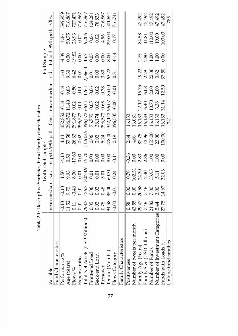
“mainupfv2” — 2021/6/1 — 20:22 — page 77 — #93

Tabl

e2.

1:D

escr

ipti

veSt

atis

tics

,Fun

dFa

mily

char

acte

rist

ics

Twit

ter

Subs

ampl

eFu

llSa

mpl

eV

aria

ble

mea

nm

edia

ns.

d.1s

tpct

l.99

thpc

tl.

Obs

.m

ean

med

ian

s.d.

1stp

ctl.

99th

pctl

.O

bs.

Fund

Cha

ract

eris

tics

Perf

orm

ance

%-0

.13

-0.1

31.

50-4

.13

4.14

352,

852

-0.1

4-0

.14

1.63

-4.3

94.

3659

9,95

9A

ge(Y

ears

)11

.52

9.75

9.93

0.50

57.5

839

6,57

211

.40

9.83

9.30

0.50

50.7

571

6,86

7Fl

ows

%0.

11-0

.46

6.30

-17.

6026

.63

391,

877

0.02

-0.5

06.

42-1

9.82

26.9

370

7,47

1Ex

pens

era

tio

0.01

0.01

0.01

0.00

0.02

396,

572

0.01

0.01

0.01

0.00

0.02

716,

867

Tota

lNet

Ass

ets

(USD

Mill

ions

)79

8.7

136.

73,

023.

915

.70

11,6

13.5

396,

572

663.

112

6.1

2,56

6.3

15.7

9,20

671

6,86

7Fr

ont-

end

Load

0.05

0.06

0.01

0.03

0.06

76,7

550.

050.

060.

010.

030.

0610

4,28

1Ba

ck-e

ndLo

ad0.

020.

020.

010.

000.

0238

,174

0.02

0.02

0.00

0.00

0.02

78,8

33Tu

rnov

er0.

780.

485.

010.

005.

2439

6,57

20.

650.

383.

800.

004.

9671

6,86

7Te

nure

(Mon

ths)

94.5

885

.00

60.3

18.

0027

8.00

342,

112

96.0

785

.00

63.2

28.

0029

5.00

501,

654

Flow

sC

ateg

ory

-0.0

0-0

.01

0.24

-0.1

40.

1939

6,53

5-0

.00

-0.0

10.

81-0

.14

0.17

716,

741

Fam

ilyC

hara

cter

isti

csPo

siti

vene

ss0.

580.

000.

78-0

.36

2.64

16,1

33N

umbe

rof

twee

tspe

rm

onth

43.5

50.

0010

2.31

0.00

468

16,0

81Fa

mily

Age

(Yea

rs)

29.4

720

.58

24.3

02.

8387

.75

16,1

3322

.12

16.7

519

.22

2.75

84.5

847

,492

Fam

ilySi

ze(U

SDBi

llion

s)7.

467.

462.

402.

8612

.96

16,1

336.

406.

082.

292.

8011

.81

47,4

92N

umbe

rof

Fund

s21

.82

7.00

33.9

51.

0015

5.00

16,1

3310

.70

2.00

22.8

61.

0011

0.00

47,4

92N

umbe

rof

Inve

stm

entC

ateg

orie

s5.

443.

005.

111.

0023

.00

16,1

333.

382.

003.

821.

0019

.00

47,4

92Fu

nds

wit

hLo

ads

%27

.75

14.6

732

.03

0.00

100.

0016

,133

31.1

412

.50

37.5

00.

0010

0.00

47,4

92U

niqu

efu

ndfa

mili

es24

178

5

77

“mainupfv2” — 2021/6/1 — 20:22 — page 78 — #94

Note: This table contains summary statistics of fund and fund family char-acteristics for two samples. The first sample, Twitter Subsample, consistsof fund families managing US equity funds that have tweeted at least oncefrom January 2009 to October 2017. The Full Sample includes all familiesmanaging US equity funds in the same period. The first set of rows showdescriptive statistics for variables computed at the fund-month level. Per-formance is the monthly CAPM alpha computed from the asset-weightedaverage return of all share classes of the fund. Age is the number of yearssince the inception of the oldest share class in the fund. Flows is the fund’smonthly growth in the fund’s total net assets net of the fund’s return. Ex-pense ratio is the asset-weighted average across all share classes of thefund, expressed in decimal units. Total Net Assets is the sum of total netassets of all share classes of the fund. Front-end and back-end loads denotethe asset-weighted average of the maximum loads across all share classes.Turnover denotes the annual turnover of the fund’s portfolio. Tenure is thenumber of months since the manager took over the fund. Flows Categorydenotes the relative flows to all the funds in the same Lipper investmentcategory as the fund in question. The second set of rows display familycharacteristics. Number of Tweets in the total number of posts on Twit-ter by the family in a given month. Positiveness is defined as in equation(2.3). Family Age is the age in years of the family’s oldest fund. FamilySize is the sum of Total Net Assets across all of the family’s funds. Num-ber of Funds is the total number of funds managed by the family. Num-ber of Investment Categories is the number of different Lipper investmentcategories to which the family’s funds belong. Funds with loads is thepercentage of funds in the family that charge either front-end or back-endload. Expense Ratio is the Asset weighted average of the expense ratios ofall funds within each fund family. Volatility is the asset weighted averageof the rolling 12 month volatility of the returns of each fund within eachfamily presented in percentage.

78

“mainupfv2” — 2021/6/1 — 20:22 — page 79 — #95

Tabl

e2.

2:D

eter

min

ants

ofTw

itte

rA

ctiv

ity

(1)

(2)

(3)

(4)

(5)

(6)

Twit

ter

Twit

ter

Twit

ter

#of

Twee

ts#

ofTw

eets

#of

Twee

ts

Fam

ilyA

ge0.

026

0.00

40.

023

-0.4

89**

*-0

.450

***

-0.4

65**

*(0

.027

)(0

.027

)(0

.026

)(0

.077

)(0

.080

)(0

.083

)Fa

mily

Size

0.06

1***

0.11

0***

(0.0

10)

(0.0

17)

Num

ber

ofFu

nds

0.15

7***

0.05

9*(0

.022

)(0

.033

)In

v.C

ateg

orie

s0.

231*

**0.

130*

*(0

.038

)(0

.050

)C

APM

alph

a1.

967*

*2.

053*

*2.

143*

*1.

338*

**1.

428*

**1.

429*

**(0

.921

)(0

.899

)(0

.901

)(0

.342

)(0

.348

)(0

.348

)Ex

pens

eR

atio

5.65

91.

949

2.71

771

.226

***

64.0

56**

*63

.864

***

(4.2

06)

(3.9

67)

(3.9

78)

(6.1

14)

(5.8

85)

(5.9

04)

Fund

sw

ith

load

s0.

035

0.05

10.

046

0.14

9*0.

156*

0.15

9**

(0.0

43)

(0.0

43)

(0.0

43)

(0.0

81)

(0.0

82)

(0.0

80)

Vola

tilit

y-2

.443

**-2

.232

*-2

.738

**-9

.649

***

-9.9

95**

*-1

0.14

3***

(1.1

88)

(1.1

79)

(1.1

89)

(1.3

20)

(1.3

91)

(1.3

89)

Obs

erva

tion

s68

768

768

715

613

1561

315

613

Adj

uste

dR

2(%

)9.

2411

.23

9.64

71.6

671

.62

71.6

3Ti

me

FEN

oN

oN

oYe

sYe

sYe

sFa

mily

FEN

oN

oN

oYe

sYe

sYe

sEs

tim

atio

nC

ross

-sec

t.C

ross

-sec

t.C

ross

-sec

t.Pa

nel

Pane

lPa

nel

Sam

ple

Full

Full

Full

Twit

ter

Twit

ter

Twit

ter

79

“mainupfv2” — 2021/6/1 — 20:22 — page 80 — #96

Note: This table shows estimation results for regressions of Twitteractivity on family characteristics. Columns (1) to (3) display results forcross-sectional regressions of a dummy variable that equals 1 if a fundfamily has tweeted at least once in our sample, on family characteristics.Columns (4) to (6) provide results of running a regression of the naturallogarithm of one plus the number of tweets (# of Tweets) posted by a fundfamily in a given month on fund family characteristics. In columns (1)to (3) explanatory variables are averaged across time for each family. Incolumns (4) to (6) the unit of observation is family-month and family char-acteristics are lagged one month. Flows to the family are calculated usingequation (2.5) with the Total Net Assets of the fund family and the asset-weighted average return of the family. Family Age is the natural logarithmof one plus the age of the oldest fund in the family in years. Family sizeis the natural logarithm of all the total net assets managed by the com-pany in USD millions. Number of Funds is the log of the number of fundsmanaged by the family. Inv. Categories denotes the log of the numberof different Lipper investment categories across all funds in the family.The CAPM alpha is the asset-weighted average 12-month CAPM alphaacross funds in the family. Expense Ratio is is the asset-weighted averageof expense ratios across funds in the family. Funds with loads denotes thepercentage of funds in the family that charge front-end or back-end loads.Volatility is the asset-weighted average of each fund’s 12-month rollingvolatility of returns. In columns (1) to (3) robust standard errors are pre-sented in parentheses, while in columns (4) to (6) robust standard errorsare clustered at the time level. *** p 0.01, ** p 0.05, *p 0.1.

80

“mainupfv2” — 2021/6/1 — 20:22 — page 81 — #97

Table 2.3: Flows and Twitter Activity

(1) (2) (3) (4) (5) (6)

Number of Tweets 0.00 0.00(0.01) (0.01)

Positiveness 0.05** 0.05**(0.02) (0.03)

Low OAR 0.47*** 0.47*** 0.47***(0.04) (0.04) (0.04)

Mid OAR 0.56*** 0.56*** 0.56***(0.03) (0.03) (0.03)

High OAR 0.96*** 0.96*** 0.96***(0.05) (0.05) (0.05)

Low Rank 3.29*** 3.29*** 3.29***(0.27) (0.27) (0.27)

Mid Rank 1.64*** 1.64*** 1.64***(0.07) (0.07) (0.07)

High Rank 8.76*** 8.77*** 8.78***(0.61) (0.61) (0.61)

Size -0.79*** -0.79*** -0.79*** -0.81*** -0.81*** -0.80***(0.04) (0.04) (0.04) (0.04) (0.04) (0.04)

Flows to the same category -0.24*** -0.24*** -0.25*** -0.04 -0.04 -0.04(0.09) (0.09) (0.09) (0.03) (0.03) (0.03)

Volatility -29.88*** -29.88*** -29.84*** -29.42*** -29.42*** -29.38***(2.47) (2.47) (2.47) (2.48) (2.48) (2.48)

Expense ratio 5.95 5.81 5.27 14.36 14.30 13.71(18.43) (18.43) (18.44) (18.54) (18.54) (18.56)

Age -1.54*** -1.54*** -1.55*** -1.57*** -1.57*** -1.57***(0.16) (0.16) (0.16) (0.16) (0.16) (0.16)

Lagged Flows 0.14*** 0.14*** 0.14*** 0.14*** 0.14*** 0.14***(0.01) (0.01) (0.01) (0.01) (0.01) (0.01)

Family Size 0.39*** 0.39*** 0.38*** 0.38*** 0.38*** 0.38***(0.07) (0.07) (0.07) (0.07) (0.07) (0.07)

Family Age -0.10 -0.10 -0.10 -0.11 -0.11 -0.11(0.11) (0.11) (0.11) (0.11) (0.11) (0.11)

Constant 9.07*** 9.06*** 9.04*** 8.36*** 8.36*** 8.33***(1.17) (1.17) (1.17) (1.17) (1.18) (1.17)

Observations 277509 277509 277509 277542 277542 277542Adjusted R2 (%) 14.82 14.82 14.82 14.68 14.68 14.68Time FE Yes Yes Yes Yes Yes YesInv. Category FE Yes Yes Yes Yes Yes YesFund FE Yes Yes Yes Yes Yes YesFund Family FE Yes Yes Yes Yes Yes Yes

81

“mainupfv2” — 2021/6/1 — 20:22 — page 82 — #98

Note: This table shows estimation results for regressions of mutual fundflows (in %) on Number of Tweets, Positiveness, and control variables.Flows are computed using equation (2.5). Number of Tweets is computedas the natural logarithm of one plus the number of tweets posted by thefund’s fund family in the previous month. Positiveness is computed in theprevious month as in equation (2.3). Low, Mid, and High Performance arecomputed using objective adjusted 12-month CAPM alphas (normalizedto have zero average and unit standard deviation across all funds withthe same Lipper class investment objective). Low, Mid, and High Ranksare computed using ranks based on the 12-month CAPM alpha of eachfund under the same Lipper class investment objective. Size is the naturallogarithm of the total net assets under management of a fund in the pre-vious month. Flows to the same category are computed as the percentageof contemporaneous net flows to all funds with the same Lipper class in-vestment objective. Volatility is the 12 month rolling volatility of returns.Expense Ratio is in decimal units. Age is the natural logarithm of the ageof the fund in months. Lagged Flows denotes one-month lagged flows tothe fund. Family size is the natural logarithm of the assets under man-agement by the fund family in the previous month, and family age is thenatural logarithm of one plus the age of the family in months. Robust stan-dard errors, clustered at the month, fund family, and month-fund familylevels, are shown in parentheses. *** p 0.01, ** p 0.05, *p 0.1.

82

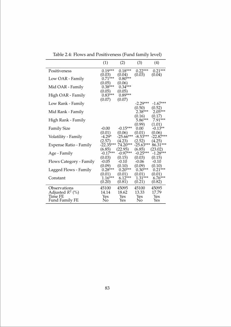
“mainupfv2” — 2021/6/1 — 20:22 — page 83 — #99

Table 2.4: Flows and Positiveness (Fund family level)

(1) (2) (3) (4)

Positiveness 0.19*** 0.18*** 0.22*** 0.21***(0.03) (0.04) (0.03) (0.04)

Low OAR - Family 0.71*** 0.80***(0.05) (0.06)

Mid OAR - Family 0.38*** 0.34***(0.05) (0.05)

High OAR - Family 0.83*** 0.89***(0.07) (0.07)

Low Rank - Family -2.29*** -1.67***(0.50) (0.52)

Mid Rank - Family 2.38*** 2.05***(0.16) (0.17)

High Rank - Family 5.86*** 7.91***(0.99) (1.01)

Family Size -0.00 -0.15*** 0.00 -0.13**(0.01) (0.06) (0.01) (0.06)

Volatility - Family -4.29* -25.66*** -8.53*** -22.87***(2.57) (4.23) (2.52) (4.25)

Expense Ratio - Family -22.35*** 74.20*** -25.63*** 86.31***(6.85) (22.95) (6.85) (23.02)

Age - Family -0.17*** -0.97*** -0.25*** -1.28***(0.03) (0.15) (0.03) (0.15)

Flows Category - Family -0.05 -0.10 -0.06 -0.10(0.09) (0.10) (0.09) (0.10)

Lagged Flows - Family 0.28*** 0.20*** 0.30*** 0.21***(0.01) (0.01) (0.01) (0.01)

Constant 1.16*** 6.12*** 1.31*** 6.76***(0.20) (0.81) (0.21) (0.82)

Observations 45100 45095 45100 45095Adjusted R2 (%) 14.14 18.62 13.33 17.79Time FE Yes Yes Yes YesFund Family FE No Yes No Yes

83

“mainupfv2” — 2021/6/1 — 20:22 — page 84 — #100

Note: This table shows estimation results for regressions of mutual fundflows (in %) on Positiveness and control variables. Flows are computed us-ing equation (2.5). Positiveness is computed in the previous month as inequation (2.3). Family-level aggregated variables are asset-weighted aver-ages across funds in the family, except for Family Size, which is the naturallogarithm of the sum of all the TNAs among the funds in the family, andFamily Age, which is the natural logarithm of one plus the age of the oldestfund in months. Low, Mid, and High Performance are computed using ob-jective adjusted 12-month CAPM alphas (normalized to have zero averageand unit standard deviation across all funds with the same Lipper class in-vestment objective). Low, Mid, and High Ranks are computed using ranksbased on the 12-month CAPM alpha of each fund under the same Lipperclass investment objective. Size is the natural logarithm of the total netassets under management of a fund in the previous month. Flows to thesame category are computed as the percentage of contemporaneous netflows to all funds with the same Lipper class investment objective. Volatil-ity is the 12 month rolling volatility of returns. Expense Ratio is in deci-mal units. Age is the natural logarithm of the age of the fund in months.Lagged Flows denotes one-month lagged flows to the fund. Family sizeis the natural logarithm of the assets under management by the fund fam-ily in the previous month, and family age is the natural logarithm of oneplus the age of the family in months. Robust standard errors, clusteredat the month, fund family, and month-fund family levels, are shown inparentheses. *** p 0.01, ** p 0.05, *p 0.1.

84

“mainupfv2” — 2021/6/1 — 20:22 — page 85 — #101

Table 2.5: Flows, Positiveness and Other Information(1) (2) (3) (4) (5)

Positiveness 0.05* 0.05* 0.05* 0.05* 0.05*(0.03) (0.03) (0.03) (0.03) (0.03)

Change Family -0.31(0.32)

Change Manager -0.36(0.65)

Number of external tweets 0.03(0.04)

External Positiveness 0.01(0.05)

Fraction of stars in Family 0.56***(0.15)

Low Rank 3.29*** 3.29*** 3.29*** 3.29*** 3.28***(0.27) (0.27) (0.27) (0.27) (0.27)

Mid Rank 1.64*** 1.64*** 1.64*** 1.64*** 1.63***(0.07) (0.07) (0.07) (0.07) (0.07)

High Rank 8.75*** 8.75*** 8.75*** 8.75*** 8.66***(0.61) (0.61) (0.61) (0.61) (0.61)

Size -0.81*** -0.81*** -0.81*** -0.81*** -0.81***(0.04) (0.04) (0.04) (0.04) (0.04)

Flows to the same category -0.04 -0.04 -0.04 -0.04 -0.04(0.03) (0.03) (0.03) (0.03) (0.03)

Volatility -28.41*** -28.41*** -28.41*** -28.42*** -28.53***(2.48) (2.48) (2.48) (2.48) (2.48)

Expense ratio 17.37 17.39 17.58 17.36 17.32(18.36) (18.36) (18.37) (18.36) (18.36)

Age -1.61*** -1.61*** -1.61*** -1.61*** -1.61***(0.16) (0.16) (0.16) (0.16) (0.16)

Lagged Flows 0.14*** 0.14*** 0.14*** 0.14*** 0.14***(0.01) (0.01) (0.01) (0.01) (0.01)

Family Size 0.39*** 0.39*** 0.39*** 0.39*** 0.40***(0.07) (0.07) (0.07) (0.07) (0.07)

Family Age -0.14 -0.14 -0.14 -0.14 -0.14(0.11) (0.11) (0.11) (0.11) (0.11)

Observations 277542 277542 277542 277542 277542Adjusted R2 (%) 14.63 14.63 14.63 14.63 14.64Time FE Yes Yes Yes Yes YesFund Family FE Yes Yes Yes Yes YesFund FE Yes Yes Yes Yes Yes

85

“mainupfv2” — 2021/6/1 — 20:22 — page 86 — #102

Note: This table shows estimation results for regressions of mutual fundflows (in %) on Positiveness, variables that capture fundamental informa-tion about the fund, and control variables. Flows are computed usingequation (2.5). Positiveness is computed in the previous month as in equa-tion (2.3). Change Family is a dummy that equals 1 if the CRSP identifiermgmt cd changes in the previous. Change Manager is a dummy that takesthe value of one if the name of the manager provided by CRSP changes inthe previous month. The number of external tweets is defined as the nat-ural logarithm of one plus the number of third-party tweets mentioningthe fund family in the previous month. External Positiveness is defined asin equation (2.3) using only third-party tweets that mention a fund fam-ily. Fraction of Star Funds is the number of funds inside the fund familythat are in the top 5 % of one-month CAPM alpha within their invest-ment objective category in the previous month, divided by the total num-ber of funds under management. Low, Mid, and High Performance arecomputed using objective adjusted 12-month CAPM alphas (normalizedto have zero average and unit standard deviation across all funds withthe same Lipper class investment objective). Low, Mid, and High Ranksare computed using ranks based on the 12-month CAPM alpha of eachfund under the same Lipper class investment objective. Size is the naturallogarithm of the total net assets under management of a fund in the pre-vious month. Flows to the same category are computed as the percentageof contemporaneous net flows to all funds with the same Lipper class in-vestment objective. Volatility is the 12 month rolling volatility of returns.Expense Ratio is in decimal units. Age is the natural logarithm of the ageof the fund in months. Lagged Flows denotes one-month lagged flows tothe fund. Family size is the natural logarithm of the assets under man-agement by the fund family in the previous month, and family age is thenatural logarithm of one plus the age of the family in months. Robust stan-dard errors, clustered at the month, fund family, and month-fund familylevels, are shown in parentheses.

86

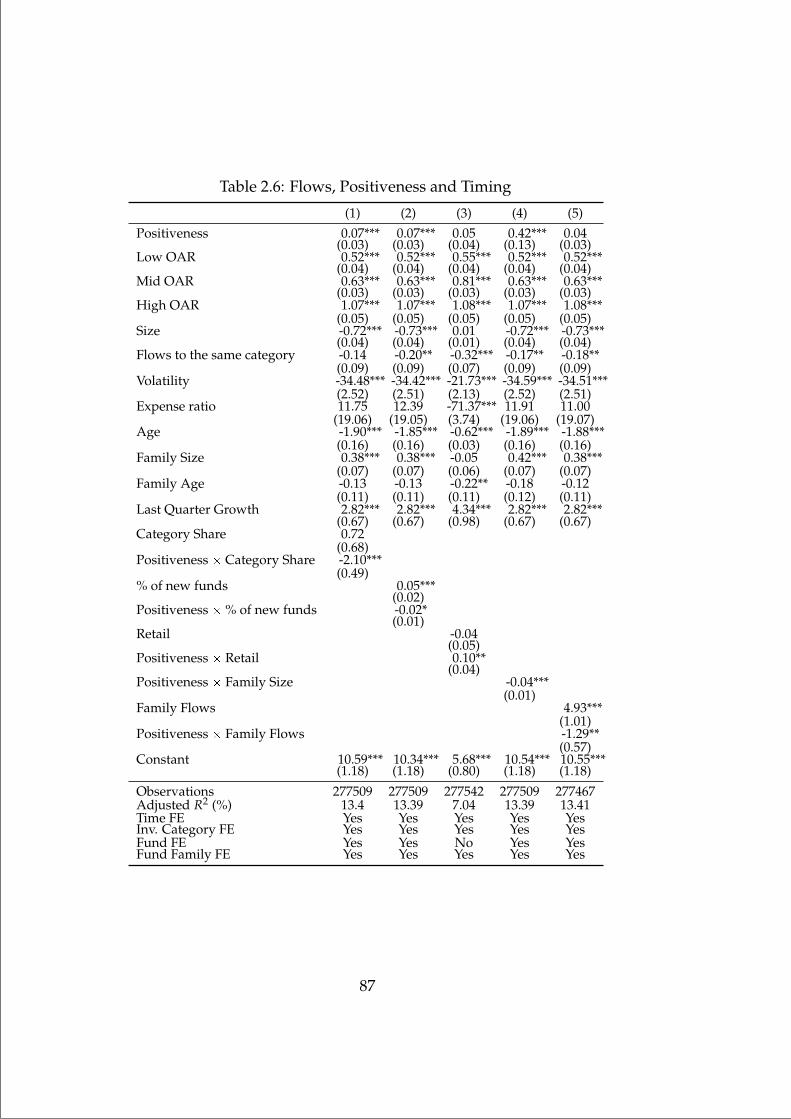
“mainupfv2” — 2021/6/1 — 20:22 — page 87 — #103

Table 2.6: Flows, Positiveness and Timing

(1) (2) (3) (4) (5)Positiveness 0.07*** 0.07*** 0.05 0.42*** 0.04

(0.03) (0.03) (0.04) (0.13) (0.03)Low OAR 0.52*** 0.52*** 0.55*** 0.52*** 0.52***

(0.04) (0.04) (0.04) (0.04) (0.04)Mid OAR 0.63*** 0.63*** 0.81*** 0.63*** 0.63***

(0.03) (0.03) (0.03) (0.03) (0.03)High OAR 1.07*** 1.07*** 1.08*** 1.07*** 1.08***

(0.05) (0.05) (0.05) (0.05) (0.05)Size -0.72*** -0.73*** 0.01 -0.72*** -0.73***

(0.04) (0.04) (0.01) (0.04) (0.04)Flows to the same category -0.14 -0.20** -0.32*** -0.17** -0.18**

(0.09) (0.09) (0.07) (0.09) (0.09)Volatility -34.48*** -34.42*** -21.73*** -34.59*** -34.51***

(2.52) (2.51) (2.13) (2.52) (2.51)Expense ratio 11.75 12.39 -71.37*** 11.91 11.00

(19.06) (19.05) (3.74) (19.06) (19.07)Age -1.90*** -1.85*** -0.62*** -1.89*** -1.88***

(0.16) (0.16) (0.03) (0.16) (0.16)Family Size 0.38*** 0.38*** -0.05 0.42*** 0.38***

(0.07) (0.07) (0.06) (0.07) (0.07)Family Age -0.13 -0.13 -0.22** -0.18 -0.12

(0.11) (0.11) (0.11) (0.12) (0.11)Last Quarter Growth 2.82*** 2.82*** 4.34*** 2.82*** 2.82***

(0.67) (0.67) (0.98) (0.67) (0.67)Category Share 0.72

(0.68)Positiveness Category Share -2.10***

(0.49)% of new funds 0.05***

(0.02)Positiveness % of new funds -0.02*

(0.01)Retail -0.04

(0.05)Positiveness Retail 0.10**

(0.04)Positiveness Family Size -0.04***

(0.01)Family Flows 4.93***

(1.01)Positiveness Family Flows -1.29**

(0.57)Constant 10.59*** 10.34*** 5.68*** 10.54*** 10.55***

(1.18) (1.18) (0.80) (1.18) (1.18)

Observations 277509 277509 277542 277509 277467Adjusted R2 (%) 13.4 13.39 7.04 13.39 13.41Time FE Yes Yes Yes Yes YesInv. Category FE Yes Yes Yes Yes YesFund FE Yes Yes No Yes YesFund Family FE Yes Yes Yes Yes Yes

87

“mainupfv2” — 2021/6/1 — 20:22 — page 88 — #104

Note: This table shows estimation results for regressions of mutual fund flows(in %) on Positiveness, variables that capture fundamental information about thefund, control variables, and variables that capture the timing of . Flows are com-puted using equation (2.5). Positiveness is computed in the previous month asin equation (2.3). Change Family is a dummy that equals 1 if the CRSP identifiermgmt cd changes in the previous. Change Manager is a dummy that takes thevalue of one if the name of the manager provided by CRSP changes in the pre-vious month. The number of external tweets is defined as the natural logarithmof one plus the number of third-party tweets mentioning the fund family in theprevious month. External Positiveness is defined as in equation (2.3) using onlythird-party tweets that mention a fund family. Fraction of Star Funds is the num-ber of funds inside the fund family that are in the top 5 % of one-month CAPMalpha within their investment objective category in the previous month, dividedby the total number of funds under management. Low, Mid, and High Perfor-mance are computed using objective adjusted 12-month CAPM alphas (normal-ized to have zero average and unit standard deviation across all funds with thesame Lipper class investment objective). Low, Mid, and High Ranks are com-puted using ranks based on the 12-month CAPM alpha of each fund under thesame Lipper class investment objective. Size is the natural logarithm of the totalnet assets under management of a fund in the previous month. Flows to the samecategory are computed as the percentage of contemporaneous net flows to allfunds with the same Lipper class investment objective. Volatility is the 12 monthrolling volatility of returns. Expense Ratio is in decimal units. Age is the naturallogarithm of the age of the fund in months. Lagged Flows denotes one-monthlagged flows to the fund. Family size is the natural logarithm of the assets undermanagement by the fund family in the previous month, and family age is the nat-ural logarithm of one plus the age of the family in months. Last Quarter growthis defined as the percentage increase of total net assets in the last three months.The market excess return is defined as the factor mktrf from Keneth French’s web-site. Category Share is defined as the total net assets of the fund over the total netassets of all funds in the same lipper category. Family share is defined as the to-tal net assets of the fund over the total net assets of the fund family. % of newfunds is defined as the percentage increase in the number of funds of the samelipper category in the sample. Robust standard errors, clustered at the month,fund family, and month-fund family levels, are shown in parentheses.

88

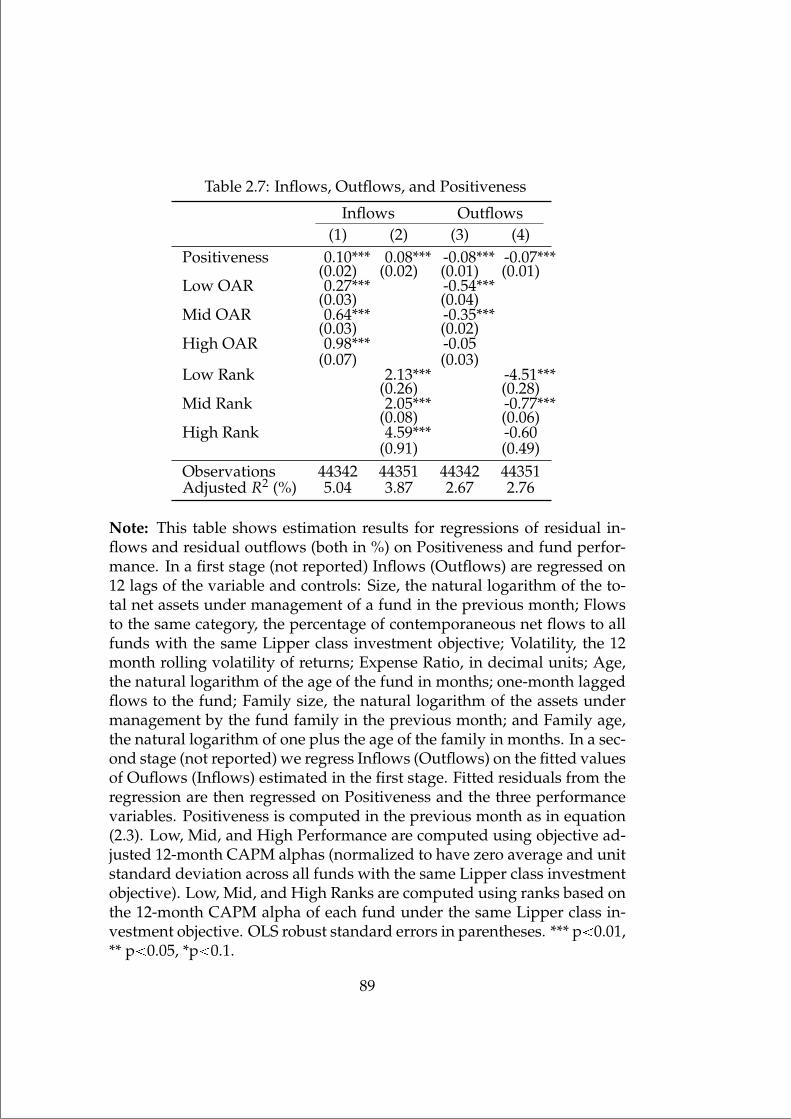
“mainupfv2” — 2021/6/1 — 20:22 — page 89 — #105

Table 2.7: Inflows, Outflows, and Positiveness

Inflows Outflows(1) (2) (3) (4)

Positiveness 0.10*** 0.08*** -0.08*** -0.07***(0.02) (0.02) (0.01) (0.01)

Low OAR 0.27*** -0.54***(0.03) (0.04)

Mid OAR 0.64*** -0.35***(0.03) (0.02)

High OAR 0.98*** -0.05(0.07) (0.03)

Low Rank 2.13*** -4.51***(0.26) (0.28)

Mid Rank 2.05*** -0.77***(0.08) (0.06)

High Rank 4.59*** -0.60(0.91) (0.49)

Observations 44342 44351 44342 44351Adjusted R2 (%) 5.04 3.87 2.67 2.76

Note: This table shows estimation results for regressions of residual in-flows and residual outflows (both in %) on Positiveness and fund perfor-mance. In a first stage (not reported) Inflows (Outflows) are regressed on12 lags of the variable and controls: Size, the natural logarithm of the to-tal net assets under management of a fund in the previous month; Flowsto the same category, the percentage of contemporaneous net flows to allfunds with the same Lipper class investment objective; Volatility, the 12month rolling volatility of returns; Expense Ratio, in decimal units; Age,the natural logarithm of the age of the fund in months; one-month laggedflows to the fund; Family size, the natural logarithm of the assets undermanagement by the fund family in the previous month; and Family age,the natural logarithm of one plus the age of the family in months. In a sec-ond stage (not reported) we regress Inflows (Outflows) on the fitted valuesof Ouflows (Inflows) estimated in the first stage. Fitted residuals from theregression are then regressed on Positiveness and the three performancevariables. Positiveness is computed in the previous month as in equation(2.3). Low, Mid, and High Performance are computed using objective ad-justed 12-month CAPM alphas (normalized to have zero average and unitstandard deviation across all funds with the same Lipper class investmentobjective). Low, Mid, and High Ranks are computed using ranks based onthe 12-month CAPM alpha of each fund under the same Lipper class in-vestment objective. OLS robust standard errors in parentheses. *** p 0.01,** p 0.05, *p 0.1.

89

“mainupfv2” — 2021/6/1 — 20:22 — page 90 — #106

Table 2.9: Predictive Regressions

(1) (2) (3) (4)αtÑt12 αtÑt36 αtÑt48 αtÑt60

Positivenesst 0.013 -0.148*** -0.258*** -0.323***(0.017) (0.034) (0.044) (0.055)

αt3Ñt -0.028*** 0.070*** 0.073*** 0.105***(0.005) (0.009) (0.011) (0.012)

Size -0.099*** -0.347*** -0.438*** -0.559***(0.010) (0.021) (0.026) (0.033)

Expense ratio -0.412*** -1.295*** -1.677*** -2.011***(0.011) (0.021) (0.026) (0.032)

Past Flows 0.017* 0.063*** 0.059** 0.008(0.010) (0.019) (0.024) (0.029)

Turnover -0.064*** -0.123*** -0.166*** -0.086**(0.010) (0.022) (0.027) (0.034)

Volatility -37.321*** -170.662*** -252.267*** -317.325***(1.714) (3.075) (3.605) (4.009)

Family Size -0.112*** -0.063* -0.143*** -0.116*(0.016) (0.035) (0.043) (0.061)

Family Age 0.040 -0.010 0.068 -0.041(0.040) (0.084) (0.111) (0.184)

Charges Loads 0.012 0.063*** 0.103*** 0.142***(0.009) (0.018) (0.022) (0.027)

Fund Age 0.014 0.023 -0.045* -0.092***(0.011) (0.021) (0.027) (0.034)

Constant -0.142* 2.490*** 5.488*** 9.227***(0.077) (0.151) (0.192) (0.238)

Observations 254375 166729 130398 98268Adjusted R2 (%) 17.99 32.36 38.29 43.02Time FE Yes Yes Yes YesInvestment Category FE Yes Yes Yes YesFund FE No No No NoFund Family FE Yes Yes Yes Yes

90

“mainupfv2” — 2021/6/1 — 20:22 — page 91 — #107

Table 2.8: Predictive Regressions

(1) (2) (3) (4)αt1 αt1 α4F

t1 α4Ft1

Positivenesst -0.008 -0.009* -0.003 -0.005(0.005) (0.005) (0.004) (0.004)

αt3:t -0.001 -0.014***(0.002) (0.002)

α4Ft3:t 0.012*** -0.005***

(0.002) (0.002)Size -0.011*** -0.176*** -0.005** -0.114***

(0.003) (0.008) (0.002) (0.006)Expense ratio -0.035*** 0.068*** -0.032*** 0.013

(0.003) (0.016) (0.002) (0.012)Lagged Flows 0.002 -0.009*** 0.008*** -0.001

(0.003) (0.003) (0.002) (0.002)Turnover 0.003 0.032*** -0.010*** 0.013***

(0.003) (0.005) (0.002) (0.004)Volatility -2.507*** 3.331*** -6.429*** -4.532***

(0.560) (0.670) (0.418) (0.488)Charges Loads 0.002 0.011 0.000 -0.024**

(0.003) (0.016) (0.002) (0.011)Fund Age 0.001 0.029** 0.002 0.029***

(0.003) (0.012) (0.002) (0.009)Family Size -0.103*** -0.100*** -0.055*** -0.053***

(0.005) (0.005) (0.003) (0.003)Family Age 0.025** 0.021* 0.023** 0.022**

(0.012) (0.012) (0.009) (0.009)Constant -0.023 -0.270*** 0.143*** 0.061***

(0.024) (0.028) (0.018) (0.021)Observations 301443 301406 301443 301406Adjusted R2 (%) 11.63 11.84 9.77 10.25Time FE Yes Yes Yes YesInvestment Category FE Yes Yes Yes YesFund FE No Yes No YesFund Family FE Yes Yes Yes Yes

91

“mainupfv2” — 2021/6/1 — 20:22 — page 92 — #108

Note: This table shows estimation results of regressions of fund’s monthlyalpha (in %) on Positiveness, past performance, and control variables.Positiveness is defined as in equation (2.3). Performance is defined intwo ways: The CAPM abnormal return compounded over the last threemonths αpt 3 : tq and the four-factor abnormal return compounded overthe last three months αpt 3 : tq. Size is the natural logarithm of the totalnet assets of the fund. The expense ratio is in decimal units. Lagged Flowsare the net flows to the fund in the previous month. Turnover is the fund’sportfolio turnover. Volatility is the 12-month rolling volatility of returns.Charges Loads is a dummy that equals 1 if the fund charges eith front-endor back-end loads. Age is the natural logarithm of the age of the fund inmonths. Family size is the natural logarithm of the total net assets of thefund family. Family Age is the natural logarithm of the age of the fam-ily in months. Robust standard errors clustered at the family, month, andfamily-month levels are presented in parentheses. *** p 0.01, ** p 0.05,*p 0.1.

92

“mainupfv2” — 2021/6/1 — 20:22 — page 93 — #109

Table 2.10: Flows, Positiveness, and Family Characteristics

(1) (2) (3) (4) (5)Positiveness 0.07*** 0.07*** 0.05 0.42*** 0.04

(0.03) (0.03) (0.04) (0.13) (0.03)Low OAR 0.52*** 0.52*** 0.55*** 0.52*** 0.52***

(0.04) (0.04) (0.04) (0.04) (0.04)Mid OAR 0.63*** 0.63*** 0.81*** 0.63*** 0.63***

(0.03) (0.03) (0.03) (0.03) (0.03)High OAR 1.07*** 1.07*** 1.08*** 1.07*** 1.08***

(0.05) (0.05) (0.05) (0.05) (0.05)Size -0.72*** -0.73*** 0.01 -0.72*** -0.73***

(0.04) (0.04) (0.01) (0.04) (0.04)Flows to the same category -0.14 -0.20** -0.32*** -0.17** -0.18**

(0.09) (0.09) (0.07) (0.09) (0.09)Volatility -34.48*** -34.42*** -21.73*** -34.59*** -34.51***

(2.52) (2.51) (2.13) (2.52) (2.51)Expense ratio 11.75 12.39 -71.37*** 11.91 11.00

(19.06) (19.05) (3.74) (19.06) (19.07)Age -1.90*** -1.85*** -0.62*** -1.89*** -1.88***

(0.16) (0.16) (0.03) (0.16) (0.16)Family Size 0.38*** 0.38*** -0.05 0.42*** 0.38***

(0.07) (0.07) (0.06) (0.07) (0.07)Family Age -0.13 -0.13 -0.22** -0.18 -0.12

(0.11) (0.11) (0.11) (0.12) (0.11)Last Quarter Growth 2.82*** 2.82*** 4.34*** 2.82*** 2.82***

(0.67) (0.67) (0.98) (0.67) (0.67)Category Share 0.72

(0.68)Positiveness Category Share -2.10***

(0.49)% of new funds 0.05***

(0.02)Positiveness % of new funds -0.02*

(0.01)Retail -0.04

(0.05)Positiveness Retail 0.10**

(0.04)Positiveness Family Size -0.04***

(0.01)Family Flows 4.93***

(1.01)Positiveness Family Flows -1.29**

(0.57)Constant 10.59*** 10.34*** 5.68*** 10.54*** 10.55***

(1.18) (1.18) (0.80) (1.18) (1.18)Observations 277509 277509 277542 277509 277467Adjusted R2 (%) 13.4 13.39 7.04 13.39 13.41Time FE Yes Yes Yes Yes YesInv. Category FE Yes Yes Yes Yes YesFund FE Yes Yes No Yes YesFund Family FE Yes Yes Yes Yes Yes

93

“mainupfv2” — 2021/6/1 — 20:22 — page 94 — #110

Note: This table shows estimation results of regressions of fund flows (in %) onPositiveness, past performance, and controls. Flows are computed using equa-tion (2.5). Positiveness is computed in the previous month as in equation (2.3).Low, Mid, and High Performance are computed using objective adjusted 12-month CAPM alphas (normalized to have zero average and unit standard de-viation across all funds with the same Lipper class investment objective). Low,Mid, and High Ranks are computed using ranks based on the 12-month CAPMalpha of each fund under the same Lipper class investment objective. Size isthe natural logarithm of the total net assets under management of a fund in theprevious month. Flows to the same category are computed as the percentage ofcontemporaneous net flows to all funds with the same Lipper class investmentobjective. Volatility is the 12 month rolling volatility of returns. Expense Ratio isin decimal units. Age is the natural logarithm of the age of the fund in months.Lagged Flows denotes one-month lagged flows to the fund. Family size is the nat-ural logarithm of the assets under management by the fund family in the previousmonth, and family age is the natural logarithm of one plus the age of the family inmonths. Number of Funds denotes the number of funds managed by the familyin the previous month (in logs). Number of Investment Categories is the numberof different investment categories to which the family’s funds belong. All fourfamily-level variables are cross-sectionally standardized. Robust standard errors,clustered at the month, fund family, and month-fund family levels, are shown inparentheses. *** p 0.01, ** p 0.05, *p 0.1.

94

“mainupfv2” — 2021/6/1 — 20:22 — page 95 — #111

Chapter 3

Learning from Quant(Qual)-itative Information

I develop a model in which mutual fund investors learn about man-agerial ability from past returns and a qualitative signal. When in-vestors observe past returns, they update their beliefs following Bayesrule, but follow a more general Pseudo-Bayesian rule after observ-ing the qualitative signal. I study how capital allocation is affectedwhen investors learn about managerial ability from the qualitativesignal and the strategic transmission of qualitative information byfund managers. My model predicts that: flows are increasing in thetone of the qualitative signal, reputation costs decrease the probabil-ity of investors verifying information, and verification costs and riskaversion decrease the probability of funds manipulating information.

3.1 Introduction

Rational investors use all relevant information to make an investment de-cision. This includes both quantitative and qualitative information. Ifqualitative information conveys relevant knowledge about the future, in-vestors should include this information when forming expectations. De-spite the theoretical relevance that qualitative information has, we do notfully understand its role in financial markets.1 I contribute to this debateby presenting a rational model in which mutual fund investors learn fromboth a qualitative and a quantitative signal about managerial ability. Ra-tional models about mutual fund investors come in different flavours, but

1Qualitative information such as: press, analyst reports, share holder letters, tweets,conference calls among many others are available for investors at a low cost.

95

“mainupfv2” — 2021/6/1 — 20:22 — page 96 — #112

most of them consider investors learning about the ability of managersto generate positive abnormal returns (managerial ability). Since the pi-oneer work of Berk and Green (2004) the theoretical literature on activemanagement studies how capital is allocated among funds as the result ofinvestors learning about managerial ability. In this literature, the learningprocess is modelled assuming bayesian-investors that update their beliefsafter observing the realization of a quantitative signal (e.g. fund returns),and invest in those funds that provide a better risk adjusted expected re-turn.

This paper will address the following questions: How do rational in-vestors learn about managerial ability when qualitative information is avail-able? What is the role of qualitative information in capital allocation? Howdo fund managers optimally transmit this information to investors? To thebest of my knowledge my model is the first to explicitly include qualitativeinformation in the theoretical debate of how mutual fund investors learnabout managerial ability, and how fund managers strategically disclosethis information.

To address these questions I borrow from the axiomatic decision makingliterature a framework called pseudo-bayesian updating (Zhao 2020). Underthis paradigm, qualitative information is modelled as a statement aboutthe likelihood of future events. Consider an investor reading news abouta fund manager winning an award, her favourite fund earning an extraMornigstar star, or an article about the growth of cheap passive invest-ments. Under this framework, the investor translates any of these state-ments into a relation of the form ”Event A is more likely than event B”.For example: ”It is more likely that the fund’s abnormal expected return(α) is above the average of the cohort of managers than below it”. If thestatement can be expressed using events that have a probability assignedinvestors update their beliefs by choosing the closest probability distribu-tion such that the qualitative statement is included in the new distribution.2

My model only includes the role of qualitative information in a friction-less environment, therefore failing to capture the convex relation betweenpast performance and net flows as documented in the literature (Sirri andTufano 1998, Chevalier and Ellison 1997).

The model assumes investors observe first the return of the fund (quan-titative signal) and after updating their beliefs following Bayes rule, theyobserve a qualitative signal and update their beliefs following the pseudo-bayesian updating rule. First I consider a variation of the friction-less modelof Berk and Green (2004) in which capital flows inelastically to funds with

2Formally the events must be measurable w.r.t. the investor’s posterior distribution.

96

“mainupfv2” — 2021/6/1 — 20:22 — page 97 — #113

positive expected abnormal returns, and there are dis-economies of scalein the fund’s technology that decrease these expected returns toward zero.I depart from Berk and Green (2004) assuming investors observe a publicqualitative signal about a fund, after observing its return. I find that fundflows react positively to the tone of the qualitative information, and theshape of the performance flow relation changes in the presence of qualita-tive information.

Next I study the investor’s capital allocation decision in a model sim-ilar to Huang et al. (2007) in which investors allocate capital to a risk freeasset and a mutual fund that provides a risky return. I study how the qual-itative signal affects the posterior distribution of investors and thereforetheir optimal capital allocation. Even though it is not possible to obtaina closed form solution of the optimal portfolio choice I derive a systemof equations that can be solved numerically to understand how capitalallocation reacts to the qualitative signal. This set-up is then extendedby explicitly modelling the strategic transmission of information by fundmanagers.

Since qualitative information is soft information, it is easy to manip-ulate by fund managers in an attempt to receive higher flows and there-fore more fees. To model this situation I develop a game in which in-vestors verify the qualitative signal issued by fund managers at a cost. Ifinvestors verify the qualitative signal and find that indeed fund managershave manipulated it, funds face a reputation cost. 3 However, if investorsprocess a signal that has been manipulated at face-value, they maximizetheir expected utility as if the signal issued by managers was the true sig-nal, leading to over-investment in the fund and a loss in expected utility.In the mixed Nash equilibrium, the probability of investors verifying thesignal is decreasing in the fund’s reputation costs and increasing in theopportunity cost, faced by managers, of not manipulating the signal. Onthe other hand, the probability of funds manipulating the qualitative sig-nal increases with the costs faced by investors when verifying the signal,and decreases with the loss of expected utility faced by investors whenthe fund managers manipulate the signal and investors interpret it at face-value.

My model contributes to the theoretical literature on the determinantsof mutual funds (see Christoffersen et al. (2014) for an empirical and the-oretical review). The theoretical literature of investors learning about mu-tual fund ability dates back to the attempt of Berk and Green (2004) to

3The reputation cost models the fact that if investors notice that a fund is manipulatinginformation they would invest less in that fund in the future.

97

“mainupfv2” — 2021/6/1 — 20:22 — page 98 — #114

reconcile two empirical observations: Flows are increasing on past perfor-mance, and performance is not persistent over time (Carhart 1997, Sirriand Tufano 1998, Chevalier and Ellison 1997, Ippolito 1992). The authorsreconcile these observations by modelling bayesian-investors that learnabout managerial ability from past returns, and dis-economies of scale. Inthis framework, funds with higher returns receive more flows since theperceived managerial ability increases, and performance is not persistentsince dis-economies of scale cause extra flows to decrease the expectedreturn to zero.

There is evidence of convexity in the performance-flow relation (Sirriand Tufano 1998, Chevalier and Ellison 1997). Money flows more to re-cent winners and it fails to escape from recent losers. This observationcan arise in rational models with the presence of market frictions. Huanget al. (2007) show how this convexity can arise when there are participa-tion costs to invest in mutual funds. In their model, new investors need topay a cost in order to learn about the prior distribution of managerial abil-ity -how the alpha of a fund is distributed- and will only pay the cost if theperceived benefit of investing is greater than the participation cost. Thisbenefit is increasing on past performance, which leads to funds with recentgood performance receiving disproportionately more flows. Lynch andMusto (2003) show that this convex relation can be the result of fund incen-tives. Funds discard those strategies that underperform. Bad performanceis less informative about future returns when funds discard these strate-gies, so flows are less sensitive to performance when they are poor. Pastorand Stambaugh (2012) model investors that learn jointly about managerialability and decreasing returns to scale. Their model extends the idea ofBerk and Green (2004) to assume investors learn about how much returnsdecrease when the size of the active management industry increases. Theauthors reconcile the observation that the size of the active managementindustry remains large despite its performance remaining poor comparedto passive strategies. Dumitrescu and Gil-Bazo (2017) show that by includ-ing market frictions in the model of Berk and Green (2004) differences inthe performance of funds are likely to persist, and those funds targeted toless sophisticated investors exhibit higher dispersion in expected perfor-mance.

The model of Dumitrescu and Gil-Bazo (2016) is the closest to my model.In their paper, the authors model investors that learn about two differentquantitative signals, the return of the fund, and a non-return signal thatcaptures everything from which an investor can learn. The main differencebetween their model and mine, is that I model the qualitative signal explic-itly, and rely on a pseudo-bayesian updating rule to incorporate this signal

98

“mainupfv2” — 2021/6/1 — 20:22 — page 99 — #115

into the investors posterior. The capital allocation results of both modelsare similar but, in my model, the presence of qualitative information cre-ates some room for its manipulation. On the contrary, in Dumitrescu andGil-Bazo (2016), fund managers can only decide whether or not to issuethe signal not whether to manipulate it. My model also contributes to theliterature on non-bayesian investors. While my model assumes rationalinvestors, the literature on behavioural non-bayesian investors is wide,covering topics like investor sentiment (Barberis et al. 1998), confirmationbias (Rabin and Schrag 1999), bounded rationality (Mullainathan 2002),law of small numbers (Rabin 2002), coarsely thinking (Mullainathan et al.2008) or local thinking (Gennaioli and Shleifer 2010) among others.The rest of the paper is organized as follows: Section 3.2.1 explains howqualitative information can be included in the learning process by investors.Section 3.2.2 extends the model of Berk and Green (2004) to understandhow qualitative information affects capital allocation in a setup in whichcapital supply is perfectly inelastic and there is perfect competition. Sec-tion 3.2.3 studies the role of qualitative information by modelling the port-folio decision of investors extending the model of Huang et al. (2007). Sec-tion 3.3 studies the strategic transmission of qualitative information byfund managers. Section 3.4 provides concluding remarks. All proofs arepresented in the appendix.

3.2 The Model

3.2.1 Preliminaries

The literature on non-bayesian updating models consider decision mak-ers (e.g. investors) that would normally use bayes rule, but deviate fromit due to some bias like temptation or bounded rationality. In this paperI use the pseudo-bayesian updating rule proposed recently by Zhao (2020)which generalizes the notion of bayesian updating to consider more gen-eral information. The main difference between the model of Zhao (2020)and models in the non-bayesian literature is the assumption of rational-ity.Even with qualitative information investors are able to behave ratio-nally just like if they were bayesian. I impose this assumption in my modelto study the effect of qualitative information in the light of standard ratio-nal models of mutual funds.

The starting point of my model comes from the axiomatic decision mak-ing literature. I borrow both the definition of a qualitative signal, and theway investors rationally learn about it. I follow Zhao (2020) who proposes

99

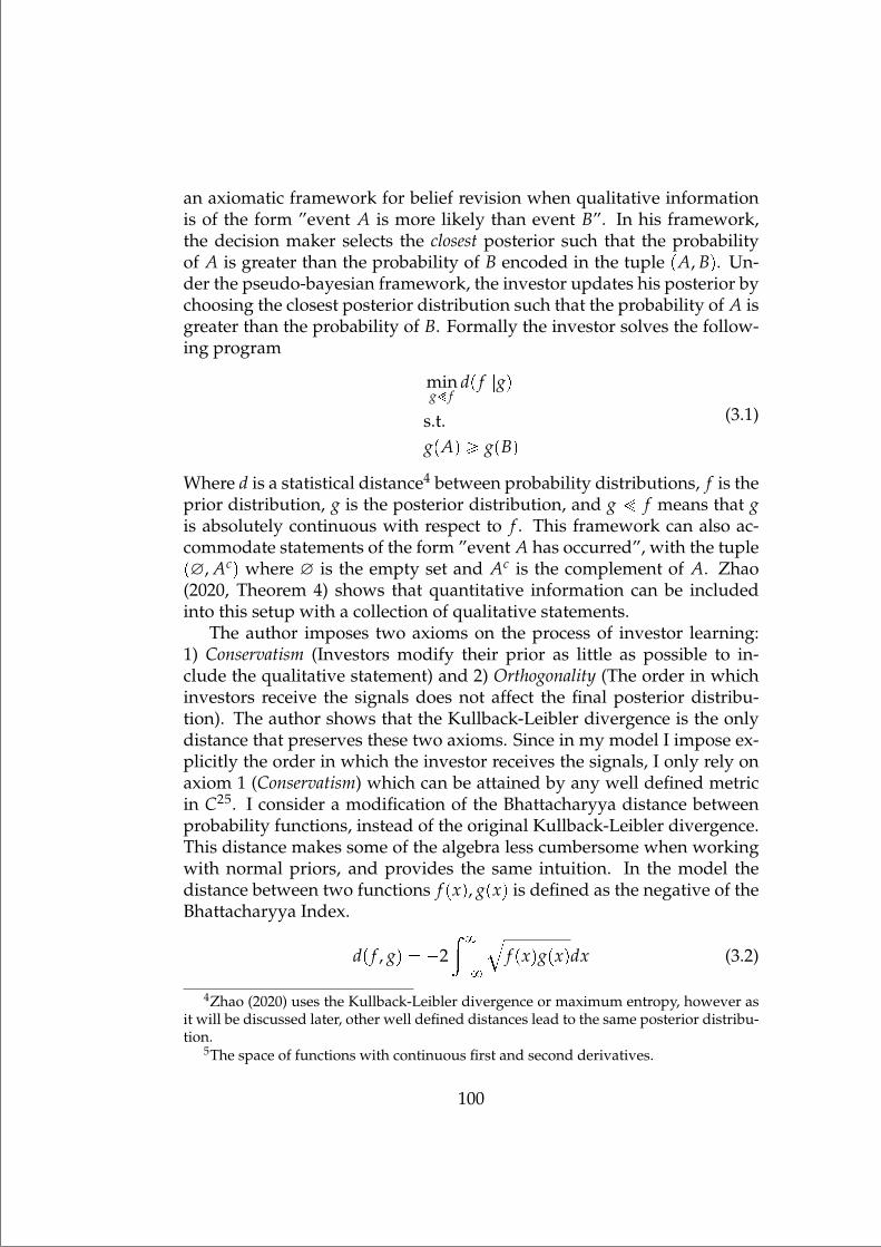
“mainupfv2” — 2021/6/1 — 20:22 — page 100 — #116

an axiomatic framework for belief revision when qualitative informationis of the form ”event A is more likely than event B”. In his framework,the decision maker selects the closest posterior such that the probabilityof A is greater than the probability of B encoded in the tuple pA, Bq. Un-der the pseudo-bayesian framework, the investor updates his posterior bychoosing the closest posterior distribution such that the probability of A isgreater than the probability of B. Formally the investor solves the follow-ing program

mingÎ f

dp f ||gq

s.t.gpAq ¥ gpBq

(3.1)

Where d is a statistical distance4 between probability distributions, f is theprior distribution, g is the posterior distribution, and g Î f means that gis absolutely continuous with respect to f . This framework can also ac-commodate statements of the form ”event A has occurred”, with the tuplep∅, Acq where ∅ is the empty set and Ac is the complement of A. Zhao(2020, Theorem 4) shows that quantitative information can be includedinto this setup with a collection of qualitative statements.

The author imposes two axioms on the process of investor learning:1) Conservatism (Investors modify their prior as little as possible to in-clude the qualitative statement) and 2) Orthogonality (The order in whichinvestors receive the signals does not affect the final posterior distribu-tion). The author shows that the Kullback-Leibler divergence is the onlydistance that preserves these two axioms. Since in my model I impose ex-plicitly the order in which the investor receives the signals, I only rely onaxiom 1 (Conservatism) which can be attained by any well defined metricin C25. I consider a modification of the Bhattacharyya distance betweenprobability functions, instead of the original Kullback-Leibler divergence.This distance makes some of the algebra less cumbersome when workingwith normal priors, and provides the same intuition. In the model thedistance between two functions f pxq, gpxq is defined as the negative of theBhattacharyya Index.

dp f , gq 2» 8

8

bf pxqgpxqdx (3.2)

4Zhao (2020) uses the Kullback-Leibler divergence or maximum entropy, however asit will be discussed later, other well defined distances lead to the same posterior distribu-tion.

5The space of functions with continuous first and second derivatives.

100

“mainupfv2” — 2021/6/1 — 20:22 — page 101 — #117

I also depart from Zhao (2020) in the way the qualitative signal is receivedby investors. In my model investors receive a signal of the form ”EventA is equally likely than event B”. If A and B are measurable events wecan find an event A1 such that PrpAq ¥ PrpBq Ñ PrpA1q PrpBq. In mymodel, given a prior p.d.f. f , the investor chooses the posterior g thatminimizes (3.2) such that GpAq GpBq where for any measurable event E,GpEq ³

E gpxqdx. Minimizing the distance between the prior and the pos-terior is consistent with Axiom 2 (Conservatism) in Zhao (2020), investorsadjust their beliefs no more than necessary to include the new informationavailable. For the rest of the paper I assume fund returns (before fees andtransaction costs) satisfy the following stochastic process:

Rt α εt (3.3)

Where α is the true managerial ability unknown by fund managers andinvestors, and εt is white noise that represents the idiosyncratic risk ofthe fund investments. Rt can be understood as the return over a bench-mark or passive portfolio with the same systematic risk. Investors have aprior distribution on α and after receiving a qualitative statement they up-date their beliefs following the pseudo-bayesian updating rule discussedabove. Given the prior distribution on α Npµ, σ2q we define the qualita-tive statement investors receive as:

Gpα ¤ αq Gpα ¡ αq (3.4)

which translates to Gpα ¤ αq 12 . The qualitative information can be seen

as a signal that moves the investor’s median value of α from µ towardsα. I model the qualitative signal in this way to measure good information(tone, sentiment) in terms of α. If f is a normal p.d.f. with mean µ and vari-ance σ2, the program investors solve after receiving the qualitative signalis:

minGPC2

2» 8

8

expt12p xµ

σ q2u?2πσ

dGdx

12 dx

s.t.

Gpαq 12

limxÑ8

Gpxq 1

limxÑ8

Gpxq 0

(3.5)

101

“mainupfv2” — 2021/6/1 — 20:22 — page 102 — #118

The objective function is the negative of the Bhattacharyya Index betweena normal prior and an unknown p.d.f. dG

dx . The first constrain says that theprobability mass on the left of the qualitative signal parameter α has to beequal to the probability mass to the right. The last two constraints ensurethat the resulting anti derivative G is a proper c.d.f.. By modelling theprogram in terms of the c.d.f. and not the p.d.f. I only impose continuityin G and not on its derivative. We will see that in this formulation theposterior p.d.f. will not be continuous to accommodate one half of theprobability mass before and after α. The following proposition states thesolution to program (3.5).

Proposition 6. The non trivial solution to program (3.5) is given by the c.d.f.

Gpxq

$'&'%

Φpxµσ q

2Φp αµσ q if x ¥ α

Φpxµσ q

2p1Φp αµσ qq if x α

(3.6)

and the p.d.f.

gpxq

$'&'%

φpxµσ q

2Φp αµσ q if x ¥ α

φpxµσ q

2p1Φp αµσ qq if x α

(3.7)

where φ and Φ are the p.d.f. and c.d.f. of a standard normal variable.

Proof. See Appendix.

Figure (3.3) shows what happens to the prior distribution after receiv-ing a good qualitative signal, and Figure (3.4) after receiving a bad quali-tative signal. We can interpret a signal being good for the fund if µ α,bad if µ ¡ α and neutral if α µ. Note that in the case in which α µ theeffect is neutral since the prior distribution remains unchanged6.

6For bayesian-updaters, any realization of the quantitative signal increases the preci-sion of their posterior distribution. In my model, neutral information does not affect theshape of the distribution.

102

“mainupfv2” — 2021/6/1 — 20:22 — page 103 — #119

ααµ α

Figure 3.1: Prior (solid) and posterior (dashed) distributions after receiv-ing a good signal about α, α ¡ µ

ααµα

Figure 3.2: Prior (solid) and posterior (dashed) distributions after receiv-ing a bad signal about α, α µ

I derive the moment generating function m.g.f. and the first two mo-ments to be used in Section (3.2.2). When working with exponential util-ities having the m.g.f. helps finding a expression for the expected utilitywithout the expectation operator (Dumitrescu and Gil-Bazo 2016,Huanget al. 2007, Huang et al. 2012). The following propositions describe the

103

“mainupfv2” — 2021/6/1 — 20:22 — page 104 — #120

main characteristics of the investor posterior.

Proposition 7. The Moment Generating Function m.g.f. of α under the posteriordistribution (3.7) is:

Ψptq exptµt σ2t2

2 u2

Φp αpµσ2tq

σ qΦp αµ

σ q 1Φp αpµσ2tqσ q

p1Φp αµσ qq

(3.8)

where Φ is the c.d.f. of a standard normal variable.

Proof. See Appendix

Proposition 8. The mean and variance of the posterior distribution are:

µ µ σθφ

2(3.9)

σ2 σ2

1 12

θφp α µ

σq 1

2θφ

(3.10)

where θφ φpαµ

σ q

1Φp αµσ q

φpαµ

σ q

Φp αµσ q

, and where φ and Φ are the p.d.f. and c.d.f. of a

standard normal variable.

Proof. See Appendix

3.2.2 Fund flows under perfect competition and inelasticcapital supply

In this section I extend the model of Berk and Green (2004) and explorethe implications when investors learn from a qualitative signal. I start bydiscussing the main assumptions of the model and the main variations Ipropose to study the effects of qualitative information on capital alloca-tion.Consider an economy that lasts for three periods t 0, 1, 2, all investorsare symmetrically informed, and funds differ on their manager’s ability togenerate abnormal returns. In order for managers to obtain positive ab-normal returns they must seek undervalued securities and trade, movingthe price against them, decreasing the return available to pay to investors.To model this situation I assume funds have a monetary cost of managingan amount qt of capital expressed by Cpqtq such that Cp0q 0, C1pqtq ¥0, and C2pqtq ¡ 0. For simplicity I assume the parametrization Cpqq aq2

as in Berk and Green (2004). Investors allocate capital to funds inelasticallyuntil the point in which the expected abnormal return is zero.

104

“mainupfv2” — 2021/6/1 — 20:22 — page 105 — #121

Let Rt α εt be the return over the benchmark that a fund gener-ates at time t 1, 2 (for simplicity I suppress the fund index for most ofthe analysis that follows). εt is normally distributed with mean zero andvariance 1ω where ω captures the precision of the quantitative signal. In-vestors begin with a prior on α which is normally distributed with meanα0 and variance 1γ, where γ is the precision of the prior distribution. Iconsider the simplest case of the model in which managers receive a fixedfee f for each dollar under management. The total payout received byinvestors at time 1 is:

TPt1 qtRt1 aq2t qt f (3.11)

Defining r1 as the abnormal return that investors receive after costs andfees

rt1 Rt1 aqt f (3.12)

Where aqt f cpqtq Cpqtqqt

f is the unit cost. At time 0 investors havea prior on the true managerial ability of fund managers, and invest anamount q0 on each fund. At time t 1 investors observe a return r1 anda qualitative signal of the form Prpα ¥ αq Prpα αq and derive theirposterior distribution first incorporating r1 following Bayes rule, and thenα following the pseudo-bayesian updating rule 7. Denote as αt EtpRtq theperceived managerial ability of a fund conditional on all information avail-able up to time t. In every period, investors allocate capital on those fundswith a positive expected abnormal return and withdraw capital from thosewith a negative expected abnormal return. In equilibrium the capital al-located to every fund makes its expected abnormal return equal to zero:

E0pr1q E1pr2q 0 (3.13)

Which implies

αt aqt f (3.14)

As the perceived managerial ability αt changes the amount of capital un-der management qt changes to ensure equation (3.14) is satisfied at allpoints in time.

7I will talk undistinguishably between investors receiving the signal Prpα ¥ αq Prpα αq and receiving the signal α.

105

“mainupfv2” — 2021/6/1 — 20:22 — page 106 — #122

Proposition 9. For any fund the evolution of α1 and the amount of capital undermanagement q1 satisfies:

α1 pα0 ω

γωr1q 1

2?

γω

φ

Jpα, r1, α0q

1Φ

Jpα, r1, α0q φ

Jpα, r1, α0q

Φ

Jpα, r1, α0q

(3.15)

q1 α1 fa

(3.16)

Where Jpα, r1, α0q ?γωpα α0 ω

γω r1q.

Using proposition (9) I express the flow of new funds F q1q0p1r1qq0

toa fund at time 1 as

F ω

aq0pγωq 1r1

φ

Jpα, r1, α0q

2aq0?

γω

11Φ

Jpα, r1, α0q

1Φ

Jpα, r1, α0q

(3.17)the following proposition tells the relation between the tone of the quali-tative information and net flows

Proposition 10. Fund flows are increasing in the tone of the qualitative signal

BFBα

¡ 0

Proof. See Appendix

The tone of a signal α depends on the realization of r1 which meanstheir analysis has to be done jointly. r1 modifies the median of the pos-terior distribution towards α0 ω

γω r1 making α good news only if α ¡α0 ω

γω r1. In this way of modelling qualitative information, the tone ofthe signal is not absolute but depends on past quantitative performance.Figure (3.3) plots the performance-flow relation for a neutral, good andbad realization of the qualitative signal. Flows are increasing in past quan-titative performance - apart from the region in which the constraint q1 ¥ 0binds - and for a given realization of r1 a good realization of the qualitativesignal increases the level of flows.

3.2.3 Optimal Portfolio Choice in the presence of qualita-tive information

Consider a three period economy t 0, 1, 2 in which investors allocate abudget between a risk free asset and a mutual fund. I normalize the return

106

“mainupfv2” — 2021/6/1 — 20:22 — page 107 — #123

on the risk free asset to be zero and at time t 1, 2 and the mutual fundproduces a risky return rt

8 following the process:

rt α εt (3.18)

The term α represents the managerial ability of the mutual fund managerto generate positive abnormal returns over a benchmark. This ability isconstant over time, and is unknown both for investors and managers. Theterm εt Np0, σ2

ε q is independently and identically distributed (i.i.d.) overtime. At time t 0 investors have a prior distribution on managerialability that is normally distributed:

α Npα0, σ20 q (3.19)

At time 1 investors observe the realized return r1 of the mutual fundand derive their posterior distribution following Bayes rule.

α Npα1, σ21 q (3.20)

where

α1 σ2ε

σ20 σ2

ε

α0 σ2

0

σ20 σ2

ε

r1, σ21

σ20 σ2

ε

σ20 σ2

ε

(3.21)

After observing the return r1 investors receive a qualitative statement asdefined in Section (1) of the form Prpα ¡ αq Prpα ¤ αq and updatetheir posterior distribution following the pseudo-bayesian updating ruledescribed in Section (1). After updating their beliefs investors solve thefollowing program

maxX1¥0

E eγW2 |r1, α

s.t.W2 W1 X1r2

(3.22)

The following proposition describes the optimal holding at t 1

Proposition 11. The optimal holding at time 1 X1 after receiving the quantita-

tive signal r1 and the qualitative signal α is given by:

X1 maxtXu

1 , 0u8In Huang et al. (2007) there are no dis-economies of scale and the return rt is given

completely to investors, that is why I choose to define the process using r and not R.

107

“mainupfv2” — 2021/6/1 — 20:22 — page 108 — #124

where Xu1 is the solution to the following system of equations which yields the

optimal holding when short sales are allowed,

φpyqΦα py α

σαqpΦα

2 ΦαΦpyqq 0

y zα Xu1 σαγ

and where zα αα1σα

, Φα 1Φpzαq

11Φpzαq

, Φα1 1

Φpzαq, Φα

2 11Φpzαq

andσ2

α pσ21 σ2

ε q.Proof. See Appendix

Since I do not have a closed-form solution I can only infer the relationbetween net-flows and the signals received by investors graphically. Fig-ure (3.4) plots the performance-flow relation for a neutral, good and badrealization of the qualitative signal. Flows are increasing in past quantita-tive performance - apart from the region in which the constraint X1 ¥ 0binds - and for a given realization of r1 a good realization of the qualita-tive signal increases the level of flows. The results are similar to the onesobtained in the more simpler framework of section 3.2.2, however the re-sults in this section will let us understand the strategic transmission ofinformation described in the next section.

3.3 Strategic transmission of qualitative informa-tion

It is possible to manipulate qualitative information to make it look moreappealing for investors. Empirical research in textual analysis has shownthat managers tend to disclose negative information by making it morecomplex to read -an issue concerning the readability of financial information-in an attempt to make the bad information look better (See e.g. Li (2008),Loughran and McDonald (2014)). In this section I analyze the strategicdisclosure of qualitative information by the fund managers. Consider riskneutral managers that are willing to maximize fund flows into the fund.Define as Fpr1, αq the flows to the fund after investors observe the returnr1 and the qualitative signal α at time 1. From subsection (3.2.2) and (3.2.3)we know that Fr1 ¡ 0 and Fα ¡ 0. On the other hand consider an investormaximizing expected utility as in subsection (3.2.2), we can rewrite themaximum expected utility of program 3.22 as:

EUpW2pXpr1, αqq, r1, αq E exptγW2pXpr1, αqqu

r1, α

(3.23)

108

“mainupfv2” — 2021/6/1 — 20:22 — page 109 — #125

Where Xpr1, αq is the solution to program 3.22, and W2pXpr1, αqq is theterminal wealth after investing Xpr1, αq in the fund. Since Xpr1, αq maxi-mizes program 3.22 for any α α

EUpW2pXpr1, αqq, r1, αq ¡ EUpW2pXpr1, αqq, r1, αq (3.24)

In particular imagine the situation in which a fund, having the control ontransmitting the information to investors, transmits a signal α ∆ whenthe true signal is α. Investors will maximize program (3.22) assuming thequalitative signal is the one issued by the fund managers. Figure (3.5)shows the loss in expected utility that investors face if take the signal thatthe managers issue at face value. In this case investors maximize a fakeutility function, leading to a sub-optimal capital allocation. In the nextsection I study the case in which investors can decide to verify the signalthat funds transmit at a cost, and a reputation cost for fund managers incase they are caught manipulating the signal.

3.3.1 The game

The quantitative signal r1 is public knowledge among the investors andthe fund managers while the qualitative signal α is first observed by thefund manager and then transmitted to investors. My game is similar to theone in Dumitrescu and Gil-Bazo (2016) but instead of the manager decid-ing whether or not to censor the qualitative signal, I assume that the fundcan modify the signal to make it look more appealing to investors - thiscaptures the idea of making bad information more complex for investorsto understand. The fund manager transmits a signal α ∆ where ∆ ¡ 0since Fα. Investors can either take this signal at face-value and risk makingan investment decision based on incorrect information, or verify the signalfrom some other source at a cost C 9. I assume that the cost of verifying islow enough such that if the investor is sure that the manager is lying aboutthe qualitative signal she will decide always to verify the information. Ifthe manager is in fact lying and the investor verifies the information, thefund manager will suffer a reputation cost K that is assumed to be fixed.When the investor decides to trust the manager and not verify the infor-mation, if the manager manipulates the signal, the expected utility of theinvestor will be below optimal since the investor will behave as if α ∆was the true qualitative signal therefore investing too much in the fund

9Investors can verify the signal by looking at the financial press, analyst reports, rat-ings, etc

109

“mainupfv2” — 2021/6/1 — 20:22 — page 110 — #126

(Xpr1, α ∆q ¡ Xpr1, αq). The following table presents the game and thebest responses of the players:

InvestorBelieve Suspect

Fund manager α ∆ Fpr1, α ∆q Fpr1, αq KEUpW2pXpr1, α ∆qq, r1, αq EUpW2pXpr1, αqq C, r1, αq

α Fpr1, αq Fpr1, αqEUpW2pXpr1, αqq, r1, αq EUpW2pXpr1, αqq C, r1, αq

Assuming that the cost of verifying C is small C C where C is thesolution to EUpW2pXpr1, α∆qq, r1, αq EUpW2pXpr1, αqq C, r1, αq. Sincethere are no Nash equilibria in pure strategies I proceed to find it in mixedstrategies.

Proposition 12. Nash Equilibrium: The unique Nash equilibrium of the abovegame is given by the mixed strategies:#

α ∆ with probability pα with probability 1-p

where

p EUpW2pXpr1, αqq, r1, αq EUpW2pXpr1, αqq C, r1, αqEUpW2pXpr1, αqq, r1, αq EUpW2pXpr1, α ∆qq, r1, αq

for the fund manager, and#Believe with probability qSuspect with probability 1 q

for the investor, where

q KFpr1, α ∆q Fpr, αq K

Proof. See Appendix

The mixed strategy gives us an idea of the distribution of funds thatwill lie in equilibrium, to understand how this proportion changes withrespect of the parameters of the model we can derive the following com-parative statistics.

Proposition 13. The first order comparative statistics of the Nash equilibriumare:

110

“mainupfv2” — 2021/6/1 — 20:22 — page 111 — #127

• The fraction of investors that believe on what fund managers transmit in-creases with the reputation costs that fund managers have if caught manip-ulating information

BqBK

¡ 0

• The fraction of funds that manipulate information increases with the verifi-cation cost by investors:

BpBC

¡ 0

• If flows are strictly convex on the qualitative signal B2FBα2 ¡ 0 the higher the

qualitative signal the more investors will suspect of the signal and verify.

BqBα

0

• The more fund managers can manipulate the signal, the more investors willsuspect and verify it.

BqB∆

0

Figure (3.6) shows how the probabilities of a fund manipulating infor-mation p and of an investor verifying the information q change with theperformance of fund r1. First we observe that there exists a threshold valuer such that if the return of the fund is larger, the fraction of investors thatverify the signal increases dramatically. This is due to the fact that afterthis threshold the benefit of investors verifying the information is greaterthan the cost of verifying. My model predicts that if past performanceis good enough (above threshold r) every investor will verify the signalsince managers will have an extra incentive to manipulate the information.We can observe from the plots of (p) for different levels of the qualitativesignal, that when past performance is good enough, good information ismore likely to be manipulated than bad information. My model suggeststhat the behaviour described in Li (2008) and Loughran and McDonald(2014) in which firms manipulate textual information, should be strongeramong those funds that perform better instead of the worst performingones.

3.4 Conclusion

I develop a theoretical model of mutual fund investors that explicitly mod-els qualitative information in the optimal portfolio decision of investors.

111

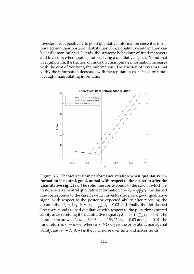
“mainupfv2” — 2021/6/1 — 20:22 — page 112 — #128

Investors react positively to good qualitative information since it is incor-porated into their posterior distribution. Since qualitative information canbe easily manipulated, I study the strategic behaviour of fund managersand investors when issuing and receiving a qualitative signal. ”I find thatin equilibrium, the fraction of funds that manipulate information increaseswith the cost of verifying the information. The fraction of investors thatverify the information decreases with the reputation costs faced by fundsif caught manipulating information.

-0.4 -0.2 0 0.2 0.4 0.6

-1

0

1

2

3

4

5

Flo

w

Theoretical flow-performance relation

Figure 3.3: Theoretical flow performance relation when qualitative in-formation is neutral, good, or bad with respect to the posterior after thequantitative signal r1. The solid line corresponds to the case in which in-vestors receive neutral qualitative information α α0 ω

γω r1, the dashedline corresponds to the case in which investors receive a good qualitativesignal with respect to the posterior expected ability after receiving thequantitative signal r1, α α0 ω

γω r1 0.02 and finally the dot-dashedline corresponds to bad qualitative with respect to the posterior expectedability after receiving the quantitative signal r1 α α0 ω

γω r1 0.02. Theparameters are a 1, ω 39.06, γ 156.25, α0 0.03 and f 0.01.Thefund return is r1 α ε1 where α Npα0, 1

γq is the prior about managerialability, and ε1 Np0, 1

ω q is the i.i.d. noise over time and across funds.

112

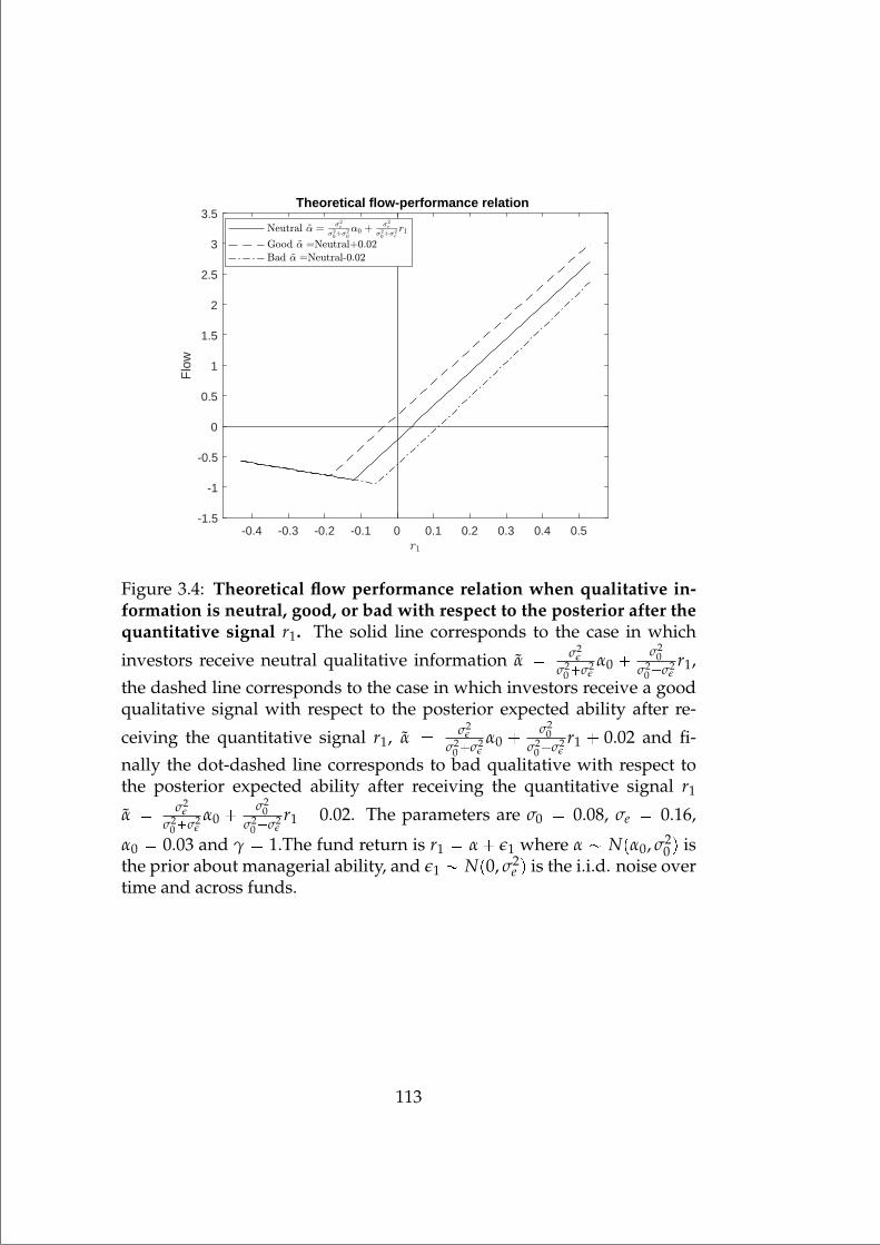
“mainupfv2” — 2021/6/1 — 20:22 — page 113 — #129

-0.4 -0.3 -0.2 -0.1 0 0.1 0.2 0.3 0.4 0.5-1.5

-1

-0.5

0

0.5

1

1.5

2

2.5

3

3.5

Flo

wTheoretical flow-performance relation

Figure 3.4: Theoretical flow performance relation when qualitative in-formation is neutral, good, or bad with respect to the posterior after thequantitative signal r1. The solid line corresponds to the case in which

investors receive neutral qualitative information α σ2ε

σ20σ2

εα0 σ2

0σ2

0σ2εr1,

the dashed line corresponds to the case in which investors receive a goodqualitative signal with respect to the posterior expected ability after re-

ceiving the quantitative signal r1, α σ2ε

σ20σ2

εα0 σ2

0σ2

0σ2εr1 0.02 and fi-

nally the dot-dashed line corresponds to bad qualitative with respect tothe posterior expected ability after receiving the quantitative signal r1

α σ2ε

σ20σ2

εα0 σ2

0σ2

0σ2εr1 0.02. The parameters are σ0 0.08, σe 0.16,

α0 0.03 and γ 1.The fund return is r1 α ε1 where α Npα0, σ20 q is

the prior about managerial ability, and ε1 Np0, σ2e q is the i.i.d. noise over

time and across funds.

113

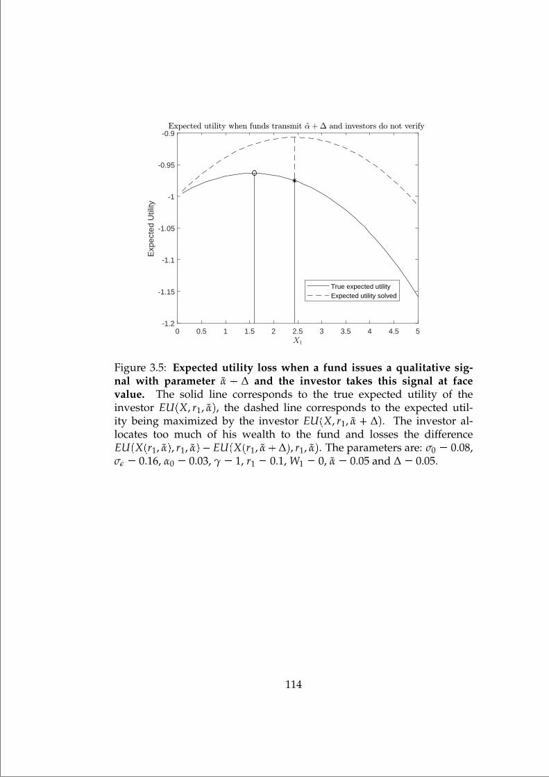
“mainupfv2” — 2021/6/1 — 20:22 — page 114 — #130

0 0.5 1 1.5 2 2.5 3 3.5 4 4.5 5-1.2

-1.15

-1.1

-1.05

-1

-0.95

-0.9

Exp

ecte

d U

tility

True expected utilityExpected utility solved

Figure 3.5: Expected utility loss when a fund issues a qualitative sig-nal with parameter α ∆ and the investor takes this signal at facevalue. The solid line corresponds to the true expected utility of theinvestor EUpX, r1, αq, the dashed line corresponds to the expected util-ity being maximized by the investor EUpX, r1, α ∆q. The investor al-locates too much of his wealth to the fund and losses the differenceEUpXpr1, αq, r1, αq EUpXpr1, α ∆q, r1, αq. The parameters are: σ0 0.08,σε 0.16, α0 0.03, γ 1, r1 0.1, W1 0, α 0.05 and ∆ 0.05.

114

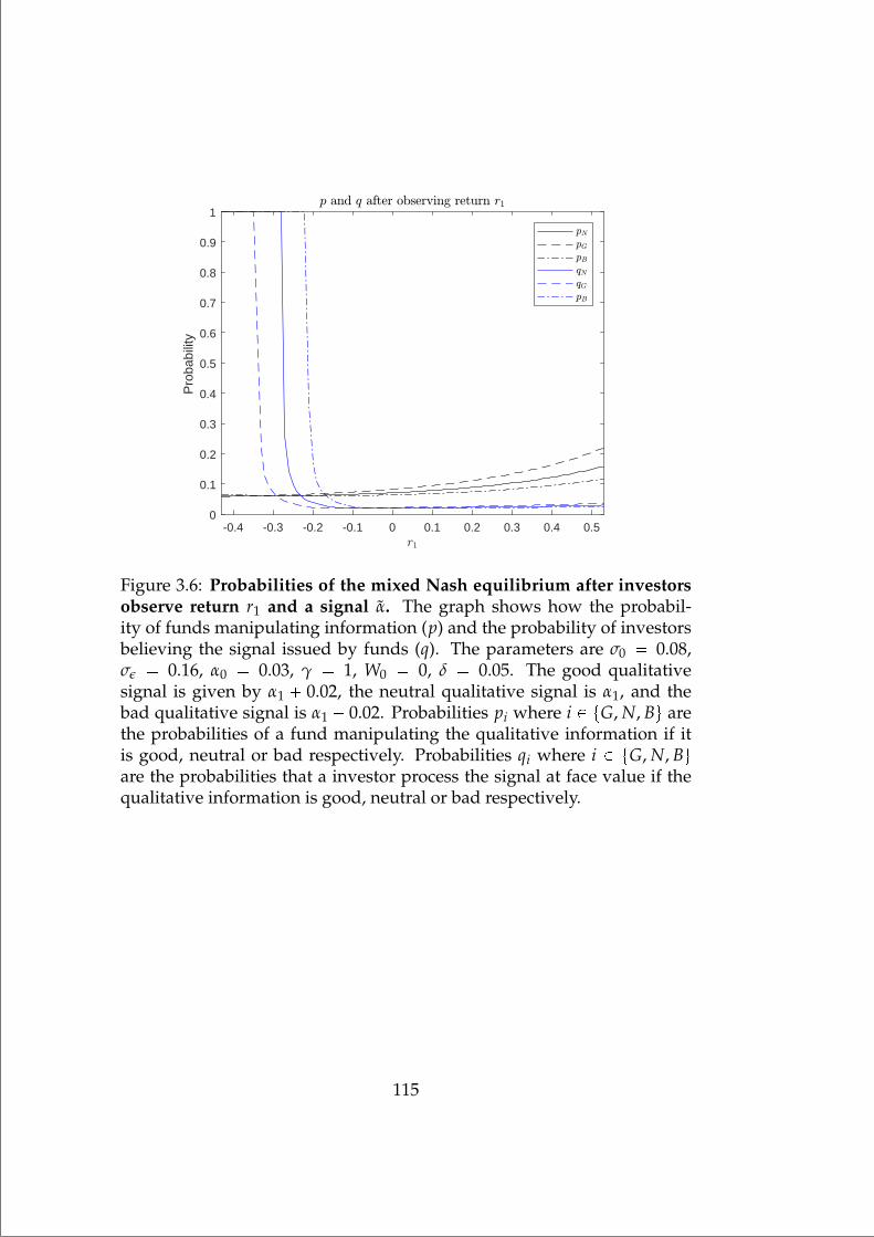
“mainupfv2” — 2021/6/1 — 20:22 — page 115 — #131

-0.4 -0.3 -0.2 -0.1 0 0.1 0.2 0.3 0.4 0.50

0.1

0.2

0.3

0.4

0.5

0.6

0.7

0.8

0.9

1

Pro

babi

lity

Figure 3.6: Probabilities of the mixed Nash equilibrium after investorsobserve return r1 and a signal α. The graph shows how the probabil-ity of funds manipulating information (p) and the probability of investorsbelieving the signal issued by funds (q). The parameters are σ0 0.08,σε 0.16, α0 0.03, γ 1, W0 0, δ 0.05. The good qualitativesignal is given by α1 0.02, the neutral qualitative signal is α1, and thebad qualitative signal is α1 0.02. Probabilities pi where i P tG, N, Bu arethe probabilities of a fund manipulating the qualitative information if itis good, neutral or bad respectively. Probabilities qi where i P tG, N, Buare the probabilities that a investor process the signal at face value if thequalitative information is good, neutral or bad respectively.

115

“mainupfv2” — 2021/6/1 — 20:22 — page 116 — #132

“mainupfv2” — 2021/6/1 — 20:22 — page 117 — #133

Appendix A

Appendix - Stroke of a Pen:Investment and Stock Returnsunder Energy Policy Uncertainty

A.1 Energy Price Uncertainty and Investment -Alternative Formulation

In this section I develop a small model of investment based on Stewart(1978). Consider a representative firm that uses two inputs, capital (K)and energy (E) to produce a final product. The firm purchases energy in acompetitive market at a price we per unit and combines energy with capital(e.g. property plant equipment PPE) to produce its final product, and allother factors required such as labor are maximized out of the equation.The firm’s profit at any period is given by

π pqweE rK (A.1)

where p is the output price, q is the quantity produced, and r is the unitcost of capital including opportunity costs, or financing costs. I assumethat input substitution between energy and capital is possible. More pre-cisely, if the firm uses technology q f pK, Eq to convert capital and energyinto the final product, substitution implies that for any fixed output q andcapital K, the quantity of energy required

E gpq, Kq (A.2)

satisfies BgBK 0. I assume that the firm’s PPE configuration is not in-stantaneously adjustable, so that capital has to be determined in advance,

117

“mainupfv2” — 2021/6/1 — 20:22 — page 118 — #134

and that the price of energy we follows a mean preserving spread process

we βν θ (A.3)

where β and θ are constant shift parameters, and ν is a positive randomvariable. Finally, I assume the firm’s manager is risk averse and maximizesexpected utility over profit π with a standard von Neumann and Morgen-stern (1947) utility function U. If we express the optimization problem interms of capital and output

pqwegpq, Kq rK (A.4)

a necessary condition for utility maximization is therefore

ErU1pπqpweBgBK

rqs 0 (A.5)

To study how uncertainty on energy prices impacts investment, I considerfirst the benchmark case in which the manager is risk neutral so U1pπq is aconstant. In this situation the first order condition of profit maximizationimplies the manager chooses next period capital satisfying

BgBK

rErwes (A.6)

equating the marginal rate of technical substitution to the expected factorprice ratio. On the other hand, a risk averse manager with concave utilityfunction will depart from this first order condition. Expressing (A.5) incovariance form yields

ErU1pπqpweBgBK

rqs ErU1pπqsErpweBgBK

rqs covprU1pπq, pweBgBK

rqq 0(A.7)

U is a concave function so U1pπq is increasing in we, and since the termwe

BgBK r is also increasing in we we have that the covariance term in

(A.7) is strictly positive, which implies

ErpweBgBK

rqs 0 Ñ BgBK

rErwes (A.8)

so a risk averse manager demands more capital than its risk neutral coun-terparty. This results shows that in the presence of uncertainty regardingfuture energy prices we a risk averse manager increases investment.

118

“mainupfv2” — 2021/6/1 — 20:22 — page 119 — #135

A.2 Robustness Analysis to the Information Set

A.2.1 Theoretical Setup

In this section I explain how I construct a measure of energy policy un-certainty using a large battery of macroeconomic, financial, and politicaldata. To keep the notation self-contained I explain an extension of theforecasting model based on Jurado et al. (2015), including extra politicalvariables in the forecasting exercise. For technical details I refer the readerto the original paper. Policy uncertainty arises from the impossibility ofeconomic agents to perfectly forecast politician’s decisions. I follow the lit-erature on uncertainty and define energy policy uncertainty as the condi-tional volatility of the unforecastable component of the number of energyrelated executive orders from the point of view of an economic agent. Inparticular, given investor’s information set It, I define the k-period aheadenergy political uncertainty on topic i as

Utpkq b

Erpeoenergytk Ereoenergy

tk |Itsq2|Its (A.9)

where eoenergyt is the total number of executive orders signed by the U.S.

President during month t. To model the information set It, I use a largebattery of macroeconomic and financial time series, as well as political in-formation.1 The information set comprises variables that help forecast thenumber of executive orders within a one month, one quarter, and one yearhorizons. I include the current political agenda, the number of public lawsand executive orders being passed on each topic. I use information aboutthe party in power in each one of the two chambers as well as the presi-dent’s affiliation. This allows me to control for differences in the agendaof both parties, which are reflected in next periods’ political decisions. Fi-nally I include the original 132 time-series of macroeconomic variables andthe 147 financial variables presented in Ludvigson and Ng (2009) and Lud-vigson and Ng (2007), and used in Jurado et al. (2015) for the uncertaintyestimations.

The forecasting procedure is explained as follows. LetPt ppl1t, ..., plNtqbe a vector containing the number of public laws for every topic, andEt peo1t, ..., eoNtq a vector containing the number of executive ordersfor every topic i. Also, let XJLN

t pX JLN1t , ..., X JLN

Nt q1 denote the original

1As noted by Jurado et al. (2015), many proxies of economic uncertainty fail to accountfor the forecastable component of the time series being analysed, which pervades theuncertainty estimations with predictive variation.

119

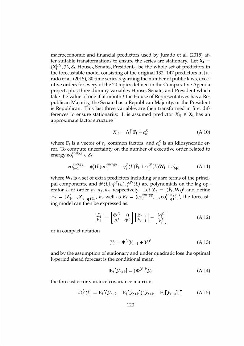
“mainupfv2” — 2021/6/1 — 20:22 — page 120 — #136

macroeconomic and financial predictors used by Jurado et al. (2015) af-ter suitable transformations to ensure the series are stationary. Let Xt pXLN

t ,Pt, Et, Houset, Senatet, Presidenttq be the whole set of predictors inthe forecastable model consisting of the original 132+147 predictors in Ju-rado et al. (2015), 30 time series regarding the number of public laws, exec-utive orders for every of the 20 topics defined in the Comparative Agendaproject, plus three dummy variables House, Senate, and President whichtake the value of one if at month t the House of Representatives has a Re-publican Majority, the Senate has a Republican Majority, or the Presidentis Republican. This last three variables are then transformed in first dif-ferences to ensure stationarity. It is assumed predictor Xit P Xt has anapproximate factor structure

Xit ΛF1i Ft eX

it (A.10)

where Ft is a vector of rF common factors, and eXit is an idiosyncratic er-

ror. To compute uncertainty on the number of executive order related toenergy eoenergy

t P Et

eoenergyt1 φe

j pLqeoenergyt γF

j pLqFt γWj pLqWt ve

t1 (A.11)

where Wt is a set of extra predictors including square terms of the princi-pal components, and φepLq, φFpLq, φWpLq are polynomials on the lag op-erator L of order ne, n f , nw respectively. Let Zt pFt, Wtq1 and defineZt pZ1

t, ..., Z1tq1q, as well as Et peoenergy

t , ..., eoenergytq1q1, the forecast-

ing model can then be expressed as:ZtEt

ΦZ 0Λ1 ΦE

Zt1Et1

VZtVE

t

(A.12)

or in compact notation

Yt ΦYYt1 VYt (A.13)

and by the assumption of stationary and under quadratic loss the optimalk-period ahead forecast is the conditional mean

EtrYtks pΦY qkYt (A.14)

the forecast error variance-covariance matrix is

ΩYt pkq EtrpYtk EtrYtksqpYtk EtrYtksq1s (A.15)

120

“mainupfv2” — 2021/6/1 — 20:22 — page 121 — #137

the k ¡ 1 ahead forecast error variance matrix evolves accordingly to

ΩYt pkq ΦYΩYt pk 1qΦYj1 ErVYtkV

Y 1tks (A.16)

where ΩYt p1q ErVYt1VY 1t1s. The political uncertainty estimation can then

be estimated as:

Utpkq b

11energyΩYt pkq1energy (A.17)

where 1energy is an adequate selector operator. Finally the components inErVYj,thV

Y 1j,ths can be estimated imposing a stochastic volatility structure

on the residuals in Zt and Et assuming an autoregressive behaviour of theelements of Zt:

Zt ΦZZt1 vZt (A.18)

where Zt P Zt, the residual term admits vZt σZ

t εZt and εZ

t Np0, 1q andthe forecast residual vy

t1 σt1εyt , the stochastic volatility model used

assumes an AR(1) process on the square of the log volatility

logpσZt q2 αZ βZ logpσZ

t1q2 τZηZt (A.19)

logpσyt1q2 α β logpσy

t q2 τeηt1 (A.20)

where parameters pαZ, βZ, τZ, α, β, τeq are estimated via MCMC. The stochas-tic volatility model allows us to express the volatility as:

EtrσZtks exp

αZ

k1

s0

pβZqs pτZq22

k1

s0

pβZq2s pβZqk logpσZt q2

(A.21)

and

Etrσyj,tks exp

α

yj

k1

s0

pβ jqs pτjq22

k1

s0

pβ jq2s pβ jqk logpσyjtq2

(A.22)

elements in ErVYj,tkVY 1j,tks are estimated using the fact that Etrσy

j,tks2 Etrvy

j,tks2 and EtrσZtks2 EtrvZ

tks2.

121

“mainupfv2” — 2021/6/1 — 20:22 — page 122 — #138

A.2.2 Estimation

I follow Jurado et al. (2015) and set rF 10, and Zt rFt, F2t , Gts where

Gt is the first principal component of X2t . The polynomials on the lag op-

erator used in the forecasting regressions are assumed to have degreesny 4, n f 2, nw 2, and lags q t4p T

100q29u. On a first stage the el-ements of Zt are pruned to keep only those ones that provide individualsignificance with t-statistics greater than 2.575 in the multivariate forecast-ing regression of yt1 on the candidate predictors known at time t. Onceresiduals are estimated, the parameters in the stochastic volatility modelare estimated via a Markov Chain Montecarlo Method.2

2I thank Serena Ng for making available the code used in Jurado et al. (2015) on herwebpage.

122

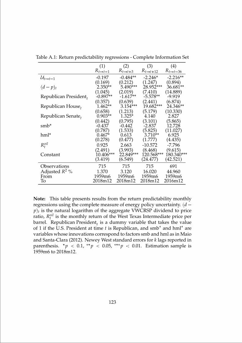
“mainupfv2” — 2021/6/1 — 20:22 — page 123 — #139

Table A.1: Return predictability regressions - Complete Information Set

(1) (2) (3) (4)RtÑt1 RtÑt3 RtÑt12 RtÑt36

UtÑt1 -0.197 -0.484** -2.246* -2.216**(0.169) (0.212) (1.247) (0.894)

pd pqt 2.350** 5.490*** 28.952*** 36.681**(1.045) (2.019) (7.410) (14.889)

Republican Presidentt -0.897** -1.617** -5.578** -9.919(0.357) (0.639) (2.441) (6.874)

Republican Houset 1.462** 3.154*** 19.682*** 24.346**(0.658) (1.213) (5.179) (10.330)

Republican Senatet 0.903** 1.325* 4.140 2.827(0.442) (0.795) (3.101) (5.865)

smb* -0.437 -0.442 -2.837 12.728(0.787) (1.533) (5.825) (11.027)

hml* 0.467* 0.613 3.710** 6.925(0.278) (0.477) (1.777) (4.435)

Roilt 0.925 2.663 -10.572 -7.796

(2.491) (3.993) (8.468) (9.615)Constant 10.406*** 22.849*** 120.568*** 180.340***

(3.419) (6.549) (24.477) (42.521)Observations 715 715 715 691Adjusted R2 % 1.370 3.120 16.020 44.960From 1959m6 1959m6 1959m6 1959m6To 2018m12 2018m12 2018m12 2016m12

Note: This table presents results from the return predictability monthlyregressions using the complete measure of energy policy uncertainty. pdpqt is the natural logarithm of the aggregate VWCRSP dividend to priceratio, Roil

t is the monthly return of the West Texas Intermediate price perbarrel. Republican Presidentt is a dummy variable that takes the valueof 1 if the U.S. President at time t is Republican, and smb and hml arevariables whose innovations correspond to factors smb and hml as in Maioand Santa-Clara (2012). Newey West standard errors for k lags reported inparenthesis. p 0.1, p 0.05, p 0.01. Estimation sample is1959m6 to 2018m12.

123

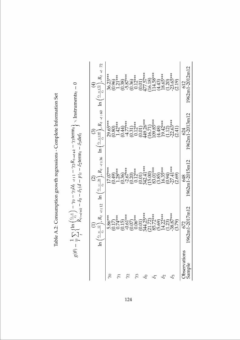
“mainupfv2” — 2021/6/1 — 20:22 — page 124 — #140

Tabl

eA

.2:C

onsu

mpt

ion

grow

thre

gres

sion

s-C

ompl

ete

Info

rmat

ion

Set

gpθq

1 T

¸ t

! ln c t

k

c t

γ

0

γ1U

tÑt

1

γ2R

tÑt

k

γ3t

erm

t

RtÑ

tk

δ 0

δ 1pd

pqt

δ 2te

rmt

δ 3de

f t

) In

stru

men

tst

0

(1)

(2)

(3)

(4)

ln c t

Ñc

12c t

,RtÑ

t12

ln c t

Ñc

36c t

,RtÑ

t36

ln c t

Ñc

60c t

,RtÑ

t60

ln c t

Ñc

72c t

,RtÑ

t72

γ0

5.86

***

17.0

7***

29.6

5***

36.2

3***

(0.1

7)(0

.49)

(0.8

0)(0

.96)

γ1

0.74

***

1.28

***

1.42

***

1.21

***

(0.1

5)(0

.36)

(0.4

4)(0

.38)

γ2

-0.6

1***

-2.6

7***

-4.7

7***

-5.8

7***

(0.0

7)(0

.20)

(0.3

1)(0

.36)

γ3

0.06

***

0.12

***

0.12

***

0.12

***

(0.0

1)(0

.01)

(0.0

1)(0

.01)

δ 034

4.25

***

342.

41**

*44

9.26

***

477.

57**

*(2

1.72

)(1

5.00

)(1

6.71

)(1

6.18

)δ 1

85.7

2***

83.0

1***

109.

85**

*11

4.58

***

(5.6

9)(3

.85)

(4.4

8)(4

.43)

δ 214

.22*

**16

.35*

**19

.42*

**18

.65*

**(1

.23)

(0.9

4)(1

.12)

(1.2

0)δ 3

-38.

87**

*-2

7.41

***

-22.

63**

*-2

3.65

***

(3.7

9)(2

.69)

(2.4

1)(2

.19)

Obs

erva

tion

s67

264

862

461

2Sa

mpl

e19

62m

1-20

17m

1219

62m

1-20

15m

1219

62m

1-20

13m

1219

62m

1-20

12m

12

124

“mainupfv2” — 2021/6/1 — 20:22 — page 125 — #141

Note: Parameters θ tγ0, γ1, γ2, γ3, δ0, δ1, δ2, δ3u minimize gpθq1 Igpθq andInstruments: Constant, UtÑt1, term, d p, def. And, I is the identity ma-trix. This table presents results from the return and consumption growthpredictability regressions on energy policy uncertainty. Parameters are es-timated via GMM. RtÑtk is the cumulative log return of the VWCRSPportfolio between month t and t k. Ut is the level of energy policy un-certainty. Controls include the log dividend to price ration pd pqt, theterm structure (termt), the default spread (deft). lnpctkctq is the growthon consumption between month t and t k measured as aggregate per-sonal consumption expenses. p 0.1, p 0.05, p 0.01. Estimationsample of the predictability regression is 1962m1 to 2018m12.

125

“mainupfv2” — 2021/6/1 — 20:22 — page 126 — #142

Table A.3: Cross-sectional return regressions - Complete Information Set

Size and Book-to-Market(1) (2) (3) (4) (5)

µmktr f 0.007*** 0.006*** 0.006*** 0.006*** 0.007***(0.002) (0.002) (0.002) (0.002) (0.002)

γmktr f 2.301* 2.609* 4.786** 5.182*** 8.620***(1.359) (1.507) (1.941) (1.741) (2.290)

µsmb 0.001 0.001(0.001) (0.001)

γsmb 2.575 5.586**(2.080) (2.587)

µhml 0.003** 0.003**(0.001) (0.001)

γhml 3.941 0.806(2.496) (5.442)

µcma 0.285***(0.091)

γcma 0.046(0.105)

µrmw 0.341***(0.107)

γrmw 0.107**(0.046)

µme 0.002 0.002(0.001) (0.001)

γme 5.977*** 10.443***(2.167) (2.761)

µia 0.003*** 0.003***(0.001) (0.001)

γia 9.064** 2.380(4.349) (5.291)

µroe 0.005*** 0.006***(0.001) (0.001)

γroe 11.250*** -3.314(4.259) (6.553)

µeg 0.008***(0.001)

γeg 42.471***(14.441)

µpol 0.492*** 0.491*** 0.492*** 0.489*** 0.484***(0.041) (0.041) (0.043) (0.043) (0.043)

γpol -1.525*** -1.429*** -1.079*** -0.898** -0.890**(0.413) (0.461) (0.401) (0.385) (0.423)

Observations 468 468 468 468 468MAE % .26 .15 .12 .11 .09

126

“mainupfv2” — 2021/6/1 — 20:22 — page 127 — #143

Note: This table presents results from estimating the price of risk in ex-pected return - covariance form by extending the CAPM model, Fama andFrench three and five factor models, and the q4 and q5 models. Estimationsare performed via GMM in which factor loadings (covariances) and co-variance prices of risk are estimated jointly. Factors smb, hml, cma, rmw,correspond to the Fama and French factors related to size, book-to-market,investment and profitability. Factors, me, ia, roe, and eg, correspond tofactors related to size, investment, profitability, and expected investmentgrowth. Factor pol corresponds to the innovations to energy policy un-certainty. p 0.1, p 0.05, p 0.01. Estimation sample of thecross-sectional regression is 1956m1 to 2018m12.

127

“mainupfv2” — 2021/6/1 — 20:22 — page 128 — #144

Table A.4: Investment Cross-sectional Regressions - Complete InformationSet

(1) (2) (3) (4)Invit Invit Invit Invit

Profitabilityit 6.06*** 2.73*** 6.07*** 2.74***(0.69) (0.41) (0.69) (0.41)

logpQitq 0.54*** 0.63*** 0.52*** 0.61***(0.02) (0.02) (0.02) (0.02)

Sizeit -0.09*** -0.13*** -0.09*** -0.13***(0.01) (0.01) (0.01) (0.01)

UtÑt1 7.61** 6.31** 5.38** 3.81*(3.31) (2.98) (2.49) (2.10)

UtÑt1 logpQitq 5.31* 5.95**(3.03) (3.01)

Constant 1.94*** 2.26*** 1.94*** 2.27***(0.06) (0.06) (0.06) (0.06)

Observations 338253 338253 338253 338253Adjusted R2 (%) 4.46 24.63 4.47 24.64Industry F.E. No Yes No YesFrom 2000m1 2000m1 2000m1 2000m1To 2018m10 2018m10 2018m10 2018m10

Note: This table presents results from monthly cross-sectional invest-ment regressions. Quarterly accounting variables are merged with pricingdata with a two month lag to account for look ahead bias. Investment isdefined as the difference between the cumulative quarterly capital expen-ditures (capxy) between quarters n and n 1 for n ¡ 1 divided over totalassets. Profitability is measured as operating income after depreciation(oiadpq) over the sum of book debt (dlcq+dlttq) and market equity (prccq cshoq). Average Q is computed as the book value of debt plus equity(dlcq+dlttq+prc cshoq) divided by total assets (atq), size is the naturallogarithm of market equity (prc cshoq), Ut corresponds to energy policyuncertainty. Standard errors clustered by gvkey reported in parenthesis.p 0.1, p 0.05, p 0.01.

128

“mainupfv2” — 2021/6/1 — 20:22 — page 129 — #145

A.2.3 Mathematical Appendix

Proof. of proposition (6) The positive relation between investment and un-certainty in equation (1.2) can be written as

Iit Y1β

αi,t1

r f t

βpErMt1sErwt1s ρσMσeq

βα

the derivative of investment with respect to energy policy uncertainty is

BIit

Bσe β

αY

1βα

i,t1

r f t

βpErMt1sErwt1s ρσMσeq

βαα

ρσMσe

given that Mt1 ¡ 0, wt1 ¡ 0, we have that ErMt1wt1s ErMt1sErwt1sρσMσe ¡ 0 so the sign of the partial derivative depends directly on the signof ρ.

To compute the second derivative we forget about the term βα Y

1βα

i,t1ρσM

which for the partial derivative is assumed constant and positive. The

derivative of the remaining term

r f tβ pErMt1sErwt1s ρσMσeq

βαα

σe is

r f t

βpErMt1sErwt1s ρσMσeq

βαα

β α

α

r f t

βpErMt1sErwt1s ρσMσeq

β2αα

ρσMσe

(A.23)whose sign is ambiguous given that the term β α can be either positiveor negative. If β α ¡ 0 the second derivative is always positive, howeverif α ¡ β the second derivative is positive if

r f t

βpErMt1sErwt1s ρσMσeq

βαα

β α

α

r f t

βpErMt1sErwt1s ρσMσeq

β2αα

ρσMσe ¡ 0

α β

αρσM

r f t

βp

ErMt1sErwt1s

σe ρσMq

ρσMpβ

r f t

α β

α 1q

ErMt1sErwt1s

σe

σe ¡ErMt1sErwt1s

ρσMpβ

r f t

αβα 1q

σ

(A.24)

where the last change in the inequality sign comes from the fact thatβ

r f t

αβα 1. Since σ 0 the second derivative is positive for every value of

σe.

129

“mainupfv2” — 2021/6/1 — 20:22 — page 130 — #146

Proof. of proposition (7). If households consume the aggregate differenceY I, expected consumption growth is given by

gt,t1 E Yt1

Yt It

(A.25)

as all capital is depreciated by the end of t 1. Its derivative with respectto σe is

Bgt,t1

Bσe E

BYt1Bσe

pYt Itq Yt1BItBσe

pYt Itq2

(A.26)

Since the denominator is always positive, the sign depends on the term

BYt1

BσepYt Itq Yt1

BIt

Bσe(A.27)

I will show that BYt1Bσe

is non negative which concludes the proof. We canexpress future output Yt1 as

BIit

Bσe β

αY

1βα

i,t1

r f t

βpErMt1sErwt1s ρσMσeq

βαα

ρσMσe

Yt1 α

βBIitBσe

r f tβ pErMt1sErwt1s ρσMσeq

βαα

ρσMσe

α1β

(A.28)

whose derivative is

BYt1

Bσe

α

1 β

αβBIitBσe

r f tβ pErMt1sErwt1s ρσMσeq

βαα

ρσMσe

αβ11β

looooooooooooooooooooooooooooooooooooooomooooooooooooooooooooooooooooooooooooooon¡0

1 r f t

β pErMt1sErwt1s ρσMσeq βα

αρσMσe

2α

β

B2 It

Bσ2e

r f t

βpErMt1sErwt1s ρσMσeq

βαα

ρσMσe

α

β

BIt

Bσe

r f t

βpErMt1sErwt1s ρσMσeq

βαα

β α

α

r f t

βpErMt1sErwt1s ρσMσeq

β2αα

ρσMσe

(A.29)

Now, the sign of the term depends on the sign of

α

β

B2 It

Bσ2e

r f t

βpErMt1sErwt1s ρσMσeq

βαα

ρσMσe

α

β

BIt

Bσe

r f t

βpErMt1sErwt1s ρσMσeq

βαα

β α

α

r f t

βpErMt1sErwt1s ρσMσeq

β2αα

ρσMσe

130

“mainupfv2” — 2021/6/1 — 20:22 — page 131 — #147

I will prove that this term is non negative by contradiction. Assume it is

strictly negative, dividing both sides by αβ

r f tβ pErMt1sErwt1s ρσMσeq

βαα

ρσMσe ¡0

B2 It

Bσ2e BIBσe

1ρσMσe

β α

α

r f t

βpErMt1sErwt1s ρσMσeq

1 0

(A.30)given that the first derivative of investment on energy policy uncertaintyis positive,

B2 ItBσ2

eBItBσe

1ρσMσe

β α

α

r f t

βpErMt1sErwt1s ρσMσeq

1(A.31)

replacing the definition of the first and second derivatives

βα Y

1βα

i,t1

r f tβ pErMt1sErwt1s ρσMσeq

βαα

βαα

r f tβ pErMt1sErwt1s ρσMσeq

β2αα

ρσMσe

βα Y

1βα

i,t1

r f tβ pErMt1sErwt1s ρσMσeq

βαα

ρσMσe

1ρσMσe

β α

α

r f t

βpErMt1sErwt1s ρσMσeq

1

(A.32)

which is true if1

ρσMσe

β α

α

r f t

βpErMt1sErwt1s ρσMσeq

1

1ρσMσe

β α

α

r f t

βpErMt1sErwt1s ρσMσeq

1(A.33)

which is a contradiction, so it must be that BYt1Bσe

¥ 0 which means thatBgt1Bσe

¡ 0 .

Proof. of propositions (8) and (9).The proof proceeds by inspection of the term Iit inside the expression, it

can be observed that increasing investment decreases the numerator given

the term I α

β

it for α ¡ 0, β ¡ 0, and equivalently investment increases the

term in the denominator IitYi,t1

1 a Iit

Kit

of equation (1.4).

131

“mainupfv2” — 2021/6/1 — 20:22 — page 132 — #148

“mainupfv2” — 2021/6/1 — 20:22 — page 133 — #149

Appendix B

Appendix - Tweeting for Money:Social Media and Mutual FundFlows

B.1 Tweet Classification and Examples

In this appendix we explain how we classify tweets and provide some ex-amples. Classifying tweets into positive and negative requires knowinghow these tweets are written, what information they contain, and whothey are directed to. The positiveness of a tweet depends on whether thetweet contains financial information that can be translated into good orbad news for the fund family, or other type of information which, even ifpositive, may not be related to the business in which these companies op-erate. Loughran and McDonald (2011) describe in detail this issue whenclassifying good or bad information. Dictionaries, or other techniquesused in textual analysis need to be corrected when considering financialinformation. Information related to finance and economics may containspecialized jargon, or even words with a different tone and interpretationthan in other fields.1 To overcome this issue we develop a two stage clas-sification procedure in which tweets are first classified into one of twotypes: financial tweets, which are more likely to contain financial informa-tion; and nonfinancial tweets.

We start by explaining the data pre-processing process with an exam-ple. Most of the textual analysis applications in the literature consider a

1The best example is the word liability. While in dictionaries such as the Harvard IV-4dictionary the word is classified as being negative, in a more financial context it has adifferent tone.

133

“mainupfv2” — 2021/6/1 — 20:22 — page 134 — #150

bag of words approach, in which the position of the word within a sen-tence is not relevant and the only important feature is the appearanceor frequency of a word in the text. Since the language used in tweets islimited by the 140-character length restriction, just the presence of wordsmight not be informative enough to classify them.2 At the same time theinformality of communications increases the use of words with less definedtonal categories, and provides less informative features to predict labels.To obtain a more informative set of features from tweets, we consider boththe appearance of a word as well as its role in the sentence - also known asPart of Speech (POS).3

The in- and out-of-sample performance of machine learning dependson the algorithm chosen by the researcher. To avoid subjectivity on thechoice of an algorithm we use six different algorithms: Naive-Bayes classi-fier, Multinomial-Naive-Bayes classifier, Bernoulli Naive-Bayes classifier,Stochastic Gradient Descent, Support Vector Machines, and Logistic Re-gression. We then consider a voting scheme that consists of classifyingeach tweet with the most voted label among the different algorithms. Ifthree algorithms classify a tweet as positive and three as negative, we con-sider the tweet to have a neutral tone. The procedure also provides uswith a measure of agreement between the algorithms. Even though thismethodology increases the computational efforts, we believe it reducesthe subjective judgement of the decision maker, and provides a naturalway to quantify the confidence of a classification.

The selection of algorithms satisfies two criteria: their implementationis relatively fast using available programming packages, and the replica-tion of results among platforms can be attained by providing detailed de-scription of the algorithms. As argued by Loughran and McDonald (2016),the current state of textual analysis in Financial Economics needs to standfor replicability of results rather than using more sophisticated machineryin the analysis of textual data. We decide to rule out more accurate classi-fiers and keep the analysis replicable by presenting a detailed explanationof the algorithms.

Our analysis focuses on positiveness - a measure of how positive a textis - which can be decomposed as positiveness conditional on a tweet hav-ing financial information, positiveness conditional on a tweet having non-financial information, and the unconditional positiveness of tweets.

We start by extracting two important features of each tweet: Words,2Twitter changed to 240 the character limit of tweets only starting in 2017.3One of the grammatical groups, such as noun, verb, and adjective,

into which words are divided depending on their use. Retrieved from:https://dictionary.cambridge.org/dictionary/english/part-of-speech

134

“mainupfv2” — 2021/6/1 — 20:22 — page 135 — #151

and Part of Speech (POS). We start by applying a tokenization based onregular expressions to automatically split the text into words. We proceedby using a POS tagger (an algorithm that tags each word with its morelikely POS) to identify the role of each word within the sentence. Thefollowing example describes the procedure we use:

Figure B.1: Example of a financial tweet posted by Bloomberg @businesson September 27 2017, 14:00.

The first step consists of tokenizing the tweet to isolate its components.We use a special tokenization procedure to account for hyperlinks, emoti-cons, and punctuation. The tokenization splits the tweet as follows:

Fidelity, Chairman, and, CEO, Abigail, Johnson, discusses, the, struggle, between, activeand, passive, investing, https://www.bloomberg.com/...

Once the tweet is tokenized, we apply a POS tagger which applies an op-timization algorithm that maximizes the likelihood of tuples of the formptoken, POSq to appear in a sentence. After the POS tagger is applied, thetweet becomes:

Fidelitylooomooonproper noun, singular

Chairmanloooomoooonproper noun, singular

andloomooncoordinating conjunction

CEOloomoonproper noun, singular

Abigailloomoonproper noun, singular

Johnsonlooomooonproper noun, singular

discussesloooomoooonverb, 3rd person, singular, present

theloomoondeterminer

strugglelooomooonnoun singular

betweenlooomooonpreposition/subordinating conjunction

activeloomoonadjective

andloomooncoordinating conjunction

passivelooomooonadjective

investingloooomoooonnoun singular

https://www.bloomberg.com/...looooooooooooooooooooomooooooooooooooooooooonnoun singular

After tokenizing and extracting the POS of every tweet in our database weproceed to extract the most common features. We do this by calculating

135

“mainupfv2” — 2021/6/1 — 20:22 — page 136 — #152

the frequency of each tuple ptoken, POSq and select the most common 4000features.

We proceed by first classifying tweets depending on whether they con-tain financial or nonfinancial information, and then classify them into pos-itive or negative. The machine learning algorithms we use are super-vised algorithms. They require an initial set of tweets labelled accordingto whether they contain financial information or not, and whether theyare positive or negative. The algorithms then find common patters whichare applied to classify unlabelled tweets. We train our algorithms witha sample of 10,000 tweets manually classified by two research assistants(undergraduate students in economics and management science respec-tively). To ensure the training sample has enough tweets from all possiblecategories in both dimensions we randomly select them from the accountsof the Financial Times (FT) and The Wall Street Journal (WSJ). We use thissource of tweets instead of those posted by fund families since negativeinformation is less likely to be disclosed.

Table (B.1) presents shows the classification of tweets in the trainingsample. 42 percent of all tweets re classified as financial, and within thiscategory 62 percent are classified as positive. To classify non-financialtweets into positive or negative tweets, we use a sample of 10,000 tweetsrandomly selected from the Sentiment Analysis Training Corpus Datasetfrom the University of Michigan which contains more than million and ahalf of tweets classified into positive or negative tweets. There is a largecorpora of labelled tweets available for research, however this corporacontains Twitter information that covers a widely range of topics. Sincefund families also post financial information, using a database with non-financial tweet to train our algorithms can lead to important biases in theresults. Non-financial tweets on the other hand are not affected by thisissue, and their tone can be inferred by training the same algorithms witha more general corpora of tweets. We train each one of the 6 algorithmsusing the same training samples. For a more robust analysis, we sort ran-domly the training sample and divide it into 4 sets of equal length. Wethen train and test each one of the algorithms using three of the sets astraining set and 1 set as test.

Sample 1 Sample 2 TotalFinancial Positive 1187 664 1851

Negative 728 398 1126Non financial 3085 3938 7023

Total 10000

Table B.1: Manual classification of tweets in the training sample

136

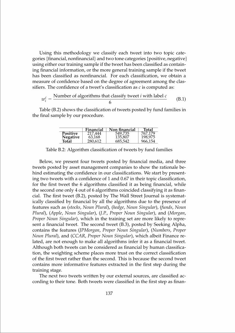
“mainupfv2” — 2021/6/1 — 20:22 — page 137 — #153

Using this methodology we classify each tweet into two topic cate-gories tfinancial, nonfinancialu and two tone categories tpositive, negativeuusing either our training sample if the tweet has been classified as contain-ing financial information, or the more general training sample if the tweethas been classified as nonfinancial. For each classification, we obtain ameasure of confidence based on the degree of agreement among the clas-sifiers. The confidence of a tweet’s classification as c is computed as:

wci

Number of algorithms that classify tweet i with label c6

(B.1)

Table (B.2) shows the classification of tweets posted by fund families inthe final sample by our procedure.

Financial Non financial TotalPositive 217,444 549,735 767,179Negative 63,168 135,807 198,975Total 280,612 685,542 966,154

Table B.2: Algorithm classification of tweets by fund families

Below, we present four tweets posted by financial media, and threetweets posted by asset management companies to show the rationale be-hind estimating the confidence in our classifications. We start by present-ing two tweets with a confidence of 1 and 0.67 in their topic classification,for the first tweet the 6 algorithms classified it as being financial, whilethe second one only 4 out of 6 algorithms coincided classifying it as finan-cial. The first tweet (B.2), posted by The Wall Street Journal is systemat-ically classified by financial by all the algorithms due to the presence offeatures such as (stocks, Noun Plural), (hedge, Noun Singular), (funds, NounPlural), (Apple, Noun Singular), (J.P., Proper Noun Singular), and (Morgan,Proper Noun Singular), which in the training set are more likely to repre-sent a financial tweet. The second tweet (B.3), posted by Seeking Alpha,contains the features (JPMorgan, Proper Noun Singular), (Numbers, ProperNoun Plural), and (CCAR, Proper Noun Singular), which albeit Finance re-lated, are not enough to make all algorithms infer it as a financial tweet.Although both tweets can be considered as financial by human classifica-tion, the weighting scheme places more trust on the correct classificationof the first tweet rather than the second. This is because the second tweetcontains more informative features extracted in the first step during thetraining stage.

The next two tweets written by our external sources, are classified ac-cording to their tone. Both tweets were classified in the first step as finan-

137

“mainupfv2” — 2021/6/1 — 20:22 — page 138 — #154

cial tweets, which requires using our own training sample to classify themaccording to their tone. The first tweet (B.4) posted by Financial News, isclassified as positive with a confidence of one for containing the features(Why, Adverb), (rule, Verb), (Wall, Noun Singular), and (Street, Noun Singu-lar), which are enough to make all algorithms coincide with a positive clas-sification. The last tweet, posted also by Financial News (B.5), is classifiedas negative only with a confidence of only 4 out of 6 algorithms. The tweetcan be understood as containing negative information, although from themachine learning algorithms the only word that is informative about thenegative tone is scorn.

We repeat the analysis with some tweets posted by asset managementcompanies in our sample. The first example (B.6) corresponds to a postwritten by Northern Trust which is classified as negative by the six algo-rithms. The feature (challenge, Noun Singular) together with (growth, NounSingular) are informative enough to make all algorithms coincide with theclassification. The second tweet (B.7) written by State Farm is classified aspositive with a confidence of 1. In this tweet the features (outperforms, Verb3rd person singular), (industry, Noun Singular), and (average, Noun Singular)are informative enough to make all algorithms coincide with the classifi-cation.

Finally, tweet (B.8) written by Pax World is classified as financial witha confidence of only 0.67 (4 out of 6 algorithms agreed on the classifica-tion). The tweet only contains features such as (business, Noun Singular)and (work, Verb) which are not informative enough to make all algorithmsagree with the classification.

B.2 Data pre-processing and Machine Learningalgorithms

B.2.1 Tweet Tokenization

The english-language that tweets have is not the same style of english thatinvestors will find in SEC fillings, shareholder letters or press. Tweetsare designed to provide a more informal type of communication. Thismakes the language in tweets more familiar to people, but it gives roomto spelling mistakes, typos, words not separated by spaces, punctuation,and emoticons. To obtain a bag-of-words representation of a tweet beforeapplying the POS algorithm we tokenize each one of the tweets. In thissection we provide the exact procedure used for the tweet tokenization.

138

“mainupfv2” — 2021/6/1 — 20:22 — page 139 — #155

We provide the exact regular expressions used by the algorithm to dealwith each procedure. 4

1. URLs contain symbols that are not encoded in the standard utf-8 for-mat. Before decoding non utf-8 characters we make sure those onepresent in the URL are kept.

2. usernames

(?:@[\w_]+)

3. Replace characters that are repeated more than 3 times consecutivewith only 3 times by replacing the regular expression \1\1\1 with(.)\12,.

4. Shorten problematic sequences of non-alpha numeric characters toonly 3 occurrences.

([ˆa-zA-Z0-9])\13,’

5. HTML tags

<[ˆ>\s]+>

6. ASCII Arrows

[\-]+>|<[\-]+

7. Hashtags

(?:\#+[\w_]+[\w\’_\-]*[\w_]+)

8. numbers, including fractions and decimals

(?:[+\-]?\d+[,/.:-]\d+[+\-]?)

9. words without apostrophes or dashes

4The procedure is explained based on our interpretation of the source codeof the class TweetTokenize from the Natural Language Toolkit (NLTK) inpython. For the original code visit the official documentation available at:http://www.nltk.org/ modules/nltk/tokenize/casual.html#TweetTokenizer

139

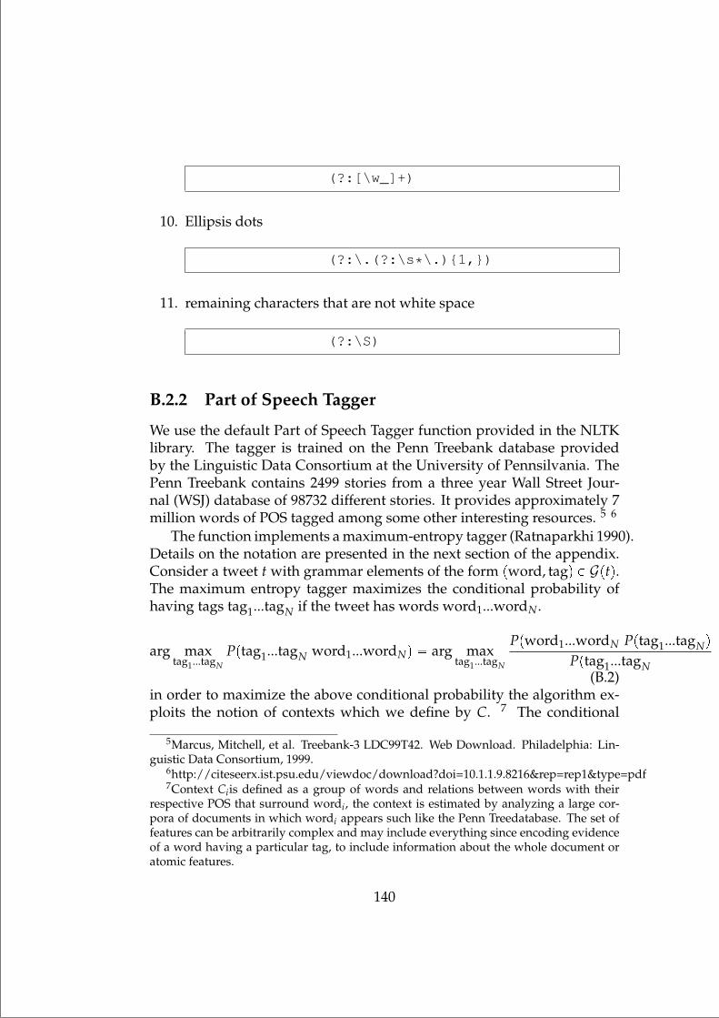
“mainupfv2” — 2021/6/1 — 20:22 — page 140 — #156

(?:[\w_]+)

10. Ellipsis dots

(?:\.(?:\s*\.)1,)

11. remaining characters that are not white space

(?:\S)

B.2.2 Part of Speech Tagger

We use the default Part of Speech Tagger function provided in the NLTKlibrary. The tagger is trained on the Penn Treebank database providedby the Linguistic Data Consortium at the University of Pennsilvania. ThePenn Treebank contains 2499 stories from a three year Wall Street Jour-nal (WSJ) database of 98732 different stories. It provides approximately 7million words of POS tagged among some other interesting resources. 5 6

The function implements a maximum-entropy tagger (Ratnaparkhi 1990).Details on the notation are presented in the next section of the appendix.Consider a tweet t with grammar elements of the form pword, tagq P Gptq.The maximum entropy tagger maximizes the conditional probability ofhaving tags tag1...tagN if the tweet has words word1...wordN.

arg maxtag1...tagN

Pptag1...tagN|word1...wordNq arg maxtag1...tagN

Ppword1...wordN|Pptag1...tagNqPptag1...tagN

(B.2)in order to maximize the above conditional probability the algorithm ex-ploits the notion of contexts which we define by C. 7 The conditional

5Marcus, Mitchell, et al. Treebank-3 LDC99T42. Web Download. Philadelphia: Lin-guistic Data Consortium, 1999.

6http://citeseerx.ist.psu.edu/viewdoc/download?doi=10.1.1.9.8216&rep=rep1&type=pdf7Context Ciis defined as a group of words and relations between words with their

respective POS that surround wordi, the context is estimated by analyzing a large cor-pora of documents in which wordi appears such like the Penn Treedatabase. The set offeatures can be arbitrarily complex and may include everything since encoding evidenceof a word having a particular tag, to include information about the whole document oratomic features.

140

“mainupfv2” — 2021/6/1 — 20:22 — page 141 — #157

probability can be approximated as:

Pptag1...tagN|word1...wordNq N¹

i1

Pptagi|Ciq (B.3)

given a list of words twordiuNi1 and their respective contexts tCiuN

i1. Thealgorithm estimates each probability as

Pptag|Cq 1ZpCq expt

N

i1

λifeatureipC, tagqu (B.4)

where featurei is defined as:

fipC, tagq !

1, if wordi P C and tagi tag0, otherwise (B.5)

and ZpCq is a normalization constant to ensure P is a probability distribu-tion. The optimal sequence of tags is then calculated using beam search, anheuristic that prunes branches of the tree spanned by all sequences of tagi.

B.2.3 Notation

For every tweet t denote Gptq the set of words tokenized and their respec-tive POS. Define by F the set of relevant features. Every tweet is repre-sented by the following set:

f ptq tpx, IGptqpxqq : x P Fu (B.6)

where IGptqpxq is the indicator function

IGptqpxq !

1, if x P Gptq0, if x R Gptq (B.7)

The set f ptq contains information about the presence or absence of eachfeature in every tweet.

Features

The input of all of the classifiers used in the empirical analysis is a listof labelled tweets, their relevant features and the label. Since the amountof words used in tweeting is restricted to 140 characters, using just thepresence of words in a tweet is not an informative feature. We expandthe feature set by considering not only the appearance of words withintweets but also the Part of Speech (POS) of the word. The POS of a worddetermines its role within a sentence. Words are classified into one of thefollowing categories:

141

“mainupfv2” — 2021/6/1 — 20:22 — page 142 — #158

Abbreviation Part of Speech ExampleCC coordinating conjunction and, but, orCD cardinal digit 1,99DT determiner a, the, everyEX existential clause there is a problemFW foreign word laissez-faireIN preposition/subordinating conjunction before, after, untilJJ adjective big

JJR adjective, comparative biggerJJS adjective, superlative biggestLS list marker 1)

MD modal could, willNN noun, singular desk

NNS noun plural desksNNP proper noun, singular Harrison

NNPS proper noun, plural AmericansPDT predeterminer all the kidsPOS possessive ending parent’sPRP personal pronoun I, he, shePRP$ possessive pronoun my, his, hers

RB adverb very, silently,RBR adverb, comparative betterRBS adverb, superlative bestRP particle give upTO to go to the store.UH interjection Yoo-hooVB verb, base form take

VBD verb, past tense tookVBG verb, gerund/present participle takingVBN verb, past participle takenVBP verb, singular. present, non-3rd person takeVBZ verb, 3rd person sing. present takesWDT wh-determiner whichWP wh-pronoun who, whatWP$ possessive wh-pronoun whoseWRB wh-abverb where, when

Classification

This section explains the procedure used to classify tweets. We train our classi-fiers using a database of 10,000 tweets randomly selected from the accounts ofthe Financial Times (@FT), Wall Street Journal (@WSJ). We randomly give to twoundergradutae students in economics and management science an independentsample of 5000 tweets each. The use of dictionaries is a common technique intextual analysis to infer the sentiment or tone from documents. We decided notto use standard dictionaries and rely our analysis in machine learning algorithmsfor the following reasons:

1. Dictionaries have been applied in studies concerning longer textual finan-cial information. Tweets are limited to 140 characters which makes the vo-

142

“mainupfv2” — 2021/6/1 — 20:22 — page 143 — #159

cabulary used an endogenous decision by the person writing the tweet.

2. Financial dictionaries were made by analyzing financial disclosure docu-ments such as 10-K fillings. Even though our tweets are financial and maycontain similar words, the whole language used in Twitter is less formal.

However the accuracy of machine learning algorithms in understanding finan-cial information has been widely criticized. Instead of relying our estimations ina single algorithm, we use a custom classifier based on a vote-scheme of 6 dif-ferent classifiers. The algorithm returns the most voted label for a tweet togetherwith a confidence indicator represented as the degree of consensus between theclassifiers. There is more confidence of a tweet being positive if all 6 classifiershave agreed on the same label for the tweet than if 4 have agreed on the tweethaving a positive tone and 2 of having a negative tone. We will use this confi-dence measure to weight our results when aggregating tweet labels over a periodof time.

Naive Bayes Classifiers

The Naive Bayes Classifier is the oldest of the algorithms used to classify objects.The main assumption of this machine learning technique is that the appearanceof words is independent, and therefore it helps reduce the dimensionality of theproblem. In its simplest interpretation, the algorithm applies the Bayes rule todetermine the likelihood that the features of a tweet f ptq belong to a specific topicor tone. The probability of a tweet having label l can be calculated using Bayesrule: 8

Ppl| f ptqq Pp f ptq|lqPplq (B.8)

where Pp f ptq|lq is the probability of observing features f ptq in a tweet labeled asl, and Pplq is the unconditional probability of observing a tweet labeled as l. Thealgorithm assumes features within a tweet are independent, and therefore givena label l the conditional probability Pp f ptq|lq can be calculated as:

Pp f ptq|lq ¹

xP f ptqPpx|lq (B.9)

where Ppx|lq is the probability of observing feature x in a tweet labeled as l.

8The classification can be extended to any finite set of classifications (e.g Positive, Neu-tral, or Negative)

143

“mainupfv2” — 2021/6/1 — 20:22 — page 144 — #160

The Naive Bayes classifier has a strong assumption of independence betweenfeatures. The multinomial Naive Bayes classifier goes one step beyond and im-poses a multinomial distribution on Ppx|lq, x P f ptq, rather than calculating theprobability based on the frequency of labeled tweets in the data.

Linear Support Vector Classification

To apply the linear SVC algorithm we convert the relevant features of a tweet f ptqinto an edge in a |F | dimensional hypercube. Using any arbitrary sort of the setF t f1, f2, ... f|F |u the coordinates of the features f ptq of a tweet are:

cptq

2 IGptqp f1q 12 IGptqp f2q 1

...2 IGptqp f|F |q 1

(B.10)

If a tweet contains feature fi a 1 will be assigned as the coordinate in the i dimen-sions, and a 1 otherwise. This parametrization allows us to map tweets into ahigh dimensional space, and have a defined gap between edges that will allowus to build a hyperplane splitting sets. If we have a training sample codified aspoints pci, yiq where ci corresponds to a set of coordinates for each training ele-ment, and yi a variable that takes the value of 1 or 1 for each one of the labels. Ifthe training set is linearly separable there exists a vector w such that the followingtwo hyperplanes

wc b 1 (B.11)wc b 1 (B.12)

are separated by a distance 2||w|| . The goal of the algorithm is to minimize the dis-

tance between both hyperplanes, once the hyperplane is built ,the classificationof each cptq is completely determined by its surrounding neighbours ci which arecalled support vectors.

144

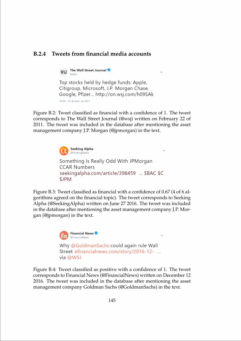
“mainupfv2” — 2021/6/1 — 20:22 — page 145 — #161

B.2.4 Tweets from financial media accounts

Figure B.2: Tweet classified as financial with a confidence of 1. The tweetcorresponds to The Wall Street Journal (@wsj) written on February 22 of2011. The tweet was included in the database after mentioning the assetmanagement company J.P. Morgan (@jpmorgan) in the text.

Figure B.3: Tweet classified as financial with a confidence of 0.67 (4 of 6 al-gorithms agreed on the financial topic). The tweet corresponds to SeekingAlpha (@SeekingAlpha) written on June 27 2016. The tweet was includedin the database after mentioning the asset management company J.P. Mor-gan (@jpmorgan) in the text.

Figure B.4: Tweet classified as positive with a confidence of 1. The tweetcorresponds to Financial News (@FinancialNews) written on December 122016. The tweet was included in the database after mentioning the assetmanagement company Goldman Sachs (@GoldmanSachs) in the text.

145

“mainupfv2” — 2021/6/1 — 20:22 — page 146 — #162

Figure B.5: Tweet classified as negative with a confidence of 0.67 (4 of 6algorithms agreed on the negative tone). The tweet corresponds to Fi-nancial News (@FinancialNews) written on October 9 2017. The tweetwas included in the database for mentioning Vanguard Group (@Van-guard Group) in the text.

146

“mainupfv2” — 2021/6/1 — 20:22 — page 147 — #163

B.2.5 Tweets from asset management companies

Figure B.6: Tweet classified as negative with a confidence of 1. The tweetwas written by asset management company Northern Trust (@Northern-Trust) on October 1 2013.

Figure B.7: Tweet classified as positive with a confidence of 1. The tweetwas written by asset management company State Farm (@StateFarm) onNovember 11 2008.

147

“mainupfv2” — 2021/6/1 — 20:22 — page 148 — #164

Figure B.8: Tweet classified as financial with a confidence of 0.67 (4 of 6algorithms agreed on the topic). The tweet was written by asset manage-ment company PaxWorld (@PaxWorld) on November 18 2015. PaxWorldfunds are adviced by Impax Asset Management LLC, formerly Pax WorldManagement LLC

B.2.6 Nonfinancial tweets

Figure B.9: Tweet classified as nonfinancial with a confidence of 0.67 (4 of6 algorithms agreed on the tone). The tweet was written by asset manage-ment company JP Morgan (@jpmorgan) on January 10 2019.

148

“mainupfv2” — 2021/6/1 — 20:22 — page 149 — #165

Appendix C

Appendix - Learning from Quant(Qual)-itative Information

C.1 Mathematical Appendix

Proof. of Proposition (6). The extrema of a functional of the form Jrys ³ba Hpypxq, y1pxq, xqdx

with boundary conditions ypaq ya and ypbq yb is given by the solution to thedifferential equation Hypypxq, y1pxq, xq d

dx Hy1pypxq, y1pxq, xq 0 where Hy, Hy1

are the partial derivatives of H with respect to y and y1 (See Dacorogna (1992,Theorem 2.1)). For the particular case in which the functional is of the form ofequation (3.2) the Euler-Lagrange equation can be written as:

d2Gdx2

dFdx

dGdx

d2Fdx2 0

or for a normal prior with mean µ and variance σ2

d2Gdx2 px µ

σ2 qdGdx

0

The integrating factor expt x22µx2σ2 Cu where C is a constant can be rewritten as

C1 expt 12p xµ

σ q2uwhere C1 exptp µ2

2σ2 Cqu. This leads to the following generalsolution:

dGdx

C2 expt12px µ

σq2u (C.1)

The value of the constant C2 can be calculated based on the boundary conditions.There is no guarantee for the function dG

dx to be smooth, however we can split thedifferential equation into two differential equations with boundaries at p8, αsand pα,8q as follows:

149

“mainupfv2” — 2021/6/1 — 20:22 — page 150 — #166

For the interval p8, αs

C2

» α

8expt1

2px µ

σq2udx 1

2Ñ C2 1

2?

2πσΦp αµσ q

and the interval pα,8q

C2

» α

8expt1

2px µ

σq2udx 1

2Ñ C2 1

2?

2πσp1Φp αµσ qq

replacing both solutions to C2 in equation (C.1) gives us the p.d.f. in Proposition(6), finally integrating from p8, xq gives us the c.d.f.

Proposition 14. zΦpzq φpzq ¥ 0

Proof. 1

zΦpzq φpzq » z

8zφpxqdx φpzq ¥

» z

8xφpxqdx φpxq|x8 φpxq 0

Proof. of Proposition (7): If x has the p.d.f. in 3.7

Ψptq E

etx

» 8

8etx dGpxq

dxdx

1?8πσ

» α

8

1Φp αµ

σ q etx 12 p

xµσ q2

dx» 8

α

1p1Φp αµ

σ qq etx 12 p

xµσ q2

dx

To derive the m.g.f. let us focus first on the term:»exp

!tx 1

2σ2 px2 2xµ µ2q)

dx»exp

! 1

2σ2 px2 2xµ 2xσ2µ µ2q)

dx»exp

! 1

2σ2 px2 2xpµ σ2tq µ2q)

dx»exp

! 1

2σ2 px2 2xpµ σ2tq pµ σ2tq2 pµ σ2tq2 µ2q)

dx»exp

! 1

2σ2 ppx pµ σ2tqq2 pµ σ2tq2 µ2q)

dx

1I thank Dilip Sarwate for his elegant proof available in math.stackexchange.com

150

“mainupfv2” — 2021/6/1 — 20:22 — page 151 — #167

Moving out of the integral all terms that do not depend on x, and plugging it intothe original expression:

epµ2pµσ2tq2q

2σ2

2

1

Φp αµσ q

» α

8

1?2πσ2

e12 p

xpµσ2tqσ q2

dx 1p1Φp αµ

σ qq

» 8

α

1?2πσ2

e12 p

xpµσ2tqσ q2

dx

epµ2pµσ2tq2q

2σ2

2

Φp αpµσ2tq

σ qΦp αµ

σ q 1Φp αpµσ2tqσ q

p1Φp αµσ qq

eµ2µ22µσ2tσ4t2

2σ2

2

Φp αpµσ2tq

σ qΦp αµ

σ q 1Φp αpµσ2tqσ q

p1Φp αµσ qq

Ψptq eµt σ2t22

2

Φp αpµσ2tq

σ qΦp αµ

σ q 1Φp αpµσ2tqσ q

p1Φp αµσ qq

Proof. of Proposition (8): The first and second derivatives of Ψptq are:

ddt

Ψptq exptµt σ2t2

2 u2

pµ σ2tqΦp αpµσ2tq

σ qΦp αµ

σ q 1Φp αpµσ2tqσ q

p1Φp αµσ qq

σφp αpµσ2tq

σ qΦp αµ

σ q φp αpµσ2tqσ q

1Φp αµσ q

d2

dt2 Ψptq exptµt σ2t2

2 u2

2pµ σ2tqσφp αpµσ2tqσ q

1Φp αµσ q

φp αpµσ2tqσ q

Φp αµσ q

σ2p α pµ σ2tqσ

qφp αpµσ2tqσ q

1Φp αµσ q

φp αpµσ2tqσ q

Φp αµσ q

σ2Φp αpµσ2tqσ q

Φp αµσ q 1Φp αpµσ2tq

σ qp1Φp αµ

σ qq pµ σ2tq2Φp αpµσ2tq

σ qΦp αµ

σ q 1Φp αpµσ2tqσ q

p1Φp αµσ qq

evaluating the first derivative at t 0

µ µ σφp αµσ q

2

11Φp αµ

σ q 1

Φp αµσ q

now to get the second moment we evaluate the second derivative at t 0 whichgives us:

µ2 σ2 µσ φp αµ

σ q1Φp αµ

σ q φp αµ

σ qΦp αµ

σ q σ2

2p α µ

σqp φp αµ

σ q1Φp αµ

σ q φp αµ

σ qΦp αµ

σ qq

151

“mainupfv2” — 2021/6/1 — 20:22 — page 152 — #168

Substracting the square of the first moment µ2 I obtain

σ2 σ2 σ2

2 α µ

σ

φp αµσ q

1Φp αµσ q

φp αµσ q

Φp αµσ q

σ2

4 φp αµ

σ q1Φp αµ

σ q φp αµ

σ qΦp αµ

σ q2

and after some algebra

σ2 σ2

1 12 φp αµ

σ q1Φp αµ

σ q φp αµ

σ qΦp αµ

σ qp α µ

σq 1

2p φp αµ

σ q1Φp αµ

σ q φp αµ

σ qΦp αµ

σ qq

Proof. of Proposition (9): After receiving the quantitative signal r1 investors pos-terior at time 1 is normally distributed with mean pα0 ω

γω r1q and standard de-viation 1?

γω(See. Berk and Green (2004) Proposition (1)). Replacing this as µ

and σ in equation 3.9 gives the desired result.

Proof. of Proposition (10): The sign of BFBα 1

aq0

Bα1Bα is equal to the sign of Bα1

Bα ,defining Φ ΦpJpα, r1, α0qq, φ φpJpα, r1, α0qq and z Jpα, r1, α0q

Bα1

Bα

12

zΦ 2Φ2 3Φ 1

φ 2Φ2 2Φ 1

φ2

pΦ 1q2Φ2

since φ ¡ 0 the sign of the derivative depends on the sign of the following ex-pression:

f pzq Φz2Φ2 3Φ 1

2Φ2 2Φ 1φ

which can be factorized as:

f pzq pzΦ φqp2Φ2 2Φ 1q zΦ2

In order to prove that the expression is strictly positive I will prove that the func-tion is (i) continuous,(ii) it tends to zero in the limits 8, (iii) there Dz P R :f pzq ¡ 0 and (iv) the function has no real roots. This implies that the functionnever crosses the x-axis which means it is strictly positive everywhere.(i) f is continuous since it is a composition of continuous functions φ, Φ and z.(ii) Its behaviour approaching 8 is:

limzÑ8 f pzq lim

zÑ8 2zΦ3 2zΦ2 zΦ 2φΦ2 2φΦ φ zΦ2

limzÑ8 zΦp1Φqp1 2Φq 0

152

“mainupfv2” — 2021/6/1 — 20:22 — page 153 — #169

since the limit of the term 2φΦ2 2φΦ φ is 0 when z Ñ 8.I use the fact that if z ¥ 1 Ñ p1 Φpzqq ¤ φpzq and that limzÑ8 zkφpzq 0 fork ¡ 0, we know that limzÑ8 zp1Φpzqq 0 and since Φpzq 1Φpzqwe knowthat limzÑ8 zΦ 0, plugging this limits into the limit of zΦp1 Φqp1 2Φqshows that the limit of f pzq is zero in 8.(iii, iv) I can show that the function is strictly positive for all z 0 and sincethe function is even there are no real roots. I start by looking at the sign of thefollowing functions: zΦ φ ¥ 0 from Proposition (14), 2Φ2 2Φ 1 ¡ 0 sinceit has no real roots and its convex, and zΦ2 ¡ 0 when z 0. Finally we justneed to prove that the function is even, we can use the fact that φ is even and thatΦpzq 1Φpzq.

f pzq pzp1Φq φqp2p1Φq2 2p1Φq 1q zp1Φq2

pzΦ φ zqp2p1 2ΦΦ2q 2Φ 2 1q zp1 2ΦΦ2q pzΦ φ zqp2Φ2 4Φ 2 2Φ 2 1q zp1 2ΦΦ2q pzΦ φ zqp2Φ2 2Φ 1q zp1 2ΦΦ2 Φ2 Φ2q pzΦ φqp2Φ2 2Φ 1q zΦ2

f pzq

Which means that there are no real roots, and the function is strictly positive alsofor z ¡ 0, which concludes the proof.

Proof. of Proposition 11. Defining:

µ W1 X1α1

σ2 X21pσ2

1 σ2ε q

α W1 X1α

σ2α pσ2

1 σ2ε q

And replacing t γ we have that the expected utility of the investor is equalto:

exptpW1 X1α1qγ X21σ2

α γ2

2 u2

Φp αα1

σα X1σαγq

Φp αα1σα

q 1Φp αα1σα

X1σαγqp1Φp αα1

σαqq

Taking the derivative with respect to X1 gives us:

153

“mainupfv2” — 2021/6/1 — 20:22 — page 154 — #170

γσαφp αα1

σα X

1 γσαqΦp αα1

σαq γσαφp αα1

σα X

1 γσαq1Φp αα1

σαq

pX1 σ2

α γ2 α1γq

1Φp αα1σα

X1 σαγq

1Φp αα1σα

q Φp αα1σα

X1 σαγq

Φp αα1σα

q

0

φp α α1

σα X

1 γσαq

1Φp αα1

σαq

11Φp αα1

σαq

pX1 σαγ α1

σαq

1Φp αα1σα

X1 σαγq

1Φp αα1σα

q Φp αα1σα

X1 σαγq

Φp αα1σα

q

0

Defining αα1σα

zα, Φα 1Φpzαq

11Φpzαq , Φα

1 1Φpzαq , and Φα

2 11Φpzαq the first

order condition becomes:

φpzα X1γσαqΦα pX1σαγ α1

σαqpΦα

2p1Φpzα Xσαγqq Φα1pΦpzα Xσαγqqq 0

or

φpzα X1γσαqΦα pX1σαγ α1

σαqpΦα

2 ΦαΦpzα Xσαγqq 0

re arranging terms the optimal holding is the solution to the following system ofequations

φpyqΦα py α

σαqpΦα

2 ΦαΦpyqq 0

y zα X1σαγ

Proof. of Proposition 12: The Nash equilibrium is the solution to the equations:

qFpr1, α ∆q p1 qqFpr, αq Fpr, αq

and,

pEUpW2pXpr1, α ∆qq, r1, αq p1 pqEUpW2pXpr1, αqq, r1, αq EUpW2pXpr1, αqq C, r1, αq

solving for p and q gives the desired result.

Proof. of Proposition 13:

154

“mainupfv2” — 2021/6/1 — 20:22 — page 155 — #171

• BqBK Fpr1,α∆qFpr,αq

pFpr1,α∆qFpr,αqKq2 ¡ 0

• The sign of BpBC can be inferred by observing that the larger C is, the differ-

enceEUpW2pXpr1, αqq, r1, αq EUpW2pXpr1, αqq C, r1, αq

becomes larger and therefore the derivative is positive.

• BqBα

Kp BFpr1,αqBα BFpr1,α∆q

Bα qpFpr1,α∆qFpr,αqKq2 0 if F is convex on α (e.g. BFpr1,αq

Bα BFpr1,α∆qBα 0)

and 0 if F is linear on α.

155

“mainupfv2” — 2021/6/1 — 20:22 — page 156 — #172

“mainupfv2” — 2021/6/1 — 20:22 — page 157 — #173

Bibliography

Abel, A. and Eberly, J. (1994). A unified model of investment under uncertainty.American Economic Review, 84(5):1369–84.

Abramowitz, M. J. (2017). Stop the manipulation of democracy online. New YorkTimes, December 11.

Antweiler, W. and Frank, M. Z. (2004). Is all that talk just noise? the informationcontent of internet stock message boards. Journal of Finance, 59(3):1259–1294.

Aral, S. and Eckles, D. (2019). Protecting elections from social media manipula-tion. Science, 365(6456):858–861.

Bachmann, R. and Bayer, C. (2014). Investment dispersion and the business cycle.American Economic Review, 104(4):1392–1416.

Bai, Y., Kehoe, P., and Arellano, C. (2011). Financial Markets and Fluctuations inUncertainty. Technical report.

Baker, S. R., Bloom, N., and Davis, S. J. (2016). Measuring Economic Policy Un-certainty*. The Quarterly Journal of Economics, 131(4):1593–1636.

Bali, T. G., Del Viva, L., El Hefnawy, M., and Trigeorgis, L. (2019). The valueuncertainty premium. Available at SSRN: https://ssrn.com/abstract=3299582.

Bansal, R. and Yaron, A. (2004). Risks for the long run: A potential resolution ofasset pricing puzzles. The Journal of Finance, 59(4):1481–1509.

Barber, B., Huang, X., and Odean, T. (2016). Which factors matter to investors?Evidence from mutual fund flows. Review of Financial Studies, 29(10):2600–2642.

Barberis, N., Shleifer, A., and Vishny, R. (1998). A model of investor sentiment.Journal of Financial Economics, 49(3):307–343.

Barnett, S. A. and Sakellaris, P. (1998). Nonlinear response of firm investmentto q: Testing a model of convex and non-convex adjustment costs. Journal ofMonetary Economics, 42(2):261–288.

157

“mainupfv2” — 2021/6/1 — 20:22 — page 158 — #174

Barradale, M. J. (2010). Impact of public policy uncertainty on renewable en-ergy investment: Wind power and the production tax credit. Energy Policy,38(12):7698–7709.

Basu, S. and Bundick, B. (2012). Uncertainty shocks in a model of effective de-mand. NBER Working Papers 18420, National Bureau of Economic Research,Inc.

Berk, J. B. and Green, R. (2004). Mutual fund flows and performance in rationalmarkets. Journal of Political Economy, 112(6):1269–1295.

Berk, J. B. and van Binsbergen, J. (2016). Assessing asset pricing models usingrevealed preference. Journal of Financial Economics, 119(1):1–23.

Bertomeu, J. and Marinovic, I. (2016). A theory of hard and soft information. TheAccounting Review, 91(1):1–20.

Bialkowski, J., Gottschalk, K., and Wisniewski, T. (2008). Stock market volatilityaround national elections. Journal of Banking & Finance, 32(9):1941–1953.

Bianchi, D., Buchner, M., and Tamoni, A. (2020). Bond Risk Premiums with Ma-chine Learning. The Review of Financial Studies, 34(2):1046–1089.

Blankespoor, E., Miller, G. S., and White, H. D. (2014). The role of disseminationin market liquidity: Evidence from firms’ use of TwitterTM. The AccountingReview, 89(1):79–112.

Bloom, N. (2009). The impact of uncertainty shocks. Econometrica, 77(3):623–685.

Bloom, N., Floetotto, M., Jaimovich, N., Saporta-Eksten, I., and Terry, S. J. (2018).Really uncertain business cycles. Econometrica, 86(3):1031–1065.

Bollen, J., Mao, H., and Zeng, X. (2011). Twitter mood predicts the stock market.Journal of Computational Science, 2(1):1–8.

Bolton, P., Chen, H., and Wang, N. (2011). A unified theory of tobin’s q, corporateinvestment, financing, and risk management. Journal of Finance, 66(5):1545–1578.

Bolton, P. and Kacperczyk, M. (2021). Do investors care about carbon risk? Journalof Financial Economics. forthcoming.

Breeden, D. T. (1979). An intertemporal asset pricing model with stochasticconsumption and investment opportunities. Journal of Financial Economics,7(3):265–296.

Breeden, D. T. and Litzenberger, R. H. (1978). Prices of state-contingent claimsimplicit in option prices. The Journal of Business, 51(4):621–51.

158

“mainupfv2” — 2021/6/1 — 20:22 — page 159 — #175

Brennan, M. J., Wang, A. W., and Xia, Y. (2004). Estimation and test of a simplemodel of intertemporal capital asset pricing. The Journal of Finance, 59(4):1743–1776.

Brøgger, A. and Kronies, A. (2020). Skills and sentiment in sustainable investing.Working Paper.

Brinkerink, J., Chegut, A., and Letterie, W. (2019). Energy performance and capi-tal expenditures in manufacturing industries. Energy Efficiency, 12:2011–2038.

Brogaard, J. and Detzel, A. (2015). The asset-pricing implications of governmenteconomic policy uncertainty. Management Science, 61(1):3–18.

Bulusu, N. and Gomez Biscarri, J. (2012). Frequency of consumption adjustmentand the equity premium. Working Paper.

Campbell, J. Y., Hilscher, J., and Szilagyi, J. (2008). In search of distress risk. TheJournal of Finance, 63(6):2899–2939.

Campbell, J. Y. and Yogo, M. (2006). Efficient tests of stock return predictability.Journal of Financial Economics, 81(1):27 – 60.

Carhart, M. (1997). On persistence in mutual fund performance. Journal of Finance,52(1):57–82.

Chassot, S., Hampl, N., and Wustenhagen, R. (2014). When energy policy meetsfree-market capitalists: The moderating influence of worldviews on risk per-ception and renewable energy investment decisions. Energy Research & SocialScience, 3:143–151.

Chen, J., Hong, H., Huang, M., and Kubik, J. D. (2004). Does fund size erodemutual fund performance? the role of liquidity and organization. AmericanEconomic Review, 94(5):1276–1302.

Chevalier, J. and Ellison, G. (1997). Risk taking by mutual funds as a response toincentives. Journal of Political Economy, 105(6):1167–1200.

Chiang, I.-H. E., Hughen, W. K., and Sagi, J. S. (2015). Estimating oil risk factorsusing information from equity and derivatives markets. The Journal of Finance,70(2):769–804.

Christiano, L., Motto, R., and Rostagno, M. (2010). Financial factors in economicfluctuations. Working Paper Series 1192, European Central Bank.

Christiano, L. J., Motto, R., and Rostagno, M. (2014). Risk shocks. American Eco-nomic Review, 104(1):27–65.

159

“mainupfv2” — 2021/6/1 — 20:22 — page 160 — #176

Christoffersen, S. E., Musto, D. K., and Wermers, R. (2014). Investor Flows to As-set Managers: Causes and Consequences. Annual Review of Financial Economics,6(1):289–310.

Christoffersen, S. E. K., Evans, R., and Musto, D. K. (2013). What Do Consumers’Fund Flows Maximize? Evidence from Their Brokers’ Incentives. Journal ofFinance, 68(1):201–235.

Cochrane, J. (2009). Asset Pricing: Revised Edition. Princeton University Press.

Cochrane, J. H. (1991). Production-based asset pricing and the link between stockreturns and economic fluctuations. The Journal of Finance, 46(1):209–237.

Cochrane, J. H. (2008). The Dog That Did Not Bark: A Defense of Return Pre-dictability. Review of Financial Studies, 21(4):1533–1575.

Cochrane, J. H. and Piazzesi, M. (2005). Bond risk premia. American EconomicReview, 95(1):138–160.

Colak, G., Durnev, A., and Qian, Y. (2017). Political uncertainty and ipo activity:Evidence from u.s. gubernatorial elections. Journal of Financial and QuantitativeAnalysis, 52(06):2523–2564.

Cooper, R. and Ejarque, J. (2003). Financial frictions and investment: Requiem inq. Review of Economic Dynamics, 6(4):710–728.

Cornelli, F., Kominek, Z., and Ljungqvist, A. (2013). Monitoring managers: Doesit matter? Journal of Finance, 68(2):431–481.

Cronqvist, H. (2006). Advertising and portfolio choice. Working Paper.

Dacorogna, B. (1992). Introduction to the Calculus of Variations.

DeMiguel, V., Gil-Bazo, J., Nogales, F. J., and A. P. Santos, A. (2021). Can machinelearning help to select portfolios of mutual funds?

Demir, E., Gozgor, G., Lau, C. K. M., and Vigne, S. A. (2018). Does economic policyuncertainty predict the bitcoin returns? an empirical investigation. FinanceResearch Letters, 26:145 – 149.

Dickey, D. and Fuller, W. (1979). Distribution of the estimators for autoregressivetime series with a unit root. JASA. Journal of the American Statistical Association,74.

Dimson, E. (1979). Risk measurement when shares are subject to infrequent trad-ing. Journal of Financial Economics, 7(2):197 – 226.

160

“mainupfv2” — 2021/6/1 — 20:22 — page 161 — #177

Dou, W., Ji, Y., and Wang, P. (2020a). Granular uncertainty and disastrous misal-location. Working Paper.

Dou, W., Kogan, L., and Wu, W. (2020b). Common fund flows: Flow hedging andfactor pricing. Working Paper.

Dou, W. W. (2017). Embrace or Fear Uncertainty: Growth Options, Limited RiskSharing, and Asset Prices. Technical report, University of Pennsylvania.

Dopke, J. and Pierdzioch, C. (2006). Politics and the stock market: Evidence fromgermany. European Journal of Political Economy, 22(4):925–943.

Duffie, D. and Epstein, L. (1992). Stochastic differential utility. Econometrica,60(2):353–94.

Dumitrescu, A. and Gil-Bazo, J. (2016). Information and investment under uncer-tainty. Economics Letters, 148(C):17–22.

Dumitrescu, A. and Gil-Bazo, J. (2017). Market Frictions, Investor Sophistication,and Persistence in Mutual Fund Performance. Journal of Financial Markets forth-coming.

Dye, R. A. and Sridhar, S. (2004). Reliability-relevance trade-offs and the effi-ciency of aggregation. Journal of Accounting Research, 42(1):51–88.

Edelstein, P. and Kilian, L. (2009). How sensitive are consumer expenditures toretail energy prices? Journal of Monetary Economics, 56(6):766–779.

Epstein, L. G. and Zin, S. E. (1989). Substitution, risk aversion, and the temporalbehavior of consumption and asset returns: A theoretical framework. Econo-metrica, 57(4):937–969.

Evans, R. B. and Sun, Y. (2020). Models or stars: The role of asset pricing modelsand heuristics in investor risk adjustment. The Review of Financial Studies.

Fama, E. (1991). Efficient capital markets: Ii. Journal of Finance, 46(5):1575–617.

Fama, E. and French, K. (1992). The cross-section of expected stock returns. Jour-nal of Finance, 47(2):427–65.

Fama, E. and French, K. (1993). Common risk factors in the returns on stocks andbonds. Journal of Financial Economics, 33(1):3–56.

Fama, E. and French, K. (1995). Size and book-to-market factors in earnings andreturns. Journal of Finance, 50(1):131–55.

Fama, E. and French, K. (1996). Multifactor explanations of asset pricing anoma-lies. Journal of Finance, 51(1):55–84.

161

“mainupfv2” — 2021/6/1 — 20:22 — page 162 — #178

Fama, E. F. and French, K. (1988). Dividend yields and expected stock returns.Journal of Financial Economics, 22(1):3–25.

Fama, E. F. and French, K. (1989). Business conditions and expected returns onstocks and bonds. Journal of Financial Economics, 25(1):23–49.

Fama, E. F. and French, K. R. (2015). A five-factor asset pricing model. Journal ofFinancial Economics, 116(1):1–22.

Fuss, R. and Bechtel, M. M. (2008). Partisan politics and stock market perfor-mance: The effect of expected government partisanship on stock returns in the2002 german federal election. Public Choice, 135(3):131–150.

Gala, V. D., Gomes, J. F., and Liu, T. (2019). Investment without q. Journal ofMonetary Economics.

Gallaher, S. T., Kaniel, R., and Starks, L. T. (2015). Advertising and mutual funds:From families to individual funds. Working Paper.

Gennaioli, N. and Shleifer, A. (2010). What comes to mind. The Quarterly Journalof Economics, 125(4):1399–1433.

Gholampour, V. and van Wincoop, E. (2017). What can we learn from euro-dollartweets? Working Paper 23293, National Bureau of Economic Research.

Gil-Bazo, J. and Ruiz-Verdu, P. (2009). The relation between price and perfor-mance in the mutual fund industry. Journal of Finance, 64(5):2153–2183.

Gilje, E., Ready, R., and Roussanov, N. (2016). Fracking, Drilling, and Asset Pric-ing: Estimating the Economic Benefits of the Shale Revolution. NBER WorkingPapers 22914, National Bureau of Economic Research, Inc.

Gomes, J. F. (2001). Financing investment. American Economic Review, 91(5):1263–1285.

Goodell, J. and Vahamaa, S. (2013). Us presidential elections and implied volatil-ity: The role of political uncertainty. Journal of Banking & Finance, 37(3):1108–1117.

Grotteria, M. (2019). Follow the money. Technical report, London BusinessSchool.

Gu, C. and Kurov, A. (2020). Informational role of social media: Evidence fromtwitter sentiment. Journal of Banking and Finance, 121:105969.

Gu, S., Kelly, B., and Xiu, D. (2020). Empirical Asset Pricing via Machine Learning.The Review of Financial Studies, 33(5):2223–2273.

162

“mainupfv2” — 2021/6/1 — 20:22 — page 163 — #179

Gulen, H. and Ion, M. (2015). Policy Uncertainty and Corporate Investment. TheReview of Financial Studies, 29(3):523–564.

Gustafson, A., Goldberg, M. H., Kotcher, J. E., Rosenthal, S. A., Maibach, E. W.,Ballew, M. T., and Leiserowitz, A. (2020). Republicans and democrats differ inwhy they support renewable energy. Energy Policy, 141:111448.

Ha, Y. and Ko, K. (2019). Misspecifications in the fund flow-performance relation-ship. Journal of Financial Intermediation, 38:69–81.

Haller, S. A. and Hyland, M. (2014). Capital–energy substitution: Evidence froma panel of irish manufacturing firms. Energy Economics, 45:501 – 510.

Hansen, L. (1982). Large sample properties of generalized method of momentsestimators. Econometrica, 50(4):1029–54.

Hansen, L. and Jagannathan, R. (1991). Implications of security market data formodels of dynamic economies. Journal of Political Economy, 99(2):225–62.

Harvey, C. (1988). The real term structure and consumption growth. Journal ofFinancial Economics, 22(2):305–333.

Harvey, C., Liu, Y., and Zhu, H. (2016). Editor’s choice . . . and the cross-sectionof expected returns. Review of Financial Studies, 29(1):5–68.

Harvey, C. R., Liu, Y., and Saretto, A. (2019). An evalua-tion of alternative multiple testing methods for finance applica-tions. Available at ssrn: https://ssrn.com/abstract=3480087 orhttp://dx.doi.org/10.2139/ssrn.3480087.

Hassett, K. A. and Metcalf, G. E. (1993). Energy conservation investment: Doconsumers discount the future correctly? Energy Policy, 21(6):710–716.

Hayashi, F. (1982). Tobin’s marginal q and average q: A neoclassical interpreta-tion. Econometrica, 50(1):213–224.

Hillert, A., Niessen-Ruenzi, A., and Ruenzi, S. (2016). Mutual fund shareholderletters: Flows, performance, and managerial behavior. Technical report.

Hong, H., Li, F. W., and Xu, J. (2019). Climate risks and market efficiency. Journalof Econometrics, 208(1):265–281.

Hortacsu, A. and Syverson, C. (2004). Product differentiation, search costs, andcompetition in the mutual fund industry: A case study of S&P 500 index funds.Quarterly Journal of Economics, 119(2):403–456.

Hou, K., Mo, H., Xue, C., and Zhang, L. (2020). An Augmented q-factor Modelwith Expected Growth. Review of Finance. rfaa004.

163

“mainupfv2” — 2021/6/1 — 20:22 — page 164 — #180

Hou, K., Xue, C., and Zhang, L. (2014). Digesting Anomalies: An InvestmentApproach. The Review of Financial Studies, 28(3):650–705.

Huang, J., Wei, K. D., and Yan, H. (2007). Participation costs and the sensitivity offund flows to past performance. The Journal of Finance, 62(3):1273–1311.

Huang, J. C., Wei, K. D., and Yan, H. (2012). Investor learning and mutual fundflows. Technical report.

Ippolito, R. A. (1992). Consumer reaction to measures of poor quality: Evidencefrom the mutual fund industry. Journal of Law and Economics, 35(1):45–70.

Jain, P. C. and Wu, J. S. (2000). Truth in mutual fund advertising: Evidence onfuture performance and fund flows. Journal of Finance, 55(2):937–958.

Jin, Y. and Jorion, P. (2006). Firm value and hedging: Evidence from u.s. oil andgas producers. The Journal of Finance, 61(2):893–919.

Jones, C. M. and Kaul, G. (1996). Oil and the stock markets. Journal of Finance,51(2):463–91.

Jurado, K., Ludvigson, S. C., and Ng, S. (2015). Measuring uncertainty. AmericanEconomic Review, 105(3):1177–1216.

Kaldor, N. (1966). Marginal productivity and the macro-economic theories of dis-tribution: Comment on samuelson and modigliani. Review of Economic Studies,33(4):309–319.

Karnizova, L. and Li, J. C. (2014). Economic policy uncertainty, financial marketsand probability of us recessions. Economics Letters, 125(2):261 – 265.

Kelly, B., Pastor, L., and Veronesi, P. (2016). The price of political uncertainty:Theory and evidence from the option market. Journal of Finance, 71(5):2417–2480.

Khorana, A. (2001). Performance changes following top management turnover:Evidence from open-end mutual funds. Journal of Financial and QuantitativeAnalysis, 36(3):371–393.

Kim, O. and Verrecchia, R. (1991). Trading volume and price reactions to publicannouncements. Journal of Accounting Research, 29(2):302–321.

Kloßner, S. and Sekkel, R. (2014). International spillovers of policy uncertainty.Economics Letters, 124(3):508 – 512.

Kogan, L. and Papanikolaou, D. (2012). Economic activity of firms and assetprices. Annual Review of Financial Economics, 4(1):361–384.

164

“mainupfv2” — 2021/6/1 — 20:22 — page 165 — #181

Kogan, L. and Papanikolaou, D. (2013). Firm Characteristics and Stock Re-turns: The Role of Investment-Specific Shocks. The Review of Financial Studies,26(11):2718–2759.

Kogan, L. and Papanikolaou, D. (2014). Growth opportunities, technologyshocks, and asset prices. The Journal of Finance, 69(2):675–718.

Li, F. (2008). Annual report readability, current earnings, and earnings persis-tence. Journal of Accounting and Economics, 45(2–3):221 – 247. Economic Conse-quences of Alternative Accounting Standards and Regulation.

Li, J. and Born, J. A. (2006). Presidential election uncertainty and common stockreturns in the united states. Journal of Financial Research, 29(4):609–622.

Li, Z. and Zhong, J. (2020). Impact of economic policy uncertainty shocks onchina’s financial conditions. Finance Research Letters, 35:101303.

Lintner, J. (1965). Security prices, risk, and maximal gains from diversification.Journal of Finance, 20(4):587–615.

Liu, L. and Zhang, T. (2015). Economic policy uncertainty and stock marketvolatility. Finance Research Letters, 15:99 – 105.

Liu, L. X., Whited, T. M., and Zhang, L. (2009). Investment-Based Expected StockReturns. Journal of Political Economy, 117(6):1105–1139.

Loughran, T. and McDonald, B. (2011). When is a liability not a liability? textualanalysis, dictionaries, and 10-ks. Journal of Finance, 66(1):35–65.

Loughran, T. and McDonald, B. (2014). Measuring readability in financial disclo-sures. The Journal of Finance, 69(4):1643–1671.

Loughran, T. and McDonald, B. (2016). Textual analysis in accounting and fi-nance: A survey. Journal of Accounting Research, 54(4):1187–1230.

Lucas, R. (1978). Asset prices in an exchange economy. Econometrica, 46(6):1429–45.

Ludvigson, S. and Ng, S. (2007). The empirical risk-return relation: A factor anal-ysis approach. Journal of Financial Economics, 83(1):171–222.

Ludvigson, S. C. and Ng, S. (2009). A Factor Analysis of Bond Risk Premia. NBERWorking Papers 15188, National Bureau of Economic Research, Inc.

Lynch, A. W. and Musto, D. K. (2003). How investors interpret past fund returns.Journal of Finance, 58(5):2033–2058.

165

“mainupfv2” — 2021/6/1 — 20:22 — page 166 — #182

Maio, P. and Santa-Clara, P. (2012). Multifactor models and their consistency withthe icapm. Journal of Financial Economics, 106(3):586–613.

Margolis, R. M. and Kammen, D. M. (1999). Evidence of under-investment inenergy r&d in the united states and the impact of federal policy. Energy Policy,27(10):575–584.

Mattozzi, A. (2008). Can we insure against political uncertainty? evidence fromthe u.s. stock market. Public Choice, 137(1):43–55.

McCracken, M. W. and Ng, S. (2015). FRED-MD: A Monthly Database for Macroe-conomic Research. Working Papers 2015-12, Federal Reserve Bank of St. Louis.

Merton, R. (1973). An intertemporal capital asset pricing model. Econometrica,41(5):867–87.

Mossin, J. (1966). Equilibrium in a capital asset market. Econometrica, 34(4):768–783.

Mullainathan, S. (2002). A memory-based model of bounded rationality. TheQuarterly Journal of Economics, 117(3):735–774.

Mullainathan, S., Schwartzstein, J., and Shleifer, A. (2008). Coarse Thinking andPersuasion. The Quarterly Journal of Economics, 123(2):577–619.

Nanda, V., Wang, Z. J., and Zheng, L. (2004). Family values and the star phe-nomenon: Strategies of mutual fund families. Review of Financial Studies,17(3):667–698.

Newey, W. and West, K. (1987). A simple, positive semi-definite, heteroskedastic-ity and autocorrelation consistent covariance matrix. Econometrica, 55(3):703–08.

Palmer, M. A. (2002). Kenneth R. Mayer. With the Stroke of the Pen: ExecutiveOrders and Presidential Power. Princeton: Princeton University Press. 2001.The American Historical Review, 107(5):1553–1554.

Papanikolaou, D. (2011). Investment shocks and asset prices. Journal of PoliticalEconomy, 119(4):639–685.

Pastor, L. and Stambaugh, R. (2012). On the size of the active management indus-try. Journal of Political Economy, 120(4):740 – 781.

Pastor, L., Stambaugh, R. F., and Taylor, L. A. (2015). Scale and skill in activemanagement. Journal of Financial Economics, 116(1):23–45.

166

“mainupfv2” — 2021/6/1 — 20:22 — page 167 — #183

Pastor, L., Stambaugh, R. F., and Taylor, L. A. (2019). Sustainable Investing inEquilibrium. NBER Working Papers 26549, National Bureau of Economic Re-search, Inc.

Pastor, L. and Veronesi, P. (2006). Was there a nasdaq bubble in the late 1990s?Journal of Financial Economics, 81(1):61 – 100.

Pastor, L. and Veronesi, P. (2009). Technological revolutions and stock prices. TheAmerican Economic Review, 99(4):1451–1483.

Pastor, L. and Veronesi, P. (2012). Uncertainty about government policy and stockprices. Journal of Finance, 67(4):1219–1264.

Pastor, L. and Veronesi, P. (2013). Political uncertainty and risk premia. Journal ofFinancial Economics, 110(3):520 – 545.

Pastor, L. and Veronesi, P. (2017). Political Cycles and Stock Returns. CEPR Dis-cussion Papers 11864, C.E.P.R. Discussion Papers.

Pastor, L. and Veronesi, P. (2018). Inequality Aversion, Populism, and the Back-lash Against Globalization. NBER Working Papers 24900, National Bureau ofEconomic Research, Inc.

Popp, D. (2002). Induced innovation and energy prices. American Economic Re-view, 92(1):160–180.

Rabin, M. (2002). Inference by believers in the law of small numbers. The QuarterlyJournal of Economics, 117(3):775–816.

Rabin, M. and Schrag, J. L. (1999). First impressions matter: A model of confir-matory bias. The Quarterly Journal of Economics, 114(1):37–82.

Ranco, G., Aleksovski, D., Caldarelli, G., Grcar, M., and Mozetic, I. (2015). Theeffects of twitter sentiment on stock price returns. PloS one, 10(9):e0138441.

Ready, R. C. (2017). Oil Prices and the Stock Market*. Review of Finance, 22(1):155–176.

Reuter, W. H., Szolgayova, J., Fuss, S., and Obersteiner, M. (2012). Renewableenergy investment: Policy and market impacts. Applied Energy, 97:249–254.

Riem, M. (2016). Corporate investment decisions under political uncertainty. ifoWorking Paper Series 221, ifo Institute - Leibniz Institute for Economic Re-search at the University of Munich.

Rubinstein, M. (1976). The valuation of uncertain income streams and the pricingof options. Bell Journal of Economics, 7(2):407–425.

167

“mainupfv2” — 2021/6/1 — 20:22 — page 168 — #184

Santa-Clara, P. and Valkanov, R. (2003). The presidential puzzle: Political cyclesand the stock market. The Journal of Finance, 58(5):1841–1872.

Sharpe, W. (1964). Capital asset prices: A theory of market equilibrium underconditions of risk. Journal of Finance, 19(3):425–442.

Sirri, E. R. and Tufano, P. (1998). Costly search and mutual fund flows. Journal ofFinance, 53(5):1589–1622.

Snowberg, E., Wolfers, J., and Zitzewitz, E. (2007). Partisan impacts on the econ-omy: evidence from prediction markets and close elections. The Quarterly Jour-nal of Economics, 122(2):807–829.

Stambaugh, R. (1999). Predictive regressions. Journal of Financial Economics,54(3):375–421.

Stambaugh, R. F. and Yuan, Y. (2016). Mispricing Factors. The Review of FinancialStudies, 30(4):1270–1315.

Stewart, M. B. (1978). Factor-price uncertainty with variable proportions. TheAmerican Economic Review, 68(3):468–473.

Tobin, J. (1969). A general equilibrium approach to monetary theory. Journal ofMoney, Credit and Banking, 1(1):15–29.

Tovar, M. A. and Iglesias, E. M. (2013). Capital-Energy Relationships: An Analysiswhen Disaggregating by Industry and Different Types of Capital. The EnergyJournal, 0(Number 4).

von Neumann, J. and Morgenstern, O. (1947). Theory of games and economic behav-ior. Princeton University Press.

Yogo, M. (2006). A consumption-based explanation of expected stock returns. TheJournal of Finance, 61(2):539–580.

You, W., Guo, Y., and Peng, C. (2017). Twitter’s daily happiness sentiment andthe predictability of stock returns. Finance Research Letters, 23:58–64.

Zhang, L. (2005). The value premium. The Journal of Finance, 60(1):67–103.

Zhang, L. (2017). The investment capm. European Financial Management,23(4):545–603.

Zhao, C. (2020). Pseudo-bayesian updating. Working paper.

Zhu, M. (2018). Informative fund size, managerial skill, and investor rationality.Journal of Financial Economics, 130(1):114–134.

168