temptation and self-control: some evidence and applications
TRANSCRIPT
Federal Reserve Bank of MinneapolisResearch Department Staff Report 367
January 2006
Temptation and Self-Control: Some Evidence and Applications†
Kevin X.D. HuangFederal Reserve Bank of Philadelphia
Zheng LiuEmory Universityand Federal Reserve Bank of Minneapolis
Qi ZhuEmory University
ABSTRACT
This paper studies the empirical relevance of temptation and self-control using household-leveldata from the Consumer Expenditure Survey. We estimate an infinite-horizon consumption-savings model that allows, but does not require, temptation and self-control in preferences. Tohelp identify the presence of temptation, we exploit an implication of the theory that a temptedindividual has a preference for commitment. In the presence of temptation, the cross-sectionaldistribution of the wealth-consumption ratio, in addition to that of consumption growth, becomesa determinant of the asset-pricing kernel, and the importance of this additional pricing factordepends on the strength of temptation. The estimates that we obtain provide statistical evidencesupporting the presence of temptation. Based on our estimates, we explore some quantitativeimplications of this class of preferences on equity premium and on the welfare cost of businesscycles.
† We are grateful to Narayana Kocherlakota and Luigi Pistaferri for helpful suggestions, and toseminar participants at the Federal Reserve Bank, the University of Minnesota, the SED 2005Annual Meeting, and the Midwest Macro 2005 Annual Meeting for comments. Liu thanks theFederal Reserve Bank of Minneapolis and the University of Minnesota for their hospitality. Theviews expressed herein are those of the authors and do not necessarily reflect the views of theFederal Reserve Bank of Philadelphia, the Federal Reserve Bank of Minneapolis, or the FederalReserve System.
1 Introduction
Experimental studies find that, as time passes, subjects exhibit “preference reversals” in that they
would prefer the larger and later of two prizes when both are offered in the distant future, whereas
they would choose the smaller and earlier award if both prizes are drawn instantaneously (e.g.,
Loewenstein, 1996; Rabin, 1998). A manifestation of this behavior is that, when planning for the
long run, one intends to meet deadlines, exercise regularly, and eat healthy; but the short-run
behavior is rarely consistent with the long-run plan.1 One interpretation of this kind of behavior
is that decision makers discount future preferences hyperbolically rather than exponentially (e.g.,
Laibson, 1994, 1996, 1997; Harris and Laibson, 2001; Angeletos et al., 2001). A main critique of
this interpretation is that the underlying preferences are time-inconsistent: today’s self would be
different from tomorrow’s self, and the “selves” in different time periods often have conflicting
goals. The time inconsistency in preferences often complicates studies of public policy issues,
since it is difficult to find an agreeable social welfare objective.2
An alternative interpretation of the behavioral observations builds on axiomatic foundations
for preferences that allow for temptation and self-control. This specification allows one to capture
the potential conflict between an agent’s ex ante long-run ranking of options and her ex post
short-run urges in a rational and time-consistent framework. A typical agent faces temptation in
each period of time, and she exercises costly self-control efforts to resist the temptation. Thus,
she might be better off if facing a smaller opportunity set that excludes the ex ante inferior but ex
post tempting alternatives. What makes this approach different from the hyperbolic-discounting
approach is that, at any point in time, the individual would not regret an earlier decision, since she
has done her best resisting temptations in every period. In other words, the resulting preference
representation is time-consistent, which makes it easier to study public policy issues than if time-
inconsistent preferences were used (e.g., Gul and Pesendorfer, 2001, 2004a, 2004b, 2005a).
Another advantage of the axiom-based approach is that it allows for a recursive representation
of preferences: one can reduce an infinite-horizon planning problem into a recursive, two-period
problem, making theoretical characterization and solution much easier. This is perhaps an im-
portant reason why this class of preferences has gained popularity since its initial theoretical
development by Gul and Pesendorfer a few years ago. For example, Krusell, Kuruscu, and Smith1For recent evidence on temptation and the lack of self-control in consumption-savings decision based on a survey
of TIAA-CREF participants, see Ameriks et al. (2004). Their survey also indicates that self-control is linked to
“conscientiousness” in planning, an idea that takes its root in Strotz (1956) and Peleg and Yaari (1973).2For some related issues concerning this type of preferences, see, for example, Jagannathan and Kocherlakota
(1996), Rubinstein (2003), Krusell and Smith (2003), and Gul and Pesendorfer (2004a).
2

(2002) and DeJong and Ripoll (2003) apply the theory with self-control preferences to asset pric-
ing, Krusell, Kuruscu, and Smith (2003) to taxation, Ameriks et al. (2004) to survey designs,
Gul and Pesendorfer (2004a, 2004b) to consumption-savings decisions and welfare, and Gul and
Pesendorfer (2005b) to harmful addiction.3
Applied work in this rapidly growing literature has encountered a short supply of empirical
evidence that is needed for quantifying the strength of temptation and self-control, or the lack
thereof, which is crucial for assessing the significance of their effects in the areas of greatest
economic importance. Researchers in this area have thus far relied on calibration of key parameters
based on aggregate data (e.g., Laibson, Repetto, and Tobacman, 1998; Krusell, Kuruscu, and
Smith, 2002). As pointed out by Krusell, Kuruscu, and Smith (2002), the “results are hard to
judge quantitatively since we do not have any independent information regarding the strength or
nature of the possible savings urges among investors.”
The current paper intends to fill this gap by estimating the quantitative strength of temptation
and self-control. For this purpose, we construct an infinite-horizon consumption-savings model
that allows for, but does not require, temptation and self-control in preferences. Since our model
nests the standard consumption-savings model without temptation as a special case, testing the
statistical significance of the presence of temptation boils down to a model-restriction test. We
implement this test by first estimating an unrestricted model that allows for temptation using
the generalized method of moments (GMM), and then a restricted model that corresponds to the
standard model without temptation. It is then straightforward to construct a Wald statistic to
test the null hypothesis of the absence of temptation and self-control.
Our work shares a similar goal as DeJong and Ripoll (2003), who estimate the strength of
temptation based on a version of the Lucas (1978) model of asset pricing. A main difference is that
we use household-level data from the Consumer Expenditure Survey (CEX) to build a pseudo-
panel with synthetic birth-year cohorts for our estimation, whereas DeJong and Ripoll rely on
aggregate time series data.4 From this perspective, our work is perhaps more closely related
to that by Paserman (2004), Fang and Silverman (2004), and Laibson, Repetto, and Tobacman
(2004), who all employ panel or field data in estimating the quantitative effects of self-control
problems under preference specifications with hyperbolic discounting.
The use of micro data in our estimation is essential for several reasons. First, it allows us
to capture individual differences in the strength of temptation and self-control. This level of3Related theoretical and applied work also includes Benhabib and Bisin (2005) and Bernheim and Rangel (2002),
among others.4The pseudo-panel approach that we use is proposed by Attanasio and Weber (1989, 1993, 1995) in the spirit of
Browning, Deaton, and Irish (1985), Deaton (1985), and Heckman and Robb (1985).
3

heterogeneity is particularly useful for identifying the presence of temptation, since our model
implies that an individual who is more susceptible to temptation would be more likely to hold
commitment assets, as holding commitment assets helps reduce the cost of self control.5 Sec-
ond, allowing for preference heterogeneity and idiosyncratic risks is essential, especially in the
absence of a complete insurance market. Without complete insurance, estimating intertemporal
Euler equations based on aggregate data would be problematic, since agents would be exposed to
important uninsurable idiosyncratic risks. Third, as intertemporal Euler equations hold only for
those individuals who participate in asset market transactions, using aggregate data may lead to
inconsistent estimates of the parameters of interest as the limited-participation aspect would be
ignored in the process of aggregation.6
In practice, we estimate jointly the elasticity of intertemporal substitution (EIS) and the
temptation parameter using GMM in our baseline model. We parameterize the utility function
to be consistent with balanced growth and recent evidence on the cointegrating relations between
consumption, income, and wealth (e.g., Lettau and Ludvigson, 2001, 2004). We focus on esti-
mating a log-linearized Euler equation, which is linear in parameters, based on pseudo-panel data
constructed using the synthetic cohort approach. We try to control the aggregation process and
deal with potential measurement errors in the individual level data. This is fundamentally the
same approach taken by Vissing-Jorgensen (2002), among others, under the standard preferences
without temptation.
As we allow for temptation and self-control, the cross-sectional distribution of wealth-consumption
ratios, in addition to the cross-sectional distribution of consumption growth rates, becomes a
determinant of the intertemporal marginal rate of substitution (IMRS) (also known as the asset-
pricing kernel or the stochastic discount factor), and the importance of this additional factor
depends on the strength of temptation and self-control. The wealth-consumption ratio appears
in the asset-pricing kernel because, if the individual agent succumbs to temptation, she would
consume her entire income and accumulated (liquid) assets, which correspond to our definition of
wealth. In other words, wealth is the “temptation consumption.”5Della Vigna and Paserman (2004) present evidence on cross-sectional variation in the level of self-control and
show that it predicts cross-sectional variation in behaviors. Krusell, Kuruscu, and Smith (2002) argue for the
realism of differing degrees of temptation and self-control among consumers, and they demonstrate the potential
significance of such heterogeneity in accounting for the high equity premium and low risk-free rate. See also Ameriks
et al. (2004) for some evidence on the heterogeneity in the degree of temptation and self-control in a survey sample
of TIAA-CREF participants.6For some recent studies that emphasize the importance of idiosyncratic risks and limited participation, see
Brav, Constantinides, and Geczy (2002), Cogley (2002), Vissing-Jorgensen (2002), and Jacobs and Wang (2004).
For a survey of this literature, see Constantinides (2002).
4
The estimates that we obtain provide statistical evidence supporting the existence of tempta-
tion and self-control in preferences. With reasonable precisions, we obtain a significant estimate
of the strength of present-biased temptation, and we reject the null hypothesis of no temptation
at common confidence levels.
To distinguish self-control preferences from other classes of preferences such as habit formation
(e.g., Constantinides, 1990; Campbell and Cochrane, 1999) or non-expected utility (e.g., Epstein
and Zin (1989, 1991), we exploit an implication of self-control preferences that an individual who
is more susceptible to temptation would be more likely to hold commitment assets, which are
assets that cannot be easily re-traded (e.g., Gul and Pesendorfer, 2004b). To implement this idea,
we include in our estimation equation an interaction term between the wealth-consumption ratio
and an education dummy. The education dummy takes a value of one if the underlying individual
has received 16 or more years of schooling, and zero otherwise. Since education can be viewed as
a form of commitment asset (e.g., Kocherlakota, 2001), we should expect those individuals with
higher levels of education to also have a larger temptation parameter. Indeed, this is borne out
by our estimation. Further, we find evidence that individuals with higher education levels are
also more likely to contribute to pensions. Since pensions can be reasonably viewed as another
form of commitment assets, this evidence lends further support to the presence of temptation and
self-control in preferences.
To illustrate the potential applications of the temptation and self-control preferences, we ex-
plore how the presence of temptation, with a reasonable magnitude as suggested by our estimates,
can affect equity premium and calculations of the welfare costs of business cycles. There, we find
that the presence of temptation in itself does not explain the equity premium puzzle. But more
encouragingly, we obtain some welfare results that are somewhat surprising yet quite intuitive.
The rest of the paper is organized in the following order. Section 2 presents an infinite-horizon
consumption-savings model that allows for temptation and self-control, with the utility function
parameterized to be consistent with balanced growth and the cointegration properties between
consumption, income, and wealth. Section 3 describes the data construction and aggregation
approach. Section 4 explains our estimation strategies. Section 5 reports the estimation results
and offers some discussions. Section 6 discusses some quantitative implications of the temptation
preferences in light of our estimation results. Section 7 concludes.
5
2 A Consumption-Savings Model with Temptation and Self-Control
In this section, we first consider an infinite-horizon consumption-savings problem that allows, but
does not require, the possibility of temptation and self-control in preferences, as formalized by
Gul and Pesendorfer (GP) (2001, 2004a, 2004b). We then characterize the stochastic discount
factor (SDF) in the presence of temptation and dynamic self-control.
2.1 An Axiom-Based Representation for Self-Control Preferences
Gul and Pesendorfer (2001, 2004a) consider decision problems by agents who are susceptible to
temptations in the sense that ex ante inferior choice may tempt the decision maker ex post.
They develop an axiom-based and time-consistent representation of self-control preferences that
identifies the decision maker’s commitment ranking, temptation ranking, and cost of self-control.
According to their definition, “an agent has a preference for commitment if she strictly prefers a
subset of alternatives to the set itself; she has self-control if she resists temptation and chooses an
option with higher ex ante utility.” They show that, to obtain a representation for the self-control
preferences, it is necessary, in addition to the usual axioms (completeness, transitivity, continuity,
and independence), to introduce a new axiom called “set betweenness,” which states that A º B
implies A º A⋃
B º B for any choice sets A and B. Under this axiom, an option that is not
chosen ex post may affect the decision maker’s utility at the time of decision because it presents
temptation; and temptation is costly since an alternative that is not chosen cannot increase the
decision maker’s utility.
Under these axioms, GP (2001) show that a representation for the self-control preferences
takes the form
W (A) = maxx∈Au(x) + v(x)−maxy∈Av(y), (1)
where both u and v are von Neumann-Morgenstern utility functions over lotteries and W (A)
is the utility representation of self-control preferences over the choice set A. The functions u
and v describe the agent’s commitment ranking and temptation ranking, respectively. The term
maxy∈Av(y)− v(x) is non-negative for all x ∈ A, and it represents the utility cost of self-control.
2.2 The Infinite-Horizon Consumption-Savings Problem
Consider now a consumption-savings problem in an infinite-horizon economy with a large number
(H) of households, who face idiosyncratic risks and incomplete insurance. The households have
access to an asset market, where they trade I types of assets, including a risk-free asset. Let cht
6

denote consumption by household h, eht his endowment, and bh
t = (b1ht , b2h
t , . . . , bIht )′ his asset-
holding position at the beginning of period t, for h ∈ {1, 2, . . . , H}. Let qit and di
t denote the price
and the dividend payoff of asset i ∈ {1, . . . , I} in period t. Each household takes as given the asset
prices and dividends, his endowment, and current asset positions, and chooses consumption and
new asset positions to maximize his expected lifetime discounted utility. In the decision problem, a
household faces a temptation to consume all his wealth that consists of current endowment and the
market value of his current assets. He may exert costly efforts to resist such temptations. As shown
by GP (2004a), an infinite-horizon consumption planning problem, like the one described here,
can be formulated in a recursive form. Denote by z(b) the infinite-horizon planning problem when
the current asset position is b. The decision problem for a generic household is then described by
the dynamic programming problem
W (z(b)) = maxc,b
{u(c) + v(c) + δEW (z(b))− v(w)
}, (2)
subject to the budget constraintI∑
i=1
qibi = e +I∑
i=1
(qi + di)bi − c, (3)
where u and v are von Neumann-Morgenstern utility functions, δ ∈ (0, 1) is a discount factor, and
E is an expectation operator, and the tilde terms denote variables in the next period. To keep the
notations brief, we have dropped the household index h. The term w denotes the maximum level
of consumption admissible by the budget constraint if the household succumbs to temptation,
that is,
w = e +I∑
i=1
(qi + di)bi. (4)
Let Rit+1 = (qi
t+1 + dit+1)/qi
t denote the gross return on asset i between period t and t + 1.
Then, for any asset i ∈ {1, . . . , I}, the intertemporal Euler equation is given by
u′(ct) + v′(ct) = δEt[u′(ct+1) + v′(ct+1)− v′(wt+1)]Rit+1, (5)
where u′(·) and v′(·) denote the marginal commitment utility and the marginal temptation utility,
respectively, Et is a conditional expectation operator. More generally, the intertemporal Euler
equation can be written as
1 = Etmt+1Rt+1, (6)
where, with a slight abuse of notation, Rt+1 denotes the gross return on a generic asset, and mt+1
denotes the intertemporal marginal rate of substitution, also known as the stochastic discount
factor (SDF), and is given by
mt+1 =δ[u′(ct+1) + v′(ct+1)− v′(wt+1)]
u′(ct) + v′(ct). (7)
7

Our goal is to test the empirical importance of temptation and self-control in preferences. For
this purpose, we follow Krusell and Smith (2003) and restrict our attention to a class of constant
relative risk aversion (CRRA) utility functions, with the commitment utility and the temptation
utility functions given by
u(c) =c1−γ
1− γ, , v(c) = λu(c), (8)
where γ is the coefficient of relative risk aversion and λ > 0 measures the strength of temptation.
Under this specification, both the commitment utility u and the temptation utility v are concave,
so that the household is risk-averse in consumption but risk-seeking in wealth (since −v(w) is
convex). In other words, the household exhibits more risk aversion when choosing among lotteries
that promise immediate consumption rewards than when choosing among those that promise risky
future returns. This pattern of risk attitudes is consistent with recent experimental evidence
(e.g., Noussair and Wu, 2003). An immediate implication is that variations in consumption tend
to make the household worse off, whereas variations in wealth (consisting of income and asset
accumulations) tend to reduce the utility cost of resisting temptation and is thus desirable for the
household. This feature has important implications for calculations of the welfare cost of business
cycles, as we show in Section 6.
With the utility functions so parameterized, the SDF defined in (7) is given by
mt+1 = δ
(ct+1
ct
)−γ[1− λ
1 + λ
(wt+1
ct+1
)−γ]
. (9)
Clearly, without temptation, that is, with λ = 0, the SDF reduces to
mt+1 = δ
(ct+1
ct
)−γ
. (10)
We are thus testing the hypothesis that the SDF is characterized by (9) against the alternative
that it is described by (10).
Temptation and self-control give rise to the presence of the wealth-consumption ratio in the
SDF. This complicates empirical estimation of the parameters of interest based on the intertem-
poral Euler equation, especially if there are measurement errors. Under some conditions, however,
one can still obtain consistent estimates of the elasticity of intertemporal substitution (EIS) and
the temptation parameter even in the presence of measurement errors. Inspecting the expres-
sion for the SDF in (9), we see that a sufficient condition for obtaining consistent estimates for
these parameters is that the measurement errors in individual consumption and in wealth are
multiplicative and proportional to each other (with a constant proportionality), and that they are
independent of the true levels of consumption and wealth, independent of asset returns and the
8
instruments.7 These conditions on the measurement errors appear quite stringent. This motivates
our choice of estimating a log-linearized version of the Euler equation.8
For the purpose of obtaining a log-linearized Euler equation, we assume that the consumption
growth rate and the wealth-consumption ratio are both stationary.9 A log-linear approximation
to the SDF around the steady state is given by
ln(mt+1) = ln(δ)− ln(1 + φ)− γ ln(
ct+1
ct
)+ γφ
[ln
(wt+1
ct+1
)− ln
(w
c
)]+ κt+1, (11)
where the term κt+1 includes the second or higher moments in consumption growth and the
wealth-consumption ratio, and the parameter φ is given by
φ =λ
(1 + λ)χγ − λ, (12)
with χ = w/c denoting the steady-state ratio of wealth to consumption. Using (6) and (11), we
obtain an empirical version of the consumption Euler equation in the presence of temptation:
ln(
ct+1
ct
)= b0 + σ ln(Rt+1) + φ ln
(wt+1
ct+1
)+ νt+1, (13)
where the intercept term b0 contains the constants and unconditional means of the second or higher
moments of consumption growth, wealth-consumption ratio, and asset returns, and the error term
νt+1 summarizes expectation errors and approximation errors (i.e., deviations of second or higher
moments of the relevant variables from their unconditional means).
In the restricted model without temptation, the SDF reduces to ln(mt+1) = ln(δ)−γ ln(ct+1/ct).
An empirical version of the intertemporal Euler equation is then given by
ln(
ct+1
ct
)= a0 + σ ln(Rt+1) + εt+1, (14)
where σ = 1/γ is the EIS, the intercept term a0 summarizes the constants and the unconditional
mean of the second (or, in case of non-lognormal distributions, higher) moments of consump-
tion growth and real asset returns, while the error term εt+1 contains expectation errors and7For a similar argument in the context of estimating EIS alone (based on a CRRA utility function without
temptation), see Attanasio and Weber (1995), Vissing-Jorgensen (2002), and Kocherlakota and Pistaferri (2004).8The approach to estimating preference parameters based on log-linearized Euler equations is not without
controversy. For a recent debate on some potential problems with and some main advantages of this approach, see
the exchange between Carroll (2001) and Attanasio and Low (2004) (see also Ludvigson and Paxson, 2001). Despite
its potential problems, the log-linear approach allows us to control the aggregation process, which is essential to
capture the heterogeneity in individual preferences and to control for other aggregation biases and measurement
errors. In the absence of a better approach to deal with aggregation biases and measurement errors, especially
in a sample with a short time-series dimension of each individual household, as in the CEX survey, we view the
log-linear approach as a useful compromise.9Lettau and Ludvigson (2001, 2004) provide evidence that, in aggregate U.S. data, wealth and consumption are
cointegrated so that this ratio is stationary.
9
approximation errors. This equation forms the basis for estimating the EIS in the literature (e.g.,
Attanasio and Weber, 1989; Vissing-Jorgensen, 2002).
To test the empirical presence of temptation is thus equivalent to testing the Euler equation
(13) under GP preferences against its alternative (14) under CRRA utility. We implement this
empirical task by first obtaining joint estimates of the EIS parameter given by σ and the temp-
tation parameter represented by λ using GMM, and then testing the null hypothesis that λ = 0.
To implement the GMM estimation, we use the log-linearized Euler equations (14) and (13) for
the two alternative specifications of preferences, which, under rational expectations, lead to the
moment conditions Et(Ztεt+1) = 0 under the standard CRRA utility and Et(Ztνt+1) = 0 under
the GP preferences, for any vector of variables Zt that lie in the information set of period t.10
Note that, to obtain an estimate for λ under GP preferences, we first estimate σ and φ from (13),
and then compute the point estimate of λ from the relation
λ =φχ1/σ
1 + φ(1− χ1/σ), (15)
where a hatted variable denotes its point estimate. One can then obtain a 95% confidence interval
for the estimate of λ using the delta method. Clearly, the null hypothesis that λ = 0 is equivalent
to φ = 0.
3 The Data
In this section, we describe the data that we use to estimate the intertemporal Euler equations.
The household-level data are taken from the Consumer Expenditure Survey (CEX) provided by
the Bureau of Labor Statistics (BLS). In what follows, we present a general overview of CEX data
(Section 3.1), discuss our procedure to construct a pseudo panel with synthetic birth-year cohorts
of households (Section 3.2), describe our sample selection criteria (Section 3.3), and explain how
to construct measures of consumption growth (Section 3.4), wealth-consumption ratio (Section
3.5), and asset returns (Section 3.6).10One cannot rule out the possibility that deviations of the conditional second or higher moments in the Euler
equations from their unconditional means might be highly persistent. This may make the use of lagged variables
as instruments problematic in estimating Euler equations. Yet, Attanasio and Low (2004) show that, when utility
is isoelastic and a sample covering a long time period is available, estimates from log-linearized Euler equations
with varying interest rates are not systematically biased. A related issue is the control of measurement errors in
the process of aggregation. When there are large enough cross-sectional observations, measurement errors in the
linear terms tend to cancel out in the aggregation process, but those in the second or higher order terms contained
in νt+1 may not cancel, and may become even worse.
10
3.1 Overview
The CEX survey has been conducted on an ongoing basis by the BLS in every quarter since 1980.
It is a representative sample of the universe of U.S. households. In each quarter, the BLS chooses
about 5,000 households randomly according to the stratification criteria determined by the U.S.
Census. The households are asked to report how much they have spent on a variety of goods
and services in the previous three months. The 5,000 interviews are split more or less evenly over
the three months of the quarter. Each household participates in the survey for five consecutive
quarters, including one training quarter with no data recorded and four “regular” quarters, during
which expenditure, income, and demographic information are recorded. Financial information is
gathered only in the last interview, in which households report both the current stock of their
assets and the flows over the previous 12 months. In each quarter, roughly one-fifth of the
participating households are replaced by new households. Thus, CEX data are a rotating panel,
which covers a relatively long time period and contains a considerable amount of demographic
information.
The survey accounts for about 95% of all quarterly household expenditures in each consump-
tion category from a highly disaggregated list of consumption goods and services. This gives
CEX data a main advantage over other micro-panel data, such as the Panel Studies of Income
Dynamics (PSID), which reports consumption expenditures for food only.11 CEX data would be
particularly useful if preferences are nonseparable among different types of consumption goods
and services in the theoretical model (e.g., Hall and Mishkin, 1982; Zeldes, 1989; Altug and Miller,
1990; Cochrane, 1991; Mankiw and Zeldes. 1991; Jacobs, 1999). Because of their broad coverage
of consumption expenditures, CEX data have been widely used in the literature as an attractive
alternative to aggregate macro data such as those in the National Income and Product Accounts
(NIPA). For instance, CEX data have been used for the studies of a variety of issues, such as
inequality (e.g.,Deaton and Paxson, 1994), consumption smoothing (e.g., Attanasio and Weber,
1995; Attanasio and Davis, 1996; Kruger and Fernandez-Vilaverde, 2004), and asset pricing (e.g.,
Vissing-Jorgensen, 2002), Brav, Constantinides, and Geczy, 2002; Cogley, 2002; Jacobs and Wang,
2004).
3.2 The Synthetic Cohorts
The short panel dimension of CEX data makes the use of direct panel techniques problematic.
Since each individual household is interviewed only five times (including a training period), one11Attanasio and Weber (1995) argue that food consumption is a poor measure of total consumption expenditures
for investigating issues related to intertemporal substitution or asset pricing.
11

would be seriously constrained by the time-series dimension in estimating Euler equations if
individual household data were to be used. For this reason, we do not rely on individual household
data. We follow instead a pseudo-panel approach proposed by Attanasio and Weber (1989, 1993,
1995), which exploits the repeated nature of the CEX surveys, and which takes its original root
in Browning, Deaton and Irish (1985), Deaton (1985), and Heckman and Robb (1985). As new
households from a randomly selected large sample of the U.S. population keep entering the survey,
consumption by the sampled households contains information about the mean consumption of
the group to which they belong. Thus, a relatively long time series can be constructed for each
synthetic cohort, that is, a typical group defined by observable and relatively fixed characteristics.
The characteristic that we use to construct our synthetic cohorts is the birth years of household
heads, as in Attanasio and Weber (1995). We define a birth-year cohort as a group of individuals
who were born within a given five-year interval. We follow the households in each cohort through
the entire sample period to generate a balanced panel. We exclude households whose heads
were born after 1963 (younger than 21 in 1984) or before 1898 (older than 86 in 1984). The
remaining households are assigned to 13 cohorts (i.e., 13 five-year intervals) based on their ages
in 1984. We further narrow down our sample by excluding households whose heads are younger
than 30 years or older than 55 years in 1984. We exclude those younger than 30 years because
these households may not have had a chance to accumulate sufficient wealth, thus are likely to
be liquidity constrained and, as a result, the Euler equations may not hold. We exclude those
older than 55 years because these households are likely to retire before the end of our sample
(the beginning of 2002), and households at retirement ages typically experience a discrete jump
in consumption expenditures, and it is not clear whether or not the jump is consistent with the
Euler equations.12 With these restrictions, we end up with five birth-year cohorts in our sample,
with the ages of the household heads lying between 31 and 55 years in 1984 and between 48 and
72 years at the end of the sample.
We also report results based on a simple cohort technique, an approach used, for example, by
Vissing-Jorgensen (2002). Under this approach, we pool the five birth-year cohorts into a single
cohort, and compute the resulting cohort’s consumption growth and wealth-consumption ratio
by taking cross-sectional averages for each time period. This procedure results in a single time
series.12For a survey of the literature that documents the jump in consumption at retirement age and attempts to explain
the jump, see, for example, Attanasio (1999). See Laitner and Silverman (2004) for a more recent explanation.
12

3.3 Limited Participation and Sample Selection Criteria
The intertemporal Euler equation holds only for those households who participate in asset market
transactions. But not all households participate. The importance of limited participation has
been widely recognized in the literature (e.g., Mankiw and Zeldes, 1991; Brav, Constantinides,
and Geczy, 2002; Cogley, 2002; and Vissing-Jorgensen, 2002, among others).
To recognize the importance of limited participation, we select a subsample of households
who are classified as “asset holders” based on a similar set of criteria used by Cogley (2002)
and Jacobs and Wang (2004). For a household’s Euler equation between period t and t + 1 to
hold, the household must hold financial assets at the beginning of period t, which corresponds
to the beginning of the household’s first interview period. Our first category of asset holders
includes households who report positive holdings of “stocks, bonds, mutual funds, and other such
securities” or “U.S. savings bonds” at the beginning of the first interview.13 Our second category
of asset holders includes households who report positive contributions to “an individual retirement
plan, such as IRA or Keogh” during the first two interview quarters (i.e, during period t). Our
final category includes households who report receipts of positive dividend income or interest
income during the first two interviews. Based on these criteria, we categorize 42% of households
as asset holders. This number is comparable to that in Cogley (2002) (40%) and in Haliassos and
Bertaut (1995) (36.8%), but somewhat larger than that in Jacobs and Wang (2004) (31%) and
in Mankiw and Zeldes (1991) (27.6%), who all use a similar selection criterion but with a shorter
sample in the time-series dimension.
To minimize the influence of measurement errors and other problems caused by poor quality
of the data in our estimation, we apply some further restrictions to our sample in constructing the
consumption growth data. First, we drop from our sample households who report non-positive
real quarterly consumption. Second, as in Zeldes (1989) and Vissing-Jorgensen (2002), we drop
outliers in the data for consumption growth rates, since these data may reflect reporting or coding13This is the category of asset holders used by Vissing-Jorgensen (2002) in the context of estimating the EIS.
As in Vissing-Jorgensen (2002), we use two pieces of information in the CEX survey to construct this category of
asset holders. First, a typical household reports whether its holdings of the asset category have remained the same,
increased, or decreased, compared to a year ago; second, a typical household reports the difference in the estimated
market value of the asset category held by the household in the previous month with that held a year before. Thus,
we infer that the household has a positive value of holdings of the asset category at the beginning of period t if the
household holds a positive amount of asset at the time of the interview and the asset value has either remained the
same or decreased in the past year. If the household reports an increase in the asset value and the amount of the
increase does not exceed the holdings at the time of the interview, we also infer that the household has a positive
holding of the asset category at the beginning of period t.
13
errors. Third, we drop the households with any missing interviews, since we cannot compute the
semiannual consumption growth rate for these households. Fourth, we drop non-urban households,
those residing in student housing, and those with incomplete income reports. Finally, we exclude
from our sample households that report a change in the age of the household head between any
two interviews by more than one year or less than zero. We do this to rule out the possibility of
drastic changes in consumption behavior due to changes in household heads. In addition, starting
in the first quarter of 1986, the BLS changed its household identification numbering system,
leaving no information about the correspondence between the household identification numbers
in 1985:Q4 and 1986:Q1. We have to drop some observations (seven monthly observations) because
of this mismatching problem. A similar problem also occurred in 1996, and we have to drop four
additional monthly observations.
3.4 The Consumption Growth Rate
We measure consumption by the sum of expenditures on nondurable goods and services. We
construct a consumption basket for each household in the CEX survey based on the definition
of nondurables and services in the NIPA. A typical consumption basket includes food, alcoholic
beverages, tobacco, apparel and services, gasoline and auto oil, household operations, utilities,
public transportation, personal care, entertainment, and miscellaneous expenditures.14 We deflate
nominal consumption expenditures by the consumer price index for nondurables (unadjusted for
seasonality), with a base period of 1982–1984.
To construct data for our estimation, we focus on semiannual frequencies, for two reasons.
First, using lower frequency data helps mitigate problems caused by measurement errors, as
argued by Vissing-Jorgensen (2002). Second, unique to our model with temptation, we need to
construct wealth data for our estimation, and there is only one observation of wealth for each
household in the CEX survey. Given the semiannual data that we construct, each household faces
two decision periods: t and t + 1, which corresponds to the first and the second half of the year
during which the household is interviewed.
The semiannual consumption growth rate is defined as
cht+1
cht
=chm+6 + ch
m+7 + chm+8 + ch
m+9 + chm+10 + ch
m+11
chm + ch
m+1 + chm+2 + ch
m+3 + chm+4 + ch
m+5
, (16)
where m refers to the first month that a household makes its consumption decision. Thus, m + 3
is the month when the first interview is conducted, at which the household reports expenditures14By leaving out expenditures on durable goods, we implicitly assume that the utility function is separable in
consumption of durables and of nondurables and services.
14
incurred during the previous three months (i.e., chm, ch
m+1, and chm+2), m + 6 is the month for the
second interview, at which the household reports consumption expenditures incurred during m+3,
m + 4, and m + 5, and so on. For each household who has four complete interviews recorded, we
obtain one observation of semiannual consumption growth rate. Given the rotating-panel feature
of the CEX survey, we can construct a cohort-specific semiannual consumption growth rate for
each month, which is the cross-sectional average of the consumption growth rates for households
in the same cohort. The average consumption growth rate for a specific cohort j is given by
cgjt+1 =
1Hj
t
Hjt∑
h=1
ln
(cjht+1
cjht
), (17)
where Hjt denotes the number of households in cohort j in period t, and cjh
t denotes the period
t consumption of household h in cohort j. Note that, if complete insurance against idiosyncratic
risks were available, then all households would have identical consumption growth, and the average
consumption growth rate would be identical to the growth rate of aggregate consumption per
capita (aggregated in the spirit of NIPA). In general, if there are uninsurable idiosyncratic risks,
consumption growth would not be identical across households, so that our measure of consumption
growth rate as described in (17) would be more appropriate than the one obtained from aggregate
data.
Table 1 presents some summary statistics of our measure of semiannual consumption growth,
sorted by asset holder status and cohort groups. The table reveals a high degree of heterogeneity
in consumption growth rates across households, suggesting the existence of important uninsurable
consumption risks.15
3.5 The Wealth-Consumption Ratio
We now describe how we construct a theory-consistent measure of the wealth-consumption ratio.
In our model, a household’s wealth wt is the maximum amount of resources available at the
beginning of period t for consumption if the household succumbs to temptation. It equals the15Each time series has 199 monthly observations, covering the sample period from October 1983 to March 2001,
where 11 monthly observations are missing because of the mismatching problem in the identification numbering
system in 1986 and 1996. Note that the earliest interview period is the first quarter of 1984, when the households
report consumption expenditures in the past three months, so that the time series of cohort-specific consumption
growth rates starts in October 1983. The last interview period in our sample is the first quarter of 2002. Since
a household’s intertemporal consumption-savings decision shifts consumption between the first half year and the
second half during the interview period, we need a whole year’s consumption data to construct a consumption
growth rate for a given household, so that the available consumption growth observations end by March 2001.
15
sum of period t income, including labor income and dividend income, and the market value of
liquid financial assets available at t.
The CEX survey provides information on a household’s asset holdings only for the last inter-
view, at which the household reports both the current stock of assets and the flows during the
previous 12 months. We retrieve asset holdings at the beginning of the period t by subtracting
the asset flows during the entire interview period from the end-of-interview asset stocks. This
information helps pin down∑I
i=1 qitb
iht . But what is relevant for the intertemporal Euler equation
is the wealth-consumption ratio at the beginning of period t + 1. Thus, we need to calculate the
value of wht+1. For this purpose, we assume that the households follow a “buy-and-hold” strategy
between their decision periods t and t + 1, so that the wealth at the beginning of period t + 1 can
be imputed based on reported income for t + 1, the market value of the household’s assets at the
beginning of t, and the market return between t and t + 1. Specifically, we have
wht+1 = yh
t+1 +I∑
i=1
Rit+1q
itb
iht , (18)
where yht+1 = eh
t+1 +∑I
i=1 dit+1b
iht+1 is the flow of reported income, consisting of labor income (i.e.,
endowment) and dividend income.
The asset categories that we use in constructing the wealth data include liquid asset holdings
in the household’s “checking accounts, brokerage accounts, and other similar accounts,” “saving
accounts,” “U.S. savings bonds,” and “stocks, bonds, mutual funds, and other such securities.”16
To compute the total value of holdings of different types of assets, we assume a zero net return on
the first category of assets (i.e., checking accounts, etc.); we use returns on the 30-day Treasury
bills for the second and the third category of assets (i.e., savings and savings bonds); and finally,
we use the New York Stock Exchange (NYSE) value-weighted returns for the last asset category
(i.e., “stocks, bonds, mutual funds, and other such securities”).17
In addition to the value of financial assets, we need to have income data to construct our
imputed wealth measure in (18). The CEX survey reports, for each interview, the “amount of
total income after tax by household in the past 12 months.” To calculate a household’s semiannual16We include here only liquid assets because the wealth in our model corresponds to the maximum amount of
consumption if the household succumbs to temptation. The assets must have sufficient liquidity so that they can
serve as “temptation.” We have also examined a broader definition of asset holdings by including property values
(mainly housing), and obtained very similar results (not reported).17Clearly, we can obtain only one observation of asset value for each household during the entire interview period.
But this does not present a problem for constructing our sample with semiannual data, since we can obtain only
one observation of semiannual consumption growth rate for each household during the entire interview period, as
discussed in Section 3.1, so we need only one observation for the wealth-consumption ratio for each household.
16
income yht (i.e., income earned during the first half year of the household’s interview period), we
first divide the reported annual income at the time of each interview by four, and then add up the
resulting quarterly incomes for the first and the second quarters in the interview period. Similarly,
the income earned during the second half year of the household’s interview period (i.e., yht+1) is the
sum of the household’s average quarterly incomes for the third and the fourth interview quarters.
To get the wealth-consumption ratio for period t, we further need to construct the consump-
tion data cht for household h in period t. This is done by adding up the household’s reported
consumption expenditures during the first two interview quarters. To obtain cht+1, we add up
the household h’s reported consumption expenditures during the last two interview quarters. We
then divide the wealth measure by the consumption expenditures to obtain the relevant wealth-
consumption ratio wht+1/ch
t+1. Finally, we average across households in a given synthetic cohort j
to obtain a time series of the cohort’s wealth-consumption ratio
χjt+1 =
1Hj
t
Hjt∑
h=1
ln
(wjh
t+1
cjht+1
). (19)
Note that because of the rotating-panel feature of the CEX survey, we can construct the semi-
annual wealth-consumption ratio for each month within the sample period for a given cohort.
Table 2 presents some summary statistics of the wealth-consumption ratio, sorted by asset holder
status and birth-year cohorts. Evidently, there is also a high degree of heterogeneity in the
wealth-consumption ratios across households.
3.6 Asset Returns and Some Timing Issues
We use monthly NYSE value-weighted returns as a measure of nominal returns on risky assets
and monthly 30-day Treasury bill returns as a measure of nominal returns on risk-free assets.
To calculate real returns, we use the consumer price index for urban households as a deflator.
As discussed above, we are able to construct only one observation of consumption growth and
of wealth-consumption ratio for each household at the semiannual frequency. Thus, we need to
convert the monthly asset returns into semiannual returns.
Obtaining semiannual asset returns based on monthly returns involves a somewhat subtle tim-
ing issue. By construction, the consumption growth rate is measured by the ratio of a household’s
total consumption during the last two quarters of interview to that during the first two quarters
(see (16)). The consumption-savings decision can be made in any month during the first two
quarters. If the intertemporal consumption-savings decision is made between the first and the
seventh month, then the relevant semiannual asset return should be Rm+1Rm+2 · · ·Rm+6, where
Rm+1 denotes the gross real asset return between month m and m + 1, Rm+2 denotes the return
17
between month m + 1 and m + 2, and so on. But if the intertemporal decision occurs between,
for instance, the fourth and the tenth month, then the relevant semiannual return should be
Rm+4Rm+2 · · ·Rm+9. Our measure of the semiannual consumption growth rate does not distin-
guish between these two cases. We thus need to take a stand on what measure of the compounded
returns is appropriate to serve our purpose of estimating the Euler equation. For simplicity and
ease of comparison, we follow Vissing-Jorgensen (2002) and use the middle six months of relevant
asset returns as a proxy for the asset returns of interest. In particular, we use Rm+3 · · ·Rm+8 as
a measure of semiannual asset returns.
Since the asset holders in our sample can hold a broad range of assets, we measure the asset
returns in our estimation by an average between the real value-weighted NYSE returns and the
real 30-day Treasury bill returns (i.e., joint returns). For comparison with the literature, we also
examine an alternative measure of asset returns, which is the real value-weighted NYSE returns
(i.e., stock returns).
4 The Estimation Methods
We estimate a log-linearized conditional Euler equation derived from our model using the general-
ized method of moments (GMM). We test the statistical significance of the temptation parameter
by also estimating a restricted version of the model that does not allow for self-control preferences
and thereby constructing a Wald test statistic. In what follows, we describe the equations to be
estimated, the instrumental variables to be used, and the estimation and testing procedure.
4.1 The Estimation Equations
We estimate the log-linearized intertemporal Euler equation (13) augmented by a factor that
controls for family size and by 12 monthly dummies that adjust for seasonality. In particular,
the estimation equation for a particular cohort j that consists of Hjt households in period t is
specified as
cgjt+1 = σ ln(Rt+1) + φχj
t+1 + α1
Hjt
Hjt∑
h=1
∆lnF jht+1 +
12∑
m=1
δmDm + µjt+1, (20)
where σ is the EIS, the D’s are monthly dummies, and ∆ lnF jht+1 is the the cross-sectional average
of log changes in the households’ family size. The variables cgjt+1 and χj
t+1, to reiterate, are
respectively the consumption growth rate and the wealth-consumption ratio for cohort j. The
coefficients in front of the monthly dummies (i.e., the δ’s) are functions of the subjective discount
factor, the unconditional mean of the wealth-consumption ratio, and the conditional second or
18
higher moments of the log asset returns, log consumption growth, and log wealth-consumption
ratio.
A distinct feature of self-control preferences is that an individual who is more susceptible to
temptation has incentive to hold more commitment assets, that is, assets that cannot be easily
re-traded (e.g., Gul and Pesendorfer, 2004b). One form of such assets is education (e.g., Kocher-
lakota, 2001). To capture the preference for commitment, and thereby to distinguish self-control
preferences from other preference specifications such as habit formation (e.g., Constantinides,
1990) or non-expected utility (e.g., Epstein and Zin, 1989, 1991), we include an interaction term
in the regression between the wealth-consumption ratio and an education dummy. The education
dummy takes a value of one if the head of a household has a bachelor’s degree or higher level
of education, and zero otherwise. Specifically, we assume that the temptation parameter is a
function of the education dummy (denoted by “EDUC”), so that
φ = φ0 + φ1EDUC. (21)
Substituting this expression for φ in (20), we obtain
cgjt+1 = σ ln(Rt+1) + φ0χ
jt+1 + φ1
1Hj
t
Hjt∑
h=1
EDUCjh × ln
(wjh
t+1
cjht+1
)
+α1
Hjt
Hjt∑
h=1
∆lnF jht+1 +
12∑
m=1
δmDm + µjt+1, (22)
where EDUCjh is an education dummy for household h in cohort j.
The error term µjt+1 in these regression equations consists of expectation errors in the Euler
equation and measurement errors in log consumption growth and log wealth-consumption ratio.
It is also possible that the conditional second or higher moments contained in the δ’s are not
constant, in which case, the δ terms capture the unconditional means of the second or higher
moment terms, and the error term µjt+1 contains the deviations of these higher moments from
their unconditional means.
4.2 The Instrumental Variables
An appropriate instrumental variable should be correlated with the explanatory variables includ-
ing asset returns and the wealth-consumption ratio, but uncorrelated with the error term µt+1.
There are three types of errors in µt+1, including expectation errors, approximation errors, and
measurement errors. Under rational expectations, the expectation errors in µt+1 are uncorre-
lated with variables in the information set of period t. For simplicity, we assume that the second
or higher moment terms of the relevant variables in the estimation equations (20) and (22) are
19

either constant or uncorrelated with variables in the information set of period t. Under these
assumptions, any variable dated t or earlier can serve as an appropriate instrument if there are
no measurement errors. However, since we use CEX data, we need to confront issues related to
measurement errors in the consumption growth rate and the wealth-consumption ratio when we
select our instruments.
The instruments that we use for the asset returns include (i) a log dividend-price ratio mea-
sured by the ratio of dividends paid during the previous 12 months to the current-period S&P 500
index price, (ii) lagged, log real value-weighted NYSE returns, and (iii) lagged, log real 30-day
Treasury bill returns. All these financial variables are known to be good predictors of real stock
returns and Treasury bill returns.18 Some caution needs to be applied in constructing the lags.
A decision period in our model is one-half of a year, while the time-series variables for our esti-
mation are of monthly frequencies. The consumption growth rate of a given cohort for adjacent
months contains overlapping months and thus overlapping expectation errors. For this reason,
the expectation error component of µt+1 may be autocorrelated. To ensure that the instruments
are uncorrelated with the error term, we use the compounded return Rm−5Rm−4 · · ·Rm as the
lagged asset returns in our set of instrumental variables.
The instrument that we use for the wealth-consumption ratio is the lagged wealth-income
ratio (i.e., ln(wt/yt)). Since our measure for wealth wt+1 is constructed under a “buy-and-hold”
assumption (see (18)), it should be correlated with lagged wealth wt. In the case where an
interaction term between the wealth-consumption ratio and the education dummy is included as
an explanatory variable, we use an interaction term between the lagged wealth-income ratio and
the education dummy as an additional instrument.19
Table 3 reports the first-stage regression of the wealth-consumption ratio on the instrumental
variables. The table reveals that the lagged wealth-income ratio is highly correlated with the
wealth-consumption ratio, with regression coefficients significant at the 1% level under both the
simple-cohort specification and the synthetic cohort approach.18The financial time series here are downloaded from the Center for Research of Security Prices (CRSP).19To the extent that measurement errors in wealth are serially uncorrelated, the lagged wealth-income ratio should
be an appropriate instrument. Motivated by concerns that measurement errors might be serially correlated, we also
estimated a Euler equation without using the lagged wealth-income ratio as an instrument, and we obtained similar
results (not reported). Note that we use the lagged wealth-income ratio instead of the lagged wealth-consumption
ratio as an instrument, since the latter would be correlated with measurement errors in the consumption growth
rate.
20

4.3 The Estimation and Testing Procedure
We estimate the EIS and the temptation parameter using GMM with an optimal weighting ma-
trix. In our estimation, we explicitly account for autocorrelations of the MA(6) form and for
heteroscedasticities of arbitrary forms in the error term. Autocorrelations in the error term may
arise from the overlapping nature of consumption growth and thus of expectation errors, and
heteroscedasticities may be present because the size of the cohort cells may vary over time.
We estimate our model based on the birth-year cohort approach proposed by Attanasio and
Weber (1995). Our birth-year cohorts consist of five-year intervals, and we have five birth-year
cohorts and thus five cohort-specific time series for each variable in the estimation equation. For
comparison, we also estimate our model based on a simple-cohort approach, under which we
obtain a single time series for each variable of interest by taking the cross-sectional average of the
relevant variable at the household level across all households classified as asset holders.
To test the statistical significance of the presence of temptation, we follow two steps. First, we
estimate the unrestricted model described by (20) or (22). Second, we estimate a restricted model
by imposing φ = 0 (or φ0 = φ1 = 0 if the interaction term is included). Under this restriction, we
are estimating a standard Euler equation with CRRA utility. We test the null hypothesis that
φ = 0 using a Wald statistic obtained as the ratio of the minimized quadratic objective in the
restricted model to that in the unrestricted model, adjusted by the sample size and the degree of
freedom. In the case where the interaction term is included in the estimation, we test the joint
null hypothesis that φ0 = 0 and φ1 = 0. The test statistic has a χ2 distribution with a degree of
freedom equal to the number of restrictions.
5 The Results
The results of the GMM estimations of the log-linearized model of equation (20) and (22) are
shown in Table 4. We report the estimated values of the parameters of interest under both the
simple-cohort approach and the synthetic-cohort panel specification.
The first three columns (1)–(3) in Table 4 present the estimates with a single time series
constructed by following the simple-cohort technique. The asset returns used here are a simple
average between the real value-weighted NYSE returns and real 30-day Treasury bill returns
(i.e., joint returns).20 Column (1) reports the estimated value of the EIS in the model without
temptation (i.e., φ = 0). The point estimate for EIS here is σ = 0.516, with a standard error20We obtained similar results under the simple-cohort approach when we used stock returns instead of joint
returns as a proxy for asset returns (not reported).
21
of 0.499. The estimated EIS is not statistically significant, although one cannot reject the over-
identification restrictions based on Hansen’s J statistic. Column (2) reports the estimated values
for σ and φ in the model with temptation, but without the interaction term between education
and the wealth-consumption ratio. The point estimate for σ increases to 0.730, which remains
insignificant, with a standard error of 0.340. The point estimate for φ is 0.023, with a standard
error of 0.023. Similar to the model without temptation, one cannot reject the over-identification
restrictions based on the J statistic. Yet, one cannot reject the null hypothesis that φ = 0 based
on the Wald statistic with a p value of 0.55. Column (3) reports the results when the interaction
term between education and the wealth-consumption ratio is included. The point estimate for the
EIS is lowered to 0.440 and is statistically insignificant. A notable feature is that, when we allow
for the interaction term to capture the temptation parameter for individuals with high levels of
education, the point estimate for the temptation parameter in this subgroup of individuals with
high levels of education is much larger than its population counterpart: it increases by an order
of magnitude from 0.023 to 0.237. To the extent that education is a form of commitment assets,
this result is consistent with the model’s implication that a tempted individual has a preference
for commitment. A problem with the estimates obtained under the simple-cohort approach is
that the estimates are insignificant, and one cannot reject the null that the temptation parameter
is zero. However, the rejection of the presence of temptation, as well as the inaccurate estimates
of the EIS and the temptation parameter, may simply reflect a small-sample problem associated
with the simple-cohort approach.
The synthetic cohort approach based on birth-year cohorts does not share this problem.
Columns (4)–(9) report the estimation results using the pseudo-panel data constructed based
on birth-year cohorts. Here, instead of having a single time series, we have a pseudo panel of data
consisting of five time series, corresponding to the five birth-year cohorts. The sample size is now
988, close to five times as much as that under the simple-cohort technique.21
Columns (4)–(6) report the estimation and testing results using the joint returns as a proxy
for asset returns. The point estimate for the EIS in the model without temptation is similar to
that obtained under the simple-cohort specification. In the model with temptation but without
the interaction term, the point estimate for the EIS is σ = 0.905, with a standard error of 0.430;
and the point estimate for the temptation parameter is φ = 0.031, with a standard error of 0.015.
When the interaction term is included, the point estimate for the EIS increases slightly to 0.999
with a standard error of 0.449, the estimated coefficient on the wealth-consumption ratio is close21In the pseudo panel, some birth-year cohort cells are empty, so that the total number of observations in the
panel is slightly less than five times that under the simple-cohort approach.
22

to zero and insignificant, and the estimated coefficient on the interaction term is 0.162 with a
standard error of 0.089. Thus, similar to the case with a simple cohort, individuals with high
levels of education also have a high estimated value of the temptation parameter. This result
lends support to the presence of temptation and self-control in preferences. In contrast to the
case with a simple cohort, the estimated values of the temptation parameter under the synthetic
cohort approach are statistically significant. The Wald statistics and the associated p values
overwhelmingly rejects the null hypothesis that φ = 0 and the joint hypothesis that φ0 = 0 and
φ1 = 0. In this sense, temptation and self-control preferences are indeed an empirically important
feature that characterizes individuals’ optimal intertemporal decisions.
To examine the robustness of the results, we also estimate and test the models using some other
proxies for asset returns. Columns (7)–(9) report the results when we replace the joint returns
by stock returns measured by the value-weighted NYSE returns. The estimates for the EIS, with
or without temptation, are now notably smaller than those obtained using joint returns. In the
presence of temptation, the EIS estimates are significant at the 5% level. The point estimates for
the temptation parameter are quite close to those obtained using joint returns as a proxy for asset
returns. The Wald test of model restrictions overwhelmingly rejects the null that the temptation
parameter is zero. This, again, suggests the presence of temptation and self-control.22
5.1 Further Evidence
Under the Gul-Pesendorfer preferences, an individual who is more susceptible to temptation has
incentive to hold more commitment assets, as these assets help reduce the cost of self-control. We
exploit this theoretical implication in our empirical study of the GP preferences by including in our
estimation equation an interaction term between the wealth-consumption ratio and an education
dummy, as education is often viewed as a form of commitment assets (e.g., Kocherlakota, 2001).
We find that the temptation parameter is larger for individuals who have received higher levels
of education. This finding lends empirical support to the GP preferences.
In addition to education, there are other forms of commitment assets, such as pensions. In our
empirical estimation, we include an interaction term involving an education dummy to capture the
effects of commitment on intertemporal decisions. We do not include interactions with pensions22In obtaining the estimates reported in Table 4, we use an aggregation approach that allows for the possibility
of imperfect risk sharing among households (see Section 3). To examine the role of risk sharing, we have also
estimated a version of the model with complete risk sharing, in which the consumption growth rate is measured by
the growth rate of mean consumption and the wealth-consumption ratio is measured by the ratio of mean wealth
to mean consumption. The point estimate for the temptation parameter φ is close to zero and insignificant. This
result is consistent with what DeJong and Ripoll (2003) have obtained using NIPA data.
23

because, while education levels are likely exogenous for intertemporal decisions, pensions may
not be. Since an individual who is more susceptible to temptation should have incentive to hold
more commitment assets, we should observe positive correlations between education and pension
contributions.
Table 5 shows the patterns of pension contributions for individuals with different levels of
education. In the whole sample of asset holders, about 35% of households report positive contri-
butions to retirement accounts (Panel A). In the high-education group (i.e., those with a bachelor’s
or higher degree, as represented by our education dummy), the fraction of pension contributors is
about 40%, much higher than that in the low-education group (30%) and that in the whole sam-
ple. Individuals who report positive contributions would save on average about 5.95% of income
in retirement accounts, and the rate of retirement saving does not differ much between the two
education groups (6.00% vs. 5.90%). However, since individuals in the high-education group are
more likely to contribute than those in the low-education group, the mean retirement saving rate
in the high-education group is significantly higher (2.44% vs. 1.77%).
These observations are consistent with the presence of temptation in intertemporal decisions,
but the correlations between education and pension contributions might also be driven by some
other factors. For instance, wealthy individuals are likely to have both high levels of education
and high probabilities of retirement savings. To control for the wealth effect, we split the sample
of households according to their wealth levels, and report the relation between education and
pension contributions for each wealth group. Panels B–D in Table 5 reveal that, while wealthier
individuals are more likely to contribute to pensions regardless of education levels, an individual
with a higher level of education within each wealth group is more likely to save for retirement,
just as in the whole sample. In particular, in the low-wealth group ($25, 000 or below), 33% of
households who hold a bachelor’s or higher degree report positive contributions, compared to 23%
for those with lower levels of education; in the mid-wealth group (between $25, 000 and $50, 000),
educated individuals are also more likely to contribute, although the difference across the two
education groups is slightly smaller (37% vs. 31%) than that in the low-wealth group; in the
high-wealth group (above $50, 000), individuals with higher levels of education are again more
likely to save for retirement (46% vs. 37%). Thus, a general pattern stands out: individuals who
spend more years in school are also more likely to contribute to retirement accounts, regardless
of their wealth levels.
To summarize, we find that individuals with higher levels of education have a larger temptation
parameter. Further, these same individuals are also more likely to contribute to pension funds.
As both education and pension contributions may have commitment values, our findings lend
24

empirical support to the theory that temptation and self-control is an important characteristic in
intertemporal consumption-savings decisions.
6 Some Applications
The presence of temptation and self-control in preferences not only changes the form of the utility
function, but also augments the asset-pricing kernel with the wealth-consumption ratio. Based on
our estimates of the strength of temptation, we now examine the quantitative implications of this
class of preferences for two issues: the equity premium and the welfare cost of business cycles.
6.1 Equity Premium and the Hansen-Jagannathan Bound
Let Rft denote the gross return of a risk-free asset between period t and t+1, and Re
t+1 = Rt+1−Rft
the excess return of risky assets. The risk-free return equals the inverse of the conditional mean
of the SDF. That is,
Rft =
1Et(mt+1)
. (23)
Using this relation and the intertemporal Euler equation (6), we obtain the unconditional mean
of the excess return
E(Re) = −Cov(m,Re)E(m)
. (24)
Let ρ(m,Re) denote the correlation coefficient between the SDF and the excess return and
σ(x) denote the standard deviation of a variable x. Using the relation that Cov(m,Re) =
σ(m)σ(Re)ρ(m,Re) and the fact that ρ(m,Re) ≤ 1, we obtain from (24) the Hansen-Jagannathan
(1991) (HJ) bound|E(Re)|σ(Re)
≤ σ(m)E(m)
≈ σ(lnm), (25)
where, to obtain the last approximation, we have assumed a lognormal distribution of the SDF.
Using (11), we obtain
|E(Re)|σ(Re)
≤ σ(m)E(m)
≈√
σ2(lnm) = γ√
σ2(∆ ln ct+1) + φΓ, (26)
where ∆ ln ct+1 = ln(ct+1/ct) denotes the log-growth rate of consumption, and
Γ = σ(lnχt+1) [φσ(lnχt+1)− 2σ(∆ ln ct+1)ρ(∆ ln ct+1, lnχt+1)] , (27)
where χt+1 = wt+1/ct+1 denotes the wealth-consumption ratio.
Clearly, without temptation and self-control, φ = 0 so that σ(lnm) = γσ(∆ ln ct+1) and the
HJ bound takes the standard form
|E(Re)|σ(Re)
≤ σ(m)E(m)
≈ γσ(∆ ln ct+1). (28)
25
In the U.S. data, average excess return is about 0.8 percent and the standard deviation of the
excess return is about 0.16 percent, so that the sharp ratio is about |E(Re)|σ(Re) = 0.5 (see, for example,
Cochrane, 2005, p.456). Since the standard deviation of consumption growth in aggregate U.S.
data is around 0.01 percent, the HJ bound requires risk aversion of an implausible magnitude: γ
has to be greater than or equal to 50! This illustrates a version of the equity premium puzzle first
presented by Mehra and Prescott (1985).
A natural question is then: Does introducing temptation and self-control in the utility function
help resolve the equity premium puzzle? Comparing the HJ bound under the GP preferences (26)
and the one under the standard CRRA utility (28), we see that the answer depends on the sign
and magnitude of the term φΓ, where Γ is given by (27). As long as consumption growth and
the wealth-consumption ratio are negatively correlated, we would have Γ > 0 and things would
be moving in the right direction. Indeed, in our sample of households who hold assets in the
CEX data, the correlation coefficient between consumption growth and wealth-consumption ratio
is about −0.09, so that Γ > 0. Now, what about the magnitude? To see how large the temptation
parameter φ is required to meet the HJ bound, we first fix the risk aversion parameter at γ = 1,
which is close to its point estimate in the presence of temptation, as reported in Table 4 (column
(5)). We then use the sample standard deviation of consumption growth given by σ(∆ ln c) = 0.04,
the standard deviation of logged wealth-consumption ratio given by σ(lnχ) = 0.39, and a sample
correlation of ρ(∆ ln c, lnχ) = −0.09 between these two variables to compute a lower bound for φ
so that the HJ bound in (26) is satisfied, that is, γ√
var(∆ ln ct+1) + φΓ ≥ 0.5. It turns out that to
satisfy the HJ bound requires φ > 1.26. In contrast, the point estimate for φ is about 0.03, much
lower than that required to satisfy the HJ bound. Figure 1 plots the combinations of γ and φ that
are required to meet the HJ bound (the solid line), along with our point estimates of these two
parameters (the circle). Clearly, the point estimates lie far from the HJ bound. Thus, although
the strength of temptation is empirically significant, allowing for temptation and self-control in
utility does not seem to help explain the equity premium puzzle.
6.2 Temptation and Welfare
We now examine the quantitative implications of temptation preferences on the welfare cost of
business cycles based on our estimated strength of temptation. Following Lucas (1987), we focus
on a representative-agent economy, and we do not attempt to model the driving forces of the
business cycle properties of consumption and wealth; instead, we assume that these variables
26
follow the same stochastic processes as observed in U.S. data.23 We imagine the existence of
a (black-box) model that is capable of generating exactly the same business cycle properties of
consumption and wealth as in the data. In practice, we assume that the logarithm of the level of
real consumption per capita follows a trend-stationary process,
ct = c + µt− 12σ2
z + zt, (29)
where zt is an i.i.d. white-noise process with mean 0 and standard deviation σz. We also make
an assumption that the log-level of real wealth per capita follows a trend-stationary process,
wt = w + µt− 12σ2
u + ut, (30)
where ut is an i.i.d. white-noise process with mean 0 and standard deviation σu. To help expo-
sition, we assume that ut and zt are independent processes.24 The assumption that consumption
and wealth share a common trend is motivated by empirical evidence on the existence of a cointe-
gration relation between the two variables in U.S. data (e.g., Lettau and Ludvigson, 2001, 2004).
The terms σ2z/2 and σ2
u/2 are subtracted from the log of consumption and the log of wealth to
ensure that changes in the variances of the innovation terms are mean-preserving spreads on the
corresponding levels.
In the spirit of Lucas (1987), we ask the following question: What would be the maximum wel-
fare gains if all uncertainties in consumption and wealth are eliminated? To answer this question,
we measure the welfare gains by the percentage increase in consumption that the representative
household needs to be compensated in the economy with uncertainties specified in (29) and (30),
so that the household would be indifferent between living in the stochastic economy and living
in a hypothetical benchmark economy without uncertainties. We call this measure of welfare the
“compensation consumption equivalence” (CCE). With some algebra, we can show that the CCE
is given by
CCE1 = exp(
12σ2
z −λ
2(1 + λ)σ2
u
)− 1, (31)
for the case with γ = 1 (i.e., the log utility), and by
CCE2 = exp(
γ
2σ2
z
) {1 +
λ
1 + λ
(W
C
)1−γ [exp
(−γ(1− γ)
2σ2
u
)− 1
]} 11−γ
− 1, (32)
23One should view the analysis here as a first pass to a more ambitious investigation that takes into account
potential effects of household heterogeneity and market incompleteness, among other frictions. For a survey of
recent progress in this literature, see, for example, Barlevy (2004).24Allowing for cross correlations between these processes does not change the qualitative results. A more ambitious
exercise should consider general equilibrium interactions between consumption and wealth, which we leave for future
research.
27

for the general case with γ 6= 1.
Evidently, the welfare cost of business cycle fluctuations increases with consumption volatility
(i.e., σ2z) and, if λ > 0, decreases with wealth volatility (i.e., σ2
u). Lucas’s original calculation
based on standard preferences without temptation suggests that the welfare costs of business
cycles are likely small. Our calculation here suggests that, in the presence of temptation (i.e.,
λ > 0), the costs would be even smaller. Further, depending on the volatility of wealth relative
to that of consumption and on the strength of temptation, the welfare costs of fluctuations can
even be negative!
It is clear that risk-averse individuals dislike fluctuations in consumption, so that an increase
in consumption volatility raises the welfare cost of fluctuations. It is less transparent why the
welfare cost decreases with wealth volatility in the presence of temptation. To understand this
result, it helps to inspect the utility function (2). There, it is clear that, as wealth increases,
the household needs to exert more efforts to resist the temptation of overconsumption, although
it enables the household to afford more. Since the temptation utility with respect to wealth is
concave, larger volatilities in wealth fluctuations tend to lower the expected temptation utility,
and thus to reduce the efforts needed to resist temptation. In this sense, fluctuations in wealth
provide some commitment value that increases welfare. This is why an increase in the variance of
wealth tends to reduce the welfare costs, as revealed by the expressions in (31) and (32). These
expressions also reveal that, as the strength of temptation measured by λ increases, the welfare
cost declines for given volatilities in consumption and wealth, as illustrated by Figure 2.25
A natural question is then: What is the quantitative size of the welfare costs of business cycle
fluctuations in the U.S. economy? To answer this question, we need to calibrate the volatilities
σz and σu, the parameters γ and λ, and the wealth-consumption ratio W/C. For the purpose of
illustration, we calibrate the volatilities and the wealth-consumption ratio using two alternative
sources of data. One is the aggregate time series of consumption, income, and asset holdings
constructed by Lettau and Ludvigson (2001) based on NIPA data; and the other is CEX data.
The trends in the data are removed by applying the Hodrick-Prescott filter (for CEX data, we
also make seasonal adjustments before applying the HP filter). From NIPA data, we obtain
σz = 0.008, σu = 0.025, and W/C = 6.1. From CEX data, we obtain σz = 0.025, σu = 0.039, and
W/C = 8.6.25The welfare costs in Figure 2 are calculated based on the assumption of log utility, with the average wealth-
consumption ratios and the volatilities of consumption and wealth calibrated to NIPA data and CEX data,
respectively, as we describe below.
28
Given the average wealth-consumption ratio in our samples, we then calibrate the parameters
γ and λ using our estimates for the EIS parameter σ and the temptation parameter φ, as well as
the relation in (15). Our estimate for σ (based on joint returns) suggests that γ is close to 1, so
we set γ = 1 as a benchmark value. Given the value of γ, a point estimate of 0.031 for φ implies
that λ = 0.2849 if NIPA data are used to construct the average wealth-consumption ratio, and
λ = 0.4795 if CEX data are used instead. These parameter values imply that CCE = −0.0037
percent for NIPA data and CCE = 0.0066 percent for CEX data. These results suggest that the
welfare costs of business cycle fluctuations are not only small but can even be negative with our
estimated strength of temptation in preferences.
What does this finding say about stabilization policies? Lucas (1987) concludes from his wel-
fare exercises that stabilization policies may improve social welfare, but they are far less important
than policies that promote economic growth. Our results lend support to his view. Further, our
results suggest that stabilization policies, especially those aiming at smoothing income and there-
fore wealth fluctuations, can be counterproductive, since fluctuations in income and wealth serve
to reduce the efforts needed for individuals to resist temptation. In this sense, though fluctua-
tions in consumption may reduce welfare, some fluctuations in income and wealth can be socially
desirable and might not deserve to be targets of stabilization policies.
It is easy to generalize our welfare calculations to evaluate alternative stochastic consump-
tion paths in the presence of temptation. Consider two stochastic equilibria in two economies
characterized by
E = {µ, σz, σu} and E ′ = {µ′, σ′z, σ′u}
respectively, and denote
∆µ = µ− µ′, ∆σ2z = σ2
z − σ′2z, ∆σ2u = σ2
u − σ′2u.
We then pose the following general question: What uniform percentage variation in consumption
in E needs to be made so that the household would be indifferent between living in E and E ′?With some algebra, we can show that, in the case with log utility (i.e., γ = 1), the answer to
this question is given by
SCE(E , E ′) = exp(
δ
(1− δ)(1 + λ)∆µ +
12∆σ2
z −λ
2(1 + λ)∆σ2
u
)− 1, (33)
where SCE (stochastic consumption equivalence) is our welfare measure, and δ is the subjective
discount factor.26 Clearly, in the special case where E ′ = {µ, 0, 0}, that is, in the deterministic26We have also obtained a corresponding expression for the more general case with γ 6= 1, but we omit it here to
conserve space.
29
economy without fluctuations and with the same trend growth rate as that in E , the welfare
expression would reduce to CCE1 in (31). In general, the welfare cost of moving from one
stochastic economy to another depends on the differences in trend growth rates, in consumption
volatilities, and in wealth volatilities. The general conclusion is that, by moving from one economy
to another, the welfare cost increases if the consumption volatility increases, the wealth volatility
decreases, or the trend growth rate falls.
7 Conclusion
In a series of important contributions, Gul and Pesendorfer (2001, 2004a) have laid down a
theoretical, axiomatic foundation for the representation of preferences that allows for temptation
and self-control. One of the main attractions of the axiomatic approach is that such preference
representation is time-consistent, and is thus suitable for studying optimal policies. Temptation
and self-control preferences have many important implications on macroeconomic issues, such as
social security reform, income tax reform, and a variety of asset-pricing issues (e.g., Krusell and
Smith, 2003; Krusell, Kuruscu, and Smith, 2002, 2003; DeJong and Ripoll, 2003; and the survey
by Gul and Pesendorfer, 2004b). To assess with confidence the quantitative importance of such
preferences for these prominent issues, one needs to get a sense about whether or not the presence
of temptation and self-control in preferences is supported by data.
This paper provides a first attempt to estimate the strength of temptation and self-control us-
ing household-level data. We have presented a simple infinite-horizon consumption-savings model
that allows, but does not require, temptation and self-control in preferences. We have shown that,
in the presence of temptation and self-control, the asset-pricing kernel is a function of not only
consumption growth, as in standard models with CRRA utility, but also the wealth-consumption
ratio, a feature unique to the model with temptation and self-control preferences. Using indi-
vidual household-level data on consumption and wealth from the U.S. Consumer Expenditure
Survey, we have obtained statistically significant joint estimates of the elasticity of intertemporal
substitution and the parameter measuring the strength of temptation and self-control. The use of
household-level data allows us to take into account limited participation in asset market transac-
tions, and our aggregation procedure allows for the possibility of uninsurable idiosyncratic risks.
Our empirical results lend support to the presence of temptation and self-control in individuals’
preferences.
To illustrate the economic significance of temptation preferences, we have recalculated the eq-
uity premium and the welfare costs of business cycle fluctuations based on our estimated strength
30

of temptation. It turns out that the equity premium puzzle documented in the literature based
on standard preferences is still a puzzle under temptation preferences. A somewhat surprising
finding is that the presence of temptation further reduces the welfare cost of fluctuations, and can
even make the welfare cost negative. This result arises because there are two offsetting forces that
drive the welfare cost of business cycles. The first works through fluctuations in consumption,
which tend to reduce welfare since individuals are risk-averse with respect to consumption, just
as in the standard model without temptation. The second works through fluctuations in income
and wealth, which tend to improve welfare since, in the presence of temptation, the utility of
wealth enters negatively so that individuals are risk-seeking with respect to wealth. In this sense,
some fluctuations in income and wealth can be socially desirable if individuals are exposed to
temptation and costly self-control.
Our findings also have potential implications for asset-pricing issues. In the presence of temp-
tation, the wealth-consumption ratio and the consumption growth rate for asset holders jointly
determine the asset-pricing kernel. Thus, looking into this class of preferences may also help build
a theoretical underpinning for empirical work that aims at forecasting future asset returns and for
explaining the cross-sectional variations of asset returns based on the wealth-consumption ratio
for asset holders. Of course, temptation preferences may also play a potentially important role
in understanding some issues of great economic significance, especially on public finance issues,
such as the optimal design of social security and taxation systems. Quantitative assessment of
these issues are promising, as they have important implications on public policy. Doing so would
certainly require reliable empirical estimates of the strength of temptation and self-control, and
our work represents a first step toward this direction.
References
Altug, Sumru, and Robert A. Miller, 1990. Household Choices in Equilibrium. Econometrica
58(3), 543–570.
Ameriks, John, Andrew Caplin, John Leahy, and Tom Tyler, 2004. Measuring Self-Control.
NBER Working Paper No. W10514.
Angeletos, George-Marios, David Laibson, Andrea Repetto, Jeremy Tobacman, and Stephen
Weinberg, 2001. The Hyperbolic Consumption Model: Calibration, Simulation, and Empirical
Evaluation. Journal of Economic Perspectives 15(3), 47–68.
Attanasio, Orazio P., 1999. Consumption. Chapter 11 of Handbook of Macroeconomics, Vol 1,
J.B. Taylor and M. Woodford (ed), Elsevier Science B.V. 1999.
31
Attanasio, Orazio P., and Steven J. Davis, 1996. Relative Wage Movements and the Distribution
of Consumption. Journal of Political Economy 104(6), 1227–1262.
Attanasio, Orazio P., and Hamish Low, 2004. Estimating Euler Equations. Review of Economic
Dynamics 7(2), 406–435.
Attanasio, Orazio P., and Guglielmo Weber, 1989. Intertemporal Substitution, Risk Aversion and
the Euler Equation for Consumption. Economic Journal 99(395), Supplement: Conference
Papers 59–73.
Attanasio, Orasio P., and Guglielmo Weber, 1993. Consumption Growth, the Interest Rate and
Aggregation. Review of Economic Studies 60(204), 631–649.
Attanasio, Orazio P., and Guglielmo Weber, 1995. Is Consumption Growth Consistent with
Intertemporal Optimization? Evidence from the Consumer Expenditure Survey. Journal of
Political Economy 103(6), 1121–1157.
Barlevy, Gadi, 2004. The Cost of Business Cycles and the Benefits of Stabilization: A Survey.
NBER Working Paper No. 10926.
Benhabib, Jess, and Alberto Bisin, 2005. Modelling Internal Commitment Mechanisms and Self-
Control: A Neuroeconomic Approach to Consumption-Saving Decisions. Games and Economic
Behavior 52(2), 460–492.
Bernheim, B. Douglas, and Antonio Rangel, 2002. Addiction and Cue-Conditioned Cognitive
Processes. NBER Working Paper No. 9329.
Brav, Alon, George Constantinides, and Christopher Geczy, 2002, Asset Pricing with Hetero-
geneous Consumers and Limited Participation: Empirical Evidence. Journal of Political
Economy 110(4), 793–824.
Browning, Martin, Angus Deaton, and Margaret Irish, 1985, A Profitable Approach to Labor
Supply and Commodity Demands over the Life-Cycle. Econometrica 53(3), 503–543.
Campbell, John Y., and John H. Cochrane, 1999. By Force of Habit: A Consumption-Based
Explanation of Aggregate Stock Market Behavior. Journal of Political Economy 107(2), 205-
251.
Carroll, Christopher D., 2001. Death to the Log-Linearized Consumption Euler Equation! (And
Very Poor Health to the Second-Order Approximation), Advances in Macroeconomics 1(1),
Article 6, http://www.econ.jhu.edu/people/ccarroll/death.pdf.
Cochrane, John H., 1991. A Simple Test of Consumption Insurance. Journal of Political Economy
99(5), 957–976.
Cochrane, John H., 2005. Asset Pricing. Princeton, NJ: Princeton University Press.
32
Cogley, Timothy, 2002. Idiosyncratic Risk and the Equity Premium: Evidence from the Consumer
Expenditure Survey. Journal of Monetary Economics 49(2), 309–334.
Constantinides, George M., 1990. Habit Formation: A Resolution of the Equity Premium Puzzle.
Journal of Political Economy 98(3), 519-543.
Constantinides, George M., 2002. Rational Asset Prices. Journal of Finance 57(4), 1567–1591.
Deaton, Angus, 1985. Panel Data from Time Series of Cross-Sections. Journal of Econometrics
30(1–2), 109–126.
Deaton, Angus, and Christina Paxson, 1994. Intertemporal Choice and Inequality. Journal of
Political Economy 102(3), 437–467.
DeJong, David, and Marla Ripoll, 2003. Self-Control Preferences and the Volatility of Stock
Prices. Working Paper, University of Pittsburgh.
Della Vigna, Stefano, and M. Daniele Paserman, 2004. Job Search and Impatience. Working
Paper, University of California, Berkeley.
Epstein, Larry G., and Stanley E. Zin, 1989. Substitution, Risk Aversion, and the Temporal
Behavior of Consumption and Asset Returns: A Theoretical Framework. Econometrica 57(4),
937–969.
Epstein, Larry G., and Stanley E. Zin, 1991. Substitution, Risk Aversion, and the Temporal
Behavior of Consumption and Asset Returns: An Empirical Analysis. Journal of Political
Economy 99(2), 263–286.
Fang, Hanming, and Dan Silverman, 2004. Time Inconsistency and Welfare Program Participa-
tion: Evidence from the NLSY. Cowles Foundation Discussion Paper No. 1465, Yale University.
Gul, Faruk, and Wolfgang Pesendorfer, 2001. Temptation and Self-Control. Econometrica 69(6),
1403–1435.
Gul, Faruk, and Wolfgang Pesendorfer, 2004a. Self-Control and the Theory of Consumption.
Econometrica 72(1), 119–158.
Gul, Faruk, and Wolfgang Pesendorfer, 2004b. Self-Control, Revealed Preference and Consump-
tion Choice. Review of Economic Dynamics 7(2), 243–264.
Gul, Faruk, and Wolfgang Pesendorfer, 2005a. The Revealed Preference Theory of Changing
Tastes. Review of Economic Studies 72(2), 429–448.
Gul, Faruk, and Wolfgang Pesendorfer, 2005b. Harmful Addiction. Review of Economic Studies
(forthcoming).
Haliassos, Michael, and Carol C. Bertaut, 1995. Why Do So Few Hold Stocks? Economic Journal
105(432), 1110–1129.
33

Hall, E. Robert, and Frederic Mishkin, 1982. The Sensitivity of Consumption to Transitory
Income: Estimates from Panel Data on Households. Econometrica 50(2), 461–481.
Hansen, Lars P., Ravi Jagannathan, 1991. Implications of Security Market Data for Models of
Dynamic Economies. Journal of Political Economy 99(2), 225–262.
Harris, Christopher, and David Laibson, 2001. Dynamic Choices of Hyperbolic Consumers.
Econometrica 69(4), 935–957.
Heckman, James.J., and Richard Robb, 1985. Alternative Methods for Evaluating the Impact of
Interventions. In James J. Heckman and Burton Singer (eds.), Longitudinal Analysis of Labor
Market Data. Cambridge: Cambridge University Press.
Jacobs, Kris, 1999. Incomplete Markets and Security Prices: Do Asset-Pricing Puzzles Result
from Aggregation Problems? Journal of Finance 54(1), 123–164.
Jacobs, Kris, and Kevin Q. Wang, 2004. Idiosyncratic Consumption Risk and the Cross Section
of Asset Returns. Journal of Finance 59(5), 2211–2252.
Jagannathan, Ravi, and Narayana R. Kocherlakota, 1996. Why Should Older People Invest Less
in Stocks Than Younger People? Federal Reserve Bank of Minneapolis Quarterly Review 20(3),
11–23.
Kocherlakota, Narayana R., 2001. Looking for Evidence of Time-Inconsistent Preferences in Asset
Market Data. Federal Reserve Bank of Minneapolis Quarterly Review 25(3), 13–24.
Kocherlakota, Narayana R., and Luigi Pistaferri, 2004. Asset Pricing Implications of Pareto
Optimality with Private Information. Mimeo, Stanford University.
Krueger, Dirk, and Jesus Fernandez-Villaverde, 2004. Consumption over the Life Cycle: Facts
from Consumer Expenditure Survey Data. Working Paper, University of Pennsylvania.
Krusell, Per, and Anthony A. Smith, Jr., 2003. Consumption-Savings Decisions with Quasi-
Geometric Discounting. Econometrica 71(1), 365–375.
Krusell, Per, Burhanettin Kuruscu, and Anthony A. Smith, Jr., 2002. Time Orientation and
Asset Prices. Journal of Monetary Economics 49(1), 107–135.
Krusell, Per, Burhanettin Kuruscu, and Anthony A. Smith, Jr., 2003. Temptation and Taxation.
Working Paper, Yale University.
Laibson, David, 1994. Self-Control and Savings. Ph.D. dissertation, MIT.
Laibson, David, 1996. Hyperbolic Discount Functions, Undersaving, and Savings Policy. NBER
Working Paper No. 5635.
Laibson, David, 1997. Golden Eggs and Hyperbolic Discounting. Quarterly Journal of Economics
112(2), 443–477.
34
Laibson, David I., Andrea Repetto, and Jeremy Tobacman, 1998. Self-Control and Saving for
Retirement. Brookings Papers on Economic Activity 1, 91–172.
Laibson, David I., Andrea Repetto, and Jeremy Tobacman, 2004. Estimating Discount Functions
from Lifecycle Consumption Choices. Working Paper, Harvard University.
Laitner, John, and Dan Silverman, 2004. Estimating Life-Cycle Parameters from the Retirement-
Consumption Puzzle. Working Paper, University of Michigan.
Lettau, Martin, and Sydney Ludvigson, 2001. Consumption, Aggregate Wealth, and Expected
Stock Returns. Journal of Finance 56(3), 815–849.
Lettau, Martin, and Sydney Ludvigson, 2004. Understanding Trend and Cycle in Asset Values:
Reevaluating the Wealth Effect on Consumption. American Economic Review 94(1), 276–299.
Loewenstein, George, 1996. Out of Control: Visceral Influences on Behavior. Organizational
Behavior and Human Decision Processes 65(3), 272–292.
Lucas, Robert J., 1978. Asset Prices in an Exchange Economy. Econometrica 46(6), 1429–1445.
Lucas, Robert J., 1987, Models of Business Cycles. Oxford: Basil Blackwell.
Ludvigson, Sydney, and Christina H. Paxson, 2001. Approximation Bias in Linearized Euler
Equations. Review of Economics and Statistics 83(2), 242–256.
Mankiw, N. Gregory, and Stephen P. Zeldes, 1991. The Consumption of Stockholders and Non-
stockholders. Journal of Financial Economics 29(1), 97–112.
Mehra, Rajnish, and Prescott, Edward C., 1985. The Equity Premium: A Puzzle. Journal of
Monetary Economics 15(2), 145-161.
Noussair, Charles, and Ping Wu, 2003. Risk Tolerance in the Present and the Future: An
Experimental Study. Managerial and Decision Economics (forthcoming).
Paserman, Daniele, 2004. Job Search and Hyperbolic Discounting: Structural Estimation and
Policy Evaluation. Working Paper, Hebrew University.
Peleg, Bezalel, and Manahem E. Yaari, 1973. On the Existence of a Consistent Course of Action
when Tastes are Changing. Review of Economic Studies 40(3), 391–401.
Rabin, Matthew, 1998. Psychology and economics. Journal of Economic Literature 36(1), 11–36.
Rubinstein, Ariel, 2003. “Economics and Psychology”? The Case of Hyperbolic Discounting.
International Economic Review 44(4), 1207–1216.
Strotz, R.H., 1956. Myopia and Inconsistency in Dynamic Utility Maximization. Review of
Economic Studies 23(3), 165–180.
Vissing-Jorgensen, Annette, 2002. Limited Asset Market Participation and the Elasticity of
Intertemporal Substitution. Journal of Political Economy 110(4), 825–853.
35

Zeldes, Stephen P., 1989. Consumption and Liquidity Constraints: An Empirical Investigation.
Journal of Political Economy 97(2), 305–346.
36
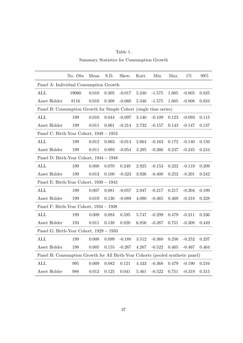
Table 1.
Summary Statistics for Consumption Growth
No. Obs Mean S.D. Skew. Kurt. Min Max 1% 99%
Panel A: Individual Consumption Growth
ALL 19060 0.010 0.305 -0.017 5.240 -1.575 1.605 -0.805 0.825
Asset Holder 8116 0.010 0.308 -0.060 5.346 -1.575 1.605 -0.808 0.834
Panel B: Consumption Growth for Simple Cohort (single time series)
ALL 199 0.010 0.044 -0.097 3.140 -0.109 0.123 -0.093 0.115
Asset Holder 199 0.011 0.061 -0.214 2.732 -0.157 0.143 -0.147 0.137
Panel C: Birth-Year Cohort, 1949− 1953
ALL 199 0.012 0.063 -0.014 2.664 -0.163 0.172 -0.140 0.150
Asset Holder 199 0.011 0.093 -0.054 3.295 -0.266 0.247 -0.245 0.244
Panel D: Birth-Year Cohort, 1944− 1948
ALL 199 0.008 0.070 0.249 2.925 -0.153 0.222 -0.119 0.209
Asset Holder 199 0.013 0.100 -0.323 3.926 -0.408 0.252 -0.201 0.242
Panel E: Birth-Year Cohort, 1939− 1943
ALL 199 0.007 0.081 -0.057 2.947 -0.217 0.217 -0.204 0.199
Asset Holder 199 0.019 0.130 -0.089 4.090 -0.465 0.469 -0.318 0.328
Panel F: Birth-Year Cohort, 1934− 1938
ALL 199 0.009 0.094 0.595 5.747 -0.299 0.479 -0.211 0.236
Asset Holder 193 0.011 0.138 0.820 6.856 -0.387 0.751 -0.308 0.449
Panel G: Birth-Year Cohort, 1929− 1933
ALL 199 0.008 0.099 -0.188 3.512 -0.368 0.256 -0.252 0.237
Asset Holder 198 0.005 0.155 -0.267 4.267 -0.522 0.465 -0.467 0.464
Panel H: Consumption Growth for All Birth-Year Cohorts (pooled synthetic panel)
ALL 995 0.009 0.082 0.121 4.433 -0.368 0.479 -0.190 0.216
Asset Holder 988 0.012 0.125 0.041 5.461 -0.522 0.751 -0.319 0.315
37
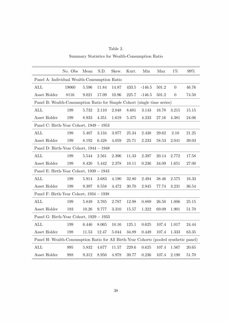
Table 2.
Summary Statistics for Wealth-Consumption Ratio
No. Obs Mean S.D. Skew. Kurt. Min Max 1% 99%
Panel A: Individual Wealth-Consumption Ratio
ALL 19060 5.596 11.84 14.87 433.5 -146.5 501.2 0 46.76
Asset Holder 8116 9.021 17.09 10.96 225.7 -146.5 501.2 0 74.50
Panel B: Wealth-Consumption Ratio for Simple Cohort (single time series)
ALL 199 5.732 2.110 2.048 8.601 3.143 16.78 3.215 15.15
Asset Holder 199 8.933 4.351 1.619 5.475 4.233 27.16 4.381 24.06
Panel C: Birth-Year Cohort, 1949− 1953
ALL 199 5.407 3.134 3.977 25.34 2.438 29.62 2.10 21.25
Asset Holder 199 8.192 6.428 4.059 25.71 2.233 58.53 2.041 39.03
Panel D: Birth-Year Cohort, 1944− 1948
ALL 199 5.544 2.561 2.396 11.33 2.397 20.14 2.772 17.58
Asset Holder 199 8.420 5.442 2.378 10.11 0.236 34.09 1.651 27.00
Panel E: Birth-Year Cohort, 1939− 1943
ALL 199 5.914 3.683 4.190 32.80 2.494 38.46 2.575 16.33
Asset Holder 199 9.397 8.558 4.472 30.70 2.945 77.74 3.231 36.54
Panel F: Birth-Year Cohort, 1934− 1938
ALL 199 5.849 3.765 2.787 12.98 0.889 26.50 1.006 25.15
Asset Holder 193 10.26 9.777 3.310 15.57 1.322 69.09 1.901 51.70
Panel G: Birth-Year Cohort, 1929− 1933
ALL 199 6.446 8.065 10.16 125.1 0.625 107.4 1.017 24.44
Asset Holder 198 11.53 12.47 5.044 34.89 0.449 107.4 1.333 63.35
Panel H: Wealth-Consumption Ratio for All Birth-Year Cohorts (pooled synthetic panel)
ALL 995 5.832 4.677 11.57 229.6 0.625 107.4 1.567 20.65
Asset Holder 988 9.312 8.950 4.978 39.77 0.236 107.4 2.190 51.70
38
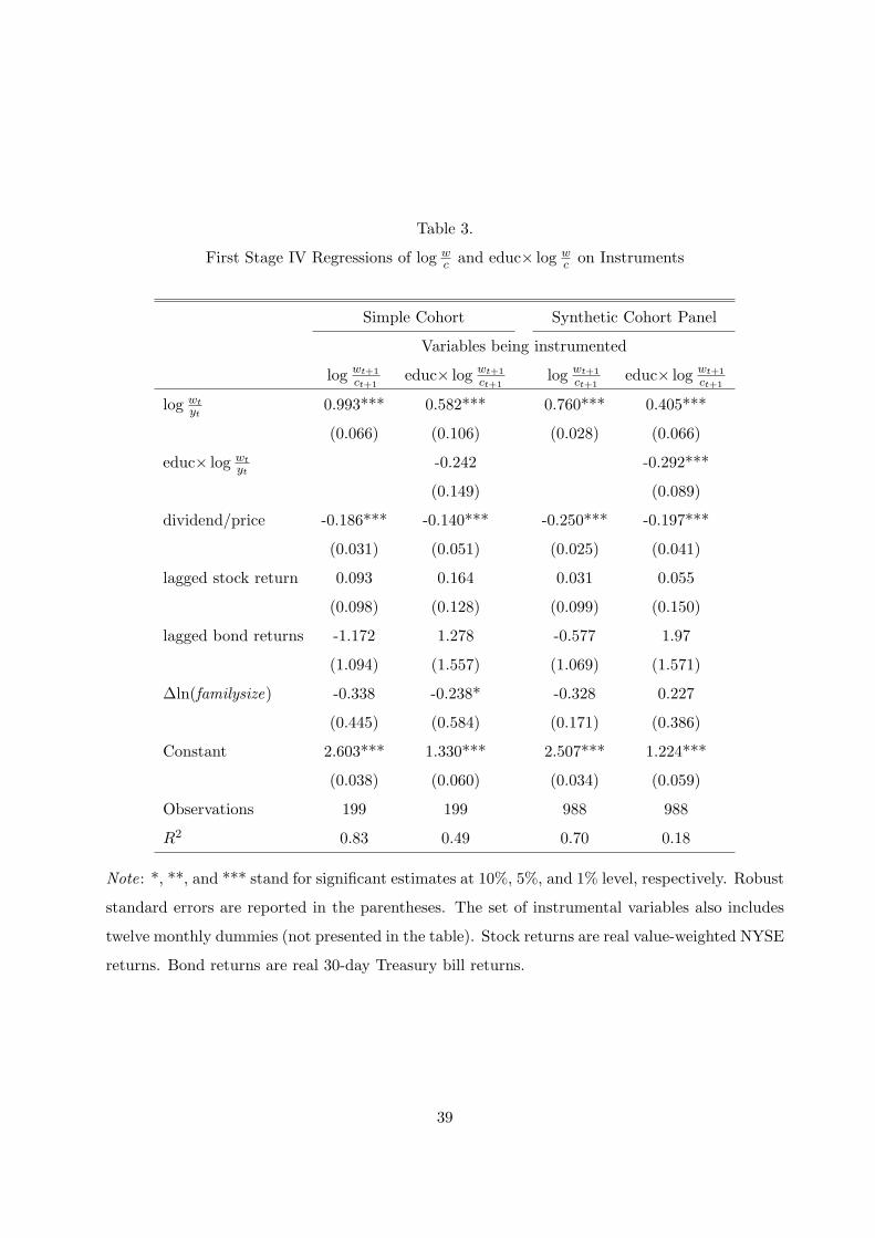
Table 3.
First Stage IV Regressions of log wc and educ× log w
c on Instruments
Simple Cohort Synthetic Cohort Panel
Variables being instrumented
log wt+1
ct+1educ× log wt+1
ct+1log wt+1
ct+1educ× log wt+1
ct+1
log wtyt
0.993*** 0.582*** 0.760*** 0.405***
(0.066) (0.106) (0.028) (0.066)
educ× log wtyt
-0.242 -0.292***
(0.149) (0.089)
dividend/price -0.186*** -0.140*** -0.250*** -0.197***
(0.031) (0.051) (0.025) (0.041)
lagged stock return 0.093 0.164 0.031 0.055
(0.098) (0.128) (0.099) (0.150)
lagged bond returns -1.172 1.278 -0.577 1.97
(1.094) (1.557) (1.069) (1.571)
∆ln(familysize) -0.338 -0.238* -0.328 0.227
(0.445) (0.584) (0.171) (0.386)
Constant 2.603*** 1.330*** 2.507*** 1.224***
(0.038) (0.060) (0.034) (0.059)
Observations 199 199 988 988
R2 0.83 0.49 0.70 0.18
Note: *, **, and *** stand for significant estimates at 10%, 5%, and 1% level, respectively. Robust
standard errors are reported in the parentheses. The set of instrumental variables also includes
twelve monthly dummies (not presented in the table). Stock returns are real value-weighted NYSE
returns. Bond returns are real 30-day Treasury bill returns.
39
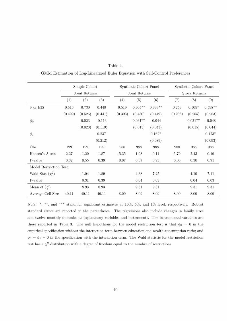
Table 4.
GMM Estimation of Log-Linearized Euler Equation with Self-Control Preferences
Simple Cohort Synthetic Cohort Panel Synthetic Cohort Panel
Joint Returns Joint Returns Stock Returns
(1) (2) (3) (4) (5) (6) (7) (8) (9)
σ or EIS 0.516 0.730 0.440 0.519 0.905** 0.999** 0.259 0.505* 0.598**
(0.499) (0.525) (0.441) (0.393) (0.430) (0.449) (0.238) (0.265) (0.283)
φ0 0.023 -0.113 0.031** -0.044 0.031** -0.048
(0.023) (0.119) (0.015) (0.043) (0.015) (0.044)
φ1 0.237 0.162* 0.173*
(0.212) (0.089) (0.093)
Obs 199 199 199 988 988 988 988 988 988
Hansen’s J test 2.27 1.20 1.87 5.35 1.98 0.14 5.79 2.43 0.19
P-value 0.32 0.55 0.39 0.07 0.37 0.93 0.06 0.30 0.91
Model Restriction Test:
Wald Stat (χ2) 1.04 1.89 4.38 7.25 4.19 7.11
P-value 0.31 0.39 0.04 0.03 0.04 0.03
Mean of (wc ) 8.93 8.93 9.31 9.31 9.31 9.31
Average Cell Size 40.11 40.11 40.11 8.09 8.09 8.09 8.09 8.09 8.09
Note: *, **, and *** stand for significant estimates at 10%, 5%, and 1% level, respectively. Robust
standard errors are reported in the parentheses. The regressions also include changes in family sizes
and twelve monthly dummies as explanatory variables and instruments. The instrumental variables are
those reported in Table 3. The null hypothesis for the model restriction test is that φ0 = 0 in the
empirical specification without the interaction term between education and wealth-consumption ratio; and
φ0 = φ1 = 0 in the specification with the interaction term. The Wald statistic for the model restriction
test has a χ2 distribution with a degree of freedom equal to the number of restrictions.
40
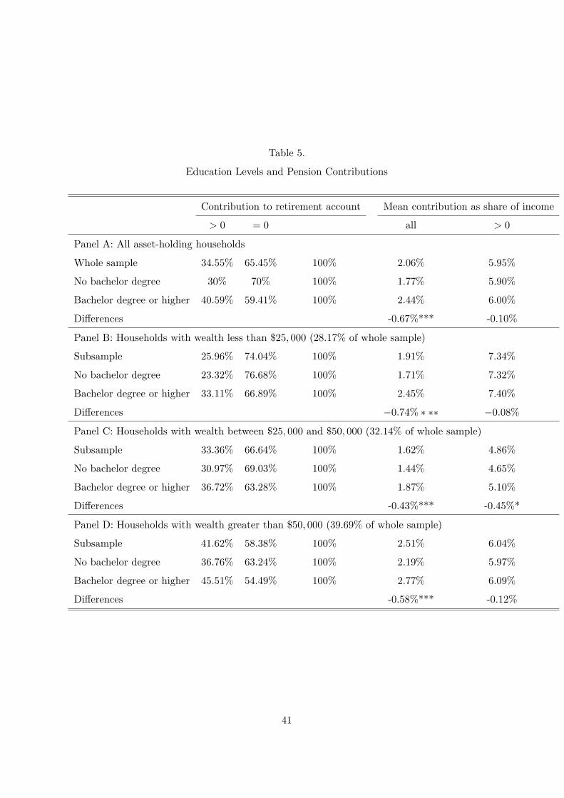
Table 5.
Education Levels and Pension Contributions
Contribution to retirement account Mean contribution as share of income
> 0 = 0 all > 0
Panel A: All asset-holding households
Whole sample 34.55% 65.45% 100% 2.06% 5.95%
No bachelor degree 30% 70% 100% 1.77% 5.90%
Bachelor degree or higher 40.59% 59.41% 100% 2.44% 6.00%
Differences -0.67%*** -0.10%
Panel B: Households with wealth less than $25, 000 (28.17% of whole sample)
Subsample 25.96% 74.04% 100% 1.91% 7.34%
No bachelor degree 23.32% 76.68% 100% 1.71% 7.32%
Bachelor degree or higher 33.11% 66.89% 100% 2.45% 7.40%
Differences −0.74% ∗ ∗∗ −0.08%
Panel C: Households with wealth between $25, 000 and $50, 000 (32.14% of whole sample)
Subsample 33.36% 66.64% 100% 1.62% 4.86%
No bachelor degree 30.97% 69.03% 100% 1.44% 4.65%
Bachelor degree or higher 36.72% 63.28% 100% 1.87% 5.10%
Differences -0.43%*** -0.45%*
Panel D: Households with wealth greater than $50, 000 (39.69% of whole sample)
Subsample 41.62% 58.38% 100% 2.51% 6.04%
No bachelor degree 36.76% 63.24% 100% 2.19% 5.97%
Bachelor degree or higher 45.51% 54.49% 100% 2.77% 6.09%
Differences -0.58%*** -0.12%
41

1 2 3 4 5 6 7 8 9 100
0.2
0.4
0.6
0.8
1
1.2
1.4
Risk aversion: γ
Tem
pta
tion: φ
CEX dataPoint estimates
Figure 1:—Temptation and the Hansen-Jagannathan bound
42
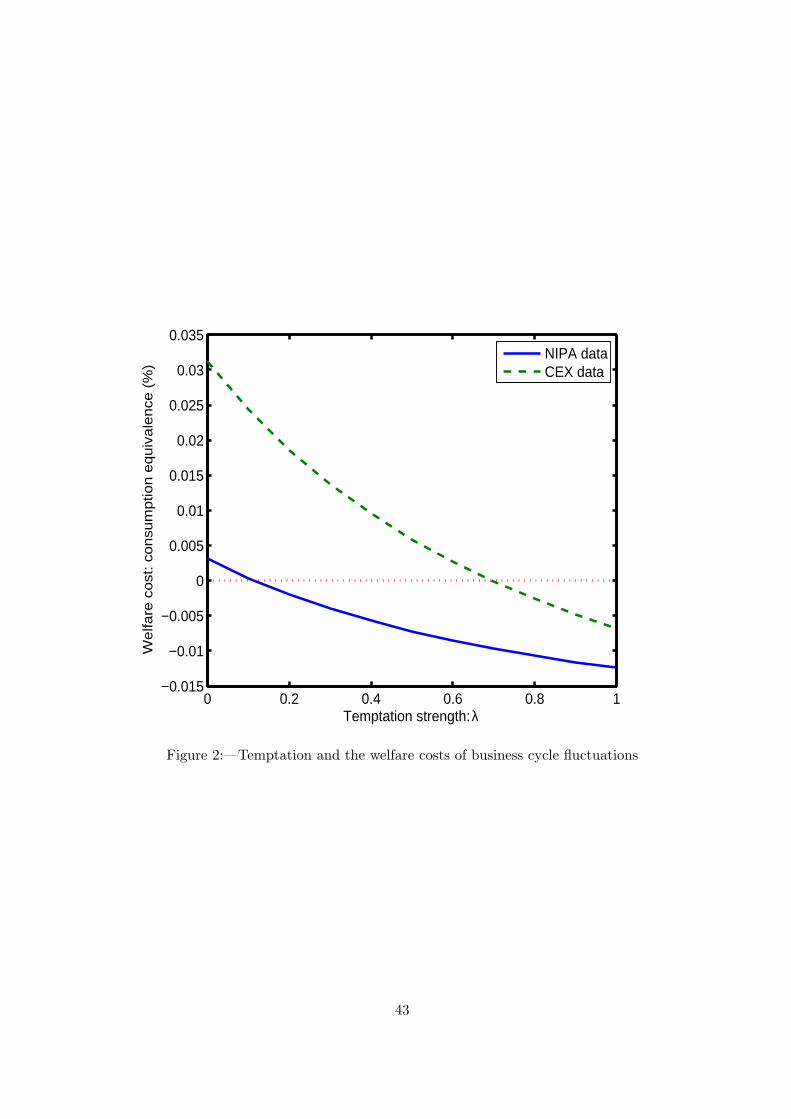
0 0.2 0.4 0.6 0.8 1−0.015
−0.01
−0.005
0
0.005
0.01
0.015
0.02
0.025
0.03
0.035
Temptation strength: λ
We
lfare
co
st:
con
sum
ptio
n e
qu
iva
len
ce (
%)
NIPA dataCEX data
Figure 2:—Temptation and the welfare costs of business cycle fluctuations
43