can temptation explain housing choices in later life?
TRANSCRIPT

Viola Angelini, Alessandro Bucciol, Matthew Wakefield and Guglielmo Weber Can Temptation Explain Housing Choices in Later Life?
DP 05/2013-021
1
Can Temptation Explain Housing Choices in Later Life?*
Viola Angelini†
Alessandro Bucciol‡
Matthew Wakefield§
Guglielmo Weber**
This version: 26 May 2013
Abstract. We use individual life-history data on twelve European countries to investigate the role of
temptation in explaining the decision to become home-owners relatively late in life. The model we
consider takes into account the standard motives for saving and investing in illiquid assets such as
housing and individual retirement accounts, but recognizes that illiquid assets may be used by
individuals who find it hard to procrastinate current consumption to control the temptation linked to
having plenty of cash on hand. The evidence we produce is consistent with the notion that tempted
individuals first resort to illiquid financial assets to control temptation, but as retirement age approaches
they are more likely to use home-ownership as a commitment device.
JEL codes: D12; D14; G11.
Keywords: Temptation; Housing; Duration models; Bivariate mixed proportional hazard.
* The paper is part of the project entitled “Temptation and Housing in Later Life” and financed by the 2012 Netspar research grant. We thank Monika Bütler for useful suggestions and Hans Melberg for sharing his Stata code with us. The usual disclaimers apply. This paper uses data from SHARE wave 2 release 2.5.0, as of May 24th 2011 and SHARELIFE release 1, as of November 24th 2010. The SHARE data collection has been primarily funded by the European Commission through the 5th Framework Programme (project QLK6-CT-2001-00360 in the thematic programme Quality of Life), through the 6th Framework Programme (projects SHARE-I3, RII-CT-2006-062193, COMPARE, CIT5- CT-2005-028857, and SHARELIFE, CIT4-CT-2006-028812) and through the 7th Framework Programme (SHARE-PREP, N° 211909, SHARE-LEAP, N° 227822 and SHARE M4, N° 261982). Additional funding from the U.S. National Institute on Aging (U01 AG09740-13S2, P01 AG005842, P01 AG08291, P30 AG12815, R21 AG025169, Y1-AG-4553-01, IAG BSR06-11 and OGHA 04-064) and the German Ministry of Education and Research as well as from various national sources is gratefully acknowledged (see www.share-project.org for a full list of funding institutions). † University of Groningen and Netspar. E-mail: [email protected] ‡ University of Verona and Netspar. E-mail: [email protected] § University of Bologna and IFS. E-mail: [email protected] ** University of Padua and IFS. E-mail: [email protected]

2
1. Introduction
The standard life-cycle model predicts that households should accumulate assets while working, and
decumulate these assets to fund consumption spending in retirement. Recent economic research has
identified certain stylised facts about retirement saving that seem puzzling within this benchmark. One
strand of literature has discussed the “retirement savings puzzle” that households seem to experience a
discrete drop, rather than a smooth change, in consumption at the time they retire. A second puzzle is
the fact that households seem to demand assets that commit them to lock away their funds for fixed
periods of time, even though such commitment reduces the opportunity to use wealth in times of
unexpected “rainy day” need. A third fact that relatively simple models cannot easily explain is the
relatively slow rate at which older households seem to decumulate wealth, with some retirees even
continuing to save. (See Attanasio and Weber, 2010, for a review of this and other puzzles). To this (by
no means exhaustive) list, we may add the issue that elderly households seem reluctant to utilise their
housing wealth to fund spending (a “no downsizing puzzle”). Angelini et al. (2009), for example,
document using European (SHARE) data that many elderly households are house-rich and cash-poor
but do not use their housing equity to fund non-housing consumption after retirement.
Many different ways to explain puzzles such as those listed above have been suggested. As highlighted
by Attanasio and Weber (2010), non-standard preferences, such as quasi-hyperbolic discounting
(Laibson, 1997, O’Donoghue and Rabin, 1999) or temptation preferences (Gul and Pesendorfer, 2001,
2004; Bucciol, 2012), may explain a taste for commitment in investment decisions and so contribute to
the explanation of several apparent puzzles. The aim of this paper is, using European data, to
investigate the empirical support for the idea that temptation, and a consequent taste for commitment,
may be important in shaping retirement saving decisions. As we describe below, our interest is not only
in financial accumulation, but particularly in the choices of older workers and retirees about home-
ownership.
Understanding how and why individuals make the (retirement) saving and investment decisions that
they do is of interest for both academic audiences and pensions practitioners. Understanding the
reasons why individuals choose to own their home and largely fail to reduce housing equity in the last
years of their life, is also an interesting research agenda for economists and social scientists (Venti and
Wise, 2004; Angelini et al., 2012) and has important policy implications in ageing societies.
As emphasized above, we are particularly interested in understanding the “no downsizing puzzle” or
even the “upsizing puzzle” whereby many households are observed to purchase their homes late in life
(at least late in the working life). Several possible explanations have been proposed: see Nakajima and
Telyukova (2011) for a survey and detailed analysis of home equity release in old age in a rich life-cycle

3
model under uncertainty. The innovation of our research is to examine whether temptation
preferences, which can plausibly help to explain other consumption-saving puzzles for older
households, might also help explain not only the reluctance to spend housing wealth, but also the
decision to purchase the main residence relatively late in life.
Temptation preferences give a high value to the commitment property of illiquid assets such as
housing: since illiquid wealth cannot be disinvested immediately, agents cannot succumb to the
temptation to spend it on current consumption. Removing this temptation can make agents better-off
as they face lower self-control costs in trying to implement optimal forward-looking consumption and
saving plans. Tempted individuals – who typically face a no-unsecured-borrowing condition that
prevents them from falling into heavy debt early in life – look for ways to tie their hands, for example
through holding illiquid assets. After retirement (once retirement accounts enter the decumulation
phase), housing is the main (or often the only) illiquid asset that families can still choose to invest in. If
temptation is a key driver of saving decisions, and particularly decisions about retirement savings, then
this should affect households’ decisions about how much to invest in housing in the run up to
retirement, and about how quickly (or slowly) they run down housing wealth once retired.
Prima facie evidence for the role of housing wealth as a commitment device can be sought in micro
data by investigating whether mature home-owners are more likely to have engaged in other activities
that also help control temptation. In particular, individuals may engage in long-term saving plans by
investing in life-insurance policies and/or individual retirement accounts. An ideal household level
dataset containing information on holdings of these different assets is SHARE (Survey of Health,
Ageing and Retirement in Europe). Using this dataset we are able to relate behaviour regarding holding
and accumulation of these different assets to characteristics such as education and risk-taking
behaviour, as well demographic and economic variables.
The purpose of this paper is to understand whether the decision to purchase a house for the first time
is influenced by the holding of illiquid financial assets (retirement accounts and life insurance policies),
that can be seen as ways to tie one’s hands (commitment devices). We perform a discrete-time duration
analysis through a logit regression model. This allows us to estimate the hazard rate of first owning a
house, conditional on the ownership of illiquid financial assets and a number of observable
characteristics, including a measure of permanent income. Given that ownership of illiquid financial
assets may proxy for differences in unobserved characteristics, we also allow for unobserved
heterogeneity, and check how the relationship between becoming a homeowner and the ownership of
illiquid financial assets varies across the population of interest.

4
The remainder of the paper is organised as follows. Section 2 sketches a theoretical framework for the
temptation and self-control motive; Section 3 describes the data; Sections 4 and 5 comment on the
parameter estimates of the duration model with and without unobserved heterogeneity. Section 6
concludes.
2. A Theoretical Framework
Gul and Pesendorfer (2001) build a theoretical framework for temptation and a self-control motive,
where agents have preferences not only over alternatives but also over sets of alternatives. They define
as tempting those alternatives that are sub-optimal from a forward-looking perspective, but optimal
from a myopic perspective. When making their decisions, agents face a utility cost to exert self-control
and avoid tempting alternatives. In the framework of Gul and Pesendorfer (2001), an agent may
therefore prefer a given set of alternatives to another, larger set that includes the first set plus some
further tempting alternatives. Hence, the use of commitment devices may lead to an improvement in
wellbeing. For instance in the context of consumption decisions, a mandatory pension system is a
commitment device because it forces an individual to postpone consumption in to old age. Our analysis
derives from a variant of this framework that also includes housing and illiquid assets. We briefly
describe it below.
Consider a life-cycle model where an individual lives at most for T years and every year t has to choose
non-durable consumption 0tc , the allocation of private savings between liquid and illiquid assets
(through the portfolio weight 0,1tw of savings allocated to illiquid assets), and housing tenure,
1,0th conditional on cash-on-hand (financial wealth plus disposable income) at the beginning of the
year, tx , and housing tenure in the previous period, 1th . The housing tenure state variable is just an
indicator for renting ( 0th ) or owning ( 1th ) the home.
Cash-on-hand tx evolves according to exogenous factors (income and market returns) and endogenous
factors (consumption and the purchase/selling of a house). When purchasing/selling a house, a
transaction cost φ proportional to the house price is paid. In addition, every year the homeowner
spends a fraction 0,1 of the owned house value on repair and maintenance costs (Li and Yao,
2007). In contrast, when a household rents a house, it is free to change the rent size every year at no
additional costs. The intertemporal budget constraint is then

5
1
0
1 1
11 1 2
t
t t
t t t t t h
t t
t t t t t t h h
x c p h p Ix R y
p h p h p h I
where R is the exogenous market return (that we assume fixed and certain), 1ty is next-year’s income,
tp is the rent cost (rent prices are a fraction ρ of ownership prices)1, 1 t tp h is the cost of
buying a new house, grossed up by the transaction cost, and 11 t tp h is the amount, net of
transaction costs, received after selling the old house. If the individual opts for making no change in
housing owned from one year to another, then 1t th h and the term 12
t tt t h h
p h I
removes
transaction costs from the equation. 0thI
is an index function that takes value 1 if the individual is a
renter ( 0th ), and 0 otherwise, while 1t th hI
is an index function that has value 1 if there is no
change in housing tenure (when 1t th h ), and 0 otherwise.
As regards liquid and illiquid assets, for the sake of simplicity we assume that they provide the same
return R, so that the portfolio allocation between liquid and illiquid assets is not driven by their returns.
The decision on the portfolio weight tw is instead relevant on the immediate availability of savings for
consumption and housing needs: only liquid assets are immediately available, while illiquid assets will be
available only after a certain amount of time (s periods, say). In this context, a non-tempted individual
should always prefer the liquid asset, whilst tempted individuals will prefer to hold a fraction of wealth
in illiquid assets, because of their commitment role.
The individual is liquidity constrained, which means that her consumption tc cannot exceed the
portion of cash-on-hand available at the moment, that is, 11 1t t t t t tc w x p p h . That is,
the tempting alternative is the fraction of cash-on-hand tx invested in liquid assets (1 tw ), net of the
rent cost tp , plus the lump-sum value of the house owned in period t-1, and sold in period t with a
transaction cost φ. Notice that the largest consumption at time t can be achieved only in the presence
of: i) full investment in liquid assets; and, ii) home rent rather than home ownership; and it coincides
with *
1max 1t t t t t tc c x p p h .
In a fashion similar to Gul and Pesendorfer (2001, 2004), the uniperiodal utility function is defined as
(1) 1, , , 1 ,0 ,t t t t t t t t t t t tU c h x u c h u x p p h u c h
1 That is, the ownership of one unit of housing costs (1/ρ) times the rent of the same unit of housing.

6
where the first addend, ,t tu c h , is the utility function in standard models, and the second addend
describes a temptation motive with parameter λ, where 11 1 ,0t t t t tu w x p p h is the
utility reflecting the tempting, myopic behaviour, obtained with home renting and the largest possible
immediate consumption, and ,t tu c h is the utility reflecting the actual decisions. The second addend
can also be seen as the cost of exerting self-control and resisting temptation.
In order to increase the utility function (1), an agent should reduce the cost of self-control. In a myopic
perspective, this is possible if she succumbs to temptation, and makes tempting decisions. In a forward-
looking perspective, a preferable alternative may be that the agent ties her hands and commits herself to
some decisions (e.g., home ownership and investment in illiquid assets) that reduce the future
consumption choice set, therefore lowering the size of the tempting alternative. Throughout our
analysis, therefore, we interpret the ownership of illiquid assets and housing as evidence of temptation.
3. The Data
Our main source of micro data is SHARELIFE, the third wave of the Survey of Health, Ageing and
Retirement in Europe (SHARE), that asks respondents aged 50 and over to record life-history events
regarding housing, health, children, relationships and financial investments. For our purposes
information on previous investments in retirement accounts and life insurance policies (i.e., illiquid
financial assets) is particularly relevant. Those who have invested are also asked about the year in which
the first investment in each type of asset occurred. The respondents are a representative sample of the
50+ population in thirteen European countries but we exclude Poland from the analysis because of
unreliable retrospective information on income. Information from SHARELIFE is merged with
information on income and education from the second wave of SHARE (we consider the average over
the 5 “constructed variables” imputations), and with permanent income estimates elaborated from
Weiss (2012).
We reshape SHARELIFE as a longitudinal dataset, that is, for each respondent we have as many
observations as her previous years of adult age. By “adult age” we mean any age between 19 and 80, or
between the age in which the individual became independent (when she started to live on her own or
when she established her own household) and the age in the year before the interview. Our benchmark
analysis concentrates on the age range 40-70, when the temptation motive for home-ownership is most
likely to be playing a key role (Angelini et al, 2012, document the presence of a non-negligible number
of rent-own transitions in many European countries until age 70).

7
Our dependent variable is the dummy variable “owner”, taking the value 1 if the individual is home-
owner at a given age, and 0 otherwise. We include in the sample all observations from individuals who
have never been home-owners (for whom the variable “owner” is equal to 0 at all ages), and, for
individuals who have owned their home, all observations up to the age at which the home-ownership
first occurred (thus for these observations the variable “owner” is equal to 0 at all ages but the last one).
Appendix Table A1 reports the definition of all the variables used in this analysis. The specification is
made of five groups of variables: financial ones (illiquid assets, i.e., life insurance policies and retirement
accounts, and risk tolerance2), demographics (age, years of independence, gender, education, health
status), household composition (marital status, children, household size), occupation (unemployment,
retired, permanent income), and finally control variables (country, cohort). Most variables are taken in
their level one year before. For the asset variables, we consider the level two years before, plus the
number of years elapsed since the first investment. Summary statistics of these variables are reported in
Table 1 for the full sample and in Table 2 for the sample in age 40-70.
TABLE 1 ABOUT HERE
TABLE 2 ABOUT HERE
4. Estimates from a model without unobserved heterogeneity
We first present parameter estimates of a discrete duration model, estimated with a standard logit
regression following Jenkins (1995). Tables 3 and 4 display the estimates of the coefficients of main
interest, respectively in the full sample and in the sample aged 40-70. We refer to the Appendix for the
whole set of parameter estimates.
TABLE 3 ABOUT HERE
2 We use the self-assessed answer to a question on portfolio allocation between riskless and risky assets. Available options are: (1) Take substantial financial risks expecting to earn substantial returns; (2) Take above average financial risks expecting to earn above average returns; (3) Take average financial risks expecting to earn average returns; (4) Not willing to take any financial risks. Most answers are concentrated in option (4). The variable we include in the specification is a dummy equal to 1 if the individual declares to be willing to take at least some risk, i.e., if she reports any option between (1) and (3).

8
Columns (1) to (3) of Table 3 display the parameters of interest for the equation explaining the
probability of first becoming a home-owner as a function of income (respectively current, permanent
including pensions, and permanent excluding pensions), ownership of liquid assets and risk attitude,
controlling for age, gender, education, time-varying demographics (family size, marital status, presence
of children), employment status, country and cohort dummies. Column (4) displays instead the average
marginal effects corresponding to column (3) estimates, multiplied by 100.
We see from column (1) that current income has a strong, positive effect – having illiquid assets also
has a major, positive impact (in line with our expectations if consumers use them as a commitment
device to keep temptation under control), but the longer the individual has had them, the weaker the
effect (in fact, the sign is reversed after 14 years of holding them). Risk tolerance (defined as a dummy
equal to one if the individual declares at least some willingness to take financial risk) also increases the
probability of becoming a home-owner.
In column (2) we replace the log of current income with the log of permanent income, computed as the
discounted present value at age ten of all future earnings plus pension benefits (for details on how this
measure was computed see Weiss, 2012). This is a much more appropriate conditioning variable, as it
captures long term differences in resources that should explain why people choose to purchase illiquid
financial assets and to become home-owners. Permanent income plays a very strong role in explaining
the transition into home-ownership, but the coefficients on the other variables of interest are fairly
stable.
In column (3) we focus on a narrower definition of permanent income that includes earnings but
excludes pensions (as these may be in part affected by the decision to invest in individual retirement
accounts). This measure also has the predicted, very strong, positive coefficient, with little effect on the
other coefficients.
To better understand the economic meaning of the estimated coefficients, we report in column (4) the
average marginal effects multiplied by 100: this can be interpreted as the effect of a unit increase in the
explanatory variable on the percentage probability of transiting into home-ownership in a given year.
Thus a 1% increase in permanent income increase the probability of becoming a home-owner by .33%;
having illiquid assets increases the probability by almost half a percentage point, but this effect is halved
after six years; finally, individuals classified as risk tolerant are almost one percent more likely to
become home-owners in any given year (conditionally on not being home-owners already).
A potentially more interesting analysis is presented in Table 4, where the sample is restricted to the 40-
70 age band. Home-ownership early in life is likely to be dominated by family formation and the birth
of children, as well as by access to credit. By age forty, most individuals have reached a stable situation
in terms of income, demographics (except for cases such as divorce, which we control for in our

9
regressions) and credit worthiness, so housing transitions become rarer, particularly the rent-own
transitions we focus on in this paper.
We see that the signs and significance of estimated coefficients is broadly in line between tables 3 and 4,
but with larger absolute values of the coefficients on illiquid assets. Average marginal effects are instead
all smaller, reflecting the decreased number of transitions in the 40-70 sample. However, the average
marginal effect of having illiquid assets is slightly more important in relative terms compared to
permanent income (but the relative difference is quite small), and is now reversed after about 25 years
of holding the asset (rather than 14).
TABLE 4 ABOUT HERE
We conclude the section with a graphical representation of the hazard rates of home ownership,
conditional on the holding on non-liquid financial assets. The hazard rate of home ownership at age t
can be computed as
1
1 expth t x
x
where x is the set of average explanatory variables, and are the parameter estimates from the model
using permanent income without pensions (column (3) of Appendix tables A2-A3); the hazard rate age
profiles are similar using the output from the other columns.
Figure 1 plots the hazard rate-age profile from the full sample, showing a standard inverted-U shape
peaking at age 40. Importantly, hazard rates for households holding illiquid assets are persistently
higher than hazard rates for households not holding them.3 This evidence is confirmed in Figure 2
when restricting the attention to the sample in age 40-70.
FIGURE 1 ABOUT HERE
FIGURE 2 ABOUT HERE
3 The two curves in each figure are identical apart from the assumption on the holdings of illiquid assets two years before.
10
5. Estimates from a model that allows for unobserved heterogeneity
The estimates presented above do not take into account the potential confounding effect of
unobserved heterogeneity in the desire to resist temptation or access to illiquid financial investment. It
is possible that equally tempted individuals react differently to their temptation: some are more likely to
lock themselves in IRAs, to later become home-owners (as a way to have a guaranteed stream of
housing consumption services for the rest of their lives); others instead cannot do so, because this form
of financial investment is not available to them, or will not do so because they don’t value future
consumption enough (they are not only tempted, but also highly impatient).
This type of issue has been recently investigated in the context of drug use. There the question of
substance is whether the strong cross-sectional association between cannabis use and hard drugs use is
due to some innate personality trait (frailty) or instead one can identify a “gateway effect” whereby
cannabis is a stepping stone for hard drugs. Both van Ours (2003) and Melberg et al (2010) tackle this
issue by specifying a latent class model where the hazard of using hard drugs is affected by previous use
of cannabis, but some or all estimated parameters can differ across endogenously determined sub-
groups of the population. Typically, this analysis highlights the presence of two such groups, one of
which appears more prone to using drugs, the other more resistant. The estimates of the coefficients of
interest typically change when heterogeneity is allowed to play a role, and this allows the identification
of what part of the cannabis use effect is due to unobserved heterogeneity, and what part instead can
be interpreted as a causal (gateway) effect.
Here we adopt the more general approach taken by Melberg et al (2010), whereby all parameters
entering the logit model are allowed to vary across the two groups. The authors use the bivariate mixed
proportional hazard model with shared frailty introduced in Abbring and Van Den Berg (2003). The
model is made of two logistic regression equations, describing the outcome and treatment variables. In
our case the treatment is identified by the ownership of illiquid assets (life insurance policies or
retirement accounts), while the outcome is identified by home ownership. This model allows us to
estimate how the probability to become a home-owner changes with and without the holding of illiquid
assets. We also estimate the probability that each observation belongs to either group. In Table 5 we
report key average marginal effects (multiplied by 100) based on parameter estimates for the full
sample, while in Table 6 we present the same results for the 40-70 age group. Descriptive statistics for
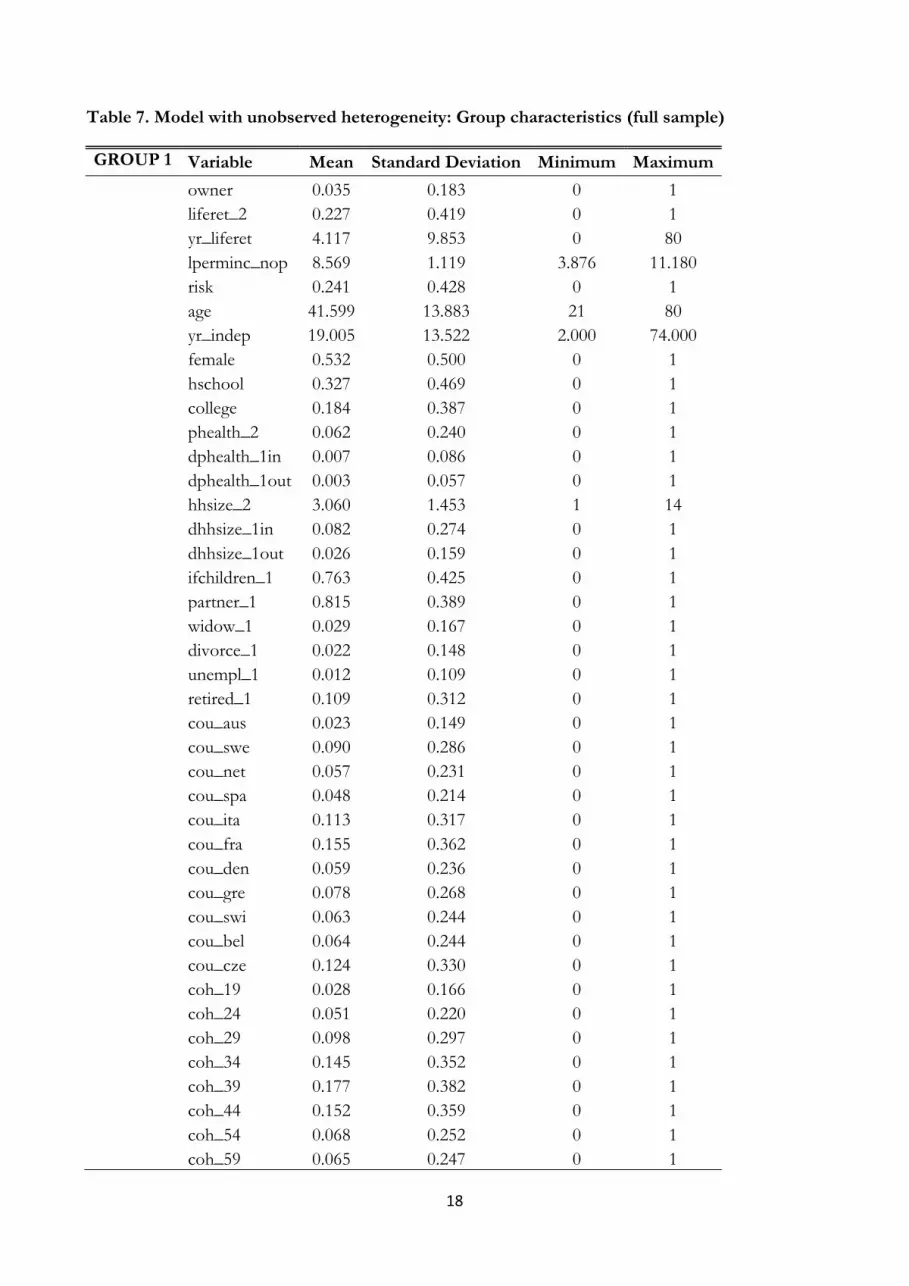
all variables, weighted by the predicted probability of belonging to each group, are presented in tables 7
and 8.
In column (2) of Table 5 we report the average marginal effects corresponding to the no heterogeneity
model already presented in column (4) in Table 3. Column (1) does the same for the equation

11
predicting the probability of becoming the owner of illiquid assets. The estimated effects for this
outcome variable of permanent income and risk tolerance are very large and significant. Columns (3)
and (4) present the same effects computed using as weights the probabilities of belonging to group 1;
this group is characterized by a larger proportion of illiquid financial asset holders – so we may call
them “temptation resisters” – but also higher permanent income – so we may expect them to have
easier access to credit. Columns (5) and (6) use instead the probability of belonging to group 2. It is
worth stressing that a different logistic regression is estimated across the two groups (so differences in
average marginal effects do not reflect solely differences in variable means), and that each individual in
the sample can belong to either one group, or the other group, or both, depending on its predicted
probabilities (that generate the individual weights in the logistic regressions).
TABLE 5 ABOUT HERE
Given that temptation is a more plausible determinant of the rent-own transition in the 40-70 age
range, we repeat our exercise in this subsample; here we discuss the results presented in Table 6. It is
worth stressing that, for this age band, group 1 individuals have 10% more permanent income on
average than group 2 individuals, but are much more likely to own illiquid financial assets (39.5% of
group 1 households do, compared to 22.3% in group 2). See Table 8 for further details.
TABLE 6 ABOUT HERE
Perhaps the most striking feature of Table 6 is the huge difference between the estimated effect of
permanent income and risk tolerance on the probability of holding illiquid financial assets: when no
heterogeneity is included, these effects are larger than when unobserved heterogeneity is allowed for.
This difference is particularly strong for permanent income. Estimated average marginal effects are
much less affected by allowance for unobserved heterogeneity: permanent income and risk tolerance
are largely in line between the two groups, while we notice that for “temptation resisters” (group 1) the
probability of becoming a home-owner is less strongly affected by illiquid asset holding. This pattern of
coefficients seems in line with an explanation that focuses on limited access to illiquid financial
investment for group 2 individuals – and this can explain why permanent income effects are so
different across columns (1), (3) and (5) in both Tables 5 and 6.
12
TABLE 7 ABOUT HERE
TABLE 8 ABOUT HERE
6. Conclusion
In this paper we have used individual life-history data on twelve European countries to investigate the
role of temptation in explaining the decision to become home-owners relatively late in life.
The model we considered takes in to account the standard motives for saving and investing in illiquid
assets such as housing or retirement accounts. It also recognizes that illiquid assets may be used by
individuals who find it hard to resist the temptation presented by a large stock of accessible “cash on
hand”.
The prima facie evidence we produced is consistent with the notion that tempted individuals first resort
to illiquid financial assets to control temptation, but as retirement age approaches they are more likely
to use home-ownership as a commitment device. However, our estimates also suggest that there is a lot
of heterogeneity in the access to illiquid financial investment prior to home purchase, something that
may reflect institutional features of this specific type of financial markets, or more broadly different
access to credit across Europe at different points in time.
The analysis we presented in this paper is suggestive, but tentative – a structural model is necessary to
better investigate the commitment effect of the temptation preferences as opposed to limited access to
financial markets, credit constraints or other reasons (e.g., strategic interactions between non-
cooperative family members) that may induce a fraction of individuals to purchase their home relatively
late in their lives. This is left for future research.

13
References
Abbring J.H.. and G. Van Den Berg (2003). The Non-parametric Identification of Treatment Effects in
Duration Models. Econometrica, 71, 1491-1517
Angelini V., A. Brugiavini and G. Weber (2009). Ageing and Unused Capacity in Europe: Is There an
Early Retirement Trap? Economic Policy, 59, 453-508
Angelini V., A. Brugiavini and G. Weber (2012). The Dynamics of Homeownership among the 50+ in
Europe. CEPR Discussion Paper 888. Forthcoming, Journal of Population Economics.
Attanasio O. and G. Weber (2010). Consumption and Saving: Models of Intertemporal Allocation and
Their Implications for Public Policy. Journal of Economic Literature, 48, 693-751
Attanasio O., A. Leicester and M. Wakefield (2011). Do House Prices Drive Consumption Growth?
The Coincident Cycles of House Prices and Consumption in the UK. Journal of the European Economic
Association, 9, 399 - 435
Bucciol A. (2012). Measuring Self-control Problems: A Structural Estimation. Journal of the European
Economic Association, 10, 1084-1115
Gul F. and W. Pesendorfer (2001). Temptation and Self-Control. Econometrica, 69, 1403-1435.
Gul F. and W. Pesendorfer (2004). Self-Control and the Theory of Consumption. Econometrica, 72, 119-
158.
Jenkins S.P. (1995). Easy Estimation Methods for Discrete-Time Duration Models. Oxford Bulletin of
Economics and Statistics, 57, 129-136.
Laibson D. (1997). Golden Eggs and Hyperbolic Discounting. The Quarterly Journal of Economics, 112,
443-77.
Li W. and R. Yao (2007). The Life-Cycle Effects of House Price Changes. Journal of Money, Credit and
Banking, 39, 1375-1409.
Melberg H.O., A. Jones and A.L. Bretteville-Jensen (2010). Is Cannabis a Gateway to Hard Drugs?
Empirical Economics, 38, 583-603.
Nakajima M. and I.A. Telyukova (2011). Home Equity in Retirement. WP 11-15, the Federal Reserve
Bank of Philadelphia.
O'Donoghue T. and M. Rabin (1999). Doing It Now or Later. American Economic Review, 89, 103-124.
van Ours J.C. (2003). Is Cannabis a Stepping-Stone for Cocaine?, Journal of Health Economics, 22, 539-
554.
Venti S.F. and D.A. Wise (2004). Aging and Housing Equity: Another Look. In D. A. Wise (Ed.)
Perspectives on the Economics of Aging, University of Chicago Press, 127-180.
Weiss, C.T. (2012), “Two Measures of Lifetime Resources for Europe using SHARELIFE,” SHARE Working Paper (06-2012), Munich Center for the Economics of Aging (MEA).

14
Table 1. Summary statistics (full sample, N=248,628).
Variable Mean Standard Deviation Minimum Maximum
owner 0.035 0.184 0 1
liferet_2 0.205 0.404 0 1
yr_liferet 3.461 8.897 0 80
lperminc_nop 8.579 1.122 3.876 11.180
risk 0.251 0.434 0 1
age 41.441 13.962 21 80
yr_indep 19.080 13.599 2 74
female 0.556 0.497 0 1
hschool 0.340 0.474 0 1
college 0.187 0.390 0 1
phealth_2 0.061 0.239 0 1
dphealth_1in 0.008 0.087 0 1
dphealth_1out 0.004 0.059 0 1
hhsize_2 3.012 1.443 1 14
dhhsize_1in 0.082 0.274 0 1
dhhsize_1out 0.027 0.163 0 1
ifchildren_1 0.756 0.430 0 1
partner_1 0.803 0.398 0 1
widow_1 0.031 0.172 0 1
divorce_1 0.023 0.150 0 1
unempl_1 0.013 0.114 0 1
retired_1 0.105 0.306 0 1
cou_aus 0.039 0.194 0 1
cou_swe 0.075 0.263 0 1
cou_net 0.111 0.314 0 1
cou_spa 0.034 0.181 0 1
cou_ita 0.080 0.271 0 1
cou_fra 0.114 0.318 0 1
cou_den 0.081 0.272 0 1
cou_gre 0.047 0.211 0 1
cou_swi 0.091 0.288 0 1
cou_bel 0.093 0.291 0 1
cou_cze 0.119 0.324 0 1
coh_19 0.018 0.131 0 1
coh_24 0.050 0.218 0 1
coh_29 0.093 0.290 0 1
coh_34 0.133 0.340 0 1
coh_39 0.155 0.362 0 1
coh_44 0.174 0.379 0 1
coh_54 0.143 0.350 0 1
coh_59 0.065 0.247 0 1

15
Table 2. Summary statistics (restricted sample in age 40-70, N=110,795)
Variable Mean Standard deviation Minimum Maximum
owner 0.021 0.143 0 1
liferet_2 0.284 0.451 0 1
yr_liferet 5.633 11.029 0 70
lperminc_nop 8.475 1.121 3.925 11.056
risk 0.218 0.413 0 1
age 51.810 8.278 40 70
yr_indep 28.520 9.586 2 64
female 0.545 0.498 0 1
hschool 0.343 0.475 0 1
college 0.154 0.361 0 1
phealth_2 0.096 0.295 0 1
dphealth_1in 0.011 0.105 0 1
dphealth_1out 0.005 0.071 0 1
hhsize_2 3.199 1.507 1 14
dhhsize_1in 0.010 0.097 0 1
dhhsize_1out 0.048 0.214 0 1
ifchildren_1 0.850 0.357 0 1
partner_1 0.810 0.392 0 1
widow_1 0.046 0.209 0 1
divorce_1 0.034 0.182 0 1
unempl_1 0.019 0.138 0 1
retired_1 0.160 0.367 0 1
cou_aus 0.043 0.202 0 1
cou_swe 0.057 0.231 0 1
cou_net 0.117 0.321 0 1
cou_spa 0.035 0.184 0 1
cou_ita 0.085 0.278 0 1
cou_fra 0.101 0.301 0 1
cou_den 0.055 0.228 0 1
cou_gre 0.049 0.215 0 1
cou_swi 0.100 0.300 0 1
cou_bel 0.083 0.275 0 1
cou_cze 0.149 0.356 0 1
coh_19 0.019 0.138 0 1
coh_24 0.056 0.231 0 1
coh_29 0.102 0.302 0 1
coh_34 0.149 0.356 0 1
coh_39 0.170 0.376 0 1
coh_44 0.188 0.390 0 1
coh_54 0.113 0.316 0 1
coh_59 0.041 0.197 0 1

16
Table 3. Rent-Own transitions: model without unobserved heterogeneity (full sample)
(1) (2) (3) (4) Coefficients Coefficients Coefficients AME from (3)
Log current income 0.160*** (0.014) Log permanent income 0.148*** (0.017) Log permanent income 0.100*** 0.333*** (excluding pensions) (0.013) (0.042) Illiquid assets (t-2) 0.144*** 0.149*** 0.144*** 0.480*** (0.040) (0.044) (0.044) (0.147) Years with -0.011*** -0.013*** -0.012*** -0.041*** illiquid assets (0.003) (0.003) (0.003) (0.001) Risk tolerant 0.219*** 0.243*** 0.251*** 0.835*** (0.023) (0.024) (0.025) (0.082) Observations 319,530 255,254 248,628 248,628 Log-likelihood -44,680.774 -36,274.928 -35,445.548 -35,445.548 McFadden’s R2 0.061 0.065 0.066 0.066
Note. Column (1): we exclude observations reporting no income. Columns (2)-(3): we exclude observations on self-employed workers (8.89% of
the respondents) as well as the top and bottom 1% of the permanent income estimates. Column (4) reports 100 times the average marginal effects
(AME) from the model in Column (3). The full regression output is reported in the Appendix Table A2. Standard errors in parentheses; ***
p<0.01, ** p<0.05, * p<0.1
Table 4. Rent-Own transitions: model without unobserved heterogeneity (ages 40-70)
(1) (2) (3) (4)
Coefficients Coefficients Coefficients AME from (3)
Log current income 0.188***
(0.026)
Log permanent income 0.194***
(0.032)
Log permanent income 0.125*** 0.252***
(excluding pensions) (0.023) (0.047)
Illiquid assets (t-2) 0.155** 0.168** 0.186** 0.375**
(0.076) (0.083) (0.084) (0.170)
Years with -0.004 -0.007* -0.008** -0.015**
illiquid assets (0.003) (0.004) (0.004) (0.008)
Risk tolerant 0.242*** 0.321*** 0.323*** 0.652***
(0.045) (0.049) (0.049) (0.101)
Observations 144,174 114,205 110,795 110,795
Log-likelihood -14,066.649 -11,091.964 -10,716.014 -10,716.014
McFadden’s R2 0.044 0.045 0.046 0.046
Note. Column (1): we exclude observations reporting no income. Columns (2)-(3): we exclude observations on self-
employed workers (8.89% of the respondents) as well as the top and bottom 1% of the permanent income estimates.
Column (4) reports 100 times the average marginal effects (AME) from the model in Column (3). The full regression
output is reported in the Appendix Table A3. Standard errors in parentheses; *** p<0.01, ** p<0.05, * p<0.1

17
Table 5. Model with unobserved heterogeneity: key marginal effects (full sample)
No heterogeneity Heterogeneity, group 1 Heterogeneity, group 2
(1)
Illiquid assets
(2)
Home-
Ownership
(3)
Illiquid assets
(4)
Home-
Ownership
(5)
Illiquid assets
(6)
Home-
Ownership
Log permanent income 3.430*** 0.333*** 1.053*** 0.264*** 0.942*** 0.408***
(excluding pensions) (0.093) (0.042) (0.074) (0.054) (0.086) (0.059)
Illiquid assets (t-2) 0.480*** 0.459** 1.204***
(0.147) (0.210) (0.252)
Years with -0.041*** -0.069*** 0.001
illiquid assets (0.001) (0.013) (0.015)
Risk tolerant 3.341*** 0.835*** 1.425*** 0.719*** 1.754*** 0.935***
(0.176) (0.082) (0.140) (0.108) (0.155) (0.115)
Observations 248,628 248,628 206,925 206,925 155,536 155,536
Log-likelihood -111,405.190 -35,445.548 -22,797.909 -18,726.990 -22,710.209 -16,575.558
McFadden’s R2 0.162 0.066 0.690 0.057 0.615 0.083
Note. The table reports 100 times the average marginal effects from the bivariate mixed proportional hazard analysis
on the holding of illiquid assets and home ownership, unweighted (Columns (1)-(2)), and weighted, using as weights
the probability to belong to group 1 (Columns (3)-(4)) or group 2 (Columns (5)-(6)). The full regression output is
reported in the Appendix Table A4. Standard errors in parentheses; *** p<0.01, ** p<0.05, * p<0.1
Table 6. Model with unobserved heterogeneity: key marginal effects (ages 40-70)
No heterogeneity Heterogeneity, group 1 Heterogeneity, group 2
(1)
Illiquid assets
(2)
Home-
Ownership
(3)
Illiquid assets
(4)
Home-
Ownership
(5)
Illiquid assets
(6)
Home-
Ownership
Log permanent income 4.728*** 0.252*** 0.314*** 0.275*** 1.201*** 0.240***
(excluding pensions) (0.150) (0.047) (0.119) (0.070) (0.107) (0.063)
Illiquid assets (t-2) 0.375** 0.475* 0.803***
(0.170) (0.259) (0.285)
Years with -0.015** -0.016 -0.005
illiquid assets (0.008) (0.010) (0.013)
Risk tolerant 5.910*** 0.652*** 3.006*** 0.689*** 0.820** 0.626***
(0.295) (0.1011) (0.224) (0.141) (0.187) (0.137)
Observations 110,795 110,795 90,537 90,537 68,073 68,073
Log-likelihood -57,180.815 -10,716.014 -9,590.687 -4,780.764 -9,511.313 -5,902.912
McFadden’s R2 0.158 0.046 0.718 0.045 0.702 0.052
Note. The table reports 100 times the average marginal effects from the bivariate mixed proportional hazard analysis
on the holding of illiquid assets and home ownership, unweighted (Columns (1)-(2)), and weighted, using as weights
the probability to belong to group 1 (Columns (3)-(4)) or group 2 (Columns (5)-(6)). The full regression output is
reported in the Appendix Table A5. Standard errors in parentheses; *** p<0.01, ** p<0.05, * p<0.1
18
Table 7. Model with unobserved heterogeneity: Group characteristics (full sample)
GROUP 1 Variable Mean Standard Deviation Minimum Maximum
owner 0.035 0.183 0 1 liferet_2 0.227 0.419 0 1 yr_liferet 4.117 9.853 0 80 lperminc_nop 8.569 1.119 3.876 11.180 risk 0.241 0.428 0 1 age 41.599 13.883 21 80 yr_indep 19.005 13.522 2.000 74.000 female 0.532 0.500 0 1 hschool 0.327 0.469 0 1 college 0.184 0.387 0 1 phealth_2 0.062 0.240 0 1 dphealth_1in 0.007 0.086 0 1 dphealth_1out 0.003 0.057 0 1 hhsize_2 3.060 1.453 1 14 dhhsize_1in 0.082 0.274 0 1 dhhsize_1out 0.026 0.159 0 1 ifchildren_1 0.763 0.425 0 1 partner_1 0.815 0.389 0 1 widow_1 0.029 0.167 0 1 divorce_1 0.022 0.148 0 1 unempl_1 0.012 0.109 0 1 retired_1 0.109 0.312 0 1 cou_aus 0.023 0.149 0 1 cou_swe 0.090 0.286 0 1 cou_net 0.057 0.231 0 1 cou_spa 0.048 0.214 0 1 cou_ita 0.113 0.317 0 1 cou_fra 0.155 0.362 0 1 cou_den 0.059 0.236 0 1 cou_gre 0.078 0.268 0 1 cou_swi 0.063 0.244 0 1 cou_bel 0.064 0.244 0 1 cou_cze 0.124 0.330 0 1 coh_19 0.028 0.166 0 1 coh_24 0.051 0.220 0 1 coh_29 0.098 0.297 0 1 coh_34 0.145 0.352 0 1 coh_39 0.177 0.382 0 1 coh_44 0.152 0.359 0 1 coh_54 0.068 0.252 0 1 coh_59 0.065 0.247 0 1

19
GROUP 2 Variable Mean Standard Deviation Minimum Maximum
owner 0.036 0.186 0 1
liferet_2 0.181 0.385 0 1
yr_liferet 2.724 7.615 0 80
lperminc_nop 8.590 1.124 3.876 11.006
risk 0.263 0.440 0 1
age 41.264 14.048 21 80
yr_indep 19.164 13.686 2 67
female 0.584 0.493 0 1
hschool 0.353 0.478 0 1
college 0.192 0.394 0 1
phealth_2 0.060 0.238 0 1
dphealth_1in 0.008 0.087 0 1
dphealth_1out 0.004 0.062 0 1
hhsize_2 2.958 1.429 1 13
dhhsize_1in 0.082 0.275 0 1
dhhsize_1out 0.029 0.167 0 1
ifchildren_1 0.747 0.434 0 1
partner_1 0.790 0.407 0 1
widow_1 0.032 0.177 0 1
divorce_1 0.024 0.152 0 1
unempl_1 0.014 0.118 0 1
retired_1 0.099 0.299 0 1
cou_aus 0.057 0.232 0 1
cou_swe 0.058 0.233 0 1
cou_net 0.172 0.377 0 1
cou_spa 0.018 0.134 0 1
cou_ita 0.043 0.202 0 1
cou_fra 0.068 0.251 0 1
cou_den 0.105 0.306 0 1
cou_gre 0.012 0.108 0 1
cou_swi 0.122 0.327 0 1
cou_bel 0.127 0.333 0 1
cou_cze 0.113 0.317 0 1
coh_19 0.005 0.073 0 1
coh_24 0.049 0.215 0 1
coh_29 0.087 0.282 0 1
coh_34 0.120 0.325 0 1
coh_39 0.210 0.407 0 1
coh_44 0.170 0.376 0 1
coh_54 0.133 0.339 0 1
coh_59 0.062 0.241 0 1

20
Table 8. Model with unobserved heterogeneity: Group characteristics (ages 40-70)
GROUP 1 Variable Mean Standard Deviation Minimum Maximum
owner 0.020 0.140 0 1
liferet_2 0.375 0.484 0 1
yr_liferet 7.800 12.530 0 70
lperminc_nop 8.530 1.088 3.925 11.002
risk 0.221 0.415 0 1
age 51.695 8.192 40 70
yr_indep 28.451 9.471 2 64
female 0.534 0.500 0 1
hschool 0.318 0.466 0 1
college 0.169 0.375 0 1
phealth_2 0.101 0.301 0 1
dphealth_1in 0.012 0.108 0 1
dphealth_1out 0.005 0.073 0 1
hhsize_2 3.175 1.446 1 14
dhhsize_1in 0.009 0.094 0 1
dhhsize_1out 0.049 0.215 0 1
ifchildren_1 0.856 0.351 0 1
partner_1 0.819 0.385 0 1
widow_1 0.046 0.210 0 1
divorce_1 0.035 0.185 0 1
unempl_1 0.021 0.145 0 1
retired_1 0.156 0.363 0 1
cou_aus 0.039 0.194 0 1
cou_swe 0.063 0.244 0 1
cou_net 0.083 0.276 0 1
cou_spa 0.015 0.123 0 1
cou_ita 0.110 0.313 0 1
cou_fra 0.056 0.230 0 1
cou_den 0.061 0.240 0 1
cou_gre 0.059 0.235 0 1
cou_swi 0.117 0.321 0 1
cou_bel 0.103 0.305 0 1
cou_cze 0.152 0.359 0 1
coh_19 0.004 0.066 0 1
coh_24 0.096 0.295 0 1
coh_29 0.070 0.255 0 1
coh_34 0.099 0.299 0 1
coh_39 0.190 0.393 0 1
coh_44 0.195 0.396 0 1
coh_54 0.121 0.326 0 1
coh_59 0.046 0.209 0 1

21
GROUP 2 Variable Mean Standard Deviation Minimum Maximum
owner 0.021 0.145 0 1
liferet_2 0.207 0.405 0 1
yr_liferet 3.801 9.187 0 70
lperminc_nop 8.429 1.146 3.925 11.056
risk 0.215 0.411 0 1
age 51.908 8.348 40 70
yr_indep 28.579 9.682 2 64
female 0.555 0.497 0 1
hschool 0.364 0.481 0 1
college 0.142 0.349 0 1
phealth_2 0.092 0.289 0 1
dphealth_1in 0.011 0.102 0 1
dphealth_1out 0.005 0.069 0 1
hhsize_2 3.219 1.556 1 14
dhhsize_1in 0.010 0.101 0 1
dhhsize_1out 0.048 0.213 0 1
ifchildren_1 0.845 0.362 0 1
partner_1 0.802 0.398 0 1
widow_1 0.046 0.209 0 1
divorce_1 0.033 0.179 0 1
unempl_1 0.018 0.132 0 1
retired_1 0.164 0.370 0 1
cou_aus 0.046 0.209 0 1
cou_swe 0.051 0.219 0 1
cou_net 0.146 0.353 0 1
cou_spa 0.052 0.222 0 1
cou_ita 0.063 0.243 0 1
cou_fra 0.139 0.346 0 1
cou_den 0.049 0.216 0 1
cou_gre 0.040 0.195 0 1
cou_swi 0.086 0.281 0 1
cou_bel 0.065 0.247 0 1
cou_cze 0.146 0.354 0 1
coh_19 0.032 0.177 0 1
coh_24 0.022 0.148 0 1
coh_29 0.129 0.335 0 1
coh_34 0.191 0.393 0 1
coh_39 0.153 0.360 0 1
coh_44 0.181 0.385 0 1
coh_54 0.106 0.308 0 1
coh_59 0.036 0.187 0 1

22
Figure 1. Hazard of home ownership (full sample)
Note. Hazard rates are estimated from Column (3) of Table A2.
Figure 2. Hazard of home ownership (ages 40-70)
Note. Hazard rates are estimated from Column (3) of Table A3.

23
APPENDIX Table A1. Variable definitions
Variable Meaning
owner Dummy =1 if home owner, =0 otherwise liferet Dummy =1 if owner of illiquid assets (life insurance and /or
retirement accounts) linc Logarithm of household total net income, corrected for PPP-adjusted
exchange rate [from SHARE] (excluding observations with null income, 0.8% of the sample)
lperminc Logarithm of lifetime earnings estimate as of age ten, for the head and the partner (excluding self-employed workers)
lperminc_nop Logarithm of lifetime earnings estimate as of age ten, for the head and the partner, net of pensions (excluding self-employed workers)
liferet_2 Dummy =1 if held illiquid assets (life insurance or retirement accounts) two years before
yr_ liferet Years (≥2) since first holding of illiquid assets risk Dummy =1 if risk lover (categories 1-3 in question as068_, wave 2) age Age age2 Age^2 yr_indep Years the individual became independent (established own household) female Dummy =1 if female hschool Dummy =1 if high school degree at most [from SHARE] college Dummy =1 if college degree at most [from SHARE] phealth_2 Dummy =1 if poor health status two years before dphealth_1in Dummy =1 if entered poor health status one year before dphealth_1out Dummy =1 if exited poor health status one year before hhsize_2 Household size two years before dhhsize_1in Dummy =1 if increase in household size one year before dhhsize_1out Dummy =1 if decrease in household size one year before ifchildren_1 Dummy =1 if had children one year before partner_1 Dummy =1 if with a partner one year before widow_1 Dummy =1 if widow one year before divorce_1 Dummy =1 if divorced one year before unempl_1 Dummy =1 if unemployed one year before retired_1 Dummy =1 if retired one year before cou_X Dummy =1 if country X (baseline is Germany) coh_XX Dummy =1 if born in years 19XX-4 – 19XX (baseline is years 1945-
1949)
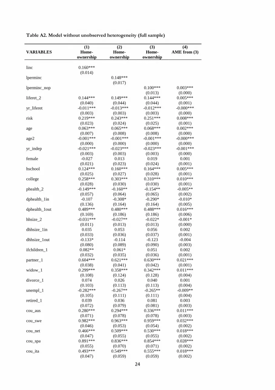
24
Table A2. Model without unobserved heterogeneity (full sample)
(1) (2) (3) (4)
VARIABLES Home-
ownership
Home-
ownership
Home-
ownership
AME from (3)
linc 0.160***
(0.014)
lperminc 0.148***
(0.017)
lperminc_nop 0.100*** 0.003***
(0.013) (0.000)
liferet_2 0.144*** 0.149*** 0.144*** 0.005***
(0.040) (0.044) (0.044) (0.001)
yr_liferet -0.011*** -0.013*** -0.012*** -0.000***
(0.003) (0.003) (0.003) (0.000)
risk 0.219*** 0.243*** 0.251*** 0.008***
(0.023) (0.024) (0.025) (0.001)
age 0.063*** 0.065*** 0.068*** 0.002***
(0.007) (0.008) (0.008) (0.000)
age2 -0.001*** -0.001*** -0.001*** -0.000***
(0.000) (0.000) (0.000) (0.000)
yr_indep -0.021*** -0.023*** -0.023*** -0.001***
(0.003) (0.003) (0.003) (0.000)
female -0.027 0.013 0.019 0.001
(0.021) (0.023) (0.024) (0.001)
hschool 0.124*** 0.160*** 0.164*** 0.005***
(0.025) (0.027) (0.028) (0.001)
college 0.258*** 0.303*** 0.310*** 0.010***
(0.028) (0.030) (0.030) (0.001)
phealth_2 -0.149*** -0.160** -0.154** -0.005**
(0.057) (0.064) (0.065) (0.002)
dphealth_1in -0.107 -0.308* -0.290* -0.010*
(0.136) (0.164) (0.164) (0.005)
dphealth_1out 0.489*** 0.480*** 0.488*** 0.016***
(0.169) (0.186) (0.186) (0.006)
hhsize_2 -0.031*** -0.027** -0.022* -0.001*
(0.011) (0.013) (0.013) (0.000)
dhhsize_1in 0.035 0.053 0.056 0.002
(0.033) (0.036) (0.037) (0.001)
dhhsize_1out -0.133* -0.114 -0.123 -0.004
(0.080) (0.089) (0.090) (0.003)
ifchildren_1 0.082** 0.061* 0.051 0.002
(0.032) (0.035) (0.036) (0.001)
partner_1 0.604*** 0.621*** 0.630*** 0.021***
(0.038) (0.041) (0.042) (0.001)
widow_1 0.299*** 0.358*** 0.342*** 0.011***
(0.108) (0.124) (0.128) (0.004)
divorce_1 0.074 0.026 0.040 0.001
(0.103) (0.113) (0.113) (0.004)
unempl_1 -0.282*** -0.267** -0.265** -0.009**
(0.105) (0.111) (0.111) (0.004)
retired_1 0.039 0.036 0.081 0.003
(0.072) (0.079) (0.081) (0.003)
cou_aus 0.280*** 0.294*** 0.336*** 0.011***
(0.071) (0.078) (0.078) (0.003)
cou_swe 0.982*** 0.963*** 0.959*** 0.032***
(0.046) (0.053) (0.054) (0.002)
cou_net 0.466*** 0.509*** 0.530*** 0.018***
(0.047) (0.055) (0.055) (0.002)
cou_spa 0.891*** 0.836*** 0.854*** 0.028***
(0.055) (0.070) (0.071) (0.002)
cou_ita 0.493*** 0.549*** 0.555*** 0.018***
(0.047) (0.059) (0.059) (0.002)

25
cou_fra 0.648*** 0.674*** 0.682*** 0.023***
(0.043) (0.052) (0.052) (0.002)
cou_den 1.194*** 1.168*** 1.161*** 0.039***
(0.043) (0.051) (0.051) (0.002)
cou_gre 0.679*** 0.721*** 0.701*** 0.023***
(0.049) (0.062) (0.064) (0.002)
cou_swi 0.056 0.047 0.064 0.002
(0.054) (0.063) (0.062) (0.002)
cou_bel 0.985*** 0.994*** 1.005*** 0.033***
(0.041) (0.050) (0.051) (0.002)
cou_cze -0.499*** -0.532*** -0.565*** -0.019***
(0.063) (0.070) (0.070) (0.002)
coh_19 -0.633*** -0.628*** -0.647*** -0.022***
(0.103) (0.114) (0.123) (0.004)
coh_24 -0.351*** -0.354*** -0.352*** -0.012***
(0.059) (0.067) (0.069) (0.002)
coh_29 -0.371*** -0.409*** -0.415*** -0.014***
(0.046) (0.052) (0.053) (0.002)
coh_34 -0.208*** -0.294*** -0.313*** -0.010***
(0.038) (0.043) (0.044) (0.001)
coh_39 -0.102*** -0.143*** -0.149*** -0.005***
(0.035) (0.038) (0.039) (0.001)
coh_44 -0.039 -0.087** -0.093*** -0.003***
(0.033) (0.036) (0.036) (0.001)
coh_54 0.081** 0.081** 0.080** 0.003**
(0.032) (0.035) (0.035) (0.001)
coh_59 0.032 0.033 0.020 0.001
(0.040) (0.044) (0.044) (0.001)
Constant -6.693*** -6.541*** -6.091***
(0.194) (0.227) (0.197)
Observations 319,530 255,254 248,628 248,628
Note. Column (1): we exclude observations reporting no income. Columns (2)-(3): we exclude observations on self-
employed workers (8.89% of the respondents) as well as the top and bottom 1% of the permanent income estimates.
Column (4) reports average marginal effects (AME) from the model in Column (3). Standard errors in parentheses; ***
p<0.01, ** p<0.05, * p<0.1
26
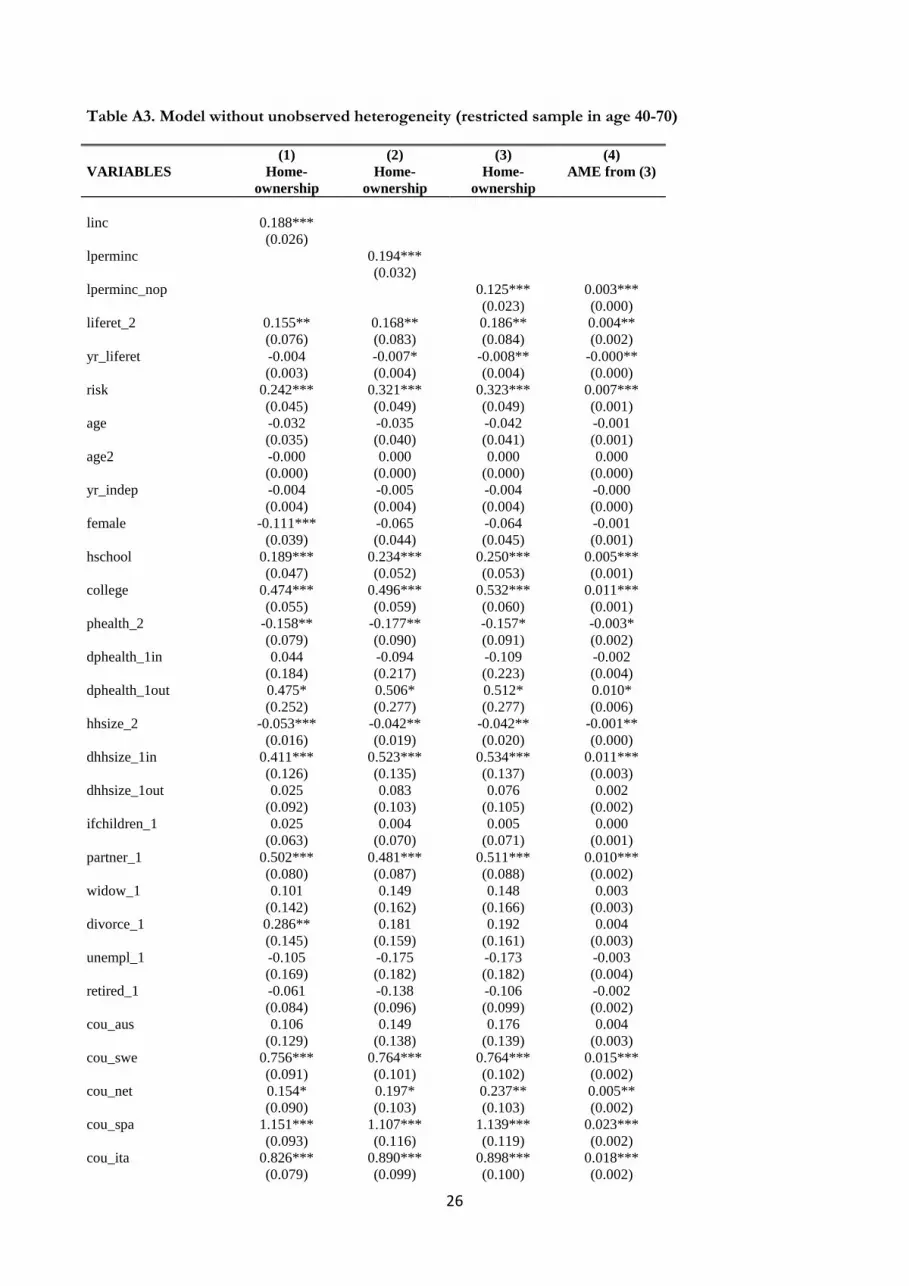
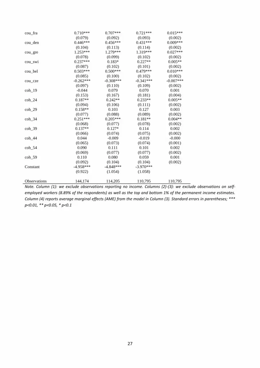
Table A3. Model without unobserved heterogeneity (restricted sample in age 40-70)
(1) (2) (3) (4)
VARIABLES Home-
ownership
Home-
ownership
Home-
ownership
AME from (3)
linc 0.188***
(0.026)
lperminc 0.194***
(0.032)
lperminc_nop 0.125*** 0.003***
(0.023) (0.000)
liferet_2 0.155** 0.168** 0.186** 0.004**
(0.076) (0.083) (0.084) (0.002)
yr_liferet -0.004 -0.007* -0.008** -0.000**
(0.003) (0.004) (0.004) (0.000)
risk 0.242*** 0.321*** 0.323*** 0.007***
(0.045) (0.049) (0.049) (0.001)
age -0.032 -0.035 -0.042 -0.001
(0.035) (0.040) (0.041) (0.001)
age2 -0.000 0.000 0.000 0.000
(0.000) (0.000) (0.000) (0.000)
yr_indep -0.004 -0.005 -0.004 -0.000
(0.004) (0.004) (0.004) (0.000)
female -0.111*** -0.065 -0.064 -0.001
(0.039) (0.044) (0.045) (0.001)
hschool 0.189*** 0.234*** 0.250*** 0.005***
(0.047) (0.052) (0.053) (0.001)
college 0.474*** 0.496*** 0.532*** 0.011***
(0.055) (0.059) (0.060) (0.001)
phealth_2 -0.158** -0.177** -0.157* -0.003*
(0.079) (0.090) (0.091) (0.002)
dphealth_1in 0.044 -0.094 -0.109 -0.002
(0.184) (0.217) (0.223) (0.004)
dphealth_1out 0.475* 0.506* 0.512* 0.010*
(0.252) (0.277) (0.277) (0.006)
hhsize_2 -0.053*** -0.042** -0.042** -0.001**
(0.016) (0.019) (0.020) (0.000)
dhhsize_1in 0.411*** 0.523*** 0.534*** 0.011***
(0.126) (0.135) (0.137) (0.003)
dhhsize_1out 0.025 0.083 0.076 0.002
(0.092) (0.103) (0.105) (0.002)
ifchildren_1 0.025 0.004 0.005 0.000
(0.063) (0.070) (0.071) (0.001)
partner_1 0.502*** 0.481*** 0.511*** 0.010***
(0.080) (0.087) (0.088) (0.002)
widow_1 0.101 0.149 0.148 0.003
(0.142) (0.162) (0.166) (0.003)
divorce_1 0.286** 0.181 0.192 0.004
(0.145) (0.159) (0.161) (0.003)
unempl_1 -0.105 -0.175 -0.173 -0.003
(0.169) (0.182) (0.182) (0.004)
retired_1 -0.061 -0.138 -0.106 -0.002
(0.084) (0.096) (0.099) (0.002)
cou_aus 0.106 0.149 0.176 0.004
(0.129) (0.138) (0.139) (0.003)
cou_swe 0.756*** 0.764*** 0.764*** 0.015***
(0.091) (0.101) (0.102) (0.002)
cou_net 0.154* 0.197* 0.237** 0.005**
(0.090) (0.103) (0.103) (0.002)
cou_spa 1.151*** 1.107*** 1.139*** 0.023***
(0.093) (0.116) (0.119) (0.002)
cou_ita 0.826*** 0.890*** 0.898*** 0.018***
(0.079) (0.099) (0.100) (0.002)
27
cou_fra 0.710*** 0.707*** 0.721*** 0.015***
(0.079) (0.092) (0.093) (0.002)
cou_den 0.446*** 0.456*** 0.431*** 0.009***
(0.104) (0.113) (0.114) (0.002)
cou_gre 1.253*** 1.279*** 1.319*** 0.027***
(0.078) (0.099) (0.102) (0.002)
cou_swi 0.237*** 0.183* 0.227** 0.005**
(0.087) (0.102) (0.101) (0.002)
cou_bel 0.503*** 0.500*** 0.479*** 0.010***
(0.085) (0.100) (0.102) (0.002)
cou_cze -0.262*** -0.308*** -0.341*** -0.007***
(0.097) (0.110) (0.109) (0.002)
coh_19 -0.044 0.079 0.070 0.001
(0.153) (0.167) (0.181) (0.004)
coh_24 0.187** 0.242** 0.233** 0.005**
(0.094) (0.106) (0.111) (0.002)
coh_29 0.158** 0.103 0.127 0.003
(0.077) (0.088) (0.089) (0.002)
coh_34 0.251*** 0.205*** 0.181** 0.004**
(0.068) (0.077) (0.078) (0.002)
coh_39 0.137** 0.127* 0.114 0.002
(0.066) (0.074) (0.075) (0.002)
coh_44 0.044 -0.009 -0.019 -0.000
(0.065) (0.073) (0.074) (0.001)
coh_54 0.090 0.111 0.101 0.002
(0.069) (0.077) (0.077) (0.002)
coh_59 0.110 0.080 0.059 0.001
(0.092) (0.104) (0.104) (0.002)
Constant -4.958*** -4.848*** -3.970***
(0.922) (1.054) (1.058)
Observations 144,174 114,205 110,795 110,795
Note. Column (1): we exclude observations reporting no income. Columns (2)-(3): we exclude observations on self-
employed workers (8.89% of the respondents) as well as the top and bottom 1% of the permanent income estimates.
Column (4) reports average marginal effects (AME) from the model in Column (3). Standard errors in parentheses; ***
p<0.01, ** p<0.05, * p<0.1

28
Table A4. Model with unobserved heterogeneity (marginal effects, full sample)
Heterogeneity, group 1 Heterogeneity, group 2
VARIABLES (1)
Illiquid assets
(2)
Home-
Ownership
(3)
Illiquid assets
(4)
Home-
Ownership
lperminc_nop 0.011*** 0.003*** 0.009*** 0.004***
(0.001) (0.001) (0.001) (0.001)
liferet_2 0.005** 0.012***
(0.002) (0.003)
yr_liferet -0.001*** 0.000
(0.000) (0.000)
risk 0.014*** 0.007*** 0.018*** 0.009***
(0.001) (0.001) (0.002) (0.001)
age 0.015*** 0.002*** 0.017*** 0.003***
(0.000) (0.000) (0.000) (0.000)
age2 -0.000*** -0.000*** -0.000*** -0.000***
(0.000) (0.000) (0.000) (0.000)
yr_indep 0.000 -0.001*** 0.000*** -0.001***
(0.000) (0.000) (0.000) (0.000)
female -0.040*** 0.002 -0.025*** -0.000
(0.001) (0.001) (0.001) (0.001)
hschool -0.009*** 0.006*** 0.014*** 0.005***
(0.002) (0.001) (0.002) (0.001)
college 0.010*** 0.010*** 0.024*** 0.010***
(0.002) (0.001) (0.002) (0.001)
phealth_2 0.013*** -0.003 0.004* -0.008**
(0.002) (0.003) (0.002) (0.003)
dphealth_1in 0.017*** -0.009 0.003 -0.011
(0.006) (0.007) (0.006) (0.008)
dphealth_1out 0.015* -0.001 0.007 0.030***
(0.009) (0.010) (0.010) (0.008)
hhsize_2 -0.003*** -0.001** -0.005*** -0.001
(0.001) (0.001) (0.001) (0.001)
dhhsize_1in 0.003 -0.001 0.011*** 0.005***
(0.003) (0.002) (0.003) (0.002)
dhhsize_1out -0.004 -0.007* 0.001 -0.001
(0.004) (0.004) (0.004) (0.004)
ifchildren_1 0.019*** 0.003** 0.012*** 0.000
(0.002) (0.002) (0.002) (0.002)
partner_1 0.025*** 0.024*** 0.021*** 0.019***
(0.002) (0.002) (0.002) (0.002)
widow_1 0.014*** 0.009 0.026*** 0.016***
(0.004) (0.006) (0.004) (0.006)
divorce_1 0.001 0.002 0.024*** 0.001
(0.004) (0.005) (0.005) (0.005)
unempl_1 -0.031*** -0.001 -0.003 -0.018***
(0.005) (0.005) (0.006) (0.005)
retired_1 0.005** 0.001 0.008*** 0.003
(0.003) (0.004) (0.003) (0.004)
cou_aus 0.207*** 0.004 -0.389*** 0.025***
(0.003) (0.004) (0.006) (0.003)
cou_swe 0.027*** 0.033*** 0.070*** 0.029***
(0.002) (0.002) (0.003) (0.003)
cou_net 0.306*** 0.015*** -0.383*** 0.029***
(0.003) (0.003) (0.004) (0.003)
cou_spa -0.145*** 0.023*** -0.123*** 0.042***
(0.006) (0.003) (0.004) (0.003)
cou_ita -0.139*** 0.013*** -0.103*** 0.032***
(0.004) (0.002) (0.003) (0.003)
cou_fra -0.069*** 0.022*** -0.016*** 0.025***
(0.003) (0.002) (0.003) (0.003)
cou_den 0.291*** 0.035*** -0.313*** 0.050***

29
(0.002) (0.003) (0.003) (0.003)
cou_gre -0.392*** 0.017*** -0.133*** 0.052***
(0.030) (0.002) (0.006) (0.003)
cou_swi 0.261*** 0.006* -0.311*** 0.010***
(0.002) (0.003) (0.002) (0.003)
cou_bel 0.220*** 0.037*** -0.345*** 0.041***
(0.002) (0.002) (0.003) (0.003)
cou_cze -0.121*** -0.011*** -0.192*** -0.028***
(0.003) (0.003) (0.002) (0.004)
coh_19 -0.551*** -0.027*** 0.172*** -0.010
(0.037) (0.005) (0.010) (0.007)
coh_24 -0.047*** -0.008*** -0.127*** -0.016***
(0.003) (0.003) (0.004) (0.003)
coh_29 -0.057*** -0.013*** -0.115*** -0.015***
(0.003) (0.002) (0.003) (0.002)
coh_34 -0.046*** -0.008*** -0.070*** -0.014***
(0.002) (0.002) (0.003) (0.002)
coh_39 0.155*** -0.006*** -0.377*** -0.003
(0.002) (0.002) (0.003) (0.002)
coh_44 -0.027*** -0.001 -0.042*** -0.006***
(0.002) (0.002) (0.002) (0.002)
coh_54 0.001 0.004** 0.020*** 0.001
(0.002) (0.001) (0.002) (0.002)
coh_59 0.019*** 0.001 0.037*** -0.001
(0.003) (0.002) (0.003) (0.002)
Observations 206,925 206,925 155,536 155,536
Log-likelihood -22,797.909 -18,726.990 -22,710.209 -16,575.558
McFadden’s R2 0.690 0.057 0.615 0.083
Note. The table reports the average marginal effects from the bivariate mixed proportional hazard analysis on the
holding of illiquid assets and home ownership, using as weights the probability to belong to group 1 (Columns (1)-(2))
or group 2 (Columns (3)-(4)). Standard errors in parentheses; *** p<0.01, ** p<0.05, * p<0.1
30
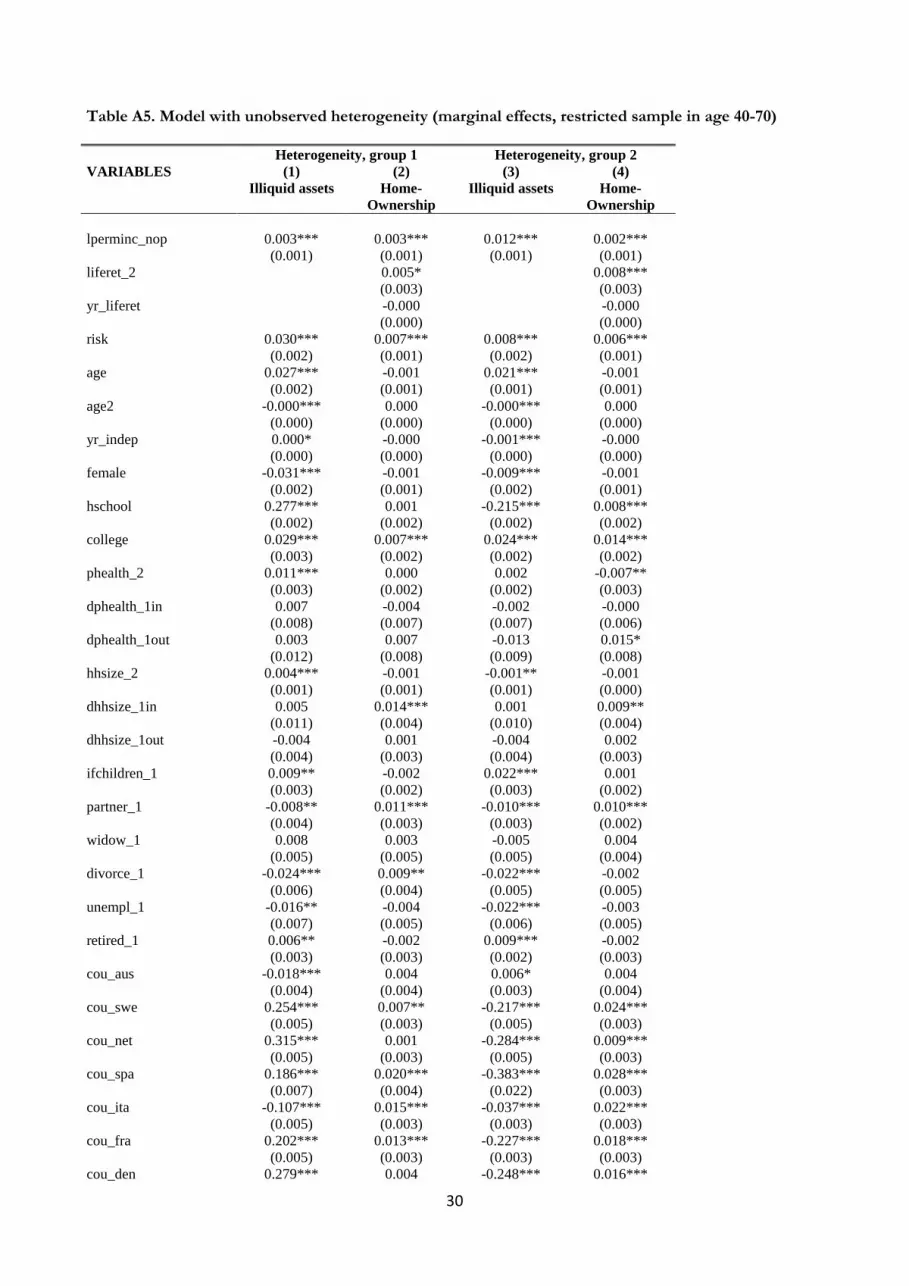
Table A5. Model with unobserved heterogeneity (marginal effects, restricted sample in age 40-70)
Heterogeneity, group 1 Heterogeneity, group 2
VARIABLES (1)
Illiquid assets
(2)
Home-
Ownership
(3)
Illiquid assets
(4)
Home-
Ownership
lperminc_nop 0.003*** 0.003*** 0.012*** 0.002***
(0.001) (0.001) (0.001) (0.001)
liferet_2 0.005* 0.008***
(0.003) (0.003)
yr_liferet -0.000 -0.000
(0.000) (0.000)
risk 0.030*** 0.007*** 0.008*** 0.006***
(0.002) (0.001) (0.002) (0.001)
age 0.027*** -0.001 0.021*** -0.001
(0.002) (0.001) (0.001) (0.001)
age2 -0.000*** 0.000 -0.000*** 0.000
(0.000) (0.000) (0.000) (0.000)
yr_indep 0.000* -0.000 -0.001*** -0.000
(0.000) (0.000) (0.000) (0.000)
female -0.031*** -0.001 -0.009*** -0.001
(0.002) (0.001) (0.002) (0.001)
hschool 0.277*** 0.001 -0.215*** 0.008***
(0.002) (0.002) (0.002) (0.002)
college 0.029*** 0.007*** 0.024*** 0.014***
(0.003) (0.002) (0.002) (0.002)
phealth_2 0.011*** 0.000 0.002 -0.007**
(0.003) (0.002) (0.002) (0.003)
dphealth_1in 0.007 -0.004 -0.002 -0.000
(0.008) (0.007) (0.007) (0.006)
dphealth_1out 0.003 0.007 -0.013 0.015*
(0.012) (0.008) (0.009) (0.008)
hhsize_2 0.004*** -0.001 -0.001** -0.001
(0.001) (0.001) (0.001) (0.000)
dhhsize_1in 0.005 0.014*** 0.001 0.009**
(0.011) (0.004) (0.010) (0.004)
dhhsize_1out -0.004 0.001 -0.004 0.002
(0.004) (0.003) (0.004) (0.003)
ifchildren_1 0.009** -0.002 0.022*** 0.001
(0.003) (0.002) (0.003) (0.002)
partner_1 -0.008** 0.011*** -0.010*** 0.010***
(0.004) (0.003) (0.003) (0.002)
widow_1 0.008 0.003 -0.005 0.004
(0.005) (0.005) (0.005) (0.004)
divorce_1 -0.024*** 0.009** -0.022*** -0.002
(0.006) (0.004) (0.005) (0.005)
unempl_1 -0.016** -0.004 -0.022*** -0.003
(0.007) (0.005) (0.006) (0.005)
retired_1 0.006** -0.002 0.009*** -0.002
(0.003) (0.003) (0.002) (0.003)
cou_aus -0.018*** 0.004 0.006* 0.004
(0.004) (0.004) (0.003) (0.004)
cou_swe 0.254*** 0.007** -0.217*** 0.024***
(0.005) (0.003) (0.005) (0.003)
cou_net 0.315*** 0.001 -0.284*** 0.009***
(0.005) (0.003) (0.005) (0.003)
cou_spa 0.186*** 0.020*** -0.383*** 0.028***
(0.007) (0.004) (0.022) (0.003)
cou_ita -0.107*** 0.015*** -0.037*** 0.022***
(0.005) (0.003) (0.003) (0.003)
cou_fra 0.202*** 0.013*** -0.227*** 0.018***
(0.005) (0.003) (0.003) (0.003)
cou_den 0.279*** 0.004 -0.248*** 0.016***

31
(0.007) (0.003) (0.007) (0.003)
cou_gre -0.204*** 0.023*** -0.081*** 0.031***
(0.007) (0.003) (0.005) (0.003)
cou_swi -0.258*** 0.001 0.244*** 0.005*
(0.003) (0.003) (0.003) (0.003)
cou_bel -0.279*** 0.010*** 0.198*** 0.007**
(0.005) (0.003) (0.004) (0.003)
cou_cze -0.136*** -0.008*** -0.069*** -0.005
(0.003) (0.003) (0.003) (0.003)
coh_19 0.405*** 0.024*** -0.535*** -0.004
(0.021) (0.007) (0.015) (0.004)
coh_24 -0.387*** 0.007** 0.260*** -0.000
(0.006) (0.003) (0.005) (0.004)
coh_29 0.088*** 0.005* -0.251*** 0.001
(0.008) (0.003) (0.004) (0.002)
coh_34 0.147*** 0.006** -0.239*** 0.003
(0.005) (0.002) (0.003) (0.002)
coh_39 -0.072*** 0.004* -0.050*** 0.001
(0.003) (0.002) (0.003) (0.002)
coh_44 -0.025*** 0.001 -0.036*** -0.002
(0.003) (0.002) (0.002) (0.002)
coh_54 0.043*** 0.006*** 0.045*** -0.002
(0.003) (0.002) (0.003) (0.002)
coh_59 0.088*** 0.002 0.072*** 0.000
(0.005) (0.003) (0.004) (0.003)
Observations 90,537 90,537 68,073 68,073
Log-likelihood -9,590.687 -4,780.764 -9,511.313 -5,902.912
McFadden’s R2 0.718 0.045 0.702 0.052
Note. The table reports the average marginal effects from the bivariate mixed proportional hazard analysis on the
holding of illiquid assets and home ownership, using as weights the probability to belong to group 1 (Columns (1)-(2))
or group 2 (Columns (3)-(4)). Standard errors in parentheses; *** p<0.01, ** p<0.05, * p<0.1