taposh analysis dual cusum

IEEE TRANSACTIONS ON WIRELESS COMMUNICATIONS, VOL. 10, NO. 1, JANUARY 2011 91

Generalized Analysis of a DistributedEnergy Efficient Algorithm for Change Detection

Taposh Banerjee, Vinod Sharma, Veeraruna Kavitha, and A. K. JayaPrakasam

Abstract—We propose an energy efficient distributed cooper-ative Change Detection scheme called DualCUSUM based onPage’s CUSUM algorithm. In the algorithm, each sensor runsa CUSUM and transmits only when the CUSUM is abovesome threshold. The transmissions from the sensors are fusedat the physical layer. The channel is modeled as a MultipleAccess Channel (MAC) corrupted with noise. The fusion centerperforms another CUSUM to detect the change. The algorithmperforms better than several existing schemes when energy isat a premium. We generalize the algorithm to also includenonparametric CUSUM and provide a unified analysis. Ourresults show that while the false alarm probability is smaller forobservation distribution with a lighter tail, the detection delay isasymptotically the same for any distribution. Consequently, weprovide a new viewpoint on why parametric CUSUM performsbetter than nonparametric CUSUM. In the process, we alsodevelop new results on a reflected random walk which can be ofindependent interest.

Index Terms—Nonparametric CUSUM, decentralized changedetection, reflected random walk.

I. INTRODUCTION

THE detection of an abrupt change in the distribution ofa sequence of random variables is a classical problem

in statistics. In this problem, a decision maker observes a se-quence of random variables. At some point of time, unknownto the decision maker, the distribution of these observationschanges. The decision maker has to detect this change of lawas soon as possible subject to some false alarm constraint. Thisis also called the centralized version of the change detectionproblem and has been well studied. When the observationsare independent and identically distributed (iid) conditionedon the time of change and the distribution of the change timeT is known (this is called the Bayesian setting), the optimalalgorithm was obtained by Shiryaev ([29]). When distributionof T is not known, the CUSUM algorithm, first proposed byPage in [23], was shown by Lorden ([17]) and Moustakides([22]) to minimize the worst case delay (Min-Max optimality).

In the distributed version of the change detection problem,multiple geographically distributed sensors take observationsand send the processed information to a decision maker

Manuscript received August 5, 2009; revised June 24, 2010; acceptedAugust 14, 2010. The associate editor coordinating the review of this paperand approving it for publication was D. Zeghlache.

V. Sharma and A. K. J. are with the Dept. of Electrical Communi-cation Engineering, IISc, Bangalore, India (e-mail: [email protected],[email protected]).

T. Banerjee is with the University of Illinois at Urbana-Champaign (e-mail:[email protected]).

V. Kavitha is with the University of Avignon, France (e-mail:Kavitha.Voleti [email protected]).

Preliminary versions of this paper have been presented at ICASSP 2008and MSWiM 2009.

Digital Object Identifier 10.1109/TWC.2010.110510.091177

(fusion center) for the detection of change. This model findsapplication in biomedical signal processing, intrusion detec-tion in computer and sensor networks ([35], [33]), finance,quality control engineering, and recently, distributed detectionof spectrum holes in cognitive radio networks ([16], [28]).The distribution of the observations of all the sensors changessimultaneously at some random point of time. While thismodel is slightly restrictive, it is the most widely studiedmodel in the literature. As evident from the work in [3], [37]and in this paper, even this model is not well explored.

In the absence of communication and resource constraints,the sensors can send the raw observations to the fusion centerand the problem reduces to the centralized one discussedabove. However, in applications like sensor networks, thesensors are low power, battery operated devices and thus thereare severe constraints on their communication and processingcapabilities. Therefore, it is suggested that sensors send pro-cessed version (e.g., quantized) of their observations to thefusion center and the fusion center fuses the information fromvarious sensors to make the decision (see [7], [33], [35], [36]for various processing possibilities).

Several distributed algorithms have been proposed for de-tection of change. When sensors send quantized version oftheir observations to the fusion center, the author in [35] hasobtained asymptotically optimal algorithms in the Bayesiansetting. In [20], a CUSUM based algorithm is proposed whichis shown to be asymptotically Min-Max optimal. In thisalgorithm, each sensor runs the CUSUM algorithm and sendsa ’1’ if it detects a change and a ’0’ otherwise. The fusioncenter declares a change when all the sensors transmit a ’1’simultaneously. In [33] and [34], various distributed changedetection algorithms are compared.

The above problem formulations do not explicitly takeenergy consumption in to account. Furthermore, these algo-rithms ignore the unreliability of the communication channel.Recently, a Bayesian formulation of the decentralized changedetection problem with energy constraints was considered in[37]. The problem is solved using dynamic programming byrestricting the solution to a class of algorithms.

In this paper we propose a CUSUM based algorithm calledDualCUSUM and show that, for given constraints on falsealarm probability and energy, its mean detection delay is muchless than that in [37]. Also, DualCUSUM is computationallymuch less complex and requires no feedback from the fusionnode. We also provide the false alarm and delay analysis ofour algorithm.

DualCUSUM uses physical layer fusion to reduce transmis-sion delays from different nodes. Physical layer fusion requiresphase, frequency and time synchronization of different nodes.

1536-1276/11$25.00 c⃝ 2011 IEEE

92 IEEE TRANSACTIONS ON WIRELESS COMMUNICATIONS, VOL. 10, NO. 1, JANUARY 2011

This is feasible in sensor networks ([19], [30]). However, ifone does not provide for such synchronization, DualCUSUMcan be used without physical layer fusion (using other MAClayer protocols, e.g., TDMA). Due to other features mentionedabove, it still provides good performance (compared to thealgorithms available in literature). Even in the absence ofan energy constraint, our preliminary investigations indicatethat DualCUSUM performs better than other distributed algo-rithms, some of which have been identified to be asymptoti-cally optimal ([20], [33], [35]).

DualCUSUM has been used for cooperative spectrum sens-ing in Cognitive Radio Systems in [28] and shown to providebetter performance than other algorithms available in literaturenot only in delay but also in saving energy.

Although this algorithm has many desirable features, thereis one practical limitation: to use CUSUM one needs thedistribution of observations before and after change at eachsensor node. This may not be a realistic assumption in manycases. For example, there can be random time varying fadingin the wireless channels in sensor networks (see other articlesin [30]), and in the Cognitive Radio Systems ([16], [28]). Seealso [7] for other practical examples. Thus in this paper wealso extend DualCUSUM to a nonparametric set up.

We analyze a generalized version of DualCUSUM of whichparametric and nonparametric versions are special cases. Afew interesting facts emerge from this analysis: mean detectiondelay is insensitive to the distribution of the observations butthe false alarm probability crucially depends on the tail behav-ior of the distributions at least for the nonparametric CUSUM.The lighter the tail, the lower the false alarm probability. Wealso show that the log likelihood function converts a heavytailed distribution to a light tail distribution. Since, parametricCUSUM uses log likelihood and nonparametric CUSUM doesnot, the former performs better than the latter for a givendistribution of observations.

Since CUSUM is, or will be a fundamental element of manydistributed algorithms for detection of change, the tools andtechniques used here can be of general interest. Also, sincethe CUSUM algorithm is essentially a reflected random walk,during our analysis, we obtain new results on passage times,overshoot distribution and excursion above a level for reflectedrandom walks. Despite extensive studies on random walks,there are comparatively few results on reflected random walks([10]).

The paper is organized as follows. We explain the modeland introduce the algorithm in Section II. Section III analyzesthe performance of the algorithm and provides comparisonwith simulations. Section IV concludes the paper.

II. MODEL AND ALGORITHM

Let there be L sensors in a sensor field, sensing observationsand transmitting to a fusion node. The transmissions fromthe sensor nodes to the fusion node are over a MAC. In oursystem we assume that all the sensor nodes can transmit atthe same time. There is physical layer fusion at the fusionnode (commonly studied Gaussian MAC is a special case).The fusion node receives data over time and decides if thereis a change in distribution of the observations at the sensors.

Let Xk,l be the observation made at sensor l at time k. Sensorl transmits Yk,l at time k after processing Xk,l and its pastobservations. The fusion node receives Yk = ∑L

l=1Yk,l +ZMAC,where {ZMAC} is iid receiver noise. The distribution of theobservations at each sensor changes simultaneously at a ran-dom time T , with a known distribution. The {Xk,l , l ≥ 1} areindependent and identically distributed (iid) over l and areindependent over k, conditioned on change time T . Before thechange Xk,l have density f0 and after the change the densityis f1. The expectation under fi will be denoted by Ei, i= 0,1,and P∞ and P1 denote the probability measure under no changeand when change happens at time 1, respectively.

These assumptions are commonly made in the literature (seee.g., [7], [35], [36]). Physical layer fusion is considered in [21]and [37].

The objective of the fusion center is to detect this change assoon as possible at time τ (say) using the messages transmittedfrom all the L sensors, subject to an upper bound α on the

probability of False Alarm PFA△= P[τ < T ] and E0 on the

average energy used. Often the desired α is quite low, e.g.,≤ 10−6 in intrusion detection in sensor networks. Then, thegeneral problem is:

minEDD△=E[(τ−T)+],

Subj to PFA ≤α and Eavg= E

[τ

∑k=1

Y 2k,l

]≤ E0,1 ≤ l ≤ L (1)

For this distributed optimization problem there is no opti-mal solution available so far although asymptotically optimalsolution have been identified ([33] - [35]). In the followinginstead of solving the optimization problem directly, wedevelop an efficient parametric class of algorithms. We alsoanalyze its performance. This analysis can be used to optimizeits parameter. Our algorithm has several desirable featuresto provide better performance than the algorithms we areaware of (including the asymptotically optimal solutions). Thisalgorithm is called DualCUSUM and is as follows:

1) Sensor l uses CUSUM,

Wk,l = max{0,Wk−1,l + log

[f1(Xk,l

)/f0(Xk,l

)]}, (2)

where, W0,l = 0,1 ≤ l ≤ L.Remark: One can see that the CUSUM is a reflectedrandom walk.

2) Sensor l transmits Yk,l = b1{Wk,l>γ}. Here 1A denotes theindicator function of set A.Remark: This is the energy saving step. The parameter bis chosen offline based on the energy constraint.

3) Physical layer fusion (as in [37]) is used to reducetransmission delay, i.e., Yk = ∑L

l=1Yk,l + ZMAC,k, whereZMAC,k is the receiver noise.

4) Finally, Fusion center runs CUSUM:

Fk = max

{0,Fk−1+ log

gI(Yk)

g0(Yk)

}; F0 = 0, (3)

where g0 is the density of ZMAC,k, the MAC noise at thefusion node, and gI is the density of ZMAC,k +bI, I beinga design parameter.Remark: In the absence of MAC noise, it is Min-Max

BANERJEE et al.: GENERALIZED ANALYSIS OF A DISTRIBUTED ENERGY EFFICIENT ALGORITHM FOR CHANGE DETECTION 93

−6 −5.5 −5 −4.5 −4 −3.5 −3 −2.5 −20

5

10

15

20

25

ln(PFA

)

ED

D

Shiryaev CentralizedLeena−RajeshShiryaev−CUSUMDualCUSUM

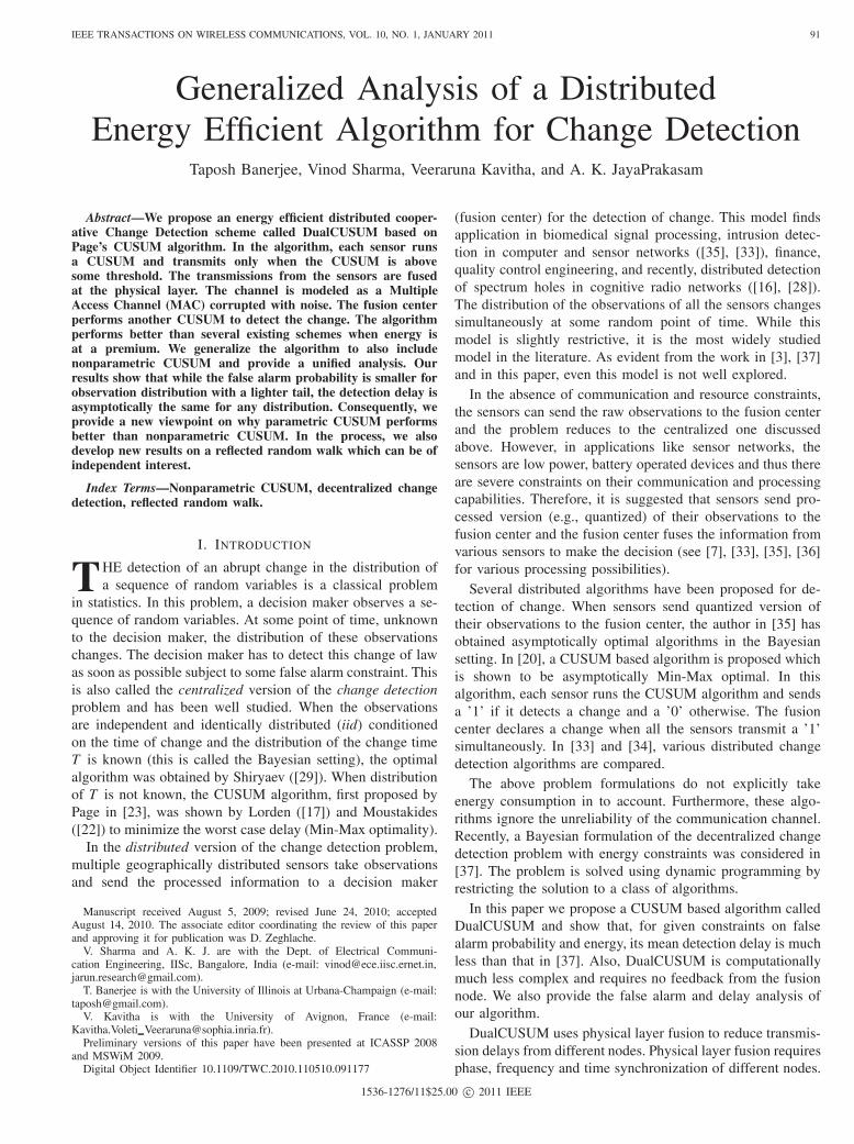
Fig. 1. ln(PFA) (x axis) vs EDD comparison with [37].

optimal for the fusion center to declare change whenYk = Lb. In the presence of noise, such a decision is notpossible and hence we use another CUSUM to detect thechange. Before the change, sensors transmit rarely andhence Yk can be approximated by N(0,σ2

M). Also, wellafter the change has taken place, when all the sensors aretransmitting, Yk ∼ N(Lb,σ2

M). But the number of sensorstransmitting evolves from 1 to L after the change andhence, we represent Yk, post change, by N(Ib,σ2

M) andoptimize over the choice of I (1 ≤ I ≤ L).

5) The fusion center declares a change at time τ(β ,γ,b, I)when Fk crosses a threshold β :

τ(β ,γ,b, I) = inf{k : Fk > β}.Remark: After the change, when the mean of Yk is Lb,the drift of Fk will be positive (because 1 ≤ I ≤ L) andchange will be detected with probability 1.

Multiple values of (β ,γ,b, I) will satisfy both the false

alarm and the energy constraint. One can minimize EDD△=

E[(τ−T )+] over this parameter set. In Section III we obtainthe performance of DualCUSUM for given values (β ,γ,b, I)which then can be used to solve the optimization problem:

(β ∗,γ∗,b∗, I∗) = arg min(β ,γ,b,I)

EDD(β ,γ,b, I) (4)

subj to P[τ(β ,γ,b, I) < T ] ≤ α , energy Eavg(β ,γ,b, I) ≤ E0.For the case of Gaussian distribution and Geometric T andexplicit optimization algorithm is provided in [3] to solve (4).

Figure (1) compares the optimal DualCUSUM (obtained viathe optimization algorithm in [3]) with the scheme in [37] andthe optimal centralized Shiryaev scheme via simulation. Weuse the parameters: L = 2, I = 1, f0 ∼ N(0,1), f1 ∼ N(0.75,1),ZMAC,k ∼N(0,1), T ∼Geom(ρ = 0.05) and E0 = 7.61. ClearlyDualCUSUM performs better than [37] and the performancetends to improve as PFA decreases.

If the distribution of T is known, then for a single node,Shiryaev algorithm is optimal ([15], [35]). One could possiblyuse that also in our setup at the secondary or fusion nodes.However, especially, in cooperative setup its performanceanalysis may become intractable. DualCUSUM itself has beendifficult to analyze. Thus for cooperative Shiryaev algorithmgetting optimal parameters will be almost impossible exceptvia simulations. Furthermore, surprisingly DualCUSUM per-

forms as well as an algorithm where Shiryaev algorithm isused at the local nodes and CUSUM at the fusion node. Thiscomparison is also shown in Figure 1. Surprisingly our initialinvestigations also show that DualCUSUM may work betterthan the algorithm which uses Shiryaev algorithm at boththe local nodes as well as at the fusion center. In addition,DualCUSUM can be used in the non-Bayesian setup. Most ofthe analysis remains the same.

More recently we have used DualCUSUM for spectrumsensing and shown in [28] that it performs better than severalrecently proposed algorithms. This motivates us to studyDualCUSUM further.

DualCUSUM, as the original CUSUM itself, has a stronglimitation. It requires exact knowledge of f0 and f1. Thisinformation will be available apriori to varying degrees in apractical scenario. Depending upon the type of uncertainty inf0, f1, different algorithms/variations on CUSUM are available([9], [15]). One common algorithm, called nonparametricCUSUM is to replace (2) by

Wk+1,l = max{0,Wk,l +Xk+1,l −D}, (5)

where, D is an appropriate constant such that E[Xk,l −D] isnegative before change and positive after change. If the meanof Xk,l is known before and after the change, D can be chosenas the average of the two means. For Gaussian and exponentialdistributions, nonparametric CUSUM becomes CUSUM forsome appropriate D and scaling. If at the fusion node g0 isnot known (in our CUSUM algorithm (3) at the fusion node,gI(x) = Ib+ g0(x)), then one can use (5) even at the fusionnode.

In the following we will compute PFA and EDD for ageneralized class of algorithms where at the sensor nodes andat the fusion node we use the algorithm,

Wk+1 = max{0,Wk +Zk+1}, (6)

where, {Zk} is an iid sequence with different distributionsbefore and after the change. (At the fusion node the situationis more complicated; we will comment on it as and whenneeded). We will assume that E[Zk] < 0 before the changeand E[Zk]> 0 after the change. We will denote by fZ ,FZ andPZ the density, cdf and probability measure for Zk.

Algorithm (6) contains CUSUM and nonparametricCUSUM as special cases. In the next section we analyze thegeneralized DualCUSUM with (6). We emphasize that unlikeDualCUSUM, this algorithm may not require knowledge off0 and f1, (e.g., we only need to choose D appropriatelyfor nonparametric CUSUM). But, the performance of thisalgorithm, as we show in the next section, does depend onthe underlying distribution. This is typical of such algorithms.

III. ANALYSIS

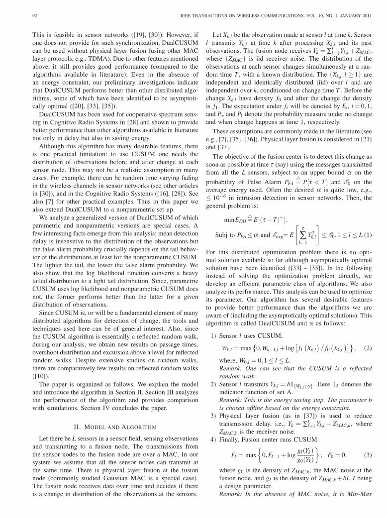
In this section, we first compute the false alarm probabilityPFA and then the delay EDD. The idea is to model the timesat which the CUSUM {Wk} at the local sensors, crosses thethreshold γ (we drop subscript l for convenience) and the localnodes transmit to the fusion node (Fig. 2).

Computing PFA requires finding (when Zk has distributionf0) the distribution of τγ , the first time Wk crosses γ , the


Wk Sojourn time above γ

γ

τγ

Γ

τ0

Fig. 2. Excursions of Wk above γ can be approximated by a compoundPoisson process. A local node transmits to the fusion node during theseexcursions.

amount of time it stays above γ (excursion time above γ), andthe probability that the fusion node declares a change duringan excursion time. These are computed in Sections III-A-III-E.The delay EDD is computed in Section III-G.

We will need the following notations and definitions. Let Xbe a random variable with distribution F . Then F∗n denotesthe n-fold convolution of F and F̄(x) = 1−F(x). A functionl is slowly varying if for all λ > 0, l(λx)/l(x)→ 1 as x → ∞.

Definition 1: ([1]) F is heavy tailed if for any ε > 0,E[eε∣X ∣] =∞. F is subexponential if F̄∗2(x)/F̄(x)→ 2 as x →∞. If F is not heavy tailed, we call it light tailed. If 1−F(x) =l(x)x−α ,α > 0 where l is slowly varying then F is regularlyvarying with index −α .

Gaussian, Exponential and Laplace distributions are lighttailed. Pareto, Lognormal and Weibull distributions are subex-ponential. Subexponential distributions are a subclass of heavytailed distributions and regularly varying distributions are asubclass of subexponential distributions. We will also be con-cerned with a sub family S ∗ of subexponential distributionsdefined in [11] which contains all the above members ofsubexponential family if they have a finite mean.

Often it is said that light tailed distributions may providebetter system behavior than the heavy tailed ([8]). We demon-strate this for the probability of false alarm. In particular wewill show that if the positive tail of FZ is light then PFA ismuch less than if it is heavy tailed. Interestingly, we will alsoshow that EDD is largely insensitive to the tail behavior of FZ .

CUSUM has the interesting property that it transforms alarge class of heavy tailed distributions into light tailed dis-tributions. This important property of log likelihood seems tohave escaped the attention of investigators before. This makesCUSUM perform better than the nonparametric CUSUM.Lemma 1 (in Appendix A) states this property in reasonablegenerality.

A. Behavior of Wk under P∞

The process {Wk} is a reflected random walk with negativedrift under P∞. Figure (2) shows a typical sample path for{Wk}. The process visits 0 (regenerates) a finite number oftimes before it crosses the threshold γ at,

τγ△= inf{k ≥ 1 : Wk ≥ γ}. (7)

We call τγ the First Passage Time (FPT). The overshoot Γis defined as Wτγ − γ . The time between two regenerations is

inter-regeneration time τ . Under P∞, E[τ]< ∞. Let

τ0△= inf{k : k > τγ ;Wk ≤ 0}− τγ and,

η = #{k : Wk ≥ γ;τγ ≤ k ≤ τγ + τ0}. (8)

During time η (called a batch) a local node transmits tothe fusion node. Thus, these are the times during which thefusion node will most likely declare a change. The overshootΓ can have significant impact on η .

It has been shown in [24] that the point process of ex-ceedances of γ by Wk, converges to a compound Poissonprocess as γ →∞. The points appear as clusters. The intervalsbetween the clusters have the same distribution as that of τγin (7) and the distribution of η in (8) gives the distribution ofthe size of the cluster, i.e., the batch of the compound Poissonprocess. Since, one has to choose large values of γ to keep PFA

small, a batch Poisson process provides a good approximationin our scenario.

In the next few sections we give results on the distributionof τγ , overshoot Γ, and the distribution of the batch η whichwill be used in computing PFA.

B. First Passage Time under P∞

From the compound Poisson process approximation men-tioned above,

limγ→∞

P∞[τγ > x] = exp(−λγx), x > 0, (9)

where, λγ a positive constant. In [3] a formula for λγ was usedwhich is computable for Gaussian distribution only. However,by solving integral equations obtained via renewal arguments([25]), one can obtain the mean of FPT for any distribution.Epochs when Wk = 0 are renewal epochs for this process. LetL(s) be the mean FPT with W0 = s ≥ 0. Hence λγ = 1/L(0).Then from renewal arguments:

L(s) = FZ(−s)(L(0)+ 1)

+

∫ γ−s

−s(L(s+ z)+ 1)dFZ(z)dz+P[Z > γ− s]. (10)

This equation is obtained by conditioning on Z0 = z. IfZ0 ≤−s, then W1 = 0, providing the first term on the right. IfZ > γ− s, then the threshold is approached in one step only,providing the last term.

Equation (10) can be shown to be a Fredholm integral equa-tion of second kind ([26]). Theorem 1 shows that Equation(10) has a unique continuous solution in our set up underweak conditions.

Theorem 1: If FZ is continuous and FZ(γ)< 1 then (10) hasa unique continuous solution L.

Proof: See Appendix B.Equation (10) can be solved recursively on L(s),0 ≤ s ≤ γ .

An efficient algorithm is provided in [18].From (10) not only we can compute the E[τγ ] exactly, but

can also get some asymptotic rates. Taking s = 0 in (10), andwriting L(0) as Lγ (0) to make dependence on γ explicit, weget (since Lγ (0)≥ Lγ (y) for 0 ≤ y ≤ γ)

Lγ(0) = 1+FZ(0)Lγ (0)+∫ γ0 Lγ (y) fZ(y)dy

≤ 1+FZ(0)Lγ(0)+Lγ(0)(FZ(γ)−FZ(0)).


TABLE IMEAN FPT E[τγ ] FOR PARETO (K = 2.1) AND GAUSSIAN WITH

EZk =−0.5.

γ E[τγ ] Gauss E[τγ ] Pareto5 930 8006 2551 11007 6950 14558 19020 1880

Thus,

Lγ (0)≤ 11−FZ(γ)

. (11)

Equation (11) provides the dependence of E[τγ ] on the tail ofdistribution of FZ . For example, if 1−FZ(γ)∼ γ−α ,α > 0, thenE[τγ ]≤ γα and if FZ is light tailed (∼ e−αγ ) then E[τγ ]∼ eαγ .

Although (11) only gives an upper bound on the growth ofE[τγ ] with γ , it turns out that this upper bound in fact givesthe exact rate of growth. This can be seen from the followingfacts (due to lack of space we will be brief). Let pγ be theprobability of Wk exceeding γ in one regeneration length. LetE[τ] be the mean regeneration length. From [14],

pγE[τγ ]E[τ]

→ 1 as γ → ∞. (12)

From [1], if Z has subexponential distribution then for γ large,pγ ≈ P[Z > γ]E[τ] and hence from (12), E[τγ ] ∼ 1/P[Z > γ].If there exists an γ̄ > 0 with E[eγ̄Z ] = eγ̄ then from [27],γ−1 log pγ →−γ̄ and hence from (12) we get γ−1 logE[τγ ]→ γ̄ .

Table I provides E[τγ ] for Pareto distribution with K = 2.1and Gaussian distribution with E[Zk] = −0.5 and var(Zk) =1. We see that as γ increases E[τγ ] for Gaussian distributionbecomes much larger than for the Pareto distribution. Thisimplies that PFA for the Gaussian distribution should be muchless than for Pareto, K = 2.1 if γ is large.

C. Distribution of overshoot

Next we consider the mean and the distribution of theovershoot Γ. From renewal equations as in (10), we canexactly compute E[Γ] for any distribution. If R(x) = E[Γ] withW0 = x,

R(x) = E[Zk − (γ− x)∣Zk > (γ− x)]PZ[Zk > γ− x]+∫ γ

y=0R(y) fZ(y− x)dy+R(0)FZ(−x). (13)

The mean overshoot E[Γ] equals R(0). Similar to the equation(10), this is also a Fredholm integral equation of second kind.Thus, we can obtain existence of a unique continuous solutionof this equation as in Theorem 1 under the same conditions.For light tails E[Γ] converges quickly to a constant value asγ → ∞. Thus for light tails (13) can be evaluated for a muchsmaller value of γ which can then be used for all higher valuesof threshold as well.

As in case of (10), (13) also provides some asymptotic ratesand dependence of E[Γ] on the tails of Z. Taking x= 0 in (13)and denoting R(0) as Rγ(0), we get

Rγ (0) = E[Z− γ∣Z > γ]P[Z > γ]+Rγ(0)FZ(0)

+

∫ γ

y=0Rγ (y) fZ(y)dy,

and hence Rγ(0)≥ E[Z−γ)∣Z>γ]P[Z>γ]1−FZ(0)

.If 1−FZ is of regular variation with index −α then

E[Z− γ)∣Z > γ]P[Z > γ] =∫ ∞

γzdPZ(z)− γP[Z > γ]

is of regular variation with index −α+ 1 and hence Rγ(0)≥l(γ)γ−α+1 for slowly varying function l.

If Z is of exponential type, i.e., limx→∞fZ(x+γ)fZ(x)

= e−λγ for

all γ > 0 for some λ > 0, then Rγ(0) ≥ βe−λγ for large γ .This suggests that for heavy tailed Z mean overshoot will bemuch more. The following results further strengthen this. LetM(τ) = max{Wk,0 ≤ k ≤ τ− 1}.

Theorem 2: The following hold:

(a) If Z ∈ S ∗ then for x > 0, P[Γ(γ) > x] ≤ P[M(τ) > γ +x∣M(τ)> γ]→ 1 as γ → ∞ and M(τ) is subexponential.

(b) If Z is regular with index −α , α > 1, then M(τ) is regular

with index −α and for any ε > 0, Γ(γ)γ−1

(α−ε) → 0 a.s. and

E[Γ(γ)]γ−1

(α−ε) → 0 as γ → ∞.(c) If there is an α > 0 such that E[eαZ] = 1 then Γ is light

tailed and E[Γ(γ)]⪅ e−αγ .Proof: See Appendix C.

Theorem 2(c) states that if Z is light tailed, E[Γ(γ)] decaysexponentially with γ . The following discussion suggests thatΓ(γ) has an exponential distribution as γ → ∞.

To express the results related to distribution of the over-shoot, we need the concept of Maximum Domain of Attraction(MDH). Let Mn =max{W1, . . . ,Wn}. Since, {Wk} is Harris er-

godic and hence strongly mixing, (see [1]), an(Mn−bn)d→H,

whered→ denotes convergence in distribution and an,bn are

appropriate positive constants. Here H is either a Frechetdistribution, H(x) = exp(−x−α),x ≥ 0, for some α > 0 orthe Gumbel distribution, H(x) = exp(−e−x),−∞< x<∞. Thedistribution of Wk is said to belong to the MDA of H. The MDAof Subexponential distributions is a Frechet distribution, whilelight tailed distributions belong to the MDA of the Gumbeldistribution.

For subexponential distributions, with Zk in MDA of an Hwith parameter α , ([1]),

limx→∞

F̄ (γ)(ω(γ)y) = Pα(y), (14)

where, F̄ (γ)(x) = 1−(F0(x+γ)−F0(x))/F̄0(x), ω(γ) = E[Zk−γ∣Zk > γ] and Pα is the generalized Pareto distribution, with

Pα(y) =

⎧⎨⎩

(1+ y/(α− 1))−α , α < ∞,y > 0.

e−y α = ∞,(15)

Here, α < ∞ corresponds to the Frechet case and α = ∞ tothe Gumbel case.

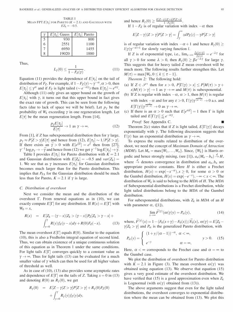
We plot the distribution of overshoot for Pareto distributionwith K = 2.1 in Figure (3). The mean overshoot ω(γ) wasobtained using equation (13). We observe that equation (15)gives a very good estimate of the overshoot distribution. Wehave verified that (15) is a good approximation even when Zk

is Lognormal (with ω(γ) obtained from (13)).The above arguments suggest that even for the light tailed

distributions, the overshoot converges to exponential distribu-tion where the mean can be obtained from (13). We plot this


0 20 40 600

0.2

0.4

0.6

0.8

1

Simulation Analysis

Fig. 3. Complementary CDF of Γ for Pareto K = 2.1, EZk = −0.3 andvar(Zk) = 1 and γ = 8.

0 1 2 30

0.2

0.4

0.6

0.8

1

SimulationAnalysis

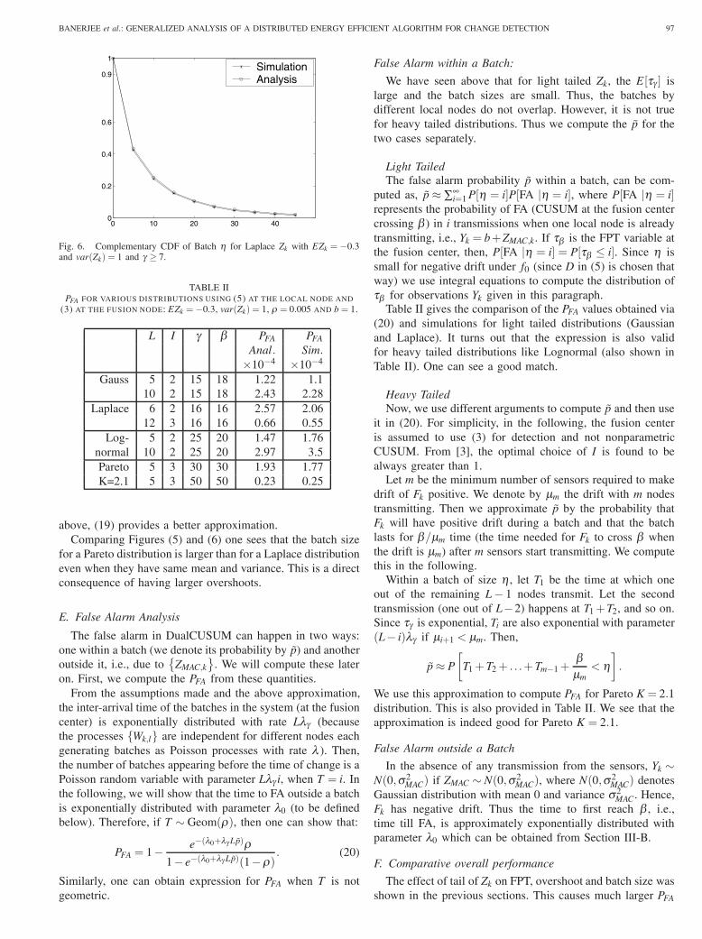
Fig. 4. Complementary CDF of Γ for Zk ∼ N(−0.3,1) and γ ≥ 6.

approximation for Gaussian distribution in Figure (4) and findan excellent match with simulations. We have verified this forLaplace distribution also.

Comparing Figures (3) and (4), we see that the overshootfor Pareto distribution is much more than for the Gaussiandistribution.

D. Distribution of the Batch

In this section we give the distribution of the batch. Al-though the distribution of batch for sub-exponential tails isgiven in [1], the one for light tails is not previously availablein the literature (for example, it is not explicitly provided in[24]).

1) Distribution of batch for heavy tail: From Theorem2.4 of [1], the batch size distribution for subexponential Z(belonging to the MDA of a Frechet distribution H withparameter α) satisfies

E[Z]ω(γ)

η d→ Yα , (16)

as γ →∞, where ω(γ) =E[Z−γ∣Z > γ] and Yα has distributionPα .

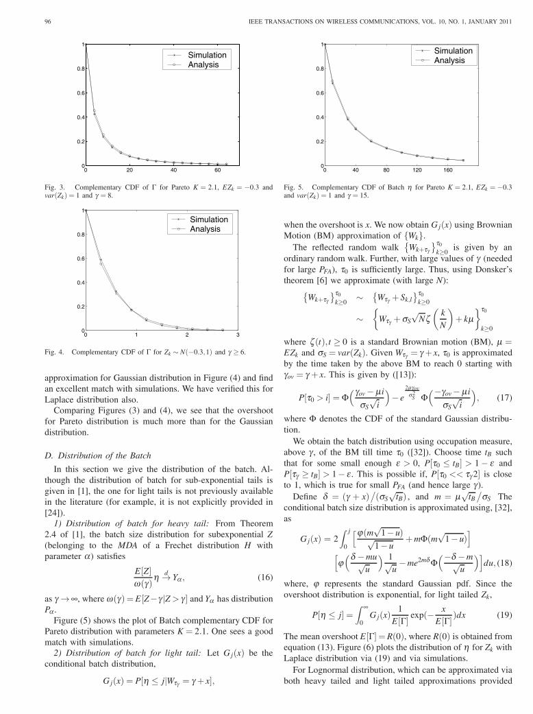
Figure (5) shows the plot of Batch complementary CDF forPareto distribution with parameters K = 2.1. One sees a goodmatch with simulations.

2) Distribution of batch for light tail: Let Gj(x) be theconditional batch distribution,

Gj(x) = P[η ≤ j∣Wτγ = γ+ x],

0 40 80 120 1600

0.2

0.4

0.6

0.8

1SimulationAnalysis

Fig. 5. Complementary CDF of Batch η for Pareto K = 2.1, EZk = −0.3and var(Zk) = 1 and γ = 15.

when the overshoot is x. We now obtain Gj(x) using BrownianMotion (BM) approximation of {Wk}.

The reflected random walk{Wk+τγ

}τ0k≥0

is given by anordinary random walk. Further, with large values of γ (neededfor large PFA), τ0 is sufficiently large. Thus, using Donsker’stheorem [6] we approximate (with large N):{

Wk+τγ}τ0

k≥0∼ {

Wτγ + Sk,l}τ0

k≥0

∼{

Wτγ +σS

√Nζ

(kN

)+ kμ

}τ0

k≥0

where ζ (t), t ≥ 0 is a standard Brownian motion (BM), μ =EZk and σS = var(Zk). Given Wτγ = γ+x, τ0 is approximatedby the time taken by the above BM to reach 0 starting withγov = γ+ x. This is given by ([13]):

P[τ0 > i] =Φ(γov − μ i

σS√

i

)− e

2μγovσ2S Φ

(−γov− μ i

σS√

i

), (17)

where Φ denotes the CDF of the standard Gaussian distribu-tion.

We obtain the batch distribution using occupation measure,above γ , of the BM till time τ0 ([32]). Choose time tB suchthat for some small enough ε > 0, P[τ0 ≤ tB] > 1− ε andP[τγ ≥ tB] > 1− ε . This is possible if, P[τ0 << τγ2] is closeto 1, which is true for small PFA (and hence large γ).

Define δ = (γ + x)/(σS

√tB) , and m = μ

√tB/σS The

conditional batch size distribution is approximated using, [32],as

Gj(x) = 2∫ j

0

[ϕ(m√1− u)√

1− u+mΦ(m

√1− u)

][ϕ(δ −mu√

u

) 1√u−me2mδΦ

(−δ −m√u

)]du, (18)

where, ϕ represents the standard Gaussian pdf. Since theovershoot distribution is exponential, for light tailed Zk,

P[η ≤ j] =∫ ∞

0Gj(x)

1E[Γ]

exp(− xE[Γ]

)dx (19)

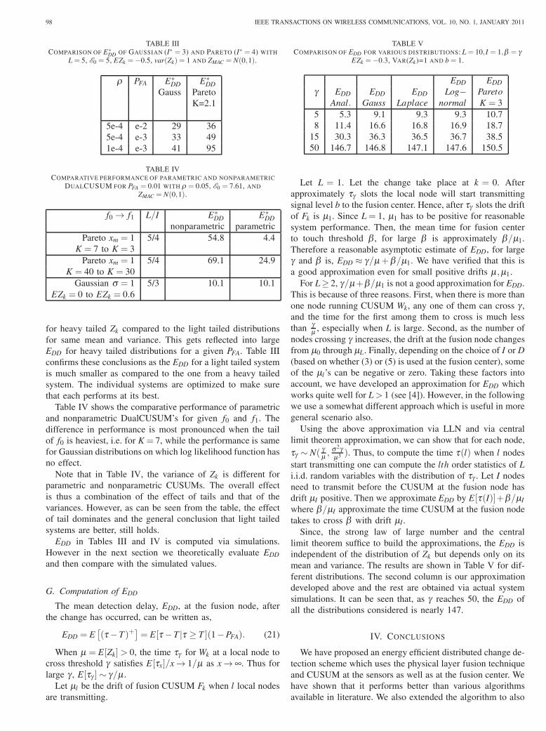
The mean overshoot E[Γ] =R(0), where R(0) is obtained fromequation (13). Figure (6) plots the distribution of η for Zk withLaplace distribution via (19) and via simulations.

For Lognormal distribution, which can be approximated viaboth heavy tailed and light tailed approximations provided


0 10 20 30 400

0.2

0.4

0.6

0.9

1SimulationAnalysis

Fig. 6. Complementary CDF of Batch η for Laplace Zk with EZk =−0.3and var(Zk) = 1 and γ ≥ 7.

TABLE IIPFA FOR VARIOUS DISTRIBUTIONS USING (5) AT THE LOCAL NODE AND

(3) AT THE FUSION NODE: EZk =−0.3, var(Zk) = 1, ρ = 0.005 AND b = 1.

L I γ β PFA PFA

Anal. Sim.×10−4 ×10−4

Gauss 5 2 15 18 1.22 1.110 2 15 18 2.43 2.28

Laplace 6 2 16 16 2.57 2.0612 3 16 16 0.66 0.55

Log- 5 2 25 20 1.47 1.76normal 10 2 25 20 2.97 3.5Pareto 5 3 30 30 1.93 1.77K=2.1 5 3 50 50 0.23 0.25

above, (19) provides a better approximation.Comparing Figures (5) and (6) one sees that the batch size

for a Pareto distribution is larger than for a Laplace distributioneven when they have same mean and variance. This is a directconsequence of having larger overshoots.

E. False Alarm Analysis

The false alarm in DualCUSUM can happen in two ways:one within a batch (we denote its probability by p̃) and anotheroutside it, i.e., due to

{ZMAC,k

}. We will compute these later

on. First, we compute the PFA from these quantities.From the assumptions made and the above approximation,

the inter-arrival time of the batches in the system (at the fusioncenter) is exponentially distributed with rate Lλγ (becausethe processes {Wk,l} are independent for different nodes eachgenerating batches as Poisson processes with rate λ ). Then,the number of batches appearing before the time of change is aPoisson random variable with parameter Lλγ i, when T = i. Inthe following, we will show that the time to FA outside a batchis exponentially distributed with parameter λ0 (to be definedbelow). Therefore, if T ∼ Geom(ρ), then one can show that:

PFA = 1− e−(λ0+λγLp̃)ρ1− e−(λ0+λγLp̃)(1−ρ)

. (20)

Similarly, one can obtain expression for PFA when T is notgeometric.

False Alarm within a Batch:

We have seen above that for light tailed Zk, the E[τγ ] islarge and the batch sizes are small. Thus, the batches bydifferent local nodes do not overlap. However, it is not truefor heavy tailed distributions. Thus we compute the p̃ for thetwo cases separately.

Light TailedThe false alarm probability p̃ within a batch, can be com-

puted as, p̃ ≈ ∑∞i=1 P[η = i]P[FA ∣η = i], where P[FA ∣η = i]

represents the probability of FA (CUSUM at the fusion centercrossing β ) in i transmissions when one local node is alreadytransmitting, i.e., Yk = b+ZMAC,k. If τβ is the FPT variable atthe fusion center, then, P[FA ∣η = i] = P[τβ ≤ i]. Since η issmall for negative drift under f0 (since D in (5) is chosen thatway) we use integral equations to compute the distribution ofτβ for observations Yk given in this paragraph.

Table II gives the comparison of the PFA values obtained via(20) and simulations for light tailed distributions (Gaussianand Laplace). It turns out that the expression is also validfor heavy tailed distributions like Lognormal (also shown inTable II). One can see a good match.

Heavy TailedNow, we use different arguments to compute p̃ and then use

it in (20). For simplicity, in the following, the fusion centeris assumed to use (3) for detection and not nonparametricCUSUM. From [3], the optimal choice of I is found to bealways greater than 1.

Let m be the minimum number of sensors required to makedrift of Fk positive. We denote by μm the drift with m nodestransmitting. Then we approximate p̃ by the probability thatFk will have positive drift during a batch and that the batchlasts for β/μm time (the time needed for Fk to cross β whenthe drift is μm) after m sensors start transmitting. We computethis in the following.

Within a batch of size η , let T1 be the time at which oneout of the remaining L− 1 nodes transmit. Let the secondtransmission (one out of L−2) happens at T1+T2, and so on.Since τγ is exponential, Ti are also exponential with parameter(L− i)λγ if μi+1 < μm. Then,

p̃ ≈ P

[T1+T2+ . . .+Tm−1+

βμm

< η].

We use this approximation to compute PFA for Pareto K = 2.1distribution. This is also provided in Table II. We see that theapproximation is indeed good for Pareto K = 2.1.

False Alarm outside a Batch

In the absence of any transmission from the sensors, Yk ∼N(0,σ2

MAC) if ZMAC ∼ N(0,σ2MAC), where N(0,σ2

MAC) denotesGaussian distribution with mean 0 and variance σ2

MAC. Hence,Fk has negative drift. Thus the time to first reach β , i.e.,time till FA, is approximately exponentially distributed withparameter λ0 which can be obtained from Section III-B.

F. Comparative overall performance

The effect of tail of Zk on FPT, overshoot and batch size wasshown in the previous sections. This causes much larger PFA


TABLE IIICOMPARISON OF E∗

DD OF GAUSSIAN (I∗ = 3) AND PARETO (I∗ = 4) WITH

L = 5, E0 = 5, EZk =−0.5, var(Zk) = 1 AND ZMAC = N(0,1).

ρ PFA E∗DD E∗

DDGauss Pareto

K=2.1

5e-4 e-2 29 365e-4 e-3 33 491e-4 e-3 41 95

TABLE IVCOMPARATIVE PERFORMANCE OF PARAMETRIC AND NONPARAMETRIC

DUALCUSUM FOR PFA = 0.01 WITH ρ = 0.05, E0 = 7.61, AND

ZMAC = N(0,1).

f0 → f1 L/I E∗DD E∗

DDnonparametric parametric

Pareto xm = 1 5/4 54.8 4.4K = 7 to K = 3

Pareto xm = 1 5/4 69.1 24.9K = 40 to K = 30

Gaussian σ = 1 5/3 10.1 10.1EZk = 0 to EZk = 0.6

for heavy tailed Zk compared to the light tailed distributionsfor same mean and variance. This gets reflected into largeEDD for heavy tailed distributions for a given PFA. Table IIIconfirms these conclusions as the EDD for a light tailed systemis much smaller as compared to the one from a heavy tailedsystem. The individual systems are optimized to make surethat each performs at its best.

Table IV shows the comparative performance of parametricand nonparametric DualCUSUM’s for given f0 and f1. Thedifference in performance is most pronounced when the tailof f0 is heaviest, i.e. for K = 7, while the performance is samefor Gaussian distributions on which log likelihood function hasno effect.

Note that in Table IV, the variance of Zk is different forparametric and nonparametric CUSUMs. The overall effectis thus a combination of the effect of tails and that of thevariances. However, as can be seen from the table, the effectof tail dominates and the general conclusion that light tailedsystems are better, still holds.

EDD in Tables III and IV is computed via simulations.However in the next section we theoretically evaluate EDD

and then compare with the simulated values.

G. Computation of EDD

The mean detection delay, EDD, at the fusion node, afterthe change has occurred, can be written as,

EDD = E[(τ−T )+

]= E[τ−T ∣τ ≥ T ](1−PFA). (21)

When μ = E[Zk]> 0, the time τγ for Wk at a local node tocross threshold γ satisfies E[τx]/x → 1/μ as x → ∞. Thus forlarge γ , E[τγ ]∼ γ/μ .

Let μl be the drift of fusion CUSUM Fk when l local nodesare transmitting.

TABLE VCOMPARISON OF EDD FOR VARIOUS DISTRIBUTIONS: L = 10,I = 1,β = γ

EZk =−0.3, VAR(Zk)=1 AND b = 1.

EDD EDD

γ EDD EDD EDD Log− ParetoAnal. Gauss Laplace normal K = 3

5 5.3 9.1 9.3 9.3 10.78 11.4 16.6 16.8 16.9 18.7

15 30.3 36.3 36.5 36.7 38.550 146.7 146.8 147.1 147.6 150.5

Let L = 1. Let the change take place at k = 0. Afterapproximately τγ slots the local node will start transmittingsignal level b to the fusion center. Hence, after τγ slots the driftof Fk is μ1. Since L = 1, μ1 has to be positive for reasonablesystem performance. Then, the mean time for fusion centerto touch threshold β , for large β is approximately β/μ1.Therefore a reasonable asymptotic estimate of EDD, for largeγ and β is, EDD ≈ γ/μ+β/μ1. We have verified that this isa good approximation even for small positive drifts μ ,μ1.

For L≥ 2, γ/μ+β/μ1 is not a good approximation for EDD.This is because of three reasons. First, when there is more thanone node running CUSUM Wk, any one of them can cross γ ,and the time for the first among them to cross is much lessthan γ

μ , especially when L is large. Second, as the number ofnodes crossing γ increases, the drift at the fusion node changesfrom μ0 through μL. Finally, depending on the choice of I or D(based on whether (3) or (5) is used at the fusion center), someof the μl’s can be negative or zero. Taking these factors intoaccount, we have developed an approximation for EDD whichworks quite well for L> 1 (see [4]). However, in the followingwe use a somewhat different approach which is useful in moregeneral scenario also.

Using the above approximation via LLN and via centrallimit theorem approximation, we can show that for each node,τγ ∼ N( γμ ,

σ2γμ3 ). Thus, to compute the time τ(l) when l nodes

start transmitting one can compute the lth order statistics of Li.i.d. random variables with the distribution of τγ . Let I nodesneed to transmit before the CUSUM at the fusion node hasdrift μI positive. Then we approximate EDD by E[τ(I)]+β/μI

where β/μI approximate the time CUSUM at the fusion nodetakes to cross β with drift μI .

Since, the strong law of large number and the centrallimit theorem suffice to build the approximations, the EDD isindependent of the distribution of Zk but depends only on itsmean and variance. The results are shown in Table V for dif-ferent distributions. The second column is our approximationdeveloped above and the rest are obtained via actual systemsimulations. It can be seen that, as γ reaches 50, the EDD ofall the distributions considered is nearly 147.

IV. CONCLUSIONS

We have proposed an energy efficient distributed change de-tection scheme which uses the physical layer fusion techniqueand CUSUM at the sensors as well as at the fusion center. Wehave shown that it performs better than various algorithmsavailable in literature. We also extended the algorithm to also


include the nonparametric CUSUM. We have theoreticallycomputed the probability of false alarm and mean delay inchange detection for the general algorithm. The analyticalresults provide good approximations for different distributions.Our analysis provides interesting conclusions and insights.One is that the tail of the distribution has significant effecton the performance of nonparametric CUSUM. We also showwhy parametric CUSUM is relatively insensitive to the tails.In the process we obtain new results on the reflected randomwalk which can be of independent interest.

APPENDIX A

This section states and proves Lemma 1 which shows thatlog likelihood converts a large class of distributions into lighttailed distributions. Let Z = log f1(x)

f0(x)and g(x) = f1(x)

f0(x). Then,

the following hold:Lemma 1: (a) If g(x)≤ xβ for some β > 0, and all x large

enough and 1 − F0(x) ≤ x−α0 for all large x then thepositive tail of distribution of Z decays exponentially withparameter α0/β .

(b) If g(x)≤ exp(αxβ ) for some α,β > 0 and all x large and1−F0(x) ≤ exp(−α0xβ0) for α0,β0 > 0, then P[z > x] <exp(−α0

xαβ0/β ).

Proof: (a) For x> 0, P0[Z > x] = P0[g(X)> ex]≤P0[Xβ >ex]≤ e−xα0/β .(b) For x > 0, P0[Z > x] = P0[g(X) > ex] ≤ P0[exp(αXβ ) >ex] = P0[αXβ > x]≤ exp(−α0

xαβ0/β ).

The above Lemma covers a large number of cases as weillustrate now. Part (a) of the theorem shows that if f0 and f1are heavy tailed, Z can become light tailed. Part (b) of theoremshows that light tailed f0, f1 will keep Z light tailed. Forexample let F1 and F0 be of regular variation with parameters−α0 and −α1, i.e., 1−Fi(x) = li(x)x−αi , i = 1,2 for x > 0,where li are slowly varying functions, and αi > 0 with α0 ∕=α1.Then, Theorem 1(a) applies. If α0 > α1, g(x) = l(x)xα0−α1 ≤xα0−α1+β1 for any β1 > 0 for all large x. Also, 1−F0(x) ≤xα0+β2 for any β2 > 0 for x large enough. Chose 0< β2 < α0.Hence, P0[Z > x]< exp(−x(−α0+β2)/(α0−α1+β1)) for allx large enough providing Z with light tail under P0. If α0 <α1, then g(x) < xβ1 for any β1 > 0 and we get P0[Z > x] <exp(−x(α0−β2)

β1).

Next consider exponential distributions: fi(x) =λi exp(−λix), λi > 0, x > 0, λ0 ∕= λ1. Then, g(x) ≤ e∣λ1−λ0∣xand P0[Z > x]< e−λ0(x−logλ1/λ0)/∣λ1−λ0∣. Thus Z is light tailedunder P0.

Now we show the versatility of the above result by consider-ing f1(x)= β1x−α1 and f0(x)= exp(−(x−μ0)

2/2σ2)/√

2πσ0.Then, g(x) = β1x−α1 exp((x− μ0)

2/2σ2)√

2πσ0 ≤ exp(αx2)for appropriately chosen α > 0 for all large x. Thus, since

1−F0(x) ≤ exp(−(x− μ0)2/4σ2

0 )

≤ exp(α0x2),

P0[Z > x] ≤ exp(−α0xα1

).

APPENDIX B

This appendix provides the proof of Theorem 1.

Proof: Obtain an equation for L(0) by substituting 0 fors in (10) and then plug in the expression for L(0) in (10). Weobtain

L(s) =

(1+

FZ(−s)1−FZ(0)

)+

∫ γ

0Lγ (y)

(fZ(y− s)+

fZ(y)FZ(−s)1−FZ(0)

)dy (22)

which is Fredholm integral equation of second kind withkernel k(s,y) = fZ(y− s) + fZ(y)FZ(−s)

1−FZ(0)and we consider the

mapping f �→ g defined by

g(s) =∫ γ

0k(s,y) f (y)dy (23)

on the space of functions L2([0,γ]). From [26] (pp. 269-270),to show that (22) has a continuous solution, for FZ continuouswe need to show that φ(s) =

∫ γ0 k(s,y)φ(y)dy has a unique

solution which then is the trivial solution φ(s) = 0.For this we show that (23) is a contraction mapping on the

space of continuous functions on [0,γ] (with sup norm). We

have, for ∥ f∥ △= sup0≤y≤γ ∣ f (y)∣,

∥g∥ = sup0≤s≤γ

∣∫ γ

0k(s,y) f (y)dy∣

≤ ∥ f∥ sup0≤s≤γ

[∫ γ

0fZ(y− s)dy+

∫ γ

0fZ(y)

FZ(−s)1−FZ(0)

dy

]

= ∥ f∥ sup0≤s≤γ

[FZ(γ− s)−FZ(−s)+

FZ(−s)(FZ(γ)−FZ(0))1−FZ(0)

]

= ∥ f∥ sup0≤s≤γ

[(FZ(γ− s)(1−FZ(0))+FZ(−s)(FZ(γ)− 1)

1−FZ(0)

]< ∥ f∥ sup

0≤s≤γFZ(γ− s)

≤ ∥ f∥FZ(γ).

Thus if FZ(γ)< 0, this operator is a contractor and hence hasa unique fixed point which is the trivial function φ(s) = 0.

APPENDIX C

This appendix provides the proof of Theorem 2.Proof: (a) If Z ∈ S ∗ then from [1], Theorem 2.1

P[M(τ)> x]≈ E[τ]P[Z > x] (24)

for large x. Thus M(τ) is subexponential if Z is. Let {Yk} bei.i.d. with the distribution of M(τ). Let N(γ) = inf{n :Yn > γ}.Then Wτγ ≤st YN(γ) (X ≤st Y denotes P[X ≤ x]≥ P[Y ≤ x] forall x). Thus for x > 0,

P[Wτγ − γ > x] ≤ P[YN(γ)− γ > x]

=∞

∑n=1

P[Yn > γ+ x,N(γ) = n]

=∞

∑n=1

P[Yn > γ+ x, max1≤k≤n−1

Yk ≤ γ]

= P[Y > γ+ x]∞

∑n=1

(P[Y ≤ γ])n−1

=P[Y > γ+ x]

P[Y > γ]. (25)


Because Y is subexponential P[Y > γ + x]/P[Y > γ] → 1 asY → ∞. Also taking expectations in above inequality E[Γ] ≤E[Y − γ∣Y > γ].(b) From (24), if Z is of regular variation with index −α ,α > 1 then M(τ) is of regular variation with index −α . Alsothen E[Z] < ∞ and E[M(τ)] < ∞. Therefore, E[Yα−ε ] < ∞for any ε > 0. Hence, from Gut [12], Chapter 1, Th.2.3,

(Γ(γ))γ−1

(α−ε) ≤ YN(γ)γ−1

(α−ε) → 0 a.s. because N(γ) → ∞ a.s.as γ → ∞ and N(γ)/γ → 1/E[γ] a.s. Also since {N(γ)/γ} isuniformly integrable (Gut [12], P.54), we get from Gut [12],Chapter 1, Thm.7.2, limγ→∞

E[Γ(γ)]γ1/(α−ε) = 0.

(c) From [2], Chapter 7, P[M(τ) > x] ≈ ce−uα for u > 0 forsome c > 0. Thus from (25)

P[Γ(γ)> x] = P[Wτγ − γ > x]

≤ P[Y > γ+ x]P[Y > γ]

≈ e−αx as γ → ∞. (26)

ACKNOWLEDGEMENTS

This work was supported in part by a grant from theAerospace and Networking Research Consortium and byDRDO sensor network project.

REFERENCES

[1] S. Asmussen, “Subexponential asymptotics for stochastic processes: ex-tremal behavior, stationary distribution and first passage probabilities,”Ann. Appl. Prob. vol. 8, no. 2, pp. 354-374, 1998.

[2] S. Asmussen, Applied Probability and Queues, 2nd edition. Springer,2003.

[3] T. Banerjee, V. Kavitha, and V. Sharma, “Energy efficient changedetection over a MAC using physical layer fusion,” in Proc. IEEEICASSP, Las Vegas, Apr. 2008.

[4] T. Banerjee and V. Sharma, “Generalized analysis of a distributedenergy efficient algorithm for change detection,” 12th ACM Interna-tional Conference on Modeling, Analysis and Simulation of Wirelessand Mobile Systems (MSWiM09), Spain, Oct. 2009.

[5] H. M. Barakat and Y. H. Abdul Kader, “Computing the moments oforder statistics from nonidentical random variables,” Statistical Methodsand Applications, vol. 13. Springer, 2003.

[6] P. Billingsley, Weak Convergence of Measures: Applications in Proba-bility. John Wiley and Sons, Inc., 1987.

[7] R. S. Blum, S. A. Kassam, and H. V. Poor, “Distributed detection withmultiple sensors—part II: advanced topics,” Proc. IEEE, vol. 85, no. 1,pp. 64-79, 1997.

[8] O. J. Boxma and J. W. Cohen, The Single Server Queue: Heavy Tailsand Heavy Traffic in self-Similar Network Traffic and PerformanceEvaluation, K. Park and W. Willinger (editors.) Wiley, 2000.

[9] B. E. Brodsky and B. S. Darkhovsky, Nonparametric Methods inChange Point Problems. Kluwer Academic Publishers, 1993.

[10] R Doney, R. Maller, and M. Savov, “Renewal theorems and stabilityfor the reflected process,” Stochastic Processes and Their Applications,vol. 119, pp. 1290–1297, 2009.

[11] C. M. Goldie and C. Kliippelberg, “Subexponential distributions,” inPractical Guide to Heavy Tails, R. Adler, R. Feldman and M. S. Taqqu,editors. Birkhauser, 1998.

[12] A. Gut, Stopped Random Walks: Limit Theorems and Applications.Springer, 1988.

[13] J. M. Harrison, Brownian Motion and Stochastic Flow Systems. JohnWiley and Sons, 1985.

[14] J. Keilson, Markov Chain Models—Rarity and Exponentiality. Springer,1979.

[15] T. L. Lai, “Sequential change point detection in quality control anddynamical systems,” J. Royal Statistical Society, Series B (Methodolog-ical), vol. 57, no. 4, pp. 613-658, 1995.

[16] K. B. Lataief and W. Zhang, Cooperative Spectrum Sensing in CognitiveWireless Communication Networks, E. Hossain and V. K. Bhargava,editors. Springer, 2007.

[17] G. Lorden, “Procedures for reacting to a change in distribution,” Ann.Math. Statist., vol. 41, pp. 1897–1908, 1971.

[18] A. Luceno and J. Puig-Pey, “Evaluation of the run-length probabilitydistribution for CUSUM charts: assessing chart performance,” Techno-metrics, vol. 42, no. 4, pp. 411-416, 2000.

[19] R. Mudumbai, G. Barriac, and U. Madhow, “On the feasibility ofdistributed beamforming in wireless networks, IEEE Trans. WirelessCommun., vol. 6, no. 5, pp. 1754-1763, May 2007.

[20] Y. Mei, “Information bounds and quickest change detection in decen-tralized decision systems,” IEEE Trans. Inf. Theory, vol. 51, pp. 2669-2681, July 2005

[21] G. Mergen and L. Tong, “Type based estimation over multiaccesschannels,” IEEE Trans. Signal Process., vol. 54, no. 2, Feb. 2006.

[22] G. V. Moustakides, “Optimal stopping times for detecting changes indistribution,” Ann. Statist., vol. 14, pp. 1379–1387, 1986.

[23] E. S. Page, “Continuous inspection schemes,” Biometrica, vol. 41, no.1/2, pp. 100-115, June 1954.

[24] H. Rootzen, “Maxima and exceedances of stationary Markov chains,”Adv. in Appl. Prob., vol. 20, no. 2, pp. 371-390, June 1998.

[25] S. Ross, Stochastic Processes, 2nd edition. Wiley, 1996.[26] T. L. Saaty, Nonlinear Integral Equations. Dover Publications, 1981.[27] J. Sadowsky, “Large deviation theory and efficient simulation of exces-

sive backlogs in a GI/G/m Queue,” IEEE Trans. Auto. Cont., vol. 36,no. 12, pp. 1383-1394, 1991.

[28] V. Sharma and A. K. Jaya Prakasam, “An efficient algorithm forcooperative spectrum sensing in cognitive radio networks,” in Proc.National Conf. on Comm. (NCC), Jan. 2009, Guwahati, India.

[29] A. N. Shiryaev, “On optimal methods in quickest detection problems,”Theory Probab. Appl., vol. 8, pp. 22-46, 1963.

[30] W. Su, Time-Synchronization Challenges and Techniques in WirelessSensor Networks and Applications, Y. Li, M. T. Thai, and W. Wu,editors. Springer, 2008.

[31] R. Tantra and A. Sahai, “SNR walls for signal detection,” IEEE J. Sel.Topics Signal Process., vol. 2, pp. 4-17, Feb. 2008.

[32] L. Takacs, “On a generalization of the ARC-SINE law,” Ann. Appl.Probab., vol. 6, no. 3, pp. 1035-1040, 1996.

[33] A. Tartakovsky and V. V. Veeravalli, “Quickest change detection indistributed sensor systems,” in Proc. 6th Int. Sym. on Inf. Fusion,Australia, July 2003, pp. 756-763.

[34] A. G. Tartakovsky and H. Kim, “Performance of certain decentralizeddistributed change detection procedures,” in Proc. Int. Sym. on Inf.Fusion.

[35] V. V. Veeravalli, “Decentralized quickest change detection,” IEEETrans. Inf. Theory, vol. 47, no. 4, pp. 1657-1665, May 2001.

[36] R. Viswanathan and P. K. Varshney, “Distributed detection with multiplesensors–part I: fundamentals,” Proc. IEEE, vol. 85, no. 1, pp. 54-63,1997.

[37] L. Zacharias and R. Sundaresan, “Decentralized sequential changedetection using physical layer fusion,” in Proc. ISIT, France, June 2007.

Taposh Banerjee received the B.E. degree in elec-tronics engineering from the Nagpur University,Nagpur, India in 2000 and the M.E. degree intelecommunication from the Indian Institute of Sci-ence, Bangalore, India in 2003. He is currentlypursuing his Ph.D. from the University of Illinois atUrbana-Champaign. He has worked for three yearswith Samsung India Software Operations, Bangalorefrom 2003-2005 and worked as a Project Associatein the ECE department of the Indian Institute ofScience, Bangalore from 2007-2009. His research

interests include detection theory, applied probability and communicationsystems.

Vinod Sharma completed his B Tech in 1978 fromIIT Delhi and Ph.D. in 1984 from CMU in Pitts-burgh in Electrical Engg. He worked at NortheasternUniv., Boston and UCLA before joining Indian Insti-tute of Science in 1988. Currently he is a Professorand Chairman of Electrical Communication EnggDept. He is on the editorial boards of Interna-tional Journal of Information and Coding Theory(Inderscience), Journal of Electrical and ComputerEngineering (Hindawai), and International Journalof Advanced Computer Engineeringg (Serials Pub-

lications). Prof Sharma’s research interests are in Wireless communication,Information Theory and Communication Networks.


Veeraruna Kavitha received her B.E. degree inElectronics from UVCE, Bangalore in 1994 andthe M.Sc (Engg) and Ph.D. degree from Dept. ofECE, Indian Institute of Science (IISc), Bangalorein 2002 and 2007 respectively. From 1994-2000,She was involved in the design and developmentof GPS, CDMA and Voice band modems at AccordS/W and Systems, Bangalore. She was a NBHM(National Board for Higher Mathematics) scholarat Tata Insititue of Fundamental Research (TIFR),Bangalore, during 2007-08. From 2008 onwards,

She has been a post doctoral researcher with MAESTRO, INRIA, SophiaAntipolis, France and LIA, University of Avignon, France. Her researchinterests span communication theory, wireless networks, signal processing,game theory and optimization.

Arunkumar Jayaprakasam received his B.E. de-gree from Regional Engineering College, Tiruchira-palli in 2002. He recieved his M.Sc (Engg) fromIndian Institute of Science in 2010. He was withTexas Instruments (India) Pvt. Ltd., Bangalore from2002 - 2008 where he was involved in ADSLand GSM/GPRS/EDGE modem development. He iscurrently with Nokia (India) Pvt. Ltd. His researchinterests include Wireless Communication and Com-munication Networks.

taposh analysis dual cusum

Documents