tags: scalable threshold-based algorithms for proximity computation in graphs
TRANSCRIPT
TAGs: Scalable Threshold-Based Algorithmsfor Proximity Computation in Graphs
A. LyritsisDepartment of Informatics
Aristotle University54124 Thessaloniki, Greece
A. N. PapadopoulosDepartment of Informatics
Aristotle University54124 Thessaloniki, [email protected]
Y. ManolopoulosDepartment of Informatics
Aristotle University54124 Thessaloniki, [email protected]
ABSTRACTA fundamental and very useful operation in graphs is thecomputation of the proximity between nodes, i.e., the de-gree of dissimilarity (or similarity) between two nodes v andu. This is an important tool both in graph databases andgraph mining applications, because it provides the base tosupport more complex tasks such as graph partitioning, clus-tering, classification, to name a few. All methods proposedin the literature assume that proximity is computed on a sin-gle graph by using a single distance measure. In addition,most of them focus on the proximity between node pairs. Inthis work, we present for the first time, scalable algorithmsthat: (i) they support proximity computation in multiplegraph instances, (ii) they enable the utilization of several dis-tance measures, (iii) they support proximity queries arounda source node without limiting to node pairs and (iv) theysupport extensions for metric-based and skyline query pro-cessing. The main result of our work is the design of Thresh-old Algorithms for Graphs (denoted as TAGs), which arestudied and evaluated experimentally by using real-life aswell as synthetic graphs, based on both the G(n, p) Erdos-Renyi model and power law degree distributions.
Categories and Subject DescriptorsH.2 [Database Management]: Systems; H.2.8 [DatabaseManagement]: Database Applications—Data Mining ; G.2.2[Discrete Mathematics]: Graph Theory—Graph Algo-rithms
General TermsAlgorithms
Keywordsgraph databases, proximity query processing
Permission to make digital or hard copies of all or part of this work forpersonal or classroom use is granted without fee provided that copies arenot made or distributed for profit or commercial advantage and that copiesbear this notice and the full citation on the first page. To copy otherwise, torepublish, to post on servers or to redistribute to lists, requires prior specificpermission and/or a fee.EDBT 2011, March 22–24, 2011, Uppsala, Sweden.Copyright 2011 ACM 978-1-4503-0528-0/11/0003 ...$10.00
1. INTRODUCTIONGraph mining is an important research direction [1, 3, 6]
that recently has attracted significant interest. The mainreason for this trend, is that real-life networks have grownin size and therefore scalable mining tasks are required fornetwork analysis purposes. Node proximity [5] is a funda-mental operation that is required by complex mining tasks,such as partitioning, clustering and outlier detection. In itssimplest form, node proximity is requested for a particularpair of entities (nodes) s and t, which generally do not havea direct connection between them. The way node proximityis computed depends on application requirements and alsoon the data representation and data semantics.
As an example, consider a co-authorship network, wherenodes represent authors and a connection between two au-thors declares that they have a paper in common. In thisapplication, one may be interested in the similarity betweenauthors s and t, who may not have a common paper. Thelarger the proximity between s and t in the co-authorshipnetwork, the larger the similarity of their research interests.As a second example, assume an information retrieval ap-plication where nodes represent named entities (e.g., placenames) extracted from a text collection, and two entities aredirectly connected if they appear in the same document, inthe same section or in the same paragraph (according to ap-plication needs). The network-based proximity between twoentities s and t quantifies the semantic similarity betweenthese entities.
Different techniques have been proposed to determine prox-imity in networks [5, 21]. However, previously proposedmethods are characterized by three important limitations.First, proximity computation is supported for a specific ver-tex pair s, t. In many applications, like graph-based in-formation retrieval for example [25], there is a need to sup-port additional operations that are considered important: (i)given a query entity s determine all entities with distance atmost r from s, and (ii) given a query entity s determine the kmost proximal entities to s. A second limitation of proposedmethods is that they are based on a single distance mea-sure to compute proximity (e.g., random walk with restart,shortest path, maximum flow). Finally, a third shortcom-ing is that only a single graph has been used to determineproximity. However, entities may be associated in many dif-ferent ways [26] resulting in many graph instances. In sucha case, multiple graphs are required for proximity computa-tion, and therefore distance measures must be combined in aconvenient way to obtain a semantically meaningful result.For example, researchers may form a graph G with paper
. . .
G1 G2 GN
top-k query- source vertex- ranking function- k
DF1
DF2
DFN
...
results: ranked list of k nodes andcorresponding distances
proximity computation engine:support for multiple graphs
and distance measures
range query- source vertex- ranking function- r
skyline query- source vertex
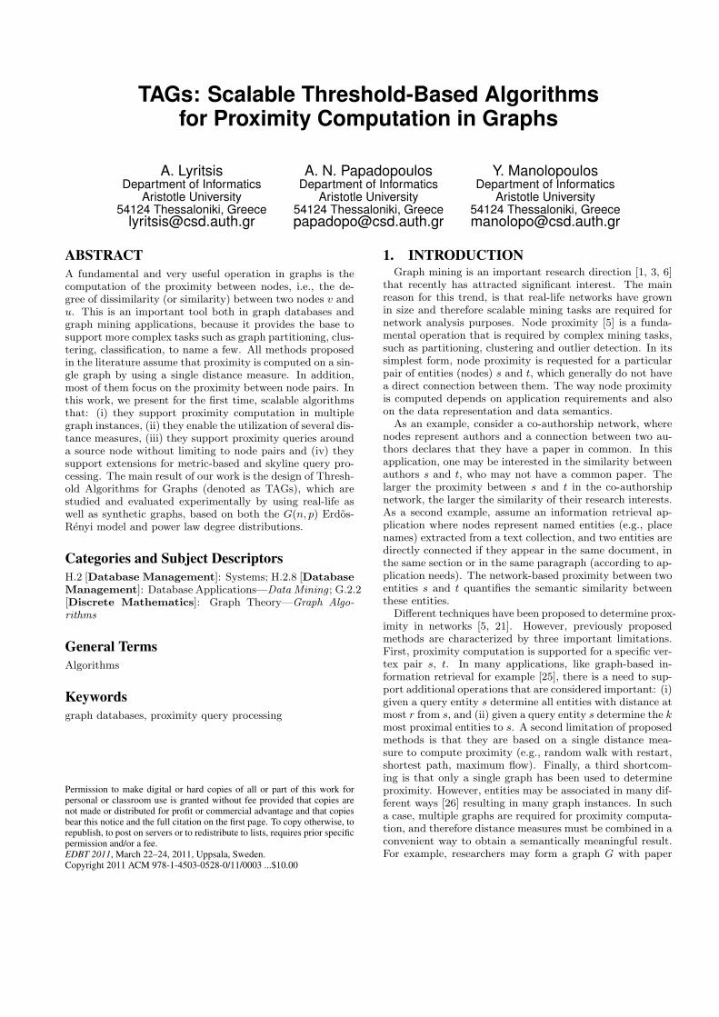
Figure 1: Query processing with multiple graphsand multiple distance measures.
co-authorship information and also may formulate anothergraph H capturing their cooperation in project proposals.Both graphs should be utilized to compute the similaritybetween two researchers regarding their research interestsin general.Figure 1 depicts a bird’s eye view of a system offering
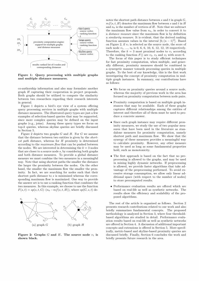
query processing services in multiple graphs with multipledistance measures. The illustrated query types are just a fewexamples of selection-based queries that may be supported,since more complex queries may be defined on the inputgraphs (e.g., joins). Among these query types we focus ontop-k queries, whereas skyline queries are briefly discussedin Section 5.Figure 2 depicts two graphs G and H. For G we assume
that the distance between two entities is given by the short-est path distance, whereas for H proximity is determinedaccording to the maximum flow that can be pushed betweenthe nodes. We are interested in determining the k = 3 nodesthat are closer to a source node s, by considering both graphsand both distance measures. To provide a global distancemeasure we must combine the two measures in a meaningfulway. Note that using shortest paths the smaller the distancethe larger the proximity between the nodes. On the otherhand, the smaller the maximum flow the smaller the prox-imity. In fact, we are searching for nodes such that theirshortest path distance to s is minimized whereas the corre-sponding maximum flow is maximized. One way to providethe answer set is to use a ranking function that combines thetwo measures. In this example, we choose to use the functionF (s, t) = sp(s, t, G) ·(nh−mf(s, t,H)), where sp(G, s, t) de-
v1
v2
v4
v3
v5
v7
v8
v6
v1 v
4v5
v2
v3
v6 v
7
v8
(a) graph G (b) graph H
Figure 2: Graphs G and H. The source node v1 isshown black.
notes the shortest path distance between s and t in graph G,mf(s, t,H) denotes the maximum flow between s and t in Hand nh is the number of vertices of H. Note that we subtractthe maximum flow value from nh, in order to convert it toa distance measure since the maximum flow is by definitiona similarity measure. It is evident, that the derived rankingfunction assumes values in the interval [0, (n − 1)2]. Basedon Figure 2, if v1 is selected as the source node, the score ofeach node v1, ..., v8 is 0, 6, 6, 10, 6, 12, 12, 18 respectively.Therefore, the k = 3 most proximal nodes to v1 accordingto the ranking function F () are v2, v3 and v5 with score 6.
The focus of this paper is to study efficient techniquesfor fast proximity computation, when multiple, and gener-ally different, proximity measures should be combined ina synergetic manner towards processing queries in multiplegraphs. To the best of our knowledge, this is the first workinvestigating the concept of proximity computation in mul-tiple graph instances. In summary, our contributions haveas follows:
• We focus on proximity queries around a source node,whereas the majority of previous work in the area hasfocused on proximity computation between node pairs.
• Proximity computation is based on multiple graph in-stances that may be available. Each of these graphscaptures different relationships among the entities ofinterest and therefore all of them must be used to pro-duce a concrete answer.
• Since each graph instance may require different prox-imity measures, we study the use of two popular mea-sures that have been used in the literature as stan-dalone measures for proximity computation, namelyshortest path and maximum flow. We show that thesynergy of these measures provides a meaningful wayto calculate proximity. However, any other measuremay be used as long as some fundamental propertieshold, such as monotonicity.
• The first approach is based on the fact that no pre-processing is allowed to the graphs, and may be usedin mining highly dynamic networks. If preprocessingis allowed, we provide faster algorithms that take ad-vantage of the preprocessing performed. To avoid ex-cessive storage consumption, we allow only linear ad-ditional space (with respect to the number of nodes)to store precomputed results.
• Performance evaluation results are offered which arebased on real-life as well as synthetic networks. Theresults show the efficiency and scalability of the pro-posed algorithms.
The rest of the article is organized as follows. Section 2presents research contributions related to our work and alsobriefly summarizes fundamental concepts. The proposedmethodology is analyzed in Section 3, where four threshold-based algorithms ate studied in detail. Performance evalu-ation results based on real-life as well as synthetic networksare offered in Section 4. A discussion of additional importantconcepts and extensions is offered in Section 5. More specif-ically, metric-based and skyline-based proximity queries arediscussed briefly. Finally, Section 6 concludes the work andbriefly presents future research in the area.
2. BACKGROUNDThe role of this section is twofold: (i) to briefly discuss
related research in the area and (ii) to present some funda-mental concepts regarding the algorithms studied.
2.1 Related ResearchThe problem of proximity computation in networks has
attracted significant interest due to its importance in morecomplex data mining tasks. An interesting proposal forproximity computation is offered in [20]. However, this methodcannot be used to answer neighborhood queries since it onlysupports pair-wise proximity computation. The nice prop-erty of this algorithm is that it does not require the inves-tigation of the whole graph. However, in order to answerneighborhood queries around a source vertex s, all nodeproximities from s must be computed, leading to increasedcomputational cost.Random walk with restart (RWR) has been used in [27] to
determine proximity. In fact, this method supports neigh-borhood formation [25] around a source vertex since it com-putes proximities in one-to-all fashion. To determine theproximity between s and t, a random walk is performed,and the proximity between the nodes is determined by usingthe steady-state probability. This method can be easily in-corporated in our proposal as a potential distance measure.A limitation of RWR is that since the triangle inequalitydoes not hold, we cannot use metric-based access methodsto organize the nodes.The main limitation with all proposed approaches is that
a single graph is assumed and only one distance measure isapplied to determine proximity. To support multiple graphsand multiple distance measures we need efficient tools tocombine the graphs and provide efficient means of graphsearch to get the final answer. Our work is inspired by Fa-gin’s significant work [8] for threshold-based top-k compu-tation in information retrieval. According to Fagin’s idea,if multiple streams of object attributes are available sortedin non-increasing order of significance, a global ranking maybe achieved by providing a monotone scoring function. Inour case, each node v may be represented as a tuple wherethe i-th attribute corresponds to the distance between v andthe source s in the i-th graph. This observation allows theuse of threshold algorithms in our case.Although many distance measures could have been used,
we focus on shortest paths and maximum flows, because oftheir simplicity, their extensive use in diverse applicationsand the nice properties that arise from their combination.As we are going to demonstrate in the sequel, all maxi-mum flow values between nodes can be recorded in a tree-like structure, the Gomory-Hu tree [15], which can be con-structed by executing n−1 maximum flow operations. Thisstructure allows for efficient sorted access around a sourcenode s, and saves computational cost since maxflow opera-tions are expensive. The Gomory-Hu tree has been used alsoin [12] for community discovery in networks and in [19] forpartitioning web graphs. In general, it may be used whenefficient maxflow computations are required.Another work that motivated us to conduct this research is
[26], where the authors study graph clustering by taking intoconsideration multiple graph instances. In this paper, wedescribe threshold-based algorithms to allow for proximitycomputation using multiple graphs and (where applicable)multiple distance measures.
2.2 Fundamental ConceptsFor the rest of the paper we assume that each network
is modeled by an undirected graph G, where VG is the setof vertices (nodes) and EG the set of edges (direct connec-tions). Moreover, without loss of generality we assume thatbetween two vertices vi and vj there could be at most oneconnection, represented by the edge ei,j , which is possiblyweighted. Extensions for multigraphs are straight-forward.The support of directed graphs is also possible, providedthat the absence of the symmetry property in node proxim-ity does not pose any problems; otherwise, adaptations arerequired. Table 1 shows the most frequently used symbols.
Symbol Interpretation
G an undirected (possibly weighted) graphVG, EG nodes and edges of Gng,mg number of nodes and edges of Gvi the i-th node of a graphei,j edge joining nodes vi and vjk number of requested proximal nodesw(vi, vj) weight of the edge between vi and vjsp(vi, vj , G) shortest distance between vi, vj in Gmf(vi, vj , G) maxflow between vi, vj in GT (G) the Gomory-Hu tree of graph G
Table 1: Frequently used symbols.
Without loss of generality, we assume that the relation-ships of our entities (represented as graph vertices) are cap-tured by two graphs G and H (generalizations for any num-ber of graphs are straight-forward) where multiple vertexproximity measures are available. In addition, we assumethat both graphs contain the same set of nodes. In a differ-ent case, several approaches may be followed. For example,if there is a node v contained in G but not in H then its dis-tance from the source node may be set to infinite to excludeit from the result set. It is evident that the source node smust be present in both graphs.
We focus on two very popular distance measures thathave been used in the literature for proximity computation,namely the shortest path (applied on G) and the maximumflow (applied on H). The use of these two measures is quiteintuitive. In an undirected and unweighted graph, the short-est path distance between nodes s and t captures how faror near t lies with respect to the source node s. In fact, theshortest path distance equals the minimum number of hopsrequired to reach t starting at s. The smallest the shortestpath the larger the similarity between s and t. Accordingto Menger’s theorem [23], the maximum flow between s andt equals the number of edge disjoint paths connecting s andt. This measure captures the number of different ways onecan use to reach t from s (and vice versa). The more pathsavailable the stronger the connection between s and t. Theproblem tackled in this work has as follows:
PROBLEM DEFINITIONGiven two graphs G and H, where proximity in G is mea-sured by using the shortest path and proximity in H is givenby the maximum flow, determine an efficient method to com-pute the k vertices that are closer to a source vertex s, bytaking into account both measures.
v1
v2
v3 v
4
v5
v6
(a) (b)
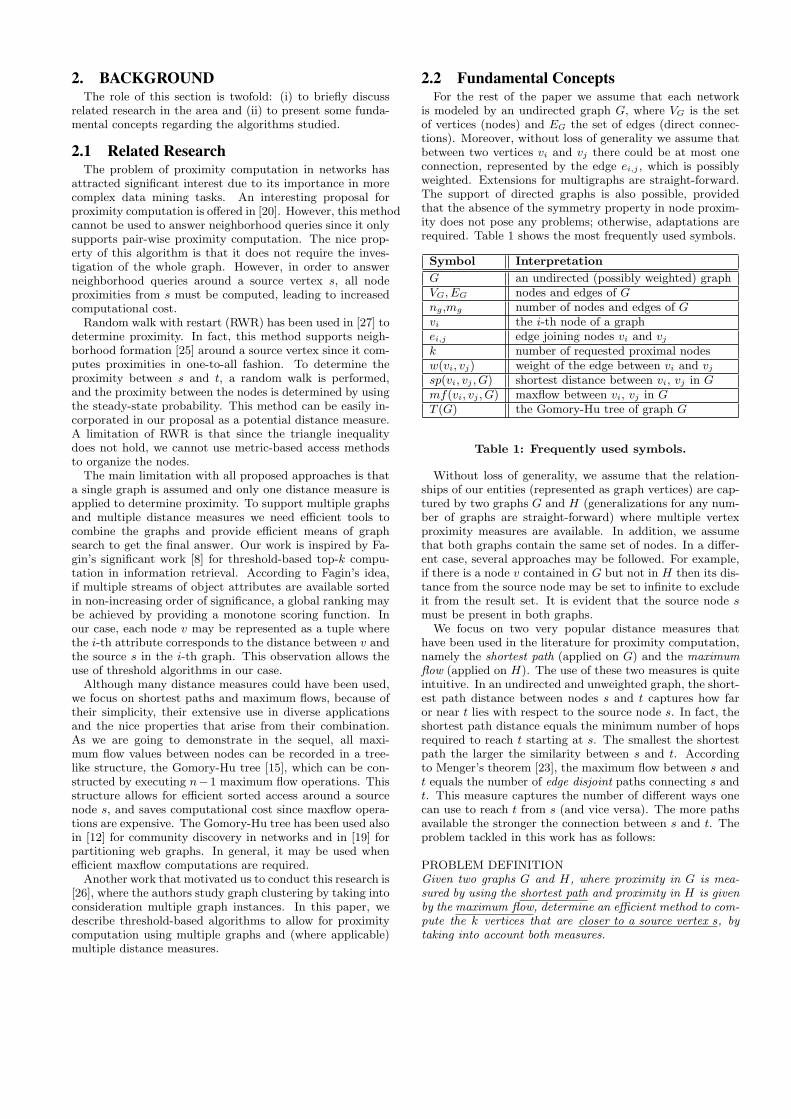
Figure 3: Vertices with different proximities.
A justification regarding the usefulness of a synergetic com-bination of shortest path and maximum flow is illustrated inFigure 3. Recall that the best proximity between two nodesis achieved when the shortest path distance is as minimumas possible and the maximum flow similarity is as maximumas possible. There are four possible cases: (i) small shortestpath distance and large max flow similarity (e.g., nodes v1,v2), (ii) small shortest path distance and small max flow sim-ilarity (e.g., nodes v5, v6), (iii) large shortest path distanceand large max flow similarity (e.g., nodes v3, v4) and (iv)large shortest path distance and small max flow similarity(e.g., nodes v5, v4). For example, the proximity between v1and v2 should be larger than the proximity between v3 andv4, because although the maximum flow between the twopairs is 4, the shortest path distance between v1 and v2 issmaller than the one between v3 and v4. For the rest of thework we assume that the score of a node v is computed bytaking the product score(v) = sp(s, v,G)·(nh−mf(s, v,H)),where sp(s, v,G) is the shortest path distance between s andv in graph G, and mf(s, v,H) is the maxflow between s andv in graph H. Although the two measures if they are usedalone are not adequate [10] their synergy is very important.The product enforces that both factors should be minimizedto get the best result [28]. Alternative ranking functions aswell as different approaches are discussed in Section 5.A simple technique that can be used to solve the problem
is to compute the score for each node and then select thek nodes with the best scores. Although this algorithm issimple to implement, it suffers from performance degrada-tion, especially in large graphs. For this reason, we excludethis naive solution from the subsequent study. In the se-quel, we describe in detail the TAG (Threshold Algorithmsin Graphs) family of algorithms, which use thresholding withthe necessary early-termination conditions, to avoid unnec-essary computational costs. The algorithms presented inthe sequel, differ in the following aspects: (i) the degreeof preprocessing of the input graphs and (ii) the degree ofintermediate result materialization that may be used.
3. THRESHOLD ALGORITHMSIn this section, we develop our proposal for proximity
computation using threshold-based algorithms. The funda-mental differences among the techniques presented lie in thepreprocessing requirements and the materialization of inter-mediate results.
3.1 TAG-IIn this section, we present the basic version of the threshold-
based algorithm which is applied when no time-consuming
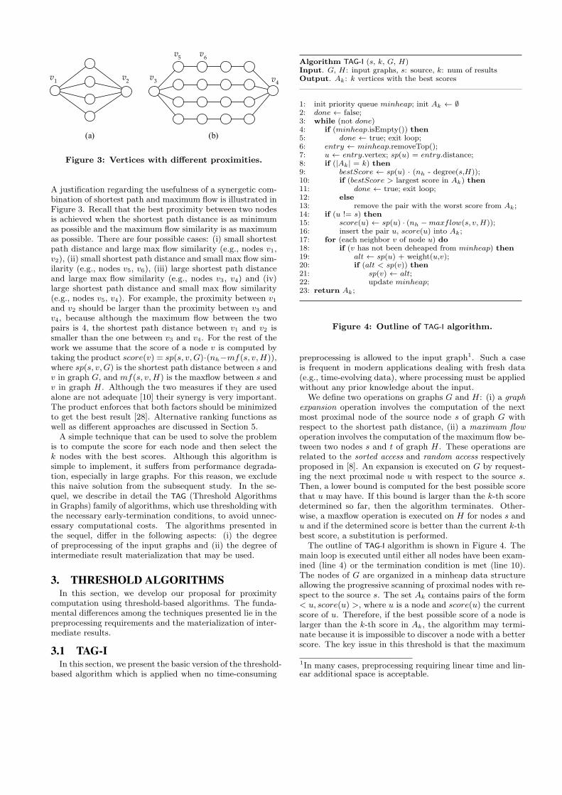
Algorithm TAG-I (s, k, G, H)Input. G, H: input graphs, s: source, k: num of resultsOutput. Ak: k vertices with the best scores
1: init priority queue minheap; init Ak ← ∅2: done ← false;3: while (not done)4: if (minheap.isEmpty()) then5: done ← true; exit loop;6: entry ← minheap.removeTop();7: u ← entry.vertex; sp(u) = entry.distance;8: if (|Ak| = k) then9: bestScore ← sp(u) · (nh - degree(s,H));10: if (bestScore > largest score in Ak) then11: done ← true; exit loop;12: else13: remove the pair with the worst score from Ak;14: if (u != s) then15: score(u) ← sp(u) · (nh −maxflow(s, v,H));16: insert the pair u, score(u) into Ak;17: for (each neighbor v of node u) do18: if (v has not been deheaped from minheap) then19: alt ← sp(u) + weight(u,v);20: if (alt < sp(v)) then21: sp(v) ← alt;22: update minheap;23: return Ak;
Figure 4: Outline of TAG-I algorithm.
preprocessing is allowed to the input graph1. Such a caseis frequent in modern applications dealing with fresh data(e.g., time-evolving data), where processing must be appliedwithout any prior knowledge about the input.
We define two operations on graphs G and H: (i) a graphexpansion operation involves the computation of the nextmost proximal node of the source node s of graph G withrespect to the shortest path distance, (ii) a maximum flowoperation involves the computation of the maximum flow be-tween two nodes s and t of graph H. These operations arerelated to the sorted access and random access respectivelyproposed in [8]. An expansion is executed on G by request-ing the next proximal node u with respect to the source s.Then, a lower bound is computed for the best possible scorethat u may have. If this bound is larger than the k-th scoredetermined so far, then the algorithm terminates. Other-wise, a maxflow operation is executed on H for nodes s andu and if the determined score is better than the current k-thbest score, a substitution is performed.
The outline of TAG-I algorithm is shown in Figure 4. Themain loop is executed until either all nodes have been exam-ined (line 4) or the termination condition is met (line 10).The nodes of G are organized in a minheap data structureallowing the progressive scanning of proximal nodes with re-spect to the source s. The set Ak contains pairs of the form< u, score(u) >, where u is a node and score(u) the currentscore of u. Therefore, if the best possible score of a node islarger than the k-th score in Ak, the algorithm may termi-nate because it is impossible to discover a node with a betterscore. The key issue in this threshold is that the maximum
1In many cases, preprocessing requiring linear time and lin-ear additional space is acceptable.
flow between two nodes s and t is bounded by the minimumdegree among the two nodes. This is easily obtained takinginto account that the maximum value of a mincut in a graphis bounded by the minimum degree of the graph [30].
Lemma 3.1. Let sk be the k-th best score determined sofar, u the node at the top of the minheap and bs(u) the bestpossible score that node u may achieve. If bs(u) > sk thenthe algorithm may terminate since it is impossible to improvefurther the result set Ak.
Proof. By the definition of the expansion operation, it isguaranteed that nodes in G are discovered in non-decreasingdistance from the source node s. This is because the mainloop of TAG-I is similar to Dijkstra’s algorithm. Therefore,every time we get the next node from minheap, we aresure that its shortest path distance from s will be largeror equal to that of the previously discovered node (see [7]for a thorough study of this issue). According to the waythe best score of u is computed, it holds that bsu = sp(u)· (n − mindegree(s)). The only factor that depends onu is the shortest path distance sp(u). The second factor(n − mindegree(s)) depends only on the number of nodesand the degree of the source node. Therefore, if we discovera node u such that the value bs(u) is larger than the k-thscore contained in Ak, we are sure that u as well as all nodesdiscovered after u cannot contribute to the final result. Theopposite would suggest that if node v is discovered after uthen bs(v) < bs(u), meaning that sp(v) < sp(u) which is acontradiction.
To illustrate the way TAG-I works an example is given basedon the graphs shown in Figure 2. We run a top-3 proximityquery starting at node v1. The first deheaped node is v1and therefore its neighbors v2, v3 and v5 are checked andthe appropriate decrease-key operations are performed. Thenext deheaped node is v2. It holds that sp(v2) = 1 and since|Ak| < 3 a maxflow operation is performed. The score of v2is score(v2) = sp(v2) · (n − mf(v1, v2)) = 1 · 6 = 6. In thesame way, the scores of v3 and v5 are also set to 6. Thenext deheaped node is v4. Since |Ak| = 3 we check the bestpossible score of v4, which is bs(v4) = 2 · (8− 5) = 6. Thismeans that a maxflow computation will be performed forv4 as well as for v6 and v7. However, when v8 is deheaped,its best score is set to bs(v8) = 3 · 3 = 9. Since bs(v8) > 6this means that the termination condition is satisfied andthe algorithm terminates since no further improvement onAk may be achieved. The final answer comprises the pairs< v2, 6 >, < v3, 6 > and < v5, 6 >.
Lemma 3.2. Let α(s) denote the number of nodes of Greached through expansion operations starting at source nodes (evidently α(s) > k). Then, the worst case complexity ofTAG-I algorithm is:
O(mg logng + α(s)(logng +mhnh log(n2
h/mh)))
Proof. As in the case of Dijkstra’s algorithm, at mostmg decrease-key operations are required, due to the loopof Figure 4. By assuming an ordinary binary heap, thiscost is O(mg · logng). In addition, the complexity of amaxflow computation by using the push-relabel algorithmof Goldberg and Tarjan [13] which uses dynamic trees, isO(nh · mh log(n2
h/mh)). A maxflow operation is required
for every deheaped node, until the termination condition ismet. Since the number of deheaped nodes is α(s) the resultfollows.
The previous lemma suggests that the most important factoraffecting the performance of TAG-I algorithm is the numberof maxflow computations involved, which depends on thevalue of α(s). In addition, every maxflow computation ongraph H requires O(nh · mh log(n2
h/mh)) cost which is sig-nificant. In the sequel, we investigate techniques that leadto more efficient processing, by introducing some form ofpreprocessing on the input graphs.
3.2 TAG-IIRecall that algorithm TAG-I does not use any kind of pre-
processing and therefore, it can be applied immediately tothe input graphs. However, in many cases we are allowed toapply preprocessing towards speeding up subsequent prox-imity computations. Based on this fact, we perform pre-processing to the input graph H where maxflow computa-tions are performed. Our goal is to provide a boost on theperformance of maxflow computation by using only linearadditional space, offering at least linear time on the applica-tion of each maxflow computation. The resulting algorithmis termed TAG-II, and it is based on the concept of flow-equivalent trees.
Evidently, a straight-forward way to speed-up maxflowoperations, which are invoked in line 15 of Figure 4, is toprecompute the maxflow values for each pair of nodes andstore them in a matrix. Although this offers O(1) time formaxflow computations, it requires O(n2
h) space, which is notacceptable for large graphs. Note that this matrix is dense(all cells are full) and therefore, techniques used for sparsematrices cannot be applied. According to [15], for any graphH one can build a flow-equivalent tree T (H), such that themaxflow between two nodes in H equals their maxflow inT (H). Such a tree is termed Gomory-Hu tree or mincut tree.Essentially, the existence of a flow-equivalent tree suggeststhat for a graph H with nh nodes there are at most nh−1different maxflow values between node pairs. This is a directconsequence of the fact that the Gomory-Hu tree containsexactly nh − 1 edges, since it is connected (assuming thatthe input graph is also connected).
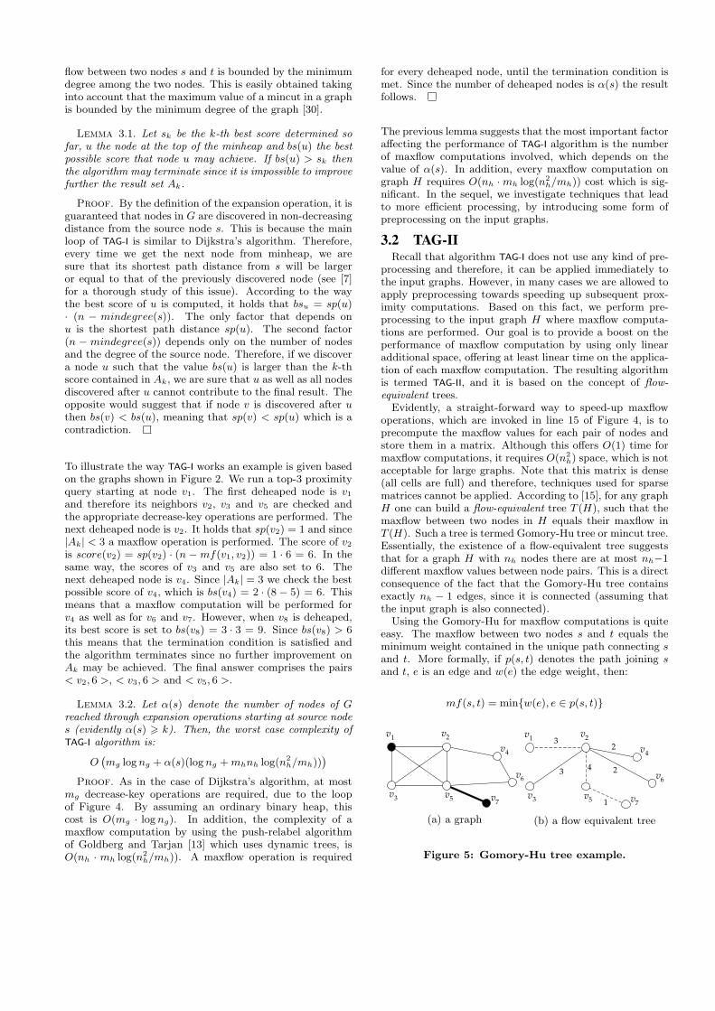
Using the Gomory-Hu for maxflow computations is quiteeasy. The maxflow between two nodes s and t equals theminimum weight contained in the unique path connecting sand t. More formally, if p(s, t) denotes the path joining sand t, e is an edge and w(e) the edge weight, then:
mf(s, t) = min{w(e), e ∈ p(s, t)}
v1
v2
v4
v3
v5
v6
v7
(a) a graph
v1
v2
v4
v3
v5
v6
v7
3
3 2
2
4
1
(b) a flow equivalent tree
Figure 5: Gomory-Hu tree example.
...
v1v2v3
vn-1vn
...
v1
v2
v3
vn-1
vn
(a) worst case (b) best case
v1
5
2
31
23
1
v2
v3
v4
v5
v6
v7
v8
(c) a typical case
Figure 6: Worst, best and typical tree formation.
Figure 5 depicts an example of a graph and its associatedflow-equivalent Gomory-Hu tree. According to the proper-ties of Gomory-Hu trees, the maxflow between nodes v1 andv7 is 1, since it is the minimum edge weight in the path fromv1 to v7 (shown with dashed lines). This may be easily val-idated by inspecting the graph in Figure 5(a) and verifyingthat indeed the maxflow is 1, since if the bold line is deletedthen v1 and v7 become disconnected.Since there is a unique path joining any pair of nodes s, t in
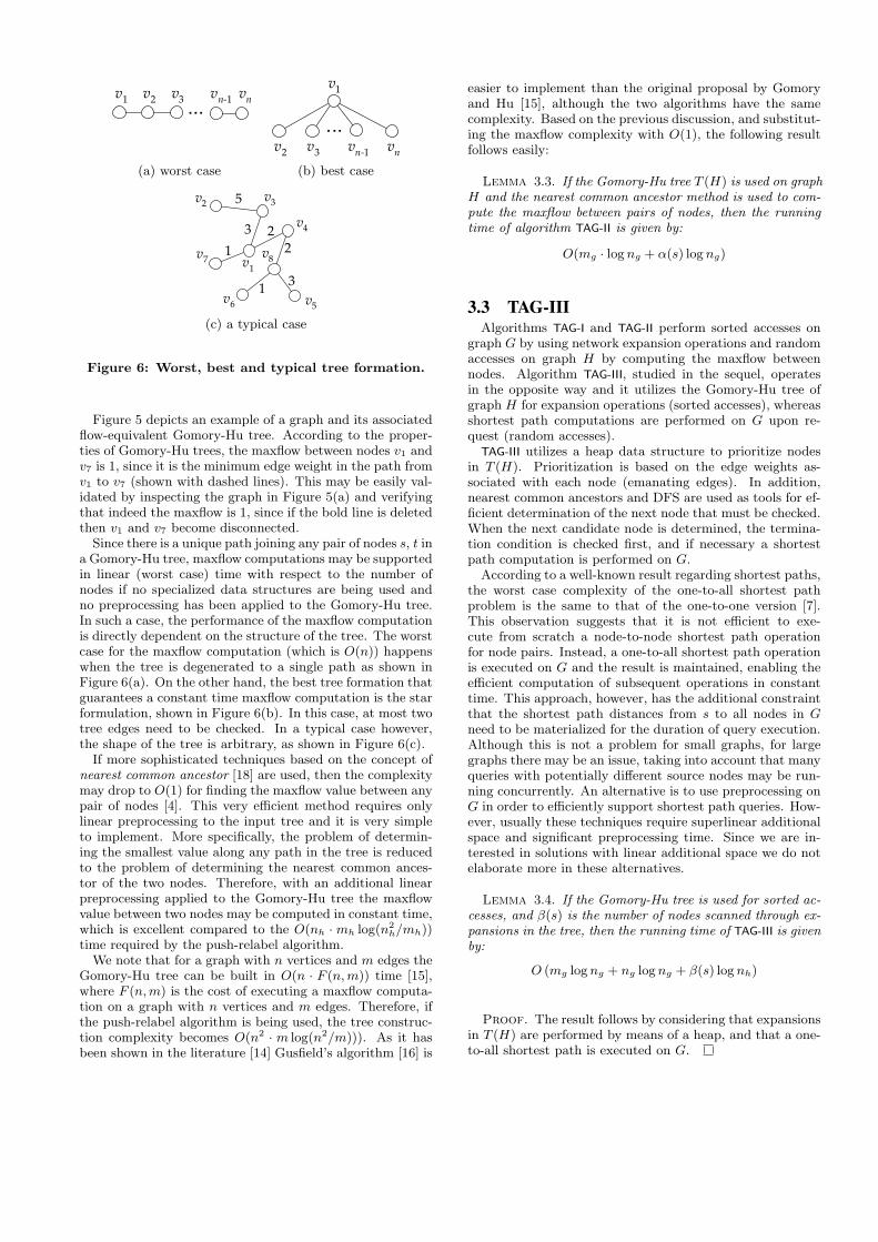
a Gomory-Hu tree, maxflow computations may be supportedin linear (worst case) time with respect to the number ofnodes if no specialized data structures are being used andno preprocessing has been applied to the Gomory-Hu tree.In such a case, the performance of the maxflow computationis directly dependent on the structure of the tree. The worstcase for the maxflow computation (which is O(n)) happenswhen the tree is degenerated to a single path as shown inFigure 6(a). On the other hand, the best tree formation thatguarantees a constant time maxflow computation is the starformulation, shown in Figure 6(b). In this case, at most twotree edges need to be checked. In a typical case however,the shape of the tree is arbitrary, as shown in Figure 6(c).If more sophisticated techniques based on the concept of
nearest common ancestor [18] are used, then the complexitymay drop to O(1) for finding the maxflow value between anypair of nodes [4]. This very efficient method requires onlylinear preprocessing to the input tree and it is very simpleto implement. More specifically, the problem of determin-ing the smallest value along any path in the tree is reducedto the problem of determining the nearest common ances-tor of the two nodes. Therefore, with an additional linearpreprocessing applied to the Gomory-Hu tree the maxflowvalue between two nodes may be computed in constant time,which is excellent compared to the O(nh · mh log(n2
h/mh))time required by the push-relabel algorithm.We note that for a graph with n vertices and m edges the
Gomory-Hu tree can be built in O(n · F (n,m)) time [15],where F (n,m) is the cost of executing a maxflow computa-tion on a graph with n vertices and m edges. Therefore, ifthe push-relabel algorithm is being used, the tree construc-tion complexity becomes O(n2 · m log(n2/m))). As it hasbeen shown in the literature [14] Gusfield’s algorithm [16] is
easier to implement than the original proposal by Gomoryand Hu [15], although the two algorithms have the samecomplexity. Based on the previous discussion, and substitut-ing the maxflow complexity with O(1), the following resultfollows easily:
Lemma 3.3. If the Gomory-Hu tree T (H) is used on graphH and the nearest common ancestor method is used to com-pute the maxflow between pairs of nodes, then the runningtime of algorithm TAG-II is given by:
O(mg · logng + α(s) log ng)
3.3 TAG-IIIAlgorithms TAG-I and TAG-II perform sorted accesses on
graph G by using network expansion operations and randomaccesses on graph H by computing the maxflow betweennodes. Algorithm TAG-III, studied in the sequel, operatesin the opposite way and it utilizes the Gomory-Hu tree ofgraph H for expansion operations (sorted accesses), whereasshortest path computations are performed on G upon re-quest (random accesses).
TAG-III utilizes a heap data structure to prioritize nodesin T (H). Prioritization is based on the edge weights as-sociated with each node (emanating edges). In addition,nearest common ancestors and DFS are used as tools for ef-ficient determination of the next node that must be checked.When the next candidate node is determined, the termina-tion condition is checked first, and if necessary a shortestpath computation is performed on G.
According to a well-known result regarding shortest paths,the worst case complexity of the one-to-all shortest pathproblem is the same to that of the one-to-one version [7].This observation suggests that it is not efficient to exe-cute from scratch a node-to-node shortest path operationfor node pairs. Instead, a one-to-all shortest path operationis executed on G and the result is maintained, enabling theefficient computation of subsequent operations in constanttime. This approach, however, has the additional constraintthat the shortest path distances from s to all nodes in Gneed to be materialized for the duration of query execution.Although this is not a problem for small graphs, for largegraphs there may be an issue, taking into account that manyqueries with potentially different source nodes may be run-ning concurrently. An alternative is to use preprocessing onG in order to efficiently support shortest path queries. How-ever, usually these techniques require superlinear additionalspace and significant preprocessing time. Since we are in-terested in solutions with linear additional space we do notelaborate more in these alternatives.
Lemma 3.4. If the Gomory-Hu tree is used for sorted ac-cesses, and β(s) is the number of nodes scanned through ex-pansions in the tree, then the running time of TAG-III is givenby:
O (mg logng + ng logng + β(s) log nh)
Proof. The result follows by considering that expansionsin T (H) are performed by means of a heap, and that a one-to-all shortest path is executed on G.
3.4 TAG-IVThe main property of the previously studied algorithms is
that sorted accesses are performed to one of the two graphs,whereas random accesses are performed on H for maxflowcomputation (for TAG-I, TAG-II algorithms) and on G for short-est path computation (for TAG-III algorithm). A natural ex-tension is to consider a more general scheme, where a syn-chronized traversal is used to control sorted and randomaccesses. Algorithm TAG-IV, described in the sequel, doesexactly this.
TAG-IV works as the threshold algorithm (TA) proposedin [8]. More specifically, a buffer of k slots is maintainedhosting the k best nodes determined so far. In each sortedaccess, two expansion operations are performed, one in Gand one in T (H). If different nodes are retrieved, then tworandom accesses are performed to fill-in the missing values,one in G to compute the shortest path distance and one inT (H) to compute the maxflow distance. If the score of thenewly discovered nodes is better than the k-th best scorefound in the buffer, then a substitution is performed, oth-erwise the buffer remains as it is. Then, a threshold th iscomputed by computing the scoring function for the valuesseen in the last sorted access. If all scores in the buffer arebetter than the current threshold, then the algorithm termi-nates since it is not possible to improve the results further.Otherwise, another sorted access is performed, a new valuefor the threshold is determined and the algorithm continuousas previously. The following lemma follows from the previ-ous discussion, where γ(s) is the number of sorted accessesperformed by the algorithm.
Lemma 3.5. If γ(s) is the number of sorted accesses per-formed, then the running time of TAG-IV is given by:
O (mg logng + ng logng + γ(s) log nh)
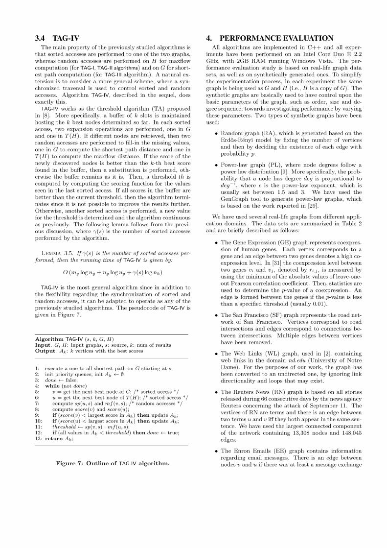
TAG-IV is the most general algorithm since in addition tothe flexibility regarding the synchronization of sorted andrandom accesses, it can be adapted to operate as any of thepreviously studied algorithms. The pseudocode of TAG-IV isgiven in Figure 7.
Algorithm TAG-IV (s, k, G, H)Input. G, H: input graphs, s: source, k: num of resultsOutput. Ak: k vertices with the best scores
1: execute a one-to-all shortest path on G starting at s;2: init priority queues; init Ak ← ∅3: done ← false;4: while (not done)5: v = get the next best node of G; /* sorted access */6: u = get the next best node of T (H); /* sorted access */7: compute sp(u, s) and mf(v, s); /* random accesses */8: compute score(v) and score(u);9: if (score(v) < largest score in Ak) then update Ak;10: if (score(u) < largest score in Ak) then update Ak;11: threshold ← sp(v, s) · mf(u, s);12: if (all values in Ak < threshold) then done ← true;13: return Ak;
Figure 7: Outline of TAG-IV algorithm.
4. PERFORMANCE EVALUATIONAll algorithms are implemented in C++ and all exper-
iments have been performed on an Intel Core Duo @ 2.2GHz, with 2GB RAM running Windows Vista. The per-formance evaluation study is based on real-life graph datasets, as well as on synthetically generated ones. To simplifythe experimentation process, in each experiment the samegraph is being used as G and H (i.e., H is a copy of G). Thesynthetic graphs are basically used to have control upon thebasic parameters of the graph, such as order, size and de-gree sequence, towards investigating performance by varyingthese parameters. Two types of synthetic graphs have beenused:
• Random graph (RA), which is generated based on theErdos-Renyi model by fixing the number of verticesand then by deciding the existence of each edge withprobability p.
• Power-law graph (PL), where node degrees follow apower law distribution [9]. More specifically, the prob-ability that a node has degree deg is proportional todeg−ϵ, where ϵ is the power-law exponent, which isusually set between 1.5 and 3. We have used theGenGraph tool to generate power-law graphs, whichis based on the work reported in [29].
We have used several real-life graphs from different appli-cation domains. The data sets are summarized in Table 2and are briefly described as follows:
• The Gene Expression (GE) graph represents coexpres-sion of human genes. Each vertex corresponds to agene and an edge between two genes denotes a high co-expression level. In [31] the coexpression level betweentwo genes vi and vj , denoted by ri,j , is measured byusing the minimum of the absolute values of leave-one-out Pearson correlation coefficient. Then, statistics areused to determine the p-value of a coexpression. Anedge is formed between the genes if the p-value is lessthan a specified threshold (usually 0.01).
• The San Francisco (SF) graph represents the road net-work of San Francisco. Vertices correspond to roadintersections and edges correspond to connections be-tween intersections. Multiple edges between verticeshave been removed.
• The Web Links (WL) graph, used in [2], containingweb links in the domain nd.edu (University of NotreDame). For the purposes of our work, the graph hasbeen converted to an undirected one, by ignoring linkdirectionality and loops that may exist.
• The Reuters News (RN) graph is based on all storiesreleased during 66 consecutive days by the news agencyReuters concerning the attack of September 11. Thevertices of RN are terms and there is an edge betweentwo terms u and v iff they both appear in the same sen-tence. We have used the largest connected componentof the network containing 13,308 nodes and 148,045edges.
• The Enron Emails (EE) graph contains informationregarding email messages. There is an edge betweennodes v and u if there was at least a message exchange
Graph #nodes #edges min degree max degree avg degree availability
Reuters News (RN) 13,308 148,035 1 2265 22.24 http://vlado.fmf.uni-lj.si/pub/networks/data/Microarray (MA) 8791 314,816 1 409 71.62 thanks to Xifeng Yan [31]San Francisco (SF) 174,956 221,802 1 7 2.54 http://www.rtreeportal.orgWeb Links (WL) 325,729 1,497,135 1 10,721 9.19 http://vlado.fmf.uni-lj.si/pub/networks/data/Enron Emails (EE) 36,692 367,662 1 1385 11.57 http://snap.stanford.edu/data/index.htmlCo-Authors (CA) 18,772 396,160 1 504 22.53 http://snap.stanford.edu/data/index.html
Table 2: Real-life graphs from different domains used in performance evaluation.
0.01
0.1
1
10
0 20 40 60 80 100 120 140
runnin
g t
ime
(sec
)
number of proximal nodes (k)
TAG-ITAG-II
TAG-IIITAG-IV
(a) Reuters News
0.01
0.1
1
10
0 20 40 60 80 100 120 140
runnin
g t
ime
(sec
)
number of proximal nodes (k)
TAG-ITAG-II
TAG-IIITAG-IV
(b) Gene Expression
10
0 20 40 60 80 100 120 140
runnin
g t
ime
(sec
)
number of proximal nodes (k)
TAG-ITAG-II
TAG-IIITAG-IV
(c) San Francisco
0.1
1
10
0 20 40 60 80 100 120 140
runnin
g t
ime
(sec
)
number of proximal nodes (k)
TAG-ITAG-II
TAG-IIITAG-IV
(d) Web Links
1
10
0 20 40 60 80 100 120 140
runnin
g t
ime
(sec
)
number of proximal nodes (k)
TAG-ITAG-II
TAG-IIITAG-IV
(e) Enron Emails
0.01
0.1
1
10
0 20 40 60 80 100 120 140
runnin
g t
ime
(sec
)number of proximal nodes (k)
TAG-ITAG-II
TAG-IIITAG-IV
(f) Co-Authors
Figure 8: Running time (sec.) vs k for real-life graphs.
10
100
1000
10000
100000
10 30 50 100 150 500
num
ber
of
sort
ed a
ccesses
k
TAG-II
TAG-III
TAG-IV
(a) Reuters News
10
100
1000
10000
100000
10 30 50 100 150 500
num
ber
of
sort
ed a
ccesses
k
TAG-II
TAG-III
TAG-IV
(b) Gene Expression
100
1000
10000
100000
10 30 50 100 150 500
num
ber
of
sort
ed a
ccesses
k
TAG-II
TAG-III
TAG-IV
(c) Enron Emails
Figure 9: Number of sorted accesses vs k for real-life graphs.
between them. This data set has been also used in [22]to explore graph properties over time.
• The Co-Authors (CA) graph has been extracted fromarXiv and represents scientific collaborations betweenauthors regarding papers submitted to Astro Physicsarea. There is an edge between authors u and v iffthey both appear as co-authors in at least one paper.This data set has been also used in [22].
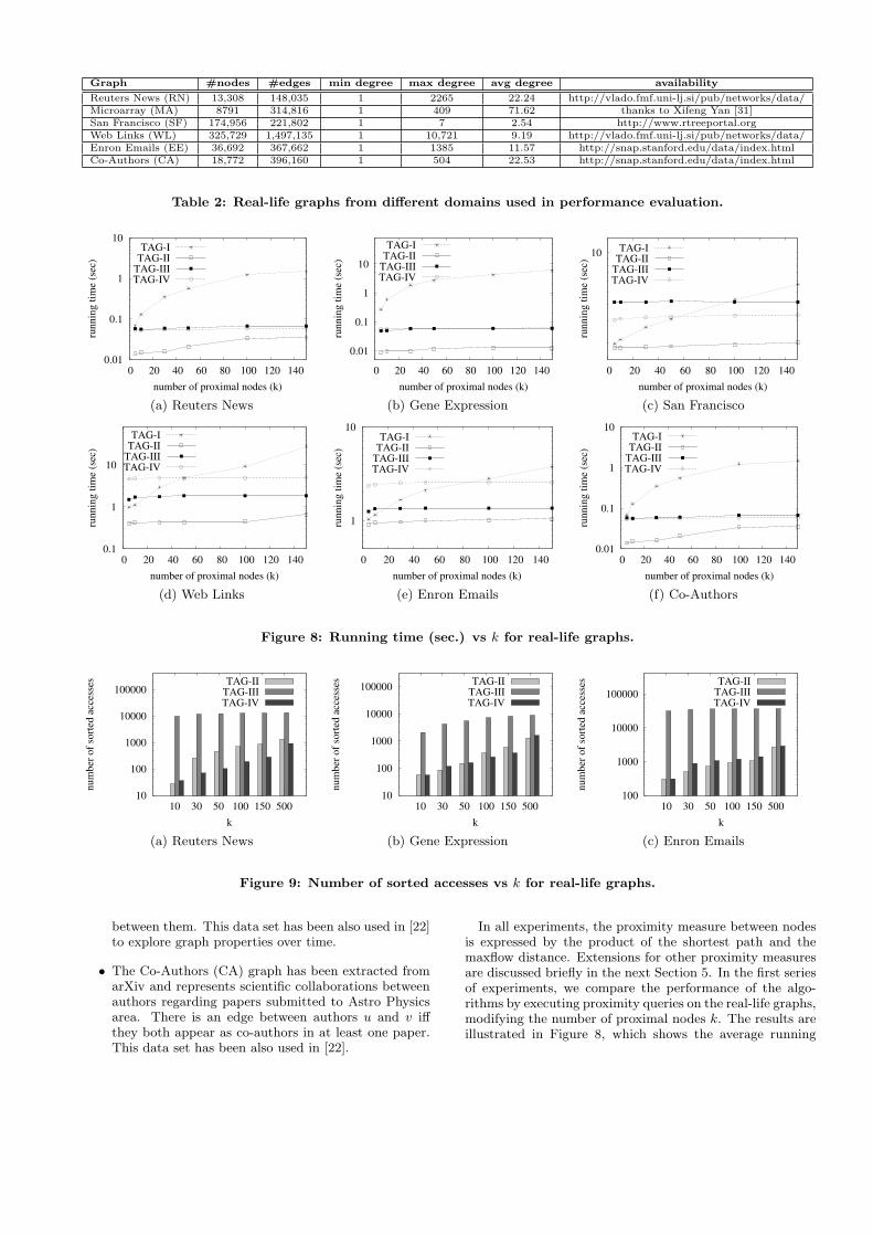
In all experiments, the proximity measure between nodesis expressed by the product of the shortest path and themaxflow distance. Extensions for other proximity measuresare discussed briefly in the next Section 5. In the first seriesof experiments, we compare the performance of the algo-rithms by executing proximity queries on the real-life graphs,modifying the number of proximal nodes k. The results areillustrated in Figure 8, which shows the average running
0.01
0.1
1
10
100
1000
0 100 200 300 400 500
runnin
g t
ime
(sec
)
number of proximal nodes (k)
TAG-ITAG-II
TAG-IIITAG-IV
(a) 20K nodes, 1.2M edges (p=0.01)
0.01
0.1
1
10
100
1000
10000
100000
0 100 200 300 400 500
runnin
g t
ime
(sec
)
number of proximal nodes (k)
TAG-ITAG-II
TAG-IIITAG-IV
(b) 50K nodes, 6.3M edges (p=0.01)
0.01
0.1
1
10
100
1000
10000
100000
0 100 200 300 400 500
runnin
g t
ime
(sec
)
number of proximal nodes (k)
TAG-ITAG-II
TAG-IIITAG-IV
(c) 100K nodes, 2.5M edges (p=0.001)
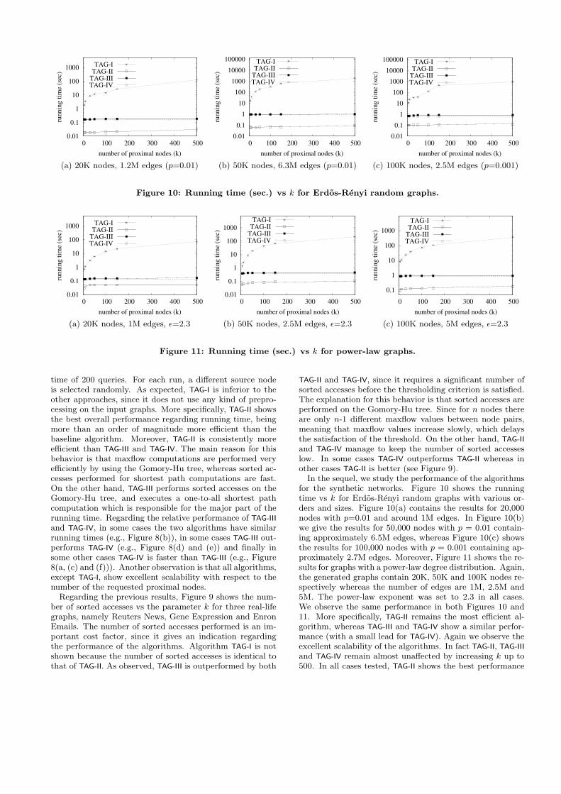
Figure 10: Running time (sec.) vs k for Erdos-Renyi random graphs.
0.01
0.1
1
10
100
1000
0 100 200 300 400 500
runnin
g t
ime
(sec
)
number of proximal nodes (k)
TAG-ITAG-II
TAG-IIITAG-IV
(a) 20K nodes, 1M edges, ϵ=2.3
0.01
0.1
1
10
100
1000
0 100 200 300 400 500
runnin
g t
ime
(sec
)
number of proximal nodes (k)
TAG-ITAG-II
TAG-IIITAG-IV
(b) 50K nodes, 2.5M edges, ϵ=2.3
0.1
1
10
100
1000
0 100 200 300 400 500
runnin
g t
ime
(sec
)
number of proximal nodes (k)
TAG-ITAG-II
TAG-IIITAG-IV
(c) 100K nodes, 5M edges, ϵ=2.3
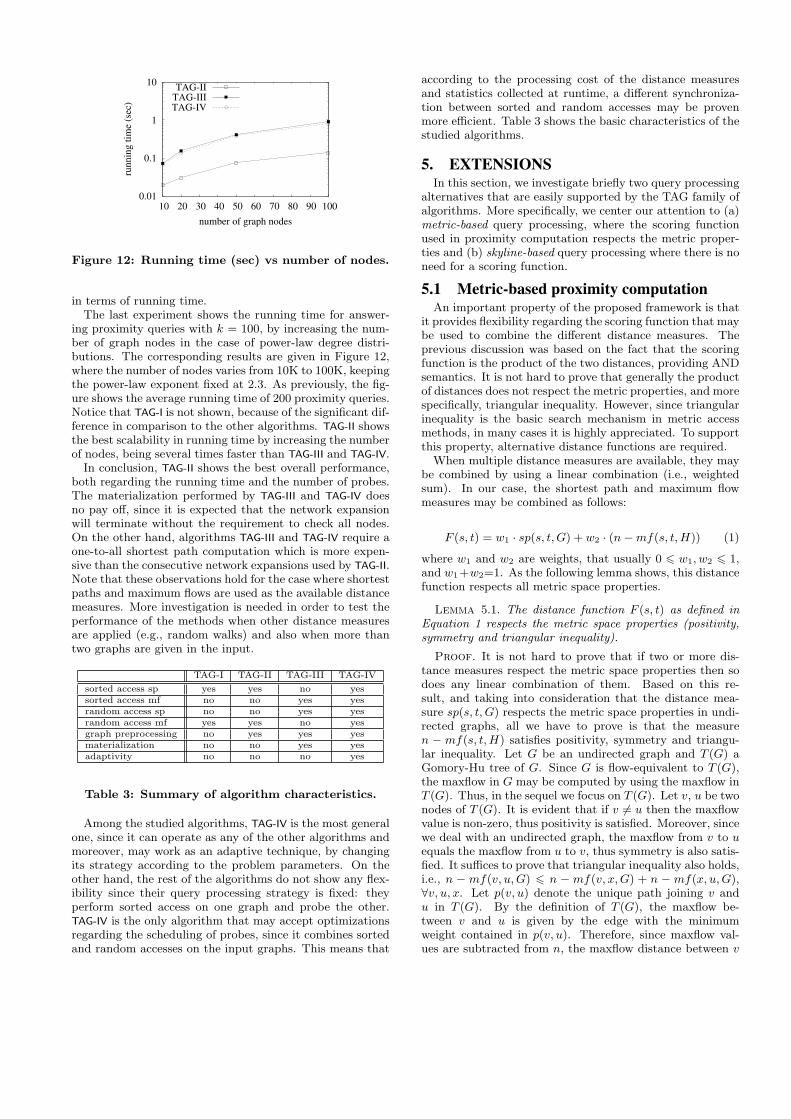
Figure 11: Running time (sec.) vs k for power-law graphs.
time of 200 queries. For each run, a different source nodeis selected randomly. As expected, TAG-I is inferior to theother approaches, since it does not use any kind of prepro-cessing on the input graphs. More specifically, TAG-II showsthe best overall performance regarding running time, beingmore than an order of magnitude more efficient than thebaseline algorithm. Moreover, TAG-II is consistently moreefficient than TAG-III and TAG-IV. The main reason for thisbehavior is that maxflow computations are performed veryefficiently by using the Gomory-Hu tree, whereas sorted ac-cesses performed for shortest path computations are fast.On the other hand, TAG-III performs sorted accesses on theGomory-Hu tree, and executes a one-to-all shortest pathcomputation which is responsible for the major part of therunning time. Regarding the relative performance of TAG-IIIand TAG-IV, in some cases the two algorithms have similarrunning times (e.g., Figure 8(b)), in some cases TAG-III out-performs TAG-IV (e.g., Figure 8(d) and (e)) and finally insome other cases TAG-IV is faster than TAG-III (e.g., Figure8(a, (c) and (f))). Another observation is that all algorithms,except TAG-I, show excellent scalability with respect to thenumber of the requested proximal nodes.Regarding the previous results, Figure 9 shows the num-
ber of sorted accesses vs the parameter k for three real-lifegraphs, namely Reuters News, Gene Expression and EnronEmails. The number of sorted accesses performed is an im-portant cost factor, since it gives an indication regardingthe performance of the algorithms. Algorithm TAG-I is notshown because the number of sorted accesses is identical tothat of TAG-II. As observed, TAG-III is outperformed by both
TAG-II and TAG-IV, since it requires a significant number ofsorted accesses before the thresholding criterion is satisfied.The explanation for this behavior is that sorted accesses areperformed on the Gomory-Hu tree. Since for n nodes thereare only n-1 different maxflow values between node pairs,meaning that maxflow values increase slowly, which delaysthe satisfaction of the threshold. On the other hand, TAG-IIand TAG-IV manage to keep the number of sorted accesseslow. In some cases TAG-IV outperforms TAG-II whereas inother cases TAG-II is better (see Figure 9).
In the sequel, we study the performance of the algorithmsfor the synthetic networks. Figure 10 shows the runningtime vs k for Erdos-Renyi random graphs with various or-ders and sizes. Figure 10(a) contains the results for 20,000nodes with p=0.01 and around 1M edges. In Figure 10(b)we give the results for 50,000 nodes with p = 0.01 contain-ing approximately 6.5M edges, whereas Figure 10(c) showsthe results for 100,000 nodes with p = 0.001 containing ap-proximately 2.7M edges. Moreover, Figure 11 shows the re-sults for graphs with a power-law degree distribution. Again,the generated graphs contain 20K, 50K and 100K nodes re-spectively whereas the number of edges are 1M, 2.5M and5M. The power-law exponent was set to 2.3 in all cases.We observe the same performance in both Figures 10 and11. More specifically, TAG-II remains the most efficient al-gorithm, whereas TAG-III and TAG-IV show a similar perfor-mance (with a small lead for TAG-IV). Again we observe theexcellent scalability of the algorithms. In fact TAG-II, TAG-IIIand TAG-IV remain almost unaffected by increasing k up to500. In all cases tested, TAG-II shows the best performance
0.01
0.1
1
10
10 20 30 40 50 60 70 80 90 100
runnin
g t
ime
(sec
)
number of graph nodes
TAG-IITAG-IIITAG-IV
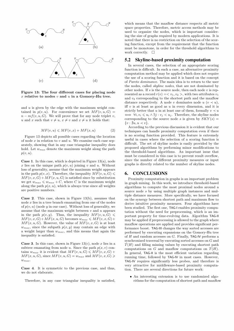
Figure 12: Running time (sec) vs number of nodes.
in terms of running time.The last experiment shows the running time for answer-
ing proximity queries with k = 100, by increasing the num-ber of graph nodes in the case of power-law degree distri-butions. The corresponding results are given in Figure 12,where the number of nodes varies from 10K to 100K, keepingthe power-law exponent fixed at 2.3. As previously, the fig-ure shows the average running time of 200 proximity queries.Notice that TAG-I is not shown, because of the significant dif-ference in comparison to the other algorithms. TAG-II showsthe best scalability in running time by increasing the numberof nodes, being several times faster than TAG-III and TAG-IV.In conclusion, TAG-II shows the best overall performance,
both regarding the running time and the number of probes.The materialization performed by TAG-III and TAG-IV doesno pay off, since it is expected that the network expansionwill terminate without the requirement to check all nodes.On the other hand, algorithms TAG-III and TAG-IV require aone-to-all shortest path computation which is more expen-sive than the consecutive network expansions used by TAG-II.Note that these observations hold for the case where shortestpaths and maximum flows are used as the available distancemeasures. More investigation is needed in order to test theperformance of the methods when other distance measuresare applied (e.g., random walks) and also when more thantwo graphs are given in the input.
TAG-I TAG-II TAG-III TAG-IV
sorted access sp yes yes no yessorted access mf no no yes yesrandom access sp no no yes yesrandom access mf yes yes no yesgraph preprocessing no yes yes yesmaterialization no no yes yesadaptivity no no no yes
Table 3: Summary of algorithm characteristics.
Among the studied algorithms, TAG-IV is the most generalone, since it can operate as any of the other algorithms andmoreover, may work as an adaptive technique, by changingits strategy according to the problem parameters. On theother hand, the rest of the algorithms do not show any flex-ibility since their query processing strategy is fixed: theyperform sorted access on one graph and probe the other.TAG-IV is the only algorithm that may accept optimizationsregarding the scheduling of probes, since it combines sortedand random accesses on the input graphs. This means that
according to the processing cost of the distance measuresand statistics collected at runtime, a different synchroniza-tion between sorted and random accesses may be provenmore efficient. Table 3 shows the basic characteristics of thestudied algorithms.
5. EXTENSIONSIn this section, we investigate briefly two query processing
alternatives that are easily supported by the TAG family ofalgorithms. More specifically, we center our attention to (a)metric-based query processing, where the scoring functionused in proximity computation respects the metric proper-ties and (b) skyline-based query processing where there is noneed for a scoring function.
5.1 Metric-based proximity computationAn important property of the proposed framework is that
it provides flexibility regarding the scoring function that maybe used to combine the different distance measures. Theprevious discussion was based on the fact that the scoringfunction is the product of the two distances, providing ANDsemantics. It is not hard to prove that generally the productof distances does not respect the metric properties, and morespecifically, triangular inequality. However, since triangularinequality is the basic search mechanism in metric accessmethods, in many cases it is highly appreciated. To supportthis property, alternative distance functions are required.
When multiple distance measures are available, they maybe combined by using a linear combination (i.e., weightedsum). In our case, the shortest path and maximum flowmeasures may be combined as follows:
F (s, t) = w1 · sp(s, t, G) + w2 · (n−mf(s, t,H)) (1)
where w1 and w2 are weights, that usually 0 6 w1, w2 6 1,and w1+w2=1. As the following lemma shows, this distancefunction respects all metric space properties.
Lemma 5.1. The distance function F (s, t) as defined inEquation 1 respects the metric space properties (positivity,symmetry and triangular inequality).
Proof. It is not hard to prove that if two or more dis-tance measures respect the metric space properties then sodoes any linear combination of them. Based on this re-sult, and taking into consideration that the distance mea-sure sp(s, t, G) respects the metric space properties in undi-rected graphs, all we have to prove is that the measuren − mf(s, t,H) satisfies positivity, symmetry and triangu-lar inequality. Let G be an undirected graph and T (G) aGomory-Hu tree of G. Since G is flow-equivalent to T (G),the maxflow in G may be computed by using the maxflow inT (G). Thus, in the sequel we focus on T (G). Let v, u be twonodes of T (G). It is evident that if v = u then the maxflowvalue is non-zero, thus positivity is satisfied. Moreover, sincewe deal with an undirected graph, the maxflow from v to uequals the maxflow from u to v, thus symmetry is also satis-fied. It suffices to prove that triangular inequality also holds,i.e., n − mf(v, u,G) 6 n − mf(v, x,G) + n − mf(x, u,G),∀v, u, x. Let p(v, u) denote the unique path joining v andu in T (G). By the definition of T (G), the maxflow be-tween v and u is given by the edge with the minimumweight contained in p(v, u). Therefore, since maxflow val-ues are subtracted from n, the maxflow distance between v
u
x
v
v u
x
y
(a) (b)
v u
x
v u
x
(c) (d)
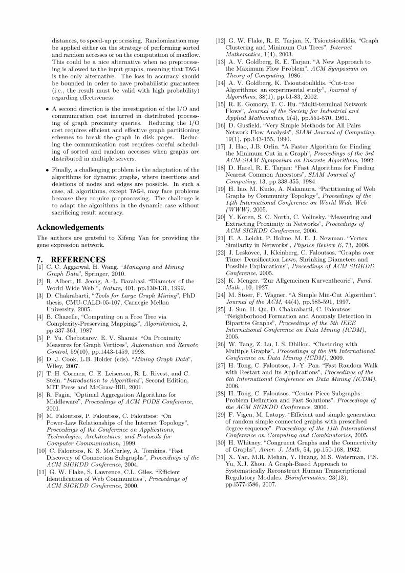
Figure 13: The four different cases for placing nodex relative to nodes v and u in a Gomory-Hu tree.
and u is given by the edge with the maximum weight con-tained in p(v, u). For convenience we set MF (v, u,G) =n −mf(v, u,G). We will prove that for any node triplet v,u and x such that v = u, x = v and x = u it holds that:
MF (v, u) 6 MF (v, x) +MF (x, u) (2)
Figure 13 depicts all possible cases regarding the locationof node x in relation to v and u. We examine each case sep-arately, showing that in any case triangular inequality doeshold. Let wmax denote the maximum weight along the pathp(v, u).
Case 1. In this case, which is depicted in Figure 13(a), nodex lies on the unique path p(v, u) joining v and u. Withoutloss of generality, assume that the maximum weight appearsin the path p(v, x). Therefore, the inequality MF (v, u,G) 6MF (v, x,G)+MF (x, u,G) is satisfied since by substitutionwe get wmax 6 wmax +C, where C is the maximum weightalong the path p(x, u), which is always true since all weightsare positive numbers.
Case 2. This case, shown in Figure 13(b), assumes thatnode x lies in a tree branch emanating from one of the nodesof p(v, u) (node y in our case). Without loss of generality, weassume that the maximum weight between v and u appearsin the path p(v, y). Thus, the inequality MF (v, u,G) 6MF (v, x,G)+MF (x, u,G) becomes wmax 6 MF (v, x,G)+MF (x, u,G). However, the value of MF (v, x,G) is at leastwmax, since the subpath p(x, y) may contain an edge witha weight larger than wmax, and this means that again theinequality is satisfied.
Case 3. In this case, shown in Figure 13(c), node x lies in asubtree emanating from node u. Since the path p(x, v) con-tains wmax it is evident that MF (v, u,G) 6 MF (v, x,G) +MF (x, u,G), since MF (v, u,G) = wmax and MF (v, x,G) >wmax.
Case 4. It is symmetric to the previous case, and thus,we do not elaborate.
Therefore, in any case triangular inequality is satisfied,
which means that the maxflow distance respects all metricspace properties. Therefore, metric access methods may beused to organize the nodes, which is important consider-ing the size of graphs required by modern applications. It isnoted that there is no restriction on the selection of the scor-ing function, except from the requirement that the functionmust be monotone, in order for the threshold algorithms towork correctly.
5.2 Skyline-based proximity computationIn several cases, the selection of an appropriate scoring
function is difficult. In such a case, an alternative proximitycomputation method may be applied which does not requirethe use of a scoring function and it is based on the conceptof Pareto dominance. The main idea is to return to the userthe nodes, called skyline nodes, that are not dominated byother nodes. If s is the source node, then each node v is rep-resented as a record r(v) =< v1, v2 >, with two attributes v1and v2 corresponding to the shortest path and the maxflowdistance respectively. A node v dominates node u (v ≺ u),iff v is at least as good as u in every dimension, and it isstrictly better that u in at least one of them, formally v ≺ u⇐⇒ ∀i, vi 6 ui ∧∃j : vj < uj . Therefore, the skyline nodescorresponding to the source node s is given by SKY (s) ={v : @u, u ≺ v}.
According to the previous discussion it is evident that ourtechniques can handle proximity computation even if thereis no scoring function provided. This feature is extremelyuseful in cases where the selection of a scoring function isdifficult. The set of skyline nodes is easily provided by theproposed algorithms by performing minor modifications tothe threshold-based algorithms. An important issue thatmust be considered in this case is to prevent result overflow,since the number of different proximity measures or inputgraphs is directly related to the number of skyline nodes.
6. CONCLUSIONSProximity computation in graphs is an important problem
in graph mining. In this work, we introduce threshold-basedalgorithms to compute the most proximal nodes around asource node s by using multiple graph instances and mul-tiple distance measures. More specifically, we have focusedon the synergy between shortest path and maximum flow toderive intuitive proximity measures. Four algorithms havebeen studied. The first one, TAG-I enables proximity compu-tation without the need for preprocessing, which is an im-portant property for time-evolving data. Algorithm TAG-II
may be applied if preprocessing is allowed to the graph wheremaxflow operations are applied and provides significant per-formance boost. TAG-III changes the way sorted accesses areperformed by executing expansions on the Gomory-Hu treeof H and random accesses on G. Finally, TAG-IV performs asynchronized traversal by executing sorted accesses onG andT (H) and filling missing values by executing shortest pathcomputations on G and maxflow computations on T (H).In general, TAG-II is the most efficient variation regardingrunning time, followed by TAG-IV in most cases. However,TAG-IV requires significantly less probes, and therefore isvery attractive for middleware-based proximity computa-tion. There are several directions for future work:
• An interesting extension is to use randomized algo-rithms for the computation of shortest path and maxflow
distances, to speed-up processing. Randomization maybe applied either on the strategy of performing sortedand random accesses or on the computation of maxflow.This could be a nice alternative when no preprocess-ing is allowed to the input graphs, meaning that TAG-I
is the only alternative. The loss in accuracy shouldbe bounded in order to have probabilistic guarantees(i.e., the result must be valid with high probability)regarding effectiveness.
• A second direction is the investigation of the I/O andcommunication cost incurred in distributed process-ing of graph proximity queries. Reducing the I/Ocost requires efficient and effective graph partitioningschemes to break the graph in disk pages. Reduc-ing the communication cost requires careful schedul-ing of sorted and random accesses when graphs aredistributed in multiple servers.
• Finally, a challenging problem is the adaptation of thealgorithms for dynamic graphs, where insertions anddeletions of nodes and edges are possible. In such acase, all algorithms, except TAG-I, may face problemsbecause they require preprocessing. The challenge isto adapt the algorithms in the dynamic case withoutsacrificing result accuracy.
AcknowledgementsThe authors are grateful to Xifeng Yan for providing thegene expression network.
7. REFERENCES[1] C. C. Aggarwal, H. Wang. “Managing and Mining
Graph Data”, Springer, 2010.[2] R. Albert, H. Jeong, A.-L. Barabasi. “Diameter of the
World Wide Web ”, Nature, 401, pp.130-131, 1999.[3] D. Chakrabarti, “Tools for Large Graph Mining”, PhD
thesis, CMU-CALD-05-107, Carnegie MellonUniversity, 2005.
[4] B. Chazelle, “Computing on a Free Tree viaComplexity-Preserving Mappings”, Algorithmica, 2,pp.337-361, 1987
[5] P. Yu. Chebotarev, E. V. Shamis. “On ProximityMeasures for Graph Vertices”, Automation and RemoteControl, 59(10), pp.1443-1459, 1998.
[6] D. J. Cook, L.B. Holder (eds). “Mining Graph Data”,Wiley, 2007.
[7] T. H. Cormen, C. E. Leiserson, R. L. Rivest, and C.Stein. “Introduction to Algorithms”, Second Edition,MIT Press and McGraw-Hill, 2001.
[8] R. Fagin, “Optimal Aggregation Algorithms forMiddleware”, Proceedings of ACM PODS Conference,2001.
[9] M. Faloutsos, P. Faloutsos, C. Faloutsos: “OnPower-Law Relationships of the Internet Topology”,Proceedings of the Conference on Applications,Technologies, Architectures, and Protocols forComputer Communication, 1999.
[10] C. Faloutsos, K. S. McCurley, A. Tomkins. “FastDiscovery of Connection Subgraphs”, Proceedings of theACM SIGKDD Conference, 2004.
[11] G. W. Flake, S. Lawrence, C.L. Giles. “EfficientIdentification of Web Communities”, Proceedings ofACM SIGKDD Conference, 2000.
[12] G. W. Flake, R. E. Tarjan, K. Tsioutsiouliklis. “GraphClustering and Minimum Cut Trees”, InternetMathematics, 1(4), 2003.
[13] A. V. Goldberg, R. E. Tarjan. “A New Approach tothe Maximum Flow Problem”. ACM Symposium onTheory of Computing, 1986.
[14] A. V. Goldberg, K. Tsioutsiouliklis. “Cut-treeAlgorithms: an experimental study”, Journal ofAlgorithms, 38(1), pp.51-83, 2002.
[15] R. E. Gomory, T. C. Hu. “Multi-terminal NetworkFlows”, Journal of the Society for Industrial andApplied Mathematics, 9(4), pp.551-570, 1961.
[16] D. Gusfield. “Very Simple Methods for All PairsNetwork Flow Analysis”, SIAM Journal of Computing,19(1), pp.143-155, 1990.
[17] J. Hao, J.B. Orlin. “A Faster Algorithm for Findingthe Minimum Cut in a Graph”, Proceedings of the 3rdACM-SIAM Symposium on Discrete Algorithms, 1992.
[18] D. Harel, R. E. Tarjan: “Fast Algorithms for FindingNearest Common Ancestors”, SIAM Journal ofComputing, 13, pp.338-355, 1984.
[19] H. Ino, M. Kudo, A. Nakamura. “Partitioning of WebGraphs by Community Topology”, Proceedings of the14th International Conference on World Wide Web(WWW), 2005.
[20] Y. Koren, S. C. North, C. Volinsky. “Measuring andExtracting Proximity in Networks”, Proceedings ofACM SIGKDD Conference, 2006.
[21] E. A. Leicht, P. Holme, M. E. J. Newman. “VertexSimilarity in Networks”, Physics Review E, 73, 2006.
[22] J. Leskovec, J. Kleinberg, C. Faloutsos. “Graphs overTime: Densification Laws, Shrinking Diameters andPossible Explanations”, Proceedings of ACM SIGKDDConference, 2005.
[23] K. Menger. “Zur Allgemeinen Kurventheorie”, Fund.Math., 10, 1927.
[24] M. Stoer, F. Wagner. “A Simple Min-Cut Algorithm”.Journal of the ACM, 44(4), pp.585-591, 1997.
[25] J. Sun, H. Qu, D. Chakrabarti, C. Faloutsos.“Neighborhood Formation and Anomaly Detection inBipartite Graphs”, Proceedings of the 5th IEEEInternational Conference on Data Mining (ICDM),2005.
[26] W. Tang, Z. Lu, I. S. Dhillon. “Clustering withMultiple Graphs”, Proceedings of the 9th InternationalConference on Data Mining (ICDM), 2009.
[27] H. Tong, C. Faloutsos, J.-Y. Pan. “Fast Random Walkwith Restart and Its Applications”, Proceedings of the6th International Conference on Data Mining (ICDM),2006.
[28] H. Tong, C. Faloutsos. “Center-Piece Subgraphs:Problem Definition and Fast Solutions”, Proceedings ofthe ACM SIGKDD Conference, 2006.
[29] F. Vigen, M. Latapy. “Efficient and simple generationof random simple connected graphs with prescribeddegree sequence”. Proceedings of the 11th InternationalConference on Computing and Combinatorics, 2005.
[30] H. Whitney. “Congruent Graphs and the Connectivityof Graphs”, Amer. J. Math, 54, pp.150-168, 1932.
[31] X. Yan, M.R. Mehan, Y. Huang, M.S. Waterman, P.S.Yu, X.J. Zhou. A Graph-Based Approach toSystematically Reconstruct Human TranscriptionalRegulatory Modules. Bioinformatics, 23(13),pp.i577-i586, 2007.