synopsys identify® microsemi edition debugger user guide
TRANSCRIPT

LO
Preface
© 2018 Synopsys, Inc. Identify for Microsemi Edition User Guide2 January 2018
Copyright Notice and Proprietary Information© 2018 Synopsys, Inc. All rights reserved. This software and documentation contain confidential and proprietary information that is the property of Synopsys, Inc. The software and documentation are furnished under a license agreement and may be used or copied only in accordance with the terms of the license agreement. No part of the software and documentation may be reproduced, transmitted, or translated, in any form or by any means, electronic, mechanical, manual, optical, or otherwise, without prior written permission of Synopsys, Inc., or as expressly provided by the license agree-ment.
Destination Control StatementAll technical data contained in this publication is subject to the export control laws of the United States of America. Disclosure to nationals of other countries contrary to United States law is prohibited. It is the reader’s responsibility to determine the applicable regulations and to comply with them.
DisclaimerSYNOPSYS, INC., AND ITS LICENSORS MAKE NO WARRANTY OF ANY KIND, EXPRESS OR IMPLIED, WITH REGARD TO THIS MATERIAL, INCLUDING, BUT NOT LIMITED TO, THE IMPLIED WARRANTIES OF MERCHANTABILITY AND FITNESS FOR A PARTICULAR PURPOSE.
TrademarksSynopsys and certain Synopsys product names are trademarks of Synopsys, as set forth athttp://www.synopsys.com/Company/Pages/Trademarks.aspx.All other product or company names may be trademarks of their respective owners.
Preface
Identify for Microsemi Edition User Guide © 2018 Synopsys, Inc.January 2018 3
Third-Party LinksAny links to third-party websites included in this document are for your convenience only. Synopsys does not endorse and is not responsible for such websites and their practices, including privacy practices, availability, and content.
Synopsys, Inc.690 East Middlefield RoadMountain View, CA 94043www.synopsys.com
January 2018

LO
Preface
© 2018 Synopsys, Inc. Identify for Microsemi Edition User Guide4 January 2018
Identify for Microsemi Edition User Guide © 2018 Synopsys, Inc.January 2018 5
Contents
Chapter 1: Using the DebuggerConfiguring and Invoking the Debugger . . . . . . . . . . . . . . . . . . . . . . . . . . . . . . . . . . . 8
Reviewing the Instrumentation Settings . . . . . . . . . . . . . . . . . . . . . . . . . . . . . . . . 8Changing the Communication Settings . . . . . . . . . . . . . . . . . . . . . . . . . . . . . . . . 8Reviewing the JTAG Chain Settings . . . . . . . . . . . . . . . . . . . . . . . . . . . . . . . . . . 9Saving the Debugged Design . . . . . . . . . . . . . . . . . . . . . . . . . . . . . . . . . . . . . . 10Invoking the Debugger . . . . . . . . . . . . . . . . . . . . . . . . . . . . . . . . . . . . . . . . . . . . 10
Debugger Windows . . . . . . . . . . . . . . . . . . . . . . . . . . . . . . . . . . . . . . . . . . . . . . . . . 11IICE Instrumentation Window . . . . . . . . . . . . . . . . . . . . . . . . . . . . . . . . . . . . . . . 12Console Window . . . . . . . . . . . . . . . . . . . . . . . . . . . . . . . . . . . . . . . . . . . . . . . . 14Project Window . . . . . . . . . . . . . . . . . . . . . . . . . . . . . . . . . . . . . . . . . . . . . . . . . 15
Commands and Procedures . . . . . . . . . . . . . . . . . . . . . . . . . . . . . . . . . . . . . . . . . . . 16Opening and Saving Projects . . . . . . . . . . . . . . . . . . . . . . . . . . . . . . . . . . . . . . . 16Executing a Script File . . . . . . . . . . . . . . . . . . . . . . . . . . . . . . . . . . . . . . . . . . . . 17Activating/Deactivating an Instrumentation . . . . . . . . . . . . . . . . . . . . . . . . . . . . 17Selecting Multiplexed Instrumentation Sets . . . . . . . . . . . . . . . . . . . . . . . . . . . . 21Activating/Deactivating Folded Instrumentation . . . . . . . . . . . . . . . . . . . . . . . . . 22Run Command . . . . . . . . . . . . . . . . . . . . . . . . . . . . . . . . . . . . . . . . . . . . . . . . . . 25Sampled Data Compression . . . . . . . . . . . . . . . . . . . . . . . . . . . . . . . . . . . . . . . 26Sample Buffer Trigger Position . . . . . . . . . . . . . . . . . . . . . . . . . . . . . . . . . . . . . 28Sampled Data Display Controls . . . . . . . . . . . . . . . . . . . . . . . . . . . . . . . . . . . . . 29Saving and Loading Activations . . . . . . . . . . . . . . . . . . . . . . . . . . . . . . . . . . . . . 33Cross Triggering . . . . . . . . . . . . . . . . . . . . . . . . . . . . . . . . . . . . . . . . . . . . . . . . . 35Listing Watchpoints and Signals . . . . . . . . . . . . . . . . . . . . . . . . . . . . . . . . . . . . 36
HAPS Deep Trace Debug . . . . . . . . . . . . . . . . . . . . . . . . . . . . . . . . . . . . . . . . . . . . 39Running Deep Trace Debug . . . . . . . . . . . . . . . . . . . . . . . . . . . . . . . . . . . . . . . 39Viewing Captured Deep Trace Debug Samples . . . . . . . . . . . . . . . . . . . . . . . . 40Hardware Configuration Verification . . . . . . . . . . . . . . . . . . . . . . . . . . . . . . . . . 41
Debugging on a Different Machine . . . . . . . . . . . . . . . . . . . . . . . . . . . . . . . . . . . . . . 43Simultaneous Debugging . . . . . . . . . . . . . . . . . . . . . . . . . . . . . . . . . . . . . . . . . . . . . 44
LO
Contents
© 2018 Synopsys, Inc. Identify for Microsemi Edition User Guide6 January 2018
Waveform Display . . . . . . . . . . . . . . . . . . . . . . . . . . . . . . . . . . . . . . . . . . . . . . . . . . . 48Generating the Fast Signal Database . . . . . . . . . . . . . . . . . . . . . . . . . . . . . . . . 50
Logic Analyzer Interface Parameters . . . . . . . . . . . . . . . . . . . . . . . . . . . . . . . . . . . . 51Logic Analyzer Scan Tab . . . . . . . . . . . . . . . . . . . . . . . . . . . . . . . . . . . . . . . . . . 51Logic Analyzer Properties Tab . . . . . . . . . . . . . . . . . . . . . . . . . . . . . . . . . . . . . . 53Logic Analyzer Submit Tab . . . . . . . . . . . . . . . . . . . . . . . . . . . . . . . . . . . . . . . . 53IICE Assignments Report Tab . . . . . . . . . . . . . . . . . . . . . . . . . . . . . . . . . . . . . . 54
Chapter 2: IICE Hardware DescriptionJTAG Communication Block . . . . . . . . . . . . . . . . . . . . . . . . . . . . . . . . . . . . . . . . . . . 55
Breakpoint and Watchpoint Blocks . . . . . . . . . . . . . . . . . . . . . . . . . . . . . . . . . . . . . . 56Breakpoints . . . . . . . . . . . . . . . . . . . . . . . . . . . . . . . . . . . . . . . . . . . . . . . . . . . . 56Watchpoints . . . . . . . . . . . . . . . . . . . . . . . . . . . . . . . . . . . . . . . . . . . . . . . . . . . . 57Multiple Activated Breakpoints and Watchpoints . . . . . . . . . . . . . . . . . . . . . . . . 57
Sampling Block . . . . . . . . . . . . . . . . . . . . . . . . . . . . . . . . . . . . . . . . . . . . . . . . . . . . . 58
Complex Counter . . . . . . . . . . . . . . . . . . . . . . . . . . . . . . . . . . . . . . . . . . . . . . . . . . . 59Creating a Complex Counter . . . . . . . . . . . . . . . . . . . . . . . . . . . . . . . . . . . . . . . 59Debugging with the Complex Counter . . . . . . . . . . . . . . . . . . . . . . . . . . . . . . . . 60Disabling the Counter . . . . . . . . . . . . . . . . . . . . . . . . . . . . . . . . . . . . . . . . . . . . . 62
State Machine Triggering . . . . . . . . . . . . . . . . . . . . . . . . . . . . . . . . . . . . . . . . . . . . . 63Simple or Advanced Triggering . . . . . . . . . . . . . . . . . . . . . . . . . . . . . . . . . . . . . 63Advanced Triggering Mode . . . . . . . . . . . . . . . . . . . . . . . . . . . . . . . . . . . . . . . . 64State-Machine Editor . . . . . . . . . . . . . . . . . . . . . . . . . . . . . . . . . . . . . . . . . . . . . 74State-Machine Examples . . . . . . . . . . . . . . . . . . . . . . . . . . . . . . . . . . . . . . . . . . 77
Chapter 3: Connecting to the Target SystemBasic Communication Connection . . . . . . . . . . . . . . . . . . . . . . . . . . . . . . . . . . . . . . 86
Debugger Communications Settings . . . . . . . . . . . . . . . . . . . . . . . . . . . . . . . . . 86Debugger Configuration . . . . . . . . . . . . . . . . . . . . . . . . . . . . . . . . . . . . . . . . . . . 89
UMRBus Communications Interface . . . . . . . . . . . . . . . . . . . . . . . . . . . . . . . . . . . . . 98UMRBus Communication Debugging . . . . . . . . . . . . . . . . . . . . . . . . . . . . . . . . . 98
JTAG Communication Interface . . . . . . . . . . . . . . . . . . . . . . . . . . . . . . . . . . . . . . . 101JTAG Hardware in Instrumented Designs . . . . . . . . . . . . . . . . . . . . . . . . . . . . 102Adding Microsemi Soft JTAG TAP Controllers . . . . . . . . . . . . . . . . . . . . . . . . . 108JTAG Communication Debugging . . . . . . . . . . . . . . . . . . . . . . . . . . . . . . . . . . 109
Identify for Microsemi Edition User Guide © 2018 Synopsys, Inc.January 2018 7
C H A P T E R 1
Using the Debugger
Before a design can be debugged, the instrumentor is first used to define the specific signals to be monitored and then to generate an instrumentation design constraints (idc) file containing the instrumented signals and break points. The design is synthesized and the device is programmed with the debuggable design. The debugger is then launched to analyze the design while it is running in the target system
The debugger enables HDL designs to be analyzed by interacting with the instrumented HDL design implemented in the target hardware system. You can activate breakpoints and watchpoints to cause trigger events within the IICE™ on the target device. These triggers cause signal data to be captured in the IICE. The data is then transferred to the debugger through a communications port where it can be displayed in a variety of formats. This chapter describes:
• Configuring and Invoking the Debugger, on page 8
• Debugger Windows, on page 11
• Commands and Procedures, on page 16
• HAPS Deep Trace Debug, on page 39
• Debugging on a Different Machine, on page 43
• Simultaneous Debugging, on page 44
• Waveform Display, on page 48
• Logic Analyzer Interface Parameters, on page 51
LO
Chapter 1: Using the Debugger Configuring and Invoking the Debugger
© 2018 Synopsys, Inc. Identify for Microsemi Edition User Guide8 January 2018
Configuring and Invoking the Debugger To configure a design for debugging, click the project tab to reopen the project window (reopening the project window shows the instrumentation and communication settings). Configuring and invoking the debugger is described in the following sections:
• Reviewing the Instrumentation Settings, on page 8
• Changing the Communication Settings, on page 8
• Reviewing the JTAG Chain Settings, on page 9
• Saving the Debugged Design, on page 10
• Invoking the Debugger, on page 10
Reviewing the Instrumentation SettingsThe instrumentation settings are displayed in the Instrumentation settings section of the project window. Because these configuration settings are inher-ited from the instrumentor and used to construct the IICE, you cannot change these settings in the debugger.
Changing the Communication SettingsThe cable type and port specification communication settings can be set or changed from the project window.
There is a list of possible vendor cable-type settings available from the Cable type drop-down menu. A umrbus setting is also available to setup UMRBus communications between the host and the HAPS® board system (see UMRBus Communications Interface, on page 98). Set Cable type value according to the type of cable you are using to connect to the programmable device.
Adjust the port setting based on the port where the communication cable is connected. Most often, lpt1 is the correct setting for parallel ports.

Configuring and Invoking the Debugger Chapter 1: Using the Debugger
Identify for Microsemi Edition User Guide © 2018 Synopsys, Inc.January 2018 9
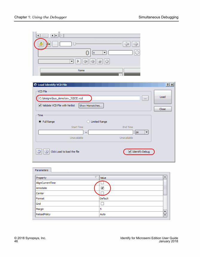
Reviewing the JTAG Chain SettingsThe JTAG chain settings are viewed by clicking the Show chain button in the Communication settings section of the project window. Normally, the JTAG chain settings for the devices are automatically extracted from the design. When the chain settings cannot be determined, they must be created and/or edited using the chain command in the console window. The settings shown below are for a 2-device chain that has JTAG identification register lengths of 8 and 10 bits. In addition, the device named “fpga” has been enabled for debugging.
“fpga” device enabled for debugging
LO
Chapter 1: Using the Debugger Configuring and Invoking the Debugger
© 2018 Synopsys, Inc. Identify for Microsemi Edition User Guide10 January 2018
Saving the Debugged DesignSaving your design in the debugger saves the following additional information to the project definition file:
• IICE settings
• Instrumentations and activations
To save your design definition in the debugger, click the Save current activations icon or select File->Save activations from the menu.
Invoking the DebuggerBefore you can open a design in the debugger, the design must have been created with the instrumentor (only the instrumentor can configure a design for debugging) and synthesized. The debugger can be launched directly from a synthesis project or opened directly from
a Windows or Linux prompt. Invoking the debugger includes:
• Synthesis Tool Launch, on page 10
• Operating System Invocation, on page 10
Synthesis Tool LaunchFrom Synplify Pro, highlight the Identify implementation and select Run->Launch Identify Debugger from the menu bar or popup menu, or click the Launch Identify Debugger icon in the top menu bar.
The debugger IICE instrumentation window opens with the corresponding project displayed (see IICE Instrumentation Window, on page 12).
Operating System InvocationThe debugger runs on both the Windows and Linux platforms. To explicitly invoke the debugger from a Windows system, either:
• double click the Identify Debugger icon on the desktop
• run identify_debugger.exe from the /bin directory of the installation path
To explicitly invoke the debugger from a Linux system:
• run identify_debugger from the /bin directory of the installation path
Debugger Windows Chapter 1: Using the Debugger
Identify for Microsemi Edition User Guide © 2018 Synopsys, Inc.January 2018 11
The initial debugger project window opens. To display the instrumentation window, do either of the following:
• Click the Open existing project icon in the menu bar and, in the Open Project File dialog box, navigate to the project directory and open the corresponding project (prj) file.
• Select File->Open project from the main menu and, in the Open Project File dialog box, navigate to the project directory and open the corresponding project (prj) file.
The debugger instrumentation (IICE) window opens with the corresponding project displayed (see Project Window, on page 15).
Debugger WindowsThe Graphical User Interface for the debugger has three major areas:
• IICE Instrumentation Window, on page 12
• Console Window, on page 14
• Project Window, on page 15
In this section, each of these areas and their uses are described. The following discussions assume that:
• an HDL design has been loaded into the instrumentor and instrumented
• the design has been synthesized in the synthesis tool
• the synthesized output netlist has been placed and routed by the place and route tool
• the resultant bit file has been used to program the FPGA with the instrumented design
• the board containing the programmed FPGA is cabled to your host for analysis by the debugger
LO
Chapter 1: Using the Debugger Debugger Windows
© 2018 Synopsys, Inc. Identify for Microsemi Edition User Guide12 January 2018
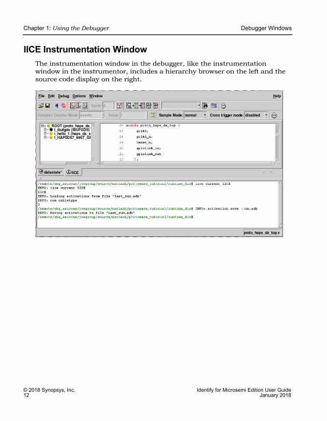
IICE Instrumentation WindowThe instrumentation window in the debugger, like the instrumentation window in the instrumentor, includes a hierarchy browser on the left and the source code display on the right.
Debugger Windows Chapter 1: Using the Debugger
Identify for Microsemi Edition User Guide © 2018 Synopsys, Inc.January 2018 13
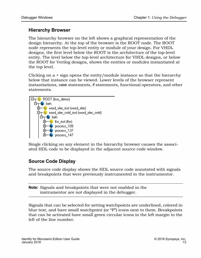
Hierarchy BrowserThe hierarchy browser on the left shows a graphical representation of the design hierarchy. At the top of the browser is the ROOT node. The ROOT node represents the top-level entity or module of your design. For VHDL designs, the first level below the ROOT is the architecture of the top-level entity. The level below the top-level architecture for VHDL designs, or below the ROOT for Verilog designs, shows the entities or modules instantiated at the top level.
Clicking on a + sign opens the entity/module instance so that the hierarchy below that instance can be viewed. Lower levels of the browser represent instantiations, case statements, if statements, functional operators, and other statements.
Single clicking on any element in the hierarchy browser causes the associ-ated HDL code to be displayed in the adjacent source code window.
Source Code DisplayThe source code display shows the HDL source code annotated with signals and breakpoints that were previously instrumented in the instrumentor.
Note: Signals and breakpoints that were not enabled in the instrumentor are not displayed in the debugger.
Signals that can be selected for setting watchpoints are underlined, colored in blue text, and have small watchpoint (or “P”) icons next to them. Breakpoints that can be activated have small green circular icons in the left margin to the left of the line number.

LO
Chapter 1: Using the Debugger Debugger Windows
© 2018 Synopsys, Inc. Identify for Microsemi Edition User Guide14 January 2018
Selecting the watchpoint or “P” icon next to a signal (or the signal itself) allows you to select the Watchpoint Setup dialog box from the popup menu. This dialog box is used to specify a watchpoint expression for the signal. See Setting a Watchpoint Expression, on page 17.
Selecting the green breakpoint icon to the left of the source line number causes that breakpoint to become armed when the run command is executed. See Run Command, on page 25.
Console WindowThe debugger console window displays commands that have been executed, including those executed by menu selections and button clicks. The console window also allows you to enter debugger commands and to view the results of command execution.
Debugger Windows Chapter 1: Using the Debugger
Identify for Microsemi Edition User Guide © 2018 Synopsys, Inc.January 2018 15
To capture all the text written to the console, use the log console command (see the Reference Manual). Alternately, you can click the right mouse button inside the console window and select Save Console Output from the menu. To capture all commands executed in the console window, use the transcript command (see the Reference Manual).
To clear the text in the console window, use the clear command or click the right mouse button inside the console window and select clear from the menu.
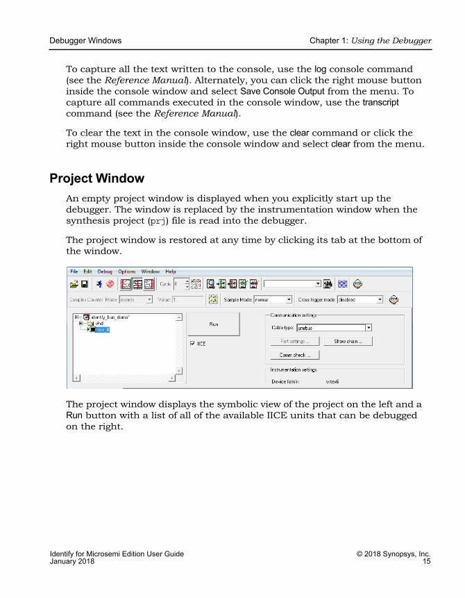
Project WindowAn empty project window is displayed when you explicitly start up the debugger. The window is replaced by the instrumentation window when the synthesis project (prj) file is read into the debugger.
The project window is restored at any time by clicking its tab at the bottom of the window.
The project window displays the symbolic view of the project on the left and a Run button with a list of all of the available IICE units that can be debugged on the right.
LO
Chapter 1: Using the Debugger Commands and Procedures
© 2018 Synopsys, Inc. Identify for Microsemi Edition User Guide16 January 2018
Commands and ProceduresThis section describes the typical operations performed in the debugger and includes the following topics:
• Opening and Saving Projects, on page 16
• Executing a Script File, on page 17
• Activating/Deactivating an Instrumentation, on page 17
• Selecting Multiplexed Instrumentation Sets, on page 21
• Activating/Deactivating Folded Instrumentation, on page 22
• Run Command, on page 25
• Sampled Data Compression, on page 26
• Sample Buffer Trigger Position, on page 28
• Sampled Data Display Controls, on page 29
• Saving and Loading Activations, on page 33
• Cross Triggering, on page 35
• Listing Watchpoints and Signals, on page 36
Opening and Saving ProjectsThe debugger commands to open and save projects are available as menu items and icons.
Function Menu BarIcon
Menu Command
Open existing project File->Open project
Save current activations
File->Save activations
Commands and Procedures Chapter 1: Using the Debugger
Identify for Microsemi Edition User Guide © 2018 Synopsys, Inc.January 2018 17
When opening a project:
• The working directory is automatically set from the corresponding project file.
• If the project was saved with encrypted original sources, you are prompted to enter the original password used to encrypt the files. This password is then used to read any encrypted files.
Executing a Script FileA script file contains Tcl commands and is a convenient way to capture a command sequence that you would like to repeat. To execute a script file, select the File->Execute Script menu selection and navigate to your script file location or use the source command (see source, on page 80 in the Reference Manual).
Activating/Deactivating an InstrumentationThe trigger conditions used to control the sampling buffer comprise break-points, watchpoints, and counter settings (see Chapter 2, IICE Hardware Description). Activation and deactivation of breakpoints and watchpoints are discussed in this chapter.
Setting a Watchpoint ExpressionAny signal that has been instrumented for triggering can be activated as a watchpoint in the debugger. A watchpoint is defined by assigning it one or two HDL constant expressions. When a watched signal changes to the value of its watchpoint expression, a trigger event occurs.
A watchpoint is set on a signal by clicking-and-holding on the signal or the watchpoint icon next to the signal and then selecting the Set Trigger Expressions menu item to bring up the Watchpoint Setup dialog box.
A watchpoint is set on a partial bus signal by clicking-and-holding on the signal or the “P” icon next to the signal, selecting the partial bus group from the list displayed, and then selecting the Set Trigger Expressions menu item to bring up the Watchpoint Setup dialog box.
LO
Chapter 1: Using the Debugger Commands and Procedures
© 2018 Synopsys, Inc. Identify for Microsemi Edition User Guide18 January 2018
There are two forms of watchpoints: value and transition.
• A value watchpoint triggers when the watched signal attains a specific value.
• A transition watchpoint triggers when the watched signal has a specific value transition.
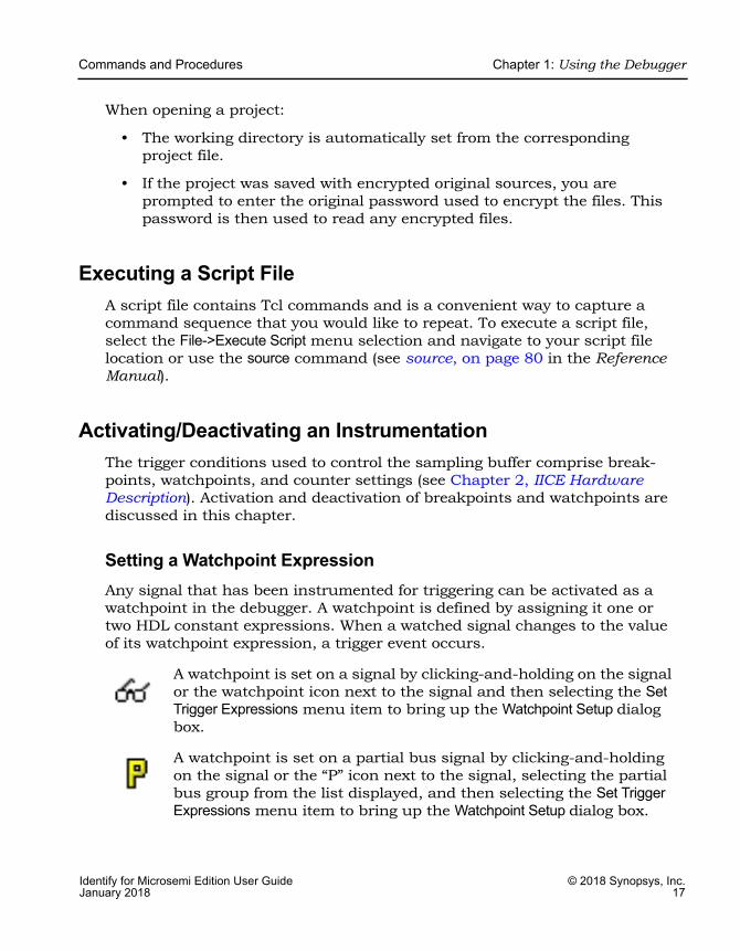
To create a value watchpoint, assign a single, constant expression to the watchpoint. A value watchpoint triggers when the watched signal value equals the expression. In the example below, the signal is a 4-bit signal, and the watchpoint expression is set to “0010” (binary). Any legal VHDL or Verilog (as appropriate) constant expression is accepted.
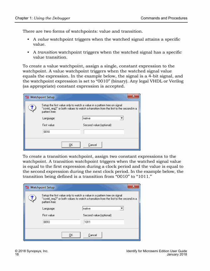
To create a transition watchpoint, assign two constant expressions to the watchpoint. A transition watchpoint triggers when the watched signal value is equal to the first expression during a clock period and the value is equal to the second expression during the next clock period. In the example below, the transition being defined is a transition from “0010” to “1011.”

Commands and Procedures Chapter 1: Using the Debugger
Identify for Microsemi Edition User Guide © 2018 Synopsys, Inc.January 2018 19
The VHDL or Verilog expressions that are entered in the Watchpoint Setup dialog box can also contain “X” values. The “X” values allow the value of some bits of the watched signal to be ignored (effectively, “X” values are don’t-care values). For example, the above value watchpoint expression can be specified as “X010” which causes the watchpoint to trigger only on the values of the three right-most bits.
Hexadecimal values can additionally be entered as watchpoint values using the following syntax:
x"hexValue"
As shown, a hexadecimal value is introduced with an x character and the value must be enclosed in quotation marks. Similarly, you can include a hexadecimal entry in an equivalent Tcl command by literalizing the quote marks with back slashes as shown in the following example:
watch enable -iice IICE -condition 0 /structural/reg_fout x\"aa\"
Clicking OK on the Watchpoint Setup dialog box activates the watchpoint (the watchpoint or “P” icon changes to red) which is then armed in the hardware the next time the Run button is pressed.
Deactivating a WatchpointBy default, a watchpoint that does not have a watchpoint expression is inactive. A watchpoint that has a watchpoint expression can be temporarily deactivated. A deactivated watchpoint retains the expression entered, but is not armed in the hardware and does not result in a trigger.
To deactivate a watchpoint, click-and-hold on the signal or the associated watchpoint icon. The watchpoint popup menu appears.
To deactivate a partial-bus watchpoint, click-and-hold on the signal or the associated “P” icon and select the bus segment from the list of segments displayed. The watchpoint popup menu appears.
LO
Chapter 1: Using the Debugger Commands and Procedures
© 2018 Synopsys, Inc. Identify for Microsemi Edition User Guide20 January 2018
The Watch menu selection will have a check mark to indicate that the watch-point is activated. Click on the Watch menu selection to toggle the check mark and deactivate the watchpoint.
Reactivating a WatchpointTo reactivate an inactive watchpoint, click-and-hold on the signal or the associated watchpoint or “P” icon. Clicking the watchpoint icon redisplays the watchpoint popup menu: clicking the “P” icon, lists the partial bus segments; select the bus segment from the list displayed to display the watchpoint popup menu. Click the Watch menu selection to toggle the check mark and reactivate the watchpoint.
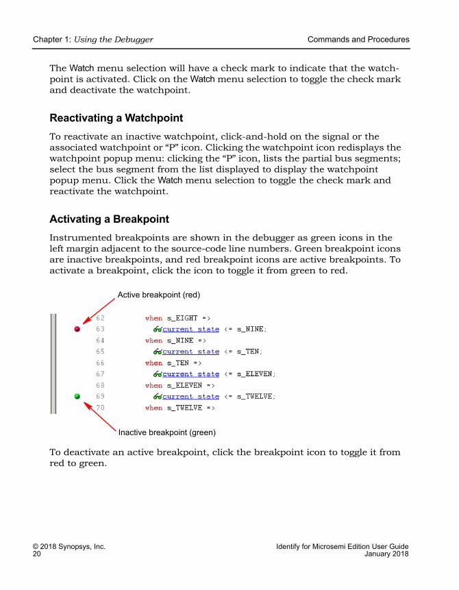
Activating a BreakpointInstrumented breakpoints are shown in the debugger as green icons in the left margin adjacent to the source-code line numbers. Green breakpoint icons are inactive breakpoints, and red breakpoint icons are active breakpoints. To activate a breakpoint, click the icon to toggle it from green to red.
To deactivate an active breakpoint, click the breakpoint icon to toggle it from red to green.
Inactive breakpoint (green)
Active breakpoint (red)

Commands and Procedures Chapter 1: Using the Debugger
Identify for Microsemi Edition User Guide © 2018 Synopsys, Inc.January 2018 21
Selecting Multiplexed Instrumentation SetsMultiplexed groups of instrumented signals defined in the instrumentor can be individually selected for activation in the debugger (for information on defining a multiplexed group in the instrumentor, see Multiplexed Groups, on page 36 in the Identify Instrumentor User Guide).
Using multiplexed groups can substantially reduce the amount of pattern memory required during debugging when all of the originally instrumented signals are not required to be loaded into memory at the same time.
To activate a predefined multiplexed group in the debugger:
1. Click the IICE icon in the top menu to display the Enhanced Settings for IICE Unit dialog box.
2. Use the drop-down menu in the Mux Group section to select the group number to be active for the debug session.
3. The signals group command can be used to assign groups from the console window (see signals, on page 75 of the Reference Manual).

LO
Chapter 1: Using the Debugger Commands and Procedures
© 2018 Synopsys, Inc. Identify for Microsemi Edition User Guide22 January 2018
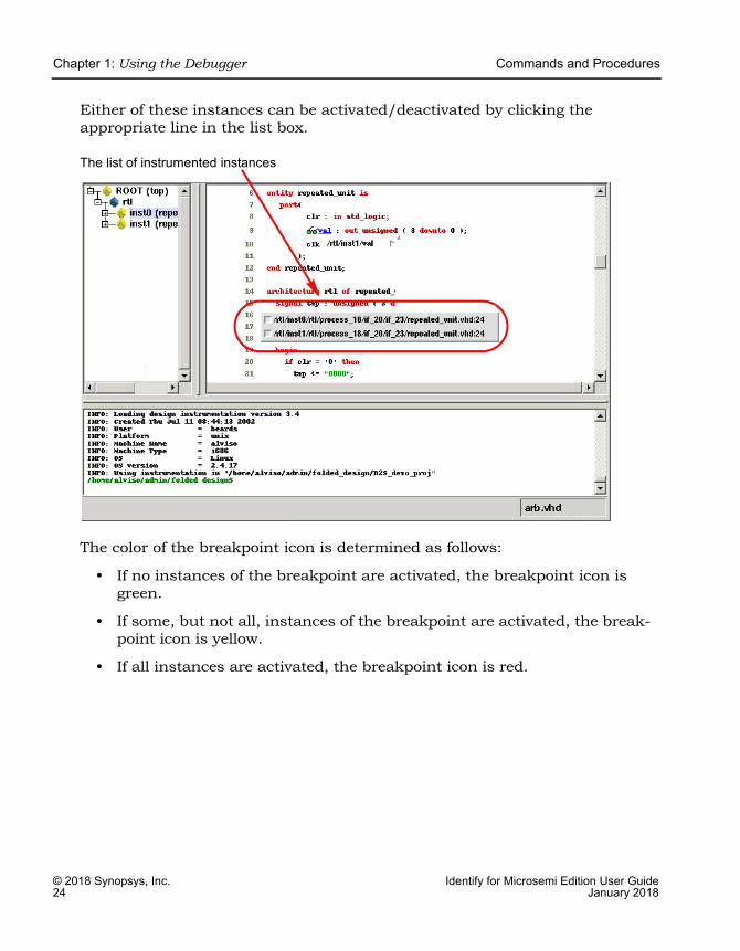
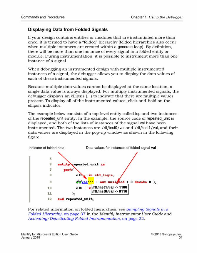
Activating/Deactivating Folded InstrumentationIf your design contains entities or modules that are instantiated more than once, the design is termed to have a “folded” hierarchy (folded hierarchies also occur when multiple instances are created within a generate loop). By definition, there will be more than one instance of every signal and breakpoint in a folded entity or module. During instrumentation, it is possible to instrument more than one instance of a signal or breakpoint.
When debugging an instrumented design with multiple instrumented instances of a breakpoint or signal, the debugger allows you to activate/deactivate each of these instrumented instances independently. Independent selection is accomplished by displaying a list of the instrumented instances when the breakpoint or signal is selected for activation/deactivation.
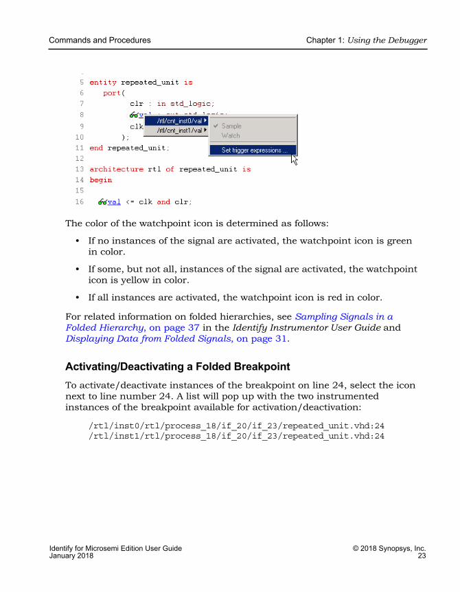
Activating/Deactivating a Folded WatchpointThe following example consists of a top-level entity called folded2 and two instances of the repeated_unit entity. The source code of repeated_unit is displayed. In this folded entity, multiple instances of the signal val and the breakpoint at line 24 (not shown) are instrumented.
To activate/deactivate instances of the val signal, select the watchpoint icon next to the signal. A list will pop up with the two instrumented instances of the signal val available for activation/deactivation:
/rtl/cnt_inst0/val/rtl/cnt_inst1/val
Either of these instances is activated/deactivated by clicking on the appropriate line in the list box to bring up the watchpoint menu shown in the following figure.
Commands and Procedures Chapter 1: Using the Debugger
Identify for Microsemi Edition User Guide © 2018 Synopsys, Inc.January 2018 23
The color of the watchpoint icon is determined as follows:
• If no instances of the signal are activated, the watchpoint icon is green in color.
• If some, but not all, instances of the signal are activated, the watchpoint icon is yellow in color.
• If all instances are activated, the watchpoint icon is red in color.
For related information on folded hierarchies, see Sampling Signals in a Folded Hierarchy, on page 37 in the Identify Instrumentor User Guide and Displaying Data from Folded Signals, on page 31.
Activating/Deactivating a Folded BreakpointTo activate/deactivate instances of the breakpoint on line 24, select the icon next to line number 24. A list will pop up with the two instrumented instances of the breakpoint available for activation/deactivation:
/rtl/inst0/rtl/process_18/if_20/if_23/repeated_unit.vhd:24/rtl/inst1/rtl/process_18/if_20/if_23/repeated_unit.vhd:24
LO
Chapter 1: Using the Debugger Commands and Procedures
© 2018 Synopsys, Inc. Identify for Microsemi Edition User Guide24 January 2018
Either of these instances can be activated/deactivated by clicking the appropriate line in the list box.
The color of the breakpoint icon is determined as follows:
• If no instances of the breakpoint are activated, the breakpoint icon is green.
• If some, but not all, instances of the breakpoint are activated, the break-point icon is yellow.
• If all instances are activated, the breakpoint icon is red.
The list of instrumented instances
Commands and Procedures Chapter 1: Using the Debugger
Identify for Microsemi Edition User Guide © 2018 Synopsys, Inc.January 2018 25
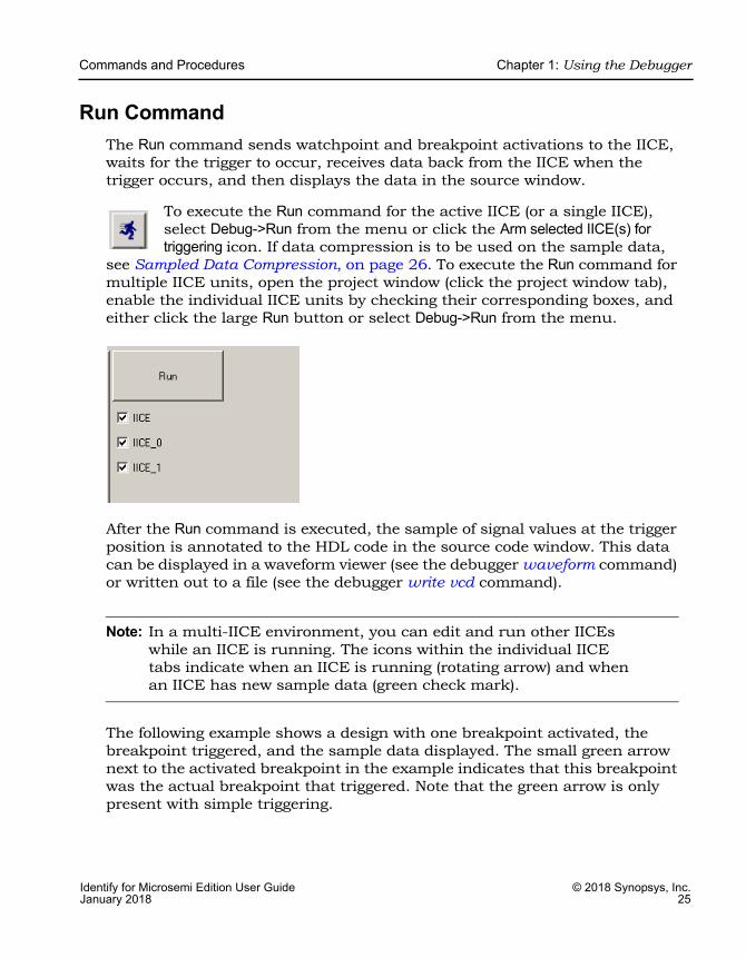
Run CommandThe Run command sends watchpoint and breakpoint activations to the IICE, waits for the trigger to occur, receives data back from the IICE when the trigger occurs, and then displays the data in the source window.
To execute the Run command for the active IICE (or a single IICE), select Debug->Run from the menu or click the Arm selected IICE(s) for triggering icon. If data compression is to be used on the sample data,
see Sampled Data Compression, on page 26. To execute the Run command for multiple IICE units, open the project window (click the project window tab), enable the individual IICE units by checking their corresponding boxes, and either click the large Run button or select Debug->Run from the menu.
After the Run command is executed, the sample of signal values at the trigger position is annotated to the HDL code in the source code window. This data can be displayed in a waveform viewer (see the debugger waveform command) or written out to a file (see the debugger write vcd command).
Note: In a multi-IICE environment, you can edit and run other IICEs while an IICE is running. The icons within the individual IICE tabs indicate when an IICE is running (rotating arrow) and when an IICE has new sample data (green check mark).
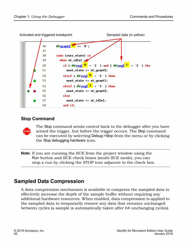
The following example shows a design with one breakpoint activated, the breakpoint triggered, and the sample data displayed. The small green arrow next to the activated breakpoint in the example indicates that this breakpoint was the actual breakpoint that triggered. Note that the green arrow is only present with simple triggering.
LO
Chapter 1: Using the Debugger Commands and Procedures
© 2018 Synopsys, Inc. Identify for Microsemi Edition User Guide26 January 2018
Stop CommandThe Stop command sends control back to the debugger after you have armed the trigger, but before the trigger occurs. The Stop command can be executed by selecting Debug->Stop from the menu or by clicking the Stop debugging hardware icon.
Note: If you are running the IICE from the project window using the Run button and IICE check boxes (multi-IICE mode), you can stop a run by clicking the STOP icon adjacent to the check box.
Sampled Data Compression A data compression mechanism is available to compress the sampled data to effectively increase the depth of the sample buffer without requiring any additional hardware resources. When enabled, data compression is applied to the sampled data to temporarily remove any data that remains unchanged between cycles (a sample is automatically taken after 64 unchanging cycles).
Activated and triggered breakpoint Sampled data (in yellow)
Commands and Procedures Chapter 1: Using the Debugger
Identify for Microsemi Edition User Guide © 2018 Synopsys, Inc.January 2018 27
Data compression is enabled from the project view by clicking the IICE icon to display the Enhanced Settings for IICE Unit dialog box and clicking the Enable check box in the Data Compression section or from the command prompt by entering the following command:
iice sampler -datacompression 1
Data compression must be set prior to executing the Run command and applies to all enabled IICE units. Data compression is not available when using state-machine triggering, or qualified or always-armed sampling.
Sample Data MaskingA masking option is available with data compression to selectively mask individual bits or buses from being considered as changing values within the sample data. This option is only available through the Tcl interface using the following syntax:
iice sampler -enablemask 0 |1 [-msb integer -lsb integer] signalName
For example, the following command masks bits 0 through 3 of vector signal mybus[7:0] from consideration by the data compression mechanism:
iice sampler -enablemask 1 -msb 3 -lsb 0 mybus
Similarly, to reinstate the masked signals in the above example, use the command:
iice sampler -enablemask 0 -msb 3 -lsb 0 mybus
LO
Chapter 1: Using the Debugger Commands and Procedures
© 2018 Synopsys, Inc. Identify for Microsemi Edition User Guide28 January 2018
Sample Buffer Trigger PositionThe purpose of the activated watchpoints and breakpoints is to cause a trigger event to occur. The trigger event causes sampling to terminate in a controlled fashion. Once sampling terminates, the data in the sample buffer is communicated to the debugger and then displayed in the GUI.
The sample buffer is continuously sampling the design signals. Conse-quently, the exact relationship between the trigger event and the termination of the sampling can be controlled by the user. Currently, the debugger supports the following trigger positions relative to the sample buffer:
• Early
• Middle
• Late
Determining the correct setting for the trigger position is up to the user. For example, if the design behavior of interest usually occurs after a particular trigger event, set the trigger position to “early.”
The trigger position can be changed without requiring the design to be re-instrumented or recompiled. A new trigger position setting takes effect the next time the Run command is executed.
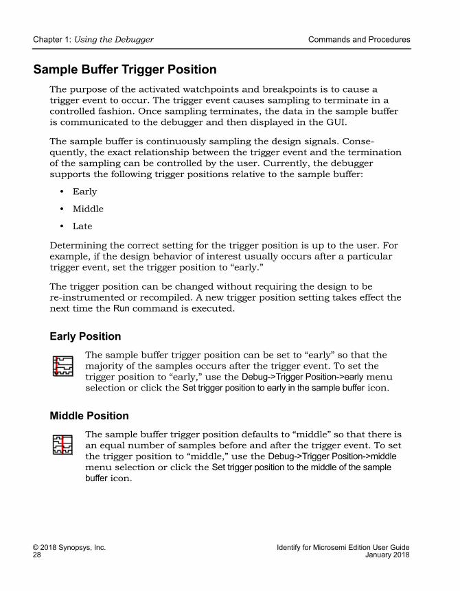
Early PositionThe sample buffer trigger position can be set to “early” so that the majority of the samples occurs after the trigger event. To set the trigger position to “early,” use the Debug->Trigger Position->early menu selection or click the Set trigger position to early in the sample buffer icon.
Middle PositionThe sample buffer trigger position defaults to “middle” so that there is an equal number of samples before and after the trigger event. To set the trigger position to “middle,” use the Debug->Trigger Position->middle menu selection or click the Set trigger position to the middle of the sample buffer icon.
Commands and Procedures Chapter 1: Using the Debugger
Identify for Microsemi Edition User Guide © 2018 Synopsys, Inc.January 2018 29
Late PositionThe sample buffer trigger position can be set to “late” so that the majority of the samples occurs before the trigger event. To set the trigger position to “late,” use the Debug->Trigger Position->late menu selection or click on the Set trigger position to late in the sample buffer icon.
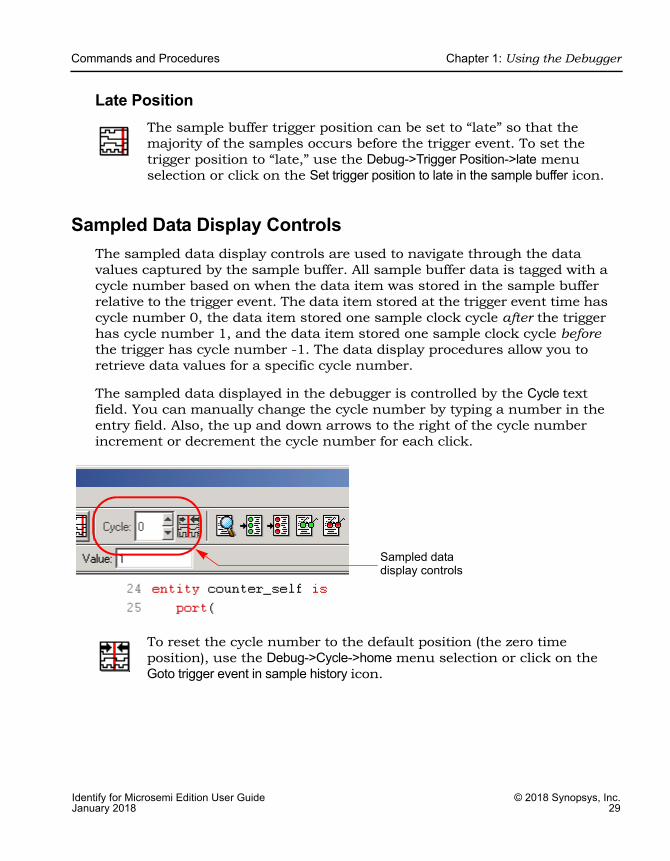
Sampled Data Display ControlsThe sampled data display controls are used to navigate through the data values captured by the sample buffer. All sample buffer data is tagged with a cycle number based on when the data item was stored in the sample buffer relative to the trigger event. The data item stored at the trigger event time has cycle number 0, the data item stored one sample clock cycle after the trigger has cycle number 1, and the data item stored one sample clock cycle before the trigger has cycle number -1. The data display procedures allow you to retrieve data values for a specific cycle number.
The sampled data displayed in the debugger is controlled by the Cycle text field. You can manually change the cycle number by typing a number in the entry field. Also, the up and down arrows to the right of the cycle number increment or decrement the cycle number for each click.
To reset the cycle number to the default position (the zero time position), use the Debug->Cycle->home menu selection or click on the Goto trigger event in sample history icon.
Sampled data display controls
LO
Chapter 1: Using the Debugger Commands and Procedures
© 2018 Synopsys, Inc. Identify for Microsemi Edition User Guide30 January 2018
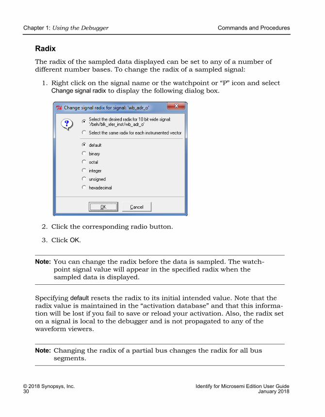
RadixThe radix of the sampled data displayed can be set to any of a number of different number bases. To change the radix of a sampled signal:
1. Right click on the signal name or the watchpoint or “P” icon and select Change signal radix to display the following dialog box.
2. Click the corresponding radio button.
3. Click OK.
Note: You can change the radix before the data is sampled. The watch-point signal value will appear in the specified radix when the sampled data is displayed.
Specifying default resets the radix to its initial intended value. Note that the radix value is maintained in the “activation database” and that this informa-tion will be lost if you fail to save or reload your activation. Also, the radix set on a signal is local to the debugger and is not propagated to any of the waveform viewers.
Note: Changing the radix of a partial bus changes the radix for all bus segments.
Commands and Procedures Chapter 1: Using the Debugger
Identify for Microsemi Edition User Guide © 2018 Synopsys, Inc.January 2018 31
Displaying Data from Folded SignalsIf your design contains entities or modules that are instantiated more than once, it is termed to have a “folded” hierarchy (folded hierarchies also occur when multiple instances are created within a generate loop). By definition, there will be more than one instance of every signal in a folded entity or module. During instrumentation, it is possible to instrument more than one instance of a signal.
When debugging an instrumented design with multiple instrumented instances of a signal, the debugger allows you to display the data values of each of these instrumented signals.
Because multiple data values cannot be displayed at the same location, a single data value is always displayed. For multiply instrumented signals, the debugger displays an ellipsis (...) to indicate that there are multiple values present. To display all of the instrumented values, click-and-hold on the ellipsis indicator.
The example below consists of a top-level entity called top and two instances of the repeated_unit entity. In the example, the source code of repeated_unit is displayed, and both of the lists of instances of the signal val have been instrumented. The two instances are /rtl/inst0/val and /rtl/inst1/val, and their data values are displayed in the pop-up window as shown in the following figure:
For related information on folded hierarchies, see Sampling Signals in a Folded Hierarchy, on page 37 in the Identify Instrumentor User Guide and Activating/Deactivating Folded Instrumentation, on page 22.
Indicator of folded data Data values for instances of folded signal val
LO
Chapter 1: Using the Debugger Commands and Procedures
© 2018 Synopsys, Inc. Identify for Microsemi Edition User Guide32 January 2018
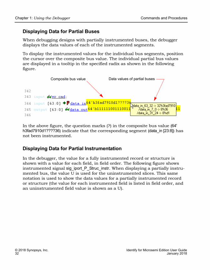
Displaying Data for Partial BusesWhen debugging designs with partially instrumented buses, the debugger displays the data values of each of the instrumented segments.
To display the instrumented values for the individual bus segments, position the cursor over the composite bus value. The individual partial bus values are displayed in a tooltip in the specified radix as shown in the following figure.
In the above figure, the question marks (?) in the composite bus value (64' h3fad7910d1????36) indicate that the corresponding segment (data_in [23:8]) has not been instrumented.
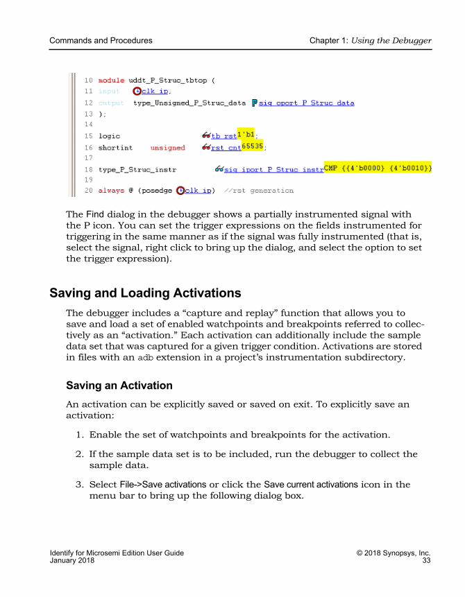
Displaying Data for Partial Instrumentation
In the debugger, the value for a fully instrumented record or structure is shown with a value for each field, in field order. The following figure shows instrumented signal sig_iport_P_Struc_instr. When displaying a partially instru-mented bus, the value U is used for the uninstrumented slices. This same notation is used to show the data values for a partially instrumented record or structure (the value for each instrumented field is listed in field order, and an uninstrumented field value is shown as a U).
Composite bus value Data values of partial buses
Commands and Procedures Chapter 1: Using the Debugger
Identify for Microsemi Edition User Guide © 2018 Synopsys, Inc.January 2018 33
The Find dialog in the debugger shows a partially instrumented signal with the P icon. You can set the trigger expressions on the fields instrumented for triggering in the same manner as if the signal was fully instrumented (that is, select the signal, right click to bring up the dialog, and select the option to set the trigger expression).
Saving and Loading ActivationsThe debugger includes a “capture and replay” function that allows you to save and load a set of enabled watchpoints and breakpoints referred to collec-tively as an “activation.” Each activation can additionally include the sample data set that was captured for a given trigger condition. Activations are stored in files with an adb extension in a project’s instrumentation subdirectory.
Saving an ActivationAn activation can be explicitly saved or saved on exit. To explicitly save an activation:
1. Enable the set of watchpoints and breakpoints for the activation.
2. If the sample data set is to be included, run the debugger to collect the sample data.
3. Select File->Save activations or click the Save current activations icon in the menu bar to bring up the following dialog box.
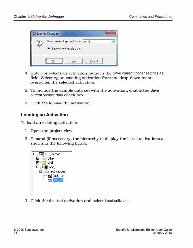
LO
Chapter 1: Using the Debugger Commands and Procedures
© 2018 Synopsys, Inc. Identify for Microsemi Edition User Guide34 January 2018
4. Enter (or select) an activation name in the Save current trigger settings as: field. Selecting an existing activation from the drop-down menu overwrites the selected activation.
5. To include the sample data set with the activation, enable the Save current sample data check box.
6. Click Yes to save the activation.
Loading an ActivationTo load an existing activation:
1. Open the project view.
2. Expand (if necessary) the hierarchy to display the list of activations as shown in the following figure.
3. Click the desired activation and select Load activation.

Commands and Procedures Chapter 1: Using the Debugger
Identify for Microsemi Edition User Guide © 2018 Synopsys, Inc.January 2018 35
Autosaving Current ActivationBy default, when you exit the debugger without explicitly saving an activa-tion, the active activation is automatically saved to the last_run.adb file. This file is automatically loaded the next time you open the project.
Note: To save a specific activation, always use Save current activations to explicitly name the file and prevent the data from overwriting the last_run.adb file.
To disable the auto-save feature, uncheck the Auto-save trigger settings and sample results check box on the Debugger Preferences dialog box (select Options->Debugger preferences).
Cross TriggeringCross triggering allows the trigger from one IICE unit to be used to qualify a trigger on another IICE unit, even when the two IICE units are in different time domains. Cross triggering is available in both the simple triggering and complex counter triggering modes (state-machine triggering supports cross triggering by allowing the IICE unit IDs to be included in the state-machine equations).
Cross triggering for an IICE unit is enabled in the instrumentor by selecting the Allow cross-triggering in IICE check box on the IICE Controller tab for the local IICE unit. The cross-trigger mode is selected from the drop-down menu in the debugger as shown below.
LO
Chapter 1: Using the Debugger Commands and Procedures
© 2018 Synopsys, Inc. Identify for Microsemi Edition User Guide36 January 2018
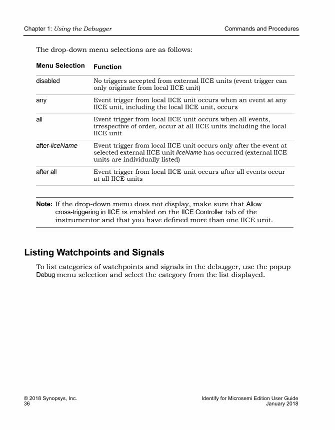
The drop-down menu selections are as follows:
Note: If the drop-down menu does not display, make sure that Allow cross-triggering in IICE is enabled on the IICE Controller tab of the instrumentor and that you have defined more than one IICE unit.
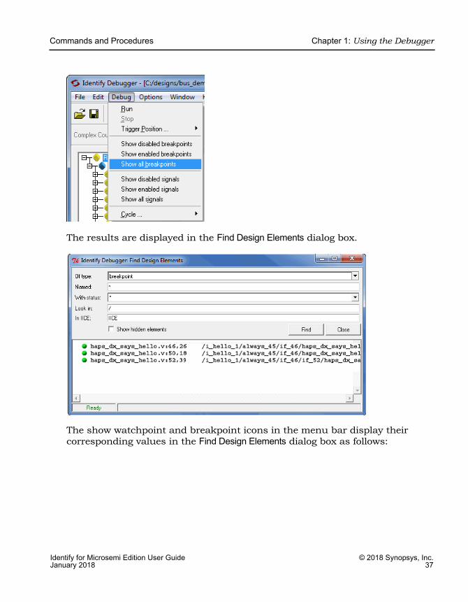
Listing Watchpoints and SignalsTo list categories of watchpoints and signals in the debugger, use the popup Debug menu selection and select the category from the list displayed.
Menu Selection Function
disabled No triggers accepted from external IICE units (event trigger can only originate from local IICE unit)
any Event trigger from local IICE unit occurs when an event at any IICE unit, including the local IICE unit, occurs
all Event trigger from local IICE unit occurs when all events, irrespective of order, occur at all IICE units including the local IICE unit
after-iiceName Event trigger from local IICE unit occurs only after the event at selected external IICE unit iiceName has occurred (external IICE units are individually listed)
after all Event trigger from local IICE unit occurs after all events occur at all IICE units
Commands and Procedures Chapter 1: Using the Debugger
Identify for Microsemi Edition User Guide © 2018 Synopsys, Inc.January 2018 37
The results are displayed in the Find Design Elements dialog box.
The show watchpoint and breakpoint icons in the menu bar display their corresponding values in the Find Design Elements dialog box as follows:
LO
Chapter 1: Using the Debugger Commands and Procedures
© 2018 Synopsys, Inc. Identify for Microsemi Edition User Guide38 January 2018
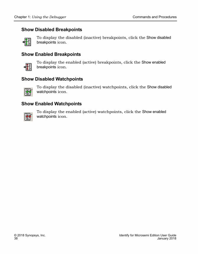
Show Disabled BreakpointsTo display the disabled (inactive) breakpoints, click the Show disabled breakpoints icon.
Show Enabled BreakpointsTo display the enabled (active) breakpoints, click the Show enabled breakpoints icon.
Show Disabled WatchpointsTo display the disabled (inactive) watchpoints, click the Show disabled watchpoints icon.
Show Enabled WatchpointsTo display the enabled (active) watchpoints, click the Show enabled watchpoints icon.
HAPS Deep Trace Debug Chapter 1: Using the Debugger
Identify for Microsemi Edition User Guide © 2018 Synopsys, Inc.January 2018 39
HAPS Deep Trace DebugThe HAPS Deep Trace Debug feature supports the HAPS SRAM_1x1_HTII memory configuration on a HAPS-60 system. Using this type of added memory provides a significantly deeper, signal-trace buffer.
With the HAPS deep trace debug mode, the flow remains unchanged. The only difference is in the configuration of the additional memory as the sample buffer using IICE parameters in the instrumentor (see Chapter 4, HAPS Deep Trace Debug in the Identify Instrumentor User Guide).
When you debug the design, the debugger automatically calculates the sample depth and source clock based on the configuration settings supplied in the instrumentor.
Running Deep Trace DebugTo maximize performance when using the expanded memory available from the SRAM daughter board, the tool automatically calculates the maximum buffer depth based on the number of signals instrumented. The configured sample depth can be varied dynamically from the minimum depth to the maximum depth.
When the sample depth is set to a large value, the captured samples are first downloaded block-by-block. Once all of the blocks are downloaded, viewing of large samples in the waveform viewer is very time consuming and also the size of the VCD/FSDB dumps becomes extremely large (for a full buffer depth, the time to download all the sample blocks can be between 30 and 40 minutes and a full VCD dump can require several hours).
To reduce these times, use the waveform writer in the debugger to dump a specific range or slice of the VCD/FSDB waveform (see Viewing Captured Deep Trace Debug Samples, on page 40). In the debugger, click on the waveform display icon to bring up the pop-up window where you can specify the cycle range over which to view the waveform. The configured sample depth can be varied in the debugger, but cannot be greater than the depth set in the instrumentor.
LO
Chapter 1: Using the Debugger HAPS Deep Trace Debug
© 2018 Synopsys, Inc. Identify for Microsemi Edition User Guide40 January 2018
Also, using deep-trace debug on a Windows-based system with minimal resources can be extremely slow, especially when downloading large captured samples or when writing the corresponding VCD/FSDB waveform dumps. Increasing the memory capacity and processor speed of the host can signifi-cantly improve performance.
Viewing Captured Deep Trace Debug SamplesA large sample depth translates to large VCD/FSDB dump files. For these cases, the debugger includes the option of viewing or writing out a slice of the FSDB or VCD waveform based the number of captured cycles.
To write out a slice of the waveform:
1. Launch the debugger with the exported runtime environment from the operating system (see Invoking the Debugger, on page 10).
2. In the debugger GUI, open the project file (debug.prj).
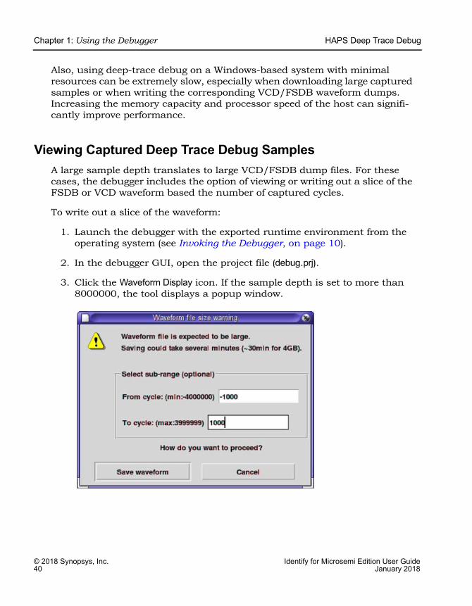
3. Click the Waveform Display icon. If the sample depth is set to more than 8000000, the tool displays a popup window.
HAPS Deep Trace Debug Chapter 1: Using the Debugger
Identify for Microsemi Edition User Guide © 2018 Synopsys, Inc.January 2018 41
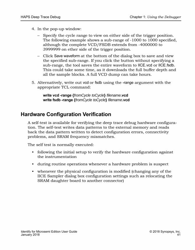
4. In the pop-up window:
– Specify the cycle range to view on either side of the trigger position. The following example shows a sub-range of -1000 to 1000 specified, although the complete VCD/FSDB extends from -4000000 to 3999999 on ether side of the trigger position.
– Click Save waveform at the bottom of the dialog box to save and view the specified sub-range. If you click the button without specifying a sub-range, the tool saves the entire waveform to IICE.vcd or IICE.fsdb. This could take some time, as it downloads the full buffer depth and all the sample blocks. A full VCD dump can take hours.
5. Alternatively, write out vcd or fsdb using the -range argument with the appropriate TCL command:
write vcd -range {fromCycle toCycle} filename.vcdwrite fsdb -range {fromCycle toCycle} filename.vcd
Hardware Configuration VerificationA self-test is available for verifying the deep trace debug hardware configura-tion. The self-test writes data patterns to the external memory and reads back the data pattern written to detect configuration errors, connectivity problems, and SRAM frequency mismatches.
The self test is normally executed:
• following the initial setup to verify the hardware configuration against the instrumentation
• during routine operations whenever a hardware problem is suspect
• whenever the physical configuration is modified (changing any of the IICE Sampler dialog box configuration settings such as relocating the SRAM daughter board to another connector)
LO
Chapter 1: Using the Debugger HAPS Deep Trace Debug
© 2018 Synopsys, Inc. Identify for Microsemi Edition User Guide42 January 2018
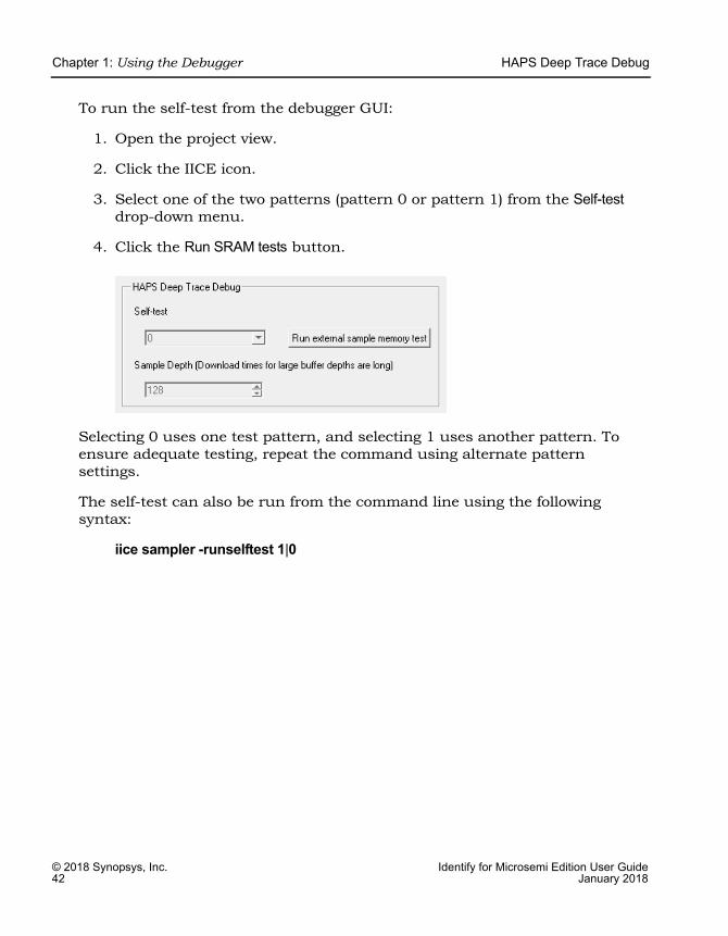
To run the self-test from the debugger GUI:
1. Open the project view.
2. Click the IICE icon.
3. Select one of the two patterns (pattern 0 or pattern 1) from the Self-test drop-down menu.
4. Click the Run SRAM tests button.
Selecting 0 uses one test pattern, and selecting 1 uses another pattern. To ensure adequate testing, repeat the command using alternate pattern settings.
The self-test can also be run from the command line using the following syntax:
iice sampler -runselftest 1|0

Debugging on a Different Machine Chapter 1: Using the Debugger
Identify for Microsemi Edition User Guide © 2018 Synopsys, Inc.January 2018 43
Debugging on a Different MachineIt is not unusual for the instrumentation phase and the debugging phase to be performed on different machines. For example, the debug machine is often located in a hardware lab. When a different machine is used for debugging, you must copy the project file (projectName.prj) and the following files to the lab machine:
• Implementation folder (for example, rev_1); it is not necessary to copy the contents of the folder
• syn.db file
• instr.db file
• orig_sources files
Because the instrumentor/debugger tool set allows you to debug your design in the HDL, the debugger must have access to the original source files. Depending on the type of your network, the debugger may be able to access the original sources files directly from the lab machine. If this is not possible or if the two computers are not networked, you must also copy the original sources to the debug machine. If the debugger cannot locate the original source files, it will open the project, but an error will be generated for each missing file, and the corresponding source code will not be visible in the source viewer.
Copying the source files to the debug machine can be done in two ways:
• The instrumentor can automatically include the original source files in the implementation directory so that when you copy the implementation directory to the lab machine, the original sources files (in the orig_sources subdirectory) are included. The debugger automatically looks in this directory for any missing source files. This preference is set before compiling the instrumented design by selecting Options->Instrumentation preference and making sure that Save original source in instrumentation directory is checked.
LO
Chapter 1: Using the Debugger Simultaneous Debugging
© 2018 Synopsys, Inc. Identify for Microsemi Edition User Guide44 January 2018
• The original source files can be manually copied to the lab machine or may already exist in a different location on this machine. In this case, it may be necessary to help locate the design files using the searchpath command. Simply call this command from the command line before loading the project file (projectName.prj). The argument is a semi-colon-separated (Windows) or colon-separated (Linux) list of directories in which to find the original source files.
searchpath {d:/temp;c:/Documents and Settings/me/my_design/}
The debugger only displays files that match the CRC generated at the time of instrumentation.
Note: If there are security issues with having the original source files on the lab machine, the instrumentor can password-protect the original sources on the development machine for use with the debugger (for information on file encryption, see Including Orig-inal HDL Source, on page 49 in the Identify Instrumentor User Guide).
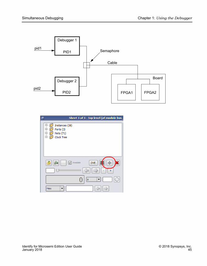
Simultaneous DebuggingWhen multiple debugger licenses are available, multiple FPGAs residing on a single, non-HAPS board can be debugged concurrently through a single cable. This capability is based on semaphores that allow more than one debugger to share the common port.
Simultaneous Debugging Chapter 1: Using the Debugger
Identify for Microsemi Edition User Guide © 2018 Synopsys, Inc.January 2018 45
Board
FPGA1 FPGA2
Cable
Semaphorepid1
pid2
Debugger 1
Debugger 2
PID1
PID2
LO
Chapter 1: Using the Debugger Simultaneous Debugging
© 2018 Synopsys, Inc. Identify for Microsemi Edition User Guide46 January 2018
Simultaneous Debugging Chapter 1: Using the Debugger
Identify for Microsemi Edition User Guide © 2018 Synopsys, Inc.January 2018 47
LO
Chapter 1: Using the Debugger Waveform Display
© 2018 Synopsys, Inc. Identify for Microsemi Edition User Guide48 January 2018
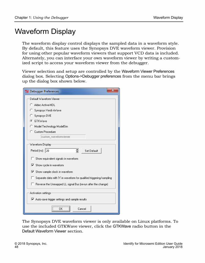
Waveform DisplayThe waveform display control displays the sampled data in a waveform style. By default, this feature uses the Synopsys DVE waveform viewer. Provision for using other popular waveform viewers that support VCD data is included. Alternately, you can interface your own waveform viewer by writing a custom-ized script to access your waveform viewer from the debugger.
Viewer selection and setup are controlled by the Waveform Viewer Preferences dialog box. Selecting Options->Debugger preferences from the menu bar brings up the dialog box shown below.
The Synopsys DVE waveform viewer is only available on Linux platforms. To use the included GTKWave viewer, click the GTKWave radio button in the Default Waveform Viewer section.
Waveform Display Chapter 1: Using the Debugger
Identify for Microsemi Edition User Guide © 2018 Synopsys, Inc.January 2018 49
The Period field sets the period for the waveform display and is independent of the design speed.
After running the debugger, the selected waveform viewer is displayed by selecting Window->Waveform from the menu or by clicking the Open Waveform Display icon in the menu bar. All sampled signals in the
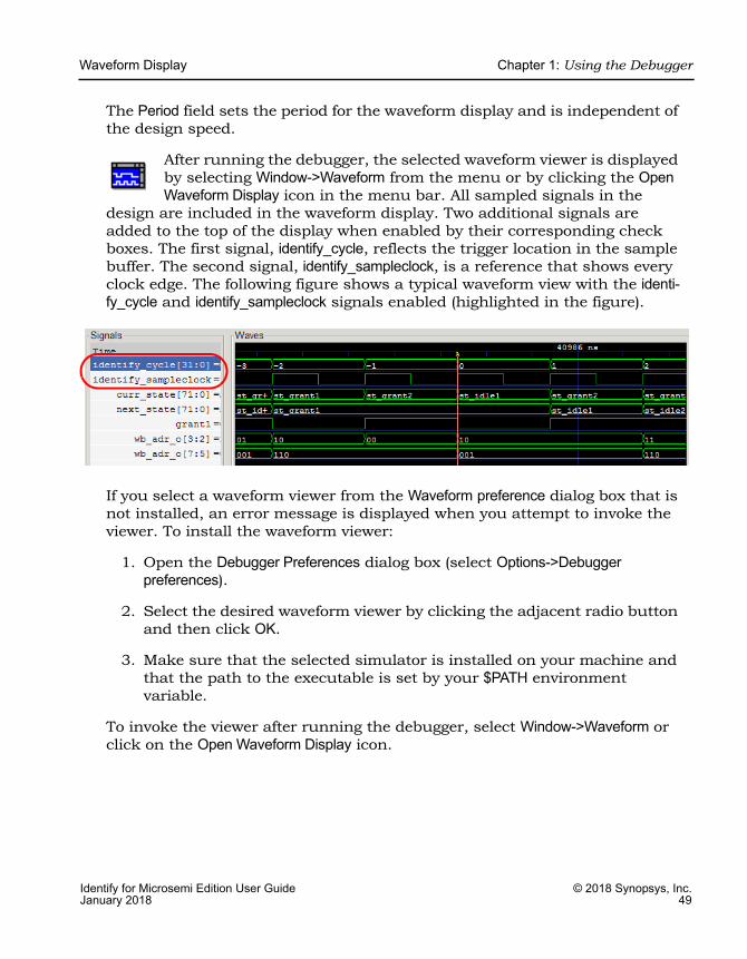
design are included in the waveform display. Two additional signals are added to the top of the display when enabled by their corresponding check boxes. The first signal, identify_cycle, reflects the trigger location in the sample buffer. The second signal, identify_sampleclock, is a reference that shows every clock edge. The following figure shows a typical waveform view with the identi-fy_cycle and identify_sampleclock signals enabled (highlighted in the figure).
If you select a waveform viewer from the Waveform preference dialog box that is not installed, an error message is displayed when you attempt to invoke the viewer. To install the waveform viewer:
1. Open the Debugger Preferences dialog box (select Options->Debugger preferences).
2. Select the desired waveform viewer by clicking the adjacent radio button and then click OK.
3. Make sure that the selected simulator is installed on your machine and that the path to the executable is set by your $PATH environment variable.
To invoke the viewer after running the debugger, select Window->Waveform or click on the Open Waveform Display icon.
LO
Chapter 1: Using the Debugger Waveform Display
© 2018 Synopsys, Inc. Identify for Microsemi Edition User Guide50 January 2018
Generating the Fast Signal DatabaseThe debugger is used to generate the fast signal database (FSDB) for the Verdi platform and for display by the Verdi nWave viewer. To generate this database:
1. Instrument the design with the essential signal list (see Instrumenting the Verdi Signal Database, on page 39 in the Identify Instrumentor User Guide).
2. Run the instrumented design in the synthesis tool and load the project into the debugger.
3. Use the Debugger Preferences dialog box and make sure that Synopsys Verdi nWave is selected as the default waveform viewer.
4. Setup the trigger conditions and click the Run button to download the sample buffer.
5. Generate the fast signal database using the following command syntax:
write fsdb -iice iiceID -showequiv fsdbFilename
6. Click the Open Waveform Display icon to view the samples in the nWave viewer.
The fast signal database file (fsdbFilename) can be imported directly back into the Verdi platform.
Logic Analyzer Interface Parameters Chapter 1: Using the Debugger
Identify for Microsemi Edition User Guide © 2018 Synopsys, Inc.January 2018 51
Logic Analyzer Interface ParametersThe logic analyzer interface parameters for the real-time debug feature in the debugger are defined on the tabs of the RTD type IICE information dialog box. To display this dialog box, click on the RTD (RTD type IICE Information/Settings) icon in the top menu. The remainder
of this section describes the individual logic analyzer tabs:
• Logic Analyzer Scan Tab, on page 51
• Logic Analyzer Properties Tab, on page 53
• Logic Analyzer Submit Tab, on page 53
• IICE Assignments Report Tab, on page 54
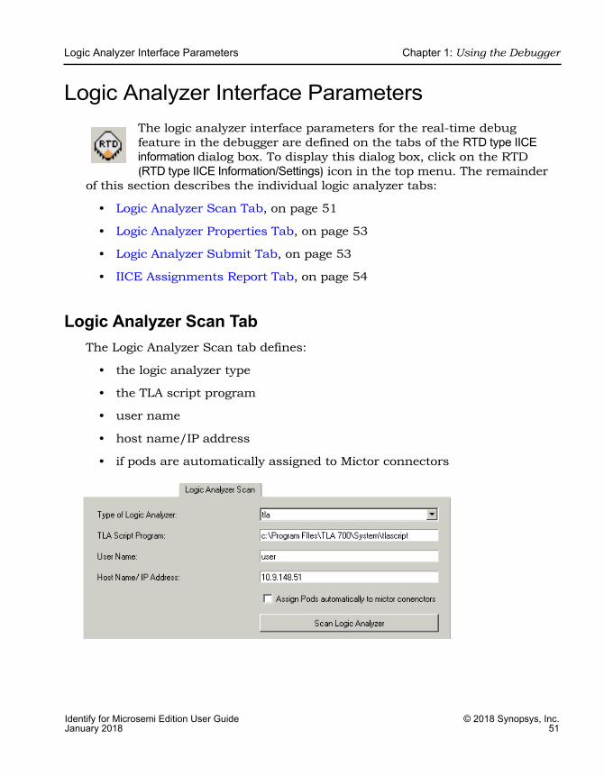
Logic Analyzer Scan TabThe Logic Analyzer Scan tab defines:
• the logic analyzer type
• the TLA script program
• user name
• host name/IP address
• if pods are automatically assigned to Mictor connectors

LO
Chapter 1: Using the Debugger Logic Analyzer Interface Parameters
© 2018 Synopsys, Inc. Identify for Microsemi Edition User Guide52 January 2018
Type of Logic AnalyzerSelects the type of logic analyzer from a drop-down menu. Current supported types are Agilent 16700 and 16900 series and Tektronix TLA series analyzers. The logic analyzer must be accessible on the local network.
TLA Script ProgramSpecifies the full path to the tlascript script file on the Tektronix logic analyzer. The default path is C:\Program Files\TLA 700\System\tlascript. If this location does not match the location expected by the Tektronix logic analyzer, change the location setting. The logic analyzer requires an rsh daemon to access the script file. To download and install the rsh daemon on the logic analyzer, see the web-site at http://rshd.sourceforge.net.
User NameIdentifies the user name on the analyzer (Tektronix only).
Host Name/IP AddressSpecifies the host name or IP address for the debugger host.
Assign Pods automatically to Mictor connectorsWhen checked, automatically assigns pods to the Mictor connectors.
Scan Logic Analyzer Clicking the Scan Logic Analyzer button scans the specified IP address and, if scanned successfully:
• opens a network connection with the given parameters
• retrieves the modules and pods information
• displays Logic Analyzer Properties and Logic Analyzer Submit tabs
Logic Analyzer Interface Parameters Chapter 1: Using the Debugger
Identify for Microsemi Edition User Guide © 2018 Synopsys, Inc.January 2018 53
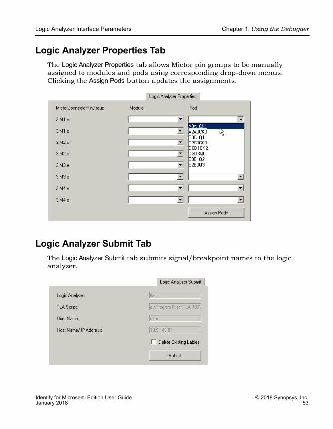
Logic Analyzer Properties TabThe Logic Analyzer Properties tab allows Mictor pin groups to be manually assigned to modules and pods using corresponding drop-down menus. Clicking the Assign Pods button updates the assignments.
Logic Analyzer Submit TabThe Logic Analyzer Submit tab submits signal/breakpoint names to the logic analyzer.
LO
Chapter 1: Using the Debugger Logic Analyzer Interface Parameters
© 2018 Synopsys, Inc. Identify for Microsemi Edition User Guide54 January 2018
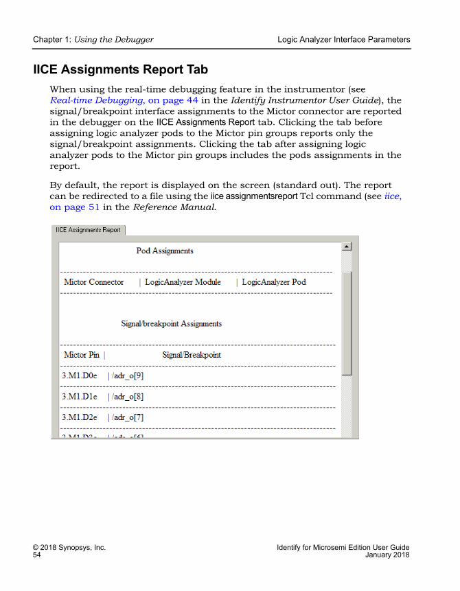
IICE Assignments Report TabWhen using the real-time debugging feature in the instrumentor (see Real-time Debugging, on page 44 in the Identify Instrumentor User Guide), the signal/breakpoint interface assignments to the Mictor connector are reported in the debugger on the IICE Assignments Report tab. Clicking the tab before assigning logic analyzer pods to the Mictor pin groups reports only the signal/breakpoint assignments. Clicking the tab after assigning logic analyzer pods to the Mictor pin groups includes the pods assignments in the report.
By default, the report is displayed on the screen (standard out). The report can be redirected to a file using the iice assignmentsreport Tcl command (see iice, on page 51 in the Reference Manual.
Identify for Microsemi Edition User Guide © 2018 Synopsys, Inc.January 2018 55
C H A P T E R 2
IICE Hardware Description
The instrumentor adds instrumentation logic to your HDL design that allows you to understand and debug design operation. There are some aspects of the instrumentation logic that are important to understand in order to use the debug environment tool set in the most effective way. In this chapter, the overall instrumentation logic is described briefly followed by descriptions of some of the more important features. A simplified functional breakdown of the instrumentation logic consists of:
• JTAG Communication Block
• Breakpoint and Watchpoint Blocks
• Sampling Block
• Complex Counter
• State Machine Triggering
JTAG Communication BlockThe JTAG communication block can be implemented using either the built-in device-specific TAP controller (the builtin option) or using the debug environment implementation of the TAP controller (the soft option). See Chapter 3, Connecting to the Target System, for more information on the JTAG controller.
LO
Chapter 2: IICE Hardware Description Breakpoint and Watchpoint Blocks
© 2018 Synopsys, Inc. Identify for Microsemi Edition User Guide56 January 2018
Breakpoint and Watchpoint BlocksThe following topics are described in this section:
• Breakpoints
• Watchpoints, on page 57
• Multiple Activated Breakpoints and Watchpoints, on page 57
BreakpointsBreakpoints are a way to easily create a trigger that is determined by the flow of control in the design.
In both Verilog and VHDL, the flow of control in a design is primarily determined by if, else, and case statements. The control state of these statements is determined by their controlling HDL conditional expressions. Breakpoints provide a simple way to trigger when the conditional expressions of one or more if, else, or case statements have particular values.
The example below shows a VHDL code fragment and its associated breakpoints.
99 process(op_code, cc, result) begin 100 case op_code is101 when "0100" =>102 result <= part_res;103 if cc = '1' then104 c_flag <= carry;105 if result = zero then106 z_flag <= '1';107 else108 z_flag <= '0';109 end if;110 end if;
Breakpoint and Watchpoint Blocks Chapter 2: IICE Hardware Description
Identify for Microsemi Edition User Guide © 2018 Synopsys, Inc.January 2018 57
The four breakpoints correspond to these control flow equations:
• Breakpoint at line number 102:
(op_code = "0100")
• Breakpoint at line number 104:
(op_code = "0100") and (cc = '1')
• Breakpoint at line number 106:
(op_code = "0100") and (cc = '1') and (result = zero)
• Breakpoint at line number 108:
(op_code = "0100") and (cc = '1') and (result != zero)
WatchpointsA watchpoint creates a trigger that is determined by the state of a signal in the design. The watchpoint can trigger either on the value of a signal or on a transition of a signal from one value to another.
Multiple Activated Breakpoints and WatchpointsHow breakpoints and watchpoints operate individually is described in the Instrumentor User Guide. Activated breakpoints and watchpoints also interact with each other in a very specific way.
Multiple Activated BreakpointsEach breakpoint is implemented as logic that watches for a particular event in the design. When an instrumented design has more than one activated breakpoint, the breakpoint events are ORed together. This effectively allows the breakpoints to operate independently – only one activated breakpoint must trigger in order to cause the sampling buffer to acquire its sample.
LO
Chapter 2: IICE Hardware Description Sampling Block
© 2018 Synopsys, Inc. Identify for Microsemi Edition User Guide58 January 2018
Multiple Activated WatchpointsEach watchpoint is implemented as logic that watches for a specific event consisting of a bit pattern or transition on a specific set of signals. When an instrumented design has more than one activated watchpoint, the watchpoint events are ANDed together. This effectively causes the watchpoints to be dependent on each other – all activated watchpoint events must occur concurrently to cause the sampling buffer to acquire its sample.
For example, if watchpoint 1 implements (count == 23) and watchpoint 2 implements (ack == ‘1’), then activating these watchpoints together effectively creates a new watchpoint: (count == 23) && (ack == ‘1’).
Combining Activated Breakpoints and Activated WatchpointsWhen an instrumented design has one or more activated breakpoints and one or more activated watchpoints, the result of the OR of the breakpoint events and the result of the AND of the watchpoint events is ANDed together. The result of this AND operation is called the Master Trigger Signal. This ANDing effectively causes the breakpoints and watchpoints to be dependent on each other – one activated breakpoint and all activated watchpoint events must occur concurrently to cause the sampling buffer to acquire its sample.
As a result, a Master Trigger Signal event can be constructed that operates like a conditional breakpoint. For example, activating a breakpoint and the two watchpoints from the previous example produces a conditional breakpoint: (breakpoint event) && (count== 23) && (ack == ‘1’).
Sampling BlockThe sampling block is basically a large memory used to store all the sampled signals. During an active debugging session, the sampled signals are contin-ually being stored in the sample block. When the sample block receives an event from the Master Trigger Signal event logic or the complex counter logic, the sampling block stops writing new data to the buffer and holds its contents. Eventually, the contents of the sample block are uploaded to the debugger for display and formatting.
Complex Counter Chapter 2: IICE Hardware Description
Identify for Microsemi Edition User Guide © 2018 Synopsys, Inc.January 2018 59
Whenever possible, the sample block should use the built-in RAM blocks that are available in most programmable chips. Otherwise, implementing the sample buffer using individual storage elements will consume large amounts of the logic capacity of the chip. If you have no choice but to use individual storage elements, analyze how much logic you have available on your chip and adjust how many signals you sample and the depth of the sample buffer.
Complex CounterThe complex counter connects the output of the breakpoint and watchpoint event logic to the sampling block and allows the user to implement complex triggering behavior.
Creating a Complex CounterThe counter is created, configured, and inserted into the HDL design during instrumentation using the instrumentor IICE Controller tab of the IICE Configura-tion dialog box or using the instrumentor iice controller command.
During configuration, the size of the counter is specified. For example, a 16-bit counter is the default. This default value produces a counter that ranges from 0 to 65535.
Setting the counter size to zero during instrumentation configuration disables counter insertion.
LO
Chapter 2: IICE Hardware Description Complex Counter
© 2018 Synopsys, Inc. Identify for Microsemi Edition User Guide60 January 2018
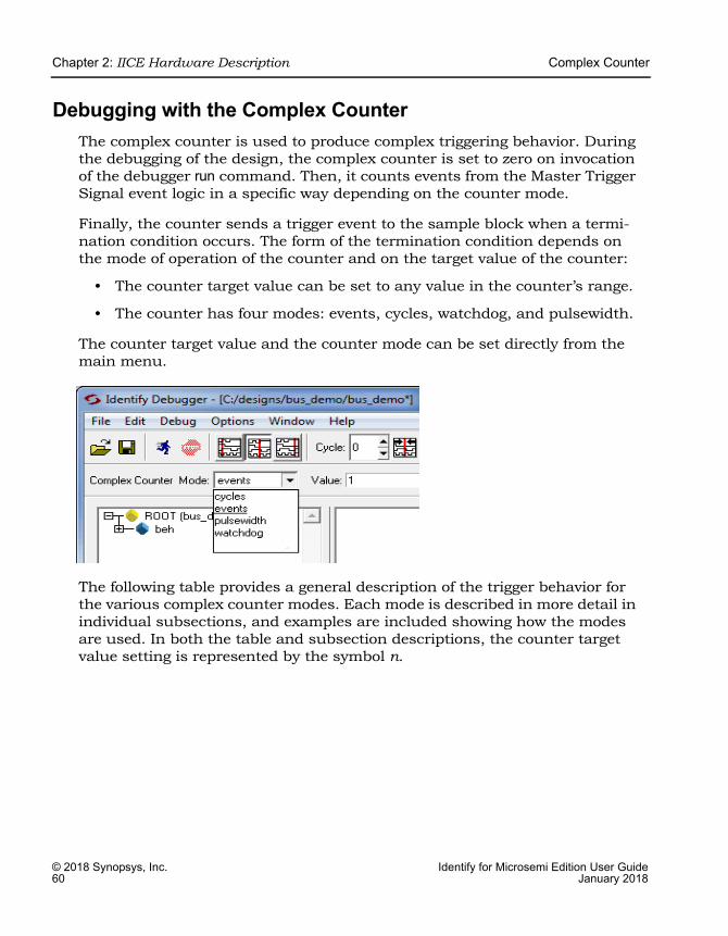
Debugging with the Complex CounterThe complex counter is used to produce complex triggering behavior. During the debugging of the design, the complex counter is set to zero on invocation of the debugger run command. Then, it counts events from the Master Trigger Signal event logic in a specific way depending on the counter mode.
Finally, the counter sends a trigger event to the sample block when a termi-nation condition occurs. The form of the termination condition depends on the mode of operation of the counter and on the target value of the counter:
• The counter target value can be set to any value in the counter’s range.
• The counter has four modes: events, cycles, watchdog, and pulsewidth.
The counter target value and the counter mode can be set directly from the main menu.
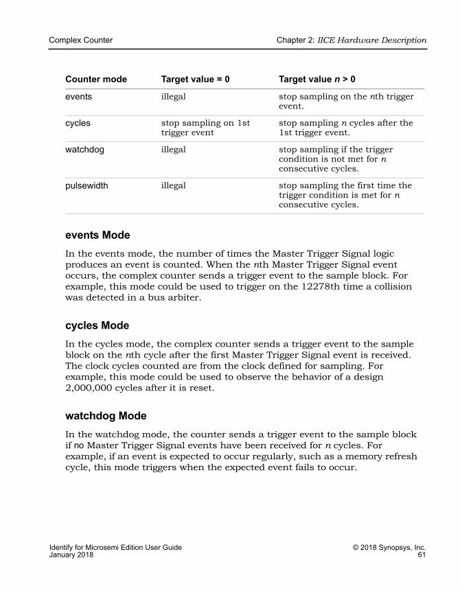
The following table provides a general description of the trigger behavior for the various complex counter modes. Each mode is described in more detail in individual subsections, and examples are included showing how the modes are used. In both the table and subsection descriptions, the counter target value setting is represented by the symbol n.
Complex Counter Chapter 2: IICE Hardware Description
Identify for Microsemi Edition User Guide © 2018 Synopsys, Inc.January 2018 61
events ModeIn the events mode, the number of times the Master Trigger Signal logic produces an event is counted. When the nth Master Trigger Signal event occurs, the complex counter sends a trigger event to the sample block. For example, this mode could be used to trigger on the 12278th time a collision was detected in a bus arbiter.
cycles ModeIn the cycles mode, the complex counter sends a trigger event to the sample block on the nth cycle after the first Master Trigger Signal event is received. The clock cycles counted are from the clock defined for sampling. For example, this mode could be used to observe the behavior of a design 2,000,000 cycles after it is reset.
watchdog ModeIn the watchdog mode, the counter sends a trigger event to the sample block if no Master Trigger Signal events have been received for n cycles. For example, if an event is expected to occur regularly, such as a memory refresh cycle, this mode triggers when the expected event fails to occur.
Counter mode Target value = 0 Target value n > 0
events illegal stop sampling on the nth trigger event.
cycles stop sampling on 1st trigger event
stop sampling n cycles after the 1st trigger event.
watchdog illegal stop sampling if the trigger condition is not met for n consecutive cycles.
pulsewidth illegal stop sampling the first time the trigger condition is met for n consecutive cycles.
LO
Chapter 2: IICE Hardware Description Complex Counter
© 2018 Synopsys, Inc. Identify for Microsemi Edition User Guide62 January 2018
pulsewidth ModeIn the pulsewidth mode, the complex counter sends a trigger event to the sample block if the Master Trigger Signal logic has produced an event during each of the most recent n consecutive cycles. For example, this mode can be used to detect when a request signal is held high for more than n cycles thereby detecting when the request has not been serviced within a specified interval.
Disabling the CounterAccording to the previous table, the counter can be disabled simply by setting its target value to 1 and its mode to events. Then, the complex counter will pass any received event from the Master Trigger Signal logic on to the sample block with no additional delay.
State Machine Triggering Chapter 2: IICE Hardware Description
Identify for Microsemi Edition User Guide © 2018 Synopsys, Inc.January 2018 63
State Machine TriggeringThis section describes the different methods of triggering available in the debugger. It explains the different choices available during instrumentation and the functionality these choices provide in the debugger as well as discussing the cost effects of the various types of instrumentation.
Simple or Advanced TriggeringThere are two triggering modes available, the simple mode and the advanced mode. The simple mode allows comparing signals to values (including don’t cares) and then triggering when the signals match those values. This scheme can be enhanced by using breakpoints to denote branches in control logic. If a breakpoint is enabled, this particular branch must be active at the same time that the signals match their respective values. The overall trigger logic involves signals and breakpoints in the following way:
• Signals: All signals must match their respective comparison values in order to trigger.
• Breakpoints: All breakpoints are OR connected, meaning that any one enabled breakpoint is enough to trigger.
• Signals and breakpoints are combined using AND, such that all signals must match their values AND at least one enabled breakpoint must occur.
The logic that implements breakpoint and signal triggering is referred to as trigger condition in the following text.
In the advanced trigger mode, multiple such trigger conditions are instru-mented, and a runtime-programmable state machine is also instrumented to allow you to specify the temporal and logical behavior that combines these trigger conditions into a complex trigger function. For instance, this state machine enables you to trigger on a certain sequence of events like “trigger if pattern A occurs exactly five cycles after pattern B, but only if pattern C does not intervene.”
By default, the instrumentor instruments the design according to the simple trigger mode. See the following for more information on how to select the advanced trigger mode.

LO
Chapter 2: IICE Hardware Description State Machine Triggering
© 2018 Synopsys, Inc. Identify for Microsemi Edition User Guide64 January 2018
Advanced Triggering ModeSetting up an instrumented design to enable advanced triggering is extremely easy. There are two iice controller command options available in the instrumentor that control the extent and cost of the instrumentation:
• -triggerconditions integer – The integer argument to this option defines how many trigger conditions are created. The range is from 1 to 16. All these trigger conditions are identical in terms of signals and breakpoints connected to them, but they can be programmed separately in the debugger.
• -triggerstates integer – The integer argument to this option defines how many states the trigger state machine will have. The range is 2 to 16; powers of 2 are preferable as other numbers limit functionality and do not provide any cost savings.
Similar to the simple-triggering mode, a counter can be instrumented to augment the functionality of the state machine. To instrument a counter, enter an iice controller -counterwidth option with an argument greater than 0 in the instrumentor console window.
Please refer to the following text to determine cost and consequences of these settings in the instrumentor.
Structural Implementation of State Machine TriggeringFor each trigger condition ci, a logic cone is implemented which evaluates the signals and the breakpoints connected to the trigger logic and culminates in a 1-bit result identical to the trigger condition in simple mode. All these 1-bit results are connected to the address inputs of a RAM table.
If a counter has been added to the instrumentation, the counter output is compared to constant 0, and the single-bit output of that comparison is also connected to the address inputs of the same RAM table.
The other address inputs are provided by the state register. The outputs of the RAM table are:
• the next-state value nstate
• the trigger signal trigger (causes the sample buffer to take a snapshot if high)
• the counter-enable signal cnten (if ‘1’, counter is decremented by 1)
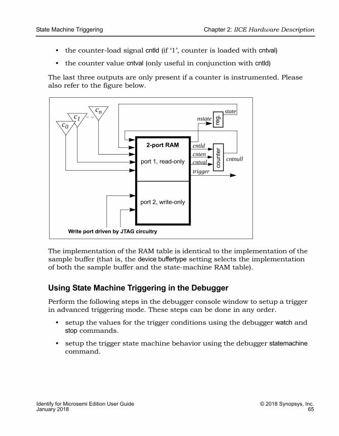
State Machine Triggering Chapter 2: IICE Hardware Description
Identify for Microsemi Edition User Guide © 2018 Synopsys, Inc.January 2018 65
• the counter-load signal cntld (if ‘1’, counter is loaded with cntval)
• the counter value cntval (only useful in conjunction with cntld)
The last three outputs are only present if a counter is instrumented. Please also refer to the figure below.
The implementation of the RAM table is identical to the implementation of the sample buffer (that is, the device buffertype setting selects the implementation of both the sample buffer and the state-machine RAM table).
Using State Machine Triggering in the DebuggerPerform the following steps in the debugger console window to setup a trigger in advanced triggering mode. These steps can be done in any order.
• setup the values for the trigger conditions using the debugger watch and stop commands.
• setup the trigger state machine behavior using the debugger statemachine command.
trigger
cntldcntencntval
nstatestate
cntnull
2-port RAM
port 1, read-only
port 2, write-only
coun
ter
reg.
Write port driven by JTAG circuitry
c1cn
c0

LO
Chapter 2: IICE Hardware Description State Machine Triggering
© 2018 Synopsys, Inc. Identify for Microsemi Edition User Guide66 January 2018
The watch command takes an additional parameter, -condition, specifying the trigger conditions that the given condition is intended for. This argument is available in simple mode as well, but as there is only one trigger condition in this case, the argument is redundant.
• watch enable -condition (triggerCondition|all) signalName value1 [value2 ...]
• watch disable -condition (triggerCondition|all) signalName
• watch info [-raw] signalName
The parameter triggerCondition is a list value conforming to the Tcl language. Examples are: 1, "1 2 3", {2 3}, or [list 1 2 3], quotes, braces, and brackets included, respectively. Alternatively, the keyword all can be specified to apply the setting to all trigger conditions.
The debugger watch info command reports status information about the signal. This information is returned in machine-processible form if the optional parameter -raw is specified.
Similarly for the debugger stop command:
• stop enable -condition (triggerCondition |all) breakpoint
• stop disable -condition (triggerCondition |all) breakpoint
• stop info [-raw] breakpoint
The semantics of the parameters are identical to the above descriptions.
The statemachine CommandDuring instrumentation, the number of states was previously defined using the -triggerstates option of the instrumentor iice controller command. Now, at debug time, you can define what happens in each state and transition depending on the pattern matches computed by the trigger conditions.
The debugger statemachine command is used to configure the trigger state machine with the desired behavior. This is very similar to the “advanced” trigger mode offered by many logic analyzers. As it is very easy to introduce errors in the process of specifying the state machine, special caution is appropriate. Also, a state-machine editor is available in the debugger user interface to facilitate state-machine development and understanding (see State-Machine Editor, on page 74). It is also important to note that the initial state for each run is always state 0 and that not all of the available states need to be defined.
State Machine Triggering Chapter 2: IICE Hardware Description
Identify for Microsemi Edition User Guide © 2018 Synopsys, Inc.January 2018 67
The syntax forms of the debugger statemachine command are:
• statemachine addtrans -from state [-to state] [-cond "equation|titriggerInID"][-cntval integer] [-cnten] [-trigger]
• statemachine clear (-all|state [state ...])
• statemachine info [-raw] (-all|state [state ...])
Subcommand statemachine addtransThe debugger addtrans subcommand defines the transitions between the states. The options are as follows:
• -from state – specifies the state this transition is exiting from.
• -to state – specifies the state this transition goes to. If this is not given, it defaults to the state given in the -from option.
• -cond "equation|titriggerInID" – specifies the condition or external trigger input under which the transition is to be taken. The default is “true” (i.e., the transition is taken regardless of input data; see below for more details).
• -cntval integer – specifies that if this transition is taken, the counter is loaded with the given value. Only valid when a counter is instrumented.
• -cnten – when this flag is given, the counter is decremented by 1 during this transition. Only valid when a counter is instrumented.
• -trigger – when this flag is given, a trigger occurs during this transition.
The order in which the transitions are added is important. In each state, the first transition condition that matches the current data is taken and any subsequent transitions in the list that match the current data are ignored.
ConditionsThe conditions are specified using Boolean expressions comprised of variables and operators. The available variables are:
• c0,... cn, where n is the number of trigger conditions instrumented. These variables represent the output bit of the respective trigger condi-tion.
• titriggerInID – the ID (0 thru 7) of an external trigger input.
LO
Chapter 2: IICE Hardware Description State Machine Triggering
© 2018 Synopsys, Inc. Identify for Microsemi Edition User Guide68 January 2018
• cntnull – true whenever the counter is equal to 0 (only available when a counter is instrumented).
• iiceID – variable used with cross triggering to define the source IICE units to be included in the equation for the destination IICE trigger.
Operators are:
• Negation: not, !, ~
• AND operators: and, &&, &
• OR operators: or, ||, |
• XOR operators: xor, ^
• NOR operators: nor, ~|
• NAND operators: nand, ~&
• XNOR operators: xnor, ~^
• Equivalence operators: ==, =
• Constants: 0, false, OFF, 1, true, ON
Parentheses ‘(‘, ‘)’ are recommended whenever the operator precedence is in question. Use the debugger statemachine info command to verify the conditions specified.
For example, valid expression examples are:
"c0 and c1" "!(c1 or c2) and c3""c0 or ti4" (condition c0 or external trigger ID ti4)
Other SubcommandsThe debugger statemachine clear command deletes all transitions from the states given in the argument, or from all states if the argument -all is speci-fied.
The debugger statemachine info command prints the current state machine settings for the states given in the argument, or for the entire state machine, if the option -all is specified. If the option -raw is given, the information is returned in a machine-processible form.

State Machine Triggering Chapter 2: IICE Hardware Description
Identify for Microsemi Edition User Guide © 2018 Synopsys, Inc.January 2018 69
State Machine ExamplesTo implement a trigger behavior that triggers when the pattern on condition 1 or condition 2 (c1 or c2) becomes true for the 10th time (a setting identical to counter mode events in the simple mode triggering), the following state machine can be used:
statemachine addtrans -from 0 -to 1 -cntval 9statemachine addtrans -from 1 -cond "(c1 | c2) & cntnull" -triggerstatemachine addtrans -from 1 -cond "c1 or c2" -cnten
A trigger condition requiring pattern c2 to occur 10 times after pattern c1 has occurred, without pattern c3 occurring in between (commonly available in logic analyzers as “Pattern 1 followed by Pattern 2 before Pattern 3”) can be achieved with the following state machine:
statemachine addtrans -from 0 -to 1 -cond c1 -cntval 9statemachine addtrans -from 1 -cond "c2 & cntnull" -triggerstatemachine addtrans -from 1 -to 0 -cond c3statemachine addtrans -from 1 -cond "c2" -cnten
These behaviors can be cascaded by moving on to the next behavior instead of triggering in the transition that has -trigger specified, as long as there are trigger conditions and states available.
LO
Chapter 2: IICE Hardware Description State Machine Triggering
© 2018 Synopsys, Inc. Identify for Microsemi Edition User Guide70 January 2018
Convenience FunctionsThere are a number of convenience functions to set up complex triggers avail-able in the file InstallDir/share/contrib/syn_trigger_utils.tcl which is loaded into the debugger at startup:
• st_events condition integer – Sets up the state machine to mimic counter mode events of the simple triggering mode as described above. The argument condition is a boolean equation setting up the condition, and integer is the counter value.
• st_watchdog condition integer – Same as st_events for watchdog mode.
• st_cycles condition integer – Same as above for cycles mode.
• st_pulsewidth condition integer – Same as above for pulsewidth mode.
• st_B_after_A conditionA conditionB [integer:=1] – Sets up a trigger mode to trigger if conditionB becomes true anytime after conditionA became true. The optional integer argument defaults to 1 and denotes how many times conditionB must become true in order to trigger.
• st_B_after_A_before_C conditionA conditionB conditionC [integer:=1] – Sets up a trigger mode to trigger if conditionB becomes true after conditionA becomes true, but without an intervening conditionC becoming true (same as the second example above). The optional integer argument defaults to 1 and denotes how many times conditionB must become true without seeing conditionC in order to trigger.
• st_snapshot_fill condition [integer] – Uses qualified sampling to sample data until sample buffer is full. The argument condition is a boolean equation defining the trigger condition, and integer is the number of samples to take with each occurrence of the trigger (default 1).
• st_snapshot_intr condition [integer] – Uses qualified sampling to sample data until manually interrupted by an debugger stop command. The argument condition is a boolean equation defining the trigger condition and integer is the number of samples to take with each occurrence of the trigger (default 1).
Please refer to the file syn_trigger_utils.tcl mentioned above for the implementa-tion of these trigger modes using the debugger statemachine command. Users can add their own convenience functions by following the examples in this file.
State Machine Triggering Chapter 2: IICE Hardware Description
Identify for Microsemi Edition User Guide © 2018 Synopsys, Inc.January 2018 71
Cross Triggering with State MachinesCross triggering allows a specific IICE unit to be triggered by one or more IICE units in combination with its own internal trigger conditions. The IICE being triggered is referred to as the “destination” IICE; the other IICE units are referred to as the “source” IICE units.
Multiple IICE designs allow triggering and sampling of signals from different clock domains. With an asynchronous design, a separate IICE unit can be assigned to each clock domain, triggers can be set on signals within each IICE unit, and then the IICE units scheduled to trigger each other on a user-defined sequence using cross triggering. In this configuration, each IICE unit is independent and can have unique IICE parameter settings including sample depth, sample/trigger options, and sample clock and clock edges.
Cross triggering is supported in all three IICE controller configurations (simple, complex counter, and state-machine triggering) and all three configurations make use of state machines.
Cross triggering is enabled in the instrumentor (cross triggering can be selectively disabled in the debugger). To enable a destination IICE unit to accept a trigger from a source IICE unit, enter the following command in the instrumentor console window (by default, cross triggering is disabled):
iice controller -crosstrigger 1
For cross triggering to function correctly, the destination and the contributing source IICE units must be instrumented by selecting breakpoints and watchpoints. Concurrently run these units either by selecting the individual IICE units and clicking the RUN button in the debugger project view or by entering one of the following commands in the debugger console window:
run -iice all
run -iice {iiceID1 iiceID2 ... iiceIDn}
LO
Chapter 2: IICE Hardware Description State Machine Triggering
© 2018 Synopsys, Inc. Identify for Microsemi Edition User Guide72 January 2018
When simple- or complex-counter triggering is selected in the destination IICE controller, the following debugger cross-trigger commands are available:
• The following debugger command causes the destination IICE to trigger normally (the triggers from source IICE units are ignored).
iice controller -crosstriggermode DISABLED
• The following debugger command causes the destination IICE to trigger when any source IICE triggers or on its own internal trigger.
iice controller -crosstriggermode ANY
• The following debugger command causes the destination IICE to trigger when all source IICE units and the destination IICE unit have triggered in any order.
iice controller -crosstriggermode ALL
• The following debugger commands cause the destination IICE to trigger after the source IICE unit triggers coincident with the next destination IICE internal trigger.
iice controller -crosstriggermode after -crosstriggeriice iiceIDiice controller -crosstriggermode after -crosstriggeriice all
The first debugger command uses a single source IICE unit (iiceID), and the second debugger command requires all source IICE units to trigger.
When state-machine triggering is selected, the state machine must be speci-fied with at least three states (three states are required for certain triggering conditions, for example, when the destination IICE is in Cycles mode and you want to configure the destination IICE to trigger after another (source) IICE.
State Machine Triggering Chapter 2: IICE Hardware Description
Identify for Microsemi Edition User Guide © 2018 Synopsys, Inc.January 2018 73
With state-machine triggering, the following debugger statemachine command sequences are available in the debugger console window:
• The following debugger command sequence is equivalent to disabling cross triggering. The destination IICE triggers on its own internal trigger condition (c0).
statemachine clear -allstatemachine addtrans -from 0 -cond "c0" -trigger
• In the following debugger command sequence, the destination IICE waits for iiceID to trigger and then triggers on its own internal trigger condition (c0). This sequence implements the “after iiceID” functionality of the simple- and complex-counter triggering modes.
statemachine clear -allstatemachine addtrans -from 0 -to 1 -cond "iiceID"statemachine addtrans -from 1 -to 0 -cond "c0" -trigger
• In the following debugger command sequence, the destination IICE triggers when the last running IICE triggers.
statemachine clear -allstatemachine addtrans -from 0 -cond "c0 and iiceID and iiceID1
and iiceID2" -triggerstatemachine addtrans -from 0 -to 1 -cond "c0"statemachine addtrans -from 1 -to 0 -cond "iiceID and iiceID1
and iiceID2" -trigger
• In the following debugger command sequence, the destination IICE waits for all the other running source IICE units to trigger and then triggers on its own internal trigger condition (c0).
statemachine clear -allstatemachine addtrans -from 0 -to 1 -cond "iiceID and iiceID1
and iiceID2"statemachine addtrans -from 1 -cond "c0" -trigger"
The incorporation of a counter in the state-machine configuration is similar to the use of a counter in non-cross trigger mode for a state machine.

LO
Chapter 2: IICE Hardware Description State Machine Triggering
© 2018 Synopsys, Inc. Identify for Microsemi Edition User Guide74 January 2018
State-Machine EditorThe debugger includes a graphical state-machine editor that is available when state-machine triggering is enabled for the active IICE unit on the IICE Controller tab in the instrumentor.
To bring up the state-machine editor in the debugger, click the Configure Statemachine Trigger icon in the debugger toolbar. Note that the icon will be grayed out if state-machine triggering was not enabled in
the instrumentor when the design was instrumented and that an error message will be generated if more than 10 states are defined. Clicking the icon displays the Statemachine Editor dialog box for the selected IICE.
Each state is defined in an individual entry field. Within each entry, you can add multiple definitions for transitioning from that state. Each transition includes either one or two actions and a condition. The actions and condi-tions are defined in the following tables.

State Machine Triggering Chapter 2: IICE Hardware Description
Identify for Microsemi Edition User Guide © 2018 Synopsys, Inc.January 2018 75
To use the dialog box:
• As an optional starting point, use Insert Macro to select predefined state-machine behaviors from the drop-down list. When a macro is selected, a corresponding Configure Statemachine Macro dialog box is displayed to set the parameters for the macro. The following figure shows the dialog box for the st_B_after_A macro.
Action Description
Decrement Counter Decrements counter when condition is true (mutually exclusive with Initialize Counter)
Initialize Counter Initializes counter to count specified by statemachine transition editor (mutually exclusive with Decrement Counter)
Trigger Sample Buf-fer
Triggers sample buffer when condition is true
Go to State Transitions to specified state when condition is true
Condition Description
c0 ... cN References trigger event in active IICE unit
cntnull True when counter is equal to 0 (available only when counter is instrumented)
iiceID References trigger event from a second IICE unit for cross triggering (cross triggering must have been enabled when the design was instrumented)
titriggerInID References external trigger originating from an IICE module in another FPGA or on-board external logic
Boolean Boolean operators used to define state-machine events (see Conditions, on page 67)
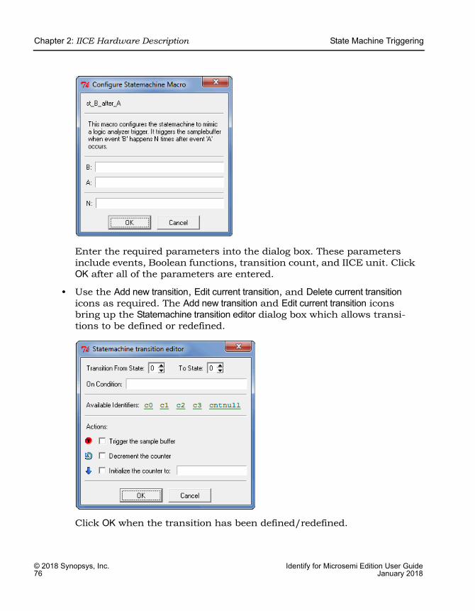
LO
Chapter 2: IICE Hardware Description State Machine Triggering
© 2018 Synopsys, Inc. Identify for Microsemi Edition User Guide76 January 2018
Enter the required parameters into the dialog box. These parameters include events, Boolean functions, transition count, and IICE unit. Click OK after all of the parameters are entered.
• Use the Add new transition, Edit current transition, and Delete current transition icons as required. The Add new transition and Edit current transition icons bring up the Statemachine transition editor dialog box which allows transi-tions to be defined or redefined.
Click OK when the transition has been defined/redefined.

State Machine Triggering Chapter 2: IICE Hardware Description
Identify for Microsemi Edition User Guide © 2018 Synopsys, Inc.January 2018 77
• Click OK in the initial Statemachine Editor dialog box when the state-machine triggering condition has been defined.
Note that you can view the corresponding state-machine commands in the debugger console window using the statemachine info -all command.
State-Machine ExamplesThe state-machine triggering feature allows the creation of counter-based state machines from sequences of trigger conditions to create very effective triggers. You can set up a state-machine trigger during instrumentation and then program the state machine dynamically during debug to create a complex, design-specific trigger.
Building a Complex State-machine TriggerWhen building a complex, state-machine trigger, you specify the number of trigger states, the trigger conditions (which can be set dynamically in the debugger), and the counter width. A common design configuration is to trigger when a specific sequence of events occurs which, in turn, causes data collection to stop and the sample data to be downloaded by the corresponding debugger executable from the FPGA. You can enable state-machine triggering and specify the states through the user interface as outlined in the following steps:
1. Make sure that the following prerequisites are done:
– In the instrumentor graphical user interface, select Actions->Configure IICE from the top menu bar or click the IICE icon.
– From the instrumentor Configure IICE dialog box, select the IICE Controller tab, click the State Machine triggering radio button, and specify the number of trigger states, trigger conditions, and the counter width in the corresponding fields.
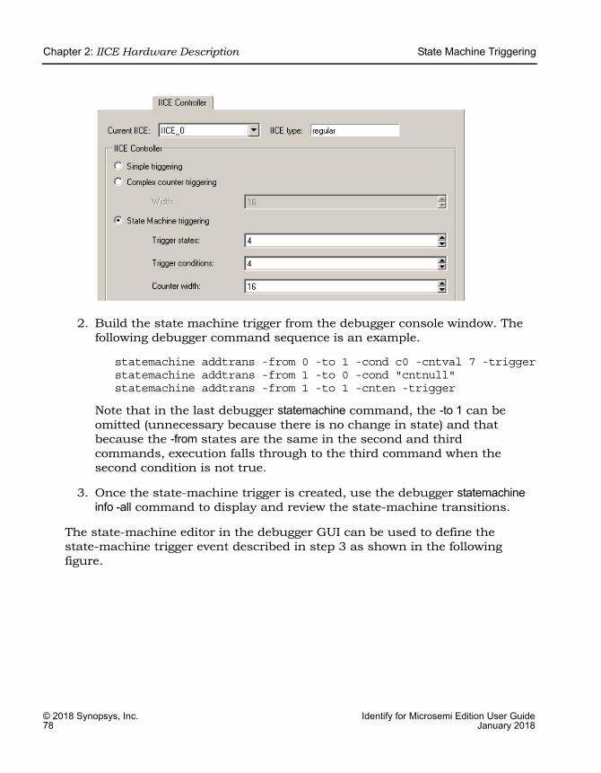
LO
Chapter 2: IICE Hardware Description State Machine Triggering
© 2018 Synopsys, Inc. Identify for Microsemi Edition User Guide78 January 2018
2. Build the state machine trigger from the debugger console window. The following debugger command sequence is an example.
statemachine addtrans -from 0 -to 1 -cond c0 -cntval 7 -triggerstatemachine addtrans -from 1 -to 0 -cond "cntnull"statemachine addtrans -from 1 -to 1 -cnten -trigger
Note that in the last debugger statemachine command, the -to 1 can be omitted (unnecessary because there is no change in state) and that because the -from states are the same in the second and third commands, execution falls through to the third command when the second condition is not true.
3. Once the state-machine trigger is created, use the debugger statemachine info -all command to display and review the state-machine transitions.
The state-machine editor in the debugger GUI can be used to define the state-machine trigger event described in step 3 as shown in the following figure.
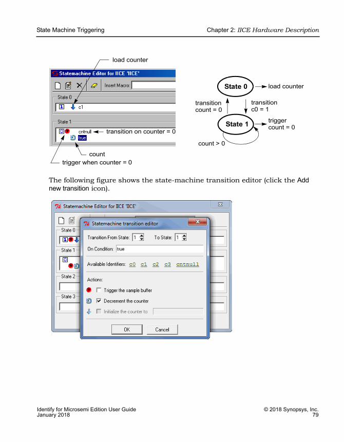
State Machine Triggering Chapter 2: IICE Hardware Description
Identify for Microsemi Edition User Guide © 2018 Synopsys, Inc.January 2018 79
The following figure shows the state-machine transition editor (click the Add new transition icon).
load counter
trigger when counter = 0count
transition on counter = 0
transitioncount = 0
count > 0
transitionc0 = 1
load counter
trigger count = 0
State 0
State 1
LO
Chapter 2: IICE Hardware Description State Machine Triggering
© 2018 Synopsys, Inc. Identify for Microsemi Edition User Guide80 January 2018
The debugger state-machine and state-machine transition editors allow:
• Graphical entry of state machines
• Editing of state transitions and trigger events
• Conditions to be combined with each other or with a counter
• Counter mode selection of up, down, or initialized to any value
State-machine Triggering with Tcl CommandsThe IICE can be configured using TCL commands entered from both the instrumentor and debugger console windows. Some of the example commands are as follows:
• To delete the state transitions from each IICE, use the following debugger command:
statemachine clear -iice all
• To enable complex counter triggering, use the following instrumentor command:
iice controller complex
• To set the counter width, use the following instrumentor command:
iice controller -counterwidth 8
• To configure an IICE for state-machine triggering, use the following instrumentor command sequence:
iice controller -iice IICE statemachine iice controller -iice IICE -counterwidth 4 iice controller -iice IICE -triggerconditions 2 iice controller -iice IICE -triggerstates 2
In addition to state-machine triggering, the above instrumentor commands set the number of trigger conditions to 2 and the number of trigger states to 2.
• To enable cross triggering, use the following instrumentor command:
iice controller -crosstrigger 1

State Machine Triggering Chapter 2: IICE Hardware Description
Identify for Microsemi Edition User Guide © 2018 Synopsys, Inc.January 2018 81
• Similarly, to configure the sample depth, use the following instrumentor command:
iice sampler -depth 2048
Note that the only option for buffer type is internal_memory.
Qualified SamplingDuring qualified sampling, a single sample of all sampled signals is collected each time the trigger condition is true. When a trigger condition occurs, instead of filling the entire buffer, the IICE collects the single sample and then waits for the next trigger to acquire the next sample. The following example uses qualified sampling to examine the data for a given number of clock cycles. To create a complex trigger event to perform qualified sampling:
1. As a prerequisite in the instrumentor GUI:
– From the Configure IICE dialog box, select the IICE Controller tab, click the State Machine triggering radio button, and enter a value in the Counter width field to define the width of the sample buffer.
– Select the IICE Sampler tab and enable the Allow qualified sampling check box.
2. From the debugger GUI, select qualified_fill or qualified_int from the Sample Mode drop-down menu. For more information, see -qualified_sampling 0|1, on page 59.
3. From the debugger GUI, click on the adjacent Configure Statemachine Trigger icon and define the state-machine trigger event.
4. From the debugger GUI, select the st_snapshot_fill macro from the Insert Macro drop-down menu.
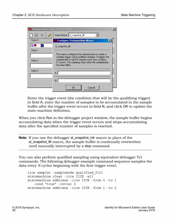
LO
Chapter 2: IICE Hardware Description State Machine Triggering
© 2018 Synopsys, Inc. Identify for Microsemi Edition User Guide82 January 2018
Enter the trigger event (the condition that will be the qualifying trigger) in field A, enter the number of samples to be accumulated in the sample buffer after the trigger event occurs in field N, and click OK to update the state-machine definition.
When you click Run in the debugger project window, the sample buffer begins accumulating data when the trigger event occurs and stops accumulating data after the specified number of samples is reached.
Note: If you use the debugger st_snapshot_intr macro in place of the st_snapshot_fill macro, the sample buffer is continually overwritten until manually interrupted by a stop command.
You can also perform qualified sampling using equivalent debugger Tcl commands. The following debugger example command sequence samples the data every N cycles beginning with the first trigger event.
iice sampler -samplemode qualified_fillstatemachine clear -iice IICE -allstatemachine addtrans -iice IICE -from 0 -to 1
-cond "true" -cntval 0statemachine addtrans -iice IICE -from 1 -to 2
State Machine Triggering Chapter 2: IICE Hardware Description
Identify for Microsemi Edition User Guide © 2018 Synopsys, Inc.January 2018 83
-cond "c0" -cntval 15 -triggerstatemachine addtrans -iice IICE -from 2 -to 2
-cond "! cntnull" -cntenstatemachine addtrans -iice IICE -from 2 -to 2
-cond "cntnull" -cntval 15 -trigger
Remote TriggeringRemote triggering allows one debugger executable to send a software trigger event to terminate data collection in the other debugger executables, effec-tively creating a remote stop button.
You can selectively set the remote trigger to:
• trigger all IICEs in all debugger executables
• trigger all IICEs in a specific debugger executable
• trigger a specific IICE in a specific debugger executable
A common design configuration is to trigger all FPGAs on a single board-level event; when that event occurs, data collection is stopped and the sample data is downloaded by the corresponding debugger executables for all FPGAs.
Remote triggering is a scripting application. The IICE/debugger targets are defined by the debugger remote_trigger command (see the command descrip-tion in the Reference Manual).
As an example, the debugger scripting sequence
run ; remote_trigger -pid 12
waits for the trigger condition in the active IICE and then sends a trigger to all IICE units in the debugger executable identified by process ID 12.
Importing External TriggersAn import external trigger capability can be used with trigger signals origi-nating from on-board logic external to the FPGA or from an IICE module in a second FPGA.

LO
Chapter 2: IICE Hardware Description State Machine Triggering
© 2018 Synopsys, Inc. Identify for Microsemi Edition User Guide84 January 2018
Identify for Microsemi Edition User Guide © 2018 Synopsys, Inc.January 2018 85
C H A P T E R 3
Connecting to the Target System
This chapter describes methods to connect the debugger to the target hardware system. The programmable device in the target system that contains the design to be debugged are usually placed on a printed circuit board along with a number of other support devices. The difficulty is that the boards differ greatly in the connections between their programmable devices, the other components, and the external connections of the boards.
This chapter outlines how to connect the debugger to most of the common board configurations and addresses the following topics:
• Basic Communication Connection, on page 86
• UMRBus Communications Interface, on page 98
• JTAG Communication Interface, on page 101
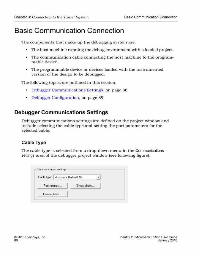
LO
Chapter 3: Connecting to the Target System Basic Communication Connection
© 2018 Synopsys, Inc. Identify for Microsemi Edition User Guide86 January 2018
Basic Communication ConnectionThe components that make up the debugging system are:
• The host machine running the debug environment with a loaded project.
• The communication cable connecting the host machine to the program-mable device.
• The programmable device or devices loaded with the instrumented version of the design to be debugged.
The following topics are outlined in this section:
• Debugger Communications Settings, on page 86
• Debugger Configuration, on page 89
Debugger Communications SettingsDebugger communications settings are defined on the project window and include selecting the cable type and setting the port parameters for the selected cable.
Cable TypeThe cable type is selected from a drop-down menu in the Communications settings area of the debugger project window (see following figure).
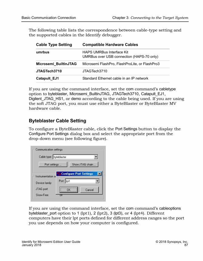
Basic Communication Connection Chapter 3: Connecting to the Target System
Identify for Microsemi Edition User Guide © 2018 Synopsys, Inc.January 2018 87
The following table lists the correspondence between cable-type setting and the supported cables in the Identify debugger.
If you are using the command interface, set the com command’s cabletype option to byteblaster, Microsemi_BuiltinJTAG, JTAGTech3710, Catapult_EJ1, Digilent_JTAG_HS1, or demo according to the cable being used. If you are using the soft JTAG port, you must use either a ByteBlaster or ByteBlaster MV hardware cable.
Byteblaster Cable Setting To configure a ByteBlaster cable, click the Port Settings button to display the Configure Port Settings dialog box and select the appropriate port from the drop-down menu (see following figure).
If you are using the command interface, set the com command’s cableoptions byteblaster_port option to 1 (lpt1), 2 (lpt2), 3 (lpt3), or 4 (lpt4). Different computers have their lpt ports defined for different address ranges so the port you use depends on how your computer is configured.
Cable Type Setting Compatible Hardware Cables
umrbus HAPS UMRBus Interface KitUMRBus over USB connection (HAPS-70 only)
Microsemi_BuiltinJTAG Microsemi FlashPro, FlashProLite, or FlashPro3
JTAGTech3710 JTAGTech3710
Catapult_EJ1 Standard Ethernet cable in an IP network

LO
Chapter 3: Connecting to the Target System Basic Communication Connection
© 2018 Synopsys, Inc. Identify for Microsemi Edition User Guide88 January 2018
The Identify debugger uses the “standard” I/O port definitions: lpt1: 0x378-0x37B, lpt2: 0x278-0x27B, lpt3: 0x3BC-0x3BF, and lpt4: 0x288-0x28B if it cannot determine the proper definitions from the operating system. If the hardware address for your parallel port does not match the addresses for lpt1 through lpt4, you can use the setsys set command variable lpt_address to set the hardware port address (for example, setsys set lpt_address 0x0378 defines port lpt1).
JTAGTech3710 Cable Settings To configure a JTAGTech3710 cable, click the Port Settings button to display the Configure Port Settings dialog box (see following figure) and enter the corre-sponding parameters (type, port, and tap number). If you are using the command interface, use the com command’s cableoptions option to set the cable-specific parameters – JTAGTech_type (takes values PCI and USB; default is PCI), JTAGTech_port (takes values 0, 1, 2, ...; default value is 0), and JTAGTech_tapnum (takes values 1, 2, 3, or 4; default is 1).
Microsemi Actel_BuiltinJTAG cable SettingsTo configure a Microsemi FlashPro, FlashProLite, or FlashPro3 cable, simply select the Microsemi_BuiltinJTAG setting from the Cable type drop-down menu. If you are using the command interface, you can additionally use the com command’s cableoptions option to set the tristate pin parameter (see the com command cableoptions option in the Reference Manual for the parameter syntax).
Catapult EJ-1 SettingsTo configure a Catapult EJ-1 cable, select the Catapult_EJ1 setting from the Cable type drop-down menu. Click the Port Settings button to display the Configure Port Settings dialog box and enter the host IP address.
Basic Communication Connection Chapter 3: Connecting to the Target System
Identify for Microsemi Edition User Guide © 2018 Synopsys, Inc.January 2018 89
Digilent_JTAG_HS1/HS3 SettingsTo configure a Digilent JTAG HS1/HS3 cable, select the Digilent_JTAG_HS1 setting from the Cable type drop-down menu. Click the Port Settings button to display the Configure Port Settings dialog box and select the appropriate commu-nication frequency from the drop-down menu.
Note that the Digilent_JTAG drivers must be installed before using the Digilent JTAG cable. The drivers are available from the Digilent website (http://store.digilentinc.com/digilent-adept-2-download-only/). Also, when using the Digilent JTAG cable as the communication cable, first close any other software applications currently using the cable.
Demo Cable SettingsThe Port Settings button is disabled when the demo cable is selected.
Debugger ConfigurationAll parts of the debugging system must be configured correctly to make a successful connection between the debugger and the instrumented device through the cable. In addition to selecting the cable type and port parameters described in Debugger Communications Settings, on page 86, the following additional requirements must be met to ensure proper communications.
Local Client-Server ConfigurationThe following figure shows a typical local server configuration.
JTAG/UMRBusHardware
USB USBSocketPort
Number
SocketPort
Number
JTAG/UMRBusServer Application
Local Communication Over TCP Sockets
Debugger Client
JTAG Server Address: localhost or 127.0.0.1
Workstation or Server with Linux or Windows

LO
Chapter 3: Connecting to the Target System Basic Communication Connection
© 2018 Synopsys, Inc. Identify for Microsemi Edition User Guide90 January 2018
The client-server configuration is set from a dialog box available by selecting Options->Configure client/server settings in the Identify debugger. The default settings are usually correct for most configurations and require changing only when the default server port address is already in use or when the debugger is being run from a remote machine that is not the same machine connected to the FPGA board/device (see Remote Client-Server Configuration, on page 92).
The available configure client-server settings in the dialog box are defined in the following table:
Basic Communication Connection Chapter 3: Connecting to the Target System
Identify for Microsemi Edition User Guide © 2018 Synopsys, Inc.January 2018 91
To establish a local client-server connection:
1. Start the debugger and open the Configure client/server settings dialog box. Select the cable type from the Cable type drop-down menu and make sure that the server address is either 127.0.0.1 or localhost.
2. Use the default client-server port (59015) if available. If this port is already in use, list the port status with the netstat command and select an unused port. Known ports for system components range from 0 through 1023, and registered ports for software components range from 1024 through 49151. The dynamic and/or private ports range from 49152 through 65535. If possible, use a port address within this range where there is usually ample room.
Setting Function
Cable type The type of interface cable (see Cable Type, on page 86).
Use client/server Check box for enabling client-server communications when the cable type is USB-based UMRBus (limited to HAPS-70 systems).
server address The address of the server. The address localhost (or 127.0.0.1) is used when the debugger is run on the same machine connected to the FPGA device. The server address is set to the name or tcp/ip4 address of the machine connected to the FPGA device/board when the debugger is run from a different machine.
client/server logfile The name of the log file.
Start/Stop Server control buttons for starting and stopping the server in stand-alone mode. The button adds a start/stop entry to the log file.
Update log Adds a start/stop entry to the log file.
LO
Chapter 3: Connecting to the Target System Basic Communication Connection
© 2018 Synopsys, Inc. Identify for Microsemi Edition User Guide92 January 2018
3. For a local client-server connection, click the OK button when satisfied with the server address and port values. Do not use the Start server button as this creates a standalone server which must then be manually stopped with the Stop server button.
4. Start the debugger client-server session with a run or com check command after loading the project. The local client-server application ends automatically when the Identify debugger session ends.
Check the Cable type setting in the main page of the debugger after loading the project.
Remote Client-Server ConfigurationThe following figure shows a client-server configuration for remote debugging.
The Identify debugger uses a client-server architecture to communicate with the device. Client-server architecture lets you work remotely with the Identify debugger using Ethernet as the backbone for the client-server communication.
Workstation or Server with Linux or Windows
Workstation or Server with Linux or Windows
Computer AComputer B
SocketPort
Number
SocketPort
Number
Debugger Client JTAG/UMRBusServer Application
USB
USB
JTAG/UMRBusHardware
CommunicateOver Network
Basic Communication Connection Chapter 3: Connecting to the Target System
Identify for Microsemi Edition User Guide © 2018 Synopsys, Inc.January 2018 93
In the client-server architecture, the machine connected to the target device hardware (Computer B in the diagram) is termed the server and any machine on the same network that is used to launch the Identify debugger and connect to the server is termed the client (Computer A). You use the Configure client/server settings dialog box described in the previous section to set up both the client and server machines so that you can remotely debug the design. Client-server communication uses the TCP/IP communication protocol over the network.
To establish a server connection for remote debugging:
1. Configure the target device with the design to be debugged.
2. To start the server on the machine connected to the target device, launch the Identify debugger, and then configure the server-side Identify debugger as described below:
– Load the design project file (debug.prj) of the design to be debugged.
– In the debugger GUI, select Configure client/server from the Options drop-down menu to display the Configure client/server settings dialog box.
– Specify the cable type, server address, port number, and log file name in the corresponding fields. Set the client/server port according to the selected cable type and enable the Use client/server check box. Configuring the client-server parameters does not start the server.
– Start the server in stand-alone mode by clicking the Start server button in the dialog box. Once started, close the dialog box by clicking OK to save any changed settings or simply click Cancel to close. With the server running, you can exit the debugger, but you must manually stop the server (click the Stop server button) after your session ends.
– If the server starts successfully, you see the umrbussrv process running in the task manager. If the server cannot be started on the host machine, an error message is displayed.
LO
Chapter 3: Connecting to the Target System Basic Communication Connection
© 2018 Synopsys, Inc. Identify for Microsemi Edition User Guide94 January 2018
3. To debug the design from a remote machine (client), launch the debugger on the client machine and load the design to be debugged. Then configure the client-side debugger as described below:
– In the debugger GUI, select Configure client/server from the Options drop-down menu.
– Specify the server address, port number, and log file name in the Configure client/server settings dialog box. Use the ipconfig (Windows) or /sbin/ifconfig (Linux) command to verify the name or tcp/ip4 address of the client. The port number must be the same as the port number used to configure the server.
– If you are using the UMRBus, enable the Use client/server check box.
Once started, close the dialog box by clicking OK to save any changed settings or simply click Cancel to close.
The following syntax shows the equivalent TCL commands to configure the server:
umrbus_server set -addr {hostName/IP_address} -port {serverPort} -logf {logFileName}
jtag_server set -addr {hostName/IP_address} -port {serverPort} -logf {logFileName}
To view the existing server configuration settings, use the jtag_server get or umrbus_server get Tcl command.
Check the client-server communication by running the com check command (click the Comm check button in the debugger design-view). If the client-server communication cannot be established, an error message is displayed in the debugger.
The client-server architecture may not always work within a WLAN. Also, firewall restrictions as well as security software such as anti-virus or anti-spyware can also impact client-server communications.
Once the client-server communication is running properly, you can debug the design remotely.
Basic Communication Connection Chapter 3: Connecting to the Target System
Identify for Microsemi Edition User Guide © 2018 Synopsys, Inc.January 2018 95
License ConsumptionIf you start a debugger session on the server machine, then load an instru-mented project, and run a communications check, the server does not start in standalone mode. With this method, you cannot terminate the debugger session, and two licenses are consumed.
You can start the umrbussrv process in stand-alone mode on the server/host machine that interfaces to the HAPS hardware system either from the debugger GUI or from the command line. Both methods are described below.
1. Start the debugger on the HAPS system host.
2. Configure the client/server.
– Select Options->Configure client/server settings.
– In the dialog box, specify the port number.
– Set the cable type.
– Click Use Client/server.
– Set the server address to the hostname of the machine (localhost or 127.0.0.1).
– Click Start Server. This starts the umrbussrv process, according to the cable type selected.
3. Close the debugger session.
The server (umrbussrv) continues to run in standalone mode, without consuming a debugger license.
4. Verify that the umrbussrv process is running, using systems tools like Task Manager or Process Explorer on Windows or ps, top, or htop on Linux.
5. As an alternative to the previous steps, start the process by running the following command from the shell or command prompt.
umrbussrv -p portNum -l logfile
Use the - option with either of the commands to verify that the process is running. For example: umrbus -. For usage information about these commands, specify the -? option.

LO
Chapter 3: Connecting to the Target System Basic Communication Connection
© 2018 Synopsys, Inc. Identify for Microsemi Edition User Guide96 January 2018
Communications Cable ConnectionsThere are two connections: cable-to-board and cable-to-host. The latest cable types use a USB connector to interface with the host and require a USB driver to be installed (see the installation procedures in the release notes). A parallel port connection is also supported and requires the installation of a parallel-port driver.
When using a parallel port, make sure that the parallel port where the cable is connected corresponds to the lpt specified using the com port command. The Identify debugger uses the “standard” I/O port definitions: lpt1: 0x378-0x37B, lpt2: 0x278-0x27B, lpt3: 0x3BC-0x3BF, and lpt4: 0x288-0x28B if it cannot determine the proper definitions from the operating system. If the hardware address for your parallel port does not match the addresses for lpt1 through lpt4, you can use the setsys set command variable lpt_address to set the hardware port address (for example, setsys set lpt_address 0x0378 defines port lpt1).
The cable-to-board connection requires a type of mating connector or inter-face pod to connect to the board containing the device. If you are using parallel JTAG cables, see JTAG Hardware in Instrumented Designs, on page 102.
Project File Make sure that the project file you load into the debugger is the same one used to create the instrumented version of your design. The debugger detects any difference between the project and hardware versions when it first attempts to communicate with the device.
JTAG Chain DescriptionIf you are using the builtin JTAG connection and the device to be debugged is part of a multi-device scan chain, the debugger first attempts to detect the devices in the scan chain. If auto-detection is unsuccessful, describe the device chain to the debugger using the chain command (see Setting the JTAG Chain, on page 105).
Basic Communication Connection Chapter 3: Connecting to the Target System
Identify for Microsemi Edition User Guide © 2018 Synopsys, Inc.January 2018 97
Device Family If you are using the Identify instrumentor/Identify debugger tool set in stand-alone mode, make sure that the device family (generic, ProASIC, ...) is correct for the type of programmable chip being used. If this is incorrect, you must go back and re-instrument your design using the proper device family.
Device Programming Make sure that you program the device with the instrumented version of your design, NOT the original version.

LO
Chapter 3: Connecting to the Target System UMRBus Communications Interface
© 2018 Synopsys, Inc. Identify for Microsemi Edition User Guide98 January 2018
UMRBus Communications InterfaceThe UMRBus is available as a communication interface between the HAPS hardware and the host machine running the debugger. With the UMRBus, all communications are performed over the UMRBus communication system, and the JTAG port is no longer used. During instrumentation, the top level of the user design is automatically extended with the additional top-level ports for the UMRBus.
The UMRBus supports both the FPGA Memory and hapsram buffer types as well as user-defined CAPIMs. The UMRBus is also used for configuring board systems. To enable the use of the UMRBus in the debugger:
• In the instrumentor, select umrbus from the Communication port drop-down menu in the design-view or set the device jtagport option to umrbus in the console window.
• In the debugger, select umrbus from the Cable type drop-down menu in the design-view or set the com cabletype option to umrbus in the console window.
Only the UMRBus cable type supports client-server deactivation and works directly with hardware via UMRBus drivers.
UMRBus Communication DebuggingThe Identify debugger performs a number of diagnostic communication tests every time the “run” function is executed either by clicking the Run button or executing the run command.
Below is a list of communication related problems associated with UMRBus communications and some additional explanations.
UMRBus Communications Interface Chapter 3: Connecting to the Target System
Identify for Microsemi Edition User Guide © 2018 Synopsys, Inc.January 2018 99
Local Client-Server CommunicationsTo eliminate as many unknowns as possible, terminate any Identify debugger and server applications such as umrbussrv and make sure that you are the only user working on the system.
• For a local test, start the Identify debugger and open the client/server dialog box. Select the cabletype, set the server address to 127.0.0.1 or localhost, and set the port number to 57015. Select Start server and check for a connection startup message. If not received, make sure that the cable type, server address, and port number entered are correct. Again select Start server. If the server starts, the problem is resolved; press Stop server.
• If the startup test still fails, either use another port or search the security software options installed on the machine. Check the rules from firewall (for the LAN adapter) and for all other components such as anti-virus or anti-spyware software. In most cases, the problem can be located through the rules, logs, or messages.
• If the problem persists, shutdown the server completely (and restart the computer) and create a new test with the client-server as the highest priority.
If the server now starts, the options from the firewall or from the security software are suspect.
Remote Client-Server CommunicationsTo eliminate as many unknowns as possible, clear memory from the debugger and server applications such as umrbussrv. Make sure that you are the only user working on the system.
WLAN is not supported directly. An administrator is required to setup the WLAN router with the appropriate rules on how the port is mapped from one network to another.
For an initial check, use the ping command:
ping computerName
Try the command from each machine with the appropriate computer name or address. If you can ping in both directions, it is safe to assume that the addresses were located and the responses received. This test is not conclusive, but it does indicate that the client server can work.

LO
Chapter 3: Connecting to the Target System UMRBus Communications Interface
© 2018 Synopsys, Inc. Identify for Microsemi Edition User Guide100 January 2018
Repeat, step-by-step, the section Local Client-Server Configuration, on page 89:
• Verify that the same cable type is specified on both the client and server sides.
• Make sure that the server address on the server side is either localhost or 127.0.0.1.
• Make sure that the server address on the client side is correct. Use the ipconfig (Windows) or /sbin/ifconfig (Linux) command to verify the name or tcp/ip4 address of the client interfacing the JTAG/UMRBus hardware.
• Verify that the same port number is specified for both the client and server sides.
If all of the above are correct and client-server communication is not running properly, individually start a local test on each computer host using only the Start server and Stop server buttons. If both computers can be started and stopped locally (but not over the network), a problem with network configura-tion and/or security software is indicated.
User Preferences File Impact on Remote DebuggingCommunication options and settings are saved in the userprefs.cfg file which is located in the user profile. When debugging a design remotely, a problem can occur if the same userprefs.cfg file is used when logging in to both the client and server (if the user profile is defined as global, the specified configuration applies to all logins by that user which would include the client host for the Identify debugger).
To avoid conflicts with dissimilar userprefs.cfg files, start the server (the host connected to the device) only after checking and changing any parameters in the dialog box or on the command line. Start the client with run/com check. Check the parameters in dialog box and change if needed. Save the settings by clicking OK and repeat this procedure each time you begin a new remote debug session.
JTAG Communication Interface Chapter 3: Connecting to the Target System
Identify for Microsemi Edition User Guide © 2018 Synopsys, Inc.January 2018 101
JTAG Communication InterfaceJTAG is a 4-wire communication protocol defined by the IEEE 1149.1 standard. The JTAG standard defines the names of the four connections as: TCK, TMS, TDI, and TDO.
The JTAG-compliant devices are connected to a host computer through a JTAG cable. Such devices can be connected directly to the cable (see following figure), or multiple devices can be connected in a serial chain.
The following topics are included in this section:
• JTAG Hardware in Instrumented Designs, on page 102
• JTAG Communication Debugging, on page 109
JTAGCable
TCKTMS
TDO
TAPControlTDI

LO
Chapter 3: Connecting to the Target System JTAG Communication Interface
© 2018 Synopsys, Inc. Identify for Microsemi Edition User Guide102 January 2018
JTAG Hardware in Instrumented DesignsWhen the debug environment uses a JTAG connection to communicate with the instrumented design, the IICE must contain a TAP controller to implement the JTAG standard. The IICE JTAG connection currently can be implemented in one of two ways:
• The IICE can be configured (using the builtin option) to use the JTAG controller that is built into the programmable chip. This approach has the advantage that the built-in TAP controller already has hard-wired connections and four dedicated pins. Accordingly, employing the debug environment does not cost extra pins. In addition, the built-in TAP controller does not require any user logic resources because it usually is implemented in hard-wired logic on the chip. Unfortunately, not all devices have a usable built-in TAP controller.
• The IICE can be configured (using the soft JTAG port option) to include a complete, JTAG-compliant TAP controller. The TAP controller is connected to external signals by using four standard I/O pins on the programmable device. Any programmable device family can utilize this type of cable connection since it only requires four standard I/O pins.
The following sections provide more detail on these two communication options.
Using the Built-in JTAG PortSome programmable device families employ a built-in TAP controller as a means for device configuration. In most cases, the IICE also can be config-ured to use this built-in TAP controller. Using this TAP controller saves the user logic necessary to implement the controller and also saves four I/O pins.
Using the built-in port is slightly more complicated than using the soft debug port because the built-in port usually has special board-level connections that facilitate the programming of the chip. Consequently, these program-ming connections must be understood to properly connect the JTAG cable to the board and to properly communicate with the IICE.
Boards with Direct JTAG ConnectionsHAPS boards and other boards that connect the built-in JTAG port directly to four header pins on the board allow the JTAG cable to simply be connected directly to the header pins. This configuration works for both directly connected devices and serially chained devices.
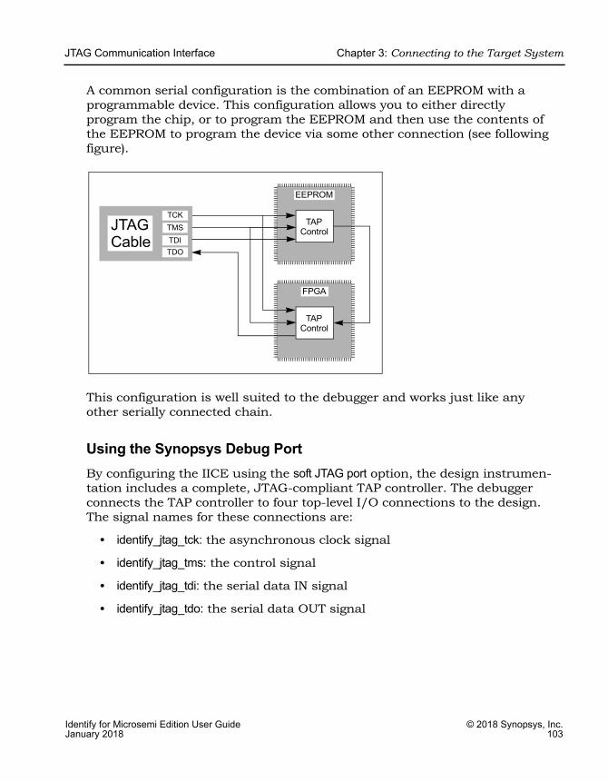
JTAG Communication Interface Chapter 3: Connecting to the Target System
Identify for Microsemi Edition User Guide © 2018 Synopsys, Inc.January 2018 103
A common serial configuration is the combination of an EEPROM with a programmable device. This configuration allows you to either directly program the chip, or to program the EEPROM and then use the contents of the EEPROM to program the device via some other connection (see following figure).
This configuration is well suited to the debugger and works just like any other serially connected chain.
Using the Synopsys Debug PortBy configuring the IICE using the soft JTAG port option, the design instrumen-tation includes a complete, JTAG-compliant TAP controller. The debugger connects the TAP controller to four top-level I/O connections to the design. The signal names for these connections are:
• identify_jtag_tck: the asynchronous clock signal
• identify_jtag_tms: the control signal
• identify_jtag_tdi: the serial data IN signal
• identify_jtag_tdo: the serial data OUT signal
TAPControl
EEPROM
JTAGCable
TAPControl
FPGA
TDOTDITMSTCK
LO
Chapter 3: Connecting to the Target System JTAG Communication Interface
© 2018 Synopsys, Inc. Identify for Microsemi Edition User Guide104 January 2018
Direct JTAG ConnectionCommonly, the host computer is directly connected to the four JTAG signals on the programmable chip as follows:
• The four JTAG I/O signals on the programmable chip are connected to a header on the circuit board that contains the programmable chip.
• A standard JTAG cable is connected to the four pins on the circuit board header.
• The other end of the JTAG cable is connected to the host computer.
Serial JTAG ConnectionA programmable chip using the Synopsys FPGA Debug Port can also be connected in a serial chain. To allow the debugger to communicate with the device, the configuration of the device chain must be successfully auto-detected or declared using the chain command (see the Reference Manual). The steps for making a serial cable connection are the same as a direct cable connection described above.
JTAG Clock ConsiderationsThe JTAG clock signal syn_tck on the JTAG port drives many flip-flops in the instrumentation logic – the number depends on the instrumentation, but can be larger than 1000 flip-flops. Consequently, the clock signal on the program-mable device must be able to drive large numbers of flip-flops and have low-skew properties. If the JTAG clock signal is not handled correctly, it is likely that the instrumentation will act erratically.
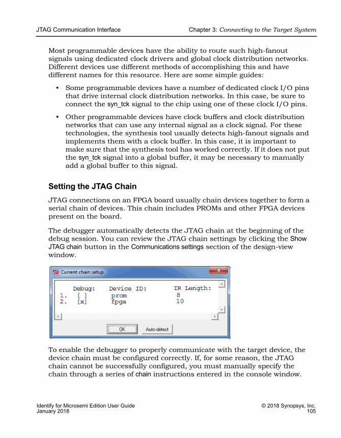
JTAG Communication Interface Chapter 3: Connecting to the Target System
Identify for Microsemi Edition User Guide © 2018 Synopsys, Inc.January 2018 105
Most programmable devices have the ability to route such high-fanout signals using dedicated clock drivers and global clock distribution networks. Different devices use different methods of accomplishing this and have different names for this resource. Here are some simple guides:
• Some programmable devices have a number of dedicated clock I/O pins that drive internal clock distribution networks. In this case, be sure to connect the syn_tck signal to the chip using one of these clock I/O pins.
• Other programmable devices have clock buffers and clock distribution networks that can use any internal signal as a clock signal. For these technologies, the synthesis tool usually detects high-fanout signals and implements them with a clock buffer. In this case, it is important to make sure that the synthesis tool has worked correctly. If it does not put the syn_tck signal into a global buffer, it may be necessary to manually add a global buffer to this signal.
Setting the JTAG ChainJTAG connections on an FPGA board usually chain devices together to form a serial chain of devices. This chain includes PROMs and other FPGA devices present on the board.
The debugger automatically detects the JTAG chain at the beginning of the debug session. You can review the JTAG chain settings by clicking the Show JTAG chain button in the Communications settings section of the design-view window.
To enable the debugger to properly communicate with the target device, the device chain must be configured correctly. If, for some reason, the JTAG chain cannot be successfully configured, you must manually specify the chain through a series of chain instructions entered in the console window.
LO
Chapter 3: Connecting to the Target System JTAG Communication Interface
© 2018 Synopsys, Inc. Identify for Microsemi Edition User Guide106 January 2018
Configuring a device chain is very similar to the steps required to program the device with a JTAG programmer.
For the debugger, the devices in the chain must be known and specified. The following information is required to configure the device chain:
• the number of devices in the JTAG chain
• the length of the JTAG instruction register for each device
Instruction register length information is usually available in the bsd file for the particular device. Specifically, it is the Instruction_length attribute listed in the bsd file.
For the board used in developing this documentation, the following sequence of commands was used to specify a chain consisting of a PROM followed by the FPGA. The instruction length of the PROM is 8 while the instruction length of the FPGA is 5. Note that the chain select command identifies the instrumented device to the system. Identifying the instrumented device is essential when a board includes multiple FPGAs.
Note: The names PROM and FPGA have no meaning to the debugger – they simply are used for convenience. The two devices could be named device1 and device2, and the debugger would function exactly the same.
Again, the sequence of chain commands is specific to the JTAG chain on your board; these commands are the chain commands for the board used to develop this document – the board you use will most likely be different.
Type the following sequence in the console window of the debugger:
chain clearchain add prom 8chain add fpga 5chain select fpga chain info
The following figure shows the results of the above command sequence.
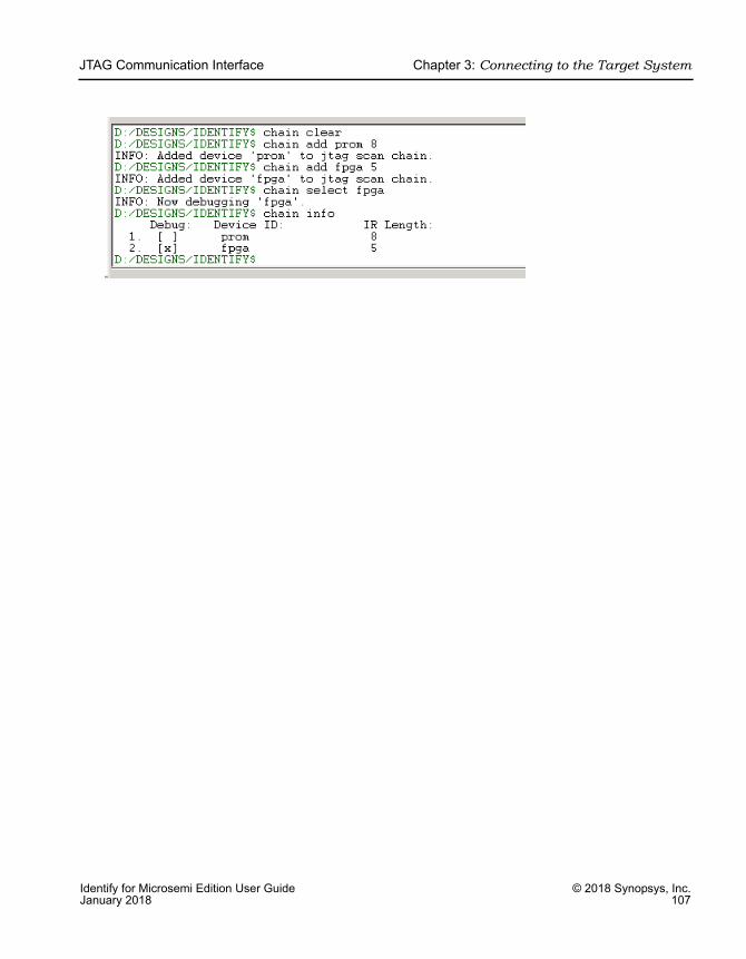
JTAG Communication Interface Chapter 3: Connecting to the Target System
Identify for Microsemi Edition User Guide © 2018 Synopsys, Inc.January 2018 107
LO
Chapter 3: Connecting to the Target System JTAG Communication Interface
© 2018 Synopsys, Inc. Identify for Microsemi Edition User Guide108 January 2018
Adding Microsemi Soft JTAG TAP Controllers
This procedure describes how to select and set up a specific Flashpro programmer, when multiple Flashpro programmers are connected to a common host.
The com cableoptions option allows you to select one among the multiple FlashPro programmers connected to a common host:
com cableoptions Microsemi_BuiltinJTAG_port <string>
The string represents the FlashPro programmer’s port name.
You can identify the port name and proceed to use the cable option as described below:
1. Start FlashPro.
2. Scan the programmers that are connected to the host and note down the port name (for example—usb32344).
3. Close FlashPro.
4. Start Identify debugger.
5. Define the cable type as:
com cabletype Microsemi_BuiltinJTAG
6. Define the cable option using the FlashPro programmer port name that you identified in Step 2. For example:
com cableoptions Microsemi_BuiltinJTAG_port usb32344
Note: For Flashpro4 programmer ports, the port name must include the usb prefix, as shown in the example above. Flashpro5 ports on the other hand, must NOT include the prefix. For example:com cableoptions Microsemi_BuiltinJTAG_port S201R1NLS
7. Check communication with the port using the com check command. If the check is successful, you can start the debugger and debug the design.
JTAG Communication Interface Chapter 3: Connecting to the Target System
Identify for Microsemi Edition User Guide © 2018 Synopsys, Inc.January 2018 109
Note that you cannot change to a different port by just re-running step 6 with the new port’s name. To select a different port, perform the following steps:
1. Stop the server using the jtag_server stop -forced 0 command. If this does not work, use -forced 1.
2. Define the new cable option. For example:
com cableoptions Microsemi_BuiltinJTAG_port usb32388
3. Run com check to check communication with the new port.
JTAG Communication DebuggingThe debugger performs a number of diagnostic communication tests. The first time the debugger connects to the on-chip TAP controller, it performs extensive communication tests. Later, every time the “run” function is executed, either by clicking the Run button or executing the run command, simpler and faster tests are executed.
Below is a list of communication related error messages with some additional explanations.
Basic Communication TestThis test sends a pattern of ones and zeros to the chip and examines the return values
• ERROR: Communication is stuck at zero. Please check the cable connection.It is likely that the debugger is unable to communicate with the instrumented chip. This error is usually a cable connection problem, or the cable type is not set correctly.
• ERROR: Communication is stuck at one. Please check the cable connection.This has the same reasons as a stuck-at-zero communication error.
• ERROR: Communication is returning incorrect IR data. Please check the cable connection. If this error is received, then the previous two errors were NOT received as the communication is returning a mixture of ones and zeroes. However, the data is not coherent and again the communication connection is suspect.

LO
Chapter 3: Connecting to the Target System JTAG Communication Interface
© 2018 Synopsys, Inc. Identify for Microsemi Edition User Guide110 January 2018
• ERROR: Communication problem - data sent is not the same as data received.This test verifies that the debugger can shift data into the instrumented chip and receive the same data back. If this error occurs, there is again a problem with your cable connection or the cable type setting is incorrect. Also, the JTAG chain may be experiencing noise immunity/signal integ-rity problems. As a troubleshooting step, select a reduced JTAG clock frequency by clicking Port settings in the debugger project window and selecting a lower clock frequency.
The last two errors can also be the result of a syn_tck signal that is not using a high-fanout clock buffer resource, and thus may show large clock skew properties. If you are using a parallel port, make sure that you have selected the correct port.
On-chip Identification RegisterThe instrumentor adds hardware to implement an on-chip identification register.
• ERROR: Cannot find valid instrumented design.The debugger cannot verify that the identification register on the instrumented design is correct or even exists. This error usually means that the design on the programmable chip is NOT the instrumented version of the design.
• ERROR: Instrumented design on FPGA differs from design loaded into Identify Debugger.The debugger verified that the chip is instrumented but the instrumentation does not match the design that was loaded into the debugger.

JTAG Communication Interface Chapter 3: Connecting to the Target System
Identify for Microsemi Edition User Guide © 2018 Synopsys, Inc.January 2018 111
JTAG Chain TestsThe debugger attempts to verify the device chain (as defined by the chain auto-detector or the chain command).
• ERROR: No hardware devices were found. Please check the cable connection.No devices can be seen in the JTAG identification register chain. Probably a bad cable connection, or the cable type is incorrect.
• ERROR: The actual number of devices differs from the defined number: ACTUAL: XX DEFINED: YYThe number of devices seen in the JTAG chain is XX, but the debugger was expecting the number to be YY (as was defined using the chain command). The chain description is incorrect.
• ERROR: The actual IR chain size differs from the defined size: ACTUAL: XX DEFINED: YYThe total number of JTAG identification register bits is incorrect. The debugger measured the hardware to have XX bits, but was expecting YY bits (as was defined using the chain command). Please review your chain configuration.
• ERROR: Communication with device number XX is not correct. Please check your chain setup.If this error appears, the previous error does not appear. Thus, the total JTAG instruction register length is correct, but the size of the instruction register of device number XX is incorrect. It is likely that the order of your devices is incorrect. Review your chain settings.

LO
Chapter 3: Connecting to the Target System JTAG Communication Interface
© 2018 Synopsys, Inc. Identify for Microsemi Edition User Guide112 January 2018
Identify for Microsemi Edition User Guide © 2018 Synopsys, Inc.January 2018 1
Index
Aactivations
auto-saving 35loading 34saving 33
asynchronous clocks 71
Bblocks
JTAG communication 55sampling 58
breakpointsactivating 20combined with watchpoints 58folded 23multiple 57
Byteblaster cable settings 87
Ccable compatibility 87cable type 86cable type settings
Byteblaster 87JTAGTech3710 88Microsemi 88
cablesconnection 96
client-server configuration 89clocks
asynchronous 71communication cable
settings 8communications settings 86complex counter 59
cycles mode 61disabling 62events mode 61
modes 60pulsewidth mode 62size 59watchdog mode 61
condition operators 67Configure IICE dialog box 51console window 14
operations 15convenience functions 70cross triggering 35, 44, 71
commands 72enabling 71state machine commands 73
cycles modecomplex counter 61
Ddata compression 26
masking 27DDR3 performance 39debug sample data
viewing 40Debugger tool
invoking 10debugger tool
opening projects 10debugging
on separate machines 43deep trace debug configurations 39dialog boxes
Configure IICE 51
Eevents mode
complex counter 61
Index
© 2018 Synopsys, Inc. Identify for Microsemi Edition User Guide2 January 2018
Ffast signal database 50files
last_run.adb 35script 17syn_trigger_utils.tcl 70
folded breakpoints 23folded signals 31folded watchpoints 22
Iidentification register 110IICE
cross triggering 71JTAG connection 102
IICE parametersindividual 51
IICE unitscross triggering 35
JJTAG
chain tests 111communication 101communication block 55communication test 109debugging 98, 109direct connection 104serial connection 104
JTAG chainsettings 9
JTAGTech3710 cable settings 88
Llast_run.adb file 35
Mmacros
st_snapshot_fill 81st_snapshot_intr 82
Microsemilcable type settings 88
modescross triggering 36
multi-IICEtabs 51
multiple signal values 31, 32multiplexed groups
selecting 21
Ooperators
condition 67original source files
searchpath 44original sources 43
Pprojects
opening in debugger 10saving 10
pulsewidth modecomplex counter 62
Qqualified sampling 81
Rradix
sampled data 30RAM resources 59remote triggering 83run command 25
Ssample buffer 29
trigger position 28sample data
viewing 40sample modes 81sampled data
changing radix 30compressing 26display controls 29
Index
Identify for Microsemi Edition User Guide © 2018 Synopsys, Inc.January 2018 3
masking 27sampling block 58sampling signals 13saving a project 10script files 17settings
cable 8JTAG chain 9
signal valuesdisplaying multiple 31, 32
signalsfolded 31listing available 13listing instrumented 13multiply instrumented 31, 32partially instrumented 32sampling selection 13status 66
source filescopying 43
st_snapshot_fill macro 81st_snapshot_intr macro 82state machines
transitions 67triggering 64, 65
statemachine command 66state-machine editor 74status reporting 66stop command 26, 66syn_trigger_utils.tcl file 70
TTAP controller 102tools
invoking Debugger 10transition watchpoint 18trigger conditions 63triggering
advance mode 64between IICEs 71modes 63remote 83state machine 64, 65
triggerscomplex 59
UUMRBus 98
Vvalue watchpoint 18Verdi nWave viewer 50
Wwatch command 66watchdog mode
complex counter 61watchpoints 57
activating 17, 20combined with breakpoints 58deactivating 19folded 22hexadecimal values 19listing 36multiple 58transition 18value 18
waveform display 48waveform viewers 48
Verdi 50windows
console 14

Index
© 2018 Synopsys, Inc. Identify for Microsemi Edition User Guide4 January 2018