Louisiana State UniversityLSU Digital Commons

LSU Master's Theses Graduate School

2014

Evaluation of Different Harvesting and StoragePractices: Sweet Sorghum and EnergycaneAna Lucia Amaya ArroyaveLouisiana State University and Agricultural and Mechanical College, aamaya2@tigers.lsu.edu

Follow this and additional works at: https://digitalcommons.lsu.edu/gradschool_theses

Part of the Engineering Science and Materials Commons

This Thesis is brought to you for free and open access by the Graduate School at LSU Digital Commons. It has been accepted for inclusion in LSUMaster's Theses by an authorized graduate school editor of LSU Digital Commons. For more information, please contact gradetd@lsu.edu.

Recommended CitationAmaya Arroyave, Ana Lucia, "Evaluation of Different Harvesting and Storage Practices: Sweet Sorghum and Energycane" (2014). LSUMaster's Theses. 3076.https://digitalcommons.lsu.edu/gradschool_theses/3076

EVALUATION OF DIFFERENT HARVESTING AND STORAGE PRACTICES:

SWEET SORGHUM AND ENERGYCANE

A Thesis

Submitted to the Graduate Faculty of the

Louisiana State University and

Agricultural and Mechanical College

in partial fulfillment of the

requirements for the degree of

Master of Science

in

The Department of Mechanical and Industrial Engineering

by

Ana Lucia Amaya Arroyave

B.Sc., Instituto Colombiano de Educacion Superior Incolda, 2010

December 2014

ii

ACKNOWLEDGMENTS

Foremost, I would like to express my sincere gratitude to my main advisor Dr. Bhaba R. Sarker of

the Department of Mechanical & Industrial Engineering for his constant guidance, support and all

the knowledge provided for my research, constant persistent help in the development of all my

research, without his guidance this thesis would not have been possible. I would like to express

my profound gratitude to my committee members Dr. Donal Day and Dr. Benjamin Legendre of

LSU Audubon Sugar Institute (LSU ASI) for their support, and insightful comments, expertise and

knowledge in the sugar cane industry and biofuels. I must thank them for their guidance provided

in the project while collecting data, subsequently analyzing them and completed the project

successfully, I am really honored in having them as members of my thesis committee. I would

sincerely like to thank Dr. Vadim Kochergin for giving me an opportunity to be part of this project

entitled, “A Regional Program for Production of Multiple Agricultural Feedstock and Processing

to Biofuels and Bio-based Chemicals”, funded by a grant from the USDA AFRI–CAP award

#2011-69005-30515. I must thank him for believing in me and providing funding for my research.

I am likewise thankful to Dr. Daira Aragon of the Audubon Sugar Institute for providing the

‘Harvest Protocol’ used for the research and for conducting the harvesting trials. I also

acknowledge Audubon Sugar Institute and its staff who extended help and support in completing

this work. I would also like to express special thanks to Lu Shyue Chardcie Verret and Iryna

Tishchkina of ASI for their help in this pursuit. I am indebted with my parents Alvaro A., Esther

L. for their unconditional love. My husband Santiago for his unconditional love and constant help.

iii

TABLE OF CONTENTS

ACKNOWLEDGMENTS .............................................................................................................. ii

ABSTRACT ................................................................................................................................... vi

CHAPTER 1: INTRODUCTION ................................................................................................... 1

CHAPTER 2: LITERATURE REVIEW ........................................................................................ 5 2.1 Importance of ethanol production from energy crops................................................... 5 2.2 Energycane and Sweet sorghum as an alternative for biofuels production .................. 7 2.3 Logistics and operational practices for energy crop supply chain system .................. 10

2.4 Supply chain logistics for agricultural productive systems ........................................ 14

CHAPTER 3: ENERGY CROPS SUPPLY SYSTEM ................................................................. 20 3.1 Supply chain system ................................................................................................... 20

3.2 Sugar cane supply system ........................................................................................... 20 3.3 Supply of sugar cane to factories ................................................................................ 21 3.4 Chemical and physical deterioration ........................................................................... 26

3.5 Sugar losses ................................................................................................................. 27 3.6 Sugarcane post-harvest deterioration .......................................................................... 30

3.7 Main factors to feedstock deterioration ...................................................................... 32

CHAPTER 4: PROBLEM STATEMENT.................................................................................... 38

4.1 Justification ................................................................................................................. 39 4.2 Main objectives ........................................................................................................... 41

4.3 Specific objectives ...................................................................................................... 41

CHAPTER 5: MATERIALS AND METHODS .......................................................................... 42 5.1 Experimental design.................................................................................................... 42

5.2 Importance of the experimental trials ......................................................................... 44 5.3 Description of the Experimental trials ........................................................................ 45

5.4 Energycane and Sweet sorghum plot characteristics .................................................. 46 5.5 Experimental trials and Sampling protocol................................................................. 47

CHAPTER 6: RESULTS AND STATISTICAL METHODOLOGY .......................................... 52 6.1 Results and Discussion ............................................................................................... 53

6.2 Weight losses of the material during storage (24 hours) ............................................ 53 6.3 %Weight losses during storage for the case of the energycane .................................. 54 6.4 %Weight losses during storage for the case of the Sweet Sorghum ........................... 54 6.5 Discussion of results ................................................................................................... 54 6.6 % Juice Yield .............................................................................................................. 56

6.7 Bulk Density of the material (ton/m3) ........................................................................ 58 6.8 Energycane Bulk Density (ton/m3) ............................................................................ 59 6.9 Sweet Sorghum Bulk Density (ton/m3) ...................................................................... 59 6.10 Bulk density (ton/m3) results and discussion ........................................................... 59 6.11 Brix and sugars (%sucrose, %glucose, %Fructose, Total fermentable sugars) ...... 61

iv

6.12 Sugars analysis for energycane ................................................................................. 61 6.13 %Brix energycane ..................................................................................................... 62 6.14 %Sucrose energycane ............................................................................................... 63 6.15 %Glucose energycane ............................................................................................... 65

6.16 %Fructose energycane .............................................................................................. 67 6.17 %Total fermentable sugars energycane .................................................................... 69 6.18 %Brix sweet sorghum ............................................................................................... 71 6.19 %Sucrose sweet sorghum ......................................................................................... 72 6.20 %Glucose sweet sorghum ......................................................................................... 73

6.21%Fructose sweet sorghum ......................................................................................... 74 6.22 Total fermentable sugars sweet sorghum .................................................................. 75 6.23 Harvester cutting system accuracy ............................................................................ 76

6.23.1 Harvester cutting accuracy – energycane 8 inches billet size ........................... 77 6.23.3 Harvester cutting accuracy – Sweet Sorghum 8 inches billet size .................... 81 6.23.4 Harvester cutting accuracy – Sweet Sorghum 6 inches billet size .................... 83

6.24 Plant composition before harvesting (%Stalk, %Leaf matter and % Seeds) ............ 85 6.25 Energycane plant composition before harvesting ..................................................... 85

6.26 Sweet Sorghum plant composition before harvesting .............................................. 86 6.27 Material composition discussion............................................................................... 86 6.28 Material composition after harvesting ...................................................................... 87

6.28.1 Material composition after harvesting energycane 8’’ billets ........................... 88 6.28.2 Material composition after harvesting energycane 6’’ billets ........................... 88

6.28.3 Material composition after harvesting Sweet Sorghum 8’’ billets .................... 88 6.28.4 Material composition after harvesting Sweet Sorghum 6’’ billets ................... 89

6.29 Discussion Material composition after harvesting energycane ................................ 90

6.30 Material composition after harvesting Sweet Sorgum .............................................. 90

6.31 Harvesting efficiency (material losses after harvesting ton/acre) ............................. 90 6.31.1 Material losses and harvesting efficiency for the case of the energycane ......... 91 6.31.2 Material losses and harvesting efficiency for the case of Sweet Sorghum ....... 92

6.31.3 Harvesting efficiency and material losses discussion ....................................... 93

CHAPTER 7: ECONOMIC MODEL FORMULATION ............................................................ 96

7.1 Agricultural production cost ....................................................................................... 98 7.2 Harvesting cost............................................................................................................ 99

7.3 Wagon cost................................................................................................................ 102 7.4 Transportation cost.................................................................................................... 103

7.4.1 Material yield .................................................................................................... 104

7.4.2 Bulk density yield (ton/ft3 or ton/m3) ............................................................... 104 7.4.3 Truck volume .................................................................................................... 105 7.4.4 Transportation distances and costs .................................................................... 105 7.4.5 Processing costs ................................................................................................. 106

7.4.6 Ethanol expected profit ..................................................................................... 110 7.4.7 Objective function ............................................................................................. 112

CHAPTER 8: MODEL SIMULATION ..................................................................................... 114 8.1 Simple and complex sugars yield calculations ......................................................... 118 8.2 Simple sugars recovery sweet sorghum .................................................................... 118

v

8.3 Simple sugars recovery from energycane ................................................................. 120 8.4 Complex sugars recovery from sweet sorghum and energycane .............................. 121 8.5 Total sugars recovery from sweet sorghum and energycane .................................... 125 8.6 Ethanol yield from the simple and complex sugars .................................................. 127

8.7 Simulation Results “Profit Maximization” ............................................................... 132 8.8 Simulation: Objective function results...................................................................... 134 8.9 Simulation results: best case scenario discussion – sweet sorghum ......................... 138 8.10 Simulation results: best case scenario discussion - energycane .............................. 141 8.11 Simulation results (sweet sorghum): worst case scenario discussion ..................... 145

8.12 Simulation results (energycane): worst case scenario discussion ........................... 149 8.13 Simulation results – Discussion .............................................................................. 152 8.14 Optimum solutions from best case scenario ........................................................... 156

8.15 Optimum solutions from worst case scenario (least feasible solutions) ................. 158

CHAPTER 9: CONCLUSIONS AND FUTURE WORK .......................................................... 160 9.1 Harvesting trials and agronomic/efficiency indicators ........................... 160

9.2 Simple sugars indicator ............................................................................................. 161 9.3 Complex sugars indicator ......................................................................................... 162

9.4 Total fermentable sugars yield .................................................................................. 163 9.5 Ethanol yield produced from simple and complex sugars ........................................ 163 9.6 Economic model formulation ................................................................................... 164

9.7 Model simulation ...................................................................................................... 166 9.8 Best case scenario simulation ................................................................................... 167

9.9 Least feasible solution simulation ............................................................................. 168 9.10 Feasible solutions .................................................................................................... 168

9.11 Considerations for future research .......................................................................... 170

REFERENCES ........................................................................................................................... 172

VITA ........................................................................................................................................... 178

vi

ABSTRACT

Two attractive potential feed stocks for biofuel production are energycane and sweet sorghum due

to the environmental adaptability, sugars concentration and yield. Evaluation and development of

harvesting, transportation and storage practices is critical for bringing the production of these crops

to industrial levels.

This research aims to analyze the supply system of energy crops and evaluate the effect of different

harvesting and storage in the yields of the feedstock and the efficiencies of the processes.

Harvesting trials were conducted at St. Gabriel, LA for evaluating the feasibility of using energy

crops as inputs for ethanol production. The parameters that were varied during the trials were:

billet size, fan speed of the extraction system. Several operational indicators were estimated in the

study: material yield (tons/acre), sugars yield (ton/acre), ethanol yield (liter/acre) and agronomic

and efficiencies indicators of the supply stages of the system.

A simulation of the conceived supply system was performed in order to measure and determine

the feasibility of the operation. The objective function of the model was defined as the profit

maximization of ethanol production. Twenty four scenarios were simulated and evaluated for

determining the optimal solutions.

It was evidenced that for increasing the sugars and ethanol yield from the energy crops, it was

necessary to reduce the lead times of the operations, enabling to process the material shortly after

harvesting. A feasible operation of the system was guarantee when a maximum distance of 35

miles was defined for transportation logistics and when an area of 100 acres was covered for

collecting the feedstock.

1

CHAPTER 1: INTRODUCTION

The necessity of generating alternative options for the production of energy and bio-fuels for the

future replacement of traditional fuels was established in the Energy Independence and Security

Act of the United States, 2007. It was also stated the importance of developing new alternative

solutions for reducing the dependence of crude oil due to the risks related in the instability of oil

prices and policies established by the countries that belong to the OPEC (non-Organization of the

Exporting Countries).

According to the “Annual Energy Outlook 2013” of the US Energy Information Administration,

there are certain key factors that determine the long term prices of petroleum and others fuels,

which are classified in four categories:

1. The economics of non-Organization of the Petroleum Exporting Countries (OPEC).

2. OPEC investment and production decisions.

3. The economics of other fuels and world demand for petroleum and other fuels (United

States Energy Information Administration, 2011).

This formulation shows the uncertainty on prices and risks related to the future of this commodity

and it indicates that most of the policies and critical decisions are mostly established by producers.

In addition, because of the high predominant cost of acquisition and its critical value as an input

to many economic activities and industrial processes, the competitiveness of any business can be

affected if there is no stability on prices in a long term scenario.

The Energy Independence Security act of 2007 stated that around 36 billions of gallons of

renewable fuels will need to be produced by the year 2022. One alternative for the production of

biofuels is the implementation of lignocellulosic biomass plant; specifically, from grassy crops

(USDA, 2010) due to their environmental adaptability and agronomic characteristics (A.Ribera,

2

2013), (Mark, 2009). It was determined that was viable to transfer and use the already established

methods and infrastructure of sugarcane with crops such as the energycane and sweet

sorghum(Zegada-Lizarazu and Monti, 2012).

Energycane and sweet sorghum are being considered as a new alternative source for producing

biofuels and alternative products thanks to their suitability for growth, high yields of

lignocellulosic and fermentable saccharides, and low agronomic requirements (Whitfield, 2013).

However, despite of the advantages that can be gained from the use of alternative feedstock and

biomass, there still are some barriers that, have not been clearly defined and solved, as was

mentioned in the “Roadmap for Agricultural Biomass Feedstock Supply in the United States”

(USDA, 2012). Some of the barriers defined are the following:

1. The risks related to the availability of adequate biomass supply to a bio refinery, and the

possible risks of success and costs implied in the infrastructure and equipment for the

supply system required (Kaldellisc, 2011).

2. The agricultural residues, such as the residues that can be obtained from the energycane

and sweet sorghum, have lower yields of biomass per acre compared to other crops (e.g.

switch grass, miscanthus). This particularity leads to the necessity of increasing the area of

harvesting, collecting and transporting the feedstock; as a result, the total cost of operations

can increase (Mapemba, 2005).

3. The lignocellulosic biomass is a renewable energy alternative that faces challenges such as

availability and logistics constraints, due to low bulk density and delivery issues.

Additionally, the transportation operation represents a high component cost of the

production of biofuels, near to 35-50% (Kumar et al. 2006).

3

For a profitable and successful utilization of agricultural feedstock and its biomass for their

conversion into alternatives products, it is necessary to link all the operations required throughout

the system, which starts from acquiring the feedstock, harvesting, transporting, delivering, storing

and processing. All these activities collectively define the basic structure required for the

agricultural supply chain system (SCS) needed for the production of alternative products, and

conforms the main factors that determine the structure of a supply chain system, as was proposed

by Porter (Porter, 1987).

The harvesting and the transportation are considered critical stages for an agricultural supply chain

that utilizes perennial grasses as inputs for the production system, because the operational cost can

vary as a function of the distance needed to cover for collecting and harvesting the feedstock (Gan

et al. 2011), (Mapemba, 2005), (Mark et al. 2009), (Sharma et al. 2013), (Cock et al. 2000).

For the case of sugar cane, it is established that transporting the material over large distances is

not a feasible option, mainly because the material is perishable, bulky and there is no tradeoff with

the costs (Cook et al. 2000); some of the main considerations formulated by the author are

summarized below:

1. The biomass from agricultural residues is characterized by a low bulk density when it is

been harvested and collected.

2. The moisture level of the biomass can affect the quality and the efficiency of the system.

3. The quality characteristics of the biomass and feedstock can be variable and inconsistent

depending on: the type of feedstock selected to work, the weather conditions, the

technologies and practices implemented, etc.

4. The calculation of the maximum distance for obtaining the feedstock should consider the

operational costs vs. the potential profit of the outputs.

4

In this way is possible to determine the feasibility of the system and the maximum distances

for transporting the material (the transportation costs can easily arise based on the distance

needed to obtain the material).

All these considerations affect the supply of the feedstock, any change can affect the costs of the

operations, the consistency of the feedstock as well as the quality, the efficiency of conversion and

the possible yields. It is indispensable to evaluate different alternatives to determine the feasibility

of establishing the system in industrial levels.

5

CHAPTER 2: LITERATURE REVIEW

In the Energy Independence and Security Act of 2007 (United States Energy Information

Administration, 2007), the necessity of producing considerable quantities of renewable fuels as an

alternative resource for the next decades was established. It was stated the necessity of producing

around 36 billions of gallons by the year 2022.

One of the alternatives for the replacement of traditional fuels is the production of biofuels from

lignocellulosic biomass plants, projecting the goal of producing around 530 million tons of

Lignocellulosic biomass for satisfying the production demand and ensuring a continuous supply.

The policy suggest the necessity of promoting and improving technologies and methodologies for

the collection and converting the material as well as a definition of the logistics practices for the

system. This integration needs to be efficient and cost effective in order to determine the optimal

configuration that the system will require for the supply, the management and the transformation

of alternative resources for the production of bio-fuels.

2.1 Importance of ethanol production from energy crops

The implementation of the energycane and the sweet sorghum as inputs for the production of

ethanol are alternative options for contributing to the independence of fossil fuels. Ethanol is a

high octane fuel used primarily as a gasoline additive (Salassi, 2007) that can be produced from

grain crops (corn and wheat) and sugar crops (sugar cane, molasses and beets).

There are several similarities of sugarcane crop with sweet sorghum and energycane, and as a

result, these crops are considered to be processed as inputs for the production of ethanol by

implementing the sugarcane operational infrastructure. The energycane and sweet sorghum are

similar in gross and shape to the sugar cane, and can be handled with the current operational

6

structure and infrastructure used for harvesting and processing sugar cane (Misook et al. 2011),

(Ribera et al. 2013). Energycane and sweet sorghum are considered potential biofuel crops due to

the environmental adaptability and capability of producing high yields of sugars (Amosson, et al.

2010).

For the production of ethanol from energy crops, it is necessary to remove the sugar through the

implementation of processes such as crushing, sacking and chemical treatment, with these

processes, the sugars can be fermentable to alcohol by the implementation of yeast and microbes.

Finally, the product is distilled until achieving the desired concentration (USDA, 2009); for

implementing ethanol with gasoline, water needs to be removed for producing “anhydrous

ethanol”. Currently, the ethanol is being used as an additive for gasoline because it is a renewable

fuel, while gasoline is a derivate of crude oil, hence, the net emissions of Green House Gases,

GHG’s, (mainly CO2), can be significantly lowered (Goldemberg, et al. 2008).

In the United States, approximately 3.9 billion gallons of ethanol are produced every year, where

97% of it is produced from corn, while the remaining is produced from sorghum, cheesy whey and

beverage waste (Renewable Fuel Association), (USDA, 2006).

For the production of ethanol, there are two main processes used, these are: the wet milling process,

which consists in fractioning the corn into starch, fiber, corn germ and protein, where only the

starch is the component used for ethanol production. The other process is called dry milling, and

basically consist of grounding the corn kernels by adding water, then the product is cooked and

enzymes are added for converting the material into sucrose. Around 40% of the production of corn

in the U.S. is utilized for the production of fuels and because the high demand, the price of a bushel

has increased by 20%, generating an increment in the prices of the food products that are produced

from this commodity (Cendrowski, 2012), (Elobeid et al. 2006).

7

The utilization of corn as an input for fuel production is already established in industrial levels in

the U.S., and several benefits are provided by the U.S. government for incentivizing the production

of corn (0.60/gal) (EIA, 2012). The utilization of this commodity for fuel purposes compete

drastically with the utilization of the crop for food production (McPhail et al. 2008), (McPhail et

al. 2012), hence, a dedicated utilization of the commodity for purposes different from food may

be constrained in the future. This suggest the necessity of finding sources for the production of

biofuels that not compete as a food commodity.

According to the Energy Policy Act of 2005, the “Renewable Fuel Standard (RFS)”, defined that

the gasoline sold in the U.S. need to contain a minimum value of renewable fuel; for this purpose,

the utilization of ethanol has been implemented.

In 2012, approximately 7.5 billion gallons of renewable fuel was used for this purpose, it was

stated by the USDA that for 2013, it was necessary the production of 250 million gallons of

cellulosic derived ethanol (USDA, 2006).

2.2 Energycane and Sweet sorghum as an alternative for biofuels production

Producing alternative products from lignocellulosic biomass is an alternative that has been

promoted by the U.S. Department of Energy (DOE); for this purpose, an alternative to work with

is the use of grassy crops. According to the USDA Roadmap on Biofuels (USDA, 2010) the

utilization of lignocellulosic biomass was a trending option because was possible to transfer

technologies and practices. It is expected to achieve the capacity of producing about 13.4 billion

gallons of advanced biofuels by 2022.

The states of the south of the U.S. are the main producers of sugarcane, specifically Florida and

Louisiana, producing around 375,000 and 390,000 acres respectively (Tyler, 2006).

8

Approximately 20% of the national sugar production is produced by the Louisiana sugar industry

achieving an economic activity of 2.2 billions of dollars (ASCL, 2011).

According to the report, “The Economic Feasibility of Ethanol Production from Sugar in the

United States” presented by the USDA, it was estimated that the average national yield of sugar

cane was around 28.8 tons per acre harvested with a recovery rate of 12.3%.

The report mentioned that the estimated sugar yield per acre was of approximately 3.55 tons of

raw sugar harvested per acre. This suggests that the current infrastructure used for collecting,

handling and transforming the material provide an effective development of the system suggesting

that the practices used for the sugar production are efficient and provide a feasible operation.

It has been mentioned that is viable to transfer and use the already established infrastructure of

sugarcane, with crops such as energycane and sweet sorghum, these alternative feedstock are being

considered as a potential source for producing biofuels and alternative products.

Energy crops are becoming an attractive option for the Southern States of the U.S. due to the

agronomic characteristics and adaptability to environmental conditions as well as the non-

competitiveness with food or fiber crops (Ribera, 2013), (Mark, 2009), (Zegada-Lizarazu et al.

2012).

The energycane and sweet sorghum provide a high biomass productivity per unit area, are non-

competiveness with food commodities and because of the similarities with sugar cane crops, its

suitable to use the already establish infrastructure (Kaldellisc, 2011).

The energycane is a crop classified as a perennial grass, which is a variety of the commercial sugar

cane and is characterized with a lower content of sucrose but a higher content of fibers, which can

be utilized as an input for the production of lignocellulosic ethanol (Misook et al. 2010).

9

Another important characteristic of the energycane, is that the crop can resist different weather

conditions and present desirable characteristics such as high material yield, appropriate geographic

adaptability, non-competitiveness with food, feed or fiber and low input requirements (Ribera et

al. 2013). On the other hand, the sweet sorghum is an annual crop that is well adapted to warm

and dry growing regions; it has been identified as a possible input for producing ethanol because

of its biomass yield and high concentration of readily fermentable sugars (Bennett & Anex, 2009).

The sweet sorghum requires fewer quantities of fertilizer and water and is high adapt to different

environmental conditions (Misook et al. 2010), (Montross et al. 2009), (Zegada-Lizarazu et al.

2011). Sweet sorghum produces lignocellulose that can be used for the production of second

generation of biofuels and because of its high content of soluble sugars and structural carbon, the

crop can be also used for the production of first generation biofuels (Zegada-Lizarazu et al. 2011).

Despite the advantages and benefits that can be obtained from the energy crops, Montross et al.

mentioned that the shelf life of the juice is short and because the high concentration of sucrose, the

juice cannot be stored for a long period of time.

It was suggested by Montross the necessity of improving the conversion methods in order to

increase the concentration of the ethanol so the storage and transportation costs can be reduced

(Montross et al. 2009). Similarly, Rooney et al. mentioned that even with the agronomic

advantages of the crop, the implementation of sweet sorghum as an energy crop is still behind of

maize, sugar cane or beet (Rooney et al. 2007).

The search for new biofuels alternatives is focused in cellulose-based plant material, mainly

because it is an abundant material that represents around 13.4% of the global energy supply for

the United States (Sims, Hastings, Schlamadinger, Taylor, & Smith, 2006). Biomass material

represents a highly viable option as a solution for finding alternative resources from the already

10

established crops; also a variety of by-products can be obtained; some of these are heat, power

and/or biofuels (Kaldellisc, 2011).

2.3 Logistics and operational practices for energy crop supply chain system

The utilization of energy crops for the production of biofuels is an option that lately has been

strengthened due to the requests stated by governmental entities in the United States (USDA,

2006).

Currently, there is no commercial scale of cellulosic plants of neither energycane nor sweet

sorghum for their use as inputs for biofuels production; hence, there is not a real measure of the

economic feasibility or a definition of the parameters and practices necessary to ensure a

continuous and efficient system operation (Zhang et al. 2012).

The supply chain system focusses in the design, planning, production and delivery of products to

the final costumer (Durand, 2012); therefore, it is necessary to define and establish the conditions,

parameters and practices for each of the stages that integrate the supply chain system.

For the case of an agricultural system that implements energy crops as inputs for biofuel

production, it has been defined that the system may be limited by the logistics of harvesting,

collection, storage and transportation (Leboreiro et al. 2011). It is necessary that each of the stages

integrating the supply chain system (SCS) need to be well-defined, and measured in order to

determine the flow of the processes, identify the critical variables necessary for assuring an optimal

development of a productive system (Porter, 1987).

Currently there is not a full scale implementation of energy crops as inputs for biofuel production,

the main stages of the supply system are not well defined (design, planning, logistics, technology

and operational practices). It is indispensable to determine the structure of these stages and the

11

feasibility of implementing the production system in industrial levels, is requested in order to

ensure the future utilization of energy crops. It is important to determine how a greater benefit can

be obtained from both, agronomic and economic so the minimization of the operational-logistics

costs, the maximizing of the products (obtain high yields from the feedstock), and the profitability

of the business can be a feasible and a competitive option for the industry.

These considerations are critical for structuring and establishing the future success of the cellulosic

industry, which at the moment stills in the design phases; consequently, the data and technical

procedures are uncertain (Tyner, 2009).

Harvesting and transportation are considered critical stages in an agricultural supply chain system

that implements alternative crops for the production of biofuels because the operational costs can

varies as a function of the distances needed to cover for collecting and harvesting the material (Gan

et al. 2011), (Mapemba, 2005), (Mark et al. 2009), (Sharma et al. 2013).

Even though the search for alternative sources for biofuel production is a promising trend, Iman

mentioned that there are serious logistic issues for the production of biofuels due to feedstock

availability and the economics of the feedstock supply (Iman et al. 2010). Iman suggested that the

material yield is a key factor for its utilization in the conversion to ethanol as well as the delivery

costs (they include the feedstock production, the harvesting, and the processing steps).

Finally, the author points out, that these two considerations are key factors that affect the selling

price of the final product and the overall sustainability of the bioethanol production. It was

mentioned by Badger, that the transportation costs and the operational efficiency of an agricultural

system mainly depends on the type of feedstock being transported; the density of the material; the

transportation modes; and the distances for covering (Badger, 2003). Similarly, it was stated that

12

the feedstock cost can be affected by the type of material, the field conditions, the climate and the

efficiency of the logistic processes (Larasati et al. 2012), (Kumar et al. 2012).

Additionally, for collecting and transporting the material, in most of the cases, the dependency of

consuming traditional fuels for the operation, is almost an unavoidable aspect (operation of

machines and trucks), representing higher costs for the fraction of the production process (Ashron

et al. 2007).

In the production of ethanol, around 20 to 40% of the total cost, is originated by the cost of

feedstock supply to the bio refineries, and 90% of these costs are based on the logistics for

delivering the material (Ekşioğlu, 2008 ). On the other hand, the feedstock acquisition cost can be

approximately 35-50% from the total production cost of the ethanol (Larasati et al. 2012).

Similarly, Hess estimated that approximately 30% of the feedstock cost was due to the

transportation cost.

For the case of sugar cane, it was mentioned by Srivastava that the current supply management

practices used for harvesting and transporting the material, present an impediment for the

successful recovery of sugars.

This phenomena occurs due to the exposure time that the feedstock have before processing and

the total loss weight that can occur during these two stages of the supply system. It was found that

a decrease of approximately 2 units of sucrose can occur by not processing the material during the

first 72 hours after harvesting (Srivastava et al. 2009).

Similarly, Larrahondo reported that for every 10% of extraneous matter on harvested cane, a

reduction of 3.7% of juice extraction occurred, consequently, a reduction of 0.9% of sucrose was

generated (Larranhondo et al. 2009). Legendre estimated that that these losses represented

approximately 15 kg of sugar losses per ton of cane (Legendre, 1973). Likewise, Saska et al.

13

reported sugar losses as a function of the time the material was stored before processing taking

special attention for the fluctuations of the internal temperature of the material stored.

In the research titled as “Determination of Sucrose Loss in Storage of Clean Unburnt Billet Cane”

it was showed that for a 24 hour period of storage, the internal temperature ranged between 17°C,

17-22°C, 22-27°C and >27°C, the sucrose losses calculated in terms of tons of sucrose for each

100 tons of initial sucrose per hour, was approximately 0.01, 0.01, 0.03 and 0.32, respectively. It

was observed that the weight loss of the material was measured, and it was concluded that the

weight losses (tons of cane per 100 tons initial per hour) when the temperature was in the two

highest ranges (22-27°C and >27°C), was approximately of 0.08 and 0.22 (Saska et al. 2009).

Based on the complex conditions that are required to consider for ensuring an efficient and

continuous supply of feedstock (harvesting, transportation, and storage), the following

considerations are necessary to contemplate for the economic success and feasibility of system:

1. Ensure minimum operating costs in the system (harvesting, transportation, delivery,

storage and processing) (Ribera et al. 2013), (Gan et al. 2011), (Sultana et al. 2011).

2. Maintain feedstock availability in order to ensure a continuous supply of the input and a

continuous operation; enabling production maximization and profitability of the business.

(Homem et al. 2010).

3. Implement practices for increasing the bulk density of the material (Leboreiro et al. 2011).

4. Due to low bulk density and low content of sugars that can be obtained, the transportation

stage is critical and expensive; therefore it should be evaluated and analyzed in detail.

5. The quality characteristics of the biomass and feedstock can be variable and inconsistent

depending on the type of feedstock selected to work, the weather conditions, the

technologies and practices implemented.

14

6. For acquiring the feedstock, it is necessary to harvest, transport and store the material

before processing. Depending on the duration of these activities the biomechanical

conversion process to ethanol can be affected (Iman et al. 2010).

7. The energy crops are perishable feedstock that requires to be processed in a short period of

time before deterioration become critical (port harvest sugar losses, chemical and physical

deterioration), (Solomon, 2009).

When the storage time and temperature increase, the physical and chemical deterioration

tend to increase over time, and the appearance of bacteria and physiological changes might

occur more rapidly (Watt et al. 2009).

2.4 Supply chain logistics for agricultural productive systems

There are several considerations that are needed to be studied in order to determine how different

practices can provide better results for handling the material before processing. It has been

mentioned that the harvesting, the transportation and the storage phases of the operational supply

are considered critical stages because of both, the criticality of the economics and the agronomics.

The quality of the material can be affected depending of the procedures implemented for acquiring

and handling the feedstock and the economics can be affected according to the parameters defined

for obtaining, collecting and handling the material before processing.

It is important to highlight that the energy crops are perishable and present physical and chemical

deterioration due to the exposure to environmental conditions, the practices used for handling the

material and the time elapsed before processing it. Also, it is important to evaluate different supply

practices that can reduce these impacts, and can increase the yield and quality of the material, and

maximize the potential conversion of the feedstock into the final outputs.

15

The complexity of structuring and defining the overall operational structure of any supply chain is

a challenge, specially, when a full scale industrial implementation has not been developed.

Currently, because there is not a full scale implementation of the crops in industrial levels, these

practices are unknown or are not well defined. There are different challenges to face, some of them

are: the operational structure of the supply; the logistics used for the supply; the practices for

acquiring and handling the material; the procedures and technologies utilized for the conversion

process.

It is important to analyze the variables, constraints and requirements that are needed to take into

consideration in an agricultural system for defining the network flow and structure of the system,

different considerations have been studied for the model formulation of the system and the

identification of the critical paths. Some of these are: spatial and temporal relationships,

geographical conditions, distances to cover, and the effect of different practices on the quality

characteristics of the feedstock (Mapemba, 2005).

At the moment, different mathematical models have been developed in the attempt of representing

the behavior of the system taking into consideration a wide range of parameters used for specific

stages of the system; some of these approaches are based on:

1. Analyze different types of feedstock such as wood, straw, sorghum and sugarcane, where

the potential yield and availability of the feedstock is analyzed based on the practices used

for obtaining and handling the feedstock before the processing (Mapemba, 2005), (Sultana

et al. 2011).

2. Different studies are focused in the biomass availability (Perlack et al. 2005), (Gant et al.

2006) where the necessity of ensuring a continuous supply is an important and critical

factor for a long term scenario.

16

3. The necessity of relating and establishing coordination of the activities between the

harvesting, the transportation and the delivery of the feedstock to the factory is a necessity

that should be defined for the efficient operation of the supply chain system, as was

mentioned by Grunow (Grunow et al. 2007). Due to the similarities of the sugarcane with

the energycane and sweet sorghum, this can be taken into account for analyzing the system.

4. Different technologies for the conversion of feedstock have been evaluated; some of these

technologies are: the thermochemical conversion, combustion, gasification, and pyrolysis

to biochemical conversion (Brechbill et al. 2008), (Charlton et al. 2009) (Sharma et al.

2013).

In these approaches the evaluation and the tradeoff between the energy required for

producing the final products and the energy obtained at the end of the process, is analyzed.

5. Evaluating the optimal location for the facility and the plant capacities has also been of

great interest for different authors aiming to define the optimal distances to travel for

acquiring the feedstock, and scheduling the operations (Gan et al. 2010), (Mapemba 2005).

6. Evaluation of different sources of lignocellulosic biomass for ensuring continuous supply

for biofuel production (wheat straw, corn stover, forest biomass), (Sultana, et al. 2011).

7. Determination of optimal plant size based on the possible quantity of biomass supply can

be obtained for ethanol production, where the biomass transportation is modeled based on

truck scheduling and transportation capacity (Leboreiro et al. 2011).

8. Biomass supply simulation where the feedstock cost is evaluated, as well as, the energy

consumption for acquiring the material and the energy consumed for the conversion

process (Zhang et al. 2012).

17

9. Determination of best locations for the construction and operation of bio refineries for the

production of biofuels and bioenergy. For these approaches, the availability of the material

is a critical parameter, the geographical conditions, and the transportation infrastructure

(Judd et al. 2012).

Supply chain system network: Due to the importance of a well-defined network of the supply

chain, a body of literature related to an efficient supply management has been developed; several

considerations and assumptions have been analyzed by different authors, focusing on:

1. Defining optimal location of multiple bio refineries using multiple feedstock (agricultural

crops, woody biomass, and perennial grasses).

For this approach, several types of feedstock were evaluated in order to define the optimal

material combination for the supply to a single bio refinery; the yields of the feedstock

were analyzed and were a decision factor for the selection.

2. Epplin developed a linear programing model for the definition of the optimal selection of

different types of grasses and agricultural residues, the area for harvest, and the quantity of

equipment was calculated and defined (Epplin et al. 2007).

3. Defining an optimal single bio refinery location using a single feedstock, where the low

cost of delivery of individual feedstock was defined based on mathematical programing

models. The author concluded that if the area of harvesting increases, the bio refinery

capacity also needs to increase. (Wang et al. 2009).

4. Other economic models have been developed in the attempt of relating the economic

feasibility of the utilization of biomass, Beeharry evaluated the utilization of sugarcane

residues for the production of energy.

18

The author concluded that by using all the leaf matter generated from the sugarcane, it was

feasible to obtain an increment near to a 50% more on the production of energy from this

resource, compared to the current practices that not included all the residues (14%)

(Beeharry, 2001).

5. Analyzing a long term investment and an economic feasibility of producing alternative

products, such as ethanol from lignocellulosic material, from crop residues like woody

biomass and energy crops, has also been studied.

Kaylen used the Net Present Value (NPV) to estimate the net income over a long term

period; similarly, Tembo and Epplin developed a multi period, multi region, mixed integer

mathematical programming model to analyze the investment by maximizing the NPV value

for a biomass bio refinery facility (Kaylen et al. 2000).

6. Other considerations for modeling biomass have been also analyzed, where the relationship

between the environmental and geographical implications were performed by the

implementation of the Geographical Information System (GIS).

This approach was studied by English and Graham (English et al. 2000); they estimated

the variability of the cost of handling biomass as a result of the environmental and

geographical conditions.

In general, it was identified by the authors that the current practices do not completely satisfy the

potential necessities that might require the implementation of alternative energy crops as inputs

for biofuels production, and its implementation in industrial levels. The necessity of improving the

practices and integrating the main components of the system will allow the definition of strategies

and methods that can help to reduce the logistics costs, enabling to obtain a sustainable and feasible

productive operation.

19

According to the literature, the utilization of biomass plants will require the evaluation of the

material availability, quality characteristics, and the distances to cover for obtaining and

transporting the material.

These critical factors must be considered, in order to carefully establish a system capable of

ensuring a continuous supply to the factory, where the quality of the material, the yield and the

operational costs can provide efficient conditions along the entire productive system, enabling the

industry to become economically sustainable. However, special attention should be taken to the

stages of harvesting, transportation and storage due to their impact to the supply system (Pantaleo

et al. 2013).

Even though different approaches have been studied, it is necessary to focus special attention to

the practices and methods defined for the supply stages of the system, so efficient practices can be

determined for obtaining benefits from both, the economics and the agronomics.

20

CHAPTER 3: ENERGY CROPS SUPPLY SYSTEM

3.1 Supply chain system

Due to the advantages and similarities of sweet sorghum and energycane with sugarcane, it is

expected to integrate and implement the current infrastructure and practices used for sugar cane

with the energy crops. It is necessary to evaluate the current operational structure used by the sugar

cane industry in order to identify and understand each of the processes that integrate the supply

system, specially the stages of acquiring, handling and processing the feedstock.

This research will take special consideration to the harvesting, transportation and storage stages in

order to evaluate how different practices can affect the yield of the sugars and the operational

efficiencies of the processes.

The research will consider the already established supply system used for the sugar cane, in order

to implement the energy crops for it conversion into ethanol.

The following sections will describe the current supply processes used by the sugar can industry;

these same system will be considered for the model and current work

3.2 Sugar cane supply system

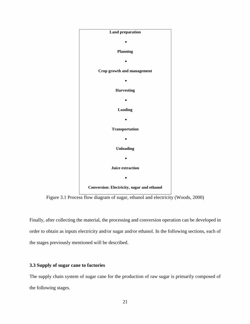
The main structure of the operational flow for acquiring the material (sugar cane) and processing

through the system is shown in Figure 3.1. The main structure for the supply system of sugar cane,

starts with the agronomic phases, which consist of the land preparation, the planting, the growth

and management.

The logistics stages for supplying the material to the factory takes place according to the maturity

of the plant, hence, the harvesting, loading, transporting and unloading processes are programed

and executed for the delivery of the material to the mill.

21

Land preparation

Planning

Crop growth and management

Harvesting

Loading

Transportation

Unloading

Juice extraction

Conversion: Electricity, sugar and ethanol

Figure 3.1 Process flow diagram of sugar, ethanol and electricity (Woods, 2000)

Finally, after collecting the material, the processing and conversion operation can be developed in

order to obtain as inputs electricity and/or sugar and/or ethanol. In the following sections, each of

the stages previously mentioned will be described.

3.3 Supply of sugar cane to factories

The supply chain system of sugar cane for the production of raw sugar is primarily composed of

the following stages.

22

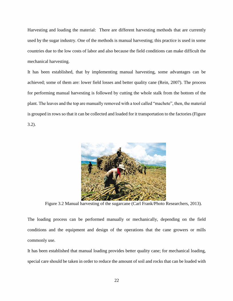
Harvesting and loading the material: There are different harvesting methods that are currently

used by the sugar industry. One of the methods is manual harvesting; this practice is used in some

countries due to the low costs of labor and also because the field conditions can make difficult the

mechanical harvesting.

It has been established, that by implementing manual harvesting, some advantages can be

achieved; some of them are: lower field losses and better quality cane (Rein, 2007). The process

for performing manual harvesting is followed by cutting the whole stalk from the bottom of the

plant. The leaves and the top are manually removed with a tool called “machete”, then, the material

is grouped in rows so that it can be collected and loaded for it transportation to the factories (Figure

3.2).

Figure 3.2 Manual harvesting of the sugarcane (Carl Frank/Photo Researchers, 2013).

The loading process can be performed manually or mechanically, depending on the field

conditions and the equipment and design of the operations that the cane growers or mills

commonly use.

It has been established that manual loading provides better quality cane; for mechanical loading,

special care should be taken in order to reduce the amount of soil and rocks that can be loaded with

23

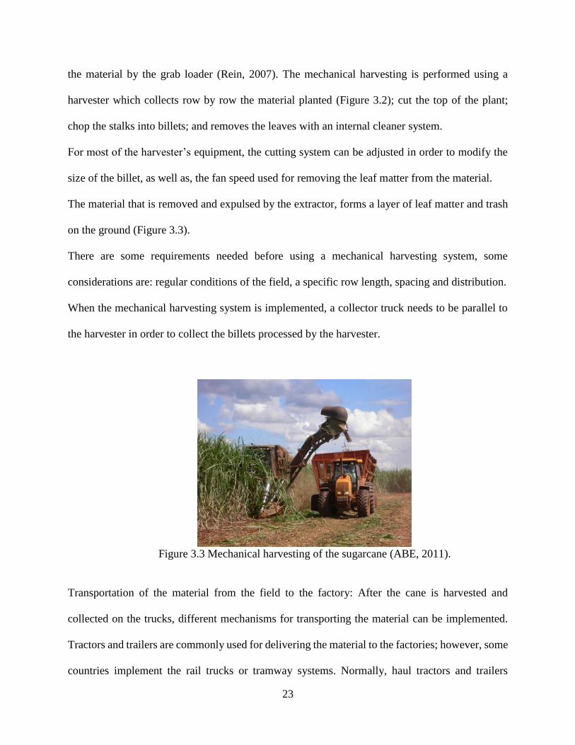
the material by the grab loader (Rein, 2007). The mechanical harvesting is performed using a

harvester which collects row by row the material planted (Figure 3.2); cut the top of the plant;

chop the stalks into billets; and removes the leaves with an internal cleaner system.

For most of the harvester’s equipment, the cutting system can be adjusted in order to modify the

size of the billet, as well as, the fan speed used for removing the leaf matter from the material.

The material that is removed and expulsed by the extractor, forms a layer of leaf matter and trash

on the ground (Figure 3.3).

There are some requirements needed before using a mechanical harvesting system, some

considerations are: regular conditions of the field, a specific row length, spacing and distribution.

When the mechanical harvesting system is implemented, a collector truck needs to be parallel to

the harvester in order to collect the billets processed by the harvester.

Figure 3.3 Mechanical harvesting of the sugarcane (ABE, 2011).

Transportation of the material from the field to the factory: After the cane is harvested and

collected on the trucks, different mechanisms for transporting the material can be implemented.

Tractors and trailers are commonly used for delivering the material to the factories; however, some

countries implement the rail trucks or tramway systems. Normally, haul tractors and trailers

24

without a significant capacity, tend to cover as a maximum distance of 10 or less kilometers to

transport the material. When tractors with capacities from 15 to 20 tons are used, the distances for

transporting the material increases.

It is common to implement a trans-loading area to supply the material harvested and transported

by smaller trucks to the trucks with greater capacity (Rein, 2007). The system employed to

transport the feedstock can be vary depending of: field and road conditions, safety policies for

roads, mills and growers’ logistical operation.

The bulk density of the material harvested is a parameter that is highly related to this stage of the

supply system and can affect the efficiency of the operation. It has been defined by several

researches that different methods for harvesting can impact the density of the load being

transported.

When more leaf matter is attached to the material during harvesting, the bulk density of the load

decreases and some quality effects can be produced during the processing of the cane. When green

cane is employed, this means that the cane is not burned in the field before harvesting, more tops

and leaves are expected to be collected, affecting the load density of the trucks and affecting the

logistical operation. It is expected to have more material but not all the material might have the

same yield during the processing operation and will affect the efficiencies of the crushing and

conversion operation.

Employing the green cane method, other effects can be produced: the harvester performance might

be reduced; moderate billeting losses in the field will occur; more material to process in the factory;

and more soil and trash will be included in the loads, (Rein, 2007). Despite of some negative

effects, some advantages can be obtained: the material is fresher and it takes more time to degrade

during the transportation and storage stages (Rein, 2007).

25

Harvesting efficiency: Another important parameter that can affect the efficiency of the harvesting

operation is the length of the billet. It is important to obtain a well cut billet of an appropriate size

that can allow a maximum load capacity of the trucks and minimize material deterioration and

proportion of leaf matter (Fuelling et al. . 1978).

It has been defined that the shorter the billet, the higher the load density of the truck, however, the

deterioration of the material might increase (Ripoli, 1996).

1. Weighing and unloading the material: After the cane is transported to the mill, the load of

the truck needs to be weighted in order to calculate the payment rate of the material.

This operation normally occurs using a weighbridge platform that registers the total weight

of the truck when it is fully loaded. Then the material is unloaded and the truck is weighted

again for defining the total amount of cane delivered.

2. Storing the material in the facility: When the cane is unloaded, the material is usually stored

in a yard next to the processing facility. Because the material is handled in billets, the area

of exposure of the material is greater compared to a whole stalk.

The deterioration of the material increases depending on the time and conditions of

exposure; this leads to increasing the possibilities of acquiring bacteria and having sugar

losses.

The gap of time between the harvesting and the processing stages is a critical period for

the efficiency of all the system, it is recommended that the time that should elapsed in

between these stages should be as short as possible, in order to reduce the losses of sucrose

in the material. It has been illustrated that for burned cane, the losses of sucrose can become

up to 0.4% for every hour elapsed after harvesting the material (Cock, 1995).

26

3. Conversion of the material into final products: After the cane is unloaded and moved for

starting the conversion process, the cane is cleaned and washed in order to eliminate, as

much as possible, any attachment of leaf matter or trash. The cane is processed by the

following main stages: milling or diffusion, heating, flashing, defecation, clarification,

evaporation, boiling and centrifuging (Grimaldo, 2013). After all the stages are performed,

the output of the system is the raw sugar, which later passes through a series of refining

processes in the refineries for direct consumption.

3.4 Chemical and physical deterioration

Due to the importance of finding alternative sources for biofuels production, it is necessary to

identify the critical path of the system in order to improve efficiencies of the supply operation, the

quality of the inputs and outputs and minimize the costs. It was mentioned that the harvesting,

transportation and storage are critical stages for an agricultural system that implements energy

crops as inputs for the biofuel production.

It is required to define and adjust the conditions of the already established system of the sugar cane

for its utilization with energycane and sweet sorghum.

The harvesting, transportation and storage practices need to ensure a continuous supply of the

material to the processing facility, where the quality of the material and the yield of the crop are

factors that should be carefully considered and analyzed.

The current research will study and evaluate how different harvesting, transportation and storage

practices affect the yield of the material, the yield of the recoverable sugars, and the efficiencies

of each of the main supply processes (harvesting, transportation and storage).

27

3.5 Sugar losses

It is important to evaluate methods that can reduce physical and chemical deterioration in order to

minimize the sugar losses and maximize quality of the material during the supply stages.

Several studies of harvesting practices, storage practices, physical and chemical deterioration have

been conducted for the case of the sugar cane, some of these approaches are described below.

For the case of the sugar cane, Srivastava evaluates different post-harvest storage methods in his

research titled as “Studies on Minimizing Quality and Quantity Losses in Stale cane”. The author

implemented five different treatments after harvesting for evaluating the sugar and weight losses.

The study analyzed the sugars and weight losses during a period of 120 hours after harvesting.

The following treatments were developed: cane stored under shade, cane water sprayed, canes with

trash cover, cane with trash cover + water spray, that include a solution of mercuric chloride,

salicylic acid, zinc sulphate, ammonium bifluoride and sodium acid, and cane stored in an open

The author conclude that changes in the temperature and in the relative humidity might rapidly

affect the weight losses of the material stored; especially, for the first 48 hours. In the other hand,

the result of the % pol tended to decrease more when the cane was stored without any storing

treatment; the authors concluded that by implementing these storage treatments a minimization of

sugar losses might be achieved.

Another approach developed for evaluating different harvesting practices was reported by

Larrahondo. The main objective was to determine levels of extraneous matter obtained after

harvesting manually and mechanically; determine the sucrose losses due to the amount of leaf

matter; the grinding efficiency; and the quality of the juice. Brix, pol, purity was measured in the

field before harvesting, and after the juice extraction, a complete sugar analysis was developed, as

well as brix test, and color, purity and turbidity tests (Larrahondo et al. 2009).

28

The pre harvest tests showed the following results: pol% cane of 14.5%, a purity of 91% a fiber %

of 17%; after harvesting manually and storing the material during a period of 48 hours, the %pol

was 14.6%, and the purity was reduced to 86%; while by the mechanical harvesting the purity was

of approximately 84.9%.

By harvesting manually it was determined that the % of extraneous matter was around 5%, while

by harvesting mechanically the percentage of extraneous matter increased up to 16%.When the

manual harvesting practice was used, the % of fiber tended to be lowered compared to the

mechanical harvesting. However, the brix and purity percentages of the juice were higher, it was

concluded that a reduction of approximately 0.18 units of sucrose occurred for every 1% increment

of leaf matter.

A different approach was studied by Pope in his research titled as “The Effect of Cane Factors on

Bin Weight”; basically the research focusses on determining the relationship of bin weight and

extraneous matter (EM). The author points out that the transportation cost represents a significant

portion of the total production cost of sugar, and that the presence of leaf matter due to green

harvesting is associated with a reduction of the weight of the bins after harvesting.

It was mentioned that a reduction of approximately 0.1-0.2 tons can occur by every 5% increase

in EM (Pope, 1998); it was also found that as the age of the ratoon increased, the bin weight tended

to decrease mainly because the billet becomes lighter on older ratoons. It was concluded that the

bin weight reduction was produced as result of effects of lighter cane and higher amount of EM.

According to the study conducted by Cerqueira, it was established that due to the necessity of

increasing the production of energy crop, it was indispensable to implement significant changes to

the current supply chain used for the sugar cane.

29

Similarly, the author mentioned that it was necessary to determine how can different practices can

be used for obtaining the maximum benefit for sugars recovery from the bagasse and the leaf

matter, thus, a better utilization of the resources can be implemented.

The main objective of the research was to evaluate and predict the impact of sugarcane trash

recovery and it potential use through the implementation of a crop simulation model (APSIM) and

the environmental life cycle assessment (LCA).For the study, all the requirement needed for the

preparation of the land in order to produce the feedstock (energy inputs, fertilizers) were measured,

in the same way, the potential transportation modes (rail and road) and the equipment needed for

collecting and transporting the cane were evaluated. Similarly, the farm requirements and the

potential profit obtained from the final products, that were produced as a result of the yield and

quality of the material collected (Cerqueira et al. 2013).

Saska reported sugar losses as a function of the time the material was stored before processing.

Special attention was taken for the fluctuations of the internal temperature of the material stored.

In the research titled as “Determination of Sucrose Loss in Storage of Clean Unburnt Billet Cane”.

The results from the study suggested that for a 24 hour period of storage, were the internal

temperature ranged between 17C°, 17-22 C°, 22-27 °C and >27°C, it was calculated that the

sucrose losses in terms of tons of sucrose for each 100 tons of initial sucrose per hour was

approximately 0.01, 0.01, 0.03 and 0.32, respectively.

In the other hand, the weight losses of the material was measured, and it was concluded that the

weight losses (tons of cane per 100 tons initial per hour) when the temperature was in the two

highest ranges (22-27 °C and >27°C), was approximately of 0.08 and 0.22 (Saska et al. 2009).

30

3.6 Sugarcane post-harvest deterioration

A different study was conducted by Bhatia in India. The research titled as “Post-Harvest Quality

Deterioration in Sugarcane under Different Environmental Conditions” evaluated how the post-

harvest practices can affect the juice quality, especially when the material was stored before

processing.

The research defined a period of storage of 12 days, in which each of the following tests were

performed every two day: weight losses %, juice extraction %, sucrose %, purity and ph. As a

result of the period of storage, the results of the test tended to decrease over time, especially, the

cane weight losses %, the purity %, sucrose %, the yield juice extraction % and ph.; consequently,

the total fermentable sugars was reduced.

It was evidenced that as the cane losses tended to increase, the percent of juice extracted tended to

be reduced over time; it was also found that the TFS tended to increase. The author mentioned that

a possible reason of this phenomena was primarily because of the moisture losses and due to the

increment of the viscosity of the juice.

Similarly, a significant reduction of the sucrose % and purity occurred as the storage period

progressed; one of the reasons of this phenomena was attributed to the presence of bacteria which

reduced the sugar purity (Bathia et al. 2009).

For evaluating the chemical and physical effect of cutting the stalk of cane during harvesting, Watt

et. al, developed a research titled as “Post-Harvest Biology of Sugar Cane.” The author point out

that the composition of the stalk might change when the stalk is portioned, especially when the

storage period before juice extraction is long.

The author stated that the chemical deterioration was due to the bacteria and fungi appearance

mainly because the microbes used the sugars as energy, and because they produced metabolic by-

31

products that cause processing problems in the factory. In the research conducted it was evidenced

that the balance of the plant was disrupted at harvesting, generating that the supply of sucrose to

the leaves stopped.

The plant respiration effect continues after harvesting; this phenomenon basically consume the

sugar available in the plant and produces energy, resulting in sugar losses (Watt et al. 2009).

The authors concluded that the sugar losses after harvesting were due to microbial presence and

ongoing plant respiration. It was found that the respiration process was highly related to the internal

temperature of the material stored, with an environmental temperature of 23°C, approximately

0.27mg of carbohydrate (sugars) are consumed per gram of stalk over a day of storage.

It was concluded that if the material presented higher levels of damage after harvesting, the bacteria

presence might increase, consequently, the physical and chemical deterioration increased,

especially when the material was stored over a long period of time and the internal temperatures

tended to increase.

Similarly to the previous research, Salomon mentioned in his research titled as “Post-Harvest

Deterioration of Sugarcane”, that most of the post harvesting practices implemented by the sugar

industry are linked to sugars losses and low sugar recovery.

Some of the factors that accelerate these effects during the post-harvest operation and contribute

to a lower sugar recovery are: harvest delays, processing delays, ambient temperature, methods of

harvesting, supply system, environmental conditions, and cane variety, period of storage and bio

deterioration (Solomon et al. 2009).

The author mentioned that the deterioration of the material after harvesting affect directly both,

the industrial processing of the material, the economics of the processes and the final profit.

32

When the material was stored for a long period before processing, a direct effect occurred in the

sugars recovery, the micro bacterial presence increase, as well as the sugar losses.

The condition of the material under these circumstances generates processing problems at the

factory, and based on an economic perspective, the author mentioned that it was not totally worth

to process material that presents chemical and physical deterioration, due to the low quality.

3.7 Main factors to feedstock deterioration

The author attributes the deterioration of the material after harvesting to different factors, these

are:

1. Varieties: besides the adaptability and potential yield of each variety other factors such as

environmental conditions and handling practices can affect drastically the sugar recovery.

It has been evaluated that fibrous varieties show higher reduction in sucrose compared to

less fibrous type.

2. Crop maturity: mature material tend to not deteriorate at the same rate of the immature

cane over mature cane.

3. Green and burnt cane: according to the literature, the author mentioned that the green cane

tends to deteriorate slower than chopped and burnt cane.

4. Environmental factors: it has been mentioned by Solomon (Solomon et al. 2009) and

Uppal (Uppal et al. 2000) that when the material is exposed to high temperatures and a

high % of humidity, the deterioration of the material tends to be greater.

In addition to the bacterial presence, as a consequence of high temperatures and humidity,

it was mentioned that the weather conditions can affect the practices implemented for

collecting and handling the material as well as the quality.

33

5. Transportation logistics: the main factors that affect the quality and yield of the material

during the transportation operation are basically: the time during transporting; the degree

of damage of the feedstock after harvesting and the storage time.

The author mentioned that due to some handling practices with different types of

equipment (grab loaders, chains, pile rakes) in conjunction of high temperatures and mud

presence, it was more likely the acceleration and population of the leucunostoc phenomena.

Finally it was determined that by transporting and storing the material in smaller storage

containers, the material was less susceptible to physical and chemical deterioration.

6. Magnitude of sugar losses: the author points out that some of the critical factors during the

post-harvest stage were the exposure to different temperatures, the bacteria presence and

propagation, and the plant respiration process that occur after the material is harvested.

According to the previous factors mentioned, the author associates them with an economic

implication. In general, the author mentioned that material deterioration after harvesting is a

critical parameter for the efficiency of the conversion process and the competitiveness of the

business.

In the same way, as the deterioration occurs, a reduction in the cane tonnage takes place mainly

because a rapid loss of moisture is produced. The author emphasizes that cane growers are affected

by this issue mainly because if the cane quality is lower and the yield of the cane tonnage is

reduced, the payment performed based on a weight basis will be significant reduced.

Reduction of material deterioration in post-harvest operations: In order to reduce all the issues

involved in the post-harvest operation, the author concluded the following strategies for

minimizing sugar losses, these are:

34

1. The material harvested should be processed as soon as possible; therefore, the reception

policies of the mills should be planned and synchronized with the supply process (cane

suppliers).

The author stated that for the case of full green cane, the material should be milled within

a period of 48 hours, when burnt full cane is used, the storage time should not be greater

than 24 hours. When billets are implemented during the harvesting operation, the material

should be processed no later than 12 hours after harvesting.

2. The material used for processing should contain a minimum amount of extraneous matter

if production of sugar is the objective; the author recommends to use varieties with high

fiber, in this way, sugar and moisture losses are minimized.

3. Avoid processing muddy cane.

4. While harvesting is recommended to no removal of the crown of leaves; otherwise, the

material will deteriorate faster.

5. Practices for handling and transporting should be improved in order to reduce the level of

damage of the material; in that way, dextran formation can be reduced.

6. Implement FIFO management policies for crushing, where the cane that firstly arrived

should be the firstly used for processing.

Another important approach for evaluating how different practices of harvesting and storing can

affect the yield of the sugars from sugarcane was performed by Legendre and Birkett in their

research titled “Deterioration of sugar cane in overnight sleeper loads”.

The authors mentioned that the sugar industry faced critical challenges in the harvesting system

because of the practices used and its effects in the yield of the material and efficiencies of the

conversion processes at the factory. The authors suggested the necessity of improving the

35

coordination of harvesting schedules and deliveries as well as the minimization of the time the

material is stored after harvesting.

The goal of the study was to determine the effect of the dextran concentration after storing billets

in sleeper loads during a period of 24 hours. For determining the concentration of dextran, the

Rapid Haze method and the ASI II was used; the average results from the results for each method

were 650ppm and 850ppm respectively.

The results suggested that between 17 to 20 hours after harvesting, the concentration of dextran

was expected to be higher; as a result, a penalty for the seller due to the condition of the material

was highly associated. The authors suggested that cane billeted should not exceed more than 20

hours before processing, they point out that the material should be processed in an interval between

5 to 8 hours.

Eggleston, reported the effect of sugar cane deterioration due to harvest and storage methods. The

author states that deterioration of sugar cane is associated to level of trash, billeted cane, material

exposition between harvesting and crushing phases. The study conducted 8 cane supply treatments

used for storing the material during 3 days; samples were collected every 24 hours. The treatments

included hand cut cane (green and burnt), harvested cane (green and burnt) and burnt whole stalks.

The results indicated that glucose and fructose were greater in billeted cane than whole stalk cane

in the sample. It was evidenced that the cane that was billeted presented an earlier deterioration

compared to whole stalk cane, especially when cane was burnt (Eggleston et al. 2012).

Similarly, in another study performed by Eggleston titled “How Combine Harvesting of Green

Cane Billets with Different Levels of Trash affects Production and Processing Part I: Field Yields

and Delivered Cane Quality”.

36

The research evaluated the effect of using different speeds in the extractor system fan in relation

to the potential amount of trash that can be obtained after harvesting; also, it the effects in the

downstream and upstream processing were evaluated.

Three fan speeds were used (650 rpm, 850 rpm and 1050 rpm) at a constant speed of 3.5mph; trash

tissues were collected, juice extraction % was measured as well as sugars analyses, pol, purity,

fiber % and others more.

The results indicated that the leaf matter composition obtained after implementing a fan speed of

650 rpm, 850 rpm and 1050 rpm was approximately of 22.7%, 18.9% and 12.1% (Eggleston et al.

2012).

It was observed that the TRS decreased when lower fan speeds were used; similarly the yield of

the material measured in tons of cane/acre tended to increased, however the % of leaf matter was

higher for these treatments (lower fan speeds). It was also evidenced that as the % of leaf matter

increased in the material that was harvested, the quality indicators tended to decrease. The authors

point out that obtaining lower quality indicators was not only due to the amount of leaf matter

attached to the material after harvesting, but also due to weather conditions, cutter height and

varieties.

Post-harvest quality indicators: In the second part of the research, Eggleston reported different

quality indicators were measured (soluble solids, sucrose, color, ash starch, mud volume during

clarification).

The results indicated that the quality indicators tended to be progressively worse as the amount of

leaf matter attached to the material harvested increased; it was determined by the authors that for

every additional 1% of trash, a decrease of approximately 0.15% occurred in the purity of the

37

mixed juice. It was also mentioned that with the increase of trash while processing, the yield of

juice extraction tended to decrease.

Inderbitzin mentioned in the article titled “Improving the Harvesting and Transport of Whole Crop

harvested Sugar Cane” mentioned that by using billeted cane instead of whole stalk cane, the mass

of the material transported and the bulk density might increase. In the research, the authors used a

shredder fan in addition to the primary extractor fan in order to reduce the particle size of the

extraneous matter, while the material was harvested into billets; with this procedure it was intended

that the particles of extraneous matter were reintroduced with the material harvested in order to be

transported with the cane.

The results indicated that the bulk density of the material increased approximately by 17%. Finally,

the authors concluded that with the implementation of the additional shredder fan in the harvester,

an increase of the bulk density of the material was obtained as well as a reduction of billet losses

in the field.

Despite different approaches have been developed at the moment, it is necessary to provide

additional strategies for improving the operational efficiencies of the harvesting and transportation

in order to improve the quality of the material.

It is evidenced that different studies have been conducted for improving the practices of the

harvesting, transportation and storage for the case of the sugarcane. This research will focus

specifically on these initial stages of the supply chain.

38

CHAPTER 4: PROBLEM STATEMENT

According to the literature review that so far has been cited, it was mentioned that the

implementation of alternative sources for the production of biofuels brings together complex

considerations that should be analyzed and evaluated before establishing the feasibility of the

operation.

So far, it has been mentioned the necessity and importance of implementing energy crops for the

future replacement of fossil fuels. It was highlighted that energy crops such as energycane and

sweet sorghum were potential sources for this purpose.

Energy crops provide greater benefits compared to other energy crops, however, it was concluded

that before implementing the current supply chain structure used for the sugar cane it was

necessary to study, analyze and improve some considerations of the system.

Especial attention should be provided to the stages of harvesting, transporting, delivery and storage

due to the critical impact that can be generated in both, the material efficiency utilization and the

economics.

In the same way, it was shown that some of the approaches that at the moment have been developed

seek to evaluate the operational, the logistic and the agronomic challenges that the biofuel trend

bring to the industry and to governmental entities. Some of these approaches attempt to evaluate

the operational structure and the logistics that should be reflected for this type of agricultural

system. In this approach, different topics have been evaluated, some of them are: transportation

network, inventory policies, plant location and capacity, transportation capacity policies and time

studies.

39

The main goal of the research conducted was to determine the structure, the strategies and the

policies that this type of supply chain system should integrate in order to provide better and greater

benefits from the operational development.

Similarly, different approaches have been carried out for analyzing the agronomic challenges

involved in the handling, transportation and the processing; these topics are carefully evaluated in

order to determine if the strategies for handling these alternative crops can ensure the sustainability

of the system and determine if it can be implemented in economic scales.

4.1 Justification

The objectives of this approach are followed by the identification of practices, methods and

strategies that can allow to greater yields, better quality characteristics and better processing

performances of the conversion processes.

Some of the main topics mentioned in the literature review were:

1. Evaluation of different parameters for harvesting in order reduce sugar losses in sugar cane.

2. Effect of extraneous matter on the yield of sugar and can affect the processing performance;

sugar cane trash recovery.

3. Storage effect in relation to weight bin losses.

4. Sucrose losses due to storage for the case of the sugar cane.

5. Post-harvest deterioration; post-harvest biology of the sugar cane.

6. Effect of the storing period and some others.

According to the literature, it was evident that considerations related to the material availability;

the necessity of improving the quality characteristics of energy crops; the harvesting-

transportation-storage practices for minimizing sugar losses.

40

Also it was critical to determine the distances to cover, are some of the key factors that should be

considered for the successful implementation and development of an agricultural system based on

energy crops.

The considerations that were mentioned before are necessary for the definition of a system capable

to ensure continuous supply to the processing facilities, where the quality of the material is a

critical factor due to the economics and the performance of the processing effects.

To establish a feasible biofuel production system from alternative sources, it is important to well

define the network of the system and the logistics needed for the development of the operations,

in order to minimize the total cost and set the optimal parameters that will lead to the maximize

the efficiencies for the supply system.

It is indispensable to determine which practices for harvesting, transporting and storing the

material can provide greater benefits for both, agronomics (material and sugars yields) and

economics, for the case of the energycane and sweet sorghum.

Even though different approaches have been developed at the moment, it is necessary to provide

additional strategies for improving the operational efficiencies of the harvesting and transportation

when alternative energy crops are implemented in a productive system. It is evidenced that

different studies have been conducted for improving the practices of the harvesting, transportation

and storage for the case of the sugarcane.

The necessity of developing a similar approaches for alternatives energy crops such as energycane

and sweet sorghum is indispensable; therefore, this research will focus specifically on these initial

stages of the supply chain for these specific crops.

41

4.2 Main objectives

The main objective of the research is:

To evaluate the feasibility of implementing energy crops as inputs for the production of ethanol

by the evaluation of different harvesting practices in order to determine the sugars yield, the

material yield and the efficiencies of the processes.

4.3 Specific objectives

The following objectives were defined in order to accomplish the main objective of the research.

1. To measure the yield of the fermentable sugars that can be obtained from the energy crops

after implementing different practices for harvesting and storing the feedstock.

2. To calculate the processes efficiencies of the initial stages of the supply system after

implementing different harvesting and storage.

3. To determine the ethanol yield that can be obtained after implementing different harvesting

and storage practices.

4. To perform an economic analysis between the operational costs and the potential profit of

the ethanol production that can be obtained from the harvesting practices in order to

determine the feasibility of the supply process.

42

CHAPTER 5: MATERIALS AND METHODS

This project investigates and evaluates different harvesting and storage practices for the

energycane and the sweet sorghum, and the effect of these practices on the yield of the sugars, the

yield of the material and operation efficiencies of the processes. Finally, the research will conduct

an economic analysis for determining the feasibility of implementing the harvesting crops based

on the operational costs and the potential profit form the ethanol production. This research attempts

to develop a set of harvesting trials in which different parameters of the operation are going to be

varied. According to the results obtained, an economic analysis will be performed in order to

determine the economics of the supply system implemented in the harvesting trials and will

evaluate the feasibility of the productive system according to the production costs and the potential

profit from the ethanol production. The experimental work performed in this research is intended

to be part as a preliminary study of the implementation of energy crops as inputs for the ethanol

production, hence, the indicators and analyzes performed are presented as preliminary findings,

further research will be conducted.

5.1 Experimental design

The methodologies, procedures and parameters used in the harvesting trials were taken from a

document prepared by Aragon (2013) in keeping with the USDA AFRI–CAP award No. 2011-

69005-30515 (Kochergin, 2012). Specifically, the procedures used in the harvesting protocols

included harvesting efficiency and transportation density, convertible sugar losses and leaf matter;

the harvesting trials were conducted by the direction of Dr. Aragon from the Audubon Sugar

Institute. Additional information on the protocols used in this study can be found in Day (2013

and 2014).

43

The design of the experimental trials were developed in order to implement different harvesting

and storage methods with the purpose of evaluating the effect of these methods on the %Brix and

Total fermentable Sugars (%sucrose, % glucose, % fructose). It was intended to measure and

determine the following indicators: potential losses of the material during storage, harvesting and

transportation, composition of the plant before and after harvesting, the temperature and %RH

effect of the feedstock after storing the material during 24 hours as was proposed by Aragon

(Aragon, 2013) and cutting system accuracy of the harvester. A statistical analysis was developed

in order to determine the existence of significant differences between the results obtained from the

variables of response based on the combination of factors evaluated in each of the treatments

executed and tested in the trials. The experimental trials design consisted in a factorial combination

where three treatments for harvesting and storing the material were defined; these factors were:

(a) fan extractor speeds (1100 rpm, 900 rpm and 0 rpm), (b) storage time of the material before

been processed (24 hours of storage), (c) billet size (6 and 8 inches). All these factors were varied

in the harvesting trials in order to measure and determine the effect on the variables of response

defined for the experiment. The variation of the parameters mentioned (fan speed, billet size,

storage time) were taken from the harvesting protocol reported from Aragon and used in the trials

(Aragon, 2013). For testing the combination of factors in the harvesting trials, a Factorial design

was developed for measuring the variable of response. Through the implementation of this

statistical design, it was possible to determine the descriptive statistics of the results for each of

the trials and determine if there were significant differences in the response variables according to

the factors implemented in each of the treatments. The dependent variables defined for the study

were assumed from the harvesting protocol defined by Aragon (Aragon, 2013). The dependent

variables defined for the trials of the study were:

44

1. Analysis of sugars (% sucrose, %fructose, %glucose, total fermentable sugars and brix).

2. Harvesting efficiency (potential losses of the material in the field after harvesting).

3. Transportation density (ton/m3).

4. Composition of the material before and after harvesting.

5. Cutting harvesting system accuracy.

6. Effect of the temperature (C) and %RH on the feedstock after 24 hours of storage.

The independent variables defined for the trials were:

1. Speed of the fan – cleaning system of the harvester (1100 rpm, 900 rpm and 0 rpm).

2. Billet size – cutting system of the harvester (billet of 6 and 8 inches).

3. Brix and Sugars effect on the juice after storing samples during 24 hours before been

processed (samples taken at time = 0 hours and at time = 24 hours).

5.2 Importance of the experimental trials

The experimental trials contributed to the work that is being developed for the USDA grant

awarded by the LSU Agcenter “A regional program for production of multiple agricultural

feedstock and processing to biofuels and bio based chemicals”. The experimental trials that were

performed in the research were alienated with the following outline project tasks:

1. Evaluate the efficiencies of the harvesting and transportation operations of the feedstock

from the field to the factory.

2. Evaluate the potential biomass recovery that can be obtained from the feedstock based on

the different parameters for handling, harvesting and transporting the feedstock.

3. Evaluate and determine the viability of using lignocellulosic material to obtain sugars

based on the optimal conditions to harvest and transport the material.

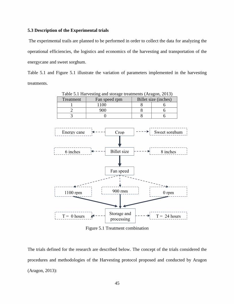
45

5.3 Description of the Experimental trials

The experimental trails are planned to be performed in order to collect the data for analyzing the

operational efficiencies, the logistics and economics of the harvesting and transportation of the

energycane and sweet sorghum.

Table 5.1 and Figure 5.1 illustrate the variation of parameters implemented in the harvesting

treatments.

Table 5.1 Harvesting and storage treatments (Aragon, 2013)

Treatment Fan speed rpm Billet size (inches)

1 1100 8 6

2 900 8 6

3 0 8 6

Figure 5.1 Treatment combination

The trials defined for the research are described below. The concept of the trials considered the

procedures and methodologies of the Harvesting protocol proposed and conducted by Aragon

(Aragon, 2013):

Crop Energy cane Sweet sorghum

Billet size 6 inches 8 inches

Fan speed

0 rpm 900 rpm 1100 rpm

T = 0 hours T = 24 hours Storage and

processing

46

1. Material yield during harvesting (ton/acre).

2. Harvesting efficiency.

3. Transportation density.

4. Composition of the biomass plant before harvesting without treatments.

5. Composition of the biomass plant after harvesting implementing the treatments.

6. Convertible sugar losses during harvesting and storage.

7. Juice Yield.

8. Material losses due to storage.

9. Harvesting cutting system accuracy.

10. Temperature and %RH effect after storing the feedstock during 24 hours.

5.4 Energycane and Sweet sorghum plot characteristics

The energycane plot characteristics:

1. Variety: energycane variety 113.

2. Area of the field: 1.5 acres.

3. Number or rows: 19 rows. 8 rows were assigned to be harvested with a billet size of 6

inches and the others 8 rows were assigned to be harvested with a billet size of 8 inches.

Sweet Sorghum plot characteristics:

1. Variety: Dura Sweet 120 days hybrid.

2. Area of the field: 2 acres.

3. Number or rows: 37 rows. 18 rows were assigned to be harvested with a billet size of

6 inches and the others 18 rows were assigned to be harvested with a billet size of 8

inches.

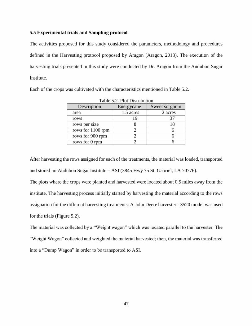
47

5.5 Experimental trials and Sampling protocol

The activities proposed for this study considered the parameters, methodology and procedures

defined in the Harvesting protocol proposed by Aragon (Aragon, 2013). The execution of the

harvesting trials presented in this study were conducted by Dr. Aragon from the Audubon Sugar

Institute.

Each of the crops was cultivated with the characteristics mentioned in Table 5.2.

Table 5.2. Plot Distribution

Description Energycane Sweet sorghum

area 1.5 acres 2 acres

rows 19 37

rows per size 8 18

rows for 1100 rpm 2 6

rows for 900 rpm 2 6

rows for 0 rpm 2 6

After harvesting the rows assigned for each of the treatments, the material was loaded, transported

and stored in Audubon Sugar Institute – ASI (3845 Hwy 75 St. Gabriel, LA 70776).

The plots where the crops were planted and harvested were located about 0.5 miles away from the

institute. The harvesting process initially started by harvesting the material according to the rows

assignation for the different harvesting treatments. A John Deere harvester - 3520 model was used

for the trials (Figure 5.2).

The material was collected by a “Weight wagon” which was located parallel to the harvester. The

“Weight Wagon” collected and weighted the material harvested; then, the material was transferred

into a “Dump Wagon” in order to be transported to ASI.

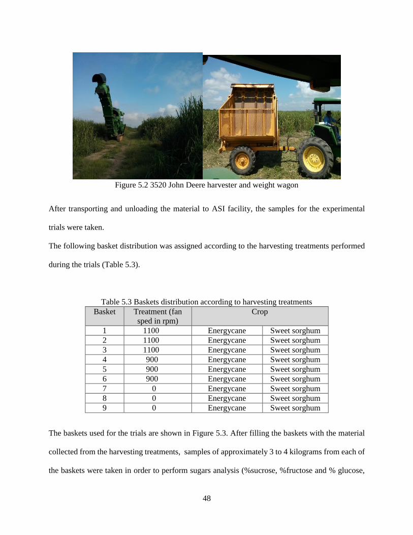
48

After transporting and unloading the material to ASI facility, the samples for the experimental

trials were taken.

The following basket distribution was assigned according to the harvesting treatments performed

during the trials (Table 5.3).

Table 5.3 Baskets distribution according to harvesting treatments

Basket Treatment (fan

sped in rpm)

Crop

1 1100 Energycane Sweet sorghum

2 1100 Energycane Sweet sorghum

3 1100 Energycane Sweet sorghum

4 900 Energycane Sweet sorghum

5 900 Energycane Sweet sorghum

6 900 Energycane Sweet sorghum

7 0 Energycane Sweet sorghum

8 0 Energycane Sweet sorghum

9 0 Energycane Sweet sorghum

The baskets used for the trials are shown in Figure 5.3. After filling the baskets with the material

collected from the harvesting treatments, samples of approximately 3 to 4 kilograms from each of

the baskets were taken in order to perform sugars analysis (%sucrose, %fructose and % glucose,

Figure 5.2 3520 John Deere harvester and weight wagon

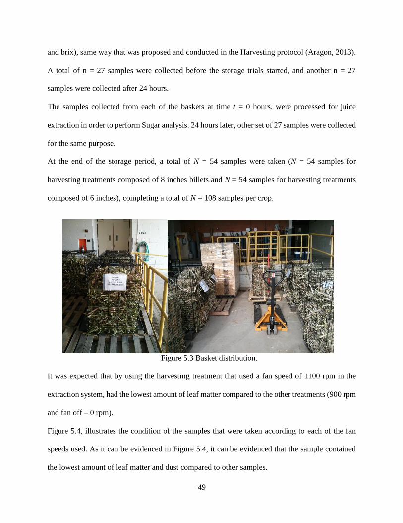
49

and brix), same way that was proposed and conducted in the Harvesting protocol (Aragon, 2013).

A total of n = 27 samples were collected before the storage trials started, and another n = 27

samples were collected after 24 hours.

The samples collected from each of the baskets at time t = 0 hours, were processed for juice

extraction in order to perform Sugar analysis. 24 hours later, other set of 27 samples were collected

for the same purpose.

At the end of the storage period, a total of N = 54 samples were taken (N = 54 samples for

harvesting treatments composed of 8 inches billets and N = 54 samples for harvesting treatments

composed of 6 inches), completing a total of N = 108 samples per crop.

Figure 5.3 Basket distribution.

It was expected that by using the harvesting treatment that used a fan speed of 1100 rpm in the

extraction system, had the lowest amount of leaf matter compared to the other treatments (900 rpm

and fan off – 0 rpm).

Figure 5.4, illustrates the condition of the samples that were taken according to each of the fan

speeds used. As it can be evidenced in Figure 5.4, it can be evidenced that the sample contained

the lowest amount of leaf matter and dust compared to other samples.

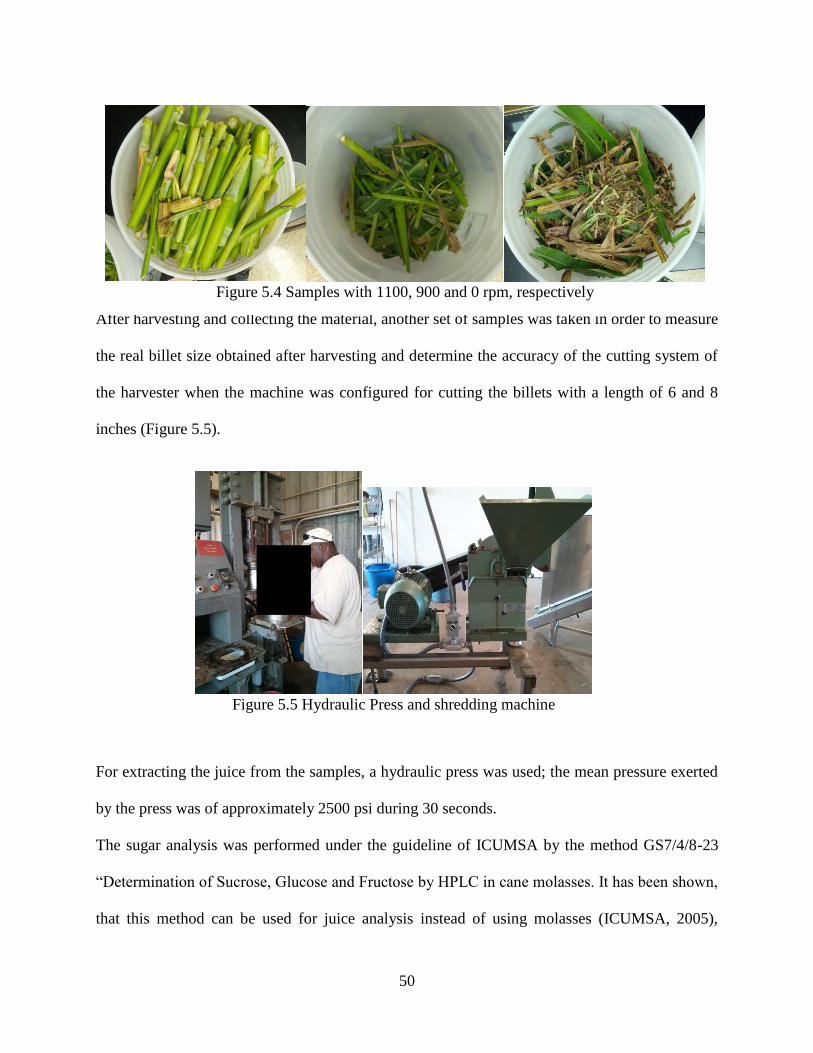
50

After harvesting and collecting the material, another set of samples was taken in order to measure

the real billet size obtained after harvesting and determine the accuracy of the cutting system of

the harvester when the machine was configured for cutting the billets with a length of 6 and 8

inches (Figure 5.5).

For extracting the juice from the samples, a hydraulic press was used; the mean pressure exerted

by the press was of approximately 2500 psi during 30 seconds.

The sugar analysis was performed under the guideline of ICUMSA by the method GS7/4/8-23

“Determination of Sucrose, Glucose and Fructose by HPLC in cane molasses. It has been shown,

that this method can be used for juice analysis instead of using molasses (ICUMSA, 2005),

Figure 5.4 Samples with 1100, 900 and 0 rpm, respectively

Figure 5.5 Hydraulic Press and shredding machine

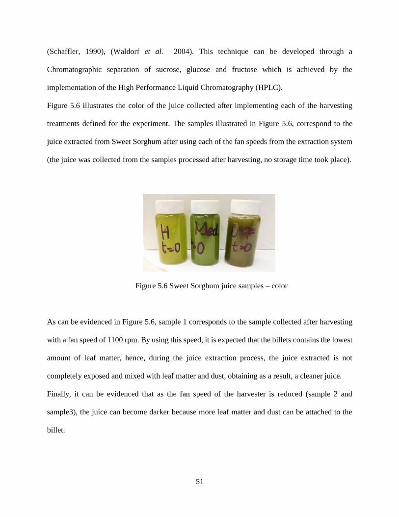
51

(Schaffler, 1990), (Waldorf et al. 2004). This technique can be developed through a

Chromatographic separation of sucrose, glucose and fructose which is achieved by the

implementation of the High Performance Liquid Chromatography (HPLC).

Figure 5.6 illustrates the color of the juice collected after implementing each of the harvesting

treatments defined for the experiment. The samples illustrated in Figure 5.6, correspond to the

juice extracted from Sweet Sorghum after using each of the fan speeds from the extraction system

(the juice was collected from the samples processed after harvesting, no storage time took place).

Figure 5.6 Sweet Sorghum juice samples – color

As can be evidenced in Figure 5.6, sample 1 corresponds to the sample collected after harvesting

with a fan speed of 1100 rpm. By using this speed, it is expected that the billets contains the lowest

amount of leaf matter, hence, during the juice extraction process, the juice extracted is not

completely exposed and mixed with leaf matter and dust, obtaining as a result, a cleaner juice.

Finally, it can be evidenced that as the fan speed of the harvester is reduced (sample 2 and

sample3), the juice can become darker because more leaf matter and dust can be attached to the

billet.

1 2 3

52

CHAPTER 6: RESULTS AND STATISTICAL METHODOLOGY

A Factorial experimental design was implemented for performing the statistical analysis; the

analysis was performed using the statistical software “SAS 9.3., SAS institute, Cary, NC.”.

The experimental design employed for analyzing the data was selected because of the necessity of

evaluating the effect of the combination of factors on the variables of response. By implementing

this experimental design, all possible interactions and effects between the factors could be tested

and analyzed in order to determine the existence of significant statistical differences between the

factor interactions from the harvesting treatments.

The statistical method implemented in the software for analyzing the data, was a Two-Way

ANOVA analysis. This procedure was performed by the implementation of a Proc Mixed

statement, which allowed to test if there were significant differences in the results obtained from

the factorial arrangement from each of the harvesting treatments.

A level of significance was tested at a P-value ≤ 0.005. The statistical analyses were executed to

the results of the variables of response obtained from the factorial combination of the harvesting

treatments. The variables of response proposed and defined in this study were followed from the

parameters and methodologies established in the Harvesting Protocols (Aragon, 2013).

In order to guarantee a correct implementation of the statistical methods and data analyses, a

normality distribution test was performed to all the results from the variables of response. The

normality test was developed in SAS by the implementation of the statement procedure Proc

univariate and through the analysis of the Shapiro-Wilk test, which guarantee the normality of the

data when the P-value is equal or greater than 0.005. By using the average results from the

treatments, the normality of the data was guaranteed; therefore, the implementation of the

53

statistical methods for identifying significant differences from the results was statistically valid for

all variables.

6.1 Results and Discussion

In the following section, the results obtained from the harvesting trials defined in Section 5 from

both of the crops are presented. The results were analyzed with a statistical analysis using a

“Factorial Design” for evaluating the interaction between the variables that were measured. The

statistical results are explained and interpreted under the considerations of the design of the

experiment defined in Section 5. The methodologies and indicators explained in the following

section considered the procedures and conceptual definitions established by Aragon in the

Harvesting Protocols (Aragon, 2013); the methodologies used in the study were followed from the

Harvesting Protocols proposed by Aragon (Aragon, 2013); the harvesting trials were conducted

by Dr. Aragon. Finally, a summary of the results is shown in each of the sections.

6.2 Weight losses of the material during storage (24 hours)

The samples were stored in baskets during a period of 24 hours under normal environmental

conditions (material protected from rain and sun). After each basket was filled with the material

collected from each of the harvesting treatments, the basket was weighted and 24 hours later, the

basket was weighted again, for calculating the material weight differences and determine the % of

material losses during a storage period of 24 hours.

The calculations were performed by using Equation 6.1 material losses:

%𝑀𝑎𝑡𝑒𝑟𝑖𝑎𝑙 𝑙𝑜𝑠𝑠𝑒𝑠 = 1 −𝑓𝑖𝑛𝑎𝑙 𝑤𝑒𝑖𝑔𝑡ℎ(𝑤𝑒𝑖𝑔𝑡ℎ 𝑜𝑓 𝑡ℎ𝑒 𝑏𝑎𝑠𝑘𝑒𝑡 𝑎𝑓𝑡𝑒𝑟 24ℎ)

𝐼𝑛𝑖𝑡𝑖𝑎𝑙 𝑤𝑒𝑖𝑔ℎ𝑡 (𝑤𝑒𝑖𝑔ℎ𝑡 𝑜𝑓 𝑡ℎ𝑒 𝑏𝑎𝑠𝑘𝑒𝑡 𝑎𝑡 𝑡 = 0ℎ𝑜𝑢𝑟𝑠) (6.1)

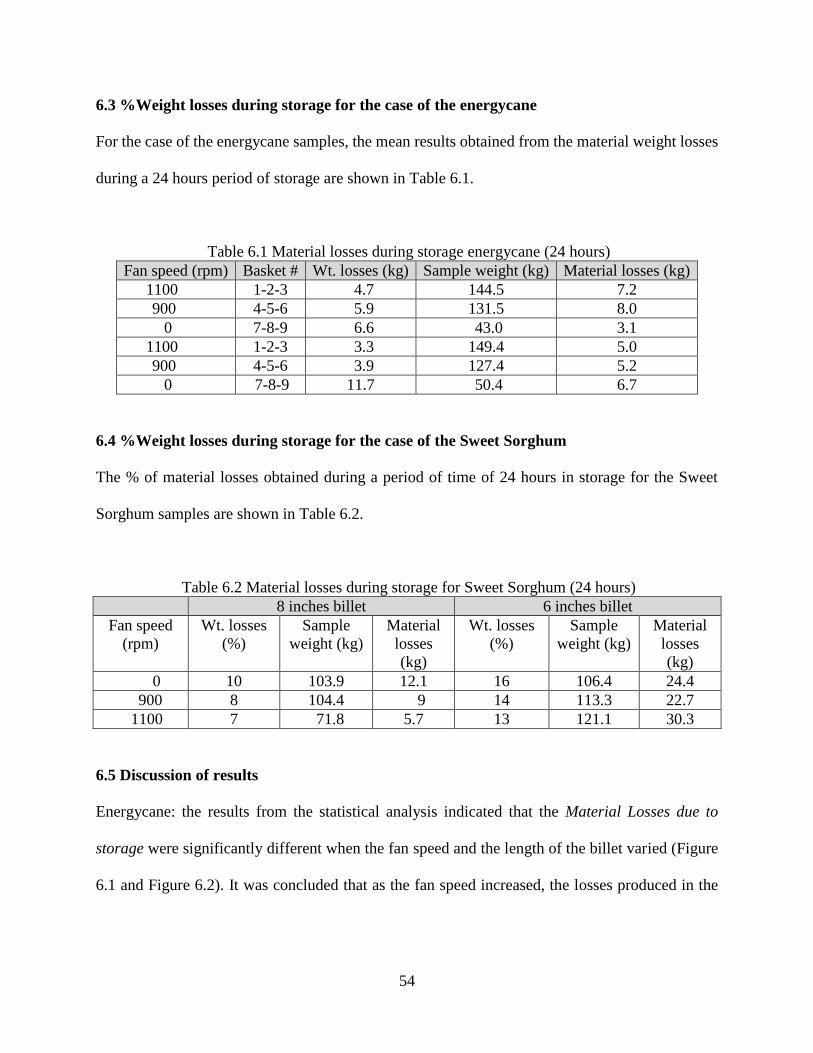
54

6.3 %Weight losses during storage for the case of the energycane

For the case of the energycane samples, the mean results obtained from the material weight losses

during a 24 hours period of storage are shown in Table 6.1.

Table 6.1 Material losses during storage energycane (24 hours)

Fan speed (rpm) Basket # Wt. losses (kg) Sample weight (kg) Material losses (kg)

1100 1-2-3 4.7 144.5 7.2

900 4-5-6 5.9 131.5 8.0

0 7-8-9 6.6 43.0 3.1

1100 1-2-3 3.3 149.4 5.0

900 4-5-6 3.9 127.4 5.2

0 7-8-9 11.7 50.4 6.7

6.4 %Weight losses during storage for the case of the Sweet Sorghum

The % of material losses obtained during a period of time of 24 hours in storage for the Sweet

Sorghum samples are shown in Table 6.2.

Table 6.2 Material losses during storage for Sweet Sorghum (24 hours)

8 inches billet 6 inches billet

Fan speed

(rpm)

Wt. losses

(%)

Sample

weight (kg)

Material

losses

(kg)

Wt. losses

(%)

Sample

weight (kg)

Material

losses

(kg)

0 10 103.9 12.1 16 106.4 24.4

900 8 104.4 9 14 113.3 22.7

1100 7 71.8 5.7 13 121.1 30.3

6.5 Discussion of results

Energycane: the results from the statistical analysis indicated that the Material Losses due to

storage were significantly different when the fan speed and the length of the billet varied (Figure

6.1 and Figure 6.2). It was concluded that as the fan speed increased, the losses produced in the

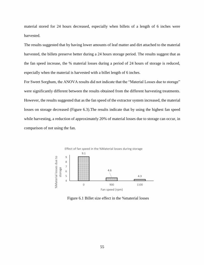
55

material stored for 24 hours decreased, especially when billets of a length of 6 inches were

harvested.

The results suggested that by having lower amounts of leaf matter and dirt attached to the material

harvested, the billets preserve better during a 24 hours storage period. The results suggest that as

the fan speed increase, the % material losses during a period of 24 hours of storage is reduced,

especially when the material is harvested with a billet length of 6 inches.

For Sweet Sorghum, the ANOVA results did not indicate that the “Material Losses due to storage”

were significantly different between the results obtained from the different harvesting treatments.

However, the results suggested that as the fan speed of the extractor system increased, the material

losses on storage decreased (Figure 6.3).The results indicate that by using the highest fan speed

while harvesting, a reduction of approximately 20% of material losses due to storage can occur, in

comparison of not using the fan.

Figure 6.1 Billet size effect in the %material losses

9.1

4.6

4.3

4

5

6

7

8

9

0 900 1100

%M

ater

ial l

oss

es d

ue

to

sto

rage

Fan speed (rpm)

Effect of fan speed in the %Material losses during storage

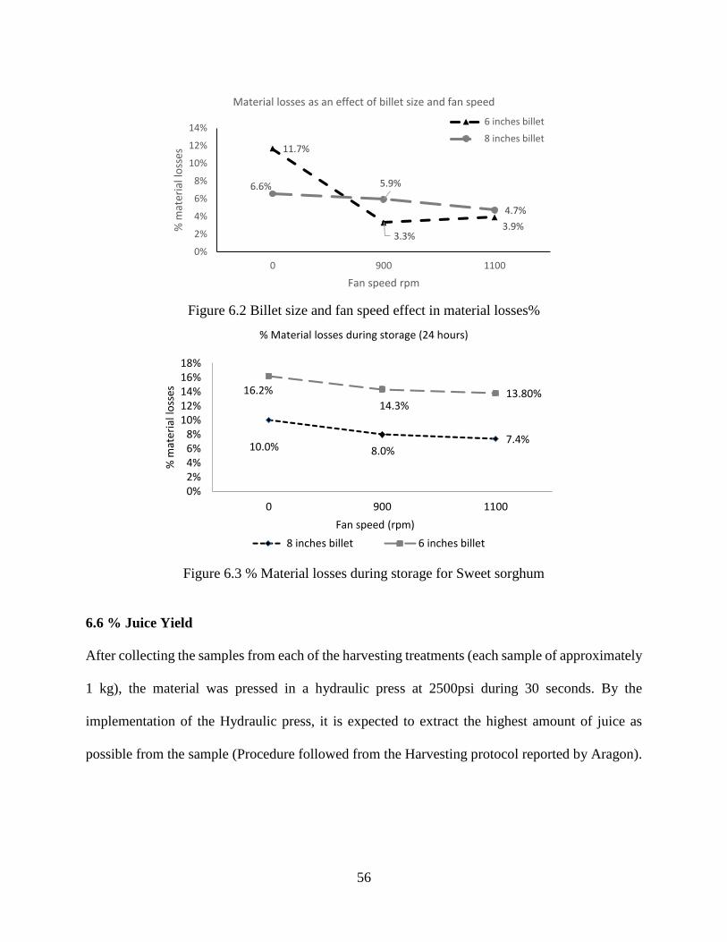
56

Figure 6.2 Billet size and fan speed effect in material losses%

Figure 6.3 % Material losses during storage for Sweet sorghum

6.6 % Juice Yield

After collecting the samples from each of the harvesting treatments (each sample of approximately

1 kg), the material was pressed in a hydraulic press at 2500psi during 30 seconds. By the

implementation of the Hydraulic press, it is expected to extract the highest amount of juice as

possible from the sample (Procedure followed from the Harvesting protocol reported by Aragon).

11.7%

3.3%3.9%

6.6% 5.9%

4.7%

0%

2%

4%

6%

8%

10%

12%

14%

0 900 1100

% m

ater

ial l

oss

es

Fan speed rpm

Material losses as an effect of billet size and fan speed

6 inches billet

8 inches billet

10.0% 8.0%7.4%

16.2%

14.3%13.80%

0%2%4%6%8%

10%12%14%16%18%

0 900 1100

% m

ater

ial l

oss

es

Fan speed (rpm)

% Material losses during storage (24 hours)

8 inches billet 6 inches billet

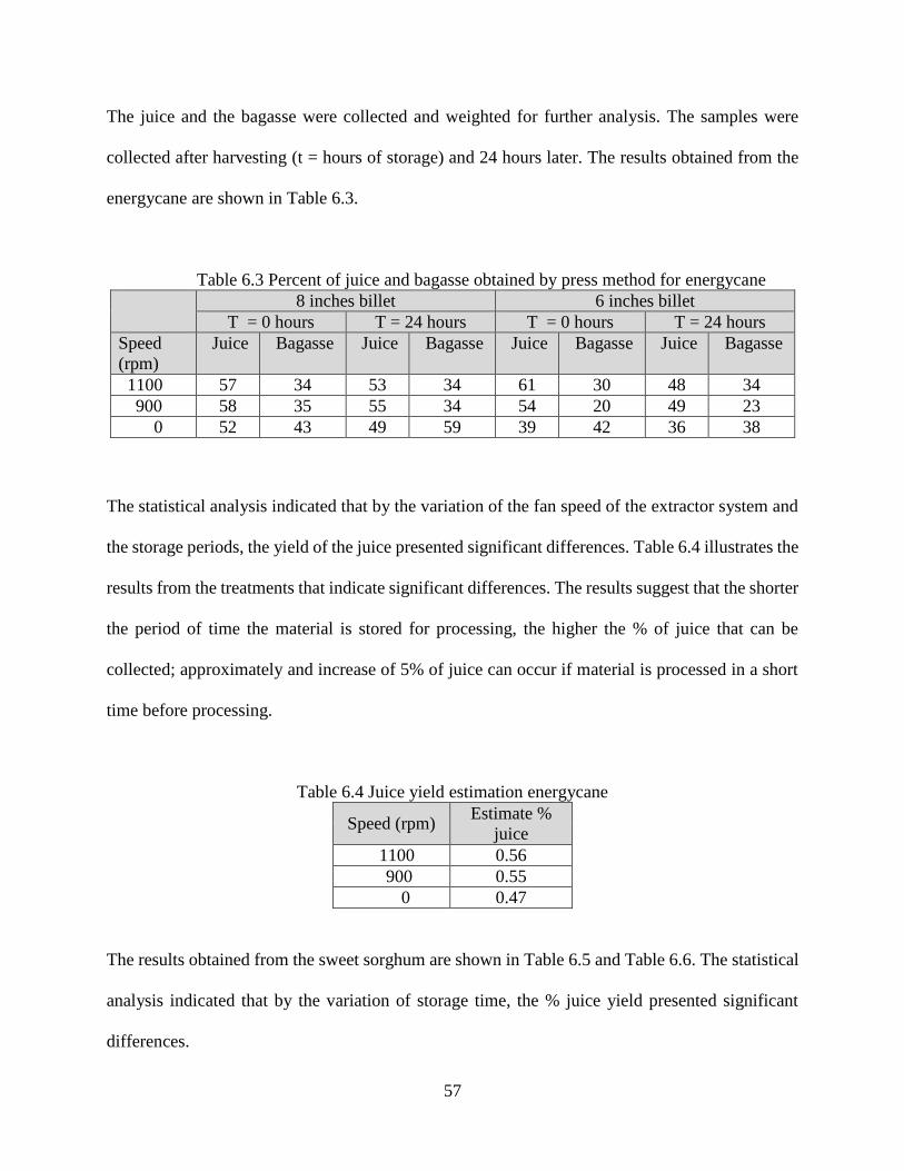
57

The juice and the bagasse were collected and weighted for further analysis. The samples were

collected after harvesting (t = hours of storage) and 24 hours later. The results obtained from the

energycane are shown in Table 6.3.

Table 6.3 Percent of juice and bagasse obtained by press method for energycane

8 inches billet 6 inches billet

T = 0 hours T = 24 hours T = 0 hours T = 24 hours

Speed

(rpm)

Juice Bagasse Juice Bagasse Juice Bagasse Juice Bagasse

1100 57 34 53 34 61 30 48 34

900 58 35 55 34 54 20 49 23

0 52 43 49 59 39 42 36 38

The statistical analysis indicated that by the variation of the fan speed of the extractor system and

the storage periods, the yield of the juice presented significant differences. Table 6.4 illustrates the

results from the treatments that indicate significant differences. The results suggest that the shorter

the period of time the material is stored for processing, the higher the % of juice that can be

collected; approximately and increase of 5% of juice can occur if material is processed in a short

time before processing.

Table 6.4 Juice yield estimation energycane

Speed (rpm) Estimate %

juice

1100 0.56

900 0.55

0 0.47

The results obtained from the sweet sorghum are shown in Table 6.5 and Table 6.6. The statistical

analysis indicated that by the variation of storage time, the % juice yield presented significant

differences.

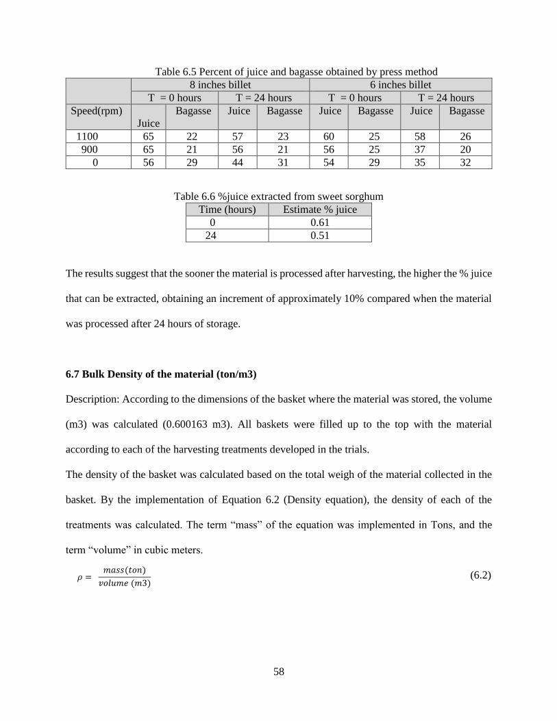
58

Table 6.5 Percent of juice and bagasse obtained by press method

8 inches billet 6 inches billet

T = 0 hours T = 24 hours T = 0 hours T = 24 hours

Speed(rpm)

Juice

Bagasse Juice Bagasse Juice Bagasse Juice Bagasse

1100 65 22 57 23 60 25 58 26

900 65 21 56 21 56 25 37 20

0 56 29 44 31 54 29 35 32

Table 6.6 %juice extracted from sweet sorghum

Time (hours) Estimate % juice

0 0.61

24 0.51

The results suggest that the sooner the material is processed after harvesting, the higher the % juice

that can be extracted, obtaining an increment of approximately 10% compared when the material

was processed after 24 hours of storage.

6.7 Bulk Density of the material (ton/m3)

Description: According to the dimensions of the basket where the material was stored, the volume

(m3) was calculated (0.600163 m3). All baskets were filled up to the top with the material

according to each of the harvesting treatments developed in the trials.

The density of the basket was calculated based on the total weigh of the material collected in the

basket. By the implementation of Equation 6.2 (Density equation), the density of each of the

treatments was calculated. The term “mass” of the equation was implemented in Tons, and the

term “volume” in cubic meters.

(6.2)

𝜌 = 𝑚𝑎𝑠𝑠(𝑡𝑜𝑛)

𝑣𝑜𝑙𝑢𝑚𝑒 (𝑚3)

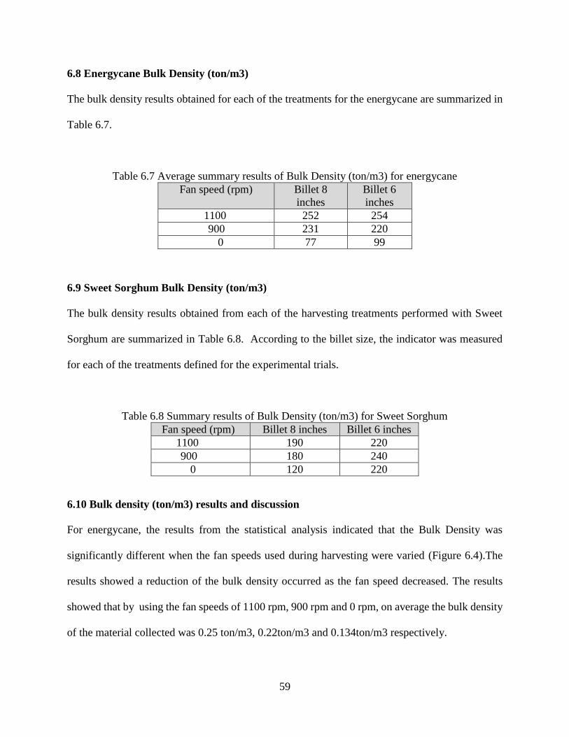
59

6.8 Energycane Bulk Density (ton/m3)

The bulk density results obtained for each of the treatments for the energycane are summarized in

Table 6.7.

Table 6.7 Average summary results of Bulk Density (ton/m3) for energycane

Fan speed (rpm) Billet 8

inches

Billet 6

inches

1100 252 254

900 231 220

0 77 99

6.9 Sweet Sorghum Bulk Density (ton/m3)

The bulk density results obtained from each of the harvesting treatments performed with Sweet

Sorghum are summarized in Table 6.8. According to the billet size, the indicator was measured

for each of the treatments defined for the experimental trials.

Table 6.8 Summary results of Bulk Density (ton/m3) for Sweet Sorghum

Fan speed (rpm) Billet 8 inches Billet 6 inches

1100 190 220

900 180 240

0 120 220

6.10 Bulk density (ton/m3) results and discussion

For energycane, the results from the statistical analysis indicated that the Bulk Density was

significantly different when the fan speeds used during harvesting were varied (Figure 6.4).The

results showed a reduction of the bulk density occurred as the fan speed decreased. The results

showed that by using the fan speeds of 1100 rpm, 900 rpm and 0 rpm, on average the bulk density

of the material collected was 0.25 ton/m3, 0.22ton/m3 and 0.134ton/m3 respectively.

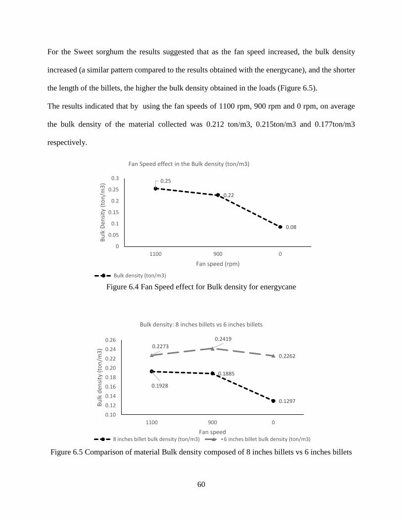
60

For the Sweet sorghum the results suggested that as the fan speed increased, the bulk density

increased (a similar pattern compared to the results obtained with the energycane), and the shorter

the length of the billets, the higher the bulk density obtained in the loads (Figure 6.5).

The results indicated that by using the fan speeds of 1100 rpm, 900 rpm and 0 rpm, on average

the bulk density of the material collected was 0.212 ton/m3, 0.215ton/m3 and 0.177ton/m3

respectively.

Figure 6.4 Fan Speed effect for Bulk density for energycane

Figure 6.5 Comparison of material Bulk density composed of 8 inches billets vs 6 inches billets

0.25

0.22

0.08

0

0.05

0.1

0.15

0.2

0.25

0.3

1100 900 0

Bu

lk D

ensi

ty (

ton

/m3

)

Fan speed (rpm)

Fan Speed effect in the Bulk density (ton/m3)

Bulk density (ton/m3)

0.1928

0.1885

0.1297

0.2273

0.2419

0.2262

0.10

0.12

0.14

0.16

0.18

0.20

0.22

0.24

0.26

1100 900 0

Bu

lk d

ensi

ty (

ton

/m3

)

Fan speed

Bulk density: 8 inches billets vs 6 inches billets

8 inches billet bulk density (ton/m3) 6 inches billet bulk density (ton/m3)

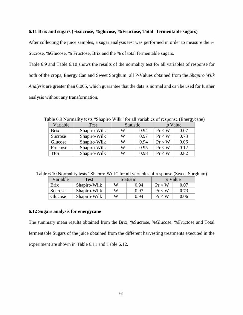
61

6.11 Brix and sugars (%sucrose, %glucose, %Fructose, Total fermentable sugars)

After collecting the juice samples, a sugar analysis test was performed in order to measure the %

Sucrose, %Glucose, % Fructose, Brix and the % of total fermentable sugars.

Table 6.9 and Table 6.10 shows the results of the normality test for all variables of response for

both of the crops, Energy Can and Sweet Sorghum; all P-Values obtained from the Shapiro Wilk

Analysis are greater than 0.005, which guarantee that the data is normal and can be used for further

analysis without any transformation.

Table 6.9 Normality tests “Shapiro Wilk” for all variables of response (Energycane)

Variable Test Statistic p Value

Brix Shapiro-Wilk W 0.94 Pr < W 0.07

Sucrose Shapiro-Wilk W 0.97 Pr < W 0.73

Glucose Shapiro-Wilk W 0.94 Pr < W 0.06

Fructose Shapiro-Wilk W 0.95 Pr < W 0.12

TFS Shapiro-Wilk W 0.98 Pr < W 0.82

Table 6.10 Normality tests “Shapiro Wilk” for all variables of response (Sweet Sorghum)

Variable Test Statistic p Value

Brix Shapiro-Wilk W 0.94 Pr < W 0.07

Sucrose Shapiro-Wilk W 0.97 Pr < W 0.73

Glucose Shapiro-Wilk W 0.94 Pr < W 0.06

6.12 Sugars analysis for energycane

The summary mean results obtained from the Brix, %Sucrose, %Glucose, %Fructose and Total

fermentable Sugars of the juice obtained from the different harvesting treatments executed in the

experiment are shown in Table 6.11 and Table 6.12.

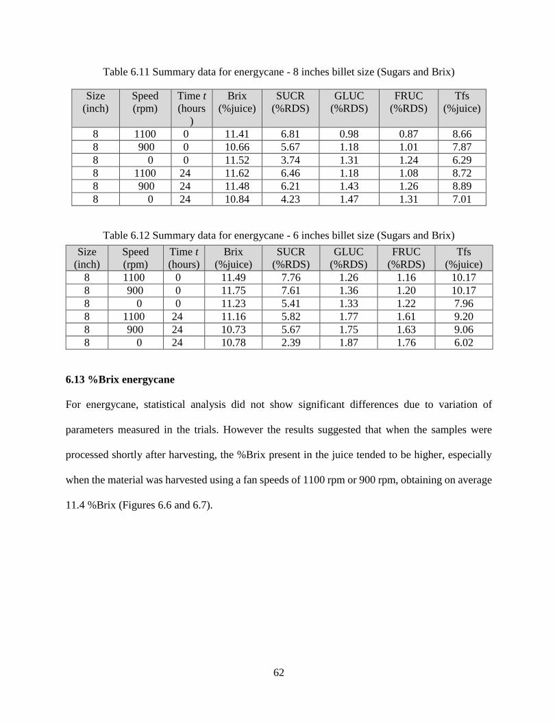
62

Table 6.11 Summary data for energycane - 8 inches billet size (Sugars and Brix)

Size

(inch)

Speed

(rpm)

Time t

(hours

)

Brix

(%juice)

SUCR

(%RDS)

GLUC

(%RDS)

FRUC

(%RDS)

Tfs

(%juice)

8 1100 0 11.41 6.81 0.98 0.87 8.66

8 900 0 10.66 5.67 1.18 1.01 7.87

8 0 0 11.52 3.74 1.31 1.24 6.29

8 1100 24 11.62 6.46 1.18 1.08 8.72

8 900 24 11.48 6.21 1.43 1.26 8.89

8 0 24 10.84 4.23 1.47 1.31 7.01

Table 6.12 Summary data for energycane - 6 inches billet size (Sugars and Brix)

6.13 %Brix energycane

For energycane, statistical analysis did not show significant differences due to variation of

parameters measured in the trials. However the results suggested that when the samples were

processed shortly after harvesting, the %Brix present in the juice tended to be higher, especially

when the material was harvested using a fan speeds of 1100 rpm or 900 rpm, obtaining on average

11.4 %Brix (Figures 6.6 and 6.7).

Size

(inch)

Speed

(rpm)

Time t

(hours)

Brix

(%juice)

SUCR

(%RDS)

GLUC

(%RDS)

FRUC

(%RDS)

Tfs

(%juice)

8 1100 0 11.49 7.76 1.26 1.16 10.17

8 900 0 11.75 7.61 1.36 1.20 10.17

8 0 0 11.23 5.41 1.33 1.22 7.96

8 1100 24 11.16 5.82 1.77 1.61 9.20

8 900 24 10.73 5.67 1.75 1.63 9.06

8 0 24 10.78 2.39 1.87 1.76 6.02

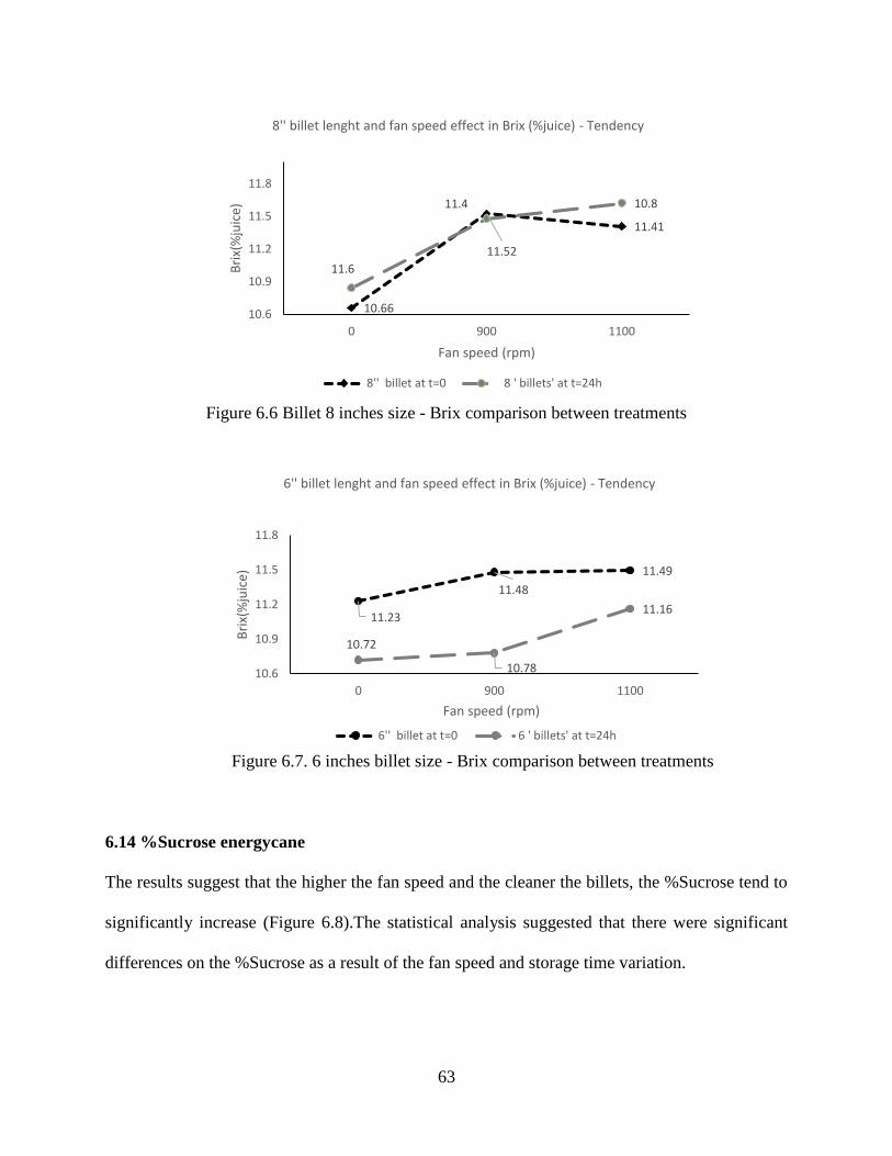
63

Figure 6.6 Billet 8 inches size - Brix comparison between treatments

Figure 6.7. 6 inches billet size - Brix comparison between treatments

6.14 %Sucrose energycane

The results suggest that the higher the fan speed and the cleaner the billets, the %Sucrose tend to

significantly increase (Figure 6.8).The statistical analysis suggested that there were significant

differences on the %Sucrose as a result of the fan speed and storage time variation.

10.66

11.52

11.41

11.6

11.4 10.8

10.6

10.9

11.2

11.5

11.8

0 900 1100

Bri

x(%

juic

e)

Fan speed (rpm)

8'' billet lenght and fan speed effect in Brix (%juice) - Tendency

8'' billet at t=0 8 ' billets' at t=24h

11.23

11.48

11.49

10.72

10.78

11.16

10.6

10.9

11.2

11.5

11.8

0 900 1100

Bri

x(%

juic

e)

Fan speed (rpm)

6'' billet lenght and fan speed effect in Brix (%juice) - Tendency

6'' billet at t=0 6 ' billets' at t=24h

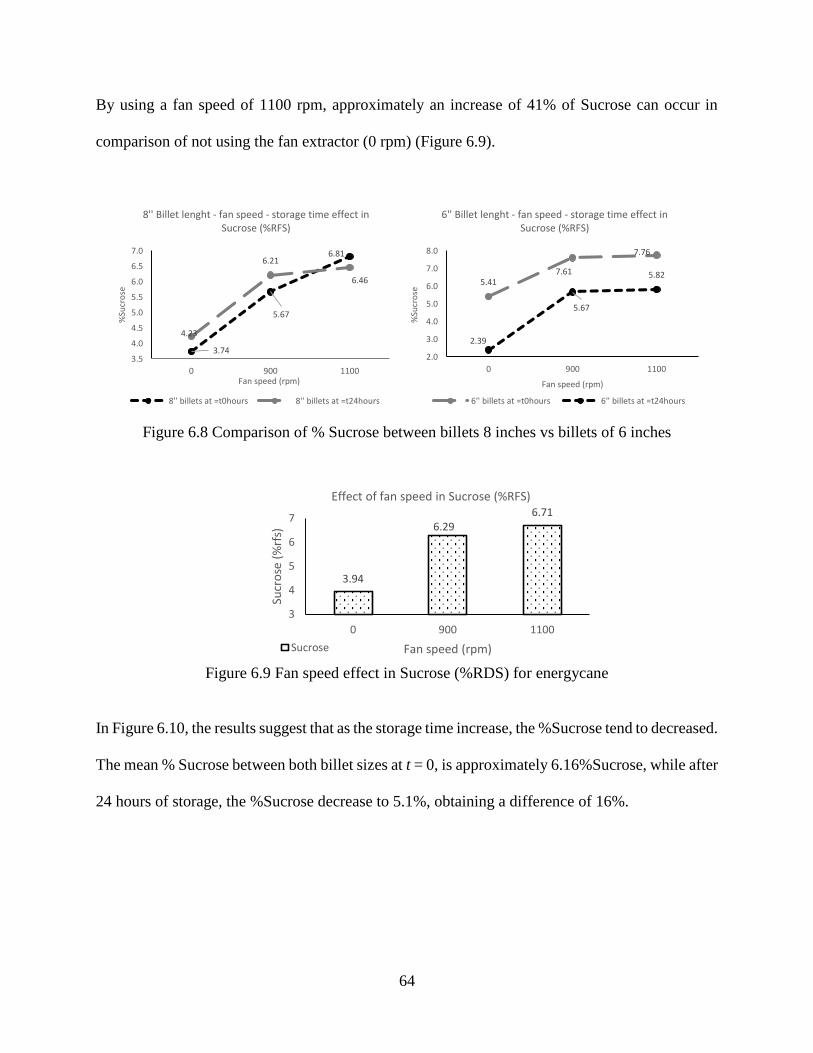
64

By using a fan speed of 1100 rpm, approximately an increase of 41% of Sucrose can occur in

comparison of not using the fan extractor (0 rpm) (Figure 6.9).

Figure 6.8 Comparison of % Sucrose between billets 8 inches vs billets of 6 inches

Figure 6.9 Fan speed effect in Sucrose (%RDS) for energycane

In Figure 6.10, the results suggest that as the storage time increase, the %Sucrose tend to decreased.

The mean % Sucrose between both billet sizes at t = 0, is approximately 6.16%Sucrose, while after

24 hours of storage, the %Sucrose decrease to 5.1%, obtaining a difference of 16%.

3.94

6.296.71

3

4

5

6

7

0 900 1100

Sucr

ose

(%

rfs)

Fan speed (rpm)

Effect of fan speed in Sucrose (%RFS)

Sucrose

3.74

5.67

6.81

4.23

6.21

6.46

3.5

4.0

4.5

5.0

5.5

6.0

6.5

7.0

0 900 1100

%Su

cro

se

Fan speed (rpm)

8'' Billet lenght - fan speed - storage time effect in Sucrose (%RFS)

8'' billets at =t0hours 8'' billets at =t24hours

5.417.61

7.76

2.39

5.67

5.82

2.0

3.0

4.0

5.0

6.0

7.0

8.0

0 900 1100

%Su

cro

se

Fan speed (rpm)

6'' Billet lenght - fan speed - storage time effect in Sucrose (%RFS)

6'' billets at =t0hours 6'' billets at =t24hours

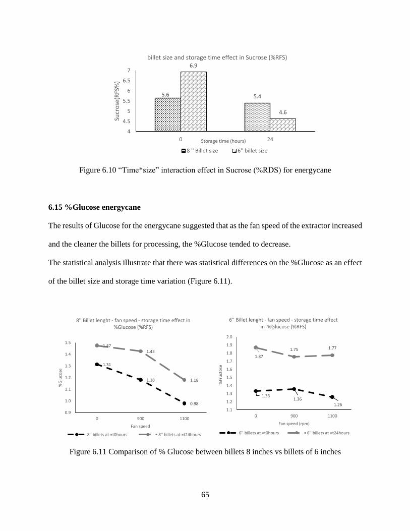
65

Figure 6.10 “Time*size” interaction effect in Sucrose (%RDS) for energycane

6.15 %Glucose energycane

The results of Glucose for the energycane suggested that as the fan speed of the extractor increased

and the cleaner the billets for processing, the %Glucose tended to decrease.

The statistical analysis illustrate that there was statistical differences on the %Glucose as an effect

of the billet size and storage time variation (Figure 6.11).

Figure 6.11 Comparison of % Glucose between billets 8 inches vs billets of 6 inches

5.6 5.4

6.9

4.6

4

4.5

5

5.5

6

6.5

7

0 24

Sucr

ose

(RFS

%)

Storage time (hours)

billet size and storage time effect in Sucrose (%RFS)

8 '' Billet size 6'' billet size

1.31

1.18

0.98

1.471.43

1.18

0.9

1.0

1.1

1.2

1.3

1.4

1.5

0 900 1100

%G

luco

se

Fan speed

8'' Billet lenght - fan speed - storage time effect in %Glucose (%RFS)

8'' billets at =t0hours 8'' billets at =t24hours

1.331.36

1.26

1.87

1.75 1.77

1.1

1.2

1.3

1.4

1.5

1.6

1.7

1.8

1.9

2.0

0 900 1100

%Fr

uct

ose

Fan speed (rpm)

6'' Billet lenght - fan speed - storage time effect in %Glucose (%RFS)

6'' billets at =t0hours 6'' billets at =t24hours

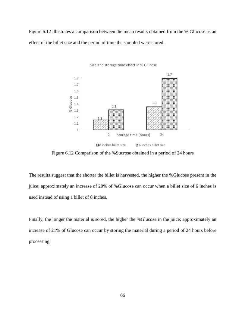
66

Figure 6.12 illustrates a comparison between the mean results obtained from the % Glucose as an

effect of the billet size and the period of time the sampled were stored.

Figure 6.12 Comparison of the %Sucrose obtained in a period of 24 hours

The results suggest that the shorter the billet is harvested, the higher the %Glucose present in the

juice; approximately an increase of 20% of %Glucose can occur when a billet size of 6 inches is

used instead of using a billet of 8 inches.

Finally, the longer the material is sored, the higher the %Glucose in the juice; approximately an

increase of 21% of Glucose can occur by storing the material during a period of 24 hours before

processing.

1.1

1.31.3

1.7

1

1.1

1.2

1.3

1.4

1.5

1.6

1.7

1.8

0 24

% G

luco

se

Storage time (hours)

Size and storage time effect in % Glucose

8 inches billet size 6 inches billet size

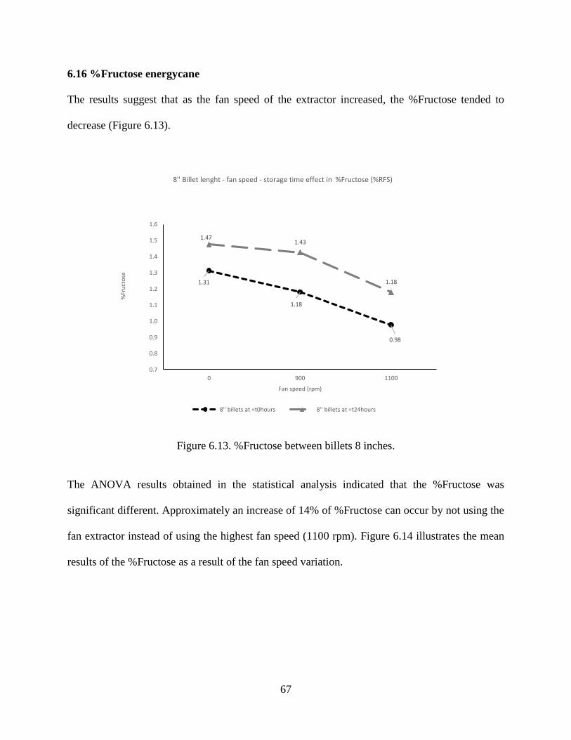
67

6.16 %Fructose energycane

The results suggest that as the fan speed of the extractor increased, the %Fructose tended to

decrease (Figure 6.13).

Figure 6.13. %Fructose between billets 8 inches.

The ANOVA results obtained in the statistical analysis indicated that the %Fructose was

significant different. Approximately an increase of 14% of %Fructose can occur by not using the

fan extractor instead of using the highest fan speed (1100 rpm). Figure 6.14 illustrates the mean

results of the %Fructose as a result of the fan speed variation.

1.31

1.18

0.98

1.471.43

1.18

0.7

0.8

0.9

1.0

1.1

1.2

1.3

1.4

1.5

1.6

0 900 1100

%Fr

uct

ose

Fan speed (rpm)

8'' Billet lenght - fan speed - storage time effect in %Fructose (%RFS)

8'' billets at =t0hours 8'' billets at =t24hours

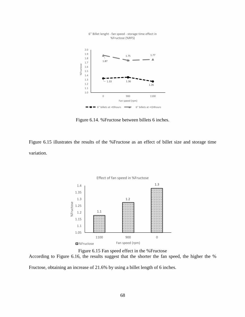
68

Figure 6.14. %Fructose between billets 6 inches.

Figure 6.15 illustrates the results of the %Fructose as an effect of billet size and storage time

variation.

Figure 6.15 Fan speed effect in the %Fructose

According to Figure 6.16, the results suggest that the shorter the fan speed, the higher the %

Fructose, obtaining an increase of 21.6% by using a billet length of 6 inches.

1.33 1.361.26

1.87

1.75 1.77

1.0

1.1

1.2

1.3

1.4

1.5

1.6

1.7

1.8

1.9

2.0

0 900 1100

%Fr

uct

ose

Fan speed (rpm)

6'' Billet lenght - fan speed - storage time effect in %Fructose (%RFS)

6'' billets at =t0hours 6'' billets at =t24hours

1.1

1.2

1.3

1.05

1.1

1.15

1.2

1.25

1.3

1.35

1.4

1100 900 0

%Fr

uct

ose

Fan speed (rpm)

Effect of fan speed in %Fructose

%Fructose

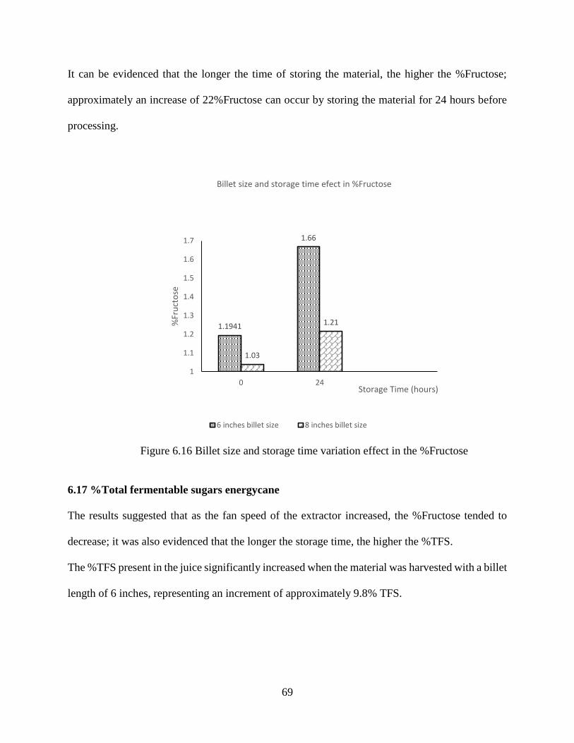
69

It can be evidenced that the longer the time of storing the material, the higher the %Fructose;

approximately an increase of 22%Fructose can occur by storing the material for 24 hours before

processing.

Figure 6.16 Billet size and storage time variation effect in the %Fructose

6.17 %Total fermentable sugars energycane

The results suggested that as the fan speed of the extractor increased, the %Fructose tended to

decrease; it was also evidenced that the longer the storage time, the higher the %TFS.

The %TFS present in the juice significantly increased when the material was harvested with a billet

length of 6 inches, representing an increment of approximately 9.8% TFS.

1.1941

1.66

1.03

1.21

1

1.1

1.2

1.3

1.4

1.5

1.6

1.7

0 24

%Fr

uct

ose

Storage Time (hours)

Billet size and storage time efect in %Fructose

6 inches billet size 8 inches billet size

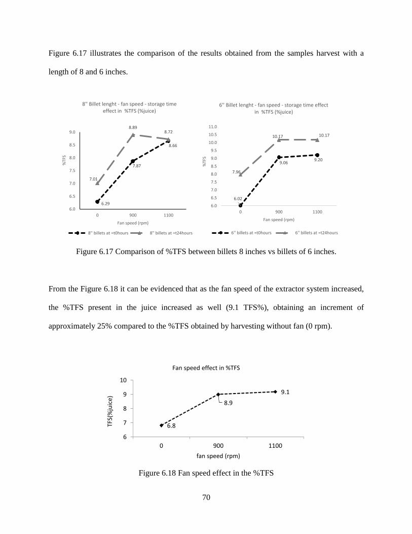
70

Figure 6.17 illustrates the comparison of the results obtained from the samples harvest with a

length of 8 and 6 inches.

Figure 6.17 Comparison of %TFS between billets 8 inches vs billets of 6 inches.

From the Figure 6.18 it can be evidenced that as the fan speed of the extractor system increased,

the %TFS present in the juice increased as well (9.1 TFS%), obtaining an increment of

approximately 25% compared to the %TFS obtained by harvesting without fan (0 rpm).

Figure 6.18 Fan speed effect in the %TFS

6.8

8.9

9.1

6

7

8

9

10

0 900 1100

TFS(

%ju

ice)

fan speed (rpm)

Fan speed effect in %TFS

6.29

7.87

8.66

7.01

8.898.72

6.0

6.5

7.0

7.5

8.0

8.5

9.0

0 900 1100

%TF

S

Fan speed (rpm)

8'' Billet lenght - fan speed - storage time effect in %TFS (%juice)

8'' billets at =t0hours 8'' billets at =t24hours

6.02

9.069.20

7.96

10.17 10.17

6.0

6.5

7.0

7.5

8.0

8.5

9.0

9.5

10.0

10.5

11.0

0 900 1100

%TF

S

Fan speed (rpm)

6'' Billet lenght - fan speed - storage time effect in %TFS (%juice)

6'' billets at =t0hours 6'' billets at =t24hours

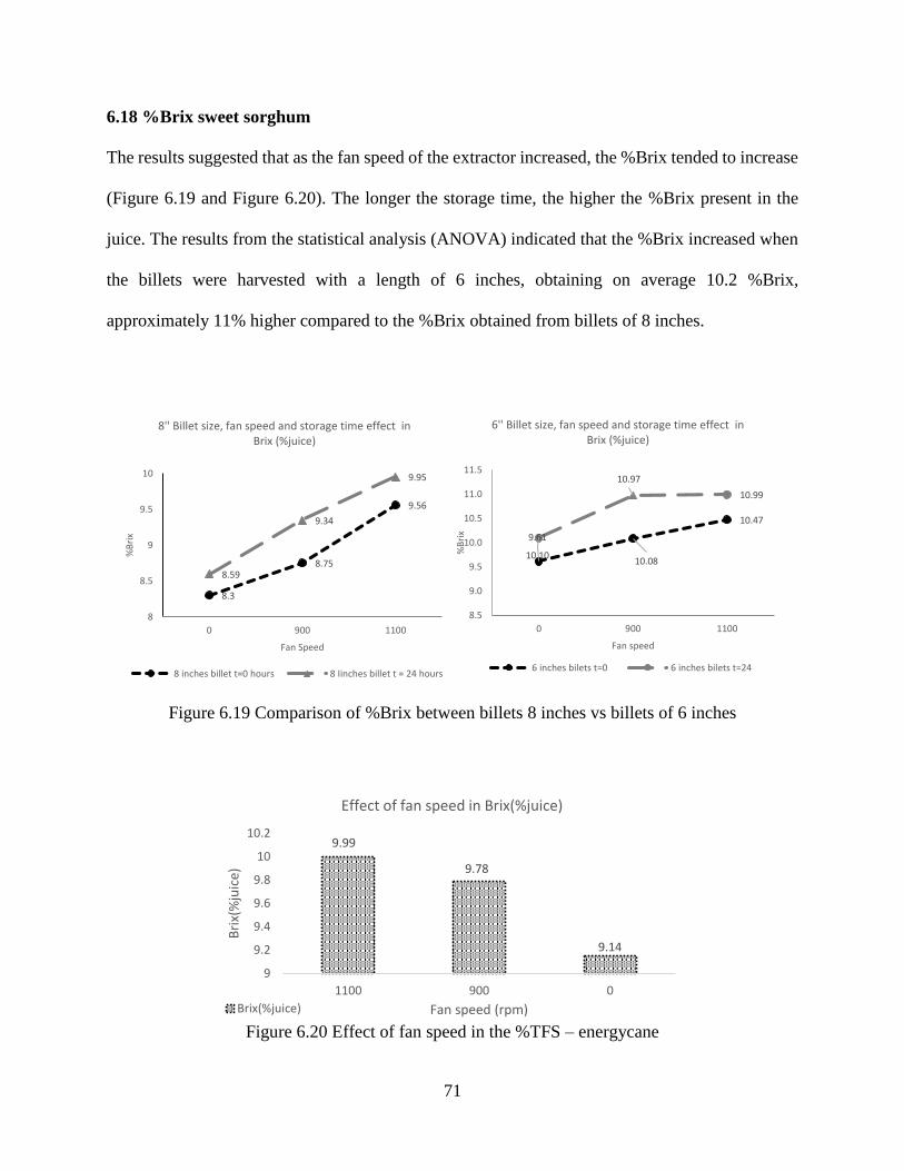
71

6.18 %Brix sweet sorghum

The results suggested that as the fan speed of the extractor increased, the %Brix tended to increase

(Figure 6.19 and Figure 6.20). The longer the storage time, the higher the %Brix present in the

juice. The results from the statistical analysis (ANOVA) indicated that the %Brix increased when

the billets were harvested with a length of 6 inches, obtaining on average 10.2 %Brix,

approximately 11% higher compared to the %Brix obtained from billets of 8 inches.

Figure 6.19 Comparison of %Brix between billets 8 inches vs billets of 6 inches

Figure 6.20 Effect of fan speed in the %TFS – energycane

9.99

9.78

9.14

9

9.2

9.4

9.6

9.8

10

10.2

1100 900 0

Bri

x(%

juic

e)

Fan speed (rpm)

Effect of fan speed in Brix(%juice)

Brix(%juice)

8.3

8.75

9.56

8.59

9.34

9.95

8

8.5

9

9.5

10

0 900 1100

%B

rix

Fan Speed

8'' Billet size, fan speed and storage time effect in Brix (%juice)

8 inches billet t=0 hours 8 Iinches billet t = 24 hours

9.61

10.08

10.47

10.10

10.97

10.99

8.5

9.0

9.5

10.0

10.5

11.0

11.5

0 900 1100

%B

rix

Fan speed

6'' Billet size, fan speed and storage time effect in Brix (%juice)

6 inches bilets t=0 6 inches bilets t=24

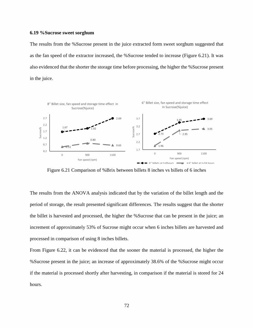
72

6.19 %Sucrose sweet sorghum

The results from the %Sucrose present in the juice extracted form sweet sorghum suggested that

as the fan speed of the extractor increased, the %Sucrose tended to increase (Figure 6.21). It was

also evidenced that the shorter the storage time before processing, the higher the %Sucrose present

in the juice.

Figure 6.21 Comparison of %Brix between billets 8 inches vs billets of 6 inches

The results from the ANOVA analysis indicated that by the variation of the billet length and the

period of storage, the result presented significant differences. The results suggest that the shorter

the billet is harvested and processed, the higher the %Sucrose that can be present in the juice; an

increment of approximately 53% of Sucrose might occur when 6 inches billets are harvested and

processed in comparison of using 8 inches billets.

From Figure 6.22, it can be evidenced that the sooner the material is processed, the higher the

%Sucrose present in the juice; an increase of approximately 38.6% of the %Sucrose might occur

if the material is processed shortly after harvesting, in comparison if the material is stored for 24

hours.

1.67 1.92

2.69

0.53

0.80

0.65

0.2

0.7

1.2

1.7

2.2

2.7

0 900 1100

Sucr

ose

%

Fan speed (rpm)

8'' Billet size, fan speed and storage time effect in Sucrose(%juice)

8'' billets at t=0hours 8'' billet at t=24 hours

2.73

3.45 3.69

1.96

2.95

3.05

1.7

2.2

2.7

3.2

3.7

0 900 1100

Sucr

ose

%

Fan speed (rpm)

6'' Billet size, fan speed and storage time effect in Sucrose(%juice)

6'' billets at t=0hours 6'' billet at t=24 hours

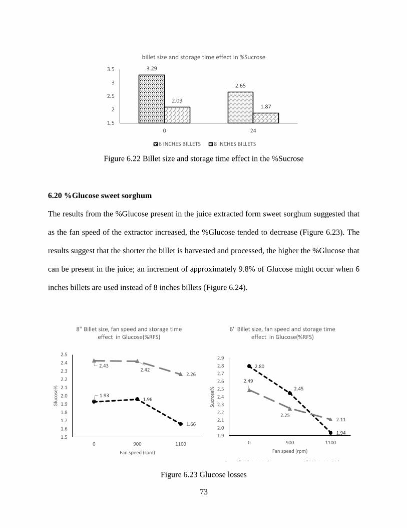
73

Figure 6.22 Billet size and storage time effect in the %Sucrose

6.20 %Glucose sweet sorghum

The results from the %Glucose present in the juice extracted form sweet sorghum suggested that

as the fan speed of the extractor increased, the %Glucose tended to decrease (Figure 6.23). The

results suggest that the shorter the billet is harvested and processed, the higher the %Glucose that

can be present in the juice; an increment of approximately 9.8% of Glucose might occur when 6

inches billets are used instead of 8 inches billets (Figure 6.24).

Figure 6.23. Sucrose differences between billet sizes

Figure 6.23 Glucose losses

3.29

2.65

2.091.87

1.5

2

2.5

3

3.5

0 24

billet size and storage time effect in %Sucrose

6 INCHES BILLETS 8 INCHES BILLETS

1.931.96

1.66

2.432.42

2.26

1.5

1.6

1.7

1.8

1.9

2.0

2.1

2.2

2.3

2.4

2.5

0 900 1100

Glu

cose

%

Fan speed (rpm)

8'' Billet size, fan speed and storage time effect in Glucose(%RFS)

8'' billets at t=0hours 8'' billet at t=24 hours

2.80

2.45

1.94

2.49

2.252.11

1.9

2.0

2.1

2.2

2.3

2.4

2.5

2.6

2.7

2.8

2.9

0 900 1100

Sucr

ose

%

Fan speed (rpm)

6'' Billet size, fan speed and storage time effect in Glucose(%RFS)

6'' billets at t=0hours 6'' billet at t=24 hours

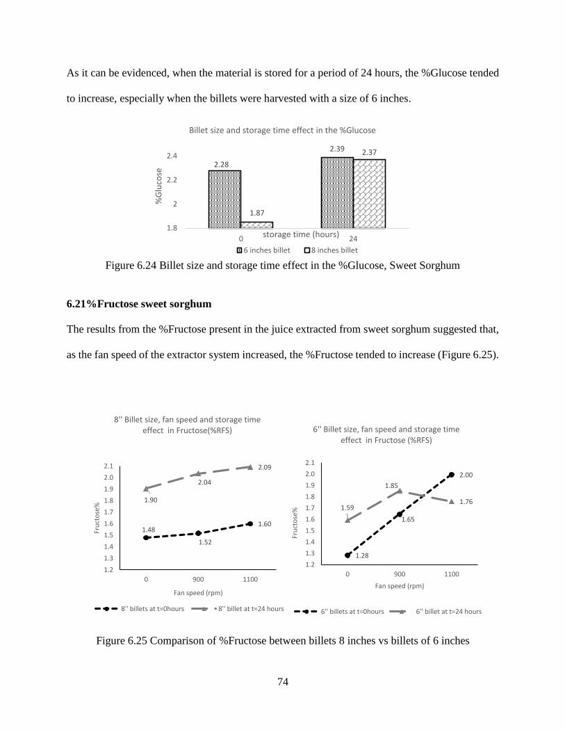
74

As it can be evidenced, when the material is stored for a period of 24 hours, the %Glucose tended

to increase, especially when the billets were harvested with a size of 6 inches.

Figure 6.24 Billet size and storage time effect in the %Glucose, Sweet Sorghum

6.21%Fructose sweet sorghum

The results from the %Fructose present in the juice extracted from sweet sorghum suggested that,

as the fan speed of the extractor system increased, the %Fructose tended to increase (Figure 6.25).

Figure 6.25 Comparison of %Fructose between billets 8 inches vs billets of 6 inches

2.28

2.39

1.87

2.37

1.8

2

2.2

2.4

0 24

%G

luco

se

storage time (hours)

Billet size and storage time effect in the %Glucose

6 inches billet 8 inches billet

1.48

1.52

1.60

1.90

2.04

2.09

1.2

1.3

1.4

1.5

1.6

1.7

1.8

1.9

2.0

2.1

0 900 1100

Fru

cto

se%

Fan speed (rpm)

8'' Billet size, fan speed and storage time effect in Fructose(%RFS)

8'' billets at t=0hours 8'' billet at t=24 hours

1.28

1.65

2.00

1.59

1.85

1.76

1.2

1.3

1.4

1.5

1.6

1.7

1.8

1.9

2.0

2.1

0 900 1100

Fru

cto

se%

Fan speed (rpm)

6'' Billet size, fan speed and storage time effect in Fructose (%RFS)

6'' billets at t=0hours 6'' billet at t=24 hours

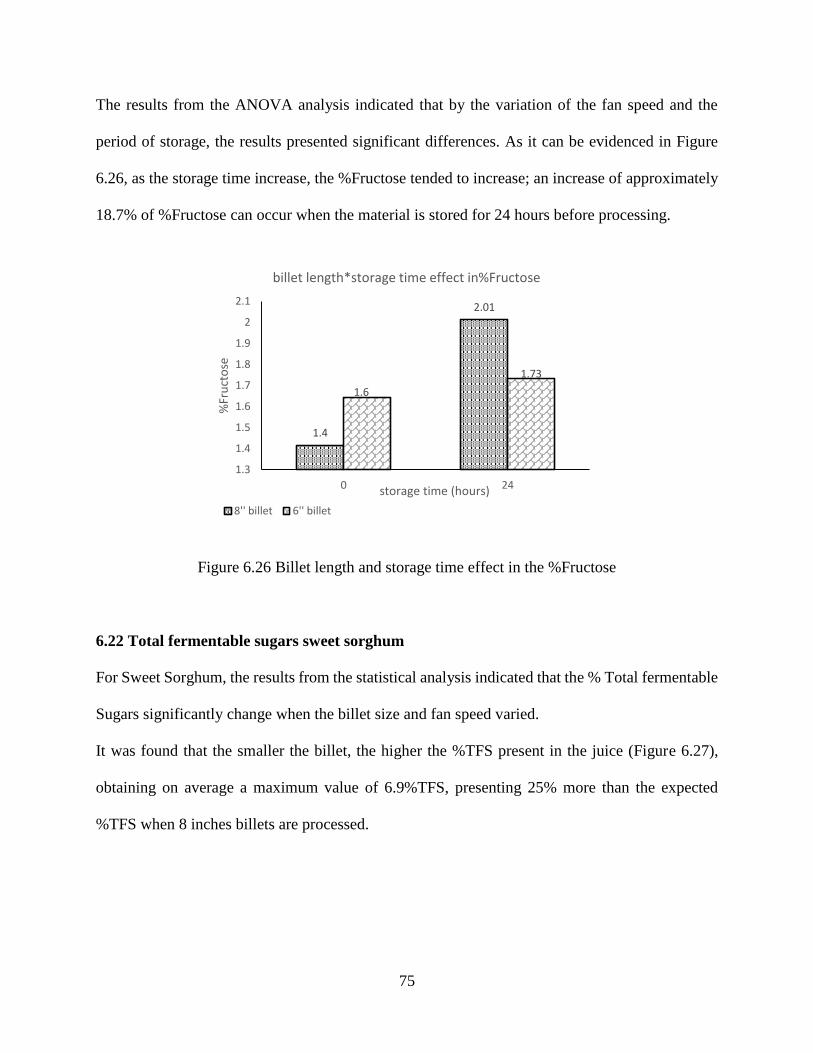
75

The results from the ANOVA analysis indicated that by the variation of the fan speed and the

period of storage, the results presented significant differences. As it can be evidenced in Figure

6.26, as the storage time increase, the %Fructose tended to increase; an increase of approximately

18.7% of %Fructose can occur when the material is stored for 24 hours before processing.

Figure 6.26 Billet length and storage time effect in the %Fructose

6.22 Total fermentable sugars sweet sorghum

For Sweet Sorghum, the results from the statistical analysis indicated that the % Total fermentable

Sugars significantly change when the billet size and fan speed varied.

It was found that the smaller the billet, the higher the %TFS present in the juice (Figure 6.27),

obtaining on average a maximum value of 6.9%TFS, presenting 25% more than the expected

%TFS when 8 inches billets are processed.

1.4

2.01

1.6

1.73

1.3

1.4

1.5

1.6

1.7

1.8

1.9

2

2.1

0 24

%Fr

uct

ose

storage time (hours)

billet length*storage time effect in%Fructose

8'' billet 6'' billet

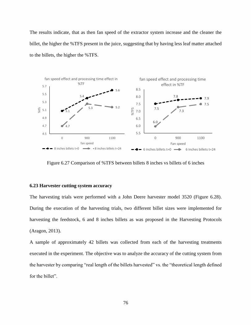
76

The results indicate, that as then fan speed of the extractor system increase and the cleaner the

billet, the higher the %TFS present in the juice, suggesting that by having less leaf matter attached

to the billets, the higher the %TFS.

Figure 6.27 Comparison of %TFS between billets 8 inches vs billets of 6 inches

6.23 Harvester cutting system accuracy

The harvesting trials were performed with a John Deere harvester model 3520 (Figure 6.28).

During the execution of the harvesting trials, two different billet sizes were implemented for

harvesting the feedstock, 6 and 8 inches billets as was proposed in the Harvesting Protocols

(Aragon, 2013).

A sample of approximately 42 billets was collected from each of the harvesting treatments

executed in the experiment. The objective was to analyze the accuracy of the cutting system from

the harvester by comparing “real length of the billets harvested” vs. the “theoretical length defined

for the billet”.

5.1

5.4

5.6

4.7

5.3 5.2

4.5

4.7

4.9

5.1

5.3

5.5

5.7

0 900 1100

%tf

s

fan speed

fan speed effect and processing time effect in %TF

8 inches billets t=0 8 inches billets t=24

7.5

7.87.9

6.0

7.3

7.5

5.5

6.0

6.5

7.0

7.5

8.0

8.5

0 900 1100

%TF

S

Fan speed

fan speed effect and processing time effect in %TF

6 inches billets t=0 6 inches billets t=24

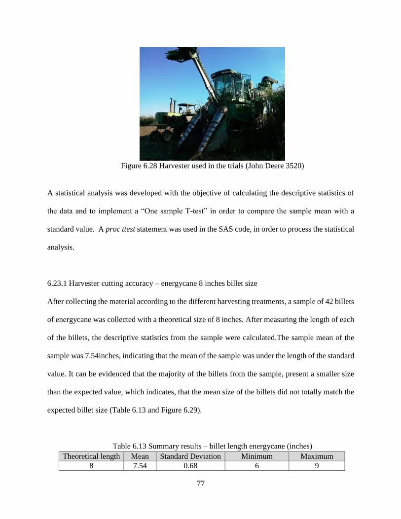
77

Figure 6.28 Harvester used in the trials (John Deere 3520)

A statistical analysis was developed with the objective of calculating the descriptive statistics of

the data and to implement a “One sample T-test” in order to compare the sample mean with a

standard value. A proc ttest statement was used in the SAS code, in order to process the statistical

analysis.

6.23.1 Harvester cutting accuracy – energycane 8 inches billet size

After collecting the material according to the different harvesting treatments, a sample of 42 billets

of energycane was collected with a theoretical size of 8 inches. After measuring the length of each

of the billets, the descriptive statistics from the sample were calculated.The sample mean of the

sample was 7.54inches, indicating that the mean of the sample was under the length of the standard

value. It can be evidenced that the majority of the billets from the sample, present a smaller size

than the expected value, which indicates, that the mean size of the billets did not totally match the

expected billet size (Table 6.13 and Figure 6.29).

Table 6.13 Summary results – billet length energycane (inches)

Theoretical length Mean Standard Deviation Minimum Maximum

8 7.54 0.68 6 9

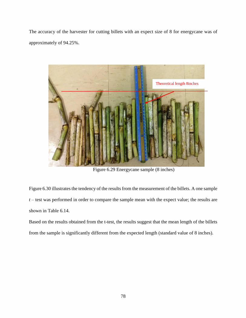
78

The accuracy of the harvester for cutting billets with an expect size of 8 for energycane was of

approximately of 94.25%.

Figure 6.30 illustrates the tendency of the results from the measurement of the billets. A one sample

t – test was performed in order to compare the sample mean with the expect value; the results are

shown in Table 6.14.

Based on the results obtained from the t-test, the results suggest that the mean length of the billets

from the sample is significantly different from the expected length (standard value of 8 inches).

Figure 6.29 Energycane sample (8 inches)

Theoretical length 8inches

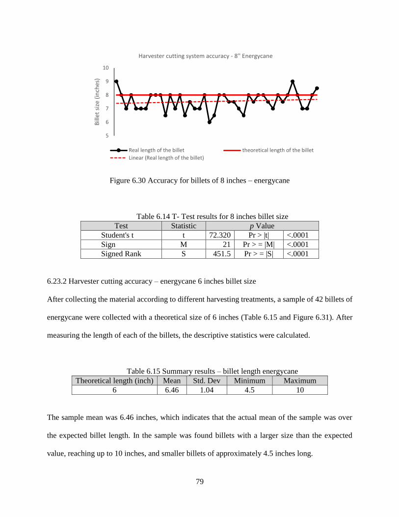
79

Figure 6.30 Accuracy for billets of 8 inches – energycane

Table 6.14 T- Test results for 8 inches billet size

Test Statistic p Value

Student's t t 72.320 Pr > |t| <.0001

Sign M 21 Pr > = |M| <.0001

Signed Rank S 451.5 Pr > = |S| <.0001

6.23.2 Harvester cutting accuracy – energycane 6 inches billet size

After collecting the material according to different harvesting treatments, a sample of 42 billets of

energycane were collected with a theoretical size of 6 inches (Table 6.15 and Figure 6.31). After

measuring the length of each of the billets, the descriptive statistics were calculated.

Table 6.15 Summary results – billet length energycane

Theoretical length (inch) Mean Std. Dev Minimum Maximum

6 6.46 1.04 4.5 10

The sample mean was 6.46 inches, which indicates that the actual mean of the sample was over

the expected billet length. In the sample was found billets with a larger size than the expected

value, reaching up to 10 inches, and smaller billets of approximately 4.5 inches long.

5

6

7

8

9

10

Bill

et s

ize

(in

ches

)

Harvester cutting system accuracy - 8'' Energycane

Real length of the billet theoretical length of the billet

Linear (Real length of the billet)

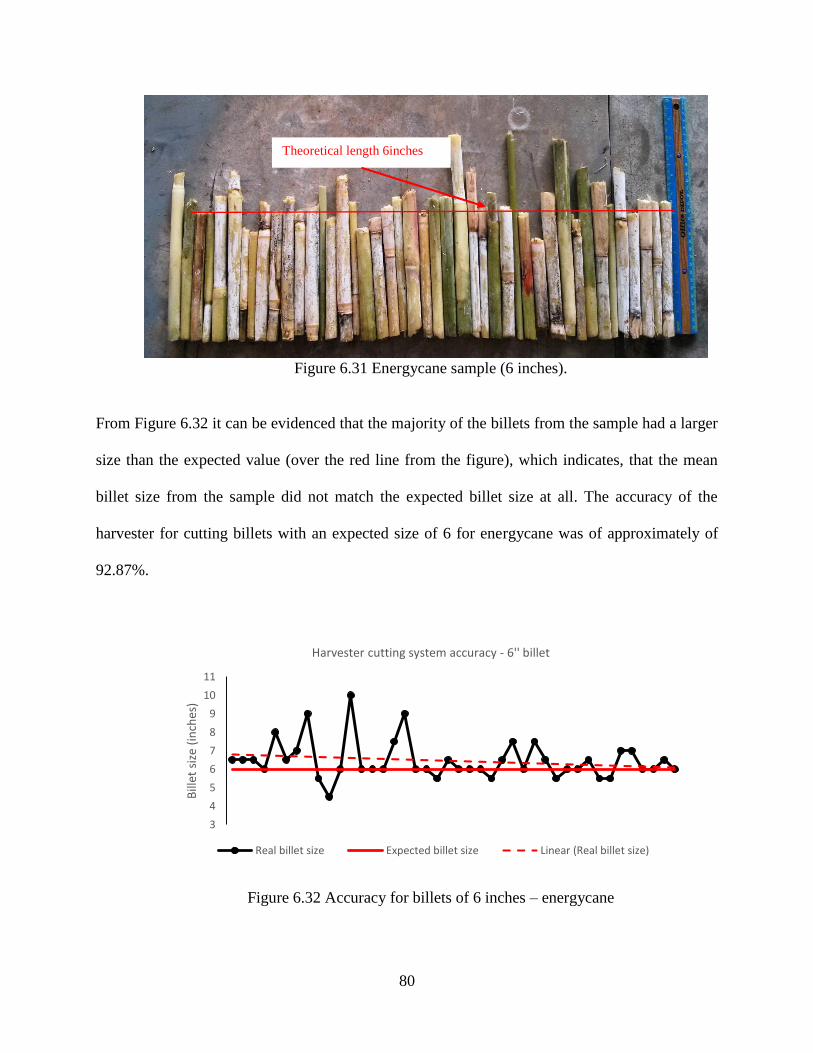
80

Figure 6.31 Energycane sample (6 inches).

From Figure 6.32 it can be evidenced that the majority of the billets from the sample had a larger

size than the expected value (over the red line from the figure), which indicates, that the mean

billet size from the sample did not match the expected billet size at all. The accuracy of the

harvester for cutting billets with an expected size of 6 for energycane was of approximately of

92.87%.

Figure 6.32 Accuracy for billets of 6 inches – energycane

3

4

5

6

7

8

9

10

11

Bill

et s

ize

(in

ches

)

Harvester cutting system accuracy - 6'' billet

Real billet size Expected billet size Linear (Real billet size)

Theoretical length 6inches

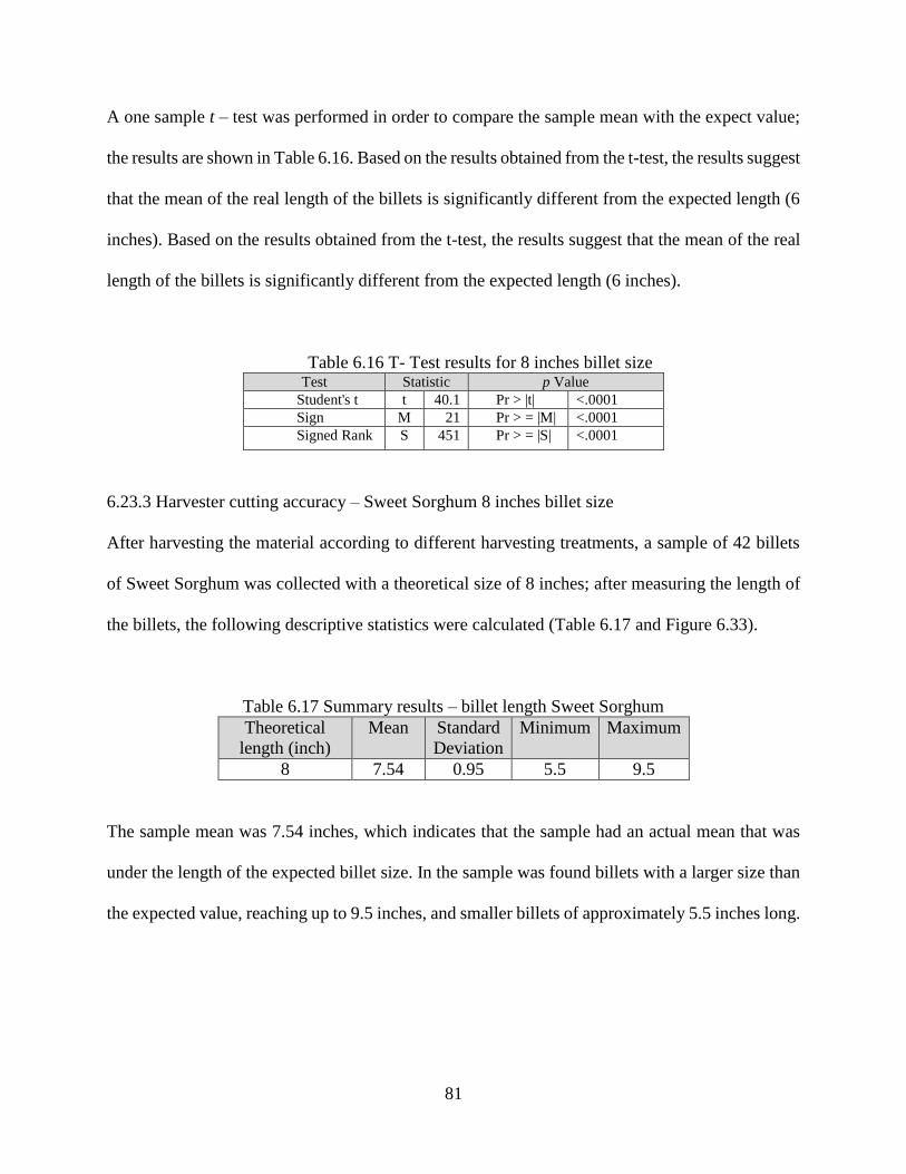
81

A one sample t – test was performed in order to compare the sample mean with the expect value;

the results are shown in Table 6.16. Based on the results obtained from the t-test, the results suggest

that the mean of the real length of the billets is significantly different from the expected length (6

inches). Based on the results obtained from the t-test, the results suggest that the mean of the real

length of the billets is significantly different from the expected length (6 inches).

Table 6.16 T- Test results for 8 inches billet size Test Statistic p Value

Student's t t 40.1 Pr > |t| <.0001

Sign M 21 Pr > = |M| <.0001

Signed Rank S 451 Pr > = |S| <.0001

6.23.3 Harvester cutting accuracy – Sweet Sorghum 8 inches billet size

After harvesting the material according to different harvesting treatments, a sample of 42 billets

of Sweet Sorghum was collected with a theoretical size of 8 inches; after measuring the length of

the billets, the following descriptive statistics were calculated (Table 6.17 and Figure 6.33).

Table 6.17 Summary results – billet length Sweet Sorghum

Theoretical

length (inch)

Mean Standard

Deviation

Minimum Maximum

8 7.54 0.95 5.5 9.5

The sample mean was 7.54 inches, which indicates that the sample had an actual mean that was

under the length of the expected billet size. In the sample was found billets with a larger size than

the expected value, reaching up to 9.5 inches, and smaller billets of approximately 5.5 inches long.

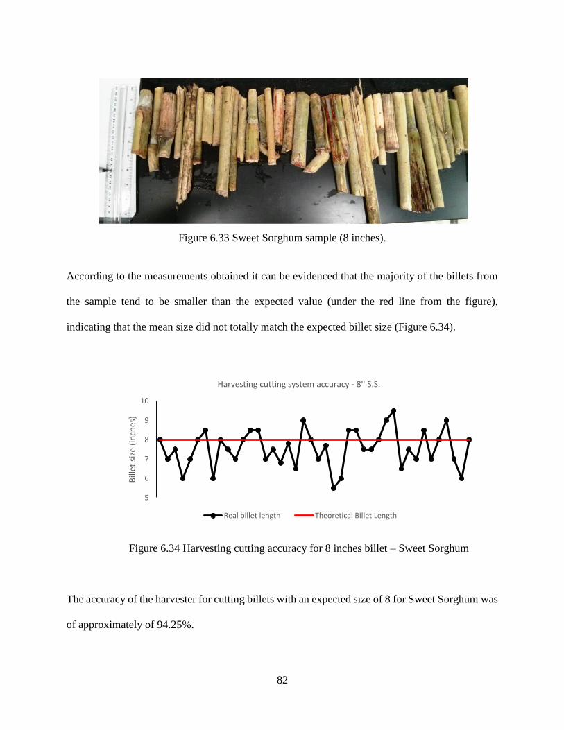
82

Figure 6.33 Sweet Sorghum sample (8 inches).

According to the measurements obtained it can be evidenced that the majority of the billets from

the sample tend to be smaller than the expected value (under the red line from the figure),

indicating that the mean size did not totally match the expected billet size (Figure 6.34).

Figure 6.34 Harvesting cutting accuracy for 8 inches billet – Sweet Sorghum

The accuracy of the harvester for cutting billets with an expected size of 8 for Sweet Sorghum was

of approximately of 94.25%.

5

6

7

8

9

10

Bill

et s

ize

(in

ches

)

Harvesting cutting system accuracy - 8'' S.S.

Real billet length Theoretical Billet Length

Theoretical length 8 inches

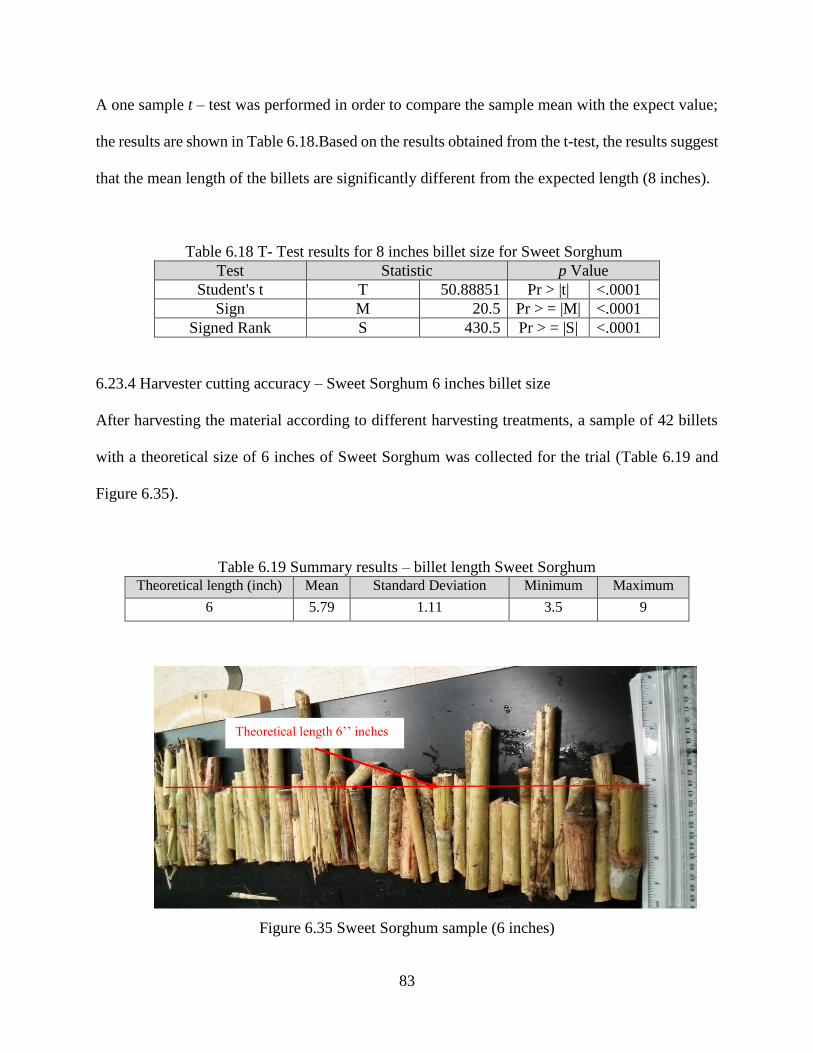
83

A one sample t – test was performed in order to compare the sample mean with the expect value;

the results are shown in Table 6.18.Based on the results obtained from the t-test, the results suggest

that the mean length of the billets are significantly different from the expected length (8 inches).

Table 6.18 T- Test results for 8 inches billet size for Sweet Sorghum

Test Statistic p Value

Student's t T 50.88851 Pr > |t| <.0001

Sign M 20.5 Pr > = |M| <.0001

Signed Rank S 430.5 Pr > = |S| <.0001

6.23.4 Harvester cutting accuracy – Sweet Sorghum 6 inches billet size

After harvesting the material according to different harvesting treatments, a sample of 42 billets

with a theoretical size of 6 inches of Sweet Sorghum was collected for the trial (Table 6.19 and

Figure 6.35).

Table 6.19 Summary results – billet length Sweet Sorghum Theoretical length (inch) Mean Standard Deviation Minimum Maximum

6 5.79 1.11 3.5 9

Figure 6.35 Sweet Sorghum sample (6 inches)

Theoretical length 6’’ inches

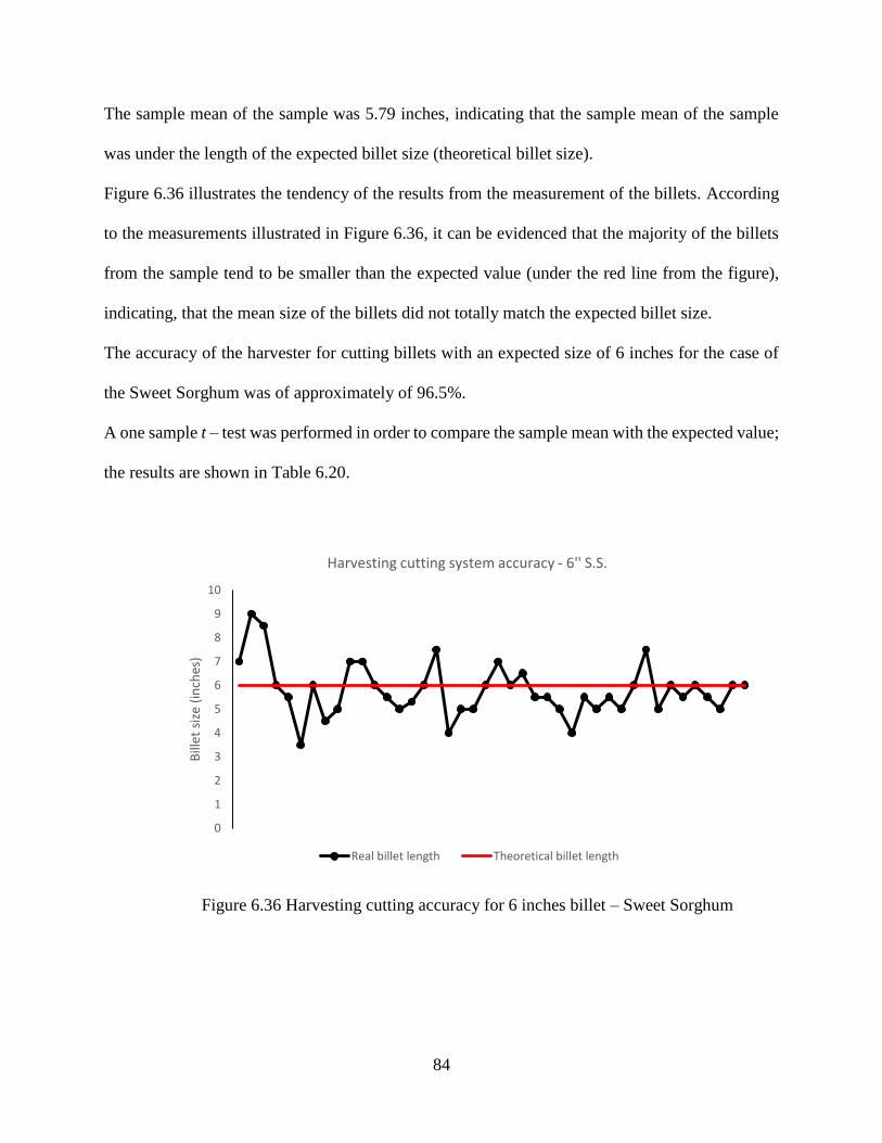
84

The sample mean of the sample was 5.79 inches, indicating that the sample mean of the sample

was under the length of the expected billet size (theoretical billet size).

Figure 6.36 illustrates the tendency of the results from the measurement of the billets. According

to the measurements illustrated in Figure 6.36, it can be evidenced that the majority of the billets

from the sample tend to be smaller than the expected value (under the red line from the figure),

indicating, that the mean size of the billets did not totally match the expected billet size.

The accuracy of the harvester for cutting billets with an expected size of 6 inches for the case of

the Sweet Sorghum was of approximately of 96.5%.

A one sample t – test was performed in order to compare the sample mean with the expected value;

the results are shown in Table 6.20.

Figure 6.36 Harvesting cutting accuracy for 6 inches billet – Sweet Sorghum

0

1

2

3

4

5

6

7

8

9

10

Bill

et s

ize

(in

ches

)

Harvesting cutting system accuracy - 6'' S.S.

Real billet length Theoretical billet length

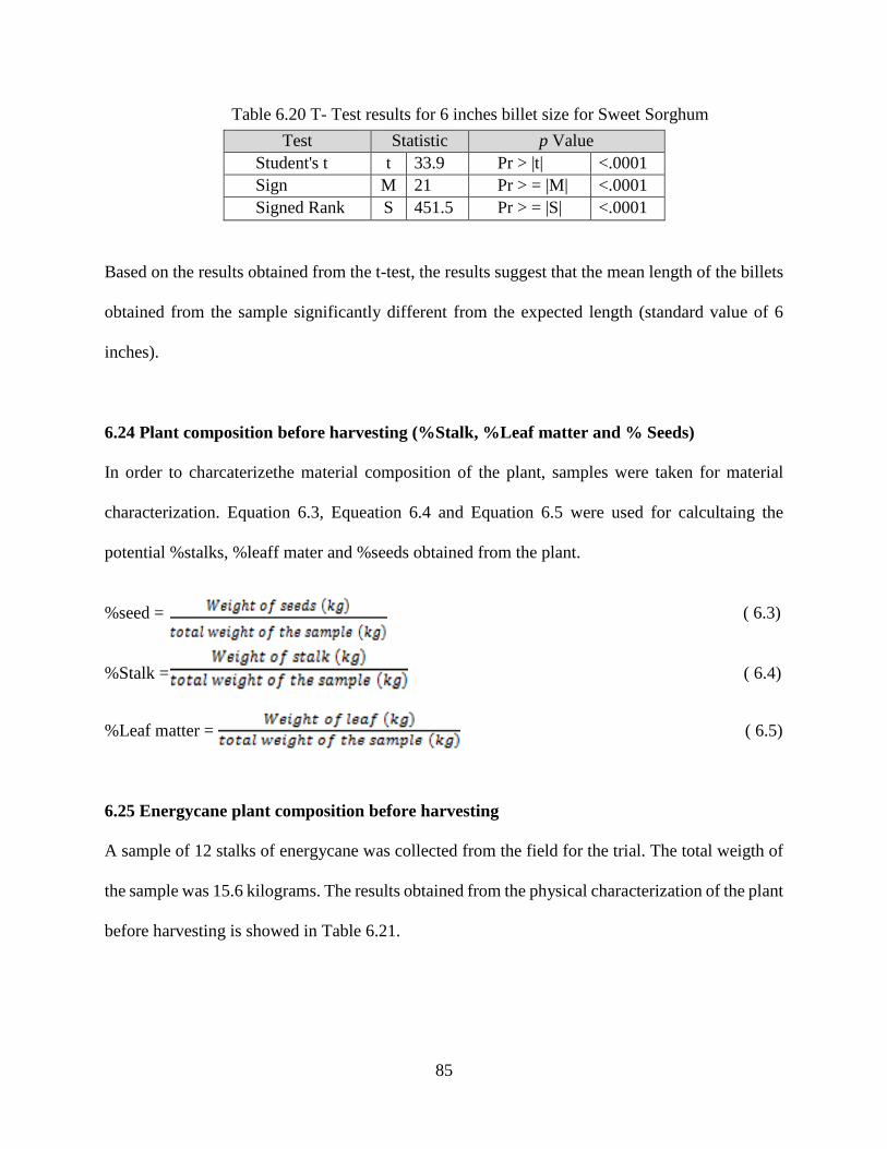
85

Table 6.20 T- Test results for 6 inches billet size for Sweet Sorghum

Based on the results obtained from the t-test, the results suggest that the mean length of the billets

obtained from the sample significantly different from the expected length (standard value of 6

inches).

6.24 Plant composition before harvesting (%Stalk, %Leaf matter and % Seeds)

In order to charcaterizethe material composition of the plant, samples were taken for material

characterization. Equation 6.3, Equeation 6.4 and Equation 6.5 were used for calcultaing the

potential %stalks, %leaff mater and %seeds obtained from the plant.

%seed = ( 6.3)

%Stalk = ( 6.4)

%Leaf matter = ( 6.5)

6.25 Energycane plant composition before harvesting

A sample of 12 stalks of energycane was collected from the field for the trial. The total weigth of

the sample was 15.6 kilograms. The results obtained from the physical characterization of the plant

before harvesting is showed in Table 6.21.

Test Statistic p Value

Student's t t 33.9 Pr > |t| <.0001

Sign M 21 Pr > = |M| <.0001

Signed Rank S 451.5 Pr > = |S| <.0001

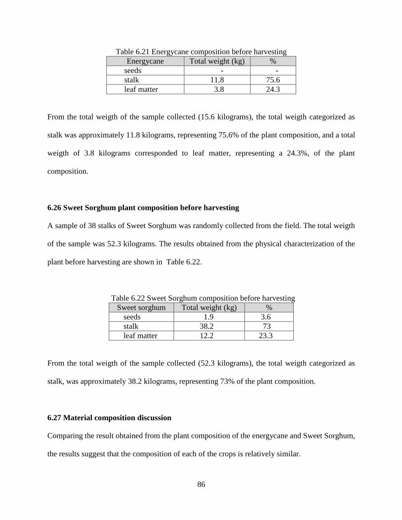
86

Table 6.21 Energycane composition before harvesting

Energycane Total weight (kg) %

seeds - -

stalk 11.8 75.6

leaf matter 3.8 24.3

From the total weigth of the sample collected (15.6 kilograms), the total weigth categorized as

stalk was approximately 11.8 kilograms, representing 75.6% of the plant composition, and a total

weigth of 3.8 kilograms corresponded to leaf matter, representing a 24.3%, of the plant

composition.

6.26 Sweet Sorghum plant composition before harvesting

A sample of 38 stalks of Sweet Sorghum was randomly collected from the field. The total weigth

of the sample was 52.3 kilograms. The results obtained from the physical characterization of the

plant before harvesting are shown in Table 6.22.

Table 6.22 Sweet Sorghum composition before harvesting

Sweet sorghum Total weight (kg) %

seeds 1.9 3.6

stalk 38.2 73

leaf matter 12.2 23.3

From the total weigth of the sample collected (52.3 kilograms), the total weigth categorized as

stalk, was approximately 38.2 kilograms, representing 73% of the plant composition.

6.27 Material composition discussion

Comparing the result obtained from the plant composition of the energycane and Sweet Sorghum,

the results suggest that the composition of each of the crops is relatively similar.

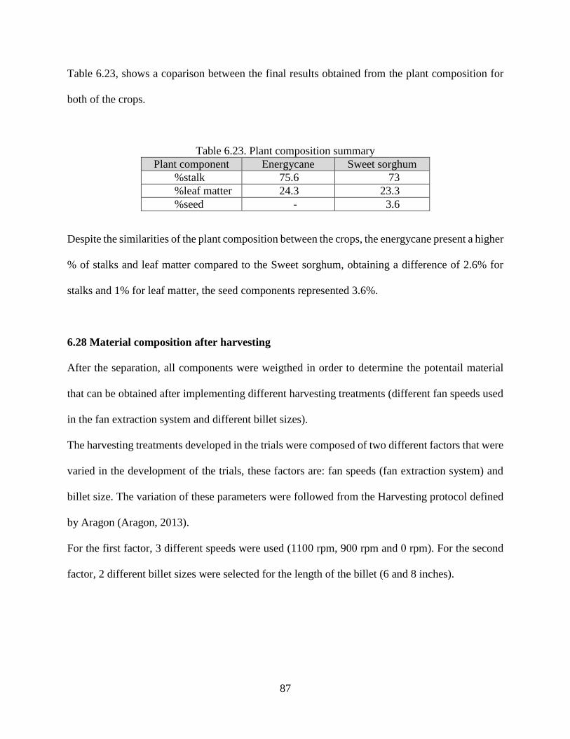
87

Table 6.23, shows a coparison between the final results obtained from the plant composition for

both of the crops.

Table 6.23. Plant composition summary

Plant component Energycane Sweet sorghum

%stalk 75.6 73

%leaf matter 24.3 23.3

%seed - 3.6

Despite the similarities of the plant composition between the crops, the energycane present a higher

% of stalks and leaf matter compared to the Sweet sorghum, obtaining a difference of 2.6% for

stalks and 1% for leaf matter, the seed components represented 3.6%.

6.28 Material composition after harvesting

After the separation, all components were weigthed in order to determine the potentail material

that can be obtained after implementing different harvesting treatments (different fan speeds used

in the fan extraction system and different billet sizes).

The harvesting treatments developed in the trials were composed of two different factors that were

varied in the development of the trials, these factors are: fan speeds (fan extraction system) and

billet size. The variation of these parameters were followed from the Harvesting protocol defined

by Aragon (Aragon, 2013).

For the first factor, 3 different speeds were used (1100 rpm, 900 rpm and 0 rpm). For the second

factor, 2 different billet sizes were selected for the length of the billet (6 and 8 inches).

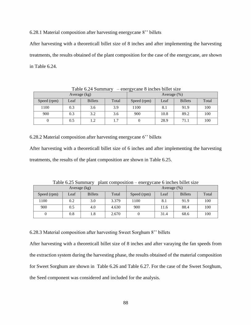
88

6.28.1 Material composition after harvesting energycane 8’’ billets

After harvesting with a theoreticall billet size of 8 inches and after implementing the harvesting

treatments, the results obtained of the plant composition for the case of the energycane, are shown

in Table 6.24.

Table 6.24 Summary – energycane 8 inches billet size Average (kg) Average (%)

Speed (rpm) Leaf Billets Total Speed (rpm) Leaf Billets Total

1100 0.3 3.6 3.9 1100 8.1 91.9 100

900 0.3 3.2 3.6 900 10.8 89.2 100

0 0.5 1.2 1.7 0 28.9 71.1 100

6.28.2 Material composition after harvesting energycane 6’’ billets

After harvesting with a theoreticall billet size of 6 inches and after implementing the harvesting

treatments, the results of the plant composition are shown in Table 6.25.

Table 6.25 Summary plant composition – energycane 6 inches billet size Average (kg) Average (%)

Speed (rpm) Leaf Billets Total Speed (rpm) Leaf Billets Total

1100 0.2 3.0 3.379 1100 8.1 91.9 100

900 0.5 4.0 4.630 900 11.6 88.4 100

0 0.8 1.8 2.670 0 31.4 68.6 100

6.28.3 Material composition after harvesting Sweet Sorghum 8’’ billets

After harvesting with a theoreticall billet size of 8 inches and after varaying the fan speeds from

the extraction system during the harvesting phase, the results obtained of the material composition

for Sweet Sorghum are shown in Table 6.26 and Table 6.27. For the case of the Sweet Sorghum,

the Seed component was considered and included for the analysis.

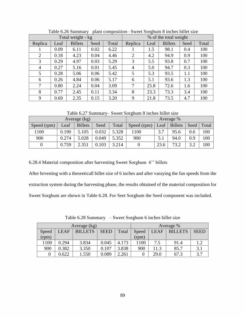
89

Table 6.26 Summary plant composition– Sweet Sorghum 8 inches billet size

Total weight - kg % of the total weight

Replica Leaf Billets Seed Total Replica Leaf Billets Seed Total

1 0.09 6.11 0.02 6.22 1 1.5 98.1 0.4 100

2 0.18 4.23 0.04 4.46 2 4.2 94.9 0.9 100

3 0.29 4.97 0.03 5.29 3 5.5 93.8 0.7 100

4 0.27 5.16 0.01 5.45 4 5.0 94.7 0.3 100

5 0.28 5.06 0.06 5.42 5 5.3 93.5 1.1 100

6 0.26 4.84 0.06 5.17 6 5.1 93.6 1.3 100

7 0.80 2.24 0.04 3.09 7 25.8 72.6 1.6 100

8 0.77 2.45 0.11 3.34 8 23.3 73.3 3.4 100

9 0.69 2.35 0.15 3.20 9 21.8 73.5 4.7 100

Table 6.27 Summary– Sweet Sorghum 8 inches billet size

Average (kg) Average %

Speed (rpm) Leaf Billets Seed Total Speed (rpm) Leaf Billets Seed Total

1100 0.190 5.105 0.032 5.328 1100 3.7 95.6 0.6 100

900 0.274 5.028 0.049 5.352 900 5.1 94.0 0.9 100

0 0.759 2.351 0.103 3.214 0 23.6 73.2 3.2 100

6.28.4 Material composition after harvesting Sweet Sorghum 6’’ billets

After hrvesting with a theoreticall billet size of 6 inches and after varaying the fan speeds from the

extraction system during the harvesting phase, the results obtained of the material composition for

Sweet Sorghum are shown in Table 6.28. For Seet Sorghum the Seed component was included.

Table 6.28 Summary – Sweet Sorghum 6 inches billet size

Average (kg) Average %

Speed

(rpm)

LEAF BILLETS SEED Total Speed

(rpm)

LEAF BILLETS SEED

1100 0.294 3.834 0.045 4.173 1100 7.5 91.4 1.2

900 0.382 3.350 0.107 3.838 900 11.3 85.7 3.1

0 0.622 1.550 0.089 2.261 0 29.0 67.3 3.7

90

6.29 Discussion Material composition after harvesting energycane

The results showed that the plant compositions after harvesting two different billet sizes with three

fan speeds of the extraction system.Comparing the results obtained after implementing different

harvesting treatments, the results suggest that as the fan speed increase, the percentage of leaf

matter tend to bereduced and the percentage of billets tend to increase.

From the results obtained in all harvesting treatments, it can be concluded that by using a billet

size of 6 inches, the % of leaf matter tend to increase more compared to the results obtained by

harvesting billets of 8 inches.

6.30 Material composition after harvesting Sweet Sorgum

It can be evidenced that the treatments composed of billets of 8 inches indicate that a higher % of

billets was collected from the material harvested compared to the harvesting treatments that used

a billet length of 6 inches. The results indicates that as increasing th fan spedd from the extraction

system while harvesting, the %of leaf matter collected from tha material harvested tend to decrease

while the %billets tendo to increase.

6.31 Harvesting efficiency (material losses after harvesting ton/acre)

The Material Losses indicator was calculated in terms of the total quantity of material losses left

in the field after harvesting. The material losses were measured by collecting all the material from

random areas with a dimension of 10ftx10ft. After harvesting the material from each row, the total

weight of the load was measure, then according to the area demarked for material losses, the

material left by the harvester after harvesting, was collected and weighted. The total yield of the

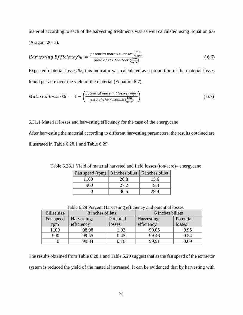
91

material according to each of the harvesting treatments was as well calculated using Equation 6.6

(Aragon, 2013).

𝐻𝑎𝑟𝑣𝑒𝑠𝑡𝑖𝑛𝑔 𝐸𝑓𝑓𝑖𝑐𝑖𝑒𝑛𝑐𝑦% = 𝑝𝑜𝑡𝑒𝑛𝑡𝑖𝑎𝑙 𝑚𝑎𝑡𝑒𝑟𝑖𝑎𝑙 𝑙𝑜𝑠𝑠𝑒𝑠 (

𝑡𝑜𝑛

𝑎𝑐𝑟𝑒)

𝑦𝑖𝑒𝑙𝑑 𝑜𝑓 𝑡ℎ𝑒 𝑓𝑒𝑒𝑠𝑡𝑜𝑐𝑘 (𝑡𝑜𝑛

𝑎𝑐𝑟𝑒)

( 6.6)

Expected material losses %, this indicator was calculated as a proportion of the material losses

found per acre over the yield of the material (Equation 6.7).

𝑀𝑎𝑡𝑒𝑟𝑖𝑎𝑙 𝑙𝑜𝑠𝑠𝑒𝑠% = 1 − (𝑝𝑜𝑡𝑒𝑛𝑡𝑖𝑎𝑙 𝑚𝑎𝑡𝑒𝑟𝑖𝑎𝑙 𝑙𝑜𝑠𝑠𝑒𝑠 (

𝑡𝑜𝑛

𝑎𝑐𝑟𝑒)

𝑦𝑖𝑒𝑙𝑑 𝑜𝑓 𝑡ℎ𝑒 𝑓𝑒𝑒𝑠𝑡𝑜𝑐𝑘 (𝑡𝑜𝑛

𝑎𝑐𝑟𝑒)

) ( 6.7)

6.31.1 Material losses and harvesting efficiency for the case of the energycane

After harvesting the material according to different harvesting parameters, the results obtained are

illustrated in Table 6.28.1 and Table 6.29.

Table 6.28.1 Yield of material harvsted and field losses (ton/acre)– energycane

Table 6.29 Percent Harvesting efficiency and potential losses

Billet size 8 inches billets 6 inches billets

Fan speed

rpm

Harvesting

efficiency

Potential

losses

Harvesting

efficiency

Potential

losses

1100 98.98 1.02 99.05 0.95

900 99.55 0.45 99.46 0.54

0 99.84 0.16 99.91 0.09

The results obtained from Table 6.28.1 and Table 6.29 suggest that as the fan speed of the extractor

system is reduced the yield of the material increased. It can be evidenced that by harvesting with

Fan speed (rpm) 8 inches billet 6 inches billet

1100 26.8 15.6

900 27.2 19.4

0 30.5 29.4

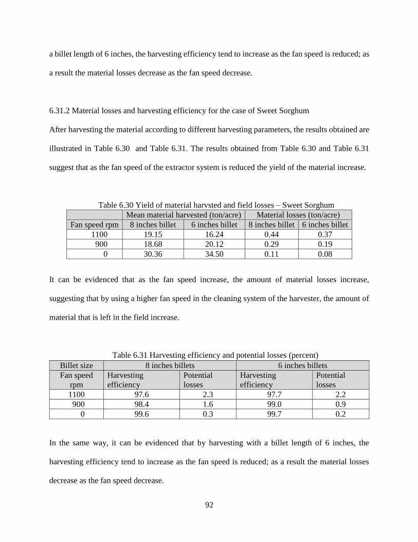
92

a billet length of 6 inches, the harvesting efficiency tend to increase as the fan speed is reduced; as

a result the material losses decrease as the fan speed decrease.

6.31.2 Material losses and harvesting efficiency for the case of Sweet Sorghum

After harvesting the material according to different harvesting parameters, the results obtained are

illustrated in Table 6.30 and Table 6.31. The results obtained from Table 6.30 and Table 6.31

suggest that as the fan speed of the extractor system is reduced the yield of the material increase.

Table 6.30 Yield of material harvsted and field losses – Sweet Sorghum

Mean material harvested (ton/acre) Material losses (ton/acre)

Fan speed rpm 8 inches billet 6 inches billet 8 inches billet 6 inches billet

1100 19.15 16.24 0.44 0.37

900 18.68 20.12 0.29 0.19

0 30.36 34.50 0.11 0.08

It can be evidenced that as the fan speed increase, the amount of material losses increase,

suggesting that by using a higher fan speed in the cleaning system of the harvester, the amount of

material that is left in the field increase.

Table 6.31 Harvesting efficiency and potential losses (percent)

In the same way, it can be evidenced that by harvesting with a billet length of 6 inches, the

harvesting efficiency tend to increase as the fan speed is reduced; as a result the material losses

decrease as the fan speed decrease.

Billet size 8 inches billets 6 inches billets

Fan speed

rpm

Harvesting

efficiency

Potential

losses

Harvesting

efficiency

Potential

losses

1100 97.6 2.3 97.7 2.2

900 98.4 1.6 99.0 0.9

0 99.6 0.3 99.7 0.2

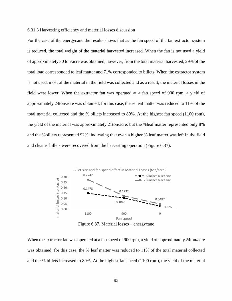
93

6.31.3 Harvesting efficiency and material losses discussion

For the case of the energycane the results shows that as the fan speed of the fan extractor system

is reduced, the total weight of the material harvested increased. When the fan is not used a yield

of approximately 30 ton/acre was obtained, however, from the total material harvested, 29% of the

total load corresponded to leaf matter and 71% corresponded to billets. When the extractor system

is not used, most of the material in the field was collected and as a result, the material losses in the

field were lower. When the extractor fan was operated at a fan speed of 900 rpm, a yield of

approximately 24ton/acre was obtained; for this case, the % leaf matter was reduced to 11% of the

total material collected and the % billets increased to 89%. At the highest fan speed (1100 rpm),

the yield of the material was approximately 21ton/acre; but the %leaf matter represented only 8%

and the %billets represented 92%, indicating that even a higher % leaf matter was left in the field

and cleaner billets were recovered from the harvesting operation (Figure 6.37).

Figure 6.37. Material losses – energycane

When the extractor fan was operated at a fan speed of 900 rpm, a yield of approximately 24ton/acre

was obtained; for this case, the % leaf matter was reduced to 11% of the total material collected

and the % billets increased to 89%. At the highest fan speed (1100 rpm), the yield of the material

0.1478

0.1046

0.0269

0.2742

0.1232

0.0487

0.00

0.05

0.10

0.15

0.20

0.25

0.30

1100 900 0

mat

eria

l lo

sses

(to

n/a

cre)

Fan speed

Billet size and fan speed effect in Material Losses (ton/acre)

6 inches billet size8 inches billet size

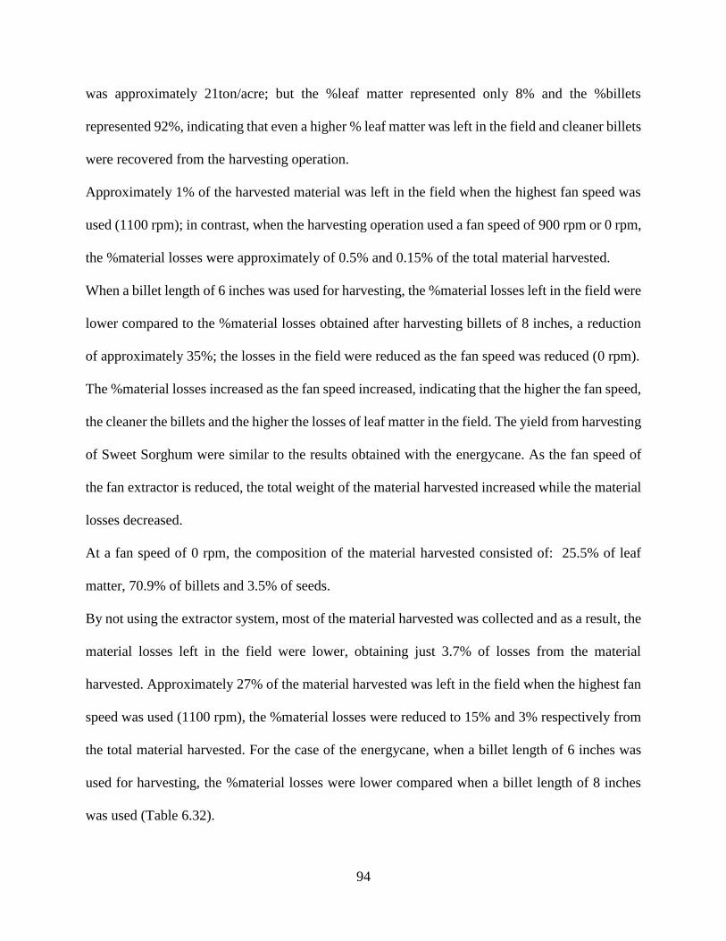
94

was approximately 21ton/acre; but the %leaf matter represented only 8% and the %billets

represented 92%, indicating that even a higher % leaf matter was left in the field and cleaner billets

were recovered from the harvesting operation.

Approximately 1% of the harvested material was left in the field when the highest fan speed was

used (1100 rpm); in contrast, when the harvesting operation used a fan speed of 900 rpm or 0 rpm,

the %material losses were approximately of 0.5% and 0.15% of the total material harvested.

When a billet length of 6 inches was used for harvesting, the %material losses left in the field were

lower compared to the %material losses obtained after harvesting billets of 8 inches, a reduction

of approximately 35%; the losses in the field were reduced as the fan speed was reduced (0 rpm).

The %material losses increased as the fan speed increased, indicating that the higher the fan speed,

the cleaner the billets and the higher the losses of leaf matter in the field. The yield from harvesting

of Sweet Sorghum were similar to the results obtained with the energycane. As the fan speed of

the fan extractor is reduced, the total weight of the material harvested increased while the material

losses decreased.

At a fan speed of 0 rpm, the composition of the material harvested consisted of: 25.5% of leaf

matter, 70.9% of billets and 3.5% of seeds.

By not using the extractor system, most of the material harvested was collected and as a result, the

material losses left in the field were lower, obtaining just 3.7% of losses from the material

harvested. Approximately 27% of the material harvested was left in the field when the highest fan

speed was used (1100 rpm), the %material losses were reduced to 15% and 3% respectively from

the total material harvested. For the case of the energycane, when a billet length of 6 inches was

used for harvesting, the %material losses were lower compared when a billet length of 8 inches

was used (Table 6.32).

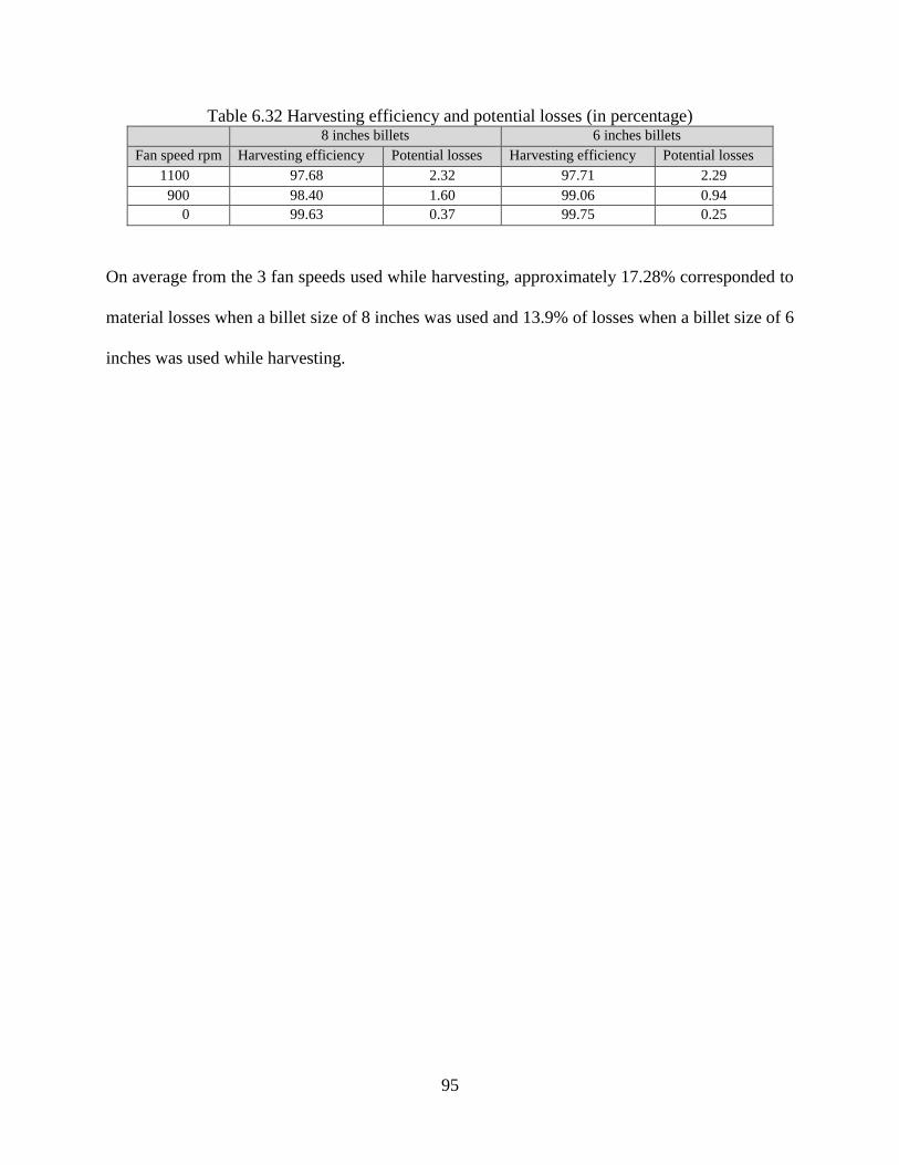
95

Table 6.32 Harvesting efficiency and potential losses (in percentage) 8 inches billets 6 inches billets

Fan speed rpm Harvesting efficiency Potential losses Harvesting efficiency Potential losses

1100 97.68 2.32 97.71 2.29

900 98.40 1.60 99.06 0.94

0 99.63 0.37 99.75 0.25

On average from the 3 fan speeds used while harvesting, approximately 17.28% corresponded to

material losses when a billet size of 8 inches was used and 13.9% of losses when a billet size of 6

inches was used while harvesting.

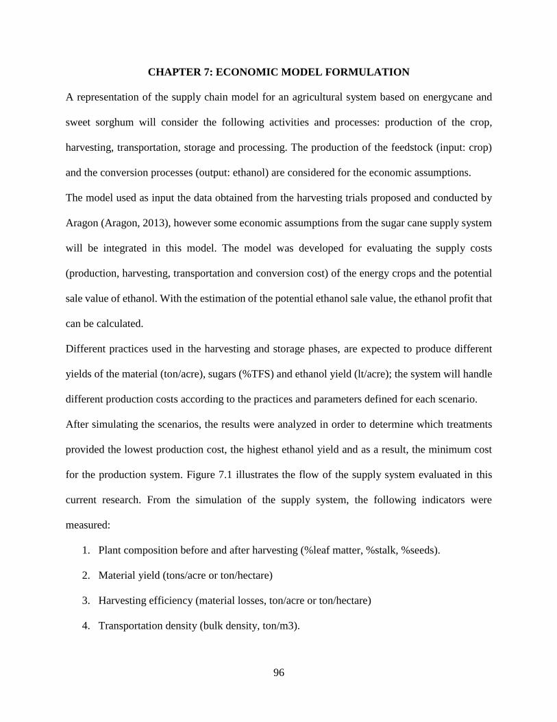
96

CHAPTER 7: ECONOMIC MODEL FORMULATION

A representation of the supply chain model for an agricultural system based on energycane and

sweet sorghum will consider the following activities and processes: production of the crop,

harvesting, transportation, storage and processing. The production of the feedstock (input: crop)

and the conversion processes (output: ethanol) are considered for the economic assumptions.

The model used as input the data obtained from the harvesting trials proposed and conducted by

Aragon (Aragon, 2013), however some economic assumptions from the sugar cane supply system

will be integrated in this model. The model was developed for evaluating the supply costs

(production, harvesting, transportation and conversion cost) of the energy crops and the potential

sale value of ethanol. With the estimation of the potential ethanol sale value, the ethanol profit that

can be calculated.

Different practices used in the harvesting and storage phases, are expected to produce different

yields of the material (ton/acre), sugars (%TFS) and ethanol yield (lt/acre); the system will handle

different production costs according to the practices and parameters defined for each scenario.

After simulating the scenarios, the results were analyzed in order to determine which treatments

provided the lowest production cost, the highest ethanol yield and as a result, the minimum cost

for the production system. Figure 7.1 illustrates the flow of the supply system evaluated in this

current research. From the simulation of the supply system, the following indicators were

measured:

1. Plant composition before and after harvesting (%leaf matter, %stalk, %seeds).

2. Material yield (tons/acre or ton/hectare)

3. Harvesting efficiency (material losses, ton/acre or ton/hectare)

4. Transportation density (bulk density, ton/m3).

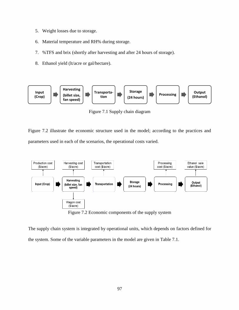
97

5. Weight losses due to storage.

6. Material temperature and RH% during storage.

7. %TFS and brix (shortly after harvesting and after 24 hours of storage).

8. Ethanol yield (lt/acre or gal/hectare).

Figure 7.1 Supply chain diagram

Figure 7.2 illustrate the economic structure used in the model; according to the practices and

parameters used in each of the scenarios, the operational costs varied.

Figure 7.2 Economic components of the supply system

The supply chain system is integrated by operational units, which depends on factors defined for

the system. Some of the variable parameters in the model are given in Table 7.1.

Input (Crop)

Harvesting

(billet size, fan speed)

Transporta-tion

Storage

(24 hours)Processing

Output (Ethanol)

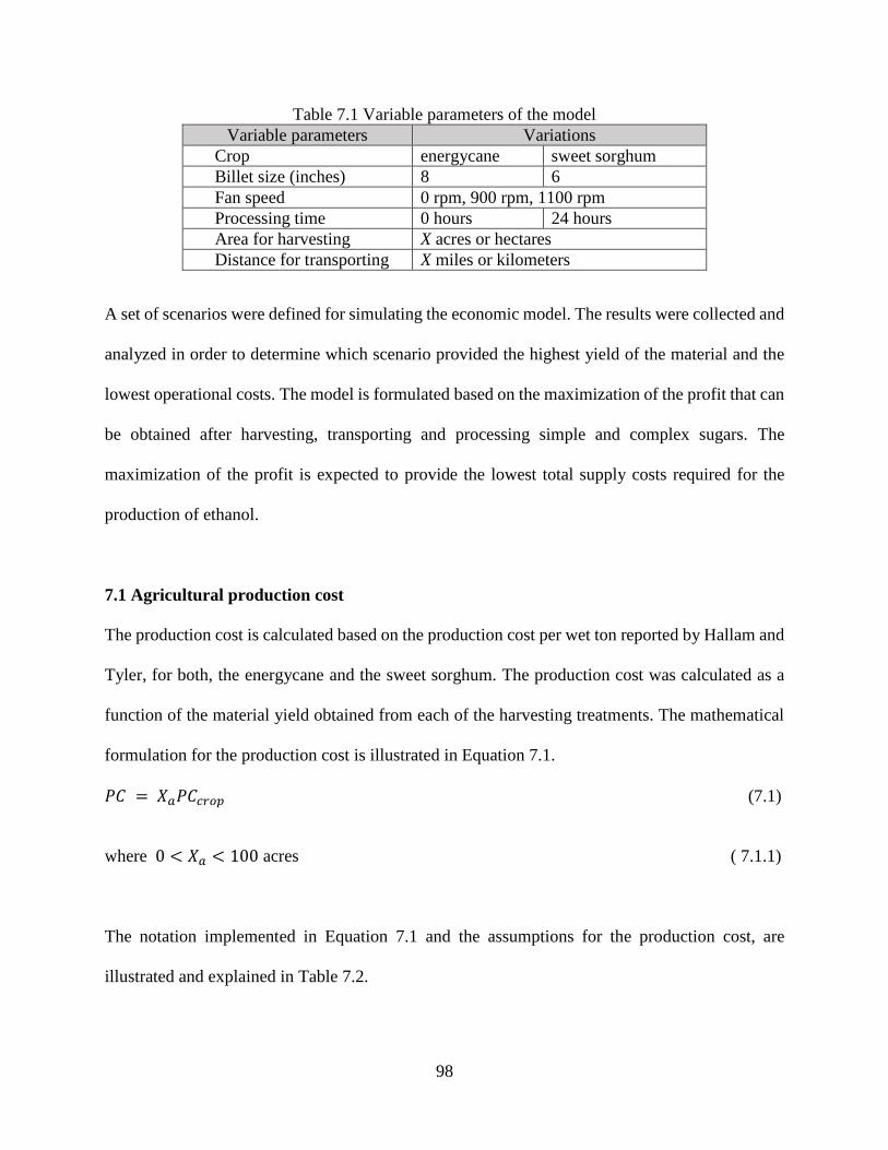
98

Table 7.1 Variable parameters of the model

Variable parameters Variations

Crop energycane sweet sorghum

Billet size (inches) 8 6

Fan speed 0 rpm, 900 rpm, 1100 rpm

Processing time 0 hours 24 hours

Area for harvesting X acres or hectares

Distance for transporting X miles or kilometers

A set of scenarios were defined for simulating the economic model. The results were collected and

analyzed in order to determine which scenario provided the highest yield of the material and the

lowest operational costs. The model is formulated based on the maximization of the profit that can

be obtained after harvesting, transporting and processing simple and complex sugars. The

maximization of the profit is expected to provide the lowest total supply costs required for the

production of ethanol.

7.1 Agricultural production cost

The production cost is calculated based on the production cost per wet ton reported by Hallam and

Tyler, for both, the energycane and the sweet sorghum. The production cost was calculated as a

function of the material yield obtained from each of the harvesting treatments. The mathematical

formulation for the production cost is illustrated in Equation 7.1.

𝑃𝐶 = 𝑋𝑎𝑃𝐶𝑐𝑟𝑜𝑝 (7.1)

where 0 < 𝑋𝑎 < 100 acres ( 7.1.1)

The notation implemented in Equation 7.1 and the assumptions for the production cost, are

illustrated and explained in Table 7.2.

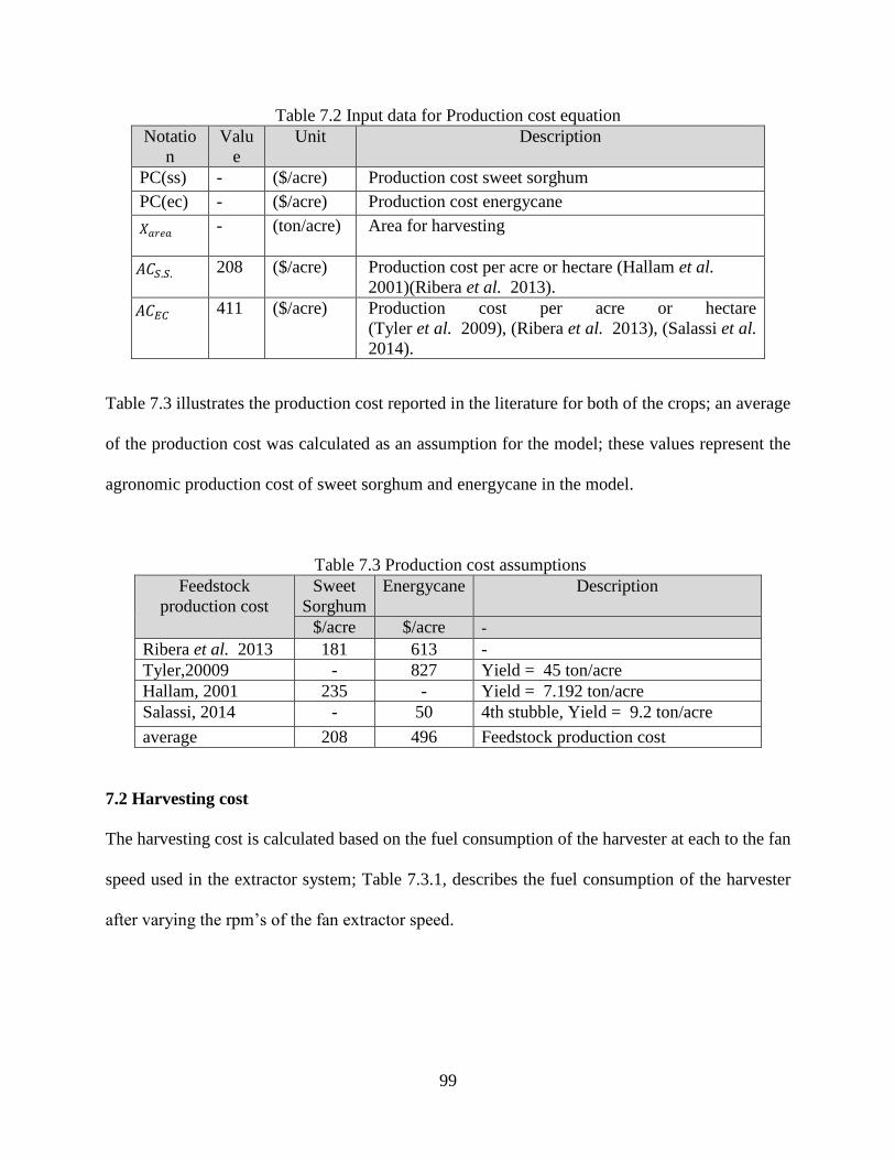
99

Table 7.2 Input data for Production cost equation

Notatio

n

Valu

e

Unit Description

PC(ss) - ($/acre) Production cost sweet sorghum

PC(ec) - ($/acre) Production cost energycane

- (ton/acre) Area for harvesting

208 ($/acre) Production cost per acre or hectare (Hallam et al.

2001)(Ribera et al. 2013).

411 ($/acre) Production cost per acre or hectare

(Tyler et al. 2009), (Ribera et al. 2013), (Salassi et al.

2014).

Table 7.3 illustrates the production cost reported in the literature for both of the crops; an average

of the production cost was calculated as an assumption for the model; these values represent the

agronomic production cost of sweet sorghum and energycane in the model.

Table 7.3 Production cost assumptions

Feedstock

production cost

Sweet

Sorghum

Energycane Description

$/acre $/acre - Ribera et al. 2013 181 613 -

Tyler,20009 - 827 Yield = 45 ton/acre

Hallam, 2001 235 - Yield = 7.192 ton/acre

Salassi, 2014 - 50 4th stubble, Yield = 9.2 ton/acre

average 208 496 Feedstock production cost

7.2 Harvesting cost

The harvesting cost is calculated based on the fuel consumption of the harvester at each to the fan

speed used in the extractor system; Table 7.3.1, describes the fuel consumption of the harvester

after varying the rpm’s of the fan extractor speed.

𝑋𝑎𝑟𝑒𝑎

𝐴𝐶𝑆.𝑆.

𝐴𝐶𝐸𝐶

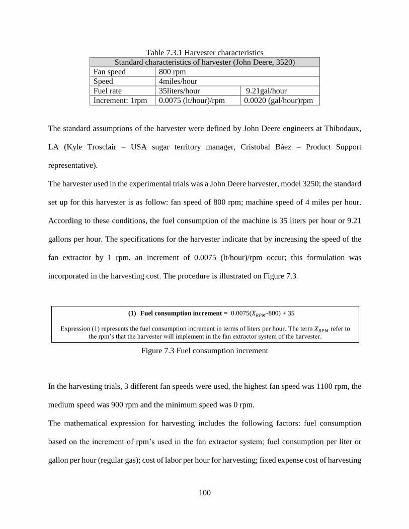
100

Table 7.3.1 Harvester characteristics

Standard characteristics of harvester (John Deere, 3520)

Fan speed 800 rpm

Speed 4miles/hour

Fuel rate 35liters/hour 9.21gal/hour

Increment: 1rpm 0.0075 (lt/hour)/rpm 0.0020 (gal/hour)rpm

The standard assumptions of the harvester were defined by John Deere engineers at Thibodaux,

LA (Kyle Trosclair – USA sugar territory manager, Cristobal Báez – Product Support

representative).

The harvester used in the experimental trials was a John Deere harvester, model 3250; the standard

set up for this harvester is as follow: fan speed of 800 rpm; machine speed of 4 miles per hour.

According to these conditions, the fuel consumption of the machine is 35 liters per hour or 9.21

gallons per hour. The specifications for the harvester indicate that by increasing the speed of the

fan extractor by 1 rpm, an increment of 0.0075 (lt/hour)/rpm occur; this formulation was

incorporated in the harvesting cost. The procedure is illustrated on Figure 7.3.

Figure 7.3 Fuel consumption increment

In the harvesting trials, 3 different fan speeds were used, the highest fan speed was 1100 rpm, the

medium speed was 900 rpm and the minimum speed was 0 rpm.

The mathematical expression for harvesting includes the following factors: fuel consumption

based on the increment of rpm’s used in the fan extractor system; fuel consumption per liter or

gallon per hour (regular gas); cost of labor per hour for harvesting; fixed expense cost of harvesting

(1) Fuel consumption increment = 0.0075(𝑋𝑅𝑃𝑀-800) + 35

Expression (1) represents the fuel consumption increment in terms of liters per hour. The term 𝑋𝑅𝑃𝑀 refer to

the rpm’s that the harvester will implement in the fan extractor system of the harvester.

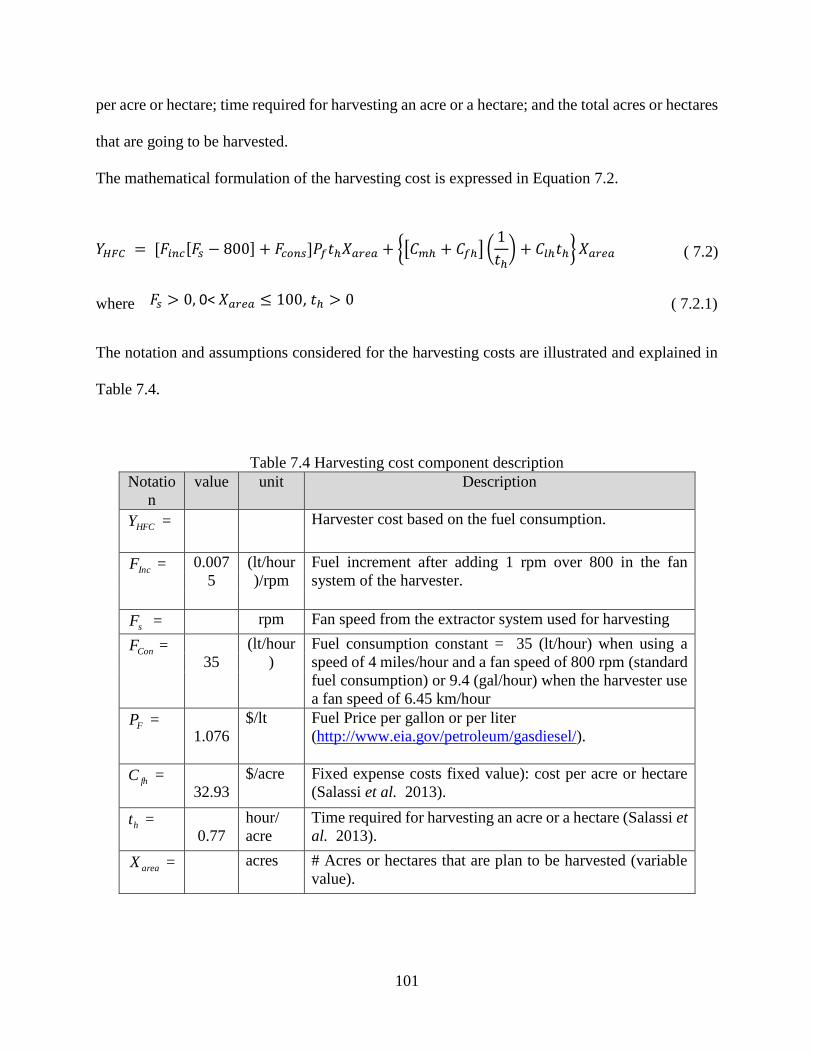
101

per acre or hectare; time required for harvesting an acre or a hectare; and the total acres or hectares

that are going to be harvested.

The mathematical formulation of the harvesting cost is expressed in Equation 7.2.

( 7.2)

where ( 7.2.1)

The notation and assumptions considered for the harvesting costs are illustrated and explained in

Table 7.4.

Table 7.4 Harvesting cost component description

Notatio

n

value unit Description

HFCY =

Harvester cost based on the fuel consumption.

IncF = 0.007

5

(lt/hour

)/rpm

Fuel increment after adding 1 rpm over 800 in the fan

system of the harvester.

sF = rpm Fan speed from the extractor system used for harvesting

ConF =

35

(lt/hour

)

Fuel consumption constant = 35 (lt/hour) when using a

speed of 4 miles/hour and a fan speed of 800 rpm (standard

fuel consumption) or 9.4 (gal/hour) when the harvester use

a fan speed of 6.45 km/hour

FP =

1.076

$/lt Fuel Price per gallon or per liter

(http://www.eia.gov/petroleum/gasdiesel/).

fhC =

32.93

$/acre Fixed expense costs fixed value): cost per acre or hectare

(Salassi et al. 2013).

ht =

0.77

hour/

acre

Time required for harvesting an acre or a hectare (Salassi et

al. 2013).

areaX =

acres # Acres or hectares that are plan to be harvested (variable

value).

𝐹𝑠 > 0

0< 𝑋𝑎𝑟𝑒𝑎 ≤100

𝑡ℎ > 0

𝐹𝑠 > 0, 0< 𝑋𝑎𝑟𝑒𝑎 ≤ 100, 𝑡ℎ > 0

𝑌𝐻𝐹𝐶 = [𝐹𝑖𝑛𝑐[𝐹𝑠 − 800] + 𝐹𝑐𝑜𝑛𝑠]𝑃𝑓𝑡ℎ𝑋𝑎𝑟𝑒𝑎 + {[𝐶𝑚ℎ + 𝐶𝑓ℎ] (1

𝑡ℎ) + 𝐶𝑙ℎ𝑡ℎ} 𝑋𝑎𝑟𝑒𝑎

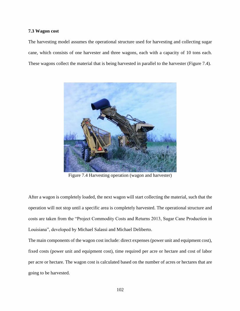
102

7.3 Wagon cost

The harvesting model assumes the operational structure used for harvesting and collecting sugar

cane, which consists of one harvester and three wagons, each with a capacity of 10 tons each.

These wagons collect the material that is being harvested in parallel to the harvester (Figure 7.4).

Figure 7.4 Harvesting operation (wagon and harvester)

After a wagon is completely loaded, the next wagon will start collecting the material, such that the

operation will not stop until a specific area is completely harvested. The operational structure and

costs are taken from the “Project Commodity Costs and Returns 2013, Sugar Cane Production in

Louisiana”, developed by Michael Salassi and Michael Deliberto.

The main components of the wagon cost include: direct expenses (power unit and equipment cost),

fixed costs (power unit and equipment cost), time required per acre or hectare and cost of labor

per acre or hectare. The wagon cost is calculated based on the number of acres or hectares that are

going to be harvested.

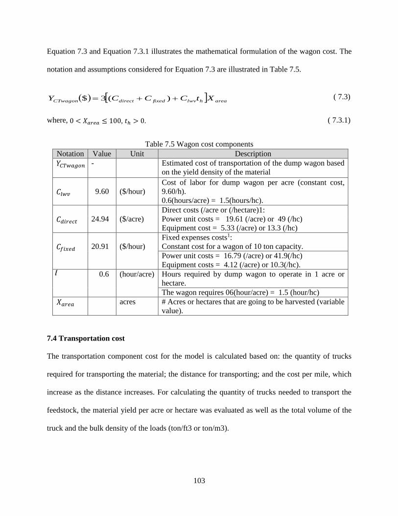
103

Equation 7.3 and Equation 7.3.1 illustrates the mathematical formulation of the wagon cost. The

notation and assumptions considered for Equation 7.3 are illustrated in Table 7.5.

areahlwvfixeddirectCTwagon XtCCCY )(3$ ( 7.3)

where, ( 7.3.1)

Table 7.5 Wagon cost components

7.4 Transportation cost

The transportation component cost for the model is calculated based on: the quantity of trucks

required for transporting the material; the distance for transporting; and the cost per mile, which

increase as the distance increases. For calculating the quantity of trucks needed to transport the

feedstock, the material yield per acre or hectare was evaluated as well as the total volume of the

truck and the bulk density of the loads (ton/ft3 or ton/m3).

Notation Value Unit Description

𝑌𝐶𝑇𝑤𝑎𝑔𝑜𝑛

- Estimated cost of transportation of the dump wagon based

on the yield density of the material

𝐶𝑙𝑤𝑣

9.60

($/hour)

Cost of labor for dump wagon per acre (constant cost,

9.60/h).

0.6(hours/acre) = 1.5(hours/hc).

𝐶𝑑𝑖𝑟𝑒𝑐𝑡

24.94

($/acre)

Direct costs (/acre or (/hectare)1:

Power unit costs = 19.61 (/acre) or 49 (/hc)

Equipment cost = 5.33 (/acre) or 13.3 (/hc)

𝐶𝑓𝑖𝑥𝑒𝑑

20.91

($/hour)

Fixed expenses costs1:

Constant cost for a wagon of 10 ton capacity.

Power unit costs = 16.79 (/acre) or 41.9(/hc)

Equipment costs = 4.12 (/acre) or 10.3(/hc).

0.6 (hour/acre) Hours required by dump wagon to operate in 1 acre or

hectare.

The wagon requires 06(hour/acre) = 1.5 (hour/hc)

𝑋𝑎𝑟𝑒𝑎

acres # Acres or hectares that are going to be harvested (variable

value).

0 < 𝑋𝑎𝑟𝑒𝑎 ≤ 100, 𝑡ℎ > 0.

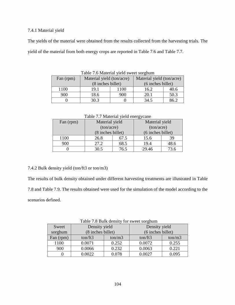
104

7.4.1 Material yield

The yields of the material were obtained from the results collected from the harvesting trials. The

yield of the material from both energy crops are reported in Table 7.6 and Table 7.7.

Table 7.6 Material yield sweet sorghum

Fan (rpm) Material yield (ton/acre)

(8 inches billet)

Material yield (ton/acre)

(6 inches billet)

1100 19.1 1100 16.2 40.6

900 18.6 900 20.1 50.3

0 30.3 0 34.5 86.2

Table 7.7 Material yield energycane

Fan (rpm) Material yield

(ton/acre)

(8 inches billet)

Material yield

(ton/acre)

(6 inches billet)

1100 26.8 67.5 15.6 39

900 27.2 68.5 19.4 48.6

0 30.5 76.5 29.46 73.6

7.4.2 Bulk density yield (ton/ft3 or ton/m3)

The results of bulk density obtained under different harvesting treatments are illustrated in Table

7.8 and Table 7.9. The results obtained were used for the simulation of the model according to the

scenarios defined.

Table 7.8 Bulk density for sweet sorghum

Sweet

sorghum

Density yield

(8 inches billet)

Density yield

(6 inches billet)

Fan (rpm) ton/ft3 ton/m3 ton/ft3 ton/m3

1100 0.0071 0.252 0.0072 0.255

900 0.0066 0.232 0.0063 0.221

0 0.0022 0.078 0.0027 0.095

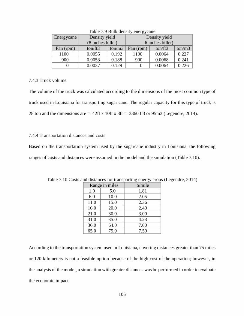
105

Table 7.9 Bulk density energycane

Energycane Density yield

(8 inches billet)

Density yield

6 inches billet)

Fan (rpm) ton/ft3 ton/m3 Fan (rpm) ton/ft3 ton/m3

1100 0.0055 0.192 1100 0.0064 0.227

900 0.0053 0.188 900 0.0068 0.241

0 0.0037 0.129 0 0.0064 0.226

7.4.3 Truck volume

The volume of the truck was calculated according to the dimensions of the most common type of

truck used in Louisiana for transporting sugar cane. The regular capacity for this type of truck is

28 ton and the dimensions are = 42ft x 10ft x 8ft = 3360 ft3 or 95m3 (Legendre, 2014).

7.4.4 Transportation distances and costs

Based on the transportation system used by the sugarcane industry in Louisiana, the following

ranges of costs and distances were assumed in the model and the simulation (Table 7.10).

Table 7.10 Costs and distances for transporting energy crops (Legendre, 2014)

Range in miles $/mile

1.0 5.0 1.81

6.0 10.0 2.05

11.0 15.0 2.36

16.0 20.0 2.40

21.0 30.0 3.00

31.0 35.0 4.23

36.0 64.0 7.00

65.0 75.0 7.50

According to the transportation system used in Louisiana, covering distances greater than 75 miles

or 120 kilometers is not a feasible option because of the high cost of the operation; however, in

the analysis of the model, a simulation with greater distances was be performed in order to evaluate

the economic impact.

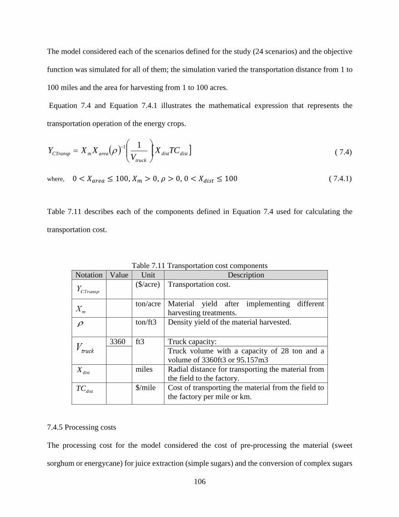
106

The model considered each of the scenarios defined for the study (24 scenarios) and the objective

function was simulated for all of them; the simulation varied the transportation distance from 1 to

100 miles and the area for harvesting from 1 to 100 acres.

Equation 7.4 and Equation 7.4.1 illustrates the mathematical expression that represents the

transportation operation of the energy crops.

distdist

truck

areamCTransp TCXV

XXY

11 ( 7.4)

where, ( 7.4.1)

Table 7.11 describes each of the components defined in Equation 7.4 used for calculating the

transportation cost.

Table 7.11 Transportation cost components

Notation Value Unit Description

($/acre) Transportation cost.

ton/acre Material yield after implementing different

harvesting treatments.

ton/ft3 Density yield of the material harvested.

3360 ft3 Truck capacity:

Truck volume with a capacity of 28 ton and a

volume of 3360ft3 or 95.157m3

distX miles Radial distance for transporting the material from

the field to the factory.

distTC

$/mile Cost of transporting the material from the field to

the factory per mile or km.

7.4.5 Processing costs

The processing cost for the model considered the cost of pre-processing the material (sweet

sorghum or energycane) for juice extraction (simple sugars) and the conversion of complex sugars

0 < 𝑋𝑎𝑟𝑒𝑎 ≤ 100, 𝑋𝑚 > 0, 𝜌 > 0, 0 < 𝑋𝑑𝑖𝑠𝑡 ≤ 100

107

extracted from the fiber and the biomass; the model assumed both sugars, the complex and simple

sugars. The simple sugars are recovered from the juice, and the complex sugars could be recovered

from the fiber and the biomass of the feedstock.

The component costs of the processing cost consider the costs of processing and conversion. The

treatment assumed in the model for recovering complex sugars was lime pretreatment; the cost

and the assumption were taken from the research developed by Day, 2012 titled Bio refinery

Development Using Multiple Feedstock’s.

The cost of the treatment for recovering and converting complex sugars reported in the literature

were found very high and in order to simulate feasible solutions in the study, it was assumed that

the complex sugars treatment cost was 0.022 $/ton produced, leading to a total of $48.40 per ton

processed for the case of the sweet sorghum.

For the case of the energycane, the treatment cost for the conversion into complex sugars 0.023$/lb

produced and a total of $50.60 per ton processed for the case of the energycane.

The model assumed a conversion cost lower compared to the data reported in the literature; this

was assumed in order to obtain feasible solutions in the model. It is important that the conversion

costs of simple and complex in the future should be reduced in order to have a feasible system

operation. For the complex sugars recovery, it is assumed that the fiber and biomass that is

processed shortly after harvesting contains approximately 50% moisture and when the material is

processed after 24 hours, the moisture level is less than 50%. Finally, for the complex sugars

recovery, the model assumed that approximately 60% of the total fermentable sugars can be

recovered from the fiber for both of the energy crops. Equation 7.5 and Equation 7.5.1 illustrates

the mathematical formulation of the processing cost.

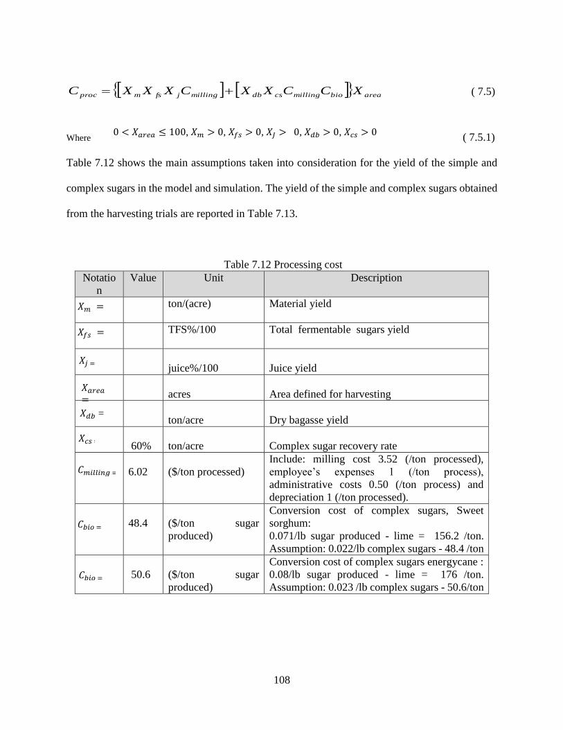
108

areabiomillingcsdbmillingjfsmproc XCCXXCXXXC ( 7.5)

Where ( 7.5.1)

Table 7.12 shows the main assumptions taken into consideration for the yield of the simple and

complex sugars in the model and simulation. The yield of the simple and complex sugars obtained

from the harvesting trials are reported in Table 7.13.

Table 7.12 Processing cost

Notatio

n

Value Unit Description

ton/(acre) Material yield

TFS%/100 Total fermentable sugars yield

juice%/100

Juice yield

acres

Area defined for harvesting

ton/acre

Dry bagasse yield

60%

ton/acre

Complex sugar recovery rate

6.02

($/ton processed)

Include: milling cost 3.52 (/ton processed),

employee’s expenses 1 (/ton process),

administrative costs 0.50 (/ton process) and

depreciation 1 (/ton processed).

48.4

($/ton sugar

produced)

Conversion cost of complex sugars, Sweet

sorghum:

0.071/lb sugar produced - lime = 156.2 /ton.

Assumption: 0.022/lb complex sugars - 48.4 /ton

50.6

($/ton sugar

produced)

Conversion cost of complex sugars energycane :

0.08/lb sugar produced - lime = 176 /ton.

Assumption: 0.023 /lb complex sugars - 50.6/ton

0 < 𝑋𝑎𝑟𝑒𝑎 ≤ 100, 𝑋𝑚 > 0, 𝑋𝑓𝑠 > 0, 𝑋𝐽 > 0, 𝑋𝑑𝑏 > 0, 𝑋𝑐𝑠 > 0

𝑋𝑚 =

𝑋𝑓𝑠 =

𝑋𝑗 =

𝑋𝑎𝑟𝑒𝑎 =

𝑋𝑑𝑏 =

𝑋𝑐𝑠 =

𝐶𝑚𝑖𝑙𝑙𝑖𝑛𝑔 =

𝐶𝑏𝑖𝑜 =

𝐶𝑏𝑖𝑜 =

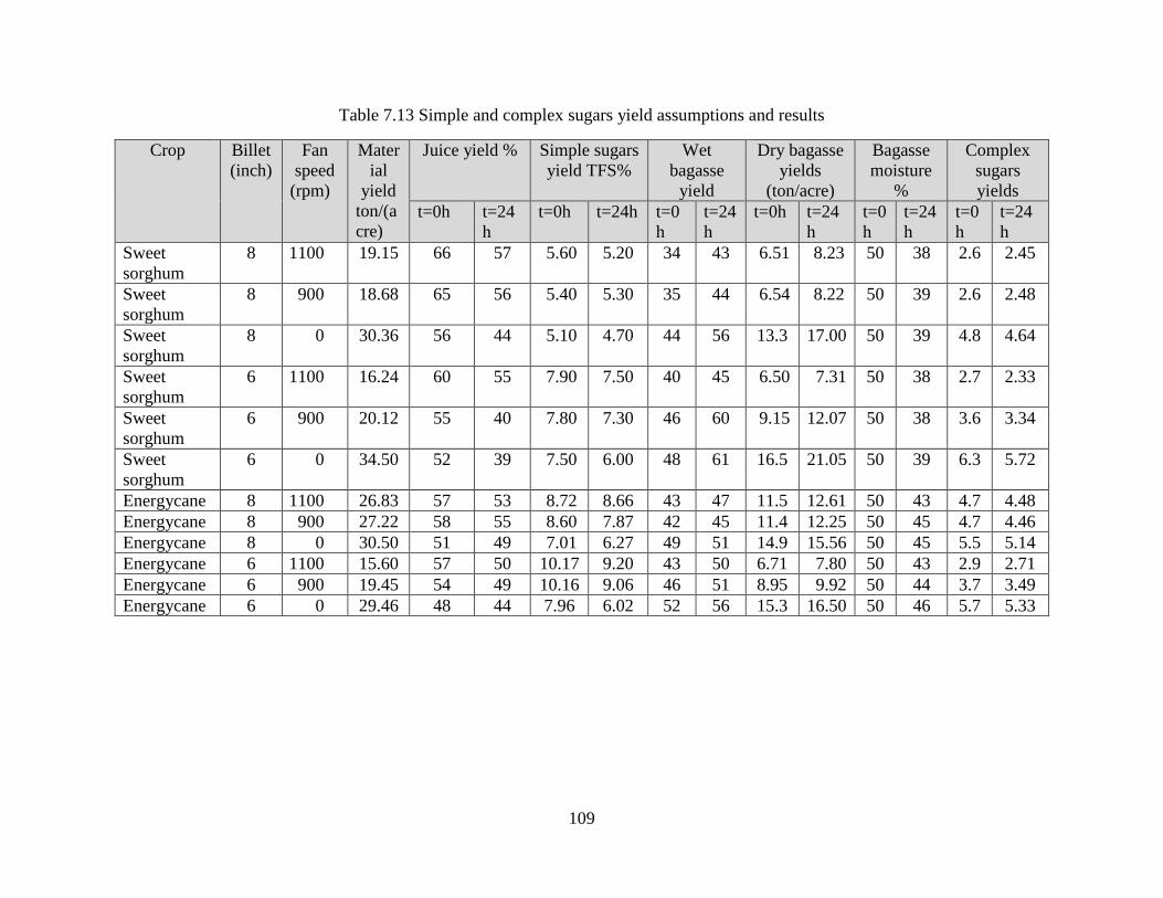
109

Table 7.13 Simple and complex sugars yield assumptions and results

Crop Billet

(inch)

Fan

speed

(rpm)

Mater

ial

yield

ton/(a

cre)

Juice yield % Simple sugars

yield TFS%

Wet

bagasse

yield

Dry bagasse

yields

(ton/acre)

Bagasse

moisture

%

Complex

sugars

yields

t=0h t=24

h

t=0h t=24h t=0

h

t=24

h

t=0h t=24

h

t=0

h

t=24

h

t=0

h

t=24

h

Sweet

sorghum

8 1100 19.15 66 57 5.60 5.20 34 43 6.51 8.23 50 38 2.6 2.45

Sweet

sorghum

8 900 18.68 65 56 5.40 5.30 35 44 6.54 8.22 50 39 2.6 2.48

Sweet

sorghum

8 0 30.36 56 44 5.10 4.70 44 56 13.3 17.00 50 39 4.8 4.64

Sweet

sorghum

6 1100 16.24 60 55 7.90 7.50 40 45 6.50 7.31 50 38 2.7 2.33

Sweet

sorghum

6 900 20.12 55 40 7.80 7.30 46 60 9.15 12.07 50 38 3.6 3.34

Sweet

sorghum

6 0 34.50 52 39 7.50 6.00 48 61 16.5 21.05 50 39 6.3 5.72

Energycane 8 1100 26.83 57 53 8.72 8.66 43 47 11.5 12.61 50 43 4.7 4.48

Energycane 8 900 27.22 58 55 8.60 7.87 42 45 11.4 12.25 50 45 4.7 4.46

Energycane 8 0 30.50 51 49 7.01 6.27 49 51 14.9 15.56 50 45 5.5 5.14

Energycane 6 1100 15.60 57 50 10.17 9.20 43 50 6.71 7.80 50 43 2.9 2.71

Energycane 6 900 19.45 54 49 10.16 9.06 46 51 8.95 9.92 50 44 3.7 3.49

Energycane 6 0 29.46 48 44 7.96 6.02 52 56 15.3 16.50 50 46 5.7 5.33

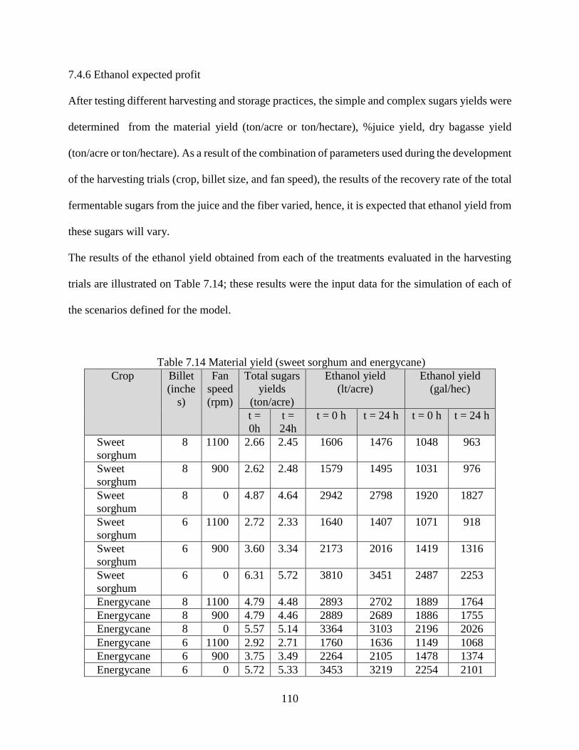
110

7.4.6 Ethanol expected profit

After testing different harvesting and storage practices, the simple and complex sugars yields were

determined from the material yield (ton/acre or ton/hectare), %juice yield, dry bagasse yield

(ton/acre or ton/hectare). As a result of the combination of parameters used during the development

of the harvesting trials (crop, billet size, and fan speed), the results of the recovery rate of the total

fermentable sugars from the juice and the fiber varied, hence, it is expected that ethanol yield from

these sugars will vary.

The results of the ethanol yield obtained from each of the treatments evaluated in the harvesting

trials are illustrated on Table 7.14; these results were the input data for the simulation of each of

the scenarios defined for the model.

Table 7.14 Material yield (sweet sorghum and energycane)

Crop Billet

(inche

s)

Fan

speed

(rpm)

Total sugars

yields

(ton/acre)

Ethanol yield

(lt/acre)

Ethanol yield

(gal/hec)

t =

0h

t =

24h

t = 0 h t = 24 h t = 0 h t = 24 h

Sweet

sorghum

8 1100 2.66 2.45 1606 1476 1048 963

Sweet

sorghum

8 900 2.62 2.48 1579 1495 1031 976

Sweet

sorghum

8 0 4.87 4.64 2942 2798 1920 1827

Sweet

sorghum

6 1100 2.72 2.33 1640 1407 1071 918

Sweet

sorghum

6 900 3.60 3.34 2173 2016 1419 1316

Sweet

sorghum

6 0 6.31 5.72 3810 3451 2487 2253

Energycane 8 1100 4.79 4.48 2893 2702 1889 1764

Energycane 8 900 4.79 4.46 2889 2689 1886 1755

Energycane 8 0 5.57 5.14 3364 3103 2196 2026

Energycane 6 1100 2.92 2.71 1760 1636 1149 1068

Energycane 6 900 3.75 3.49 2264 2105 1478 1374

Energycane 6 0 5.72 5.33 3453 3219 2254 2101

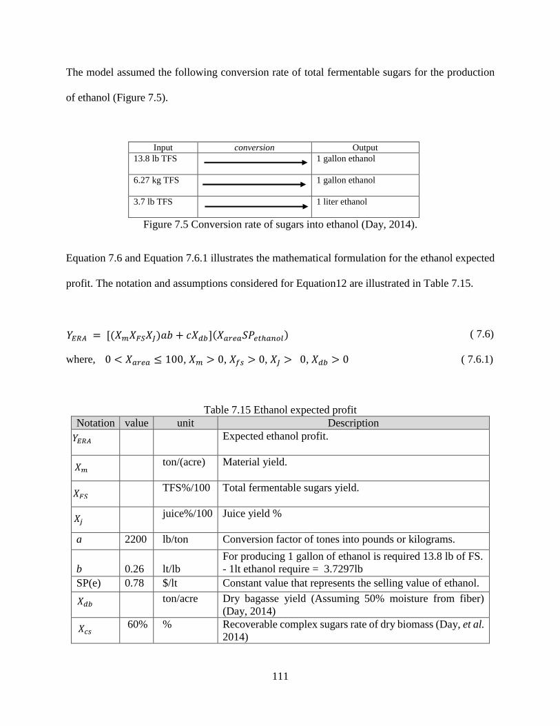
111

The model assumed the following conversion rate of total fermentable sugars for the production

of ethanol (Figure 7.5).

Input conversion Output

13.8 lb TFS

1 gallon ethanol

6.27 kg TFS

1 gallon ethanol

3.7 lb TFS

1 liter ethanol

Figure 7.5 Conversion rate of sugars into ethanol (Day, 2014).

Equation 7.6 and Equation 7.6.1 illustrates the mathematical formulation for the ethanol expected

profit. The notation and assumptions considered for Equation12 are illustrated in Table 7.15.

( 7.6)

where, ( 7.6.1)

Table 7.15 Ethanol expected profit

Notation value unit Description

Expected ethanol profit.

ton/(acre) Material yield.

TFS%/100 Total fermentable sugars yield.

juice%/100 Juice yield %

a 2200 lb/ton Conversion factor of tones into pounds or kilograms.

b

0.26

lt/lb

For producing 1 gallon of ethanol is required 13.8 lb of FS.

- 1lt ethanol require = 3.7297lb

SP(e) 0.78 $/lt Constant value that represents the selling value of ethanol.

ton/acre Dry bagasse yield (Assuming 50% moisture from fiber)

(Day, 2014)

60% % Recoverable complex sugars rate of dry biomass (Day, et al.

2014)

𝑌𝐸𝑅𝐴 = [(𝑋𝑚𝑋𝐹𝑆𝑋𝐽)𝑎𝑏 + 𝑐𝑋𝑑𝑏](𝑋𝑎𝑟𝑒𝑎𝑆𝑃𝑒𝑡ℎ𝑎𝑛𝑜𝑙)

0 < 𝑋𝑎𝑟𝑒𝑎 ≤ 100, 𝑋𝑚 > 0, 𝑋𝑓𝑠 > 0, 𝑋𝐽 > 0, 𝑋𝑑𝑏 > 0

𝑋𝑑𝑏

𝑋𝑐𝑠

𝑌𝐸𝑅𝐴

𝑋𝑚

𝑋𝐹𝑆

𝑋𝑗

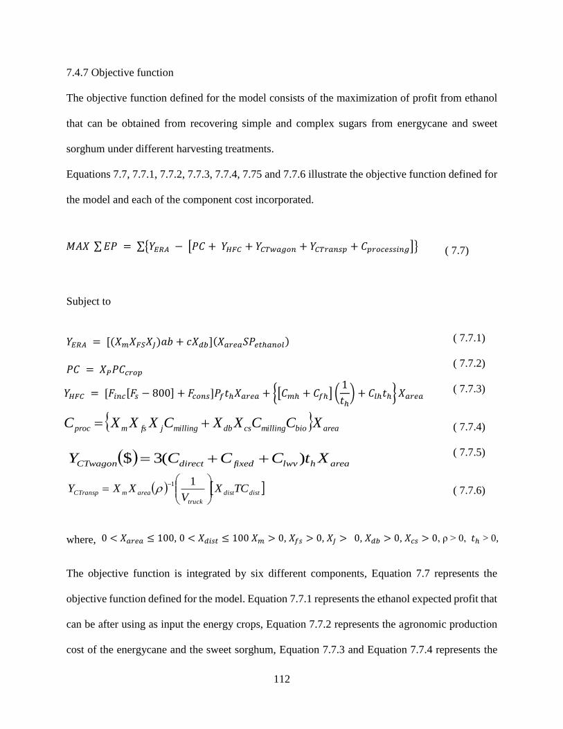
112

7.4.7 Objective function

The objective function defined for the model consists of the maximization of profit from ethanol

that can be obtained from recovering simple and complex sugars from energycane and sweet

sorghum under different harvesting treatments.

Equations 7.7, 7.7.1, 7.7.2, 7.7.3, 7.7.4, 7.75 and 7.7.6 illustrate the objective function defined for

the model and each of the component cost incorporated.

( 7.7)

Subject to

𝑃𝐶 = 𝑋𝑃𝑃𝐶𝑐𝑟𝑜𝑝

areabiomillingcsdbmillingjfsmproc XCCXXCXXXC

where,

The objective function is integrated by six different components, Equation 7.7 represents the

objective function defined for the model. Equation 7.7.1 represents the ethanol expected profit that

can be after using as input the energy crops, Equation 7.7.2 represents the agronomic production

cost of the energycane and the sweet sorghum, Equation 7.7.3 and Equation 7.7.4 represents the

𝑀𝐴𝑋 ∑ 𝐸𝑃 = ∑{𝑌𝐸𝑅𝐴 − [𝑃𝐶 + 𝑌𝐻𝐹𝐶 + 𝑌𝐶𝑇𝑤𝑎𝑔𝑜𝑛 + 𝑌𝐶𝑇𝑟𝑎𝑛𝑠𝑝 + 𝐶𝑝𝑟𝑜𝑐𝑒𝑠𝑠𝑖𝑛𝑔]}

𝑌𝐻𝐹𝐶 = [𝐹𝑖𝑛𝑐[𝐹𝑠 − 800] + 𝐹𝑐𝑜𝑛𝑠]𝑃𝑓𝑡ℎ𝑋𝑎𝑟𝑒𝑎 + {[𝐶𝑚ℎ + 𝐶𝑓ℎ] (1

𝑡ℎ) + 𝐶𝑙ℎ𝑡ℎ} 𝑋𝑎𝑟𝑒𝑎

𝑌𝐸𝑅𝐴 = [(𝑋𝑚𝑋𝐹𝑆𝑋𝐽)𝑎𝑏 + 𝑐𝑋𝑑𝑏](𝑋𝑎𝑟𝑒𝑎𝑆𝑃𝑒𝑡ℎ𝑎𝑛𝑜𝑙)

0 < 𝑋𝑎𝑟𝑒𝑎 ≤ 100, 0 < 𝑋𝑑𝑖𝑠𝑡 ≤ 100 𝑋𝑚 > 0, 𝑋𝑓𝑠 > 0, 𝑋𝐽 > 0, 𝑋𝑑𝑏 > 0, 𝑋𝑐𝑠 > 0, ρ > 0, 𝑡ℎ > 0,

areahlwvfixeddirectCTwagon XtCCCY )(3$

distdist

truck

areamCTransp TCXV

XXY

11

( 7.7.1)

( 7.7.2)

( 7.7.3)

( 7.7.4)

( 7.7.5)

( 7.7.6)

113

harvesting and wagon cost. Equation 7.7.5 and Equation 7.7.6 represents the cost of transporting

the material from the field to the bio refinery and the processing cost. Finally the non-negativity

and boundary limits are given.

114

CHAPTER 8: MODEL SIMULATION

The model considered the economics of the harvesting, collection, transportation, processing and

conversion of simple and complex sugars into ethanol, and its estimates the ethanol expected profit

that can be obtained under different harvesting practices.

Finally, the objective function of the model was defined in terms of the profit maximization that

can be obtained after simulating different scenarios.

After implementing different harvesting and storage practices, it was expected that the previous

indicators would change between treatments, especially when the area for harvesting and the

distance for transporting the material was varied during the simulation.

The main parameters that were varied in the scenarios were the followings:

1. Type of crop (sweet sorghum – energycane).

2. Billet size (8 and 6 inches).

3. Fan speed of the extractor system (0, 900 and 1100 rpm’s).

4. Processing time or the period of time in which the material was stored before been

processed for simple and complex sugars recovery (processing time at t = 0 hours and

processing time after 24 hours).

5. Area for harvesting

6. Distance for transporting the material from the field to the factory.

A total of 24 scenarios were defined and simulated using the model, 12 of these scenarios

considered the simple and complex sugars recovered from sweet sorghum for ethanol production

and 12 scenarios, considered the sugars recovered from the energycane.

115

The execution and simulation of the model was developed in Microsoft Excel, version 2010. The

model included all the mathematical formulation for each of the component costs shown in

Section8 that integrate the supply system used for the production of ethanol defined in the study.

The mathematical formulation developed in Microsoft Excel used as input for the simulation of

the scenarios, all the results obtained from the harvesting trials; this data that was used for the

calculation of the simple and complex sugars yield from the crops and the agronomic and

efficiency indicators defined in the study; these results are reported in Section 7.

The model simulated the 24 scenarios that were defined for the study. The simulation considered

an area for harvesting between 1 to 100 acres and a distance for transporting the material from the

field to the factory that ranged between 1 to 100 miles.

The total cost of the supply system was calculated first, as well as the potential ethanol sale value,

then, the ethanol profit was calculated in the matrixes based on the distances and area covered for

transporting and harvesting the material.

Table 8.1 and Table 8.2 illustrates each of the scenarios defined for the model and the parameter

configuration established for the simulation of each of the scenarios.

Finally, after simulating the scenarios, an analysis of the results was performed in order to

determine which parameters and condition satisfied the objective function.

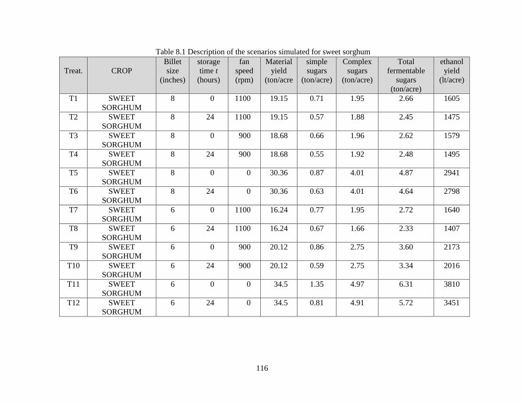
116

Table 8.1 Description of the scenarios simulated for sweet sorghum

Treat.

CROP

Billet

size

(inches)

storage

time t

(hours)

fan

speed

(rpm)

Material

yield

(ton/acre

simple

sugars

(ton/acre)

Complex

sugars

(ton/acre)

Total

fermentable

sugars

(ton/acre)

ethanol

yield

(lt/acre)

T1 SWEET

SORGHUM

8 0 1100 19.15 0.71 1.95 2.66 1605

T2 SWEET

SORGHUM

8 24 1100 19.15 0.57 1.88 2.45 1475

T3 SWEET

SORGHUM

8 0 900 18.68 0.66 1.96 2.62 1579

T4 SWEET

SORGHUM

8 24 900 18.68 0.55 1.92 2.48 1495

T5 SWEET

SORGHUM

8 0 0 30.36 0.87 4.01 4.87 2941

T6 SWEET

SORGHUM

8 24 0 30.36 0.63 4.01 4.64 2798

T7 SWEET

SORGHUM

6 0 1100 16.24 0.77 1.95 2.72 1640

T8 SWEET

SORGHUM

6 24 1100 16.24 0.67 1.66 2.33 1407

T9 SWEET

SORGHUM

6 0 900 20.12 0.86 2.75 3.60 2173

T10 SWEET

SORGHUM

6 24 900 20.12 0.59 2.75 3.34 2016

T11 SWEET

SORGHUM

6 0 0 34.5 1.35 4.97 6.31 3810

T12 SWEET

SORGHUM

6 24 0 34.5 0.81 4.91 5.72 3451

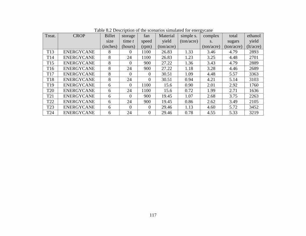
117

Table 8.2 Description of the scenarios simulated for energycane

Treat. CROP Billet

size

(inches)

storage

time t

(hours)

fan

speed

(rpm)

Material

yield

(ton/acre)

simple s.

(ton/acre)

complex

s.

(ton/acre)

total

sugars

(ton/acre)

ethanol

yield

(lt/acre)

T13 ENERGYCANE 8 0 1100 26.83 1.33 3.46 4.79 2893

T14 ENERGYCANE 8 24 1100 26.83 1.23 3.25 4.48 2701

T15 ENERGYCANE 8 0 900 27.22 1.36 3.43 4.79 2889

T16 ENERGYCANE 8 24 900 27.22 1.18 3.28 4.46 2689

T17 ENERGYCANE 8 0 0 30.51 1.09 4.48 5.57 3363

T18 ENERGYCANE 8 24 0 30.51 0.94 4.21 5.14 3103

T19 ENERGYCANE 6 0 1100 15.6 0.90 2.01 2.92 1760

T20 ENERGYCANE 6 24 1100 15.6 0.72 1.99 2.71 1636

T21 ENERGYCANE 6 0 900 19.45 1.07 2.68 3.75 2263

T22 ENERGYCANE 6 24 900 19.45 0.86 2.62 3.49 2105

T23 ENERGYCANE 6 0 0 29.46 1.13 4.60 5.72 3452

T24 ENERGYCANE 6 24 0 29.46 0.78 4.55 5.33 3219

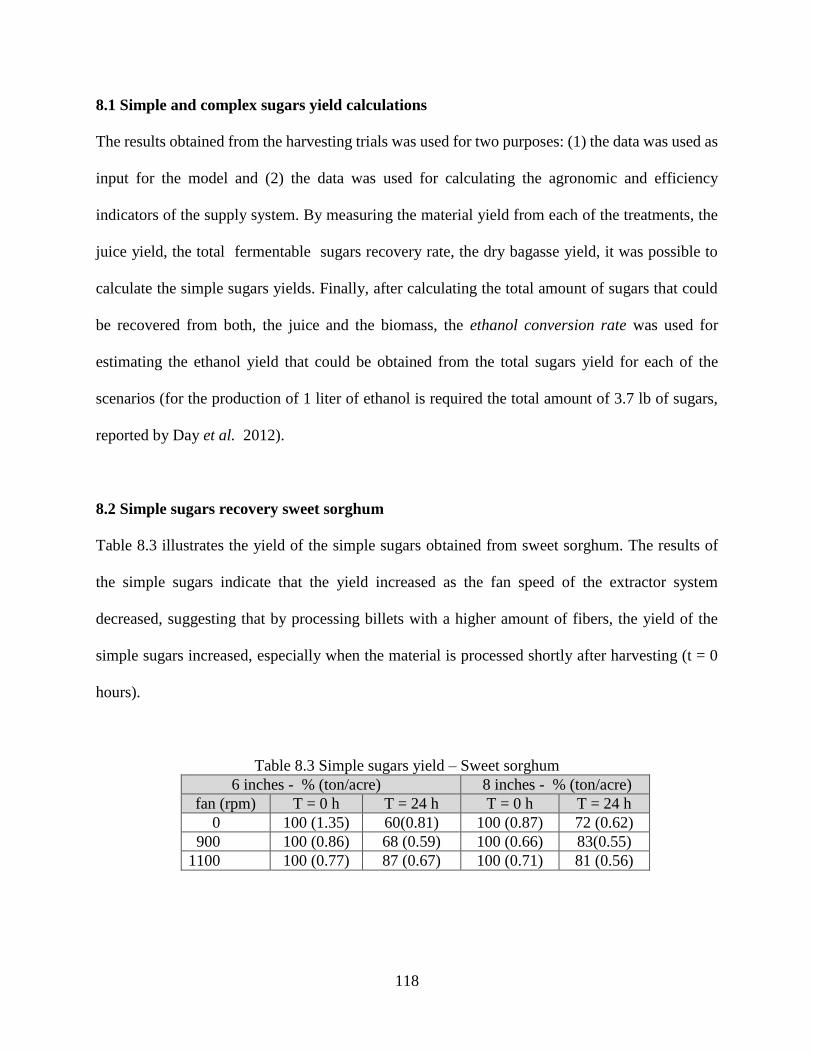
118

8.1 Simple and complex sugars yield calculations

The results obtained from the harvesting trials was used for two purposes: (1) the data was used as

input for the model and (2) the data was used for calculating the agronomic and efficiency

indicators of the supply system. By measuring the material yield from each of the treatments, the

juice yield, the total fermentable sugars recovery rate, the dry bagasse yield, it was possible to

calculate the simple sugars yields. Finally, after calculating the total amount of sugars that could

be recovered from both, the juice and the biomass, the ethanol conversion rate was used for

estimating the ethanol yield that could be obtained from the total sugars yield for each of the

scenarios (for the production of 1 liter of ethanol is required the total amount of 3.7 lb of sugars,

reported by Day et al. 2012).

8.2 Simple sugars recovery sweet sorghum

Table 8.3 illustrates the yield of the simple sugars obtained from sweet sorghum. The results of

the simple sugars indicate that the yield increased as the fan speed of the extractor system

decreased, suggesting that by processing billets with a higher amount of fibers, the yield of the

simple sugars increased, especially when the material is processed shortly after harvesting (t = 0

hours).

Table 8.3 Simple sugars yield – Sweet sorghum

6 inches - % (ton/acre) 8 inches - % (ton/acre)

fan (rpm) T = 0 h T = 24 h T = 0 h T = 24 h

0 100 (1.35) 60(0.81) 100 (0.87) 72 (0.62)

900 100 (0.86) 68 (0.59) 100 (0.66) 83(0.55)

1100 100 (0.77) 87 (0.67) 100 (0.71) 81 (0.56)

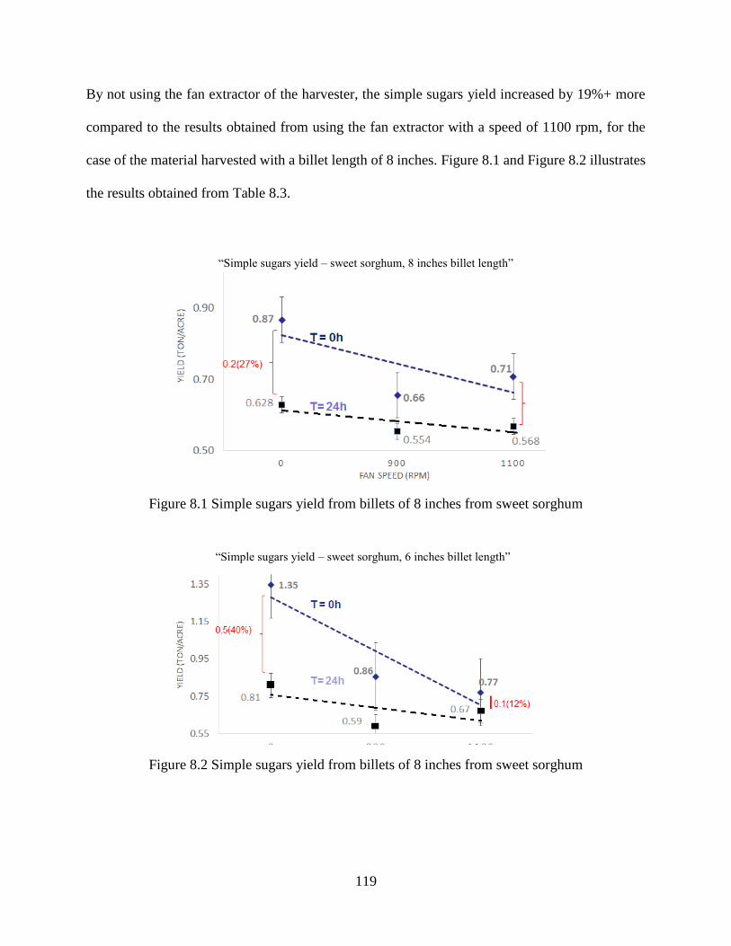
119

By not using the fan extractor of the harvester, the simple sugars yield increased by 19%+ more

compared to the results obtained from using the fan extractor with a speed of 1100 rpm, for the

case of the material harvested with a billet length of 8 inches. Figure 8.1 and Figure 8.2 illustrates

the results obtained from Table 8.3.

Figure 8.1 Simple sugars yield from billets of 8 inches from sweet sorghum

Figure 8.2 Simple sugars yield from billets of 8 inches from sweet sorghum

“Simple sugars yield – sweet sorghum, 8 inches billet length”

“Simple sugars yield – sweet sorghum, 6 inches billet length”

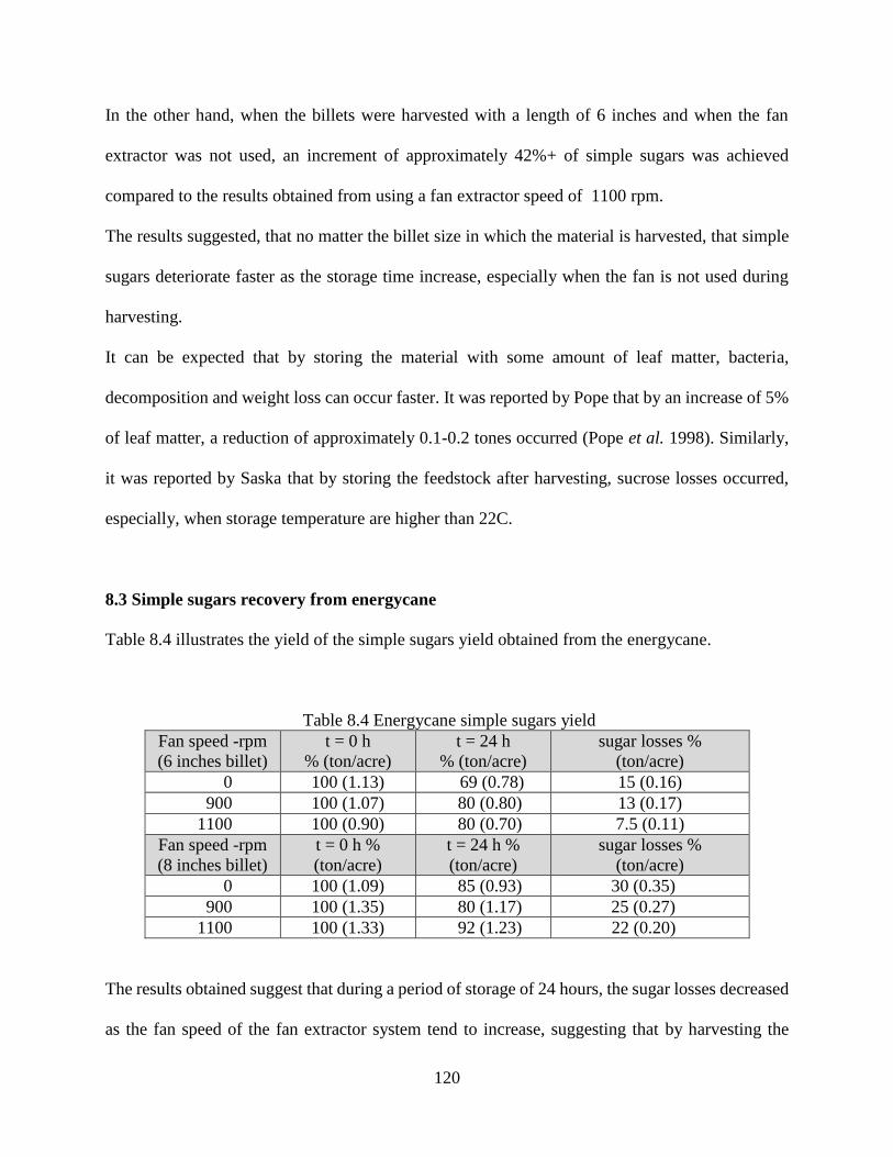
120

In the other hand, when the billets were harvested with a length of 6 inches and when the fan

extractor was not used, an increment of approximately 42%+ of simple sugars was achieved

compared to the results obtained from using a fan extractor speed of 1100 rpm.

The results suggested, that no matter the billet size in which the material is harvested, that simple

sugars deteriorate faster as the storage time increase, especially when the fan is not used during

harvesting.

It can be expected that by storing the material with some amount of leaf matter, bacteria,

decomposition and weight loss can occur faster. It was reported by Pope that by an increase of 5%

of leaf matter, a reduction of approximately 0.1-0.2 tones occurred (Pope et al. 1998). Similarly,

it was reported by Saska that by storing the feedstock after harvesting, sucrose losses occurred,

especially, when storage temperature are higher than 22C.

8.3 Simple sugars recovery from energycane

Table 8.4 illustrates the yield of the simple sugars yield obtained from the energycane.

Table 8.4 Energycane simple sugars yield

The results obtained suggest that during a period of storage of 24 hours, the sugar losses decreased

as the fan speed of the fan extractor system tend to increase, suggesting that by harvesting the

Fan speed -rpm

(6 inches billet)

t = 0 h

% (ton/acre)

t = 24 h

% (ton/acre)

sugar losses %

(ton/acre)

0 100 (1.13) 69 (0.78) 15 (0.16)

900 100 (1.07) 80 (0.80) 13 (0.17)

1100 100 (0.90) 80 (0.70) 7.5 (0.11)

Fan speed -rpm

(8 inches billet)

t = 0 h %

(ton/acre)

t = 24 h %

(ton/acre)

sugar losses %

(ton/acre)

0 100 (1.09) 85 (0.93) 30 (0.35)

900 100 (1.35) 80 (1.17) 25 (0.27)

1100 100 (1.33) 92 (1.23) 22 (0.20)

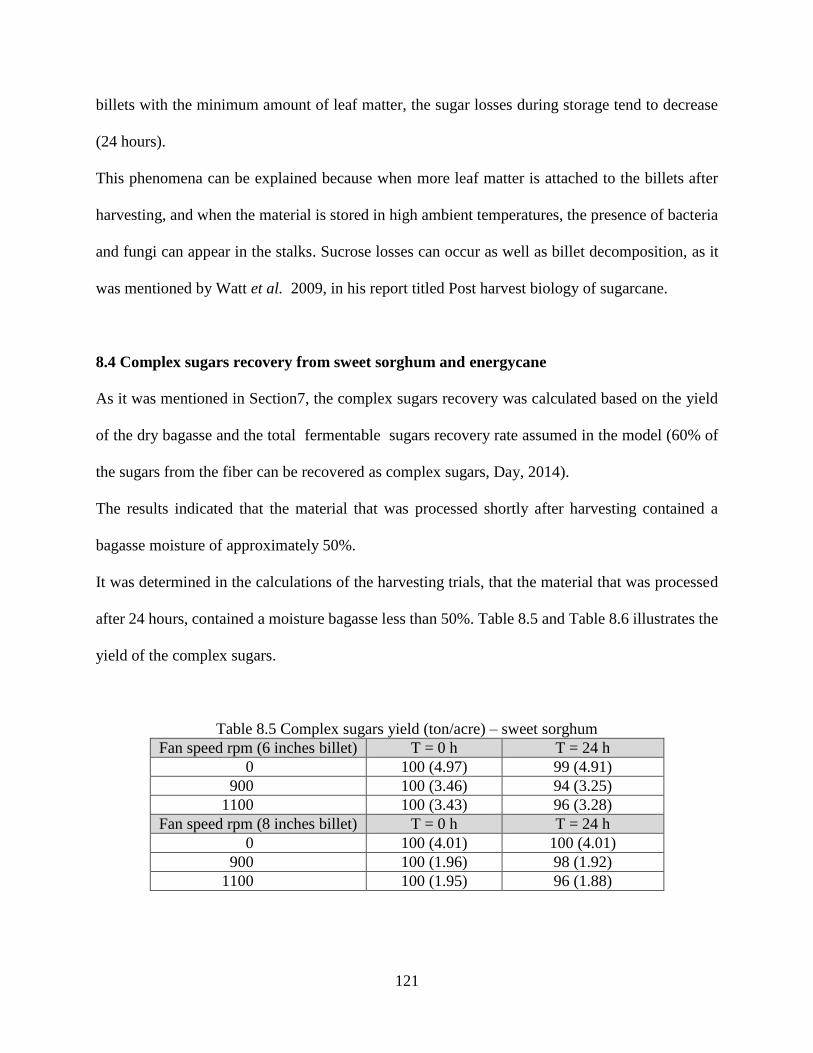
121

billets with the minimum amount of leaf matter, the sugar losses during storage tend to decrease

(24 hours).

This phenomena can be explained because when more leaf matter is attached to the billets after

harvesting, and when the material is stored in high ambient temperatures, the presence of bacteria

and fungi can appear in the stalks. Sucrose losses can occur as well as billet decomposition, as it

was mentioned by Watt et al. 2009, in his report titled Post harvest biology of sugarcane.

8.4 Complex sugars recovery from sweet sorghum and energycane

As it was mentioned in Section7, the complex sugars recovery was calculated based on the yield

of the dry bagasse and the total fermentable sugars recovery rate assumed in the model (60% of

the sugars from the fiber can be recovered as complex sugars, Day, 2014).

The results indicated that the material that was processed shortly after harvesting contained a

bagasse moisture of approximately 50%.

It was determined in the calculations of the harvesting trials, that the material that was processed

after 24 hours, contained a moisture bagasse less than 50%. Table 8.5 and Table 8.6 illustrates the

yield of the complex sugars.

Table 8.5 Complex sugars yield (ton/acre) – sweet sorghum

Fan speed rpm (6 inches billet) T = 0 h T = 24 h

0 100 (4.97) 99 (4.91)

900 100 (3.46) 94 (3.25)

1100 100 (3.43) 96 (3.28)

Fan speed rpm (8 inches billet) T = 0 h T = 24 h

0 100 (4.01) 100 (4.01)

900 100 (1.96) 98 (1.92)

1100 100 (1.95) 96 (1.88)

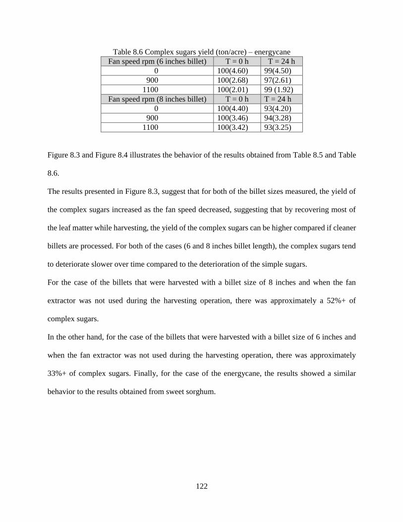
122

Table 8.6 Complex sugars yield (ton/acre) – energycane

Fan speed rpm (6 inches billet) T = 0 h T = 24 h

0 100(4.60) 99(4.50)

900 100(2.68) 97(2.61)

1100 100(2.01) 99 (1.92)

Fan speed rpm (8 inches billet) T = 0 h T = 24 h

0 100(4.40) 93(4.20)

900 100(3.46) 94(3.28)

1100 100(3.42) 93(3.25)

Figure 8.3 and Figure 8.4 illustrates the behavior of the results obtained from Table 8.5 and Table

8.6.

The results presented in Figure 8.3, suggest that for both of the billet sizes measured, the yield of

the complex sugars increased as the fan speed decreased, suggesting that by recovering most of

the leaf matter while harvesting, the yield of the complex sugars can be higher compared if cleaner

billets are processed. For both of the cases (6 and 8 inches billet length), the complex sugars tend

to deteriorate slower over time compared to the deterioration of the simple sugars.

For the case of the billets that were harvested with a billet size of 8 inches and when the fan

extractor was not used during the harvesting operation, there was approximately a 52%+ of

complex sugars.

In the other hand, for the case of the billets that were harvested with a billet size of 6 inches and

when the fan extractor was not used during the harvesting operation, there was approximately

33%+ of complex sugars. Finally, for the case of the energycane, the results showed a similar

behavior to the results obtained from sweet sorghum.

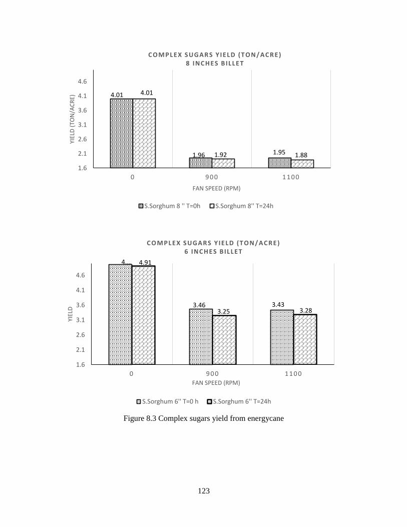
123

Figure 8.3 Complex sugars yield from energycane

4.01

1.96 1.95

4.01

1.92 1.88

1.6

2.1

2.6

3.1

3.6

4.1

4.6

0 9 0 0 1 1 0 0

YIEL

D (

TON

/AC

RE)

FAN SPEED (RPM)

C O M P LEX S UGAR S Y IELD (T O N/ AC R E)8 INC H ES BILLET

S.Sorghum 8 '' T=0h S.Sorghum 8'' T=24h

4.…

3.46 3.43

4.91

3.25 3.28

1.6

2.1

2.6

3.1

3.6

4.1

4.6

0 9 0 0 1 1 0 0

YIEL

D

FAN SPEED (RPM)

C O M P LEX S UGAR S Y IELD (T O N/ AC R E)6 INC H ES BILLET

S.Sorghum 6'' T=0 h S.Sorghum 6'' T=24h

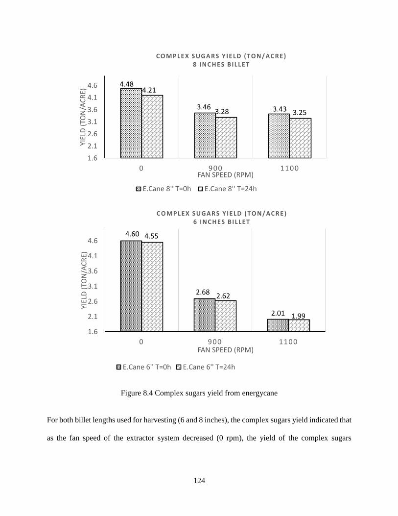
124

Figure 8.4 Complex sugars yield from energycane

For both billet lengths used for harvesting (6 and 8 inches), the complex sugars yield indicated that

as the fan speed of the extractor system decreased (0 rpm), the yield of the complex sugars

4.01

1.96 1.95

4.01

1.92 1.88

1.6

2.1

2.6

3.1

3.6

4.1

4.6

0 9 0 0 1 1 0 0

YIEL

D (

TON

/AC

RE)

FAN SPEED (RPM)

C O M P LEX S UGAR S Y IELD (T O N/ AC R E)8 INC H ES BILLET

S.Sorghum 8 '' T=0h S.Sorghum 8'' T=24h

4.…

3.46 3.43

4.91

3.25 3.28

1.60

2.10

2.60

3.10

3.60

4.10

4.60

0 9 0 0 1 1 0 0

YIEL

D (

TON

/AC

RE)

FAN SPEED (RPM)

C O M P LEX S UGAR S Y IELD (T O N/ AC R E)6 INC H ES BILLET

S.Sorghum 6'' T=0 h S.Sorghum 6'' T=24h

4.48

3.46 3.43

4.21

3.28 3.25

1.6

2.1

2.6

3.1

3.6

4.1

4.6

0 900 1100

YIEL

D (

TON

/AC

RE)

FAN SPEED (RPM)

C O M P LEX S UGAR S Y IELD (T O N/ AC R E)8 INC H ES BILLET

E.Cane 8'' T=0h E.Cane 8'' T=24h

4.60

2.68

2.01

4.55

2.62

1.99

1.6

2.1

2.6

3.1

3.6

4.1

4.6

0 900 1100

YIEL

D (

TON

/AC

RE)

FAN SPEED (RPM)

C O M P LEX S UGAR S Y IELD (T O N/ AC R E)6 INC H ES BILLET

E.Cane 6'' T=0h E.Cane 6'' T=24h

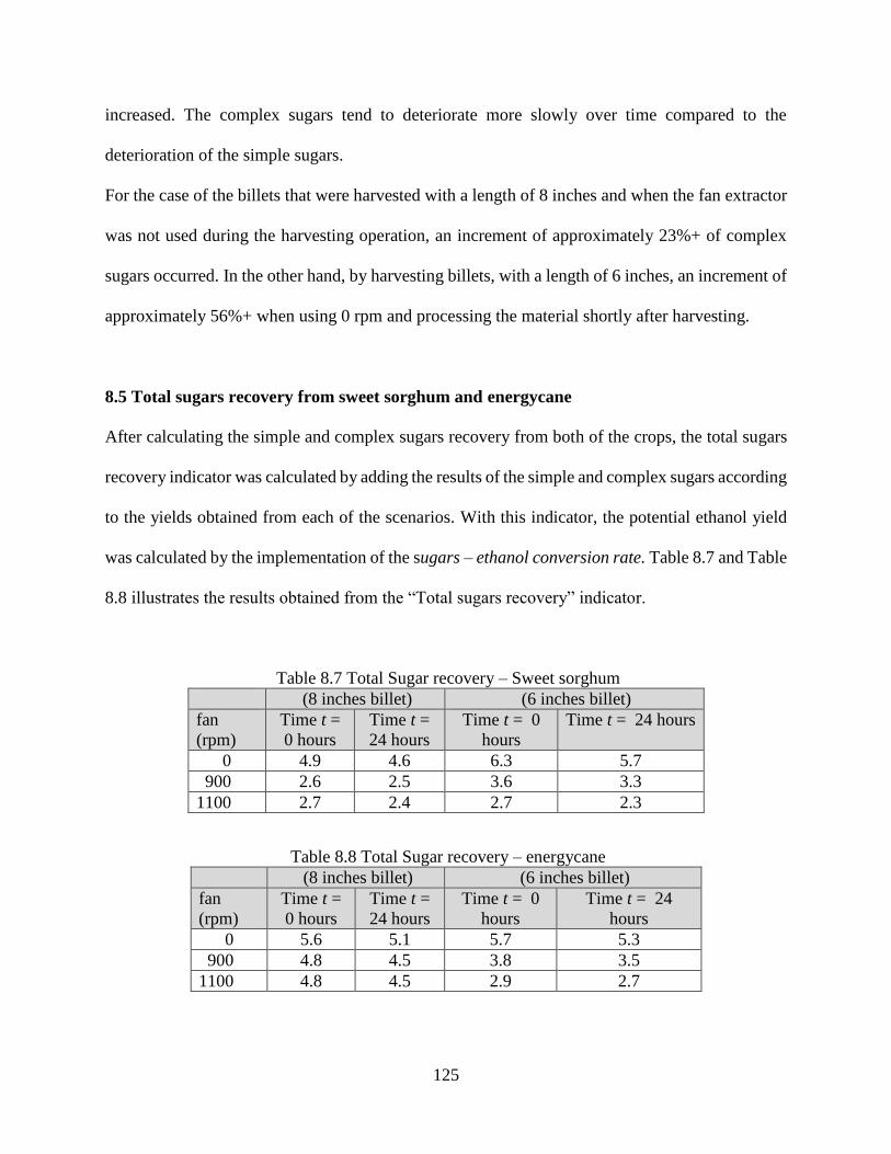
125

increased. The complex sugars tend to deteriorate more slowly over time compared to the

deterioration of the simple sugars.

For the case of the billets that were harvested with a length of 8 inches and when the fan extractor

was not used during the harvesting operation, an increment of approximately 23%+ of complex

sugars occurred. In the other hand, by harvesting billets, with a length of 6 inches, an increment of

approximately 56%+ when using 0 rpm and processing the material shortly after harvesting.

8.5 Total sugars recovery from sweet sorghum and energycane

After calculating the simple and complex sugars recovery from both of the crops, the total sugars

recovery indicator was calculated by adding the results of the simple and complex sugars according

to the yields obtained from each of the scenarios. With this indicator, the potential ethanol yield

was calculated by the implementation of the sugars – ethanol conversion rate. Table 8.7 and Table

8.8 illustrates the results obtained from the “Total sugars recovery” indicator.

Table 8.7 Total Sugar recovery – Sweet sorghum

(8 inches billet) (6 inches billet)

fan

(rpm)

Time t =

0 hours

Time t =

24 hours

Time t = 0

hours

Time t = 24 hours

0 4.9 4.6 6.3 5.7

900 2.6 2.5 3.6 3.3

1100 2.7 2.4 2.7 2.3

Table 8.8 Total Sugar recovery – energycane

(8 inches billet) (6 inches billet)

fan

(rpm)

Time t =

0 hours

Time t =

24 hours

Time t = 0

hours

Time t = 24

hours

0 5.6 5.1 5.7 5.3

900 4.8 4.5 3.8 3.5

1100 4.8 4.5 2.9 2.7

126

As can be seen from the yield of the total sugars obtained from sweet sorghum, the results suggest

that as the fan speed decrease, the yield of the total sugars recovery increases, especially when the

material is processed shortly after harvesting. It also was evidenced that by storing the material for

24 hours, the yield of the total sugars recovery decreased. The following behavior of the results

was evidenced for the case of the sweet sorghum:

1. When the material was harvested with a billet length of 8 inches and processed shortly after

harvesting with a fan speed of 0 rpm, the yield of the Total fermentable sugars (TFS),

increased by 6% compared to the results obtained 24 hours later.

2. When the material was harvested with a billet length of 8 inches and processed shortly after

harvesting with a fan speed of 900 rpm, the yield of the Total fermentable sugars (TFS),

increased by 4% compared to the results obtained 24 hours later.

3. When the material was harvested with a billet length of 8 inches and processed shortly after

harvesting with a fan speed of 1100 rpm, the yield of the Total fermentable sugars (TFS),

increased by 11% compared to the results obtained 24 hours later.

4. When the material was harvested with a billet length of 6 inches and processed shortly after

harvesting with a fan speed of 0 rpm, the yield of the Total fermentable sugars (TFS),

increased by 9% compared to the results obtained 24 hours later.

5. When the material was harvested with a billet length of 6 inches and processed shortly after

harvesting with a fan speed of 900 rpm, the yield of the Total fermentable sugars (TFS),

increased by 8% compared to the results obtained 24 hours later.

6. When the material was harvested with a billet length of 6 inches and processed shortly after

harvesting with a fan speed of 1100 rpm, the yield of the Total fermentable sugars (TFS),

increased by 14% compared to the results obtained 24 hours later.

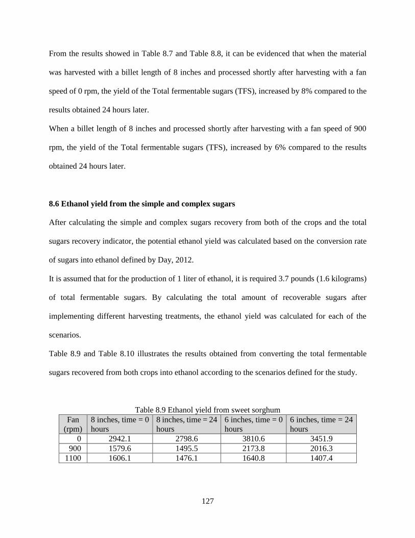
127

From the results showed in Table 8.7 and Table 8.8, it can be evidenced that when the material

was harvested with a billet length of 8 inches and processed shortly after harvesting with a fan

speed of 0 rpm, the yield of the Total fermentable sugars (TFS), increased by 8% compared to the

results obtained 24 hours later.

When a billet length of 8 inches and processed shortly after harvesting with a fan speed of 900

rpm, the yield of the Total fermentable sugars (TFS), increased by 6% compared to the results

obtained 24 hours later.

8.6 Ethanol yield from the simple and complex sugars

After calculating the simple and complex sugars recovery from both of the crops and the total

sugars recovery indicator, the potential ethanol yield was calculated based on the conversion rate

of sugars into ethanol defined by Day, 2012.

It is assumed that for the production of 1 liter of ethanol, it is required 3.7 pounds (1.6 kilograms)

of total fermentable sugars. By calculating the total amount of recoverable sugars after

implementing different harvesting treatments, the ethanol yield was calculated for each of the

scenarios.

Table 8.9 and Table 8.10 illustrates the results obtained from converting the total fermentable

sugars recovered from both crops into ethanol according to the scenarios defined for the study.

Table 8.9 Ethanol yield from sweet sorghum

Fan

(rpm)

8 inches, time = 0

hours

8 inches, time = 24

hours

6 inches, time = 0

hours

6 inches, time = 24

hours

0 2942.1 2798.6 3810.6 3451.9

900 1579.6 1495.5 2173.8 2016.3

1100 1606.1 1476.1 1640.8 1407.4

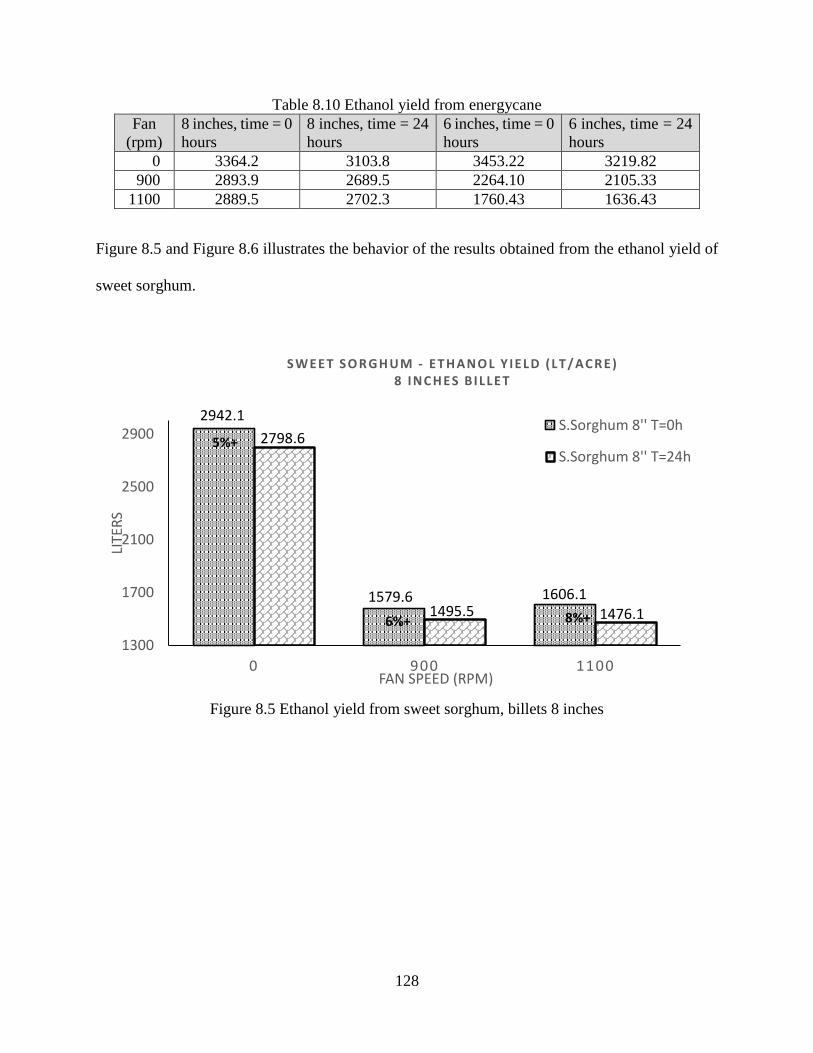
128

Table 8.10 Ethanol yield from energycane

Fan

(rpm)

8 inches, time = 0

hours

8 inches, time = 24

hours

6 inches, time = 0

hours

6 inches, time = 24

hours

0 3364.2 3103.8 3453.22 3219.82

900 2893.9 2689.5 2264.10 2105.33

1100 2889.5 2702.3 1760.43 1636.43

Figure 8.5 and Figure 8.6 illustrates the behavior of the results obtained from the ethanol yield of

sweet sorghum.

Figure 8.5 Ethanol yield from sweet sorghum, billets 8 inches

2942.1

1579.6 1606.1

2798.6

1495.5 1476.1

1300

1700

2100

2500

2900

0 900 1100

LITE

RS

FAN SPEED (RPM)

S W EET S O R GH UM - ET H ANO L Y IELD (LT / AC R E)8 INC H ES BILLET

S.Sorghum 8'' T=0h

S.Sorghum 8'' T=24h5%+

6%+ 8%+

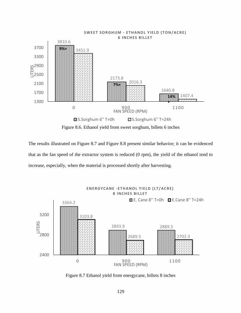
129

Figure 8.6. Ethanol yield from sweet sorghum, billets 6 inches

The results illustrated on Figure 8.7 and Figure 8.8 present similar behavior; it can be evidenced

that as the fan speed of the extractor system is reduced (0 rpm), the yield of the ethanol tend to

increase, especially, when the material is processed shortly after harvesting.

Figure 8.7 Ethanol yield from energycane, billets 8 inches

3810.6

2173.8

1640.8

3451.9

2016.3

1407.41300

1700

2100

2500

2900

3300

3700

0 900 1100

LITE

RS

FAN SPEED (RPM)

S W EET S O R GH UM - ET H ANO L Y IELD (T O N/ AC R E)6 INC H ES BILLET

S.Sorghum 6'' T=0h S.Sorghum 6'' T=24h

9%+

7%+

14%+

3364.2

2893.9 2889.5

3103.8

2689.5 2702.3

2400

2800

3200

0 900 1100

LITE

RS

FAN SPEED (RPM)

ENER GY C ANE - ET H ANO L Y IELD (LT / AC R E)8 INC H ES BILLET

E. Cane 8'' T=0h E.Cane 8'' T=24h

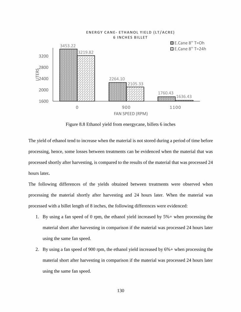
130

Figure 8.8 Ethanol yield from energycane, billets 6 inches

The yield of ethanol tend to increase when the material is not stored during a period of time before

processing, hence, some losses between treatments can be evidenced when the material that was

processed shortly after harvesting, is compared to the results of the material that was processed 24

hours later.

The following differences of the yields obtained between treatments were observed when

processing the material shortly after harvesting and 24 hours later. When the material was

processed with a billet length of 8 inches, the following differences were evidenced:

1. By using a fan speed of 0 rpm, the ethanol yield increased by 5%+ when processing the

material short after harvesting in comparison if the material was processed 24 hours later

using the same fan speed.

2. By using a fan speed of 900 rpm, the ethanol yield increased by 6%+ when processing the

material short after harvesting in comparison if the material was processed 24 hours later

using the same fan speed.

3453.22

2264.10

1760.43

3219.82

2105.33

1636.431600

2000

2400

2800

3200

0 900 1100

LITE

RS

FAN SPEED (RPM)

ENER GY C ANE - ET H ANO L Y IELD (LT / AC R E)6 INC H ES BILLET

E.Cane 8'' T=OhE.Cane 8'' T=24h

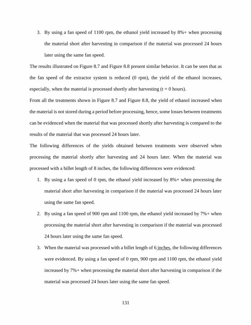
131

3. By using a fan speed of 1100 rpm, the ethanol yield increased by 8%+ when processing

the material short after harvesting in comparison if the material was processed 24 hours

later using the same fan speed.

The results illustrated on Figure 8.7 and Figure 8.8 present similar behavior. It can be seen that as

the fan speed of the extractor system is reduced (0 rpm), the yield of the ethanol increases,

especially, when the material is processed shortly after harvesting (t = 0 hours).

From all the treatments shown in Figure 8.7 and Figure 8.8, the yield of ethanol increased when

the material is not stored during a period before processing, hence, some losses between treatments

can be evidenced when the material that was processed shortly after harvesting is compared to the

results of the material that was processed 24 hours later.

The following differences of the yields obtained between treatments were observed when

processing the material shortly after harvesting and 24 hours later. When the material was

processed with a billet length of 8 inches, the following differences were evidenced:

1. By using a fan speed of 0 rpm, the ethanol yield increased by 8%+ when processing the

material short after harvesting in comparison if the material was processed 24 hours later

using the same fan speed.

2. By using a fan speed of 900 rpm and 1100 rpm, the ethanol yield increased by 7%+ when

processing the material short after harvesting in comparison if the material was processed

24 hours later using the same fan speed.

3. When the material was processed with a billet length of 6 inches, the following differences

were evidenced. By using a fan speed of 0 rpm, 900 rpm and 1100 rpm, the ethanol yield

increased by 7%+ when processing the material short after harvesting in comparison if the

material was processed 24 hours later using the same fan speed.

132

8.7 Simulation Results “Profit Maximization”

The simulation of the model was performed using Microsoft Excel, version 2010. 24 scenarios

were defined in the model and were simulated. A total of 240.000 iterations of the ethanol profit

function were obtained after simulating all the scenarios.

In the simulation, the total supply cost function was defined, which considered the following costs:

agronomic production of the crop ($/acre), the harvesting cost ($/acre) and the wagon cost ($/acre).

Also, in the simulation was defined the processing cost ($/material obtained from an acre), all these

costs were constant per treatment, and were calculated based on the mathematical definition

developed on Section 7 and also were calculated based on the input data for the model (harvesting

trials data).

The transportation cost was not defined as a fixed cost, because it varies according to the distance

parameter defined from the simulation (range between 1 to 100 miles). Table 8.11, provide the

results of the supply cost (cost/acre), the processing cost (cost$/acre) and the ethanol sale value

($/acre).

The ethanol sale value was calculated from the yield of the total sugars obtained from each of the

treatments and was converted into the potential ethanol yield per acre (lt/acre). By using the selling

price of the ethanol, the expected ethanol sale value was calculated ($/acre).

It can be evidenced from Table 8.11 that treatment number 1 illustrate the following results:

1. Treatment configuration: “sweet sorghum” harvested with a billet size of 8 inches, a

fan speed of 1100 rpm, and a processing time of t = 0h.

2. The expected ethanol yield per acre was approximately 1605.89 liters

3. The supply cost per acre was estimated in 484.19 dollars.

4. The processing cost per acre was estimated in 573.39 dollars.

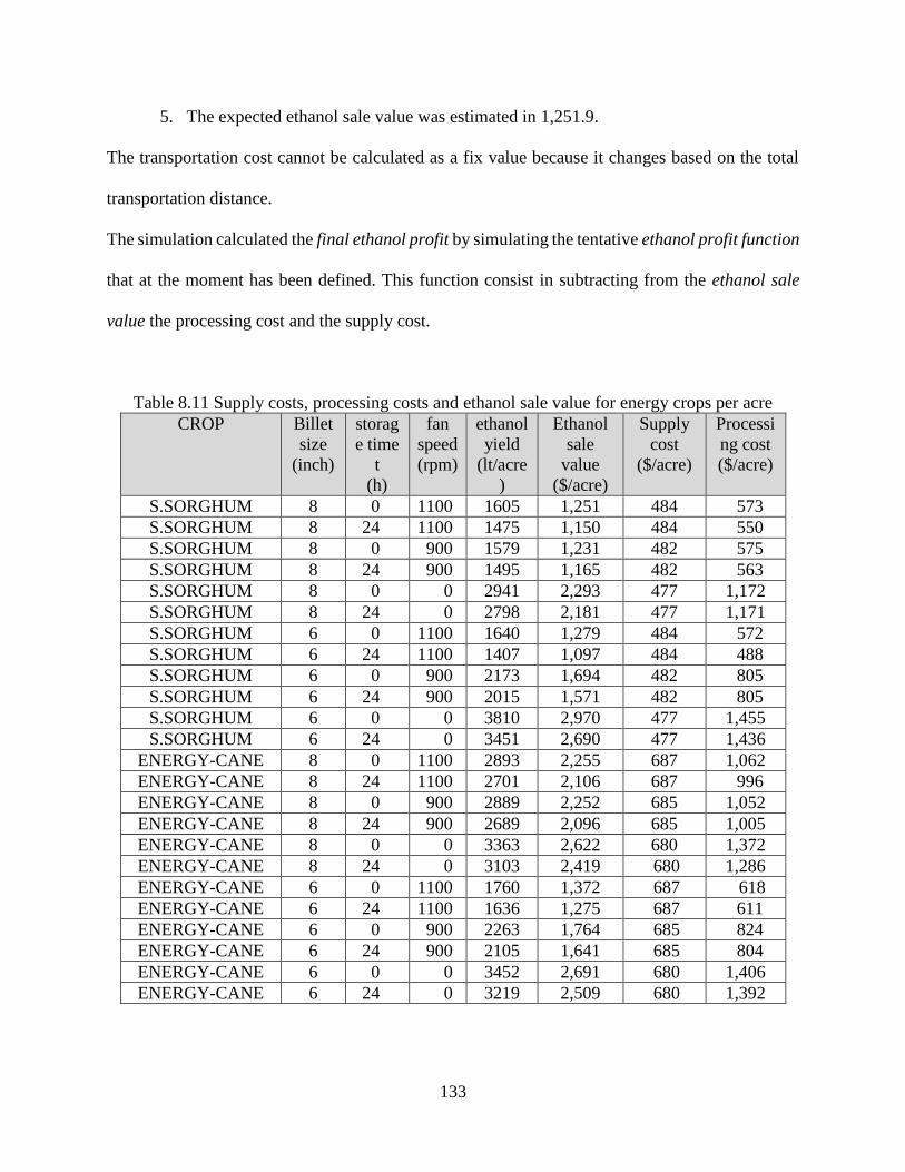
133

5. The expected ethanol sale value was estimated in 1,251.9.

The transportation cost cannot be calculated as a fix value because it changes based on the total

transportation distance.

The simulation calculated the final ethanol profit by simulating the tentative ethanol profit function

that at the moment has been defined. This function consist in subtracting from the ethanol sale

value the processing cost and the supply cost.

Table 8.11 Supply costs, processing costs and ethanol sale value for energy crops per acre

CROP Billet

size

(inch)

storag

e time

t

(h)

fan

speed

(rpm)

ethanol

yield

(lt/acre

)

Ethanol

sale

value

($/acre)

Supply

cost

($/acre)

Processi

ng cost

($/acre)

S.SORGHUM 8 0 1100 1605 1,251 484 573

S.SORGHUM 8 24 1100 1475 1,150 484 550

S.SORGHUM 8 0 900 1579 1,231 482 575

S.SORGHUM 8 24 900 1495 1,165 482 563

S.SORGHUM 8 0 0 2941 2,293 477 1,172

S.SORGHUM 8 24 0 2798 2,181 477 1,171

S.SORGHUM 6 0 1100 1640 1,279 484 572

S.SORGHUM 6 24 1100 1407 1,097 484 488

S.SORGHUM 6 0 900 2173 1,694 482 805

S.SORGHUM 6 24 900 2015 1,571 482 805

S.SORGHUM 6 0 0 3810 2,970 477 1,455

S.SORGHUM 6 24 0 3451 2,690 477 1,436

ENERGY-CANE 8 0 1100 2893 2,255 687 1,062

ENERGY-CANE 8 24 1100 2701 2,106 687 996

ENERGY-CANE 8 0 900 2889 2,252 685 1,052

ENERGY-CANE 8 24 900 2689 2,096 685 1,005

ENERGY-CANE 8 0 0 3363 2,622 680 1,372

ENERGY-CANE 8 24 0 3103 2,419 680 1,286

ENERGY-CANE 6 0 1100 1760 1,372 687 618

ENERGY-CANE 6 24 1100 1636 1,275 687 611

ENERGY-CANE 6 0 900 2263 1,764 685 824

ENERGY-CANE 6 24 900 2105 1,641 685 804

ENERGY-CANE 6 0 0 3452 2,691 680 1,406

ENERGY-CANE 6 24 0 3219 2,509 680 1,392

134

In the simulation, this function was simulated considering the cost of transporting the material

between a range of 1 to 100 miles.

8.8 Simulation: Objective function results

From the 24 matrixes that were defined for the simulation (1 matrix per treatment), two indicators

were measured, the first one defined as Maximum profit from the best case scenario, which

consisted on selecting from the 10.000 iterations developed per matrix (per scenario).

The maximum expected profit that was obtained after implementing different harvesting and

storage practices and after varying different areas and distances for harvesting and transporting the

material.

Each of the matrixes simulated represented each one of the treatments illustrated in Table 8.11,

hence, after simulating and obtaining the 10.000 iterations per matrix, the solution that provided

the maximum ethanol profit was identified and selected as the optimum.

The parameter configuration obtained with this specific iteration; as a result, the maximum ethanol

profit was selected from all 24 treatments defined in the study.

The other indicator, was defined as Maximum profit from the worst case scenario (least feasible

solution), which consisted in selecting from the results of the simulation, the solution that provided

the highest ethanol profit with the maximum feasible distance and area to cover.

The results suggested that up to that range of distances and area for covering, the solution found

is feasible, however, the solution will be the least feasible solution for operating the system,

therefore, by passing the range of distances or area to cover suggested by the solution, the operation

will not be feasible. After using all the data measured in the harvesting trials, the following results

were obtained from the simulation.

135

Table 8.12 and Table 8.13 illustrates the results obtained from the Maximum profit results from

the best case scenario and Table 8.13, illustrates the results of the Maximum profit results from

the worst case scenario; these s provide the following information:

1. Maximum profit that can be achieved per treatment.

2. Optimum area for harvesting and transporting the material.

3. Profit per acre (/acre).

4. Supply costs: transportation cost, the total supply cost (agronomic production cost +

harvesting cost + wagon cost + processing cost) and the potential ethanol sale value that

can be obtained after recovering and converting all the sugars into ethanol.

5. Total amount of simple and complex sugars that are expected to be recovered from the

crop.

6. Expected cost per pound of sugar recovered.

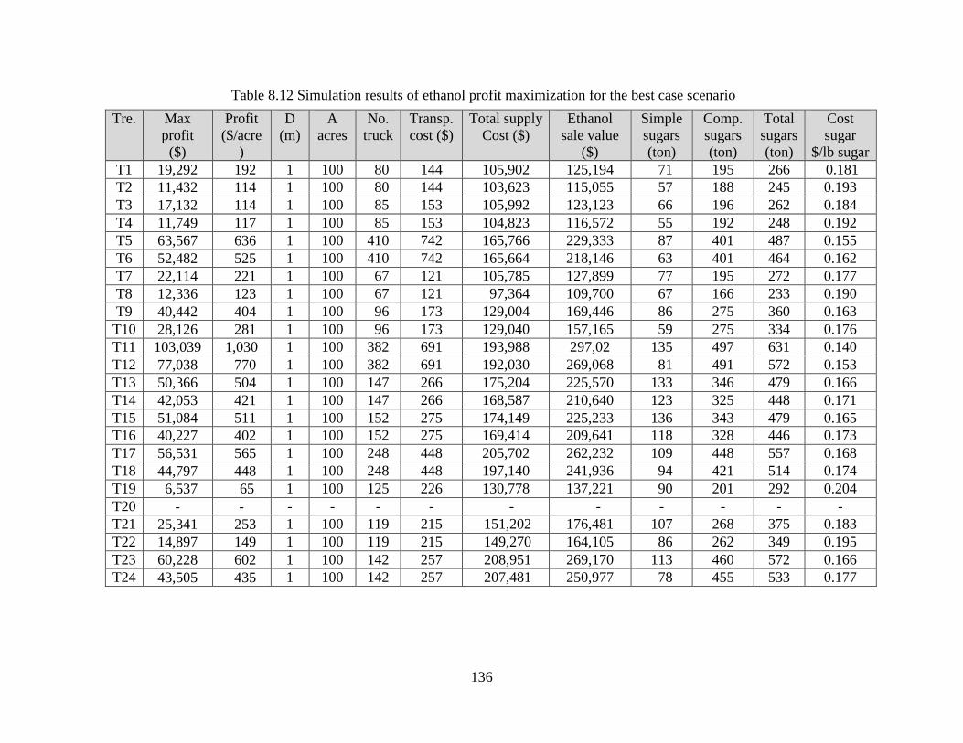
136

Table 8.12 Simulation results of ethanol profit maximization for the best case scenario

Tre. Max

profit

($)

Profit

($/acre

)

D

(m)

A

acres

No.

truck

Transp.

cost ($)

Total supply

Cost ($)

Ethanol

sale value

($)

Simple

sugars

(ton)

Comp.

sugars

(ton)

Total

sugars

(ton)

Cost

sugar

$/lb sugar

T1 19,292 192 1 100 80 144 105,902 125,194 71 195 266 0.181

T2 11,432 114 1 100 80 144 103,623 115,055 57 188 245 0.193

T3 17,132 114 1 100 85 153 105,992 123,123 66 196 262 0.184

T4 11,749 117 1 100 85 153 104,823 116,572 55 192 248 0.192

T5 63,567 636 1 100 410 742 165,766 229,333 87 401 487 0.155

T6 52,482 525 1 100 410 742 165,664 218,146 63 401 464 0.162

T7 22,114 221 1 100 67 121 105,785 127,899 77 195 272 0.177

T8 12,336 123 1 100 67 121 97,364 109,700 67 166 233 0.190

T9 40,442 404 1 100 96 173 129,004 169,446 86 275 360 0.163

T10 28,126 281 1 100 96 173 129,040 157,165 59 275 334 0.176

T11 103,039 1,030 1 100 382 691 193,988 297,02 135 497 631 0.140

T12 77,038 770 1 100 382 691 192,030 269,068 81 491 572 0.153

T13 50,366 504 1 100 147 266 175,204 225,570 133 346 479 0.166

T14 42,053 421 1 100 147 266 168,587 210,640 123 325 448 0.171

T15 51,084 511 1 100 152 275 174,149 225,233 136 343 479 0.165

T16 40,227 402 1 100 152 275 169,414 209,641 118 328 446 0.173

T17 56,531 565 1 100 248 448 205,702 262,232 109 448 557 0.168

T18 44,797 448 1 100 248 448 197,140 241,936 94 421 514 0.174

T19 6,537 65 1 100 125 226 130,778 137,221 90 201 292 0.204

T20 - - - - - - - - - - - -

T21 25,341 253 1 100 119 215 151,202 176,481 107 268 375 0.183

T22 14,897 149 1 100 119 215 149,270 164,105 86 262 349 0.195

T23 60,228 602 1 100 142 257 208,951 269,170 113 460 572 0.166

T24 43,505 435 1 100 142 257 207,481 250,977 78 455 533 0.177

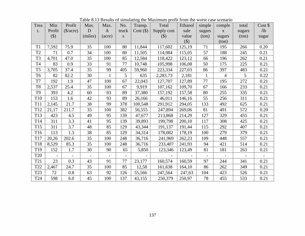
137

Table 8.13 Results of simulating the Maximum profit from the worst case scenario

Trea

t.

Min

Profit

($)

Profit

($/acre)

Max.

D

(miles)

Max.

A

(acre)

No.

truck

s

Transp.

Cost ($)

Total

Supply cost

($)

Ethanol

sale

value

($)

simple

sugars

(ton)

comple

x

sugars

(ton)

total

sugars

(ton)

Cost $

/lb

sugar

T1 7,592 75.9 35 100 80 11,844 117,602 125,19 71 195 266 0.20

T2 71 0.7 34 100 80 11,505 114,984 115,05 57 188 245 0.21

T3 4,701 47.0 35 100 85 12,584 118,422 123,12 66 196 262 0.21

T4 83 0.9 33 91 77 10,748 105,998 106,08 50 175 225 0.21

T5 3,705 37.4 35 99 405 59,960 223,334 227,03 86 397 483 0.21

T6 82 82.2 30 1 5 635 2,283.73 2,181 1 4 5 0.22

T7 192 1.9 47 100 67 22,043 127,707 127,89 77 195 272 0.21

T8 2,537 25.4 35 100 67 9,919 107,162 109,70 67 166 233 0.21

T9 393 4.2 60 93 89 37,380 157,192 157,58 80 255 335 0.21

T10 153 1.6 42 93 89 26,166 46,011 146,16 55 256 311 0.21

T11 2,145 21.7 38 99 378 100,548 291,912 294,05 133 492 625 0.21

T12 21,17 211.7 35 100 382 56,555 247,894 269,06 81 491 572 0.20

T13 423 4.5 49 95 139 47,677 213,868 214,29 127 329 455 0.21

T14 311 3.3 41 95 139 39,893 199,798 200,10 117 308 425 0.21

T15 311 3.7 48 85 129 43,344 191,137 191,44 115 292 407 0.21

T16 113 1.3 38 85 129 34,314 178,082 178,19 100 279 379 0.21

T17 20,26 202.6 35 100 248 36,716 241,969 262,23 109 448 557 0.21

T18 8,529 85.3 35 100 248 36,716 233,407 241,93 94 421 514 0.21

T19 152 1.7 30 90 65 5,850 123,346 123,49 81 181 263 0.21

T20 - - - - - - - - - - - -

T21 23 0.3 43 91 77 23,177 160,574 160,59 97 244 341 0.21

T22 2,467 24.7 35 100 85 12,58 161,638 164,10 86 262 349 0.21

T23 72 0.8 63 92 126 55,566 247,564 247,63 104 423 526 0.21

T24 598 6.0 45 100 137 43,155 250,379 250,97 78 455 533 0.21

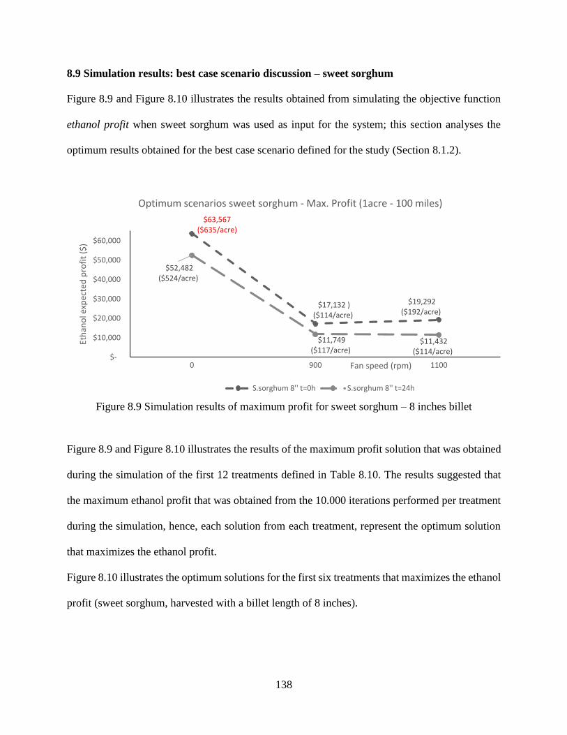
138

8.9 Simulation results: best case scenario discussion – sweet sorghum

Figure 8.9 and Figure 8.10 illustrates the results obtained from simulating the objective function

ethanol profit when sweet sorghum was used as input for the system; this section analyses the

optimum results obtained for the best case scenario defined for the study (Section 8.1.2).

Figure 8.9 Simulation results of maximum profit for sweet sorghum – 8 inches billet

Figure 8.9 and Figure 8.10 illustrates the results of the maximum profit solution that was obtained

during the simulation of the first 12 treatments defined in Table 8.10. The results suggested that

the maximum ethanol profit that was obtained from the 10.000 iterations performed per treatment

during the simulation, hence, each solution from each treatment, represent the optimum solution

that maximizes the ethanol profit.

Figure 8.10 illustrates the optimum solutions for the first six treatments that maximizes the ethanol

profit (sweet sorghum, harvested with a billet length of 8 inches).

$63,567 ($635/acre)

$17,132 )($114/acre)

$19,292 ($192/acre)

$52,482 ($524/acre)

$11,749 ($117/acre)

$11,432 ($114/acre)

$-

$10,000

$20,000

$30,000

$40,000

$50,000

$60,000

0 900 1100

Eth

ano

l exp

ecte

d p

rofi

t ($

)

Fan speed (rpm)

Optimum scenarios sweet sorghum - Max. Profit (1acre - 100 miles)

S.sorghum 8'' t=0h S.sorghum 8'' t=24h

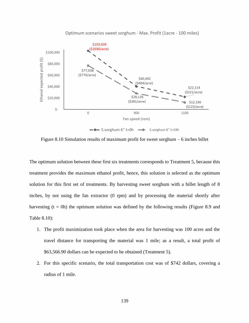
139

Figure 8.10 Simulation results of maximum profit for sweet sorghum – 6 inches billet

The optimum solution between these first six treatments corresponds to Treatment 5, because this

treatment provides the maximum ethanol profit, hence, this solution is selected as the optimum

solution for this first set of treatments. By harvesting sweet sorghum with a billet length of 8

inches, by not using the fan extractor (0 rpm) and by processing the material shortly after

harvesting (t = 0h) the optimum solution was defined by the following results (Figure 8.9 and

Table 8.10):

1. The profit maximization took place when the area for harvesting was 100 acres and the

travel distance for transporting the material was 1 mile; as a result, a total profit of

$63,566.90 dollars can be expected to be obtained (Treatment 5).

2. For this specific scenario, the total transportation cost was of $742 dollars, covering a

radius of 1 mile.

$103,039 ($1030/acre)

$40,442 ($404/acre)

$22,114 ($221/acre)

$77,038 ($770/acre)

$28,126 ($281/acre) $12,336

($123/acre) $-

$20,000

$40,000

$60,000

$80,000

$100,000

0 900 1100

Eth

ano

l exp

ecte

d p

rofi

t ($

)

Fan speed (rom)

Optimum scenarios sweet sorghum - Max. Profit (1acre - 100 miles)

S.sorghum 6'' t=0h S.sorghum 6'' t=24h

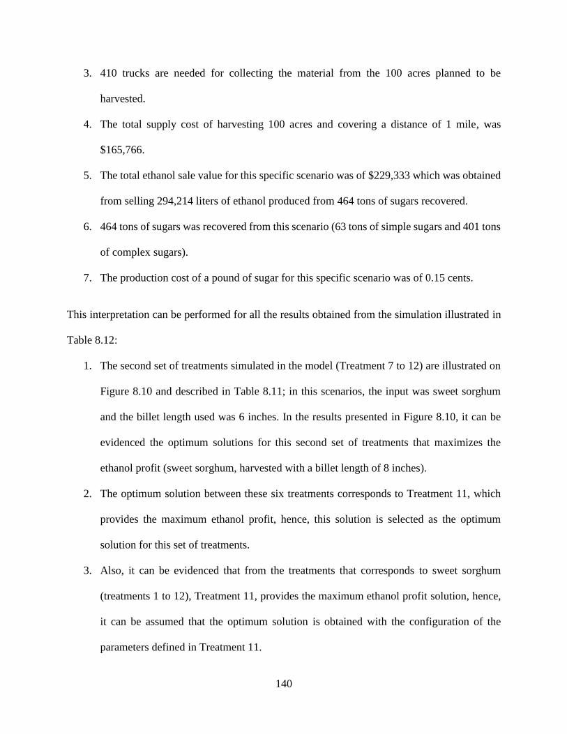
140

3. 410 trucks are needed for collecting the material from the 100 acres planned to be

harvested.

4. The total supply cost of harvesting 100 acres and covering a distance of 1 mile, was

$165,766.

5. The total ethanol sale value for this specific scenario was of $229,333 which was obtained

from selling 294,214 liters of ethanol produced from 464 tons of sugars recovered.

6. 464 tons of sugars was recovered from this scenario (63 tons of simple sugars and 401 tons

of complex sugars).

7. The production cost of a pound of sugar for this specific scenario was of 0.15 cents.

This interpretation can be performed for all the results obtained from the simulation illustrated in

Table 8.12:

1. The second set of treatments simulated in the model (Treatment 7 to 12) are illustrated on

Figure 8.10 and described in Table 8.11; in this scenarios, the input was sweet sorghum

and the billet length used was 6 inches. In the results presented in Figure 8.10, it can be

evidenced the optimum solutions for this second set of treatments that maximizes the

ethanol profit (sweet sorghum, harvested with a billet length of 8 inches).

2. The optimum solution between these six treatments corresponds to Treatment 11, which

provides the maximum ethanol profit, hence, this solution is selected as the optimum

solution for this set of treatments.

3. Also, it can be evidenced that from the treatments that corresponds to sweet sorghum

(treatments 1 to 12), Treatment 11, provides the maximum ethanol profit solution, hence,

it can be assumed that the optimum solution is obtained with the configuration of the

parameters defined in Treatment 11.

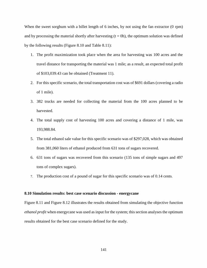
141

When the sweet sorghum with a billet length of 6 inches, by not using the fan extractor (0 rpm)

and by processing the material shortly after harvesting (t = 0h), the optimum solution was defined

by the following results (Figure 8.10 and Table 8.11):

1. The profit maximization took place when the area for harvesting was 100 acres and the

travel distance for transporting the material was 1 mile; as a result, an expected total profit

of $103,039.43 can be obtained (Treatment 11).

2. For this specific scenario, the total transportation cost was of $691 dollars (covering a radio

of 1 mile).

3. 382 trucks are needed for collecting the material from the 100 acres planned to be

harvested.

4. The total supply cost of harvesting 100 acres and covering a distance of 1 mile, was

193,988.84.

5. The total ethanol sale value for this specific scenario was of $297,028, which was obtained

from 381,060 liters of ethanol produced from 631 tons of sugars recovered.

6. 631 tons of sugars was recovered from this scenario (135 tons of simple sugars and 497

tons of complex sugars).

7. The production cost of a pound of sugar for this specific scenario was of 0.14 cents.

8.10 Simulation results: best case scenario discussion - energycane

Figure 8.11 and Figure 8.12 illustrates the results obtained from simulating the objective function

ethanol profit when energycane was used as input for the system; this section analyses the optimum

results obtained for the best case scenario defined for the study.

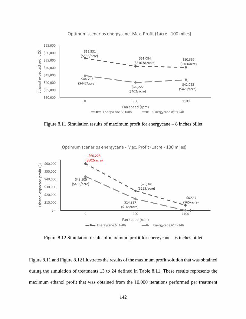
142

Figure 8.11 Simulation results of maximum profit for energycane – 8 inches billet

Figure 8.12 Simulation results of maximum profit for energycane – 6 inches billet

Figure 8.11 and Figure 8.12 illustrates the results of the maximum profit solution that was obtained

during the simulation of treatments 13 to 24 defined in Table 8.11. These results represents the

maximum ethanol profit that was obtained from the 10.000 iterations performed per treatment

$56,531 ($565/acre)

$51,084 ($510.84/acre)

$50,366 ($503/acre)

$44,797 ($447/acre)

$40,227 ($402/acre)

$42,053 ($420/acre)

$30,000

$35,000

$40,000

$45,000

$50,000

$55,000

$60,000

$65,000

0 900 1100

Eth

ano

l exp

ecte

d p

rofi

t ($

)

Fan speed (rpm)

Optimum scenarios energycane- Max. Profit (1acre - 100 miles)

Energycane 8'' t=0h Energycane 8'' t=24h

$60,228 ($602/acre)

$25,341 ($253/acre)

$6,537 ($65/acre)

$43,505 ($435/acre)

$14,897 ($148/acre)

$- $-

$10,000

$20,000

$30,000

$40,000

$50,000

$60,000

0 900 1100

Eth

ano

l exp

ecte

d p

rofi

t ($

)

Fan speed (rom)

Optimum scenarios energycane - Max. Profit (1acre - 100 miles)

Energycane 6'' t=0h Energycane 6'' t=24h

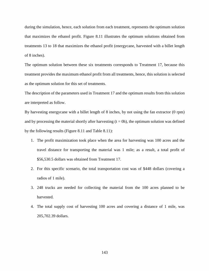
143

during the simulation, hence, each solution from each treatment, represents the optimum solution

that maximizes the ethanol profit. Figure 8.11 illustrates the optimum solutions obtained from

treatments 13 to 18 that maximizes the ethanol profit (energycane, harvested with a billet length

of 8 inches).

The optimum solution between these six treatments corresponds to Treatment 17, because this

treatment provides the maximum ethanol profit from all treatments, hence, this solution is selected

as the optimum solution for this set of treatments.

The description of the parameters used in Treatment 17 and the optimum results from this solution

are interpreted as follow.

By harvesting energycane with a billet length of 8 inches, by not using the fan extractor (0 rpm)

and by processing the material shortly after harvesting (t = 0h), the optimum solution was defined

by the following results (Figure 8.11 and Table 8.11):

1. The profit maximization took place when the area for harvesting was 100 acres and the

travel distance for transporting the material was 1 mile; as a result, a total profit of

$56,530.5 dollars was obtained from Treatment 17.

2. For this specific scenario, the total transportation cost was of $448 dollars (covering a

radios of 1 mile).

3. 248 trucks are needed for collecting the material from the 100 acres planned to be

harvested.

4. The total supply cost of harvesting 100 acres and covering a distance of 1 mile, was

205,702.39 dollars.

144

5. The total ethanol sale value obtained for this specific scenario was of $262,232.92 dollars,

which was obtained from selling 336,421 liters of ethanol produced from 557 tons of sugars

recovered.

6. 557 tons of sugars was recovered from this scenario (109 tons of simple sugars and 448

tons of complex sugars).

7. The production cost of a pound of sugar for this specific scenario was of 0.16 cents.

The second set of treatments simulated in the model for the case of the energycane (Treatments 19

to 24) are illustrated on Figure 8.12 and described in Table 8.11; these scenarios used as input

energycane with a billet length of 6 inches.

The information presented in Figure 8.11, illustrates the optimum results that maximizes the

ethanol profit obtained from the 10.000 iterations simulated in each of the treatments. The

optimum solution between these six treatments corresponds to Treatment 23, which provides the

maximum ethanol profit, hence, this solution is selected as the optimum solution for this set of

treatments.

The description of the parameters used in Treatment 23 and the optimum results are interpreted as

follow. By harvesting energycane with a billet length of 6 inches, by not using the fan extractor (0

rpm) and by processing the material shortly after harvesting (t = 0h), the optimum solution was

defined by the following results:

1. The profit maximization took place when the area for harvesting was 100 acres and the

travel distance for transporting the material was 1 mile; as a result, an expected total profit

of $60,228.27 dollars can be obtained (Treatment 23).

2. For this specific scenario, the total transportation cost was of 257 dollars for covering a

radial distance of 1 mile.

145

3. 142 trucks are needed for collecting the material from the 100 acres planned to be

harvested.

4. The total supply cost of harvesting 100 acres and covering a distance of 1 mile, was

$208,951.29 dollars.

5. The total ethanol sale value for this specific scenario was of $269,170.51 dollars which

was obtained from 345,321 liters of ethanol produced from 572 tons of sugars recovered.

6. 572 tons of sugars were recovered from this solution (113 tons of simple sugars and 460

tons of complex sugars).

7. The production cost of a pound of sugar for this specific scenario was of $0.17 cents.

8.11 Simulation results (sweet sorghum): worst case scenario discussion

The results presented in the worst case scenario represents the least feasible solution obtained from

each of the 24 treatments after varying the objection function based on a combination of different

distances and area to cover.

Based on the parameter configuration suggested by the solution selected as the worst case

scenario, it is not feasible to over pass the distances for transporting the material or the area for

harvesting the material. In the model was defined that up to the specific range of the solution, the

system can operate and be feasible, however, these solutions are the least feasible alternatives for

the system.

Figure 8.13 and Figure 8.14 illustrates the results (treatment 1 to 12) obtained from simulating the

objective function ethanol profit when sweet sorghum was used as input for the system.

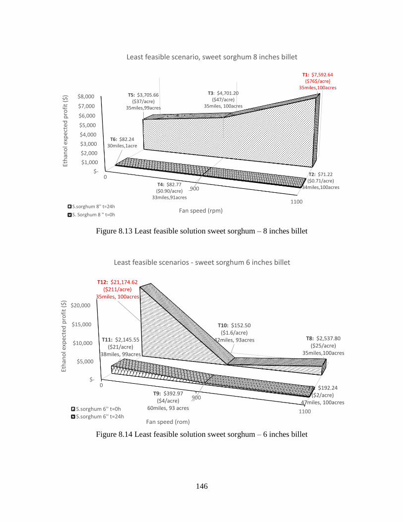
146

Figure 8.13 Least feasible solution sweet sorghum – 8 inches billet

Figure 8.14 Least feasible solution sweet sorghum – 6 inches billet

$-

$1,000

$2,000

$3,000

$4,000

$5,000

$6,000

$7,000

$8,000

0

900

1100

T6: $82.24 30miles,1acre

T4: $82.77 ($0.90/acre)

33miles,91acres

T2: $71.22 ($0.71/acre)

34miles,100acres

T5: $3,705.66 ($37/acre)

35miles,99acres

T3: $4,701.20 ($47/acre)

35miles, 100acres

T1: $7,592.64 ($76$/acre)

35miles,100acres

Eth

ano

l exp

ecte

d p

rofi

t ($

)

Fan speed (rpm)

Least feasible scenario, sweet sorghum 8 inches billet

S.sorghum 8'' t=24h

S. Sorghum 8 '' t=0h

$-

$5,000

$10,000

$15,000

$20,000

0

900

1100

T11: $2,145.55 ($21/acre)

38miles, 99acres

T9: $392.97 ($4/acre)

60miles, 93 acres

T7: $192.24 ($2/acre)

47miles, 100acres

T12: $21,174.62 ($211/acre)

35miles, 100acres

T10: $152.50 ($1.6/acre)

42miles, 93acres T8: $2,537.80 ($25/acre)

35miles,100acres

Eth

ano

l exp

ecte

d p

rofi

t ($

)

Fan speed (rom)

Least feasible scenarios - sweet sorghum 6 inches billet

S.sorghum 6'' t=0h

S.sorghum 6'' t=24h

147

Figure 8.13 illustrates the optimum least feasible solutions obtained from treatments 1 to 6; these

solutions maximizes the ethanol profit in the worst case scenario. The optimum solution between

these six treatments corresponds to Treatment 1 (T1), because this treatment provides the

maximum ethanol profit, hence, this solution is selected as the optimum solution for this set of

treatments.

The description of the parameters used in Treatment 1 and the optimum results from this solution

are interpreted as follow. Treatment 1: By harvesting sweet sorghum with a billet length of 8

inches, by not using the fan extractor (0 rpm) and by processing the material shortly after

harvesting (t = 0h), the optimum solution was defined by the following results:

1. The profit maximization took place when the area for harvesting was 100 acres and the

travel distance for transporting the material was 35 miles; as a result, a total profit of

$7,592.64 was obtained from Treatment 1.

2. For this specific scenario, the total transportation cost was of $11,844.0 dollars (covering

a maximum distance of 35 miles).

3. 80 trucks are needed for collecting the material from the 100 acres planned to be harvested.

4. The total supply cost of harvesting 100 acres and covering a distance of 35 miles, was

$117,602.13 dollars.

5. The total ethanol sale value obtained for this specific scenario was of $125,194.64 dollars,

which was obtained from selling 160,613 liters of ethanol produced from 266 tons of sugars

recovered.

6. 266 tons of sugars was recovered from this scenario (71 tons of simple sugars and 195 tons

of complex sugars).

7. The production cost of a pound of sugar for this specific scenario was of 0.20 cents.

148

The second set of treatments simulated in the model for the case of the sweet sorghum (Treatments

7 to 12) are illustrated on Figure 8.15; these scenarios used as input sweet sorghum with a billet

length of 6 inches.

The information presented illustrates the optimum least feasible solutions obtained from treatments

7 to 12; these solutions maximizes the ethanol profit in the worst case scenario.

From the treatments illustrated on Figure 8.14, the optimum solution corresponds to Treatment 12,

which provides the maximum ethanol profit, hence, this solution is selected as the optimum

solution for this set of treatments.

When the sweet sorghum with a billet length of 6 inches, by not using the fan extractor (0 rpm)

and by processing the material shortly after harvesting (t = 0h), the optimum solution was defined

by the following results:

1. The profit maximization took place when the area for harvesting was 100 acres and the

travel distance for transporting the material was 1 mile; as a result, an expected total profit

of $21,174.6 dollars can be obtained (Treatment 12).

2. For this specific scenario, the total transportation cost was of $56,555.1 dollars for covering

a radial distance of 35 miles.

3. 382 trucks are needed for collecting the material from the 100 acres planned to be

harvested.

4. The total supply cost of harvesting 100 acres and covering a distance of 1 mile, was

$208,951.29 dollars.

5. The total ethanol sale value for this specific scenario was of $269,068.67 dollars which

was obtained from 345,191 liters of ethanol produced from 572 tons of sugars recovered.

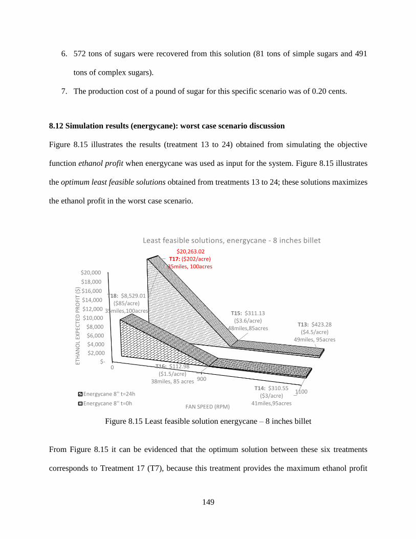
149

6. 572 tons of sugars were recovered from this solution (81 tons of simple sugars and 491

tons of complex sugars).

7. The production cost of a pound of sugar for this specific scenario was of 0.20 cents.

8.12 Simulation results (energycane): worst case scenario discussion

Figure 8.15 illustrates the results (treatment 13 to 24) obtained from simulating the objective

function ethanol profit when energycane was used as input for the system. Figure 8.15 illustrates

the optimum least feasible solutions obtained from treatments 13 to 24; these solutions maximizes

the ethanol profit in the worst case scenario.

Figure 8.15 Least feasible solution energycane – 8 inches billet

From Figure 8.15 it can be evidenced that the optimum solution between these six treatments

corresponds to Treatment 17 (T7), because this treatment provides the maximum ethanol profit

$-

$2,000

$4,000

$6,000

$8,000

$10,000

$12,000

$14,000

$16,000

$18,000

$20,000

0

900

1100

T18: $8,529.01 ($85/acre)

35miles,100acres

T16: $112.98 ($1.5/acre)

38miles, 85 acresT14: $310.55

($3/acre)41miles,95acres

$20,263.02 T17: ($202/acre)

35miles, 100acres

T15: $311.13 ($3.6/acre)

48miles,85acresT13: $423.28

($4.5/acre)49miles, 95acres

ETH

AN

OL

EXP

ECTE

D P

RO

FIT

($)

FAN SPEED (RPM)

Least feasible solutions, energycane - 8 inches billet

Energycane 8'' t=24h

Energycane 8'' t=0h

150

from all treatments, hence, this solution is selected as the optimum solution for this set of

treatments.

The description of the parameters used in Treatment 17 and the optimum results from this solution

are interpreted as follow:

Treatment17: By harvesting energycane with a billet length of 8 inches, by not using the fan

extractor (0 rpm) and by processing the material shortly after harvesting (t = 0h), the optimum

solution was defined by the following results (Figure 8.16):

1. The profit maximization took place when the area for harvesting was 100 acres and the

travel distance for transporting the material was 35 miles; as a result, a total profit of

$20,263.02 was obtained from Treatment 17.

2. For this specific scenario, the total transportation cost was of $36,716.5 dollars (covering

a maximum distance of 35 miles).

3. 248 trucks are needed for collecting the material from the 100 acres planned to be

harvested.

4. The total supply cost of harvesting 100 acres and covering a distance of 35 miles, was

$241,969.92 dollars.

5. The total ethanol sale value obtained for this specific scenario was of $262,232.92 dollars,

which was obtained from selling 336,421 liters of ethanol produced from 557 tons of sugars

recovered.

6. 577 tons of sugars was recovered from this scenario (109 tons of simple sugars and 448

tons of complex sugars).

7. The production cost of a pound of sugar for this specific scenario was of 0.20 cents.

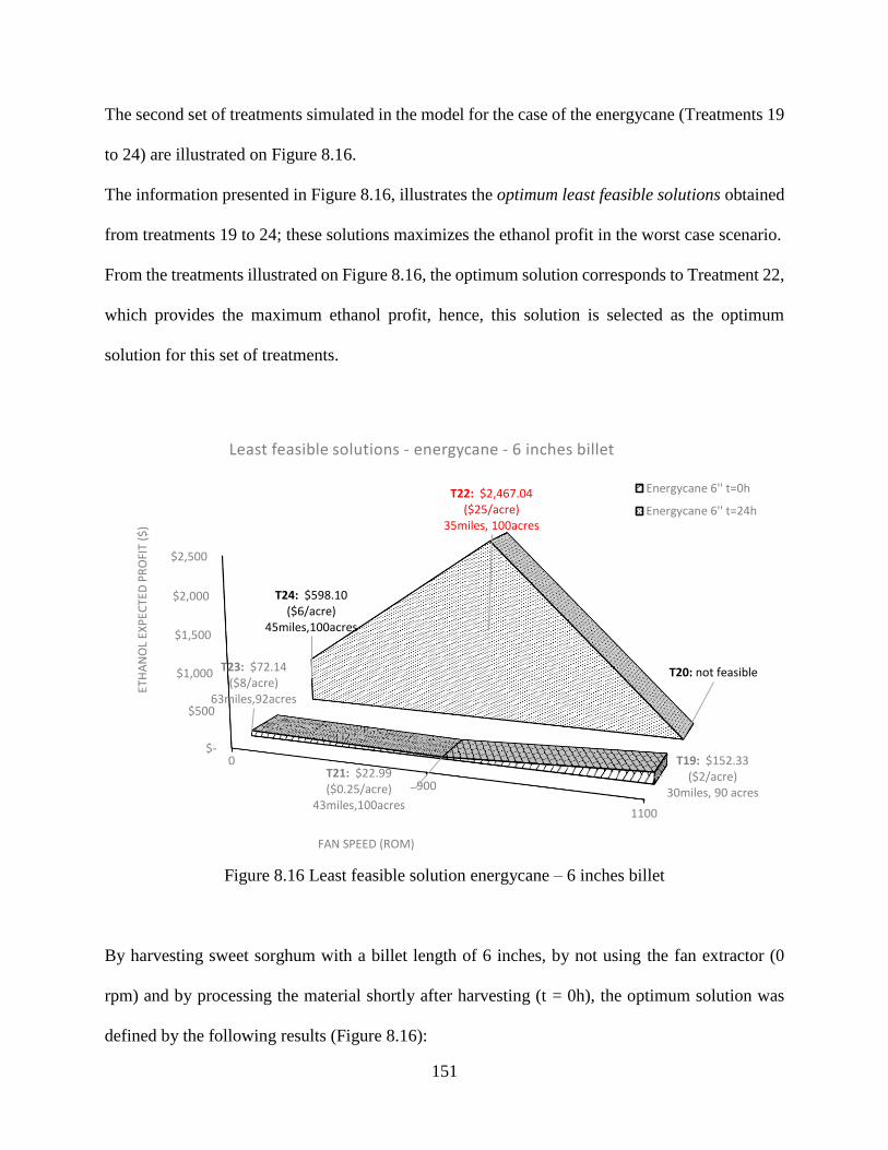
151

The second set of treatments simulated in the model for the case of the energycane (Treatments 19

to 24) are illustrated on Figure 8.16.

The information presented in Figure 8.16, illustrates the optimum least feasible solutions obtained

from treatments 19 to 24; these solutions maximizes the ethanol profit in the worst case scenario.

From the treatments illustrated on Figure 8.16, the optimum solution corresponds to Treatment 22,

which provides the maximum ethanol profit, hence, this solution is selected as the optimum

solution for this set of treatments.

Figure 8.16 Least feasible solution energycane – 6 inches billet

By harvesting sweet sorghum with a billet length of 6 inches, by not using the fan extractor (0

rpm) and by processing the material shortly after harvesting (t = 0h), the optimum solution was

defined by the following results (Figure 8.16):

$-

$500

$1,000

$1,500

$2,000

$2,500

0

900

1100

T23: $72.14 ($8/acre)

63miles,92acres

T21: $22.99 ($0.25/acre)

43miles,100acres

T19: $152.33 ($2/acre)

30miles, 90 acres

T24: $598.10 ($6/acre)

45miles,100acres

T22: $2,467.04 ($25/acre)

35miles, 100acres

T20: not feasible

ETH

AN

OL

EXP

ECTE

D P

RO

FIT

($)

FAN SPEED (ROM)

Least feasible solutions - energycane - 6 inches billet

Energycane 6'' t=0h

Energycane 6'' t=24h

152

1. The profit maximization took place when the area for harvesting was 100 acres and the

travel distance for transporting the material was 35 miles; as a result, an expected total

profit of $2,467.04 dollars can be obtained (Treatment 22).

2. For this specific scenario, the total transportation cost was of $12,584.25 dollars for

covering a radial distance of 35 miles.

3. 85 trucks are needed for collecting the material from the 100 acres planned to be harvested.

4. The total supply cost of harvesting 100 acres and covering a distance of 35 miles, was

161,638.93 dollars.

5. The total ethanol sale value for this specific scenario was of $164,105.9 dollars which was

obtained from 210,533 liters of ethanol produced from 349 tons of sugars recovered.

6. 349 tons of sugars were recovered from this solution (86 tons of simple sugars and 263

tons of complex sugars).

7. The production cost of a pound of sugar for this specific scenario was of 0.21 cents.

8.13 Simulation results – Discussion

The simulation of the model consisted on simulating the ethanol profit function obtained after

implementing different harvesting and storages practices. The objective function was calculated

and simulated based on an area range for harvesting that ranged between 1 to 100 acres and a

distance range for transporting the material of 1 to 100 miles. Finally, the objective function was

calculated after subtracting all the costs involved in the system (agronomic production cost of the

crop, the harvesting cost, transportation cost and conversion of simple and complex sugars cost).

From the 24 treatments that were defined in the model, the following categories were defined

(Table 8.11):

153

- Treatment 1 to 6, implemented sweet sorghum as input for the system. In these treatments,

the material was harvested with a billet length of 8 inches.

In treatment 1, 3, 5, the material was processed shortly after harvesting, hence, the

processing time was defined as t = 0 hours.

In the other hand, the material from treatments 2, 4 and 6 was also collected by using a

billet size of 8 inches, but the processing was performed 24 hours later (material stored 24

hours).

- Treatment 7 to 12, implemented sweet sorghum as input for the system. In these treatments,

the material was harvested with a billet length of 6 inches.

In treatment 7, 9, 11, the material was processed shortly after harvesting, hence, the

processing time was defined as t = 0 hours. In the other hand, the material from treatments

8, 10 and 12 was also collected by using a billet size of 8 inches, but the processing was

performed 24 hours later (material stored 24 hours).

- Treatment 13 to 18, implemented energycane as input for the system. In these treatments,

the material was harvested with a billet length of 8 inches.

In treatment 13, 15, 17, the material was processed shortly after harvesting, hence, the

processing time was defined as t = 0 hours. In the other hand, the material from treatments

14, 16 and 18 was also collected by using a billet size of 8 inches, but the processing was

performed 24 hours later (material stored 24 hours).

- Treatment 19 to 24, implemented energycane as input for the system. In these treatments,

the material was harvested with a billet length of 6 inches.

In treatment 19, 21, 23, the material was processed shortly after harvesting, hence, the

processing time was defined as t = 0 hours. In the other hand, the material from treatments

154

20, 22 and 24 was also collected by using a billet size of 6 inches, but the processing was

performed 24 hours later (material stored 24 hours).

This classification was performed because for each set of treatments, an optimum solution was

found; the practices and parameters defined for each of the scenarios are different, hence, selecting

only one optimum solution from all the treatments defined in the study will skew all the potential

solutions that can be implemented for the system.

All 24 treatments defined for the model were simulated, treatments 1 to 12 were assigned for sweet

sorghum and treatments 13 to 24 were assigned for energycane. After simulating the objective

function of the model according to the characteristics of each of the 24 scenarios, 10.000 iterations

per treatments were obtained and a total of 240.000 iterations were developed for the model.

Two different indicators were evaluated in the simulation, the first one called Maximum profit from

the best case scenario which basically consisted on selecting the solution which allow the

maximum ethanol expected profit after implementing different harvesting and storage practices.

After identifying the solution that maximizes the profit function, the parameters of the solutions

were defined as the optimum configuration of the system.

The second indicator was called Maximum profit from the worst case scenario (least feasible

solution) which basically consisted on selecting the solution that allowed the highest ethanol profit

as a result of covering the maximum feasible distance and area to cover for collecting and

transporting the feedstock.

The main objective of the mathematical formulation for the supply system defined in the study,

was to characterize the component costs of the supply system required for the production of ethanol

from energy crops. With the mathematical definition of the component costs, it was possible to

define the objective function, which consisted on the maximization of the ethanol profit obtained

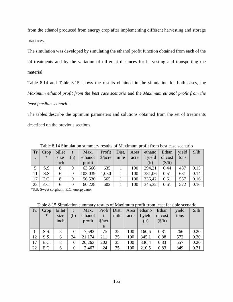
155

from the ethanol produced from energy crop after implementing different harvesting and storage

practices.

The simulation was developed by simulating the ethanol profit function obtained from each of the

24 treatments and by the variation of different distances for harvesting and transporting the

material.

Table 8.14 and Table 8.15 shows the results obtained in the simulation for both cases, the

Maximum ethanol profit from the best case scenario and the Maximum ethanol profit from the

least feasible scenario.

The tables describe the optimum parameters and solutions obtained from the set of treatments

described on the previous sections.

Table 8.14 Simulation summary results of Maximum profit from best case scenario

*S.S: Sweet sorghum, E.C: energycane.

Table 8.15 Simulation summary results of Maximum profit from least feasible scenario

Tr. Crop

*

billet

size

inch

t

(h)

Max.

ethanol

profit

Profi

t

$/acr

e

Dist.

mile

Area

acre

ethano

l yield

(lt)

Ethan

ol cost

($/lt)

yield

tons

$/lb

1 S.S. 8 0 7,592 75 35 100 160,6 0.81 266 0.20

12 S.S. 6 24 21,174 211 35 100 345,1 0.88 572 0.20

17 E.C. 8 0 20,263 202 35 100 336,4 0.83 557 0.20

22 E.C. 6 0 2,467 24 35 100 210,5 0.83 349 0.21

Tr

.

Crop

*

billet

size

inch

t

(h)

Max.

ethanol

profit

Profit

$/acre

Dist.

mile

Area

acre

ethano

l yield

(lt)

Ethan

ol cost

($/lt)

yield

tons

$/lb

5 S.S 8 0 63,566 635 1 100 294,21 0.44 487 0.15

11 S.S 6 0 103,039 1,030 1 100 381,06 0.51 631 0.14

17 E.C. 8 0 56,530 565 1 100 336,42 0.61 557 0.16

23 E.C. 6 0 60,228 602 1 100 345,32 0.61 572 0.16

156

8.14 Optimum solutions from best case scenario

From Table 8.14, the optimum solution from the best case scenario from the set of treatments

assigned to sweet sorghum (Treatment 1 to 6), was Treatment 5, which provided a solution that

maximized the ethanol profit 63,566.90 by harvesting 100 acres and traveling a distance of 1mile.

The results obtained were: 294,214 liters of ethanol can be produced with a cost of 0.44/lt and 487

tons of sugars can be recovered with at a cost per pound of 0.15/lb.

It also can be evidenced from Table 8.14, that the optimum solution from the best case scenario

from the set of treatments assigned to sweet sorghum (Treatment 7 to 12), was Treatment 11, which

obtained a maximum ethanol profit of 103,039.4 by harvesting 100 acres and traveling a distance

of 1mile.

The results obtained in this treatment were: 381,060 liters of ethanol can be produced at a cost per

liter of 0.51/lt and 631 tons of sugars can be recovered at a cost per pound of 0.14/lb.

As a result of the selection of the optimum solutions in the best case scenario, it can be concluded

the following:

1. Treatment 5 provided the optimum solution which maximized the ethanol profit and

minimized the production per liter of ethanol and the production per pound of sugars. From

all the treatments that included the crop of sweet sorghum and billet size configuration of

8 inches, Treatment 5 was the optimum.

2. Treatment 11 provided the optimum solution which maximized the ethanol profit and

minimized the production per liter of ethanol and the production per pound of sugars. From

all the treatments that included the crop of sweet sorghum and billet size configuration of

6 inches, Treatment 11 was the optimum.

157

In the other hand, for the case of the energycane, it can be evidenced from 63, that the optimum

solution from the set of treatments 13 to 18 (8 inches billet), was Treatment 17, which allowed to

obtained a maximum ethanol profit of 56,530.54 by harvesting 100 acres and traveling a distance

of 1mile.

The result of the treatment were: 336,421 liters of ethanol can be produced at a cost per liter of

0.61/lt and 557 tons of sugars can be recovered with at a cost per pound of 0.16$/lb. It also can be

evidenced from Table 8.14, that the optimum solution from the best case scenario from the set of

treatments 19 to 24, was Treatment 23. With this treatment, a maximum ethanol profit of

$60,228.27 by harvesting 100 acres and traveling a distance of 1mile; as a result, 345,321 liters of

ethanol can be produced at a cost per liter of 0.61$/lt and 572 tons of sugars can be recovered at a

cost per pound of 0.16$/lb.

From the results it was defined the following conclusions:

1. Treatment 17 provided the optimum solution which maximized the ethanol profit and

minimized the production per liter of ethanol and the production per pound of sugars.

From all the treatments that included the crop of energycane and billet size configuration

of 8 inches, Treatment 17 was the optimum.

2. Treatment 23 provided the optimum solution which maximized the ethanol profit and

minimized the production per liter of ethanol and the production per pound of sugars.

From all the treatments that included the crop of energycane and billet size configuration

of 6 inches, Treatment 17 was the optimum.

158

8.15 Optimum solutions from worst case scenario (least feasible solutions)

From Table 8.15, the optimum solution simulated on the least feasible scenario from the set of

treatments that implemented sweet sorghum as input for the system (8 inches billet, Treatment 1

to 6), was Treatment 1.The results obtained from the treatment were: maximum ethanol profit of

$7,592.64 by harvesting 100 acres and traveling a distance of 35 miles. As a result, 160,613 liters

of ethanol can be produced with a cost of 0.81$/lt and 266 tons of sugars can be recovered with at

a cost per pound of 0.20/lb.

The optimum solution simulated on the least feasible scenario from the set of treatments

characterized with sweet sorghum (6 inches billet, Treatment 7 to 12), was Treatment 12. With

this treatment a maximum ethanol profit of $21,174.6 by harvesting 100 acres and traveling a

distance of 35 miles; as a result, 345,191 liters of ethanol can be produced at a cost per liter of

0.88$/lt and 572 tons of sugars can be recovered at a cost per pound of 0.20$/lb.

In the other hand, for the case of the energycane, the optimum solution from the least feasible

scenario from the set of treatments characterized with energycane (8 inches billet, Treatment 13

to 18), was Treatment 17.

A maximum ethanol profit of $20,263 by harvesting 100 acres and traveling a distance of 35 miles;

as a result, 336,421 liters of ethanol can be produced at a cost per liter of 0.83$/lt and 557 tons of

sugars can be recovered with at a cost per pound of 0.20$/lb.

The optimum solution from the least feasible scenario from the set of treatments characterized

with energycane (6 inches billet size, Treatment 19 to 24), was Treatment 22, which obtained a

maximum ethanol profit of $2,467 by harvesting 100 acres and traveling a distance of 35mile.

210,533 liters of ethanol can be produced at a cost per liter of 0.83$/lt and 349 tons of sugars can

159

be recovered at a cost per pound of 0.20$/lb. The optimum solutions found in the simulation are

described below:

1. Treatment 17 provided the optimum solution which maximized the ethanol profit and

minimized the production per liter of ethanol and the production per pound of sugars. From

all the treatments that included the crop of energycane and billet size configuration of 8

inches, Treatment 17 was the optimum.

2. Treatment 22 provided the optimum solution which maximized the ethanol profit and

minimized the production per liter of ethanol and the production per pound of sugars. From

all the treatments that included the crop of energycane and billet size configuration of 6

inches, Treatment 17 was the optimum.

160

CHAPTER 9: CONCLUSIONS AND FUTURE WORK

In this study a set of harvesting and storage trials with energycane and sweet sorghum were

conducted in order to evaluate the effect of the variation of harvesting practices on the sugars yield,

ethanol yield and the economics of the system. With the development of the harvesting trials, a

characterization of the supply system was developed for the case of sweet sorghum and

energycane; in the same way, different agronomic and efficiency indicators were calculated.

Finally, the development of a mathematical model integrated by the main component costs of the

supply system was defined and tested; 24 treatments were simulated on the model based on the

objective function defined for the study.

The optimum configuration of parameters for the system were defined, allowing to obtain the

maximum ethanol profit and the minimum production cost of ethanol and sugars.

9.1 Harvesting trials and agronomic/efficiency indicators

Planning and execution of harvesting trials with energycane and sweet sorghum for the calculation

of the following indicators:

1. Quality indicators (%Sugars, %Brix, Material yield, %juice yield, material composition

before and after harvesting, %weight losses due to storage and internal temperature and

RH% of the material stored).

2. Efficiency indicators of the supply processes (harvesting efficiency, cutting system

accuracy of the harvester, transportation bulk density, potential ethanol profit).

The harvesting trials were developed based on the variation of several parameters from the supply

processes, such as billet size (6 and 8 inches), level of leaf matter (fan speed, 0 rpm, 900 rpm, and

1100 rpm), and storage time before processing the feedstock (24 hour). According to the variation

161

of parameters, a set of scenarios were defined and evaluated for both of the crops; the results of

the indicators measured were different between treatments and crops.

9.2 Simple sugars indicator

One of the main indicators measured and calculated from the harvesting trials was the simple

sugars yield indicator. The results of the simple sugars yield obtained when sweet sorghum was

used as input, suggested that an increment of approximately 27% of simple sugars can be recovered

when a billet size of 8 inches is used, when the fan speed of the extractor system decrease to 0 rpm

and when the material is processed shortly after harvesting (t = 0h). The increment evidenced

occurred by comparing the treatments that presented the same conditions but had different

processing time (storage time = 24 hours). By processing the material shortly after harvesting, it

can be obtained a simple sugars yield of approximately 0.87 ton/acre (sweet sorghum, 8 inches

billet, processing time t = 0h), but when the material is stored during 24 hours, the yield tend to

decrease to 0.62 tons/acre.

For the case when the sweet sorghum was harvested with a billet length of 6 inches, the yield of

the simple sugars tend to increase by reducing the fan speed of the extractor system; under these

conditions it was obtained a simple sugars yield of approximately 1.35 ton/acre (sweet sorghum,

6 inches billet, processing time t = 0h). When the material was stored during 24 hours, the yield

tend to decrease up to 0.8 tons/acre, indicating a reduction of approximately 40%.

For the case of the energycane, the results of the simple sugars yield suggested that by storing the

material during 24 hours before processing, the sugar losses tend to decrease when the billets were

harvested cleaner. Finally, it can be concluded that the yield of the simple sugars is highly affected

by two factors, the amount of leaf matter obtained while harvesting and the storage time of the

162

feedstock. By increasing the amount of leaf matter, it was evidenced that the yield of the simple

sugars tend to increase, however, this extra amount of leaf matter can produce some problems in

the processing facilities. Finally, it was evidenced that the storage time significantly impact the

yield of the simple sugars, suggesting that the greater the storage time is, the lower the yield of

simple sugars will be.

9.3 Complex sugars indicator

Another important indicator measured and calculate in the study was the Yield of the complex

sugars. The complex sugars were assumed to be recovered from the fiber of the feedstock. In this

case, it was assumed that the Total fermentable sugars that were able to be recovered from the dry

fiber was approximately 60%.

In the case of the complex sugars, it was evidenced that the time the material was stored before

processing did not significantly affect the yield. It was concluded that the deterioration of the

complex sugars over time was slower compared to the deterioration occurred to the simple sugars.

Also, it was evidenced that by reducing the fan speed of the extractor system, the yield of the

complex sugars tend to increase.

When sweet sorghum was harvested with a billet length of 8 inches and when the fan extractor

was of 0 rpm, a yield of approximately 4.97 ton/acre was achieved. When the material was

harvested with a fan speed of 1100 rpm, the yield tend to decrease to 2 tons/acre, a reduction of

approximately 59% of the potential material that can be delivered in the factory.

This same behavior occurred when the material was harvested with a billet length of 6 inches. In

the other hand, for the case of the energycane, when the harvester used a billet length of 8 inches

and when the fan speed of the extractor was 0 rpm, a yield of approximately 4.4 ton/acre was

163

obtained. When the material was harvested with a fan speed of 1100 rpm, the yield tend to decrease

to 3.42 tons/acre, representing a reduction of approximately 22%.

9.4 Total fermentable sugars yield

As a result of the behavior of the simple and complex sugars indicators, the total fermentable

sugars yield presented the same pattern; as then fan speed of the extractor system tend to decrease

(0 rpm), the yield of the sugars tend to increase. The results suggested that by recovering leaf

matter and fiber while harvesting, the % of sugars (simple and complex) that can be recovered

from the field can be higher. This pattern especially occurs when the material was processed

shortly after harvesting (t = 0 hours).

For the case of the sweet sorghum when the fan extractor was not used (8 inches billet, 0 rpm fan

speed and t = 0 h) a yield of 4.9ton/acre was recovered; in the other hand when the highest fan

speed was used (1100 rpm) the yield decreased to 2.7 tons/acre, a reduction of approximately 44%.

Finally, when the energycane was as input and by not using the fan extractor while harvesting (8

inches billet, t = 0h) a yield of 5.6ton/acre was achieved. When the highest fan speed was used

(1100 rpm), the yield decreased to 4.8 tons/acre, representing a reduction of approximately15%.

9.5 Ethanol yield produced from simple and complex sugars

By using the conversion rate of sugars into ethanol, the results indicated that the ethanol yield

(lt/acre) tend to increase when the feedstock was processed shortly after harvesting (t = 0h) and

when the fan speed used while harvesting was reduced to 0 rpm.

164

The results suggest that the fiber and the leaf matter that can be recovered from the crop while

harvesting, provide sugars that can be recovered from both, the simple sugars (juice) and the

complex sugars (fiber) for ethanol production.

In the case of the sweet sorghum (8 inches billet, 0 rpm fan speed and t = 0h) an ethanol yield of

2942lt/acre was able to be produced from the sugars recovered; however, by using a higher fan

speed 1100 rpm while harvesting, the yield decreased to 1606 liters/acre, representing a reduction

of approximately 45%.In the other hand, when the sweet sorghum was harvested with a billet size

of 6 inches and a fan speed of 0 rpm, the ethanol yield obtained was 3810lt/acre. By using a higher

fan speed (1100 rpm), the yield decreased to 1640liters/acre, suggesting a reduction of

approximately 56%.

For the case of the energycane (8 inches billet, 0 rpm fan speed and t = 0h) a yield of 3364liters/acre

can be produced when the fan extractor is not used; in the other hand, when the highest fan speed

was used (1100 rpm), the yield tend to decrease to 2889 tons/acre. Finally, when the energycane

was harvested with a billet size of 6 inches and a fan speed of 0 rpm, a yield of 3453lt/acre was

achieved; however, by using a higher fan speed (1100 rpm), the yield decreased to 1760 liters/acre,

representing a reduction of approximately 49%.

9.6 Economic model formulation

In the mathematical formulation of the model, the objective function was defined as the

maximization of the ethanol profit; the objective function was calculated after subtracting all the

component costs defined for the supply system.

The costs defined for the system were:

1. Agronomic production cost of the crop

165

2. Harvesting cost (based on fuel consumption)

3. Wagon cost

4. Transportation cost

5. Processing cost

All the component costs consider the main activities and costs required for the supply of energy

crops for the production of ethanol; all the consideration and assumption used in the model, were

described and explained on Section8. According to the calculations of the costs of each of the

supply stages defined in the model, the following insights were defined:

1. Agronomic production cost per acre: for sweet sorghum: 208/acre; this value was

calculated as an average cost per acre from the literature defined by Hallam and Ribera

(Hallam et al. 2001), (Ribera et al. 2013).

2. Agronomic production cost per acre for energycane: 411/acre. This value was calculated

as an average cost per acre from the literature defined by Tyler, Salassi and Tyler (tyler et

al. 2009), (Ribera et al. 2013) and (Salassi et al. 2014).

3. Harvesting cost per acre: The harvester cost was defined based on the fuel consumption.

By using different rpm’s in the extractor system of the harvester, the consumption of fuel

changed. By using a fan speed of 1100 rpm, 900 rpm and 0 rpm, the cost per acre is $120.5,

$119.3 and $113 respectively. These costs were calculated considering the cost of the fuel

consumption, the cost of labor, maintenance cost, and fixed expenses.

4. Wagon cost: For the harvesting operations was assumed the utilization of 3 wagon trucks

for collecting the material obtained per acre. The component cost included were: labor cost,

fixed expenses costs and fuel consumption. As a result, a fixed cost per acre was calculated

154.8 per truck used in an acre.

166

5. Transportation cost: This cost varied in function of the total distance needed to cover for

transporting the material, hence, in the simulation model a distance from 1 to 100 miles

were simulated. The cost per mile for transporting was assumed with similar costs that the

current sugar industry in Louisiana charged (Legendre, 2014).

This cost also varied in function of the total trucks needed to transport the material; for

calculating this indicator, the data from the harvesting trials was used according to each of

the treatments defined for the study (material yield, bulk density, truck volume).

6. Processing cost: The processing cost considered the costs of recovering and converting

simple and complex sugars from the energy crops into ethanol. The milling cost was also

considered (6.02/ton) and the conversion cost of complex sugars by using the lime

treatment reported by Day (Day, 2012).

However, because the cost of recovering complex sugars was significantly high, the cost

assumed for the model were reduced to a cost of 48/ton for the case of the sweet sorghum

and a cost of 50.6/ton for the case of the energycane.

9.7 Model simulation

The main components required in the simulation were: material yield (ton/acre); simple and

complex sugars yield (ton/acre), ethanol yield (lt/acre); expected ethanol sale value (/acre), supply

and conversion costs (/acre) and ethanol profit (/acre). From the treatments defined for the study,

24 matrixes of dimension 100 x 100 were calculated using as variable parameters the distance for

transporting the feedstock and the area for harvesting (100miles and 100acre). 10.000 iterations

of the ethanol profit function were obtained per treatment, obtaining a total of 24.000 iterations.

167

From the results obtained from the simulation, two different indicators were defined for selecting

the optimum solutions for the system.

The first indicator was called Maximum profit from the best case scenario, which consisted on

selecting the solutions which allowed to obtain the maximum ethanol expected profit after

implementing different harvesting and storage practices.

The second indicator was called least feasible solution, which consisted on selecting the solution

that allowed the highest ethanol profit from the worst case scenarios obtained after covering the

maximum feasible distance and area for collecting and transporting the feedstock. This indicator

found the solution that allowed covering the “maximum feasible distance and area” for operating

the system, guaranteeing a feasible solution (least feasible solution), therefore, after the area and

distance defined, the operation of the system was not feasible.

9.8 Best case scenario simulation

Based on the classification of the treatments defined in the study, 4 different solutions for the best

case scenario and another 4 different solutions for the least feasible scenario were obtained from

the simulation; these solution are the optimum solutions from each set of treatments defined.

The optimum configuration of the system according to the optimum solutions selected from the

best case scenario consist on:

- Harvesting sweet sorghum (6 inches billet, processing time t = 0 hours) covering an area

of 100 acres and radial distance of 1 mile allowed to obtain a maximum profit of 103,039

dollars (1030/acre). A yield of 381,060 liters of ethanol (production cost per liter of 0.51

cents), 631 ton of sugars (production cost per pound of 0.14 cents).

168

- Harvesting energycane (6 inches billet, processing time t = 0 hours) covering an area of

100 acres and radial distance of 1 mile allowed to obtain a maximum profit of 60,228

dollars (602/acre). A yield of 345,321 liters of ethanol was obtained (production cost per

liter of 0.61 cents), 572 ton of sugars (production cost per pound of 0.16 cents).

9.9 Least feasible solution simulation

In the other hand, the optimum configuration of the system according to the optimum solutions

selected from the “least feasible solution – worst case scenario” consist on:

1. Harvesting sweet sorghum (6 inches billet, processing time t = 0 hours) covering an area

of 100 acres and radial distance of 35 miles allowed to obtain a maximum profit of $21,174

dollars (2110/acre). A yield of 345, 19 liters of ethanol (production cost per liter of $0.88

cents), 572 ton of sugars (production cost per pound of $0.20 cents).

2. Harvesting energycane (8 inches billet, processing time t = 0 hours) covering an area of

100 acres and radial distance of 35 mile allowed to obtain a maximum profit of $20,263

dollars (202/acre). A yield of 336,42 liters of ethanol was obtained (production cost per

liter of $0.83 cents), 557 ton of sugars (production cost per pound of $0.20 cents).

9.10 Feasible solutions

According to the optimum solutions defined from both scenarios best and worst scenario, it was

defined a distance and area range that can be implemented in the operation of the system

guaranteeing a feasible solution; these are:

1. Profit maximization under best case scenario solutions:

169

All four solutions selected as optimum solutions for these scenarios consisted on harvesting

an area of 100acres and covering a radial distance of 1 mile for transporting the material,

hence, the range of area and distance for covering that will guarantee the maximum profit

can be defined as:

- Transporting distance: 0.1miles ≤ distance < 1mile.

- Area for harvesting: 0.1≤ area ≤ 100 acres; as the area for harvesting increase in this range,

the ethanol expected profit tend to increase.

Because all four solutions obtained from the best case scenario provided the same

configuration of distances and areas to cover, the range defined previously can be applied

for any of the optimum solution obtained for this scenario. Based on the range given, any

combination of the area or distance for harvesting and transporting the material, will

guarantee a feasible operation.

2. Profit maximization under least feasible options solutions: In contrast of what occurred

with the solutions found in the best case scenario, the optimum solution under the

conditions of the worst case scenario, suggested different distances and area to cover.

The configuration between the optimum solutions that were selected between treatments is

the same, which indicates that, for all four solutions, the least feasible distance to cover for

transporting the material from the field to the factory is 35 miles and an area for harvesting

of 100acres.

By overpassing 25 miles and 100 acres the operation will not be feasible, hence, the limit

for transporting the material is covering a radial distance of 35 miles and the limit for

harvesting is 100 acres. As a result, the following ranges are suggested to be incorporated

while running the operation of the system in order to guarantee a feasible operation:

170

- Transporting distance: 0.1miles ≤ distance ≤ 35 miles

- Area for harvesting: 0.1≤ area ≤ 100 acres.

Any combination of distance for harvesting and transporting the material according to the

treatments defined in the study, will guarantee a feasible operation, however, under the

considerations of the worst case scenario, the solutions suggested previously are feasible

but are not the optimum solutions for the system, mainly because the solution do not

guarantee the maximization of the objective function, nevertheless, the solutions

guarantees that a profit can be obtained from the operation.

9.11 Considerations for future research

It was evidenced that was possible to simulated the supply stages of a system that implements

energy crops as inputs for it conversion into ethanol (harvesting, transporting, processing – juice

extraction and storage). It was viable to implement the practices of the supply system used by the

sugar industry in Louisiana with alternative energy crops such as energycane and sweet sorghum;

the same equipment used with sugar cane during the supply activities, was used for handling and

processing (samples) the feedstock (harvester, wagons, hydraulic press for juice extraction).

It is important to continue developing more harvesting trials in order to understand better the

conditions of the system and the parameters that should be used for maximizing the yields of the

material and the quality of the final products; by the implementation of the indicators illustrated in

the current study, an approach for this goal can be performed. It important to continue evaluating

mechanisms to increase the yield of these energy crops, so the yields of the sugars can increase as

well as the profit of the operation.

171

The cost of recovering and converting simple and complex sugars into ethanol is significantly high,

hence, these costs affects the feasibility of the system and constraint the conditions of operations.

Also, it is important to reduce the agronomic production cost of the crops, the harvesting and the

transportation costs; these components represents a cost in the supply system of 12%, 16% and 2%

respectively from the total cost of the system.

172

REFERENCES

Alvarez, J., Rodriguez, E., Esteban, M. and Ibarra, I. (2012), "Cyclical Behavior Of Crude Oil

Markets and Economic Recessions in the Period 1986–2010." Technological Forecasting

and Social Change, 71(9), 47–58.

American Sugar Cane League, ASCL, (2011), “The Louisiana Sugar Industry,” American Sugar

Cane League. [Online]. Available: http:amscl.org/public_html/sugarindustry.pdf.

Amosson, S., Girase, J., Brent, B., Rooney, W. and Becker, J. (2010), "Economic Analysis of

Sweet Sorghum for Biofuels Production in the Texas High Plains." Agricultural research,

Texas A&M research and extension center. [Online] http://amarillo.tamu.edu/amarillo-

center-programs/agronomy/bioenergy-sorghum/

Aragon, D. (2013), “A Regional Program for the Production of Multiple Agricultural

Feedstocksand Processing to biofuels and Biobased Chemicals, AFRI-CAP Award #2011-

69005-30515): Harvesting Protocols" Audubon Sugar Institute, Louisiana State

Agricultural Center, March 2013.

http://www.lsuagcenter.com/MCMS/RelatedFiles/%7B0D513D6E-DD9C-40CF-AD2D-

553FCCC2A1BD%7D/Harvesting-protocol_v2.pdf

Bathia, S., Uppal, S., Thind, S. and Batta, K., (2009), “Post harvest quality in sugarcane under

different environmental conditions.” Sugar Tech, 11(2), 154-160.

Beeharry, R. (2001), “Strategies for augmenting sugarcane biomass availability for power

production in Mauritius.” Biomass Bioenergy 20(2), 421–429.

Bennett, A. and Anex, R. (2009), "Production, Transportation and Milling Costs of Sweet

Sorghum as a Feedstock for Centralized Bioethanol Production in the Upper Midwest."

Bioresource Technology, 100(1), 595–607.

Brechbill, S. and Tyner, W. (2008), “The Economics of Biomass Collection, Transportation, and

Supply to Indiana Cellulosic and Electric Utility Facilities.” Department of Agricultural

Economics, Purdue University. Working Paper #08-03.

Cameron, J., Amit, K. and Flynn, P. (2003), "Biomass Power Cost and Optimum Plant Size in

Western Canada." Biomass Bioenergy, 24(6), 445–464.

Cendrowski, S. (2012), "The Food-Fuel Dilemma". Fortune 165.

Cerqueira, L., Verde, L., Barbosa, C., Wylliam, G. and Gaya, S. (2009), “Can Brazil replace 5%

of the 2025 gasoline world demand with ethanol?.” Energy 34(5), 655-661.

Charlton, A., Elias, R., Fish, S., Fowler, P. and Galla, G. (2009), “The biorefining opportunities in

Wales: Understanding the scope for building a sustainable, biorenewable economy using

plant biomass.” Chemical Engeenering Research Design 87(2), 1147–1161.

173

Cock, J. (1995), “Manejo de la Cana para Cosecha en Estado Verde”. Cenicana. El Cultivo de la

Cana en Zona Azucarera de Colombia 1, 23-27.

Combs, S. (2011), "Ethanol". Texas Comporler of Public Accounts, Window on State Goverment.

[Online]. Available www.window.state.tx.us/specialrpt/energy/renewable/ethanol.php.

Day, D. (2012), "Biorefinery Development Using Multiple Feedstocks." Measuring Results.

Day, D. (2013), “A Regional Program for the Production of Multiple Agricultural Feedstocks and

Processing to biofuels and Biobased Chemicals, Interim Report, September 2013,

http://www.lsuagcenter.com/MCMS/RelatedFiles/%7B09F30244-2F03-4F5B-88A0-

B7247C9E20A0%7D/Year2d.pdf.

Day, D. (2014), “A Regional Program for the Production of Multiple Agricultural Feedstocks and

Processing to biofuels and Biobased Chemicals,” A paper presented at the USDA-NIFA

AFRI Sustainable Bioenergy Annual Project Director (PD) Meeting at Renaissance Capital

View Arlington Hotel, 2800 South Potomac Avenue, Arlington, VA 22202; October 29-31,

2014, http://www.cpe.vt.edu/biopd/pdbook2014.pdf.

Day, D. (2014), Adubon Sugar Institute. Personal communication.

Durand, G., Diaz, F., Diego, M., Guillén, G. and Bandoni, A. (2012), "Design and Planning of the

Bioethanol Supply Chain Via Simulation-Based Optimization: The Case of Argentina."

Simposio Argentino de Informática Industrial.

Eggleston, G., Birkett, H., Gay, J., Legendre, B., Jackson, W., Schudmak, C., Monge, A.,

Andrzejewski, B., Viator, R. and Charlet, T. (2012), "How Combine Harvesting of Green

Cane Billets with Different Levels of Trash Affects Production and Processing Part I: Field

Yields and Delivered Cane Quality." International Sugar Journal 114.

Eggleston, G., Birkett, H., Gay, J., Legendre, B., Jackson, W., Schudmak, C., Monge, A.,

Andrzejewski, B., Viator, R. and Charlet, T. (2012), " How Combine Harvesting of Green

Cane Billets with Different Levels of Trash Affects Production and Processing Part II: Pilot

Plant Processing to Sugar". International Sugar Journal 114.

Ekşioğlu, S., Song, L., Shu, Z., Shahabaddine, S., (2010), "Analyzing the Impact of Intermodal

Facilities to the Design and Management of Biofuels Supply Chain." Transportation

Research Record: Journal of the Transportation Research Board. 21(91), 144-151.

Elobeid, A., Tokgoz, S., Hayes, D., Babcock, B. and Hart, C. (2006), "The Long-run Impact of

Corn-based Ethanol on the Grain, Oilseed, and Livestock Sectors: A Preliminary

Assessment." Center for Agricultural and Rural Development Iowa State University CARD

Briefing Paper 49.

EGan, J. and Smith, C. (2011), "Optimal Plant Size and Feedstock Supply Radius: A Modeling

Approach to Minimize Bioenergy Production Costs." Biomass and Bioenergy 35, 3350–

3359.

174

Epplin, F., Clark, C., Roverts, R. and Hwang, S. (2007). "Challenges to the development of a

dedicated energy crop' . American. Journal of Agricultural Economics, 89, 1296–1302.

Fuelling, T., Henkel, C., Leverington, K. and Wegener, M. (1978), “Sugar Cane Harvester

Performance.” Sugar Cane Technology 45.

Goldemberg, J., Coelho, S. and Guardabassi, P., (2008), "The Sustainability of Ethanol Production

from Sugarcane." Energy pocily 36, 2086-2097.

Grunow, M., Günther, H. and Westinner, R., (2007), "Supply Optimization for the Production of

Raw Sugar." International Journal of Production Economics 110(1), 224–239.

Hallam, A., Anderson, I. and Buxton, D., (2001), "Comparative Economic Analysis of Perenial,

Annual and Intercrops for Biomass Production." Biomass and Bioenergy 21, 36-42.

Hess, R., and Christopher, T. (2007), “Cellulosic Biomass Feedstock and Logistics for Ethanol

Production.” Biofuels, Bio products and Bio refining 1, 181-190.

Homem, T., Balbo, R. and Florentino H. (2007), "Optimal Energy Generation with Biomass of

Sugarcane Harvest." Transmission and Distribution Conference and Exposition: Latin

America (T&D-LA) 2, 653–658.

Inderbitzin, M. and Beattie, F. (2012), “Improving the harvesting and transport of whole crop

harvested sugar cane.” Proceedings of the Australian Society of Sugar Cane Technologists,

34, 1-11.

Inman, D., Nagle, N., Jacobson, J., Searcy, E. and Allison, E. (2010), "Feedstock Handling and

Processing Effects on Biochemical Conversion to Biofuels." Biofuels, Bio-products and

Bio refining 4, 562–573.

Judd, D., Sarin, S. and Cundiff, J. (2012), “Design, modeling, and analysis of feedstock logistics

system.” Bioresource Technology 103, 209-218.

Kaldellisc, J., Papastolou, C. and Kondili, E. (2011), "Modelling Biomass and Biofuels Supply

Chains." European Symposium on Computer Aided Process Engineering 2, 34-47.

Kaylen, M., Van, D., Choi,Y. and Blasé.M. “Economic feasibility of producing ethanol from

lignocellulosic feedstocks.” Bioresource Technology 1(7) 91-97.

Kochergin, V. (2012), "Sustainable Bioproduct Initiative (SUBI): A Regional Program for

Production of Multiple Agricultural Feedstocks and Processing to Biofuels and Biobased

Chemicals", NIFA-AFRI Regional Sustainable Bioenergy Systems, Coordinated

Agricultural Projects (A6101), Award No. 2011-69005-30515.

http://www.nifa.usda.gov/nea/plants/pdfs/2012_sustainable_bio_ag_projects_facts.pdf

175

Larasati, A., Tieming, L. and Francis, E. (2012). "An Analysis of Logistics Costs to Determine

Optimal Size of a Bio Refinery." Engineering Management Journal 24, 12-17.

Larrahondo, J., Castillo, E., Peralta, Y. and Jaramillo, A. (2009), "Impact of Exytraneous Matter

on Post Harvest Sucrose Losses and Quality Parameters in Sugarcane." Sugar Tech 11(2),

171-175.

Leboreiro, J. and Ahmad, K. (2011), "Biomass Transportation Model and Optimum Plant Size for

the Production of Ethanol." Bioresource Technology 2(3), 2712-23.

Legendre, B. (2014), Audubon Sugar Institute. Personal communication.

Legendre, B. and Irvine, J. (1974), "Some Effects of Cane Trash Milling Quality of Sugarcane".

Procedding of ASSCT meeting, 3.

Mapemba, L. (2005), "Cost to Delivever Lignocelullosic Biomass to a Biorefinery". PhD Thesis

Dissertation University of Oklahoma. AAT 317955.

Mark, T., Salassi, M. and Derby, P. (2009), "Energycane Usage for Cellulosic Ethanol: Estimation

of Feedstock Costs." Southern Agricultural Economics Association Annual Meeting.

[Online] http://purl.umn.edu/46837.

Misook, M. and Day, Don. (2011), "Composition of Sugar Cane, energycane and Sweet

Sorghum Suitable for Ethanol Production at Louisiana Sugar Mills." Journal of

Industrial Microbial Biotechnol 38(7).

Montross, M., Pfeiffer, T., Crofcheck, C., Shearer, S. and Dillon, C. (2009). "Feasibility of Ethanol

Production From Sweet Sorghum in Kentucky." Final report project PO1-885-

0700011360. Plant and Soil sciences, University of Kentucky.

Overend, R. (1982), "The Average Haul Distance and Transportation Work Factor for Biomass

Delivered to a Central Plant." Biomass 2(1), 75-79.

Pantaleo, A. and Shah, N. (2013), “The Logistics of Bioenergy Routes for Heat and Power.” The

Logistics of Bioenergy Routes for Heat and Power Biofuels - Economy, Environment and

Sustainability, ISBN: 978-953-51-0950-1, InTech, DOI: 10.5772/52651.

Pope, G. (1998), "The effect of Cane Factors on Bin Weigths." Procedings. Australia Society

Sugar Cane Technol. 20, 22-27.

Porter, M. (1987), "Competitive Advantage Creating and Sustaining Superior Performance". New

York: Collier Macmillan.

Ribera, L., Monge, J., Jiffon, J. and Da Silva, J. (2013), "Economics of Lignocellulosic Ethanol

Production From energycane." Southern Agricultural Economics Association (SAEA)

Annual Meeting.

176

Ripoli, T. (1996), “Testing & Crtification of Machines to Harvest Sugar Cane.” Máquinas

Agrícolas: Ensaios & Certificação 2, 635-673.

Rismiller, C. and Wallace, T. (2009), "Cellulosic Biofuels Analysis: Economic Analysis of

Alternative Technologies." Purdue University.

Rooney, W., Bean, B. and Mullet, J. (2007), "Designing Sorghum As a Dedicated Bioenergy

Feedstock." Biofuels Bioprod Bior 1, 147-157.

Salassi, M. (2007), "The Economic Feasibility of Ethanol Production From Sugar Crops."

Lousiana agricultural magazine, Agcenter, Louisiana University.

Salassi, M., Brown, K., Hilbun, B., Deliberto, M., Gravois, K., Mark, B. and Falconer, L. (2014),

"Farm Scale Cost of Producing Perennial energycane as Biofuel Feedstock." Bioenergie

Resources 7, 609-619.

Saska, M., Goudeau, S. and Marquette, I. (2009), "Determination of Sucrose Loss in Storage of

Clean Unburnt Billet Cane." Journal of the American Society of Sugar Cane Technologist

29, 12-18.

Sharma, P., Vlosky, R. and Romagnoli, J. (2013), "Strategic Value Optimization and Analysis of

Multi-product Biomass Refineries with Multiple Stakeholder Considerations". Computers

& Chemical Engineering 50, 105-129.

Sims, R., Hastings, A., Schlamadinger, B., Taylor, G. and Smith, P. (2006), "Energy Crops:

Current Status and Future Prospects." Global Change Biology 12, 2054–2076.

Solomon, S., (2009), "Post Harvest Deterioration of Sugarcane." Sugar Tech. 11, 109-123.

Srivastava, R., Siddhant, M. and Sharma, L. (2009), "Studies on Minimizing Quality and Quantity

Losses in Stale Cane." Sugar Tech. 11, 176-180.

Sultana, A., and Amit, K. (2011), "Optimal Configuration and Combination of Multiple

Lignocellulosic Biomass Feedstock Delivery to a Biorefinery." Bioresource Tech. 102.

Tanner, S. (2013), "Biofuels of the Third Generation". Insitute Technology of Zurich

United States Department of Agriculture, USDA, (2006), "The Economic Feasibility of Ethanol

Production from Sugar in the United States." Midwest Area US., Bioenergy Research.

United States Department of Agriculture, USDA. (2009), "Process Technologies for Producing

Biofuels and Coproducts from Lignocellulosic Feedstocks." Midwest Area US., Bioenergy

Research.

United States Energy Information Administration. (2007), "Energy Independence and Security Act

of 2007". Washington, D.C. U.S. G.P.O. :Supt. of Docs., U.S. G.P.O., distributor

177

United States Energy Information Administration USDA. (2010), "Summary Report of

Stakeholder Responses to USDA’s Regional Biofuel Roadmap". USDA Biofuels Strategic

Production Report.

United States Energy Information Administration. (2013), "Annual Energy Outlook 2013 Early

Release Overview. Annual Energy Outlook 2013 Early Release Overview.". U.S. Energy

Information Administration.

United States Energy Information Administration ,USDA. (2013), "A USDA Regional Roadmap

to Meeting the Biofuels Goals of the Renewable Fuels Standard by 2022." USDA Biofuels

Strategic Production Report.

Uppal, S., Sharma, S. and Sidhu, G. (2000), “Remove from marked Records Response of sugarcane

genotypes to post-harvest deterioration under natural field conditions (exposed to sun) vs.

shade.” Crop Research (Hisar), 19(1), 13-16.

Watt, D. and Cramer, M., (2009), "Post-Harvest Sugarcane". Sugar Tech 11(2), 142-145.

Whitfield, M., Mari, S. and Matthew, W. (2012), “Processing of Materials Derived from Sweet

Sorghum for Bio Based Products.” Industrial Crops and Products 37, 362-375.

Zegada, L. and Monti, A. (2012), "Are We Ready To Cultivate Sweet Sorghum As a Bioenergy

Feedstock? A Review on Field Management Practices." Biomass and Bioenergy, 40, 1–12.

Zhang, F., Johnson, D. and Johnson, M. (2012), “Development of a Simulation Model of Biomass

Supply Chain for Biofuel Production”. Renewable Energy 44.

178

VITA

Ana Lucia Amaya, a native of Cali, Colombia, received her bachelor’s degree in Industrial

Engineering at ICESI University in Cali, Colombia in 2010. Afterwards, she worked as a Planning

and Logistics Engineer at Colombina del Cauca for a year after which she received an offer from

ICESI University for the position of Quality Process engineer. Finally she had the opportunity of

working with an outsourcing company called EFICACIA S.A. As her interest in supply chain and

logistics grew, she pursued a Master degree in Industrial Engineering at Louisiana State

University, Baton Rouge, LA and hopes to receive this degree in December 2014.