i

SUSTAINABLE DESIGN AND OPTIMIZATION OF SHALE GAS ENERGY

SYSTEMES

A Dissertation

Presented to the Faculty of the Graduate School

of Cornell University

In Partial Fulfillment of the Requirements for the Degree of

Doctor of Philosophy

by

Jiyao Gao

August 2018

ii

© 2018 Jiyao Gao

iii

SUSTAINABLE DESIGN AND OPTIMIZATION OF SHALE GAS ENERGY

SYSTEMS

Jiyao Gao, Ph. D.

Cornell University 2018

This dissertation centers on the sustainable design and optimization of shale gas energy

systems with mathematical programming models and tailored solution algorithms.

Specifically, three research aims are proposed, including modeling sustainability in

shale gas energy systems, leveraging data and statistical learning for hedging against

uncertainty in shale gas energy systems, and modeling and optimization of decentralized

shale gas energy systems.

There are three distinct research projects under the research topic of modeling

sustainability in shale gas energy systems. In the first related project, we propose a novel

mixed-integer nonlinear fractional programming model to investigate the economic and

environmental implications of incorporating modular manufacturing into well-to-wire

shale gas supply chains. To systematically evaluate the full spectrum of environmental

impacts, an endpoint-oriented life cycle optimization framework is applied that accounts

for up to 18 midpoint impact categories and three endpoint impact categories. Total

environmental impact scores are obtained to evaluate the comprehensive life cycle

environmental impacts of shale gas supply chains. In the second project, we analyzes

the life cycle environmental impacts of shale gas by using an integrated hybrid life cycle

analysis (LCA) approach. Based on this integrated hybrid LCA framework, we further

develop an integrated hybrid life cycle optimization (LCO) model, which enables

automatic identification of sustainable alternatives in the design and operations of shale

gas supply chains. In the third project, we propose a novel modeling framework

iv

integrating the dynamic material flow analysis (MFA) approach with LCO methodology

for sustainable design of energy systems. This dynamic MFA-based LCO framework

provides high-fidelity modeling of complex material flow networks with recycling

options, and it enables detailed accounting of time-dependent life cycle material flow

profiles. The resulting optimization problem is formulated as a mixed-integer linear

fractional program and solved by an efficient parametric algorithm.

The second aim centers on hedging against uncertainty in the shale gas energy system

with special focus on stochastic optimization approach. In the corresponding project,

we address the optimal design and operations of shale gas supply chains under

uncertainty of estimated ultimate recovery (EUR). A two-stage stochastic mixed-integer

linear fractional programming (SMILFP) model is developed to optimize the levelized

cost of energy generated from shale gas. To reduce the model size and number of

scenarios, we apply a sample average approximation method to generate scenarios based

on the real-world EUR data. In addition, a novel solution algorithm integrating the

parametric approach and the L-shaped method is proposed for solving the resulting

SMILFP problem within a reasonable computational time.

The third aim addresses the modeling and optimization of decentralized shale gas energy

systems. In the relevant project, we propose a novel game-theory-based stochastic

model that integrates two-stage stochastic programming with a single-leader-multiple-

follower Stackelberg game scheme for optimizing decentralized supply chains under

uncertainty. Both the leader’s and the followers’ uncertainties are considered, which

directly affect their design and operational decisions. The resulting model is formulated

as a two-stage stochastic mixed-integer bilevel nonlinear program. An illustrative

example of flight booking under uncertain flight delays and a large-scale application to

shale gas supply chains is presented to demonstrate the applicability of the proposed

framework.

v

BIOGRAPHICAL SKETCH

Jiyao Gao grew up in Nanyang, China. He graduated from Tsinghua University, China

in July 2013 with a Bachelor’s degree in Chemical Engineering. He joined Professor

Fengqi You’s research group in late 2013 at Northwestern University to pursue a Ph.D.

degree. In 2016 summer, he transferred to Cornell University with Professor You to

continue his Ph.D. program. Jiyao’s Ph.D. research focus on the sustainable design and

optimization of shale gas energy systems.

vi

ACKNOWLEDGMENTS

First and foremost, I want to express my deep gratitude to my parents, who have been

constantly supporting me even during my darkest time. I will never be able to go this

far without their encouragement and love.

I would like to thank Professor Fengqi You for his support and guidance throughout the

past five years. As my advisor in research and mentor in life, he was always there willing

to talk and help. I have received extremely valuable educational experience and

scientific training from the working experience with him. His meticulous attention to

details and dedication to research will cast a life-long impact on my future work. Also,

I would like to thank my committee members, Professor Jefferson Tester and Professor

Linda Nozick, for their patience and guidance. They have offered very constructive

comments and thoughtful feedbacks to make this dissertation possible.

Last but not the least, I need to thank all my colleagues, who has made the Ph.D. life so

colorful and instructive. Dr. Dajun Yue was always the go-to person when I encountered

any type of questions. I learned so much from him in my research. Dr. Jian Gong, as my

senior colleague and close friend, was always willing to communicate and helped me

get through so many challenges. Daniel Garcia and Karson Leperi helped me a lot by

raising critical comments about my presentations and manuscripts. Most importantly,

they were both amazing friends and I would never forget the happy hours we spent

together. Dr. Chao Shang and Chao Ning helped me a lot in learning data-driven

approaches and robust optimization . Xueyu Tian, Cen Guo, Shipu Zhao, and Aaron

Mihorn, I wish I could have more time with you. Visiting scholars including Dr. Chang

He, Minbo Yang, Dr. Hua Zhou, Dr. Na Luo, and Dr. Liang Zhao, thank you guys for

the wonderful time with me.

vii

TABLE OF CONTENTS

BIOGRAPHICAL SKETCH .......................................................................................... v

ACKNOWLEDGMENTS ............................................................................................. vi

TABLE OF CONTENTS ............................................................................................. vii

LIST OF FIGURES ........................................................................................................ x

LIST OF TABLES ...................................................................................................... xvi

INTRODUCTION .......................................................................................................... 1

1.1 Shale gas and natural gas liquids ..................................................................... 3

1.2 Overview of shale gas energy systems ............................................................ 6

1.3 Literature review ............................................................................................ 18

1.4 Outline of the dissertation .............................................................................. 22

AN ENDPOINT-ORIENTED LIFE CYCLE OPTIMIZATION FRAMEWORK AND

APPLICATION OF MODULAR MANUFACTURING ............................................ 25

2.1 Introduction .................................................................................................... 25

2.2 Problem statement .......................................................................................... 28

2.3 Model formulation and solution method ....................................................... 39

2.4 Tailored global optimization algorithm ......................................................... 42

2.5 Results and discussion ................................................................................... 45

2.6 Summary ........................................................................................................ 66

2.7 Appendix A: Superstructure configuration description ................................. 67

2.8 Appendix B: Detailed model formulation for the overall-performance LCO

model 89

2.9 Appendix C: Detailed computational performance of proposed tailored global

optimization algorithm ............................................................................................. 90

2.10 Nomenclature ............................................................................................. 90

viii

INTEGRATED HYBRID LIFE CYCLE ASSESSMENT AND OPTIMIZATION . 100

3.1 Introduction .................................................................................................. 100

3.2 Integrated hybrid LCA of shale gas ............................................................. 102

3.3 Integrated hybrid LCO model of shale gas supply chains ........................... 117

3.4 Summary ...................................................................................................... 134

3.5 Appendix A: Detailed model formulation for the hybrid LCO model of shale

gas supply chains .................................................................................................... 135

3.6 Appendix B: Hybrid LCO models minimizing life cycle water consumption

and energy consumption ......................................................................................... 150

3.7 Appendix C: Optimization results of process-based LCO model ................ 153

3.8 Appendix D: Computational performance of the proposed tailored global

optimization algorithm ........................................................................................... 155

3.9 Nomenclature ............................................................................................... 156

DYNAMIC MATERIAL FLOW ANALYSIS-BASED LIFE CYCLE

OPTIMIZATION ....................................................................................................... 163

4.1 Introduction .................................................................................................. 163

4.2 Dynamic MFA-based LCO framework ....................................................... 166

4.3 Problem statement ........................................................................................ 168

4.4 Model formulation and solution algorithm .................................................. 173

4.5 Results and discussion ................................................................................. 192

4.6 Summary ...................................................................................................... 205

4.7 Nomenclature ............................................................................................... 206

DECIPHERING AND HANDLING UNCERTAINTY WITH TWO-STAGE

STOCHASTIC PROGRAMMING ............................................................................ 212

ix

5.1 Introduction .................................................................................................. 212

5.2 Problem statement ........................................................................................ 215

5.3 Model formulation ....................................................................................... 218

5.4 Solution approaches ..................................................................................... 226

5.5 Results and discussion ................................................................................. 235

5.6 Summary ...................................................................................................... 245

5.7 Appendix A .................................................................................................. 246

5.8 Appendix B .................................................................................................. 248

5.9 Appendix C .................................................................................................. 250

5.10 Appendix D .............................................................................................. 251

5.11 Nomenclature ........................................................................................... 253

A STOCHASTIC GAME THEORETIC FRAMEWORK FOR DECENTRALIZED

OPTIMIZATION OF MULTI-STAKEHOLDER SUPPLY CHAINS UNDER

UNCERTAINTY ........................................................................................................ 257

6.1 Introduction .................................................................................................. 257

6.2 General problem statement and model formulation .................................... 259

6.3 Application to multi-stakeholder shale gas supply chain optimization ....... 264

6.4 Summary ...................................................................................................... 287

6.5 Nomenclature ............................................................................................... 288

CONCLUSIONS ........................................................................................................ 293

REFERENCES ........................................................................................................... 299

x

LIST OF FIGURES

Figure 1.Overview of global shale gas resource (Source: EIA). .................................... 2

Figure 2. Illustrative figure of horizontal drilling and hydraulic fracturing. .................. 4

Figure 3. Overview of a shale gas energy system. ......................................................... 7

Figure 4. Summary of shale water management strategies and corresponding

technologies. ................................................................................................................. 10

Figure 5. Generalized shale gas processing flowsheet. ................................................ 14

Figure 6. Flowsheet of the basic turbo-expander process scheme. .............................. 16

Figure 7. Illustrative shale gas supply chain network. ................................................. 29

Figure 8. Life cycle stages of shale gas in a well-to-wire system boundary (unit

processes associated with modular manufacturing are in the red box). ....................... 32

Figure 9. Illustrative figure of midpoint and endpoint environmental impact categories

considered in the endpoint-oriented LCO model. ........................................................ 35

Figure 10. Pseudo-code of the tailored global optimization algorithm for MINLFP

problems. ...................................................................................................................... 43

Figure 11. Reference map of the well-to-wire shale gas supply chain based on Marcellus

Shale in the case study. ................................................................................................. 46

Figure 12. Shale gas supply chain network considered in the case study. ................... 48

Figure 13. Pareto-optimal curve illustrating the trade-offs between LCOE and ReCiPe

endpoint environmental impact score per MWh electricity generation with breakdowns:

pie charts for the LCOE breakdowns and donut charts for the breakdowns of

environmental impact score per MWh electricity generation. ..................................... 49

xi

Figure 14. Design and planning decisions for modular LNG plants in different Pareto-

optimal solutions. ......................................................................................................... 53

Figure 15. Summary of CAPEX and OPEX regarding conventional processing plants

and modular LNG plants in different Pareto-optimal solutions. .................................. 54

Figure 16. Drilling schedules and shale gas production profiles of different Pareto-

optimal solutions. ......................................................................................................... 56

Figure 17. Midpoint environmental impact score breakdowns of different Pareto-

optimal solutions. ......................................................................................................... 58

Figure 18. Absolute midpoint environmental impact scores of point A. ..................... 59

Figure 19. Endpoint environmental impact score breakdowns and comparison of

different Pareto-optimal solutions (The environment-oriented solution A is selected as

the reference solution and all the other solutions are presented with ratios of their results

to that of point A). ........................................................................................................ 61

Figure 20. Sensitivity analysis of average EUR of shale wells, average NGL

composition in shale gas, average transportation distance, CAPEX for modular plant

installation, and electricity demand. ............................................................................. 63

Figure 21. Comparison of Pareto-optimal solutions of the proposed functional-unit-

based LCO problem optimizing the functional-unit-based economic and environmental

performances and the overall-performance LCO problem optimizing the overall

economic and environmental performances. ................................................................ 65

Figure 22. Drilling schedules and production profiles in the Pareto-optimal solution

point E of the functional-unit-based LCO problem and the Pareto-optimal solution point

E’ of the overall-performance LCO problem. .............................................................. 66

xii

Figure 23． Illustration of integrated hybrid LCA approach. .................................... 104

Figure 24. Illustrative figure of the 896 × 896 two-region IO table [135]. ................ 109

Figure 25. Structure of the integrated hybrid LCA model for shale gas. ................... 109

Figure 26. Breakdowns of (A) life cycle GHG emissions, (B) life cycle water

consumption, and (C) life cycle energy consumption based on upstream of the process

systems, downstream of the process systems, and the EIO systems (the best, balance,

and worst cases corresponding to the lowest, the medium, and the highest environmental

impacts, respectively). ................................................................................................ 111

Figure 27．Integrated hybrid LCA results regarding (A) life cycle GHG emissions, (B)

life cycle water consumption, and (C) life cycle energy consumption with detailed

contribution breakdowns (the best, balance, and worst cases corresponding to the

lowest, the medium, and the highest environmental impacts, respectively). ............. 114

Figure 28．Result comparison of the integrated hybrid LCA with existing shale gas

LCA studies [17, 79, 84, 85, 95, 118, 132, 149]. ....................................................... 115

Figure 29. Comparison of life cycle GHG emissions of shale gas and other fossil fuels

for electricity generation [137, 150]. .......................................................................... 117

Figure 30. Pseudo-code of the tailored global optimization algorithm. ..................... 124

Figure 31. Reference map of the shale gas supply chain in the UK [154, 156]. ........ 127

Figure 32. Pareto-optimal curve illustrating the trade-offs between LCOE and life cycle

GHG emissions with breakdowns: pie charts for the LCOE breakdowns and donut charts

for the breakdowns of life cycle GHG emissions. ...................................................... 129

Figure 33. Life cycle GHG emission breakdowns based on the 40 basic processes

(indexed by m) of the process systems listed in Table 1. ........................................... 130

xiii

Figure 34. Drilling schedules and production profiles of solution points A and B. ... 132

Figure 35. Summary of shale gas supply chain design and flow information for Pareto-

optimal solution point A and point B. ........................................................................ 133

Figure 36. Optimal water management strategies of solution points A and B. .......... 134

Figure 37. Illustration of the dynamic MFA-based LCO framework. ....................... 168

Figure 38. Illustrative MFA figure of the shale gas energy system. .......................... 169

Figure 39. Pseudo code of the parametric algorithm for MILFP problems. .............. 192

Figure 40. 3D-Pareto optimal surface illustrating the trade-offs between economic,

environmental, and resource performances. ............................................................... 194

Figure 41. Contour plot of the Pareto optimal surface on the X-Y surface. ............... 195

Figure 42. Breakdowns of (a) levelized cost of unit net energy output, (b) GHG

emissions per unit net energy output, and (c) water consumption per unit net energy

output. ......................................................................................................................... 198

Figure 43. Life cycle profiles of (a) total GHG emissions and (b) total water

consumption of Pareto optimal solution points A, B, C, and D. ................................ 200

Figure 44. Optimal drilling schedules (axis on the left) and shale gas production profiles

(axis on the right) of Pareto optimal solution points A, B, C, and D throughout the

planning horizon. ........................................................................................................ 201

Figure 45. MFA of Pareto optimal solution point D. ................................................. 203

Figure 46. Key material flow profiles associated with Pareto optimal solution point D.

.................................................................................................................................... 205

Figure 47. Superstructure of shale gas supply chain network. ................................... 215

Figure 48. Flowchart on determining the sample size. ............................................... 227

xiv

Figure 49. Comparison of EUR distribution between exact data for Marcellus derived

from literature and data from sample average approximation. ................................... 229

Figure 50. Flowchart of the solution algorithm integrating parametric approach and L-

shaped method. ........................................................................................................... 231

Figure 51. Pseudo-code of the global optimization algorithm. .................................. 234

Figure 52. Converging process of the proposed algorithm. ....................................... 237

Figure 53. Optimal design of shale gas supply chain network under EUR uncertainty.

.................................................................................................................................... 238

Figure 54. Results of EVPI and VSS with 300 scenarios considered. ....................... 240

Figure 55. Possibility distribution of solutions from (a) deterministic model with

nominal uncertainty value and (b) model with perfect information. .......................... 242

Figure 56. Sankey diagram of shale gas flow in the supply chain network. .............. 244

Figure 57. Cost breakdown regarding capital investment and operating cost. ........... 245

Figure 58. Illustration of the modeling framework for optimization of decentralized

multi-stakeholder supply chains under uncertainty. ................................................... 261

Figure 59. Optimal NPVs of leader and followers in 200 scenarios based on the optimal

strategy obtained in the two-stage stochastic MIBP model. ....................................... 280

Figure 60. Optimal expected NPVs of the leader and followers in the two-stage

stochastic MIBP model and deterministic game theoretic models. ............................ 282

Figure 61. Cumulative probability distribution of the leader’s NPV based on 200

scenarios in the two-stage stochastic MIBP model (solid line) and deterministic game

theoretic models (dash lines). ..................................................................................... 283

Figure 62. Optimal drilling schedule and shale gas production profile of the leader. 285

xv

Figure 63. Leader’s optimal strategy regarding selection of processing contracts from

followers. .................................................................................................................... 286

Figure 64. Optimal processing fees provided by the followers for different processing

contracts. ..................................................................................................................... 287

xvi

LIST OF TABLES

Table 1. Summary of basic processes considered in the process systems. ................. 106

1

CHAPTER 1

INTRODUCTION

Natural gas is recognized as a primal energy source that is widely used for heating,

electricity generation, transportation, and chemical manufacturing. In recent decades,

technological advancements, including the development of hydraulic fracturing and

horizontal drilling, have led to a “shale revolution” that stimulated tremendous

production of shale gas in the U.S. [1]. From 2005 to 2013, the dry natural gas

production in the U.S. increased by 35%, and the natural gas share of total U.S. energy

consumption rose from 23% to 28%. It is expected that the U.S. will become a net

exporter of natural gas by 2017 [2]. Moreover, this unconventional energy source (i.e.

shale gas) has drawn serious attention from countries all over the world (Figure 1).

Based on the recent estimation from the U.S. EIA, there are 35,782 Trillion cubic feet

(Tcf) risked shale gas in-place for 41 countries, of which 7,299 Tcf shale gas is

considered technically recoverable. Countries that are known with the most recoverable

shale gas reserves include the China, Argentina, Algeria, U.S., Canada, and Mexico.

These countries in total possess more than two-thirds of the assessed, technically

recoverable shale gas resources of the world [3]. Although currently only the U.S. and

Canada have significant shale gas production, it is foreseeable that the global shale gas

industry will undergo a rapid expansion in the near future.

2

Figure 1.Overview of global shale gas resource (Source: EIA).

Under the current low price of natural gas as well as pressing environmental and social

concerns on shale gas industry, it is imperative to design and optimize shale gas energy

systems that are economically efficient [4, 5], environmentally sustainable [6, 7], and

socially responsible [8, 9]. Towards this goal, the main research challenge is to develop

3

an integrated energy systems modeling framework that can systematically identify the

optimal design and operational strategies and comprehensively account for multiple

sustainability criteria. Additionally, there are other challenges impeding the design and

optimization of shale gas energy systems, including optimization under multiple types

of uncertainties, addressing conflict of interest among different stakeholders, and

modeling multi-scale decisions with emerging technologies/operations in the shale gas

energy systems. By properly tackling these challenges, the resulting shale gas energy

system modeling framework is expected to be robust against uncertainty, reflect

stakeholders’ rational behaviors, and capture the multi-scale decisions as well as latest

technological/operational advances. Therefore, it is the objective of this thesis to

identify key research challenges and opportunities in the design and optimization of

shale gas energy systems, and also chart a path to address these challenges.

1.1 Shale gas and natural gas liquids

Shale gas is normally embedded in shale rocks that are a few thousand feet deep. Due

to the low permeability of shales, special techniques are required to create artificial

fractures for extra permeability, so the shale gas production in commercial quantities is

possible. Hydraulic fracturing is a well-stimulation technique as shown in Figure 2. By

pumping millions of gallons of fracturing fluid into the wellbore under high pressure,

fractures are created and held open, forcing the shale gas flow back to the surface.

Furthermore, the introduction of horizontal drilling technology boosts the production of

shale gas by allowing multiple wells drilled at one shale pad. Horizontal drilling, as

shown in Figure 2, allows the wellbore to be turned horizontally at depth. Compared

4

with vertical drilling sites, horizontal well sites generate more shale gas with less

wellbores, so the corresponding capital cost is significantly reduced [10].

Figure 2. Illustrative figure of horizontal drilling and hydraulic fracturing.

Shale gas production profile for a single well generally features a high initial production

rate, followed by a significant decline ranging from 60% to 90% after the first three

years [11]. Such a characteristic is caused by the pressure depletion and inherently low

permeability of the shale reservoir. As a consequence, shale gas operators need to

regularly drill new wells or to refracture existing ones to maintain a stable production

profile [12]. Depending on the geological location, shale gas produced from different

wells will have variant compositions. In addition to the primal component, methane,

shale gas typically includes heavier hydrocarbons, namely ethane, propane, butanes,

etc., and other impurities, such as carbon dioxide, nitrogen, and hydrogen sulfide [13].

When the heavier hydrocarbons are processed and purified into final products, they are

collectively referred to as “NGLs”. Based on the amount of NGLs, the raw shale gas

can be classified as dry gas and wet gas. Dry gas is considered almost pure methane

5

with trace NGLs, while in wet gas, the amount of NGLs is significant enough to require

further separation [14].

Natural gas is generally considered as a cleaner bridge energy between traditional fossil

fuels and renewable energy sources. However, methane itself is a greenhouse gas

(GHG) that is 25 times more potent than carbon dioxide based on the 100-year global

warming potential [15]. Therefore, any leakage of shale gas during the production or

transmission may result in non-negligible environmental impacts. According to the most

recent life cycle analysis studies, the life cycle GHG emissions associated with shale

gas are comparable to the conventional natural gas, but less than those of coal [16, 17].

In addition to the concerns on climate change, shale gas production based on hydraulic

fracturing is known for its significant water footprint. The total direct water

consumption for each shale well ranges from 2 to 20 million gallons of freshwater [18,

19]. Meanwhile, in the drilling and completion phases of shale gas production, large

amount of flowback water and produced water is generated as highly contaminated

water [20]. Improper handling of the wastewater could pollute to the local water

resource and affect the public health [21, 22].

The NGLs are heavier hydrocarbons contained in the raw shale gas, including ethane,

propane, butanes, pentanes, and even higher molecular weight hydrocarbons [13]. The

raw shale gas produced in different shale regions has distinct amount of NGLs [23]. For

shale plays that produce only dry gas, such as the Fayetteville and Haynesville shale

plays, only dehydration and impurity removal processes are required to meet the

pipeline specifications. Meanwhile for the wet wells in Marcellus and Barnett shale

plays, the content of NGLs in shale gas is significant enough for further processing [24].

6

The presence of NGLs brings both challenges and opportunities to the shale gas

industry. First, NGLs provide shale gas operators with extra income stream. This is

evidenced by the fact that drilling activities in recent years have shown obvious

movement towards wet shale plays [25]. However, the composition of NGLs normally

varies from well to well, so properly addressing the shale gas composition uncertainty

becomes crucial in shale gas development. Second, the processing, storage, and

transportation of NGLs add more complexity to the design and operations of shale gas

energy systems. The raw shale gas produced from shale wells requires extra processing

service from midstream processing companies, so that pipeline-quality sales gas and

NGLs are separated, and NGLs can be further fractionated. This leads to the problem of

properly determining the location and capacity of processing plants, processing

technologies, and processing contracts. Additionally, the increase of NGL production

in recent years requires expansion of current midstream and downstream infrastructure,

including shale gas processing, fractionation, ethylene cracking, and transportation

facilities [26]. Last but not least, the production of NGLs connect the shale gas

production with petrochemical industry. Primal components in the NGLs, namely

ethane and propane, act as important feedstocks in the petrochemical plants and can be

used to produce various high-value chemical products [27].

1.2 Overview of shale gas energy systems

The shale gas energy system is a complex system consisting of multiple stages and

various decisions. Depending on the physical locations and specific functionalities, a

typical shale gas energy system can be divided into the upstream, midstream, and

7

downstream sectors (Figure 3). The goal of this section is to provide a comprehensive

overview of a shale gas energy system and the major design and operations decisions.

Figure 3. Overview of a shale gas energy system.

1.2.1 Upstream

The upstream activities include construction of shale sites for preparation, drilling and

fracturing shale wells to bring shale gas to the surface, and the water acquisition, as well

as produced water treatment. We go through these major activities one by one in the

following subsections.

1.2.1.1 Shale site construction

To construct a shale site, a geological evaluation is first conducted to identify the

potential shale site. Then, the shale gas operators/producers need to reach a lease

agreement with the corresponding landowners and to obtain the drilling permits [28].

The operators bear the responsibility to guarantee that all the drilling and production

activities taking place at the shale site will be carried out in accordance with relevant

regulations. After the approval of the operator’s permit by local environmental

8

regulation agencies, the site construction can officially begin. Typical shale site

constructions follow these steps: First one is the clearance of proposed area and

accommodation of equipment; a road is then constructed to provide access to the shale

site; next, impoundments are constructed to handle the fluids generated during drilling

and fracturing processes; subsequently, transportation infrastructure (including

gathering pipelines, injection lines, and water supply lines) are installed, and storage

facilities such as storage tanks are built [29].

1.2.1.2 Well drilling and completion

Once a shale site is constructed, the drilling rig is moved on site and assembled. A

conductor hole is predrilled, followed by injection of conductor pipes. Depending on

the number, depth, and length of horizontal wells to be drilled, the drilling process can

last for a few months [30]. During this period, a constant supply of drilling fluid is

required, and proper handling of sediments and flowback water is needed. Besides, well

casings made of steel are inserted into the corresponding drilling section of wellbore

and cemented in place to prevent contamination of underground water resource. After

the well drilling phase, the well completion phase starts, which refers to the process of

finishing a well to make it ready for producing shale gas. The well completion phase

includes three main stages [31, 32]. The first stage is perforation, where an electric

current is sent by wire to a perforating gun, and the resulting charge shoots holes through

the casing to a short distance into the shale. The second stage is hydraulic fracturing,

where a mixture of water, sand, and chemical additives is injected underground at a high

pressure to break up the shale-rock formations, so that fractures are created and the shale

gas is extracted. The last stage is production. When all of the drilling and fracturing

9

activities are completed, a wellhead is constructed and the local gathering pipelines are

prepared for the controlled extraction of natural gas.

1.2.1.3 Water management

As mentioned above, shale gas development relies heavily on the usage of water

resource. Both drilling and hydraulic fracturing operations require a significant amount

of freshwater, resulting in a few million gallons of net water consumption for each well

[18]. In water scarce regions such as the Eagle Ford shale play at south Texas, the

significant withdrawal of water amplifies the water supply issue and affects the regular

production plan [33]. In other regions where water scarcity is not so severe, such as

Marcellus shale play, the spatial and seasonal variability of stream flow still raises the

risk that water withdrawals may negatively impact local water resources [34].

In the drilling phase, drilling fluid with a water base is used. Meanwhile, drilling

wastewater is generated and mostly reused in drilling processes. The remaining

wastewater can either be injected underground or treated for discharge. Hydraulic

fracturing takes place after well drilling. A certain percentage of water flows back to the

surface as highly contaminated water, known as flowback water. Flowback water is

normally defined as the water produced after hydraulic fracturing and is made up of

hydraulic fracturing fluid and formation water, featuring relatively large flowrate and

slightly lower total dissolved solids (TDS) concentration. Later, when the shale well

begins producing shale gas, produced water is generated with small flowrate and high

TDS concentration, and it is mainly composed of formation water [9]. Improper

handling and disposal of the flowback/produced water is recognized as the main cause

of water contamination [20]. Thus, in order to guarantee the water supply and minimize

10

the environmental impacts, shale gas operators have to develop sustainable strategies

for water management.

Figure 4. Summary of shale water management strategies and corresponding

technologies.

In general, there are three major approaches to manage the wastewater generated in

shale gas production, as shown in Figure 4 [22, 35]. The first option is injection into

Class II disposal wells, which are defined as disposal wells for injection of brine

associated with oil and gas operations in EPA’s Underground Injection Control program

[21, 36]. The application of underground injection is normally constrained by the

availability of disposal wells. For states where abundant disposal wells exist, such as

Ohio and Texas, underground injection is a cost-effective option since no extra water

treatment process is required. However, for states with very limited number of Class II

disposal wells, such as Pennsylvania [37], the underground injection option suffers from

the high transportation cost and becomes less attractive [38]. Additionally, there are

concerns on the risks of underground water contamination and induced seismicity by

11

injecting wastewater into Class II disposal wells, so both the injection rate and total

injection amount of wastewater need to be well regulated [39, 40].

The second option is the centralized wastewater treatment (CWT) facilities that are

capable of treating flowback and produced water. The treated water can either be

discharged to surface water bodies or be recycled to shale sites for reuse [37]. In general,

a CWT facility consists of a sequence of treatment processes, including filtration to

remove large objects, settling tank to allow settling of heavy solids and removal of free

oil, softening with agitation, aeration and pH adjustment, ultrafiltration to remove

particulates and macromolecules, desalination with membrane or thermal distillation

techniques, and toxic elements removal [21]. The CWT treatment option brings water

recycling to the shale water treatment, and features a relatively lower treatment cost as

well as large operating capacities than onsite treatment. However, the economic

viability of this option might be affected by the proximity of CWT facilities to shale

sites. Besides, accidental discharges or spills during the transportation and treatment

pose potential risks of water contamination, and the transportation activities add extra

carbon footprint to the shale gas [9, 40].

The last option is onsite treatment for reuse, which is usually performed by mobile

wastewater treatment units. The onsite treatment usually consists of three levels of

treatment technologies, namely the primary, secondary, and tertiary treatment [21, 22].

The primary treatment only involves clarification to remove suspended matter, free oil

and grease, iron, and microbiological contaminants. Technologies for the primary

treatment include coagulation, flocculation, disinfection, microfiltration/ultrafiltration,

adsorption, ozonation, and use of a hydrocyclone. The secondary treatment mainly

12

involves softening, where hardness ions such as Ba2+, Sr2+, Ca2+, and Mn2+ are removed.

The corresponding technologies include lime softening, ion exchange, and activated

carbon. The tertiary treatment targets on desalination to remove the TDS. Major

desalination technologies include membrane separation (e.g., reverse osmosis, forward

osmosis, and membrane distillation) and thermal technologies (e.g., multi-effect

distillation, multi-stage flash, and vapor compression) [41]. Notably, the wastewater

treated by primary and secondary treatment normally needs to be blended with a certain

percentage of make-up water to reduce the TDS concentration, so the reuse specification

can be satisfied. For the tertiary treatment, wastewater will be blended with a certain

amount of water to reduce the TDS concentration before the treatment, so it can be

treated effectively by the following desalination technologies [41]. The wastewater

treated onsite, after blended with some make-up water, can be reused for hydraulic

fracturing. There is no transportation cost involved in onsite treatment. However, onsite

treatment is limited by capacity and technical constraints, and its economic efficiency

highly depends on the wastewater composition and the treatment technology applied.

Apart from these three water management options, wastewater can be stored temporarily

at the shale sites within tanks or impoundments [42], which function like inventory that

can provide ‘buffer’ for transportation or treatment activities over time.

1.2.2 Midstream

The midstream of shale gas supply chain is mainly managed by shale gas processing

companies, who provide shale gas processing service to the upstream producers and link

the upstream production with the downstream market through its distribution networks.

13

The midstream activities cover the gathering of raw shale gas from different shale sites,

shale gas separation at processing plants, storage of natural gas as well as NGLs, and

distribution of shale gas products.

1.2.2.1 Shale gas gathering

Shale gas is mainly transported through pipeline systems, which include all the

necessary equipment such as pipelines, compressors, valves, and monitoring devices.

Once the raw shale gas is produced, water and condensate are first removed at or near

wellhead. Next, shale gas produced at different sites are gathered through the gathering

pipeline network. Depending on the content of NGLs, the shale gas may be transported

either to processing plants for separation or to the pipeline system for distribution [24].

1.2.2.2 Gas processing

As shown in Figure 5, the shale gas processing starts at the well head. When raw shale

gas is produced, water and condensate need to be removed first before it enters the

gathering pipeline. The shale gas processing commonly mentioned refers to the

contract-based separation service provided by the midstream shale gas processors.

There are three main types of processing contracts, known as the fee-based contracts,

percentage of proceeds contracts, and keep-whole contracts [14, 43]. Under fee-based

contracts, the processor charges the producer based on the amount of shale gas they

process. In this case, the processor has no direct sensitivity to commodity prices since

its revenue is solely linked to volume. Under percentage of proceeds contracts, the

upstream producer retains title to both the gas and NGLs. Meanwhile, the processor is

reimbursed by the producer with an agreed upon percentage of the actual proceeds of

14

the sales of gas and NGLs in addition to the basic operation cost. In this case, shale gas

producer and processor share the risk of price fluctuations. Under keep-whole contracts,

the processor retains the NGLs extracted and return the processed natural gas or

equivalent value to the producer. In this case, processor gets a mix of commodity

exposure. The duration of processing contracts ranges from a few months to several

years. Intermediate terms of 1 to 10 years are also common [5, 14]. Based on the

fluctuation of market prices, the processing company may choose different types of

processing contract to maximize the margin [44].

Figure 5. Generalized shale gas processing flowsheet.

From a process design perspective, a shale gas processing plant is a dedicated separation

train consisting of four major processes, namely gas sweetening, dehydration, NGL

recovery, and N2 rejection. If economically feasible, the NGLs extracted from shale gas

can be further fractionated into ethane, propane, butanes, and C5+ streams in an

additional fractionation train [14]. The gas sweetening process aims for removal of acid

impurities, such as H2S and CO2, to prepare the shale gas for processing [45]. Depending

on the gas composition, there are multiple process schemes that can be employed to

15

neutralize the shale gas, including the scavenger process, chemical absorption-based

acid gas removal (AGR) process, and sulfur recovery process [46]. The shale gas that

goes through the sweetening section is considered as sweet gas, which will pass a

dehydration section to remove the water vapor, thus preventing condensation inside the

pipelines during transportation. Regenerable adsorption in liquid triethylene glycol is a

common technology applied in the dehydration section [47]. Once these impurities are

removed from the feedstock, hydrocarbons are sent to the NGL recovery section to

separate the gas and NGLs. Currently, most NGL recovery sections use cryogenic

separation to separate heavy fractions [48]. A turbo-expansion configuration combined

with an external refrigerant as shown in Figure 6 is able to recovery more than 80% of

ethane from the dry gas [49]. Besides, there are a number of process scheme options

evolved from the basic turbo-expander process scheme, including the gas sub-cooled

(GSP), cold residue (CRR), recycle vapor-split (RSV) process schemes and enhanced

NGL recovery process schemes (IPSI-1 and IPSI-2) [50]. The remaining gas, also called

sales gas that mainly consists of methane, can be compressed as pipeline gas directly if

its N2 content is low enough; Otherwise, it needs to go through a N2 rejection section

since high N2 content would make the heating value of the pipeline gas lower than

pipeline specification [14]. The marketable NGLs, including ethane, propane, butanes

etc., are sequentially extracted by passing through a fractionation train consisting of a

series of separation columns.

16

Figure 6. Flowsheet of the basic turbo-expander process scheme.

1.2.2.3 Storage and distribution

Like other commodities, produced pipeline-quality sales gas that is not directly

transported to interstate/intrastate pipeline systems for distribution can be stored in

underground reservoirs for an indefinite period of time. There are three principle types

of underground storage sites in the U.S., including the depleted natural gas or oil fields,

aquifers, and salt caverns [51]. Similarly, there are underground storage caverns and

above ground storage tanks used to store mixed and pure NGLs. In the operation of

shale gas supply chain, these storage facilities act as a “buffer” to accommodate

fluctuations in demand and price for natural gas/NGLs. Despite the storage option, most

shale gas enters the distribution system directly. While large customers such as power

plants may receive gas directly from the interstate or intrastate pipelines, most

individual customers buy gas from distribution companies.

17

1.2.3 Downstream

The downstream of a shale gas supply chain involves the marketing and end use of shale

gas. The sales gas (i.e. methane) is sent to the natural gas market for sale, and NGLs are

normally traded as important feedstocks in petrochemical industry.

1.2.3.1 Marketing

Natural gas is priced and traded as a commodity at market hubs, which are normally

located at the intersection of major pipeline systems. For instance, the largest market

hub of natural gas in the U.S. is Henry Hub located in Louisiana, where the spot and

future natural gas prices are generally considered as the primary price set for the North

American natural gas market [52]. In addition to market hubs, natural gas can also be

priced at citygates, which are defined as points or measuring stations where a

distributing gas utility receives gas from a natural gas pipeline company or transmission

system. There are two primary types of natural gas marketing and trading: physical

trading and financial trading. Physical natural gas marketing is carried out through

physical contracts negotiated between buyers and sellers. Main types of such contracts

include swing contracts, base load contracts, and firm contracts. Financial trading

involves derivatives and sophisticated financial instruments in which the buyer and

seller never take physical delivery of the natural gas [38, 53].

1.2.3.2 End use

Most natural gas is sent to four major types of end-use customers, namely the electric

power plants, residential customers, commercial customers, and industrial customers.

Natural gas is recognized as the primal source of energy in residential and commercial

18

sectors. Moreover, the abundant supply of shale gas has expanded its usage in electric

power generation and even the transportation sectors. In addition, shale gas boom

significantly increases interest in C1, C2, and C3 chemistry to convert methane, ethane,

and propane to value-added products, respectively. For instance, the current industrial

practice of stream reforming uses methane to produce syngas, which is an important

intermediate to produce other chemical commodities. Besides, methane and ethane are

recognized as two major chemicals that potentially lead to integration opportunities with

other chemical manufacturing systems. These opportunities include, but are not limited

to producing liquid fuels from methane [54], producing methanol from methane [55],

and producing ethylene from ethane [49]. Different usage of shale gas resources will

result in distinct life cycle energy, economic and environmental performance. The

diversity of end uses has also created competitions with other energy sources among

different sectors.

1.3 Literature review

There is a rapidly growing number of publications on the design and optimization of

shale gas energy system in recent years. These publications cover various topics,

including the scheduling of drilling activity, planning of shale gas production,

construction of infrastructure, shale water management, design of shale gas supply

chain, exploration of processing schemes, selection of technologies and contracts,

mitigation of environmental impacts, and modeling of new operations, etc. Besides, the

scales of problems addressed in the literature range from a single process to the global

shale gas industry.

19

By reviewing the existing literature, we can obtain the following remarks. First,

although the global economic and environmental impacts of shale energy have been

well acknowledged by both industry and academia, almost all the existing studies at

national or global-scales are still limited to simple systems analysis. This is due to the

limitation of computational power for exascale computing problems to account for

many complex decisions in shale gas energy systems. Besides, a shale region normally

includes thousands of shale wells, so it could easily result in a exascale mathematical

problem that is computationally intractable. On the other hand, different shale plays

feature distinctive production properties, environmental conditions, and regulation

policies. Each shale well has its own ultimate recovery and shale gas composition that

are usually different from others. Thus, integrated modeling of shale gas energy systems

could involve huge amount of data and uncertainty. These challenges motivate the need

of developing novel modeling frameworks and more efficient solution strategies for the

shale gas energy systems. Second, most of the PSE publications mainly put their efforts

on the supply chain scale problems. However, these articles either focus on the design

and operations of shale gas supply chain [4, 5, 56] or center on the water management

problem [57-59]. The water management issue is brought about by the shale gas

development. Meanwhile, the shale gas production can be limited by multiple water-

related constraints, such as fresh water availability and wastewater treatment. Therefore,

it is necessary to develop an integrated modeling framework taking into consideration

both shale gas development as well as water management. There are a few publications

presenting such integrated modeling frameworks [6, 60]. Nevertheless, these models

20

either suffer from oversimplifications and restricted optimization criteria, or are

computationally challenging to solve for large-scale applications.

Despite the importance of optimizing the shale gas processing system, there are only

limited number of publications exploring the potential opportunities in process design

and potential integration. To make use of the methane feedstock from shale gas industry,

Martín and Grossmann [54] presented a superstructure optimization approach for the

simultaneous production of liquid fuels and hydrogen from switchgrass and shale gas.

Ehlinger, et al. [55] presented a shale gas processing design that aims to produce

methanol with shale gas feedstock. In another work by Noureldin, et al. [61], an

optimization model was proposed targeting on modeling and selection of reforming

strategies for syngas generation from natural/shale gas. This work was further extended

to account for economic and environmental performances for the production of

methanol from shale gas [62]. In addition to methane, ethane is another important

product from shale gas energy systems. He and You [49] proposed three novel process

designs for integrating shale gas processing with ethylene production. Following this

work, the authors extend the scope and further develop a novel process design for

making chemicals from shale gas and bioethanol [63]. Recently, the same authors

develop a mega-scale shale gas supply chain olefin production network model with

explicit consideration of process designs, energy integration, and alternative processing

technologies [64]. Additionally, an efficient cold energy integration scheme is proposed

to integrate NGLs recovery from shale gas and liquefied natural gas (LNG)

regasification at receiving terminals [65]. However, most works on shale processing

design and synthesis are based on an isolated system, neglecting the impacts of shale

21

gas supply chains. Meanwhile, existing shale gas supply chain models typically

approximate the shale gas processing plant as a simple input-output process without

considering sufficient details. Now that shale gas processing is a crucial component in

the shale gas supply chain, it is important to develop integrated multi-scale optimization

frameworks for shale gas supply chain with explicit consideration of process design and

operational decisions.

Moreover, although sustainable design of shale gas energy system is of great interest to

both academy and public, current research on this topic heavily relies on the life cycle

analysis (LCA) approach. The drawback of LCA approach is its incapability of

discerning the optimal solution among multiple design alternatives. The environmental

performance is normally calculated based on the average estimation of shale gas

development. Thus, with different data and assumptions, the LCA approach may easily

lead to disparate conclusions. To overcome this shortcoming, several studies aimed to

incorporate sustainability perspectives into the design and optimization of shale gas

energy systems. Attempts are made including choosing environment-oriented objective

functions [57, 58], integrating LCA approach with multiobjective optimization [6, 7],

introducing extra environmental constraints in the optimization model [59], and

addressing safety concerns with quantitative risk analysis [66]. However, there are still

a number of knowledge gaps: First, only certain types of environmental impact are

considered, such as water consumption and GHG emissions, while a comprehensive

evaluation of systems sustainability is absent in the literature. Besides, process-based

LCA is the dominating method applied in the environmental impact analysis, which

succeeds in modeling detail but suffers from systems boundary truncation. More

22

advance approaches such as hybrid LCA is expected to overcome this shortcoming [67,

68]. Besides, although multiple methodologies have been recognized as useful tools in

sustainable design of energy systems [69], including material flow analysis (MFA),

LCA, and mathematical optimization, they were typically applied in isolation. Since

each tool has its advantages and drawback, it is of great value to explore the synergies

among these tools and develop an integrated approach for the sustainable design of shale

gas energy systems. Last but not least, important issues that are not fully addressed in

the current literature includes hedging against multiple types of uncertainty, capturing

interactions among multiple stakeholders, and modeling multi-scale decisions as well

as emerging technologies and operations.

1.4 Outline of the dissertation

This dissertation addresses the sustainable design and optimization of shale gas energy

systems. The roadmap of the dissertation is provided as follows.

In Chapter 2, we propose a novel mixed-integer nonlinear fractional programming

model to investigate the economic and environmental implications of incorporating

modular manufacturing into well-to-wire shale gas supply chains. An endpoint-oriented

life cycle optimization framework is applied that accounts for up to 18 midpoint impact

categories and three endpoint impact categories. Total environmental impact scores are

obtained to evaluate the comprehensive life cycle environmental impacts of shale gas

supply chains. A case study of a well-to-wire shale gas supply chain based on Marcellus

Shale is presented to illustrate the application of the proposed modeling framework and

solution algorithm.

23

In Chapter 3, we analyze the life cycle environmental impacts of shale gas by using an

integrated hybrid LCA and optimization approach. Three environmental categories,

namely the life cycle greenhouse gas emissions, water consumption, and energy

consumption, are considered. We further developed an integrated hybrid life cycle

optimization (LCO) model, which enables automatic identification of sustainable

alternatives in the design and operations of shale gas supply chains. We applied the

model to a well-to-wire shale gas supply chain in the UK to illustrate the applicability.

In Chapter 4, we propose a novel modeling framework integrating the dynamic MFA

approach with LCO methodology for sustainable design of energy systems. This

dynamic MFA-based LCO framework provides high-fidelity modeling of complex

material flow networks with recycling options, and it enables detailed accounting of

time-dependent life cycle material flow profiles. The resulting optimization problem is

formulated as a mixed-integer linear fractional program and solved by an efficient

parametric algorithm. To illustrate the applicability of the proposed modeling

framework and solution algorithm, a case study of Marcellus shale gas supply chain is

presented.

In Chapter 5, we address the optimal design and operations of shale gas supply chains

under uncertainty of estimated ultimate recovery (EUR). A two-stage stochastic mixed-

integer linear fractional programming (SMILFP) model is developed in order to

optimize the levelized cost of energy generated from shale gas. We apply a sample

average approximation method to generate scenarios based on the real-world EUR data.

In addition, a novel solution algorithm integrating the parametric approach and the L-

shaped method is proposed for solving the resulting SMILFP problem within a

24

reasonable computational time. The proposed model and algorithm are illustrated

through a case study based on the Marcellus shale play.

In Chapter 6, we propose a novel game-theory-based stochastic model that integrates

two-stage stochastic programming with a single-leader-multiple-follower Stackelberg

game scheme for optimizing decentralized supply chains under uncertainty. Both the

leader’s and the followers’ uncertainties are considered. The resulting model is

formulated as a two-stage stochastic mixed-integer bilevel nonlinear program. A large-

scale application to shale gas supply chains are presented to demonstrate the

applicability of the proposed framework.

The dissertation concludes in Chapter 7.Equation Chapter (Next) Section 1

25

CHAPTER 2

AN ENDPOINT-ORIENTED LIFE CYCLE OPTIMIZATION FRAMEWORK AND

APPLICATION OF MODULAR MANUFACTURING

2.1 Introduction

In recent years, the rapid expansion of shale gas industry leads to continuing growth in

shale gas production. However, the lack of midstream infrastructure impedes the

exploitation of shale gas resources [70]. On the one hand, conventional shale gas

processing facilities involve tremendous capital investment and lengthy construction

time, resulting in significant risks for shale gas developers. On the other hand,

exploitation of remote shale gas reserves can be economically infeasible under the

current low price of natural gas [71]. Modular manufacturing has been proposed as a

viable approach to address the aforementioned issues [72, 73]. Modular manufacturing

devices are small-scale, highly mobile process units that are produced as individual

modules and shipped to the sites of interest for quick assembling. Thanks to the mass

production of modular components, these modular manufacturing devices can

potentially alter the disadvantaged economies of small scale and maintain relatively low

capital expenditures. When a certain shale gas reserve is depleted, the associated

modular manufacturing devices can be easily disassembled and transferred to the next

hot spot [73]. With the application of modular manufacturing devices, shale gas from

distant shale gas reserves can be directly converted to valuable liquid products at local

modular manufacturing devices and further trucked to markets. Therefore, shale

reserves that are originally inaccessible due to the lack of midstream infrastructure can

be economically exploited. Besides, methane leakage during gas transportation through

26

pipelines can be mitigated. Thus, compared with the conventional shale gas processing

plants, the modular manufacturing devices have the potential of reducing the capital

expenditures, improving the accessibility of shale gas energy resource, and mitigating

the life cycle environmental impacts. There are existing literature addressing various

aspects on design and operations of shale gas energy systems, including the strategic

design of shale gas supply chains [4, 60], water management [57, 58], process synthesis

and integration [49, 74, 75], shale gas related uncertainties [56, 76], and noncooperative

stakeholders [77, 78]. However, none of them account for the emerging modular

manufacturing approach. To systematically investigate the economic and environmental

implications of shale gas modular manufacturing, it is imperative to account for and

optimize relevant modular manufacturing options in shale gas supply chain design and

operations for better economic and environmental sustainability.

Optimization models were proposed to simultaneously address the economic and

environmental concerns in the optimal design and operations of shale gas supply chains

[7, 59, 63]. However, existing literature considering environmental impacts of shale gas

restrict their perspectives to certain midpoint environmental impact indicators, namely

the GHG emissions, energy use, and water consumption [19, 64, 79, 80]. Despite the

importance of these environmental impact categories, other impact categories, such as

land occupation, ecotoxicity, and resource depletion, are equally important and should

be taken into account in the sustainable design and operations of shale gas supply chains

[81]. Although focusing on a specific environmental impact category might reduce the

modeling complexity, such a restricted perspective may lead to biased solutions, and

fail to yield a full picture of the environmental impacts of shale gas. More importantly,

27

limited by the midpoint life cycle impact assessment (LCIA) approach, the endpoint

environmental impacts of shale gas on the ecosystem, human health, and natural

resources remain unclear. To tackle these research challenges, it is essential to develop

an endpoint-oriented LCO framework for shale gas supply chains with consideration of

comprehensive midpoint and endpoint environmental impact categories.

There are two main research objectives of this work. The primary objective is to

investigate the economic and environmental implications of incorporating modular

manufacturing devices in shale gas supply chains. A novel mixed-integer nonlinear

fractional programming (MINLFP) model is proposed, where design and operational

decisions regarding both the conventional processing plants and modular manufacturing

devices are considered. The allocation, capacity selection, installment, moving, and

salvage decisions of modular manufacturing devices are modeled with corresponding

integer variables and logic constraints. The second objective of this work is to develop

a general endpoint-oriented LCO framework that can quantify the full spectrum of

environmental impacts in the optimal design and operations of shale gas supply chains.

An endpoint-oriented LCIA method ReCiPe is adopted, which comprises of 18

midpoint impact categories and three endpoint impact categories [82]. This endpoint-

oriented LCIA approach is further integrated into a functional-unit-based multiobjective

LCO framework to connect the optimization decisions with their environmental impact

scores characterized by ReCiPe. In this LCO framework, we consider the well-to-wire

life cycle of shale gas from the well drilling at shale sites to electricity generation at

natural gas combined cycle (NGCC) power plants. Correspondingly, the environmental

objective is formulated as minimizing the total endpoint environmental impact score per

28

Megawatt-hour (MWh) of electricity generation. The economic objective is minimizing

the levelized cost of electricity (LCOE) generated from shale gas. This multiobjective

LCO model allows for the establishment of tradeoffs between the economic and

comprehensive environmental performances of shale gas supply chains in a systematic

way. We further present a tailored global optimization algorithm integrating the

parametric algorithm with a branch-and-refine algorithm to solve the resulting MINLFP

problem efficiently. To illustrate the applicability of proposed modeling framework and

tailored global optimization algorithm, a case study of a well-to-wire shale gas supply

chain based on Marcellus Shale is considered.

The major novelties of this work are summarized below:

• A novel MINLFP model is proposed to systematically investigate the economic

and environmental implications of incorporating modular manufacturing in

shale gas supply chains with explicit consideration of corresponding design and

operational decisions;

• An endpoint-oriented LCO framework is proposed that considers the full

spectrum of environmental impacts in the LCO of shale gas supply chains;

• A case study of a well-to-wire shale gas supply chain based on Marcellus Shale

is considered.

2.2 Problem statement

In this section, we formally state the endpoint-oriented LCO framework for shale gas

supply chains with modular manufacturing devices. This endpoint-oriented LCO

framework integrates the four phases of LCA, namely the goal and scope definition,

29

inventory analysis, impact assessment, and interpretation [83], with a multiobjective

MINLFP model. It can systematically identify the optimal design and operational

strategies for shale gas supply chains with modular manufacturing devices under both

economic and environmental criteria. The details of this LCO framework are introduced

in the following subsections.

2.2.1 Goal and scope definition

The primary goal of this LCO framework is to optimize the design and operations of

shale gas supply chains with modular manufacturing devices considering both economic

and comprehensive environmental performances. This LCO framework accounts for the

well-to-wire life cycle of shale gas, which starts with the well drilling at shale sites and

ends with the electricity generation at NGCC power plants, following existing LCA

studies of shale gas systems [79, 84]. The shale gas supply chain network is illustrated

in Figure 7.

Figure 7. Illustrative shale gas supply chain network.

30

The system boundary of this well-to-wire life cycle of shale gas includes three major

life cycle stages: shale gas production, shale gas processing and upgrading, and end use

of shale gas. In addition to the conventional elements of a well-to-wire shale gas supply

chain reported in the literature [64, 85, 86], we add new components regarding modular

manufacturing, including modular liquefied natural gas (LNG) plants, LNG storage

facilities, and corresponding transportation systems. The shale gas production stage

involves all the development activities at a shale site, including the construction of shale

sites, well drilling, hydraulic fracturing, water management, and shale gas production.

The raw shale gas produced at shale sites then enters the shale gas processing and

upgrading stage, where the shale gas can be either sent to the conventional processing

plants or transported to the nearby modular manufacturing devices through pipelines.

At both conventional processing plants and modular LNG plants, the raw shale gas goes

through a series of processes, where impurities, such as water content, acid gas, and

nitrogen, are removed, and two major products known as “pipeline-quality” natural gas

and natural gas liquids (NGLs) are obtained [63]. In the modular LNG plants, the

processed natural gas is further used to produce LNG. Since we focus on shale gas in

this study, the separated NGLs are treated as by-products and sold at factory gate price

in the well-to-wire shale gas supply chain directly [87]. Additionally, unlike the

conventional processing plants, modular plants can be disassembled and moved to a

new location throughout its life time [73]. We note that modular LNG plants are not the

only application of modular manufacturing in monetizing shale gas. Another important

application is to perform gas-to-liquids (GTL) conversion [72]. However, the GTL

process leads to other types of products (e.g., diesel) that will not be used for electric

31

power generation. To better compare the economic and environmental performances of

conventional and modular manufacturing devices in the well-to-wire shale gas supply

chain, we focus on the modular LNG plants in this work. The natural gas from

conventional processing plants can be directly distributed to local NGCC power plants

through pipelines for electricity generation. Meanwhile, the LNG from modular plants

can be either stored at storages facilities for a certain period or transported to the NGCC

power plants when needed. Besides the power generation, there are other end uses of

LNG. For instance, the report by the U.S. Department of Energy (DOE) summarized

that the LNG chain provides natural gas consumed in homes and manufacturing and

power generation facilities [88]. A recent report by GE claimed that rail, mining, remote

stationary-power generation and trucking are the main markets for LNG produced at

GE small-scale LNG plants [89]. However, to be consistent with the well-to-wire system

boundary and compare the economic and environmental performances of modular LNG

plants with conventional processing plants, we focus on the end use of power generation

for both types of midstream equipment [90]. Unlike natural gas that is typically

transported through pipelines, LNG can be easily transported by transport trailers [91].

In this study, corresponding to the well-to-wire life cycle of shale gas, we employ a

functional unit of generating one MWh of electricity following the existing shale gas

LCA studies [17, 79, 92]. Accordingly, both the economic and environmental

performances are evaluated based this functional unit.

32

2.2.2 Inventory analysis

In the inventory analysis phase, the life cycle inventory (LCI) is established based on

the predefined life cycle system boundary and functional unit to quantify the mass and

energy input-output balance of each unit process across the shale gas life cycle. A

detailed flow model is constructed based on the following flow chart in Figure 8, which

consists of all the major unit process blocks and corresponding input and output flows

within the well-to-wire system boundary. Specifically, the unit processes associated

with modular manufacturing, including shale gas processing, LNG production, LNG

storage, and distribution of LNG, are all considered and highlighted in the red box. The

main data sources of this basic LCI are the most up-to-date LCA studies on shale gas

and the Ecoinvent database v3.3 [19, 79, 81, 93]. Based on the basic LCI, an aggregated

LCI is further developed to be compatible with the design and operational decisions in

the LCO model. Accordingly, the mass and energy balance relationships of each unit

process are formulated as mathematical constraints. In this way, the LCI of a set of

design and operational alternatives can be simultaneously evaluated.

Figure 8. Life cycle stages of shale gas in a well-to-wire system boundary (unit

processes associated with modular manufacturing are in the red box).

33

2.2.3 Impact assessment

In the phase of impact assessment, the LCI results are translated into corresponding

environmental impacts under different impact categories based on the selected LCIA

approaches. There are two types of impact categories, namely the midpoint impact

categories reflecting the direct environmental impacts (e.g., climate change, ozone

depletion, terrestrial acidification, etc.) of interventions, and the endpoint impact

categories evaluating the ultimate environmental impacts from interventions or the

midpoint impacts to the areas of protection (e.g., human health, ecosystem diversity,

and resource availability). Based on these two types of environmental impact categories,

there are midpoint-oriented LCIA methods, such as the one defined by the Handbook

on Life Cycle Assessment [83] and endpoint-oriented methods, including the Eco-

indicator 99 and the state-of-the-art ReCiPe methods [82, 94]. As mentioned before,

most existing LCA studies of shale gas limit environmental impact assessments to

certain midpoint indicators, namely the GHG emissions, energy use, and water

consumption, instead of evaluating the comprehensive environmental impacts of shale

gas [80, 92, 95-97]. In this study, we choose the endpoint-oriented LCIA approach

ReCiPe to quantify the full spectrum of life cycle environmental impacts of shale gas

supply chains with modular manufacturing devices. There are a total of 18 impact

categories addressed at the midpoint level, including climate change, ozone depletion,

terrestrial acidification, freshwater eutrophication, marine eutrophication, human

toxicity, photochemical oxidant formation, particulate matter formation, terrestrial

ecotoxicity, freshwater ecotoxicity, marine ecotoxicity, ionizing radiation, agricultural

land occupation, urban land occupation, natural land transformation, water depletion,

34

mineral resource depletion, and fossil fuel depletion [82]. These midpoint impact

categories are further converted and aggregated based on corresponding environmental

mechanisms into three endpoint impact categories: damage to human health, damage to

ecosystem diversity, and damage to resource availability [82]. A total endpoint

environmental impact score can be obtained by following the ReCiPe methodology. A

comprehensive environmental objective function can be further formulated. This

environmental objective function in the LCO model enables automatic quantification of

comprehensive environmental impacts of various design and operational alternatives.

Figure 9 presents these environmental impact categories considered in this endpoint-

oriented LCO framework. Here we emphasize the midpoint impact categories in blue

boxes and the three endpoint impact categories, which are not addressed in most existing

shale gas LCA studies.

35

Figure 9. Illustrative figure of midpoint and endpoint environmental impact categories

considered in the endpoint-oriented LCO model.

2.2.4 Interpretation

The interpretation phase is combined with solving the endpoint-oriented LCO problem.

Through a comprehensive analysis of the economic and environmental performances

associated with the optimal solutions, we can identify the key design and operational

decisions that lead to the most economically and environmentally sustainable results.

The trade-offs between economic and environmental performances are illustrated by a

Pareto-optimal curve consisting of a series of solution points. The advantages and

disadvantages of both the conventional processing plants and modular LNG plants can

also be demonstrated under different preferences towards both criteria.

36

2.2.5 Detailed problem statement for endpoint-oriented LCO of shale gas

supply chains with modular manufacturing devices

In this section, we present the general endpoint-oriented LCO problem of the well-to-

wire shale gas supply chain with modular manufacturing devices. The objective is to

identify the optimal design and operational strategies in the shale gas supply chain,

especially those regarding the modular manufacturing devices, considering both

economic and comprehensive environmental performances.

We consider a planning horizon consisting of a set of time periods with identical

intervals. Thus, the resulting LCO problem is a multi-period optimization problem.

There are a set of shale sites, including existing ones with drilled wells ready to produce

shale gas and potential ones to be developed. Each shale site allows multiple wells to be

drilled, and the maximum number of wells that can be drilled at each shale site is given.

The productivity profile, estimated ultimate recovery (EUR), and shale gas composition

of each shale well are given as well. Three water management options are considered

for handling wastewater, including centralized wastewater treatment (CWT), onsite

treatment for reuse, and deep injection disposal wells [22, 36, 98]. For onsite treatment,

we consider three wastewater treatment technologies, namely multi-stage flash (MSF),

multi-effect distillation (MED), and reverse osmosis (RO) [99, 100]. Technology

specific data regarding each of the water management options, such as capacities and

water recovery factors, are all given.

The raw shale gas produced at shale sites is either sent to conventional processing plants

or transported to modular LNG plants. We are given a set of existing processing plants

and a set of potential ones to be constructed. Similarly, a set of existing and potential

37

modular LNG plants are given for gas processing and LNG production. For each

modular LNG plant, there are a set of capacity levels to choose from. Once a modular

LNG plant is constructed, it can be disassembled and moved to another location at any

time. The processing efficiency of conventional processing plants and the production

efficiency of modular LNG plants are all given. Besides, the salvage value of a modular

LNG plant at the end of the planning horizon is given as a function of the modular

device’s life time.

The sales gas from the conventional processing plants is sent to a set of NGCC power

plants with known electricity generation efficiency. LNG produced at modular plants,

on the other hand, can be sent to a set of storage facilities for temporary storage or

transported to a NGCC power plant directly for electricity generation. The capacities of

storage facilities and electricity demand at each NGCC power plant are given.

There are two types of transportation links in this shale gas supply chain. Raw shale gas

and sales gas are transported by pipelines, and LNG is transported by transport trailers.

We are given a set of capacity levels for the pipeline network, and the transportation

distance between each pair of locations is also given.

In this problem, the economic data, including the capital expenditure (CAPEX)

associated with all the design decisions, as well as operating expenditure (OPEX)

associated with all the operational decisions, are given. Additionally, the environmental

impact scores associated with all the operational decisions are known. Based on the

endpoint LCIA approach ReCiPe, these environmental impact scores are categorized

into 18 midpoint impact categories and three endpoint impact categories.

38

Based on the given information, the objective of this LCO problem is to simultaneously

optimize the economic and comprehensive environmental performances of the shale gas

supply chain with modular manufacturing devices by optimizing the following

decisions:

• Drilling schedule, production profile, and water management strategy at each

shale site;

• Construction and capacity choices of conventional processing plants, locations

and specs of modular manufacturing devices, moving schedule of modular

manufacturing devices, and production planning of these two types of midstream

processing infrastructure throughout the planning horizon;

• Installment and capacity selection of gathering pipeline networks, planning of

transportation activities, and storage inventory management;

• Electric power generation profile at each NGCC power plant.

In accordance with the predefined well-to-wire system boundary and the functional unit

of one MWh of electricity generation, we consider the following objective functions:

• Minimizing the LCOE generated from shale gas, which is formulated as the total

net present cost (i.e., the summation of all the discounted future costs)

throughout the shale gas supply chain divided by the total amount of electricity

generated from shale gas.

• Minimizing the endpoint environmental impact score associated with producing

one MWh of electricity, which is formulated as the total endpoint environmental

impact score divided by the total amount of electricity generated from shale gas.

39

2.3 Model formulation and solution method

According to the problem statement in the previous section, a multiobjective MINLFP

model is proposed to address the endpoint-oriented LCO of shale gas supply chains with

modular manufacturing devices. For the compactness purpose, a general model

formulation is presented here, and the detailed formulation is provided in Appendix A.

All the parameters are denoted with lower-case symbols, and all the decision variables

are denoted with upper-case symbols. The economic objective is to minimize the LCOE

generated from shale gas, denoted as LCOE and formulated as the total net present cost

(TC) divided by the total amount of electricity generation (TGE). The total net present

cost (TC) equals the summation of all the discounted future costs, including the CAPEX

associated with the shale gas processing devices ( C Xproc

APEC ) and gathering pipelines (

CAPEXtransC ), and the OPEX related to water management ( ,

OPEXwater tC ), drilling activities (

,OPEXdrill tC ), shale gas production operations ( ,

OPEXprod tC ), shale gas processing and upgrading

( ,proc tOPEXC ), transportation activities ( ,

OPEXtrans tC ), LNG storage ( ,

OPEXstor tC ), and electric power

generation ( ,OPEXpower tC ). C X

procAPEC involves concave terms that are formulated as exponential

functions to calculate the CAPEX of conventional processing plants, as given by

constraint (A3). The discount rate (dr) is considered to account for the time value of

money. TGE equals the summation of electricity generated by each NGCC power plant

(indexed by g) at each time period (indexed by t), denoted as GEg,t. The environmental

objective is to minimize the endpoint environmental impact score per MWh electricity

generation, denoted as UE and formulated as the total environmental impact score (TE)

divided by the total amount of electricity generation (TGE). The total environmental

40

impact score accounts for the full spectrum of environmental impacts associated with

water management (Ewater), shale well drilling, stimulation, and completion (Edrill), shale

gas production (Eprod), shale gas processing (Eproc), transportation (Etrans), LNG storage

(Estor), and electric power generation (Epower). We note that both the numerator (i.e., TC

and TE) and the denominator (TGE) of the economic and environmental objective

functions are major decisions variables to be optimized, thus resulting in two fractional

objective functions. These fractional objective functions enable simultaneous

optimization of economic and comprehensive environmental performances of the shale

gas supply chain from a functional-unit-based perspective.

Economic Objective:

( ), , , , , ,,

,

1min

pOPEX OPEX OPEX OPEX OPEX OPEX OPEXwater t drill t prod t trans t stor t power tCAPEX CAPEX

trans tt T

g tg G t T

roc tproc

C C C C C C CC C

drTCLCOETGE GE

∈

∈ ∈

+ + + + + ++ +

+ = =∑

∑∑ (A1)

Environmental Objective:

,

min prwater drill prod trans stor power

g t

oc

g G t T

E E E E E E ETEUETGE GE

∈ ∈

+ + + + + += =

∑∑ (A24)

s.t. Economic Constraints (A2)-(A23)

Environmental Constraints (A25)-(A41)

Mass Balance Constraints (A42)-(A56)

Capacity Constraints (A57)-(A68)

Bounding Constraints (A69)-(A72)

Logic Constraints (A73)-(A85)

41

The constraints can be classified into six types, namely the economic constraints,

environmental constraints, mass balance constraints, capacity constraints, bounding

constraints, and logic constraints:

• Economic and environmental constraints are used to quantify the overall

economic and environmental performances. Specifically, constraints (A2)-

(A23) calculate the net present cost associated with different unit processes.

Constraints (A25)-(A41) are used to evaluate the full spectrum of environmental

impacts caused by different unit processes.

• Mass balance constraints describe the input-output mass balance relationships

of different flows in all the unit processes across the shale gas supply chain.

Specifically, the mass balance relationships associated with shale sites,

conventional processing plants, modular manufacturing devices, LNG storage

facilities, and NGCC power plants are presented by constrains (A42)-(A48),

constraints (A49)-(A50) and (A53), constraints (A51)-(A52) and (A54),

constraint (A55), and constraint (A56), respectively.

• Capacity constraints describe the capacity restrictions of different unit processes,

including different water management options (constraints (A57)-(A60)),

conventional shale gas processing (constraints (A61)), LNG production at

modular manufacturing devices (constraints (A62)), LNG storage (constraints

(A63)-(A65)), transportation (constraints (A66)-(A67)), and electricity

generation (constraint (A68)).

• Bounding constraints link the midstream infrastructure design decisions with

their corresponding operational decisions, including those regarding gathering

42

pipelines (constraints (A69)-(A70)), modular manufacturing devices

(constraints (A71)), and conventional processing plants (constraints (A72)).

• Logic constraints describe the logic relationships among different strategic

decisions, including those involved in well drilling (constraints (A73)-(A76)),

water management (constraints (A77)), installment of gathering pipelines

(constraints (A78)-(A79)), and construction and relocation activities of modular

manufacturing devices (constraints (A80)-(A85)).

The economic and environmental objective functions of the proposed model are both

fractional. As mentioned above, the economic objective function includes concave

terms for calculating the CAPEX of conventional processing plants. All the constraints

are linear with both integer and continuous variables. Therefore, the resulting problem

is a nonconvex mixed-integer nonlinear programming (MINLP) problem that is

computationally challenging for global optimization.

2.4 Tailored global optimization algorithm

The resulting multiobjective MINLFP problem is computationally challenging to be

optimized globally. Due to the combinatorial nature and pseudo-convexity of fractional

objectives, large-scale mixed-integer fractional programming problems can be

computationally intractable for general-purpose MINLP solvers [101, 102]. The

concave terms in the fractional objective function introduce further computational

complexity for global optimization [103, 104]. Based on the problem structure, we apply

a tailored global optimization algorithm integrating the parametric algorithm [105] with

a branch-and-refine algorithm [103, 106] to tackle this computational challenge.

43

Specifically, the parametric algorithm is implemented to tackle the fractional objectives,

where an auxiliary parameter q is introduced to reformulate the original fractional

objective function into a parametric one. Thus, the original optimal solution is identical

to the optimal solution of the reformulated parametric problem with the parameter q*

such that F(q*)=0 [107]. The exact Newton’s method is applied to iteratively converge

to the optimal q*. In each iteration of the parametric algorithm, we are facing a

nonconvex MINLP due to the exponential function of CAPEX in the objective function.

To tackle the separable concave functions, we adopt the branch-and-refine algorithm

based on successive piecewise linear approximation. A pseudo-code of this algorithm

is presented in Figure 10 to provide a comprehensive idea.

Tailored Global Optimization Algorithm for MINLFP Problem 1: Set q0= 0, 1outIter = , obj = +∞ 2: while outobj Tol≥ 3: Set LB = −∞ , UB = +∞ , 1inIter = , gap = +∞ 4: Initialize the insertion points for piecewise approximation 5: while ingap Tol≥

6: Solve piecewise approximated problem, and obtain optimal solution x* and optimal objective function value objlo

7: Evaluate the original objective function with x*, and obtain objup 8: Reconstruct relaxed problem by adding a new partition point

9: Set max{ , }loLB LB obj= , min{ , }upUB UB obj= , 1 /gap LB UB= − ,

1in inIter Iter= + 10: end while

11: Update *

**

TCqTGE

= , 1out outIter Iter= +

12: end while 13: output q*and x* Figure 10. Pseudo-code of the tailored global optimization algorithm for MINLFP

problems.

44

In this pseudo-code, q0 indicates the initial value of auxiliary parameter q. Iterout and

Iterin are the iteration counting numbers for the outer loop and inner loop, respectively.

Tolout and Tolin are the optimality tolerance for the parametric algorithm in the outer

loop and the optimality tolerance for the branch-and-refine algorithm in the inner loop,

respectively. UB and LB are the upper bound and lower bound for the inner loop,

respectively. gap is an auxiliary parameter to record the relative gap between UB and

LB. objlo and objup are auxiliary parameters to record the optimal objective values F(q)

by solving the piecewise approximated problem and evaluating the original nonlinear

objective function, respectively. As can be seen, the exact parametric algorithm is

implemented in the outer loop to handle the fractional objective functions with q0 set to

0. Notably, the reformulated parametric problem is still a nonconvex MINLP with

concave terms in the objective function F(q). Thus, we replace the concave terms with

successive piecewise linear approximation functions, and solve the resulting MILP

problems iteratively following the branch-and-refine algorithm. The optimal objective

value of this MILP provides a lower bound (LB) of the objective value, and an upper

bound (UB) can be obtained by evaluating the original nonlinear objective function

based on the optimal solution x* of MILP. When the optimality criterion in the inner

loop is satisfied, the next outer loop iteration starts with updated parameter q*. This

tailored global optimization algorithm is guaranteed to converge within finite iterations

[108].

45

2.5 Results and discussion

To illustrate the applicability of the proposed endpoint-oriented LCO model of shale

gas supply chains with modular manufacturing devices, we consider a case study of a

well-to-wire shale gas supply chain based on Marcellus Shale with both conventional

shale gas processing plants and modular LNG plants. The detailed problem description

is given below, and a reference map is provided in Figure 11. The shale site locations

are based on the data reported by MarcellusGas.org [109]. Information on the existing

conventional processing plants is reported by MarkWest Energy Partners, L.P [110].

The locations of power plants are based on the data provided by U.S. Energy

Information Administration [111]. Notably, the proposed endpoint-oriented LCO

framework and global optimization algorithm are general enough, so their applications

are not limited to shale gas supply chains at any specific region.

46

Figure 11. Reference map of the well-to-wire shale gas supply chain based on

Marcellus Shale in the case study.

As can be seen in Figure 11, a total of 12 shale sites are considered, among which six

shale sites are existing ones with active wells and six shale sites are potential ones to be

developed. Each shale site allows for drilling of up to four to eight shale wells [112].

The EUR of each shale well is estimated based on the data reported in Marcellus Shale

[2, 113]. There are two existing and one potential conventional shale gas processing

plants [49]. Up to six locations are considered for the modular LNG plants, among

which locations 2, 4, and 6 are installed with modular plants, and locations 1, 3, and 5

are candidate ones for the installation of modular plants . Based on the report by GE Oil

& Gas [114], there are three capacity levels for the modular LNG plants, corresponding

47

to 25 kgal, 50 kgal, and 100 kgal maximum LNG production per day, respectively. For

the gathering pipelines, we consider three capacity levels, which correspond to 4-inch,

8-inch, and 12-inch specs, respectively [70]. There are two LNG storage facilities where

LNG products can be temporarily stored before being sent to the market. In this well-

to-wire shale gas supply chain, there are three NGCC power plants with combined cycle

gas turbines, and the average efficiency is 50% on a lower heating value (LHV) basis

[96, 115]. A 10-year planning horizon is considered, which is close to the real

productive life of Marcellus shale wells [116, 117]. The planning horizon is divided into

20 time periods, and each time period represents half a year. The corresponding shale

gas supply chain network is presented in Figure 12, where existing facilities are

presented in color and potential ones are given in grayscale. All detailed input data are

based on existing literature and the Ecoinvent database v3.3 [4, 19, 64, 79, 81, 93, 96,

118-120]. Specifically, the CAPEX of conventional processing plants is calculated

based on a typical concave function, which is widely applied in designs of general

chemical processes and shale gas processing plants [4, 121]. Meanwhile, we adopt a

capital cost curve from the literature to estimate the CAPEX associated with modular

LNG plants [72]. The detailed model formulation is provided in Appendix A. Notably,

the modular manufacturing technologies are still relatively immature in the market, so

variations in the costs associated with modular plants are inevitable. To evaluate the

influences of uncertainties, we conduct sensitivity analysis of multiple key parameters,

including the average EUR of shale wells, average NGL composition in shale gas,

average transportation distance, CAPEX for modular plant installation, and electricity

demand. Moreover, to demonstrate the advantage of proposed functional-unit-based

48

LCO model over the conventional LCO model optimizing the overall economic and

environmental performances (named as overall-performance LCO model), we add one

section in the case study to present the difference in terms of their overall performances

and specific optimal strategies.

Figure 12. Shale gas supply chain network considered in the case study.

Based on the proposed LCO model, the resulting MINLFP problem has 4,012 integer

variables, 13,767 continuous variables, and 9,556 constraints. All the models and

solution procedures are coded in GAMS 24.7.3 [122] on a PC with an Intel® Core™

i7-6700 CPU and 32GB RAM, running the Window 10 Enterprise, 64-bit operating

system. Furthermore, the MILP subproblems are solved using CPLEX 12.6.3. The

absolute optimality tolerance of CPLEX is set to 10-6. The absolute optimality gap for

the outer loop parametric algorithm (Tolout) is set to 10-6. The relative optimality gap

(Tolin) for the inner loop branch-and-refine algorithm is set to 10-2. The detailed

computational performance is presented in Appendix C.

49

2.5.1 Economic and environmental implications of modular manufacturing

devices

The resulting MIBLFP problem is solved using the presented tailored global

optimization algorithm and a Pareto-optimal curve consisting of 13 Pareto-optimal

solutions is shown in Figure 13. The x-axis represents the ReCiPe endpoint

environmental impact score per MWh electricity generation from shale gas. The y-axis

represents the LCOE in the shale gas supply chain.

Figure 13. Pareto-optimal curve illustrating the trade-offs between LCOE and ReCiPe

endpoint environmental impact score per MWh electricity generation with

breakdowns: pie charts for the LCOE breakdowns and donut charts for the

breakdowns of environmental impact score per MWh electricity generation.

Along this Pareto-optimal curve, we choose 5 solution points from point A to point E

for comparison. Point A indicates the optimal solution with the smallest ReCiPe

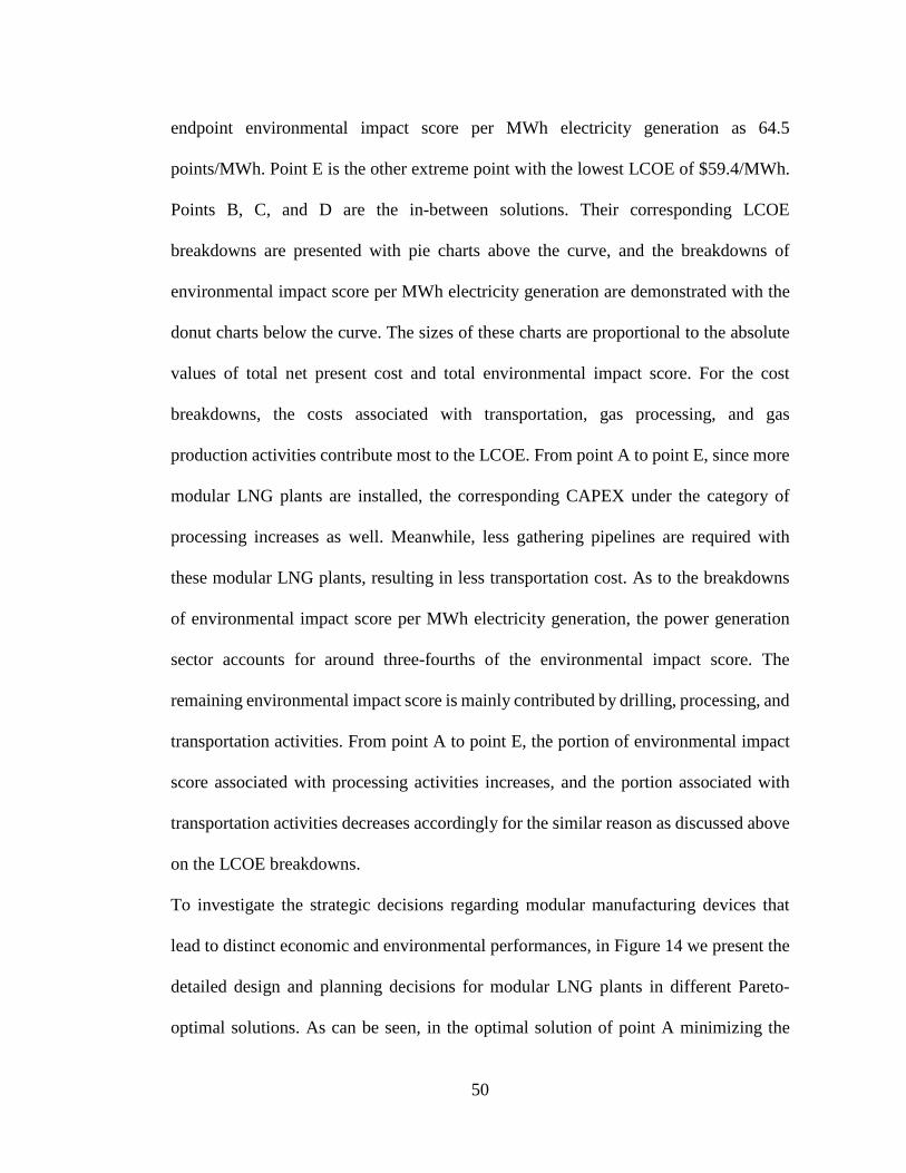
50

endpoint environmental impact score per MWh electricity generation as 64.5

points/MWh. Point E is the other extreme point with the lowest LCOE of $59.4/MWh.

Points B, C, and D are the in-between solutions. Their corresponding LCOE

breakdowns are presented with pie charts above the curve, and the breakdowns of

environmental impact score per MWh electricity generation are demonstrated with the

donut charts below the curve. The sizes of these charts are proportional to the absolute

values of total net present cost and total environmental impact score. For the cost

breakdowns, the costs associated with transportation, gas processing, and gas

production activities contribute most to the LCOE. From point A to point E, since more

modular LNG plants are installed, the corresponding CAPEX under the category of

processing increases as well. Meanwhile, less gathering pipelines are required with

these modular LNG plants, resulting in less transportation cost. As to the breakdowns

of environmental impact score per MWh electricity generation, the power generation

sector accounts for around three-fourths of the environmental impact score. The

remaining environmental impact score is mainly contributed by drilling, processing, and

transportation activities. From point A to point E, the portion of environmental impact

score associated with processing activities increases, and the portion associated with

transportation activities decreases accordingly for the similar reason as discussed above

on the LCOE breakdowns.

To investigate the strategic decisions regarding modular manufacturing devices that

lead to distinct economic and environmental performances, in Figure 14 we present the

detailed design and planning decisions for modular LNG plants in different Pareto-

optimal solutions. As can be seen, in the optimal solution of point A minimizing the

51

environmental impact score per MWh electricity generation, there are four modular

LNG plants. In addition to the existing modular plants installed at locations 2, 4, and 6,

another modular plant with a capacity of 25 kgal LNG/day is installed at location 1 in

the beginning. Since the construction time of modular plants considered in this case

study is one year, the newly installed modular plant at location 1 becomes available after

the first year [123]. Both point B and point C share the same design and planning

decisions on modular LNG plants. Specifically, in addition to the existing ones, two

modular plants with capacities of 25 kgal LNG/day are installed at location 1 and

location 5 in the beginning, respectively. No moving activities are observed in the

solutions of point A, point B, and point C. Points D and E have the same modular LNG

plants as point B and point C installed in the beginning. However, relocation of modular

LNG plants is observed in the optimal solutions of point D and point E. Specifically,

for point D, the modular plant at location 5 with a capacity of 25 kgal LNG/day is moved

to location 6 after three and a half years; meanwhile, the modular LNG plant at location

6 with a capacity of 50 kgal LNG/day is moved to location 5. For point E, the modular

plant at location 5 with a capacity of 25 kgal LNG/day is moved to location 6 three years

later, and the modular plant at location 6 with a capacity of 50 kgal LNG/day is moved

to location 5 half a year later. Such an exchange of modular LNG plants matches the

varying demand of processing capacity at different regions. Since no new shale wells

are drilled near location 6, and the production of existing wells are decreasing with time,

the original modular LNG plant (50 kgal LNG/day) provides more processing capacity

than needed after a few years. Meanwhile, the modular plant at location 5 (25 kgal

LNG/day) cannot handle the extra shale gas feedstock from the newly-drilled shale

52

wells. Therefore, it is considered more cost-effective to exchange the modular LNG

plants at locations 5 and 6 than installing extra ones. The moving process takes around

six months to complete, so the relocated modular LNG plant will be ready half a year

later. The moving option of modular LNG plants offers more flexibility in the operations

of a shale gas supply chain, and the overall economic performance can be improved.

Nevertheless, the moving activities of modular plants incur extra environmental

impacts, such as land use change, energy consumption, and emissions. Thus, the

relocation of modular plants may not be preferred when minimizing the comprehensive

environmental impacts is the main objective. These environmental impact results will

be discussed in detail in the following “comprehensive environmental impacts

assessment” subsection. Additionally, it is worth noting that these optimal strategies

regarding the modular LNG plants are only obtained based on the specific model and

input data considered in this study, and the actual strategy in practice may vary from

case to case.

53

Figure 14. Design and planning decisions for modular LNG plants in different Pareto-

optimal solutions.

In Figure 15, we summarize the CAPEX and OPEX regarding conventional processing

plants and modular LNG plants of the five Pareto-optimal solutions. For all the five

solution points, a conventional processing plant is constructed with 10 Tscf/year

processing capacity in addition to two existing ones. Thus, all the five points have the

same CAPEX for conventional processing plants. However, the OPEX of conventional

processing plants in each solution is quite different. We identify that when the OPEX

54

associated with conventional processing plant decreases, the OPEX resulted from

modular LNG plants increases accordingly, as can be induced by going from point A to

point E. This is because the raw shale gas in each Pareto-optimal solution will be either

processed by the conventional processing plants or sent to the modular LNG plants for

LNG production. Therefore, we conclude that the application of modular LNG plants

helps improve the economic performance of a shale gas supply chain. However, in terms

of mitigating the overall environmental impacts, the modular LNG plants show no

advantage over the conventional processing plants.

Figure 15. Summary of CAPEX and OPEX regarding conventional processing plants

and modular LNG plants in different Pareto-optimal solutions.

Next, we present the detailed drilling schedules (on the left) and shale gas production

profiles (on the right) corresponding to points A to E in Figure 16. From this

comparison, we expect to gain some insight into the connection between upstream

production and midstream infrastructure designs. For all the solution points, more shale

55

wells need to be drilled after the initial drilling activities to compensate for the

decreasing production of shale wells. From the drilling schedules, we can find that more

shale wells are drilled in the beginning in point A and point B, resulting in a higher peak

in terms of shale gas production in the first few years. As to point D and point E, they

have similar drilling schedules, which result in almost identical shale gas production

profiles. Moreover, the drilling schedules of point D and point E show that three new

wells are drilled at shale site 10 in the fourth year, resulting in a larger shale gas output

near location 5 to be processed. This explains why the modular plant at location 6 with

a capacity of 50 kgal LNG/day is moved to location 5 in the same year, as presented in

Figure 14. The drilling schedule and corresponding shale gas production profile of point

C are balanced between the environment-oriented solutions (point A and point B) and

the economics-oriented solutions (point D and point E).

56

Figure 16. Drilling schedules and shale gas production profiles of different Pareto-

optimal solutions.

In this section, we present and analyze the comprehensive environmental impact

profiles of different Pareto-optimal solutions. As mentioned in the introduction section,

57

the ReCiPe approach for LCIA comprises of 18 midpoint impact categories and three

endpoint impact categories [82]. The detailed midpoint environmental impact score

breakdowns associated with Pareto-optimal solutions A to E are presented in Figure 17.

As can be seen, all the five points share similar environmental impact score breakdowns

except point A and point B, which differ in the category of water management. The

impacts of climate change to human health (in green) and climate change to ecosystems

(in orange) stand out as two major contributors especially in the life cycle stages of shale

gas production, LNG storage, and power generation. Fossil depletion is one of the major

midpoint impact categories in water management, drilling, shale gas processing, and

transportation, which are all energy-intense processes. The human toxicity is another

key midpoint impact category especially in water management and drilling phases,

when large amounts of chemicals and additives are used in drilling and fracturing fluids.

The different wastewater treatment strategies also result in disparate environmental

performance. Thus, when the objective focuses on mitigating the environmental impacts

as shown in point A and point B, we observe a different environmental impact

breakdown. By investigating the corresponding water management strategies, we

identify RO technology for onsite treatment as the optimal wastewater treatment

technology in point A and point B. Nevertheless, in points C to E, all the wastewater is

treated by remote CWT facilities for a better economic performance.

58

Figure 17. Midpoint environmental impact score breakdowns of different Pareto-

optimal solutions.

To identify the key midpoint impact categories that contribute most to the environmental

impact score in the life cycle of shale gas, we further investigate the absolute midpoint

environmental impact scores associated with different Pareto-optimal solutions. Since

all the five Pareto-optimal solutions have similar midpoint environmental impact score

59

breakdowns, we present the absolute midpoint environmental impact scores of point A

in Figure 18 for illustration. From this result, we identify the climate change impact on

human health, climate change on ecosystems, and human toxicity as the most significant

midpoint environmental impact categories. These impact categories contribute to

around 91% of the total environmental impact score. Other important midpoint

environmental impact categories include metal depletion, fossil depletion, particulate

matter formation, and natural land transformation.

Figure 18. Absolute midpoint environmental impact scores of point A.

In Figure 19, we further present the endpoint environmental impact breakdowns

corresponding to different Pareto-optimal solutions. Here we select the environment-

oriented solution point A as the reference solution, and all the other solutions are

presented with their ratios based on the result of point A. As can be seen, for all the

three endpoint impact categories, namely ecosystem quality, human health, and

resources, all the three points from C to E have higher environmental impact scores than

60

point A in certain life cycle stages, including water management, shale gas processing,

and storage. The endpoint environmental impact score distribution of point B is similar

to that of point A except a slightly higher impact score in storage. The endpoint

environmental impact score distributions of points D and E are almost identical. Since

the total endpoint environmental impact score is the summation of scores from the three

endpoint impact categories, from the shapes of these four distributions we conclude that

the environmental impacts on ecosystem quality and human health contribute most to

the environmental impact score. Specifically, the environmental impacts on ecosystem

quality account for 37%-39% of the total environmental impact score; the

environmental impacts on human health contribute 54%-55% of the total environmental

impact score; and the environmental impacts on resources result in 6%-7% of the total

environmental impact score. The water management strategies and design and planning

of midstream infrastructure are the key decisions that lead to distinct environmental

performances.

61

Figure 19. Endpoint environmental impact score breakdowns and comparison of

different Pareto-optimal solutions (The environment-oriented solution A is selected as

the reference solution and all the other solutions are presented with ratios of their

results to that of point A).

2.5.2 Sensitivity analysis

In this section, we present a sensitivity analysis regarding several key parameters,

including the average EUR of shale wells, average NGL composition in shale gas,

average transportation distance, CAPEX for modular plant installation, and electricity

demand. Their impacts on the two optimization objectives, namely the LCOE and the

endpoint environmental impact score per MWh of electricity generation are summarized

in Figure 20. A variance range of 80% to 120% is considered for the five types of

uncertainties. As can be seen, the LCOE is most sensitive to the average transportation

distance. Longer transportation distance results in extra transportation cost, and thus

62

leads to a higher LCOE. Another important factor is the average EUR of shale wells.

With greater average EUR of shale wells, the cost efficiency of a certain shale well

improves, resulting in a lower LCOE. The impact of CAPEX for modular plant

installation is straightforward. More CAPEX leads to a higher value of LCOE. As the

average NGL composition in the raw shale gas increases, the LCOE decreases due to

the extra income from the sales of NGLs. The LCOE is least sensitive to the electricity

demand. The endpoint environmental impact score per MWh of electricity generation

does not follow the same trend as LCOE. The sensitivity analysis of average

transportation distance leads to some interesting results. First, from the range of 80% to

100%, there is no significant change in the endpoint environmental impact score per

MWh of electricity generation. This is mainly because transportation only contributes a

small portion (3%) of the total environmental impact score. However, when the

transportation distance increases to 120%, a different midstream design strategy will be

adopted. More modular plants are installed to produce LNG instead of relying on the

conventional processing plants. The change of midstream design strategy further leads

to a higher endpoint environmental impact score per MWh of electricity generation.

Both the electricity demand and the average EUR of shale wells have significant impacts

on the endpoint environmental impact score per MWh of electricity generation. As the

average EUR of shale wells increases, more shale gas can be produced with the same

environmental impact score. The impacts of average NGL composition in shale gas and

CAPEX for modular plant installation on the endpoint environmental impact score per

MWh of electricity generation are almost negligible.

63

Figure 20. Sensitivity analysis of average EUR of shale wells, average NGL

composition in shale gas, average transportation distance, CAPEX for modular plant

installation, and electricity demand.

2.5.3 Comparison with the overall-performance LCO model

Functional-unit-based LCO model is known for its superiority in leading to more

sustainable designs than traditional LCO models optimizing the overall economic and

environmental performances of a product system. To demonstrate the advantage of

proposed functional-unit-based LCO model, we consider another case study based on

an overall-performance LCO model. In this overall-performance LCO model, the

economic objective is to minimize the total net present cost (TC), which is identical to

the numerator of the economic objective function in the functional-unit-based LCO

model. The economic objective function TC is nonlinear with separable concave terms

calculating the CAPEX of conventional processing plants. The environmental objective

is to minimize the total ReCiPe endpoint environmental impact score (TE), which is the

64

numerator of the environmental objective function in the functional-unit-based LCO

model. All the constraints in the overall-performance LCO model are identical to those

in the functional-unit-based LCO model. The detailed formulation of this overall-

performance LCO model is summarized in Appendix B.

By solving the overall-performance LCO problem, another Pareto-optimal curve can be

obtained demonstrating the trade-offs between the total net present cost (TC) and the

total ReCiPe endpoint environmental impact score (TE). To give a clear comparison,

we present the Pareto-optimal solutions obtained by solving the overall-performance

LCO problem (orange points) and the functional-unit-based LCO problem (blue points)

in Figure 21. From this comparison, we can see the advantage of the proposed

functional-unit-based LCO model on providing more sustainable solutions from both

economic and environmental perspectives. The whole Pareto-optimal frontier of the

overall-performance LCO problem lies within the suboptimal region of the functional-

unit-based LCO problem, indicating that these Pareto-optimal solutions of the overall-

performance LCO problem would incur higher cost or environmental impact score than

those of the functional-unit-based LCO problem by producing one MWh of electricity.

Specifically, we select two sets of extreme points, namely the environment-oriented

solutions A and A’, and the economics-oriented solutions E and E’, for further

comparison. As can be seen, the LCOE of point A’ is slightly higher than that of point

A, and the ReCiPe endpoint environmental impact score per MWh electricity generation

of point A’ is about 9% higher than that of point A. Although the ReCiPe endpoint

environmental impact score per MWh electricity generation of point E’ is slightly lower

65

than that of point E, its LCOE is 5% higher than that of point E, which can result in a

significant difference in terms of economic performance.

Figure 21. Comparison of Pareto-optimal solutions of the proposed functional-unit-

based LCO problem optimizing the functional-unit-based economic and

environmental performances and the overall-performance LCO problem optimizing

the overall economic and environmental performances.

Additionally, in Figure 22, we present the optimal drilling schedules and shale gas

production profiles obtained by solving the functional-unit-based LCO problem and the

overall-performance LCO problem to further demonstrate the difference. Point E and

point E’ in Figure 21 are selected here for comparison. As can be observed, although

both point E and point E’ are optimizing the economic performance, the different

objective functions adopted in the functional-unit-based LCO model and the overall-

performance LCO model can lead to distinct design and operational decisions.

Specifically, more wells are drilled in the optimal solution of the functional-unit-based

LCO problem (point E) than in the optimal solution of the overall-performance LCO

66

problem (point E’). Consequently, the optimal shale gas production profile in point E

deviates from that of point E’.

Figure 22. Drilling schedules and production profiles in the Pareto-optimal solution

point E of the functional-unit-based LCO problem and the Pareto-optimal solution

point E’ of the overall-performance LCO problem.

2.6 Summary

In this work, a novel endpoint-oriented LCO model was proposed to investigate the

economic and environmental implications of incorporating modular manufacturing

devices in the optimal design and operations of shale gas supply chains. The resulting

problem was formulated as an MINLFP problem, and a tailored global optimization

algorithm was introduced to tackle this computational challenge. The applicability of

proposed endpoint-oriented LCO framework and tailored global optimization algorithm

was illustrated by a well-to-wire shale gas supply chain based on Marcellus Shale. Major

67

design and operational decisions, especially those regarding the modular manufacturing

devices, such as allocation, capacity selection, installment, moving, and salvage

decisions, were all captured. Through a detailed analysis and discussion, we came to a

few important conclusions: (1) application of modular manufacturing devices could

improve the economic performance of a shale gas supply chain. However, there was no

obvious advantage of modular manufacturing devices over the conventional processing

plants in terms of mitigating the overall environmental impacts; (2) the proposed

endpoint-oriented LCO framework enabled quantification of the full spectrum of life

cycle environmental impacts of shale gas supply chains, and thus leading to more

sustainable solutions; (3) major design decisions regarding drilling schedule, water

management, and midstream infrastructure design and planning were identified as the

key factors that led to distinct economic and environmental performances in a shale gas

supply chain.

2.7 Appendix A: Superstructure configuration description

2.7.1 Economic objective

The economic objective is to minimize the LCOE generated from shale gas, formulated

as the total net present cost divided by the total electric power generation. The total net

present cost comprises of the CAPEX associated with the shale gas processing devices

( C Xproc

APEC ) and gathering pipelines ( CAPEXtransC ), and the OPEX related to water management

( ,OPEXwater tC ), drilling activities ( ,

OPEXdrill tC ), shale gas production operations ( ,

OPEXprod tC ), shale gas

68

processing and upgrading ( ,proc tOPEXC ), transportation activities ( ,

OPEXtrans tC ), LNG storage (

,OPEXstor tC ), and electric power generation ( ,

OPEXpower tC ).

( ), , , ,, , ,

,

1min

procOPEX OPEX OPEX OPEX OPEX OPEX OPEXwater t drill t prod t trans t stor t power tCAPEX CAPEX

trans tt T

g tg G t T

tproc

C C C C C C CC C

drLCOE

GE∈

∈ ∈

+ + + + + ++ +

+ =∑

∑∑ (A1)

The CAPEX of shale gas processing devices comprises of the CAPEX associated with

conventional processing plants ( _proc coX

nvCAPEC ) and the CAPEX corresponding to modular

manufacturing devices ( _proc moX

dCAPEC ).

_ _proc proc convCAPEX CAPEX CAPE

proc mX

odC C C= + (A2)

_proc coX

nvCAPEC is the total CAPEX associated with construction of conventional processing

plants. In this study, we adopt a typical nonlinear function to calculate the CAPEX

following the existing literature [4, 121].

_n

pCAPEsfp

proc conX

p Pv

PCC

prcpci

rpcpri

i∈

= ⋅

⋅∑ (A3)

where pri denotes the reference CAPEX of conventional processing plants. PCp denotes

the capacity of conventional processing plant p. prc denotes the reference capacity of

conventional processing plants. sfp denotes the size factor of conventional processing

plants. pci denotes the chemical engineering plant cost index for conventional

processing plants. rpci denotes the chemical engineering plant cost index for

conventional processing plant of the reference year.

_proc moX

dCAPEC is the net CAPEX associated with modular LNG plants, given as the total

installment cost subtracted by the total salvage value of modular LNG plants. The

69

CAPEX of modular LNG plant is estimated based on a capital cost curve from the

literature, which is obtained by fitting the data on capital costs from existing and

hypothetical LNG plants from the literature [72].

( )_, , ,

, , ,1m k m k tCAPEX

k t m k ttm M k K t T

proc modm M k K t T

cam ZIC csm ZI

dr∈ ∈ ∈ ∈ ∈ ∈

⋅= − ⋅

+∑ ∑∑ ∑ ∑∑ (A4)

where camm,k denotes the CAPEX for installing a modular LNG plant with capacity level

k at location m. ZIm,k,t is a binary variable that equals 1 if a modular LNG plant with

capacity level k is installed at location m in time period t. dr is the discount rate per time

period. csmk,t denotes the discounted salvage value of a modular LNG plant with

capacity level k installed at time period t.

CAPEXtransC indicates the total CAPEX of gathering pipelines, calculated by,

, , , , , ,CAPEXtrans r i p r i p r i m r i m

i I p P r R i I p P r RC tpri XP lsp tpri XM lsm

∈ ∈ ∈ ∈ ∈ ∈

= ⋅ ⋅ + ⋅ ⋅∑∑∑ ∑∑∑ (A5)

where tprir denotes the reference CAPEX of gathering pipelines with capacity level r.

XPi,p,r is a binary variable that equals 1 if the gathering pipeline with capacity level r is

installed to transport shale gas from shale site i to conventional processing plant p. lspi,p

is the distance between shale site i and conventional processing plant p. Similarly,

XMi,m,r is a binary variable that equals 1 if the gathering pipeline with capacity level r is

installed to transport shale gas from shale site i to modular LNG plant at location m.

lsmi,m is the distance between shale site i and modular LNG plant at location m.

The water management cost consists of water acquisition cost (Cacq,t) and wastewater

treatment costs corresponding to different technologies, namely Class-II disposal wells

(Cdisp,t), CWT facilities (Ccwt,t), and onsite treatment (Consite,t).

70

, , , , ,OPEXwater t acq t disp t cwt t onsite tC C C C C= + + + (A6)

Cacq,t indicates the acquisition cost of freshwater in time period t, which is proportional

to the amount of freshwater,

, ,acq tI

ii

tfaC FWc∈

⋅=∑ (A7)

where fac denotes the unit acquisition cost of freshwater. FWi,t stands for the amount of

freshwater acquired from water source to shale site i in time period t.

Cdisp,t denotes the cost associated with underground injection of disposal wells in time

period t, given by,

, , disp ti I

i tvC WTDd∈

⋅=∑ (A8)

where vd denotes the unit cost for underground injection of wastewater. WTDi,t denotes

the amount of wastewater transported from shale site i to disposal wells at time period

t.

Ccwt,t indicates the cost associated with CWT treatment facilities in time period t,

calculated by,

, , i I

cwt t i tvcC WTC∈

⋅=∑ (A9)

where vc denotes the unit treatment cost of wastewater at CWT facilities. WTCi,t denotes

the amount of wastewater transported from shale site i to CWT facilities at time period

t.

Consite,t is the total onsite treatment cost in time period t, given by,

, , , onsite t i o to O

oi I

C Wv To O∈ ∈

= ⋅∑∑ (A10)

71

where voo denotes the unit treatment cost of wastewater by onsite treatment technology

o. WTOi,o,t denotes the amount of wastewater treated by onsite treatment technology o

at shale site i in time period t.

,OPEXdrill tC indicates the total OPEX associated with drilling activities in time period t,

, ,,OPE

i ti I

Xdrill t i tsdC NNc

∈

⋅=∑ (A11)

where sdci,t denotes the unit cost for shale well drilling and completion at shale site i in

time period t. NNi,t denotes the number of wells drilled at shale site i in time period t.

,OPEXprod tC stands for the total cost associated with shale gas production activities in time

period t, calculated as the difference between the gross cost proportional to the amount

of shale gas production and the salvage value of shale wells at the end of planning

horizon.

( ), , ,, ,i ti I

OPEXprod t i t i t i i t

i Ispc psgC SP NN eur SP

∈ ∈

= − ⋅ −⋅ ⋅∑ ∑ (A12)

where spci,t denotes the unit cost for shale gas production at shale site i in time period t.

SPi,t denotes the shale gas production rate at shale site i in time period t. psg denotes the

estimated average unit profit of shale gas remains to be produced in shale wells. euri

denotes the estimated ultimate recovery of shale gas for a shale well at shale site i.

,proc tOPEXC indicates the total OPEX for both modular LNG plant and conventional

processing plant in time period t, calculated by,

, _ , _ _ ,, ,proc t mod oper t modOPEX

conv opermove t t NGL tC C C C I= + + − (A13)

_ ,mod oper tC is the total OPEX of modular LNG plants, calculated by,

72

, , , ,_ ,m k i m k ti I m M

mod oper tk K

C vmo SMP∈ ∈ ∈

= ⋅∑ ∑ ∑ (A14)

where vmom,k denotes the unit OPEX for modular LNG plant at location m with capacity

level k. SMPi,m,k,t denotes the amount of shale gas sent from shale site i to modular LNG

plant at location m with capacity level k in time period t.

_ ,mod move tC stands for the moving cost of modular LNG plants in time period t, which

can by calculated by the following equation,

( ), ' , '_ ,, ,'

k k m m kmod m m m k tm

oveM m M K

tk

C cdm cmm ldm crm ZR∈ ∈ ∈

= + ⋅ + ⋅∑ ∑ ∑ (A15)

where cdmk denotes the cost of dissembling a modular LNG plant with capacity level k.

cmmk denotes the cost of moving a modular LNG plant with capacity level k for unit

distance. ldmm,m’ denotes the distance between potential modular LNG plant locations

m and m’. crmk denotes the cost of reassembling a modular LNG plant with capacity

level k. ZRm,m’,k,t is a binary variable that equals 1 if a modular LNG plant with capacity

level k is moved from location m to m’ in time period t.

_ ,conv oper tC is the total OPEX of conventional processing plants in time period t, given

by,

_ , , ,conv oper t p i p ti I p P

C vro SRP∈ ∈

= ⋅∑∑ (A16)

where vrop denotes the unit OPEX for conventional processing plant p. SRPi,p,t denotes

the amount of shale gas transported from shale site i to conventional processing plant p

in time period t.

INGL,t denotes the income from sales of NGLs in time period t, given as the summation

of incomes from both conventional processing plants and modular LNG plants.

73

, , ,p tNGL t t t mm M

tp P

I pl plSRPL SMPL∈ ∈

= ⋅ + ⋅∑ ∑ (A17)

where plt denotes the average unit price of NGLs in time period t. SRPLp,t denotes the

amount of NGLs produced at conventional processing plant p in time period t. SMPLm,t

denotes the amount of NGLs produced at modular LNG plant at location m in time

period t.

,OPEXtrans tC stands for the total OPEX associated with all the transportation activities in time

period t, given by,

, _ , _ ,_ ,OPEXtra transns t trans conv t trans power tmod tC C C C= + + (A18)

_ ,trans conv tC indicates the variable transportation cost of shale gas from shale sites to

conventional processing plants in time period t, given by,

_ , , , ,trans conv t i p i p ti I p P

C vrt lsp SRP∈ ∈

= ⋅ ⋅∑∑ (A19)

where vrt denotes the unit transportation cost of shale gas.

_ ,trans mod tC is the variable transportation cost associated with modular LNG plants,

including the variable transportation cost of shale gas from shale sites to modular LNG

plants and variable transportation cost of LNG from modular LNG plants to LNG

storage facilities.

, , , , ,_ , , , i m i m k t m s m s ti I m

trans mod tsM k K m M S

C vmt lsm SMP lvt ss m SMPS∈∈ ∈ ∈ ∈

= ⋅ ⋅ + ⋅ ⋅∑ ∑ ∑ ∑∑ (A20)

where vmt denotes the unit transportation cost of shale gas from shale sites to modular

LNG plants. vts denotes the unit transportation cost of LNG. lmsm,s denotes the distance

between modular LNG plants and LNG storage facility s. SMPSm,s,t denotes the amount

74

of LNG transported from modular LNG plant at location m to storage facility s in time

period t.

_ ,trans power tC indicates the variable transportation cost associated with power plants in

time period t, given as,

_ , , ,, , ,

,

,

, ,

trans power t s g t mss S m

g tg

g mG

gg G

p g

M

p g tg Gp P

C Slsvts vtg lmgSG Ss

v

MP

t g SPGp

G

lp∈ ∈

∈

∈ ∈

∈

⋅ ⋅ ⋅ ⋅

⋅

= +

⋅+

∑∑ ∑ ∑

∑∑ (A21)

where lsgs,g denotes the distance from storage facility s to power plant g. SSGs,g,t denotes

the amount of LNG transported from storage facility s to power plant g in time period

t. lmgm,g denotes the distance from modular LNG plant at location m to power plant g.

SMPGm,g,t denotes the amount of LNG transported from modular LNG plant at location

m to power plant g in time period t. vtp denotes the unit transportation cost of natural

gas, lpgp,g denotes the distance from conventional processing plant p to power plant g.

SPGp,g,t denotes the amount of natural gas transported from conventional processing

plant p to power plant g in time period t.

,OPEXstor tC is the total LNG storage cost in time period t, calculated by,

, , , , , , OPEXstor t m s t s g t s t

mS s SMs g GC SMPS Svsi SG INLvso vs

∈ ∈ ∈ ∈

= ⋅ + + ⋅

⋅∑ ∑ ∑ ∑ (A22)

where vsi denotes the operating cost for unit input of LNG at storage facilities, vso

denotes the operating cost for unit output of LNG at storage facilities. vs denotes the

unit storage cost for LNG. INLs,t denotes the amount of LNG stored at LNG storage

facility s in time period t.

75

,OPEXpower tC indicates the total variable cost associated with electric power generation in

time period t, calculated by,

, , , , , , ,OPEXpower t p g t m g t s g

g G Sg t

p P m M sC SPG SMPGve SSG

∈ ∈∈ ∈

= ⋅ + +

∑ ∑ ∑ ∑ (A23)

where veg denotes the unit cost for electricity generation from natural gas at power plant

g.

2.7.2 Environmental objective

The environmental objective is to minimize the ReCiPe endpoint environmental score

per MWh electricity generation from shale gas. The total environmental impact score

accounts for the environmental impacts associated with water management (Ewater),

shale well drilling, stimulation, and completion (Edrill), shale gas production (Eprod),

shale gas processing (Eproc), transportation (Etrans), LNG storage (Estor), and electric

power generation (Epower).

,

min prwater drill prod trans stor power

g t

oc

g G t T

E E E E E E ETEUETGE GE

∈ ∈

+ + + + + += =

∑∑ (A24)

The environmental impacts of water management account for activities including water

acquisition (Eacq) and wastewater treatment corresponding to different technologies,

namely Class-II disposal wells (Edisp), CWT facilities (Ecwt), and onsite treatment

(Eonsite).

water acq disp cwt onsiteE E E E E= + + + (A25)

76

Eacq indicates the environmental impact score resulting from freshwater acquisition

activities, which is proportional to the amount of freshwater acquired from water

sources.

,acq i ti I t T i

cc IC

iE eac FW∈ ∈ ∈

⋅=∑∑ ∑ (A26)

where eacic denotes the environmental impact score under impact category ic associated

with acquisition of unit amount of freshwater.

Edisp represents the environmental impact score associated with underground wastewater

injection, given by,

, disp iici I ic IC

tt T

E We d Tw D∈∈∈

⋅=∑ ∑∑ (A27)

where ewdic denotes the environmental impact score under impact category ic associated

with underground injection of unit amount of wastewater at disposal wells.

Ecwt indicates the environmental impact score regarding water treatment activities at

CWT facilities, calculated by,

, iccwti I ic IT C

i tt

E c Te Ww C∈∈ ∈

⋅= ∑∑∑ (A28)

where ewcic denotes the environmental impact score under impact category ic associated

with treatment of unit amount of wastewater at CWT facilities.

Eonsite stands for the environmental impact score associated with onsite wastewater

treatment, which is proportional to the amount of wastewater and dependent on the

specific onsite treatment technology, calculated by,

, ,, onsite i oic IC

o ici I

to O t T

eE w WTOo∈∈ ∈ ∈

= ⋅∑∑ ∑∑ (A29)

77

where ewoo,ic denotes the environmental impact score under impact category ic

associated with treating unit amount of wastewater by onsite treatment technology o.

Edrill indicates the environmental impact score induced by shale wells drilling activities,

where a series of processes including well pad construction, drilling, stimulation, and

completion are considered.

, ,drill ii ici I ic IC

tt T

E Nd Nes∈ ∈∈

⋅= ∑∑∑ (A30)

where esdi,ic denotes the environmental impact score under impact category ic associated

with the drilling process of a shale well at shale site i.

Eprod represents the environmental impact score resulting from shale gas production

activities, including fracturing fluid additive manufacture, sand mining, energy usage of

pump and compressors, hydraulic fracturing, workover flowback, venting, field

separation, and corresponding transportation, etc.

, ,prod ii ici I ic IC

tt T

E Sp Pes∈ ∈∈

⋅= ∑∑∑ (A31)

where espi,ic denotes the environmental impact score under impact category ic associated

with producing unit amount of shale gas at shale site i.

Eproc is the environmental impact score associated with operations and movement of

modular LNG plants as well as operations of conventional processing plants.

_ __mod oper mod moveproc conv operE E E E= + + (A32)

Emod_oper indicates the environmental impact score associated with shale gas processing

and LNG production at modular LNG plants, given by,

, , , ,_ k ic i m km todi I

operm M k K t T ic IC

E emp SMP∈ ∈ ∈ ∈ ∈

= ⋅∑ ∑ ∑∑∑ (A33)

78

where empk,ic denotes the environmental impact score under impact category ic

associated processing unit amount of shale gas at modular LNG plant with capacity

level k.

Emod_move stands for the environmental impact score induced by the movement of

modular LNG plants, calculated by,

, , ' , ',_ ,'

mod m k ic m m m m k tm M m M k K t T i I

oc

veC

E emm ldm ZR∈ ∈ ∈ ∈ ∈

= ⋅ ⋅∑ ∑ ∑∑∑ (A34)

where emmk,ic denotes the environmental impact score under impact category ic

associated with moving modular LNG plant with capacity level k for unit distance.

Econv_oper is the environmental impact score corresponding to shale gas processing at

conventional processing plants, given by,

_ , , ,conv oper p ic i p ti I p P t T ic IC

E erp SRP∈ ∈ ∈ ∈

= ⋅∑∑∑∑ (A35)

Where erpp,ic denotes the environmental impact score under impact category ic

associated with processing unit amount of shale gas at conventional processing plant p.

Etrans indicates the environmental impact score associated with all the transportation

activities, including those associated with the conventional processing plants

(Etrans_conv), modular LNG plants (Etrans_mod), and power plants (Etrans_power), calculated

by,

_ _ _trans trans conv trans mod trans powerE E E E= + + (A36)

Etrans_conv represents the environmental impact score induced by transporting shale gas

from shale sites to conventional processing plants, given by,

, , ,_ ic i p i p ti

trans cI p P t T ic

onvIC

E est lsp SRP∈ ∈ ∈ ∈

= ⋅ ⋅∑∑∑∑ (A37)

79

where estic denotes the environmental impact score under impact category ic associated

with transportation of unit amount of shale gas for unit distance.

Etrans_mod indicates the environmental impact score associated with transporting shale

gas from shale sites to modular LNG plants and from modular LNG plants to LNG

storage facilities, given by,

, , , , , , ,_ ic i m i m k t ic m s m s ti I m M k K t T ic IC m M ic I

trans mods S Ct T

E est lsm SMP elt lms SMPS∈ ∈ ∈ ∈∈ ∈ ∈ ∈ ∈

= ⋅ ⋅ + ⋅ ⋅∑ ∑ ∑∑∑ ∑∑∑∑

(A38)

where eltic denotes the environmental impact score under impact category ic associated

with transporting unit amount of LNG for unit distance.

Etrans_power represents the total environmental impact score associated with transporting

natural gas or LNG from LNG storage facilities, modular LNG plants, and conventional

processing plants to NGCC power plants, calculated by,

, , ,, ,

,

_ ,

, ,

s g t m gic s g m g

p g

tg G ic IC g G ic IC

p g tg G ic

trans power ics S t T m M t T

icp P ICt T

E SSG Selt lsg lmgelt

est

MPG

Pg S Glp∈ ∈ ∈ ∈∈ ∈ ∈ ∈

∈ ∈∈ ∈

⋅ ⋅ ⋅ ⋅

⋅

= +

+ ⋅

∑∑∑∑ ∑ ∑∑∑

∑∑∑∑ (A39)

Estor stands for the environmental impact score induced by LNG storage activities,

calculated by,

,istor s tic IC

cs S t T

E NLs Ies∈ ∈ ∈

= ⋅∑∑ ∑ (A40)

where essic denotes the environmental impact score under impact category ic associated

with storage of unit amount of LNG.

Epower indicates the environmental impact score associated with electric power

generation, given by,

80

, , , , ,, ,power p g t m g t s g tt T p P m M s

gg I S

icc CG i

eE SPGp SMPG SSg G∈ ∈ ∈ ∈∈∈

= ⋅ + +

∑∑∑ ∑ ∑ ∑ (A41)

where epgg,ic denotes the environmental impact score under impact category ic

associated with electricity generation from unit amount of natural gas at power plant g.

2.7.3 Mass balance constraints

The total water supply at each shale site comprises of freshwater from water sources

and reused water from onsite treatment.

,, , , , , i t i o to O

to iFDWFW WTl O i to∈

+ ⋅ = ∀∑ (A42)

where loo denotes the recovery factor for treating wastewater of onsite treatment

technology o. FDWi,t denotes the freshwater demand of shale site i in time period t.

,,, , , i

i t it

ii tw

wrfWP

NN iF d tDW + ∀= ⋅ (A43)

The wastewater production rate during the fracking process is proportional to the total

shale gas production rate at a shale site [124],

, , , , i t i i tWP cc SP i t= ⋅ ∀ (A44)

where cci is the correlation coefficient for shale gas production and wastewater

production of a shale well at shale site i.

At each shale site, the total amount of wastewater, including the wastewater from

drilling, hydraulic fracturing, and completion, should equal to the total amount of water

treated by different water management options, including CWT, disposal, and onsite

treatment.

81

, , , , , , , , i t i i i t i t i t i o to O

WP wd wrd NN WTC WTD WTO i t∈

+ ⋅ ⋅ = + + ∀∑ (A45)

where wdi denotes the average drilling water usage for each well at shale site i. wrdi

denotes the recovery ratio for drilling process at shale site i.

The total amount of shale gas produced at existing shale sites can be calculated by,

, , , , i t i i t eSP ne spp i I t= ⋅ ∀ ∈ (A46)

where nei denotes the number of existing shale wells drilled at shale site i. sppi,t denotes

the shale gas production of a shale well of age t at shale site i.

The total shale gas production rate at a shale site equals the summation of that of

different wells.

1

, , ' , '' 1

, , 2t

i t i t i t t nt

SP NN spp i I t−

−=

= ⋅ ∀ ∈ ≥∑ (A47)

where sppi,t-t’ denotes the shale gas production profile of a shale well drilled at time

period t’ at shale site i in time period t. Thus, the age of this well would be t- t’. We use

this time-dependent parameter to describe the decreasing feature of the shale gas

production profile of a certain well.

The shale gas production at each shale site is either transported to the conventional

processing plants or modular LNG plants.

, , , , , , , , i t i p t i m k tp P m M k K

SP SRP SMP i t∈ ∈ ∈

= + ∀∑ ∑ ∑ (A48)

The methane and NGLs are separated at conventional processing plants, and their

corresponding amounts are dependent on the processing efficiency and the composition

of raw shale gas.

82

, , , , , i p t p ti I

ipef mecSRP SRPM p t∈

⋅ ∀⋅ =∑ (A49)

, , , , , i p t p ti I

ipef lSRP SRPL pc t∈

⋅ = ∀⋅∑ (A50)

where pef denotes the NGL recovery efficiency at conventional processing plants. meci

denotes the methane composition in shale gas at shale site i. lci denotes the NGL

composition in shale gas at shale site i.

Similarly, the shale gas sent to modular LNG plants are processed first to separate

natural gas and NGLs.

, , , , , , i m k t m ti I K

ik

mefSMP SMPM m tmec∈ ∈

⋅ ∀⋅ =∑∑ (A51)

, , , , , , i m k t m ti I k K

imeSMP SMPL mf lc t∈ ∈

⋅ ∀⋅ =∑∑ (A52)

where mef denotes the NGL recovery efficiency at modular LNG plants.

The total amount of natural gas separated at a conventional processing plant equals the

summation of natural gas transported from the processing plant to different power

plants.

, , , , , p t p g tg G

SRPM SPG p t∈

= ∀∑ (A53)

The LNG produced at a modular LNG plant can either be transported to power plants

for electric power generation directly or be transported to LNG storage facilities for

temporary storage.

, , , , , , , m t m g t m s tg G s S

SMPM SMPG SMPS m t∈ ∈

= + ∀∑ ∑ (A54)

For LNG at each LNG storage facility, the following input-output mass balance

relationship should be satisfied.

83

, 1 ,, , , , , , 2 s t s tm s t s g tm M g G

SMPS SSGINL INL s t∈ ∈

− ++ = ∀ ≥∑ ∑ (A55)

The total amount of electricity generation at a power plant in each time period is

proportional to the amount of natural gas transported to the power plant from different

sources, including the conventional processing plants, modular LNG plants, and LNG

storage facilities.

, , , , , , , , , g t p g t m g t s g tp P m M s S

uGE SPG SMPG SSG g te∈ ∈ ∈

= + + ∀

⋅ ∑ ∑ ∑ (A56)

where ue denotes the amount of electricity generated per unit natural gas input.

2.7.4 Capacity constraints

The total amount of wastewater from different shale sites treated by each CWT facility

cannot exceed its capacity, given by,

, , i ti I

tW ccaTC t∈

≤ ∀∑ (A57)

where ccat denotes the capacity for wastewater treatment at CWT facility in time period

t.

Similarly, the total amount of wastewater from all the shale sites handled by disposal

wells should not exceed their disposal capacities,

, , i ti I

tW dcaTD t∈

≤ ∀∑ (A58)

where dcat denotes the capacity for underground injection at disposal wells in time

period t.

If a certain onsite treatment technology is applied at a shale site, the amount of

wastewater treated onsite should be bounded by its capacity; otherwise, the amount of

84

wastewater treated onsite should be zero. This relationship can be modeled by the

following inequality,

, , , , , , , o i o i o t o i oocl YO WTO ocu YO i o t⋅ ≤ ≤ ⋅ ∀ (A59)

where oclo and ocuo denote the minimum and maximum treatment capacities for onsite

treatment technology o, respectively. YOi,o is a binary variable that equals 1 if onsite

treatment technology o is applied at shale site i.

To satisfy the reuse specification for hydraulic fracturing, the blending ratio of

freshwater to treated water from onsite treatment must be greater than a certain value,

given by,

, , , , , i o t i to O

o o WTO Fr W i tf lo∈

⋅ ⋅ ≤ ∀∑ (A60)

where rfo denotes the ratio of freshwater to wastewater required for blending after

treatment by onsite treatment technology o.

The total amount of shale gas processed at a conventional processing plant cannot

exceed its capacity,

, , , , i p t pi I

SRP PC p t∈

≤ ∀∑ (A61)

Similarly, the amount of shale gas sent to a modular LNG plant is constrained by its

working capacity,

, , , , , , , , i m k t m k ti I

SMP MC m k t∈

≤ ∀∑ (A62)

where MCm,k,t denotes the capacity of modular LNG plant at location m with capacity k

in time period t.

85

For the LNG storage facilities, there are capacity constraints for the LNG in stock, LNG

input, and LNG output streams, as given below.

, , , s t sINL sca s t∀≤ (A63)

, , , , m s tm

sM

S ssicMPS t∈

≤ ∀∑ (A64)

, , , , s g tg G

sSSG s tsoc∈

≤ ∀∑ (A65)

where scas denotes the capacity of LNG storage facility s. sics denotes the input capacity

of LNG storage facility s. socs denotes the output capacity of LNG storage facility s.

The total amount of shale gas transported from a shale site to a conventional processing

plant or a modular LNG plant is constrained by the transportation capacity of

corresponding gathering pipeline.

, , , , , , , i p t i p rr R

SRP TCP i p t∈

≤ ∀∑ (A66)

, , , , , , , , i m k t i m rk K r R

SMP TCM i m t∈ ∈

≤ ∀∑ ∑ (A67)

The total electric power generation is constrained by the lower bound and upper bound

of local demand.

, , , , , g t g t g tdml GE dmup g t≤ ≤ ∀ (A68)

where dmlg,t and dmupg,t denote the minimum demand and maximum demand of

electricity at power plant g in time period t, respectively.

2.7.5 Bounding constraints

If a gathering pipeline is installed, its capacity equals the reference capacity

corresponding to its capacity level; otherwise, its capacity should be zero.

86

, , , , , , ,i p r r i p rTCP tprc XP i p r= ⋅ ∀ (A69)

, , , , , , ,i m r r i m rTCM tprc XM i p r= ⋅ ∀ (A70)

where tprcr denotes the reference capacity of gathering pipelines with capacity level r.

Similarly, if a modular LNG plant is constructed, its capacity equals the reference

capacity of the design capacity level; otherwise, its capacity should be zero.

, , , , , , , m k t k m k tMC rmc ZE m k t= ⋅ ∀ (A71)

where rmck denotes the reference capacity of modular LNG plants with capacity level

k. ZEm,k,t is a binary variable that equals 1 if a modular LNG plant with capacity level k

exists at location m in time period t.

If a processing plant is established, its processing capacity should be bounded by the

corresponding capacity range; otherwise, its capacity should be zero. This relationship

can be modeled by the following inequality:

, p p p p ppcl YP PC pcup YP p⋅ ≤ ≤ ⋅ ∀ (A72)

where pclp and pcupp denote the minimum and maximum capacities of conventional

processing plant p, respectively. YPp is a binary variable that equals 1 if a conventional

processing plant p is constructed.

2.7.6 Logic constraints

There can be a certain number of wells drilled at each shale site in each time period,

given by,

, ,0

1, , imn

i n tn

YD i t=

= ∀∑ (A73)

87

where YDi,n,t is a binary variable that equals 1 if n shale wells at shale site i are dilled in

time period t. mni denotes the maximum number of wells that can be drilled at shale site

i per time period.

The total number of wells drilled at shale site i in time period t can be calculated by,

, , ,0

, , imn

i t i n tn

NN n YD i t=

= ⋅ ∀∑ (A74)

The total number of wells that can be drilled at shale site i over the planning horizon is

bounded, given by,

, , i tt T

iNN itmn∈

≤ ∀∑ (A75)

where tmni denotes the maximum number of wells that can be drilled at shale site i over

the planning horizon.

The existing shale sites are fully developed, so there will be no further drilling activities

at these shale sites,

, 0, , i t eNN i I t= ∀ ∈ (A76)

For the selection of onsite treatment technologies, we note that at most one technology

can be chosen at a shale site. This constraint is given by,

, 1, i oo O

YO i∈

≤ ∀∑ (A77)

Only a certain capacity level can be chosen for each gathering pipeline among shale

sites, conventional processing plants, and modular LNG plants, given by,

, , 1, , i p rr R

XP i p∈

≤ ∀∑ (A78)

, , 1, , i m rr R

XM i m∈

≤ ∀∑ (A79)

88

The existence of a modular LNG plant with a certain capacity level at a certain location

in any time period depends on the previous condition, the installment decisions, and

moving decisions of modular LNG plants. The complex logic relationship among these

decision variables is depicted by the following equation,

{ } { }, , , , 1 , , 1 , ', , ', , , 1

' ', , , 2m k t m k t m k t m m k t m m k t

m M m m M mZE ZE ZI ZR ZR m k t− − −

∈ ∈

= + − + ∀ ≥∑ ∑

(A80)

For each potential location, there is no more than one modular LNG plant installed,

given by,

, , 1, m k tk K t T

ZI m∈ ∈

≤ ∀∑∑ (A81)

The moving of modular LNG plants only exists between two distinct locations,

, , , 0, , , m m k tZR m k t= ∀ (A82)

The moving of a modular LNG plant can only happen once between any two locations,

, ', , 1, , ', m m k tt T

ZR m m k∈

≤ ∀∑ (A83)

There exists no more than one modular LNG plant at one location in any time period,

, , 1, , m k tk K

ZE m t∈

≤ ∀∑ (A84)

Only existing modular LNG plants can be moved from one location to another,

, , , ', ,'

, , , m k t m m k tm M

ZE ZR m k t∈

≥ ∀∑ (A85)

89

2.8 Appendix B: Detailed model formulation for the overall-

performance LCO model

In this section, we present the specific model formulation of the overall-performance

LCO model. The economic objective is to minimize the total net present cost (TC).

Notably, _proc coX

nvCAPEC involves concave terms calculating the CAPEX of conventional

processing plants, so the overall economic objective function TC is nonlinear. The

environmental objective is to minimize the total ReCiPe endpoint environmental impact

score (TE). All the constraints are identical to those in the functional-unit-based LCO

model. Therefore, we use the same equation numbers to indicate the specific

formulation.

Economic Objective:

( ), , , ,, , ,min

1

OPEX OPEX OPEX OPEX OPEX OPEX OPEXwater t drill t prod t trans t stor t power tCAPEX C procAPEX

transt

rt

c tT

p o

C C C C C C CTC C C

dr∈

+ + + + + += + +

+ ∑

Environmental Objective:

min processingwater drill production transportation storage powerTE E E E E E E E= + + + + + +

s.t. Economic Constraints (A2)-(A23)

Environmental Constraints (A25)-(A41)

Mass Balance Constraints (A42)-(A56)

Capacity Constraints (A57)-(A68)

Bounding Constraints (A69)-(A72)

Logic Constraints (A73)-(A85)

90

2.9 Appendix C: Detailed computational performance of proposed

tailored global optimization algorithm

In this section, we present the detailed converging process for the solution of point E

using the proposed tailored global optimization algorithm. As shown in Table C1, the

tailored global optimization algorithm takes three outer loop iterations to find the

optimal objective value of problem (P2). For each outer loop iteration, it takes one to

two inner loop iterations to converge. During the inner loop, the upper bound decreases

while the lower bound increases until they are close enough to satisfy the inner loop

stopping criterion. In the last iteration of the outer loop, the reformulated linear objective

function *( )F q TC q TGE= − ⋅ equals 0, indicating the convergence of this tailored

global optimization algorithm. The total computational time is 5,910 CPU seconds.

Notably, the absolute computational time varies when solving for different Pareto-

optimal solutions. However, all the optimization problems can be solved to global

optimum within a few hours.

Table C1. Converging process for the solution of point E.

Iterout q Iterin LB UB F(q) CPU seconds

1 0 1 306,109,900 307,325,000 306,109,900 1,509

2 0.062 1 -18,971,300 -17,948,700 -18,971,300 672

0.062 2 -17,948,700 -17,948,700 17,948,700 1,531

3 0.059 1 -1,022,630 0 -1,022,630 304

0.059 2 0 0 0 1,894

2.10 Nomenclature

Sets

91

G Set of power plants indexed by g

I Set of shale sites indexed by i

K Set of capacity levels for the modular LNG plant indexed by k

M Set of potential modular LNG plant locations indexed by m

N Set of number of wells indexed by n

O Set of onsite treatment technologies indexed by o

(o1: MSF; o2: MED; o3: RO)

P Set of conventional processing plants indexed by p

R Set of capacity levels for the gathering pipelines indexed by r

S Set of storage facilities indexed by s

T Set of time periods indexed by t

Subsets

( )eI i Subset of existing shale site indexed by ie

( )nI i Subset of newly constructed shale site indexed by in

'( )M m Subset of potential modular LNG plant locations indexed by m’

( )nM m Subset of modular LNG plants that are potentially to be built indexed

by mn

( )nP p Subset of conventional processing plants that are potentially to be built

indexed by pn

'( )T t Subset of time periods when wells are drilled indexed by t’

Parameters

,m kcam Capital investment for installing a modular LNG plant with capacity level k at location m

92

icc Correlation coefficient for shale gas production and wastewater production of a shale well at shale site i

tcca Capacity for wastewater treatment at CWT facility in time period t

kcdm Cost of dissembling a modular plant with capacity level k

kcmm Cost of moving a modular plant with capacity level k for unit distance

kcrm Cost of reassembling a modular plant with capacity level k

,k tcsm The discounted salvage value of a modular LNG plant with capacity level k installed at time period t

tdca Capacity for underground injection at disposal wells in time period t

,g tdml Minimum demand of electricity at power plant g in time period t

,g tdmup Maximum demand of electricity at power plant g in time period t

dr Discount rate per time period

iceac Environmental score under impact category ic associated with acquisition of unit amount of freshwater

icelt Environmental score under impact category ic associated with transporting unit amount of LNG for unit distance

,k icemm Environmental score under impact category ic associated with moving modular LNG plant with capacity level k for unit distance

,k icemp Environmental score under impact category ic associated processing unit amount of shale gas at modular LNG plant with capacity level k

,g icepg Environmental score under impact category ic associated with electricity generation of unit amount of natural gas at power plant g

,p icerp Environmental score under impact category ic associated with processing unit amount of shale gas at conventional processing plant p

,i icesd Environmental score under impact category ic associated with the drilling process of a shale well at shale site i

93

,i icesp Environmental score under impact category ic associated with producing unit amount of shale gas at shale site i

icess Environmental score under impact category ic associated with storage of unit amount of LNG

icest Environmental score under impact category ic associated with transportation of unit amount of shale gas for unit distance

ieur Estimated ultimate recovery of shale gas for a shale well at shale site i

icewc Environmental score under impact category ic associated with treatment of unit amount of wastewater at CWT facilities

icewd Environmental score under impact category ic associated with underground injection of unit amount of wastewater at disposal wells

,o icewo Environmental score under impact category ic associated with treating unit amount of wastewater by onsite treatment technology o

fac Unit acquisition cost of freshwater

ilc NGL composition in shale gas at shale site i

, 'm mldm Distance from potential modular LNG plant location m to m’

olo Recovery factor for treating wastewater of onsite treatment technology o

,m glmg Distance from modular LNG plant m to power plant g

,m slms Distance from modular LNG plant m to storage facility s

,p glpg Distance from conventional processing plant p to power plant g

, s glsg Distance from storage facility s to power plant g

, i mlsm Distance from shale site i to modular LNG plant m

,i plsp Distance from shale site i to conventional processing plant p

94

imec Methane composition in shale gas at shale site i

mef NGL recovery efficiency at modular LNG plant

imn Maximum number of wells that can be drilled at shale site i per time period

ine Number of existing shale wells drilled at shale site i

oocl Minimum treatment capacity for onsite treatment technology o

oocu Maximum treatment capacity for onsite treatment technology o

pci Chemical engineering plant cost index for conventional processing plant

ppcl Minimum capacity of conventional processing plant p

ppcup Maximum capacity of conventional processing plant p

pef NGL recovery efficiency at conventional processing plant

tpl Average unit price of NGLs in time period t

prc Refence capacity of conventional processing plant

pri Reference capital investment of conventional processing plant

psg Estimated average unit profit of shale gas remains to be produced in shale wells

orf Ratio of freshwater to wastewater required for blending after treatment of onsite treatment technology o

krmc Reference capacity of modular LNG plant with capacity level k

rpci Chemical engineering plant cost index for conventional processing plant of the reference year

ssca Capacity of LNG storage facility s

95

,i tsdc Unit cost for shale well drilling and completion at shale site i in time period t

sfp Size factor of conventional processing plants

ssic Input capacity of LNG storage facility s

ssoc Output capacity of LNG storage facility s

,i tspc Unit cost for shale gas production at shale site i in time period t

,ispp τ Shale gas production of a shale well of age at shale site i

itmn Maximum number of wells that can be drilled at shale site i over the planning horizon

rtprc Reference capacity of gathering pipeline with capacity level r

rtpri Reference capital investment of gathering pipeline with capacity level r

ue Amount of electricity generated per unit natural gas input

vc Unit cost for wastewater treatment at CWT facility

vd Unit cost for underground injection of wastewater at disposal well

gve Unit cost for electricity generation from natural gas at power plant g

, m kvmo Unit OPEX for a modular LNG plant at location m with capacity level k

vmt Unit transportation cost of shale gas from shale sites to modular LNG plants

ovo Levelized unit cost for wastewater treatment of onsite treatment technology o

pvro Unit OPEX for conventional processing plant p

vrt Unit transportation cost of shale gas from shale sites to conventional processing plants

τ

96

vs Unit storage cost for LNG

vsi OPEX for unit input of LNG at storage facilities

vso OPEX for unit output of LNG at storage facilities

vtp Unit transportation cost of natural gas

vts Unit transportation cost of LNG

iwd Average drilling water usage for each well at shale site i

iwrd Recovery ratio of water for drilling process at shale site i

iwrf Recovery ratio of water for hydraulic fracturing process at shale site i

Nonnegative Continuous variables

,i tFDW Freshwater demand of shale site i in time period t

,i tFW Amount of freshwater acquired from water source to shale site i in

time period t

,g tGE Amount of electricity generated at power plant g in time period t

,s tINL Amount of LNG stored at storage facility s in time period t

, ,m k tMC Capacity of modular LNG plant at location m with capacity k in time

period t

,i tNN Number of wells drilled at shale site i in time period t

pPC Capacity of conventional processing plant p

, , ,i m k tSMP Amount of shale gas sent from shale site i to modular LNG plant at

location m with capacity level k in time period t

97

, ,m g tSMPG Amount of LNG transported from modular LNG plant at location m

to power plant g in time period t

,m tSMPL Amount of NGLs produced at modular LNG plant at location m in

time period t

,m tSMPM Amount of methane produced at modular LNG plant at location m in

time period t

, ,m s tSMPS Amount of LNG transported from modular LNG plant at location m

to storage facility s in time period t

,i tSP Shale gas production rate at shale site i in time period t

, ,p g tSPG Amount of natural gas transported from conventional processing

plant p to power plant g in time period t

, ,i p tSRP Amount of shale gas transported from shale site i to conventional

processing plant p in time period t

,p tSRPL Amount of NGLs produced at conventional processing plant p in

time period t

,p tSRPM Amount of methane produced at conventional processing plant p in

time period t

, ,s g tSSG Amount of LNG transported from storage facility s to power plant g

in time period t

, ,i m rTCM Capacity of gathering pipeline with capacity level r between shale

site i and modular LNG plant m

98

, ,i p rTCP Capacity of gathering pipeline with capacity level r between shale

site i and conventional processing plant p

, i tWP Wastewater production rate at shale site i in time period t

,i tWTC Amount of wastewater transported from shale site i to CWT facility

in time period t

,i tWTD Amount of wastewater transported from shale site i to disposal well

in time period t

, ,i o tWTO Amount of wastewater treated by onsite treatment technology o at

shale site i in time period t

Binary variables

, ,i m rXM 0-1 variable. Equal to 1 if gathering pipeline with capacity level r is

installed to transport shale gas from shale site i to modular LNG plant

m

, ,i p rXP 0-1 variable. Equal to 1 if gathering pipeline with capacity level r is

installed to transport shale gas from shale site i to conventional

processing plant p

, ,i n tYD 0-1 variable. Equal to 1 if n shale wells at shale site i are drilled in time

period t

,i oYO 0-1 variable. Equal to 1 if onsite treatment technology o is applied at

shale site i

pYP 0-1 variable. Equal to 1 if conventional processing plant p is

constructed

99

, ,m k tZE 0-1 variable. Equal to 1 if a modular LNG plant with capacity level k

exists at location m in time period t

, ,m k tZI 0-1 variable. Equal to 1 if a modular LNG plant with capacity level k

is newly installed at location m in time period t

, ', ,m m k tZR 0-1 variable. Equal to 1 if a modular LNG plant with capacity level k

is moved from location m to m’ in time period t

Equation Chapter (Next) Section 1

100

CHAPTER 3

INTEGRATED HYBRID LIFE CYCLE ASSESSMENT AND OPTIMIZATION

3.1 Introduction

Shale gas is considered as a “transition fuel” towards a low carbon economy [2].

However, producing shale gas requires significant amounts of water and energy

resources with horizontal drilling and hydraulic fracturing technologies [3, 60, 80, 125].

Moreover, there are concerns that even small leakages of methane during shale gas

extraction may offset the effects of lower carbon dioxide emissions [126-128]. LCA is

a systematic way to investigate the environmental impacts of shale gas [64, 96, 97, 129].

Furthermore, LCO models integrating LCA with multiobjective optimization

techniques are proposed to automatically identify the optimal design and operational

alternatives in shale gas supply chains and process systems [6, 63, 130, 131]. Most

existing shale gas LCA studies and all the LCO applications in the literature adopt a

process-based LCA approach [1, 17, 79, 80, 84, 95, 118, 132]. Although process-based

LCA provides more accurate and detailed process information, it suffers from system

truncation, and thus underestimates the true environmental impacts [133]. Alternatively,

the economic input-output (EIO)-based LCA utilizes national EIO data coupled with

sectoral environmental impact factors to evaluate the environmental impacts of a

product system [118]. Since all transaction activities within a country are recorded in

national table, the system boundary of EIO-based LCA is generally considered more

complete than that of process-based LCA. However, with aggregation of industries and

commodities, the process-scale details are missing, which eventually affects the

precision of EIO-based LCA results. Consequently, we are unable to guarantee the

101

accuracy and precision of LCA results simultaneously by solely relying on either the

process-based LCA or the EIO-based LCA.

To address the aforementioned research challenge, we adopt an integrated hybrid LCA

method to analyze the life cycle environmental impacts of shale gas. The integrated

hybrid LCA approach has been applied to evaluate the environmental impacts of

multiple systems, such as construction process, wind power generation, solar PV, and

electricity generation [134-137]. To the best of our knowledge, this was the first

integrated hybrid LCA study of shale gas. The integrated hybrid LCA combines the

strengths of both process-based LCA and EIO-based LCA [68]. On the one hand, the

process details associated with major processes within the system boundary are

guaranteed by explicit process analysis. On the other hand, the truncated system is

supplemented by the EIO systems. Moreover, the interactions between the process

systems and the macroeconomic systems are explicitly modeled by upstream and

downstream cutoff matrices. Thus, this integrated hybrid LCA approach overcomes the

drawbacks of traditional process-based and EIO-based LCAs, and quantifies the life

cycle environmental impacts of shale gas in a more precise and comprehensive manner.

In this study, we consider life cycle GHG emissions, water consumption, and energy

consumption. Based on this multi-criterion integrated hybrid LCA, a functional unit-

based multi-objective hybrid LCO model is further developed, which enables automatic

identification of the optimal design and operational alternatives in a “well-to-wire” shale

gas supply chain. Major decisions associated with shale well drilling, fracturing and

completion, shale gas production, water management, shale gas processing,

transportation, and end use for electricity generation are all modeled and linked with

102

their corresponding economic and environmental impacts. The resulting hybrid LCO

problem is a mixed-integer nonlinear programming (MINLP) problem that is

computationally intractable for general-purpose global optimizers. Thus, a tailored

global optimization algorithm integrating the parametric algorithm and a branch-and-

refine algorithm is applied to tackle this computational challenge. The applicability of

the proposed hybrid LCO model and global optimization algorithm is illustrated through

a case study on shale gas supply chain design in UK.

3.2 Integrated hybrid LCA of shale gas

3.2.1 Integrated hybrid LCA approach

LCA approaches that integrate process-based and EIO-based analyses and combine the

strengths of both are generally considered as hybrid LCA approaches [68]. Depending

on how the life cycle inventory (LCI) is compiled, hybrid LCA approaches are classified

into tiered hybrid LCA, EIO-based hybrid LCA, and integrated hybrid LCA [133, 138].

The tiered hybrid LCA is a combination of process-based LCA and EIO-based LCA by

treating them separately. Process-based LCA is utilized to compile the LCIs of use and

disposal phases as well as other important upstream processes, and the remaining LCIs

are constructed using EIO-based LCA. The overall LCI is a summation of LCIs obtained

by the process-based LCA and EIO-based LCA. Moriguchi et al. pioneered the

advantage of the tiered hybrid approach [139], and its application is soon acknowledged

by other LCA practitioners [140, 141]. Jiang et al. evaluated the life cycle GHG

emissions and water consumption of shale gas using the tiered hybrid approach [19,

118]. The input-output (IO)-based hybrid LCA is carried out by disaggregating industry

103

sectors in the EIO table to improve the accuracy of the augmented EIO table.

Meanwhile, the tiered hybrid LCA approach is applied to calculate the life cycle

inventories of post-consumer phases, namely use and disposal [142].

In this study, we adopt the integrated hybrid LCA approach, which inherits the

advantages and overcomes the drawbacks of these hybrid LCA methods [68, 143].

Specifically, the integrated hybrid LCA method uses explicit process analysis to

estimate the environmental impacts associated with key life cycle processes in the

“foreground process systems” [144]. Since process-specific data are generally

considered more reliable than EIO-based data, this step improves the precision of

analysis as compared with EIO-based LCA. Meanwhile, the truncated system boundary

is complemented by including the “background macroeconomic systems” that the

process systems interact with following the EIO-based LCA approach [140, 141].

Therefore, the resulting hybrid LCI not only retains the level of detail and specificity

from process-based LCA but also has the completeness of macroeconomic systems from

EIO-based LCA [145]. An illustrative figure is presented in Figure 23 to demonstrate

the idea of integrated hybrid LCA approach.

104

Figure 23． Illustration of integrated hybrid LCA approach.

Notably, unlike tiered hybrid LCA where the process systems and the macroeconomic

systems are treated separately, the interactions between the process systems and the EIO

systems are systematically captured in the integrated hybrid LCA by upstream and

downstream cutoffs matrices. As can be seen in Figure 23, upstream cutoff flows are

the inputs from industrial sectors in the EIO systems to the process systems.

Downstream cutoff flows are the outputs from the process systems that are consumed

by industrial sectors in the EIO systems. Therefore, the mathematical formulation for

the integrated hybrid LCA model is given as follows:[133]

1

Total environmental impact0

p dp io

u io

A C yE E

C I A

−− = − −

(1)

where Ap is the process matrix that represents the exchanges of goods among processes

within the process system boundary. Aio is the direct requirements matrix describing the

interdependencies among industrial sectors within the EIO systems. Cu and Cd are the

upstream cutoff matrix and downstream cutoff matrix, respectively. The process matrix

Ap and downstream cutoff matrix Cd are typically given in physical units. By contrast,

105

the direct requirements matrix Aio and upstream cutoff matrix Cu are typically specified

in monetary units. The conversions between physical units and monetary units are done

by using market price data. Ep and Eio are the environmental extension vectors

corresponding to the process systems and the EIO systems, respectively. [ ]0 Ty is the

functional unit column indicating the amount of final product that is produced per

functional unit. With this integrated hybrid LCA methodology, we can quantify the total

life cycle environmental impacts of shale gas, which consist of the environmental

impacts originating from the foreground process systems of a shale gas supply chain

(process environmental impacts) and the environmental impacts associated with

background industrial sectors in the EIO systems (IO environmental impacts). We

consider the specific application of this integrated hybrid LCA approach to shale gas in

the following section. Furthermore, the hybrid LCA results are compared with those

based on process-based LCA in the literature to demonstrate the need of taking the

integrated hybrid LCA approach.

3.2.2 Hybrid LCA results

In this section, we formally state the hybrid LCA study of shale gas. Specifically, we

consider UK shale gas to illustrate the integrated hybrid LCA approach, and the reasons

are summarized as follows. First, there have been extensive LCA studies on US shale

gas [96, 129]. Meanwhile, shale gas extraction in the UK is in its early stage, and

corresponding LCA studies are relatively rare. More importantly, the integrated hybrid

LCA approach requires EIO data to be both up-to-date and comprehensive. However,

the newest EIO data for the US are based on 2015 with 71 industries considered.

106

Although the 2007 version considers 389 industries, the data may not accurately reflect

the current structure of the economy [16, 146]. To improve the accuracy of results, this

study adopts a two-region (the UK and rest of the world) IO model recently reported for

the UK that is considered state-of-the-art with sufficient completeness [135].

Accordingly, UK shale gas is selected for illustration to be consistent with this IO

model. The four phases of this integrated hybrid LCA, namely the goal and scope

definition, inventory analysis, impact assessment, and interpretation, are introduced

sequentially as follows.

The goal of this hybrid LCA study is to evaluate the life cycle environmental impacts

of shale gas for electricity generation considering both process and IO environmental

impacts. For the process systems, a “well-to-wire” system boundary is considered that

starts with the well drilling at shale sites and ends with electricity generation at

combined cycle gas turbine (CCGT) power plants, following existing process-based

LCA studies of shale gas [17, 79, 95]. The life cycle stages considered in the process

systems include shale pad construction, shale well drilling, hydraulic fracturing and

completion, water acquisition, wastewater treatment, shale gas production, processing,

transportation, and end use of shale gas for electricity generation at CCGT power plants.

Consistent with the “well-to-wire” process system boundary, we employ a functional

unit of generating one Megawatt-hour (MWh) electricity from shale gas. Accordingly,

the life cycle environmental impacts are evaluated based on this functional unit.

Table 1. Summary of basic processes considered in the process systems.

Process ID Description Process ID Description

107

m1 Steel production, converter, chromium steel 18/8 m21 Soda ash, dense, to generic

market for neutralizing agent

m2 Concrete production, for civil engineering, with cement CEM I m22 Sodium persulfate production

m3 Tap water production, direct filtration treatment m23 Sodium borates production

m4 Diesel production, low-sulfur m24 Citric acid production

m5 Diesel, burned in building machine m25 Pesticide production, unspecified

m6 Diesel, burned in diesel-electric generating set, 18.5kW m26 N, N-dimethylformamide

production

m7 Barite production m27 UK electricity generation, with mixed energy inputs

m8 Bentonite quarry operation m28 Transport, freight, lorry, all sizes, EURO3 to generic market for transport, freight, lorry, unspecified

m9 Chemical production, inorganic m29 Injection in disposal well

m10 Chemical production, organic m30 Wastewater treatment by CWT

m11 Lignite mine operation m31 Onsite treatment with MSF

m12 Treatment of inert waste, inert material landfill m32 Onsite treatment with MED

m13 Treatment of drilling waste, landfarming m33 Onsite treatment- with RO

m14 Silica sand production m34 Steam production, in chemical industry

m15 Petroleum refinery operation m35 Tap water production, direct filtration treatment

m16 Isopropanol production m36 Transporting gas through pipelines

m17 Hydrochloric acid production, from the reaction of hydrogen with chlorine

m37 Ethanolamine production

m18 Ethylene glycol production m38 Ethylene glycol production

m19 Potassium chloride production m39 Fugitive emissions of CO2

m20 Carboxymethyl cellulose production, powder m40 Fugitive emissions of CH4

The LCI is established based on the predefined process system boundary and functional

unit to quantify the mass and energy balances of all the processes across the life cycle

108

of shale gas. In this study, we adopt the data reported in the most recent LCA study for

UK shale gas, as well as the Ecoinvent database v3.3 to construct the process-based LCI

[81, 93]. Specifically, the process data of shale site preparation, shale well drilling, and

well completion are provided by Cuadrilla, the largest shale gas company in the UK

[147]. Meanwhile, the remaining data gaps are filled with the Ecoinvent database v3.3.

with preference to the UK-specific data. A total of 40 basic processes are considered in

the process systems, including steel, concrete, water, chemicals, transportation service,

etc., as given in Table 1. The processes for raw material inputs cover the corresponding

transportation activities. The drilling waste is handled by either landfill or landfarming

options. Notably, the fugitive emissions of CO2 and CH4 are modeled explicitly as

individual processes [23]. For the EIO systems, we adopt a two-region IO model as

reported in the literature [135]. The resulting direct requirements matrix consists of four

parts, including supply and use tables for the UK, and supply and use tables for the rest

of the world (ROW). In each table, there are 224 sectors/commodities considered under

the following broad categories: agriculture, mining, construction, manufacturing,

wholesale trade, retail trade, transportation and warehousing, finance, professional and

business services, education and health care, arts and entertainment, government, and

others. Thus, the resulting direct requirement matrix has a dimension of 896 × 896. An

illustrative IO table is presented in Figure 24, where the value of each cell is presented

with color scales ranging from red to blue as the value increases [135]. Following the

idea of sensitivity analysis, three cases with distinct LCIs are adopted from the LCA

literature of UK shale gas, namely the best, balance, and worst cases corresponding to

109

the lowest, the medium, and the highest environmental impacts, respectively [81]. The

overall structure of this integrated hybrid LCA model is illustrated with Figure 25.

Figure 24. Illustrative figure of the 896 × 896 two-region IO table [135].

Figure 25. Structure of the integrated hybrid LCA model for shale gas.

Unlike most existing shale gas LCA studies that only consider GHG emissions, we

consider three key environmental categories for shale gas, namely the life cycle GHG

110

emissions, water consumption, and energy consumption in this work [80]. Due to the

limited availability of data, especially those regarding the environmental extension

vectors corresponding to the EIO systems, we focus on these three environmental

impacts. The GHG emissions considered include CO2, CH4, N2O, HFCs, PFCs, and SF6.

We use the 100-year global warming potential (GWP) factors reported in the fifth

assessment report by IPCC to convert these GHG emissions to carbon dioxide

equivalents [148]. As for the water consumption and energy consumption, we consider

not only the direct resource consumption in the whole system, but also the indirect

consumption incurred by all the material inputs and activities. In Figure 26, we

summarize the breakdowns of life cycle GHG emissions, life cycle water consumption,

and life cycle energy consumption based on upstream of the process systems,

downstream of the process systems, and the EIO systems. Specifically, the upstream of

the process systems indicates the life cycle stages from shale site preparation at shale

sites to the distribution of sales gas to the CCGT power plants. The downstream of the

process systems represents electricity generation activity at CCGT power plants. The

environmental impacts associated with inputs from the EIO systems to the process

systems are all counted under the category of EIO systems.

111

Figure 26. Breakdowns of (A) life cycle GHG emissions, (B) life cycle water

consumption, and (C) life cycle energy consumption based on upstream of the process

systems, downstream of the process systems, and the EIO systems (the best, balance,

and worst cases corresponding to the lowest, the medium, and the highest

environmental impacts, respectively).

As can be seen in Figure 26, the three environmental categories have different

breakdown results. The downstream of the process systems, namely the electricity

generation process where natural gas is burnt directly and turned into carbon dioxide,

contributes the most GHG emissions ranging from 45% to 87% in the three cases.

Correspondingly, the IO emissions resulting from the EIO systems contribute a

relatively small portion of the total life cycle GHG emissions. However, the amount of

IO emissions is comparable to that of the upstream process emissions. In the worst case,

112

the upstream process emissions are more than double of those in other cases due to the

pessimistic estimation of LCI. Meanwhile, the IO emissions are also more significant in

the worst case. In terms of water consumption, since a vast amount of cooling water is

required in the electricity generation process, the downstream process systems

contribute a large amount of water consumption. The upstream process water

consumption does not change much in the best and the balance cases of LCI.

Nevertheless, in the worst case, both the water consumption in the drilling process and

the IO water consumption are substantial. In the last figure of energy consumption, we

observe the significant role of the EIO systems, which contribute about 60% of the life

cycle energy consumption throughout the three cases. The remaining energy

consumption mainly comes from the upstream process activities, including drilling,

processing, transportation, etc. The downstream electricity generation process

consumes much less energy compared with other processes.

In Figure 27, we present the integrated hybrid LCA results regarding the three

environmental categories. The stacked columns demonstrate the detailed contributions

from different processes. In the best case, the life cycle GHG emissions, water

consumption, and energy consumption are 320 kg CO2-eq/MWh, 1,717 kg/MWh, and

654 MJ/MWh, respectively. For the balance case, the life cycle GHG emissions, water

consumption, and energy consumption are 435 kg CO2-eq/MWh, 2,254 kg/MWh, and

1,109 MJ/MWh, respectively. These environmental impact indicators are much higher

in the worst case, given as 932 kg CO2-eq/MWh, 5,799 kg/MWh, and 10,805 MJ/MWh,

respectively. The shale well drilling, gas transportation, and electricity generation

processes are the main sources of GHG emissions. In the shale gas production process,

113

we consider the flaring and venting activities, of which the GHG emissions are much

smaller than other life cycle processes. As for water consumption, shale gas processing

results in more water consumption than transportation activities. For shale gas

processing, we consider the energy consumption of electricity, material inputs of steam,

cooling water, ethanolamine, ethylene glycol, and fugitive emissions involved in the

shale gas processing process. The drilling process, including hydraulic fracturing and

completion, is identified as the most energy-intense process from a life cycle

perspective. The EIO systems play a key role in evaluating the life cycle environmental

impacts of shale gas, especially when a pessimistic LCI is considered or the energy

consumption is of interest.

114

Figure 27．Integrated hybrid LCA results regarding (A) life cycle GHG emissions,

(B) life cycle water consumption, and (C) life cycle energy consumption with detailed

contribution breakdowns (the best, balance, and worst cases corresponding to the

lowest, the medium, and the highest environmental impacts, respectively).

115

3.2.3 Comparison with existing LCA studies

To illustrate the different results obtained using process-based LCA approach and

integrated hybrid LCA approach, we compare the shale gas life cycle GHG emissions

obtained in the previous section with those of the representative shale gas LCA studies

in Figure 28.

Figure 28．Result comparison of the integrated hybrid LCA with existing shale gas

LCA studies [17, 79, 84, 85, 95, 118, 132, 149].

As can be seen, most LCA studies of shale gas originate in the US where shale gas

extraction is much greater than other regions. The report by MacKay and Stone is the

only UK-based case study evaluating the life cycle GHG emissions of shale gas [149].

All the existing shale gas LCA studies rely on process-based LCA approach except the

study by Jiang et al., where tiered hybrid LCA approach is applied to estimate the total

life cycle GHG emissions [118]. With the integrated hybrid LCA approach, we can

quantify both the process GHG emissions as well as the IO GHG emissions, which are

presented in blue and red, respectively. In the best and the balance cases, the IO GHG

emissions are relatively small mainly because the downstream combustion at CCGT

power plants plays a dominant role (up to 90%) in generating GHG emissions.

116

Meanwhile, the indirect GHG emissions are comparable to the total GHG emissions

from all the upstream activities. In the worst case, due to the pessimistic estimation of

LCI, the resulting life cycle GHG emissions are 932 kg CO2-eq/MWh. The process and

IO GHG emissions increase correspondingly to 841 kg CO2-eq/MWh and 91 kg CO2-

eq/MWh, respectively.

In this section, we also compare the life cycle GHG emissions of shale gas with other

fossil fuels, namely coal, oil, and conventional natural gas, for electricity generation.

Notably, all the results presented in Figure 29 are evaluated based on the integrated

hybrid LCA approach [137, 150]. We use stacked columns to show the breakdowns of

direct GHG emissions (blue), such as CO2, CH4, and N2O, and indirect GHG emissions

(red) resulting from material inputs and process activities. As can be observed, under

the three specific cases considered in this study, namely the best, balance, and worst

cases adopted from existing literature [81], the life cycle GHG emissions of shale gas

estimated by the integrated hybrid LCA approach are lower than those of coal and oil.

However, the results may vary when different sets of data are adopted. However, the

carbon footprint of shale gas is comparable to that of conventional natural gas and may

vary within a wide range from region to region. For all the energy sources, although the

direct GHG emissions are the dominant source, the indirect GHG emissions are

significant enough to be explicitly considered.

117

Figure 29. Comparison of life cycle GHG emissions of shale gas and other fossil fuels

for electricity generation [137, 150].

3.3 Integrated hybrid LCO model of shale gas supply chains

In general, the application of LCA approaches is limited to the analysis phase with static

LCI data. Thus, all the processes and exchanges within the investigated system are

predetermined and fixed. However, a typical shale gas supply chain involves various

design and operational decisions, such as exploration of shale reserves, drilling

schedules of shale wells, water management strategies, gas production planning,

construction of processing and transportation infrastructure, and transmission of sales

gas. The combination of these decisions can lead to a huge number of scenarios that

cannot be analyzed one by one [129]. Therefore, we further propose an integrated hybrid

LCO model that seamlessly integrates the integrated hybrid LCA model with

multiobjective optimization techniques. On the one hand, the integrated hybrid LCA of

shale gas provides the necessary LCI data for the integrated hybrid LCO model that

118

connects the major design and operational decisions with their environmental impacts.

On the other hand, the integrated hybrid LCO model includes numerous design and

operational alternatives that cannot be investigated explicitly one-by-one with the

integrated hybrid LCA approach. Although there are existing shale gas supply chain

models considering environmental impacts in the optimization, the corresponding

environmental impact estimations are all based on process-based LCIs and miss the

environmental impacts associated the EIO systems [6, 7, 59]. As the first integrated

hybrid LCO model of shale gas supply chains, this model captures the environmental

impacts from both the process systems and the EIO systems, and it enables automatic

identification of optimal design and operational alternatives in a shale gas supply chain

[67].

3.3.1 Problem statement of hybrid LCO model

The general problem statement of this hybrid LCO model is presented as follows. A

planning horizon consisting of a set of time periods is given, so the resulting hybrid

LCO problem is a multi-period optimization problem. There are a set of shale sites.

Some of them already exist with drilled shale wells, and the remaining shale sites are

potential ones to be developed. At each shale site, the maximum number of wells that

can be drilled is known. In addition, the production profile, estimated ultimate recovery,

and shale gas composition of each shale well are given. Both drilling and hydraulic

fracturing activities require freshwater supply and generate wastewater simultaneously.

Thus, it is necessary to make corresponding decisions regarding water management.

Two wastewater treatment options are considered, including centralized wastewater

119

treatment (CWT) facilities and onsite wastewater treatment units. For the latter, we

consider three typical wastewater treatment technologies, namely multi-stage flash

(MSF), multi-effect distillation (MED), and reverse osmosis (RO) [99, 100]. The

technological information regarding each water treatment option, such as the treatment

capacities, energy efficiency, and recovery factors, is given.

Raw shale gas can be produced at shale sites once the corresponding shale wells are

completed. The raw shale gas is first sent to processing plants, where impurities, such

as water, acid gas, and nitrogen are removed, and the pipeline-quality natural gas and

heavier hydrocarbons, known as natural gas liquids (NGLs), are separated. The

transportation of raw shale gas from shale sites to processing plants requires the

construction of gathering pipelines. There are a set of pipeline specs with given capital

costs and capacities to select from. The processing plants include existing ones with

fixed processing capacities and potential ones to be designed and constructed.

After the processing plants, natural gas is sent to a set of CCGT power plants for

electricity generation. The distribution of natural gas from processing plants to power

plants also requires the readiness of transmission pipelines. The transportation distance

between each pair of locations is given. For the power plants, we are given the electricity

demand in each time period as well as the electricity generation efficiency.

All the economic data, including the capital and operating costs associated with all the

design and operational decisions are given. Meanwhile, the environmental data

corresponding to the process systems as well as the EIO systems are given as well. In

this hybrid LCO model, we consider three environmental impact indicators, namely the

life cycle GHG emissions, water consumption, and energy consumption. Since life cycle

120

GHG emissions are commonly applied as environmental impact indicator in relevant

literature, we focus on this environmental impact factor in the case study section,

although other environmental impact indicators could be similarly used in LCO [6, 79,

85, 130]. In this model, the shutdowns and failures of shale wells are not considered.

Instead, we use distinct estimated ultimate recoveries to address the uncertain outcomes

of drilled shale wells. To avoid the over-complexity of model formulations, we choose

not to model the composition of wastewater explicitly. The optimization results of extra

case studies minimizing the life cycle water consumption and energy consumption are

provided in Appendix B for interested readers. Additionally, we also provide a case

study based on the traditional process-based LCO model for comparison. The detailed

optimization results are included in Appendix C. Consistent with the “well-to-wire”

system boundary, a functional unit of generating one Megawatt-hour (MWh) of electric

power is employed. To simultaneously optimize the economic and environmental

performances associated with production of one functional unit, we adapt the following

fractional objectives, which reflect the life cycle performances of the shale gas supply

chain [6, 151].

• Minimizing the levelized cost of electricity (LCOE) generated from shale gas,

formulated as the total net present cost (i.e., the summation of all the discounted

future costs) divided by the total amount of electricity generated from shale gas.

• Minimizing the total life cycle GHG emissions per MWh of electricity

generation, formulated as the total GHG emissions generated throughout the

process systems and EIO systems divided by the total electricity generation from

shale gas.

121

• Minimizing the total water consumption per MWh of electricity generation,

formulated as the total water consumption throughout the process systems and

EIO systems divided by the total electricity generation from shale gas.

• Minimizing the total energy consumption per MWh of electricity generation,

formulated as the total energy consumption throughout the process systems and

EIO systems divided by the total electricity generation from shale gas.

These economic and environmental objectives are optimized considering the following

design and operational decisions:

• Development planning of shale sites;

• Drilling schedule, production profile, and water management strategies at each

shale site;

• Locations and capacities of shale gas processing plants;

• Installation and spec selection of transportation pipelines, as well as planning of

corresponding transportation activities;

• Electricity generation profiles at CCGT power plants.

3.3.2 Model formulation and solution algorithm

A multi-objective, multi-period MINLP model (P0) is developed to address the

sustainable design and operations of shale gas supply chains. For compactness, we

provide the detailed model formulation in Appendix A.

Economic Objective: min ( )1

opercap

tt T

TCTCdr

LCOETGE∈

++

=∑

(2)

Environmental Objectives: min pro IOTE TEUETGE+

= (3)

122

min pro IOTW TWUWTGE+

= (4)

min pro IOTG TGUGTGE+

= (5)

s.t. Economic Constraints (A3)-(A15)

Environmental Constraints (A16)-(A26)

Mass Balance Constraints (A27)-(A37)

(P0) Capacity Constraints (A38)-(A43)

Composition Constraints (A44)

Bounding Constraints (A45)-(A47)

Logic Constraints (A48)-(A53)

As stated in the problem statement section, LCOE indicates the levelized cost of

electricity, which is formulated as the summation of total capital cost (TCcap) and the

total discounted value of operating cost (TCoper) divided by the total electricity

generation (TGE). UE denotes the life cycle GHG emissions associated with one MWh

of electricity generation, formulated as the summation of process emissions (TEpro) and

IO emissions (TEIO) divided by the total electricity generation. UW denotes the life cycle

water consumption associated with one MWh of electricity generation, formulated as

the summation of process water consumption (TWpro) and IO water consumption (TWIO)

divided by the total electricity generation. UG denotes the life cycle energy consumption

associated with one MWh of electricity generation, formulated as the summation of

process energy consumption (TGpro) and IO energy consumption (TGIO) divided by the

total electricity generation. These objectives are optimized subject to the following

constraints:

123

• Economic constraints calculating the capital and operating costs associated with

all the design and operational decisions across the shale gas supply chain.

• Environmental constraints calculating the GHG emissions resulting from both

the process systems and the EIO systems following the integrated hybrid LCA

approach.

• Mass balance constraints describing the detailed input-output mass balance

relationships among shale sites, processing plants, and CCGT power plants

throughout the shale gas supply chain.

• Capacity constraints describing the capacity restrictions of different unit

processes, including water management options, gas processing, transportation,

and demand of electricity generation at power plants.

• Composition constraints describing the reuse specification of onsite treatment

technologies.

• Bounding constraints linking the supply chain design decisions with

corresponding operational decisions, including those associated with processing

plants and transportation pipelines.

• Logic constraints describing the logic relationships among strategic decisions,

including those regarding well drilling, wastewater treatment, construction of

processing plant, and pipeline installment.

Both the economic and environmental objective functions are formulated as fractional

terms to reflect the functional-unit-based life cycle performances. There are nonlinear

terms introduced in the economic objective function to calculate the capital cost of

processing plants. All the other constraints are linear with both integer and continuous

124

variables. Thus, the resulting problem is a nonconvex MINLP problem. Due to the

combinatorial nature and pseudo-convexity of fractional objectives as well as separable

concave terms for capital cost estimation, mixed-integer nonlinear fractional

programming problems have been known as computationally challenging problems for

general-purpose MINLP solvers [102-104, 152]. Therefore, we apply a tailored global

optimization algorithm that integrates the parametric algorithm [107] with a branch-

and-refine algorithm [103, 106] to tackle this computational challenge. A pseudo-code

of this algorithm is given below.

1: Set q0= 0, 1outIter = , obj = +∞ 2: while outobj Tol≥ 3: Set LB = −∞ , UB = +∞ , 1inIter = , gap = +∞ 4: Initialize the insertion points for piecewise approximation 5: while ingap Tol≥

6: Solve piecewise approximated problem, and obtain optimal solution x* and optimal objective function value objlo

7: Evaluate the original objective function with x*, and obtain objup 8: Reconstruct relaxed problem by adding a new partition point

9: Set max{ , }loLB LB obj= , min{ , }upUB UB obj= , 1 /gap LB UB= − , 1in inIter Iter= +

10: end while

11: Update *

**

TCqTGE

= , 1out outIter Iter= +

12: end while 13: output q*and x*

Figure 30. Pseudo-code of the tailored global optimization algorithm.

In this tailored global optimization algorithm, an auxiliary parameter q is introduced to

reformulate the fractional objective into a parametric function F(q) following the

parametric algorithm. Thus, the optimal solution of the original MINLP problem is

identical to the optimal solution of the reformulated parametric problem with the

parameter q* such that F(q*)=0 [107]. We apply the exact Newton’s method to

125

iteratively update the parameter q in each iteration of the parametric algorithm.

Meanwhile, we adopt a branch-and-refine algorithm based on successive piecewise

linear approximations to tackle the separable concave functions for modeling the capital

costs in the economic objective. The optimal solution of the resulting mixed-integer

linear programming (MILP) problem provides a lower bound for the objective function

(objlo). An upper bound (objup) can be obtained by evaluating the original nonlinear

objective function based on the optimal solution x* of this MILP. When the optimality

criterion in the inner loop is satisfied, the next outer loop iteration starts with updated

parameter q*. This tailored global optimization algorithm is guaranteed to converge

within finite iterations [108, 153].

3.3.3 Application to a shale gas supply chain

To illustrate the applicability of the proposed integrated hybrid LCO model of shale gas

supply chains and the tailored global optimization algorithm, we considered a case study

of a “well-to-wire” shale gas supply chain in the UK. As shown in Figure 31, a reference

map of the shale gas supply chain is provided consisting of shale sites, processing plants,

and CCGT power plants [154, 155]. Specifically, there were seven existing shale sites

with active shale wells, and eight potential shale sites to be developed. Each shale site

allowed multiple shale wells to be drilled. A total of four processing plants were

considered, among which two processing plants already existed with given capacities,

and two processing plants were potential ones to be designed. The pipeline-quality sales

gas obtained at processing plants was distributed to six CCGT power plants for

electricity generation. Meanwhile, the NGLs were sold separately as by-products. The

126

average efficiency of the CCGT power plants was 50% on a lower heating value (LHV)

basis [96, 120]. Both the raw shale gas and the processed sales gas were transported

through pipelines. We considered three capacity levels of pipelines, which correspond

to 4-inch, 8-inch, and 12-inch diameter, respectively. A 10-year planning horizon and

40 time periods with equal time intervals were considered. In this case study, we focused

on the environmental impact indicator of life cycle GHG emissions following the

existing literature [79, 95, 118]. The extra case studies considering other environmental

categories (e.g. water consumption and energy consumption) are presented in Appendix

B.

127

Figure 31. Reference map of the shale gas supply chain in the UK [154, 156].

The resulting MINLP problem has 414 integer variables, 11,797 continuous variables,

and 15,370 constraints. All the models and solution procedures are coded in GAMS

24.7.3 [122] on a PC with an Intel® Core™ i7-6700 CPU and 32GB RAM, running the

Windows 10 Enterprise, 64-bit operating system. Furthermore, the MILP subproblems

are solved using CPLEX 12.7.0. The absolute optimality tolerance of CPLEX is set to

be 10-6. The absolute optimality gap for the outer loop parametric algorithm (Tolout) is

set as 10-6. The relative optimality gap (Tolin) for the inner loop branch-and-refine

algorithm is set as 10-2. For all the Pareto-optimal solutions, the outer loop

corresponding to the parametric algorithm converges within 4 to 6 iterations, and the

128

inner loop takes 2 to 6 iterations to converge. The total computational time varies from

a few thousand CPU seconds to more than 10 hours depending on the number of inner

and outer iterations involved. An illustrative figure on the converging process of the

tailored global optimization algorithm is provided in Appendix D. Additionally, we

solve the resulting MINLP problem with general-purpose global optimizers, including

the SCIP 3.2 and BARON 15, for comparison [157, 158]. However, both optimizers

failed to converge to the global optimum within the 20-hour computational time limit,

and the optimality gaps were still positive infinite.

By solving the resulting MINLP problem, we obtain the Pareto-optimal curve consisting

of 10 Pareto-optimal solutions in Figure 32. The x-axis represents the life cycle GHG

emissions for generating one MWh of electricity from shale gas. The y-axis represents

the LCOE across the shale gas supply chain. We select two extreme Pareto-optimal

solutions, namely point A with the lowest life cycle GHG emissions and point B with

the lowest LCOE, for further investigation and comparison. Additionally, the cost

breakdowns as well as GHG emission breakdowns for some of the Pareto-optimal

solutions are provided by pie charts and donut charts, respectively. The sizes of these

charts are proportional to the absolute values of GHG emissions and total cost.

129

Figure 32. Pareto-optimal curve illustrating the trade-offs between LCOE and life

cycle GHG emissions with breakdowns: pie charts for the LCOE breakdowns and

donut charts for the breakdowns of life cycle GHG emissions.

Pareto-optimal solution point A has the lowest life cycle GHG emissions of 473.5 kg

CO2-eq/MWh and the highest LCOE of £71.1/MWh. By contrast, point B has lowest

LCOE of £51.8/MWh, but the corresponding life cycle GHG emissions are 480.7 kg

CO2-eq/MWh. From the cost breakdowns, we can see that the upstream activities across

the shale gas supply chain, including shale well drilling, gas production, processing, and

transportation activities contribute the most to the total cost. However, downstream

electricity generation plays a dominant role in terms of life cycle GHG emissions. Apart

from electricity generation, upstream activities, including well drilling and gas

transportation, as well as the EIO systems, also contribute significant amounts of GHG

emissions. Both cost and GHG emission breakdowns for these Pareto-optimal solutions

are similar, and the overall trend is consistent with that of the hybrid LCA results. To

130

further investigate the key impact factors associated with the life cycle GHG emissions,

we present the following GHG emission breakdowns based on the 40 basic processes

of the process systems (listed in Table 1).

Figure 33. Life cycle GHG emission breakdowns based on the 40 basic processes

(indexed by m) of the process systems listed in Table 1.

Figure 33 presents the life cycle GHG emissions contributed by each basic process

following the clockwise sequence. The detailed descriptions of these 40 processes are

provided in Table 1. As a result, we can easily recognize the key processes in the process

systems that lead to the most life cycle GHG emissions. Fugitive emissions of CO2 and

CH4 are identified as the major impact factors, which in total contribute about 93% of

the total process GHG emissions. Other processes, including electricity generation, tap

water production, and gas transportation, also contribute a significant amount of GHG

emissions throughout the process systems. The overall GHG emission breakdowns of

both solutions are similar. However, we can see that the process of wastewater treatment

by CWT facility results in less GHG emissions in point A. Meanwhile, the process of

131

onsite treatment with RO technology incurs a considerable amount of GHG emissions

in point A, but this process contributes no GHG emissions in point B. Such a difference

is due to the different optimal water management strategies obtained in these Pareto-

optimal solutions.

In Figure 34, we summarize and present the optimal drilling schedules and shale gas

productions profiles of solution point A (minimizing the life cycle GHG emissions) and

point B (minimizing the LCOE). More shale wells are drilled in the optimal solution of

point A than that of point B. Specifically, a total of 105 shale wells are drilled in the

optimal solution of point A, and 82 shale wells are drilled in the optimal solution of

point B. Here we highlight the development of shale site 15 in the optimal solution of

point A. With these extra wells at shale site 15 drilled, the corresponding shale gas

production of point A is expected to be larger than that of point B. The shale gas

production profiles of both solution points are similar, where the production peak is

reached around the 13th quarter, namely the beginning of the fourth year. This is the

time when no more shale wells are drilled, and overall shale gas production starts to

decrease afterwards due to the decreasing production profiles of existing shale wells.

132

Figure 34. Drilling schedules and production profiles of solution points A and B.

The optimal shale gas supply chain designs with corresponding mass flows are

summarized in Figure 35, which is given in the form of a Sankey diagram. As can be

seen, although the structures of both shale gas supply chains in points A and B are

similar, the overall shale gas production at each shale site, the capacities of processing

plants, and the distribution planning of sales gas are different in these two solution

points. As discussed above, shale site 15 is developed in the optimal solution of point

A, resulting in a larger shale gas production near processing plant 4. Therefore, the

working capacity of shale gas processing plant 4 is 3.50 billion standard cubic feet

(Bscf) per year in the optimal solution of point A in contrast to 3.18 Bscf per year in the

optimal solution of point B. For a similar reason, the capacity of processing plant 3 in

the optimal solution of point A is 6.27 Bscf per year, greater than the 6.05 Bscf per year

of processing plant 3 in the optimal solution of point B. The sales gas from processing

plant 1 is mainly consumed by power plants 1 and 2. All the sales gas from processing

133

plant 2 is sent to power plants. Power plants 3 and 6 obtain all their gas feedstock from

processing plant 3. The sales gas from processing plant 4 is distributed to power plants

4 and 5. The NGLs are sold to its own market for extra income.

Figure 35. Summary of shale gas supply chain design and flow information for Pareto-

optimal solution point A and point B.

Next, we summarize the optimal water management strategies of solution points A and

B in Figure 36. As can be observed, for both solution points, the hydraulic fracturing

process results in more wastewater than the drilling process. In the optimal solution of

point A, the onsite treatment with RO technology is selected as the main water treatment

option that handles a total of 109,409 m3 wastewater. Meanwhile, 3,636 m3 water is

transported to the CWT facility for centralized treatment. Thanks to the application of

onsite treatment technology, 71,116 m3 of treated water can be recycled as inputs for

drilling and hydraulic fracturing. As a result, even though more shale wells are drilled

in the optimal solution of point A, the total freshwater consumption is smaller than that

134

of point B. By contrast, in the optimal solution of point B, a total of 106,032 m3

wastewater is sent to CWT facility for treatment, which is considered more cost-

effective than the onsite treatment options. The corresponding requirement of

freshwater input is 512,947 m3.

Figure 36. Optimal water management strategies of solution points A and B.

3.4 Summary

We analyzed the life cycle environmental impacts of shale gas using the integrated

hybrid LCA approach. In contrast to the traditional process-based LCA approach that

suffered system boundary truncation, this integrated hybrid LCA approach provided a

way to estimate the total environmental impacts resulted from both the process systems

and the EIO systems. We considered three environmental impact factors, including

GHG emissions, water consumption, and energy consumption, for the integrated hybrid

135

LCA of shale gas. The LCA results were comprehensively compared with existing shale

gas LCA studies as well as integrated hybrid LCA studies of other fossil fuels. We

further developed a hybrid LCO model to automatically identify the optimal design and

operational alternatives in a “well-to-wire” shale gas supply chain considering both

economic and environmental criteria. A tailored global optimization algorithm

integrating the parametric algorithm and a branch-and-refine algorithm was

implemented to tackle the resulting MINLP problem. The applicability of the proposed

hybrid LCO model and global optimization algorithm was illustrated through a case

study of shale gas supply chain. In this case study, the lowest levelized cost of electricity

generated from shale gas was £51.8/MWh, and the optimal life cycle GHG emissions,

water consumption, and energy consumption were 473.5 kg CO2-eq/MWh, 2,263

kg/MWh, and 1,009 MJ/MWh, respectively. Based on the results, we concluded that

environmental impacts induced by the EIO systems could constitute a significant part

of the overall life cycle environmental impacts of shale gas, especially with pessimistic

LCI estimations or certain environmental categories.

3.5 Appendix A: Detailed model formulation for the hybrid LCO

model of shale gas supply chains

The hybrid LCO model is a mixed-integer nonlinear program, of which the general

formulation is provided in the main text. Here we present the detailed description of all

the constraints as well as objective functions. All the parameters are denoted with lower-

case symbols, and all the variables are denoted with upper-case symbols.

136

3.5.1 Objective functions

3.5.1.1 Economic objective

The economic objective is to minimize the LCOE generated from shale gas, formulated

as the total net present cost divided by the total electric power generation (TGE). The

total net present cost comprises the capital investment ( capTC ) associated with shale gas

processing plants and gas pipelines, and the operating cost ( opertTC ) related to water

management, drilling activities, shale gas production operations, shale gas processing,

transportation activities, and electric power generation. Since the GHG emissions are

modeled as an individual environmental objective function, we do not consider any

types of externalities in this model.

( )1min

opercap t

tt T

TCTCdr

LCOETGE∈

++

=∑

(A1)

3.5.1.2 Life Cycle GHG Emissions Objective

The environmental objective is to minimize the life cycle GHG emissions associated

with generating one MWh electricity in the “well-to-wire” shale gas supply chain

network (UE), defined as summation of process emissions (TEpro) and IO emissions

(TEIO) divided by the total electricity generation (TGE).

min pro IOTE TEUETGE+

= (A2)

137

3.5.2 Constraints

3.5.2.1 Economic constraints

The total capital investment equals the summation of capital cost for constructing

processing plants and capital cost for installing pipeline networks.

cap cap capproc pipeTC C C= + (A3)

pproccaC is the total capital cost associated with construction of processing plants, calculated

by the following nonlinear function,

n

sfp

prpca

ocp

p P

PCC

ppr

rcpci

rpcii

∈

= ⋅

⋅∑ (A4)

where pri denotes the reference capital cost of constructing processing plants. PCp

denotes the capacity of processing plant p. prc denotes the reference capacity of

processing plants. sfp denotes the size factor of processing plants. pci denotes the

chemical engineering plant cost index for processing plants. rpci denotes the chemical

engineering plant cost index for processing plant of the reference year. Notably, this is

a separable concave function. In addition to the fractional objective functions, this

constraint is identified as the only nonlinear term involved in the MINLP model.

cappipeC indicates the total capital cost of installing pipelines, including the gathering

pipelines transporting raw shale gas from shale sites to processing plants and the

distribution pipelines transporting processed sales gas from processing plants to CCGT

power plants, calculated by,

, , , , , ,cappipe r i p r i p r p g r p g

i I p P r R p P g G r RC tpri XP lsp tpri XPG lpg

∈ ∈ ∈ ∈ ∈ ∈

= ⋅ ⋅ + ⋅ ⋅∑∑∑ ∑∑∑ (A5)

138

where tprir denotes the reference capital cost of pipelines with capacity level r. lspi,p is

the distance between shale site i and processing plant p. lpgp,g is the distance between

processing plant p and CCGT power plant g.

The total operating cost in each time period includes the operating costs associated with

water management, drilling activities, shale gas production operations, shale gas

processing, transportation activities, and electric power generation.

, , , , , ,oper oper oper o

proper oper oper oper

t water t drill t prod t trans tc power ttTC C C C C C C= + + + + + (A6)

The water management cost consists of water acquisition cost (Cacq,t) and wastewater

treatment costs corresponding to CWT facilities (Ccwt,t), and onsite treatment (Consite,t).

, , , ,operwater t acq t cwt t onsite tC C C C= + + (A7)

Cacq,t indicates the acquisition cost of freshwater in time period t, which is proportional

to the amount of freshwater,

, ,acq tI

ii

tfaC FWc∈

⋅=∑ (A8)

where fac denotes the unit acquisition cost of freshwater.

Ccwt,t indicates the cost associated with CWT treatment facilities in time period t,

calculated by,

, , i I

cwt t i tvcC WTC∈

⋅=∑ (A9)

where vc denotes the unit wastewater treatment cost of CWT facilities.

Consite,t is the total onsite treatment cost in time period t, given by,

, , , onsite t i o to O

oi I

C Wv To O∈ ∈

= ⋅∑∑ (A10)

139

where voo denotes the unit wastewater treatment cost of onsite treatment units with

technology o.

,operdrill tC indicates the total operating cost associated with drilling activities in time period

t,

, ,,n

operi t

i Idrill t i tsdcC NN

∈

⋅=∑ (A11)

where sdci,t denotes the unit cost for shale well drilling and completion at shale site i in

time period t.

,operprod tC stands for the total operating cost associated with shale gas production activities

in time period t, which is proportional to the amount of shale gas production.

, ,,operprod t ti

i IitspcC SP

∈

⋅=∑ (A12)

where spci,t denotes the unit operating cost for shale gas production at shale site i in time

period t.

,proc toperC indicates the total operating cost for processing plants in time period t, given as

the gross cost of shale gas processing subtracted by the income from sales of NGLs.

, , , ,oper

p i p t p ti I p

proc t tP p P

C vp STP Lpl SP∈ ∈ ∈

= ⋅ − ⋅∑∑ ∑ (A13)

where vpp denotes the unit operating cost for processing plant p. plt denotes the average

unit price of NGLs in time period t.

,opertrans tC stands for the total operating cost associated with all the transportation activities

in time period t, given by,

, , , ,, , ,opertrans t i p i p t p g t

i I p Pg

p P g GpC vtp lsp STP STPvtp Glpg

∈ ∈∈ ∈

= ⋅⋅ ⋅ + ⋅∑∑ ∑∑ (A14)

140

where vtp denotes the unit gas transportation cost via pipelines.

,operpower tC indicates the total operating cost associated with electric power generation in

time period t, calculated by,

, , ,oper

g Ggpower t p g t

p PC Sve TPG

∈ ∈

= ⋅∑∑ (A15)

where veg denotes the unit cost for electricity generation from natural gas at power plant

g.

3.5.2.2 Environmental constraints

The process emissions indicate the GHG emissions generated during all the activities in

the process systems, calculated by the following equation.

mpro pro

mTE e Q= (A16)

where prome is the environmental impact factors of basic process m. Qm is the total net

input of process m from all activities, including water management, well drilling, shale gas production, processing, transportation, and electricity generation, in the process systems.

Based on the definition of Qm, it can be calculated by the following equation.

, ,. , , , ,m water m drill m prod m proc m trans m power mQ Q Q Q Q QQ= + + + + + (A17)

Qwater,m is the total input of process m associated with water management activities, including wastewater treatment at CWT facilities and onsite treatment units.

,, , , , ,_ _i t i m i o t o mi I t T i I o O t T

water mQ WTC inv cwt WTO inv onsite∈ ∈ ∈ ∈ ∈

= ⋅ + ⋅∑∑ ∑∑∑ (A18)

where inv_cwti,m is the amount of input from process m for treating unit amount of wastewater from shale site i at CWT facilities. inv_onsiteo,m indicates the amount of input from process m for treating unit amount of wastewater with onsite treatment technology o.

141

Qdrill,m is the total input of process m regarding drilling activities, which can be

calculated by,

, , ,_n

i t i mi I

d lT

ri l mt

Q NN inv drill∈ ∈

= ⋅∑∑ (A19)

where inv_drilli,m indicates the amount of input from process m for drilling a shale well

at potential shale site i.

Qprod,m represents the total input of process m associated with shale gas production

activities, given by,

,, ,_i t i mi I

pr dt T

o mQ SP inv prod∈ ∈

= ⋅∑∑ (A20)

where inv_prodi,m indicates the amount of input from process m for producing unit

amount of shale gas at shale site i.

Qproc,m represents the total input of process m associated with shale gas processing

activities, calculated by,

, , , ,_i p t p mi I p P t

p oT

r c mQ STP inv proc∈ ∈ ∈

= ⋅∑∑∑ (A21)

where inv_procp,m indicates the amount of input from process m for processing unit

amount of raw shale gas at processing plant p.

Qtrans,m represents the total input of process m associated with gas transportation

activities, which is calculated by,

, , ,, ,_ _i t i p m i t p g mi

transI p P t T p P g

mG t T

Q STP lsp inv trans STPG lpg inv trans∈ ∈ ∈ ∈ ∈ ∈

= ⋅ ⋅ + ⋅ ⋅∑∑∑ ∑∑∑ (A22)

where inv_transm indicates the amount of input from process m for transporting unit

amount of shale gas for unit distance.

142

Qpower,m represents the total input of process m associated with electricity generation

activities, given by,

,, , ,_p g t g mp P g G t

p we mT

o rQ STPG inv power∈ ∈ ∈

= ⋅∑∑∑ (A23)

where inv_powerg,m indicates the amount of input from process m for consuming unit

amount of shale gas to generate electricity at CCGT power plant g.

The IO emissions indicate the GHG emissions generated in the EIO systems, calculated

by the following equation.

IO IOn nssTE e P= (A24)

where IOnse is the environmental impact factors of industrial sector ns. Pns is the total

output of sector ns in the EIO systems.

The total output of each industrial sector Pns minus the direct requirement of all sectors

in the EIO systems should be no less than the upstream inputs required by the process

systems, given by,

, ''

ns ns nsns

nNS

s nsP Paio UP∈

− ⋅ ≥∑ (A25)

where aions,ns’ is the technical coefficient connecting industrial sector ns and ns’ in the

EIO table. UPns indicates the upstream input from industrial sector ns to the process

systems.

The upstream input from industry sector ns to the process systems UPns can be

calculated by the following equation,

,nsn m mm

s mM

c price QUP∈

= ⋅ ⋅∑ (A26)

where cns,m is the upstream technical coefficient linking industrial sector ns and process

m. pricem indicates the unit price input from process m.

143

3.5.2.3 Mass balance constraints

The total water supply at each shale site comprises of freshwater from water sources

and reused water from onsite treatment.

,, , , , , i t i o to O

to iFDWFW WTl O i to∈

+ ⋅ = ∀∑ (A27)

where FWi,t stands for the amount of freshwater acquired from water sources to shale

site i in time period t. loo denotes the recovery factor for treating wastewater of onsite

treatment technology o. WTOi,o,t denotes the amount of wastewater treated by onsite

treatment technology o at shale site i in time period t. FDWi,t denotes the freshwater

demand of shale site i in time period t.

The amount of freshwater required at each shale site in each time period equals the

summation of water usage for drilling and hydraulic fracturing. The drilling water usage

is proportional to the number of wells being drilled, and the hydraulic fracturing water

usage is proportional to the amount of wastewater produced at shale site i.

,,, , , i

i t it

ii tw

wrfWP

NN iF d tDW + ∀= ⋅ (A28)

where WPi,t denotes the wastewater production rate during fracking process at shale site

i in time period t. wrfi is the recovery ratio of water for hydraulic fracturing process at

shale site i. wdi denotes the average drilling water usage at shale site i. NNi,t stands for

the number of wells drilled at shale site i in time period t.

The wastewater production rate during the fracking process is proportional to the total

shale gas production rate at a shale site, and the coefficient is estimated based on real

data.[124]

, , , , i t i i tWP cc SP i t= ⋅ ∀ (A29)

144

where cci is the correlation coefficient for shale gas production and wastewater

production of a shale well at shale site i. SPi,t is the shale gas production rate at shale

site i in time period t.

At each shale site, the total amount of wastewater, including the wastewater from

drilling, hydraulic fracturing, and completion, should equal to the total amount of water

treated by different water management options, including CWT and onsite treatment.

, , , , , , , i t i i i t i t i o to O

WP wd wrd NN WTC WTO i t∈

+ ⋅ ⋅ = + ∀∑ (A30)

where wrdi denotes the recovery ratio for drilling process at shale site i. WTCi,t denotes

the amount of wastewater transported from shale site i to CWT facilities in time period

t.

The total amount of shale gas produced at any existing shale site i at any time period t

can be calculated by,

, , , , i t i i t eSP ne spp i I t= ⋅ ∀ ∈ (A31)

where nei denotes the number of existing shale wells drilled at shale site i. sppi,t denotes

the shale gas production of a shale well of age t at shale site i.

The total shale gas production rate at a shale site equals the summation of that of

different wells.

1

, , ' , '' 1

, , 2t

i t i t i t t nt

SP NN spp i I t−

−=

= ⋅ ∀ ∈ ≥∑ (A32)

where sppi,t-t’ denotes the shale gas production profile of a shale well drilled at time

period t’ at shale site i in time period t. Thus, the age of this well would be t- t’. We use

145

this time-dependent parameter to describe the decreasing feature of the shale gas

production profile of a certain well.

The shale gas production at each shale site is then transported to different processing

plants.

, , , , , i t i p tp P

SP STP i t∈

= ∀∑ (A33)

where STPi,p,t denotes the amount of shale gas transported from shale site i to processing

plant p in time period t.

The methane and NGLs are separated at processing plants, and their corresponding

amounts are dependent on the processing efficiency and the composition of raw shale

gas.

, , , , , i ip t p ti I

pef mSTP SPM p tc∈

⋅ ∀⋅ =∑ (A34)

, , , , , i p t p ti I

ipef lSTP SPL pc t∈

⋅ = ∀⋅∑ (A35)

where pef denotes the NGL recovery efficiency at processing plants. mci denotes the

methane composition in shale gas at shale site i. lci denotes the NGL composition at

shale site i. SPMp,t is the amount of natural gas produced at processing plant p in time

period t. lci is the average NGLs composition in shale gas at site i. SPLp,t stands for the

amount of NGLs produced at processing plant p in time period t.

The total amount of natural gas separated at a processing plant equals the summation of

natural gas transported from the processing plant to different power plants.

, , , , , p t p g tg G

SPM STPG p t∈

= ∀∑ (A36)

146

where STPGp,g,t denotes the amount of natural gas transported from processing plant p

to power plant g in time period t.

The total amount of electricity generation at a power plant in each time period is

proportional to the amount of natural gas transported to the power plant from processing

plants.

, , , , , g t p g tp P

ueGE STPG g t∈

= ∀⋅∑ (A37)

where GEg,t denotes the amount of electricity generated at power plant g in time period

t. ue denotes the amount of electricity generated from unit natural gas input.

3.5.2.4 Capacity constraints

The total amount of wastewater from different shale sites treated by each CWT facility

cannot exceed its capacity, given by,

, , i ti I

tW ccaTC t∈

≤ ∀∑ (A38)

where ccat denotes the capacity for wastewater treatment at CWT facility in time period

t.

If a certain onsite treatment technology is applied at a shale site, the amount of

wastewater treated onsite should be bounded by its capacity; otherwise, the amount of

wastewater treated onsite should be zero. This relationship can be modeled by the

following inequality,

, , , , , , , o i o i o t o i oocl YO WTO ocu YO i o t⋅ ≤ ≤ ⋅ ∀ (A39)

147

where oclo and ocuo denote the minimum and maximum treatment capacities for onsite

treatment technology o, respectively. YOi,o is a binary variable that equals 1 if onsite

treatment technology o is applied at shale site i.

The total amount of shale gas processed at a processing plant cannot exceed its capacity,

, , , , i p t pi I

STP PC p t∈

≤ ∀∑ (A40)

where PCp denotes the capacity of processing plant p.

The total amount of shale gas transported from a shale site to a processing plant is

constrained by the transportation capacity of corresponding gathering pipeline.

, , , , , , , i p t i p rr R

STP TCP i p t∈

≤ ∀∑ (A41)

where TCPi,p,r denotes the capacity of pipeline from shale site i to processing plant p

with capacity level r.

Similarly, the amount of natural gas transported from processing plant p to power plant

g is bounded by the capacity of corresponding pipeline,

, , , , , , , p g t p g rr R

STPG TCPG p g t∈

≤ ∀∑ (A42)

where TCPGp,g,r denotes the capacity of pipeline from processing plant p to power plant

g with capacity level r.

The total electric power generation is constrained by the lower bound and upper bound

of local demand.

, , , , , g t g t g tdgl GE dgup g t≤ ≤ ∀ (A43)

where dglg,t and dgupg,t denote the minimum demand and maximum demand of

electricity at power plant g in time period t, respectively.

148

3.5.2.5 Composition constraints

To satisfy the reuse specification for hydraulic fracturing, the blending ratio of

freshwater to treated water from onsite treatment must be greater than a certain value,

given by,

, , , , , i o t i to O

o o WTO Fr W i tf lo∈

⋅ ⋅ ≤ ∀∑ (A44)

where rfo denotes the ratio of freshwater to wastewater required for blending after

treatment by onsite treatment technology o.

3.5.2.6 Bounding constraints

If a gathering pipeline is installed, its capacity equals the reference capacity

corresponding to its capacity level; otherwise, its capacity should be zero.

The constraints for the capacity of pipeline transporting shale gas from shale site i to

processing plant p are given by,

, , , , , , ,i p r r i p rTCP tprc XP i p r= ⋅ ∀ (A45)

where tprcr denotes the reference capacity of gathering pipelines with capacity level r.

XPi,p is a binary variable that equals 1 if pipeline is installed to transport shale gas from

shale site i to processing plant p.

Similarly, the constraints for the capacity of pipeline transporting natural gas from

processing plant p to power plant g are given by,

, , , , , , ,p g r r p g rTCPG tprc XPG p p g r= ⋅ ∀ ∈ (A46)

where XPGp,g is a binary variable that equals 1 if corresponding pipeline is installed

between potential processing plant p and power plant g.

149

If a processing plant is established, its processing capacity should be bounded by the

corresponding capacity range; otherwise, its capacity should be zero. This relationship

can be modeled by the following inequality:

, p p ppcl YP PC pcup YP p PN⋅ ≤ ≤ ⋅ ∀ ∈ (A47)

where pcl and pcup denote the minimum and maximum capacities of potential

processing plants, respectively. YPp is a binary variable that equals 1 if processing plant

p is constructed.

3.5.2.7 Logic constraints

For the selection of onsite treatment technologies, we note that at most one technology

can be chosen. This constraint is given by,

, 1, i oo O

YO i∈

≤ ∀∑ (A48)

There can only be a certain number of wells drilled at each shale site in each time period,

, ,0

1, , imn

i n t nn

YD i I t=

= ∀ ∈∑ (A49)

where YDin,n,t is a binary variable that equals 1 if n shale wells at potential shale site i

are dilled in time period t. mni denotes the maximum number of wells that can be drilled

at potential shale site i per time period.

The total number of wells drilled at potential shale site i in time period t can be

calculated by,

, , ,0

, , imn

i t i n t nn

NN n YD i I t=

= ⋅ ∀ ∈∑ (A50)

150

The total number of wells that can be drilled at potential shale site in over the planning

horizon is bounded, given by,

, , i t nt T

it imnNN I∈

≤ ∀ ∈∑ (A51)

where tmnin denotes the maximum number of wells that can be drilled at potential shale

site in over the planning horizon.

Only one capacity level can be selected for the gathering pipeline from shale site i to

processing plant p, given by,

, , , , 1 i p rr R

XP i p∈

≤ ∀∑ (A52)

Similarly, there can only be one capacity level for the transmission pipeline from

processing plant p to power plant g, given by,

, , ,1 ,p g rr R

XPG p g∈

≤ ∀∑ (A53)

3.6 Appendix B: Hybrid LCO models minimizing life cycle water

consumption and energy consumption

In this section, we present the optimization results of extra case studies considering other

environmental categories, namely the water consumption (P1) and energy consumption

(P2), using the proposed hybrid LCO model of shale gas supply chains. Compared with

the hybrid LCO model minimizing the life cycle GHG emissions, these extra hybrid

LCO models adopt different environmental objectives minimizing the life cycle water

consumption (UW) and energy consumption (UG), respectively. TWpro and TWIO

indicate the life cycle water consumption resulting from activities in the process systems

151

and industrial sectors in the EIO systems, respectively. Similarly, TGpro and TGIO are

the total energy consumption associated with the process systems and the EIO systems,

respectively. All the remaining constraints are identical to those presented in Appendix

A.

(P1) min pro IOTW TWUWTGE+

= (B1)

s.t. Constraints (A3)-(A53)

(P2) min pro IOTG TGUGTGE+

= (B2)

s.t. Constraints (A3)-(A53)

In Figure B1, we summarize the optimal life cycle economic and environmental

performances of both hybrid LCO models (P1) and (P2). As can be seen, in the optimal

solution of (P1), the unit water consumption is 2,263 kg/MWh, most of which is

contributed by shale gas processing and electricity generation activities. The IO water

consumption is even greater than that of drilling activities. The corresponding LCOE is

£71.4/MWh, close to the optimal LCOE obtained in the original hybrid LCO model

minimizing the life cycle GHG emissions. The detailed cost breakdown regarding

different processes is consistent with that given in Figure 32, where drilling and

transportation activities result in a large portion of total cost. In the optimal solution of

(P2), the EIO systems are identified as the most significant impact factor in terms of

energy consumption. The unit energy consumption is 1,009 MJ/MWh, and the IO

energy consumption itself contributes 643 MJ/MWh energy consumption. In the process

systems, well drilling, gas processing, and transportation activities are all energy-intense

152

processes. The corresponding LCOE is £58.2/MWh, 18% lower than that obtained in

model (P1).

Figure B1. Optimal economic and environmental performances of hybrid LCO

models: (P1) minimizing the life cycle water consumption and (P2) minimizing the

life cycle energy consumption.

The distinct economic and environmental performances obtained in (P1) and (P2) are

essentially caused by their corresponding optimal design and operational decisions

made across the shale gas supply chain. In Figure B2, we summarize the optimal drilling

schedules and shale gas production profiles obtained in models (P1) and (P2)

minimizing life cycle water consumption and energy consumption, respectively. As can

be seen, shale site 9 is developed in the optimal solution of (P1), resulting in a total of

83 shale wells. By contrast, only 59 shale wells are drilled in the optimal solution of

153

(P2), and the resulting shale gas production in each time period is smaller than that of

(P1).

Figure B2. Comparison of drilling schedules and production profiles in the optimal

solutions of models (P1) and (P2) for minimizing the life cycle water consumption and

minimizing the life cycle energy consumption, respectively.

3.7 Appendix C: Optimization results of process-based LCO model

To demonstrate the difference between the integrated hybrid LCO model and the

traditional process-based LCO model, we consider another case study that focuses on

the process systems. In this process-based LCO model (P3), the objective is to minimize

the life cycle process GHG emissions, as given in equation (C1). All the constraints

remain the same to those provided in Appendix A.

(P3) min pro

P TWUETGE

= (C1)

s.t. Constraints (A3)-(A53)

154

The optimal economic and environmental performances are summarized in Figure C1.

The resulting life cycle GHG emissions are 475.2 kg CO2-eq/MWh, where the process

systems contribute 450.9 kg CO2-eq/MWh GHG emissions. Although the process GHG

emissions are lower than that (451.6 kg CO2-eq/MWh) obtained in the original hybrid

LCO model (P0), the EIO systems result in more GHG emissions, which are 24.3 kg

CO2-eq/MWh. The optimal LCOE is £66.1/MWh, which lies between the highest

LCOE (£71.1/MWh) and the lowest LCOE (£51.8/MWh) of Pareto optimal solutions A

and B.

Figure C1. Optimal economic and environmental performances of process-based LCO

model (P3) minimizing the life cycle process GHG emissions.

Moreover, we note that this process-based LCO model leads to a completely different

production strategy in the shale gas supply chain. The detailed drilling schedule and

corresponding shale gas production profile are provided in Figure C2. Up to six potential

shale sites are developed in addition to the existing ones, and a total of 129 shale wells

are drilled throughout the planning horizon. As a result, the quantity of shale gas flow

is greater than that of point A. From this extra case study, we demonstrate the necessity

of incorporating EIO systems in analyzing the life cycle environmental impacts. In the

155

LCO of shale gas supply chains, the integrated hybrid model can lead to a completely

different optimal solution compared with the traditional process-based LCO model.

Figure C2. Optimal drilling schedule and production profile of process-based LCO

model (P3).

3.8 Appendix D: Computational performance of the proposed

tailored global optimization algorithm

In this section, we present the detailed converging process for the solution point B using

the proposed tailored global optimization algorithm. As can be seen in Figure D1, the

proposed tailored global optimization algorithm takes four outer loop iterations to

converge. Apart from the first outer loop iteration that converges in one inner loop

iteration, all the remaining outer loop iterations take two inner loop iterations to

converge. In the last outer loop iteration, the reformulated linear objective function F(q)

converges to 0, indicating the convergence of this tailored global optimization

algorithm. The total computational time is 38,973 CPU seconds, and the computational

time of each inner loop iteration ranges from 4,126 to 7,973 CPU seconds.

156

Figure D1. Converging process for the solution of point B.

3.9 Nomenclature

Sets

G Set of power plants indexed by g

I Set of shale sites indexed by i

M Set of processes indexed by m

N Set of number of wells indexed by n

NS Set of industrial sectors indexed by ns

O Set of onsite treatment technologies indexed by o

(o1: MSF; o2: MED; o3: RO)

P Set of processing plants indexed by p

R Set of capacity levels for gas pipelines indexed by r

T Set of time periods indexed by t

Subsets

157

( )eI i Subset of existing shale sites indexed by i

( )nI i Subset of potential shale sites indexed by i

( )nP p Subset of potential processing plants to be constructed indexed by p

'( )T t Subset of time periods when wells are drilled indexed by t’

Parameters

, 'ns nsaio Technical coefficient connecting industrial sector ns and ns’ in the EIO table

,ns mc Upstream technical coefficient linking industrial sector ns and process m

icc Correlation coefficient for shale gas production and wastewater production of a shale well at shale site i

tcca Capacity for wastewater treatment at CWT facility in time period t

,g tdgl Minimum demand of electricity at CCGT power plant g in time

period t

,g tdgup Maximum demand of electricity at CCGT power plant g in time

period t

dr Discount rate per time period

prome Environmental impact factors of basic process m

IOnse Environmental impact factors of industrial sector ns

fac Unit acquisition cost of freshwater

,_ i minv cwt Amount of input from process m for treating unit amount of wastewater from shale site i at CWT facilities

158

,_ o minv onsite Amount of input from process m for treating unit amount of wastewater with onsite treatment technology o

,_ i minv drill Amount of input from process m for drilling a shale well at shale site i.

,_ i minv prod Amount of input from process m for producing unit amount of shale gas at shale site i

,_ p minv proc Amount of input from process m for processing unit amount of raw shale gas at processing plant p

_ minv trans Amount of input from process m for transporting unit amount of shale gas for unit distance

,_ g minv power Amount of input from process m for consuming unit amount of shale gas to generate electricity at CCGT power plant g

ilc NGL composition in shale gas at shale site i

olo Recovery factor for treating wastewater of onsite treatment technology o

,p glpg Distance from processing plant p to power plant g

,i plsp Distance from shale site i to processing plant p

imc Methane composition in shale gas at shale site i

imn Maximum number of wells that can be drilled at shale site i per time period

ine Number of existing shale wells drilled at shale site i

oocl Minimum treatment capacity for onsite treatment technology o

oocu Maximum treatment capacity for onsite treatment technology o

ppce Capacity of existing processing plant p

pci Chemical engineering plant cost index for processing plant

159

pcl Minimum capacity of processing plants

pcup Maximum capacity of processing plants

pef NGL recovery efficiency at processing plants

tpl Average unit price of NGLs in time period t

prc Reference capacity of processing plant

pri Reference capital investment of processing plant

mprice Unit price input from process m

orf Ratio of freshwater to wastewater required for blending after treatment of onsite treatment technology o

rpci Chemical engineering plant cost index for processing plant of the reference year

,i tsdc Unit cost for shale well drilling and completion at shale site i in time period t

sfp Size factor of processing plants

,i tspc Unit cost for shale gas production at shale site i in time period t

,i tspp Shale gas production of a shale well with age t at shale site i

itmn Maximum number of wells that can be drilled at shale site i over the planning horizon

rtprc Reference capacity of gas pipeline with capacity level r

rtpri Reference capital investment of gas pipeline with capacity level r

ue Amount of electricity generated per unit natural gas input

vc Unit cost for wastewater treatment at CWT facility

gve Unit cost for electricity generation from natural gas at CCGT power plant g

160

ovo Unit cost for wastewater treatment of onsite treatment technology o

pvp Unit processing cost at processing plant p

vtp Unit transportation cost of shale gas via pipelines

iwd Average drilling water usage for each well at shale site i

iwrd Recovery ratio of water for drilling process at shale site i

iwrf Recovery ratio of water for hydraulic fracturing process at shale site i

Nonnegative Continuous variables

,i tFDW Freshwater demand of shale site i in time period t

,i tFW Amount of freshwater acquired from water source to shale site i

in time period t

,g tGE Amount of electricity generated at power plant g in time period t

,i tNN Number of wells drilled at shale site i in time period t

nsP Total output of industrial sector ns in the EIO systems

pPC Capacity of processing plant p

mQ Total net input of process m from all activities in the process

systems

,water mQ Total input of process m associated with water management

activities

,drill mQ Total input of process m regarding drilling activities

161

,prod mQ Total input of process m associated with shale gas production

activities

,proc mQ Total input of process m associated with shale gas processing

activities

,trans mQ Total input of process m associated with gas transportation

activities

,power mQ Total input of process m associated with electricity generation

activities

,i tSP Shale gas production rate at shale site i in time period t

, ,i p tSTP Amount of shale gas transported from shale site i to processing

plant p in time period t

, ,p g tSTPG Amount of sales gas transported from processing plant p to

CCGT power plant g in time period t

,p tSPL Amount of NGLs produced at processing plant p in time period t

,p tSPM Amount of methane produced at processing plant p in time period

t

, ,i p rTCP Capacity of gas pipeline with capacity level r between shale site

i and processing plant p

, ,p g rTCPG Capacity of gas pipeline with capacity level r between processing

plant p and CCGT power plant g

nsUP Upstream input from industrial sector ns to the process systems

, i tWP Wastewater production rate at shale site i in time period t

162

,i tWTC Amount of wastewater transported from shale site i to CWT

facilities in time period t

, ,i o tWTO Amount of wastewater treated by onsite treatment technology o

at shale site i in time period t

Binary variables

, ,i p rXP 0-1 variable. Equal to 1 if gathering pipeline with capacity level r is

installed to transport shale gas from shale site i to processing plant

p

, ,p g rXPG 0-1 variable. Equal to 1 if gathering pipeline with capacity level r is

installed to transport sales gas from processing plant p to CCGT

power plant g

, ,i n tYD 0-1 variable. Equal to 1 if n shale wells at shale site i are drilled in

time period t

,i oYO 0-1 variable. Equal to 1 if onsite treatment technology o is applied

at shale site i

pYP 0-1 variable. Equal to 1 if processing plant p is constructed

Equation Chapter (Next) Section 1

163

CHAPTER 4

DYNAMIC MATERIAL FLOW ANALYSIS-BASED LIFE CYCLE

OPTIMIZATION

4.1 Introduction

Sustainability has received increasing research attention in design and operations of

energy systems. Thus, tools and indicators are developed for assessing and

benchmarking sustainability performance of different systems [159]. Among these

tools, LCA is one of the most widely applied methods to systematically quantify the

environmental impacts of a product from a life cycle perspective [138, 160]. As an

analysis tool, LCA is designed to evaluate the environmental impacts based on a certain

or a collection of design alternatives. However, the sustainable design and operations of

energy systems generally involve substantially large number of design alternatives

[161]. Using LCA approach to manually analyze each alternative system can be tedious

or even infeasible. Therefore, it is imperative to develop an optimization framework that

can automatically identify sustainable alternatives in energy systems design and

operations.

To tackle this challenge, the LCO methodology was developed, which integrates LCA

with multiobjective optimization technique into a holistic optimization model [151,

162]. In an LCO model, both the design and operational decisions are connected to their

corresponding environmental consequences through mathematical constraints. By

solving the resulting LCO problem, we can obtain the optimal design and operational

decisions considering both economic and environmental performances [155, 163].

Despite the successful application of LCO in various energy systems, the framework

164

itself has its shortcomings inherited from LCA approaches [129, 161]. First, LCA is

normally designed for general product systems based on simplified models, and the

corresponding inventory data are estimated based on average values [17, 79-81, 84, 86,

95, 118]. This leads to the loss of precision and lack of customization in the investigation

of specific systems. Additionally, it is challenging to depict the material flow

relationships in systems with complex recycling flows using LCA. Consequently, the

benefits of recycling for improving sustainability in certain complex energy systems

may not be properly addressed with traditional LCO. More importantly, LCA might not

holistically recognize resource depletion as a potential sustainability concern [164-166].

By solely evaluating the environmental impacts, the optimal design obtained in

traditional LCO could not be truly sustainable, especially in terms of resource

efficiency. To tackle these research challenges, it is necessary to develop a novel LCO

framework that can effectively overcome the shortcomings of LCA by integrating with

dynamic material flow (MFA) analysis.

In this study, we propose a dynamic MFA-based LCO framework in pursuit of

sustainable design and operations of energy systems. MFA is considered as a

complementary tool to LCA that can capture flows and stocks of materials with high-

fidelity models and sufficient details for specific complex systems [167-170].

Moreover, dynamic MFA enables establishment of life cycle material flow profiles and

investigation of detailed environmental mechanisms for more sustainable decisions

[171-174]. Therefore, with the integration of dynamic MFA and LCA, we expect to

overcome their shortcomings and contribute to better sustainable designs of energy

systems [175-177]. Specifically, in this dynamic MFA-based LCO framework, various

165

input, output, and recycling material/energy flows of processes are captured with

precision throughout their life time. Meanwhile, by introducing an extra dimension of

resource sustainability in addition to economic and environmental performances, we

aim to provide a more comprehensive evaluation of sustainable system designs. Based

on the functional unit, we define three fractional objective functions, corresponding to

the economic, environmental, and resource sustainability performances, respectively.

The resulting optimization problem is formulated as a multiobjective mixed-integer

linear fractional programing (MILFP) problem that is computationally challenging due

to the fractional objective functions. Thus, we further adopt an efficient parametric

algorithm to facilitate the solution [107]. To illustrate the applicability of proposed

modeling framework and solution algorithm, we consider an application to a Marcellus

shale gas supply chain. In this application, major design and operational decisions,

including shale pad development, well drilling schedule, water treatment and recycling,

pipeline network design, allocation and capacity selection of processing plants,

production planning, transportation arrangement, and more, are fully addressed. The

corresponding key material flows, such as concrete, steel, barite, bentonite,

organic/inorganic chemical additives, proppant, water diesel, electricity, heat, steam,

and more, are taken into account and incorporated into the MFA-based LCO model.

Through a detailed result analysis, a Pareto optimal solution balancing economic,

environmental, and resource performances can be recognized, and the corresponding

optimal material flow profiles are obtained.

166

4.2 Dynamic MFA-based LCO framework

In this section, we formally introduce the dynamic MFA-based LCO framework. To

facilitate the introduction, an illustrative diagram is presented in Figure 37, where four

major phases are identified. The first phase is goal and scope definition, where key

settings of this dynamic MFA-based LCO framework are defined, including the goal of

this study, functional unit, system boundary, and key assumptions. For instance, the goal

of this study is improving the sustainability of shale gas supply chains considering both

design and operational decisions. The functional unit is generally defined as generating

unit amount of major product or performing a certain service, such as producing unit

amount of shale gas or supplying unit energy output. By defining the system boundary,

we can identify the main life cycle stages and corresponding processes that need to be

considered in the model. Identifying key assumptions helps us determine and describe

the quantitative and logical relationships to be included in the LCO model.

Next, based on the functional unit and system boundary, we enter the second phase of

conducting dynamic MFA for each unit process. After the process diagram is

constructed, we can identify and summarize the basic materials involved in all the unit

processes. Then, the mass balance relationship among input, stock, and output flows of

each basic material in each time period is established [178]. In contrast to the static life

cycle inventory analysis, the material stock and flow in a certain time period is derived

from the input, output, and earlier stock, thus providing high-fidelity, time-dependent

material flow profiles [174]. The second phase lays the foundation of the dynamic MFA-

based LCO model.

167

The third phase involves linking the design and operational decisions in the investigated

system with their corresponding optimization indicators. As shown in Figure 37, the

proposed modeling framework allows consideration of multiple optimization criteria,

including economic, environmental, and resource performances. Based on the dynamic

MFA in the previous phase, we establish unit material flow matrices corresponding to

different design and operational decisions. Each unit material flow matrix contains full

profiles of input, output, and stock flows related to a certain design or operational

decision. Therefore, by choosing appropriate environmental impact assessment and

resource consumption quantification methods, we can connect design and operational

decisions with their corresponding environmental impacts and resource consumption.

In addition to certain midpoint indicators, such as GHG emissions, for evaluating the

environmental impacts [92, 96], we can also adopt up-to-date endpoint-oriented life

cycle impact assessment approaches, such as ReCiPe, to quantify the full spectrum of

life cycle environmental impacts [82]. Moreover, this dynamic MFA-based LCO

framework offers sufficient flexibility in evaluating resource sustainability through

incorporation of customizable resource indicators.

In the last phase, a holistic dynamic MFA-based LCO model is formulated to optimize

the economic, environmental, and resource sustainability criteria simultaneously subject

to constraints for mass balances, capacity limitation, logic relationships, economic

evaluation, environmental impact assessment, and resource consumption. Through a

comprehensive analysis of the trade-offs among economic, environmental, and resource

performances, we can seek a balance among these criteria and identify the

corresponding optimal design and operational decisions. Moreover, with the optimal

168

material flow profiles, we can better understand the transition of material flow with time

and gain more insights on the relationship between design and operational decisions, as

well as their impacts on the sustainability performances of the investigated system

[179].

Figure 37. Illustration of the dynamic MFA-based LCO framework.

4.3 Problem statement

In this study, we consider an application to the sustainable design and operations of a

Marcellus shale gas supply chain with the proposed dynamic MFA-based LCO

framework. The life cycle system boundary is restricted to “well-to-gate”, which starts

from the shale pad development at wellhead to the gate of natural gas market [56]. The

functional unit is defined as generating one megajoule (MJ) net energy from shale gas.

Following the dynamic MFA methodology, we keep track of the material flows

associated with all the life cycle stages in this shale gas supply chain throughout the

planning horizon. Specifically, a total of 36 key material flows are considered, including

169

concrete, steel, barite, bentonite, lignite, inorganic chemicals, organic chemicals,

proppant, friction reducer, surfactant, hydrochloric acid, scale inhibitor, clay stabilizer,

gelling agent, pH adjusting agent, breaker, crosslinker, iron control, biocide, corrosion

inhibitor, water, diesel, electricity, heat, steam, ethanolamine (MEA), triethylene glycol

(TEG), drilling wastewater, flowback water, produced water, raw shale gas, natural gas,

natural gas liquids (NGL), solid waste, fugitive methane, and carbon dioxide. An

illustrative MFA diagram for this shale gas energy system is presented in Figure 38.

Figure 38. Illustrative MFA figure of the shale gas energy system.

In this shale gas supply chain, a set of shale sites are given, including existing ones with

active shale wells and potential ones to be developed. Each potential shale site allows

drilling of multiple shale wells. The maximum number of shale wells and their

corresponding production profiles at each shale site are given. As shown in Figure 38,

development of shale pads and drilling and fracturing of shale wells require a series of

material inputs, including water, diesel, electricity, concrete, steel, bentonite, chemicals,

170

etc. Meanwhile, raw shale gas and wastewater is generated at shale sites. Depending on

the life cycle stages of shale wells, wastewater can be further classified into drilling

wastewater, flowback water, and produced water with different properties,

corresponding to well drilling, hydraulic fracturing, and gas production stages,

respectively. The wastewater can be handled in three ways, including the underground

injection into remote Class-II disposal wells, treatment by centralized wastewater

treatment (CWT) facilities, and onsite wastewater treatment and recycling through

mobile water treatment units [21]. For the onsite wastewater treatment option, three

types of water treatment technologies are considered, namely multi-stage flash, multi-

effect distillation, and reverse osmosis [58, 180]. The wastewater injected underground

is considered as consumptive water use. The treated water from CWT facilities is sent

to surface discharge and considered as nonconsumptive water use. The wastewater

treated onsite by mobile water treatment units can be mixed with freshwater and

recycled for future drilling and fracturing activities at corresponding shale sites [19,

181].

Once the raw shale gas exits the shale wells, after the initial processing near the

wellhead, it is transported to a set of potential processing plants through the gathering

pipeline network. At the processing plants, raw shale gas goes through a series of

processes, including gas sweetening, dehydration, NGL recovery, and N2 rejection [64].

At the processing plants, impurities including water, acid gas, and nitrogen are removed

from the raw shale gas, and the pipeline-quality natural gas and heavier hydrocarbons,

known as natural gas liquids (NGLs), are separated. The pipeline-quality natural gas is

the main product of this shale gas supply chain that will be sold to the market for later

171

energy generation. The NGLs, on the other hand, are considered as byproducts and sold

for extra income. The shale gas processing stage requires the following key material

inputs: cooling water, electricity, steam, MEA, and TEG [74]. Throughout the life cycle

of shale gas, solid waste and GHG emissions are generated. The solid waste from

different life cycle stages can be sent to landfill and landfarming. The GHG emissions

mainly consist of the methane leakage from the drilling and production phases, and

direct/indirect CO2 emissions associated with activities, materials, and energy inputs

[128, 182, 183].

To comprehensively address the sustainability concern in the design and operations of

shale gas supply chains, we consider three distinct objective functions in this problem.

The aim is to simultaneously optimize the economic, environmental, and resource

performances of this shale gas supply chain for generating one functional unit of

product. Specifically, the economic performance is evaluated by the levelized cost of

unit net energy output. The environmental performance is quantified with the GHG

emissions (in terms of CO2 equivalent based on 100-year time horizon) [97]. The water

consumption is adopted as the resource indicator [19]. We note that the selection of

indicators is not limited to any specific ones. In this study, we stick to the most

representative indicators following the existing literature [96, 129]. Notably, these three

objective functions are all formulated into fractional form with both numerators and

denominators dependent on the design and operational decisions. Compared with their

linear counterparts, these fractional objective functions address the optimization criteria

from a functional-unit perspective. In the models with linear objective functions, the

production of functional units is always pushed to the maximum/minimum level, which

172

may not be the most sustainable design from a functional-unit perspective. By contrast,

the functional-unit-based fractional objectives can automatically identify the optimal

amount of functional units to generate for the best sustainability performance.

Moreover, there are extensive studies in the literature demonstrating the advantage of

fractional objective functions in leading to more sustainable system designs [6, 130].

Therefore, we adopt the following fractional objectives in this study:

Minimizing the levelized cost of one MJ net energy output, formulated as the total net

present cost (i.e., the summation of all discounted future costs) divided by the total

amount of net energy generation from shale gas;

• Minimizing the GHG emissions associated with one MJ net energy output,

formulated as the total life cycle GHG emissions throughout the shale gas supply

chain divided by the total amount of net energy generation from shale gas;

• Minimizing the water consumption associated with one MJ net energy output,

formulated as the total water consumption throughout the shale gas supply chain

divided by the total amount of net energy generation from shale gas.

The net energy generation can be calculated by subtracting the energy consumption (in

terms of fossil fuel, electricity, heat, etc.) throughout the shale gas supply chain from

the direct energy output of produced shale gas. These three objectives are optimized

simultaneously considering the following design and operational decisions:

• Development of potential shale sites;

• Drilling schedule of shale wells at each shale site;

• Design of gathering pipeline networks;

• Allocation and capacity selection of processing plants;

173

• Shale gas production profile of each shale well;

• Water management strategy at each shale site;

• Transportation planning of water and shale gas;

• Sales of natural gas and NGLs.

4.4 Model formulation and solution algorithm

Following the proposed MFA-based LCO framework, the resulting problem is

formulated as a multiobjective MILFP problem. The general model formulation is given

below, followed by the detailed formulations of objective functions and constraints. All

the variables are denoted with upper-case symbols, and all the parameters are denoted

with lower-case symbols.

min TCTENG

(27)

min TETENG

(38)

min TWTENG

(49)

s.t. Mass balance constraints (1)-(10)

Capacity constraints (11)-(19)

Logic constraints (20)-(26)

Economic constraints (28)-(37)

Environmental constraints (39)-(48)

Resource constraints (50)-(70)

Here TC stands for the total net present cost. TE is the total life cycle GHG emissions.

TW represents the total water consumption. TENG indicates the total net energy

174

generation from shale gas, which equals the direct energy output of produced shale gas

minus the energy consumption throughout the shale gas supply chain. These three

objective functions are optimized simultaneously subject to the following constraints:

• Mass balance constraints describing the basic input-output mass balance

relationships for each unit process involved in the shale gas supply chain.

• Capacity constraints addressing the capacity limitations of unit processes,

including various water management options, shale gas processing at each

processing plant, gas transportation through pipeline network, and demand of

shale gas at corresponding market.

• Logic constraints modeling the logic relationships and basic assumptions among

design decisions, including those associated with shale well drilling, pipeline

installment, selection of water treatment technology, and design of processing

facilities.

• Economic constraints calculating the capital investment and operating costs

associated with the design and operational decisions in the shale gas supply

chain, including those regarding shale well drilling, shale gas production, gas

processing, transportation, and water management.

• Environmental constraints quantifying the GHG emissions resulting from

different unit processes throughout the shale gas supply chain, including well

pad development, well drilling, hydraulic fracturing, shale gas production, water

management, gas transportation, gas processing, and solid waste handling.

175

• Resource constraints calculating the total water consumption crossing the shale

gas supply chain and net energy output from shale gas at the gate of natural gas

market.

The economic, environmental, and resource objectives are all formulated in fractional

form as a ratio of two linear functions, representing the functional-unit-based economic

performance, environmental impact, and resource efficiency, respectively. All the

constraints are linear ones with both integer and continuous variables. Therefore, the

resulting problem is a multiobjective MILFP problem. The detailed model formulation

is presented in the following subsections.

4.4.1 Constraints

The water supply at each shale site in each time period is satisfied by both the fresh

water acquisition and recycled water from onsite wastewater treatment.

,, , , , , i t i o to O

to iFDWFW WTl O i to∈

+ ⋅ = ∀∑ (1)

where loo denotes the recovery factor for treating wastewater of onsite wastewater

treatment technology o. FDWi,t denotes the freshwater demand of shale site i in time

period t.

The water supplied at each shale site is used to satisfy the shale well drilling and

hydraulic fracturing activities. In this model, the drilling water usage is proportional to

the number of wells drilled, and the water usage for hydraulic fracturing is proportional

to the amount of wastewater generated at shale sites [41].

,,, , , i

i t it

ii tw

wrfWP

NN iF d tDW + ∀= ⋅ (2)

176

where WPi,t denotes the amount of wastewater generated at shale site i in time period t.

wrfi is the recovery ratio of water at shale site i. wdi denotes the average drilling water

usage of a shale well at shale site i.

The amount of wastewater generated during hydraulic fracturing at each shale site is

proportional to the shale gas production rate, and the coefficient is estimated based on

given industrial data [124].

, , , , i t i i tWP cc SP i t= ⋅ ∀ (3)

where cci is the correlation coefficient between shale gas production and wastewater

production.

The wastewater generated from both drilling and hydraulic fracturing activities is

handled in three ways, namely treatment by CWT facilities, underground injection into

Class-II disposal wells, and onsite wastewater treatment and recycling, given as follows,

, , , , , , , , i t i i i t i t i t i o to O

WP wd wrd NN WTC WTD WTO i t∈

+ ⋅ ⋅ = + + ∀∑ (4)

where wrdi is the recovery ratio of water for drilling process at shale site i.

The raw shale gas is produced from both existing shale sites and potential ones to be

developed. The shale gas output from existing shale sites can be calculated by the

following equation.

, , , , i t i i t eSP ne spp i I t= ⋅ ∀ ∈ (5)

where nei denotes the number of existing shale wells at shale site i. sppi,t denotes the

shale gas production rate of a shale well of age t at shale site i.

177

The shale gas production of potential shale sites in each time period is dependent on the

specific drilling schedule, specifically when and how many shale wells are drilled at

each shale site in each time period.

1

, , ' , '' 1

, , 2t

i t i t i t t nt

SP NN spp i I t−

−=

= ⋅ ∀ ∈ ≥∑ (6)

where sppi,t-t’ represents the shale gas production profile of a shale well drilled at time

period t’ at shale site i in time period t. Thus, the age of this well would be t- t’. This

time-dependent parameter is used to describe the decreasing shale gas production

profiles of shale wells.

As stated in the problem statement section, the raw shale gas produced at each shale site

is transported to the midstream processing plants for further separation. This mass

balance relationship is described as follows.

, , , , , i t i p tp P

SP STP i t∈

= ∀∑ (7)

At the processing plants, raw shale gas goes through a series of processes to remove the

impurities and separate two major products, the pipeline-quality sales gas and NGLs.

The sales gas output and NGL output can be calculated using the following equations

(8) and (9), respectively.

, , , , , i p t p ti I

ipef meSTP STPM pc t∈

⋅ = ∀⋅∑ (8)

, , , , , i p t p ti I

ipef lSTP STPL pc t∈

⋅ = ∀⋅∑ (9)

where pef denotes the processing efficiency at processing plants. meci and lci are the

methane and NGL composition in shale gas at shale site i, respectively. STPMp,t denotes

the amount of natural gas produced at processing plant p in time period t.

178

The sales gas produced at processing plants is the source of energy output in this shale

gas supply chain, given by,

, , , , p t p tSTPM SPM p t= ∀ (10)

The amount of wastewater handled by each of the water management options cannot

exceed its corresponding capacity, given by the following constraints.

, , i ti I

tW ccaTC t∈

≤ ∀∑ (11)

, , i ti I

tW dcaTD t∈

≤ ∀∑ (12)

, , , , , , i o t o i oWTO ocu YO i o t≤ ⋅ ∀ (13)

where ccat, dcat, and ocuo are the capacities of underground injection, the CWT facility,

and onsite wastewater treatment with technology o, respectively. YOi,o is a binary

variable that equals 1 if onsite wastewater treatment technology o is applied at shale site

i.

The wastewater treated onsite for recycling needs to be blended with a certain

percentage of freshwater to satisfy the reuse specification, given by,

, , , , , o o i o to

i tO

rf lo WTO i tFW∈

⋅ ⋅ ≤ ∀∑ (14)

where rfo denotes the required blending ratio of freshwater to wastewater after treatment

by onsite wastewater treatment technology o.

The piecewise linear approximation approach with specially ordered set variables of

type 2 (SOS2) variables is used to estimate the capital cost for processing plant

construction. Accordingly, the processing capacity of a processing plant can be

calculated using the following equation, given as,

179

, , , p p pt p tpt PT

PC pcap Y p∈

= ⋅ ∀∑ (15)

where PCp is the capacity of processing plant p, and pcapp,pt denotes the corresponding

reference capacity of processing plant p.

The amount of raw shale gas processed at a processing plant cannot exceed its

processing capacity, given as,

, , , , i p t pi I

STP PC p t∈

≤ ∀∑ (16)

There are a set of pipeline capacity levels that can be selected for the installation of

gathering pipeline networks between shale sites and processing plants. The capacity of

a certain gathering pipeline can be calculated by,

, , , , , , , i p r r i p rTCP tprc XP i p r= ⋅ ∀ (17)

where TCPi,p,r denotes the capacity of gathering pipeline between shale site i and

processing plant p with capacity level r, and tprcr is the corresponding reference pipeline

capacity.

The amount of shale gas transported from a shale site to a processing plant is constrained

by the corresponding gathering pipeline capacity, given as,

, , , , , , , i p t i p rr R

STP TCP i p t∈

≤ ∀∑ (18)

The total amount of sales gas produced from the shale gas supply chain in each time

period is bounded by the minimum demand and maximum demand of the market.

, ,t p t tdml SPM dmup t≤ ≤ ∀ (19)

where dmlt and dmupt are the minimum demand and maximum demand of natural gas

in time period t, respectively.

180

In each time period, a certain number of shale wells can be drilled at each potential shale

site, given as,

, ,0

1, , imn

i n t nn

YD i I t=

= ∀ ∈∑ (20)

where YDi,n,t is a binary variable that equals 1 if n wells are drilled at shale site i in time

period t.

The number of shale wells drilled at each shale site in each time period is calculated by,

, , ,0

, , imn

i t i n t nn

NN n YD i I t=

= ⋅ ∀ ∈∑ (21)

The maximum number of shale wells that can be drilled in each shale site is given as,

, , i t nt T

it imnNN I∈

≤ ∀ ∈∑ (22)

where tmni is the maximum number of wells that can be drilled at shale site i.

In this model, no extra shale wells will be drilled in the existing shale sites, given by,

, 0 , i t eNN i I= ∀ ∈ (23)

In each shale site, at most one onsite wastewater treatment technology will be selected.

, 1, i oo O

YO i∈

≤ ∀∑ (24)

For each transportation link between shale sites and processing plants, at most one

capacity level can be selected for the corresponding gathering pipeline, given as,

, , , , 1 i p rr R

XP i p∈

≤ ∀∑ (25)

The SOS2 variable regarding construction of processing plants should satisfy the

following constraint.

181

, , 1p ptpt PT

YP p∈

= ∀∑ (26)

4.4.2 Objective functions

4.4.2.1 Economic objective

The economic objective is to minimize the levelized cost of one MJ net energy output,

formulated as the total net present cost (TC) divided by the total amount of net energy

generation from shale gas (TENG).

min TCTENG

(27)

The total net present cost TC includes the capital and operating costs associated with

water management (Cwater), well drilling (Cdrilling), shale gas production (Cproduction),

processing (Cprocessing), and transportation (Ctransportation), given as follows.

water drilling productio processingn transportationTC C C C C C= + + + + (28)

The water management cost can be further sorted into water acquisition cost (Cacquisition),

water handling cost by Class-II disposal wells (Cdisposal), water treatment cost by CWT

facilities (Ccwt), and onsite water treatment cost (Consite).

water acquisition disposal cwt onsiteC C C C C= + + + (29)

The water acquisition cost is proportional to the amount of freshwater acquired,

calculated by,

( )

,

1i t

acquisition ti I t T

fac FWC

dr∈ ∈

⋅=

+∑∑ (30)

182

where fac denotes the unit freshwater acquisition cost. FWi,t represents the amount of

freshwater acquired at shale site i in time period t. dr is the average discount rate for

each time period.

Similarly, the wastewater treatment costs associated with different water management

options can be calculated by the following equations,

( )

,

1i t

disposal ti I t T

vd WTDC

dr∈ ∈

⋅=

+∑∑ (31)

( )

,

1i t

cwt ti I t T

vc WTCC

dr∈ ∈

⋅=

+∑∑ (32)

( )

, ,

1o i o t

onsite ti I o O t T

vo WTOC

dr∈ ∈ ∈

⋅=

+∑∑∑ (33)

where vd, vc, and voo are the unit treatment costs associated with underground injection,

CWT facility, and onsite wastewater treatment with technology o. WTDi,t, WTCi,t, and

WTOi,o,t are the corresponding variables indicating the amount of wastewater handled

by each of these options at shale site i in time period t.

The total shale well drilling cost is calculated by the following equation,

( )

, ,

1i t i t

drilling ti I t T

sdc NNC

dr∈ ∈

⋅=

+∑∑ (34)

where sdci,t indicates the unit drilling cost at shale site i in time period t. NNi,t denotes

the number of wells drilled at shale site i in time period t.

The total shale gas production cost equals the total operating cost associated with shale

gas production subtracted by the remaining value of shale gas to be produced at the end

of planning horizon, calculated by,

183

( )

( )( )

,,, ,

1 1i t

t ti I

i t i i ti tproduction

t tT i I T

NN eur SPSPC

psgspcdr dr∈∈ ∈ ∈

⋅⋅ ⋅ −−

+ +=∑∑ ∑∑ (35)

where spci,t denotes the unit shale gas production cost, and SPi,t is the corresponding

shale gas production at shale site i in time period t. psg indicates the estimated unit value

of shale gas to be produced. euri is the average estimated ultimate recovery of shale

wells at shale site i.

The total cost associated with shale gas processing includes three parts, namely the

capital investment for construction of processing plants, operating cost associated with

shale gas processing, and income from sales of NGL products.

( ) ( )

, , ,, , 1 1

p i pp

t t p tp pt p pt t troces

p P psi

t PT i I p P t T p P t Tng

vro STP pl STPLC pcc Y

dr dr∈ ∈ ∈ ∈ ∈ ∈ ∈

⋅ ⋅= ⋅ + −

+ +∑ ∑ ∑∑∑ ∑∑

(36)

Notably, here we adopt piecewise linear approximation approach with SOS2 to estimate

the capital cost for processing plant construction [184]. pccp,pt denotes the capital cost

of processing plant p associated with interpolated point pt, and Yp,pt is an SOS2 variable

for calculating the capital cost of processing plant p with interpolated point pt. vrop is

the unit processing cost at processing plant p. STPi,p,t represents the amount of raw shale

gas transported from shale site i to processing plant p in time period t. plt is the unit

price of NGLs in time period t, and STPLp,t denotes the amount of NGLs produced at

processing plant p in time period t.

The total transportation cost is comprised of three parts, including the capital cost for

installment of the gathering pipeline network between shale sites and processing plants,

the operating cost for transporting raw shale gas from shale sites to processing plants,

184

and the operating cost for transporting processed natural gas from processing plants to

the corresponding market, calculated by,

( ) ( )

, , ,

, , , , 1 1

transportation r i p r i pi I p P r R

i p i p t p p tt t

i I p P t T p P t T

C tpri XP lsp

vrt lsp STP vtp lpm SPM

dr dr

∈ ∈ ∈

∈ ∈ ∈ ∈ ∈

= ⋅ ⋅

⋅ ⋅ ⋅ ⋅+ +

+ +

∑∑∑

∑∑∑ ∑∑ (37)

where tprir denotes the reference capital cost of gathering pipeline with capacity level

r. XPi,p,r is a binary variable that equals 1 if a gathering pipeline with capacity r is

installed between shale site i and processing plant p. lspi,p is the distance between shale

site i and processing plant p. vrt and vtp are the unit transportation cost of raw shale gas

and sales gas, respectively. lpmp denotes the distance from processing plant p to the

market. SPMp,t denotes the amount of sales gas sold to the market from processing plant

p in time period t.

4.4.2.2 Environmental objective

The environmental objective is to minimize the GHG emissions associated with one MJ

net energy output, formulated as the total life cycle GHG emissions (TE) throughout the

shale gas supply chain divided by the total amount of net energy generation from shale

gas (TENG).

min TETENG

(38)

The total life cycle GHG emissions (TE) equals the sum of GHG emissions from life

cycle stages including water management (Ewater), well drilling (Edrilling), shale gas

production (Eproduction), processing (Eprocessing), and transportation (Etransportation), given as

follows.

185

water drilling productio processingn transportationTE E E E E E= + + + + (39)

The GHG emissions generated from the water management activities are contributed by

the water acquisition activities (Eacquisition), underground injection into Class-II disposal

wells (Edisposal), water treatment by CWT facilities (Ecwt), and onsite water treatment

activities (Eonsite).

water acquisition disposal cwt onsiteE E E E E= + + + (40)

Specifically, the GHG emissions resulting from each of these water management

activities can be calculate by the following equations, given as,

, ,_acquisition mm i mm i ti I mm MM t T

E fems inv acquisition FW∈ ∈ ∈

= ⋅ ⋅∑ ∑ ∑ (41)

, ,_disposal mm i mm i ti I mm MM t T

E fems inv disposal WTD∈ ∈ ∈

= ⋅ ⋅∑ ∑ ∑ (42)

, ,_cwt mm i mm i ti I mm MM t T

E fems inv cwt WTC∈ ∈ ∈

= ⋅ ⋅∑ ∑ ∑ (43)

, , ,_onsite mm o mm i o ti I mm MM t T

E fems inv onsite WTO∈ ∈ ∈

= ⋅ ⋅∑ ∑ ∑ (44)

where femsmm denotes the GHG emission factor associated with basic material flow mm.

The unit material flow matrices corresponding to different water management activities,

namely freshwater acquisition at shale site i, wastewater underground injection from

shale site i, wastewater treatment by CWT facility from shale site i, and onsite

wastewater treatment with technology o, are given by inv_acquisitioni,mm,

inv_disposali,mm, inv_cwti,mm, and inv_onsiteo,mm, respectively.

Similarly, the GHG emissions generated from well drilling activities can be calculated

by,

186

, ,_drilling mm i mm i ti I mm MM t T

E fems inv drilling NN∈ ∈ ∈

= ⋅ ⋅∑ ∑ ∑ (45)

where inv_drillingi,mm is the unit material flow matrix associated with shale well drilling

activity representing the input of basic material mm for drilling one shale well at shale

site i.

The GHG emissions resulting from shale gas production can be calculated as follows.

, ,_production mm i mm i ti I mm MM t T

E fems inv production SP∈ ∈ ∈

= ⋅ ⋅∑ ∑ ∑ (46)

where inv_productioni,mm is the unit material flow matrix associated with shale gas

production indicating the input of material mm for producing a unit amount of raw shale

gas at shale site i.

The GHG emissions contributed by shale gas processing is calculated by the following

equation.

, , ,_mm p mm i p ti I p P m

processingm MM t T

processingE fems inv STP∈ ∈ ∈ ∈

= ⋅ ⋅∑∑ ∑ ∑ (47)

where inv_processingp,mm denotes the unit material flow matrix for shale gas processing

activity representing the input of material mm for processing a unit amount of raw shale

gas at processing plant p.

The GHG emissions from transportation activities can be calculated by the following

equation.

, , ,

,

_

_

transportation mm mm i p i p ti I p P mm MM t T

mm mm p p tp P mm MM t T

E fems inv trans lsp STP

fems inv trans lpm SPM∈ ∈ ∈ ∈

∈ ∈ ∈

= ⋅ ⋅ ⋅

+ ⋅ ⋅ ⋅

∑∑ ∑ ∑

∑ ∑ ∑ (48)

187

where inv_transmm is the unit material flow matrix for transportation activity indicating

the input of material mm for transporting a unit amount of shale gas through pipeline

for unit distance.

4.4.2.3 Resource objective

The resource objective is to minimize the water consumption associated with one MJ

net energy output, formulated as the total water consumption (TW) throughout the shale

gas supply chain divided by the total amount of net energy generation from shale gas

(TENG).

min TWTENG

(49)

The total water consumption (TW) equals the sum of water consumed in water

management (Wwater), well drilling (Wdrilling), shale gas production (Wproduction),

processing (Wprocessing), and transportation (Wtransportation) activities, calculated by,

water drilling productio processingn transportationTW W W W W W= + + + + (50)

The water consumption in the water management activities consists of water

consumption in water acquisition activity (Wacquisition), water consumption in

underground injection into Class-II disposal wells (Wdisposal), water consumption in

water treatment by CWT facilities (Wcwt), and water consumption in onsite water

treatment activity (Wonsite).

water acquisition disposal cwt onsiteW W W W W= + + + (51)

The amount of water resource consumed in each of these water management activities

can be calculated by the following equations.

188

, ,_acquisition mm i mm i ti I mm MM t T

W fwat inv acquisition FW∈ ∈ ∈

= ⋅ ⋅∑ ∑ ∑ (52)

, ,_disposal mm i mm i ti I mm MM t T

W fwat inv disposal WTD∈ ∈ ∈

= ⋅ ⋅∑ ∑ ∑ (53)

, ,_cwt mm i mm i ti I mm MM t T

W fwat inv cwt WTC∈ ∈ ∈

= ⋅ ⋅∑ ∑ ∑ (54)

, , ,_onsite mm o mm i o ti I mm MM t T

W fwat inv onsite WTO∈ ∈ ∈

= ⋅ ⋅∑ ∑ ∑ (55)

where fwatmm denotes the water consumption factor of basic material mm.

Similar to the environmental constraints, the water consumption in the life cycle stage

of shale well drilling can be calculated by,

, ,_drilling mm i mm i ti I mm MM t T

W fwat inv drilling NN∈ ∈ ∈

= ⋅ ⋅∑ ∑ ∑ (56)

The water consumption associated with shale gas production can be calculated as

follows.

, ,_production mm i mm i ti I mm MM t T

W fwat inv production SP∈ ∈ ∈

= ⋅ ⋅∑ ∑ ∑ (57)

The water consumption during shale gas processing is calculated by,

, , ,_mm i mm i p ti I p P m

processingm MM t T

processingW fwat inv STP∈ ∈ ∈ ∈

= ⋅ ⋅∑∑ ∑ ∑ (58)

The water consumption resulting from transportation activities can be calculated by the

following equation.

, , ,

,

_

_

transportation mm mm i p i p ti I p P mm MM t T

mm mm p p tp P mm MM t T

W fwat inv trans lsp STP

fwat inv trans lpm SPM∈ ∈ ∈ ∈

∈ ∈ ∈

= ⋅ ⋅ ⋅

+ ⋅ ⋅ ⋅

∑∑ ∑ ∑

∑ ∑ ∑ (59)

The total net energy output (TENG) equals the total energy generation from shale gas

minus the total energy consumed in the shale gas supply chain (TEC), given by:

189

,p tp P t T

TENG ue SPM TEC∈ ∈

= ⋅ −∑∑ (60)

where ue denotes the unit heat content of natural gas.

The total energy consumption TEC throughout the shale gas supply chain can be

calculated with the following equations.

water drilling producti processingon transportationTEC EC EC EC EC EC= + + + + (61)

where the energy consumption in the water management activities equals the sum of

energy consumption in water acquisition activity (ECacquisition), underground injection

into Class-II disposal wells (ECdisposal), water treatment by CWT facilities (ECcwt), and

onsite water treatment activity (EConsite).

water acquisition disposal cwt onsiteEC EC EC EC EC= + + + (62)

The energy consumption in each of these water management activities can be calculated

by the following equations.

, ,_acquisition mm i mm i ti I mm MM t T

EC feng inv acquisition FW∈ ∈ ∈

= ⋅ ⋅∑ ∑ ∑ (63)

, ,_disposal mm i mm i ti I mm MM t T

EC feng inv disposal WTD∈ ∈ ∈

= ⋅ ⋅∑ ∑ ∑ (64)

, ,_cwt mm i mm i ti I mm MM t T

EC feng inv cwt WTC∈ ∈ ∈

= ⋅ ⋅∑ ∑ ∑ (65)

, , ,_onsite mm o mm i o ti I mm MM t T

EC feng inv onsite WTO∈ ∈ ∈

= ⋅ ⋅∑ ∑ ∑ (66)

where fengmm represents the energy consumption factor of basic material mm.

The energy consumption in life cycle stage of shale well drilling can be calculated by,

, ,_drilling mm i mm i ti I mm MM t T

EC feng inv drilling NN∈ ∈ ∈

= ⋅ ⋅∑ ∑ ∑ (67)

190

The energy consumption associated with shale gas production can be calculated as

follows.

, ,_production mm i mm i ti I mm MM t T

EC feng inv production SP∈ ∈ ∈

= ⋅ ⋅∑ ∑ ∑ (68)

The energy consumed in shale gas processing can be calculated by the following

equation.

, , ,_mm i mm i p ti I p P m

procesm M

st T

ingM

processinEC feng inv g STP∈ ∈ ∈ ∈

= ⋅ ⋅∑∑ ∑ ∑ (69)

The energy consumption resulting from transportation activities can be calculated by

the following equation.

, , ,

,

_

_

transportation mm mm i p i p ti I p P mm MM t T

mm mm p p tp P mm MM t T

EC feng inv trans lsp STP

feng inv trans lpm SPM∈ ∈ ∈ ∈

∈ ∈ ∈

= ⋅ ⋅ ⋅

+ ⋅ ⋅ ⋅

∑∑ ∑ ∑

∑ ∑ ∑ (70)

4.4.3 Solution algorithm

The resulting problem is formulated as a multiobjective MILFP problem. Both design

and operational decisions, including those for drilling schedule, pipeline installment,

processing plant construction, technology selection, production planning, and

transportation arrangement, are described with corresponding integer and continuous

variables. As a special class of MINLP, this MILFP problem features three fractional

objective functions formulated as ratios of linear functions. All the constraints are linear

ones, and both discrete and continuous variables are involved in the objective functions

and constraints. Notably, MILFP problems can be solved with general-purpose MINLP

algorithms. However, large-scale MILFP problems, due to its combinatorial nature and

pseudo-convexity, can be computationally intractable for general-purpose MINLP

191

methods. Local MINLP solvers, such as DICOPT and SBB, are generally more

computationally efficient than global optimizers. Nevertheless, they cannot guarantee

the global optimality and may lead to suboptimal solutions. To overcome this challenge,

we adopt the parametric algorithm based on Newton’s method in this study for efficient

solution of this MILFP problem [107]. The original MILFP problem is first transformed

into an equivalent parametric MILP problem F(q), which has the same constraints as

the original MILFP problem and new objective functions given as the difference

between the numerator and the denominator multiplied by a parameter q. The parametric

function F(q) has such an important property that when F(q)=0, the reformulated MILP

problem has a unique optimal solution that is identical to that of the original MILFP

problem. Since F(q) does not have a closed-form analytical expression, we apply

numerical root-finding methods, namely Newton’s method, to find the optimal value of

parameter q. By iteratively updating the parameter q based on the optimal solutions

obtained from solving the corresponding MILP subproblems, we can guarantee the

convergence to the global optimum within a finite number of iterations. The detailed

procedures are illustrated by the Pseudo code provided in Figure 39.

Parametric Algorithm

1. ( ) ( ) min min F qTC TENG TC q TENG= − ⋅→

2. Initialization: 0q = , 1Iter =

3.

while ( ( )F q Tol≥ ) do

Solve the resulting MILP subproblem

Denote the optimal solution as TC* and TENG*

192

4. Update * *TC Tq ENG= ,

1Iter Iter += .

5. end while

6. Output q* Figure 39. Pseudo code of the parametric algorithm for MILFP problems.

4.5 Results and discussion

To illustrate the applicability of the proposed dynamic MFA-based LCO

framework, we consider a case study of a “well-to-gate” shale gas supply chain based

on Marcellus shale. In this shale gas supply chain, a total of 12 shale sites are considered,

where six shale sites are existing ones with active shale wells and six shale sites are

potential ones to be developed. Each shale site allows for drilling of up to five shale

wells. Three potential locations are considered for the construction of midstream shale

gas processing plants. A 10-year planning horizon is considered, which is further

divided into 10 equal time periods. A 10% discount rate is adopted for each year. The

material flow profiles of 36 key materials are tracked throughout the given planning

horizon. The resulting problem has 627 integer variables, 7,553 continuous variables,

and 7,718 constraints. All the models and solution procedures are coded in GAMS

24.8.5. on a PC with an Intel® Core™ i7-6700 CPU and 32GB RAM, running the

Windows 10 Enterprise, 64-bit operating system. The reformulated MILP subproblems

are solved using CPLEX 12.7.1.0. The optimality tolerance is set to 0.1%. For all the

Pareto-optimal solution points, the parametric algorithm converges in 3 to 5 iterations.

193

The total computational time varies from a few CPU seconds to a few hundred seconds

depending on the number of iterations.

4.5.1 Pareto optimal surface

In this case study, we choose the economic objective function as the primary

objective function and transform the remaining environmental and resource objective

functions into ε-constraints. By first optimizing the economic, environmental, and

resource objectives individually, we obtain the lower bounds and upper bounds of the

ε-constraints associated with environmental and resource performances. Based on the

bounding information, we choose 20 points for the environmental ε-parameter and 20

points for the resource ε-parameter with identical intervals. Thus, by varying the

combination of these two types of ε-parameters, a total of 400 Pareto-optimal solutions

are obtained. A 3D-Pareto optimal surface is plotted using these solutions, as shown in

Figure 40.

194

Figure 40. 3D-Pareto optimal surface illustrating the trade-offs between economic,

environmental, and resource performances.

In Figure 40, the x-axis represents the life cycle GHG emissions corresponding to

unit net energy output, given in kg CO2-eq/GJ. The y-axis represents the water

consumption associated with unit net energy output, given in ton/GJ. The z-axis

represents the levelized cost of unit net energy output, given in $/GJ. On the Pareto

optimal surface, we choose four representative Pareto-optimal solution points for further

demonstration. Point A is the extreme solution with the best economic performance,

namely the lowest levelized cost per unit net energy output of $5.22/GJ. Point B is the

extreme solution with the least environmental impacts, namely the lowest GHG

emissions per unit net energy output of 5.70 kg CO2-eq/GJ. Point C is the extreme

solution with the best resource performance, namely the lowest water consumption per

195

unit net energy output, which is 0.107 ton/GJ. In addition to these three extreme solution

points, we pick a “good choice” solution point that maintains a good balance among the

three optimization criteria. Specifically, the levelized cost of unit net energy output of

point D is $6.05/GJ, 15.9% higher than that of extreme solution point A ($5.22/GJ), but

37.5% lower than that of point B ($9.68/GJ) and 41.0% lower than that of point C

($10.26/GJ). However, the GHG emissions and water consumption per unit net energy

output of point D are only 5.91 kg CO2-eq/GJ and 0.110 ton/GJ, respectively. To provide

a better illustration of the Pareto optimal surface, we present the contour plot of the 3D-

Pareto optimal surface projected on the X-Y surface in Figure 41.

Figure 41. Contour plot of the Pareto optimal surface on the X-Y surface.

The Pareto optimal surface is not a smooth surface, as can be seen from the contour

lines. The trade-off between economic performance and environmental performance is

similar to that between the economic performance and resource performance. To

196

mitigate the life cycle GHG emissions and water consumption associated with unit net

energy output, some sacrifice in economic performance is necessary, reflected by a

higher levelized cost of energy. Moreover, when the GHG emissions per unit net energy

output is greater than 5.90 kg CO2-eq/GJ, and the water consumption per unit net energy

output is greater than 0.110 ton/GJ, the corresponding Pareto optimal surface area is

relatively flat, indicating insignificant trade-offs among these criteria in this region.

However, once crossing the aforementioned boundaries, the trade-offs between

economic and the other criteria become increasingly significant. This trend can be

observed from the increasing density of contour lines toward the top left corner in Figure

41. Notably, we select the “good choice” solution point D based on this observation,

which lies near the turning point of this 3D-Pareto optimal surface.

4.5.2 Comparison among Pareto optimal solutions

In Figure 42, we present the detailed breakdowns of the economic, environmental, and

resource performances regarding five key life cycle stages in the shale gas supply chain,

namely water management, shale well drilling, shale gas production, shale gas

processing, and transportation. We summarize the results of Pareto optimal solutions

points A to D for better comparison and analysis. As can be seen, solution point A leads

to the lowest levelized cost for generating unit amount of net energy, followed by point

D. In descending order, the activities that contribute most to the total cost are shale gas

processing, transportation, shale gas production, and well drilling activities. Pareto

optimal solution points B and C result in much higher levelized cost of unit net energy

output mainly due to extraordinarily higher transportation costs. By checking their

197

corresponding supply chain design decisions, we note that the high transportation cost

of points B and C results from their radical design strategy of gathering pipeline network

with extensive transportation links and large pipeline capacities. For instance, the capital

investment associated with gathering pipelines of points B and C are $221.3 MM and

$212.3 MM, respectively. Meanwhile, the pipeline network design of point D only leads

to $78.5 MM capital cost. In terms of GHG emissions per unit net energy output, point

B outperform other solution points by a small margin. All the four solution points share

similar GHG emission breakdowns, where the transportation life cycle stage contributes

the most GHG emissions due to the direct methane leakage and indirect emissions from

energy consumption in compressing and pumping the gas. Other life cycle stages,

including shale well drilling, shale gas production, and processing, contribute

significant amount of GHG emissions as well. By contrast, the GHG emissions incurred

during the water management activities, namely water acquisition and different

wastewater handling options, are relatively negligible. The water consumption

breakdowns in terms of different life cycle stages are quite different from the others.

Point C results in the least water consumption for unit net energy output, although all

four points have similar water consumption breakdowns. While drilling and fracturing

even a single shale wells requires significant amount of freshwater, the water

consumption for generating unit amount of energy in a shale gas supply chain in this

study is significantly mitigated by onsite wastewater treatment and recycling operations.

However, the shale gas processing stage, where a large amount of cooling water is

consumed, is a relatively water-intensive process, contributing the most to water

consumption from a functional-unit perspective.

198

Figure 42. Breakdowns of (a) levelized cost of unit net energy output, (b) GHG

emissions per unit net energy output, and (c) water consumption per unit net energy

output.

As mentioned in the introduction section, one advantage of the dynamic MFA-based

LCO framework is that it enables tracking of the environmental impacts and resource

consumption throughout the planning horizon. In Figure 43, we summarize the life cycle

profiles regarding total GHG emissions and water consumption of the Pareto optimal

solution points A to D. As can be observed, all the Pareto-optimal solution points

confront a peak of GHG emissions and water consumption in the third year, and slowly

199

return to a stable level afterwards. By comparing the four Pareto-optimal solution points,

we note that point A maintains high GHG emissions and water consumption throughout

the 10-year planning horizon in exchange for the best economic performance. Points B

and C sacrifice part of the economic performance to achieve relatively stable GHG

emissions and water consumption, respectively. It is worth pointing out that point C not

only features the lowest water consumption per unit net energy output, but also results

in the least total GHG emissions and water consumption throughout the planning

horizon. Meanwhile, although the total GHG emissions and water consumption of point

B is the second highest, it outperforms other solution points in terms of GHG emissions

per unit net energy output. From this comparison, we conclude that the solution with

the lowest total GHG emissions/water consumption is not necessarily the most

sustainable one from a functional-unit perspective. Point D in general maintains the

most stable GHG emission and water consumption profiles, which lie between those of

point A and points B and C.

200

Figure 43. Life cycle profiles of (a) total GHG emissions and (b) total water

consumption of Pareto optimal solution points A, B, C, and D.

To further investigate the design decisions associated with different solution points that

lead to distinct economic, environmental, and resource performances, we present the

optimal drilling schedules and corresponding shale gas production profiles associated

with points A through D in Figure 44. The drilling schedules are presented with stacked

columns, and the total shale gas production profiles for different solution points are

illustrated by scatter plots with lines. We note the total shale gas production includes

both the existing shale wells and the newly drilled shale wells. Overall, all four solution

points have similar trends in terms of drilling activities. Most new shale wells are drilled

in the beginning of the planning horizon. As the drilled shale wells age, the

201

corresponding productivity decreases rapidly. Thus, extra shale wells are drilled to

maintain a relatively stable raw shale gas output. The total number of shale wells drilled

in point A, point B, point C, and point D are 16 shale wells, 13 shale wells, 13 shale

wells, and 14 shale wells, respectively, in addition to the existing 10 shale wells.

Notably, the profiles of shale gas production have similar shapes as those of total GHG

emissions and water consumption. This implies that the total carbon footprint and water

resource consumption are directly related to the amount of shale gas produced.

Figure 44. Optimal drilling schedules (axis on the left) and shale gas production

profiles (axis on the right) of Pareto optimal solution points A, B, C, and D throughout

the planning horizon.

4.5.3 Optimal material flow profiles of the “good choice” Pareto optimal

solution

Next, we investigate the detailed design decisions of “good choice” solution point D for

more insights into the sustainable design of shale gas supply chains. A comprehensive

MFA of point D is presented in Figure 45. The width of each flow shape is proportional

202

to the quantity of corresponding material flow. Based on the optimal drilling schedule

of point D, a total of 14 shale wells are drilled, where shale site 6, shale site 8, shale site

10, and shale site 11 have 3 wells, 3 wells, 4 wells, and 4 wells drilled, respectively. To

support the drilling and fracturing activities, key materials, namely steel, proppant,

chemicals, electricity, diesel, and water are sent to these shale sites. The chemicals here

denote all the chemical additives (such as those listed in Figure 38) used during the

drilling and hydraulic fracturing processes. In addition to the newly developed shale

sites, existing shale sites, namely shale site 4, shale site 5, shale site 7, and shale site 9,

are producing shale gas as well. Meanwhile, wastewater is generated at each shale site.

Up to 99.7% of the wastewater will be treated onsite with reverse osmosis technology

and blended with freshwater for recycling. The remaining 0.3% of the generated

wastewater will be transported to Class-II disposal wells for underground injection. By

examining the specific water management operations, we find that the disposal wells

function as a supplemental option to onsite treatment for wastewater handling,

especially in years when intense drilling activities are observed. In the midstream, two

shale gas processing plants at location 2 and location 3 are constructed, where

processing plant 2 is designed with a processing capacity of 12.43 billion standard cubic

feet (Bscf) raw shale gas per year, and processing plant 3 is capable of processing 10.00

Bscf raw shale gas per year. Although processing plant 2 is designed with larger

processing capacity to handle peak shale gas output in certain years, most raw shale gas

is eventually sent to processing plant 3 for impurity removal and further separation.

From the specific flow results, we note that processing plant 3 processes 87.2% of the

total raw shale gas, and processing plant 2 receives 12.8% of the raw shale gas. Due to

203

the varying composition of raw shale gas from different shale sites, processing plant 3

consequently produces 85.3% of the natural gas and 84.7% of the NGL. The remaining

natural gas and NGL output is contributed by processing plant 2. The life cycle stage of

shale gas processing requires the inputs of water, steam, MEA, and TEG. The processed

pipeline-quality natural gas and NGL are sold to the market afterwards. Across the shale

gas supply chain, a significant amount of methane will be leaked, and both direct and

indirect CO2 emissions will be generated, resulting in the key sources of GHG

emissions. Although the quantity of methane leakage is comparable to that of CO2

emissions, methane leakage results in more significant GHG emissions due to the high

global warming potential of methane. From this MFA, we identify transportation

activities as the main source of methane leakage. By contrast, the CO2 emissions are

mainly contributed by the drilling and production activities at shale sites as well as shale

gas processing activities at processing plants. The solid waste produced during shale

site development is sent to landfill and landfarming, which handle 40.0% and 60.0% of

the solid waste, respectively.

Figure 45. MFA of Pareto optimal solution point D.

204

In Figure 46, we summarize the profiles of nine key material flows, including steel,

water, diesel, proppant, chemical additives, electricity, steam, TEG, and MEA,

associated with Pareto optimal solution point D. As can be seen, among the nine

materials, material flows of steel, diesel, proppant, and chemical additives share similar

profiles, where nearly half of the total material flows occur in the first year, and a small

peak is observed near year 7. These profiles are consistent with the optimal drilling

schedule of point D, indicating that these four materials flows are mainly consumed in

the shale site development and well drilling phases. The other material flows, namely

water, electricity, steam, TEG, and MEA, have relatively stable profiles, which match

the constant shale gas output associated with point D. This observation indicates that

these five materials are mainly consumed in shale gas production, processing, and

transportation activities.

205

Figure 46. Key material flow profiles associated with Pareto optimal solution point D.

4.6 Summary

We developed a dynamic MFA-based LCO framework to investigate the sustainable

design of energy systems. In contrast to the traditional LCO framework, the integration

of dynamic MFA approach enabled high-fidelity modeling of the various input, output,

and recycling material flows within the complex energy systems. Moreover, both the

environmental impacts and resource efficiency were incorporated in a holistic

optimization model, which provides comprehensive evaluation of a system’s

sustainability performance. The resulting problem was formulated as a multiobjective

MILFP problem that simultaneously optimized the economic, environmental, and

resource performances associated with one functional unit of major product. An

efficient parametric algorithm was implemented to tackle the resulting MILFP problem.

206

To illustrate the applicability of the proposed modeling framework, we presented a case

study on the sustainable design and operations of a Marcellus shale gas supply chain.

The results and analysis lead to the following conclusions: (1) there are clear trade-offs

among economic, environmental, and resource performances in the shale gas energy

system, and the proposed MFA-based LCO framework offers an effective way to find

an optimal solution with well-balanced sustainability performance; (2) the investigation

of optimal material flow profiles provides more insights in the mechanisms of

environmental impacts and resource consumption; (3) the application of recycling

technology, such as onsite wastewater treatment in shale gas supply chains, can

substantially improve the sustainability of an energy system.

4.7 Nomenclature

Sets

I Set of shale sites indexed by i

MM Set of basic materials indexed by mm

N Set of number of wells indexed by n

O Set of onsite wastewater treatment technologies indexed by o

(o1: MSF; o2: MED; o3: RO)

P Set of processing plants indexed by p

PT Set of interpolated points indexed by pt

R Set of capacity levels for gas pipelines indexed by r

T Set of time periods indexed by t

Subsets

207

( )eI i Subset of existing shale sites indexed by i

( )nI i Subset of potential shale sites indexed by i

'( )T t Subset of time periods when wells are drilled indexed by t’

Parameters

icc Correlation coefficient for shale gas production and wastewater production of a shale well at shale site i

tcca Capacity for wastewater treatment at CWT facility in time period t

tdca Capacity for underground injection in Class-II disposal wells in time period t

tdml Minimum demand of natural gas at local market in time

period t

tdmup Maximum demand of natural gas at local market in time

period t

dr Discount rate per time period

ieur Estimated ultimate recovery of shale gas at shale site i

fac Unit acquisition cost of freshwater

mmfems GHG emission factor associated with basic material mm

mmfwat Water consumption factor associated with basic material mm

mmfeng Energy consumption factor associated with basic material mm

,_ i mminv acquisition Unit material flow matrices corresponding to freshwater acquisition at shale site i and basic material mm

,_ i mminv disposal Unit material flow matrices corresponding to wastewater underground injection from shale site i and basic material mm

208

,_ i mminv cwt Unit material flow matrices corresponding to wastewater treatment by CWT facility from shale site i and basic material mm

,_ o mminv onsite Unit material flow matrices corresponding to onsite wastewater treatment with technology o and basic material mm

,_ i mminv drilling Unit material flow matrices corresponding to shale well drilling at shale site i and basic material mm

,_ i mminv production Unit material flow matrices corresponding to shale gas production at shale site i and basic material mm

,_ p mminv processing Unit material flow matrices corresponding to shale gas processing at processing plant p and basic material mm

_ mminv trans Unit material flow matrices corresponding to transportation and basic material mm

ilc NGL composition in shale gas at shale site i

olo Recovery factor for onsite wastewater treatment technology o

plpm Distance from processing plant p to local market

,i plsp Distance from shale site i to processing plant p

imec Methane composition in shale gas at shale site i

imn Maximum number of wells that can be drilled at shale site i per time period

ine Number of existing shale wells drilled at shale site i

oocl Minimum capacity for onsite wastewater treatment technology o

oocu Maximum capacity for onsite wastewater treatment technology o

209

,p ptpcap Reference capacity of processing plant p with interpolated point pt

,p ptpcc Capital cost of processing plant p associated with interpolated point pt

pef NGL recovery efficiency at processing plants

tpl Average unit price of NGLs in time period t

psg Estimated average unit profit of shale gas remains to be produced in shale wells

orf Ratio of freshwater to wastewater required for blending after treatment of onsite wastewater treatment technology o

,i tsdc Unit cost for shale well drilling and completion at shale site i in time period t

,i tspc Unit cost for shale gas production at shale site i in time period t

,i tspp Shale gas production of a shale well with age t at shale site i

itmn Maximum number of wells that can be drilled at shale site i over the planning horizon

rtprc Reference capacity of gas pipeline with capacity level r

rtpri Reference capital investment of gas pipeline with capacity level r

ue Unit heat content in unit amount of natural gas

vc Unit cost for wastewater treatment at CWT facility

vd Unit cost for underground injection of wastewater into disposal wells

ovo Unit cost for wastewater treatment of onsite wastewater treatment technology o

pvro Unit processing cost at processing plant p

210

vrt Unit transportation cost of shale gas from shale sites to processing plant

vtp Unit transportation cost for transportation natural gas from processing plants to local market

iwd Average drilling water usage for each well at shale site i

iwrd Recovery ratio of water for drilling process at shale site i

iwrf Recovery ratio of water for hydraulic fracturing process at shale site i

Nonnegative Continuous variables

,i tFDW Freshwater demand of shale site i in time period t

,i tFW Amount of freshwater acquired from water source to shale site i in

time period t

,i tNN Number of wells drilled at shale site i in time period t

pPC Capacity of processing plant p

,i tSP Shale gas production rate at shale site i in time period t

, ,i p tSTP Amount of shale gas transported from shale site i to processing plant

p in time period t

,p tSTPM Amount of natural gas produced at processing plant p in time period

t

,p tSTPL Amount of NGLs produced at processing plant p in time period t

,p tSPM Amount of natural gas sold to market from processing plant p in

time period t

211

, ,i p rTCP Capacity of gas pipeline with capacity level r between shale site i

and processing plant p

, i tWP Wastewater production rate at shale site i in time period t

,i tWTC Amount of wastewater transported from shale site i to CWT

facilities in time period t

,i tWTD Amount of wastewater transported from shale site i to Class-II

disposal wells in time period t

, ,i o tWTO Amount of wastewater treated by onsite wastewater treatment

technology o at shale site i in time period t

Binary variables

, ,i p rXP 0-1 variable. Equal to 1 if gathering pipeline with capacity level r is

installed to transport shale gas from shale site i to processing plant

p

, ,i n tYD 0-1 variable. Equal to 1 if n shale wells at shale site i are drilled in

time period t

,i oYO 0-1 variable. Equal to 1 if onsite wastewater treatment technology o

is applied at shale site i

SOS2 variables

,p ptY SOS2 variable for calculating the capital cost of processing plant p

with interpolated point pt.

Equation Chapter (Next) Section 1

212

CHAPTER 5

DECIPHERING AND HANDLING UNCERTAINTY WITH TWO-STAGE

STOCHASTIC PROGRAMMING

5.1 Introduction

In recent years, the widespread application of horizontal drilling and hydraulic

fracturing has led to a “shale revolution”, which further results in the U.S. transitioning

from an importer to a net exporter of natural gas [1]. Despite the optimistic forecast of

shale gas production given by the EIA, a recent report by Post Carbon Institute unveils

the fact that the actual future of shale gas may not be as bright as the EIA suggests [12].

From a well-by-well based calculation of shale gas production throughout the U.S., they

conclude that the actual profitability of a shale well can be significantly affected by the

uncertainty in the estimated ultimate recovery (EUR) and astounding decline rates of

production ranging from 60% to 90% in the first three years. Considering the significant

influence of the shale gas industry on the overall U.S. energy sector, it is essential to

design and operate emerging shale gas supply chains with explicit consideration of EUR

uncertainty and actual shale gas production profiles.

Supply chain design and optimization under uncertainty has long been known as a

challenging problem that is vital to the success of industrial concerns [185, 186].

Currently, there are publications regarding design and operations of shale gas supply

chains [38, 79, 187, 188], and some works present a general analysis of the uncertainty

in shale gas supply chains [189-192], while only a few of them provide a quantitative

solution using mathematical programming tools. Yang and Grossmann [57] presented a

mixed-integer linear programming (MILP) model optimizing water use life cycle for

213

shale wells. Cafaro and Grossmann [116] proposed a mixed-integer nonlinear

programming (MINLP) model to determine the optimal design of a shale gas supply

chain. However, operational decisions are not addressed, and the actual lifetime of shale

wells are not properly addressed. Gao and You [58] proposed a mixed-integer linear

fractional programming (MILFP) model to address the optimal design and operations

of a shale water supply chain. Yang and Grossmann [125] presented a new MILP model

for optimizing capital investment decisions for water use for shale gas production

through a State-Task Network. Recently, Gao and You [6] conducted a life cycle

optimization of the shale gas supply chain addressing both design and operational

decisions to reveal the trade-off between economic performance and GHG emissions.

By reviewing the existing works, we have identified the absence of a comprehensive

shale gas supply chain model that considers design and planning decisions under

uncertainty. Meanwhile, recently published papers on the life cycle assessment of shale

gas highlights the large influence of EUR uncertainty, identified as the most critical

source of uncertainty that can significantly influence both the economic and

environmental performances of shale gas supply chains [79, 80, 96, 97]. Therefore, we

consider it necessary and important to develop a shale gas supply chain model that not

only considers both design and planning decisions, but also properly addresses EUR

uncertainty.

To achieve this goal, the following challenges need to be addressed. First, it is necessary

to select the correct data and approach to decipher EUR uncertainty. The second

challenge is to develop a novel and comprehensive model based on the EUR distribution

that can optimize the economic performance regarding both design and planning

214

decisions under uncertainty. Finally, we need to be able to solve the resulting large-scale

optimization problem in a reasonable amount of time. In this work, we derive the EUR

distribution based on real data reported in existing literature [1, 113]. There are two

methods commonly applied to handle uncertainty in optimization problems [193]. The

first one involves Robust Optimization (RO) methods [194, 195]. Although RO is

known for its superior computational tractability, it is designed to address optimization

problems with uncertain data that are only known to belong to some uncertainty set.

Moreover, because RO considers the worst case, it may suffer from its conservativeness

and fail to give an economically attractive optimal solution. By reviewing the reported

EUR data, we identify a wide distribution of EUR with distinct “long tails”, which is

not suitable for applying RO approach. Therefore, we adopt the scenario-based

stochastic programming approach to explicitly account for the EUR uncertainty.

Stochastic programming has been widely used to quantitatively account for uncertainty

in design, planning and scheduling problems [196, 197]. A two-stage stochastic mixed-

integer linear fractional programming (SMILFP) model is hereby proposed to minimize

the levelized cost of energy in a shale gas supply chain. The objective is to find a

solution with the best expected performance under all scenarios. Due to the dependence

of stochastic programming on the scenarios, the resulting problem size may increase

exponentially as the number of scenarios increases. To tackle this challenge, we adopt

a sample average approximation (SAA) approach to generate scenarios based on the

real-world EUR distribution data [196, 198]. This is combined with statistical methods

to determine the required number of scenarios to achieve the desired accuracy [199,

200]. The required number of scenarios is significantly reduced with guaranteed

215

solution quality due to the SAA method. In order to further boost the solution process

of the resulting two-stage SMILFP problem, a novel algorithm integrating the

parametric approach and the L-shaped method is developed to solve large-scale

problems efficiently. Finally, a case study based on the Marcellus shale play is presented

to illustrate the application of the proposed modeling framework and solution

approaches.

5.2 Problem statement

In this section, we formally state the problem of optimal design and operations of a shale

gas supply chain under uncertainty. A superstructure of the shale gas supply chain

network taken as a reference in this study is depicted in Figure 47.

Figure 47. Superstructure of shale gas supply chain network.

As can be seen, such a network includes a set of shale sites with potential wells that can

be drilled, a set of processing plants where sales gas and NGLs are separated, and a set

of end customers, namely power plants, industrial customers, commercial customers,

and residential customers, where natural gas is consumed to provide energy. Following

existing literature, the storage option is neglected in this shale gas supply chain to

216

simplify the complex network [116], although the proposed modeling framework and

solution algorithm are general enough to be easily adapted to consider this issue. Shale

gas is transported through pipelines that need to be designed with appropriate capacity.

In this problem, we are given the following parameters:

• Reference capital investment data regarding well drilling, construction of

processing plants, and installation of gas pipelines;

• Operating costs with respect to hydraulic fracturing, shale gas production, shale

gas processing, and transportation;

• Reference capacity data related to potential processing plants and pipelines;

• Problem specific data, including the reference production profile of shale gas,

EUR sampling data of shale well, maximum number of wells that can be drilled

for each shale site, composition of shale gas, processing efficiency at processing

plants, sale price of NGL, minimum demand of natural gas and average energy

generation efficiency for different end customers.

Corresponding to the two-stage stochastic programming method, major decision

variables comprise two stages. The first-stage decisions correspond to all the design

decisions, which are made “here-and-now” prior to the realization of EUR uncertainty.

The second-stage decisions are all the operational decisions that are postponed to a

“wait-and-see” mode after EUR uncertainty and the shale gas production profile is

revealed. Details of these decisions variables are given as the following:

Stage I: Design Decisions

• Number of wells to be drilled in each shale site;

• Constructions of processing plants and corresponding capacities;

217

• Installation and corresponding capacities of pipelines between shale sites,

processing plants, and end customers.

Stage II: Operational Decisions

• Amount of shale gas produced at each shale site in each time period;

• Amount of shale gas processed at each processing plant in each time period;

• Amount of gas being sent to each end customer in each time period;

• Amount of energy generated corresponding to different end use.

In this work, we make the following assumptions:

• Maximum number of wells that can be drilled at each shale site is known

beforehand;

• Shale wells within the same shale site is lumped together in the supply chain;

• The total operational cost regarding all the activities related to shale gas

production, such as hydraulic fracturing, pumping, water management, etc., is

proportional to the amount of shale gas produced;

• NGL is known to have higher unit economic value than methane. Yet, NGL is

considered as by-product of shale gas and sold at processing plants, because we

focus on shale gas supply chain in this work;

• Minimum demand of natural gas for different end customer is estimated based

on the overall scale of shale gas supply chain considered in this work.

The objective of this two-stage stochastic programming problem is to optimize the

expected Levelized Cost of Energy (LCOE) generated from Shale gas, which is

formulated as minimizing the total expected cost of shale gas supply chain divided by

the total energy generation [115]. The LCOE can be regarded as the cost at which energy

218

must be generated in order to break-even over the lifetime of the project [201].

Therefore, it is considered as an ideal economic indicator in a shale gas supply chain

[6]. As a result, the goal of this model is to seek the best average economic performance

of shale gas for energy generation under uncertainties of EUR of shale sites. It is also

worth noting that currently the non-cooperative supply chain optimization problem is

still very challenging to tackle. In this work, we assume a cooperative model in this

work following the pattern of most existing supply chain optimization work.

5.3 Model formulation

According to the general problem statement in the previous section, we present the

model formulation for the optimal design and operations of shale gas supply chain

networks. A list of indices, sets, parameters and variables is given in the Nomenclature,

where all of the parameters are denoted with lower-case symbols, and all of the variables

are denoted with upper-case symbols. A general description of the mathematical model

is given as follows:

Objective: 1 2 ,

2 ,

min ( )st nd js js

js JS

nd js jsjs JS

TC TC pTCLCOE

TEG TEG p∈

∈

+ ⋅Ε = =

⋅

∑∑

s.t. Mass balance constraints (11)-(15)

Capacity constraints (16)-(20)

Bounding constraints (21)-(23)

Logic constraints (24)-(28)

219

5.3.1 Objective function

The objective of this stochastic programming model is to optimize the expected LCOE,

which is formulated as total expected net present cost (TC) divided by total expected

energy generation (TEG). The numerator TC equals the sum of the first-stage cost

(TC1st) and the expected second-stage cost. TC1st accounts for the total capital

investment, including the capital cost of shale well drilling and completion, installation

of pipelines, and construction of processing plants. The expected second-stage cost is

the summation of the products of the scenario probability pjs and the associated scenario

cost TC2nd,js. Since we consider NGLs as by-products of sales gas, there are negative

terms accounting for the extra income from selling NGLs. Positive terms include costs

related to shale gas production operations, shale gas processing, and gas transportation.

The denominator is the product of the scenario probability pjs and the associated

scenario energy generation TEG2nd,js.

The first-stage cost refers to total capital investment at the beginning of the planning

horizon, calculated by:

1 1 1 1drilling processing

spipel

t st stine

stTC C C C= + + (1)

where 1drist

llingC is the capital investment of shale well drilling and completion. 1proces gst

sinC

is the capital investment for construction of processing plants, and 1pipst

elineC is the capital

investment of pipeline networks that connect shale sites, processing plants, and end

customers of natural gas. The first term is calculated by:

1drilling

Is

it iisdcC NN

∈

= ⋅∑ (2)

220

where NNi is an integer variable that denotes the number of wells to be drilled at shale

site i; sdci denotes the capital cost for shale well drilling and completion at shale site i;

The second term is given by:

( ) 11 1 , , 1 ,

1

r rst r p r p r r p rpro

p P r R r

cessing

r

pri priC pri YP PC prc YPprc prc

−− −

∈ ∈ −

−= ⋅ + − ⋅ ⋅ − ∑∑ (3)

where PCp,r denotes the processing capacity for range r processing plant p; YPp is binary

variable that equals 1 if processing plant p is constructed; prir is the reference capital

investment for processing plant with capacity range r; and prcr is the corresponding

reference capacity for processing plant with capacity range r.

The last term is modelled as follows:

( )

( )

11 1 , , , , 1 , ,

1

11 , , , , 1 , ,

1

r rst r i p r i p r r i p r

i I p P r R r r

r rr p m r p m r r p m r

p m M r R r

pi l e

r

pe in tpri tpriC tpri XP TPC tprc XPtprc tprc

tpri tpritpri XPM TPMC tprc XPMtprc tprc

−− −

∈ ∈ ∈ −

−− −

∈ ∈ −

−= ⋅ + − ⋅ ⋅ −

−+ ⋅ + − ⋅ ⋅ −

∑∑∑

∑∑P∈∑

(4)

where TPCi,p,r denotes the transportation capacity of a range r pipeline from shale site i

to processing plant p; TPMCp,m,r denotes the transportation capacity of a range r pipeline

from processing plant p to end customer m; XPi,p,r is a binary variable that equals 1 if a

pipeline is installed to transport shale gas from shale site i to processing plant p; XPMp,m,r

is a similar binary variable indicating the construction of a pipeline transporting natural

gas from processing plant p to end customer m; tprir is the reference capital investment

of a pipeline within capacity range r for transporting gases; and tprcr is the

corresponding reference capacity of a pipeline within capacity range r.

221

The second-stage cost equals the summation of expected costs for shale gas production,

shale gas processing, and gas transportation, subtracted by the expected income from

sales of NGLs, given as:

2 , 2 , 2 , 2 , 2 ,production processing trans

nd js ndportat

js ndion

js nd jsNGLsnd jsTC C C C I= + + − (5)

2 ,producnd js

tionC refers to the operating costs in shale gas production that is proportional to the

amount of shale gas produced, calculated by:

( )

, , ,2 , 1

i t ipr t jsnd j

oductis

I t Tit

on sp SC

c

dr

P

∈ ∈ +

⋅=∑∑ (6)

where SPi,t,js is the shale gas production rate at shale site i in time period t in scenario js;

spci,t is the unit cost for shale gas production at shale site i in time period t; dr is the

discount rate per time period.

2 ,procesnd js

singC refers to the operating costs in processing plants that is proportional to the

amount of shale gas processed, given by:

( )

, , ,2 , 1

i p t jsnd

processing

i Is

Pj

t Tt

p

STPC

vp

dr∈ ∈ ∈

⋅

+=∑∑∑ (7)

where STPi,p,t,js denotes amount of shale gas transported from shale site i to processing

plant p in time period t in scenario js; vp is the unit processing cost for shale gas.

2 ,transportand

njs

tioC indicates the total transportation cost, including the transportation of shale

gas from shale sites to processing plants and transportation of sales gas between

processing plants and different end customers.

( ) ( ), , ,, , , ,

2 ,,

1 1i p p mtransportation

i I p P t T

i p t js p m t jsnd js t t

p P m M t T

vtcs lsp vtcm lpmSTP STPM

dr drC

∈ ∈ ∈∈ ∈ ∈

++ +

⋅ ⋅ ⋅=

⋅∑ ∑∑∑∑ ∑ (8)

222

where STPMp,m,t,js denotes the amount of natural gas transported from processing plant

p to end customer m in time period t in scenario js; vtcs and vtcm indicate unit variable

transportation costs for pipeline transportation of shale gas and sales gas, respectively;

lspi,p and lpmp,m indicate the distance from shale site i to processing plant p and the

distance from processing plant p to end customers m, respectively.

2 ,nd jss

NGLI denotes the income of selling NGL at processing plants, calculated by,

( )

, ,2 , 1

p t jsnd

tNGLs

p Pjs t

t T

PLpl

dr

SI

∈ ∈ +

⋅= ∑∑ (9)

where PLSp,t,js denotes the amount of NGL sold at processing plant p in time period t in

scenario js; plt denotes the average unit price of NGL in time period t.

The total energy generation TEG2nd,js corresponding to scenario js equals the summation

of energy generated from different end customers, including the electric power

consumption, industrial consumption, commercial consumption, and residential

consumption, calculated by:

2 , , , ,nd js m p m t jsm M t T js JS p P

TEG ue ect STPM∈ ∈ ∈ ∈

= ⋅ ⋅∑ ∑ ∑ ∑ (10)

where uem denotes the average energy utilizing efficiency at end customer m; ect is the

energy content of natural gas.

5.3.2 Constraints

5.3.2.1 Mass balance constraints

The total shale gas production rate at a shale site equals the sum of the individual

production rates of the different wells. Therefore, the total shale gas production at each

shale site in each time period can be calculated by:

223

, , , , , , , i t js i i t i jsSP NN spp eur i t js= ⋅ ⋅ ∀ (11)

where sppi,t denotes the shale gas production profile of a shale well at shale site i in time

period t; we use this time-dependent parameter to account for the decreasing feature of

the shale gas production profile of a certain well [6, 116]. euri,js is the parameter

accounting for different EURs of the shale well at shale site i in scenario js.

The total amount of shale gas production at each shale site is equal to the total amount

of shale gas transported to different processing plants,

, , , , , , , , i t js i p t jsp P

SP STP i t js∈

= ∀∑ (12)

The total methane produced at a processing plant is equal to the methane composition

of the total shale gas transported from different shale sites taking into account

processing efficiency. The amount of NGLs produced at a processing plant is

determined by similar equations.

, , , , , , , , ii p t js p t jsi I

pefSTP SPM t sm p jc∈

⋅ =⋅ ∀∑ (13)

, , , , , , , , ii p t js p t jsi I

pefSTP SPL t sl p jc∈

⋅ =⋅ ∀∑ (14)

where SPMp,t,js is the amount of natural gas produced at processing plant p in time period

t in scenario js; pef is the processing efficiency in terms of raw shale gas; mci denotes

the average methane composition in shale gas at shale site i; SPLp,t,js stands for the

amount of NGLs produced at processing plant p in time period t in scenario js; lci is the

average NGL composition in shale gas at site i.

The total amount of natural gas produced at a processing plant is equal to the sum of

natural gas transported from the processing plant to different end customers.

, , , , , , , , p t js p m t jsm M

SPM STPM p t js∈

= ∀∑ (15)

224

5.3.2.2 Capacity constraints

The amount of shale gas transported by pipeline from shale site i to processing plant p

is bounded by the capacity of pipelines, given by:

, , , , , , , , ,i p t js i p rr R

STP TPC i p t js∈

≤ ∀∑ (16)

The amount of natural gas transported by pipeline from processing plant p to end

customer m is bounded by the capacity of pipelines, given by the following constraints:

, , , , , , , , , p m t js p m rr R

STPM TPMC p m t js∈

≤ ∀∑ (17)

The total amount of shale gas from all the shale sites processed by each processing plant

should not exceed its processing capacity,

, , , , , , , i p t js p ri I r R

STP PC p t js∈ ∈

≤ ∀∑ ∑ (18)

The total amount of natural gas transported from all the processing plants to each end

customer should meet their minimum demands,

, , ,, , , , p m t jP

m t sp

STPM m jm sd t∈

≤ ∀∑ (19)

where dmm,t denotes the minimum demand of natural gas at demand node m in time

period t.

Similarly, the total amount of NGLs sold at all the processing plants is also bounded

below by its minimum demand, given as:

, , , , p t jsp

tP

Pdl LS t js∈

≤ ∀∑ (20)

where dlt denotes the minimum demand for NGLs in time period t.

5.3.2.3 Bounding constraints

The constraints for the capacity of pipeline transporting shale gas from shale site i to

processing plant p are given by:

225

1 , , , , , , , , , 2r i p r i p r r i p rtprc XP TPC tprc XP i p r− ⋅ ≤ ≤ ⋅ ∀ ≥ (21)

Similarly, the constraints for the capacity of pipelines transporting natural gas are given

by:

1 , , , , , , , , , 2r p m r p m r r p m rtprc XPM TPMC tprc XPM p m r− ⋅ ≤ ≤ ⋅ ∀ ≥ (22)

If a processing plant is established, its processing capacity should be bounded by the

corresponding capacity range; otherwise, its capacity should be zero. This relationship

can be modeled by the following inequality:

,1 , , , , 2r rp r p r p rprc pYP PC YP p rrc− ⋅ ≤ ≤ ⋅ ∀ ≥ (23)

5.3.2.4 Logic constraints

For the drilling issue of the shale well, we have the following logic constraints.

The total number of wells drilled all shale sites should satisfy the following constraint:

, ii I

NN tln i∈

≥ ∀∑ (24)

where tln denotes the minimum total number of wells that are planned to be drilled in

this project.

The total number of wells that can be drilled at shale site i over the planning horizon is

bounded by:

, ii tmnNN i≤ ∀ (25) where tmni denotes the maximum number of wells that can be drilled at shale site i.

For all the pipelines in this supply chain, we assume only one capacity range r can be chosen, , , 1, , i p r

r RXP i p

∈

≤ ∀∑ (26)

, , 1, , p m rr R

XPM p m∈

≤ ∀∑ (27)

Similarly, only one capacity range r can be selected for all processing plants.

226

, 1, p rr R

YP p∈

≤ ∀∑ (28)

5.4 Solution approaches

Scenario-based stochastic programming models are often computationally demanding,

because their model size will increase exponentially as the number of scenarios

increases [202]. In this shale gas supply chain model, if we only consider 3 shale sites

in total and 100 independent EUR scenarios for each of them, then there will be 1003 =

1,000,000 scenarios in total. Moreover, the resulting problem is a large-scale two-stage

SMILFP problem, which is known to be computationally challenging due to its

combinatorial natural and pseudo-convexity [107]. Considering the complexity of this

shale gas supply chain model, it is necessary to develop solution strategies to circumvent

these computational challenges and improve solution efficiency.

5.4.1 Sample average approximation method

In this work, we consider a Sample Average Approximation (SAA) approach for the 2-

stage stochastic programming problem [198]. As a common approach to reduce a

scenario set to a manageable size, the basic idea of this approach is to generate a sample

of the uncertain parameter (normally the parameters are assumed to be independent

identically distributed) to approximate the original expected objective value by

calculating the sample average. We use Monte Carlo methods to generate scenarios

based on existing EUR data of 2,600 shale wells as reported in the Marcellus shale play

[113, 200]. Oracle Crystal Ball [203] software is applied as the sample generator.

In the SAA approach, the number of scenarios is determined by the desired level of

solution accuracy, which can be measured by the confidence interval of the optimal

227

solution. A well-controlled choice of the sample can significantly reduce the

computational time and improve the accuracy of optimal solutions. In this work, we

determine the proper sample size following the framework given in Figure 48 [196].

Figure 48. Flowchart on determining the sample size.

As can be seen in Figure 48, to determine the “optimal” number of scenarios N*, we first

solve the stochastic programming problem with a small initial sample size n0 (e.g. 10-

100). Based on the optimal solutions obtained, we can then calculate the Monte Carlo

sampling variance estimator S(n0) using the following equation:

02

10

0

( ( ) )( )

1

n

ss

LCOE LCOES n

n=

Ε −=

−

∑ (29)

where LCOE, as mentioned before, is the levelized cost of energy generated from shale

gas, i.e. our objective value, and LCOEs corresponds to scenario s. Based on this

228

sampling variance estimator, we are able to calculate the confidence interval of 1-α,

given as:

/2 0 /2 0

0 0

( ) ( )( ) , ( )a az S n z S nLCOE LCOEn n

Ε − Ε +

(30)

where zα/2 is the standard normal deviation such that 1-α/2 satisfies a standard normal

distributed variable z ~ N(0,1), Pr(z ≤ zα/2) = 1-α/2. For example, if we consider a 98%

confidence interval (1-α = 98%), then zα/2 = 2.06.

Given the sampling variance estimator S(n0) and the desired confidence interval H, we

can calculate the minimum number of required scenarios by the following equation:

2

* /2 0( )z S nNH

α = (31)

Based on the minimum number of scenarios obtained above, we update the sample size

and then solve the new stochastic programming problem again following the same

strategy. A verifying step is added to make sure the required confidence interval is

achieved after solving the updated stochastic programming problem. If this stopping

criterion is satisfied, the corresponding optimal solution is taken as a good

approximation of the exact optimal solution of the original stochastic programming

problem [196, 199].

In this work, by setting an initial sample size of 100 scenarios and considering a 98%

confidence interval, we finalize the required number of scenarios as 300. In Figure 49,

a comparison between the exact EUR distribution data derived from literature [113] and

that from sample approximation is presented.

229

Figure 49. Comparison of EUR distribution between exact data for Marcellus derived

from literature and data from sample average approximation.

As can be seen, the SAA approach provides an excellent approximation of the original

EUR distribution. In addition, suppose we consider 100 discrete EUR scenarios for each

of the 10 shale sites, the total number of scenarios would be 10010 (~1020). By applying

the SAA technique, a sample size of around 300 is enough to find the optimal solution

with 98% possibility. However, we note that the resulting stochastic program is still a

large-scale two-stage SMILFP problem that can be challenging to solve. In the

following section, we introduce a novel algorithm taking advantage of the special

structure of the problem to tackle the resulting SMILFP problem.

5.4.2 A novel optimization algorithm

SMILFP is a specially class of MINLP that includes both fractional objective resulting

from MILFP and L-shaped constraints due to the stochastic programming formulation.

The large-scale two-stage stochastic programming problem is difficult to solve [202,

204]. Moreover, it is known that global optimization of MILFP problems can be

230

computationally intractable because of their combinatorial nature and pseudo-convexity

[6, 151, 205]. Consequently, as a combination of these two types of challenging

optimization problems, the resulting two-stage SMILFP problem is not expected to be

solved efficiently by any off-the-shelf solvers. By exploiting the problem structure, we

propose a novel and efficient optimization algorithm that combines the parametric

approach as well as the L-shaped method as an effective way to tackle this difficult

problem. In this work, we first apply the parametric algorithm based on the exact

Newton’s method to circumvent the computational challenge resulting from the

fractional objective function [107]. As a result, a parameter uc is introduced to replace

the fractional objective function with a linear parametric function, and the original

SMILFP problem is transformed to a set of stochastic mixed-integer linear

programming (SMILP) subproblems targeting on finding the optimal value of uc. In

order to further improve the computational efficiency, the resulting two-stage SMILP

subproblem is solved using the L-shaped method [196, 206, 207]. To provide a

comprehensive idea of this algorithm, a flowchart of this novel solution algorithm is

given at first. Afterwards we present the general-form model formulation and solution

strategies. At last, a pseudo-code of this novel solution algorithm is provided. The

detailed model formulations of dual-subproblems and the corresponding cutting planes

are included in Appendix B.

231

Figure 50. Flowchart of the solution algorithm integrating parametric approach and L-

shaped method.

The whole solution algorithm is summarized in Figure 50. As can be seen, this solution

algorithm integrates the parametric algorithm and the L-shaped method through the

inner and outer loops. In the outer loop, we apply the parametric algorithm to transform

the original SMILFP problem to an equivalent parametric SMILP problem. In the inner

loop, L-shaped method is used to tackle the two-stage SMILP problem. Based on the

solution of each subproblem corresponding to different scenarios considered, we are

able to updates either optimality cuts or feasibility cuts to the master problem, thus

232

updating the LB and UB in the inner loop. Once the inner loop converges, the parameter

uc can be updated, which leads to the next outer iteration.

Next, we consider a general form of the SMILFP model formulation (P0) to illustrate

this solution approach in detail.

(P0) ,

mins

T Ts s s

s STx y

s s ss S

c x p q y

p r y∈

∈

+∑∑

(32)

s.t. , 0Ax b x= ≥ (33)

, 0, s s s sWy h T x y s S= − ≥ ∈ (34)

First, by applying parametric algorithm, (P0) can be transformed into the following

parametric form (P1):

(P1) ,

min ( )s

T T Ts s s s s sx y s S s S

F uc c x p q y uc p r y∈ ∈

= + − ⋅∑ ∑ (35)

s.t. , 0Ax b x= ≥ (36)

, 0, s s s sWy h T x y s S= − ≥ ∈ (37)

then the target is to find a parameter uc such that F(uc) = 0 [107]. Since F(uc) does not

have a closed-form analytical expression, we can apply a numerical root finding method,

namely the exact Newton’s method, to solve the subproblem and update the parameter

uc.

Because (P1) is an SMILP problem, we can apply the well-known L-shaped method

and solve the resulting two-stage SMILP [208, 209]. The corresponding master problem

and subproblem are given as follows:

Master Problem:

233

(P2) ,

mins

T

x yc x θ+ (38)

s.t. , 0Ax b x= ≥ (39)

, 1...o oe x d o Nθ ≥ + = (40)

'0, 1...f fe x d o N+ ≤ = (41)

Subproblem:

(P3) ,

min ( )s

T Ts s s s s sx y s S s S

F uc p q y uc p r y∈ ∈

= − ⋅∑ ∑ (42)

s.t. , 0, s s s sWy h T x y s S= − ≥ ∈ (43)

where the inequalities (40) and (41) in (P2) are “optimality cuts” and “feasibility cuts”,

respectively that link the master problem and the subproblem; eo, do, ef and df are

coefficients for the Benders cut, which can be calculated based on the solution to the

corresponding subproblems. In each inner iteration of the L-shaped method, we first

solve the master problem to obtain the initial first-stage decisions. These design

decisions are then fixed in the solution of subproblems. Corresponding optimality cuts

and feasibility cuts are generated following the above formulations. Depending on the

solution of all the subproblems, we update the cut planes in the master problem and go

to the next iteration. Detailed formulation of these equations are provided in Appendix

B. To better illustrate the proposed solution algorithm, a pseudo-code is given in the

following Figure 51.

234

Figure 51. Pseudo-code of the global optimization algorithm.

235

5.5 Results and discussion

In order to illustrate the applicability of the proposed model and solution strategy, one

specific case study based on the Marcellus shale play is considered in this work. A

detailed description of this problem is given below. It is worth noting that the proposed

modeling framework and optimization algorithm are general enough, so their

application is not limited to any specific case study region. Moreover, to illustrate the

practicality of the proposed SMILFP model, we consider a traditional SMILP model

that minimizes the total cost for comparison. The corresponding results are summarized

in Appendix D.

In this case study, a total of 10 potential shale sites are considered, and each of them can

drill up to 4 to 8 shale wells at maximum [112]. All the drilling decisions are made at

the beginning of the planning horizon. An exponentially decreasing approximation of

the shale gas production profile is considered, which is a function of time and given in

Appendix A [116]. There are 3 potential shale gas processing plants. Four types of end

customers of shale gas are considered, including power plants, industrial customers,

commercial customers, and residential customers. The capital investment of processing

plants and pipelines are evaluated using a piecewise approximation approach, and 4

capacity ranges are considered with respect to corresponding design decisions. The total

planning horizon is 10 years, which is close to the real lifetime of shale wells, and it is

divided into 10 time periods (one year per time period) [116, 210]. In this work, we

adopt a 10% discount rate for each year [121]. All the detailed input data are based on

existing literature and given in Appendix A. The resulting problem has 174,375

236

continuous variables (Stage I: 180; Stage II: 174,195), 190 discrete variables (Stage I:

190; Stage II: 0), and 249,421 (Stage I: 433; Stage II: 248,988) constraints. All of the

models and solution procedures are coded in GAMS 24.4.1 [122] on a PC with an Intel®

Core™ i5-2400 CPU @ 3.10GHz and 8.00 GB RAM, running Window 8, 64-bit

operating system. Furthermore, the MILP problems are solved using CPLEX 12.6. The

absolute optimality tolerance for all solvers is set to 10-6. The optimality tolerance for

the inner loop in the proposed global optimization method is set to 10-2, and the

optimality tolerance for the outer loop is set to 10-3.

5.5.1 Computational results

As discussed in the solution approach section, we propose a novel global optimization

algorithm to tackle this two-stage SMILFP problem, which integrates the parametric

algorithm as well as the L-shaped method. By applying the parametric algorithm, we

are able to circumvent the fractional-form objective and solve an MILP problem instead.

In each iteration of the outer loop, the introduced parameter uc is updated. Meanwhile,

the inner loop of this algorithm consists of the L-shaped method. Through a set of

iterations between the master problem and subproblem, the lower bound and upper

bound keep updating until the final stopping criterion is satisfied. In this work, we

choose CPLEX as the MILP solver, and the initial value of uc is set to 0. We note that

general-purpose global MINLP solvers, namely BARON and SBB, cannot return any

feasible solution to this problem within 10 hours, so we only present the computational

results of the proposed solution algorithm. In Figure 52, we explicitly present the

converging process of this algorithm as it solves the case study.

237

Figure 52. Converging process of the proposed algorithm.

The total computational time is 1,590 CPU seconds, and there are a total of three outer

loop iterations corresponding to the parametric algorithm. In the first outer loop

iteration, the L-shaped method takes 17 inner iterations to converge. In the second outer

loop iteration, where the parameter uc is updated, the L-shaped method takes 34 inner

iterations to converge. In the third outer loop iteration, 95 inner iterations are required

for the L-shaped method to converge to the optimal value of parameter uc*, such that

F(uc*) is smaller than the optimality tolerance. It is worth noting that as the value of the

parametric objective function approaches the optimal value, more inner iterations are

required to converge to the specified tolerance.

238

5.5.2 Optimization results

Figure 53. Optimal design of shale gas supply chain network under EUR uncertainty.

As can be seen in Figure 53, we present the optimal design of the shale gas supply chain

under EUR uncertainty. The overall trend is to build a centralized supply chain network.

Instead of drilling evenly in more shale sites with less shale wells for each site, only 3

shale sites, namely shale site 2, shale site 7, and shale site 10, are selected among the 10

potential shale sites as the optimal shale gas producers. A total of 12 shale wells are

drilled, of which 5 wells are assigned to shale site 2, 4 wells are assigned to shale site 7,

and 3 wells are assigned to shale site 10. By exploring the possible reasons, we find that:

firstly, the chosen shale sites 2, 7 and 10 have relatively higher average EUR considering

the given sample data. In addition, the distances between the aforementioned shale sites

and processing plant 2, which is planned to be constructed, are relatively shorter.

Therefore, we conclude that the final selection of these shale sites is a decision based

on simultaneous considerations of both EUR and transportation factors. As a result,

more shale gas is expected to be produced under a fixed drilling, fracturing, and

completion cost. Moreover, the corresponding transportation investment as well as

operating cost can be reduced to some extent. Similar to the drilling decisions, only one

239

of the three potential shale gas processing plants is constructed with a large processing

capacity, given as 22.8 Billion Standard Cubic Feet per year (Bscf/year). Although it

might be possible to reduce the overall transportation cost by building more processing

plants with smaller sizes considering the relative position of shale sites and processing

plants, the overall capital investment of processing plants is expected to be greater due

to the economies of scale, and more importantly, uncertain shale gas production for each

shale site. To summarize, we conclude that a single, large size processing plant is a more

reliable and economical choice under EUR uncertainty.

In order to illustrate the value of our stochastic programming model, we present the

results of the Expected Value of Perfect Information (EVPI) and the Value of the

Stochastic Solution (VSS) [208]. The EVPI measures the maximum price a decision

maker would be ready to pay in return for complete and accurate information about the

future (i.e. the exact EUR data in this work). To calculate the EVPI, we solve each

scenario in isolation and then compute the average of the individual optimal solutions.

This value is known as the average performance in case of perfect information. The

EVPI is defined as the difference between the average performance with perfect

information and the optimal stochastic solution. On the other hand, The VSS shows the

superiority of the optimal stochastic solution over that of a single deterministic model

with all uncertainties replaced by their expected values. To obtain the VSS, we solve

the deterministic model where all EUR parameters are replaced by their expectations,

and then we evaluate that solution (fixing all design decisions) against all the scenarios,

and compute its average performance. The VSS is defined as the difference between the

240

optimal stochastic solution and the average performance of the deterministic solution.

The results are given in Figure 54.

Figure 54. Results of EVPI and VSS with 300 scenarios considered.

As shown in Figure 54, the orange line is the objective value obtained by solving the

SMILFP problem, which is $0.0038/MJ. The green dots indicate the exact objective

values obtained with fixed design decisions from the deterministic model. Depending

on the exact scenarios, the deviation can be significant, leading to the conclusion that

EUR uncertainty does pose great impacts on the final economic efficiency of a shale

gas supply chain. The green line crossing these green dots shows the average

performance of the deterministic model, which is $0.0055/MJ. Similarly, the blue dots

are the objective values obtained with perfect information (no uncertainty) on EUR for

all scenarios, and the corresponding blue line shows the average performance in case of

perfect information, which is $0.0037/MJ. We notice a smaller spread of the blue dots

compared with that of the green dots, which indicates that improper design decisions

from deterministic models will exaggerate the impacts of uncertain EUR on economic

performance. Based on these values, we calculate the EVPI and VSS as $0.0001/MJ and

241

$0.0017/MJ, respectively. The stochastic programming model certainly shows great

potential to improve the overall economic performance of shale gas supply chain over

a deterministic one: the LCOE is improved by over 30%. Additionally, the stochastic

programming model performs quite well even compared with the perfect information

model, of which the LCOE is only 3% less.

In Figure 55, we rearrange the results of the green and blue dots to present the

corresponding possibility distributions to better present the solutions from both the

deterministic model and the model with perfect information. In addition, we present the

drilling schedule and the supply chain design corresponding to the deterministic model

for a better comparison, included in Appendix C.

242

(a) Possibility distribution of solution with fixed design corresponding to

deterministic model

(b) Possibility distribution of solution with perfect information

Figure 55. Possibility distribution of solutions from (a) deterministic model with

nominal uncertainty value and (b) model with perfect information.

From the comparison, we conclude that when EUR uncertainty are taken into account,

the deterministic model based on nominal values will result in significant variance of

economic performance depending on the exact realization of uncertainty, and the

average economic performance is much worse than that of stochastic model (30% higher

LCOE). Moreover, it is impressive to see that the stochastic model can provides an

optimal solution whose average performance is very close to the ideal one with perfect

243

information (3% lower LCOE). Therefore, it is proven to be of great importance to

account for the EUR uncertainty when conducting shale gas supply chain optimization.

In the rest of this section, we focus on analyzing the optimal solutions obtained from

the stochastic programming problem. One important concern is about the shale gas flow

through the shale gas supply chain network. In Figure 56, we use a Sankey diagram to

visualize the flow of shale gas within this shale gas supply chain network. As can be

seen, with different shale wells drilled, shale sites 2, 7, and 10 produce different amounts

of shale gas. Approximately 19.9 Bscf of shale gas is expected to be produced at shale

site 2, 15.0 Bscf of shale gas is expected to be produced at shale site 7, and 11.7 Bscf at

shale site 10. A total of 46.6 Bscf of shale gas is transported to processing plant 2 via

pipeline. After being processed and separated, the sales gas is transported to different

end customers, while NGLs are sold to nearby market. According to the optimal results,

3.2% of the natural gas is sent directly to power plants for electricity generation; 4.2%

of the natural gas is transported to industrial customers; 70.4% of the natural gas is

transported commercial customers, and 22.1% of the natural gas is sent to residential

customers. The decision on the final distribution of natural gas involves comprehensive

consideration of product transportation as well as the average energy generation

efficiency corresponding to different end customers.

244

Figure 56. Sankey diagram of shale gas flow in the supply chain network.

The overall cost distribution is summarized in Figure 57, in which the total expected

cost is classified into two categories, namely capital investment and operating cost, and

further analyzed corresponding to different processes within this shale gas supply chain.

A total cost of $275.1 million is expected over this planning horizon, of which 61.0% is

the operating cost, including $2.9 million spent on transportation, $121.1 million on

shale gas processing, and $43.8 million on the shale gas production. The remaining 39%

of the total cost is capital investment, of which $18.9 million is spent on pipeline

installation, $55.0 million is contributed to construction of processing plants, and $33.4

million is for well drilling activities. The detailed cost breakdowns are given in the pie-

charts as shown below. From this cost breakdown, we conclude that shale gas

production and processing account for the major operating costs, and decisions on

construction of processing plants and drilling activities lead to the greatest capital

investment. Correspondingly, the variables related to these activities are expected to be

the key drivers for operating cost and capital invest.

245

Figure 57. Cost breakdown regarding capital investment and operating cost.

5.6 Summary

To the best of our knowledge, this is the first work that systematically addresses the

optimal design and operations of shale gas supply chains under uncertainty. A scenario-

based two-stage stochastic programming model was developed as a large-scale SMILFP

problem. The objective was to optimize the levelized cost of energy generated from

shale gas. All of the design decisions are made in the master problem, including drilling

schedule, decisions on construction of processing plants, and corresponding pipeline

designs. Meanwhile, recourse operating decisions are made in subproblems

corresponding to different EUR sampling data, including the shale gas production,

planning on shale gas processing, and distribution to end customers. To solve this

computationally challenging problem efficiently, we applied the sample average

approximation method and proposed a novel algorithm integrating the parametric

algorithm and the L-shaped method to take advantage of the model structure. One case

study based on the Marcellus shale play was presented to illustrate the applicability of

246

the proposed modeling framework and solution algorithm. The results indicated that the

stochastic programming model was a superior choice for determining the optimal

economic performance of a shale gas supply chain under EUR uncertainty. The shale

gas production and processing activities account for the major operating costs, and

decisions on construction of processing plants and drilling activities lead to the greatest

capital investment. It is worth noting that the proposed model and solution approaches

could be easily extended to consider other uncertainties, such as prices, demands, and

property parameters.

5.7 Appendix A

In this section, we provide the input data of the Case Studies Section.

Table A1. Input Data for the Case Studies.

Parameter

Indices Value Reference

tdl (Mscf/year) - 2,000-3,000 [211]

,m tdm (Mscf/year)

m1 m2 m3 m4

87,934-107,474 50,011-61,125 34,258-41,871 55,699-68,076

[211]

ect (MJ/Mscf) - 1,105 [212]

,i jseur - 2.46-49.79 [1, 113]

ilc - 0.05-0.15 [116]

,p mlpm (mile) - 5-30 [116]

,i plsp (mile) - 5-30 [116]

247

imc - 0.85-0.95 [116]

pef - 0.97 [116]

tpl ($/Mscf gas) - 20-40 [213]

rprc (Mscf/year) r1 r2 r3

12,000,000 120,000,000

1,200,000,000 [49]

rpri ($) r1 r2 r3

40,326,500 160,542,690 639,131,600

[49]

isdc ($/well) - 270,000-292,000 [19]

,i tspc ($/Mscf) - 1.2-1.4 [19]

,ispp τ (Mscf/year) -

,b

ispp a tτ = ⋅ ;

a:16,000-18,000; b:-

0.37

[116]

tln - 12 [112, 211]

itmn - 4-8 [112]

rtprc (Mscf/year)

r1 r2 r3 r4

64,094 402,213

2,600,166 16,809,161

[116]

rtpri (Mscf/year) r1 r2 r3

45,954 138,327 423,871

[116]

248

r4 1,297,056

mue

m1 m2 m3 m4

0.50 0.64 0.80 0.76

[214-216]

vp ($/Mscf) - 3.6 [49]

vtcm ($/Mscf) - 0.003 [19, 116]

vtcs ($/Mscf) - 0.003 [19, 116]

5.8 Appendix B

In this work, we propose a novel solution algorithm integrating parametric approach

and L-shaped method to tackle the two-stage SMILFP problem. In the inner loop of this

novel algorithm, a classical L-shaped method is implemented. By solving the dual-

problem of the original subproblem in the inner iteration, we are able to obtain the

corresponding Benders cut and update solution to the master problem. In this section,

we present the detailed model formulation of both the dual-subproblem and Benders

cuts:

, , , ,

, , , ,

, , , ,

, ,

max 1

1

2

3

i t

fixi js i t i t

i I t Tfix

i p r i p ti I p P t T r R

fixp m r p m t

p P m M t T r R

fixp r p t

p t T r R

fsub NN eur spp umb

TPC vcp

TPMC vcp

PC vcp

∈ ∈

∈ ∈ ∈ ∈

∈ ∈ ∈ ∈

∈ ∈

= ⋅ ⋅ ⋅

− ⋅

− ⋅

− ⋅

∑∑

∑∑∑∑

∑∑∑∑

∑∑

, , 4

5

P

m t m tm M t T

t tt T

dm vcp

dl vcp

∈

∈ ∈

∈

+ ⋅

+ ⋅

∑

∑∑

∑

(44)

249

s.t. ,, ,1 2

(1 )i t

i t i t t

spcumb umb

dr+ ≤

+ (45)

,4 5

(1 )t

p t t t

plumb vcpdr

− + ≤ −+

(46)

, ,3 5 0p t p tumb umb− + ≤ (47)

,, , , , , ,2 3 4 1 3

(1 )i p

i t i p t i p t i p t p t t

vp vtcs lspumb pef mc umb pef lc umb vcp vcp

dr+ ⋅

− + ⋅ ⋅ + ⋅ ⋅ − − ≤+

(48)

6umb uc≤ − (49)

Where umb1i,t, umb2i,t, umb3p,t, umb4p,t, umb5p,t, umb6 are dual variables corresponding

to original mass balance constraints (11), (12), (13), (14), (15), and (10), respectively.

Similarly, vcp1i,p,t, vcp2p,m,t, vcp3p,t, vcp4m,t, vcp5t are dual variables corresponding to

original capacity constraints (16), (17), (18), (19), and (20), respectively. After solving

the subproblem, the corresponding optimality cut and feasibility cut can be calculated

by the following equations:

Optimality Cut:

, , , , ,

, , , , , , , , , ,

4 5 1

1 2 3

fix fix fixm t m t t t i js i t i t i

m M t T m M t Tfix fix fixi p t i p r p m t p m r p t p r

dm vcp dl vcp eur spp umb NN

vcp TPC vcp TPMC vcp PC

θ∈ ∈ ∈ ∈

≥ ⋅ + ⋅ + ⋅ ⋅ ⋅

− ⋅ − ⋅ − ⋅

∑ ∑ ∑∑

(50)

Feasibility Cut:

, , , , ,

, , , , , , , , , ,

4 5 1

1 2 3 0

fix fix fixm t m t t t i js i t i t i

m M t T m M t Tfix fix fixi p t i p r p m t p m r p t p r

dm vcp dl vcp eur spp umb NN

vcp TPC vcp TPMC vcp PC∈ ∈ ∈ ∈

⋅ + ⋅ + ⋅ ⋅ ⋅

− ⋅ − ⋅ − ⋅ ≤

∑ ∑ ∑∑

(51)

250

By adding these newly generated cuts to the master problem, we can solve the updated

master problem to obtain an updated solution, which further leads to the updates of

lower and upper bounds for this two-stage SMILFP problem.

5.9 Appendix C

In this section, we present the detailed design decisions obtained by solving the

deterministic model, which is given by the following Figure C1.

Figure C1. Optimal design of shale gas supply chain network for deterministic model.

As can be seen in Figure C1, though the same shale sites are chosen, the number of

wells being drilled in each shale site is different. The main difference regarding the

design decisions is on the construction of the processing plants. In the two-stage

SMILFP model, only processing plant 2 is constructed, while in the deterministic model,

both processing plant 1 and processing plant 3 are constructed with 5.0 Bscf/year and

5.2 Bscf/year processing capacity, respectively. As a result, the downstream distribution

of natural gas is different. Natural gas from processing plant 1 will be transported to

industrial and commercial customers for end use. Meanwhile, processing plant 3 targets

on satisfying the demand of power plants and residential customers. The different design

251

decisions of deterministic model result in the sacrifice of economic efficiency when the

EUR uncertainty is taken into account, causing a 31% higher unit cost of energy in the

deterministic model than the stochastic programming one.

5.10 Appendix D

In this section, we summarize the difference between solutions from the proposed

SMILFP model and that from a SMILP model. The objectives of them are minimizing

the LCOE generated from shale gas and minimizing the total cost, respectively. A

similar optimal shale gas supply chain network can be obtained from this SMILP model,

as shown in Figure D1.

Figure D1. Optimal design of shale gas supply chain network under EUR uncertainty

for SMILP model.

As can be seen, the major difference is about the drilling schedule. Shale sites 6, 7, 8

and 9 are chosen for shale gas production, and up to 7 wells are drilled in shale site 9.

In the SMILP model, the processing plant 3 is constructed with identical capacity to

processing plant 2 as in the SMILFP model. Although the total cost of the SMILP model

252

is 2.2% lower due to a 9.6% reduction in shale gas production, the corresponding LCOE

is $0.0041/MJ, 11% higher than $0.0037/MJ obtained from SMILFP model.

The expected shale gas flow is presented in a similar Sankey diagram as shown in Figure

D2. As can be seen, since in the SMILP model, the only objective is minimizing the

total cost without considering economic efficiency. Thus, almost all of the natural gas

is transported to the nearest customer, known as industrial customer in this specific case

study, to save corresponding transportation cost and investment. Obviously, a more

balanced end-use distribution of natural gas can be obtained by solving the SMILFP

model against the SMILP one.

Figure D2. Sankey diagram of shale gas flow in the supply chain network for SMILP

model.

At last, we present the cost breakdown of the solution to this SMILP model in Figure

D3. As can be observed, though the exact costs for different process in this shale gas

supply chain are different, the overall cost breakdowns for both operating cost as well

as capital investment remain the same.

253

Figure D3. Cost breakdown regarding capital investment and operating cost for SMILP

model.

To conclude, first of all the SMILP model verifies some of the results obtained from the

proposed SMILFP model, namely the supply chain design and cost breakdown.

Meanwhile, the advantage of SMILFP model over the SMILP model in obtaining more

meaningful solutions is demonstrated through the analysis of shale gas flow and LCOE.

5.11 Nomenclature

Sets

I Set of shale sites indexed by i

M Set of end customers indexed by m

P Set of processing plants indexed by p

T Set of time periods indexed by t

R Set of capacity levels indexed by r

JS Set of scenarios indexed by js

Parameters

254

tdl Minimum demand for NGL in time period t

,m tdm Minimum demand of natural gas at end customer m in time period t

dr Discount rate per time period

ect Energy content of natural gas

,i jseur Parameter accounting for different EUR at shale site i in scenario js

ilc NGL composition in shale gas at shale site i

,p mlpm Distance from processing plant p to end customer m

,i plsp Distance from shale site i to processing plant p

imc Methane composition in shale gas at shale site i

pef Processing efficiency of shale gas

tpl Average unit price of NGL in time period t

rprc Reference capacity for processing plant with capacity range r

rpri Reference capital investment for processing plant with capacity range

r

isdc Unit cost for shale well drilling and completion at shale site i in time

period t

,i tspc Unit cost for shale gas production at shale site i in time period t

,ispp τ Shale gas production of a shale well of age τ at shale site i

tln Minimum total number of wells to be drilled in this project

255

itmn Maximum number of wells that can be drilled at shale site i over the

planning horizon

rtprc Reference capacity of pipeline with capacity range r transporting

gases

rtpri Reference capital investment of pipeline with capacity range r

transporting gases

ue Average energy utilizing efficiency at end customer m

vp Unit processing cost for shale gas

vtcm Unit variable transportation cost for pipeline transporting natural gas

vtcs Unit variable transportation cost for pipeline transporting shale gas

Continuous Variables

,p rPC Processing capacity for range r processing plant p

, ,p t jsPLS Amount of NGL sold at processing plant p in time period t in

scenario js

, ,i t jsSP Shale gas production rate at shale site i in time period t in scenario

js

, ,p t jsSPL Amount of NGL produced at processing plant p in time period t in

scenario js

, ,p t jsSPM Amount of natural gas produced at processing plant p in time period

t in scenario js

, , ,i p t jsSTP Amount of shale gas transported from shale site i to processing plant

p in time period t in scenario js

256

, , ,p m t jsSTPM Amount of natural gas transported from processing plant p to end

customer m in time period t in scenario js

, ,i p rTPC Transportation capacity of range r pipeline from shale site i to

processing plant p

, ,p m rTPMC Transportation capacity of range r pipeline from processing plant p

to end customer m

Binary Variables

,i pXP 0-1 variable. Equal to 1 if pipeline is installed to transport shale gas

from shale site i to processing plant p

,p mXPM 0-1 variable. Equal to 1 if pipeline is installed to transport natural

gas from processing plant p to end customer m

pYP 0-1 variable. Equal to 1 if processing plant p is constructed

Integer Variables

iNN Number of wells to be drilled at shale site i

Equation Chapter (Next) Section 1

257

CHAPTER 6

A STOCHASTIC GAME THEORETIC FRAMEWORK FOR DECENTRALIZED

OPTIMIZATION OF MULTI-STAKEHOLDER SUPPLY CHAINS UNDER

UNCERTAINTY

6.1 Introduction

The management of supply chains normally involves multiple stakeholders, each of

which controls part of the supply chain. These stakeholders may pursue different

objectives, thus leading to compromised solutions [217]. Nevertheless, most existing

studies on optimal design and operations of supply chains rely on centralized

optimization models, where a single decision maker is assumed to optimize the design

and operations decisions under a universal objective function for the whole supply chain

[161, 185, 218-220]. Consequently, the optimal solutions of centralized models can be

suboptimal or even infeasible in a decentralized, multi-stakeholder supply chain,

because the actual interest of each stakeholder is not properly captured in such

centralized optimization models. To address this research challenge, multiple game

theoretic models are developed to explicitly account for the performance of multi-

stakeholder systems. Examples include optimization models for cooperative multi-

enterprise supply chains based on the generalized Nash bargaining solution approach

[221-224]. On the other hand, optimization models integrating Stackelberg game and

Nash-equilibrium are proposed for noncooperative supply chain optimization [77, 130,

225-227]. However, these models assume perfect information sharing among different

stakeholders. In other words, the resulting optimal decisions are based on deterministic

information. In practice, various types of uncertainties, such as price and productivity

258

fluctuation, exist concerning the decision-making processes of stakeholders. These

uncertainties may significantly influence the rational behaviors of stakeholders. There

are a couple of studies aiming to analyze the influences of uncertainty on the

optimization of decentralized supply chains [228, 229]. However, they use a post-

optimization Monte-Carlo sampling approach to study the influences of uncertainty,

instead of directly accounting for uncertainty in the stakeholders’ decision-making

process. Therefore, it remains a research challenge to simultaneously consider

decentralized features of multi-stakeholder supply chains and incorporate uncertainty in

the noncooperative stakeholders’ optimal decision-making process for supply chain

design and operations. To fill this knowledge gap, it is necessary to develop a holistic

game theoretic model of multi-stakeholder decentralized supply chains that captures the

influences of uncertainty on stakeholders’ optimal decisions in a systematical way.

In this work, we propose a novel modeling framework to investigate the influences of

uncertainty in decentralized optimization of supply chains. This modeling framework

integrates the Stackelberg game with stochastic programming approach into a holistic

two-stage stochastic game theoretic model. Specifically, this modeling framework

allows consideration of one leader and multiple followers. Following the sequence of

decision making process, decision variables for both the leader and the followers are

classified into design decisions that must be made “here-and-now” and operational

decisions that are postponed to a “wait-and-see” mode after the realization of

uncertainties. As a result, both types of stakeholders interact with each other to

determine their optimal design strategies at the first stage. After uncertainties from both

the leader and the followers are realized, all stakeholders then determine their

259

operational strategies as “recourse” decisions of the uncertainty information based on

their previous design decisions. Following the stochastic programming approach,

uncertainties are depicted with discrete scenarios with known probabilities. The

objectives of the leader and the followers are to maximize their own expected net present

value (NPV). The resulting problem is formulated as a two-stage stochastic mixed-

integer bilevel programming (MIBP) problem. The upper-level problem corresponding

to the leader’s optimization problem is formulated as a mixed-integer nonlinear

programming (MINLP) problem with bilinear terms, each of which is a product of a

continuous variable and a binary variable. The lower-level problems corresponding to

the planning optimization problems of the followers are formulated as linear

programming (LP) problems with continuous variables only. The applicability of the

proposed modeling framework is demonstrated with an illustrative example on flight

booking under uncertain flight delays and a large-scale application to Marcellus shale

gas supply chains.

6.2 General problem statement and model formulation

In this section, we formally state the general modeling framework for decentralized

optimization of multi-stakeholder supply chains under uncertainty. The general model

formulation is provided as well.

6.2.1 General problem statement

In this work, we consider a multi-stakeholder decentralized supply chain with one

(aggregated) leader and a set of followers. Stackelberg games with multiple leaders are

260

beyond the scope of this paper [230]. An illustrative figure is presented in Figure 58.

Following the Stackelberg game, two types of stakeholders are identified, namely the

leader and the followers [230]. The leader enjoys priority in the decision-making

process to optimize its own objective, whereas each follower is considered as an

individual stakeholder driven by its own interest. After the observation of the leader’s

decisions, the followers react rationally to pursue their own objectives [226]. The

optimality of such a noncooperative supply chain optimization problem is defined by

the generalized Nash equilibrium [231]. In the proposed modeling framework, we adopt

the two-stage stochastic programming approach to tackle uncertainty [202, 208]. In this

way, all possible outcomes of uncertainties are captured with discrete scenarios, and all

stakeholders seek to optimize their expected performance under all the scenarios.

Additionally, based on the sequence of decision making, each stakeholder’s decisions

can be classified into first-stage decisions and second-stage decisions. In general, the

first-stage decisions are mainly design decisions, such as those associated with

infrastructure development, technology selection, and price setting, which must be made

“here-and-now” before the realization of uncertainties. In such a multi-stakeholder

supply chain, there are various types of uncertainties related to both the leader and the

followers. Consequently, both the leader and the followers need to account for

uncertainties before making their design decisions. The second-stage decisions are

related to detailed operations that can be postponed to “wait-and-see” mode after the

uncertainty realization. For instance, the planning of production, transportation, and

inventory of each stakeholder are generally considered as operational decisions, which

are made based on the actual performance of other stakeholders. Therefore, in the first

261

stage, the leader and followers interact with each other to determine their design

decisions based on their expectations of the uncertain performances of other

stakeholders. After the uncertainties are realized, the leader and followers enter the

second stage to make corrective actions and determine their operational decisions based

on the given uncertainty realization as well as their predetermined design decisions.

Figure 58. Illustration of the modeling framework for optimization of decentralized

multi-stakeholder supply chains under uncertainty.

6.2.2 General model formulation

According to the general problem statement, we develop a two-stage stochastic MIBP

model to tackle the optimization problem of decentralized supply chains with multiple

stakeholders under uncertainty. The general mathematical model formulation (P0) is

presented as follows.

min ( ) ( ), ,leader u l u lEC F y y G x xξ ξ = +

(P0) ( )s.t. , , ,u u l lH x y x y rξ ξ ζ≤ ,

262

, u ux yξ + +∈ ∈

{ ( ) ( )( )

}

,( , ) argmax :

, , ,

,

l l follower l l l

u u l l

l l

x y EP f y g x

h x y x y s

x y l L

ξ ξ

ξ ξ ξ

ξ + +

∈ = +

≤

∈ ∈ ∀ ∈

In this general model formulation, the upper-level problem and the lower-level

problems correspond to the leader’s and the followers’ optimization problems,

respectively. All the optimization problems need to be optimized simultaneously to

reach an optimum defined by generalized Nash equilibrium. The leader’s objective

function is to minimize its total expected cost, denoted by ECleader. We note that ECleader

equals the sum of capital investment associated with the first-stage design decisions

(calculated by function ( ),u lF y y ) and the expected operating cost dependent on the

second-stage operational decisions (calculated by function ( ),u lG x xξ ξ ). Specifically, the

leader’s design decisions and operational decisions are denoted by uy and uxξ ,

respectively. The subscript ξ indicates that the variables are dependent on the uncertain

parameters. Meanwhile, the objective function of the lth follower is to maximize its own

total expected profit EPfollower,l, which equals the sum of the negative follower’s capital

investment (calculated by ( )lf y ) and the follower’s expected profit (calculated by

( )lg xξ ). The follower’s design decisions and operational decisions are denoted by ly

and lxξ , respectively. Notably, the choice of objective functions of the leader and the

followers in this modeling framework is flexible, and the minimizing/maximizing forms

263

are interchangeable. The constraints for the optimization problems of the leader and the

followers can be classified into four groups:

• Mass balance constraints that describe the input-output balance relationships of

material flows at each node.

• Economic constraints calculating the economic performance associated with

design and operational decisions for different stakeholders.

• Capacity constraints describing the capacity limits of different activities,

including supply availability, production capacity, transportation, inventory

level, market demand, etc.

• Logic constraints addressing the basic assumptions and logical relationships of

major decisions, especially those regarding infrastructure construction,

technology selection, and price setting.

The resulting problem is a two-stage stochastic MIBP problem, where the upper-level

problem is an MINLP problem with bilinear terms formulated as products of a

continuous variable and a binary variable, and a set of lower-level LP problems are

involved in the constraints. Such bilevel optimization problems cannot be directly

handled using any off-the-shelf mathematical programming solvers. Thus, we

reformulate this MIBP problem into a single-level MINLP problem by replacing the

lower-level problems with their equivalent Karush-Kuhn-Tucker (KKT) conditions

[232]. The KKT conditions are sufficient and necessary conditions for optimality,

because all the lower-level problems are LPs [226]. To make this MINLP problem more

tractable, we apply the Glover’s linearization approach to tackle the bilinear terms in

264

the upper-level problem. Meanwhile, the bilinear terms introduced in the

complementary slackness constraints are handled using the big-M approach [232].

Therefore, the single-level MINLP problem can be eventually reformulated into an

equivalent mixed-integer linear programming (MILP) problem by introducing auxiliary

variables and constraints [233]. We note that the extended mathematical programming

(EMP) tools embedded in GAMS suit the same purpose through reformulation based on

KKT conditions and solution with nonlinear subsolvers. In this paper, we aim to provide

a more general approach to tackle this two-stage stochastic MIBP problem with only

MILP solvers.

6.3 Application to multi-stakeholder shale gas supply chain

optimization

To further demonstrate the applicability of the proposed optimization framework for

decentralized supply chains with multiple stakeholders under uncertainty, we consider

an application to a shale gas supply chain in this section. There are several existing shale

gas supply chain models [4-7, 58-60, 125], including those addressing optimization

under uncertainty [56, 76] and those considering noncooperative shale gas supply chains

[77, 130]. However, none of these studies tackle the uncertainties of multiple

stakeholders with a holistic optimization framework [129]. In this work, we consider a

shale gas supply chain based on the Marcellus shale following existing literature [77,

79]. The specific problem statement and model formulation are presented in the

following subsections.

265

6.3.1 Specific problem statement of the shale gas supply chain application

Following the proposed general modeling framework, the upstream shale gas producer

is regarded as the leader in this shale gas supply chain, and the midstream shale gas

processors are identified as the followers. As the leader in this Stackelberg game, the

shale gas producer seeks to optimize its design and operational decisions to maximize

its expected NPV. The leader’s major decisions include:

First-stage design decisions:

• Exploration of candidate shale sites;

• Scheduling of drilling activities at each shale site;

• Design of gathering pipeline network;

• Selection of processing contracts offered by processors.

Second-stage operational decisions:

• Amount of freshwater acquired for drilling and hydraulic fracturing in each time

period;

• Amount of wastewater handled by different types of water management options

in each time period;

• Amount of raw shale gas produced at each shale well in each time period;

• Amount of raw shale gas transported from shale sites to processing plants in

each time period;

• Amount of raw shale gas sold to markets directly in each time period.

The leader makes decisions based on the following given information:

• Potential shale sites to be developed and corresponding shale wells to be drilled;

266

• Actual shale well productivity of each shale site in each scenario;

• Estimated ultimate recovery of each shale well;

• Shale gas composition at each shale site;

• Candidate water management options for wastewater handling;

• Cost data on capital investment and operating cost associated with different

design and operational decisions;

• Actual performance ratio of processing plants in each time period;

• Demand and price of natural gas and natural gas liquids at the market;

• Planning horizon of this project.

Once observing the leader’s decisions, the followers react rationally to maximize their

own NPVs. In this study, we consider the fee-based processing contracts between the

shale gas producer and the processors [14, 43]. In other words, the processing plants

will offer a fixed fee for unit processing capacity to the shale gas producer in each time

period. Depending on the raw shale gas output, the producer may choose to sign

processing contracts of varying processing capacities with the processors [5]. The

followers’ major decisions include:

First-stage design decisions:

• Unit processing fee for their processing contracts.

Second-stage operational decisions:

• Amount of shale gas processed in each time period;

• Amount of natural gas and natural gas liquid sold to the market.

These decisions are made according to the following information:

267

• Actual shale well productivity of each shale site in each scenario;

• Composition of raw shale gas from each shale site;

• Cost data on capital investment and operating cost associated with different

design and operational decisions;

• Actual performance ratio of processing plants in each time period;

• Demand and price of natural gas and natural gas liquids at the market;

• Planning horizon of this project.

In this problem, we consider the following assumptions:

• All the design decisions are considered as the first-stage decisions to be made at

the beginning of project;

• The probability distributions of uncertainties are known;

• Time delays regarding water treatment, well development, and transportation

activities can be neglected compared with the long-term planning horizon.

The resulting problem is a multi-period decentralized supply chain optimization

problem under uncertainty. There are uncertainties associated with both the leader and

the followers, namely the uncertain shale well productivity in each time period and the

uncertain performance ratio of processing plants in each time period. The uncertainty

associated with shale well productivity accounts for the production fluctuations of active

shale wells, and the uncertainty of performance ratio describes the uncertain processing

performance of existing processing facilities. Therefore, both types of stakeholders need

to take into account the uncertain performances of other stakeholders before making

their design and operational decisions.

268

6.3.2 Specific model formulation of the shale gas supply chain application

The specific model formulation for this shale gas supply chain application is presented

in this section. The economic objective function in the leader’s problem is given by

equation (1) maximizing the expected NPV of the shale gas producer. The objective in

the follower’s problem is given by equation (29) maximizing the expected NPV of each

shale gas processor. Four types of constraints are included in this model, including

economic constraints, mass balance constraints, capacity constraints, and logic

constraints. Specifically, constraints (2)-(13) are the economic constraints for the

leader’s problem; constraints (14)-(19) refer to the mass balance relationship in the

leader’s problem; constraints (20)-(23) describe the capacity constraints in the leader’s

problem; and constraints (24)-(28) correspond to the logic constraints in the leader’s

problem. Meanwhile, constraints (30)-(31) calculate the economic performance in the

follower’s problem, and constraint (32) determines the capacity constraints in the

follower’s problem. All the parameters are denoted with lower-case symbols, and all

the variables are denoted with upper-case symbols.

6.3.2.1 Leader’s objective function

As stated above, the upstream shale gas producer is considered as the leader, whose

objective is to maximize its own expected NPV, given by,

1 2 ,max producer producer producerst nd s s

s STP TC TP pr

∈

= − + ⋅∑ (1)

269

where 1producerstTC is the leader’s first-stage cost accounting for various “here-and-now”

capital investments. 2 ,producernd sTP is the leader’s second-stage NPV of scenario s. The

parameter prs is the probability of scenario s.

Specifically, 1producerstTC covers the first-stage capital investment on shale well drilling

and completion ( 1drillstTC ), gathering pipeline installation ( 1

pipelinestTC ), and processing

contracts ( 1contractstTC ), calculated by,

1 1 1 1producer drill pipeline contractst st st stTC TC TC TC= + + (2)

The first-stage cost on shale well drilling and completion can be calculated by,

( )

,1 1

i i tdrillst t

i I t T

sdc NNdr

TC∈ ∈

⋅=

+∑∑ (3)

where sdci is the capital cost for drilling and completion of a single shale well at shale

site i. NNi,t is an integer variable indicating the number of wells to be drilled at shale site

i in time period t. The parameter dr is the discount rate per time period.

The first-stage cost on installation of gathering pipelines is calculated by,

( ) 11 1 , , , 1 , ,

1

pipeline r rst r i r i p i r r i r i p

i I p P r R r r

tpri tpriTC tpri XP lsp TCP tprc XP lsptprc tprc

−− −

∈ ∈ ∈ −

−= ⋅ ⋅ + − ⋅ ⋅ ⋅ − ∑∑∑

(4)

where TCPi,r denotes the transportation capacity of a range r gathering pipeline

associated with shale site i and processing plants. XPi,r is a binary variable that equals 1

if the gathering pipeline within capacity range r associated with shale site i and

processing plants is installed. The parameter tprir is the reference capital investment of

270

a pipeline within capacity range r for transporting gases; and tprcr is the corresponding

reference capacity of a pipeline within capacity range r. The parameter lspi,p denotes the

distance between shale site i and processing plant p.

The first-stage cost on processing contracts are calculated by,

( )

, , , , ,1 1

c p c p t c p tcontractst t

c C p P t T dr

pc VP XSCTC

∈ ∈ ∈

⋅ ⋅=

+∑∑∑ (5)

where pcc,p is the reference processing capacity of processing contract c at processing

plant p. VPc,p,t is the unit processing fee of processing contract c offered by processing

plant p in time period t. XSCc,p,t is a binary variable that equals 1 if processing contract

c offered by processing plant p is selected by the producer in time period t. We highlight

the bilinear term as a product of lower-level continuous variable VPc,p,t and upper-level

binary variable XSCc,p,t.

The leader’s second-stage profit is scenario-dependent, which equals the difference

between the second-stage income and cost. The second-stage income consists of

revenue from sales of natural gas and natural gas liquids (NGL) ( 2 ,salesnd sTR ), the salvage

value of shale wells at the end of planning horizon ( 2 ,salvagend sTR ), and income from sales of

raw shale gas ( 2 ,rawnd sTR ). The second-stage cost includes the costs involved in shale gas

production activities ( 2 ,productionnd sTC ), water management activities ( 2 ,

waternd sTC ),

transportation activities ( 2 ,transportationnd sTC ), and royalty payment ( 2 ,

royaltynd sTC ).

2 , 2 , 2 , 2 , 2 , 2 , 2 , 2 ,producer sales salvage raw production water transportation royaltynd s nd s nd s nd s nd s nd s nd s nd sTP TR TR TR TC TC TC TC= + + − − − −

(6)

271

2 ,salesnd sTR indicates the total income from sales of separated natural gas and NGL,

calculated by,

( ) ( )

, ,2 , 1 1

t t s t t ssalesnd s t t

t T t Tdrpng TNG pnl TNL

dTR

r∈ ∈

⋅ ⋅

+ += +∑ ∑ (7)

where pngt is the unit price of natural gas in time period t. TNGt,s is the amount of natural

gas extracted at processing plants in time period t of scenario s. Similarly, pnlt is the unit

price of NGL in time period t. TNLt,s is the amount of NGL extracted at processing plants

in time period t of scenario s.

2 ,salvagend sTR denotes the total salvage value of shale wells at the end of the planning horizon,

calculated by,

( )2 , , , ,salvagend s i t i i t s

i I t TTR psgd NN eur SP

∈ ∈

= ⋅ ⋅ −∑∑ (8)

where psgd is the average estimated unit profit of shale gas remained to be produced

in shale wells. The parameter euri is the estimated ultimate recovery of wells at shale

site i. SPi,t,s is the amount of raw shale gas produced at shale site i in time period t of

scenario s.

The shale gas producer has the option to sell raw shale gas to local markets directly

when the midstream processing capacity is insufficient for the raw shale gas output. The

corresponding income is denoted as 2 ,rawnd sTR and calculated by,

( ), , ,

2 , 1i t i t sraw

nd s ti I t T

pse STPXTR

dr∈ ∈

⋅=

+∑∑ (9)

272

where psei,t denotes the average unit profit gained from shale gas from shale site i sold

directly in time period t. STPXi,t,s is the amount of raw shale gas sold directly at shale

site i in time period t of scenario s.

The second-stage shale gas production cost 2 ,productionnd sTC can be calculated by,

( )

, ,2 , 1

i i t sproductionnd s t

i I t T

spc SPTC

dr∈ ∈

⋅=

+∑∑ (10)

where spci denotes the unit production cost of raw shale gas at shale site i.

The second-stage water management cost 2 ,waternd sTC includes freshwater acquisition cost

and wastewater handling cost, and it is calculated by,

( ) ( )

, , , , ,2 , 1 1

i t s w i w t swaternd s t t

i I t T i I w W t T

fwc FW wtc WWTC

dr dr∈ ∈ ∈ ∈ ∈

⋅ ⋅= +

+ +∑∑ ∑∑∑ (11)

where fwc is the unit freshwater acquisition cost, FWi,t,s represents the amount of

freshwater acquired at shale site i in time period t of scenario s. The parameter wtcw

denotes the unit wastewater handling cost with water management option w. WWi,w,t,s is

the amount of wastewater handled at shale site i by water management option w in time

period t of scenario s.

The second-stage transportation cost includes the cost of transporting shale gas from

shale sites to processing plants, the cost of transporting natural gas from processing

plants to markets, and the cost of transporting NGL to markets. This cost item is given

by,

( ) ( ) ( )

, , , , , ,2 , 1 1 1

i p i p t s t s t stransportationnd s t t t

i I p P t T t T t T

vtcs lsp STP vtcm lpd TNG vtcl lpm TNLTC

dr dr dr∈ ∈ ∈ ∈ ∈

⋅ ⋅ ⋅ ⋅ ⋅ ⋅= + +

+ + +∑∑∑ ∑ ∑

(12)

273

where vtcs is the unit transportation cost for pipeline transporting shale gas, STPi,p,t,s

indicates the amount of shale gas transported from shale site i to processing plant p in

time period t of scenario s. The parameters vtcm and vtcl are the unit transportation costs

for natural gas and NGL, respectively. The parameters lpd and lpm are the distance from

processing plants to natural gas market and the distance from processing plants to NGL

market, respectively.

The second-stage cost regarding royalty payment is calculated as follows,

( )

, , ,2 , 1

i i t i t sroyaltynd s t

i I t T

psg SPTC

drγ

∈ ∈

⋅ ⋅=

+∑∑ (13)

where iγ indicates the percentage of the value of extracted shale gas paid for royalty at

shale site i. The parameter psgi,t is the average unit price of raw shale gas produced at

wellhead i in time period t.

6.3.2.2 Leader’s constraints

The leader’s objective function is optimized subject to the following constraints:

The total shale gas production rate at a shale site equals the sum of that of different

wells, which can be calculated by:

1

, , , , , ' , '' 1

, , 2,t

i t s i t s i t t i tt

SP ufp spp NN i t s−

−=

= ⋅ ⋅ ∀ ≥∑ (14)

where ufpi,t,s is the uncertainty factor accounting for the actual shale gas production at

shale site i in time period t of scenario s. The parameter sppi,t indicates the shale gas

production of a shale well with age t at shale site i. The subscript t’ denotes the time

274

period that a certain shale well is drilled. Therefore, t-t’ is the age of a shale well drilled

at t’ in time period t.

The shale gas produced at each shale site can be either transported to different

processing plants or sold directly to local markets. This mass balance relationship is

modeled by,

, , , , , , , , , , i t s i p t s i t sp P

SP STP STPX i t s∈

= + ∀∑ (15)

The total amount of freshwater required for shale site i is dependent on the shale gas

production rate as well as the number of wells drilled,

, ,, , , , , , i t si t is i i tSP NN i t sf wF wW d+ ∀= ⋅ ⋅ (16)

where iwf is the unit water usage for hydraulic fracturing and production at shale site

i, and iwd denotes the average drilling water usage for each well at shale site i.

The total amount of wastewater is approximately proportional to the shale gas

production rate [58, 124].

, , , , , , , i w t i i t sw W

WW wt SP i t s∈

= ⋅ ∀∑ (17)

where iwt indicates the produced water generation rate associated with unit shale gas

production at shale site i.

The total amount of methane separated from processing plants is determined by the

methane composition of the shale gas transported from different shale sites as well as

processing efficiency. The amount of NGLs produced at a processing plant is calculated

by a similar equation, given by,

275

, , , , , , t s i p t si I

ip P

pefTNG ST tcP sm∈ ∈

= ⋅ ∀⋅∑∑ (18)

, , , , , , t s i p t si I

ip P

pefTNL STP t sl lc∈ ∈

= ⋅ ∀⋅∑∑ (19)

where pef is the processing factor accounting for processing efficiency of natural gas.

The parameter pefl denotes the processing factor accounting for NGL processing

efficiency. The parameters imc and ilc are the composition factors for methane and

NGLs, respectively.

The total amount of shale gas transported from shale site i in time period t of scenario s

should not exceed the capacity of corresponding gathering pipelines,

, , , , , , , si p t s i rp P r R

STP TCP i t∈ ∈

≤ ∀∑ ∑ (20)

The total amount of shale gas from all the shale sites processed by each processing plant

should not exceed its available processing capacity determined by both the processing

contract and the performance ratio,

, , , , , , , , , , ,i p t s p t s c p c p ti I c C

STP ufc pc XSC p t s∈ ∈

≤ ⋅ ⋅ ∀∑ ∑ (21)

where ufcp,t,s is the uncertainty factor accounting for the actual processing capacity of

processing plant p available in time period t of scenario s.

The producer’s total processing cost cannot exceed its budget for shale gas processing

services, given by,

( )

, , , , ,

1c p c p t c p t

tc C p P t T d

pc VP Xg

r

SCb t

∈ ∈ ∈

⋅ ⋅

+≤∑∑∑ (22)

where bgt is the producer’s total budget for the processing service of processing plants.

276

The total amount of natural gas produced is bounded by the minimum and maximum

demands of the local market in each time period, given by,

, , , t t s tdmlp TNG dmup t s≤ ≤ ∀ (23)

where dmlpt is the minimum demand of natural gas in time period t, and dmupt is the

maximum demand of natural gas in time period t.

The number of wells that can be drilled in each time period is constrained by the number

of available drilling rigs. This relationship is given by,

, , i ti I

NN tmn∈

≤ ∀∑ (24)

where mn indicates the maximum number of wells that can be drilled for all shale sites

in each time period.

At each shale site, there is normally a maximum number of wells that can be drilled. In

other words, the total number of wells that can be drilled at shale site i over the planning

horizon is bounded. This relationship is given by,

, , i tt T

iNN itmn∈

≤ ∀∑ (25)

where tmni denotes the maximum number of wells that can be drilled at shale site i over

the planning horizon.

If a gathering pipeline is installed, its transportation capacity should be bounded by the

corresponding capacity range; otherwise, its capacity should be zero. This relationship

can be modeled by the following inequality:

1 , , , , ,r i r i r r i rtprc XP TCP tprc XP i r− ⋅ ≤ ≤ ⋅ ∀ (26)

277

At most one capacity range of gathering pipeline can be chosen for a shale site. This

constraint is modeled by,

, 1, i rr R

XP i∈

≤ ∀∑ (27)

At most one processing contract can be selected for each processing plant in each time

period t, given by,

, , 1, , c p tc C

XSC p t∈

≤ ∀∑ (28)

6.3.2.3 Followers’ objective function

Each shale gas processor seeks to maximize its own expected NPV, given as the

difference between income from processing contracts and the expected operating cost.

1 , 2 , ,max , processor processor processorp st p nd p s s

s STP TP TC pr p

∈

= − ⋅ ∀∑ (29)

The first-stage income of shale gas processor p is denoted by 1 ,processorst pTP , calculated by,

( )

, , , , ,1 , 1

c p c p t c p tprocessorst p t

c C p P t T

pc VP XSCTP

dr∈ ∈ ∈

⋅ ⋅=

+∑∑∑ (30)

Notably, the upper-level binary variables , ,c p tXSC are considered as fixed values in the

lower-level optimization problems.

The second-stage operating cost of processing plant p of scenario s is denoted by

2 , ,processornd p sTC , which is calculated by,

( )

, , ,2 , , 1

p i p t sprocessornd p s t

i I t T

vpc

dr

STPTC

∈ ∈

⋅=

+∑∑ (31)

where vpcp is the unit operating cost at processing plant p.

278

6.3.2.4 Followers’ constraints

Each follower’s objective function is optimized subject to the following constraints:

The unit processing fee of processing contract c offered by processing plant p in time

period t cannot exceed its corresponding lower and upper bounds, as given by,

, , , , , c p tvplp VP vpup c p t≤ ≤ ∀ (32)

where vplp and vpup are the minimum unit processing fee and maximum unit processing

fee, respectively. The corresponding data are obtained from the financial data reported

by midstream processing companies [44].

Similar to the illustrative example of flight booking problem, the resulting problem is a

two-stage stochastic MIBP problem with MINLP upper-level problem and LP lower-

level problems. Thus, by simultaneously applying the KKT conditions and Glover’s

linearization approach, we can reformulate it into a more tractable single-level MILP

problem.

6.3.3 Results and discussion

In this application, we consider a case study of a Marcellus shale gas supply chain [77].

A total of five candidate shale sites are considered, and each shale site allows drilling

of up to four to eight horizontal shale wells [234]. The composition of raw shale gas

from different shale sites ranges from 1% to 20% [235]. Each shale well features a

distinct shale gas production profile that decreases with time [4]. The estimated ultimate

recovery of each shale site is taken from literature data [113]. The wastewater generated

during drilling and fracturing stages at shale sites can be handled by five water

management options, including the underground injection into Class-II disposal wells

279

[37], centralized treatment by commercial facilities [21], and onsite treatment with

multi-stage flash, multi-effect distillation, and reverse osmosis technologies [99]. Three

shale gas processing plants are considered, representing three autonomous followers.

Each processing plant offers three types of fee-based processing contracts to the shale

gas producer, corresponding to 50%, 75%, and 100% of their total processing capacities,

respectively. Four capacity levels are considered for the design of gathering pipelines.

The total planning horizon is 10 years, which is divided into 10 time periods (one year

per time period) [4, 188]. Two types of uncertainties are considered, namely the

uncertain shale well productivity in each time period and the uncertain performance

ratio of processing plants in each time period. We consider normal distributions for these

uncertainties following existing studies [76]. In addition, a sample average

approximation approach is adopted to discretize the continuous probability distribution

functions and to generate scenarios [198]. Specifically, by setting an initial sample size

of 100 scenarios and considering a 98% confidence interval, we finalize the required

number of scenarios as 200 [236]. The resulting problem is a two-stage stochastic MIBP

problem, where the upper-level MINLP problem has 160 integer variables, 114,221

continuous variables, and 64,292 constraints; and the lower-level LP problem has 90

continuous variables, and 184 constraints. After applying the KKT conditions and

Glover’s linearization approach, the reformulated single-level MILP problem has 341

integer variables, 115,016 continuous variables, and 65,557 constraints. The MILP

problems are solved using CPLEX 12.7.1. The absolute optimality tolerance is set to

10-6. The resulting single-level MILP can be globally optimized within 6,761 CPU

seconds.

280

By solving this optimization problem, we find that the expected NPV for the leader is

$68.9 MM. The three followers corresponding to three processing plants are expected

to achieve $2.57 MM, $3.39 MM, and $1.21 MM NPVs, respectively. To evaluate the

value of the obtained stochastic solution, in Figure 59, we summarize the leader’s and

the followers’ NPVs in 200 scenarios generated using Monte-Carlo simulation to

demonstrate the impact of uncertainties on the overall economic performance of

different stakeholders. Each point in this figure indicates a specific solution point

associated with a scenario. All the solution points share the same first-stage design

decisions obtained from the two-stage stochastic MIBP model. The straight line

indicates the expected NPV throughout the 200 scenarios considered in this case study.

For the leader, the lowest NPV is $55.2 MM, while the highest NPV is up to $77.4 MM.

Meanwhile, the lowest NPVs of followers 1, 2 and 3 are $1.61 MM, $2.15 MM, and

$0.72 MM, respectively. The highest NPVs of followers 1, 2, and 3 are $3.71 MM,

$4.72 MM, and $2.04 MM, respectively.

Figure 59. Optimal NPVs of leader and followers in 200 scenarios based on the

optimal strategy obtained in the two-stage stochastic MIBP model.

281

To demonstrate the advantage of this two-stage stochastic MIBP model, we further

compare the optimal results obtained in the proposed two-stage stochastic game

theoretic model with those of the deterministic game theoretic models. Notably, in the

deterministic game theoretic model, each stakeholder makes decisions based on its

deterministic expectation of other stakeholders instead of considering all the

possibilities. Consequently, when the leader and the followers have different

perspectives on the others’ performances, there may be a significant discrepancy in the

resulting optimal strategies obtained in the deterministic game theoretic models. In this

case study, we use distinct cases to address this issue. To be more specific, the leader

may hold optimistic, neutral, or pessimistic expectations toward the follows’ actual

performance, and vice versa. The optimistic expectation corresponds to 150%

expectation. The neutral corresponds to 100% expectation. The pessimistic corresponds

to 50% expectation. Thus, a total of nine cases are considered for the deterministic

model, including the pessimistic-pessimistic, neutral-neutral, optimistic-optimistic,

optimistic-pessimistic, pessimistic-optimistic, optimistic-neutral, pessimistic-neutral,

neutral-pessimistic, and neutral-optimistic cases. For instance, the optimistic-

pessimistic case indicates that the leader expects the followers to deliver 150% of their

promised performance, and the followers expect the leader to produce only 50% of shale

gas estimated in advance. The optimal expected NPVs of the leader and the followers

associated with these nine cases are summarized in Figure 60.

282

Figure 60. Optimal expected NPVs of the leader and followers in the two-stage

stochastic MIBP model and deterministic game theoretic models.

As can be observed in Figure 60, the optimistic-optimistic case returns the highest

expected NPV of $79.4 MM for this decentralized shale gas supply chain, where the

leader gets a total of $71.6 MM NPV, and the followers’ NPVs are $3.17 MM, $1.51

MM, and $3.10 MM, respectively. This result is followed by the neutral-neutral case

with the second highest expected NPV of $78.5 MM. The optimal solution of the

proposed two-stage stochastic game theoretic model, with $76.1 MM expected NPV,

has economic performance that is close to these two deterministic cases. From this

comparison, we conclude that when the leader and the followers hold a relatively

positive expectation toward others, they are more likely to achieve an optimal solution

with better overall performance. By contrast, when stakeholders hold a negative

expectation toward other supply chain participants, they may reach a compromised

strategy and lose potential profits. Such a phenomenon can be observed in the neutral-

pessimistic, pessimistic-neutral, and pessimistic-pessimistic cases. However, the worst

economic performance is observed in cases where the leader and the followers have

283

opposite expectations to each other. For example, the expected NPVs in the pessimistic-

optimistic case and in the optimistic-pessimistic case are as low as $51.9 MM and $58.2

MM, respectively. Additionally, by comparing the optimistic-optimistic, optimistic-

neutral, and optimistic-pessimistic cases, we conjecture that when the follower is

pessimistic about the leader’s performances, follower 1 with a smaller processing

capacity is more likely to seize this opportunity and gain more profit; otherwise,

follower 2 and follower 3 with relatively larger processing capacities hold more

advantage. Moreover, the followers may leverage the pessimistic expectation from the

leader to make more profit, as can be observed in the pessimistic-pessimistic,

pessimistic-neutral, and pessimistic-optimistic cases. The expected NPVs of followers

in these cases are $10.6 MM, $12.9 MM, and $14.9 MM, respectively, which are

significantly higher than in other cases.

Figure 61. Cumulative probability distribution of the leader’s NPV based on 200

scenarios in the two-stage stochastic MIBP model (solid line) and deterministic game

theoretic models (dash lines).

284

In Figure 61, we further present the cumulative probability distribution of the leader’s

NPV based on 200 scenarios associated with the proposed stochastic game theoretic

model and its deterministic counterparts. The cumulative probability distribution of the

proposed two-stage stochastic MIBP model is presented in solid line, and deterministic

ones are denoted by dash lines. Consistent with the previous results, positive

expectations from both the leader and the followers lead to better overall economic

performance, as given by the optimistic-optimistic, neutral-neural, and optimistic-

neutral cases. By contrast, negative expectations can result in compromised strategies,

and the worst scenario happens when the leader and the followers hold opposite

expectations toward each other. The two-stage stochastic game theoretic model provides

competitive solutions by considering uncertain performances of stakeholders.

Moreover, by comparing the probability distribution of the leader’s NPV in different

models, we notice that the proposed two-stage stochastic game theoretic model results

in a “short tail” at the bottom left side of the probability distribution curve. Such a

feature indicates that the stochastic game theoretic model works well in hedging against

extreme cases when there is significant discrepancy between performances of the leader

and the followers. For instance, the lowest leader’s NPV in the stochastic game theoretic

model is $59.1 MM, which is higher than the lowest leader’s NPVs in the optimistic-

optimistic and neutral-neutral cases, given as $57.2 MM and $57.4 MM, respectively.

285

Figure 62. Optimal drilling schedule and shale gas production profile of the leader.

In Figure 62, we present the optimal drilling schedule and corresponding average shale

gas production profile based on 200 scenarios. As can be seen, a total of 27 shale wells

are drilled within the 10-year planning horizon. Specifically, 10 shale wells are drilled

in the beginning at shale sites 1, 2 and 3 to satisfy the initial natural gas demand. Later,

based on the forecasted price of natural gas, there is a price increase in the fourth year.

As a result, the leader drills 12 extra shale wells at shale sites 1, 3, and 4 in year 4 to

maximize the profit. Since shale wells generally feature an exponentially decreasing

production profile, five more shale wells are drilled in the sixth year to compensate for

the production decrease. Despite the uncertainty of productivity at each shale well, this

optimal drilling schedule generally determines the overall shale gas production profile.

After the initial shale gas production, two extra production peaks appear in the fourth

year and the sixth year.

286

Figure 63. Leader’s optimal strategy regarding selection of processing contracts from

followers.

The leader adjusts its optimal strategy on the selection of processing contracts according

to the shale gas production profile. As shown in Figure 63, the leader acts conservatively

to sign a processing contract with only one processing plant in most years, and 50% of

the total processing capacity is generally considered enough for the total raw shale gas

output. Since different processing plants have distinct processing capabilities, the leader

may turn to other processing plants in response to production fluctuation. In the fourth

year, with 12 extra shale wells drilled, additional processing capacity is required. Thus,

the leader signs processing contracts with both processing plants 2 and 3 for 75% and

100% of their processing capacities, respectively. Similarly, after the sixth year, the

leader switches to processing plant 1 with smaller processing capacity to handle the

decreasing shale gas output. Notably, the leader’s strategy is also affected by the

followers’ price setting decisions. In Figure 64, we summarize the unit processing fees

of different processing contracts provided by the followers. By investigating the detailed

price setting strategies, we can obtain the following insights: (a) processing plants tend

287

to offer a lower unit processing fee for smaller processing capacity contracts, which

result in a lower financial risk considering the uncertain performances of other

stakeholders; (b) processing plants have higher chances to be selected by the producer

when their unit processing fees are lower than other competitors.

Figure 64. Optimal processing fees provided by the followers for different processing

contracts.

6.4 Summary

A novel optimization framework was proposed that integrated the leader-follower

Stackelberg game with two-stage stochastic programming approach into a holistic two-

stage stochastic game theoretic model. This modeling framework enabled us to

288

investigate the optimal design and operations of decentralized supply chains involving

multiple stakeholders under uncertainty. The resulting problem was formulated into a

two-stage stochastic MIBP problem. To facilitate the solution of the resulting problem,

we applied KKT conditions and Glover’s linearization approach simultaneously to

reformulate this two-stage stochastic MIBP problem into a single-level MILP problem.

To illustrate the application, we considered an illustrative example of a flight booking

problem under uncertain flight delays. An application to a multi-stakeholder

decentralized Marcellus shale gas supply chain optimization was further presented.

Based on the optimization results, we concluded that stakeholders tended to choose

more conservative strategies when considering uncertainties in the optimization of

decentralized supply chains. Although the conservatism might affect the overall

performance of stakeholders, it effectively hedged against the risk of extreme cases

when stakeholders wrongly anticipated others’ performances.

6.5 Nomenclature

Sets

C Set of processing contracts indexed by c

(c1: 50% processing capacity; c2: 75% processing capacity; c3:

100% processing capacity)

I Set of shale sites indexed by i

P Set of candidate processing plant indexed by p

R Set of capacity levels indexed by r

S Set of scenarios indexed by s

T Set of time periods indexed by t

289

W Set of water treatment options indexed by w (w1: disposal well; w2:

CWT; w3: onsite treatment with MSF; w4: onsite treatment with

MED; w5: onsite treatment with RO)

Parameters

bgt Producer’s budge for purchasing processing capacity

tdmlp Minimum demand of natural gas at delivery node in time period t

tdmup Maximum demand of natural gas at delivery node in time period t

dr Discount rate per time period

ieur Average EUR of shale site i

fwc Unit cost for freshwater acquisition

ilc NGL composition factor in shale gas at shale site i

lpd Distance from processing plant to natural gas delivery node

lpm Distance from processing plant to NGL market

,i plsp Distance from shale site i to delivery node of processing plant p

imc Methane composition factor in shale gas at shale site i

mn Maximum total number of wells that can be drilled for in each time

period

,c ppc Reference processing capacity of processing contract c at processing

plant p

pef Processing factor accounting for processing efficiency of natural gas

pefl Processing factor accounting for NGL processing efficiency

tpng Average unit price of natural gas in time period t

tpnl Average unit price of NGL in time period t

,i tpse Average unit profit gained from shale gas at shale site i in time period

t

290

,i tpsg Average unit price of raw shale gas produced at wellhead i in time

period t

psgd Average estimated unit profit of shale gas remains to be produced

isdc Unit cost for shale well drilling and completion at shale site i

ispc Unit cost for shale gas production at shale site i

,i tspp Shale gas production of a shale well of age t at shale site i

itmn Maximum number of wells that can be drilled at site i over the

planning horizon

ptpc Maximum processing capacity of processing plant p

rtprc Reference capacity of pipeline transporting gas with capacity range

r

rtpri Reference capital investment of pipeline transporting gas with

capacity range r

, ,p t sufc Uncertainty factors accounting for the performance ratio of

processing plant p in time period t of scenario s

, ,i t sufp Uncertainty factors accounting for the actual shale well productivity

at shale site i in time period t of scenario s

pvpc Unit operating cost at processing plant p

vplp Minimum processing price at processing plants

vpup Maximum processing price at processing plants

vtcl Unit variable transportation cost for transporting NGL

vtcm Unit variable transportation cost for transporting natural gas

vtcs Unit variable transportation cost for transporting shale gas

iwd Average drilling water usage for each well at shale site i

iwf Unit water usage for hydraulic fracturing and production at shale site

i

291

iwt Wastewater generation rate associated with unit gas production at

shale site i

wwtc Unit wastewater treatment cost for treatment option w

iγ Percentage of the value of extracted shale gas paid for royalty at

shale site i

Nonnegative continuous variables

, ,i t sFW Amount of freshwater required at shale site i in time period t of

scenario s

, ,i t sSP Amount of shale gas produced at shale site i in time period t of

scenario s

, , ,i p t sSTP Amount of shale gas transported from shale site i to processing plant

p in time period t of scenario s

, ,i t sSTPX Amount of shale gas sold directly at shale site i in time period t of

scenario s

,i rTCP Capacity of pipeline from shale site i to delivery node with capacity

range r

,t sTNG Amount of natural gas extracted at processing plants in time period t

of scenario s

,t sTNL Amount of NGL extracted at processing plants in time period t of

scenario s

, ,c p tVP Unit processing fee for processing contract c offered by processing

plant p in time period t

, , ,i w t sWW Amount of wastewater generated at shale site i and treated by option

w in time period t of scenario s

Integer variables

,i tNN Number of wells drilled at shale site i in time period t

Binary variables

292

,i rXP 0-1 variable. Equal to 1 if pipeline is installed to transport shale gas

from shale site i to delivery node with capacity range r

, ,c p tXSC 0-1 variable. Equal to 1 if processing contract c offered by processing

plant p is chosen by producer in time period t

293

CONCLUSIONS

6.6 Summary of the contributions

The sustainable design and optimization of shale gas energy systems has been addressed

with emphasis on three different aspects, namely the modeling of sustainability,

handling of uncertainty, and decentralized optimization, in this thesis. A series of novel

modeling frameworks are proposed with efficient solution algorithms to provide better

strategies and insights in applications. We believe that the research presented in this

dissertation lays a foundation for designing sustainable shale gas energy systems.

Moreover, the proposed modeling frameworks and solution algorithms can be readily

employed in the sustainable design and operations of other energy systems. The

summary of the dissertation are provided in the following.

We propose a novel mixed-integer nonlinear fractional programming model to

investigate the economic and environmental implications of incorporating modular

manufacturing into well-to-wire shale gas supply chains. Both design and operational

decisions regarding modular manufacturing are considered, including modular plant

allocation, capacity selection, installment planning, moving scheduling, and salvage

operation, as well as other decisions for shale gas supply chain design and operations,

such as drilling schedule, water management, and pipeline network construction. To

systematically evaluate the full spectrum of environmental impacts, an endpoint-

oriented life cycle optimization framework is applied that accounts for up to 18 midpoint

impact categories and three endpoint impact categories. Total environmental impact

scores are obtained to evaluate the comprehensive life cycle environmental impacts of

294

shale gas supply chains. A tailored global optimization algorithm is also presented to

efficiently solve the resulting computationally challenging problem. The applicability

of proposed modeling framework is illustrated through a case study of a well-to-wire

shale gas supply chain based on Marcellus Shale. The results show that modular

manufacturing succeeds in improving the economic performance of a shale gas supply

chain, but it is less attractive in terms of mitigating the comprehensive environmental

impacts.

We analyze the life cycle environmental impacts of shale gas by using an integrated

hybrid LCA and optimization approach. Unlike the process-based LCA that suffers

system truncation, the integrated hybrid LCA supplements the truncated system with a

comprehensive economic input-output system. Compared with the economic input-

output-based LCA that loses accuracy from process aggregation, the integrated hybrid

LCA retains the precision in modeling major unit processes within the well-to-wire

system boundary. Three environmental categories, namely the life cycle greenhouse gas

emissions, water consumption, and energy consumption, are considered. Based on this

integrated hybrid LCA framework, we further developed an integrated hybrid life cycle

optimization model, which enables automatic identification of sustainable alternatives

in the design and operations of shale gas supply chains. We applied the model to a well-

to-wire shale gas supply chain in the UK to illustrate the applicability. According to the

optimization results, the lowest levelized cost of electricity generated from shale gas is

£51.8/MWh, and the optimal life cycle GHG emissions, water consumption, and energy

consumption are 473.5 kg CO2-eq/MWh, 2,263 kg/MWh, and 1,009 MJ/MWh,

respectively.

295

We propose a novel modeling framework integrating the dynamic MFA approach with

LCO methodology for sustainable design of energy systems. This dynamic MFA-based

LCO framework provides high-fidelity modeling of complex material flow networks

with recycling options, and it enables detailed accounting of time-dependent life cycle

material flow profiles. The decisions regarding input, output, and stock of materials are

seamlessly linked to their environmental impacts for rigorous quantification of

environmental consequences. Moreover, by incorporating an additional dimension of

resource sustainability, the proposed modeling framework facilitates the sustainable

energy systems design and operations with a more comprehensive perspective. The

resulting optimization problem is formulated as a mixed-integer linear fractional

program and solved by an efficient parametric algorithm. To illustrate the applicability

of the proposed modeling framework and solution algorithm, a case study of an energy

supply chain is presented.

We address the optimal design and operations of shale gas supply chains under

uncertainty of estimated ultimate recovery (EUR). A two-stage stochastic mixed-integer

linear fractional programming (SMILFP) model is developed in order to optimize the

levelized cost of energy generated from shale gas. In this model, both design and

planning decisions are considered with respect to shale well drilling, shale gas

production, processing, multiple end-uses, and transportation. In order to reduce the

model size and number of scenarios, we apply a sample average approximation method

to generate scenarios based on the real-world EUR data. In addition, a novel solution

algorithm integrating the parametric approach and the L-shaped method is proposed for

solving the resulting SMILFP problem within a reasonable computational time. The

296

proposed model and algorithm are illustrated through a case study based on the

Marcellus shale play, and a deterministic model is considered for comparison.

We investigate the influences of uncertainty in multi-stakeholder non-cooperative

supply chains, and the corresponding optimal strategies based on game theory to hedge

against uncertainty in design and operations of such decentralized supply chains. We

propose a novel game-theory-based stochastic model that integrates two-stage

stochastic programming with a single-leader-multiple-follower Stackelberg game

scheme for optimizing decentralized supply chains under uncertainty. Both the leader’s

and the followers’ uncertainties are considered, which directly affect their design and

operational decisions regarding infrastructure development, contracts selection, price

setting, production profile, transportation planning, and inventory management. The

resulting model is formulated as a two-stage stochastic mixed-integer bilevel nonlinear

program, which can be further reformulated into a tractable single-level stochastic

mixed-integer linear program by applying KKT conditions and Glover’s linearization

method. A large-scale application to shale gas supply chains is presented to demonstrate

the applicability of the proposed framework.

6.7 Future work

In this thesis, we proposed a series of life cycle optimization frameworks for more

sustainable design and operations of shale gas energy systems. Despite their advantages

compared with traditional approaches, there are still some knowledges gaps remaining

to be addressed. First, the popularity of sustainable design has movtivated the

development of more and more comprehensive environmental impact indicators, such

297

as the ReCiPe approach adopted in the endpoint-oriented LCO framework. However,

most of them still pertain a relatively restrictive perspective that is limited to the

environmental dimension. Although the social dimension has long been recognized as

one of the three pillars regarding sustainability, there is still no effective approach

proposed to quantify the social impacts associated with design and operations of energy

systems both precisely and comprehensively. The hybrid LCO framework is definitely

a big step forward from the traditional LCO framework. Nevertheless, one obvious

drawback of the hybrid LCO framework is its reliance on the up-to-date economic input

ouput data, which can be hardly available in most cases. The Dynamic MFA-based LCO

framework provides an effective way to overcome the inherited shortcomings from

LCA approach. Yet, this framework is still immature and can be improved in many

ways. For instance, although the resource consumption is incroportated as an additional

sustainable optimization criterion, the current framework only allows consideration of

one specific material as the optimization indicator. It is expected to develop more

comprehensive resource quantification approaches for more representative results.

To hedge against uncertainty in shale gas energy systems, we proposed a two-stage

stochastic MILFP model considering the EUR uncertainty. The advantage of stochastic

programming relies on the assumption that the probability distribution of uncertainty is

known. However, in most cases the precise probability distribution information of

uncertainty is difficult to get, and only a set of historical data are available. Thus, if we

continue to rely on the traditional two-stage stochastic programming approach, the

optimal solutions obtained based on the estimated distribution can be biased and

suboptimal for the true problem. Such a research challenge can be addressed by a data-

298

driven stochastic optimization approach by leveraging the power of big data analytics

and machine learning for stochastic programming. Instead of assuming a known

probability distribution of each uncertain parameter, a confidence set can be constructed

to ensure that the true distribution of uncertainty lies within this set with a certain

confidence interval based on statistical inference. In this way, the objective of this data-

driven stochastic optimization problem is to optimize the expected performance under

the worst-case distribution in the given confidence set. The data-driven stochastic

optimization approach is a promising choice for hedging against uncertainty in shale

gas energy systems: On one hand, the data-driven stochastic optimization approach

provides a suitable path to taking advantage of the data information. On the other hand,

by optimizing the expected performance under the worst-case distribution, the data-

driven stochastic optimization approach adds extra robustness to the optimal solution.

Finally, the proposed stochastic game theoretic modeling framework is first of its kind

to account for the uncertain behaviors of multiple stakeholders in a decentralized

system. It can certainly be extended to account for more general problems. For example,

the current modeling framework only considers a one-leader-multiple-follower scenario;

the lower-level optimization problem is limited to the linear programming case with no

integer decision variables; the tractable problem size is still relatively small due to its

complex model structure. Overcoming these challenges requires more advanced

modeling techniques and development of efficient solution algorithms.

299

REFERENCES

[1] EIA, "Review of emerging resources: U.S. shale gas and shale oil plays," U. S. Energy Information Administration, Washington, DC 20585, 2011.

[2] EIA, "Annual Energy Outlook 2015 with projections to 2040," U.S. Energy Information Administration, Washington, DC 20585, 2015.

[3] EIA, "Technically Recoverable Shale Oil and Shale Gas Resources: An Assessment of 137 Shale Formations in 41 Countries Outside the United States," U. S. Energy Information Administration, 2015.

[4] D. C. Cafaro and I. E. Grossmann, "Strategic planning, design, and development of the shale gas supply chain network," AIChE J, vol. 60, pp. 2122-2142, 2014.

[5] M. G. Drouven and I. E. Grossmann, "Multi-period planning, design, and strategic models for long-term, quality-sensitive shale gas development," AIChE J, vol. 62, pp. 2296-2323, 2016.

[6] J. Gao and F. You, "Shale gas supply chain design and operations toward better economic and life cycle environmental performance: MINLP model and global optimization algorithm," ACS Sustain Chem Eng, vol. 3, pp. 1282-1291, 2015.

[7] T. V. Bartholomew and M. S. Mauter, "Multiobjective optimization model for minimizing cost and environmental impact in shale gas water and wastewater management," ACS Sustain Chem Eng, vol. 4, pp. 3728-3735, 2016.

[8] M. J. Small, P. C. Stern, E. Bomberg, S. M. Christopherson, B. D. Goldstein, A. L. Israel, et al., "Risks and Risk Governance in Unconventional Shale Gas Development," Environ Sci Technol, vol. 48, pp. 8289-8297, 2014.

[9] A. Vengosh, R. B. Jackson, N. Warner, T. H. Darrah, and A. Kondash, "A Critical Review of the Risks to Water Resources from Unconventional Shale Gas Development and Hydraulic Fracturing in the United States," Environ Sci Technol, vol. 48, pp. 8334-8348, 2014.

[10] J. D. Hughes, "Energy: A reality check on the shale revolution," Nature, vol. 494, pp. 307-308, 2013.

[11] EIA, "Annual Energy Outlook 2012 with Projections to 2035," U.S. Energy Information Administration, 2012.

[12] J. D. Hughes, "Drilling Deeper: A Reality check on U.S. Government Forecasts for A Lasting Tight Oil & Shale Gas Boom," Post Carbon Institute, California, Santa Rosa 95404, 2014.

[13] NETL, "Modern Shale Gas Development in the United States: An Update," NATIONAL ENERGY TECHNOLOGY LABORATORY, 2013.

[14] EIA, "Natural gas processing: The crucial link between natural gas production and its transportation to market," Energy Information Administration, Washington, DC, 2006.

[15] R. W. Howarth, R. Santoro, and A. Ingraffea, "Methane and the greenhouse-gas footprint of natural gas from shale formations," Climatic Change, vol. 106, pp. 679-690, 2011.

[16] DOE/NETL, "Role of alternative energy sources: natural gas power technology assessment," DOE/NETL, 2012.

300

[17] A. Burnham, J. Han, C. E. Clark, M. Wang, J. B. Dunn, and I. Palou-Rivera, "Life-cycle greenhouse gas emissions of shale gas, natural gas, coal, and petroleum," Environ Sci Technol, vol. 46, pp. 619-627, 2011.

[18] C. E. Clark, R. M. Horner, and C. B. Harto, "Life Cycle Water Consumption for Shale Gas and Conventional Natural Gas," Environ Sci Technol, vol. 47, pp. 11829-11836, 2013.

[19] M. Jiang, C. T. Hendrickson, and J. M. VanBriesen, "Life Cycle Water Consumption and Wastewater Generation Impacts of a Marcellus Shale Gas Well," Environ Sci Technol, vol. 48, pp. 1911-1920, 2014.

[20] B. G. Rahm and S. J. Riha, "Toward strategic management of shale gas development: Regional, collective impacts on water resources," Environmental Science & Policy, vol. 17, pp. 12-23, 2012.

[21] J. A. Veil, "Final Report Water Management Technologies Used by Marcellus Shale Gas Producers," U.S. Department of Energy, Argonne, IL, 2010.

[22] J. M. Wilson and J. M. VanBriesen, "Oil and Gas Produced Water Management and Surface Drinking Water Sources in Pennsylvania," Environmental Practice, vol. 14, pp. 288-300, 2012.

[23] D. Zavala-Araiza, D. T. Allen, M. Harrison, F. C. George, and G. R. Jersey, "Allocating methane emissions to natural gas and oil production from shale formations," ACS Sustain Chem Eng, vol. 3, pp. 492-498, 2015.

[24] K. A. Bulba and P. E. Krouskop, "Composition variety complicates processing plans for US shale gas," Oil & Gas Journal, vol. 107, pp. 50-55, 2009.

[25] EIA. (2014, 9/21). High value of liquids drives U.S. producers to target wet natural gas resources. Available: http://www.eia.gov/todayinenergy/detail.cfm?id=16191#

[26] J. F. Goellner, "Expanding the shale gas infrastructure," Chemical Engineering Progress, vol. 2, 2012.

[27] J. J. Siirola, "The impact of shale gas in the chemical industry," AIChE J, vol. 60, pp. 810-819, 2014.

[28] "Modern Shale Gas Development in the United States: A Primer," Ground Water Protection Council, Washington, DC 20585, 2009.

[29] W. E. Hefley, S. M. Seydor, M. K. Bencho, I. Chappel, M. Dizard, J. Hallman, et al., "The Economic Impact of the Value Chain of a Marcellus Shale Well," University of Pittsburgh, 2011.

[30] J. G. Speight, "Chapter 3 - Production Technology," in Shale Gas Production Processesvol. http://dx.doi.org/10.1016/B978-0-12-404571-2.00003-0, J. G. Speight, Ed., ed Boston: Gulf Professional Publishing, 2013, pp. 69-100.

[31] S. A. Holditch, "Getting the Gas out of the Ground," Chemical Engineering Progress, vol. 108, pp. 41-48, 2012.

[32] E. Brzycki, T. Wilson, E. Wiley, S. Nelson, L. Miller, S. Vashaw, et al. (2016, 9/21). Explore Shale. Available: http://exploreshale.org/#

[33] M. S. Mauter, P. J. J. Alvarez, A. Burton, D. C. Cafaro, W. Chen, K. B. Gregory, et al., "Regional Variation in Water-Related Impacts of Shale Gas Development and Implications for Emerging International Plays," Environ Sci Technol, vol. 48, pp. 8298-8306, 2014.

301

[34] M. Mauter and V. Palmer, "Expert Elicitation of Trends in Marcellus Oil and Gas Wastewater Management," Journal of Environmental Engineering, vol. 140, p. B4014004, 2014.

[35] M. O. Gay, S. Fletcher, N. Meyer, and S. Gross, "Water Management in Shale Gas Plays," IHS, 2012.

[36] J. A. Slutz, J. A. Anderson, R. Broderick, and P. H. Horner, "Key Shale Gas Water Management Strategies: An Economic Assessment," in International Conference on Health Safety and Environment in Oil and Gas Exploration and Production, Perth, Austrailia, 2012.

[37] M. G. Puder and J. A. Veil, "Offsite Commercial Disposal of Oil and Gas Exploration and Production Waste: Availability, Options, and Costs," Argonne National Laboratory for the U.S. Department of Energy, Office of Fossil Energy, National Energy Technology Laboratory ANL/EVS/R-06/5, 2006.

[38] S. M. Seydor, E. Clements, S. Pantelemonitis, and V. Deshpande, "Understanding the Marcellus Shale Supply Chain," Pittsburgh, PA 15260, 2012.

[39] EPA, "Plan to Study the Potential Impacts of Hydraulic Fracturing on Drinking Water Resources," Office of Research and Development U.S. EPA, Washington, D.C., 2011.

[40] R. D. Vidic, S. L. Brantley, J. M. Vandenbossche, D. Yoxtheimer, and J. D. Abad, "Impact of shale gas development on regional water quality," Science, vol. 340, p. 1235009, 2013.

[41] H. R. Acharya, C. Henderson, H. Matis, H. Kommepalli, and H. Wang, "Cost effective recovery of low TDS frac flowback water for re-use," Department of Energy, Niskayuna, NY 12309-1027 DE-FE0000784, 2011.

[42] EPA. (2014, August). The Process of Hydraulic Fracturing. Available: http://www2.epa.gov/hydraulicfracturing/process-hydraulic-fracturing

[43] I. Pan. (2013, 9/21). Natural gas processing contracts and how they affect profits and valuation. Available: http://marketrealist.com/2013/01/natural-gas-processing-contracts-and-how-they-affect-profits-and-valuation/

[44] DCP. (2016, 09/21). Margin by Contract Type. Available: http://www.dcpmidstream.com/investors/margin-by-contract-type

[45] S. Mokhatab, W. A. Poe, and J. G. Speight, "Chapter 7 - Acid gas treating," in Handbook of Natural Gas Transmission and Processingvol. http://dx.doi.org/10.1016/B978-075067776-9/50012-9, ed Burlington: Gulf Professional Publishing, 2006, pp. 261-294.

[46] L. E. Parks, D. Perry, and R. Fedich, "FLEXSORB ®SE A Proven Reliable Acid Gas Enrichment Solvent A2 - Benyahia, Farid," in Proceedings of the 2nd Annual Gas Processing Symposium. vol. 2, F. T. Eljack, Ed., ed Amsterdam: Elsevier, 2010, pp. 229-235.

[47] S. Mokhatab, W. A. Poe, and J. G. Speight, "Chapter 9 - Natural gas dehydration," in Handbook of Natural Gas Transmission and Processingvol. http://dx.doi.org/10.1016/B978-075067776-9/50014-2, ed Burlington: Gulf Professional Publishing, 2006, pp. 323-364.

[48] S. Mokhatab, W. A. Poe, and J. G. Speight, "Chapter 10 - Natural gas liquids recovery," in Handbook of Natural Gas Transmission and Processingvol.

302

http://dx.doi.org/10.1016/B978-075067776-9/50015-4, ed Burlington: Gulf Professional Publishing, 2006, pp. 365-400.

[49] C. He and F. You, "Shale Gas Processing Integrated with Ethylene Production: Novel Process Designs, Exergy Analysis, and Techno-Economic Analysis," Ind Eng Chem Res, vol. 53, pp. 11442-11459, 2014.

[50] M. Getu, S. Mahadzir, N. V. D. Long, and M. Lee, "Techno-economic analysis of potential natural gas liquid (NGL) recovery processes under variations of feed compositions," Chem Eng Res Des, vol. 91, pp. 1272-1283, 2013.

[51] EIA. (9/29). Underground Natural Gas Storage. Available: http://www.eia.gov/pub/oil_gas/natural_gas/analysis_publications/ngpipeline/undrgrnd_storage.html

[52] EIA. (2016, May 2016). Natural Gas Prices. Available: https://www.eia.gov/dnav/ng/ng_pri_sum_dcu_nus_m.htm

[53] NaturalGas.org. (2013, 9/21). Marketing. Available: http://naturalgas.org/naturalgas/marketing/

[54] M. Martín and I. E. Grossmann, "Optimal use of hybrid feedstock, switchgrass and shale gas for the simultaneous production of hydrogen and liquid fuels," Energy, vol. 55, pp. 378-391, 2013.

[55] V. M. Ehlinger, K. J. Gabriel, M. M. B. Noureldin, and M. M. El-Hawagi, "Process Design and Integration of Shale Gas to Methanol," ACS Sustain Chem Eng, vol. 2, pp. 30-37, 2014.

[56] J. Gao and F. You, "Deciphering and handling uncertainty in shale gas supply chain design and optimization: Novel modeling framework and computationally efficient solution algorithm," AIChE J, vol. 61, pp. 3739-3755, 2015.

[57] L. Yang, I. E. Grossmann, and J. Manno, "Optimization models for shale gas water management," AIChE J, vol. 60, pp. 3490-3501, 2014.

[58] J. Gao and F. You, "Optimal design and operations of supply chain networks for water management in shale gas production: MILFP model and algorithms for the water-energy nexus," AIChE Journal, vol. 61, pp. 1184-1208, 2015.

[59] L. F. Lira-Barragan, J. M. Ponce-Ortega, M. Serna-Gonzalez, and M. M. El-Halwagi, "Optimal reuse of flowback wastewater in hydraulic fracturing including seasonal and environmental constraints," AIChE J, vol. 62, pp. 1634-1645, 2016.

[60] O. J. Guerra, A. J. Calderón, L. G. Papageorgiou, J. J. Siirola, and G. V. Reklaitis, "An optimization framework for the integration of water management and shale gas supply chain design," Comput Chem Eng., vol. 92, pp. 230-255, 2016.

[61] M. M. B. Noureldin, N. O. Elbashir, and M. M. El-Halwagi, "Optimization and Selection of Reforming Approaches for Syngas Generation from Natural/Shale Gas," Ind Eng Chem Res, vol. 53, pp. 1841-1855, 2014.

[62] L. M. Julián-Durán, A. P. Ortiz-Espinoza, M. M. El-Halwagi, and A. Jiménez-Gutiérrez, "Techno-Economic Assessment and Environmental Impact of Shale Gas Alternatives to Methanol," ACS Sustain Chem Eng, vol. 2, pp. 2338-2344, 2014.

[63] C. He and F. You, "Toward more cost-effective and greener chemicals production from shale gas by integrating with bioethanol dehydration: Novel

303

process design and simulation-based optimization," AIChE J, vol. 61, pp. 1209-1232, 2015.

[64] C. He and F. You, "Deciphering the true life cycle environmental impacts and costs of the mega-scale shale gas-to-olefins projects in the United States," Energy & Environmental Science, vol. 9, pp. 820-840, 2016.

[65] M. Wang, J. Zhang, and Q. Xu, "A novel conceptual design by integrating NGL recovery and LNG regasification processes for maximum energy savings," AIChE J, vol. 59, pp. 4673-4685, 2013.

[66] J. Martinez-Gomez, F. Nápoles-Rivera, J. M. Ponce-Ortega, and M. M. El-Halwagi, "Optimization of the production of syngas from shale gas with economic and safety considerations," Applied Thermal Engineering, vol. 110, pp. 678-685, 2017.

[67] D. Yue, S. Pandya, and F. You, "Integrating Hybrid Life Cycle Assessment with Multiobjective Optimization: A Modeling Framework," Environ Sci Technol, vol. 50, pp. 1501-1509, 2016.

[68] S. Suh, "Functions, commodities and environmental impacts in an ecological–economic model," Ecological Economics, vol. 48, pp. 451-467, 2004.

[69] J. Gong and F. You, "Sustainable design and synthesis of energy systems," Curr Opin Chem Eng, vol. 10, pp. 77-86, 2015.

[70] Kevin Petak, Ananth Chikkatur, Julio Manik, Srirama Palagummi, and K. Greene, "North American Midstream Infrastructure Through 2035: Leaning into the Headwinds," The INGAA Foundation, Inc., 20 F Street, NW, Suite 450, Washington, DC 20001, 2016.

[71] J. Gao and F. You, "Design and optimization of shale gas energy systems: Overview, research challenges, and future directions," Comput Chem Eng., vol. DOI: http://dx.doi.org/10.1016/j.compchemeng.2017.01.032, 2017.

[72] S. H. Tan and P. I. Barton, "Optimal dynamic allocation of mobile plants to monetize associated or stranded natural gas, part I: Bakken shale play case study," Energy, vol. 93, Part 2, pp. 1581-1594, 2015.

[73] M. Stewart, "LNG on the Go: GE’s Modular Liquefied Natural Gas Facility Offers Field Flexibility," GE, 2015.

[74] J. Gong, M. Yang, and F. You, "A systematic simulation-based process intensification method for shale gas processing and NGLs recovery process systems under uncertain feedstock compositions," Comput Chem Eng., vol. 105, pp. 259-275, 2017.

[75] M. Yang and F. You, "Comparative Techno-Economic and Environmental Analysis of Ethylene and Propylene Manufacturing from Wet Shale Gas and Naphtha," Ind Eng Chem Res, vol. 56, pp. 4038-4051, 2017.

[76] L. F. Lira-Barragán, J. M. Ponce-Ortega, G. Guillén-Gosálbez, and M. M. El-Halwagi, "Optimal water management under uncertainty for shale gas production," Ind Eng Chem Res, vol. 55, pp. 1322-1335, 2016.

[77] J. Gao and F. You, "Game theory approach to optimal design of shale gas supply chains with consideration of economics and life cycle greenhouse gas emissions," AIChE J, vol. 63, pp. 2671-2693, 2017.

304

[78] J. Gao and F. You, "A leader-follower game-based life cycle optimization framework and application," in Comput Aided Chem Eng. vol. 38, K. Zdravko and B. Miloš, Eds., ed: Elsevier, 2016, pp. 541-546.

[79] I. J. Laurenzi and G. R. Jersey, "Life cycle greenhouse gas emissions and freshwater consumption of Marcellus shale gas," Environ Sci Technol, vol. 47, pp. 4896-4903, 2013.

[80] A. T. Dale, V. Khanna, R. D. Vidic, and M. M. Bilec, "Process based life-cycle assessment of natural gas from the Marcellus shale," Environ Sci Technol, vol. 47, pp. 5459-5466, 2013.

[81] L. Stamford and A. Azapagic, "Life cycle environmental impacts of UK shale gas," Applied Energy, vol. 134, pp. 506-518, 2014.

[82] M. Goedkoop, R. Heijungs, M. Huijbregts, A. De Schryver, J. Struijs, and R. van Zelm, "ReCiPe 2008-A life cycle impact assessment method which comprises harmonised category indicators at the midpoint and the endpoint level," 2009.

[83] J. Guinée, Handbook on Life Cycle Assessment: Operational Guide to the ISO Standards vol. 7: Springer Science & Business Media, 2002.

[84] T. Stephenson, J. E. Valle, and X. Riera-Palou, "Modeling the relative GHG emissions of conventional and shale gas production," Environ Sci Technol, vol. 45, pp. 10757-10764, 2011.

[85] G. A. Heath, J. Meldrum, N. Fisher, D. Arent, and M. Bazilian, "Life cycle greenhouse gas emissions from Barnett Shale gas used to generate electricity," Journal of Unconventional Oil and Gas Resources, vol. 8, pp. 46-55, 2014.

[86] P. R. O'Donoughue, G. A. Heath, S. L. Dolan, and M. Vorum, "Life cycle greenhouse gas emissions of electricity generated from conventionally produced natural gas," Journal of Industrial Ecology, vol. 18, pp. 125-144, 2014.

[87] J. Tobin, P. Shambaugh, and E. Mastrangelo, "Natural Gas Processing: The Crucial Link Between Natural Gas Production and Its Transportation to Market," EIA, 2006.

[88] DOE. (2005, September 2017). Liquefied Natural Gas: Understanding the Basic Facts. Available: https://energy.gov/sites/prod/files/2013/04/f0/LNG_primerupd.pdf

[89] M. Stewart. (2015, September 2017). LNG on the Go: GE’s Modular Liquefied Natural Gas Facility Offers Field Flexibility. Available: https://gereports.ca/lng-go-ges-modular-liquefied-natural-gas-facility-offers-field-flexibility/#

[90] K. Punnonen. (2013, September 2017). Small and Medium size LNG for Power Production. Available: https://www.wartsila.com/docs/default-source/oil-gas-documents/white-paper-o-ogi-2013-lng-power-production.pdf

[91] B. Price, M. Mahaley, and W. Shimer. (2014, September 2017). Optimize small-scale LNG production with modular SMR technology. Available: http://www.gasprocessingnews.com/features/201404/optimize-small-scale-lng-production-with-modular-smr-technology.aspx

[92] DOE/NETL, "Life cycle greenhouse gas inventory of natural gas extraction, delivery and electricity production," 2011.

305

[93] (2017, May 2017). Ecoinvent database v3.3. Available: http://www.ecoinvent.org

[94] M. Goedkoop and R. Spriensma, "The Eco-indicator 99-A damage oriented method for Life Cycle Impact Assessment—Methodology Report, PRé Consultants. Amersfoort, Netherlands," ed, 1999.

[95] N. Hultman, D. Rebois, M. Scholten, and C. Ramig, "The greenhouse impact of unconventional gas for electricity generation," Environmental Research Letters, vol. 6, p. 044008, 2011.

[96] C. L. Weber and C. Clavin, "Life cycle carbon footprint of shale gas: Review of evidence and implications," Environ Sci Technol, vol. 46, pp. 5688-5695, 2012.

[97] G. A. Heath, P. O’Donoughue, D. J. Arent, and M. Bazilian, "Harmonization of initial estimates of shale gas life cycle greenhouse gas emissions for electric power generation," Proc Natl Acad Sci, vol. 111, pp. E3167-E3176, 2014.

[98] P. Horner, B. Halldorson, and J. A. Slutz, "Shale Gas Water Treatment Value Chain-A Review of Technologies including Case Studies," in SPE Annual Technical Conference and Exhibition, 2011.

[99] M. T. Al-Nory, A. Brodsky, B. Bozkaya, and S. C. Graves, "Desalination supply chain decision analysis and optimization," Desalination, vol. 347, pp. 144-157, 2014.

[100] G. Raluy, L. Serra, and J. Uche, "Life cycle assessment of MSF, MED and RO desalination technologies," Energy, vol. 31, pp. 2361-2372, 2006.

[101] F. You, P. M. Castro, and I. E. Grossmann, "Dinkelbach's algorithm as an efficient method to solve a class of MINLP models for large-scale cyclic scheduling problems," Computers and Chemical Engineering, vol. 33, pp. 1879-1889, 2009.

[102] W. Dinkelbach, "On Nonlinear Fractional Programming," Management Science, vol. 13, pp. 492-498, 1967.

[103] F. You and I. E. Grossmann, "Stochastic inventory management for tactical process planning under uncertainties: MINLP models and algorithms," AIChE J, vol. 57, pp. 1250-1277, 2011.

[104] D. Yue and F. You, "Planning and scheduling of flexible process networks under uncertainty with stochastic inventory: MINLP models and algorithm," AIChE J, vol. 59, pp. 1511-1532, 2013.

[105] Z. X. Zhong and F. Q. You, "Globally convergent exact and inexact parametric algorithms for solving large-scale mixed-integer fractional programs and applications in process systems engineering," Comput Chem Eng, vol. 61, pp. 90-101, 2014.

[106] F. You, J. M. Pinto, I. E. Grossmann, and L. Megan, "Optimal Distribution-Inventory Planning of Industrial Gases. II. MINLP Models and Algorithms for Stochastic Cases," Ind Eng Chem Res, vol. 50, pp. 2928-2945, 2011.

[107] Z. Zhong and F. You, "Globally convergent exact and inexact parametric algorithms for solving large-scale mixed-integer fractional programs and applications in process systems engineering," Comput Chem Eng., vol. 61, pp. 90-101, 2014.

306

[108] J. Gong and F. You, "Global Optimization for Sustainable Design and Synthesis of Algae Processing Network for CO2 Mitigation and Biofuel Production Using Life Cycle Optimization," AIChE J, vol. 60, pp. 3195-3210, 2014.

[109] (2017, May 2017). Information Related to Pennsylvania Deep Gas Well Activity. Available: https://www.marcellusgas.org/index.php

[110] (2017, May 2017). MarkWest Energy Partners. Available: http://www.markwest.com/operations/marcellus/

[111] EIA. (2016, May 2017). Form EIA-860 detailed data. Available: https://www.eia.gov/electricity/data/eia860/

[112] J. Ladlee and J. Jacquet, "The implications of multi-well pads in the Marcellus Shale," Community and Regional Development Institute at Cornell (CaRDI) Research and Policy Brief Series, vol. 43, 2011.

[113] G. S. Swindell, "Marcellus Shale in Pennsylvania: A 2,600 Well Study of Estimated Ultimate Recovery," presented at the SPE Annual Meeting, Dallas, TX, 2014.

[114] GE, "Helping you harness the energy of opportunity," GE Oil & Gas, 4425 Westway Park Blvd. Houston, TX 77041, 2014.

[115] EIA, "Levelized Cost and Levelized Avoided Cost of New Generation Resources in the Annual Energy Outlook 2015," U.S. Energy Information Administration, 2015.

[116] D. C. Cafaro and I. E. Grossmann, "Strategic planning, design, and development of the shale gas supply chain network," AIChE Journal, vol. 60, p. 21, 2014.

[117] A. J. Calderón, O. J. Guerra, L. G. Papageorgiou, J. J. Siirola, and G. V. Reklaitis, "Preliminary Evaluation of Shale Gas Reservoirs: Appraisal of Different Well-Pad Designs via Performance Metrics," Ind Eng Chem Res, vol. 54, pp. 10334-10349, 2015.

[118] M. Jiang, G. W. Michael, H. Chris, J. Paulina, V. Jeanne, and V. Aranya, "Life cycle greenhouse gas emissions of Marcellus shale gas," Environmental Research Letters, vol. 6, p. 034014, 2011.

[119] R. Jayakumar and R. Rai, "Impact of Uncertainty in Estimation of Shale-Gas-Reservoir and Completion Properties on EUR Forecast and Optimal Development Planning: A Marcellus Case Study," vol. 10.2118/162821-PA, 2014.

[120] EIA, "Levelized cost and levelized avoided cost of new generation resources in the annual energy outlook 2016," U.S. Energy Information Administration, Washington, DC 20585, 2016.

[121] L. T. Biegler, I. E. Grossmann, and A. W. Westerberg, Systematic Methods of Chemical Process Design: Prentice Hall PTR, 1997.

[122] A. Brooke, D. A. Kendrick, A. Meeraus, and R. E. Rosenthal, GAMS: A User's Guide: Course Technology, 1988.

[123] U. Kumar, "Accelerating adoption of LNG fuelling infrastructure," GE Oil & Gas, 2013.

[124] C. Karapataki, "Techno-economic analysis of water management options for unconventional natural gas developments in the Marcellus Shale," Master thesis,

307

Engineering Systems Division, Technology and Policy Program, Massachusetts Institute of Technology, Cambridge, MA 02139-4307, 2012.

[125] L. Yang, I. E. Grossmann, M. S. Mauter, and R. M. Dilmore, "Investment optimization model for freshwater acquisition and wastewater handling in shale gas production," AIChE J, vol. 61, pp. 1770-1782, 2015.

[126] R. W. Howarth, "A bridge to nowhere: methane emissions and the greenhouse gas footprint of natural gas," Energy Science & Engineering, vol. 2, pp. 47-60, 2014.

[127] D. T. Allen, "Atmospheric Emissions and Air Quality Impacts from Natural Gas Production and Use," Annual Review of Chemical and Biomolecular Engineering, vol. 5, pp. 55-75, 2014.

[128] D. T. Allen, "Methane emissions from natural gas production and use: reconciling bottom-up and top-down measurements," Curr Opin Chem Eng, vol. 5, pp. 78-83, 2014.

[129] J. Gao and F. You, "Design and optimization of shale gas energy systems: Overview, research challenges, and future directions," Comput Chem Eng., vol. 106, pp. 699-718, 2017.

[130] J. Gao and F. You, "Economic and Environmental Life Cycle Optimization of Noncooperative Supply Chains and Product Systems: Modeling Framework, Mixed-Integer Bilevel Fractional Programming Algorithm, and Shale Gas Application," ACS Sustain Chem Eng, vol. 5, pp. 3362-3381, 2017.

[131] J. Gong and F. You, "A new superstructure optimization paradigm for process synthesis with product distribution optimization: Application to an integrated shale gas processing and chemical manufacturing process," AIChE J, vol. 10.1002/aic.15882.

[132] T. Skone, J. Littlefield, and J. Marriott, "Life cycle greenhouse gas inventory of natural gas extraction, delivery and electricity production," DOE/NETL-2011/1522.: US Department of Energy, National Energy Technology Laboratory, Pittsburgh, PA, USA., 2011.

[133] S. Suh and G. Huppes, "Methods for Life Cycle Inventory of a product," J Clean Prod, vol. 13, pp. 687-697, 2005.

[134] M. Bilec, R. Ries, H. S. Matthews, and A. L. Sharrard, "Example of a Hybrid Life-Cycle Assessment of Construction Processes," Journal of Infrastructure Systems, vol. 12, pp. 207-215, 2006.

[135] T. O. Wiedmann, S. Suh, K. Feng, M. Lenzen, A. Acquaye, K. Scott, et al., "Application of Hybrid Life Cycle Approaches to Emerging Energy Technologies – The Case of Wind Power in the UK," Environ Sci Technol, vol. 45, pp. 5900-5907, 2011.

[136] R. Bush, D. A. Jacques, K. Scott, and J. Barrett, "The carbon payback of micro-generation: An integrated hybrid input–output approach," Applied Energy, vol. 119, pp. 85-98, 2014.

[137] K. Feng, K. Hubacek, Y. L. Siu, and X. Li, "The energy and water nexus in Chinese electricity production: A hybrid life cycle analysis," Renewable and Sustainable Energy Reviews, vol. 39, pp. 342-355, 2014.

308

[138] G. Finnveden, M. Z. Hauschild, T. Ekvall, J. Guinée, R. Heijungs, S. Hellweg, et al., "Recent developments in Life Cycle Assessment," Journal of Environmental Management, vol. 91, pp. 1-21, 2009.

[139] Y. Moriguchi, Y. Kondo, and H. Shimizu, "Analysing the life cycle impacts of cars: the case of CO2," Industry and Environment, vol. 16, 1993.

[140] G. J. Treloar, P. E. D. Love, O. O. Faniran, and U. Iyer-Raniga, "A hybrid life cycle assessment method for construction," Construction Management and Economics, vol. 18, pp. 5-9, 2000.

[141] S. Suh and G. Huppes, "Missing inventory estimation tool using extended input-output analysis," Int J Life Cycle Assess, vol. 7, pp. 134-140, 2002.

[142] S. Joshi, "Product environmental life‐cycle assessment using input‐output techniques," Journal of industrial ecology, vol. 3, pp. 95-120, 1999.

[143] G. P. Peters and E. G. Hertwich, "A comment on “Functions, commodities and environmental impacts in an ecological–economic model”," Ecological Economics, vol. 59, pp. 1-6, 2006.

[144] R. Heijungs and S. Suh, The computational structure of life cycle assessment vol. 11: Springer Science & Business Media, 2013.

[145] Y. Kondo and S. Nakamura, "Evaluating alternative life-cycle strategies for electrical appliances by the waste input-output model," Int J Life Cycle Assess, vol. 9, p. 236, 2004.

[146] BEA. (2017, August 2017). Input-Output Accounts Data. Available: https://www.bea.gov/industry/io_annual.htm

[147] "The Energy and Climate Change Committee, 2011. Shale gas: fifth report of session 2010–12.," London: The Stationery Office, 2011.

[148] T. Stocker, Climate change 2013: the physical science basis: Working Group I contribution to the Fifth assessment report of the Intergovernmental Panel on Climate Change: Cambridge University Press, 2014.

[149] D. J. MacKay and T. J. Stone, "Potential Greenhouse Gas Emissions Associated with Shale Gas Extraction and Use," 2013.

[150] B. Singh, A. H. Strømman, and E. Hertwich, "Life cycle assessment of natural gas combined cycle power plant with post-combustion carbon capture, transport and storage," International Journal of Greenhouse Gas Control, vol. 5, pp. 457-466, 2011.

[151] D. Yue, M. A. Kim, and F. You, "Design of Sustainable Product Systems and Supply Chains with Life Cycle Optimization Based on Functional Unit: General Modeling Framework, Mixed-Integer Nonlinear Programming Algorithms and Case Study on Hydrocarbon Biofuels," ACS Sustain Chem Eng, vol. 1, pp. 1003-1014, 2013.

[152] F. You, P. M. Castro, and I. E. Grossmann, "Dinkelbach's algorithm as an efficient method to solve a class of MINLP models for large-scale cyclic scheduling problems," Comput Chem Eng., vol. 33, pp. 1879-1889, 2009.

[153] D. Garcia and F. You, "Network-Based Life Cycle Optimization of the Net Atmospheric CO2-eq Ratio (NACR) of Fuels and Chemicals Production from Biomass," ACS Sustain Chem Eng, vol. 3, pp. 1732-1744, 2015.

309

[154] (2017, August 2017). Frack off-extreme energy action network. Available: http://frack-off.org.uk/

[155] J. Gong and F. You, "Consequential Life Cycle Optimization: General Conceptual Framework and Application to Algal Renewable Diesel Production," ACS Sustain Chem Eng, vol. 5, pp. 5887-5911, 2017.

[156] (2017, August 2017). Mapped: How the UK generates its electricity. Available: https://www.carbonbrief.org/mapped-how-the-uk-generates-its-electricity

[157] T. Achterberg, "SCIP: solving constraint integer programs," Mathematical Programming Computation, vol. 1, pp. 1-41, 2009.

[158] M. Tawarmalani and N. V. Sahinidis, "A polyhedral branch-and-cut approach to global optimization," Math. Program., vol. 103, pp. 225-249, 2005.

[159] G. Finnveden and Å. Moberg, "Environmental systems analysis tools – an overview," J Clean Prod, vol. 13, pp. 1165-1173, 2005.

[160] J. B. Guinée, R. Heijungs, G. Huppes, A. Zamagni, P. Masoni, R. Buonamici, et al., "Life Cycle Assessment: Past, Present, and Future," Environ Sci Technol, vol. 45, pp. 90-96, 2011.

[161] D. Garcia and F. You, "Supply chain design and optimization: Challenges and opportunities," Comput Chem Eng., vol. 81, pp. 153-170, 2015.

[162] F. You and B. Wang, "Life Cycle Optimization of Biomass-to-Liquid Supply Chains with Distributed–Centralized Processing Networks," Ind Eng Chem Res, vol. 50, pp. 10102-10127, 2011.

[163] D. Yue and F. You, "Functional-Unit-Based Life Cycle Optimization for Design of Sustainable Product Systems with Application on Biofuel Supply Chains," Comput Aided Chem Eng, vol. 33, pp. 1063-1068, 2014.

[164] C.-L. Huang, J. Vause, H.-W. Ma, and C.-P. Yu, "Using material/substance flow analysis to support sustainable development assessment: A literature review and outlook," Resources, Conservation and Recycling, vol. 68, pp. 104-116, 2012.

[165] E. Cimren, J. Fiksel, M. E. Posner, and K. Sikdar, "Material Flow Optimization in By-product Synergy Networks," Journal of Industrial Ecology, vol. 15, pp. 315-332, 2011.

[166] M. Ruhrberg, "Assessing the recycling efficiency of copper from end-of-life products in Western Europe," Resources, Conservation and Recycling, vol. 48, pp. 141-165, 2006.

[167] D. Laner and H. Rechberger, "Material Flow Analysis," in Special Types of Life Cycle Assessmentvol. 10.1007/978-94-017-7610-3_7, M. Finkbeiner, Ed., ed Dordrecht: Springer Netherlands, 2016, pp. 293-332.

[168] D. B. Müller, "Stock dynamics for forecasting material flows—Case study for housing in The Netherlands," Ecological Economics, vol. 59, pp. 142-156, 2006.

[169] M. D. Gerst and T. E. Graedel, "In-Use Stocks of Metals: Status and Implications," Environ Sci Technol, vol. 42, pp. 7038-7045, 2008.

[170] I. Daigo, Y. Igarashi, Y. Matsuno, and Y. Adachi, "Accounting for Steel Stock in Japan," ISIJ International, vol. 47, pp. 1065-1069, 2007.

[171] H. Bergsdal, H. Brattebø, R. A. Bohne, and D. B. Müller, "Dynamic material flow analysis for Norway's dwelling stock," Building Research & Information, vol. 35, pp. 557-570, 2007.

310

[172] S. Glöser, M. Soulier, and L. A. Tercero Espinoza, "Dynamic Analysis of Global Copper Flows. Global Stocks, Postconsumer Material Flows, Recycling Indicators, and Uncertainty Evaluation," Environ Sci Technol, vol. 47, pp. 6564-6572, 2013.

[173] E. Müller, L. M. Hilty, R. Widmer, M. Schluep, and M. Faulstich, "Modeling Metal Stocks and Flows: A Review of Dynamic Material Flow Analysis Methods," Environ Sci Technol, vol. 48, pp. 2102-2113, 2014.

[174] H. Bergsdal, H. Brattebø, and D. B. Müller, "Dynamic material flow analysis for PCBs in the Norwegian building stock," Building Research & Information, vol. 42, pp. 359-370, 2014.

[175] T. Hawkins, C. Hendrickson, C. Higgins, H. S. Matthews, and S. Suh, "A Mixed-Unit Input-Output Model for Environmental Life-Cycle Assessment and Material Flow Analysis," Environ Sci Technol, vol. 41, pp. 1024-1031, 2007.

[176] L. Rincón, A. Castell, G. Pérez, C. Solé, D. Boer, and L. F. Cabeza, "Evaluation of the environmental impact of experimental buildings with different constructive systems using Material Flow Analysis and Life Cycle Assessment," Applied Energy, vol. 109, pp. 544-552, 2013.

[177] C. Vadenbo, S. Hellweg, and G. Guillén-Gosálbez, "Multi-objective optimization of waste and resource management in industrial networks – Part I: Model description," Resources, Conservation and Recycling, vol. 89, pp. 52-63, 2014.

[178] P. Brunner and H. Rechberger, "Practical handbook of material flow analysis. 2004," New York: Lewis, vol. 317.

[179] H. Hatayama, I. Daigo, Y. Matsuno, and Y. Adachi, "Outlook of the World Steel Cycle Based on the Stock and Flow Dynamics," Environ Sci Technol, vol. 44, pp. 6457-6463, 2010.

[180] V. C. Onishi, A. Carrero-Parreño, J. A. Reyes-Labarta, E. S. Fraga, and J. A. Caballero, "Desalination of shale gas produced water: A rigorous design approach for zero-liquid discharge evaporation systems," J Clean Prod, vol. 140, pp. 1399-1414, 2017.

[181] V. C. Onishi, R. Ruiz-Femenia, R. Salcedo-Díaz, A. Carrero-Parreño, J. A. Reyes-Labarta, E. S. Fraga, et al., "Process optimization for zero-liquid discharge desalination of shale gas flowback water under uncertainty," J Clean Prod, vol. 164, pp. 1219-1238, 2017.

[182] D. Liu, R. Agarwal, and Y. Li, "Numerical simulation and optimization of CO2 enhanced shale gas recovery using a genetic algorithm," J Clean Prod, vol. 164, pp. 1093-1104, 2017.

[183] P. Balcombe, N. P. Brandon, and A. D. Hawkes, "Characterising the distribution of methane and carbon dioxide emissions from the natural gas supply chain," J Clean Prod, vol. 172, pp. 2019-2032, 2018.

[184] B. A. McCarl, "McCarl GAMS User Guide," GAMS Development Corporation, 2014.

[185] L. G. Papageorgiou, "Supply chain optimisation for the process industries: Advances and opportunities," Comput Chem Eng, vol. 33, pp. 1931-1938, 2009.

311

[186] D. J. Garcia and F. You, "Supply chain design and optimization: Challenges and opportunities," Comput Chem Eng, vol. http://dx.doi.org/10.1016/j.compchemeng.2015.03.015, p. DOI:10.1016/j.compchemeng.2015.03.015, 2015.

[187] R. Weijermars, "Value chain analysis of the natural gas industry: Lessons from the US regulatory success and opportunities for Europe," Journal of Natural Gas Science and Engineering, vol. 2, pp. 86-104, 2010.

[188] A. J. Calderón, O. J. Guerra, L. G. Papageorgiou, J. J. Siirola, and G. V. Reklaitis, "Financial considerations in shale gas supply chain development," in Comput Aided Chem Eng. vol. 37, J. K. H. Krist V. Gernaey and G. Rafiqul, Eds., ed: Elsevier, 2015, pp. 2333-2338.

[189] F. Gracceva and P. Zeniewski, "Exploring the uncertainty around potential shale gas development – A global energy system analysis based on TIAM (TIMES Integrated Assessment Model)," Energy, vol. 57, pp. 443-457, 2013.

[190] R. Jayakumar and R. R. Rai, "Impact of Uncertainty in Estimation of Shale Gas Reservoir and Completion Properties on EUR Forecast and Optimal Development Planning: A Marcellus Case Study," 2012.

[191] M. M. Chaudhri, "Numerical Modeling of Multifracture Horizontal Well for Uncertainty Analysis and History Matching: Case Studies From Oklahoma and Texas Shale Gas Wells," 2012.

[192] N. R. Harding, "Application of Stochastic Prospect Analysis for Shale Gas Reservoirs," 2008.

[193] N. V. Sahinidis, "Optimization under uncertainty: state-of-the-art and opportunities," Comput Chem Eng, vol. 28, pp. 971-983, 2004.

[194] D. Bertsimas, D. B. Brown, and C. Caramanis, "Theory and Applications of Robust Optimization," SIAM Review, vol. 53, pp. 464-501, 2011.

[195] A. Ben-Tal and A. Nemirovski, "Robust optimization – methodology and applications," Math. Program., vol. 92, pp. 453-480, 2002.

[196] F. You, J. M. Wassick, and I. E. Grossmann, "Risk management for a global supply chain planning under uncertainty: Models and algorithms," AIChE Journal, vol. 55, pp. 931-946, 2009.

[197] B. H. Gebreslassie, Y. Yao, and F. You, "Design under Uncertainty of Hydrocarbon Biorefinery Supply Chains: Multiobjective Stochastic Programming Models, Decomposition Algorithm, and A Comparison between CVaR and Downside Risk," AIChE J, vol. 58, pp. 2155-2179, 2012.

[198] A. Shapiro and T. Homem-de-Mello, "A Simulation-Based Approach to Two-Stage Stochastic Programming with Recourse," Math. Program., vol. 81, pp. 301-325, 1998.

[199] A. J. Kleywegt, A. Shapiro, and T. Homem-de-Mello, "The Sample Average Approximation Method for Stochastic Discrete Optimization," SIAM Journal on Optimization, vol. 12, pp. 479-502, 2002.

[200] A. Shapiro, "Monte Carlo Sampling Methods," in Handbooks in Operations Research and Management Science. vol. Volume 10, A. Ruszczynski and A. Shapiro, Eds., ed: Elsevier, 2003, pp. 353-425.

312

[201] N. R. C. National Academy of Engineering, Committee on America's Energy Future, Division on Engineering and Physical Sciences, America's Energy Future: Technology and Transformation: National Academies Press, 2009.

[202] J. R. Birge, "State-of-the-Art-Survey—Stochastic Programming: Computation and Applications," INFORMS Journal on Computing, vol. 9, pp. 111-133, 1997.

[203] Oracle. (6/19). Oracle Crystal Ball. Available: http://www.oracle.com/appserver/business-intelligence/crystalball/index.html

[204] G. Laporte and F. V. Louveaux, "The Integer L-Shaped Method for Stochastic Integer Programs with Complete Recourse," Operations Research Letters, vol. 13, pp. 133-142, 1993.

[205] S. Liu, A. S. Simaria, S. S. Farid, and L. G. Papageorgiou, "Optimising Chromatography Strategies of Antibody Purification Processes by Mixed Integer Fractional Programming Techniques," Comput Chem Eng., vol. 68, pp. 151-164, 2014.

[206] J. R. Birge and F. V. Louveaux, "A Multicut Algorithm for Two-Stage Stochastic Linear Programs," Eur J Oper Res, vol. 34, pp. 384-392, 1988.

[207] R. M. V. Slyke and R. Wets, "L-Shaped Linear Programs with Applications to Optimal Control and Stochastic Programming," SIAM Journal on Applied Mathematics, vol. 17, pp. 638-663, 1969.

[208] J. R. Birge and F. Louveaux, Introduction to Stochastic Programming: Springer, 2011.

[209] P. Kali and S. W. Wallace, Stochastic programming: Wiley Press, Chichester, 1994.

[210] Marcellus-Shale.us. (2013, 8/29). Real Marcellus Gas Production. Available: http://www.marcellus-shale.us/

[211] EIA. (6/16). Natural Gas Consumption by End Use. Available: http://www.eia.gov/dnav/ng/ng_cons_sum_dcu_spa_a.htm

[212] EIA. (6/16). Heat Content of Natural Gas Consumed. Available: http://www.eia.gov/dnav/ng/ng_cons_heat_dcu_nus_a.htm

[213] EIA. (2014, 5/20). High value of liquids drives U.S. producers to target wet natural gas resources. Available: http://www.eia.gov/todayinenergy/detail.cfm?id=16191#

[214] DOE. (6/16). Energy Efficiency & Renewable Energy. Available: http://www.regulations.doe.gov/certification-data/CCMS-81578122497.html

[215] EIA. (6/16). Gas furnace efficiency has large implications for residential natural gas use. Available: http://www.eia.gov/todayinenergy/detail.cfm?id=14051

[216] L. Steven and A. Thekdi, "Industrial Natural Gas Energy Efficiency Calculator Tools," Sempra Energy – Southern California Gas Company CEC‐500‐2014‐066, 2013.

[217] G. Cachon and S. Netessine, "Game Theory in Supply Chain Analysis," in Handbook of Quantitative Supply Chain Analysis. vol. 74, D. Simchi-Levi, S. D. Wu, and Z.-J. Shen, Eds., ed: Springer US, 2004, pp. 13-65.

313

[218] I. E. Grossmann, "Challenges in the new millennium: product discovery and design, enterprise and supply chain optimization, global life cycle assessment," Comput Chem Eng., vol. 29, pp. 29-39, 2004.

[219] D. Yue, F. You, and S. W. Snyder, "Biomass-to-bioenergy and biofuel supply chain optimization: Overview, key issues and challenges," Comput Chem Eng., vol. 66, pp. 36-56, 2014.

[220] C. Lima, S. Relvas, and A. P. F. D. Barbosa-Póvoa, "Downstream oil supply chain management: A critical review and future directions," Comput Chem Eng., vol. 92, pp. 78-92, 2016.

[221] J. Gjerdrum, N. Shah, and L. G. Papageorgiou, "Transfer Prices for Multienterprise Supply Chain Optimization," Ind Eng Chem Res, vol. 40, pp. 1650-1660, 2001.

[222] J. Gjerdrum, N. Shah, and L. G. Papageorgiou, "Fair transfer price and inventory holding policies in two-enterprise supply chains," Eur J Oper Res, vol. 143, pp. 582-599, 2002.

[223] D. Zhang, N. J. Samsatli, A. D. Hawkes, D. J. L. Brett, N. Shah, and L. G. Papageorgiou, "Fair electricity transfer price and unit capacity selection for microgrids," Energ Econ, vol. 36, pp. 581-593, 2013.

[224] D. Yue and F. You, "Fair profit allocation in supply chain optimization with transfer price and revenue sharing: MINLP model and algorithm for cellulosic biofuel supply chains," AIChE J, vol. 60, pp. 3211-3229, 2014.

[225] M. A. Zamarripa, A. M. Aguirre, C. A. Méndez, and A. Espuña, "Improving supply chain planning in a competitive environment," Comput Chem Eng., vol. 42, pp. 178-188, 2012.

[226] D. Yue and F. You, "Game-theoretic modeling and optimization of multi-echelon supply chain design and operation under Stackelberg game and market equilibrium," Comput Chem Eng., vol. 71, pp. 347-361, 2014.

[227] D. Yue and F. You, "Stackelberg-game-based modeling and optimization for supply chain design and operations: A mixed integer bilevel programming framework," Comput Chem Eng., vol. 102, pp. 81-95, 2017.

[228] K. Hjaila, J. M. Laínez-Aguirre, L. Puigjaner, and A. Espuña, "Scenario-based dynamic negotiation for the coordination of multi-enterprise supply chains under uncertainty," Comput Chem Eng., vol. 91, pp. 445-470, 2016.

[229] K. Hjaila, L. Puigjaner, J. M. Laínez, and A. Espuña, "Integrated game-theory modelling for multi enterprise-wide coordination and collaboration under uncertain competitive environment," Comput Chem Eng., vol. 98, pp. 209-235, 2017.

[230] H. Von Stackelberg, Market structure and equilibrium: Springer Science & Business Media, 2010.

[231] J. Nash, "Non-Cooperative Games," Annals of Mathematics, vol. 54, pp. 286-295, 1951.

[232] J. F. Bard, Practical Bilevel Optimization: Algorithm and Applications. Dordrecht: Kluwer Academic Publishers, 1998.

[233] F. Glover, "Improved Linear Integer Programming Formulations of Nonlinear Integer Problems," Management Science, vol. 22, pp. 455-460, 1975.

314

[234] J. Ladlee and J. Jacquet, "The implications of multi-well pads in the Marcellus Shale," Research & Policy Brief Series, vol. 43, 2011.

[235] D. T. Allen, V. M. Torres, J. Thomas, D. W. Sullivan, M. Harrison, A. Hendler, et al., "Measurements of methane emissions at natural gas production sites in the United States," Proc Natl Acad Sci, vol. 110, pp. 17768-17773, 2013.

[236] F. Q. You, J. M. Wassick, and I. E. Grossmann, "Risk Management for a Global Supply Chain Planning Under Uncertainty: Models and Algorithms," AIChE J, vol. 55, pp. 931-946, 2009.