Elsevier Editorial System(tm) for Nano Communication Networks Manuscript Draft Manuscript Number: NANOCOMNET-D-15-00011R1 Title: Survey and Evaluation of Neural Computation Models for Bio-Integrated Systems Article Type: SI:Bio-Nano CNS Keywords: computational models of spiking neurons, spike-timing dependent connectivity changes, plasticity models, Spike-Timing Dependent Plasticity, network connectivity analysis methods, bio-integrated systems Corresponding Author: Dr. Francois Christophe, D.Sc.(Tech.) Corresponding Author's Institution: Tampere University of Technology First Author: Francois Christophe, D.Sc.(Tech.) Order of Authors: Francois Christophe, D.Sc.(Tech.); Vafa Andalibi; Teemu Laukkarinen, M.Sc.(Tech.); Tommi Mikkonen, D.Sc.(Tech.); Kai Koskimies, D.Sc.(Tech.) Abstract: Integrating neurobiological cultures with computer systems presents an opportunity to enhance computational energy efficiency. These Bio-Integrated Systems (BISs) require knowledge about structure and behavior of neural components and their interfacing. In the early design phases, modeling neurons offers cost, failure-free and retrial benefits compared to laboratory grown neural networks. The usefulness of these models lays in characteristics of being realistic but also computationally efficient. This survey reviews computational models of spiking neurons and their changes in connections, known as plasticity. The review studies models that are faithful to real neural cultures, and are computational efficient for real-time BISs. Also, criteria and methods for comparing models with 'in-vitro' experiments are reviewed to conclude on the level of realism of models in comparison with biological setups. Izhikevich's model of spiking neurons is recommended due to its accuracy in reproducing real neural firing patterns, computational efficiency, and ease of parameter adjustment. The model of Spike-timing dependent plasticity is recommended as current basis for representing neuron changes in connections. For the analysis of network connectivity and connectivity changes in BIS, the Cox method is recommended because it evaluates connections based on activities from all recorded neurons as opposed to pair-wise approaches.

Francois Christophe, D.Sc.(Tech.) Department of Pervasive Computing Tampere University of Technology PO BOX 553 FI-33101 Tampere Professor Ilangko Balasingham, Norwegian University of Science and Technology Area Editor Nano Communication Networks Journal Special Issue on Bio-Nano Communications, Networks and Systems May 20th, 2015 Dear Professor Balasingham, We are very pleased to present you the revised version of our paper entitled “Survey and Evaluation of Neural Computation Models for Bio-Integrated Systems” for possible publication in Nano Communication Networks. This paper was revised very carefully according to all the issues raised by the referees. We would like to thank referees for their comments which we think have helped improving considerably the quality of this survey. We would particularly like to thank reviewer #3 for his/her efforts in giving very precise guidelines for the modification of this paper. This very thorough review will clearly improve the clarity of the paper and all these detailed comments were modified as suggested. Please also find enclosed the notes of the detailed revision applied to our paper. We sincerely hope that this revision will fit with the standards of quality of your journal and that our paper would be accepted in the forthcoming special issue on “Bio-Nano Communications, Networks and Systems”. We are waiting forward to reading from you. Sincerely yours, Francois Christophe

Cover Letter

Revision notes

Reviewer #1: The submitted paper is a good survey with good number of references about the subject. The paper is well organized in a logical manner. However there are some problems that should be corrected:

1 - Figures 4 and 5 are difficult to read; Figures 4 and 5 are now of better quality and every character in these figures is readable. 2 - There is a disconnection between Table 1 and text on section 3.2. On some passages of this section the text contradicts the Table and vice versa; This comment is very relevant to the improvement of the paper. Modifications through the entire Section 3.2 have been applied with the focus of tracking contradictions between this section and table 2 (former table 1) and correcting them. Contradiction 1: MI and MSC methods are crossed in Table 2 as being binless methods. This is a misleading mistake from the authors as these methods belong to statistical, pair-wise categories only. Therefore, crosses were removed for these two methods from the binless category. Contradiction 2: “… quantification of phase locking. In the latter, the understanding of phase locking condition is clearer in statistical sense [47];” In this contradiction, one could understand that Phase synchronization methods are statistical whereas these categories are clearly disjoint as expressed in [43]. This contradiction was modified as: “In the latter, the relative phases of signals from two neurons are compared and if this comparison presents phase locking, then the neurons are connected [47].” Contradiction 3: “This class of methods also contains several other methods addressing second-order measures such as pair-wise dependencies characterization methods [3–7] or pair-wise spike coincidence analysis [8,9].” This sentence might give the reader the impression that cross-correlation function method can find non-linear relations between cells. Therefore, the part “addressing second-order measures” was removed to avoid confusion. The other methods in the class of pair-wise comparison methods were simply stated. Sentence was modified as: “This class of methods also contains several other methods such as pair-wise dependency characterization methods [50–54] or pair-wise spike coincidence analysis [55,56].”

Detailed Response to Reviewers

Contradiction 4: “Secondly, even though methods like ML or GLM take into account factors such as the recent spiking activity of the studied neuron, other neurons, and the activity of external stimuli, their weakness resides in their dependence on the size of the testing window (bin) as noted in [29,59].” This sentence most certainly leads reader to confusion as one might think from this that methods using Maximum Likelihood (ML) estimates are necessarily bin-dependent methods. It is not the case and ML estimates can be used for both bin-dependent methods and binless methods (e.g. the Cox method). Therefore, this sentence was modified as follows to avoid confusion: “In the case of bin-dependent methods, e.g. GLM, they take into account factors of recent spiking activity from the studied neuron, other neurons, and from the activity of external stimuli. However, the weakness of bin-dependent methods resides in their dependency on the size of the testing window (bin) as noted in [29,59].”

3 - The Izhikevich model is not described on section 2, is only cited on Figure 2. If this model is recommended to reproduce real neural firing patterns, it should be described on the text. The comment results from an omission of the authors to mention that the model described with equation (3) corresponds to Izhikevich simple model of neuronal behavior. This omission is corrected in the text as: “Therefore, Izhikevich simple model of neuronal behavior [10,11] (see equation(3)) is currently favored by the research community as it shows very accurate dynamical behavior of neurons in comparison with reality [12]. While being accurate, the model of Izhikevich (equation(3)) is also computationally simple in comparison with the model from Hodgkin-Huxley.”

Reviewer #3: The authors provide a survey on neurons, their computational models, and plasticities. Overall, the survey is very comprehensive and provides the fundamentals in neural networks and a comparison of the complexity and limitations of the models available in the literature, but some parts are not written well and are disconnected from the main body. There are also lots of typos and sentences need to be revised and suggestions listed as follows: 1 -Page 2, paragraph starting with line-46, authors can use numbering, e.g., a) and b) to separate and clarify the topics under review. Similarly, for the sub-topics they can use i), ii) and so on. This will also ease the job of reader. This paragraph was modified using numbering list as suggested. Changes are observable as follows: “This survey reviews two important topics for creating BISs with neuronal cultures:

a) Computational models used in the field of neuroscience.

This part covers two different dynamic aspects:

i) the firing behavior aspect of one neuron, and

ii) dynamic changes of connectivity between neurons.

b) Criteria and methods for evaluating the proximity of computational models from ‘in-vitro’

experiments. Such evaluation criteria and methods are targeted at the accuracy of models

according to the two dynamic aspects previously reviewed (i and ii).”

2 -Page 2, lines 53-55, revise: "As there are different analysis methods for different scales, this study is also made according to the same dynamic aspects as in the review of models: neuron firing types and connectivity."

This sentence was revised as: “Such evaluation criteria and methods are targeted at the accuracy of models according to the two dynamic aspects previously reviewed (i and ii).”

3 -Page 3, Section 2.1. A Table of Notations for the parameters described here will be useful. A table of notations was inserted in the text for the entire section 2. This table is presented at the end of the paragraph introducing the content of this section.

4 -Page 4, there are some indentation problems here and throughout the rest of the paper. All equation numbers and cross-references are fixed which solved the indentation issues.

5 -Page 4, line 36, 'drawn by hand'-> is this a correct wording? Replaced for “literally hand drawn”

6 -Page 4, eq. (2), please space the equations from each other, you can use \quad Equations in eq. (2) are now spaced. 7 -Page 4, line 54, "contains fewer"->"contain fewer" Typography corrected.

8 -Page 5, check and revise the 1st sentence, and give a reference for Fig. 2 explanation on Pyramidal cells. This sentence is revised and reference to the behavior of pyramidal cells is given in the text and in Fig.2. The sentence was split as: “Figure 2 presents an example of dynamical behavior of the Izhikevich model. This model is set with parameters fitting Regular Spiking neurons. For instance, pyramidal cells from layer 5 of the rat cortex exhibit such regular spiking behavior [13].”

9 -Figures are all copy-paste. Authors can regenerate at least some of them. Figures 1 to 4 were regenerated with own implementation of the models described simulated with BRIAN simulator. Figure 5 was modified to represent better the process of evaluating the accuracy of signaling of a model with data from experiments. Figure 6 was removed as considered irrelevant to this section of the review.

10 -Page 6, lines 11-26. This paragraph contains valuable information but does not convey it very well. The writing should be improved, especially for the last sentence. The sentences of this paragraph were written in a simpler and more straightforward manner. This should improve the readability of information. Changes are proposed as follows: “Equation (6) expresses Oja’s learning rule [14], i.e. the rule used as model of growth of connection strength between neurons in a network. This rule, measures the growth rate between pre-synaptic neuron and post-synaptic neuron according to a learning rate and the current value of the connection strength . Besides artificial modeling of synaptic behavior, Oja’s rule is used to infer and test convergence rules and features of an entire network in the long run. From such test, it has been deduced that finding the point of convergence of a network is equivalent to finding the covariance matrix of connectivity of the network by Oja’s rule as principal component analyzer. Equation (7) illustrates the Generalized Hebbian Algorithm (GHA) proposed by Sanger [15]. In this equation learning rate γ is a function of time and represents connection strength between the ith

input and the jth output. This equation combines Oja’s rule and the Gram-Schmidt process of

orthogonalizing independent vectors of an n-dimensional space into a base. Sanger and Oja both came to the same conclusion that “the weights converge to the eigenvectors of the input distribution”. Wheras a network trained with Oja’s rule converges to the first principal component, Sanger could find all of the eigenvectors of a Principal Component Analysis with GHA [16].”

11 -Page 6-7, lines 56-57 and continues on the next page. This sentence is too long and mixed, please split it. This sentence was split and explanations of parameters were simplified as: “In Equation (8), represents the change of synaptic strength at synapse j. This change is calculated

according to sums of a STDP function . In this function W, represents the nth spiking time

of the postsynaptic neuron and

represents the fth spiking time of the presynaptic neuron j.”

12 -Page 7, Section 3, line 48, "spike trains of four types"-> three types... Figure 5 was modified and therefore, this comment is not applicable anymore. 13 -Page 7, line 55, "between signals produces by the model as variable of frequency"-> varying with the frequency... This correction is applied as suggested.

14 -Page 8, lines 7-12, this paragraph is poorly written, needs to be rewritten. This transitioning paragraph was rewritten as: “The aforementioned techniques are very valuable for accuracy analysis of behavioral models of a neuron according to real measurements. However, these techniques are not applicable when considering the analysis of connection changes within a network. The following section presents methods for such analyses.”

15 -Page 9, Section 3.2. "Nevertheless in [42] it is shown that the neural interaction is usually not synchronous but nonlinear." This sentence is disconnected from the rest of the paragraph. This part of the paragraph was modified accordingly this comment as: “Correlation, coherence and synchrony analyses consider respectively time domain, frequency domain and simultaneous firing. These three analyses rely on the assumption of linear relations between cells. However, it is shown in [17] that neural interactions are usually asynchronous and nonlinear. Methods taking into account these aspects of non-linearity and asynchrony interactions between neurons in a network have the characteristics of being statistical methods.”

16 -Page 9, lines 16-17, "Therefore, this section aims at providing..." -> revise -What do you mean by "robust independently from neuron models"? This paragraph was modified as follows: “This review gives indications for selecting a method having features according to [12]. These features for a method to be:

- accurate independently from the heterogeneity in firing types of neurons in the network,

- sensitive to fine grain changes, and

- highly specific in order to decrease the number of false connections found.”

17 -Page 10, Section 3.2.2., "probably the most widely used is the..."-> "probably" makes it ambiguous. “probably” has been removed as this statement is confirmed by reference [48].

18a -Page 10, line 16, "pair-wise dependencies"->dependency

18b -Page 10, "Using the statistical information of the join space between two random variables,"-> joint? “Dependencies” changed for “dependency” in this context. “join space” changed for “joint space”.

19 -Page 10, lines 31-32, "Alternative methods to pair-wise comparison methods consider that spike trains from the entire network have an effect on the spike train of consideration." ->This sentence is not clear. This sentence was clarified as: “Alternative methods to pair-wise comparison methods consider the activity of the entire network on one of its neuron for the computation of connections to this neuron.”

20 -Page 10, Section 3.2.3, "For instance, the generalized linear models (GLM approach) is"->For instance, GLM approach, which is a generalized linear model, is... Modified as suggested for: “For instance, the GLM approach, which is a generalized linear model, is one of these methods and is applied to different cases of neural connectivity analysis [18–22].”

21 -Page 10, line 53, "... the number of parameters it estimates is too large to be applied to more than tens of trains"->Please revise this sentence. This sentence is revised as follows: “However, this method needs long recording of network activity. Moreover, due to the large number of parameters to estimate, it becomes computationally heavy for networks of more than ten neurons [23].”

22 -What is "Binless"? Models that do not involve windows? Binless was explained in the following sentences: “On the opposite, binless methods are methods that do not require a testing window. Therefore, these methods do not rely on the size of the recording frame.”

23 -Page 10, line 60, "...higher order correlations by estimating if the computation of high-orders is needed."->revise This sentence was split and revised as: “The CuBIC method [24] is a successful attempt to suppress the effect of the bin in the computation of higher order correlations. The need for higher-order computation is estimated and computation is stopped when the estimate considers this order not required.”

24 -Page 11, line 8, "modulated by other spike trains of the network, the modulated renewal process (MRP)."-> i.e., the modulated ... This sentence was reversed for more clarity: “Another approach, the Cox method [3,25] is based on the assumption of modulated renewal process (MPR), i.e. a spike train is considered to be modulated by others.”

25 -Page 11, line 11, "relatively to all inter-spike intervals of a spike train of length t or more"-> this sentence is not clear. This sentence is clarified as: “This MRP is modeled in [23] and [12] as a hazard function expressing the conditional probability of a spike at time t relatively to all spiking activity of the network prior to that time.”

26 -Page 11, line 21, "the parameters \beta_i are being estimated"-> ... are estimated Modified as suggested.

27 -Page 11, lines 40-41, "it is validated using the Hodgkin-Huxley model [18] and with implemented parameters from [70]" What do you mean by implemented parameters? In this sense, the parameters are in fact the values of the parameters from the Hodgkin-Huxley model. This ambiguity was modified as: “This method is implemented for the analysis of neural networks in [26]. The validation of this implementation is tested on simulated networks of neurons modeled with Hodgkin-Huxley model and the various values for the parameters of this model are made available in [27].”

28 -Page 11, lines 50-51, "pair-wise dependency models should not be used in the study of connectivity of a neural network"-> these pair-wise dependency models are not sufficient to characterize the connectivity of neural networks. Modified as suggested for: “Therefore, these pair-wise dependency methods are not sufficient to characterize the connectivity of neural networks.”

29 -Page 11, lines 57-60, what is "constant analysis of connectivity"? “Constant” was replaced for continuously and this sentence was modified as follows: “Finally, based on the time scale of ‘in-vitro’ experiment protocols, the use of real-time method for continuously and instantly analyzing the connectivity of a neural network was not considered as relevant for the purpose of BIS development.”

30 -Page 12, "Secondly, analyzing the connection changes enables being proactive in selecting a new route for communicating between two nodes of the network. Thirdly, having an evaluation of communication delays between nodes of the network enables message scheduling so as to avoid collision and information losses."-> Are these points mentioned for possible bio-inspired engineering applications? Please clarify. Yes, these points are mentioned for possible use of the Cox method for engineering BIS applications. This part was really unclear. It was clarified as follows: “The perceived benefits of using the Cox method in engineering BIS applications are:

a) evaluating the connection strength between nodes of a network gives information on the

reliability of using this path for communication,

b) analyzing the connection changes enables being proactive in selecting a new route for

communicating between two nodes of the network, and

c) having an evaluation of communication delays between nodes of the network enables message

scheduling so as to avoid collision and information losses.”

31 -Page 12, "Hebb's theory that "neurons that fire together, wire together"". Please give a related reference for this. Reference given for this statement: [74] K.D. Miller, Synaptic economics: competition and cooperation in synaptic plasticity, Neuron. 17 (1996) 371–374.

32 -Page 13, line 33, "and to infer on its capacities to realize certain functionalities"-> its capacity or its capabilities Changed for: “…and to infer on its capacity”

33 -Page 13, line 59, "the bio-neural network within BIS in the same way than a component of a system provides" in the same way as... Changed for: “… in the same way as …”

34 - REFERENCES: Please check the reference format. The references are not consistent. References were verified and modified accordingly. The Nano Communication Network style was used for our reference manager. Consistency issues are now fixed.

1 2 3 4 5 6 7 8 9 10 11 12 13 14 15 16 17 18 19 20 21 22 23 24 25 26 27 28 29 30 31 32 33 34 35 36 37 38 39 40 41 42 43 44 45 46 47 48 49 50 51 52 53 54 55 56 57 58 59 60 61 62 63 64 65

Survey and evaluation of neural computation models for bio-integrated systems

Francois Christophea*, Vafa Andalibia, Teemu Laukkarinena, Tommi Mikkonena, Kai Koskimiesa

a Department of Pervasive Computing, Tampere University of Technology, Finland

firstname.lastname@tut.fi

Abstract

Integrating neurobiological cultures with computer systems presents an opportunity to enhance

computational energy efficiency. These Bio-Integrated Systems (BISs) require knowledge about structure

and behavior of neural components and their interfacing. In the early design phases, modeling neurons

offers cost, failure-free and retrial benefits compared to laboratory grown neural networks. The

usefulness of these models lays in characteristics of being realistic but also computationally efficient.

This survey reviews computational models of spiking neurons and their changes in connections, known

as plasticity. The review studies models that are faithful to real neural cultures, and are computational

efficient for real-time BISs. Also, criteria and methods for comparing models with ‘in-vitro’ experiments

are reviewed to conclude on the level of realism of models in comparison with biological setups.

Izhikevich’s model of spiking neurons is recommended due to its accuracy in reproducing real neural

firing patterns, computational efficiency, and ease of parameter adjustment. The model of Spike-timing

dependent plasticity is recommended as current basis for representing neuron changes in connections.

For the analysis of network connectivity and connectivity changes in BIS, the Cox method is

recommended because it evaluates connections based on activities from all recorded neurons as

opposed to pair-wise approaches.

1. Introduction

Integrating biological components as part of sensor networks and software systems is a current

challenge as it could help decreasing the energy consumption of applications while keeping their

computation performance high [1–3]. These systems, called Bio-Integrated Systems (BISs), have started

to raise the attention of researchers from diverse disciplines such as robotics [4,5] and communication

networks [6–8]. An interesting step toward BISs consists in interfacing neural networks with non-

biological system controllers by culturing neurons on an electrode grid surface, such as a Micro-

Electrode Array (MEA) that is capable to both stimulate neurons and record their firing patterns [9].

Example of state-of-the-art achievements with regard to interfacing the living cultures with non-

biological systems would be the closed-loop stimulus-response system developed by Potter et al. [10],

the robot with a biological brain developed by Warwick et al. [4] as well as the Lego Mindstorm robot

created by Shahaf et al. [11] in which data produced by ultrasonic sensors, i.e. “the eyes” of the robot,

*ManuscriptClick here to view linked References

1 2 3 4 5 6 7 8 9 10 11 12 13 14 15 16 17 18 19 20 21 22 23 24 25 26 27 28 29 30 31 32 33 34 35 36 37 38 39 40 41 42 43 44 45 46 47 48 49 50 51 52 53 54 55 56 57 58 59 60 61 62 63 64 65

are used to stimulate large random networks of cortical neurons to obtain proper command from

neurons. The experiments from Shahaf et al. [11] were used to show the non-deterministic behavior in

the motion of the robot. As an example for this survey, it is reasonable to consider a BIS setup as

composed of a 64 electrodes MEA interacting with a neural network composed of 300000 cells.

Electrodes can be used alternatively for sending stimuli to the biological network and for recording the

activity of some of the cell of this network. An average of the electrochemical activity of 10 neurons can

be separated from the signal recorded from one electrode. Thus, MEA recordings can only provide

sparse information on the entire network.

In-vitro experiments of growing neural cells in laboratory environment are sensitive to several

parameters such as initial growth conditions, simple variations of protocols, or other unexpected

factors. These parameters may even not be related to the experiment itself but can affect it in such way

that experiments need to be repeated several times to obtain relevant empirical certainty [12].

Therefore, there is a necessity to plan and design in-vitro experiments in a robust manner to limit the

number of experiments and reduce unfruitful trials. Modeling and simulating in-vitro experiment

beforehand could reduce experiments to a limited number, thus emphasizing on the quality of

experiments over the quantity. This hypothesis is valid only if the computational models offer the

possibility of simulating the activity of neural networks in a relatively realistic manner.

When engineering BISs, it is important to have a certain level of determinism on the functions required

from a biological network. For example, knowing that a robot will never hit an obstacle is the level of

determinism required from a biological network even if there is no way to determine the different paths

it is going to take. For that purpose, having control over the firing type of cells in this network and their

connectivity as in [13] is required in BISs. Neurons are classified according to their firing patterns and

they can even change classes under different situations [14–16]. The firing patterns of neurons influence

their connectivity. Therefore, this survey reviews the possibility for computational models to reproduce

accurately the firing patterns of different types of neurons and their behavior in creating connections

with neighbor cells. In turn, such model could allow planning and designing biological networks of

known connectivity and thus known functionality.

This survey reviews two important topics for creating BISs with neuronal cultures:

a) Computational models used in the field of neuroscience.

This part covers two different dynamic aspects:

i) the firing behavior aspect of one neuron, and

ii) dynamic changes of connectivity between neurons.

b) Criteria and methods for evaluating the proximity of computational models from ‘in-vitro’

experiments. Such evaluation criteria and methods are targeted at the accuracy of models

according to the two dynamic aspects previously reviewed (i and ii).

This paper is organized as follows. Section 2 reviews computational models of neurons and their

connectivity by presenting: first, different models of firing at the scale of a single neuron and secondly

presenting models of the manner neurons create and reinforce connections based on the activity of

their neighbors. This ability of neurons to create and reinforce some connections preferably to other

ones is called synaptic plasticity. Then, Section 3 presents methods for evaluating computational models

based not only on their accuracy to reproduce firing patterns of single neurons but also based on the

1 2 3 4 5 6 7 8 9 10 11 12 13 14 15 16 17 18 19 20 21 22 23 24 25 26 27 28 29 30 31 32 33 34 35 36 37 38 39 40 41 42 43 44 45 46 47 48 49 50 51 52 53 54 55 56 57 58 59 60 61 62 63 64 65

realistic connectivity of a network and how changes in connectivity reproduce accurately in-vitro

experiments. Particularly, this survey draws attention to such aspect of connectivity and proposes a

classification of methods applied for connectivity analysis. Section 4 summarizes the strengths and

limitations noted from the models and methods reviewed in this survey, and attempts to draw future

directions in the field of computational modeling of neural networks. Finally, in Section 5, conclusions

are advising models and methods to be used for the purpose of designing and developing BISs.

2. Neural computational models

Neural computational models are mathematical models that represent the electrochemical behavior of

neural cells and the way they grow to connect together. In the case of a cell electrochemical behavior,

the models represent the electric potential variations of the cell’s membrane as a function of the flow of

ions, electrical currents, from outside the cell to inside and vice versa. In the case of neural connecting

behavior, i.e. plasticity, the models covered here are mostly based on the synchronized activity between

two neurons. The connection, named synapse, between these two neurons grows as neurons fire

synchronously. This section reviews in order these two types of representations. The notations for the

different parameters used in this section are presented in Table 1.

Table 1 – Table of notations of the parameters used to describe neuronal behaviors

Variable Description

INa Membrane Sodium current

IK Membrane Potassium current

Il Membrane Leakage current

CM, C Membrane Capacitance

ENa Sodium equilibrium potential

EK Potassium equilibrium potential

El Leakage potential

Rl Leakage Resistivity

RNa Sodium Resistivity

RK Potassium Resistivity

V, v Membrane Potential

I Membrane Current

gleak Leakage conductance of the membrane

Eleak Leakage equilibrium potential of the membrane

vpeak Peak value of a spike

Vreset Reset value of membrane potential

u Membrane recovery current

k, a, b, c, d Constant parameters in Izhikevich model

Vthresh Threshold value of membrane potential

wi Connection strength of the synapse j between pre-synaptic and post-synaptic neurons

xi Pre-synaptic neuron

y Post-synaptic neuron

n Number of pre-synaptic neurons

α, γ Learning rate

wij connection strength between the ith input and the jth output

1 2 3 4 5 6 7 8 9 10 11 12 13 14 15 16 17 18 19 20 21 22 23 24 25 26 27 28 29 30 31 32 33 34 35 36 37 38 39 40 41 42 43 44 45 46 47 48 49 50 51 52 53 54 55 56 57 58 59 60 61 62 63 64 65

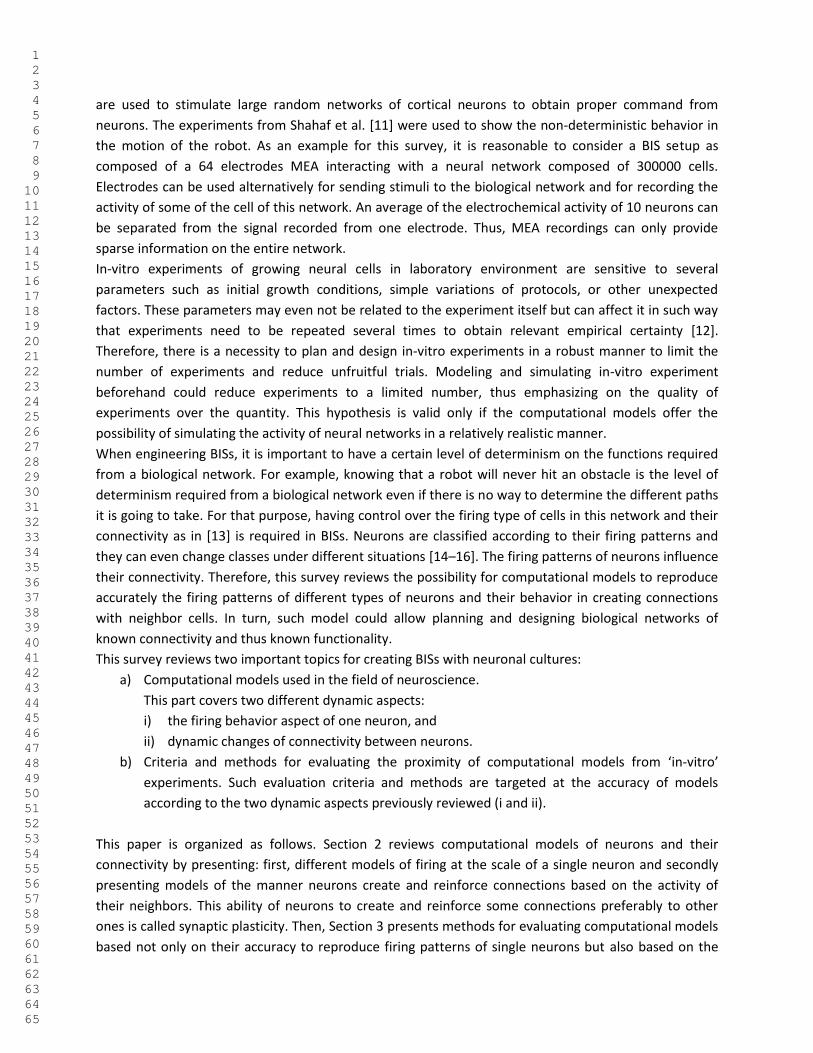
Sliding threshold

Non-linear function modulating Hebbian rule of presynaptic activity

Change of synaptic strength at synapse j

STDP function

Firing time of the presynaptic neuron j at the time of spiking f

Firing time of the postsynaptic neuron at the time of spiking n

2.1. Models of firing of a neuron

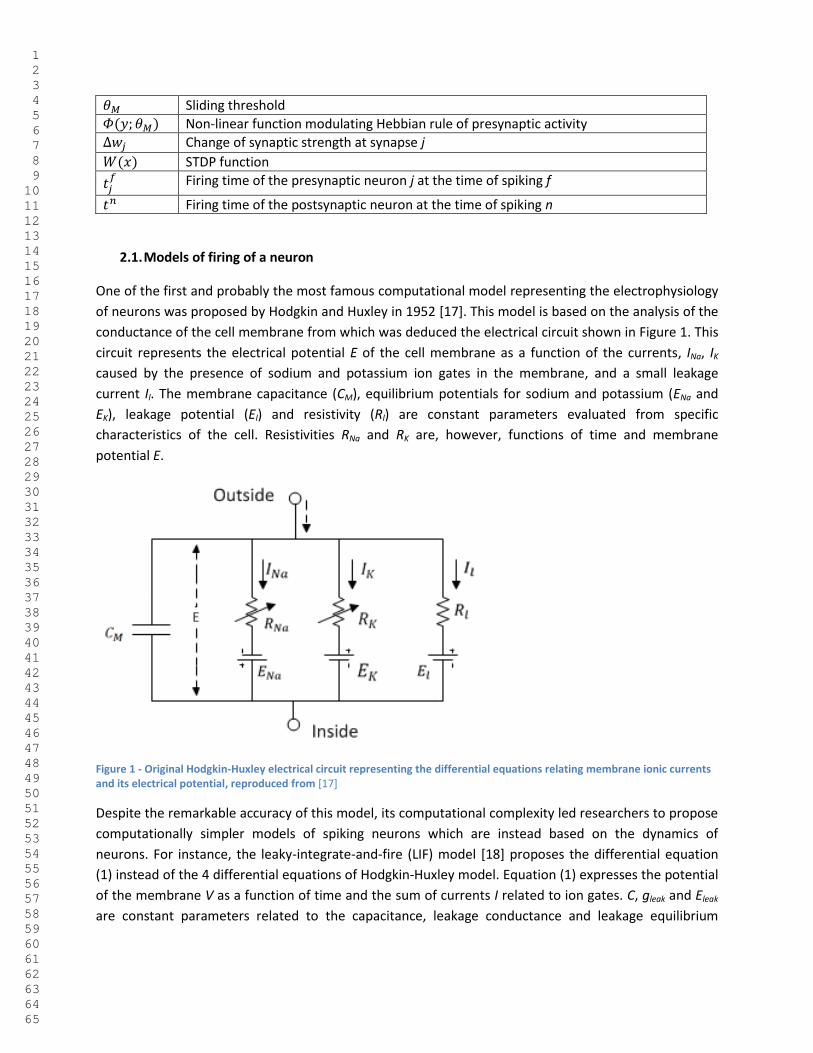
One of the first and probably the most famous computational model representing the electrophysiology

of neurons was proposed by Hodgkin and Huxley in 1952 [17]. This model is based on the analysis of the

conductance of the cell membrane from which was deduced the electrical circuit shown in Figure 1. This

circuit represents the electrical potential E of the cell membrane as a function of the currents, INa, IK

caused by the presence of sodium and potassium ion gates in the membrane, and a small leakage

current Il. The membrane capacitance (CM), equilibrium potentials for sodium and potassium (ENa and

EK), leakage potential (El) and resistivity (Rl) are constant parameters evaluated from specific

characteristics of the cell. Resistivities RNa and RK are, however, functions of time and membrane

potential E.

Figure 1 - Original Hodgkin-Huxley electrical circuit representing the differential equations relating membrane ionic currents and its electrical potential, reproduced from [17]

Despite the remarkable accuracy of this model, its computational complexity led researchers to propose

computationally simpler models of spiking neurons which are instead based on the dynamics of

neurons. For instance, the leaky-integrate-and-fire (LIF) model [18] proposes the differential equation

(1) instead of the 4 differential equations of Hodgkin-Huxley model. Equation (1) expresses the potential

of the membrane V as a function of time and the sum of currents I related to ion gates. C, gleak and Eleak

are constant parameters related to the capacitance, leakage conductance and leakage equilibrium

1 2 3 4 5 6 7 8 9 10 11 12 13 14 15 16 17 18 19 20 21 22 23 24 25 26 27 28 29 30 31 32 33 34 35 36 37 38 39 40 41 42 43 44 45 46 47 48 49 50 51 52 53 54 55 56 57 58 59 60 61 62 63 64 65

potential of the membrane, respectively. When V reaches a threshold potential value, the neuron is

considered as firing an action potential, a spike.

(1)

However, this model cannot be considered as a spiking model as spikes are literally hand drawn when

the potential V reaches a certain threshold. In order to address this threshold issue, Ermentrout [19]

introduced the quadratic integrate-and-fire neuron model based on equation (2), where b represents a

constant potential:

, if , then (2)

This quadratic model allows the variable v, representing the potential of the membrane, to exhibit a

spiking feature as its derivate behaves like v2 for large values of v and thus v can reach infinity in a finite

time. Before this variable reaches infinity, v is reset to a value of vreset when v reaches a peak value vpeak.

The first introduction of this real spiking model, i.e. where v reaches infinity, is proposed by the θ-

neuron model where the state variable θ is defined as the angle of a circle; such trigonometric

transformation enables avoiding infinity [20,21]. The success of this model is due to its intrinsic capacity

of generating spikes as opposed to LIF: the variable vpeak of the model does not correspond to a

threshold like in LIF but to the peak value of a spike. While the Hodgkin-Huxley model contains many

parameters related to the electrophysiological conductance of neurons which are difficult to measure in

practice, quadratic models [19,22–24] contain fewer parameters. Additionally, the few parameters from

quadratic models are easily adjustable to fit with in-vitro recordings. Therefore, Izhikevich simple model

of neuronal behavior [25,26] (see equation (3)) is currently favored by the research community as it

shows very accurate dynamical behavior of neurons in comparison with reality [27]. While being

accurate, the model of Izhikevich (equation (3)) is also computationally simple in comparison with the

model from Hodgkin-Huxley. In equation (3), u is a variable representing the recovery current of the

membrane; k, a, b, c, and d are constant parameters; vrest correspond to the resting potential of the

membrane and vthresh corresponds to its firing potential; other parameters have similar meanings than in

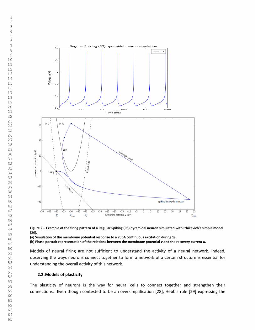
previous equations. Figure 2 presents an example of dynamical behavior of the Izhikevich model. This

model is set with parameters fitting Regular Spiking neurons. For instance, pyramidal cells from layer 5

of the rat cortex exhibit such regular spiking behavior [26].

, if , then ,

(3)

1 2 3 4 5 6 7 8 9 10 11 12 13 14 15 16 17 18 19 20 21 22 23 24 25 26 27 28 29 30 31 32 33 34 35 36 37 38 39 40 41 42 43 44 45 46 47 48 49 50 51 52 53 54 55 56 57 58 59 60 61 62 63 64 65

Figure 2 – Example of the firing pattern of a Regular Spiking (RS) pyramidal neuron simulated with Izhikevich’s simple model [26]. (a) Simulation of the membrane potential response to a 70pA continuous excitation during 1s. (b) Phase portrait representation of the relations between the membrane potential v and the recovery current u.

Models of neural firing are not sufficient to understand the activity of a neural network. Indeed,

observing the ways neurons connect together to form a network of a certain structure is essential for

understanding the overall activity of this network.

2.2. Models of plasticity

The plasticity of neurons is the way for neural cells to connect together and strengthen their

connections. Even though contested to be an oversimplification [28], Hebb’s rule [29] expressing the

1 2 3 4 5 6 7 8 9 10 11 12 13 14 15 16 17 18 19 20 21 22 23 24 25 26 27 28 29 30 31 32 33 34 35 36 37 38 39 40 41 42 43 44 45 46 47 48 49 50 51 52 53 54 55 56 57 58 59 60 61 62 63 64 65

fact that “neurons that fire together strengthen their synaptic connections” is still broadly used as

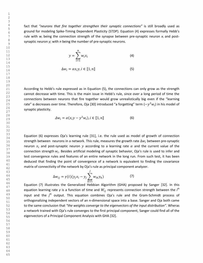
ground for modeling Spike-Timing Dependent Plasticity (STDP). Equation (4) expresses formally Hebb’s

rule with wi being the connection strength of the synapse between pre-synaptic neuron xi and post-

synaptic neuron y; with n being the number of pre-synaptic neurons.

(4)

(5)

According to Hebb’s rule expressed as in Equation (5), the connections can only grow as the strength

cannot decrease with time. This is the main issue in Hebb’s rule, since over a long period of time the

connections between neurons that fire together would grow unrealistically big even if the “learning

rate” α decreases over time. Therefore, Oja [30] introduced “a forgetting” term ( ) in his model of

synaptic plasticity.

(6)

Equation (6) expresses Oja’s learning rule [31], i.e. the rule used as model of growth of connection

strength between neurons in a network. This rule, measures the growth rate between pre-synaptic

neuron and post-synaptic neuron according to a learning rate and the current value of the

connection strength . Besides artificial modeling of synaptic behavior, Oja’s rule is used to infer and

test convergence rules and features of an entire network in the long run. From such test, it has been

deduced that finding the point of convergence of a network is equivalent to finding the covariance

matrix of connectivity of the network by Oja’s rule as principal component analyzer.

(7)

Equation (7) illustrates the Generalized Hebbian Algorithm (GHA) proposed by Sanger [32]. In this

equation learning rate γ is a function of time and represents connection strength between the ith

input and the jth output. This equation combines Oja’s rule and the Gram-Schmidt process of

orthogonalizing independent vectors of an n-dimensional space into a base. Sanger and Oja both came

to the same conclusion that “the weights converge to the eigenvectors of the input distribution”. Wheras

a network trained with Oja’s rule converges to the first principal component, Sanger could find all of the

eigenvectors of a Principal Component Analysis with GHA [32].

1 2 3 4 5 6 7 8 9 10 11 12 13 14 15 16 17 18 19 20 21 22 23 24 25 26 27 28 29 30 31 32 33 34 35 36 37 38 39 40 41 42 43 44 45 46 47 48 49 50 51 52 53 54 55 56 57 58 59 60 61 62 63 64 65

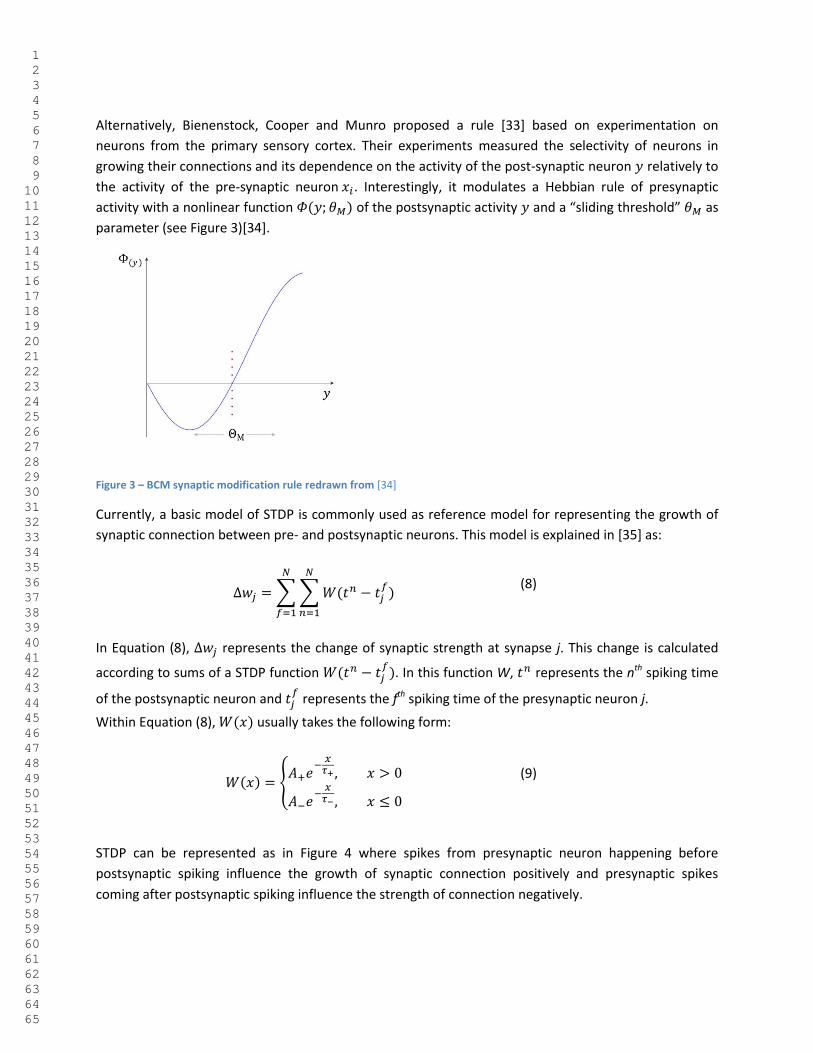
Alternatively, Bienenstock, Cooper and Munro proposed a rule [33] based on experimentation on

neurons from the primary sensory cortex. Their experiments measured the selectivity of neurons in

growing their connections and its dependence on the activity of the post-synaptic neuron relatively to

the activity of the pre-synaptic neuron . Interestingly, it modulates a Hebbian rule of presynaptic

activity with a nonlinear function of the postsynaptic activity and a “sliding threshold” as

parameter (see Figure 3)[34].

Figure 3 – BCM synaptic modification rule redrawn from [34]

Currently, a basic model of STDP is commonly used as reference model for representing the growth of

synaptic connection between pre- and postsynaptic neurons. This model is explained in [35] as:

(8)

In Equation (8), represents the change of synaptic strength at synapse j. This change is calculated

according to sums of a STDP function . In this function W, represents the nth spiking time

of the postsynaptic neuron and

represents the fth spiking time of the presynaptic neuron j.

Within Equation (8), usually takes the following form:

(9)

STDP can be represented as in Figure 4 where spikes from presynaptic neuron happening before

postsynaptic spiking influence the growth of synaptic connection positively and presynaptic spikes

coming after postsynaptic spiking influence the strength of connection negatively.

1 2 3 4 5 6 7 8 9 10 11 12 13 14 15 16 17 18 19 20 21 22 23 24 25 26 27 28 29 30 31 32 33 34 35 36 37 38 39 40 41 42 43 44 45 46 47 48 49 50 51 52 53 54 55 56 57 58 59 60 61 62 63 64 65

Figure 4 – Schematic Spike-timing dependent plasticity drawn after 60 spike pairings from [36], regression curves reproduced with Eq. (9)

3. Criteria and methods for evaluating models

This section presents two criteria for evaluating the faithfulness of models towards ‘in-vitro’

experiments: faithfulness in reproducing firing patterns, and faithfulness in connection dynamics.

Methods for analyzing models according to both criteria are reviewed in respective order.

3.1. Signal error comparison

The first benchmark for a model of neural network is the comparison between the individual signals

generated by a model with signals recorded from real experiments. There are different ways for

achieving such comparison. Probably the most straight forward manner to compare two signals is to

subtract one to the other and to observe the value of the resulting error. This practice is commonly used

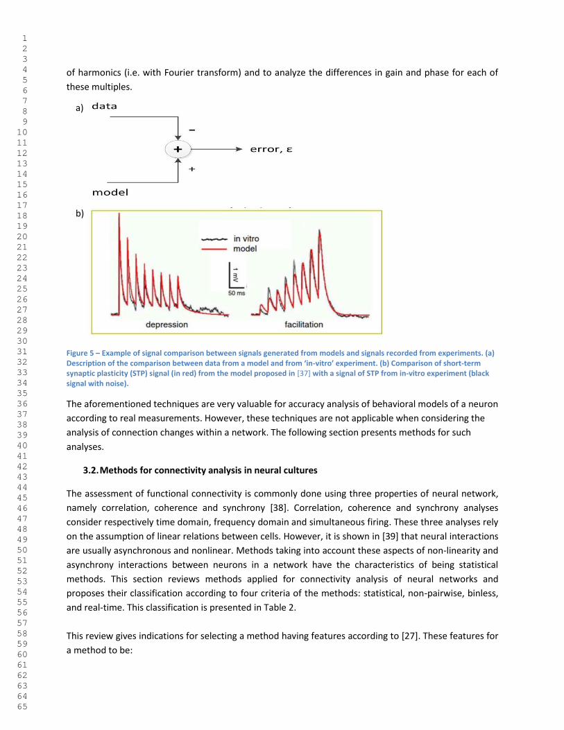
in closed-loop control and is illustrated in Figure 5-a. As an example of this model validation practice

presented in Figure 5-b, the short-term plasticity (STP) in ‘in-vitro’ environment (black curves with noise)

is almost identical to the red curves generated by the STP model proposed in [37]. Another way to

characterize the limits of use of a model is to analyze the differences in Gain and Phases between signals

produced by the model varying with the frequency. This enables showing that, for example, the model is

close to reality in the case of low frequencies but diverges after reaching a certain range and becomes

inaccurate for high frequencies. Similarly, it is also possible to decompose signals according to multiple

1 2 3 4 5 6 7 8 9 10 11 12 13 14 15 16 17 18 19 20 21 22 23 24 25 26 27 28 29 30 31 32 33 34 35 36 37 38 39 40 41 42 43 44 45 46 47 48 49 50 51 52 53 54 55 56 57 58 59 60 61 62 63 64 65

of harmonics (i.e. with Fourier transform) and to analyze the differences in gain and phase for each of

these multiples.

Figure 5 – Example of signal comparison between signals generated from models and signals recorded from experiments. (a) Description of the comparison between data from a model and from ‘in-vitro’ experiment. (b) Comparison of short-term synaptic plasticity (STP) signal (in red) from the model proposed in [37] with a signal of STP from in-vitro experiment (black signal with noise).

The aforementioned techniques are very valuable for accuracy analysis of behavioral models of a neuron

according to real measurements. However, these techniques are not applicable when considering the

analysis of connection changes within a network. The following section presents methods for such

analyses.

3.2. Methods for connectivity analysis in neural cultures

The assessment of functional connectivity is commonly done using three properties of neural network,

namely correlation, coherence and synchrony [38]. Correlation, coherence and synchrony analyses

consider respectively time domain, frequency domain and simultaneous firing. These three analyses rely

on the assumption of linear relations between cells. However, it is shown in [39] that neural interactions

are usually asynchronous and nonlinear. Methods taking into account these aspects of non-linearity and

asynchrony interactions between neurons in a network have the characteristics of being statistical

methods. This section reviews methods applied for connectivity analysis of neural networks and

proposes their classification according to four criteria of the methods: statistical, non-pairwise, binless,

and real-time. This classification is presented in Table 2.

This review gives indications for selecting a method having features according to [27]. These features for

a method to be:

a)

b)

1 2 3 4 5 6 7 8 9 10 11 12 13 14 15 16 17 18 19 20 21 22 23 24 25 26 27 28 29 30 31 32 33 34 35 36 37 38 39 40 41 42 43 44 45 46 47 48 49 50 51 52 53 54 55 56 57 58 59 60 61 62 63 64 65

- accurate independently from the heterogeneity in firing types of neurons in the network,

- sensitive to fine grain changes, and

- highly specific in order to decrease the number of false connections found.

In [38], functional connectivity measures are divided in two general categories: statistical measures and

phase synchronization (PhS) measures. This division is integrated in the classification of methods

proposed in Table 2 as the first classification criterion.

Table 2 - Classification of methods for analysis of connectivity of neural networks

Criteria

St

atis

tica

l

No

n-p

airw

ise

Bin

less

Rea

l-ti

me

Met

ho

ds

Kalman Filter X X x x

Cox X X X

CuBIC X X X

GLM X X

MI X

MSC X

Cross-correlation X

Phase-Synchro.

Instant phase estimation

3.2.1. Phase synchronization methods

Because of the intrinsic stochastic nature of the neural structure, PhS methods are not applicable, as it is

based on deterministic dynamical system principle. However, these methods have been tried for neural

systems as in [40].

Synchronization analysis consists of two steps: estimation of instantaneous phase and quantification of

phase locking. In the former, the Hilbert transform is one example of the methods presented in [41]. In

the latter, the relative phases of signals from two neurons are compared and if this comparison presents

phase locking, then the neurons are connected [42]. The relative phase distribution is uniform for

independent time series of x(t) and y(t) within a given time window. Phase locking detection is achieved

by computing the distance between relative phase and uniform distribution.

3.2.2. Pair-wise comparison methods

Among pair-wise comparison methods for connectivity analysis, the most widely used is the cross-

correlation function method [43,44]. This class of methods also contains several other methods such as

pair-wise dependency characterization methods [45–49] or pair-wise spike coincidence analysis [50,51].

Using the statistical information of the joint space between two random variables, other statistical

methods Mutual Information (MI) [52] and Mean-Square-Contingency (MSC) [53] can be used to

1 2 3 4 5 6 7 8 9 10 11 12 13 14 15 16 17 18 19 20 21 22 23 24 25 26 27 28 29 30 31 32 33 34 35 36 37 38 39 40 41 42 43 44 45 46 47 48 49 50 51 52 53 54 55 56 57 58 59 60 61 62 63 64 65

quantify statistical dependencies [38]. MSC quantifies the dependency based on an independence test

and MI compute the Kullback–Leibler divergence between joint and product of the two marginal

probability distributions.

The major issue about this class of methods is that they do not consider influences from other spike

trains than the pair of trains being studied. Therefore, pair-wise estimates can show inaccurate results

when considering highly interconnected networks as shown in [27,54]. For this reason, it is important to

consider approaches that address the influences from the entire spike trains of the network when

analyzing the connectivity within this network. Alternative methods to pair-wise comparison methods

consider the activity of the entire network on one of its neuron for the computation of connections to

this neuron.

3.2.3. Bin-dependent methods

The basis for such stochastic method lies on the study of the probability of appearance of a spike

resulting from influences of all other spike trains and even its own previous activity. This probability is

evaluated with the search for maximum of a likelihood function (ML).

The initial hypothesis that the spike of a neuron is influenced by its own recent activity, the recent

activity of the entire network of consideration and external factors such as stimuli gave birth to

statistical methods taking into account all these influences. For instance, the GLM approach, which is a

generalized linear model, is one of these methods and is applied to different cases of neural connectivity

analysis [55–59].

Despite the heavy computational expense, based on the analysis of functional connectivity analysis in

[60], it is deduced that the best practice for functional connectivity is to use multiple time scales. The

principal limitation of such approach is that results depend on the size of the testing window (bin) [60].

Another method for finding higher order correlations was developed in [61,62]. However, this method

needs long recording of network activity. Moreover, due to the large number of parameters to estimate,

it becomes computationally heavy for networks of more than ten neurons [54]. On the opposite, binless

methods are methods that do not require a testing window. Therefore, these methods do not rely on

the size of the recording frame.

3.2.4. Binless methods

The CuBIC method [63] is a successful attempt to suppress the effect of the bin in the computation of

higher order correlations. The need for higher-order computation is estimated and computation is

stopped when the estimate considers this order not required.

This method is based on the previous development of Martignon in [61,62]. The CuBIC method has also

been improved with the integration of a non-stationary Poisson process [64].

Another approach, the Cox method [45,65] is based on the assumption of modulated renewal process

(MRP), i.e. a spike train is considered to be modulated by others. This MRP is modeled in [54] and [27] as

a hazard function expressing the conditional probability of a spike at time t relatively to all spiking

activity of the network prior to that time.

1 2 3 4 5 6 7 8 9 10 11 12 13 14 15 16 17 18 19 20 21 22 23 24 25 26 27 28 29 30 31 32 33 34 35 36 37 38 39 40 41 42 43 44 45 46 47 48 49 50 51 52 53 54 55 56 57 58 59 60 61 62 63 64 65

Considering a network of size n+1, this proportional hazard function of spike train of neuron A, , is

modulated in this model by the possible influence of other spike trains from other neurons Bi of the

network as:

(10)

In equation (10), represents the time spent from the last spike of neuron A. Most importantly, the

parameters of interest for this connectivity analysis are as they represent the respective strength of

connection from neuron Bi to A. represents an influence function of Bi on A. With the Cox

method, the parameters are estimated by maximizing the log likelihood function, where is the

vector of , of the hazard function in equation (10). Finding the maximum of implies finding the

estimate of such that . Such equation can be solved with different iteration methods

such as Newton-Raphson or regularized multivariate Newton’s method as in [54] or [27].

3.2.5. Real-time analysis

In general, a real-time connection analysis method should be statistical in nature, be robust to error, and

have real-time implementation capabilities. Although Cox method was implemented in [27] to analyze

the connectivity changes in neural networks, it is not appropriate for real-time analysis due to its

demand for heavy computational power.

Due to estimation of uncertainties in addition to connection parameters, the Kalman filter is a plausible

solution for this problem. In [66] it is shown that with use of a finite weighted ensemble, an ensemble

Kalman filter (EnKF) is capable of approximating a non-linear system. This method is implemented for

the analysis of neural networks in [67]. The validation of this implementation is tested on simulated

networks of neurons modeled with Hodgkin-Huxley model and the various parameters of this model are

made available in [68]. This method can be an asset in neural simulation as well as pharmacological

studies which can provide the researchers the real-time analysis of an effect of a stimulation of

pharmacological experiment.

3.2.6. Conclusion on methods for the analysis of connectivity and connectivity changes

As shown in [59], a spike from one neuron is influenced by many more factors than a spike train from

one post-synaptic neuron. Therefore, pair-wise dependency methods are not sufficient to characterize

the connectivity of neural networks. In the case of bin-dependent methods, e.g. GLM, they take into

account factors of recent spiking activity from the studied neuron, other neurons, and from the activity

of external stimuli. However, the weakness of bin-dependent methods resides in their dependency on

the size of the testing window (bin) as noted in [27,54]. For this reason, it is preferable to select binless

methods as they show good sensitivity with short recording times (over 95% accuracy from 20s

recording) [27]. Finally, based on the time scale of ‘in-vitro’ experiment protocols, the use of real-time

method for continuously and instantly analyzing the connectivity of a neural network was not

considered as relevant for the purpose of BIS development.

The Cox method can be used at different time scales for two different purposes. First, it can be used to

find out about connection strength and delays between pre- and post-synaptic spikes. Secondly, it can

1 2 3 4 5 6 7 8 9 10 11 12 13 14 15 16 17 18 19 20 21 22 23 24 25 26 27 28 29 30 31 32 33 34 35 36 37 38 39 40 41 42 43 44 45 46 47 48 49 50 51 52 53 54 55 56 57 58 59 60 61 62 63 64 65

be used as in [27] to find out about changes in connections. The perceived benefits of using the Cox

method in engineering BIS applications are:

a) evaluating the connection strength between nodes of a network gives information on the

reliability of using this path for communication,

b) analyzing the connection changes enables being proactive in selecting a new route for

communicating between two nodes of the network, and

c) having an evaluation of communication delays between nodes of the network enables message

scheduling so as to avoid collision and information losses.

4. Discussion and future directions

First, this survey presented a state-of-the-art of computational models of spiking neurons. From this

review, it is possible to conclude that the most accurate model when considering the analysis of a single

neuron remains the model proposed by Hodgkin and Huxley. However, this model becomes

computationally heavy when considering a large number of neurons due to the number of parameters

to be set according to different neuron types, and the number of differential equations to be solved at

each computation time. Therefore, simpler models of a spiking neuron were developed to provide

simulations on large-scale models of neural networks.

Among the simpler models, the simplest is Integrate-and-Fire model, and one of the most widely used

models is the Enhanced Leaky Integrate and Fire model (ELIF) [69]. However, the simple model

developed by Izhikevich in [70] shows more possibilities to reproduce accurately the signals from all

various types of firing neurons while being at the same time computationally efficient. This model has

been used to simulate a mammalian brain containing 1 million neurons with which different rhythms

(e.g. alpha, gamma) of the brain were reproduced [71]. It is well suited for simulating in-vitro

experiments with MEA as one dish typically contains an average of 300000 neural cells. The simple

model of Izhikevich could be used in the future to dynamically change the firing type of one neuron

based on its previous activity and the activity of its pre-synaptic neurons as neurons can change from

one firing type to another [66]. Another improvement could be to include on the side of spiking models

attributes related to aging and longevity of cells, an average number of connections they create or other

evolving parameters.

Second, models representing the plasticity of neurons based on their firing activity have been reviewed.

Currently, the most prominent model used by the research community is the model of STDP as it is

derived from experimental studies confirming Hebb’s theory that “neurons that fire together, wire

together” [72]. However, this model of plasticity is recently being questioned and seen as an over

simplification by several researchers [28,35,73,74]. So far only the electrical behavior of neurons has

been considered for the study of plasticity whereas plasticity probably involves more processes and

different cells (e.g. astrocytes, glial cells) than neurons [74–76]. Therefore, we would expect that this

branch of research will propose different models of plasticity in the near future. Such model should

include the effect of astrocytes on plasticity and how different types of nutrition or toxic chemicals can

have strong positive or negative effects on the ability for neurons to connect with each other.

Third, connectivity analysis methods have been reviewed and their classification has been proposed.

This review shows that pair-wise analysis methods are not suitable for the study of neural connectivity.

1 2 3 4 5 6 7 8 9 10 11 12 13 14 15 16 17 18 19 20 21 22 23 24 25 26 27 28 29 30 31 32 33 34 35 36 37 38 39 40 41 42 43 44 45 46 47 48 49 50 51 52 53 54 55 56 57 58 59 60 61 62 63 64 65

However, despite the fact that these methods tend to have low specificity issues (methods give many

false positives), it is noted that the cross-correlation function (CCF) method is still the widely used to

assess connectivity of a network. This is likely due to the computational complexity of methods

accounting for the activity of every neuron from the network to evaluate connections. We concluded

that CCF should not be used alone and another method should be used to cross check the results from

CCF analysis. The Cox method is shown very robust despite its complexity. In this area, future direction

could attempt to parallelize the methods for applying high-performance computing and, therefore

reduce the execution time of analysis. This might help adopting such method more widely. Another

direction is to propose methods enabling the analysis of connectivity changes in real-time in a robust

manner. These methods could involve the use of probabilistic and statistical approaches such as hidden

Markov chains, Bayesian networks or Kalman filter.

5. Conclusion

This survey has reviewed different computational models of spiking neurons, their plasticity and

methods for analyzing the connectivity of a network. As conclusion, for the purpose of designing and

developing BISs, it is important to use models that are accurate with reality but at the same time not too

computationally expensive. Therefore, for the firing patterns of individual neurons, the simple model

from Izhikevich is advised. In the case of plasticity, the most realistic solution when considering a model

of neural cells stimulated and recorded from MEA plates is probably the model of STDP. Even if this

model is considered as an over-simplification, no other model of connectivity changes caused by

electrical stimulation has yet been proposed to our knowledge. In order to analyze the topology of a

network during experiments and to infer on its capacity to realize certain functionalities, the Cox

method provides robust results on the analysis of connectivity of the network. It allows observing the

connections between different points of the network, the changes in connectivity as well as the delays

of information from one point of the network to another.

Modeling and simulating BIS during the early phases of development shows a crucial advantage for

securing the feasibility of integration of a bio-neural network. This advantage lies mainly in the capability

to prepare, and to a certain extent to foresee, the dynamic behavior of the biological neural network

integrated as component of BIS. The realistic features of the reviewed computational models offer the

potential of engineering complex biological components and to simulate their dynamic evolution when

integrated in a digital system, such as a sensor network. Furthermore, the Cox method for analyzing the

connectivity of a neural network offers BIS the benefits of evaluating the reliability of communicating

from one point to another of the neural network as it evaluates the connection strength between nodes

of this network. This method also gives the possibility when used on a periodic basis to foresee changes

in connectivity, and therefore, could be used to plan replacement paths for communication from one

point to another when the precedent path becomes unreliable. The Cox method can additionally be

useful in scheduling communication between nodes of the neural network as it also evaluates spiking

delays between the connected nodes. Mostly, the strongest interest in analyzing the connectivity of a

biological network lays in the use of this analysis for engineering a network of previously defined

topology. Such defined topology could exhibit a specific function of the bio-neural network within BIS in

the same way as a component of a system provides services to the rest of the system.

1 2 3 4 5 6 7 8 9 10 11 12 13 14 15 16 17 18 19 20 21 22 23 24 25 26 27 28 29 30 31 32 33 34 35 36 37 38 39 40 41 42 43 44 45 46 47 48 49 50 51 52 53 54 55 56 57 58 59 60 61 62 63 64 65

Acknowledgement

This research is funded by the Academy of Finland under project named “Bio-integrated Software

Development for Adaptive Sensor Networks”, project number 278882.

References

[1] M. Kocaoglu, D. Malak, O.B. Akan, Fundamentals of Green Communications and Computing: Modeling and Simulation, Computer (Long. Beach. Calif). 45 (2012) 40–46. doi:10.1109/MC.2012.248.

[2] L. Chiaraviglio, M. Mellia, S. Member, F. Neri, Minimizing ISP Network Energy Cost : Formulation and Solutions, 20 (2012) 463–476.

[3] A. Tero, S. Takagi, T. Saigusa, K. Ito, D.P. Bebber, M.D. Fricker, et al., Rules for biologically inspired adaptive network design., Science. 327 (2010) 439–42. doi:10.1126/science.1177894.

[4] K. Warwick, Implications and consequences of robots with biological brains, Ethics Inf. Technol. 12 (2010) 223–234. doi:10.1007/s10676-010-9218-6.

[5] J.L. Krichmar, F. Röhrbein, Value and Reward Based Learning in Neurorobots, Front. Neurorobot. 7 (2013). doi:10.3389/fnbot.2013.00013.

[6] S. Balasubramaniam, N.T. Boyle, A. Della-Chiesa, F. Walsh, A. Mardinoglu, D. Botvich, et al., Development of artificial neuronal networks for molecular communication, Nano Commun. Netw. 2 (2011) 150–160. doi:10.1016/j.nancom.2011.05.004.

[7] D. Malak, O.B. Akan, A Communication Theoretical Analysis of Synaptic Multiple-Access Channel in Hippocampal-Cortical Neurons, 61 (2013).

[8] S. Balasubramaniam, S. Ben-Yehuda, S. Pautot, A. Jesorka, P. Lio’, Y. Koucheryavy, A review of experimental opportunities for molecular communication, Nano Commun. Netw. 4 (2013) 43–52. doi:10.1016/j.nancom.2013.02.002.

[9] T.B. DeMarse, D.A. Wagenaar, A.W. Blau, S.M. Potter, The neurally controlled animat: Biological brains acting with simulated bodies, Auton. Robots. 11 (2001) 305–310. doi:10.1023/A:1012407611130.

[10] S.M. Potter, D.A. Wagenaar, R.M.R. Madhavan, T.B. DeMarse, Long-term bidirectional neuron interfaces for robotic control, and in vitro learning studies, Proc. 25th Annu. Int. Conf. IEEE Eng. Med. Biol. Soc. (IEEE Cat. No.03CH37439). 4 (2003). doi:10.1109/IEMBS.2003.1280959.

[11] G. Shahaf, D. Eytan, A. Gal, E. Kermany, V. Lyakhov, C. Zrenner, et al., Order-based representation in random networks of cortical neurons, PLoS Comput. Biol. 4 (2008). doi:10.1371/journal.pcbi.1000228.

1 2 3 4 5 6 7 8 9 10 11 12 13 14 15 16 17 18 19 20 21 22 23 24 25 26 27 28 29 30 31 32 33 34 35 36 37 38 39 40 41 42 43 44 45 46 47 48 49 50 51 52 53 54 55 56 57 58 59 60 61 62 63 64 65

[12] K.M. Joo, B.G. Kang, J.Y. Yeon, Y.J. Cho, J.Y. An, H.S. Song, et al., Experimental and clinical factors influencing long-term stable in vitro expansion of multipotent neural cells from human adult temporal lobes, Exp. Neurol. 240 (2013) 168–177. doi:10.1016/j.expneurol.2012.11.021.

[13] Á. Szabó, G. Vattay, D. Kondor, A cell signaling model as a trainable neural nanonetwork, Nano Commun. Netw. 3 (2012) 57–64. doi:10.1016/j.nancom.2012.01.002.

[14] H. Markram, M. Toledo-Rodriguez, Y. Wang, A. Gupta, G. Silberberg, C. Wu, Interneurons of the neocortical inhibitory system., Nat. Rev. Neurosci. 5 (2004) 793–807. doi:10.1038/nrn1519.

[15] P.A. Pahapill, A.M. Lozano, The pedunculopontine nucleus and Parkinson ’ s disease, Brain. 123 (2000) 1767–1783.

[16] M. Steriade, Neocortical cell classes are flexible entities., Nat. Rev. Neurosci. 5 (2004) 121–34. doi:10.1038/nrn1325.

[17] A.L. Hodgkin, A.F. Huxley, A quantitative description of membrane current and its application to conduction and excitation in nerve, J. Physiol. (1952) 500–544.

[18] R.B. Stein, Some models of neuronal variability., Biophys. J. 7 (1967) 37–68. doi:10.1016/S0006-3495(67)86574-3.

[19] B. Ermentrout, Type I membranes, phase resetting curves, and synchrony, Neural Comput. 8 (1996) 979–1001.

[20] N. Kopell, G.B. Ermentrout, Symmetry and phaselocking in chains of weakly coupled oscillators, Commun. Pure Appl. Math. 39 (1986) 623–660. doi:10.1002/cpa.3160390504.

[21] G.B. Ermentrout, N. Kopell, Parabolic Bursting in an Excitable System Coupled with a Slow Oscillation, SIAM J. Appl. Math. 46 (1986) 233–253. doi:10.1137/0146017.

[22] E.M. Izhikevich, Hybrid spiking models., Philos. Trans. A. Math. Phys. Eng. Sci. 368 (2010) 5061–70. doi:10.1098/rsta.2010.0130.

[23] R. Brette, W. Gerstner, Adaptive exponential integrate-and-fire model as an effective description of neuronal activity., J. Neurophysiol. 94 (2005) 3637–3642. doi:10.1152/jn.00686.2005.

[24] J. Touboul, Importance of the cutoff value in the quadratic adaptive integrate-and-fire model., Neural Comput. 21 (2009) 2114–2122. doi:10.1162/neco.2009.09-08-853.

[25] E.M. Izhikevich, Simple model of spiking neurons., IEEE Trans. Neural Netw. 14 (2003) 1569–72. doi:10.1109/TNN.2003.820440.

[26] E.M. Izhikevich, Chapter 8 - Simple models, in: Dyn. Syst. Neurosci. Geom. Excit. Bursting, The MIT Press, Cambridge, Massachusetts, 2007: pp. 267 – 321.

1 2 3 4 5 6 7 8 9 10 11 12 13 14 15 16 17 18 19 20 21 22 23 24 25 26 27 28 29 30 31 32 33 34 35 36 37 38 39 40 41 42 43 44 45 46 47 48 49 50 51 52 53 54 55 56 57 58 59 60 61 62 63 64 65

[27] T. Berry, F. Hamilton, N. Peixoto, T. Sauer, Detecting connectivity changes in neuronal networks., J. Neurosci. Methods. 209 (2012) 388–97. doi:10.1016/j.jneumeth.2012.06.021.

[28] J. Lisman, N. Spruston, Questions about STDP as a general model of synaptic plasticity, Front. Synaptic Neurosci. (2010) 1–5. doi:10.3389/fnsyn.2010.00140.

[29] D.O. Hebb, The Organization of Behavior: A Neuropsychological Theory, Wiley, 1949. https://books.google.fi/books?id=dZ0eDiLTwuEC.

[30] E. Oja, A simplified neuron model as a principal component analyzer., J. Math. Biol. 15 (1982) 267–273. doi:10.1007/BF00275687.

[31] E. Oja, Oja learning rule, Scholarpedia. 3 (2008) 3612. doi:10.4249/scholarpedia.3612.

[32] T.D. Sanger, Optimal unsupervised learning in a single-layer linear feedforward neural network, Neural Networks. 2 (1989) 459–473. doi:10.1016/0893-6080(89)90044-0.

[33] E.L. Bienenstock, L.N. Cooper, P.W. Munro, Theory for the development of neuron selectivity: orientation specificity and binocular interaction in visual cortex., J. Neurosci. 2 (1982) 32–48. doi:10.1371/journal.ppat.0020109.

[34] B.S. Blais, L. Cooper, BCM theory, Scholarpedia. 3 (2008) 1570. doi:10.4249/scholarpedia.1570.

[35] P.J. Sjöström, W. Gerstner, Spike-timing dependent plasticity, in: Spike-Timing Depend. Plast., Frontiers Media SA, 2012: pp. 35 – 44. doi:10.3389/978-2-88919-043-0.

[36] G.Q. Bi, M.M. Poo, Synaptic modifications in cultured hippocampal neurons: dependence on spike timing, synaptic strength, and postsynaptic cell type., J. Neurosci. 18 (1998) 10464–10472.

[37] E.M. Izhikevich, G.M. Edelman, Large-scale model of mammalian thalamocortical systems., Proc. Natl. Acad. Sci. U. S. A. 105 (2008) 3593–8. doi:10.1073/pnas.0712231105.

[38] L. Li, I. Memming Park, S. Seth, J.C. Sanchez, J.C. Príncipe, Functional Connectivity Dynamics Among Cortical Neurons: A Dependence Analysis, IEEE Trans. Neural Syst. Rehabil. Eng. 20 (2012) 18–30.

[39] A.S. Ecker, P. Berens, G.A. Keliris, M. Bethge, N.K. Logothetis, A.S. Tolias, Decorrelated neuronal firing in cortical microcircuits., Science. 327 (2010) 584–587. doi:10.1126/science.1179867.

[40] E. Pereda, R.Q. Quiroga, J. Bhattacharya, Nonlinear multivariate analysis of neurophysiological signals, Prog. Neurobiol. 77 (2005) 1–37. doi:10.1016/j.pneurobio.2005.10.003.

[41] S. Mallat, A Wavelet Tour of Signal Processing, in: A Wavelet Tour Signal Process., 1999: pp. 20–41. doi:10.1016/B978-012466606-1/50004-0.

1 2 3 4 5 6 7 8 9 10 11 12 13 14 15 16 17 18 19 20 21 22 23 24 25 26 27 28 29 30 31 32 33 34 35 36 37 38 39 40 41 42 43 44 45 46 47 48 49 50 51 52 53 54 55 56 57 58 59 60 61 62 63 64 65

[42] M. Rosenblum, A. Pikovsky, J. Kurths, C. Schafer, P.A. Tass, Phase synchronization: from theory to data analysis, Handb. Biol. Phys. (2003) 279–321. papers://0cc5b277-5c1a-4a08-a78e-b6f9891a651e/Paper/p2553.

[43] D.H. Perkel, G.L. Gerstein, G.P. Moore, Neuronal spike trains and stochastic point processes. II. Simultaneous spike trains., Biophys. J. 7 (1967) 419–40. doi:10.1016/S0006-3495(67)86597-4.

[44] R. Miller, Time and the Brain, CRC Press - Taylor & Francis Group, 2000.

[45] D.R. Cox, P.A.W. Lewis, Multivariate point processes, in: Sixth Berkeley Symp., Berkeley, California, 1972: pp. 401–448.

[46] D.R. Brillinger, Nerve Cell Spike Train Data Analysis : A Progression of Technique, 87 (1992) 260–271.

[47] M.S. Bartlett, An introduction to stochastic processes, with special reference to methods and applications, First, Cambridge: Cambridge University Press Archive, 1978.

[48] D. Brillinger, J. Bryant HughL., J. Segundo, Identification of synaptic interactions, Biol. Cybern. 22 (1976) 213–228. doi:10.1007/BF00365087.

[49] G.L. Gerstein, D.H. Perkel, Simultaneously Recorded Trains of Action Potentials: Analysis and Functional Interpretation, Science. 164 (1969) 828 – 830. doi:10.1126/science.164.3881.828.

[50] T.E. Combinatorial, G. Pipa, M. Diesmann, S. Gru, Significance of Joint-Spike Events Based on Trial-Shuffling by Efficient Combinatorial Methods ¨, 8 (2003) 79–86.

[51] L. Stuart, M. Walter, R. Borisyuk, The correlation grid: analysis of synchronous spiking in multi-dimensional spike train data and identification of feasible connection architectures., Biosystems. 79 (2005) 223–33. doi:10.1016/j.biosystems.2004.09.011.

[52] P.M. DiLorenzo, J.D. Victor, Binless Estimation of Mutual Information in Metric Spaces, in: Spike Timing Mech. Funct., CRC Press, 2013: pp. 121 – 136.

[53] L. Li, I. Park, S. Seth, J.C. Sanchez, J.C. Principe, Neuronal Functional Connectivity Dynamics in Cortex : An MSC-based Analysis, in: 32nd Conf. IEEE EMBS, Buenos Aires, 2010: pp. 4136–4139.

[54] M.S. Masud, R. Borisyuk, Statistical technique for analysing functional connectivity of multiple spike trains., J. Neurosci. Methods. 196 (2011) 201–19. doi:10.1016/j.jneumeth.2011.01.003.

[55] D.R. Brillinger, Maximum likelihood analysis of spike trains of interacting nerve cells., Biol. Cybern. 59 (1988) 189–200. doi:10.1007/BF00318010.

[56] E.S. Chornoboy, L.P. Schramm, A.F. Karr, Maximum likelihood identification of neural point process systems, Biol. Cybern. 59 (1988) 265–275. doi:10.1007/BF00332915.

1 2 3 4 5 6 7 8 9 10 11 12 13 14 15 16 17 18 19 20 21 22 23 24 25 26 27 28 29 30 31 32 33 34 35 36 37 38 39 40 41 42 43 44 45 46 47 48 49 50 51 52 53 54 55 56 57 58 59 60 61 62 63 64 65

[57] M. Okatan, M.A. Wilson, E.N. Brown, Analyzing functional connectivity using a network likelihood model of ensemble neural spiking activity., Neural Comput. 17 (2005) 1927–1961. doi:10.1162/0899766054322973.

[58] W. Truccolo, U.T. Eden, M.R. Fellows, J.P. Donoghue, E.N. Brown, A point process framework for relating neural spiking activity to spiking history, neural ensemble, and extrinsic covariate effects., J. Neurophysiol. 93 (2005) 1074–1089. doi:10.1152/jn.00697.2004.

[59] I.H. Stevenson, J.M. Rebesco, L.E. Miller, K.P. Körding, Inferring functional connections between neurons., Curr. Opin. Neurobiol. 18 (2008) 582–8. doi:10.1016/j.conb.2008.11.005.

[60] S. Eldawlatly, R. Jin, K.G. Oweiss, Identifying functional connectivity in large-scale neural ensemble recordings: a multiscale data mining approach., Neural Comput. 21 (2009) 450–477. doi:10.1162/neco.2008.09-07-606.

[61] L. Martignon, H. Von Hassein, S. Grün, A. Aertsen, G. Palm, Detecting higher-order interactions among the spiking events in a group of neurons, Biol. Cybern. 73 (1995) 69–81. doi:10.1007/BF00199057.

[62] L. Martignon, G. Deco, K. Laskey, M. Diamond, W. Freiwald, E. Vaadia, Neural coding: higher-order temporal patterns in the neurostatistics of cell assemblies., Neural Comput. 12 (2000) 2621–2653. doi:10.1162/089976600300014872.

[63] B. Staude, S. Rotter, S. Grün, CuBIC: cumulant based inference of higher-order correlations in massively parallel spike trains., J. Comput. Neurosci. 29 (2010) 327–50. doi:10.1007/s10827-009-0195-x.

[64] B. Staude, S. Grün, S. Rotter, Higher-order correlations and cumulants, in: Anal. Parallel Spike Trains, Springer, 2010: pp. 253–280.

[65] G.N. Borisyuk, R.M. Borisyuk, A.B. Kirillov, E.I. Kovalenko, V.I. Kryukov, A new statistical method for identifying interconnections between neuronal network elements, Biol. Cybern. 52 (1985) 301–306. doi:10.1007/BF00355752.

[66] E. Kalnay, Atmospheric modeling, data assimilation, and predictability, Cambridge University Press, 2003.

[67] F. Hamilton, T. Berry, N. Peixoto, T. Sauer, Real-time tracking of neuronal network structure using data assimilation, Phys. Rev. E. 88 (2013) 052715. doi:10.1103/PhysRevE.88.052715.

[68] H. Hasegawa, Responses of a Hodgkin-Huxley neuron to various types of spike-train inputs, Phys. Rev. E. 61 (2000) 718–726.

[69] W. Gerstner, W.M. Kistler, R. Naud, L. Paninski, Neuronal Dynamics: From Single Neurons to Networks and Models of Cognition, Cambridge University Press, 2014. http://neuronaldynamics.epfl.ch/online/index.html.

1 2 3 4 5 6 7 8 9 10 11 12 13 14 15 16 17 18 19 20 21 22 23 24 25 26 27 28 29 30 31 32 33 34 35 36 37 38 39 40 41 42 43 44 45 46 47 48 49 50 51 52 53 54 55 56 57 58 59 60 61 62 63 64 65

[70] E.M. Izhikevich, Simple model of spiking neurons., IEEE Trans. Neural Netw. 14 (2003) 1569–72. doi:10.1109/TNN.2003.820440.

[71] E.M. Izhikevich, G.M. Edelman, Large-scale model of mammalian thalamocortical systems., Proc. Natl. Acad. Sci. U. S. A. 105 (2008) 3593–8. doi:10.1073/pnas.0712231105.

[72] K.D. Miller, Synaptic economics: competition and cooperation in synaptic plasticity, Neuron. 17 (1996) 371–374.

[73] J. Lisman, N. Spruston, Postsynaptic depolarization requirements for LTP and LTD: a critique of spike timing-dependent plasticity., Nat. Neurosci. 8 (2005) 839–841. doi:10.1038/nn0705-839.

[74] M. López-Hidalgo, J. Schummers, Cortical maps: a role for astrocytes?, Curr. Opin. Neurobiol. 24 (2014) 176–89. doi:10.1016/j.conb.2013.11.001.

[75] M. Nedergaard, A. Verkhratsky, Artifact versus reality--how astrocytes contribute to synaptic events., Glia. 60 (2012) 1013–23. doi:10.1002/glia.22288.

[76] B.S. Chander, V.S. Chakravarthy, A computational model of neuro-glio-vascular loop interactions., PLoS One. 7 (2012) e48802. doi:10.1371/journal.pone.0048802.

Table 1 – Table of notations of the parameters used to describe neuronal behaviors

Variable Description

INa Membrane Sodium current

IK Membrane Potassium current

Il Membrane Leakage current

CM, C Membrane Capacitance

ENa Sodium equilibrium potential

EK Potassium equilibrium potential

El Leakage potential

Rl Leakage Resistivity

RNa Sodium Resistivity

RK Potassium Resistivity

V, v Membrane Potential

I Membrane Current

gleak Leakage conductance of the membrane

Eleak Leakage equilibrium potential of the membrane

vpeak Peak value of a spike

Vreset Reset value of membrane potential

u Membrane recovery current

k, a, b, c, d Constant parameters in Izhikevich model

Vthresh Threshold value of membrane potential

wi Connection strength of the synapse j between pre-synaptic and post-synaptic neurons

xi Pre-synaptic neuron

y Post-synaptic neuron

n Number of pre-synaptic neurons

α, γ Learning rate

wij connection strength between the ith input and the jth output

Sliding threshold

Non-linear function modulating Hebbian rule of presynaptic activity

Change of synaptic strength at synapse j

STDP function

Firing time of the presynaptic neuron j at the time of spiking f

Firing time of the postsynaptic neuron at the time of spiking n

Table 1

Table 2 - Classification of methods for analysis of connectivity of neural networks

Criteria

Stat

isti

cal

No

n-p

airw

ise

Bin

less

Rea

l-ti

me

Met

ho

ds

Kalman Filter X X x x

Cox X X X

CuBIC X X X

GLM X X

MI X

MSC X

Cross-correlation X

Phase-Synchro.

Instant phase estimation

Table 2

Figure 1Click here to download high resolution image

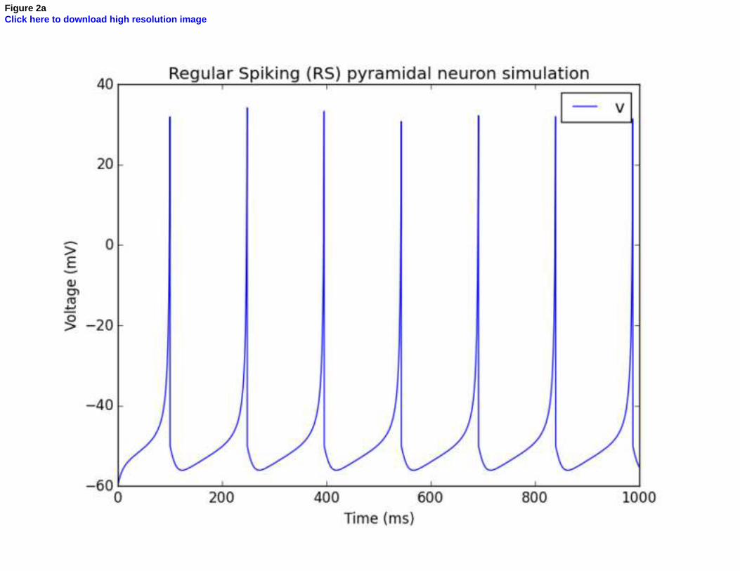
Figure 2aClick here to download high resolution image

Figure 2bClick here to download high resolution image

Figure 3Click here to download high resolution image

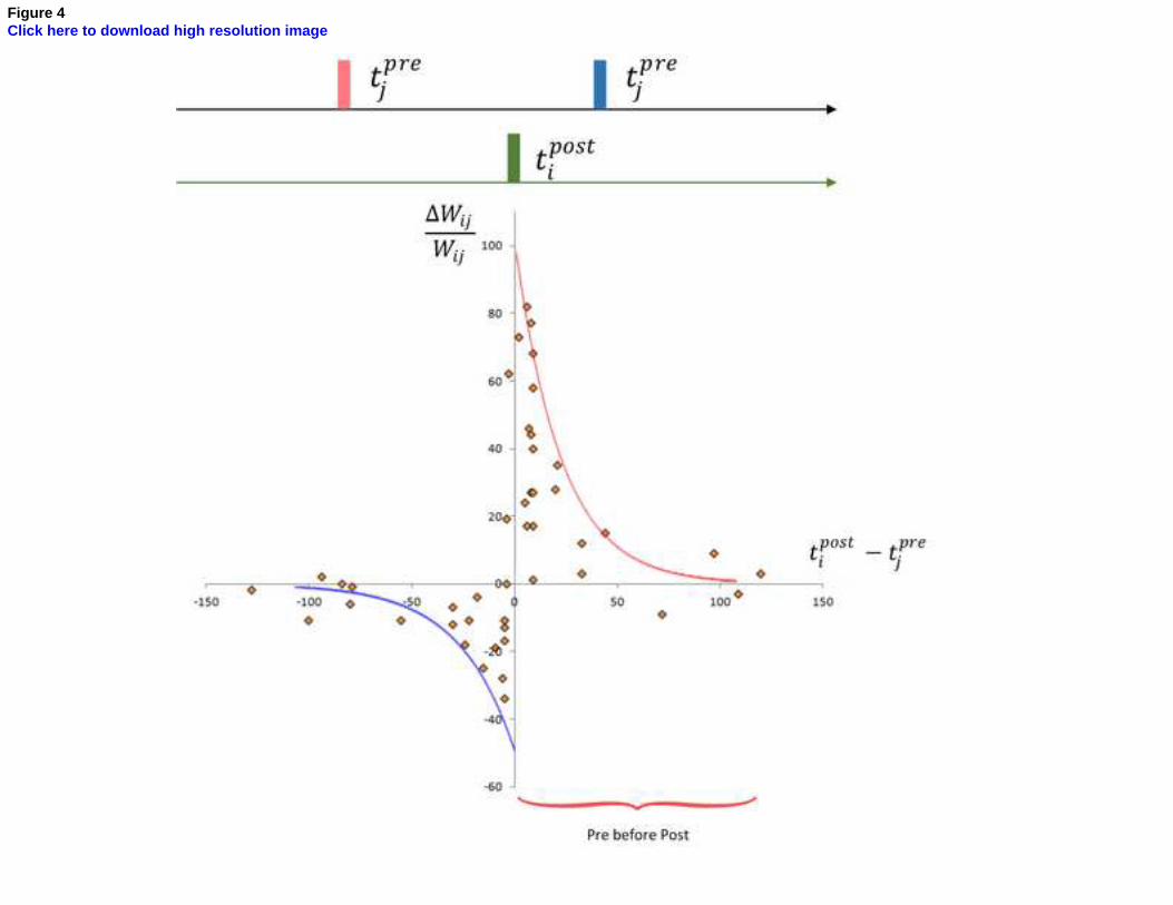
Figure 4Click here to download high resolution image

Figure 5aClick here to download high resolution image

Figure 5bClick here to download high resolution image

François Christophe received his bachelor in Signal processing and Automation from University of West

Brittany (France) in 2004, and his Master degree in Computer and Software Engineering from Brest

National Engineering School (France) in 2007. He received his Ph.D. degrees from Aalto University

(Finland) and Nantes Centrale Engineering School (France) in 2012. François works currently as post-

doctoral researcher in the Department of Pervasive Computing at Tampere University of Technology. His

research interests include computational models and modeling methods for the integration of biological

components in digital and software applications.

*Brief Biography author 1Click here to download Brief Biography: Francois Christophe Biography Jan 2015.docx

Vafa Andalibi obtained his Bachelor degree in Computer Hardware Engineering from Iran University of

Science and Technology in 2012. He is currently pursuing a M.Sc.(Tech.) with a double major degree in

Biomedical Engineering and Communication Systems and Networks. He works as research assistant in

the Department of Pervasive Computing at Tampere University of Technology. His research interests

include Bio-Integrated Systems (BIS), bio-measurements, computational neuroscience, neural modeling,

neuron-computer interface and functional organization of neuronal circuits.

*Brief Biography author 2Click here to download Brief Biography: Vafa Andalibi Biography Jan 2015.docx

Teemu Laukkarinen received M.Sc. degree in computer science from Tampere University of Technology

(TUT) in 2010. He is currently pursuing towards Ph.D. in the Department of Pervasive Computing at TUT.

He has been researching Wireless Sensor Networks (WSNs) since 2006. He has published several

international peer reviewed journal and conference articles about WSNs. His teaching experience covers

computer architecture, microcontroller systems and wireless sensor network applications. He took part

on launching a spin-off company from the WSN research at TUT in 2010. His research interests include

operating systems, applications, abstractions, and bio-integrations with WSNs.

*Brief Biography author 3Click here to download Brief Biography: Teemu Laukkarinen Biography Jan 2015.docx

Prof. Tommi Mikkonen (MSc 1992, Lic. Tech. 1995, Dr. Tech 1999, all from Tampere University of

Technology, Tampere, Finland) works on software architectures, software engineering and open source

software development at the Institute of Software Systems at Tampere U of Tech. Over the years, he has

written a number of research papers, and supervised theses and research projects on software

engineering. At present, he is working as the head of the Department of Pervasive Computing at TUT.

*Brief Biography author 4Click here to download Brief Biography: Tommi Mikkonen Biography Jan 2015.docx

Kai Koskimies is Professor Emeritus of Software Engineering, retired in 2014 from Tampere University of

Technology. His main research interests have been recently software architectures and the application

of heuristic approaches in software system development. He has published in and served in the program

committees of frontline software engineering conferences like ICSE, ESEC, FASE, and software

architecture conferences like ECSA and WICSA.

*Brief Biography author 5Click here to download Brief Biography: Kai Koskimies Biography Jan 2015.docx

*Author 1 PhotoClick here to download high resolution image

*Author 2 PhotoClick here to download high resolution image

*Author 3 PhotoClick here to download high resolution image

*Author 4 PhotoClick here to download high resolution image

*Author 5 PhotoClick here to download high resolution image