surface self-compensated hydrostatic bearings - dspace@mit
TRANSCRIPT
Surface Self-Compensated Hydrostatic Bearings
by
Nathan R. Kane
B.S.M.E., Mechanical EngineeringUniversity of Texas at Austin, (1991)
M.S.M.E., Mechanical EngineeringUniversity of Texas at Austin, (1993)
SUBMITTED TO THE DEPARTMENT OF MECHANICAL ENGINEERINGIN PARTIAL FULFILLMENT OF THE DEGREE OF
DOCTOR OF PHILOSOPHY IN MECHANICAL ENGINEERING
at the
MASSACHUSETTS INSTITUTE OF TECHNOLOGY
June 1999
© 1999 Massachusetts Institute of TechnologyAll rights reserved
Signature of Author .................. .............................Department of Mechanical Engineering
May 20, 1999
Certified by .................. . .....................................-Alexander H. Slocum
Professor of Mechanical EngineeringThsueervisor
Accepted by ........................................ -" ....'-Ain A. Sonin
Professor of Mechanical EngineeringChairman, Committee for Graduate Students
ARCHIVES
MASSACHUSETTS INSTITUTEOF TECHNOLOGY
JUL 121999
LIBRARIES

2

Surface Self-Compensated Hydrostatic Bearings
by
NATHAN R. KANE
Submitted to the Department of Mechanical Engineeringon May 20, 1999 in Partial Fulfillment of the
Requirements for the Degree of Doctor of Philosophyin Mechanical Engineering at the Massachusetts Institute of Technology
ABSTRACT
It has long been known in the machine tool industry that hydrostatic bearing technologyhas several unique advantages over rolling element bearings. The thin fluid film betweenthe bearing pads and the rail provides virtually infinite motion resolution due to lack ofstatic friction, very low straightness ripple, high squeeze film damping, potentially infinitebearing life, immunity to fretting, tolerance to ceramic swarf, and superior shock loadcapacity. However, a major impediment to the use of hydrostatic bearings is that there areno standard, pre-engineered designs that are commercially available, and custom design-ing a bearing is often prohibitively expensive and time consuming.
In light of the opportunity just mentioned, the goal of this thesis is to present and demon-strate the feasibility of a family of novel modular hydrostatic bearings which are wellsuited for mass production and are designed to be bolt-for-bolt compatible with modularrolling element bearings. A size 35 prototype of one of the novel designs is presentedalong with measured and predicted performance (load verses deflection, flow rate, pump-ing power). The novel design that is tested uses a set of auxiliary restricting surfaces on aprofile rail and form fitting truck that make an acute angle relative to each load bearingpocket they supply, thus allowing the truck to be machined and ground as one piece, andeliminating the need for capillaries, diaphragms, or other unmachinable features. In addi-tion to the first prototype work, a second engineered embodiment of the novel design ispresented which, via a sophisticated mathematical model, is designed to have an accept-able stiffness and load capacity variation given realistic production manufacturing toler-ances.
Thesis Supervisor: Prof. Alexander H. SlocumTitle: Professor of Mechanical Engineering

4 ABSTRACT

ACKNOWLEDGMENTS
A million thankyous to all the people who helped me with this thesis. I could never havedone this thesis without you.
Alex SlocumAlex, you are the best. You always keep the faith, and you keep me going. You keep us allgoing. I have never met a more can-do, open minded, and positive person than you. Youare a good and kind person to the core. You are one of the few people that is persistentenough to cut through my skeptical attitude and keep things moving forward. I owe you alot.
Jason Jarboe the super-UROPI think there must be a gene for thinking machines are cool, just for themselves. Jason hasit, and I have it; and I think that is why we get along so well. If the ordinary MIT student'smind is like a sponge, then Jason's mind is like ultra pampers (I can't think of somethingmore flattering that is more absorbent right now, but I bet Jason could tell me; just like hecan explain every thing from faster-than-light data transmission due to "spooky" quantumphysics, to why duct tape is sticky. That's cool, man.) By the way, thanks, Jason, for find-ing that old daq board in the lab and doing all those awesome deflection tests with dataacquisition !
Heinz Gaub at Jung, Gmbh in GermanyHeinz and his crew at Jung did a spectacular job making the prototype hydrorail bearings.They checked everything twice, made all the parts perfectly the first time, and Heinz dedi-cated a top engineer (I know him as Herr Junker) to help me run tests at Jung for an entireweek. Heinz has been a great advocate for the bearings as well. Thanks Heinz.
Herr Junker at Jung, Gmbh in GermanyThanks Herr Junker for helping me in germany. You really prepared everything so well.And say thanks to all the other people who worked on the prototype. They did a great job.
Joachim Sihler (aka Yaw-kum or Yo-heem, depending on the person addressing him!)It was great to work with you on the hydroround. Your persistence and thoroughness islegendary. Have a great summer at Star Cutter! ! I am looking forward to helping you writethe article. And hey Joachim, keep having more great ideers (We, know, we know, Jason,you don't have to tell us again its pronounced i-d-e-a).
Professor Sanjay SarmaThanks for being on my thesis committee and for all of the good advice you have givenme over the years.
5

6 ACKNOWLEDGMENTS
Professor John Lienhard VThanks for being on my thesis committee and for being supportive at the last committeemeeting.
Ebbe BambergThank you so much Ebbe for your time and patience in helping me with ProE, my laptop,the network, and all kinds of software issues that could have made my life so difficult.Your generosity has set the tone of helpfulness that permeates our entire lab.
Dennis Barnes at Mannesmann RexrothThanks so much for all your help and support. You guys are great.
Tim Ruiz at Mannesmann RexrothThanks for answering so many questions about hydraulic systems.
Greg Lyon at Thomson Bay Co.Thanks for all your excellent advice, and for donating the AccuGlide and AccuMax linearguides.
Peter MugglestoneThanks for the advice and support. By the way, I found you on the web running in the Bos-ton marathon. Very cool.
Steve Fantone at OptikosThanks for loaning me your autocollimator for the bed straightness tests.
Jim Flinchbaugh at Weldon Machine ToolThanks for employing me for a summer and being such a loyal advocate of our lab'shydrostatic bearings.
Newman M. Marsilius at Moore ToolThanks for allowing us to do tests on the hydroround at your company, and for offeringadvice and support.
Zygo CorporationThanks so much for donating the laser we used for straightness tests to our lab. That wasreally awesome.
Trilogy Systems CorporationThanks for loaning us the linear motor we used for straightness tests, and being so helpfulin debugging it.
Delta Tau ControlsThanks for loaning us the controller we used for straightness tests.

ACKNOWLEDGMENTS 7
Rolland DoubledayThanks for working so hard over the summer doing those additional tests while I was atWeldon.
Zaf at Ford Motor Co.Thanks doing the lithography models of the bearing prototype for free. The models wereof immense value in helping the engineers at Jung understand and plan the manufacture ofthe bearing prototype.
Fannie and John Hertz FoundationThanks for paying for such a large proportion of my education at MIT. I am honored tohave been an Fannie and John Hertz fellow.
Don O'SullivanThanks for your role in making the thesis template and answering all my questions aboutframemaker. The template was fabulous - I have scarcely had to think of formatting.
Steve LudwickThanks for loaning us Dr. Trumper's cap probes and showing us how to use them. Goodluck on the faculty position search!!!
Felipe VarelaIt was great fun finishing my thesis with you in room 35-008. Thanks for answering myquestions. Good luck at motorola!
And I want to say thanks again to all my former and current labmates, who are all suchawesome people:Sami KotainenAsha Balakrishnan - thanks Asha for organizing so many events!!! You are cool.James WhiteMike Schmidt-LangEbbe BambergDon O'SullivanFelipe VarelaJoachim SihlerThe now Professor Samir NeyfehMarty CulpepperSep KianiRyan ValianceCarsten Hochmi!thKevin WassonPaul Scagnetti
And Most of all My Loving Mother and Father. Mom and dad, this is a poem for both ofyou. Mom, I know dad and I are both stress cases, and you are always the one to calm us

8 ACKNOWLEDGMENTS
down. So I think you will understand this poem better than anyone. This is called "uncon-ditionally":
Stepped out off at the wrong floorUsed the wrong key in my doorAnd only yesterday I sworeI wouldn't do that any more
An hour staring at my screenI haven't done a single thingWhere else could that file beDamn its right in front of me
Dialed a number while half asleepHeard a whistle and a beepMan that's so embarrassingI just called a fax machine
Woe is my poor tortured brainWhy is it in so much painEven very simple thingsAre never easy
People tell meTo just be happyBut that adviceDoesn't work for me
Its not that simpleIts not that easyGuess that's another thingThat's wrong with me
And then a friend said somethingThat I thinkIs pretty cool
She said now close your eyesAnd stop everythingAnd think of someone you love unconditionally
She said now don't just tryTo be happyAnd don't keep thinkingAbout the way you should be

ACKNOWLEDGMENTS 9
So now I'm closing my eyesAnd stopping everythingAnd I'm thinking of all the people I love in my life
Unconditionally

10 ACKNOWLEDGMENTS

TABLE OF CONTENTS 11
TABLE OF CONTENTS
Abstract. . . . . . . . . ... . .. 3
Acknowledgments
Table of contents . . .
5
11
List of Figures .....
List of Tables .. . .. .
Chapter 1. Introduction.
1.1 Overview of Modular Linear Guides .
1.2 Specifications and Room for Improvement
i.3 Applications for a Linear Hydrostatic Guide1.3.1 Immediate Markets for a Linear Hydro,1.3.2 Motto for the Future: "No Contact - For
1.4 Fundamental Contributions of Thesis .
................. .21................. .21................. .22................. .31static Guide .......... 31rever Perfect" ......... 32
................. .33Chapter 2. Comparison Of Different Hydrostatic Designs . . ....
2.1 Criteria for a Hydrostatic Guide to be a Viable Commercial Product
2.2 Novel Contributions Studied for Thesis.
2.3 Design Concepts Considered .....................2.3.1 Constant Flow Compensation.2.3.2 Capillary or Orifice Compensation . . . . . . . . . . . .
2.3.3 Diaphragm Compensation.2.3.4 Self Compensation with Internal Passages .. . .. . ....2.3.5 Angled Surface Self Compensation ..............
2.4 Overview of Analysis Issues .....................2.4.1 Desired Load Capacity and Static Stiffness are Linked . .
2.4.2 Checking for Minimum Static Stiffness . . . . . .. . .. . .
2.4.3 Two Optimization Scenarios.
2.4.4 Thermal Control of Fluid: Area for Future. Work . . . . . . .2.4.5 Approximations Made for Analysis of Hydrostatic Designs
2.5 Comparison of Hydrostatic and Rolling Element Systems ......
.... 37.... 37... . 39
.... 42
... . 42
. . . . 43
.... 44
.... 46
... . 47
.... 48
... . 48
.... 48
... . 49
... . 50
... . 51
... . 52
... . . . . . . 15
19
11TABLE OF CONTENTS
TABLE OF CONTENTS
2.5.1 Load Capacity and Stiffness Comparison Matrix2.5.2 Static and Shock Load Capacity Discussion . .2.5.3 Load Capacity Versus Life Comparison Plot2.5.4 Static Stiffness Comparison Plots .......2.5.5 Dynamic Friction Comparison Plots ......2.5.6 Manufacturing Comparison Matrix.2.5.7 Robustness Comparison Matrix ........
2.6 Conclusions of Design Study.
........... .535454
56
59
60
63
65
Chapter 3. Lumped Parameter Bearing Model ..........
3.1 Profile Geometry ........................3.1.1 Representing a Profile of Flats and Rounds .......3.1.2 Computing x and y Distances on a Profile ........3.1.3 Profile Constraints and Unknowns3.1.4 Representing Bearing Gaps3.1.5 Computing a Slave Radius from Three Gaps.3.1.6 Profile Dimensions Sent to ProE Solid Model ......
3.2 Computing Fluid Resistance and Effective Area ........3.2.1 Validity of Fully Developed Laminar Flow.3.2.2 Effect of Viscous Heating on Viscosity and Gamma . .3.2.3 Single Rectangular Element . . . . . . . . . . . . . .
3.2.4 Effect of Pad Tilting on Resistance ...........3.2.5 Chain of Parallel Plate Elements with Common Width3.2.6 Chain of Parallel Plate Elements with Common Length3.2.7 General Function Used in Code .............
3.3 Lumped Resistance Circuit ...................3.3.1 Assumptions.
3.3.2 Computing the Lumped Resistances ...........3.3.3 Solving for Node Pressures and Flow . . . . . . ....3.3.4 Lumped Effective Areas .................
3.4 Incorporating Elastic Deflection from 2D FEA Models ....3.4.1 Problems that are Addressed in this Section .......3.4.2 Subproblem 1: FEA Simulations
67
.... 67
.... 6868
70
70
70
70
.... 7374
76
78
80
82
85
86
87
87
89
89
91
91
92................... .933.4.3
3.4.4Subproblem 2: Computing Array of Reference Gap ChangesSubproblem 3: Computing Array of Gap Changes .....
Chapter 4. Angled Surface Self Compensation Prototype ........
4.1 Size 35 Angled Surface Self Compensation Prototype .........
93
95
97
97
12
........................................................................
. . .
. . .
. . .
. . .
. . .
. . .
. . .
· .
.. .
TABLE OF CONTENTS
4.2 Deflection Versus Load . . . . . . . . . . . . . . . . .
4.2.1 Test Set-Up for Deflection Vs. Load ...............4.2.2 Matching Pocket Pressures and Flow to Account for Gap Errors4.2.3 Load Versus Displacement Plots .................
4.3 Dynamic Stiffness Tests.
4.3.1 Test Set-Up for Measuring Dynamic Stiffness4.3.2 Measured Dynamic Stiffness (Hydro, Ball, & Roller Systems)
Chantar Vnnehilcinnc A nl ]sihire Wnrlrl
5.1 Conclusions
5.2 Future Work
References.
Appendix A. Test Bed ...........
A.1 Overall View of Test Bed System
A.2 Carriage System ...........
A.3 Bed Design and Manufacture ....
A.4 Component Mounting ........A.4.1 Rail Mounting ........
A.4.2 Carriage Plate Mounting . . .
A.5 Rail Groove Straightness.
A.6 Linear Motor Drive System .....
A.7 Interferometer System Discussion
....... 111
....... 111....... .112
..................... .115
..................... .117
..................... .117
..................... .120..................... .120
..................... .122..................... .122..................... .123
..................... .124
..................... .127
..................... .128Appendix B. Straightness And Dynamic Stiffness Measurements
B.1 Straightness.
B.2 Dynamic Stiffness.
B.3 Friction Force.
B.4 Conclusions ...........................
....... 131
....... . 131
....... 134....... 137....... . 137
... 99... 99... 102. . 103
. . 107
. . 107
. . 108
13
I ...- _- - I- - . . . .

14 TABLE OF CONTENTS

LIST OF FIGURES 15
LIST OF FIGURES
Figure 1.1 Size 35 roller rail damaged by fretting on a cam grinder after 9 months; therail was supposed to last 3 years. ............... . ... 24
Figure 1.2 A roller bearing rail which has been worn away by ceramic dust in betweenthe roller and the rail. The lighter gray line is the region where the rollertravels and has been worn away over a period of about 6 months. . . . 25
Figure 1.3 Close up of a rail surface damaged by ceramic particles (photo from Paul A.Scagnetti, Ph.D., MIT Dissertation) ................... 25
Figure 1.4 Straightness ripple caused by rolling element circulation, measured for ultraprecision lightly preloaded AccuGlide and AccuMax bearing trucks. Theripple is non repeatable because of roller slippage. .......... 28
Figure 1.5 Fundamental contribution of thesis: Angled Surface Self compensation, andits application to a modular linear bearing rail. .............. 34
Figure 2.1 Illustration of a novel feature and novel hydrostatic bearing design studied inthis thesis, applied to a modular linear rail. ................ 40
Figure 2.2 Illustration of how Angled Surface Self Compensation achieves vertical andlateral stiffness. . . . . . . . . . . . . . . . . . .......... 41
Figure 2.3 Constant flow compensation. ...................... 42
Figure 2.4 Capillary compensation implemented in a Size 35 modular bearing, with andwithout the NGBP feature. ....................... 44
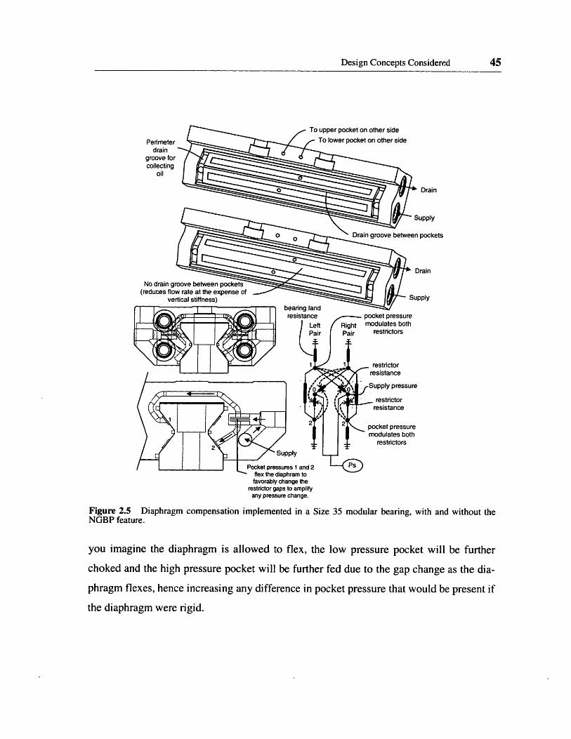
Figure 2.5 Diaphragm compensation implemented in a Size 35 modular bearing, withand without the NGBP feature. ..................... .. 45
Figure 2.6 Self Compensation with Internal Passages implemented in a Size 35 modularbearing, with and without the NGBP feature. .............. 46
Figure 2.7 Angled Surface Self Compensation implemented in a Size 35 modular bearing...................................... 47
Figure 2.8 Illustration of static stiffness in a hydrostatic bearing truck. ...... 49
Figure 2.9 Load versus life of rolling element bearings shown with hydrostatic bearingdesigns operating at 100 W per truck. ....... . . . ...... 55
Figure 2.10 Initial static stiffness (based on catalogue data) of rolling element bearingsversus OAF . . . . . . . . . . . . . . . . . . . . . . . . . .... 57
Figure 2.11 Minimum final static stiffness versus OactX shown for hydrostatic bearingdesigns operating at 100 W per truck. ............... 58

16 LIST OF FIGURES
Figure 2.12 Friction force versus travel velocity for rolling element systems and hydro-static systems operating at different oil viscosities. ............ 59
Figure 2.13 Friction power versus travel velocity for rolling element systems and hydro-static systems operating at different oil viscosities. ............ 61
Figure 3.1 A profile of flats and rounds is represented in an angle array T(i,rl) and alength array S(i,rl). ............................ 68
Figure 3.2 Four types of distances frequently computed from a profile of flats and rounds...................................... 69
Figure 3.3 The dx and dy increments for a flat and a round segment "i", used to code thefunction FnDpr[cs, i, j, T, S, rl, xy]. ................... 69
Figure 3.4 Constraints used on Size 35 Face to Face and Back to Back designs. . 71
Figure 3.5 Representing bearing gaps in the array H(i,rl) . ...... .. 72
Figure 3.6 Computing a slave radius from three gaps . ......... 73
Figure 3.7 A single parallel plate element "i". ................... 79
Figure 3.8 Force Component "a" and Force Component "b" on parallel plate element "i"Figure 3.9 Tilted paral. ..................................... 80
Figure 3.9 Tilted parallel plate element ...................... . 81
Figure 3.10 Chain of parallel plate elements with a common width. . . . . . ... 83
Figure 3.11 Chain of Parallel Plate Elements with Common Length. . . . . . ... 85
Figure 3.12 Lumped resistance circuit used to predict pocket pressures. . . . . .. 88
Figure 3.13 Shows each point "p" marked on the truck and rail FEA models, and theregions over which the three reference pressures act. Each point "p" is a tan-gent point between a flat and a round, and hence is a natural vertex generatedby ProMechanica. ............................ 94
Figure 3.14 FEA simulations run to fill the array ExyRRl(p, rl, xy, Id, tr). For the simula-tions Pref(l,1) = P(2,1) = P(3,1) = 1 MPa. ............... 95
Figure 3.15 Shows the midpoint of each segment "i", at which a gap change is stored inthe array HEref(i, rl, Id, Irl). ....................... 96
Figure 4.1 Basic features of the Size 35 alpha prototype design. . . . . . . . ... 98
Figure 4.2 Design bearing gaps and some key profile dimensions used for Size 35 alphaprototype ................................. 98
Figure 4.3 Profile grinding of a bearing rail and a truck half at Jung, GmbH, Goeppin-gen, Germany. . . . . . . . . . . . . . . . . ... .. . . . . . . . . . 99
Figure 4.4 Test rig used to load a truck in compression and tension. Only the deflectionof the left truck was measured. Thin spacers were placed under the whiffle

LIST OF FIGURES 17
tree block, above each truck, to prevent the steel carriage plate from bendingwhen a force is applied on the transducer. ............... 100
Figure 4.5 Test rig used to load both trucks laterally. Unlike for the vertical loading set-up, the load on the right and left trucks is not statically determined. For expe-diency, the lateral load component on the truck being measured was assumedto be half the force transducer load. The small vertical component was com-puted using a FBD of the set-up. ................... . 101
Figure 4.6 Free body diagram of the lateral load test set-up. ............ 101
Figure 4.7 Gap errors used to match initial pocket pressures at Ps = 34.5 Bar and theflow correlation at the other Ps values. ........ . . . . . . ... 103
Figure 4.8 Measured and predicted downward and lateral deflection versus force ofprototype bearing truck. ......................... 104
Figure 4.9 Measured and predicted tensile deflection versus force of prototype bearingtruck .................................... 105
Figure 4. 10 Dynamic stiffness testing using a hammer and accelerometer. The force andaccelerometer data are fed to a signal analyzer to obtain the Acceleration/Force transfer function. Dividing by frequency squared and inverting yieldsForce/Displacement, i.e. the dynamic stiffness versus frequency of the scenario...................................... 107
Figure 4.11 Measured dynamic stiffness of an alpha prototype hydrostatic truck andlightlypreloadedAccuglideandAccuMaxtrucks,bothofstandardlength(109mm)...................................... ........ .108
Figure A. I1 Side view of test bed system designed for measuring straightness ... 118
Figure A.2 Top view of test bed system designed for measuring straightness ... 119
Figure A.3 End view of bed, showing shear dampers(TM). ......... . 121
Figure A.4 Scale drawing of rail mounted with tapered gib. . ........ 122
Figure A.5 Scale drawing of a truck mounted to the carriage plate. ........ 123
Figure A.6 Rail groove names. ........... ................ 125
Figure A.7 Autocollimator straightness of rail groove #1. . ......... 126
Figure A.8 Autocollimator straightness of rail groove #2. ............. 126
Figure A.9 Flexural coupling used to drive the carriage plate. . ...... . 128
Figure B. 1 The bearing truck under test. . . . . . . . . . . . . . . . . . . . 132
Figure B.2 Measured straightness of an AccuGlideTM truck (ball system, ultra preci-sion, lightly preloaded at 0.03%C, Standard length of L=109mm). . . 133
Figure B.3 Measured straightness of an AccuMaxTM truck (roller system, ultra preci-sion, lightly preloaded at 0.03%C, Standard length of L=109mm). . . 133

18 LIST OF FIGURES
Figure B.4 The two test scenarios for dynamic stiffness testing. .......... 135
Figure B.5 Compressive dynamic stiffness of AccuGlideTM (ball system) and Accu-Max (roller system) trucks, lightly preloaded (0.03%C), standard length ofL=109mm, shown with the response measured on top of the rail alone. Thehydrostatic prototype could not be tested under these conditions because it isnot stable in tilt. ............................. 136
Figure B.6 Compressive dynamic stiffness of AccuGlideTM (ball system) and Accu-Max (roller system) trucks, lightly preloaded (0.03%C), standard length ofL=109mm, and the hydrostatic prototype, L=134mm, shown with theresponse measured on top of the rail alone. ............... 136

LIST OF TABLES 19
LIST OF TABLES
TABLE 1.1
TABLE 1.2
TABLE 2.1
TABLE 2.2
TABLE 2.3
TABLE 2.4
TABLE 3.1
TABLE 3.2
TABLE 3.3
TABLE 3.4
TABLE 4.1
TABLE B.1
TABLE B.2
TABLE B.3
Advantages and Applications for a Linear Hydrostatic Guide. .... 31
Immediate Markets for a Linear Hydrostatic Guide . . . . . . . ... 32
Advantages and Disadvantages of Using Water Versus Using a HydraulicOil ................................... 39
Load Capacity and Stiffness Comparison Matrix of Size 35 Hydrostatic andRolling Element Systems ........................ 53
Manufacturing Comparison Matrix . . . . . . . . . . . . . ..... 62
Robustness Comparison Matrix ................... . 64
Reynolds number and undeveloped length of flow through a practical bear-ing restrictor. . . . . . . . . . . . . . . . . . . . . . . . . . . 75
Change in viscosity that will occur due to Poiseuille flow through a practi-cal bearing. . . . . . . . . . . . . . . . . . . . . . . . ...... 77
Estimate of how much viscous heating will effect the gamma ratio. . 78
The relative resistance errorversus have, when atilt of6 micrometers is present.82
Summary of Load Versus Deflection Test Results ........... 106
Measured straightness and straightness ripple. ............. 132
Summary of compressive static and dynamic stiffnesses. ....... 137
Measured static friction per truck. ................... 137

20 LIST OF TABLES

Chapter 1
INTRODUCTION
The purpose of this chapter is to motivate the development of a modular linear hydrostatic
bearing that is bolt-for-bolt compatible with rolling element linear guides. After the moti-
vation is provided, the fundamental contributions of this thesis are outlined.
1.1 Overview of Modular Linear Guides
Briefly stated, modular linear guides are rolling element linear bearings whose rail and
truck are designed with industry-wide standard dimensions, so that a linear guide manu-
factured by one company is bolt-for-bolt interchangeable with a linear guide made by
another. The popularity of linear guides is indicated by the numerous manufactures of
them, including the STAR, Thomson Bay Company, Schneeberger, INA, THK, SKF, IKO,
and others. A major application of linear guides is for precision machine tools, such as
machining centers, CNC lathes, surface and cylindrical grinders, centerless grinders, jig
grinders, etc.. Modular linear guides have tremendous market appeal because they are
easy and fast to design with, and their use greatly reduces assembly time and labor costs of
a machine. For companies designing new machines on a tight schedule, modular linear
guides are rightly or wrongly often the default choice. Since all currently available modu-
lar linear guides have rolling elements, however, which physically contact the truck and
the rail, they have inherent performance limitations which can give disappointing machine
performance for demanding applications. These limitations include limited motion resolu-
21

22 INTRODUCTION
tion due to mechanical contact effects, straightness ripple due to ball or roller entry and
exit, low to moderate damping, and premature failure due to particle infiltration.
To provide superior performance in the categories just mentioned, hydrostatic bearing
technology is ideal. The thin fluid film between the bearing pads and the rail provide virtu-
ally infinite motion resolution, very low straightness ripple (when pump pressure varia-
tions are properly attenuated), high squeeze film damping, and potentially infinite bearing
life. Despite the superior performance of hydrostatic bearings, they are seldom used
because no standard, pre-engineered designs are commercially available, and custom
designing a bearing is often an arduous task. In addition, conventional hydrostatic bear-
ings typically have small orifices and capillaries which can clog, and their stiffness and
load capacity are highly sensitive to manufacturing errors. Since designers do not have
time, nor do they wish to take the risk of designing a conventional hydrostatic bearing
themselves, they and the machine tool buyers they sell t choose to live with the limita-
tions of existing rolling element technology.
In light of the opportunity just outlined, the goal of this thesis is the invention, design,
modeling and testing of an alpha prototype size 35 modular hydrostatic bearing, and
design of a beta prototype hydrostatic bearing suitable for mass production.
If such a product became available on the market, builders who use modular linear guides
could offer high performance hydrostatic machines to users. Or, the users themselves
could afford to retrofit an existing machine. Due to the performance advantages, modular
hydrostatic bearings could become a commonly used bearing for top-of-the-line machine
tools.
1.2 Specifications and Room for Improvement
In this section, the following specifications for linear guides are explained, and aspects of
rolling element linear guides that could be improved upon are discussed.
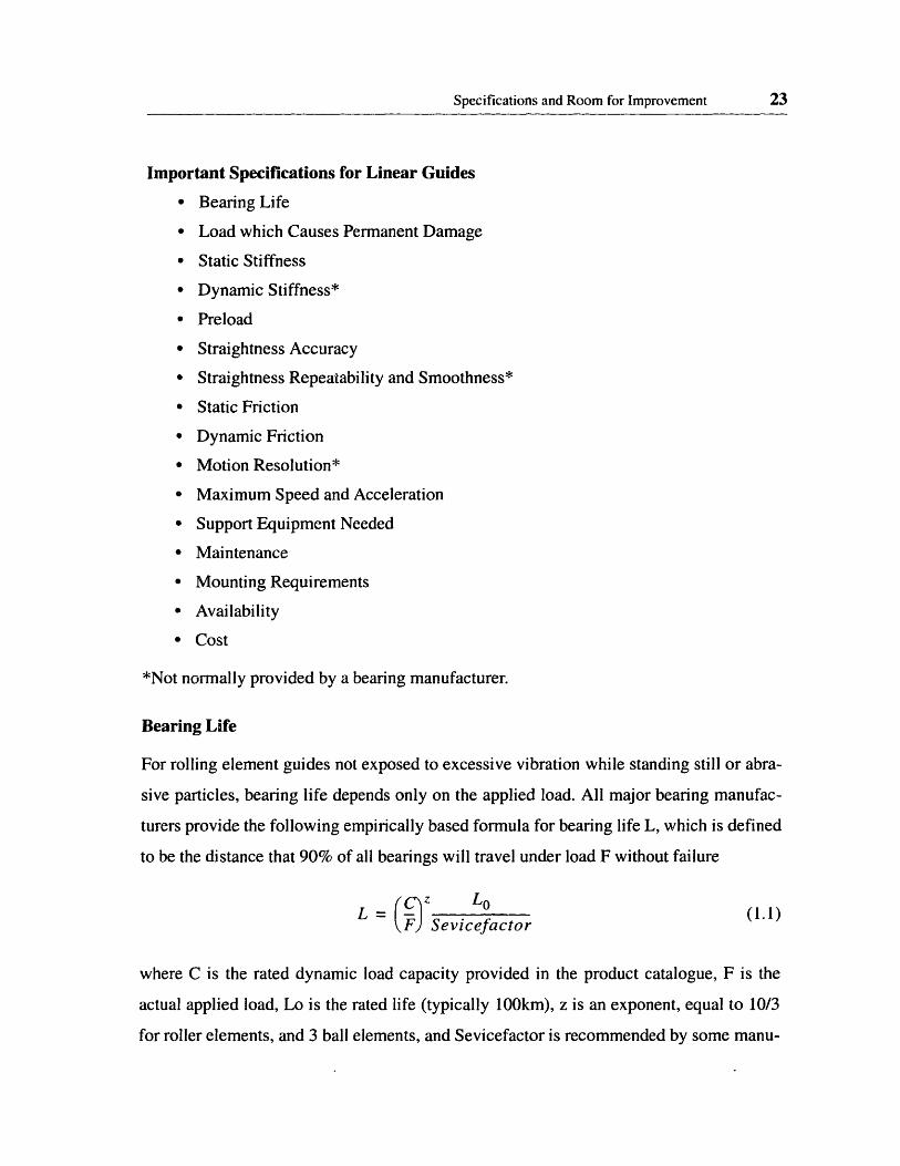
Specifications and Room for Improvement
Important Specifications for Linear Guides
· Bearing Life
· Load which Causes Permanent Damage
* Static Stiffness
* Dynamic Stiffness*
* Preload
* Straightness Accuracy
* Straightness Repeatability and Smoothness*
* Static Friction
* Dynamic Friction
* Motion Resolution*
· Maximum Speed and Acceleration
* Support Equipment Needed
* Maintenance
* Mounting Requirements
* Availability
* Cost
*Not normally provided by a bearing manufacturer.
Bearing Life
For rolling element guides not exposed to excessive vibration while standing still or abra-
sive particles, bearing life depends only on the applied load. All major bearing manufac-
turers provide the following empirically based formula for bearing life L, which is defined
to be the distance that 90% of all bearings will travel under load F without failure
L = (2JSeviceactor
where C is the rated dynamic load capacity provided in the product catalogue, F is the
actual applied load, Lo is the rated life (typically 100km), z is an exponent, equal to 10/3
for roller elements, and 3 ball elements, and Sevicefactor is recommended by some manu-
23
24 INTRODUCTION
factures to be 3 under severe vibration conditions (as recommended by the manufacturer
for a particular application), and to be I under normal conditions.
Rolling element bearings can fail before Equation 1.1 predicts by either fretting or by par-
ticle contamination. These two modes of failure are discussed below.
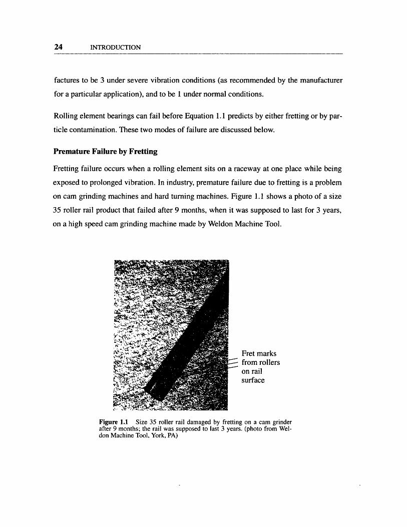
Premature Failure by Fretting
Fretting failure occurs when a rolling element sits on a raceway at one place while being
exposed to prolonged vibration. In industry, premature failure due to fretting is a problem
on cam grinding machines and hard turning machines. Figure 1.1 shows a photo of a size
35 roller rail product that failed after 9 months, when it was supposed to last for 3 years,
on a high speed cam grinding machine made by Weldon Machine Tool.
Fret marks2 from rollers
on railsurface
Figure 1.1 Size 35 roller rail damaged by fretting on a cam grinderafter 9 months; the rail was supposed to last 3 years. (photo from Wel-don Machine Tool, York, PA)

Specifications and Room for Improvement
Premature Failure by Particle Contamination
Due to mechanical contact, rolling element bearings are very sensitive to particle contam-
ination. Any slight damage is aggravated quickly as an element rolls over the damaged
area over and over again. In industry contamination is a problem on machines that mill
and grind ceramics and graphite. Figure 1.2 and Figure 1.3 shows typical damage to a rail
that occurs after only six months of grinding aluminum oxide on a machine at Wilbanks
International. These machines are overhauled every six months.
Figure 1.2 A roller bearing rail which has been worn away by ceramicdust in between the roller and the rail. The lighter gray line is the regionwhere the roller travels and has been worn away over a period of about 6months. (photo from Paul A. Scagnetti, Ph.D., MIT Dissertation)
Figure 1.3 Close up of a rail surface damaged by ceramic particles(photo from Paul A. Scagnetti, Ph.D., MIT Dissertation)
11 ' MO.Mm- _m~1
25
1211%_`4111A~~ii10 tk_

26 INTRODUCTION
Load which Causes Permanent Damage
For rolling element bearings, the maximum allowed load capacity CO is between 40% and
80% larger than the rated dynamic load capacity C. When Co is exceed, the rolling ele-
ments permanently brinnel the rail and truck races, and the damaged area quickly deterio-
rates. In practice CO is exceeded by the impact of a crash as opposed to being exceeding
during normal use. As a result, in practice linear guides are often chosen one or two sizes
larger than needed to avoid damage if a crash should occur.
Static Stiffness
Rolling element linear guides provide excellent static stiffness, and since a preload is
present, there is never any lost motion, as there can be with sliding bearings. In practice,
the static stiffness of linear guides more than adequate, compared to other compliances in
the structural loop of a machine tool. For grinding, it should be noted that the cutting
forces at sparkout are very low, and as such the error caused by roller recirculation, (about
1 micrometer), thermal drift, and straightness errors, will be much more than caused by
bearing deflection.
Dynamic Stiffness
Dynamic stiffness is an important characteristic that is not normally not quoted in product
literature. Dynamic stiffness refers to stiffness as a function of the frequency of an applied
oscillatory force. Rolling element bearings are always highly under damped, and hence
they do not help to reduce vibration due to cutting forces. In practice, the poor damping of
linear guides is problem on most types of grinding machines, especially machines that
grind ceramics, on hard turning machines, and on some high speed machine tools. At the
same time, it is well know in industry that the squeeze film damping effect of hydrostatic
and hydrodynamic bearings provide excellent damping and such bearings provide the
smoothest possible surface finish.

Specifications and Room for Improvement
Straightness Accuracy
The highest accuracy class specified in product catalogues is typically 3 micrometers of
error motion of one truck relative to its rail per meter of rail length. However, it should be
noted that in practice the actual bearing straightness is dictated by the straightness error of
the machine bed the rails are bolted to. Another important effect is that an assembly of
four trucks on two rails results in a good deal of error averaging which improves straight-
ness. The net result is that in practice ultra precision linear guides provide a straightness
that is usually no worse, if not better than, the straightness of the machine bed the rails are
bolted to.
Straightness Repeatability and Smoothness
Straightness repeatability is more important than straightness accuracy for machines that
can compensate for errors. For rolling element linear guides, ball entry and exit zones at
the truck races can create a non-repeatable straightness ripple of up to 2 micrometer in
amplitude. Appendix B shows 0.6 and 0.4 micron straightness ripple that was measured
for lightly preloaded ultra precision AccuGlide and AccuMax trucks, respectively. The
results are shown again in Figure 1.4. As with all types of linear bearings, heat generated
by the motion can introduce non-repeatable thermal drift.
Static And Dynamic Friction
Static friction is due to the rolling elements, and dynamic friction is due to both the wipers
and the rolling elements.
In practice, static friction of linear guides is not a problem on most machine tools of today,
but there are notable cases where there is unwanted reversal error on machines that do
high speed CNC contour milling. An important example is high speed milling of scroll
27

INTRODUCTION
4.5 -- 4
e 3.5' 3
2.
§ 1.5Ra 1
X 0.5a 0
o -05-1
-1 .5
/ 50 \ 100/ Unused sc
Location of screw in ral (80rrn spacing)
E
I
150rew hole in bed
200 250 300 350 400
Travel distance (mm)
Points easured using an autocolirnator sled on bed ral,/5 1 w as mounted to (a bad point sorretes occurs when a
4 5 i / sled foot overlaps a srmal lip present around some rai
4 . /I screw holes)
35i /Vertical straightness of truck rrtion3 / | / measured
251 Note raised p around this screw using terferometer systemhole in bed did not cause notcabl 0 4 moron average staghtness ripplestraightness error of truck mobon / / Thomson Accullax Truck (er systerm
1 5 Leng=109 mx Lightly preloaded (3/OC)
05
.11
-1 5 +o- _ 10-- -4111----- i0- - -- -- - -v1 - - -- * 4 -000 /5000 10000 15000 20000 25000 30000 35000 40000
Travel distance (mm)Locabon of screw n rail (40mn spacing)
Figure 1.4 Straightness ripple caused by rolling element circulation, measured for ultra precision lightlypreloaded AccuGlide and AccuMax bearing trucks. The ripple is non repeatable because of roller slippage.See appendix B for more details.
compressors, where even a nipple due to reversal of 2 micrometers (0.0008 inch) can
cause premature failure of mating scrolls.
In practice, dynamic friction of linear guides is not a problem on most machine tools used
today, which move slower than 0.3 m/s. However, for machines that move 1 m/s or faster,
the heat generated can cause significant thermal error, and for such cases an effective
means for cooling would be a useful attribute.
28
Points measured using an autocolimator sled on bed rail w as- rrmounted to. (a bad point sometrmes occurs w hen a sled foot
/ overlaps a snmall lip present around some rail screw holes)-s of truck motion measured.r system.straightness ripple
eeTruck (Bal system)ghtly preloaded (30/C)
*;
----
___ ___ __

Specifications and Room for Improvement
Motion Resolution
Motion resolution refers to the smallest increment of motion the bearing can be moved in
the axial direction repeatable, using an actuator with much higher motion resolution capa-
bility. Motion resolution is not quoted in product literature, and it is difficult to quote reli-
ably because it depends on the stiffness and resolution of the actuator that is used. In one
study [Futami] one on rolling element bearings, it was found that in a range from 0 to
micrometer, nanoscale resolution was possible, but in the range from 1 to 10 micrometers
resolution of about 1 micrometer was possible. The explanation given was that in the
former range, the rolling elements act like flexural bearings and thus provide smooth
motion, whereas in the latter range, the elements begin to roll, but because of the finite
Hertzian contact areas, they exhibit some stick-slip like behavior.
In practice, motion resolution is a major concern on grinding machines and high accuracy
milling machines.
Maximum Speed and Acceleration
The maximum speed and acceleration of a rolling element bearing is limited by jamming
or excessive slipping of the elements. Typical values quoted by manufacturers are 2 m/s,
and 50 m/s2, although higher values are possible (the manufacturer must be contacted for a
specific application). In practice, for most high speed machines, jamming is not a problem
unless lubrication is poor.
Support Equipment Needed
To achieve the longest life, automatic lubing systems are required for rolling element lin-
ear guides. This involves a pump, lubrication lines, and drainage gutters.
Maintenance
For bearings without an automatic lubrication system, grease is required regularly, and
periodic inspection of the rails and bellows is required to insure contaminants are not leak-
ing in.
29

30 INTRODUCTION
Mounting Requirements
While mounting methods for linear guides are similar, the required tolerances of the mat-
ing surfaces may differ between designs. All linear guide trucks are designed to allow
bolting from above and below. Standard rails allow bolting from above, while custom rails
can be ordered to allow bolting from below. A critical requirement for mounting is that
jibs or push plates be used to push at least one rail up against a precision shoulder, before
tightening the rail bolts.
Availability
While modular linear guides are always available, they can have lead times of 6 weeks or
more, depending on the rail length and accuracy class.
Cost
In general, bearings that use ball elements cost less than bearings that use cylindrical ele-
ments. For the rails, the cost ranges from $20 per foot for small, low precision rails to
$200 per foot for large, high precision rails. For trucks, the cost ranges from $50 to $600
per truck, depending on size and accuracy class.
1.3 Applications for a Linear Hydrostatic Guide
At a fundamental level, because there is no mechanical contact, a hydrostatic bearing
offers several advantages over rolling element bearings. These advantages are listed in
Table 1.1, along with applications that could most benefit from the advantage.

Applications for a Linear Hydrostatic Guide
TABLE 1.1 Advantages and Applications for a Linear Hydrostatic Guide.
Advantages of aHydrostatic Linear GuideNo wearNot vulnerable to frettingTolerant to particlesCrash resistantHigh dynamic stiffnessStraightness repeatabilitySmoothness of motionZero static frictionLow dynamic friction
Promising Applications in Industry
Hard turning, high speed machiningHard turning, high speed grinding and machiningGrinding ceramics, graphiteSome high speed machinesGrinding, hard turning, high speed machiningGrindingGrindingGrinding, contour millinghigh speed machining
From this list it can be seen that grinding processes can benefit in the greatest number of
ways from hydrostatic bearing technology. Other important applications are high speed
machining (more than I m/s traverse rate) and hard turning.
1.3.1 Immediate Markets for a Linear Hydrostatic Guide
At this time, several companies are interested in a being a beta sight for testing a modular
linear hydrostatic bearing. Table 1.2 lists these companies, along with the reasons they are
interested, from most important to least important, and the estimated number of machines
equipped with the hydrostatics that they could sell a year.
TABLE 1.2 Immediate Markets for a Linear Hydrostatic Guide
Desired EstimatedCompanies to date that advantage (most market,want to beta test a linear important to machineshydrostatic bearing Application least) per year2
Hardinge Hard Turning 1,2,5 100Weldon Machine Tool Cam Grinding 1,2,5,7,8,6,3 2
Grinding Ceramics 3,5,7,8,6 5Jung Surface Grinding 5,7,8,6 10Moore Tool Optics Grinding 5,7,8,6 5Star Cutter Tool grinding 5,7,8,6 10'Advanages listed in previous table2Cost of hydrostatic system will be about $5,000 more per machine tool than a rolling element system
This represents anywhere from a 3% to 10% increase in price of a machine tool system
This preliminary market data reveals some important insights.
1
23456789
__
.
31

32 INTRODUCTION
* The hard turning market is an order of magnitude larger than any individualgrinding market, and its primary need is no wear. The no wear and relatedfeatures appears at this time to be the most valuable asset of a hydrostaticmodular guide.
* Grinding is the only other known immediate market, and the dominant needis dynamic stiffness. Dynamic stiffness appears to be the second most valu-able asset of a hydrostatic modular guide.
1.3.2 Motto for the Future: "No Contact - Forever Perfect"
Looking at the longer term market of high speed machining, a modular linear hydrostatic
bearing is ideal for use with linear motors. By using all hydrostatic bearings actuated by
direct drive motors, all the precision motion elements of the machine tool could be non
contacting and hence free of wear.
Such a non contact Hydrostatic / Direct Drive machine would have the following very sig-
nificant advantages over existing machines:
Advantages of a Hydrostatic / Direct Drive Machine
· Accuracy of axes will not degrade over time
* No need to overhaul the bearing axes
* One axis can stay in place indefinitely and not be damaged by vibration
* Tolerant to ceramic swarf
* Bearings will not be damaged by a high speed crash
· The best possible damping to accommodate high speed motion
* All bearings are temperature controlled via their fluid
* No need to tune and retune the controllers to eliminate reversal errors
* Zero static friction makes all aspects of control very deterministic
An affordable off-the-shelf hydrostatic guide will be an important enabling component of
the machine tool of the future with all of the features described above.
Fundamental Contributions of Thesis 33
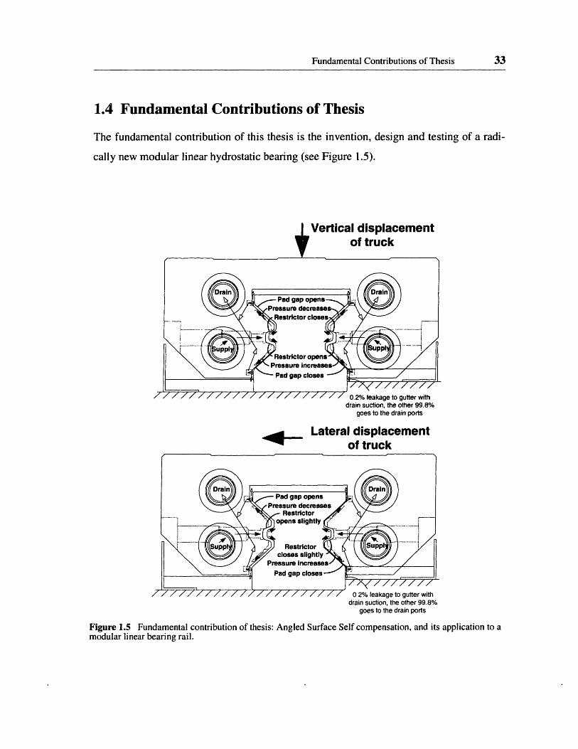
1.4 Fundamental Contributions of Thesis
The fundamental contribution of this thesis is the invention, design and testing of a radi-
cally new modular linear hydrostatic bearing (see Figure 1.5).
Vertical displacementof truck
goes to the drain ports
+am Lateral displacementof truck
drain suction, the other 99.8%goes to the drain ports
Figure 1.5 Fundamental contribution of thesis: Angled Surface Self compensation, and its application to amodular linear bearing rail.
34 INTRODUCTION
The core innovative feature, called angled surface self-compensation, is a set of auxiliary
restricting surfaces on a profile rail and truck that make an acute angle relative to each
load bearing pocket they supply.
This deceptively simple innovation, as will be explained in Chapter 2, leads to several
very significant manufacturing advantages over prior art hydrostatic bearing designs that
can be applied to a modular bearing rail. The fundamental advantages of the novel design
are summarized below.
Fundamental Manufacturing Advantages over Standard Hydrostatic Concepts
1. Only design known by author to be economical to manufacture using exist-ing manufacturing equipment of linear bearing manufacturers.
2. Truck is monolithic without intricate internal passages.
3. All critical precision features (restrictor and bearing pads) can be profileground in one set-up.
Fundamental Performance Advantages over Standard Hydrostatic Concepts
1. Feedback is the most efficient for vertical loading, where it is needed most.
2. More squeeze film area is present, providing better dynamic stiffness.
Fundamental Robustness Advantages over Standard Hydrostatic Concepts
1. Tolerant to dirt and "goo" because all gaps are subjected to shearing.
2. No passage between restrictor and pocket is present, so stiffness degradingair bubbles can't be trapped between.
Fundamental Marketing Advantage over Standard Hydrostatic Products
1. Bolt-for-bolt interchangeable with modular rolling element bearings (35, 45,55 etc.).

Fundamental Contributions of Thesis 35

36 INTRODUCTION

Chapter 2
COMPARISON OF DIFFERENTHYDROSTATIC DESIGNS
In this chapter, criteria are presented for a hydrostatic linear guide to be a viable commer-
cial product, and then seven possible hydrostatic bearing designs are compared in a
detailed design study.
2.1 Criteria for a Hydrostatic Guide to be a Viable CommercialProduct
Based on Alexander Slocum's and my experience working with several machine tool
companies and two major linear guide manufacturers, we developed the following criteria
for making a hydrostatic bearing into a viable commercial product:
Size
Must be bolt-for-bolt compatible with rolling element linear guides. Size 35, Size 45, and
Size 55 normal width and narrow width are most commonly desired. To gain extra load
capacity, we can use the long truck option as it will fit in most machines that use a stan-
dard truck length.
Manufacturing
1. Must be mass producable using profile grinding technology, which is alreadyin place and has proven to be economical for rolling element bearings.
2. Minimum number features to be machined and parts to be assembled. A onepiece rail and a one piece truck with a few holes and pockets is the ideal.
37

COMPARISON OF DIFFERENT HYDROSTATIC DESIGNS
Simplicity should be comparable to a rolling element linear guide minus therolling elements themselves.
3. "Grind and go" design - no hand tuning or delicate hand assembly of partsrequired.
Performance
1. Infinite life load capacities of 1000 lb, 1800 lb, and 2600 lb for sizes 35, 45and 55, respectively. These load capacities are adequate for most precisionmachine tool applications. While over a short travel life of 100 km, rollingelement guides can provide many times these load capacities, over 10,000km of travel, generally regarded as an "infinite" life, the load capacities ofrolling element guides are roughly comparable under ideal conditions. How-ever, if grit or excessive vibration is present, rolling element guides can failwell below 10,000 km, regardless of loading.
2. Static stiffnesses of about 3 Ib/uin, 5 b/uin, and 7 b/uin for sizes 35, 45, and55 respectively. These are comparable to typical rolling element guides witha medium preload.
3. A 1.5 hp, 4 gallon per minute pump required to power two linear axes with 8trucks (regardless of bearing size). It is desirable for the pressure to be keptbelow 700 psi so that less expensive hoses can be used.
Fluid
Depending on the application, water or oil can be used. The main motivation for using
water is for compatibility with a water based cutting fluid. However, since water is about
10 to 60 times less viscous than light and medium hydraulic oil, respectively, the pump
power required when using water will be 10 to 60 times greater at the same supply pres-
sure. Table 2.1 summarizes the advantages and disadvantages of using water versus using
hydraulic oil.
38

Novel Contributions Studied for Thesis
TABLE 2.1 Advantages and Disadvantages of Using Water Versus Using a Hydraulic Oil
Advantages
Not vulnerable to contamination of a waterbased cutting fluid
10 to 60 times less viscous drag
Particles are more difficult to filterPump life is less in some casesCan gum up small orificesErodes small pasageways faster
Because of the many difficulties of using water, for most machine tool applications it will
probably be easier to isolate the hydraulic oil using drain grooves and bellows.
Dirt Tolerance
1. Highly desirable if all restricting surfaces move so that any goopy blobswhich can cause clogging, (common in the water based machine tool cool-ants that may be used) can be sheared away. This feature would precludeusing orifices and capillaries for the final bearing.
2. Highly desirable if there is a means for large dirt chunks and chips, whichare inevitably in a newly plumbed system, to be flushed out of all the truckswhen they are first turned on by opening a valve. We want this featurebecause several of our older bearings used on machines clogged with chipsand dirt when they were first turned on, and they had to be taken apart atleast once to be cleaned. After the initial cleaning the bearings ran with noproblems. While meticulous flushing of the plumbing before assembly couldeliminate this problem, we would prefer to eliminate the need for suchmeticulousness.
3. Desirable is there is a means for small dirt particles that are nearly the size ofthe bearing gap to leave the bearing pockets through an escape path, withoutallowing excessive leakage out of the bearing. While we have found thatwith good filtration, bearings without this feature have run without problemsfor over 3 years, we would like extra insurance against a bad filter or asloppy filter change.
2.2 Novel Contributions Studied for Thesis
Figure 2.1 illustrates a novel feature and a novel design that will be studied in this thesis.
The significance of these innovations are discussed below.
.Disadvantages
10 to 60 times more pump power,causing heat which can reduce accuracyFluid system is at least 50% moreexpensive than comperable oil system
39

COMPARISON OF DIFFERENT HYDROSTATIC DESIGNS
Novel Feature toReduce Flow:
No drain groove between bearingpockets (NGBP)
Prior Art Applied to;Modular Rail:Planar bearing bads
Drain /Grinding
Relief
Novel Design to SimplifyManufacturing:
Angled Surface Self Compensation
Figure 2.1 Illustration of a novel feature and novel hydrostatic bearing design studied in this thesis, appliedto a modular linear rail.
Novel Feature: No Drain Groove Between Bearing Pockets (NGBP)
The idea is to have a continuous profile between the upper and lower bearing pockets on a
modular bearing carriage, rather than having planar bearing pads that are separated by a
drain groove. The benefit is that flow rate to the atmosphere is reduced by 40%, but the
penalty is that the vertical stiffness is reduced because a short exists between the upper and
lower pockets. The net benefits will be discussed in Section 2.3.
DrainF
i
I
I
I
i
)rain
P,
P,
40
I
0
I5
in

Novel Contributions Studied for Thesis
Novel Hydrostatic Bearing (Angled Surface Self Compensation)
The idea is to eliminate the need for capillaries, diaphragms, or complex internal passages
by using a special profile that has a set of angled restricting surfaces that feed each load
bearing pocket. To illustrate the concept, Figure 2.2 shows qualitatively how vertical and
lateral stiffness is achieved.
Lateraldisplacement
m og l-nf trl.rk
Figure 2.2 Illustration of how Angled Surface Self Compensation achieves vertical and lateral stiffness.
The major advantage of this design is that, unlike prior art concepts that are known to the
author, the angled surface design is the only one that can be manufactured using well
known processes and equipment that are already used by makers of modular rolling ele-
ment bearings (i.e. the angled surface design will not require investment and R&D into
unfamiliar manufacturing equipment or processes). Performance wise, the design provides
relatively high vertical stiffness but low lateral stiffness when compared to other designs.
These trade-offs will be discussed in more detail in the Comparison section.
�
41

COMPARISON OF DIFFERENT HYDROSTATIC DESIGNS
2.3 Design Concepts Considered
The purpose of this section is to present the compensation principle that underlies the prior
art and novel bearing designs that are studied and compared in this thesis. In simple lan-
guage, compensation is what makes a pocket pressure go up when the bearing gap closes,
and equivalently what makes a pocket pressure go down when the bearing gap opens.
Hence compensation provides static stiffness to a hydrostatic bearing. It is the way com-
pensation is achieved that distinguishes one hydrostatic bearing design from another.
2.3.1 Constant Flow Compensation
This method uses a constant flow source connected to each pocket to achieve compensa-
tion. The principle is as follows: as a bearing gap gets smaller, its resistance to flow goes
up, and because flow is forced to be constant, the pocket pressure must go up. A schematic
of a constant flow system is shown in Figure 2.3, along with the resistance circuit used to
model the bearing.
Fluid circuit for a fourpocket system using
constant flowcompensation
As bearing gapdecreases, pocket Left Rightpressure increases Pair Pairbecause resistance Each pocketgoes up while flow requires a
is forced to be separatew
Upper pocket bearingland resistance
Upper pocketpressure
h pocket requires aarate constant flowrce. This is a majorctical disadvantageause of the specialmp and numeroushoses required.
Figure 2.3 Constant flow compensation.
cor
42

Design Concepts Considered 43
The constant flow method is not studied in this thesis because it has a major practical
drawback. A standard constant pressure hydraulic system cannot be used to power it.
Instead, each load bearing pocket must have its own constant flow source. This results in
several major problems:
Major Problems With Constant Flow System
* Each pocket requires a constant flow pump and a separate hose (4 bearingtrucks must have at least 16 pockets, requiring 16 pumps and hoses).
* Compliance in long hoses will reduce static and dynamic stiffness.
m Flow ripple of pumps will make bearing vibrate, reducing accuracy, andaccumulators can not be used else static stiffness will be effected.
Since the author cannot think of a remedy to these problems, the constant flow system was
not studied in this thesis.
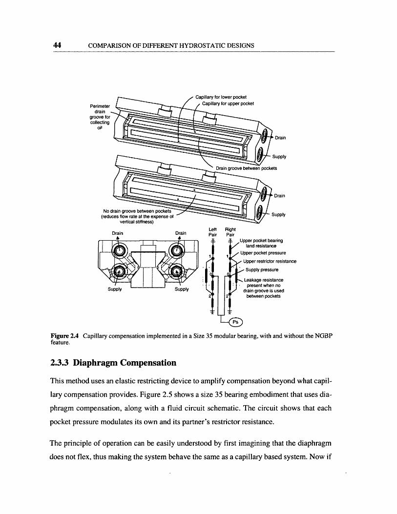
2.3.2 Capillary or Orifice Compensation
This method is the most commonly used in industry, and it is readily adapted to a modular
bearing profile. It uses a fluid resisting device (either a capillary or an orifice) placed in
series with each bearing pocket. The principle of operation is as follows: when a bearing
gap closes, its resistance goes up, dropping the flow rate through the capillary or orifice,
and in turn reducing the pressure drop that occurs across the capillary or orifice, thus
increasing the pressure in the bearing pocket. Figure 2.4 shows an implementation of cap-
illary compensation in a size 35 bearing, with and without a drain groove placed in
between the bearing pockets. The fluid circuit used to analyze the bearing is also shown.
COMPARISON OF DIFFERENT HYDROSTATIC DESIGNS
Perindra
groovcollec
oi
)rain
ipply
rain
pply
Left RightDrain Drain Pair Pair
Upper pocket bearingland resistance
1 1 Upper pocket pressureUpper restrictor resistance
I Go Supply pressure
Leakage resistanceI . present when no
drain aroove is usedj j 2 between pockets
Figure 2.4 Capillary compensation implemented in a Size 35 modular bearing, with and without the NGBPfeature.
2.3.3 Diaphragm Compensation
This method uses an elastic restricting device to amplify compensation beyond what capil-
lary compensation provides. Figure 2.5 shows a size 35 bearing embodiment that uses dia-
phragm compensation, along with a fluid circuit schematic. The circuit shows that each
pocket pressure modulates its own and its partner's restrictor resistance.
The principle of operation can be easily understood by first imagining that the diaphragm
does not flex, thus making the system behave the same as a capillary based system. Now if
44
Design Concepts Considered 45
To upper pocket on other sidef To lower pocket on other sidePerimeter
draingroove forcollecting
oil
No drain gr
Drain
Supply
Drain
Supply
restrictors
restrictor gaps to amplifyany pressure change.
Figure 2.5 Diaphragm compensation implemented in a Size 35 modular bearing, with and without theNGBP feature.
you imagine the diaphragm is allowed to flex, the low pressure pocket will be further
choked and the high pressure pocket will be further fed due to the gap change as the dia-
phragm flexes, hence increasing any difference in pocket pressure that would be present if
the diaphragm were rigid.

COMPARISON OF DIFFERENT HYDROSTATIC DESIGNS
2.3.4 Self Compensation with Internal Passages
This method uses miniature bearing lands that act as the restrictors [Slocum]. The fluid
flowing out of each restrictor is routed to an opposed bearing pocket via internal passages
or external hoses. Using this method, feedback is twice as effective as with a capillary sys-
tem, because each restrictor resistance changes in the opposite sense as each bearing resis-
tance. Figure 2.6 shows a size 35 bearing embodiment that uses self-compensation with
internal passages, along with a fluid circuit model.
Perimetdrain
groove Icollectir
oil
(rvertical stiffness) Left Right
Pair Pair
Figure 2.6 Self Compensation with Internal Passages implemented in a Size 35 modular bearing, with andwithout the NGBP feature.
46

Design Concepts Considered 47
2.3.5 Angled Surface Self Compensation
Like self compensation with internal passages, this method also uses miniature bearing
lands that act as restrictors, except that rather than using internal passages to carry fluid
from each restrictor to each pocket, each restrictor is placed right next to each bearing
pocket on an auxiliary surface that makes an acute angle relative to each pocket.
Figure 2.7 shows a size 35 bearing embodiment that uses self-compensation with angled
auxiliary surfaces, along with a fluid circuit model.
Perimeterdrain
groove forcollecting
oil
Drain
Supply
bearing
;t pressureictorpressurepressure
rs simulatingto pockets 1
and 2
Figure 2.7 Angled Surface Self Compensation implemented in a Size 35 modular bearing.
, .XX %. _..
e

COMPARISON OF DIFFERENT HYDROSTATIC DESIGNS
2.4 Overview of Analysis Issues
Prior to the comparison sections, the definitions of load capacity, minimum static stiffness,
and optimization scenarios are discussed.
2.4.1 Desired Load Capacity and Static Stiffness are Linked
In general, a designer must make a trade-off between a hydrostatic bearing's desired load
capacity and the minimum stiffness that it will provide when it is loaded with a force that
is less than or equal to the desired load capacity. Having said this, load capacity must be
clearly defined for a hydrostatic bearing system.
Definition of Load Capacity for a Hydrostatic Bearing: Load which canbe applied to the bearing in all directions that causes no more than an x %closure of the bearing gap.
Factors Effecting Choice of Max. % Gap Closure:
1. Trade-off between load capacity and stiffness. At a given supply pressure,or at a given pumping power, to achieve a relatively high static stiffness witha penalty of a relatively low allowed load capacity, the bearing should beoptimized using a relatively low max. gap closure (20% is relatively low inpractice). To achieve a relatively high load capacity with a penalty of rela-tively low minimum stiffness that occurs using allowed loads, the bearingshould be optimized using a relatively high max. gap closure (60% is rela-tively high in practice).
2. Max. tilt error expected for bearing pads. The chosen Max. gap closureshould be less than or equal to an amount that will prevent a corner of a mis-aligned bearing pad from touching down.
2.4.2 Checking for Minimum Static Stiffness
For optimization one must check the minimum static stiffness Ks(Fapl, 0 ap, OAF) of the 4
pad hydrostatic bearing system that occurs for all allowed loading scenarios. Given a max-
imum allowed force Flc, one needs to check the minimum stiffness that occurs in the zone
FapI <= Fc, 0apI = [ to 2nc], and 0aF = [0 to 7]. Figure 2.8 illustrates the parameters Fapl,
0ap1, and OAF.
48

Overview of Analysis Issues 49
Figure 2.8 Illustration of static stiffness in a hydrostatic bearing truck.
2.4.3 Two Optimization Scenarios
This section provides a discussion of two standard types of optimization normally sug-
gested for hydrostatic bearings. For ease of understanding, these scenarios are presented in
a Given, Find format.
Scenario 1: Pumping Power is Primary Concern, Hydraulic System can Supply Mostany Supply Pressure Required.
Given: External Dimensions Do, Max. Allowed Load Fic, Pump Power Wp
Find: Internal Dimensions D1 which maximize the min. stiffness Ks thatoccurs in the zone Fapl <= Flc, 0 apl = [0 to 27t], and 0AF = [0 to 7t]
Illustration of Fapl, Oapl and OaF in Static Stiffness
Ks(F,p, Oapl, AF)
1
COMPARISON OF DIFFERENT HYDROSTATIC DESIGNS
Scenario 2: Practical Limit on Available Supply Pressure Due to Nature of PumpSystem, Pump Power is of Secondary Importance.
Given: External Dimensions Do, Max. Allowed Load Flc, Supply PressurePs, and Max. Allowed Pump Power Wpmax
Find: Internal Dimensions D1 which maximize the min. stiffness Ks thatoccurs in the zone Fapl <= Flc, Oapl = [ to 2i7], and 0AF = [O to n]
2.4.4 Thermal Control of Fluid: Area for Future Work
For use in machine tools, it should be noted that the reason one wants to keep pump power
low is not primarily because of pump system cost, it is because one wants as little heat as
possible transferred to the machine bed. It should be noted that what really matters is
keeping thermal drift of the machine tool to a minimum. A non optimal pump power
may not matter, so long as the fluid temperature can be kept as constant as possible
using a chiller system to keep the thermal drift of the machine to a minimum. Based
on this insight, the author poses the following questions and hypothesizes answers which
point the way to future work.
Question 1: For accurate temperature control of the machine bed, at a given pumppower and viscosity which is better: Low Ps and High Q, or High Ps and Low Q?
The author hypothesizes that Low Ps, High Q is better because the temperature rise of the
oil will be less for the latter scenario, and it is likely a smaller temperature rise is more
desirable from a controls standpoint.
Question 2: Is it worthwhile to design for low Ps without regard to pump power toallow for accurate temperature control of the bearing fluid?
The author hypothesizes that in the end designing for low Ps at a given load capacity
requirement and viscosity will make little difference over using a design optimized for
minimum pumping power. However he welcomes proof to the contrary. The author
believes that proper choice of viscosity will make a much bigger difference on thermal
controllability and stability.
50
Overview of Analysis Issues 51
Question 3: Given the average travel velocity of the carriage, what fluid viscosityshould be chosen to allow for temperature control which ultimately optimizesthermal stability of the machine tool?
For brute force accurate control of fluid temperature, one would choose a low viscosity
because this will reduce shear power, which is variable, at the expense of pump power,
which is steady and hence controllable. The unanswered question is how low should the
viscosity choice be before the large pump power significantly effects thermal drift of the
machine.
2.4.5 Approximations Made for Analysis of Hydrostatic Designs
The following approximations were made in predicting load capacity and stiffness of the
different hydrostatic designs. Most of these assumptions tend to make the predicted per-
formance better than what an actual production bearing will provide, so the resulting anal-
ysis is an optimistic estimate of bearing performance.
1. No bearing gap errors present.
2. Effect on gamma due to initial elastic deflection caused by initial pocketpressures not accounted for. However, gaps could be ground so that theyopen to what they should be.
3. Effect of elastic deflection on static stiffness was accounted for in a roughfashion: a hydrostatic compliance Chy (1/stiffness) was first computed in agiven direction 0 AF, assuming a perfectly rigid truck, and then it was addedto an effective elastic compliance Ceffe in direction OAF. For the size 35 truckwith L=164mm, Ceffe(OAF) was computed by making elliptical quadrantsfrom a lateral elastic compliance reference of Ceffex = 1/1400 (m/N), a ten-sile elastic compliance reference of Ceffey(+) = 1/2500 (rm/N), and a com-pressive elastic compliance reference of Ceffey(-) = 1/3000 (m/N).
4. For the diaphragm system, it is assumed the diaphragm is tuned so that itgives the same static feedback as a self compensating bearing. It should benoted that the elastic compliance of the truck will result in a diminishingreturn in increasing hydrostatic stiffness, and there is not a great benefit todesigning for extremely high hydrostatic stiffness.
5. The effect that the (NGBP) feature has on diminishing pocket pressures wasaccounted for roughly by reducing the difference between the upper andlower pocket pressures computed with a groove by 20%. This was deter-

COMPARISON OF DIFFERENT HYDROSTATIC DESIGNS
mined to be reasonable based on an approximate analysis for a capillary sys-tem.
2.5 Comparison of Hydrostatic and Rolling Element Systems
In this section, the size 35 embodiments shown in the Design Concepts section are com-
pared. A size 35 was chosen for this study because its sells the most to machine tool com-
panies. While other common sizes (30, 45, and 55) are not compared, their proportions are
within a few percent and hence the relative performance will be similar.
To allow the reader to quickly assimilate the current state of knowledge of the author, key
information predicted for the size 35 hydrostatic embodiments and size 35 ball and roller
bearings currently on the market have been tabulated for quick comparison in three cate-
gories: Load capacity and stiffness, manufacturability, and robustness. Each matrix is pre-
sented first, then plots are presented to supplement the matrices.
52

Comparison of Hydrostatic and Rolling Element Systems 53
2.5.1 Load Capacity and Stiffness Comparison MatrixTABLE 2.2 Load Capacity and Stiffness Comparison Matrix of Size 35 Hydrostatic and Rolling ElementSystems
Load Capacity and Stiffness Comparison Matrix of Size 35 Desins I. I
Eto
aCC
.
o0-Jcn
C,
Size 35 Hydrostatic systems (Predicted)(L=164mm long truck) KNCapillary (D = 0.2 mm, L = 10mm) ??'Capillary NGBP ??Diaphram ??'Diaphram NGBP ??'SC, Internal passages ??'SC, Internal passages NGBP ??'SC, Angled surface ??
Size 35 Ball Systems (From Catalogue)rhomson, L=109mm 3% 47Thomson, L=109mm 8% 47Thomson, L=109mm 13% 47
0Eco
C3
.0
03.a
C)
r000
ci,
KN??????????????
4747
47Thomson, L=134mm 3% 66 66Thomson, L=134mm 8% 66 66homson, L=134mm 13% 66 66
'tar, L=105mm 8% 54 54Star, L=133mm 8% 81 81Size 35 Roller Systems (From Catalogue)'homson, L=109mm 3% 80 80Thomson, L=109mm 8% 80 80Thomson, L=109mm 13% 80 80itar, L=1' 4mm 13% 114 114itar, L=138mm 13% 149 149cchnecberger, L=109mm 3% 93 93
Schneeberger, L=109mm 8% 93 93Schneeberger, L=109mm 13% 93 93Schneeberger, L=136mm 3% 129 129Schneeberger, L=136mm 8% 129 129
Schneeberger, L=136mm 13% 129 129
.E0.C
co.N 0
E CD
3e-
E-co(9 C
CD
V)00
Ca 0 E 2
CCCR al ao
.0 0
Eco 4Ž0c ( CbC a
7, 11
CDO C6 C
00..X000oIIg
.2CL
0Oo
o2a;a
M.
E0cI
i3amma bo Ps Flow
# mm Bar Ipm2.9 4.5 112 0.542.7 4.7 151 0.408.4 4.4 172 0.356.4 5.2 225 0.278.5 4.0 129 0.477.5 4.0 142 0.42:L.5 2.3 114 0.52
Load values shown forrolling elements basedon DIN ISO 281 with10A4 km Life and1% Failure Rate
I
Q.
oE
E0
II
O4 '' 30
°
v a
-J
U:
E
O.
to0.
'O
co0.00
4)0
FIcKN %9.9 100%12.0 121%17.6 178%20.5 207%11.0 111%
11.3 114%9.5 96%
KN %3.6 36%2.0 20%0.0 0%
5.3 53%3.0 30%0.0 0%
2.3 24%3.1 31%
7.3 74%5.4 55%1.9 19%
2.3 23%2.9 29%8.2 83%6.0 61%2.1 21%11.2 114%8.3 84%
2.9 30%
o
'ao
0c',
00(D
coCo.,
0CD>0
-0E ,
coa0 o_ 01
Kmin
0Cr-
o 0nc Eo >a aa: E
O EO ._E r
_ E
For Hydrostatic Systems,Truck Length L=164mmAt Same Pump PowerWp = 100 W per truck,u=60 cSt, h=20um
Load cap. scaling: Wp(0.5)Stiffness Scaling: WpA(0.4)Wp scaling: 1 /
439 100% 2.2 200469 107% 2.2 214624 142% 2.2 285636 145% 2.2 291419 95% 2.2 191400 91% 2.2 183315 72% 2.2 144
N / Hm % Q Kdyn250 57% 5.5 45400 91% 5.5 73500 114% 5.5 91320 73% 5.5 58512 117% 5.5 93640 146% 5.5 116500 114% 5.5 91669 152% 5.5 122
N / lm % Q Kdyn667 152% 10.6 63714 163% 10.6 67769 175% 10.6 731000 228% 10.6 941261 287% 10.6 119541 123% 10.6 51833 190% 10.6 791111 253% 10.6 105706 161% 10.6 671089 248% 10.6 103
1452 331% 10.6 137
'Designs with features unique to thesis?? Shock load capacity will be superior to rolling elements, however prediction is beyond the scope of this thesis
I I I I - I I I1. W
COMPARISON OF DIFFERENT HYDROSTATIC DESIGNS
Table 2.2 shows the predicted performance of different Size 35 hydrostatic designs operat-
ing with 100W per truck, oil viscosity of 60 cSt (60 times more viscous than water; a
medium weight oil) and with a 20 micron nominal bearing gap, compared to existing ball
and roller bearing systems. The 20 micron gap was determined to be practical given pro-
duction tolerances and mounting tolerances allowed for rolling element bearings. The 60
cSt was chosen because it is typical for machine tool hydraulic systems. The Wp=100W
per truck was chosen as a reasonable value for machine tools. The load capacity scales
with WpA0.5 and the static stiffness scales roughly with Wp^0.4 (if the truck and rail were
perfectly rigid, scaling would precisely be Wp^0.5).
2.5.2 Static and Shock Load Capacity Discussion
These two categories refer to the maximum static load and sudden shock load a bearing
can support before permanent damage occurs. As stated in most product catalogues, the
static and shock load capacities of ball and roller systems are the same and are a result of
permanent deformation of the races due to hertzian stress. The failure quantities shown
were obtained from the product catalogues.
Due to squeeze film damping, those experienced with fluid film bearings know that fluid
bearings have a much greater shock load capacity than rolling element bearings of the
same size. Static load capacity will also be much higher, but if touch down occurs while
the bearing is moving very slowly, galling could result. Predicting galling and shock load
capacity is beyond the scope of this thesis and has been left as an area for further research.
2.5.3 Load Capacity Versus Life Comparison Plot
To fully understand how hydrostatic systems compare with rolling element systems in
terms of load capacity, one must look at the load versus life curve shown in Figure 2.9.
54
Comparison of Hydrostatic and Rolling Element Systems 55
Comparison of Hydrostatic and Rolling Element Load Capacity Vs. Lifeand Rolling Elements with 10% and 1% Fatigue Failure
according to DIN ISO 281
Premature rolling element failure-Fretting-Hard particles and subricron sw arf
Load Causing X% Failure-, According to DIN ISO 281
" LL L=136 mm (Long Truck)oI . Hydrostatic Systems,
Roller Systems (Star and Schneeberger) Truck Length L=164mm
-- Light Preload (3%C) At Same Pump Power
tF=60 cSt, hb=20um-- Heavy Preload (13%C) Load cap. scaling: Wp(0.5)
Ball Systems (Thomson and Star) Stiffness Scaling: Wp(0.4)-- Light Preload (3%C)Wp scaling: 1 / u
-- Medium Preload (8%C)*Diaphram NGBP, 246 Bart l - .-- agy Relad (3%C)-r1
l\ .Z 9 .~~ L o__~ -Diaphran 179 Barit \I /. -- --*Capillary NGBP, 157 Bar/*SC, Internal passages NGBP, 145 Bar
I *SQ hternal passages, 129 Bar
-- L ' ^r, 11y 44Bar
C------ ------------- _____I..
- lIt I5000 10000 15000 20000 25000 30000 35000 40000
1.6 3.2 4.8 46.4 1sye I ar years lyears Iyears I
45000 50000
[3.0I BearLLoads required in amachine tool
Travel Time at 0.2 m/s Travel Life (kn); 124 hrs/day, 365 days/yr I
Figure 2.9 Load versus life of rolling element bearings shown with hydrostatic bearing designs operating at100 W per truck.
Conclusions from Load Versus Life Plot:
1. For a typical bearing load on a size 35 truck, under normal conditions andassuming perfect mounting, 99% of lightly preloaded ball systems andmedium and a lightly preloaded roller system will essentially last forever.
40
35
30
UU0.UcocoUM
IZ
25
20
15
10
Heavy -5
Typical . n
I
It- -
-1
.0anr
I
--
!
L --
--
I
A
0
9

COMPARISON OF DIFFERENT HYDROSTATIC DESIGNS
2. For a heavy bearing load on a size 35 truck, under normal conditions andassuming perfect mounting, 99% of lightly preloaded roller systems willessentially last forever.
3. In a real machine, mounting errors and thermal growth of the machine car-riage can cause higher forces than those shown. The force can be estimatedusing the static stiffness of a truck and the estimated error displacement.
4. All hydrostatic designs provide more than enough load capacity at 100 W.The diaphragm systems can offer the best load capacity when optimized for60% gap closure, while the other designs are fairly close.
5. The NGBP feature boosts load capacity by about 20% for the Capillary andDiaphragm systems, but provides little benefit for Self Compensation withInternal Passages.
6. Angled Surface Self Compensation provides a load capacity close to Capil-lary and Internal Passage designs.
2.5.4 Static Stiffness Comparison Plots
To have a more complete understanding of how hydrostatic systems compare with rolling
element systems in terms of static stiffness, it is helpful to look at the initial static stiffness
versus direction 0AF of the perturbing load. Figure 2.10 shows such a plot.
Conclusions from Initial Static Stiffness Plot:
1. Hydrostatic designs operating at Wp = 100W will have a static stiffnesscomparable to a medium to heavy preloaded ball system. Hydrostatic stiff-ness scales roughly with WpA(0.4).
2. A heavily preloaded roller system will be 2 to 3 times more statically stiffthan the hydrostatic designs operating at 100W per truck.
For the hydrostatic designs, the minimum static stiffness Ksmin was computed at Fap =
Flc for several directions ap1. The result is shown in Figure 2.11..
Conclusions from Final Static Stiffness Plot:
1. The diaphragm system can provide the best all around static stiffness, whilethe other designs are comparable in terms of stiffness magnitude.
2. The angled surface design differs from the others fundamentally in that itsminimum stiffness occurs laterally, while for the others it occurs vertically.The advantage of this attribute depends on the application.
56

Comparison of Hydrostatic and Rolling Element Systems
Figure 2.10 Initial static stiffness (based on catalogue data) of rolling element bearings versus OAF shownwith hydrostatic bearing designs operating at 100 W per truck.
57
COMPARISON OF DIFFERENT HYDROSTATIC DESIGNS
Min. Static Stiffness at F,: Ksmin(D,, F,,--=F,, o,, 0F=[0,n1) ofOptimal Designs Vs. o0,
Size 35, Wp = 100W, u = 60 cSt, h,, = 20 gm
Min. static stiffness at Fc actingin direction A,,, for all 6e
Figure 2.11 Minimum final static stiffness versus 0ap shown for hydrostatic bearing designs operating at100 W per truck.
_ _ I __ _ _ _ _ _ _ __ ______ _ __ _ ____
I _ _ _ _ _ _
58

Comparison of Hydrostatic and Rolling Element Systems
2.5.5 Dynamic Friction Comparison Plots
Figure 2.12 shows a plot of dynamic friction of a size 35 roller bearing system versus a
hydrostatic system operating with different oil viscosities.
Figure 2.12 Friction force versus travel velocity for rolling element systems and hydrostatic systems oper-ating at different oil viscosities.
I.
59
COMPARISON OF DIFFERENT HYDROSTATIC DESIGNS
In order to draw meaningful conclusions, it is helpful to look at friction power per truck
versus the travel velocity.
Conclusions from Friction Power Versus Travel Velocity Plot:
1. The friction power of a rolling bearing becomes significant beyond 1 m/s. Itis known that roller systems overheat severely if they are not actively cooled.
2. A hydrostatic system produces lower friction power at high speeds and theheat can be actively removed by a chiller system, along with pumpingpower. The cooling means coupled with low friction power is a major advan-tage of a hydrostatic bearing for high speed machining.
2.5.6 Manufacturing Comparison Matrix
Table 2.3 compares the manufacturability of the different hydrostatic designs. Each crite-
ria is discussed below.
60
Comparison of Hydrostatic and Rolling Element Systems
Figure 2.13 Friction power versus travel velocity for rolling element systems and hydrostatic systems oper-ating at different oil viscosities.
I
61
62 COMPARISON OF DIFFERENT HYDROSTATIC DESIGNS
TABLE 2.3 Manufacturing Comparison Matrix
0==
c0 a8 0C 'E
C
(( 0 UoE
0.
C0
CD
O)co._
0
a
.a
oa)'O
ccQ.c/)a
10._
ED)R._
{/)o
cca)
Size 35 Hydrostatic systems (Predicted)
Capillary (D = 0.2 mm, L = 10mm No ??
*Capillary NGBP No ??
Diaphram No ??*Diaphram NGBP No ??
'SC, Internal passages No ??'SC, Internal passages NGBP No ??
'SC, Angled surface Yes Yes
NoNoNoNoYesYesYes
NoNoNoNo
YesYesNo
NoNoNoNoNoNoNo
NoNoNoNoNoNoNo
Can Be Made "Right Now"
Of all the hydrostatic designs studied for this thesis, the angled surface design is the only
one that can be made economically using the existing equipment used by makers of rolling
element linear bearings. To make any of the other designs, further investigation will be
required into manufacturing methods to find an economical means for production. The
problem with each of the other designs is discussed below.
Capillary Systems: One issue is the capillary needed will have dimensionsD = 0.2 +/-0.005 mm, L = 10 mm) In small quantities the cost for such acapillary is about $75 each, although research may uncover a cheapersource. The target manufacturing cost for an entire bearing truck is $300.Another issue is assembling the capillaries into the bearing truck.
Diaphragm Systems: These are much more complex than a capillary sys-tem, so cost is even more of an issue.
.2e-
'5C0c:.0Ccao
Manufacturina Comoarison Matrixl IE S | . - z .
a).rCt

Comparison of Hydrostatic and Rolling Element Systems
Self Compensation With Internal Passages: The difficulty is making theinternal passages. A lost wax or 3-D printing method could be used, butneither are economical enough.
Can Be Monolithic
Of all the designs considered, only the angled surface design can be made in one piece.
This relates to its economy.
All Precision Features Can Be Ground in One Set Up
By definition, all self compensating designs have this attribute, and other designs do not.
This attribute relates to the number of steps required for manufacturing, and hence relates
to the bearing's economy.
Sensitivity to Manufacturing Errors
Only self compensation with internal passages is insensitive to spread error. All the other
designs are sensitive to all types of error. The relative sensitivity of each design will likely
be similar, but further analysis will be required.
2.5.7 Robustness Comparison Matrix
Table 2.3 compares the manufacturability of the different hydrostatic designs. Each crite-
ria is discussed below.
63
COMPARISON OF DIFFERENT HYDROSTATIC DESIGNS
TABLE 2.4 Robustness Comparison Matrix
0cC
XEr-
¢0EC0
>
XoZ
_(3m
EE 0
0 CDa.a O
X 00 ._ a)Da0
o0W C)0
C)co-'S co
Q 3E X0 3s
E
_ II
I3c) 840
QOX "CD 0Eq -
Size 35 Hydrostatic systems (Predicted)
Capillary (D = 0.2 mm, L = 10mm) No
*Capillary NGBP NoDiaphram No
*Diaphram NGBP No'SC, Internal passages Yes'SC, Internal passages NGBP Yes'SC, Angled surface Yes
YesYesNoNoNoNo
Yes
YesYesNoNoNoNo
Yes
7.9
8.6
12.2
12.0
7.7
8.2
8.7
3.0
3.2
4.6
4.5
2.9
3.1
3.3
Shearing at all Restricting Surfaces (Self Cleaning)
A major advantage of the self compensating designs is that shearing occurs at all restrict-
ing surfaces, thus shearing away "goo" that may be present in the hydraulic oil. The other
designs are vulnerable to clogging over time.
Can be Hydraulically Clamped to One Side of Rail
This means that oil can be supplied to one half of the bearing truck, thus locking it to one
side of the rail. This can be useful for aligning the trucks to the rail when the machine tool
is being assembled.
5 DOF Stability Feasible
All designs presented are not stable in tilt; they must be bolted to a carriage plate with at
least two other trucks. However, if one would want a single truck to have tilt stability, this
C
m
U,(co
t5Q)O
C(a0c)
C
cn.@
:.
U-1LA
64
Robustness Comparison Matrix
= ~ ~ ~ ~ ~ _
.
n-w-l -
w -
Conclusions of Design Study 65
is only practical for the capillary and the angled surface designs. The other designs would
be prohibitively complex and would have a greatly reduced bearing area.
Lateral Displacement that Reduces Load Capacity to 5000N (for Benchmarkoperating conditions)
A major concern for some applications is lateral displacement imposed on the trucks due
to thermal expansion of a spindle carriage. For the benchmark conditions, the diaphragm
designs are most tolerant to such an expansion, while the other designs are comparable.
2.6 Conclusions of Design Study
The following conclusions are drawn from the preceding design study:
1. For ordinary operating conditions, a medium or lightly preloaded roller bear-ing will work well. For long life, a hydrostatic bearing will only be usefulwhen severe vibration is present.
2. The static stiffness of hydrostatic designs will be about the same as amedium to lightly preload ball system.
3. For high speed machining at greater than 0.3 m/s, the inherent coolingattribute of the hydrostatic systems is a major advantage over rolling elementbearings.
4. The angled surface hydrostatic design has strong manufacturing advantages,and its load capacity and all around stiffness are comparable to all designsexcept the diaphragm systems. Therefore, it is a good choice for furtherdevelopment.

66 COMPARISON OF DIFFERENT HYDROSTATIC DESIGNS

Chapter 3
LUMPED PARAMETER BEARINGMODEL
The goal of this chapter is to create a model which can predict bearing load capacity,
stiffness, friction, flow rate, and pump power of a bearing truck given the external
dimensions, rail profile, bearing gaps, and bearing gap errors. Each section shows the
steps involved.
An accurate bearing model is needed so that the best trade-off between load capacity in the
presence of gap errors and pumping power can be made. In production, the bearing gaps
along a typical profile can vary by about +/-5 micrometers (each profile can vary +/- 2.5
microns), and unfortunately, this is a significant portion of a typical bearing gap of 20
micrometers or so that will give a reasonable pump power. If we choose a larger gap to
boost load capacity in the presence of errors, pump power goes up with the cube of the
gap, and thus the pumping power quickly goes up. If we choose a smaller gap to lower
pump power, load capacity can be severely hampered given the worst case profile errors.
In order to be sure we are making a good compromise between load capacity in the
presence of errors and pumping power, an accurate model is needed.
3.1 Profile Geometry
For this thesis, a profile for either the truck or rail is defined as being a chain of flats
connected by rounds. This section shows how a such a profile is represented in arrays,
how unknowns in such a profile can be computed, how gaps are represented, and how a
67

LUMPED PARAMETER BEARING MODEL
slave profile can be computed from a master profile and the gaps between the slave and
the master profiles.
3.1.1 Representing a Profile of Flats and Rounds
For the purpose of modeling, each flat or round on a right or left profile is assigned a
number i, an angle T(i,rl), and a length or radius (as the case may be) dimension S(i,rl),
where rl=l is for a parts' right profile, and rl=2 is for a parts left profile. Figure 3.1 shows
a generalized back to back profile used to model the Hydrorail, with some sample T(i,rl)
and S(i,rl) values to show what they mean.
Generalizedh.1. -. har- Rinht nrnfil
Profile
Angles(deg)
T(i,rl) T(1,1) = 0T(2,1) = -22T(3,1) = -44T(4,1) = -44
T(16,1) = 22
Ect.
ArraysLength orRadius(mm) Surface
S(i,r) typeS(1,1)= 2.0 FlatS(2,1) = -0.9 Convex radiusS(3,1) = 4.0 FlatS(4,1) = 4.0 Flat
S(16,1) = 0.9 Concave Radius
Ect.
R+
R
Figure 3.1 A profile of flats and rour.ns is represented in an angle array T(i,rl) and a length array S(i,rl).
3.1.2 Computing x and y Distances on a Profile
Given T(i,rl) and S(i,rl) of a profile, it is often necessary to compute the x and y
coordinates of one point relative to another point on the profile. Figure 3.2 describes the
four types of distances which are routinely computed from T(i,rl) and S(i,rl) from a
distance finding function FnDpr[cs, i, j, T, S, rl, xy].
68

Profile Geometry 69
Distance Finding Function FnDpr[cs, i, j, T, S, rl, xy]cs = 1, FnDpr = distance from lead of segment i to trail of segment jcs = 2, FnDpr = distance from lead of segment i to midpoint of segment behind jcs = 3, FnDpr = distance from lead of segment i to center of radius jcs = 4, FnDpr = distance from center of radius i to center of radius jrl = 1 for right profile, rl = 2 for left profilexy = 1 for x direction, xy =2 for y direction Right profile
Examples of the 4 types odistances described above
FnDpr[1,O,10, T, S, 1,2]FnDpr[2,0,10, T, S. 1,2]FnDpr[3,0,12, T, S, 1, 2]
FnDpr[4,2,12, T, S, 1, 2]
(rl 1), - midpoint of segment i
1 tangent point (can be,'- a lead or a trail)
:nDprl1,3,5, T, S, 1, 1]:nDpr[2,3,6, T, S, 1, 1]
;nDpr3,3,6, T, S, 1, 1]:nDprf4,2,8, T, S, 1, 1]
Figure 3.2 Four types of distances frequently computed from a profile of flats and rounds.
The distance finding function FnDpr[cs, i, j, T, S, rl, xy] was coded using the geometric
relationships shown in Figure 3.3 for a flat segment "i" and a round segment "i".
dx and dy for a flat
Tangent point
I Midpoint of fl,
dylT( i ) T((i)dxl
dy2 T(i
dx2
dxl = S(i)/2Sin[T(i)]dx2 = S(I2'Sin[T(i)]dyl = -S(i)/2*Cos[T(i)]dy2 = -S(i)/2*Cos[T(i)]
dx and dy for a roundy,T When "i" is a roundL x T(i)=(T(i-1)+T(i+ 1))/2
T(i-1) S(i) + = concave radius (as shown)at i Sa (i)- = convex radius
dxla dx2ady2a T(i+1)
dx2
Tangent point i+lMidpoint of round i
dxla = S(i)*Cos[T(i-1)]dx2b = S(i)*Sin[T(i-1)dyla = S(i)*Cos[T(i+l)]dy2b = S(i)*Sin[T(i+l)]dxl = dxla - S(i)*Cos[T(i)]dx2 = S(i)*Cos[T(i)] - dx2adyl = dyla - S(i)*Sin[T(i)]dy2 = S(i)*Sin[T(i)] - dy2a
Figure 3.3 The dx and dy increments for a flat and a round segment "i", used to code the functionFnDpr[cs, i, j, T, S, rl, xy].
v
LUMPED PARAMETER BEARING MODEL
3.1.3 Profile Constraints and Unknowns
For the design study later in this thesis, a face to face and a back to back design is consid-
ered. The two designs can both be fully represented by the T(i,rl) and S(i,rl) arrays. An
important operation is to compute unknown T(i,rl) and S(i,rl) values given dimension con-
straints on the rail and truck. Figure 3.4 lists the constraints on a Size 35 modular bearing
sets up the geometry problem to be solved for both the face to face and back to back
designs.
3.1.4 Representing Bearing Gaps
At the midpoint of segment i (for i up to i=21 only), a bearing gap H(i,rl) is present.
Figure 3.5 shows some example H(i,rl) values. As will be shown in later sections, the mid-
point values H(i,rl) will be used to compute the fluid resistance and affective area of vari-
ous gap regions.
3.1.5 Computing a Slave Radius from Three Gaps
For the most general design case, the design gap at the midpoint of a round can be set
independently of the design gaps at either of the neighboring flats. In order to compute a
complete slave profile that will provide the desired gaps relative to a master profile, a
means is needed to compute the magnitude of a slave radius, given the magnitude of a
master radius and the three desired design gaps associated with it. Figure 3.6 shows show
a step by step procedure for how a slave radius and the x and y coordinates of its center
have been computed from a master profile.
3.1.6 Profile Dimensions Sent to ProE Solid Model
For the sake of efficiency and to reduce data transfer hassles, the code written to model
bearing performance computes all of the profile dimensions needed to drive a ProE solid
model. To avoid any stack up errors (PrGE regenerates to no better than 0.1 of a micron,
which may cause a stack-up problem if serial the dimensions S(i,rl) are used) the magni-
70

Profile Geometry
Practical Face to Face Practical Back to Back
Constraints for Size 35 Face to Face Profile:h total = 48 mmh above rail >= 0.5 mmh plate >= 11.5 mm Therefore hrail <= 36 mmhtop = 3 mm with cover strip, 0 mm withouthu >= 5.5 mmwrail = 34 mmdh = 13 mm (Head DIA of M8 screw)ci >= 1 mmc2 >= 3 mm
Setting above to minimum allowed values to maximize pad area:hactive = 27 5 mm with cover strip, 30.5 mm withoutwmin = 10.5 mm
Geometery Problem that is Solved:Given' htotal, hu, htop, wmin, wrail, ws
All T(i) except i = evenAll S(i) except i = 4,18,23,25,27
Find: All unknown T(i) and S(i) values
Constraints for Size 35 Back to Back Profile:h total = 48 mmh above rail >= 0.5 mmh plate >= 11 5 mm Therefore hrail <= 36 mmhtop = 3 mm with cover strip, 0 mm withouthu >= 5.5 mmwrail = 34 mmdh = 13 mm (Head DIA of M8 screw)c1 >= 1 mmc2 >= 1.5 mm
Setting above to minimum allowed values to maximize pad area:hactive = 27.5 mm with cover strip, 30.5 mm withoutwmin = 9 mm
Geometry Problem that is Solved:Given: htotal, hu, htop, wmin, wrail, dw, Tave=(T(3)+T(17))/2
All T(i) except i = even,3,5,17,19All S(i) except i = 4,18,25,27
Find: All unknown T(i) and S(i) values
Figure 3.4 Constraints used on Size 35 Face to Face and Back to Back designs.
tude and absolute x and y center coordinates of each profile radius were sent to the ProE
models of both the rail and truck. For the rail (the master profile), FnDpr[cs=4, i, j, T, S, rl,
xy] function was used to compute the x and y center coordinates of each round, using
T(i,rl) and S(i,rl). For the truck (the slave profile), a slave radius function is used to com-
71
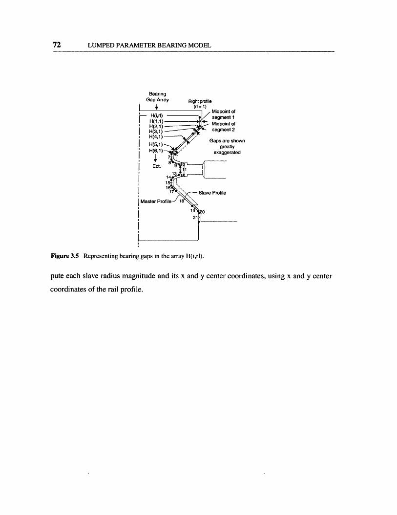
LUMPED PARAMETER BEARING MODEL
BearingGap Array Right profile
Figure 3.5 Representing bearing gaps in the array H(i,rl).
pute each slave radius magnitude and its x and y center coordinates, using x and y center
coordinates of the rail profile.
72
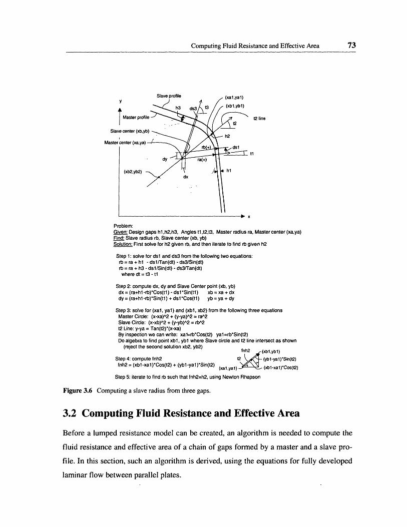
Computing Fluid Resistance and Effective Area
y
t Master profi
Slave center (xb,y
Master center (xa,ya)
73
t2 line
tl
(xb2,yb2)
Problem:Given: Design gaps hl ,h2,h3, Angles tl ,t2,t3, Master radius ra, Master center (xa,ya)Find: Slave radius rb, Slave center (xb, yb)Solution: First solve for h2 given rb, and then iterate to find rb given h2
Step 1: solve for dsl and ds3 from the following two equations:rb = ra + hl - ds1/Tan(dt) - ds3/Sin(dt)rb = ra + h3 - dsl/Sin(dt) - ds3/Tan(dt)where dt = t3 -tl1
Step 2: compute dx, dy and Slave Center point (xb, yb)dx = (ra+hl-rb)*Cos(tl) - dsl Sin(tl) xb = xa + dxdy = (ra+hl -rb)*Sin(tl) + ds *Cos(tl) yb = ya + dy
Step 3: solve for (xal, yal) and (xbl, xb2) from the following three equationsMaster Circle: (x-xa)A2 + (y-ya)A2 = raA2Slave Circle: (x-xb)A2 + (y-yb)A2 = rbA2t2 Line: y-ya = Tan(t2)*(x-xa)By inspection we can write: xa1=rb*Cos(t2) yal =rb*Sin(t2)Do algebra to find point xbl, ybl where Slave circle and t2 line intersect as shown
(reject the second solution xb2, yb2) fnh2 (xb1,yb1)
Step 4: compute fnh2 t2 > (yb1-ya1)*Sin(t2)fnh2 = (xbl-xal)*Cos(t2) + (ybl-yal)*Sin(t2) (xal yal) (xb1-xal)Cos(t2)
Step 5: iterate to find rb such that fnh2=h2, using Newton Rhapson
Figure 3.6 Computing a slave radius from three gaps.
3.2 Computing Fluid Resistance and Effective Area
Before a lumped resistance model can be created, an algorithm is needed to compute the
fluid resistance and effective area of a chain of gaps formed by a master and a slave pro-
file. In this section, such an algorithm is derived, using the equations for fully developed
laminar flow between parallel plates.
o! .... '.'{lA
lb"
LUMPED PARAMETER BEARING MODEL
3.2.1 Validity of Fully Developed Laminar Flow
This section shows that the assumption of fully developed laminar flow is valid for practi-
cal bearings studied in this thesis.
According to Fox and McDonald, flow between parallel plates is laminar when Reynolds
number Reh = (Pumh)/lp < 1400, where p is fluid density, um is mean flow velocity, h is the
bearing gap, and ji is the fluid viscosity. According to Shah, the length of undeveloped
flow between parallel plates Lhy is
Lhy = 0.011DhReDh (3.1)
where hydraulic diameter Dh and Reynolds number ReDh are
Dh - (4Area)/(Perimeter) (3.2)
Reh P Dh (3.3)
In order to study how ReDh and Lhy vary with typical bearing design conditions, it is con-
venient to express ReDh and Lhy in terms of a pressure difference (Pa-Pb) which forces a
flow of fluid with properties p and v through a bearing restrictor with a gap h and a land
length L. Assuming fully developed flow occurs the mean flow velocity is
h 2
U 1 (Pa Pb) (3.4)
The above expression, along with the definition
_ ppv (3.5)
and the hydraulic diameter for a small gap between parallel plates
Dh =2h
.74
(3.6)

Computing Fluid Resistance and Effective Area
yields the following convenient expressions for the Reynolds number and undeveloped
length for a parallel plate system with a driving pressure (Pa - Pb)-
h 3
ReDh = 2 (Pa- Pb) (3.7)6pv L
Lhy 0.022hReDh-L~~~~ L=~~~ ~(3.8)
L L
Since the restrictor land of the bearings being studied here have both the largest gap h and
the smallest length L of all lands, ReDh will be highest for the restrictor and hence only the
restrictor need be investigated for laminar flow. Table 3.1 shows ReDh and Lhy / L for a
restrictor whose land is L=1.5 mm long, whose bearing gap is 30 micrometers, and which
has a pressure drop of 50 Bars (all of these are practical design values).
TABLE 3.1 Reynolds number and undeveloped length of flow through a practical bearing restrictor.
Values For a Practical Bearing Restrictor LandMedium Oil Liaht Oil Water
Dynamic Viscocity u cSt 60 10 1Density kg/mA3 870 870 1000Bearing Gap h urnm 30 30 30
Land Length L mm 1.5 1.5 1.5
Pressure Drop Pa-Pb Bar 50 50 50All above units are converted to SI units for calcs.
When ReDh < 2800 flow is laminar
Lh, is length of undeveloped flow
Reynolds Number ReDh - 4.8 172 15000
Normalized Undeveloped Lhy/ L % 0.21% 7.59% 660.00%Flow Length,,
This study shows that
1. For both oils laminar flow occurs.
2. Using medium oil fully developed flow is a very good approximationwhereas for light oil it is fair.
3. If water were used the flow would not be laminar and hence the fluid resis-tance would be significantly higher than laminar theory predicts. For goodaccuracy using water a turbulence model would have to be used.
75
LUMPED PARAMETER BEARING MODEL
3.2.2 Effect of Viscous Heating on Viscosity and Gamma
In this section the amount fluid viscosity and the gamma ratio changes due to Poiseuille
flow friction is investigated, and the expected error is predicted for the present model
(which currently does not include a variable viscosity).
Temperature Rise of Fluid Due to Poiseuille Flow
Assuming all friction energy goes to heating the fluid, the energy equation applied to a
pure Poiseuille flow scenario yields
(Pa - Pb)Q = pQcp(ATp) (3.9)
The resulting temperature rise ATp is
(Pa-Pb)AT (Pa b (3.10)PCP
As can be seen, the energy equation shows that for pure Poiseuille flow, when no heat
leaves the fluid, the fluid temperature rise due to viscous heating only depends on the driv-
ing pressure, the density, and the heat capacity.
Fluid Viscosity Versus Temperature
The viscosity gl of both oil and water can be accurately represented by the empirical equa-
tion [Fox]
=A B/(T+ 273.15) (3.11)p
where A and B are constants and T is the fluid temperature in degrees C. For practical cal-
culations it is convenient to compute A and B given two viscosities at two different refer-
ence temperatures.
76

Computing Fluid Resistance and Effective Area
n (VREFI)
,VREF2J(3.12)
1 1
(TREF1 + 273.15) (TREF2 + 273.15)
A = (REFe )
A = (vREFI)e TREF1 (3.13)
Calculating the Change in Viscosity and Gamma
As an example, Table 3.2 shows that at a supply pressure of 70 Bar, which is expected for
most bearing applications, the exiting oil viscosity (for both medium and light oils) due to
the driving pressure will be around 13% for real oils. The increase in overall flow rate will
TABLE 3.2 Change in viscosity that will occur due to Poiseuille flow through a practical bearing.
Medium Oil
Reference Temp. 1 TREF1 deg C 40
Reference Temp. 2 TREF2 deg C 100
Reference Visc. 1 UREF1 cSt 33
Reference Visc. 2 UREF2 cSt 6.5
Density P kg/m^3 877Specific Heat C, kJ/kg/K 1.95
Supply Pressure Pa-Pb Bar 70
Temperature Rise Tb-Ta deg C 4.1
Operating Temp. I T de C 25 29.1lOperating Visc.
Light Oil40
100
9.6
2.68701.95
704.1
1 25 29.1 I u I cSt I 55 I 48 I I 14
Relative Change in Viscosity: -13%I 13 1
-11%
be somewhere around half the 13% value associated with the exit viscosity.
The resulting change in gamma, which is equal to a bearing's restrictor resistance divided
by a bearing's land resistance, has been estimated by starting with a typical gamma value,
computing the mean viscosity over a restrictor land and a bearing land, and then comput-
ing the expected change in gamma. Table 3.3 shows such a calculation for an operating
pressure of 70 Bar.
77

LUMPED PARAMETER BEARING MODEL
TABLE 3.3 Estimate of how much viscous heating will effect the gamma ratio.
PressureFluid In Supply Groovel Bar 70
Average Viscosity Across Restrictor:
Fluid In Pocket I Bar 21Average Viscosity Across Bearing Land:
Fluid In Drain I Bar 0Gamma:
NoViscousHeatingRelativeViscosity
1.00
1.00
1.00
1.00
1.00
2.33
WithViscousHeatingRelativeViscosity
1.00
0.95
0.91
0.89
0.87
2.50Estimated Relative Change in Gamma = 0.95/0.89-1 = 7%
The resulting change in gamma is estimated from the relative mean viscosities as 0.95/
0.89-1 = 7%. While viscosity is assumed to be constant for the present bearing model,
heating can be accounted for by choosing a gamma that is about 7% or so lower than what
the model says is optimum, if 70 Bar is the target operating pressure.
3.2.3 Single Rectangular Element
This section shows the basic equations for the fluid resistance and effective area of a sin-
gle rectangular gap element. These element equations will subsequently be used to com-
pute the resistance and effective area of a chain of elements which form a profile.
The previous two sections in this chapter show that using a medium or light oil the follow-
ing assumptions are reasonable conditions for the actual bearings being studied for this
thesis.
1. Fluid is Newtonian
2. Fully developed laminar flow between infinite parallel plates applies
3. Viscosity is constant (temperature effect is neglected)
Figure 3.7 shows a single rectangular gap element and the parameters associated with it.
Using the basic equations for fully developed laminar flow between parallel plates, the
flow Qi and resistance constant Ri are given by
78

Computing Fluid Resistance and Effective Area
Fully developed laminar flowthrough a parallel plate element
Element i
/ Fnow A
Pressure Pa Pressure P,
Viscosity A -
gap h, L,
/w
Figure 3.7 A single parallel plate element "i".
Qi = (Pa - Pb)/Ri
12gLiRi - i3
(3.14)
(3.15)
The viscous skin drag Fdi and friction coefficient Cdi associated with a parallel plate ele-
ment "i" are given by
Fdi = Vrel Cd
Cdi
(3.16)
CtwiLi(3.17)
Where vrel is the relative velocity between the plate elements.
In a 2D plane, the net force on one of the plates of element "i", due to pressures Pa and Pb,
is given by
FXi = AXaiPa + AXbiPb
Fyi = AyaiPa+AYbiPb
(3.18)
(3.19)
Figure 3.8 visually shows the components of Fxi and Fyi.
79
I

LUMPED PARAMETER BEARING MODEL
Force ForceComponent "a" Component b" Total Force on Flat i
Figure 3.8 Force Component "a" and Force Component "b"on parallel plate element "i".
The proportionality constant associated with Pa will be called effective area "a", and the
proportionality constant associated with Pb will be called effective area "b". For a simple
parallel gap element, effective area "a" is always equal to effective area "b", and both are
equal to half the element's projected area.
Axai = AXb i = 0.5Liwicos(Ti) (3.20)
Ayai = Ayb i = O.Liwisin(Ti) (3.21)
It should be noted at this point that for a chain of parallel plates with different gaps that all
share the same w dimension, effective areas "a" and "b" are not necessarily equal, and
hence it is important to not think of the two quantities as being the same, even though they
happen to be equal for an individual parallel plate element.
3.2.4 Effect of Pad Tilting on Resistance
This sections shows the amount of error in resistance values that will result by neglecting
a tilt error of the truck along its length. Figure 3.9 shows a wide short land as is present
down the length of a truck.
Approximating the resistance using the average gap yields the expression
Rhve C3 (3.22)Whaveave
80

Computing Fluid Resistance and Effective Area
W>>L
X
Figure 3.9 Tilted parallel plate element.
The actual resistance in terms of hi and h2 is closely approximated for W>>L by the inte-
gral
Rh, =· [L((h2- h)h
,0 _j~3d1-(3.23)
A relative resistance error can be computed by evaluating the above integral, simplifying,
and then dividing by Rhve and subtracting 1, yielding
Rhlh2 (hl + h2)2R 1 = -1hve 2(h 2+ h )
(3.24)
Table 3.4 shows the resistance error given a realistic gap error of 6 micrometers for pro-
gressively smaller values of have, starting at 20 micrometers and going down to 5
micrometers
81

82 LUMPED PARAMETER BEARING MODEL
TABLE 3.4 The relative resistance error versus have, when a tilt of 6 micrometers is present.
How resistance error changes with the average gapqiven a realistic tilt error of 6 urn
hi have h2 % Error
(um) (urn) (urn) (R 21 Raue-1)*23 20 17 -2%18 15 12 -4%
13 10 7 -8%8 5 2 -26%
*(Resistance using hi, h2 shown) I (Resistance using h, shown) - 1
This analysis shows that resistance drops with tilt, an when the average gap is less than 10
micrometers, the resistance drops by less than 10%, and hence neglecting tilt is reason-
able. To compensate for the lower resistance due to tilting, gamma should be made smaller
than a non tilted design suggests.
3.2.5 Chain of Parallel Plate Elements with Common Width
In this section, the total resistance and "a" and "b" effective areas are derived for a chain of
parallel plates that share the same width dimension. This problem is stated below in a
Given, Find format.
Given: Common "w" Chain with i =1 to n elements with Ri, Cdi, AXai,AXbi, Ayai, Aybi
Find: R, Cd, AXa, AXb, Aya, Ayb for the chain
Figure 3.10 shows a side view of a chain of parallel plate elements that share the same
width.
Because the resistances Ri are in series, the total resistance R is simply
1I
R = Ri (3.25)i=l I
The viscous drag coefficients Cdi also add as well
--- , * , .
Computing Fluid Resistance and Effective Area
Each Flatcomprises oneParallel Plate
Element 2!S(1) C
Pi Element 1
N< , Li
Note: the i index for T(i), S(i), His not the same as the i index fcParallel Plate Elements
Each Round comprisesseveral Parallel Plate
S(2) Elements
(
Each Flat) comprises one
Parallel PlateElement
P ,+1
Q
Figure 3.10 Chain of parallel plate elements with a common width.
n
Cd = Cdii= I
(3.26)
For the total effective area derivation, only the derivation for the x effective area compo-
nent is shown because the y component derivation is identical. To begin, by the definition
of an "a" and "b" effective area, the total force Fx on the chain is
Fx PIAXa + Pn, + IAXb (3.27)
The total force Fx is also equal to the sum of the force that each element exerts.
n
Fx = (PiAxai jPi+ AXbi)i= I
(3.28)
The total effective areas AXa and AXb can be derived by making use of the fact that the
flow through each element is the same because the elements are in series. Therefore we
can write
83

84 LUMPED PARAMETER BEARING MODEL
P - Pn + P! - PiQ = i (3.29)R i-I
Rjj=
Performing some algebra on the above relation, the pressure Pi can be solved for in terms
of P1 and Pn+l
Pi = P( l-Zi -I ) + Pn + 1zi -I (330)
E Rjj=
Zi = R ,Z 0 (3.31)
Using Equation 3.29 we can eliminate Pi and Pi+l in Equation 3.28, and then factor out PI
and Pn+l After the factoring operation, the coefficient associated with PI is the total "a"
effective area, and the coefficient associated with Pn+l is the total "b" effective area of the
entire chain. Doing the algebra yields the following result:
n
AXa = E [AXai(Zi - 1) +AXbi(Zi - 1) (3.32)i= 1
1l
AXb = E [AXai(Zi- ) +AXbi(Z i) (3.33)i= 1
The analysis for the total y effective area is exactly the same, and hence yields:
Il
Aya = A [AYai(Zi_ l -1) +AYbi(Zi -1)] (3.34)i=l I
Computing Fluid Resistance and Effective Area
I
AYb = E [Ayai(Zi-l) +AYbi(Zi)]i= I
(3.35)
3.2.6 Chain of Parallel Plate Elements with Common Length
In this section, the total resistance and "a" and "b" effective areas are derived for a chain of
parallel plates that share the same length dimension. This problem is stated below in a
Given, Find format.
Given: Common "L" Chain with i =1 toAyai, AYbi
Find: R, Axa, AXb, Aya, Ayb for the chain
Figure 3.11 shows a side view of a chain of para
length.
Each flatcomprises oneparallel plate
elementS(1) Ea(
Element 1 A S(2)
n elements with R i , AXai, AXbi,
Lllel plate elements that share the same
ch round comprises severalparallel plate elements
,c:
Pa one end Q
Pb at other end
Note: the i index for T(i), S(i), H(i)is not the same as the i index forParallel Plate Elements
4
Each flat3) comprises one
parallel plateelement
on
Figure 3.11 Chain of Parallel Plate Elements with Common Length.
Making the approximation that no cross flow occurs between the plate elements, the resis-
tances Ri are all in parallel, and the total resistance R is thus
85

LUMPED PARAMETER BEARING MODEL
R E R (3.36)
The viscous drag coefficients Cdi add, yielding
n
Cd= Cdi (3.37)i= I
Making the approximation that no cross flow occurs between the plate elements, the effec-
tive areas simply add.
n
Ax = [Axail (3.38)i= 1
AXb = X [AXbi] (3.39)= I
Aya = [Ayai] (3.40)i=l I
Arb = [Abi] (3.41)= I
3.2.7 General Function Used in Code
The formulas presented in the previous sections were coded into a single function
FnEpr[cs, i, j, LL, T, S. H, hpk] that computes R, Cd, and the effective areas of a chain of
parallel plate elements. Exploiting symmetry, FnEpr computes the properties of four
chains that are mirrors of one another and stores the output in the array Epr(tb, rl, xyaf,
ab). The inputs and outputs are summarized below.
86
Lumped Resistance Circuit 87
Function that finds R, Cd, and effective areas for a chain of parallelplate elements:
FnEpr[cs, i, j, LL, T, S, H, hpk] Inputs
cs = I to 3, 1 for common "1" chain, 2 for common "w" chain, 3 for apocket
i = I to 11, marks the first element of a chain on the top half of a profile
j = I to 11, marks the last element of a chain on the top half of a profile
LL(rl, tb) = common "L" or common "W" dimension for a chain on rightprofile, left profile, top half of the profile, and bottom half of the profile
T(i, rl) = angle of segment "i" on right and left profiles
S(i, rl) = length or radius of segment "i" on right and left profiles
H(i, rl) = gap at midpoint of segment "i" on right and left profiles
hpk = depth of pocket (only applies when cs = 3)
Output array Epr(tb, rl, xyaf, ab).
tb = 1 to 2, 1 for top half of profile, 2 for bottom half of profile
rl = I to 2, 1 for right profile, 2 for left profile
xyaf = I to 4, 1 for Ax, 2 for A, 3 for admittance (1/R), 4 for viscous dragcoefficient (Cd)
ab = I to 2, 1 for "a" effective area, 2 for "b" effective area
3.3 Lumped Resistance Circuit
Figure 3.12 shows the anatomy of the lumped resistance circuit used to predict pocket
pressures. Taking advantage of symmetry, a resistance circuit need only be created for one
end of one side of a truck.
3.3.1 Assumptions
To model this bearing as a lumped resistance system, several approximations were made.
These are described below, one point at a time:

LUMPED PARAMETER BEARING MODEL
Common"w" chain
Commonchain
nn=6
Neck ResistorPatches
-3)
nn=6
)ssureassure
nn=6 IIUU li Ll1dII b
Figure 3.12 Lumped resistance circuit used to predict pocket pressures.
The Neck Resistor Patches
For a practical bearing, the total force contribution due to the neck region is only about
20%. Therefore, there is not a great incentive to model this region exactly. Although not
exact, the overlapping Neck Resistor Patches shown are intended to simulate the leakage
that occurs from the neck region to the upper and lower bearing pockets. The Neck Resis-
tor Patches are computed using a function that uses the Common "w" and Common "L"
equations for a chain of flats and rounds.
88
Lumped Resistance Circuit 89
Uniform Gaps Along Truck Length
The present model computes performance using a uniform gap along the length of the
truck. The analysis in Section 3.2.4 showed this to be a reasonable approximation.
The Supply Slot and Bearing Pockets
These are treated as nodes, because the are at least 10 times deeper than the bearing gaps
and hence their resistance is about 10^3 or 1000 times lower.
The Restrictor Lands
These are modeled as a single rectangular element. The flow out of the sides is accounted
for via the neck resistor patches.
The Bearing Lands
Each bearing land comprises an long Common "w" flat/round/flat chain and a short Com-
mon "L" flat/flat chain at the end. The flow out of the corners is not specifically accounted
for, but region 3 on the end bearing land accounts for some flow out the corners.
3.3.2 Computing the Lumped Resistances
The above assumptions allow each resistance Rpq (where p and q are adjacent nodes) in
the circuit shown in Figure 3.12 to be systematically computed using the Common "w"
and Common "L" chain algorithms. As an example, resistance R41 is computed using the
Common "L" chain algorithm, which in turn uses the profile's angle array T(i,rl), the flat/
round array S(i,rl), the gap array H(i,rl), and the common width Xe, where the index "i"
goes from 10 to 5,
3.3.3 Solving for Node Pressures and Flow
This section explains the algorithm used for solving for node pressures and the total flow
rate given the circuit shown in Figure 3.12 (which applies to one end of one side of a
truck). The problem at hand is presented in a given, find format.

LUMPED PARAMETER BEARING MODEL
Given: Circuit in Figure 3.12 with nn nodes, Rpq (p, q are adjacent nodes),
Po, P6=0
Find: PI to Pnn-l, QTrSide = 2(Qol+Qo 2 +Q0 2)
At this point it is convenient to convert all resistances to admittances
A = - (3.42)Pq Rpq
Qpq = Apq(Pp - Pq) (3.43)
A set of nn-l linear equations with the unknown node pressures can systematically be cre-
ated by applying continuity at each node. In general, for any resistance circuit, an efficient
way to express continuity at each node i is
Ql2ntoNodei=AiAdjPAdj - (AiAdj)Pi = 0 (3.44)
Where AiAdj is the admittance between node i and an adjacent node, PAdj is the pressure at
the corresponding adjacent node, and Pi is the pressure at node i. As an example of using
this equation, continuity for node I yields
nl-I nn
QIntoNodel=A lOPO+ i AiPi-AO+ Ali Pl = 0i=3 i=3
Applying the continuity equation to nodes 1 through nn-1 yields a total of nn-1 linear
equations with nn-l Pi values, which are put into the matrix form
[A]P = B (3.46)
where the admittance matrix [A] comprises the coefficients in front of PI through Pn.nl, P
is the unknown vector of P1 through Pnn-I pressures, and B is the negative of all terms that
90
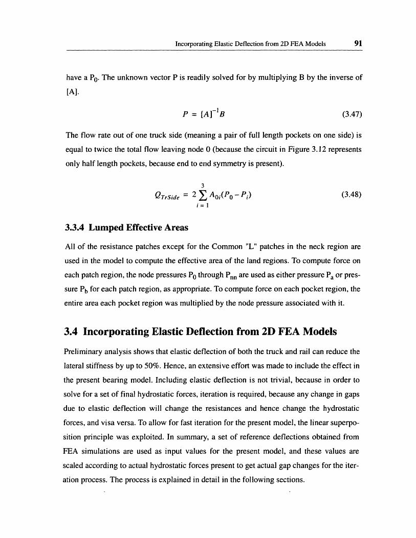
Incorporating Elastic Deflection from 2D FEA Models
have a Po. The unknown vector P is readily solved for by multiplying B by the inverse of
[A].
P = [A]- B (3.47)
The flow rate out of one truck side (meaning a pair of full length pockets on one side) is
equal to twice the total flow leaving node 0 (because the circuit in Figure 3.12 represents
only half length pockets, because end to end symmetry is present).
3
QTrSide = 2 A Aoi(P0 - Pi) (3.48)i= I
3.3.4 Lumped Effective Areas
All of the resistance patches except for the Common "L" patches in the neck region are
used in the model to compute the effective area of the land regions. To compute force on
each patch region, the node pressures PO through Pnn are used as either pressure Pa or pres-
sure Pb for each patch region, as appropriate. To compute force on each pocket region, the
entire area each pocket region was multiplied by the node pressure associated with it.
3.4 Incorporating Elastic Deflection from 2D FEA Models
Preliminary analysis shows that elastic deflection of both the truck and rail can reduce the
lateral stiffness by up to 50%. Hence, an extensive effort was made to include the effect in
the present bearing model. Including elastic deflection is not trivial, because in order to
solve for a set of final hydrostatic forces, iteration is required, because any change in gaps
due to elastic deflection will change the resistances and hence change the hydrostatic
forces, and visa versa. To allow for fast iteration for the present model, the linear superpo-
sition principle was exploited. In summary, a set of reference deflections obtained from
FEA simulations are used as input values for the present model, and these values are
scaled according to actual hydrostatic forces present to get actual gap changes for the iter-
ation process. The process is explained in detail in the following sections.
91

LUMPED PARAMETER BEARING MODEL
3.4.1 Problems that are Addressed in this Section
For this section, only the problem of how to compute gap changes caused by hydrostatic
forces is addressed. As mentioned earlier, to solve for a final set of hydrostatic forces, iter-
ation is required because any change in gaps due to elastic deflection will change the resis-
tances and hence change the hydrostatic forces, and visa versa.
Three subproblems are solved in this section that lead to the ultimate goal of finding gap
changes due to elastic deflections caused by a set of hydrostatic forces. The subproblems
are explained below.
Index symbols used for data arrays in the three subproblems:
p= 1 to 10, # of point "p"
i = 1 to 21, # of point "i"
rl = I to 2, 1 for deflection on right profile, 2 for deflection on left profile
xy = I to 2, 1 for x direction, 2 for y direction
Id= 1 to 3, loads 1 to 3
Irl = I to 2, 1 for load on right profile, 2 for load on left profile
Subproblem 1: FEA Simulations
Given: Truck and rail solid models
Pref(ld, Irl=1) Array of three reference load pressures acting on the rightprofile of both the truck and rail.
Find: ExyRRl(p, rl, xy, Id, tr) Array of x and y elastic deflections. Thisarray consists of the deflection at each point "p" at the right and left pro-files, in the x and y direction, caused by reference load pressures Pref(ld, ),acting on both the truck or the rail.
Subproblem 2: Computing array of reference gap changes at the midpoint of eachsegment "i"
Given: ExyRR1(p, rl, xy, Id, tr)
Find: HEref(i, rl, Id, Irl) Array of reference gap change values at the mid-point of each segment "i" at the right and left profiles caused by the refer-ence pressures Pref(ld, Irl) acting on the right and left profiles.
92

Incorporating Elastic Deflection from 2D FEA Models
Subproblem 3: Computing array of gap changes at the midpoint of each segment "i"
Given: Pref(ld, Irl)
Aref(ld, Irl) Area over which each reference pressure acts.
HEref(i, rl, Id, Irl)
Fhy(ld,lrl) Array of three hydrostatic forces acting on right and left pro-files.
Find: HEE(i,rl) Array of gap changes due to elastic deflection at the mid-point of each segment "i" at the right and left profiles.
3.4.2 Subproblem 1: FEA Simulations
The goal of this section is explain how the array ExyRRl(p,rl,xy,ld,tr) is filled via FEA
simulations. Figure 3.13 shows 10 "p" points on the right and left side of both the truck
and rail which were marked in ProMechanica. The x and y deflection at each point "p"
was marked as a "measure" in ProMechanica. Each point "p" shown is easy to mark on a
meshed ProMechanica model because it is a point of tangency between an adjacent flat
and round.
Figure 3.14 shows the six FEA simulations that are run to generate all of the deflections
present in the array ExyRRl(p, rl, xy, Id, tr). For the simulations, Pref(l,l) = Pref(2,1) =
Pref(3,1) = MPa.
3.4.3 Subproblem 2: Computing Array of Reference Gap Changes
The goal of this section is to explain how the array HEref(i, rl, Id, rl) is filled. Figure 3.15
shows the midpoint of each segment "i" on the right and left profile of both the truck and
rail, at which we seek a compute gap change at "i" in the array HEref(i, rl, Id, rl).
To fill HEref(i, rl, Id, Irl) starting with ExyRRl(p, rl, xy, Id, tr), a linear deformation for-
mula was used to compute the deflections at the "i" points which are in between the "p"
points, yielding a new array ExyRR2(i, rl, xy, Id, tr). Using ExyRR2(i, rl, xy, Id, tr), the
93
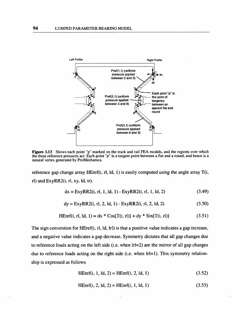
LUMPED PARAMETER BEARING MODEL
Left Profile Right Profile
int"p ist of
anflat and
Figure 3.13 Shows each point "p" marked on the truck and rail FEA models, and the regions over whichthe three reference pressures act. Each point "p" is a tangent point between a flat and a round, and hence is anatural vertex generated by ProMechanica.
reference gap change array HEref(i, rl, Id, 1) is easily computed using the angle array T(i,
rl) and ExyRR2(i, rl, xy, Id, tr).
dx = ExyRR2(i, rl, 1, Id, 1) - ExyRR2(i, rl, 1, Id, 2) (3.49)
dy = ExyRR2(i, rl, 2, Id, 1) - ExyRR2(i, rl, 2, Id, 2) (3.50)
HEref(i, rl, Id, 1) = dx * Cos[T(i, rl)] + dy * Sin[T(i, rl)] (3.51)
The sign convention for HEref(i, rl, Id, Irl) is that a positive value indicates a gap increase,
and a negative value indicates a gap decrease. Symmetry dictates that all gap changes due
to reference loads acting on the left side (i.e. when lrl=2) are the mirror of all gap changes
due to reference loads acting on the right side (i.e. when Irl=1). This symmetry relation-
ship is expressed as follows
HEref(i, 1, Id, 2) = HEref(i, 2, Id, 1) (3.52)
HEref(i, 2, Id, 2) = HEref(i, 1, Id, 1)
94
(3.53)
Incorporating Elastic Deflection from 2D FEA Models
Lv/ / / / / /
I
7I ,
Figure 3.14 FEA simulations run to fill the array ExyRRl(p, rl, xy, id, tr). For the simulations Pref(l,l) =P(2,1) = P(3,1) = I MPa.
The array HEref(i, rl, Id, Irl) is now complete. Now the gap change at each point "i" can be
computed efficiently given any arbitrary set of hydrostatic forces Fhy(ld, Irl).
3.4.4 Subproblem 3: Computing Array of Gap Changes
The elastic gap change HEE(i, rl) at midpoint "i" can be computed by linearly combining
the reference gap changes stored in HEref(i, rl, Id, Irl). In order to perform the scaling, an
equivalent uniform pressure Peq(ld, Irl) must be computed for each hydrostatic force
Fhy(ld, Irl), using the area over which the reference pressures act Aref(ld, Irl).
Peq(ld, Irl) = Fhy(ld, Irl) / Aref(ld, Irl) (3.54)
The gap change at each midpoint "i" is equal to the sum of the gap changes caused each of
the six equivalent pressures Peq(ld,lrl).
95
I
I
L ,f
. . . . .

LUMPED PARAMETER BEARING MODEL
Left Profile Right Profile
:h point i" ismidpoint ofment 'i"
Figure 3.15 Shows the midpoint of each segment "i", at which a gap change is stored in the array HEref(i,rl, Id, Irl). The reference pressures Pref(ld, Irl) are uniform and they act on both the truck and rail over thesame area as is specified in Figure 3.13.
HEE(i, rl) = SUM[HEref(i, rl, Id, lrl)*Peq(ld, Irl)/Pref(ld, Irl), Id=l to 3, lrl=l to 2] (3.55)
The principle of linear superposition is valid because the part size is much larger than the
deflections being studied (all deflections are less than 10 micrometers, whereas the rail
width is 35mm, or 350 times larger).
96

Chapter 4
ANGLED SURFACE SELFCOMPENSATION PROTOTYPE
In this chapter, a prototype angled surface self compensation design is presented along
with test results.
4.1 Size 35 Angled Surface Self Compensation Prototype
The the first prototype of the hydrorail was designed to prove the concept presented in
Chapter 2. and to allow a comparison with the detailed mathematical model presented in
Chapter 3. To lower the cost of the first prototype, a three piece design was chosen. The
design is shown in Figure 4.1. The bearing gaps used are shown in Figure 4.2.
The reasoning behind the design choices made for the alpha prototype are listed below.
Design Choices Made for Alpha Prototype
1. To lower the cost of prototyping a three piece truck design was chosen. Thetwo identical halves can be ground with a large diameter grinding wheel,hence making grinding much easier.
2. To lower costs and to make load capacity high, no seal or drain groove sys-tem was designed.
3. Nominal gaps at bearing pads were chosen to be 12.7 micrometers, which isrelatively small but makes using water feasible (about 1.5 hp for 4 trucks),and hence provided us the option of using water.
97
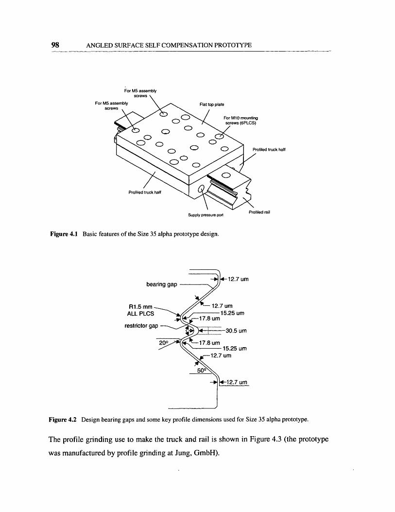
ANGLED SURFACE SELF COMPENSATION PROTOTYPE
For M5 assembly
For M5 asscrei
filed truck half
Supply pressure port
Figure 4.1 Basic features of the Size 35 alpha prototype design.
Profiled rail
R1.5 nALL PL
restricto
Figure 4.2 Design bearing gaps and some key profile dimensions used for Size 35 alpha prototype.
The profile grinding use to make the truck and rail is shown in Figure 4.3 (the prototype
was manufactured by profile grinding at Jung, GmbH).
98

Deflection Versus Load 99
Figure 4.3 Profile grinding of a bearing rail and a truck half at Jung, GmbH, Goeppingen, Germany.
4.2 Deflection Versus Load
In this section, the measured and predicted deflection versus load is presented for lateral,
compressive, and tensile loading cases.
4.2.1 Test Set-Up for Deflection Vs. Load
Figure 4.4 shows the rig that was used to load a truck in compression and in tension, and
to measure the resulting vertical deflection and the pressure in the four bearing pockets.
To prevent bending of the steel carriage plate, which would cause undesired tilting of the
bearing truck being measured, thin strips were placed above both trucks, under a "whiffle
tree" block, upon which the force was applied.
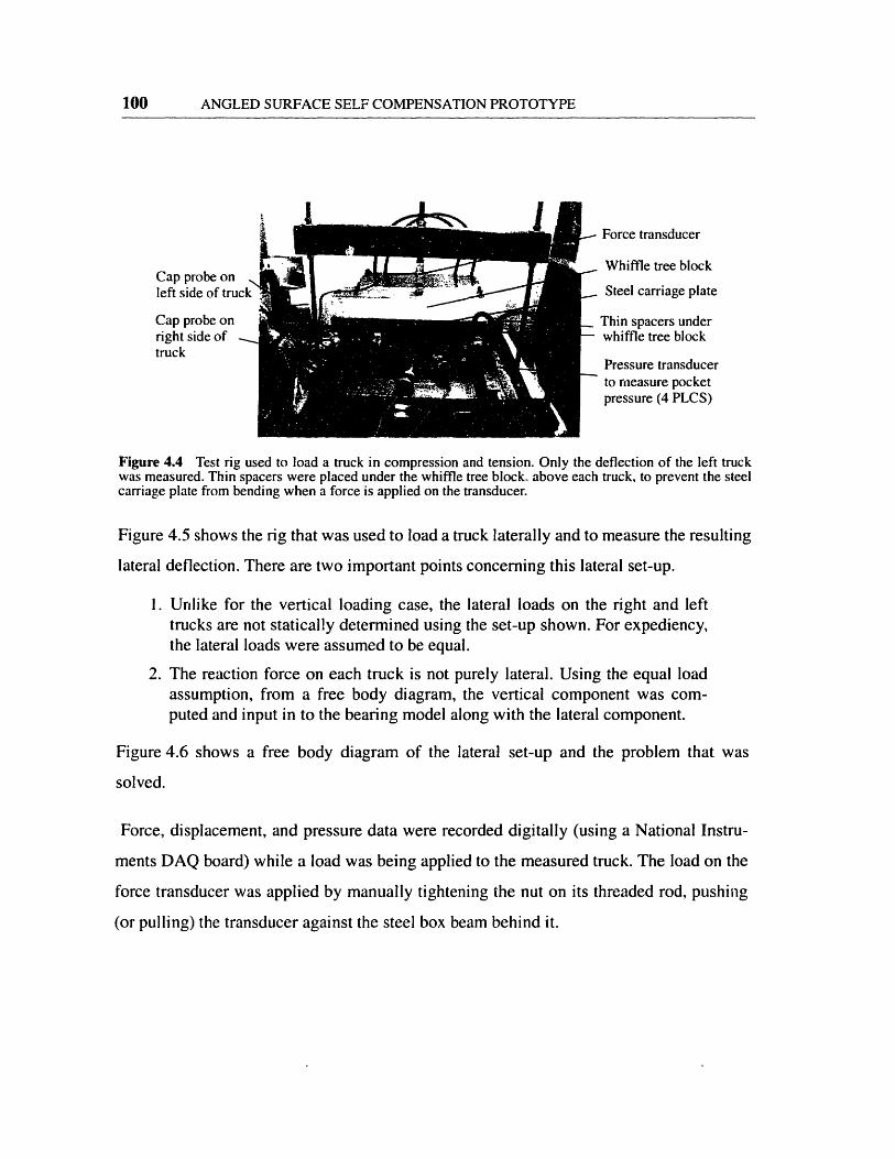
ANGLED SURFACE SELF COMPENSATION PROTOTYPE
Cap probe onleft side of truck
Cap probe onright side of truck
- Force transducer
- Whiffle tree block
- Steel carriage plate
_Thin spacers under- whiffle tree block
Pressure transducerto measure pocketpressure (4 PLCS)
Figure 4.4 Test rig used to load a truck in compression and tension. Only the deflection of the left truckwas measured. Thin spacers were placed under the whiffle tree block, above each truck, to prevent the steelcarriage plate from bending when a force is applied on the transducer.
Figure 4.5 shows the rig that was used to load a truck laterally and to measure the resulting
lateral deflection. There are two important points concerning this lateral set-up.
1. Unlike for the vertical loading case, the lateral loads on the right and lefttrucks are not statically determined using the set-up shown. For expediency,the lateral loads were assumed to be equal.
2. The reaction force on each truck is not purely lateral. Using the equal loadassumption, from a free body diagram, the vertical component was com-puted and input in to the bearing model along with the lateral component.
Figure 4.6 shows a free body diagram of the lateral set-up and the problem that was
solved.
Force, displacement, and pressure data were recorded digitally (using a National Instru-
ments DAQ board) while a load was being applied to the measured truck. The load on the
force transducer was applied by manually tightening the nut on its threaded rod, pushing
(or pulling) the transducer against the steel box beam behind it.
100

Deflection Versus Load
Force transducer
Cap probe on leftside of truck
Pressure transducerto measure pocket -pressure (4 PLCS)
- Cap probe onright side oftruck
Figure 4.5 Test rig used to load both trucks laterally. Unlike for the vertical loading set-up, the load on theright and left trucks is not statically determined. For expediency, the lateral load component on the truckbeing measured was assumed to be half the force transducer load. The small vertical component was com-puted using a FBD of the set-up.
Vertical force on truck to account forovercontraint and gravity (when F iszero, Fe, is computed to using initial
pocket pressures) For actual test set-up ( is in the range of 9to 15 degrees when Ft is at a maximum
X
Assumptions: Fix = F2, Feffi does not change with Ft
Problem that is solved:Given: Feffi that matches pocket pressures when Ft = O, F t, W, y1, xFind: Fix, Fly
Figure 4.6 Free body diagram of the lateral load test set-up.
101
I
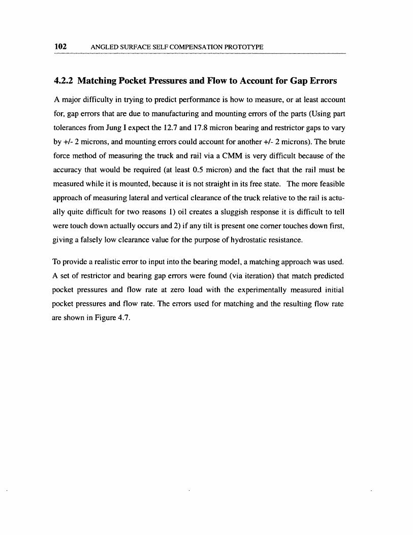
ANGLED SURFACE SELF COMPENSATION PROTOTYPE
4.2.2 Matching Pocket Pressures and Flow to Account for Gap Errors
A major difficulty in trying to predict performance is how to measure, or at least account
for, gap errors that are due to manufacturing and mounting errors of the parts (Using part
tolerances from Jung I expect the 12.7 and 17.8 micron bearing and restrictor gaps to vary
by +/- 2 microns, and mounting errors could account for another +/- 2 microns). The brute
force method of measuring the truck and rail via a CMM is very difficult because of the
accuracy that would be required (at least 0.5 micron) and the fact that the rail must be
measured while it is mounted, because it is not straight in its free state. The more feasible
approach of measuring lateral and vertical clearance of the truck relative to the rail is actu-
ally quite difficult for two reasons 1) oil creates a sluggish response it is difficult to tell
were touch down actually occurs and 2) if any tilt is present one corner touches down first,
giving a falsely low clearance value for the purpose of hydrostatic resistance.
To provide a realistic error to input into the bearing model, a matching approach was used.
A set of restrictor and bearing gap errors were found (via iteration) that match predicted
pocket pressures and flow rate at zero load with the experimentally measured initial
pocket pressures and flow rate. The errors used for matching and the resulting flow rate
are shown in Figure 4.7.
102

Deflection Versus Load 103
Assumed Gap ErrorsBearing Which Match
Gap Array PRighlt Initial Pocket Pressures,,I ,of~ Desian GaDs and Flow
I (rl=1)Midpoint of
H(i.rl) segment 1H(1,rl) Midpoint ofH(2,r)H(3,l) segment 2H(4, rlH(4,) Gaos are shownH(5,rl) ,..- greatlyH(6,rl exaggerated
Ect. i
I , _ ~4.'T':~'~ ......_.i.._1516
17 1" Slave Profile
Master Profile 18 \
i1
123456789101112131415161718192021
Left Profile Right ProfileHD(1,i) HD(2,i)12.70 12.7012.70 12.7012.70 12.7012.70 12.7012.70 12.7013.78 13.7815.25 15.2516.72 16.7217.80 17.8027.01 27.0130.50 30.5027.01 27.0117.80 17.8016.72 16.7215.25 15.2513.78 13.7812.70 12.7012.70 12.7012.70 12.7012.70 12.7012.70 12.70
Left Profile Right ProfileHerr(1,1) Herr(2,1)
5.7 5.75.7 5.75.7 5.75.7 5.75.7 5.70.0 0.00.0 0.00.0 0.00.0 0.00.0 0.00.0 0.00.0 0.00.0 0.00.0 0.00.0 0.00.0 0.05.7 5.75.7 5.75.7 5.75.7 5.75.7 5.7
2/11/99 Flow Tests, Truck with pressure tapsrho (g/1 870
Ps Temp. Temp. I dmass dtime(Bar) F C cSt (g) (sec)17.2 74 23.3 65 100 33234.5 74 23.3 65 10C 20468.9 89 31.7 46 200 187
Mesured' Ppump PredictedQ/Truck Wp Q/Truck
(Ipm) (W) (Ipm) Error0.021 0.60 0.017 25%0.034 1.9 0.034 Flow Matc,0.074 8.5 0.084 -12% I
Figure 4.7 Gap errors used to match initial pocket pressures at Ps = 34.5 Bar and the flow correlation at theother Ps values.
4.2.3 Load Versus Displacement Plots
Compression
Figure 4.8 and Figure 4.9 shows the measured and predicted deflection under compres-
sive, lateral, and tensile loading.
I

104 ANGLED SURFACE SELF COMPENSATION PROTOTYPE
Measured and predicted downward and lateral deflection versus force of prototype bearing
Deflection Vs. Compressive Load
EC00.2a
X
3a0inC00p
Downward Force (N)
E
oC00
E8a)FL
-J
Lateral Component of Truck Reaction (N)
Figure 4.8truck.
-

Deflection Versus Load 105
Figure 4.9 Measured and predicted tensile deflection versus force of prototype bearing truck.

106 ANGLED SURFACE SELF COMPENSATION PROTOTYPE
TABLE 4.1 Summary of Load Versus Deflection Test Results
CompressionTensionLateral
CompressionTensionLateral
CompressionTension
Lateral
(Bar)17.217.217.234.534.534.568.968.968.9
a)
Ca.O
Cu 0)
0co c
Coa,'-U) 9DX2 cu
0'ac 00) -
to
(1)0)_a)0 &
(N)117030013752338800
22514700N.A.N.A.
a,
COc)co
cua,
E-aC a)Ca.)C) i Cu)
.5>.00a) '~!a)D
0 a 0a
. .CL ,C_
(jIm)8.12.912.610.14.214.110.7N.A.N.A.
0c
0).CEi,
-caBC0
-oa 2
I =
(N)28782324185254294925365110406100857200
ts-o
E9a)'-C)c
C oZ C.0 cm
D C
._';E
Lc:(Am)20.816.014.119.618.415.019.221.116.8
oa,
r00)
a)
'00 C
0
(N/pm)144103109231190160439331302
0
1,0a,Ca)
I C
a)-.0) zrC>0 cUo-E '
a,X Cu
CL)IrE(N/lm)
107120110241212205474458367
w
35%-14%
0%-4%
-10%-22%
-7%-28%-18%
Conclusions Drawn from Each Load Vs. Deflection Test:
1. In Compression correlation was good. By stacking weights contact wasobserved at 68.9 Bar at about 4700 N, however contact was not clearly visi-ble in the tests.
2. In Tension premature touchdown was observed. Because the bearing is sym-metrical this is likely due to the bolted joints causing excessive deflection.At 68.9 Bar, however, touchdown is not clearly observable, most likelybecause the initial pocket pressures spread the truck halves open enough todelay touchdown significantly.
3. Laterally the correlation is good except at 34.5 Bar. It may be that the bear-ing is touching prematurely at 68.9 Bar, but further testing is required to ver-ify this.
Overall Conclusions Drawn from Load Vs. Deflection Tests
1. Model correlates reasonably well after matching pocket pressure and flowrate, even though a very rough assumption was made about the profile errorsto enable matching.
2. 12.7 um nominal bearing gap is likely too tight given the accuracy of theparts and set-up, because premature touch down occurred.
- l
l - - - -
| | - - -
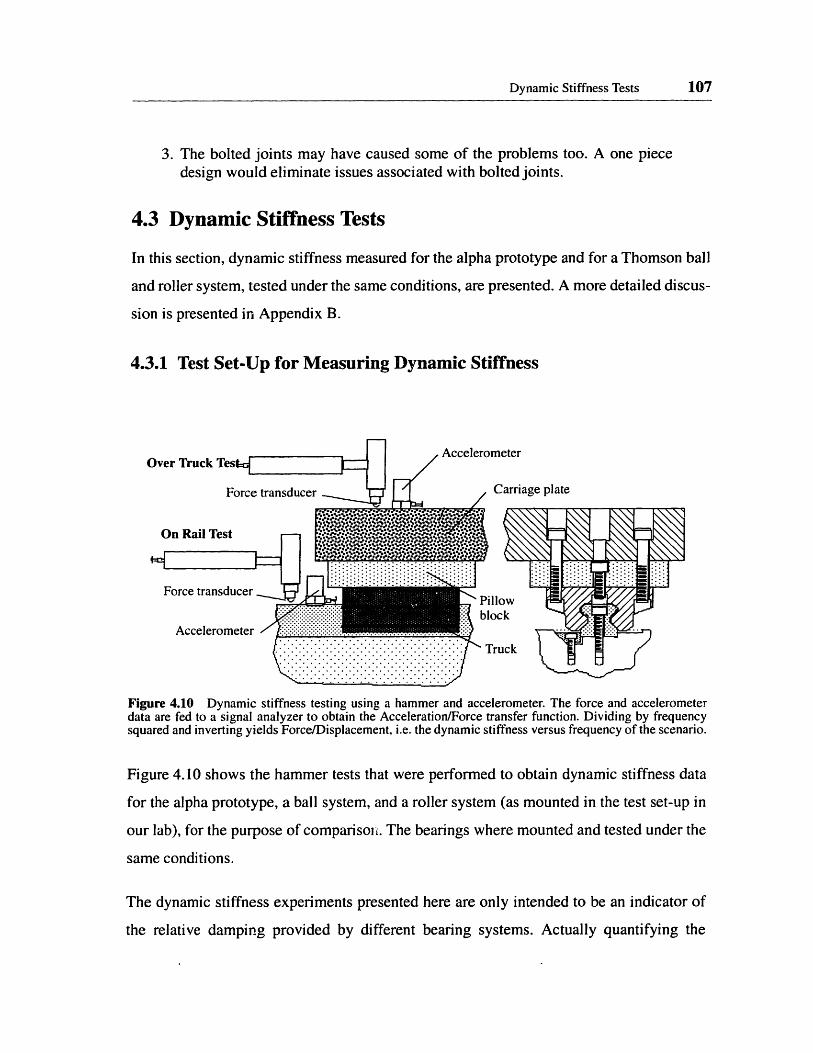
Dynamic Stiffness Tests 107
3. The bolted joints may have caused some of the problems too. A one piecedesign would eliminate issues associated with bolted joints.
4.3 Dynamic Stiffness Tests
In this section, dynamic stiffness measured for the alpha prototype and for a Thomson ball
and roller system, tested under the same conditions, are presented. A more detailed discus-
sion is presented in Appendix B.
4.3.1 Test Set-Up for Measuring Dynamic Stiffness
Over Truck Te s /
Force transducer _ Carriage plate
..r..-.. ,,, "..
. . . . . . . . . .. . . . . . . . . . . . . . . . - .-- T{ .......... . . . . . . . . . . . . . . . . . . .rs. . . . . . . . . . . . . . . . . . . . ... ................... ...........................'---'X''---- '---- '"'--'-----,......................
Figure 4.10 Dynamic stiffness testing using a hammer and accelerometer. The force and accelerometerdata are fed to a signal analyzer to obtain the Acceleration/Force transfer function. Dividing by frequencysquared and inverting yields Force/Displacement, i.e. the dynamic stiffness versus frequency of the scenario.
Figure 4.10 shows the hammer tests that were performed to obtain dynamic stiffness data
for the alpha prototype, a ball system, and a roller system (as mounted in the test set-up in
our lab), for the purpose of comparison. The bearings where mounted and tested under the
same conditions.
The dynamic stiffness experiments presented here are only intended to be an indicator of
the relative damping provided by different bearing systems. Actually quantifying the
7-gl,-1_,1W4rW-rU4t' ZF'!{:f -<'f 'XZ{f·f~f~f~r _·r_·r _·r_·r_·r_ f· f
iI

ANGLED SURFACE SELF COMPENSATION PROTOTYPE
damping of each bearing system, and then predicting dynamic stiffness of a structure that
a given bearing is mounted to, is beyond the scope of this thesis. From both a marketing
and engineering standpoint, dynamic stiffness is a difficult beast because it may well be
important for preventing chatter, but one really won't be able to convince a skeptic of the
true benefit of a better damped bearing unless the bearing is tried on the machine in ques-
tion under the actual cutting conditions.
4.3.2 Measured Dynamic Stiffness (Hydro, Ball, & Roller Systems)
Figure 4.11 shows a plot of the dynamic stiffness measured for the alpha prototype, a
lightly preloaded Thomson Accuglide(TM) bearing (ball system), and a lightly preloaded
Thomson AccuMax(TM) bearing (roller system). The method of testing is shown in Fig-
ure Figure 4.10 (for more details, consult Appendix B). The conclusions drawn from the
dynamic stiffness tests are summarized below.
Over Truck Test for alphaeasure On Rail Test for all hydrostatic prototype truckbelow 170 Z thrn hnrint (134 mmn long truck)
R
FHest for lighlyonsonI) (Ball systerr),;th (109 rnm)
Ily
o 105 Num resonance for 47 Numfor ACCUIVaX( IIV (HOller system)I On Rail Test Ball Standard length (109 mrm)
0 200 400 600 800 1000 1200 1400 1600
Frequency of Excitation (Hz)
Figure 4.11 Measured dynamic stiffness of an alpha prototype hydrostatic truck and lightly preloadedAccuglide and AccuMax trucks, both of standard length (109mm).
Unable to maccurately t
X 10CD
_ _
108
Jrc

Dynamic Stiffness Tests 109
Conclusions Drawn from Dynamic Stiffness Tests
1. The hydrostatic prototype shows improved damping because it did not addany resonances to those exhibited by the on rail test, unlike the roller sys-tems.
2. In fairness to the ball and roller systems, a light preload, standard lengthtruck (L=109mm) is the worst case scenario in terms of static stiffness (andmost likely for dynamic stiffness). For further research, tests should be per-formed on medium and heavily preloaded systems, to see if a significant dif-ference exists. However, it should be noted that a heavier preload will resultin greater straightness ripple (more than the 0.6 and 0.4 microns for thelightly preloaded AccuGlide and AccuMax, respectively) so the best trade-off must be made.

110 ANGLED SURFACE SELF COMPENSATION PROTOTYPE
Chapter 5
CONCLUSIONS AND FUTURE WORK
5.1 Conclusions
1) A modular hydrostatic bearing is promising for the following applications:
* Cam Grinding
* Ceramics Grinding
* General Precision Grinding
* Hard Turning
* Very High Speed Machining
2) For ordinary machining applications rolling element bearings are still the best choice.
3) A major benefit of hydrostatic systems is for speeds of I m/s or greater, where the
inherent cooling that can be provided by chilling the hydraulic fluid is a very important
advantage over standard rolling element guides.
4) Initial damping tests show that the hydrostatic system does not introduce resonances.
The direct benefit this provides to a customer needs to be proven by run-off tests.
111

CONCLUSIONS AND FUTURE WORK
5) The best possible hydrostatic system studied for this thesis (a diaphragm based system),
operating at 100W, 60 cSt viscosity and usirg a bearing gap of 20 gm (reasonable for pro-
duction tolerances and mounting errors), will provide roughly a static stiffness that is com-
parable to a heavy preloaded ball system or a lightly preloaded roller system.
6) The novel angled surface design presented, operating at 100W, 60 cSt viscosity and
using a bearing gap of 20 gim (reasonable for production tolerances and mounting errors),
will provide a static stiffness that is between a lightly preloaded and medium preloaded
ball system.
7) Because it is the only design of the ones studied that can be manufactured using exist-
ing manufacturing processes at linear bearing companies, the novel angled surface design
presented is highly preferable over other designs in terms of cost.
5.2 Future Work
It is important to realize that a key advantage of a hydrostatic system is better damping,
but the direct benefit to the customer of damping must be established by experiments done
on real machines. To address this key question, the following plan will be carried out in a
partnership with a major linear bearing manufacturer (whose name must be kept confiden-
tial at this point in the research).
Finish Design of Beta Prototype For Production Tolerances
According to a preliminary error study a bearing gap of 20 gtm (as opposedto 12.7 tm for the prototype) is viable for production. A full design reviewmust be done with production engineers to finalize the design bearing gap,or perhaps two different gaps will be selected and tested.
Make and Test Beta Prototype on In-House Grinder at the Linear Guide Factory
A promising first application is on an in-house bearing grinder at the linearguide factory that grinds linear races for very small bearings. For the appli-cation, surface finish (and hence smoothness of motion and dynamic stiff-ness) is critical.
112
Future Work 113
If Significant Improvement is Observed
* Then implement on other in-house grinders, and assess markets.
If No Significant Improvement is Observed
* Then assess cam grinding and ceramics grinding markets, where a hydro-static bearing has definitive advantages.

114 CONCLUSIONS AND FUTURE WORK
REFERENCES
[Slocum, 1992] Slocum, A., Precision Machine Design, Prentice-Hall, 1992.
[Fox, 1985] Fox, R. W., and McDonaid, A. T., Introduction to Fluid Mechanics, JohnWiley & Sons, 1985.
[Shah, 1978] Shah, R. K., "A Correlation for Laminar Hydrodynamic Entry Length Solu-tions for Circular and Noncircular Ducts", Journal of Fluids Engineering, Vol.100, pp. 177-179, 1978.
[Stansfield, 1970] Stansfield, F. M., Hydrostatic Bearings for Machine Tools and OtherApplications, The Machinery Publishing Co., 1970.
[Futami, 1990] Futami, S., Furutani, A., and Yoshida, S., "Nanorneter Positioning and itsMicrodynamics", Nanotechnology, Vol. 1, No. 1, pp. 31-37, 1990.
[Scagnetti, 1996] Scagnetti, P. A., "Design of an Industrial Precision Ceramic GrindingMachine", Ph.D. Dissertation in Mechanical Engineering, M.I.T., 1996.
[Thomson Catalogue] Thomson Industries, Inc., Port Washington, NY, 11050 USA.
[Schneeberger Catalogue] Schneeberger, Inc., 11 DeAngelo Drive, Bedford, MA, 01730.
[Star Linear Catalogue] A division of Mannesmann Rexroth, 14001 South Lakes Drive,Charlotte, NC 28273.
115

116 REFERENCES
Appendix A
TEST BED
In this appendix, the test bed used to measure vertical straightness and dynamic stiffness
of size 35 linear guides is explained in detail. In the sections that follow, the bed design,
truck and rail mounting methods, and the laser interferometer system used for straightness
measurements are all described.
A.1 Overall View of Test Bed System
Figure A.1 shows a side view, and Figure A.2 shows a top view of the system used for
measuring the straightness of size 35 modular linear guides. In summary, the system con-
sists of a carriage plate mounted on four size 35 trucks, which travel along two rails bolted
to a bed. The bed is supported by three feet which rest on a granite surface plate, which is
in turn supported by four pneumatic feet. A Zygo ZMI-1000 laser interferometer system is
used to measure the vertical straightness over one of the bearing trucks, and the x-travel
position of the carriage. A Trilogy linear motor is used to drive the carriage back and
fourth. A PC is used with software provided by Zygo to acquire straightness data from the
ZMI-1000, and another PC is used to send command signals to the linear motor, using
Delta-Tau P-Mac hardware and software.
117

118 APPENDIX A
C0
m E*S E
co
0)I.X
co .x
.4 *
.:,
-.'
A U
M
.0ML
0) (Il 0.
Figure A.1 Side view of test bed system designed for measuring straightness.
.TI1 1 .?-
'- L,= ~ .
.Li
.... -- 1%-h-
i -
L? "ili
APPENDIX A
errse
er
amitter
feromete
earitor
'O[ectorirrorirse
irror,at
icalror
isrferomete
rrorrse
Figure A.2 Top view of test bed system designed for measuring straightness.
119
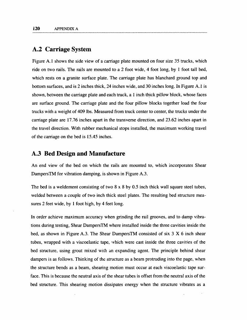
120 APPENDIX A
A.2 Carriage System
Figure A.1 shows the side view of a carriage plate mounted on four size 35 trucks, which
ride on two rails. The rails are mounted to a 2 foot wide, 4 foot long, by 1 foot tall bed,
which rests on a granite surface plate. The carriage plate has blanchard ground top and
bottom surfaces, and is 2 inches thick, 24 inches wide, and 30 inches long. In Figure A. 1 is
shown, between the carriage plate and each truck, a 1 inch thick pillow block, whose faces
are surface ground. The carriage plate and the four pillow blocks together load the four
trucks with a weight of 409 lbs. Measured from truck center to center, the trucks under the
carriage plate are 17.76 inches apart in the transverse direction, and 23.62 inches apart in
the travel direction. With rubber mechanical stops installed, the maximum working travel
of the carriage on the bed is 15.45 inches.
A.3 Bed Design and Manufacture
An end view of the bed on which the rails are mounted to, which incorporates Shear
DampersTM for vibration damping, is shown in Figure A.3.
The bed is a weldement consisting of two 8 x 8 by 0.5 inch thick wall square steel tubes,
welded between a couple of two inch thick steel plates. The resulting bed structure mea-
sures 2 feet wide, by 1 foot high, by 4 feet long.
In order achieve maximum accuracy when grinding the rail grooves, and to damp vibra-
tions during testing, Shear DampersTM where installed inside the three cavities inside the
bed, as shown in Figure A.3. The Shear DampersTM consisted of six 3 X 6 inch shear
tubes, wrapped with a viscoelastic tape, which were cast inside the three cavities of the
bed structure, using grout mixed with an expanding agent. The principle behind shear
dampers is as follows. Thinking of the structure as a beam protruding into the page, when
the structure bends as a beam, shearing motion must occur at each viscoelastic tape sur-
face. This is because the neutral axis of the shear tubes is offset from the neutral axis of the
bed structure. This shearing motion dissipates energy when the structure vibrates as a
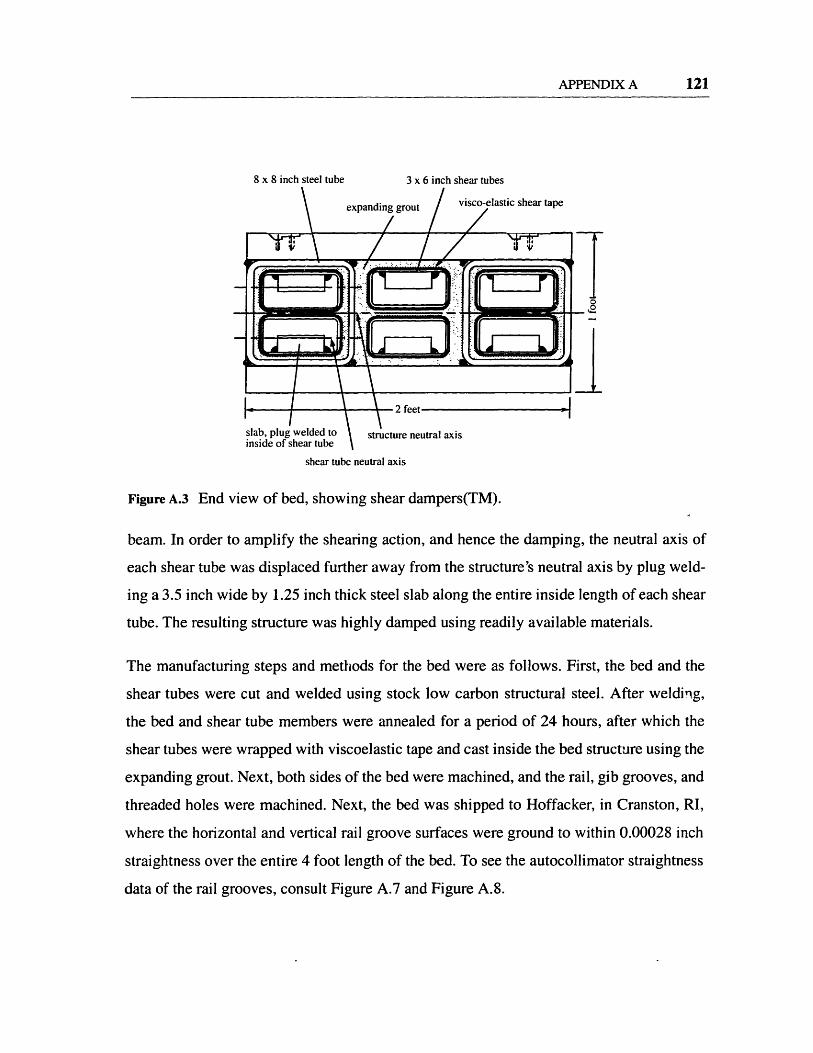
APPENDIX A 121
8 x 8 inch steel tube 3 x 6 inch shear tubes
expanding grout visco-elastic shear tape
0.__
I
2 feet 'slab, plug welded to \ structure neutral axisinside of shear tube
shear tube neutral axis
Figure A.3 End view of bed, showing shear dampers(TM).
beam. In order to amplify the shearing action, and hence the damping, the neutral axis of
each shear tube was displaced further away from the structure's neutral axis by plug weld-
ing a 3.5 inch wide by 1.25 inch thick steel slab along the entire inside length of each shear
tube. The resulting structure was highly damped using readily available materials.
The manufacturing steps and methods for the bed were as follows. First, the bed and the
shear tubes were cut and welded using stock low carbon structural steel. After welding,
the bed and shear tube members were annealed for a period of 24 hours, after which the
shear tubes were wrapped with viscoelastic tape and cast inside the bed structure using the
expanding grout. Next, both sides of the bed were machined, and the rail, gib grooves, and
threaded holes were machined. Next, the bed was shipped to Hoffacker, in Cranston, RI,
where the horizontal and vertical rail groove surfaces were ground to within 0.00028 inch
straightness over the entire 4 foot length of the bed. To see the autocollimator straightness
data of the rail grooves, consult Figure A.7 and Figure A.8.
I ... ... ...
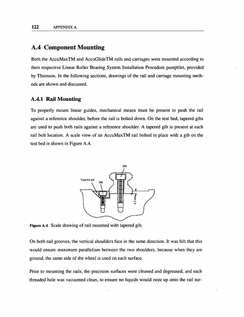
122 APPENDIX A
A.4 Component Mounting
Both the AccuMaxTM and AccuGlideTM rails and carriages were mounted according to
their respective Linear Roller Bearing System Installation Procedure pamphlet, provided
by Thomson. In the following sections, drawings of the rail and carriage mounting meth-
ods are shown and discussed.
A.4.1 Rail Mounting
To properly mount linear guides, mechanical means must be present to push the rail
against a reference shoulder, before the rail is bolted down. On the test bed, tapered gibs
are used to push both rails against a reference shoulder. A tapered gib is present at each
rail bolt location. A scale view of an AccuMaxTM rail bolted in place with a gib on the
test bed is shown in Figure A.4.
M8
Figure A.4 Scale drawing of rail mounted with tapered gib.
On both rail grooves, the vertical shoulders face in the same direction. It was felt that this
would ensure maximum parallelism between the two shoulders, because when they are
ground, the same side of the wheel is used on each surface.
Prior to mounting the rails, the precision surfaces were cleaned and degreased, and each
threaded hole was vacuumed clean, to ensure no liquids would ooze up onto the rail sur-
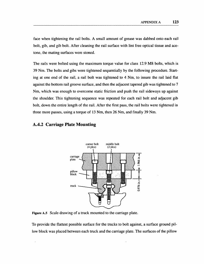
APPENDIX A 123
face when tightening the rail bolts. A small amount of grease was dabbed onto each rail
bolt, gib, and gib bolt. After cleaning the rail surface with lint free optical tissue and ace-
tone, the mating surfaces were stoned.
The rails were bolted using the maximum torque value for class 12.9 M8 bolts, which is
39 Nm. The bolts and gibs were tightened sequentially by the following procedure. Start-
ing at one end of the rail, a rail bolt was tightened to 4 Nm, to insure the rail laid flat
against the bottom rail groove surface, and then the adjacent tapered gib was tightened to 7
Nm, which was enough to overcome static friction and push the rail sideways up against
the shoulder. This tightening sequence was repeated for each rail bolt and adjacent gib
bolt, down the entire length of the rail. After the first pass, the rail bolts were tightened in
three more passes, using a torque of 13 Nm, then 26 Nm, and finally 39 Nm.
A.4.2 Carriage Plate Mounting
corner bolt middle bolt
carriagplate
pillowblock
truck
Figure A.5 Scale drawing of a truck mounted to the carriage plate.
To provide the flattest possible surface for the trucks to bolt against, a surface ground pil-
low block was placed between each truck and the carriage plate. The surfaces of the pillow

124 APPENDIX A
blocks were match ground on an Okomoto surface grinder, to achieve maximum unifor-
mity in thickness. Each truck was bolted to each pillow block via the two middle bolts,
and then each truck and pillow block assembly was bolted to the carriage plate via the four
corner bolts. This arrangement assured that the center region of each truck was bolted
against the very flat surface of each pillow block, before the truck and pillow block assem-
blies were secured to the carriage plate. All of the carriage bolts, which were class 12.9
M1O's, were tightened using a torque of 77 Nm, as stated in the Linear Roller Bearing Sys-
tem Installation Procedure pamphlet.
A.5 Rail Groove Straightness
The vertical straightness of each rail groove was measured using a Nikon Model 6D man-
ual autocollimator, and using a sled moved along the rail groove in increments equal to the
center-to-center distance between the rear sled pad and the front sled pad (1.024 inches).
The autocollimator had a resolution of 0.5 seconds (2.42 E-6 radians). Each sled pad was
0.208 inches (5.28 mm) wide in the travel direction, and 1.629 inches (41.38 mm) long
transverse to the travel. Using the pad center-to-center length, the resolution using the sled
for measuring vertical straightness was thus 2.5 microinches (0.063 microns). The accu-
racy of the autocollimator was quoted to be 1 arcsecond, corresponding to a straightness
measuring accuracy of 5 microinches (0.127 microns). The actual accuracy is less due to
mechanical contact non-repeatabilities.
The test procedure using the autocollimator was as follows. First, marks were placed
beside the rail groove, spaced 1.024 inches apart. Next, the groove and sled surfaces were
stoned, the sled was placed at the first location, and the autocollimator was zeroed. The
sled was moved forward to subsequent marks and readings were taken. After every seven
readings were recorded, the groove and sled pad surfaces were stoned again, and the sled
was placed on the first location again to verify that the reading at the first location was still
zero, insuring thermal drift was not occurring. For each rail groove, the measurements
were repeated in the described fashion three times. For each rail groove, after the three

APPENDIX A 125
tests, the sled was placed at the first location once again, and the reading was found to be
zero, verifying no thermal drift occurred.
Figure A.6 shows rail groove #1 and rail groove #2 on the bed, and Figure A.7 and
Figure A.8 show the vertical straightness of each groove vs. X, generated using the auto-
collimator angular data. Each plot shows data from the three repeated tests.
I -X / M8 x 1.25 threaded bolt holefor rail mounting
Rail Groove #1
Rail Groove #2
Figure A.6 Rail groove names.
From Figure A.7, in the range from X=O to X=393 mm, rail groove #1 is straight to within
2.2 m (87 plin), and the profile changes gradually. In the range from X=783 mm to
X=1200 mm, rail groove #1 is straight to within 1.5 gm (59 lin), and the profile changes
gradually as well. In the range from X=393 mm to X=783 mm, however, the rail groove is
straight to within 7 lm (276 in), and the profile has alternating high and low points.
Looking at Figure A.7, one can see that every high point is near a bolt hole in the rail
groove. Numerical investigation showed that every high point was within 6.6 gm from a
bolt hole center, which meant the sled foot was overlapping the hole rim. However, it was
also found that in the non-oscillatory regions, several points within 6.6 gm of hole centers
were not high spots. One cause for the high points could be that the autocollimator tests
were done after two sets of rails had been previously bolted to the bed (using the recom-
mended bolt torque of 39 Nm for class 12.9 M8 bolts), and some rim deformation
.*, N S* S : 9S : - XW * , e. * ' W! ; * *1 *.e -- 4 feet (1219.2 mm) ,----p

126 APPENDIX A
occurred. Why high points occur over a sequence of some bolt hole rims and not others, is
unknown at this time.
Vertical Straightness of Rail Groove #1 (hree test runs shown)
4 Results of three test runs are show n. Points w ere n' 3 measured using an autocolimator sled on surface rail
w as mounted to. A bad point sometimes occurs w hen a ;E 2 sled foot overlaps a small lip present around some rail
screw holes. |Ai I
E~~~~~~~~~~~~~~~~~~~~~~~~~~~~~~~ t :1 -3
-4 o o q o 0 o o o O O 0 O , 0 0 0 _ _ , 0 0 0 0 010.0 200.0 400.0 600.0 800.0 1000.0 12000
Screw hole in bed for rrmounting rail X location on rall groove (mm)
Figure A.7 Autocollimator straightness of rail groove #1.
Figure A.8 Autocollimator straightness of rail groove #2.
Vertical Straightness of Rail Groove #2 (Three test runs shown)
0
5U
02 4-3E
=1
-a 0.2
-1
-2CScrew hole in bed for mounting rail X location on rail groove (mm)
I~ ~ ·
D.cl
APPENDIX A 127
For the highest precision applications, the source of this problem should be further investi-
gated, to determine if it is specific to this test bed, or could be a problem with production
machines sold in the marketplace.
From Figure A.8, it can be seen that in the range from X=211 mm to 965 mm, rail groove
#2 is straight to within 2.5 gm (98 gin). However, oscillating surfaces were present at
either end of the rail, in the ranges from X=0 to X=211 mm, and from X=965 mm to
X=1200 mm. As with rail groove #1, further investigation showed that each high point
was within 6.6 gtm of a bolt hole center. However, in the non-oscillatory region, it was also
found that several points within 6.6 jim of a hole center were not high points.
A.6 Linear Motor Drive System
In order to drive the carriage continuously for straightness testing, a Trilogy linear motor
stage was used, in conjunction with Delta Tau P-mac hardware and software to send com-
mand signals to the motor. The linear motor stage includes its own carriage, supported by
its own set of bearings. To prevent the linear motor carriage from "fighting" the test car-
riage motion, thereby tainting the straightness measurements, a flexural coupling was
designed to connect the two. The flexural coupling is shown in Figure A.9.
The coupling was designed with two flexure regions, so that it could accommodate a lat-
eral translation error. The part was machined from a single piece of 6061-T6 aluminum.
To insure an absolute minimum of flexing required by the coupling, the linear motor stage
was mounted parallel to one of the rails to within 0.001 inch, by using spacer blocks for
precise alignment. To prevent axial vibrations from being transmitted to the carriage, a
damping rubber was placed between the flexure and the carriage, and between the mount-
ing bolts and the carriage.
128 APPENDIX A
top view of flexure plate
carnage plate, rests onfour trucks (not shown)
f AVAA
bed linear motor base section AA of flexure
Figure A.9 Flexural coupling used to drive the carriage plate.
A.7 Interferometer System Discussion
A Zygo ZMI-1000 laser interferometer was used to measure both the vertical straightness,
and X position of the carriage. Figure A.2 shows most of the optical components, and the
mounting horses and mirror boat.
The laser rests on a laser horse, which is a weldement fabricated from 8 x 8 square steel
tubes. In front of the laser is a beam splitter. The undiverted beam is used to measure ver-
tical straightness; the diverted beam is used to measure the X position of the carriage.
The undiverted beam measures vertical straightness via a differential interferometer, in
conjunction with an 18" long Zerodur optical mirror, straight to within 1 in (0.0254 gm),
which is supported at its quarter points via pins which pass through the mirror boat,
located above the differential interferometer. The mirror boat has three feet which rest on
_
__ -Ir __r TE - I --T I 1
APPENDIX A 129
the two mirror horses. The mirror horses are steel weldements which each have three
rounded foot pods.
The diverted beam measures straightness via a linear interferometer mounted to the laser
horse in conjunction with a retroreflector mounted on the moving carriage.
The two main sources of error in the interferometer measurements are due to changes in
the air's index of refraction, and thermal deflections of the mirror boat, horses, and/or bed.
For the preliminary straightness tests, each straightness reading was taken over a period of
79 seconds, so significant thermal changes over this time span are not of major concern.
When the carriage is stationary, noise in the signal was 0.067 gm. When the carriage is
moved from X=0 forward and then back to X=0, the Z reading always returns to zero
within the Z repeatability of the bearing itself, which is as great at I micron in the case of
the AccuGlideTM.
The straightness data is sent to a DOS program provided by Zygo. The program was set to
acquire 1050 points over a period of 79 seconds, with the carriage traveling at 5 mm/s.

130 APPENDIX A

Appendix B
STRAIGHTNESS AND DYNAMICSTIFFNESS MEASUREMENTS
In this appendix, the results of straightness and dynamic stiffness tests done on an
AccuGlideTM (ball system, L=109mm, lightly preloaded) and an AccuMaxTM (roller
system, L=109mm, lightly preloaded) bearing are presented and discussed.
B.1 Straightness
The vertical straightness of both an AccuGlideTM and an AccuMaxTM truck was mea-
sured by placing the interferometer on top of the carriage plate over the center of a truck.
Figure B.1 shows the bearing truck under test. Figure B.2 and Figure B.3 show the laser
interferometer data (with the best fit straight line subtracted) taken for the AccuGlideTM
and AccuMaxTM bearings, respectively, along with the autocollimator data taken for the
rail groove, and the rail bolt locations. For the interferometer data, the linear motor veloc-
ity was 5 mm/s, and, a point was taken about every 0.37 mm (0.015 in) of travel. Table B. I
shows a summary of the results.
131
132 APPENDIX B
Carriage plate
113.8 mm
interferometer
Figure B.1 The bearing truck under test.
TABLE B.1 Measured straightness and straightness ripple.
Vertical Straightness400mm travel
0.07 gm noise in measurementsTruck specs: Lightly Preloaded
Ultra PrecisionLength = 109mm (standard)
Absolute
Estimated relative to autocollima-tor data for rail groove
Average straightness ripple (due tocirculating rolling elements)
Average wavelength of ripple fromdata
Ball or Roller diameter
AccuGlide (ball AccuMax (rollersystem) system)
1.9 gm 2.4 gm
I m 1 am
0.6 gm 0.4 gm
13.1 mm 8.4 mm(close to 21DIA) (close to 2DIA)
6.35 mm 4 mm
-
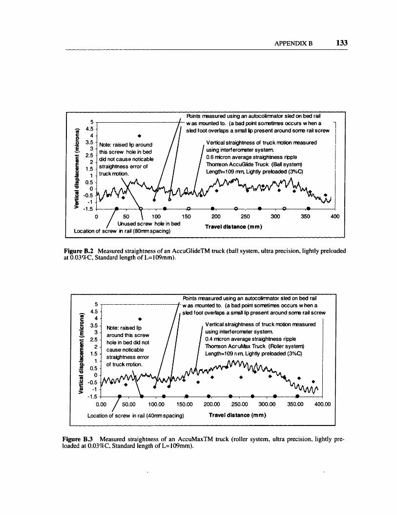
APPENDIX B
Points measured using an autocolimnator sled on bed railI . ......Note: raised lip aroundthis screw hole in beddid not cause noticable
straightness error oftruck motion.
-w as mounted to. (a bad point somnetimes occurs w hen asled foot overlaps a smrrall lip present around some rail screw
Vertical straightness of truck rrmotion measured
using interferometer system0.6 micron average straightness rippleThomson AccuGlide Truck (Ball system)Length=109 mn, Lightly preloaded (3%C)A *
Location of screw in rail (80rnnspacing)
150 200 250
Travel distance (mm)
300 350
Figure B.2 Measured straightness of an AccuGlideTM truck (ball system, ultra precision, lightly preloadedat 0.03%C, Standard length of L=109mm).
Points measured using an autocolirmnator sled on bed railt w as rmounted to. (a bad point sometimes occurs w hen a
overlaps a smll lip present around some rail screw
Vertical straightness of truck motion measured
using interferometer system0.4 micron average straightness rippleThornson AccuMax Truck (Roller system)Length=109 nWT, Lightly prebaded (3%C)
-l A
0.00 / 50.00 100.00
Location of screw in rail (40mnspaci
150.00 200.00 250.00 300.00 350.00 400.00
ing) Travel distance (mm)
Figure B.3 Measured straightness of an AccuMaxTM truck (roller system, ultra precision, lightly pre-loaded at 0.03%C, Standard length of L=109mm).
5
C
i.a
'a
4.54
3.53
2.52
1.51
0.50
-0.5-1
-1 r, .400
5I
4.3
'2 3.5- 3
2.5£ 2
1.5
0.
0
-0.5* -1
-1.5
�
v, w ' w , w 'w----C--
133
i.,
¢,
1. Iv It

134 APPENDIX B
It is informative to note that the spike (which, as explained in Section A.5, occurs locally
around the rim of some rail mounting holes) has almost no effect on the AccuMaxTM
truck straightness, for which every hole in the rail groove is used. For the AccuGlideTM,
however, the spike, which is 4.5 gtm high, causes only about a I gam rise in the truck
motion.
The ripple observed is caused by circulating elements. As expected, the AccuMaxTM had
a smaller wave amplitude than the AccuGlideTM because its rolling elements are smaller
(the more elements in contact at one time, the less effect one element entering or exiting
has). The amplitude of the ripple is close to twice an element diameter, as expected
(because the truck moves twice as fast relative to the rail as do the elements relative to the
truck.)
B.2 Dynamic Stiffness
The dynamic stiffness measurements on a bearing truck were performed via a hammer
test, using an HP35670A Signal Analyzer, and a PCB modally tuned hammer and acceler-
ometer. A hammer test utilizes a modally tuned hammer with a force transducer on its tip,
and an accelerometer, both sending signals to the signal analyzer. Upon striking the device
under test, the signal analyzer records the force impulse signal from the hammer, and the
acceleration, and from these calculates the frequency response of the device under test.
The frequency response data, which has units of acceleration per unit force, is input into a
spreadsheet where it is converted to stiffness verses frequency by dividing each accelera-
tion by frequency squared.
For both an AccuGlideTM and an AccuMaxTM truck, two test scenarios were performed.
For the first scenario, only a pillow block was bolted to a truck (using all six holes), and
for the second, the carriage plate was bolted in place according to the original test set up.
Fig} re B.4 shows the two test scenarios.

APPENDIX B 135
oIt
Withcarriageplate
_ZZ
JFigure B.4 The two test scenarios for dynamic stiffness testing.
Figure B.5 shows the results with the pillow block only for the AccuGlide and AccuMax,
and Figure B.6 shows the results with the hydrostatic prototype included (the hydrostatic
truck could not be tested objectively with pillow block only because it is not stable in tilt).
Table B.2 summarizes the minimum stiffnesses observed, along with the reduction in
stiffness Q that occurs at resonance.
-1, Ik~1 l

APPENDIX B
10000
EC
a
1000
100
100 500 1000 1500 2000 2500 3000 3500
Frequency (WH)
Figure B.5 Compressive dynamic stiffness of AccuGlideTM (ball system) and AccuMax (roller system)trucks, lightly preloaded (0.03%C), standard length of L=109mm, shown with the response measured on topof the rail alone. The hydrostatic prototype could not be tested under these conditions because it is not stablein tilt.
'urr
.un
00
est for Ightlylotmon) (Bal system),th (109 am)
MYC U,Z.. 4
r-4n
1921
Hydr
10
Wumfor \ 80 Numtor oler preloaded Thorsono 105 Num resonance for 47 Wum for Accurx(T4o (Rller system)
I OnF la Test BaH Standard length (109 ram)
0 200 400 600 800 1000 1200 1400 1600
Frequency of Excitation (Hz)
Figure B.6 Compressive dynamic stiffness of AccuGlideTM (ball system) and AccuMax (roller system)trucks, lightly preloaded (0.03%C), standard length of L=109mm, and the hydrostatic prototype, L=134mm,shown with the response measured on top of the rail alone.
136
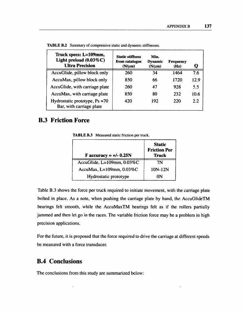
APPENDIX B 137
TABLE B.2 Summary of compressive static and dynamic stiffnesses.
Truck specs: L=109mm, Static stiffness Min.Light preload (0.03% C) from catalogue Dynamic Frequency
Ultra Precision (N/lm) (N/utm) (Hz) Q
AccuGlide, pillow block only 260 34 1464 7.6
AccuMax, pillow block only 850 66 1720 12.9
AccuGlide, with carriage plate 260 47 928 5.5
AccuMax, with carriage plate 850 80 232 10.6
Hydrostatic prototype, Ps =70 420 192 220 2.2Bar, with carriage plate
B.3 Friction Force
TABLE B.3 Measured static friction per truck.
StaticFriction Per
F accuracy = +/- 0.25N Truck
AccuGlide, L=109mm, 0.03%C 7N
AccuMax, L=109mm, 0.03%C 1ON-12N
Hydrostatic prototype ON
Table B.3 shows the force per truck required to initiate movement, with the carriage plate
bolted in place. As a note, when pushing the carriage plate by hand, the AccuGlideTM
bearings felt smooth, while the AccuMaxTM bearings felt as if the rollers partially
jammed and then let go in the races. The variable friction force may be a problem in high
precision applications.
For the future, it is proposed that the force required to drive the carriage at different speeds
be measured with a force transducer.
B.4 Conclusions
The conclusions from this study are summarized below:

138 APPENDIX B
Conclusions Drawn from Straightness Tests
1. The straightness of both rolling element systems would be about 1 micron ifthey were bolted to a perfectly flat rail groove.
2. The straightness ripple of the lightly preloaded AccuGlide and AccuMaxwas about 0.6 and 0.4 microns, respectively. With a higher preload we wouldexpect more ripple. The AccuMax has better ripple in part because its rollersare have a smaller diameter (6.35 mm for AccuGlide, 4 mm for AccuMax).
3. The period of ripple was close to twice the element diameter, as expected. Ifa part surface had ripple with these periods, ripple from the linear guideswould be the culprit.
Conclusions Drawn from Dynamic Stiffness Tests
1. The hydrostatic prototype shows improved damping because it did not addany resonances to those exhibited by the on rail test, unlike the roller sys-tems.
2. In fairness to the ball and roller systems, a light preload, standard lengthtruck (L=109mm) is the worst case scenario in terms of static stiffness (andmost likely for dynamic stiffness). For further research, tests should be per-formed on medium and heavily preloaded systems, to see if a significant dif-ference exists.
3. The rolling elements showed better damping with the carriage plate bolted inplace. This could be due to the effects of being over constrained.

THESIS PROCESSING SLIP .
FIXED FIELD: ill.
index
* COPIES: Aero
Lindgren Music
TITLE VARIES: -
Dewey
Rotch S(
name
biblio
ng Hum
tience
NAME VARIES: 4"," (, .X i
IMPRINT: (COPYRIGHT) _
* COLLATION:
* ADD: DEGREE:
SUPERVISORS:
(32 P
P. DEPT.:
cat'r: dt
cat'r: date:page:
I11C. D DEGREE: _.__, ) _
:v \ "-kV CA,-
NOTES:
. DEPT:
. YEAR:
. NAME:
I
-- -- -
- -~~~~~~~~~~~~~~~~~~~~~~~~~~~~~~~~~~~~~~~~~~~~~~~~~~~~
_ .
_ _ _ .
-