surface relief analysis for illustrative shading

Eurographics Symposium on Rendering 2012Fredo Durand and Diego Gutierrez(Guest Editors)

Volume 31 (2012), Number 4

Surface Relief Analysis for Illustrative ShadingLucas Ammann†, Pascal Barla, Gaël Guennebaud, Xavier Granier, Patrick Reuter

Inria - Univ. Bordeaux - IOGS - CNRS

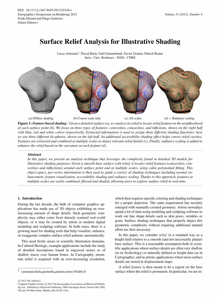
(a) Diffuse shading (b) Coarse scale only (c) All scales (d) + Radiance scaling

Figure 1: Feature-based shading: Given a detailed surface (a), we analyze its relief to locate relief features in the neighborhoodof each surface point (b). We focus on three types of features: convexities, concavities, and inflexions, shown on the right halfwith blue, red and white colors respectivelly. Extracted information is used to assign them different shading functions: herewe use three different lit-spheres, shown on the left half. An additional accessibility shading effect helps convey relief cavities.Features are extracted and combined at multiple scales to depict relevant relief details (c). Finally, radiance scaling is added toenhance the relief based on the curvature at each feature (d).

AbstractIn this paper, we present an analysis technique that leverages the complexity found in detailed 3D models forillustrative shading purposes. Given a smooth base surface with relief, it locates relief features (concavities, con-vexities and inflections) around each surface point and at multiple scales, using cubic-polynomial fitting. Thisobject-space, per-vertex information is then used to guide a variety of shading techniques including normal en-hancement, feature visualization, accessibility shading and radiance scaling. Thanks to this approach, features atmultiple scales are easily combined, filtered and shaded, allowing users to explore surface relief in real-time.

1. IntroductionDuring the last decade, the bulk of computer graphics ap-plications has made use of 3D objects exhibiting an ever-increasing amount of shape details. Such geometric com-plexity may either come from densely scanned real-worldobjects, or it may be created by artists in modern digitalmodeling and sculpting software. In both cases, there is agrowing need for shading tools that help visualize, enhance,or exaggerate complex surface relief patterns automatically.

This need firstly arises in scientific illustration domains.In Cultural Heritage, example applications include the studyof detailed inscriptions found in engraved stones or ofshallow traces over human bones. In Cartography, moun-tain relief is acquired with an ever-increasing resolution,

† {ammann,barla,guenneba,granier,reuter}@labri.fr

which then requires specific coloring and shading techniquesfor a proper depiction. The same requirement has recentlyemerged with manually-created geometry. Artists nowadaysspend a lot of time using modeling and sculpting software towork out fine shape details such as skin pores, wrinkles orgrain. Surface shading techniques that properly depict thisgeometric complexity without requiring additional manualeffort are then necessary.

In this paper, we consider relief in a standard way as aheight field relative to a smooth (and not necessarily planar)base surface. This is a reasonable assumption both in scien-tific applications where surface details are often very shallow(as in Archeology) or naturally defined as height data (as inCartography), and in artistic applications where most surfacedetails are stored in displacement maps.

A relief feature is then meant to be a region on the basesurface where the relief is prominent. In particular, we are in-

c© 2012 The Author(s)Computer Graphics Forum c© 2012 The Eurographics Association and Blackwell Publish-ing Ltd. Published by Blackwell Publishing, 9600 Garsington Road, Oxford OX4 2DQ,UK and 350 Main Street, Malden, MA 02148, USA.

DOI: 10.1111/j.1467-8659.2012.03144.x

L. Ammann & P.Barla & G. Guennebaud & X. Granier & P.Reuter / Surface Relief Analysis for Illustrative Shading

terested in three types of features — convexities, inflectionsand concavities — and the ways these are nested at multiplescales. Take for instance a relief ridge pitted with small cav-ities, as shown on the shoulder of the statue in Figure 1(a):a point anywhere inside one of the small pits belongs to aconcave feature at a small scale, and to a convex feature ata larger scale. Conveying surface relief through illustrativeshading then amounts to assigning a proper shading value toeach surface point, in a way that depends on the multi-scalefeatures it belongs to. This raises two major issues: 1) how tolocate relief features in the neighborhood of a surface point?2) how to combine features found at various scales (i.e., atincreasing neighborhood sizes)?

We address these issues by introducing an efficientbottom-up, multi-scale relief analysis technique based on cu-bic polynomial fitting. It locates relief features (concavities,convexities and inflections) in a neighborhood around eachsurface point, and provides a straightforward solution to themulti-scale combination problem. We illustrate the benefitsof our approach by adapting shading techniques to take ad-vantage of non-local relief information available at each sur-face point. An example is shown in Figure 1(b-d), whereshading color is assigned based on the distance to the closestfeature center, first at a single (large) scale, then at multiplescales. The result is a far more legible depiction of relief fea-tures occuring at various scales (including the small pits onthe shoulder). Our system only requires a short pre-processfor the completion of the bottom-up analysis step. It then al-lows users to explore surface relief in real-time, by varyingthe contribution of each scale, or by modifying shading andfiltering parameters.

2. Previous work

One of the earliest shading methods explicitly designedto convey shape features is accessibility shading [Mil94].Together with its most popular variant ambient occlusion(e.g., [PG04]), these methods produce images that depictcavities by darkening hardly-accessible surface points. How-ever, they have two main drawbacks. First, they demandlong pre-processing times when done accurately in objectspace. But most importantly, they provide limited control interms of surface feature depiction: shading and analysis arenot separated and mainly convey deep concavities with verysmooth shading variations.

More accurate surface measurements are obtained withdifferential geometry operators [dC76]. In particular, thesecond- and third-order tensors provide information aboutcurvature and curvature variations at a surface point. Suchmeasurements only apply to small surface neighborhoodsthough (infinitesimal neighborhoods for smooth surfaces).They have thus traditionally been used for identifying sur-face points that exactly lie on extremal curves such asridges and valleys [OBS04] or demarcating curves [KST08].Some methods have used similar operators for larger surfaceneighborhoods (e.g., [CP05, CPG09]) by first fitting a local

plane to the surface, and then fitting a quadratic function onrelative height values. When the surface “folds-over” itself,complex issues arise that can be overcome using total least-square fits [GGG08]. Such analysis methods are limited topurely local surface feature measurements, while we are in-terested in locating salient relief features, which we recallare to be found in the neighborhood of each surface point.In particular, these methods provide no simple way to knowthe distance to the nearest feature center of a given type, tocombine features found at multiple scales, or to filter out lessprominent features (e.g., shallow relief).

Another approach for analysing relief at multiple scalesconsists in decomposing surface normals into different lay-ers, which also avoids fold-over issues. Such a decomposi-tion has first been applied to normal enhancement [CST05,ZCF∗10], where a single relief layer is manipulated to ex-aggerate or attenuate surface details through shading. Simi-lar enhancement techniques have been applied to polynomialtexture maps [MWGA06]. In both cases, only two scales areconsidered. These methods have been extended to multiplescales in the exaggerated shading technique [RBD06]. Dif-ferent levels of smoothed normals are used to align a sin-gle light source at grazing angles. Shading values are thencomputed at each scale through half-Lambertian shading,and combined with a weighted sum to exaggerate multi-scale surface relief. The drawback with this approach is thatscale combination depends on the choice of light directionand shading parameters, which not only produces artifactswhen the light is moved around, but also makes it difficult tocontrol which type of feature is depicted.

Normal variations in image space have also been used toconvey surface details by letting them drive variations of in-coming radiance (e.g., [VPB∗10b]). This is an improvementcompared to exaggerated shading, since it works for arbi-trary materials and illumination and is devoid of temporalartifacts. However, the method is confined to a single scaleper point, and provides limited control over the type of de-picted feature as before.

When an accurate depiction of surface relief is targeted, itis preferable to decompose surface geometry into base andrelief layers. Various methods have been proposed to per-form this decomposition (e.g., [ZTS09]). The goal of thispaper is not to present a novel decomposition though, butrather to provide analysis solutions specifically targeted tothe relief layer. Only a few existing techniques have tack-led this problem. The prominent field technique [KST09b]combines output of second- and third-order tensors to iden-tify a direction field along which prominent relief featuresare likely to be located. This direction field has proven to beuseful for feature-aware smoothing, curvature-based shad-ing, and more recently line-based rendering [KST09a]. Asimilar solution has been proposed to identify feature linesin image-space, using fitting techniques [VVC∗11]. The ad-vantage of using a direction field is that it locates more ac-curately surface features around a point of interest. Unfortu-

c© 2012 The Author(s)c© 2012 The Eurographics Association and Blackwell Publishing Ltd.

1482


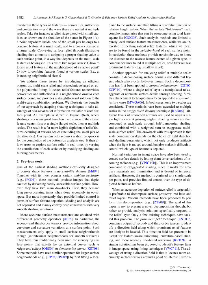
nately, as depicted in Figure 2 using a single direction alsointroduces artifacts around field singularities, and since thefield is likely to change at different scales, it is not clear howto perform scale combination.

(a) Mean curvature (b) Directional curvature

Figure 2: Artifacts due to singularities. As opposed toisotropic measurements (a), the use of a directional field toanalyse relief produces artifacts at it singularities (b).

3. OverviewOur approach focuses on surface relief and assumes in-put geometry to be decomposed into base and relief lay-ers. We first locate relief features in the neighborhood of asurface point, at a number of scales and directions. This isdone thanks to cubic polynomial fitting as explained in Sec-tion 4.1. We then combine features together and filter themin a way that preserves only the most pertinent data. Thisis permited by a weighting scheme based on the informa-tion conveyed by individual fits, as explained in Section 4.2.Shading techniques are finally adapted to depict propertiesof the relief features found around each surface point, as de-scribed in Section 5.

Details of our GPU implementation are given in Sec-tion 6: it requires a short pre-process for analysis, after whichit runs in real-time with interactive scale combination, fil-tering and shading abilities. Our solution does not rely onany parametrization of the base surface, and we demonstrateour system on both height-fields and detailed 2D manifolds.Moreover, for dynamic scenes, there is no need to update theanalysis during animation since in most cases, only the basesurface is deformed.

4. Relief analysisOur analysis takes as input a surface S de-fined as a smooth base surface B displacedalong its normal field nnnB by a height func-tion h. Mathematically, any point bbb ∈ Byields a point ppp on the surface S with:

ppp = bbb+h(bbb)nnnB(bbb) .

The scalar function h corresponds to the relief of the sur-face. For instance, sculpting tools are able to directly providea base surface with a displacement map. With acquired ob-jects though, the base and relief layers must be extracted inpre-process. The presentation of this step is out of the scopeof our paper, and we refer to, e.g., Zatzarinni et al. [ZTS09]

for such a base/relief decomposition technique. For the sakeof simplicity, and without loss of generality, we assume thatB is provided as a dense (regular or irregular) triangularmesh, while h is given as a scalar value per vertex.

4.1. 1D Analysis

The key idea of our approach is to analyse relief along 1Dneighborhoods of the base surface, in multiple directionsaround each point bbb. The main reasons for this choice arethat 1) the localisation of relief feature centers (e.g., curva-ture extrema) around bbb is made considerably simpler in onedimension, and 2) no 2D parametrization is required. Thisstrategy is also significantly faster for large scales.

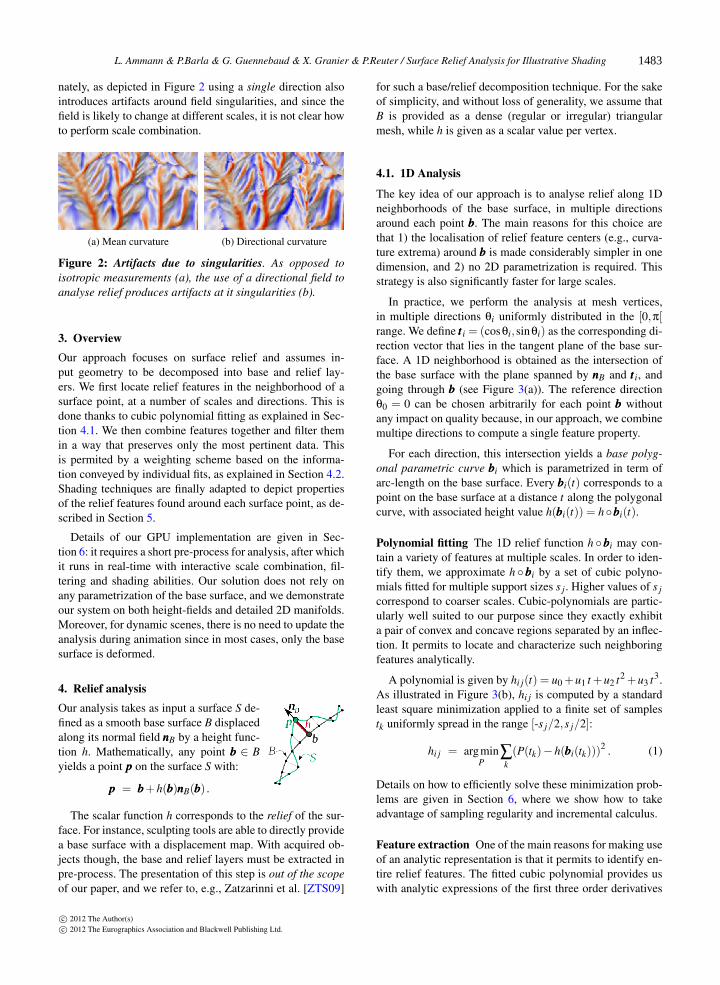
In practice, we perform the analysis at mesh vertices,in multiple directions θi uniformly distributed in the [0,π[range. We define ttti = (cosθi,sinθi) as the corresponding di-rection vector that lies in the tangent plane of the base sur-face. A 1D neighborhood is obtained as the intersection ofthe base surface with the plane spanned by nnnB and ttti, andgoing through bbb (see Figure 3(a)). The reference directionθ0 = 0 can be chosen arbitrarily for each point bbb withoutany impact on quality because, in our approach, we combinemultipe directions to compute a single feature property.

For each direction, this intersection yields a base polyg-onal parametric curve bbbi which is parametrized in term ofarc-length on the base surface. Every bbbi(t) corresponds to apoint on the base surface at a distance t along the polygonalcurve, with associated height value h(bbbi(t)) = h◦bbbi(t).

Polynomial fitting The 1D relief function h ◦bbbi may con-tain a variety of features at multiple scales. In order to iden-tify them, we approximate h ◦bbbi by a set of cubic polyno-mials fitted for multiple support sizes s j . Higher values of s jcorrespond to coarser scales. Cubic-polynomials are partic-ularly well suited to our purpose since they exactly exhibita pair of convex and concave regions separated by an inflec-tion. It permits to locate and characterize such neighboringfeatures analytically.

A polynomial is given by hi j(t) = u0 +u1 t +u2 t2 +u3 t3.As illustrated in Figure 3(b), hi j is computed by a standardleast square minimization applied to a finite set of samplestk uniformly spread in the range [-s j/2,s j/2]:

hi j = argminP

∑k(P(tk)−h(bbbi(tk)))

2 . (1)

Details on how to efficiently solve these minimization prob-lems are given in Section 6, where we show how to takeadvantage of sampling regularity and incremental calculus.

Feature extraction One of the main reasons for making useof an analytic representation is that it permits to identify en-tire relief features. The fitted cubic polynomial provides uswith analytic expressions of the first three order derivatives


1483


(a) Neighborhood sampling (b) Polynomial fitting at point p in 1 direction (c) Error measures at point p in all directions

Figure 3: 1D analysis. (a) The curves bbbi on the detailed surface S are extracted in multiple directions by intersecting planesdefined relative to the base surface B. (b) The height along a curve h◦bbbi on a support of size s j is fitted with a cubic polynomialhi j from which we compute the curvature function κi j and feature center locations t?i j (? ∈ {_,^,∼}) analytically. (c) For eachdirection, we compute the distance d?

i j to a particular feature center and the normal deviation ηi j of the detailed surface.

h′i j , h′′i j , and h′′′i j , as well as the curvature κi j:

κi j(t) =h′′i j(t)

(1+h′i j(t)2)

32

. (2)

We use these differential quantities to identify the positionsof the convexity (t_i j ), concavity (tî j ), and inflexion (t∼i j )points. We define the first two as the locations of the curva-ture extrema which are obtained as the zero-crossings of thecurvature variation. More precisely, t_i j and tî j are the roots ofthe rational polynomial κ

′i j(t) for which explicit formulas are

given in the Appendix. We observe that these roots do not co-incide with the local extrema of the cubic defined as the zero-crossings of the first-order derivative h′i j , even though theyare often very close (see Figure 3(b)). This choice is partic-ularly important when the cubic is monotone but not linear:curvature extrema can still be found whereas the value ex-trema do not exist. Curvature extrema thus constitute a morerobust choice in general. The position of the inflexion pointt∼i j is given by the zero-crossing of the second-order deriva-tive (P′′i j (t

∼i j ) = 0).

Normalized distances and error measure Features ex-tracted from the polynomial approximation may not alwaysbe pertinent. First, specific feature locations may be identi-fied outside the support used to fit the relief data. We thuscompute a truncated and normalized distance for each typeof relief feature (? ∈ {_,^,∼}):

d?i j =

⌊2|t?i j|

s j

⌉, (3)

where bxe is a function that clamps x to the [0,1] range.

Second, the detailed surface normals may substantiallydeviate from the plane used to intersect the base surfacegeometry. Indeed, with a large normal deviation, a smallchange in direction implies a large change in the fittedheights. We take into account this source of error by mea-suring for each fit the average normal deviation ηi j:

ηi j =1s j

∑k|nnn(tk) · (ttti×nnnB)| , (4)

where nnn is the normal of the detailed surface S, and ttti×nnnBis the normal of the plane supporting the cubic. Both typesof error measures are visualized in Figure 3(c) as a functionof direction θi at a single scale j.

4.2. Combination and FilteringOur multi-scale and multi-direction analysis provides adense relief description around a surface point, which en-sures that most nearby relevant relief features are properlyidentified by at least one fitted polynomial. We now presentcombination and filtering mechanisms that make such infor-mation exploitable by subsequent shading techniques.

Feature combination The key idea of our approach is tocombine scalar feature values fi j instead of polynomialsthemselves, to yield a single scalar F . For instance fi j couldbe taken to be the convexity curvature κi j(t_i, j), yielding anaverage curvature K. Combination is done in two steps. Wefirst average feature values at each scale over all directions:

Fj = ∑i

wi j fi j, wi j =wi j

∑i′ wi′ j, (5)

using wi j = (1− ηi j)(1− d?i j) for the weights. The factor

1−ηi j favors directions of low normal deviation for whichextracted feature values are most pertinent. This may be seenas a generalization of principal curvature directions, sincefor a quadratic surface, they exactly correspond to the direc-tions of zero normal deviation. For choices of fi j involvingeither t_i j , tî j or t∼i j , the weights 1− d?

i j also decrease as the

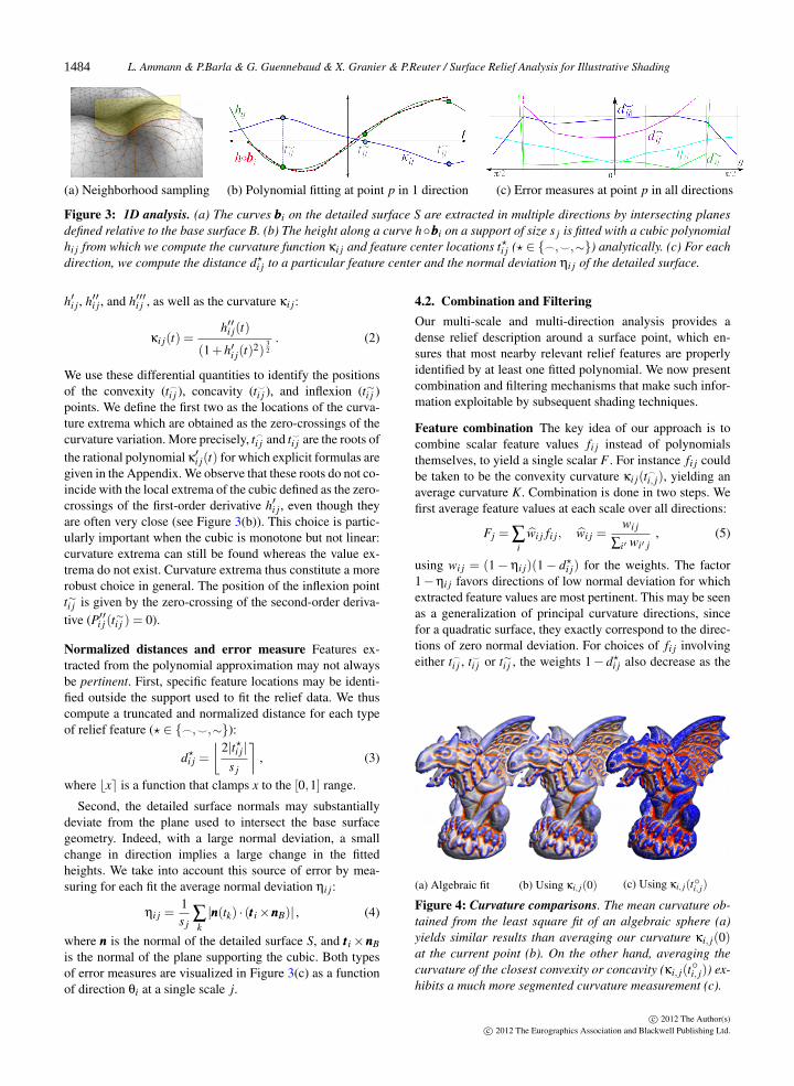
(a) Algebraic fit (b) Using κi, j(0) (c) Using κi, j(t◦i, j)

Figure 4: Curvature comparisons. The mean curvature ob-tained from the least square fit of an algebraic sphere (a)yields similar results than averaging our curvature κi, j(0)at the current point (b). On the other hand, averaging thecurvature of the closest convexity or concavity (κi, j(t◦i, j)) ex-hibits a much more segmented curvature measurement (c).


1484


(a) Coarse scale only (b) Fine scale only (c) All scales (ours) (d) All scales (uniform)

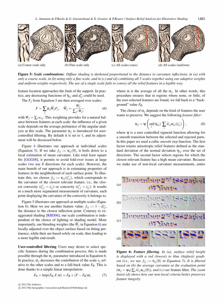
Figure 5: Scale combinations: Diffuse shading is darkened proportional to the distance to curvature inflections, in (a) withonly a coarse scale, in (b) using only a fine scale, and in (c) and (d) combining all 3 scales together using our adaptive weightsand uniform weights respectively. The use of a single scale fails to convey all the relief features in a legible way.

feature location approaches the limit of the support. In prac-tice, any decreasing functions of ηi j and d?

i j could be used.The Fj from Equation 5 are then averaged over scales:

F = ∑j

α jWjFj, Wj =Wj

∑ j′Wj′. (6)

with Wj = ∑i wi j. This weighting provides for a natural bal-ance between features at each scale: the influence of a givenscale depends on the average pertinence of the angular anal-ysis at this scale. The parameter α j is introduced for user-controlled filtering. By default it is set to 1, and its adjust-ment will be discussed below.

Figure 4 illustrates our approach at individual scales(Equation 5). If we take fi j := κi j(0), it boils down to alocal estimation of mean curvature. Like total least squarefits [GGG08], it permits to avoid fold-over issues at largescales (we use 8 directions for each scale). However, themain benefit of our approach is in estimating properties offeatures in the neighborhood of each surface point. To illus-trate this, we choose fi j := κi j(t◦i, j), which corresponds tothe curvature of the closest relevant feature, i.e., the clos-est convexity (t◦i, j = t_i j ) or concavity (t◦i, j = t^i j ). It resultsin a much more segmented measurement of curvature, eachpoint displaying the curvature of the convexity it belongs to.

Figure 5 illustrates our approach at multiple scales (Equa-tion 6). Here we use another feature value: fi j := 1− d∼i j ,the distance to the closest inflection point. Contrary to ex-aggerated shading [RBD06], our scale combination is inde-pendent of the choice of lighting or shading model. Moreimportantly, our blending weights (the Wj in Equation 6) arelocally adjusted over the object surface based on fitting per-tinence, while their are based solely on scale, thus leading toa more legible end-result.

User-controlled filtering Users may desire to select spe-cific features during the combination process; this is madepossible through the α j parameter introduced in Equation 6.In practice, α j decreases the contribution of the scale s j rel-ative to the other scales and to a fall-back value FB. This isdone thanks to a simple linear interpolation:

Fα = lerp(FB,F,α) = FB +(F−FB)α, (7)

where α is the average of all the α j. In other words, thisprocedure ensures that in regions where none, or little, ofthe user-selected features are found, we fall back to a “back-ground” value FB.

The choice of α j depends on the kind of features the userwants to preserve. We suggest the following feature filter:

α j = ψ

(std

i(ηi j) ∑

iwi jκi j(t

_i j )

), (8)

where ψ is a user controlled sigmoid function allowing fora smooth transition between the selected and rejected parts.In this paper we used a cubic smooth step function. The firstfactor retains anisotropic relief features defined as the stan-dard deviation of the normal deviation ηi j over the set ofdirections. The second factor selects regions for which theclosest relevant feature has a high mean curvature. Becausewe make use of non-local curvature measurements, entire

(a)

(b)

(c)

(d)

Figure 6: Feature filtering. In (a), surface relief heightis displayed with a red (lowest) to blue (highest) gradi-ent (i.e., we use fi j := hi j(0) in Equation 5). It is filteredbased on (b) the average curvature at the evaluation point(α j = ψκ(∑i wi jκi j(0)), and (c) our feature filter. The zoominsets (d) shows how our non-local criteria better preservesfeature integrity.


1485


(a) Normal and visibility angles

(b) Membership functions

(c) Curvature functions

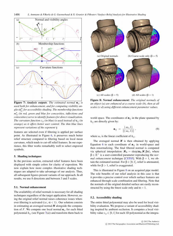
Figure 7: Analysis outputs. The estimated normal nnni j isused both for enhancement, and for computing visibility an-gles φ

±i j for accessibility shading. The membership functions

m?i j (in red, green and blue for concavities, inflections and

convexities) serve to identify features for direct visualization.The curvature function ci j (in blue) is used instead of κi j (inorange) as it offers better user control. The thin blue linesrepresent variations of the exponent γ.

features are selected even if filtering is applied per surfacepoint. As illustrated in Figure 6, it preserves much betterrelief structure compared to filtering based on local meancurvature, which tends to cut-off relief features. In our expe-rience, this filter works remarkably well to select engravedsymbols.

5. Shading techniques

In the previous section, extracted relief features have beendisplayed with simple colors for clarity of exposition. Wenow explain how more complex illustrative shading tech-niques are adapted to take advantage of our analysis. Thus,all subsequent figures present variants of our approach. In allresults, we use 8 directions and between 3 and 5 scales.

5.1. Normal enhancement

The availability of relief normals is necessary for all shadingtechniques regardless of the target application. However, us-ing the original relief normal raises coherence issues when-ever filtering is activated (i.e., α < 1) . Our solution consistsin estimating an averaged normal NNN alongside the computa-tion of F . We compute one local normal nnni j for each fittedpolynomial hi j (see Figure 7(a)) and transform them back to

(a) Original normals (b) Coarse scale only (β = 5)

(c) All scales (β = 5) (d) All scales (β = 1)

Figure 8: Normal enhancement: The original normals ofan object (a) are enhanced at a coarse scale (b), then at allscales (c-d) using different enhancement parameter values.

world space. The coordinates of nnni j in the plane spanned byhi j are directly given by:

nnni j =(-u1,1)‖(-u1,1)‖

, (9)

where u1 is the linear coefficient of hi j.

The averaged normal NNN is then obtained by applyingEquation 6 to each coordinate of nnni j in world-space andthen renormalizing. The final filtered normal is computedvia spherical interpolation: NNNα = slerp(nnnB,NNN,βα), whereβ ∈ R+ is a user-controlled parameter reproducing the nor-mal enhancement technique [CST05]. With β = 1, we ob-tain the estimated normal. For β ∈ [0,1], relief is attenuated,while for β > 1, relief is exaggerated.

This is illustrated in Figure 8 on an acquired pipe model.The sole benefits of our relief analysis in this case is thatit provides a precise control over which surface features areenhanced through scale combination and filtering. Note thatthe normals of the original detailed surface are easily recon-structed by using the finest scale only and α = 1.

5.2. Accessibility shading

The entire fitted polynomial may also be used for local visi-bility evaluation. We propose a variant of accessibility shad-ing inspired by ambient occlusion. It computes a local visi-bility value vi j ∈ [0,1] for each 1D polynomial as the integra-


1486


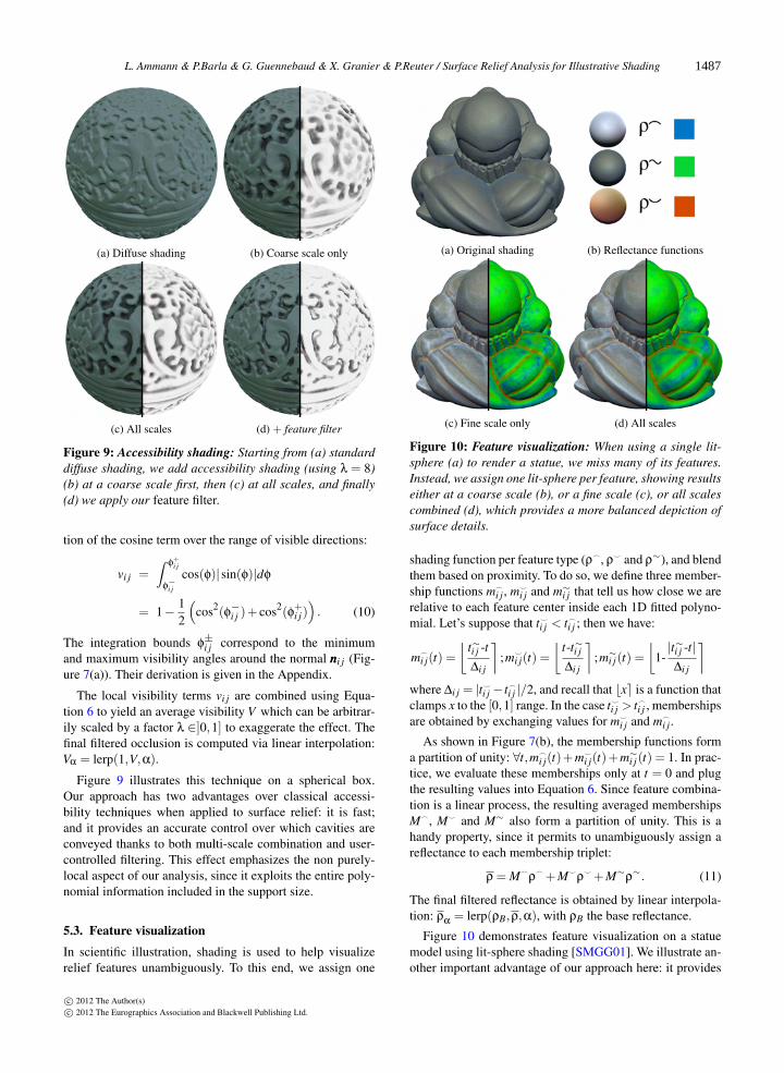
(a) Diffuse shading (b) Coarse scale only

(c) All scales (d) + feature filter

Figure 9: Accessibility shading: Starting from (a) standarddiffuse shading, we add accessibility shading (using λ = 8)(b) at a coarse scale first, then (c) at all scales, and finally(d) we apply our feature filter.

tion of the cosine term over the range of visible directions:

vi j =∫ φ

+i j

φ−i j

cos(φ)|sin(φ)|dφ

= 1− 12

(cos2(φ−i j )+ cos2(φ+i j)

). (10)

The integration bounds φ±i j correspond to the minimum

and maximum visibility angles around the normal nnni j (Fig-ure 7(a)). Their derivation is given in the Appendix.

The local visibility terms vi j are combined using Equa-tion 6 to yield an average visibility V which can be arbitrar-ily scaled by a factor λ ∈]0,1] to exaggerate the effect. Thefinal filtered occlusion is computed via linear interpolation:Vα = lerp(1,V,α).

Figure 9 illustrates this technique on a spherical box.Our approach has two advantages over classical accessi-bility techniques when applied to surface relief: it is fast;and it provides an accurate control over which cavities areconveyed thanks to both multi-scale combination and user-controlled filtering. This effect emphasizes the non purely-local aspect of our analysis, since it exploits the entire poly-nomial information included in the support size.

5.3. Feature visualization

In scientific illustration, shading is used to help visualizerelief features unambiguously. To this end, we assign one

(a) Original shading (b) Reflectance functions

(c) Fine scale only (d) All scales

Figure 10: Feature visualization: When using a single lit-sphere (a) to render a statue, we miss many of its features.Instead, we assign one lit-sphere per feature, showing resultseither at a coarse scale (b), or a fine scale (c), or all scalescombined (d), which provides a more balanced depiction ofsurface details.

shading function per feature type (ρ_, ρ^ and ρ

∼), and blendthem based on proximity. To do so, we define three member-ship functions m_

i j, mî j and m∼i j that tell us how close we are

relative to each feature center inside each 1D fitted polyno-mial. Let’s suppose that tî j < t_i j ; then we have:

m_i j(t) =

⌊t∼i j -t∆i j

⌉;m^

i j(t) =⌊

t-t∼i j

∆i j

⌉;m∼i j(t) =

⌊1-|t∼i j -t|∆i j

⌉where ∆i j = |tî j − t_i j |/2, and recall that bxe is a function thatclamps x to the [0,1] range. In the case tî j > t_i j , membershipsare obtained by exchanging values for m^

i j and m_i j.

As shown in Figure 7(b), the membership functions forma partition of unity: ∀t,m_

i j(t)+mî j(t)+m∼i j(t) = 1. In prac-

tice, we evaluate these memberships only at t = 0 and plugthe resulting values into Equation 6. Since feature combina-tion is a linear process, the resulting averaged membershipsM_, M^ and M∼ also form a partition of unity. This is ahandy property, since it permits to unambiguously assign areflectance to each membership triplet:

ρ = M_ρ_ +M^

ρ^ +M∼ρ

∼. (11)

The final filtered reflectance is obtained by linear interpola-tion: ρ

α= lerp(ρB,ρ,α), with ρB the base reflectance.

Figure 10 demonstrates feature visualization on a statuemodel using lit-sphere shading [SMGG01]. We illustrate an-other important advantage of our approach here: it provides


1487


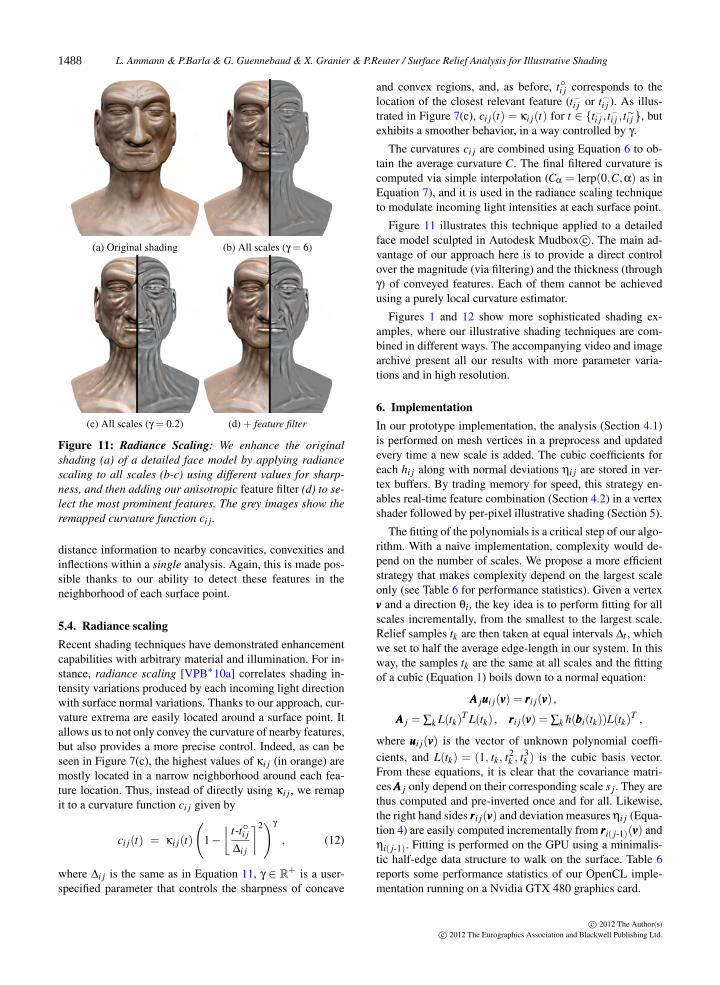
(a) Original shading (b) All scales (γ = 6)

(c) All scales (γ = 0.2) (d) + feature filter

Figure 11: Radiance Scaling: We enhance the originalshading (a) of a detailed face model by applying radiancescaling to all scales (b-c) using different values for sharp-ness, and then adding our anisotropic feature filter (d) to se-lect the most prominent features. The grey images show theremapped curvature function ci j.

distance information to nearby concavities, convexities andinflections within a single analysis. Again, this is made pos-sible thanks to our ability to detect these features in theneighborhood of each surface point.

5.4. Radiance scalingRecent shading techniques have demonstrated enhancementcapabilities with arbitrary material and illumination. For in-stance, radiance scaling [VPB∗10a] correlates shading in-tensity variations produced by each incoming light directionwith surface normal variations. Thanks to our approach, cur-vature extrema are easily located around a surface point. Itallows us to not only convey the curvature of nearby features,but also provides a more precise control. Indeed, as can beseen in Figure 7(c), the highest values of κi j (in orange) aremostly located in a narrow neighborhood around each fea-ture location. Thus, instead of directly using κi j, we remapit to a curvature function ci j given by

ci j(t) = κi j(t)

(1−

⌊t-t◦i j

∆i j

⌉2)γ

, (12)

where ∆i j is the same as in Equation 11, γ ∈ R+ is a user-specified parameter that controls the sharpness of concave

and convex regions, and, as before, t◦i j corresponds to thelocation of the closest relevant feature (t^i j or t_i j ). As illus-trated in Figure 7(c), ci j(t) = κi j(t) for t ∈ {t^i j , t

_i j , t∼i j }, but

exhibits a smoother behavior, in a way controlled by γ.

The curvatures ci j are combined using Equation 6 to ob-tain the average curvature C. The final filtered curvature iscomputed via simple interpolation (Cα = lerp(0,C,α) as inEquation 7), and it is used in the radiance scaling techniqueto modulate incoming light intensities at each surface point.

Figure 11 illustrates this technique applied to a detailedface model sculpted in Autodesk Mudbox c©. The main ad-vantage of our approach here is to provide a direct controlover the magnitude (via filtering) and the thickness (throughγ) of conveyed features. Each of them cannot be achievedusing a purely local curvature estimator.

Figures 1 and 12 show more sophisticated shading ex-amples, where our illustrative shading techniques are com-bined in different ways. The accompanying video and imagearchive present all our results with more parameter varia-tions and in high resolution.

6. ImplementationIn our prototype implementation, the analysis (Section 4.1)is performed on mesh vertices in a preprocess and updatedevery time a new scale is added. The cubic coefficients foreach hi j along with normal deviations ηi j are stored in ver-tex buffers. By trading memory for speed, this strategy en-ables real-time feature combination (Section 4.2) in a vertexshader followed by per-pixel illustrative shading (Section 5).

The fitting of the polynomials is a critical step of our algo-rithm. With a naive implementation, complexity would de-pend on the number of scales. We propose a more efficientstrategy that makes complexity depend on the largest scaleonly (see Table 6 for performance statistics). Given a vertexvvv and a direction θi, the key idea is to perform fitting for allscales incrementally, from the smallest to the largest scale.Relief samples tk are then taken at equal intervals ∆t , whichwe set to half the average edge-length in our system. In thisway, the samples tk are the same at all scales and the fittingof a cubic (Equation 1) boils down to a normal equation:

AAA juuui j(vvv) = rrri j(vvv) ,

AAA j = ∑k L(tk)T L(tk) , rrri j(vvv) = ∑k h(bbbi(tk))L(tk)

T ,

where uuui j(vvv) is the vector of unknown polynomial coeffi-cients, and L(tk) = (1, tk, t2

k , t3k ) is the cubic basis vector.

From these equations, it is clear that the covariance matri-ces AAA j only depend on their corresponding scale s j. They arethus computed and pre-inverted once and for all. Likewise,the right hand sides rrri j(vvv) and deviation measures ηi j (Equa-tion 4) are easily computed incrementally from rrri( j-1)(vvv) andηi( j-1). Fitting is performed on the GPU using a minimalis-tic half-edge data structure to walk on the surface. Table 6reports some performance statistics of our OpenCL imple-mentation running on a Nvidia GTX 480 graphics card.


1488


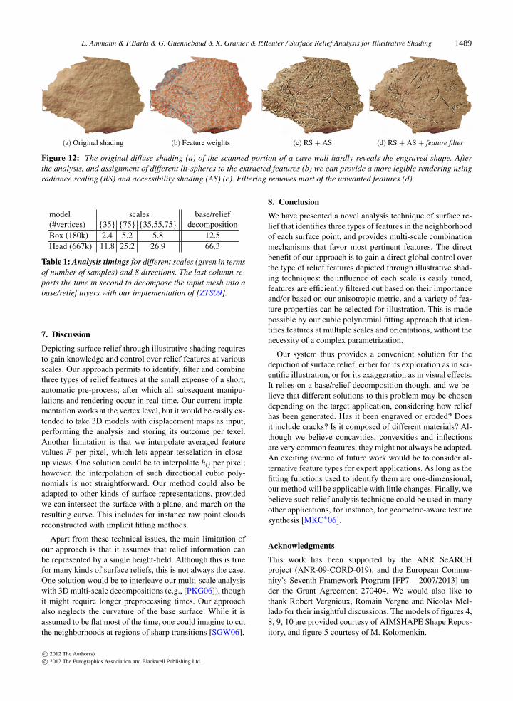
(a) Original shading (b) Feature weights (c) RS + AS (d) RS + AS + feature filter

Figure 12: The original diffuse shading (a) of the scanned portion of a cave wall hardly reveals the engraved shape. Afterthe analysis, and assignment of different lit-spheres to the extracted features (b) we can provide a more legible rendering usingradiance scaling (RS) and accessibility shading (AS) (c). Filtering removes most of the unwanted features (d).

model scales base/relief(#vertices) {35} {75} {35,55,75} decompositionBox (180k) 2.4 5.2 5.8 12.5Head (667k) 11.8 25.2 26.9 66.3

Table 1: Analysis timings for different scales (given in termsof number of samples) and 8 directions. The last column re-ports the time in second to decompose the input mesh into abase/relief layers with our implementation of [ZTS09].

7. Discussion

Depicting surface relief through illustrative shading requiresto gain knowledge and control over relief features at variousscales. Our approach permits to identify, filter and combinethree types of relief features at the small expense of a short,automatic pre-process; after which all subsequent manipu-lations and rendering occur in real-time. Our current imple-mentation works at the vertex level, but it would be easily ex-tended to take 3D models with displacement maps as input,performing the analysis and storing its outcome per texel.Another limitation is that we interpolate averaged featurevalues F per pixel, which lets appear tesselation in close-up views. One solution could be to interpolate hi j per pixel;however, the interpolation of such directional cubic poly-nomials is not straightforward. Our method could also beadapted to other kinds of surface representations, providedwe can intersect the surface with a plane, and march on theresulting curve. This includes for instance raw point cloudsreconstructed with implicit fitting methods.

Apart from these technical issues, the main limitation ofour approach is that it assumes that relief information canbe represented by a single height-field. Although this is truefor many kinds of surface reliefs, this is not always the case.One solution would be to interleave our multi-scale analysiswith 3D multi-scale decompositions (e.g., [PKG06]), thoughit might require longer preprocessing times. Our approachalso neglects the curvature of the base surface. While it isassumed to be flat most of the time, one could imagine to cutthe neighborhoods at regions of sharp transitions [SGW06].

8. Conclusion

We have presented a novel analysis technique of surface re-lief that identifies three types of features in the neighborhoodof each surface point, and provides multi-scale combinationmechanisms that favor most pertinent features. The directbenefit of our approach is to gain a direct global control overthe type of relief features depicted through illustrative shad-ing techniques: the influence of each scale is easily tuned,features are efficiently filtered out based on their importanceand/or based on our anisotropic metric, and a variety of fea-ture properties can be selected for illustration. This is madepossible by our cubic polynomial fitting approach that iden-tifies features at multiple scales and orientations, without thenecessity of a complex parametrization.

Our system thus provides a convenient solution for thedepiction of surface relief, either for its exploration as in sci-entific illustration, or for its exaggeration as in visual effects.It relies on a base/relief decomposition though, and we be-lieve that different solutions to this problem may be chosendepending on the target application, considering how reliefhas been generated. Has it been engraved or eroded? Doesit include cracks? Is it composed of different materials? Al-though we believe concavities, convexities and inflectionsare very common features, they might not always be adapted.An exciting avenue of future work would be to consider al-ternative feature types for expert applications. As long as thefitting functions used to identify them are one-dimensional,our method will be applicable with little changes. Finally, webelieve such relief analysis technique could be used in manyother applications, for instance, for geometric-aware texturesynthesis [MKC∗06].

Acknowledgments

This work has been supported by the ANR SeARCHproject (ANR-09-CORD-019), and the European Commu-nity’s Seventh Framework Program [FP7 – 2007/2013] un-der the Grant Agreement 270404. We would also like tothank Robert Vergnieux, Romain Vergne and Nicolas Mel-lado for their insightful discussions. The models of figures 4,8, 9, 10 are provided courtesy of AIMSHAPE Shape Repos-itory, and figure 5 courtesy of M. Kolomenkin.


1489


References[CP05] CAZALS F., POUGET M.: Estimating differential quanti-

ties using polynomial fitting of osculating jets. Computer AidedGeometric Design 22, 2 (2005). 2

[CPG09] CIPRIANO G., PHILIPS JR G., GLEICHER M.: Multi-Scale Surface Descriptors. IEEE Trans. Visualization and Com-put. Graph. 15, 6 (2009), 1201–1208. 2

[CST05] CIGNONI P., SCOPIGNO R., TARINI M.: A simplenormal enhancement technique for interactive non-photorealisticrenderings. Computers & Graphics 29 (2005), 125–133. 2, 6

[dC76] DO CARMO M. P.: Differential Geometry of Curves andSurfaces. Prentice-Hall, Englewood Cliffs, NJ, 1976. 2

[GGG08] GUENNEBAUD G., GERMANN M., GROSS M.: Dy-namic sampling and rendering of algebraic point set surfaces.Computer Graphics Forum 27, 2 (2008). 2, 5

[KST08] KOLOMENKIN M., SHIMSHONI I., TAL A.: Demar-cating Curves for Shape Illustration. ACM Trans. Graph. (Proc.SIGGRAPH Asia) 27, 5 (2008). 2

[KST09a] KOLOMENKIN M., SHIMSHONI I., TAL A.: On edgedetection on surfaces. In IEEE conf. Comput. Vision and PatternRecognition (CVPR) (June 2009), Ieee, pp. 2767–2774. 2

[KST09b] KOLOMENKIN M., SHIMSHONI I., TAL A.: Promi-nent field for shape processing of archaeological artifacts. InIEEE Int. Conf. Comput. Vision Workshop (ICCVW) (Sept. 2009),Ieee, pp. 915–922. 2

[Mil94] MILLER G.: Efficient algorithms for local and globalaccessibility shading. In Proceedings of the 21st annual con-ference on Computer graphics and interactive techniques (NewYork, NY, USA, 1994), SIGGRAPH ’94, ACM, pp. 319–326. 2

[MKC∗06] MERTENS T., KAUTZ J., CHEN J., BEKAERT P.,DURAND F.: Texture transfer using geometry correlation. InRendering Techniques (2006), pp. 273–284. 9

[MWGA06] MALZBENDER T., WILBURN B., GELB D., AM-BRISCO B.: Surface Enhancement Using Real-time PhotometricStereo and Reflectance Transformation. In Eurographics Sympo-sium on Rendering (2006), Eurographics. 2

[OBS04] OHTAKE Y., BELYAEV A., SEIDEL H.-P.: Ridge-valleylines on meshes via implicit surface fitting. In ACM SIGGRAPH2004 Papers (New York, NY, USA, 2004), SIGGRAPH ’04,ACM, pp. 609–612. 2

[PG04] PHARR M., GREEN S.: GPU Gems. Addison-Wesley,2004, ch. Ambient Occlusion. 2

[PKG06] PAULY M., KOBBELT L. P., GROSS M.: Point-basedmultiscale surface representation. ACM Trans. Graph. 25 (April2006), 177–193. 9

[RBD06] RUSINKIEWICZ S., BURNS M., DECARLO D.: Ex-aggerated shading for depicting shape and detail. ACM Trans.Graph. (Proc. SIGGRAPH) 25, 3 (July 2006), 1199. 2, 5

[SGW06] SCHMIDT R., GRIMM C., WYVILL B.: Interactive de-cal compositing with discrete exponential maps. ACM Trans.Graph. 25 (July 2006), 605–613. 9

[SMGG01] SLOAN P.-P. J., MARTIN W., GOOCH A., GOOCHB.: The lit sphere: a model for capturing npr shading from art.In No description on Graphics interface 2001 (Toronto, Ont.,Canada, Canada, 2001), GRIN’01, Canadian Information Pro-cessing Society, pp. 143–150. 7

[VPB∗10a] VERGNE R., PACANOWSKI R., BARLA P.,GRANIER X., SCHLICK C.: Radiance Scaling for Versa-tile Surface Enhancement. In Proc. symposium on Interactive3D and games (I3D) (2010), ACM. 8

[VPB∗10b] VERGNE R., PACANOWSKI R., BARLA P.,GRANIER X., SHLICK C.: Improving Shape Depiction underArbitrary Rendering. IEEE Trans. Visualization and Comput.Graph. PrePrint, 99 (Dec. 2010), 1–12. 2

[VVC∗11] VERGNE R., VANDERHAEGHE D., CHEN J., BARLAP., GRANIER X., SCHLICK C.: Implicit Brushes for StylizedLine-based Rendering. Comp. Graph. Forum (Proc. Eurograph-ics) 30, 2 (2011). 2

[ZCF∗10] ZHANG X., CHEN W., FANG J., WANG R., PENG Q.:Perceptually-motivated Shape Exaggeration. The Visual Comp.(Proc. CGI) 26, 6-8 (2010), 985–995. 2

[ZTS09] ZATZARINNI R., TAL A., SHAMIR A.: Relief Analysisand Extraction. ACM Trans. Graph. (Proc. SIGGRAPH Asia) 28,5 (2009), 1–10. 2, 3, 9

AppendixRelief analysis - feature locationsAs explained in Section 4.1, the convexity and concavity lo-cations t_, t^ are the roots of the rational polynomial κ

′(t),where κ (Equation 2) corresponds to the curvature of a cu-bic polynomial h(t) = u0 +u1t +u2t2 +u3t3. If u3 6= 0, thenthere exist only two real roots, t_ and t^, given by:

±

√3√

9u23u2

1-6u3u22u1 +u4

2 +5u23-6u3u1 +2u2

2

3√

5u3-

u2

3u3(13)

The inflexion position t∼ is then obtained as the unique rootof the second-order derivative polynomial (h′′(t∼) = 0):

t∼ =-u23u3

=t_ + t^

2. (14)

On the other hand, if u3 = 0 but u2 6= 0, then there is only aunique concavity or convexity point at t = -u1/2u2, and noinflexion point can be detected. If u2 is also zero, then nofeature points can be extracted. In these cases, the respectiveundefined d?

i j values are set to 1.

Accessibility shading - integration boundsThe computation of the accessibility term of Equation 10relies on the determination of the cosine of the two integra-tion bounding angles φ

±. In the case of a cubic polynomialh(t), they are given by the clamped dot product betweenthe normal direction nnn (as defined in Equation 9), and thetwo normalized vectors (xxx±−ooo), where xxx± = (t±,h(t±))are the two extremity points of the curve visible from theobserver location ooo = (0, -u0) (see Figure 7). Since thecurve is clamped to the range [-s j/2,s j/2], they either co-incide with the boundaries of the curves, or with the pointyyy = (ty,h(ty)) for which the vector (yyy−ooo) is tangent to thecurve at yyy. It is obtained by solving for the cubic equation(-h′(ty),1) · (yyy−ooo) = 0, which admits a single non null root:ty = -u2/(2u3). The two positions t−, t+ of the visible ex-tremities xxx± = (t±,h(t±)) are finally given by:

(t−, t+) =

(

-s j

2, min

( s j

2, ty))

if ty > 0,(max

(-s j

2, ty),

s j

2

)otherwise.

(15)


1490

surface relief analysis for illustrative shading

Documents