supplemental material for optimizing allocation for a delayed influenza vaccination campaign

Supplemental Material forOptimizing allocation for a delayedinfluenza vaccination campaign

Jan Medlock∗† Lauren A. Meyers‡§ Alison P. Galvani¶

November 19, 2009

We extended the age-structured SEIR (susceptible, latent, infectious, re-covered) model of Medlock and Galvani [6] to include two levels of risk forcomplications due to influenza infection and parametrized this model usingdata from the 2009 H1N1 influenza pandemic. We also extended the frame-work to incorporate staggered delivery of vaccine doses.

Here we detail the model construction and parametrization and reviewthe results.

S1 Mathematical ModelS1.1 Transmission ModelFor modeling influenza transmission in the United States, we divide the pop-ulation into the 17 age groups for ages 0, 1–4, 5–9, 10–14, 15–19, 20–24,25–29, 30–34, 35–39, 40–44, 45–49, 50–54, 55–59, 60–64, 65–69, 70–74, and75+. The numbers of people in each age group were parametrized using theestimated US 2007 population [17].∗Department of Mathematical Sciences, Clemson University, Box 340975, Clemson, SC

29634†Corresponding author. Email: [email protected]‡Section of Integrative Biology, The University of Texas at Austin, Austin, TX 78712§Santa Fe Institute, 1399 Hyde Park Road, Santa Fe, NM 87501¶Department of Epidemiology and Public Health, Yale University School of Medicine,

135 College Street, New Haven, CT 06520

1

mailto:[email protected]

Within each age, we further divide the population into low risk and highrisk for influenza complications, with high risk being identified by existingmedical conditions such as asthma, heart disease, and pregnancy. The pro-portion high risk by age is given in Table S1 [8]. (Where the age groups forthe proportion at high risk do not line up with our model age groups, weassumed that people are distributed uniformly within the model age groups.E.g. we assume that from the age group 15–19, 80% are under 18 and 20%are over 18.)

Each of the age–risk groups is then stratified by infection status. LetSLUa(t), ELUa(t), ILUa(t), and RLUa(t) be the respective numbers of un-vaccinated low-risk susceptible, latent, infectious, and recovered people inage groups a = 1, 2, . . . , 17. Let SHUa(t), EHUa(t), IHUa(t), and RHUa(t) bedefined similarly, but for unvaccinated high-risk people. Now, let SLVa(t),ELVa(t), ILVa(t), RLVa(t), SHVa(t), EHVa(t), IHVa(t), RHVa(t) be defined sim-ilarly for vaccinated people.

2

Table S1: Proprtion at high risk for influenza complications.Proportion

Ages High Risk, PHa

< 6 m 1.51%6 m–1 4.22%1–4 8.86%5–18 11.92%19–24 18.79%25–49 20.15%50–64 33.83%65+ 53.15%

Compiled by the MIDAS High-Risk Segmentation Group [8]. High risk forinfluenza complications is defined as having a chronic condition that is in-dications receiving influenza vaccine, having an immunocompromised con-dition, or being pregnant. For adults, the chronic conditions that indicatevaccination are: current asthma, chronic bronchitis, emphysema, coronaryheart disease, angina, heart attack, diabetes, stroke, weak kidney, epilepsy,cerebral palsy, movement disorders, and muscular dystrophies [2]. For chil-dren, these chronic conditions are: current asthma, congenital heart disease,ever diabetes, Down syndrome, ever cerebral palsy, ever muscular dystrophy,ever cystic fibrosis, ever sickle cell anemia, and seizures in past 12 months[2]. For children under 6 months, birth weight less than 1500 gm is alsoincluded [2]. Immunocompromised conditions are: cancer in the past 3 years[2], HIV/AIDS [3], dialysis [16], and having had an organ transplant [11].Pregnancy is also included [2].

3

The infection dynamics are described by the differential equations

dSLUa

dt = −λaSLUa, (S1a)dELUa

dt = λaSLUa − τELUa, (S1b)dILUa

dt = τELUa − (γ + νLUa)ILUa, (S1c)dRLUa

dt = γILUa, (S1d)dSHUa

dt = −λaSHUa, (S1e)dEHUa

dt = λaSHUa − τEHUa, (S1f)dIHUa

dt = τEHUa − (γ + νHUa)IHUa, (S1g)dRHUa

dt = γIHUa, (S1h)dSLVa

dt = −(1− εa)λaSLVa, (S1i)dELVa

dt = (1− εa)λaSLVa − τELVa, (S1j)dILVa

dt = τELVa − (γ + νLVa)ILVa, (S1k)dRLVa

dt = γILVa, (S1l)dSHVa

dt = −(1− εa)λaSHVa, (S1m)dEHVa

dt = (1− εa)λaSHVa − τEHVa, (S1n)dIHVa

dt = τEHVa − (γ + νHVa)IHVa, (S1o)dRHVa

dt = γIHVa (S1p)

for a = 1, . . . , 17. The progression rate to infectiousness is τ and the recoveryrate is γ. The influenza-induced death rates for people in age group a areνLUa, νHUa, νLVa, and νHVa, respectively, for unvaccinated low-risk, unvacci-nated high-risk, vaccinated low-risk, and vaccinated high-risk people. The

4

force of infection is given by

λa =17∑α=1

βσaφaα (ILUα + IHUα + ILVα + IHVα)N

= βσaN

17∑α=1

φaα (ILUα + IHUα + ILVα + IHVα) .(S1q)

Here φaα is the number of contacts between a person in age group a withpeople in age group α, β is the probability of infection for a susceptible personwho has contact with an infectious person, and σa is the relative susceptibilityof people in age group a. The relative susceptibility incorporates the potentialfor older people to have some immunity to the current 2009 H1N1 strain dueto exposure to a similar virus in the distant past. The total population sizeis N :

Na = SLUa + ELUa + ILUa +RLUa + SHUa + EHUa + IHUa +RHUa

+ SLVa + ELVa + ILVa +RLVa + SHVa + EHVa + IHVa +RHVa,(S1r)

N =∑a

Na. (S1s)

The demographic effects of aging, birth, and death by causes not related toinfluenza are not included because we only model one influenza season, wherethese demographic effects are small.

The epidemic is initiated with the entire population unvaccinated, withone person of each age infectious, and the remaining population susceptible.

5

That is

SLUa(t0) = (1− PHa)Na − 1, (S2a)SHUa(t0) = PHaNa − 1, (S2b)SLVa(t0) = 0, (S2c)SHVa(t0) = 0, (S2d)ELUa(t0) = 0, (S2e)EHUa(t0) = 0, (S2f)ELVa(t0) = 0, (S2g)EHVa(t0) = 0, (S2h)ILUa(t0) = 1, (S2i)IHUa(t0) = 1, (S2j)ILVa(t0) = 0, (S2k)IHVa(t0) = 0, (S2l)RLUa(t0) = 0, (S2m)RHUa(t0) = 0, (S2n)RLVa(t0) = 0, (S2o)RHVa(t0) = 0, (S2p)

where Na is the number of people of age a (from the estimated 2007 USpopulation [17]) and PHa is the proportion of age group a who are high risk(Table S1).

Numerical solution of the model differential equations was done using theLSODA routine [5].

S1.2 Basic Reproductive NumberThe basic reproductive number (R0) of model (S1) was calculated using thenext-generation matrix ([4, 6, 18]). No closed form expression is available forR0 for model (S1): rather, it is given by the leading eigenvalue of a matrixdepending on the model parameters.

Consider the case when no one in the population has been exposed to the

6

pathogen and there is no vaccination. Define the sub-matrices

FL = [FLaα] =[βσa

(1− PHa)Na

Nφaα

], (S3a)

FH = [FHaα] =[βσa

PHaNa

Nφaα

], (S3b)

VL = [VLaα] = [γ + νLUaδaα] , (S3c)VH = [VHaα] = [γ + νHUaδaα] . (S3d)

Here, δaα is the Dirac delta:

δaα =

1, if a = α,

0, otherwise.(S4)

Now define the matrices

F =[FL 00 FH

], (S5a)

V =[VL 00 VH

]. (S5b)

Finally,R0 = ρ

(FV−1

), (S6)

where ρ(M) is the largest magnitude of the eigenvalues of the matrix M.This calculation of R0 is easily extended to include a population with

both unvaccinated and vaccinated people.

S1.3 Optimal Vaccine AllocationA vaccine delivery schedule is a list of amounts of vaccine available (vr) andthe time (in days) at which they are available (tr), for r = 1, 2, . . . , R, for atotal of R batches of vaccine availability. For example, a schedule with 45million doses available on day t1 and 20 million doses available each weekthereafter for 3 weeks would have t1 = t1, v1 = 45 000 000, t2 = t1 + 7, v2 =20 000 000, t3 = t1 + 14, v3 = 20 000 000, and t4 = t1 + 21, v4 = 20 000 000.

Let pLraL be the proportion of the vaccine that is available at time tr thatis given to low-risk people in age group aL and pHraH be the proportion givento high-risk people in age group aH; these are the control variables. New

7

age groups, aL = 1, 2, . . . , AL and aH = 1, 2, . . . , AH have been introduced toallow for vaccine policies that have different age groups than those in model(S1) itself. In particular, we will consider that we wish to find the best wayto distribute vaccine to the 5 low-risk age groups (AL = 5) 0–4, 5–17, 18–44,45–64, and 65+ and a single group for high-risk people of all ages (AH = 1).The factor GLaaL is the fraction of low-risk people in model age group a whoare also in vaccination age group aL and GHaaH is defined similarly for high-risk people: these convert between the age groups used in model (S1) andthose used as the basis for vaccine distribution. For our age groups, theseare

GL =

1 1 0 0 0 0 0 0 0 0 0 0 0 0 0 0 00 0 1 1 0.8 0 0 0 0 0 0 0 0 0 0 0 00 0 0 0 0.2 1 1 1 1 1 0 0 0 0 0 0 00 0 0 0 0 0 0 0 0 0 1 1 1 1 0 0 00 0 0 0 0 0 0 0 0 0 0 0 0 0 1 1 1

, (S7a)

with 0.8 and 0.2 arising because we assume that 80% of 15–19 year-olds areunder 18 and 20% are 18 or older, and

GH =[1 1 1 1 1 1 1 1 1 1 1 1 1 1 1 1 1

], (S7b)

since high-risk people of all ages are combined into one vaccination group.Then, given the proportions vaccinated in the vaccination age groups, pLraL

and pHraH , the quantities

qLra =∑aL

GLaaLpLraL , (S8a)

qHra =∑aH

GHaaHpHraH , (S8b)

are the proportions vaccinated in the model age groups.We take vaccination to only be done to unvaccinated susceptible people

and to instantaneously protect people, so that the state variables changediscontinuously at t = tr:

SLUa(t+r ) = (1− qLra)SLUa(t−r ), (S9a)SHUa(t+r ) = (1− qHra)SHUa(t−r ), (S9b)SLVa(t+r ) = SLVa(t−r ) + qLraSLUa(t−r ), (S9c)SHVa(t+r ) = SHVa(t−r ) + qHraSHUa(t−r ), (S9d)

8

with the other state variables remaining the same.The cumulative number of infections at time T is

NILUa(T ) = NLUa(0) +∑r

[SLUa(t+r )− SLUa(t−r )

]− SLUa(T ), (S10a)

NIHUa(T ) = NHUa(0) +∑r

[SHUa(t+r )− SHUa(t−r )

]− SHUa(T ), (S10b)

NILVa(T ) = NLVa(0) +∑r

[SLVa(t+r )− SLVa(t−r )

]− SLVa(T ), (S10c)

NIHVa(T ) = NHVa(0) +∑r

[SHVa(t+r )− SHVa(t−r )

]− SHVa(T ), (S10d)

for unvaccinated low-risk, unvaccinated high-risk, vaccinated low-risk, andvaccinated high-risk people, respectively. The middle terms in equations(S10), those with the summations, account for the change in vaccinationstatus when vaccine is distributed. Here

NLUa = SLUa + ELUa + ILUa +RLUa, (S11a)NHUa = SHUa + EHUa + IHUa +RHUa, (S11b)NLVa = SLVa + ELVa + ILVa +RLVa, (S11c)NHVa = SHVa + EHVa + IHVa +RHVa, (S11d)

are the numbers of people summed over infection status. The cumulativenumber of deaths is

NDa(T ) = Na(0)−Na(T ), (S12)where Na is the total number of people in age group a

Na = NLUa +NHUa +NLVa +NHVa. (S13)

We will minimize, at the end time T , the objective function that is eithertotal deaths

D(T ) =∑a

NDa(T ) (S14)

or total hospitalizations

H(T ) =∑a

[cLaNILa(T ) + cHaNIHa(T )] , (S15)

where

NILa = NILUa +NILVa, (S16a)NIHa = NIHUa +NIHVa, (S16b)

9

are the numbers of infections in age group a to low-risk and high-risk people,respectively, and cLa and cHa are the case hospitalizations for low-risk andhigh-risk people in age group a. Note that here we have assumed that therisk of hospitalization is independent of vaccination status.

The problem is, given the starting time (t0), the end time (T ) and thevaccine delivery schedule (t1, t2, . . . , tR and v1, v2, . . . , tR), find the pLraL andpHraH that minimize objective function (S14) or (S15), subject to the feasi-bility conditions

0 ≤ pLraL ≤ 1, (S17a)0 ≤ pHraH ≤ 1, (S17b)∑

a

[qLraSLUa + qHraSHUa] ≤ vr, (S17c)

the latter of which ensures that the number of vaccines used is below thenumber available; the initial conditions (S2) at t = t0; the differential equa-tions (S1) on tk < t ≤ tk+1 for k = 0, 1, 2, . . . , R, where tR+1 = T ; and thejump conditions (S9) at t = tr for r = 1, 2, . . . R.

For a given vaccine distribution schedule, the optimal vaccine allocationswere found numerically using the constrained optimization by linear approx-imation (COBYLA) algorithm [12], run 3 times with random initial vaccina-tion levels. We took the optimum to be the result with the smallest value ofthe objective function among these 3 runs.

S2 Parameter ValuesThe model epidemiological parameters are listed in Table S2. The latentperiod, the time between becoming infected and becoming infectious, hasnot been estimated directly, but the incubation period, the time betweenbecoming infected and becoming symptomatic, has [10, 15]. We assumedthat a person becomes infections 1 day before becoming symptomatic [10],so that the latent period is 1 day shorter than the incubation period. Analysisof the first 11 cases of 2009 H1N1 documented by the U.S. Centers for DiseaseControl and Prevention found a median incubation period of 3 days [15]. Theinfectious period is not known for 2009 H1N1, so we have taken it to be 7days as the upper end of the range from seasonal influenzas [10].

In addition, we parametrized the contact matrix (φaα), which describesthe number of potentially transmitting contacts per day between a person in

10

Table S2: Epidemiological parameter values.Parameter Ages Value Reference

Latent period, 1/τ all 2 d [10, 15]Infectious period, 1/γ all 7 d [10]

Relative 0–4 1 [8]susceptibility, 5–24 0.98

σa 25–49 0.9450–64 0.9165+ 0.66

Vaccine efficacy < 6 m 0 [1]against infection, 6 m–64 0.75

εa 65+ 0.5Vaccine efficacy 0–19 0.75 [7]against death, 20–64 0.7

δa 65+ 0.6Case mortality 0–4 0.22 [13](per 1000 cases), 5–17 0.09

da 18–64 1.3665+ 0.28

Case hospitalization 0–4 21.9 [13](per 1000 cases) 5–17 5.3

ca 18–64 26.665+ 5.7

age group a and people in age group α, as in Medlock and Galvani [6], usingsurvey-based data [9].

In our model, the only impact of being in the high-risk group was anincreased risk of averse outcomes, death and hospitalization, from influenzainfection. We assumed that high-risk people are 9 times more likely to diefrom an infection and 3 times more likely to be hospitalized. These risk ratiosare consistent with those found for seasonal influenzas [see 7, and referencestherein].

We assumed that the empirical case mortality (da, Table S2) was to peo-ple with the same proportion of the risk groups as the overall population(Table S1) and, of course, to all unvaccinated people. The case mortality for

11

low-risk, unvaccinated people is then

dLUa = da(1− PHa) + 9PHa

. (S18)

Then the case mortality in terms of the model parameters recovery rate (γ)and death rate for low-risk, unvaccinated people (νLUa), is

dLUa = νLUa

γ + νLUa. (S19)

Therefore,νLUa = γ

dLUa

1− dLUa. (S20a)

This is the death rate for low-risk, unvaccinated people. The case mortalityfor low-risk, vaccinated people is then reduced by the vaccine efficacy againstdeath (δa), giving

νLVa = γ(1− δa)dLUa

1− (1− δa)dLUa. (S20b)

We assume high-risk people have a 9 times higher risk of death (Table S3),so that the death rates are

νHUa = γ9dHUa

1− 9dHUa, (S20c)

νHVa = γ9(1− δa)dHUa

1− 9(1− δa)dHUa. (S20d)

Note here that we have assumed that the vaccine efficacy against death re-duces the case mortality by the same relative amount in both low-risk andhigh-risk people.

Similarly, we took the empirical case hospitalization (ca) to be to peoplein the same proportion of the risk groups as the overall population. Thenthe model case hospitalization for low-risk people (cLa) is

cLa = ca(1− PHa) + 3PHa

. (S21)

and the case hospitalization for high-risk people to be 3 times higher (Ta-ble S3), cHa = 3cLa.

The one remaining parameter, the probability of transmission given asuitable contact (β), was then chosen so that the model’s basic reproductivenumber (in the absence of vaccination) had a proscribed value. We consideredR0 = 1.2, 1.4, 1.7, and 2.0.

12

Table S3: Relative risk of averse outcomes for high-risk people versus low-riskpeople.

RelativeOutcome RiskDeath 9

Hospitalization 3From Meltzer et al. [7]. See text for more.

S3 ResultsFigure S1 shows epidemic curves for different age groups for an outbreak withR0 = 1.4 and no vaccination. The transmission model has 17 age groups: the17 age groups were combined into just 5 age groups to simplify the figure.

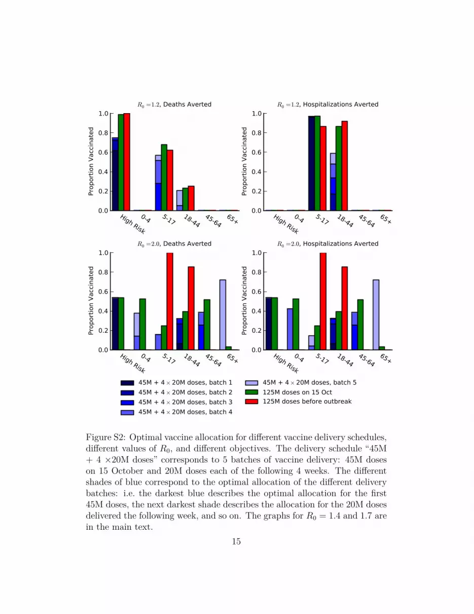
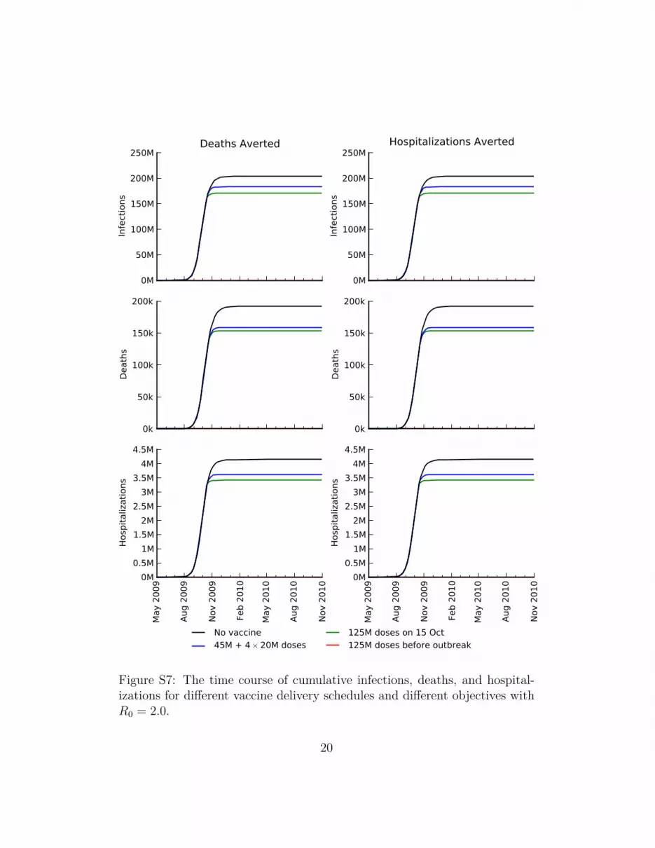
To simulate the ongoing 2009 H1N1 influenza pandemic, we took theestimate of 1 million cumulative cases on 1 August 2009 [14] and the vaccinedelivery schedule as 45 million doses on 15 October 2009 and 20 milliondoses each week thereafter. We compared vaccine delivery schedules withonly the first batch of 45 million doses; with two batches, a 45 million dosebatch and then a 20 million dose batch; with three batches, 45 million dosebatch and then two 20 million dose batches; and so on, up to a 45 milliondose batch followed by eight 20 million dose batches. In addition, we alsocompared two more delivery schedules, a single batch of 125 million doses on15 October and a single batch of 125 million doses before the outbreak began.For each of these vaccine delivery schedules, we found the optimal age- andrisk-dependent allocation that minimized either deaths or hospitalizations(Figures 1, 2, & S2–S15).

Figures S8–S15 show the optimal allocations of multiple batches of vaccinefor a given number of batches. Of particular interest is that the optimalallocations for multiple batches cannot be found by iteratively finding theoptimal allocation for the first batch, then for the second batch given theallocation for the first batch, and so on. The optimal allocation in eachbatch depends on the total number of batches. For example, for R0 = 1.2and deaths averted (Figure S8), the optimal allocation when there are 2 totalbatches of vaccine includes vaccinating some 18–44 year olds in the secondbatch, while, when there are 3 total batches of vaccine, vaccinating 18–44year olds is not optimal.

13

May 2009 Aug 2009 Nov 2009 Feb 2010 May 2010 Aug 2010 Nov 20100.000

0.005

0.010

0.015

0.020

0.025

0.030

0.035

0.040

Prop

ortio

n In

fect

ious

0-45-1718-4445-6465+

Figure S1: Model epidemic curves for different age groups with R0 = 1.4 andno vaccination.

14

High Risk

0-4 5-1718-44

45-6465+

0.0

0.2

0.4

0.6

0.8

1.0

Prop

ortio

n Va

ccin

ated

R0 =1.2, Deaths Averted

High Risk

0-4 5-1718-44

45-6465+

0.0

0.2

0.4

0.6

0.8

1.0

Prop

ortio

n Va

ccin

ated

R0 =1.2, Hospitalizations Averted

High Risk

0-4 5-1718-44

45-6465+

0.0

0.2

0.4

0.6

0.8

1.0

Prop

ortio

n Va

ccin

ated

R0 =2.0, Deaths Averted

High Risk

0-4 5-1718-44

45-6465+

0.0

0.2

0.4

0.6

0.8

1.0Pr

opor

tion

Vacc

inat

edR0 =2.0, Hospitalizations Averted

45M + 4× 20M doses, batch 145M + 4× 20M doses, batch 245M + 4× 20M doses, batch 345M + 4× 20M doses, batch 4

45M + 4× 20M doses, batch 5125M doses on 15 Oct125M doses before outbreak

Figure S2: Optimal vaccine allocation for different vaccine delivery schedules,different values of R0, and different objectives. The delivery schedule “45M+ 4 ×20M doses” corresponds to 5 batches of vaccine delivery: 45M doseson 15 October and 20M doses each of the following 4 weeks. The differentshades of blue correspond to the optimal allocation of the different deliverybatches: i.e. the darkest blue describes the optimal allocation for the first45M doses, the next darkest shade describes the allocation for the 20M dosesdelivered the following week, and so on. The graphs for R0 = 1.4 and 1.7 arein the main text.

15

0M

15M

30M

45M

60M

75M

Infe

ctio

ns

0k

15k

30k

45k

60k

Dea

ths

R0 =1.2

0M

0.5M

1M

1.5M

Hosp

italiz

atio

ns

0M

40M

80M

120M

160M

200M

Infe

ctio

ns

0k

40k

80k

120k

160k

Dea

ths

R0 =1.7

0M

1M

2M

3M

4M

Hosp

italiz

atio

ns

DeathsAverted

Hospitalizations

Averted

0M

50M

100M

150M

200M

250M

Infe

ctio

ns

DeathsAverted

Hospitalizations

Averted

0k

40k

80k

120k

160k

200k

Dea

ths

R0 =2.0

DeathsAverted

Hospitalizations

Averted

0M

1M

2M

3M

4M

5M

Hosp

italiz

atio

ns

No vaccine45M + 4× 20M doses

125M doses on 15 Oct125M doses before outbreak





Figure S3: The impact on infections, deaths, and hospitalizations for differentvaccine delivery schedules, different values of R0, and different objectives.The graphs for R0 = 1.4 are in the main text.

16

0M

10M

20M

30M

40M

50M

60M

70M

Infe

ctio

ns

Deaths Averted

0k

10k

20k

30k

40k

50k

60k

Dea

ths

May

200

9

Aug

2009

Nov

2009

Feb

2010

May

201

0

Aug

2010

Nov

2010

0M

0.2M

0.4M

0.6M

0.8M

1M

1.2M

1.4M

Hosp

italiz

atio

ns

0M

10M

20M

30M

40M

50M

60M

70M

Infe

ctio

ns

Hospitalizations Averted

0k

10k

20k

30k

40k

50k

60k

Dea

ths

May

200

9

Aug

2009

Nov

2009

Feb

2010

May

201

0

Aug

2010

Nov

2010

0M

0.2M

0.4M

0.6M

0.8M

1M

1.2M

1.4M

Hosp

italiz

atio

ns



Figure S4: The time course of cumulative infections, deaths, and hospital-izations for different vaccine delivery schedules and different objectives withR0 = 1.2.

17

0M

20M

40M

60M

80M

100M

120M

Infe

ctio

ns

Deaths Averted

0k

20k

40k

60k

80k

100k

120k

Dea

ths

May

200

9

Aug

2009

Nov

2009

Feb

2010

May

201

0

Aug

2010

Nov

2010

0M

0.5M

1M

1.5M

2M

2.5M

Hosp

italiz

atio

ns

0M

20M

40M

60M

80M

100M

120M

Infe

ctio

ns


0k

20k

40k

60k

80k

100k

120k

Dea

ths

May

200

9

Aug

2009

Nov

2009

Feb

2010

May

201

0

Aug

2010

Nov

2010

0M

0.5M

1M

1.5M

2M

2.5M

Hosp

italiz

atio

ns




18

0M20M40M60M80M

100M120M140M160M180M

Infe

ctio

ns

Deaths Averted

0k20k40k60k80k

100k120k140k160k

Dea

ths

May

200

9

Aug

2009

Nov

2009

Feb

2010

May

201

0

Aug

2010

Nov

2010

0M

0.5M

1M

1.5M

2M

2.5M

3M

3.5M

Hosp

italiz

atio

ns

0M20M40M60M80M

100M120M140M160M180M

Infe

ctio

ns


0k20k40k60k80k

100k120k140k160k

Dea

ths

May

200

9

Aug

2009

Nov

2009

Feb

2010

May

201

0

Aug

2010

Nov

2010

0M

0.5M

1M

1.5M

2M

2.5M

3M

3.5M

Hosp

italiz

atio

ns




19

0M

50M

100M

150M

200M

250M

Infe

ctio

ns

Deaths Averted

0k

50k

100k

150k

200k

Dea

ths

May

200

9

Aug

2009

Nov

2009

Feb

2010

May

201

0

Aug

2010

Nov

2010

0M0.5M

1M1.5M

2M2.5M

3M3.5M

4M4.5M

Hosp

italiz

atio

ns

0M

50M

100M

150M

200M

250M

Infe

ctio

ns


0k

50k

100k

150k

200k

Dea

ths

May

200

9

Aug

2009

Nov

2009

Feb

2010

May

201

0

Aug

2010

Nov

2010

0M0.5M

1M1.5M

2M2.5M

3M3.5M

4M4.5M

Hosp

italiz

atio

ns




20

0.0

0.2

0.4

0.6

0.8

1.0Pr

opor

tion

Vacc

inat

ed

0.0

0.2

0.4

0.6

0.8

1.0

0.0

0.2

0.4

0.6

0.8

1.0

0.0

0.2

0.4

0.6

0.8

1.0

Prop

ortio

n Va

ccin

ated

0.0

0.2

0.4

0.6

0.8

1.0

0.0

0.2

0.4

0.6

0.8

1.0

High Risk

0-4 5-1718-44

45-6465+

0.0

0.2

0.4

0.6

0.8

1.0

Prop

ortio

n Va

ccin

ated

High Risk

0-4 5-1718-44

45-6465+

0.0

0.2

0.4

0.6

0.8

1.0

High Risk

0-4 5-1718-44

45-6465+

0.0

0.2

0.4

0.6

0.8

1.0

Batch 1Batch 2

Batch 3Batch 4

Batch 5Batch 6

Batch 7Batch 8

Batch 9

Figure S8: Optimal vaccine allocation for different numbers of vaccinebatches for R0 = 1.2 and deaths averted. The delivery schedules consistof from 1 to 8 batches of vaccine delivered in intervals of 1 week, with thefirst batch being 45M doses and subsequent batches being 20M doses. Eachgraph shows the optimal allocation given the number of batches of vaccineavailable.

21

0.0

0.2

0.4

0.6

0.8

1.0Pr

opor

tion

Vacc

inat

ed

0.0

0.2

0.4

0.6

0.8

1.0

0.0

0.2

0.4

0.6

0.8

1.0

0.0

0.2

0.4

0.6

0.8

1.0

Prop

ortio

n Va

ccin

ated

0.0

0.2

0.4

0.6

0.8

1.0

0.0

0.2

0.4

0.6

0.8

1.0

High Risk

0-4 5-1718-44

45-6465+

0.0

0.2

0.4

0.6

0.8

1.0

Prop

ortio

n Va

ccin

ated

High Risk

0-4 5-1718-44

45-6465+

0.0

0.2

0.4

0.6

0.8

1.0

High Risk

0-4 5-1718-44

45-6465+

0.0

0.2

0.4

0.6

0.8

1.0

Batch 1Batch 2

Batch 3Batch 4

Batch 5Batch 6

Batch 7Batch 8

Batch 9

Figure S9: Optimal vaccine allocation for different numbers of vaccinebatches for R0 = 1.2 and hospitalizations averted. The delivery schedulesconsist of from 1 to 8 batches of vaccine delivered in intervals of 1 week, withthe first batch being 45M doses and subsequent batches being 20M doses.Each graph shows the optimal allocation given the number of batches ofvaccine available.

22

0.0

0.2

0.4

0.6

0.8

1.0Pr

opor

tion

Vacc

inat

ed

0.0

0.2

0.4

0.6

0.8

1.0

0.0

0.2

0.4

0.6

0.8

1.0

0.0

0.2

0.4

0.6

0.8

1.0

Prop

ortio

n Va

ccin

ated

0.0

0.2

0.4

0.6

0.8

1.0

0.0

0.2

0.4

0.6

0.8

1.0

High Risk

0-4 5-1718-44

45-6465+

0.0

0.2

0.4

0.6

0.8

1.0

Prop

ortio

n Va

ccin

ated

High Risk

0-4 5-1718-44

45-6465+

0.0

0.2

0.4

0.6

0.8

1.0

High Risk

0-4 5-1718-44

45-6465+

0.0

0.2

0.4

0.6

0.8

1.0

Batch 1Batch 2

Batch 3Batch 4

Batch 5Batch 6

Batch 7Batch 8

Batch 9


23

0.0

0.2

0.4

0.6

0.8

1.0Pr

opor

tion

Vacc

inat

ed

0.0

0.2

0.4

0.6

0.8

1.0

0.0

0.2

0.4

0.6

0.8

1.0

0.0

0.2

0.4

0.6

0.8

1.0

Prop

ortio

n Va

ccin

ated

0.0

0.2

0.4

0.6

0.8

1.0

0.0

0.2

0.4

0.6

0.8

1.0

High Risk

0-4 5-1718-44

45-6465+

0.0

0.2

0.4

0.6

0.8

1.0

Prop

ortio

n Va

ccin

ated

High Risk

0-4 5-1718-44

45-6465+

0.0

0.2

0.4

0.6

0.8

1.0

High Risk

0-4 5-1718-44

45-6465+

0.0

0.2

0.4

0.6

0.8

1.0

Batch 1Batch 2

Batch 3Batch 4

Batch 5Batch 6

Batch 7Batch 8

Batch 9


24

0.0

0.2

0.4

0.6

0.8

1.0Pr

opor

tion

Vacc

inat

ed

0.0

0.2

0.4

0.6

0.8

1.0

0.0

0.2

0.4

0.6

0.8

1.0

0.0

0.2

0.4

0.6

0.8

1.0

Prop

ortio

n Va

ccin

ated

0.0

0.2

0.4

0.6

0.8

1.0

0.0

0.2

0.4

0.6

0.8

1.0

High Risk

0-4 5-1718-44

45-6465+

0.0

0.2

0.4

0.6

0.8

1.0

Prop

ortio

n Va

ccin

ated

High Risk

0-4 5-1718-44

45-6465+

0.0

0.2

0.4

0.6

0.8

1.0

High Risk

0-4 5-1718-44

45-6465+

0.0

0.2

0.4

0.6

0.8

1.0

Batch 1Batch 2

Batch 3Batch 4

Batch 5Batch 6

Batch 7Batch 8

Batch 9


25

0.0

0.2

0.4

0.6

0.8

1.0Pr

opor

tion

Vacc

inat

ed

0.0

0.2

0.4

0.6

0.8

1.0

0.0

0.2

0.4

0.6

0.8

1.0

0.0

0.2

0.4

0.6

0.8

1.0

Prop

ortio

n Va

ccin

ated

0.0

0.2

0.4

0.6

0.8

1.0

0.0

0.2

0.4

0.6

0.8

1.0

High Risk

0-4 5-1718-44

45-6465+

0.0

0.2

0.4

0.6

0.8

1.0

Prop

ortio

n Va

ccin

ated

High Risk

0-4 5-1718-44

45-6465+

0.0

0.2

0.4

0.6

0.8

1.0

High Risk

0-4 5-1718-44

45-6465+

0.0

0.2

0.4

0.6

0.8

1.0

Batch 1Batch 2

Batch 3Batch 4

Batch 5Batch 6

Batch 7Batch 8

Batch 9


26

0.0

0.2

0.4

0.6

0.8

1.0Pr

opor

tion

Vacc

inat

ed

0.0

0.2

0.4

0.6

0.8

1.0

0.0

0.2

0.4

0.6

0.8

1.0

0.0

0.2

0.4

0.6

0.8

1.0

Prop

ortio

n Va

ccin

ated

0.0

0.2

0.4

0.6

0.8

1.0

0.0

0.2

0.4

0.6

0.8

1.0

High Risk

0-4 5-1718-44

45-6465+

0.0

0.2

0.4

0.6

0.8

1.0

Prop

ortio

n Va

ccin

ated

High Risk

0-4 5-1718-44

45-6465+

0.0

0.2

0.4

0.6

0.8

1.0

High Risk

0-4 5-1718-44

45-6465+

0.0

0.2

0.4

0.6

0.8

1.0

Batch 1Batch 2

Batch 3Batch 4

Batch 5Batch 6

Batch 7Batch 8

Batch 9


27

0.0

0.2

0.4

0.6

0.8

1.0Pr

opor

tion

Vacc

inat

ed

0.0

0.2

0.4

0.6

0.8

1.0

0.0

0.2

0.4

0.6

0.8

1.0

0.0

0.2

0.4

0.6

0.8

1.0

Prop

ortio

n Va

ccin

ated

0.0

0.2

0.4

0.6

0.8

1.0

0.0

0.2

0.4

0.6

0.8

1.0

High Risk

0-4 5-1718-44

45-6465+

0.0

0.2

0.4

0.6

0.8

1.0

Prop

ortio

n Va

ccin

ated

High Risk

0-4 5-1718-44

45-6465+

0.0

0.2

0.4

0.6

0.8

1.0

High Risk

0-4 5-1718-44

45-6465+

0.0

0.2

0.4

0.6

0.8

1.0

Batch 1Batch 2

Batch 3Batch 4

Batch 5Batch 6

Batch 7Batch 8

Batch 9


28

References[1] N. E. Basta, M. E. Halloran, L. Matrajt, and I. M. Longini Jr. Esti-

mating influenza vaccine efficacy from challenge and community-basedstudy data. Am J Epidemiol, 170(6):679–686, 2008.

[2] Centers for Disease Control and Prevention. National Health InterviewSurvey, 2006–2008. URL http://www.cdc.gov/NCHS/nhis/.

[3] Centers for Disease Control and Prevention. HIV/AIDS SurveillanceReport, 2007. URL http://www.cdc.gov/hiv/topics/surveillance/resources/reports/2007report/default.htm.

[4] O. Diekmann, J. Heesterbeek, and J. Metz. On the definition and thecomputation of the basic reproduction ratio r0 in models for infectiousdiseases in heterogeneous populations. J Math Biol, 28(4):365–382, 1990.ISSN 0303-6812.

[5] A. C. Hindmarsh. Brief Description of ODEPACK - A SystematizedCollection of ODE Solvers Double Precision Version, Accessed 12 June2008. URL http://www.netlib.org/odepack/opkd-sum.

[6] J. Medlock and A. P. Galvani. Optimizing influenza vaccine distribution.Science, 325(5948):1705–1708, 2009.

[7] M. I. Meltzer, N. J. Cox, and K. Fukuda. Modeling the economic im-pact of pandemic influenza in the United States: implications for set-ting priorities for intervention: background paper. Tech. rep., Centersfor Disese Control and Prevention, 1999. URL http://www.cdc.gov/ncidod/EID/vol5no5/meltzerback.htm. Accessed 28 July, 2007.

[8] MIDAS High-Risk Segmentation Group. H1N1 modeling parameterswith high risk data. Personal communication (Diane Wagener), 2009.

[9] J. Mossong, N. Hens, M. Jit, P. Beutels, K. Auranen, R. Mikola-jczyk, M. Massari, S. Salmaso, G. S. Tomba, J. Wallinga, J. Heĳne,M. Sadkowska-Todys, M. Rosinska, and W. J. Edmunds. Social con-tacts and mixing patterns relevant to the spread of infectious diseases.PLoS Med, 5(3):e74, 2008. doi:10.1371/journal.pmed.0050074.

29

http://www.cdc.gov/NCHS/nhis/

http://www.cdc.gov/hiv/topics/surveillance/resources/reports/2007report/default.htm

http://www.cdc.gov/hiv/topics/surveillance/resources/reports/2007report/default.htm

http://www.netlib.org/odepack/opkd-sum

http://www.cdc.gov/ncidod/EID/vol5no5/meltzerback.htm

http://www.cdc.gov/ncidod/EID/vol5no5/meltzerback.htm

http://dx.doi.org/10.1371/journal.pmed.0050074

[10] Novel Swine-Origin Influenza A (H1N1) Virus Investigation Team.Emergence of a novel swine-origin influenza A (H1N1) virus in humans.N Engl J Med, 360(25):2605, 2009.

[11] Organ Procurement and Transplantation Network. 2009. URL http://optn.transplant.hrsa.gov/.

[12] M. J. D. Powell. A direct search optimization method that models theobjective and constraint function by linear interpolation. NumericalAnalyses Report DAMTP 1992/NA5, University of Cambridge, 1992.

[13] A. M. Presanis, M. Lipsitch, D. De Angelis, New York City Depart-ment of Health and Mental Hygiene, The Swine Flu InfestigationTeam, A. Hagy, C. Reed, S. Riley, B. Cooper, P. Biedrzycki, andL. Finelli. The severity of pandemic H1N1 influenza in the UnitedStates, April–July 2009. PLoS Curr Influenza, RRN1042, Accessed 20October, 2009. URL http://knol.google.com/k/anne-m-presanis/the-severity-of-pandemic-h1n1-influenza/agr0htar1u6r/16?collectionId=28qm4w0q65e4w.1&position=6#.

[14] President’s Council of Advisors on Science and Technology. Report to thePresident on U.S. preparations for 2009-H1N1 influenza, Accessed Octo-ber 20, 2009. URL http://www.whitehouse.gov/assets/documents/PCAST_H1N1_Report.pdf.

[15] V. Shinde, C. B. Bridges, T. M. Uyeki, B. Shu, A. Balish, X. Xu, S. Lind-strom, L. V. Gubareva, V. Deyde, R. J. Garten, M. Harris, S. Gerber,S. Vagasky, F. Smith, N. Pascoe, K. Martin, D. Dufficy, K. Ritger,C. Conover, P. Quinlisk, A. Klimov, J. S. Bresee, and L. Finelli. Triple-reassortant swine influenza A (H1) in humans in the United States,2005–2009. N Engl J Med, 360(25):2616–2125, 2009.

[16] United States Renal Data System. 2009. URL http://www.usrds.org/.

[17] U.S. Census Bureau. Monthly Postcensal Resident Population,6/1/2007, Accessed June 29, 2007. URL http://www.census.gov/popest/national/asrh/2006_nat_res.html.

[18] P. van den Driessche and J. Watmough. Reproduction numbers andsub-threshold endemic equilibria for compartmental models of diseasetransmission. Math Biosci, 180:29–48, 2002. ISSN 0025-5564.

30

http://optn.transplant.hrsa.gov/

http://optn.transplant.hrsa.gov/

http://knol.google.com/k/anne-m-presanis/the-severity-of-pandemic-h1n1-influenza/agr0htar1u6r/16?collectionId=28qm4w0q65e4w.1&position=6#



http://www.whitehouse.gov/assets/documents/PCAST_H1N1_Report.pdf

http://www.whitehouse.gov/assets/documents/PCAST_H1N1_Report.pdf

http://www.usrds.org/

http://www.census.gov/popest/national/asrh/2006_nat_res.html

http://www.census.gov/popest/national/asrh/2006_nat_res.html

supplemental material for optimizing allocation for a delayed influenza vaccination campaign

Documents