International Journal of

Geo-Information

Article

Study of NSSDA Variability by Means of AutomaticPositional Accuracy Assessment Methods

Juan José Ruiz-Lendínez *, Francisco Javier Ariza-López and Manuel Antonio Ureña-Cámara

Department of Cartographic Engineering, University of Jaén, 23071 Jaén, Spain; fjariza@ujaen.es (F.J.A.-L.);maurena@ujaen.es (M.A.U.-C.)* Correspondence: lendinez@ujaen.es; Tel.: +34-953-21-24-70; Fax: +34-953-21-28-54

Received: 18 September 2019; Accepted: 2 December 2019; Published: 2 December 2019�����������������

Abstract: Point-based standard methodologies (PBSM) suggest using ‘at least 20’ check points inorder to assess the positional accuracy of a certain spatial dataset. However, the reason for decreasingthe number of checkpoints to 20 is not elaborated upon in the original documents provided bythe mapping agencies which develop these methodologies. By means of theoretical analysis andexperimental tests, several authors and studies have demonstrated that this limited number of pointsis clearly insufficient. Using the point-based methodology for the automatic positional accuracyassessment of spatial data developed in our previous study Ruiz-Lendínez, et al (2017) and specifically,a subset of check points obtained from the application of this methodology to two urban spatialdatasets, the variability of National Standard for Spatial Data Accuracy (NSSDA) estimations hasbeen analyzed according to sample size. The results show that the variability of NSSDA estimationsdecreases when the number of check points increases, and also that these estimations have a tendencyto underestimate accuracy. Finally, the graphical representation of the results can be employed inorder to give some guidance on the recommended sample size when PBSMs are used.

Keywords: spatial data accuracy; automatic assessment; standards; NSSDA estimations

1. Introduction

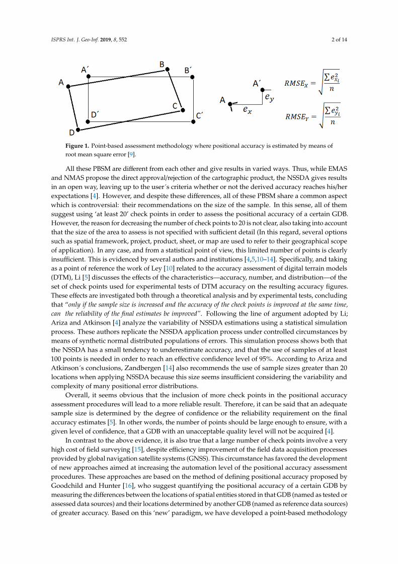
The position is the basis of mapping and navigation, which are essential for engineering, naturalsciences, land management, etc. Consequently, the assessment of the positional quality of cartographicproducts has become an issue of particular significance and relevance [1,2]. Positional quality isdetermined by positional accuracy [3] which, in turn, is evaluated by means of statistical methodsbased on measuring positional discrepancies between the location of “well-defined point entities” storedin a geospatial database (GDB) and their true (real world) location [1]. In this sense, there are severalpoint-based standard methodologies (PBSM) which can be used for computing the positional accuracyof GDBs. In these methodologies the positional accuracy is estimated by means of a statistical evaluationof random and systematic errors and mainly specified through two metrics or estimators: root meansquare error (RMSE) (Figure 1) or mean value of errors (µ), and their standard deviation (σ) [4,5].Among the PBSM which can be employed for defining the positional accuracy of spatial data wehighlight: The National Map Accuracy Standard (NMAS) developed in 1947 by the US Bureau of theBudget [6], the Engineering Map Accuracy Standard (EMAS) developed in 1983 by the Committee onCartographic Surveying of the American Society of Civil Engineering [7], and the National Standardfor Spatial Data Accuracy (NSSDA) published in 1998 by the Federal Geographic Data Committee [8].

ISPRS Int. J. Geo-Inf. 2019, 8, 552; doi:10.3390/ijgi8120552 www.mdpi.com/journal/ijgi

ISPRS Int. J. Geo-Inf. 2019, 8, 552 2 of 14

- 2 -

Figure 1. Point-based assessment methodology where positional accuracy is estimated by means of root mean square error [9].

All these PBSM are different from each other and give results in varied ways. Thus, while EMAS and NMAS propose the direct approval/rejection of the cartographic product, the NSSDA gives results in an open way, leaving up to the user´s criteria whether or not the derived accuracy reaches his/her expectations [4]. However, and despite these differences, all of these PBSM share a common aspect which is controversial: their recommendations on the size of the sample. In this sense, all of them suggest using ‘at least 20’ check points in order to assess the positional accuracy of a certain GDB. However, the reason for decreasing the number of check points to 20 is not clear, also taking into account that the size of the area to assess is not specified with sufficient detail (In this regard, several options such as spatial framework, project, product, sheet, or map are used to refer to their geographical scope of application). In any case, and from a statistical point of view, this limited number of points is clearly insufficient. This is evidenced by several authors and institutions [4,5,10–14]. Specifically, and taking as a point of reference the work of Ley [10] related to the accuracy assessment of digital terrain models (DTM), Li [5] discusses the effects of the characteristics—accuracy, number, and distribution—of the set of check points used for experimental tests of DTM accuracy on the resulting accuracy figures. These effects are investigated both through a theoretical analysis and by experimental tests, concluding that “only if the sample size is increased and the accuracy of the check points is improved at the same time, can the reliability of the final estimates be improved”. Following the line of argument adopted by Li; Ariza and Atkinson [4] analyze the variability of NSSDA estimations using a statistical simulation process. These authors replicate the NSSDA application process under controlled circumstances by means of synthetic normal distributed populations of errors. This simulation process shows both that the NSSDA has a small tendency to underestimate accuracy, and that the use of samples of at least 100 points is needed in order to reach an effective confidence level of 95%. According to Ariza and Atkinson´s conclusions, Zandbergen [14] also recommends the use of sample sizes greater than 20 locations when applying NSSDA because this size seems insufficient considering the variability and complexity of many positional error distributions.

Overall, it seems obvious that the inclusion of more check points in the positional accuracy assessment procedures will lead to a more reliable result. Therefore, it can be said that an adequate sample size is determined by the degree of confidence or the reliability requirement on the final accuracy estimates [5]. In other words, the number of points should be large enough to ensure, with a given level of confidence, that a GDB with an unacceptable quality level will not be acquired [4].

In contrast to the above evidence, it is also true that a large number of check points involve a very high cost of field surveying [15], despite efficiency improvement of the field data acquisition processes provided by global navigation satellite systems (GNSS). This circumstance has favored the development of new approaches aimed at increasing the automation level of the positional accuracy assessment procedures. These approaches are based on the method of defining positional accuracy proposed by Goodchild and Hunter [16], who suggest quantifying the positional accuracy of a certain GDB by measuring the differences between the locations of spatial entities stored in that GDB (named as tested or assessed data sources) and their locations determined by another GDB (named as reference data sources) of greater accuracy. Based on this ‘new’ paradigm, we have developed a

Figure 1. Point-based assessment methodology where positional accuracy is estimated by means ofroot mean square error [9].

All these PBSM are different from each other and give results in varied ways. Thus, while EMASand NMAS propose the direct approval/rejection of the cartographic product, the NSSDA gives resultsin an open way, leaving up to the user´s criteria whether or not the derived accuracy reaches his/herexpectations [4]. However, and despite these differences, all of these PBSM share a common aspectwhich is controversial: their recommendations on the size of the sample. In this sense, all of themsuggest using ‘at least 20’ check points in order to assess the positional accuracy of a certain GDB.However, the reason for decreasing the number of check points to 20 is not clear, also taking into accountthat the size of the area to assess is not specified with sufficient detail (In this regard, several optionssuch as spatial framework, project, product, sheet, or map are used to refer to their geographical scopeof application). In any case, and from a statistical point of view, this limited number of points is clearlyinsufficient. This is evidenced by several authors and institutions [4,5,10–14]. Specifically, and takingas a point of reference the work of Ley [10] related to the accuracy assessment of digital terrain models(DTM), Li [5] discusses the effects of the characteristics—accuracy, number, and distribution—of theset of check points used for experimental tests of DTM accuracy on the resulting accuracy figures.These effects are investigated both through a theoretical analysis and by experimental tests, concludingthat “only if the sample size is increased and the accuracy of the check points is improved at the same time,can the reliability of the final estimates be improved”. Following the line of argument adopted by Li;Ariza and Atkinson [4] analyze the variability of NSSDA estimations using a statistical simulationprocess. These authors replicate the NSSDA application process under controlled circumstances bymeans of synthetic normal distributed populations of errors. This simulation process shows both thatthe NSSDA has a small tendency to underestimate accuracy, and that the use of samples of at least100 points is needed in order to reach an effective confidence level of 95%. According to Ariza andAtkinson´s conclusions, Zandbergen [14] also recommends the use of sample sizes greater than 20locations when applying NSSDA because this size seems insufficient considering the variability andcomplexity of many positional error distributions.

Overall, it seems obvious that the inclusion of more check points in the positional accuracyassessment procedures will lead to a more reliable result. Therefore, it can be said that an adequatesample size is determined by the degree of confidence or the reliability requirement on the finalaccuracy estimates [5]. In other words, the number of points should be large enough to ensure, with agiven level of confidence, that a GDB with an unacceptable quality level will not be acquired [4].

In contrast to the above evidence, it is also true that a large number of check points involve a veryhigh cost of field surveying [15], despite efficiency improvement of the field data acquisition processesprovided by global navigation satellite systems (GNSS). This circumstance has favored the developmentof new approaches aimed at increasing the automation level of the positional accuracy assessmentprocedures. These approaches are based on the method of defining positional accuracy proposed byGoodchild and Hunter [16], who suggest quantifying the positional accuracy of a certain GDB bymeasuring the differences between the locations of spatial entities stored in that GDB (named as tested orassessed data sources) and their locations determined by another GDB (named as reference data sources)of greater accuracy. Based on this ‘new’ paradigm, we have developed a point-based methodology

ISPRS Int. J. Geo-Inf. 2019, 8, 552 3 of 14

for the automatic positional accuracy assessment (APAA) of spatial data [1,9]. This methodology hasallowed us not only to increase significantly the number of entities (points) used in the assessmentprocess (by means of the PBSM application) but also to empirically verify the conclusions reachedby Ariza and Atkinson [4] with regard to the variability of NSSDA estimations, without the need togenerate synthetic populations of errors, when the number of check points increases.

This paper takes as its starting point our previous work [1]. Specifically, a subset of the homologouspoints obtained between two urban GDBs according to the automated methodology developed in it,and is focused on the second aspect mentioned above, that is, to verify that the variability of NSSDAresults decreases when the number of check points increases, and their tendency to underestimateaccuracy. To this end, and starting from the aforementioned set of homologous points (check pointspopulation), we have applied the NSSDA standard for assessing the positional accuracy to differentsample sizes. Just as a reminder, it must be noted that the calculation of these homologous points wasdeveloped in two main steps (Figure 2): (i) Matching of polygonal shapes (buildings) between the twodatasets by means of an inter-elements similarity quantification procedure (Figure 2a). This procedureis based on a weight-based classification methodology using low-level polygon feature descriptorsand a genetic algorithm [17], and (ii) the matching of points by means of an intra-elements metric forcomparing two polygonal shapes (Figure 2b). This metric is based on a procedure developed by Arkinet al. [18] which compares two polygonal curves by means of their turn angle representations.

- 3 -

point-based methodology for the automatic positional accuracy assessment (APAA) of spatial data [1,9]. This methodology has allowed us not only to increase significantly the number of entities (points) used in the assessment process (by means of the PBSM application) but also to empirically verify the conclusions reached by Ariza and Atkinson [4] with regard to the variability of NSSDA estimations, without the need to generate synthetic populations of errors, when the number of check points increases.

This paper takes as its starting point our previous work [1]. Specifically, a subset of the homologous points obtained between two urban GDBs according to the automated methodology developed in it, and is focused on the second aspect mentioned above, that is, to verify that the variability of NSSDA results decreases when the number of check points increases, and their tendency to underestimate accuracy. To this end, and starting from the aforementioned set of homologous points (check points population), we have applied the NSSDA standard for assessing the positional accuracy to different sample sizes. Just as a reminder, it must be noted that the calculation of these homologous points was developed in two main steps (Figure 2): (i) Matching of polygonal shapes (buildings) between the two datasets by means of an inter-elements similarity quantification procedure (Figure 2a). This procedure is based on a weight-based classification methodology using low-level polygon feature descriptors and a genetic algorithm [17], and (ii) the matching of points by means of an intra-elements metric for comparing two polygonal shapes (Figure 2b). This metric is based on a procedure developed by Arkin et al. [18] which compares two polygonal curves by means of their turn angle representations.

Figure 2. (a) Inter-elements matching (polygon-to-polygon with 1:1, 1:n, n:m, 1:0 correspondences), and (b) intra-elements matching (vertex-to-vertex correspondence between 1:1 corresponding polygons pairs) [1].

As already stated, both procedures are extensively detailed in [1]. It is, therefore, necessary to emphasize that they are not addressed here. In this study we focus on reproducing the experiment of Ariza and Atkinson [4] employing a population of errors automatically obtained from true—or real—locations. Therein lies the main innovative features of our methodological approach: (i) in the use of a check points population that is automatically generated, which ensures that there is no selection bias; (ii) in the use and manipulation of large volumes of empirical data (what is currently known as big data analysis) in order to verify the validity of the experiments developed by means of traditional tools from synthetic data—as in the case of [4]; (iii) in the specific characteristics of APAA procedures because the collection, management, processing, and analysis of the empirical data is cheap, quick, and requires a low computational time compared to traditional methodologies (especially if we consider fieldwork for GNSS data acquisition). On the other hand, our results should serve to convincingly demonstrate that the proposals and suggestions made by some of the authors and institutions above mentioned [4,12–14] have contributed significantly to improve the technical definition of the NSSDA in aspects which require special attention, such as:

• Give information about the statistical behavior of the methodology.

Figure 2. (a) Inter-elements matching (polygon-to-polygon with 1:1, 1:n, n:m, 1:0 correspondences),and (b) intra-elements matching (vertex-to-vertex correspondence between 1:1 corresponding polygonspairs) [1].

As already stated, both procedures are extensively detailed in [1]. It is, therefore, necessary toemphasize that they are not addressed here. In this study we focus on reproducing the experimentof Ariza and Atkinson [4] employing a population of errors automatically obtained from true—orreal—locations. Therein lies the main innovative features of our methodological approach: (i) in the useof a check points population that is automatically generated, which ensures that there is no selectionbias; (ii) in the use and manipulation of large volumes of empirical data (what is currently known asbig data analysis) in order to verify the validity of the experiments developed by means of traditionaltools from synthetic data—as in the case of [4]; (iii) in the specific characteristics of APAA proceduresbecause the collection, management, processing, and analysis of the empirical data is cheap, quick, andrequires a low computational time compared to traditional methodologies (especially if we considerfieldwork for GNSS data acquisition). On the other hand, our results should serve to convincinglydemonstrate that the proposals and suggestions made by some of the authors and institutions abovementioned [4,12–14] have contributed significantly to improve the technical definition of the NSSDAin aspects which require special attention, such as:

• Give information about the statistical behavior of the methodology.• Related to the previous, give a clear and better recommendation about the number and distribution

of check points and their influence on the variability and reliability of results.

ISPRS Int. J. Geo-Inf. 2019, 8, 552 4 of 14

Finally, our study pays special attention to the characterization of the distribution of positionalerror. As will be explained below, a key assumption of the NSSDA standard is that the positionalerrors follow a normal distribution; which is also assumed by the experiment of Ariza and Atkinson [4].However, the non-normal distribution of positional error observed in several applications presentsa serious challenge to map accuracy standards, which rely on assumptions of normality and utilizesimple statistics to characterize its distribution.

The rest of the paper is organized in the following main sections: the next section presents theurban databases used and the conditions that needed to be fulfilled by them in order to apply ourmethodology as well as the homologous points population (check points). After this, the followingsection explains the sampling procedure with a particular focus on normality testing on the populationdistribution, and the sample design and composition. Following this, effects of the sample size andsample distribution on the automatic positional accuracy estimations by means NSSDA are presentedand discussed in the next section. Finally, general conclusions are presented.

2. Urban Databases Used and Points Population

As already mentioned, our APAA procedure [9] quantifies positional accuracy by measuringthe positional discrepancies (Hereinafter referred to as errors (statistical estimators we are going towork with)) between the locations of “well-defined punctual entities” stored in two GDBs —tested andreference. However, there are some conditions that need to be fulfilled by any two spatial datasets inorder to apply our approach. A large part of these conditions or constraints is closely linked to theinteroperability between these datasets.

From a cartographic point of view, interoperability can be defined as the capability that two spatialdatasets—from different sources—have to interact with each other [19]. According to this, the positionalcomponent seems essential to achieving a satisfactory level of interoperability. So much so that someauthors, such as Giordano and Veregin [20], prefer to use the term Confrontability, defining it as the levelat which it is possible to operate with spatial datasets that occupy the same geographical region, that isto say, the same spatial position. However, there are some other aspects that must be considered—apartfrom position—in order to assure interoperability between spatial data. Thus, in our specific caseinteroperability must also be guaranteed to two other levels: semantic and topological. Therefore, for theimplementation of our APAA procedure, two GDBs must not only occupy the same geographic regionand be mapped with the same coordinate reference system (CRS), but there must also be semantichomogeneity (i.e., no differences in the intended meaning of terms in specific contexts [1]), and theirtopological relationships must be preserved. Apart from this, the two GDBs must meet two obviousconstraints: (i) all the elements used must exist in both datasets (the coexistence constraint), and (ii)both datasets must be independently produced (the independence constraint). The first constraint,despite its logic, is not always fulfilled in the real world, since two GDBs generated at different scalesare normally not at the same level of generalization. With regard to the second one, neither of the twoGDBs can be derived from another cartographic product of a larger scale through any process, such asgeneralization, which means that their quality has not been degraded.

With regard to specific cartographic products, we have used two official cartographic databasesin Andalusia (Southern Spain). As the tested source we have used the BCN25 (“Base CartográficaNumérica E25k”) and as the reference source, we have used the MTA10 (“Mapa Topográfico deAndalucía E10k”). Both GDBs are presented as a set of vector covers distributed by layers, includinga vector layer of buildings (city-blocks) that contains the same type of geometrical information.Their description, the degree of fulfillment of the previously mentioned interoperability requirements,as well as the justification for the selection of features—buildings as polygonal features for developingthe inter-elements matching procedure and the vertexes which define their contour as well-definedpunctual features for assessing the positional accuracy—are provided in detail in [1,2], so once againwe must note that these issues will not be addressed here. With regard to the independence andcoexistence constraints, both GDBs were independently produced which means that the tested source

ISPRS Int. J. Geo-Inf. 2019, 8, 552 5 of 14

(BCN25) is not derived from the reference source (MTA10), and thanks to the limitations imposed bythe matching methodology used—through a matching accuracy indicator [1]—all the elements used inour APAA procedure exist in both datasets. This last indicator also avoids—with a confidence level of95% [1]—matching between non-homologous pairs of points. This assertion was also corroborated bymeans of a visual inspection procedure.

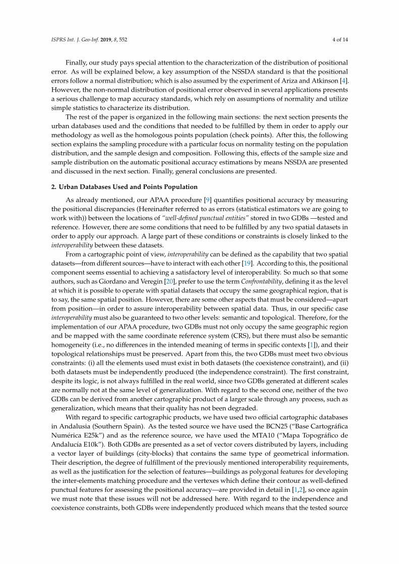
Finally, and with regard to the urban area selected, this is included in sheet number 1009-IV ofthe MTN25k—National Topographic Map of Spain at scale 1:25000—belonging to the city of Granada(Andalusia, Spain) and covered by both the BCN25 and the MTA10. This area is coded as 1009_07and 1009_08 in our previous study [1] (Figure 3). The reason for choosing these databases is twofold:(i) Because of their size, since they provide a great number of matched features, both polygons(buildings), and points (vertexes which define their boundary). This characteristic is essential toextracting samples with a range of sizes that allows us to analyze the variability of NSSDA resultsaccording to the conditions established in [4]; and (ii) because of their strictly urban nature, since theyoffer a wide range of building types which means a huge variety with respect to the shape and size ofthe polygons that integrate them. This increases the probability of pairing polygons that provide ahigh number of check points. This last characteristic is very useful for analyzing the effect of sampledistribution on the NSSDA results.

- 5 -

the inter-elements matching procedure and the vertexes which define their contour as well-defined punctual features for assessing the positional accuracy—are provided in detail in [1,2], so once again we must note that these issues will not be addressed here. With regard to the independence and coexistence constraints, both GDBs were independently produced which means that the tested source (BCN25) is not derived from the reference source (MTA10), and thanks to the limitations imposed by the matching methodology used—through a matching accuracy indicator [1]—all the elements used in our APAA procedure exist in both datasets. This last indicator also avoids—with a confidence level of 95% [1]—matching between non-homologous pairs of points. This assertion was also corroborated by means of a visual inspection procedure.

Finally, and with regard to the urban area selected, this is included in sheet number 1009-IV of the MTN25k—National Topographic Map of Spain at scale 1:25000—belonging to the city of Granada (Andalusia, Spain) and covered by both the BCN25 and the MTA10. This area is coded as 1009_07 and 1009_08 in our previous study [1] (Figure 3). The reason for choosing these databases is twofold: (i) Because of their size, since they provide a great number of matched features, both polygons (buildings), and points (vertexes which define their boundary). This characteristic is essential to extracting samples with a range of sizes that allows us to analyze the variability of NSSDA results according to the conditions established in [4]; and (ii) because of their strictly urban nature, since they offer a wide range of building types which means a huge variety with respect to the shape and size of the polygons that integrate them. This increases the probability of pairing polygons that provide a high number of check points. This last characteristic is very useful for analyzing the effect of sample distribution on the NSSDA results.

Figure 3. Layer of buildings belonging to the Urban area selected from sheet 1009-IV of the MTN25k (City of Granada, Andalusia, Spain).

Table 1 shows the total number of polygons comprising these databases, the number of polygons matched, as well as the homologous points population (denoted as matched vertexes) computed for them (input data for this study). According to the data presented in this table, and despite being a very large number, the homologous points population represented by the number of matched vertexes constitutes a relatively low percentage compared to the total number of vertexes, reaching values of around 30% for BCN25 and 15% in the case of MTA10. As stated above, this is due both to the limitations imposed by the matching methodology used and to certain factors such as the level of detail associated with the scale at which each product is generated. Such is the case of the polygons highlighted in Figure 4c. These three polygons which are composed of four vertexes each on the BCN25 are represented by means of much more complex shapes on the MTA10. Thus, although the three polygons are matched according to our inter-elements matching procedure—they are filled in

Figure 3. Layer of buildings belonging to the Urban area selected from sheet 1009-IV of the MTN25k(City of Granada, Andalusia, Spain).

Table 1 shows the total number of polygons comprising these databases, the number of polygonsmatched, as well as the homologous points population (denoted as matched vertexes) computed forthem (input data for this study). According to the data presented in this table, and despite being avery large number, the homologous points population represented by the number of matched vertexesconstitutes a relatively low percentage compared to the total number of vertexes, reaching valuesof around 30% for BCN25 and 15% in the case of MTA10. As stated above, this is due both to thelimitations imposed by the matching methodology used and to certain factors such as the level ofdetail associated with the scale at which each product is generated. Such is the case of the polygonshighlighted in Figure 4c. These three polygons which are composed of four vertexes each on theBCN25 are represented by means of much more complex shapes on the MTA10. Thus, although thethree polygons are matched according to our inter-elements matching procedure—they are filled inblack in Figure 4a,b—they do not add any homologous point after applying the intra-elements metric.In any case, this also avoids including erroneous check points in our APAA procedure.

ISPRS Int. J. Geo-Inf. 2019, 8, 552 6 of 14

Table 1. Percentage distribution of matched points for each database (95% confidence level).

SheetUrbanArea

DENOMINATION

Number ofPolygonsBCN25/MTA10

Total Number ofFeatures Matched

Features Matched with 95%Confidence Level

PolygonsMatched

Total Number ofVertexes

% ofMatchedPolygons

Number ofMatchedVertexes

% of MatchedVertexes

BCN25 MTA10 BCN25 MTA10

1009 Granada_08 1309/1345 1303 4494 11481 22.79 668 14,86 5,811009 Granada_07 2250/2301 2223 8999 16144 45.07 3378 37.53 20.92

TOTAL 3559/3656 3526 13493 27625 38.67 4046 29.98 14.64

- 6 -

black in Figure 4a,b—they do not add any homologous point after applying the intra-elements metric. In any case, this also avoids including erroneous check points in our APAA procedure.

Table 1. Percentage distribution of matched points for each database (95% confidence level).

Sheet

Urban Area

DENOMINATION

Number of

Polygons

BCN25/MTA10

Total Number of Features Matched

Features Matched with 95% Confidence Level

Polygons Matched

Total Number of Vertexes

% of matched polygons

Number of

Matched Vertexes

% of Matched Vertexes

BCN25 MTA10

BCN25

MTA10

1009

Granada_08

1309/1345 1303 4494 11481 22.79 668 14,86 5,81

1009

Granada_07

2250/2301

2223 8999 16144 45.07 3378 37.53 20.92

TOTAL 3559/365

6 3526 13493 27625 38.67 4046 29.98 14.64

Figure 4. (a) Spatial distribution of matched and non-matched polygons (BCN25); (b) spatial distribution of matched and non-matched polygons (MTA10); (c) spatial distribution of homologous points (on BCN25 database) [1].

3. Sampling Procedure

3.1. Normality Testing

Normality is the most widely-assumed hypothesis in the case of control of quantitative variables and, in the specific case of mapping, positional error is not an exception [5,21–23]. Thus, one key assumption of the NSSDA standard is that the data do not contain any systematic errors and that the positional errors follow a normal distribution. However, this assumption has not undergone much testing and is not elaborated upon in the original Federal Geographic Data Committee (FGDC) documents on NSSDA [14]. Even some authors [24] have criticized as inappropriate the Greenwalt and Schutz [25] approximations used in the NSSDA, in particular when the values for RMSE(x) and

Figure 4. (a) Spatial distribution of matched and non-matched polygons (BCN25); (b) spatial distributionof matched and non-matched polygons (MTA10); (c) spatial distribution of homologous points (onBCN25 database) [1].

3. Sampling Procedure

3.1. Normality Testing

Normality is the most widely-assumed hypothesis in the case of control of quantitative variablesand, in the specific case of mapping, positional error is not an exception [5,21–23]. Thus, one keyassumption of the NSSDA standard is that the data do not contain any systematic errors and thatthe positional errors follow a normal distribution. However, this assumption has not undergonemuch testing and is not elaborated upon in the original Federal Geographic Data Committee (FGDC)documents on NSSDA [14]. Even some authors [24] have criticized as inappropriate the Greenwaltand Schutz [25] approximations used in the NSSDA, in particular when the values for RMSE(x) andRMSE(y) are very different, or when the error distribution in the x and y directions are not independent.Furthermore, there is strong evidence to suggest that many spatial data types are not normallydistributed. In this sense, Zandbergen [14] performs—as a preliminary step for the development ofhis own analysis—an interesting review of several empirical studies that examine the distributionof positional error in different types of spatial data. According to this review, while the studies ofVonderohe and Chrisman [26] on the positional error of USGS digital line graphs data, and Bolstadet al. [27] on the accuracy of manually digitized map data show evidence of non-normality or findstatistically significant differences between the observed error distribution and a normal distribution,several other studies mainly developed by members of the Institut Géographique National (IGN)—the

ISPRS Int. J. Geo-Inf. 2019, 8, 552 7 of 14

French Mapping Agency—including studies by Vauglin [28] and Bel Hadj Ali [29] on the positionalaccuracy of lines and areas, suggest that the error distribution is largely normal.

In the view of such variable results, in his own study Zandbergen [14] focuses his attention on thedevelopment of a rigorous characterization of the positional error distribution in four different types ofspatial data: GPS locations, street geocoding, TIGER roads, and LIDAR elevation data; concluding thatin all cases the positional error could be approximated with a normal distribution, although there issome evidence of non-stationary behaviors resulting in a lack of normality. More recent studies [30–34]follow the line of argument adopted by Zandbergen in his work defending that positional errorscould be not normally distributed. Among these last studies, Ariza-López et al. [34] argue that thereare six main causes of the non-normality of many positional error distributions: (i) the presence oftoo many extreme values (i.e., outliers), (ii) the overlap of two or more processes, (iii) insufficientdata discrimination (e.g., round-off errors, poor resolution), (iv) the elimination of data from thesample, (v) the distribution of values close to zero or the natural limit, and (vi) data following adifferent distribution. The presence of any of these cases can have several consequences dependingon the degree of non-normality of the data and the robustness of the method applied. In the specificcase of the positional errors obtained by means of our APAA procedure the incidence of the causesaforementioned is minimized thanks mainly to the limitations imposed by the matching proceduresemployed—through a matching accuracy indicator [1]. We must note that this is another importantadvantage of our approach compared to traditional methodologies. In any case, the simulation processdeveloped by Ariza and Atkinson [4] was performed using a normal N (µP = 0; σ2

P = 1) distributedpopulation of errors, so in order to reproduce their experiment under similar conditions it was necessaryto carry out data analysis to verify their normal distribution.

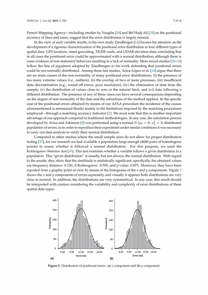
Compared to other studies where the small sample sizes do not allow for proper distributiontesting [35], for our research we had available a population large enough (4046 pairs of homologouspoints) to assess whether it followed a normal distribution. For this purpose, we used theKolmogorov–Smirnov test [36]. This test examines whether a variable follows a given distribution in apopulation. This “given distribution” is usually, but not always, the normal distribution. With regardto the results, they show that the similitude is statistically significant, specifically, the obtained valuesare frequency distance: 0.120; Z-Kolmogorov: 0.595, and p-value: 0.875. Moreover, they have beenreported from a graphic point of view by means of the histograms of the x and y components. Figure 5shows the x and y components of errors separately, and visually it appears both distributions are veryclose to normal. In addition, the distributions are very symmetrical. In any case, this result shouldbe interpreted with caution considering the variability and complexity of error distributions of thesespatial data types.

- 8 -

Figure 5. Distribution of positional errors. (a) x component and (b) y component.

3.2. Sample Design

One of the most controversial aspects of all the PBSM is the spatial distribution of control elements because, among other things, it could condition the validity of the sampling procedure [4]. In this regard, we must note that the related literature is scarce, so there are few references and, in any case, they refer to other types of cartographic products. As an example, in the specific case of the accuracy assessment of DTMs, the main research efforts have been focused on determining the best option with regard to the distribution of check points [5,37–39]. Thus, while some authors, and institutions such as the ISPRS, prefer to distribute the check points in a grid pattern, others consider that the sample of heights should be randomly selected from the entire model. Furthermore, some additional conditions are also established such as that the control points must be located at a certain distance from structural elements of the terrain and taken in flat areas or areas of uniform slope, less than 20% [40].

With regard to the case of planimetric data, most of the PBSMs indicate very briefly what the most appropriate distribution of check points must be, and only in a few cases a proposal of distribution agreed between producer and user is recommended [41]. Thus, the main suggested guidelines are based on the specific recommendations provided by the FGDC [8]. These recommendations are subjected to compliance with some requirements, such as the homogeneity of the area to assess with regard to the importance of their components and the homogeneous behavior of the uncertainty [42]. According to these recommendations, the points have to be located with a minimum distance between each point and the next of at least 10% of the greater diagonal of the study area. Moreover, each quadrant of the study area has to contain more than 20% of the total number of check points (Figure 6a) [8].

Figure 5. Distribution of positional errors. (a) x component and (b) y component.

ISPRS Int. J. Geo-Inf. 2019, 8, 552 8 of 14

3.2. Sample Design

One of the most controversial aspects of all the PBSM is the spatial distribution of control elementsbecause, among other things, it could condition the validity of the sampling procedure [4]. In thisregard, we must note that the related literature is scarce, so there are few references and, in any case,they refer to other types of cartographic products. As an example, in the specific case of the accuracyassessment of DTMs, the main research efforts have been focused on determining the best option withregard to the distribution of check points [5,37–39]. Thus, while some authors, and institutions such asthe ISPRS, prefer to distribute the check points in a grid pattern, others consider that the sample ofheights should be randomly selected from the entire model. Furthermore, some additional conditionsare also established such as that the control points must be located at a certain distance from structuralelements of the terrain and taken in flat areas or areas of uniform slope, less than 20% [40].

With regard to the case of planimetric data, most of the PBSMs indicate very briefly what the mostappropriate distribution of check points must be, and only in a few cases a proposal of distributionagreed between producer and user is recommended [41]. Thus, the main suggested guidelines are basedon the specific recommendations provided by the FGDC [8]. These recommendations are subjected tocompliance with some requirements, such as the homogeneity of the area to assess with regard to theimportance of their components and the homogeneous behavior of the uncertainty [42]. According tothese recommendations, the points have to be located with a minimum distance between each pointand the next of at least 10% of the greater diagonal of the study area. Moreover, each quadrant of thestudy area has to contain more than 20% of the total number of check points (Figure 6a) [8].

- 9 -

Figure 6. (a) Federal Geographic Data Committee (FGDC) recommendations regarding the spatial distribution of check points, (b) example of a sample grid pattern developed in our case.

In our case, in order to have an adequate representation of the assessment a sample design with a robust statistical basis was necessary. This design should produce an unbiased estimate, being robust to different population spatial patterns and densities. To this end, and according to the PBSM’s recommendations, a grid sampling pattern was defined (covering all the terrain) where samples (pairs of homologous points) were randomly collected within each cell generated (Figure 6b). With regard to the grid configuration, the number of cells and their size will depend on the geographical area covered and the size of the sample. In our case, this number was set for each sampling procedure. Thus, if a sample is composed of 25 points the geographical area covered by the study GDB will be divided into a grid of 5 × 5 cells, so that as far as possible, a homogeneous distribution of the points according to the cited specifications is produced. In addition, in order to avoid biasing the final results obtained when the effect of sample size on NSSDA estimations is analyzed, and wherever possible, only one point by polygon was used. Such is the case for a polygon that occupies part of two or more cells of the sampling grid (Figure 6b). Thus, if we select the vertex V1 belonging to the highlighted polygon and included in the cell D4 to calculate the positional accuracy, we may not use the vertex V2 (included in the cell E4) because it belongs to the same polygon. In this case, we must use another vertex, V3, to be included in any other polygon.

3.3. Sample Sizes and Application of the NSSDA Standard

With regard to the sizes of the sample (n) and in order, once again, to reproduce the experiment of Ariza and Atkinson [4] under similar conditions, we used 18 different sizes between n = 10 and n = 500 and with the following distribution: from n = 10 to n = 100 the Δn was set to 10, and from n = 150 to n = 500 the Δn was set to 50. In addition, for each sample size (n = 10, 20, 30, etc.) the number of random samples used was 1000. Finally, for each sample size resulting values of NSSDA accuracies were aggregated, deriving means and deviations variability. Table 2 summarizes the steps for applying the NSSDA standard.

Table 2. Summary of the National Standard for Spatial Data Accuracy (NSSDA) (BCN25 and MTA10 cases).

1- Select a sample of a minimum of 20 check points (n> = 20).

2- Compute individual errors for each point i: 𝑒 𝑥 𝑥 𝑒 𝑦 𝑦

3- Compute RMSE for each component:

𝑅𝑀𝑆𝐸 = ∑ 𝑒𝑛 𝑅𝑀𝑆𝐸 = ∑ 𝑒𝑛

Figure 6. (a) Federal Geographic Data Committee (FGDC) recommendations regarding the spatialdistribution of check points, (b) example of a sample grid pattern developed in our case.

In our case, in order to have an adequate representation of the assessment a sample design witha robust statistical basis was necessary. This design should produce an unbiased estimate, beingrobust to different population spatial patterns and densities. To this end, and according to the PBSM’srecommendations, a grid sampling pattern was defined (covering all the terrain) where samples (pairsof homologous points) were randomly collected within each cell generated (Figure 6b). With regard tothe grid configuration, the number of cells and their size will depend on the geographical area coveredand the size of the sample. In our case, this number was set for each sampling procedure. Thus, if asample is composed of 25 points the geographical area covered by the study GDB will be divided intoa grid of 5 × 5 cells, so that as far as possible, a homogeneous distribution of the points according tothe cited specifications is produced. In addition, in order to avoid biasing the final results obtainedwhen the effect of sample size on NSSDA estimations is analyzed, and wherever possible, only onepoint by polygon was used. Such is the case for a polygon that occupies part of two or more cells of thesampling grid (Figure 6b). Thus, if we select the vertex V1 belonging to the highlighted polygon and

ISPRS Int. J. Geo-Inf. 2019, 8, 552 9 of 14

included in the cell D4 to calculate the positional accuracy, we may not use the vertex V2 (included inthe cell E4) because it belongs to the same polygon. In this case, we must use another vertex, V3, to beincluded in any other polygon.

3.3. Sample Sizes and Application of the NSSDA Standard

With regard to the sizes of the sample (n) and in order, once again, to reproduce the experiment ofAriza and Atkinson [4] under similar conditions, we used 18 different sizes between n = 10 and n = 500and with the following distribution: from n = 10 to n = 100 the ∆n was set to 10, and from n = 150to n = 500 the ∆n was set to 50. In addition, for each sample size (n = 10, 20, 30, etc.) the number ofrandom samples used was 1000. Finally, for each sample size resulting values of NSSDA accuracieswere aggregated, deriving means and deviations variability. Table 2 summarizes the steps for applyingthe NSSDA standard.

Table 2. Summary of the National Standard for Spatial Data Accuracy (NSSDA) (BCN25 and MTA10 cases).

1- Select a sample of a minimum of 20 check points (n> = 20).2- Compute individual errors for each point i:

exi=x10ki − x25ki eyi=y10ki − y25ki

3- Compute RMSE for each component:

RMSEX =

√∑e2xi

nRMSEY =

√∑e2

yi

n

4- Compute the horizontal RMSE using appropriate expression:- If RMSEX = RMSEY then NSSDA (H) = 2.44771/2

∗ RMSER = 2.4477 ∗ RMSEX- If RMSEX , RMSEY and 0.6 < (RMSEmin/RMSEmax) < 1 then

NSSDA (H) = 2.4477 ∗ 0.5 ∗ (RMSEX + RMSEY)

Note: If error is normally distributed and independent in each of the x- and y-components, the factor2.4477 is used to compute horizontal accuracy at the 95% confidence level [25].

It must be noted that this way of proceeding is only possible because of the large number of checkpoints provided by our APAA procedure, which is a significant improvement in comparison withother methods. In our particular case, the size of the population is large enough to allow us to workwith sample sizes larger than those we have used. However, we have constrained ourselves to workaccording to the conditions established in [4] to allow the analysis of the results.

4. Effect of Sample Size and Sample Distribution on NSSDA Variability

4.1. Effect of Sample Size on NSSDA Variability

Before analyzing the effect of the sample size of points on the NSSDA variability by means ofautomatic positional accuracy estimations, it is necessary to highlight the differences between twostatistical concepts which can lead to confusion: Firstly, the statistical estimator used for definingpositional accuracy and secondly, the process of estimation itself. With regard to the statistical estimator, asindicated in the Introduction, there are two different estimators that must be highlighted: mean errorand RMSE. The first one (mean error) tends to zero for a single dimension when systematic pattern oferror is absent. In this case, error is said to be random [43]. The second one (RMSE) is a measure of themagnitude of error and does incorporate bias in the X, Y, and Z domains [43,44]. Under the assumptionthat the positional error follows a statistical distribution—like the normal distribution—statisticalinference tests can be performed, and confidence limits derived for point locations [14]. As shown inTable 2, in the case of the NSSDA standard, the statistical estimator used is RMSE.

ISPRS Int. J. Geo-Inf. 2019, 8, 552 10 of 14

From a statistical point of view, the process of estimation refers to the procedure by which one makesinferences about a population, based on information obtained from a sample. The result from thisprocess is usually expressed as a mean value for the statistical estimator and its deviation, or variabilityfrom this mean value, with both mean and deviation being affected by sample size, but especiallydeviation [44]. Thus, a high variability of an estimator means that the estimation is not fine. In ourcase we can express our estimation in the following form [4]:

Accuracy NSSDA = Accuracy NSSDA (estimator) ± Deviation. (1)

The results obtained from the estimation process by means of our APAA procedure are shown inTable 3. The second column shows the estimator value, the next deviation or variability expressed inthe same units as the estimator (m), and the following in percentage (%).

Table 3. Mean NSSDA accuracy values and variability obtained.

SampleSize n

NSSDAAccuracy

(m)

Deviation±(m)

Variation±(%)

SampleSize n

NSSDAAccuracy

(m)

Deviation±(m)

Variation±(%)

10 12.224 1.495 12.2 100 12.627 0.650 5.120 12.392 1.376 11.1 150 12.635 0.545 4.330 12.475 1.182 9.5 200 12.642 0.482 3.840 12.520 1.048 8.4 250 12.640 0.421 3.350 12.552 0.978 7.8 300 12.655 0.342 2.760 12.580 0.867 6.9 350 12.659 0.273 2.270 12.598 0.798 6.3 400 12.662 0.218 1.780 12.610 0.747 5.9 450 12.662 0.161 1.390 12.614 0.685 5.4 500 12.665 0.112 0.9

Because of the large number of samples for each size, the final results are very sound. As canbe observed in Table 3, for the size (n = 20) recommended by PBSM in general, and by the NSSDAin particular, the observed value obtained Equation (1) is ACCURACY NSSDA = 12.392 ± 1.376 m,which supposes a ±11.1% of variability with respect to the mean observed value. The variation rangedecreases when sample size increases. In this way, taking a sample size of 100 points the mean observedvalue is ACCURACY = 12.627 ± 0.650 m and the variability is within ± 4.9% of that value. These resultsare in accordance with those obtained by Ariza and Atkinson [4] (Figure 7a) by means of syntheticnormal distributed populations of errors. In addition, the values obtained show a clear tendency of theNSSDA standard to underestimate accuracy.

- 11 -

40 12,520 1,048 8,4 250 12, 640 0,421 3,3 50 12,552 0,978 7,8 300 12, 655 0,342 2,7 60 12,580 0,867 6,9 350 12,659 0,273 2,2 70 12,598 0,798 6,3 400 12,662 0,218 1,7 80 12,610 0,747 5,9 450 12,662 0,161 1,3 90 12,614 0,685 5,4 500 12,665 0,112 0,9 Because of the large number of samples for each size, the final results are very sound. As can be

observed in Table 3, for the size (n = 20) recommended by PBSM in general, and by the NSSDA in particular, the observed value obtained (Ec. 1) is ACCURACY NSSDA = 12.392 ± 1.376 m, which supposes a ±11.1% of variability with respect to the mean observed value. The variation range decreases when sample size increases. In this way, taking a sample size of 100 points the mean observed value is ACCURACY = 12.627 ± 0.650 m and the variability is within ± 4.9% of that value. These results are in accordance with those obtained by Ariza and Atkinson [4] (Figure 7a) by means of synthetic normal distributed populations of errors. In addition, the values obtained show a clear tendency of the NSSDA standard to underestimate accuracy.

The same results shown in Table 3 are expressed graphically in Figure 7. Here the x-axis refers to the size of the control sample, and the y-axis to the mean estimated by means of NSSDA. Regarding the behavior of the curve obtained, it presents a clear tendency, approaching the theoretical value when the sample size is increased. In addition, this curve can be employed in order to give some guidance on the recommended sample size when PBSMs are used, specifically, when APAA methods are used for evaluating the positional quality of urban GDBs. Thus, the slope of the curve is approaching zero—NSSDA variability tends to zero—when the sample size is greater than 100–120 points. Obviously, this curve has been obtained from two specific urban GDBs, MTA10 and BCN25.

Figure 7. (a) Variation of NSSDA. The dashed line from Ariza and Atkinson [4] and the black line from this study; (b) mean accuracy values of NSSDA.

4.2. Effect of Sample Distribution on NSSDA Variability

Finally, and in order to analyze the effect of the sample distribution of points on the NSSDA variability by means of automatic positional accuracy estimations, the standard has been calculated by increasing the number of points selected for each pair of polygons. With this way of working, the errors introduced by the polygons which provide a high number of points to the process will have more influence on the results.

Table 4 shows the NSSDA accuracy values obtained and Figure 8 expresses these same results in a graphic way. Regarding the data presented in this table, although there are polygons with a number of vertexes greater than 20, the maximum number of matched points which has been obtained from a pair of homologous polygons is 19. Following the same reasoning, and as explained in Section 2 (Figure. 4), there are pairs of polygons matched according to our inter-elements matching procedure that do not add any homologous point after applying the intra-elements metric.

Figure 7. (a) Variation of NSSDA. The dashed line from Ariza and Atkinson [4] and the black line fromthis study; (b) mean accuracy values of NSSDA.

ISPRS Int. J. Geo-Inf. 2019, 8, 552 11 of 14

The same results shown in Table 3 are expressed graphically in Figure 7. Here the x-axis refers tothe size of the control sample, and the y-axis to the mean estimated by means of NSSDA. Regarding thebehavior of the curve obtained, it presents a clear tendency, approaching the theoretical value whenthe sample size is increased. In addition, this curve can be employed in order to give some guidanceon the recommended sample size when PBSMs are used, specifically, when APAA methods are usedfor evaluating the positional quality of urban GDBs. Thus, the slope of the curve is approachingzero—NSSDA variability tends to zero—when the sample size is greater than 100–120 points. Obviously,this curve has been obtained from two specific urban GDBs, MTA10 and BCN25.

4.2. Effect of Sample Distribution on NSSDA Variability

Finally, and in order to analyze the effect of the sample distribution of points on the NSSDAvariability by means of automatic positional accuracy estimations, the standard has been calculatedby increasing the number of points selected for each pair of polygons. With this way of working,the errors introduced by the polygons which provide a high number of points to the process will havemore influence on the results.

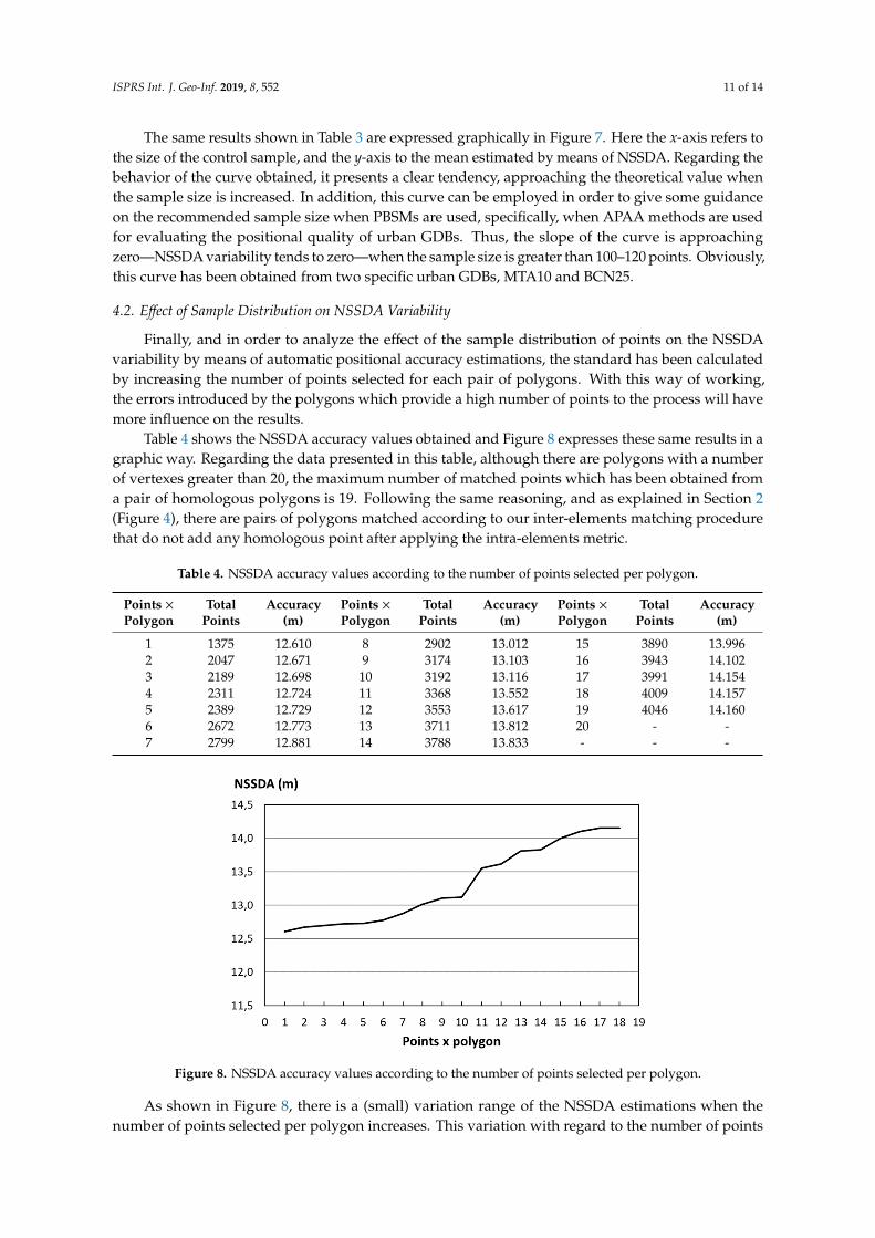
Table 4 shows the NSSDA accuracy values obtained and Figure 8 expresses these same results in agraphic way. Regarding the data presented in this table, although there are polygons with a numberof vertexes greater than 20, the maximum number of matched points which has been obtained froma pair of homologous polygons is 19. Following the same reasoning, and as explained in Section 2(Figure 4), there are pairs of polygons matched according to our inter-elements matching procedurethat do not add any homologous point after applying the intra-elements metric.

Table 4. NSSDA accuracy values according to the number of points selected per polygon.

Points ×Polygon

TotalPoints

Accuracy(m)

Points ×Polygon

TotalPoints

Accuracy(m)

Points ×Polygon

TotalPoints

Accuracy(m)

1 1375 12.610 8 2902 13.012 15 3890 13.9962 2047 12.671 9 3174 13.103 16 3943 14.1023 2189 12.698 10 3192 13.116 17 3991 14.1544 2311 12.724 11 3368 13.552 18 4009 14.1575 2389 12.729 12 3553 13.617 19 4046 14.1606 2672 12.773 13 3711 13.812 20 - -7 2799 12.881 14 3788 13.833 - - -

- 12 -

Table 4. NSSDA accuracy values according to the number of points selected per polygon.

Points x

Polygon

Total Points

Accuracy (m)

Points x

Polygon

Total Points

Accuracy (m)

Points x

Polygon

Total Points

Accuracy (m)

1 1375 12,610 8 2902 13,012 15 3890 13,996 2 2047 12,671 9 3174 13,103 16 3943 14,102 3 2189 12,698 10 3192 13,116 17 3991 14,154 4 2311 12,724 11 3368 13,552 18 4009 14,157 5 2389 12,729 12 3553 13,617 19 4046 14,160 6 2672 12,773 13 3711 13,812 20 - - 7 2799 12,881 14 3788 13,833 - - -

Figure 8. NSSDA accuracy values according to the number of points selected per polygon.

As shown in Figure 8, there is a (small) variation range of the NSSDA estimations when the

number of points selected per polygon increases. This variation with regard to the number of points employed indicates less positional accuracy of those polygons with a greater number of vertexes. This is probably due to processes associated with generalization.

5. Conclusions

In this study, we have reproduced the experiment of Ariza and Atkinson [4] employing a population of errors generated from real data. The use of a point-based procedure for the automatic positional accuracy assessment of spatial data has provided a population of errors large enough to extract samples with a range of sizes that allows us to analyze the variability of NSSDA results according to the conditions established in the aforementioned experiment. The availability of this large volume of empirical geospatial data, the capability to obtain them in an automatic way and the possibility of combining them according to different selection criteria have been possible only thanks to the development of this type of APAA procedure.

As stated in the Introduction, the results achieved in this study have demonstrated that some of

the proposals and suggestions made by some authors [4,12–14] related the statistical behavior of the NSSDA, its recommendations about the number and distribution of check points, and the influence of this number of points on the variability and reliability of results have served to provide a better

Figure 8. NSSDA accuracy values according to the number of points selected per polygon.

As shown in Figure 8, there is a (small) variation range of the NSSDA estimations when thenumber of points selected per polygon increases. This variation with regard to the number of points

ISPRS Int. J. Geo-Inf. 2019, 8, 552 12 of 14

employed indicates less positional accuracy of those polygons with a greater number of vertexes.This is probably due to processes associated with generalization.

5. Conclusions

In this study, we have reproduced the experiment of Ariza and Atkinson [4] employing apopulation of errors generated from real data. The use of a point-based procedure for the automaticpositional accuracy assessment of spatial data has provided a population of errors large enoughto extract samples with a range of sizes that allows us to analyze the variability of NSSDA resultsaccording to the conditions established in the aforementioned experiment. The availability of thislarge volume of empirical geospatial data, the capability to obtain them in an automatic way and thepossibility of combining them according to different selection criteria have been possible only thanksto the development of this type of APAA procedure.

As stated in the Introduction, the results achieved in this study have demonstrated that some ofthe proposals and suggestions made by some authors [4,12–14] related the statistical behavior of theNSSDA, its recommendations about the number and distribution of check points, and the influenceof this number of points on the variability and reliability of results have served to provide a betterunderstanding of the spatial data accuracy standards. Obviously, this also implies that the mainconclusions derived from our research—in the specific case of the NSSDA—are in accordance withthose reached by Ariza and Atkinson in their work [4]:

• The NSSDA presents a small tendency to underestimate accuracy.• For the minimum proposed sample size n = 20 points (size recommended by the FGDC and

suggested by most of the PBSM), the variability of results is in the order of ±11%.• The variation range decreases when the sample size increases.• For a sample size n = 100 points (size recommended by several authors [4,14]) the variability of

results is in the order of ±4.9%.• When the results are expressed graphically, the curve obtained can be employed in order to give

some guidance on the recommended sample size when PBSM is used, specifically, when APAAmethods are used for evaluating the positional quality of urban GDBs.

• When the number of points selected for each pair of polygons increases the positional accuracydetermined by the NSSDA estimations decreases, probably due to the generalization processes.

Finally, we must note that these results have been obtained from two specific urban GDBs, MTA10and BCN25. However, in our opinion these results may be extrapolated to other cases. In fact, in futurestudies we plan to diversify our work to different map scales (including a new set of GDBs withdifferent density both in polygons and number of vertexes).

Author Contributions: The research was conducted by the main author, Juan José Ruiz-Lendínez, under thesupervision of the co-authors Manuel Antonio Ureña-Cámara and Francisco Javier Ariza-López. All authorsjointly drafted and critically revised the paper. All authors read and approved the final manuscript.

Funding: This research was funded by the Ministry of Education and Culture of Spain, Grant number CAS18/00024(“José Castillejo” Mobility Support for Stay Abroad Program).

Conflicts of Interest: The authors declare no conflict of interest.

References

1. Ruiz-Lendínez, J.J.; Ureña-Cámara, M.A.; Ariza-López, F.J. A Polygon and Point-Based Approach to MatchingGeospatial Features. ISPRS Int. J. Geo-Inf. 2017, 6, 399. [CrossRef]

2. Ariza-López, F.J.; Ruiz-Lendinez, J.J.; Ureña-Cámara, M.A. Influence of Sample Size on Automatic PositionalAccuracy Assessment Methods for Urban Areas. ISPRS Int. J. Geo-Inf. 2018, 7, 200. [CrossRef]

3. Morrison, J. Spatial data quality. In Elements of Spatial Data Quality; Guptill, S.C., Morrison, J.L., Eds.;Pergamon Press: Oxford, UK, 1995; pp. 1–12.

ISPRS Int. J. Geo-Inf. 2019, 8, 552 13 of 14

4. Ariza-López, F.J.; Atkinson-Gordo, A. Variability of NSSDA Estimations. J. Surv. Eng. 2008, 134, 39–44.[CrossRef]

5. Li, Z. Effects of check points on the reliability of DTM accuracy estimates obtained from experimental test.Photogramm. Eng. Remote Sens. 1991, 57, 1333–1340.

6. U.S. Bureau of the Budget (USBB). United States National Map Accuracy Standards; U.S. Bureau of the Budget(USBB): Washington, DC, USA, 1947.

7. American Society of Civil Engineering (ASCE). Map Uses, Scales and Accuracies for Engineering and AssociatedPurposes; ASCE Committee on Cartographic Surveying, Surveying and Mapping Division: New York, NY,USA, 1983.

8. Federal Geographic Data Committee (FGDC). Geospatial Positioning Accuracy Standards, Part 3: NationalStandard for Spatial Data Accuracy; FGDC-STD-007; FGDC: Reston, VA, USA, 1998.

9. Ruiz-Lendinez, J.J.; Ariza-López, F.J.; Ureña-Cámara, M.A. A point-based methodology for the automaticpositional accuracy assessment of geospatial databases. Surv. Rev. 2016, 48, 269–277. [CrossRef]

10. Ley, R. Accuracy assessment of digital terrain models. In Proceedings of the Auto-Carto, London, UK,14–19 September 1986; pp. 455–464.

11. Newby, P.R. Quality management for surveying, photogrammetry and digital mapping at the ordnancesurvey. Photogramm. Rec. 1992, 79, 45–58. [CrossRef]

12. Minnesota Planning Land Management Information Center (MPLMIC). Positional Accuracy Handbook;MPLMIC: St. Paul, MN, USA, 1999.

13. Atkinson-Gordo, A. Control de Calidad Posicional en Cartografía: Análisis de los Principales Estándares yPropuesta de Mejora. Ph.D. Thesis, University of Jaén, Jaén, Spain, 2005.

14. Zandbergen, P. Positional Accuracy of Spatial Data: Non-Normal Distributions and a Critique of the NationalStandard for Spatial Data Accuracy. Trans. GIS 2008, 12, 103–130. [CrossRef]

15. Ruiz-Lendinez, J.; Ureña-Cámara, M.; Mozas-Calvache, A. GPS survey of roads networks for the positionalquality control of maps. Surv. Rev. 2009, 41, 374–383. [CrossRef]

16. Goodchild, M.; Hunter, G. A simple positional accuracy measure for linear features. Int. J. Geogr. Inf. Sci.1997, 11, 299–306. [CrossRef]

17. Herrera, F.; Lozano, M.; Verdegay, J. Tackling real-coded genetic algorithms: Operators and tools forbehavioral analysis. Artif. Intell. Rev. 1998, 12, 265–319. [CrossRef]

18. Arkin, E.; Chew, L.; Huttenlocher, D.; Kedem, K.; Mitchell, J. An Efficiently Computable Metric for ComputingPolygonal Shapes. IEEE Trans. Pattern Anal. Mach. Intell. 1991, 13, 209–216. [CrossRef]

19. Ruiz-Lendinez, J.J.; Ariza-López, F.J.; Ureña-Cámara, M.A.; Blázquez, E. Digital Map Conflation: A Reviewof the Process and a Proposal for Classification. Int. J. Geogr. Inf. Sci. 2011, 25, 1439–1466. [CrossRef]

20. Giordano, A.; Veregin, H. Il Controllo di Qualitá nei Sistemi Informative Territoriali; Cardo Editore: Venetia,Italy, 1994.

21. Goodchild, M.; Gopal, S. Accuracy of Spatial Data Bases; Taylor & Francis: London, UK, 1989.22. Leung, Y. A locational error model for spatial features. Int. J. Geogr. Inf. Sci. 1998, 12, 607–620. [CrossRef]23. Shi, W.; Liu, W. A stochastic process-based model for the positional error of a line segments in GIS. Int. J.

Geogr. Inf. Sci. 2001, 12, 131–143. [CrossRef]24. McCollum, J.M. Map error and root mean square. In Proceedings of the Towson University GIS Symposium,

Baltimore, MD, USA, 2–3 June 2003.25. Greenwalt, C. and Shultz, M. Principles of Error Theory and Cartographic Applications; Technical Report-96;

ACIC: St Louis, MO, USA, 1962.26. Vonderohe, A.P.; Chriman, N.R. Tests to establish the quality of digital cartographic data: Some example

from the Dane County Land Records Project. In Proceedings of the Auto-Carto 7, Washington, DC, USA,11–14 March 1985; pp. 552–559.

27. Bolstad, P.V.; Gessler, P.; Lillesand, T.M. Positional uncertainty in manually digitized map data. Int. J. Geogr.Inf. Syst. 1990, 4, 399–412. [CrossRef]

28. Vauglin, F. Modèles statistiques des imprécisions géométriques des objets géographiques linéaires. Ph.D.Dissertation, University of Marne-La-Vallée, Champs-sur-Marne, France, 1997.

29. Bel Hadj, A. Moment representation of polygons for the assessment of their shape quality. J. Geogr. Syst.2002, 4, 209–232.

ISPRS Int. J. Geo-Inf. 2019, 8, 552 14 of 14

30. Zandbergen, P.A. Characterizing the error distribution of Lidar elevation data for North Carolina. Int. J.Remote Sens. 2011, 32, 409–430. [CrossRef]

31. Liu, X.; Hu, P.; Hu, H.; Sherba, J. Approximation Theory Applied to DEM Vertical Accuracy Assessment.Trans. GIS. 2012, 16, 397–410. [CrossRef]

32. Rodríguez-Gonzálvez, P.; Garcia-Gago, J.; Gomez-Lahoz, J.; González-Aguilera, D. Confronting passive andactive sensors with non-gaussian statistics. Sensors 2014, 14, 13759–13777. [CrossRef]

33. Rodríguez-Gonzálvez, P.; González-Aguilera, D.; Hernández-López, D.; González-Jorge, H. Accuracyassessment of airborne laser scanner dataset by means of parametric and non-parametric statistical methods.IET Sci. Meas. Technol. 2015, 9, 505–513. [CrossRef]

34. Ariza-López, F.J.; Rodríguez-Avi, J.; González-Aguilera, D.; Rodríguez-Gonzálvez, P. A New Method forPositional Accuracy Control for Non-Normal Errors Applied to Airborne Laser Scanner Data. Appl. Sci.2019, 9, 3887. [CrossRef]

35. Van Niel, T.G.; McVicar, T.R. Experimental evaluation of positional accuracy estimates from a linear networkusing point- and line-based testing methods. Int. J. Geogr. Inf. Sci. 2002, 16, 455–473. [CrossRef]

36. Marsaglia, G.; Tsang, W.W.; Wang, J. Evaluating Kolmogorov’s distribution. J. Stat. Softw. 2003, 8, 1–4.[CrossRef]

37. Chauve, A.; Vega, C.; Durrieu, S.; Bretar, F.; Allouis, T.; Pierrot-Deseilligny, M.; Puech, W. Advancedfull-waveform LiDAR data echo detection: Assessing quality of derived terrain and tree height models in analpine coniferous forest. Int. J. Remote Sens. 2009, 30, 5211–5228. [CrossRef]

38. Estornell, J.; Ruiz, L.; Velázquez-Martí, B.; Hermosilla, T. Analysis of the factors affecting LiDAR DTMaccuracy in a steep shrub area. Int. J. Digit. Earth 2011, 4, 521–538. [CrossRef]

39. Razak, K.A.; Straatsma, M.W.; Van Westen, C.J.; Malet, J.P.; de Jong, S.M. Airborne laser scanning of forestedlandslides characterization: Terrain model quality and visualization. Geomorphology 2011, 126, 186–200.[CrossRef]

40. National Digital Elevation Program (NDEP). Guidelines for digital elevation data-The National Map; 3D ElevationProgram Standards and Specifications: Washington, DC, USA, 2006.

41. US Army Corps of Engineers (USACE). Engineering and Design-Photogrammetric Mapping; EM 1110-1-1000;US Army Corps of Engineers (USACE): Washington, DC, USA, 2002.

42. Ariza-López, F.J.; Atkinson, A. Metodologías de Control Posicional. Visión general y Análisis crítico; TechnicalReport-CT-148 AENOR; Universidad de Jaén: Jaén, Spain, 2006.

43. Ariza-López, F.J. Guía para la evaluación de la exactitud posicional de datos espaciales; Publicación 557: Serie dedocumentos especializados; Instituto Panamericano de Geografía e Historia: Montevideo, Uruguay, 2019.

44. Ariza-López, F.J.; Rodríguez-Avi, J. A Statistical Model Inspired by the National Map Accuracy Standard.Photogramm. Eng. Remote Sens. 2014, 80, 271–281.

© 2019 by the authors. Licensee MDPI, Basel, Switzerland. This article is an open accessarticle distributed under the terms and conditions of the Creative Commons Attribution(CC BY) license (http://creativecommons.org/licenses/by/4.0/).