1

Structure-aware reinforcement learning fornode-overload protection in mobile edge computingAnirudha Jitani, Student Member, IEEE, Aditya Mahajan, Senior Member, IEEE, Zhongwen Zhu, Member, IEEE,

Hatem Abou-zeid, Member, IEEE, Emmanuel Thepie Fapi, and Hakimeh Purmehdi, Member, IEEE

Abstract—Mobile Edge Computing (MEC) refers to the con-cept of placing computational capability and applications at theedge of the network, providing benefits such as reduced latencyin handling client requests, reduced network congestion, andimproved performance of applications. The performance andreliability of MEC are degraded significantly when one or severaledge servers in the cluster are overloaded. Especially when aserver crashes due to the overload, it causes service failuresin MEC. In this work, an adaptive admission control policy toprevent edge node from getting overloaded is presented. Thisapproach is based on a recently-proposed low complexity RL(Reinforcement Learning) algorithm called SALMUT (Structure-Aware Learning for Multiple Thresholds), which exploits thestructure of the optimal admission control policy in multi-classqueues for an average-cost setting. We extend the framework towork for node overload-protection problem in a discounted-costsetting. The proposed solution is validated using several scenariosmimicking real-world deployments in two different settings —computer simulations and a docker testbed. Our empiricalevaluations show that the total discounted cost incurred bySALMUT is similar to state-of-the-art deep RL algorithms suchas PPO (Proximal Policy Optimization) and A2C (AdvantageActor Critic) but requires an order of magnitude less time totrain, outputs easily interpretable policy, and can be deployed inan online manner.

Index Terms—Reinforcement learning, structure-aware rein-forcement learning, Markov decision process, mobile edge com-puting, node-overload protection.

I. INTRODUCTION

IN the last decade, we have seen a shift in the computingparadigm from co-located datacenters and compute servers

to cloud computing. Due to the aggregation of resources, cloudcomputing can deliver elastic computing power and storageto customers without the overhead of setting up expensivedatacenters and networking infrastructures. It has speciallyattracted small and medium-sized businesses who can leveragethe cloud infrastructure with minimal setup costs. In recentyears, the proliferation of Video-on-Demand (VoD) services,Internet-of-Things (IoT), real-time online gaming platforms,and Virtual Reality (VR) applications has lead to a strong

Anirudha Jitani is with the School of Computer Science, McGill Universityand Montreal Institute of Learning Algorithms. Aditya Mahajan is withthe Department of Electrical and Computer Engineering, McGill University,Canada.Emails: anirudha.jitani@mail.mcgill.ca, aditya.mahajan@mcgill.ca

Zhongwen Zhu, Emmanuel Thepie Fapi, and Hakimeh Purmehdi are withGlobal AI Accelerator, Ericsson, Montreal, Canada. Hatem Abou-zeid is withEricsson, Ottawa, Canada.Emails: zhongwen.zhu@ericsson.com, emmanuel.thepie.fapi@ericsson.com,hakimeh.purmehdi@ericsson.com, hatem.abou-zeid@ericsson.com.

This work was supported in part by MITACS Accelerate, Grant IT16364.

focus on the quality of experience of the end users. The cloudparadigm is not the ideal candidate for such latency-sensitiveapplications owing to the delay between the end user and cloudserver.

This has led to a new trend in computing called Mobile EdgeComputing (MEC) [1], [2], where the compute capabilities aremoved closer to the network edges. It represents an essentialbuilding block in the 5G vision of creating large distributed,pervasive, heterogeneous, and multi-domain environments.Harvesting the vast amount of the idle computation powerand storage space distributed at the network edges can yieldsufficient capacities for performing computation-intensive andlatency-critical tasks requested by the end-users. However, itis not feasible to set-up huge resourceful edge clusters alongall network edges that mimic the capabilities of the clouddue to the sheer volume of resources that would be required,which would remain underutilized most of the times. Due tothe limited resources at the edge nodes and fluctuations in theuser requests, an edge cluster may not be capable of meetingthe resource and service requirements of all the users it isserving.

Computation offloading methods have gained a lot ofpopularity as they provide a simple solution to overcomethe problems of edge and mobile computing. Data andcomputation offloading can potentially reduce the processingdelay, improve energy efficiency, and even enhance securityfor computation-intensive applications. The critical problemin the computation offloading is to determine the amount ofcomputational workload, and choose the MEC server from allavailable servers. Various aspects of MEC from the point ofview of the mobile user have been investigated in the literature.For example, the questions of when to offload to a mobileserver, to which mobile server to offload, and how to offloadhave been studied extensively. See, [3]–[7] and referencestherein.

However, the design questions at the server side have notbeen investigated as extensively. When an edge server receivesa large number of requests in a short period of time (forexample due to a sporting event), the edge server can getoverloaded, which can lead to service degradation or evennode failure. When such service degradation occurs, edgeservers are configured to offload requests to other nodes inthe cluster in order to avoid the node crash. The crash ofan edge node leads to the reduction of the cluster capacity,which is a disaster for the platform operator as well as the endusers, who are using the services or the applications. However,performing this migration takes extra time and reduces the

arX

iv:2

107.

0102

5v1

[cs

.NI]

29

Jun

2021

2

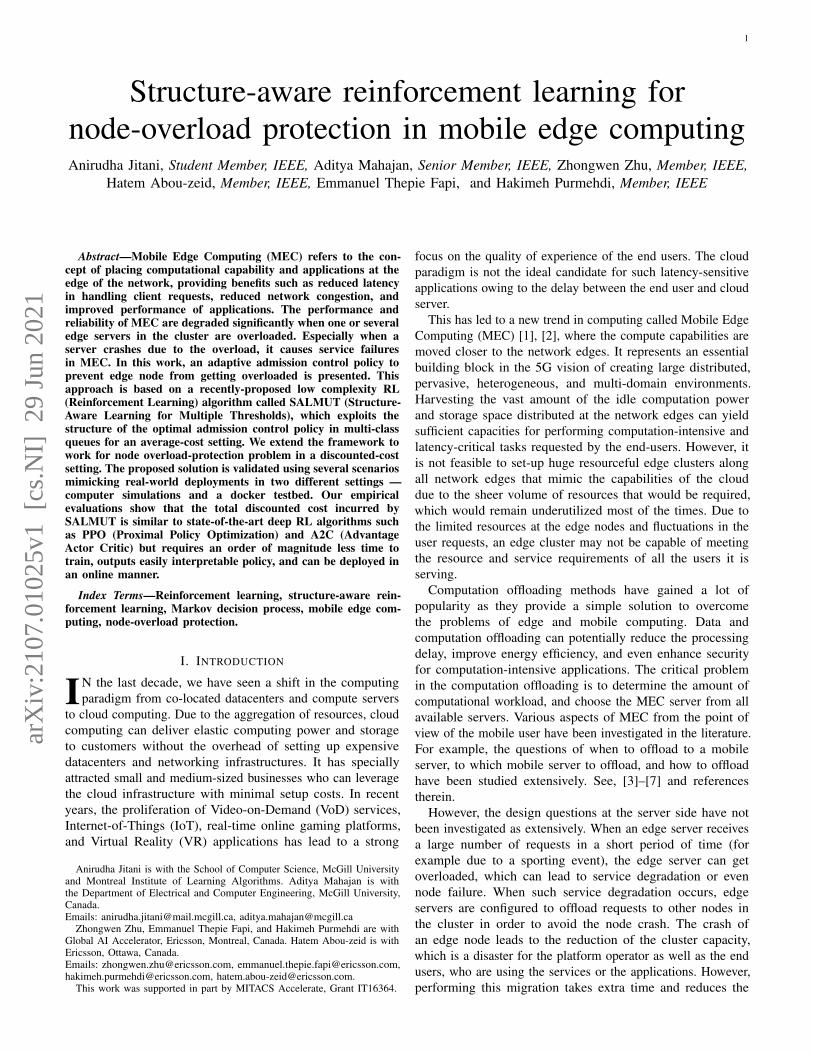
Fig. 1. A Mobile Edge Computing (MEC) system. User may be mobile andwill connect to the closest edge server. The MEC servers are connected to thebackend cloud server or datacenters through the core network.

resources availability for other services deployed in the cluster.Therefore, it is paramount to design pro-active mechanismsthat prevent a node from getting overloaded using dynamicoffloading policies that can adapt to service request dynamics.

The design of an offloading policy has to take into ac-count the time-varying channel conditions, user mobility,energy supply, computation workload and the computationalcapabilities of different MEC servers. The problem can bemodeled as a Markov Decision Process (MDP) and solvedusing dynamic programming. However, solving a dynamicprogram requires the knowledge of the system parameters,which are not typically known and may also vary with time.In such time-varying environments, the offloading policy mustadapt to the environment. Reinforcement Learning (RL) [8]is a natural choice to design such adaptive policies as theydo not need a model of the environment and can learn theoptimal policy based on the observed per-step cost. RL hasbeen successfully applied for designing adaptive offloadingpolicies in edge and fog computing in [9]–[15] to realize oneor more objectives such as minimizing latency, minimizingpower consumption, association of users and base stations.Although RL has achieved considerable success in the previouswork, this success is generally achieved by using deep neuralnetworks to model the policy and the value function. Suchdeep RL algorithms require considerable computational powerand time to train, and are notoriously brittle to the choiceof hyper-parameters. They may also not transfer well fromsimulation to the real-world, and output policies which aredifficult to interpret. These features make them impractical tobe deployed on the edge nodes to continuously adapt to thechanging network conditions.

In this work, we study the problem of node-overloadprotection for a single edge node. Our main contributionsare as follows:

• We present a mathematical model for designing anoffloading policy for node-overload protection. The modelincorporates practical considerations of server holding,processing and offloading costs. In the simplest case,

when the request arrival process is time-homogeneous,we model the system as a continuous-time MDP anduse the uniformization technique [16], [17] to convertthe continuous-time MDP to a discrete-time MDP, whichcan then be solved using standard dynamic programmingalgorithms [18].

• We show that for time-homogeneous arrival process,the value function and the optimal policy are weaklyincreasing in the CPU utilization.

• We design a node-overload protection scheme thatuses a recently proposed low-complexity RL algorithmcalled Structure-Aware Learning for Multiple Thresholds(SALMUT) [19]. The original SALMUT algorithm wasdesigned for the average cost models. We extend thealgorithm to the discounted cost setup and prove thatSALMUT converges almost surely to a locally optimalpolicy.

• We compare the performance of Deep RL algorithmswith SALMUT in a variety of scenarios in a simulatedtestbed which are motivated by real world deployments.Our simulation experiments show that SALMUT performsclose to the state-of-the-art Deep RL algorithms such asPPO [20] and A2C [21], but requires an order of magnitudeless time to train and provides optimal policies which areeasy to interpret.

• We developed a docker testbed where we run actualworkloads and compare the performance of SALMUTwith the baseline policy. Our results show that SALMUTalgorithm outperforms the baseline algorithm.

A preliminary version of this paper appeared in [22], wherethe monotonicity results of the optimal policy (Proposition 1and 2) were stated without proof and the modified SALMUTalgorithm was presented with a slightly different derivation.However, the convergence behavior of the algorithm (Theorem2) was not analyzed. A preliminary version of the comparisonon SALMUT with state of the art RL algorithms on acomputer simulation were included in [22]. However, thedetailed behavioral analysis (Sec. V) and the results for thedocker testbed (Sec. VI) are new.

The rest of the paper is organized as follows. We present thesystem model and problem formulation in Sec. II. In Sec. III,we present a dynamic programming decomposition for the caseof time-homogeneous statistics of the arrival process. In Sec. IV,we present the structure aware RL algorithm (SALMUT)proposed in [19] for our model. In Sec. V, we conduct adetailed experimental study to compare the performance ofSALMUT with other state-of-the-art RL algorithms usingcomputer simulations. In Sec. VI, we compare the performanceof SALMUT with baseline algorithm on the real-testbed.Finally, in Sec. VII, we provide the conclusion, limitations ofour model, and future directions.

II. MODEL AND PROBLEM FORMULATION

A. System model

A simplified MEC system consists of an edge server andseveral mobile users accessing that server (see Fig. 1). Mobileusers independently generate service requests according to

3

Fig. 2. System model of admission control in a single edge server.

TABLE ILIST OF SYMBOLS USED

Symbol Description

𝑋𝑡 Queue length at time 𝑡

𝐿𝑡 CPU load of the system at time 𝑡

𝐴𝑡 Offloading action taken by agent at time 𝑡

𝑘 Number of cores in the edge node𝑅 CPU resources required by a request

𝑃 (𝑟 ) PMF of the CPU resources required` Processing time of a single core in the edge node_ Request arrival rate of userℎ Holding cost per unit time

𝑐 (ℓ) Running cost per unit time𝑝 (ℓ) Penalty for offloading the packet

𝜌(𝑥, ℓ, 𝑎) Cost function in the continuous MDP𝜋 Policy of the RL agent𝛼 Discount factor in continuous MDP

𝑉 𝜋 (𝑥, ℓ) Performance of the policy 𝜋

𝑝 (𝑥′, ℓ′ |𝑥, ℓ, 𝑎) Transition probability function𝛽 Discount factor in discrete MDP

�̄�(𝑥, ℓ, 𝑎) Cost function in the discrete MDP𝑄 (𝑥, ℓ, 𝑎) Q-value for state (𝑥, ℓ) and action 𝑎

𝜏 Threshold vector𝜋𝜏 Optimal Threshold Policy for SALMUT

𝐽 (𝜏) Performance of the SALMULT policy 𝜋𝜏𝑓 (𝜏 (𝑥) , ℓ) Probability of accepting new request

𝑇 Temperature of the sigmoid function` (𝑥, ℓ) Occupancy measure on the states starting from

(𝑥0, ℓ0)𝑏1𝑛 Fast timescale learning rate

𝑏2𝑛 Slow timescale learning rate

𝐶off Number of requests offloaded by edge node𝐶ov Number of times edge node enters an overloaded

state

a Poisson process. The rate of requests and the number ofusers may also change with time. The edge server takes CPUresources to serve each request from mobile users. When a newrequest arrives, the edge server has the option to serve it oroffload it to other healthy edge server in the cluster. The requestis buffered in a queue before it is served. The mathematicalmodel of the edge server and the mobile users is presentedbelow.

1) Edge server: Let 𝑋𝑡 ∈ {0, 1, . . . ,X} denote the numberof service requests buffered in the queue, where X denotes thesize of the buffer. Let 𝐿𝑡 ∈ {0, 1, . . . , L} denote the CPU loadat the server where L is the capacity of the CPU. We assumethat the CPU has 𝑘 cores.

We assume that the requests arrive according to a (potentiallytime-varying) Poisson process with rate _. If a new requestarrives when the buffer is full, the request is offloaded toanother server. If a new request arrives when the buffer is not

full, the server has the option to either accept or offload therequest.

The server can process up to a maximum of 𝑘 requestsfrom the head of the queue. Processing each request requiresCPU resources for the duration in which the request is beingserved. The required CPU resources is a random variable 𝑅 ∈{1, . . . ,R} with probability mass function 𝑃. The realizationof 𝑅 is not revealed until the server starts working on therequest. The duration of service is exponentially distributedrandom variable with rate `.

Let A = {0, 1} denote the action set. Here 𝐴𝑡 = 1 meansthat the server decides to offload the request while 𝐴𝑡 = 0means that the server accepts the request.

2) Traffic model for mobile users: We consider multiplemodels for traffic.• Scenario 1: All users generate requests according to the

same rate _ and the rate does not change over time. Thus,the rate at which requests arrive is _𝑁 .

• Scenario 2: In this scenario, we assume that all usersgenerate requests according to rate _𝑀𝑡

, where 𝑀𝑡 ∈{1, . . . ,M} is a global state which changes over time.Thus, the rate at which requests arrive in state 𝑚, where𝑚 ∈ 𝑀𝑡 , is _𝑚𝑁 .

• Scenario 3: Each user 𝑛 has a state 𝑀𝑛𝑡 ∈ {1, . . . ,M}.

When the user 𝑛 is in state 𝑚, it generates requestsaccording to rate _𝑚. The state 𝑀𝑛

𝑡 changes over time.Thus, the rate at which requests arrive at the server is∑𝑁

𝑛=1 _𝑀𝑛𝑡

.• Time-varying user set: In each of the scenarios above,

we can consider the case when the number of users is notfixed and changes over time. We call them Scenario 4, 5,and 6 respectively.

3) Cost and the optimization framework: The system incursthree types of a cost:• a holding cost of ℎ per unit time when a request is buffered

in the queue but is not being served.• a running cost of 𝑐(ℓ) per unit time for running the CPU

at a load of ℓ.• a penalty of 𝑝(ℓ) for offloading a packet at CPU load ℓ.

We combine all these costs in a cost function

𝜌(𝑥, ℓ, 𝑎) = ℎ[𝑥 − 𝑘]+ + 𝑐(ℓ) + 𝑝(ℓ)1{𝑎 = 1}, (1)

where 𝑎 denotes the action, [𝑥]+ is a short-hand for max{𝑥, 0}and 1{·} is the indicator function. Note that to simplify theanalysis, we assume that the server always serves min{𝑋𝑡 , 𝑘}requests. It is also assumed that 𝑐(ℓ) and 𝑐(ℓ) + 𝑝(ℓ) areincreasing in ℓ.

Whenever a new request arrives, the server uses a memory-less policy 𝜋 : {0, 1, . . . ,X} × {0, 1, . . . , L} → {0, 1} to choosean action

𝐴𝑡 = 𝜋𝑡 (𝑋𝑡 , 𝐿𝑡 ).

The performance of a policy 𝜋 starting from initial state(𝑥, ℓ) is given by

𝑉 𝜋 (𝑥, ℓ) = E[∫ ∞

0𝑒−𝛼𝑡 𝜌(𝑋𝑡 , 𝐿𝑡 , 𝐴𝑡 )𝑑𝑡

���� 𝑋0 = 𝑥, 𝐿0 = ℓ

],

(2)

4

where 𝛼 > 0 is the discount rate and the expectation is withrespect to the arrival process, CPU utilization, and servicecompletions.

The objective is to minimize the performance (2) for thedifferent traffic scenarios listed above. We are particularlyinterested in the scenarios where the arrival rate and potentiallyother components of the model such as the resource distributionare not known to the system designer and change during theoperation of the system.

B. Solution framework

When the model parameters (_, 𝑁, `, 𝑃, 𝑘) are known andtime-homogeneous, the optimal policy 𝜋 can be computedusing dynamic programming. However, in a real system,these parameters may not be known, so we are interestedin developing a RL algorithm which can learn the optimalpolicy based on the observed per-step cost.

In principle, when the model parameters are known, Scenar-ios 2 and 3 can also be solved using dynamic programming.However, the state of such dynamic programs will include thestate 𝑀𝑡 of the system (for Scenario 2) or the states (𝑀𝑛

𝑡 )𝑁𝑛=1of all users (for Scenario 3). Typically, these states change ata slow time-scale. So, we will consider reinforcement learningalgorithms which do not explicitly keep track of the statesof the user and verify that the algorithm can adapt quicklywhenever the arrival rates change.

III. DYNAMIC PROGRAMMING TO IDENTIFY OPTIMALADMISSION CONTROL POLICY

When the arrival process is time-homogeneous, the process{𝑋𝑡 , 𝐿𝑡 }𝑡≥0 is a finite-state continuous-time MDP controlledthrough {𝐴𝑡 }𝑡≥0. To specify the controlled transition probabilityof this MDP, we consider the following two cases.

First, if there is a new arrival at time 𝑡, then

P(𝑋𝑡 = 𝑥 ′, 𝐿𝑡 = ℓ′ | 𝑋𝑡− = 𝑥, 𝐿𝑡− = ℓ, 𝐴𝑡 = 𝑎)

=

𝑃(ℓ′ − ℓ), if 𝑥 ′ = 𝑥 + 1 and 𝑎 = 01, if 𝑥 ′ = 𝑥, ℓ′ = ℓ, and 𝑎 = 10, otherwise.

(3)

We denote this transition function by 𝑞+ (𝑥 ′, ℓ′ |𝑥, ℓ, 𝑎). Notethat the first term 𝑃(ℓ′ − ℓ) denotes the probability that theaccepted request required (ℓ′ − ℓ) CPU resources.

Second, if there is a departure at time 𝑡,

P(𝑋𝑡 = 𝑥 ′, 𝐿𝑡 = ℓ′ | 𝑋𝑡− = 𝑥, 𝐿𝑡− = ℓ)

=

{𝑃(ℓ − ℓ′), if 𝑥 ′ = [𝑥 − 1]+

0, otherwise.(4)

We denote this transition function by 𝑞− (𝑥 ′, ℓ′ |𝑥, ℓ). Note thatthere is no decision to be taken at the completion of a request,so the above transition does not depend on the action. Ingeneral, the reduction in CPU utilization will correspond to theresources released after the client requests are served. However,keeping track of those resources would mean that we wouldneed to expand the state and include (𝑅1, . . . , 𝑅𝑘 ) as part of thestate, where 𝑅𝑖 denotes the resources required by the request

which is being processed by CPU 𝑖. In order to avoid such anincrease in state dimension, we assume that when a requestis completed, CPU utilization reduces by amount ℓ − ℓ′ withprobability 𝑃(ℓ − ℓ′).

We combine (3) and (4) into a single controlled transitionprobability function from state (𝑥, ℓ) to state (𝑥 ′, ℓ′) given by

𝑝(𝑥 ′, ℓ′ | 𝑥, ℓ, 𝑎) = _

_ +min{𝑥, 𝑘}` 𝑞+ (𝑥′, ℓ′ | 𝑥, ℓ, 𝑎)

+ min{𝑥, 𝑘}`_ +min{𝑥, 𝑘}` 𝑞− (𝑥

′, ℓ′ | 𝑥, ℓ). (5)

Let a = _ + 𝑘` denote the uniform upper bound on thetransition rate at the states. Then, using the uniformizationtechnique [16], [17], we can convert the above continuous timediscounted cost MDP into a discrete time discounted cost MDPwith discount factor 𝛽 = a/(𝛼+a), transition probability matrix𝑝(𝑥 ′, ℓ′ |𝑥, ℓ, 𝑎) and per-step cost

�̄�(𝑥, ℓ, 𝑎) = 1𝛼 + a 𝜌(𝑥, ℓ, 𝑎).

Therefore, we have the following.

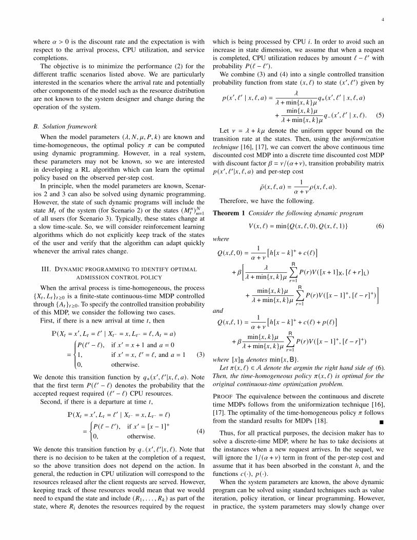
Theorem 1 Consider the following dynamic program

𝑉 (𝑥, ℓ) = min{𝑄(𝑥, ℓ, 0), 𝑄(𝑥, ℓ, 1)} (6)

where

𝑄(𝑥,ℓ, 0) = 1𝛼 + a

[ℎ[𝑥 − 𝑘]+ + 𝑐(ℓ)

]+ 𝛽

[_

_ +min{𝑥, 𝑘}`

R∑︁𝑟=1

𝑃(𝑟)𝑉 ( [𝑥 + 1]X, [ℓ + 𝑟]L)

+ min{𝑥, 𝑘}`_ +min{𝑥, 𝑘}`

R∑︁𝑟=1

𝑃(𝑟)𝑉 ( [𝑥 − 1]+, [ℓ − 𝑟]+)]

and

𝑄(𝑥,ℓ, 1) = 1𝛼 + a

[ℎ[𝑥 − 𝑘]+ + 𝑐(ℓ) + 𝑝(ℓ)

]+ 𝛽 min{𝑥, 𝑘}`

_ +min{𝑥, 𝑘}`

R∑︁𝑟=1

𝑃(𝑟)𝑉 ( [𝑥 − 1]+, [ℓ − 𝑟]+)

where [𝑥]B denotes min{𝑥,B}.Let 𝜋(𝑥, ℓ) ∈ A denote the argmin the right hand side of (6).

Then, the time-homogeneous policy 𝜋(𝑥, ℓ) is optimal for theoriginal continuous-time optimization problem.

PROOF The equivalence between the continuous and discretetime MDPs follows from the uniformization technique [16],[17]. The optimality of the time-homogeneous policy 𝜋 followsfrom the standard results for MDPs [18]. �

Thus, for all practical purposes, the decision maker has tosolve a discrete-time MDP, where he has to take decisions atthe instances when a new request arrives. In the sequel, wewill ignore the 1/(𝛼 + a) term in front of the per-step cost andassume that it has been absorbed in the constant ℎ, and thefunctions 𝑐(·), 𝑝(·).

When the system parameters are known, the above dynamicprogram can be solved using standard techniques such as valueiteration, policy iteration, or linear programming. However,in practice, the system parameters may slowly change over

5

time. Therefore, instead of pursuing a planning solution, weconsider reinforcement learning solutions which can adapt totime-varying environments.

IV. STRUCTURE-AWARE REINFORCEMENT LEARNING

Although, in principle, the optimal admission control prob-lem formulated above can be solved using deep RL algorithms,such algorithms require significant computational resources totrain, are brittle to the choice of hyperparameters, and generatepolicies which are difficult to interpret. For the aforementionedreasons, we investigate an alternate class of RL algorithmswhich circumvents these limitations.

A. Structure of the optimal policyWe first establish basic monotonicity properties of the value

function and the optimal policy.

Proposition 1 For a fixed queue length 𝑥, the value functionis weakly increasing in the CPU utilization ℓ.

PROOF The proof is present in Appendix A. �

Proposition 2 For a fixed queue length 𝑥, if it is optimal toreject a request at CPU utilization ℓ, then it is optimal to rejecta request at all CPU utilizations ℓ′ > ℓ.

PROOF The proof is present in Appendix B. �

B. The SALMUT algorithmProposition 2 shows that the optimal policy can be repre-

sented by a threshold vector 𝜏 = (𝜏(𝑥))X𝑥=0, where 𝜏(𝑥) ∈

{0, . . . , L} is the smallest value of the CPU utilization suchthat it is optimal to accept the packet for CPU utilization lessthan or equal to 𝜏(𝑥) and reject it for utilization greater than𝜏(𝑥).

The SALMUT algorithm was proposed in [19] to exploit asimilar structure in admission control for multi-class queues.It was originally proposed for the average cost setting. Wepresent a generalization to the discounted-time setting.

We use 𝜋𝜏 to denote a threshold-based policy with theparameters (𝜏(𝑥))X

𝑥=0 taking values in {0, . . . , L}X+1. The keyidea behind SALMUT is that, instead of deterministic threshold-based policies, we consider a random policy parameterizedwith parameters taking value in the compact set [0, L]X+1.Then, for any state (𝑥, ℓ), the randomized policy 𝜋𝜏 choosesaction 𝑎 = 0 with probability 𝑓 (𝜏(𝑥), ℓ) and chooses action𝑎 = 1 with probability 1 − 𝑓 (𝜏(𝑥), ℓ), where 𝑓 (𝜏(𝑥), ℓ) is anycontinuous decreasing function w.r.t ℓ, which is differentiablein its first argument, e.g., the sigmoid function

𝑓 (𝜏(𝑥), ℓ) = exp((𝜏(𝑥) − ℓ)/𝑇)1 + exp((𝜏(𝑥) − ℓ)/𝑇) , (7)

where 𝑇 > 0 is a hyper-parameter (often called “temperature”).Fix an initial state (𝑥0, ℓ0) and let 𝐽 (𝜏) denote the perfor-

mance of policy 𝜋𝜏 . Furthermore, let 𝑝𝜏 (𝑥 ′, ℓ′ |𝑥, ℓ) denote thetransition function under policy 𝜋𝜏 , i.e.

𝑝𝜏 (𝑥 ′, ℓ′ |𝑥, ℓ) = 𝑓 (𝜏(𝑥), ℓ)𝑝(𝑥 ′, ℓ′ |𝑥, ℓ, 0)+ (1 − 𝑓 (𝜏(𝑥), ℓ))𝑝(𝑥 ′, ℓ′ |𝑥, ℓ, 1) (8)

Fig. 3. Illustration of the two-timescale SALMUT algorithm.

Similarly, let �̄�𝜏 (𝑥, ℓ) denote the expected per-step rewardunder policy 𝜋𝜏 , i.e.

�̄�𝜏 (𝑥, ℓ) = 𝑓 (𝜏(𝑥), ℓ) �̄�(𝑥, ℓ, 0) + (1− 𝑓 (𝜏(𝑥), ℓ)) �̄�(𝑥, ℓ, 1).(9)

Let ∇ denote the gradient with respect to 𝜏.From Performance Derivative formula [23, Eq. 2.44], we

know that

∇𝐽 (𝜏) = 11 − 𝛽

X∑︁𝑥=0

L∑︁ℓ=0

`(𝑥, ℓ)[∇�̄�𝜏 (𝑥, ℓ)

+ 𝛽X∑︁

𝑥′=0

L∑︁ℓ′=0∇𝑝𝜏 (𝑥 ′, ℓ′ |𝑥, ℓ)𝑉𝜏 (𝑥 ′, ℓ′)] (10)

where `(𝑥, ℓ) is the occupancy measure on the states startingfrom the initial state (𝑥0, ℓ0).

From (8), we get that

∇𝑝𝜏 (𝑥 ′, ℓ′ |𝑥, ℓ) = (𝑝(𝑥 ′, ℓ′ |𝑥, ℓ, 0) − 𝑝(𝑥 ′, ℓ′ |𝑥, ℓ, 1))∇ 𝑓 (𝜏(𝑥), ℓ). (11)

Similarly, from (9), we get that

∇�̄�𝜏 (𝑥, ℓ) = ( �̄�(𝑥, ℓ, 0) − �̄�(𝑥, ℓ, 1))∇ 𝑓 (𝜏(𝑥), ℓ). (12)

Substituting (8) & (9) in (10) and simplifying, we get

∇𝐽 (𝜏) = 11 − 𝛽

X∑︁𝑥=0

L∑︁ℓ=0

`(𝑥, ℓ) [Δ𝑄(𝑥, ℓ)]∇ 𝑓 (𝜏(𝑥), ℓ), (13)

where Δ𝑄(𝑥, ℓ) = 𝑄(𝑥, ℓ, 0) −𝑄(𝑥, ℓ, 1).Therefore, when (𝑥, ℓ) is sampled from the stationary

distribution `, an unbiased estimator of ∇𝐽 (𝜏) is proportionalto Δ𝑄(𝑥, ℓ)∇ 𝑓 (𝜏(𝑥), ℓ).

Thus, we can use the standard two time-scale Actor-Criticalgorithm [8] to simultaneously learn the policy parameters 𝜏

and the action-value function 𝑄 as follows. We start with aninitial guess 𝑄0 and 𝜏0 for the action-value function and theoptimal policy parameters. Then, we update the action-valuefunction using temporal difference learning:

𝑄𝑛+1 (𝑥, ℓ, 𝑎) = 𝑄𝑛 (𝑥, ℓ, 𝑎) + 𝑏1𝑛

[�̄�(𝑥, ℓ, 𝑎)

+ 𝛽 min𝑎′∈𝐴

𝑄𝑛 (𝑥 ′, ℓ′, 𝑎′) −𝑄𝑛 (𝑥, ℓ, 𝑎)], (14)

6

and update the policy parameters using stochastic gradientdescent while using the unbiased estimator of ∇𝐽 (𝜏):

𝜏𝑛+1 (𝑥) = Proj[𝜏𝑛 (𝑥) + 𝑏2

𝑛∇ 𝑓 (𝜏(𝑥), ℓ)Δ𝑄(𝑥, ℓ)], (15)

where Proj is a projection operator which clips the values tothe interval [0, L] and {𝑏1

𝑛}𝑛≥0 and {𝑏2𝑛}𝑛≥0 are learning rates

which satisfy the standard conditions on two time-scale learning:∑𝑛 𝑏

𝑘𝑛 = ∞,

∑𝑛 (𝑏𝑘𝑛)2 < ∞, 𝑘 ∈ {1, 2}, and lim𝑛→∞ 𝑏2

𝑛/𝑏1𝑛 = 0.

Algorithm 1: Two time-scale SALMUT algorithmResult: 𝜏

Initialize action-value function ∀𝑥,∀ℓ, 𝑄(𝑥, ℓ, 𝑎) ← 0Initialize threshold vector ∀𝑥, 𝜏(𝑥) ← rand(0, L)Initialize start state (𝑥, ℓ) ← (𝑥0, ℓ0)while TRUE do

if EVENT == ARRIVAL thenChoose action 𝑎 according to Eq. (7)Observe next state (𝑥 ′, ℓ′)Update 𝑄(𝑥, ℓ, 𝑎) according to Eq. (14)Update threshold 𝜏 using Eq. (15)(𝑥, ℓ) ←− (𝑥 ′, ℓ′)

endend

The complete algorithm is presented in Algorithm 1 andillustrated in Fig. 3.

Theorem 2 The two time-scale SALMUT algorithm describedabove converges almost surely and lim𝑛→∞ ∇𝐽 (𝜏𝑛) = 0.

PROOF The proof is present in Appendix C. �

Remark 1 The idea of replacing the "hard" threshold 𝜏(𝑥) ∈{0, . . . , L}X+1 with a "soft" threshold 𝜏(𝑥) ∈ [0, L]X+1 issame as that of the SALMUT algorithm [19]. However, oursimplification of the performance derivative (10) given by(13) is conceptually different from the simplification presentedin [19]. The simplification in [19] is based on viewing∑X

𝑥′=0∑L

ℓ′=0 ∇𝑝𝜏 (𝑥 ′, ℓ′ |𝑥, ℓ)𝑉𝜏 (𝑥 ′, ℓ′) term in (10) as

2E[(−1) 𝛿∇ 𝑓 (𝜏(𝑥), ℓ)𝑉𝜏 (𝑥, ℓ̂)]

where 𝛿 ∼ Unif{0, 1} is an independent binary random variableand (𝑥, ℓ̂) ∼ 𝛿𝑝(·|𝑥, ℓ, 0) + (1 − 𝛿)𝑝(·|𝑥, ℓ, 1). In contrast, oursimplification is based on a different algebric simplificationthat directly simplifies (10) without requiring any additionalsampling.

V. NUMERICAL EXPERIMENTS - COMPUTER SIMULATIONS

In this section, we present detailed numerical experimentsto evaluate the proposed reinforcement learning algorithm onvarious scenarios described in Sec. II-A.

We consider an edge server with buffer size X = 20, CPUcapacity L = 20, 𝑘 = 2 cores, service-rate ` = 3.0 for each core,holding cost ℎ = 0.12. The CPU capacity is discretized into20 states for utilization 0 − 100%, with ℓ = 0 corresponding toa state with CPU load ℓ ∈ [0% − 5%), and so on.

The CPU running cost is modelled such that it incurs apositive reinforcement for being in the optimal CPU range,and a high cost for an overloaded system.

𝑐(ℓ) =

0 for ℓ ≤ 5−0.2 for 6 ≤ ℓ ≤ 1710 for ℓ ≥ 18

The offload penalty is modelled such that it incurs a fixedcost for offloading to enable the offloading behavior only whenthe system is loaded and a very high cost when load is systemis idle to discourage offloading in such scenarios.

𝑝(ℓ) ={

1 for ℓ ≥ 310 for ℓ ≤ 3

The probability mass function of resources requested perrequest is as follows

𝑃(𝑟) ={

0.6 if 𝑟 = 10.4 if 𝑟 = 2

.

Rather than simulating the system in continuous-time, wesimulate the equivalent discrete-time MDP by generating thenext event (arrival or departure) using a Bernoulli distributionwith probabilities and costs described in Sec. III. We assumethat the parameter 1/(𝛼 + a) in (6) has been absorbed in thecost function. We assume that the discrete time discount factor𝛽 = 𝛼/(𝛼 + a) equals 0.95.

A. Simulation scenarios

We consider a number of traffic scenarios which areincreasing in complexity and closeness to the real-world setting.Each scenario runs for a horizon of 𝑇 = 106. The scenarioscapture variation in the transmission rate and the number ofusers over time, their realization can be seen in Fig. 4.

The evolution of the arrival rate _ and the number of users𝑁 for the more dynamic environments is shown in Fig. 4.

a) Scenario 1: This scenario tests how the learningalgorithms perform in the time-homogeneous setting. Weconsider a system with 𝑁 = 24 users with arrival rate _𝑖 = 0.25.Thus, the overall arrival rate _ = 𝑁_𝑖 = 6.

b) Scenario 2: This scenario tests how the learningalgorithms adapt to occasional but significant changes to arrivalrates. We consider a system with 𝑁 = 24 users, where eachuser generates requests at rate _low = 0.25 for the interval(0, 3.33 × 105], then generates requests at rate _high = 0.375for the interval (3.34 × 105, 6.66 × 105], and then generatesrequests at rate _low again for the interval (6.67 × 105, 106].

c) Scenario 3: This scenario tests how the learningalgorithms adapt to frequent but small changes to the arrivalrates. We consider a system with 𝑁 = 24 users, where each usergenerates requests according to rate _ ∈ {_low, _high} where_low = 0.25 and _high = 0.375. We assume that each userstarts with a rate _low or _high with equal probability. At timeintervals 𝑚 × 104, each user toggles its transmission rate withprobability 𝑝 = 0.1.

7

(a) Scenario 1 (b) Scenario 2

(c) Scenario 3 (d) Scenario 4

(e) Scenario 5 (f) Scenario 6

Fig. 4. The evolution of _ and 𝑁 for the different scenarios that we described.In scenarios 1 and 4, _ and 𝑁 overlap in the plots.

d) Scenario 4: This scenario tests how the learningalgorithm adapts to change in the number of users. In particular,we consider a setting where the system starts with 𝑁1 = 24 user.At every 105 time steps, a user may leave the network, stay inthe network or add another mobile device to the network withprobabilities 0.05, 0.9, and 0.05, respectively. Each new usergenerates requests at rate _.

e) Scenario 5: This scenario tests how the learningalgorithm adapts to large but occasional change in the arrivalrates and small changes in the number of users. In particular,we consider the setup of Scenario 2, where the number ofusers change as in Scenario 4.

f) Scenario 6: This scenario tests how the learningalgorithm adapts to small but frequent change in the arrivalrates and small changes in the number of users. In particular,we consider the setup of Scenario 3, where the number ofusers change as in Scenario 4.

B. The RL algorithms

For each scenarios, we compare the performance of thefollowing policies

1) Dynamic Programming (DP), which computes the opti-mal policy using Theorem 1.

2) SALMUT, as described in Sec. IV-B.3) Q-Learning, using (14).4) PPO [20], which is a family of trust region policy gradient

method and optimizes a surrogate objective functionusing stochastic gradient ascent.

5) A2C [21], which is a two time-timescale learningalgorithms where the critic estimates the value functionand actor updates the policy distribution in the directionsuggested by the critic.

6) Baseline, which is a fixed-threshold based policy, wherethe node accepts requests when ℓ < 18 (non-overloadedstate) and offloads requests otherwise. Such static policiesare currently deployed in many real-world systems.

For SALMUT, we use ADAM [24] optimizer with initiallearning rates (𝑏1 = 0.03, 𝑏2 = 0.002). For Q-learning, weuse Stochastic Gradient Descent with 𝑏1 = 0.01. We used thestable-baselines [25] implementation of PPO and A2C withlearning rates 0.0003 and 0.001 respectively.

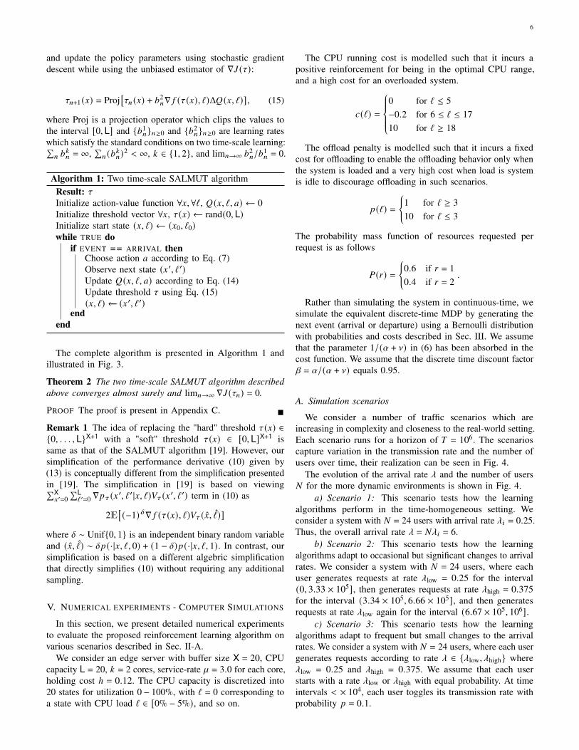
C. ResultsFor each of the algorithm described above, we train

SALMUT, Q-learning, PPO, and A2C for 106 steps. Theperformance of each algorithm is evaluated every 103 stepsusing independent rollouts of length 𝐻 = 1000 for 100 differentrandom seeds. The experiment is repeated for the 10 samplepaths and the median performance with an uncertainty bandfrom the first to the third quartile are plotted in Fig. 5.

For Scenario 1, all RL algorithms (SALMUT, Q-learning,PPO, A2C) converge to a close-to-optimal policy and remainstable after convergence. Since all policies converge quickly,SALMUT, PPO, and A2C are also able to adapt quicklyin Scenarios 2–6 and keep track of the time-varying arrivalrates and number of users. There are small differences in theperformance of the RL algorithms, but these are minor. Notethat, in contrast, Q-learning policy does not perform well whenthe dynamics of the requests changes drastically, whereas thebaseline policy performs poorly when the server is overloaded.

The plots for Scenario 1 (Fig. 5a) show that PPO convergesto the optimal policy in less than 105 steps, SALMUT and A2Ctakes around 2 × 105 steps, whereas Q-learning takes around5 × 105 steps to converge. The policies for all the algorithmsremain stable after convergence. Upon further analysis on thestructure of the optimal policy, we observe that the structureof the optimal policy of SALMUT (Fig. 6b) differs from thatof the optimal policy computed using DP (Fig. 6a). There is aslight difference in the structure of these policies when buffersize (x) is low and CPU load (ℓ) is high, which occurs becausethese states are reachable with a very low probability and henceSALMUT doesn’t encounter these states in the simulation oftento be able to learn the optimal policy in these states. The plotsfrom Scenario 2 (Fig. 5b) show similar behavior when _ isconstant. When _ changes significantly, we observe all RLalgorithms except Q-learning are able to adapt to the drasticbut stable changes in the environment. Once the load stabilizes,all the algorithms are able to readjust to the changes andperform close to the optimal policy. The plots from Scenario3 (Fig. 5c) show similar behavior to Scenario 1, i.e. small butfrequent changes in the environment do not impact the learningperformance of reinforcement learning algorithms.

The plots from Scenario 4-6 (Fig. 5d-5f) show consistentperformance with varying users. The RL algorithms includingQ-learning show similar performance for most of the time-stepsexcept in Scenario 5, which is similar to the behavior observedin Scenario 2. The Q-learning algorithm also performs poorlywhen the load suddenly changes in Scenarios 4 and 6. Thiscould be due to the fact that Q-learning takes longer to adjustto a more aggressive offloading policy.

8

(a) Scenario 1 (b) Scenario 2 (c) Scenario 3

(d) Scenario 4 (e) Scenario 5 (f) Scenario 6

Fig. 5. Performance of RL algorithms for different scenarios.

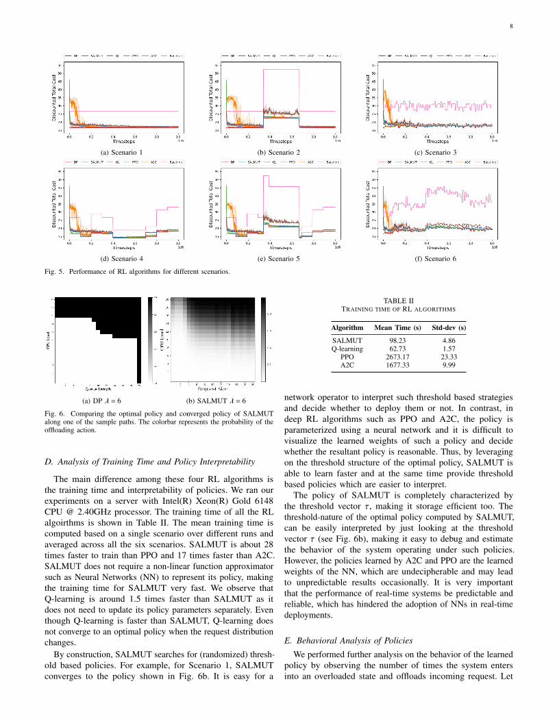
(a) DP _ = 6 (b) SALMUT _ = 6

Fig. 6. Comparing the optimal policy and converged policy of SALMUTalong one of the sample paths. The colorbar represents the probability of theoffloading action.

D. Analysis of Training Time and Policy Interpretability

The main difference among these four RL algorithms isthe training time and interpretability of policies. We ran ourexperiments on a server with Intel(R) Xeon(R) Gold 6148CPU @ 2.40GHz processor. The training time of all the RLalgoirthms is shown in Table II. The mean training time iscomputed based on a single scenario over different runs andaveraged across all the six scenarios. SALMUT is about 28times faster to train than PPO and 17 times faster than A2C.SALMUT does not require a non-linear function approximatorsuch as Neural Networks (NN) to represent its policy, makingthe training time for SALMUT very fast. We observe thatQ-learning is around 1.5 times faster than SALMUT as itdoes not need to update its policy parameters separately. Eventhough Q-learning is faster than SALMUT, Q-learning doesnot converge to an optimal policy when the request distributionchanges.

By construction, SALMUT searches for (randomized) thresh-old based policies. For example, for Scenario 1, SALMUTconverges to the policy shown in Fig. 6b. It is easy for a

TABLE IITRAINING TIME OF RL ALGORITHMS

Algorithm Mean Time (s) Std-dev (s)

SALMUT 98.23 4.86Q-learning 62.73 1.57

PPO 2673.17 23.33A2C 1677.33 9.99

network operator to interpret such threshold based strategiesand decide whether to deploy them or not. In contrast, indeep RL algorithms such as PPO and A2C, the policy isparameterized using a neural network and it is difficult tovisualize the learned weights of such a policy and decidewhether the resultant policy is reasonable. Thus, by leveragingon the threshold structure of the optimal policy, SALMUT isable to learn faster and at the same time provide thresholdbased policies which are easier to interpret.

The policy of SALMUT is completely characterized bythe threshold vector 𝜏, making it storage efficient too. Thethreshold-nature of the optimal policy computed by SALMUT,can be easily interpreted by just looking at the thresholdvector 𝜏 (see Fig. 6b), making it easy to debug and estimatethe behavior of the system operating under such policies.However, the policies learned by A2C and PPO are the learnedweights of the NN, which are undecipherable and may leadto unpredictable results occasionally. It is very importantthat the performance of real-time systems be predictable andreliable, which has hindered the adoption of NNs in real-timedeployments.

E. Behavioral Analysis of Policies

We performed further analysis on the behavior of the learnedpolicy by observing the number of times the system entersinto an overloaded state and offloads incoming request. Let

9

(a) Scenario 1 (b) Scenario 2 (c) Scenario 3

(d) Scenario 4 (e) Scenario 5 (f) Scenario 6

Fig. 7. Comparing the number of times the system goes into the overloaded state at each evaluation step. The trajectory of event arrival and departure is fixedfor all evaluation steps and across all algorithms for the same arrival distribution.

(a) Scenario 1 (b) Scenario 2 (c) Scenario 3

(d) Scenario 4 (e) Scenario 5 (f) Scenario 6

Fig. 8. Comparing the number of times the system performs offloading at each evaluation step. The trajectory of event arrival and departure is fixed for allevaluation steps and across all algorithms for the same arrival distribution.

us define 𝐶ov to be the number of times the system entersinto an overloaded state and 𝐶off to be the number of timesthe system offloads requests for every 1000 steps of trainingiteration. We generated a set of 106 random numbers between0 and 1, defined by 𝑧𝑡 , where 𝑡 is the step count. We use thisset of random numbers to fix the trajectory of events (arrivalor departure) for all the experiments in this section. Similarto the experiment in the previous section, the number of users𝑁 and the arrival rate _ are fixed for 1000 steps and evolveaccording to the scenarios described in Fig. 4. The event is setto arrival if 𝑧𝑡 is less than or equal to _𝑡/(_𝑡 +min{𝑥𝑡 , 𝑘}`),and set to departure otherwise. These experiments were carriedout during the training time for 10 different seeds. We plotthe median of the number of times a system goes into an

overloaded state (Fig. 7) and the number of requests offloadedby the system (Fig. 8) along with the uncertainty band fromthe first to the third quartile for every 1000 steps.

We observe in Fig. 7, that all the algorithms (SALMUT,Q-learning, PPO, A2C) learn not to enter into the overloadedstate. As seen in the case of total discounted cost (Fig. 5),PPO learns it instantly, followed by SALMUT, Q-learning, andA2C. The observation is valid for all the different scenarioswe tested. We observe that for Scenario-4, PPO enters theoverloaded state at around 0.8 × 106 which is due to the factthe

∑𝑖 _𝑖 increases drastically at that point (seen in Fig. 4d)

and we also see its effect on the cost in Fig. 5d at that time.We also observe that SALMUT enters into overloaded stateswhen the request distribution changes drastically in Scenario

10

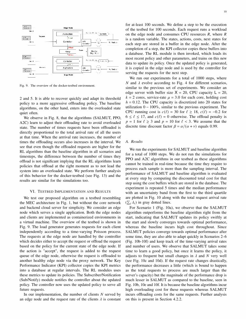
Fig. 9. The overview of the docker-testbed environment.

2 and 5. It is able to recover quickly and adapt its thresholdpolicy to a more aggressive offloading policy. The baselinealgorithms, on the other hand, enters into the overloaded statequiet often.

We observe in Fig. 8, that the algorithms (SALMUT, PPO,A2C) learn to adjust their offloading rate to avoid overloadedstate. The number of times requests have been offloaded isdirectly proportional to the total arrival rate of all the usersat that time. When the arrrival rate increases, the number oftimes the offloading occurs also increases in the interval. Wesee that even though the offloaded requests are higher for theRL algorithms than the baseline algorithm in all scenarios andtimesteps, the difference between the number of times theyoffload is not significant implying that the RL algorithms learnpolicies that offload at the right moment as to not lead thesystem into an overloaded state. We perform further analysisof this behavior for the docker-testbed (see Fig. 13) and theresults are similar for the simulations too.

VI. TESTBED IMPLEMENTATION AND RESULTS

We test our proposed algorithm on a testbed resemblingthe MEC architecture in Fig. 1, but without the core networkand backend cloud server for simplicity. We consider an edgenode which serves a single application. Both the edge nodesand clients are implemented as containerized environments ina virtual machine. The overview of the testbed is shown inFig. 9. The load generator generates requests for each clientindependently according to a time-varying Poisson process.The requests at the edge node are handled by the controllerwhich decides either to accept the request or offload the requestbased on the policy for the current state of the edge node. Ifthe action is "accept", the request is added to the requestqueue of the edge node, otherwise the request is offloaded toanother healthy edge node via the proxy network. The KeyPerformance Indicator (KPI) collector copies the KPI metricsinto a database at regular intervals. The RL modules usesthese metrics to update its policies. The Subscriber/Notification(Sub/Notify) module notifies the controller about the updatedpolicy. The controller now uses the updated policy to serve allfuture requests.

In our implementation, the number of clients 𝑁 served byan edge node and the request rate of the clients _ is constant

for at-least 100 seconds. We define a step to be the executionof the testbed for 100 seconds. Each request runs a workloadon the edge node and consumes CPU resources 𝑅, where 𝑅

is a random variable. The states, actions, costs, next states foreach step are stored in a buffer in the edge node. After thecompletion of a step, the KPI collector copies these buffers intoa database. The RL module is then invoked, which loads itsmost recent policy and other parameters, and trains on this newdata to update its policy. Once the updated policy is generated,it is copied in the edge node and is used by the controller forserving the requests for the next step.

We run our experiments for a total of 1000 steps, where𝑁 and _ evolve according to Fig. 4 for different scenarios,similar to the previous set of experiments. We consider anedge server with buffer size X = 20, CPU capacity L = 20,𝑘 = 2 cores, service-rate ` = 3.0 for each core, holding costℎ = 0.12. The CPU capacity is discretized into 20 states forutilization 0 − 100%, similar to the previous experiment. TheCPU running cost is 𝑐(ℓ) = 30 for ℓ ≥ 18, 𝑐(ℓ) = −0.2 for6 ≤ ℓ ≤ 17, and 𝑐(ℓ) = 0 otherwise. The offload penalty is𝑝 = 1 for ℓ ≥ 3 and 𝑝 = 10 for ℓ < 3. We assume that thediscrete time discount factor 𝛽 = 𝛼/(𝛼 + a) equals 0.99.

A. Results

We run the experiments for SALMUT and baseline algorithmfor a total of 1000 steps. We do not run the simulations forPPO and A2C algorithms in our testbed as these algorithmscannot be trained in real-time because the time they require toprocess each sample is more than the sampling interval. Theperformance of SALMUT and baseline algorithm is evaluatedat every step by computing the discounted total cost for thatstep using the cost buffers which are stored in the database. Theexperiment is repeated 5 times and the median performancewith an uncertainty band from the first to the third quartileare plotted in Fig. 10 along with the total request arrival rate(∑

𝑖 _𝑖) in gray dotted lines.For Scenario 1 (Fig. 10a), we observe that the SALMUT

algorithm outperforms the baseline algorithm right from thestart, indicating that SALMUT updates its policy swiftly atthe start and slowly converges towards optimal performance,whereas the baseline incurs high cost throughout. SinceSALMUT policies converge towards optimal performance aftersome time, they are also able to adapt quickly in Scenarios 2–6(Fig. 10b-10f) and keep track of the time-varying arrival ratesand number of users. We observe that SALMUT takes sometime to learn a good policy, but once it learns the policy, itadjusts to frequent but small changes in _ and 𝑁 very well(see Fig. 10c and 10d). If the request rate changes drastically,the performance decreases a little (which is bound to happenas the total requests to process are much larger than theserver’s capacity) but the magnitude of the performance drop ismuch lesser in SALMUT as compared to the baseline, seen inFig. 10b, 10e and 10f. It is because the baseline algorithms incurhigh overloading cost for these requests whereas SALMUTincurs offloading costs for the same requests. Further analysison this is present in Section 4.2.2.

11

(a) Scenario 1 (b) Scenario 2 (c) Scenario 3

(d) Scenario 4 (e) Scenario 5 (f) Scenario 6

Fig. 10. Performance of RL algorithms for different scenarios in the end-to-end testbed we created. We also plot the total request arrival rate (∑

𝑖 _𝑖) on theright-hand side of y-axis in gray dotted lines.

(a) Scenario 1 (b) Scenario 2 (c) Scenario 3

(d) Scenario 4 (e) Scenario 5 (f) Scenario 6

Fig. 11. Comparing the number of times the system goes into the overloaded state at each step in the end-to-end testbed we created. We also plot the totalrequest arrival rate (

∑𝑖 _𝑖) on the right-hand side of y-axis in gray dotted lines.

B. Behavioral Analysis

We perform behavior analysis of the learned policy byobserving the number of times the system enters into anoverloaded state (denoted by 𝐶ov) and the number of incomingrequest offloaded by the edge node (denoted by 𝐶off) in awindow of size 100. These plots are shown in Fig. 11 & 12.

We observe from Fig. 11 that the number of times theedge node goes into an overload state while following policyexecuted by SALMUT is much less than the baseline algorithm.Even when the system goes into an overloaded state, it isable to recover quickly and does not suffer from performancedeterioration. From Fig. 12b and 12e we can observe that in

Scenarios 2 and 5, when the request load increases drastically(at around 340 steps), 𝐶off increases and its effects can also beseen in the overall discounted cost in Fig. 10b and 10e at aroundthe same time. SALMUT is able to adapt its policy quickly andrecover quickly. We observe in Fig. 12 that SALMUT performsmore offloading as compared to the baseline algorithm.

A policy that offloads often and does not go into anoverloaded state may not necessarily minimize the total cost.We did some further investigation by visualizing the scatter-plot (Fig. 13) of the overload count (𝐶ov) on the y-axis andthe offload count (𝐶off) on the x-axis for both SALMUT andthe baseline algorithm for all the scenarios described in Fig. 4.

12

(a) Scenario 1 (b) Scenario 2 (c) Scenario 3

(d) Scenario 4 (e) Scenario 5 (f) Scenario 6

Fig. 12. Comparing the number of times the system performs offloading at each step in the end-to-end testbed we created. We also plot the total requestarrival rate (

∑𝑖 _𝑖) on the right-hand side of y-axis in gray dotted lines.

(a) Scenario 1 (b) Scenario 2 (c) Scenario 3

(d) Scenario 4 (e) Scenario 5 (f) Scenario 6

Fig. 13. Scatter-plot of 𝐶ov Vs 𝐶off for SALMUT and baseline algorithm in the end-to-end testbed we created. The width of the points is proportional to itsfrequency.

We observe that SALMUT keeps 𝐶ov much lower than thebaseline algorithm at the cost of increased 𝐶off . We observefrom Fig. 13 that the slope for the plot is linear for baselinealgorithms because they are offloading reactively. SALMUT,on the other hand, learns a behavior that is analogous to pro-active offloading, where it benefits from the offloading actionit takes by minimizing 𝐶ov.

VII. CONCLUSION AND LIMITATIONS

In this paper we considered a single node optimal policyfor overload protection on the edge server in a time varyingenvironment. We proposed a RL-based adaptive low-complexityadmission control policy that exploits the structure of the

optimal policy and finds a policy that is easy to interpret. Ourproposed algorithm performs as well as the standard deepRL algorithms but has a better computational and storagecomplexity, thereby significantly reducing the total trainingtime. Therefore, our proposed algorithm is more suitable fordeployment in real systems for online training.

The results presented in this paper can be extended in severaldirections. In addition to CPU overload, one could considerother resource bottlenecks such as disk I/O, RAM utilization,etc. It may be desirable to simultaneously consider multipleresource constraints. Along similar lines, one could considermultiple applications with different resource requirements anddifferent priority. If it can be established that the optimal policy

13

in these more sophisticated setup has a threshold structuresimilar to Proposition 2, then we can apply the frameworkdeveloped in this paper.

The discussion in this paper was restricted to a single node.These results could also provide a foundation to investigatenode overload protection in multi-node clusters where addi-tional challenges such as routing, link failures, and networktopology shall be considered.

APPENDIX APROOF OF PROPOSITION 1

Let 𝛿(𝑥) = _/(_ + min(𝑘, 𝑥)`). We define a sequence ofvalue functions {𝑉𝑛}𝑛≥0 as follows

𝑉0 (𝑥, ℓ) = 0and for 𝑛 ≥ 0

𝑉𝑛+1 (𝑥, ℓ) = min{𝑄𝑛+1 (𝑥, ℓ, 0), 𝑄𝑛+1 (𝑥, ℓ, 1)},where

𝑄𝑛+1 (𝑥,ℓ, 0) =1

𝛼 + a[ℎ[𝑥 − 𝑘]+ + 𝑐(ℓ)

]+ 𝛽

[𝛿(𝑥)

R∑︁𝑟=1

𝑃(𝑟)𝑉𝑛 ( [𝑥 + 1]X, [ℓ + 𝑟]L)

+ (1 − 𝛿(𝑥))R∑︁𝑟=1

𝑃(𝑟)𝑉𝑛 ( [𝑥 − 1]+, [ℓ − 𝑟]+)]

and

𝑄𝑛+1 (𝑥,ℓ, 1) =1

𝛼 + a[ℎ[𝑥 − 𝑘]+ + 𝑐(ℓ) + 𝑝(ℓ)

]+ 𝛽(1 − 𝛿(𝑥))

R∑︁𝑟=1

𝑃(𝑟)𝑉𝑛 ( [𝑥 − 1]+, [ℓ − 𝑟]+),

where [𝑥]B denotes min{𝑥,B}.Note that {𝑉𝑛}𝑛≥0 denotes the iterates of the value iteration

algorithm, and from [18], we know that

lim𝑛→∞

𝑉𝑛 (𝑥, ℓ) = 𝑉 (𝑥, ℓ), ∀𝑥, ℓ (16)

where 𝑉 is the unique fixed point of (6).We will show that (see Lemma 1 below) each 𝑉𝑛 (𝑥, ℓ)

satisfies the property of Proposition 1. Therefore, by (16) weget that 𝑉 also satisfies the property.

Lemma 1 For each 𝑛 ≥ 0 and 𝑥 ∈ {0, ..., 𝑋}, 𝑉𝑛 (𝑥, ℓ) isweakly increasing in ℓ.

PROOF We prove the result by induction. Note that 𝑉0 (𝑥, ℓ) = 0and is trivially weakly increasing in ℓ. This forms the basis ofthe induction. Now assume that 𝑉𝑛 (𝑥, ℓ) is weakly increasingin ℓ. Consider iteration 𝑛 + 1. Let 𝑥 ∈ {0, ..., 𝑋} and ℓ1, ℓ2 ∈{0, ..., 𝐿} such that ℓ1 < ℓ2. Then,

𝑄𝑛+1 (𝑥,ℓ1, 0) =1

𝛼 + a[ℎ[𝑥 − 𝑘]+ + 𝑐(ℓ1)

]+ 𝛽

[𝛿(𝑥)

R∑︁𝑟=1

𝑃(𝑟)𝑉𝑛 ( [𝑥 + 1]X, [ℓ1 + 𝑟]L)

+ (1 − 𝛿(𝑥))R∑︁𝑟=1

𝑃(𝑟)𝑉𝑛 ( [𝑥 − 1]+, [ℓ1 − 𝑟]+)]

(𝑎)≤ 1

𝛼 + a[ℎ[𝑥 − 𝑘]+ + 𝑐(ℓ2)

]+ 𝛽

[𝛿(𝑥)

R∑︁𝑟=1

𝑃(𝑟)𝑉𝑛 ( [𝑥 + 1]X, [ℓ2 + 𝑟]L)

+ (1 − 𝛿(𝑥))R∑︁𝑟=1

𝑃(𝑟)𝑉𝑛 ( [𝑥 − 1]+, [ℓ2 − 𝑟]+)]

= 𝑄𝑛+1 (𝑥, ℓ2, 0), (17)

where (𝑎) follows from the fact that 𝑐(ℓ) and 𝑉𝑛 (𝑥, ℓ) areweakly increasing in ℓ.

By a similar argument, we can show that

𝑄𝑛+1 (𝑥, ℓ1, 1) ≤ 𝑄𝑛+1 (𝑥, ℓ2, 1). (18)

Now,

𝑉𝑛+1 (𝑥, ℓ1) = min{𝑄𝑛+1 (𝑥, ℓ1, 0), 𝑄𝑛+1 (𝑥, ℓ1, 1)}(𝑏)≤ min{𝑄𝑛+1 (𝑥, ℓ2, 0), 𝑄𝑛+1 (𝑥, ℓ2, 1)}= 𝑉𝑛+1 (𝑥, ℓ2), (19)

�

where (𝑏) follows from (17) and (18). Eq. (19) shows that𝑉𝑛+1 (𝑥, ℓ) is weakly increasing in ℓ. This proves the inductionstep. Hence, the result holds for the induction.

APPENDIX BPROOF OF PROPOSITION 2

PROOF Let 𝛿(𝑥) = _/(_ +min{𝑥, 𝑘}`). Consider

Δ𝑄(𝑥, ℓ) = B 𝑄(𝑥, ℓ, 1) −𝑄(𝑥, ℓ, 0)

= −𝛽𝛿(𝑥)R∑︁𝑟=1

𝑃(𝑟)𝑉 ( [𝑥]X, [ℓ + 𝑟]L) − 𝑝.

For a fixed 𝑥, by Proposition 1, Δ𝑄(𝑥, ℓ) is weakly decreasingin ℓ. If it is optimal to reject a request at state (𝑥, ℓ) (i.e.,Δ𝑄(𝑥, ℓ) ≤ 0), then for any ℓ′ > ℓ,

Δ𝑄(𝑥, ℓ′) ≤ Δ𝑄(𝑥, ℓ) ≤ 0; �

therefore, it is optimal to reject the request.

APPENDIX CPROOF OF OPTIMALITY OF SALMUT

PROOF The choice of learning rates implies that there is aseparation of timescales between the updates of (14) and (15).In particular, since 𝑏2

𝑛/𝑏1𝑛 → 0, iteration (14) evolves at a

faster timescale than iteration (15). Therefore, we first considerupdate (15) under the assumption that the policy 𝜋𝜏 , whichupdates at the slower timescale, is constant.We first provide a preliminary result.

Lemma 2 Let 𝑄𝜏 denote the action-value function correspond-ing to the policy 𝜋𝜏 . Then, 𝑄𝜏 is Lipscitz continuous in 𝜏.

PROOF This follows immediately from the Lipscitz continuityof 𝜋𝜏 in 𝜏. �

14

Define the operator M𝜏 : RN → RN, where N = (X+ 1) × (L+1) ×A, as follows:

[M𝜏𝑄] (𝑥, ℓ, 𝑎) =[�̄�(𝑥, ℓ, 𝑎) + 𝛽

∑︁𝑥′,ℓ′

𝑝(𝑥 ′, ℓ′ |𝑥, ℓ, 𝑎)

min𝑎′∈A

𝑄(𝑥 ′, ℓ′, 𝑎′)] −𝑄(𝑥, ℓ, 𝑎). (20)

Then, the step-size conditions on {𝑏1𝑛}𝑛≥1 imply that for a

fixed 𝜋𝜏 , iteration (14) may be viewed as a noisy discretizationof the ODE (ordinary differential equation):

¤𝑄(𝑡) = M𝜏 [𝑄(𝑡)] . (21)

Then we have the following:

Lemma 3 The ODE (21) has a unique globally asymptoticallystable equilibrium point 𝑄𝜏 .

PROOF Note that the ODE (21) may be written as

¤𝑄(𝑡) = B𝜏 [𝑄(𝑡)] −𝑄(𝑡)where the Bellman operator B𝜏 : RN → RN is given by

B𝜏 [𝑄] (𝑥, ℓ) =[�̄�(𝑥, ℓ, 𝑎) + 𝛽

∑︁𝑥′,ℓ′

𝑝(𝑥 ′, ℓ′ |𝑥, ℓ, 𝑎)

× min𝑎′∈A

𝑄(𝑥 ′, ℓ′, 𝑎′)] . (22)

Note that B𝜏 is a contraction under the sup-norm. Therefore,by Banach fixed point theorem, 𝑄 = B𝜏𝑄 has a unique fixedpoint, which is equal to 𝑄𝜏 . The result then follows from [26,Theorem 3.1]. �

We now consider the faster timescale. Recall that (𝑥0, ℓ0) isthe initial state of the MDP. Recall

𝐽 (𝜏) = 𝑉𝜏 (𝑥0, ℓ0)and consider the ODE limit of the slower timescale iteration(15), which is given by

¤𝜏 = −∇𝐽 (𝜏). (23)

Lemma 4 The equilibrium points of the ODE (23) are thesame as the local optima of 𝐽 (𝜏). Moreover, these equilibriumpoints are locally asymptotically stable.

PROOF The equivalence between the stationary points of theODE and local optima of 𝐽 (𝜏) follows from definition. Nowconsider 𝐽 (𝜏(𝑡)) as a Lyapunov function. Observe that

𝑑

𝑑𝑡𝐽 (𝜏(𝑡)) = −

[∇𝐽 (𝜏(𝑡))]2 < 0,

as long as ∇𝐽 (𝜏(𝑡)) ≠ 0. Thus, from Lyapunov stability criteriaall local optima of (23) are locally asymptotically stable. �

Now, we have all the ingredients to prove convergence. Lemmas2-4 imply assumptions (A1) and (A2) of [27]. Thus, theiteration (14) and (15) converges almost surely to a limit point(𝑄◦, 𝜏◦) such that 𝑄◦ = 𝑄𝜏◦ and ∇𝐽 (𝜏◦) = 0 provided that theiterates {𝑄𝑛}𝑛≥1 and {𝜏𝑛}𝑛≥1 are bounded.Note that {𝜏𝑛}𝑛≥1 are bounded by construction. The boundnessof {𝑄𝑛}𝑛≥1 follows from considering the scaled version of(21):

¤𝑄 = M𝜏,∞𝑄 (24)

where,

M𝜏,∞𝑄 = lim𝑐→∞

M𝜏 [𝑐𝑄]𝑐

.

It is easy to see that

[M𝜏,∞𝑄] (𝑥, ℓ, 𝑎) = 𝛽∑︁𝑥′,ℓ′

𝑝(𝑥 ′, ℓ′ |𝑥, ℓ, 𝑎) min𝑎′∈A

𝑄(𝑥 ′, ℓ′, 𝑎′)

−𝑄(𝑥, ℓ, 𝑎) (25)

Furthermore, origin is the asymptotically stable equilibriumpoint of (24). Thus, from [28], we get that the iterates {𝑄𝑛}𝑛≥1of (14) are bounded. �

ACKNOWLEDGMENT

The numerical experiments were enabled in part by supportprovided by Compute Canada. The authors are grateful toPierre Thibault from Ericsson Systems for setting up thevirtual machines to run the docker-testbed experiments. Theauthors also acknowledge all the help and support from EricssonSystems, especially the Global Aritifical Intelligent Accelerator(GAIA) Montreal Team.

REFERENCES

[1] M. Satyanarayanan, “The emergence of edge computing,” Computer,vol. 50, no. 1, pp. 30–39, 2017.

[2] Y. Mao, C. You, J. Zhang, K. Huang, and K. B. Letaief, “A survey onmobile edge computing: The communication perspective,” IEEE Commun.Surveys & Tutorials, vol. 19, no. 4, pp. 2322–2358, 2017.

[3] J. Liu, Y. Mao, J. Zhang, and K. B. Letaief, “Delay-optimal computationtask scheduling for mobile-edge computing systems,” in Int. Symp. Inform.Theory (ISIT), 2016, pp. 1451–1455.

[4] F. Wang, J. Xu, X. Wang, and S. Cui, “Joint offloading and computingoptimization in wireless powered mobile-edge computing systems,” IEEETrans. Wireless Commun., vol. 17, no. 3, pp. 1784–1797, 2017.

[5] D. Van Le and C.-K. Tham, “Quality of service aware computationoffloading in an ad-hoc mobile cloud,” IEEE Trans. Veh. Technol., vol. 67,no. 9, pp. 8890–8904, 2018.

[6] M. Chen and Y. Hao, “Task offloading for mobile edge computing insoftware defined ultra-dense network,” IEEE J. Sel. Areas Commun.,vol. 36, no. 3, pp. 587–597, 2018.

[7] S. Wang, R. Urgaonkar, M. Zafer, T. He, K. Chan, and K. K. Leung,“Dynamic service migration in mobile edge computing based on Markovdecision process,” IEEE/ACM Trans. Netw., vol. 27, no. 3, pp. 1272–1288,Jun. 2019.

[8] R. S. Sutton and A. G. Barto, Reinforcement learning: An introduction.The MIT Press, 2018.

[9] X. Chen, H. Zhang, C. Wu, S. Mao, Y. Ji, and M. Bennis, “Optimizedcomputation offloading performance in virtual edge computing systemsvia deep reinforcement learning,” IEEE Internet Things J, vol. 6, no. 3,pp. 4005–4018, 2018.

[10] L. Huang, S. Bi, and Y.-J. A. Zhang, “Deep reinforcement learningfor online computation offloading in wireless powered mobile-edgecomputing networks,” IEEE Transactions on Mobile Computing, vol. 19,no. 11, pp. 2581–2593, 2019.

[11] J. Wang, J. Hu, G. Min, W. Zhan, Q. Ni, and N. Georgalas, “Computationoffloading in multi-access edge computing using a deep sequential modelbased on reinforcement learning,” IEEE Commun. Mag., vol. 57, no. 5,pp. 64–69, 2019.

[12] J. Li, H. Gao, T. Lv, and Y. Lu, “Deep reinforcement learning basedcomputation offloading and resource allocation for mec,” in 2018 IEEEWireless Communications and Networking Conference (WCNC). IEEE,2018, pp. 1–6.

[13] X. Chen, H. Zhang, C. Wu, S. Mao, Y. Ji, and M. Bennis, “Optimizedcomputation offloading performance in virtual edge computing systemsvia deep reinforcement learning,” IEEE Internet of Things Journal, vol. 6,no. 3, pp. 4005–4018, 2018.

[14] D. Van Le and C.-K. Tham, “Quality of service aware computationoffloading in an ad-hoc mobile cloud,” IEEE Transactions on VehicularTechnology, vol. 67, no. 9, pp. 8890–8904, 2018.

15

[15] Z. Tang, X. Zhou, F. Zhang, W. Jia, and W. Zhao, “Migration mod-eling and learning algorithms for containers in fog computing,” IEEETransactions on Services Computing, vol. 12, no. 5, pp. 712–725, 2018.

[16] A. Jensen, “Markoff chains as an aid in the study of Markoff processes,”Scandinavian Actuarial Journal, vol. 1953, no. sup1, pp. 87–91, 1953.

[17] R. A. Howard, Dynamic Programming and Markov Processes. TheMIT Press, 1960.

[18] M. Puterman, Markov decision processes: Discrete Stochastic DynamicProgramming. John Wiley and Sons, 1994.

[19] A. Roy, V. Borkar, A. Karandikar, and P. Chaporkar, “Online rein-forcement learning of optimal threshold policies for Markov decisionprocesses,” arXiv:1912.10325, 2019.

[20] J. Schulman, F. Wolski, P. Dhariwal, A. Radford, and O. Klimov,“Proximal policy optimization algorithms,” arXiv:1707.06347, 2017.

[21] Y. Wu, E. Mansimov, S. Liao, R. Grosse, and J. Ba, “Scalable trust-region method for deep reinforcement learning using kronecker-factoredapproximation,” arxiv:1708.05144, 2017.

[22] A. Jitani, A. Mahajan, Z. Zhu, H. Abou-zeid, E. T. Fapi, and H. Purmehdi,“Structure-aware reinforcement learning for node overload protectionin mobile edge computing,” in IEEE International Conference onCommunications (ICC), 2021.

[23] X. Cao, Stochastic Learning and Optimization - A Sensitivity-BasedApproach. Springer, 2007. [Online]. Available: https://doi.org/10.1007/978-0-387-69082-7

[24] D. P. Kingma and J. Ba, “Adam: A method for stochastic optimization,”arXiv preprint arXiv:1412.6980, 2014.

[25] A. Raffin, A. Hill, M. Ernestus, A. Gleave, A. Kanervisto, and N. Dor-mann, “Stable baselines3,” https://github.com/DLR-RM/stable-baselines3,2019.

[26] V. S. Borkar and K. Soumyanatha, “An analog scheme for fixed pointcomputation – Part I: Theory,” IEEE Transactions on Circuits and SystemsI: Fundamental Theory and Applications, vol. 44, no. 4, pp. 351–355,1997.

[27] V. S. Borkar, “Stochastic approximation with two time scales,” Systems& Control Letters, vol. 29, no. 5, pp. 291–294, 1997.

[28] V. S. Borkar and S. P. Meyn, “The ODE method for convergence ofstochastic approximation and reinforcement learning,” SIAM Journal onControl and Optimization, vol. 38, no. 2, pp. 447–469, 2000.

Anirudha Jitani received the B.Tech degree inComputer Science and Engineering from VelloreInstitute of Technology, India in 2015. He is pursuinghis M.Sc. in Computer Science at McGill University,Montreal since 2018. He is a research assistant atMontreal Institute of Learning Algorithms (MILA)and a Data Scientist Intern at Ericsson Systems.He also worked as a software developer for CiscoSystems and Netapp. His research interests includeapplication of machine learning techniques such asdeep reinforcement learning, multi-agent reinforce-

ment learning, and graph neural networks in communication and networks.

Aditya Mahajan (S’06-M’09-SM’14) receivedB.Tech degree from the Indian Institute of Tech-nology, Kanpur, India, in 2003, and M.S. and Ph.D.degrees from the University of Michigan, Ann Arbor,USA, in 2006 and 2008. From 2008 to 2010, he wasa Postdoctoral Researcher at Yale University, NewHaven, CT, USA. He has been with the departmentof Electrical and Computer Engineering, McGillUniversity, Montreal, Canada, since 2010 where he iscurrently Associate Professor. He serves as AssociateEditor of Springer Mathematics of Control, Signal,

and Systems. He was an Associate Editor of the IEEE Control Systems SocietyConference Editorial Board from 2014 to 2017. He is the recipient of the 2015George Axelby Outstanding Paper Award, 2014 CDC Best Student Paper Award(as supervisor), and the 2016 NecSys Best Student Paper Award (as supervisor).His principal research interests include decentralized stochastic control, teamtheory, multi-armed bandits, real-time communication, information theory, andreinforcement learning.

Zhongwen Zhu received the B.Eng in MechanicalEngineering and M.Eng. in Turbomachinery fromShanghai Jiao Tong University, Shanghai, P.R. China,and also a Ph.D. in Applied Science from FreeUniversity of Brussels, Belgium, in 1996. He joinedin Aerospace Lab in National Research Council ofCanada (NRC) in 1997. One year later, he started towork in Bombardier Aerospace. Since 2001, he hasbeen working for Ericsson Canada with differentroles, e.g. Data Scientist, SW Designer, Systemmanager, System designer, System/Solution Architect,

Product owner, Product manager, etc. He was an associated editor for Journal ofSecurity and Communication Network (Wiley publisher). He was the invitedTechnical committee member for International Conference on MultimediaInformation Networking and Security. He was the recipient of the bestpaper award in 2008 IEEE international conference on Signal Processingand Multimedia applications. His current research interests are 5G network,network security, edge computing, Reinforcement learning, Machine learningfor 2D/3D object detections, IoT (Ultra Reliable Low Latency application),etc.

Hatem Abou-Zeid is a 5G Systems Developerat Ericsson Canada. He has 10+ years of R&Dexperience in communication networks spanningradio access networks, routing, and traffic engineer-ing. He currently leads 5G system designs andintellectual property development in the areas ofnetwork intelligence and low latency communications.He serves on the Ericsson Government IndustryRelations and University Engagements Committeewhere he directs academic research partnershipson autonomous networking and augmented reality

communications. His research investigates the use of reinforcement learning,stochastic optimization, and deep learning to architect robust 5G/6G networksand applications - and his work has resulted in 60+ filed patents andpublications in IEEE flagship journals and conferences. Prior to joiningEricsson, he was at Cisco Systems designing scalable traffic engineeringand IP routing protocols for service provider and data-center networks. Heholds a Ph.D. in Electrical and Computer Engineering from Queen’s University.His collaborations with industry through a Bell Labs DAAD RISE Fellowshipled to the commercialization of aspects of predictive video streaming, and hisThesis was nominated for an Outstanding Thesis Medal.

Emmanuel Thepie Fapi is currently a Data Scientistwith Ericsson Montreal, Canada. He holds a master’sdegree in engineering mathematics and computertools from Orleans University in France and aPhD in signal processing and telecommunicationsfrom IMT Atlantique in France (former Ecole desTelecommunications de Bretagne) in 2009. From2010 to 2016 he worked with GENBAND US LLC,QNX software System Limited as audio softwaredeveloper, MDA system as analyst and EasyG assenior DSP engineer in Vancouver, Canada. In 2017

he joined Amazon Lab 126 in Boston, USA as audio software developerfor echo dot 3rd generation. His main areas of interest are 5G network,anomaly detection-based AI/ML, multi-resolution analysis for advancedsignal processing, real-time embedded OS and IoT, voice and audio qualityenhancement.

16

Hakimeh Purmehdi is a data scientist at EricssonGlobal Artificial Intelligence Accelerator, which leadsinnovative AI/ML solutions for future wireless com-munication networks. She received her Ph.D. degreein electrical engineering from the Department ofElectrical and Computer Engineering, University ofAlberta, Edmonton, AB, Canada. After completing apostdoc in AI and image processing at the RadiologyDepartment, University of Alberta, she co-foundedCorowave, a startup to develop bio sensors to monitorhuman vital signals by leveraging radio frequency

technology and machine learning. Before joining Ericsson, she was withMicrosoft Research (MSR) as a research engineer, and contributed in thedevelopment of TextWorld, which is a testbed for reinforcement learningresearch projects. Her research focus is basically on the intersection ofwireless communication (5G and beyond including resource managementand edge computing), AI solutions (such as online learning, federated learning,reinforcement learning, deep learning), optimization, and biotech.