Structural Techniques and Performance Bounds ofStochastic Petri Net ModelsJavier Campos and Manuel SilvaDpto. de Ingenier��a El�ectrica e Inform�aticaCentro Polit�ecnico SuperiorUniversidad de ZaragozaMar��a de Luna 350015 Zaragoza, SPAINAbstractIn this paper we overview some recent results obtained by the authors andcollaborators on the performance bounds analysis of some stochastic Petri netsystems. The mathematical model can be seen either as a result of the additionof a particular random timing interpretation to an \autonomous" Petri netor as a generalization of classical queueing networks with the addendum of ageneral synchronization primitive. It constitutes an adequate tool for both thevalidation of logical properties and the evaluation of performance measures ofconcurrent and distributed systems.Qualitative and quantitative understandings of Petri net models are stressedhere making special emphasis on structural techniques for the analysis of log-ical and performance properties. Important aspects from the performancepoint of view, such as relative throughput of stations (transitions), and num-ber of servers present at them, are related to Petri net concepts like P- orT-semi ows or liveness bounds of transitions. For the particularly interest-ing case of Markovian Petri net systems, some improvements of the boundscan be achieved. Marked graphs and free choice are net subclasses for whichthe obtained results have special quality, therefore an additional attention isfocussed on them.Keywords: graph theory, linear algebra and linear programming techniques,Markovian systems, performance evaluation, P- and T-semi ows, qualita-tive and quantitative analysis, stochastic Petri net systems, structural tech-niques, synchronized queueing networks, throughput bounds, transforma-tion/reduction techniques. 1

Contents1. Introduction2. Stochastic Petri nets and synchronized queueing networks2.1. On Stochastic Petri Nets2.2. Queueing networks with synchronizations3. Relative throughput of transitions: Visit ratios3.1. Classical queueing networks: ow of customers3.2. Stochastic Petri nets: ow of tokens4. Number of servers at transitions: Enabling and liveness bounds5. Insensitive upper bounds on throughput5.1. Little's law and P-semi ows5.2. About the reachability of the bound5.3. Some derived results6. Insensitive lower bounds on throughput7. Throughput bounds for Markovian Petri net systems7.1. Embedded queueing networks7.2. Transformation techniques8. Bounds for other performance indices9. Conclusions1 IntroductionThe increasing complexity of parallel and distributed systems is forcing the researchers todeeply improve the techniques for the analysis of correctness and e�ciency using mathe-matical models. These two faces, the qualitative validation and the quantitative analysis ofmodels, have been usually developed quasi-independently: \Stochastic Petri Nets (SPN)were initially proposed by researchers active in the applied stochastic modelling �eld asa convenient graphical notation for the abstract de�nition of Markovian models. As aconsequence, the basic de�nitions of SPN (and of their variations as well) were originallymore concerned with the characteristics of the underlying stochastic process, rather thanwith the structure of the underlying Petri net model" (quoted from [AM90]). Neverthelessit is easy to accept that SPN represent a meeting point for people working in Petri netsand Performance Evaluation.Petri nets are a well known mathematical tool extensively used for the modelling andvalidation of parallel and distributed systems [Pet81, Sil85, Mur89]. Their success has

been due not only to the graphical representation, useful in design phases, but mainly tothe well-founded theory that allows to investigate a great number of logical properties ofthe behaviour of the system.In the framework of Performance Evaluation, queueing networks (QN) are the mostcommonly used models for the analysis of computer systems [Kle76, LZGS84, Lav89].Such models have the capability of naturally express sharing of resources and queueing,that are typical situations of traditional computer systems. E�cient solution algorithms,of polynomial complexity on the size of the model, have been developed for importantclasses of these models, contributing to their increasing success. Many proposals existto extend the modelling power of queueing networks by adding various synchronizationconstraints to the basic model [SMK82, VZL87, CCS91b]. Unfortunately, the introductionof synchronization primitives usually destroys the product form solution, so that generalparallel and distributed systems are not easily studied with this class of models.More recently, many SPN models have been introduced as formalisms re ecting boththe logical aspects, and capable of naturally represent synchronization and concurrency[TPN85, PNPM87, PNPM89, PNPM91]. One of the main problems in the actual use ofSPN models for the quantitative evaluation of large systems is the explosion of the com-putational complexity of the analysis algorithms. In general, exact performance resultsare impossible to compute. Under important restrictions, enumerative techniques canbe employed. For instance, assuming boundedness and exponentially distributed randomvariables for the transition �ring times, performance indices can be computed through thenumerical solution of a continuous time Markov chain, whose dimension is given by thesize of the marking space of the model [Mol82, FN85]. Structural computation of exactperformance measures has been only possible for some subclasses of nets, such as thosewith state machine topology. These nets, under certain assumptions on the stochastic in-terpretation are isomorphic to Gordon and Newell's networks [GN67], in queueing theoryterminology. In the general case, e�cient methods for the derivation of exact performancemeasures are still needed.The �nal objective of analytical modelling is to obtain information about some per-formance measures of interest in the system, such as productivity indices (e.g., throughputof transitions), responsiveness indices (e.g., response time at places), and other derivedutilization measures. Several possibilities can be explored depending upon accuracy ofresults and complexity of algorithms. In this paper we select performance bounds compu-tation based on Petri net structure techniques, that usually lead to very e�cient solutionalgorithms. We try to contribute to bridge the \historical" separation between qualitativeand quantitative techniques in the analysis of SPN models: \It should however be stressedthat the structural properties of SPN models are today used to either ease the model de�-nition, or to compute very partial results" [AM90]. [AMBCC87] is an example for the �rstcase. [Mol85] and [ZZ90] are examples of the second case: in [Mol85] throughput boundsare obtained under saturation conditions for the most basic SPN model [Mol82], while in[ZZ90] some transformation rules preserving throughput are suggested in a very informalway for a deterministic timing interpretation of net models. We centre our e�ort in theuse of both structure theory of nets and transformation/reduction techniques for derivinge�cient methods for performance evaluation. As in the case of qualitative analysis of\autonomous" Petri nets, more powerful results are expected for particular net subclasses(marked graphs, free choice nets: : : ).

Several problems, preliminary to the exact analysis of stochastic Petri nets, can beconsidered that were trivially or easily solved for classical queueing networks in the past.The �rst of them is the meaning of an average behaviour of the model in the limit oftime, i.e., the existence of a steady-state behaviour. The concept of ergodicity, classicalin the framework of Markov processes, was introduced in the �eld of SPN by G. Florinand S. Natkin [FN85]. It allows to speak about the average behaviour estimated on thelong run of the system, but it is valid only for very strong assumptions on the probabilitydistribution functions (PDF) de�ning the timing of the model. For instance, determin-istic duration of activities do not lead frequently to this kind of ergodic systems. Weakergodicity, introduced in [CCCS89], allows the estimation of long run performances also inthe case of deterministic models. Given that we will concentrate on performance boundsinstead of exact performance indices, the discussion on ergodicity will not be addressedhere. The reader is referred to [FN85, CCS91a, CCS91c].The �rst step in the analysis of classical closed queueing networks is the computationof the relative throughput of stations or visit ratios. It is achieved by solving a systemof ow equations, which, for each station, equates the rate of ow of customers into tothe rate of ow out of the station [Kle75]. Only routing rates among stations are neededin order to do that, thus the visit ratios are the same for arbitrary service times of sta-tions and distribution of customers in the network. The analogous problem is a bit morecomplicated for SPN. The computation of the relative throughput of transitions indepen-dently of the token distribution and of the service times of transitions is only possiblefor some net subclasses, like FRT-nets, a mild generalization of free choice nets [Cam90].This computation needs the knowledge of the routing of tokens through the net system,based on the deterministic routing (�xed by the net structure) and the conditional routing(de�ning the resolution of free con icts).A complementary aspect to the de�nition of routing of tokens through the net systemis the speci�cation of the semantics of enabling and �ring of transitions [AMBB+89].Related concepts in the framework of queueing networks, such as the the number ofservers at each station, can be rede�ned for stochastic Petri nets. If we consider markingbounded systems, it does not make sense to strictly speak about \in�nite" number ofservers at transitions. Therefore, a �rst goal must be to determine the real maximumenabling degree of transitions (or enabling bound), that will correspond to the numberof servers used at them. The maximum number of servers available in steady state willbe characterized by the liveness bound, a quantitative generalization of the concept ofliveness of a transition.The paper is organized as follows. In section 2, several aspects about the introductionof time in Petri net systems are considered. Relationships between stochastic Petri netsystems and queueing networks with synchronizations are indicated. The computationof relative throughput of transitions is presented in section 3, while several concepts ofdegree of enabling of transitions are introduced and related in section 4. Sections 3and 4 introduce concepts and results needed in the rest of the paper: the content ofsection 3 (section 4) is of primary importance for sections 5, 6, and 7.1 (6, 7.1, and 7.2).The computation of insensitive throughput bounds (bounds valid for any probabilitydistribution of service times) is considered in sections 5 and 6. For the case of MarkovianPetri nets some improvements of the insensitive bounds are achieved in section 7. Theidea of deriving bounds for other performance indices from throughput bounds is brie y

introduced in section 8. Finally, some conclusions are summarized in section 9.2 Stochastic Petri nets and synchronized queueingnetworksIn the original de�nition, Petri nets did not include the notion of time, and tried to modelonly the logical behaviour of systems by describing the causal relations existing amongevents. Nevertheless the introduction of a timing speci�cation is essential if we wantto use this class of models for performance evaluation of distributed systems. In thissection, some considerations are made about the di�erent implications that the additionof a timing interpretation has in Petri net models. The close relations between queueingnetworks with synchronization primitives and stochastic Petri nets are remarked.We assume the reader is familiar with the structure, �ring rule, and basic propertiesof net models [Pet81, Sil85, Mur89] Let us just introduce some notations and terminologyto be extensively used in the sequel. N = hP; T; Pre; Posti is a net with n = jP j placesand m = jT j transitions. We assume N to be strongly connected. If the Pre andPost incidence functions take values in f0; 1g, N is said ordinary. PRE, POST , andC = POST � PRE are n�m matrices representing the Pre, Post, and global incidencefunctions. Vectors Y � 0, Y T �C = 0 (X � 0, C �X = 0) represent P-semi ows, also calledconservative components (T-semi ows, also called consistent components). The supportof a vector is the set of indices corresponding to non-null components, then the supportjjY jj (jjXjj) of Y (X) is a subset of places (transitions). A semi ow is elementary if ithas minimal support (in the sense of set inclusion) and the greatest common divisor ofnon-null elements is 1. M (M0) is a marking (initial marking). hN;M0i is a net system(or marked net). The symbol � represents a �rable sequence, while ~� is the �ring countvector associated to �: ~�(ti) is equal to the number of times ti appears in �. If M isreachable from M0 (i.e., 9� such that M0[�iM), then M =M0 + C � ~� � 0 and ~� � 0.Among the net subclasses considered in the sequel, state machines, marked graphs, freechoice nets, and simple nets are well-studied in the literature (see, for instance, [Mur89])Finally, we call mono-T-semi ow nets [CCS91a] to those having a unique minimal T-semi ow.Stochastic Petri nets are de�ned through a stochastic interpretation of the net model,i.e., \SPN = PN + stochastic interpretation". Looking at the topological and untimedbehavioural analogy of strongly connected State Machines and the networks of queues,for certain stochastic interpretations, it can be informally stated that \SPN = QN +synchronizations". The modelling paradigm of SPN in our context is �xed in section 2.1,while section 2.2 consider synchronized queueing networks (SQN) and SPN.2.1 On Stochastic Petri NetsTime has been introduced in Petri net models in many di�erent ways (see, for instance,references in surveys like [AM90, FFN91, Zub91]). Since Petri nets are bipartite graphs,historically there have been two ways of introducing the concept of time in them, namely,associating a time interpretation with either transitions [Ram74] or with places [Sif78].Since transitions represent activities that change the state (marking) of the net system,

A

R

n

F

J

Adquisition

Release

Fork

Join

Reservoir of nresources

(b) Extended queueing network representation.

FJ

RA F

1

R

2

A

J

(a) Stochastic Petri net system representation.

C=3

C

t 1

t 2

t 3

t 4

t 5

t6 t 7t 8

t 9 t 10

p2 p4

p5

p7

p8 p11

p14

p6

p1

p3 p9p12

p13

t 4

p14

p2p1

t 1 t 2

t 3 t 5 p7-

p4

p5

p3

p6 t6-

p10

p10

p8

t 7

p11

p12

t 8

t 9 p9 t 10-

p13

delaystation

Informally: "SPNs = PNs + stochastic interpretation = = QNs + general synchronization primitive"

SPNs Synchronized QNs

places

transitionstimed

immediate

waiting rooms (queues)

stations (servers)

routing

A

R

F

Jsynchronizations

splits

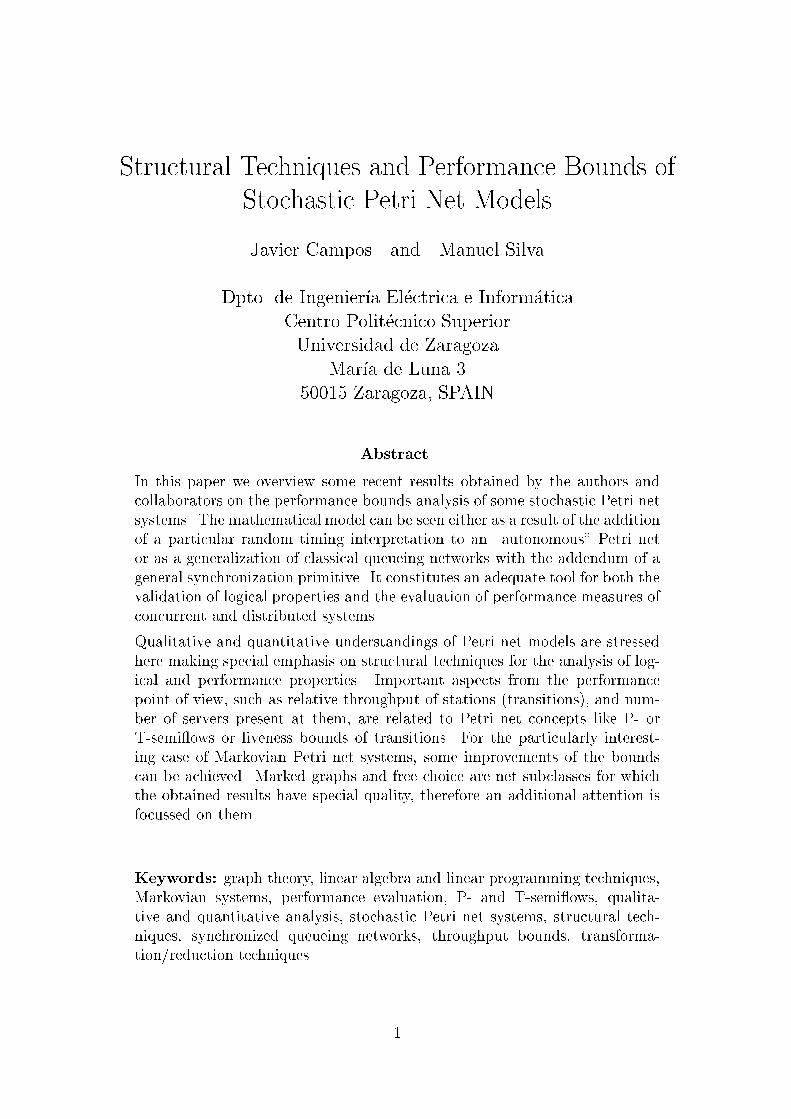
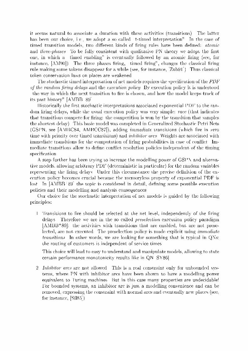
Figure 1: A stochastic net and the corresponding synchronized queueing network.

it seems natural to associate a duration with these activities (transitions). The latterhas been our choice, i.e., we adopt a so called \t-timed interpretation". In the case oftimed transition models, two di�erent kinds of �ring rules have been de�ned: atomicand three-phases. To be fully consistent with qualitative PN theory we adopt the �rstone, in which a \timed enabling" is eventually followed by an atomic �ring (see, forinstance, [AM90]). The three phases �ring, \timed �ring", changes the classical �ringrule making some tokens disappear for a while (see, for instance, [Zub91]). Thus classicaltoken conservation laws on places are weakened.The stochastic timed interpretation of net models requires the speci�cation of the PDFof the random �ring delays and the execution policy. By execution policy it is undertood\the way in which the next transition to �re is chosen, and how the model keeps track ofits past history" [AMBB+89].Historically the �rst stochastic interpretations associated exponential PDF to the ran-dom �ring delays, while the usual execution policy was very simple: race (that indicatesthat transitions compete for �ring: the competition is won by the transition that samplesthe shortest delay). This basic model was completed in Generalized Stochastic Petri Nets(GSPN, see [AMBC84, AMBCC87]), adding immediate transitions (which �re in zerotime with priority over timed transitions) and inhibitor arcs. Weights are associated withimmediate transitions for the computation of �ring probabilities in case of con ict. Im-mediate transitions allow to de�ne con ict resolution policies independent of the timingspeci�cation.A step further has been trying to increase the modelling power of GSPN and alterna-tive models, allowing arbitrary PDF (deterministic in particular) for the random variablesrepresenting the �ring delays. Under this circumstance the precise de�nition of the ex-ecution policy becomes crucial because the memoryless property of exponential PDF islost. In [AMBB+89] the topic is considered in detail, de�ning some possible executionpolicies and their modelling and analysis consequences.Our choice for the stochastic interpretation of net models is guided by the followingprinciples:1. Transitions to �re should be selected at the net level, independently of the �ringdelays. Therefore we are in the so called preselection execution policy paradigm[AMBB+89]: the activities with transitions that are enabled, but are not prese-lected, are not executed. The preselection policy is made explicit using immediatetransitions. In other words, we are looking for something that is typical in QNs:the routing of customers is independent of service times.This choice will lead to easy to understand and manipulate models, allowing to statecertain performance monotonicity results like in QN [SY86].2. Inhibitor arcs are not allowed. This is a real constraint only for unbounded sys-tems, where PN with inhibitor arcs have been shown to have a modelling powerequivalent to Turing machines. But in this case many properties are undecidable!For bounded systems, an inhibitor arc is just a modelling convenience and can beremoved, expressing the constraint with normal arcs and eventually new places (see,for instance, [Sil85]).

3. Priorities in the �ring of transitions are forbidden, except for the two levels derivedfrom the use of immediate and timed transitions.4. Synchronizations may be immediate, and we discard the \pathological" situationconsisting of a circuit in the net including only immediate transitions.Under the above choices our stochastic interpretation grounds in a very general framework:1. Firing delays are random variables with arbitrary PDF. They are assumed to betime and marking independent.2. If a transition is enabled several times, let us say q times, then q �rings progressin parallel at the same time. In other words, we assume the idea that the naturalinterpretation of parallelism in a PN model leads to an in�nite-server semantics, inQN terminology. If this is not appropiated for the system because the number ofservers should be constrained to k, then a place self-loop around the transition withk tokens will guarantee the k-server semantics.3. Any policy for con ict resolution among immediate transitions is allowed (e.g., de-�ned through a deterministic scheduler, through a probabilistic choice: : : ).In practice, for computing performance bounds, only the mean �ring (service) time oftransitions and long run routing rates will be needed by us. More precisely, si, themean �ring time for transition ti(i = 1; : : : ; m) is given, and each subset of transitionsft1; : : : ; tkg � T that are in con ict in one or several reachable markings are consideredimmediate, and the constants r1; : : : ; rk 2 IN+ are explicitly de�ned in the net interpreta-tion in such a way that when t1; : : : ; tk are enabled, transition ti, i = 1; : : : ; k, �res withrelative frecuency, ri=(Pkj=1 rj). Note that the routing rates are assumed to be strictlypositive, i.e., all possible outcomes of any con ict may �re.In summary, we model services by means of timed transitions, routing by means ofimmediate transitions in con ict, and both kinds of transitions, timed and immediate,can be used as fork (split) nodes and join (synchronization) nodes.The main price we pay for the adopted modelling paradigm is the unability to \di-rectly" model situations like preempting scheduling disciplines, time-out mechanisms orunreliable processors which can \fail" during the processing stage. What we basically gainis the possibility of using many results from structure theory of Petri nets and queueingnetwork theory.A more restricted but easier to analyse stochastic interpretation, associating time andmarking independent exponential PDF to the �ring of transitions and time and markingindependent discrete probability distributions to immediate transitions, will be called inthe present framework Markovian Petri net systems (section 7).2.2 Queueing networks with synchronizationsMany extensions have been proposed to introduce synchronization primitives into thequeueing network formalism, in order to allow the modelling of distributed synchronoussystems: passive resources, fork and join, customer splitting, etc. Some very restricted

q1

t 1

q 2

q 3

t 2

t 3e1

s2

s3

r12

r13

q

s

t e

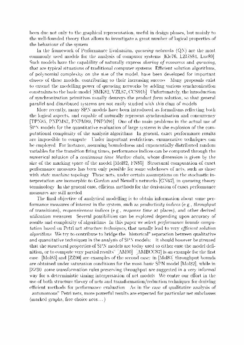
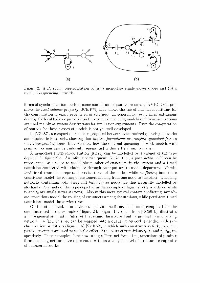
(a) (b)Figure 2: A Petri net representation of (a) a monoclass single server queue and (b) amonoclass queueing network.forms of synchronization, such as some special use of passive resources [AMBCD86], pre-serve the local balance property [BCMP75] that allows the use of e�cient algorithms forthe computation of exact product form solutions. In general, however, these extensionsdestroy the local balance property, so the extended queueing models with synchronizationsare used mainly as system descriptions for simulation experiments. Even the computationof bounds for these classes of models is not yet well developed.In [VZL87], a comparison has been proposed between synchronized queueing networksand stochastic Petri nets, showing that the two formalisms are roughly equivalent from amodelling point of view. Here we show how the di�erent queueing network models withsynchronizations can be uniformly represented within a Petri net formalism.A monoclass single server station [Kle75] can be modelled by a subnet of the typedepicted in �gure 2.a. An in�nite server queue [Kle75] (i.e., a pure delay node) can berepresented by a place to model the number of customers in the system and a timedtransition connected with the place through an input arc to model departures. Persis-tent timed transitions represent service times of the nodes, while con icting immediatetransitions model the routing of customers moving from one node to the other. Queueingnetworks containing both delay and �nite server nodes are thus naturally modelled bystochastic Petri nets of the type depicted in the example of �gure 2.b (t1 is a delay, whilet2 and t3 are single server stations). Also in this more general context con icting immedi-ate transitions model the routing of customers among the stations, while persistent timedtransitions model the service times.On the other hand, stochastic nets can assume forms much more complex than theone illustrated in the example of �gure 2.b. Figure 1.a, taken from [CCS91b], illustratesa more general stochastic Petri net that cannot be mapped onto a product form queueingnetwork. In fact, this net can be mapped onto a queueing network extended with syn-chronization primitives (�gure 1.b) [SMK82], in which such constructs as fork, join, andpassive resources are used to map the e�ect of the pairs of transitions t2{t7 and t9{t10, re-spectively. These examples show how, using a Petri net formalism, extensions of productform queueing networks are represented with an analogous level of structural complexityof Jackson networks.

As a very particular case in which the interest of making a deep bridge between PN andQN theories appears, in [DLT90] it has be pointed out the isomorphism between Fork/JoinQueueing Networks with Blocking (FJQN/B) and stochastic strongly connected MarkedGraphs.Finally, let us remark that stochastic Petri nets with weighted arcs (i.e., non-ordinarynets) can be used for the modelling of bulk arrivals and bulk services [Kle75], with deter-ministic size of batches (given by the weights of arcs).3 Relative throughput of transitions: Visit ratiosOne of the most usual indices of productivity in performance evaluation of computersystems is the throughput of the di�erent components, i.e., the number of jobs or tasksprocessed by each component in the unit time. In classical queueing network models,components are represented by stations, and throughput of each component is the averagenumber of service completions of the correspondent station per unit time. For stochasticPetri nets, since actions are represented with transitions, the throughput of a componentis the number of �rings per unit time of the corresponding transition.3.1 Classical queueing networks: ow of customersIn a classical monoclass queueing network, the following system can be derived by equatingthe rate of ow of customers into each station to the rate of ow out of the station [Kle75]:X(j) = X0j + mXi=1X(i) rij; j = 1; : : : ; m (1)where X(i) is the limit throughput of station i, i.e., the average number of service comple-tions per unit time at station i, i = 1; : : : ; m; rij, is the probability that a customer exitingcenter i goes to j (i; j = 1; : : : ; m); and X0j is the external arrival rate of customers tostation j (j = 1; : : : ; m).If the network is open (i.e., if there exists a station j with positive external arrivalrate, X0j > 0 and also customers can leave the system), then the above m equations arelinearly independent, and the exact throughputs of stations can be derived (independentlyof the service times, si, i = 1; : : : ; m). This is not the case for closed networks. If X0j = 0,j = 1; : : : ; m, then only m� 1 equations are linearly independent, and thus only ratios ofthroughputs can be determined. These relative throughputs which are often called visitratios, denoted as vi for each station i, summarize all the information given by the routingthat we use for the computation of the throughput bounds. The visit ratios normalized,for instance, for station j are de�ned as:v(j)i def= X(i)X(j) ; i = 1; : : : ; m (2)For a restricted class of queueing networks, called product form networks, the exact steady-state solution can be shown to be a product of terms, one for each station, where theform of term i is derived from the visit ratio vi and the service time si. The steady-stateprobability �(~n) of state ~n = (n1; : : : ; nm)T (where ni is the number of customers at

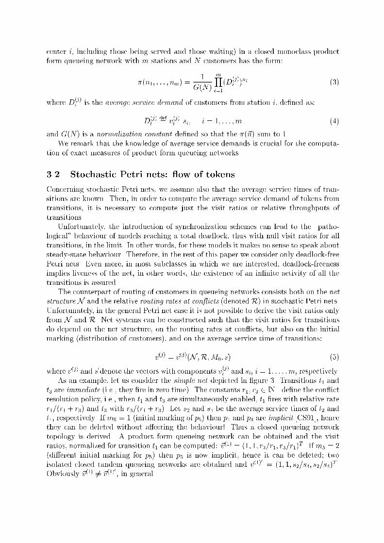
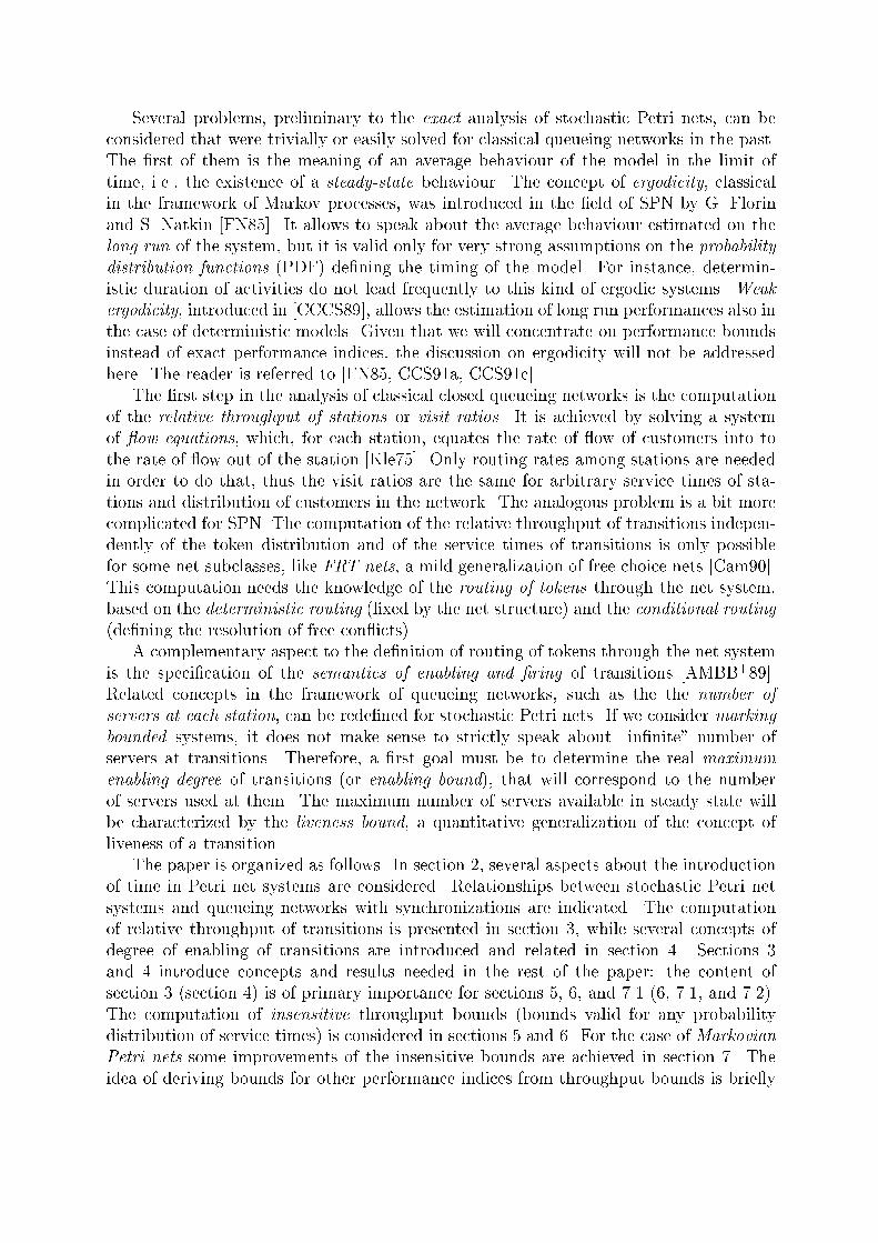
center i, including those being served and those waiting) in a closed monoclass productform queueing network with m stations and N customers has the form:�(n1; : : : ; nm) = 1G(N) mYi=1(D(j)i )ni (3)where D(j)i is the average service demand of customers from station i, de�ned as:D(j)i def= v(j)i si; i = 1; : : : ; m (4)and G(N) is a normalization constant de�ned so that the �(~n) sum to 1.We remark that the knowledge of average service demands is crucial for the computa-tion of exact measures of product form queueing networks.3.2 Stochastic Petri nets: ow of tokensConcerning stochastic Petri nets, we assume also that the average service times of tran-sitions are known. Then, in order to compute the average service demand of tokens fromtransitions, it is necessary to compute just the visit ratios or relative throughputs oftransitions.Unfortunately, the introduction of synchronization schemes can lead to the \patho-logical" behaviour of models reaching a total deadlock, thus with null visit ratios for alltransitions, in the limit. In other words, for these models it makes no sense to speak aboutsteady-state behaviour. Therefore, in the rest of this paper we consider only deadlock-freePetri nets. Even more, in most subclasses in which we are interested, deadlock-freenessimplies liveness of the net, in other words, the existence of an in�nite activity of all thetransitions is assured.The counterpart of routing of customers in queueing networks consists both on the netstructure N and the relative routing rates at con icts (denoted R) in stochastic Petri nets.Unfortunately, in the general Petri net case it is not possible to derive the visit ratios onlyfrom N and R. Net systems can be constructed such that the visit ratios for transitionsdo depend on the net structure, on the routing rates at con icts, but also on the initialmarking (distribution of customers), and on the average service time of transitions:~v(j) = ~v(j)(N ;R;M0; ~s) (5)where ~v(j) and ~s denote the vectors with components v(j)i and si, i = 1; : : : ; m, respectively.As an example, let us consider the simple net depicted in �gure 3. Transitions t1 andt3 are immediate (i.e., they �re in zero time). The constants r1; r3 2 IN+ de�ne the con ictresolution policy, i.e., when t1 and t3 are simultaneously enabled, t1 �res with relative rater1=(r1 + r3) and t3 with r3=(r1 + r3). Let s2 and s4 be the average service times of t2 andt4, respectively. If m5 = 1 (initial marking of p5) then p1 and p3 are implicit [CS91], hencethey can be deleted without a�ecting the behaviour! Thus a closed queueing networktopology is derived. A product form queueing network can be obtained and the visitratios, normalized for transition t1 can be computed: ~v(1) = (1; 1; r3=r1; r3=r1)T . If m5 = 2(di�erent initial marking for p5) then p5 is now implicit, hence it can be deleted; twoisolated closed tandem queueing networks are obtained and ~v(1)0 = (1; 1; s2=s4; s2=s4)T .Obviously ~v(1) 6= ~v(1)0 , in general.

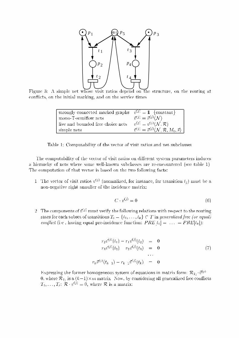
p1 p5 p 3

p4p2

t 1

t 2

t 3

t 4

m5

Figure 3: A simple net whose visit ratios depend on the structure, on the routing atcon icts, on the initial marking, and on the service times.strongly connected marked graphs ~v(j) = 11 fconstantgmono-T-semi ow nets ~v(j) = ~v(j)(N )live and bounded free choice nets ~v(j) = ~v(j)(N ;R)simple nets ~v(j) = ~v(j)(N ;R;M0; ~s)Table 1: Computability of the vector of visit ratios and net subclasses.The computability of the vector of visit ratios on di�erent system parameters inducesa hierarchy of nets where some well-known subclasses are re-encountered (see table 1).The computation of that vector is based on the two following facts:1. The vector of visit ratios ~v(j) (normalized, for instance, for transition tj) must be anon-negative right annuller of the incidence matrix:C � ~v(j) = 0 (6)2. The components of ~v(j) must verify the following relations with respect to the routingrates for each subset of transitions Ti = ft1; : : : ; tkg � T in generalized free (or equal)con ict (i.e., having equal pre-incidence function: PRE[t1] = : : : = PRE[tk]):r2~v(j)(t1)� r1~v(j)(t2) = 0r3~v(j)(t2)� r2~v(j)(t3) = 0 (7)� � �rk~v(j)(tk�1)� rk�1~v(j)(tk) = 0Expressing the former homogeneous system of equations in matrix form: RTi �~v(j) =0, whereRTi is a (k�1)�mmatrix. Now, by considering all generalized free con ictsT1; : : : ; Tr: R � ~v(j) = 0, where R is a matrix:

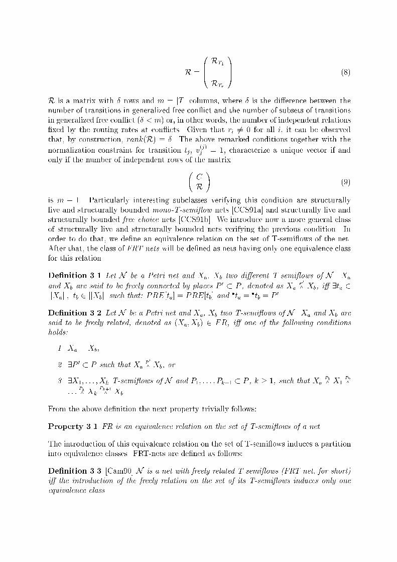
R = 0BB@ RT1...RTr 1CCA (8)R is a matrix with � rows and m = jT j columns, where � is the di�erence between thenumber of transitions in generalized free con ict and the number of subsets of transitionsin generalized free con ict (� < m) or, in other words, the number of independent relations�xed by the routing rates at con icts. Given that ri 6= 0 for all i, it can be observedthat, by construction, rank(R) = �. The above remarked conditions together with thenormalization constraint for transition tj, v(j)j = 1, characterize a unique vector if andonly if the number of independent rows of the matrix CR ! (9)is m � 1. Particularly interesting subclasses verifying this condition are structurallylive and structurally bounded mono-T-semi ow nets [CCS91a] and structurally live andstructurally bounded free choice nets [CCS91b]. We introduce now a more general classof structurally live and structurally bounded nets verifying the previous condition. Inorder to do that, we de�ne an equivalence relation on the set of T-semi ows of the net.After that, the class of FRT-nets will be de�ned as nets having only one equivalence classfor this relation.De�nition 3.1 Let N be a Petri net and Xa, Xb two di�erent T-semi ows of N . Xaand Xb are said to be freely connected by places P 0 � P , denoted as Xa P 0̂ Xb, i� 9ta 2jjXajj; tb 2 jjXbjj such that: PRE[ta] = PRE[tb] and �ta = �tb = P 0.De�nition 3.2 Let N be a Petri net and Xa, Xb two T-semi ows of N . Xa and Xb aresaid to be freely related, denoted as (Xa; Xb) 2 FR, i� one of the following conditionsholds:1. Xa = Xb,2. 9P 0 � P such that Xa P 0̂ Xb, or3. 9X1; : : : ; Xk T-semi ows of N and P1; : : : ; Pk+1 � P , k � 1, such that Xa P1̂ X1 P2̂: : : Pk̂ Xk Pk+1^ Xb.From the above de�nition the next property trivially follows:Property 3.1 FR is an equivalence relation on the set of T-semi ows of a net.The introduction of this equivalence relation on the set of T-semi ows induces a partitioninto equivalence classes. FRT-nets are de�ned as follows:De�nition 3.3 [Cam90] N is a net with freely related T-semi ows (FRT-net, for short)i� the introduction of the freely relation on the set of its T-semi ows induces only oneequivalence class.

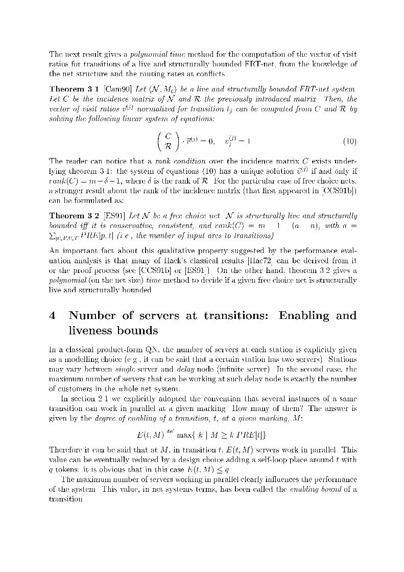
The next result gives a polynomial time method for the computation of the vector of visitratios for transitions of a live and structurally bounded FRT-net, from the knowledge ofthe net structure and the routing rates at con icts.Theorem 3.1 [Cam90] Let hN ;M0i be a live and structurally bounded FRT-net system.Let C be the incidence matrix of N and R the previously introduced matrix. Then, thevector of visit ratios ~v(j) normalized for transition tj can be computed from C and R bysolving the following linear system of equations: CR ! � ~v(j) = 0; v(j)j = 1 (10)The reader can notice that a rank condition over the incidence matrix C exists under-lying theorem 3.1: the system of equations (10) has a unique solution ~v(j) if and only ifrank(C) = m���1, where � is the rank of R. For the particular case of free choice nets,a stronger result about the rank of the incidence matrix (that �rst appeared in [CCS91b])can be formulated as:Theorem 3.2 [ES91] Let N be a free choice net. N is structurally live and structurallybounded i� it is conservative, consistent, and rank(C) = m � 1 � (a � n), with a =Pp2P;t2T PRE[p; t] (i.e., the number of input arcs to transitions).An important fact about this qualitative property suggested by the performance eval-uation analysis is that many of Hack's classical results [Hac72] can be derived from itor the proof process (see [CCS91b] or [ES91]). On the other hand, theorem 3.2 gives apolynomial (on the net size) time method to decide if a given free choice net is structurallylive and structurally bounded.4 Number of servers at transitions: Enabling andliveness boundsIn a classical product-form QN, the number of servers at each station is explicitly givenas a modelling choice (e.g., it can be said that a certain station has two servers). Stationsmay vary between single server and delay node (in�nite server). In the second case, themaximum number of servers that can be working at such delay node is exactly the numberof customers in the whole net system.In section 2.1 we explicitly adopted the convention that several instances of a sametransition can work in parallel at a given marking. How many of them? The answer isgiven by the degree of enabling of a transition, t, at a given marking, M :E(t;M) def= maxf k j M � k PRE[t]gTherefore it can be said that at M , in transition t, E(t;M) servers work in parallel. Thisvalue can be eventually reduced by a design choice adding a self-loop place around t withq tokens: it is obvious that in this case E(t;M) � q.The maximum number of servers working in parallel clearly in uences the performanceof the system. This value, in net systems terms, has been called the enabling bound of atransition.

t

2

p 1 1 t 2

t 3

p2

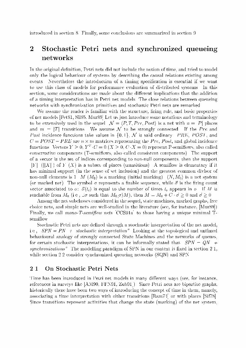
p3Figure 4: E(t1) = 2, while L(t1) = 1 (i.e., L(t1) < E(t1)).De�nition 4.1 [CCCS89] Let hN ;M0i be a net system. The enabling bound of a giventransition t of N isE(t) def= max f k j 9�;M0[�iM : M � k PRE[t] g (11)The enabling bound is a quantitative generalization of the basic concept of enabling, andis closely related to the concept of marking bound of a place.De�nition 4.2 Let hN ;M0i be a net system. The marking bound of a given place p ofN is B(p) def= max f M(p) j M0[�iM g (12)Since we are interested in the steady-state performance of a model, one can ask thefollowing question: how many servers can be available in transitions in any possible steady-state condition? The answer is given by the de�nition of the liveness bound concept.De�nition 4.3 [CCS91a] Let hN ;M0i be a net system. The liveness bound of a giventransition t of N isL(t) def= max f k j 8M 0 :M0[�iM 0; 9M :M 0[�0iM ^M � k PRE[t] g (13)The above de�nition generalizes the classical concept of liveness of a transition. In par-ticular, a transition t is live if and only if L(t) > 0, i.e., if there is at least one workingserver associated with it in any steady-state condition. The following is also obvious fromthe de�nitions.Property 4.1 [CCS91a] Let hN ;M0i be a net system. For any transition t in N , E(t) �L(t) (see �gure 4).Since for any reversible net system (i.e., such thatM0 can be recovered from any reachablemarking: M0 is a home state) the reachability graph is strongly connected, the followingcan be stated:Property 4.2 [CCS91a] Let hN ;M0i be a reversible net system. For any transition t inN , E(t) = L(t).

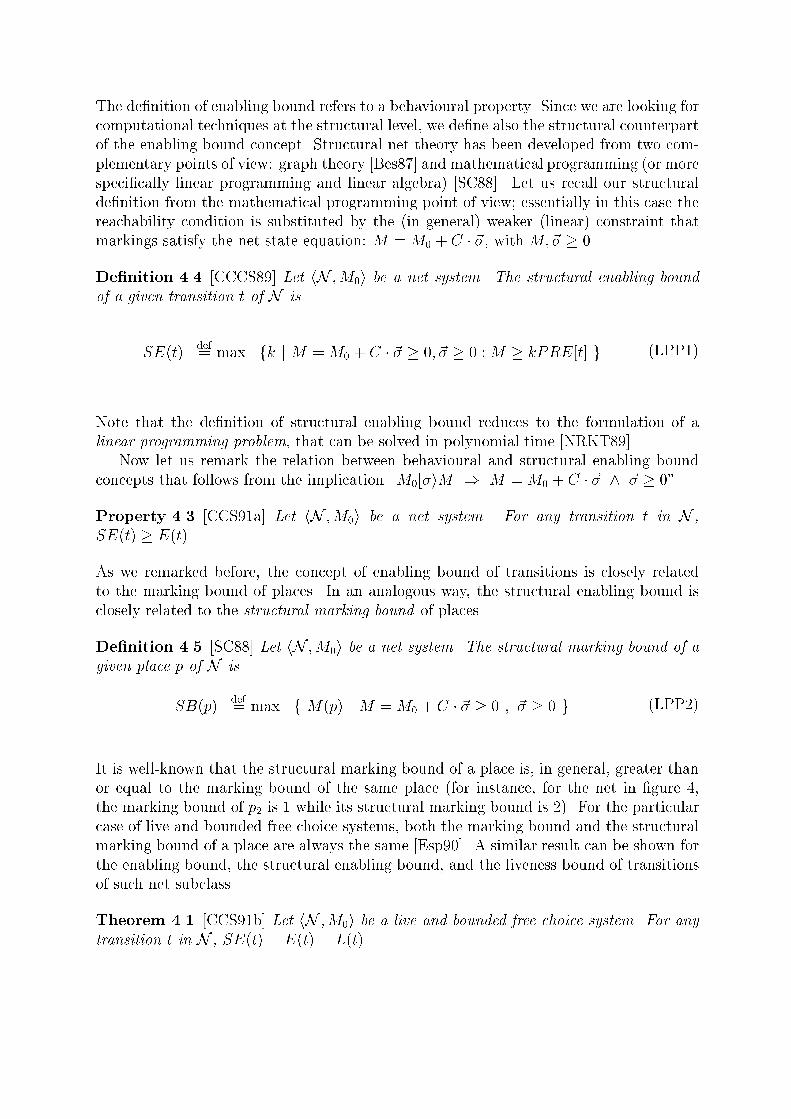
The de�nition of enabling bound refers to a behavioural property. Since we are looking forcomputational techniques at the structural level, we de�ne also the structural counterpartof the enabling bound concept. Structural net theory has been developed from two com-plementary points of view: graph theory [Bes87] and mathematical programming (or morespeci�cally linear programming and linear algebra) [SC88]. Let us recall our structuralde�nition from the mathematical programming point of view; essentially in this case thereachability condition is substituted by the (in general) weaker (linear) constraint thatmarkings satisfy the net state equation: M =M0 + C � ~�, with M;~� � 0.De�nition 4.4 [CCCS89] Let hN ;M0i be a net system. The structural enabling boundof a given transition t of N isSE(t) def= max fk j M =M0 + C � ~� � 0; ~� � 0 :M � kPRE[t] g (LPP1)Note that the de�nition of structural enabling bound reduces to the formulation of alinear programming problem, that can be solved in polynomial time [NRKT89].Now let us remark the relation between behavioural and structural enabling boundconcepts that follows from the implication \M0[�iM ) M =M0 + C � ~� ^ ~� � 0".Property 4.3 [CCS91a] Let hN ;M0i be a net system. For any transition t in N ,SE(t) � E(t).As we remarked before, the concept of enabling bound of transitions is closely relatedto the marking bound of places. In an analogous way, the structural enabling bound isclosely related to the structural marking bound of places.De�nition 4.5 [SC88] Let hN ;M0i be a net system. The structural marking bound of agiven place p of N isSB(p) def= max f M(p) j M =M0 + C � ~� � 0 ; ~� � 0 g (LPP2)It is well-known that the structural marking bound of a place is, in general, greater thanor equal to the marking bound of the same place (for instance, for the net in �gure 4,the marking bound of p2 is 1 while its structural marking bound is 2). For the particularcase of live and bounded free choice systems, both the marking bound and the structuralmarking bound of a place are always the same [Esp90]. A similar result can be shown forthe enabling bound, the structural enabling bound, and the liveness bound of transitionsof such net subclass.Theorem 4.1 [CCS91b] Let hN ;M0i be a live and bounded free choice system. For anytransition t in N , SE(t) = E(t) = L(t).

Now, from the previous theorem and taking into account that for any transition t thecomputation of the structural enabling bound SE(t) can be formulated in terms of theproblem (LPP1), the following monotonicity property of the liveness bound of a transitionwith respect to the initial marking is obtained.Corollary 4.1 [CCS91b] If hN ;M0i is a live and bounded free choice system and M 00 �M0 then the liveness bound of t in hN ;M 00i is greater than or equal to the liveness boundof t in hN ;M0i.The previous result appears to be a generalization (stated for the particular case ofbounded nets) of the classical liveness monotonicity property for free choice systems (see,e.g., [Bes87]).Once the computability of visit ratios and enabling/liveness bounds have been ad-dressed using concepts and techniques from linear (algebra/programming) structure the-ory, bounds on throughput are presented in the following sections.5 Insensitive upper bounds on throughputIn this section we present the computation of upper bounds for the throughput of tran-sitions for stochastic Petri nets with general distribution of service times. The obtainedbounds are called insensitive because they are valid for arbitrary forms of the probabilitydistribution functions of service (including deterministic timing), since only mean valuesof random variables are used.Let us just precise for stochastic Petri net systems the weak ergodicity notions for themarking and �ring processes:De�nition 5.1 [CCS91b] The marking process M� , where � � 0 represents the time, ofa stochastic marked net is weakly ergodic i� the following limit exists:lim�!1 1� Z �0 Mu du =M < ~1; a.s. (14)and the constant vector M is called the limit average marking.The �ring process ~�� , where � � 0 represents the time, of a stochastic marked net isweakly ergodic i� the following limit exists:lim�!1 ~��� = ~� < ~1; a.s. (15)and the constant vector ~� is the limit of transition throughputs (or limit �ring ow vector).For bounded net systems, the existence of a home state (i.e., a marking reachable fromany other) is a su�cient condition for weak marking ergodicity [Cam90].

5.1 Little's law and P-semi owsThree of the most signi�cant performance measures for a closed region of a network inthe analysis of queueing systems are related by Little's formula [Lit61], which holds undervery general (i.e., weak) conditions. This result can be applied to each place of a weaklyergodic net system. Denoting M(pi) the limit average number of tokens at place pi, ~�the limit vector of transition throughputs, and R(pi) the average time spent by a tokenwithin the place pi (average residence time at place pi), the above mentioned relationshipis stated as follows (see [FN85]):M(pi) = (PRE[pi] � ~�) R(pi) (16)where PRE[pi] is the ith row of the pre-incidence matrix of the underlying Petri net, thusPRE[pi] � ~� is the output rate of place pi.In the study of computer systems, Little's law is frequently used when two of therelated quantities are known and the third one is needed. This is not exactly the casehere. In the equation (16), ~� can be computed except for a scaling factor for importantnet system subclasses (see section 3): ~� = 1�(j) ~v(j) (17)where ~v(j) is the vector of visit ratios normalized for tj and �(j) is the inverse of the limitthroughput of transition tj, that we call the mean inter�ring time of that transition, i.e.,the mean time between two consecutive �rings of tj.The average residence timeR(pi) at places with more than one output transition is nullbecause such transitions are considered immediate. For the places pi with only one outputtransition, the average response time can be expressed as sum of the average waiting timedue to a possible synchronization in the output transition and the mean service timeassociated with that transition. Thus the average residence times can be lowerly boundedfrom the knowledge of the mean service times of transitions, si, i = 1; : : : ; m, and thefollowing system of inequalities can be derived from (16) and (17):�(j) M � PRE � ~D(j) (18)where ~D(j) is the vector of average service demands, introduced in section 3.1: D(j)k =v(j)k sk.The limit average marking M is unknown. However, taking the product with a P-semi ow Y (i.e., Y � 0, Y T � C = 0, thus Y T �M0 = Y T �M = Y T �M for all reachablemarking M), the following inequality can be derived:�(j) � max8<:Y T � PRE � ~D(j)Y T �M0 j Y T � C = 0 ; Y � 0 9=; (19)The previous lower bound for the mean inter�ring time (or its inverse, an upper boundfor the throughput) can be formulated in terms of a fractional programming problem[NRKT89] and later, after some considerations, transformed into a linear programmingproblem.

p3p16

p 7

p 10

p12

p 9

p 8

p11

t 1

t 2

t 3

t 4 t 5

p 1

p2

p4

p5

t6

p 6p13

p14

p15

t 13

t 7

t 8 t 9

t 10 t 11

t 12

N 1

N 2N 2

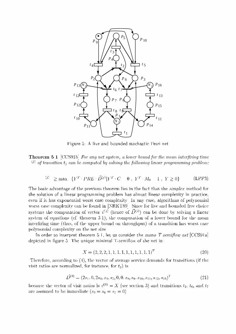
Figure 5: A live and bounded stochastic Petri net.Theorem 5.1 [CCS91b] For any net system, a lower bound for the mean inter�ring time�(j) of transition tj can be computed by solving the following linear programming problem:�(j) � max fY T � PRE � ~D(j)jY T � C = 0 ; Y T �M0 = 1 ; Y � 0g (LPP3)The basic advantage of the previous theorem lies in the fact that the simplex method forthe solution of a linear programming problem has almost linear complexity in practice,even if it has exponential worst case complexity. In any case, algorithms of polynomialworst case complexity can be found in [NRKT89]. Since for live and bounded free choicesystems the computation of vector ~v(j) (hence of ~D(j)) can be done by solving a linearsystem of equations (cf. theorem 3.1), the computation of a lower bound for the meaninter�ring time (thus, of the upper bound on throughput) of a transition has worst casepolynomial complexity on the net size.In order to interpret theorem 5.1, let us consider the mono-T-semi ow net [CCS91a]depicted in �gure 5. The unique minimal T-semi ow of the net is:X = (2; 2; 2; 1; 1; 1; 1; 1; 1; 1; 1; 1; 1)T (20)Therefore, according to (4), the vector of average service demands for transitions (if thevisit ratios are normalized, for instance, for t3) is~D(3) = (2s1; 0; 2s3; s4; s5; 0; 0; s8; s9; s10; s11; s12; s13)T (21)because the vector of visit ratios is ~v(3) = X (see section 3) and transitions t2, t6, and t7are assumed to be immediate (s2 = s6 = s7 = 0).

p 7 p 8

t 2

t 3

t 4 t 5

p 1

p2 p3

p4

p5

t6

p 6

t 7

t 8 t 9

p 10p 9

t 4 t 5

p16

p 7p12

p 8

p11

t 6

p13

p14

p15

t 13

t 7

t 8 t 9

t 10 t 11

t 12

t 1

N 1

N 2 N 2

Figure 6: Subsystems of the net system in �gure 5 generated by minimal P-semi ows.The minimal P-semi ows (minimal support solutions of Y T �C = 0; Y � 0) of this netare: Y1 = (2; 1; 1; 2; 1; 1; 2; 2; 0; 0; 0; 0; 0; 0; 0; 0)TY2 = (0; 0; 0; 0; 0; 0; 0; 0; 1; 1; 0; 0; 0; 0; 0; 0)TY3 = (0; 0; 0; 0; 0; 0; 1; 0; 0; 0; 1; 1; 1; 0; 0; 0)TY4 = (0; 0; 0; 0; 0; 0; 0; 1; 0; 0; 0; 0; 0; 1; 1; 1)T (22)Then, the application of (LPP3) gives:�(3) � max f (4s1 + 2s3 + 2s4 + s5 + 2s8 + 2s9)=2N1;s4 + s5;(s8 + s10 + s12)=N2;(s9 + s11 + s13)=N2 g (23)where N1 > 0 is the initial marking of place p1, and N2 > 0 is the initial marking ofp13 and p16. Now, let us consider the P-semi ow decomposed view of the net: the foursubnets generated by Y1, Y2, Y3, and Y4 are depicted in isolation in �gure 6.The exact mean inter�ring times of (all the transitions of) the second, third, and forthsubnets are s4 + s5, (s8 + s10 + s12)=N2, and (s9 + s11 + s13)=N2, respectively (rememberthat in�nite-server semantics is assumed). The exact mean inter�ring time of t3 in the�rst subnet (generated by Y1) cannot be computed in a compact way (like the others),because it includes synchronizations (it has not queueing network topology). In any case,its mean inter�ring time is greater than (4s1+2s3+2s4+s5+2s8+2s9)=2N1, because thiswould be the cycle time of a queueing network (without delays due to synchronizations) ofin�nite-server stations with the same average service demands and number of customers.

t 1 t 2

t 3 t 4

t 5

p1

p2 p

3

p4 p5

q 1-q

t 1 t 2

t 3 t 4

t 5

p 1

p2 p3

p4 p5

q 1-q

p6

(a) (b)Figure 7: (a) A live and safe free choice system and (b) the addition of the implicit placep6.Therefore, the lower bound for the mean inter�ring time of t4 in the original net given by(23) is computed looking at the \slowest subnet" (net with minimum throughput for t4)generated by the elementary P-semi ows, considered in isolation.In the particular case of strongly connected marked graphs, the problem of �nding anupper bound for the steady-state throughput (lower bound for the mean inter�ring time)can be solved looking at the mean inter�ring time associated with each elementary circuit(minimal P-semi ows for marked graphs) of the net, considered in isolation. These timescan be computed making the summation of the mean service times of all the transitionsinvolved in the P-semi ow (service time of the whole circuit), and dividing by the numberof tokens present in it (customers in the circuit).5.2 About the reachability of the boundThe above bound, that holds for any probability distribution function of servicetimes of transitions, happens to be the same that has been obtained for stronglyconnected deterministically timed marked graphs by other authors (see for example[Ram74, Sif78, RH80]), but here it is considered in a practical linear programming form.For deterministically timed marked graphs, the reachability of this bound has been shown[Ram74, RH80]. Even more, it has been shown [CCCS89, CCCS90] that the previousbound cannot be improved, for the case of strongly connected marked graphs, only on thebase of the knowledge of the coe�cients of variation for the transition service times.We remark that the importance of a tightness result for performance bounds lies inthe fact that the bounds cannot be improved without increasing the information aboutthe model (in particular, the moments of order greater than two of the associated randomvariables).For the more general case of live and bounded free choice systems, the bound given bytheorem 5.1 cannot be reached for some models, for any probability distribution functionof service times. Let us consider, for instance, the live and safe free choice system in�gure 7.a.Let s3 and s4 be the mean service times associated with t3 and t4, respectively. Let

t1, t2, and t5 be immediate transitions (i.e., they �re in zero time). Let q; 1� q 2 (0; 1) bethe probabilities de�ning the resolution of con ict at place p1. The vector of visit ratios(normalized for t5) is ~v(5) = (q; 1� q; q; 1� q; 1)T (24)The elementary P-semi ows are Y1 = (1; 1; 0; 0; 1)TY2 = (1; 0; 1; 1; 0)T (25)Applying (LPP3) the following lower bound for the mean inter�ring time of transition t5is obtained: �(5) � max f qs3; (1� q)s4 g (26)while the actual mean inter�ring time for this transition is�(5) = qs3 + (1� q)s4 (27)independently of the higher moments of the probability distribution functions associatedwith transitions t3 and t4. Therefore the bound given by theorem 5.1 is non-reachable forthe net system in �gure 7.a.Methods for the improvement of this bound have been presented in [CCS91c] and[CC91]. We just summarize here some ideas about them. The �rst one concerns theaddition of implicit places to the net system. From a pure qualitative point of view, in[CS91] it is shown that the addition of \judicious" implicit places eliminates some of thespurious solutions of the linear relaxation of a net system (i.e., those integer solutions ofM =M0 +C � ~� � 0; ~� � 0 that are non reachable). In [CCS91b], an analogous improve-ment is shown to hold at the performance level. Let us explain here this improvement byusing again the example depicted in �gure 7.a: consider the net in �gure 7.b, where theimplicit place p6 has been added to the original net. The addition of implicit places cangenerate more elementary P-semi ows. In this case:Y3 = (1; 1; 1; 0; 0; 1)T (28)Then, the application of (LPP3) can eventually lead to an improvement of the previousbound. For this net system:�(5) � max f qs3; (1� q)s4; qs3 + (1� q)s4 g = qs3 + (1� q)s4 (29)which is exactly the actual mean inter�ring time of t5.Details on this technique can be found in [CCS91c]. Moreover, it should be pointedout that the addition of implicit places does not guarantee the bound to be reachable.As an example, look at the net in �gure 8.a. The exact mean inter�ring time of t7 fordeterministic timing is:�(7) = max f qs3+s6; (1�q)s4+s5; qs3+(1�q)s4+(1�q)s5+qs6; qs5+(1�q)s6 g+s7 (30)

t 1 t 2

t 3 t 4

t 5

p1

p2 p3

p 4 p 5

q 1-q

t 7

p6 p 7

t 6

(a) (b)

t 1 t 2

t 3 t 4

t 5

p1

p2 p 3

p4 p5

q

t 7

p 6 p7

t 6p

8

1-q

Figure 8: (a) A live and safe free choice system and (b) the addition of the implicit placep8.and its clearly greater than the bound obtained after the addition of the implicit place p8(�gure 8.b): �(7) � max f qs3 + s6; (1� q)s4 + s5; qs3 + (1� q)s4 g+ s7 (31)The reader can check that addition of any set of implicit places to the system in �gure 8.adoes not allow to reach the value in (30).Another approach for improving the throughput upper bound of theorem 5.1 is pre-sented in [CC91], for the case of live and safe free choice systems. It is based on theconsideration of some speci�c multisets of circuits of the net in which elementary circuitsappear a number of times according to the visit ratios of the involved transitions. Basi-cally, it is a generalization (in the graph theory sense) of the application of theorem 5.1for the case of marked graphs, because circuits (P-semi ows) of the marked graph aresubstituted now by multisets of circuits. The improvement is based on the applicationof a linear programming problem to a net obtained from the original one after a trans-formation of linear size increasing. The transformation, that is a modi�cation of theLautenbach transformation for the computation of minimal traps in a net [Lau87], willnot be presented here (interested readers are referred to [CC91]). The application of thismethod to the net in �gure 8.a gives exactly the mean inter�ring time of t7, given by (30),for deterministic service times of transitions.5.3 Some derived resultsLinear programming problems give an easy way to derive results and interpret them.Looking at (LPP3), the followingmonotonicity property can be obtained: the lower boundfor the mean inter�ring time of a transition does not increase if ~s (the mean service timesvector) decreases or if M0 increases.

p1

t 1 t 2p2

p3p6 p7

t 4t 3 p4

p5

t1 3

4

2

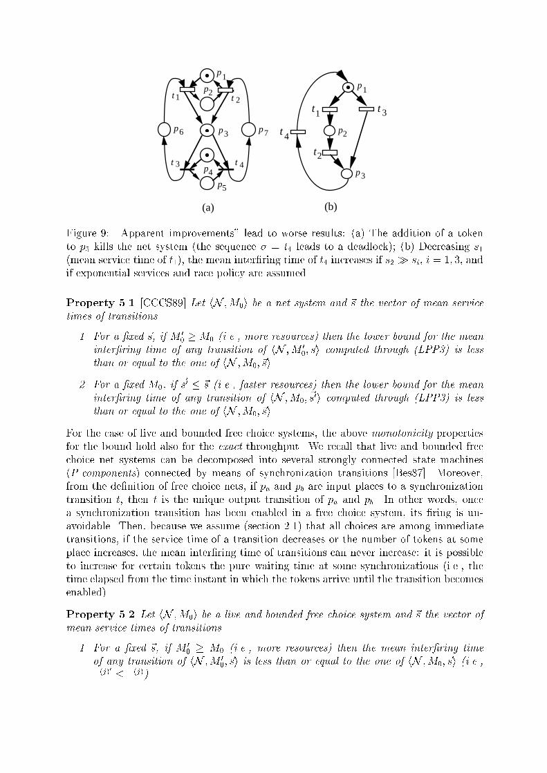
(a) (b)

p1

p2

p3

t

t

t

Figure 9: \Apparent improvements" lead to worse results: (a) The addition of a tokento p5 kills the net system (the sequence � = t4 leads to a deadlock); (b) Decreasing s1(mean service time of t1), the mean inter�ring time of t4 increases if s2 � si, i = 1; 3, andif exponential services and race policy are assumed.Property 5.1 [CCCS89] Let hN ;M0i be a net system and ~s the vector of mean servicetimes of transitions.1. For a �xed ~s, if M 00 �M0 (i.e., more resources) then the lower bound for the meaninter�ring time of any transition of hN ;M 00; ~si computed through (LPP3) is lessthan or equal to the one of hN ;M0; ~si.2. For a �xed M0, if ~s0 � ~s (i.e., faster resources) then the lower bound for the meaninter�ring time of any transition of hN ;M0; ~s0i computed through (LPP3) is lessthan or equal to the one of hN ;M0; ~si.For the case of live and bounded free choice systems, the above monotonicity propertiesfor the bound hold also for the exact throughput. We recall that live and bounded freechoice net systems can be decomposed into several strongly connected state machines(P-components) connected by means of synchronization transitions [Bes87]. Moreover,from the de�nition of free choice nets, if pa and pb are input places to a synchronizationtransition t, then t is the unique output transition of pa and pb. In other words, oncea synchronization transition has been enabled in a free choice system, its �ring is un-avoidable. Then, because we assume (section 2.1) that all choices are among immediatetransitions, if the service time of a transition decreases or the number of tokens at someplace increases, the mean inter�ring time of transitions can never increase: it is possibleto increase for certain tokens the pure waiting time at some synchronizations (i.e., thetime elapsed from the time instant in which the tokens arrive until the transition becomesenabled).Property 5.2 Let hN ;M0i be a live and bounded free choice system and ~s the vector ofmean service times of transitions.1. For a �xed ~s, if M 00 � M0 (i.e., more resources) then the mean inter�ring timeof any transition of hN ;M 00; ~si is less than or equal to the one of hN ;M0; ~si (i.e.,�(j)0 � �(j)).

0.1 1 2

14.8714.88

15.1515.34

s2

Γ

s = (0, s ,0,7,2,0,1,7)2T

Service times vector :

15.54

3

p1

t 1

t 2 t 5

p2 p6

t 3 t 6

p3 p7

t 4 t 7

p4 p8

t 8

p9

p5

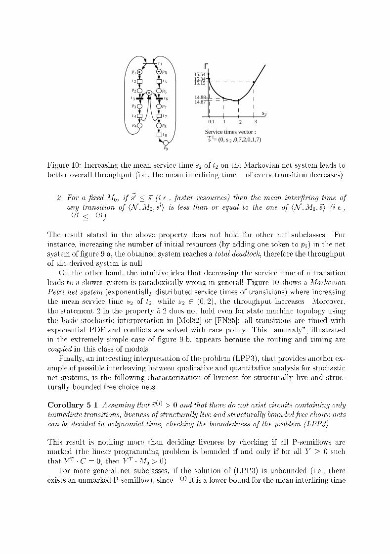
Figure 10: Increasing the mean service time s2 of t2 on the Markovian net system leads tobetter overall throughput (i.e., the mean inter�ring time � of every transition decreases).2. For a �xed M0, if ~s0 � ~s (i.e., faster resources) then the mean inter�ring time ofany transition of hN ;M0; ~s0i is less than or equal to the one of hN ;M0; ~si (i.e.,�(j)0 � �(j)).The result stated in the above property does not hold for other net subclasses. Forinstance, increasing the number of initial resources (by adding one token to p5) in the netsystem of �gure 9.a, the obtained system reaches a total deadlock, therefore the throughputof the derived system is null.On the other hand, the intuitive idea that decreasing the service time of a transitionleads to a slower system is paradoxically wrong in general! Figure 10 shows a MarkovianPetri net system (exponentially distributed service times of transitions) where increasingthe mean service time s2 of t2, while s2 2 (0; 2), the throughput increases. Moreover,the statement 2 in the property 5.2 does not hold even for state machine topology usingthe basic stochastic interpretation in [Mol82] or [FN85]: all transitions are timed withexponential PDF and con icts are solved with race policy. This \anomaly", illustratedin the extremely simple case of �gure 9.b, appears because the routing and timing arecoupled in this class of models.Finally, an interesting interpretation of the problem (LPP3), that provides another ex-ample of possible interleaving between qualitative and quantitative analysis for stochasticnet systems, is the following characterization of liveness for structurally live and struc-turally bounded free choice nets.Corollary 5.1 Assuming that ~v(j) > 0 and that there do not exist circuits containing onlyimmediate transitions, liveness of structurally live and structurally bounded free choice netscan be decided in polynomial time, checking the boundedness of the problem (LPP3).This result is nothing more than deciding liveness by checking if all P-semi ows aremarked (the linear programming problem is bounded if and only if for all Y � 0 suchthat Y T � C = 0, then Y T �M0 > 0).For more general net subclasses, if the solution of (LPP3) is unbounded (i.e., thereexists an unmarked P-semi ow), since �(j) it is a lower bound for the mean inter�ring time

of transition tj, the non-liveness can be assured (in�nite inter�ring time). Nevertheless,a net system can be non-live and the obtained lower bound for the mean inter�ring timebe �nite (e.g., the mono-T-semi ow net in �gure 9.a with the addition of a token in placep5).6 Insensitive lower bounds on throughputIn this section, lower bounds on throughput are presented, independent of the highermoments of the service time probability distribution functions, based on the computationof the vector of visit ratios for transitions as introduced in section 3 and on the transitionliveness bounds, de�ned in section 4.A \trivial" lower bound in steady-state performance for a live net system with a givenvector of visit ratios for transitions is of course given by the inverse of the sum of theservices times of all the transitions weighted by the vector of visit ratios. Since the netsystem is live, all transitions must be �rable, and the sum of all service times multiplied bythe number of occurrences of each transition in the average cycle of the model correspondsto any complete sequentialization of all the transition �rings. This pessimistic behaviour isalways reached in a marked graph consisting on a single loop of transitions and containinga single token in one of the places, independently of the higher moments of the probabilitydistribution functions (this observation can be trivially con�rmed by the computation ofthe upper bound, which in this case gives the same value).This trivial lower bound has been improved in [CCS91b] for the case of live andbounded free choice systems based on the knowledge of the liveness bound L(t) for alltransitions t of the net system.Theorem 6.1 [CCS91b] For any live and bounded free choice system, an upper boundfor the mean inter�ring time �(j) of transition tj can be computed as follows:�(j) � mXi=1 D(j)iL(ti) = mXi=1 v(j)i siL(ti) (32)We recall (cf. theorem 4.1) that in the case of live and bounded free choice systems:1. The liveness bound equals the structural enabling bound for each transition (The-orem 4.1) and this one can be computed by solving (LPP1).2. The vector of visit ratios for transitions is obtained by solving the linear system ofequations (10).Therefore, the lower bound for the throughput of live and bounded free choice systemscan be computed e�ciently. Its worst case complexity is polynomial time on the net size.The lower bound in performance given by the computation of theorem 6.1 can beshown [CCCS89] to be reachable for any marked graph topology and for some assignmentof PDF to the service time of transitions. Therefore, if nothing but the average value isknown about the PDF of the service time of transitions, the bound provided by Theorem6.1 is tight.

p1

p3

p4

p2

t 1

t 2 t 3

2

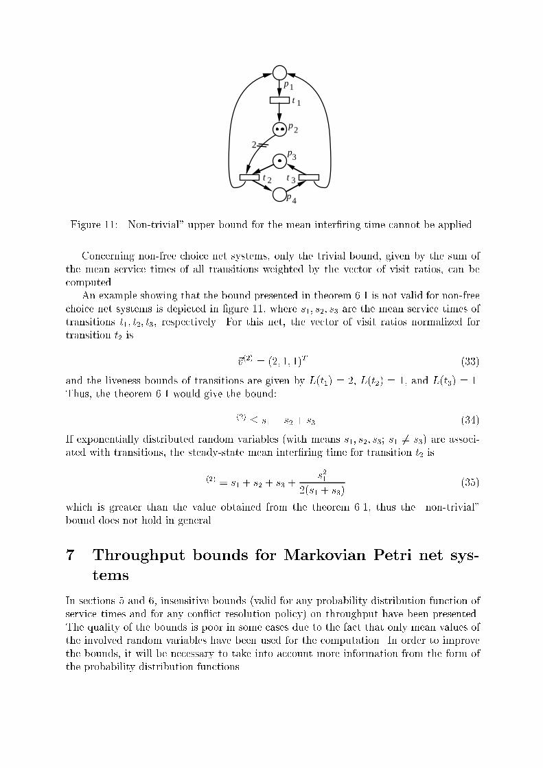
Figure 11: \Non-trivial" upper bound for the mean inter�ring time cannot be applied.Concerning non-free choice net systems, only the trivial bound, given by the sum ofthe mean service times of all transitions weighted by the vector of visit ratios, can becomputed.An example showing that the bound presented in theorem 6.1 is not valid for non-freechoice net systems is depicted in �gure 11, where s1; s2; s3 are the mean service times oftransitions t1; t2; t3, respectively. For this net, the vector of visit ratios normalized fortransition t2 is ~v(2) = (2; 1; 1)T (33)and the liveness bounds of transitions are given by L(t1) = 2, L(t2) = 1, and L(t3) = 1.Thus, the theorem 6.1 would give the bound:�(2) � s1 + s2 + s3 (34)If exponentially distributed random variables (with means s1; s2; s3; s1 6= s3) are associ-ated with transitions, the steady-state mean inter�ring time for transition t2 is�(2) = s1 + s2 + s3 + s212(s1 + s3) (35)which is greater than the value obtained from the theorem 6.1, thus the \non-trivial"bound does not hold in general.7 Throughput bounds for Markovian Petri net sys-temsIn sections 5 and 6, insensitive bounds (valid for any probability distribution function ofservice times and for any con ict resolution policy) on throughput have been presented.The quality of the bounds is poor in some cases due to the fact that only mean values ofthe involved random variables have been used for the computation. In order to improvethe bounds, it will be necessary to take into account more information from the form ofthe probability distribution functions.

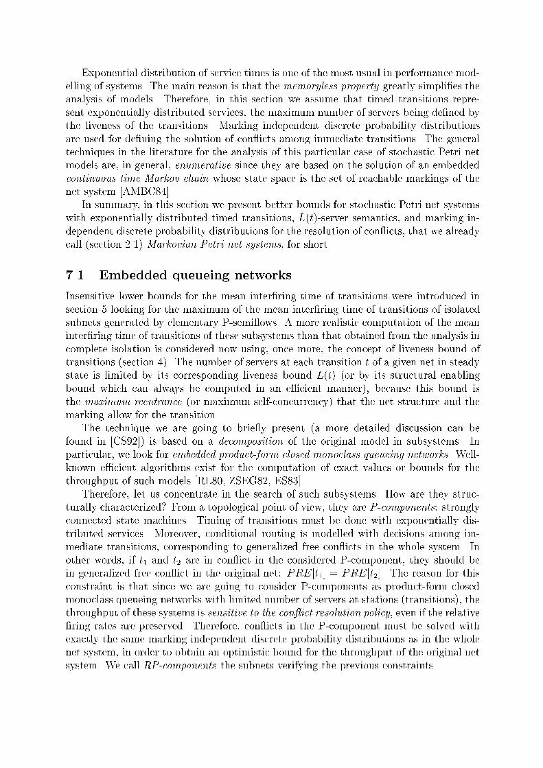
Exponential distribution of service times is one of the most usual in performance mod-elling of systems. The main reason is that the memoryless property greatly simpli�es theanalysis of models. Therefore, in this section we assume that timed transitions repre-sent exponentially distributed services, the maximum number of servers being de�ned bythe liveness of the transitions. Marking independent discrete probability distributionsare used for de�ning the solution of con icts among immediate transitions. The generaltechniques in the literature for the analysis of this particular case of stochastic Petri netmodels are, in general, enumerative since they are based on the solution of an embeddedcontinuous time Markov chain whose state space is the set of reachable markings of thenet system [AMBC84].In summary, in this section we present better bounds for stochastic Petri net systemswith exponentially distributed timed transitions, L(t)-server semantics, and marking in-dependent discrete probability distributions for the resolution of con icts, that we alreadycall (section 2.1) Markovian Petri net systems, for short.7.1 Embedded queueing networksInsensitive lower bounds for the mean inter�ring time of transitions were introduced insection 5 looking for the maximum of the mean inter�ring time of transitions of isolatedsubnets generated by elementary P-semi ows. A more realistic computation of the meaninter�ring time of transitions of these subsystems than that obtained from the analysis incomplete isolation is considered now using, once more, the concept of liveness bound oftransitions (section 4). The number of servers at each transition t of a given net in steadystate is limited by its corresponding liveness bound L(t) (or by its structural enablingbound which can always be computed in an e�cient manner), because this bound isthe maximum reentrance (or maximum self-concurrency) that the net structure and themarking allow for the transition.The technique we are going to brie y present (a more detailed discussion can befound in [CS92]) is based on a decomposition of the original model in subsystems. Inparticular, we look for embedded product-form closed monoclass queueing networks. Well-known e�cient algorithms exist for the computation of exact values or bounds for thethroughput of such models [RL80, ZSEG82, ES83].Therefore, let us concentrate in the search of such subsystems. How are they struc-turally characterized? From a topological point of view, they are P-components: stronglyconnected state machines. Timing of transitions must be done with exponentially dis-tributed services. Moreover, conditional routing is modelled with decisions among im-mediate transitions, corresponding to generalized free con icts in the whole system. Inother words, if t1 and t2 are in con ict in the considered P-component, they should bein generalized free con ict in the original net: PRE[t1] = PRE[t2]. The reason for thisconstraint is that since we are going to consider P-components as product-form closedmonoclass queueing networks with limited number of servers at stations (transitions), thethroughput of these systems is sensitive to the con ict resolution policy, even if the relative�ring rates are preserved. Therefore, con icts in the P-component must be solved withexactly the same marking independent discrete probability distributions as in the wholenet system, in order to obtain an optimistic bound for the throughput of the original netsystem. We call RP-components the subnets verifying the previous constraints.

p 1

t 2

t 5

t 8

t 11

p3

p6

p 9

p12

t 3

t 6

t 9

t 12

p4

p7

p 10

p13

t 1

t 4

t 7

t 10

p2

p5

p 8

p11

N

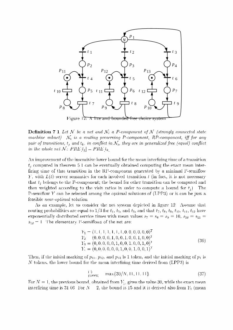
Figure 12: A live and bounded free choice system.De�nition 7.1 Let N be a net and Ni a P-component of N (strongly connected statemachine subnet). Ni is a routing preserving P-component, RP-component, i� for anypair of transitions, tj and tk, in con ict in Ni, they are in generalized free (equal) con ictin the whole net N : PRE[tj] = PRE[tk].An improvement of the insensitive lower bound for the mean inter�ring time of a transitiontj computed in theorem 5.1 can be eventually obtained computing the exact mean inter-�ring time of that transition in the RP-component generated by a minimal P-semi owY , with L(t){server semantics for each involved transition t (in fact, it is not necessarythat tj belongs to the P-component; the bound for other transition can be computed andthen weighted according to the visit ratios in order to compute a bound for tj). TheP-semi ow Y can be selected among the optimal solutions of (LPP3) or it can be just afeasible near-optimal solution.As an example, let us consider the net system depicted in �gure 12. Assume thatrouting probabilities are equal to 1=3 for t1, t2, and t3, and that t7, t8, t9, t10, t11, t12 haveexponentially distributed service times with mean values s7 = s8 = s9 = 10, s10 = s11 =s12 = 1. The elementary P-semi ows of the net are:Y1 = (1; 1; 1; 1; 1; 1; 1; 0; 0; 0; 0; 0; 0)TY2 = (0; 0; 0; 0; 1; 0; 0; 1; 0; 0; 1; 0; 0)TY3 = (0; 0; 0; 0; 0; 1; 0; 0; 1; 0; 0; 1; 0)TY4 = (0; 0; 0; 0; 0; 0; 1; 0; 0; 1; 0; 0; 1)T (36)Then, if the initial marking of p11, p12, and p13 is 1 token, and the initial marking of p1 isN tokens, the lower bound for the mean inter�ring time derived from (LPP3) is�(1)(LPP3) = maxf30=N; 11; 11; 11g (37)ForN = 1, the previous bound, obtained from Y1, gives the value 30, while the exact meaninter�ring time is 31.06. For N = 2, the bound is 15 and it is derived also from Y1 (mean

N �(1) �(1)(Y1)L �(1)(LPP3)1 31.06 30 302 21.05 20 153 17.71 16.67 114 16.03 15 115 15.03 14 1110 13.02 12 1115 12.35 11.34 11Table 2: Exact mean inter�ring time of t1, bounds obtained using (LPP3), and theimprovements presented in this section, for di�erent initial markings of p1 in the netsystem of �gure 12.inter�ring time of the P-component generated by Y1, considered in isolation with in�niteserver semantics for transitions). This bound does not take into account the queueingtime at places due to synchronizations (t4, t5, and t6), and the exact mean inter�ring timeof t1 is �(1) = 21:05. For larger values of N , the bound obtained from (LPP3) is equalto 11 (and is given by P-semi ows Y2, Y3 and Y4). This bound can be improved if theP-component generated by Y1 is considered with liveness bounds of transitions t7, t8, andt9 reduced to 1 (which is the liveness bound of these transitions in the whole net).The results obtained for di�erent values of N are collected in table 2. Exact values ofmean inter�ring times for the P-component generated by Y1 were computed using themeanvalue analysis algorithm [RL80]. This algorithm has O(A2B) worst case time complexity,where A = Y T �M0 is the number of tokens at the P-component and B = Y T � PRE � 11is the number of involved transitions (11 is a vector with all entries equal to 1). Exactcomputation on the original system takes several minutes in a Sun SPARC Workstationwhile bounds computation takes only a few seconds.We also remark that other techniques for the computation of throughput upper bounds(instead of exact values) of closed product-form monoclass queueing networks could beused, such as, for instance, balanced throughput upper bounds [ZSEG82] or throughput up-per bounds hierarchies [ES83]. Hierarchies of bounds guarantee di�erent levels of accuracy(including the exact solution), by investing the necessary computational e�ort. This pro-vides also a hierarchy of bounds for the mean inter�ring time of transitions of MarkovianPetri net systems.Finally, the technique sketched in this section can be applied to the more general caseof Coxian distributions (instead of exponential) for the service time of those transitionshaving either liveness bound equal to one (i.e., single-server stations) or liveness boundequal to the number of tokens in the RP-component (i.e., delay stations). The reasonis that in these cases the embedded queueing network has also product-form solution,according to a classical theorem of queueing theory: the BCMP theorem [BCMP75].

p1in p

2in

t 1 t 2

p1out p

2out

tJ

tF

(a)

tF

tJ

pJ

pF

t12

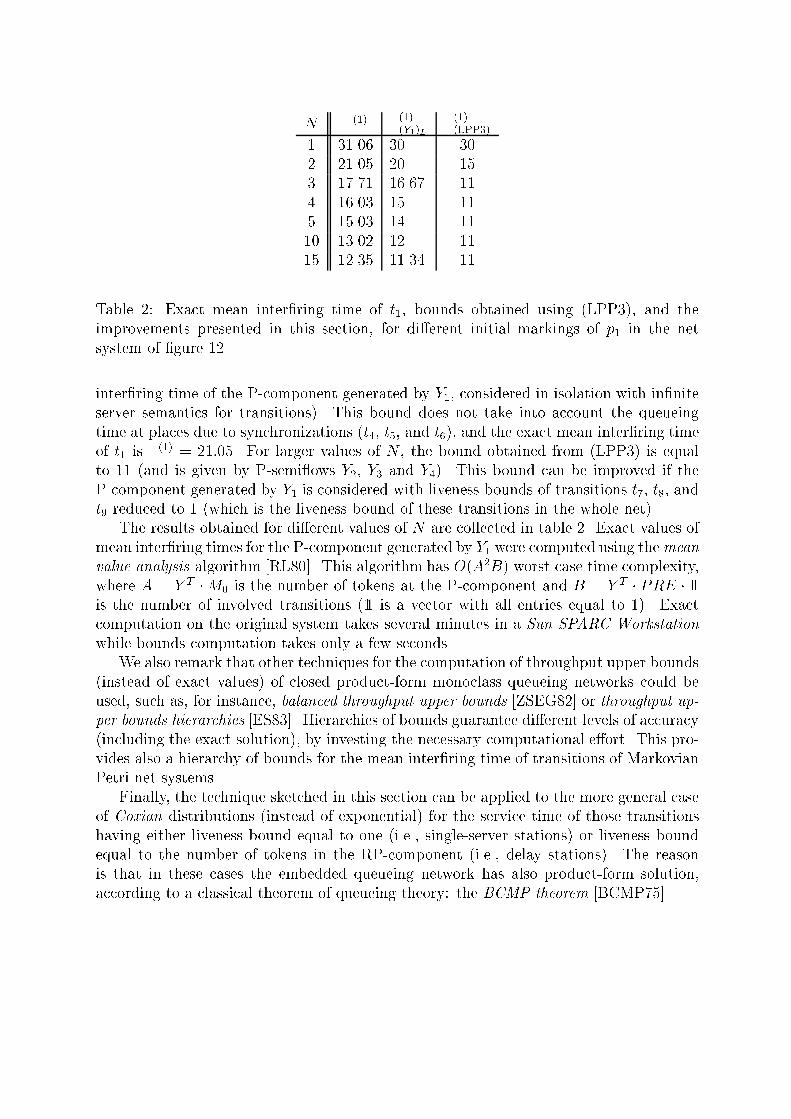
(b)Figure 13: (a) Elementary fork-join and (b) its reduction.7.2 Transformation techniquesThe lower bounds for the throughput of transitions presented in section 6 are valid forany probability distribution function of service times but can be very pessimistic in somecases. In this section, an improvement of such results is brie y explained for the caseof those net systems in which the following performance monotonicity property holds:a local pessimistic transformation leads to a slower transformed net system (i.e., a pes-simistic local transformation guarantees a pessimistic global behaviour). This property isnot always true as already mentionned (see, for instance, �gure 10). Using the conceptof stochastic ordering [Ros83], a pessimistic transformation is, for example, to substitutethe PDF of a service (or token-subnet traversing) time by a stochastically greater PDF.Live and bounded free choice is a class of systems for which the above performance mono-tonicity property holds (property 5.2 is a particular case). Details about the techniquespresented here can be found in [CSS91]. The basic ideas are:1. To use local pessimistic transformation rules to obtain a net system \simpler" thanthe original (e.g., with smaller state space) and with equal or less performance.2. To evaluate the performance for the derived net system, using insensitive boundspresented in section 6, exact analysis, or any other applicable technique.In order to obtain better bounds (after these two steps) than the values computed insection 6, at least one of the transformation rules of item 1 must be less pessimisticthan a total sequentialization of the involved transitions. We present �rst a rule whoseapplication allows such strict improvement: the fork-join rule. Secondly, a rule that doesnot change at all the performance (deletion of multistep preserving places) is presented.Finally, a rule that does not follow the above ideas is also presented: the goal of this rule(split of a transition) is to make reapplicable the other transformation rules.The most simple case of fork-join subnet that can be considered is depicted in �g-ure 13.a. In this case, if transitions t1 and t2 have exponential services X1 and X2 withmeans s1 and s2, they are reduced to a single transition (�gure 13.b) with exponentialservice time and mean:

s12 = E[maxfX1; X2g] = s1 + s2 � � 1s1 + 1s2��1 (38)Therefore, even if the mean traversing time of the reduced subnet by a single token hasbeen preserved, it has been substituted by a stochastically greater variable. A trivialextension can be applied if the fork-join subnet includes more than two transitions inparallel.Other transformation rules that have been presented in [CSS91] are:Deletion of a multistep preserving place: allows to remove some places without changingthe exact performance indices of the stochastic net system. In fact the places thatcan be deleted are those whose elimination preserves the multisets of transitionssimultaneously �rable in all reachable markings (e.g., place p14 in �gure 14.a). Thesize of the state space of the model is preserved and also the exact throughput oftransitions of the system.Reduction of transitions in sequence: reduces a series of exponential services to a singleexponential service with the same mean. Intuitively, this transformation makes in-divisible the service time of two or more transitions representing elementary actionswhich always occur one after the other and lead to no side condition (e.g., transi-tions t6 and t9 in �gure 14.a). Therefore, the state space of the model is reduced.The throughput of transitions is, in general, reduced.Split of a transition: this is not a state space reduction rule since it increases the statespace of the transformed net system. The advantage of the rule is that it allowsto proceed further in the reduction process using again the previous rules (e.g.,transition t3 in �gure 14.c).An example of application of all above transformation rules is depicted in �gure 14 fora strongly connected marked graph with exponential timing. Let us assume that meanservice times of transitions are: si = 1, i = 1; 2; 3; 7; 8; 12; 13; 14 and si = 10 otherwise.In order to compute �rstly the insensitive lower bounds on throughput introduced insection 6, it is necessary to derive the liveness bounds of transitions (section 4). In thiscase it is easy to see that L(tj) = 2 for every transition tj.The vector of visit ratios of a marked graph is the unique minimal T-semi ow of thenet: ~v(j) = 11, for all transitions tj. Therefore, the insensitive upper bound (valid forany probability distribution function of service times) of the mean inter�ring time of anytransition of the net system is � � 34. This value can be reached for some distributionsof service times (see comment on tightness on section 6). Nevertheless, if services areexponential the exact mean inter�ring time of transitions is � = 14:15.The quantitative results of the transformation process illustrated in �gure 14 are shownin table 3. We remark that the bound has been improved in polynomial time from 34 to19.2.8 Bounds for other performance indicesUp to this point we just concentrated on throughput bounds. The purpose of this sectionis to bring the idea that given some throughput bounds, bounds for other performance

(a) (b) (c)

(d) (e)

(g) (h) (i)

p1

p2 p3

t1

t2 t3

p6 p7

t7

p8 p9

t8

p14p15 p16 p17

t9

p10 p11 p12

t10 t11

p1p1

t1 t1

p2 p3 p2

t2

p4,5

t4,5

p8,9

t8

p13

p6

t6,9

p15

t12

p19

t13

p16,17

t10,11

p11,12

t7

p7

t3 t2,4,5,8

p13 p6 p7

t6,9

p15

t7,10,11,13

p19

t12

p18

t14

p1 p1

p3

t3

p4 p5

t4 t5 t6

t14t14

p18p18 p19

p13

t12 t13

t1

p2p'3 p"3

t1

p2p'3 p"3

t2,4,5,8t'3 t"3 t2,4,5,8

t'3,6,9t"3,7,10,11,13

p13 p6 p7p13 p15

p19

p15

p19

t7,10,11,13

t6,9

t12

p18

t14

t12

p18

t14

(f)

p1

t1

p'2,3p"3

t'2,4,5,8,3,6,9t"3,7,10,11,13

p13,15

p19

t12

p18

t14

p1

t1

p2,3 p"3

t'2,4,5,8,3,6,9,12

p18 p19

t14

t"3,7,10,11,13

p1

t1

p2,3,3

2..13t

p18,19

t14

t1..14

p1

Figure 14: A complete reduction process. The relative error between insensitive boundand exact value diminishes from 140% to 35%.

System �ub Relative errorFig. 14.a 34 140 %Fig. 14.b 29 105 %Fig. 14.c 29 105 %Fig. 14.d 29.5 108 %Fig. 14.e 29.5 108 %Fig. 14.f 24.8 75 %Fig. 14.g 24.8 75 %Fig. 14.h 19.2 35 %Fig. 14.i 19.2 35 %Table 3: Successive improvements of the upper bound for the mean inter�ring time oftransitions of the net in �gure 14 and relative errors with respect to the exact value� = 14:15.indices can be computed using classical formulas in QN theory such as Little's formula.The number of tokens in a place de�nes the lenght of the represented queue (includingthe customers in service!). Thus it may be important to known bounds on average markingof places.As an example, in [CCS91b] it has been shown that the following are lower and upperbounds for the average marking, M :M lb = PRE � S � ~�lb (39)Mub(p) = max f M(p) j BT �M = BT �M0 ; M �M lb g (LPP4)where S = diag (si) and the rows of BT are the basis of left annullers of C (the incidencematrix of the net).As an interesting remark, the reader can check that a structural absolute bound forthe marking of a place is given for conservative nets (i.e., 9Y > 0, Y T � C = 0) by thefollowing expression:SB(p) = max f M(p) j BT �M = BT �M0 ; M � 0 g (LPP5)The constraint in (LPP5) being weaker than that in (LPP4) (M � M 1b is transformedinto M � 0), it is obvious that Mub � SB(p).9 ConclusionsThe main motivation to write this paper has been to show how the qualitative theory (andin particular the structural analysis techniques) of net systems can be useful in perfor-mance bounds computation for stochastic Petri net models. Several interesting questionsthat were easily answered in the past for classical queueing networks turn into non-trivial

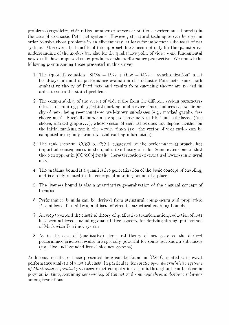
problems (ergodicity, visit ratios, number of servers at stations, performance bounds) inthe case of stochastic Petri net systems. However, structural techniques can be used inorder to solve those problems in an e�cient way, at least for important subclasses of netsystems. Moreover, the bene�ts of this approach have been not only for the quantitativeunderstanding of the models but also for the qualitative point of view: some fundamentalnew results have appeared as by-products of the performance perspective. We remark thefollowing points among those presented in this survey:1. The (quoted) equation \SPNs = PNs + time = QNs + synchronization" mustbe always in mind in performance evaluation of stochastic Petri nets, since bothqualitative theory of Petri nets and results from queueing theory are needed inorder to solve the stated problems.2. The computability of the vector of visit ratios from the di�erent system parameters(structure, routing policy, initial marking, and service times) induces a new hierar-chy of nets, being re-encountered well-known subclasses (e.g., marked graphs, freechoice nets). Specially important appear those nets as FRT and subclasses (freechoice, marked graphs: : : ), whose vector of visit ratios does not depend neither onthe initial marking nor in the service times (i.e., the vector of visit ratios can becomputed using only structural and routing information).3. The rank theorem [CCS91b, ES91], suggested by the performance approach, hasimportant consequences in the qualitative theory of nets. Some extensions of thattheorem appear in [CCS90b] for the characterization of structural liveness in generalnets.4. The enabling bound is a quantitative generalization of the basic concept of enabling,and is closely related to the concept of marking bound of a place.5. The liveness bound is also a quantitative generalization of the classical concept ofliveness.6. Performance bounds can be derived from structural components and properties:P-semi ows, T-semi ows, multisets of circuits, structural enabling bounds: : :7. An step to extend the classical theory of qualitative transformation/reduction of netshas been achieved, including quantitative aspects, for deriving throughput boundsof Markovian Petri net system.8. As in the case of (qualitative) structural theory of net systems, the derivedperformance-oriented results are specially powerful for some well-known subclasses(e.g., live and bounded free choice net systems).Additional results to those presented here can be found in [CS90], related with exactperformance analysis of a net subclass. In particular, for totally open deterministic systemsof Markovian sequential processes, exact computation of limit throughput can be done inpolynomial time, assuming consistency of the net and some synchronic distance relationsamong transitions.

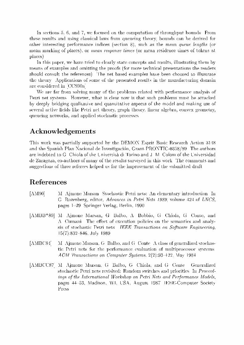
In sections 5, 6, and 7, we focused on the computation of throughput bounds. Fromthese results and using classical laws from queueing theory, bounds can be derived forother interesting performance indices (section 8), such as the mean queue lengths (ormean marking of places), or mean response times (or mean residence times of tokens atplaces).In this paper, we have tried to clearly state concepts and results, illustrating them bymeans of examples and omitting the proofs (for more technical presentations the readersshould consult the references). The net based examples have been choosed to illustratethe theory. Applications of some of the presented results in the manufacturing domainare considered in [CCS90a].We are far from solving many of the problems related with performance analysis ofPetri net systems. However, what is clear now is that such problems must be attackedby deeply bridging qualitative and quantitative aspects of the model and making use ofseveral active �elds like Petri net theory, graph theory, linear algebra, convex geometry,queueing networks, and applied stochastic processes.AcknowledgementsThis work was partially supported by the DEMON Esprit Basic Research Action 3148and the Spanish Plan Nacional de Investigaci�on, Grant PRONTIC-0358/89. The authorsare indebted to G. Chiola of the Universit�a di Torino and J. M. Colom of the Universidadde Zaragoza, co-authors of many of the results surveyed in this work. The comments andsuggestions of three referees helped us for the improvement of the submitted draft.References[AM90] M. Ajmone Marsan. Stochastic Petri nets: An elementary introduction. InG. Rozenberg, editor, Advances in Petri Nets 1989, volume 424 of LNCS,pages 1{29. Springer-Verlag, Berlin, 1990.[AMBB+89] M. Ajmone Marsan, G. Balbo, A. Bobbio, G. Chiola, G. Conte, andA. Cumani. The e�ect of execution policies on the semantics and analy-sis of stochastic Petri nets. IEEE Transactions on Software Engineering,15(7):832{846, July 1989.[AMBC84] M. Ajmone Marsan, G. Balbo, and G. Conte. A class of generalized stochas-tic Petri nets for the performance evaluation of multiprocessor systems.ACM Transactions on Computer Systems, 2(2):93{122, May 1984.[AMBCC87] M. Ajmone Marsan, G. Balbo, G. Chiola, and G. Conte. Generalizedstochastic Petri nets revisited: Random switches and priorities. In Proceed-ings of the International Workshop on Petri Nets and Performance Models,pages 44{53, Madison, WI, USA, August 1987. IEEE-Computer SocietyPress.

[AMBCD86] M. Ajmone Marsan, G. Balbo, G. Chiola, and S. Donatelli. On the product-form solution of a class of multiple-bus multiprocessor system models. Jour-nal of Systems and Software, 6(1,2):117{124, May 1986.[BCMP75] F. Baskett, K. M. Chandy, R. R. Muntz, and F. Palacios. Open, closed, andmixed networks of queues with di�erent classes of customers. Journal of theACM, 22(2):248{260, April 1975.[Bes87] E. Best. Structure theory of Petri nets: The free choice hiatus. In W. Brauer,W. Reisig, and G. Rozenberg, editors, Advances in Petri Nets 1986 - PartI, volume 254 of LNCS, pages 168{205. Springer-Verlag, Berlin, 1987.[Cam90] J. Campos. Performance Bounds for Synchronized Queueing Networks. PhDthesis, Departamento de Ingenier��a El�ectrica e Inform�atica, Universidad deZaragoza, Spain, October 1990. Research Report GISI-RR-90-20.[CC91] J. Campos and J. M. Colom. A reachable throughput upper bound forlive and safe free choice nets. In Proceedings of the Twelfth InternationalConference on Application and Theory of Petri Nets, pages 237{256, Gjern,Denmark, June 1991.[CCCS89] J. Campos, G. Chiola, J. M. Colom, and M. Silva. Tight polynomial boundsfor steady-state performance of marked graphs. In Proceedings of the 3rdInternational Workshop on Petri Nets and Performance Models, pages 200{209, Kyoto, Japan, December 1989. IEEE-Computer Society Press.[CCCS90] J. Campos, G. Chiola, J. M. Colom, and M. Silva. Properties and perfor-mance bounds for timed marked graphs. Research Report GISI-RR-90-17, Departamento de Ingenier��a El�ectrica e Inform�atica, Universidad deZaragoza, Spain, July 1990. To appear in IEEE Transactions on Circuitand Systems.[CCS90a] J. Campos, J. M. Colom, and M. Silva. Performance evaluation of repeti-tive automated manufacturing systems. In Proceedings of the Rensselaer'sSecond International Conference on Computer Integrated Manufacturing,pages 74{81, Rensselaer Polytechnic Institute, Troy, NY, USA, May 1990.IEEE-Computer Society Press.[CCS90b] J. M. Colom, J. Campos, and M. Silva. On liveness analysis through lin-ear algebraic techniques. In Proceedings of the Annual General Meeting ofESPRIT Basic Research Action 3148 Design Methods Based on Nets (DE-MON), Paris, France, June 1990.[CCS91a] J. Campos, G. Chiola, and M. Silva. Ergodicity and throughput bounds ofPetri nets with unique consistent �ring count vector. IEEE Transactions onSoftware Engineering, 17(2):117{125, February 1991.[CCS91b] J. Campos, G. Chiola, and M. Silva. Properties and performance boundsfor closed free choice synchronized monoclass queueing networks. IEEETransactions on Automatic Control, 36(12):1368{1382, December 1991.

[CCS91c] J. Campos, J. M. Colom, and M. Silva. Improving throughput upperbounds for net based models. In Proceedings of the IMACS-IFAC SYM-POSIUM Modelling and Control of Technological Systems, pages 573{582,Lille, France, May 1991. To appear in the IMACS Transactions.[CS90] J. Campos and M. Silva. Steady-state performance evaluation of totally opensystems of Markovian sequential processes. In M. Cosnard and C. Girault,editors, Decentralized Systems, pages 427{438. Elsevier Science PublishersB.V. (North-Holland), Amsterdam, The Netherlands, 1990.[CS91] J. M. Colom and M. Silva. Improving the linearly based characterization ofP/T nets. In G. Rozenberg, editor, Advances in Petri Nets 1990, volume483 of LNCS, pages 113{145. Springer-Verlag, Berlin, 1991.[CS92] J. Campos and M. Silva. Embedded queueing networks and the improvementof insensitive performance bounds for Markovian Petri net systems. ResearchReport GISI-RR-92-10, Departamento de Ingenier��a El�ectrica e Inform�atica,Universidad de Zaragoza, Spain, February 1992.[CSS91] J. Campos, B. S�anchez, and M. Silva. Throughput lower bounds for Marko-vian Petri nets: Transformation techniques. In Proceedings of the 4rd Inter-national Workshop on Petri Nets and Performance Models, pages 322{331,Melbourne, Australia, December 1991. IEEE-Computer Society Press.[DLT90] Y. Dallery, Z. Liu, and D. Towsley. Equivalence, reversibility and symmetryproperties in fork/join queueing networks with blocking. Technical report,MASI 90-32, University Paris 6, 4 Place Jussieu, Paris, France, June 1990.[ES83] D. L. Eager and K. C. Sevcik. Performance bound hierarchies for queueingnetworks. ACM Transactions on Computer Systems, 1(2):99{115, May 1983.[ES91] J. Esparza and M. Silva. On the analysis and synthesis of free choice systems.In G. Rozenberg, editor, Advances in Petri Nets 1990, volume 483 of LNCS,pages 243{286. Springer-Verlag, Berlin, 1991.[Esp90] J. Esparza. Structure Theory of Free Choice Nets. PhD thesis, Departamentode Ingenier��a El�ectrica e Inform�atica, Universidad de Zaragoza, Spain, June1990. Research Report GISI-RR-90-03.[FFN91] G. Florin, C. Fraize, and S. Natkin. Stochastic Petri nets: Properties,applications and tools.Microelectronics and Reliability, 31(4):669{698, 1991.[FN85] G. Florin and S. Natkin. Les r�eseaux de Petri stochastiques. Technique etScience Informatiques, 4(1):143{160, February 1985. In French.[GN67] W. J. Gordon and G. F. Newell. Closed queueing systems with exponentialservers. Operations Research, 15:254{265, 1967.[Hac72] M. H. T. Hack. Analysis of production schemata by Petri nets. M. S. Thesis,TR-94, M.I.T., Boston, USA, 1972.

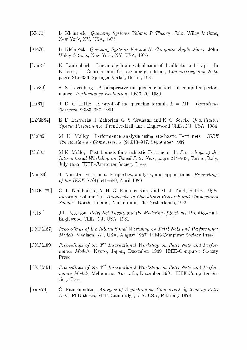
[Kle75] L. Kleinrock. Queueing Systems Volume I: Theory. John Wiley & Sons,New York, NY, USA, 1975.[Kle76] L. Kleinrock. Queueing Systems Volume II: Computer Applications. JohnWiley & Sons, New York, NY, USA, 1976.[Lau87] K. Lautenbach. Linear algebraic calculation of deadlocks and traps. InK. Voss, H. Genrich, and G. Rozenberg, editors, Concurrency and Nets,pages 315{336. Springer-Verlag, Berlin, 1987.[Lav89] S. S. Lavenberg. A perspective on queueing models of computer perfor-mance. Performance Evaluation, 10:53{76, 1989.[Lit61] J. D. C. Little. A proof of the queueing formula L = �W . OperationsResearch, 9:383{387, 1961.[LZGS84] E. D. Lazowska, J. Zahorjan, G. S. Graham, and K. C. Sevcik. QuantitativeSystem Performance. Prentice-Hall, Inc., Englewood Cli�s, NJ, USA, 1984.[Mol82] M. K. Molloy. Performance analysis using stochastic Petri nets. IEEETransaction on Computers, 31(9):913{917, September 1982.[Mol85] M.K. Molloy. Fast bounds for stochastic Petri nets. In Proceedings of theInternational Workshop on Timed Petri Nets, pages 244{249, Torino, Italy,July 1985. IEEE-Computer Society Press.[Mur89] T. Murata. Petri nets: Properties, analysis, and applications. Proceedingsof the IEEE, 77(4):541{580, April 1989.[NRKT89] G. L. Nemhauser, A. H. G. Rinnooy Kan, and M. J. Todd, editors. Opti-mization, volume 1 of Handbooks in Operations Research and ManagementScience. North-Holland, Amsterdam, The Netherlands, 1989.[Pet81] J.L. Peterson. Petri Net Theory and the Modeling of Systems. Prentice-Hall,Englewood Cli�s, NJ, USA, 1981.[PNPM87] Proceedings of the International Workshop on Petri Nets and PerformanceModels, Madison, WI, USA, August 1987. IEEE-Computer Society Press.[PNPM89] Proceedings of the 3rd International Workshop on Petri Nets and Perfor-mance Models, Kyoto, Japan, December 1989. IEEE-Computer SocietyPress.[PNPM91] Proceedings of the 4rd International Workshop on Petri Nets and Perfor-mance Models, Melbourne, Australia, December 1991. IEEE-Computer So-ciety Press.[Ram74] C. Ramchandani. Analysis of Asynchronous Concurrent Systems by PetriNets. PhD thesis, MIT, Cambridge, MA, USA, February 1974.

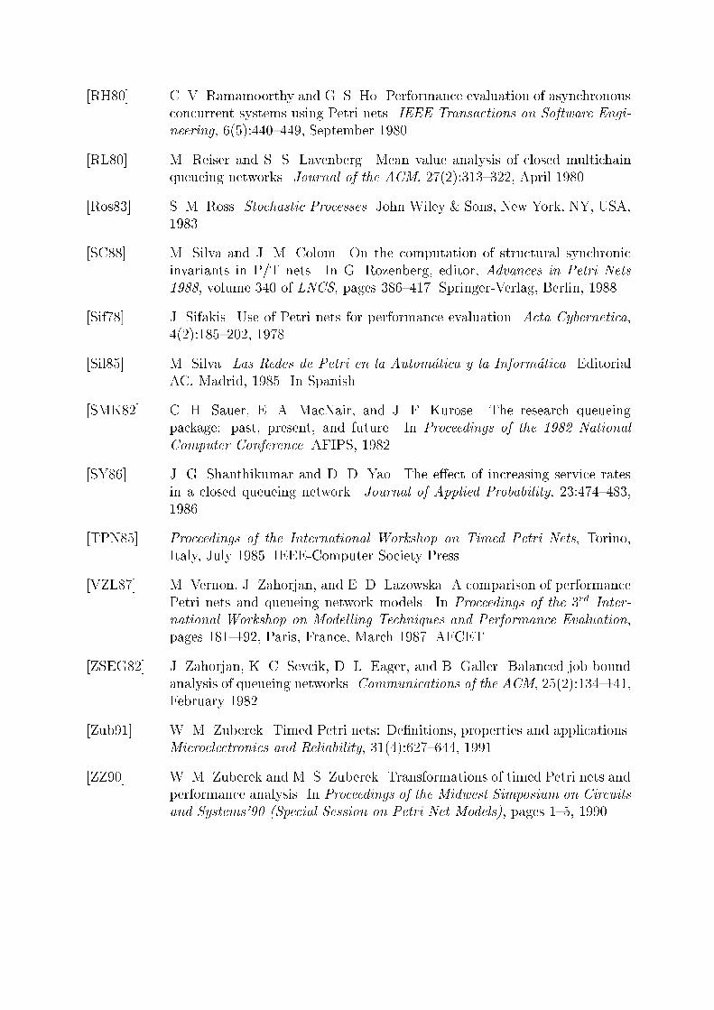
[RH80] C. V. Ramamoorthy and G. S. Ho. Performance evaluation of asynchronousconcurrent systems using Petri nets. IEEE Transactions on Software Engi-neering, 6(5):440{449, September 1980.[RL80] M. Reiser and S. S. Lavenberg. Mean value analysis of closed multichainqueueing networks. Journal of the ACM, 27(2):313{322, April 1980.[Ros83] S. M. Ross. Stochastic Processes. John Wiley & Sons, New York, NY, USA,1983.[SC88] M. Silva and J. M. Colom. On the computation of structural synchronicinvariants in P/T nets. In G. Rozenberg, editor, Advances in Petri Nets1988, volume 340 of LNCS, pages 386{417. Springer-Verlag, Berlin, 1988.[Sif78] J. Sifakis. Use of Petri nets for performance evaluation. Acta Cybernetica,4(2):185{202, 1978.[Sil85] M. Silva. Las Redes de Petri en la Autom�atica y la Inform�atica. EditorialAC, Madrid, 1985. In Spanish.[SMK82] C. H. Sauer, E. A. MacNair, and J. F. Kurose. The research queueingpackage: past, present, and future. In Proceedings of the 1982 NationalComputer Conference. AFIPS, 1982.[SY86] J. G. Shanthikumar and D. D. Yao. The e�ect of increasing service ratesin a closed queueing network. Journal of Applied Probability, 23:474{483,1986.[TPN85] Proceedings of the International Workshop on Timed Petri Nets, Torino,Italy, July 1985. IEEE-Computer Society Press.[VZL87] M. Vernon, J. Zahorjan, and E. D. Lazowska. A comparison of performancePetri nets and queueing network models. In Proceedings of the 3rd Inter-national Workshop on Modelling Techniques and Performance Evaluation,pages 181{192, Paris, France, March 1987. AFCET.[ZSEG82] J. Zahorjan, K. C. Sevcik, D. L. Eager, and B. Galler. Balanced job boundanalysis of queueing networks. Communications of the ACM, 25(2):134{141,February 1982.[Zub91] W. M. Zuberek. Timed Petri nets: De�nitions, properties and applications.Microelectronics and Reliability, 31(4):627{644, 1991.[ZZ90] W. M. Zuberek and M. S. Zuberek. Transformations of timed Petri nets andperformance analysis. In Proceedings of the Midwest Simposium on Circuitsand Systems'90 (Special Session on Petri Net Models), pages 1{5, 1990.