on exact equilibrium distributions of stochastic petri nets
TRANSCRIPT
On Exact Equilibrium Distributions of
Stochastic Petri Nets
by
Diana Lucic
B.Sc.(Ma.)(Hons.), University of Adelaide, South Australia
C( r r,-i+ t "i'q
t'-¿i\
Thesis submitted for the degree
of Doctor of Philosophy
in the
Department of Applied Mathematics
University of Adelaide.
November 1990.
I
l
I
I
l
Contents
List of Figures
Surnrnary
Declaration
Acknowledgemeuts
1 Introduction
2 An Introduction to Petri Nets, Tirned Petri Nets and Stochastic
Petri Nets
2.1 The Behavioural and Structural Properties of Petri Nets
2.L.L Behavioural Properties .
2.1.2 Analysing the Behavioural Properties
2.1.3 Structural Properties
2.2 Subclasses of PNs
2.3 Time Extended Models
2.4 Deterministic Delays
2.4.1 Timed Transitions
2.4.2 Timed Places
2.5 Stochastic Petri Nets
2.5.L Timed Tra¡rsitions
lv
vl
vll
vlu
1
6
I
I
I74
16
16
L7
77
2T
27
22
30
I
2.5.2 Timed Places
3 Closed Forrn Solutions
3.1 Product Form Solutions
3.2 Description of the lt{odel
3.3 The Routeing Process
3.4 The Extended Product Form Solution
3.5 Examples
3.6 Other \Mork on Product Form solutions in SPNs
4 Insensitivity Theory Applied to SPNs
4.I A Survey of the Theory of Insensitivity
4.2 SPNs with Generally Distributed Firing Times
4.2.1 Use of the semi-\{arkov Process
4.2.2 SPN Approximation of General Distributions
4.3 A Generalised semi-\{arkov Process
4.4 Balance Equations, Insensitivit¡' utrd Applications .
4.5 Age Dependent Routeing
4.6 Transition lr{erging .
4.7 MarkingAmalgamation
4.8 Simultaneousl¡' Enabled Generally Distributed Transitions
4.9 General Fork-Join Sections
5 Aggregation and Disaggregation in SPNs
5.1 Approximation Techniques. .
5.2 An Introduction to Aggregation and Disaggregation at the Net
Level
5.3 Definitions and Basic Results
5.4 Aggregation
31
32
ttJtJ
40
À,4TI
50
65
68
69
73
74
/Ð
/o
78
E4
86
90
97
106
110
110
114
116
119
5.5 Disaggregation
ll
12r

5.5.1 The Supplemented and Unsupplemented Equilibrium Dis-
tributions for the SPN P
5.5.2 The General Theory
. 722
. r25
t29
131
135
t4L
145
6 Conclusions
Appendix A
Appendix B
Appendix C
Bibliography
lll
List of Figures
Figure 2.1
Figure 2.2
Figure 2.3
Figure 2.4
Figure 3.1
Figure 3.2
Figure 3.3
Figure 3.4
Figure 3.5
Figure 3.6
Figure 3.7
Figure 3.8
Figure 4.1
Figure 4.2
Figure 4.3
Figure 4.4
Figure 4.5
Figure 4.6
Figure 4.7
Figure 4.8
Figure 4.9
Figure 4.10
A SPN to iliustrate the coverability tree approach.
The coverability tree of the SPN in Figure 2.1.
An example of conflict.
A simple SPN representing concurrent activities.
An example of a SPN with marking dependent firing rates
The SPN for Example 3.4.
An unbounded SPN
A SPN representation of a simple open Jackson network.
A SPN representation of a simple closed Jackson network.
The SPN for Example 3.8.
The transition merged SPN for Example 3.8.
An unbounded SPN
A SPN representation of the Erlaog-r distribution.
A GSPN representation of the Erlang-r distribution. . : .
A SPN representation of a simplified dual processor modcl
The dual processor model of Lazar and Robertazzi.
A high level PN of a circuit switched netrvork.
An altered dual processor model to illustrate transition
merging.
The dual processor of Figure 4.6 with a merged transition.
A coloured SPN to illustrate marking amalgamation.
The amalgamated process of the SPN in Figure 4.8.
A 3-dimensional fork-join section.
10
10
20
22
J/
38
42
49
51
54
54
59
/Ð
75
79
79
81
88
88
93
95
99
lv

Figure 4.11
Figure 5.1
Figure 5.2
Figure 5.3
Figure 5.4
Figure 5.5
Figure 5.6
An n-dimensional fork-join section.
A simple SPN to illustrate aggregation. . .
The aggregated SPN of Figure 5.1.
The dual processor of Figure 4.3 with complex memory
access stage.
The aggregated SPN of Figure 5.3.
A partially expanded SPN of Figure 5.4.
A subnet of Figure 5.5. . .
106
116
116
119
119
L23
126
v
Surnrnary
Chapter 1 introduces a PN and its time extended counterparts. the timed PN
and the SPN. The problems associated rvith theìr analysis are presentecl and a
summary of the techniques we use in an attempt to overcome these problems is
given.
Chapter 2 gives a survey of the t¡1pes of properties that are analvsed in PNs.
Time-extended PNs are then introduced and a survey of the different models used
is given.
Chapter 3 describes the extended product form solutions for SPNs and gives
some explanatory examples.
Chapter 4 addresses the problems related to generally distributed firing tines.
It contains an introduction to the topics of insensitivity and Generalised Semi-
Markov processes. The concepts are then applied to SPNs, and further extensions
are introduced, allorving the consideration of transition merging, marking amal-
gamation and another extension to the theory of insensitivity.
Chapter 4 is used as the foundation for the work in Chapter 5. Using the
theor¡' of insensitivity, rr'e shorv horv to aggregate and then disaggregate SPNs to
yield exact equilibrium distributions.
Chapter 6 contains conclusions and some ideas for further research, arising
from the rvork presented in this thesis.
1.I

Declaration
I declare that the contents of this thesis have not been submitted to anv
university for the purpose of obtaining any other degree or diploma.
Also, to the best of my knorvledge and belief, this thesis contains no material
previously published or s'ritten by another person, except where due reference is
made in the text.
I consent to this thesis being made available for photocopying and loan.
Diana Lucic
vll

Acknowledgements
I would like to sincerely thank my supervisor Bill Henderson, for his endless
patience and encouragement throughout the work toward this thesis. I u,ouÌd
also like to thank my parents for their support and for providing me with this
opportunity. Also, thanks go to Allan Bramley, for proof reading this thesis in
it's later stages.
The receipt of a Commonwealth Postgraduate Research Award, and a short
term Adelaide Scholarship, supplemented by a grant from the Teletraffic Research
Centre at the University of Adelaide are acknowledged.
Finally, I would like to thank Nigel for his encouragement, for being so tolerant
and for his a^stounding patience. Thank you also, for drawing my pictures and
proof reading this thesis. Most importantly, thank you for all your love.
vllt
Chapter 1
Introduction
A Petri Net (PN) is a graph model, designed to include the analysis of systems
which exhibit concurrent and conflicting behaviour. As a graphical tool, PNs share
the same task as a flow chart, block diagram or network. In addition, tokens are
used to simulate the dynamic and concurrent activities in the model.
Historically, the basic concepts of PN theory were developed from the s'ork of
Carl Adam Petri [80], in his doctoral dissertation. Further developments of the
theory came from a report by Holt and Commoner [44], in rvhich it was shou'n
how PNs could be applied to the modelling and analysis of systems of concurrent
components.
Formally, a PN is a bipartite directed graph, which can be defined by the
follorving five-tuple,
N : (P,T,I,O,*o).t
P : {pt.,...,p,}, r : lPl, is a finite set of places, represented by circles, and
T -- {rt,...,f"}, r : l7l, is a finite set of transitions, represented b1' ba¡s. The
directed arcs, connect places to transitions and transitions to places. The input
function, I : T -- Z', isa mapping from a transition t e T to its input bag I(/),
which is an r x I colunn vector, giving the input places (including multiplicity)
of transition t. The output function, O : T - Z', is a mapping from a transition
ú to its output bag O(t), which is an r x 1 column vector, giving the outputlNote that boldface characters will be used at all times to represent vectors, components of a
vector will be in normal type.
1

piaces (including multiplicity) of ú . These represent the pre- and post- conditions
respectively. The use of bags, rather than sets, allows a place to be a multiple
input or multiple output, (for a brief discussion on bag theory see Peterson [7g]).
A marking, m, is an r x 1 column vector, rvhich assigns to each place a non-
negative integer. For example, the ith component, *(i), is the number of tokens
in place P; e P. The initial marking, rn¡, r€pr€sents the initial token distribution.
In the modelling of PNs, it is often useful to identify places rvith conditions
and to identify the firing of transitions with events. Before a transition can fire,
or an event can occur, a pre-condition must be satisfied and is given by,
('o-I(ú))>0
That is, for every input place into a transition, there must be at least as many
tokens in it, as there are arcs from the place to the transition. \\¡hen this condi-
tion is satisfied, the transition is said to be enabled and ma¡- then fire. \\rhen a
transition fires, tokens are removed from its input places and deposited in its out-
put places, one token for each arc. This is executed instantaneously for PNs and
executed in two phases for time extended PNs. In the first phase, the transition
becomes enabled and waits for a period of time, until it fires (if it still can). In the
second phase the transition starts firing, thereb¡' removing tokens from it's input
places. At the end of the firing time, the tokens are deposited into it's output
places.
The state of the PN is defined by its marking. When a transition fires, there
is a cha^nge in the token distribution and therefore in the marking of the net. The
result of firing a transition, from a marking rn, is a new marking rn'. Successive
firings of the enabled transitions in the PN, result in a set of markin gs, M, which
are conrl,ected through the firing sequence. The state space of the PN is called a
reachability tree/graph.
The analysis of PNs, has revolved around checking correctness, and observing
the behaviour, of the system modelled by the PN. Consequentl¡ a rrariety of
2
behavioural and structural properties have been observed, which have therefore
induced the creation of several analysis techniques. In Chapter 2, we give a sample
of the types of properties analvsed and the techniques used to verify them.
The concept of time was not explicitll' given in the original definition of PNs
(see Petri [80]). When timing rvas introduced, it was in the form of time delays,
associated with either the firing of the transitions, or the time spent by the tokens
in the places of the net. If the time delal,s a^re given deterministicaJly, the nets
axe commonly known as timed PNs and if they are given probabilistically, they
a¡e known as Stochastic PNs (SPNs).
With the advent of time-extended PNs, analysts in the field have turned their
attention to the performance evaluation of the system being modelled by the time-
extended PN. We continue s'ith the same theme in this thesis, and aim to find
the equilibrium distribution of SPNs in exact form. Conventional methods have
relied on analysing the underlying Markov process, however, there are inherent
difficulties in attempting to find the equilibrium distribution in this rva¡ and
so alternative methods are required. The techuiques \áe present, for finding the
equilibrium distribution i¡r exact form, avoid some of these stumbling blocks.
There are two problems that make solving the global bala¡rce equations un-
suitable. Firstly, using any firing time other than the negative exponentially dis-
tributed firing time, causes the underlying process to lose it's Markovian nature.
Secondly, the number of markings in the \{arkov process, grorÃ/s exponentially
with the number of tokens and places in the net.
Obviously, the first problem does not arise if no other firing time distribution
but the negative exponential distribution is used in the model. However, if reality
is to be modelled accurately, this is a harsh restriction. In Sections 2.3, 2.4 and
2.5, we give a survey, from the literature, of the types of models that incorporate
generally distributed firing times (we include deterministic firing times in this
class) and the type of restrictions imposed to ensure that a solution can be easily
3
extracted. In Chapter 4, tl'e introduce the theory of "insensitivity" in generalised
semi-Markov processes and apply this theory to SPNs. In blief, the concept of
insensitivity is that the governing distributions in the process, mav be replaced
by other distributions, each rvith the same mean, without altering the equilibrium
distribution of the process. Therefore, the difÊculties associated with the general
distributions can be reduced to a relatively simple problem, invoh'ing onl1, ¡"*-ative exponential distributions, or other convenient distributions, s'itir the same
means.
Further extensions to the theory of insensitivity, by Rumservicz and Hender-
son [87] discussed in Section 4.5, create the foundations for some nerv results
presented in the remainder of Chapter 4. In Section 4.6, we present the theory
on transition merging. In Section 4.7, we consider marking amalgamation of the
underlying process and provide conditions for which u¡e are able to extract exact
marginal distributions for the original SPN. The procedure is to amalgamate the
markings of the process, so that the resultant process is insensitive to its generally
distributed firing times. In Section 4.8 an extension to the theory of insensitivity
is given, which allows a set of generally distributed fuing times to be enabled
simultaneously.
The marking amalgamation procedure outlined above, reduces the number of
markings and therefore the size of the process that must be analvsecl. In Chapter
3, we present a solution technique which also reduces the effect of the marking
explosion problem. Note that the marking explosion problem is not unique to
SPNs. A similar problem in networks of queues lead researchers in the field, to
look for a method of finding the equilibrium distribution, which did not require
the analysis of the state space. The result was what is called the product form
solution. Standard assumptions iu queueing theory are, that customers arrive
and are routed through the network in a mar¡ner which may depend on the state,
but not on thê routeing of other customers. In a SPN this is not true, as the
4

tokens move around in batches and the routeing of individual tokens is correlated.
Consequently, the theory on product form solutions for queueing netrvorks has
not been applicable to SPNs. In Chapter 3, we adapt the work of Henderson and
Taylor [41], who incorporate batch movement and correlated routeing into their
queueing netrvork. In doing this we achieve an extended product form solution for
SPNs. The centra.l feature of this technique, is to consider the transitions of the
SPN to be the states of a Markov chain, called the routeing process. This is an
obvious advantage, since the number of transitions in the net will, almost always,
be fewer in number than the markings of the net.
In Chapter 5, we present another technique which reduces the effect of the
marking explosion problem, by aggregating and disaggregating the subnets of the
SPN, using the results of Chapter 4. The aim of this technique, is to amalgamate
subnets of the SPN, so that the remaining "skeleton" net is insensitive to the time
spent in the subnets. Once this is established, the exact marginal distribution
for the original net can be obtained. \\¡e then use the results of insensitivity
theory, to disaggregate the subnets, and obtain the equilibrium distribution for
the original net in exact form. The benefit of this approach, is that the size of
the ma¡king process has been reduced considerably, either when extracting the
marginal distribution using the skeleton net, or when disaggregating to find the
equilibrium distribution for the original net.
b
Chapter 2
An Introduction to Petri Nets, TirnedPetri Nets and Stochastic Petri Nets
PNs have no time associated with an activitf in the model and are therefore not
relevant in analysing time dependent performance measures, such as an equilib-
rium distribution. As was stated in the introduction, it is the focus of this thesis
to extract such time dependent behaviour. For this reason r¡'e do not dwell on
the explanation and use of PNs, rather rve give a brief overvierv, and direct those
readers who may be interested to a list of references given below. The extension
of time in PNs u'ill be addressed later in this chapter.
From 1970 to 1975 the Computation Structure Group from \{.I.T. produced
many reports and theses on PNs. The first book concerned with PNs was written
by J.L. Peterson [79] in 1980, a second book was written by W. Reisig [86] in
1984. These two books contain references for most of the PN related works up to
and including 1984.
Since then there have been numerous s'orkshops and conferences devoted to
PNs a¡rd time extended PNs. The proceedings are mostly limited to the conference
participants, however, some selected papers and other articles have been published
in Ailaances in Petri Nets. The 1987 volume contains the most comprehensive
bibliography of papers concerned r+'ith PNs and time extended PNs, from 1962
to 1987. For an updated bibliography on rvhere to find further publications see
Murata [76].
A series of international conferences concerned mainly with timed and Stochas-
6

tic PNs began in 1985 and have since been held biennially. Each of these work-
shops is accompanied by proceedings; all three are available from the IEEE Com-
puter Society Press.
In the next section, \\'e discuss the types of properties searched for in PNs.
Since \Me are interested in the performance analysis of time extended PNs, this
section will give a brief summary. For further information we suggest Peterson
[79], Reisig [86] or Murata [76], amongst others.
2.L The Behavioural and Structural Propertiesof Petri Nets
As mentioned in Chapter 1, PNs were initially proposed as a tool for checking cor-
rectness and observing behaviour in parallel systems. This lead to a classification
of the type of behavioural and structural properties observed and therefore some
methods of analysis. In this section, rve list the properties, provide a motivation
for their analysis and briefly summarise the techniques used to study them.
The distinction betu'een the two types of property, behavioural and structural,
lies in the dependence on the initial marking. Those properties which depend on
the initial marking are classified as behavioural properties a¡rd those which do not,
are classified as structural properties. We begin by discussing the behavioural
properties.
2.L.L Behavioural Properties
One of the most basic analysis problems for PNs is to determine rvhich markings
are reachable from either the initial marking or any other marking in the reach-
ability tree. First define, for a PN, N, R(N, rn) to be a set of all the markings
that are reachable from m.
Deflnition 2.1: Immediately Reachabl
If there exists a transition, t, enabled by a marking, rn, which when fired creates
l
a new marking, ¡¡1' : m - I(¿) + O(¿), then these markings are said to be imme-
diately reachable.
Defi nitio n 2.2: Reachability
Given a PN, N, and markings rn; and rn¡, m¡ is said to be reachable from m; if
m; € -R(N, rr. ¡)
Note that the reachability relationship is the reflexive, transitive closure of the
immediately reachable relationship. lr{any of the otirer properties can be stated
in terms of the reachability problem. For example, reachabilit)' analysis can be
used to detect deadlock.
Definition 2.3: Deadlock
Deadlock in a PN, is a marking in which no transition can fire, halting the execu-
tion of the PN. This is of interest, for example, in resource allocation rvhere an¡'
sequence of allocation resulting in deadlock can be identified and then eliminated.
Another problem related to the reachability problem is the coverability problem.
Defl nitio n 2.4: Coverability
Given a PN, N, with initial marking ms and marking rn; € R(^t, ms), then m;
is said to be coverable if there is a reachable marking mj € l?(^r, ms), rn; * ^,,such that m, I m;. The coverability problem is referred to later u,hen n,e turn
our attention to analysing the behavioural properties of PNs.
Deff nition 2.5: Conservative
A PN, N, rvith initial marking m6 is conservative., if, Vrn¡ € R(N, rns),
I *r(pr): D mo(p¡).pieP p'eP
Deffnition 2.6: Boundedness
Boundedness is the property rvhereby each place in the PN cannot contain more
than a predefined upper bound of tokens. For example, if the upper bound is
defined by an integer /c, then m(p) < k, Vp € P and Vm € r?(N, rns). The pN
is termed k-bounded in this case. If. k : 1 the PN is said to be safe. Places
8
in PNs are often used to represent buffers and registers for storing intermediate
data. By verifying boundedness, it is guaranteed that there will be no overfl.ow in
the buffers or registers.
Definition 2.7: Liveness
Liveness implies a complete absence of deadlock in the model. It is, horvever, a
stronger property and is defined as follows. A transition. f , is potentially fireable
in a marking, rn, if there exists a marking, nl' € l?(N, m), such that f is enabled
in m'. A transition is live in a marking, rn, if it is potentiaìly fireable in every
marking in .R(N, m). A PN is live, if every transition is live in the initial marking,
Ill6.
Definition 2.8: Persistence
A persistent PN is one in which a transition, once enabled, will remain enabled
until fired. A set of conflicting transitions behave in exactly the opposite way.
When one of the members in the conflict set fires, it disables the remaining tran-
sitions which must be re-enabled in order to compete for firing once again. A
conflict free net is persistent.
Defl nitio n 2.9: Recoverability
A recoverable PN will return to the initial marking or some home state eventually.
This property is called reversibility in the literature, horvever we shall reserve the
term reversibility for an idea discussed further in Section 4.4.
2.L.2 Analysing the Behavioural Properties
The methods of analysing these behavioural properties a¡e well documented (see
Peterson [79], Reisig [86] a¡¡d Murata [76]) and have been classified into three
groups. These are the coverability tree method, the matrix equation approach
and the reduction technique. We shall proceed by briefly explaining how each
technique is performed.
If the PN is unbounded, that is any number of tokens may be found in some
place, the reachability graph will grow infinitely large. The coverability tree ap-
I
proach is used to keep the tree frnite in size, by employing an algorithm lvhich
alters markings by introducing a symbol, ø, into the fi.rst marking that is cov-
erable by another marking. The alteration is made in the following way: If rn;
is coverable by rn;, then replace m¡(p) by a s¡'mbol c.r, for each place, p, such
that m¡(p) > *t(p). If such an altered marking is revisited, that branch does
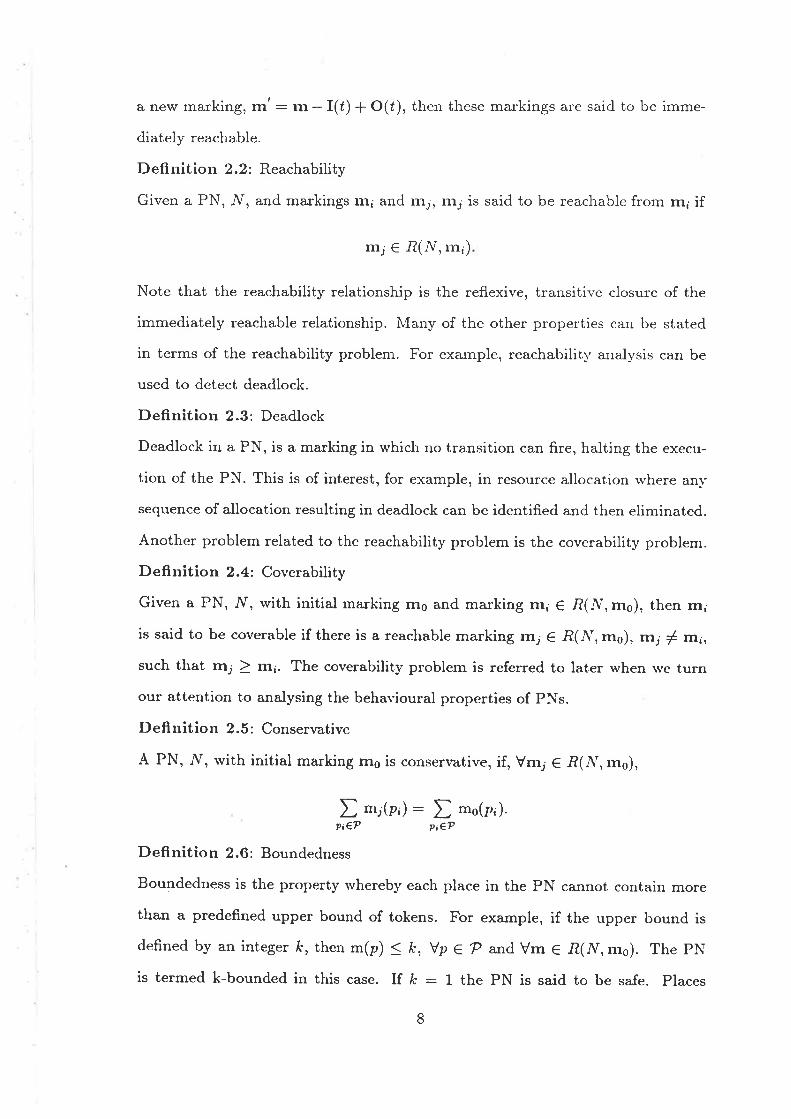
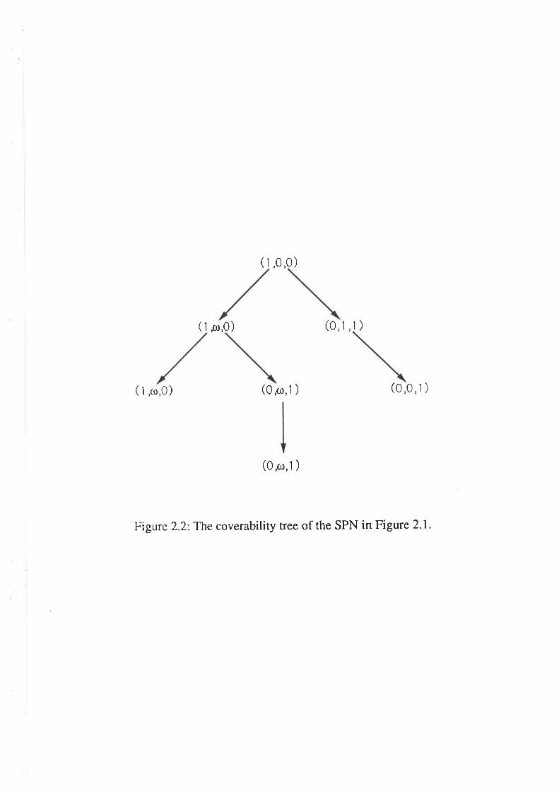
not have to be checked for coverability again. Figure 2.2 is the coverability tree
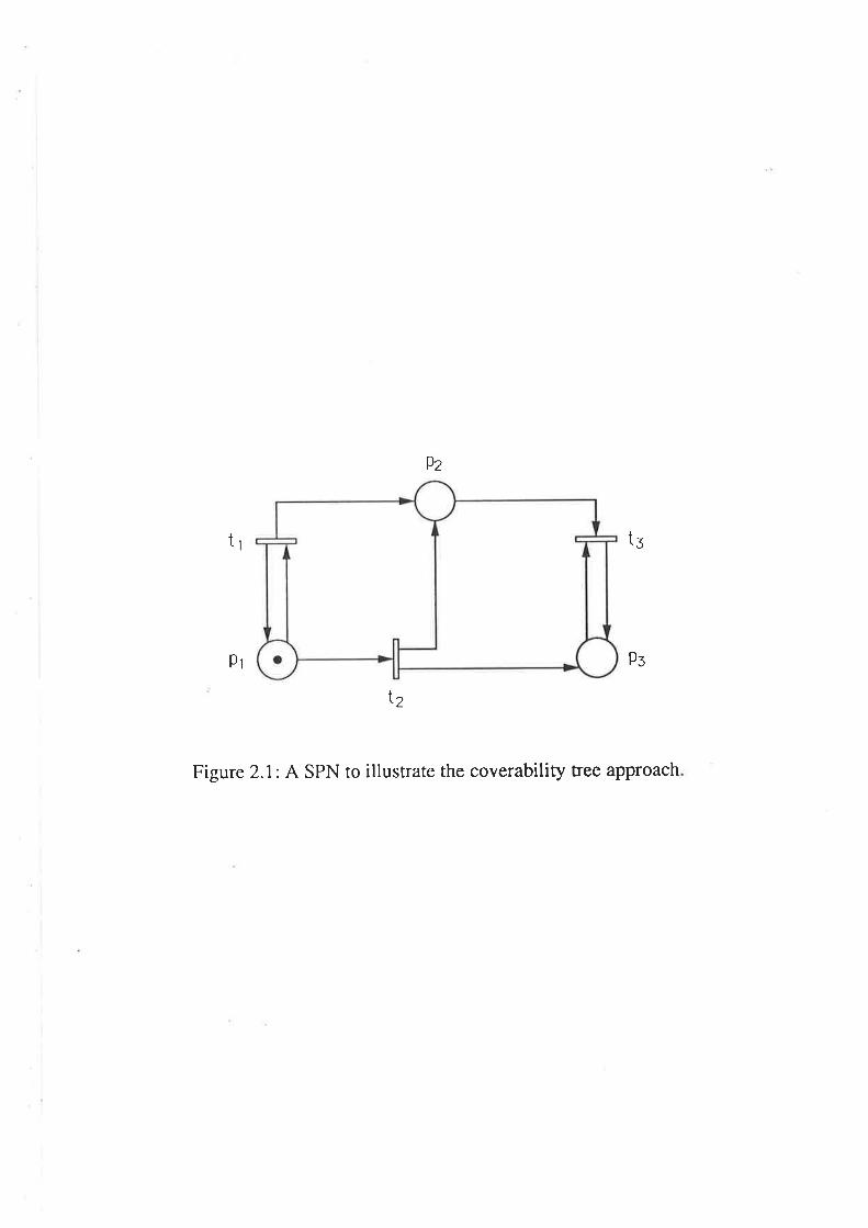
of the unbounded PN given in Figure 2.1. The initial marking is (1,0,0). ff.t,
fires frrst, a token is removed from p1 and a token is deposited in both p2 and ps,
creating marking (0, 1,1) as indicated on the coverability tree. If ú3 then fires, a
token will be removed from p2 -d p. and a token wiil be deposited it p., creat-
ing marking (0,0,1) and so creating a deadlock. Suppose now that ú1 frres first,
creating marking (1,1,0). From this marking, t1 can fire again creating (1,2,0).
Since (1,2,0) covers (1, 1,0) rve alter the marking by replacing the entry for m(2)
by the symbol ø. That is, the first marking in that branch becomes (1,c.r,0) as
indicated on the coverability tree. The search dos'n that branch is now complete.
A simila¡ argument holds if ú2 fires after ú1, creating the other branch on the left
hand side. The disadrrantages of this method are that it is a time consuming
operation and information is inr"ariably lost due to the lumping of the markings.
lr{urata [76] notes that since some information has been lost, only a subclass of
the behavioural properties of the PN may be analysed. The reachability problem
and liveness problem cannot be solved by this method alone.
A second approach is based on the matrix equations which govern the dynamic
behaviour of the PN. Consider a PN, N, 'with s transitions and r places. The
incidence matrix, .4., is an s x r matrix of integers with entries given by,
a;j:alj-a;j,
where, a{ is the number of output arcs from t; to p¡ (which may be interpreted as
the number of tokens deposited in p¡ after f; fi.res), and o¡. is the number of input
a¡cs to f; from p¡ (which may be interpreted as the number of tokens removed
10
9z
t1 tg
Pl Þs
l2
Figure 2.1: A SPN to illustrate the coverability tree approach
( I ,c¡,0)
(1,0,0)
(0,c0,1 )
(0,1 , t)
( 1 ,o,o) (0,0,I )
(o,co,1 )
Figure 2.2:The coverability tree of the SPN in Figure 2.1
frorn p¡ when f; fires). o,ij ca;rr therefore be interpreted as the total change in the
number of tokens in p¡ when ú; fires. Convention in the PN literature has ,4.T as the
incidence matrix. However, Murata [76] points out that incidence matrices u.r" ul*
defined for directed graphs, but unfortunately the directed graph incidence matrix
corresponds to A rather than ,4". In a small attempt to encourage consistency in
the operations research literature u'e shall use the same notation.
Transition ú; is enabled in marking rn, iff,
a;¡<m(p¡), 7< j <r.
This is an expression of the pre-condition for firing f;. Define un, an s x 1 column
vector, to be the nth firing vector, indicating n'hich transition fires at the nth
firing in a firing sequence ø. A one, in the ith position, indicates that ú; fires at
the nth fi.ring. The remaining entries are equal to zero. Assume that the nth
firing is feasible, then, from Murata [76], the state equation for À¡ may be written
ast
lnr.:lln-r*-4?u., n:!r2... (2.1)
where mr. is an r x 1 column vector.
Additional results follow directll' from Equation (2.1). For example,
ll1'.:rnef"Ët*, (2'2)À=l
which says that marking tn,. is reachable from rrs through a firing sequence
{ur,ur,..-ru.}.A non-negative integer solution, x + 0, of the equation,
is called a T-invariant. For recoverable PNs, the T-invariant indicates how often,
sta.rting from some marking, each transition has to fire to reproduce that marking.
A non-negative integer solution , y + O, of the equation,
Ay:o,
áTx : O,
11
is called an S-invariant. It is a rveighting factor, such that the inner product of
the S-invariant and any marking in the reachability graph, is a constant.
To gain insight into these invariants consider Equation (2.2).Let x : Ë .tu.Ä=1
x is an s x 1 coiurnn vector of non-negative integers and is commonly called the
fi.ring count vector. The ith entry denotes the number of times that ú¡ must fire
to transform rrrs into rn,. \Vith this substitution Equation (2.2) becomes,
III':nfo*ATX. (2.3)
Therefore, a T-invariant, x, rvith áTx: 0, implies that Equation (2.3) becomes,
nln: mot
which is consistent rvith the definition of a T-invariant given earlier.
Now consider the inner product of lrl,,, from Equation (2.3), and an S-invariant
Y'
mfy : mf,y * xr Ay. (:2.4)
Therefore, an S-invariant y, .n'ith ,4.y : O, implies that Equation (2.3) becomes,
-fy:*ly:constant.
Implying that the net is consenative with respect to the weighting factor y.
This method is limited because of the non-deterministic nature of PNs, and
because the solutions must be found es non-negative integers. of, and o¡. do not
cater for probabilistic routeing in the PN, therefore we are restricted to determin-
istic PNs when using this technique. In Section 3.3 we suggest a techniquelvhich
overcomes this problem.
A third technique is called the reduction technique as it physically reduces
the PN. To aid in the analysis of a large system, it is often possible to reduce
the model to a simpler one. For example, an implicit place is one whose addition
to (or elimination from) the net does not modify the firing seguence. Note that
an implicit place has also been called a redundant place in the PN literature. A
T2
modified net can be obtained by removing such a place along u'ith it's input and
output arcs. 'We use th definition of an implicit piace from Silva and Colom [92].
Defrnition 2.10: Implicit Place
A place, p;, is an implicit place of a PN, N, with initial marking rn6, if there exists
an r x 1 vector, y, of positive rationalr (V I O) and a rational, pr, such that for
any ur € lR(l/, ms):
1.*(pt) >rnrv-lp llvll ç 2\{pti.
2. Vtx€T, Yp¡€ P\{pt}, m(p;) > akj + m(p;) } o ;.
llyll : {p I y@) > 0} and llyll i. the set of implying places. The second part of
condition 1 implies that y(p¡) : 0. Note that this definition can include pi as arì
implicit place if it is a sole input place to some transition. This is contrary to the
idea that the removal, or addition, of p; should not effect the firing sequence of
the PN. For this reason ¡r¡e exclude any places that are sole input places for any
transitions.
To aid in the understanding of this definition r¡'e give our interpretation. If
rn(p;) ) mry, V m € R(N, m¡), then let p :0 and Condition 1 is atisfied. If
m(pi) ( *ty, for some m e Ã(N, rn6), then let,
-p :-eåì1{o,"1 {mry - -(p,)} ,
and Condition 1 is satisûed. If the supremum does not exist, we cannot find ¡r
given our choice of y to satisfy Condition 1 and therefore p; is not implicit. This
is a technical condition ensuring that if the weighted number of tokens in the
implying places is unbounded, the difference betrveen the number of tokens in the
implicit place and the implying places is bounded.
Condition 2 is an instructive condition. For every marking it asks the question,
"for every transition t¡, does place p; obey the pre-condition for firing, given that
another place satisfies the pre-condition for firing ?". If p; does, then it is an
implicit place.
13
Alternative reduction techniques involve fusion of a series of places, fusion of
a series of transitions, fusion of palallel places and fusion of parallel transitions.
For further information on these methods refer to Berthelot, Roucairoi and Valk
[10], Berthelot [9], Johnsonbaugh and \4urata [48] and Chu [22]. Reduction is
particularly relevant in SPNs, and so u'e appl¡' the technique to the examples in
Chapter 3.
2.L.3 Structural Properties
The inva¡iants discussed in the last section have been shown to be powerful tools
for studying, not only the behavioural, but also the structural properties of PNs
(see Reisig [86] and Murata [76]). The structural properties of a PN are those
that depend on the topological structure and not on any initiat token distribution.
Consequently they are functions of only the incidence matrix, ,4,, which contains
the information on the multiplicitl' of the input and output arcs of the PN. These
properties are listed below with their corresponding methods of analysis.
Deffnition 2.11: Structurally Live
A PN is structurally live, if there exists a live initial marking. This is a difficult
property to check for general PNs. Horvever, it can be shown that a subclass of
PNs, namely the marked graph, is structuralll' live (see Murata [76] for details).
Deflnition 2.L2: Completely Controllable
A PN is completely controllable, if an1' marking is reachable from any other. Ifa PN is completely controllable then Rank(-A) : ". For the proof of this result
refer to Murata [76]. This propertf is independent of the initial marking, whereas,
the property of ¡ecoverability is not. Consequently, completely controllable is a
stronger property.
Deflnition 2.13: Structurally Bounded
A PN is structurally bounded, if for an arbitrary finite initial marking, rns, the
PN is bounded. If there exists an r x I column vector, y ) O, of integers such that
Ay < o, then from Equation (2.a) rnly < *ly. Therefore m(p), the number of
L4

tokens in place p is bounded by,
m(P) < ["lv]'v\p )
where V(p) ir the pth entry of y, V p e P.
Definitio n 2.L4: Repetitive
If there exists an initial ma^rking ûr¡, and a firing sequence from rns where every
transition fires infinitely often, ihe PN is repetitive. An equivalent result is that
there exists an s x 1 integer column vector, x ) 0, such that .4."x ) 0. If rve
substitute ATx ) 0 into Equation (2.3), then there exist markings, m6 and. m,
such that, tttn-mo ) 0, that is mr, ) rns. Therefore, given that there are enough
tokens in rns (and therefore rn,), so that the tokens will not be exhausted during
the firing sequence, every transition can fire infinitely often in the firing sequence.
Repetitive is a stronger property than coverability since it is independent of the
reachability graph, whereas coverability is not.
Deflnition 2.15: Consistent
If there exists an initial marking nrs, and a firing sequence which connects ms
back to rns, such that every transition fires at least once, the PN is said to be
consistent. An equivalent result is that there exists an s x 1 integer column vector,
x ) O, such that ATx : O. Applying the same argument as above, substitution
into Equation (2.3) yields m. - ttl6 : O. Therefore, given that there are enough
tokens in me, the firing seguence can be executed. Note that if the net is consistent
with this initial marking then it will also be recoverable.
Defl nition 2.16: Structurally Implicit
A place, p, is a structurally implicit place, if there exists an r x 1 vector, y ) 0,
where llyll, given in Definition 2.10, obeys llyll _c P \ {p,}, such rhat,
Ay < A(p),
where A(p) is the column of the incidence matrix corresponding to place p. Ay
gives the total weighted change in the number of tokens in the implying places.
15

,4(p) gives the total change in the number of tokens in p. Therefore, the condition
requires that more tokens are deposited into place p, than the implying places,
and less tokens axe removed from p, than the implying places.
Note that it is possible to make a structurally implicit place, p, implicit. This
is achieved by adding tokens to p in the initial marking 1116, so that p is implicit
in the new initial marking.
2.2 Subclasses of PNs
Some subclasses of PNs include:
1. State machines: A state machine is a PN such that each transition has
exactly one input and one output place. This is analogous to a queueing
network.
2. Marked Graphs: A marked graph is a PN such that each place has exactly
one input transition and exactly one output transition.
3. Free Choice PNs: In a free choice net any conflict situation must involve
only one place.
4. Simple PNs: A simple PN requires that each transition has at most one
input place that is shared rvith another transition. (For details see \{urata
[76i).
2.3 Time Extended Models
A summary of PNs rvith deterministic delays and related works follows in Section
2.4. A summary of SPNs follorvs in Section 2.5 (for a review on both types of
net see Wong and Henderson [fOO] and Marsan [60]). Although timed PNs can
be treated as SPNs, with degenerate probability distributions, there are conflict
problems which arise with deterministic delays that require special consideration.
16
Consequently, although there are sections of this thesis in which SPNs can have
deterministic delays, we will treat them separately in the following sections.
As mentioned in Chapter 1, the frring delays may be associated with either
the transitions or the places in the PN. In the following section, v/e separate the
two types of time-extended PNs and discuss them individually.
2.4 Deterministic Delays
2.4.L Timed Tlansitions
One of the first rvorks to involve time delays in PNs can be attributed to Ram-
chandani [Af]. fne model required that the transitions had to wait a deterministic
length of time betu'een becoming enabled and frring. This is called a Timed PN
(TdPN).
Another model of importance, first introduced by Merlin [Oa] ana later used by
Merlin [69] and Merlin and Farber ([70], [71]), called a Time PN (TPN) introduced
a firing interval associated lvith each transition. The conditions for enablement
remained unchanged from the classical structure, however the firing had to occur
somewhere in the interval [ú*¡r,, ú*"r], a minimum and maximum time, beginning
from the moment the transition s'as enabled. In both the first and second model,
the firing of a transition is instantaneous, that is, the tokens are removed from all
of the input places and are then deposited immediately into their output places.
Recently, Menasche [67] noted that a TPN can be considered a generalisation of
a TdPN.
A rrariation is presented in Razouk [83]. In this model transitions are allocated
two times, an enabling time, 1", and a firing time, ú¡. The transition waits for a
time t, after it is first enabled, before it begins firing, at which point it absorbs the
tokens from its input places. The tokens remain absorbed, while the transition
continues to fire for a period f1. After the transition finishes firing, tokens are
deposited into its output places. This model differs from the first two because
77
tokens disappear for a period of time, and because tu'o times, t, and t¡, a;re
required to execute the firing process.
Since groups of transitions can become enabled and fire concurrently, when
using deterministic lifetimes, the following authors address the issues involved in
analysing models with conflicting transitions.
Zuberek [102], assigns a probability of firing to every transition in a conflict
set, with these probabilities summing to one. The firing time is restricted to
be a non-negative integer a¡rd the nets are restricted to be safe and free-choice.
This ensures, that among a^ny set of conflicting transitions, either all or none are
enabled, and firing one disables the firing of all other transitions in the set. No
subset of a set of conflicting transitions can be enabled in any marking. The
disabled transitions follow the pre-emptive repeat discipline.
In the paper described above, and then later in ([103],[104],[105],[106]), Zu-
berek introduces an extension called escape arcs. They are represented by .tt
arc, from a place to a transition, with a black circle on the end connected to
the transition, rather than an arrowhead. The escape arcs remove a token, from
the place connected to the escape arc, but no tokens from these input places are
deposited into the transitions output places. These arcs can be used to model
timeout, without having to interrupt a transitions firing time, a propertl'required
in a realistic timeout.
Zuberek's use of time, assumes that when a transition is enabled it starts firing
by absorbing its input tokens. The tokens remain absorbed until the end of the
firing time, at which point they are released and deposited into the output places.
Since the firing time is deterministic, the underlying process is not memor¡'less and
therefore not Markovian. In order to malie the equilibrium solution tractable, it is
necessary to record the history of the transition firings. in other words, record the
residual lifetimes of the transitions. Zuberek follorvs the traditional "supplemen-
tary variable" technique, by supplementing the state description with a vector of
18
residual lifetimes, and so creates a discrete time Markov chain vvith an extended,
but finite, state space.
To aid in evaluating the pelfolmance of a model, Zuberek then creates a re-
duced state space, retaining the original supplemented states oniy if they are
connected to more than one state in the state space. The remaining states a¡e
aggregated, and the time delays taken to traverse these aggregates is evaluated
by adding the time delays for each state within the aggregate. The reduced state
space is then used to measure throughput and resource allocation.
Razouk [83] and Razouk and Phelps [84], introduce a different version of time-
extended PNs by incorporating Merlin's ú-i,, time as a¡ enabling time. This way a
transition in the net must remain enabled, for a period of time, before it can frre.
The enabling time is also restricted to be a non-negative integer. The transition
then follows the same firing rules as in Zuberek's model. The firing time is also
restricted to be a non-negative integer. With the introduction of enabling times,
they include a vector of residual enabling lifetimes as well as the vector of residual
firing times, to the state description, in order to create a finite state, discrete time,
Markov chain. They relax the free-choice restriction but retain the restriction that
conflicting transitions be mutually disabling. They refer to each set of conflicting
transitions as a conflict set, defined in the follou'ing way: Every ú; belongs to
exactly one conflict set, C, such that,
c : {rjl r(új)ll l(¿r) + o}.
With each transition ú; in the conflict set, let f, be the firing frequency. The next
marking probabilities are evaluated by working out the probability of the first
transition to fire. Tra¡rsition ú; fires first, and so defines the next rnarking, with
probability given by,
f¡
Df¡jll¡ ñreable in C
Holliday and Vernon [43] relax all net restrictions, except, that the state space
19
be flnite and call their model a generalised timed PN (GTPN). As opposed to
Zuberek and Razouk and Phelps, u'ho allow only non-negative integer valued firing
times, this model allorvs non-negati'r'e real valued firing times. They introduce a
generalised conflict set, which is the transitive closure of the following relation
defined onT,
ú; conflicts $'ith ú; itr I(¿i) n I(¿j) I 0
Note, that by including the transitive closure, this definition generalises the defi-
nition of the conflict sets in Razouk and Phelps. They identify a set of transitions,
called a local maximal, in the generalised conflict set, which when fired, disables
the remaining transitions in the set. They define the probability of such a set, -s;,
firing, as
Comb(s;) il frP(",)ffi, (2.õ)
5t nlt.6a,
where Comb(s;) is the number of rva¡'s tokens may be removed from the input
places. The next state probability, is then simply the product of all the probabil-
ities of local maximals, s¡, selected to fire,
II P(",).s, ælectcd
With this model the authors compute performance estimates. They note, that
the times at which state changes occur, form an embedded, discrete time lvlarkov
chain. They then proceed, by aggregating the states, to form a reduced state
space' as do Zuberek and Razouk and Phelps, and from there find performance
estimates of the reduced state space.
In Woo, Phelps and Sidwell [101], the conflict resolution probabilities are de-
termined using simple random sampling without replacement. They call the next
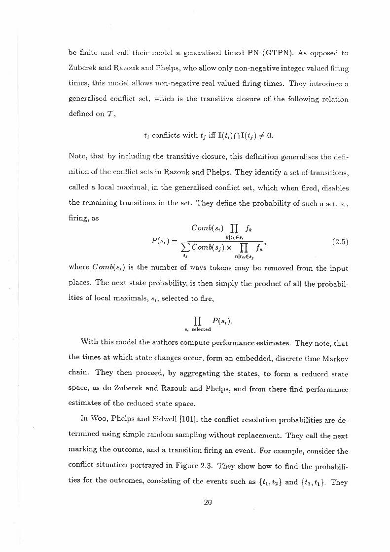
ma"rking the outcome, and a transition firing a¡r event. For example, consider the
conflict situation portrayed in Figure 2.3. They show how to find the probabili-
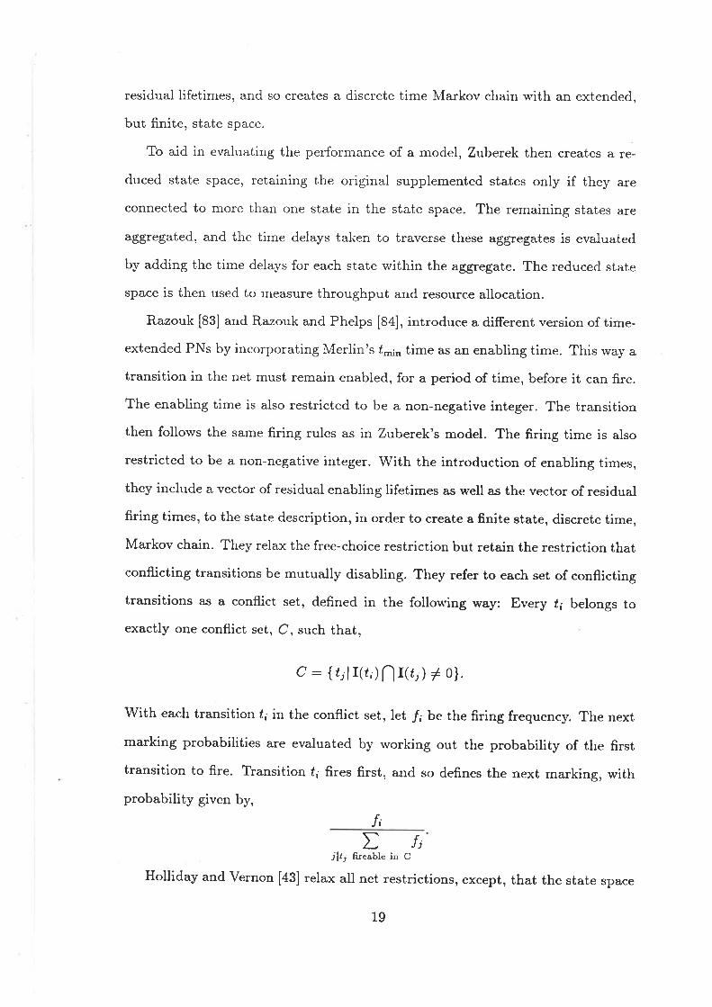
ties for the outcomes, consisting of the events such as {tr,tz} and {f1,ú1}. They
20
Pr 9z Ps
t1 l2
Figure 2.3: An example of conflict.
oa oo
evaluate these probabilities, using simple random sampling, where the sample is
considered to be an ordered sequence of transition firings. If each sample consists
of one outcome, the probability model is termed simple. StrictlS', simple random
sampiing describes a probability model that gives equal probability to all of its
ordered samples. Woo, Phelps and Sidwell [101], deviate slightly by defining the
probabilities on the discrete events comprising the sample space, rather than on
the samples. A sample's probability is therefore determined by the product of
it's discrete events' probabilities. An outcome probability is then the sum of the
probabilities of the samples that comprise the outcome. Say, we rvish to evaluate
the probability of the sequence of transition firings {t-,.,tr}. Since each event is
equally likely,
1+ trl.Also,
P({t,,tr}) :
2.4.2 Timed Places
Sifakis [91], first proposed a PN model whereby a delay is associated rvith each
place. This model is called a Timed Place tansition Net (TpTN). \\rhen a
token is deposited in a place, it stays there for a duration of time, after which itbecomes available and is allowed to participate in the enabling of a transition. The
transitions have no delays associated with firing and therefore fire instantaneousl¡,
as in the classical PN model.
2.5 Stochastic Petri Nets
In this section, we will consider SPNs where the ûring time of a transition is a
randorn variable drawn from a continuous distribution. In these nets, the conflict
problems which arise, take on different aspects from those of TPNs. \\/ithin a con-
flict set, transitions can be pre-empted by the removal of all or part of its input
P({tr,ú2}) : P({¿r,tr}) + P({úr,úr}) : ;";
11-x-.22
21
bag. Most authors assume that s'hen the pre-emptecl transition is again enabled,
the new iifetime is drawn from the same distribution (pre-emptive repeat differ-
ent). Other possible choices are to restart u'ith the sarne lifetime (pre-emptive
repeat identical) or to restart the lifetime from rvhere it was pre-empted (pre-
emptive resume). The overall effect, is that the lifetimes themseh'es dictate rvhich
transitions will fire. Marsan, Balbo, Bobbio. Chiola. Conte and Cumani ([61],
[62]), describe these policies and their impact on rnodelling. \Me rvill give an
account of their papers, in more detail, in Section 2.õ.1.
2.5.t Timed Tlansitions
Molloy [73] initiated the study of performa¡rce eraluation in SPNs rvith negative
exponential distributions, b¡' noting that these SPNs are isomorphic to homo-
geneous Markov chains. The key factors. allorving the isomorphism to be con-
structed, are the countabilit¡' of the markings and the memorvless property of
the negative exponential distributions. That is. if a transition fires to change the
marking, the distribution of time remaining on the other enabled transitions'life-
tirnes is the same as if tirey rvere first enabled. It is therefore possible to apply
the standard techniques in N'farkov chains. As a precursor to Chapter 4, where
rve examine the global balance equations for insensiti.r'itv. the follou'ing example
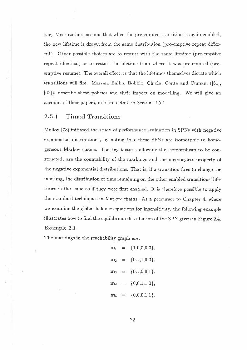
illustrates how to find the equilibrium distribution of the SPN given in Figure 2.4.
Example 2.1
The markings in the reachability graph are,
trr1 : { 1.0.0,0.0},
rtl2 : {0.1,1,0,0},
ms : {0.1.0.0,1},
ln4 : {0.0.1,1,0},
m5 : {0.0,0,1,1}.
22
Pl
Figure 2.4; A simple SPN representing conculrent activities.
Let transitions ú; fire u'ith rate À¡, for 1 ( i I 4, rvhere À, I is the mean of the neg-
ative exponential distribution. The equilibrium distribution, is found by soiving
the set of global balance equations given belorv, where z'(m;) is the equilibrium
probability of being in state rn;.
The solution to these equations is given by,
zr(nr2) : 7r-(mr)
7T'(m3) : zI'(lnt)
r(rna) : z¡(rnr)
a-(m1)À1 : zr(ms)À4.
zr(rn2)(À2 a À.) : r'(m1)ìr.
z'(rn3))2 : ?r(m2))3.
r(ma)13 : 7r(m2)À2.
z'(m5)Àa : ?r'(rn3)Àz * zr(ma))3.5
! z'(m;) : 1.i=l
)r(lz * Às)'
)rÀ"Àr(À, .t À.)'
)t),
(2.6)
(2.7)
(2.8)
(2.e)
(2.10)
(2.11)
(2.r2)
(2.i3)
(2.r4)À.(À, 1 )a)'
z'(m5) : o1,r,)|, (2.1b)À4
subject to Equation (2.11). Using the equilibrium distribution, the throughput or
average delay (using Little's result) can be era.luated.
Even though we stress the use of time extended PNs in this thesis, one must
recognise the usefulness of classical PNs in the modelling of interactions betu,ee¡r
activities, which are of a logical nature and which do not consume time. The tran-
sitions rvhich fire in zero time a¡e called immediate transitions and therefore must
have a higher prioritl' than timed transitions. Nets which have both immediate
transitions and transitions s'hich fire according to negative exponential distribu-
tions, are called Generalised SPNs (GSPNs) and are discussed in Marsan, Conte
and Balbo [65]. As with deterministically timed transitions, in Section 2.4.1, it is
23
necessary to have some lvay of resolving conflict among a set of concurrentll' en-
abled immediate transitions. This is achieved, by what is called a random ss'itch
in Marsan, Conte and Balbo [65]. The random switch is defined on the set of
immediate transitions and an associated probability distribution. The definition
of a random switch is dependent on the marking, therefore, the reachability graph
of the GSPN must be constructed before it can be assigned. Such an assignment
depends on the local and already identified behaviour of the model, and so a for-
mal definition of a random switch is not possible, but is illustrated b5' the use
of examples in lt.{arsan, Conte a¡rd Balbo [65]. Marsan, Balbo, Chiola and Conte
[63], identify a ciass of GSPNs in which the random switch can be defined at the
net level, implying that the reachability graph does not have to be constructed.
This is achieved by using a priority structure, for the immediate transitions. by
assigning weights, to¡, to each transition, f;, in the set of simultaneouslv enabled
immediate transitions, C. Following Razouk [83] and Razouk and Phelps [E4], the
probability that ú¡ fires in this set, C, is then given bv,
I.,jjV'ec
Again, these weights depend on the local behaviour of the model. If a mixture of
immediate and negative exponentially distributed transitions are enabled concur-
rently, the immediate transition, chosen by the random ss'itch, rvill take ¡rriority.
If a set of negative exponentially distributed transitions are enabled concurrently,
the first to fire u'ill be given by the probability,
À;
D À*'À
rvhere, À; is the firing rate of transition ú;, and the sum in the denominator is
taken over all the enabled transitions.
The evaluation of equilibrium probabilities, for the markings in the GSPN,
is not as straight forward as the approach given in Example 2.1. This becomes
?x;
24
clear, if we note that the reachabilitv set of a GSPN is a subset of the reachability
set of the associated PN. The reason, is due to the firing priority introduced
with the immediate transitions, resulting in not all of the states being reachable.
Marsan, Conte and Balbo [65] call markings that enable negative exponentially
distributed transitions, tangible markings, and markings which enable immediate
transitions, vanishing markings. The approach taken, is to make use of the one
to one correspondence between the GSPN markings and the states in a stochastic
point process. Further, a stationary embedded Markov chain is recognised within
the stochastic point process. The anall'sis of the embedded Ma¡kov chain allows
the evafuation of the equilibrium probabilities of the GSPN markings.
An obvious extension to introduce norv, is to mix different types of firing
distributions in the net in order to increase modelling power.
Natkin [77] and Bertoni and Torelli [11], rvere the first authors to move in this
direction. They restrict the SPN structure to be a semi-lUarkov process (to be
discussed in Section 4.1). Although this approach is appropriate in some cases, it
fails when parallel activities need to be modelled, because of the lack of memorv
necessary after every generally distributed firing time ends.
As mentioned at the start of this section, the Markovian analysis performed
on SPNs requires the memoryless property. Only negative exponential and the
discrete time analogue, the geometric distribution, have this propert¡,. As a ne\\,
marking is entered, the geometric distribution has the property that the probabil-
ity that a particular enabled transition s'ill fire, in the next discrete time interrral,
is the sarne after any multiple of that interval. Results concerning the combination
of deterministic transitions, rvith geometrically timed PNs, have been reported by
Molloy [7a] and Holliday and Vernon [a3].
In Molloy [74], the deterministic firing times are restricted to be non-zero
multiples of some unit time step, and all the conflicting transitions which fire
with deterministic delays, must have equal probability of firing. In the paper by
25

Hoiliday and Vernon [43], discussed in Section 2.4.I, we notecl that the GTPN
allowed firing times to be any non-negative real va,lue. This implies that the
GTPN can represent geometric holding times, thus bridging the gap between the
TPN and SPN models.
In Bobbio and Cumani [12], probabilistic branching (through the use of im-
mediate transitions) and general distributions, are rnixed in the SPN. Holvever,
the general distributions cause the resulting associated stochastic process to be
no longer Markovian. They use phase type distributions (refer to Section 4.2.2
for details) to approximate these general distributions. After expanding the state
space, with the appropriate SPN representation of the phase type distribution,
a continuous time, discrete state, homogeneous Markov process is constructed,
which can then be anal¡'sed in the usual way.
Dugan, Geist, Nicola and Trisedi [28], introduce more generality for modelling,
by classifying a type of SPN s'hich includes general distributions and negative ex-
ponential distributions. They add inhibitor arcs to the PN structure and introduce
probabilistic branching. An inhibitor arc, from a place to a transition, has a small
circle, rather than an arros'head. connected to the transition. The firing rule is
changed in the follos'ing wa¡'. A transition is enabled when tokens are present
in all of its (normal) input places and no tokens are present in the inhibiting in-
put places. When a transition fires, the tokens are removed from all the normal
(without inhibitor arcs) input places and deposited in the output places as usrral,
rvith the number of tokens in the inhibiting input place remaining zero. A proba-
bilistic arc, from a transition to a set of output places, deposits a token in one of
the places in the set. The choice of u'hich place receives the token is determined
by the probabilities assigned to each arc. The net is called an Extended SPN
(ESPN). The structure of the ESPN is restricted to be of the following form:
1. The firing time of transitions, rvhich are enabled concurrently, must be ex-
ponentially distributed.
26
2. The firing time of an exclusive transition (that is, no otirer transition is
enabled at the same time) may be generally distributed.
3. A transition in conflict (that is when the firing of a transition disables the
fi.ring of all others) may be generally distributed. It is assumed that the
transition, when re-enabled, has a firing time independent of, but identically
distributed to, the pre-empted firing time.
Dugan, Geist, Nicola and Trivedi [28] also consider marking amalgamation
for ESPNs, where at most one generally distributed transition is enabled in any
marking, and where each marking is visited only once. They suggest the amal-
gamation procedure, of combining all markings which have a common generally
distributed transition enabled. In Chapter 4, we derive further results along these
lines, using the theor¡'of insensitivity applied to marking amalgamation.
Marsan and Chiola [64], consider an extension of the GSPN model by incorpo-
rating deterministic firing times. They refer to this model, including the combina-
tion of deterministic, exponential and immediate firing times, as a Deterministic
and Stoch+tic PN (DSPN). The restrictions placed on the DSPN are, that ex-
clusive transitions may have any firing time, transitions i¡r conflict may have any
firing time, and not more than one transition u'ith deterministic firing time may
be enabled concurrentll', unless the set of concurrently enablecl transitions satisfy
the following conditions.
1. The set of concurrently enabled transitions (rvhich may include both deter-
ministic and exponentiall¡' distributed firing tirnes) must be enabled at the
sarne insta¡rt.
2. Each of these transitions can also be connected to a chain of tra¡rsitions
(that is a transition connected to a place connected. to another transition
etc.), however, the type of firing distribution must be the same for each
transition in the chain.
27
The time points of the plocess are then taken to be the instant that the deter-
ministic transition starts firing, or has just been disabled. At the end of each
interval, the process s'ill change states, probabilistically, according to whether or
not an exponentialll' distributed transition (or a set of exponentially distributed
transitions) fired rvithin the inten'al.
\{arsan, Balbo, Bobbio, Ciriola, Conte and Cumani's ([61], [62]) definition
of their model, includes a specification of the selection of the next transition
to fi.re, and they refer to these specifications as an execution policy. The¡' use
supplementary variables to record the spent lifetimes in each marking. Note that
supplementary variables are not required, if the execution of the SPN only relies
on the firing of exclusive transitions. However, for combinations of competitir-e
and concurrent transitions it is necessary to record spent lifetimes, for the case
when transitions pre-empt the firing of others. This publication gives a good
account of the impact of the execution policies, on the analysis of SPN models
which have generalll' distributed firing times. We will now give a summarv of
these policies and the effect they have on the SPN.
The most common rvay of selecting which transition will fire, from a set of
enabled transitions, is to choose the one whose firing time is statistically the min-
imum. This is what is referred to as the race policy model. The other policl,,
knorvn as preselection. chooses the next transition to fire according to a proba-
bility mass function.
The supplementan'lz,riables are recorded in three different \¡¡ays.
1. If a transitionis pre-empted, the supplementaryvariable is set to zero. ryhen
once again enabled. This is termed pre-emptive repeat.
2. If a transition is pre-empted, the supplementary variable is set equal to the
spent lifetime a¡d when re-enabled, the firing rvill resume from where it rvas
pre-empted. This is termed pre-emptive resume.
28
3. If a transition is pre-empted, the supplementary variable is set to zero, unless
it remains enabled in the next marking, rvhen it is set to the spent lifetime.
From Marsan, Balbo, Bobbio, Chiola, Conte and Cumani ([61], [62]) this is
called age-enabling.
\Mhere possible, we have tried to remain consistent ',r'ith the literature in other
areas of operations research. In this case we follow the nomenclature of the lit-
erature on queueing networks. The concept of age-enabling, is the status quo
assumption in stochastic systems and is not usually given a special title.
Mansan, Balbo, Bobbio, Chiola, Conte and Cumani ([61], [62]) consider com-
binations of both the race and pre-selection polic¡ together with the three alter-
native choices in recording the supplementary r,rariable, are then presented and
the corresponding resultant process is described. For both the pre-selection and
race policies, with pre-emptive repeat, the process is a Slr{P rvith well knos'n so-
lution techniques. For the race policy, with pre-emptive resume or age-enabling,
the corresponding process is no longer a SMP and the authors suggest the use of
supplementary variables, to extract the equilibrium distribution.
Marsan, Balbo, Bobbio, Chiola, Conte and Cumani [62] also mention the po-
tential for introducing marking dependent firing times. In addition, the paper
describes how to approximate a generally distributed firing time, by using a phase
type distribution, substituted directly into the state space rather than at the net
level. The reason they do this, is to avoid enlarging the reachability tree unnec-
essarily (for more details see Section 4.2.2).
Henderson and Taylor [41], discuss discrete time SPNs, rvhich can have mix-
tures of negative exponentially distributed and generally distributed transitions,
that form a SMP. Both firing and enabling intervals are used in their model, by
assuming alternating enabling and firing time points. They define a class of net,
which has an extended product form solution, based on the work of Henderson,
Lucic and Ta¡'l6r [37], (see Chapter 3). This will be discussed in more detail in
29

Chapter 5.
This is a small sample of the different types of suggested models for SPNs used
in the literature, more detail will follorv in later chapters.
2.5.2 Tirned Places
The condition/event interpretation of nets with timed piaces is as follorvs. The
firing of a transition, which inputs into a place, represents the start of execution.
The presence of tokens in a place, represents a condition of the process in execu-
tion, and the firing of output transitions of a place, represents the completion of
a process.
'Wong, Dillon and Forward [99] consider PNs with timed places (TPPN). These
nets are restricted to be safe, marked graphs,, in order to make the following
analysis tractable. They decompose the marked graph into elementary loops,
such that each place and transition has one input and one output arc. These
elementary loops are found by the S-inr,ariants. The method then describes horv
to frnd the distribution of the cycle time of the marked graph. They define a
random variable, X;, to be the loop time of the elementary loop, i. The c¡'cle
time is then the maximum of the loop times. Hence, the distribution function
of the cycle time is the product of the distribution functions of the loop times.
Such a result is shown to be useful in providing upper and lower bounds on the
execution times of component modules.
30

Chapter 3
Closed Forrn Solutions
The major problem in finding the performance measures of SPNs, is the need to
work with the equilibrium distribution based on the reachability graph. The size
of the reachability graph gro$¡s exponentially, with both the number of places and
the initial token distribution, making such analysis very difficult for even moder-
ately sized SPNs. Since this creates such a major problem, we aim to devote a
Iarge proportion of this thesis to finding some form of solution technique, rvhich
eliminates the problem of having to generate the reachability graph. In this chap-
ter, we are concerned with finding a closed form solution for SPNs, a¡¡d in Chapter
5, we give a technique for aggregation and disaggregation which rvill hopefully shed
some light onto finding equilibrium distributions, without necessarily generating
the entire reachability graph.
A similar problem in queueing theory, lead resea¡chers to look for a simplified
method of finding the equilibrium distribution. The investigation produced ap-
proximation techniques, and a class of Ma¡kov processes for which there exists a
product form equilibrium solution, (see Jackson ([45], [46]), I{elly [50] and Bas-
kett, Chandy, Muntz a¡rd Palacios [8]). Along with this product form solution
also came the creation of computationally efficient algorithms for their eraluation
(see Buzen [1a] and Reiser and Lavenberg [85]).
When there is a product form solution, the joint equilibrium distribution of
the network involves a product, over the uodes of the network of the equilibrium
distribution of the individual nodes, treated as though in isolation (a normalising
31
constarÌt is involved in the expression which normalises the inrrariant measure).
Product form solutions are of great interest, because they avoid the direct numer-
ical solution of the global balance equations, which is computationally expensive.
'While the calculation of the normalising constant may not be trivial, the evalua-
tion of product form solutions is still computationally and analytically preferable,
to solving very large systems of linear equations.
3.1- Product Form Solutions
Product form equilibrium solutions have their origin with Jackson [45] and Gordon
and Newell [31]. Jackson [45], considered an open network of. K, many server
queues a¡rd one customer type. Let s(i) be the number of servers at queue i,
where s(z) is an integer. Customers arrive at the netrvork to queue i, according to
a Poisson process with rate )(i), that is, according to the distribution function,
p(n arrivals in (0,¿)): (À(1)¿)""-^1t¡'.
The service rate at queue i is negative exponentially distributed with mean [p,]-t.
After completion of service, customers leave queue i and move to queue
j with probability p{i,j), or leave the network with probability q(i). Let
¡ : (n(f),n(2),...,"(K)) be the state of the netrvork. The joint equilibrium
distribution for the state of the network is of the form
Kzr(n) : B(/í) lI (,('"(¿)),
1
n(i)!if0<n(i)<s(d),
1
s(i)!s(i
(3.1)d=l
where e ("(¿)) is the equilibrium distribution of the ith queue, treated as though
in isolation a¡rd is given by,
Ç(n(i)) :
32
"(d)if n(i) >
"(i),
(3.2)
where {y(i), 1 < i < -K} satisfy,
Ky(i): )(i) + Ðy(j)p(j,i). (3.3)
j=l
B(I{) is the normalising constant, and, for a Jackson open network, is the product
of the normalising constants for each queue in the network.
Jackson [46], extended this work to include service rates ¡l;(n(i)) rvhere n(i) is
the number of customers at queue i. In this case,
"(i)(,('(i)) : [y(i)]'(i) fllp,(/)l-'. (8.4)l=1
He also included an a¡rival rate which could depend upon the total number of
customers in the network. Gordon and Newell [31], considered a closed network
of queues of the type defrned by Jackson [a5]. The joint equilibrium distribution
of this network was shown to be of the same form as Equation (3.1).
'Whittle [97], referred to the network described by Jackson [45] as a migration
process, rather than a network of queues, because no account is made of the
positions of the individuals in the queues. \\¡hen a service facility is ready to
serve a customer, the choice of which customer to serve is random. Other later
extensions, by authors such as Baskett, Chandy, Muntz and Palacios [8] and l(elly
[49], include customers of different types, different service disciplines and generally
distributed service times.
Jackson ([45], [46]), proved the product form result by substituting into the
global balance equations. Whittle ([97], [g8]), provided a valuable new view on
the theory, by showing that the global balance equations could be broken down
into partial balance equations, each of which u'ere satisfied by the product form
solution. Define the flux, from state n to state m to be zr(n)q(n, m), where g(n, rn)
is the rate/intensity from state n to state rn. The global balance equations can
then be interpreted as, the flux out of state n : fl.ux into state n, V n. Whittle's
partial balance equations are:
1. Flux out of n, due to an externa.l arrival : flux into n, due to an external
33
departure. (3.5 )
2. Flux out of n, due to a departure from queue i : flux into n, due to an
arrival at queue i. (3.6)
Kelly [49], extended the theory further, by generalising the service rate at
queue i to be of the form,
pi(n) - d(tt- i'), (3.7)d(") )
where e; is a vector, with a 1 in the ith position and zeros elsewhere, repre-
senting the state with a single customer at the ith queue. The joint equilibrium
distribution becomes,
Kzr(n) : B(/í)/(n) fllv(¿)l"rtr. (3.8)
i=1
When applied to netu'orks of queues, product form originally referred to the prod-
uct over the nodes of the network. The product form of Equation (3.8), is no longer
a product over the nodes, rather it is a product of two functions. /(n) is related
to the service rate and the product of the y(í)'s is a function of the routeing of
the network.
Sta¡rdard assumptions in queueing theoryr axe that customers arrive, are served
singly, and after service, are routed through the network in a manner which may
depend on the state, but does not depend on the routeing of other customers.
The state machine, which is analogous to a queueing network, has this property.
However, these properties are rarelv found in general SPNs. In general, tokens
are fired in a batch, by . transition, and transformed into an output bag. Tokens
are not routed independently of one another, since their movement through the
net depends on the input bag to rvhich they belong. In summarJ¡, the tokens move
in batches, and the routeing of the individual tokens is correlated. Consequentl¡
the theory on product form solutions has not been applicable to SPNs. Authors
such as Walrand [95] and Henderson, Pearce, Taylor and Van Dijk [38], have
found equilibrium distributions for queueing netrvorks with batch movement and
34

independent routeing. Henderson and Taylor 1421, however, incorporated both
batch movement and correlated routeing into their queueing network. In applying
the same approach to SPNs, Henderson, Lucic and Taylor [37] found classes of
SPNs with an extended product form solution. Generally, tokens in SPNs do not
have a position in a place so, this extended product form solution is a solution
to the migration process discussed ea¡lier with, batch arrivals and batch sen'ices.
The following work uses the approach developed by Henderson and Taylor [42],
but differs in one significant aspect, which ma^kes it more relevant to SPNs. The
difference is illustrated in Example 3.5 in Section 3.3.
3.2 Description of the Model
Since the problem of finding a product form solution for SPNs has been ap-
proached by extending the present queueing net'rvork literature, the group of SPNs
that can be analysed using this method, do not naturatly fit into the standard
SPN classifications. For example, the equilibrium distribution of arbitrary marked
graphs can not be found. Horvever, the theory unifies a number of aspects not
collectively covered by general SPNs, such as probabilistic routeing, arbitrary ini-
tial markings, marking dependent firing rates, marking dependent blocking and
coloured tokens. Although u'e do not classify the type of SPN for which the theory
can be applied in standard terms, as we progress through this chapter, we will
identify a new class which supports the extended product form solution. As a
start, we note that SPNs need to be live, but not necessarily bounded, provided
the underlying Markov Process is stationary.
Consider a SPN, with a finite set P : {pr,...,pl¡1} of places, and a finite
set, T : {tr, . . .,,tvl} of transitions. The Ma¡kov process representing the spN,
has markings m € 2lPl, b denote the state when there are rn(i) tokens at
place p;. 'When the state is m, transition t e T has a negative exponentially
distributed firing time, which is rvorked off at a state dependent rate g(m, t).
35
When transition ú fires, tokens move from an input bag, I(t) e %lPl, to one
of a set of possible output bags, Or(¿) € %lPl, rvith probabitity p(I(¿),¿,Oj(f)),
where Dp(I(¿),¿,Oi(¿)):1. Thus the rnarking of the net changes from rn toJ
rn - I(t) + Oj(ú) with probability p(I(l), ú, Oj(f )).
It is worth noting that there are a variety of SPN structures which can be
transformed to give a net of the above form. Two examples follow.
1. If a set, ,4, of tra¡sitions enabled together can fi.re simultaneously, as well as
independently, rve can alter the original SPN by adding a ne\ry transition to
replace the firing time "clock" for the set, "4. The neu' transition will have
input bag given ¡y U I(l) and output b"e U O(¿), where I(ú) and O(ú) are
input and output b'.'Ä respectively for tr.ris€lioo ú. This nerv SPN is equiv-
alent to the original. The reason for maliing such a technical change is to
prevent transitions firing simultaneously and so keep the notation relatively
simple.
2. Without loss of generality, we can &ssume that there is a one to one corre-
spondence betrveen input bags and transitions. Any SPN in which a set of
transitions , A ç T have a common input bag, can be modelled by amalga-
mating the transitions in .,4 into a single transition. Note, that whenever
one of these transitions is enabled, all are enabled. For any state m in
which the transitions in A arc enabled, the firing time distribution of the
new transition will be negative exponential, s'ith parameter D q(-, s). The
routeing probabilities for the next marking are weighted by tír€Jprobabilities,l_ 1-t
q(m, t) I Dq(*, ") I ,, t e A, indicating rvhich transition has fired.L"-e,1 J
Assumption 1
The above procedures can be performed on any SPN before analysis takes place.
Thus, without loss of generality, \\'e can assume henceforth, that the SpN is
structured so that tra¡sitions fire at different times from one another, and no
two transitions have the same input bag.
36
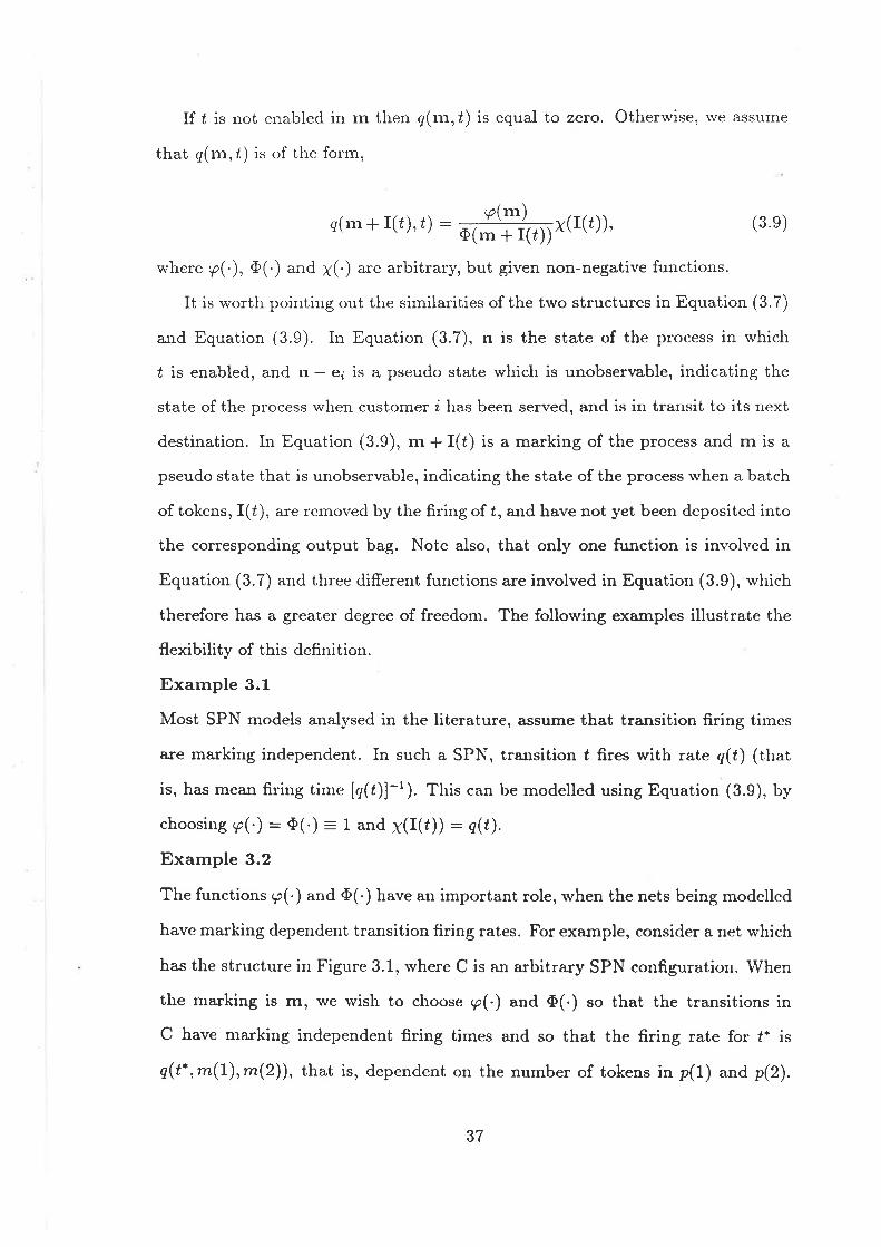
If f is not enabled in rr. then g(rr. , ú) is equal to zero. Otherwise, we assume
that q(m,f) is of the form,
q(r-n f I(ú), ¿) : = ,
t(T],,., x(I(ú)), (3 9)Õ(rn * I(ú)) ^'-'
where p(.), O(') and ¡(.) are arbitrary, but given non-negative functions.
It is worth pointing out the similarities of the two structures in Equation (3.7)
and Equation (3.9). In Equation (3.7), n is the state of the process in which
ú is enabled, and n - ei is a pseudo state rvhich is unobservable, indicating the
state of the process when customer i has been served, and is in transit to its next
destination. In Equation (3.9), m + I(t) is a marking of the process and m is a
pseudo state that is unobservable, indicating the state of the process when a batch
of tokens, I(l), are removed by the frring of ú, and have not yet been deposited into
the corresponding output bag. Note also, that only one function is involved in
Equation (3.7) and three different functions a¡e involved in Equation (3.9), which
therefore has a greater degree of freedom. The following exaurples illustrate the
flexibility of this definit,ion.
Example 3.1
Most SPN models analysed in the literature, a^ssume that tra¡¡sition firing times
are marking independent. In such a SPN, transition ú fires with rate q(t) (that
is, has mean firing time [q(t)]-1). This can be modelled using Equation (3.9), by
choosing p(.) : O(.) = 1 and X(I(ú)) : q(t).
Example 3.2
The functions g(.) and iÞ(') have an important role, when the nets being modelled
have marking dependent transition firing rates. For example, consider a net which
has the structure in Figure 3.1, where C is an arbitrary SPN configuration. When
the marking is m, we wish to choose 9(.) and A(.) so that the transitions in
C have marking independent firing times and so that the firing rate for ú' is
q(tt,m(7),*(2)), that is, dependent on the number of tokens in p(1) and p(2).
37
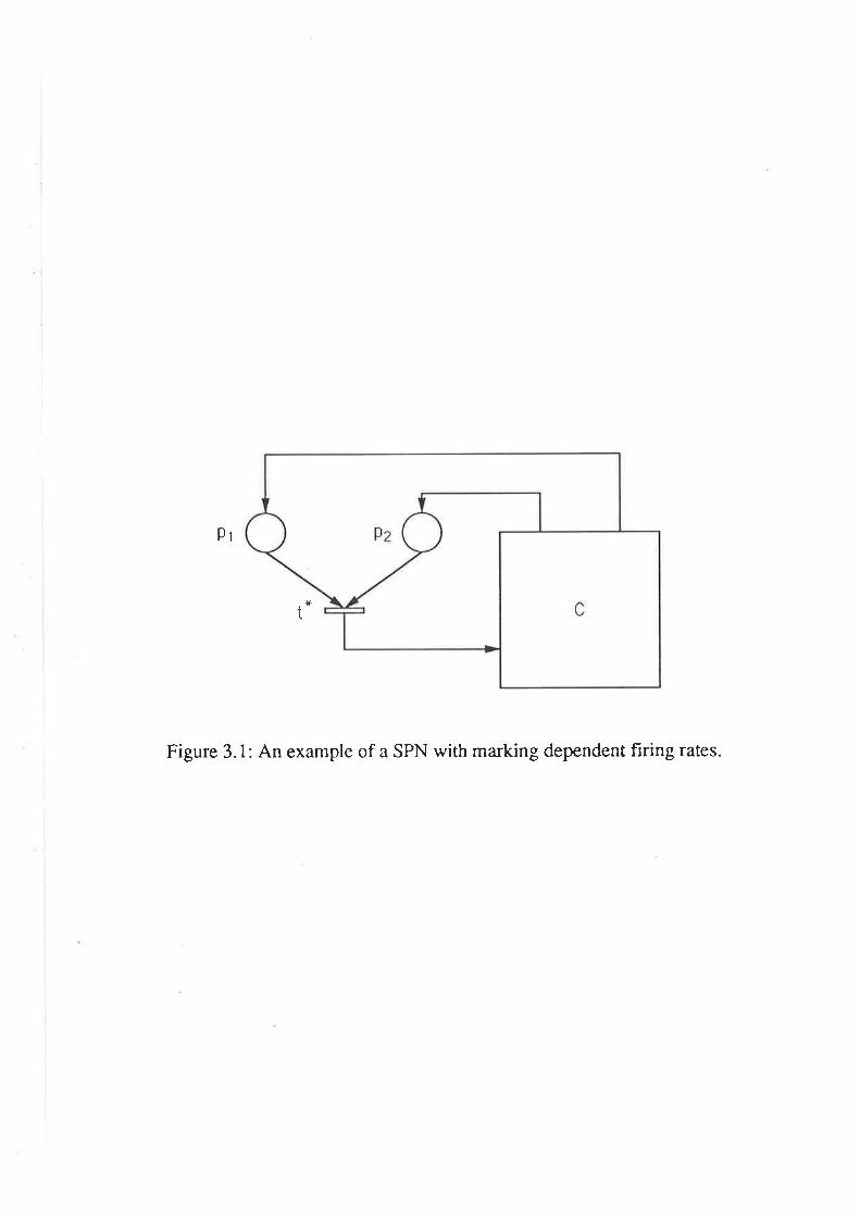
Pl
Figure 3.1: An example of a SPN with marking dependent firing rates.
*t
Deflne
and
II
1
q(ú )x(r(ú)) : ift:f'.
othenvise,
m;n(m(t\,m(2))
Õ(*) : p(m) : ll lq(t",tn (1) - l,rn(2) - 1)l-'l=0
Substitution into Equation (3.9) gives,
q(m, ú) :q(ú-, m(1), *(2)) if ú : f*,
q(t) otherrn'ise,
as required.
Example 3.3
Using Figure 3.1, rve can introduce more generalitl' by letting, X(I(¿')) : 1,, and
O(*) : q(t',-(1), rn(2))p(rn - €1 - e2). This again gives the result q(m, t') :
q(t',rn(7),*(2)), without placing any restrictions on the transitions in C.
Exarnple 3.4
Consider Figure 3.2. We will shorv how marking dependent firing rates, including
l-rlocking, can be incorporated into the model, using the appropriate choice of the
p(') *d Õ(') functions. Suppose that we wish to model the situation where f¡,t2
and ú3 have firing restrictions, which halt firing r¡'hen the number of tokens in
places þt,p¿ *d pr satisfy certain criteria. To model this, let,
p(rn): 0 if rn€?,p'(nr) othern'ise,
for an arbitrary choice of.D e M. For example, let D be defined b1'the expression,
rn(1) + m(2) 1W, for some integer 14¡. Then g(m * I(¿), ú) : 0, rvhenever nr has
insufficient tokens in places p1 and p2. Equivalently, transitions f1,ú2 and Í3 can
not fire, when pt,pt and p5 have too many tokens in them.
The above is a simple example to illustrate blocking in a SPN, with the firing
rates given by Equation (3.9). Norv that a blocking assumption is in place, we can
add to the model, by incorporating marking dependent firing rates, as follows.
38
9qPs
3t2t
Ps
4t
t
t65t
Pr 9z
Figure 3.2:The SPN for Example 3.4.
Let
and let,
Q-(rn(t), m(2)): l' ry# i,#According to this description, transitions Í;, 1 S i ( 3, will frre at the follog,ing
state dependent rate,
ç'(rn - €1 - "r) : 11(nz(1))r2 (m(Z))r7@t(1), m(2))Õ-(nz(1), *(2)),
s(rn,ú¡): ##rl,##x(r(t,)). (3.10)
Consider q(m,úr) and note that I(ú1): (1,0,0,0,0) so that,
?'(m - r(¿'))
: :ï; ;:,,:,'r:;,]n,-,,,, *(z)r l)Õ-(nz(1), m(2) * 1),
Substitution in Equation (3.10) yields,
g(m, tr)
: rr(m(1))r2(rn(2) * t)a(n(l), m(2) + 1)t'i'*Íl-,"-_i:'#
i'i# ^iÍ,'"llii,"
x(r(¿' ))-
After cancellation this gives,
s(m, f r) = rr (m(1))ra(rn(Z))Tì(-(1), m(2) * 1)¡(I(r¡ )).
Similarly,
s( m, úz) :'r (m( 1 ) )r 2(m(2))rt(-( 1 ), m(2) )¡(r(r, )),
s(m, ús) : 's("n(1))rr(m(2))Tt(-(r) + L,rn(2))x(I(¿.)).
In conclusion, we have shown that the firing rates can depend on the number oftokens, not only in the input places of the transition, which is conventional, but
on the token distribution in any of the places.
39
3.3 The Routeing Process
The central feature of our anal¡.sis is to consider the transitions of the SPN. to
be themselves states in a Markov chain, which we call the routeing process. This
is achieved, by first considering the input and output bags of the SPN to be the
states of a Markov chain, and under suitable conditions, finding a one to one
correspondence between the states of this Markov chain and the transitions of the
net.
Although each transition, ú, of our SPN has a unique input bag, the proba-
bilistic routeing a-llorvs for a number of different output bags. Let O(t), be the set
of output bags of transition ú and define,
a: U o(t)u U {rt¿l}.r€T teT
7? is the set of all vectors rvhich are either output or input bags for the SPN. \\re
assume the net is such that R. is finite.
Define single step transition probabilities on the set 7t as, whenever there
exists a transition f, rvith r : I(t),
P(r'r J:
If r is not the input bag of some transition, then P(r, r') : órr, where ó"", is the
I(ronecker delta. Note, the requirement that no vector can be the input bag of
trvo distinct transitions, means these probabilities are well defined.
Now define the set,
f : {f(.),/(r) > 0, x(r),f("): !x("')/("')p(r',r), Vre 7è},rt
where ¡(r) is the function given in Equation (3.9), when r : I(f) for some f.
X(r) : 1 otherwise. X(.)/(.) is therefore an invariant measure for the routeing
process. In Section 3.4, u'e need .F to be non-empt¡'. The effect of this assumption
on the structure of the net is examined in the follorving results.
p(I(f ),ú, Oj(¿)) if I j | "' : O¡(¿),
0 otherrvise.
40
Lernrna 3.1
For f to be non-empty, all vectors I(t), t e T, must be in positive recurrent
communicating classes of the routeing process.
Proof
For ú to fire in some marking, x(I(f)) > 0. Assume there exists a function,
/(.) € F, impl¡'ing therefore, that X(I(¿))/(I(I)) is positive, Since the set 7t. is
finite, and ¡(')/(') is an invariant measure of the routeing process, I(1) is in a
positive recurrent communicating class. r
Corollary 3.1
For .F to be non-empty,
(a) att r e R must be the input bag for some transition, f ,
(b) all r € R must be an output bag for some transition, ú
Proof
(a) Assume .F is non-empty and that r is not an input bag for anv transition.
Since state r is not the input bag to some transition, p(r,r,): á¡¡,, and
r is an absorbing state in the routeing process. Hence r resides in its orvn
communicating class. Also, r e O(t) for some transition, f , means that there
exists unr' f r, such that p(r',r) > 0,implying that r'is not in a positive
recurrent communicating class. This contradicts Lemma 3.1.
(b) If r is not the output bag for any transition, then there exists no. r' f r,
rvith p(r', r) > 0. Thus r must be a transient state. This contradicts Lemma
3.1 in conjunction with Corollary 3.1(a). r
Corollary 3.2
If f is non-emptrl', there exists a one to one correspond.ence between distinct ele-
ments of 7i. and elements of T.
4l
Proof
It follows from Corollary 3.1(a), that each vector r €R is the input bag for some
transition t eT. By the assumptionin Section 3.2, each input bag has a unique
tra¡rsition. The result follows. rRemark 3.1
Corollary 3.1, states that for nets with non-empty f , each output bag of a transi-
tion is the input bag of another transition. This implies that u'henever an output
bag O¡(t) is deposited by transition f, then O;(J) : f(s), for some transition s.
Note that this matching input and output bag criterion does not imply that s is
the only transition enabled by O;(t). There axe many other transitions enabled
by Or(f), that may even be more likely to fire. For example, in Figure 3.3, the
firing of transition ú3 enables both transitions t1 and t2, but I(tr) : O(f3), so
F(ts,fr) > 0 and p(t3,úz) : 0.
Example 3.õ
At this point we will reveal the difference bets'een the extended product form
solution for queueing networks, developed by Henderson and Taylor [42], and the
adapted theory for SPNs.
Henderson and Taylor use a vector, a : (a(0), o(i)), to represent the total
number of customers released into the netu'ork. c(i) represents the total number
of customers released from node i and o(0) represents the number of customers
which enter (leave) the network from (to) the outside. Using Figure 3.3, u,e will
shor¡'that it is not possible to achieve the matching input and output bag criterion
given by Corollary 3.1, if the vector a is used in place of input and output bags.
That is, let I'(ú) be the normal input bag of transition I appended by an entry
placed at the beginning of the vector, which represents the tokens that enter the
SPN from the outside. o'(r) is formed in a similar wa]¡. For Figure 3.3, u,e give
I'(ú) and the corresponding O'(f ) for each transition.
I'(t, ¡ : (0, 1, 1, 0, 0), O'(¿, ) : (0, 0, 0, 1. 1),
42
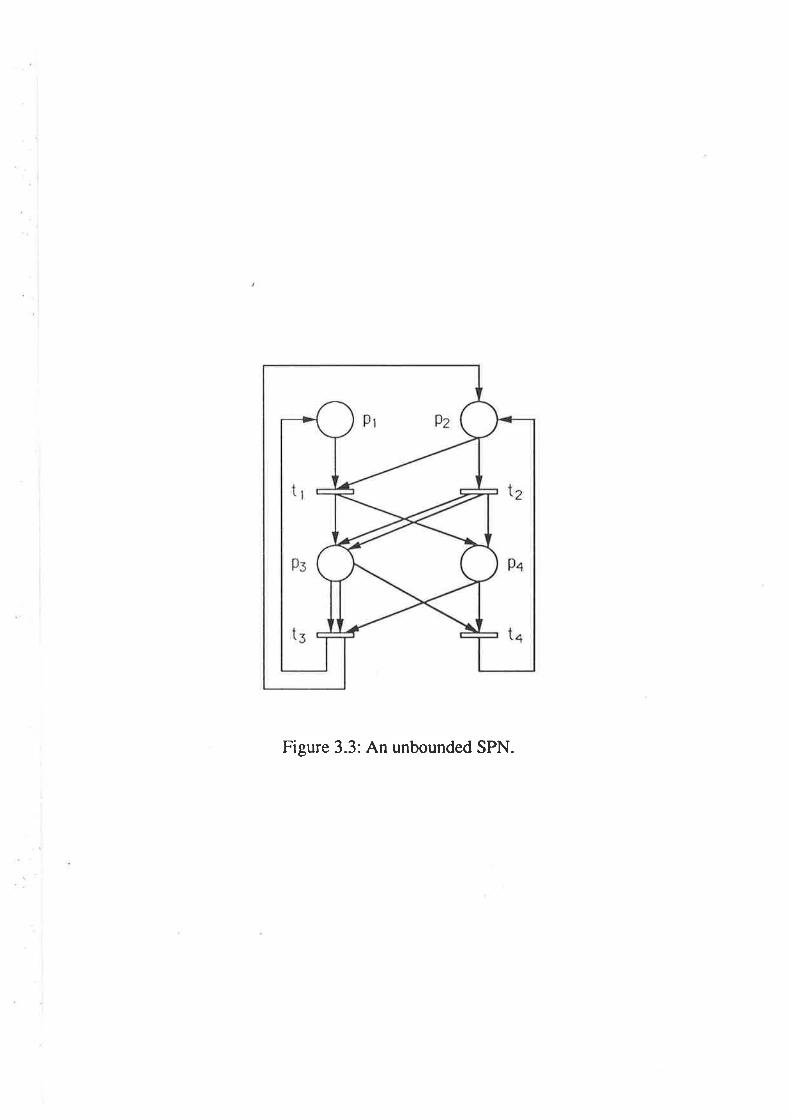
Figure 3.3: An unbounded SPN.
I'(tr) - (2,0, 1,0,0),
r'(rr) - (0,0,0,2,1),
I'(¿r) : (0,0,0, 1, 1),
O'(¿r) : (0,0,0,2, 1),
O'(¿.) : (1, 1. 1,0,0),
O'(¿n) : (1,0, 1.0,0).
Corollary 3.1 is not satisfied, since there is no matching output bag for I'(t1) or
I'(tr) and therefore the theory of Henderson and Ta¡,lor can not applied directly.
However, this does not imply that tokens can not be created or destroved, when
the theory is applied to SPNs, since, the a(0) term has been incorporatecl into
the original input and output bags I(f) and O(¿). Since the definition of a SPN
allows the destruction and creation of tokens, I(ú) and O(t) automaticalll' absorb
the a(0) term. Therefore, accounting for the a(0) term is superfluous and can
destroy the matching input and output bag criterion.
Remark 3.2
Let the transitions corresponding to the non-zero entries of a T-invariant be rewrit-
ten as aset of transitions,C;. If. the SPN, describedin Section 3.2, does not have
probabilistic routeing, C¡ indicates which transitions belong to the ith positive
recurrent communicating class. If the SPN, described in Section 3.2. has prob-
abilistic routeing the follorving alteration must be made to eliminate the proba-
bilistic routeing (recall that the T-inrariant can only be found for deterministic
PNs). For each transition, t, rvith more than one output bag, replace t s'ith a set
of transitions, "4(t), one for each output bag. Each transition in "4(t) s'ill share
I(f ), and have one output bag. This is effectively the rel,erse operation described
in item 2 in Section 3.2. The firing rates do not need to be evaluated. since rve
are only interested in the structure of the net. From this altered net, the positive
recurrent communicating classes for the original net are er"aluated in the following
way. For each transition, t, and for each C;, such that C, n ,4(f ) + {}, rervrite C;
witlr the elements of AQ) replaced by f, rvhere {} is the empty set. Norv, for each
i,j, such that C; aC¡ * {}, let C*:C; UC;. Continue this process until all of the
remaining sets, C;, are mutually disjoint. The remaining sets, Ç, are the positive
43
recurrent communicating classes for the original net. For an illustration of this
process on a net which includes probabilistic routeing) see Exarnple 3.8.
Remark 3.3
Note that Corollary 3.2 implies that each r € ß can be uniquely identified r+,ith a
transition. Consequently, rü/e can defrne the routeing process to be a lrfarkov chain
on the set of transitions , T, rather than on the set of input and output bags, 7?.
Without loss of generality, we will retain the same notation, by assuming that the
one step transition probabilities for the routeing process orr T are,
F(ú, ") : p-(I(ú),I(r)), s, t € T
Let us stress again that p(ú, s) is not the probabitity that s will fire after /.
In fact the set {s : p(ú,s) > 0} is a subset of the set of transitions rvhich can fire
after f fires. Transition s rvill be enabled by the output bag of I with probabilitl,
Þ(ú, s). Ho$'ever, as we have seen in Example 3.3, and in many other examples,
many other tra¡rsitions will be enabled after t fires, and any of these can fire after
ú fires. Examples 3.8 and 3.9, illustrate this for the probabilistic routeing case and
for the deterministic routeing case, respectively.
f can now be redefined as,
î: {f(.): /(ú) > 0, ¡(t)/(t): Dx(")/(")p(",ú), y t eT}, (3.11)seT
and ¡(')/(') is an invariant nìeasure for the routeing process. As the routeing pro-
cess consists of only positive recurrent communicating classes, it ma¡' be assumed
thar ¡(ú)/(r) > 0, v t e T.
3.4 The Extended Product Form Solution
Lemrna 3.2 (Theorem 1.13 from l(elly [51])
Let x(ú) be a stationary Markov process with transition rates g(m, n), m, n €S, where S is the state space. If we can find a collection of numbers,
44
qÌ(rn,n), rn, n € S, such that,
I q(nt,.r) : D gR(m, n), Vm € s,¡r€ S neS
and a collection of positive numbers r(*), rn € S, summing to unity, such that,
zr(rn)q(rn, n) : z¡1n¡0"(r, *) rn, n € S,
then gn(rn, tt), m, n € S, are the transition rates of the reversed process X(r -t)and zr'(rn), m € S is the equilibrium distribution of both X(ú) and X(r - t).
Lemrna 3.3 (Adapted from Lemma 3.2 for SPNs)
Let X(ú) be the stationary Markov process of a SPN described in Section 3.2 ri'ith
transition rates g(m,t)p(t,s), rn € M, s,t e T, which is the rate of moving from
marking m, to marking rn - I(f) + I(s). If we can find a collection of numbers
gR(nr.m + I(ú) - I(")), rn € M, s,t € T, such that,
t D q(m, ú)¡{ú,") : D I q^(*, m* I(s) - I(¿)),teT seT IET sC,T
or equiralently,
I q(-,¿) : D D q^(*, m+ r(s) - r(ú)), (3.12)teT teT teT
since ! P(ú, s) : 1, and a collection of positive numbers zr(m*I(ú)), m ç Jv1, t eteT
7, summing to unity, such that,
a'(m*I(t))q(m + I(t), t)Fþ,s): r(rrr+I(s))qRlm*I(s),m + I(t)), (8.13)
then qR(m*/(s),rr+I(ú)), nt € M, s,ú € T ate the transition rates of the
reversed process X(" - f) and ur(rnf I(f)), rn e M, t €T, is the equilibrium
distribution of both X(t) and X(r - t).
Theorern 3.1
Assume that there exists a function /(.) € F, and a function g(.) : ZlPl - IR,
which has the property that, for all ú € T and rn * I(ú) in the reachability grap
e(rn + I(t)) _ f(t)g(rn+I(")) -.f(")'
45
(3.14)
whenever F(t, ") ) 0. Then the equiiibrium distribution of the SPI{ is given by,
zr(rn) : I(Õ(rn)g(to), (3.15)
where A(.) is given in Equation (3.9) an .Ií is a nornalising consrant.
Theorem 3.1 gives a product form solution. The product is betu'een two dis-
tinct terms, as in Equation (3.8), rvhich was discussed in Section 3.1. The first
of these is Õ(.), a function related to the transition firing rates and to marking
dependent properties of the SPN. The second, g('), can be evaluated by analysing
the network skeleton provided by the transitions and the routeing process. The
effect is to reduce th problem of finding an equilibrium distribution for the num-
ber of tokens in each place of a SPN, from that of solving balance equations for
a Markov process on the markings, n'hich grows exponentiall¡' in size rvith an in-
crease in the number of tokens, to solving balance equations for a \.farkov chain on
the transitions, the size of which does not change rvith an increase in the number
of tokens. The examples in Section 3.5 illustrate this effect.
Proof
Let us propose, that the reversed time transition probabilities for the routeing
process are,
pR(", t¡ : x(¿){(l)_P(l, "). (a.16)x(s)f(") '
and ¡rostulate an equilibrium distributio for the SPN given b1.(3.15) subject to
(3.14).
Note that any marking change of the SPN begins *'ith a marking ¡n * r(ú) u'ith
t e T enabled. Transition ú fires, producing an output bag, rvhich because f is
non-empty, is the input bag of another transition, s sa],. The resultant marking is
m * I(s), and transition s is enabled. In reversed time, the markings and enabled
transitions a¡e unchanged but the reverse operation occurs.
Postulate that the marking change rate for the SPN in reversed time is,
sÊ(rn * I(s), rn * I(ú)) : s(m * I(s), s)p-R(s, t) (3.17)
46
From Lemma 3.3, the validity of Equations (3.12) and (3.13) is sufficient to estab-
lish that *(rn), as given by Equation (3.15) subject to (3.1a). is the equilibrium
distribution of the SPN and that the postulate of Equation (3.17) is correct.
Consider the right hand side of Equation (3.13). Substituting the form for
*(m + 1(")), from Equation (3.15) and gR(rn * -I(s), rn + I(/)), from Equarions
(3.16) and (3.17) yields,
f(t)/(")
: /{s(rn + I(s)) e(m)¡(l)p-(ú, s), (3.1s)
but from Equation (3.14),
g(ur f /(s))4Ð - o(nt +T(t'õ:e(rn+r(ú))Substitution into Equation (3.18) ¡-ields,
/ís(m + I(t))p(m)¡(ú)p-(t, s),
: /t'o(m + I(t))e(m + rtrl)affi&p(ú,"),
: zr(m + I(t))q(m + I(t), f )p-(f , s),
b1' Equations (3.15) and (3.9). This is the left hand side of Equation (3.13), rvhich
shows that Equation (3.13) is satisfied, V nt € M, s,t €T. Consider norv the
right hand side of Equation (3.12) and substitute,
gR(tn, rr *,I(s) - I(¿)) : Q(rn, r)pR(f, s),
which gives,
D t q(m, t)pR(r, ") - I q(m, ¿),
t€T s€T teT
since f pÆ(Ú,s):1. This shorvs that Equation (3.12) is satisfied and thereforec€T
proves that, a'(m) as given by Equation (3.15), is the equilibrium distribution of
47
the SPN. ITheorerr-^ 3.2
For the SPN of Theorem 3.1, the equilibrium distribution given by Equation (3.15)
subject to Equation (3.14), satisfies the following partial balance equation.
flux out of rn * I(t), due to the firing of ú
: flux into rn + I(¿), due to the bag I(f ) being deposited by a transiai"l:'tg)
Proof
Consider transitions s and ú, in the same positive recurrent communicating class
C. The flux into rn * I(l) from nr * I(s), where the output bag of s is the input
bag of t, is
D '(* + I(s))q(rn * I(s), s)p(s, ú).
By Equation (3.9),
s€.C
t€.C
: tr(m+I(s))p(m) , \
.-1mffi¡(s)P(s't)Using Equation (3.15),
: p(rr) f rrslm + I(s))¡(s)p(", t)s€C
Substituting for 9(m + I(s)) using Equation (3.14),
: Iiç(m) t e(m + I(t)) f(")f (t)
¡(s)p(s, ú),¡€C
e(rn+ I(f))Í(t)
: /íp(m) I /(")x(")p(", ú).c€C
But ! /(")x(r)p(s. f ) : /(t)x(¿), is the global balance equation on the routeingsÉ.C
chain. So,
: /fçr(m)e(rn + I(ú)) f(t)Í(t)
: I(ça(m)s(m f l(t))x(t).
48
x(r),
Once again, using Equation (3.i5) and (3.9)'
:r(,,,)ffi#ß*(,),
: zr(rn + I(l))q(rn + I(ú), t)
\Mhich is the flux out of m * I(ú) due to the frring of transition t. ¡
Remark 3.4
The partial balance equations given by Equation (3.19) above, are a generalisa-
tion of 'Whittle's, given by Equations (3.5) and (3.6). \\¡hittle's partial balance
equations apply to open queueing networks, t'here there is purely single customer
movement. In a SPN, this corresponds to having a single input and output arc per
transition and an extra transition, f6, to represent the "outside". Let T' :TlJto
and let the input bag of ú¡ be place p,, say. Norv assume that a token s'ill arrive
at place pi, rÄ'ith rate À(i). Therefore, let fs fire with rate | À(i). Connect onei=l
probabilistic arc from Ís, to every place p¡ in the SPN, such that fe rvill deposit
|-tPt l-'a token in p; rvith probability À(i) Itlf¡ll Also, let the tokens depart the
Lj- JSPN with rate g(i), from place p¡. Consequently, O(t¡) : O, s'hich represents
the "outside", u'ith probability q(i), or is the next place p; (since pj e O(ti))
rvith probability F$;,t¡). Similarly, I(¿o) : O. Note that, u'e have maintained the
matching input and output bag criterion, in using probabilistic output bags.
Figure 3.4 is a SPN representation of a simple open queueing netrvork. Tokens
arrive to place p1 from the "outside", rvith probability )(1)XÐiiø' or internallY
rvith probability p(tz,tr). Tokens leave p¡, and depart externally, u'ith probability
q(1), or move on to the next place with probability p(tt,tz).
Equation (3.19), relates the flux out of rn*I(t;), due to a token leaving p¡ with
the flux into m + I(új), due to a token being deposited into pr'. This is Equation
(3.6), if m * I(fi) : n and p¡ represents queue j. Equation (3.19) also relates
the flux out of rn+0, due to a token entering the SPN from the "outside", rvith
the flux into m { 0, due to a token leaving the SPN to the "outside". This is
49
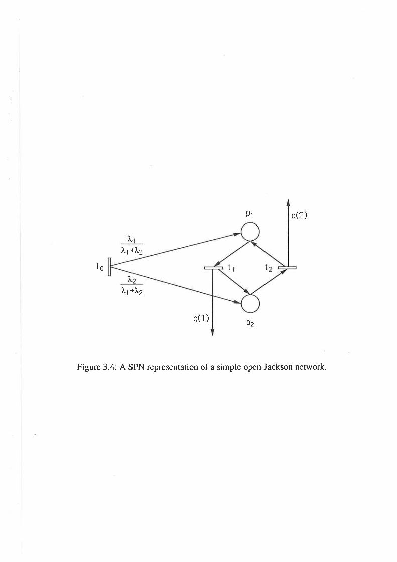
Pr qQ)
¡,
7v *?"2
te
ïtt+LZ
q(l)9z
Figure 3.4: A SPN representation of a simple open Jackson network.
Equation (3.5), if rn * 0 : n.
The frring rates in our model also incorporate more general marking dependent
firing rates and blocking, as in Example 3.4, rvhich \Mhittle does not consider.
In Example 3.6, it is shown how the solution to the Jackson nets'orks can be
derived as a special case of the results in this section.
3.5 Examples
Exarnple 3.6: Jackson Networks
Consider a SPN as defined in Remark 3.4. Since each place is connected to
a unique transition by one arc, the number of times transition l; must fire to
remove ,n(p;) tokens from place p; is given by -(p¡), rvhich in this case can
be written, without loss of generality, as m(t;). Let ¡(t;) : 1,Vú; e. T, y(ts):lPl -(ri)Dr(¿) and Q(rn) : p(m) : II lI (q(¿t, ¡))-t. \ryirh these paramere.r'arues andi=l t;cT l=lassumptions on the net structure, /(.) e .F satisfies,
.f(ú;) : I ¡(¿;)p(t¡,t;)+/(¿o)x(¿o)p(úo,¿,), v t; € T, (8.20)treT
and
q(rn,l;):*#
m(f,)-l
l=l
-(t¡)
rr€1\{r,} ¡=r|| s(t¡,1)-r || lI q(ú¡,1)-'
m(¿i): q(ti,m(ú¡))
^(tt)ll ø(t,,t¡-' f[ fJ q(¿¡,1)-'l=l tr€7\{t,} ¡=l
Equation (3.20), is the standard traffc equation for the open Jackson netrvor.k,
given by Equation (3.3) in Section 3.1, as ca¡r be shown by the follou,ing. Let
"f(úo): 1, so, /(¿o)x(¿o)p-(¿o,¿;) : À(i). Substirurion yields,
"f(f;) : À(t) + D ¡U)p(t¡,t;)IreT
50
(3.21)
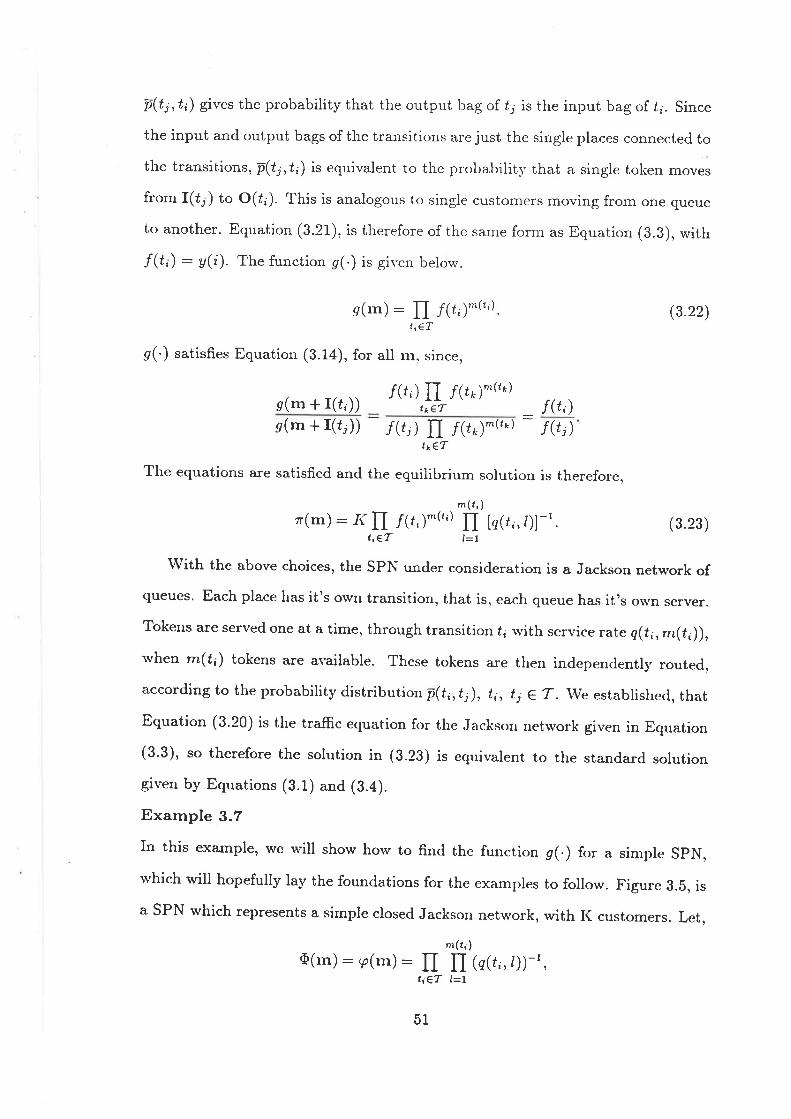
Þ(t¡,,t;) gives the probability that the output bag of ú¡ is the input bag of ú;. Since
the input and output bags of the transitions are just the single places connected to
the transitions, F(t¡,t¡) is equivalent to the probabilitv that a single token moves
from l(fr') to O(f.). This is analogous to single customers moving from one queue
to another. Equation (3.21), is therefore of the same form as Equation (3.3), with
f U;) : y(i). The function g(.) is gir-en below.
g(rn): II f (t,¡^u't (3.22)tí€T
g(.) satisfies Equation (3.14), for all rn. since,
e(m + I(t;))g(m * I(¿¡))
/(t,) lI fQo¡^art1t€T- /(¿¡) fl /(to)-"*,
: f (t;)f (t¡)
tx€T
The equations a¡e satisfied and the equilibrium solution is therefore,
''.(t¡)
'.-(m): rí fI /(t,;".(t.) fI [q(r,,/)]-'. (3.28)a;€T l=l
With the above choices, the SPN under consid.eration is a Jackson network ofqueues' Each place has it's orvn transition, that is, each queue has it's og,n server.
Tokens are served one at a time, through transition t, rvith service rate q(t;, m(út)),
when m(t¡) tokens are available. These tokens are then independentl¡, routed,
according to the probability distribution p(ú¡, t j), t¿, t¡ € T. we established, that
Equation (3.20) is the traffic equation for the Jackson netrvork given in Equation
(3'3)' so therefore the solution in (3.23) is equivalent to the standard solution
given by Equations (3.1) and (B.a).
Example 3.7
In this example, we u'ill show how to find the function g(.) for a simple SpN,
which will hopefully lay the foundations for the examples to follow. Figure B.b, is
a SPN which represents a simple closed Jackson network, with I( customers. Let,
-(¿;)@(rn) : e(m) : If lI (q(¿,, ¿))-',
t¡ÊT l=l
51
tg
Pl
l2 t1
Figure 3.5: A SPN representation of a simple closed Jackson network
Ps
9z
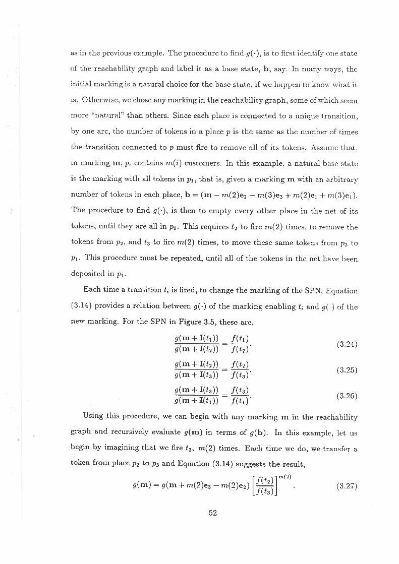
as in the previous example. The procedure to flnd g(.), is to first identify one state
of the reachability graph and label it as a base state, b, say In many x'avs, the
initial marking is a natural choice for the base state, if we happen to knou' rvhat it
is. Otherwise, tt'e chose any marking in the reachability graph, some of u'hich seem
more "natural" than others. Since each place is connected to a unique transition,
by one arc, the number of tokens in a place p is the same as the number of times
the transition connected to p must fire to remove all of its tokens. Assume that,
in marking rn, p; contains m(i) customers. In this example, a natural base state
is the marking rvith all tokens ir pr, that is, given a marking rn with an arbitrary
number of tokens in each place, b : (m - rn(2)e2 - m(3)e3 * m(2)e1* m(3)e1).
The procedure to find g(.), is then to empty every other place in the net of its
tokens, until the¡' are all ir pr. This requires 12 to fire ,n(2) times, to remove the
tokens frorn p2, and ú3 to fire m(2) times, to move these same tokens from p3 to
p1. This procedure must be repeated, until all of the tokens in the net have been
deposited i. pr.
Each time a transition ú; is fired, to change the marking of the SpN, Equation
(3.i4) provides a relation betrveen g(-) of the marking enabling ú; and 9(.) of the
nerv marking. For the SPN in Figure 3.b, these are,
e(m + I(¿'))s(rn * I(¿¿))
s(m f I(¿r))
e(m + I(¿s))
f(tr)f (tr)'
- f(tr),f(¿r)'
(3.24)
(3.25)
g(rn+I(úe)) _ f(t")s(rn * r(t'))
: 1õ' (3'26)
Using this procedure, we can begin with any marking m in the reachability
graph and recursively evaluate g(m) in terms of g(b). In this example, let us
begin by imagining that we fire t2, m(2) times. Each time s,e do, we transfer a
token from place pz to ps and Equation (8.14) suggests the result,
g(m) - s(m * rrz(2)e3 - nr(2)e2) lffi]-t" (r.27)
52
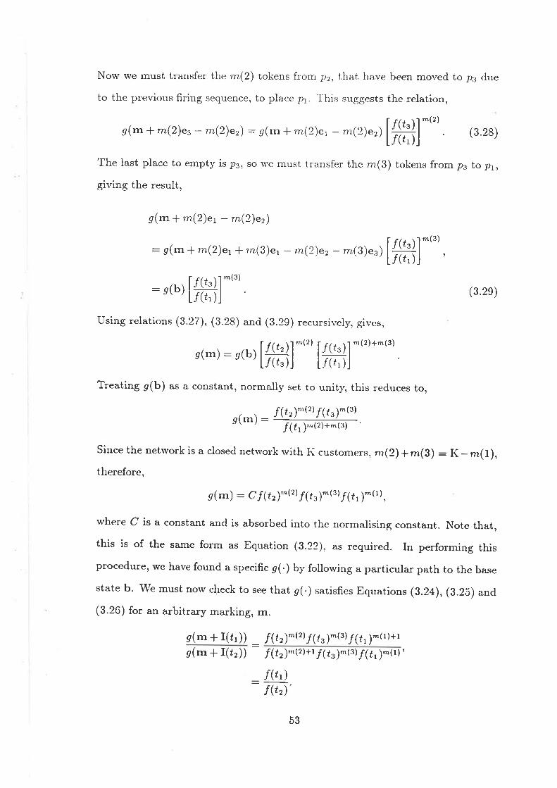
Now we must transfer the m(2) tokens frorn p2, that have been moved to p3 due
to the previous firing sequence, to place pl. This suggests the relation,
g(rn + m(2)es - m(2)e2): e('r f nz(2)e1 - m(2)e') l{!t'll-t" ..,) L/(ój (3 28)
The last place to empty is p3, so \r,e must transfer the m(3) tokens from p3 lo pt.,
giving the result,
s(m+m(2)e1 -m(2)e2)
: e(m r m(2)e1* m(3)e1 - m(2)e2- rn(3)e3) lffi]-''' ,
: s(b) l{!t'}l-"' .Lml (3'2e)
Using relations (3.27), (3.28) and (8.29) recursively, gives,
g(,n) : e(b) lffi]-"' lffi1 *{z)+-{s)
Treating g(b) * a constant, normally set to unity, this reduces to,
s(m) - /(¿-' )'t'1,{(t')î,ttl .
/(út ¡-tz¡"*tt'
Since the netrvork is a closed netrvork rvith Ii customers , m(2)+ m(3) : ( - -(1),therefore,
g(nr) : C f (tz)^(z)¡11.;-(3)¡1t, ¡-(t),
r¡'here C is a constant and is absorbed into the normalising constant. Note that,
this is of the same form as Equation (3.22). as required. In performing this
procedure, we have found a specific g(.) by follorving a particular path to the base
state b. We must now check to see that 9(.) satisfies Equations (s.24), (3.2b) and
(3.26) for an arbitra^ry marking, m.
e(m + I(¿' )) _ f (tr)^(r)/(¿3)-(3)/(ú, ¡-{r)+rs(m + I(¿r)) - r(tr¡^12¡¡, f (t"¡^tsl ¡(ú, ¡*1r¡ '
f(tr)- f$r)
53
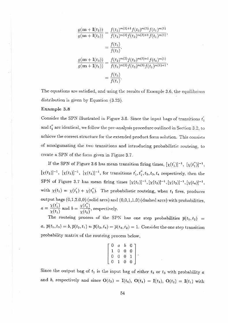
s(lrr + I(¿r)) f (tr¡^tz\+t f (t"¡^{st ¡(t' ¡-(tlg(rn + I(¿r)) f (tr)^tzl ¡çú3)m(s¡''t1t(r, ¡*1t¡'
f(t')/(t.)
g(rn + I(l')) _ f (t r)^(r) ¡1r. ¡".t:l+l ¡1r, ¡"'tt )
g(rn + I(¿t)) f (t")*tzl ¡(ú3)-(3)/(ú1)-(r)+r'
/(¿')/(¿')'
The equations are satisfied, and using the resuits of Example 3.6. the equilibrium
distribution is given by Equation (3.23).
Example 3.8
Consider the SPN illustrated in Figure 3.6. Since the input bags of transitions ú',
and li are identical, we follow the pre-analysis procedure outlined in Section 3.2, to
achieve the correct structure for the extended product form solution. This consists
of amalgamating the two transitions and introducing probabilistic routeing, to
create a SPN of the form given in Figure 3.7.
If the SPN of Figure 3.6 has mean rransition firing rimes, [X(/l)]-t, [X(úi)]-t,
[x(tr)]-t, [x(úr)]-t, Ix(úo)]-t, for transitions t'r,t'i,tz,tz,úa respectively, then the
SPN of Figure 3.7 has mean firing times [X(tr)]-t, [X(¿r)]-t,[X(¿r)]-t, [X(¿o)]-t,
with ¡(t¡) : X(t't) + x(¿i). The probabilistic routeing, when f1 fires, produces
output bags (0,1,2,0,0) (solid arcs) arrd (0,0,1,1.0) (dashed arcs) u'ith probabilities,
o : I(tl and ö: t!1i¿, respectir-elr'.X(tr) X(úr)'The routeing process of the SPN has one step probabilities p(tr, t2) :
a, F(tt,úr) : b,-p(tz,úr) : F(ts,t,t) : Þ(úr, tz):1. Considertheone step transition
probability matrix of the routeing process belorv,
Since the output bag of ú1 is the input bag of either t2 ot ts rvith probability a
and ó, respectively and since O(f3) : I(ú¿), O(¿n) : I(úz), O(tr) : I(fr) with
0 ab 0
100000010100
54
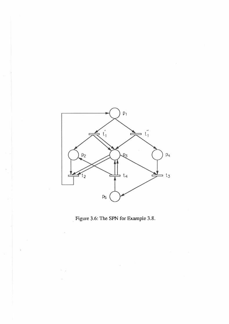
Pl
t
Pq
l2
Þs
. Figure 3.6: The SPN for Example 3.8.
tg
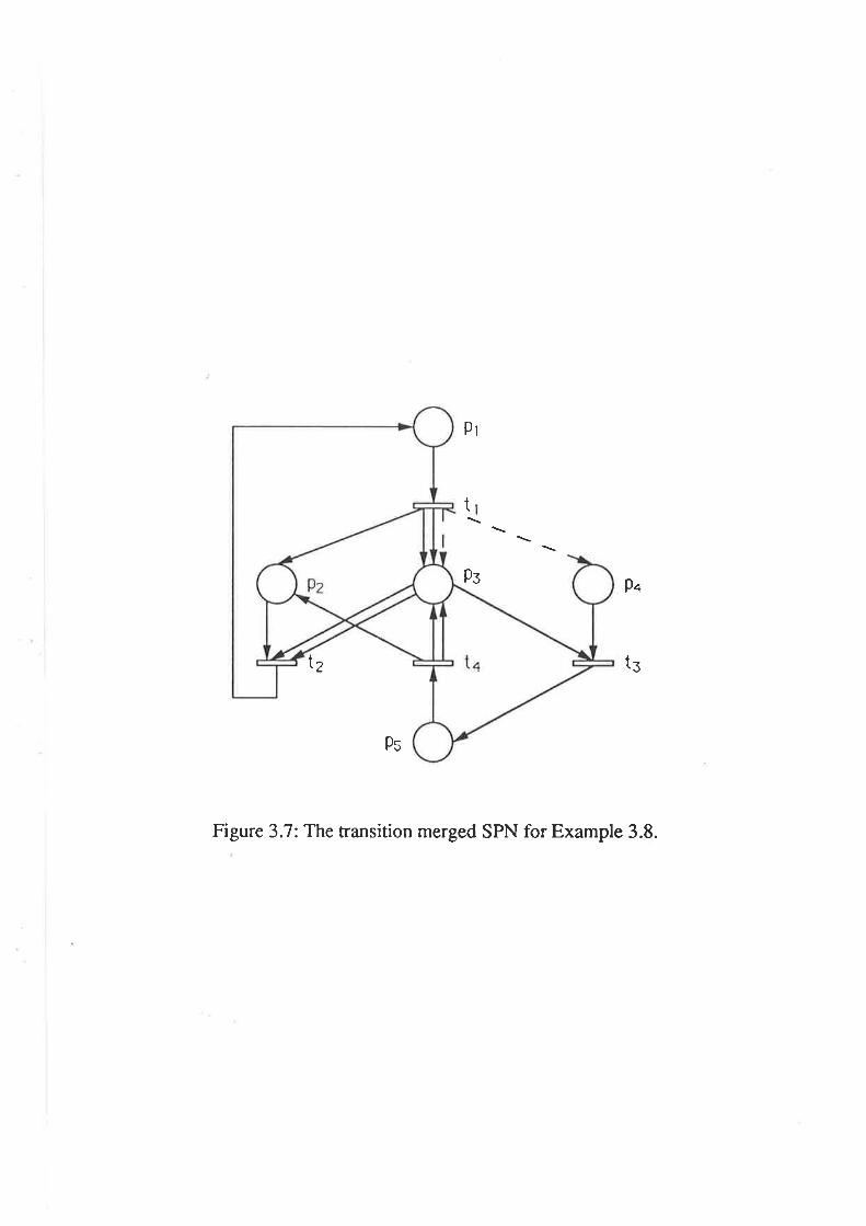
Pr
t
PsP4
l2 tg
Ps
Figure 3.7: The transition merged SPN for Example 3.8.
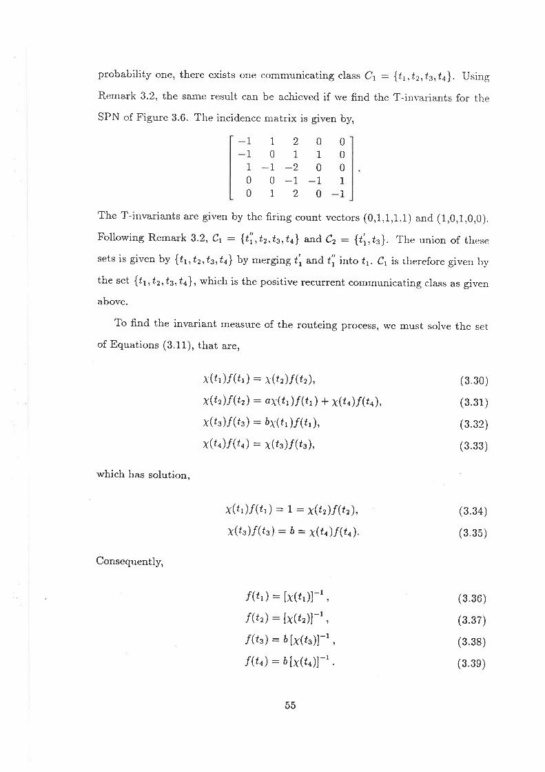
probability one, there exists one communicating class C1 : {f , ,t2,ts,ta}. Using
Remark 3.2, the same result can be achieved if rve find the T-inrrariants for the
SPN of Figure 3.6. The incidence matrix is given by,
I201
-1 -20 -172The T-invariants are given by the firing count vectors (0,1,1,1.1) and (1,0,1,0,0).
Following Remark 3.2, Cr: {t'i,tz,ts,úa} and C2: {t'r,h}. The union of these
sets is given by {tt,tz,ts,ún} by merging ti and t'j into tr. C, is therefore given b¡,
the set {tr,tr,tz,ta}, which is the positive recurrent communicating class as given
above.
To find the invariant measure of the routeing process, we must solve the set
of Equations (3.11), that are,
0
0
0
1
1
0
1
0
1
0
1
1
1
0
0
which has solution,
Consequently,
x(úr ),f(úr ) : x(rr).f(úz),
x(t2)f (tr): dX(úr)/(¿,) * x(fo).f(rr),
x(¿3)/(ú3) : öx(fr )/(¿, ),
xþ q) f (t o) : x(/¡ ).f (f e ),
x(úl)/(ú1) : t - x(t2)f(t2),
x(ú3)/(ú3) : å : x(tq)f(to),
"f(ú') : [x(t')]-' ,
r(tr) : [x(rr)]-' ,
.f(ú.): å[x(¿r)]-',
f (tn) : ó [x(¿.)]-' .
(3.30)
(3.31)
(3.32)
(3.33)
(3.34)
(3.35)
(3.36)
(3.37)
(3.38)
(3.3e)
b,)
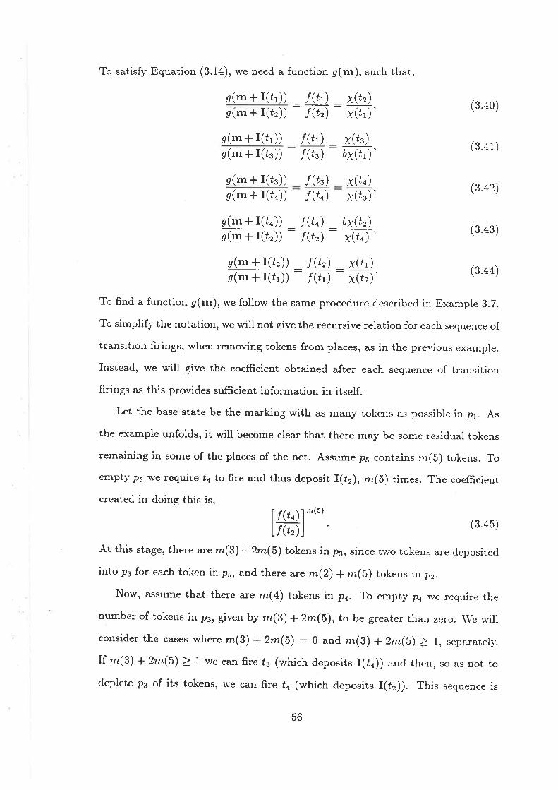
To satisfy Equation (3.14), we need a function g(rn), such that,
g(**I(¿')) _ f(tl) _x(t2)e(rn+I(¿r)) - f(tr) x(¿1)'
e(rntI(¿')) _f(t') _ x(¿g)e(mfI(¿.)) f(t") öx(¿,)'
(3.40)
(3.41)
e(m + I(¿.)) /(¿') x(tt) (3.42)e(rn * I(¿n)) f (tn) x(ús)'
g(m+I(¿.)) _ r(tn) _bx(tr)g(rn+ r(¿,)Í
: ñ: ftt' (3 43)
s(ln+r(t,)) _ f(tr) _ x(ú,)g(m*r(¿ii:1õ: ñ)' (3 44)
To find a function g(m), we follow the same procedure described in Example 3.7.
To simplify the notation, \ 'e will not give the recursive relation for each. sequence of
transition firings, when removing tokens from places, as in the previous example.
Instead, we will give the coefficient obtained after each sequence of transition
firings as this provides sufficient information in itself.
Let the base state be the marking with as marry tokens as possible in p1. As
the example unfolds, it will become clear that there may be some residual tokens
remaining in some of the places of the net. Assum. p, contains m(5) tokens. To
empty Ps we require fa to fire and thus deposit I(¿z), rn(5) times. The coefÊcient
created in doing this is,
f /(¿o)l-(')L¡t',lJ (3'45)
At this stage, there are m(3) +2rn(5) tokens ir p., since two tokens are deposited
into p3 for each token ir pr, and there arc m(2) + m(b) tokens \n pr.
Now, assume that there arc m(4) tokens ir pn. To empty p4 we require the
number of tokens it p., given by m(3) *2rn(5), to be greater than zero. \\Ie ç'ill
consider the cases where rn(B) + 2rn(5): 0 and m(g) + 2rn(5) ) 1, separately.
If rn(3) + 2m(5) ) 1 we ca¡¡ fire ú3 (which deposits I(¿n)) and then, so as not to
deplete Pe of its tokens, we can fire úa (which deposits I(¿r)). This sequence is
56
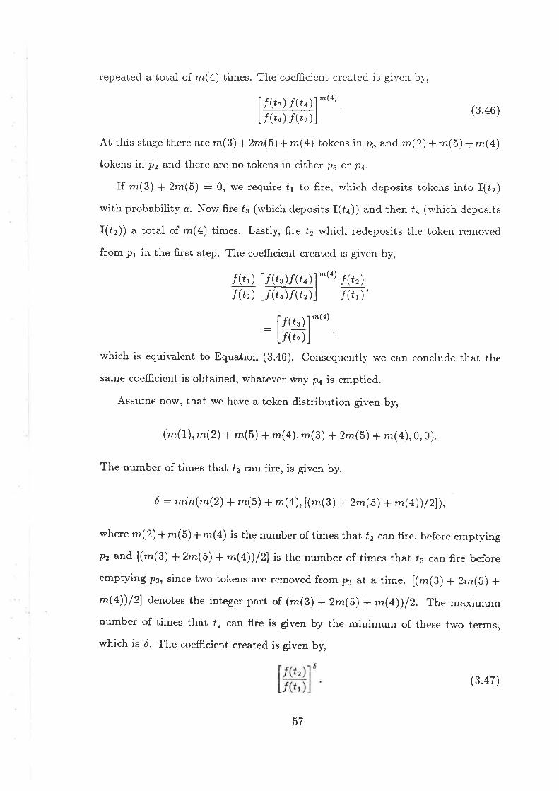
repeated a total of m(4) times. The coefficient created is given b1',
f ,r(¿.) /(¿o)l-(o)LaÐictl (3 46)
At this stage there are rn(3) +2m(5) + rn@) tokens in p3 and nr.(2) * m(5) + m(a)
tokens in p2 and there are no tokens in either ps or ps.
If m(3) + 2m(5) : 0, we require t1 to fire, rvhich deposits tokens into I(12)
with probability a. Now fire f3 (which deposits I(¿n)) and then fa (u'hich deposits
I(tr)) a total of m(! times. Lastly, fire ú2 which redeposits the token removed
from p1 in the first step. The coefficient created is given by,
/(t') U(¿.)/(¿.)l^'n' f (tr)f @) L/(ú.)/(Ðl i(Ð'
- [/(¿.)l-(o)L/(i')j
which is equivalent to Equation (3.46). Consequently we can conclude that the
same coefficient is obtained, whatever wa)'pa is emptied.
Assume now, that we have a token distribution given by,
(-(1), m(2) + m(5) + m(4),,m(3) + 2rn(5) * m(4),0,0).
The number of times that ú2 can fire, is given by,
6 : min(m(2) + m(5) + *(4), [("r(g) + 2m(b) + nt(Q)/2]),
where m(2) + m(5)+ m(4) is the number of times that t2 can fire, before empt¡'ing
p2 and [(-(g) + 2rn(5) + m@))/21 is the number of times that /3 can fire before
emptying p3, since two tokens are removed from ps at a time. [(-(3) + 2m(5) +m(4))12) denotes the integer part of (m(B) + 2m(5) + m(a))12. The maximum
number of times that ú2 can fire is given by the minimum of these tu,o terms,
which is ó. The coefficient created is given by,
(3.47)
57
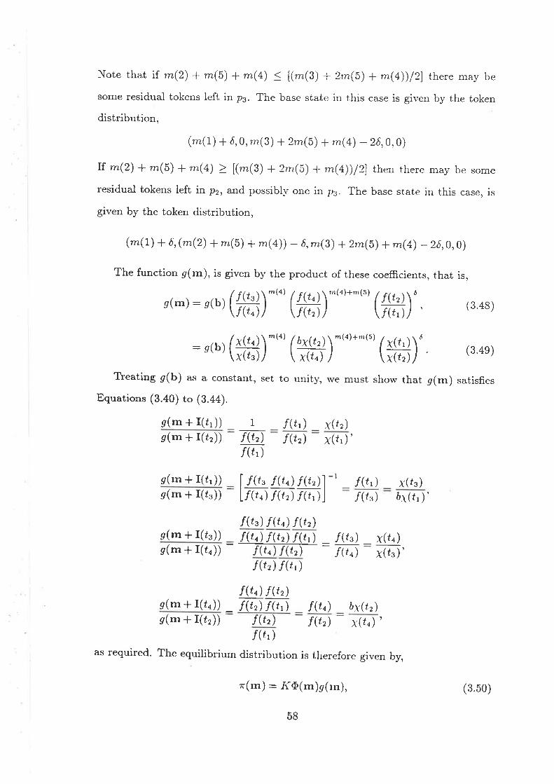
Note that iÎ m(2) + nz(5) + m(a) S [(-(e) + 2m(b) + mg))l2l there may be
some residual tokens left in p3. The base state in this case is given by the token
distribution,
(nz(1) * ó, 0, nr(3) * %n(5) + rn@) - 2ó, 0, 0)
rf m(2) + rn(5) + rn(a) 2 [(-(g) + 2m(b) + rn@))/21 then there may be some
residual tokens ieft in pz, and possibl¡'one in p3. The base state in this case, is
given by the token distribution,
(-(t) + 6,(m(2) +rn(5) + m(a)) - á,rn(3) +2rn(5) +m(a) - 2á,0,0)
The function g(m), is given by the product of these coefficients, that is,
g(rn):e(b)(ffi)-"' (ffi¡-{n)+n{s) (ffi)" (348)
:e(b)(#)-'"(ffi¡n{'<)+mts)(#)' (34e)
Treating g(b) as a constant, set to unity, rve must shorv that g(m) satisfies
Equations (3.40) to (3.44).
e(m + I(¿'))e(m + I(¿r)) -
g(rn + I(¿'))g(m * I(¿.)) -
e(m + I(¿.))e(m + I(¿o))
g(m + I(¿n))g(m + r(úr))
:
1
@/(t' )
/(¿' ) x(úz)f (tz) x(r' ) '
-lI f Q" f fto) f(t,)lLm/ft-tF,,)J
/(t') x(t¡)/(t') år(f , )'
f Gs) f ftc) f (tr): f (to=) f (tr) f (t.,) _
f(to) f(tr)f(t') Í(tr)
/(t¡) _ x(ú¿)
f (to) x(ús)'
f(to) f(tr)f U,) f (t,) f (tn) óx(úr)
f(tr) Í(tr) x(l¿) '/(¿')
as required. The equilibrium distribution is therefore given by,
z'(m) : ¡íÕ(m)g(rn),
58
(3.50)
with 9(rn) given in (3.a9).
Note that p3 is structurally implicit, because the vector y : (0,2,0,1,0)
satisfies the condition Ay <
as condition 2 of Definition 2.10 can be violated. rr. rn(2) + rn(B) + m(a) >
[(-(g) I2m,(5) + m(a))l2l then there are reachable markings, such that p2 ri,ill
satisfy ú2's precondition for firing, but p3 will not. This violates condition 2.
Therefore p3 can not in general, be removed from the net. In performing the
procedure for finding g(.), rve have made no allorvances for implicit places, hou,-
ever, \ry'e hasten to add that the function g(.) rve found, is valid for any arbitrarl'
marking. In additiorì, we note the follorving points:
1. Note that neither g(.) nor Õ(.) have yet been specified, but that the so-
lution has been found. As shorvn in Section 3.2, choosi"s p(.) and a(.)
appropria¡¿11,, can result in meaningful marking dependent firing rates.
2. The initial marking has not been used to find the solution given by Equation
(3.50)' therefore any choice of the initial marking would result in the SPN
having the same equilibrium solution. The solution given by Equation (3.b0)
has normalising constant .Ii, as it's only unknown. Once the initial marking
is specified, the reachability graph comprising the set of markings, ,{4, may
be found' By summing Equation (3.50) over the markings in M and noting
that ! n'(m): 1, the normalising constant can be calculated by,úe¡-I
D [o('")g(m)]-'." --a
Exarnple 3.9
Figure 3.8 (which is equivalent to Figure 3.3), is another example of a SPN in
which the input and output bags, given below, match.
I(úr) : (1,1,0.0),
I(¿2) : (0,1,0,0),
O(¿t ) : (0, 0, 1, 1),
o(¿r) : (0,0,2, 1),
59
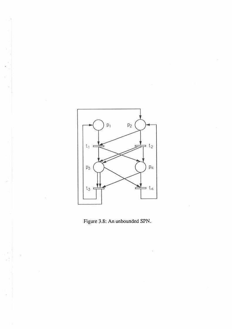
Figure 3.8: An unbounded SPN.
I(t3) : (0,0,2, 1),
I(ú4) : (0,0,1, 1),
O(¿.) : (1, 1,0,0),
O(¿n) : (0, 1,0,0).
The one step probabilities are given by F(tr,ta), F(tz,ús), p(fs, tr), Fþn,ú2) and
are equal to one, so there is one positive recurrent communicating class given
by Ct : {ft,t2,ts,ta}. 'We can also find the recurrent classes by frnding the T-
invariants for the SPN of Figure 3.8. The incidence matrix is given by,
1121
-2 -1-1 -1
The T-invariant is (1,1,1,1), therefore, C1 : {q,tz,ts,fa} which is the positive
recurrent communicating class, as given above.
Of interest in this example, is that place p3 can accumulate tokens by firing
the sequencet2, úa arbitrarily often. Thus the SPN is unbounded. Hoq,ever, \\¡e
are still able to find the equilibrium distribution for the SPN using the extended
product form solution, as long as the underlying Markov process is stationary.
The invariant measure for the routeing chain is trivially,
/(¿;)x(¿;): 1, Vi.
Which implies that,
,f(t;):[x(t;)]-l , v;.
To satisfy Equation (3.14), we need to find a function g(.), so that,
s(rn * I(¿')) /(¿') x(¿4)(3.51)
e(rn f I(¿n)) Í(tn) x(t1)'
x(¿s)
x(t2)'e(nr t I(¿z)) l(tz)
(3.52)s(ur f I(¿.))
:--/(¿')
-10
1
0
1
1
1
1
s(m+r(ú3)) _ /(¿') _ x(¿r)s(m f I(¿')) /(¿') x(fs)'
g(rn + r(r¿)) _ l(tn) _ x(tz)e(rn*I(¿r)) - f$z) x!s)
(3.53)
60
(3.54)
We use the same procedure for finding g(.) "s
in Example 3.8.
Let the base state be the marking with all of the tokens in places pz. To emptr-
place p¡, we need /3 to fire, however, f3 requires tokens in both p3 and. pa. we
consider the case that m(4), m(1), ^(2) > 0 first. so as not to deplete pa of ir's
tokens, we fire t1 (rvhich deposits r(¿r)) first, and then f3 (which deposits r(¿r))
next. This sequence is performed nz(3) times which gives the coefÊcient,
I r(t,) /(¿.)l-(s) _ l/{t.¡1-t'rLicJicJl : LreJJ (B bõ)
The marking of the SPN is now (-(1), ,n(2),0, m(a)). Note thar the SpN isnot conservative, since the m(3) tokens from p3 have disappeared. However, this
does not effect the end result. Now we take time out, to consider the boundarv
conditions. Since we are assuming that we are dealing with a stationa¡y SpN, the
initial markings that give deadlock can not occur.
1. If m(1),m(2) : 0, $'e must fire ú3 (which deposits r(f1)) first. ihis step
remo\zes tu'o tokens from p3, leaving m(B) - 2 tokens, removes on token from
pa, leaving m(4)- 1 tokens, and also deposits one token into places p1 and. p2.
Now fire the sequence, ú1 (u'hich deposits r(ta)) a¡rd then t3 (rvhich deposits
r(¿t))' a total of m(3) - 2 rimes. This gives the coefÊcient,
l¡(¿.)l U(¿, ) /(rs)l m(3)-2
Lmj LmlÐJ (356)
The token distribution after this sequence of transition firings is now,
(1, 1,0, m(a) - 1).
The next step, requires that \\'e remove the m(a) - l tokens from pa. To clo
this, u'e frte t2 (which deposits r(¿")) once, and then fire úa (*,hich deposits
r(¿z)) twice, for a total of m(4) - 1 times. This gives the coefficient,
| ¡ç,¡ //(¿.)\ 2l'n(4)-'
LnÐ(nÐl I (357)
The token distribution is now, (1, m(4),0,0).
61
To reach the base state, we must remove the single token from p1 to p2. To
do this, fire t1 (which deposits I(¿r)) and then frre úa (which deposits I(¿r)).
The coefficient created is,
f¡t¿,)lLictl (3 58)
The token distribution is now, (0, m(4),0,0) rvhich is the base marking. the
function g(.) ir the product of Equations (3.56), (3.57) and (3.58), which
gives,
g(m):e(b) tffi]-''' i#jffij]-"' (35e)
2. If m (1),rn(4) : 0, we can fire ú2 (rvhich deposits I(¿r)) once, to deposit
tokens in p3 and pa, and fire ú3 (which deposits l(tr)) which deposits a token
in p1 and p2. Now we are able to follow the first firing sequence chosen,
*'hichfires f1 (and deposits I(f4)) and then t3 (which deposits I(ú1)). This
sequence of firings creates the coefficient,
I f (tr) /(¿.)l l/(¿' ).f(rr)l -(')
Lmml Li('.)/(Ðl
_ l,r(ú,)l If(¿.)1-('):Lñl tml (360)
The marking of the SPN is now (1,m(2),0,0). To get to the base state we
must now remove the single token in p¡ and deposit it into p2. The firing
sequence ú1 (rvhich deposits I(¿o)) and then úa (which deposits r(t2)) does
this and gives the coef;Êcient,
lffiffil :[#] (36,)
The marking is now (0,m(2),0,0), rvhich is the base marking since no other
tokens are in any places other than p2. The function g(.) is the product of
the coefficients in Equations (3.60) and (3.61) rvhich gives,
g(rn) : e(b) tffi] tffi]-"' [8],62
(3.62)
as 9(b) : 1. Note that Equation (3.62) is the same as Equation (3.55).
Consequently we obtain the same coefficient whatever $,aJ' p3 is emptied,
subject to no deadlock.
Assume now that we have emptied the tokens from p3 and are in marking
(*(1), ,n(2),0, m( )). \Me now want to remove the m(4) tokens from pa. To do
so, we fi.re ú2 (which deposits I(¿.)) once and then fire úa (rvhich deposits I(¿r))
twice, for a total of m(4) times. This creates the coefÊ.cient,
lm(ffi)']-"' (36s)
The marking of the SPN is now given by (m(1),m(2)+m( ),0,0)" \\re must norv
consider the boundary conditions.
1. Suppose m(1), rn(3) : 0 (therefore the first step s'hich removed tokens from
p3 was not performed). The same sequence of transition firings, given above,
can be used in this situation.
Assume now that \Ã/e are in marking (m(1),m(2)+m(4),0,0). To reach the base
state, the last step to be performed is to remove the m(1) tokens out of p1. The
sequence of transition firings given by, ú, (rvhich deposits l(to)) and then úa (u'hich
deposits I(¿r)) executed m(1) times, n'ill empty pr. The coefficient created, is given
by'
I f (tt) r(t^) l-"' : f /(r, )l -(')
Lmml :Lnt)l (364)
The marking is now given by (0,m(2)+m(+),0,0) u'hich is the base marking.
The function g(.) is given by the product of Equations (3.55), (3.63) and (8.64),
which gives,
/(t.)Í(to)
-(e)u(ú,)lL¡(¿.)l
-1e) | ruò' I -(o)
[.f(¿, )l *(')
Lro/(Ðl Lmlg(rn): s(b)
63
(3.65)
Note that, Equation (3.59) is of the sarne form as Equation (3.61) with m(1) : 3,
again reinforcing the fact that, g(.) is found to be the same, independent of the
order of transitions firings. To check that g(') satisfies Equation (3.14), we let
g(b) : 1 and substitute it into Equations (3.51) to (3.54),
/(¿')g(rn*I(¿r)) _ Í(tr) _/(¿,)e(rnfl(¿o)) /(¿.) f(tn)' - f(tn)'
f (tn)
g(rn + I(¿,)) [/¡(,,)\' f (to), I,(''' + (rt) : L\i(Ð/ iGtl(Ðj
-1 f(tr)"f(ú.)'
/(¿') ' f(to)'g(rr + I(¿')) f(to) f ts f(tr)e(m { I(¿,)) r t1
/(¿.)"f(út )'
f(tr)g(lr-+r(rn)) _ /(¿.) f(tn), _ f(to)s(m * I(¿,)) - /(to) f (tùf Qù f @)
which confirms that g(m) does satisfy (3.14). Therefore the equilibrium distribu-
tion, is given by,
z'(m) : ¡íÕ(m)g(m), (3.66)
with 9(m) given in Equation (3.65).
Note that there are no structurally implicit places in this SPN. Again there
exist markings in vvhich some places are implicit and other markings for s,hich
they are not, however, g(.) is valid for any arbitrary initial marking.
Again in this example, rve have found g(.) attd norv have the freedom to choose
an arbitrary O(') and çe(') to determine the inva¡iant measure, There is also no
need to give the initial marking. \\¡ith the appropriate choice of the functions
O(') and tp('), state dependent firing rates or blocking can be introduced as in
Example 3.4. Again the initial marking specifies the reachability graph, and
therefore influences the solution only through the normalising constant.
64

3.6 Other \Mork on Product Forrn solutions rnSPNs
Lazar and Robertazzi 155) consider the underlying geometry of the sta,te transition
diagram of a SPN, to find some identifiable structure that has a product form
equilibrium distribution. The motivation for this research, was to classif¡' models,
u'hich contained biocking and rvhich had a product form solution. Other papers
applying the theory include, Lazar and Robettazzi ([56], [58]) and Cireng and
Robertazzi [21].
They recognise that the state transition diagram of some SPNs have identifi-
able geometric shapes, in the form of multidimensional toroids and called them
building blocks. When taken in isolation, the global balance equations for these
building blocks give partial balance equations for the original process. In com-
parison, a queueing netrvork rvith k queues, has building blocks which are formed
bythesetof states nand ¡-€i, 1<i < k. When takenin isolation, theglobal
balance equations for the building block are the partial balance equations for the
original queueing netrvork.
Once the geometric shapes have been identified, there is no guarantee that the
global balance equations on the building blocks, are consistent over the different
building blocks. To overcome this, Lazat and Robertazzi [55] construct u'hat is
called a consistenc¡' graph from the building blocks. The va^lues associated rvith
the movement from one state to another (indicated on the arcs of the consistency
graph) are given by the ratios of the suggested equilibrium distributions at the
states. For consistency validation, the product of these values around anl' closed
path in the consistency graph must multiply to one.
The next Theorem links the routeing chain with the building blocks defined
above.
Theorem 3.3
Any positive recurrent communicating class in the routeing chain determines a
65
building block.
Proof
Consider the positive recurrent communicating class in the routeing chain, C;,
that contains transition ú. From Theorem 3.2, the flux out of m * I(ú), clue to the
firing of f is equal to the flux into rn + I(¿), due to the bag I(ú) being deposited
by another transition. Hence,
z'(m * I(t))q(rn + I(ú), ¿) t F(t,"): t r(rn * I(s))q(m * I(s), s)p(s, f).u€.C¡ s€C¡
(3.67)
Note that D p-(t, u) : 1, but we leave it in for clarit¡,.u€.C;
This relation carl be expressed equivalently, by noting the following. Let rn be a
base state. m + I(ú) is a marking of the process and m is a pseudo state as defined
in Section 3.2. Let g(rn + I(ú), ú)p(¿, u), rvhich is the rate of moving from m + I(¿)
to m + I(u) due to the firing of ú and deposition of I(u) (where O¡(¿) : I(u) for
some j), b" equal tci q(m + I(¿), rn * I(u)). Nore rhat q(m * I(f ), ú) D"eci p(t,u),
which is the rate out of m + I(ú), due to the firing of ú and deposition of O(ú),
can also be expressed as D q(rrr + I(¿), rn + I(u)).
Thus, the left hand "iäTäf Equation (3.62) is equiralent to
r(rn * I(¿)) t q(m + I(ú), m + I(u)),u€.C¡
and the right hand side is equivalent to,
! z'(m + I(s))q(rn * I(s), m + I(¿))s€.C;
Let B¡(m) : {m + I(z)lz , C;} be the set of states created by firing successive
transitions in C;. Hence, Equation (8.62) becomes,
z'(m+I(t)) f s(m*I(ú),n) : t z.(n)q(n,m+r(t)) (s.68)ne E¡(ru) neB¡(m)
These equations are the partial balance equations for the original Markov pro-
cess' on the set of states defined by B;(m). These are also the global balance
66

equations on the set of states, B¡(m). Thus, B¡(m) is a building block deter-
mined by C;. IRernark 3.5
The building blocks ol Lazar and Robettazzi are multi-dimensional toroids. \4¡e
have placed no physical restriction on the shape of the building block, as it results
from the topological structure of the recurrent classes of the routeing chain.
67
Chapter 4
Insensitivity Theory Applied to SPNs
The type of firing distribution assigned to the transitions in a SPN are sometimes
crucial in order to realistically model systems. For example, as mentioned earlier,
reality would suffer if timeouts in a communication protocol were assumed to be
negative exponential distributions instead of deterministic dela¡'s.
\\rhen using firing times which are all negative exponentially distributed, the
underlying process of the SPN is li{arkovian. Consequently, the evaluation of the
equilibrium distribution can theoretically be found by standard techniques such
as the solution of the global balance equations. Or, as we pointed out in Chapter
3, for a certain class of SPN, an extended product form solution can be found.
Hon'et'er with the introduction of generally distributed firing times the SPN no
longer yields these useful forms of solution.
This chapter will be devoted to the theory of insensitivity as applied to SPNs.
\\rithout going into too much detail at this stage, a process is said to be "in-
sensitive" to it's generally distributed lifetimes, if the equilibrium distribution of
the process depends upon these generally distributed lifetimes only through their
means. Therefore, what rvas once a potentialiy difficult problem due to general
distributions can be reduced to a relatively simple problem involving only nega-
tive exponential distributions or an]' other convenient distribution u'ith the same
mean
In the following section u'e give a survey of the work using the theory of
insensitivity.
68
4.L A Survey of the Theory of Insensitivity
The fi.rst example of insensitivity rvas discovered by Erlang [29] when he sho's'ed
that the r¿ server loss system rvith exponential service times of mean [¡l]-1., has
the same steady state distribution as the r¿ server loss system with deterministic
service times of mean [p]-t. I(osten [5a] and Fortet [30] elabora,ted on this find,
showing that the service time distribution for an r¿ server loss system can actually
be general with mean [p]-t, without affecting the form of the steady state dis-
tribution. Both authors. use supplementary variables to evaluate the equilibrium
distribution.
Another queueing system which has similar properties to the Erlang loss svs-
tem is the Engset loss system. This was shorvn to be insensitive with respect
to generaliy distributed, but independent service times by Cohen [23] and u'ith
respect to successive sen'ice times, rvhich come from a stationary point process
by Könis [52]."
Insensitivity, or robustness to many statisticians, has been historically studied
within the framework of generalised semi-Markov processes (GSMPs) and conse-
quently it is often difficult for the practising modeller to appreciate the value and
relevance of the results. The remainder of this section is a brief summary of the
work conducted on insensitivitf in GS\{Ps and then, of more practical interest, a
brief summary of the insensitivity properties that appear regularly in the theory
of networks of queues.
Matthes [66] created the GS\,{P to study insensitivity u'ithin a wide class of
stochastic processes. The GSlr{P is a generalisation of the semi-Markov process
(SMP) as suggested bf its name. The SMP resides in a particular state for a
generally distributed length of time and then undergoes a transition to another
state for a generally distributed length of time. In a GSMP, multiple generally
distributed lifetimes can be alive simultaneously and the death of any one of them
causes a transition to another state. To study the insensitivity of the GSMP, only
69

one generally distributed lifetime is allowed to die in any transition, therefore the
next state to be entered is restricted to the set of states that have the remaining
generally distributed Iifetimes alive.
Matthes [66] shorved that a GSMP is insensitive with respect to a lifetime, if
and only if, a set of balance equations are satisfied by the equilibrium distribution,
when all of the lifetimes are taken to be exponential. These balance equations
state that in equilibrium, the probability flux into any arbitrary state due to the
creation of the lifetime s, is equal to the probability flux out of the same state due
to the death of that lifetime. Using the defrnition of a SMP above, the balance
equations for a SMP are always satisfied since there is only ever one generally
distributed lifetime alive at one time. Therefore every SMP is insensitive to it's
generally distributed lifetimes. A formal description of a GSMP and the equations
for insensitivity rvill be given in Section 4.3 and Section 4.4 respectively.
A further generalisation u'as given in l(önig and Jansen [53] who introduced
state dependent speeds c(s, g), at which the lifetime s is worked off when the state
is g. The practical uses of these speeds a¡e rÌumerous, in particular, thel' can be
used to represent zero speeds. For example, it is possible to model the situation
where a lifetime is not worked on at all in some states, and I'et still retains it's
spent or residual lifetime. This is useful, for example, when modelling the pre-
emptive resume protocol. The instant a lifetime is pre-empted, the speed at rvhich
it is worked off is set to zero. This ensures that when a lifetime is re-enabled, it
will resume from rvhere it rvas pre-empted.
The existence of zero speeds introduces difficulties when proving the equiv-
alence of insensitivity, product form and partial balance. In analysing svstems
with zero speeds, I(önig and Jansen [53] assumed a property called instantaneous
attention. This property requires a lifetime to be worked on at a positive speed
immediately after being created. I(önig and Jansen [53] point out that if a process
does not possess instantaneous attention, it can be modified into one that does, by
70
the addition of suitable extra states. Ta¡'lor [93] sho',r'ed that it is not necessary to
do this, as it is possible to treat insensitivity in processes without instantaneous
attention directly and that it is the behaviour of the positive speed states that is
important in determining whether a process is insensitive-
I(önig and Jansen [53] and Schassberger [90] sholed that the supplemented
equilibrium distribution, when using residual lifetimes, can break down into a
product of two terms. One term for the discrete part, the other for the continuous
part. That is, the process behaves as if the discrete and continuous parts of the
states are independent.
Schassberger ([88],[89]), proved Matthes' result using the method of phases
and in [90] extended the result to incorporate speeds.
Henderson [35], considered the structure of the time reverse GSMP, a¡rd showed
that a number of conditions are equivalent to insensitivity in a GSMP, P. In par-
ticular he observed that P is insensitive, if and only if, the supplemented equilib-
rium distribution, when the supplementary variables denote residual lifetimes, is
the same as the supplemented equilibrium distribution, when the supplementary
variables denote the spent lifetimes.
Henderson and Taylor [39], studied processes in which the generally distributed
iifetimes could be prematurely ended by the deaths of other lifetimes, with subse-
quent state changes depending upon horv the generalll' distributed lifetime died.
As in the theory of insensitivity outlined above, Henderson and Taylor's [39] re-
sults depend upon the generally distributed lifetimes only through one parameter
of each distribution. However, in this case, the parameter is no longer the mean,
but the Laplace-Stieltjes transforrn of the distribution evaluated at a particular
value. Rumsewicz and Henderson [87] followed, by allowing state changes to de-
pend arbitrarily on the ages of the generally distributed lifetimes at their deaths.
The equilibrium distribution for the Rumsewicz and Henderson [87] process, are
derived using insensitivity concepts, but no longer depend on only a single pa-
7T

rameter of each distribution.
A major application and source of results in insensitivity theorJ' is in product
form queueing networks. A model of a queueing network where the service time
at a node is not always negative exponentially distributed, was considered by
Baskett, Chandy, Muntz and Palacios [E] (BCMP). They allowed the nodes in the
network to be of four different service disciplines, rvhich are
1. First come first served: The service times are then negative exponentiall¡'
distributed.
2. Processor sharing: Each customer may have a general service time distribu-
tion, given that the distribution has a rational Laplace transform.
3. Last come first served: Each customer may have a general service time
distribution, given that the distribution has a rational Laplace transform.
4. Infinite server: The number of servers at a queue is greater than or equal
to the maximum number of customers that can be queued at each queue.
Each customer may have a general service time distribution, given that the
distribution has a rational Laplace transform.
The condition of having a rational Laplace transform allows the service centre
to be represented by a series of negative exponential stages. In Section 4.2.2 we
summarise how some of the authors in the SPN literature have approximated
generally distributed firing times b¡' a series of negative exponential phases.
I(elly [50] showed that the ke¡'to allorving generally distributed service times in
queueing networks, involves a class of queues called symmetric queues. The reason
is that the equilibrium distribution of the network is insensitive to the service time
distribution at a symmetric queue. Note that the service disciplines in BCMP,
that allow generally distributed service times, are exarnples of symmetric queues.
Other examples such as the queues u'ith the WIERDP discipline of Chandy and
72
Martin [19] and the Last Batch Processor Sharing discipline of Noetzel [78], can
also be represented as symmetric queues.
I(elly's techniques of proof were different to those of earlier authors. Instead of
showing that symmetric queues satisfy partial balance equations, he used the time
reversed process to shorv that postulated forms of the equilibrium distribution were
correct. He also showed that a symmetric queue is quasi-reversible (see Ketly [51],
pg 65) and hence a network involving symmetric queues with generally distributed
service times has a product form given by Jackson or BCMP.
Chandy, Howard and Towsley [18], looked at rvhat is essentially a symmetric
queue in terms of local balance and station balance, rather than quasi-reversibilitl'
and derived insensitivity and product form results. Jansen and l(önig [47], modi-
fied this 'work to include different classes of customers and showed that the output
processes for nodes in a queueing network are Poisson, when the net'rvork possesses
product form and insensitivity.
The results of Henderson and Taylor [39] and Rumsewicz and Henderson [87]
on interruption processes and age dependent routeing, were successfully applied
to Jackson/I{elly networks to show that a generalised product form solution still
occurs' when the routeing of a departure from a symmetric queue is an arbitrary
function of the length of service that the customer requested at the queue.
In the following sections rve apply the theory of insensitivity to SpNs.
4.2 SPNs withTimes
Generally Distributed Firing
The techniques used in handling generally distributed firing times, can be classified
into two categories. The first analyses the corresponding process of the SpN and
the second replaces transitions which have generally distributed firing times, by a
SPN which best approximates the distribution.
73

4.2.L llse of the semi-Markov Process
In Section 2.5.1 we gave a summary of some of the different SPN models which
use generally distributed firing times. These include deterministic firing times
and arbitrariiy distributed frring times. The one feature that the models such as
Natkin [77] Bertoni and Torelli [11] and Dugan, Geist, Nicola and Trivedi [28]
have in common, is that their underlying process is semi-Markovian.
Ma¡san and Chiola [64] impose the same restrictions as Dugan, Geist, Nicola
and Trivedi in the DSPN model that governs r¡'hich transitions can be given
deterministic firing times, ho$'ever, under special circumstances they introduce
an extension. Recall from Section 2.5.1.
1. The set of concurrently enabled transitions (rvhich may include exponen-
tially distributed firing times) must be enabied at the same instant.
2. Each of these transitions can also represent a chain of transitions (that
is a transition connected to a place connected to another transition etc.),
however the frring distribution must be the sarne for each transition in the
chain.
For the purposes of finding the equilibrium distribution, the time points of the
process a¡e then talien to be the instant that the deterministic transition sta¡ts
firing, or has just been disabled. At the end of each interval the process rvill
change states probabilistically, according to whether an exponentially distributed
transition (or a set of exponentially distributed transitions) does, or does not fire
within the interval. Under these conditions and using the suggested embedding
procedure the process is a SMP.
Marsan, Balbo, Bobbio, Chiola, conte and cumani [61], [62] also use sMps.
As discussed in Section 2.5.1, the combination of the pre-selection and race policy
with pre-emptive repeat gives a S\4P. The combination of the race policy with
pre-emptive resume or age-enabling gives a process that is not a SMP and is not
74
necessarily a GSMP, so therefore the solution can often be intractable.
4.2.2 SPN Approximation of General Distributions
The second category approximates the general distributions, by using a series
or parallel (or both) combination of exponential stages. The basic idea rvas first
established by Erlang [29], who shorved that a general distribution with coefficient
of variation less than one, can be represented by a series of r I 2 exponential
stages. This is the rvell known Erlang-r distribution. For a general distribution
with coefficient of variation greater than one, r ) 2 parallel exponential stages
can be used as a representation. This is the hyperexponential-r distribution.
Cox [25], contributed further by showing that an¡'distribution with a rational
Laplace transform can be modelled by the combination of series and parallel
stages.
one of the first applications of this idea to SPNs, was by Molloy [72]. Fig-
ure 4.1 is an example of a SPN representation of an Erlang-r distribution from
Chen Bruell and Balbo [20], with mean service ti-" l. In order to achieve thisp
representation, it is necessary to have r tra¡rsitions and r + 1 places. For the
hyperexponential-r distribution, it is necessary to have r + 2 places and 12 tran-
sitions.
It is clear to see, that the problem rvith direct substitution of these subnets is
that the transitions and places, required to approximate the general distributions,
enlarge the state space unnecessarih'.
Chen, Bruell and Balbo [20] improve on this technique, by creating compact
GSPN representations for Erlang's method of stages. In addition, the paper de-
scribes how the race policy with pre-emptive repeat, pre-emptive resrrme ancf
age-enabling ere incorporated into the model; this becomes necessary when there
exist concurrent and conflicting transitions in the SPN. Figure 4.2 is an example of
their representation of an Erlang-r distribution. This construction requires only b
places and 3 transitions for the race policy with pre-emptive resume. The GSPN
75
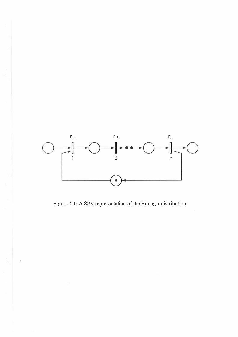
rLlrprLr
oo
Figure 4.1: A SPN representation of the Erlang-r distribution.
2 r
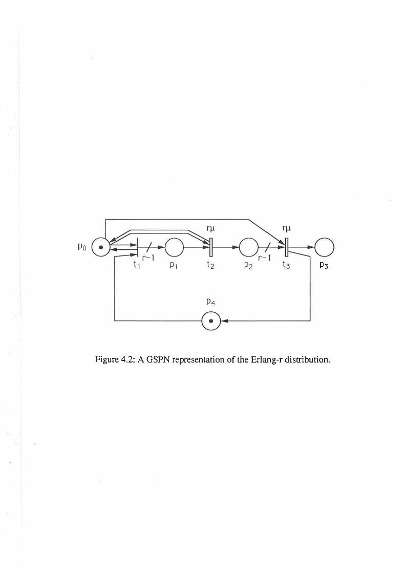
Po
ry
Ps
Figure 4.2: A GSPN representation of the Erlang-r disribution.

representations are automatically inserted into the SPN during the solution er.al-
uation stage, the user is only required to specif¡' the number of stages and the
mean of the distribution. The resulting net is a GSPN, which can be solved using
the techniques described in Section 2.5.1.
Another technique by Marsan, Balbo, Chiola, Conte and Cuma¡ri [62] men-
tioned in the last section, performs a stage expansion on the reachability graph.
Each marking in the reachability graph is supplemented by a vector, which records
the stage of firing for each transition. The different execution policies, race rvith
pre-emptive repeat, pre-emptive resume or age-enabling are also incorporated into
this technique. The expansion of the reachability tree is performed by an algo-
rithm which has been automated in a software package by Cumani [27], called
ESP.
Our aim in this chapter is to generalise the current work on SPNs with gener-
ally distributed firing times. This entails introducing the GSMP in detail, which
we do in the following section. We then proceed by applying knonn insensitivitl,
results for GSMPs to SPNs in Section 4.4 and then give the conditions for insen-
sitivity. However, to obtain more poq'erful results we turn to some extensions to
GSMPs, namely the age dependent routeing processes of Rumsewicz and Hender-
son [87] given in Section 4.5. These results give the foundations for the work on
transition merging in Section 4.6 and marking amalgamation in Section 4.2. \\¡e
introduce another extension to insensitivity in Sections 4.8 which is generalised
in Section 4.9, where we show horv to obtain equilibrium distributions for nets,
which allow simultaneously enabled generally distributed firing times. Sections
4.3 to 4.7 arc based on the paper by Henderson and Lucic [36].
4.3 A Generalised semi-Markov Process
A GSMP is defined on a set of states {g , g € G}. Within each of these states are
active elements s, from the set .9 rvhich decay at the rate c(s, g), s € ^g. 'When
76
the active element s dies, the process moves to state g' € G, with probabilit¡'
p(8, s, g'). If s € S', the element -s has a negative exponentially distribuied life-
time, and if s € ^9* it has an arbitrar¡' general distributior, ^9 : ^5'U .S*. In order
to establish insensitivitl'results it is standard to inciude the restriction that when
the process changes from state g to state g', due to the death of s, no t'"r'o ele-
ments from the set ,S* may be actirated or die simultaneously, and the remaining
elements from g fl ,S* retain their spent lifetimes.
'We usually define the marking of a SPN, by the number and colours of tokens
in each place. If the state of the SPN comprises this marking, along with the
set of transitions enabled by this marking, then a GSMP structure is realised.
State changes may be caused by either the firing of exponentially, or generally
distributed transitions.
To model a SPN using a GS\ÍP, the above definition requires that a state
cha.nge cannot enable or fire, rnore than one generally distributed transition si-
multaneously and all other generalll' distributed transitions carry over their spent
lifetimes to the next marking. Therefore, at first glance it would appear that no
marking change can enable more than one transition simultaneouslv, nor can a
transition firing disable other transitions. Fortunately u'e carr, up to a point, relax
both of these assumptions by utilising the results of Henderson and Taylor [39] and
Rumsewicz and Henderson [87] and b¡'noting that the GSMP definition allo*,s
the residual lifetimes of the active elements to decay at a state dependent speed.
In particular, if transitions in conflict disable one another, 1ve can set the decal'
rate of the disabled transitions to zero. The effect is to introduce a pre-emptive
resume policy into the SPN, so that anv transition re-enabled after it has earlier
been disabled (without having fired). restarts its firing time from where it left
off. We give examples in Section 4.5 s'hich illustrate insensitivity in SPNs with
conflict, rvhen pre-emptive resume policies are adopted for disabled transitions.
tt

4.4 Balance Equations, Insensitivity and Appli-cations
In this section, \áe present the balance equations, that are necessary for insensi-
tivity of a process n'ith respect to a lifetime. Following this, rn'e give examples to
help reinforce the concept of insensitivity as applied to SPNs.
Within the framework of GSMPs, Matthes [66], showed that the follos'ing t's'o
statements are equivalent:
1. The process is insensitive with respect to the elements of .S*. That is, the
general distributions of the lifetimes of the elements of S*, can be replaced
by any other distributions with the same mean, and yet the process still
retains the same equilibrium distribution.
2. \\Ihen all elements of ^9* are assumed to be negative exponentiall¡' dis-
tributed, the flux out of each state due to the death of an element of 5-. is
equivalent to the flux into that state due to the birth of that elernent.
The equivalent statements for SPNs with generally distributed transitions a¡e:
1. The SPN is insensitive to each generally distributed transition ú. That is.
tra¡rsition ú's firing distribution can be replaced by any other distribution
u'ith the same mean, rvithout altering the equilibrium distribution of the
SPN.
2. The purely Markov process, i.e. when .9': .S, has the property that for all
transitions ú, and for all the markings mj that enable transition ú, the flux
into marking m¡ which enables ú, is balanced by the flux out of marking m;
due to the death of transition ú.
Statement 2 is the "insensitivity balance equation" for transition ú. There are
some spebial circumstances, in which insensitivity balance is equivalent to the
detail balance associated with reversibility and others when it is equivalent to the
78
Whiiile (or local) balance (see Section 3.1), linked with product form queueing
networks. In some cases insensitivity balance arises naturally in the global balance
equations but, in general, it is none of the above and has a niche of its ou'n in
the fascinating relationship bets'een properties of processes and certain kinds of
balance equations.
As an illustration consider the following example.
Exarnple 4.1
The SPN of Figure 4.3 represents a simplified model of a dual processor computer
system given by Lazar and Robertazzi [57). It consists of two processors vying for
a common shared memory. The model Laza¡ and Robertazzi [57] use, is shown
in Figure 4.4. The difference in the models, is that the access phase now has a
more general distribution consisting of the additional property that a processor,
interrupted in its attempt at accessing the memory) retains its access stage s'hile
the memory is being utilised by the other processor. The latter is an example
of a pre-emptive resume policl'. Lazar and Robertazzi [57] find the equilibrium
distribution, after assuming that alt transitions have negative exponentially dis-
tributed firing times. Let us return to Figure 4.3 and try to incorporate both of
Laza¡ and Robertazzi's extensions into the simplified model, by introducing gen-
eral distributions and examining the system for insensitivity. Consider the SPN
of Figure 4.3 modelled as a GS\{P with the initial marking as illustrated. The
states of the GS\{P are
mr - (1, 1, 1,0,0, s1, s2),
tltz - (0,0, 1, 1,0, s2, s3),
tll3 : (1, 0, 0, 0, 1,s1, sa).
where s¡ is the element of ^S corresponding to transitior ú;, 1 < i ( 4. Note the
important point, that although states rn2 and m3 contain the active transitions f2
and ú1, respectivell', they are being worked offat azeto speed, that is c(s2,rn2) -0: c(sr,me). As the definition of a GSMP does not allou, trvo lifetimes to die
79
Þl Ps
9z
Figure 4.3: A SPN representation of a simplified dual processor model.
o
2t
Ps
ta
Pc
5t
t
oo
o
9c
Po
+(5
t5
t1
t6
I2
9t
4t
Ps
a aPl 9z Ps
Figure 4.4: The dual processor model of Lazar and Robertazzi.
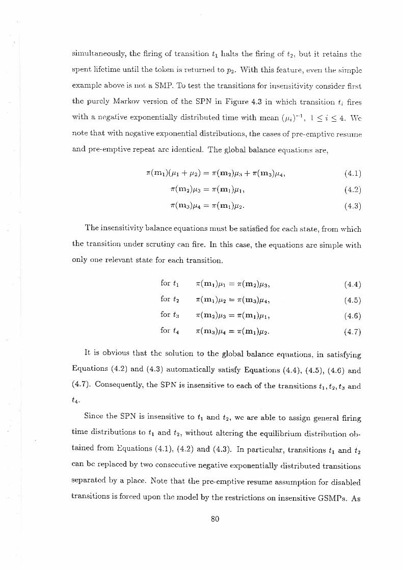
simultaneously, the firing of transition ú1 halts the firing of t2, but ii retains the
spent lifetime until the token is returned lo pr. With this feature) even the sinple
exampie above is not a SMP. To test the transitions for insensitivity consider first
the purely Markov version of the SPN in Figure 4.3 in which transition t; fi.res
with a negative exponentially distributed time lvith mean (p,)-t, 1 ( i ( 4. \\¡e
note that with negative exponential distributions, the cases of pre-emptive resume
and pre-emptive repeat are identical. The global balance equations are,
z(rrr1)(p1 + p2): T(rln2)p3 a n(rn3)¡-ra,
z-(m2)¡r3 : zr(rn1)¡r1,
zr(nr3)¡.ra : T (r7¡r) p2.
(4.1)
(4.2)
(4.3)
(4.4)
(4.5)
(4.6)
(4.7)
The insensitivity balance equations must be satisfied for each state, from s'hich
the transition under scrutiny can fire. In this case, the equations are simple s'ith
only one relevant state for each transition.
for ú1
for fu
for t3
for ú¡
z'(mr)¡rr : ¡r(rnz)ps,
n(mt)pz: r(mg)pr,
tr(rrrz)pe: r(mr)pr,
a'(rn3)¡ra : r(rett)pz.
It is obvious that the solution to the global balar¡ce equations, in satisf,ving
Equations (4.2) and (4.3) automatically satisfy Equations (4.4), (4.5), (a.6) and
(4-7). Consequentl¡ the SPN is insensitive to each of the transitions t1,t2,ú3 and
ta.
Since the SPN is insensitive to ú1 and t2, we are able to assign general firing
time distributions to t1 and ú2, without altering the equilibrium distribution ob-
tained from Equations (4.1), (4.2) and (4.3). In particular, transitions t1 and f2
can be replaced by two consecutive negative exponentially distributed transitions
separated by a place. Note that the pre-emptive resume assumption for disabled
transitions is forced upon the model by the restrictions on insensitive GSMPs. As
80
the two stages of the distribution are memoryless, we need not record the exact
age of the spent lifetime, we need only ensure that the token freezes in its current
place until the next transition in the sequence is re-enabled. This is Lazar and
Robertazzi's model.
Wang and Roberlazzi [96] generalised the SPN of Figure 4.4 by allos'ing the
firing time distribution of each transition ú;, 1 S i ( 6 to be the sum of two
negative exponential distributions. As in the previous example, this can be in-
corporated into the simplified model in Figure 4.3 using insensitivity. From the
same argument used for Lazar and Robertazzi's model, we replace the firing time
distribution of Í1 and ú2 by the sum of four negative exponential distributions and
assume' as do W.ttg and Robertazzi [96], that the sequence of stages obey the
pre-emptive resume protocol. Transitions ú3 and t4 a;te also replaced by the sum
of two negative exponential stages. There is no question that ú3 and la obey the
pre-emptive resume protocol, as they are never enabled together. The simplified
model can be extended further, by allowing the firing time distributions of. t1,t2,t3
and Úa to be the sum of an arbitrary number of negative exponential distributions.
Again, this translates to having an arbitrary number of consecutive transitions
separated by places.
Example 4.2
Now consider the same problem but in a more general setting. The structurally
simple SPN of Figure 4.5, has a collection of resources ara,ilable in place p1 and
a set of labelled customers in place p2. The resources can, for example, be buses
a¡d memories as in the last example or circuits in a circuit srvitched netrvork.
Note that different customers require different sets of resources.
Label the customers 1,2,.. . ,? and assume that a customer j e 1r, 2,. . . ,T\requires the set A¡ of resources to complete its task. Tra¡rsition f1 is a folded
transition which serves all customers. Customer j draws a time from a general
distribution, with mean (À¡)-t, and waits (or rvorks) for that length of time before
81
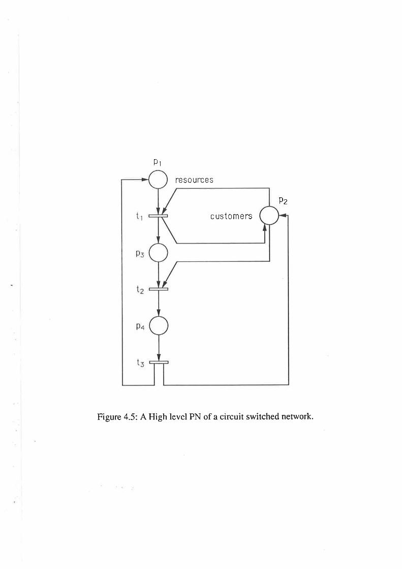
CUSIOMEf^S
Pl
res0urces
Þz
Figure 4.5: A High level PN of a circuit switched network.
accessing the resources. If the set of resources, A¡, are unavailable during that
time period the countdown is temporarily halted for customer j, until the nec-
essary resources become available ir pt. When these, "times to access service",
a.re negative exponentially distributed, they are memoryless and manJ' interpre-
tations of the service procedure are possibie. For example, we can assume that
the countdotv\¡n never stops and customers who request service but do not find the
resources available, wait for alother negative exponential period before making
another request. Customer j accesses resources (in place p3) for a period of time
with mean,, (tt¡)-', before returning the resources to pr and themselves to p2.
Define the state of the system as n, a l?l vector of zeros and ones, the ones
indicating the customers currently utilising resources (i" pr). Consequently, n also
indicates the active elements as sjo or sjr, depending upon whether customer j is
waiting to access or is accessing the resources, respectively. The lifetimes sjo, sjr
have meanr ()¡)-t and (¡i¡)-r respectively.
If all lifetimes are negative exponentially distributed and n : (r, ,r12,. . . ,nr),nj : 0,1, Vj - I,2,. .. ?, then the process is reversible rn'ith equilibrium distribu-
tion,T À
n1
Jr(n) : Ç fl (4.8)j=l llj
\\¡here C, the normalising constant, is evaluated over all the feasible states of the
process.
If n is a feasible state with nj : I,and e; : (0,0,...,0, 1,0,...,0) represents
the state where only customer j is using resources, then the insensitivity balance
equation for s¡r is found in the following rvay. The flux out of state n due to the
death of s¡r,
The flux into n due to the birth of s,r,
: zr(n - er)À¡.
( p)tl7f
82
Consequently, the insensitivity balance equation for s¡r is,
n(n)p¡: n'(n - e;))., (4 e)
Equation (4.9) follou's immediately from Equation (4.8) and is the insensitivity
equation for s¡o also. For the case where customer j's resources are availabie in
p1, this is clearly true. Now consider the implication of Equation (4.9) on the
behaviour of the Ma¡kov process when n is an infeasible state and n - ej is feasi-
ble. This occurs when customer j's resources are not available in n - ej. For this
case, z'(n) : 0 and the pre-emptive resume policl' freezes the decay of the lifetime
s;o in state n - ej, so c(s¡o,n - e¡) : 0, and thus we have equality in Equation
(4.9). Therefore with zero speed in this situation, we have a pre-emptive resume
protocol at ú1 which satisfies the necessary balance equations for all markings and
is therefore insensitive to all of its active elements. Relating back to Example
4.1, rve can therefore find performance measures based on the equilibrium distri-
bution, when any number of processors are tn'ing to access any set of memories
with an arbitrary bus architecture, with any sequence of negative exponentially
distributed transitions as per Wang and Robertazzi and with generally distributed
memory utilisation times.
Equation (4.9) not only gives information on insensitivitl', it also tells us that
the SPN of Example 4.2 is reversible. 'We can further conclucle x'ith a little thought
that the characteristic detailed balance equations of reversibility alu'ays indicate
some form of insensitivity. However, as we pointed out, care must be taken u,hen
establishing the meaning of the active elements, and their behaviour when state
changes occur, others'ise the insensitivity property can be lost.
Let us again stress, that there are many insensitive processes which are not
reversible and many reversible purely Markov processes which, when arbitrarily
given general distributions, are not insensitive.
83
4.5 Ag" Dependent Routeirtg
The results derived in the pler.ious sections relied on basic insensitivity theory.
In this section, we use the extensions to insensitivity from the work on GS\zIPs
with interruptions bv Her.:.delson and Taylor [39], and GSMPs with age depen-
dent routeing by Rumseu'icz ¿nd Henderson [87], to analyse SPNs further. For
example, in order to simplifl' the SPN structure, and underlying process, n'e turn
to techniques such as transition merging in Section 4.6, marking amalgamation in
Section 4.7 ard aggregation of subnets of the SPNs in Chapter 5.
Although it is instructive to understand the rvork of Henderson and Taylor
[39], from both a¡r information and a modelling point of view, it is sufÊcient, for
the purposes of this thesis, to present the defrnitions and results on age dependent
routeing in GSMPs. due to Rumservicz and Henderson [87].
The following results s'ere given originallf in terms of GSMPs. As ure are
simply translating them into an SPN structure, to obtain Theorem 4.1, rve give
no proof here but instead refer the interested reader to Rumseu'icz and Henderson
[87].
Let the process of the original SPN be denoted by P. Now alter the original
process P by either performing marking amalgamation or aggregating subnets of
the SPN. Assume that in performing any of these techniques we have created a
process with markings ñ €. 14, *'hich has the following routeing structure. Define
Æ,m(y, Ú) to be the probability of moving from marking ñ to marking ñr due to
transition Í firing at age y. Let P be the process which has, after the firing of a
transition ú with general distribution Gr(.), age dependent routeing probabilities
given by pn,m(', f ). Assume that the age dependent routeing probabilities of P are
sufficient to define P. Thus, F and P are structurally different but mathematically
equivalent.
Let Q be the aueraged process of P which has, after the firing of transition f
84
with general distribution G¿(.), age independent routeing probabilities given b5',
.fæpiï,iñ(l) : /o pn,m(y, t)dG{y).
Define M to be the process r,vhich differs from the Q process, only in that t is
now negative exponentially distributed with mean given by the mean of G¡('). The
next marking probability for 14 is given bV pn,m(f) for the merged transitions or
otherwise from the original SPN. Let "r(n), f. e M be the equilibrium distribution
of being in state n of the -ôy' process.
In generai, the P, Q and tì,í processes, will have different equilibrium distribu-
tions. Theorem 4.1 tells us u'hen they all ha'r'e the same equilibrium distribution,
and therefore when the distribution of. M is an exact marginal distribution of P.
Theorern 4.1 (Theorem 2 from Rumsewicz a¡rd Henderson [87])
If Q is insensitive to its generally distributed transitions, then the equilibriurn
distribution of Q is identical to the equilibrium distribution of P and is given by
the equilibrium distribution of. M.
Proof
See Rumsewicz a¡rd Henderson [87] r
Theorem 4.2 follorvs immediately from Theorem 4.1 and the definition of in-
sensitivity.
Theorem 4.2
If the Q process is insensitive to its generally distributed transitions then the
marginal equilibrium distribution of the original process P is zr(R), Í, e M.
Proof
Since we have stipulated that the age dependent routeing probabilities of P are
sufficient to define P, the two processes are structurally different, but mathemat-
ically equivalent and therefore the equilibrium distribution for P is the marginal
distribution for P. From Theorem 4.1, the equilibrium distribution of the Q pro-
cess, which is z'(R), n eM, is the marginal distribution for the P process. ¡
85
Procedure:
The procedure, therefore, is to find the averaged Q process, establish the insen-
sitivity, construct the related purely Markov process and soh'e for zr(n).r e M.
Such a procedure is much simpler than working with phase type distributions, or
supplementary variables.
In the next section we consider transition merging. The next corollar¡'applies
to transition merging and follows directly from Theorern 4.2.
Corollary 4.1
If P is formed from P by transition merging then, if Q is insensitive to its gener-
ally distributed transitions, the equilibrium distribution of P is z'(n), n € M.
Proof
Wiren applying this procedure the markings in P remain unchanged from the
original process. Therefore M : M and so let n : lt in Theoren 4.2. As the
state space of Q is the sarne as the state space of P, the marginal distribution
equilibrium distribution, in Theorern 4.2, becomes the equilibrium distribution. r
4.6 Transition Merging
Recall that the definition of a GSMP entails the creation and death of at most
one generally distributed lifetime per marking change. In a SPN it is common for
a number of transitions to be enabled simultaneously. In this section, rve seek the
equilibrium distribution for SPNs with sets of mutually disabling, simultaneously
enabled, arbitrarily distributed transitions. The remainder of the SPN. can have
any structure which is Markovian, that is, the other transitions are all negative
exponentially distributed. Wé use the results of Section 4.5, to obtain equilibrium
distributions for these SPNs.
Let the original SPN be P. Transform P into a SPN P which has age depen-
dent routeing, by merging the mutually disabling transitions.
86
Consider any markitrB, r, of P, in which there exists at least one set of mutually
disabling, arbitrarily distributed transitions, which were enabled at the same time
point. Assume that there are k transitions in this set, labelled (for simpiicity)
1,2,. .. ,k, and that transition ú¿, i e {f , 2,. . . ,k} has firing time hazard function
å;(.), which satisfies,
h;(u):-ä49#, (4 10)
a¡d consequently,
t - G;(ù - exp {- I"' h;(u)du}. (4.11)
Let marking rrri be the next r¡arking entered if úi fired first. Now combine the k
conflicting transitions into one transition, ?, rvhich has a firing time distribution,
G.('), given by the minimum of the k merged transition firing time distributions.
The probability of moving into marking m; from the original marking n, rvhen ?fires at a time y, is given by,
h¡(yPu,-,(Y, T) :
, hív) (4.r2)
It must be noted that a simplified notation has been adopted and that fr and
å;(y)' 1 < i ( n are functions of ?. This procedure is followed for each set of
mutually disabling, simultaneously enabled, arbitrarily distributed transitions.
Following the results of Section 4.5, r,r'e call the transition merged SPN, P.
The averaged SPN Q, based on P, has transitions ?, with firing time distributions
Gr(.) as defined earlier, and next marking probabilities given by,
p,,,*(?) : lo* #fu dGr(y). (4.1s)
Define thé SPN, M, so that ? is now negative exponentially distributed lvith
mean given by the mean of Gr(.). The next marking probabilities for Àt[, are
given by Equation (a.13) when the merged transition fires. Otherwise, they are
determined in the original SPN. Let zr(n), n e M be the equilibrium distribution
of being in state n of the SPN, M. From Corollary 4.1, if Q is insensitive to the
general distributions G7(.), the equilibrium distribution for P is zr(.).
87
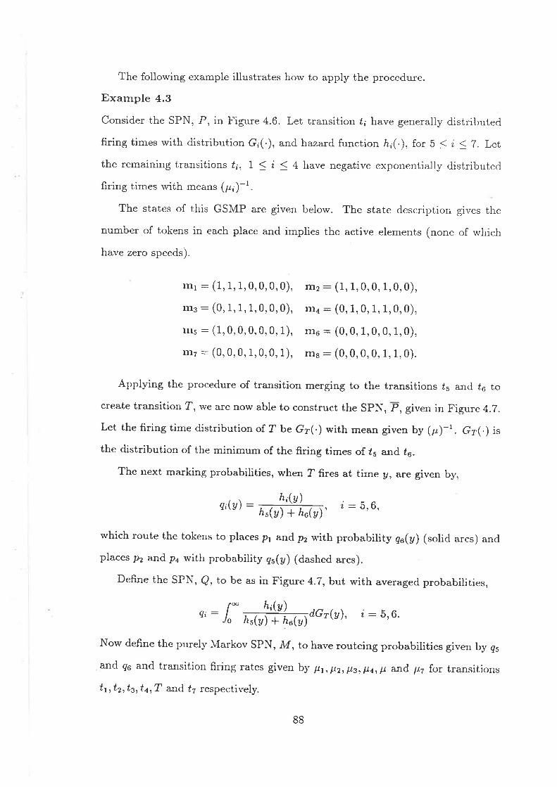
The following example illustrates horv to apply the procedure.
Example 4.3
Consider the SPN, P, in Figure 4.6. Let transition ú; have generally distributed
firing times with distribution G,(.), and hazard function ä;(.), for b < i ( 7. Let
the remaining transitions ú¡, 1 S i ( 4 have negative exponentiallv distributed
firing tirnes with means (pi)-r.
The states of this GSMP are given below. The state description gives the
number of tokens in each place and implies the active elements (none of rvhich
have zero speeds).
lrrl : (1, 1, 1, 0,0,0, 0),
lll3 - (0, 1, 1, 1,0,0,0),
m5 : (1,0,0,0,0,0, 1),
lIlT : (0,0,0, 1,0,0, 1),
rlr2 : (1,1,0,0, 1,0,0),
lrr4 : (0,1,0,1, 1,0,0),
ttt6 : (0,0, 1,0,0,1,0),
lrls : (0,0,0,0, 1,1,0).
Applying the procedure of transition merging to the transitions 15 and ú6 to
create transition ?, we are norv able to construct the SPN, P, given in Figure 4.7.
Let the firing time distribution of ? be Gr(.) with mean given by (p)-t. G7(.) is
the distribution of the minimum of the firing times of f5 and f6.
The next marking probabilities, when ? fires at time v, are given by,
q;(y):ü#ä, i:5,6,
whichroute the tokens to placespl andp2 n'ith probability qa(y) (solid arcs) and
places p2 and pa with probability qs(y) (dashed arcs).
Define the SPN, Q, to be as in Figure 4.?, but with averaged probabilities,
f* å;(p)e' : Jo EGËt Gt
dGrtu)' i : 5' 6'
Now define the purely Markov SPN, M, to have routeing probabilities given by 95
and 96 and t¡ansition firing rates given bJ' p, ,l1z,lt3,ltt, þ and ¡t7 for transitions
tt, tzrtertqr? and ú7 respectively.
88
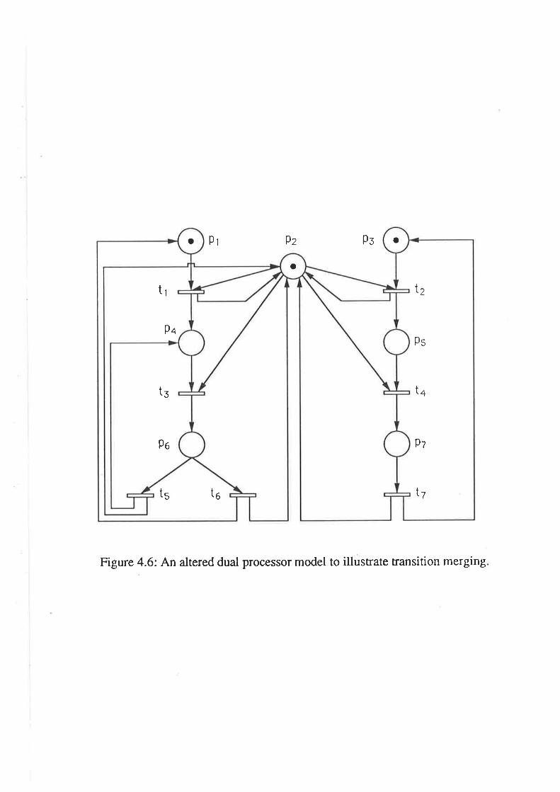
Po
3t
9q
t1
o
t5 6t t7
Ps
9t
4t
2t
o oPr Þz Ps
Figure 4.6: An altered dual processor model to illustrate transition merging
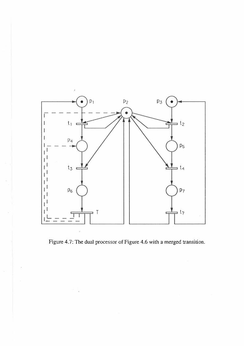
T
o
t7
l2
Qt
4t
Þs
_L
Po
9+
tl
t5
oo Þl Pz Ps
Figure 4.7:The dual processor of Figure 4.6 with a merged transition.
The global balance equations are,
zr(rrr1)(p1 -t ltz): 7I'(rrrs)pz * r(rn6)¡tqu,
r(nz)(ø * pt) : ?r-(rrrl)p z t r(rne)pqe,
,r(nz)(p'z + t-a): z-(n1r)É¿1 a n-(m7)p.7 | n(n:^6)¡-t,q5,
n(rna)(¡r3 * t-ra) : T(rn2)trr * zr(rn3) p.z I r(rns) pqt,
r(m5)P'7 : r(rrtz)pt,
a'(rn6)¡-r : zr(rr3)¡r3,
n(rnr)Pz : r(tn¿)P¿,
zr(rns)p : r(r:tt)pt,8
I z.(m;) : 1.i=l
(4.11)
(4.15)
(4 16)
(4.17)
(4.18)
(4.1e)
(4.20)
(4.2r)
(4.22)
(4.23)
(4.24)
(4.25)
(4.26)
The insensitivity balance equations for the two generally distributed lifetimes are.
f.or T r(mo)p :7r(rn3)p¿3,
z'(ma)p : r(m.r)ts,
¡'(ms)¡rz : T(r¡z)pc,
r(nz)pz :'rî(r¡.A)p,.
for t7
Clearly the insensitivity balance equations are satisfied by the global balance
equations, and thus the SPN of Figure 4.7 is insensitive to both ? and t7. TbeQ
process is therefore insensitive and by Corollar]'4.1, the equilibrium distribution
of the SPN of Figure 4.6 is given by solving Equations (4.14) b @.22).
This example illustrates the power of insensitivitl' theory in solving potentiallv
difficult problems. In general, once the insensitivit¡' of a SPN to somc of its
transitions is established, a large class of generalisations of the original SPN can
be defined, ¿ll of which have the same equilibrium distribution. In the follorving
section, we show how the same insensitivity results of Section 4.5, can be used
with some kinds of marking amalgamation.
89
4.7 Marking Arnalgamation
Many authors have had to tackle the problem of large state spaces whether their
modelling tool was queueing networks, SPNs or any of the other frameworks useful
for modelling systems. Aggregation is a necessary procedure in each discipline,
in order to simplify the state space and thereby extract results. In queueing
networks, authors such as Courtois [24], Vantilborgh [94], Balsamo and Iazeolta [Z]
and Chandy, Herzog and'Woo [17], have used aggregation procedures on product
form networks, principally so that the normalising constant could be evaluated
more readily.
In this section we will suggest a procedure for marking amalgamation in SPNs,
using the results of Section 4.4 a¡rd 4.b.
Dugan, Geist, Nicola and Trivedi [28], consider SPNs u,here at most one gen-
erally distributed transition is enabled in any marking and u,here each marking
is visited only once. They suggest the amalgamation procedure of combining all
markings which have a common generally distributed transition enabled. In the
example provided in [28] the resultant amalgamated process is a SMP. In general,
the amalgamation procedure described above, does not necessarily yield a SMp,
since, the routeing between amalgamated markings may depend upon the past
history- This problem does not occur, as u¡as the case in the example of Dugan,
Geist, Nicola and Trivedi [2S], u'hen the routeing probabilities are only functions
of the marking itself and the time spent in that marking.
An additional problem with this amalgamation procedure can be seen by con-
sidering a GIM/L queue. Combining all states.w,ith the same set of generally
distributed active element, results in a simple renewal process, but provides no
information on the state of the queue. In this case too much detail has been lost
because of the over zealous amalgamation.
In this section, 1{/e suggest a general amalgamation procedure for use when the
SPN exhibits markings, with at least one generally distributed enabled transition.
90
Using the results of Section 4.4 and 4.5, we derive conditions under which this
procedure gives an exact marginal equilibrium distribution for the original SPN.
Procedure:
From the original SPN, P, with state space M amlgamate arbitrary sets of mark-
ings which have in common the same generally distributed enabled transitions.
The amalgamation will alu'a]-s define a simplified state space, M. It may
not, however, naturally define a ne\\' process. For instance, there is no guara¡rtee
that, in amalgamating markings, the routeing probabilities between markings
of M can be evaluated. However, since the procedure involves arbitrary sets of
markings, there is a great deal of flexibility a¡rd therefore many alternative choices
in creating the markings in M. Finding the best .,\1, which has well defined
routeing probabilities, retains all the necessary information and is manageable,
is a skill required of the analyst rvhen using this procedure. When the routeing
probabilities between amalgamated markings can be determined exactly, we label
the new p.ocess P.
The P process in the example of Dugan, Geist, Nicola and tivedi [28] is in-
sensitive and, as we have observed. insensitivity is a powerful modelling tool. Our
aim in this section is to create an insensitive P process, by marking amalgamation
and show that exact marginal distributions for P can be found from this P pro-
cess. Theorem 4.3 is a prelimitr-l'theorem rvhich illustrates that the insensitivit¡r
of P implies the insensitivity of any F, when an amalgamation is performed in
the suggested way.
Theorem 4.3
If P is insensitive to the transitions with generally distributed lifetimes, then Fis also inscnsitive to these lifetimes.
Proof
For each marking n, let y be a vector of, either the spent or the residual lifetimes
of each of the generally distributed transitions enabled in n. Let (n, y), be the
91
marking of the SPN supplemented by these lifetimes.
As P is insensitive, the results of Matthes [66] and the subsequent extensions
of l{önig and Jansen [53] on spent lifetimes, a¡rd Henderson [35] on both spent
and residual lifetimes, give the result,
a (rr, y) : o(n) lI pr(1 - G,(y,)) (4.27)
G;(') is the distribution associated with the lifetime y¡ and [p,]-t is the mean of
this distribution.
Summing (4.27) over all markings in the amalgamated marking n and noting
that each of these markings has the same set of generally distributed enabled
transitions gives,
7r(tr, y) : zr.(n) lI ¡r,(l - G;(v;)). (4.28)
As the form of Equation (4.27)i. ,1"."r.*y and sufficient for insensitivity
and Equation (4.28) is valid for every marking Í e Jvl, P is insensitive rvith
equilibrium distribution given by (a.28). rEven though rvell defined routeing probabilities are not guaranteed when amal-
gamating markings, the consequence of Theorem 4.3, is that the equilibrium dis-
tribution on the amalgamated markingsM has a simple form, given by (a.2g)
whenever P is insensitive.
To calculate the equilibrium distribution zr(n), u,e have tu,o choices. \\¡e can
recognise the insensitivity of the P process, replace the general clistributions ç,ith
negative exponential distributions, perform the amalgamation and solve the re-
sulting system. Alternatively, ne can amalgamate first, taking the general dis-
tributions into account, insert negative exponential distributions in place of the
general distributions and then solve. The first approach works when P is insen-
sitive. We proceed to shos' that the second alternative produces exact results in
many situations even rvhen P is not insensitive.
Let us now assume that we have a well defined P process.
92

The age dependent probabilities for moving from the amalgarnated marking
f. € M to the next reachable markings in the process, are found by working out
the probability of traversing a path rvithin the amalgamated marking, which n'ill
lead to the next marking after the generally distributed transition fires.
The related age independent process Ç, and the purely lv{arkovian process l.fare obtained as in Section 4.5. Let M have an equilibrium distribution given b1'
?r(n),ñ eM. Then from Theorem 4.2, if Q is insensitive, an exact marginal
equilibrium distribution for the SPN P is given by z-(n), r € M.
The natural situations in which the conditions of Theorem 4.2 are satisfied
are
(a) The marking which first enables the generally distributed transition is aln al's
the same
(b) The routeing probabilities in the P process from each marking in the amal-
gamated marking are independent of the entry point.
Note that Theorem 4.2 can accommodate the situation where the only set of
enabled transitions a¡e a set of mutually disabling transitions running concur-
rently with a set of negative exponentially distributed transitions. By merging
the generally distributed, simultaneously enabled, mutually disabling transitions
into one transition, as in Section 4.6, rve obtain a Q process rvith a single generally
distributed transition, which runs concurrently with some negative exponentiallv
distributed transitions. Under the right conditions, Theorem 4.2 can norv be
applied to rnarking amalgamation.
The following example illustrates state amalgamation.
Example 4.4
Figure 4.8 is a high level stochastic Petri net comprising the following features.
The initial marking consists of a hashed and a white token in p1 and trvo neu-
tral tokens in place p2. Transitions f1 and ú3 are both negative exponentiallv
distributed with rate ¡t1. Transition ú2 is a folded transition representing trvo
93
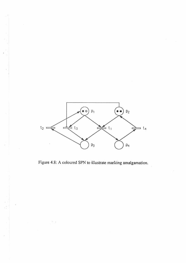
oo@o Qz
l2 tq
Figure 4.8: A coloured SPN to illustrate marking amalgamation.
9qPs
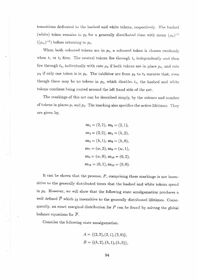
transitions dedicated to the hashed and white tokens, respectively. The hashed
(white) token remains in p3 for a generally distributed time rvith mean (pn)-,
((p-)-t) before returning to pr.
When both coloured tokens are in ptt a coloured token is chosen randomly
when ú1 or ú3 fires. The neutral tokens fire through ú1 independentlS, and then
fire throughta, individuallywith rate pa if both tokens are in placepa, and rate
p5 if only one token is in pa. The inhibitor arc from p2 to ú3 ensures that, even
though there may be no tokens in pr, which disables 11, the hashed and white
tokens continue being routed around the left hand side of the net.
The ma¡kings of this net can be described simply, by the colours and number
of tokens in piaces pr a¡rd p2. The marking also specifies the active lifetimes. The1,
are given by,
rrrl : (2,2), rrl2 - (2, 1),
rrr3 : (2,0), ttl4 : (h,2),
rrl5 : (h,1), û16 : (å.,0),
ln7 : (.12), ttls : (-,1),
lrte : (trl,0), tttls : (0,2),
lÌr11 - (0, 1), m12 : (0,0).
It can be shown that the process, P, comprising these markings is not insen-
sitive to the generall¡' distributed times that the hashed and rvhite tokens spend
it p.. However, we will show that the following state amalgamation produces a
well defined P which is insensitive to the generally distributed lifetimes. Conse-
quently, an exact marginal distribution for P can be found by solving the global
balance equations for P.
Consider the follorving state amalgamation.
A : {(2,2),, (2,1), (2, 0)},
B : {(h,,2),(h,1), (å,0)},
94
C : {(-,2), (-,1), (u,, 0)},
D : {(0,2), (0, 1), (0,0)}.
State .,4. represents all states which enable only negative exponentially distributed
lifetimes. State B represents the set of states in '¡'hich the white lifetime is en-
abled at t2. State C represents the set of states in which the hashed lifetime is
enabled at t2. State D represents the set of states in which both the hashed and
white lifetimes are enabled. Since both active elements are alive in state D, the
amalgamated process P of Figure 4.9 is a GSMP but not a SMp.
Choosing this amalgamation has created a process with age independent route-
ing probabilities. Therefore, the issue of age dependent routeing does not have
to be treated by averaging the routeing probabilities. Consequentl-v the P and Q
processes are equivalent and an insensitivity anall'sis on the P process, is all that
is required.
In this case it is possible, with ca.re, to write dos,n the global ba-lance equations
for M directly. However, we find it more insightful to produce the M equations
by summing the appropriate terms of the purely \,Iarkov version of the original
process P, that is, where f2 fires the hashed and u'hite tokens accord.ing to negative
exponential distributions with means (p^)-t and (p-)-r respectively. The global
balance equations for this process a.re,
r(mr)p,r : 7r(m2)ps * a'(mo) F-,* r(rn7)¡tn, (4.2g)
n(mzXpr + p5) : î(ms)p- * zr(rns) ln * r(rns)po, (4.30)
r(msxpr + p4): z'(rn6)¡r- a zr(me)¡r¡,
zr(m¿X¡rr + p-): ur(rnro)¡,r¡ f zr(rn5)¡r5,
,r(msxpr * t -+ Fs) -"(^ùî *z(m6)¡rr *z-(m11)¡rn,
r(rnoXpr * t"- + Fe) : "(*r)T * rlnn)po + n(rn")L,
(4.31)
(4.32)
(4.33)
95
(4.34)
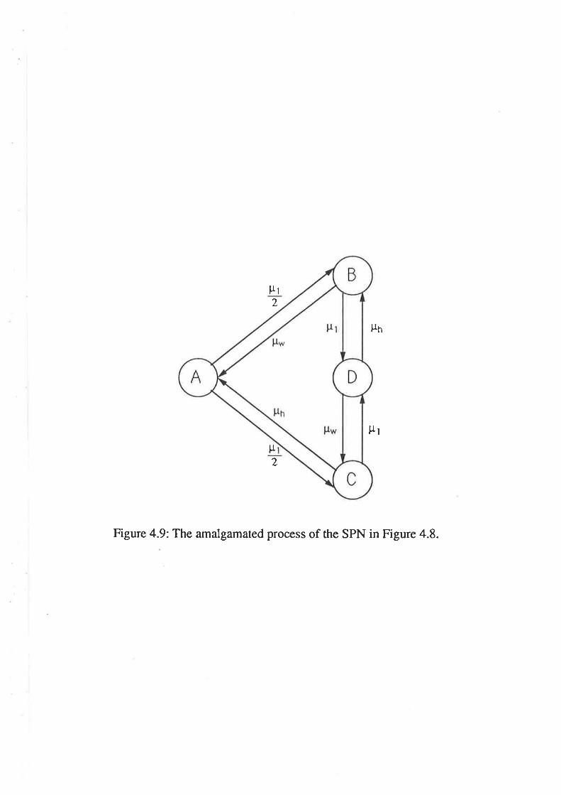
Fl2
Fn
ttl
tr2
Figure 4.9: The amalgamated process of the SPN in Figure 4.8.
n(rnr)(p, * pn): zi(m1s)p- * zr(ms)ps,
z'(nrs)(¡-r1 * t"n+ ps):zr(rnr)f f n'(mr)¡r s*r(¡r^1.)p-,
*(rnnXp, I t"n + pt): "(n..r)\ + n!nn)p- + o(rnr)4,
(4.35)
t(rntoXp¿ t tr-): zr(rn11)¡-r5, (4.38)
¡(mtrXp¿ I tt- + ps) : n(rmn)pn -f r(rnn)¡tt * r(rnz)h, (4.3e)
n(rnt")1rn * t"- + tto) : zr'(rn5)¡-r1 * zr(ms)¡.rr + n(mo) ttt I n(tns)h, (4.40)
t2
!zr(m¡):1.
(4.36)
(4.37)
(4.41)
(4.43)
(4.44)
i=l
Since state A is the result of amalgamating states rï11, rrr2 and m3, adding Equa-
tions (4.29), (4.30) and (4.31) will give the balance equation for state ,4. The
equations for states B, C and D are found by adding the appropriate equations
and are given below.
,r(A)p, : t(B) p- * r(C)¡t¡ (4.42)
"(B)(p, * p-) : n(D)pn + r(A) ltt2
"(C)(p, * pn) : ¡r(D)p- + r(A) ltt2'
"(D)(pn * p-) : þr(B) + {C))p,1. (4.45)
t : n(A) + r(B) + r(C) + r(D). (4.46)
To show that P is insensitive to the times that the hashed and white tokens
spend it pt, we check for consistency between the global balance equations given
above and the insensitivity balance equations.
96
The insensitivity balance equations are given by,
for t2 (white) : state B n(B)p- : "Ø)î, (4.47)
for t2 (wlrite) : state D n(D)p- : n(C)pt, (4.48)
for t2 (hashed) : state C "(C)pn: r(A) ltt2' (4.4e)
for t2 (hashed) : state D n(D)pn : r(B)pt. (4.50)
Equations (4.47) to (a.50) satisfy Equations (4.42) to (a.a5) and therefore the P
process is insensitive. Since insensitivity has been established, \r'e are able to solve
the global balance equations, (4.42) to (4.46), to obtain the marginal distribution
for P as,
n(B): "Ø)#,, (4.b1)
n(c): r@)!1, Ø.52)¿ltt'
tr(D): "Ø)#^, (4.5s)
1] '. (4.54)
In this example, we have illustrated how the appropriate choice of marking
amalgamation, results in an insensitive P proc""r. There is a lot of flexibility in
choosing the amalgamation, since there are many marking combinations possible.
To re-iterate, the aim is to choose an amalgamation which produces well defined
routeing probabilities, does not lose excessive information and which is insensitive.
4.8 Simultaneously Enabled Generally Dis-tributed Tbansitions
In the previous sections, we noted that the theory of insensitivity was essentially
restricted to models in which at most one lifetime could be born or die at any
97
time instant. In this section. \\'e present some preliminary ideas which relax the
simultaneous births assumption.
Throughout this chapter. s'e have shorvn that the strength of insensitivity
theory lies is in the fact that generally distributed firing times, may be replaced
b1' negative exponentiall¡' distributed firing times with the same rnean. We will
aim for the same end result. rvhen rve apply our theory to fork-join sections in a
SPN. In brief, so as not to pre-empt the definition, a fork-join section in a SPN
may have an arbitrary number of generally distributed lifetimes enabled at the
same time. As stated before. this poses a problem when trying to extract an
equilibrium distribution. Ho*'e'r'er, we will extend the theory of insensitivity and
present a theory u'hich allorvs the generally distributed firing times in the fork-
join section to be replaced bv state dependent negative exponentially distributed
firing times r¡'ith the same means. The price to be paid in removing the general
distributions, are the state dependent firing rates, which are functions of the
distributions themselves. \\;e u'ill start by presenting a simple example, to aid
in the understanding of the theory, before immersing ourselves in the notation
necessary for the general case.
Consider a fork-join section in a SPN. Following Baccelli, Maliowski and
Schwartz [5], ttt n-dimensional fork-join queue is represented by n parallel servers
rvith synchronised arrival and departure streams. Customers arrive at the fork-
join queue in batches less than or equal to n and then split up to be served by
the n servers in parallel. This is the fork. As soon as the batch has been served,,
the customers are reunited. This is achieved by storing the customers, who have
already been served, in an extra buffer of infinite size. They wait here until the
other customers in the batch har-e been serræd. This is the join.
The analysis of fork-join gueues can be applied to production systems, where
a batch customer is interpreted as a customer order with several components re-
quiring different services. Parallel processing is another area of application, where
98
a batch customer can be viewed as a program composed of several subroutines,
each to be executed by a diffelent processor.
In the context of SPNs, an n-dimensional fork-join section is the subnet con-
tained within an n-dimensional fork and an n-dimensional join. The subnet is
executed in the same manner as described above, except, the batch is restricted
to be of exactly size n. An n-dimensional fork in a SPN occurs when a transition
deposits n tokens in n places simultaneously. An n-dimensional join in a SPN
occurs when a transition removes all n tokens within the fork-join section at the
same time. Note that the following analysis is applicable for only one batch of
tokens moving through the fork-join section at a time. A new batch cannot enter
the section until it is empty.
In the following example, we show how to convert the original SPN rvith general
firing time distributions, into a structura.lly equivalent purely Markov SPN with
state dependent firing rates that has the same equilibrium distribution.'We note, that there is a strong link betrveen this rvork and that in the next
chapter, which is concerned with the aggregation and disaggregation of subnets
within a SPN. If lve consider the sole general distribution, as the time spent in
the fork-join section, lr'e have a SMP and therefore insensitivity. It is therefore
possible to use the supplementary variable to disaggregate and find detailed infor-
mation about the markings in the subnet. This is the theme of the next chapter.
Our aim in this section, is to find the equilibrium distribution of the detailed
states of the fork-join section, using the information gi.r,en about the transitions
in the subnet. In doing so, we establish a different and potentially interesting
result.
Example 4.5
Consider the SPN of Figure 4.10. Transition úr creates a 3-dimensional fork inthe SPN, by depositing 3 tokens into places pz¡ps *d pn. The subnet of the
fork-join section is formed by places pz¡pz,ps¡ps¡pa ^d p, and transitions t2,f3
99
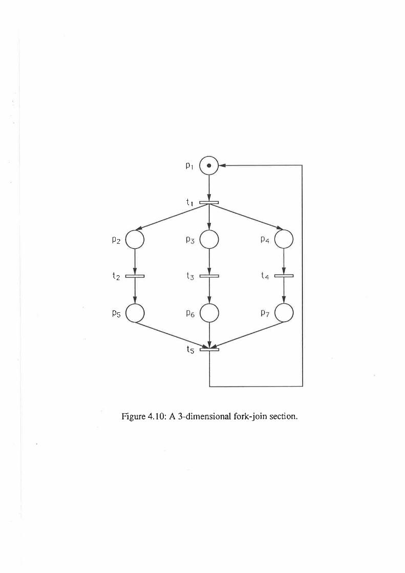
9z
l2
Ps
Pr
t1
t5
Figure 4.10: A 3-dimensional fork-join section
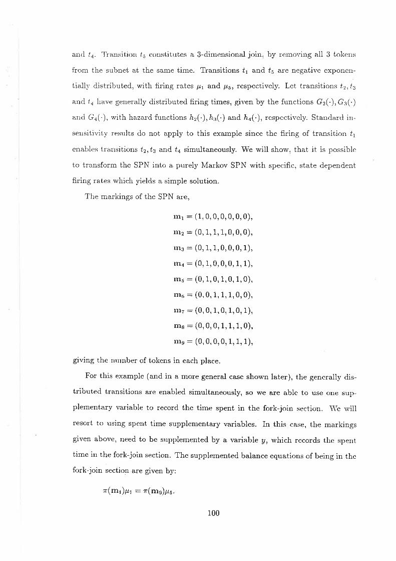
and ¿{. Transition ú5 constitutes a 3-dimensional join, by removing all 3 tokens
from the subnet at the same time. Transitions t1 and ú5 are negative exponen-
tiall¡.distributed, with firing rates pr and ¡r5, respectively. Let transitions f2,f3
and úa h.ave generally distributed firing times, given by the functions Gr(.),G.(.)
and Ga(-), rvith hazard functions ä2(.), å.3(.) and hn(.), respectively. Standard in-
sensitivity results do not apply to this example since the firing of transition t1
enables transitions f2, ú3 and úa simultaneously. \Me will show, that it is possible
to transform the SPN into a purely Markov SPN with specific, state dependent
firing rates which yields a simple solution.
The markings of the SPN are,
rrrl - (1, 0,0, 0, 0, 0, 0),
rtlz - (0, 1, 1,1,0,0,0),
lTt3 : (0, 1, 1,0,0, 0, 1),
llr4 : (0, 1,0,0,0,1, 1),
IIl5 : (0, 1,0,1,0,1,0),
1116 : (0,0, 1, 1,1,0,0),
ItlT : (0,0,1,0, 1,0, 1),
rtls : (0, 0,0, 1, 1., 1,0),
Ille - (0,0,0,0, 1, 1, 1),
giving the number of tokens in each place.
For this example (and in a more general case shown later), the generally dis-
tributed transitions are enabled simultaneously, so u/e are able to use one sup-
plementary variable to record the time spent in the fork-join section. \\¡e s,ill
resort to using spent time supplementary variables. In this case, the markings
given above, need to be supplemented by a variable y, which records the spent
time in the fork-join section. The supplemented balance equations of being in the
fork-join section are given by:
z'(mr)pr : r(mg)ps.
100
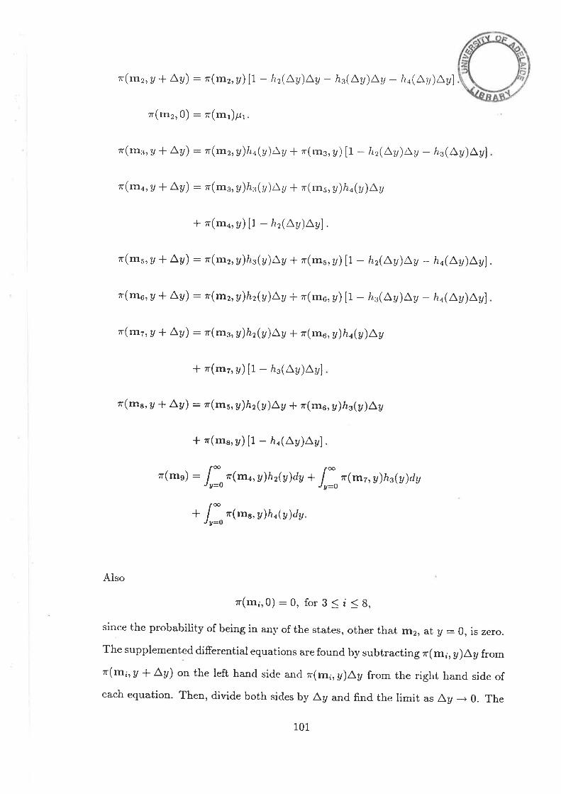
zr(m2, a * L'y): r(rn2,y)[1 - h2(Ly)Ls - h3(Ay)Ay - ha(Ly)Ly)
n(tor,O) : "r(rnr)/rt
t(ms, y + Ly): r(mz, V)hn(a)^y f zr(rr- 3, s) [1 - h2(Ly)Ly - h,3(Ay)Ay]
r(rnn, A + LA): r(ms, y)hr(A)La f n'(rn5, y)ho(y)LV
-| zr(ma, s)[1 - hr(Ly)Ly].
zr(nr5, A + L,y): zr(rn2, a)ht(ùLV * a-(m5,y) [1 - h2(Ly)Ly - ha(Ly)Ly].
r(mo, v + Ly): r(mz, y)hz(y)Lv * z(m6, y) [1 - fu(A.y)Ly - ha(Ly)Ly]
r(rnz,V + Ly): rr(rn3, a)hz(y)LV f zr(rn6, y)hn(y)Ly
* z'(m7, y) [1 - h3(Ay)Ay]
r(rna, u + L,y): r(lrs, ùhz(u)Lv * zr(m6, y)hs(y)Lv
* zr(ma, y) [1 - åa(Ay)Ay] .
,.(ms) : lr:r(m¿, ùhz(y)dy * Ir:":¡r(mz, y)hz(y)dv
+ [* ,r(ma, ùhofu)dyJv=o
AIso
zr(rn;,O) :0, for 3 ( i < 8,
since the probability of being in anl'of the states, other that m2, at y - 0, is zero.
The supplemented difierential equations are found by subtracting zr(m;, y)ay from
*(m¡, a + Lv) on the left hand side and r'(rn;, v)La f¡om the right hand side of
each equation. Then, divide both sides by ay and find the limit as ay --+ 0. The
101
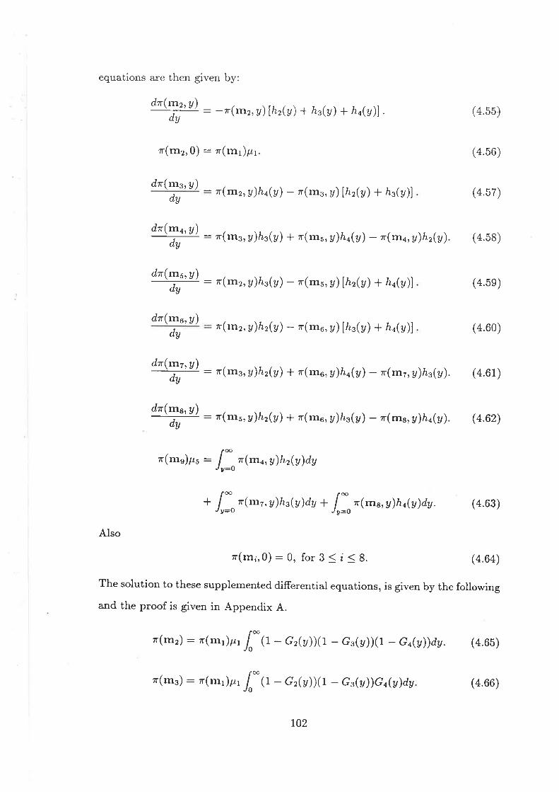
equations are then given by:
dtr( rut.- u\--i; : z(rn2, ùh"(v) - r(rns, y)lhr(a) + Iro(y)l
T(rraz,0) : r(prr)/-¿r
dtr(ms,y) _dy
r(rnz, a)hq(a) - r(me, y)lhz(y) + ås(v)l
dtr(rna,y) ,
Ë:zr(rn3,a)h"(a){zr(rn5,y)ho(y)-T(m¿,y)h,(a)
(4.55)
(4.56)
(4.57)
(4.58)
(4.5e)
drr(rn6,y)zr(nr2, a)hz(a) - r(mo, a)lhz(y) + hn(ùl (4.60)dy
dr(rn7,y) ,--6-: zr(rn3, y)hz(v) * a-(rn6. y)ho(y) - r(mz, ùh"(y). (4.61)
dzr(m6, y) ,-ã-: zr(rr5, y)hz@) * zr(me, y)hs(U) - r(me, V)hn(V) (4.62)
z'(mn)p, : lr:":r(mo,
y)h2(y)dy
* l":"Lr(m7, y)t4(y)dy * l":n(rns, ùho(ùdv. (4.63)
Also
o(m;,O):0, for3(i<8. (4.64)
The solution to these supplemented differential equations, is given by the follou,ing
and the proof is given in Appendix A.
z'(mz) : r(mr)pr l"*(1- G,(y)Xl - c.(v))(l - Go(ù)dy. (4.65)
r(ms) : 7¡-(nlr)p, /-{r - cr(y)X1 - Gr(ù)Go(ùdu (4.66)
r02
lo*
l"*zr(rn6) : zr'(mr)/¿r (t - Ga(u)Xl - Gn(y))G,(v)da,
z'(rn3) [q(m., *o) * q(ma, m7)] - zr(m2)q(mz, m¡).
zr(ma)q(rn¿, ms) : zr(m3)q(ms, mr) * zr(m5)q(ms, m¡).
zr'(rn5) [g(*r, rne) * g(rns, ma)] : n'(m2)q(mz, rns)
zr(m6) [g(*u, rnz) * g(rno, ms)] - zr(m2)q(rn2, m6).
z'(mr)q(mz, rng) : 7T'(m3)q(m3, m7) * zr(rn6)q(rno, mz)
z(ms)q(me, rng) : ¡'(mo)q(rn6, m6) * z'(rn5)q(rn5, rn6)
"'(ma) - zr(rn1)¡;1 (t - G "(y))G "(a)G
o(a)da,
l"*r'(rn5) : zr'(m1)¡.rr (t - G"(y)Xl - G¿(v))Gs(a)da, (4.68)
(4.67)
r(rn7) : ?r(ml)p, /-{t - Gr(v))c r(y)Gn(ùda, (4.70)
zr(rns) : 7r(m1)p, /-{t - Gn(ù)Gr(y)G"(ùdu,
(4.6e)
(4.75)
z (rne) : r'(rnr)4. ( 4.72)lts
Note that r(rnr)¡.¿r is the normalising constant.
Assume now that the SPN is purely Markov, with state dependent frring rates.
If Equations (4.65) b (a-72) satisfy the global balance equations of the purel¡'
Markov SPN with state dependent frring rates, then an equivalent SPN u'ith
negative exponential state dependent firing rates can be created. Therefore, the
next step is to find these state dependent firing rates from the global balance
equations given belorv, using our knowledge of the zr(.)'s.
¡'(mr)¡rr :7r(me)ps. (4.73)
7r(m2) [q(^r, ms) * q(mz, rns) * g(mz, rttu)] : :r(mr)¡rr
(4.71)
(4.74)
(4.76)
(4.77)
(4.78)
(4.7e)
(4.80)
103
n(^n)t"t: î(m4)q(rrra, rne) * r(rnr)q(m7, rÌre) * n(rns)q(ms, mg). (4.8i)
Let us define some notation to reduce the complexiby of some future expressions.
First label the transitions {2,3,...,n*I} : Af and let the set of labels for the
transitions which have fired be given by the set 6 C .A/. Let
A(ß:Ð: l" |J (t - G¡(y)¡dG;(ù,j€^r\{6u{t}}
(4.82)
where A(B : i) represents the probability that transition f ; fires first from the set
of tra¡rsitions with labels ¡f \ B. Let {} denote the empty set and so ,4({} : i) is
the probability of the transition ú; firing first, when B : {}. Also define lt[(B) to
be the expected residual time to the firing of the first transition with a label from
¡/ \ 6, after all the transitions with labels in B have fired. This is written,
M(B): E [(-åï
s x*--s r,)*1 , (4.83)
lI (r - c¡(v)) n.c,@)au,: lo* (4.84)
ien/\B jen
where X; is the random variable associated with the lifetime of ú¡ and (")+ :max(ø,0).
Let the state dependent firing rate ¡t(B: j), be the rate of ú, firing when the
transitions with labels in 6 have fired. By substituting the form for the r(.)'sfrom Equations (4.65) to (4.72), into Equations (4.73) to (4.E1), we can solve for
the state dependent firing rates giving,
q(rnz,*r) : p({} : a) : A({} :4M({}) '
q(mz,rrrr): ¡r({} : t): ##,
q(rnz,*u) : p1t'r', -'a({} : 2).4) - M({Ð ,
104
q(ms, -r) : t (4j :2) : A({+} :-2) x A({} : a)' -/ ¡/({4})
q(ms, *n) : /-,({3} : 4) : ¿({r} :-¿-) I -¡({} : s).' .-/ ¡4({3}) '
q(ms, m.) : p,({B} :2) : ¿({g} : ?ì I .'1({i : s).
' .-/ ¡r({3}) '
g(mo, ttt) : p({2}
g(m¡, *r) : p,({3,4} :2),
s(mo,-r) : pe2': B) : ¿({z}'.1),4 .'1({}' z).
' -/ M({2}) '
A({3,4} 2)lA({4}: 3) x A({} 4)+A({3}:a)xe({}:s)l¡f( {3, 4} )
q(mz, *n) : p({2,,4} : 3),
A({2,4} 3) [,4({4} : 2) x á({} , 4) + A(12} : a) x ,4({} : 2)l
^[({2,4}g(ma, mn) : p({2,3} : 4),
A({2,3} : a) [á({3} : 2 ) " .a({} : 3) +,a({2 ):3)x,4({}:2)l¡r({2,3})
That is, we have found by using the state dependent firing rates, we obtain the
sarne equilibrium distribution as though we used the general distributions. If we
can now find a general procedure to produce these state dependent intensities, we
will have side-stepped both the need to introduce supplementary variables for the
general distributions and the need to solte integral equations. The concept is an
extension of the standard insensitivity theory, where generally distributed firing
105
rates could be replaced simply by their means.
In order to shed some light on how these state dependent firing rates are
formed, we will discuss three representative expressions. The denominator of
q(mz, rn3), is the expected firing time of the frrst transition to fire between t2. t3
and ta, that is, .Ð[min(X2,Xr,Xr)], u'here X¡ i" the random variable associated
with the lifetime of transition ú¡. The numerator is the probability that transition
ta will fire first betrveen ú2,f3 and ta.
The denominator of q(rn3, rna), is the expected residual firing time of the first
transition, out of t2 and t3, to fire after úa has fired. Mathematicall¡ this is
written * ø [(*i"(Xr,,{.) - Xr)).] u,here (r)+ denotes max(r,0). The numer-
ator consists of the probability of úa firing first then f3 firing second leaving f2
still enabled. The denominator of q(ma, me) is again the expected residual firing
time of f2 after ú3 and ta have already fired. Mathematically, this is written as
A [{.X, - max(X3,Xo))*]. The numerator consists of a sum of tu,o probabilities.
which represent tu'o different orderings of the firing sequence. The first term rep-
resents the probability of the firing sequence ta -+ t3 ---+ úz and the second term
represents the firing sequence ts + tl - tz.
In the next section \¡/e use these observations to give state dependent intensities
for the general fork-join case.
4.9 General Fork-Join Sections
Consider a SPN which enables n generally distributed transitions, within an n-
dimensional fork-join section, given in Figure 4.11. Let t1 and 1,12 have neg-
ative exponential firing times with mea¡r [¡.,r]-t md [F"+z]-t, ,"rp"ctively. Let
tz,tz,...:ún*r have generallydistributedfiring times given by Gi(.), 21i 1n*Iwith hazard functions h;(.), 2 < í < n + 1. Also, let rn1 denote the marking *,ith
one token in place p¡. Before embarking on the theory for the general case, \\'e
will give some additional definitions.
106
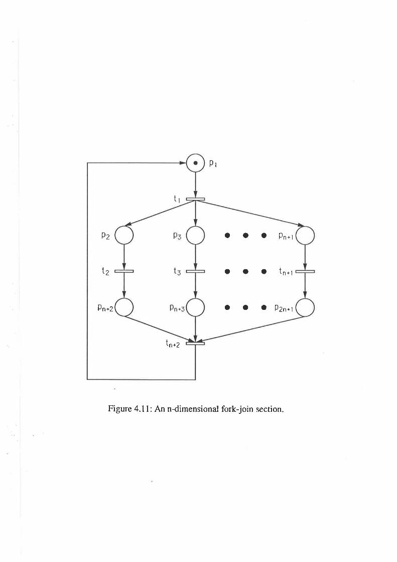
Pt
Figure 4.71: An n-dimensional fork-join section.
OOOPn*l
OOOtn*l
O O a Pzn*l9n*2
9z
2t
t
tn*2
Definition 4.1
Recursively define, P(B), a measure of the likelihood of being in the state where
the transitions with labels in 6 have fired, as,
P(B):tP(6\ {i})A(B \{i}:i), B+{},ieB
(4.85)
(4.87)
(4.8e)
with P({}) : 1 and where ¿({} ' i) is the probabilitl' of ¿i frring first when no
other transitions in .Â/ have fired. Note, that this can be normalised without
effecting Theorem 4.5 or it's proof, however this is unnecessary.
Deflnition 4.2
For¡r €^f \8,P(B 'i)'
P(B) Aln '\: u-çs¡o(B 'i), (4'86)
where tt(B : j) is the firing rate of ú; when the transitions with labels in 6 have
already fired, M(B) is defined in Equations (4.83) and (4.8a) and ,4(B : j) is
defined in Equation (a.82).
Theorem 4.5.
The equilibrium distribution for the purely Markov n-dimensional fork-join sec-
tion, with state dependent firing rates given by Equation (4.86), is given by,
r(B): I{I,I(B).
Proof
The global balance equations for the purely Markov n-dimensional fork-join sec-
tion, are,
r(mt)pt : n(N)p^+r, (4.88)
'({}) Lt*',,, 'r,]t)h,: zr(rrr
",u, t.ì ur(u'r,] :
Ð"*ru\ {¿})p(6 \ {r} ' i), B { {}. (4 e0)
707
Substitute Equations (4.86) and (a.87) into the left hand side of Equation (4.89)
gr\¡es.
r(M({})Le^##r]
: /( D ,a({} ,-i).je¡Í
Since I ¿ttt , j):1, this implies o(rnr)É¿r - I{, as was noted in Section 4.8J€,\T
u'ith reference to the 3-dimensional fork-join section.
Substitution from Equations (4.86) and (4.87), into the right hand side of
Equation (4.90) yields,
\xmçn \ {i})P(B \ {i})A(B \ {i} : i)
M(B \ {i})Using Equation (4.85) gives the right hand side as,
: Ii P(B).
Substitution into the left hand side yields,
..,.,-. I \- P(B)A(B : i)fri M(B) | )L;cir1u M(B)
J
Honever, I A(B : /) : 1 so the left hand sideJ€,V\B
: Ii P(B).
There is no need to satisfy Equation (4.88) as it is redundant. ¡Theorem 4.6
The equilibrium distribution for the fork-join section with n generally distributed
transitions is given b1' Equation (4.82).
Proof
Consider the supplemented equations for the n-dimensional fork-join section and
conjecture that
r(B,y): ti lI tr - G;(ù)IlG,(ù¿y,
i€B
(4.e1)t€^f\B
108
jes
are the soiutions to the supplernented differential equations. In general form the
supplemented differential equations are given by,
d"(?'a) : -n(ß,y) I ä¡(s) + Ðn(B\ UÌ, ùh¡(ù. (4.s2)dY ,€^/\ri jes
Substitution from (4.91) into tire ieft hand side of (4.92) gives,
dltr(B,,y)ldy
- -r{ Ð h¿(ù II (r - c*(u)) lI c;(y)¿€^r\B fr€J\r\B jet3
+K II (t - cr(s)) IrL¡er¡
h¡(ùQ-G¡(y)) || Gx(y)¡€.^f\B fr€B\U)
: -n(B,a) D h¡(a) + t h¡(v)e - G¡(y)) lI tr - Gíù) |[ Gx(y),€^r\6 jes ¡€^f\¿l fr€ß\U)
: -n(B,y) D h¡(a) +Dh¡(ù fI (1 -Gr(v)) |I G¡(y).€,^/\¿3 jet3 J€¡/u{j}\6 À€B\{j}
Since ^f
\ {B \ U}} : AÍ uU} \ s,
"(B \ {j},a): II 1r _ Gr(v)) II GÁv).t€.vuu)\¿3 [-€6\ij]
Hence,
dln(B.,'v)l : tr(B,a) t h¡(ù+ D o(6 \ {j},y)h¡(ù,d,y '\- ) ù' ¡ãv jes
rvhich is Equation (4.92). Norv integrate Equation (4.91) over y and using Equa-
tion (4.8a) this gives (4.87) a^s reqnired. r
The theory is applicable to any n-dimensional fork-join section within any SPN
as long as the SPN is insensitive to the time spent in the n-dimensional fork-join
section. This will be discussed in more detail in Chapter b.
109
Chapter 5
Agg"egation and Disaggregation inSPNs
5.1- Approxirnation Techniques
In Chapters 3 and 4, we provided classes of SPNs that have simple and. exact
solutions, using the extended product form solution and the theory of insensitivity.
However, we have only just scratched the surface. Authors concerned with the
performance analysis of SPNs, have responded to the need of finding a larger class
of SPN with tractable solutions, bv using a r"ariety of approximation techniques.
In this chapter, we give a survey of these techniques and then introduce our
contribution to the area. In brief, our work is based on the aggregation and
disaggregation of subnets of the SPN, but differs from previous work, by achieving
exact solutions, whilst at the same time reducing the size of the reachability graph.
The approximation techniques used can be naturally divided into two cate-
gories, the first dealing rvith the underlying Markov process the second with the
structure of the net.
Haas and Shedla¡ ([32], [33], [34]) find steady state estimation procedures
for the discrete event simulation of SPNs, based on the underlying regenerative
process structure and may therefore be included in the first category. They de-
fine the marking process of the SPN in terms of a GSMP (see Section 4.3 for
a definition). The characteristic property of a regenerative stochastic process,
is that there exists random time points, referred to as regeneration points, at
110
which the process probabilisticaliy restarts. The evolution of the process between
regeneration points, is statistically identical to the process in anv other cycie.
Given that some mild regularity conditions are satisfied (see Crane and Iglehart
[26]), a regenerative stochastic process, iX(ú); t > 0], has a limiting distribu-
tion, {X(t) - X as ú --+ oo}, provided the expected time between regeneration
points is finite. Haas and Shedlar [32] provide the conditions which ensure that the
marking process is a regenerative process, in continuous time, with finite expected
time between regeneration points. They extend their results to allow simultaneous
transition firings in [33] and then analyse GSPNs in [3a].
Ramamoorthy and Ho [82], were the first to find approximations based on
the net structure. They use the property of marked graphs, that the number of
tokens in a cycle, defined by the initial marking, remains the same after any firing
sequence. We note that the S-invariant can be used to detect these cycles, as
in Wong, Dillon and Forward [99], as outlined in Section 2.5.2. Ramamoorthy
and Ho [82] compute the minimum cycle time to return to the initial marking, b1'
finding the minimum time taken over all of the cycles. An approach for computing
upper and lower bounds for cycle times, in conservative general SPNs is suggested,
however, they comment that these bounds may not be tight.
Molloy [75], takes another approach, by finding fast upper bounds for the
throughput in a SPN, using bottleneck analysis. Using this technique, the mark-
ings do not have to be generated. The SPN is restricted to have at most one arc
between any place and any transition. By noting that ar¡erage token flos,s in a net
are conserved at steady state, a series of flow balance equations are constructed.
Token flows are conserved in places, so the sum of all flows into a place is balanced
by the sum of all flows out. This can be written as,
D /(¿r, pj) : I f@i,ú;), v p¡ €P,t¡ÉT ti€T
where f1¿,p¡) is the flow from transition ú; to place p¡ and f(p¡,t,) is the flo.n,
from place p¡ to transition f;. Since there is at most one arc bets,een any place
111
and transition, the token flows, f,, on the input and output arcs of a transition
are equal. So, V t; e T, 3 /¿, such that.
f(t¡,p¡):f o i{oü:o,I n if a¿1 :1,
f (p¡,tt) : 0 if o,j:0,fr, if au : 1,
where, cj and a¡ are the elements from s,hich the incidence matrix is constructed.,
as defined in Section 2.1.2. The solution to these equations gives the token florvs
for loops in the SPN to within a constant. From the example given, the loops
are chosen by the natural flows of the net, that is, by observing the cycles that
tokens may flow around. Molloy [75] states that it is only possible to find an
approximation for this constant, for a sufficiently large number of tokens in m6.
As the number of tokens increases, the operation of the SPN tends toward a
limit, if the average flow through a transition is less than the average firing rate.
Therefore a further set of inequalities can be formed, given by,
frlÀr,YteT
These inequalities, define a feasible region for the vector of average token flows.
The boundary of feasible solutions for these equations, defines the bounds of token
flow through the net. That is, the boundary ft : Àt, constitutes a bottleneck in
the system, u'hich limits the throughput to some maximum value.
Campos, Chiola, Colom and Silva [15] create linear programs defined on the
incidence matrix, and use them to compute the upper and lower bounds for the
throughput of transitions. The throughput of the transition is defined as the
average number of firings per unit time. The SPN is restricted to be a live and
bounded marked graph, and the underlf ing Markov process must be ergodic.
The upper and lower bounds for the throughput, are found to depend on the
initial marking and the mean values of the d.ela1,s, but not on the probability
distributions. This approach is different from that of Molloy [7b], in that only the
IT2
initial marking is required, rather than having to compute the limiting behaviour
for a large number of tokens. A companion paper by Campos, Chiola and Silva
[16] extends these results to live and bounded nets.
Bruell and Ghanta [i3], give an informal account on hos' to compute the
upper and lower throughput bounds for GSPNs, which are bounded, live, conser-
vative and have marking independent firing intensities. The proposed algorithm
simplifies the GSPN, by removing fork-join structures such as those described in
Sections 4.8 and 4.9. They find the upper bound on throughput of the simplified
GSPN by using the following technique. The aim is to reduce the SPN to a simple
structure, in which tokens are delayed because of the time taken for a transition
to fire, rather than in the contention for the use of shared resources. The paths
within the fork-join section that contain contention, are replaced by a transition
whose rate is given by the maximum time talien to traverse the fork-join section.
This maximum is taken over the paths rvithout contention and the path being
considered, with the contention removed. This procedure is continued until each
path in the fork-join section does not contain contention. The entire fork-join
section is then replaced by the slot'est path that a token can follow, from the
moment it forks to the moment it joins. The throughput is then evaluated on
the simplified SPN in the usual rvay. To evaluate the lower bound, in a shared
resource section, they evaluate the shortest time taken to traverse the section, by
using the upper bound, rvhich effects how often the tokens are arailable.
This chapter is constructed as follows: In Section 5.2 we give a survey of
other work concerned with aggregation and disaggregation at the net level and
also introduce our technique. In Section 5.3 we give the definitions and basic
results required for the follos'ing sections. Sectic¡n 5.4 illustrates the aggregation
technique using an example that shorvs horv insensitive skeleton nets provide exact
marginal distributions for the original net. Two difierent approaches for the exact
disaggregation of the skeleton net, are given in Section 5.5.
113
5.2 An Introduction to Aggregation and Disag-gregation at the lr[et Level
As briefly mentioned at the start of this chapter, we are interested in extending the
class of SPNs which can be ana-l¡'ssd exactly, using aggregation and disaggregation
of subnets in the SPN. Our approach, is to aggregate subnets to create "skeleton
nets", which yield exact marginal distributions for the originai SPN. The key to
this method, is to use the results of insensitivity theory to create these "skeleton
nets". Moreover, we show that whenever our approach is applicable, the strength
of insensitivity theory can be used to rebuild the exact equilibrium distribution of
the original net. A feature of our aggregation technique, is that we do not propose
a step by step approach, but instead defrne an aim, rvhich is to create a skeleton net
which is insensitive to it's general distributions. It is rvorth noting, that for each
insensitive skeleton net there are an uncountable number of original nets for u,hich
the skeleton net provides exact results. Consequently, a library of insensitive nets,
or an understanding of the properties of insensitive nets, is essentia^l for effectively
utilising this approach. To fill in the entire picture, we proceed by summarising
other work concerned with aggregation and disaggregation in spNs.
Balbo, Bruell and Ghanta [6], aggregate subnets of GSpNs with their main
concern being computational efficiency. Consequently, they choose subnets which
have the BCMP type product form or rvhich are GSPN structures, that can then
be handled using available softrvare. They follow the equivalent server idea ofChandy, Herzog and \ü'oo [17], to piece together an approximation for the equi-
librium distribution of the SpN.
The papers by Ammar and Isram ([2], [g]), Ammar, Huang and Liu [1], and
Ammar and Liu [4], present an aggregation technique at the net level, which
is used to compute bounds for SPNs. They aggregate subnets, rrvhich contain
transitions with significantly faster firing rates, than those transitions rvhich join
these subnets together to form the SPN. They then replace these subnets by
r74
representative places, connected to the slo'¡' firing transitions. The number of
tokens in each representative place, is the total number in the original subnet.
The adjusted firing rates of the transitions with slow firing rates, are marking
dependent, and are determined using their original rates and the token distribution
in the connected subnet (for details see Ammar and Islam [3]). An analysis of
these subnets in isolation, yields a choice of throughput rates, which are then used
to give upper and lower bounds for the marking probabilities of the skeleton net.
Dugan, Geist, Nicola and Trevedi [28] and Section 4.6 of this thesis use aggrega-
tion to merge sets of transitions which are in conflict. Another form of aggregation
which achieves an improvement in graphical complexity is used in the construction
of high level SPNs (see Lin and Marinescu [59]). Briefly, a hierarchical representa-
tion is created which makes it possible to find a simpler representation of a SPN.
A high level SPN can be considered a structurally folded version of a regular SPN,
if the number of colours is finite. That is, it can be unfolded into a regular SPN
by unfolding each place p into a set of places, one for each colour of token that
place p may hold, and by unfolding each transition f into a set of transitions, one
for each way that ú may fire.
Henderson and Taylor [41], introduce flexibility into the model of Henderson,
Lucic and Taylor [37], by absorbing the time spent in certain subnets into specially
chosen intervals. They find the equilibrium distribution of the process, embedded
at the time points at the ends of these intervals. Properties of the continuous time
equilibrium distribution, can then be derived from the equilibrium distribution of
the embedded process. By choosing appropriate embedding points, they shorv
that it is possible to find marginal distributions for some SPNs, which do not fitthe structure required by Henderson, Lucic and Taylor [37]. We will follow along
a similar line, but do not restrict ourselves to finding an extended product form
structure. There may be some value in aggregating to find an extended product
form structure but it is outside the consideration of this thesis. Further, we will
115
show that under certain conditions, lr¡e can disaggregate the subnet to find the
exact equilibrium distribution for the original net.
5.3 Definitions and Basic Results
Using the notation introduced in Section 4.5, starting u'ith the net P. the airn
is to create, by aggregating subnets, an insensitive skeleton net Q f.or s,hich an
equilibrium distribution can be found. Recall from Section 4.5, that the process
of aggregating states of the reachability graph does not necessarily achieve a new
process. Likewise, aggregation at the net level, which defines a simplified net,
may not naturally define a new process. For instance, there is no guarantee that,
in aggregating places and transitions, the resuitant routeing probabilities when
transitions fire can be evaluated as functions of the nerv places and nerv transitions.
For example, consider the SPN given in Figure 5.1. Imagine that rve rvish to
aggregate tt,tz,p2 and p3 into a single transition ú, follos'ed by a single place p as
in Figure 5.2. If 11 and t2 a;te negative exponentially distributed with means (p, )-tand (r¡z), 1, the tokens leaving p go up with probability l' and dos,n rvith- ttr I ¡t2probability -
=.
Although in the negative exponential case these routeingltt I ¡t2
probabilities are exact,this is not the case when general distributions are involved.
For example, if ú1 has a deterministic firing time distribution, with mean (ø, )-t,a token leaving p moves uprvard rvith probability one, if it's firing time through ú
i" (pt)-t, .ttd zero,if. it is less than (¡r¡)-r. With more complex distributions for
the firing times of ú¡ and ú2, the routeing can be explicitly defined in terms of the
hazard functions of the trvo distributions and now becomes crucially dependent
on the time at which ú fires. The situation becomes even more complicated when
a second transition fires tokens into, for exampL, p". The routeing out of p may
then become a function of, not only how long t took to fire, but also the method
by which tokens enter p.
For the purpose of explaining the aggregation technique as simply as possible,
116
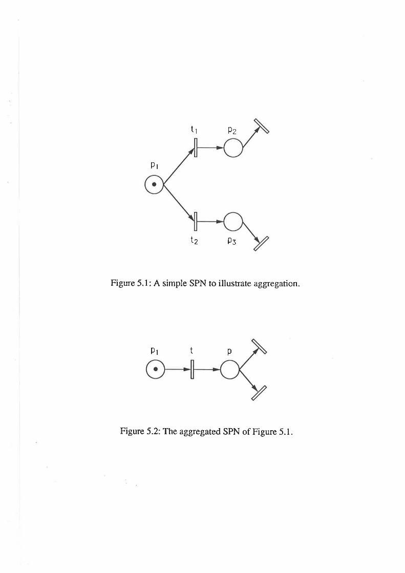
t1 Pz
Figure 5.1: A simple SPN to illustrate aggregation.
Pr
Pr
12 Þs
t p
Figure 5.2: The aggregated SPN of Figure 5.1.
we shall assume that the aggregation of transitions and places, yields a net in
which the future routeing through the net is only a function of the time spent in
the aggregated subnet. An aggregated net has this property when, for example,
1. the aggregated subnets have only one entry point, or,
2. the routeing probabilities rvithin the subnet are independent of the entry
point. In this case, more than one entry point is allowed.
\Mith this assumption, u'e define the aggregation procedure, incorporating the
age dependent routeing results of Rumsewicz and Henderson [87] given in Section
4.5, as follows:
1. From the original net P, amalgamate sets of transitions and places and
replace them with a box ó and a transition f , to create a net p. Let G¡(.)
be the firing time distribution for ú, which represents the time spent in the
aggregated subnet ó of the net P. Assume that, after tokens have taken
time y to be processed by ú, the marking changes from ñ to ñ, with age
dependent probability pn,m(ú, y).
2. create the averaged net Q from P so that, due to tokens being fired by f out
of ô, the marking changes from h- to rr[, with age independent probabilitl,
pñ,ñî(ú):l- ^,-(r,
y) dG{y).
3. \Mithout altering the collection of routeing probabilities p5,5(ú), nor the
means of the distributions G6(.), create the net M,by replacing all distri_
butions G6(') with negati'e exponential distributions.
As explained in the introduction, the aim is to create a net, e, which isinsensitive to its generally distributed firing times. Since the above procedure
involves amalgamating arbitrary combinations of places and transitions, there is
a great deal of flexibility and therefore many alternatives to choose from in creating
the skeleton net. An aggregation rvhich results in an insensitive net, e.,and which
717
also has an extended product form solution is the ideal aim. Nevertheless, the
advantages in succeeding to find only an insensitive Q are significant, as we will
proceed to show.
Since we have stipulated that P is to be an exact amalgamated net of. P,
the age dependent routeing probabilities in P, are sufficient to define P. Conse-
quently, from Theorern 4.2 the equilibrium distribution of P is an exact marginal
distribution of P. Unfortunately, P has general distributions as well as age de-
pendent routeing, therefore, finding the equilibrium distribution of P is just as, if
not more difficult, than finding the equilibrium distribution of P. Thus in solving
one problem r¡¡e have created another.
Let the state space for M be M.. Let zr(m), ñ e Jvl be the equilibrium
distribution for M . Note that an equilibrium distribution for lt[ can be evaluated
using simulation, direct evaluation, approximation or, occasionally, by creating
M so that it has an extended product form solution. For each marking rn of
the net, Q, let y be a vector of either the spent, or residual, lifetimes of each of
the generally distributed transitions, enabled in rr. For our purposes, it does not
matter which of these lifetimes is used. Recall from Section 4.1, that Henderson
[35] found that rvhen Q is insensitive, the equilibrium distribution is the sarne
when the state space is supplemented rvith either spent or residual lifetimes. l,et
(m' y) be the marking of the net supplemented bv these lifetimes. From Equation
4.27 if Q is insensitive, the equilibrium distribution of being in state (m, y) is,
r(Iñ, y) : z-(m)fI p,(t - G¡(s¡)) (5.1)
where G,(.) i" the distribution associated with the lifetime !¡ and (p,)-t is the
mean of this distribution.
In Section 5.5, we shorv that Equation 5.1 is the pivotal idea in reversing the
aggregation procedure to give exact results for the original sPN.
118
5.4 Aggregation
Aggregation procedures must als'ays be questionable, unless they are supported
by some measure of their error. 'We stress that our approach is concerned rvith
aggregated nets, in which there is no error. The procedure provides exact equilib-
rium distributions, and exact marginal equilibrium distributions for the original
net. That is, we achieve aggregation procedures in which no information or accu-
racy is lost.
As pointed out in Section 5.2, we do not propose a step by step approach to ag-
gregation, and consequently rve feel the best way to demonstrate the aggregation
procedure is through an example. In the following example, we illustrate the aim
in aggregating subnets of the SPN, that is to achieve exact marginal distributions
for the original net. We use the simplified version of the dual processor, given in
Figure 4.3, but introduce a more complex memory access stage. In reality, the
access of common memory can involve more complex mechanisms, including ac-
cessing different areas of the memory a¡rd internal feedback. The SPN needed to
model such a procedure, would normally be large and complex, but for simplicity,
let us consider the net in Figure 5.3. Let transitions ú¡, have generally distributed
firing times according to the function G;(.),u'ith hazard functions å¡(.), and with
corresponding mean. (p;)-t, for 1 < i < 10. In this model, the processor is able
to access two different areas of memory concurrently, represented by the places ps
*d pu for processor 1 and places pe and p1s for processor 2.
Even if we assume that transitions ts,tc,ts, ú0, tz,terúe and ú1s have negative
exponentially distributed firing times, the equilibrium distribution of the SPN
is not of a simple form. Norv let us amalgamate places pq,ps,pa and p7, and
transitions t3,ú4,ú5 and ú6, and represeut the amalgamation by a box, ö1 and
a transition, ?r. A symmetric procedure can be performed to create box, ö2
and transition, ?2. These amalgamations give the SPN, p, of Figure b.4. Step
119
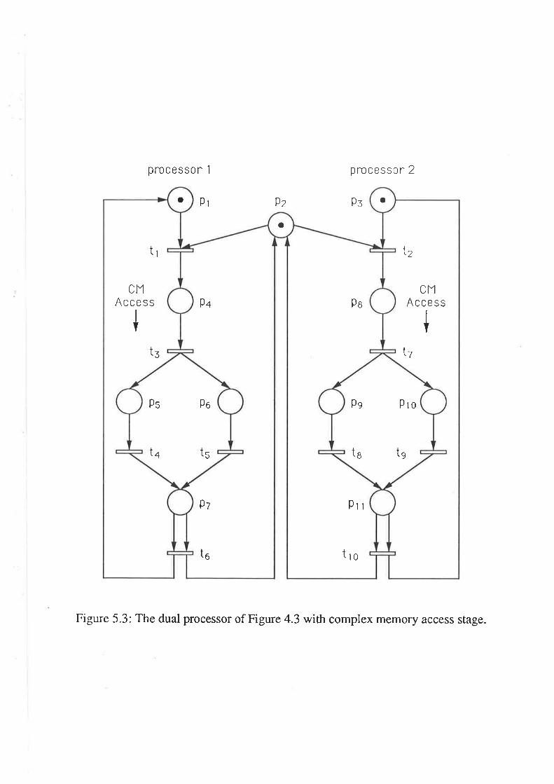
processor 1 processon 2
Pl 9z Ps
Figure 5.3: The dual processor of Figure 4.3 with complex memory access stage.
Ps Plo
tet6
Þs Po
t5ta
Prr
Pa
tro
Þc
Pt
t6
a
ct1Access
t7
+t2
CXAccess
t5
t1
ao
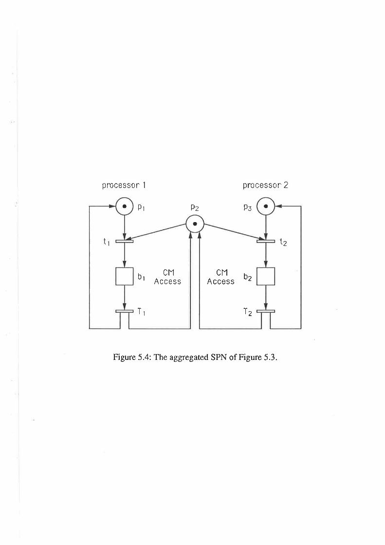
b2
f2
CNAccess
T¡
b¡ ct1Access
o
2tt
aa
processo n 1 processor 2
Pr 9z
Figure 5.4: The aggregated SPN of Figure 5.3.
Þs
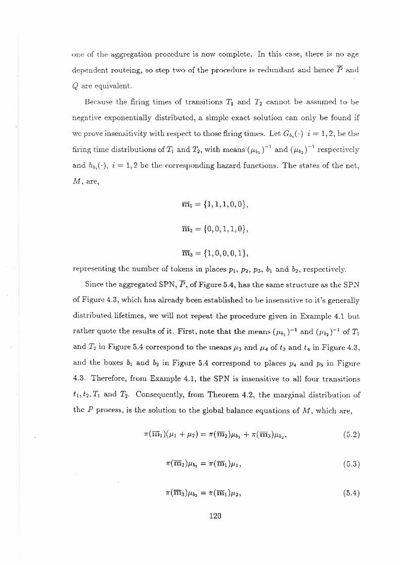
one of the aggregation procedure is now complete. In this case, there is no age
dependent routeing, so step trvo of the procedure is redundant and hence P and
Q are equivalent.
Because the firing times of transitions T1 and 7z cannot be assumed to be
negative exponentially distributed, a simple exact solution can only be found if
we prove insensitivity with respect to those firing times. Let G6,(.) t : 1,2, be the
firing tirne distributions of T1 and ?2, with means (po, )-t and (¡16, )-1 respe.tively
and h6,(.), i -- 1,2 be the corresponding hazard functions. The states of the net,
l\l , are,
ñr - {1,1,1,0,0},
ffi2 - {0,0,1, 1,0},
r-r¡ - {1,0,0,0,1},
representing the number of tokens in places pt, pz,, ps, bt and ö2, respectively.
Since the aggregated SPN, P, of Figure 5.4, has the same structure as the SPN
of Figure 4.3, which has already been established to be insensitive to it's generally
distributed lifetimes, we will not repeat the procedure given in Example 4.1 but
rather quote the results of it. First, note that the means (p¡, )-t and (par)-t of ?,
and ?z in Figure 5.4 correspond to the means pr3 and þa of. f3 and úa in Figure 4.3,
and the boxes b1 and ó2 in Figure 5.4 correspond to places p.{ and ps in Figure
4.3. Therefore, from Example 4.1, the SPN is insensitive to all four transitions
tt,tz,T1 and Tl. Consequently, from Theorem 4.2, the marginal distribution of
the P process, is the solution to the global balance equations of. lt'[ , rvhich are,
/_ \/ . \7r(nì11(pr + ltz) : 7¡'(m2)pör f n'(rTt3)pr6r, (5.2)
r(ñz)pu: z(mr)tr, (5.3)
/- \zr(rrl3)1.16, : 7r(rnl )p2,
r20
(5.4)
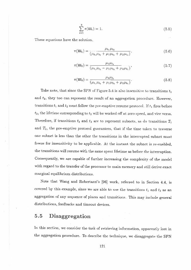
3
I zr(rrr-¡) : 1
d=1
These equations have the solution,
(5.5)
/-\rr(rïr1 ¡ - .Ilúlf,bz\ ¡/ (Par lra, I lttltt, + tlzl,Lbt)'
/- \ þtllozllyir¿1:-,Utar lto, * l.qpa, I ttztLa, )'
(5.6)
(5.7)
r(ms):ffi' (õ.8)
Take note, that since the SPN of Figure 5.4 is also insensitive to transitions ú1
and f2, they too can represent the result of an aggregation procedure. However,
transitions f1 and f2 must follow the pre-emptive resume protocol. If /1 fires before
t2, the lifetime corresponding to ú2 rvill be worked off at zero speed, and vice versa.
Therefore, if transitions ú1 and /2 are to represent subnets, as do transitions fiand ?2, the pre-emptive protocol guarantees, that if the time taken to trayerse
one subnet is less than the other the transitions in the interrupted subnet must
freeze for insensitivity to be applicable. At the instant the subnet is re-enabled,
the transitions will resume with the sarne spent lifetime as before the interruption.
Consequentl¡ we a^re capable of further increasing the complexitl, of the model
with regard to the transfer of the processor to main memory and still clerive exact
marginal equilibrium distributions.
Note that Wang and Robertazzi's [96] work, referred to in Section 4.4, is
covered by this example, since we are able to use the transitions 11 and 12 as an
aggregation of any sequence of places and transitions. This may include general
distributions, feedbacks and timeout devices.
5.5 Disaggregation
In this section, we consider the task of retrieving information., apparently lost in
the aggregation procedure. To describe the technique, we disaggregate the SPN
121
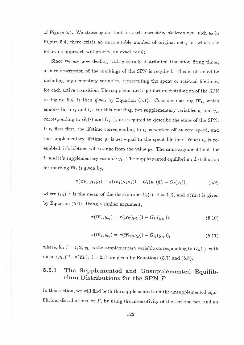
of Figure 5.4. We stress again, that for each insensitive skeleton net, such as in
Figure 5.4, there exists an uncountable number of original nets, for rvhich the
following approach wili provide an exact result.
Since we are now dealing rvith generally distributed transition firing times,
a fi.ner description of the narkings of the SPN is required. This is obtained by
inciuding supplementary variables, representing the spent or residual lifetimes,
for each active transition. The supplemented equilibrium distribution of the SPN
in Figure 5.4, is then given by Equation (5.1). Consider marking rr1, which
enables both f1 and ú2. For this marking, two supplementary variables !1 ar,d y2,
corresponding to Gr(') and G2(.), are required to describe the state of the SPN.
If ú1 fires first, the lifetime corresponding to ú2 is worked off at zero speed, and
the supplementa^ry lifetime y2 is set equal to the spent lifetime. \Á¡hen f2 is re-
enabled, it's lifetime will resume from the ra.lue Vz. The same argument holds for
Ú1 and it's supplementary variable y¡. The supplemented equilibrium distribution
for marking m1 is given b¡
z'(rñr, h,Uz): ir(rrr)prpr(I - Gr(Vr)Xt - Gz(Vz)), (5.9)
where (p,)-t is the mean of the distribution G;(.), i:7,2, and r(ñr) is given
by Equation (5.6). Using a similar argument,
t(ñ2, ybt) : r(ñ2)pbr(1 - Gr,(yr, )), (5.10)
zr(r-r¡, yb") : z(Fis)É¿or(l - Gor(y¿, )), (5.11)
u'here, for i : 1,2, !t, is the supplementary variable corresponding to G6,(.), rvith
mean (¡¿¡,)-t. ?r(mi), i:2,3 are given by Equations (b.Z) and (b.g).
5.5.1 The supplemented and unsupplemented Equilib-rium Distributions for the SpN .P
In this section, we will find both the supplemented and the unsupplemented equi-
librium distributions for P, by using the insensitivity of the skeleton net, an{ an
722
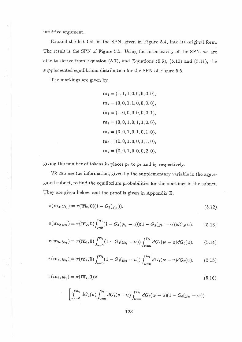
intuitive argument.
Expand the left half of the SPN, given in Figure 5.4, into its original form.
The result is the SPN of Figure 5.5. Using the insensitivity of the SPN, u,e are
able to derive from Equation (5.7), and Equations (5.9), (5.10) and (b.11), the
supplemented equilibrium distribution for the SPN of Figure 5.5.
The markings are given by,
rr11 : (1, 1, 1, 0, 0, 0,0, 0),
lll2 : (0,0, 1, 1,0,0,0,0),
Irl3 : (1,0,0,0,0,0,0, 1),
rTt4 : (0,0, 1,0,1, 1,0,0),
lrr5 : (0,0, 1,0,1,0,1,0),
1116 : (0,0, 1,0,0, 1, 1,0),
lrr7 : (0, 0, 1, 0,0, 0,2, 0),
giving the number of tokens in places pr to pz an¿ ó2 respectivelr'.
\AIe can use the information, given by the supplementary variable in the aggre-
gated subnet, to find the equilibrium probabilities for the markings in the subnet.
They are given belorv, and the proof is given in Appendix B.
T(rnz,ybt) : r(ñ2,0X1 - Gr(yu, )) (5.12)
r(rna, ab,) : ¡(rñ2, q I"':G - Go(vo, - ,)X1 - Gr(yø, - u))dGs(u). (5.13)
o(ms, abt): '(ñ2, q 1,"::Q - G^(a¡, -,r)) ll=),o"rrw - tldG3(u). (b.14)
zr(mo, uo,): z'(rr2, q l,':o - Gr(vo, - r)) Il=',,a"^(w - u)dG3(u). (b.1b)
r(mz, Abl) : z'(m2, 0)x
lÏ:dQ@) l.'=:oru, - ù I::'"dG5(u- ,x1 - Gu(vo,- -))
L23
(5.16)
processo f' 1 processor 2
Pl þz Ps
Figure 5.5: A partially expanded SPN of Figure 5.4.
Þs Þo
ta t5
CXAccess b2
ï2
CHAccess
+
tg
t¡
* 1,"::d,Gs(u) l,"l,ac,{u - ù I::',,d,Ga@-,,X1 - Ge(aa,-,))]
From Equation (5.10), n(rnz,0) : r.(mz)pa, where r(m2) is the probability of
being in a marking with a token in å1 and is given by Equation (5.7) and (p6, )-1
is the mean time spent in ó1. The equilibrium distribution for zr(mr,Ut,!z) and
zr(n¡, Ua, ) remain unchanged from Equations (5.9) and (5.i1).
Note that the form of zr(m;, vor), 2 < i < 7 is intuitive. For example, consider
n(rnr,y¿, ). Marking rn2 is defined by a token in places p3 and pa. The supplemen-
tary variable starts recording the time spent in ó1, ¿rs soon as a token is deposited
into the subnet, that is, deposited into pa. r(m2,0) is the probability of being
in a marking in which a token has just entered ór. The term (1 - Gr(ya,)) is the
probability that transition ú3 has not fired at time y6,. Using this information,
n(rnr,ya, ), the probability of being in ma¡king mz at time g¿,, is the probability
that a token entered b1 at y6r: 0 and ú3 hasn't fired at time 96,.
Now consider zr(rna,y¡,). I,t_-O - Gn(yu, - r)X1 - Gu(au, - z))dG3(z) can
be interpreted as the probability that tra¡rsition ú3 fired at time u 1 Utt, an{
that transitions úa and ú5 have not fired in the time y6, - u. The product of this
integral and z'(8I2,0), gives the probabitity of the tokens being in places ps,ps
and p6, which is the probability of being in ma¡king Eq, at time ya,. The form
for zr(rn5, ga, ) and zr(rn6, U¿, ) can be argued in the same way.
The form of rr(rn7, U¿, ) is a little more complicated, so, we rvill give an expla-
nation. The first integral in the expression can be interpreted as the probability
that transition t3 fired at time u, u < v < r, < ua,, transition úa fired at time
u, rs 1to 1u,, having been enabled for time u - u, transition 15 fired at time
u, u ( y6, having been enabled for time u) - u and transition ú6 has not fired in
time y6' - tr.'. The second integral can be interpreted as the probability that transi-
tion fs fired at time u, u 1t¡ <rD <u¡,, transitionf5 firedat time u, u 1u labthaving been enabled for time o - z, transition Ía fired at time tr.r, u I ubt having
been enabled for time to - u and transition ú6 has not fired in time ub, - u. since
L24
there exist two sequences of transition firings that reach rrr7, and each integral
is the probability of such a firing sequence, the addition of the tu,o integrals,
multiplied by zi(m2,0), gives the probability of being in rn7.
The intuitive reasoning applied to this example, can be used for any aggre-
gated subnet, but, as can be seen with this example, the equations can become
complicated. In Section 5.5.2, we will give a more general and. much more useful
procedure, again, making use of the insensitivity of the skeleton net.
Now we integrate out the supplementary variables from Equations (5.12)-
(5.16) and Equations (5.9) and (5.11), to find the exact unsupplemented equi-
librium distribution for P. The unsupplemented equilibrium equations a.re given
by the following and the proof is given in Appendix C.
zr(mz) : "(mù*, (5.12)ltz
zr(rna) : "(mù;!l;, (b.18)Fa -f ¡r5
r(rns) : nçm) -ff-, (5.1e)ltt\lta -f lts)
?r(m6) : rlmr¡--!!!7-.Ps(P¿ + Ps)'
(5.20)
z'(rn7) - zr(rn-z)Pa'
,lte
where zr(ñr), rr(mr) and n'(r-r¡) a.re given by Equations (b.6), (b.z) and (5.g).'We note that the right hand side of the SPN of Figure 5.5 can be disaggregated
in a similar manner.
5.5.2 The General Theory
Although the intuitive approach given in the previous section for disaggregation,
works for the example given, the complexity increases when larger subnets are
being aggregated. In its present form, with combinations of complex integrals, itis also of limited practical value. There is however an alternative approach, which
(5.21)
725

naturally lends itself to a variety of simple and practical techniques and is given
in Result 5.1.
Result 5.1
From Equation (5.1), rve note that an insensitive net has a product form solution
in'ol'ing the marginal distribution ,-(m) and a product of terms u;Q - G;(ù).Each y; gives information on how long a token has been in the appropriate ag-
gregated subnet, and hence the state of the subnet. The product form indicates
independence betr¡'een the marginal state and the states of the aggregated sub-
nets. Consequently, if rve wish to find the equilibrium distribution for the original
SPN we need to find:
1. The corresponding marginal equilibrium distribution of the skeleton net
2. The equiiibrium distribution for the aggregated subnets considered in isola-
tion
To find the equilibrium distributions for the skeleton net a¡rd aggregated subnets
we can use simulation, global balance equations, the extended product form so-
lution or any other technique available. The big advantage is, that each of the
resultant processes has a state space considerably smaller than the original, and
therefore relatively trivial to handle.
Consider any marginal marking in which tokens are in ô1. In this example, rn2
is the only relevant marking, rvith one token somewhere inside ö1. Norv isolate
this subnet with one token in place p¿, âs in Figure 5.6, and close the subnet by
looping the token back to place pa, rvhen it fires out of ú5.
Let (i, j,k,l) be a state of the subnet, representi\gi, j,fr and I tokens in places
PnrPs,p6 and pz, respectively. An invariant measure for the subnet of Figure b.6,
is,
r(0, 1, 1,0) : zr(1,0, O,O)(rr.f ,r,
126
(5.22)
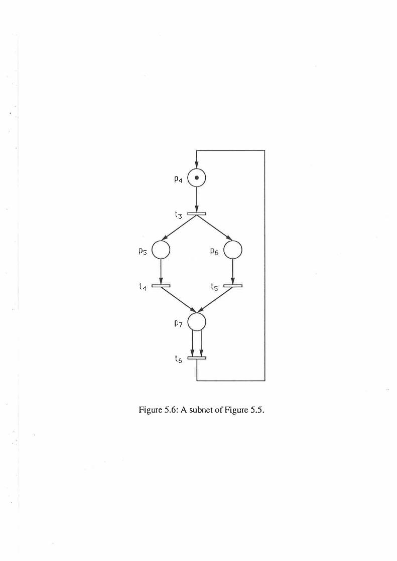
Ðq
Ps
t3
ta
t6
Figure 5.6: A subnet of Figure 5.5.
9t
zr(0, 1,0, 1) : î-(1,0,0,0) l-tzlts(5.23)
zr(0,0, 1,1) : z(1,0,0,0)
P+1ta + ls)'
llsltt (5.24)t"t1tn I ps)'
er'(0,0,0,2) : zr(1,0,0,0)f . (b.25)lte
Using the independence established in Result 5.1, it is nou, possible to construct
the equilibrium probabilities for the original SPN. This is achieved by multiplying
each of the Equations (5.22) to (5.25) by n(mz) and reconstructing the token
distributions for the original SPN. For example, (1,0,0,0) corresponds to marking
m2 in the original net since the entries for pa,ps,pe -d p, are equivalent. Let
z'(1,0,0,0): C, then,
zr(m2): Czr(rnz), (5.26)
/\T(msl : O7r(tl-t2) Irs(5.27)
(ua + Pt)'
î'(ms) : Cz-(ñz) ltslts(5.28)
7r(rn6) : Cz'(prz)
ttn(ttc + f/s) '
lttlt¿(5.2e)þ"0t0I Ps)'
a'(nr7) : C"(mù?. (5.80)lte
It is clear, that Equations (b.12) to (b.21), and Equations (5.26) to (b.80), are
equivalent invariant measures, with C : +. Fa, which can be estimated usinglts
simulation, if necessary, but in this example it can be eraluated analyticall¡ since
the mean time to traverse the subnet is,
1 _1*l+l+Fb, ltz qta lta lts tta * ¡t5
This is an interesting result, rvhich may be useful in evaluating the normalising
constant for some SPNs. \\re s'ill discuss this idea further in Chapter 6.
We a¡e now able to link the results of Section 4.9, *'ith the results of this sec-
tion. Let an aggregated subnet be an n-dimensional fork-join section, as described
I27
in Section 4.9. Using the results of this Chapter we are able to d.isaggregate the
subnet in the following way. Suppose, marking m¡ of the skeleton net, is the only
marking with a token in the subnet. Let m¡ be a ma¡king of the original SpN,
with token distribution in the subnet corresponding to the token distribution of
state 6 (as defined in Sections 4.8 and 4.9). The Equilibrium distribution of the
original SPN, is given b¡
?T'(mi): zr(6)zr(m¡),
where n'(6) is defined in Equation (4.82).
128
Chapter 6
Conclusions
In Chapter 3 of this thesis, v¡e gave the theory on the extended product form
solution for SPNs. \Mhilst finding the invariant measure for some nets is greatly
simplified using this theory, the normalising constant must still be evaluated by
generating the reachability graph. Note that, there are exceptions where the
normalising constant can be found in a closed form, as illustrated in Example 3 in
Henderson and Taylor [a1]. Also, the normalising constant for the SPN of Figures
4.11 and the subnet of Figure 5.6 were found in closed form. ft mav be possible to
use these examples as a basis for finding an approach to evaluate the normalising
constant in closed form. Future research in this area should include finding a
technique, similar to Buzen's algorithm in queueing networks, which evaluates
the normalising constant without having to generate the reachability graph.
In Chapters 4 and 5 rve illustrated that insensitivity is a strong property of
SPNs. It allows general distributions to be replaced by negative exponential
distribution's' age dependent routeing to be replaced by age independent routeing,
aggregations to yield exact marginal distributions and disaggregations to yield
the exact equilibrium distribution for the original SPN. 'We suspect, but have not
proved, that in general, insensitivity is the only property that will allorv the aboye
procedures to be performed, while yielding an exact result. Also, we would haye
liked to present a complete theory involving the insensitivity balance equations,
reversed time structures and the necessary and sufficient conditions but, if this
is at all possible, it requires much more work, which is beyond the scope of this
729

thesis.
Further work that should prove fruitful, is to first, simplify the conversion
from age dependent routeing to age independent routeing. Secondly, since the
modeller applying the theory of insensitivity must rely on their experience of
structures possessing this property. It would beneficial to provide an approach
which easily identifies these structures, such as the symmetric queue in queueing
theory.
In this thesis we have concentrated on finding the exact equilibrium distribu-
tion for SPNs. In queueing theory, networks which have a product form solution
or which are insensitive (or both) have been used to find bounds for queueing
networks which do not possess these useful properties. We suggest, that a similar
tactic ought to be applicable for SPNs. Using a suitable choice of SPN rvhich
displays an exact solution, it may be possible to give performance bounds for nets
which are otherwise difficult to solve.
130
Appendix A
In this appendix, we will prove that the supplemented differential equations, given
by Equations (4.1) to (4.10) have solution given by Equations (4.11) to (A.1s).
dtr(rn2,,y) ,
Ë: -zr(ffi2, v)Ihz(y) + /rr(y) + t o(y)l .
r(m2,0) : n(mr)¡rr.
dtr(rn3,y) ,--ø- : r(ûrz, U)hn(y) - r(me, g)Ihz(ù + /rr(V)]
dr(rna,y) : r(ms, y)l¡s(V) * zr(ms, y)h¿(y) - r(m¡, ùhz(y). (A.4)dy
dzr(m5, y) : r(rnz, y)l¿¡(v) - r(ms, y)[hz(y) + lr¡(y)]dy
dz'(m6, y)
(A.5)
dy
dr(m7,y)
: zr(nr2, V)åz(V) - r(mo, V) Ur¡(V) + ,ro(v)] . (A.6)
r(ms, y)hz(y) * r(mo, y)hn(ù - r(mz, y)hs(y). (A.Z)
dzr(rns,y) ,
-Ë.: r(ms, a)hz(v) * z-(mo, v)h"(v) -,(me, y)hn(ù. (A.8)
zr(ms)ps : lr:r(m¡, ùhz(ùdu
* I,:"rn(m7, ùhs(y)du * l":,,r(ma, ùho(ùdv. (A.e)
(A.1)
(A.2)
(A.3)
dy
zr(m;,Q):0, for 3 ( i < 8.
Also
131
(A.10)
The solution to these supplemented differential equa,tions is given by,
z-(rrr2) : z-(rn1)¡;, ll.,t - Gr(ù)(r- c.(v)X1 - Go(y))dy, (A.11)
rr(ms) : r(ml)p'l]r,t - Gr(v)X1 - G.(y))G n(a)da, (4.12)
r(m¿) : z.(rn1)p, I"I"O - cr(ù)Gs(v)Ga(v)da, (A.13)
,,(rrr,) : r(rn 1)¡r, ll f t - G r(ù)(t - G n(ù) G "(y)
dy, (A.14)
z'(mu) : ,.(rnr)p, l]-,r - c.(y)Xl - cn(ù)Gr(ùdy, (A.15)
o(-,) :,<r'.)p, l]",r - c"(y))Gr(y)Go(y)dy, (A.16)
,r(*.) : zr(rn1)¡-r, ll,t - Go(ù)Gr(y)Gr(y)dy,, (A.17)
t(*r): r(*r)4, (A.18)þs
consider Equation (4.1). The integrating factor is the term,
."o {/=" hr(u)* /r3(u) + he(u)du}
Now multiply both sides of Equation (4.1) by this integrating factor giving,
: -r(m2, y)lhr(ù + t¿e(y) + hn(y))"-o {l=. hr(r,)* tr3(u) + ha(u)du\ .
This is equivalent to,
#l"rr"r,v) exp U,'=rhr(r)* å3(u) * ha(u)du)] : o,
or, after integration,
hr(u)*å3(u)*ha(u)dun(rnz,g) : Cr exp
732
i
where C1 is the constant of integration. Using Equation (4.11) gives,
(rYì""pt J"_ohr(")+å3(u) +ha(u)duj:(1 - G,(ù)(t -cr(v)X1 -Go(ù),
and hence the solution,
zr(m2, a): C{7 - Gr(y)Xi - G.(v)Xl - Gn(aÐ.
Using Equation (A'.2), the relevant initial condition, we obtain,
r(rnz,y) : z(rnr)pt(r - cr(y)Xl - c.(v)X1 - Gn(y)). (A'.19)
Integrating both sides rvith respect to y yields,
z'(mz) : ?r(rrrl)p, I"lrtr- cr(v)X1 - cr(y)Xl - Gn(ù)da,
which is Equation (,{.11) as required. Non, consider Equation (4.3), the integrat-
ing factor is the term,
".o {l=, h,(,)+ ås(u)du} .
Now multiply both sides of Equation (.{.3) by this integrating factor giving,
ryÐ"*' {l=" h,(u)+ år(u)du}
: -zr(urs, ùlhr(y)+ t¿e(y)j*o {l=" hr(u)+ he(u)du}
f z(m2, y)ho(ù..o {l=, hr(u)+ nr(u)du} .
This is equivalent to
!* l" rr"",v ) exp
U,'=" hr(r)+ år( u )du i]
: zr(rn2, y)hn(y)*o {l=, hr(u) + hs(u)du} ,
or, after integration,
r(mr, y) exp U,t="hr(u) + hs(u)du\
: lr, * I:="o(mz,u,)ha(u)""o {l:" h,(u) + r,zç,¡a,\ a-],
133

where Cz is the constant of integration. Using equation (4.19) and (4.1f ) this
reduces to,
zr(rn3, y) : (1 - Gr(ù)(t - C.(y)) " [O*
I]=""(^,)t,,0_G,(to))(1_G3(U)X1_Ga(to))ha(wlffi,,]That is,
r('os, v) : (1 - Gr(y)Xl - cr(y)) 1"" *r(mr)É,r I_=rf, - Ga(w))h4(u)d,,f .
Using the initial condition, Equation (4.10), gives Cz:0. In addition, Equation
(4.10) implies,
I-="f, - Ga(w))haþr:)du : G n(a),
and hence,
r(ms, u) : r(mr)pr(r - Gr(ù)(t - cs(v)) Gn(s)
Integrating both sides with respect to y yields,
zr(me) : 7r(mr)p' I"l"o - Gr(y))(r - Gr(v)) Go(ùdy,
which is Equation (4.12). we will not give the proof for Equarions (A.13) to(4.18), since they follow in the same vein. r
134
Appendix B
In this appendix, rve prove that the follorving equations are the supplemented
equilibrium equations for the markings in b1.
r(mr, Ab,) : r(mz,0X1 - Gr(y¿, )) (8.1)
r(m¿, abt): n(ñz't)Ë; G - Gn(vt, - r)X1 - Gr(yo, - u))de(u). (8.2)
t(ms, ubt) : r(rn-z, t) Ë Q - Go(go, - ,r)) l_=',,o"rftu - u)dGs(u). (B.g)
z-(mo, vbt): r(¡n-2, q l,':(1 - Gu(ya, - r)) Il=',,a"^rw - u)dG3(u). (8.4)
T(rnz,A,,) : zr(mr,0)x (B.5)
[¿:; dQ@)
I,'=:0"^r, - "¡ |-=',,dG5(to- ,xl - Gu(ya,- .,))
* I,':"d,Gs(u) l"'=:a"U" - ") l::,"dGa(to _ ,Xl _ Gu(ya,_ .,,))]
consider box, ö1. Transition f3 is enabled first, úa and ú5 are enabled con-
currently, and f6 is enabled last. As the three sets of transitions are enabled
at different timcs we must use three supplementary variables to find the supple-
mented equilibrium distribution. The supplemented global balance equations forthe markings in ô1 can be rvritten as.
r(rnz,u + ô'u): zr(rn2, r) [1 - fu(u)A,u),,
135
r(m¿, U * Lry,u) -- r(rna,A,u)[t - hn(y - ")LA - hr(U - u)Ly],
r(ms, a I A,y,u) : zr'(ms,u,u)lI - hn(u - ")/'y)* rr(m¿, y,u)hs(a - u)Åly,
r(rnu, y I Ly,z) : r(rr- o,U,u)[I - hr(a- ")AV]
-| r(m¡, A,,u)ha(A - u)/ry,
r(rn7,z I A.z,a,u) : r(tnz,z,a,u)[I - h6(z - ùð¿).
Rearranging, and taking the limit as Au, L,yr\,z + 0, we get a set of differ_
ential equations.
*o!r,r,,u) : -zr(m 2,u)fu(u), (8.6)
#n!,.n,a,u): -o(m¿, y,u)Íht(v- u) + h"(y -u)1, (8.7)
d
¿¡r(ms,U,u) : -zr(ms, y,,u)h¿(u - u) + o(rno, u,u)hs(U - u), (8.8)
(B.e)
d
¿r(wrz, z,U,u): -r(rrr2, z,y,u)h6(z _ y).
Their boundary conditions are given b¡
T(rrrz,0) : n(rr:¡,0),
(8.10)
(8.11)
o(m¿, u.,u) - T(mz, u)hs(u), (8.12)
z'(ms, u, u) : Q, (B.13)
zr(mo, uru) :0, (8.14)
t(retz,U,,U,u): r(ûrs, y,u)h(y - u) + r(mo, y,u)hs(a - u). (8.15)
136
Equation (8.6) is a first order differential equation and rl,e can conclude that,
zr (rn2, u) : tr (¡r2, 0) exp h3(t)dt
Using the boundary condition given by Equation (I!.11) and Equation (4.11),
zr(rn2, u) : zr(mr,0) [1 - G.(")] .
This is Equation (B.1) with u :9¿,
Equation (8.7) is also a first order differential equation and rve can conclud.e
that,
'(mn, a,u):rr(rna,u,u)exp {- l::" å4(¿) + hs(Ðdt},
: zr(rna, u, z) exp {- I::" h.(t)dt\.*o {- l'-" n,çt¡at} ,
: zr(rna, u,u)IL - Go(V - u)] II - Gr(U - u )] .
Using the boundary condition given by Equation (8.12),
r(m', a,u): r(mz, u)fu(u)ll - Go(u - ")l [1 - Gr(v - ")].we can now integrate out the variable u, which ranges from 0 to y. Therefore,
t(mo, ,): f*u,=ot(mo, y,u)du,
r(mz, u)hs(u) [1 - G.(v - ")][1 - Gs(y - u))du,
r(ffi2,0) [1 - G.(")] Lr(u) II - Go(y - ")] [1 - Gr(a - u))du
Using equation (4.10), yields,
r(rna' o) : I,u=o:r(Iñ2,0) [1 - Gn(y -r)] [1 - Gr(v - u)] dGs(u),
: r(ñ2, o) I*u=o[l - Go(v - r)][1 - Gr(y - u)]de(u)
1!: Ju=o
: r*|=o
137
This is Equation (8.2) with y : Ub,.
The third differential equation is slightly more complicated and requires theuse of an integrating facror. A suirable choice is exp {l::" na@at}. This gi'es,
ftl*O^,,y, u)exp {l::" h4(¿)dr}] : r(r,,¿, a,u)hs(y- u)exp U""-" h,(t)dt} .
Hence,
r(rn5, y, z) exp {l::" n{lat\
: ct t I),_,"(^^,w,u)hs(u - u) exp {l::" rtae)at} dr.o,
where C1 is the constant of integration. The boundary condition, Equation (8.18),implies that C1 :0. So,
'r(mu, v,u)lt - Gn(y - ")]-t
: I:=,Lr(rna, w,u)hl(w - ,) [1 - Ge(u - u)]-1 d,w,,
: I:=,n(rn2, u)fu(u)[I - Ga(o - u)][1 - G5(to - ,)]
x hs(w - ") [1 - Ga(w - u)]-1 du,
: r(ñ2, q I:=,[1 - G3(u)]hs(u)dG5(- - u).
Then,
'(mu, a,u) : n(h2,0) [1 - cr(")] h"(u)[t - Gn(a - ")] l:=,dG5(w _ u).(8.16)
Once again we can integrate out the dependence on u, so,
t(mr, ,): f,u=on(rn5, y,u)d.u,
î!: Ju=o'r(Erz,0) [t - cr(")] är(") lr _ Gn(y _
"\ l:=,d.Gs(u _ u)du,
: r(ñ2, o) I,',=o[r - Gn(a - ù] I:=,dGs(w - u)dGs(u).
138
This is Equation (8.3) rvith y : Aû.
\Me will not give the detaiis for the solution of Equation (8.9) as it is similar
to that given above. Hon'ever, for future use,
r(mu, v,u) : '('rr,0) [1 - G.(")] h"(u)[1 - Gr(v - ")] l::.d,Gaeo - u). (8.17)
Equation (8.10) is a first order differential equation. Therefore,
r(rn7,z,a,u): r(mz, a,u,u)"*o {- l'-t n"ç¡at}
: ['(mu, a,u)h(y - u ) + zr(mo, y,u)hs(y - z)]exp {- l:"' h6(Ðdt}
: [*(ms, u,u)hs(y - u) + T(mo, V,u)hs(y - ")] [1 - Ga(, - y)] .
substitution for r(ms,y,u) and r(mu,y,u) from Equations (B.16) and (8.12),
grves,
r(mr, z,A,u): T(nr-2,0) [1 - G6(z - y))x
I
Lf t - G'(")l år(") Ít - Gn(v - u))ho(v - r) f"u=.dG5(u - u)
+ [1 - c.(r)]/rr(r) [1 - Gr(v - u))hu(y - u) f,u=,dGa(u- "r]
Integrating out the dependence on u gives,
r(rnz, z, a)': f ,',=on(^r, z,y, u)d,u,
1,"=or(nrz,0) [1 - G6(z - y)) x
Ift - Gr(r)] h"(u)[t-Gn(y -u))ho(y -ù |"u=,dG5(u -u)
+ [1 - c.(r)] h"(u)[t - Gu(u - u)]hr(y - ù f,u=.dGa(u - ù]ar,
139
: r(ñz, o) [1 _ G6(z _ y)] x
U:"dGs(u) lt - G n(y -,)l hn(a - ù f"o=,d.G5(u - u)
* l,:=rd.e(u)ll - Gr(a - u)lhu(y - ù l,u=,dGa(u- ")]
Now integrating out the dependence on gr gives,
r(rn7, z) :1,"=,
r(mz, z,A)dU,,
7r( rrr2
lr,"=,
,o) |,",=odGs(u) x
IL - Gn(a - ")] hn(y -") [1 - Gø(z - ù) I,u:,dGs(u - u)da
* Ir"=,[1 - Gr(y - r))hr(y - r) [1 - Gø(" - ù) f,n=,dGa(u - ùorf,
: zr(ñ2,0) x
l|"dG3(u) I,-.or^to- ,) [1 - Ga(" - ù) f"o=,dGs(u - u)
* |,",=odGs(u) fr"=.a"u{o - ,) [1 - Ga(" - ùl !"u=,dGa(u- "r]
Changing the order of integration from
r(rn7, z)
: 7r(ñ2, o) f,',=od,Q(u) f,'=,dcr{u - ù |:=,d.Ga(u: - r) [1 - Ga(z -.)]dy
* zr(ñr, o) f,"=odQ(u) f""=,d,Gn:u - ù l:=,d.Gs(u- ,.,) [1 - Ga(, - -))dv.
f ,"=, I,n=, ^ 1""=, f '-u
Biu"",
Which is Equation (B.5) rvith z : Ab,.
140
Appendix C
In this appendix, we u'ill derive the follorving unsupplemented equations from the
supplemented balance equations given by Equations (8.1)-(8.5) in Appendix B.
zr(rn2) : ,r(mz)&,ltt
z'(rna) : ,r(rrt-r) Fu'
l.tq * lts'
zr(rrr5) : r(tttz) .;þb'þ5Ps(tu + Ps)'
a'(rn6):n(mù4Ltrs(po + ps)'
(c.1)
(c.2)
(c.3)
(c 4)
(c.5)
(c 6)
(c.7)
zr(rn7) -T\r'It2)pb|
þa
(7 - G¡(yt,))dy6,, Yi
To remove the supplementary variable, we integrate Equations (8.1)-(8.5)over yö, from 0 to oo. Equations (8.1) and (b.10) give,
?T(m2) : Iri,=o:,r(rn2, ut,)d.yu,: z-(inz)Êr, ll=.,t - G"(yt,))daa,.
However
Therefore,
1
lt;
zr'(m2) : "(mùf ,
which is Equation (C.1), as required. Equation (8.2) gives,
n'(m¿) : [* - zr(lra, !a,)d,gu,,u lbt=g
r41
: r(rln2)pu, [.* -^ 1,",-o - Ga(au, - ,)Xr - Gr(aa, - u))dG3(u)dyu,.J g¿'=o '
Swapping the order of integration, gives,
z-(rn¿) : r(ñ2)t10, l,:-o lri,=,rt - Gn(va, - ,)x1 Gs(va, - u))dGs(r)daa,
: r(ñ2)Lrt, 1,7"1 l"i,=,r'- G(at, - u))dvo,d'G3(u),
where G(.) is the distribution with hazard function än(.)+ås(.) and so, bv equation
(C.6), has mean ø+B Hence,
r(m¿) :7r(ñ2)pö, [* oc"(r)-]-,Ju=o lt¿ I lts
: o(mr) trn T ,;
r¡'hich is Equation (C.2), as required. Equation (8.3) gives,
z'(ms) : [* - r(ms, at,)dyu,,J uùt =g
: r(ñz)ttu, Iui,=ol=itt - Gn(au, - u)) ll=).0""rw - u)dGs(u)dy6,,
-- r<ñz)ttr, lui,=o 1.|*O - Gn(yø, - u))Gr(v - u)dG3(u)dya,.
Srvapping the order of integration, gives,
?T'(ms)
: r(ñ2)pr, I,: Ii,-_,U - Go(yt, - u))Gr(y - tt)dG3(tt)dyu,,
: r(ñ2)po, I,:" Ii,=,u - Gn(aa, - ,)) [1 - (1 - Gu(au,- ,))] d,Gs(u)dy6,,
: 7r(ñ2)p,, I,: I:=.[,t - ".,16, - u))
- (1 - Gn(au - ")X1 - Gu(at, - "))
142
dGs(u)dy6,
Now, by Equation (C.6) and the comments in the derivation of Equation (C.2),
: z(rrr:)/ o, [* lr - _+ I dGs(u),Ju=o ll-ta ltn -f ¡t5 I
: ?r( ltr2 )pôl
: T\n;rz)ltu,
This is Equation (C.3), as required, and a similar argument holds for obtaining
Equation (C.4).
The form for a'(m7) is more difficult so lve give the derivation belou,. Equation
(8.5) gives,
l,:,="zr'(m7) : n(mr,aû)dyo,,
: T\Èmz)pù x
u,-" [: l"': l]=',"ac"{,)dGa(u - u)dG5þa- ,) [1 - Gu(vu, - -))dvu,
* l":,="1"':1"":: fuo',dc"çu)dG5(u - u)dGa(u:- r) [1 - Gu(yu, - -))¿vr,)
[¿- I:-" I:-" l,:,=.[1 - Ge (v¿' - -)] dv5,d'Gs(ta - u)dGa(u - u)dGs(u)
* l,: l":-,l:" I:,=-[1 - Gu(ya, - -)] d.y6,d,Ga(ro - u)dG5(u - ùac"fu)]
Integrating out the dependence on uô, and using Equation (c.6) gives,
zr(mz) : 1r(ñ2)p,, [å l,: l":.l* "ac,ç-
- u)dGa(u - u)dQ(u)
Changing the order of integration, to enable us to remove the dependence on yör,
grves,
z'(mz) : zr(ffi2)¡.r6, x
143
Now change the order of integration of the last two integrals, in the first expression
only, to get,
l,:, l :_" dG aþt - u) d.G s(u - u )dc,(u )]
*; I,:-" I:.I:"d'Ga(u - u)d'G5(u- u)dG3(")]
rc(rn7j : Ttlt't72)pbl l: Ë" f"- ,dcn{u - u)d,G5(u; - u)de(u)
1r*+- |¡t6 J u-o
zr(rn7) : 1r(ñ2)t1" [; l,:" I:GaQ)dG5(z)d,Q(u)
1
þa
Evaluating the two inner integrals,
+þe
Change the variable of integration, to get,
,(m,) : tr(rnz)tl,, lå l: Ë"Go(- - u)dG5(a - u)dGs(u)
I:" I:.[L - Ga(u - ,)] dG.(u- ,)dc,(,)]1
Combining the two integrals gives,
* * I,:-" Ii"tt - G o( ")l ¿ç,ç z) dG s@)]
,r( m7) : 7r (m2)p" [; l":" l,:"ac,Q)ac"@)f
Evaluate the two remaining integrals consecutively, to get
r(mz) -n(ñ')Pu',ltø
which is Equation (C.5), as required.
(c.8)
I
L44
Bibliography
[1] Ammar H.H., Huang Y.F. and Liu R.w. (1987) - Hierarchical Models forSystems Reliabili,ty, Maintainability and Auai,Iability,IEEE Trans Circuits
and Systems, CAS-34, no. 6, pp 629-638, 1987.
[2] Ammar H.H and Islam S.M.R. (1989) - On Bound.s for Tolcen Probabilities
in a Class of Generalised Stochastic Petri Nets, Proc. 3rd Int. Conf. on Petri
Nets and Performance Models, I(yoto, Japan, pp 22I-222, Dec. 1989.
[3] Ammar H.H and Islam S.M.R (1989) - Time Scale Decornposition of a Class
of Generalised' Stoch.astic Petri /{efs, IEEE Trans on Softrvare Engineering,
15, no. 6, pp 809-820, 1989.
[4] Ammar H.H and Liu R.W. (1985) - Analysis of the Generaliseil Stochastic
Petri Net by State Aggregation, Proc. Int. workshop on Timed petri Nets,
Torino, Ital¡ July 1985.
[5] Baccelli F., Makorvski A.M. and Schwartz A. (19gg) - The Fork Join Queue
anil Relateil Systems wilh Synchronisation Constraints: Stochastic Orilering
and, Computable Bounds, Adr,. Appl. prob., 21, pp 621-660, 1ggg.
[6] Balbo G., Bruell S.C. and Ghanta S. (1g8S) - Combining Queueing Networks
and Generalized" Stocl¿astic Petti Nets for th,e Solution of Complet Moilels
of system Behauiour, IEEE Trans. on computers, 32, pp 12b1-126g, 1ggg.
[7] Balsamo S. and Iazeolla G. (1984) - Aggregation anil Disaggregøtion in
Queueing Networks: Th,e Principle of Prod,uct-Form Synthesis, Mathemat-
ical Computer Performance and Reliability, G. Iazeolla, P.J, Courtois and
L45
A. Hordijk (editors), Elsevier Science Publishers, B.v. (North-Holland), pp
95-109,1984.
[8] Baskeit F., chandy Ii., Muntz R., and Palacios J.(1925) - open, closed. and.
Mfued' Networks of Queues with Different Classes of Customers, J. Assoc.
Comp. Mach., 22 ,pp 248-260, 1975.
[9] Berthelot G. (i986) - Checking Properties of Nets using Transformations,,
Lecture Notes in Computer Science, New York: Springer-verlag, 222, pp
19-40,1996.
[10] Bertheiot G., Roucairol G. and \¡alk R. (1gs0) - Red.uction of Nets and.
Parallel Prograrns, Lecture Notes in Computer Science, New York: Springer-
Verlag, 84, pp 277-290,1980.
[11] Bertoni A. and Torelli\{., (1981) - Probabilistic Petri Nets anil Semi-Marlioa
Processes, Proc. 2nd European \\Iorkshop on petri Nets, Bad Honnef, \Ä¡est
Germany, Sept. 1981.
[12] Bobbio A. and Cumani A. (1984) - Discrete State Stochastic Systems with
Phase-Type Distributed, Transition Times, Proc. AMSE Intl. Conf. on Mod-
elling and Simulation, Athens, pp i73-1g2,1994.
[13] Bruell S.C. and Ghanta S. (1985) - Throughput Bounds for Generalised,
Stochastic Petri Nets, Proc. Int. \\¡orkshop on Timed petri Nets, Torino,
Italy, July 1985.
[14] Buzen J.P. (1973)- Computational Algorithms for CIoseiI Queueing Networlcs
with Exponential seruers, commun. ACM, 16, pp 527-5JL,1gzB.
[15] Campos J., Chiola G., Colom J.Nf. and Siha M. (19gg) - Tight polynornial
Bound"s for Stead'y State Perforrnance of Mørlced. Graphs, Proc. 3rd Int.
conf. on Petri Nets and Performance Moders, I(yoto, Japan, pp 200-209,
Dec. 1989.
146
[16] Campos J., Chiola G. and Silva M. (1989) - Properties and Steady State
Performance Bounds for Petri Nets with Unique Repetitiae Firing Count
Vector Proc. 3rd Int. Conf. on Petri Nets and Performance Models, I{yoto.
Japan, pp 270-220, Dec 1989.
[17] Chandy K.M., Herzog U. and Woo L. (197b) - pararnetric Analysis of
Queueing Networks,IBM J. Res. Develop., 1g, pp 36-42, 7975.
[ra] Chandy I{.M., Horvard J. and Towsley D. (1927) - prod"uct Form and, Local
Balance in Queueing Networks, J. Assoc. comp. Mach., 24, pp 2b0-263.
7977.
[rO] Chandy I{.M. and Martin J. (1983) - A Characterization of Prod.ttct Form
Queueing Networks, J.Assoc. Comp. Mach., BO, pp 250-26J,1gg8.
[20] Chen P., Bruell S.C. and Balbo G. (1989) - Alternatiue Methods for fncor-
porating Non-Exponentiøl Distributions into Stochastic Timed. Petri Net-q,
Proc. 3rd Intl. 'Workshop on Petri Nets and Performance Models, I(yoto,
Japan, pp 187-197, Dec. 1989.
[21] Cheng Y. and Robertazzi T.G. (1988) - The Lattice Geometry of petri Net-
uorlc Mod,els of Multilt'op Radio Netutorlcsr 22nd Annual Conference on In-
formation Sciences and systems, princeton, N.J., N{arch 1ggg.
[22] Chu T.A. (1987) - A Methoil of Abstra.ction for petri Nets, proc. Inr. \\¡ork-
shop on Petri Nets and Performance Models, Madison, wI, pp r64-rTJ.
Aug. 1987.
[23] Cohen J. (1957) - The Ge¡¿eraliseil Engset Forrnulae, Philips Telecomm
Review, 18, pp 1b8-120, 1952.
[24] courtois P.J. (1977) - Decomposability, Academic press, New York, rgTT
747
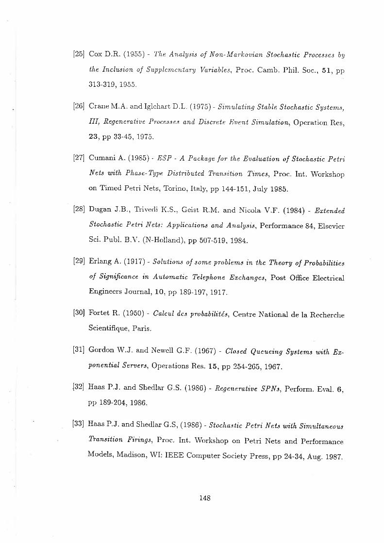
[25] Cox D.R. (19o-c) - The Analysis of Non-Marlcoaian Stochastic Processes by
the Inclusion of Supplernentary Variaåles, Proc. Camb. Phil. Soc., 51, pp
313-319, 1955.
[26] Crane M.A. and Iglehalt D.L. (1975) - Simulating Stable Stochastic Systerns,
III, Regeneratite Processes and Discrete Euent Simulation, Operation Res,
23, pp 33-45, 1975.
[27] Cumani A. (1985) - ESP - A Paclcage for tl¿e Eaaluation of Stochaslic Petri,
Nets uitl¿ Phase-Type Distributeil Transition Times, Proc. Int. 'Workshop
on Timed Petri Nets, Torino, Italy, pp 144-1b1, July 198b.
[28] Dugan J.8., Trivedi I{.S., Geist R.M. and Nicola v.F. (1gg4) - ExtenìIed,
Stochaslic Petri Nets: Applications and. AnøIysis, Performance 84, Elsevier
Sci. Publ. B.V. (N-Holland), pp b07-b19, 1984.
[29] Erlang A. (1917) - Solutions of some problems in the Theory of Probabilities
of Significance in Automatic Telephone Exchanges, Post Office Electrical
Engineers Journal, 10, pp 189-192, 1912.
[30] Fortet R. (1950) - Calcul des probabilités, Centre National de la Recherche
Scientifique, Paris.
[31] Gordon W.J. and Ne*'ell G.F. (1907) - CIoseiI Queueing Sgstems with Ez-
ponentiøI Sertters, Operations Res. 15, pp 254-265,1962.
[32] Haas P.J. and Shedlar G.S. (1986) - Regeneratiae SpNs, perform. Eval.6,
pp 189-204, 1986
[33] Haas P.J. and Shedlar G.S, (1986) - Stochastic Petri Nets with Simultaneous
Transition Firings, Proc. Int. Workshop on Petri Nets and Performance
Models, Madison, wI: IEEE computer Society press, pp 24-34, Aug. 1ggz.
148
[34] Haas P.J. and Shedlar G.S. (19S9) - Stochastic Petri Net Representation of
D'iscrete Euent Simulations, IEEE Trans on Software Engineering, 15, no.
4, pp 381-393, 1989.
[35] Henderson W. (1983) - Insensitiuity and, Reaersed, Marlcoa Processes, Aiv
Appl. Prob, 15, pp 752-768,1983.
[36] Henderson 'W. and Lucic D. (1983)- Applications of Genenl.ised Semi
Markov Processes úo Súocåastic Petri Nets, Performance of Distributed and
Parallel systems, Ed. T. Hasegarva, H. Takagi, Y. Takahashi, pp. 815-32g,
1988.
[37] Henderson'W., Lucic D. and Taylor P.G. (1989) - A Net Leuel perforrnance
Analysis of Stochastic Petri Nets,J. Aust. Math. Soc. Ser.B,81, pp 126-182,
1989.
[38] Henderson w., Pearce c.E.tr,f., Taylor P.G. and van Dijk N.M. (1gg0) -
closeil Queueing Networks with Batch serrices, euESTA, 6, pp 57-70,
1990.
[39] Henderson W. and Taylor P.G. (1989) - Insensitiuity of Processes uith in-
tenuptions, J. Appl. Prob., 2G, pp 242-258,1989.
[40] Henderson W. and Taylor P.G. (1989) - Aggregation Metlrod,s in Exact Anal-
ysis of Stochastic Petri.lÍefs, The 3rd International Workshop on Petri Nets
and Performance Models, I(¡'oto, Japan, pp 12-18, Dec. 1gg9.
[a1] Henderson W. and Taylor P.G. (1990) - Embed.d,ed. Processes in Stochastic
Petri Nets, to be published in IEEE, Trans. on Software Engineering, 19g1.
[42] Henderson W. and Taylor P.G. (1990) - Product Form in Netuorks of Queues
with Batch Arriuals and Batch. seruices, euESTA, 6, pp z1-gg, 1gg0
149
[43] Holliday M.A. and Vernon M.I(. (1987) - A Generalised Ti,med, Petri Net
Mod'el for Perforn'Lance Analysisr IEEE Transactions on Software Engineer-
ing, SE-13, No. L2, pp 1297-1310, 1987.
{aa] Holt A.W. and Commoner F. (1970) - Euents and Conditions, Princeton,
N.J., Applied Data Research Inc., Information System Theory Project. Also:
Record Project MAC Conf. Concurrent Systems Parallel Computation, pp
3-52, 1970.
[45] Jackson J. (1957) - Networlcs of Waiting Lines, Operations Research,5, pp
518-521,1957.
[46] Jackson J. (19ô3) - Jobshop lilce Queueing Systerns, Management Science,
1O, pp 131-142, 1963.
[47] Jansen U. and I{önig D. (1980) - Insensitiaity of Stead,y State probabilities
in Proiluct Fonn for Queueing NetworÃ;s, Elektron, Informatsionsyerarb.
I{ybernetik., 16, pp 285-3g2, 1980.
[48] Johnsonbaugh R. and Murata T. (1981) - Aild.itional Method,s for Reiluction
and, Expansion of Mørkeil Graphs,IEEE Trans. Circuit Syst., cAS-2g, no.
10, pp 1009-1014, Oct. 1981.
[a9] I{elly F. (1975) - Networks of Queues With Customers of Different Types,
J. Appl. Prob., 12, pp 542-544,192b.
[50] I{ellv F. (1976) - Networks of Queues, Adv. Appl. prob., 8, pp 416-432,
1976.
[51] I(elly F. (1gzg) - Reuersibility and, stochastic Netuorks,'wiley, London,
1979.
[52] König D. (1965) - Verallgerneinerungen d,er Erlanschen Formeln lr{ath.
Nachr., 28, pp 145-155, 1965.
150
[53] König D. and Jansen U., (1974) - Stochastic Processes and Properties of
fnuariance for Queueing Systens witl¿ Speeds and Ternporaru Interruptions,
Trans 7th Prague Conference Inf. Th., Stat. Dec. Fns. and Rand. proc., pp
335-343. 1974.
[54] I{ostenL. (1942) - O" tt¿e Validity of the Erlang and Engset Loss Formulae,
Het P.T.T. Bedrijf, 2, pp 42-45,1942.
[55] Lazar A.A. and Robertazzi T.G. (19s4) - The Geornetry of Lattices forMarlcouian Queueing Networks, Columbia University and SU NY at Stony
Brook, Departments of Electricai Engineering, 1984.
[56] Lazar A.A. and Robertazzi T.G. (i986) - Markoaian Petri Net Protocols with
Product Form Solution, Columbia University and SU Ny at Stony Brook,
Departments of Electrical Engineering, 1g86.
l57l Lazar A.A. and Robertazzi r.G. (1gs6) - Th.e Algebraic and, Geometric
Structure of Markouian Petri Netuork Lattices, 24th. Allerton Conference
on Communication, Control and Computing, University of Illinois, 1986.
[58] Lazar A.A' and Robertazzi T.G. (1932) - The Lattíce Structure of ø Bus Ori-
ented Multiprocessor Mode¿, 25th. Allerton Conference on Communication,
control and computing, urbana-champaigne, Ill, oct. 19g2.
[59] Lin C' and Marinescu D.C. (1988) - Stochastic Eigh-Leuel petri Nets anil
Applications, IEEE Trans. on computers, 37, pp g15-g25, 1ggg.
[60] Marsan I{.4. (1989) - Stochastic Petri Nets: An elementary introiluction,
Advances in Petri Nets 1g89, Lecture Notes in comp. sci., springer-Verlag,
pp 1-29, 1989.
[61] Marsan M.4., Balbo G., Bobbio 4., chiola G., conte G. and cumani A.
(1985) - on Petri Nets uith stochastic Timing, proc. Int. workshop on
Timed Petri Nets, Torino, Italy, pp g0-g7, July 1gg5.
151

[62] Marsan M.4., Balbo G., Bobbio 4., Chiola G., Conte G. and Cumani A.
(1989) - The effect of Execution Policies on the Semantics and, Analysis of
Stochasti,c Petri Nets,IEEE Trans. on Softrvare Engineering, 15, pp 832-84b,
1989.
[63] Marsan M.4., Balbo G., Chiola G. and Conte G. (1987) - Generalized,
Stochastic Petri Nets Reuisited: Random Suitches and Prioriti,es, Proc. Int.
workshop on Petri Nets and Performance Models, Madison, \MI, pp 44-58,
Aug. 1987.
[64] Marsan M.A. and Chiola G. (1986) - O" petri Nets uith d,eterrninistic and,
Erponential Transition Firing Times, Proc. Zth European 'Workshop on
Application and Theory of Petri Nets, oxford, UI{, pp 1b1-16b, June 19g6.
[65] Marsan M.4., Conte G. and Balbo G. (1984) - ,4 Class of Generalised,
Stochastic Petri Nets for the PerforrrLo,nce Analysis of Multiprocessor Sys-
tems, ACM Transactions on Computers, 2, no. 2, pp gS-I22,1gg4.
[66J Matthes I{. (1962) - Zur Theorie d,er Bed,ienungsproze.rse, tans. 3rd prague
Conference Inf. Th., Stat. Dec. Fns. and Rand. proc., pp 513-52g, 1962.
[67] Menasche M. (1985) - PAREDE: An Automateil Tools for the Analysis of
Time(d') Petri y'Ùeús, International \\¡orkshop on Timed Petri Nets, Torino,
Italy, pp 162-169, July 198b.
[68] Merliri P. (1974) - A Study of the Recouerabitity of Computer Systems ph.
D. Dissertation, University of California. Irvine lgl4.
[69] Mertin P. (1979) - Specif,cation and. Valíitation of Protocols, IEEE Trans
Comm, COli.4-27, No. 11, pp 1621-16g0, Nov. 1g7g.
[70] Merlin P. and Farber D.J. (1976) - A Metlrod,ology for the Design anil lrnple-
mentation of Cornmunication Protocol-s, IEEE Trans. on Communications,
COM-24, no. 6, pp 614-621, June 1926.
L52
[71] Merlin P. and Farber D.J. (1976) - Recoaerability of Cornrnunico.tions Proto-
cols - Irnplications of a Tlteoretical Stuily IEEE Trans. on Comrnunications,
CO}v{-24, no. 9, pp 1036-1042, Sept. 1976.
[72] Molloy M.I(. (1931) - On th.e Interyretation of Delay o,nd Tl¿roughput Mea-
sures in Distributed Processing Mod.els, Ph. D. Dissertation, University of
California, Los Angeles, 1981.
[73] Molloy M.K. (1982) - Performance Analysis using Stochastic Petri Nets
IEEE Trans. on Computers, C-31, no. 9, pp 913-917, Sept. 1982.
[74] Molloy M.I(. (1985) - Discrete Time Stochastic Petri /[efs, IEEE Trans on
Software Engineering, SE-11, no. 4, pp 477-423, April 1985.
[75] Molloy M.I(. (1985) - Fast Bounds for Stochastic Petri .l[eús, Proc. Int
Workshop on Timed Petri Nets, Torino, Italy, pp 244-24g, July 19S5.
[76] Murata T. (1989) - Petri Nets: Prcperties, Analysis and Applications. Proc
of the IEEE, 77 No. 4, pp 541-bg0, lggg.
[77] Natkin S. (1930) - Les Reseaux ile Petri Stocho.stiques et leur Appli,cation
a l'Eualuation d'es Systemes Infonnatiqzes, These de Docteur Ingegneur,
CNAM, Paris, FYance, June 1980.
[78] Noetzel A. (1979) - ,{ Generalízeil Queueing Discipline for Prod,uct Forrn
Queueing Networks, J. Assoc. Comp. Mach., 26, pp ZTg-TgJ,1g7g.
[79] Peterson J.L. (1981) - Petri Net Theory and the Moil"elling of Systems. [;n-
glewood Cliffs, NJ: Prentice-Hall, Inc., 1g81.
[80] Petri C.A. (1962) Kommunikation mit Autornaten,Ph. D. clissertation, Uni-
versity of Bonn, west Germany, (In German); Also: M.I.T. À{emorandum
MAC-M-212, Project MAC, Massachusetts Institute of rechnology, Cam-
bridge, Massachusetts; Also: Clifford F. Greene Jr. (translator), Cornmuni-
153
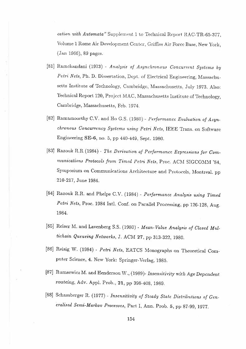
cation wi'th Autornølø" Suppl.ement 1 to Technical Report RAC-TR-65-3TT,
Volume 1 Rome Air Development Center, Griffiss Air Fo¡ce Base, New \brk,
(Jan 1966), 89 pages.
[81] Ramchandani (1973) - Analysis of Asynchronous Concurrent Systems by
Petri y'Íels, Ph. D. Dissertation, Dept. of Electrical Engineering, Massachu-
setts Institute of Technology. Cambridge, \Iassachusetts. July 1973. Also:
Technical Report 120, Project N4AC, Massachusetts Institute of Technolog,,
Cambridge, Massachusetts, Feb. 1g74.
[82] Ramamoorthy C.V. and Ho G.S. (1980) - perforrnance Eualuation of Asyn-
chronous Concurrency Systems using Petri Nets,IEEE Trans. on Softrvare
Engineering SE-6, no. 5, pp 440-44g, Sept. 1980.
[83] Razouk R.R (1984) - The Deriuation of Performance Expressions for Com-
rnunications Protocols from Tímed. Petri y'fefs, Proc. ACNÍ SIGCON{\{ 'E4,
Symposium on Communications Architecture and Protocols. I{ontreal. pp
210-217, June 1984.
[84] Razouk R.R. and Phelps C.V. (1984) - Perfortnance Analysis using Timeil
Petri y'{ets, Proc. 1984 Intl. Conf. on parallel processir,g, pp 126-12g, Aug.
1984.
[85] Reiser M. and Lavenberg s.s. (1gg0) - Mean-value Analy.<is of closed, MuI-
tichain Queueing Networlcs, J. ACM 2T , pp JIJ_822,1gg0.
[86] Reisig w. (1934) - Petri Nets, EATCS lr{onographs on Theoretical com-
puter Science, 4. New York: Springer-\/erlag, 1ggb.
[87] Rumsewicz M. and Henderson \\¡., (1ggg)- rnsensiúj vity with Age Dependent
routeing, Adv. Appl. prob.,2!,pp Agg_40g, 1ggg.
[88] Schassberger R. (1977) - Insensitiaity of stead,y state Distributions of Gen-
eraliseil semi-Marlcou Processes, part I, Ann. prob.5, pp g7-gg, lgzl.
r54
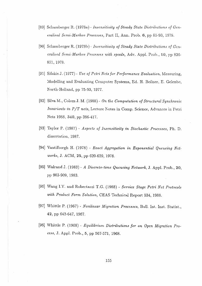
[89] Schassberger R. (1978a) - Insensitiuity of Stead,g State Distributions of Gen-
eralised Semi-Marlcou Processes, Part II, Ann- Prob. 6, pp 85-93, 1978.
[90] Schassberger R. (1978b) - Insensitiuity of Steaily State Distributions of Gen-
eralised Semi-Markoa Processes with speed.s, Adv. Appl. Prob., 1O, pp 836-
851, 1979.
[91] Sifakis J. (1977) - Use of Petri Nets for Perforrnance Eualuation, Measuring,
Modelling and Evaluating Computer Systems, Ed. H. Beilner, E. Gelenbe,
North-Holland, pp 75-93, 1977.
[92] Silva M., Colom J. M. (1988) - On the Conputation of Structural Synchronic
Inuariants in P/T nets,Lecture Notes in Comp. Science, Advances in Petri
Nets 1988, 340, pp 386-417.
[93] Taylor P. (1987) - Aspects of Insensitiaitg in Stochastic Processes, Ph. D.
dissertation, 1987.
[94] Vantilborgh H. (1978) - Eract Aggregation in Exponential Queueing Net-
works, J. ACN4, 26, pp 620-629, 1978.
[95] walrand J. (1983) - ,{ Discrete-time Queueing Netusork, J. Appl.prob., 20,
pp 903-909, 1983.
[96] Wang LY. and Robertazzi T.G. (1988) - Serttice Stoge Petri Net Protocols
with Product Form solution, CEAS Technical Report 534, 1988.
[97] Whittle P. (1967) - Nonlinear Migration Proces.ses, Bull. Int. Inst. Statist.,
42, pp 642-647,1967.
[98] Whittle P. (1968) - Equitibriurn Distributions for an Open Migration Pro-
cess, J. Appl.Prob.,5, pp 567-57I,1908.
155
[99] Wong C.Y., Dillon T.S. and Forward I{.E (1985) - Timed Places Petri Nets
with Stochastic Representation of Place Times, Proc. Int. \\rorkshop on
Timed Petri Nets, Torino, Italy, pp 96-103, July 1980.
[100] Wong C.Y. and Henderson W. (1987) - Time-Ertend.ed Petri Net Models
- An Oueruiew, 2nd Australian Teletraffic Research Seminar, organised by
Teletraffic Research Centre, University of Adelaide. 1987.
[101] \Moo D.L., Phelps C.V. and Sidwell R.D. (1986) - Tirned Petri Nets Proba-
bility Semantics, Proc. 7th European Workshop on Applications and Theory
of Petri Nets, Oxford, UI(, pp 131-149, June 1986.
[102] Zuberek 'W.M. (1980) - Timed, Petri Nets and Preliminary Perfortnance
Eaaluation, 7th Annual Symposium on Computer Architecture, La Baule,
France, pp 88-96, May 1980.
[i03] Zuberek 'W.M. (1985) - M-Timed, Petri Nets, Prioritie-c, Preernption and.
Perforrnance Eaaluation of Systems, Advances in Petri )iets (LNCS 222),
ed. G. Rozenburg, Springer-Verlag, pp 478-4g6, July 1985.
[104] Zuberek W.M. (1986) - Mod,ifi.ed D-Timed. Petri Nets, Timeouts anil Moit-
elling of Communication Protocols, Proc. 6th Intl. Conf. on Distributed
Computer Systems, pp 452-457, 1986.
[tOS] Zuberek W.M. (1986) - Ezteniled, D-Timed Petri Nets, Timeouts and. Anal-
ysis of Comn¿unication Protocols, Proc. 1985 ACN,Í Ann. Conf., Denver, pp
10-15, Oct. 1986.
[iO6] Zrrberek W.M. (1987) - Pre-emptiue D-Timeil, Petri Nets, Tirneout-s, Moil-
elling and Analysis of Cornrnunication Protocols,I¡{FOCOM 87, San Fran-
sisco, pp 72I-730, April 1987.
156