ORI GIN AL PA PER

Structural Determinants of Homicide: The Big Three

Maria Tcherni

Published online: 23 March 2011� Springer Science+Business Media, LLC 2011

Abstract Building upon and expanding the previous research into structural determinants

of homicide, particularly the work of Land, McCall, and Cohen (1990), the current paper

introduces a multilevel theoretical framework that outlines the influences of three major

structural forces on homicidal violence. The Big Three are poverty/low education, racial

composition, and the disruption of family structure. These three factors exert their effects

on violence at the following levels: neighborhood/community level, family/social inter-

personal level, and individual level. It is shown algebraically how individual-level and

aggregate-level effects contribute to the size of regression coefficients in aggregate-level

analyses. In the empirical part of the study, the presented theoretical model is tested using

county-level data to estimate separate effects of each of the Big Three factors on homicide

at two time periods: 1950–1960 and 1995–2005 (chosen to be as far removed from one

another as the availability of data allows). All major variables typically used in homicide

research are included as statistical controls. The results of analyses show that the effects of

the three major structural forces—poverty/low education, race, and divorce rates—on

homicide rates in US counties are remarkably strong. Moreover, the effect sizes of each of

the Big Three are found to be identical for both time periods despite profound changes in

the economic and social situation in the United States over the past half-century. This

remarkable stability in the effect sizes implies the stability of homicidal violence in

response to certain structural conditions.

Keywords Homicide � Poverty � Divorce � Race � Counties � Causes of violence �Structural determinants � Structural factors � Time periods

Introduction

The 1990 paper by Land, McCall, and Cohen on structural covariates of homicide rates is

considered a milestone in homicide research. The authors’ main goal was to explain

M. Tcherni (&)School of Criminal Justice, University at Albany, SUNY, 135 Western Ave., Albany, NY 12222, USAe-mail: tcherni@gmail.com

123

J Quant Criminol (2011) 27:475–496DOI 10.1007/s10940-011-9134-x

inconsistencies across studies in the effects of structural variables such as poverty, pop-

ulation and family structure, as well as racial composition, unemployment, and other

related covariates, on homicide rates. The authors argued that collinearity among inde-

pendent variables, which leads to what Gordon (1968) called partialling fallacy, is the main

culprit in conflicting findings. To deal with this problem, the authors used the principal

components analysis to simplify the covariate space by combining collinear variables into

indices. They tested their hypotheses using three different units of analysis (cities, SMSAs,

and states) at different points in time (1960, 1970, and 1980). The authors found that, when

the partialling fallacy was resolved, their measures of resource deprivation, population size

and density, and divorce rates showed a consistent and significant positive relationship

with homicide rates, across all datasets used. Additionally, 1950 data for cities and states

were used to test the conclusions, and similar results were obtained. Later, the extension of

this work in McCall et al. (2010) found similar effects on US cities in 1990 and 2000.

The authors of the original paper (Land et al. 1990) have beautifully accomplished the

task of explaining the inconsistencies found in previous research. To achieve it, Land and

his colleagues intentionally based their research solely on investigating empirical data

patterns without imposing a theoretical structure onto their analyses. As a result, the

authors had to combine some theoretically distinct variables into the same component. For

example, due to high correlations and thus clustering along the same eigenvector in

principal components analyses, variables representing poverty, racial composition, and

single-parent households were merged into a single index of resource deprivation. While

this approach allowed resolving the problem of multicollinearity and partialling fallacy and

explaining the contradictory findings reported in previous research, it precluded separating

the effects of such theoretically distinct variables as race, poverty, and family structure, on

homicide rates.

Currently, after many published empirical studies following in the footsteps of Land

et al. (1990) and with a wider range of available data, it is time to take the next logical step

and disentangle the underlying structural determinants of homicide both theoretically and

empirically. This is what the current study intends to accomplish. It extends the work of

Land et al. (1990) in several important respects.

First and foremost, a comprehensive theoretical framework is laid out to explain three

major structural forces (hereinafter called the Big Three) influencing homicide rates: (1)

poverty combined with low education, (2) disruption of family structure, and (3) racial

composition. The theoretical analysis identifies distinct levels that the Big Three impact

violence in general and lethal violence in the form of homicide specifically. Three levels of

influence—individual, family/interpersonal, and neighborhood/community level—each

with a unique set of causal pathways, are described and tied together into a cogent

structure. The interplay between the effects of variables at the aggregate and at the indi-

vidual level is discussed.

Second, it is expressed algebraically how individual-level and aggregate-level effects

contribute to the size of regression coefficients in aggregate-level analyses. The present

study focuses specifically on the effect sizes for each of the Big Three structural factors and

their stability over time. Land et al. (1990) proved that, when a properly specified statistical

model is used, the influence of structural variables related to resource deprivation on

homicide rates is consistently positive and statistically significant. Now, building on their

findings, it is possible to test the stability of the effect sizes for each specific variable or

factor over time. It is especially important considering that poverty, race, and divorce rates

are theoretically distinct factors, each with its own unique pathway leading to its separate

effect on violence and homicide.

476 J Quant Criminol (2011) 27:475–496

123

Third, to provide an initial test of the proposed theoretical model, the current study

disentangles the separate, distinct influences of the Big Three—poverty, family structure,

and racial composition—on homicide. To accomplish this goal, empirical analyses are

performed using a different unit of aggregation: US counties. Being a smaller and more

homogenous unit of analysis, counties allow finer distinctions and capture more diverse

populations (including rural). In addition, the models are estimated for two different time

periods: 1950–1960 and 1995–2005 (the two periods are as far removed from one another

as the availability of data would allow).

Fourth, the results of analyses presented in the paper show that the effects of poverty/

low education, family disruption, and race on homicide rates in US counties (as reflected in

their respective regression slopes) were the same during 1995–2005 as they were during

1950–1960. Differences between the regression slopes in the two time periods for each of

the three factors were tested formally and found to be statistically indistinguishable from

zero. This means that the effect sizes of poverty/low education, family disruption, and

racial composition on homicide rates in US counties were virtually the same about half a

century ago and as recently as the past decade, despite many changes in the socio-eco-

nomic and political realities of life over the period of almost 50 years. This is the main

empirical contribution of this paper to the state of our knowledge about the effects of major

structural forces on homicide rates. It implies the stability of human response to structural

conditions in how much they translate into extreme violence.

Theory and Research

Homicide research has a long history of looking into variations in structural factors

believed to be causally related to variations in homicide or violence rates (Porter 1847;

Shaw and McKay 1942; Bullock 1955; Quinney 1965; Gordon 1967). Early on, there was

general consensus that socio-economic indicators were strong predictors of high rates of

violent crime and homicide. Overtime, though, some alternative hypotheses had emerged.

A main alternative to the ‘‘structural factors’’ hypotheses is the Southern ‘‘culture of

violence’’ approach (Hackney 1969; Gastil 1971). After the publication of Gastil’s and

Hackney’s papers and the famous re-evaluation of their findings by Loftin and Hill (1974),

several waves of debates ensued concerning the influence of structure versus culture on

homicide rates and violence.

One of the major contributions towards this discussion came from Land et al. (1990).

The authors were able to account for conflicting findings reported in empirical studies of

homicide determinants by showing that the process that Gordon (1967, 1968) called the

partialling fallacy was often to blame for erroneous conclusions about weak or inconsistent

effects of poverty and related structural factors. The partialling fallacy occurs when two

explanatory variables included into the same regression equation are more highly corre-

lated with each other than with the outcome variable. In a case like that, the regression

estimation algorithms may assign all of the explained variance to one of the regressors and

not the other. Under slightly different conditions (for example, if a random subsample of

the original sample is used), the estimation may result into assigning all explained variance

to the other regressor and none to the first one. The partialling fallacy problem is different

from the traditional interpretation of multicollinearity identified using such measures as the

Variance Inflation Factor (VIF). The partialling fallacy may occur even when the corre-

lation between the regressors is not high enough to deem the variables collinear using the

VIF criterion.

J Quant Criminol (2011) 27:475–496 477

123

To resolve the identified problem, Land et al. (1990) applied principal components

analysis to analyze and simplify the dimensionality of the structural covariate space using

nine datasets: three different units of analysis (cities, SMSAs, and states) at three different

points in time (1960, 1970 and 1980). Principal components analysis decomposes a

covariance or correlation matrix of observed variables algebraically into its underlying

eigenvalue/eigenvector structure. The advantage of this method is that it does not require

an assumption of underlying latent factors or a need to interpret the resulting clusters of

variables theoretically.

Land and his colleagues identified two clusters of variables that consistently ‘‘hung

together’’ and could be combined into indices to simplify the covariate space: (1) median

family income, the percentage of families living below the official poverty line, the Gini

index of family income inequality, the percentage of population that is black, and the

percentage of children age 18 or under not living with both parents (resource deprivation

index), and (2) population size and population density (population structure index).

In the regression analyses that included the created indices along with other stand-alone

independent variables, the authors found that the most consistent effects on homicide rates

were exhibited by the resource deprivation index, population structure index, and per-

centage of males who are divorced.

Land, McCall and Cohen intentionally chose to rely on the empirical data patterns

without imposing a theoretical structure onto their analyses as this was the most reasonable

approach to resolve the partialling fallacy problems. Because of this, the authors were

forced to combine several theoretically distinct variables into a single index. For example,

their index of resource deprivation merged at least three distinct structural factors: poverty,

race, and family structure. Each of these factors has been reemerging in later empirical

research as a significant determinant of homicide and/or violence. Now, the conditions are

ripe for the next logical step: a theoretical synthesis of knowledge in the area of structural

causes of violence.

While the current paper was undergoing a process of peer review, a special issue of the

Homicide Studies journal was published in 2010, devoted to revisiting and extending the

findings of the Land et al. (1990) paper 20 years later. Several important research pieces

were included into this issue but one most relevant for the topic of the current study is the

paper by McCall et al. (2010) extending the original analyses published in 1990 to

incorporate analyses of data on US cities for years 1990 and 2000. The authors find support

for the claims of invariance in the influence of the original determinates of homicide

established in the 1990 paper. Again, the authors are careful in re-iterating that their

analyses are based on empirical covariates combined into indices and not on identifying

theoretically meaningful factors. Thus, the current study fills the void by introducing a

comprehensive theoretical account of separate influences of the three major structural

forces on homicide, along with an initial empirical confirmation of the proposed theoretical

model.

So, the theoretical framework presented here describes the influence of the following

three major structural forces determining homicide and—more generally—violence: (1)

poverty combined with low education, (2) disruption of family structure, and (3) racial

composition. The effects of these Big Three factors are expected to operate at several

levels: neighborhood/community level, family/social interpersonal level, and individual

level. In the following paragraphs, some of the causal mechanisms of these processes are

identified for each structural force at each level, embedded in the overview of existing

theoretical and empirical literature relevant to the discussion.

478 J Quant Criminol (2011) 27:475–496

123

As can be inferred from the theoretical perspective of social disorganization (Shaw and

McKay 1942; Sampson and Wilson 1995), poverty-stricken neighborhoods lack social

control and cohesion, which ultimately leads to the state of disorganization in the com-

munity. Due to absence or prohibitive costs of educational programs and after-school

activities, and due to lack of supervision in most poor communities, the youths have

opportunities to occupy their time with activities of their choice. And, predictably, those

choices are mostly shaped by the processes going on within the community. Disorgani-

zation in poor communities means higher tolerance for (or lack of ability to summon a

collective action against) vice and disorder such as prostitution, drug trade and drug use,

gambling, proximity of drinking establishments, and so on. Young people who live in these

poor communities are inevitably exposed to higher incidences of interpersonal conflicts

that can lead to violence and, occasionally, homicide. Lauritsen and White (2001) report

that in their analyses ‘‘neighborhood disadvantage does indeed have an independent

influence on an individual’s risk for violence, controlling for individual factors and other

area conditions’’ (p. 49).

At the interpersonal/family level, poverty is shown to be associated with harsher and

less consistent discipline (Klebanov et al. 1994; Pinderhughes et al. 2001; Simons et al.

2004), frequent use of physical force and higher levels of domestic abuse (Miles-Doan

1998; Tolman and Raphael 2000; Benson et al. 2004). Another possible pathway, sug-

gested by Heimer and Matsueda (1987), is related to the lack of supervision of youths in

low-income families: weak monitoring from parents leads to less control over their chil-

dren’s friendships and to higher likelihood of their children associating with aggressive

peers, from whom these children learn definitions favorable to violence. To summarize,

poverty leads to higher incidence of conflict in relationships that is due, in part, to com-

petition for scarce resources and low interpersonal skills for resolving these conflicts.

At the individual level, poverty’s entrenched union with low education ensures that life

in poverty is mostly about organic survival, simple pleasures (mostly physical), and simple

reactions (again, mostly physical) in the pursuit of those pleasures. Conflicts are more

likely to be resolved through physical means rather than discussion or legal intervention

(Heimer 1997). Moreover, the situation is aggravated by the lack of hope for a brighter

future as poverty goes hand in hand with education of low quality and insufficient quantity.

Thus, passions run high, untamed by reflection and long-term planning. Delay in gratifi-

cation is unwarranted and unwelcome as the future does not hold much promise. Brezina

et al. (2009) show how anticipation of early death, along with the sense of hopelessness

and ‘‘futurelessness’’, lies behind many risk-taking and reckless behaviors that can lead to

injury or death.

The second major structural force of interest is divorce, often resulting into disruption of

a traditional two-parent family, or ‘‘broken home’’. At the community level, family dis-

ruption operates in ways similar to the effects of poverty: single parents lack the economic

resources, time, and energy to communicate with neighbors, organize and supervise

activities of their own and others’ children, get involved in community processes (Sampson

and Groves 1989). Thus, the effects of family disruption at the individual and family level

(described below) are amplified at the neighborhood level through the weakening of

informal social control.

At the interpersonal/family level, family disruption may operate in several ways to

increase violence. First, there is a documented relationship between divorce and elevated

levels of interpersonal violence involving estranged spouses or ex-spouses and/or their new

partners (Johnson and Hotton 2003; Stolzenberg and D’Alessio 2007; Brownridge et al.

2008). Conflicts arise for many reasons: jealousy (love triangles), disputes over property,

J Quant Criminol (2011) 27:475–496 479

123

division of parental responsibilities and custody of children, and more (Hardesty 2002).

Second, family disruption, unstable household arrangements, and frequent changes in

living situations often have adverse effects on children, both early in life and later, during

adolescence (Rebellon 2002). Besides leaving in its wake strained relationships between

the youth and their parents, divorce often creates a family situation where each of the

parents (most importantly, the resident parent) is less involved and has less time and ability

to monitor and supervise his/her children, get to know their friends and whereabouts, and

so on (Bank et al. 1993). Moreover, re-marriage and the presence of a stepparent does not

remedy the situation much (Apel and Kaukinen 2008), and sometimes the arrival of half-

siblings may exacerbate it further (Gennetian 2005; Stewart 2005). Studies that specifically

looked into possible mediating factors that determine the higher delinquency of adoles-

cents from ‘‘broken homes’’ show that in fact it is the family-level processes that play a

crucial role (Anderson 2002; Demuth and Brown 2004).

The divorce rate variable would operate at the individual level as an indicator of an

increased volume of conflicts. First, more divorces conceivably mean there are more

people in a state of conflict (either prior, during, or after divorce), likely lacking inter-

personal skills and patience to resolve ‘‘irreconcilable differences’’ and get along as a

family, which might have led to divorce in the first place. Third, in line with the routine

activities theory, divorce implies a higher likelihood that divorced people would go out

more, frequent places where they would be able to meet potential mates, engage in more

activities outside of the house, thus increasing the volume of interpersonal encounters and

possible grounds for conflict. Even if the majority of conflicts are resolved peacefully,

some of them still escalate into violence. Thus, from a purely statistical perspective, the

larger the volume of all conflicts (as indicated by higher divorce rates), the larger the

number of conflicts resulting into violence.

The third major structural force examined in this paper—racial composition of the

area—deserves a special discussion. The link between race (Black) and violence is a

complicated one. Most scholars believe that individual-level risk factors operate similarly

for both blacks and whites (Moses 1947; Blau and Blau 1982; Sampson and Wilson 1995;

Shihadeh and Ousey 1998; Krivo and Peterson 2000; McNulty 2001; Lauritsen and White

2001; Benson et al. 2004) and that differences in violent offending reflect the differences in

ecological contexts/environments—so called ‘‘racial invariance assumption’’ (Ousey

1999). As McNulty (2001) convincingly demonstrated at the neighborhood level, blacks

and whites live in very different conditions, so different indeed that it basically precludes

any possibility of meaningful comparisons. It is extremely rare that whites live in neigh-

borhoods of high disadvantage typical for blacks. McNulty calls it ‘‘the problem of

restricted distributions’’. Bruce (2004, p. 67) puts it even more explicitly: ‘‘antisocial

behaviors that have been typically thought of as reflections of African American culture

were, in fact, a reflection of the resource-deprived neighborhoods in which the group

existed.’’

So, the racial invariance assumption holds that structural factors work similarly for all

races and thus any effects attributable to race can be explained away by common structural

forces. The author of the current study firmly shares this assumption. The only caveat in

trying to explain the effects of race away seems to be the fact that structural forces, though

common in theory, are not that comparable for blacks and whites in reality. A much larger

proportion of Blacks than Whites are poor and live in spatially segregated and disorga-

nized, high-poverty, high-crime neighborhoods (Sampson and Wilson 1995; McNulty

2001; Charles 2003; Peterson and Krivo 2005); Blacks’ social heritage is also exacerbated

by much higher rates of family disruption and instability of living arrangements for the

480 J Quant Criminol (2011) 27:475–496

123

youth1 (Ruggles 1997; Teachman et al. 2000; Sampson et al. 2005), low quality of edu-

cation and high unemployment for generations of family members (Parker 2004), striking

levels of imprisonment and mortality from unnatural causes2 (Pettit and Western 2004).

Putting this into a historical perspective, it is important to consider the immensity of

changes in the pattern of areas inhabited by blacks 100 years ago and currently. Before the

‘‘Great Migration’’ (roughly from 1910 to 1970), nearly 90% of blacks in the US lived in

rural areas of the South (White et al. 2005). According to the latest available census data

(U.S. Census Bureau, Census 2000, SF-2), only 10% of blacks live in rural areas now

(9.5% of all blacks live in the rural areas of the South). As Katz et al. (2005) put it, the

‘‘bulk of African Americans started the twentieth century clustered in America’s poorest

spaces, rural southern farms; they ended it again concentrated disproportionately in the

nation’s least promising spaces—now, central cities’’ (p. 80).

Thus, the problem of compounded disadvantages and accumulated adversities for blacks

versus whites makes it extremely difficult to measure structural factors in a way that would

capture the racial inequality of circumstances. This is especially true for analyses at an

aggregate level. As a result, the variable of racial composition of the area (percent black)

stands as a proxy for all the spill-over effects of racial disparities that are not captured by

other variables in the model.

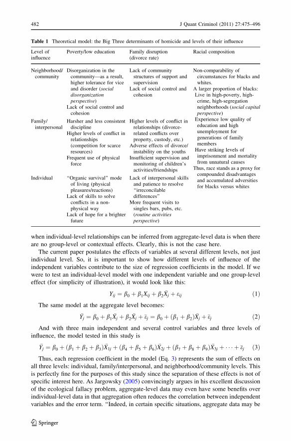
The summary of the proposed theoretical framework is presented in Table 1.

The empirical part of this paper follows the lead of Land and his colleagues and unpacks

the effects of the Big Three structural forces—poverty/education, divorce/family disrup-

tion, and racial composition—on homicide. Using aggregate-level analyses, the effects of

the Big Three on homicide rates in US counties are estimated at two different points in

time: 1950–1960 and 1995–2005. The two time periods are chosen to be as far removed

from one another as the data would allow. (Not only reliable data on homicides in US

counties are required but also comparable measures of divorce rates, education, poverty,

racial composition of counties, and other relevant variables.)

Though aggregate-level analyses would not allow us to test the exact mechanisms by

which the Big Three factors affect homicide rates, it is possible to determine the magnitude

and estimate the stability of these influences using aggregate-level data.

It is important to mention that the issue of ‘‘ecological fallacy’’ often arises when

aggregate-level data are used to test individual-level processes. This question should be

addressed here. Firebaugh (1978) presents an excellent discussion of the now widely

accepted point that regression coefficients estimated using aggregate-level data generally

cannot provide unbiased estimates of individual-level effects. In fact, the only situation

1 On the issue of significant differences between races in family situation dynamics, Cavan’s (1959)comparison of white and black institutionalized delinquents provides a good illustration:

Many boys had lived in several types of families during their lives (e.g., with both parents at onetime, with a parent and step-parent at another, with relatives at some other time, and so on). Negroboys had a median of 2.1 different family situations, whites a median of 1.0. Half of the whites butonly a fifth of the Negroes had continuously lived in the same family situation; at the other extreme,17 per cent of the Negro boys but only 5 per cent of the white boys had lived in four or more differenttypes of families. Moreover, almost four times as many Negro boys as white (37 and 10 per cent) hadlived at some point with relatives and 18 and 4 per cent respectively had at some time resided in thehomes of people to whom they were not related. (Cavan 1959, pp. 235–236).

2 Pettit and Western (2004) estimated that among black men born between 1965 and 1969, 20% had servedtime in prison by their early thirties (compared to only 3% of white men). This number—already unbe-lievably high—further climbs to 30% for black men without college education, and to 60% for high schooldropouts among blacks.

J Quant Criminol (2011) 27:475–496 481

123

when individual-level relationships can be inferred from aggregate-level data is when there

are no group-level or contextual effects. Clearly, this is not the case here.

The current paper postulates the effects of variables at several different levels, not just

individual level. So, it is important to show how different levels of influence of the

independent variables contribute to the size of regression coefficients in the model. If we

were to test an individual-level model with one independent variable and one group-level

effect (for simplicity of illustration), it would look like this:

Yij ¼ b0 þ b1Xij þ b2�Xj þ eij ð1Þ

The same model at the aggregate level becomes:

�Yj ¼ b0 þ b1�Xj þ b2

�Xj þ �ej ¼ b0 þ ðb1 þ b2Þ �Xj þ �ej ð2Þ

And with three main independent and several control variables and three levels of

influence, the model tested in this study is

�Yj ¼ b0 þ ðb1 þ b2 þ b3Þ �X1j þ ðb4 þ b5 þ b6Þ �X2j þ ðb7 þ b8 þ b9Þ �X3j þ � � � þ �ej ð3Þ

Thus, each regression coefficient in the model (Eq. 3) represents the sum of effects on

all three levels: individual, family/interpersonal, and neighborhood/community levels. This

is perfectly fine for the purposes of this study since the separation of these effects is not of

specific interest here. As Jargowsky (2005) convincingly argues in his excellent discussion

of the ecological fallacy problem, aggregate-level data may even have some benefits over

individual-level data in that aggregation often reduces the correlation between independent

variables and the error term. ‘‘Indeed, in certain specific situations, aggregate data may be

Table 1 Theoretical model: the Big Three determinants of homicide and levels of their influence

Level ofinfluence

Poverty/low education Family disruption(divorce rate)

Racial composition

Neighborhood/community

Disorganization in thecommunity—as a result,higher tolerance for viceand disorder (socialdisorganizationperspective)

Lack of social control andcohesion

Lack of communitystructures of support andsupervision

Lack of social control andcohesion

Non-comparability ofcircumstances for blacks andwhites.

A larger proportion of blacks:Live in high-poverty, high-crime, high-segregationneighborhoods (social capitalperspective)

Experience low quality ofeducation and highunemployment forgenerations of familymembers

Have striking levels ofimprisonment and mortalityfrom unnatural causes

Thus, race stands as a proxy forcompounded disadvantagesand accumulated adversitiesfor blacks versus whites

Family/interpersonal

Harsher and less consistentdiscipline

Higher levels of conflict inrelationships(competition for scarceresources)

Frequent use of physicalforce

Higher levels of conflict inrelationships (divorce-related conflicts overproperty, custody, etc.)

Adverse effects of divorce/instability on the youths

Insufficient supervision andmonitoring of children’sactivities/friendships

Individual ‘‘Organic survival’’ modeof living (physicalpleasures/reactions)

Lack of skills to solveconflicts in a non-physical way

Lack of hope for a brighterfuture

Lack of interpersonal skillsand patience to resolve‘‘irreconcilabledifferences’’

More frequent visits tosingles bars, pubs, etc.(routine activitiesperspective)

482 J Quant Criminol (2011) 27:475–496

123

better than individual data for testing hypotheses, even if those hypotheses are about

individual behavior’’ (Jargowsky 2005, p. 721).

A question may arise about whether it is even possible to separate the effects at each

level, considering how interconnected all three levels are (see the discussion about the race

variable above). This question is better left for future empirical testing.

Detailed specifications of the variables and the description of data and methods are

provided in the section that follows.

Data and Methods

In the current study, counties are used as the unit of analysis. There are several advantages

to using counties as opposed to cities, SMSAs or states. First, counties are smaller and

more homogenous units of analysis than states or SMSAs. Second, counties allow for

wider variations in the independent variables and for the inclusion of rural populations that

are typically ignored when cities and SMSAs are chosen for analyses.

On the other hand, there is a price to pay for the use of counties rather than bigger units.

First, counties share boundaries with adjacent counties and thus the issue of spatial

interdependence may arise. Whether or not spatial autocorrelation biases the results of

county-level analyses is a topic of continuing debate (see Wasserma and Stack 1995;

Mencken and Barnett 1999; Baller et al. 2001). In regression analysis, geographical

dependency among counties may cause spatial autocorrelation, which violates the ordinary

least squares assumption that the error terms are uncorrelated, potentially leading to

underestimated standard errors. In addition, spatial regression effects unaccounted for in

the regression models can bias parameter estimates (see Land and Deane 1992 for a

discussion of this issue). To test the assumption of spatial dependence, a two-stage least

squares (2SLS) technique proposed by Land and Deane (1992) was employed. All models

originally estimated using OLS regression were re-estimated using the Land-Deane 2SLS

approach. However, no significant spatial effects were detected and thus only the results of

OLS regression analyses are reported in the current paper to simplify the presentation.3

The second issue related to the use of counties as a unit of analysis is that population

counts in some counties are rather small. Thus, these counties cannot be used in the

analyses since they would produce inconsistent and often times extreme values on the

homicide rate variable since homicide is a rare event. To guard against this problem,

several procedures and checks were implemented.

First, a period of 11 years was used to record homicide events and calculate homicide

rates in counties4: 1950 through 1960 (historical dataset) and 1995 through 2005 (con-

temporary dataset). Second, various population cut-off thresholds were used to test the

robustness of results: counties over 10,000 population, counties over 5,000, and counties

over 1,000 (as measured by the corresponding mid-point decennial census or arithmetic

mean of census values at end-points). Also, a thorough check for outliers has been done to

ensure the stability of estimates. Since the results of analyses remain essentially identical

3 The spatial-effects coefficient failed to reach statistical significance under the traditional p \ .05 level ofsignificance. The results of analyses are available upon request from the author.4 MA and NYC exceptions for the historical dataset: for counties in the state of Massachusetts, homicidecounts were available for 6 years out of 11 (1950–1952, 1955, 1959–1960); and for New York City counties(boroughs), separate homicide counts were available for 8 years out of 11 (1950, 1954–1960). No impu-tation procedures were used. Homicide rates were calculated using the available number of years in thedenominator.

J Quant Criminol (2011) 27:475–496 483

123

for all three thresholds, the lowest threshold (counties over 1,000 residents) is used for the

data reported here since it allows for the inclusion of more counties, and a larger variety of

them.

Initially, the 1950–1960 dataset included 3,081 counties, and the 1995–2005 dataset

included 3,075 counties. However, to make the two datasets as comparable as possible,

only counties that existed in both periods of time (and had all necessary data available)

were used for analyses (for more details, see Appendices A and B). Thus, for example,

Alaska and Hawaii were excluded from analyses since data for these two states are not

available in the 1950–1960 dataset.

The dependent variable was constructed using data on homicide mortality by county

from the Vital Statistics provided by the National Center for Health Statistics (Centers

for Disease Control and Prevention 1950–1960 and 1995–2005). Since Supplementary

Homicide Reports by the FBI only go back as far as the 1970s, the only source of

comparable homicide data for the 1950s and the 2000s is the Vital Statistics. The years

1950 through 1960 were chosen because this is the earliest historical point for which good

data on both homicide and structural factors are available.

Data on structural factors were taken from the Vital Statistics and from the corre-

sponding decennial censuses (most variables archived by Haines and the ICPSR 2005).

Structural variables from the 1950 and 1960 censuses were averaged for the first dataset,

and data for year 2000 were used for the second dataset. All data handling was performed

using SPSS 16 while data analyses were performed in Stata 9.2; Stat/Transfer software

utility was used to handle data transfers between the two statistical packages.

The independent variables included the three main variables of interest: poverty/low

education (percent families in poverty and percent people aged 25? with low education—

hereinafter, percent uneducated—were summed up to form an index of poverty5), divorce

rate,6 and percent black.7 Also, a set of control variables was included in the model along

with the independent variables. The following measures that proved consequential for

homicide rates in previous studies were included as control variables:

1) percent urban (alternatively: population density was used, producing almost identical

results);

2) percent unemployed in civilian labor force;

3) residential mobility;

4) percent young (percent people aged 15–29);

5 To form the index of poverty, the variables for percent of families in poverty and percent ‘‘uneducated’’were summed up in their original metric (non-standardized). This has been done for several reasons: (1) topreserve the absolute zero of the original scales, (2) to let the original distributions determine which of thetwo variables contributes more to the index of poverty, depending on the time period; (3) for easierinterpretability of results in further analyses (slopes for logged variables in OLS regressions are interpretedas a percent change impact on the dependent variable).6 Ideally, ‘‘percent children in single-parent families’’ needs to be included along with the divorce rate toform the index of family structure. However, this measure is available for the 1995–2005 dataset but not forthe 1950–1960 dataset. Thus, only divorce rate remained as a measure of family disruption in the model.7 ‘‘Percent non-white’’ from 1950 to 1960 census data is the best approximation of ‘‘percent black’’ in the2000 census data. Unfortunately, the exact same measure—percent black—was not available in the earliercensus data but considering that the US had very few residents representing other racial groups than blacksand whites, ‘‘percent non-white’’ can be taken as a valid measure of percent black in 1950 and 1960. Inaddition, one of the anonymous reviewers suggested restricting analyses to counties with 1,000 or moreblack residents to test the sensitivity of estimates to the size of black population in the counties. The datawere re-analyzed with these restrictions in place (resulting in a loss of slightly over 10% of the sample) andvery similar estimates were obtained for all variables of interest.

484 J Quant Criminol (2011) 27:475–496

123

5) percent old (percent people aged 65 and above); and

6) region.8

Detailed descriptions of variables, data sources, and variable correlation matrices are

provided in ‘‘Appendix A’’ for the 1950–1960 dataset and in ‘‘Appendix B’’ for the

1995–2005 dataset.

It is important to mention that all variables were analyzed to ensure maximum com-

parability of all measures across the two time periods. As a result, some of the variables

have different thresholds to reflect differences in economic realities of the time (adjustment

for inflation for poverty measures9 and adjustment for educational shifts in the low edu-

cation measure10). Additional analyses have been performed to test the sensitivity of

results to the chosen measures and comparable results were obtained under various

operationalizations of the poverty/education index.11

To make sure that none of the control variables loaded excessively onto any of the Big

Three variables of interest, a principal components factor analysis was estimated on all

independent and control variables. This procedure was applied to both datasets separately.

The only consistent pattern involving a substantial correlation of variables in both datasets, as

expected, was found for the percent families in poverty and percent uneducated. The cor-

relation was .72 for the historical dataset and .75 for the contemporary dataset (both statis-

tically significant at a .001 level). These two variables were summed up to form the index of

poverty. Since these results are pretty straightforward and since there is nothing illuminating

in the specifics of the above-described factor analyses, they are not included into the current

paper to save space and avoid distracting the reader with unnecessary details.

After frequency distributions for all variables in both datasets were examined, it became

clear they were overwhelmingly positively skewed, which in turn affected the linearity

(or rather non-linearity) of relationships between the dependent and most of the inde-

pendent/control variables. Thus, logarithmic transformation of the skewed variables was

warranted. All continuous variables—dependent, independent, and control—in both

datasets were subject to natural log transformation.12 This had an additional benefit for

the interpretation of regression coefficients—elasticity.

8 To accommodate some recent sentiments in research literature that the West is now becoming what theSouth used to be in terms of the rate of violence (see Parker and Pruitt 2000), and also to measure regionalpeculiarities in a more comprehensive manner, regions are designated by dummy variables using traditionalcensus divisions: South, West, and Midwest, with Northeast being the reference category.9 The percent of families in poverty is calculated using the threshold of family income ‘‘less than $2000’’ in1950, ‘‘less than $3000’’ in 1959 (for 1960), and ‘‘below poverty level in 1999’’ (for 2000). The officialpoverty level is determined by the family size and does not vary geographically (though it is regularlyupdated for inflation).10 Low education is measured as the percentage of persons 25 years and older with ‘‘less than 5 years ofeducation’’ for 1950, ‘‘less than 4 years of education’’ for 1960, and ‘‘less than high school education’’ for2000. These thresholds reflect the availability of data (for the earlier periods of time) as well as changesoccurring over time in the importance of education for increasing the prospects of well-being for individualsand families.11 In fact, one of the anonymous reviewers suggested using ‘‘less than 8 years of schooling’’ as a measure oflow education for year 2000. So, this measure was obtained from the 2000 Census data (‘‘percentage ofpeople 25 and older with educational attainment of less than 9th grade’’ since ‘‘less than 8th grade’’ is notavailable). After the new measure of low education was incorporated into the poverty index and the modelsre-estimated, very similar results were obtained. Moreover, the regression coefficient for the poverty indexwas 0.41, which is even closer to the regression coefficient of 0.43 obtained for the 1950–1960 dataset.12 All variables had one added to all their values before the log transformation was applied (to eliminatezero or near-zero values since logarithm of zero does not exist). As a result of the log transformation,

J Quant Criminol (2011) 27:475–496 485

123

Besides logarithmic transformation, there are other ways to ameliorate the situation with

excessive zeros in the distribution of homicide rates. One of them is to use negative

binomial regression (NBR) analyses in addition to ordinary least squares (OLS) regression.

Thus, NBR analyses were performed and they yielded very similar results to the results of

OLS regressions. However, since NBR analyses do not produce some useful information,

for example, the coefficient of determination, and NBR coefficients are not as easily

interpretable, the OLS regressions are still preferred.13 Thus, in the section that follows,

OLS regression results are reported.14

Results and Discussion

The effects of the Big Three structural forces—poverty index (poverty ? low education),

racial composition (percent black), and the family structure variable (percent divorced/

separated)—on logged homicide rates, along with the effects of control variables included

into all analyses, are presented in Table 2 (the Big Three are highlighted in bold font).

Now we can compare the regression coefficients (slopes) to see if the amount of influence

that each of the Big Three contributes towards homicide rates were similar during each

time period. Amazingly, the regression slopes seem to be very similar for the two time

periods despite the changes that occurred in almost a half-century. Even if all the social,

economic, and political changes that occurred since the 1950s are left outside of the current

discussion, just by looking at the descriptive statistics and correlations for our main

variables of interest, we can see some drastic changes: divorce rate has almost quadru-

pled—from about 3 to 11%—between 1960 and 2000 (see Table 3), percent of families in

poverty is about one quarter of what it was 45 years ago—around 11% compared to 40%

(see Table 3); the correlation between poverty and divorce has grown from very weak .08

to solid medium .33 (Table 4); and the correlation between percent black and divorce has

dropped almost one third—from .58 to .40 (see Table 4).

However, despite all these changes, the regression coefficients—that is, the amount of

influence of each regressor on homicide rates—remain stable. As shown in Table 2, each

one-percent rise in the percentage of families in poverty or people with low education

Footnote 12 continuedfrequency distributions for logged variables were much closer to the shape of the normal distributioncompared to the original variables and their relationships with the dependent variable straightened out aswell. The only variable whose frequency distribution was not significantly improved by the logarithmictransformation was the dependent variable—homicide rate. Because of the heavy clustering of valuesaround zero, there is no readily available way to transform this variable to bring it closer to the shape of thenormal distribution. However, log transformation still seems beneficial in this case because it draws the longright tale of the original homicide rate distribution closer to the more frequent values and thus, gets rid ofpotential outliers.13 As an additional check, the residuals in all OLS regression analyses were examined for possible het-eroscedasticity that may have resulted from excess zeros in the dependent variable. Upon examination, thepresence of heteroscedasticity was ruled out.14 In addition, all regression analyses were re-estimated to test the robustness of the results against possibleeffects of the partialling fallacy as some control variables (for example, unemployment) were more highlycorrelated with some of the main predictors than with the outcome variable. The exclusion of such controlvariables from the model did not change the pattern of results and thus confirmed the stability of estimatesunder various conditions and specifications of the model. As noted by anonymous reviewers, the changingeffects of unemployment on homicide rates, as well as the shifts in regional patterns of homicide, are worthexploring further but this topic is important enough to become a subject of a separate study. Thus it is notdiscussed in this paper to avoid diverting the narrative from the main subject.

486 J Quant Criminol (2011) 27:475–496

123

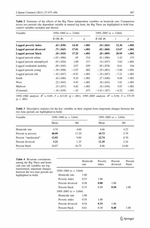
Table 3 Descriptive statistics for the key variables in their original form (important changes between thetwo time periods are highlighted in bold)

Variable 1950–1960 (n = 3,044) 1995–2005 (n = 3,044)

Mean SD Mean SD

Homicide rate 4.74 4.60 4.66 4.23

Percent in poverty 40.09 17.10 10.73 5.79

Percent ‘‘uneducated’’ 12.83 9.89 22.74 8.70

Percent divorced 3.21 1.35 11.29 2.24

Percent black 10.87 16.75 8.86 14.60

Table 4 Bivariate correlationsamong the Big Three and homi-cide rate (all variables are log-transformed, important changesbetween the two time periods arehighlighted in bold)

Homiciderate

Povertyindex

Percentdivorced

Percentblack

1950–1960 (n = 3,044)

Homicide rate 1.00

Poverty index 0.53 1.00

Percent divorced 0.58 0.08 1.00

Percent black 0.75 0.50 0.58 1.00

1995–2005 (n = 3,044)

Homicide rate 1.00

Poverty index 0.55 1.00

Percent divorced 0.54 0.33 1.00

Percent black 0.61 0.38 0.40 1.00

Table 2 Estimates of the effects of the Big Three independent variables on homicide rate: Comparisonacross two periods (the dependent variable in natural log form, the Big Three are highlighted in bold font,control variables included and shown)

Variable 1950–1960 (n = 3,044) 1995–2005 (n = 3,044)

B (SE B) t p B (SE B) t p

Logged poverty index .43 (.030) 14.45 <.001 .54 (.043) 12.36 <.001

Logged percent divorced .73 (.043) 17.01 <.001 .82 (.060) 13.67 <.001

Logged percent black .18 (.010) 17.25 <.001 .20 (.009) 20.95 <.001

Logged percent urban \.01 (.006) .65 .514 .01 (.006) 1.43 .153

Logged percent unemployed .03 (.026) 1.00 .317 .14 (.037) 3.62 \.001

Logged residential mobility .09 (.045) 2.07 .039 .05 (.078) 0.61 .544

Logged percent young -.30 (.098) -3.07 .002 -.29 (.081) -3.60 \.001

Logged percent old -.42 (.047) -8.93 \.001 -.34 (.047) -7.21 \.001

South .42 (.046) 9.24 \.001 .27 (.040) 6.68 \.001

West .22 (.045) 4.93 \.001 .30 (.043) 7.01 \.001

Midwest .15 (.037) 4.02 \.001 .18 (.036) 5.07 \.001

(Constant) -.16 (.039) -.42 .673 -1.63 (.387) -4.22 \.001

1950–1960 analysis: R2 = 0.69; F = 613.03 (p \ .001). 1995–2005 analysis: R2 = 0.58; F = 375.59(p \ .001)

J Quant Criminol (2011) 27:475–496 487

123

produced about a half-percent increase (0.43–0.54%) in homicide rates. Each one-percent

change in the percentage of divorced/separated people produces about three quarters of a

percent (0.73–0.82%) increase in homicide rates. Each one-percent rise in the percentage

of blacks produces about a one-fifth percent increase (0.18–0.20%) in homicide rates. The

percentage of variance in homicide rates explained by all factors combined is also quite

high for both time periods (R squared = 0.69 for the 1950–1960 dataset, R squared = 0.58

for the 1995–2005 dataset).15

Thus, Table 2 provides some face validity for the argument that the effect sizes of the

three main predictors of homicide remain amazingly stable over time. However, to draw

firm conclusions about the similarity of the regression slopes, we have to corroborate the

impression of stability of regression coefficients with some solid statistical evidence.

Unfortunately, there is no straightforward comparison test for regression coefficients

from two non-independent samples, unlike the one applicable to independent samples (see

Brame et al. 1998). Since here we have the same sample measured twice, though with a

40–50-year interval, we cannot expect to meet the independence requirement.

One remedy would be to pool the two datasets together and estimate the OLS regression

on the combined dataset (N = 6,088), including interactions of the main three variables

with period and taking into account the ‘‘paired’’ clustering of observations when calcu-

lating standard errors. This can be done using the Huber-White method (so called

‘‘sandwich’’ estimator) that adjusts the covariance matrix correcting for the lack of inde-

pendence of observations within clusters. Essentially, clusters are used as units of obser-

vation when standard errors are calculated.16 Thus, robust standard errors, and

consequently, corrected t-statistics are obtained. To execute the plan properly, all variables

in the dataset should be mean-centered around the period mean to ensure that changes in

the levels of homicide, divorce, etc. over time would not affect the comparisons.17 After

the period-mean-centering, the OLS regression on the pooled dataset is estimated using the

same three main variables, along with the same control variables (see Table 5).

Now the interaction terms can be examined (highlighted in bold in Table 5). Since there

are plenty of reasons to be concerned with the possibility of committing a Type I error

(finding a difference where there is none) when such a large dataset is used, the level of

15 If all control variables are removed from the model, with only the Big Three determinants left in, themodel still explains about 65% of variance in the dependent variable for the 1950–1960 dataset, and about55% for the 1995–2005 dataset. The inclusion of any other single control variable into the equation does notimprove the explanatory power of the model by much more than about 2%. If all of the control variables areincluded, in addition to the Big Three, they together contribute only an extra 2–4% towards the varianceexplained.16 Though with so few observations within each cluster (in this case, each cluster is comprised of twocounties, or the same county measured twice 45 years apart) and a huge number of clusters (3,044), therobust standard errors would not be very different from the ones produced by usual OLS estimation.17 Another good reason for mean-centering is that it removes the collinearity between the original inde-pendent variables and the dummy variable for the period. If there was a big change in the means of somevariables from one time period to the other, then even in their logged form these variables would be highlycorrelated with the dummy variable for the period unless they are centered around the period mean. Forexample, the divorce rate has almost quadrupled since 1960—from 3 to 11% of adult population (compareTables 7, 10 in Appendices A and B, respectively). Either in its original form or in its log-transformedmetric, the divorce rate variable has a correlation of more than 0.90 with the period dummy variable, soincluding the period dummy and the logged divorce rate (non-centered) into the same equation would lead tohugely inflated statistics of collinearity (VIF over 10 for the divorce variable). On the other hand, if thelogged divorce rate is centered around the period mean, this solves the problem.

488 J Quant Criminol (2011) 27:475–496

123

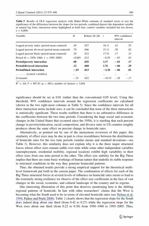
significance should be set at 0.01 (rather than the conventional 0.05 level). Using this

threshold, 99% confidence intervals around the regression coefficients are calculated

(shown in the two right-most columns in Table 5). Since the confidence intervals for all

three interaction terms include zero, it can be concluded that none of the three interactions

is statistically significant. These results reaffirm that there is no substantive difference in

the coefficients between the two time periods. Considering the huge social and economic

changes in the United States that occurred since the 1950s, it is startling that each percent

change in poverty/education, racial composition, and divorce rates in US counties roughly

produces about the same effect on percent change in homicide rates.

Alternatively, as pointed out by one of the anonymous reviewers of this paper, this

similarity of effect sizes may be due in part to close resemblance between the distributions

of homicide rates for the two time periods (similar means and standard deviations—see

Table 3). However, this similarity does not explain why it is the three major structural

forces whose effect sizes remain stable over time while some other independent variables

(unemployment, residential mobility, regional location) exhibit high variability in their

effect sizes from one time period to the other. The effect size stability for the Big Three

implies that there are some basic workings of human nature that underlie its stable response

to structural conditions in the way they generate homicidal patterns.

Thus, the obtained results provide a strong empirical support for the theoretical multi-

level framework put forth in the current paper. The combination of effects for each of the

Big Three structural forces at several levels of influence on homicide rates seems to lead to

the extremely strong resilience we observe of the effect size coefficients in the face of vast

changes in the social, economic, and cultural landscape of the country and its regions.

One interesting illustration of this point that deserves mentioning here is the shifting

regional patterns of homicide. In line with other researchers’ claims that the West is

becoming what the South used to be in terms of elevated homicide rates (see Nelsen et al.

1994; Parker and Pruitt 2000), Table 2 clearly shows that the regression slope for the South

does indeed drop about one third (from 0.42 to 0.27) while the regression slope for the

West rises about one third (from 0.22 to 0.30) from 1950–1960 to 1995–2005. Thus,

Table 5 Results of OLS regression analysis with Huber-White estimate of standard errors to test thesignificance of the differences between the slopes for two periods: combined dataset (the dependent variablein natural log form, interaction terms highlighted in bold font, control variables included but not shown,n = 6,088)

Variable B Robust SE (B) t 99% confidenceinterval

Logged poverty index (period-mean-centered) .49 .027 18.11 .42 .55

Logged percent divorced (period-mean-centered) .70 .046 15.11 .58 .82

Logged percent black (period-mean-centered) .20 .012 17.51 .17 .23

Period (0 = 1950–1960; 1 = 1995–2005) \0.001 .012 -0.29 -.03 .03

Period/poverty interaction .08 .035 2.17 2.01 .17

Period/divorced interaction .12 .068 1.76 2.06 .29

Period/black interaction 2.03 .013 22.10 2.06 .01

… … … [control variables] … … … … …(Constant) -.23 .022 -10.33 -.28 -.17

R2 = .64; F = 887.81 (p \ .001); number of clusters = 3,044

J Quant Criminol (2011) 27:475–496 489

123

homicide rates are now almost the same for these two regions (actually, even slightly

higher in the West than in the South). Judging by the effect of excluding the region variable

on the other coefficients in the model, it seems that these changes in the allocation of

homicide rates between the South and West are primarily due to changes in the distribution

of poverty/low education among the regions. Poverty was heavily concentrated in the

South back in the 1950s, and now poverty is more evenly spread between the South and the

West. This fact is an additional illustration of the main point of this line of work—the

power and stability of the effects of the major structural forces in determining violence/

homicide rates despite the major changes in patterns of geographical distribution of

homicide that occurred over the half-century period.

Conclusions

The current paper laid out a multi-level theoretical framework organizing the current state

of knowledge in the field of structural determinants of homicide and violence in general.

The Big Three major structural forces are identified: poverty/low education, family dis-

ruption, and racial composition. Their effects are described at several interrelated levels of

influence: neighborhood, family, and individual level. These combined multi-level effects

are then tested for each of the three factors using US counties as the unit of analysis at two

periods of time: 1950–1960 and 1995–2005.

The effects of all three major structural forces proved to be extremely powerful in

determining homicide rates during both time periods examined. Moreover, all three factors

exhibited high stability over time in the amount of their influence on homicide rates:

regression slopes for each of the Big Three remain virtually identical in the 1950s and in

the 2000s despite fairly drastic changes in the economic and social situation that occurred

in the United States over this period of time. This finding implies that the basic workings of

the human nature and its response to certain structural conditions remain stable over time.

However, the current study is not equipped to test the exact mechanisms by which

poverty, racial composition, and family disruption generate such stable and prominent

increases in the incidence of homicide. Again, the regression coefficients represent the sum

of effects at all levels of influence—neighborhood, family, and individual level—for each

variable. What exactly it is about these structural conditions that produces stable effects on

homicide remains to be an open question for future research and theory.

Acknowledgments This paper would not have been possible without wise and generous advice from ColinLoftin, Alan Lizotte, and David McDowall. My heartfelt thanks also go to the anonymous reviewers andeditors of the Journal whose criminological expertise and meticulous attention to detail helped improve thepaper tremendously through several rounds of reviews and revisions.

Appendix A: Detailed Information on Variables Included into Initial Analyses:Historical Dataset (1950–1960)

See Tables (6, 7, 8).

490 J Quant Criminol (2011) 27:475–496

123

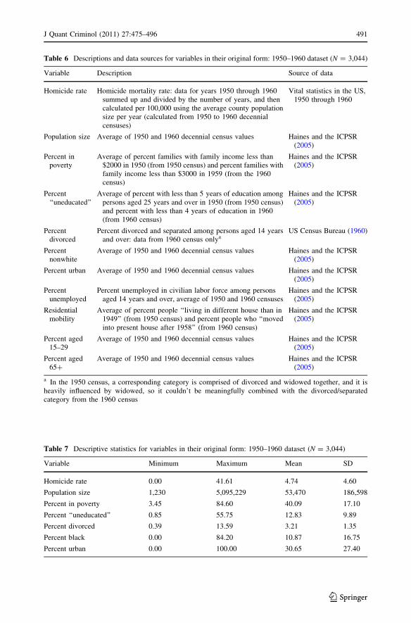
Table 6 Descriptions and data sources for variables in their original form: 1950–1960 dataset (N = 3,044)

Variable Description Source of data

Homicide rate Homicide mortality rate: data for years 1950 through 1960summed up and divided by the number of years, and thencalculated per 100,000 using the average county populationsize per year (calculated from 1950 to 1960 decennialcensuses)

Vital statistics in the US,1950 through 1960

Population size Average of 1950 and 1960 decennial census values Haines and the ICPSR(2005)

Percent inpoverty

Average of percent families with family income less than$2000 in 1950 (from 1950 census) and percent families withfamily income less than $3000 in 1959 (from the 1960census)

Haines and the ICPSR(2005)

Percent‘‘uneducated’’

Average of percent with less than 5 years of education amongpersons aged 25 years and over in 1950 (from 1950 census)and percent with less than 4 years of education in 1960(from 1960 census)

Haines and the ICPSR(2005)

Percentdivorced

Percent divorced and separated among persons aged 14 yearsand over: data from 1960 census onlya

US Census Bureau (1960)

Percentnonwhite

Average of 1950 and 1960 decennial census values Haines and the ICPSR(2005)

Percent urban Average of 1950 and 1960 decennial census values Haines and the ICPSR(2005)

Percentunemployed

Percent unemployed in civilian labor force among personsaged 14 years and over, average of 1950 and 1960 censuses

Haines and the ICPSR(2005)

Residentialmobility

Average of percent people ‘‘living in different house than in1949’’ (from 1950 census) and percent people who ‘‘movedinto present house after 1958’’ (from 1960 census)

Haines and the ICPSR(2005)

Percent aged15–29

Average of 1950 and 1960 decennial census values Haines and the ICPSR(2005)

Percent aged65?

Average of 1950 and 1960 decennial census values Haines and the ICPSR(2005)

a In the 1950 census, a corresponding category is comprised of divorced and widowed together, and it isheavily influenced by widowed, so it couldn’t be meaningfully combined with the divorced/separatedcategory from the 1960 census

Table 7 Descriptive statistics for variables in their original form: 1950–1960 dataset (N = 3,044)

Variable Minimum Maximum Mean SD

Homicide rate 0.00 41.61 4.74 4.60

Population size 1,230 5,095,229 53,470 186,598

Percent in poverty 3.45 84.60 40.09 17.10

Percent ‘‘uneducated’’ 0.85 55.75 12.83 9.89

Percent divorced 0.39 13.59 3.21 1.35

Percent black 0.00 84.20 10.87 16.75

Percent urban 0.00 100.00 30.65 27.40

J Quant Criminol (2011) 27:475–496 491

123

Appendix B: Detailed Information on Variables Included into Initial Analyses:Contemporary Dataset (1995–2005)

See Tables (9, 10, 11).

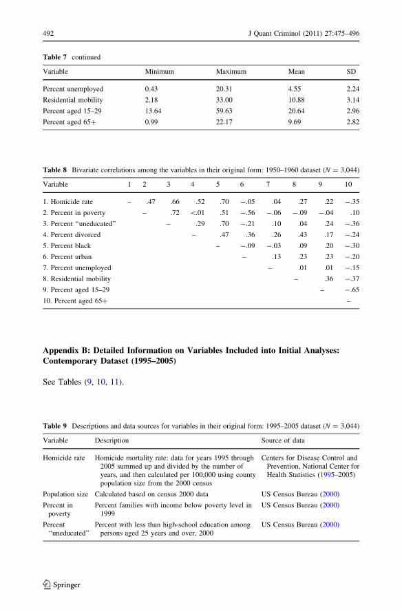
Table 8 Bivariate correlations among the variables in their original form: 1950–1960 dataset (N = 3,044)

Variable 1 2 3 4 5 6 7 8 9 10

1. Homicide rate – .47 .66 .52 .70 -.05 .04 .27 .22 -.35

2. Percent in poverty – .72 \.01 .51 -.56 -.06 -.09 -.04 .10

3. Percent ‘‘uneducated’’ – .29 .70 -.21 .10 .04 .24 -.36

4. Percent divorced – .47 .36 .26 .43 .17 -.24

5. Percent black – -.09 -.03 .09 .20 -.30

6. Percent urban – .13 .23 .23 -.20

7. Percent unemployed – .01 .01 -.15

8. Residential mobility – .36 -.37

9. Percent aged 15–29 – -.65

10. Percent aged 65? –

Table 9 Descriptions and data sources for variables in their original form: 1995–2005 dataset (N = 3,044)

Variable Description Source of data

Homicide rate Homicide mortality rate: data for years 1995 through2005 summed up and divided by the number ofyears, and then calculated per 100,000 using countypopulation size from the 2000 census

Centers for Disease Control andPrevention, National Center forHealth Statistics (1995–2005)

Population size Calculated based on census 2000 data US Census Bureau (2000)

Percent inpoverty

Percent families with income below poverty level in1999

US Census Bureau (2000)

Percent‘‘uneducated’’

Percent with less than high-school education amongpersons aged 25 years and over, 2000

US Census Bureau (2000)

Table 7 continued

Variable Minimum Maximum Mean SD

Percent unemployed 0.43 20.31 4.55 2.24

Residential mobility 2.18 33.00 10.88 3.14

Percent aged 15–29 13.64 59.63 20.64 2.96

Percent aged 65? 0.99 22.17 9.69 2.82

492 J Quant Criminol (2011) 27:475–496

123

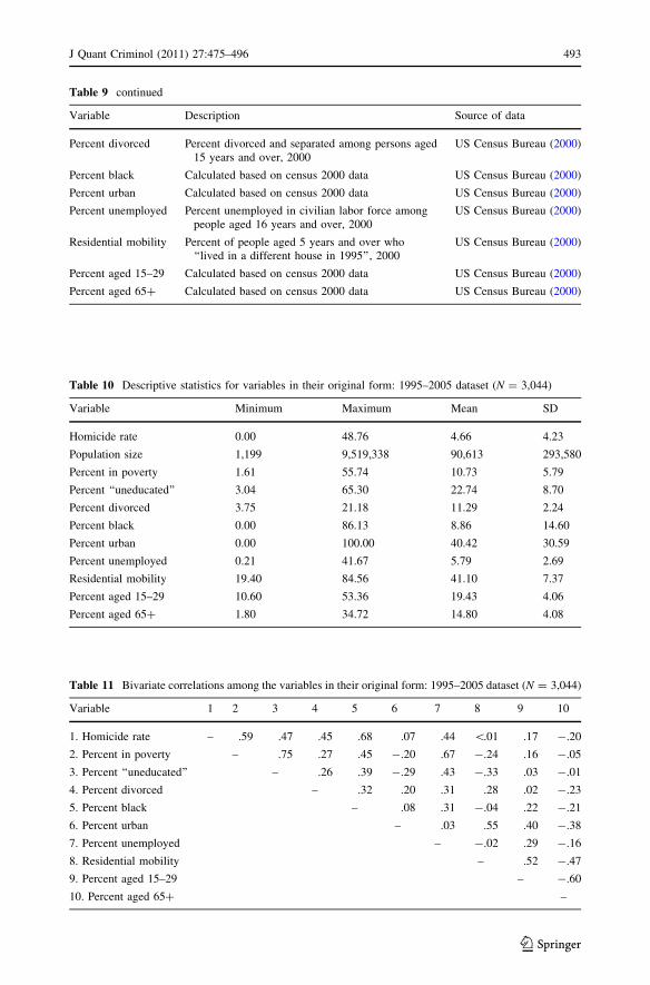
Table 10 Descriptive statistics for variables in their original form: 1995–2005 dataset (N = 3,044)

Variable Minimum Maximum Mean SD

Homicide rate 0.00 48.76 4.66 4.23

Population size 1,199 9,519,338 90,613 293,580

Percent in poverty 1.61 55.74 10.73 5.79

Percent ‘‘uneducated’’ 3.04 65.30 22.74 8.70

Percent divorced 3.75 21.18 11.29 2.24

Percent black 0.00 86.13 8.86 14.60

Percent urban 0.00 100.00 40.42 30.59

Percent unemployed 0.21 41.67 5.79 2.69

Residential mobility 19.40 84.56 41.10 7.37

Percent aged 15–29 10.60 53.36 19.43 4.06

Percent aged 65? 1.80 34.72 14.80 4.08

Table 11 Bivariate correlations among the variables in their original form: 1995–2005 dataset (N = 3,044)

Variable 1 2 3 4 5 6 7 8 9 10

1. Homicide rate – .59 .47 .45 .68 .07 .44 \.01 .17 -.20

2. Percent in poverty – .75 .27 .45 -.20 .67 -.24 .16 -.05

3. Percent ‘‘uneducated’’ – .26 .39 -.29 .43 -.33 .03 -.01

4. Percent divorced – .32 .20 .31 .28 .02 -.23

5. Percent black – .08 .31 -.04 .22 -.21

6. Percent urban – .03 .55 .40 -.38

7. Percent unemployed – -.02 .29 -.16

8. Residential mobility – .52 -.47

9. Percent aged 15–29 – -.60

10. Percent aged 65? –

Table 9 continued

Variable Description Source of data

Percent divorced Percent divorced and separated among persons aged15 years and over, 2000

US Census Bureau (2000)

Percent black Calculated based on census 2000 data US Census Bureau (2000)

Percent urban Calculated based on census 2000 data US Census Bureau (2000)

Percent unemployed Percent unemployed in civilian labor force amongpeople aged 16 years and over, 2000

US Census Bureau (2000)

Residential mobility Percent of people aged 5 years and over who‘‘lived in a different house in 1995’’, 2000

US Census Bureau (2000)

Percent aged 15–29 Calculated based on census 2000 data US Census Bureau (2000)

Percent aged 65? Calculated based on census 2000 data US Census Bureau (2000)

J Quant Criminol (2011) 27:475–496 493

123

References

Anderson AL (2002) Individual and contextual influences on delinquency: the role of the single-parentfamily. J Crim Justice 30:575–587

Apel R, Kaukinen C (2008) On the relationship between family structure and antisocial behavior: parentalcohabitation and blended households. Criminology 46:35–70

Baller RD, Anselin L, Messner SF, Deane G, Hawkins DF (2001) Structural covariates of U.S. countyhomicide rates: incorporating spatial effects. Criminology 39:561–590

Bank L, Forgatch MS, Patterson GR, Fetrow RA (1993) Parenting practices of single mothers: mediators ofnegative contextual factors. J Marriage Fam 55:371–384

Benson ML, Wooldredge J, Thistlethwaite AB, Fox GL (2004) The correlation between race and domesticviolence is confounded with community context. Soc Prob 51:326–342

Blau JR, Blau PM (1982) Cost of inequality: metropolitan structure and violent crime. Am Sociol Rev47:114–129

Brame R, Paternoster R, Mazerolle P, Piquero A (1998) Testing for the equality of maximum-likelihoodregression coefficients between two independent equations. J Quant Criminol 14:245–262

Brezina T, Tekin E, Topalli V (2009) ‘‘Might bot be a tomorrow’’: a multimethods approach to anticipatedearly death and youth crime. Criminology 47:1091–1129

Brownridge DA, Chan KL, Hiebert-Murphy D, Ristock J, Tiwari A, Leung W-C, Santos SC (2008) Theelevated risk for non-lethal post-separation violence in Canada: a comparison of separated, divorced,and married women. J Interpers Viol 23:117–135

Bruce MA (2004) Contextual complexity and violent delinquency among Black and White males. J BlackStud 35:65–98

Bullock HA (1955) Urban homicide in theory and fact. J Crim Law Criminol Police Sci 45:565–575Cavan RS (1959) Negro family disorganization and juvenile delinquency. J Negro Ed 28:230–239Centers for Disease Control and Prevention, National Center for Health Statistics (1950–1960). Vital sta-

tistics in the United States. 1950–1960 [data books]. Available from NCHS web site http://www.cdc.gov/nchs/products/pubs/pubd/vsus/1963/1963.htm

Centers for Disease Control and Prevention, National Center for Health Statistics (1995–2005). Compressedmortality file 1979–1998; Compressed mortality file 1999–2005—CDC WONDER On-line database.Available from CDC web site http://wonder.cdc.gov

Charles CZ (2003) The dynamics of racial residential segregation. Annu Rev Sociol 29:167–207Demuth S, Brown S (2004) Family structure, family processes, and adolescent delinquency: the significance

of parental absence versus parental gender. J Res Crime Del 41:58–81Firebaugh G (1978) A rule for inferring individual-level relationships from aggregate data. Am Sociol Rev

43:557–572Gastil RD (1971) Homicide and a regional culture of violence. Am Sociol Rev 36:412–427Gennetian L (2005) One or two parents? Half or step siblings? The effect of family structure on young

children’s achievement. J Pop Econ 18:415–436Gordon RA (1967) Issues in the ecological study of delinquency. Am Sociol Rev 32:927–944Gordon RA (1968) Issues in multiple regression. Am J Sociol 73:592–616Hackney S (1969) Southern violence. Am Histor Rev 74:906–925Haines MR, the Inter-university Consortium for Political and Social Research (2005) Historical, demo-

graphic, economic, and social data: the United States, 1790–2000 [data file], (ICPSR 02896-v2).Available from ICPSR web site http://www.icpsr.umich.edu/

Hardesty JL (2002) Separation assault in the context of postdivorce parenting. Viol Against Women8:597–625

Heimer K (1997) Socioeconomic status, subcultural definitions, and violent delinquency. Soc Forces75:799–833

Heimer K, Matsueda RL (1987) Race, family structure, and delinquency: a test of differential associationand social control theories. Am Sociol Rev 52:826–840

Jargowsky P (2005) Ecological fallacy. In: Kempf-Leonard K (ed) Encyclopedia of social measurement, vol1. Academic Press, San Diego, pp 715–722

Johnson H, Hotton T (2003) Losing control: homicide risk in estranged and intact intimate relationships.Hom Stud 7:58–84

Katz MB, Stern MJ, Fader JJ (2005) The new African American inequality. J Am Hist 92:75–108Klebanov PK, Brooks-Gunn J, Duncan GJ (1994) Does neighborhood and family poverty affect mothers’

parenting, mental health, and social support? J Marriage Fam 56:441–455Krivo LJ, Peterson RD (2000) The structural context of homicide: accounting for racial differences in

process. Am Sociol Rev 65:547–559

494 J Quant Criminol (2011) 27:475–496

123

Land KC, Deane G (1992) On the large-sample estimation of regression models with spatial- or networkeffects terms: a two-stage least squares approach. Sociol Methodol 22:221–248

Land KC, McCall PL, Cohen LE (1990) Structural covariates of homicide rates: are there any invariancesacross time and social space? Am J Sociol 95:922–963

Lauritsen JL, White NA (2001) Putting violence in its place: the influence of race, ethnicity, gender, andplace on the risk for violence. Crim Pub Pol 1:37–59

Loftin C, Hill RH (1974) Regional subculture and homicide: an examination of the Gastil–Hackney thesis.Am Sociol Rev 39:714–724

McCall PL, Land KC, Parker KF (2010) An empirical assessment of what we know about structuralcovariates of homicide rates: a return to a classic 20 years later. Hom Stud 14:219–243

McNulty TL (2001) Assessing the race-violence relationship at the macrolevel: the assumption of racialinvariance and the problem of restricted distributions. Criminology 39:467–489

Mencken FC, Barnett C (1999) Murder, nonnegligent manslaughter, and spatial autocorrelation in mid-South counties. J Quant Criminol 15:407–422

Miles-Doan R (1998) Violence between spouses and intimates: does neighborhood context matter? SocForces 77:623–645

Moses ER (1947) Differentials in crime rates between Negroes and Whites, based on comparisons of foursocio-economically equated areas. Am Sociol Rev 12:411–420

Nelsen C, Corzine J, Huff-Corzine L (1994) The violent West reexamined: a research note on regionalhomicide rates. Criminology 32:149–161

Ousey GC (1999) Homicide, structural factors, and the racial invariance assumption. Criminology37:405–425

Parker KF (2004) Polarized labor markets, industrial restructuring and urban violence: a dynamic model ofthe economic transformation and urban violence. Criminology 42:619–645

Parker KF, Pruitt MV (2000) How the West was one: explaining the similarities in race-specific homiciderates in the West and South. Soc Forces 78:148–1508

Peterson RD, Krivo LJ (2005) Macrostructural analyses of race, ethnicity, and violent crime: recent lessonsand new directions for research. Annu Rev Sociol 31:331–356

Pettit B, Western B (2004) Mass imprisonment and the life course: race and class inequality in U.S.incarceration. Am Sociol Rev 69:151–169

Pinderhughes EE, Nix R, Foster EM, Jones D (2001) Parenting in context: impact of neighborhood poverty,residential stability, public services, social networks, and danger on parental behaviors. J Marriage Fam63:941–953

Porter GR (1847) The influence of education, shown by facts recorded in the criminal tables for 1845 and1846. J Stat Soc Lond 10:316–344

Quinney R (1965) Suicide, homicide, and economic development. Soc Forces 43:401–406Rebellon C (2002) Reconsidering the broken homes/delinquency relationship and exploring its mediating

mechanism(s). Criminology 40:103–135Ruggles S (1997) The rise of divorce and separation in the United States, 1880–1990. Demography

34:455–466Sampson RJ, Groves WB (1989) Community structure and crime: testing social-disorganization theory.

Am J Sociol 94:774–802Sampson RJ, Wilson WJ (1995) Toward a theory of race, crime, and urban inequality. In: Hagan J, Peterson

R (eds) Crime and inequality. Stanford University Press, Stanford, pp 37–56Sampson RJ, Morenoff JD, Raudenbush S (2005) Social anatomy of racial and ethnic disparities in violence.

Am J Public Health 95:224–232Shaw CR, McKay HD (1942) Juvenile delinquency and urban areas. University of Chicago Press, ChicagoShihadeh ES, Ousey GC (1998) Industrial restructuring and violence: the link between entry-level jobs,

economic deprivation, and black and white homicide. Soc Forces 77:185–206Simons RL, Kuei-Hsiu L, Gordon LC, Brody GH, Murry V, Conger RD (2004) Community differences in

the association between parenting practices and child conduct problems. J Marriage Fam 64:331–345Stewart S (2005) How the birth of a child affects involvement with stepchildren. J Marriage Fam

67:461–473Stolzenberg L, D’Alessio SJ (2007) The effect of divorce on domestic crime. Crime Delinq 53:281–302Teachman JD, Tedrow LM, Crowder KD (2000) The changing demography of America’s families. J Mar-

riage Fam 62:1234–1246Tolman RM, Raphael J (2000) A review of research on welfare and domestic violence. J Soc Issues

56:655–682

J Quant Criminol (2011) 27:475–496 495

123

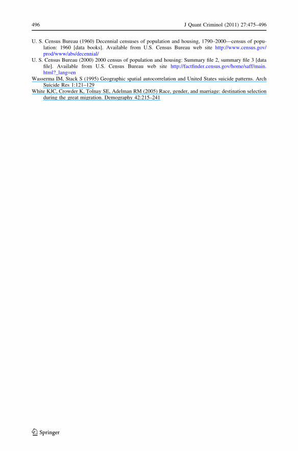
U. S. Census Bureau (1960) Decennial censuses of population and housing, 1790–2000—census of popu-lation: 1960 [data books]. Available from U.S. Census Bureau web site http://www.census.gov/prod/www/abs/decennial/

U. S. Census Bureau (2000) 2000 census of population and housing: Summary file 2, summary file 3 [datafile]. Available from U.S. Census Bureau web site http://factfinder.census.gov/home/saff/main.html?_lang=en

Wasserma IM, Stack S (1995) Geographic spatial autocorrelation and United States suicide patterns. ArchSuicide Res 1:121–129

White KJC, Crowder K, Tolnay SE, Adelman RM (2005) Race, gender, and marriage: destination selectionduring the great migration. Demography 42:215–241

496 J Quant Criminol (2011) 27:475–496

123