arX

iv:0

910.

2160

v2 [

hep-

th]

26

Feb

2010

JHEP02(2010)093 arXiv:0910.2160

String theory as a diffusing system

Gianluca Calcagni

Institute for Gravitation and the Cosmos, Department of Physics,

The Pennsylvania State University,

104 Davey Lab, University Park, Pennsylvania 16802, U.S.A.

Max Planck Institute for Gravitational Physics (Albert Einstein Institute)

Am Muhlenberg 1, D-14476 Golm, Germany

E-mail: calcagni@aei.mpg.de

Giuseppe Nardelli

Dipartimento di Matematica e Fisica, Universita Cattolica,

via Musei 41, 25121 Brescia, Italia

INFN Gruppo Collegato di Trento, Universita di Trento,

38100 Povo (Trento), Italia

E-mail: nardelli@dmf.unicatt.it

Abstract: Recent results on the effective non-local dynamics of the tachyon mode of

open string field theory (OSFT) show that approximate solutions can be constructed

which obey the diffusion equation. We argue that this structure is inherited from the

full theory, where it admits a universal formulation. In fact, all known exact OSFT

solutions are superpositions of diffusing surface states. In particular, the diffusion

equation is a spacetime manifestation of OSFT gauge symmetries.

Keywords: Tachyon Condensation, String Field Theory.

Contents

1. Motivation 1

2. OSFT 4

2.1 OSFT action and tachyon 4

2.2 Wedge states and projectors 5

2.3 Vacuum revolution 8

2.4 Marginal deformations 9

2.5 String field theories and gauge equivalence 10

3. Effective spacetime action and diffusing solutions 11

3.1 Lowest-level non-local spacetime actions 11

3.2 Diffusion equation method 12

3.3 Solutions in integral form 15

4. Diffusion equation in string theory 18

4.1 Why spacetime diffusing solutions are approximate (but good) 21

5. Applications to OSFT and non-local theories 23

5.1 Wild oscillations 23

5.2 Finite superposition of solutions 27

5.3 Integrated solutions of non-local models 28

5.4 Toy models with polynomial potentials 30

6. Conclusions 31

1. Motivation

String field theory is a non-perturbative approach aiming to describe, at least in some

of its parts, the microscopical geometrodynamics of Nature. Two of its most widely

studied incarnations are open string field theory [1, 2, 3] (OSFT; e.g., [4, 5, 6])

and boundary string field theory [7, 8, 9, 10] (BSFT; e.g., [5]), both of which are

playgrounds whereon to develop new physical and mathematical ideas.

In particular, the OSFT effective action of the tachyon field, associated with the

decay of unstable brane configurations, is manifestly non-local, inasmuch as it con-

tains an infinite number of spacetime derivatives through operators of the form e,

– 1 –

where = ∂µ∂µ is the target (that is, spacetime) d’Alembertian. It entails a novel

type of dynamics [11, 12], often too complicated to be solved except with perturba-

tive or numerical methods of limited range of validity. Stimulated by this problem,

analytical non-perturbative methods have been found, and sometimes rediscovered

from not-so-recent literature, which allow to handle pseudo-differential operators and

find solutions of the non-local effective dynamics.

One of these methods [13, 14, 15, 16, 17] introduces an auxiliary coordinate r

along which the system is made to evolve according to the diffusion equation

(+ ∂r)φ = 0 , (1.1)

where φ = φ(r, x) is a scalar field (in the OSFT case, the tachyon). The infinite

number of degrees of freedom corresponding to the initial conditions of the non-local

‘Cauchy problem’ is encoded in the continuous variable r. The main consequences of

eq. (1.1) are that (i) dynamical equations become algebraic equations [14, 15, 17, 18],

(ii) the action of the e operator is a translation along the r direction [13, 14, 15],

(iii) the spacetime dynamics is reduced to a well-defined local Cauchy problem [15],

and (iv) explicit solutions can be constructed. Regarding string theory, approximate

analytic solutions were found for the Lorentzian bosonic and supersymmetric (susy)

OSFT tachyon [13] and for the Euclidean supersymmetric OSFT tachyon [16, 17],

while an exact solution of the p-adic string was recovered [16].

In parallel, some surprising relations were found between OSFT and BSFT so-

lutions [13, 16], which all pointed towards an interpretation of string theory as a

diffusing system. Further support was gained in [17], where the lower-level action

of the OSFT supersymmetric tachyon was reconstructed starting from the diffusion

equation for a scalar field with certain boundary conditions.

All these results are based upon effective equations and, once these are given, the

embedding within string theory can be forgotten. In doing so, however, it becomes

increasingly difficult to explain and properly assess virtues and limitations of the

method within the big picture of the full theory. The level of accuracy of solutions of

OSFT equations of motion [13, 16, 17] and the brane tension ratio in a brane decay

process [17] are so good that one wonders how this can happen considering that

several approximations (level truncation, effective potential, and so on) are entailed.

It is the purpose of this paper to address these issues and discuss the link between

the diffusion equation method and the universal structure of string field theory. Al-

though approaches based on truncated actions have partly become obsolete because

of the recent success in treating the full bosonic theory without integrating out the

massive spectrum (see [6] for a review), the same techniques will make us better un-

derstand why and under what circumstances string field theory can be described, at

the level of target embedding, as a diffusing system. Conversely, the heat-equation

recipe for the construction of explicit tachyon solutions is potentially relevant also

for different brane configurations or other fields of the string spectrum. Moreover, it

– 2 –

was instrumental for the construction of kink solutions interpolating different vacua

of the theory [16, 17]. These solutions are still out of the scope of analytic techniques

of modern OSFT, which have been applied to vacuum or marginally deformed con-

figurations. Thereby, non-vacuum solutions with non-vanishing momentum are an

open subject of study.

We will show that the diffusion equation (1.1) implements a gauge transformation

at the level of the effective spacetime action, which allows one to construct non-trivial

solutions from trivial configurations in a different frame. These configurations are the

analogue of projector states in the conformal field theory (CFT) formulation, which

are non-normalizable states formally satisfying the equation of motion. The target

solutions found so far have a structure mimicking the exact analytic solutions of the

non-truncated theory, corresponding to integral representations of the solution in

terms of surface states. The relation between the CFT and spacetime results suggests

novel applications of the same techniques. We give an example by arguing that also

perturbative (marginal deformations) and non-perturbative (lumps, kinks) geometric

configurations admit an integral representation in the bosonic and supersymmetric

full theory.

The paper is organized as follows. In section 2 we review bosonic OSFT and its

analytic solutions from the point of view of the string worldsheet. The spacetime

effective theory and the solutions found with the diffusion equation method are dis-

cussed in section 3, which also contains new material (section 3.3) about the integral

representation of solutions. The latter, eq. (3.23), plays a crucial role in establishing

the link between the full theory and the spacetime framework. In section 4 we discuss

how spacetime effective solutions are expected to obey the diffusion equation on the

grounds of the conformal properties of the exact solutions. The first goal is to argue

from the properties of full OSFT that spacetime solutions are expected to be diffus-

ing, while so far the diffusion equation method has been just a useful trick without

any such motivation. A second goal is to explain why certain initial conditions of

the diffusion equation did not work as well as others. Concrete novel applications of

these results to SFT and other non-local models are described in section 5. The only

solution constructed both in the target effective system and the full theory is the

bosonic rolling tachyon with wild oscillations (marginal deformations). We draw a

new detailed comparison between the diffusing and the exact solution in section 5.1.

Examples of finite superpositions of solutions are given in section 5.2, while sections

5.3 and 5.4 are devoted to solutions of non-local toy models. Future directions are

outlined in section 6.

– 3 –

2. OSFT

2.1 OSFT action and tachyon

In α′ = 1 units, the OSFT bosonic action is [1]

S = − 1

g2o

∫(

1

2Ψ ∗QΨ +

1

3Ψ ∗Ψ ∗Ψ

)

, (2.1)

where go is the open string coupling, * is a non-commutative product describing the

gluing interaction of open strings, Q is a BRST operator, and the string field Ψ is

a linear superposition of states whose coefficients correspond to the particle fields of

the string spectrum. The open string field equation of motion is

QΨ+Ψ ∗Ψ = 0 . (2.2)

Contrary to the bosonic open string, there are several proposals for open super-

string field theory, the first being Witten’s [19, 20, 21, 22, 23, 24]. The action was

later modified in [25, 26, 27]: on a single non-BPS Dp-brane,

S = − 1

g2o

∫

Y−2

(

1

2Ψ+ ∗QΨ+ +

1

3Ψ+ ∗Ψ+ ∗Ψ+ +

1

2Ψ− ∗QΨ− −Ψ+ ∗Ψ− ∗Ψ−

)

,

(2.3)

where Y−2 is a double-step inverse picture-changing operator and the string field

Ψ± is a linear superposition of states (made of matter (super)fields Xµ, ψµ and

(super)ghosts b, c, β, γ) in the GSO(±) sectors [28], respectively.

Although we will often recall results for the susy version of OSFT, for simplicity

we concentrate on the bosonic case, eq. (2.1). This action is invariant under the

infinitesimal gauge transformations

δΨ = QΨ +Ψ ∗ Λ− Λ ∗Ψ , (2.4)

where Λ is a zero ghost number state. The gauge group of string theory is very

large and, to the best of our knowledge, its full extent is still unknown. It in-

cludes spacetime diffeomorphisms and supersymmetry transformations [29], as well

as reparametrizations of the open string (mappings of the string coordinate patch

on the same region of the complex plane) [30]. In particular, when two states are

related by a reparametrization, they are gauge equivalent. The converse may not

be true, since one can define, e.g., one-parameter families of maps which are not

reparametrizations for certain values of the parameter [31].

In terms of the perturbative vacuum, the string field is a superposition of particle

modes,

Ψ ∼= |Ψ〉 = [φ(x) + . . . ]c1|0〉 , (2.5)

– 4 –

where the first step indicates the state-vertex operator isomorphism, c1 is a Laurent

coefficient of the c ghost, c1|0〉 is the ghost vacuum with ghost number −1/2, and x

is the string center of mass. At the lowest truncation level, all particle fields in Ψ

are neglected except the tachyonic one φ. The zero-momentum tachyon state c1|0〉belongs to the universal subalgebra Huniv of the algebra of open string fields [32, 33].

As already pointed out from the very beginning [1], conservation of the BRST

current implies invariance under reparametrizations of the open string, so one can

make a partial gauge fixing and choose a particular parametrization, for instance one

which locates the string midpoint at a convenient place in the conformal plane (by

‘convenient,’ we mean one simplifying technical calculations).

For practical purposes one has to choose a CFT wherein to represent the string

content. Different mappings of the string on this plane (conformal frames) are pos-

sible [6, 34], from upper half disks [4] to strips and cylinders [6]; these are associated

with gluing procedures [32, 33, 35, 36] which describe the Witten vertex. In par-

ticular, the representation of a string as a semi-infinite cylinder turned out to be

very effective in the construction of an exact vacuum (translation invariant) solu-

tion in bosonic OSFT [30, 37, 38, 39, 40, 41, 42] and in Berkovits’ [43] and cubic

(polynomial) superstring field theories [44, 45, 46, 47]. Different CFT’s in the same

conformal frame can describe different geometries; in this sense the CFT formulation

of OSFT can be regarded as background independent [48, 49].

2.2 Wedge states and projectors

An essential tool for the construction of OSFT solutions are surface states [34], of

which wedge states and the sliver projector are the most studied examples [33, 50,

51, 52, 53, 54, 55, 56, 57, 58, 59, 60, 61, 62, 63, 64, 65, 66, 67, 68, 69, 70] (for

the supersymmetric case, see [62, 63, 66]). Recent discussions on the subject are

[37, 64, 71].

Wedge states |Wr〉, often indicated as |r〉 = |Wr−1〉, are a commutative subalge-

bra (with zero ghost number) of the string field star algebra [33]:

|Wr〉 ∗ |Wq〉 = |Wr+q〉 . (2.6)

In the CFT presentation on the unit disk, |Wr〉 corresponds to a wedge of the disk

with opening angle πr at the origin, while in the cylinder presentation it is a semi-

infinite strip of width π(r + 1)/2 (see [6, 54]). The state |W0〉 corresponds to the

identity state |I〉 [33, 64, 72, 73, 74, 75, 76], |W1〉 is the SL(2,R) invariant vacuum|0〉, |W2〉 = |0〉 ∗ |0〉, while |W∞〉 is the sliver state.

Wedge states are made of an infinite superposition of eigenstates (L+)n|0〉 of L0:

|Wr〉 = e1−r2

L+ |0〉 , r ≥ 0 , (2.7)

– 5 –

where L+ = L0+L†0 and L0 is the zero mode of the stress-energy tensor in the sliver

conformal frame, defined in terms of Virasoro generators [37, 64]:

L0 ≡ L0 − 2

∞∑

k=1

(−1)k

4k2 − 1L2k .

The perturbative vacuum c1|0〉 is an eigenstate of L0. In general, eigenstates of L0

are formed by arbitrary powers of L†0, B†

0 and c ghosts, where

B0 ≡ b0 − 2

∞∑

k=1

(−1)k

4k2 − 1b2k .

Surface states are convenient because they entail a change of representation of the

string field Fock space, from one where the interaction term in eq. (2.2) is complicated

and the BRST charge Q is diagonal to one where the former term is converted to

a linear form (see the discussion on squeezed states in [50]). In eq. (2.7), r can be

thought of as defining the size of a ‘probe’ making a scale-dependent ‘measurement’

on the Fock vacuum. Solutions are non-local inasmuch as they are composed of

probes at all scales r ≥ 0 (see below). Equation (2.7) defines a solution of

(

2∂r + L+)

|Wr〉 = 0 , (2.8)

which is a universal diffusion equation. By universal we mean that involves only

Virasoro (and, later, ghosts) operators [32]. The inner product of a wedge state with

a primary field Oh of weight h is proportional to the vacuum expectation value of

the field with rescaled argument:

〈0|Oh(z)|Wr〉 =(

2

r

)h

〈0|Oh

(

2z

r

)

|0〉 . (2.9)

The rescaling of the argument of Oh is typical of diffusing fields.

Projectors [33, 34, 77, 78], in particular special projectors [40], were first intro-

duced in vacuum string field theory (VSFT) [51, 79, 80, 81, 82]; they are defined as

surface states whose corresponding Riemann surfaces feature the string midpoint in

their boundary. This implies that they are idempotent states for the star product,

|P∞〉 ∗ |P∞〉 = |P∞〉 . (2.10)

They are important as they define conformal frames wherein OSFT can be solved.

Equation (2.10), in fact, is the equation of motion of the matter sector of VSFT.

The sliver projector |W∞〉 is a solution representing the bosonic D25-brane [52]

but it can also be constructed for boundary CFT’s associated with other geometric

configurations (for instance, the D-instanton sliver [53, 60, 61]). It does not have

finite norm but is instrumental for the construction of analytic solutions.

– 6 –

The sliver is only one of an infinite set of projector states, but others have been

constructed, for instance the butterfly state [33, 34, 77, 83, 84, 85] and the nothing

state [33, 34, 77]. In general [40], one can define surface states which obey eq. (2.6),

|Pr〉 = e−r2L+ |I〉 r ≥ 0 , (2.11)

where L+ = (L0+L⋆0)/s, s > 0, and [L0,L⋆

0] = s(L0+L⋆0). ⋆ denotes BPZ conjugation

(Ln → (−1)nL−n), which coincides with Hermitian conjugation for all twist-even

projectors (such as the sliver, s = 1). The diffusion equation (2.8) is unaltered,

and L0|P1〉 = 0; in particular, |P1〉 = |0〉 in the sliver-based family of wedge states.

|Pr〉 are wedge states if L+ is defined in the conformal frame of the sliver. There

(cylinder presentation), the operator e−qL+

creates a semi-infinite strip of width πq.

Pure-gauge solutions do not contain a component along the vacuum state |P1〉 (in

this sense, their normalization is arbitrary). The only common state of different

families of surface states is the identity |P0〉 = |I〉. Since L0|P∞〉 = 0 [40], L0 is

the zero-mode Virasoro operator in the special projector conformal frame. In these

conformal frames the string midpoint is on the boundary and the left and right

half-strings behave as independent objects.

Different projector frames associated with the same boundary CFT give gauge-

equivalent solutions. To any twist-invariant, single-split projector there corresponds a

solution in a different gauge; special projectors yield simpler solutions [40]. Projectors

are related with each other (in particular, the sliver) by finite midpoint-preserving

reparametrizations (i.e., large gauge symmetries) of the open string coordinate τ .

Corresponding to a reparametrization τ ′ = ϕ(τ), there is an operator Uϕ acting on the

space of string fields and representing an OSFT gauge transformation, |Wr〉 = Uϕ|Pr〉.Within a given family of surface states, there is also a reparametrization leaving

the projector invariant and mapping the states into one another, |Pr〉 → |Peβr〉, whereβ is real. This corresponds to a conformal rescaling Pr → Pr′ of the associated one-

punctured disk in the presentation where the local coordinate patch is that of the

projector |P∞〉. In the sliver family, any wedge state can be made to approach the

sliver [30, 83], although regular surface states cannot be mapped to projectors by a

finite reparametrization as they define different topologies.

The main features of the solutions of OSFT are shown by a toy model with zero

ghost number. The general solution of its equation of motion

(L0 − 1)Ψ + Ψ ∗Ψ = 0 (2.12)

is [40]

|Ψs〉 = |P∞〉+∫ ∞

0

drµs(r)L+|Pr〉 , (2.13)

where µs is a one-parameter family of measures. Projectors automatically solve

eq. (2.12). The number of special projectors for a given s is argued to be finite.

– 7 –

Examples are the sliver (s = 1), the butterfly and the moth (s = 2). In the first case,

2µ1 =∑∞

n=1 δ(r − n). Otherwise, the integral measure is 0 for r < 1. The solution

can be also recast as

|Ψs〉 = fs(L+)|I〉 ,

where fs(x) = [1F1(1, 1 + 1/s, x/2)]−1. The measure µs(r) is the inverse Laplace

transform of fs(2x)/(2x). It is amusing that the Kummer function 1F1 appears

both in the full zero-ghost-number theory (as a functional of the Virasoro operator

L+) and, in special cases, also in the effective target system [14, 16] (as lowest-level

solutions of the effective equation with non-local operators).

As a superposition of surface states, the solution eq. (2.13) ‘interpolates’ between

the identity state and the special projector. We shall see that this is the same

structure of target effective solutions.

2.3 Vacuum revolution

In order to construct solutions to the OSFT equation of motion, the simple sub-

algebra of wedge states must be modified introducing ghost operators. The zero-

momentum tachyon vacuum solution was first found by Schnabl [37] as a sum over

wedge states with insertions, ψr:

Ψ = ψ∞ −∞∑

r=0

∂rψr . (2.14)

This solution is normalizable, as the divergence from the sliver cancels out the one

from the infinite sum of states. Notice that wedge states with insertions can be

written as [38] ψr = 2c1|0〉 ∗ |Wr−1〉 ∗B+c1|0〉, where B+ = B0+B†0, so they obey the

diffusion-type equation

∂rψr + c1|0〉 ∗ |Wr−1〉 ∗B+L+c1|0〉 = 0 , r ≥ 1. (2.15)

As it is constructed on a specific conformal frame (the sliver’s), this solution

is frame dependent but this does not result in any loss of generality, as Schnabl’s

solution can be built on other projector frames [30]. Like eq. (2.8), it is universal but

background dependent, in the sense that it is formulated only in terms of Virasoro

and ghost operators which describe a particular brane configuration/CFT.

Schnabl’s solution obeys the gauge condition B0Ψ = 0, which does not fix the

gauge completely [86]. Indeed, the second piece of the solution can be written as the

limit of a pure gauge state satisfying the B0 gauge [38] (star product is understood):

∞∑

r=0

∂rψr = limλ→1

Ψλ = limλ→1

λ(QΦ)1

1− λΦ= lim

λ→1e−Λ(λ)QeΛ(λ) , (2.16)

where Λ(λ) = − ln(1−λΦ) =∑∞

n=1(λΦ)n/n and Φ = B+c1|0〉 is the tachyon vacuum

with ghost operator B+. When λ < 1, eq. (2.16) is gauge equivalent to Ψλ = 0. The

– 8 –

construction of non-trivial solutions from pure gauge configurations was formalized

in [38, 41, 87, 88] (see also [46, 47] for the vacuum solution of cubic open superstring

field theory).

2.4 Marginal deformations

When the worldsheet action of the CFT is deformed by an exactly marginal operator

J at the boundary, one obtains a one-parameter family of boundary conditions which

represents a dynamical perturbation of the same geometric configuration, typically a

Dp-brane [48, 89, 90, 91, 92, 93, 94]. Wilson lines and the rolling tachyon are exam-

ples of marginal deformations. Perturbative tachyon solutions for exactly marginal

deformations were constructed for bosonic OSFT [43, 87, 88, 95, 96, 97, 98, 99, 100]

and Berkovits’ OSFT [43, 87, 101, 102, 103]. These rolling tachyon solutions are

interpreted as the beginning (or the end, if the tachyon vacuum is perturbed [99]) of

a brane decay, but they do not capture the whole dynamical process since the initial

and final geometric configurations of the decay are very different in terms of the

underlying boundary CFT. In particular, lumps and kinks are not exactly marginal

deformations, and we do not expect them to be described by a perturbative series in

the deformation parameter λ.

Let J(z) = cO(z), where O is a dimension-one matter primary operator. The

operatorO(z) = eX0(z) describes a tachyon field which starts rolling from the unstable

vacuum at x0 = −∞ towards the non-perturbative vacuum [104, 105]. The time-

dependent bosonic solution is [95, 96]

Ψλ =

+∞∑

n=1

λnψn , (2.17)

where ψ1 = J(0)|0〉 is a solution of the linear equation Qψ1 = 0 and ψn are wedge

states with n insertions of J on their boundary in the sliver frame, and are determined

recursively from ψ1. This is almost of the same form as the vacuum solution (2.14),

with the difference that the latter is pure gauge when λ < 1, ill-defined when λ > 1,

and physical when λ = 1, while eq. (2.17) is a family of physical solutions also for

λ < 1. This family of solutions respects the Schnabl gauge if J has regular operator

product expansion (OPE), otherwise one must add perturbative counterterms which

violate it. In the superstring case, O is a superconformal primary field of dimension

1/2 [87, 101] and, due to the form of Berkovits’ equation of motion, the solutions

also happen to be pure gauge configurations from the perspective of bosonic OSFT.

In [88] an interesting variant of the above construction was proposed, where one

starts with an exact solution in a ‘large’ Hilbert space (where states are in general

non-normalizable) and defines a singular gauge transformation which pushes this

solution into a perturbative solution in the physical Hilbert space. In other words

[99], the solution is of the form Ψλ = e−Λ(λ)QeΛ(λ). When eΛ ≈ I + Λ can be

– 9 –

deformed to the identity state, Ψλ is a pure gauge solution, otherwise Λ defines a

large (even singular) gauge transformation and the solution becomes physical. The

procedure of [88] makes use of integrated vertex operators and a general construction

was obtained in [97]. The solutions of [95, 96] (non-integrated vertex operators) and

[88, 97] are all gauge equivalent [100].

Diffusing states will be important in what follows and it is worth noticing that

solutions with marginal deformations are constructed in terms of generalized wedge

states [97]. These are defined as

|Ur〉 =∞∑

n=0

λn|U (n)r 〉 = |Wr〉+O(λ) , (2.18)

and they obey the usual composition rule Ur • Uq ≡ Ur ∗ U−10 ∗ Uq = Ur+q under a

deformed star product •. These states are closed for the BRST operator Q on the

deformed background, Q|Ur〉 = 0.

2.5 String field theories and gauge equivalence

We conclude this section by reviewing the relations between different solutions in the

same SFT and solutions of different SFT’s. Regarding the former, it was established

in [31] that, if the BRST operator Q around the tachyon vacuum has no cohomology

at any ghost number, every solution Ψ of bosonic OSFT can be written as a formal

gauge transformation of the tachyon vacuum,

Ψ = U−1QU . (2.19)

If the transformation U is singular (or, perhaps, just large), the solution is physical.

This happens when U annihilates a rank-one projector |P∞〉 of the star algebra, i.e.,when |P∞〉 is in the right kernel of U , U |P∞〉 = 0. The examples considered in [31]

include all known cases: the non-perturbative vacuum (|P∞〉 = |0〉, by definition),

the perturbative vacuum (|P∞〉 = |W∞〉, sliver), marginal deformations with trivial

OPE [95, 96] (|P∞〉 = |U∞〉, generalized sliver of [97]) and marginal deformations

with non-trivial OPE [43, 88, 97] (|P∞〉 = |U−1/2U∞U−1/2〉).

As far as different theories of interacting strings are concerned, solutions of OSFT

and BSFT can be mapped onto each other, as pointed out in [13, 31, 86, 106]. The

marginal rolling tachyon solution can be mapped to the bounded BSFT solution, so

that its wild oscillations [12, 13, 106, 107] are interpreted as an artifact of a compli-

cated time-dependent gauge transformation [86]. Within OSFT’s, there also exists

a mapping between supersymmetric and bosonic classical solutions [43, 87], cubic

and Berkovits’ supersymmetric SFT’s [47, 108], and between different polynomial

supersymmetric SFT’s [109]. For these reasons, it is not restrictive to consider solu-

tions of one particular SFT (for instance, those of eq. (2.3)) and, on the other hand,

– 10 –

the physical interpretation of such solutions can be made more transparent when

considering their duals in another theory.

By merging the above results, it is reasonable to expect that (a) the findings of

[31] can be extended to superstring field theory and (b) solutions with and without

marginal deformations can be treated on the same ground, eq. (2.19). These are

important points as the susy effective non-local system stemming from eq. (2.3)

admits solutions which do not correspond to marginally deformed CFT’s but have

been constructed with the same method (diffusion equation) as for bosonic and susy

solutions for marginal deformations. Therefore, it is natural to ask whether this

method is actually a spacetime formulation or approximation of the gauge properties

of the CFT framework. Once this question was answered, one could have a clearer

guidance for future applications of the same techniques. We will argue the answer

to be affirmative.

3. Effective spacetime action and diffusing solutions

3.1 Lowest-level non-local spacetime actions

Let us consider the bosonic action eq. (2.1) introduced in section 2.1. In Siegel

gauge (b0Ψ = 0) and around the perturbative vacuum, the BRST operator is Q =

c0L0 = (p2 − 1)c0 + . . . , where L0 is the Virasoro zero mode of the total stress-

energy tensor in the upper-half disk presentation and −p2 is the Fourier transform

of the d’Alembertian. At lowest truncation level in eq. (2.5), one can write down

an effective spacetime action for the tachyon, which exhibits a non-local interaction

[2, 3]:

S =1

g2o

∫

dDx

[

1

2φ(+ 1)φ− e3r∗

3φ3

]

, (3.1)

where φ ≡ er∗φ and

r∗ = ln(33/2/4) ≈ 0.2616 . (3.2)

The value of r∗ is dictated by conformal invariance (which partly survives although

level truncation breaks gauge invariance even without explicit gauge fixing) and

does not depend on the type of presentation chosen for the string worldsheet. It also

appears in susy OSFT, for instance in the formulation given by eq. (2.3).

There, the operator Y−2 can be either chiral and local [26, 27] or non-chiral and

bilocal [25] (see the literature and the review [4] for details). These two theories

predict the same tree-level on-shell amplitudes but different off-shell sectors. The

non-local effective action for the tachyon has been constructed for the non-chiral

version [25, 110, 111]. In the 0 picture and at level (1/2, 1), which is the lowest for

the susy tachyon effective action, all particle fields in Ψ± are neglected except the

tachyonic one and an auxiliary level −1 field u(x). This field is responsible for the

emergence of a quartic effective potential for the tachyon. In fact, the Fock-space

– 11 –

expansion of the string field is truncated so that the spacetime action on a Dp-brane

reads [110, 111]

S =1

g2o

∫

dp+1x

[

1

2φφ+

1

4φ2 + u2 − e2r∗

3(er∗u)(er∗φ)2

]

. (3.3)

Combining the equations of motion for u and φ, one obtains an equation for φ alone:(

+1

2

)

e−2r∗φ− e4r∗

9φ e2r∗φ2 = 0 . (3.4)

The effective potential is extremely complicated and until recently [17] it has made

it prohibitive to find even numerical solutions of this system.

3.2 Diffusion equation method

The form of the effective equations (3.1) and (3.4) triggered a considerable amount

of work on non-local theories [11, 12, 112, 113, 114, 115, 116, 117, 118, 119, 120,

121]. The difficulties one meets when dealing with non-local operators are both

interpretative and technical. On one hand, the construction of non-perturbative

solutions is a highly non-trivial task also for a Minkowski metric. A truncation of

e operators leads to a higher-derivative effective theory, which is arguably different

from the original in all respects, unless certain unverifiable conditions (for instance,

slow variation of the fields or convergence of perturbative series) are satisfied. On the

other hand, the Cauchy problem is unclear, as one should specify an infinite number

of initial conditions which would correspond to the knowledge of the solution (if

analytic) around the initial point.

Among the attempts to address these issues, the diffusion equation method

turned out to be a convenient mathematical tool. Its early applications to OSFT

and the p-adic string [122, 123, 124] were soon followed by an extensive study of

the dynamics of these diffusing systems with analytic, semi-analytic, or numerical

techniques [13, 14, 15, 16, 17, 18, 125, 126, 127, 128, 129]. The method can be

summarized as follows [13, 15, 16].

• Interpret r∗ as a fixed value of an auxiliary evolution variable r, so that the

scalar field φ = φ(r, x) is thought to live in 1 + D dimensions and evolve via

the diffusion equation (1.1).

• Given the initial condition φ(0, x) at r = 0, the solution of the diffusion equation

is

φ(r, x) = erφ(0, x) . (3.5)

• In particular, the effect of the non-local operator eq is a shift of the auxiliary

variable r:

eqφ(r, x) = e−q ∂rφ(r, x) = φ(r − q, x) . (3.6)

– 12 –

• As a consequence, the system becomes local in spacetime variables. For this

reason the Cauchy problem is well-defined and one has to specify only a finite

number of initial conditions [14, 15, 120]. Intuitively, the infinite number of

degrees of freedom of the non-local system have been transferred into a field

configuration at r = 0. The (1+D)-dimensional system solved by some φ(r, x)

is referred to as localized.

• The Hamiltonian and conjugate momenta are easily constructed from non-local

Lagrangian systems. Quantization of the degrees of freedom, if desired, stems

from a finite symplectic structure.

• Not only the calculation of the energy-momentum tensor Tµν for the localized

system is much simpler than in the non-local case [130], but it shows that

the form of Tµν is precisely the one for a diffusing scalar [15]. This is a self-

consistent check that all known solutions of the original non-local model obey

the diffusion equation.

The construction of explicit solutions goes through the following steps.

(A) Find a solution φ(0, x) of the corresponding local system (r = r∗ = 0 every-

where). This is the initial condition for a system that evolves in r.

(B1) If the initial condition is chosen to be constant almost everywhere, the final

configuration φ(r∗, x) obtained by diffusion along r is a smooth function which

solves (exactly or approximately) the original non-local system.

(B2) If the initial condition is chosen to be continuous, then:

(B2a) Solve the eigenvalue equation of the d’Alembertian operator, Gp(x) =

−p2Gp(x). The eigenfunctions Gp are just plane waves in the Minkowski

case, so the checklist below is easy to carry out for string theory [13]. It

is much less trivial on curved backgrounds [14].

(B2b) Write the local solution φ(0, x) as a linear combination (sum or inte-

gral) of the eigenfunctions of the d’Alembertian operator, e.g., φ(0, x) =∑

p cpGp(x).

(B2c) Look for non-local solutions φ(r, x) of the type φ(r, x) = erφ(0, x) =∑

p e−rp2cpGp(x), for some constant r.

(C) The constant r∗ and the normalization such that φ(r∗, x) is a solution (exact

or approximate) can be found by looking at the asymptotic behaviours of the

equation of motion.

Examples of a constant initial condition in the sense of distributions are the p-adic

string [16], supersymmetric OSFT [16, 17], and some cosmological toy models [18].

– 13 –

In the first case, the equation of motion admits φ = 0 as constant solution, so that

φ(0, x) = δ(x) is a local solution everywhere except at the origin. The diffusion

equation (1.1) smoothens it to a Gaussian lump; this solution is exact. In the second

case, the initial condition is a step function corresponding to the position of the two

local minima of the tachyon potential (φ = ±1). Upon diffusion, this configuration

evolves to a one-dimensional kink:

φ = erf

(

x√4r

)

(3.7)

for some r, where erf is the error function. This solution is approximate with very

good accuracy [17]. No such solution has yet been found in the full theory.

Examples of continuous initial conditions are the rolling tachyon with marginal

deformations [13, 123] and some cosmological toy models [14]. In the first case the

bosonic tachyon profile is

φ = et −+∞∑

n=2

(−1)ncnent , (3.8)

where t = x0 is the time coordinate and [13, 107, 123]

cn = 61−nne−(4n2−9n+5)r∗ , (3.9)

while for the non-chiral bilocal susy OSFT [13]

φ = 3

+∞∑

n=0

(−1)ne−r∗(2n+1)2e(2n+1)t/√2. (3.10)

Both solutions are approximate and display the well-known wild oscillations.

The pseudo-differential operator e may be seen also as a rescaling, rather than

a translation, in r. This happens when the diffusion equation is of the form

(+ r∂r)φ = 0 , (3.11)

where now the r gradient is logarithmic. Then, defining ≡ ln r,

eqφ(r, x) = e−q∂φ(e, x)

= φ(e−q, x)

= φ(e−qr, x) . (3.12)

We shall use this property to prove one the main results of the next section.

– 14 –

3.3 Solutions in integral form

At this point we stress a property of the solutions of the diffusion equation which have

been often noticed informally. For simplicity we only discuss the one-dimensional

homogeneous case, where the heat equation is (we adopt signature −+· · ·+)

(∂2t − α∂r)φ = 0 . (3.13)

If α = +1 (eq. (1.1)), diffusion occurs towards the natural direction and the solution

of (3.13) is C∞. On the other hand, when α = −1 one expects to find a singularity

somewhere during the field evolution (see [13] below eq. (35)). On general grounds,

if a solution φ(r, t) of eq. (3.13) is not C∞, then its Wick-rotated version φ(r, it) (i.e.,

the Euclidean solution if the starting point was Minkowski) is a regular solution.

Of course, it is not guaranteed that φ(r, it) is also a solution of the Wick-rotated

equation of motion; in fact, this hope has been betrayed in all known cases [13, 16].

Another way to recast these considerations is to construct a solution of eq. (3.13)

in integral form, once the initial condition in r is known. If the diffusion coefficient

is positive, the standard procedure is based on the heat kernel

K(r, σ) =e−

σ2

4r

2√πr

. (3.14)

The normalization is chosen so that

limr→0

K(r, σ) = δ(σ) , (3.15)

in the sense of distributions. Since K(r, σ) is the solution of the heat equation

(∂2σ − ∂r)K = 0 (3.16)

with eq. (3.15) as initial condition, any solution φ(r, t) of the heat equation with

initial condition φ(0, t) can be easily obtained as the convolution of the heat kernel

with the initial condition:

φ(r, t) =

∫ +∞

−∞dt′K(r, t− t′)φ(0, t′) . (3.17)

The simplest non-trivial example of (smooth) solution of this form is the error func-

tion eq. (3.7) (x = t), corresponding to the initial condition φ(0, t) = sgn(t).

If the diffusion coefficient is negative, the convolution with the heat kernel cannot

be done directly in general. However, one can apply a different method. Let us

consider an harmonic function u in the variables (t, σ),

∇2u(t, σ) = ∂2σu+ ∂2t u = 0 , (3.18)

– 15 –

and let φ(0, t) = u(t, 0). Then,

φ(r, t) =

∫ +∞

−∞dσK(r, σ) u(t, σ) (3.19)

is the solution of the diffusion equation (3.13) with α = −1 and initial condition

φ(0, t), provided u(t, σ) satisfies certain conditions. The initial condition is trivially

satisfied by virtue of eq. (3.15). Then, (∂2t + ∂r)φ(r, t) = 0, where we have used

eqs. (3.18) and (3.16) and integrated by parts twice.

Therefore, the conditions required on u are those that legitimate the double

integration by parts, i.e., u and its first σ derivative do not possess singularities

along the real σ axis and, asymptotically, u be polynomially bounded (then, Ku

tends to zero at σ → ∞). The spiky solutions of [13] are indeed of this form; see

eqs. (23) and (40) therein, but with the limit taken in the strong sense. In the bosonic

case, u(t, σ) ∝ (1 + cosh t cosσ)/(cosh t + cosσ)2. At t = 0 the denominator of u

develops poles in the integrand, which are responsible for the spike at the origin. Also

the wildly oscillating solutions (bosonic and susy) can be written in integral form,

eq. (45) of [13] (they are actually the analytic continuation of the spiky solutions

with t < 0). On the other hand, there is no regular harmonic function associated

with either the error function or any other solution of the diffusion equation with

distribution-like initial condition.1 After regularizing the initial condition, however,

one can apply eq. (3.18), and eq. (3.19) follows when removing the regulator.

Equations (3.17) and (3.19) are two different ways to write the solution of the

diffusion equation. However, while eq. (3.19) cannot be recast as eq. (3.17), the

converse is true. Suppose to take eq. (3.19) with u being a function obeying the

wave (rather than Laplace) equation. Then, the resulting φ is a solution of the

diffusing equation with α = +1, hence always regular. To pass from one case to the

other, it is sufficient to make a Wick rotation σ → iσ or t→ it.

To summarize, solutions of the diffusion equation (3.13) always admit the integral

representation eq. (3.19), where u is harmonic in its variables and u(t, 0) = φ(0, t).

If α = −1, u = u(t, σ), while if α = +1 one has u = u(t, iσ).

We now further manipulate eq. (3.19) into a very useful form to be invoked later.

Since K is even in σ, one has

φ(r, t) =

∫ +∞

0

dσe−

σ2

4r

√πr

w(t, σ) ,

where w is (proportional to) the even part of u:

2w(t, σ) = u(t, σ) + u(t,−σ) , w(t, 0) = φ(0, t). (3.20)

Notice that

1The Gaussian lump of the p-adic string is the other notable example [16]

– 16 –

(a) If u obeys the Laplace or wave equation, so will w. In the first case,

∂2tw + ∂2σw = 0 . (3.21)

(b) Since ∂σw is odd by construction, it vanishes at the origin:

∂σw(t, σ)∣

∣

∣

σ=0= 0 . (3.22)

After the change of variable

ρ ≡ σ2

4r,

one gets

φ(r, t) =

∫ +∞

0

dρ µ(ρ) w(t, 2√rρ) , (3.23)

where we defined the measure

µ(ρ) ≡ e−ρ

√πρ

,

∫ +∞

0

dρ µ(ρ) = 1 . (3.24)

Now all the (t, r) dependence is in w and since φ solves the diffusion equation in

these variables, so must w at least upon integration. To prove it, one notices that

w solves, say, the Laplace equation with respect to the (t, σ) variables but, on the

other hand, inside the integral a second derivative with respect to σ can be replaced

by a first derivative with respect to r. Then, the Laplace equation is equivalent to

the heat equation (if w obeys the wave equation, one will get the heat equation with

opposite coefficient). In fact,

∫ +∞

0

dρ µ(ρ) ∂rw(t, 2√rρ) =

∫ +∞

0

dρe−ρ

√πr

∂σw(t, 2√rρ)

= − e−ρ

√πr∂σw

∣

∣

∣

∣

+∞

0

+

∫ +∞

0

dρe−ρ

√πr

∂ρ∂σw(t, 2√rρ)

=

∫ +∞

0

dρ µ(ρ) ∂2σw(t, 2√rρ)

= −∫ +∞

0

dρ µ(ρ) ∂2tw(t, 2√rρ) , (3.25)

where σ = 2√ρr and in the last equality we used eq. (3.22).

Moreover, the r and ρ dependence of w is symmetric, so that a logarithmic

derivative in r is also equal to a logarithmic derivative with respect to ρ:

r∂rw = ρ ∂ρw . (3.26)

– 17 –

This implies that, when integrated with measure µ(ρ), w obeys a diffusion equation in

ρ and t like eq. (3.11), which differs from eq. (1.1) simply by how the extra coordinate

transforms: rescaling in the first case (eq. (3.12)), translating in the second.

Therefore, we conclude that

φ(r, t) can be written as an integral with measure µ(ρ)dρ, eq. (3.24), times

a function w(t, 2√rρ) which, upon integration, is a solution of the diffu-

sion equation in ρ and t.

In section 3.2 we outlined the diffusion equation method as conceived in previous

papers. There, we identified spacetime solutions to the diffusion equation in r frozen

at a particular value r = r∗ [16] with solutions of the dynamical system. The integral

representation (3.23) brings a different and, as we shall see, more fertile perspective.

The parameter r is a rescaling of the argument of a solution of the heat equation in

ρ, whose value is determined by the system dynamics.

4. Diffusion equation in string theory

In a series of papers, we developed the diffusion equation method as a tool to solve

the spacetime effective equation of motion of the string tachyon and the p-adic string.

In most cases these solutions were approximate but the level of approximation was

good and under control. Some results, such as the brane tension ratio of [17], were

perhaps impressive. Regardless the encouraging positivity of these achievements,

the situation is unsatisfactory because we do not have an explanation of the method

within OSFT. Without such explanation, the method would be just a fortunate,

sometimes miraculous, trick. In fact, it applies to the lowest-truncation-level equa-

tion of motion of just one field of the string spectrum, and the obtained solutions

are not exact. There is no obvious reason why, in such a crude scenario, one would

obtain correctly all the qualitative and most of the quantitative features of tachyon

condensation. Moreover, the main drawback of the method is that it provides no

existence condition for the solutions of the non-local scalar equation, also because

there is no systematic way to choose the initial field configuration. Summarizing, it

is desirable to answer the following questions:

(Q1) Can we justify the status of the diffusion equation method within OSFT?

(Q2) How to choose the initial conditions of the diffusion equation? Why, and in

which sense, is the kink solution more accurate than the one with wild oscilla-

tions?

(Q3) Can the spacetime-based method yield information which presently has not yet

been extracted from the full theory? Do we expect the kink solution to have a

counterpart in the full theory and, if so, of which form?

– 18 –

We shall now partly fill these gaps.

Having revisited some results in the worldsheet and effective spacetime formula-

tions, we are in a position to interpret the diffusion equation in terms of the former.

The starting point is to observe, for instance in the Polyakov action [131, 132], that

a conformal transformation Ω2(z) of the worldsheet metric can be regarded also as

a conformal rescaling Ω2(X) of the D-dimensional target metric ηµν (the converse is

not true).

This statement filters down to the effective theory as follows. Consider a D-

dimensional metric gµν and a conformal transformation gµν ≡ Ω−2gµν , where Ω =

Ω(x) is a function of the coordinates. We also define the vector Ωµ ≡ ∂µ ln Ω. Let φ

be a massless scalar field which obeys the free Klein–Gordon equation

φ = 0 (4.1)

in the g frame. Then, in the other frame

Ω2φ = [+ (D − 2)Ωµ∂µ]φ = 0 . (4.2)

The above equation is nothing but the diffusion equation (1.1) as soon as one denotes

the Lie derivative along the vector Ωµ as ∂r = (D − 2)L~Ω.

The choice of metric gµν and initial conditions will determine which class of

functions Ω(x) realizes the conformal transformation dual to the diffusion process

associated with the solution φ(r, x). For instance, let us take the kink eq. (3.7)

solving the diffusion equation (∂2x−∂r)φ = 0. A quick check shows that the resulting

conformal factor is

Ω(x) = Ω0 exp

[

− x2

4(D − 2)r

]

, (4.3)

where Ω0 is an arbitrary constant.

The conformal transformation can be seen as one going from zero2 to finite

momentum. As we have recalled, in the CFT state space this can be understood

as a reparametrization of the vacuum. But the diffusion equation (1.1) (whose CFT

counterpart are eqs. (2.8) and (2.15)) is a background-dependent way to implement

it. Therefore, in the effective theory one has to find the equivalent of the operator U

of section 2.5 realizing a large/singular gauge transformation.

Recently, the vacuum solution (2.14) was written in a very appealing form, that

is, as an integral over wedge states [133]:

Ψ =

∫ +∞

0

dre−rPWr , (4.4)

where P = c+cL+B+c/4. For non-vacuum solutions, the form of the operator P will

be different. We are now able to collect evidence that a large class of exact OSFT

2One can always redefine the scalar field so that a mass term be reabsorbed. Given a constant

β, the field φ = e−βrφ obeys the massive diffusion equation (+ β + ∂r)φ = 0.

– 19 –

solutions admit an integral representation where they are expanded on a basis of

diffusing states (surface states).

This ‘large class’ contains at least the exact analogues of the known spacetime

diffusing solutions (bosonic marginal deformations, supersymmetric marginal defor-

mations, supersymmetric kink configurations), and it is likely to be much wider.

The point is that eq. (3.23) is the spacetime counterpart of eq. (4.4). Since (a)

diffusing solutions of the target effective theory, bosonic and supersymmetric, have

all the same structure as the known full solutions, (b) they all admit the integral

representation (3.23), and (c) they include marginal deformations and non-trivial

configurations such as kinks (full brane decay), then also the CFT counterparts of

the wild oscillations (so far known only as a perturbative series in the bosonic the-

ory) and the kink (so far unknown) should be of the form (4.4). This conclusion is

supported also by the discussion in section 2.5 on the bosonic string.

In fact, the diffusion equation can be regarded as a change of gauge which sim-

plifies the problem and recasts the effective dynamics of OSFT in a gauge convenient

form. In particular, in [17] we started from a solution around the tachyon vacuum,

i.e., a distributional constant solution φ = sgn, representing the minima of the ef-

fective double-well potential. This is tantamount to asking that in the gauge frame

g the solution be constant (eq. (4.2)) and extremizes the effective potential, so that

the equation of motion (2.2) is the free equation. In this frame the solution plays the

same role of a projector, as it is idempotent (Ψ ∗Ψ = Ψ) and closed (QΨ = 0) in the

sense of eq. (4.1). Equations (2.7) and (2.11) are nothing but the universal version

of the statement that solutions of the diffusion equation are of the form eq. (3.5)

and one can identify surface states (eventually with insertions) as such solutions,

and the initial condition in eq. (3.20) which evolves via eq. (3.23) as a projector

which ‘evolves’ via eq. (4.4). The conformal mappings describing the sliver state

are singular but the state itself is well-defined [54]. In the background-dependent

framework of the diffusing system, the initial condition in diffusion time may be a

discontinuous distribution, but the diffusion flow smears it to a smooth spacetime

function, eq. (3.23).

This should answer question (Q1). The diffusion equation method works be-

cause it is recognized to be an implementation at spacetime level of the gauge

(reparametrization) freedom of the full theory. Therefore, spacetime solutions in-

herit the diffusing property of the exact ones, as long as the initial conditions are

chosen correctly. This is unexpected. One of the most beautiful achievements in

string theory is that non-trivial solutions to the equation of motion are built starting

from a non-normalizable state living in an ‘enlarged’ Hilbert space and performing a

large or singular gauge transformation on this state, which ‘drags’ it into the physi-

cal Hilbert space. The non-normalizable state is a trivial formal solution, the ending

point is a non-trivial physical solutions. Here we find that the same construction

applies to effective spacetime solutions. In general relativity or quantum field the-

– 20 –

ory we do not enjoy of such inheritance property: to find a solution entails a gauge

choice (of the metric, of the frame, etc.) which spoils the symmetries of the theory

(diffeomorphism and Lorentz invariance). Here, on the other hand, we start with

a theory endowed with a certain symmetry group. We make some approximations,

choose frames and CFT’s (backgrounds), employ a mysterious diffusion equation,

and so on. We end up with solutions which common sense would label as qualitative

at best. They are not, because the ‘diffusing’ character of the full theory propagates

down to them. This has very concrete consequences, partly explored in previous pa-

pers and partly below. In this sense, the most logical and appealing way to present

the method would have been first to understand its interpretation, and then support

it via the results of [13, 15, 16, 17].

An answer to question (Q3) is also within reach. We already have two concrete

examples of solutions not yet constructed in the full theory: a supersymmetric OSFT

profile with wild oscillations and a kink solution obeying Sen’s descent relation.

The last is important also for another reason. The conjecture that general exact

solutions are superpositions of surface states is not new, but here we formulate it

upon the integral form eq. (4.4) and include non-marginal deformations explicitly,

while noticing the existence of examples (wild oscillations, kink) supporting the claim.

4.1 Why spacetime diffusing solutions are approximate (but good)

Diffusing solutions of the effective lowest-order theory do not encode all the infor-

mation of a full solution but they capture their main behaviour according to their

accuracy. This was verified both for the rolling tachyon with marginal deformations

in bosonic and susy OSFT [13] and the kink solution of susy OSFT [16, 17]. In the

first case, the solution reproduced all the qualitative features of the wild oscillations,

the coefficients of the series representation being all very close to those obtained with

perturbative techniques. In the second case, the solution was global and very accu-

rate, and it was shown to realize a brane decay, the brane tension ratio being close

to the expected value at 1% level. These solutions are lowest-level in the truncation

scheme and approximate, yet they describe the tachyon dynamics quantitatively in

agreement with independent results.

From the usual formulation of the diffusion method of section 3.2, it would be

natural to explain why spacetime solutions are approximate by interpreting them as

‘semiclassical’ solutions peaked at one surface state in the continuum basis. Then,

one could try to improve a solution by taking finite or infinite superpositions of

copies of the solution with different r’s. However, the reinterpretation of section

3.3 via eq. (3.23) demonstrates that all diffusing spacetime solutions can already be

written as integrals of formal solutions of the diffusion equation times an appropriate

weight function. Thus, any attempt to reduce the global error by considering finite

or infinite superpositions of solutions is bound to fail. We checked it explicitly. Even

if these ‘integrated solutions’ are not of much use in string theory, below we report

– 21 –

these results in detail because they will incidentally indicate a route towards solutions

of other non-local models such as the p-adic string.

Having excluded the ‘semiclassical’ interpretation of spacetime approximate so-

lutions, the most obvious source of inaccuracy is level truncation. This claim is

not trivial. On one hand, the level-0 approximation is good, at least for marginal

deformations and brane decay configurations, only because non-locality (off-shell po-

tential) is taken into account. On the other hand, the diffusion equation method

yields approximate solutions of the truncated effective theory but its roots go be-

yond level truncation, deep into the structure of the full theory (eqs. (2.8) and (4.4)).

This is why all qualitative and most of the quantitative features of the full theory of

tachyon condensation are captured by diffusing spacetime solutions.

Question (Q2) has also been answered in part. The diffusion equation is nothing

but a reparametrization of a solution which is trivial in the distributional sense

(the initial condition), so non-trivial initial profiles should be illegal. If the initial

conditions are close enough to the analogue of a ‘trivial state’, then they should

still be able to catch some qualitative features. A comparative example is the kink

solution versus wild oscillations (below analyzed in detail). Also, solutions of the

diffusion equation are already superpositions of diffusing states, so it is not useful to

consider such superpositions. The next section provides explicit examples.

Interestingly, there may be also another explanation for the approximate nature

of spacetime diffusing solutions. Before the discovery of Schnabl’s gauge, a method

for finding normalizable solutions was proposed [83]. There, VSFT is regularized,

so that the regularized sliver state is an approximate solution of the theory when

the regulator is kept finite, and it reduces to the sliver projector when the latter is

removed. In particular, one defines a deformed Siegel gauge (or deformed CFT) with

kinetic operator Q = c0(1 + a−1L0). When a → 0, Q tends to the BRST operator,

while when a → ∞ it is the pure ghost operator of VSFT. In [77, 85] it was shown

that there exists a unique (regularized) gauge invariant surface state in (regularized)

bosonic VSFT, and that upon removing the regulator this state is the butterfly and

solves VSFT exactly. If the regulator a is kept finite, then the ‘deformed butterfly’ is

an approximate solution of the equation of motion (it is a projector only at leading

order in a regulator expansion). A generalization to other projectors was studied in

[78].

The spacetime diffusing solutions could be regarded also as configurations with

a finite regulator. Then, the coefficient a−1 in front of the kinetic operator can be

reabsorbed in a coordinate redefinition, which in turn can be seen as a rescaling of the

perturbative tachyon mass. Extending the same philosophy to the supersymmetric

theory, this would explain why the most accurate kink solution of the OSFT lowest-

level action with non-local potential (eq. (3.4)) featured a value r∗ different from

that of OSFT (this can be readjusted by rescaling the coordinate and then the mass)

[17]. On the other hand, the solution of the simplified system with approximate non-

– 22 –

locality (local potential, eq. (5.10)) has the usual value of the mass [17]. In either

case, the expected brane tension ratio is reproduced, so at this stage it is not clear

whether the finite regulator picture is useful or not.

5. Applications to OSFT and non-local theories

We would like to see whether and how the results of the previous section affect

the construction of spacetime solutions. We have already argued that the diffusion

equation method is a spacetime implementation of the gauge freedom of the full

theory, thus explaining its physical origin. This also enables us to better select the

initial conditions or combinations of diffusing states which will produce a solution

of the equation of motion; sections 5.1, 5.2 and part of 5.3 are devoted to this task.

The rest of 5.3 and section 5.4 discuss the general structure and some examples of

approximate solutions of string-inspired non-local models.

5.1 Wild oscillations

As an application of formula (3.23), one can easily recover eq. (3.10) starting from

the initial condition

φ(0, t) = 32sech(t) . (5.1)

For brevity, we have rescaled time by a factor√2 which can be restored at the end of

the calculation. An analytic function f(t+ iσ) whose real part coincides with ψ(0, t)

at σ = 0 is, by construction,

f(t+ iσ) =3

2

1

cosh(t+ iσ)

=3 cos(σ) cosh(t)

cos(2σ) + cosh(2t)− i

3 sin(σ) sinh(t)

cos(2σ) + cosh(2t). (5.2)

When t < 0 we get

φ(r, t) =3

2

∫ +∞

0

dρe−ρ

√πρ

Re

[

1

cosh(t+ 2i√rρ)

]

= 3

∫ +∞

0

dρe−ρ

√πρ

Re

[ ∞∑

n=0

(−1)ne(2n+1)(t+i2√rρ)

]

= 3

+∞∑

n=0

(−1)ne−r(2n+1)2e(2n+1)t, (5.3)

which indeed coincides with eq. (3.10) under rescaling t → t/√2. In the above

equation, the domain t < 0 was chosen to justify the expansion of the hyperbolic se-

cant and the subsequent term-by-term integration. Once integrated, the convergence

domain of the series extends to the whole t axis.

– 23 –

The bosonic and susy solutions with wild oscillations of [13] were not global

solutions, although they did capture the qualitative behaviour of the well-known

solutions in series representation [12, 96, 106, 107]. The reason is now clear: even

if the initial condition (5.1) is a solution of the susy equation of motion with r =

0, this corresponds to case (B2) of section 3.2, which does not correspond to a

free field solution (i.e., one extremizing the tachyon potential). This might suggest

that case (B2) never leads to exact solutions, as one could have already noticed

from the discussion of section 4. A way to find global solutions with continuous

initial conditions is to generalize the free equation (4.1) in the g frame with an

interaction or a source term. Only restrictions on the source term will allow one to

solve the dynamical problem concretely. Let the inhomogeneous diffusion equation

be (+∂r)φ = f , where f(x) is some function. The non-local exponential operator

acts on φ as a translation along the r direction, plus an extra contribution:

esφ(r, x) = φ(r − s, x) +(

es − 1)

f . (5.4)

If f is a polynomial or an eigenstate of , the non-local term in the right-hand side

can be computed explicitly.

Here we will not consider the interesting consequences of this modification of

the diffusion equation recipe. For the time being, we stress that case (B2) is still

allowable from a phenomenological point of view, at least for the bosonic rolling

tachyon with marginal deformations. Since this is the only non-trivial solution we

know in both the full bosonic theory and the effective spacetime picture, it is worth

collecting sparse results in the literature on the coefficients cn of the bosonic series

eq. (3.8) and draw an explicit comparison of the numerical values obtained with

perturbative techniques [106, 107], the diffusion equation method [13, 123] and the

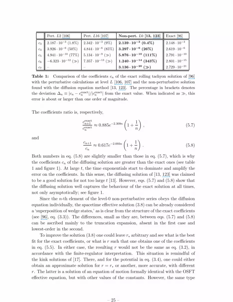
exact result in the full theory [96]. These are summarized in table 1. The coefficient

c2 = 26/311/2 ≈ 0.152 is the same in all cases. Errors of order 100% are still acceptable

as the coefficients have the same order of magnitude and are exponentially suppressed

(in fact, a better estimate of the error is on the logarithmic coefficients, ∆n in figure

1). With the only exception of level-2 c5, all the other coefficients of the diffusing

non-perturbative series are much closer to the exact values than those computed

with other methods. This is because the level-0 calculation takes non-local effects

into account, while higher-level results are obtained on-shell (local models).

The coefficients of the exact solution are given in integral form, and numerically

up to n = 7, in [96]. We checked that they can be well described by the non-linear

fit

cexactn ≈ 1.069n e1.032n−1.154n2

, (5.5)

while the coefficients (3.9) of the level-0 diffusing solution are

cn ≈ 1.622n e0.563n−1.046n2

. (5.6)

– 24 –

Pert. L2 [106] Pert. L16 [107] Non-pert. L0 [13, 123] Exact [96]

c3 2.187 · 10−3 (1.8%) 2.342 · 10−3 (9%) 2.139 · 10−3 (0.4%) 2.148 · 10−3

c4 3.926 · 10−6 (50%) 4.844 · 10−6 (85%) 3.297 · 10−6 (26%) 2.619 · 10−6

c5 4.941 · 10−10 (77%) 5.134 · 10−9 (≫) 5.876 · 10−10 (111%) 2.791 · 10−10

c6 −6.323 · 10−12 (≫) 7.357 · 10−13 (≫) 1.240 · 10−14 (343%) 2.801 · 10−15

c7 – – 3.136 · 10−20 (≫) 2.729 · 10−21

Table 1: Comparison of the coefficients cn of the exact rolling tachyon solution of [96]

with the perturbative calculations at level L [106, 107] and the non-perturbative solution

found with the diffusion equation method [13, 123]. The percentage in brackets denotes

the deviation ∆n ≡ |cn − cexactn |/|cexactn | from the exact value. When indicated as ≫, this

error is about or larger than one order of magnitude.

The coefficients ratio is, respectively,

cexactn+1

cexactn

≈ 0.885e−2.309n

(

1 +1

n

)

, (5.7)

andcn+1

cn≈ 0.617e−2.093n

(

1 +1

n

)

. (5.8)

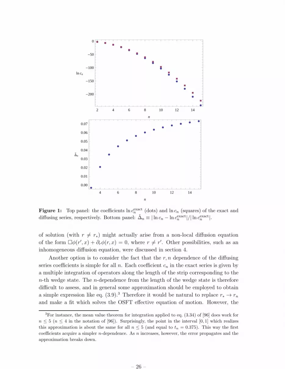
Both numbers in eq. (5.8) are slightly smaller than those in eq. (5.7), which is why

the coefficients cn of the diffusing solution are greater than the exact ones (see table

1 and figure 1). At large t, the time exponentials start to dominate and amplify the

error on the coefficients. In this sense, the diffusing solution of [13, 123] was claimed

to be a good solution for not too large t [13]. However, eqs. (5.7) and (5.8) show that

the diffusing solution well captures the behaviour of the exact solution at all times,

not only asymptotically; see figure 1.

Since the n-th element of the level-0 non-perturbative series obeys the diffusion

equation individually, the spacetime effective solution (3.8) can be already considered

a ‘superposition of wedge states,’ as is clear from the structure of the exact coefficients

(see [96], eq. (3.3)). The differences, small as they are, between eqs. (5.7) and (5.8)

can be ascribed mainly to the truncation expansion, absent in the first case and

lowest-order in the second.

To improve the solution (3.8) one could leave r∗ arbitrary and see what is the best

fit for the exact coefficients, or what is r such that one obtains one of the coefficients

in eq. (5.5). In either case, the resulting r would not be the same as eq. (3.2), in

accordance with the finite-regulator interpretation. This situation is remindful of

the kink solutions of [17]. There, and for the potential in eq. (3.4), one could either

obtain an approximate solution for r = r∗ or another, more accurate, with different

r. The latter is a solution of an equation of motion formally identical with the OSFT

effective equation, but with other values of the constants. However, the same type

– 25 –

ææ

æ

æ

æ

æ

æ

æ

æ

æ

æ

æ

æ

æ

àà

àà

à

à

à

à

à

à

à

à

à

à

2 4 6 8 10 12 14

-200

-150

-100

-50

0

n

ln cn

æ

æ

æ

æ

æ

æ

æ

ææ

ææ

ææ

4 6 8 10 12 14

0.00

0.01

0.02

0.03

0.04

0.05

0.06

0.07

n

D

n

Figure 1: Top panel: the coefficients ln cexactn (dots) and ln cn (squares) of the exact and

diffusing series, respectively. Bottom panel: ∆n ≡ | ln cn − ln cexactn |/| ln cexactn |.

of solution (with r 6= r∗) might actually arise from a non-local diffusion equation

of the form φ(r′, x) + ∂rφ(r, x) = 0, where r 6= r′. Other possibilities, such as an

inhomogeneous diffusion equation, were discussed in section 4.

Another option is to consider the fact that the r, n dependence of the diffusing

series coefficients is simple for all n. Each coefficient cn in the exact series is given by

a multiple integration of operators along the length of the strip corresponding to the

n-th wedge state. The n-dependence from the length of the wedge state is therefore

difficult to assess, and in general some approximation should be employed to obtain

a simple expression like eq. (3.9).3 Therefore it would be natural to replace r∗ → rnand make a fit which solves the OSFT effective equation of motion. However, the

3For instance, the mean value theorem for integration applied to eq. (3.34) of [96] does work for

n ≤ 5 (n ≤ 4 in the notation of [96]). Surprisingly, the point in the interval [0, 1] which realizes

this approximation is about the same for all n ≤ 5 (and equal to tn = 0.375). This way the first

coefficients acquire a simpler n-dependence. As n increases, however, the error propagates and the

approximation breaks down.

– 26 –

discussion in section 4.1 suggests that naive superpositions of a spacetime solution

with different r’s would not yield improved solutions. It may be instructive to show

this in a particular instance.

5.2 Finite superposition of solutions

A new kink-type candidate solution could be made of the sum of a number of copies

of the kink eq. (3.7), each with coefficient rn 6= rl. This might increase the accuracy

of the result with respect to the simplest case rn = rl, ∀ l, n. Let us take the

superposition of just two one-dimensional kinks with same asymptotics as eq. (3.7),

φ = C erf

(

x√4r1

)

+ (1− C) erf

(

x√4r2

)

, (5.9)

where C is a constant. For illustrative purposes and without loss of generality, we

are interested in a simplified version of eq. (3.4) [111] where the scalar potential is a

pure power without non-local insertions:(

∂2x +1

2

)

e−2r∗∂2xφ = σφ3 . (5.10)

For the kink solution, this approximation was shown to lead to the same dynamics

of eq. (3.4) [17].

The asymptotics at x = ∞ fixes the coupling σ = 1/2 (or, alternatively, the

normalization of the solution for a given σ). Moreover, since the leading term in a

x ∼ 0 expansion of the right-hand side of eq. (5.10) is cubic, the O(x) term in the

left-hand side must vanish. This fixes the coefficient C = C(r1, r2, r∗). Setting, e.g.,

r1 = 1.5, there remains only one free parameter to be tuned in order for the error on

the equation of motion to be minimized. The latter is defined as

∆max ≡ supx

∆(x) ≡ supx

∣

∣

∣

∣

l.h.s.− r.h.s.

scale

∣

∣

∣

∣

, (5.11)

where l.h.s. and r.h.s. are, respectively, the left- and right-hand side of eq. (5.10),

and the denominator is some characteristic scale of the solution. A typical choice

is l.h.s. + r.h.s., but others are possible and do not change much the error estimate

(see [13, 14, 17] for details). One can show that values around r2 = 1.3 minimize the

error to ∆max ≈ 1.4%. This is only slightly smaller than the error for the single-kink

solution of the equation of motion with the same values of the parameters r∗, m and

σ, which is ∆max ≈ 1.5% (it can be calculated directly on the second duplication

formula of [17]).

Repeating the same procedure for a three-kink solution, we checked that it is

possible to fix the parameters r1,2,3 and the coefficients of the linear combination so

that the error is about ∆max ≈ 1.4%, but not lower. Therefore, the tachyonic kink

solution is not improved appreciably by a linear superposition of kinks.

– 27 –

Rather than fixing r1 beforehand, one can set all the free parameters by imposing

the coefficients of the coordinate expansion near the origin to vanish, but to no avail.

This typically happens in cases where one is not using a complete functional basis

to express a solution to the equations of motion, but we have shown that this is not

the case. A possibility, which we shall not pursue here, is to consider a finite linear

combination of diffusing solutions with different boundary conditions. Another is to

take an infinite superposition of kinks.

5.3 Integrated solutions of non-local models

Let φ(r, x) be an approximate or exact solution of both the diffusion equation and

the non-local equation of motion of a given model. We define as the ‘integrated

solution’ the function

ψ =

∫

I

dr µ(r)φ(r, x) , (5.12)

where I = [a, b], a and b are non-negative and µ is a one-dimensional measure weight

such that∫

I

dr µ(r) = 1 , (5.13)

in order for ψ to have the same normalization as φ.

There is a caveat regarding the integration interval [a, b]. Because the heat

equation is a conformally transformed free Klein–Gordon equation, all its (one-

dimensional) solutions depend on the argument y ≡ x2/(4r). Every value of y can be

achieved by any other value of the space(time) coordinate under a suitable rescaling

in r. In particular, the points y = 0 and y = ∞ are degenerate as they correspond

to two different asymptotics: one in space(time) (x = 0 and x = ∞, respectively)

and one in the extra direction (r = ∞ and r = 0). Therefore, if one integrates the

solution on the whole positive real axis one may encounter unwanted singularities in

the solution or its derivatives.

The following proposition (valid in one dimension but easily extendable to the

general case) holds which prevents this to happen. All C∞ integrated solutions (5.12)

which can be analytically continued on the whole real axis are of the form

ψ =

∫ +∞

0

dr µ(r)φ(r, y) , (5.14)

where

µ(n)(0) = 0 , n ∈ N , (5.15)

and the superscript (n) denotes the n-th derivative. For instance, weights of the form

µ ∼ rne−r produce a discontinuity in ψ(n+2), since µ(n)(0) 6= 0. On the other hand,

there exist weights which respect the singularity-free and normalization requirements.

– 28 –

Examples are (all l, n positive integers)

µ(r) ∝ e−1/rn

r2, µ(r) ∝ (rn + r−n)−l , (5.16)

µ(r) =4n

πr0

(

r

r0

)n−11

[(r/r0)n + (r0/r)n]2, (5.17)

where I = R+ and r0 is a scale. The last measure has two interesting properties: for

n = 1 it is invariant under the inversion r → 1/r, and in the large n limit it tends to

µ ∼ δ(r − r0).

As anticipated, the integrated kink (which is still a kink) is no longer a solution

of the effective equation of motion with potential ψ3, for any of the above measures.

This is true also for eq. (3.4) (non-local potential).4

It is instructive to draw a comparison between non-integrated and integrated

solutions for another model, a modified p-adic equation of motion:

(e−s −m2)ψ = σψn. (5.19)

This toy model was often considered in the literature [125, 127, 129, 134, 135, 136,

137] as a useful hybrid between the string field tachyon and the p-adic string. On one

hand, the mass term is strictly non-zero as for the OSFT tachyon, our reason being

technical (see below). On the other hand, the equation of motion becomes purely

algebraic in the local limit, as for the p-adic string.

The parameter s is a constant we will assume to be either s = +1 or s =

−1. Consider the case n = 3, s = −1 and one-dimensional spatial configurations,

e−s = e∂2x . As a characteristic scale of the problem, we take the denominator

of eq. (5.11) to be 1 (the asymptotics of the solution). Then, one can show that

eq. (3.7) is an approximate solution and the error (5.11) is minimized at ∆max . 0.1%

for r ≈ 1.78. The mass is fixed by the vanishing of the O(x) term in eq. (5.19),

m2 =√

r/(r + s) ≈ 1.511 (this is the reason why m 6= 0), while the normalization

of the potential is σ = 1−m2 < 0.

The integrated solution

ψ(x) = β

∫ +∞

0

dre−β/r

r2erf

(

x√4r

)

=x

√

x2 + 4β

4To show it, one has to employ the formula

erf

(

x√4r1

)

erf

(

x√4r2

)

≈ 1− e−

x2

π

√

r1r2 , (5.18)

which can be obtained in a way similar to the duplication formulæ of [17] and is valid also upon

integration in r1 and r2. The integration intervals I1,2 = [a,+∞) are chosen so that a > 2r∗ and

both sides of eq. (3.4) (which have different signs in the non-local exponents, and thus require a

limitation of the domains) are well-defined.

– 29 –

is a kink with same asymptotics as the error function but different slope. This is

a candidate solution for the n = 3, s = +1 system. We checked that the error is

minimized for β ≈ 0.7 and m2 ≈ 0.62 (σ > 0), but the global error is rather high,

∆max . 6%. The same result holds for the measure µ = e−β/r2/r2, but not for

eq. (5.17): an r0 = 0.33 yields an error of about 2%. All these features are valid also

when taking a different integration interval I (e.g., I = [a,+∞) with a 6= 0).

The operation of integrating a solution for a given non-local system with chosen

s will yield a candidate solution for the same system but with s → −s. In the p-

adic case this change of sign can be regarded as a switch from the Minkowski to the

Euclidean problem (or vice versa).

5.4 Toy models with polynomial potentials

We conclude with the construction of kink solutions for a family of toy models of the

form

φ(γx) = V [φ(x)] , (5.20)

where γ is a constant. The p-adic string equation is of this type. On the left-hand

side, the rescaling of the coordinate can be achieved by a generic pseudo-differential

operator. Here we limit ourselves to the exponential operator and φ = erf. Then,

around the origin

√πφ(γx) = 2γx− 2γ3x3

3+γ5x5

5+O(x7) .

To match all powers up to O(xl+1), the right-hand side of eq. (5.20) should be of the

form

V [φ] =l

∑

n=0

an(γ)φn , (5.21)

for some set of coefficients an(γ) which can be obtained recursively order by order.

In this case, a2n = 0, a1 = γ, a3 = −πγ(γ2 − 1)/12, and so on. The solution at large

x is fixed by the polynomial equation

l∑

n=0

an(γ) = 1 , (5.22)

Up to O(x12), one gets an l = 11 potential and a solution with global error ∆max ≈10−5 for any of the four allowed values of γ 6= 1 according to eq. (5.22).

The massive p-adic model (5.19) corresponds to the case l = 3. Equation (5.22)

gives γ = (√

1 + 48/π − 1)/2 ≈ 1.517 (then, a3 = 1 − γ ≈ −0.517) and minimizes

the error to ∆max ≈ 0.1%, all numbers in agreement with section 5.3. The error can

be lowered to 0.04% by a slightly different value, γ = 1.511.

– 30 –

6. Conclusions

In this paper we have shown that the structure of all known analytic solutions of

open string field theory is inherited by tachyonic solutions of the effective spacetime

action; compare eqs. (3.23) and (4.4). In both cases, the diffusion equation plays an

important role for the construction of solutions. We have established a connection

between two rather different setups (one exact and universal, the other approximate

and spacetime dependent) which can be instrumental to finding other solutions in

either framework. In particular, the construction of an exact supersymmetric solution

with marginal deformations (in series and integral form) and of a non-perturbative

non-marginal kink in the full theory will help to verify, and hopefully strengthen, the

picture advanced here.

Acknowledgments

G.C. thanks S. Alexander for his kind hospitality at Haverford College, where this

work was initiated. G.C. is partly supported by NSF grant PHY0854743, The George

A. and Margaret M. Downsbrough Endowment and the Eberly research funds of Penn

State. G.N. is partly supported by INFN of Italy.

Open Access. This article is distributed under the terms of the Creative Commons

Attribution Noncommercial License which permits any noncommercial use, distribu-

tion, and reproduction in any medium, provided the original author(s) and source

are credited.

References

[1] E. Witten, Non-commutative geometry and string field theory, Nucl. Phys. B 268

(1986) 253.

[2] V.A. Kostelecky and S. Samuel, The static tachyon potential in the open bosonic

string theory, Phys. Lett. B 207 (1988) 169.

[3] V.A. Kostelecky and S. Samuel, On a nonperturbative vacuum for the open bosonic

string, Nucl. Phys. B 336 (1990) 263 .

[4] K. Ohmori, A review on tachyon condensation in open string field theories,

hep-th/0102085.

[5] A. Sen, Tachyon dynamics in open string theory, Int. J. Mod. Phys. A 20 (2005)

5513 [hep-th/0410103].

[6] E. Fuchs and M. Kroyter, Analytical solutions of open string field theory,

arXiv:0807.4722.

– 31 –

[7] E. Witten, On background independent open-string field theory, Phys. Rev. D 46

(1992) 5467 [hep-th/9208027].

[8] E. Witten, Some computations in background independent off-shell string theory,

Phys. Rev. D 47 (1993) 3405 [hep-th/9210065].

[9] S. Shatashvili, Comment on the background independent open string theory, Phys.

Lett. B 311 (1993) 83 [hep-th/9303143].

[10] S. Shatashvili, On the problems with background independence in string theory, Alg.

Anal. 6 (1994) 215 [hep-th/9311177].

[11] D.A. Eliezer and R.P. Woodard, The problem of nonlocality in string theory, Nucl.

Phys. B 325 (1989) 389.

[12] N. Moeller and B. Zwiebach, Dynamics with infinitely many time derivatives and

rolling tachyons, JHEP 10 (2002) 034 [hep-th/0207107].

[13] G. Calcagni and G. Nardelli, Tachyon solutions in boundary and cubic string field

theory, Phys. Rev. D 78 (2008) 126010 [arXiv:0708.0366].

[14] G. Calcagni, M. Montobbio and G. Nardelli, Route to nonlocal cosmology, Phys. Rev.

D 76 (2007) 126001 [arXiv:0705.3043].

[15] G. Calcagni, M. Montobbio and G. Nardelli, Localization of nonlocal theories, Phys.

Lett. B 662 (2008) 285 [arXiv:0712.2237].

[16] G. Calcagni and G. Nardelli, Nonlocal instantons and solitons in string models,

Phys. Lett. B 669 (2008) 102 [arXiv:0802.4395].

[17] G. Calcagni and G. Nardelli, Kinks of open superstring field theory, Nucl. Phys. B

823 (2009) 234 [arXiv:0904.3744].

[18] G. Calcagni and G. Nardelli, Cosmological rolling solutions of nonlocal theories, Int.

J. Mod. Phys. D (2010) in press [arXiv:0904.4245].

[19] E. Witten, Interacting field theory of open superstrings, Nucl. Phys. B 276 (1986)

291.

[20] M.V. Green and N. Seiberg, Contact interactions in superstring theory, Nucl. Phys.

B 299 (1988) 559.

[21] J. Greensite and F.R. Klinkhamer, Superstring amplitudes and contact interactions,

Nucl. Phys. B 304 (1988) 108.

[22] I.Ya. Aref’eva and P.B. Medvedev, Anomalies in Witten’s field theory of the NSR

string, Phys. Lett. B 212 (1988) 299.

[23] C. Wendt, Scattering amplitudes and contact interactions in Witten’s superstring

field theory, Nucl. Phys. B 314 (1989) 209.

– 32 –

[24] P.-J. De Smet and J. Raeymaekers, The tachyon potential in Witten’s superstring

field theory, JHEP 08 (2000) 020 [arXiv:hep-th/0004112].

[25] C.R. Preitschopf, C.B. Thorn and S.A. Yost, Superstring field theory, Nucl. Phys. B

337 (1990) 363.

[26] I.Ya. Aref’eva, P.B. Medvedev and A.P. Zubarev, Background formalism for

superstring field theory, Phys. Lett. B 240 (1990) 356.

[27] I.Ya. Aref’eva, P.B. Medvedev and A.P. Zubarev, New representation for string field

solves the consistency problem for open superstring field theory, Nucl. Phys. B 341

(1990) 464.

[28] A. Sen, Non-BPS states and branes in string theory, hep-th/9904207.

[29] Z.-a. Qiu and A. Strominger, Gauge symmetries in (super)string field theory, Phys.

Rev. D 36 (1987) 1794.

[30] Y. Okawa, L. Rastelli and B. Zwiebach, Analytic solutions for tachyon condensation

with general projectors, hep-th/0611110.

[31] I. Ellwood, Singular gauge transformations in string field theory, arXiv:0903.0390.

[32] A. Sen, Universality of the tachyon potential, JHEP 12 (1999) 027 [hep-th/9911116].

[33] L. Rastelli and B. Zwiebach, Tachyon potentials, star products and universality,

JHEP 09 (2001) 038 [hep-th/0006240].

[34] D. Gaiotto, L. Rastelli, A. Sen and B. Zwiebach, Star algebra projectors, JHEP 04

(2002) 060 [hep-th/0202151].

[35] A. LeClair, M.E. Peskin and C.R. Preitschopf, String field theory on the conformal

plane. I. Kinematical principles, Nucl. Phys. B 317 (1989) 411.

[36] A. LeClair, M.E. Peskin and C.R. Preitschopf, String field theory on the conformal

plane. II. Generalized gluing, Nucl. Phys. B 317 (1989) 464.

[37] M. Schnabl, Analytic solution for tachyon condensation in open string field theory,

Adv. Theor. Math. Phys. 10 (2006) 433 [arXiv:hep-th/0511286].

[38] Y. Okawa, Comments on Schnabl’s analytic solution for tachyon condensation in

Witten’s open string field theory, JHEP 04 (2006) 055 [hep-th/0603159].

[39] E. Fuchs and M. Kroyter, On the validity of the solution of string field theory, JHEP

05 (2006) 006 [hep-th/0603195].

[40] L. Rastelli and B. Zwiebach, Solving open string field theory with special projectors,

JHEP 01 (2008) 020 [hep-th/0606131].

[41] I. Ellwood and M. Schnabl, Proof of vanishing cohomology at the tachyon vacuum,

JHEP 02 (2007) 096 [hep-th/0606142].

– 33 –

[42] I. Kishimoto and T. Takahashi, Vacuum structure around identity based solutions,

Prog. Theor. Phys. 122 (2009) 385 [arXiv:0904.1095].

[43] E. Fuchs and M. Kroyter, Marginal deformation for the photon in superstring field

theory, JHEP 11 (2007) 005 [arXiv:0706.0717].

[44] T. Erler, Tachyon vacuum in cubic superstring field theory, JHEP 01 (2008) 013

[arXiv:0707.4591].

[45] I.Ya. Aref’eva, R.V. Gorbachev and P.B. Medvedev, Tachyon solution in cubic

Neveu-Schwarz string field theory, Theor. Math. Phys. 158 (2009) 320

[arXiv:0804.2017].

[46] I.Ya. Aref’eva, R.V. Gorbachev, D.A. Grigoryev, P.N. Khromov, M.V. Maltsev and

P.B. Medvedev, Pure gauge configurations and tachyon solutions to string field

theories equations of motion, JHEP 05 (2009) 050 [arXiv:0901.4533].

[47] I.Ya. Aref’eva, R.V. Gorbachev and P.B. Medvedev, Pure gauge configurations and

solutions to fermionic superstring field theories equations of motion, J. Phys. A 42

(2009) 304001 [arXiv:0903.1273].

[48] A. Sen, On the background independence of string field theory, Nucl. Phys. B 345

(1990) 551.

[49] A. Sen and B. Zwiebach, A proof of local background independence of classical closed

string field theory, Nucl. Phys. B 414 (1994) 649 [hep-th/9307088].

[50] V.A. Kostelecky and R. Potting, Analytical construction of a nonperturbative vacuum

for the open bosonic string, Phys. Rev. D 63 (2001) 046007 [hep-th/0008252].

[51] L. Rastelli, A. Sen and B. Zwiebach, Classical solutions in string field theory around

the tachyon vacuum, Adv. Theor. Math. Phys. 5 (2002) 393 [hep-th/0102112].

[52] L. Rastelli, A. Sen and B. Zwiebach, Half-strings, projectors, and multiple D-branes

in vacuum string field theory, JHEP 11 (2001) 035 [hep-th/0105058].

[53] D.J. Gross and W. Taylor, Split string field theory I, JHEP 08 (2001) 009

[hep-th/0105059].

[54] L. Rastelli, A. Sen and B. Zwiebach, Boundary CFT construction of D-branes in

vacuum string field theory, JHEP 11 (2001) 045 [hep-th/0105168].

[55] Y. Matsuo, BCFT and sliver state, Phys. Lett. B 513 (2001) 195 [hep-th/0105175].

[56] D.J. Gross and W. Taylor, Split string field theory II, JHEP 08 (2001) 010

[hep-th/0106036].

[57] K. Furuuchi and K. Okuyama, Comma vertex and string field algebra, JHEP 09

(2001) 035 [hep-th/0107101].

– 34 –

[58] H. Hata and T. Kawano, Open string states around a classical solution in vacuum

string field theory, JHEP 11 (2001) 038 [hep-th/0108150].

[59] P. Mukhopadhyay, Oscillator representation of the BCFT construction of D-branes

in vacuum string field theory, JHEP 12 (2001) 025 [hep-th/0110136].

[60] N. Moeller, Some exact results on the matter star-product in the half-string

formalism, JHEP 01 (2002) 019 [hep-th/0110204].

[61] G.W. Moore and W. Taylor, The singular geometry of the sliver, JHEP 01 (2002)

004 [hep-th/0111069].

[62] I.Ya. Aref’eva, A.A. Giryavets and P.B. Medvedev, NS matter sliver, Phys. Lett. B

532 (2002) 291 [hep-th/0112214].

[63] M. Marino and R. Schiappa, Towards vacuum superstring field theory: the

supersliver, J. Math. Phys. 44 (2003) 156 [hep-th/0112231].

[64] M. Schnabl, Wedge states in string field theory, JHEP 01 (2003) 004

[hep-th/0201095].

[65] Y. Okawa, Open string states and D-brane tension from vacuum string field theory,

JHEP 07 (2002) 003 [hep-th/0204012].

[66] K. Ohmori, Comments on solutions of vacuum superstring field theory, JHEP 04

(2002) 059 [hep-th/0204138].

[67] C. Maccaferri and D. Mamone, Star democracy in open string field theory, JHEP 09

(2003) 049 [hep-th/0306252].

[68] L. Bonora, C. Maccaferri, R.J. Scherer Santos and D.D. Tolla, Ghost story. I. Wedge

states in the oscillator formalism, JHEP 09 (2007) 061 [arXiv:0706.1025].

[69] L. Bonora, C. Maccaferri, R.J. Scherer Santos and D.D. Tolla, Ghost story. II. The

midpoint ghost vertex, JHEP 11 (2009) 075 [arXiv:0908.0055].

[70] L. Bonora, C. Maccaferri and D.D. Tolla, Ghost story. III. Back to ghost number

zero, JHEP 11 (2009) 086 [arXiv:0908.0056].

[71] E. Fuchs and M. Kroyter, Universal regularization for string field theory, JHEP 02

(2007) 038 [hep-th/0610298].

[72] D. Gross and A. Jevicki, Operator formulation of interacting string field theory (I),

Nucl. Phys. B 283 (1987) 1.

[73] D. Gross and A. Jevicki, Operator formulation of interacting string field theory (II),

Nucl. Phys. B 287 (1987) 225.

[74] J. Kluson, Exact solutions of open bosonic string field theory, JHEP 04 (2002) 043

[hep-th/0202045].

– 35 –

[75] T. Takahashi and S. Tanimoto, Marginal and scalar solutions in cubic open string

field theory, JHEP 03 (2002) 033 [hep-th/0202133].

[76] N. Drukker, On different actions for the vacuum of bosonic string field theory, JHEP

08 (2003) 017 [hep-th/0301079].

[77] M. Schnabl, Anomalous reparametrizations and butterfly states in string field theory,

Nucl. Phys. B 649 (2003) 101 [hep-th/0202139].

[78] H. Yang, Solving Witten’s SFT by insertion of operators on projectors, JHEP 09

(2004) 002 [hep-th/0406023].

[79] L. Rastelli, A. Sen and B. Zwiebach, String field theory around the tachyon vacuum,

Adv. Theor. Math. Phys. 5 (2002) 353 [hep-th/0012251].

[80] L. Bonora, D. Mamone and M. Salizzoni, Vacuum string field theory with B field,

JHEP 04 (2002) 020 [hep-th/0203188].

[81] L. Bonora, D. Mamone and M. Salizzoni, Vacuum string field theory ancestors of the

GMS solitons, JHEP 01 (2003) 013 [hep-th/0207044].

[82] L. Bonora, C. Maccaferri, D. Mamone and M. Salizzoni, Topics in string field theory,

hep-th/0304270.

[83] D. Gaiotto, L. Rastelli, A. Sen and B. Zwiebach, Ghost structure and closed strings

in vacuum string field theory, Adv. Theor. Math. Phys. 6 (2003) 403

[hep-th/0111129].

[84] Y. Okawa, Some exact computations on the twisted butterfly state in string field

theory, JHEP 01 (2004) 066 [hep-th/0310264].

[85] Y. Okawa, Solving Witten’s string field theory using the butterfly state, Phys. Rev. D

69 (2004) 086001 [hep-th/0311115].

[86] I. Ellwood, Rolling to the tachyon vacuum in string field theory, JHEP 12 (2007)

028 [arXiv:0705.0013].

[87] T. Erler, Marginal solutions for the superstring, JHEP 07 (2007) 050

[arXiv:0704.0930].

[88] E. Fuchs, M. Kroyter and R. Potting, Marginal deformations in string field theory,

JHEP 09 (2007) 101 [arXiv:0704.2222].

[89] A. Recknagel and V. Schomerus, Boundary deformation theory and moduli spaces of

D-Branes, Nucl. Phys. B 545 (1999) 233 [hep-th/9811237].

[90] A. Sen and B. Zwiebach, Large marginal deformations in string field theory, JHEP

10 (2000) 009 [hep-th/0007153].

– 36 –

[91] A. Iqbal and A. Naqvi, On marginal deformations in superstring field theory, JHEP

01 (2001) 040 [hep-th/0008127].

[92] T. Takahashi and S. Tanimoto, Wilson lines and classical solutions in cubic open

string field theory, Prog. Theor. Phys. 106 (2001) 863 [hep-th/0107046].

[93] J. Kluson, Exact solutions in SFT and marginal deformation in BCFT, JHEP 12

(2003) 050 [hep-th/0303199]

[94] I. Kishimoto and T. Takahashi, Marginal deformations and classical solutions in

open superstring field theory, JHEP 11 (2005) 051 [hep-th/0506240].

[95] M. Schnabl, Comments on marginal deformations in open string field theory, Phys.

Lett. B 654 (2007) 194 [hep-th/0701248].

[96] M. Kiermaier, Y. Okawa, L. Rastelli and B. Zwiebach, Analytic solutions for

marginal deformations in open string field theory, JHEP 01 (2008) 028

[hep-th/0701249].

[97] M. Kiermaier and Y. Okawa, Exact marginality in open string field theory: a general

framework, JHEP 11 (2009) 041 [arXiv:0707.4472].

[98] B.H. Lee, C. Park and D.D. Tolla, Marginal deformations as lower dimensional

Dbrane solutions in open string field theory, arXiv:0710.1342.

[99] O-K. Kwon, Marginally deformed rolling tachyon around the tachyon vacuum in

open string field theory, Nucl. Phys. B 804 (2008) 1 [arXiv:0801.0573].

[100] I. Kishimoto, Comments on gauge invariant overlaps for marginal solutions in open

string field theory, Prog. Theor. Phys. 120 (2008) 875 [arXiv:0808.0355].

[101] Y. Okawa, Analytic solutions for marginal deformations in open superstring field

theory, JHEP 09 (2007) 084 [arXiv:0704.0936].

[102] Y. Okawa, Real analytic solutions for marginal deformations in open superstring

field theory, JHEP 09 (2007) 082 [arXiv:0704.3612].

[103] M. Kiermaier and Y. Okawa, General marginal deformations in open superstring

field theory, JHEP 11 (2009) 042 [arXiv:0708.3394].

[104] A. Sen, Rolling tachyon, JHEP 04 (2002) 048 [hep-th/0203211].

[105] A. Sen, Time evolution in open string theory, JHEP 10 (2002) 003

[hep-th/0207105].

[106] E. Coletti, I. Sigalov and W. Taylor, Taming the tachyon in cubic string field

theory, JHEP 08 (2005) 104 [hep-th/0505031].

[107] V. Forini, G. Grignani and G. Nardelli, A solution to the 4-tachyon off-shell

amplitude in cubic string field theory, JHEP 04 (2006) 053 [hep-th/0603206].

– 37 –

[108] E. Fuchs and M. Kroyter, On the classical equivalence of superstring field theories,

JHEP 10 (2008) 054 [arXiv:0805.4386].

[109] M. Kroyter, Comments on superstring field theory and its vacuum solution, JHEP

08 (2009) 048 [arXiv:0905.3501].

[110] I.Ya. Aref’eva, A.S. Koshelev, D.M. Belov and P.B. Medvedev, Tachyon

condensation in cubic superstring field theory, Nucl. Phys. B 638 (2002) 3

[hep-th/0011117].

[111] I.Ya. Aref’eva, L.V. Joukovskaya and A.S. Koshelev, Time evolution in superstring

field theory on non-BPS brane. I. Rolling tachyon and energy-momentum

conservation, JHEP 09 (2003) 012 [hep-th/0301137].

[112] J. Llosa and J. Vives, Hamiltonian formalism for nonlocal Lagrangians, J. Math.

Phys. 35 (1994) 2856.

[113] J. Gomis, K. Kamimura and J. Llosa, Hamiltonian formalism for space-time

non-commutative theories, Phys. Rev. D 63 (2001) 045003 [hep-th/0006235].

[114] K. Bering, A note on non-locality and Ostrogradski’s construction, hep-th/0007192.

[115] T.-C. Cheng, P.-M. Ho and M.-C. Yeh, Perturbative approach to higher derivative

and nonlocal theories, Nucl. Phys. B 625 (2002) 151 [hep-th/0111160].

[116] V.S. Vladimirov and Ya.I. Volovich, On the nonlinear dynamical equation in the

p-adic string theory, Theor. Math. Phys. 138 (2004) 297 [math-ph/0306018].

[117] J. Gomis, K. Kamimura and T. Ramırez, Physical degrees of freedom of non-local

theories, Nucl. Phys. B 696 (2004) 263 [hep-th/0311184].

[118] D.V. Prokhorenko, On some nonlinear integral equation in the (super)string theory,

math-ph/0611068.

[119] V. Vladimirov, Nonlinear equations for p-adic open, closed, and open-closed strings,

Theor. Math. Phys. 149 (2006) 1604 [arXiv:0705.4600].

[120] N. Barnaby and N. Kamran, Dynamics with infinitely many derivatives: the initial

value problem, JHEP 02 (2008) 008 [arXiv:0709.3968].

[121] N. Barnaby and N. Kamran, Dynamics with infinitely many derivatives: variable

coefficient equations, JHEP 12 (2008) 022 [arXiv:0809.4513].

[122] Ya.I. Volovich, Numerical study of nonlinear equations with infinite number of

derivatives, J. Phys. A 36 (2003) 8685 [math-ph/0301028].

[123] V. Forini, G. Grignani and G. Nardelli, A new rolling tachyon solution of cubic

string field theory, JHEP 03 (2005) 079 [hep-th/0502151].

– 38 –

[124] V.S. Vladimirov, On the equation of the p-adic open string for the scalar tachyon

field, Izv. Math. 69 (2005) 487 [math-ph/0507018].

[125] L.V. Joukovskaya, Dynamics in nonlocal cosmological models derived from string

field theory, Phys. Rev. D 76 (2007) 105007 [arXiv:0707.1545].

[126] L. Joukovskaya, Rolling solution for tachyon condensation in open string field

theory, arXiv:0803.3484.

[127] D.J. Mulryne and N.J. Nunes, Diffusing non-local inflation: solving the field

equations as an initial value problem, Phys. Rev. D 78 (2008) 063519

[arXiv:0805.0449].

[128] L. Joukovskaya, Dynamics with infinitely many time derivatives in

Friedmann-Robertson-Walker background and rolling tachyons, JHEP 02 (2009) 045

[arXiv:0807.2065].

[129] N.J. Nunes and D.J. Mulryne, Non-linear non-local cosmology, AIP Conf. Proc.

1115 (2009) 329 [arXiv:0810.5471].

[130] G. Calcagni, Cosmological tachyon from cubic string field theory, JHEP 05 (2006)

012 [hep-th/0512259].

[131] J. Polchinski, String theory, Cambridge University Press, Cambridge U.K. (1998).

[132] B. Zwiebach, A first course in string theory, Cambridge University Press,

Cambridge U.K. (2009).

[133] T. Erler and M. Schnabl, A simple analytic solution for tachyon condensation,

JHEP 10 (2009) 066 [arXiv:0906.0979].

[134] I.Ya. Aref’eva and L.V. Joukovskaya, Time lumps in nonlocal stringy models and

cosmological applications, JHEP 10 (2005) 087 [hep-th/0504200].

[135] I.Ya. Aref’eva, L.V. Joukovskaya and S.Yu. Vernov, Bouncing and accelerating

solutions in nonlocal stringy models, JHEP 07 (2007) 087 [hep-th/0701184].

[136] I.Y. Aref’eva, L.V. Joukovskaya and S.Yu. Vernov, Dynamics in nonlocal linear

models in the Friedmann-Robertson-Walker metric, J. Phys. A 41 (2008) 304003

[arXiv:0711.1364].

[137] S.Yu. Vernov, Localization of non-local cosmological models with quadratic potentials

in the case of double roots, Class. Quant. Grav. 27 (2010) 035006 [arXiv:0907.0468].

– 39 –