cosmos-e′-gtachyon from string theory

TIFR/TH/15-33

COSMOS-e’-GTachyonfrom String TheorySayantan Choudhury 1a Sudhakar PandabaDepartment of Theoretical Physics, Tata Institute of Fundamental Research, Colaba, Mum-bai - 400005, IndiabInstitute of Physics, Sachivalaya Marg, Bhubaneswar, Odisha - 751005, India

E-mail: [email protected], [email protected]

Abstract: In this article, our prime objective is to study the inflationary paradigmfrom generalized tachyon (GTachyon) living on the world volume of a non-BPS stringtheory. The tachyon action is considered here is getting modified compared to theoriginal action. One can quantify the amount of the modification via a power qinstead of 1/2 in the effective action. Using this set up we study inflation fromvarious types of tachyonic potentials, using which we constrain the index q within,1/2 < q < 2, and a specific combination (∝ α

′M4

s /gs) of Regge slope α′ , stringcoupling constant gs and mass scale of tachyon Ms, from the recent Planck 2015and Planck+BICEP2/Keck Array joint data. We explicitly study the inflationaryconsequences from single field, assisted field and multi-field tachyon set up. Specifi-cally for single field and assisted field case we derive the results in the quasi-de-Sitterbackground in which we will utilize the details of cosmological perturbations andquantum fluctuations. Also we derive the expressions for all inflationary observablesusing any arbitrary vacuum and Bunch-Davies vacuum. For single field and assistedfield case we derive-the inflationary flow equations, new sets of consistency relations.Also we derive the field excursion formula for tachyon, which shows that assistedinflation is in more safer side compared to the single field case to validate effectivefield theory framework. Further we study the features of CMB Angular power spec-trum from TT, TE and EE correlations from scalar fluctuations within the allowedrange of q for each potentials from single field set-up. We also put constraints fromthe temperature anisotropy and polarization spectra, which shows that our analysisis consistent with the Planck 2015 data. Finally, using δN formalism we derive theexpressions for inflationary observables in the context of multi-field tachyons.

Keywords: Inflation, Cosmological perturbations, Cosmology beyond the standardmodel, Tachyon Condensation, Effective Field Theories.

1Presently working as a Visiting (Post-Doctoral) fellow at DTP, TIFR, Mumbai,Alternative E-mail: [email protected].

arX

iv:1

511.

0573

4v2

[he

p-th

] 1

9 N

ov 2

015

mailto:[email protected], [email protected]

Contents

1 Introduction 1

2 GTachyon in string theory 5

3 Variants of tachyonic models in string theory 103.1 Model I: Inverse cosh potential 133.2 Model II: Logarithmic potential 163.3 Model III: Exponential potential-Type I 183.4 Model IV: Exponential potential-Type II (Gaussian) 213.5 Model V: Inverse power-law potential 23

4 Cosmological dynamics from GTachyon 264.1 Unperturbed evolution 264.2 Dynamical solution for various phases 34

5 Inflationary paradigm from GTachyon 475.1 Computation for Single field inflation 48

5.1.1 Condition for inflation 485.1.2 Analysis using Slow-roll formalism 515.1.3 Basics of tachyonic perturbations 595.1.4 Computation of scalar power spectrum 635.1.5 Computation of tensor power spectrum 715.1.6 Modified consistency relations 785.1.7 Field excursion for tachyon 835.1.8 Semi analytical study and Cosmological parameter estimation 905.1.9 Analyzing CMB power spectrum 128

5.2 Computation for Assisted inflation 1395.2.1 Condition for inflation 1405.2.2 Analysis using Slow-roll formalism 1425.2.3 Basics of tachyonic perturbations 1475.2.4 Computation of scalar power spectrum 1535.2.5 Computation of tensor power spectrum 1555.2.6 Modified consistency relations 1575.2.7 Field excursion for tachyon 1605.2.8 Semi analytical study and Cosmological parameter estimation 166

5.3 Computation for Multi-field inflation 1685.3.1 Condition for inflation 1685.3.2 Analysis using Slow-roll formalism 171

– i –

5.3.3 The δN formalism for Multi tachyons 1765.3.4 Computation of scalar power spectrum 1805.3.5 Computation of tensor power spectrum 1855.3.6 Analytical study for Multi-field model 186

6 Conclusion 189

1 Introduction

The primordial inflationary paradigm is a very sublime thought to explain variousaspects of the early universe, which creates the perturbations and the matter. Forrecent developments see refs. [1–10]. The success of primordial inflation, can begauged by the current observations arising from the cosmic microwave background(CMB) radiation [11–13]. The observations from Planck have put interestingly tightbounds on a number of cosmological observables related to the perturbations, whichalso determines any departure from the Gaussian perturbations and the constrainton tensor-to-scalar ratio, r?, which can potentially unearth the scale of New Physicswithin any given effective field theory set-up. But a big issue may crop up in modeldiscrimination and also in the removal of the degeneracy of cosmological parametersobtained from CMB observations. Non-canonical interactions in the effective theoryset-up [14–23] is one of the possibilities through which one can address this issue 1.The natural source for such non-canonical interactions is string theory. The mostpromising example is the Dirac-Bonn-Infeld (DBI) effective action for tachyon field[47–50]. In this paper, we will only focus on tachyons in weakly coupled type IIA/IIB string theory [51].

The phenomena of tachyon condensation was introduced in refs. [47, 48], wheretype IIA/IIB string theory and the tachyon instability on D-branes have studiedelaborately. The rolling tachyon [52–54] in weakly coupled type IIA/ IIB string the-ory may be described in terms of an effective field theory for the tachyon condensatein refs. [55–71]. The cosmological implications of the tachyon were studied in [72–84]. For more details see also refs. [85–93]. In the context of cosmology, the detailedconsequences have been studied in the following topics over many years:

1. Inflationary paradigm [73–84, 90],

2. Primordial non-Gaussianity and CMB aspects [94–101],1The other possibilities are- non-minimal interactions between the matter and gravity sector

(example: SM Higgs with Einstein gravity [24, 25]), addition of higher derivative terms in thegravity sector (example: Starobinsky model [26]), modification of gravity sector through extradimensions (example: 5D membrane models [27–46]).

– 1 –

3. Reheating scenario and particle creation [102, 103],

4. Late time cosmic acceleration (Dark Energy) [104–107].

In this work, we introduce the most generalized version of the tachyon effectiveaction in which we are interested to study the cosmological consequences from thenon-canonical higher dimensional effective field theory operators, originated fromstring theory. Technically we rename such a non-canonical fields to be generalizedtachyon (GTachyon), which we will frequently use throughout the rest of the paper.The prime motivation of writing this paper is following 2:

• To update the present status of non-canonical interaction for stringy tachyonfield appearing within the framework of string theory after releasing the Planck2015 data.

• To explicitly study the role of tachyon field and its generalized version GTachyon,to explain the observed temperature anisotropy and polarization in CMB An-gular power spectrum.

• To study the specific role of the most generalized version of non-canonicalhigher dimensional effective field theory Wilsonian operators.

• To give a broad overview of the present constraints on inflationary paradigmfrom the most generalized version of the tachyon string theory.

• To test the explicit dynamical features of various tachyonic potentials obtainedfrom string theory and also to know about the specific structural form of effec-tive field theory operators for a specific type of potential.

Throughout the paper we have taken the following assumptions:

1. Tachyon field T is minimally coupled to the Einstein gravity sector.

2. Initial condition for inflation is fixed via Bunch-Davies (BD) vacuum [108]. Forthe completeness we also present the results obtained from arbitrary vacuum(AV). For a classical initial condition the amplitude of the primordial gravi-tational waves would be very tiny and practically undetectable, therefore thiscan be treated as the first observable proof of quantum theory gravity, such as

2Since Gtachyon contains non-minimal interactions, it is naturally expected that it will suffi-ciently modify the consistency relations. Also due to such non-canonical interactions it is expectedthat the amount of primordial non-Gaussianity is getting enhanced by a sufficient amount, by break-ing the non-Gaussian consistency relations known in cosmological literature. For the completenessit is important to mention here that, we have not investigated the issues related to primordialnon-Gaussianity yet in this paper. We will report on these issues in our future work.

– 2 –

string theory. However, apart from the importance and applicability of quan-tum version of Bunch-Davis vacuum on its theoretical and observational groundit is still not at all well understood from the previous works in this area whetherthe quantum Bunch-Davies vacuum is the only possible source of generatinglarge value of tensor-to-scalar ratio during inflationary epoch or not. One of theprime possibilities commming from the deviation from quantum Bunch-Daviesvacuum aka consideration of quantum non-Bunch-Davies or arbitrary vacuumin the present non-canonical picture which may also responsible for the gener-ation of large tensor-to-scalar ratio and large non-Gaussianity during inflation.Within the framework of effective field theory, such an arbitrary vacuum iscommonly identified to be the α-vacua [109–115], which has string theoreticorigin.

3. Sound speed is cS < 1 in general for non-canonical interactions [14–23], which isthe most promising ingradient for tachyonic set-up, to generate simultaneouslythe detectable amount of tensor-to-scalar ratio and large non-Gaussianity. Thisfact can be more clearly visualized when we go to all higher order expansion inslow-roll or more precisely by taking the exact solution of the mode functionsfor scalar and tensor fluctuations as obtained from cosmological perturabationtheory by appropriately choosing Bucnch-Davies or any arbitary initial condi-tions for inflation.

4. UV cut-off of the effective field theory is fixed at ΛUV ∼ Mp, where Mp =

2.43 × 1018 GeV is the reduced Planck mass. But in principle one can fix thescale between GUT scale and reduced Planck scale i.e. ΛGUT < ΛUV ≤ Mp.But in such a situation ΛUV acts as a regulating parameter in the effective fieldtheory [23, 116].

5. Within the region of N?(= Ncmb) ≈ O(50 − 70) e-foldings, we will use thefollowing constarints in the background of ΛCDM model for:

Planck (2015)+WMAP-9+high L(TT) data:[117]

r(k?) ≤ 0.11 (within 2σ C.L.), (1.1)

ln(1010PS) = 3.089± 0.036 (within 2σ C.L.), (1.2)

nS = 0.9569± 0.0077 (within 3σ C.L.), (1.3)

αS = dnS/d ln k = 0.011+0.014−0.013 (within 1.5σ C.L.), (1.4)

κS = d2nS/d ln k2 = 0.029+0.015−0.016 (within 1.5σ C.L.) . (1.5)

– 3 –

Planck (2015)+BICEP2/Keck Array joint data:[118]

r(k?) ≤ 0.12 (within 2σ C.L.), (1.6)

ln(1010PS) = 3.089+0.024−0.027 (within 2σ C.L.), (1.7)

nS = 0.9600± 0.0071 (within 3σ C.L.), (1.8)

αS = dnS/d ln k = −0.022± 0.010 (within 1.5σ C.L.), (1.9)

κS = d2nS/d ln k2 = 0.020+0.016−0.015 (within 1.5σ C.L.) . (1.10)

The plan of the paper is as follows:

• In section 2, we have discussed the role of tachyon in non-BPS barnes in weaklycoupled type IIA/ IIB string theory and also introduced the GTachyon in theeffective action of string theory.

• In section 3, we have introduced and studied the features from variants oftachyonic potentials inspired from non-BPS branes in string theory.

• In section 4, we have studied the cosmological dynamics from GTachyons, inwhich we have explicitly discussed the unperturbed evolution and dynamicalsolution in various phases of the universe.

• In section 5, we have explicitly studied inflationary paradigm from single, as-sisted and multi-field Gtachyons. Particularly for single field and assisted fieldcase in presence of GTachyon, we have derived-the inflationary Hubble flow andpotential dependent flow equations, new sets of consistency relations, which arevalid in the slow-roll regime and field excursion formula for tachyon in termsof inflationary observables.

• In section 6, we have mentioned the future prospects of the present work andsummarized the context of the present work.

In this paper, we have explored various cosmological consequences from GTachyonicfield. We start with the basic introduction of tachyons in the context of non-BPSstring theory, where we also introduce the GTachyon field, in presence of whichthe tachyon action is getting modified and one can quantify the amount of themodification via a superscript q instead of 1/2. This modification exactly mim-ics the role of effective field theory operators and studying the various cosmologicalfeatures from this theory, one of our final objectives is to constrain the index q

and a specific combination (∝ α′M4

s /gs) of Regge slope parameter α′ , string cou-pling constant gs and mass scale of tachyon Ms, from the recent Planck 2015 andPlanck+BICEP2/Keck Array joint data. To serve this purpose, we introduce vari-ous types of tachyonic potentials-Inverse cosh, Logarithmic, Exponential and Inversepolynomial, using which we constrain the index q. To explore this issue in details,

– 4 –

we start with the characteristic features of the each potentials. Next we discussthe dynamics of GTachyon as well as usual tachyon for single, assisted and multi-field scenario. Next we have explicitly studied the inflationary paradigm from singlefield, assisted field and multi-field tachyon set up. Specifically for single field andassisted field case we have derived the results in the quasi-de-Sitter background inwhich we have utilized the details of- (1) cosmological perturbations and quantumfluctuations for scalar and tensor modes, (2) Slow-roll prescription. In this contextwe have derived the expressions for all inflationary observables using any arbitraryvacuum and also for Bunch-Davies vacuum. For single field and assisted field casein presence of GTachyon we have derived-the inflationary Hubble flow and poten-tial dependent flow equations, new sets of consistency relations valid in the slow-rollregime and also derived the expression for the field excursion formula for tachyon interms of inflationary observables from both of the solutions obtained from arbitraryand Bunch-Davies initial conditions for inflation. Particularly the derived formulafor the field excursion for GTachyon can be treated as an one of the important probesthrough which one can distinguish between various tachyon models and also checkthe validity of effective field theory prescription and compare the results obtainedfrom assisted inflation as well. The results obtained in this context explicitly showsthat assisted inflation is better compared to the single field inflation from the tachyonportal, provided the number of identical tachyon fields are required to be large tovalidate effective field theory prescription. Next using the explicit for of the tachy-onic potentials we have studied the inflationary constraints and quantify the allowedrange of the generalized index q for each potentials. Hence using the each specificform of the tachyonic potentials in the context of single filed scenario, we have stud-ied the features of CMB Angular power spectrum from TT, TE and EE correlationsfrom scalar fluctuations within the allowed range of q for each potentials. We also putthe constraints from the Planck temperature anisotropy and polarization data, whichshows that our analysis is consistent with the data. We have additionally studiedthe features of tensor contribution in the CMB Angular power spectrum from TT,BB, TE and EE correlations, which will give more interesting information in nearfuture while the signature of primordial B-modes can be detected. Further, using δNformalism, we have derived the expressions for inflationary observables in the contextof multi-field tachyons and demonstrated the results for Inverse cosh potential forcompleteness.

2 GTachyon in string theory

In this section we explicitly study the world volume actions for non-BPS braneswhich finally govern their cosmological dynamics. For the sake of simplicity in thisdiscussion we neglect the contribution from the fermions and concentrate only onthe massless bosonic fields for the non-BPS branes. The world volume action for

– 5 –

non-BPS branes is described by the sum of the Dirac-Born-Infeld (DBI) and theWess-Zumino (WZ) term in type IIA/IIB string theory. The effective action for DBIin a non-BPS p-brane is given by [119, 120]:

S(p)DBI = −Tp

∫dp+1σ e−φ

√−det (Zµν + Fµν), (2.1)

where the metric has signature (−,+,+,+) and Zµν is defined as:

Zµν = Gµν + α′∂µT∂νT. (2.2)

Here T is the dimensionless tachyon field whose properties have been discussed laterin details. Also in Eq (2.1) Tp represents the brane tension defined as [119, 120]:

Tp =√

2(2π)−pg−1s

(2.3)

and α′ represents the Regge slope parameter in string theory. Here type IIA/IIB

string theory contains the non-BPS Dp-branes [121], which have precisely those di-mensions which BPS D-branes do not have explicitly. This implies that type IIAstring theory has non-BPS Dp-branes for only odd p and type IIB string theory hasnon-BPS Dp-branes for only even p in the present context. Additionally, it is im-portant to note that, gs characterizes the string coupling constant. Also in Eq (2.1),Gµν is defined via the following transformation equation:

Gµν = GMN∂µXM∂νX

N . (2.4)

In Eq (2.4) M,N characterize the ten dimensional (D = 10) indices which runsfrom 0, 1, · · · , 9; σµ(0 ≤ µ ≤ p) denotes the world volume coordinates of the Dpbrane. Also it is important to note that, in this discussion, GMN represents theten-dimensional (D = 10) background metric for type IIA/IIB string theory.

It is important to mention here that, in the context of non-BPS D-brane, stringytachyon comes from only one specific sector of string theory and consequently itis a real scalar field using which we will explain the cosmological dynamics in thisarticle for p = 3. Additionally it is also important to note that, Type IIA/IIB stringtheories contain unstable non-BPS D-branes in their spectrum. The most easiest wayto define these types of D-branes in the context of IIA/IIB string theory is to startthe computation with a coincident BPS Dp - Dp-brane pair in type IIB/IIA stringtheory, and then take an specific orbifold of the string theory by (−1)FL , where FLsignifies the specific contribution to the space-time fermion number from the left-moving sector of the world-sheet string theory. Now in this context the RamondRamond (RR) fields are odd under (−1)FL transformation and consequently all theRamond Ramond (RR) fields of type IIB/IIA string theory are projected out by thesame amount via (−1)FL projection. As a result the twisted sector stringy states

– 6 –

then give us back the Ramond Ramond (RR) fields of type IIA/IIB string theoryin the present context. Most importantly, here the (−1)FL projection reverses thesignature of the Ramond Ramond (RR) charge and consequently it transforms aBPS Dp-brane to a Dp-brane and vice versa. This further implies that due to itsoperation on the open string states on a Dp-Dp-brane stringy system will do the jobof conjugate operation on the Chan-Paton factor by the action of exchange operatorσ1 in this context. Thus technically the modding out operation on the Dp-Dp-braneby exactly the amount of (−1)FL eliminates all the open string states which carryChan-Paton factor σ2 and σ3, as both of them anti-commute with exchange operatorσ1. Additionally it is important to note that, this operation finally keeps the openstring states which are characterized via the Chan-Paton factors I and σ1. Finallyall such operations gives us a non-BPS Dp-brane in the present context. Although inthis discussion we are only interested in the non-BPS D-branes, the most importantcharacteristic feature that distinguishes the physics of non-BPS D-branes from BPSD-branes is that the mass spectrum of open strings on a non-BPS D-brane containsa single mode of negative mass squared besides infinite number of other modes ofpositive definite mass squared. This negative mass squired mode is identified to bethe tachyonic mode which is exactly equivalent to a particular linear combination ofthe two tachyonic modes living on the original brane-antibrane pair stringy systemthat survives the previously mentioned (−1)FL projection and contains the exactlysame mass squared contribution.

In our analysis for the sake of simplicity we have neglected the contributionfrom the antisymmetric Kalb-Ramond 2-form field from the effective action but thegauge invariance of the action requires the presence of all such antisymmetric tensorcontributions in the original version of the string effective action. In the presentcontext, iy is important to note that, Gµν can be physically interpreted as the inducedmetric on the membrane. Additionally it is important to note that, the backgroundmetric GMN is not at all arbitrary for the present setup but the structural form ofthe metric is restricted in a specific sense that it has to satisfy the sets of backgroundfield equations in this context. Also in our discussion the transverse component ofthe fluctuations of the D-membrane is described by (9 − p) number of scalar fieldsX i, where the index i runs from p+ 1 ≤ i ≤ 9, and the gauge field Aµ describes thefluctuations along the longitudinal direction of the membrane.

Before writing down the total effective action for non-BPS D-brane in stringtheory it is important toi mention that the non-BPS p-brane has an extra tachyonfield appearing in both of the Dirac-Born-Infeld (DBI) and the Wess-Zumino (WZ)stringy effective actions. The corresponding effective actions can be written in the

– 7 –

non-BPS string theory setup as [119, 120]:

S(p)DBI = −

∫dp+1σ e−φ

√−det (Zµν + Fµν) Θ(T, ∂µT,Dµ∂νT ), (2.5)

S(p)WZ =

∫dp−1σ C ∧ dT ∧ eF , (2.6)

where the field C contains Ramond-Ramond (RR) fields and the leading term has a(p+1)-differential form. This also mimics the role of a source term for the membraneand its presence is explicitly required for consistency of the specific version of thefield theory like anomaly cancellation within the setup of string theory. Also fornon-BPS case Fµν is explicitly defined as [119, 120]:

Fµν = Bµν + 2πα′Fµν + ∂µY

I∂νYI + (GIJ +BIJ) ∂µY

I∂νYJ

+ (GµI +BµI) ∂νYI + (GIν +BIν) ∂µY

I , (2.7)

and T represents the dimensionless tachyon field and Θ characterizes the generalizedfunctional in non-BPS p-membrane. In Eq (2.7), the rank-2 field strength tensor Fµνis defined as:

Fµν = ∂[µAν] (2.8)

and Bµν represents a rank-2 Kalb-Ramond field and sometimes this can be inter-preted as the pullback of BMN onto the D-brane world-volume. Using this specificaction mentioned in Eq (2.7), we can compute the source contributions and terms forvarious closed string fields produced by the membrane. Additionally, it is importantto note that, on a non-BPS Dp-membrane world volume we have infinite tower ofmassive fields, a U(1) gauge field Aµ with the restriction on gauge indices, 0 ≤ µ ≤ p,and a set of scalar fields Y I , one for each direction yI transverse besides the tachyonicfield to the D-brane. Here it is important note that, (p+ 1) ≤ I ≤ D, where D being9 for superstring theory and 25 for bosonic string theory. Within the present setupthe tachyon field is defined in such a way that for

T = 0, F = Tp (2.9)

constraint condition is explicitly satisfied. For non-BPS p membrane the field contentC as appearing in the Wess-Zumino (WZ) action contains the Ramond-Ramond (RR)fields but careful observation clearly indicates that the leading order contribution inC is characterized by p-form in the effective action. Also it is important to mentionhere that, for constant tachyon background T , the Wess-Zumino (WZ) effectiveaction automatically vanishes in the present context as:

dT = 0 (2.10)

and for such a specific background the generalized functional Θ can be recast in thefollowing form as:

Θ(T, ∂µT,Dµ∂νT ) = V (T ), (2.11)

– 8 –

where V (T ) represents the effective tachyon potential within which the contributionfrom the membrane tension is already taken. Consequently Eq (2.5) can be recastin the following simplified form as:

S(p)DBI = −

∫dp+1σ e−φ V (T )

√−det (Zµν + Fµν). (2.12)

For non-BPS string theory in the constant dilaton background the purely tachyonicpart of the action, after inclusion of the massless fields on the Dp-membrane world-volume around the tachyon vacuum is given by:

S(p)D = −

∫dp+1σ V (T )

√−det (Zµν + Fµν + ∂µY I∂νY I). (2.13)

After neglecting the contribution from the massless fields for non-BPS string theorythe tachyonic part of the effective action describing the Dp-brane world-volume isgiven by [119, 120] the following simplified form:

S(p)D = −

∫dp+1σ V (T )

√−det (Zµν)

= −∫dp+1σ V (T )

√−det (Gµν + α′∂µT∂νT )

= −∫dp+1σ

√−g V (T )

√1 + α′gµν∂µT∂νT . (2.14)

In a more generalized prescription Eq (2.14) can be modified into the following ef-fective action as:

S(pq)D = −

∫dp+1σ

√−g V (T )

(1 + α

′gµν∂µT∂νT

)q. (2.15)

which we identified to be the most generalized Gtachyon action in string theory. Herefor p = 3 i.e. for D3 brane, Eq (2.14) refers to the following crucial issues:

• for q = 1/2 corresponds to the tachyonic behavior in cosmological dynamics,

• for q = 1 corresponds to the usual single field behavior in cosmological dynam-ics.

• for 1/2 < q < 1 or q < 1/2 or q > 1 corresponds to the some non-trivialfeatures in cosmological dynamics.

For a multi-tachyonic field scenario one can generalize the tachyonic part of thenon-BPS action as stated in Eq (2.14) and Eq (2.15) as:

S(p)D = −

N∑i=1

∫dp+1σ

√−g V (Ti)

√1 + α′gµν∂µTi∂νTi, (2.16)

S(pq)D = −

N∑i=1

∫dp+1σ

√−g V (Ti)

(1 + α

′gµν∂µTi∂νTi

)q. (2.17)

– 9 –

In this case one can introduce a total effective potential of tachyonic fields VE(T ),which can be expressed in terms of N component tachyonic fields as:

VE(T ) =N∑i=1

V (Ti) (2.18)

which is very useful to study the cosmological dynamics for p = 3 case i.e. for D3

brane.Also for assisted case one can assume all the multi-tachyonic N number of fields

are identical to each other i.e.

Ti = T ∀ i = 1, 2, 3, ......, N. (2.19)

Consequently in such a prescription Eq (2.16) and Eq (2.17) can be re-written as:

S(p)D = −

N∑i=1

∫dp+1σ

√−g V (T )

√1 + α′gµν∂µT∂νT

= −∫dp+1σ

√−g NV (T )

√1 + α′gµν∂µT∂νT , (2.20)

S(pq)D = −

N∑i=1

∫dp+1σ

√−g V (T )

(1 + α

′gµν∂µT∂νTi

)q= −

∫dp+1σ

√−g NV (T )

(1 + α


)q. (2.21)

In this case the total effective potential of tachyonic fields VE(T ) can be recast as:

VE(T ) =N∑i=1

V (Ti) =N∑i=1

V (T ) = NV (T ). (2.22)

Henceforth to avoid further confusion In the next section we will discuss the variousaspects of tachyonic potential V (T ) and also mention the various models of tachyonicpotential that can be derived from string theory background.

3 Variants of tachyonic models in string theory

Before going to the details let us start the discussion on general string theoreticgrounds in which one can easily argued that at the specified minimum T0 of theeffective tachyonic potential V (T ) vanishes [119, 120] i.e.

V (T0) = 0. (3.1)

Consequently the world volume action identically vanishes in the present contextand in this specific physical situation the gauge field mimics the role of Lagrange

– 10 –

multiplier field as appearing in the context of generalized version of field theory.Finally, this additional condition imposes a constraint on the non-BPS string theorysetup such that the gauge current also vanishes identically. This clearly implies thatall the stringy states which are charged under this gauge field will finally disappearfrom the mass spectrum. Also it is important to mention that, another importantfeature of the tachyonic potential in which it admits kink profile for the stringytachyonic field within the framework of effective theory. Additionally, on an unstablenon-BPS p-membrane tachyon condensation phenomena occurs to exactly form akink profile and finally it forms a stable BPS (p− 1) brane configuration within thepresent setup. This kink profile for the tachyon is expected to give a Dirac δ-functionfrom the dT - contribution in the effective action and thus finally will reproduce thestandardWess Zumino (WZ) term in the resulting effectiveD(p−1)-membrane. Mostimportantly, it is important to note that, in this context the kink solution effectivelyreduces the dimension of the world-volume by exactly one. Although, finding outan explicit closed form of the tachyonic potential is a very very difficult job in thecontext of generalized field theoretic setup, but within the framework of string fieldtheory it is possible to predict and in some cases also derive the approximated formof the tachyonic effective potential. Additionally, we also assume that the tachyoniceffective potential V (T ) satisfies the following important properties to describe thecosmological dynamics for non-BPS D3 brane setup:

1. Tachyonic potential at T = 0 satisfies the following constraint equation in thepresent context:

V (T = 0) = λ =M4

s

(2π)3gs, (3.2)

where gs is the string coupling constant and Ms signifies the mass scale of thetachyonic string theory. For multi tachyonic field and assisted case Eq (3.2) ismodified as:

VE(T = 0) =N∑i=1

V (Ti = 0) =N∑i=1

λi =N∑i=1

M4s

(2π)3g(i)s

, (3.3)

VE(T = 0) =N∑i=1

V (Ti = T = 0) =N∑i=1

λi = Nλ =M4

sN

(2π)3gs. (3.4)

Here g(i)s represents the string coupling constant for the ith field content, which

are not same for all N number of tachyonic degrees of freedom. For the sake ofsimplicity, here we also assume that the mass scale asscociated with N numberof tachyons for muli-tachyonic case and assisted case is identical for all degreesof freedom. On the other hand, for assisted case we assume all couplings areexactly identical and consequently we get an overall factor of N multiplied withthe result obtained for single tachyonic field case.

– 11 –

2. Inflation generally takes place at an energy scale given by the following relation:

V1/4inf = V 1/4(T0) ∝ λ1/4 (3.5)

where the single tachyon field fixed at the scale:

T ∼ T0, (3.6)

and within the setup of string theory T0 is identified to be the mass scale ofthe tachyon by the following fashion:

T0 ∼Ms. (3.7)

For multi tachyonic field case Eq (3.5) and Eq (3.5) are modified as:

V1/4inf = V

1/4E =

{N∑i=1

V (T0i)

}1/4

∝

{N∑i=1

λi

}1/4

=

{N∑i=1

M4s

(2π)3g(i)s

}1/4

,(3.8)

T0 ∼N∑i=1

T0i = Ms. (3.9)

Similarly for assisted inflationary case Eq (3.5) and Eq (3.5) are modified as:

V1/4inf = V

1/4E =

{N∑i=1

V (T0i)

}1/4

∝

{N∑i=1

λi

}1/4

= (Nλ)1/4 =

{M4

sN

(2π)3gs

}1/4

, (3.10)

T0 ∼N∑i=1

T0i =N∑i=1

T0 = NT0 = NMs. (3.11)

3. For T > 0 the first derivative of the single tachyonic potential is always positivei.e.

V′(T > 0) > 0 (3.12)

where ′ represents differentiation with respect to tachyon field T . For multitachyonic and assisted case Eq (3.12) can be recast as:

V′

E(T > 0) =N∑i=1

dV (Ti > 0)

dTi> 0, (3.13)

V′

E(T > 0) =N∑i=1

dV (Ti > 0)

dTi=

N∑i=1

dV (T > 0)

dT= NV

′(T > 0) > 0. (3.14)

– 12 –

4. At the asymptotic case of the single tachyonic field |T | → ∞ the potentialsatisfy the following constraint condition:

V (|T | → ∞)→ 0. (3.15)

For multi tachyonic and assisted case Eq (3.14) can be recast as:

VE(|T | → ∞) =N∑i=1

V (|Ti| → ∞)→ 0, (3.16)

VE(|T | → ∞) =N∑i=1

V (|Ti| → ∞) = NV (|T | → ∞)→ 0. (3.17)

5. Also one can also consider that the tachyonic potential contains a global max-imum at the scale T = 0 i.e.

V′′(T = 0) < 0 (3.18)

for which the value of the potential is given by Eq (3.2). Similarly for multitachyonic and assisted case Eq (3.19) can be recast as:

V′′

E (T = 0) =N∑i=1

d2V (Ti > 0)

dT 2i

< 0, (3.19)

V′′

E (T = 0) =N∑i=1

d2V (Ti > 0)

dT 2i

=N∑i=1

d2V (T > 0)

dT 2= NV

′′(T = 0) < 0. (3.20)

In the next subsections we mention variants of tachyonic potentials which satisfy thevarious above mentioned characteristics.

3.1 Model I: Inverse cosh potential

For single field case the first model of tachyonic potential is given by [53, 54, 82, 122]:

V (T ) =λ

cosh(TT0

) , (3.21)

and for multi tachyonic and assisted case the total effective potential is given by:

VE(T ) =

N∑i=1

λi

cosh(TiT0i

) , for Multi tachyonic

N∑i=1

λ

cosh(TT0

) =Nλ

cosh(TT0

) , for Assisted tachyonic.

(3.22)

Here the potential satisfies the following criteria:

– 13 –

• At T = 0 for single field tachyonic potential:

V (T = 0) = λ (3.23)

and for multi tachyonic and assisted case we have:

VE(T = 0) =N∑i=1

λi, (3.24)

VE(T = 0) =N∑i=1

λi = Nλ. (3.25)

• At T = T0 for single field tachyonic potential:

V (T = T0) =λ

cosh(1)6= 0 (3.26)


VE(T = 0) =N∑i=1

λicosh(1)

6= 0, (3.27)

VE(T = 0) =N∑i=1

λicosh(1)

=Nλ

cosh(1)6= 0. (3.28)

• For single field tachyonic potential:

V′(T ) = − λ

T0

sech

(T

T0

)tanh

(T

T0

), (3.29)

V′′(T ) = − λ

T 20

[sech3

(T

T0

)− sech

(T

T0

)tanh2

(T

T0

)]. (3.30)

Now to find the extrema of the potential we substitute

V′(T ) = 0 (3.31)

which give rise to the follwing solutions for the the tachyonic field:

|T | = 2m T0π, (2m+ 1) T0π (3.32)

wherem ∈ Z. Further substituting the solutions for tachyonic field in Eq (3.30)we get:

V′′(|T | = 2m T0π) = − λ

T 20

, (3.33)

V′′(|T | = (2m+ 1) T0π) = − λ

T 20

, (3.34)

– 14 –

and at these points the value of the potential is computed as:

V (|T | = 2m T0π) =λ

cosh (2m π)= λ sech (2m π) , (3.35)

V (|T | = (2m+ 1) T0π) =λ

cosh ((2m+ 1) π)= λ sech ((2m+ 1) π) . (3.36)

It is important to note for single tachyonic case that for λ > 0, V ′′(|T | =

2m T0π, (2m+ 1) T0π) > 0 i.e. we get maxima on the potential and for theassisted case the results are same, provided following replacement occurs:

λ→ Nλ. (3.37)

and finally for multi tachyonic case we have:

V′(Ti) = − λi

T0i

sech

(TiT0i

)tanh

(TiT0i

), (3.38)

V′′(Ti) = − λi

T 20i

[sech3

(TiT0i

)− sech

(TiT0i

)tanh2

(TiT0i

)]. (3.39)


V′(Tj) = 0∀j = 1, 2, ..., N (3.40)

which give rise to the follwing solutions for the the jth tachyonic field:

|Tj| = 2m T0jπ, (2m+ 1) T0jπ ∀j = 1, 2, ....., N (3.41)

wherem ∈ Z. Further substituting the solutions for tachyonic field in Eq (3.39)we get:

V′′(|Tj| = 2m T0jπ) = − λj

T 20j

, (3.42)

V′′(|Tj| = (2m+ 1) T0jπ) = − λj

T 20j

, (3.43)

and at these points the value of the total effective potential is computed as:

V(1)E =

N∑j=1

V (|Tj| = 2m T0jπ) =N∑j=1

λjcosh (2m π)

= sech (2m π)N∑j=1

λj, (3.44)

V(2)E =

N∑j=1

V (|Tj| = (2m+ 1) T0jπ) =N∑j=1

λjcosh ((2m+ 1) π)

= sech ((2m+ 1) π)N∑j=1

λj. (3.45)

– 15 –

It is important to note for multi tachyonic case that for λj > 0, V ′′(|Tj| =

2m T0jπ, (2m+ 1) T0jπ) > 0 i.e. we get maxima on the potential V (Tj) aswell as in VE(T ).

3.2 Model II: Logarithmic potential

For single field case the second model of tachyonic potential is given by [77]:

V (T ) = λ

{(T

T0

)2 [ln

(T

T0

)]2

+ 1

}, (3.46)


VE(T ) =

N∑i=1

λi

{(TiT0i

)2 [ln

(TiT0i

)]2

+ 1

}, for Multi tachyonic

N∑i=1

λ

{(T

T0

)2 [ln

(T

T0

)]2

+ 1

}

= Nλ

{(T

T0

)2 [ln

(T

T0

)]2

+ 1

}, for Assisted tachyonic.

(3.47)Here the potential satisfies the following criteria:


V (T = 0) = λ (3.48)


VE(T = 0) =N∑i=1

λi, (3.49)

VE(T = 0) =N∑i=1

λi = Nλ. (3.50)


V (T = T0) = λ (3.51)


VE(T = T0) =N∑i=1

λi, (3.52)

VE(T = T0) =N∑i=1

λi = Nλ. (3.53)

– 16 –


V′(T ) =

2Tλ

T 20

ln

(T

T0

)[1 + ln

(T

T0

)], (3.54)

V′′(T ) =

2λ

T 20

[1 + 3 ln

(T

T0

)+ ln2

(T

T0

)]. (3.55)


V′(T ) = 0 (3.56)

which give rise to the follwing solutions for the the tachyonic field:

T = 0, T0,T0

e. (3.57)

Further substituting the solutions for tachyonic field in Eq (3.55) we get:

V′′(T = 0) → ∞, (3.58)

V′′(T = T0) =

2λ

T 20

, (3.59)

V′′(T =

T0

e

)= −2λ

T 20

, (3.60)

(3.61)


V (T = 0) = λ, (3.62)

V (T = T0) = λ, (3.63)

V

(T =

T0

e

)= λ

(1 +

1

e2

). (3.64)

It is important to note for single tachyonic case that for λ > 0, V ′′(T = T0) > 0

and V ′′(T = T0

e) < 0 i.e. we get both maxima and minia on the potential. For

the assisted case the results are same, provided following replacement occurs:

λ→ Nλ. (3.65)


V′(Ti) =

2λiTiT 2

0i

ln

(TiT0i

)[1 + ln

(TiT0i

)], (3.66)

V′′(Ti) =

2λiT 2

0i

[1 + 3 ln

(TiT0i

)+ ln2

(TiT0i

)]. (3.67)


V′(Tj) = 0∀j = 1, 2, ..., N (3.68)

– 17 –


Tj = 0, T0j,T0j

e∀j = 1, 2, ....., N. (3.69)


V′′(Tj = 0) → ∞, (3.70)

V′′(Tj = T0j) =

2λjT 2

0j

, (3.71)

V′′(Tj =

T0j

e

)= −2λj

T 20j

, (3.72)


V(1)E =

N∑j=1

V (Tj = 0) =N∑j=1

λj, (3.73)

V(2)E =

N∑j=1

V (Tj = T0j) =N∑j=1

λj, (3.74)

V(3)E =

N∑j=1

V

(Tj =

T0j

e

)=

(1 +

1

e2

) N∑j=1

λj. (3.75)

It is important to note for multi tachyonic case that for λj > 0, V ′′(T = T0j) > 0

and V′′(T =

T0j

e) < 0 i.e. we get both maxima and minima on the potential

V (Tj) as well as in VE(T ).

3.3 Model III: Exponential potential-Type I

For single field case the third model of tachyonic potential is given by [81]:

V (T ) = λ exp

(− TT0

), (3.76)


VE(T ) =

N∑i=1

λi exp

(− TiT0i

), for Multi tachyonic

N∑i=1

λ exp

(− TT0

)= Nλ exp

(− TT0

), for Assisted tachyonic.



V (T = 0) = λ (3.78)

– 18 –


VE(T = 0) =N∑i=1

λi, (3.79)

VE(T = 0) =N∑i=1

λi = Nλ. (3.80)


V (T = T0) =λ

e(3.81)


VE(T = T0) =1

e

N∑i=1

λi, (3.82)

VE(T = T0) =1

e

N∑i=1

λi =Nλ

e. (3.83)


V′(T ) = − λ

T0

exp

(− TT0

), (3.84)

V′′(T ) =

λ

T 20

exp

(− TT0

). (3.85)


V′(T ) = 0 (3.86)

which give rise to the follwing solution for the the tachyonic field:

T →∞. (3.87)


V′′(T →∞) → 0, (3.88)

and also at the points T = 0, T0 we have:

V′′(T = 0) =

λ

T 20

, (3.89)

V′′(T = T0) =

λ

eT 20

, (3.90)

– 19 –


V (T →∞) → 0, (3.91)

V (T = 0) = λ, (3.92)

V (T = T0) =λ

e. (3.93)

It is important to note for single tachyonic case that for λ > 0, V ′′(T = 0, T0) >

0 i.e. we get an asymptotic behavior of the potential. For the assisted case theresults are same, provided following replacement occurs:

λ→ Nλ. (3.94)


V′(Ti) = −λi

T0

exp

(− TiT0i

), (3.95)

V′′(Ti) =

λiT 2

0i

exp

(− TiT0i

). (3.96)


V′(Tj) = 0∀j = 1, 2, ..., N (3.97)


Tj →∞. (3.98)


V′′(Tj →∞) → 0, (3.99)

and also at the points Tj = 0, T0j we have:

V′′(Tj = 0) =

λjT 2

0j

, (3.100)

V′′(Tj = T0j) =

λjeT 2

0j

, (3.101)


V(1)E =

N∑j=1

V (Tj →∞) → 0, (3.102)

V(2)E =

N∑j=1

V (Tj = 0) =N∑j=1

λj, (3.103)

V(3)E =

N∑j=1

V (Tj = T0j) =1

e

N∑j=1

λj. (3.104)

– 20 –

It is important to note for multi tachyonic case that for λj > 0, V ′′(T =

0, T0j) > 0 i.e. we get an asymptotic behavior of the potential V (Tj) as wellas in VE(T ).

3.4 Model IV: Exponential potential-Type II (Gaussian)

For single field case the first model of tachyonic potential is given by [123]:

V (T ) = λ exp

[−(T

T0

)2], (3.105)


VE(T ) =

N∑i=1

λ exp

[−(T

T0

)2], for Multi tachyonic

N∑i=1

λ exp

[−(T

T0

)2]

= Nλ exp

[−(T

T0

)2], for Assisted tachyonic.



V (T = 0) = λ (3.107)


VE(T = 0) =N∑i=1

λi, (3.108)

VE(T = 0) =N∑i=1

λi = Nλ. (3.109)


V (T = T0) =λ

e(3.110)


VE(T = T0) =1

e

N∑i=1

λi, (3.111)

VE(T = T0) =1

e

N∑i=1

λi =Nλ

e. (3.112)

– 21 –


V′(T ) = −2λT

T 20

exp

[−(T

T0

)2], (3.113)

V′′(T ) = −2λ

T 20

exp

[−(T

T0

)2]{

1− 2T 2

T 20

}. (3.114)


V′(T ) = 0 (3.115)


T = 0, ∞. (3.116)


V′′

(T = 0) = −2λ

T 20

, (3.117)

V′′(T →∞) → 0 (3.118)

and also additionally for T = T0 we have:

V′′(T = T0) =

2λ

eT 20

, (3.119)


V (T →∞) → 0, (3.120)

V (T = 0) = λ, (3.121)

V (T = T0) =λ

e. (3.122)

It is important to note for single tachyonic case that for λ > 0, V ′′(T =

0, T0) > 0 i.e. we get maxima on the potential. For the assisted case theresults are same, provided following replacement occurs:

λ→ Nλ. (3.123)


V′(Ti) = −2λiTi

T 20i

exp

[−(TiT0i

)2], (3.124)

V′′(Ti) = −2λi

T 20i

exp

[−(TiT0i

)2]{

1− 2T 2i

T 20i

}. (3.125)

– 22 –


V′(Tj) = 0∀j = 1, 2, ..., N (3.126)


Tj = 0, ∞. (3.127)


V′′(Tj = 0) = −2λ

T 20

, (3.128)

V′′(Tj →∞) → 0, (3.129)

Additionally for the point Tj = T0j we have:

V′′(Tj = T0j) =

2λjeT 2

0j

, (3.130)


V(1)E =

N∑j=1

V (Tj →∞) → 0, (3.131)

V(2)E =

N∑j=1

V (Tj = 0) =N∑j=1

λj, (3.132)

V(3)E =

N∑j=1

V (Tj = T0j) =1

e

N∑j=1

λj. (3.133)


0, T0j) > 0 i.e. we get maxima on the potential V (Tj) as well as in VE(T ).

3.5 Model V: Inverse power-law potential

For single field case the first model of tachyonic potential is given by [84, 124]:

V (T ) =λ[

1 +(TT0

)4] , (3.134)


VE(T ) =

N∑i=1

λi[1 +

(TiT0i

)4] , for Multi tachyonic

N∑i=1

λ[1 +

(TT0

)4] =

Nλ[1 +

(TT0

)4] , for Assisted tachyonic.


– 23 –


V (T = 0) = λ (3.136)


VE(T = 0) =N∑i=1

λi, (3.137)

VE(T = 0) =N∑i=1

λi = Nλ. (3.138)


V (T = T0) =λ

2(3.139)


VE(T = T0) =1

2

N∑i=1

λi, (3.140)

VE(T = T0) =1

2

N∑i=1

λi =Nλ

2. (3.141)


V′(T ) = − 4λT 3

T 40

[1 +

(TT0

)4]2 , (3.142)

V′′(T ) =

32λT 6

T 80

[1 +

(TT0

)4]3 −

12λT 2

T 40

[1 +

(TT0

)4]2 . (3.143)


V′(T ) = 0 (3.144)


T = 0, ∞. (3.145)


V′′

(T = 0) = 0, (3.146)

V′′(T →∞) → 0 (3.147)

– 24 –


V′′(T = T0) =

λ

T 20

, (3.148)


V (T →∞) → 0, (3.149)

V (T = 0) = λ, (3.150)

V (T = T0) =λ

2. (3.151)

It is important to note for single tachyonic case that for λ > 0, V ′′(T =

0, T0) > 0 i.e. we get maxima on the potential. For the assisted case theresults are same, provided following replacement occurs:

λ→ Nλ. (3.152)


V′(Ti) = − 4λiT

3i

T 40i

[1 +

(TiT0i

)4]2 , (3.153)

V′′(Ti) =

32λiT6i

T 80i

[1 +

(TiT0i

)4]3 −

12λiT2i

T 40i

[1 +

(TiT0i

)4]2 . (3.154)

Now to find the extrema of the potential we substitute:

V′(Tj) = 0∀j = 1, 2, ..., N (3.155)


Tj = 0, ∞. (3.156)


V′′(Tj = 0) = 0, (3.157)

V′′(Tj →∞) → 0, (3.158)


V′′(Tj = T0j) =

λjT 2

0j

, (3.159)

– 25 –


V(1)E =

N∑j=1

V (Tj →∞) → 0, (3.160)

V(2)E =

N∑j=1

V (Tj = 0) =N∑j=1

λj, (3.161)

V(3)E =

N∑j=1

V (Tj = T0j) =1

2

N∑j=1

λj. (3.162)


0, T0j) > 0 i.e. we get maxima on the potential V (Tj) as well as in VE(T ).

4 Cosmological dynamics from GTachyon

4.1 Unperturbed evolution

For p = 3 non-BPS branes the total tachyonic model action can be written as:

ST =

∫d4σ√−g

[M2

p

2R− V (T )


], for Single∫

d4σ√−g

[M2

p

2R−

N∑i=1

V (Ti)√

1 + α′gµν∂µTi∂νTi

], for Multi∫

d4σ√−g

[M2

p

2R− NV (T )


], for Assisted .

(4.1)and in a more generalized situation Eq (4.1) is modified as:

S(q)T =

∫d4σ√−g

[M2

p

2R− V (T )

(1 + α


)q], for Single∫

d4σ√−g

[M2

p

2R−

N∑i=1

V (Ti)(

1 + α′gµν∂µTi∂νTi

)q], for Multi∫

d4σ√−g

[M2

p

2R− NV (T )

(1 + α


)q], for Assisted

(4.2)where Mp is the reduced Planck mass, Mp = 2.43× 1018GeV. By varying the actionas stated in Eq (4.1) and Eq (4.2), with respect to the metric gµν we get the followingequation of motion:

Gµν =TµνM2

p

(4.3)

– 26 –

where Gµν is defined as:

Gνν = Rµν −1

2gµνR (4.4)

and the energy-momentum stress tensor Tµν is defined as:

Tµν = − 2√−g

δ(√−gLTachyon)

δgµν(4.5)

where LTachyon be the tachyonic part of the Lagrangian for non-BPS setup. Explicitlyusing Eq (4.1) the energy-momentum stress tensor can be computed as:

Tµν =

V (T )

[α′∂µT∂νT√

1 + α′gµν∂µT∂νT− gµν


], for Single

N∑i=1

V (Ti)

[α′∂µTi∂νTi√

1 + α′gµν∂µTi∂νTi− gµν

√1 + α′gµν∂µTi∂νTi

], for Multi

NV (T )

[α′∂µT∂νT√

1 + α′gµν∂µT∂νT− gµν


], for Assisted .

(4.6)and similarly in a more generalized situation using Eq (4.2) the energy-momentumstress tensor can be computed as:

T (q)µν =

V (T )

[2qα

′∂µT∂νT

(1 + α′gµν∂µT∂νT )1−q − gµν(

1 + α′gµν∂µT∂νT

)q], for Single

N∑i=1

V (Ti)

[2qα

′∂µTi∂νTi

(1 + α′gµν∂µTi∂νTi)1−q − gµν

(1 + α

′gµν∂µTi∂νTi

)q], for Multi

NV (T )

[2qα

′∂µT∂νT

(1 + α′gµν∂µT∂νT )1−q − gµν(

1 + α′gµν∂µT∂νT

)q], for Assisted .

(4.7)It clearly appears that, for q = 1/2, the result is perfectly consistent with the Eq (4.6).Further using the perfect fluid assumption the energy-momentum stress tensor canbe written as:

Tµν =

(ρ+ p)uµuν + gµνp , for SingleN∑i=1

(ρi + pi)u(i)µ u

(i)ν + gµνpi , for Multi

N [(ρ+ p)uµuν + gµνp] , for Assisted .

(4.8)

where for the assisted case we assume that the density and pressure of all identicaltachyonic modes are same. Here uµ signifies the four velocity of the fluid, which is

– 27 –

defined as:

uµ =

∂µT√−gαβ∂αT∂βT

, for Single

N∑i=1

∂µTi√−gαβ∂αTi∂βTi

, for Multi

N∂µT√−gαβ∂αT∂βT

, for Assisted .

(4.9)

Further comparing Eq (4.6) and Eq (4.8) the density ρ and pressure p for tachyonicfield can be computed as:

ρ =

V (T )√1− α′T 2

, for Single

N∑i=1

V (T )√1− α′T 2

, for Multi

NV (T )√1− α′T 2

, for Assisted .

(4.10)

and

p =

−V (T )√

1− α′T 2 , for Single

−N∑i=1

V (T )√

1− α′T 2 , for Multi

−NV (T )√

1− α′T 2 , for Assisted .

(4.11)

Similarly for the generalized situation comparing Eq (4.7) and Eq (4.8) the densityρ and pressure p for tachyonic field can be computed as:

ρ =

V (T )(1− α′T 2

)1−q

[1− α′(1− 2q)T 2

], for Single

N∑i=1

V (Ti)(1− α′T 2

i

)1−q

[1− α′(1− 2q)T 2

i

], for Multi

NV (T )(1− α′T 2

)1−q

[1− α′(1− 2q)T 2

], for Assisted .

(4.12)

– 28 –

and

p =

−V (T )(

1− α′T 2)q

, for Single

−N∑i=1

V (Ti)(

1− α′T 2i

)q, for Multi

−NV (T )(

1− α′T 2)q

, for Assisted .

(4.13)

Next using Eq (4.10) and Eq (4.11) one can write down the expression for the equationof state parameter:

w =

p

ρ=(α′T 2 − 1

), for Single

N∑i=1

piρi

=N∑i=1

(α′T 2i − 1

), for Multi

Np

ρ= N

(α′T 2 − 1

), for Assisted .

(4.14)

and for the generalized case using Eq (4.12) and Eq (4.13) one can write down theexpression for the equation of state parameter:

w =

p

ρ=

(α′T 2 − 1

)[1− α′(1− 2q)T 2

] , for Single

N∑i=1

piρi

=N∑i=1

(α′T 2i − 1

)[1− α′(1− 2q)T 2

i

] , for Multi

Np

ρ=

N(α′T 2 − 1

)[1− α′(1− 2q)T 2

] , for Assisted .

(4.15)

Further using the spatially flat k = 0 FLRW metric defined through the followingline element:

ds2 = −dt2 + a2(t)dx2 (4.16)

the Friedmann equations can be written as:

H2 =

(a

a

)2

=ρ

3M2p

, (4.17)

H +H2 =a

a= −(ρ+ 3p)

6M2p

. (4.18)

where the density ρ and pressure p is computed in Eq (4.10)-Eq (3.17). Also H isthe Hubble parameter, defined as:

H =1

a(t)

da(t)

dt=a

a. (4.19)

– 29 –

On the other hand, varying the action as stated in Eq (4.1) with respect to thetachyon field the equation of motion can be written as:

0 =

1√−g

∂µ

(√−gV (T )

√1 + gαβ∂αT∂βT

)=

α′T(

1− α′T 2) + 3Hα

′T +

dV (T )

V (T )dT, for Single

1√−g

∂µ

(√−gV (Ti)

√1 + gαβ∂αTi∂βTi

)=

α′Ti(

1− α′T 2i

) + 3Hα′Ti +

dV (Ti)

V (Ti)dTi, for Multi

1√−g

∂µ

(√−gV (T )

√1 + gαβ∂αT∂βT

)=

α′T(

1− α′T 2) + 3Hα

′T +

dV (T )

V (T )dT, for Assisted .

(4.20)Similarly, in the most generalized case, varying the action as stated in Eq (4.2) withrespect to the tachyon field the equation of motion can be written as:

0 =

1√−g

∂µ(√−gV (T )

(1 + gαβ∂αT∂βT

)q)=

2qα′T(

1− α′T 2) + 6qα

′H

T

1− α′(1− 2q)T 2+

dV (T )

V (T )dT, for Single

1√−g

∂µ(√−gV (Ti)

(1 + gαβ∂αTi∂βTi

)q)=

2qα′Ti(

1− α′T 2i

) + 6qα′H

Ti

1− α′(1− 2q)T 2i

+dV (Ti)

V (Ti)dTi, for Multi

1√−g

∂µ(√−gV (T )

(1 + gαβ∂αT∂βT

)q)=

2qα′T(

1− α′T 2) + 6qα

′H

T

1− α′(1− 2q)T 2+

dV (T )

V (T )dT, for Assisted .

(4.21)Further using Eq (4.10), Eq (4.11) and Eq (5.328) the expression for the adiabaticsound speed cA turns out to be:

cA =

√p

ρ=

√−w

[1 +

2

3Hα′T

dV (T )

V (T )dT

], for Single√√√√ N∑

i=1

piρi

=

√√√√ N∑i=1

{−wi

[1 +

2

3Hα′Ti

dV (Ti)

V (Ti)dTi

]}, for Multi√

Np

ρ=

√−wN

[1 +

2

3Hα′T

dV (T )

V (T )dT

], for Assisted .

(4.22)

– 30 –

and for the generalized case using Eq (4.10), Eq (4.11) and Eq (4.21) the expressionfor the adiabatic sound speed turns out to be:

cA =

√√√√√√√√√√−w

[1 +

(1−α′ (1−2q)T2

)3qHα

′T

dV (T )V (T )dT

][(

1q− 1

){1− (1−2q)

(1−q) w}{

1 +

(1−α′ (1−2q)T2

)6qHα

′T

dV (T )V (T )dT

}−

(1−α′ (1−2q)T2

)6qHα

′T

dV (T )V (T )dT

] , for Single

√√√√√√√√√√N∑i=1

−wi

[1 +

(1−α′ (1−2q)T2

i

)3qHα

′Ti

dV (Ti)V (Ti)dTi

][(

1q− 1

){1− (1−2q)

(1−q) wi}{

1 +

(1−α′ (1−2q)T2

i

)6qHα

′Ti

dV (Ti)V (Ti)dTi

}−

(1−α′ (1−2q)T2

i

)6qHα

′Ti

dV (Ti)V (Ti)dTi

] , for Multi

√√√√√√√√√√−wN

[1 +

(1−α′ (1−2q)T2

)3qHα

′T

dV (T )V (T )dT

][(

1q− 1

){1− (1−2q)

(1−q) w}{

1 +

(1−α′ (1−2q)T2

)6qHα

′T

dV (T )V (T )dT

}−

(1−α′ (1−2q)T2

)6qHα

′T

dV (T )V (T )dT

] , for Assisted .

(4.23)It is important to mention here that, substituting q = 1/2 in Eq (4.23) one can getback the result obtained in Eq (4.22). Similarly in the present context the effectivesound speed cS is defined as:

cS =

√√√√ ∂p

∂T 2

∂ρ

∂T 2

=√−w , for Single√√√√ N∑

i=1

∂pi∂T 2

i

∂ρi∂T 2

i

=

√√√√− N∑i=1

wi , for Multi√√√√N

∂p

∂T 2

∂ρ

∂T 2

=√−wN , for Assisted .

(4.24)

and for the generalized case the effective sound speed cS is defined as:

cS =

√√√√ ∂p

∂T 2

∂ρ

∂T 2

=

√[1 +

2(q − 1)(1 + w)

1 + (1− 2q)(2w + 1)


i=1

∂pi∂T 2

i

∂ρi∂T 2

i

=

√√√√ N∑i=1

[1 +

2(q − 1)(1 + wi)

1 + (1− 2q)(2wi + 1)

], for Multi√√√√N

∂p

∂T 2

∂ρ

∂T 2

=

√N

[1 +

2(q − 1)(1 + w)

1 + (1− 2q)(2w + 1)

], for Assisted .

(4.25)

– 31 –

Finally comparing Eq (4.22), Eq (4.23), Eq (4.24) and Eq (4.25) we get the followingrelationship between adiabatic and effective sound speed in tachyonic field theory:

cA =

√p

ρ= cS

√[1 +

2

3Hα′T

dV (T )

V (T )dT


i=1

piρi

=

√√√√ N∑i=1

{c2S,i

[1 +

2

3Hα′Ti

dV (Ti)

V (Ti)dTi

]}, for Multi√

Np

ρ= cS

√[1 +

2

3Hα′T

dV (T )

V (T )dT

], for Assisted .

(4.26)and for the generalized case we get:

cA =

√√√√√√√√√√√√

c2S[

1+(1−2q)(1−q)

(c2S−1)][1 +

(1−α′ (1−2q)T2

)3qHα

′T

dV (T )V (T )dT

]( 1

q− 1

)1 +

(1−2q)(1−q) c

2S[

1+(1−2q)(1−q)

(c2S−1)]{

1 +

(1−α′ (1−2q)T2

)6qHα

′T

dV (T )V (T )dT

}−

(1−α′ (1−2q)T2

)6qHα

′T

dV (T )V (T )dT

, for Single

√√√√√√√√√√√√√N∑i=1

c2S,i[

1+(1−2q)(1−q)

(c2S,i−1)][1 +

(1−α′ (1−2q)T2

i

)3qHα

′Ti

dV (Ti)V (Ti)dTi

]( 1

q− 1

)1 +

(1−2q)(1−q) c

2S,i[

1+(1−2q)(1−q)

(c2S,i−1)]{

1 +

(1−α′ (1−2q)T2

i

)6qHα

′Ti

dV (Ti)V (Ti)dTi

}−

(1−α′ (1−2q)T2

i

)6qHα

′Ti

dV (Ti)V (Ti)dTi

, for Multi

√√√√√√√√√√√√√√√

c2S[

1+(1−2q)(1−q)

(c2SN−1

)][1 +

(1−α′ (1−2q)T2

)3qHα

′T

dV (T )V (T )dT

]( 1

q− 1

)1 +

(1−2q)(1−q) c

2S

N

[1+

(1−2q)(1−q)

(c2SN−1

)]{

1 +

(1−α′ (1−2q)T2

)6qHα

′T

dV (T )V (T )dT

}−

(1−α′ (1−2q)T2

)6qHα

′T

dV (T )V (T )dT

, for Assisted .

(4.27)Let us mention other crucial issues which we use throughout the analysis performedin this paper:

1. At early times the tachyonic field satisfy the following small field criteria tovalidate Effective Field Theory prescription within the framework of tachyonicstring theory:

|T |Mp

<< 1, (4.28)

|T | << 1√α′

(4.29)

and for the generalized q 6= 1/2 case additionally we have to satisfy anotherconstraint: √

(1− 2q)|T | << 1√α′. (4.30)

2. At early times using Eq (4.28), Eq (4.29) and Eq (4.30) in Eq (4.14) andEq (4.15), the equation of state parameter w can be approximated as:

w ≈ −1. (4.31)

– 32 –

3. At late times the tachyonic field satisfy the following small field criteria withinthe framework of tachyonic string theory:

|T |Mp

∼ 1, (4.32)

|T |M2

p

∼ 1√α′

(4.33)


(1− 2q)|T | ∼ 1√α′. (4.34)

4. At late times using Eq (4.32), Eq (4.33) and Eq (4.34) in Eq (4.14) andEq (4.15), the equation of state parameter w can be approximated as:

w ≈ 0. (4.35)

5. There might be another interesting possibility appear in the present context,where the tachyonic modes satisfy the large field criteria, represented by thefollowing constraint:

|T |Mp

>> 1, (4.36)

|T | >> 1√α′

(4.37)


(1− 2q)|T | >> 1√α′. (4.38)

6. Further using Eq (4.36), Eq (4.37) and Eq (4.38) in Eq (4.14) and Eq (4.15),the equation of state parameter w can be approximated as:

w =

p

ρ= α

′T 2 , for Single

N∑i=1

piρi

=N∑i=1

α′T 2i , for Multi

Np

ρ= Nα

′T 2 , for Assisted .

(4.39)

– 33 –

and for the generalized q 6= 1/2 case we have:

w =

p

ρ=

1

(2q − 1), for Single

N∑i=1

piρi

=N∑i=1

1

(2q − 1), for Multi

Np

ρ=

N

(2q − 1), for Assisted .

(4.40)

Here one can control the parameter q and N to get the desired value of equationof state parameter w, which is necessarily required to explain the cosmologicaldynamics.

7. Additionally, it is important to note that, within the setup of string theorythe tachyonic modes can form cluster on small scales. Consequently tachyonicstring theory can be treated as a unified prescription to explain inflation anddark matter.

8. Reheating and creation of matter in models where the minimum of the tachyonpotential V (T ) is at T →∞ is little bit tricky because the tachyon field in suchstring theories does not oscillate. If the universe after inflation is dominated bythe energy density of the tachyon condensate, it will always remain dominatedby the tachyons. It might happen that the tachyon condensation is responsiblefor a short stage of inflation initially at a nearly Planckian density, but onewould need to have a second stage of inflation after that. This would implythat the tachyon played no role in the post inflationary universe until the verylate stages of its evolution. All these problems do not appear in the context ofhybrid inflationary setup where the complex tachyon field has a minimum atsub-Planckian regime given by the constraint as stated in Eq (4.28), Eq (4.29)and in Eq (4.30). Here inflation is driven by some other mechanism, but theend of inflation occurs due to tachyon condensation.

9. The energy density of tachyons after inflation should be fine tuned to be sub-dominant until the very later stages of the cosmological evolution of the uni-verse.

4.2 Dynamical solution for various phases

In this section our prime objective is to study the dynamical behavior of the tachyonicfield in the background of spatially flat FLRW metric and in presence of EinsteinHilbert term in the gravity sector. Below we explicitly show that the solution for thetachyonic field can explain various phases of the universe starting from inflation to

– 34 –

the dust formation. To study the cosmological dynamics from the tachyonic stringfield theoretic setup let us start with the following solution ansatz of tachyon field:

T =

1√α′

exp(

2tbT0

)− 1

exp(

2tbT0

)+ 1

=1√α′

tanh

(t

bT0

), for Single

N∑i=1

Ti =N∑i=1

1√α′

exp(

2tbT0i

)− 1

exp(

2tbT0i

)+ 1

=N∑i=1

1√α′

tanh

(t

bT0i

), for Multi

N√α′

exp(

2tbT0

)− 1

exp(

2tbT0

)+ 1

=N√α′

tanh

(t

bT0

), for Assisted .

(4.41)which will satisfy the equation of motion of tachyon field as stated in Eq (5.328) andEq (4.21) respectively. Here b is a new parameter of the theory which has inversesquare mass dimension i.e. [M ]−1. Consequently the argument of the hyperbolicfunctions i.e. ( t

bT0) is dimensionless. From various cosmological observations it is

possible to put stringent constraint on the newly introduced parameter b. Furtherintegrating Eq (4.41) we get the following solutions for the tachyonic field:

T (t) =

bT0√α′

ln

[cosh

(t

bT0

)], for Single

N∑i=1

Ti(t) =N∑i=1

bT0i√α′

ln

[cosh

(t

bT0i

)], for Multi

NbT0√α′

ln

[cosh

(t

bT0

)], for Assisted .

(4.42)

For both of the cases we fix the boundary condition in such a way that the tachy-onic field T satisfy the constraint: T (t = 0) = T (0) = 0. Further using Eq (4.17)and Eq (5.328) we get the following constraint condition for the cosmological timedependent potential V (t):

0 =

1

bT0

+V

Vcoth

(t

bT0

)+

√√√√ 3V

cosh(

tbT0

) sinh(

tbT0

)Mp

, for Single

N∑i=1

1

bT0i

+V

Vcoth

(t

bT0i

)+

√√√√ 3V

cosh(

tbT0i

) sinh(

tbT0i

)Mp

, for Multi

N

1

bT0

+V

Vcoth

(t

bT0

)+

√√√√ 3V

cosh(

tbT0

) sinh(

tbT0

)Mp

, for Assisted

(4.43)

– 35 –

and for the generalized case we get:

0 =

1

bT0

+1

2q

V

Vcoth

(t

bT0

)+

√3V

cosh(

tbT0

)sinh(

tbT0

)Mp

[1− (1− 2q)tanh2

(tbT0

)] , for Single

N∑i=1

1

bT0i

+1

2q

V

Vcoth

(t

bT0i

)+

√3V

cosh(

tbT0i

)sinh(

tbT0i

)Mp

[1− (1− 2q)tanh2

(t

bT0i

)] , for Multi

N

1

bT0

+1

2q

V

Vcoth

(t

bT0

)+

√3V

cosh(

tbT0

)sinh(

tbT0

)Mp

[1− (1− 2q)tanh2

(tbT0

)] , for Assisted

(4.44)Solutions of Eq (4.43) and Eq (4.44) is given by:

V (t) =

λ

cosh(

tbT0

) 1

1 +√

3λbT0

2Mp

{tbT0− tanh

(tbT0

)}2

, for Single

N∑i=1

Vi(t) =N∑i=1

λi

cosh(

tbT0i

) 1

1 +√

3λbT0i

2Mp

{t

bT0i− tanh

(t

bT0i

)}2

, for Multi

Nλ

cosh(

tbT0

) 1

1 +√

3λbT0

2Mp

{tbT0− tanh

(tbT0

)}2

, for Assisted


V (t) =

λ[cosh

(tbT0

)]2q

1

1 +√

3λbT0

2Mp

{tbT0− tanh

(tbT0

)}2

, for Single

N∑i=1

Vi(t) =N∑i=1

λi[cosh

(t

bT0i

)]2q

1

1 +√

3λbT0i

2Mp

{t

bT0i− tanh

(t

bT0i

)}2

, for Multi

Nλ[cosh

(tbT0

)]2q

1

1 +√

3λbT0

2Mp

{tbT0− tanh

(tbT0

)}2

, for Assisted

(4.46)where to get the analytical solution from the generalized case we assume that timescale of consideration satisfy the following constraint:

t << bT0 tanh−1

[√1

2q − 1

](4.47)

– 36 –

which is valid for all values of q except q 6= 1/2. For usual tachyonic case and for thegeneralized situation we use the following normalization condition:

V (t = 0) = V (0) = λ (4.48)

to fix the value of arbitrary integration constant. Further using the explicit solutionfor the tachyonic field as appearing in Eq (4.42), we can write the time as a functionof tachyonic field as:

t =

bT0

[cosh−1

{exp

(√α′T

bT0

)}], for Single

N∑i=1

bT0i

[cosh−1

{exp

(√α′T

bT0i

)}], for Multi

NbT0

[cosh−1

{exp

(√α′T

bT0

)}], for Assisted .

(4.49)

and further substituting Eq (4.49) in Eq (4.45) and Eq (4.46) we get the followingexpression for the potential as a function of tachyonic field:

V (T ) =

λ exp

−√α′T

bT0

1

1 +

√3λbT02Mp

{cosh−1

{exp

(√α′T

bT0

)}− tanh

(cosh−1

{exp

(√α′T

bT0

)})}

2

, for Single

N∑i=1

λi exp

−√α′Ti

bT0i

1

1 +

√3λbT0i2Mp

{cosh−1

{exp

(√α′Ti

bT0i

)}− tanh

(cosh−1

{exp

(√α′Ti

bT0i

)})}

2

, for Multi

Nλ exp

−√α′T

bT0

1

1 +

√3λbT02Mp

{cosh−1

{exp

(√α′T

bT0

)}− tanh

(cosh−1

{exp

(√α′T

bT0

)})}

2

, for Assisted


V (T ) =

λ exp

− 2q√α′T

bT0

1

1 +

√3λbT02Mp

{cosh−1

{exp

(2q

√α′T

bT0

)}− tanh

(cosh−1

{exp

(2q

√α′T

bT0

)})}

2

, for Single

N∑i=1

λi exp

− 2q√α′Ti

bT0i

1

1 +

√3λbT0i2Mp

{cosh−1

{exp

(2q

√α′Ti

bT0i

)}− tanh

(cosh−1

{exp

(2q

√α′Ti

bT0i

)})}

2

, for Multi

Nλ exp

− 2q√α′T

bT0

1

1 +

√3λbT02Mp

{cosh−1

{exp

(2q

√α′T

bT0

)}− tanh

(cosh−1

{exp

(2q

√α′T

bT0

)})}

2

, for Assisted .

(4.51)Next we use the following redefinition in the tachyonic field :

√α′T

bT0

→ T

T0

, (4.52)√α′T

bT0i

→ T

T0i

. (4.53)

– 37 –

Hence using the redefinition, the potential as stated in Eq (4.50) and Eq (4.51) canbe re-expressed as:

V (T ) =

λ exp

(−T

T0

) 1

1 +

√3λbT02Mp

{cosh−1

{exp

(√α′T

bT0

)}− tanh

(cosh−1

{exp

(√α′T

bT0

)})}

2

, for Single

N∑i=1

λi exp

(−Ti

T0i

) 1

1 +

√3λbT0i2Mp

{cosh−1

{exp

(√α′Ti

bT0i

)}− tanh

(cosh−1

{exp

(√α′Ti

bT0i

)})}

2

, for Multi

Nλ exp

(−T

T0

) 1

1 +

√3λbT02Mp

{cosh−1

{exp

(√α′T

bT0

)}− tanh

(cosh−1

{exp

(√α′T

bT0

)})}

2

, for Assisted


V (T ) =

λ exp

(−

2qT

T0

) 1

1 +

√3λbT02Mp

{cosh−1

{exp

(2q

√α′T

bT0

)}− tanh

(cosh−1

{exp

(2q

√α′T

bT0

)})}

2

, for Single

N∑i=1

λi exp

(−

2qTi

T0i

) 1

1 +

√3λbT0i2Mp

{cosh−1

{exp

(2q

√α′Ti

bT0i

)}− tanh

(cosh−1

{exp

(2q

√α′Ti

bT0i

)})}

2

, for Multi

Nλ exp

(−

2qT

T0

) 1

1 +

√3λbT02Mp

{cosh−1

{exp

(2q

√α′T

bT0

)}− tanh

(cosh−1

{exp

(2q

√α′T

bT0

)})}

2

, for Assisted .

(4.55)Now let us explicitly study the limiting behavior of the potential V (T ) in detail,which is appended below:

• At T << T0 and Ti << T0i limiting case one can use the following approxima-tion for the usual tachyonic case:

ln

[cosh

(t

bT0

)]<< 1, (4.56)

ln

[cosh

(t

bT0i

)]<< 1. (4.57)

Using this approximation one can use the following expansion:

ln

[cosh

(t

bT0

)]≈ 1

2

(t

bT0

)2

, (4.58)

ln

[cosh

(t

bT0i

)]≈ 1

2

(t

bT0i

)2

. (4.59)

Hence using the solution obtained for tachyonic field as stated in Eq (4.42) we

– 38 –

get:

T (t) =

T0

2

(t

bT0

)2

, for Single

N∑i=1

Ti(t) =N∑i=1

T0i

2

(t

bT0i

)2

, for Multi

NT0

2

(t

bT0

)2

, for Assisted .

(4.60)

and by inverting Eq (4.60) the associated time scale can be computed as:

t =

bT0

√2T

T0

, for Single

N∑i=1

bT0i

√2T

T0i

, for Multi

NbT0

√2T

T0

, for Assisted .

(4.61)

Consequently we have:

Single : tanh

(t

bT0

)≈ tanh

(√2T

T0

)≈√

2T

T0

, (4.62)

Multi : tanh

(t

bT0i

)≈ tanh

(√2T

T0i

)≈√

2T

T0i

, (4.63)

Assisted : tanh

(t

bT0

)≈ tanh

(√2T

T0

)≈√

2T

T0

. (4.64)

and finally for the usual tachyonic case the potential V (T ) can be approximatedas:

V (T ) =

λ exp

(− TT0

), for Single

N∑i=1

V (Ti) =N∑i=1

λi exp

(− TiT0i

), for Multi

Nλ exp

(− TT0

), for Assisted

(4.65)

– 39 –

and for the generalized case we have:

V (T ) =

λ exp

(−2qT

T0

), for Single

N∑i=1

V (Ti) =N∑i=1

λi exp

(−2qTiT0i

), for Multi

Nλ exp

(−2qT

T0

), for Assisted .

(4.66)

where the behavior of these types of potentials has been elaborately mentionedin the earlier section.

• At T >> T0 and Ti >> T0i limiting case one can use the following approxima-tion for the usual tachyonic case:

ln

[cosh

(t

bT0

)]>> 1, (4.67)

ln

[cosh

(t

bT0i

)]>> 1. (4.68)

Using this approximation one can use the following expansion:

ln

[cosh

(t

bT0

)]≈ ln

[1

2exp

(t

bT0

)]≈ t

bT0

, (4.69)

ln

[cosh

(t

bT0i

)]≈ ln

[1

2exp

(t

bT0i

)]≈ t

bT0i

. (4.70)

Hence using the solution obtained for tachyonic field as stated in Eq (4.42) weget:

T (t) =

t

b, for SingleN∑i=1

Ti(t) =N∑i=1

t

2b=Nt

b, for Multi

Nt

b, for Assisted .

(4.71)

and by inverting Eq (4.78) the associated time scale can be computed as:

t =

bT , for SingleN∑i=1

bTi , for Multi

NbT , for Assisted .

(4.72)

– 40 –

Consequently we have:

Single : tanh

(t

bT0

)≈ 1, (4.73)

Multi : tanh

(t

bT0i

)≈ 1, (4.74)

Assisted : tanh

(t

bT0

)≈ 1. (4.75)

and finally for the usual tachyonic case the potential V (T ) can be approximatedas:

V (T ) =

4M2p

3b2T 20

(T0

T

)2

exp

(− TT0

), for Single

N∑i=1

V (Ti) =N∑i=1

4M2p

3b2T 20i

(T0i

Ti

)2

exp

(− TiT0i

), for Multi

4M2pN

3b2T 20

(T0

T

)2

exp

(− TT0

), for Assisted

(4.76)and for the generalized case we have:

V (T ) =

4M2p

3b2T 20

(T0

T

)2

exp

(−2qT

T0

), for Single

N∑i=1

V (Ti) =N∑i=1

4M2p

3b2T 20i

(T0i

Ti

)2

exp

(−2qTiT0i

), for Multi

4M2pN

3b2T 20

(T0

T

)2

exp

(−2qT

T0

), for Assisted .

(4.77)where the scale of inflation for the usual tachyonic case is fixed by:

V1/4inf ∝

λ1/4 , for Single{N∑i=1

λi

}1/4

, for Multi

(Nλ)1/4 , for Assisted .

(4.78)

– 41 –

and for the generalized case it is fixed by:

V1/4inf ∝

(4M2

p

3b2T 20

)1/4

, for Single{N∑i=1

4M2p

3b2T 20i

}1/4

, for Multi(4M2

pN

3b2T 20

)1/4

, for Assisted .

(4.79)

Here the potential satisfy the following criteria:

– At T = 0 for single field tachyonic potential:

V (T = 0)→∞ (4.80)


VE(T = 0) → ∞. (4.81)

– At T = T0 for single field tachyonic potential:

V (T = T0) =4M2

p

3eb2T 20

(4.82)

and also for multi tachyonic and assisted case we have:

VE(T = T0) =N∑i=1

4M2p

3eb2T 20i

, (4.83)

VE(T = T0) =4M2

pN

3eb2T 20

. (4.84)

For the generalized case one can repeat the same computation with thefollowing redefinition of the b parameter of tachyonic field theory:

b−2 exp(−2q)→ b−2. (4.85)

– For single field tachyonic potential:

V′(T ) = −

4M2p

3b2T 3exp

(− TT0

)(2 +

T

T0

), (4.86)

V′′(T ) =

4M2p

3b2T 4exp

(− TT0

){6 + 4

(T

T0

)+

(T

T0

)2}. (4.87)


V′(T ) = 0 (4.88)

– 42 –

which give rise to the following solution for the the tachyonic field:

T = −2T0, ∞. (4.89)


V′′

(T = −2T0) =e2M2

p

6b2T 40

, (4.90)

V′′(T →∞) → 0 (4.91)


V′′(T = T0) =

44M2p

3eb2T 40

, (4.92)


V (T →∞) → 0, (4.93)

V (T = −2T0) =e2M2

p

3b2T 20

, (4.94)

V (T = T0) =4M2

p

3b2T 20

. (4.95)

It is important to note for single tachyonic case that:

∗ for b2 > 0, V ′′(T = −2T0, T0) > 0 i.e. we get maxima on thepotential.∗ for b2 < 0, V ′′(T = −2T0, T0) < 0 i.e. we get minima on the

potential.

and for the assisted case the results are same, provided following replace-ment occurs:

λ→ Nλ. (4.96)


V′(Ti) = −

4M2p

3b2T 3i

exp

(− TiT0i

)(2 +

TiT0i

), (4.97)

V′′(Ti) =

4M2p

3b2T 4i

exp

(− TiT0i

){6 + 4

(TiT0i

)+

(TiT0i

)2}. (4.98)

Now to find the extrema of the potential we substitute:

V′(Tj) = 0∀j = 1, 2, ..., N (4.99)

– 43 –


Tj = −2T0j, ∞. (4.100)


V′′

(Tj = −2T0j) =e2M2

p

6b2T 40j

, (4.101)

V′′(Tj →∞) → 0 (4.102)


V′′(Tj = T0j) =

44M2p

3eb2T 40j

, (4.103)

and at these points the value of the total effective potential is computedas:

V(1)E =

N∑j=1

V (Tj →∞) → 0, (4.104)

V(2)E =

N∑j=1

V (Tj = −2T0j) =N∑j=1

e2M2p

3b2T 20j

, (4.105)

V(3)E =

N∑j=1

V (Tj = T0j) =4NM2

p

3b2T 20

. (4.106)

It is important to note for multi tachyonic case that:

∗ for b2 > 0, V ′′(T = −2T0j, T0j) > 0 i.e. we get maxima on thepotential Vj(T ) as well in VE(T ).∗ for b2 < 0, V ′′(T = −2T0j, T0j) < 0 i.e. we get minima on the

potential Vj(T ) as well in VE(T ).

Next using Eq (4.17) Hubble parameter can be expressed in terms of the usualtachyonic potential V (T ) as:

H2(t) =

λ

3M2p

1

1 +√

3λbT0

2Mp

{tbT0− tanh

(tbT0

)}2

, for Single

N∑i=1

Hi(t) =N∑i=1

λi3M2

p

1

1 +√

3λbT0i

2Mp

{t

bT0i− tanh

(t

bT0i

)}2

, for Multi

Nλ

3M2p

1

1 +√

3λbT0

2Mp

{tbT0− tanh

(tbT0

)}2

, for Assisted

(4.107)

– 44 –


H2(t) =

λ

3M2p

[cosh

(tbT0

)]2(2q−1)

1

1 +√

3λbT0

2Mp

{tbT0− tanh

(tbT0

)}2

, for Single

N∑i=1

λi

3M2p

[cosh

(t

bT0i

)]2(2q−1)

1

1 +√

3λbT0i

2Mp

{t

bT0i− tanh

(t

bT0i

)}2

, for Multi

Nλ

3M2p

[cosh

(tbT0

)]2(2q−1)

1

1 +√

3λbT0

2Mp

{tbT0− tanh

(tbT0

)}2

, for Assisted

(4.108)Let us study the limiting situation from the expression obtained for Hubble parameterexplicitly:

• In the T << T0 and Tj << T0j limiting situation the Hubble parameter can beapproximated for the usual tachyonic case as:

H2(t) =

λ

3M2p

, for Single

N∑i=1

λi3M2

p

, for Multi

Nλ

3M2p

, for Assisted

(4.109)


H2(t) =

λ

3M2p

[cosh

(tbT0

)]2(2q−1), for Single

N∑i=1

λi

3M2p

[cosh

(t

bT0i

)]2(2q−1), for Multi

Nλ

3M2p

[cosh

(tbT0

)]2(2q−1), for Assisted .

(4.110)

In this limiting situation the solution for the scale factor a(t) from Eq (4.109)

– 45 –

can be expressed as:

a(t) =

ainf exp

[ √λ√

3Mp

(t− tinf )

], for Single

N∑i=1

ainf exp

[√λi

3M2p

(t− tinf )

], for Multi

ainf exp

[ √Nλ√3Mp

(t− tinf )

], for Assisted

(4.111)

which is exactly the de-Sitter solution required for inflation. Here at the infla-tionary time scale t = tinf the scale factor is given by:

ainf = a(t = tinf ). (4.112)

On the other hand for the generalized case we have the following solution forthe scale factor a(t):

a(t) =

ainf exp

[√λbT0√3Mp

{sinh

(t

bT0

)2F1

[1

2, q;

3

2;− sinh2

(t

bT0

)]}ttinf

], for Single

N∑i=1

ainf exp

[√λibT0i√3Mp

{sinh

(t

bT0i

)2F1

[1

2, q;

3

2;− sinh2

(t

bT0i

)]}ttinf

], for Multi

ainf exp

[√NλbT0√3Mp

{sinh

(t

bT0

)2F1

[1

2, q;

3

2;− sinh2

(t

bT0

)]}ttinf

], for Assisted

(4.113)which replicates the behaviour of quasi de-Sitter solution during inflation. Forq = 1/2 case it exactly follows the de-Sitter behavior.

• In the T >> T0 and Tj >> T0j limiting situation the Hubble parameter can beapproximated for the usual tachyonic case as:

H2(t) =

4

9t2, for Single

N∑i=1

4

9t2, for Multi

4N

9t2, for Assisted

(4.114)

– 46 –


H2(t) =

4

9t2[

12

exp(

tbT0

)]2(2q−1), for Single

N∑i=1

4

9t2[

12

exp(

tbT0i

)]2(2q−1), for Multi

4N

9t2[

12

exp(

tbT0

)]2(2q−1), for Assisted

(4.115)

In this limiting situation the solution for the scale factor a(t) from Eq (4.114)can be expressed as:

a(t) =

adust

(t

tdust

)2/3

, for Single

N∑i=1

adust

(t

tdust

)2/3

, for Multi

adust

(t

tdust

)2/3

, for Assisted

(4.116)

which is exactly the dust like solution required for the formation of dark matter.Here at the inflationary time scale t = tdust the scale factor is given by:

adust = a(t = tdust). (4.117)

On the other hand for the generalized case we have the follwing solution forthe scale factor a(t):

a(t) =

adust exp

[4q

3

{Ei[(

t

bT0

)− 2q

]− Ei

[(tdustbT0

)− 2q

]}], for Single

N∑i=1

adust exp

[4q

3

{Ei[(

t

bT0i

)− 2q

]− Ei

[(tdustbT0i

)− 2q

]}], for Multi

adust exp

[N4q

3

{Ei[(

t

bT0

)− 2q

]− Ei

[(tdustbT0

)− 2q

]}], for Assisted

(4.118)which replicates the behaviour of quasi dust like solution. For q = 1/2 case itexactly follows the dust like behavior.

5 Inflationary paradigm from GTachyon

It is a very well known fact that during cosmological inflation, quantum fluctuationsare stretched on the scales larger than the size of the horizon. Consequently, they

– 47 –

are frozen until they re-enter the horizon at the end of inflationary phase. In thepresent context a single tachyonic field drives inflationary paradigm, which finallygiving rise to the large scale perturbations with a quasi scale invariant primordialpower spectrum corresponding to the scalar and tensor modes. Deviations fromthe scale invariance in the primordial power spectrum can be measured in termsof the slow-roll parameters which we will explicitly discuss in the next subsections.By detailed computation we explicitly show that at lowest order of the primordialspectrum the scalar perturbations is exactly same as that obtained for usual singlefield inflationary setup. For completeness the next to leading order corrections to thecosmological perturbations are also derived, which finally giving rise to the sufficientchange in the cosmological consistency relations with respect to the results obtainedfor the usual single field inflationary setup. Hence we apply all the derived resultsfor the tachyonic inflationary models as explicitly mentioned in the previous sectionand study the CMB constraints by applying the recent Planck 2015 data.

5.1 Computation for Single field inflation

5.1.1 Condition for inflation

For single field tachyonic inflation, the prime condition for inflation is given by:

H +H2 =

(a

a

)= −(ρ+ 3p)

6M2p

> 0 (5.1)

which can be re-expressed in terms of the following constraint condition in the contextof single field tachyonic inflation:

V (T )

3M2p

√1− α′T 2

(1− 3

2α′T 2

)> 0. (5.2)

Here Eq (5.6) implies that to satisfy inflationary constraints in the slow-roll regimethe following constraint always holds good:

T <

√2

3α′, (5.3)

T < 3HT <

√6

α′H. (5.4)

Consequently the field equations are approximated as‘:

3Hα′T +

dV (T )

V (T )dT≈ 0 , (5.5)

Similarly, in the most generalized case,

V (T )

3M2p

(1− α′T 2

)1−q

(1− (1 + q)α

′T 2)> 0. (5.6)

– 48 –


T <

√1

α′(1 + q), (5.7)

T < 3HT <

√9

α′(1 + q)H. (5.8)


6qα′HT +

dV (T )

V (T )dT≈ 0 (5.9)

Also for both the cases in the slow-roll regime the Friedmann equation is modifiedas:

H2 ≈ V (T )

3M2p

. (5.10)

Further substituting Eq (5.10) in Eq (5.5) and Eq (5.9) we get:

√3V (T )

Mp

α′T +

dV (T )

V (T )dT≈ 0 , (5.11)

6q

√V (T )√3Mp

α′T +

dV (T )

V (T )dT≈ 0 . (5.12)

Finally the general solution for both the cases can be expressed in terms of the singlefield tachyonic potential V (T ) as:

t− ti ≈ −√

3α′

Mp

∫ T

Ti

dTV 3/2(T )

V ′(T ), (5.13)

t− ti ≈ −6qα

′

√3Mp

∫ T

Ti

dTV 3/2(T )

V ′(T ). (5.14)

Let us now re-write Eq (5.332) and Eq (5.333), in terms of the string theoretictachyonic potentials as already mentioned in the last section. For q = 1/2 situation

– 49 –

we get:

t− ti ≈

α′T 2

0

2Mp

√3λ

ln

(√

sech

(TiT0

)+ 1

)(1−

√sech

(TT0

))(√

sech

(TT0

)+ 1

)(1−

√sech

(TiT0

))

+2 tan−1

√

sech(TiT0

)−√

sech(TT0

)1 +

√sech

(TiT0

)sech

(TT0

) , for Model 1

−α′T 2

0

2Mp

√3λ ln

ln(TT0

)(ln(TiT0

)+ 1)

ln(TiT0

)(ln(TT0

)+ 1) , for Model 2

−2α′T 2

0

Mp

√3λ

{exp

[− T

2T0

]− exp

[− Ti

2T0

]}, for Model 3

−α′T 2

0

4Mp

√3λ

{Ei(− T 2

i

2T 20

)− Ei

(− T 2

2T 20

)}, for Model 4

α′T 2

0

8Mp

√3λ

ln

(√T 4

0 + T 4 + T 2√T 4

0 + T 4i + T 2

i

)+

√1 +

(T0

Ti

)4

−

√1 +

(T0

T

)4 , for Model 5

(5.15)and for any arbitrary q we get the following generalized result:

t− ti ≈

3qα′T 2

0

Mp

√λ

3

ln

(√

sech

(TiT0

)+ 1

)(1−

√sech

(TT0

))(√

sech

(TT0

)+ 1

)(1−

√sech

(TiT0

))

+ 2 tan−1

√

sech(TiT0

)−√

sech(TT0

)1 +

√sech

(TiT0

)sech

(TT0

) , for Model 1

−3qα′T 2

0

Mp

√λ

3ln

ln(TT0

)(ln(TiT0

)+ 1)

ln(TiT0

)(ln(TT0

)+ 1) , for Model 2

−12qα′T 2

0

Mp

√λ

3

{exp

[− T

2T0

]− exp

[− Ti

2T0

]}, for Model 3

−3qα′T 2

0

2Mp

√λ

3

{Ei(− T 2

i

2T 20

)− Ei

(− T 2

2T 20

)}, for Model 4

3qα′T 2

0

4Mp

√λ

3

ln

(√T 4

0 + T 4 + T 2√T 4

0 + T 4i + T 2

i

)+

√1 +

(T0

Ti

)4

−

√1 +

(T0

T

)4 . for Model 5

(5.16)Further using Eq (5.15), Eq (5.16) and Eq (5.10) we get the following solution forthe scale factor in terms of the tachyonic field for usual q = 1/2 and for generalized

– 50 –

value of q as:

a = ai ×

exp

[− α

′

M2p

∫ T

Ti

dTV 2(T )

V ′(T )

], for q = 1/2

exp

[−2qα

′

M2p

∫ T

Ti

dTV 2(T )

V ′(T )

]. for any arbitrary q

(5.17)

Finally re-writing Eq (5.334), in terms of the string theoretic tachyonic potentials asalready mentioned in the last section for q = 1/2 we get:

a ≈ ai ×

exp

α′T20 λ

M2p

ln

tanh(T

2T0

)tanh

(Ti

2T0

) , for Model 1

exp

−α′T20 λ

2M2p

ln

ln(TT0

) (ln(TiT0

)+ 1

)ln(TiT0

) (ln(TT0

)+ 1

) , for Model 2

exp

α′T20 λ

M2p

(exp

[−Ti

T0

]− exp

[−T

T0

]) , for Model 3

exp

−α′T20 λ

4M2p

{Ei

(−T2i

T20

)− Ei

(−T2

T20

)} , for Model 4

exp

−α′T40 λ

8M2p

(1

T2−

1

T2i

) , for Model 5

(5.18)

and for any arbitrary q we get:

a ≈ ai ×

exp

2qα′T2

0 λ

3M2p

ln

tanh(T

2T0

)tanh

(Ti

2T0

) , for Model 1

exp

− qα′T20 λ

M2p

ln

ln(TT0

) (ln(TiT0

)+ 1

)ln(TiT0

) (ln(TT0

)+ 1

) , for Model 2

exp

2qα′T2

0 λ

M2p

(exp

[−Ti

T0

]− exp

[−T

T0

]) , for Model 3

exp

− qα′T20 λ

2M2p

{Ei

(−T2i

T20

)− Ei

(−T2

T20

)} , for Model 4

exp

− qα′T40 λ

4M2p

(1

T2−

1

T2i

) . for Model 5

(5.19)

Hence using Eq (5.15), Eq (5.16), Eq (5.18) and Eq (5.19) one can study the para-metric behaviour of the scale factor a(t) with respect to time t and expected to beas like exact de-Sitter or quasi de-Sitter solution during inflationary slow-roll phase,as explicitly derived in the previous section.

5.1.2 Analysis using Slow-roll formalism

Here our prime objective is to define slow-roll parameters for tachyon inflation interms of the Hubble parameter and the single field tachyonic inflationary potential.Using the slow-roll approximation one can expand various cosmological observablesin terms of small dynamical quantities derived from the appropriate derivatives ofthe Hubble parameter and of the inflationary potential. To start with here we usethe horizon-flow parameters based on derivatives of Hubble parameter with respectto the number of e-foldings N , defined as:

N(t) =

∫ tend

t

H(t) dt, (5.20)

– 51 –

where tend signifies the end of inflation. Further using Eq (5.5), Eq (5.9), Eq (5.10)and eq (5.335) we get:

dT

dN=T

H=

− 2H

′

3α′H3, for q = 1/2

− 2H′

3α′H3

(1− α′(1− 2q)T 2

2q

). for any arbitrary q

(5.21)

where H ′ > 0 which makes always T > 0 during inflationary phase. Further usingEq (5.21) we get the following differential operator identity for tachyonic inflation:

1

H

d

dt=

d

dN=

d

d ln k=

− 2H

′

3α′H3

d

dT, for q = 1/2

− 2H′

3α′H3

(1− α′(1− 2q)T 2

2q

)d

dT. for any arbitrary q

(5.22)Next we define the following Hubble slow roll parameters:

ε0 =H?

H, (5.23)

εi+1 =d ln |εi|dN

, i ≥ 1 (5.24)

where H? be the Hubble parameter at the pivot scale. Further using the differentialoperator identity as mentioned in Eq (5.22) we get the following Hubble flow equationfor tachyonic inflation for i ≥ 0 :

1

H

dεidt

=dεidN

= εi+1εi =

− 2H

′

3α′H3

dεidT

, for q = 1/2

− 2H′

3α′H3

(1− α′(1− 2q)T 2

2q

)dεidT

. for any arbitrary q

(5.25)For realistic estimate from the single field tachyonic inflationary model substitutingthe free index i to i = 0, 1, 2 in Eq (5.23) and Eq (5.25) we get the contributions

– 52 –

from the first three Hubble slow-roll parameter, which can be depicted as:

ε1 =d ln |ε0|dN

= − H

H2=

2

3α′

(H′

H2

)2

=3

2α′T 2 , for q = 1/2

2

3α′

(H′

H2

)2(

1− α′(1− 2q)T 2

2q

)

=3

2α′T 2

(2q

1− α′(1− 2q)T 2


(5.26)

ε2 =d ln |ε1|dN

=H

HH+ 2ε1 =

√2

3α′ε1

ε′1

H= 2

T

HT, for q = 1/2√√√√ 2

3α′ε1

(1− α′(1− 2q)T 2

2q

)ε′1

H

=2T

HT(

1− α′(1− 2q)T 2) . for any arbitrary q

(5.27)

ε3 =d ln |ε2|dN

=1

ε2

[ ...H

H2H− 3

H

H3− H2

H2H2+ 4

H2

H4

]

=

√2ε13α′

ε′2

H=

[2...T

H2T ε2+ ε1 −

ε22

], for q = 1/2√√√√ 2ε1

3α′

(1− α′(1− 2q)T 2

2q

)ε′2

H

=

[2...T

H2T ε2+ ε1 − ε2

2

](

1− α′(1− 2q)T 2) +

4α′(1−2q)T 2

H(1− α′(1− 2q)T 2

)2 . for any arbitrary q

(5.28)

It is important to note that:

• In the present context ε1 is characterized by the part of the total tachyonicenergy density T 2. Inflation occurs when ε1 < 1 and ends when ε1 = 1 whichis exactly same like other single field slow-roll inflationary paradigm.

• The slow-roll parameter ε2 characterizes the ratio of the field acceleration rel-ative to the frictional contribution acting on it due to the expansion.

• The third slow-roll parameter ε3 is made up of both ε1 and ε2. More precisely,ε3 is made up of T , T and

...T . This clearly implies that the third slow-roll

parameter ε3 carries the contribution from the part of total tachyonic energydensity, field acceleration relative to the frictional contribution and rate ofchange of field acceleration.

– 53 –

• The slow-roll conditions stated in Eq (5.3) and Eq (5.4) are satisfied whenthe slow-roll parameters satisfy ε1 << 1, ε2 << 1 and ε3 << 1. This alsoimplies that in the slow-roll regime of the tachyonic inflation product of the twoslow-roll parameters are also less than unity. For an example from Eq (5.38)it is clearly observed that to satisfy the slow-roll condition we need to haveadditionally ε2ε3 << 1.

Now for the sake of clarity, using Hamilton-Jacobi formalism, the Friedman equationsand conservation equation can be re-written as:

0 ≈

[H′(T )]2

− 9α′

4H4(T ) +

α′

4M4p

V 2(T ) , for q = 1/2

H2(T )

1−4[H′(T )]2

9α′H4(T )

(1− α′(1− 2q)T 2

2q

)21−q

− V (T )

3M2p

1−4(1− 2q)

[H′(T )]2

9α′H4(T )

(1− α′(1− 2q)T 2

2q


(5.29)and

H′(T ) ≈

−3α

′

2H2(T )T , for q = 1/2

−3α′

2H2(T )T

(2q

1− α′(1− 2q)T 2


(5.30)Further using the definition of first Hubble slow-roll parameter ε1 in Eq (5.29) weget:H2(T )

[1− 2

3ε1(T )

]1/2

=V (T )

3M2p

, for q = 1/2

H2(T )

[1− 1

3qε1(T )

]1−q

≈ V (T )

3M2p

[1− (1− 2q)

3qε1(T )


(5.31)where for the arbitrary q we have used the following constraint condition:

1− α′(1− 2q)T 2︸︷︷︸<<1

≈ 1. (5.32)

Now as in the slow-roll regime of tachyonic inflation ε1(T ) << 1, consequently onecan expand the exponents appearing in the left hand side of Eq (5.31), which leads

– 54 –

to the following simplified expression:H2(T )

[1− 1

3ε1(T )

]+O(ε21(T )) =

V (T )

3M2p

, for q = 1/2

H2(T )

[1− 1− q

3qε1(T )

]+O(ε21(T )) ≈ V (T )

3M2p

[1− (1− 2q)

3qε1(T )


(5.33)It is important to mention here that:

• The result for q = 1/2 implies that except for the second order correction termin slow-roll i.e. O(ε21(T )) the rest of the contribution exactly matches with theknown result for the single field slow-roll inflationary models. But in the nonslow-roll limiting situation truncating at second order in slow-roll is not allowedand in that case for correct computation one need to consider the full binomialseries expansion.

• For q 6= 12i.e. for any other arbitrary q in the slow-roll regime of tachyonic infla-

tion we have allowed the second order correction term in slow-roll i.e. O(ε21(T ))

as appearing for q 6= 12. But the final result implies significant deviation from

the result that is well known for single field slow-roll inflationary models in theslow-roll regime. As mentioned earlier in the non slow-roll limiting situationtruncating at a certain order in slow-roll is not allowed and in that case forcorrect computation one need to consider the full binomial series expansion.Also for q 6= 1

2case, the right hand side of Eq (5.33) gets modified in presence

of slow-roll parameter ε1.

Our next objective is to express the Hubble slow-roll parameters in therms of thetachyon potential dependent slow-roll parameters. To serve this purpose let us startwith writing the expression for the derivatives of the potential in terms of the Hubbleslow-roll parameters. Allowing upto the second order contribution in Hubble slow-roll parameters we get [84]:

M2p

V′(T )

V (T )H(T )= −√

6ε1

(1− 2

3ε1 + ε2

6

)(1− 2

3ε1) , (5.34)

M4p

V′′(T )

V (T )H2(T )= 6ε1

(1− 2

3ε1 + ε2

6

) (1− 2

3ε1 − ε2

3

)(1− 2

3ε1)2

+ε22

(5ε1 − ε2

3− ε3

)(1− 2

3ε1) + 3

(ε1 −

ε22

), (5.35)

Further using Eq (5.36), Eq (5.37), Eq (5.38), Eq (5.34) and Eq (5.35) one can re-express the Hubble slow-roll parameters in terms of the potential dependent slow-roll

– 55 –

parameter as:

ε1 ≈

M2

p

2α′V′2(T )

V 3(T )=

εVV (T )α′

≡ εV , for q = 1/2

M2p

4qα′V′2(T )

V 3(T )=

εV2qV (T )α′

≡ εV2q. for any q

(5.36)

ε2 ≈

M2

p

α′

(3V′2(T )

V 3(T )− 2

V′′(T )

V 2(T )

)=

2 (3εV − ηV )

V (T )α′= 2 (3εV − ηV ) , for q = 1/2

M2p√

2qα′

(3V′2(T )

V 3(T )− 2

V′′(T )

V 2(T )

)=

√2q

(3εV − ηV )

V (T )α′=

√2

q(3εV − ηV ) . for any q

(5.37)

ε3ε2 ≈

M4p

V 2(T )α′2

(2V′′′

(T )V′(T )

V 2(T )− 10

V′′(T )V

′2(T )

V 3(T )+ 9

V′4(T )

V 4(T )

)=

(2ξ2V − 5ηV εV + 36ε2V )

V 2(T )α′2=(2ξ2V − 5ηV εV + 36ε2V

), for q = 1/2

M4p√

2qV 2(T )α′2

(2V′′′

(T )V′(T )

V 2(T )− 10

V′′(T )V

′2(T )

V 3(T )+ 9

V′4(T )

V 4(T )

)=

(2ξ2V − 5ηV εV + 36ε2V )√

2qV 2(T )α′2=

(2ξ2V − 5ηV εV + 36ε2V

)√

2q. for any q

(5.38)

where the potential dependent slow-roll parameters εV , ηV , ξ2V , σ

3V are defined as:

εV =M2

p

2

(V′(T )

V (T )

)2

, (5.39)

ηV = M2p

(V′′(T )

V (T )

), (5.40)

ξ2V = M4

p

(V′(T )V

′′′(T )

V 2(T )

), (5.41)

σ3V = M6

p

(V′2(T )V

′′′′(T )

V 3(T )

), (5.42)

which is exactly similar to the expression for the slow-roll parameter as appearingin the context of single field slow-roll inflationary models. However, for the sake ofclarity here we introduce new sets of potential dependent slow-roll parameters for

– 56 –

tachyonic inflation by rescaling with the appropriate powers of α′V (T ):

εV =εV

α′V (T )=

M2p

2α′V (T )

(V′(T )

V (T )

)2

, (5.43)

ηV =ηV

α′V (T )=

M2p

α′V (T )

(V′′(T )

V (T )

), (5.44)

ξ2V =

ξ2V

α′2V 2(T )=

M4p

α′2V 2(T )

(V′(T )V

′′′(T )

V 2(T )

), (5.45)

σ3V =

σ3V

α′3V 3(T )=

M6p

α′3V 3(T )

(V′2(T )V

′′′′(T )

V 3(T )

). (5.46)

Further using Eq (5.39)-Eq (5.46) we get the following operator identity for tachyonicinflation:

1

H

d

dt=

d

dN=

d

d ln k≈

√2εV

V (T )α′Mp

(1− 2

3εV

)1/4d

dT, for q = 1/2√

2εVV (T )α′

Mp

2q

(1− 1

3qεV

)1/4d

dT. for any arbitrary q

(5.47)Finally using Eq (5.47) we get the following sets of flow equations in the context oftachyoinc inflation:

dε1dN

=

dεVdN

= 2εV (ηV − 3εV )

(1− 2

3εV

)1/4

, for q = 1/2

1

2q

dεVdN

=εVq

(ηV − 3εV )

(1− 1

3qεV

)1/4

. for any q

(5.48)

dε2dN

=

2(10εV ηV − 18ε2V − ξ2

V

)(1− 2

3εV

)1/4

, for q = 1/2√2

q

(10εV ηV − 18ε2V − ξ2

V

)(1− 1

3qεV

)1/4

. for any q

(5.49)

d(ε2ε3)

dN=

(2σ3

V − 216ε3V + 2ξ2V ηV − 7ξ2

V εV + 194ε2V ηV − 10η2V εV

)(1− 2

3εV

)1/4

, for q = 1/2(2σ3

V − 216ε3V + 2ξ2V ηV − 7ξ2

V εV + 194ε2V ηV − 10η2V εV

)√

2q

(1− 1

3qεV

)1/4

. for any q

(5.50)

where we use the following consistency conditions for re-scaled potential dependentslow-roll parameters:

dεVdN

=

2εV (ηV − 3εV )

(1− 2

3εV

)1/4

, for q = 1/2


(1− 1

3qεV

)1/4

. for any q

(5.51)

– 57 –

dηVdN

=

(ξ2V − 4εV ηV

)(1− 2

3εV

)1/4

, for q = 1/2

(ξ2V − 4εV ηV

)(1− 1

3qεV

)1/4

. for any q

(5.52)

dξ2V

dN=

(σ3V + ξ2

V ηV − ξ2V εV

)(1− 2

3εV

)1/4

, for q = 1/2

(σ3V + ξ2

V ηV − ξ2V εV

)(1− 1

3qεV

)1/4

. for any q

(5.53)

dσ3V

dN=

σ3V (ηV − 12εV )

(1− 2

3εV

)1/4

, for q = 1/2

σ3V (ηV − 12εV )

(1− 1

3qεV

)1/4

. for any q

(5.54)

In terms of the slow-roll parameters, the number of e-foldings can be re-expressedas:

N(T ) =

√

3α′

2

∫ Tend

T

H(T )√ε1

dT =

√3α′

2

∫ Tend

T

H(T )√εV

dT ≈ α′

M2p

∫ T

Tend

V 2(T )

V ′(T )dT , for q = 1/2

2q

√3α′

2

∫ Tend

T

H(T )√ε1

dT =√

3α′q

∫ Tend

T

H(T )√εV

dT ≈√

2qα′

M2p

∫ T

Tend

V 2(T )

V ′(T )dT . for any q

(5.55)where Tend characterizes the tachyonic field value at the end of inflation t = tend. Itis important to mention here that in the single field tachyoinc inflationary paradigmthe field value of the tachyon at the end of inflation is computed from the followingcondition:

maxφ=φe

[εV , |ηV |, |ξ2

V |, |σ3V |]≡ 1. (5.56)

Let T? denote the value of tachyonic field T at which a length scale or more preciselythe modes crosses the Hubble radius during inflation, which is given by the momen-tum at pivot scale k? = a?H?. Here a? and H? signify the scale factor and Hubbleparameter at the horizon crossing scale or at the pivot scale. Then the definition ofthe number of e-foldings as stated in Eq (5.335) and Eq (5.55) gives:

N? = N(T?) = ln

(aenda?

), (5.57)

where aend be the scale factor at the end of inflation. Then using Eq (5.57) the cor-responding horizon crossing momentum scale or the the pivot scale can be computedas:

cSk? = a?H? = aendH? exp (−N?) . (5.58)

– 58 –

Now at any arbitrary momentum scale the number of e-foldings, N(k), between theHubble exit of the relevant modes and the end of inflation can be expressed as:

N(k) ≈ 71.21− ln

(k

k0

)+

1

4ln

(V (T?)

M4p

)+

1

4ln

(V (T?)

ρend

)+

1− 3wint12(1 + wint)

ln

(ρrehρend

), (5.59)

where ρend is the energy density at the end of inflation, ρreh is an energy scaleduring reheating, cSk0 = a0H0 is the present Hubble scale, V (T?) corresponds tothe potential energy when the relevant modes left the Hubble patch during inflationcorresponding to the momentum scale cSk? = a?H? = cSkcmb, and wint characterizesthe effective equation of state parameter between the end of inflation and the energyscale during reheating. Further using Eq (5.59) in Eq (5.57) we get the followingexpression:

N? ≈ 71.21− ln

(k?k0

)+

1

4ln

(V (T?)

M4p

)+

1

4ln

(V (T?)

ρend

)+

1− 3wint12(1 + wint)

ln

(ρrehρend

), (5.60)

which is very useful to fix the number of e-foldings within 50 < N? < 70 for tachyonicinflation.

5.1.3 Basics of tachyonic perturbations

In this subsection we explicitly discuss about the cosmological linear perturbationtheory within the framework of tachyonic inflation. Let us clearly mention that herewe have various ways of characterizing cosmological perturbations in the contextof inflation, which finally depend on the choice of gauge. Let us do the computa-tion in the longitudinal guage, where the scalar metric perturbations of the FLRWbackground are given by the following infinitesimal line element:

ds2 = − (1 + 2Φ(t,x)) dt2 + a2(t) (1− 2Ψ(t,x)) δijdxidxj, (5.61)

where a(t) is the scale factor, Φ(t,x) and Ψ(t,x) characterizes the gauge invariantmetric perturbations. Specifically, the perturbation of the FLRW metric leads tothe perturbation in the energy-momentum stress tensor via the Einstein field equa-tion or equivalently through the Friedmann equations. For the perturbed metric asmentioned in Eq (5.61), the perturbed Einstein field equations can be expressed forq = 1/2 case of tachyonic inflationary setup as:

3H(HΦ(t,k) + Ψ(t,k)

)+

k2

a2(t)= − 1

2M2p

δρ, (5.62)

Ψ(t,k) + 3H(HΦ(t,k) + Ψ(t,k)

)+HΦ(t,k)

+ 2HΦ(t,k) +k2

3a2(t)(Φ(t,k)−Ψ(t,k)) =

1

2M2p

δp, (5.63)

Ψ(t,k) +HΦ(t,k) = − α′V (T )√

1− α′T 2

T

Mp

δT, (5.64)

Ψ(t,k)−Φ(t,k) = 0. (5.65)

– 59 –

Similarly, for any arbitrary q the perturbed Einstein field equations can be expressedas:


)+

k2

a2(t)= − 1

2M2p

δρ, (5.66)

Ψ(t,k) + 3H(HΦ(t,k) + Ψ(t,k)

)+HΦ(t,k)

+ 2HΦ(t,k) +k2

3a2(t)(Φ(t,k)−Ψ(t,k)) =

1

2M2p

δp, (5.67)

Ψ(t,k) +HΦ(t,k) = −α′V (T )

[1− α′(1− 2q)T 2

](

1− α′T 2)1−q

T

Mp

δT, (5.68)

Ψ(t,k)−Φ(t,k) = 0. (5.69)

Here Φ(t,k) and Ψ(t,k) are the two gauge invariant metric perturbations in theFourier space are defined via the following transformation:

Φ(t,x) =

∫d3k Φ(t,k) exp(ik.x), (5.70)

Ψ(t,x) =

∫d3k Ψ(t,k) exp(ik.x), (5.71)

Additionally, it is important to note that in Eq (5.65), the two gauge invariant metricperturbations Φ(t,k) and Ψ(t,k) are equal in the context of minimally coupledtachyonic string field theoretic model with Einstein gravity sector. In Eq (5.62) andEq (5.63) the perturbed energy density δρ and pressure δp are given by:

δρ =

V′(T )δT√

1− α′ T 2+α′V (T )

(T δT + T 2Φ(t,k)

)(

1− α′ T 2)3/2

, for q = 1/2

{V′(T )

[1− α′(1− 2q)T 2

]δT − 4α

′(1− 2q)V (T )T δT

}(

1− α′ T 2)1−q

+2α′(1− q)V (T )

[1− α′(1− 2q)T 2

] (T δT + T 2Φ(t,k)

)(

1− α′ T 2)2−q , for any arbitrary q.

(5.72)and

δp =

−V

′(T )√

1− α′ T 2δT +α′V (T )

(T δT + T 2Φ(t,k)

)√

1− α′ T 2, for q = 1/2

−V′(T )

(1− α

′T 2)qδT +

2qα′V (T )

(T δT + T 2Φ(t,k)

)(

1− α′ T 2)1−q , for any arbitrary q.

(5.73)

– 60 –

Similarly after the variation of the tachyoinic field equation motion we get the fol-lowing expressions for the perturbed equation of motion:

0 ≈

δT + 3HδT +2α′T(T δT + T 2Φ(t,k)

)(

1− α′ T 2)

+Mp

√1− α′ T 2

α′V (T )

[(k2

a2− 3H

)Φ(t,k)− 2k2

a2Ψ(t,k)

− 3(Ψ(t,k) + 4HΨ(t,k) +HΦ(t,k) + HΦ(t,k) + 4H2Φ(t,k)

)]−

{6Hα

′T 3 − 2V

′(T )

α′V (T )

(1− α

′T 2)}

Φ(t,k)−(Ψ(t,k) + 3Ψ(t,k)

)T

−Mp

(1− α′ T 2

)α′

(V′′(T )

V (T )− V

′2(T )

V 2(T )

), for q = 1/2

δT + 3HδT +2α′T(T δT + T 2Φ(t,k)

)(

1− α′ T 2)2(1−q)

+Mp

(1− α′ T 2

)1−q

α′V (T )[1− α′(1− 2q)T 2

] [(k2

a2− 3H

)Φ(t,k)− 2k2

a2Ψ(t,k)

− 3(Ψ(t,k) + 4HΨ(t,k) +HΦ(t,k) + HΦ(t,k) + 4H2Φ(t,k)

)]−

{6Hα

′T 3 −

√2

q

V′(T )

α′V (T )

(1− α

′T 2)2(1−q)

}Φ(t,k)−

(Ψ(t,k) + 3Ψ(t,k)

)T

−Mp

(1− α′ T 2

)2(1−q)

√2qα′

(V′′(T )

V (T )− V

′2(T )

V 2(T )

), for any q.

(5.74)Further we will perform the following steps throughout the next part of the compu-tation:

• First of all we decompose the scalar perturbations into two components-(1)entropic or isocurvature perturbations which can be usually treated as theorthogonal projective part to the trajectory and (2) adiabatic or curvatureperturbations which can be usually treated as the parallel projective part tothe trajectory.

• If inflation is governed by a single scalar field then we deal with adiabatic orcurvature perturbations. On the other hand for multiple scalar fields wedeal with entropic or isocurvature perturbations.

• In the present context the inflationary dynamics is governed by a single tachy-onic field, which implies the surviving part of the cosmological perturbationsare governed by the adiabatic contribution.

• Within the framework of first order cosmological perturbation theory we definea gauge invariant primordial curvature perturbation on the scales outside the

– 61 –

horizon:

ζ = Ψ− H

ρδρ. (5.75)

• Next we consider the uniform density hypersurface in which

δρ = 0. (5.76)

Consequently the curvature perturbation is governed by:

ζ = Ψ. (5.77)

• Further, the time evolution of the curvature perturbation can be expressed as:

ζ = H

(δp

ρ+ p

), (5.78)

where δp characterizes the non-adiabatic or entropic contribution in the firstorder linearized cosmological perturbation. In the present context δp can beexpressed as:

δp = Γp, (5.79)

where Γ characterizes the relative displacement between hypersurfaces of uni-form pressure and density. Additionally, it is important to note that Eq (5.375)signifies the change in the curvature perturbation on the uniform density hy-persurfaces on the large scales. Also from Eq (5.375) it is clearly observed thatthe contribution from the time evolution of the adiabatic or curvature per-turbations are directly proportional to the non-adiabatic contribution whichcomes from significantly from the isocurvature part of pressure perturbationδp and are completely independent of the specific mathematical structure ofthe gravitational field equations in the context of Einstein gravity framework.In generalized prescription the pressure perturbation in arbitrary gauge can bedecomposed into the following two contributions:

δp = c2Sδρ+ δp, (5.80)

where c2S is the effective sound speed, which is mentioned in the earlier section

of the paper.

• Now let us consider a situation where the pressure perturbation is completelymade up of adiabatic contribution from the cosmological perturbation on largecosmological scales. Consequently we get:

δp = Γp = 0 ⇒ ζ = Constant, (5.81)

– 62 –

which is consistent with the single field slow-roll conditions in the context oftachyonic inflationary setup. Finally, in the uniform density hypersurfaces, thecurvature perturbation can be written in terms of the tachyonic field fluctua-tions on spatially flat hypersurfaces as:

ζ = −H(δT

T

). (5.82)

5.1.4 Computation of scalar power spectrum

In this subsection our prime objective is to compute the primordial power spectraof scalar quantum fluctuations from tachyonic inflation and study the cosmologicalconsequences from previously mentioned string theory originated tachyonic potentialsin the light of Planck 2015 data. To serve this purpose let us start with the followingcanonical variable vk, which can be quantized with the standard techniques:

vk ≡ z Mp ζk, (5.83)

where ζk is the curvature perturbation in the momentum space, which can be ex-pressed in terms of the curvature perturbation in position space through the followingFourier transformation:

ζ(t,x) =

∫d3k ζk(t) exp(ik.x). (5.84)

Also z is defined as:

z =a(t)

cSHMp

√ρ+ p =

√3α′a(t)T√1− α′T 2

=a(t)

cS

√2ε1 =

a(t)

cS

√2εV , for q = 1/2√

6qα′a(t)T√1− α′T 2

√1 + (1− 2q)α′T 2

1− (1− 2q)α′T 2=a(t)√

2ε1cS

=a(t)√

2εV√2qcS

, for any q.

(5.85)Next we use conformal time η instead of using the time t, which is defined via thefollowing infinitesimal transformation:

dt = a dη (5.86)

using which one can redefine the Hubble parameter in conformal coordinate systemas:

H(η) =1

a(η)

da(η)

dη= a H(t) (5.87)

Further we derive the equation of motion of the scalar fluctuation by extremizing thetachyonic model action as:[

d2

dη2+

(c2Sk

2 − 1

z

d2z

dη2

)]vk = 0 (5.88)

– 63 –

where

1

z

d2z

dη2= 2a2H2 +

Higher order slow−roll correction︷︸︸︷2

3

(1zdzdη

dε1dη + 1

2d2ε1dη2

)(1− 2

3ε1) +

1

9

(dε1dη

)2

(1− 2

3ε1)2

=

2a2H2 +2

3

(1zdzdη

dεVdη

+ 12d2εVdη2

)(1− 2

3εV) +

1

9

(dεVdη

)2

(1− 2

3εV)2

= a2H2[2 + 8εV − 3ηV + (3εV − ηV )2 + εV (3εV − ηV )

+1

2

(2ξ2V − 5ηV εV + 36ε2V

)]+ · · · , for q = 1/2

2a2H2 +1

3q

(1zdzdη

dεVdη

+ 12d2εVdη2

)(

1− 13qεV

) +1

36q2

(dεVdη

)2

(1− 1

3qεV

)2

= a2H2

[2 +

(9√2q− 1

2q

)εV −

3√2qηV +

1

2q(3εV − ηV )2

+1

(2q)3/2εV (3εV − ηV ) +

1

2√

2q

(2ξ2V − 5ηV εV + 36ε2V

)]+ · · · , for any q.

(5.89)and the factor aH can be expressed in terms of conformal time η as:

η ≈

− 1

aH(1 + εV ) + · · · , for q = 1/2

− 1

aH

(1 +

εV2q

)+ · · · , for any arbitrary q.

(5.90)

Further replacing the factor aH in Eq (5.89), we finally get the following simplifiedexpression:

1

z

d2z

dη2≈

1

η2

[(3

2+ 4εV − ηV

)2

− 1

4

]+ · · · , for q = 1/2

1

η2

[{3

2+

(1

2q+

3√2q

)εV −

1√2qηV

}2

− 1

4

]+ · · · , for any q.

(5.91)

Now for further simplification in the computation of scalar power spectrum we in-troduce a new factor ν which is defined as:

ν ≈

(

3

2+ 4εV − ηV

)+ · · · , for q = 1/2{

3

2+

(1

2q+

3√2q

)εV −

1√2qηV

}+ · · · , for any q.

(5.92)

– 64 –

Hence using Eq (5.100) in Eq (5.88), we get the following simplified form of theEquation of motion: [

d2

dη2+

(c2Sk

2 −(ν2 − 1

4

)η2

)]vk(η) = 0 (5.93)

and the most general solution of Eq (5.123) is given by:

vk(η) =√−η[C1H

(1)ν (−kcSη) + C2H

(2)ν (−kcSη)

]. (5.94)

where C1 and C2 are two arbitrary integration constants, which can be fixed from theappropriate choice of the boundary conditions. Additionally H(1)

ν and H(2)ν represent

the Hankel function of the first and second kind with rank ν. Now to impose thewell known Bunch-Davies boundary condition at early times we have used:

limkcSη→−∞

H(1)ν (−kcSη) =

√2

π

1√−η

exp (ikcSη) exp

(iπ

2

(ν +

1

2

)), (5.95)

limkcSη→−∞

H(2)ν (−kcSη) =

√2

π

1√−η

exp (−ikcSη) exp

(−iπ

2

(ν +

1

2

)). (5.96)

As a result the previously mentioned integration constants are fixed at the values:C1 =√π2, C2 = 0. Consequently the solution of the mode function for scalar fluctuations

takes the following form:

vk(η) =

√−ηπ

2H(1)ν (−kcSη) . (5.97)

On the other hand, the solution stated in Eq (5.94) determines the future evolutionof the mode including its super-horizon dynamics at cSk << aH or |kcSη| << 1 orkcSη → 0 and this is due to:

limkcSη→0

H(1)ν (−kcSη) =

i

πΓ(ν)

(−kcSη

2

)−ν. (5.98)

Consequently the solution of the mode function for scalar fluctuations takes thefollowing form:

vk(η) =

√−ηπ

2

i

πΓ(ν)

(−kcSη

2

)−ν. (5.99)

Finally combining the results obtained in Eq (5.94), Eq (5.97) and Eq (5.128) weget:

vk(η) =

√−η[C1H

(1)ν (−kcSη) + C2H

(2)ν (−kcSη)

], for AV√

−ηπ2H(1)ν (−kcSη) , for BD + |kcSη| >> 1√

−ηπ2

i

πΓ(ν)

(−kcSη

2

)−ν, for BD + |kcSη| << 1.

(5.100)

– 65 –

where AV and BD signify arbitrary vacuum and Bunch-Davies vacuum respectively.Finally the two point function from scalar fluctuation for both AV and BD can beexpressed as:

〈ζkζk′ 〉 =

(H

T

)2

〈δTkδTk′ 〉 =1

z2M2p

〈vkvk′ 〉 = (2π)3δ3(k + k′)2π2

k3∆ζ(k), (5.101)

where the primordial power spectrum for scalar modes at any arbitrary momentumscale k can be written for both AV and BD with q = 1/2 as:

∆ζ(k) ≡ k3Pζ(k)

2π2=

k3|vk|2

2π2z2M2p

=

22ν−3 (−kηcS)3−2ν

H2

8cS εV (1 + εV )2π2M2p

∣∣∣∣∣ Γ(ν)

Γ(

32

) ∣∣∣∣∣2

, for |kcSη| << 1

22ν−3c2−2νS (1 + εV )

1−2νH2

8εV π2M2p

∣∣∣∣∣ Γ(ν)

Γ(

32

) ∣∣∣∣∣2

, for |kcSη| = 1

(−kηcS)3H2|H(1)

ν (−kcSη) |2

8cS εV (1 + εV )2πM2p

, for |kcSη| >> 1.

for BD

(−kηcS)3H2∣∣∣C1H

(1)ν (−kcSη) + C2H

(2)ν (−kcSη)

∣∣∣24cS εV (1 + εV )2π2M2

p

, for AV.

(5.102)

and similarly the primordial power spectrum for scalar modes at any arbitrary mo-mentum scale k can be written for both AV and BD with any arbitrary q as:

∆ζ(k) ≡ k3Pζ(k)

2π2=

k3|vk|2

2π2z2M2p

=

22ν−3q (−kηcS)3−2ν

H2

4cS εV

(1 + 1

2q εV

)2

π2M2p

∣∣∣∣∣ Γ(ν)

Γ(

32

) ∣∣∣∣∣2

, for |kcSη| << 1

22ν−3q c2−2νS

(1 + 1

2q εV

)1−2ν

H2

4εV π2M2p

∣∣∣∣∣ Γ(ν)

Γ(

32

) ∣∣∣∣∣2

, for |kcSη| = 1

q (−kηcS)3H2|H(1)

ν (−kcSη) |2

4cS εV

(1 + 1

2q εV

)2

πM2p

, for |kcSη| >> 1.

for BD

q (−kηcS)3H2∣∣∣C1H

(1)ν (−kcSη) + C2H

(2)ν (−kcSη)

∣∣∣22cS εV

(1 + 1

2qεV

)2

π2M2p

, for AV.

(5.103)

where the effective sound speed cS is given by:

cS =

√

1− 2

3ε1 =

√1− 2

3εV , for q = 1/2√√√√ 1− 2

3ε1

1 + 2(1−2q)3q ε1

=

√√√√ 1− 13q εV

1 + (1−2q)3q2 εV

, for any q.(5.104)

– 66 –

Now starting from the expression for primordial power spectrum for scalar modesone can compute the spectral tilt at any arbitrary momentum scale k for both AV

and BD with q = 1/2 as:

nζ(k)− 1 ≡ d ln ∆ζ(k)

d ln k=d ln ∆ζ(k)

dN

≈

(3− 2ν)

[1− 2


(1− 2

3εV

)1/4]

+ · · · , for |kcSη| << 1

(3− 2ν)

[1− 2


(1− 2

3εV

)1/4]

+ · · · , for |kcSη| = 1

εV −[

2

3εV (ηV − 3εV ) + 2(ηV − 3εV )

](1− 2

3εV

)1/4

+(−cSη)

[H

(1)ν−1 (−kcSη)−H(1)

ν+1 (−kcSη)]

H(1)ν (−kcSη)

+ · · · , for |kcSη| >> 1.

for BD

εV −[

2

3εV (ηV − 3εV ) + 2(ηV − 3εV )

](1− 2

3εV

)1/4

+(−cSη)C1

[H

(1)ν−1 (−kcSη)−H(1)

ν+1 (−kcSη)]

[C1H

(1)ν (−kcSη) + C2H

(2)ν (−kcSη)

]+

(−cSη)C2

[H

(2)ν−1 (−kcSη)−H(2)

ν+1 (−kcSη)]

[C1H

(1)ν (−kcSη) + C2H

(2)ν (−kcSη)

] + · · · , for AV.

(5.105)

and for both AV and BD with any arbitrary q as:

nζ(k)− 1 ≡ d ln ∆ζ(k)

d ln k=d ln ∆ζ(k)

dN

=

(3− 2ν)

[1− 1

3qεV (ηV − 3εV )

(1− 1

3qεV

)1/4]

+ · · · , for |kcSη| << 1

(3− 2ν)

[1− 1


(1− 1

3qεV

)1/4]

+ · · · , for |kcSη| = 1

εV2q−[

1

3qεV (ηV − 3εV ) +

1

q(ηV − 3εV )

](1− 2

3εV

)1/4

+(−cSη)

[H

(1)ν−1 (−kcSη)−H(1)

ν+1 (−kcSη)]

H(1)ν (−kcSη)

+ · · · , for |kcSη| >> 1.

for BD

εV2q−[

1

3qεV (ηV − 3εV ) +

1

q(ηV − 3εV )

](1− 2

3εV

)1/4

+(−cSη)C1

[H

(1)ν−1 (−kcSη)−H(1)

ν+1 (−kcSη)]

[C1H

(1)ν (−kcSη) + C2H

(2)ν (−kcSη)

]+

(−cSη)C1

[H

(2)ν−1 (−kcSη)−H(2)

ν+1 (−kcSη)]

[C1H

(1)ν (−kcSη) + C2H

(2)ν (−kcSη)

] + · · · , for AV.

(5.106)

– 67 –

One can also consider the following approximations to simplify the final derived formof the primordial scalar power spectrum for BD vacuum with |kcSη| = 1 case:

1. We start with the Laurent expansion of the Gamma function:

Γ(ν) =1

ν− γ +

1

2

(γ2 +

π2

6

)ν − 1

6

(γ3 +

γπ2

2+ 2ζ(3)

)ν2 +O(ν3). (5.107)

where γ being the Euler Mascheroni constant and ζ(3) characterizing theReimann zeta function of order 3 originating in the expansion of the gammafunction.

2. Hence using the result of Eq (5.107) for q = 1/2 and for arbitrary q we canwrite:

Γ(ν) =

1(32

+ 4εV − ηV) − γ +

1

2

(γ2 +

π2

6

)(3

2+ 4εV − ηV

)− 1

6

(γ3 +

γπ2

2+ 2ζ(3)

)(3

2+ 4εV − ηV

)2

+ · · · , for q = 1/2

1{32

+(

12q

+ 3√2q

)εV − 1√

2qηV

} − γ+

1

2

(γ2 +

π2

6

){3

2+

(1

2q+

3√2q

)εV −

1√2qηV

}− 1

6

(γ3 +

γπ2

2+ 2ζ(3)

){3

2+

(1

2q+

3√2q

)εV −

1√2qηV

}2

+ · · · , for any q.

(5.108)

3. In the slow-roll regime of inflation all the slow-roll parameters satisfy the fol-lowing constraint:

εV << 1, (5.109)

|ηV | << 1, (5.110)

|ξ2V | << 1, (5.111)

|σ3V | << 1. (5.112)

Using these approximations the primordial scalar power spectrum can be ex-pressed as:

∆ζ,? ≈

{[1− (CE + 1)ε1 −

CE2ε2

]2H2

8π2M2p cSε1

}k?=a?H?

=

{[1− (CE + 1)εV − CE (3εV − ηV )]2

H2

8π2M2p cS εV

}k?=a?H?

, for q = 1/2{[1− (CE + 1)

εV2q− CE√

2q(3εV − ηV )

]2qH2

4π2M2p cS εV

}k?=a?H?

, for any q.

(5.113)

– 68 –

where CE is given by:

CE = −2 + ln 2 + γ ≈ −0.72. (5.114)

4. Using the slow-roll approximations one can further approximate the expressionfor sound speed as:

c2S =

1− 2

3εV +O(ε2V ) + · · · , for q = 1/2

1− (1− q)3q2

εV +O(ε2V ) + · · · , for any q.

(5.115)

5. Hence using the result in Eq (5.169) we get the following simplified expressionfor the primordial scalar power spectrum:

∆ζ,? ≈

{[1−

(CE +

5

6

)εV − CE (3εV − ηV )

]2H2

8π2M2p εV

}k?=a?H?

, for q = 1/2{[1− (CE + 1− Σ)

εV2q− CE√

2q(3εV − ηV )

]2qH2

4π2M2p εV

}k?=a?H?

, for any q.

(5.116)

where the factor Σ is defined as:

Σ =

1

6, for q = 1/2

1− q6q

, for any q.

(5.117)

6. Next one can compute the scalar spectral tilt (nS) of the primordial scalarpower spectrum as:

nζ,? − 1 ≈

−2ε1 − ε2 − 2ε21 −(

2CE +8

3

)ε1ε2 − CEε2ε3 + · · ·

= 2ηV − 8εV − 2ε2V − 2

(2CE +

8

3

)εV (3εV − ηV )

− CE(2ξ2V − 5ηV εV + 36ε2V

)+ · · · , for q = 1/2

−2ε1 − ε2 − 2ε21 − (2CE + 3− 2Σ) ε1ε2 − CEε2ε3 + · · ·

=

√2

qηV −

(1

q+ 3

√2

q

)εV −

ε2V2q2

− 2

(2q)3/2(2CE + 3− 2Σ) εV (3εV − ηV )

− CE√2q

(2ξ2V − 5ηV εV + 36ε2V

)+ · · · , for any q.

(5.118)

– 69 –

7. Next one can compute the running of the scalar spectral tilt (αS) of the pri-mordial scalar power spectrum as:

αζ,? =

(dnζ(k)

d ln k

)k?=a?H?

=

(dnζ(k)

dN

)k?=a?H?

(5.119)

≈

−{[

4εV (1 + εV )(ηV − 3εV ) + 2(10εV ηV − 18ε2V − ξ2

V

)]−CE

(2σ3

V − 216ε3V + 2ξ2V ηV − 7ξ2

V εV + 194ε2V ηV − 10ηV εV)

−(

2CE +8

3

)[2εV

(10εV ηV − 18ε2V − ξ2

V

)−4εV (3εV − ηV )2

]}(1− 2

3εV

)1/4

+ · · · , for q = 1/2

−{[√

2

q

εVq

(1 +

εV2q

)(ηV − 3εV ) +

√2

q

(10εV ηV − 18ε2V − ξ2

V

)]− CE√

2q

(2σ3

V − 216ε3V + 2ξ2V ηV − 7ξ2


−(

2CE +8

3

)[√2

qεV(10εV ηV − 18ε2V − ξ2

V

)− 4

(2q)3/2εV (3εV − ηV )2

]}(1− 1

3qεV

)1/4

+ · · · , for any q.

8. Finally, one can also compute the running of the running of scalar spectral tilt(κS) of the primordial scalar power spectrum as:

κζ,? =

(d2nζ(k)

d ln k2

)k?=a?H?

=

(d2nζ(k)

dN2

)k?=a?H?

≈

−[8εV (1 + εV )(ηV − 3εV )2 + 8ε2V (ηV − 3εV )2

+8εV (1 + εV )(ξ2V − 10εV ηV + 18ε2V

)+2(20εV ηV (ηV − 3εV ) + 10εV

(ξ2V − 4εV ηV

)−72ε2V (ηV − 3εV )−

(σ3V + ξ2

V ηV − ξ2V εV

))](1− 2

3εV

)1/4

+ · · · , for q = 1/2

−

[(2

q

)3/2

εV

(1 +

εV2q

)(ηV − 3εV )2 +

√2

q

2

q2ε2V (ηV − 3εV )2

+

√2

q

2

qεV

(1 +

εV2q

)(ξ2V − 10εV ηV + 18ε2V

)+

√2

q

(10

qεV ηV (ηV − 3εV ) + 10εV

(ξ2V − 4εV ηV

)−36

qε2V (ηV − 3εV )−

(σ3V + ξ2

V ηV − ξ2V εV

))](1− 1

3qεV

)1/4

+ · · · , for any q.

(5.120)

– 70 –

5.1.5 Computation of tensor power spectrum

In this subsection our prime objective is to compute the primordial power spectraof tensor quantum fluctuations from tachyonic inflation and study the cosmologicalconsequences from previously mentioned string theory originated tachyonic potentialsin the light of Planck 2015 data. To serve this purpose let us start with the followingcanonical variable uk, which can be quantized with the standard techniques:

uγk ≡a√2Mp h

γk, (5.121)

where hγk is the curvature perturbation in the momentum space, which can be ex-pressed in terms of the curvature perturbation in position space through the followingFourier transformation:

hγ(t,x) =

∫d3k hγk(t) exp(ik.x). (5.122)

Here the superscript γ stands for the helicity index for the transverse and tracelessspin-2 graviton degrees of freedom. In general tensor modes can be written in termsof the two orthogonal polarization basis vectors.

Further we derive the equation of motion of the tensor fluctuation by extremizingthe tachyonic model action as:[

d2

dη2+

(k2 − 1

a

d2a

dη2

)]uk = 0 (5.123)

where the helicity index γ is summed over in the Fourier modes for the tensor con-tribution uk and

1

a

d2a

dη2=

a2H2 [2− εV ] + · · · , for q = 1/2

a2H2

[2− 1

2qεV

]+ · · · , for any q.

(5.124)

Further replacing the factor aH in Eq (5.89), we finally get the following simplifiedexpression:

1

a

d2a

dη2≈

1

η2

[(3

2+ εV

)2

− 1

4

]+ · · · , for q = 1/2

1

η2

[{3

2+

1

2qεV

}2

− 1

4

]+ · · · , for any q.

(5.125)

Now for further simplification in the computation of tensor power spectrum we in-troduce a new factor µ which is defined as:

µ ≈

(

3

2+ εV

)+ · · · , for q = 1/2{

3

2+

1

2qεV

}+ · · · , for any q.

(5.126)

– 71 –

Hence using Eq (5.126) in Eq (5.123), we get the following simplified form of theEquation of motion: [

d2

dη2+

(k2 −

(µ2 − 1

4

)η2

)]uk(η) = 0 (5.127)

and the most general solution of Eq (5.127) is given by:

uk(η) =√−η[D1H

(1)µ (−kη) +D2H

(2)µ (−kη)

]. (5.128)

whereD1 andD2 are two arbitrary integration constants, which can be fixed from theappropriate choice of the boundary conditions. Additionally H(1)

µ and H(2)µ represent

the Hankel function of the first and second kind with rank µ. Now to impose thewell known Bunch-Davies boundary condition at early times we have used:

limkη→−∞

H(1)µ (−kη) =

√2

π

1√−η

exp (ikη) exp

(iπ

2

(µ+

1

2

)), (5.129)

limkη→−∞

H(2)µ (−kη) =

√2

π

1√−η

exp (−ikη) exp

(−iπ

2

(µ+

1

2

)). (5.130)

As a result the previously mentioned integration constants are fixed at the followingvalues:

D1 =

√π

2, (5.131)

D2 = 0. (5.132)

Consequently the solution of the mode function for tensor fluctuations takes thefollowing form:

uk(η) =

√−ηπ

2H(1)µ (−kη) . (5.133)

On the other hand, the solution stated in Eq (5.128) determines the future evolutionof the mode including its super-horizon dynamics at k << aH or |kη| << 1 orkη → 0 and this is due to:

limkη→0

H(1)µ (−kη) =

i

πΓ(µ)

(−kη

2

)−µ. (5.134)

Consequently the solution of the mode function for tensor fluctuations takes thefollowing form:

uk(η) =

√−ηπ

2

i

πΓ(µ)

(−kη

2

)−µ. (5.135)

– 72 –

Finally combining the results obtained in Eq (5.94), Eq (5.97) and Eq (5.128) weget:

uk(η) =

√−η[D1H

(1)µ (−kη) +D2H

(2)µ (−kη)

], for AV√

−ηπ2H(1)µ (−kη) , for BD + |kη| >> 1√

−ηπ2

i

πΓ(µ)

(−kη

2

)−µ, for BD + |kη| << 1.

(5.136)where AV and BD signify arbitrary vacuum and Bunch-Davies vacuum respectively.Finally the two point function from tensor fluctuation for both AV and BD can beexpressed as:

〈hkhk′ 〉 =

(4

M2p

)〈δψkδψk′ 〉 =

2

a2M2p

〈ukuk′ 〉 = (2π)3δ3(k + k′)2π2

k3∆h(k), (5.137)

where the primordial power spectrum for tensor modes at any arbitrary momentumscale k can be written for both AV and BD with q = 1/2 as:

∆h(k) ≡Due to graviton helicity︷︸︸︷

2 ×k3Ph(k)

2π2=

k3|uk|2

π2a2M2p

=

22µ−2 (−kη)3−2µH2

(1 + εV )2π2M2p

∣∣∣∣∣ Γ(µ)

Γ(

32

)∣∣∣∣∣2

, for |kη| << 1

22µ−2 (1 + εV )1−2µH2

π2M2p

∣∣∣∣∣ Γ(µ)

Γ(

32

)∣∣∣∣∣2

, for |kη| = 1

(−kη)3H2|H(1)µ (−kη) |2

(1 + εV )2πM2p

, for |kη| >> 1.

for BD

2 (−kη)3H2∣∣∣D1H

(1)µ (−kη) +D2H

(2)µ (−kη)

∣∣∣2(1 + εV )2π2M2

p

, for AV.

(5.138)

and similarly the primordial power spectrum for tensor modes at any arbitrary mo-

– 73 –

mentum scale k can be written for both AV and BD with any arbitrary q as:

∆h(k) ≡Due to graviton helicity︷︸︸︷

2 ×k3Ph(k)

2π2=

k3|uk|2

π2a2M2p

=

22µ−1q (−kη)3−2µH2(1 + 1

2q εV

)2π2M2

p

∣∣∣∣∣ Γ(µ)

Γ(

32

)∣∣∣∣∣2

, for |kη| << 1

22µ−1q(

1 + 12q εV

)1−2µH2

π2M2p

∣∣∣∣∣ Γ(µ)

Γ(

32

)∣∣∣∣∣2

, for |kη| = 1

2q (−kη)3H2|H(1)µ (−kη) |2

εV

(1 + 1

2q εV

)2πM2

p

, for |kη| >> 1.

for BD

4q (−kη)3H2∣∣∣C1H

(1)µ (−kη) + C2H

(2)µ (−kη)

∣∣∣2(1 + 1

2q εV

)2π2M2

p

, for AV.

(5.139)

Now starting from the expression for primordial power spectrum for tensor modesone can compute the spectral tilt at any arbitrary momentum scale k for both AV

and BD with q = 1/2 as:

nh(k) ≡ d ln ∆h(k)

d ln k=d ln ∆h(k)

dN

≈

(3− 2µ)

[1− 2


(1− 2

3εV

)1/4]

+ · · · , for |kη| << 1

(3− 2µ)

[1− 2


(1− 2

3εV

)1/4]

+ · · · , for |kη| = 1

εV −2


(1− 2

3εV

)1/4

−2(ηV − 3εV )

(1− 2

3εV

)1/4

(−η)[H

(1)µ−1 (−kη)−H(1)

µ+1 (−kη)]

H(1)µ (−kη)

+ · · · , for |kη| >> 1.

for BD

εV −2


(1− 2

3εV

)1/4

−2(ηV − 3εV )

(1− 2

3εV

)1/4

(−η)C1

[H

(1)µ−1 (−kη)−H(1)

µ+1 (−kη)]

[C1H

(1)µ (−kη) + C2H

(2)µ (−kη)

](−η)C1

[H

(2)µ−1 (−kη)−H(2)

µ+1 (−kη)]

[C1H

(1)µ (−kη) + C2H

(2)µ (−kη)

] + · · · , for AV.

(5.140)

– 74 –

and for both AV and BD with any arbitrary q as:

nh(k) ≡ d ln ∆h(k)

d ln k=d ln ∆h(k)

dN

=

(3− 2µ)

[1− 1


(1− 1

3qεV

)1/4]

+ · · · , for |kη| << 1

(3− 2µ)

[1− 1


(1− 1

3qεV

)1/4]

+ · · · , for |kη| = 1

εV2q− 1


(1− 1

3qεV

)1/4

−1

q(ηV − 3εV )

(1− 2

3εV

)1/4

(−η)[H

(1)µ−1 (−kη)−H(1)

µ+1 (−kη)]

H(1)µ (−kη)

+ · · · , for |kη| >> 1.

for BD

εV2q− 1


(1− 1

3qεV

)1/4

−1

q(ηV − 3εV )

(1− 2

3εV

)1/4

(−η)C1

[H

(1)µ−1 (−kη)−H(1)

µ+1 (−kη)]

[C1H

(1)µ (−kη) + C2H

(2)µ (−kη)

](−η)C1

[H

(2)µ−1 (−kη)−H(2)

µ+1 (−kη)]

[C1H

(1)µ (−kη) + C2H

(2)µ (−kη)

] + · · · , for AV.

(5.141)

One can also consider the following approximations to simplify the final derived formof the primordial scalar power spectrum for BD vacuum with |kcSη| = 1 case:

1. We start with the Laurent expansion of the Gamma function:

Γ(µ) =1

µ− γ +

1

2

(γ2 +

π2

6

)µ− 1

6

(γ3 +

γπ2

2+ 2ζ(3)

)µ2 +O(µ3). (5.142)

where γ being the Euler Mascheroni constant and ζ(3) characterizing theReimann zeta function of order 3 originating in the expansion of the gammafunction.

2. Hence using the result of Eq (5.142) for q = 1/2 and for arbitrary q we can

– 75 –

write:

Γ(µ) =

1(32

+ εV) − γ +

1

2

(γ2 +

π2

6

)(3

2+ εV

)− 1

6

(γ3 +

γπ2

2+ 2ζ(3)

)(3

2+ εV

)2

+ · · · , for q = 1/2

1{32

+ 12qεV

} − γ +1

2

(γ2 +

π2

6

){3

2+

1

2qεV

}

− 1

6

(γ3 +

γπ2

2+ 2ζ(3)

){3

2+

1

2qεV

}2

+ · · · , for any q.

(5.143)

3. In the slow-roll regime of inflation all the slow-roll parameters satisfy the fol-lowing constraint:

εV << 1, (5.144)

|ηV | << 1, (5.145)

|ξ2V | << 1, (5.146)

|σ3V | << 1. (5.147)

Using these approximations the primordial scalar power spectrum can be ex-pressed as:

∆h,? ≈{

[1− (CE + 1)ε1]22H2

π2M2p

}k?=a?H?

=

{[1− (CE + 1)εV ]2

2H2

π2M2p

}k?=a?H?

, for q = 1/2

{[1− (CE + 1)

εV2q

]22H2

π2M2p

}k?=a?H?

, for any q.

(5.148)

where CE is given by:

CE = −2 + ln 2 + γ ≈ −0.72. (5.149)

4. Next one can compute the scalar spectral tilt (nS) of the primordial scalar

– 76 –

power spectrum as:

nh,? ≈

−2ε1 [1 + ε1 + (CE + 1) ε2] + · · ·

= −2εV [1 + εV + 2 (CE + 1) (3εV − ηV )] + · · · , for q = 1/2

−2ε1 [1 + ε1 + (CE + 1) ε2] + · · ·

= − εVq

[1 +

εV2q

+

√2

q(CE + 1) (3εV − ηV )

]+ · · · , for any q.

(5.150)

5. Next one can compute the running of the tensor spectral tilt (αh) of the pri-mordial scalar power spectrum as:

αh,? =

(dnh(k)

d ln k

)k?=a?H?

=

(dnh(k)

dN

)k?=a?H?

(5.151)

≈

−[4εV (1 + εV )(ηV − 3εV ) + 4ε2V (ηV − 3εV )

− 8 (CE + 1) εV (ηV − 3εV )2

− 2εV(10εV ηV − 18ε2V − ξ2

V

)]?

(1− 2

3εV

)1/4

?

+ · · · , for q = 1/2

−[2εVq

(1 +

εV2q

)(ηV − 3εV ) +

1

q2ε2V (ηV − 3εV )

− 8

(2q)5/2(CE + 1) εV (ηV − 3εV )2

−√

2


V

)]?

(1− 1

3qεV

)1/4

?

+ · · · , for any q.

(5.152)

6. Finally, one can also compute the running of the running of scalar spectral tilt

– 77 –

(κS) of the primordial scalar power spectrum as:

κh,? =

(d2nh(k)

d ln k2

)k?=a?H?

=

(d2nh(k)

dN2

)k?=a?H?

≈

−[8εV (1 + εV )(ηV − 3εV )2 + 8ε2V (ηV − 3εV )2

−16 (CE + 1) εV{

(ηV − 3εV )3 − (ηV − 3εV )(10εV ηV − 18ε2V − ξ2

V

)}− 4εV (1 + εV )

(10εV ηV − 18ε2V − ξ2

V

)]?

(1− 2

3εV

)1/4

?

+ · · · , for q = 1/2

−[

4

qεV

(1 +

εV2q

)(ηV − 3εV )2 +

2

q2ε2V (ηV − 3εV )2

+2

qεV

(1 +

εV2q

)(ξ2V − 10εV ηV + 18ε2V

)−8

q(CE + 1) εV

{(ηV − 3εV )3 − (ηV − 3εV )

(10εV ηV − 18ε2V − ξ2

V

)}]?

×(

1− 1

3qεV

)1/4

?

+ · · · , for any q.

(5.153)

5.1.6 Modified consistency relations

In this subsection we derive the new (modified) consistency relations for single tachy-onic field inflation:

1. Let us first start with tenor-to-scalar ratio r, which can be defined at anyarbitrary momentum scale k for q = 1/2 case as:

r(k) ≡ ∆h(k)

∆ζ(k)= 2

Ph(k)

Pζ(k)= 2|uk|2

|vk|2(za

)2

=

16× 22(µ−ν)εV (−kηcS)2(ν−µ) c2µ−2S

∣∣∣∣Γ(µ)

Γ (ν)

∣∣∣∣2 , for |kcSη| << 1

16× 22(µ−ν)εV (1 + εV )2(ν−µ) c2ν−2S

∣∣∣∣Γ(µ)

Γ (ν)

∣∣∣∣2 , for |kcSη| = 1

8εVc2S

× |H(1)µ (−kη) |2

|H(1)ν (−kcSη) |2

, for |kcSη| >> 1.

for BD

8εVc2S

×

∣∣∣D1H(1)µ (−kη) +D2H

(2)µ (−kη)

∣∣∣2∣∣∣C1H(1)ν (−kcSη) + C2H

(2)ν (−kcSη)

∣∣∣2 , for AV.

(5.154)

Similarly for arbitrary q one can write the following expression for tenor-to-

– 78 –

scalar ratio r at any arbitrary momentum scale as:

r(k) ≡ ∆h(k)

∆ζ(k)= 2

Ph(k)

Pζ(k)= 2|uk|2

|vk|2(za

)2

=

16× 22(µ−ν)εV (−kηcS)2(ν−µ) c2µ−2S

∣∣∣∣Γ(µ)

Γ (ν)

∣∣∣∣2 , for |kcSη| << 1

16× 22(µ−ν)εV

(1 +

εV2q

)2(ν−µ)

c2ν−2S

∣∣∣∣Γ(µ)

Γ (ν)

∣∣∣∣2 , for |kcSη| = 1

8εVc2S

× |H(1)µ (−kcSη) |2

|H(1)ν (−kcSη) |2

, for |kcSη| >> 1.

for BD

8εVc2S

×

∣∣∣D1H(1)µ (−kcSη) +D2H

(2)µ (−kcSη)

∣∣∣2∣∣∣C1H(1)ν (−kcSη) + C2H

(2)ν (−kcSη)

∣∣∣2 , for AV.

(5.155)

2. Next for BD vacuum with |kcSη| = 1 case within slow-roll regime we canapproximately write the following expression for tensor-to-scalar ratio:

r? =∆h(k?)

∆ζ(k?)= 2

Ph(k?)

Pζ(k?)= 2|uk? |2

|vk?|2(za

)2

?(5.156)

=

[16ε1cS

[1− (CE + 1)ε1]2[1− (CE + 1)ε1 − CE2 ε2

]2]k?=a?H?

≈

[16εV cS

[1− (CE + 1)εV ]2

[1− (CE + 1)εV − CE (3εV − ηV )]2

]k?=a?H?

=

[16εV

[1− (CE + 1)εV ]2[1−

(CE + 5

6


]2]k?=a?H?

, for q = 1/28

qεV cS

[1− (CE + 1) εV2q

]2

[1− (CE + 1) εV2q −

CE√2q

(3εV − ηV )]2

k?=a?H?

=

8

qεV

[1− (CE + 1) εV2q

]2

[1− (CE + 1− Σ) εV2q −

CE√2q

(3εV − ηV )]2

k?=a?H?

, for any q.

(5.157)

3. Hence the consistency relation between the tensor-to-scalar ratio r and spectraltilt nT for tensor modes for BD vacuum with |kcSη| = 1 case can be written

– 79 –

as:

r? = −8nh,? ×

[cS

[1− (CE + 1)ε1]2[1− (CE + 1)ε1 − CE2 ε2

]2[1 + ε1 + (CE + 1) ε2]

]k?=a?H?

≈ −8nh,? ×

[cS

[1− (CE + 1)εV ]2

[1− (CE + 1)εV − CE (3εV − ηV )]2 [1 + εV + 2 (CE + 1) (3εV − ηV )]

]k?=a?H?

=

[1− (CE + 1)εV ]2[1−

(CE + 5

6


]2[1 + εV + 2 (CE + 1) (3εV − ηV )]

k?=a?H?

, for q = 1/2cS

[1− (CE + 1)

εV2q

]2[1− (CE + 1)

εV2q− CE√

2q(3εV − ηV )

]2 [1 +

εV2q

+√

2q

(CE + 1) (3εV − ηV )]k?=a?H?

=

[1− (CE + 1)

εV2q

]2[1− (CE + 1− Σ)

εV2q− CE√

2q(3εV − ηV )

]2 [1 +

εV2q

+√

2q

(CE + 1) (3εV − ηV )]k?=a?H?

, for any q.︸︷︷︸Correction factor

(5.158)

4. Next one can express the first two slow-roll parameters εV and ηV in terms ofthe inflationary observables as:

εV ≈

ε1 ≈ −

nh,?2

+ · · · ≈ r?16

+ · · · , for q = 1/2

2qε1 ≈ −qnh,? + · · · ≈ qr?8

+ · · · , for any q.

ηV ≈

3ε1 −ε22≈ 1

2

(nζ,? − 1 +

r?2

)+ · · · ≈ 1

2(nζ,? − 1− 4nh,?) + · · · , for q = 1/2

6qε1 −√q

2ε2 ≈

√q

2

(nζ,? − 1 +

(1

q+ 3

√2

q

)qr?8

)+ · · ·

≈√q

2

(nζ,? − 1− q

(1

q+ 3

√2

q

)nh,?

)+ · · · , for any q.

(5.159)

5. Then the connecting consistency relation between tensor and scalar spectraltilt and tensor-to-scalar ratio can be expressed as:

nh,? ≈

− r?8cS

[1− r?

16+ (1− nζ,?)− CE

{r?8

+ (nζ,? − 1)}]

+ · · · , for q = 1/2

− r?8cS

[1 +

{(3q

8

√2

q−(√

2

q+ 5

)1

16

)r? +

(1− nζ,?)√2q

}+

√2

qCE(

3qr?8− 1

2

{nζ,? − 1 +

(1

q+ 3

√2

q

)qr?8

})]+ · · · , for any q.

(5.160)

Finally using the approximated version of the expression for cS in terms of

– 80 –

slow-roll parameters one can recast this consistency condition as:

nh,? ≈

−r?8

[1− r?

24+ (1− nζ,?)− CE

{r?8

+ (nζ,? − 1)}]

+ · · · , for q = 1/2

−r?8

[1 +

{(3q

8

√2

q−(√

2

q+ 5

)1

16+

Σ

8

)r? +

(1− nζ,?)√2q

}+

√2

qCE(

3qr?8− 1

2

{nζ,? − 1 +

(1

q+ 3

√2

q

)qr?8

})]+ · · · , for any q.

(5.161)

6. Next the running of the sound speed cS can be written in terms of slow-rollparameters as:

S =cSHcS

=d ln cSdN

=d ln cSd ln k

=

−2


(1− 2

3εV

)1/4

+ · · · , for q = 1/2

−(1− q)3q2

εV (ηV − 3εV )

(1− 1

3qεV

)1/4

+ · · · , for any q.

(5.162)

which can be treated as another slow-roll parameter in the present context.One can also recast the slow-roll parameter S in terms of the inflationaryobservables as:

S =cSHcS

=d ln cSdN

=d ln cSd ln k

=

− r?

48

(nζ,? − 1 +

r?8

)(1− r?

24

)1/4

+ · · · , for q = 1/2

−(1− q)24q2

√q

2r?

(nζ,? − 1 +

r?8

)(1− r?

24

)1/4

+ · · · , for any q.

(5.163)

7. Further the running of tensor spectral tilt can be written in terms of the infla-tionary observables as:

αh,? =

(dnh(k)

d ln k

)k?=a?H?

=

(dnh(k)

dN

)k?=a?H?

(5.164)

≈

−[r?8

(1 +

r?8

)(nζ,? − 1 +

r?8

)− r?

8

(nζ,? − 1 +

r?8

)2

− CEr?8

(nζ,? − 1 +

r?8

)2](

1− r?24

)1/4+ · · · , for q = 1/2

−−[r?4

√q

2

(1 +

r?8

)(nζ,? − 1 +

r?8

)− 1

(2q)1/2(CE + 1)

r?8

(nζ,? − 1 +

r?8

)2](

1− r?24

)1/4+ · · · , for any q.

(5.165)

– 81 –

8. Next the scalar power spectrum can be expressed in terms of the other infla-tionary observables as:

∆ζ,? ≈

[1−

(CE +

5

6

)r?16

+CE2

(nζ,? − 1 +

r?8

)]22H2

?

π2M2p r?

+ · · · , for q = 1/2[1− (CE + 1− Σ)

r?16

+CE2

(nζ,? − 1 +

r?8

)]22H2

?

π2M2p r?

+ · · · , for any q.

(5.166)

9. Further the tensor power spectrum can be expressed in terms of the otherinflationary observables as:

∆h,? =

[1− (CE + 1)

r?16

]2 2H2?

π2M2p

+ · · · , for q = 1/2[1− (CE + 1)

r?16

]2 2H2?

π2M2p

+ · · · , for any q.

(5.167)

10. Next the running of the tensor to scalar ratio can be expressed in terms ofinflationary observables as:

αr,? =

(dr

d ln k

)?

=

(dr

dN

)?

= −8αh,? + · · ·

≈

[r?

(1 +

r?8

)(nζ,? − 1 +

r?8

)− r?

(nζ,? − 1 +

r?8

)2

− CEr?(nζ,? − 1 +

r?8

)2](

1− r?24

)1/4+ · · · , for q = 1/2[

2r?

√q

2

(1 +

r?8

)(nζ,? − 1 +

r?8

)− 1

(2q)1/2(CE + 1) r?

(nζ,? − 1 +

r?8

)2](

1− r?24

)1/4+ · · · , for any q.

(5.168)

11. Finally the scale of single field tachyonic inflation can be expressed in terms ofthe Hubble parameter and the other inflationary observables as:

Hinf = H?

≈

√∆ζ,?r?

2πMp[

1−(CE + 5

6

)r?16

+ CE2

(nζ,? − 1 + r?

8

)] + · · · , for q = 1/2√∆ζ,?r?

2πMp[

1− (CE + 1− Σ) r?16

+ CE2

(nζ,? − 1 + r?

8

)] + · · · , for any q.

(5.169)

– 82 –

One can recast this statement in terms of inflationary potential as:

4√Vinf = 4

√V?

≈

4

√3∆ζ,?r?

2

√πMp√[

1−(CE + 5

6

)r?16

+ CE2

(nζ,? − 1 + r?

8

)] + · · · , for q = 1/2

4

√3∆ζ,?r?

2

√πMp√[

1− (CE + 1− Σ) r?16

+ CE2

(nζ,? − 1 + r?

8

)] + · · · , for any q.

(5.170)

5.1.7 Field excursion for tachyon

In this subsection we explicitly derive the expression for the field excursion 3 fortachyonic inflation defined as:

|∆T | = |Tcmb − Tend| = |T? − Tend| (5.171)

where Tcmb, Tend and T? signify the tachyon field value at the time of horizon exit, atend of inflation and at pivot scale respectively. Here we perform the computation forboth AV and BD vacuum. For for the sake of simplicity the pivot scale is fixed atthe horizon exit scale. To compute the expression for the field excursion we performthe following steps:

1. We start with the operator identity for single field tachyon using which one canwrite expression for the tachyon field variation with respect to the momentumscale (k) or number of e-foldings (N) in terms of the inflationary observablesas:

1

H

dT

dt=dT

dN=

dT

d ln k≈

√

r

8V (T )α′Mp

(1− r

24

)1/4

+ · · · , for q = 1/2√qr

4V (T )α′Mp

2q

(1− r

24

)1/4

+ · · · . for any arbitrary q

(5.172)where the tensor-to-scalar ratio r is function of k or N .

3In the context of effective field theory, with minimally coupled scalar field with Einstein gravitywe compute the field excursion formula in refs. [43, 125–128].

– 83 –

2. Next using Eq (5.172) we can write the following integral equation:

∫ T?

Tend

dT√V (T ) ≈

∫ k?

kend

d ln k

√r

8α′Mp

(1− r

24

)1/4

+ · · ·

=

∫ N?

Nend

dN

√r

8α′Mp

(1− r

24

)1/4

+ · · · , for q = 1/2∫ k?

kend

d ln k

√qr

4α′Mp

2q

(1− r

24

)1/4

+ · · ·

=

∫ N?

Nend

dN

√qr

4α′Mp

2q

(1− r

24

)1/4


(5.173)

3. Next we parametrize the form of tensor-to-scalar ratio for q = 1/2 and for anyarbitrary q at any arbitrary scale as:

r(k) =

r? for Case I

r?

(k

k?

)nh,?−nζ,?+1

for Case II

r?

(k

k∗

)nh,?−nζ,?+1+αh,?−αζ,?

2!ln( k

k?)+···

for Case III.

for BD

qr?2c2S

×

∣∣∣D1H(1)µ (−kcSη) +D2H

(2)µ (−kcSη)

∣∣∣2∣∣∣C1H(1)ν (−kcSη) + C2H

(2)ν (−kcSη)

∣∣∣2 for AV

(5.174)where k∗ be the pivot scale of momentum. One can also express Eq (5.174) interms of number of e-foldings (N) as:

r(N) =

r? for Case I

r? exp [(N −N?)(nh,? − nζ,? + 1)] for Case II

r? exp [(N −N?) {(nh,? − nζ,? + 1)

+αh,? − αζ,?

2!(N −N?) + · · ·

}]for Case III.

for BD

qr?2c2S

×

∣∣∣D1H(1)µ (−k?cSη exp [N −N?]) +D2H

(2)µ (−k?cSη exp [N −N?])

∣∣∣2∣∣∣C1H(1)ν (−k?cSη exp [N −N?]) + C2H

(2)ν (−k?cSη exp [N −N?])

∣∣∣2 for AV

(5.175)where k andN is connected through the following expression: k

k?= exp [(N −N?)] .

Here the three possibilities for BD vacuum are:-

– 84 –

• Case I stands for a situation where the spectrum is scale invariant. This isthe similar situation as considered in case of Lyth bound. This possibilityalso surmounts to the Harrison & Zeldovich spectrum, which is completelyruled out by Planck 2015+WMAP9 data within 5σ C.L.

• Case II stands for a situation where spectrum follows power law featurethrough the spectral tilt (nζ , nh). This possibility is also tightly con-strained by the WMAP9 and Planck 2015+WMAP9 data within 2σ C.L.,

• Case III signifies a situation where the spectrum shows deviation frompower low in presence of running of the spectral tilt (αζ , αh) along withlogarithmic correction in the momentum scale as appearing in the expo-nent. This possibility is favoured by WMAP9 data and tightly constrainedwithin 2σ window by Planck+WMAP9 data.

4. For any value of q including q = 1/2 we need to compute the following integral:∫ k?

kend

d ln k

√qr

4α′Mp

2q

(1− r

24

)1/4

≈

√qr?4α′

Mp

2q

(1− r?

24

)1/4ln

(k?kend

)for Case I

√qr?4α′

Mp

q

3(nh,? − nζ,? + 1)

[{2F1

[1

2,3

4;3

2;r?24

]+ 2

(1− r?

24

)1/4}

−(kendk?

)nh,?−nζ,?+1

2

{2F1

[1

2,3

4;3

2;r?24

(kendk?

)nh,?−nζ,?+1]

+ 2

(1− r?

24

(kendk?

)nh,?−nζ,?+1)1/4

for Case II

√πqr?

α′(αh,? − αζ,?)Mp

48qe−

3(nh,?−nζ,?+1)2

4(αh,?−αζ,?)[12e

(nh,?−nζ,?+1)2

2(αh,?−αζ,?)

{erfi(nh,? − nζ,? + 1

2√αh,? − αζ,?

)− erfi

(nh,? − nζ,? + 1

2√αh,? − αζ,?

+

√αh,? − αζ,?

2ln

(kendk?

))}−√

3r?24

{erfi

(√3(nh,? − nζ,? + 1)

2√αh,? − αζ,?

)

−erfi

(√3(nh,? − nζ,? + 1)

2√αh,? − αζ,?

+

√3(αh,? − αζ,?)

2ln

(kendk?

))}]for Case III.

for BD

(5.176)

– 85 –

Similarly for AV we get the following result:

∫ k?

kend

d ln k

√qr

4α′Mp

2q

(1− r

24

)1/4

≈

√r?8α′

Mp

2cS

(1− qr?

48c2S

)1/4

ln

(k?kend

)for Case I

√r?8α′

Mp |D|2cS |C|

(1− qr?

48c2S

|D|2

|C|2

)1/4

ln

(k?kend

)for Case II.

for AV

(5.177)In terms number of e-foldings N one can re-express Eq (5.176) and Eq (5.177)as:

∫ k?

kend

d ln k

√qr

4α′Mp

2q

(1− r

24

)1/4

≈

√qr?4α′

Mp

2q

(1− r?

24

)1/4(N? −Nend) for Case I

√qr?4α′

Mp

q

3(nh,? − nζ,? + 1)

[{2F1

[1

2,3

4;3

2;r?24

]+ 2

(1− r?

24

)1/4}

−enh,?−nζ,?+1

2(Nend−N?)

{2F1

[1

2,3

4;3

2;r?24e(nh,?−nζ,?+1)(Nend−N?)

]+ 2

(1− r?

24e(nh,?−nζ,?+1)(Nend−N?)

)1/4}]

for Case II

√πqr?

α′(αh,? − αζ,?)Mp

48qe−

3(nh,?−nζ,?+1)2

4(αh,?−αζ,?)[12e

(nh,?−nζ,?+1)2

2(αh,?−αζ,?)

{erfi(nh,? − nζ,? + 1

2√αh,? − αζ,?

)− erfi

(nh,? − nζ,? + 1

2√αh,? − αζ,?

+

√αh,? − αζ,?

2(Nend −N?)

)}−√

3r?24

{erfi

(√3(nh,? − nζ,? + 1)

2√αh,? − αζ,?

)

−erfi

(√3(nh,? − nζ,? + 1)

2√αh,? − αζ,?

+

√3(αh,? − αζ,?)

2(Nend −N?)

)}]for Case III.

for BD

(5.178)

– 86 –

∫ k?

kend

d ln k

√qr

4α′Mp

2q

(1− r

24

)1/4

≈

√

r?8α′

Mp

2cS

(1− qr?

48c2S

)1/4

(N? −Nend) for Case I√r?8α′

Mp |D|2cS |C|

(1− qr?

48c2S

|D|2

|C|2

)1/4

(N? −Nend) for Case II.

for AV

(5.179)

Here the two possibilities for AV vacuum are:-

• Case I stands for a situation where the spectrum is characterized by theconstraint i) D1 = D2 = C1 = C2 6= 0, ii) D1 = D2, C1 = C2 = 0, iii)D1 = D2 = 0, C1 = C2.

• Case II stands for a situation where the spectrum is characterized by theconstraint i) µ ≈ ν, D1 = D2 = D 6= 0 and C1 = C2 = C 6= 0, ii) µ ≈ ν,D1 = D 6= 0, D2 = 0 and C1 = C 6= 0, C2 = 0, iii) µ ≈ ν, D2 = D 6= 0,D1 = 0 and C2 = C 6= 0, C1 = 0.

5. Next we assume that the generic tachyonic potential V (T ) can be expressedas:

V (T ) = V0 +∞∑n=1

1

n!

(dnV (T )

dT n

)T=T0

(T − T0)n . (5.180)

where the contribution from V0 fix the scale of potential and the higher orderTaylor expansion co-efficients characterize the shape of potential.

6. Further we need to compute the following integral:∫ T?

Tend

dT√V (T ) ≈

∫ T?

Tend

dT

√√√√V0 +∞∑n=1

1

n!

(dnV (T )

dT n

)T=T0

(T − T0)n

≈∫ T?

Tend

dT√V0

{1 +

∞∑n=1

1

2n!V0

(dnV (T )

dT n

)T=T0

(T − T0)n + · · ·

}

≈√V0∆T

1 +∞∑n=1

(dnV (T )dTn

)T=T0

2(n+ 1)n!V0

[(T? − T0)n+1 − (Tend − T0)n+1]

∆T+ · · ·

(5.181)

7. Next we assume that:

1

V0

(dnV (T )

dT n

)T=T0

[(T? − T0)n+1 − (Tend − T0)n+1]

∆T<< 1. (5.182)

– 87 –

Consequently from Eq (5.181) we get:

∫ T?

Tend

dT√V (T ) ≈

√V0∆T (5.183)

8. Finally using Eq (5.178), Eq (5.179), Eq (5.183) and Eq (5.173) we get:

∆T

Mp

≈

√qr?

4α′V0

1

2q

(1− r?

24


√qr?

4α′V0

1q

3(nh,? − nζ,? + 1)

[{2F1

[1

2,3

4;3

2;r?24

]+ 2

(1− r?

24

)1/4}

−enh,?−nζ,?+1

2(Nend−N?)

{2F1

[1

2,3

4;3

2;r?24e(nh,?−nζ,?+1)(Nend−N?)

]+ 2

(1− r?


)1/4}]

for Case II

√πqr?

α′(αh,? − αζ,?)V0

1

48qe−

3(nh,?−nζ,?+1)2

4(αh,?−αζ,?)[12e

(nh,?−nζ,?+1)2

2(αh,?−αζ,?)

{erfi(nh,? − nζ,? + 1

2√αh,? − αζ,?

)− erfi

(nh,? − nζ,? + 1

2√αh,? − αζ,?

+

√αh,? − αζ,?

2(Nend −N?)

)}−√

3r?24

{erfi

(√3(nh,? − nζ,? + 1)

2√αh,? − αζ,?

)

−erfi

(√3(nh,? − nζ,? + 1)

2√αh,? − αζ,?

+

√3(αh,? − αζ,?)

2(Nend −N?)

)}]for Case III.

for BD

(5.184)

∆T

Mp

≈

√r?

8α′V0

1

2cS

(1− qr?

48c2S

)1/4

(N? −Nend) for Case I

√r?

8α′V0

|D|2cS |C|

(1− qr?

48c2S

|D|2

|C|2

)1/4


for AV

(5.185)

– 88 –

9. Next using Eq (5.170) in eq (5.184) and Eq (5.185) we get:

∆T

Mp

≈

√qr?4α′

1

2q

√3∆ζ,?r?

2 πM2p

(1− r?

24

)1/4(N? −Nend)

[1− (CE + 1− Σ)

r?16

+CE

2√

2q(nζ,? − 1

+(

1 + 3√

2q − 6q) r?

8

)]for Case I

√qr?4α′

1

q

√3∆ζ,?r?

2πM2

p

3(nh,? − nζ,? + 1)

[{2F1

[1

2,3

4;3

2;r?24

]+ 2

(1− r?

24

)1/4}

−enh,?−nζ,?+1

2(Nend−N?)

{2F1

[1

2,3

4;3

2;r?24e(nh,?−nζ,?+1)(Nend−N?)

]+ 2

(1− r?


)1/4}]

[1− (CE + 1− Σ)

r?16

+CE

2√

2q(nζ,? − 1

+(

1 + 3√

2q − 6q) r?

8

)]for Case II

√πqr?

α′ (αh,?−αζ,?)

48q

√3∆ζ,?r?

2 πM2p

e−

3(nh,?−nζ,?+1)2

4(αh,?−αζ,?)

[12e

(nh,?−nζ,?+1)2

2(αh,?−αζ,?)

{erfi(nh,? − nζ,? + 1

2√αh,? − αζ,?

)− erfi

(nh,? − nζ,? + 1

2√αh,? − αζ,?

+

√αh,? − αζ,?

2(Nend −N?)

)}−√

3r?24

{erfi

(√3(nh,? − nζ,? + 1)

2√αh,? − αζ,?

)

−erfi

(√3(nh,? − nζ,? + 1)

2√αh,? − αζ,?

+

√3(αh,? − αζ,?)

2(Nend −N?)

)}][1− (CE + 1− Σ)

r?16

+CE

2√

2q(nζ,? − 1

+(

1 + 3√

2q − 6q) r?

8

)]for Case III.

for BD

(5.186)

– 89 –

∆T

Mp

≈

√r?8α′

(1− qr?

48c2S

)1/4(N? −Nend)

2cS

√3∆ζ,?r?

2 πM2p[

1− (CE + 1− Σ)r?16

+CE

2√

2q

(nζ,? − 1 +

(1 + 3

√2q − 6q

) r?8

)]for Case I

√r?8α′

|D|(

1− qr?48c2S

|D|2

|C|2

)1/4(N? −Nend)

2cS |C|√

3∆ζ,?r?2 πM2

p[1− (CE + 1− Σ)

r?16

+CE

2√

2q

(nζ,? − 1 +

(1 + 3

√2q − 6q

) r?8

)]for Case II.

for AV

(5.187)Further using the approximated form of the sound speed cS the expression forthe field excursion for AV can be re-written as:

∆T

Mp

≈

√r?8α′

(1− qr?

48[1− (1−q)

3qr?8

])1/4

(N? −Nend)

2√

1− (1−q)3q

r?8

√3∆ζ,?r?

2 πM2p[

1− (CE + 1− Σ)r?16

+CE

2√

2q

(nζ,? − 1 +

(1 + 3

√2q − 6q

) r?8

)]for Case I

√r?8α′

|D|

(1− qr?

48[1− (1−q)

3qr?8

] |D|2|C|2

)1/4

(N? −Nend)

2√

1− (1−q)3q

r?8 |C|

√3∆ζ,?r?

2 πM2p[

1− (CE + 1− Σ)r?16

+CE

2√

2q

(nζ,? − 1 +

(1 + 3

√2q − 6q

) r?8

)]for Case II.

for AV

(5.188)

5.1.8 Semi analytical study and Cosmological parameter estimation

In this subsection our prime objective are:

• To compute various inflationary observables from variants of tachyonic singlefield potentials as mentioned earlier in this paper,

• Estimate the relevant cosmological parameters from the proposed models,

• Next to compare the effectiveness of all of these models in the light of recentPlanck 2015 data alongwith other combined constraints.

• Finally we will check the compatibility of all of these models with the CMBTT, TE and EE angular power spectra as observed by Planck 2015.

– 90 –

Model I: Inverse cosh potentialFor single field case the first model of tachyonic potential is given by:

V (T ) =λ

cosh(TT0

) , (5.189)

where λ characterize the scale of inflation and T0 is the parameter of the model. InFig. (1) we have depicted the symmetric behavior of the Inverse cosh potential withrespect to scaled field coordinate T/T0 in dimensionless units around the origin fixedat T/T0 = 0. In this case the tachyon field started rolling down from the top hightof the potential and take part in inflationary dynamics.

-5 0 5

0.0

0.2

0.4

0.6

0.8

1.0

T�T0

VHTL

�Λ

Inverse cosh potential

Figure 1. Variation of the Inverse cosh potential V (T )/λ with field T/T0 in dimensionlessunits.

Next using specified form of the potential the potential dependent slow-roll pa-rameters are computed as:

εV =1

2g

sinh2(TT0

)cosh

(TT0

) , (5.190)

ηV =1

g

sinh2(TT0

)cosh

(TT0

) − sech

(T

T0

) , (5.191)

ξ2V =

1

g2

sinh2(TT0

)cosh

(TT0

)sinh2

(TT0

)cosh

(TT0

) − 5 sech

(T

T0

) , (5.192)

σ3V =

1

g3

sinh2(TT0

)cosh

(TT0

)sinh2

(TT0

)cosh

(TT0

)sinh2

(TT0

)cosh

(TT0

) − 18 sech

(T

T0

)+ 5 sech2

(T

T0

) , (5.193)

– 91 –

where the factor g is defined as:

g =α′λT 2

0

M2p

=M4

s

(2π)3gs

α′T 2

0

M2p

. (5.194)

Next we compute the number of e-foldings from this model:

N(T ) =

g ln

tanh(Tend2T0

)tanh

(T

2T0

) , for q = 1/2

√2q g ln

tanh(Tend2T0

)tanh

(T

2T0

) . for any arbitrary q

(5.195)

Further using the condition to end inflation:

εV (Tend) = 1, (5.196)

|ηV (Tend)| = 1, (5.197)

we get the following field value at the end of inflation:

Tend = T0 sech−1(g). (5.198)

Next using N = Ncmb = N? and T = Tcmb = T? at the horizon crossing we get,

T? = 2T0 ×

tanh−1

[exp

(−N?

g

)tanh

(1

2sech−1(g)

)], for q = 1/2

tanh−1

[exp

(− N?√

2qg

)tanh

(1

2sech−1(g)

)]. for any arbitrary q

(5.199)Consequently the field excursion can be computed as:

|∆T | = T0 ×

∣∣∣∣2 tanh−1

[exp

(−N?

g

)tanh

(1

2sech−1(g)

)]− sech−1(g)

∣∣∣∣ , for q = 1/2∣∣∣∣2 tanh−1

[exp

(− N?√

2qg

)tanh

(1

2sech−1(g)

)]− sech−1(g)

∣∣∣∣ . for any q

(5.200)In the slow-roll regime of inflation the following approximations holds good:

cosh

(T?T0

)≈

1

tanh(N?g

) , for q = 1/2

1

tanh(

N?√2qg


(5.201)

– 92 –

sinh

(T?T0

)≈

1

sinh(N?g

) , for q = 1/2

1

sinh(

N?√2qg


(5.202)

Using Eq (5.201) and Eq (5.202) in the definition of potential dependent slow-rollparameter finally we compute the following inflationary observables:

∆ζ,? ≈gλ

12π2M4p

×

sinh2

(N?

g

), for q = 1/2

2q sinh2

(N?√2qg


(5.203)

nζ,? − 1 ≈ −2

g×

1

tanh(N?g

) , for q = 1/2

1√

2q tanh(

N?√2qg


(5.204)

αζ,? ≈ −2

g2×

1

sinh2(N?g

) , for q = 1/2

1

2q sinh2(

N?√2qg


(5.205)

κζ,? ≈ −4

g3×

cosh(N?g

)sinh3

(N?g

) , for q = 1/2

cosh(N?2qg

)(2q)3/2 sinh3

(N?√2qg


(5.206)

r? ≈16

g×

1

sinh(

2N?g

) , for q = 1/2

1

2q sinh(

2N?√2qg


(5.207)

For inverse cosh potential we get the following consistency relations:

– 93 –

0.94 0.95 0.96 0.97 0.98 0.99 1.000.00

0.02

0.04

0.06

0.08

0.10

0.12

0.14

nΖ

r

r vs nΖ plot for Inverse cosh potential

(a) r vs nζ .

0 100 200 300 400 5000.00

0.02

0.04

0.06

0.08

0.10

0.12

0.14

g

r

r vs g plot for Inverse cosh potential

(b) r vs g.

Figure 2. Behaviour of the tensor-to-scalar ratio r with respect to 2(a) the scalar spec-tral index nζ and 2(b) the parameter g for Inverse cosh potential. The purple and bluecoloured line represent the upper bound of tensor-to-scalar ratio allowed by Planck+ BI-CEP2+Keck Array joint constraint and only Planck 2015 data respectively. For both thefigures red, green, brown, orange colored curve represent q = 1/2, q = 1, q = 3/2 andq = 2 respectively. The cyan color shaded region bounded by two vertical black colouredlines in 2(a) represent the Planck 2σ allowed region and the rest of the light gray shadedregion is showing the 1σ allowed range, which is at present disfavoured by the Planck dataand Planck+ BICEP2+Keck Array joint constraint. From 2(a) and 2(b), it is also observedthat, within 50 < N? < 70 the Inverse cosh potential is favoured only for the characteristicindex 1/2 < q < 2, by Planck 2015 data and Planck+ BICEP2+Keck Array joint analysis.In 2(b), we have explicitly shown that in r − g plane the observationally favoured lowerbound for the characteristic index is q ≥ 1/2.

– 94 –

70 80 90 100 110 120 130 1401. ´ 10-9

1.5 ´ 10-9

2. ´ 10-9

2.5 ´ 10-9

g

DΖ

DΖ vs g plot for Inverse cosh potential

(a) ∆ζ vs g.

0 50 100 150 2000.92

0.93

0.94

0.95

0.96

0.97

0.98

0.99

1.00

gn

Ζ

nΖ vs g plot for Inverse cosh potential

(b) nζ vs g.

0.955 0.960 0.965 0.970 0.975 0.980

1.6 ´ 10-9

1.8 ´ 10-9

2. ´ 10-9

2.2 ´ 10-9

2.4 ´ 10-9

2.6 ´ 10-9

2.8 ´ 10-9

3. ´ 10-9

nΖ

DΖ

DΖ vs nΖ plot for Inverse cosh potential

(c) ∆ζ vs nζ .

Figure 3. Variation of the 3(a) scalar power spectrum ∆ζ vs scalar spectral index nζ ,3(b) scalar power spectrum ∆ζ vs the stringy parameter g and 3(c) scalar spectral tilt nζvs the stringy parameter g. The purple and blue coloured line represent the upper andlower bound allowed by WMAP+Planck 2015 data respectively. The green dotted regionbounded by two vertical black coloured lines represent the Planck 2σ allowed region andthe rest of the light gray shaded region is disfavoured by the Planck+WMAP constraint.

– 95 –

0.92 0.94 0.96 0.98 1.00

-0.0004

-0.0003

-0.0002

-0.0001

0.0000

nΖ

ΑΖ

ΑΖ vs nΖ plot for Inverse cosh potential

(a) αζ vs nζ .

0.92 0.94 0.96 0.98 1.00

-6. ´ 10-6

-4. ´ 10-6

-2. ´ 10-6

0

nΖ

Κ Ζ

ΚΖ vs nΖ plot for Inverse cosh potential

(b) κζ vs nζ .

Figure 4. Behaviour of the 4(a) running of the scalar spectral tilt αζ and 4(b) runningof the running of the scalar spectral tilt κζ with respect to the scalar spectral index nζ forInverse cosh potential with g = 88. For both the figures red, green, brown, orange coloredcurve represent q = 1/2, q = 1, q = 3/2 and q = 2 respectively. The cyan color shadedregion bounded by two vertical black coloured lines in 4(a) and 4(a) represent the Planck2σ allowed region and the rest of the light gray shaded region is showing the 1σ allowedrange, which is at present disfavoured by the Planck data and Planck+ BICEP2+KeckArray joint constraint. From 4(a) and 4(b), it is also observed that, within 50 < N? < 70

the Inverse cosh potential is favoured for the characteristic index 1/2 < q < 2, by Planck2015 data and Planck+ BICEP2+Keck Array joint analysis.

– 96 –

r? ≈ 4(1− nζ,?)×

1

cosh2(N?g

) , for q = 1/2

√2q

cosh2(N?2qg


(5.208)

∆ζ,? ≈λ

12π2M4p (1− nζ,?)

×

sinh

(2N?

g

), for q = 1/2

√2q sinh

(2N?√2qg


(5.209)

∆ζ,? ≈2λ

3π2M4p r?×

tanh

(N?

g

), for q = 1/2

tanh

(N?√2qg


(5.210)

αζ,? ≈2

g× (nζ,? − 1)×

1

sinh(

2N?g

) , for q = 1/2

1√

2q sinh(

2N?√2qg


(5.211)

κζ,? ≈2

g2× (nζ,? − 1)×

1

sinh2(N?g

) , for q = 1/2

1

2q sinh2(

N?√2qg


(5.212)

Let us now discuss the general constraints on the parameters of tachyonic stringtheory including the factor q and on the parameters appearing in the expression forInverse cosh potential. In Fig. (2(a)) and Fig. (2(b)), we have shown the behaviorof the tensor-to-scalar ratio r with respect to the scalar spectral index nζ and themodel parameter g for Inverse cosh potential respectively. In both the figures thepurple and blue coloured line represent the upper bound of tensor-to-scalar ratioallowed by Planck+ BICEP2+Keck Array joint constraint and only Planck 2015 datarespectively. For both the figures red, green, brown, orange colored curve representq = 1/2, q = 1, q = 3/2 and q = 2 respectively. The cyan color shaded regionbounded by two vertical black coloured lines in Fig. (2(a)) represent the Planck2σ allowed region and the rest of the light gray shaded region is showing the 1σ

allowed range, which is at present disfavoured by the Planck 2015 data and Planck+BICEP2+Keck Array joint constraint. The rest of the region is completely ruled

– 97 –

out by the present observational constraints. From Fig. (2(a)) and Fig. (2(b)), itis also observed that, within 50 < N? < 70, the Inverse cosh potential is favouredonly for the characteristic index 1/2 < q < 2, by Planck 2015 data and Planck+BICEP2+Keck Array joint analysis. Also in Fig. (2(a)) for q = 1/2, q = 1, q = 3/2

and q = 2 we fix N?/g ∼ 0.8. This implies that for 50 < N? < 70, the prescribedwindow for g from r − nζ plot is given by, 63 < g < 88. In Fig. (2(b)), we haveexplicitly shown that the in r − g plane the observationally favoured lower boundfor the characteristic index is q ≥ 1/2. It is additionally important to note that, forq >> 2, the tensor-to-scalar ratio computed from the model is negligibly small forInverse cosh potential. This implies that if the inflationary tensor mode is detectednear to its present upper bound on tensor-to-scalar ratio then all q >> 2 possibilitiesfor tachyonic inflation can be discarded for Inverse cosh potential. On the contrary, ifinflationary tensor modes are never detected by any of the future observational probesthen q >> 2 possibilities for tachyonic inflation in case of Inverse cosh potential ishighly prominent. Also it is important to mention that, in Fig. (2(b)) within thewindow 0 < g < 100, if we smaller the value of g, then the inflationary tensor-to-scalar ratio also gradually decreases. To analyze the results more clearly let usdescribe the cosmological features from Fig. (2(a)) in detail. Let us first start withthe q = 1/2 situation, in which the 2σ constraint on the scalar spectral tilt is satisfiedwithin the window of tensor-to-scalar ratio, 0.015 < r < 0.025 for 50 < N? < 70.Next for q = 1 case, the same constraint is satisfied within the window of tensor-to-scalar ratio, 0.050 < r < 0.075 for 50 < N? < 70. Further for q = 3/2 case, the sameconstraint on scalar spectral tilt is satisfied within the window of tensor-to-scalarratio, 0.090 < r < 0.12 for 50 < N? < 70. Finally, for q = 2 situation, the valuefor the tensor-to-scalar ratio is r < 0.12, which is tightly constrained from the upperbound of spectral tilt from Planck 2015 observational data.

In Fig. (3(a)), Fig. (3(b)) and Fig. (3(c)), we have depicted the behavior ofthe scalar power spectrum ∆ζ vs the stringy parameter g, scalar spectral tilt nζ vsthe stringy parameter g and scalar power spectrum ∆ζ vs scalar spectral index nζfor Inverse cosh potential respectively. It is important to note that, for all of thefigures red, green, brown, orange colored curve represent q = 1/2, q = 1, q = 3/2

and q = 2 respectively. The purple and blue coloured line represent the upper andlower bound allowed by WMAP+Planck 2015 data respectively. The cyan colorshaded region bounded by two vertical black coloured lines represent the Planck2σ allowed region and the rest of the light gray shaded region is the 1σ region,which is presently disfavoured by the joint Planck+WMAP constraints. The rest ofthe region is completely ruled out by the present observational constraints. FromFig. (3(a)) it is clearly observed that the observational constraints on the amplitudeof the scalar mode fluctuations satisfy within the window 80 < g < 100. For g > 100

the corresponding amplitude falls down in a non-trivial fashion by following theexact functional form as stated in Eq (5.203). Next using the behavior as shown in

– 98 –

Fig. (3(b)), the lower bound on the stringy parameter g is constrained as, g > 50 byusing the non-trivial relationship as stated in Eq (5.204). But at this lower bound ofthe parameter g the amplitude of the scalar power spectrum is larger compared to thepresent observational constraints. This implies that, to satisfy both of the constraintfrom the amplitude of the scalar power spectrum and its spectral tilt within 2σ CLthe constrained numerical value of the stringy parameter is lying within the window80 < g < 100. Also in Fig. (3(c)) for q = 1/2, q = 1, q = 3/2 and q = 2 we fixN?/g ∼ 0.8, which further implies that for 50 < N? < 70, the prescribed window forg from ∆ζ−nζ plot is given by, 63 < g < 88. If we additionally impose the constraintfrom the upper bound on tensor-to-scalar ratio then also the allowed parameter rangeis lying within the almost similar window i.e. 88 < g < 100.

In Fig. (4(a)) and Fig. (4(b)), we have shown the behaviour of the running ofthe scalar spectral tilt αζ and running of the running of the scalar spectral tilt κζwith respect to the scalar spectral index nζ for Inverse cosh potential with g = 88

respectively. For both the figures red, green, brown, orange colored curve representq = 1/2, q = 1, q = 3/2 and q = 2 respectively. The cyan color shaded regionbounded by two vertical black coloured lines in both the plots represent the Planck2σ allowed region and the rest of the light gray shaded region is showing the 1σ

allowed range, which is at present disfavoured by the Planck data and Planck+ BI-CEP2+Keck Array joint constraint. From both of these figures, it is also observedthat, within 50 < N? < 70 the Inverse cosh potential is favoured for the characteristicindex 1/2 < q < 2, by Planck 2015 data and Planck+ BICEP2+Keck Array jointanalysis. From Fig. (4(a)) and Fig. (4(b)), it is observed that within the 2σ observedrange of the scalar spectral tilt nζ , as the value of the characteristic parameter qincreases, the value of the running αζ and running of the running κζ decreases forInverse cosh potential. It is also important to note that for 1/2 < q < 2, the numeri-cal value of the running αζ ∼ O(−10−4) and running of the running κζ ∼ O(−10−6),which are perfectly consistent with the 1.5σ constraints on running and running ofthe running as obtained from Planck 2015 data.

Model II: Logarithmic potentialFor single field case the second model of tachyonic potential is given by:

V (T ) = λ

{(T

T0

)2 [ln

(T

T0

)]2

+ 1

}, (5.213)

where λ characterize the scale of inflation and T0 is the parameter of the model. InFig. (5) we have depicted the behavior of the Logarithmic potential with respect toscaled field coordinate T/T0 in dimensionless units. In this case the tachyon fieldstarted rolling down from the top hight of the potential either from the left or righthand side and take part in inflationary dynamics.

– 99 –

0.0 0.2 0.4 0.6 0.8 1.0 1.2 1.4

1.00

1.05

1.10

1.15

1.20

T�T0

VHT

L�Λ

Logarithmic potential

Figure 5. Variation of the Logarithmic potential V (T )/λ with field T/T0 in dimensionlessunits.


εV =1

2g

4(TT0

)2

ln2(TT0

) [1 + ln

(TT0

)]2

[1 +

(TT0

)2

ln2(TT0

)]3 , (5.214)

ηV =1

g

2

{ln(TT0

)+[1 + ln

(TT0

)]2}

[1 +

(TT0

)2

ln2(TT0

)]2 , (5.215)

ξ2V =

1

g2

4 ln(TT0

) [1 + ln

(TT0

)] [3 + 2 ln

(TT0

)][1 +

(TT0

)2

ln2(TT0

)]4 , (5.216)

σ3V = − 1

g3

4 ln2(TT0

) [1 + ln

(TT0

)]2 [1 + 2 ln

(TT0

)][1 +

(TT0

)2

ln2(TT0

)]6 , (5.217)


g =α′λT 2

0

M2p

=M4

s

(2π)3gs

α′T 2

0

M2p

. (5.218)

– 100 –


N(T ) =

g

2

−2Ei[2(

ln(TT0

)+ 1)]

e2−

Ei[4(

ln(TT0

)+ 1)]

e4

+

(T

T0

)4 [11

32− 3

8ln

(T

T0

)+

1

4ln2

(T

T0

)]

+

(T

T0

)2

+ ln

ln(TT0

)1 + ln

(TT0

)

T

Tend

, for q = 1/2

√2qg

2

−2Ei[2(

ln(TT0

)+ 1)]

e2−

Ei[4(

ln(TT0

)+ 1)]

e4

+

(T

T0

)4 [11

32− 3

8ln

(T

T0

)+

1

4ln2

(T

T0

)]

+

(T

T0

)2

+ ln

ln(TT0

)1 + ln

(TT0

)

T

Tend


(5.219)Further using the condition to end inflation:

εV (Tend) = 1, (5.220)

|ηV (Tend)| = 1, (5.221)

we get the following transcendental equation:[1 + ln

(TendT0

)]2{(

TendT0

)2

ln2

(TendT0

)− 1

}= ln

(TendT0

), (5.222)

from which we get following sets of real solutions for the field value:

Tend = (0.07 T0, 0.69 T0, 1.83 T0) . (5.223)

Then using this result we need to numerically solve the transcendental equation ofT? which involves N? explicitly. However, in the slow-roll regime of inflation we getthe following simplified expression for the field value T? in terms of N?, Tend and T0

as:

T? ≈ T0 ×

√2N?

g+

(TendT0

)2

, for q = 1/2√2N?√2qg

+

(TendT0

)2


(5.224)

– 101 –

where we have explicitly used that fact that in the slow-roll regime the quadraticterm gives the dominant contribution in N?.

Also the field excursion can be computed as:

|∆T | = T0 ×

∣∣∣∣∣√

2N?

g+ c2 − c

∣∣∣∣∣ , for q = 1/2∣∣∣∣∣√

2N?√2qg

+ c2 − c

∣∣∣∣∣ . for any arbitrary q

(5.225)

where c = 0.07, 0.69, 1.83. During numerical estimation we have taken c = 0.07 as itis compatible with the observational constraints from Planck 2015 data.

Finally using the previously mentioned definition of potential dependent slow-rollparameter we compute the following inflationary observables:

∆ζ,? ≈gλ

48π2M4p

×

[1 + 1

4

(2N?g

+(TendT0

)2)

ln2(

2N?g

+(TendT0

)2)]4

(2N?g

+(TendT0

)2)

ln2

(2N?g

+(TendT0

)2)[

1 + 12

ln

(2N?g

+(TendT0

)2)]2 , for q = 1/2

2q

[1 + 1

4

(2N?√2qg

+(TendT0

)2)

ln2(

2N?√2qg

+(TendT0

)2)]4

(2N?√2qg

+(TendT0

)2)

ln2

(2N?√2qg

+(TendT0

)2)[

1 + 12

ln

(2N?√2qg

+(TendT0

)2)]2 . for any q

(5.226)

nζ,? − 1 ≈ 4

g×

ϑ?[

1 + 14

(2N?g

+(TendT0

)2)

ln2

(2N?g

+(TendT0

)2)]3 , for q = 1/2

ϑ?[1 + 1

4

(2N?√2qg

+(TendT0

)2)

ln2

(2N?√2qg

+(TendT0

)2)]3 . for any q

(5.227)

r? ≈32

g×

(

2N?g

+(TendT0

)2)

ln2(

2N?g

+(TendT0

)2)[

1 + 12

ln

(2N?g

+(TendT0

)2)]2

[1 + 1

4

(2N?g

+(TendT0

)2)

ln2

(2N?g

+(TendT0

)2)]3 , for q = 1/2

1

2q

(2N?√2qg

+(TendT0

)2)

ln2(

2N?√2qg

+(TendT0

)2)[

1 + 12

ln

(2N?√2qg

+(TendT0

)2)]2

[1 + 1

4

(2N?√2qg

+(TendT0

)2)

ln2

(2N?√2qg

+(TendT0

)2)]3 . for any arbitrary q

(5.228)where

ϑ? ≈

[1−

3

4

(2N?

g+

(Tend

T0

)2)

ln2

(2N?

g+

(Tend

T0

)2)][

1 +1

2ln

(2N?

g+

(Tend

T0

)2)]2

+1

2ln

(2N?

g+

(Tend

T0

)2)[

1 +1

4

(2N?

g+

(Tend

T0

)2)

ln2

(2N?

g+

(Tend

T0

)2)]

, for q = 1/2[1−

G

4

(N?

qg

)ln

2

(2N?√

2qg+

(Tend

T0

)2)][

1 +1

2ln

(2N?√

2qg+

(Tend

T0

)2)]2

+P

2ln

(2N?√

2qg+

(Tend

T0

)2)[

1 +1

4

(2N?√

2qg+

(Tend

T0

)2)

ln2

(2N?√

2qg+

(Tend

T0

)2)]


(5.229)Here the constants G and P are defined as:

G =1

2q

(1 + 2

√2q), (5.230)

P =1√2q. (5.231)

– 102 –

0.94 0.95 0.96 0.97 0.98 0.99 1.10-8

10-6

10-4

0.01

nΖ

r

r vs nΖ plot for Logarithmic potential

(a) r vs nζ .

10 50 100 500 1000 50001 ´ 10410-7

10-5

0.001

0.1

g

r

r vs g plot for Logarithmic potential

(b) r vs g.

Figure 6. Behaviour of the tensor-to-scalar ratio r with respect to 6(a) the scalar spec-tral index nζ and 6(b) the parameter g for Logarithmic potential. The purple and bluecoloured line represent the upper bound of tensor-to-scalar ratio allowed by Planck+ BI-CEP2+Keck Array joint constraint and only Planck 2015 data respectively. For both thefigures red, green, brown, orange colored curve represent q = 1/2, q = 1, q = 3/2 andq = 2 respectively. The cyan color shaded region bounded by two vertical black colouredlines in 6(a) represent the Planck 2σ allowed region and the rest of the light gray shadedregion is showing the 1σ allowed range, which is at present disfavoured by the Planck dataand Planck+ BICEP2+Keck Array joint constraint. From 6(a) and 6(b), it is also observedthat, within 50 < N? < 70 the Logarithmic potential is favoured for the characteristic index1/2 < q < 2, by Planck 2015 data and Planck+ BICEP2+Keck Array joint analysis. In6(a), we have explicitly shown that in r−nζ plane the observationally favoured lower boundfor the characteristic index is q ≥ 1/2.

– 103 –

0 20 40 60 80 1005. ´ 10-10

1. ´ 10-9

1.5 ´ 10-9

2. ´ 10-9

2.5 ´ 10-9

g

DΖ

DΖ vs g plot for Logarithmic potential

(a) ∆ζ vs g.

0 50 100 150 200

0.95

0.96

0.97

0.98

0.99

1.00

gn

Ζ

nΖ vs g plot for Logarithmic potential

(b) nζ vs g.

0.96 0.97 0.98 0.99 1.00

1 ´ 10-9

2 ´ 10-9

5 ´ 10-9

1 ´ 10-8

2 ´ 10-8

5 ´ 10-8

nΖ

DΖ

DΖ vs nΖ plot for Logarithmic potential

(c) ∆ζ vs nζ .

Figure 7. Variation of the 7(a) scalar power spectrum ∆ζ vs scalar spectral index nζ ,7(b) scalar power spectrum ∆ζ vs the stringy parameter g and 7(c) scalar spectral tilt nζvs the stringy parameter g. The purple and blue coloured line represent the upper andlower bound allowed by WMAP+Planck 2015 data respectively. The green dotted regionbounded by two vertical black coloured lines represent the Planck 2σ allowed region andthe rest of the light gray shaded region is disfavoured by the Planck+WMAP constraint.

– 104 –


r? ≈ 8(1− nζ,?)×

(

2N?g

+(TendT0

)2)

ln2(

2N?g

+(TendT0

)2)[

1 + 12

ln

(2N?g

+(TendT0

)2)]2

|ϑ?|, for q = 1/2(

2N?√2qg

+(TendT0

)2)

ln2(

2N?√2qg

+(TendT0

)2)[

1 + 12

ln

(2N?√2qg

+(TendT0

)2)]2

2q|ϑ?|. for any q

(5.232)

∆ζ,? ≈λ

12π2M4p

×

|ϑ?|

(nζ,? − 1)

(2N?g

+(TendT0

)2)

ln2

(2N?g

+(TendT0

)2)[

1 + 12

ln

(2N?g

+(TendT0

)2)]2 , for q = 1/2

2q|ϑ?|

(nζ,? − 1)

(2N?√2qg

+(TendT0

)2)

ln2

(2N?√2qg

+(TendT0

)2)[

1 + 12

ln

(2N?√2qg

+(TendT0

)2)]2 . for any q

(5.233)

∆ζ,? ≈2λ

3π2M4p r?×

{ [1 +

1

4

(2N?

g+

(Tend

T0

)2)

ln2

(2N?

g+

(Tend

T0

)2)]

, for q = 1/2[1 +

1

4

(2N?√

2qg+

(Tend

T0

)2)

ln2

(2N?√

2qg+

(Tend

T0

)2)]


(5.234)Let us now discuss the general constraints on the parameters of tachyonic stringtheory including the factor q and on the paramters appearing in the expression forLogarithmic potential. In Fig. (6(a)) and Fig. (6(b)), we have shown the behaviorof the tensor-to-scalar ratio r with respect to the scalar spectral index nζ and themodel parameter g for Logarithmic potential respectively. In both the figures thepurple and blue coloured line represent the upper bound of tensor-to-scalar ratioallowed by Planck+ BICEP2+Keck Array joint constraint and only Planck 2015 datarespectively. For both the figures red, green, brown, orange colored curve representq = 1/2, q = 1, q = 3/2 and q = 2 respectively. The cyan color shaded regionbounded by two vertical black coloured lines in Fig. (6(a)) represent the Planck2σ allowed region and the rest of the light gray shaded region is showing the 1σ

allowed range, which is at present disfavoured by the Planck 2015 data and Planck+BICEP2+Keck Array joint constraint. The rest of the region is completely ruled outby the present observational constraints. From Fig. (6(a)) and Fig. (6(b)), it is alsoobserved that, within 50 < N? < 70, the Logarithmic potential is favoured for thecharacteristic index 1/2 < q < 2, by Planck 2015 data and Planck+ BICEP2+KeckArray joint analysis. Also in Fig. (6(a)) for q = 1/2, q = 1, q = 3/2 and q = 2 we fixN?/g ∼ 0.7. This implies that for 50 < N? < 70, the prescribed window for g fromr−nζ plot is given by, 71.4 < g < 100. In Fig. (6(b)), we have explicitly shown thatthe in r − g plane the observationally favoured lower bound for the characteristicindex is q ≥ 1/2. It is additionally important to note that, for q >> 2, the tensor-to-scalar ratio computed from the model is negligibly small for Logarithmic potential.This implies that if the inflationary tensor mode is detected near to its presentupper bound on tensor-to-scalar ratio then all q >> 2 possibilities for tachyonicinflation can be discarded for Logarithmic potential. On the contrary, if inflationarytensor modes are never detected by any of the future observational probes thenq >> 2 possibilities for tachyonic inflation in case of Logarithmic potential is highlyprominent. Also it is important to mention that, in Fig. (6(b)) within the window

– 105 –

40 < g < 150, if we increase the value of g, then the inflationary tensor-to-scalarratio also gradually decreases. After that within 71 < g < 300 the value of tensor-to-scalar ratio slightly increases and again it falls down to lower value within the theinterval 120 < g < 1000.

In Fig. (7(a)), Fig. (7(b)) and Fig. (7(c)), we have depicted the behavior of thescalar power spectrum ∆ζ vs the stringy parameter g, scalar spectral tilt nζ vs thestringy parameter g and scalar power spectrum ∆ζ vs scalar spectral index nζ forLogarithmic potential respectively. It is important to note that, for all of the figuresred, green, brown, orange colored curve represent q = 1/2, q = 1, q = 3/2 andq = 2 respectively. The purple and blue coloured line represent the upper and lowerbound allowed by WMAP+Planck 2015 data respectively. The cyan color shadedregion bounded by two vertical black coloured lines represent the Planck 2σ allowedregion and the rest of the light gray shaded region is the 1σ region, which is presentlydisfavoured by the joint Planck+WMAP constraints. The rest of the region is com-pletely ruled out by the present observational constraints. From Fig. (7(a)) it isclearly observed that the observational constraints on the amplitude of the scalarmode fluctuations satisfy within the window g = (26, 90) for q = 1/2, g = (20, 60)

for q = 1, g = (18, 48) for q = 3/2 and g = (16, 38) for q = 2. For all the cases outsidethe mentioned window for the parameter g the corresponding amplitude graduallyincreases in a non-trivial fashion by following the exact functional form as stated inEq (5.226). Next using the behavior as shown in Fig. (7(b)), the lower bound on thestringy parameter g is constrained as, g > 45 by using the non-trivial relationshipas stated in Eq (5.227) for q = 2. Similarly by observing the Fig. (7(b)) one canfind out the other lower bounds on g from different value of q. But at this lowerbound of the parameter g the amplitude of the scalar power spectrum is very largercompared to the present observational constraints. This implies that, to satisfy bothof the constraint from the amplitude of the scalar power spectrum and its spectraltilt within 2σ CL the constrained numerical value of the stringy parameter is lyingwithin the window 48 < g < 90 in which q = 2 case is slightly disfavoured comparedto the other lower values of q studied in the present context. Also in Fig. (7(c)) forq = 1/2, and q = 1 we fix N?/g ∼ 0.7, which further implies that for 50 < N? < 70,the prescribed window for g from ∆ζ − nζ plot is given by, 71.4 < g < 100. If weadditionally impose the constraint from the upper bound on tensor-to-scalar ratiothen also the allowed parameter range is lying within the almost similar window i.e.71.4 < g < 90 and combining all the constraints the allowed value of the character-istic index is lying within 1/2 < q < 1. However, q = 1/2 is tightly constrained asdepicted in Fig. (7(c)).

Model III: Exponential potential-Type I

– 106 –

For single field case the third model of tachyonic potential is given by:

V (T ) = λ exp

(− TT0

), (5.235)

where λ characterize the scale of inflation and T0 is the parameter of the model.In Fig. (8) we have depicted the behavior of the Exponential potential-Type I withrespect to scaled field coordinate T/T0 in dimensionless units. In this case the tachyonfield started rolling down from the top hight of the potential from the left hand sideand take part in inflationary dynamics.

0 1 2 3 4 5 6

0.0

0.2

0.4

0.6

0.8

1.0

T�T0

VHT

L�Λ

Exponential potential-Type I

Figure 8. Variation of the Exponential potential-Type I V (T )/λ with field T/T0 in di-mensionless units.


εV =1

2gexp

(T

T0

), (5.236)

ηV =1

gexp

(T

T0

), (5.237)

ξ2V =

1

g2exp

(2T

T0

), (5.238)

σ3V =

1

g3exp

(3T

T0

), (5.239)


g =α′λT 2

0

M2p

=M4

s

(2π)3gs

α′T 2

0

M2p

. (5.240)

– 107 –


N(T ) =

g

[exp

(− TT0

)− exp

(−TendT0

)], for q = 1/2

√2qg

[exp

(− TT0

)− exp

(−TendT0


(5.241)Further using the condition to end inflation:

εV (Tend) = 1. (5.242)


Tend = T0 ln(2g). (5.243)


T? = T0 ×

ln

[g

12

+N?

], for q = 1/2

ln

[g

12

+ N?√2q


(5.244)


|∆T | = T0 ×

∣∣∣∣ln [ 1

1 + 2N?

]∣∣∣∣ , for q = 1/2∣∣∣∣∣ln[

1

1 + 2N?√2q

]∣∣∣∣∣ . for any arbitrary q

(5.245)

Finally we compute the following inflationary observables:

∆ζ,? ≈gλ

12π2M4p

×

(N? + 1

2

g

)2

, for q = 1/2

2q

(N?√

2q+ 1

2

g

)2


(5.246)

nζ,? − 1 ≈

− 2

N? + 12

, for q = 1/2

− 2√

2q(N?√

2q+ 1

2


(5.247)

– 108 –

0.94 0.95 0.96 0.97 0.98 0.99 1.000.00

0.02

0.04

0.06

0.08

0.10

0.12

0.14

nΖ

rr vs nΖ plot for Exponential potential-Type I

(a) r vs nζ .

0.955 0.960 0.965 0.970 0.975 0.980

1.6 ´ 10-9

1.8 ´ 10-9

2. ´ 10-9

2.2 ´ 10-9

2.4 ´ 10-9

2.6 ´ 10-9

2.8 ´ 10-9

3. ´ 10-9

nΖ

DΖ

DΖ vs nΖ plot for Exponential potential-Type I

(b) ∆ζ vs nζ .

Figure 9. In 9(a) the behaviour of the tensor-to-scalar ratio r with respect to the scalarspectral index nζ and 9(b) the parameter g for Exponential potential-Type I. The purple andblue coloured line represent the upper bound of tensor-to-scalar ratio allowed by Planck+BICEP2+Keck Array joint constraint and only Planck 2015 data respectively. For boththe figures red, green, brown, orange colored curve represent q = 1/2, q = 1, q = 3/2 andq = 2 respectively. The cyan color shaded region bounded by two vertical black colouredlines in 9(a) represent the Planck 2σ allowed region and the rest of the light gray shadedregion is showing the 1σ allowed range, which is at present disfavoured by the Planck dataand Planck+ BICEP2+Keck Array joint constraint. In 9(a), we have explicitly shown thatin r − nζ plane the observationally favoured lower bound for the characteristic index isq ≥ 1/2. Variation of the scalar power spectrum ∆ζ vs scalar spectral index nζ is shown in9(b). The purple and blue coloured line represent the upper and lower bound allowed byWMAP+Planck 2015 data respectively. The green dotted region bounded by two verticalblack coloured lines represent the Planck 2σ allowed region and the rest of the light grayshaded region is disfavoured by the Planck+WMAP constraint. From 9(a) and 9(b), it isalso observed that, within 50 < N? < 70 the Exponential potential-Type I is favoured forthe characteristic index 1 < q < 2, by Planck 2015 data and Planck+ BICEP2+Keck Arrayjoint analysis.

αζ,? ≈

− 2(

N? + 12

)2 , for q = 1/2

− 2

2q(N?√

2q+ 1

2


(5.248)

– 109 –

0.92 0.94 0.96 0.98 1.00

-0.0030

-0.0025

-0.0020

-0.0015

-0.0010

-0.0005

0.0000

nΖ

ΑΖ

ΑΖ vs nΖ plot for Exponential potential-Type I

(a) αζ vs nζ .

0.92 0.94 0.96 0.98 1.00

-0.00025

-0.00020

-0.00015

-0.00010

-0.00005

0.00000

nΖ

ΚΖ

ΚΖ vs nΖ plot for Exponential potential-Type I

(b) κζ vs nζ .

Figure 10. Behaviour of the 10(a) running of the scalar spectral tilt αζ and 10(b) runningof the running of the scalar spectral tilt κζ with respect to the scalar spectral index nζfor Exponential potential-Type I. For both the figures red colored curve represent for anyvalue of q respectively. The cyan color shaded region bounded by two vertical black colouredlines in 10(a) and 10(a) represent the Planck 2σ allowed region and the rest of the lightgray shaded region is showing the 1σ allowed range, which is at present disfavoured by thePlanck data and Planck+ BICEP2+Keck Array joint constraint. From 10(a) and 10(b), itis also observed that, within 50 < N? < 70 the Exponential potential-Type I is favouredfor the characteristic index 1 < q < 2, by Planck 2015 data and Planck+ BICEP2+KeckArray joint analysis.

– 110 –

κζ,? ≈

− 4(

N? + 12

)3 , for q = 1/2

− 4

(2q)3/2(N?√

2q+ 1

2


(5.249)

r? ≈

8(

N? + 12

) , for q = 1/2

8

2q(N?√

2q+ 1

2


(5.250)


r? ≈ 4(1− nζ,?)×

1 , for q = 1/2

1√2q. for any arbitrary q

(5.251)

∆ζ,? ≈λ

3gπ2M4p (1− nζ,?)2

×

1 , for q = 1/2

1 . for any arbitrary q

(5.252)

∆ζ,? ≈2λ

3gπ2M4p r?×

(N? +

1

2

), for q = 1/2(

N?√2q

+1

2


(5.253)

αζ,? ≈ −1

2(nζ,? − 1)2 ×

1 , for q = 1/2


(5.254)

κζ,? ≈1

2(nζ,? − 1)3 ×

1 , for q = 1/2


(5.255)

Let us now discuss the general constraints on the parameters of tachyonic stringtheory including the factor q and on the parameters appearing in the expressionfor Exponential potential-Type I. In Fig. (9(a)), we have shown the behavior of thetensor-to-scalar ratio r with respect to the scalar spectral index nζ for Exponen-tial potential-Type I respectively. In both the figures the purple and blue coloured

– 111 –

line represent the upper bound of tensor-to-scalar ratio allowed by Planck+ BI-CEP2+Keck Array joint constraint and only Planck 2015 data respectively. Forboth the figures red, green, brown, orange colored curve represent q = 1/2, q = 1,q = 3/2 and q = 2 respectively. The cyan color shaded region bounded by two verticalblack coloured lines in Fig. (9(a)) represent the Planck 2σ allowed region and the restof the light gray shaded region is showing the 1σ allowed range, which is at presentdisfavoured by the Planck 2015 data and Planck+ BICEP2+Keck Array joint con-straint. The rest of the region is completely ruled out by the present observationalconstraints. From Fig. (9(a)), it is also observed that, within 50 < N? < 70, theExponential potential-Type I is favoured for the characteristic index 1/2 < q < 2,by Planck 2015 data and Planck+ BICEP2+Keck Array joint analysis. Also inFig. (9(a)) for q = 1/2, q = 1, q = 3/2 and q = 2 we fix N?/g ∼ 0.8. This impliesthat for 50 < N? < 70, the prescribed window for g from r − nζ plot is given by,63 < g < 88. To analyze the results more clearly let us describe the cosmological fea-tures from Fig. (9(a)) in detail. Let us first start with the q = 1/2 situation, in whichthe 2σ constraint on the scalar spectral tilt is satisfied within the window of tensor-to-scalar ratio, 0.10 < r < 0.12 for 50 < N? < 70. Next for q = 1 case, the sameconstraint is satisfied within the window of tensor-to-scalar ratio, 0.07 < r < 0.11

for 50 < N? < 70. Further for q = 3/2 case, the same constraint on scalar spectraltilt is satisfied within the window of tensor-to-scalar ratio, 0.06 < r < 0.085 for50 < N? < 70. Finally, for q = 2 situation, the value for the tensor-to-scalar ratio is0.05 < r < 0.075.

In Fig. (9(b)), we have depicted the behavior of the scalar power spectrum ∆ζ vsscalar spectral tilt nζ for Exponential potential-Type I respectively. It is importantto note that, for all of the figures red, green, brown, orange colored curve representq = 1/2, q = 1, q = 3/2 and q = 2 respectively. The purple and blue colouredline represent the upper and lower bound allowed by WMAP+Planck 2015 data re-spectively. The cyan color shaded region bounded by two vertical black colouredlines represent the Planck 2σ allowed region and the rest of the light gray shadedregion is the 1σ region, which is presently disfavoured by the joint Planck+WMAPconstraints. The rest of the region is completely ruled out by the present observa-tional constraints. Also in Fig. (9(b)) for q = 1/2, q = 1, q = 3/2 and q = 2 we fixN? ∼ 70. But plots can be reproduced for 50 < N? < 70 also considering the presentobservational constraints from Planck 2015 data. It is important to mention herethat if we combine the constraints obtained from Fig. (9(a)) and Fig. (9(b)), then bycomparing the behaviour of the GTachyon in r − nζ and ∆ζ − nζ we clearly observethat the q = 1/2 case is almost discarded as it is not consistent with both of the 2σ

constraints simultaneously.In Fig. (10(a)) and Fig. (10(b)), we have shown the behaviour of the running of

the scalar spectral tilt αζ and running of the running of the scalar spectral tilt κζ withrespect to the scalar spectral index nζ for Exponential potential-Type I respectively.

– 112 –

For both the figures red colored curve represent the behavior for any arbitrary valuesof q. The cyan color shaded region bounded by two vertical black coloured lines inboth the plots represent the Planck 2σ allowed region and the rest of the light grayshaded region is showing the 1σ allowed range, which is at present disfavoured by thePlanck data and Planck+ BICEP2+Keck Array joint constraint. From both of thesefigures, it is also observed that, within 50 < N? < 70 the Exponential potential-Type I is favoured for the characteristic index 1 < q < 2, by Planck 2015 data andPlanck+ BICEP2+Keck Array joint analysis. It is also important to note that forany values of q, the numerical value of the running αζ ∼ O(−10−4) and running ofthe running κζ ∼ O(−10−5), which are perfectly consistent with the 1.5σ constraintson running and running of the running as obtained from Planck 2015 data. Forq = 1/2, q = 1, q = 3/2 and q = 2 g is not explicitly appearing in the variousinflationary observables except the amplitude of scalar power spectrum in this case.To produce the correct value of the amplitude of the scalar power spectra we fix theparameter 360 < g < 400.Model IV: Exponential potential-Type IIFor single field case the first model of tachyonic potential is given by:

V (T ) = λ exp

[−(T

T0

)2], (5.256)

where λ characterize the scale of inflation and T0 is the parameter of the model. InFig. (11) we have depicted the symmetric behavior of the Exponential potential-TypeI with respect to scaled field coordinate T/T0 in dimensionless units. In this case thetachyon field started rolling down from the top hight of the potential situated at theorigin and take part in inflationary dynamics.


εV =1

2g4

(T

T0

)2

exp

[(T

T0

)2], (5.257)

ηV =1

g

[2

(T

T0

)2

− 1

]exp

[(T

T0

)2], (5.258)

ξ2V =

1

g28

(T

T0

)2[

2

(T

T0

)2

− 3

]exp

[2

(T

T0

)2], (5.259)

σ3V =

1

g316

(T

T0

)2[

4

(T

T0

)4

− 12

(T

T0

)2

+ 3

]exp

[3

(T

T0

)2], (5.260)


g =α′λT 2

0

M2p

=M4

s

(2π)3gs

α′T 2

0

M2p

. (5.261)

– 113 –

-4 -2 0 2 4

0.0

0.2

0.4

0.6

0.8

1.0

T�T0

VHT

L�Λ

Exponential potential-Type II

Figure 11. Variation of the Exponential potential-Type II V (T )/λ with field T/T0 indimensionless units.

Next we compute the number of e-foldings from this model 4:

N(T ) ≈

g

[ln

(T

T0

)− ln

(TendT0

)], for q = 1/2

√2q g

[ln

(T

T0

)− ln

(TendT0


(5.263)


εV (Tend) = 1. (5.264)

we get the following transcendental equation to determine the field value at the endof inflation: (

TendT0

)2

exp

[(TendT0

)2]

=g

2(5.265)

4It is important to note that here we have used the following approximation:

Ei

[−(T

T0

)2]≈ γ + 2 ln

(T

T0

)+ · · · (5.262)

where all the terms represented via · · · are negligibly small in the series expansion. Here γ representsthe is Euler’s constant, with numerical value γ ' 0.577216.

– 114 –

which we need to solve numerically for a given value of g. For the sake of simplicityin the further computation one can consider the following possibilities:

Tend ≈

T0 , for g

2 ∼ e√g

2T0 . for g

2 << 1

(5.266)


T? = T0 ×

exp

[N?

g+ ln

(TendT0

)], for q = 1/2

exp

[N?√2qg

+ ln

(TendT0


(5.267)


|∆T | = T0 ×

∣∣∣∣exp

[N?

g+ ln p

]− p∣∣∣∣ , for q = 1/2∣∣∣∣exp

[N?√2qg

+ ln p

]− p∣∣∣∣ . for any arbitrary q

(5.268)

where p = 1,√

g2. But during numerical estimation we only take p =

√g2because

p = 1 is disfavoured by the Planck 2015 data.Finally we compute the following inflationary observables:

∆ζ,? ≈gλ

48π2M4p

×

exp(−2 exp

[2N?g

+ 2 ln(TendT0

)])exp

[2N?g

+ 2 ln(TendT0

)] , for q = 1/2

2qexp

(−2 exp

[2N?√

2qg+ 2 ln

(TendT0

)])exp

[2N?√

2qg+ 2 ln

(TendT0

)] . for any arbitrary q

(5.269)

nζ,? − 1 ≈

−2

g

{1 + 2

(TendT0

)2

exp

[2N?

g

]}, for q = 1/2

− 2√2q g

{1 + 2

(TendT0

)2

exp

[2N?√2qg

]}. for any arbitrary q

(5.270)

αζ,? ≈8

g2×

(TendT0

)2

exp

[2N?

g

], for q = 1/2

1

2q

(TendT0

)2

exp

[2N?√2qg


(5.271)

– 115 –

0.94 0.95 0.96 0.97 0.98 0.99 1.000.00

0.02

0.04

0.06

0.08

0.10

0.12

0.14

nΖ

r

r vs nΖ plot for Exponential potential-Type II

(a) r vs nζ .

20 40 60 80 1000.00

0.02

0.04

0.06

0.08

0.10

0.12

0.14

g

r

r vs g plot for Exponential potential-Type II

(b) r vs g.

Figure 12. Behaviour of the tensor-to-scalar ratio r with respect to 12(a) the scalar spectralindex nζ and 12(b) the parameter g for Exponential potential-Type II. The purple andblue coloured line represent the upper bound of tensor-to-scalar ratio allowed by Planck+BICEP2+Keck Array joint constraint and only Planck 2015 data respectively. For both thefigures red, green, brown, orange colored curve represent q = 1/2, q = 1, q = 3/2 and q = 2

respectively. The cyan color shaded region bounded by two vertical black coloured lines in12(a) represent the Planck 2σ allowed region and the rest of the light gray shaded regionis showing the 1σ allowed range, which is at present disfavoured by the Planck data andPlanck+ BICEP2+Keck Array joint constraint. From 12(a) and 12(b), it is also observedthat, within 50 < N? < 70 the Logarithmic potential is favoured for the characteristic index1/2 < q < 2, by Planck 2015 data and Planck+ BICEP2+Keck Array joint analysis.

– 116 –

20 40 60 80 100 120 1401. ´ 10-9

1.5 ´ 10-9

2. ´ 10-9

2.5 ´ 10-9

3. ´ 10-9

3.5 ´ 10-9

4. ´ 10-9

g

DΖ

DΖ vs g plot for Exponential potential-Type II

(a) ∆ζ vs g.

0 50 100 150 200 250 3000.94

0.95

0.96

0.97

0.98

0.99

1.00

gn

Ζ

nΖ vs g plot for Exponential potential-Type II

(b) nζ vs g.

0.94 0.95 0.96 0.97 0.98 0.991. ´ 10-9

1.5 ´ 10-9

2. ´ 10-9

2.5 ´ 10-9

3. ´ 10-9

nΖ

DΖ

DΖ vs nΖ plot for Exponential potential-Type II

(c) ∆ζ vs nζ .

Figure 13. Variation of the 13(a) scalar power spectrum ∆ζ vs scalar spectral index nζ ,13(b) scalar power spectrum ∆ζ vs the stringy parameter g and 13(c) scalar spectral tiltnζ vs the stringy parameter g. The purple and blue coloured line represent the upper andlower bound allowed by WMAP+Planck 2015 data respectively. The green dotted regionbounded by two vertical black coloured lines represent the Planck 2σ allowed region andthe rest of the light gray shaded region is disfavoured by the Planck+WMAP constraint.

– 117 –

0.92 0.94 0.96 0.98 1.00

0.0000

0.0002

0.0004

0.0006

0.0008

nΖ

ΑΖ

ΑΖ vs nΖ plot for Exponential potential-Type II

(a) αζ vs nζ .

0.92 0.94 0.96 0.98 1.00

-6. ´ 10-6

-4. ´ 10-6

-2. ´ 10-6

0

nΖ

Κ Ζ

ΚΖ vs nΖ plot for Exponential potential-Type II

(b) κζ vs nζ .



– 118 –

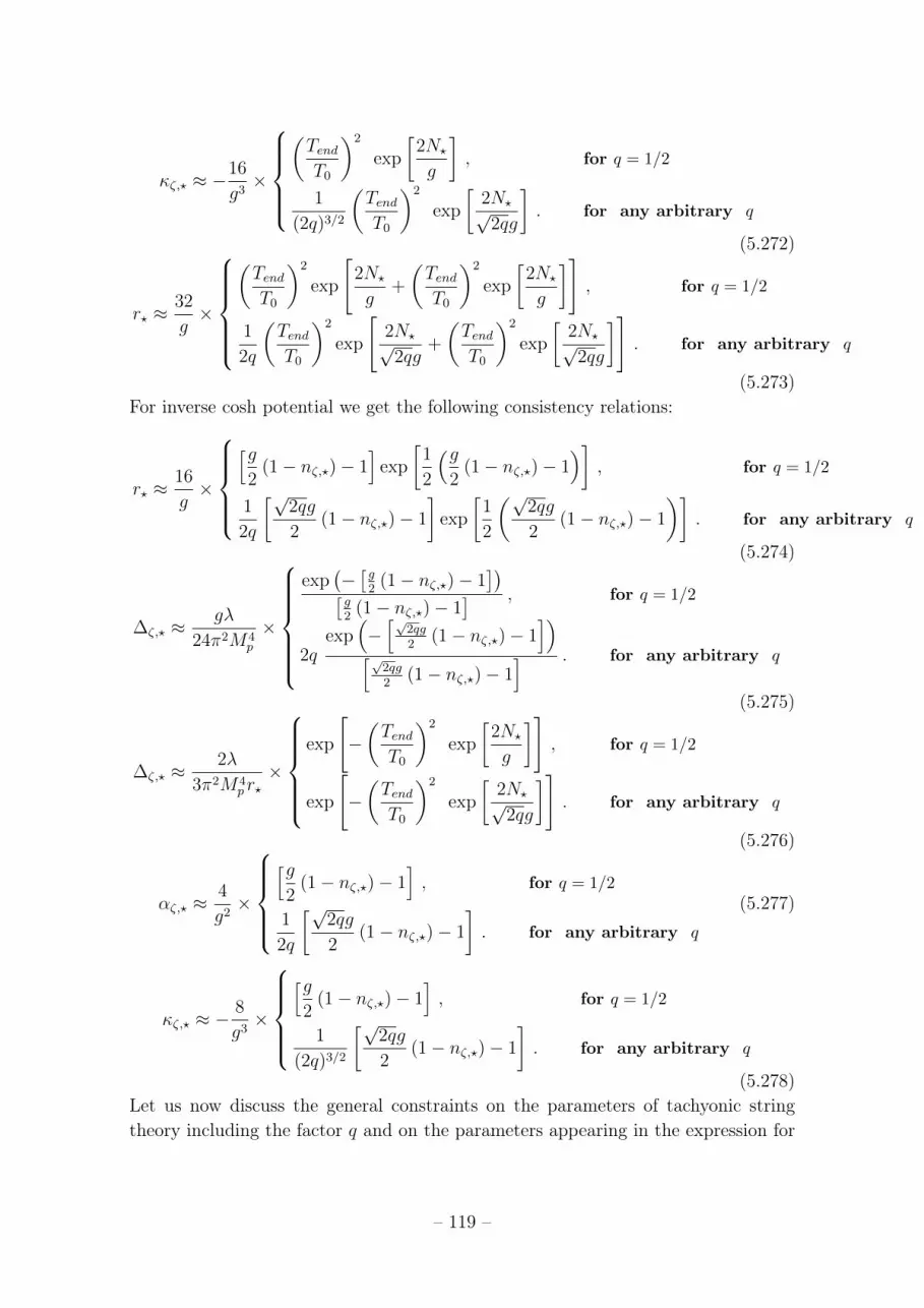
κζ,? ≈ −16

g3×

(TendT0

)2

exp

[2N?

g

], for q = 1/2

1

(2q)3/2

(TendT0

)2

exp

[2N?√2qg


(5.272)

r? ≈32

g×

(TendT0

)2

exp

[2N?

g+

(TendT0

)2

exp

[2N?

g

]], for q = 1/2

1

2q

(TendT0

)2

exp

[2N?√2qg

+

(TendT0

)2

exp

[2N?√2qg

]]. for any arbitrary q

(5.273)For inverse cosh potential we get the following consistency relations:

r? ≈16

g×

[g

2(1− nζ,?)− 1

]exp

[1

2

(g2

(1− nζ,?)− 1)]

, for q = 1/2

1

2q

[√2qg

2(1− nζ,?)− 1

]exp

[1

2

(√2qg

2(1− nζ,?)− 1


(5.274)

∆ζ,? ≈gλ

24π2M4p

×

exp(−[g2

(1− nζ,?)− 1])[

g2

(1− nζ,?)− 1] , for q = 1/2

2qexp

(−[√

2qg2

(1− nζ,?)− 1])

[√2qg2

(1− nζ,?)− 1] . for any arbitrary q

(5.275)

∆ζ,? ≈2λ

3π2M4p r?×

exp

[−(TendT0

)2

exp

[2N?

g

]], for q = 1/2

exp

[−(TendT0

)2

exp

[2N?√2qg

]]. for any arbitrary q

(5.276)

αζ,? ≈4

g2×

[g

2(1− nζ,?)− 1

], for q = 1/2

1

2q

[√2qg

2(1− nζ,?)− 1


(5.277)

κζ,? ≈ −8

g3×

[g

2(1− nζ,?)− 1

], for q = 1/2

1

(2q)3/2

[√2qg

2(1− nζ,?)− 1


(5.278)Let us now discuss the general constraints on the parameters of tachyonic stringtheory including the factor q and on the parameters appearing in the expression for

– 119 –

Exponential potential-Type II. In Fig. (12(a)) and Fig. (12(b)), we have shown thebehavior of the tensor-to-scalar ratio r with respect to the scalar spectral index nζand the model parameter g for Exponential potential-Type II respectively. In boththe figures the purple and blue coloured line represent the upper bound of tensor-to-scalar ratio allowed by Planck+ BICEP2+Keck Array joint constraint and onlyPlanck 2015 data respectively. For both the figures red, green, brown, orange coloredcurve represent q = 1/2, q = 1, q = 3/2 and q = 2 respectively. The cyan color shadedregion bounded by two vertical black coloured lines in Fig. (12(a)) represent thePlanck 2σ allowed region and the rest of the light gray shaded region is showing the 1σ

allowed range, which is at present disfavoured by the Planck 2015 data and Planck+BICEP2+Keck Array joint constraint. The rest of the region is completely ruled outby the present observational constraints. From Fig. (12(a)) and Fig. (12(b)), it is alsoobserved that, within 50 < N? < 70, the Exponential potential-Type II is favouredonly for the characteristic index 1/2 < q < 2, by Planck 2015 data and Planck+BICEP2+Keck Array joint analysis. Also in Fig. (12(a)) for q = 1/2, q = 1, q = 3/2

and q = 2 we fix N?/g ∼ 0.85. This implies that for 50 < N? < 70, the prescribedwindow for g from r − nζ plot is given by, 59 < g < 82.3 considering 1/2 < q < 2.It is additionally important to note that, for q << 1/2, the tensor-to-scalar ratiocomputed from the model is negligibly small for Exponential potential-Type II. Thisimplies that if the inflationary tensor mode is detected near to its present upperbound on tensor-to-scalar ratio then all q << 1/2 possibilities for tachyonic inflationcan be discarded for Exponential potential-Type II. On the contrary, if inflationarytensor modes are never detected by any of the future observational probes thenq << 1/2 possibilities for tachyonic inflation in case of Exponential potential-TypeII is highly prominent. Also it is important to mention that, in Fig. (12(b)) withinthe window 30 < g < 93, if we smaller the value of g, then the inflationary tensor-to-scalar ratio also gradually decreases. To analyze the results more clearly let usdescribe the cosmological features from Fig. (12(a)) in detail. Let us first start withthe q = 1/2 situation, in which the 2σ constraint on the scalar spectral tilt is satisfiedwithin the window of tensor-to-scalar ratio, 0 < r < 0.065 for 50 < N? < 70. Nextfor q = 1 case, the same constraint is satisfied within the window of tensor-to-scalarratio, 0.030 < r < 0.12 for 50 < N? < 70. Further for q = 3/2 case, the sameconstraint on scalar spectral tilt is satisfied within the window of tensor-to-scalarratio, 0.045 < r < 0.12 for 50 < N? < 70. Finally, for q = 2 situation, the value forthe tensor-to-scalar ratio is 0.060 < r < 0.12, which is tightly constrained from theupper bound of spectral tilt from Planck 2015 observational data.

In Fig. (13(a)), Fig. (13(b)) and Fig. (13(c)), we have depicted the behavior ofthe scalar power spectrum ∆ζ vs the stringy parameter g, scalar spectral tilt nζ vsthe stringy parameter g and scalar power spectrum ∆ζ vs scalar spectral index nζfor Exponential potential-Type-II respectively. It is important to note that, for allof the figures red, green, brown, orange colored curve represent q = 1/2, q = 1,

– 120 –

q = 3/2 and q = 2 respectively. The purple and blue coloured line represent theupper and lower bound allowed by WMAP+Planck 2015 data respectively. Thecyan color shaded region bounded by two vertical black coloured lines represent thePlanck 2σ allowed region and the rest of the light gray shaded region is the 1σ

region, which is presently disfavoured by the joint Planck+WMAP constraints. Therest of the region is completely ruled out by the present observational constraints.From Fig. (13(a)) it is clearly observed that the observational constraints on theamplitude of the scalar mode fluctuations satisfy within the window 55 < g < 93

considering 1/2 < q < 2. For g > 93 the corresponding amplitude falls down in anon-trivial fashion by following the exact functional form as stated in Eq (5.269).Next using the behavior as shown in Fig. (13(b)), the lower bound on the stringyparameter g is constrained as, g > 73 by using the non-trivial relationship as statedin Eq (5.270). But at this lower bound of the parameter g the amplitude of thescalar power spectrum is slightly outside to the present observational constraints.This implies that, to satisfy both of the constraint from the amplitude of the scalarpower spectrum and its spectral tilt within 2σ CL the constrained numerical value ofthe stringy parameter is lying within the window 73 < g < 93. Also in Fig. (13(c))for q = 1/2, q = 1, q = 3/2 and q = 2 we fix N?/g ∼ 0.85, which further impliesthat for 50 < N? < 70, the prescribed window for g from ∆ζ − nζ plot is givenby, 59 < g < 82.3. If we additionally impose the constraint from the upper boundon tensor-to-scalar ratio then also the allowed parameter range is lying within thewindow i.e. 73 < g < 82.3.

In Fig. (14(a)) and Fig. (14(b)), we have shown the behaviour of the running ofthe scalar spectral tilt αζ and running of the running of the scalar spectral tilt κζwith respect to the scalar spectral index nζ for Exponential potential-Type II withg = 76 respectively. For both the figures red, green, brown, orange colored curverepresent q = 1/2, q = 1, q = 3/2 and q = 2 respectively. The cyan color shadedregion bounded by two vertical black coloured lines in both the plots represent thePlanck 2σ allowed region and the rest of the light gray shaded region is showing the1σ allowed range, which is at present disfavoured by the Planck data and Planck+BICEP2+Keck Array joint constraint. From both of these figures, it is also observedthat, within 50 < N? < 70 the Exponential potential-Type II is favoured for thecharacteristic index 1/2 < q < 2, by Planck 2015 data and Planck+ BICEP2+KeckArray joint analysis. From Fig. (14(a)) and Fig. (14(b)), it is observed that withinthe 2σ observed range of the scalar spectral tilt nζ , as the value of the characteristicparameter q increases, the value of the running αζ decreases and running of the run-ning κζ increases for Exponential potential-Type II. It is also important to note thatfor 1/2 < q < 2, the numerical value of the running αζ ∼ O(10−4) and running ofthe running κζ ∼ O(−10−6), which are perfectly consistent with the 1.5σ constraintson running and running of the running as obtained from Planck 2015 data.

– 121 –

Model V: Inverse power-law potentialFor single field case the first model of tachyonic potential is given by:

V (T ) =λ[

1 +(TT0

)4] , (5.279)

where λ characterize the scale of inflation and T0 is the parameter of the model. InFig. (15) we have depicted the symmetric behavior of the Inverse power-law potentialwith respect to scaled field coordinate T/T0 in dimensionless units. In this case thetachyon field started rolling down from the top hight of the potential situated at theorigin and take part in inflationary dynamics.

-4 -2 0 2 40.0

0.2

0.4

0.6

0.8

1.0

1.2

T�T0

VHT

L�Λ

Inverse power-law potential

Figure 15. Variation of the Inverse power-law potential V (T )/λ with field T/T0 in dimen-sionless units.


εV =1

2g

16(TT0

)6[1 +

(TT0

)4] , (5.280)

ηV =1

g

4

[5(TT0

)4

− 3

][1 +

(TT0

)4] , (5.281)

– 122 –

ξ2V =

1

g2

96(TT0

)2[5(TT0

)8

− 10(TT0

)4

+ 1

][1 +

(TT0

)4]2 , (5.282)

σ3V =

1

g3

384(TT0

)6[5(TT0

)4(

7(TT0

)8

− 31(TT0

)4

+ 13

)− 1

][1 +

(TT0

)4]3 , (5.283)


g =α′λT 2

0

M2p

=M4

s

(2π)3gs

α′T 2

0

M2p

. (5.284)


N(T ) =

g

8

1(TT0

)2 −1(

TendT0

)2

, for q = 1/2

√2q

g

8

1(TT0

)2 −1(

TendT0

)2


(5.285)


εV (Tend) = 1, (5.286)

we get the following field values at the end of inflation:

Tend ∼√g

8T0. (5.287)


T? = T0 ×

1√8g

(N? + 1), for q = 1/2

1√8g

(N?√

2q+ 1) . for any arbitrary q

(5.288)


|∆T | = T0 ×

∣∣∣∣∣∣ 1√8g

(N? + 1)−√g

8

∣∣∣∣∣∣ , for q = 1/2∣∣∣∣∣∣∣∣1√

8g

(N?√

2q+ 1) −√g

8

∣∣∣∣∣∣∣∣ . for any arbitrary q

(5.289)

– 123 –

Finally we compute the following inflationary observables:

∆ζ,? ≈gλ

12π2M4p

×

1

16(

8g

(N? + 1))3 , for q = 1/2

2q

16(

8g

(N?√

2q+ 1))3 . for any arbitrary q

(5.290)

nζ,? − 1 ≈

− 3

(N? + 1), for q = 1/2

− 3(N?√


(5.291)

αζ,? ≈

− 3

(N? + 1)2 , for q = 1/2

− 3√

2q(N?√

2q+ 1)2 . for any arbitrary q

(5.292)

κζ,? ≈

− 6

(N? + 1)3 , for q = 1/2

− 6

2q(N?√

2q+ 1)3 . for any arbitrary q

(5.293)

r? ≈

16

(N? + 1), for q = 1/2

16

2q(N?√


(5.294)


r? ≈16

3(1− nζ,?)×

1 , for q = 1/2

1

2q. for any arbitrary q

(5.295)

∆ζ,? ≈g4λ(1− nζ,?)3

12π2M4p

×

1

221184, for q = 1/2

2q

221184. for any arbitrary q

(5.296)

– 124 –

0.94 0.95 0.96 0.97 0.98 0.99 1.000.00

0.02

0.04

0.06

0.08

0.10

0.12

0.14

nΖ

rr vs nΖ plot for Inverse power-law potential

(a) r vs nζ .

0.95 0.96 0.97 0.98 0.99 1.00

1.6 ´ 10-9

1.8 ´ 10-9

2. ´ 10-9

2.2 ´ 10-9

2.4 ´ 10-9

2.6 ´ 10-9

2.8 ´ 10-9

3. ´ 10-9

nΖD

Ζ

DΖ vs nΖ plot for Inverse power-law potential

(b) ∆ζ vs nζ .

Figure 16. In 16(a) the behaviour of the tensor-to-scalar ratio r with respect to the scalarspectral index nζ and 16(b) the parameter g for Inverse power-law potential. The purple andblue coloured line represent the upper bound of tensor-to-scalar ratio allowed by Planck+BICEP2+Keck Array joint constraint and only Planck 2015 data respectively. For boththe figures red, green, brown, orange colored curve represent q = 1/2, q = 1, q = 3/2 andq = 2 respectively. The cyan color shaded region bounded by two vertical black colouredlines in 16(a) represent the Planck 2σ allowed region and the rest of the light gray shadedregion is showing the 1σ allowed range, which is at present disfavoured by the Planck dataand Planck+ BICEP2+Keck Array joint constraint. In 16(a), we have explicitly shownthat in r − nζ plane the observationally disfavoured value of the characteristic index isq ≥ 1/2. Variation of the scalar power spectrum ∆ζ vs scalar spectral index nζ is shown in16(b). The purple and blue coloured line represent the upper and lower bound allowed byWMAP+Planck 2015 data respectively. The green dotted region bounded by two verticalblack coloured lines represent the Planck 2σ allowed region and the rest of the light grayshaded region is disfavoured by the Planck+WMAP constraint. In 16(b), we have explicitlyshown that in ∆ζ − nζ plane the observationally favoured value of the characteristic indexis q = 1 and q = 3/2. From 16(a) and 16(b), it is also observed that, within 50 < N? < 70

the Inverse power-law potential is favoured for the characteristic index 3/2 < q < 1, byPlanck 2015 data and Planck+ BICEP2+Keck Array joint analysis.

∆ζ,? ≈g4λr3

?

12π2M4p

×

1

33554432, for q = 1/2

(2q)3

33554432. for any arbitrary q

(5.297)

– 125 –

0.92 0.94 0.96 0.98 1.00

-0.0020

-0.0015

-0.0010

-0.0005

0.0000

nΖ

ΑΖ

ΑΖ vs nΖ plot for Inverse power-law potential

(a) αζ vs nζ .

0.92 0.94 0.96 0.98 1.00-0.00012

-0.00010

-0.00008

-0.00006

-0.00004

-0.00002

0.00000

nΖ

ΚΖ

ΚΖ vs nΖ plot for Inverse power-law potential

(b) κζ vs nζ .



– 126 –

αζ,? ≈ −1

3(nζ,? − 1)2 ×

1 , for q = 1/2

1√2q. for any arbitrary q

(5.298)

κζ,? ≈2

9(nζ,? − 1)3 ×

1 , for q = 1/2

1

2q. for any arbitrary q

(5.299)

Let us now discuss the general constraints on the parameters of tachyonic stringtheory including the factor q and on the parameters appearing in the expressionfor Inverse power-law potential. In Fig. (16(a)), we have shown the behavior of thetensor-to-scalar ratio r with respect to the scalar spectral index nζ for Inverse power-law potential respectively. In both the figures the purple and blue coloured line rep-resent the upper bound of tensor-to-scalar ratio allowed by Planck+ BICEP2+KeckArray joint constraint and only Planck 2015 data respectively. For both the figuresred, green, brown, orange colored curve represent q = 1/2, q = 1, q = 3/2 and q = 2

respectively. The cyan color shaded region bounded by two vertical black colouredlines in Fig. (16(a)) represent the Planck 2σ allowed region and the rest of the lightgray shaded region is showing the 1σ allowed range, which is at present disfavouredby the Planck 2015 data and Planck+ BICEP2+Keck Array joint constraint. Therest of the region is completely ruled out by the present observational constraints.From Fig. (16(a)), it is also observed that, within 50 < N? < 70, the Inverse power-law potential is favoured for the characteristic index 1 < q < 2, by Planck 2015 dataand Planck+ BICEP2+Keck Array joint analysis. Also in Fig. (16(a)) for q = 1/2,q = 1, q = 3/2 and q = 2 we fix N? ∼ 70. One can draw the similar characteristiccurves for any value of the e-foldings lying within the window 50 < N? < 70 also.To analyze the results more clearly let us describe the cosmological features fromFig. (16(a)) in detail. Let us first start with the q = 1/2 situation, in which the2σ constraint on the scalar spectral tilt is disfavoured for 50 < N? < 70. Next forq = 1 case, the same constraint is satisfied within the window of tensor-to-scalarratio, 0.07 < r < 0.10 for 50 < N? < 70. Further for q = 3/2 case, the same con-straint on scalar spectral tilt is satisfied within the window of tensor-to-scalar ratio,0.05 < r < 0.07 for 50 < N? < 70. Finally, for q = 2 situation, the value for thetensor-to-scalar ratio is 0.035 < r < 0.05.

In Fig. (16(b)), we have depicted the behavior of the scalar power spectrum ∆ζ

vs scalar spectral tilt nζ for Inverse power-law potential respectively. It is importantto note that, for all of the figures red, green, brown, orange colored curve representq = 1/2, q = 1, q = 3/2 and q = 2 respectively. The purple and blue colouredline represent the upper and lower bound allowed by WMAP+Planck 2015 data re-spectively. The cyan color shaded region bounded by two vertical black coloured

– 127 –

lines represent the Planck 2σ allowed region and the rest of the light gray shadedregion is the 1σ region, which is presently disfavoured by the joint Planck+WMAPconstraints. The rest of the region is completely ruled out by the present observa-tional constraints. Also in Fig. (16(b)) for q = 1/2, q = 1, q = 3/2 and q = 2

we fix N? ∼ 70. But plots can be reproduced for 50 < N? < 70 also consideringthe present observational constraints from Planck 2015 data. It is clearly observedfrom Fig. (16(b)) that the Planck 2015 constraint on amplitude of the scalar powerspectrum ∆ζ and the scalar spectral tilt nζ disfavour q = 1/2 and q = 2 values forInverse power-law potential.

In Fig. (17(a)) and Fig. (17(b)), we have shown the behaviour of the running ofthe scalar spectral tilt αζ and running of the running of the scalar spectral tilt κζ withrespect to the scalar spectral index nζ for Inverse power-law potential respectively.For both the figures red, green, brown, orange colored curve represent q = 1/2,q = 1, q = 3/2 and q = 2 respectively. The cyan color shaded region bounded bytwo vertical black coloured lines in both the plots represent the Planck 2σ allowedregion and the rest of the light gray shaded region is showing the 1σ allowed range,which is at present disfavoured by the Planck data and Planck+ BICEP2+KeckArray joint constraint. From both of these figures, it is also observed that, within50 < N? < 70 the Inverse power-law potential is favoured for the characteristicindex 1/2 < q < 2, by Planck 2015 data and Planck+ BICEP2+Keck Array jointanalysis. If we additionally impose the constraints from r − nζ and ∆ζ − nζ planethen the stringent window on the characteristic index of GTachyon is lying within1 < q < 3/2. It is also important to note that for any values of q, the numericalvalue of the running αζ ∼ O(−10−4) and running of the running κζ ∼ O(−10−5),which are perfectly consistent with the 1.5σ constraints on running and running ofthe running as obtained from Planck 2015 data. For q = 1/2, q = 1, q = 3/2 andq = 2 g is not explicitly appearing in the various inflationary observables except theamplitude of scalar power spectrum in this case. To produce the correct value of theamplitude of the scalar power spectra we fix the parameter 600 < g < 700.

5.1.9 Analyzing CMB power spectrum

In this section we explicitly study the cosmological consequences from the CMB TT,TE, EE, BB-angular power spectrum computed from all the proposed models ofinflation 5. The angular power spectra or equivalently the two point correlator of X

5In this work we have not consider possibility of other cross correlators i.e. TB, EB as thereis no observational evidence of such contributions in the CMB map. Also till date there is noobservational evidence for inflationary origin of BB angular power spectrum except from CMBlensing [129]. However, for the sake of completeness in this paper we show the theoretical BBangular power spectra from the various models of tachyonic potential.

– 128 –

and Y fields are defined as [10]:

CXY` ≡ 1

2`+ 1

l∑m=−l

〈a∗X,`maY,`m〉 , X, Y = T,E,B . (5.300)

Here l characterizes the CMB multipole and m signifies the magnetic quantum num-ber which runs from m = −l, · · · ,+l. In general, the field X(n) and Y (n) can beexpressed in terms of the following harmonic expansion:

X(n), Y (n) =

∞∑l=0

+l∑m=−l

aT,lmVlm(n) , for X = T

∞∑l=0

+l∑m=−l

aE,lmVlm(n) , for X = E

∞∑l=0

+l∑m=−l

aB,lmVlm(n) , for X = B

(5.301)

where n is the arbitrary directional unit vector in CMB map. Here Vlm(n) are thespherical harmonics which are chosen to be the basis of the harmonic expansion ofthe temperature anisotropy and E and B polarization. Further using the inflationarypower spectra at any momentum scale k:

∆(k) ≡ {∆ζ(k),∆h(k)} (5.302)

the angular power spectra for CMB temperature fluctuations and polarization canbe expressed as [10]:

CXY` =

2

π

∫k2dk ∆(k)︸︷︷︸

Inflation

ΘX`(k)ΘY `(k)︸︷︷︸Anisotropies

, (5.303)

where the anisotropic integral kernel can be written as [10]:

ΘX`(k) =

∫ η0

0

dη SX(k, η)︸︷︷︸Sources

PX`(k[η0 − η])︸︷︷︸Projection

. (5.304)

The integral (5.303) relates the inhomogeneities predicted by inflation, ∆(k), tothe anisotropies observed in the CMB, CXY

` . The correlations between the differentXand Y modes are related by the transfer functions ΘX`(k) and ΘY `(k). The transferfunctions may be written as the line-of-sight integral Eq (5.304) which factorizesinto physical source terms SX(k, η) and geometric projection factors PX`(k[η0 − η])

through combinations of Bessel functions.

– 129 –

0

1000

2000

3000

4000

5000

6000

7000

1 10 100 1000

l(l+

1)/

2π

ClT

Tµ

K2

l

CMB TT Angular power spectrum

Planck 2015 dataInverse cosh q=1/2

Inverse cosh q=1Inverse cosh q=3/2

Inverse cosh q=2

(a) l(l + 1)CTTl /2π vs l (scalar)

0

1000

2000

3000

4000

5000

6000

7000

1 10 100 1000

l(l+

1)/

2π

ClT

Tµ

K2

l


Planck 2015 dataLogarithmic q=1/2

Logarithmic q=1

(b) l(l + 1)CTTl /2π vs l (scalar)

0

1000

2000

3000

4000

5000

6000

7000

1 10 100 1000

l(l+

1)/

2π

ClT

Tµ

K2

l


Planck 2015 dataExponential-Type I q=1

Exponential-Type I q=3/2Exponential-Type I q=2

(c) l(l + 1)CTTl /2π vs l (scalar)

0

1000

2000

3000

4000

5000

6000

7000

1 10 100 1000

l(l+

1)/

2π

ClT

Tµ

K2

l


Planck 2015 dataExponential-Type II q=1/2

Exponential-Type II q=1Exponential-Type II q=3/2

Exponential-Type II q=2

(d) l(l + 1)CTTl /2π vs l (scalar)

0

1000

2000

3000

4000

5000

6000

7000

1 10 100 1000

l(l+

1)/

2π

ClT

Tµ

K2

l


Planck 2015 dataInverse power-law q=1

Inverse power-law q=3/2

(e) l(l + 1)CTTl /2π vs l (scalar)

Figure 18. We show the variation of CMB TT Angular power spectrum with respect tothe multipole, l for scalar modes for all five tachyonic models.

– 130 –

-150

-100

-50

0

50

100

150

0 500 1000 1500 2000

l(l+

1)/

2π

ClT

Eµ

K2

l

CMB TE Angular power spectrum



Inverse cosh q=2

(a) l(l + 1)CTEl /2π vs l (scalar)

-150

-100

-50

0

50

100

150

0 500 1000 1500 2000

l(l+

1)/

2π

ClT

Eµ

K2

l



Logarithmic q=1

(b) l(l + 1)CTEl /2π vs l (scalar)

-150

-100

-50

0

50

100

150

0 500 1000 1500 2000

l(l+

1)/

2π

ClT

Eµ

K2

l




(c) l(l + 1)CTEl /2π vs l (scalar)

-150

-100

-50

0

50

100

150

0 500 1000 1500 2000

l(l+

1)/

2π

ClT

Eµ

K2

l





(d) l(l + 1)CTEl /2π vs l (scalar)

-150

-100

-50

0

50

100

150

0 500 1000 1500 2000

l(l+

1)/

2π

ClT

Eµ

K2

l




(e) l(l + 1)CTEl /2π vs l (scalar)

Figure 19. We show the variation of CMB TE Angular power spectrum with respect tothe multipole, l for scalar modes for all five tachyonic models.

– 131 –

-10

0

10

20

30

40

50

0 500 1000 1500 2000

l(l+

1)/

2π

ClE

Eµ

K2

l

CMB EE Angular power spectrum



Inverse cosh q=2

(a) l(l + 1)CEEl /2π vs l (scalar)

-10

0

10

20

30

40

50

0 500 1000 1500 2000

l(l+

1)/

2π

ClE

Eµ

K2

l



Logarithmic q=1

(b) l(l + 1)CEEl /2π vs l (scalar)

-10

0

10

20

30

40

50

0 500 1000 1500 2000

l(l+

1)/

2π

ClE

Eµ

K2

l




(c) l(l + 1)CEEl /2π vs l (scalar)

-10

0

10

20

30

40

50

0 500 1000 1500 2000

l(l+

1)/

2π

ClE

Eµ

K2

l





(d) l(l + 1)CEEl /2π vs l (scalar)

-10

0

10

20

30

40

50

0 500 1000 1500 2000

l(l+

1)/

2π

ClE

Eµ

K2

l




(e) l(l + 1)CEEl /2π vs l (scalar)

Figure 20. We show the variation of CMB EE Angular power spectrum with respect tothe multipole, l for scalar modes for all five tachyonic models.

– 132 –

1e-06

1e-05

0.0001

0.001

0.01

1 10 100 1000

l(l+

1)/

2π

ClB

Bµ

K2

l

CMB BB (tensor) Angular power spectrum

Inverse cosh q=1/2Inverse cosh q=1


(a) l(l + 1)CBBl /2π vs l (tensor)

1e-09

1e-08

1e-07

1e-06

1e-05

0.0001

0.001

0.01

1 10 100 1000

l(l+

1)/

2π

ClB

Bµ

K2

l


Logarithmic q=1/2Logarithmic q=1

(b) l(l + 1)CBBl /2π vs l (tensor)

1e-06

1e-05

0.0001

0.001

0.01

1 10 100 1000

l(l+

1)/

2π

ClB

Bµ

K2

l


Exponential-Type I q=1Exponential-Type I q=3/2

Exponential-Type I q=2

(c) l(l + 1)CBBl /2π vs l (tensor)

1e-06

1e-05

0.0001

0.001

0.01

1 10 100 1000

l(l+

1)/

2π

ClB

Bµ

K2

l


Exponential-Type II q=1/2Exponential-Type II q=1


(d) l(l + 1)CBBl /2π vs l (tensor)

1e-06

1e-05

0.0001

0.001

0.01

1 10 100 1000

l(l+

1)/

2π

ClB

Bµ

K2

l


Inverse power-law q=1Inverse power-law q=3/2

(e) l(l + 1)CBBl /2π vs l (tensor)

Figure 21. We show the variation of CMB BB Angular power spectrum with respect tothe multipole, l for tensor modes for all five tachyonic models.

– 133 –

0.001

0.01

0.1

1

10

1 10 100 1000

l(l+

1)/

2π

ClT

Tµ

K2

l

CMB TT (tensor) Angular power spectrum



(a) l(l + 1)CTTl /2π vs l (tensor)

1e-08

1e-07

1e-06

1e-05

0.0001

0.001

0.01

0.1

1

10

1 10 100 1000

l(l+

1)/

2π

ClT

Tµ

K2

l



(b) l(l + 1)CTTl /2π vs l (tensor)

0.001

0.01

0.1

1

10

1 10 100 1000

l(l+

1)/

2π

ClT

Tµ

K2

l




(c) l(l + 1)CTTl /2π vs l (tensor)

0.001

0.01

0.1

1

10

1 10 100 1000

l(l+

1)/

2π

ClT

Tµ

K2

l




(d) l(l + 1)CTTl /2π vs l (tensor)

0.001

0.01

0.1

1

10

1 10 100 1000

l(l+

1)/

2π

ClT

Tµ

K2

l



(e) l(l + 1)CTTl /2π vs l (tensor)

Figure 22. We show the variation of CMB TT Angular power spectrum with respect tothe multipole, l for tensor modes for all five tachyonic models.

– 134 –

-0.4

-0.3

-0.2

-0.1

0

0.1

1 10 100 1000

l(l+

1)/

2π

ClT

Eµ

K2

l

CMB TE (tensor) Angular power spectrum



(a) l(l + 1)CTEl /2π vs l (tensor)

-0.3

-0.25

-0.2

-0.15

-0.1

-0.05

0

1 10 100 1000

l(l+

1)/

2π

ClT

Eµ

K2

l



(b) l(l + 1)CTEl /2π vs l (tensor)

-0.4

-0.3

-0.2

-0.1

0

0.1

1 10 100 1000

l(l+

1)/

2π

ClT

Eµ

K2

l




(c) l(l + 1)CTEl /2π vs l (tensor)

-0.25

-0.2

-0.15

-0.1

-0.05

0

0.05

0.1

1 10 100 1000

l(l+

1)/

2π

ClT

Eµ

K2

l




(d) l(l + 1)CTEl /2π vs l (tensor)

-0.4

-0.3

-0.2

-0.1

0

0.1

1 10 100 1000

l(l+

1)/

2π

ClT

Eµ

K2

l



(e) l(l + 1)CTEl /2π vs l (tensor)

Figure 23. We show the variation of CMB TE Angular power spectrum with respect tothe multipole, l for tensor modes for all five tachyonic models.

– 135 –

1e-06

1e-05

0.0001

0.001

0.01

1 10 100 1000

l(l+

1)/

2π

ClE

Eµ

K2

l

CMB EE (tensor) Angular power spectrum



(a) l(l + 1)CEEl /2π vs l (tensor)

1e-09

1e-08

1e-07

1e-06

1e-05

0.0001

0.001

0.01

1 10 100 1000

l(l+

1)/

2π

ClE

Eµ

K2

l



(b) l(l + 1)CEEl /2π vs l (tensor)

1e-06

1e-05

0.0001

0.001

0.01

1 10 100 1000

l(l+

1)/

2π

ClE

Eµ

K2

l




(c) l(l + 1)CEEl /2π vs l (tensor)

1e-06

1e-05

0.0001

0.001

0.01

1 10 100 1000

l(l+

1)/

2π

ClE

Eµ

K2

l




(d) l(l + 1)CEEl /2π vs l (tensor)

1e-06

1e-05

0.0001

0.001

0.01

1 10 100 1000

l(l+

1)/

2π

ClE

Eµ

K2

l



(e) l(l + 1)CEEl /2π vs l (tensor)

Figure 24. We show the variation of CMB EE Angular power spectrum with respect tothe multipole, l for tensor modes for all five tachyonic models.

– 136 –

Further expressing Eq (5.303) in terms of TT, TE, EE, BB correlation I get:

For curvature perturbation :

CTT` =

2

π

∫k2dk ∆S(k) ΘT`(k)ΘT`(k) , (5.305)

CTE` = (4π)2

∫k2dk ∆S(k) ΘT`(k)ΘE`(k) , (5.306)

CEE` = (4π)2

∫k2dk ∆S(k) ΘE`(k)ΘE`(k) , (5.307)

For tensor perturbation :

CBB` = (4π)2

∫k2dk ∆h(k) ΘB`(k)ΘB`(k) (5.308)

CTT` =

2

π

∫k2dk ∆h(k) ΘT`(k)ΘT`(k) , (5.309)

CTE` = (4π)2

∫k2dk ∆h(k) ΘT`(k)ΘE`(k) , (5.310)

CEE` = (4π)2

∫k2dk ∆h(k) ΘE`(k)ΘE`(k) . (5.311)

where the inflationary power spectra {∆ζ(k),∆h(k)} are parametrized at anyarbitrary momentum scale k as 6:

∆ζ(k) = ∆ζ,?

(k

cSk?

)nζ,?−1+αζ,?

2ln(

kcSk?

)+κζ,?

6ln2(

kcSk?

)+....

, (5.312)

∆h(k) = r(k)∆ζ(k) = ∆h,?

(k

k?

)nh,?+αh,?

2ln( k

k?)+

κh,?6

ln2( kk?

)+....

. (5.313)

It is important to note that the cosmological significance of the E and B decompo-sition of CMB polarization carries the following significant features:

• Curvature (density) perturbations create only polarizing E-modes.

• Vector (vorticity) perturbations create mainly B-modes. However, it is im-portant note that here that the contributions of vector modes decay with theexpansion of the universe and are therefore sub-dominant at the epoch of re-combination. For this reason we have neglected such sub-dominant effects fromour rest of the analysis.

6However, it is important to mention here that if we know the mode scalar and tensor modefunctions, which are obtained from the the exact solution of Mukhanov-Sasaki equation for exactlyBunch-Davies vacuum or for any arbitrary vacuum then one can implement the exact structuralform of the primordial power spectra. But within the slow-roll regime of inflation the presentedversion of the parametrization of the power spectra is exactly compatible with the exact powerspectrum from the solution of the Mukhanov-Sasaki equation.

– 137 –

• Tensor (gravitational wave) perturbations create both E-modes and B-modes.But to quantify the exact contribution of the primordial gravitational waves,specifically in the inflationary B modes, one need to separate all the othersignificant contributions in the B modes i.e. primordial magnetic field, gravi-tational lensing, non-Gaussianity etc. But at present in cosmological literatureno such sophisticated techniques or algorithms are available using which onecan separate all of these significant contributions completely.

To compute the momentum integrals numerically and to analyze the various fea-tures of CMB angular power spectra from all of the inflationary models mentionedin the last section, here we use a semi-analytical code “CAMB”. For the numericalanalysis we use here the best fit model parameters corresponding to all of the fivetachyonic models, which are compatible with Planck 2015 data. Additionally wetake ΛCDM background. Further we put all these inputs to “CAMB” and modifythe inbuilt parameterization of power spectrum for scalar and tensor modes accord-ingly. After performing all the numerical computations via “CAMB” finally fromour analysis we have generated all the theoretical CMB angular power spectra fromwhich we observed the following significant features:-

• In Fig. (18), at low ` region (2 < l < 49) the contributions from the running(αζ , αh), and running of running (κζ , κh) are very small. Their additional con-tribution to the CMB power spectrum for scalar and tensor modes becomesunity (O(1)) within low-l region and the original power spectrum becomes un-changed. As a result the tachyonic models will be well fitted with the CMB TTspectrum at low-l region within high cosmic variance as observed by Planckexcept for a few outliers according to the Planck 2013 data release 7. But toupdate our analysis with the latest Planck 2015 data set we have not shownsuch high cosmic variance explicitly. In case of WMAP9 data for CMB TTspectrum the cosmic variance in the low-l region is not very large comparedto the Planck low-l data. But our tachyonic models is also well fitted withWMAP9 low-l data also which we have not shown explicitly in the plot toupdate the analysis using Planck 2015 data. It is also important to mentionthat if we incorporate the uncertainties in the scanning multipole l for themeasurement of CMB TT spectrum, then also our prescribed analysis is prettyconsistent with the Planck 2015 data. Further if we move towards high ` regime(47 < l < 2500) the contribution of running and running of running becomestronger and this will enhance the power spectrum to a permissible value suchthat it will accurately fit high-l data within very small cosmic variance as ob-served by Planck. In this way one can easily scan over all the multipoles starting

7From Fig. (18) it is observed that for Inverse cosh and Logarithmic model q = 1/2, Exponen-tial Type-I and Type II model q = 1, Inverse power-law model q = 1 and q = 3/2 generalizedcharacteristic indices are well fitted with Planck 2015 data.

– 138 –

from low-l to high-l using the same momentum dependent parameterization oftensor-to-scalar ratio.

• From Fig. (18), we see that the Sachs-Wolfe plateau obtained from our proposedtachyonic models is non flat, confirming the appearance of running, and runningof the running in the spectrum observed for low l region (l < 47). For largervalue of the multipole (47 < l < 2500), CMB anisotropy spectrum is dominatedby the Baryon Acoustic Oscillations (BAO), giving rise to several ups anddowns in the CMB TT spectrum. In the low l region due to the presence ofvery large cosmic variance there may be other pre-inflationary scenarios whichmight be able to describe the TT-power spectrum better. In my study we haveconsidered only the possibility for which the behaviour of tachyonic models isanalyzed for both low and high l regions.

• From Fig. (18), Fig. (19), Fig. (20), we observe that if we include the uncer-tainties in multipole l as well in the observed CMB angular power spectra thenthe proposed tachyonic models is pretty consistent with the CMB TT, TE, EEfor scalar mode from Planck 2015 data.

• In Fig. (21), Fig. (22), Fig. (23) and Fig. (24) we have explicitly shown the the-oretical CMB BB, TT, TE and EE angular power spectrum from tensor mode.Most importantly, if inflationary paradigm is responsible for the nearly de-Sitterexpansion of the early universe then the CMB BB spectra for tensor modes isone of the prime components trough which one can detect the contributionfor primordial gravitational waves via tensor-to-scalar ratio. But till date onlythe contribution from the lensing B-modes are detected via South Pole Tele-scope and Planck 2015 +BICEP2/Keck Array joint mission. But confirmingthe sole inflationary origin from the detection of the de-lensed version of thesignal is not sufficient enough to draw any final conclusion 8. There are otherpossibilities as well through which it is possible to generate CMB B-modes,those components are, Primordial Magnetic Field, Gravitational Lensing, CPasymmetry in the lepton sector of particle physics etc.

5.2 Computation for Assisted inflation

In case of assisted inflation [130–133] all the tachyons would follow a similar trajectorywith a unique late time attractor 9. In more technical language one can state that:

T1 ∼ T2 ∼ · · ·TM ≡ Ti = T ∀i = 1, 2, · · · ,M. (5.314)

8In this respect one may consider the alternative frameworks of inflationary paradigm as well.9We also suggest the readers to read ref. [134] for completeness.

– 139 –

Most importantly the detailed computation of the density and tensor perturbationresponsible for the anisotropy of CMB depends on this late time attractor behaviorof the fields.


For assisted tachyonic inflation, the prime condition for inflation is given by:

H +H2 =

(a

a

)= −

M∑i=1

(ρi + 3pi)

6M2p

=(ρ+ 3p)

6M2p

> 0 (5.315)

which can be re-expressed in terms of the following constraint condition in the contextof assisted tachyonic inflation:

M∑i=1

V (Ti)

3M2p

√1− α′T 2

i

(1− 3

2α′T 2i

)=

MV (T )

3M2p

√1− α′T 2

(1− 3

2α′T 2

)> 0. (5.316)


T <

√2

3α′∀i = 1, 2, · · · ,M, (5.317)

T < 3HT <

√6

α′H ∀i = 1, 2, · · · ,M. (5.318)


3Hα′Ti +

dV (Ti)

V (Ti)dTi≈ 0 ∀i = 1, 2, · · · ,M , (5.319)

Similarly, in the most generalized case,

M∑i=1

V (Ti)

3M2p

(1− α′T 2

i

)1−q

(1− (1 + q)α

′T 2i

)=

MV (T )

3M2p

(1− α′T 2

)1−q

(1− (1 + q)α

′T 2)> 0.

(5.320)Here Eq (5.320) implies that to satisfy inflationary constraints in the slow-roll regimethe following constraint always holds good:

T <

√1

α′(1 + q)∀i = 1, 2, · · · ,M, (5.321)

T < 3HT <

√9

α′(1 + q)H ∀i = 1, 2, · · · ,M. (5.322)

– 140 –


6qα′HTi +

dV (Ti)

V (Ti)dTi≈ 0 ∀i = 1, 2, · · · ,M (5.323)


H2 ≈M∑i=1

V (Ti)

3M2p

=MV (T )

3M2p

. (5.324)

The equation of motions can be mapped to the equations of a model with singletachyonic field using the following redefinitions:

T =√MT, (5.325)

V = V (T ) = MV (T ) =M∑i=1

V (Ti). (5.326)

Now to show the late time attractor behaviour of the solution of scalar fields we keepT1, but replace the rest of the part with the redefined fields:

χi = Ti − T1 ∀i = 2, · · · ,M. (5.327)

Using Eq (5.327), at late times the equation of motion can be recast as:

0 =

1√−g

∂µ

(√−gVeff (T1, χi)

√1 + gαβ∂αχi∂βχi

)=

α′χi

(1− α′χ2i )

+ 3Hα′χi +

dVeff (T1, χi)

Veff (T1, χi)dχi, for q = 1/2

1√−g

∂µ(√−gVeff (T1, χi)

(1 + gαβ∂αχi∂βχi

)q)=

2qα′χi

(1− α′χ2i )

+ 6qα′H

χi1− α′(1− 2q)χ2

i

+dVeff (T1, χi)

Veff (T1, χi)dχi, for any q

(5.328)where Veff (T1, χi) represents the effective potential. The minimum in the χi directionis always appearing at χi = 0, regardless of the explicit behaviour of the tachyon fieldT1. Consequently the late time solutions has all the Ti equal. From this analysis itis also observed that the length of the time interval to reach this attractor behaviourwill depend on the initial separation i.e. the tachyon field value χi and the extent offrictional contribution coming from the expansion rate H.

It is important to mention that, for assisted inflation the equation of motion foreach tachyon fields follows the following simple relationship:

d lnTidt

' d lnT

dt∀i = 1, 2, · · · ,M. (5.329)

– 141 –

Further substituting Eq (5.324) in Eq (5.319) and Eq (5.323) we get:√3MV (T )

Mp

α′Ti +

dV (Ti)

V (Ti)dTi≈ 0 , (5.330)

6q

√MV (T )√

3Mp

α′Ti +

dV (Ti)

V (Ti)dTi≈ 0 . (5.331)


t− tin ≈ −√

3Mα′

Mp

∫ Ti

Tin

dTi

√V (T )V (Ti)

V ′(Ti), (5.332)

t− tin ≈ −6q√Mα

′

√3Mp

∫ Ti

Tin

dTi

√V (T )V (Ti)

V ′(Ti). (5.333)

Further using Eq (5.15), Eq (5.16) and Eq (5.324) we get the following solution forthe scale factor in terms of the tachyonic field for usual q = 1/2 and for generalizedvalue of q as:

a = ain ×

exp

[−α

′M

M2p

∫ Ti

Tin

dTiV (T )V (Ti)

V ′(Ti)

], for q = 1/2

exp

[−2qα

′M

M2p

∫ Ti

Tin

dTiV (T )V (Ti)

V ′(Ti)


(5.334)


Here our prime objective is to define slow-roll parameters for tachyon inflation interms of the Hubble parameter and the assisted tachyonic inflationary potential.Using the slow-roll approximation one can expand various cosmological observablesin terms of small dynamical quantities derived from the appropriate derivatives ofthe Hubble parameter and of the inflationary potential. To start with here we usethe horizon-flow parameters based on derivatives of Hubble parameter with respectto the number of e-foldings N , defined as:

N(t) =

∫ tend

t

H(t) dt, (5.335)

where tend signifies the end of inflation. Further using Eq (5.5), Eq (5.9), Eq (5.10)and eq (5.335) we get:

dTidN

=TiH

=

− 2H

′

3α′H3, for q = 1/2

− 2H′

3α′H3

(1− α′(1− 2q)T 2

i

2q


(5.336)

– 142 –

where H ′ > 0 which makes always Ti > 0 during inflationary phase. Further usingEq (5.336) we get the following differential operator identity for tachyonic inflation:

1

H

d

dt=

d

dN=

d

d ln k=

− 2H

′

3α′H3

d

dTi, for q = 1/2

− 2H′

3α′H3

(1− α′(1− 2q)T 2

i

2q

)d

dTi. for any arbitrary q

(5.337)Further using the differential operator identity as mentioned in Eq (5.337) we getthe following Hubble flow equation for tachyonic inflation for j ≥ 0 :

1

H

dεidt

=dεjdN

= εj+1εj =

− 2H

′

3α′H3

dεjdTi

, for q = 1/2

− 2H′

3α′H3

(1− α′(1− 2q)T 2

i

2q

)dεjdTi


(5.338)For realistic estimate from the single field tachyonic inflationary model substitutingthe free index j to j = 0, 1, 2 in Eq (5.23) and Eq (5.338) we get the contributionsfrom the first three Hubble slow-roll parameter, which can be depicted as:

ε1 =d ln |ε0|dN

= − H

H2=

2

3α′

(H′

H2

)2

=3

2α′T 2i , for q = 1/2

2

3α′

(H′

H2

)2(

1− α′(1− 2q)T 2i

2q

)

=3

2α′T 2i

(2q

1− α′(1− 2q)T 2i


(5.339)

ε2 =d ln |ε1|dN

=H

HH+ 2ε1 =

√2

3α′ε1

ε′1

H= 2

Ti

HTi, for q = 1/2√√√√ 2

3α′ε1

(1− α′(1− 2q)T 2

i

2q

)ε′1

H

=2Ti

HT(

1− α′(1− 2q)T 2i


(5.340)

– 143 –

ε3 =d ln |ε2|dN

=1

ε2

[ ...H

H2H− 3

H

H3− H2

H2H2+ 4

H2

H4

]

=

√2ε13α′

ε′2

H=

[2...T i

H2Tiε2+ ε1 −

ε22

], for q = 1/2√√√√ 2ε1

3α′

(1− α′(1− 2q)T 2

i

2q

)ε′2

H

=

[2...T i

H2Tiε2+ ε1 − ε2

2

](

1− α′(1− 2q)T 2i

) +

4α′(1−2q)T 2

i

H(1− α′(1− 2q)T 2

i


(5.341)

Further using Eq (5.339), Eq (5.340), Eq (5.343), Eq (5.34) and Eq (5.35) one can re-express the Hubble slow-roll parameters in terms of the potential dependent slow-rollparameter as:

ε1 ≈

M2

p

2α′V′2(Ti)

MV (T )V 2(Ti)=

εV (Ti)

MV (T )α′≡ εV (Ti) , for q = 1/2

M2p

4qα′V′2(Ti)

MV (T )V 2(Ti)=

εV (Ti)

2qMV (T )α′≡ εV (Ti)

2q. for any q

(5.342)

ε2 ≈

M2p

α′M

(3

V′2(Ti)

V (T )V 2(Ti)− 2

V′′(Ti)

V (T )V (Ti)

)=

2 (3εV (Ti)− ηV (Ti))

MV (T )α′= 2 (3εV (Ti)− ηV (Ti)) , for q = 1/2

M2p√

2qα′M

(3

V′2(Ti)

V (T )V 2(Ti)− 2

V′′(Ti)

V (T )V (Ti)

)=

√2q

(3εV (Ti)− ηV (Ti))

MV (T )α′=

√2

q(3εV (Ti)− ηV (Ti)) . for any q

ε3ε2 ≈

M4p

M2V 2(T )α′2

(2V′′′

(Ti)V′(Ti)

V 2(Ti)− 10

V′′(Ti)V

′2(Ti)

V 3(Ti)+ 9

V′4(Ti)

V 4(Ti)

)=

(2ξ2V (Ti)− 5ηV (Ti)εV (Ti) + 36ε2V (Ti))

M2V 2(T )α′2

=(2ξ2V (Ti)− 5ηV (Ti)εV (Ti) + 36ε2V (Ti)

), for q = 1/2

M4p

M2√

2qV 2(T )α′2

(2V′′′

(Ti)V′(Ti)

V 2(Ti)− 10

V′′(Ti)V

′2(Ti)

V 3(Ti)+ 9

V′4(Ti)

V 4(Ti)

)=

(2ξ2V (Ti)− 5ηV (Ti)εV (Ti) + 36ε2V (Ti))

M2√

2qV 2(T )α′2

=

(2ξ2V (Ti)− 5ηV (Ti)εV (Ti) + 36ε2V (Ti)

)√

2q. for any q

(5.343)

– 144 –

where ′ = d/dTi and the potential dependent slow-roll parameters εV , ηV , ξ2V , σ

3V are

defined as:

εV (Ti) =M2

p

2

(V′(Ti)

V (Ti)

)2

, (5.344)

ηV (Ti) = M2p

(V′′(Ti)

V (Ti)

), (5.345)

ξ2V (Ti) = M4

p

(V′(Ti)V

′′′(Ti)

V 2(Ti)

), (5.346)

σ3V (Ti) = M6

p

(V′2(Ti)V

′′′′(Ti)

V 3(Ti)

), (5.347)

which is exactly similar to the expression for the slow-roll parameter as appearingin the context of single field slow-roll inflationary models. However, for the sake ofclarity here we introduce new sets of potential dependent slow-roll parameters fortachyonic inflation by rescaling with the appropriate powers of α′V (T ):

εV (Ti) =εV (Ti)

Mα′V (T )=

M2p

2Mα′V (T )

(V′(Ti)

V (Ti)

)2

=εVM, (5.348)

ηV (Ti) =ηV (Ti)

Mα′V (T )=

M2p

Mα′V (T )

(V′′(Ti)

V (Ti)

)=ηVM, (5.349)

ξ2V (Ti) =

ξ2V (Ti)

M2α′2V 2(T )=

M4p

M2α′2V 2(T )

(V′(Ti)V

′′′(Ti)

V 2(Ti)

)=

ξ2V

M2, (5.350)

σ3V (Ti) =

σ3V (Ti)

M3α′3V 3(T )=

M6p

M2α′3V 3(T )

(V′2(Ti)V

′′′′(Ti)

V 3(Ti)

)=

σ3V

M3. (5.351)

where εV , ηV , ξ2V and σ3

V are the single field tachyonic slow-roll parameters. Furtherusing Eq (5.452)-Eq (5.470) we get the following operator identity for tachyonicinflation:

1

H

d

dt=

d

dN=

d

d ln k≈

√2εV (Ti)

MV (T )α′Mp

(1− 2

3εV (Ti)

)1/4d

dTi, for q = 1/2√

2εV (Ti)

MV (T )α′Mp

2q

(1− 1

3qεV (Ti)

)1/4d

dTi. for any arbitrary q

(5.352)Finally using Eq (5.352) we get the following sets of flow equations in the context oftachyoinc inflation:

dε1dN

=

dεV (Ti)

dN=

2

M2εV (ηV − 3εV )

(1− 2

3

εVM

)1/4

, for q = 1/2

1

2q

dεV (Ti)

dN=

εVqM2

(ηV − 3εV )

(1− 1

3q

εVM

)1/4

. for any q

(5.353)

– 145 –

dε2dN

=

2

M2

(10εV ηV − 18ε2V − ξ2

V

)(1− 2

3

εVM

)1/4

, for q = 1/2√2q

M2

(10εV ηV − 18ε2V − ξ2

V

)(1− 1

3q

εVM

)1/4

. for any q

(5.354)

d(ε2ε3)

dN=

1

M3

(2σ3

V − 216ε3V + 2ξ2V ηV − 7ξ2

V εV

+ 194ε2V ηV − 10ηV εV)(

1− 2

3εVεVM

)1/4

, for q = 1/2

1

M3√

2q

(2σ3

V − 216ε3V + 2ξ2V ηV − 7ξ2

V εV

+ 194ε2V ηV − 10ηV εV)(

1− 1

3q

εVM

)1/4

. for any q

(5.355)

where we use the following consistency conditions for re-scaled potential dependentslow-roll parameters:

dεVdN

=

2


(1− 2

3

εVM

)1/4

, for q = 1/2

2


(1− 1

3q

εVM

)1/4

. for any q

(5.356)

dηVdN

=

1

M2

(ξ2V − 4εV ηV

)(1− 2

3

εVM

)1/4

, for q = 1/2

1

M2

(ξ2V − 4εV ηV

)(1− 1

3q

εVM

)1/4

. for any q

(5.357)

dξ2V

dN=

1

M3

(σ3V + ξ2

V ηV − ξ2V εV

)(1− 2

3

εVM

)1/4

, for q = 1/2

1

M3

(σ3V + ξ2

V ηV − ξ2V εV

)(1− 1

3q

εVM

)1/4

. for any q

(5.358)

dσ3V

dN=

1

M4σ3V (ηV − 12εV )

(1− 2

3

εVM

)1/4

, for q = 1/2

1

M4σ3V (ηV − 12εV )

(1− 1

3q

εVM

)1/4

. for any q

(5.359)

– 146 –

In terms of the slow-roll parameters, the number of e-foldings can be re-expressedas:

N =

√3α′

2

∫ Ti,end

Ti

H(T )√ε1

dTi =

√3α′

2

∫ Tend

Ti

H(T )√εV (Ti)

dT

≈ α′M

M2p

∫ Ti

Ti,end

V (T )V (Ti)

V ′(Ti)dTi , for q = 1/2

2q

√3α′

2

∫ Ti,end

Ti

H(T )√ε1

dTi =√

3α′q

∫ Ti,end

Ti

H(T )√εV (Ti)

dTi

≈√

2qα′M

M2p

∫ Ti

Ti,end

V (T )V (Ti)

V ′(Ti)dTi . for any arbitrary q

where Ti,end characterizes the tachyonic field value at the end of inflation t = tend forall i fields participating in assisted inflation. As in the case of assisted inflation allthe M fields are identical then one can re-express the number of e-foldings as:

N =

α′M

M2p

∫ Ti

Ti,end

V 2(Ti)

V ′(Ti)dTi =

α′M

M2p

∫ T

Tend

V 2(T )

V ′(T )dT , for q = 1/2

√2qα

′M

M2p

∫ Ti

Ti,end

V 2(Ti)

V ′(Ti)dTi =

√2qα

′M

M2p

∫ T

Tend

V 2(T )

V ′(T )dT . for any arbitrary q

(5.360)

5.2.3 Basics of tachyonic perturbations

In this subsection we explicitly discuss about the cosmological linear perturbationtheory within the framework of assisted tachyonic inflation. Let us clearly mentionthat here we have various ways of characterizing cosmological perturbations in thecontext of inflation, which finally depend on the choice of gauge. Let us do thecomputation in the longitudinal gauge, where the scalar metric perturbations of theFLRW background are given by the following infinitesimal line element:

ds2 = − (1 + 2Φ(t,x)) dt2 + a2(t) (1− 2Ψ(t,x)) δijdxidxj, (5.361)

where a(t) is the scale factor, Φ(t,x) and Ψ(t,x) characterizes the gauge invariantmetric perturbations. Specifically, the perturbation of the FLRW metric leads tothe perturbation in the energy-momentum stress tensor via the Einstein field equa-tion or equivalently through the Friedmann equations. For the perturbed metric asmentioned in Eq (5.361), the perturbed Einstein field equations can be expressed for

– 147 –

q = 1/2 case of tachyonic inflationary setup as:


)+

k2

a2(t)= − 1

2M2p

δρi, (5.362)

Ψ(t,k) + 3H(HΦ(t,k) + Ψ(t,k)

)+HΦ(t,k)

+ 2HΦ(t,k) +k2

3a2(t)(Φ(t,k)−Ψ(t,k)) =

1

2M2p

δpi, (5.363)

Ψ(t,k) +HΦ(t,k) = − α′V (Ti)√

1− α′T 2i

TiMp

δTi, (5.364)

Ψ(t,k)−Φ(t,k) = 0. (5.365)

Similarly, for any arbitrary q the perturbed Einstein field equations can be expressedas:


)+

k2

a2(t)= − 1

2M2p

δρi, (5.366)

Ψ(t,k) + 3H(HΦ(t,k) + Ψ(t,k)

)+HΦ(t,k)

+ 2HΦ(t,k) +k2

3a2(t)(Φ(t,k)−Ψ(t,k)) =

1

2M2p

δpi, (5.367)

Ψ(t,k) +HΦ(t,k) = −α′V (Ti)

[1− α′(1− 2q)T 2

i

](

1− α′T 2i

)1−qTiMp

δTi, (5.368)

Ψ(t,k)−Φ(t,k) = 0. (5.369)

Here Φ(t,k) and Ψ(t,k) are the two gauge invariant metric perturbations in theFourier space. Additionally, it is important to note that in Eq (5.65), the two gaugeinvariant metric perturbations Φ(t,k) and Ψ(t,k) are equal in the context of mini-mally coupled tachyonic string field theoretic model with Einstein gravity sector. InEq (5.62) and Eq (5.63) the perturbed energy density δρ and pressure δp are given

– 148 –

by:

δρi =

V′(Ti)δTi√

1− α′T 2i

+α′V (Ti)

(TiδTi + T 2

i Φ(t,k))

(1− α′T 2

i

)3/2, for q = 1/2

{V′(Ti)

[1− α′(1− 2q)T 2

i

]δTi − 4α

′(1− 2q)V (Ti)TiδTi

}(

1− α′T 2i

)1−q

+2α′(1− q)V (Ti)

[1− α′(1− 2q)T 2

i

] (TiδTi + T 2

i Φ(t,k))

(1− α′T 2

i

)2−q , for any arbitrary q.

(5.370)

δpi =

−V ′(Ti)

√1− α′T 2

i δTi +α′V (Ti)

(TiδTi + T 2Φ(t,k)

)√

1− α′T 2, for q = 1/2

−V ′(Ti)(

1− α′T 2i

)qδTi +

2qα′V (Ti)

(TiδTi + T 2

i Φ(t,k))

(1− α′T 2

i

)1−q , for any arbitrary q.

Similarly after the variation of the tachyoinic field equation motion we get the fol-lowing expressions for the perturbed equation of motion:

0 ≈

δTi + 3HδTi +2α′Ti

(TiδTi + T2

i Φ(t,k))

(1− α′ T2

i

)+Mp

√1− α′ T2

i

α′V (Ti)

[(k2

a2− 3H

)Φ(t,k)−

2k2

a2Ψ(t,k)

− 3(Ψ(t,k) + 4HΨ(t,k) +HΦ(t,k) + HΦ(t,k) + 4H

2Φ(t,k)

)]−

6Hα′T

3i −

2V′(Ti)

α′V (Ti)

(1− α

′T

2i

)Φ(t,k)−(Ψ(t,k) + 3Ψ(t,k)

)Ti

−Mp

(1− α

′T2i

)α′

V ′′ (Ti)V (Ti)

−V′2(Ti)

V 2(Ti)

, for q = 1/2

δTi + 3HδTi +2α′Ti

(TiδTi + T2

i Φ(t,k))

(1− α′ T2

i

)2(1−q)

+Mp

(1− α

′T2i

)1−q

α′V (Ti)

[1− α′ (1− 2q)T2

i

] [( k2

a2− 3H

)Φ(t,k)−

2k2

a2Ψ(t,k)

− 3(Ψ(t,k) + 4HΨ(t,k) +HΦ(t,k) + HΦ(t,k) + 4H

2Φ(t,k)

)]−

6Hα′T

3i −

√2

q

V′(Ti)

α′V (Ti)

(1− α

′T

2i

)2(1−q)Φ(t,k)−

(Ψ(t,k) + 3Ψ(t,k)

)Ti

−Mp

(1− α

′T2i

)2(1−q)

√2qα′

V ′′ (Ti)V (Ti)

−V′2(Ti)

V 2(Ti)

, for any q.

(5.371)

Further we will perform the following steps through out the next part of the compu-tation:

• First of all we decompose the scalar perturbations into two components-(1)entropic or isocurvature perturbations which can be usually treated as theorthogonal projective part to the trajectory and (2) adiabatic or curvatureperturbations which can be usually treated as the parallel projective part tothe trajectory.

– 149 –

• Within the framework of first order cosmological perturbation theory we definea gauge invariant primordial curvature perturbation on the scales outside thehorizon:

ζ =M∑i=1

(ζr + ζTi

)= Ψ−

M∑i=1

H

ρiδρi. (5.372)

• Next we consider the uniform density hypersurface in which

δρi = 0 ∀i = 1, 2, · · · ,M. (5.373)

Consequently the curvature perturbation is governed by:

ζ =M∑i=1

(ζr + ζTi

)= Ψ. (5.374)

• Further, the time evolution of the curvature perturbation can be expressed as:

ζ = HM∑i=1

(δpi

ρi + pi

), (5.375)

where δpi characterizes the non-adiabatic or entropic contribution in the firstorder linearized cosmological perturbation. In the present context δpi can beexpressed as:

δpi = Γpi =

(∂pi∂S

)S

δS, (5.376)

where Γ characterizes the relative displacement between hypersurfaces of uni-form pressure and density. In case of assisted or multi-component fluid dy-namical system, there are two contributions to the δp are appearing in thecomputation:

δpi = δprel,Ti + δpint, (5.377)

where δprel,i and δpint characterize the relative and intrinsic contributions tothe multi-component fluid system given by:

δprel,Ti =1

3HρρrρTi

(c2r − c2

S,Ti

)SrTi ∝ ρr, (5.378)

δpint = δpint,Ti + δpint,r =∑α=r,Ti

(δpα − c2

αδρα). (5.379)

– 150 –

Here c2S,Ti

and c2r are the effective adiabatic sound speed and sound speed due

to radiation. Also the relative entropic perturbation is defined as:

SrTi = 3(ζr − ζTi

)= −3H

(δρrρr−δρTiρTi

)=

δr1 + wr

−δTi

1 + wTi, (5.380)

where wr and wTi signify the equation of state parameter due to radiationand M number of tachyonic matter, δr and δTi characterize the energy densitycontrast due to radiation and M number of tachyonic matter contents, definedas:

δα =δραρα

∀α = r, Ti(∀i = 1, 2, · · · ,M). (5.381)

In generalized prescription the pressure perturbation in arbitrary gauge can bedecomposed into the following contributions:

δp =M∑i=1

δpi = c2Sδρ+

1

3Hρρr

M∑i=1

ρTi

(c2r − c2

S,Ti

)SrTi +

M∑i=1

∑α=r,Ti

(δpα − c2

αδρα). (5.382)

As δprel,Ti ∝ ρr, the relative non-adiabatic pressure perturbation is heavilysuppressed in the computation and one can safely ignore such contributionsduring the epoch of inflation. Here the relative entropic perturbation SrTiremains small and finite in the limit of small ρr due to the smallness of thecurvature perturbations ζr and ζTi .

• Now let us consider a situation where the equation of state parameter corre-sponding to radiation is:

wr = c2r = Constant. (5.383)

Consequently the fluctuation in pressure due to radiation can be expressed interms of the fluctuation of density can be expressed as:

δpr = wrδρr = c2rδρr = Constant× δρr ∝ δρr. (5.384)

This clearly implies that:

δpint,r =(δpr − c2

rδρr)

= 0 (5.385)

i.e. the intrinsic non-adiabatic pressure vanishes identically. However, in termsof the effective tachyonic field T this situation is not very simple, as the equation

– 151 –

of state parameter and the intrinsic sound speed changes with the number ofcomponent fieldsM . During inflationary epoch the allM number of fields obeythe following equation of state:

wTi =pTiρTi' −1 = c2

S,Ti= Constant ∀i = 1, 2, · · · ,M. (5.386)

For all M number of effective tachyon fields the fluctuation in pressure can beexpressed as:

δpTi ' wTiδρTi = c2S,Ti

δρTi ' −δρTi . (5.387)

Consequently the intrinsic non-adiabatic pressure within each tachyonic fieldamongst M number of fields can be expressed as:

δpint,Ti = δpTi − c2S,Ti

δρTi ' 0. (5.388)

Now in the present context the relative contributions to the non-adiabaticpressure between theM number of tachyonic field context can be expressed as:

δprel,TiTj ∝(c2S,Ti− c2

S,Tj

)' 0, (5.389)

sincec2S,Ti' c2

S,Tj' −1 ∀i, j = 1, 2, · · · ,M. (5.390)

This implies that the total non-adiabatic pressure is negligible during inflationi.e.

δpint = δpint,Ti + δpint,r =∑α=r,Ti

(δpα − c2

αδρα)

= 0. (5.391)

and it is completely justified to write the fluctuation in the pressure for indi-vidual M number of tachyonic field content as:

δpi = δprel,Ti =1

3HρρrρTi

(c2r − c2

S,Ti

)SrTi ∝ ρr. (5.392)

Using these results the total fluctuation in the pressure can be re-expressed as:

δp =M∑i=1

δpi = c2Sδρ+

M∑i=1

δpi = c2Sδρ+ AMρr ' c2

Sδρ, (5.393)

where A is the proportionality constant and we have safely ignored the contri-bution from the isocurvatrure modes due to its smallness in the case of assistedtachyonic inflation. Consequently we get:

δpi = Γpi = AMρr ' 0 ⇒ ρr = Constant ⇒ ζ = Constant, (5.394)

– 152 –

which is exactly similar with the usual single field slow-roll conditions in thecontext of tachyonic inflationary setup discussed earlier. Finally, in the uniformdensity hypersurfaces, the curvature perturbation can be written in terms ofthe tachyonic field fluctuations on spatially flat hypersurfaces as:

ζ = −HM∑i=1

(δTi

Ti

)= −HM

(δT

T

)= −HM

(δT˙T

). (5.395)

• But in the case of multi tachyonic inflation where theM number of fields are notidentical with each other the situation is not simpler like assisted inflation. Inthat case during the short time intervals when fields decay in a very faster rateand its corresponding equation of state charges rapidly then it would be reallyinteresting to investigate the production of isocurvature perturbations. On thescale smaller than the Hubble radius any entropy perturbation rapidly becomesadiabatic perturbation of the same amplitude, as local pressure differences,due to the local fluctuations in the equation of state, re-distribute the energydensity. However, this change is slightly less efficient during the epoch ofradiation compared to the tachyonic matter dominated epoch and can onlyoccur after the decoupling between the photons and baryons, in the specific caseof baryonic isocurvature perturbation. Causality precludes this re-distributionon scales bigger than the Hubble radius, and thus any entropy perturbation onthese scales remains with constant amplitude. Also it is important to note that,the entropic or isocurvature perturbations are not affected by the Silk damping,which is exactly contrary to the curvature or adiabatic perturbations.


In this subsection we will not derive the results for assisted inflation as it is exactlysame as derived in the case of single tachyonic inflation. But we will state the resultsfor BD vacuum where the changes will appear due to the presence of M identicalcopies of the tachyon field. One can similarly write down the detailed expressions forAV as well. The changes will appear in the expressions for the following inflationaryobservables at the horizon crossing:

• In the present context amplitude of scalar power spectrum can be computedas:

∆ζ,? =

{[1− (CE + 1)

εVM− CEM

(3εV − ηV )

]2MH2

8π2M2p cS εV

}k?=a?H?

, for q = 1/2{[1− (CE + 1)

εV2qM

− CE√2qM

(3εV − ηV )

]2qMH2

4π2M2p cS εV

}k?=a?H?

, for any q.

(5.396)

– 153 –

where H2 = MV/3M2p and CE = −2 + ln 2 + γ ≈ −0.72. Using the slow-roll

approximations one can further approximate the expression for sound speed as:

c2S =

1− 2

3

εVM

+O(ε2VM2

)+ · · · , for q = 1/2

1− (1− q)3q2M

εV +O(ε2VM2

)+ · · · , for any q.

(5.397)

Hence using the result in Eq (5.408) we get the following simplified expressionfor the primordial scalar power spectrum:

∆ζ,? ≈

{[1−

(CE +

5

6

)εVM− CEM

(3εV − ηV )

]2MH2

8π2M2p εV

}k?=a?H?

, for q = 1/2{[1− (CE + 1− Σ)

εV2qM

− CE√2qM

(3εV − ηV )

]2qMH2

4π2M2p εV

}k?=a?H?

. for any q.

(5.398)

• Next one can compute the scalar spectral tilt (nS) of the primordial scalarpower spectrum as:

nζ,? − 1 ≈

1

M(2ηV − 8εV )− 2

M2ε2V −

2

M2

(2CE +

8

3

)εV (3εV − ηV )

− CEM2

(2ξ2V − 5ηV εV + 36ε2V

)+ · · · , for q = 1/2

1

M

√2

qηV −

1

M

(1

q+ 3

√2

q

)εV −

ε2V2q2M2

− 2

(2q)3/2M2(2CE + 3− 2Σ) εV (3εV − ηV )

− CE√2qM2

(2ξ2V − 5ηV εV + 36ε2V

)+ · · · , for any q.

(5.399)

• Next one can compute the running of the scalar spectral tilt (αS) of the pri-

– 154 –

mordial scalar power spectrum as:

αζ,? ≈

−{[

4

M2εV

(1 +

εVM

)(ηV − 3εV ) +

2

M2

(10εV ηV − 18ε2V − ξ2

V

)]− CEM3

(2σ3

V − 216ε3V + 2ξ2V ηV − 7ξ2


− 1

M3

(2CE +

8

3

)[2εV

(10εV ηV − 18ε2V − ξ2

V

)−4εV (3εV − ηV )2

]}(1− 2

3

εVM

)1/4

+ · · · , for q = 1/2

−{[√

2

q

εVqM2

(1 +

εV2qM

)(ηV − 3εV ) +

1

M2

√2

q

(10εV ηV − 18ε2V − ξ2

V

)]− CE√

2qM3

(2σ3

V − 216ε3V + 2ξ2V ηV − 7ξ2


− 1

M3

(2CE +

8

3

)[√2


V

)− 4

(2q)3/2εV (3εV − ηV )2

]}(1− 1

3q

εVM

)1/4

+ · · · , for any q.

• Finally, one can also compute the running of the running of scalar spectral tilt(κS) of the primordial scalar power spectrum as:

κζ,? ≈

− 1

M3

[8εV (1 + εV )(ηV − 3εV )2 +

8

Mε2V (ηV − 3εV )2

+8εV (1 + εV )(ξ2V − 10εV ηV + 18ε2V

)+2(20εV ηV (ηV − 3εV ) + 10εV

(ξ2V − 4εV ηV

)−72ε2V (ηV − 3εV )−

(σ3V + ξ2

V ηV − ξ2V εV

))](1− 2

3

εVM

)1/4

+ · · · , for q = 1/2

− 1

M3

[(2

q

)3/2

εV

(1 +

εV2qM

)(ηV − 3εV )2 +

√2

q

2

q2Mε2V (ηV − 3εV )2

+

√2

q

2

qεV

(1 +

εV2q

)(ξ2V − 10εV ηV + 18ε2V

)+

√2

q

(10

qεV ηV (ηV − 3εV ) + 10εV

(ξ2V − 4εV ηV

)−36

qε2V (ηV − 3εV )−

(σ3V + ξ2

V ηV − ξ2V εV

))](1− 1

3q

εVM

)1/4

+ · · · , for any q.

(5.400)


In this subsection we will not derive the results for assisted inflation as it is exactlysame as derived in the case of single tachyonic inflation. But we will state the results

– 155 –

for BD vacuum where the changes will appear due to the presence of M identicalcopies of the tachyon field. One can similarly write down the detailed expressions forAV as well. The changes will appear in the expressions for the following inflationaryobservables at the horizon crossing:

• In the present context amplitude of tensor power spectrum can be computedas:

∆h,? =

{[1− (CE + 1)

εVM

]2 2H2

π2M2p

}k?=a?H?

, for q = 1/2{[1− (CE + 1)

εV2qM

]22H2

π2M2p

}k?=a?H?

, for any q.

(5.401)

where CE = −2 + ln 2 + γ ≈ −0.72.

• Next one can compute the scalar spectral tilt (nS) of the primordial scalarpower spectrum as:

nh,? ≈

− 2

MεV

[1 +

εVM

+2

M(CE + 1) (3εV − ηV )

]+ · · · , for q = 1/2

− εVqM

[1 +

εV2qM

+1

M

√2

q(CE + 1) (3εV − ηV )

]+ · · · , for any q.

(5.402)

• Next one can compute the running of the tensor spectral tilt (αh) of the pri-mordial scalar power spectrum as:

αh,? ≈

−[

4

M2εV

(1 +

εVM

)(ηV − 3εV ) +

4

M3ε2V (ηV − 3εV )

− 8

M3(CE + 1) εV (ηV − 3εV )2

− 2

M3εV(10εV ηV − 18ε2V − ξ2

V

)]?

(1− 2

3

εVM

)1/4

?

+ · · · , for q = 1/2

−[2εVqM2

(1 +

εV2qM

)(ηV − 3εV ) +

1

q2M3ε2V (ηV − 3εV )

− 8

(2q)5/2M3(CE + 1) εV (ηV − 3εV )2

− 1

M3

√2


V

)]?

(1− 1

3q

εVM

)1/4

?

+ · · · , for any q.

(5.403)

• Finally, one can also compute the running of the running of scalar spectral tilt

– 156 –

(κS) of the primordial scalar power spectrum as:

κh,? ≈

−[

8

M3εV (1 + εV )(ηV − 3εV )2 +

8

M4ε2V (ηV − 3εV )2

− 16

M4(CE + 1) εV

{(ηV − 3εV )3 − (ηV − 3εV )

(10εV ηV − 18ε2V − ξ2

V

)}− 4

M3εV

(1 +

εVM

) (10εV ηV − 18ε2V − ξ2

V

)]?

(1− 2

3

εVM

)1/4

?

+ · · · , for q = 1/2

−[

4

qM3εV

(1 +

εV2qM

)(ηV − 3εV )2 +

2

q2M4ε2V (ηV − 3εV )2

+2

qM3εV

(1 +

εV2q

)(ξ2V − 10εV ηV + 18ε2V

)− 8

qM4(CE + 1) εV

{(ηV − 3εV )3 − (ηV − 3εV )

(10εV ηV − 18ε2V − ξ2

V

)}]?

×(

1− 1

3q

εVM

)1/4

?

+ · · · , for any q.

(5.404)

5.2.6 Modified consistency relations

In this subsection we derive the new (modified) consistency relations for single tachy-onic field inflation:

1. Next for BD vacuum with |kcSη| = 1 case within slow-roll regime we canapproximately write the following expression for tensor-to-scalar ratio:

r? ≈

16

MεV cS

[1− (CE + 1) εVM

]2[1− (CE + 1) εVM −

CEM (3εV − ηV )

]2

k?=a?H?

=

16

MεV

[1− (CE + 1) εVM

]2[1−

(CE + 5

6

)εVM −

CEM (3εV − ηV )

]2

k?=a?H?

, for q = 1/2

8

qMεV cS

[1− (CE + 1) εV

2qM

]2

[1− (CE + 1) εV

2qM −CE

M√

2q(3εV − ηV )

]2

k?=a?H?

=

8

qMεV

[1− (CE + 1) εV

2qM

]2

[1− (CE + 1− Σ) εV

2qM −CE

M√

2q(3εV − ηV )

]2

k?=a?H?

, for any q.

(5.405)

2. Hence the consistency relation between the tensor-to-scalar ratio r and spectraltilt nT for tensor modes for BD vacuum with |kcSη| = 1 case can be written

– 157 –

as:

r? ≈ −8nh,? ×

cS[1− (CE + 1)

εVM

]2[1− (CE + 1)

εVM− CE

M(3εV − ηV )

]2 [1 +

εVM

+ 2M

(CE + 1) (3εV − ηV )]k?=a?H?

=

[1− (CE + 1)

εVM

]2[1−

(CE + 5

6

)εVM− CE

M(3εV − ηV )

]2 [1 +

εVM

+ 2M

(CE + 1) (3εV − ηV )]k?

, for q = 1/2cS

[1− (CE + 1)

εV2qM

]2[1− (CE + 1)

εV2qM

− CEM√

2q(3εV − ηV )

]2 [1 +

εV2qM

+ 1M

√2q

(CE + 1) (3εV − ηV )]k?=a?H?

=

[1− (CE + 1)

εV2qM

]2[1− (CE + 1− Σ)

εV2qM

− CEM√

2q(3εV − ηV )

]2 [1 +

εV2qM

+ 1M

√2q

(CE + 1) (3εV − ηV )]k?

, for any q.︸︷︷︸Correction factor

(5.406)

3. Next one can express the first two slow-roll parameters εV and ηV in terms ofthe inflationary observables as:

εV ≈

ε1 ≈ −

nh,?M

2+ · · · ≈ r?M

16+ · · · , for q = 1/2

2qε1 ≈ −qnh,?M + · · · ≈ qr?M

8+ · · · , for any q.

(5.407)

ηV ≈

3ε1 −ε22≈ M

2

(nζ,? − 1 +

r?2

)+ · · · ≈ M

2(nζ,? − 1− 4nh,?) + · · · , for q = 1/2

6qε1 −√q

2ε2 ≈M

√q

2

(nζ,? − 1 +

(1

q+ 3

√2

q

)qr?8

)+ · · ·

≈M

√q

2

(nζ,? − 1− q

(1

q+ 3

√2

q

)nh,?

)+ · · · , for any q.

(5.408)

4. Then the connecting consistency relation between tensor and scalar spectraltilt and tensor-to-scalar ratio can be expressed as:

nh,? ≈

− r?8cS

[1− r?

16+ (1− nζ,?)− CE

{r?8

+ (nζ,? − 1)}]

+ · · · , for q = 1/2

− r?8cS

[1 +

{(3q

8

√2

q−(√

2

q+ 5

)1

16

)r? +

(1− nζ,?)√2q

}+

√2

qCE(

3qr?8− 1

2

{nζ,? − 1 +

(1

q+ 3

√2

q

)qr?8

})]+ · · · , for any q.

(5.409)

Finally using the approximated version of the expression for cS in terms ofslow-roll parameters one can recast this consistency condition as:

nh,? ≈

−r?8

[1− r?

24+ (1− nζ,?)− CE

{r?8

+ (nζ,? − 1)}]

+ · · · , for q = 1/2

−r?8

[1 +

{(3q

8

√2

q−(√

2

q+ 5

)1

16+

Σ

8

)r? +

(1− nζ,?)√2q

}+

√2

qCE(

3qr?8− 1

2

{nζ,? − 1 +

(1

q+ 3

√2

q

)qr?8

})]+ · · · , for any q.

(5.410)

– 158 –

5. Next the running of the sound speed cS can be written in terms of slow-rollparameters as:

S =cSHcS

=d ln cSdN

=d ln cSd ln k

=

− 2

3M2εV (ηV − 3εV )

(1− 2

3

εVM

)1/4

+ · · · , for q = 1/2

−(1− q)3q2M2

εV (ηV − 3εV )

(1− 1

3q

εVM

)1/4

+ · · · , for any q.

(5.411)

which can be treated as another slow-roll parameter in the present context.One can also recast the slow-roll parameter S in terms of the inflationaryobservables as:

S =

− r?

48

(nζ,? − 1 +

r?8

)(1− r?

24

)1/4

+ · · · , for q = 1/2

−(1− q)24q2

√q

2r?

(nζ,? − 1 +

r?8

)(1− r?

24

)1/4

+ · · · , for any q.

(5.412)

6. Further the running of tensor spectral tilt can be written in terms of the infla-tionary observables as:

αh,? =

−[r?8

(1 +

r?8

)(nζ,? − 1 +

r?8

)− r?

8

(nζ,? − 1 +

r?8

)2

− CEr?8

(nζ,? − 1 +

r?8

)2](

1− r?24

)1/4+ · · · , for q = 1/2

−[r?4

√q

2

(1 +

r?8

)(nζ,? − 1 +

r?8

)− 1

(2q)1/2(CE + 1)

r?8

(nζ,? − 1 +

r?8

)2](

1− r?24

)1/4+ · · · , for any q.

(5.413)

7. Next the scalar power spectrum can be expressed in terms of the other infla-tionary observables as:

∆ζ,? ≈

[1−

(CE +

5

6

)r?16

+CE2

(nζ,? − 1 +

r?8

)]22H2

?

π2M2p r?

+ · · · , for q = 1/2[1− (CE + 1− Σ)

r?16

+CE2

(nζ,? − 1 +

r?8

)]22H2

?

π2M2p r?

+ · · · , for any q.

(5.414)

– 159 –

8. Further the tensor power spectrum can be expressed in terms of the otherinflationary observables as:

∆h,? =

[1− (CE + 1)

r?16

]2 2H2?

π2M2p

+ · · · , for q = 1/2[1− (CE + 1)

r?16

]2 2H2?

π2M2p

+ · · · , for any q.

(5.415)

9. Next the running of the tensor to scalar ratio can be expressed in terms ofinflationary observables as:

αr,? = −8αh,? + · · ·

≈

[r?

(1 +

r?8

)(nζ,? − 1 +

r?8

)− r?

(nζ,? − 1 +

r?8

)2

− CEr?(nζ,? − 1 +

r?8

)2](

1− r?24

)1/4+ · · · , for q = 1/2[

2r?

√q

2

(1 +

r?8

)(nζ,? − 1 +

r?8

)− 1

(2q)1/2(CE + 1) r?

(nζ,? − 1 +

r?8

)2](

1− r?24

)1/4+ · · · , for any q.

(5.416)

10. Finally the scale of single field tachyonic inflation can be expressed in terms ofthe Hubble parameter and the other inflationary observables as:

Hinf = H? ≈

√∆ζ,?r?

2πMp[

1−(CE + 5

6

)r?16

+ CE2

(nζ,? − 1 + r?

8

)] + · · · , for q = 1/2√∆ζ,?r?

2πMp[

1− (CE + 1− Σ) r?16

+ CE2

(nζ,? − 1 + r?

8

)] + · · · , for any q.

(5.417)

One can recast this statement in terms of inflationary potential as:

4√Vinf = 4

√V? ≈

4

√3∆ζ,?r?

2

√πMp√[

1−(CE + 5

6

)r?16

+ CE2

(nζ,? − 1 + r?

8

)] + · · · , for q = 1/2

4

√3∆ζ,?r?

2

√πMp√[

1− (CE + 1− Σ) r?16

+ CE2

(nζ,? − 1 + r?

8

)] + · · · , for any q.

(5.418)

5.2.7 Field excursion for tachyon

In this subsection we explicitly derive the expression for the field excursion for tachy-onic inflation defined as:

|∆T | = |Tcmb − Tend| = |T? − Tend| (5.419)

– 160 –

where Tcmb, Tend and T? signify the tahyon field value at the time of horizon exit, atend of inflation and at pivot scale respectively. Here we perform the computation forboth AV and BD vacuum. For for the sake of simplicity the pivot scale is fixed atthe horizon exit scale. To compute the expression for the field excursion we performthe following steps:

1. We start with the operator identity for single field tachyon using which one canwrite expression for the tachyon field variation with respect to the momentumscale (k) or number of e-foldings (N) in terms of the inflationary observablesas:

1

H

dT

dt=dT

dN=

dT

d ln k≈

√r

8MV (T )α′Mp

(1− r

24

)1/4

+ · · · , for q = 1/2

√qr

4MV (T )α′Mp

2q

(1− r

24

)1/4


(5.420)where the tensor-to-scalar ratio r is function of k or N .

2. Next using Eq (5.172) we can write the following integral equation:

∫ T?

Tend

dT√V (T ) ≈

∫ k?

kend

d ln k

√r

8Mα′Mp

(1− r

24

)1/4

+ · · ·

=

∫ N?

Nend

dN

√r

8Mα′Mp

(1− r

24

)1/4

+ · · · , for q = 1/2

∫ k?

kend

d ln k

√qr

4Mα′Mp

2q

(1− r

24

)1/4

+ · · ·

=

∫ N?

Nend

dN

√qr

4Mα′Mp

2q

(1− r

24

)1/4


(5.421)

3. Next we use the same parametrization of the tensor-to-scalar ratio for q = 1/2

and for any arbitrary q at any arbitrary scale as mentioned earlier for the singletachyonic field case.

– 161 –

4. For any value of q including q = 1/2 we need to compute the following integral:

∫ k?

kend

d ln k

√qr

4Mα′Mp

2q

(1− r

24

)1/4

≈

√qr?

4Mα′Mp

2q

(1− r?

24

)1/4ln

(k?kend

)for Case I

√qr?

4Mα′Mp

q

3(nh,? − nζ,? + 1)

[{2F1

[1

2,3

4;3

2;r?24

]+ 2

(1− r?

24

)1/4}

−(kendk?

)nh,?−nζ,?+1

2

{2F1

[1

2,3

4;3

2;r?24

(kendk?

)nh,?−nζ,?+1]

+ 2

(1− r?

24

(kendk?

)nh,?−nζ,?+1)1/4

for Case II

√πqr?

Mα′(αh,? − αζ,?)Mp

48qe−

3(nh,?−nζ,?+1)2

4(αh,?−αζ,?)[12e

(nh,?−nζ,?+1)2

2(αh,?−αζ,?)

{erfi(nh,? − nζ,? + 1

2√αh,? − αζ,?

)− erfi

(nh,? − nζ,? + 1

2√αh,? − αζ,?

+

√αh,? − αζ,?

2ln

(kendk?

))}−√

3r?24

{erfi

(√3(nh,? − nζ,? + 1)

2√αh,? − αζ,?

)

−erfi

(√3(nh,? − nζ,? + 1)

2√αh,? − αζ,?

+

√3(αh,? − αζ,?)

2ln

(kendk?

))}]for Case III.

for BD

(5.422)Simalrly for AV we get the following result:

∫ k?

kend

d ln k

√qr

4Mα′Mp

2q

(1− r

24

)1/4

≈

√

r?

8Mα′Mp

2cS

(1−

qr?

48c2S

)1/4

ln

(k?

kend

)for Case I

√r?

8Mα′Mp |D|2cS |C|

(1−

qr?

48c2S

|D|2

|C|2

)1/4

ln

(k?

kend

)for Case II.

for AV

(5.423)In terms number of e-foldings N one can re-express Eq (5.422) and Eq (5.423)

– 162 –

as:∫ k?

kend

d ln k

√qr

4Mα′Mp

2q

(1− r

24

)1/4

≈

√qr?

4Mα′Mp

2q

(1− r?

24


√qr?

4Mα′Mp

q

3(nh,? − nζ,? + 1)

[{2F1

[1

2,3

4;3

2;r?24

]+ 2

(1− r?

24

)1/4}

−enh,?−nζ,?+1

2(Nend−N?)

{2F1

[1

2,3

4;3

2;r?24e(nh,?−nζ,?+1)(Nend−N?)

]+ 2

(1− r?


)1/4}]

for Case II

√πqr?

Mα′(αh,? − αζ,?)Mp

48qe−

3(nh,?−nζ,?+1)2

4(αh,?−αζ,?)[12e

(nh,?−nζ,?+1)2

2(αh,?−αζ,?)

{erfi(nh,? − nζ,? + 1

2√αh,? − αζ,?

)− erfi

(nh,? − nζ,? + 1

2√αh,? − αζ,?

+

√αh,? − αζ,?

2(Nend −N?)

)}−√

3r?24

{erfi

(√3(nh,? − nζ,? + 1)

2√αh,? − αζ,?

)

−erfi

(√3(nh,? − nζ,? + 1)

2√αh,? − αζ,?

+

√3(αh,? − αζ,?)

2(Nend −N?)

)}]for Case III.

for BD

(5.424)∫ k?

kend

d ln k

√qr

4α′Mp

2q

(1− r

24

)1/4

≈

√

r?

8Mα′Mp

2cS

(1−

qr?

48c2S

)1/4


√r?

8Mα′Mp |D|2cS |C|

(1−

qr?

48c2S

|D|2

|C|2

)1/4


for AV

(5.425)

Here the two possibilities for AV vacuum as appearing for assisted inflationaryframework are:-

• Case I stands for a situation where the spectrum is characterized by theconstraint i) D1 = D2 = C1 = C2 6= 0, ii) D1 = D2, C1 = C2 = 0, iii)D1 = D2 = 0, C1 = C2.

• Case II stands for a situation where the spectrum is characterized by theconstraint i) µ ≈ ν, D1 = D2 = D 6= 0 and C1 = C2 = C 6= 0, ii) µ ≈ ν,D1 = D 6= 0, D2 = 0 and C1 = C 6= 0, C2 = 0, iii) µ ≈ ν, D2 = D 6= 0,D1 = 0 and C2 = C 6= 0, C1 = 0.

– 163 –

5. Next exactly following the same steps for single field inflation and also usingEq (5.424), Eq (5.425) and Eq (5.421) we get:

∆T

Mp

≈

√qr?

4Mα′V0

1

2q

(1− r?

24

)1/4


√qr?

4Mα′V0

1q

3(nh,? − nζ,? + 1)

[{2F1

[1

2,

3

4;

3

2;r?24

]+ 2

(1− r?

24

)1/4}

−enh,?−nζ,?+1

2 (Nend−N?)

{2F1

[1

2,

3

4;

3

2;r?24e(nh,?−nζ,?+1)(Nend−N?)

]+ 2

(1− r?


)1/4}]

for Case II

√πqr?

Mα′(αh,? − αζ,?)V0

1

48qe−

3(nh,?−nζ,?+1)2

4(αh,?−αζ,?)[12e

(nh,?−nζ,?+1)2

2(αh,?−αζ,?)

{erfi(nh,? − nζ,? + 1

2√αh,? − αζ,?

)− erfi

(nh,? − nζ,? + 1

2√αh,? − αζ,?

+

√αh,? − αζ,?

2(Nend −N?)

)}−√

3r?24

{erfi

(√3(nh,? − nζ,? + 1)

2√αh,? − αζ,?

)

−erfi

(√3(nh,? − nζ,? + 1)

2√αh,? − αζ,?

+

√3(αh,? − αζ,?)

2(Nend −N?)

)}]for Case III.

for BD

(5.426)

∆T

Mp

≈

√r?

8Mα′V0

1

2cS

(1− qr?

48c2S

)1/4


√r?

8Mα′V0

|D|2cS |C|

(1− qr?

48c2S

|D|2

|C|2

)1/4


for AV

(5.427)

– 164 –

6. Next using Eq (5.418) in eq (5.426) and Eq (5.427) we get:

∆T

Mp

≈

√qr?

4Mα′1

2q√

3∆ζ,?r?2 πM2

p

(1− r?

24

)1/4

(N? −Nend)

[1− (CE + 1− Σ)

r?16

+CE

2√

2q

(nζ,? − 1 +

r?8

)]for Case I√

qr?4Mα′

1

q

√3∆ζ,?r?

2 πM2p

3(nh,? − nζ,? + 1)

[{2F1

[1

2,

3

4;

3

2;r?24

]+ 2

(1− r?

24

)1/4}

−enh,?−nζ,?+1

2 (Nend−N?)

{2F1

[1

2,

3

4;

3

2;r?24e(nh,?−nζ,?+1)(Nend−N?)

]+ 2

(1− r?


)1/4}]

[1− (CE + 1− Σ)

r?16

+CE2

(nζ,? − 1 +

r?8

)]for Case II√

πqr?Mα′ (αh,?−αζ,?)

48q√

3∆ζ,?r?2 πM2

p

e−

3(nh,?−nζ,?+1)2

4(αh,?−αζ,?)

[12e

(nh,?−nζ,?+1)2

2(αh,?−αζ,?)

{erfi(nh,? − nζ,? + 1

2√αh,? − αζ,?

)− erfi

(nh,? − nζ,? + 1

2√αh,? − αζ,?

+

√αh,? − αζ,?

2(Nend −N?)

)}−√

3r?24

{erfi

(√3(nh,? − nζ,? + 1)

2√αh,? − αζ,?

)

−erfi

(√3(nh,? − nζ,? + 1)

2√αh,? − αζ,?

+

√3(αh,? − αζ,?)

2(Nend −N?)

)}][1− (CE + 1− Σ)

r?16

+CE2

(nζ,? − 1 +

r?8

)]for Case III.

for BD

(5.428)

∆T

Mp

≈

√r?

8Mα′

(1− qr?

48c2S

)1/4

(N? −Nend)

2cS

√3∆ζ,?r?

2 πM2p[

1− (CE + 1− Σ)r?16

+CE2

(nζ,? − 1 +

r?8

)]for Case I

√r?

8Mα′|D|(

1− qr?48c2S

|D|2

|C|2

)1/4

(N? −Nend)

2cS |C|√

3∆ζ,?r?2 πM2

p[1− (CE + 1− Σ)

r?16

+CE2

(nζ,? − 1 +

r?8

)]for Case II.

for AV

(5.429)Further using the approximated form of the sound speed cS the expression for

– 165 –

the field excursion for AV can be re-written as:

∆T

Mp

≈

√r?

8Mα′

(1− qr?

48[1− (1−q)

3qr?8

])1/4

(N? −Nend)

2√

1− (1−q)3q

r?8

√3∆ζ,?r?

2 πM2p[

1− (CE + 1− Σ)r?16

+CE2

(nζ,? − 1 +

r?8

)]for Case I

√r?

8Mα′

|D|

(1− qr?

48[1− (1−q)

3qr?8

] |D|2|C|2

)1/4

(N? −Nend)

2√

1− (1−q)3q

r?8 |C|

√3∆ζ,?r?

2 πM2p[

1− (CE + 1− Σ)r?16

+CE2

(nζ,? − 1 +

r?8

)]for Case II.

for AV

(5.430)This implies that for BD and AV we get roughly the following result from thisanalysis: ∣∣∣∣∆TMp

∣∣∣∣Assisted

=1√M×∣∣∣∣∆TMp

∣∣∣∣Single

, (5.431)

which means if the number of tachyonic field particiapting in the assisted infla-tion gradually increases, then the tachyonic field excursion for assisted inflationbecomes more and more sub-Planckian compared to the single field result.

5.2.8 Semi analytical study and Cosmological parameter estimation

In this subsection our prime objective are:

• To compute various inflationary observables from variants of tachyonic poten-tials in presence of M number of identical degrees of freedom,

• Estimate the relevant cosmological parameters from the proposed models,

• Next to compare the effectiveness of all of these models in the light of recentPlanck 2015 data along with other combined constraints.

• Finally we will check the compatibility of all of these models with the CMBTT, TE and EE angular power spectra as observed by Planck 2015.

However instead of computing everything in detail we will not do any further com-putation in the context of assisted inflation using all the individual five potentials forthat we have already done the analysis in the context of single tachyonic field earlierin this paper. In this context the results are exactly same for all potentials that havealready done for single field, provided for all the models the stringy parameter g,that are appearing almost every where is rescaled by the number of identical scalar

– 166 –

fields in the present context i.e. here for the sake of simplicity here we define a newstringy parameter g which given by:

g = gM =α′λT 2

0

M2p︸︷︷︸×M =

M4s

(2π)3gs

α′T 2

0

M2p︸︷︷︸×M, (5.432)

where the terms pointed by the ︸︷︷︸ symbol signify the exact contribution from thesingle tachyonic field. Now from the observational constraints instead of constrainingthe parameter g here we need to constrain the value of g for all five tachyonic poten-tials mentioned earlier. Let us mention all the constraints on the stringy parameterg for assisted inflationary framework:

• Model I: Inverse cosh potential:For q = 1/2, q = 1, q = 3/2 and q = 2 we fix N?/g ∼ 0.8, which furtherimplies that for 50 < N? < 70, the prescribed window for g from ∆ζ + nζ plotis given by, 63 < g < 88. If we additionally impose the constraint from theupper bound on tensor-to-scalar ratio then also the allowed parameter range islying within the almost similar window i.e. 88 < g < 100.

• Model II: Logarithmic potential:For q = 1/2, and q = 1 we fix N?/g ∼ 0.7, which further implies that for50 < N? < 70, the prescribed window for g from ∆ζ + nζ plot is given by,71.4 < g < 100. If we additionally impose the constraint from the upperbound on tensor-to-scalar ratio then also the allowed parameter range is lyingwithin the almost similar window i.e. 71.4 < g < 90.

• Model III: Exponential potential-Type IFor q = 1/2, q = 1, q = 3/2 and q = 2 case g is not explicitly appearing in thevarious inflationary observables except the amplitude of scalar power spectrumin this case. To produce the correct value of the amplitude of the scalar powerspectra we fix the parameter 360 < g < 400.

• Model IV: Exponential potential-Type IIFor q = 1/2, q = 1, q = 3/2 and q = 2 we fix N?/g ∼ 0.85, which furtherimplies that for 50 < N? < 70, the prescribed window for g from ∆ζ + nζconstraints is given by, 59 < g < 82.3. If we additionally impose the constraintfrom the upper bound on tensor-to-scalar ratio then also the allowed parameterrange is lying within the window i.e. 73 < g < 82.3.

• Model V: Inverse power-law potentialFor q = 1/2, q = 1, q = 3/2 and q = 2 case g is not explicitly appearing in thevarious inflationary observables except the amplitude of scalar power spectrumin this case. To produce the correct value of the amplitude of the scalar powerspectra we fix the parameter 600 < g < 700.

– 167 –

In table (1) we have shown the comparison between the field excursion obtained fromall the tachyonic potentials from single field and assisted inflationary framework.Here we define y0 = T0/Mp, where Mp = 2.43 × 1018 GeV. The numerics clearlyimplies that the assisted tachyonic inflationary framework push the field excursionvalue to sub-Planckian value for large M with large amount, compared to the valueobtained from single inflationary setup. Technically this implies the doing effectivefield theory (EFT) with assisted framework is more safer compared to single fieldcase, as it involves an additional parameter M .

Additionally it is important to mention here that the other conclusions andthe rest of the constraints are exactly same as analyzed in case of single field case.Similarly the CMB TT, TE, EE spectrum for scalar modes are exactly same asobtained in the context of single tachyonic inflation and compatible with the observedPlanck 2015 data.

5.3 Computation for Multi-field inflation

In case of multi tachyonic inflation all the tachyons are not identical. In more tech-nical language for the most generalized prescription one can state that:

T1 6= T2 6= · · · 6= TM . (5.433)

In the next subsections we will explore the detailed features of multi tachyonic infla-tion by computing the curvature, isocurvature and tensor perturbations and then wediscuss the observational constraints and cosmological consequences from the setup.We will give all the analytical results for M number of non-identical tachyonic fieldsand for completeness also give the results forM number of non-identical inverse coshseparable potential.


For assisted tachyonic inflation, the prime condition for inflation is given by:

H +H2 =

(a

a

)= −

M∑i=1

(ρi + 3pi)

6M2p

> 0 (5.434)

which can be re-expressed in terms of the following constraint condition in the contextof assisted tachyonic inflation:

M∑i=1

V (Ti)

3M2p

√1− α′T 2

i

(1− 3

2α′T 2i

)> 0. (5.435)

Here Eq (5.316) implies that to satisfy inflationary constraints in the slow-roll regime

– 168 –

Model Parameters Single field Assisted

(2σ bound) XS := (|∆T |/Mp)Single XA := (|∆T |/Mp)Assisted

Inverse cosh potential 80 < g, g < 100 0.34y0 < XS < 1.00y00.34y0√M

< XA <1.00y0√M

1/2 < q < 2 EFT: For y0 < 1.00 EFT: For I. y0 < 1.00

II. M ≥ 2

Logarithmic potential 71.4 < g, g < 100 0.93y0 < XS < 1.12y00.93y0√M

< XA <1.12y0√M


c = 0.07 II. M ≥ 2

Exponential potential-Type I 360 < g, g < 400 4.26y0 < XS < 4.27y04.26y0√M

< XA <4.27y0√M

1 < q < 2 EFT: For y0 < 0.234 EFT: For I. y0 < 0.234

II. M ≥ 2

Exponential potential-Type II 73 < g, g < 82.3 3.18y0 < XS < 6.27y03.18y0√M

< XA <6.27y0√M


6 < p =√

g2 < 6.4 II. M ≥ 2

Inverse power-law potential 600 < g, g < 700 7.2y0 < XS < 7.9y07.2y0√M

< XA <7.9y0√M

1 < q < 3/2 EFT: For y0 < 0.127 EFT: For I. y0 < 0.127

II. M ≥ 2

Table 1. Comparison between the field excursion obtained from all the tachyonic poten-tials from single field and assisted inflationary framework. Here we define y0 = T0/Mp,where Mp = 2.43 × 1018 GeV. The numerics clearly implies that the assisted tachyonicinflationary framework push the field excursion value to sub-Planckian value for large Mwith large amount, compared to the value obtained from single inflationary setup. Tech-nically this implies the doing effective field theory (EFT) with assisted framework is moresafer compared to single field case, as it involves an additional parameter M .

the following constraint always holds good:

Ti <

√2

3α′∀i = 1, 2, · · · ,M, (5.436)

Ti < 3HTi <

√6

α′H ∀i = 1, 2, · · · ,M. (5.437)

– 169 –


3Hα′Ti +

(M∑j=1

V (Tj)

)−1

∂

∂Ti

(M∑j=1

V (Tj)

)≈ 0 , (5.438)

Similarly, in the most generalized case,M∑i=1

V (Ti)

3M2p

(1− α′T 2

i

)1−q

(1− (1 + q)α

′T 2i

)> 0. (5.439)


Ti <

√1

α′(1 + q)∀i = 1, 2, · · · ,M, (5.440)

Ti < 3HTi <

√9

α′(1 + q)H ∀i = 1, 2, · · · ,M. (5.441)


6qα′HTi +

(M∑j=1

V (Tj)

)−1

∂

∂Ti

(M∑j=1

V (Tj)

)≈ 0 (5.442)


H2 ≈M∑i=1

V (Ti)

3M2p

. (5.443)

Further substituting Eq (5.443) in Eq (5.438) and Eq (5.442) we get:√√√√ M∑j=1

V (Tj)

√3α′

Mp

Ti +

(M∑j=1

V (Tj)

)−1

∂

∂Ti

(M∑j=1

V (Tj)

)≈ 0 ∀i = 1, 2, · · · ,M , (5.444)

6q√3Mp

√√√√ M∑j=1

V (Tj)α′Ti +

(M∑j=1

V (Tj)

)−1

∂

∂Ti

(M∑j=1

V (Tj)

)≈ 0 ∀i = 1, 2, · · · ,M .(5.445)


t− tin,i ≈ −√

3α′

Mp

∫ Ti

Tin,i

dTi

√√√√ M∑j=1

V (Tj)

( M∑j=1

V (Tj)

)−1

∂

∂Ti

(M∑j=1

V (Tj)

)−1

, (5.446)

t− tin,i ≈ −6qα

′

√3Mp

∫ Ti

Tin,i

dTi

√√√√ M∑j=1

V (Tj)

( M∑j=1

V (Tj)

)−1

∂

∂Ti

(M∑j=1

V (Tj)

)−1

. (5.447)

– 170 –

Further using Eq (5.446), Eq (5.447) and Eq (5.443) we get the following solution forthe scale factor in terms of the tachyonic field for usual q = 1/2 and for generalizedvalue of q as:

a = ain,i ×

exp

−α′MM2p

∫ Ti

Tin

dTi

M∑j=1

V (Tj)

M∑j=1

V (Tj)

−1

∂

∂Ti

M∑j=1

V (Tj)

−1 , for q = 1/2

exp

−2qα′M

M2p

∫ Ti

Tin

dTi

M∑j=1

V (Tj)

M∑j=1

V (Tj)

−1

∂

∂Ti

M∑j=1

V (Tj)

−1 . for any q

(5.448)Sometimes it is convenient to identify the inflaton field direction as the direction infield space corresponding to the evolution of the background spatially homogeneoustachyonic fields during inflation. To serve this purpose one can write:

σ =

∫ M∑i=1

σiTi dt, (5.449)

where the inflaton direction is defined as:

σi ≡ T ×

[M∑j=1

T 2j

]−1/2

. (5.450)

The M number of evolution equations for the homogeneous scalar fields can bewritten as a evolution of single scalar field in the slow-roll regime as:

3Hσ +

(M∑j=1

V (Tj)

)−1

∂

∂σ

(M∑j=1

V (Tj)

)= 3Hσ +

M∑i=1

σi

(M∑j=1

V (Tj)

)−1

∂

∂Ti

(M∑j=1

V (Tj)

)= 0.

(5.451)


Here our prime objective is to define slow-roll parameters for tachyon inflation interms of the Hubble parameter and the multi tachyonic inflationary potential, wherethe M number of tachyon fields are not identical. Using the slow-roll approximationone can expand various cosmological observables in terms of small dynamical quan-tities derived from the appropriate derivatives of the Hubble parameter and of theinflationary potential. To start with , in the present context the potential dependent

– 171 –

slow-roll parameters are defined as:

εV ;TjTj(Ti) =M2

p

2

(∂TjV (Ti)

V (Ti)

)2

, (5.452)

ηV ;TjTj(Ti) = M2p

(∂Tj∂TjV (Ti)

V (Ti)

), (5.453)

ΘV ;TjTk(Ti) = M2p

(∂Tj∂TkV (Ti)

V (Ti)

), (5.454)

∆V ;TjTk(Ti) =M2

p

2

(∂TjV (Ti)∂TkV (Ti)

V 2(Ti)

), (5.455)

ξ2V ;TjTjTjTj

(Ti) = M4p

(∂TjV (Ti)∂Tj∂Tj∂TjV (Ti)

V 2(Ti)

), (5.456)

ϑ2V ;TjTjTkTk

(Ti) = M4p

(∂TjV (Ti)∂Tj∂Tk∂TkV (Ti)

V 2(Ti)

), (5.457)

ϑ2V ;TkTjTkTk

(Ti) = M4p

(∂TkV (Ti)∂Tj∂Tk∂TkV (Ti)

V 2(Ti)

), (5.458)

ϑ2V ;TjTkTkTk

(Ti) = M4p

(∂TjV (Ti)∂Tk∂Tk∂TkV (Ti)

V 2(Ti)

), (5.459)

σ3V ;TjTjTjTjTjTj

(Ti) = M6p

(∂TjV (Ti)∂TjV (Ti)∂Tj∂Tj∂Tj∂TjV (Ti)

V 3(Ti)

), (5.460)

Υ3V ;TjTjTkTkTkTk

(Ti) = M6p

(∂TjV (Ti)∂TjV (Ti)∂Tk∂Tk∂Tk∂TkV (Ti)

V 3(Ti)

), (5.461)

Υ3V ;TjTkTkTkTkTk

(Ti) = M6p

(∂TjV (Ti)∂TkV (Ti)∂Tk∂Tk∂Tk∂TkV (Ti)

V 3(Ti)

), (5.462)

Υ3V ;TjTjTjTkTjTk

(Ti) = M6p

(∂TjV (Ti)∂TjV (Ti)∂Tj∂Tk∂Tk∂TkV (Ti)

V 3(Ti)

), (5.463)

Υ3V ;TjTjTjTjTkTk

(Ti) = M6p

(∂TjV (Ti)∂TjV (Ti)∂Tj∂Tj∂Tk∂TkV (Ti)

V 3(Ti)

), (5.464)

Υ3V ;TjTjTjTjTjTk

(Ti) = M6p

(∂TjV (Ti)∂TjV (Ti)∂Tj∂Tj∂Tj∂TkV (Ti)

V 3(Ti)

), (5.465)

Υ3V ;TjTkTjTjTjTj

(Ti) = M6p

(∂TjV (Ti)∂TkV (Ti)∂Tj∂Tj∂Tj∂TjV (Ti)

V 3(Ti)

), (5.466)

Υ3V ;TjTkTjTjTjTk

(Ti) = M6p

(∂TjV (Ti)∂TkV (Ti)∂Tj∂Tj∂Tj∂TkV (Ti)

V 3(Ti)

), (5.467)

Υ3V ;TjTkTjTjTkTk

(Ti) = M6p

(∂TjV (Ti)∂TkV (Ti)∂Tj∂Tj∂Tk∂TkV (Ti)

V 3(Ti)

), (5.468)

Υ3V ;TjTkTjTkTkTk

(Ti) = M6p

(∂TjV (Ti)∂TkV (Ti)∂Tj∂Tk∂Tk∂TkV (Ti)

V 3(Ti)

). (5.469)

However, for the sake of clarity here we introduce new sets of potential dependentslow-roll parameters for multi tachyonic inflation by rescaling with the appropriate

– 172 –

powers of α′(∑M

k=1 V (Tk)):

εV ;TjTj(Ti) =εV ;TjTj(Ti)

α′(∑M

k=1 V (Tk)) , ∆V ;TjTk(Ti) =

∆V ;TjTk(Ti)

α′(∑M

j=1 V (Tj)) ,

ηV ;TjTj(Ti) =ηV ;TjTj(Ti)

α′(∑M

j=1 V (Tj)) , ΘV ;TjTk(Ti) =

ΘV ;TjTk(Ti)

α′(∑M

j=1 V (Tj)) ,

ξ2V ;TjTjTjTj

(Ti) =ξ2V ;TjTjTjTj

(Ti)

α′2(∑M

j=1 V (Tj))2 , ϑ2

V ;TjTjTkTk(Ti) =

ϑ2V ;TjTjTkTk

(Ti)

α′2(∑M

j=1 V (Tj))2 ,

ϑ2V ;TkTjTkTk

(Ti) =ϑ2V ;TkTjTkTk

(Ti)

α′2(∑M

j=1 V (Tj))2 , ϑ2

V ;TjTkTkTk(Ti) =

ϑ2V ;TkTkTjTk

(Ti)

α′2(∑M

j=1 V (Tj))2 , (5.470)

σ3V ;TjTjTjTjTjTj

(Ti) =σ3V ;TjTjTjTjTjTj

(Ti)

α′3(∑M

j=1 V (Tj))3 , Υ3

V ;TjTjTkTkTkTk(Ti) =

Υ3V ;TjTjTkTkTkTk

(Ti)

α′3(∑M

j=1 V (Tj))3 ,(5.471)

Υ3V ;TjTkTkTkTkTk

(Ti) =Υ3V ;TjTkTkTkTkTk

(Ti)

α′3(∑M

j=1 V (Tj))3 , Υ3

V ;TjTjTjTkTjTk(Ti) =

Υ3V ;TjTjTjTkTjTk

(Ti)

α′3(∑M

j=1 V (Tj))3 , (5.472)

Υ3V ;TjTjTjTjTkTk

(Ti) =Υ3V ;TjTjTjTjTkTk

(Ti)

α′3(∑M

j=1 V (Tj))3 , Υ3

V ;TjTjTjTjTjTk(Ti) =

Υ3V ;TjTjTjTjTjTk

(Ti)

α′3(∑M

j=1 V (Tj))3 , (5.473)

Υ3V ;TjTkTjTjTjTj

(Ti) =Υ3V ;TjTkTjTjTjTj

(Ti)

α′3(∑M

j=1 V (Tj))3 , Υ3

V ;TjTkTjTjTjTk(Ti) =

Υ3V ;TjTkTjTjTjTk

(Ti)

α′3(∑M

j=1 V (Tj))3 , (5.474)

Υ3V ;TjTkTjTjTkTk

(Ti) =Υ3V ;TjTkTjTjTkTk

(Ti)

α′3(∑M

j=1 V (Tj))3 , Υ3

V ;TjTkTjTkTkTk(Ti) =

Υ3V ;TjTkTjTkTkTk

(Ti)

α′3(∑M

j=1 V (Tj))3 . (5.475)

where in all cases i, j, k = 1, 2, · · · ,M and j 6= k. For the sake of simplicity let usparametrize the flow-functions in the slow roll regime via two angular parameters,by making use of the following transformation equations:

cosαV ;TjTj : =

√εV ;TjTj(Ti)

εV, (5.476)

sinαV ;TkTk : =

√εV ;TkTk(Ti)

εV, (5.477)

cos βV ;Tk : = Mp εV ;Tk , (5.478)

sin βV ;Tj : = Mp εV ;Tk . (5.479)

For the two field set set up this can be visualized in a better way. In that case weneed to fix j = 1, k = 2 or j = 2, k = 1. and i is the free index which can take values

– 173 –

i = 1, 2 depending on the field derivative, ∂T1 or ∂T2 acting on it. In the presentcontext these two sets of angular parameters physically represent the angle betweenthe adiabatic perturbation, the tangent of the first slow-roll parameter and the fieldcontents. Here also we define the following reduced parameters for multi tachyonicinflation:

εV =M∑i=1

M∑j=1

εV ;TjTj(Ti) +M∑i=1

M∑j=1

M∑k=1

(∆V ;TjTk(Ti) + ∆V ;TkTj(Ti)

), (5.480)

ηV =M∑i=1

M∑j=1

ηV ;TjTj(Ti) +M∑i=1

M∑j=1

M∑k=1

(ΘV ;TjTk(Ti) + ΘV ;TkTj(Ti)

), (5.481)

ξ2V =

M∑i=1

M∑j=1

ξ2V ;TjTjTjTj

(Ti) +M∑i=1

M∑j=1

M∑k=1

(ϑ2V ;TjTjTkTk

(Ti) + ϑ2V ;TkTjTkTk

(Ti)

+ ϑ2V ;TjTkTkTk

(Ti) + ϑ2V ;TjTkTjTk

(Ti)

+ ϑ2V ;TjTkTkTj

(Ti) + ϑ2V ;TkTkTjTk

(Ti)

+ ϑ2V ;TkTkTkTj

(Ti)), (5.482)

σ3V =

M∑i=1

M∑j=1

σ3V ;TjTjTjTjTjTj

(Ti) +M∑i=1

M∑j=1

M∑k=1

(Υ3V ;TjTjTkTkTkTk

(Ti) + Υ3V ;TjTkTkTkTkTk

(Ti)

+ Υ3V ;TjTjTjTjTkTk

(Ti) + Υ3V ;TjTjTjTjTjTk

(Ti) + Υ3V ;TjTkTjTjTjTj

(Ti)

+ Υ3V ;TjTkTjTjTjTk

(Ti) + Υ3V ;TjTkTjTjTkTk

(Ti) + Υ3V ;TjTkTjTkTkTk

(Ti) + Υ3V ;TjTjTkTjTkTk

(Ti)

+ Υ3V ;TjTjTkTkTjTk

(Ti) + Υ3V ;TjTjTkTkTkTj

(Ti) + Υ3V ;TjTjTjTkTjTk

(Ti) + Υ3V ;TjTjTjTkTkTj

(Ti)

+ Υ3V ;TjTjTkTjTkTj

(Ti) + Υ3V ;TjTjTkTjTjTk

(Ti) + Υ3V ;TjTjTjTjTkTj

(Ti) + Υ3V ;TjTjTjTkTjTj

(Ti)

+ Υ3V ;TjTjTkTjTjTj

(Ti) + Υ3V ;TkTjTjTjTjTj

(Ti)

+ Υ3V ;TjTkTjTjTkTj

(Ti) + Υ3V ;TjTkTjTkTjTj

(Ti)

+ Υ3V ;TjTkTkTjTjTj

(Ti) + Υ3V ;TkTjTjTjTjTk

(Ti)

+ Υ3V ;TkTjTjTjTkTj

(Ti) + Υ3V ;TkTjTjTkTjTj

(Ti)

+ Υ3V ;TkTjTkTjTjTj

(Ti) + Υ3V ;TjTkTjTkTjTk

(Ti)

+ Υ3V ;TjTkTkTjTjTk

(Ti) + Υ3V ;TjTkTjTkTkTj

(Ti)

+ Υ3V ;TjTkTkTjTkTj

(Ti) + Υ3V ;TkTjTjTjTkTk

(Ti)

+ Υ3V ;TkTjTjTkTjTk

(Ti) + Υ3V ;TkTjTkTjTjTk

(Ti)

+ Υ3V ;TkTjTjTkTkTj

(Ti) + Υ3V ;TkTjTkTjTkTj

(Ti)

+ Υ3V ;TjTkTkTjTkTk

(Ti) + Υ3V ;TjTkTkTkTjTk

(Ti)

+ Υ3V ;TjTkTkTkTkTj

(Ti) + Υ3V ;TkTjTjTkTkTk

(Ti)

+ Υ3V ;TkTjTkTjTkTk

(Ti) + Υ3V ;TkTjTkTkTjTk

(Ti)

+ Υ3V ;TkTjTkTkTkTj

(Ti) + Υ3V ;TjTjTjTkTkTk

(Ti)). (5.483)

– 174 –

Now simplify the results let us mention the symmetries appearing due to variouspermutation of indices:

∆V ;TjTk(Ti) = ∆V ;TkTj(Ti), (5.484)

ΘV ;TjTk(Ti) = ΘV ;TkTj(Ti), (5.485)

ϑ2V ;TjTjTkTk

(Ti) = ϑ2V ;TjTkTjTk

(Ti) = ϑ2V ;TjTkTkTj

(Ti), (5.486)

ϑ2V ;TkTjTkTk

(Ti) = ϑ2V ;TkTkTjTk

(Ti) = ϑ2V ;TkTkTkTj

(Ti), (5.487)

Υ3V ;TjTjTjTkTkTk

(Ti) = Υ3V ;TjTjTkTjTkTk

(Ti) = Υ3V ;TjTjTkTkTjTk

(Ti) = Υ3V ;TjTjTkTkTkTj

(Ti), (5.488)

Υ3V ;TjTjTjTjTkTk

(Ti) = Υ3V ;TjTjTjTkTjTk

(Ti) = Υ3V ;TjTjTjTkTkTj

(Ti) = Υ3V ;TjTjTkTjTkTj

(Ti)

= Υ3V ;TjTjTkTjTjTk

(Ti), (5.489)

Υ3V ;TjTjTjTjTjTk

(Ti) = Υ3V ;TjTjTjTjTkTj

(Ti) = Υ3V ;TjTjTjTkTjTj

(Ti) = Υ3V ;TjTjTkTjTjTj

(Ti), (5.490)

Υ3V ;TjTkTjTjTjTj

(Ti) = Υ3V ;TkTjTjTjTjTj

(Ti), (5.491)

Υ3V ;TjTkTjTjTjTk

(Ti) = Υ3V ;TjTkTjTjTkTj

(Ti) = Υ3V ;TjTkTjTkTjTj

(Ti) = Υ3V ;TjTkTkTjTjTj

(Ti), (5.492)

Υ3V ;TkTjTjTjTjTk

(Ti) = Υ3V ;TkTjTjTjTkTj

(Ti) = Υ3V ;TkTjTjTkTjTj

(Ti) = Υ3V ;TkTjTkTjTjTj

(Ti), (5.493)

Υ3V ;TjTkTjTjTkTk

(Ti) = Υ3V ;TjTkTjTkTjTk

(Ti) = Υ3V ;TjTkTkTjTjTk

(Ti) = Υ3V ;TjTkTjTkTkTj

(Ti)

= Υ3V ;TjTkTkTjTkTj

(Ti), (5.494)

Υ3V ;TkTjTjTjTkTk

(Ti) = Υ3V ;TkTjTjTkTjTk

(Ti) = Υ3V ;TkTjTkTjTjTk

(Ti) = Υ3V ;TkTjTjTkTkTj

(Ti)

= Υ3V ;TkTjTkTjTkTj

(Ti), (5.495)

Υ3V ;TkTjTjTkTkTk

(Ti) = Υ3V ;TkTjTkTjTkTk

(Ti) = Υ3V ;TkTjTkTkTjTk

(Ti) = Υ3V ;TkTjTkTkTkTj

(Ti),(5.496)

Υ3V ;TjTkTjTkTkTk

(Ti) = Υ3V ;TjTkTkTjTkTk

(Ti) = Υ3V ;TjTkTkTkTjTk

(Ti) = Υ3V ;TjTkTkTkTkTj

(Ti).(5.497)

Using these results one can finally re-express the reduced slow-roll parameters as:

εV =M∑i=1

M∑j=1

εV ;TjTj(Ti) + 2M∑i=1

M∑j=1

M∑k=1

∆V ;TjTk(Ti), (5.498)

ηV =M∑i=1

M∑j=1

ηV ;TjTj(Ti) + 2M∑i=1

M∑j=1

M∑k=1

ΘV ;TjTk(Ti), (5.499)

ξ2V =

M∑i=1

M∑j=1

ξ2V ;TjTjTjTj

(Ti) +M∑i=1

M∑j=1

M∑k=1

(3ϑ2

V ;TjTjTkTk(Ti) (5.500)

+ 3ϑ2V ;TkTjTkTk

(Ti) + ϑ2V ;TjTkTkTk

(Ti)), (5.501)

σ3V =

M∑i=1

M∑j=1

σ3V ;TjTjTjTjTjTj

(Ti) +M∑i=1

M∑j=1

M∑k=1

(Υ3V ;TjTjTkTkTkTk

(Ti) + Υ3V ;TjTkTkTkTkTk

(Ti)

+5Υ3V ;TjTjTjTjTkTk

(Ti) + 4Υ3V ;TjTjTjTjTjTk

(Ti) + 2Υ3V ;TjTkTjTjTjTj

(Ti) + 8Υ3V ;TjTkTjTjTjTk

(Ti)

+10Υ3V ;TjTkTjTjTkTk

(Ti) + 8Υ3V ;TjTkTjTkTkTk

(Ti) + 4Υ3V ;TjTjTjTkTkTk

(Ti)). (5.502)

Now in our computation we take separable potentials having same structural form forall M number of non identical tachyons. In such case, for an example if take V (T1) =

– 175 –

A1 exp(−T1/T01), V (T2) = A2 exp(−T2/T02), ....., which implies the structural form,we get the following simplified expression:

εV =M∑i=1

M∑j=1

εV ;TjTj(Ti), (5.503)

ηV =M∑i=1

M∑j=1

ηV ;TjTj(Ti), (5.504)

ξ2V =

M∑i=1

M∑j=1

ξ2V ;TjTjTjTj

(Ti), (5.505)

σ3V =

M∑i=1

M∑j=1

σ3V ;TjTjTjTjTjTj

(Ti). (5.506)

The cross terms only appears when the structural form of theM number of tachyonsare different. For an example, if we choose V (T1) = A1 exp(−T1/T01), V (T2) =

B2cosh(T2/T02), ..... then all the cross terms in slow-roll vanish. Also for non-separablepotentials this explanations works.

5.3.3 The δN formalism for Multi tachyons

In this section we have used the δN formalism to compute the inflationary observ-ables, for the multi tachyonic field setup. Here N signifies the number of e-foldingswhich can be expressed in the multi tachyonic set up as:

N =∫ tendt

Hdt =

α′

M2p

M∑i=1

∫ Ti

Ti,end

V 2(Ti)

V ′(Ti)dTi , for q = 1/2

√2qα

′

M2p

M∑i=1

∫ Ti

Ti,end

V 2(Ti)

V ′(Ti)dTi . for any arbitrary q

(5.507)In the non-attractor regime, the δN formalism shows various non trivial featureswhich has to be taken into account during explicit calculations. Once the solutionreaches the attractor behaviour, the dominant contribution comes from only on theperturbations of the scalar-field trajectories with respect to the tachyon field value atthe initial hypersurface, Ti, as the velocity, Ti, is uniquely determined by Ti where i =

1, 2, · · · ,M . However, in the non-attractor regime of solution, both the informationfrom the field value Ti and also Ti are required to determine the trajectory. Thiscan be understood by providing two initial conditions on Ti and Ti on the initialhypersurface. During the computation of the trajectories let us assume here that theuniverse has already arrived at the adiabatic limit via attractor phase by this epoch,

– 176 –

Initial flat

hypersurface

Final uniform energy density hypersurface

Time arrow

δt

Figure 25. Diagrammatic representation of δN formalism. In this schematic picture Σ(ti)

and Σ(tf ) represent the initial and final hypersurface where time arrow flows from ti → tf .

or equivalently it can be stated that a typical phase transition phenomena appearsto an attractor phase at the time t = t∗. More specifically, in the present context, wehave assumed that the evolution of the universe is unique after the value of the scalarfield arrived at T = T∗ where it is mimicking the role of standard clock, irrespectiveof the value of its velocity T∗. Let me mention that only in this case δN is equalto the final value of the comoving curvature perturbation ζ which is conserved att ≥ t∗. In figure (25) and figure (26), we have shown the schematic picture of the δNformalism and the trajectories and perturbation decompositions in the field spacefor mult-field tachyon inflation.

On sufficiently large scales for a given suitable assumptions about the dynamicalbehaviour which permit us to ignore time derivatives of the perturbations, we expectthat each horizon volume will evolve in such a manner that it were a self contained

– 177 –

Trajectory

Curvature

Adiabatic

Isocurvature

Entropy

δ

δ ( , ) δ

δ

δ

δ

Figure 26. Diagrammatic representation of trajectories and perturbation decompositionsin the field space. Here it is explicitly shown that any perturbation including field perturba-tions can be decomposed to a curvature component “curve” and an isocurvature component“iso”.

universe, and consequently the curvature perturbation can be written beyond linerorder in cosmological perturbation theory as [18, 135]:

ζ = δN

=M∑i=1

N,iδTi +

1

2!

M∑i=1

M∑j=1

N,ijδTiδT j +

1

3!

M∑i=1

M∑j=1

M∑k=1

N,ijkδTiδT jδT k + · · · , (5.508)

where we use the following short hand notations:

N,i = ∂TiN, (5.509)

N,ij = ∂Ti∂TjN, (5.510)

N,ijk = ∂Ti∂Tj∂TkN. (5.511)

More precisely here δTi∀i = 1, 2, · · · ,M represent the deviations of the fields fromtheir unperturbed values in some specified region of the universe.

– 178 –

When the potential is sum-separable, the derivatives of N can be simplified intothe following expressions:

N,i =1√

2εV (T ?i )

V (T ?i ) + Zci(∑M

j=1 V (T ?j )) , (5.512)

N,ij = δij

1− ηV (T ?i )

2εV (T ?i )

V (T ?i ) + Zci(∑M

j=1 V (T ?j ))+

1√2εV (T ?j )

(∑Mm=1 V (T ?m)

)Zcj,i, (5.513)

where Zci and Zc

i,j is defined as:

Zci =

(M∑m=1

V (T cm)

)εV (T ci )

εcV− V (T ci ), (5.514)

Zci,j = −

(∑Mm=1 V (T cm)

)2

∑Mp=1 V (T ?p )

√2

εV (Tj)

×

[M∑k=1

εV (Tk)

(εV (Ti)

εV− δik

)(εV (Tj)

εV− δjk

)(1− ηV (Tk)

εV

)]c

=

√2

εV (Tj)

(M∑m=1

V (T ?m)

)Kij, (5.515)

where ? indicates the horizon crossing and c denotes the constant density surface. Inthis context additionally we get:

dN =M∑j=1

[(V (Tj)

∂jV (Ti)

)−

M∑i=1

∂T ci∂T ?j

(V (Ti)

∂iV (Tk)

)]dT ?j , (5.516)

where

∂T ci∂T ?j

= −∑M

k=1 V (T ck )∑Mm=1 V (T ?m)

√εV (T ci )

εV (T ?j )

(εV (T ci )∑Mp=1 εV (Tp)

− δij

). (5.517)

Further using this one can write the following differential operator identity which isvery useful to compute various inflationary observables mentioned in the next section:

d

dN=

M∑j=1

[(V (Tj)

∂jV (Ti)

)−

M∑i=1

∂T ci∂T ?j

(V (Ti)

∂iV (Tk)

)]−1

d

dT ?j, (5.518)

In the next section we will write all the inflationary observables in terms of thecomponents of δN by including all the effects of non-linearities in cosmological per-turbations for multi tachyons.

– 179 –


In this subsection we start with two point function for multi tachyonic scalar modes.Implementing the δN procedure we get:

〈ζkζk′ 〉 =M∑i=1

M∑j=1

〈ζ ikζj

k′〉 = (2π)3δ3(k + k

′)2π2

k3∆ζ(k), (5.519)

where the primordial power spectrum for scalar modes at any arbitrary momentumscale k can be expressed as:

∆ζ(k) =M∑i=1

M∑j=1

N,iN′jGij k

3Pζ(k)

2π2. (5.520)

Sometimes it is convenient to express everything in terms of the normalized adiabaticcurvature power spectrum in the following way:

〈ζkζk′ 〉 = (2π)3δ3(k + k′)2π2

k3∆ζ(k), (5.521)

where

ζ = −HT0

M∑i=1

M∑j=1

ΘiδTjGij, (5.522)

∆ζ(k) =1

2εV

M∑i=1

M∑j=1

ΘiΘjGij k

3Pζ(k)

2π2. (5.523)

Here Θi = TiT0

is a basis vector that projects δTi along the direction of classicalbackground trajectory. The vector Θ and a complementary set of (M − 1) mutuallyorthonormal basis vectors sp form the kinematic basis. Applying the Gram-Schmidtorthogonalization technique one can determine sp.

On the other hand for the multi tachyonic scenario the isocurvature perturbationsSp is the orthogonal projection along the sK directions:

Sp = −HT0

M∑j=1

M∑m=1

spjGjmδTm. (5.524)

Using this one can write down the expression for the normalized isocurvature per-turbation:

〈SkSk′ 〉 =M−1∑p=1

M−1∑q=1

〈SpkSqk′ 〉 = (2π)3δ3(k + k′)2π2

k3∆S(k), (5.525)

where

∆S(k) =1

2εV

M−1∑p=1

M−1∑q=1

M∑j=1

M∑m=1

spjsqmG

jmk3Pζ(k)

2π2, (5.526)

– 180 –

where we have explicitly shown all the summations to indicate that the isocurvaturebasis vectors are (M − 1) dimensional. For the sake of simplicity applying Gram-Schmidt orthogonalization technique one can choose a basis where Gij is diagonaland given by Gij = δij.

Similarly, for the completeness one can define the adiabatic-isocurvature crossspectra by the following fashion:

〈ζkSk′ 〉 =M−1∑p=1

〈ζkSpk′ 〉 = (2π)3δ3(k + k′)2π2

k3∆ζS(k), (5.527)

where

∆ζS(k) =1

2εV

M−1∑p=1

M∑j=1

M∑m=1

Θjspm

(Gjm +Gmj

) k3Pζ(k)

2π2. (5.528)

Cross correlations are generically expected if the background trajectory is curved asmodes of interest leave the horizon.

Now we write down the the expressions for all the inflationary observables com-puted from the multi tachyonic set up at horizon crossing:

• In the present context amplitude of scalar power spectrum can be computedas:

∆ζ,? =

M∑i=1

M∑j=1

N,iN,jGij

{[1− (CE + 1)εV − CE (3εV − ηV )]2

H2

4π2cS

}?

, for q = 1/2

M∑i=1

M∑j=1

N,iN,jGij

{[1− (CE + 1)

εV2q− CE√

2q(3εV − ηV )

]2qH2

2π2cS

}?

, for any q.

(5.529)

where H2 = V/3M2p =

∑Mk=1 V (Tk)/3M

2p and CE = −2 + ln 2 + γ ≈ −0.72.

Using the slow-roll approximations one can further approximate the expressionfor sound speed as:

c2S =

1− 2

3εV +O

(ε2V)

+ · · · , for q = 1/2

1− (1− q)3q2

εV +O(ε2V)

+ · · · , for any q

(5.530)

where εV and ηV are the cumulative or total contribution to the slow-roll pa-rameter as defined earlier. Hence using the result in Eq (5.529) we get thefollowing simplified expression for the primordial scalar power spectrum:

∆ζ,? =

M∑i=1

M∑j=1

N,iN,jGij

{[1−

(CE +

5

6


]2H2

4π2

}?

, for q = 1/2

M∑i=1

M∑j=1

N,iN,jGij

{[1− (CE + 1− Σ)

εV2q− CE√

2q(3εV − ηV )

]2qH2

2π2

}?

, for any q.

(5.531)

– 181 –

Similarly using the normalized adiabatic curvature power spectrum we get:

∆ζ,? =

M∑i=1

M∑j=1

ΘiΘjGij

{[1−

(CE +

5

6


]2H2

8π2εV

}?

, for q = 1/2

M∑i=1

M∑j=1

ΘiΘjGij

{[1− (CE + 1− Σ)

εV2q− CE√

2q(3εV − ηV )

]2qH2

4π2εV

}?

, for any q.

(5.532)

• In the present context the normalized amplitude of isocurvature power spec-trum can be computed as:

∆S,? =

M−1∑p,q=1

M∑j,m=1

spjsqmG

jm

{[1− (CE + 1)εV − CE (3εV − ηV )]2

H2

8π2cS εV

}?

, for q = 1/2

M−1∑p,q=1

M∑j,m=1

spjsqmG

jm

{[1− (CE + 1)

εV2q− CE√

2q(3εV − ηV )

]2qH2

4π2cS εV

}?

, for any q.

(5.533)

where H2 = V/3M2p =

∑Mk=1 V (Tk)/3M

2p and CE = −2 + ln 2 + γ ≈ −0.72.

Further using approximated expression for cS in the slow-roll regime and alsousing the result in Eq (5.533) we get the following simplified expression for thepower spectrum:

∆S,? =

M−1∑p,q=1

M∑j,m=1

spjsqmG

jm

{[1−

(CE +

5

6


]2H2

8π2εV

}?

, for q = 12

M−1∑p,q=1

M∑j,m=1

spjsqmG

jm

{[1− (CE + 1− Σ)

εV2q− CE√

2q(3εV − ηV )

]2qH2

4π2εV

}?

, for any q.

(5.534)

• Similarly the normalized amplitude of adiabatic-isocurvature cross power spec-trum can be computed as:

∆ζS,? =

M−1∑p=1

M∑j,m=1

Θjspm

(Gjm +Gmj

){[1− (CE + 1)εV − CE (3εV − ηV )]

2 H2

8π2cS εV

}?

, for q = 1/2

M−1∑p=1

M∑j,m=1

Θjspm

(Gjm +Gmj

){[1− (CE + 1)

εV2q− CE√

2q(3εV − ηV )

]2qH2

4π2cS εV

}?

, for any q.

(5.535)

where H2 = V/3M2p =

∑Mk=1 V (Tk)/3M

2p and CE = −2 + ln 2 + γ ≈ −0.72.

Further using approximated expression for cS in the slow-roll regime and alsousing the result in Eq (5.535) we get the following simplified expression for thepower spectrum:

∆ζS,? =

M−1∑p=1

M∑j,m=1

Θjspm

(Gjm +Gmj

){[1−

(CE +

5

6


]2H2

8π2εV

}?

, for q = 12

M−1∑p=1

M∑j,m=1

Θjspm

(Gjm +Gmj

){[1− (CE + 1− Σ)

εV2q− CE√

2q(3εV − ηV )

]2qH2

4π2εV

}?

for any q.

(5.536)

– 182 –

• Next one can compute the scalar spectral tilt (nζ , nS , nζS) of the primordialadiabatic, isocurvature and cross power spectrum as:

nζ,? − 1 ≈

(2ηV − 8εV )− 2∑Mi=1

∑Mj=1N,iN,jG

ij

+2∑M

m=1 V (Tm)

∑Mn=1

∑Mi=1

∑Mj=1

∑Ml=1

∑Mk=1 V,ij(Tn)N,lN,kG

ilGjk∑Mi′=1

∑Mj′=1N,i′N,j′G

i′ j′+ · · · , for q = 1/2√

2

qηV −

(1

q+ 3

√2

q

)εV −

1

q∑Mi=1

∑Mj=1N,iN,jG

ij

+1

q∑Mm=1 V (Tm)

∑Mn=1

∑Mi=1

∑Mj=1

∑Ml=1

∑Mk=1 V,ij(Tn)N,lN,kG

ilGjk∑Mi′=1

∑Mj′=1N,i′N,j′G

i′ j′+ · · · , for any q

(5.537)

and additionally we have:

nS,? − 1 ≈ nζ,? − 1 ≈ nζS,? − 1. (5.538)

• One can also compute the expression for the running and running of the runningby following the same procedure as mentioned above.

In this context in a more generalized prescription the time dependence of adiabaticand entropy perturbations in the large-scale limit can always be written in the fol-lowing simplified form:

ζ = ΥHS, (5.539)

S = ΣHS, (5.540)

where Υ and Σ represent in general time-dependent dimensionless functions in cos-mological perturbation theory of multi-fields. Now further integrating Eqs. (5.539)over the specified time scale one can obtain the expression for the generalized formof the transfer matrix which relate the curvature and entropy perturbations gener-ated during the situation where a given fluctuating mode is stretched outside theexpansion (Hubble) scale during the epoch of inflation (k = aH = k∗ = kcmb) to thecurvature and entropy perturbations at later time via the following simplified formof the matrix equation as: ζ(t)

S(t)

=

1 TζS

0 TSS

ζ(t∗)

S(t∗)

, (5.541)

where the transfer functions are represented by the following equations in the contextof Multi tachyonic inflation from effective GTachyon setup:

TζS(t∗, t) =

∫ t

t∗

Υ(t′)TSS(t∗, t′)H(t′)dt′ ,

TSS(t∗, t) = exp

(∫ t

t∗

Σ(t′)H(t′)dt′). (5.542)

– 183 –

It is also important to note that the evolution in the large-scale limit is independentof the cosmological scale under consideration in the present context and consequentlythe derived generalized form of the transfer functions TζS and TSS are implicit func-tions of cosmological scale due to their dependence upon the cosmic time scale t∗(k)

as appearing in the argument of the transfer functions. The scale-dependence of thetransfer functions are governed by the following sets of evolution equations:

H−1∗∂TζS∂t∗

= −Υ∗ − Σ∗TζS , (5.543)

H−1∗∂TSS∂t∗

= −Σ∗TSS . (5.544)

In the present context, the scale-dependence of the generalized transfer functions formulti tachyonic inflationary paradigm is determined by Υ∗ and Σ∗ which describethe evolution of the curvature and entropy fluctuations at horizon crossing duringthe epoch of inflation.

Now one can apply the transfer matrix as stated in Eq. (5.541) to the primordialscalar power spectra explicitly computed in the previous subsection. After doing thedetailed analysis one can compute the resulting curvature and isocurvature primor-dial power spectra at the beginning point of the radiation-dominated epoch as:

∆ζ =(

1 + T 2ζS

)∆ζ,? , (5.545)

∆S = T 2SS∆ζ,? , (5.546)

∆ζS = TζS TSS∆ζ,? . (5.547)

For sake of clarity let us define a dimensionless cosmological measure of the correla-tion function in terms of a correlation angle θ in the following simplified way:

cos θ ≡ ∆ζS√∆ζ∆S

=TζS√

1 + T 2ζS

, (5.548)

sin θ ≡

√√√√1−

(∆ζS√∆ζ∆S

)2

=1√

1 + T 2ζS

, (5.549)

θ = cot−1(TζS) , (5.550)

Further using the Eq. (5.545) in Eq. (5.549), finally the scalar metric perturbation atthe horizon crossing can be expressed in terms of the observed curvature perturbationat later times and also in terms of the the cross-correlation angle as:

∆ζ,? ' ∆ζ sin2 θ . (5.551)

– 184 –

Further using Eqs. (5.545–5.547), the spectral tilts of the primordial power spec-trum are expressed as:

nζ − 1 = nζ,? − 1 +H−1∗

(∂TζS∂t∗

)sin 2θ , (5.552)

nS − 1 = nζ,? − 1 + 2H−1∗

(∂TSS∂t∗

), (5.553)

nC − 1 = nζ,? − 1 +H−1∗

[(∂TζS∂t∗

)tan θ +

(∂TSS∂t∗

)]. (5.554)

Additionally, it is important to mention here that, although the overall amplitudeof the generalized transfer functions TζS and TSS are dependent upon the evolutionafter horizon crossing via reheating phenomena and into the radiation dominatedepoch, the spectral tilts of the resulting primordial perturbation spectra can be finallyexpressed solely in terms of the slow-roll parameters at horizon crossing during theepoch of inflation and also in terms of the correlation angle θ.


In this subsection we will not derive the results for multi tachyonic inflation. Butwe will state the results for BD vacuum where the changes will appear due to thepresence of M number of different tachyon field. One can similarly write down thedetailed expressions for AV as well.

〈hkhk′ 〉 =M∑i=1

M∑j=1

〈hikhj

k′〉 = (2π)3δ3(k + k

′)2π2

k3∆h(k), (5.555)

where the primordial power spectrum for scalar modes at any arbitrary momentumscale k can be expressed as:

∆h(k) = 8

∑Mm=1

∑Mn=1 N,mN,nG

mn∑Mi=1

∑Mj=1 N,iN′jGij

k3Pζ(k)

2π2=

4k3Pζ(k)

π2. (5.556)

The changes will appear in the expressions for the following inflationary observ-ables at the horizon crossing:

• In the present context amplitude of tensor power spectrum can be computedas:

∆h,? =

{[1− (CE + 1)εV ]2

2H2

π2M2p

}?

, for q = 1/2{[1− (CE + 1)

εV2q

]22H2

π2M2p

}?

, for any q.

(5.557)

where CE = −2 + ln 2 + γ ≈ −0.72.

– 185 –

• Next one can compute the tensor spectral tilt (nh) of the primordial scalarpower spectrum as:

nh,? ≈

−2εV [1 + εV + 2 (CE + 1) (3εV − ηV )] + · · · , for q = 1/2

− εVq

[1 +

εV2q

+

√2

q(CE + 1) (3εV − ηV )

]+ · · · , for any q.

(5.558)

• Finally the tensor to scalar ratio for multi tachyonic set up can be expressedas:

r? ≈

8∑M

i

∑Mj=1N,iN,jGij

+ · · · , for q = 1/2

4

q∑M

i

∑Mj=1 N,iN,jGij

+ · · · , for any q.

(5.559)

On the other hand compared to the scalar perturbations the tensor perturbationsremain frozen-in on large scales and decoupled from the scalar perturbations at linearorder of the perturbation theory. Thus the primordial perturbation spectrum forgravitational waves is given by :

∆h = ∆h,? , (5.560)

nh = nh,? . (5.561)

The consistency condition for the tensor-scalar amplitudes at Hubble-crossingcan thus be rewritten using (??) and (5.560) as a consistency relation between thetensor-scalar amplitudes at late times:

r =∆h

∆ζ

' −8nh sin2 θ + · · · = −8nh,? sin2 θ + · · · = r? sin2 θ + · · · . (5.562)

The scale-dependence of the final scalar power spectra depends both on thescale dependence of the initial spectra (nζ,?) and on the transfer functions TζS andTSS . Here we have not explicitly discussed the cosmological parameter estimationand numerical estimations from a specific class of muti-tachyonic potentials. But tounderstand more, one can carry forward the results obtained in this section to testvarious models of muti-tachyonic potential.

5.3.6 Analytical study for Multi-field model

Here we compute the expression for Inverse cosh potential. One can repeat thecomputation for the other proposed models of multi-field inflation as well. For multifield case the Inverse cosh potential is given by:

V (Tj) =λj

cosh(TjT0j

)∀j = 1, 2, · · · ,M, (5.563)

– 186 –

and the total effective potential is given by:

V =M∑j=1

V (Tj) =M∑j=1

λj

cosh(TjT0j

) , (5.564)

where λj characterize the scale of inflation in each branch and T0j are j numberof different parameter of the model. Next using specified form of the potential thepotential dependent slow-roll parameters for i th species are computed as:

εV (Ti) =1∑M

m=1 λmsech(TmT0m

) λi

2gi

sinh2(TiT0i

)cosh

(TiT0i

) , (5.565)

ηV (Ti) =1∑M

m=1 λmsech(TmT0m

) {λigi

[tanh2

(TiT0i

)− sech2

(TiT0i

)]}. (5.566)

Also the total contribution in the slow-roll is expressed through the reduced slow-rollparameters:

εV =1∑M

m=1 λmsech(TmT0m

) M∑i=1

λi2gi

sinh2(TiT0i

)cosh

(TiT0i

) , (5.567)

ηV =1∑M

m=1 λmsech(TmT0m

) { M∑i=1

λigi

[tanh2

(TiT0i

)− sech2

(TiT0i

)]}. (5.568)

Additionally here we introduce a new factor gj for each non identical j number ofmulti tachyonic fields, defined as:

gj =α′λjT

20j

M2p

=M4

sj

(2π)3gsj

α′T 2

0j

M2p

. (5.569)


N =

M∑j=1

gj ln

tanh(Tend,j2T0j

)tanh

(Tj

2T0j

) , for q = 1/2

M∑j=1

√2q gj ln

tanh(Tend,j2T0j

)tanh

(Tj

2T0j


(5.570)


εV (Tend,i) = 1, (5.571)

|ηV (Tend,i)| = 1, (5.572)

– 187 –


Tend,i = T0i sech−1(gi). (5.573)

Next using Ni = Ncmb,i = N?,i and Ti = Tcmb,i = T ?i at the horizon crossing we get,

T ?i ≈ 2T0,i ×

tanh−1

[exp

(−N?,i

gi

)], for q = 1/2

tanh−1

[exp

(− N?,i√

2qgi


(5.574)

Using these results one can compute:

N,i =1√

2εV (T ?i )

V (T ?i )− V (T ci ) +(∑M

m=1 V (T cm))εV (T ci )

εcV(∑Mj=1 V (T ?j )

)=λisech

(T ?iT0i

)− λisech

(T ciT0i

)+(∑M

m=1 λmsech(T cmT0m

))εV (T ci )

εcV√[λigi

sinh2(TiT0i

)cosh

(TiT0i

)](∑M

j=1 λjsech(T ?jT0j

)) (5.575)

which is very very useful to further compute the inflationary observables from multi-tachyonic setup. Here ? indicates the horizon crossing and c denotes the constantdensity surface.

Using these results finally we compute the following inflationary observables:

∆ζ,? =M∑i=1

λisech

(T ?iT0i

)− λisech

(T ciT0i

)+(∑M

m=1 λmsech(T cmT0m

))εV (T ci )

εcV√[λigi

sinh2(TiT0i

)cosh

(TiT0i

)](∑M

j=1 λjsech(T ?jT0j

))

2

×

(∑M

j=1 λjsech(T ?jT0j

))12π2M2

p

?

, for q = 1/2q(∑M

j=1 λjsech(T ?jT0j

))6π2M2

p

?

, for any q.

(5.576)

∆ζ,c =

M∑i=1

λi2gi

sinh2(TiT0i

)cosh

(TiT0i

)−1

c

×

(∑M

j=1 λjsech(T ?jT0j

))2

12π2M2p

c

, for q = 1/2

q(∑M

j=1 λjsech(T ?jT0j

))2

6π2M2p

c

, for any q.

(5.577)

– 188 –

nζ,? − 1 ≈

(2ηV − 8εV )− 2

∑Mi=1

λisech

(T?i

T0i

)−λisech

(Tci

T0i

)+(∑M

m=1 λmsech(TcmT0m

))εV (Tc

i)

εcV√√√√[λi

gi

sinh2( TiT0i

)cosh( Ti

T0i)

](∑Mj=1 λjsech

(T?j

T0j

))

2 + · · · , for q = 1/2

√2

qηV −

(1

q+ 3

√2

q

)εV

− 1

q∑Mi=1

λisech

(T?i

T0i

)−λisech

(Tci

T0i

)+(∑M

m=1 λmsech(TcmT0m

))εV (Tc

i)

εcV√√√√[λi

gi

sinh2( TiT0i

)cosh( Ti

T0i)

](∑Mj=1 λjsech

(T?j

T0j

))

2 + · · · , for any q

(5.578)

nζ,c − 1 ≈

−6εV + 2

∑Mi=1 εV (Ti)ηV (Ti)

εV+ · · · , for q = 1/2

−3

√2

qεV +

∑Mi=1 εV (Ti)ηV (Ti)

qεV· · · , for any q

(5.579)

r? ≈

8

∑Mi=1

λisech

(T?i

T0i

)−λisech

(Tci

T0i

)+(∑M

m=1 λmsech(TcmT0m

))εV (Tc

i)

εcV√√√√√

λigi

sinh2( TiT0i

)cosh( Ti

T0i)

(∑Mj=1 λjsech

(T?j

T0j

))

2 + · · · , for q = 1/2

4

q∑M

i=1

λisech

(T?i

T0i

)−λisech

(Tci

T0i

)+(∑M

m=1 λmsech(TcmT0m

))εV (Tc

i)

εcV√√√√√

λigi

sinh2( TiT0i

)cosh( Ti

T0i)

(∑Mj=1 λjsech

(T?j

T0j

))

2 + · · · , for any q.

(5.580)

For Inverse cosh potential we get the following consistency relations:

nζ,? − 1 +r?4≈

(2ηV − 8εV ) + · · · , for q = 1/2√

2

qηV −

(1

q+ 3

√2

q

)εV + · · · , for any q

(5.581)

6 Conclusion

In this paper, we have explored various cosmological consequences from GTachyonicfield. We start with the basic introduction of tachyons in the context of non-BPSstring theory, where we also introduce the GTachyon field, in presence of which thetachyon action is getting modified and one can quantify the amount of the mod-ification via a superscript q instead of 1/2. This modification exactly mimics the

– 189 –

role of effective field theory operators and studying the various cosmological fea-tures from this theory our one of the final objectives is to constrain the index q

and a specific combination (∝ α′M4

s /gs) of Regge slope parameter α′ , string cou-pling constant gs and mass scale of tachyon Ms, from the recent Planck 2015 andPlanck+BICEP2/Keck Array joint data. To serve this purpose, we introduce vari-ous types of tachyonic potentials-Inverse cosh, Logarithmic, Exponential and Inversepolynomial, using which we constraint the index q. To explore this issue in detail,we start with the detailed characteristic features of the each potentials. Next wediscuss the dynamics of GTachyon as well as usual tachyon for single, assisted andmulti-field scenario. We also derive the dynamical solutions for various phases ofUniverse, including two situations- T << T0 and T >> T0, where T0 is interpretedto be the minimum or the mass scale of the tachyon. Next we have explicitly studiedthe inflationary paradigm from single field, assisted field and multi-field tachyon setup. Specifically for single field and assisted field case we have derived the resultsin the quasi-de-Sitter background in which we have utilized the details of- (1) cos-mological perturbations and quantum fluctuations for scalar and tensor modes, (2)Slow-roll prescription upto all orders. In this context we have derived the expressionsfor all inflationary observables using any arbitrary vacuum and also for Bunch-Daviesvacuum by exactly solving the Mukhanov-Sasaki equation as obtained from the fluc-tuation of scalar and tensor modes. For single field and assisted field case in presenceof GTachyon we have derived-the inflationary Hubble flow and potential dependentflow equations, new sets of consistency relations, which are valid in the slow-rollregime and also derived the expression for the field excursion formula for tachyon interms of inflationary observables from both of the solutions obtained from arbitraryand Bunch-Davies initial conditions for inflation. Particularly the derived formulafor the field excursion for GTachyon can be treated as a one of the probes throughwhich one can - (1) test the validity and the applicability of the effective field the-ory prescription within the present setup, (2) distinguish between various classes ofmodels from effective field theory point of view. Also we have shown that in case ofassisted tachyon inflation validity of effective field theory prescription is much morebetter compared to the single fiekd case. This is because of the fact that the fieldexcursion for the assisted inflation is expressed as in terms of the field excursionfor single field, provided the multiplicative scaling factor is 1/

√M , where M is the

number of identical tachyons participating in assisted inflation. This derived formulaalso suggests that if M is very large number then it is very easy to validate effectivetheory techniques, as in that case |∆T |Assisted << Mp. Next using the explicit forof the tachyonic potentials we have studied the inflationary constraints and quantifythe allowed range of the generalized index q for each potentials. Hence using theeach specific form of the tachyonic potentials in the context of single filed scenario,we have studied the features of CMB Angular power spectrum from TT, TE and EEcorrelations from scalar fluctuations within the allowed range of q for each potentials.

– 190 –

We also put the constraints from the Planck temperature anisotropy and polarizationdata, which shows that our analysis confronts well with the data. We have addition-ally studied the features of tensor contribution in the CMB Angular power spectrumfrom TT, BB, TE and EE correlations, which will give more interesting informationin near future once one can detect the signature of primordial B-modes. Further, us-ing δN formalism we have derived the expressions for inflationary observables in thecontext of multi-field tachyons. We have also demonstrated the results for two-fieldtachyonic case to understand the cosmological implications of the results in a betterway.

The future prospects of our work are appended below:

• Through this analysis contains each an every details, but one can further studythe features of primordial non-Gaussianity from single field, assisted field andmulti-field case [94, 95, 136–140]. Due to the presence of an generalized indexq one would expect that the consistency relations, which connect non-Gaussianparameters with the inflationary observables, are getting modified in the slow-roll regime of inflation and consequently one can generate large amount ofprimordial non-Gaussianity from the GTachyonic set up. Also our aim is gen-eralize the results as well as the consistency relations in all order of cosmologicalperturbations by incorporating the effect of sound speed cS and the generalizedparameter q. Using setup one can also compute the cosmological Ward iden-tities for inflation [139–141], through which one can write down the recursionrelation between correlation functions. This will help to derive the modifiedconsistency relations in the present context. Additionally, one can also explorethe possibility of devising cosmological observables which violate Bell’s inequal-ities recently pointed in ref. [142]. Such observables could be used to argue thatcosmic scale features were produced by quantum mechanical effects in the veryearly universe, specifically in the context of inflation. We are planning to reporton these issues explicitly very soon.

• One would also like to ask what happened when we add additional higherderivatives in the gravity sector within tachyonic set up, which are importantaround the string scaleMs. How the higher derivative gravity sector will changethe cosmological dynamics and detailed study of primordial non-Gaussianityin presence of non-canonical GTachyonic sector is completely unknown to all.We have also a plan to extend this project in that direction.

• The generation of the seed (primordial) magnetic field from inflationary sector[125, 143] is a long standing issue in primordial cosmology. To address thiswell known issue one can also study the cosmological consequences from theeffective field theory of inflationary magnetogenesis from GTachyon within theframework of type IIA/IIB string theory.

– 191 –

• Also, our present analysis have been performed for five different potentialsmotivated from tachyonic string theory, specifically in the context of single fieldand assisted field inflation. For multi-field we have quoted the results only for aspecific kind of separable potential. It would be really very interesting to checkwhether we can study the behaviour of non-separable potentials in the presentcontext [144, 145]. Also it is interesting to reconstruct any general form of atachyonic inflationary potential, using which one can study the applicability ofthe effective field theory framework within this present set up.

• One can also carry forward our analysis in the conext of non-minimal set upwhere the usual Einstein Hilbert term in the gravity sector is coupled with theGTachyonic field. By applying the conformal transformation in the metric onecan construct an equivalent representation of the gravity sector 10 in which thegravity sector is decoupled from the tachyonic sector and the usual tachyonicmatter sector modified in presence of an extra conformal factor. This clearlyimplies that the tachyonic potentials that we have studied in this paper allgetting modified via the additional conformal factor. Consequently it is ex-pected that the cosmological dynamics will be modified in this context. Alsoone can check the applicability of slow-roll prescription, which helps further tounderstand the exact behaviour of cosmological perturbations in presence ofconformally rescaled modified tachyonic potentials.

• The detailed study of the generation of the dark matter using effective fieldtheory framework 11, other crucial particle physics issues i.e. reheating phe-nomena, leptogenesis and baryogenesis from GTachyonic setup is also an un-explored issue till date.

Acknowledgments

SC would like to thank Department of Theoretical Physics, Tata Institute of Funda-mental Research, Mumbai for providing me Visiting (Post-Doctoral) Research Fel-lowship. SC take this opportunity to thank sincerely to Prof. Sandip P. Trivedi,Prof. Shiraz Minwalla, Prof. Soumitra SenGupta, Prof. Varun Sahni, Prof. SayanKar, Prof. Subhabrata Majumdar and Prof. Supratik Pal for their constant supportand inspiration. SC take this opportunity to thank all the active members and theregular participants of weekly student discussion meet “COSMOMEET” from De-partment of Theoretical Physics and Department of Astronomy and Astrophysics,Tata Institute of Fundamental Research for their strong support. SC also thanks

10In cosmological literature this frame is known as the Einstein frame.11For the completeness, it is important to note that, recently in ref. [146] we have explicitly

studied the effective field theory framework from membrane inflationary paradigm with RandallSundrum single brane setup.

– 192 –

Institute of Physics (IOP), Bhubaneswar and specially Prof. Sudhakar Panda for ar-ranging the official visit where the problem have been formulated and the initial parthave been done. SC also thank the organizers of COSMOASTRO, 2015, Instituteof Physics (IOP), Bhubaneswar for giving the opportunity to give an invited talkon related issues of effective field theory and primordial non-Gaussianity. SC addi-tionally thank Inter University Centre for Astronomy and Astrophysics (IUCAA),Pune and specially Prof. Varun Sahni for extending hospitality during the work.Additionally SC take this opportunity to thank the organizers of STRINGS, 2015,International Centre for Theoretical Science, Tata Institute of Fundamental Research(ICTS,TIFR) and Indian Institute of Science (IISC) for providing the local hospi-tality during the work and give a chance to discuss with Prof. Nima Arkani-Hamedon related issues, which finally helped us to improve the qualitative and quantitativediscussion in the paper. Last but not the least, we would all like to acknowledgeour debt to the people of India for their generous and steady support for research innatural sciences, especially for string theory and cosmology.

References

[1] J. Martin and C. Ringeval, “First CMB Constraints on the Inflationary ReheatingTemperature,” Phys. Rev. D 82 (2010) 023511 [arXiv:1004.5525 [astro-ph.CO]].

[2] J. Martin, C. Ringeval and V. Vennin, “EncyclopÃędia Inflationaris,” Phys. DarkUniv. (2014) [arXiv:1303.3787 [astro-ph.CO]].

[3] J. Martin, C. Ringeval and V. Vennin, “How Well Can Future CMB MissionsConstrain Cosmic Inflation?,” JCAP 1410 (2014) 10, 038 [arXiv:1407.4034[astro-ph.CO]].

[4] J. Martin, C. Ringeval, R. Trotta and V. Vennin, “Compatibility of Planck andBICEP2 in the Light of Inflation,” Phys. Rev. D 90 (2014) 6, 063501 [arXiv:1405.7272[astro-ph.CO]].

[5] J. Martin, C. Ringeval, R. Trotta and V. Vennin, “The Best Inflationary Models AfterPlanck,” JCAP 1403 (2014) 039 [arXiv:1312.3529 [astro-ph.CO]].

[6] A. Linde, “Inflationary Cosmology after Planck 2013,” arXiv:1402.0526 [hep-th].

[7] D. H. Lyth and A. Riotto, “Particle physics models of inflation and the cosmologicaldensity perturbation,” Phys. Rept. 314 (1999) 1 [hep-ph/9807278].

[8] D. H. Lyth, “Particle physics models of inflation,” Lect. Notes Phys. 738 (2008) 81[hep-th/0702128].

[9] D. Baumann and L. McAllister, “Inflation and String Theory,” arXiv:1404.2601[hep-th].

[10] D. Baumann, “Inflation,” arXiv:0907.5424 [hep-th].

– 193 –

[11] R. Durrer, “The theory of CMB anisotropies,” J. Phys. Stud. 5 (2001) 177[astro-ph/0109522].

[12] W. Hu and S. Dodelson, “Cosmic microwave background anisotropies,” Ann. Rev.Astron. Astrophys. 40 (2002) 171 [astro-ph/0110414].

[13] M. Kamionkowski and A. Kosowsky, “The Cosmic microwave background and particlephysics,” Ann. Rev. Nucl. Part. Sci. 49 (1999) 77 [astro-ph/9904108].

[14] C. Cheung, P. Creminelli, A. L. Fitzpatrick, J. Kaplan and L. Senatore, “TheEffective Field Theory of Inflation,” JHEP 0803 (2008) 014 [arXiv:0709.0293 [hep-th]].

[15] S. Weinberg, “Effective Field Theory for Inflation,” Phys. Rev. D 77 (2008) 123541[arXiv:0804.4291 [hep-th]].

[16] D. Lopez Nacir, R. A. Porto, L. Senatore and M. Zaldarriaga, “Dissipative effects inthe Effective Field Theory of Inflation,” JHEP 1201 (2012) 075 [arXiv:1109.4192[hep-th]].

[17] S. Choudhury, A. Mazumdar and E. Pukartas, “Constraining N = 1 supergravityinflationary framework with non-minimal Kahler operators,” JHEP 1404 (2014) 077[arXiv:1402.1227 [hep-th]].

[18] S. Choudhury, “Constraining N = 1 supergravity inflation with non-minimal Kahleroperators using δN formalism,” JHEP 1404 (2014) 105 [arXiv:1402.1251 [hep-th]].

[19] S. Choudhury and S. Pal, “DBI Galileon inflation in background SUGRA,” Nucl.Phys. B 874 (2013) 85 [arXiv:1208.4433 [hep-th]].

[20] S. Choudhury and S. Pal, “Primordial non-Gaussian features from DBI Galileoninflation,” Eur. Phys. J. C 75 (2015) 6, 241 [arXiv:1210.4478 [hep-th]].

[21] S. Unnikrishnan, V. Sahni and A. Toporensky, “Refining inflation usingnon-canonical scalars,” JCAP 1208 (2012) 018 [arXiv:1205.0786 [astro-ph.CO]].

[22] S. Unnikrishnan and V. Sahni, “Resurrecting power law inflation in the light ofPlanck results,” JCAP 1310 (2013) 063 [arXiv:1305.5260 [astro-ph.CO]].

[23] V. Assassi, D. Baumann, D. Green and L. McAllister, “Planck-SuppressedOperators,” JCAP 1401 (2014) 01, 033 [arXiv:1304.5226 [hep-th]].

[24] F. L. Bezrukov and M. Shaposhnikov, “The Standard Model Higgs boson as theinflaton,” Phys. Lett. B 659 (2008) 703 [arXiv:0710.3755 [hep-th]].

[25] S. Choudhury, T. Chakraborty and S. Pal, “Higgs inflation from new Kahlerpotential,” Nucl. Phys. B 880 (2014) 155 [arXiv:1305.0981 [hep-th]].

[26] A. A. Starobinsky, “A New Type of Isotropic Cosmological Models WithoutSingularity,” Phys. Lett. B 91 (1980) 99.

[27] L. Randall and R. Sundrum, “A Large mass hierarchy from a small extra dimension,”Phys. Rev. Lett. 83 (1999) 3370 [hep-ph/9905221].

[28] L. Randall and R. Sundrum, “An Alternative to compactification,” Phys. Rev. Lett.83 (1999) 4690 [hep-th/9906064].

– 194 –

[29] G. R. Dvali, G. Gabadadze and M. Porrati, “4-D gravity on a brane in 5-DMinkowski space,” Phys. Lett. B 485 (2000) 208 [hep-th/0005016].

[30] H. Maeda, V. Sahni and Y. Shtanov, “Braneworld dynamics inEinstein-Gauss-Bonnet gravity,” Phys. Rev. D 76 (2007) 104028 [Phys. Rev. D 80(2009) 089902] [arXiv:0708.3237 [gr-qc]].

[31] Y. Shtanov and V. Sahni, “Bouncing brane worlds,” Phys. Lett. B 557 (2003) 1[gr-qc/0208047].

[32] V. Sahni and Y. Shtanov, “Brane world models of dark energy,” JCAP 0311 (2003)014 [astro-ph/0202346].

[33] V. Sahni and Y. Shtanov, “New vistas in brane world cosmology,” Int. J. Mod. Phys.D 11 (2000) 1515 [gr-qc/0205111].

[34] Y. Shtanov and V. Sahni, “Unusual cosmological singularities in brane world models,”Class. Quant. Grav. 19 (2002) L101 [gr-qc/0204040].

[35] S. Kar, “Bulk-brane models: An overview and some queries,” J. Phys. Conf. Ser. 405(2012) 012002.

[36] S. Choudhury and S. Sengupta, “Features of warped geometry in presence ofGauss-Bonnet coupling,” JHEP 1302 (2013) 136 [arXiv:1301.0918 [hep-th]].

[37] S. Choudhury and S. SenGupta, “Thermodynamics of Charged Kalb Ramond AdSblack hole in presence of Gauss-Bonnet coupling,” arXiv:1306.0492 [hep-th].

[38] S. Choudhury, J. Mitra and S. SenGupta, “Modulus stabilization in higher curvaturedilaton gravity,” JHEP 1408 (2014) 004 [arXiv:1405.6826 [hep-th]].

[39] S. Choudhury and S. Pal, “Brane inflation in background supergravity,” Phys. Rev. D85 (2012) 043529 [arXiv:1102.4206 [hep-th]].

[40] S. Choudhury and S. Pal, “Reheating and leptogenesis in a SUGRA inspired braneinflation,” Nucl. Phys. B 857 (2012) 85 [arXiv:1108.5676 [hep-ph]].

[41] S. Choudhury and S. Pal, “Brane inflation: A field theory approach in backgroundsupergravity,” J. Phys. Conf. Ser. 405 (2012) 012009 [arXiv:1209.5883 [hep-th]].

[42] S. Choudhury and A. Dasgupta, “Galileogenesis: A new cosmophenomenological zipcode for reheating through R-parity violating coupling,” Nucl. Phys. B 882 (2014) 195[arXiv:1309.1934 [hep-ph]].

[43] S. Choudhury, “Can Effective Field Theory of inflation generate large tensor-to-scalarratio within RandallâĂŞSundrum single braneworld?,” Nucl. Phys. B 894 (2015) 29[arXiv:1406.7618 [hep-th]].

[44] S. Choudhury, J. Mitra and S. SenGupta, “Fermion localization and flavour hierarchyin higher curvature spacetime,” arXiv:1503.07287 [hep-th].

[45] S. Choudhury and S. SenGupta, “A step toward exploring the features of Gravidilatonsector in Randall-Sundrum scenario via lightest Kaluza-Klein graviton mass,” Eur.Phys. J. C 74 (2014) 11, 3159 [arXiv:1311.0730 [hep-ph]].

– 195 –

[46] S. Choudhury, S. Sadhukhan and S. SenGupta, “Collider constraints onGauss-Bonnet coupling in warped geometry model,” arXiv:1308.1477 [hep-ph].

[47] A. Sen, “Tachyon condensation on the brane anti-brane system,” JHEP 9808 (1998)012 [hep-th/9805170].

[48] E. A. Bergshoeff, M. de Roo, T. C. de Wit, E. Eyras and S. Panda, “T duality andactions for nonBPS D-branes,” JHEP 0005 (2000) 009 [hep-th/0003221].

[49] A. Sen, “Dirac-Born-Infeld action on the tachyon kink and vortex,” Phys. Rev. D 68(2003) 066008 [hep-th/0303057].

[50] M. Cederwall, A. von Gussich, A. R. Mikovic, B. E. W. Nilsson and A. Westerberg,“On the Dirac-Born-Infeld action for d-branes,” Phys. Lett. B 390 (1997) 148[hep-th/9606173].

[51] J. M. Maldacena, “The Large N limit of superconformal field theories andsupergravity,” Int. J. Theor. Phys. 38 (1999) 1113 [Adv. Theor. Math. Phys. 2 (1998)231] [hep-th/9711200].

[52] A. Sen, “Rolling tachyon,” JHEP 0204 (2002) 048 [hep-th/0203211].

[53] F. Leblond and A. W. Peet, “SD brane gravity fields and rolling tachyons,” JHEP0304 (2003) 048 [hep-th/0303035].

[54] C. j. Kim, H. B. Kim, Y. b. Kim and O. K. Kwon, “Electromagnetic string fluid inrolling tachyon,” JHEP 0303 (2003) 008 [hep-th/0301076].

[55] A. Sen, “Universality of the tachyon potential,” JHEP 9912 (1999) 027[hep-th/9911116].

[56] A. Sen, “Field theory of tachyon matter,” Mod. Phys. Lett. A 17 (2002) 1797[hep-th/0204143].

[57] A. Sen, “Tachyon matter,” JHEP 0207 (2002) 065 [hep-th/0203265].

[58] A. Sen, “Time and tachyon,” Int. J. Mod. Phys. A 18 (2003) 4869 [hep-th/0209122].

[59] R. Gopakumar, S. Minwalla and A. Strominger, “Symmetry restoration and tachyoncondensation in open string theory,” JHEP 0104 (2001) 018 [hep-th/0007226].

[60] S. Minwalla and T. Takayanagi, “Evolution of D branes under closed string tachyoncondensation,” JHEP 0309 (2003) 011 [hep-th/0307248].

[61] P. Basu, J. Bhattacharya, S. Bhattacharyya, R. Loganayagam, S. Minwalla andV. Umesh, “Small Hairy Black Holes in Global AdS Spacetime,” JHEP 1010 (2010) 045[arXiv:1003.3232 [hep-th]].

[62] J. R. David, M. Gutperle, M. Headrick and S. Minwalla, “Closed string tachyoncondensation on twisted circles,” JHEP 0202 (2002) 041 [hep-th/0111212].

[63] M. Aganagic, R. Gopakumar, S. Minwalla and A. Strominger, “Unstable solitons innoncommutative gauge theory,” JHEP 0104 (2001) 001 [hep-th/0009142].

– 196 –

[64] R. Gopakumar, J. M. Maldacena, S. Minwalla and A. Strominger, “S duality andnoncommutative gauge theory,” JHEP 0006 (2000) 036 [hep-th/0005048].

[65] L. Rastelli, A. Sen and B. Zwiebach, “String field theory around the tachyonvacuum,” Adv. Theor. Math. Phys. 5 (2002) 353 [hep-th/0012251].

[66] A. Sen, “Fundamental strings in open string theory at the tachyonic vacuum,” J.Math. Phys. 42 (2001) 2844 [hep-th/0010240].

[67] K. Ohmori, “A Review on tachyon condensation in open string field theories,”arXiv:hep-th/0102085.

[68] W. Taylor, “Lectures on D-branes, tachyon condensation, and string field theory,”hep-th/0301094.

[69] M. Headrick, S. Minwalla and T. Takayanagi, “Closed string tachyon condensation:An Overview,” Class. Quant. Grav. 21 (2004) S1539 [hep-th/0405064].

[70] M. Berasaluce-GonzÃąlez, M. Montero, A. Retolaza and ÃĄ. M. Uranga, “Discretegauge symmetries from (closed string) tachyon condensation,” JHEP 1311 (2013) 144[arXiv:1305.6788 [hep-th]].

[71] A. Das, S. Panda and S. Roy, “Origin of the geometric tachyon,” Phys. Rev. D 78(2008) 061901 [arXiv:0804.2863 [hep-th]].

[72] A. Sen, “Remarks on tachyon driven cosmology,” Phys. Scripta T 117 (2005) 70[hep-th/0312153].

[73] A. Deshamukhya and S. Panda, “Warm tachyonic inflation in warped background,”Int. J. Mod. Phys. D 18 (2009) 2093 [arXiv:0901.0471 [hep-th]].

[74] S. Panda, M. Sami and S. Tsujikawa, “Inflation and dark energy arising fromgeometrical tachyons,” Phys. Rev. D 73 (2006) 023515 [hep-th/0510112].

[75] P. Chingangbam, S. Panda and A. Deshamukhya, “Non-minimally coupled tachyonicinflation in warped string background,” JHEP 0502 (2005) 052 [hep-th/0411210].

[76] D. Choudhury, D. Ghoshal, D. P. Jatkar and S. Panda, “On the cosmologicalrelevance of the tachyon,” Phys. Lett. B 544 (2002) 231 [hep-th/0204204].

[77] A. Mazumdar, S. Panda and A. Perez-Lorenzana, “Assisted inflation via tachyoncondensation,” Nucl. Phys. B 614 (2001) 101 [hep-ph/0107058].

[78] G. W. Gibbons, “Thoughts on tachyon cosmology,” Class. Quant. Grav. 20 (2003)S321 [hep-th/0301117].

[79] N. Barbosa-Cendejas, J. De-Santiago, G. German, J. C. Hidalgo andR. R. Mora-Luna, “Tachyon inflation in the N–formalism,” arXiv:1506.09172[astro-ph.CO].

[80] I. E. S. G. and O. P. Santillan, “Perturbations in some models of tachyonic inflation,”arXiv:1508.03376 [gr-qc].

[81] M. Sami, P. Chingangbam and T. Qureshi, “Aspects of tachyonic inflation withexponential potential,” Phys. Rev. D 66 (2002) 043530 [hep-th/0205179].

– 197 –

[82] D. Cremades, F. Quevedo and A. Sinha, “Warped tachyonic inflation in type IIB fluxcompactifications and the open-string completeness conjecture,” JHEP 0510 (2005) 106[hep-th/0505252].

[83] L. Kofman and A. D. Linde, “Problems with tachyon inflation,” JHEP 0207 (2002)004 [hep-th/0205121].

[84] D. A. Steer and F. Vernizzi, “Tachyon inflation: Tests and comparison with singlescalar field inflation,” Phys. Rev. D 70 (2004) 043527 [hep-th/0310139].

[85] K. Nozari and N. Rashidi, “Some Aspects of Tachyon Field Cosmology,” Phys. Rev.D 88 (2013) 2, 023519 [arXiv:1306.5853 [gr-qc]].

[86] S. Li and A. R. Liddle, “Observational constraints on tachyon and DBI inflation,”JCAP 1403 (2014) 044 [arXiv:1311.4664 [astro-ph.CO]].

[87] K. Nozari and N. Rashidi, “Tachyon field inflation in light of BICEP2,” Phys. Rev. D90 (2014) 4, 043522 [arXiv:1408.3192 [astro-ph.CO]].

[88] G. W. Gibbons, “Cosmological evolution of the rolling tachyon,” Phys. Lett. B 537(2002) 1 [hep-th/0204008].

[89] A. V. Frolov, L. Kofman and A. A. Starobinsky, “Prospects and problems of tachyonmatter cosmology,” Phys. Lett. B 545 (2002) 8 [hep-th/0204187].

[90] M. Fairbairn and M. H. G. Tytgat, “Inflation from a tachyon fluid?,” Phys. Lett. B546 (2002) 1 [hep-th/0204070].

[91] G. Shiu and I. Wasserman, “Cosmological constraints on tachyon matter,” Phys. Lett.B 541 (2002) 6 [hep-th/0205003].

[92] T. Padmanabhan and T. R. Choudhury, “Can the clustered dark matter and thesmooth dark energy arise from the same scalar field?,” Phys. Rev. D 66 (2002) 081301[hep-th/0205055].

[93] S. Mukohyama, “Brane cosmology driven by the rolling tachyon,” Phys. Rev. D 66(2002) 024009 [hep-th/0204084].

[94] J. M. Maldacena, “Non-Gaussian features of primordial fluctuations in single fieldinflationary models,” JHEP 0305 (2003) 013 [astro-ph/0210603].

[95] J. M. Maldacena and G. L. Pimentel, “On graviton non-Gaussianities duringinflation,” JHEP 1109 (2011) 045 [arXiv:1104.2846 [hep-th]].

[96] G. Calcagni, “Non-Gaussianity in braneworld and tachyon inflation,” JCAP 0510(2005) 009 [astro-ph/0411773].

[97] K. Enqvist, A. Jokinen, A. Mazumdar, T. Multamaki and A. Vaihkonen,“Non-Gaussianity from instant and tachyonic preheating,” JCAP 0503 (2005) 010[hep-ph/0501076].

[98] N. Barnaby and J. M. Cline, “Nongaussianity from Tachyonic Preheating in HybridInflation,” Phys. Rev. D 75 (2007) 086004 [astro-ph/0611750].

– 198 –

[99] N. Barnaby and J. M. Cline, “Large Nongaussianity from Nonlocal Inflation,” JCAP0707 (2007) 017 [arXiv:0704.3426 [hep-th]].

[100] B. Dutta, L. Leblond and J. Kumar, “Tachyon Mediated Non-Gaussianity,” Phys.Rev. D 78 (2008) 083522 [arXiv:0805.1229 [hep-th]].

[101] M. V. Libanov, V. A. Rubakov, O. S. Sazhina and M. V. Sazhin, “CMB anisotropyinduced by tachyonic perturbations of dark energy,” J. Exp. Theor. Phys. 108 (2009)226 [Phys. Rev. D 79 (2009) 083521] [arXiv:0812.1459 [astro-ph]].

[102] J. M. Cline, H. Firouzjahi and P. Martineau, “Reheating from tachyoncondensation,” JHEP 0211 (2002) 041 [hep-th/0207156].

[103] R. K. Jain, P. Chingangbam and L. Sriramkumar, “Reheating in tachyonicinflationary models: Effects on the large scale curvature perturbations,” Nucl. Phys. B852 (2011) 366 [arXiv:0902.1067 [astro-ph.CO]].

[104] J. S. Bagla, H. K. Jassal and T. Padmanabhan, “Cosmology with tachyon field asdark energy,” Phys. Rev. D 67 (2003) 063504 [astro-ph/0212198].

[105] Z. Keresztes and L. Gergely, “Combined cosmological tests of a bivalent tachyonicdark energy scalar field model,” JCAP 1411 (2014) 11, 026 [arXiv:1408.3736[astro-ph.CO]].

[106] E. J. Copeland, M. R. Garousi, M. Sami and S. Tsujikawa, “What is needed of atachyon if it is to be the dark energy?,” Phys. Rev. D 71 (2005) 043003[hep-th/0411192].

[107] K. Bamba, S. Capozziello, S. Nojiri and S. D. Odintsov, “Dark energy cosmology:the equivalent description via different theoretical models and cosmography tests,”Astrophys. Space Sci. 342 (2012) 155 [arXiv:1205.3421 [gr-qc]].

[108] N. D. Birrell and P. C. W. Davies, “Quantum Fields in Curved Space,” CambridgeMonogr. Math. Phys..

[109] U. H. Danielsson, “On the consistency of de Sitter vacua,” JHEP 0212 (2002) 025[hep-th/0210058].

[110] J. de Boer, V. Jejjala and D. Minic, “Alpha-states in de Sitter space,” Phys. Rev. D71 (2005) 044013 [hep-th/0406217].

[111] K. Goldstein and D. A. Lowe, “A Note on alpha vacua and interacting field theory inde Sitter space,” Nucl. Phys. B 669 (2003) 325 [hep-th/0302050].

[112] H. Collins, R. Holman and M. R. Martin, “The Fate of the alpha vacuum,” Phys.Rev. D 68 (2003) 124012 [hep-th/0306028].

[113] H. Collins and M. R. Martin, “The Enhancement of inflaton loops in an alphavacuum,” Phys. Rev. D 70 (2004) 084021 [hep-ph/0309265].

[114] R. Brunetti, K. Fredenhagen and S. Hollands, “A Remark on alpha vacua forquantum field theories on de Sitter space,” JHEP 0505 (2005) 063 [hep-th/0503022].

– 199 –

[115] S. Naidu and R. Holman, “Inflaton decay in an alpha vacuum,” Phys. Rev. D 71(2005) 064026 [hep-th/0409013].

[116] S. Choudhury, B. K. Pal, B. Basu and P. Bandyopadhyay, “Measuring CP violationwithin Effective Field Theory of inflation from CMB,” arXiv:1409.6036 [hep-th].

[117] P. A. R. Ade et al. [Planck Collaboration], “Planck 2015 results. XX. Constraints oninflation,” arXiv:1502.02114 [astro-ph.CO].

[118] P. A. R. Ade et al. [BICEP2 and Planck Collaborations], “Joint Analysis ofBICEP2/KeckArray and Planck Data,” Phys. Rev. Lett. 114 (2015) 101301[arXiv:1502.00612 [astro-ph.CO]].

[119] A. Sen, “Tachyon dynamics in open string theory,” Int. J. Mod. Phys. A 20 (2005)5513 [hep-th/0410103].

[120] A. Sen, “Tachyon dynamics in string theory,” Prog. Theor. Phys. Suppl. 152 (2004)80 [Pramana 62 (2004) 403].

[121] A. Sen, “NonBPS states and Branes in string theory,” arXiv:hep-th/9904207.

[122] N. D. Lambert, H. Liu and J. M. Maldacena, “Closed strings from decayingD-branes,” JHEP 0703 (2007) 014 [hep-th/0303139].

[123] J. Raeymaekers, “Tachyonic inflation in a warped string background,” JHEP 0410(2004) 057 [hep-th/0406195].

[124] L. R. W. Abramo and F. Finelli, “Cosmological dynamics of the tachyon with aninverse power-law potential,” Phys. Lett. B 575 (2003) 165 [astro-ph/0307208].

[125] S. Choudhury, “Reconstructing inflationary paradigm within Effective Field Theoryframework,” arXiv:1508.00269 [astro-ph.CO].

[126] S. Choudhury and A. Mazumdar, “Sub-Planckian inflation & large tensor to scalarratio with r ≥ 0.1,” arXiv:1404.3398 [hep-th].

[127] S. Choudhury and A. Mazumdar, “Reconstructing inflationary potential fromBICEP2 and running of tensor modes,” arXiv:1403.5549 [hep-th].

[128] S. Choudhury and A. Mazumdar, “An accurate bound on tensor-to-scalar ratio andthe scale of inflation,” Nucl. Phys. B 882 (2014) 386 [arXiv:1306.4496 [hep-ph]].

[129] D. Hanson et al. [SPTpol Collaboration], “Detection of B-mode Polarization in theCosmic Microwave Background with Data from the South Pole Telescope,” Phys. Rev.Lett. 111 (2013) 14, 141301 [arXiv:1307.5830 [astro-ph.CO]].

[130] A. R. Liddle, A. Mazumdar and F. E. Schunck, “Assisted inflation,” Phys. Rev. D58 (1998) 061301 [astro-ph/9804177].

[131] E. J. Copeland, A. Mazumdar and N. J. Nunes, “Generalized assisted inflation,”Phys. Rev. D 60 (1999) 083506 [astro-ph/9904309].

[132] K. A. Malik and D. Wands, “Dynamics of assisted inflation,” Phys. Rev. D 59(1999) 123501 [astro-ph/9812204].

– 200 –

[133] Y. S. Piao, R. G. Cai, X. m. Zhang and Y. Z. Zhang, “Assisted tachyonic inflation,”Phys. Rev. D 66 (2002) 121301 [hep-ph/0207143].

[134] S. Dimopoulos, S. Kachru, J. McGreevy and J. G. Wacker, “N-flation,” JCAP 0808(2008) 003 [hep-th/0507205].

[135] N. S. Sugiyama, E. Komatsu and T. Futamase, “δN formalism,” Phys. Rev. D 87(2013) 2, 023530 [arXiv:1208.1073 [gr-qc]].

[136] N. Arkani-Hamed and J. Maldacena, “Cosmological Collider Physics,”arXiv:1503.08043 [hep-th].

[137] I. Mata, S. Raju and S. Trivedi, “CMB from CFT,” JHEP 1307 (2013) 015[arXiv:1211.5482 [hep-th]].

[138] A. Ghosh, N. Kundu, S. Raju and S. P. Trivedi, “Conformal Invariance and theFour Point Scalar Correlator in Slow-Roll Inflation,” JHEP 1407 (2014) 011[arXiv:1401.1426 [hep-th]].

[139] N. Kundu, A. Shukla and S. P. Trivedi, “Constraints from Conformal Symmetry onthe Three Point Scalar Correlator in Inflation,” JHEP 1504 (2015) 061[arXiv:1410.2606 [hep-th]].

[140] N. Kundu, A. Shukla and S. P. Trivedi, “Ward Identities for Scale and SpecialConformal Transformations in Inflation,” arXiv:1507.06017 [hep-th].

[141] K. Hinterbichler, L. Hui and J. Khoury, “An Infinite Set of Ward Identities forAdiabatic Modes in Cosmology,” JCAP 1401 (2014) 039 [arXiv:1304.5527 [hep-th]].

[142] J. Maldacena, “A model with cosmological Bell inequalities,” arXiv:1508.01082[hep-th].

[143] S. Choudhury, “Inflamagnetogenesis redux: Unzipping sub-Planckian inflation viavarious cosmoparticle probes,” Phys. Lett. B 735 (2014) 138 [arXiv:1403.0676 [hep-th]].

[144] F. Vernizzi and D. Wands, “Non-gaussianities in two-field inflation,” JCAP 0605(2006) 019 [astro-ph/0603799].

[145] L. Senatore and M. Zaldarriaga, “The Effective Field Theory of Multifield Inflation,”JHEP 1204 (2012) 024 [arXiv:1009.2093 [hep-th]].

[146] S. Choudhury and A. Dasgupta, “Effective Field Theory of Dark Matter frommembrane inflationary paradigm,” arXiv:1510.08195 [hep-th].

– 201 –

cosmos-e′-gtachyon from string theory

Documents