stresses in a curved laminated beam

Fibre Science and Technology 19 (1983) 243-267

Stresses in a Curved Laminated Beam

G6ran Tolf

Department of Mechanics, The Royal Institute of Technology, S-100 44 Stockholm (Sweden)

S U M M A R Y

Curved beams are frequently used in engineering applications. However, when the beam is made of a fibre-reinforced plastic and subjected to a bending moment that increases the radius of curvature of the beam, delamination o f the beam instead of fibre failure occurs. Here a simple model is made of the fibre-reinforced beam that allows us to solve for the stresses analytifally. The solution gives us normal stresses inside the beam that predict the actual failure. We compare this to calculations on a homogeneous beam with the same material symmetry, to find where this model is valid. As an example of when the simple analytical results provided by the homogeneous model can be used the weight of the curved beam is minimised. As an example of how the discrete model can be used we analyse the stresses in a sandwich element and from that try to conclude what failure process is most probable.

N O M E N C L A T U R E

a

b d E

hi k

Inner radius of beam. Outer radius of beam. Thickness of core in the sandwich element. Young's modulus. Thickness of ith layer. Stiffness per unit length.

243

Fibre Science and Technology 0015-0568/83/$03.00 © Applied Science Publishers Ltd, England, 1983. Printed in Great Britain

244 G6ran Tol l

k 1

m

M N (r, q~) s

t

ui

~ij 0 v

ff ij qJ

Stiffness. Applied moment. Applied moment per unit length. Number of layers, odd integer. Polar coordinates. Anisotropy parameter. Thickness of the beam in the z-direction. Displacement vector. Strain tensor. Rotation of a cross-section. Poisson's ratio. Stress tensor. Volume fraction of fibres.

Subscripts

f, m and c These denote properties of the fibre, matrix and respectively.

Barred symbols are made dimensionless according to eqn (10).

core

1. I N T R O D U C T I O N

Fibre composites are usually analysed by assuming the material to be homogeneous and anistropic on the macrolevel. It is not obvious that this is always possible if we are looking for the stress distribution or effective stiffness of a structural component manufactured by a material that on the microlevel is truly heterogeneous.

Here we look at a curved beam subjected to a pure bending moment which increases the radius of curvature of the beam. We have two reasons for investigating this specific problem. First this is a model that makes it possible to analyse the problem analytically so that we can obtain the actual stress distribution inside the beam in both the discrete and homogeneous case, and thus easily compare the results. Secondly, this is a case which causes problems in real structures because of delamination of the beam due to high radial stresses. We want to investigate if this can be predicted by either of the two models. Fibre composites are used because of their high stiffness-to-weight ratio. Therefore as an application of the models presented we try to minimise the weight of the curved beam under

Stresses in a curved laminated beam 245

constraints on the radial stress and on the stiffness of the beam. We also look at a sandwich construction of the beam with a low modulus core and reinforced outer layers to see what fracture processes are most probable for different geometries.

In Section 2 we describe the discrete model of the beam and what equations have to be solved for this problem while in Section 3 we do the same thing for the homogeneous beam. Section 4 compares the results from the models and it can be seen that the radial stress and the overall stiffness of the beam are described equally by both models, while the big difference in the stress level between fibre and matrix in the circumferential direction is not predicted by the homogeneous model. This model presents instead an average of these stresses, as can be expected.

Section 5 looks at the problem of minimising the weight of the beam, which turns out to be a trivial problem, resulting in a simple formula for calculating the optimal values on the thickness and height of the cross- section of the beam. It still serves as a good illustration of when we can use the analytical results provided by the homogeneous model. In this section we also study the stress field inside a curved sandwich element. We find that not only failure due to delamination is possible but also buckling of the outer layer and we give two examples illustrating the two kinds of failure process. Finally, we summarise the results in Section 6.

ma t r ~ ~

matrix

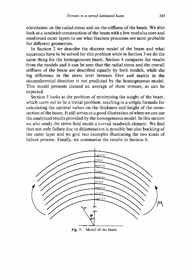
Fig. 1. Model of the beam.

\

246 Gdran Toll

2. DISCRETE M O D E L

We make a model of our anisotropic beam by taking N layers ofisotropic material, so that layers 1 ,3 , . . . , N represent the matrix while layers 2, 4 , . . . , N - 1 represent the fibres. Thus N must be an odd integer. The inner radius of the beam is a and the outer radius is b. Assuming that each layer has the same thickness h, we get the radius at the ith interface as r = a + ih. Thus h = ( b - a ) / N . We impose a bending moment M p e r unit length in the z-direction according to Fig. 1. By symmetry in the (p- direction, the solution cannot depend on ~0, and we can take the solution in the ith layer as,1

( i ) = Ai a~ 7 + B ~ ( 1 + 2 1 n r ) + 2 C ~ (l)

A. (i) _ aoo rZ- ~- Bi(3 + 2 In r) + 2C~ (2)

a(i~ = 0 (3) rq~

1 { (l +Vi) Ai_Bi(l + vi)r+2r(l _vi_ vZ)(Bilnr +Ci) } (4) b~(ri) = E// r

(i) 4 B i r c P (5)

This is in the case of plane strain. At each interface we must have the stress and displacement continuous,

i.e. (i) (i+ 1)

6,r (ri) = 6r, (ri)

Ufri)(ri) = ulri + l)(ri)

(i) (i + 1)(ri) (6) ( r i ) =

since ri is the outer radius of the ith layer. The boundary conditions at the free surfaces are

a(,})(a) = 0 (N) at, (b) = 0 (7)

making the stress there zero. Thus we have 2 + 3 ( N - 1) = 3 N - 1 equations for the 3N unknowns

Stresses in a curved laminated beam 2 4 7

Ai, Bi and C~, i = 1 , . . . , N. The last equat ion is that the momen t M must be equilibrated, which implies

- M = (r - 6)a~0~0(r)dr (8)

The minus sign occurs because the m o m e n t tries to increase the radius of curvature of the beam. ~ is the point of zero a~o~o, which then becomes a new unknown. We have assumed the only loading to be a pure moment , so eqn (8) becomes

fi 'a~o~o(r) = (9) dr 0

making the resultant force zero. At this point we introduce dimensionless quantities by putt ing:

i = r/a ffi = u i / a 6 = b/a 6 = 6/a

~ij = a i f l 2 / M Ei = E i a 2 / M M = M / M = 1

Ai = A i / M Bi = B i a 2 / M Ci = C i a 2 / M

Now from eqn (8) we have

(lO)

But the last integral vanishes according to eqn (9). Thus

l f~,p(f) d f = -- 1

and 5 disappears f rom our equations. Evaluating this integral we get N ; 2f/ - = rae~(r ) d i 1 ZS~o(? ) dZ = --( i) -

i = 1 N

i = 1

N

--2{ -A, n ~ + / ~ i ( i ~ ( 1 + In i i )

i = 1

- i l l ( 1 + I n / i _ 0 ) + C'i(i~ - i~_~)} (11)

where i o = 1.

248 G6ran T o l l

Summarising, we then have, besides eqn (11): eqns (1) and (7)

AI '~ J~l +2C1 = 0

AN 6~ +/~N(I + 2 In 6) + 26" N = 0 (12)

eqns (1), (2), (3), (4), (5) and (6)

A; f~- +/~i(1 + 21nii) + 2 C i + / ~ + (1 + 21n?~) +2C~+ ~2 1 1

1 { (1 + 'i) 3i -/~i(1 + v i ) f i + 2~i(1- v i - 2 v 2 ) ( B i l n f i + Ci)} E'i fi

_ 1 f (1 -~-Yi+l)~i + __/~i+1(1 +vi 1)/7i - - E i + l /7i 1 +

+ 2ri(1 -- vi+ 1 - - 2v]+ 0(/~i+ 1 In i i + C'i+ 1) t

Bi Bi + 1 ~ - ( 1 - v~) = ~--~+ (1 - v~Z+ 1) (13)

where i = 1 , . . . , N - 1. When i is even, we have E~ = Ef and v~ = vf, and when i is odd, E~ = Er~ and v~ = v m. F r o m the last part o f e q n (13) we see that/~i(1 - v~)/eci is the same for all the layers and thus

4/~lrcP V2m) a ~ - /~m (1--

all over the cross-section, which tells us that planes normal to the middle surface remain plane after the deformation.

Assuming that they also remain normal to the middle surface, which is a good approximation, 2 we can take as a measure of the stiffness of the beam, the ratio between the m o m e n t M and the angle ,9 that one of these planes rotates under this moment . We have that

0 = ti~°(/~) - - - 4/~1 ~(1) (1 - v~)~o Em

With the stiffness/~ defined as Ih~¢ I =/~101 = 1, where 0 = 0/~o we get

-I~ql - 4Bid Z v~) (141


The 3N eqns (11), (12) and (13) form a linear system of equations that are easily solved using a computer, and the results are presented in Section 4. First though we want to see what happens if we let N ~ ~ , i.e. if we have a homogeneous material with the symmetry of a transversely isotropic material.

3. THE H O M O G E N E O U S BEAM

When the beam is made of a completely homogeneous material with anisotropic behaviour, which here is taken to be transverse isotropy, the constitutive equations in the case of plane strain are, 3

1 - v~2 V21(1 -k- V22)trq, u, err = E ~ - - (Trr - - E 2

1 - - Y12Y21 v12 (1 + Y22)arr + (15) e ~ = - E---~ E t tr~°~

where E 1 =Young ' s modulus in the fibre direction; Ez =Young ' s modulus normal to the fibres; vii = Poisson's ratio with the first index denoting loading direction and the second the direction of contraction, i , j = 1,2, i 4:j; Vz2 = Poisson's ratio for loading in the plane normal to the fibres. Reciprocity gives us that V l 2 / E 1 = v z l / E 2.

It is easy to show that in the case of no (o-dependence, the solution

where

art = A + B s r s - 1 _ C s r - ~ - 1

cr,o ~ = A + B s 2 r s - 1 + C s 2 r - S - x

17r¢ p ~ 0 (16)

S ~ 1 - - Y 1 2 V 2 1

satisfies both the equations of equilibrium and compatibility. A, B and C are determined by the same boundary conditions as in the

previous section, i.e.

tr,,(a) = tr,,(b) = 0 and I b ra~o~o dr = ~ M

3,

250 GSran Toll

and we get (using eqn (10))

s2M ( g s - l _ 6 - s - 1 ) A = a ~ ~

B = _ _ _ s M

a~+ 1 D . ( l - 6-s 1)

a s- I sM _ C - - - ( b ' 1 _ 1 )

D where

S 3 S 3 D = (b ~+l -{-b - s - 1 - 2 ) -

s + l s - 1 (6s X _ ~ _ b - s + l - - 2 )

(17)

S 2 _ _ _ ( 6 2 - l )(6s-I _ 6 - . , I)

2

Again using eqn (I0) we obtain the stress distribution

$2 {~s- l__~-s 1 __( 1 6 - s I)F-s-I 1

- $2 {6s- l__6-s I _ S ( I _ 6 - s t)~-s-I q_s(6S-1 1)F -~-x } (18) O'tptp = O

For an isotropic material we have s = 1. This case actually corresponds to a double root of the characteristic equation, leading to the logarithmic term in eqns (1) and (2). Thus we cannot continuously extend the anisotropic solution to the isotropic case. Though by putting s close to one we will come close to the isotropic solution.

From eqn (18) we can find the maximum 6,, and where this maximum is located by just equating the derivative ol d , with respect to ~ to zero. We then obtain that this maximum is located at

[ ~ + 1 6 s - 1 - - 1 l l " 2 s

Fmax = - - 1 1Z-~ -~ -1 ] (19)

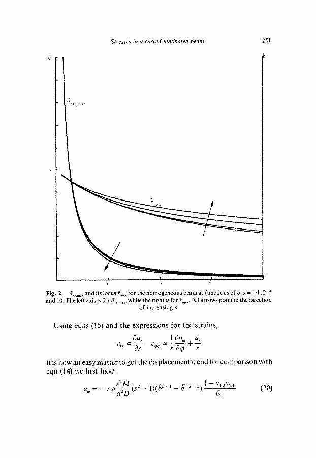
In Fig. 2 we show 6,.max and ~max as functions of 6, using s as a parameter. We can see that both quantities show a rather weak dependence on s. Normally we expect s to be around 2 for a glass-epoxy composite and 4 or 5 for a graphite-epoxy or boron-epoxy composite. It should be realised that E 1 and E: in the expression for s (eqn (16)) are the effective moduli of the composite and not the moduli of the constituents.


I0

~

° r r , m a x

5

. . . . . 3 l, 4i ~l

Fig. 2. ~ ...... and its locus fo,~x for the homogeneous beam as functions of ~;. s = l. 1,2, 5 and 10. The left axis is for 6 . . . . . while the right is for ~,~,. All arrows point in the direction

of increasing s.

U s i n g e q n s (15) a n d the e x p r e s s i o n s f o r the s t r a ins ,

~u, I ~u~o + u r

it is n o w a n e a s y m a t t e r t o ge t the d i s p l a c e m e n t s , a n d fo r c o m p a r i s o n w i th

eqn (14) we first h a v e

s2 m 2 6 - s - l ) 1 - v 1 2 v 2 1 (20)

u~ = - r q ~ a - a ~ ( s - I ) ( / ~ - x _ E l

252 Gdran To l l

We can see that also in the anisotropic case, planes normal to the middle surface remain plane. As in the previous section we now have the rotation of a cross-section

u~(a) 0 = u~ ._ ,

b - a

and with eqn (20)

M s Z ( s 2 - 1) _ 6-s 1) 1 - v12Y21 0 = - - ~ ~ a i ( /~s-1 - E1

Again we define k and /~ as in the previous section to obtain the dimensionless stiffness/~ as

O / ~ l (21) ]~ ~" $2(S 2 - - 1 ) ( b s - 1 _ / 9 - s - 1)( 1 _ v12Y21 )

where D comes from eqn (16). In the next section we will compare these results to the results from the

discrete model in Section 2.

4. C O M P A R I S O N BETWEEN T HE M O D E L S

In the discrete model the parameter showing the stiffness ratio is simply Ef/E m, while in the homogeneous model this ratio comes into action through s, which contains not Ef/E m but instead the ratio between the effective moduli, E1/E 2. To be able to compare the two models we introduce the following assumptions, 3

E 1 = (I)Ef 4- ( 1 - O)E m

E 2 = E f E m / { ~ E m + (1 - - ~ ) E f }

v12 ~ Y22 = (I)Yf + ( l - - (ID)Y m (22)

where • = v o l u m e fraction of fibres, and we get v21 through the reciprocity relation, given in Section 3.

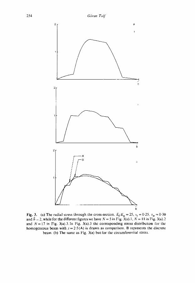
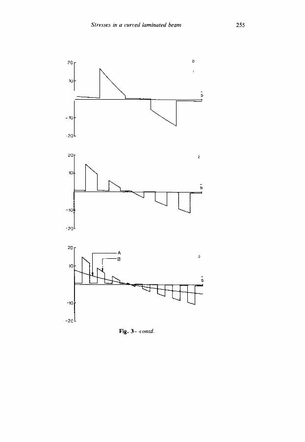
In Figs 3 and 4 we have drawn the stress distribution within the beam. First we vary the number of layers, N, in our discrete model and let/~ = 2, g f / E m = 25, Yf = 0.25 and ~)m = 0.30. Figure 3(a) shows the radial stress while Fig. 3(b) shows the circumferential stress. In the case when N = 17 (the highest value limited by the memory area in the computer), we have


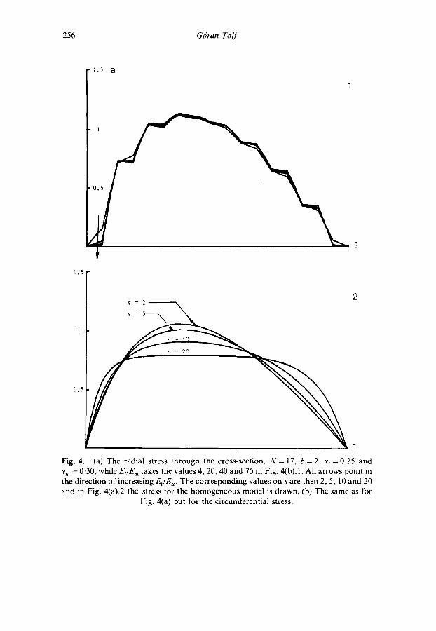
drawn also the stresses calculated from the homogeneous model, using the same values on the parameters and • = 8/17, which through eqn (22) gives s = 2.5. Actually the stress distribution for s = 2.5 hardly differs from the isotropic case. We can see that when N grows the radial stress distribution for the homogeneous model becomes a good approximation for the truly discrete material. F rom Fig, 4 we see that this is only valid when s is rather low. But as we said in the last section, s is rather low for most composites. The maximum radial stress for the discrete model is almost independent of the stiffness ratio, even if we go to higher values than shown in Fig. 4, while the same quantity in the homogeneous model is decreasing with s. In the limiting case when s is very high, we will have a constant radial stress over the cross-section. For the circumferential stress the homogeneous model is not capable of describing the high values in the fibres, but we can see that it presents a good average of the stress distribution. We can see that for high E f / E m the circumferential stress is almost exclusively carried by the fibres and gets more concentrated in the outer layers.

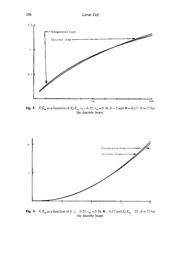
We also want to compare the stiffness of the beam, as predicted by the two models. This quantity represents an overall property of a composite and it is interesting to see if this also differs if we take account of the microstructure. In this comparison it is convenient not to look at kS, but consider instead, k / E m. We then get from the discrete model

I I k / E m = 4/)t(1 _ VZm) I (23)

To obtain a similar expression for the homogeneous model we insert eqn (22) into eqn (20).

In Figs 5 and 6 we compare this stiffness for the two models. In Fig. 5 we use/~ = 2 and vary E f / E m , while in Fig. 6 E f / E m = 25 and/~ varies. In both figures N = 17 for the discrete model and O = 8 / 1 7 for the homogeneous model. We also use the same values on vf and v m as given above. In both figures we can see a remarkably good agreement between the two models. Thus if the assumption in eqn (22) is valid, and through experiments we know that it usually is, we can see that we do not have to bother so much over what actually happens on the microlevel when describing effective mechanical properties of a composite.

Using the homogeneous model we will now explore the failure mechanisms of this composite. Figure 7 shows the ratio between the maximum circumferential stress, obtained at i = 1, and the maximum

2 54 GOran To~

A

1

Fig. 3. (a) The radial stress t h rough the cross-section. Ef/E m = 25, vf = 0.25, v m = 0.30 and b = 2, while for the different figures we have N = 5 in Fig. 3(a). 1, N = 11 in Fig. 3(a).2 and N = 17 in Fig. 3(a).3. tn Fig. 3(a).3 the cor responding stress dis t r ibut ion for the homogeneous beam with s = 2.5 (A) is drawn as compar ison. B represents the discrete

beam. (b) The same as Fig. 3(a) but for the circumferential stress.


lo t -20

20

10:

-1(3

-2C

~3 • I

20

10

-10

-2C

A

Fig . 3 ~ c o n t d .

256 G6ran Tof f

.5 ~t

1 . 5 ¸

0 . 5

2 s = 2

s = 5 ~ ' ~

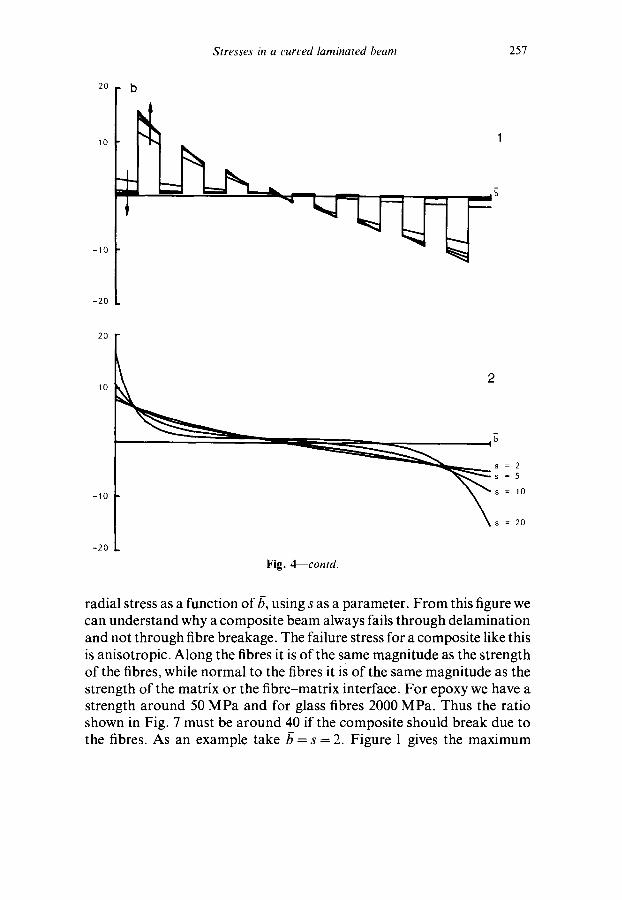
Fig. 4. (a) The radial stress th rough the cross-section. N = 17, 6 = 2, vf = 0.25 and v m = 0-30, while ErIE m takes the values 4, 20, 40 and 75 in Fig. 4(b). 1. All arrows point in the direction of increasing ErIE m. The cor responding values on s are then 2, 5, 10 and 20 and in Fig. 4(a).2 the stress for the homogeneous model is drawn. (b) The same as for

Fig. 4(a) but for the circumferential stress.

Stresses in a curt'ed laminated beam 257

20

10

-10

-20

20

~0

- 1 0

s = 2

°s 5

~ s 10

= 2 0

- 2 0

Fig. 4~contd.

radial stress as a function of/~, using s as a parameter. From this figure we can understand why a composite beam always fails through delamination and not through fibre breakage. The failure stress for a composite like this is anisotropic. Along the fibres it is of the same magnitude as the strength of the fibres, while normal to the fibres it is of the same magnitude as the strength of the matrix or the fibre-matrix interface. For epoxy we have a strength around 50 MPa and for glass fibres 2000 MPa. Thus the ratio shown in Fig. 7 must be around 40 if the composite should break due to the fibres. As an example take /~ = s = 2. Figure 1 gives the maximum

258 G6ran Tolf

1.5

0.5

Fig. 5.

Homogeneous beam

/

I I I I i I I I I I

5 0 100

/7/E m as a function of ErIE m. vf = 0.25, v m = 0.30, 6 = 2 and (I) = 8/I 7. N = 17 for

the discrete beam.

I0 Homogeneous beam /

Discrete beam

2 ~ 4

Fig. 6. ](/J~m as a funct ion of b. vf = 0"25, v m = 0 .30 , qb = 8 /17 and Ef/E m = 25. N = 17 for the discrete beam.


40

30

20

10

s=lO

s=5

s=2

S=~ . I

I ~ ! ! 2 3 4 5

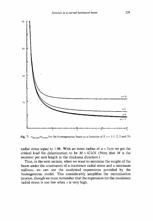
Fig. 7. a~,~ .... /a . . . . . . for the homogeneous beam as a function of ~. s = 1.1,2, 5 and 10.

radial stress equal to 1.06. With an inner radius of a = 3 cm we get the critical load for delamination to be M - - 4 2 kN. (Note that M is the moment per unit length in the thickness direction.)

Thus, in the next section, when we want to minimise the weight of the beam under the constraints of a maximum radial stress and a minimum stiffness, we can use the analytical expressions provided by the homogeneous model. This considerably simplifies the minimisation process, though we must remember that the expression for the maximum radial stress is too low when s is very high.


0,3

/7 0,2

s ~ 2

s ~ 3

0.1

s = 5

2 3 4 5

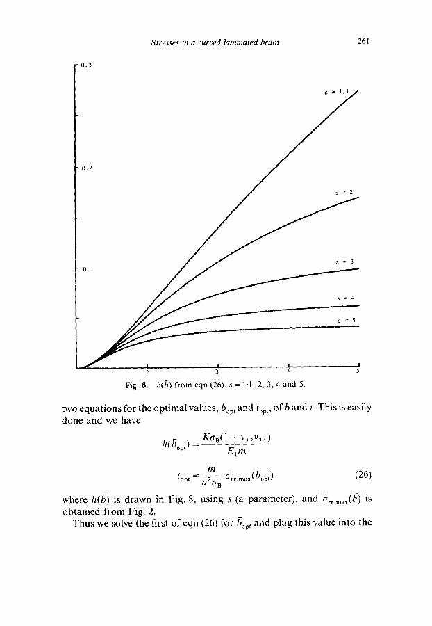
Fig. 8. h(b) from eqn (26). s= l l , 2, 3, 4 and 5.

two equat ions for the opt imal values, bop t and/opt, of b and t. This is easily done and we have

h(/~op 0 _ K a y ( 1 - v~2v 21) E t rn

m toy , = - 6, , m,~(6opt) (26) aZdB •

where h(b) is d rawn in Fig. 8, using s (a parameter) , and 6r,.m,x(/~) is obta ined f rom Fig. 2.

Thus we solve the first of eqn (26) for 6o~ , and plug this value into the

262 G6ran To~

second equation to obtain t o p t and our problem is solved. As an example taking

a~ = 50 MPa K = 300 kNm E 1 = 40 GPa E 2 = 10 G P a

V 1 2 = 0 " 2 5 V21 =0"06 m = 5 k N m a = 3 c m

we obtain /~opt = 2-4 and top t = 7cm. This results in an optimal cross- section having the area 29.4 cm 2.

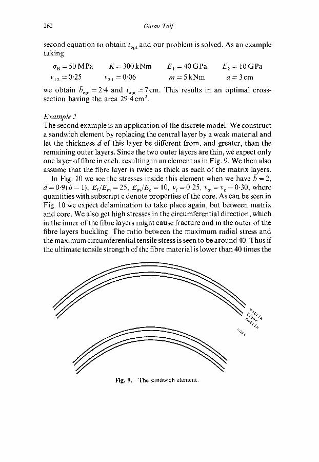
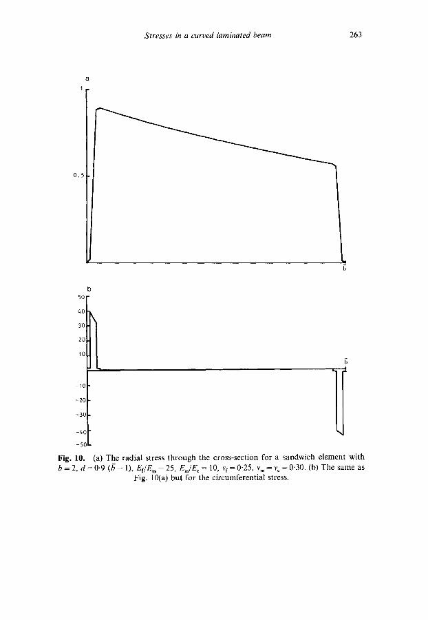
Example 2 The second example is an application of the discrete model. We construct a sandwich element by replacing the central layer by a weak material and let the thickness d of this layer be different from, and greater, than the remaining outer layers. Since the two outer layers are thin, we expect only one layer of fibre in each, resulting in an element as in Fig. 9. We then also assume that the fibre layer is twice as thick as each of the matrix layers.

In Fig. 10 we see the stresses inside this element when we have 6 = 2, 3 = 0"9(/~- 1), E f / E m = 25, Em/E c = 10, Vf = 0-25, v m = v c = 0.30, where quantities with subscript c denote properties of the core. As can be seen in Fig. 10 we expect delamination to take place again, but between matrix and core. We also get high stresses in the circumferential direction, which in the inner of the fibre layers might cause fracture and in the outer of the fibre layers buckling. The ratio between the maximum radial stress and the maximum circumferential tensile stress is seen to be around 40. Thus if the ultimate tensile strength of the fibre material is lower than 40 times the

%

Fig. 9. The sandwich element.

1

0.5


13

50]

4O

l 2O I0

-10 1 - 20

-30

-4(1

-5C

Fig. 10. (a) The radial stress through the cross-section for a sandwich element with /~=2, d = 0 - 9 ( 6 - 1), El~Era=25, E J E t = 10, vf = 0.25, vm = vc =0-30. (b) The same as

Fig. 10(a) but for the circumferential stress.

264 G6ran Toll

interfacial strength between matrix and core, then the matrix breaks due to fibre failure. This seems to be less probable though, since this ratio is around 100 in real sandwich elements. The other failure mechanism that can come into action is buckling of the outer layer due to high compressive stresses. To get an estimate of how high these stresses must be to achieve buckling, we assume that the local buckling load can be obtained as that for a double cantilever with the free buckling length l the same as say ten times the thickness of the fibre layer. We then get the critical load

where

_ 4Tc2Ef l f Pcr 12

If -df3t 12

where df = thickness of fibre layer. This gives

P¢~ 7r2 Efdf 2 n2 Ef (27)

according to the assumption above. Figure 10 shows that the ratio between the maximum radial stress and

the compressive stress in the fibre layer is around 50. Thus if the critical buckling stress, calculated from above, is lower than 50 times the interfacial strength between matrix and core, we get local buckling before delamination. With the interfacial strength OBi around 2 0 M P a and Ef = 75 GPa we get

O'~°~'c~r - - lz2E~f - 100 (28) I O'Bi I 3 0 0 0 " B i

Thus delamination is the most probable failure of this specific sandwich element.

It should be pointed out that in Reference 4 a more precise estimate of the critical buckling stress is carried out, which uses the average stress and properties over the whole outer layer, but when applied here we get nearly the same estimate.

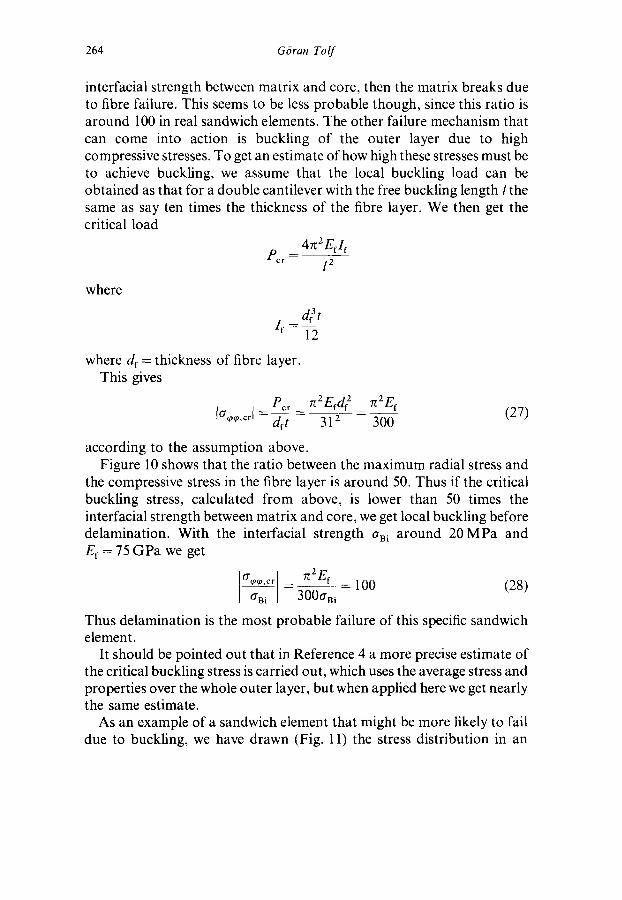
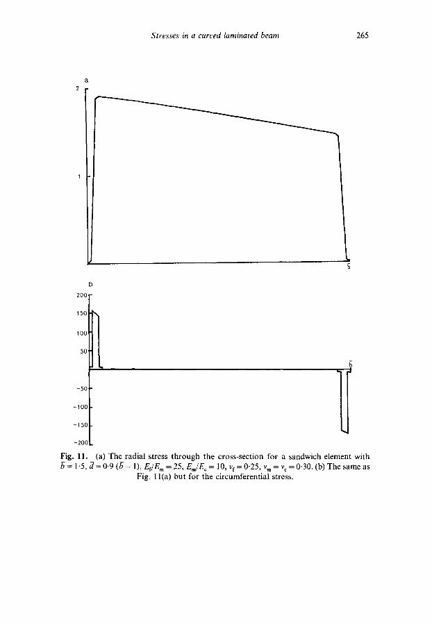
As an example of a sandwich element that might be more likely to fail due to buckling, we have drawn (Fig. 1 l) the stress distribution in an


2

1

b 200,

150 l 100

50 ~

-50

-100

-150

-200

Fig. 11. (a) The radial stress through the cross-section for a sandwich element with t~ = 1.5, d = 0"9 ( 6 - 1), Ef/E m = 25, Em/E c --- 10, vf = 0"25, v m = v c = 0'30. (b) The same as

Fig. 1 l(a) but for the circumferential stress.

266 G6ran To~

element where all parameters are the same as above except for b, which now has the value 1.5. We see that the ratio of the maximum radial stress to the maximum compressional stress is nearly 100, which indicates, according to eqn (28), that buckling is as probable as delamination.

6. C O N C L U S I O N S

The calculations show that with a simple model of a fibre-reinforced beam the actual stress distribution within that composite can be found. The result is compared to the stresses in a homogeneous beam with the same material symmetry and geometrical configuration. The comparison shows that the stresses normal to the fibres as well as macroscopic properties of the composite can be described well by the homogeneous model, while the stresses in the fibre direction are only described correctly by the discrete model. The homogeneous model, however, presents an average of the stresses in this direction.

The advantage with a homogeneous model of fibre composites is that in some cases it can present simple analytical expressions for certain wanted quantities. Here we used analytical expressions on the radial stress and the stiffness of the beam obtained by the homogeneous model, to find a simple solution on the minimum weight of the beam, as in eqns (26).

On the other hand the discrete model is necessary if we want to know the exact distribution in our composite. We used this to analyse the failure modes of a sandwich element and found that essentially two modes exist when the element is loaded by a pure moment: delamination between the core and the inner layer, and buckling of the outer layer. Which of these first comes into action depends on the properties of the element.

A C K N O W L E D G E M E N T

The author wants to thank Professor Kurt Berglund for proposing this study.

REFERENCE S

1. Y. C. Fung, Foundations of Solid Mechanics, Prentice-Hall, Inc., Englewood Cliffs, New Jersey, 1965.


2. L. Timoshenko, Applied Elasticity, Westinghouse Technical Night School Press, East Pittsburgh, Pa, 1925.

3. R. M. Jones, Mechanics of Composite Materials, Scripta Book Co., Washington, DC, 1975.

4. F. J. Plantema, Sandwich Construction. The Bending and Buckling of Sandwich Beams, Plates and Shells, John Wiley and Sons, Inc., New York, 1966.

stresses in a curved laminated beam

Documents